Generalized degrees of freedom and adaptive model selection in linear mixed-effects models

Generalized Degrees of Freedom and Adaptive Model Selectionin Linear Mixed-Effects Models

Bo Zhang1, Xiaotong Shen2, and Sunni L. Mumford1

1Division of Epidemiology, Statistics, and Prevention Research, Eunice Kennedy Shriver NationalInstitute of Child Health and Human Development, Bethesda, MD 20892, U.S.A.2School of Statistics, University of Minnesota, Minneapolis, MN 55455, U.S.A.

AbstractLinear mixed-effects models involve fixed effects, random effects and covariance structure, whichrequire model selection to simplify a model and to enhance its interpretability and predictability.In this article, we develop, in the context of linear mixed-effects models, the generalized degreesof freedom and an adaptive model selection procedure defined by a data-driven model complexitypenalty. Numerically, the procedure performs well against its competitors not only in selectingfixed effects but in selecting random effects and covariance structure as well. Theoretically,asymptotic optimality of the proposed methodology is established over a class of informationcriteria. The proposed methodology is applied to the BioCycle study, to determine predictors ofhormone levels among premenopausal women and to assess variation in hormone levels bothbetween and within women across the menstrual cycle.

KeywordsAdaptive penalty; linear mixed-effects models; loss estimation; generalized degrees of freedom

1 IntroductionIn clinical or epidemiologic studies, linear mixed-effects models (LMMs) (Laird and Ware1982; Longford 1993) are commonly used in analyzing clustered data (repeated measuresdata, longitudinal data) with continuous outcomes and multiple covariates. LMMs areattractive because they can effectively model the dependence structure that arises fromrepeated measures for the same cluster by appropriately using random effects andcovariance structure. Despite a large body of literature on LMMs, the issue of selecting theirfixed effects, random effects or covariance structure has not received much attention.Incorrect inclusion of fixed or random effects, or incorrect specification of covariancestructure can result in biased results and false interpretation. Therefore, accurate modelassessment and precise model selection procedures are essential for improving theperformance of LMMs. In this article, we focus on model selection in LMMs and develop acompetitive methodology for selecting LMMs.

Specialized model selection methods for LMMs were rarely proposed in the literature,although information criteria have been extensively applied in data analysis where LMMs

Publisher's Disclaimer: This is a PDF file of an unedited manuscript that has been accepted for publication. As a service to ourcustomers we are providing this early version of the manuscript. The manuscript will undergo copyediting, typesetting, and review ofthe resulting proof before it is published in its final citable form. Please note that during the production process errors may bediscovered which could affect the content, and all legal disclaimers that apply to the journal pertain.

NIH Public AccessAuthor ManuscriptComput Stat Data Anal. Author manuscript; available in PMC 2013 March 1.

Published in final edited form as:Comput Stat Data Anal. 2012 March 1; 56(3): 574–586. doi:10.1016/j.csda.2011.09.001.

NIH

-PA Author Manuscript

NIH


NIH


are used. Most information criteria select the optimal model M ̂ among candidate models{Mγ,γ ∈ Γ} by minimizing a model selection criterion of the form

(1)

where n is the total number of observations, kMγ is the number of independent parameters ina candidate model Mγ, and ℓMγ is the log-likelihood given by Mγ. Akaike's informationcriterion (AIC) in Akaike (1973) uses the expected Kullback-Leibler information with λ(n,kMγ) = 1; a bias-corrected version of AIC, called AICc (Hurvich and Tsai 1989), with λ(n,kMγ) = nkMγ/(n − kMγ − 1) estimates the expected Kullback-Leibler information directly in aregression model where a second order bias adjustment is made; Bayesian informationcriterion (BIC) in Schwarz (1978) uses an asymptotic Bayes factor and advocates λ(n, kMγ) =log(n)/2; risk inflation criterion (RIC) in Foster and George (1994) is based on the minimaxprinciple, and adjusts the penalization parameter to be λ(n, kMγ) = log(p), where p is thenumber of available covariates; covariance inflation criterion (CIC) in Tibshirani and Knight

(1999) with adjusts the prediction error by the average covariance ofthe predictions and responses when the prediction rule is applied to permute the data set; andmany others are available. The total number of unknown parameters kMγ in the informationcriteria characterize the model complexity that the information criteria intend to penalize on.Increasing number of unknown parameter in either random effects or the variance-covariance structure of random effects or within-cluster errors in LMM indeed increases themodel complexity. Therefore, as suggested by Pinheiro and Bates (2000), Diggle et al.(2002), and Wolfinger (1997), the total number of unknown parameters kMγ used to computeinformation criteria includes not only the parameters introduced by fixed effects but also theones introduced by random effects and variance-covariance structure. However, in (1), thepenalization parameter λ(n, kMγ) penalizes an increase in the size of a model only through afixed penalization parameter, in the sense that it is pre-determined by n and kMγ, andtherefore it is not adaptive to various model structures. The model selection procedures withform (1) are hereby referred as nonadaptive selection procedures. The nonadaptive modelselection procedures with a large penalty often yield an optimal model whose size is small,and the nonadaptive procedures with a small penalty often yield an optimal model whosesize is large. Consequently, a large penalty is likely to perform well when the true model hasa parsimonious representation, and is likely to perform poorly otherwise. This feature ofnonadaptive model selection procedures results in large selection bias in LMMs. Shen andYe (2002) and Shen, Huang, and Ye (2004) confirmed the disadvantages of thosenonadaptive procedures in linear regression, logistic regression and Poisson regression.They showed that, with the inflexibility of the penalization parameter, information criteriaignore the uncertainty of data and fail to adjust the penalization parameter for betterperformance. The need is compelling for a data-adaptive model selection procedure that canreduce the selection bias and essentially performs well over a variety of situations.

In this article, we derive the generalized degrees of freedom (GDF) (Ye 1998; Efron 2004)in LMMs, and discuss how to use data perturbation (Shen, Huang, and Ye 2004; Shen andHuang 2006) to estimate the GDF. Through the GDF, we extend the adaptive modelselection procedure proposed by Shen and Ye (2002) and Shen, Huang, and Ye (2004) to thecontext of LMMs. In simulations, we evaluate the finite sample performance of the proposedmethodology in selecting fixed effects, random effects and covariance structure of LMMs.We establish the large-sample asymptotic optimality of the proposed procedure. Theasymptotic properties are in agreement with our numerical examples that the proposedmethodology approximates the best performance over a class of information criteria with

Zhang et al.

Comput Stat Data Anal. Author manuscript; available in PMC 2013 March 1.

NIH


NIH


NIH


form (1). Finally, we apply the proposed adaptive model selection procedure to the BioCyclestudy, to determine factors that influence hormone levels of premenopausal women and toassess variation in hormone levels both between and within women across the menstrualcycle.

The rest of the article is organized as follows. Section 2 presents the GDF and the adaptivemodel selection for LMMs. Section 3 discusses the data perturbation estimation for the GDFand establishes the asymptotic optimality of adaptive model selection. In Section 4,numerical studies with small sample simulation datasets are performed to demonstrateadvantages of the proposed method over information criteria. In Section 5, we demonstratethe adaptive model selection by applying it to hormone levels data in the BioCycle study.The last section is devoted to a discussion and technical proofs is in appendix.

2 Generalized Degrees of Freedom and Adaptive Model Selection2.1 Generalized degrees of freedom

Suppose that data are collected from m independent clusters (or subjects in longitudinaldata) with response variable Yij, covariates Xij,1,⋯, Xij,p that are associated with fixedeffects, and covariates Zij,1⋯, Zij,q that are associated with random effects bi, where i = 1,2,⋯, m indicates clusters and j = 1, 2,⋯, ni indicates observations within the ith cluster.LMMs specify the response vector Yij as

(2)

where Xij = (Xij,1,⋯, Xij, p)′ is a fixed-effects covariate vector, β is a fixed-effects coefficientvector, Zij = (Zij,1,⋯, Zij,q)′ is a random-effects covariate vector, and ∊i = (∊i1,⋯, ∊ini)′ is awithin-cluster error vector that follows N(0, σ2Λi). The random effects bi are independentand identically distributed and follow N(0,Ψ). The within-cluster errors ∊i are assumed to beindependent for different i. The random effects bi and the within-cluster errors ∊i areassumed to be independent. LMMs assume the Gaussian continuous response to be a linearfunction of covariates with regression coefficients that vary over individuals, which reflectsnatural heterogeneity due to unmeasured factors. They allow flexible correlation structuresby assuming appropriate random-effects covariates Zij and covariance matrices Ψ and Λi's.

In (2), the Kullback-Leibler (KL) loss can be used to measure the accuracy of maximumlikelihood method. The KL loss measures the deviation of the estimated likelihood from thetrue likelihood as if the truth were known. Let ψ = vech(Ψ) be a vector that contains thedistinct components of Ψ, let φ = vech(Λ1,⋯,Λm) be a vector that contains the distinctcomponents of Λ1,⋯, Λm, and let ξ = (β′,ψ′, σ, φ′)′ be the vector that contains all theparameters in (2). Let Yi = (Yi1,⋯, Yini)′, Xi = (Xi1,⋯, Xini)′ and Zi = (Zi1,⋯, Zini)′. Theperformance of estimator ξ ̂ in the ith cluster can be evaluated by its closeness to ξ in terms ofthe clusterwise KL loss of ξ versus ξ ̂: ∫ p(yi∣ξ)[log p(yi∣ξ) − log p(yi∣ξ ̂))]dyi, where p(yi∣ξ) isthe likelihood function of the observations in the ith cluster. This yields the total KL loss forall independent clusters:

(3)

which, after dropping the terms that are only related to ξ, reduces to

Zhang et al.


NIH


NIH


NIH


(4)

where μi = Xiβ and are the clusterwise mean and covariance matrix,respectively; μ̂i and Σ̂i are the corresponding estimates with ξ replaced by ξ ̂. The KL lossℒ(ξ, ξ ̂) compares different LMM estimations in virtue of the true parameter value ξ. If ξwere known, then we could select the optimal model by minimizing (4) with respect tocandidate models.

Motivated by the information criteria (1), we now consider a class of KL loss estimators ofthe form

(5)

Members of this class penalize an increase in the size of a model used in estimation, with ħcontrolling the degree of penalization. Clearly, different choices of ħ yield different modelselection criteria; for instance, when ħ is the number of parameters, (5) becomes AIC.

Theorem 1—(optimal KL loss estimation). The optimal ħ that minimizes

, the expected ℓ2 distance between the KL loss (4) andthe class of loss estimators (5), is

(6)

The optimal ħ, the in (6), which measures the degrees of freedom cost in model selectionor statistical uncertainty of model selection, is thereby defined as the generalized degrees offreedom or the GDF of LMMs. When LMMs (2) degenerate into linear models bydiscarding random effects, the proposed GDF (6) becomes the GDF discussed in Ye (1998),which is a generalization of the degrees of freedom of fit in linear models (Weisberg 2005).In the rest of the article, we use to denote the GDF, and denote as (M) the GDF of aspecified model M. Moreover, by Theorem 1, the performance of M can be assessed throughits optimal KL loss “estimator”

(7)

and, for any M,

(8)

Zhang et al.


NIH


NIH


NIH


The optimal KL loss estimator (7) measures the divergence between the true likelihood andthe estimated likelihood by M. It can be used to assess and compare various models. InSection 2.2, (7) will be used to develop our adaptive model selection procedure in LMMs.

The optimal KL loss estimator (7) would be an unbiased estimator of ℒ(ξ, ξ ̂M) if it wereindependent of the true parameters. However, it usually depends on unknown parametersthrough (M), and therefore needs to be estimated by data. We will develop in Section 3 thedata perturbation estimate of (M), denoted by (M), in order to fully realize adaptive modelselection. Prior to that, we will describe the procedure of adaptive model selection in Section2.2 assuming (M) is available.

2.2 Adaptive model selectionNow consider a class of model selection criteria in the form of

(9)

for selecting the best model from a class of candidate models {Mγ, γ ∈ Γ}. To achieve thegoal of adaptive selection, we choose the optimal λ from data by selecting the optimal modelselection procedure from a class of information criteria (9) indexed by λ ∈ (0, ∞). First, foreach fixed λ ∈ (0, ∞), one model, denoted by M ̂(λ), is selected from candidate models suchthat it minimizes (9). Let the parameter estimates for M ̂(λ) be ξ ̂M ̂(λ), and let the estimatedGDF for M ̂(λ) be (M ̂(λ)). Second, the optimal λ, denoted by λ ̂, is obtained such that itminimizes the estimated loss of M ̂(λ)

(10)

with respect to λ ∈ (0, ∞). Finally, inserting λ ̂ back into (9) yields the adaptive modelselection procedure: the adaptive selection procedure chooses the optimal model M ̂(λ ̂) byminimizing the adaptive model selection criterion

(11)

over the candidate models {Mγ, γ ∈ Γ}. In (11), the λ ̂ is data-dependent as well as ourselection procedure. The adaptive penalty λ ̂ estimates the ideal optimal penalizationparameter over the class (9); its value varies depending on the data and the size of the truemodel. Therefore, it permits an approximation to the best performance of the class of modelselection criteria (9).

3 Estimation of Generalized Degrees of Freedom3.1 Estimation through data perturbation

This section estimates the GDF for LMMs through the data perturbation technique (Shen,Huang and Ye 2004; Shen and Huang 2006). Data perturbation assesses sensitivity of theestimated parameter through the pseudo response vector

Zhang et al.


NIH


NIH


NIH


(12)

which is generated from the original response vector Yi and a perturbed vector Ỹi withperturbation size τ ∈ (0,1]. To generate Ỹi, data perturbation samples Ỹi are taken from thedistribution of Yi with the unknown distribution mean replaced by Yi; that is, if we denote aspYi (·∣μ) the distribution of Yi with distribution mean μ, Ỹi is sampled from pYi (·∣Yi), for i =1,2⋯, m. In the logistic models and the Poisson models, data perturbation can beimplemented directly because of the absence of dispersion parameters (Shen, Huang and Ye2004). But in LMMs, the distribution of Yi depends on unknown dispersion parameters ψ, σ,and φ, besides μ. Thus, more precisely, we may denote the distribution of Yi as pYi (·∣μ, ψ, σ,φ). To sample Ỹi in LMMs, we suggest to use the most complex model among all candidatemodels to obtain estimates ψ̃, σ̃, and φ̃, and then sample Ỹi from pYi (·∣Yi, ψ̃, σ̃, φ̃).

To estimate the GDF, we can rewrite the GDF in (6) to be the summation of the differenceof two covariance penalties (Efron 2004):

, where Y=(Y1,⋯, Ym)′

denotes the response vector, σ ̂ijk(Y) is the jkth element of , and μ̂ij(Y) is the jthelement of μ̂i(Y). The response vector Y in the parenthesis indicates that the estimates dependon the response vector Y. With perturbed with perturbation size τ, let E*, var*, and cov*denote the conditional mean, variance, and covariance, respectively, given Yi. For anycombination of i j, and k, note that the first covariance penalty term cov(σ ̂ijk(Y)μij(Y),Yik)

equals , which can be approximated by

; whereas the secondcovariance penalty cov(σ ̂ijk(Y), YijYik)/2 equals

, which can be approximated by

,

where is the estimated variance of YijYik. For our implementation, we use aMonte Carlo numerical approximation. We sample , d = 1, 2, ⋯, D,independently from the distribution of as described earlier. Note that follows the conditional distribution of given Yi, i = 1, 2,⋯, m and d = 1, 2,⋯, D. Then theGDF is approximated by

where D is chosen to be sufficiently large to ensure an adequate Monte Carlo approximation.By the law of large numbers, the proposed Monte Carlo approximation of the GDF via dataperturbation converges to the true GDF as D → 0. However, both our simulation studies andShen, Huang and Ye (2004) found that the Monte Carlo approximation of (M) issufficiently accurate if we choose D to be greater or equal to the number of observations.

Zhang et al.


NIH


NIH


NIH


Therefore, we recommended that D be at least for the model selection problems that

we consider in LMMs. We will choose D to be in our simulations and data analysis.

In data perturbation (DP) technique, the parameter τ with τ ∈ (0,1] is called perturbationsize. In the literature, the choise of τ and the sensitivity of the performance of the adaptivemodel selection (or model assessment) to τ has been thoroughly investigated in linearmodels, logistic regression, Poisson regression. Please refer to Ye (1998), Shen and Ye(Shen2002), Shen, Huang and Ye (2004), and Shen and Huang (2006) for more details. Wehave performed the sensitivity study to τ in LMMs for the adaptive model selectionprocedure, and find that the choice of τ does not affect the performance of the adaptiveselection procedure in selecting either fixed-effects covariates, random effects, or covariancestructures. We follow Shen and Huang (2006) and use τ = 0.5 in our simulations and dataanalysis.

3.2 Asymptotic optimalityIn what follows, we investigate theoretical aspects of M ̂(λ ̂), the optimal model selected byadaptive model selection criterion, based on properties of data perturbation. Particularly, theasymptotic optimality of M ̂(λ ̂) is established in Theorem 2; that is, M ̂(λ ̂) approximates thebest performance among all models selected by the procedures with form (9).

Theorem 2—(asymptotic optimality). Assume that: (1) (integrability) for some δ > 0 and λ∈ (0, ∞), Esupτ ∈ (0, δ) ∣ (M ̂(λ))∣ < ∞; (2) (identifiability) infλ ∈ (0, ∞) ∣ℒ(ξ, ξ ̂M ̂(λ))∣ >0; (3)(finite variance estimation) for any i, j, and k,

. Let λ̂ bethe minimizer of (10), then

(13)

If it is further assumed that (4) (loss and risk) limm,ni→∞supλ ∈ (0,∞)∣ℒ(ξ, ξ ̂M ̂(λ))/E(ℒ(ξ,ξ ̂M ̂(λ))) −1∣ = 0, then

(14)

Theorems 2 establishes asymptotic optimality of the proposed adaptive model selectionprocedure in LMMs. The selected model M ̂(λ ̂) by the adaptive selection procedure is optimalin the sense that M ̂(λ ̂), the model that minimizes (11) with a data-adaptive λ ̂, asymptoticallyachieves the minimal loss among all models selected by procedures with form (9).

4 Simulation StudiesIn this section, we access the finite sample performance of the proposed selection procedurefor LMMs through simulations. The numerical studies focus on three aspects in selectingLMMs: (1) selecting fixed-effects covariates in the mean structure, (2) selecting randomeffects for the covariates and (3) selecting covariance structure for within-cluster errors. By

Zhang et al.


NIH


NIH


NIH


repeating each simulation 500 times, we compare the performance of AIC, BIC, andadaptive model selection procedure. AIC and BIC are directly applicable. The proposedadaptive procedure is implemented as described above, with λ ̂ in (11) computed through afine grid search of a large interval (0, C) instead of (0, ∞), where C is sufficiently large. In

our simulations, we use .

Example 1 (fixed effects selection for longitudinal data). This simulation example considersthe LMM

(15)

which contains a “within-cluster time-covariate” Xij,1, a “cluster-level covariate” Xi,2, andother 8 covariates Xij,3,…,Xij,10. The within-cluster time-covariate Xij,1 = xij takes values xij= (j−1)/ni,j = 1,…,ni. The covariate Xi,2 = xi takes binary values 0 or 1 with equalprobabilities. The covariates (Xij,3,…,Xij,10)′ follow the multivariate normal distribution withzero mean and covariance between the k1th and k2th element being ρ∣k1−k2∣, k1,k2 = 3,…, 10.Three values of ρ are examined: 0.5, 0, and −0.5. The random effects bi0, bi1 and within-cluster errors ∊ij are mutually independent and follow the standard normal distribution. Thesimulation data are generated from (15) with m = 20 clusters and ni = 5 observations foreach cluster. In this example, two cases are examined: (1) β0 = 2.5, β1 = 3.75, β2 = 1.5, β7 =2, and βk = 0 otherwise; and (2) β0 = 2.5, β1 = 3.75, β4 = β5 = β6 = −1.25, β8 = β9 = β10 =1.75, and β2 = β3 = β7 = 0.

Based on the criteria of AIC, BIC, and the adaptive model selection, we perform backwardstepwise selection to select fixed-effects covariates in the simulated datasets generated fromeach case. The random effects bi0 and bi1 are forced into each candidate model as we areexamining the performance on selecting fixed-effects covariates. The simulation results aresummarized in Table 1. In the first case, AIC with λ = 1 selects the highest number of fixed-effects covariates on average. Because of the large number of incorrectly selectedcovariates, the proportion of correct fit (exactly selecting the fixed-effects covariates in truemodel, see Zou and Li 2008) by AIC is the lowest. In contrast, BIC has fewer both correctlyand incorrectly selected covariates and produces 0.6 correct-fit rate. Our approach withflexible data-adaptive penalization parameter in (1), however, acts between AIC and BIC interms of correctly selected fixed-effects covariates and performs the best in terms of thecorrect-fit rate, the KL loss, and the number of incorrectly selected covariates. It introduces0.8 correct-fit rate and the lowest averaged KL loss. In the second case, three criteriacorrectly identify the true nonzero fixed-effects coefficients. Unsurprisingly, AIC collectsthe most incorrect nonzero coefficients, BIC does less than AIC, and the adaptive procedurecollects almost no incorrect fixed-effects covariates.

Example 2 (fixed effects selection for longitudinal data). This simulation example considersthe LMM

(16)

which contains one “within-cluster time-covariate” Xij,1 taking values xij = (j − 1)/ni, j =1,⋯,ni and other 29 covariates Xij,2,⋯,Xij,30. The covariates (Xij,2,⋯,Xij,30)′ follow the

Zhang et al.


NIH


NIH


NIH


multivariate normal distribution with zero mean and covariance between the k1th and k2thelement being ρ∣k1−k2∣, k1, k2 = 2,⋯, 30. Three values of ρ are considered: 0.5, 0, and −0.5.The random effects bi0, bi1 and within-cluster errors ∊ij are mutually independent and followthe standard normal distribution. The simulation data are generated from Model (16) with m= 20 clusters and ni = 5 observations from each cluster. In this example, two cases areexamined: (1) β0 = 2.5, β1 = 3.75, β10 = −β20 = β30 = 1.25, and βk = 0 otherwise; and (2) β0= 2.5, β1 = 3.75, β2 =⋯ = β9 = 1.25, β11 =⋯ = β19 = −1.25, β21 =⋯ = β29 = 1.25 and β10 =β20 = β30 = 0.

Based on the criteria of AIC, BIC, and the adaptive model selection, we perform backwardstepwise selection to select fixed-effects covariates to examine the performance of AIC,BIC, and the adaptive model selection. The random effects bi0 and bi1 are forced into eachcandidate model. The simulation results are summarized in Table 2. In the first case, allthree criteria are able to identify the true covariates. However, AIC adds several incorrectfixed-effects covariates in the selected model, whereas BIC collects fewer than AIC. Theadaptive procedure achieves exact selection in every simulation replication. Due to the non-adaptive penalization parameters, AIC and BIC have less than 0.03 and 0.5 correct-fit rate,respectively. In the second case, the adaptive model selection procedure performs the bestby offering the lowest KL loss and the highest correct-fit rate. BIC performs better than AICwhen correlation coefficient ρ = 0.5 or ρ = 0. When ρ = −0.5, BIC selects much less than 27fixed-effects covariates in some simulation replications, and therefore dramatically reducesthe numbers of incorrect and correct selected covariates.

Example 3 (random effects selection for clustered data). This simulation example considersthe LMM

(17)

which contains 10 covariates Xij,1,⋯, Xij,10 with possible random effects bi1, ⋯, bi,10.Whether or not covariate Xij,k has random effect is determined by the correspondingindicator variable δk, which takes values either 0 or 1. The covariates (Xij,1, ⋯, Xij,10)′ followthe multivariate normal distribution with zero mean and covariance between the k1th andk2th element being ρ∣k1−k2∣, k1, k2 = 1, ⋯ ,10, where ρ takes 0.5, 0, and −0.5. The randomeffects bik follow a normal distribution with mean zero and standard deviation 0.5, thewithin-subject errors ∊ij follow the standard normal distribution, and bik and ∊ij are mutuallyindependent. The simulation data are generated from (17) with m = 10 clusters and ni = 25observations from each cluster. In this example, four cases are examined: (1) δ1 = δ2 = 1,and δk = 0 otherwise; (2) δ1 = ⋯ = δ4 = 1, and δk = 0 otherwise; (3) δ1 =⋯· = δ6 = 1, and δk =0 otherwise; and (4) δ1 = ⋯= δ8 = 1, and δk = 0 otherwise. Throughout the four cases, thefixed-effects coefficients are assigned values as β0 = 1.5, β1 =⋯ = β10 = 1.25.

We conduct the best subset search for 10 random effects bi1, ⋯, bi,10. We always include thefixed-effects coefficients of ten covariates and the random intercept in the candidate models.The simulation results are summarized in Tables 3 and 4. Our proposed method achieves thebest performance in all cases in terms of the number of correctly selected random effects,the KL loss and the proportion of correct fit (exactly selecting the random effects in truemodel). In Cases 1 and 2, BIC with fixed penalization parameter λ=2.76 selects smallernumber of both correct and incorrect random effects than AIC, and it also produces highercorrect-fit rate. As a comparison, AIC with fixed penalization parameter λ=1 does muchbetter than BIC in terms of the proportion of correct fit in Cases 3 and 4, because the large

Zhang et al.


NIH


NIH


NIH


number of random effects in the true models prefers relatively small penalties. However, theadaptive model selection outperforms AIC and BIC in all cases.

Example 4 (covariance structure selection). This simulation example considers the LMM

(18)

which contains a “within-cluster time-covariate” Xij,1 taking values xij = (j −1)/ni, therandom effects bi0 and bi1 independently following N(0,0.5), and correlated within-clustererrors that are generated from a mixed autoregressive-moving average (ARMA) model (Boxand Jenkins 1994)

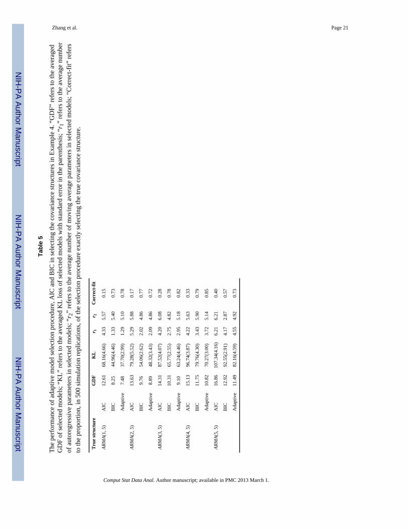
with homoscedastic noise aij independently following N(0, 0.5), r1 autoregressiveparameters ϕl1, and r2 moving average parameters θl2. The simulation data are generatedfrom (18) with m = 5 clusters and ni = 50 observations from each cluster. The goal of thecorrelation structure selection is to determine parameters r1 and r2. Five correlationstructures are examined: ARMA(s,5), s = 1, 2, ⋯, 5. For implementation, r1 and r2 areassumed to potentially take values 0, 1, ⋯, 10. We conduct an exhaustive search for LMMswith all possible ARMA(r1,r2) structures. Throughout the simulation study, β0 = β1 = 1 andϕl1 = θl2 = 0.5 for any l1 and l2. The simulation results are summarized in Table 5. Theproposed procedure yields the best performance in five situations in terms of the KL loss,the average r1 and r2 in the selected models, and the proportion of correctly selecting thetrue covariance structure. It is evident from Table V that AIC and BIC, with a nonadaptivepenalty, cannot simultaneously perform well for both large and small s.

5 Application: Estradiol Levels in the BioCycle Study5.1 The BioCycle study

The BioCycle study is an epidemiologic study of menstrual cycle function among healthy,regularly menstruating women. It was conducted by the Eunice Kennedy Shriver NationalInstitute of Child Health and Human Development and the State University of New York atBuffalo from 2005 to 2007. One of the objectives was to study endogenous reproductivehormone levels and their association with other covariates across the menstrual cycle. TheBioCycle Study followed 259 regularly menstruating premenopausal women from NewYork for up to two menstrual cycles. The study population, materials, and methods havebeen previously described in detail (Wactawski-Wende at el. 2009). In summary, healthywomen between the ages of 18–44 had to be regularly menstruating (self-reported cyclelength between 21 and 35 days for each menstrual cycle in the past 6 months) in order toparticipate. Women with conditions known to affect menstrual cycle function such aspolycystic ovary disease, uterine fibroids, or current use of hormonal contraception (i.e., 3months prior to study entry) were excluded. Eligible participants visited the study clinic 8times during each menstrual cycle, at which time fasting serum samples were collected. Thevisits were scheduled to occur during specific phases of the menstrual cycle, based on anapproximate 28-day cycle length. Hormones levels, including estradiol levels, and otherbiological markers, including insulin and lipoprotein cholesterol levels, were measured fromserum samples collected at each visit. Participants were asked to complete standardized

Zhang et al.


NIH


NIH


NIH


questionnaires at the baseline visit on lifestyle, physical activity, and reproductive history.Dietary intake was assessed four times per cycle using the 24-hour dietary recallmethodology and the Nutrition Data System for Research software version 2005 developedby the Nutrition Coordinating Center, University of Minnesota, Minneapolis, MN. Physicaland anthropometric measures were done according to standardized protocols and includedheight and weight for the calculation of body mass index.

Due to the considerable variability in hormone levels both between women and within awoman from cycle to cycle, LMMs with random effects and complex within-clustercovariance structure have typically been used to account for the correlations between andwithin women in the analysis of factors associated with hormone levels and menstrual cyclefunction (Schisterman at el. 2010; Mumford at el. 2010). One of the challenges during thedata analysis was the demand of precisely selecting covariates in LMMs as well as theirrandom effects and covariance structure. However, traditional model selection methods forLMMs have major drawbacks and sometimes fail to identify the associated factors andcorrelation structure, which can induce inaccurate prediction of hormone levels andincorrect interpretation of the association between hormone levels and the predictors. Thismotivated us to propose a novel model selection procedure with better performance, so as tobenefit not only the BioCycle study, but also other clinical or epidemiologic studies in thefuture that will use LMMs.

5.2 Modeling estradiol levelsOne of the hormones that is of particular interest is estradiol, as estradiol is the primaryestrogen secreted by the ovary and the predominant sex hormone present in females.Estradiol plays a key role in reproductive function, as well as in the development andrecurrence of breast cancer and other chronic diseases. Understanding the factors associatedwith estradiol levels may aid in understanding an individual's susceptibility to disease, aswell as offer potential strategies for disease prevention. It has also been argued thatdifferences in breast cancer incidence between populations could be due to differences indemographic characteristics associated with estradiol levels. Here we are interested inidentifying factors that are associated with estradiol levels and accessing variation inestradiol levels both between women and within a women across the menstrual cycle. Themain outcome of interest is the logarithm of estradiol levels as measured in fasting serumsamples in the BioCycle study. Potential biological factors that might influence estradiollevels include age (Xage), body mass index (Xbmi), race (white, black Xrac1, other Xrac2), pastuse of oral contraceptives (yes or no, Xoc), age at menarche (Xmen), parity (Xpar), maritalstatus (married/living as married or single/separated/divorced, Xmar), physical activity (low,moderate Xphy1, high Xphy2), smoking status (ever or never, Xsmo), insulin levels (Xins), thelogarithm of total cholesterol levels (Xcho), the logarithm of luteinizing hormone levels (Xlh),dietary fat intake (Xfat), dietary fiber intake (Xfib), and total energy intake (Xene). Weconsider LMMs that include an intercept and a subset of the 19 covariates: aforementioned17 covariates plus the standardized cycle day (XDay) and the quadratic term of standardized

cycle day . We allow the intercept, Xage, Xlh, XDay, and to potentially have randomeffects and allow correlated within-cluster errors modeled by ARMA(r1,r2) with r1 and r2possibly taking values 0, 1, · · ·, 5.

We implement the best subset selection with AIC, BIC, and our proposed procedure.Selected fixed effects, random effects, autoregressive parameters, and moving averageparameters by the three selection procedures are summarized in Table 6. Figure 1 shows thenumbers of selected fixed effects, selected random effects, selected autoregressive andmoving average parameters by the information criteria (1) with the penalization parameter λ

changing from 0.1 to 10.0. All three procedures select fixed effects Xage, Xlh, XDay, and

Zhang et al.


NIH


NIH


NIH


the intercept. AIC selects three more fixed effects, namely Xpar, Xfib, and Xphy1, while BICselects only one more fixed effect, namely Xphy1. The adaptive model selection procedurewith penalization parameter λ = 2.25, however, selects Xfib, and Xphy1. The previousliterature scientifically supports the conclusions of the proposed method. In particular, thelack of association between parity and estradiol is consistent with Westhoff et al. (1996).Moreover, high fiber intake has been associated with lower levels of estradiol in manystudies (Bagga et al 1995; Gann et al 2003; Goldin et al. 1994) presumably due to areduction in β-glucuronidase activity in feces in response to fiber intake, which subsequentlyleads to a decline in the reabsorption of estrogen in the colon. For random effects selection,all three methods select a random coefficient for the intercept. BIC and the proposed method

select an additional random effect for , while AIC selects additional random effects for

both and Xlh. For within-cluster covariance structure selection, the proposed method,AIC, and BIC select ARMA(1,1), ARMA(2, 2), and ARMA(0,1), respectively. From thesimulation studies and theoretical properties shown in the previous sections, the LMMselected by the proposed methodology has the best prediction performance and the highestprobability of correct-fit.

6 DiscussionIn the analysis of biomedical data, LMMs are useful models. For data like hormone levels inthe BioCycle study, linear mixed models provide an attractive framework. Sophisticatedmodel selection procedures can help LMMs to improve their interpretability andpredictability. This article develops the concept of GDF for LMMs, as well as a dataperturbation estimation procedure of the GDF of LMMs. As a model complexitymeasurement of LMMs, the GDF permits adaptive model selection, in which thepenalization parameter is estimated from data. We show the adaptive model selectionprocedure approximates the best performance of nonadaptive alternatives within the class(1) in model selection. We examine performance of the proposed model selection procedurein fixed effects selection, random effects selection and covariance structure selection.Numerical examples suggest that it performs well against information criteria with form (1)in terms of the KL loss and correct-fit rate. As seen from the simulations and theoreticalresults, the adaptive model selection has advantages over its nonadaptive counterparts inLMMs.

We have concentrated on developing the adaptive model selection procedure for LMMs.The idea of data-adaptive selection can be extended to other models such as survival modelsand generalized linear mixed models. Such extension works may require deriving the GDFand the optimal loss estimators for those models.

AppendixThe proof of the Theorem 1 is straightforward. Before we present the proof of Theorem 2, alemma is presented.

Lemma 1Under the Assumptions (1) and (3) in Theorem 2, the data perturbation estimator (M ̂(λ)) ofthe GDF of M ̂(λ) in Section 3.1 satisfies

(19)

Zhang et al.


NIH


NIH


NIH


Proof of Lemma 1First note that the left hand side of (19) is equal to

(20)

By the Assumption (3), the last term in (20) can be dropped. By assumption (1) anddominated convergence theorem, the first term in (20) is equal to

Similarly, the second term in (20) is equal to

Therefore, (19) holds.

Proof of Theorem 2Suppose λopt minimizes ℒ(ξ, ξ ̂M ̂(λ)) in terms of λopt = infλ ∈ (0,∞) E(ℒ(ξ, ξ ̂M ̂(λ))). By thedefinition of λopt, we have

Zhang et al.


NIH


NIH


NIH


By Lemma 1, limm,ni→∞limτ→0+(E (M ̂(λopt))− (M ̂(λopt))) = 0, and limm,ni→∞limτ→0+(E (M ̂(λ ̂) − (M ̂(λ ̂)) = 0. Therefore,

which implies (13). With Assumption (4), (14) can be further concluded.

AcknowledgmentsThe authors would like to sincerely thank Editor, Associate Editor and two anonymous referees for their insightfulcomments that have led to significant improvement of this paper. Bo Zhang and Sunni Mumford's research wassupported by the Intramural Research Program of the National Institutes of Health, Eunice Kennedy ShriverNational Institute of Child Health and Human Development. Xiaotong Shen's research was supported in part byNIH grant 1R01GM081535–01, and NSF grants DMS–0604394 and DMS–0906616. We thank the Center forInformation Technology, the National Institutes of Health, for providing access to the high performancecomputational capabilities of the Biowulf Linux cluster.

ReferencesAkaike, H. Information theory and the maximum likelihood principle. In: Petrov, V.; Csáki, F., editors.

International Symposium on Information Theory. Budapest: Akademiai Kiádo; 1973. p. 267-281.Box, GEP.; Jenkins, GM.; Reinsel, GC. Time Series Analysis: Forecasting and Control. 3rd. Holden-

Day; San Francisco: 1994.Diggle, P.; Heagerty, P.; Liang, K.; Zeger, S. Analysis of Longitudinal Data. 2nd. Oxford University

Press; Oxford: 2002.Efron B. The estimation of prediction error: covariance penalties and cross-validation. Journal of the

American Statistical Association. 2004; 99:619–642.Gann PH, Chatterton RT, Gapstur SM, Liu K, Garside D, Giovanazzi S, Thedford K, Van Horn L. The

effects of a low-fat/high-fiber diet on sex hormone levels and menstrual cycling in premenopausalwomen: a 12-month randomized trial (the diet and hormone study). Cancer. 2003; 98:1870–1879.[PubMed: 14584069]

George EI, Foster DP. The risk inflation criterion for multiple regression. The Annals of Statistics.1994; 22:1947–1975.

Hurvich CM, Tsai CL. Regression and time series model selection in small samples. Biometrika. 1989;76:297–307.

Laird NM, Ware JH. Random-effects models for longitudinal data. Biometrics. 1982; 38:963–974.[PubMed: 7168798]

Longford, NT. Random Coefficient Models. Oxford; Clarendon: 1993.Mumford SL, Schisterman EF, Siega-Riz AM, Browne RW, Gaskins AJ, Trevisan M, Steiner AZ,

Daniels JL, Zhang C, Perkins NJ, Wactawski-Wende J. A longitudinal study of serum lipoproteinsin relation to endogenous reproductive hormones during the menstrual cycle: findings from thebiocycle study. Journal of Clinical Endocrinology and Metabolism. 2010; 95:E80–E85. [PubMed:20534764]

Pinheiro, JC.; Bates, DM. Mixed-effects models in S and S-PLUS. Springer-Verlag; New York: 2000.Schisterman EF, Gaskins AJ, Mumford SL, Browne RW, Yeung E, Trevisan M, Hediger M, Zhang C,

Perkins NJ, Hovey K, Wactawski-Wende J. Influence of endogenous reproductive hormones onF2-isoprostane levels in premenopausal women: the BioCycle study. American Journal ofEpidemiology. 2010; 172:430–439. [PubMed: 20679069]

Schwarz G. Estimating the dimension of a model. The Annals of Statistics. 1978; 6:461–464.Shen X, Huang H, Ye J. Adaptive model selection and assessment for exponential family.

Technometrics. 2004; 46:306–317.Shen X, Huang H. Optimal model assessment, selection, and combination. Journal of the American

Statistical Association. 2006; 102:554–568.

Zhang et al.


NIH


NIH


NIH


Shen X, Ye J. Adaptive model selection. Journal of the American Statistical Association. 2002;97:210–221.

Tibshirani R, Knight K. The covariance inflation criterion for model selection. Journal of the RoyalStatistical Society, Ser B. 1999; 61:529–546.

Wactawski-Wende J, Schisterman EF, Hovey KM, Howards PP, Browne RW, Hediger M, Liu A,Trevisan M. BioCycle study: design of the longitudinal study of the oxidative stress and hormonevariation during the menstrual cycle. Paediatric and Perinatal Epidemiology. 2009; 23:171–184.[PubMed: 19159403]

Weisberg, S. Applied Linear Regression. 3rd. Wiley/Interscience; New York: 2005.Westhoff C, Gentile G, Lee J, Zacur H, Helbig D. Predictors of ovarian steroid secretion in

reproductive-age women. American Journal of Epidemiology. 1996; 144:381–388. [PubMed:8712195]

Wolfinger RD. An example of using mixed models and proc mixed for longitudinal data. Journal ofBiopharmaceutical Statistics. 1997; 7:481–500. [PubMed: 9358325]

Ye J. On measuring and correcting the effects of data mining and model selection. Journal of theAmerican Statistical Association. 1998; 93:120–131.

Zou H, Li R. One-step sparse estimates in nonconcave penlaized likelihood models. Annals ofStatistics. 2008; 36:1509–1533. [PubMed: 19823597]

Zhang et al.


NIH


NIH


NIH


Figure 1.Numbers of selected fixed effects, numbers of selected random effects, numbers ofautoregressive (AR) parameter and numbers of moving average (MA) parameter, byinformation criteria (1) with the penalization parameter λ changing from 0.1 to 10.0 (gridlength 0.1).

Zhang et al.


NIH


NIH


NIH


NIH


NIH


NIH


Zhang et al.

Tabl

e 1

The

perf

orm

ance

of a

dapt

ive

mod

el se

lect

ion

proc

edur

e, A

IC a

nd B

IC in

sele

ctin

g fix

ed-e

ffec

ts c

ovar

iate

s in

Exam

ple

1. “

GD

F” re

fers

to th

e av

erag

edG

DF

of se

lect

ed m

odel

s; “

KL”

refe

rs to

the

aver

aged

KL

loss

of s

elec

ted

mod

els w

ith st

anda

rd e

rror

in th

e pa

rent

hesi

s; “

C”

refe

rs to

the

aver

age

num

ber

of c

orre

ctly

sele

cted

fixe

d-ef

fect

s cov

aria

tes;

“IC

” re

fers

to th

e av

erag

e nu

mbe

r of i

ncor

rect

ly se

lect

ed fi

xed-

effe

cts c

ovar

iate

s; “

Cor

rect

-fit”

refe

rs to

the

prop

ortio

n, in

500

sim

ulat

ion

repl

icat

ions

, of t

he se

lect

ion

proc

edur

e ex

actly

sele

ctin

g th

e tru

e fix

ed-e

ffec

ts c

ovar

iate

s.

GD

FK

LC

ICC

orre

ct-fi

t

Cas

e 1

ρ =

0.5

AIC

13.4

279

.63(

4.71

)2.

931.

140.

32

BIC

10.6

078

.51(

4.34

)2.

720.

240.

61

Ada

ptiv

e8.

9277

.25(

3.61

)2.

880.

100.

80

ρ =

0A

IC12

.65

79.4

0(4.

63)

2.94

1.14

0.30

BIC

9.78

78.2

1(4.

15)

2.76

0.25

0.63

Ada

ptiv

e8.

2577

.15(

3.24

)2.

860.

110.

77

ρ = −

0.5

AIC

13.0

079

.49(

4.93

)2.

931.

130.

31

BIC

9.95

78.1

2(4.

03)

2.76

0.24

0.65

Ada

ptiv

e8.

3777

.08(

3.43

)2.

860.

090.

79

Cas

e 2

ρ =

0.5

AIC

15.8

680

.94(

5.02

)7.

000.

560.

56

BIC

14.3

380

.02(

4.64

)7.

000.

140.

87

Ada

ptiv

e13

.05

79.2

3(3.

89)

7.00

0.00

1.00

ρ =

0A

IC15

.86

80.9

3(5.

05)

7.00

0.61

0.50

BIC

14.1

379

.90(

4.72

)7.

000.

150.

86

Ada

ptiv

e12

.87

79.1

2(3.

88)

7.00

0.00

1.00

ρ = −

0.5

AIC

15.9

280

.97(

4.97

)7.

000.

570.

54

BIC

14.3

380

.03(

4.76

)7.

000.

130.

88

Ada

ptiv

e13

.33

79.4

0(4.

11)

7.00

0.01

0.99


NIH


NIH


NIH


Zhang et al.

Tabl

e 2

The

perf

orm

ance

of a

dapt

ive

mod

el se

lect

ion

proc

edur

e, A

IC a

nd B

IC in

sele

ctin

g fix

ed-e

ffec

ts c

ovar

iate

s in

Exam

ple

2. “

GD

F” re

fers

to th

e av

erag

edG

DF

of se

lect

ed m

odel

s; “

KL”

refe

rs to

the

aver

aged

KL

loss

of s

elec

ted

mod

els w

ith st

anda

rd e

rror

in th

e pa

rent

hesi

s; “

C”

refe

rs to

the

aver

age

num

ber

of c

orre

ctly

sele

cted

fixe

d-ef

fect

s cov

aria

tes;

“IC

” re

fers

to th

e av

erag

e nu

mbe

r of i

ncor

rect

ly se

lect

ed fi

xed-

effe

cts c

ovar

iate

s; “

Cor

rect

-fit”

refe

rs to

the

prop

ortio

n, in

500

sim

ulat

ion

repl

icat

ions

, of t

he se

lect

ion

proc

edur

e ex

actly

sele

ctin

g th

e tru

e fix

ed-e

ffec

ts c

ovar

iate

s.

GD

FK

LC

ICC

orre

ct-fi

t

Cas

e 1

ρ =

0.5

AIC

33.0

292

.07(

12.1

0)4.

004.

570.

02

BIC

16.2

981

.43(

6.58

)4.

000.

920.

42

Ada

ptiv

e8.

7377

.02(

2.92

)4.

000.

001.

00

ρ =

0A

IC37

.98

95.1

6(13

.82)

4.00

5.55

0.01

BIC

18.1

782

.42(

6.95

)4.

001.

120.

32

Ada

ptiv

e9.

2577

.17(

3.09

)4.

000.

001.

00

ρ = −

0.5

AIC

34.1

392

.33(

11.6

3)4.

004.

660.

02

BIC

17.4

981

.81(

6.94

)4.

000.

940.

42

Ada

ptiv

e9.

7877

.25(

3.32

)4.

000.

001.

00

Cas

e 2

ρ =

0.5

AIC

56.1

110

7.91

(16.

15)

27.0

00.

750.

42

BIC

53.2

910

5.91

(15.

20)

27.0

00.

230.

78

Ada

ptiv

e51

.54

104.

64(1

4.18

)27

.00

0.16

0.86

ρ =

0A

IC57

.69

108.

90(1

6.48

)27

.00

0.90

0.34

BIC

54.5

410

6.81

(16.

42)

26.9

70.

300.

73

Ada

ptiv

e53

.03

105.

39(1

4.73

)27

.00

0.20

0.83

ρ = −

0.5

AIC

56.9

610

8.01

(14.

63)

27.0

00.

810.

40

BIC

31.0

913

3.62

# (29

.44)

17.7

8#0.

23#

0.37

#

Ada

ptiv

e53

.64

105.

67(1

3.30

)27

.00

0.42

0.68

# BIC

sele

cts m

uch

less

than

27

fixed

-eff

ects

cov

aria

tes i

n so

me

sim

ulat

ion

repl

icat

ions

whe

n co

rrel

atio

n co

effic

ient

ρ =

−0.

5.


NIH


NIH


NIH


Zhang et al.

Tabl

e 3

The

perf

orm

ance

of a

dapt

ive

mod

el se

lect

ion

proc

edur

e, A

IC a

nd B

IC in

sele

ctin

g ra

ndom

eff

ects

in E

xam

ple

3. “

GD

F” re

fers

to th

e av

erag

ed G

DF

ofse

lect

ed m

odel

s; “

KL”

refe

rs to

the

aver

aged

KL

loss

of s

elec

ted

mod

els w

ith st

anda

rd e

rror

in th

e pa

rent

hesi

s; “

C”

refe

rs to

the

aver

age

num

ber o

fco

rrec

tly se

lect

ed ra

ndom

eff

ects

; “IC

” re

fers

to th

e av

erag

e nu

mbe

r of i

ncor

rect

ly se

lect

ed ra

ndom

eff

ects

; “C

orre

ct-f

it” re

fers

to th

e pr

opor

tion,

in 5

00si

mul

atio

n re

plic

atio

ns, o

f the

sele

ctio

n pr

oced

ure

exac

tly se

lect

ing

the

true

rand

om e

ffec

ts.

GD

FK

LC

ICC

orre

ct-fi

t

Cas

e 1

ρ =

0.5

AIC

17.9

117

1.20

(5.1

4)1.

920.

450.

59

BIC

17.8

317

1.72

(5.9

9)1.

830.

050.

79

Ada

ptiv

e16

.53

170.

28(4

.40)

1.98

0.07

0.92

ρ =

0A

IC17

.33

172.

29(5

.19)

1.98

0.45

0.61

BIC

16.8

317

2.35

(6.5

3)1.

940.

030.

91

Ada

ptiv

e15

.95

171.

41(4

.73)

1.99

0.02

0.97

ρ = −

0.5

AIC

15.3

817

0.08

(4.8

3)1.

960.

480.

60

BIC

15.2

217

0.57

(6.3

8)1.

870.

090.

83

Ada

ptiv

e13

.85

169.

17(4

.17)

2.00

0.07

0.93

Cas

e 2

ρ =

0.5

AIC

22.8

219

2.26

(9.1

4)3.

670.

270.

62

BIC

25.2

219

5.65

(11.

40)

3.33

0.05

0.45

Ada

ptiv

e21

.00

190.

45(7

.21)

3.91

0.38

0.88

ρ =

0A

IC22

.72

194.

55(8

.69)

3.90

0.29

0.68

BIC

23.9

319

6.47

(10.

87)

3.73

0.02

0.74

Ada

ptiv

e21

.46

193.

54(7

.83)

3.97

0.31

0.80

ρ = −

0.5

AIC

21.7

419

2.15

(8.6

9)3.

680.

250.

60

BIC

24.1

719

5.58

(11.

04)

3.33

0.03

0.47

Ada

ptiv

e19

.91

190.

40(7

.32)

3.92

0.31

0.87


NIH


NIH


NIH


Zhang et al.

Tabl

e 4

The

perf

orm

ance

of a

dapt

ive

mod

el se

lect

ion

proc

edur

e, A

IC a

nd B

IC in

sele

ctin

g ra

ndom

eff

ects

in E

xam

ple

3. “

GD

F” re

fers

to th

e av

erag

ed G

DF

ofse

lect

ed m

odel

s; “

KL”

refe

rs to

the

aver

aged

KL

loss

of s

elec

ted

mod

els w

ith st

anda

rd e

rror

in th

e pa

rent

hesi

s; “

C”

refe

rs to

the

aver

age

num

ber o

fco

rrec

tly se

lect

ed ra

ndom

eff

ects

; “IC

” re

fers

to th

e av

erag

e nu

mbe

r of i

ncor

rect

ly se

lect

ed ra

ndom

eff

ects

; “C

orre

ct-f

it” re

fers

to th

e pr

opor

tion,

in 5

00si

mul

atio

n re

plic

atio

ns, o

f the

sele

ctio

n pr

oced

ure

exac

tly se

lect

ing

the

true

rand

om e

ffec

ts.

GD

FK

LC

ICC

orre

ct-fi

t

Cas

e 3

ρ =

0.5

AIC

28.1

621

1.11

(10.

15)

5.50

0.18

0.58

BIC

33.1

921

7.66

(12.

96)

4.81

0.04

0.24

Ada

ptiv

e25

.63

208.

37(7

.18)

5.90

0.34

0.73

ρ =

0A

IC25

.84

214.

91(9

.48)

5.78

0.26

0.64

BIC

29.0

221

9.16

(13.

06)

5.44

0.02

0.58

Ada

ptiv

e23

.77

212.

95(7

.00)

5.97

0.32

0.73

ρ = −

0.5

AIC

25.7

221

0.79

(9.2

7)5.

430.

110.

57

BIC

31.1

121

7.75

(12.

76)

4.70

0.01

0.25

Ada

ptiv

e23

.08

207.

90(6

.44)

5.91

0.31

0.79

Cas

e 4

ρ =

0.5

AIC

31.5

422

9.83

(11.

37)

7.13

0.08

0.40

BIC

38.7

523

9.15

(15.

62)

6.05

0.02

0.09

Ada

ptiv

e27

.85

225.

75(8

.28)

7.81

0.30

0.60

ρ =

0A

IC27

.28

233.

58(9

.96)

7.68

0.09

0.69

BIC

33.5

824

1.31

(15.

14)

7.01

0.01

0.35

Ada

ptiv

e25

.23

231.

45(7

.55)

7.93

0.21

0.77

ρ = −

0.5

AIC

31.4

423

0.81

(11.

84)

7.07

0.09

0.36

BIC

38.4

623

9.99

(14.

61)

5.97

0.02

0.07

Ada

ptiv

e27

.36

226.

32(8

.49)

7.81

0.31

0.62


NIH


NIH


NIH


Zhang et al.

Tabl

e 5

The

perf

orm

ance

of a

dapt

ive

mod

el se

lect

ion

proc

edur

e, A

IC a

nd B

IC in

sele

ctin

g th

e co

varia

nce

stru

ctur

es in

Exa

mpl

e 4.

“G

DF”

refe

rs to

the

aver

aged

GD

F of

sele

cted

mod

els;

“K

L” re

fers

to th

e av

erag

ed K

L lo

ss o

f sel

ecte

d m

odel

s with

stan

dard

err

or in

the

pare

nthe

sis;

“r 1

” re

fers

to th

e av

erag

e nu

mbe

rof

aut

oreg

ress

ive

para

met

ers i

n se

lect

ed m

odel

s; “

r 2”

refe

rs to

the

aver

age

num

ber o

f mov

ing

aver

age

para

met

ers i

n se

lect

ed m

odel

s; “

Cor

rect

-fit”

refe

rsto

the

prop

ortio

n, in

500

sim

ulat

ion

repl

icat

ions

, of t

he se

lect

ion

proc

edur

e ex

actly

sele

ctin

g th

e tru

e co

varia

nce

stru

ctur

e.

Tru

e st

ruct

ure

GD

FK

Lr 1

r 2C

orre

ct-fi

t

ARM

A(1,

5)

AIC

12.6

168

.16(

4.66

)4.

335.

570.

15

BIC

8.25

44.9

6(4.

46)

1.33

5.40

0.73

Ada

ptiv

e7.

4837

.70(

2.99

)1.

295.

100.

78

ARM

A(2,

5)

AIC

13.6

379

.28(

5.52

)5.

295.

880.

17

BIC

9.76

54.0

6(2.

62)

2.02

4.86

0.77

Ada

ptiv

e8.

8948

.32(

3.43

)2.

094.

860.

72

ARM

A(3,

5)

AIC

14.3

187

.52(

4.07

)4.

206.

080.

28

BIC

10.3

165

.77(

2.55

)2.

754.

820.

78

Ada

ptiv

e9.

1063

.24(

4.46

)2.

955.

180.

82

ARM

A(4,

5)

AIC

15.1

396

.74(

3.87

)4.

225.

630.

33

BIC

11.7

579

.76(

4.30

)3.

435.

900.

79

Ada

ptiv

e10

.82

70.2

7(3.

00)

3.72

5.14

0.85

ARM

A(5,

5)

AIC

16.8

610

7.34

(4.1

6)6.

216.

210.

40

BIC

12.9

292

.55(

2.91

)4.

172.

870.

57

Ada

ptiv

e11

.49

82.1

6(4.

59)

4.55

4.92

0.73


NIH


NIH


NIH


Zhang et al.

Table 6

Estimated fixed-effects coefficients (the estimated standard deviations in parentheses), estimated standarddeviations of random effects, estimated autoregressive and moving average parameters from selected LMMsfor hormone levels data in the BioCycle study via different methods.

Adaptive(λ̂ = 2.2500) AIC(λ= 1.0000) BIC(λ = 3.7826)

Fixed effects coefficients

Intercept 2.5995(0 1132) 2.4953(0. 1262) 2.4599(0 0994)

XDay 0.1558(0.0069) 0.1502(0.0067) 0.1572(0.0070)

X2Day −0.0042(0.0002) −0.0040(0.0002) −0.0042(0.0002)

Xlh 0.2521(0.0172) 0.2598(0.0172) 0.2502(0.0173)

Xage 0.0112 (0.0029) 0.0169 (0.0040) 0.0105 (0.0030)

Xcho – – –

Xmar – – –

Xpar – −0.0494(0.0280) –

Xpar – – –

Xfat – – –

Xene – – –

Xsmo – – –

Xoc – – –

Xbmi – – –

Xmen – – –

Xfib −0.0109(0.0041) −0.0111(0.0042) –

Xphy1 – – –

Xphy2 – – –

Xrac1 0.2623(0.0624) 0.2811(0.0629) 0.2885(0.0616)

Xrac2 – – –

Random effects standard deviations

σIntercept 0.2945 0.3013 0.2865

σDay – – –

σDay2 0.0004 0.0004 0.0003

σlh – 0.0460 –

σscr – – –

Autoregressive parameters

φ1 −0.3163 −0.7187 –

φ2 – −0.7239 –

φ3 – – –

φ4 – – –

φ5 – – –

Moving average parameters

θ1 0.5730 0.9266 0.2949


NIH


NIH


NIH


Zhang et al.

Adaptive(λ̂ = 2.2500) AIC(λ= 1.0000) BIC(λ = 3.7826)

θ2 – 0.7172 –

θ3 – – –

θ4 – – –

θ5 – – –


Generalized degrees of freedom and adaptive model selection in linear mixed-effects models

Documents

Transcript of Generalized degrees of freedom and adaptive model selection in linear mixed-effects models