Model-Based Controller Design Model-Based Controller Design @BULLET Direct Synthesis Method @BULLET...
39
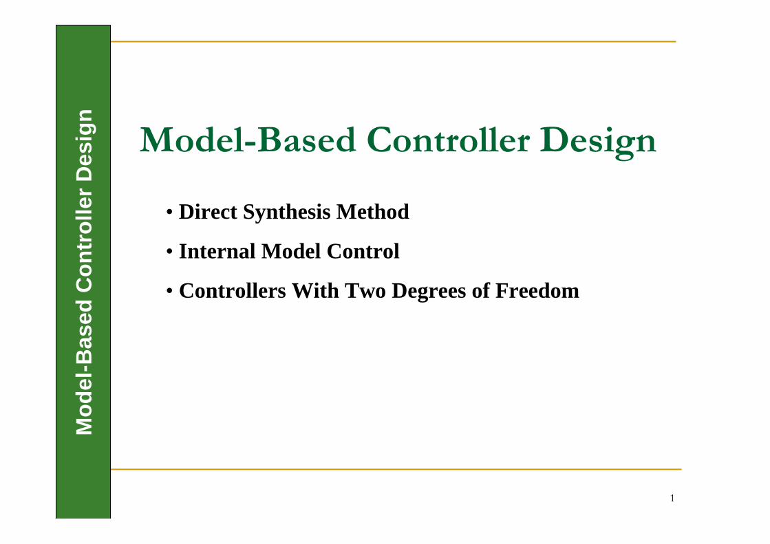
1 Model-Based Controller Design Model-Based Controller Design • Direct Synthesis Method • Internal Model Control • Controllers With Two Degrees of Freedom
Transcript of Model-Based Controller Design Model-Based Controller Design @BULLET Direct Synthesis Method @BULLET...
1
Mo
del
-Bas
ed C
on
tro
ller
Des
ign
Model-Based Controller Design
• Direct Synthesis Method
• Internal Model Control
• Controllers With Two Degrees of Freedom
2
Mo
del
-Bas
ed C
on
tro
ller
Des
ign
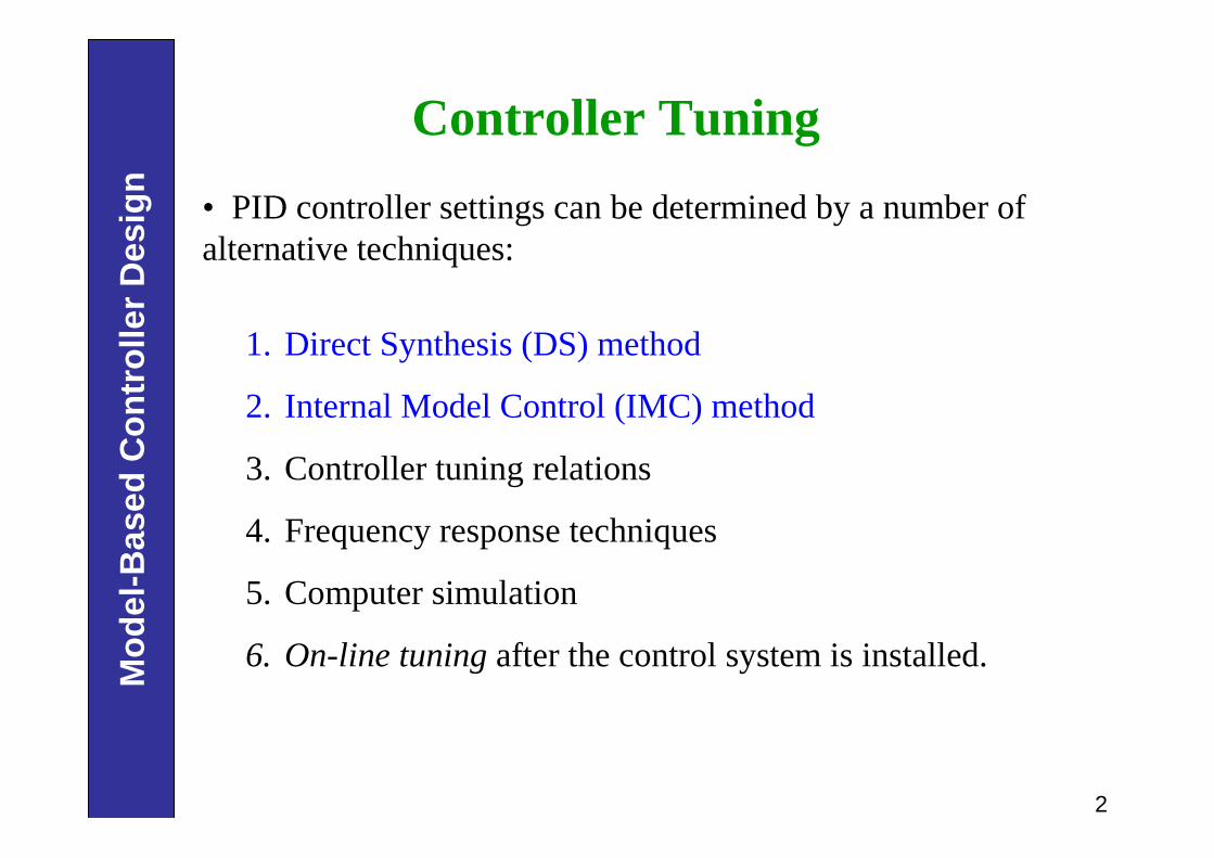
1. Direct Synthesis (DS) method
2. Internal Model Control (IMC) method
3. Controller tuning relations
4. Frequency response techniques
5. Computer simulation
6. On-line tuning after the control system is installed.
• PID controller settings can be determined by a number of alternative techniques:
Controller Tuning
3
Mo
del
-Bas
ed C
on
tro
ller
Des
ign
Direct Synthesis Method
• In the Direct Synthesis (DS) method, the controller design is based on a process model and a desired closed-loop transfer function.
• The latter is usually specified for set-point changes, but responses to disturbances can also be utilized (Chen and Seborg, 2002).
• Although these feedback controllers do not always have a PID structure, the DS method does produce PI or PID controllers for common process models.
4
Mo
del
-Bas
ed C
on
tro
ller
Des
ign
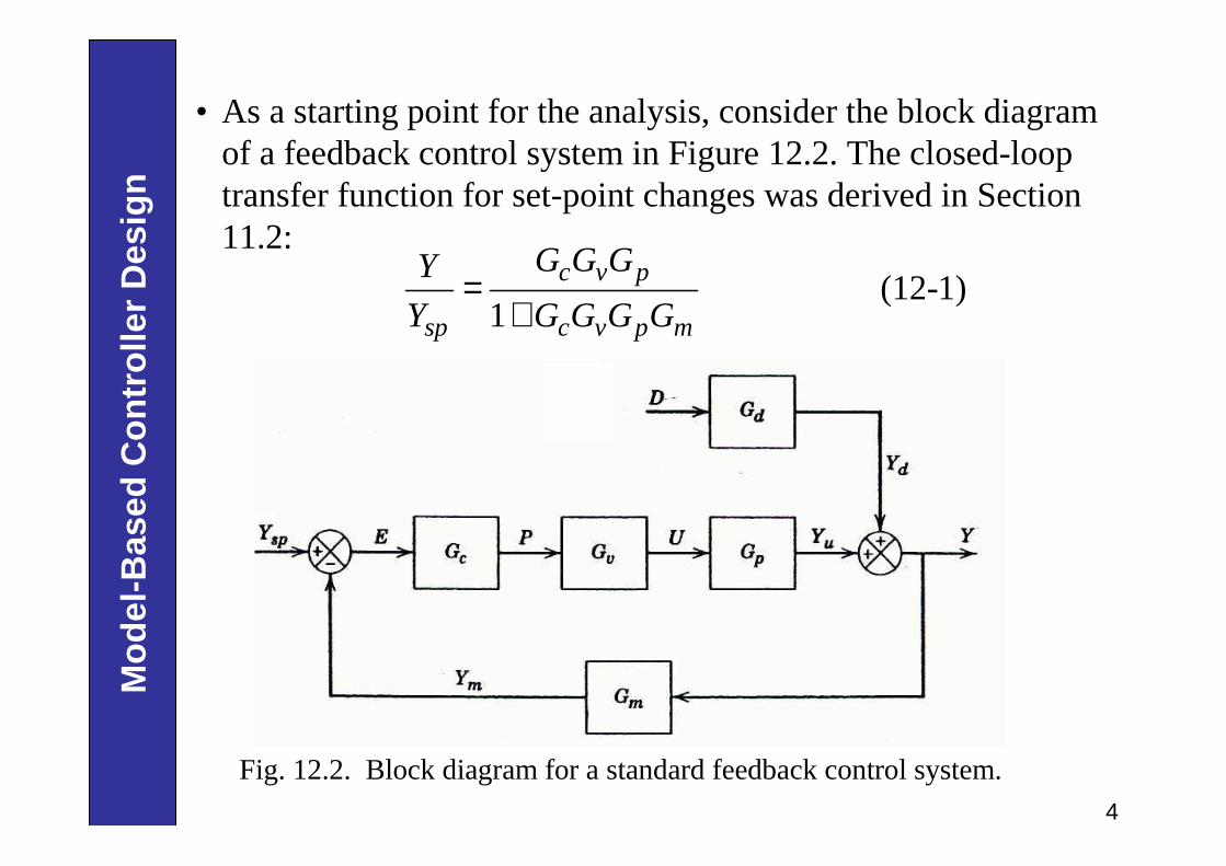
Fig. 12.2. Block diagram for a standard feedback control system.
• As a starting point for the analysis, consider the block diagramof a feedback control system in Figure 12.2. The closed-loop transfer function for set-point changes was derived in Section 11.2:
(12-1)1
=+
c v p
sp c v p m
G G GY
Y G G G G
5
Mo
del
-Bas
ed C
on
tro
ller
Des
ign
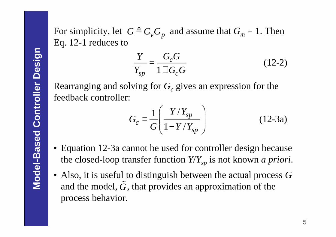
For simplicity, let and assume that Gm = 1. Then Eq. 12-1 reduces to
≜ v pG G G
(12-2)1
c
sp c
G GY
Y G G=
+
Rearranging and solving for Gc gives an expression for the feedback controller:
/1(12-3a)
1 /sp
csp
Y YG
G Y Y
= −
• Equation 12-3a cannot be used for controller design because the closed-loop transfer function Y/Ysp is not known a priori.
• Also, it is useful to distinguish between the actual process Gand the model, , that provides an approximation of the process behavior.
Gɶ
6
Mo
del
-Bas
ed C
on
tro
ller
Des
ign
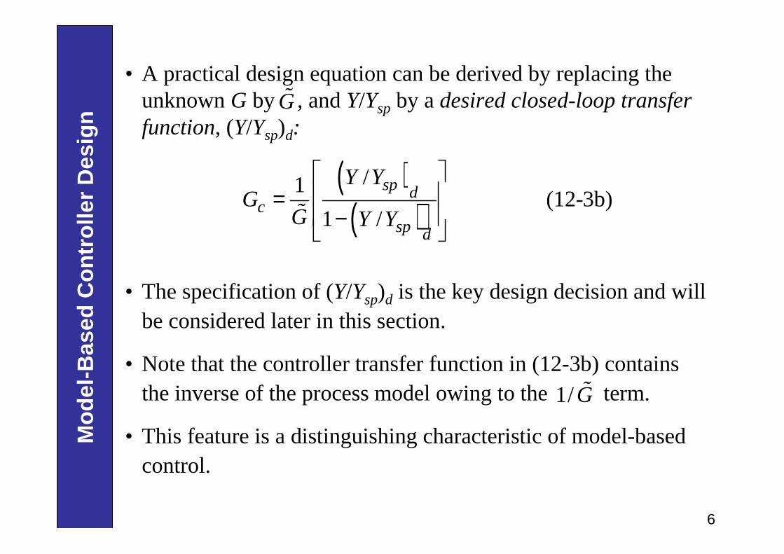
( )( )
/1(12-3b)
1 /
sp dc
sp d
Y YG
G Y Y
= − ɶ
• The specification of (Y/Ysp)d is the key design decision and will be considered later in this section.
• Note that the controller transfer function in (12-3b) contains the inverse of the process model owing to the term.
• This feature is a distinguishing characteristic of model-based control.
1/Gɶ
• A practical design equation can be derived by replacing the unknown G by , and Y/Ysp by a desired closed-loop transfer function, (Y/Ysp)d:
Gɶ
7
Mo
del
-Bas
ed C
on
tro
ller
Des
ign
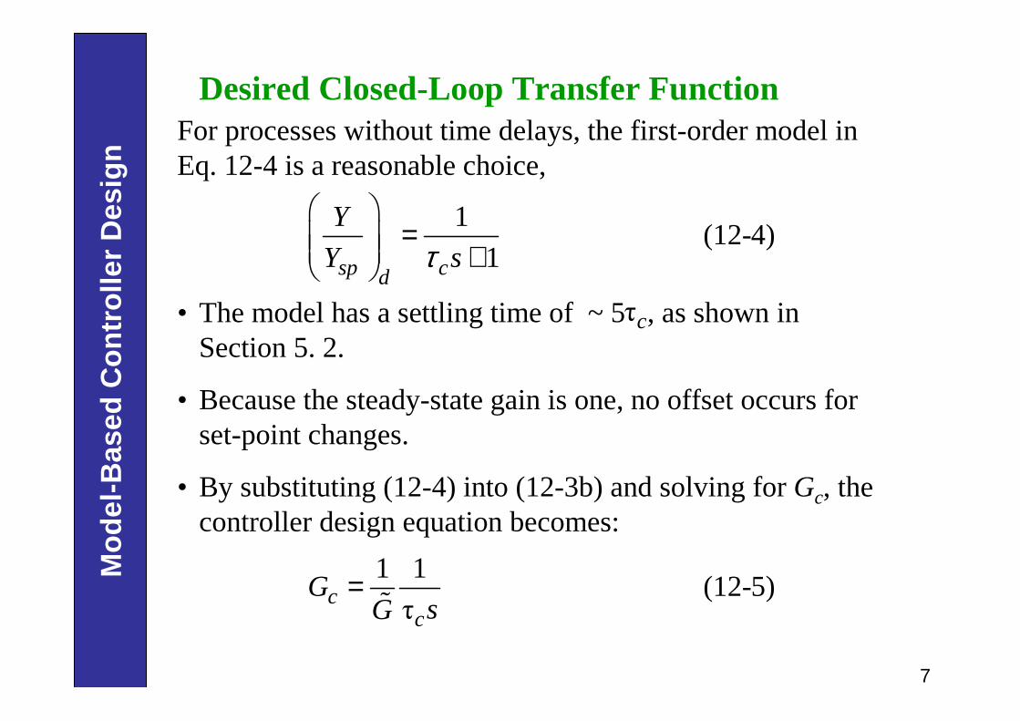
For processes without time delays, the first-order model in Eq. 12-4 is a reasonable choice,
• The model has a settling time of ~ 5 , as shown in Section 5. 2.
• Because the steady-state gain is one, no offset occurs for set-point changes.
• By substituting (12-4) into (12-3b) and solving for Gc, the controller design equation becomes:
τc
1 1(12-5)
τc
c
GsG
=ɶ
Desired Closed-Loop Transfer Function
1(12-4)
1sp cd
Y
Y sτ
= +
8
Mo
del
-Bas
ed C
on
tro
ller
Des
ign
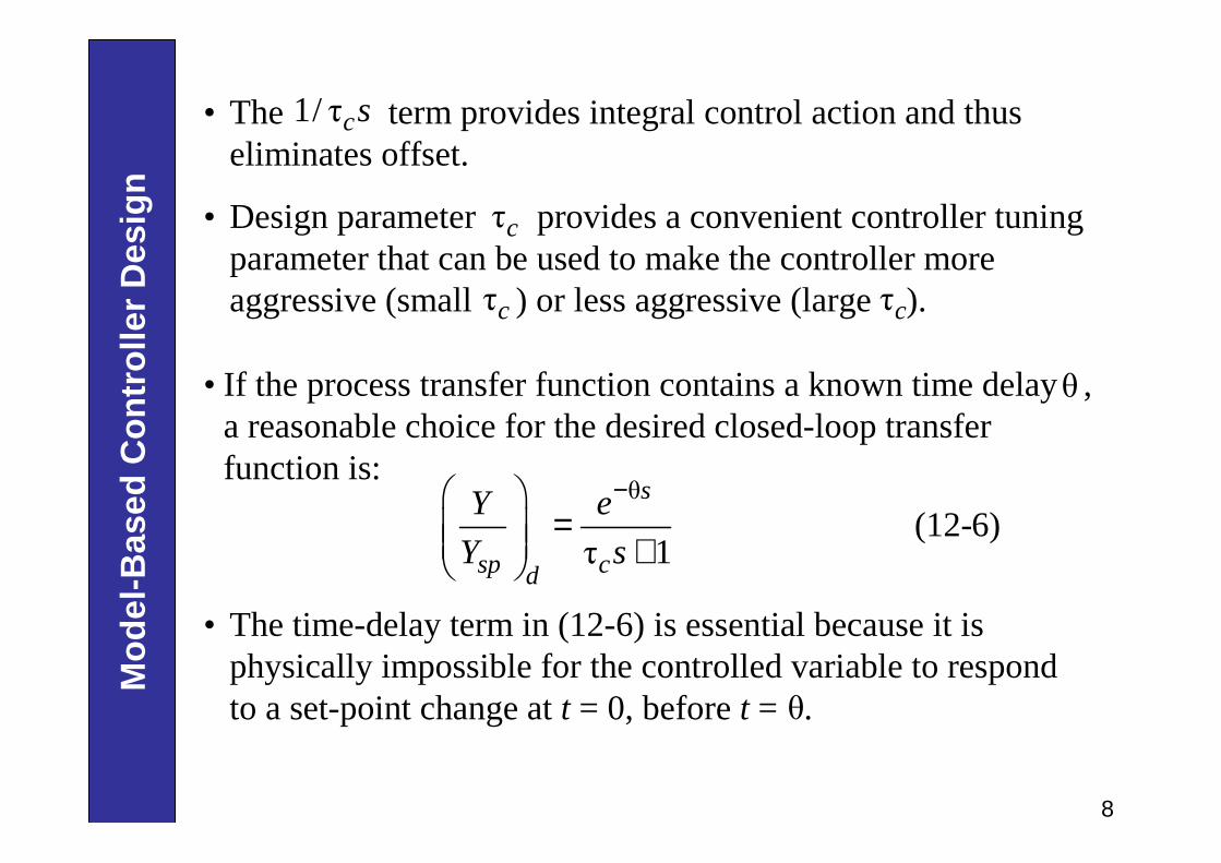
• The term provides integral control action and thus eliminates offset.
• Design parameter provides a convenient controller tuning parameter that can be used to make the controller more aggressive (small ) or less aggressive (large ).
θ
(12-6)τ 1
s
sp cd
Y e
Y s
− = +
• If the process transfer function contains a known time delay ,a reasonable choice for the desired closed-loop transfer function is:
θ
• The time-delay term in (12-6) is essential because it is physically impossible for the controlled variable to respond to a set-point change at t = 0, before t = . θ
τc
τcτc
1/ τcs

9
Mo
del
-Bas
ed C
on
tro
ller
Des
ign
• Although this controller is not in a standard PID form, it is physically realizable.
• Next, we show that the design equation in Eq. 12-7 can be used to derive PID controllers for simple process models.
• The following derivation is based on approximating the time-delay term in the denominator of (12-7) with a truncated Taylor series expansion:
θ 1 θ (12-8)se s− ≈ −
• If the time delay is unknown, must be replaced by an estimate.
• Combining Eqs. 12-6 and 12-3b gives:θ
θ
1(12-7)
τ 1
s
c sc
eG
G s e
−
−=+ −ɶ
θ
10
Mo
del
-Bas
ed C
on
tro
ller
Des
ign
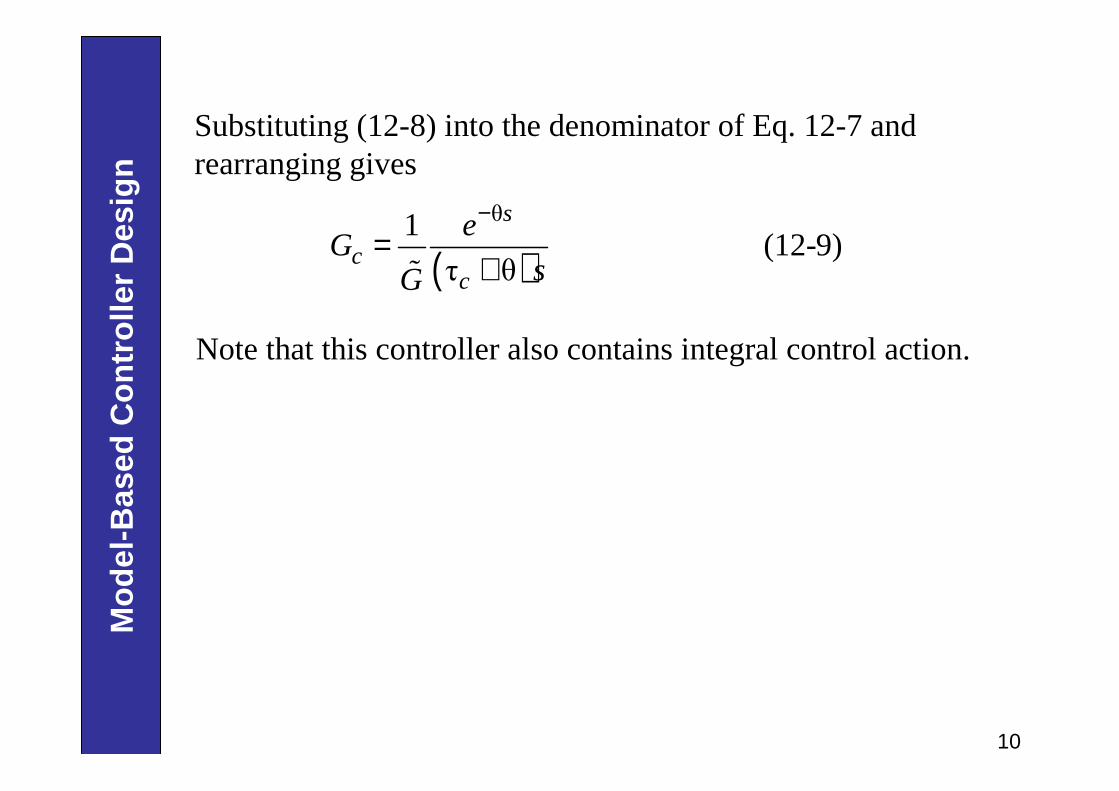
Substituting (12-8) into the denominator of Eq. 12-7 and rearranging gives
Note that this controller also contains integral control action.
( )θ1
(12-9)τ θ
−=
+ɶ
s
cc
eG
sG
11
Mo
del
-Bas
ed C
on
tro
ller
Des
ign
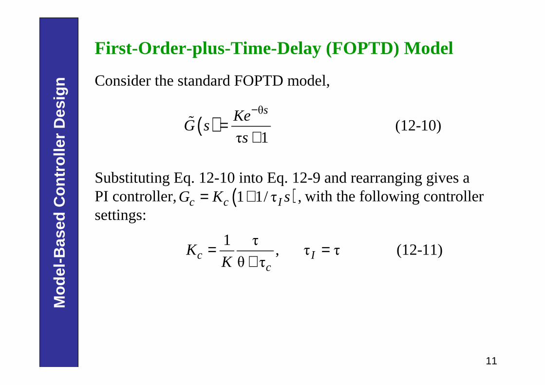
First-Order-plus-Time-Delay (FOPTD) Model
Consider the standard FOPTD model,
( )θ
(12-10)τ 1
sKeG s
s
−=
+ɶ
Substituting Eq. 12-10 into Eq. 12-9 and rearranging gives a PI controller, with the following controller settings:
( )1 1/τ ,c c IG K s= +
1 τ, τ τ (12-11)
θ τc I
c
KK
= =+
12
Mo
del
-Bas
ed C
on
tro
ller
Des
ign
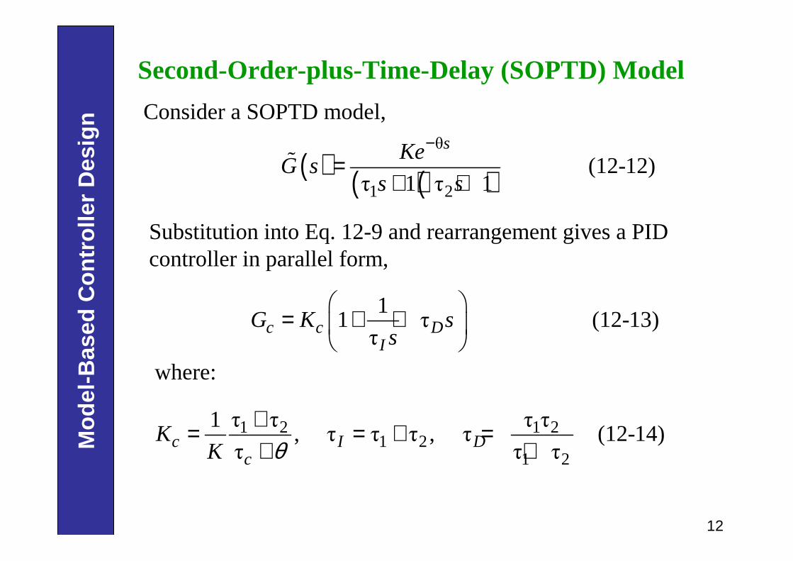
Substitution into Eq. 12-9 and rearrangement gives a PID controller in parallel form,
11 τ (12-13)τ
c c DI
G K ss
= + +
where:
1 2 1 21 2
1 2
τ τ τ τ1, τ τ τ , τ (12-14)
τ τ τθ+= = + =+ +c I D
c
KK
Second-Order-plus-Time-Delay (SOPTD) Model
Consider a SOPTD model,
( ) ( )( )θ
1 2(12-12)
τ 1 τ 1
sKeG s
s s
−=
+ +ɶ
13
Mo
del
-Bas
ed C
on
tro
ller
Des
ign
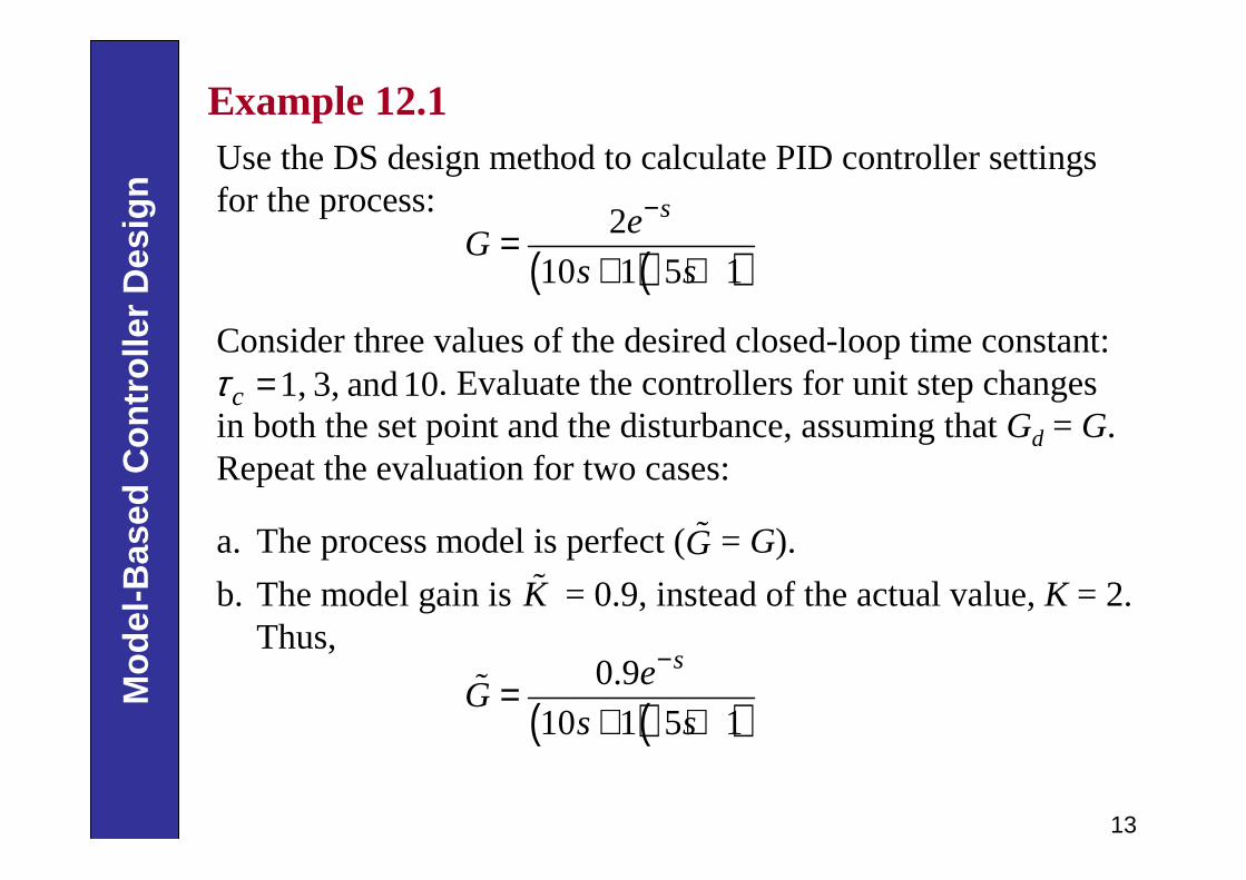
Consider three values of the desired closed-loop time constant: . Evaluate the controllers for unit step changes
in both the set point and the disturbance, assuming that Gd = G. Repeat the evaluation for two cases:
1, 3, and 10cτ =
a. The process model is perfect ( = G).
b. The model gain is = 0.9, instead of the actual value, K = 2. Thus,
Gɶ
Kɶ
( )( )0.9
10 1 5 1
seG
s s
−=
+ +ɶ
Example 12.1Use the DS design method to calculate PID controller settings for the process:
( )( )2
10 1 5 1
seG
s s
−=
+ +
14
Mo
del
-Bas
ed C
on
tro
ller
Des
ign
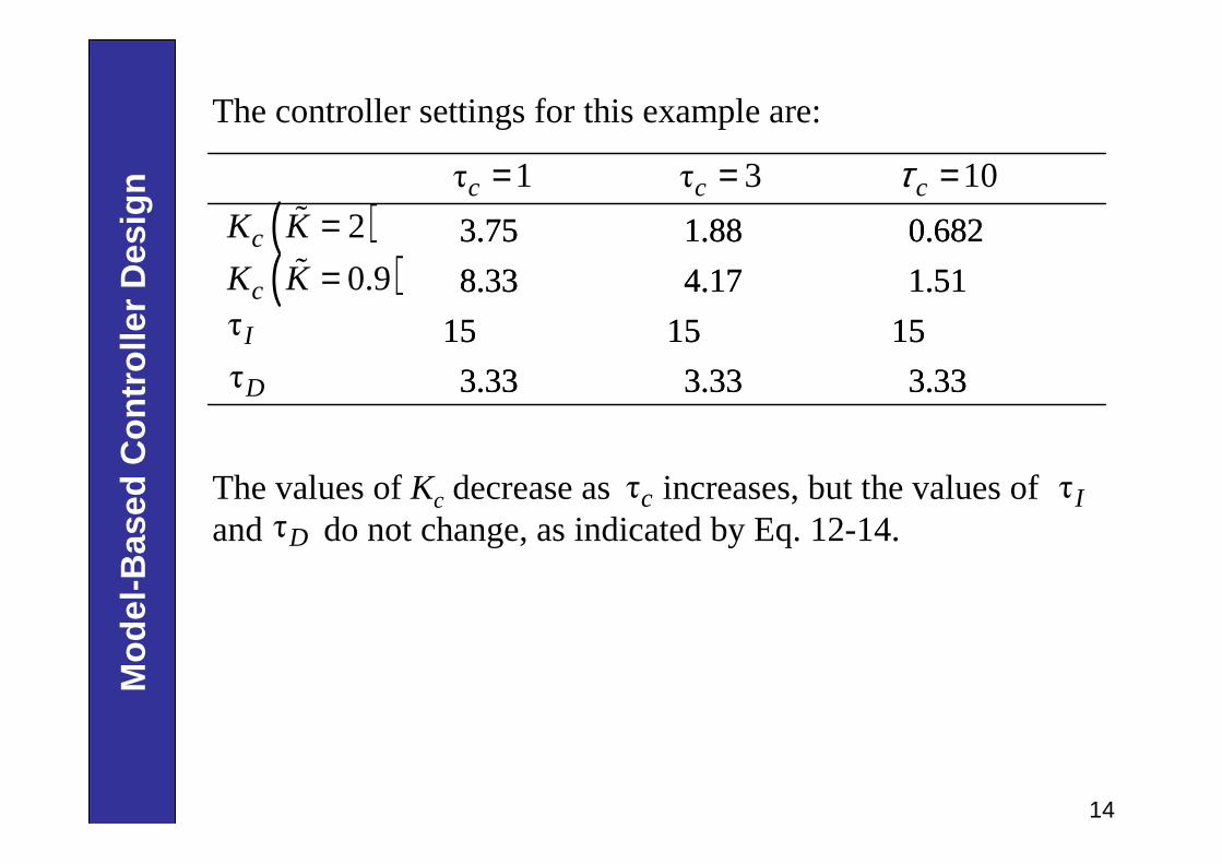
The values of Kc decrease as increases, but the values of and do not change, as indicated by Eq. 12-14.
τc τIτD
3.333.333.33
151515
1.514.178.33
0.6821.883.75
3.333.333.33
151515
1.514.178.33
0.6821.883.75
τ 1c = τ 3c = 10cτ =( )2cK K =ɶ
( )0.9cK K =ɶτI
τD
The controller settings for this example are:

15
Mo
del
-Bas
ed C
on
tro
ller
Des
ign
Figure 12.3 Simulation results for Example 12.1 (a): correct model gain.
16
Mo
del
-Bas
ed C
on
tro
ller
Des
ign
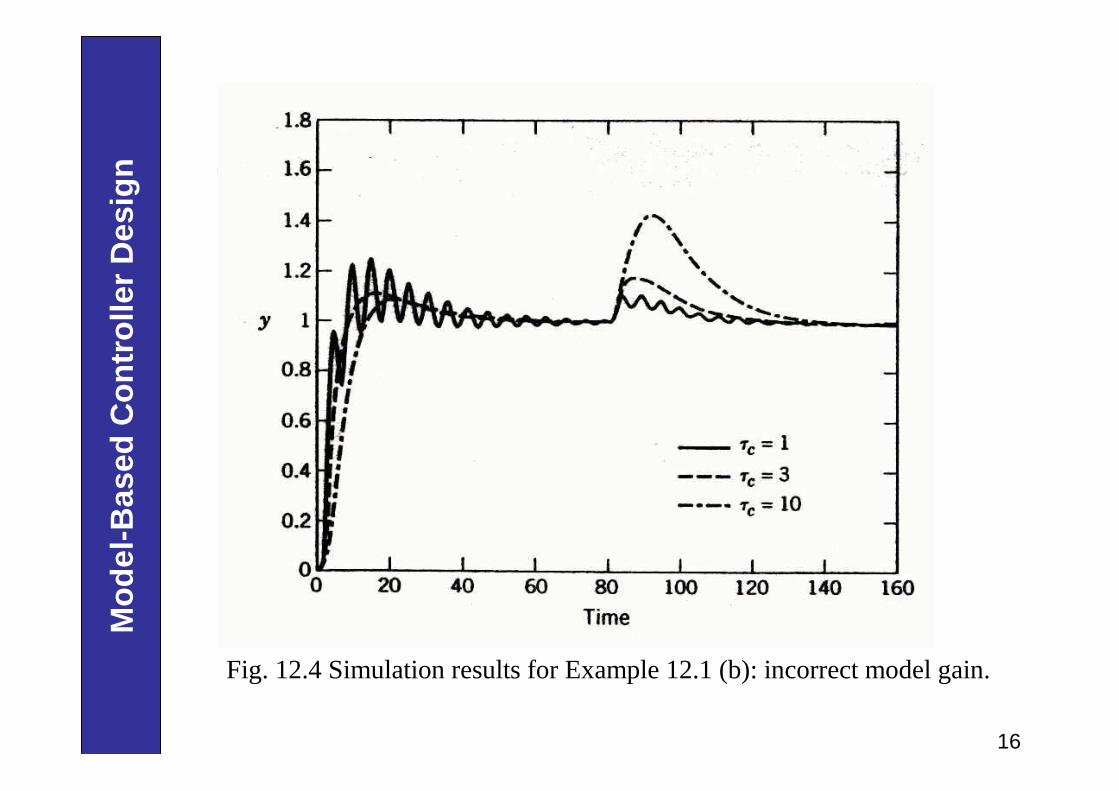
Fig. 12.4 Simulation results for Example 12.1 (b): incorrect model gain.

17
Mo
del
-Bas
ed C
on
tro
ller
Des
ign
DS - Remark• The specification of the desired closed-loop transfer
function, , should be based on the assumed process model, as well as the desired set-point response.
• The FOPTD model is a reasonable choice for many processes but not all.
• For example, if the process model contains a RHP zero , we must specify
• The DS approach should not be used directly for process models with unstable poles.
( )sp dY Y
( )1 asτ−
( ) θ1(12-15)
τ 1
sa
sp cd
s eY
Y s
τ − −= +
18
Mo
del
-Bas
ed C
on
tro
ller
Des
ign
Internal Model Control (IMC)• A more comprehensive model-based design method, Internal
Model Control (IMC), was developed by Morari and coworkers (Garcia and Morari, 1982; Rivera et al., 1986).
• The IMC method, like the DS method, is based on an assumed process model and leads to analytical expressions for the controller settings.
• These two design methods are closely related and produce identical controllers if the design parameters are specified in a consistent manner.
• The IMC method is based on the simplified block diagram shown in Fig. 12.6b. A process model and the controller output P are used to calculate the model response, .
Gɶ
Yɶ

19
Mo
del
-Bas
ed C
on
tro
ller
Des
ign
• The model response is subtracted from the actual response Y, and the difference, is used as the input signal to the IMC controller, .
• In general, due to modeling errors and unknown disturbances that are not accounted for in the model.
• The block diagrams for conventional feedback control and IMC are compared in Fig. 12.6.
Y Y− ɶ*cG
Y Y≠ ɶ ( )G G≠ɶ( )0D ≠
Figure 12.6. Feedback control strategies
20
Mo
del
-Bas
ed C
on
tro
ller
Des
ign
*cG
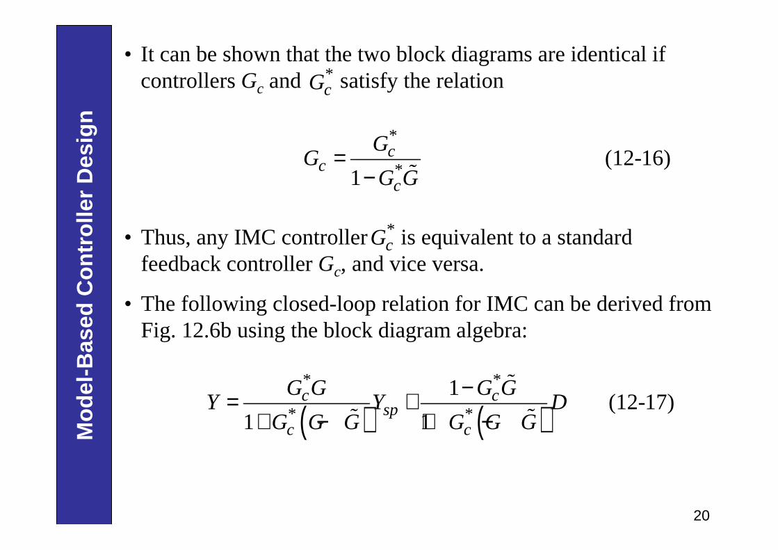
*
*(12-16)
1c
cc
GG
G G=
− ɶ
• Thus, any IMC controller is equivalent to a standard feedback controller Gc, and vice versa.
• The following closed-loop relation for IMC can be derived from Fig. 12.6b using the block diagram algebra:
*cG
( ) ( )* *
* *
1(12-17)
1 1c c
spc c
G G G GY Y D
G G G G G G
−= ++ − + −
ɶ
ɶ ɶ
• It can be shown that the two block diagrams are identical if controllers Gc and satisfy the relation

21
Mo
del
-Bas
ed C
on
tro
ller
Des
ign
For the special case of a perfect model, , (12-17) reduces toG G=ɶ
( )* *1 (12-18)c sp cY G GY G G D= + −
The IMC controller is designed in two steps:
Step 1. The process model is factored as
(12-19)G G G+ −=ɶ ɶ ɶ
where contains any time delays and right-half plane zeros.
• In addition, is required to have a steady-state gain equal to one in order to ensure that the two factors in Eq. 12-19 are unique.
G+ɶ
G+ɶ
22
Mo
del
-Bas
ed C
on
tro
ller
Des
ign
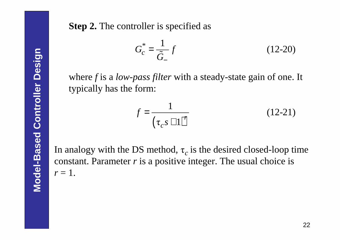
Step 2. The controller is specified as
* 1(12-20)cG f
G−=ɶ
where f is a low-pass filter with a steady-state gain of one. It typically has the form:
( )1
(12-21)τ 1
rc
fs
=+
In analogy with the DS method, is the desired closed-loop time constant. Parameter r is a positive integer. The usual choice is r = 1.
τc
23
Mo
del
-Bas
ed C
on
tro
ller
Des
ign
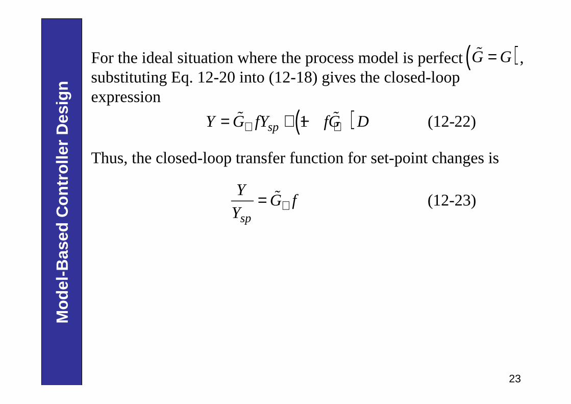
For the ideal situation where the process model is perfect , substituting Eq. 12-20 into (12-18) gives the closed-loop expression
( )G G=ɶ
( )1 (12-22)spY G fY fG D+ += + −ɶ ɶ
Thus, the closed-loop transfer function for set-point changes is
(12-23)sp
YG f
Y += ɶ
24
Mo
del
-Bas
ed C
on
tro
ller
Des
ign
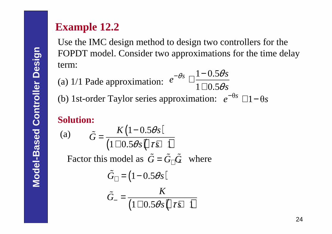
Solution:
(a)
Factor this model as where
( )( )( )
1 0.5
1 0.5 1
K sG
s s
θθ τ−
=+ +
ɶ
( )1 0.5G sθ+ = −ɶ
Example 12.2Use the IMC design method to design two controllers for the FOPDT model. Consider two approximations for the time delay term:
(a) 1/1 Pade approximation:
(b) 1st-order Taylor series approximation:
1 0.5
1 0.5s s
es
θ θθ
− −≅+
θ 1 θse s− ≅ −
G G G+ −=ɶ ɶ ɶ
( )( )1 0.5 1
KG
s sθ τ− =+ +
ɶ
25
Mo
del
-Bas
ed C
on
tro
ller
Des
ign
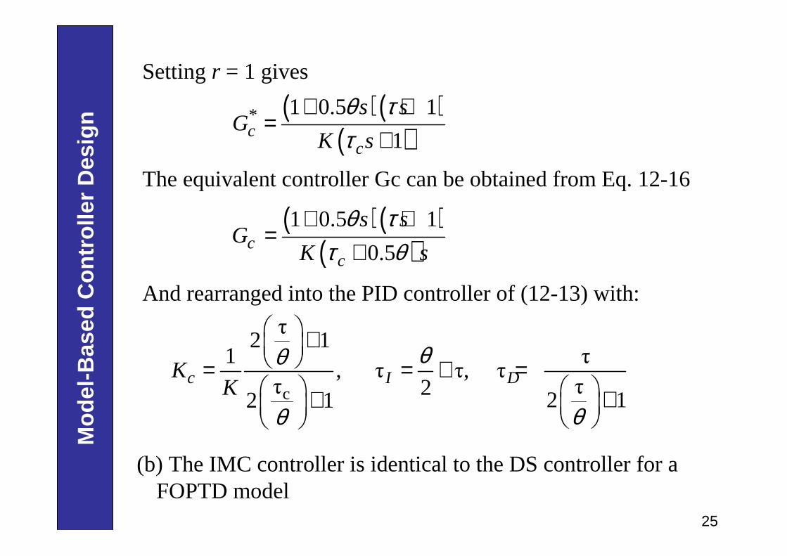
Setting r = 1 gives
The equivalent controller Gc can be obtained from Eq. 12-16
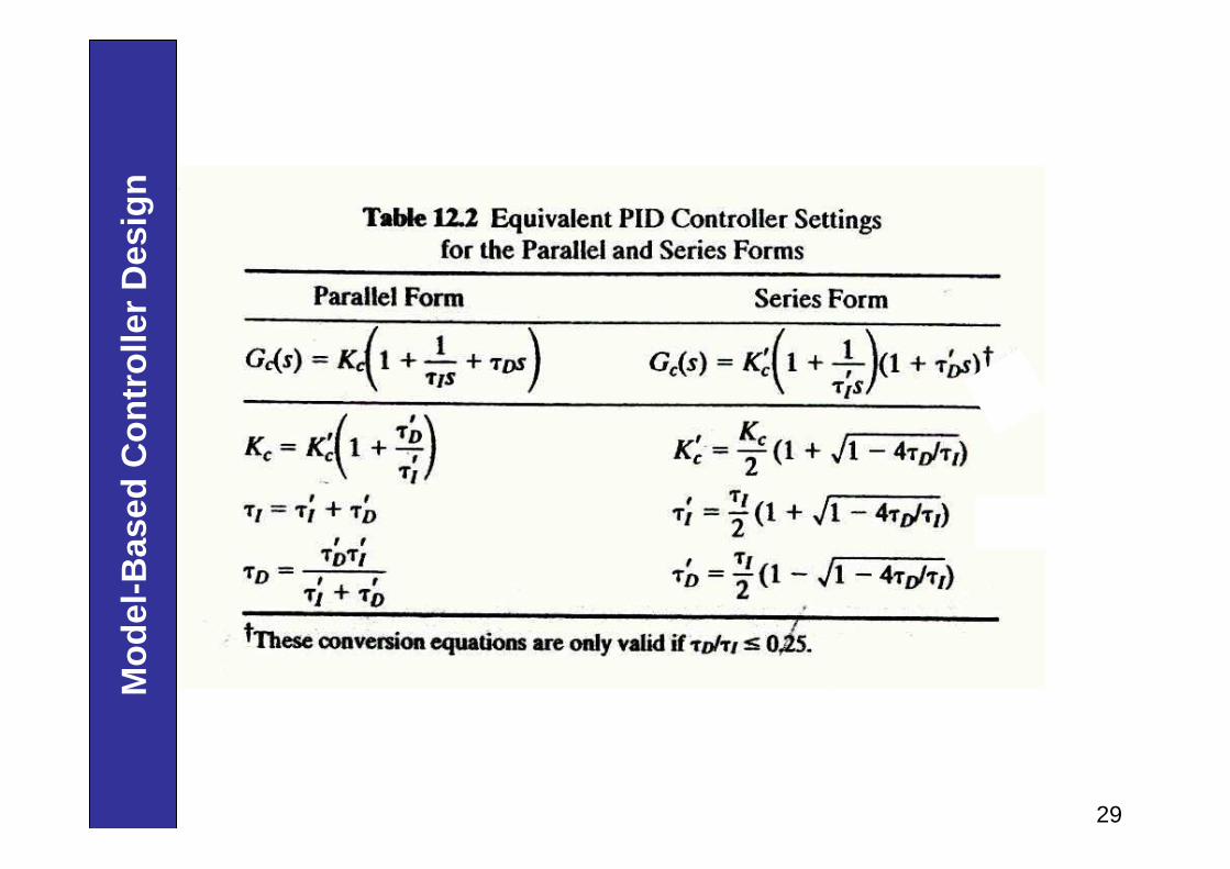
And rearranged into the PID controller of (12-13) with:
( )( )( )
* 1 0.5 1
1cc
s sG
K s
θ ττ
+ +=
+
( )( )( )
1 0.5 1
0.5cc
s sG
K s
θ ττ θ
+ +=
+
c
τ2 1
1 τ, τ τ, τ
τ τ2 2 12 1c I DK
K
θθ
θθ
+ = = + = ++
(b) The IMC controller is identical to the DS controller for a FOPTD model
26
Mo
del
-Bas
ed C
on
tro
ller
Des
ign
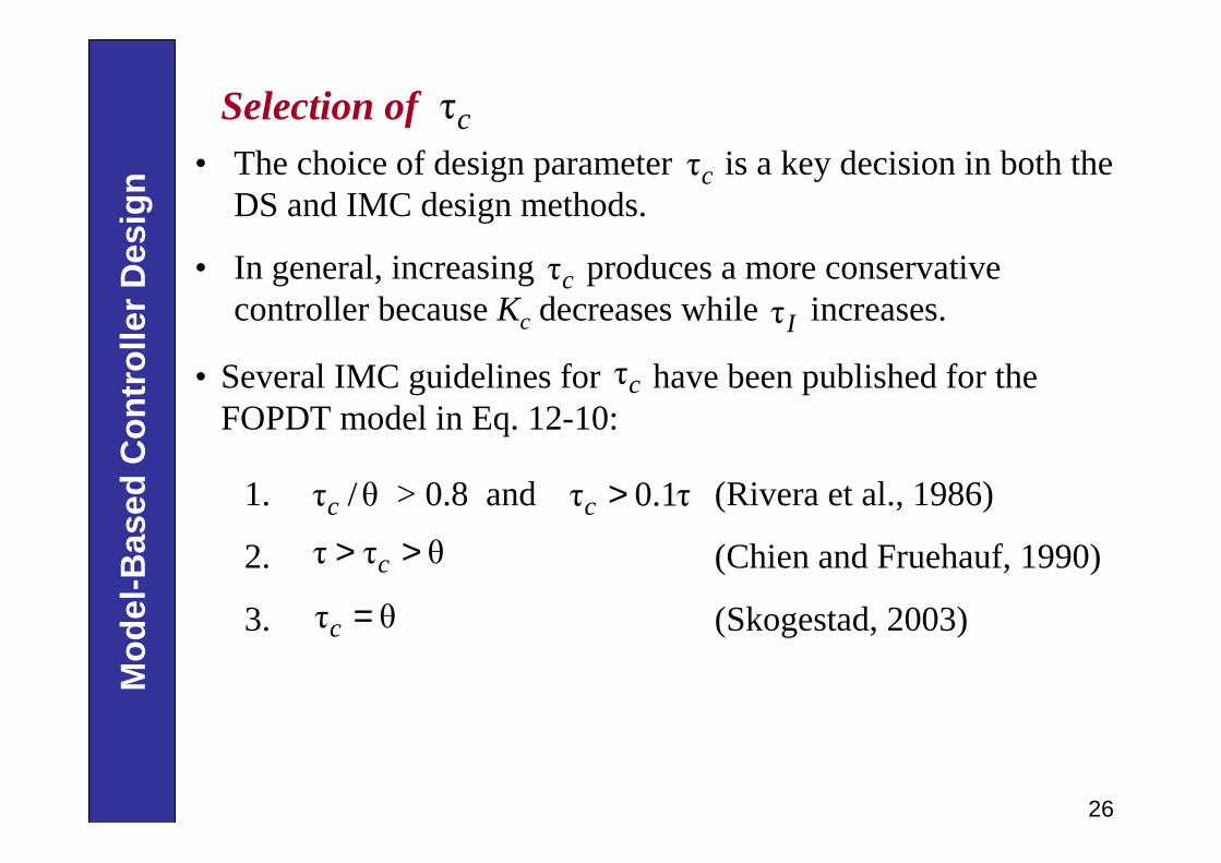
1. > 0.8 and (Rivera et al., 1986)
2. (Chien and Fruehauf, 1990)
3. (Skogestad, 2003)
τ /θc τ 0.1τc >
τ τ θc> >
τ θc =
• Several IMC guidelines for have been published for the FOPDT model in Eq. 12-10:
τc
Selection of τc
• The choice of design parameter is a key decision in both the DS and IMC design methods.
• In general, increasing produces a more conservative controller because Kc decreases while increases.
τc
τcτI
27
Mo
del
-Bas
ed C
on
tro
ller
Des
ign
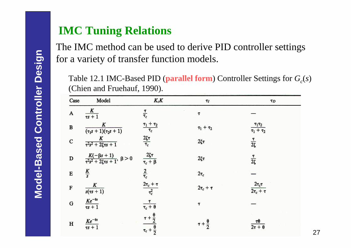
IMC Tuning RelationsThe IMC method can be used to derive PID controller settings for a variety of transfer function models.
Table 12.1 IMC-Based PID (parallel form) Controller Settings for Gc(s) (Chien and Fruehauf, 1990).

28
Mo
del
-Bas
ed C
on
tro
ller
Des
ign
Table 12.1 (Continued).
29
Mo
del
-Bas
ed C
on
tro
ller
Des
ign

30
Mo
del
-Bas
ed C
on
tro
ller
Des
ign
Tuning for Lag-Dominant Models
• First- or second-order models with relatively small time delays are referred to as lag-dominant models.
• The IMC and DS methods provide satisfactory set-point responses, but very slow disturbance responses, because the value of is very large.
• Fortunately, this problem can be solved in three different ways.
Method 1: Integrator approximation
τI
( )θ / τ 1≪
*
*
Approximate ( ) by ( )1
where / .
s sKe K eG s G s
s s
K K
−θ −θ= =
τ +τ
ɶ ɶ
≜
• Then can use the IMC tuning rules (Rule M or N) to specify the controller settings.
31
Mo
del
-Bas
ed C
on
tro
ller
Des
ign
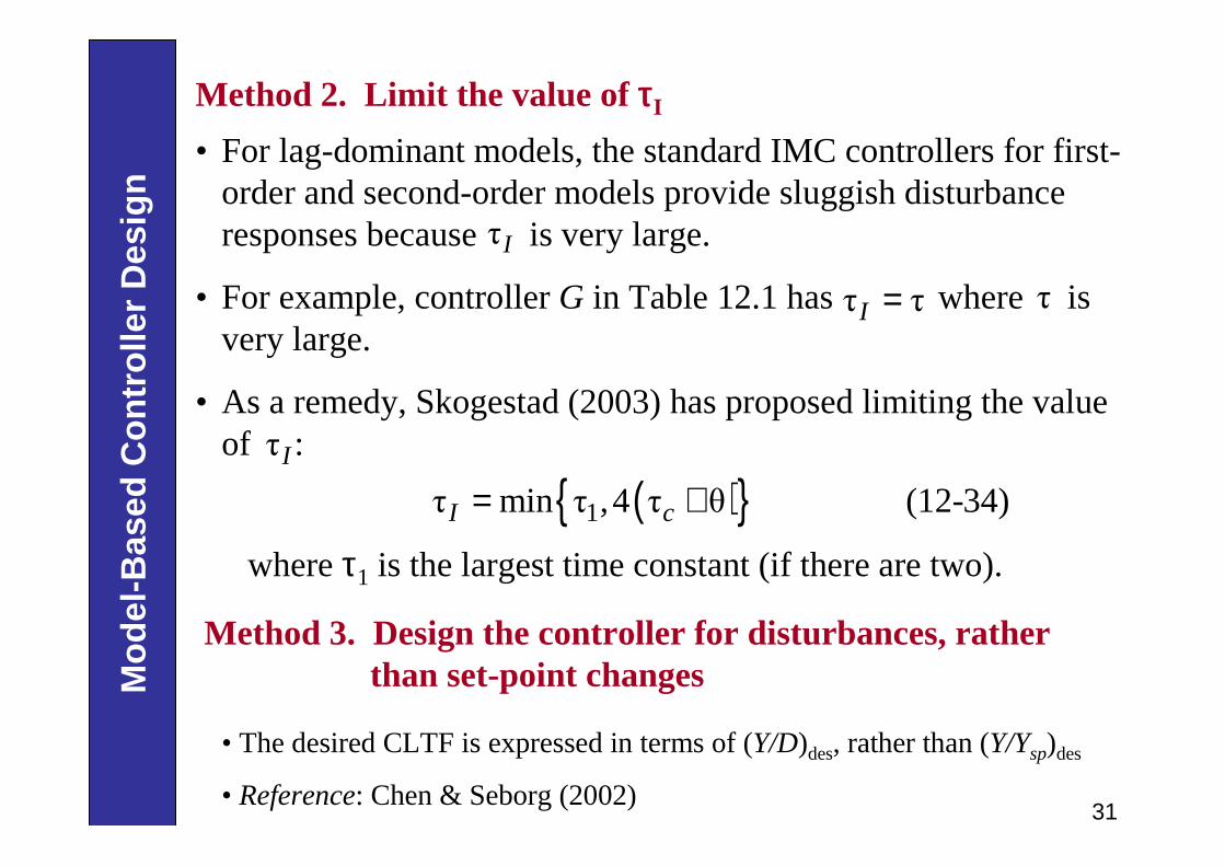
Method 2. Limit the value of ττττI
• For lag-dominant models, the standard IMC controllers for first-order and second-order models provide sluggish disturbance responses because is very large.
• For example, controller G in Table 12.1 has where is very large.
• As a remedy, Skogestad (2003) has proposed limiting the value of :
( ){ }1τ min τ ,4 τ θ (12-34)I c= +
τI
τ τI = τ
τI
whereτ1 is the largest time constant (if there are two).
Method 3. Design the controller for disturbances, rather than set-point changes
• The desired CLTF is expressed in terms of (Y/D)des, rather than (Y/Ysp)des
• Reference: Chen & Seborg (2002)
32
Mo
del
-Bas
ed C
on
tro
ller
Des
ign
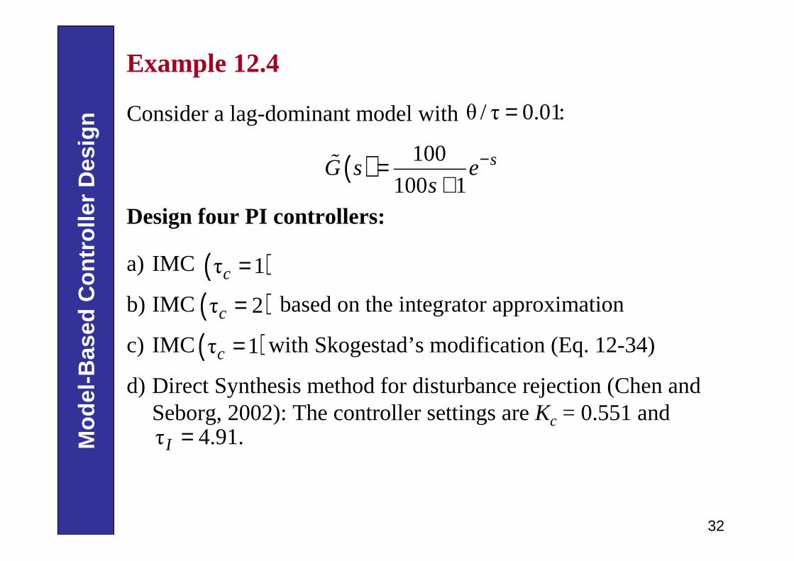
Example 12.4
Consider a lag-dominant model with θ / τ 0.01:=
( ) 100
100 1sG s e
s−=
+ɶ
Design four PI controllers:
a) IMC
b) IMC based on the integrator approximation
c) IMC with Skogestad’s modification (Eq. 12-34)
d) Direct Synthesis method for disturbance rejection (Chen and Seborg, 2002): The controller settings are Kc = 0.551 and
( )τ 1c =
( )τ 2c =
( )τ 1c =
τ 4.91.I =
33
Mo
del
-Bas
ed C
on
tro
ller
Des
ign
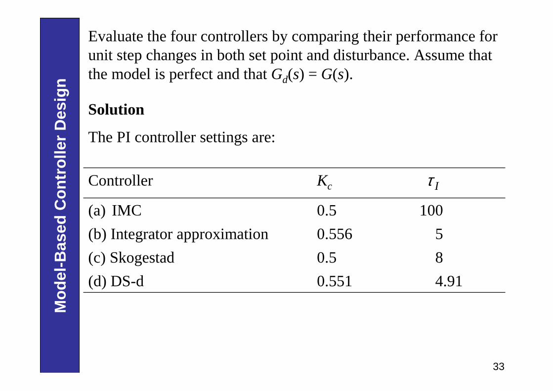
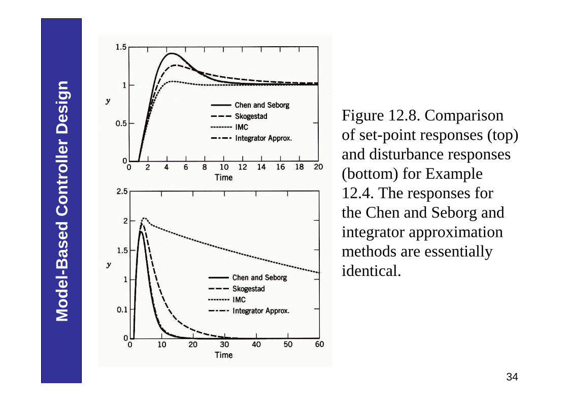
Evaluate the four controllers by comparing their performance forunit step changes in both set point and disturbance. Assume thatthe model is perfect and that Gd(s) = G(s).
Solution
The PI controller settings are:
4.910.551(d) DS-d
80.5(c) Skogestad
50.556(b) Integrator approximation
1000.5(a) IMC
KcController Iτ
34
Mo
del
-Bas
ed C
on
tro
ller
Des
ign
Figure 12.8. Comparison of set-point responses (top) and disturbance responses (bottom) for Example 12.4. The responses for the Chen and Seborg and integrator approximation methods are essentially identical.
35
Mo
del
-Bas
ed C
on
tro
ller
Des
ign
Controllers With Two Degrees of Freedom
• The specification of controller settings for a standard PID controller typically requires a tradeoff between set-point tracking and disturbance rejection.
• The strategies which can be used to adjust the set-point and disturbance independently are referred to as controllers with two-degrees-of-freedom.
• The first strategy is very simple. Set-point changes are introduced gradually rather than as abrupt step changes.
• For example, the set point can be ramped as shown in Fig. 12.10 or “filtered” by passing it through a first-order transfer function,
*1
(12-38)τ 1
sp
sp f
Y
Y s=
+
36
Mo
del
-Bas
ed C
on
tro
ller
Des
ign
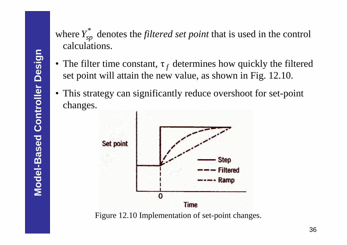
where denotes the filtered set point that is used in the control calculations.
• The filter time constant, determines how quickly the filtered set point will attain the new value, as shown in Fig. 12.10.
• This strategy can significantly reduce overshoot for set-point changes.
*spY
τ f
Figure 12.10 Implementation of set-point changes.
37
Mo
del
-Bas
ed C
on
tro
ller
Des
ign
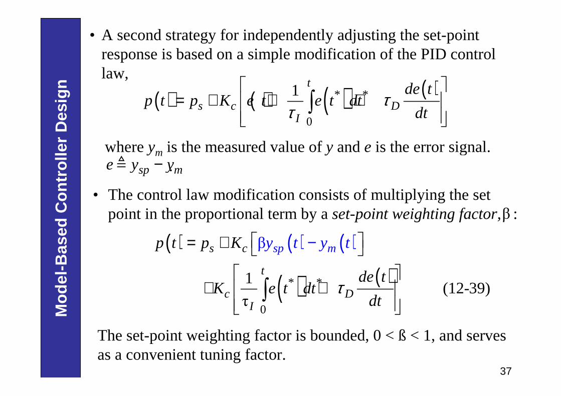
• A second strategy for independently adjusting the set-point response is based on a simple modification of the PID control law,
( ) ( ) ( ) ( )* *
0
1t
s c DI
de tp t p K e t e t dt
dtτ
τ
= + + +
∫
where ym is the measured value of y and e is the error signal. .
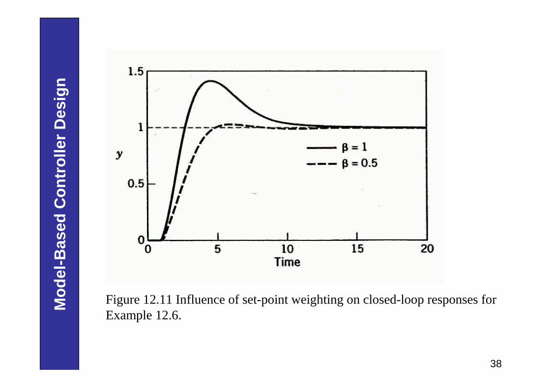
• The control law modification consists of multiplying the set point in the proportional term by a set-point weighting factor, :
sp me y y−≜
β
( ) ( ) ( )
( ) ( )* *
0
1(12
τ
β
-39)
sp ms c
t
c DI
p t p K
de tK e t d
t
tt
y t y
dτ
= +
+ +
−
∫
The set-point weighting factor is bounded, 0 < ß < 1, and serves as a convenient tuning factor.
38
Mo
del
-Bas
ed C
on
tro
ller
Des
ign
Figure 12.11 Influence of set-point weighting on closed-loop responses for Example 12.6.
39
Mo
del
-Bas
ed C
on
tro
ller
Des
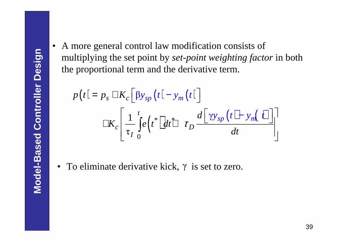
ign • A more general control law modification consists of
multiplying the set point by set-point weighting factor in both the proportional term and the derivative term.
( ) ( ) ( )
( ) ( ) ( )* *
0
β
γ1
τ
s c
t
c DI
sp m
sp m
p t p K
dK e t dt
y t y t
y t y
t
t
dτ
= +
+ +
−
−∫
• To eliminate derivative kick, is set to zero.γ