Generalized approach to resolution analysis in BSAR

Generalized Approach toResolution Analysis in BSAR

TAO ZENGBeijing Institute of Technology

MIKHAIL CHERNIAKOVUniversity of BirminghamUK

TENG LONGBeijing Institute of Technology

Bistatic synthetic aperture radars (BSARs) have been

the focus of increasing research activity over the last decade.

The generalized ambiguity function (GAF) of bistatic SAR

is introduced here. First, the GAF for BSAR is represented

in the delay-Doppler domain, and is then expanded to the

spatial (coordinates) domain. From the GAF, comprehensive

knowledge regarding the resolution of BSAR can be extracted,

including the range and azimuth resolutions, as well as the

area of a resolution cell of BSAR. These general results are also

applied to the performance analysis of several particular BSAR

geometries, including the space-surface-BSAR (SS-BSAR) system,

to demonstrate the potential ability of this newly introduced

system.

Manuscript received October 20, 2003; revised August 24, 2004;released for publication December 27, 2004.

IEEE Log No. T-AES/41/2/849013.

Refereeing of this contribution was handled by P. Lombardo.

Part of this work was supported by EPSRC (UK) under GrantGR/S69221/01.

Authors’ addresses: T. Zeng and T. Long, Dept. of ElectricalEngineering, Beijing Institute of Technology, Dept. EE 551 Lab,No. 5 Zhongg uancun, Nandajie, PO Box 327, Beijing 10081,China, E-mail: ([email protected]); M. Cherniakov, Universityof Birmingham, Communications Engineering Group, Edgbaston,Birmingham, B15 2TT, UK.

0018-9251/05/$17.00 c° 2005 IEEE

NOMENCLATURE

fc Carrier frequencyhA(t,u) Returned signalsmA(fd) Inverse Fourier transform of M̄A(u)p(¿d) Inverse Fourier transform of P̄(f)s(t) Complex envelope of transmitted

signalt,u Fast and slow timeuA Slow time instant which

maximizes MA(u)G0T(A,u), G

0R(A,u) Gain of the antenna

GT(:), GR(:) Antennas’ radiation patternMA(u) Power ratio between received and

transmitted signalsP(f) Power spectrum of ranging signalWR, WT Position vectors of transmitter

and receiverVR, VT Velocity vectors of transmitter

and receiver¿d Differential delay¿A(u) Time delay of received signal at

slow time ufd Differential Doppler frequencyP̄(f) Normalized ranging signal power

spectrumM̄A(u) Normalized received signal

magnitude pattern® Angle between £ and ¥¯ Bistatic angle±¿ Delay resolution±D Doppler resolution±r Range resolution±a Azimuth resolution±c Cross range resolution±− Resolution in direction of −±f ¡3 dB widths of P̄(f)±u ¡3 dB widths of M̄A(u)µ¿ Angle between − and £µa Angle between − and ¥!TA, !RA Angular speeds of transmitter and

receiver!E Equivalent angular speed¡T, ¡R Directions of effective velocitiesH Unit vector which is

perpendicular to both vectors £and Nb

£ Direction of bisector of bistaticangle

Nb Unit vector in direction of normalline to basic plane

¥ Direction of equivalent motion©TA, ©RA Unit vector in direction of line of

sight.

IEEE TRANSACTIONS ON AEROSPACE AND ELECTRONIC SYSTEMS VOL. 41, NO. 2 APRIL 2005 461

I. INTRODUCTION

Bistatic synthetic aperture radars (BSARs)have been the focus of increasing research activityover the last decade. This reflects the progress insynthetic aperture radar (SAR) technology, bothhardware and software, satellite positioning systemsthat allow synchronising BSAR subsystems, aswell as achievements in aerospace technology. Theengine behind this is a strong demand for the furtherimprovement in the performance of microwave remotesensing systems, and it is expected that the practicalutilisation of BSARs will respond to this demand[1]. BSAR can be used to obtain essentially newinformation regarding land and ocean surfaces [2],operate as the remote change detectors to predictnatural disasters [3], effectively use noncooperativetransmitters that reduce system costs [4], or similarlyact as an auxiliary subsystem to existing monostaticSARs [5].One of the key parameters of any remote sensing

system is the spatial resolution. In traditional radarsystems, comprehensive knowledge regarding theresolution can be obtained from the ambiguityfunction (AF) analysis [6], in terms of delay (range)and Doppler frequency (speed). Definition of ageneralized AF (GAF) was expanded in spatialresolution in SAR [7]. Similarly, in the SAR systemanalysis the point spread function (PSF) is used tocharacterize spatial resolution [8]. The GAF is usedhere for BSAR analysis to unify the approach betweentraditional aperture radars and SARs.The basic information regarding bistatic radar

can be found in classic texts [9]. If the transmitterand the receiver are stationary or following paralleltrajectories during the coherent integration time, theycan be considered as a space (time)-invariant system.Meanwhile, there are a number of new forthcomingresearches in BSAR [1, 4, 10, 11], along with others,in which the transmitter and the receiver have theirown nonparallel trajectories. From the point of viewof system analysis, this means that BSAR are nolonger space (time)-invariant systems. Their resolutionessentially depends on the observation time instantand space-variant analysis should be considered inevaluating BSAR spatial resolution.In [9], the resolution issue of BSAR is studied

in two-dimensional space, which is a relativelysimple case of BSAR geometry. In [12], several ofthe resolution equations have been researched viathe use of gradient analysis. These equations cancover the general BSAR geometry, but only applyto the rectangular spectrum shape of the rangingsignal. In order to achieve a comprehensive insightinto the problem of spatial resolution analysis, amore generalized approach is needed. The resolutionanalysis is carried out here via an introductionof BSAR spatial GAFs. This general approach

is applicable for BSAR with essentially differentconfigurations and can obtain the resolution in anarbitrary direction. The AF for the ground-basedbistatic radar has been brought forward in [21].Because of the significant difference between thegeometry of the groundbased bistatic radar and thatof BSAR, the AF introduced in [21] is quite differentfrom the AF in this work. For example, the formeris established on the delay-velocity plane, while thelatter is on the x-y-z coordinate system. Besides theresolution in a given line, the area of the resolutioncell can also be found via the AF. The resolution cellarea is a good parameter to show the resolvabilityof a system, but up until now only a few papershave discussed this issue. One such paper is [22].Unfortunately, the results of [22] are not applicableto BSAR, because the resolution cell area dependsdirectly on the widths of the antenna lobes of theradar system.In this paper, the GAF for BSAR is first

represented in the delay-Doppler domain, and thenexpanded to the spatial (coordinates) domain. Usingthis spatial presentation of GAF the range andazimuth resolution, as well as a resolution cell areaare considered relevant to different directions andcoordinate systems. Finally, obtained equations areapplied to the resolution analysis in space-surfaceBSAR (SS-BSAR).

II. AMBIGUITY FUNCTION OF BSAR

A. BSAR System Geometry

The generalized topology of BSAR is shown inFig. 1. Vectors WR, WT are the position vectors of thetransmitter and receiver respectively in the rectangularcoordinate xyz; VR, VT are their velocity vectors(they are assumed constant here), A is a vector whichspecifies an arbitrary position in the target area, andWT¡A (or WR¡A) are called the transmitter (orreceiver) line of sight.As the first step in evaluating the radar’s

resolution, we describe a received signal model inBSAR. Despite the fact that the transmitter and thereceiver possess a continuous motion, in practicalsituations the stop-and-go approach [8] can be usedfor SAR analysis, namely, during the ranging signalpropagation along the transmitter-target-receiverpath, the transmitter and receiver are assumed to bestationary, a radar measurement is made, and thenthey move to the next spatial positions. Accordingto this assumption, the received signal is modeled asa function of two variables. One variable is the fasttime t, which describes the ranging waveform and itspropagation. The second variable u is the slow time,which specifies the position of the transmitter and thereceiver. The term “slow time” comes from the factthat the motions of the transmitter and receiver are

462 IEEE TRANSACTIONS ON AEROSPACE AND ELECTRONIC SYSTEMS VOL. 41, NO. 2 APRIL 2005

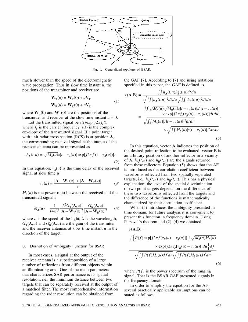
Fig. 1. Generalized topology of BSAR.

much slower than the speed of the electromagneticwave propagation. Thus in slow time instant u, thepositions of the transmitter and receiver are

WT(u) =WT(0)+ uVT

WR(u) =WR(0)+ uVR(1)

where WR(0) and WT(0) are the positions of thetransmitter and receiver at the slow time instant u= 0.Let the transmitted signal be s(t)exp(j2¼fct),

where fc is the carrier frequency, s(t) is the complexenvelope of the transmitted signal. If a point targetwith unit radar cross section (RCS) is at position A,the corresponding received signal at the output of thereceiver antenna can be represented as

hA(t,u) =pMA(u)s[t¡ ¿A(u)]exp[j2¼fc(t¡ ¿A(u))]:

(2)

In this equation, ¿A(u) is the time delay of the receivedsignal at slow time u

¿A(u) =jA¡WT(u)j+ jA¡WR(u)j

c(3)

MA(u) is the power ratio between the received and thetransmitted signals:

MA(u) =1

(4¼)3¸2G0T(A,u)jA¡WT(u)j2

G0R(A,u)jA¡WR(u)j2

(4)

where c is the speed of the light, ¸ is the wavelength,G0T(A,u) and G

0R(A,u) are the gain of the transmitter

and the receiver antennas at slow time instant u in thedirection of the target.

B. Derivation of Ambiguity Function for BSAR

In most cases, a signal at the output of thereceiver antenna is a superimposition of a largenumber of reflections from different objects withinan illuminating area. One of the main parametersthat characterizes SAR performance is its spatialresolution, i.e., the minimum distance between twotargets that can be separately received at the output ofa matched filter. The most comprehensive informationregarding the radar resolution can be obtained from

the GAF [7]. According to [7] and using notationsspecified in this paper, the GAF is defined as

Â(A,B) =RRhA(t,u)h

¤B(t,u)dtduqRR jhA(t,u)j2dtduqRR jhB(t,u)j2dtdu

=

RR pMA(u)

pMB(u)s[t¡ ¿A(u)]s¤[t¡ ¿B(u)]

£exp[j2¼fc(¿B(u)¡ ¿A(u))]dtduqRRMA(u)js[t¡ ¿A(u)]j2dtdu

£qRR

MB(u)js[t¡ ¿B(u)]j2dtdu

:

(5)

In this equation, vector A indicates the position ofthe desired point reflection to be evaluated, vector B isan arbitrary position of another reflector in a vicinityof A. hA(t,u) and hB(t,u) are the signals returnedfrom these reflectors. Equation (5) shows that the AFis introduced as the correlation coefficient betweenwaveforms reflected from two spatially separatedtargets, i.e., hA(t,u) and hB(t,u). This has a physicalexplanation: the level of the spatial discriminationof two point targets depends on the difference ofthese two waveforms reflected from the targets andthe difference of the functions is mathematicallycharacterized by their correlation coefficient.When (5) introduces the ambiguity presented in

time domain, for future analysis it is convenient topresent this function in frequency domain. UsingParseval’s theorem and (2)—(4) we obtained

Â(A,B) =R nP(f)exp[j2¼f[¿B(u)¡ ¿A(u)]]

R pMA(u)MB(u)

£exp[j2¼fc[¿B(u)¡ ¿A(u)]]duodfqRR

P(f)MA(u)df duqRR

P(f)MB(u)df du

(6)

where P(f) is the power spectrum of the rangingsignal. That is the BSAR GAF presented signals inthe frequency domain.In order to simplify the equation for the AF,

several practically applicable assumptions can bestated as follows.

ZENG ET AL.: GENERALIZED APPROACH TO RESOLUTION ANALYSIS IN BSAR 463

1) Power of signals reflected from targets A andB are approximately equal: MB(u)¼MA(u). Thisassumption follows on from the definition of theGAF: the targets have unit RCS and the correlationanalysis is specified in a vicinity of A, consequentlywe can assumes the targets are illuminated by thesame antenna patterns.2) The synthetic aperture is narrow. Denoting

the slow time instant which maximizes MA(u)as uA and the ¡3 dB width of MA(u) as ±u, i.e.,M¡uA¡ (±u=2)

¢= (12 )M(uA). The synthetic aperture is

narrow means that VT±u¿WT(uA) and VR±u¿WR(uA),i.e., the lengths of the synthetic apertures are muchsmaller than the lengths of the line of sight at theslow time instant uA. Due to this assumption, thephase term of the inner folder integral in (6) can beapproximated by its first-order Taylor expansion atu= uA

2¼fc[¿B(u)¡ ¿A(u)]¼ 2¼fc¿d+2¼fd(u¡uA): (7)

In this equation, ¿d is the delay difference between thetwo signals when u= uA

¿d =jB¡WT(uA)j+ jB¡WR(uA)j

c

¡ jA¡WT(uA)j+ jA¡WR(uA)jc

(8)

and fd is the difference of the Doppler frequencybetween these two signals at uA

fd =fcc

·VTT

B¡WT(uA)jB¡WT(uA)j

+VTR

B¡WR(uA)jB¡WR(uA)j

¸¡ fcc

·VT

T

A¡WT(uA)jA¡WT(uA)j

+VTR

A¡WR(uA)jA¡WR(uA)j

¸:

(9)

3) The ranging signal is narrowband. Denoting the¡3 dB width of P(f) as ±f , then ±f should be smallenough so that the phase term of the outer folderintegral in (6) can be approximated by the phase atslow time uA:

2¼f[¿B(u)¡ ¿A(u)]¼ 2¼f¿d: (10)

In order to guarantee (10) to be a goodapproximation, the ¡3 dB bandwidth ranging signal±f must satisfy the condition:

±f <1

2j[¿B(u)¡ ¿A(u)]¡ ¿dj

for all u in the interval ju¡ uAj< 12±u: (11)

The time resolution is the reciprocal signalbandwidth, hence the physical meaning of (11) is thatin the slow time interval ju¡ uAj< 1

2±u, the change ofthe delay difference should not exceed half of the timeresolution cell.

Due to these approximations, (6) can be reduced as

Â(A,B) = exp(j2¼fc¿d)Z 1

¡1P̄(f)exp(j2¼f¿d)df

£Z 1

¡1M̄A(u)exp(j2¼fdu)du

= exp(j2¼fc¿d)p(¿d)mA(fd) (12)

where P̄(f) = (P(f)=R1¡1P(f)df) and M̄A(u) =

(MA(u+ uA)=R1¡1MA(u+ uA)du) are the normalized

ranging signal power spectrum and the normalizedreceived signal magnitude pattern, p(¿d) is the inverseFourier transform (IFT) of P̄(f), and mA(fd) the IFTof M̄A(u).Equation (12) indicates that the amplitude of the

AF is presented as the product of two functions. Thefirst one is the IFT of the signal power spectrum,hence it is the autocorrelation function of the rangingsignal and specifies the SAR delay resolution. Thesecond term mA(fd) is the IFT of the normalizedreceived signal magnitude pattern and responsible forthe Doppler resolution. For a particular BSAR, P̄(f)and M̄A(u) are known, and the AF can be found byapplying the IFT to these functions. In many practicalcases these transforms can be obtained from Fouriertransform tables [14] and consequently the ¡3 dBwidths of the system’s delay (±¿ ) and Doppler (±D)resolution cells can be calculated by

±¿ = 2p¡1·p(0)p2

¸±D = 2m

¡1A

·mA(0)p2

¸ (13)

where p¡1(:) and m¡1A (:) are the inverse functions ofp(:) and mA(:).For the sake of solidity, but without loss of

generality, we consider two typical cases, namely,when antenna patterns and ranging waveform canbe approximated by a Gaussian or rectangle shapefunctions. IFTs of these functions are shown inTable I, where

sinc(x) =sinxx: (14)

In the case of the Gaussian model, the resolutions canbe found directly from (13):

±¿ =2ln2¼±f

±D =2ln2¼±u

(15)

where ±f and ±u are the ¡3 dB widths of P̄(f) andM̄A(u).In the rectangular model, the inverse function

cannot be expressed in closed form, but accordingto the scaling property of the Fourier transform


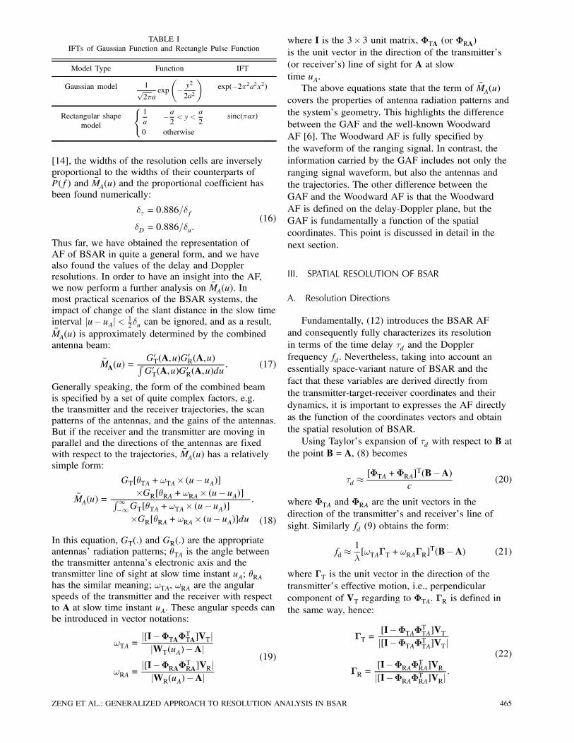
TABLE IIFTs of Gaussian Function and Rectangle Pulse Function

Model Type Function IFT

Gaussian model 1p2¼a

exp

µ¡ y2

2a2

¶exp(¡2¼2a2x2)

Rectangular shapemodel

(1a

¡ a2< y <

a

20 otherwise

sinc(¼ax)

[14], the widths of the resolution cells are inverselyproportional to the widths of their counterparts ofP̄(f) and M̄A(u) and the proportional coefficient hasbeen found numerically:

±¿ = 0:886=±f

±D = 0:886=±u:(16)

Thus far, we have obtained the representation ofAF of BSAR in quite a general form, and we havealso found the values of the delay and Dopplerresolutions. In order to have an insight into the AF,we now perform a further analysis on M̄A(u). Inmost practical scenarios of the BSAR systems, theimpact of change of the slant distance in the slow timeinterval ju¡ uAj< 1

2±u can be ignored, and as a result,M̄A(u) is approximately determined by the combinedantenna beam:

M̄A(u) =G0T(A,u)G

0R(A,u)R

G0T(A,u)G0R(A,u)du

: (17)

Generally speaking, the form of the combined beamis specified by a set of quite complex factors, e.g.the transmitter and the receiver trajectories, the scanpatterns of the antennas, and the gains of the antennas.But if the receiver and the transmitter are moving inparallel and the directions of the antennas are fixedwith respect to the trajectories, M̄A(u) has a relativelysimple form:

M̄A(u) =

GT[µTA+!TA£ (u¡ uA)]£GR[µRA+!RA£ (u¡ uA)]R1

¡1GT[µTA+!TA£ (u¡ uA)]£GR[µRA+!RA£ (u¡ uA)]du

:

(18)

In this equation, GT(:) and GR(:) are the appropriateantennas’ radiation patterns; µTA is the angle betweenthe transmitter antenna’s electronic axis and thetransmitter line of sight at slow time instant uA; µRAhas the similar meaning; !TA, !RA are the angularspeeds of the transmitter and the receiver with respectto A at slow time instant uA. These angular speeds canbe introduced in vector notations:

!TA =j[I¡©TA©TTA]VTjjWT(uA)¡Aj

!RA =j[I¡©RA©TRA]VRjjWR(uA)¡Aj

(19)

where I is the 3£ 3 unit matrix, ©TA (or ©RA)is the unit vector in the direction of the transmitter’s(or receiver’s) line of sight for A at slowtime uA.The above equations state that the term of M̄A(u)

covers the properties of antenna radiation patterns andthe system’s geometry. This highlights the differencebetween the GAF and the well-known WoodwardAF [6]. The Woodward AF is fully specified bythe waveform of the ranging signal. In contrast, theinformation carried by the GAF includes not only theranging signal waveform, but also the antennas andthe trajectories. The other difference between theGAF and the Woodward AF is that the WoodwardAF is defined on the delay-Doppler plane, but theGAF is fundamentally a function of the spatialcoordinates. This point is discussed in detail in thenext section.

III. SPATIAL RESOLUTION OF BSAR

A. Resolution Directions

Fundamentally, (12) introduces the BSAR AFand consequently fully characterizes its resolutionin terms of the time delay ¿d and the Dopplerfrequency fd. Nevertheless, taking into account anessentially space-variant nature of BSAR and thefact that these variables are derived directly fromthe transmitter-target-receiver coordinates and theirdynamics, it is important to expresses the AF directlyas the function of the coordinates vectors and obtainthe spatial resolution of BSAR.Using Taylor’s expansion of ¿d with respect to B at

the point B=A, (8) becomes

¿d ¼[©TA+©RA]

T(B¡A)c

(20)

where ©TA and ©RA are the unit vectors in thedirection of the transmitter’s and receiver’s line ofsight. Similarly fd (9) obtains the form:

fd ¼1¸[!TA¡T +!RA¡R]

T(B¡A) (21)

where ¡T is the unit vector in the direction of thetransmitter’s effective motion, i.e., perpendicularcomponent of VT regarding to ©TA. ¡R is defined inthe same way, hence:

¡T =[I¡©TA©TTA]VTj[I¡©TA©TTA]VTj

¡R =[I¡©RA©TRA]VRj[I¡©RA©TRA]VRj

:

(22)


Substituting (20) and (21) into (12), the AFbecomes

Â(A,B)¼ expµj2¼

[©TA+©RA]T(B¡A)

¸

¶p

£µ[©TA+©RA]

T(B¡A)c

¶mA

£µ[!TA¡T +!RA¡R]

T(B¡A)¸

¶: (23)

In order to uncover the physical meaning of(23), several new notations are introduced and thealternative form of the AF is deduced as

Â(A,B)¼ expµj2¼

[©TA+©RA]T(B¡A)

¸

¶p

£µ2cos(¯=2)£T(B¡A)

c

¶mA

£µ2!E¥

T(B¡A)¸

¶(24)

where ¯ is the bistatic angle (the angle between ©TAand ©RA) and £ is the unit vector in the directionalong the bisector of ¯; !E and ¥ are the moduleand unit vector of (!TA¡T +!RA¡R)=2, respectively.Equation (24) indicates that the BSAR systemspecifies two resolution directions. Following thedefinitions established by the radar community, theyare the range resolution and azimuth resolutions.The range resolution is in the direction of £, i.e., thebisector of the bistatic angle. The azimuth resolutionis in the direction of ¥. !E and ¥ are referred toas the equivalent angular speed and the equivalentmotion direction, respectively, in this paper. Thereason for this is that if a monostatic SAR is movingalong the direction of ¥ with angular speed !E, it willbe equivalent to the BSAR in terms of its azimuthresolution characteristics.It should be mentioned that in the BSAR system,

the azimuth resolution direction, in most cases, isnot normal to the range resolution direction. Thisis an important difference between BSAR and themonostatic SAR for the resolution analysis. Anotherobservation should also be kept in mind: the mostsignificant plane in the monostatic SAR system is theslant plane [9] which is the plane determined by theradar trajectory and the view direction. But in BSARsystems, the plane with a similar impact is specifiedby the vectors £ and ¥ , i.e., the range resolutiondirection and the azimuth resolution direction. Thisplane is referred to as the basic plane. The BSARsystem is a two-dimensional imaging system and bothresolution directions are confined to the basic plane.As a result, the BSAR system has no resolvabilityin the direction perpendicular to the basic plane. Inanother words, the BSAR resolution cell is like apillar standing on the basic plane. Another point that

should be stated is that although the phase term of AFhas no contribution to the system resolution, it doesplay a significant role in the interferometric BSARperformance analysis, which is out of the range of thework presented here.

B. Quantitive Presentation of the Resolution

Quantitatively, the spatial resolvability of a BSARsystem is characterized by the ¡3 dB widths of therange and azimuth resolution cells, denoted as ±r and±a. From (12), (15), (16), and (22), the calculatingequations for ±r and ±a are

±r =±¿c

2cos(¯=2)

=

8>><>>:2ln2c

2cos(¯=2)¼±fGaussian model

0:886c2cos(¯=2)±f

Rectangular model

(25)and

±a =±D¸

2!E

=

8>><>>:2ln2¸2!E¼±u

Gaussian model

0:886¸2!E±u

Rectangular model: (26)

In several papers, e.g. [9] and [12], the cross rangeresolution ±c is defined, this is due to the fact that theazimuth resolution and the range resolution are notnecessarily orthogonal in BSAR. Denoting the anglebetween £ and ¥ as ®, the cross range resolution canbe easily calculated via the following equation:

±c =±asin®

: (27)

In many cases, the resolution should be specifiedrelevant to a particular coordinate system. This newcoordinate system does not necessarily coincidewith the £ and ¥ directions. We should recall herethat BSARs are space-variant systems and £ and¥ are varying in space. Therefore the equation,which specifies the BSAR resolution in an arbitrarydirection, is needed. Let − be the unit vector in thearbitrary direction in 3-D space, the ¡3 dB resolutionin the direction of −, i.e., ±− , is

p

0B@±− cosµ¿ cos ¯2c

1CAmAµ±− cosµa!E¸

¶=

1p2

(28)

where µ¿ is the angle between − and £, and µa is theangle between − and ¥. For the Gaussian model, the


Fig. 2. Dependence of (29) roots on h.

resolution can be obtained directly by solving (28):

±− = ln2

2664¼2±2f cos

2 µ¿ cos2

µ¯

2

¶c2

+¼2±2u cos

2 µa!2E

¸2

3775¡1=2

=1p

cos2 µ¿=±2r +cos2 µa=±2a: (29)

In the rectangular shape model, (28) is not analyticallysolvable, so we turn to the numerical method.Changing the variable in (28) from ±− to x, wherex= (±−±f cos(¯=2)cosµ¿=c), it follows:

sinc(¼x)sinc(h¼x) =1p2

(30)

withh=

c±u!E cosµa¸±f cos(¯=2)cosµ¿

: (31)

Referring to the positive root of (30) as f(h), it canbe found by the numerical method, and the resultis shown in Fig. 2. For the particular system, ±r, ±a,µ¿ and µa are known, so h can be calculated by (29)and the value of f(h) be found from Fig. 2. The finalexpression of the resolution is

±− =cf(h)

±f cos(¯=2)cosµ¿: (32)

C. Resolution Cell Area

As discussed above, in BSAR the directions ofrange and azimuth resolutions are not necessarilymutually normal, therefore the resolution cell cannotbe sufficiently described only by ±r and ±a. For furtherresolution characterization, it is useful to evaluate theresolution cell area. The area of the resolution cell onthe basic plane centered at A can be expressed by thefollowing integral:

Sb =Z 1

¡1

Z 1

¡1

Z 1

¡1u

·jÂ(A, [x,y,z]T)j ¡ 1p

2

¸±

£ [([x,y,z]T¡A)TNb]dxdydz (33)

where Nb is the unit vector in the direction of thenormal line to the basic plane, ±(:) is the deltafunction and u(:) is the step function.Changing the variables from one coordinate system

x,y,z to another x0,y0,z0, where264x0

y0

z0

375= ·2ccosµ¯

2

¶£,2!E¥¸

,Nb

¸T0B@264xyz

375¡A1CA(34)

(33) takes the form,

Sb =

Z 1

¡1

Z 1

¡1

Z 1

¡1u

·jp(x0)mA(y0)j ¡

1p2

¸±(z0)jJ jdx0dy0dz0

= jJ jZ 1

¡1

Z 1

¡1u

·jp(x0)mA(y0)j ¡

1p2

¸dx0dy0: (35)

The Jacobian determinant jJj is

jJ j= 1¯̄̄̄·2ccosµ¯

2

¶£,2!E¥¸

,Nb

¸¯̄̄̄=

1

j[£,H,Nb]j

¯̄̄̄¯̄̄̄¯̄

2666642ccos

µ¯

2

¶cos®

2!E¸

0

0 sin®2!E¸

0

0 0 1

377775¯̄̄̄¯̄̄̄¯̄(36)

where H is a unit vector which perpendicular to bothvectors £ and Nb, ® is the angle between £ and ¥ .Clearly, [£,H,Nb] is a normalized matrix, thereforej[£,H,Nb]j= 1 and as a result we have

jJ j=°°°° ¸c

4cos(¯=2)!E sin®

°°°° : (37)

After some calculations, (34) can be reduced and thearea of a resolution cell can be introduced as

Sb =

8>>>>>>>><>>>>>>>>:

¼

4±r±asin®p( ) and mA( ) are Gaussian functions

0:794±r±asin®p( ) and mA( ) are rectangular shapefunctions

(38)

where again the coefficient in the rectangular model isobtained through numerical integration.In many applications the resolution cell area

on the terrain plane is the most useful. If the anglebetween the terrain and the basic planes is ´, the areaof resolution cell on the terrain plane is

St =Sbcos´

: (39)


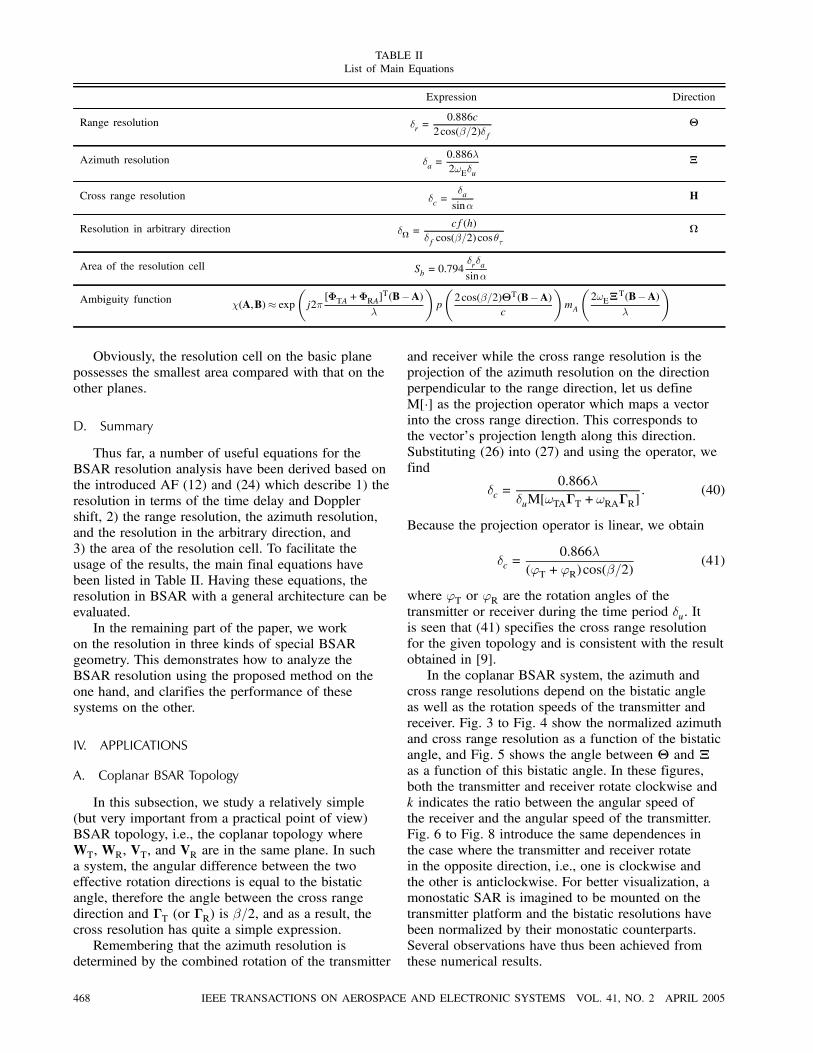
TABLE IIList of Main Equations

Expression Direction

Range resolution ±r =0:886c

2cos(¯=2)±f£

Azimuth resolution ±a =0:886¸2!E±u

¥

Cross range resolution ±c =±asin®

H

Resolution in arbitrary direction ±− =cf(h)

±f cos(¯=2)cosµ¿−

Area of the resolution cell Sb = 0:794±r±asin®

Ambiguity function Â(A,B)¼ expµj2¼

[©TA+©RA]T(B¡A)

¸

¶p

µ2cos(¯=2)£T(B¡A)

c

¶mA

µ2!E¥

T(B¡A)¸

¶

Obviously, the resolution cell on the basic planepossesses the smallest area compared with that on theother planes.

D. Summary

Thus far, a number of useful equations for theBSAR resolution analysis have been derived based onthe introduced AF (12) and (24) which describe 1) theresolution in terms of the time delay and Dopplershift, 2) the range resolution, the azimuth resolution,and the resolution in the arbitrary direction, and3) the area of the resolution cell. To facilitate theusage of the results, the main final equations havebeen listed in Table II. Having these equations, theresolution in BSAR with a general architecture can beevaluated.In the remaining part of the paper, we work

on the resolution in three kinds of special BSARgeometry. This demonstrates how to analyze theBSAR resolution using the proposed method on theone hand, and clarifies the performance of thesesystems on the other.

IV. APPLICATIONS

A. Coplanar BSAR Topology

In this subsection, we study a relatively simple(but very important from a practical point of view)BSAR topology, i.e., the coplanar topology whereWT, WR, VT, and VR are in the same plane. In sucha system, the angular difference between the twoeffective rotation directions is equal to the bistaticangle, therefore the angle between the cross rangedirection and ¡T (or ¡R) is ¯=2, and as a result, thecross resolution has quite a simple expression.Remembering that the azimuth resolution is

determined by the combined rotation of the transmitter

and receiver while the cross range resolution is theprojection of the azimuth resolution on the directionperpendicular to the range direction, let us defineM[¢] as the projection operator which maps a vectorinto the cross range direction. This corresponds tothe vector’s projection length along this direction.Substituting (26) into (27) and using the operator, wefind

±c =0:866¸

±uM[!TA¡T +!RA¡R]: (40)

Because the projection operator is linear, we obtain

±c =0:866¸

('T +'R)cos(¯=2)(41)

where 'T or 'R are the rotation angles of thetransmitter or receiver during the time period ±u. Itis seen that (41) specifies the cross range resolutionfor the given topology and is consistent with the resultobtained in [9].In the coplanar BSAR system, the azimuth and

cross range resolutions depend on the bistatic angleas well as the rotation speeds of the transmitter andreceiver. Fig. 3 to Fig. 4 show the normalized azimuthand cross range resolution as a function of the bistaticangle, and Fig. 5 shows the angle between £ and ¥as a function of this bistatic angle. In these figures,both the transmitter and receiver rotate clockwise andk indicates the ratio between the angular speed ofthe receiver and the angular speed of the transmitter.Fig. 6 to Fig. 8 introduce the same dependences inthe case where the transmitter and receiver rotatein the opposite direction, i.e., one is clockwise andthe other is anticlockwise. For better visualization, amonostatic SAR is imagined to be mounted on thetransmitter platform and the bistatic resolutions havebeen normalized by their monostatic counterparts.Several observations have thus been achieved fromthese numerical results.


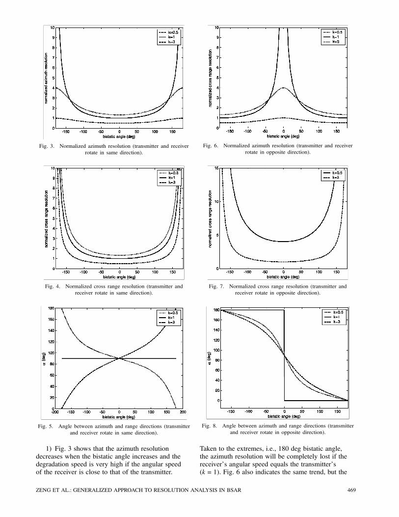
Fig. 3. Normalized azimuth resolution (transmitter and receiverrotate in same direction).

Fig. 4. Normalized cross range resolution (transmitter andreceiver rotate in same direction).

Fig. 5. Angle between azimuth and range directions (transmitterand receiver rotate in same direction).

1) Fig. 3 shows that the azimuth resolutiondecreases when the bistatic angle increases and thedegradation speed is very high if the angular speedof the receiver is close to that of the transmitter.

Fig. 6. Normalized azimuth resolution (transmitter and receiverrotate in opposite direction).

Fig. 7. Normalized cross range resolution (transmitter andreceiver rotate in opposite direction).

Fig. 8. Angle between azimuth and range directions (transmitterand receiver rotate in opposite direction).

Taken to the extremes, i.e., 180 deg bistatic angle,the azimuth resolution will be completely lost if thereceiver’s angular speed equals the transmitter’s(k = 1). Fig. 6 also indicates the same trend, but the


worst resolution corresponds to zero bistatic angles.This is due to the fact that the effect of the receiverrotation is compensated by the transmitter’s rotation.The comparison of Fig. 3 and Fig. 6 helps tounderstand the difference between these two BSARtopologies.2) The direction of the azimuth resolution always

coincides with the range resolution’s direction if thereceiver and the transmitter have equal but oppositedirections (see Fig. 8). In this situation, the crossrange resolution is totally lost. This topology cannotbe used for the two-dimensional BSAR imaging. Onthe other hand, as reported in [24], it can be useful fora side look moving target indicator (MTI) operationdue to fact that the scatter spectrum in each rangeresolution bin is very narrow.3) From Fig. 4 and Fig. 7, we know that the value

of the cross range resolution will approach infinitewhen the bistatic angle equals 180 deg. This is due tothe fact that the azimuth resolution direction tends tocoincide with the direction of the range resolution.

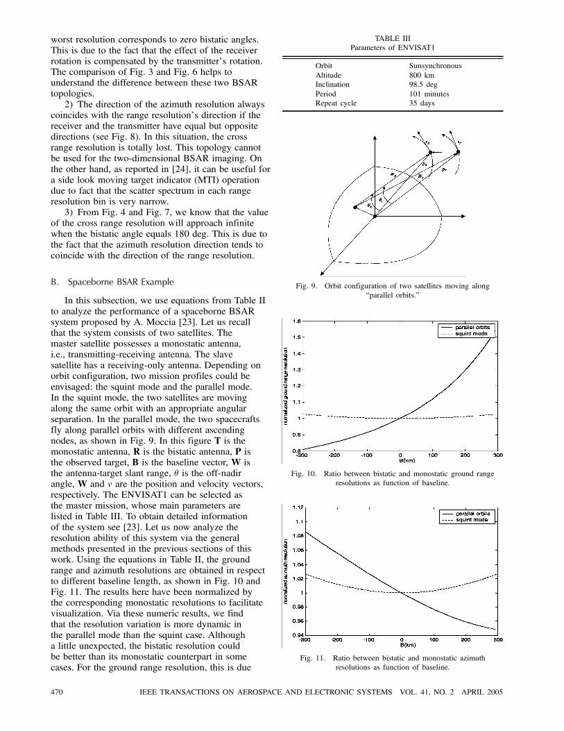
B. Spaceborne BSAR Example

In this subsection, we use equations from Table IIto analyze the performance of a spaceborne BSARsystem proposed by A. Moccia [23]. Let us recallthat the system consists of two satellites. Themaster satellite possesses a monostatic antenna,i.e., transmitting-receiving antenna. The slavesatellite has a receiving-only antenna. Depending onorbit configuration, two mission profiles could beenvisaged: the squint mode and the parallel mode.In the squint mode, the two satellites are movingalong the same orbit with an appropriate angularseparation. In the parallel mode, the two spacecraftsfly along parallel orbits with different ascendingnodes, as shown in Fig. 9. In this figure T is themonostatic antenna, R is the bistatic antenna, P isthe observed target, B is the baseline vector, W isthe antenna-target slant range, µ is the off-nadirangle, W and v are the position and velocity vectors,respectively. The ENVISAT1 can be selected asthe master mission, whose main parameters arelisted in Table III. To obtain detailed informationof the system see [23]. Let us now analyze theresolution ability of this system via the generalmethods presented in the previous sections of thiswork. Using the equations in Table II, the groundrange and azimuth resolutions are obtained in respectto different baseline length, as shown in Fig. 10 andFig. 11. The results here have been normalized bythe corresponding monostatic resolutions to facilitatevisualization. Via these numeric results, we findthat the resolution variation is more dynamic inthe parallel mode than the squint case. Althougha little unexpected, the bistatic resolution couldbe better than its monostatic counterpart in somecases. For the ground range resolution, this is due

TABLE IIIParameters of ENVISAT1

Orbit SunsynchronousAltitude 800 kmInclination 98.5 degPeriod 101 minutesRepeat cycle 35 days

Fig. 9. Orbit configuration of two satellites moving along“parallel orbits.”

Fig. 10. Ratio between bistatic and monostatic ground rangeresolutions as function of baseline.

Fig. 11. Ratio between bistatic and monostatic azimuthresolutions as function of baseline.


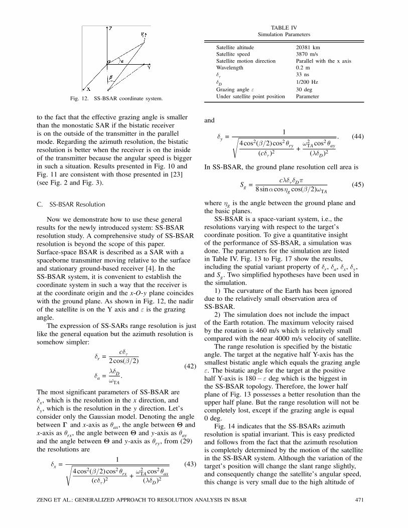
Fig. 12. SS-BSAR coordinate system.

to the fact that the effective grazing angle is smallerthan the monostatic SAR if the bistatic receiveris on the outside of the transmitter in the parallelmode. Regarding the azimuth resolution, the bistaticresolution is better when the receiver is on the insideof the transmitter because the angular speed is biggerin such a situation. Results presented in Fig. 10 andFig. 11 are consistent with those presented in [23](see Fig. 2 and Fig. 3).

C. SS-BSAR Resolution

Now we demonstrate how to use these generalresults for the newly introduced system: SS-BSARresolution study. A comprehensive study of SS-BSARresolution is beyond the scope of this paper.Surface-space BSAR is described as a SAR with aspaceborne transmitter moving relative to the surfaceand stationary ground-based receiver [4]. In theSS-BSAR system, it is convenient to establish thecoordinate system in such a way that the receiver isat the coordinate origin and the x-O-y plane coincideswith the ground plane. As shown in Fig. 12, the nadirof the satellite is on the Y axis and " is the grazingangle.The expression of SS-SARs range resolution is just

like the general equation but the azimuth resolution issomehow simpler:

±r =c±¿

2cos(¯=2)

±a =¸±D!TA

:

(42)

The most significant parameters of SS-BSAR are±x, which is the resolution in the x direction, and±y , which is the resolution in the y direction. Let’sconsider only the Gaussian model. Denoting the anglebetween ¡ and x-axis as µax, the angle between £ andx-axis as µrx, the angle between £ and y-axis as µayand the angle between £ and y-axis as µry, from (29)the resolutions are

±x =1s

4cos2(¯=2)cos2 µrx(c±¿ )2

+!2TA cos

2 µax(¸±D)2

(43)

TABLE IVSimulation Parameters

Satellite altitude 20381 kmSatellite speed 3870 m/sSatellite motion direction Parallel with the x axisWavelength 0.2 m±¿ 33 ns±D 1/200 HzGrazing angle " 30 degUnder satellite point position Parameter

and

±y =1s

4cos2(¯=2)cos2 µry(c±¿ )2

+!2TA cos

2 µay(¸±D)2

: (44)

In SS-BSAR, the ground plane resolution cell area is

Sg =c¸±¿±D¼

8sin®cos´g cos(¯=2)!TA(45)

where ´g is the angle between the ground plane andthe basic planes.SS-BSAR is a space-variant system, i.e., the

resolutions varying with respect to the target’scoordinate position. To give a quantitative insightof the performance of SS-BSAR, a simulation wasdone. The parameters for the simulation are listedin Table IV. Fig. 13 to Fig. 17 show the results,including the spatial variant property of ±r, ±a, ±x, ±y,and Sg. Two simplified hypotheses have been used inthe simulation.1) The curvature of the Earth has been ignored

due to the relatively small observation area ofSS-BSAR.2) The simulation does not include the impact

of the Earth rotation. The maximum velocity raisedby the rotation is 460 m/s which is relatively smallcompared with the near 4000 m/s velocity of satellite.The range resolution is specified by the bistatic

angle. The target at the negative half Y-axis has thesmallest bistatic angle which equals the grazing angle". The bistatic angle for the target at the positivehalf Y-axis is 180¡ " deg which is the biggest inthe SS-BSAR topology. Therefore, the lower halfplane of Fig. 13 possesses a better resolution than theupper half plane. But the range resolution will not becompletely lost, except if the grazing angle is equal0 deg.Fig. 14 indicates that the SS-BSARs azimuth

resolution is spatial invariant. This is easy predictedand follows from the fact that the azimuth resolutionis completely determined by the motion of the satellitein the SS-BSAR system. Although the variation of thetarget’s position will change the slant range slightly,and consequently change the satellite’s angular speed,this change is very small due to the high altitude of


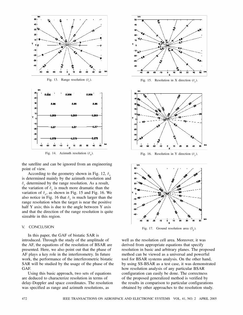
Fig. 13. Range resolution (±r).

Fig. 14. Azimuth resolution (±a).

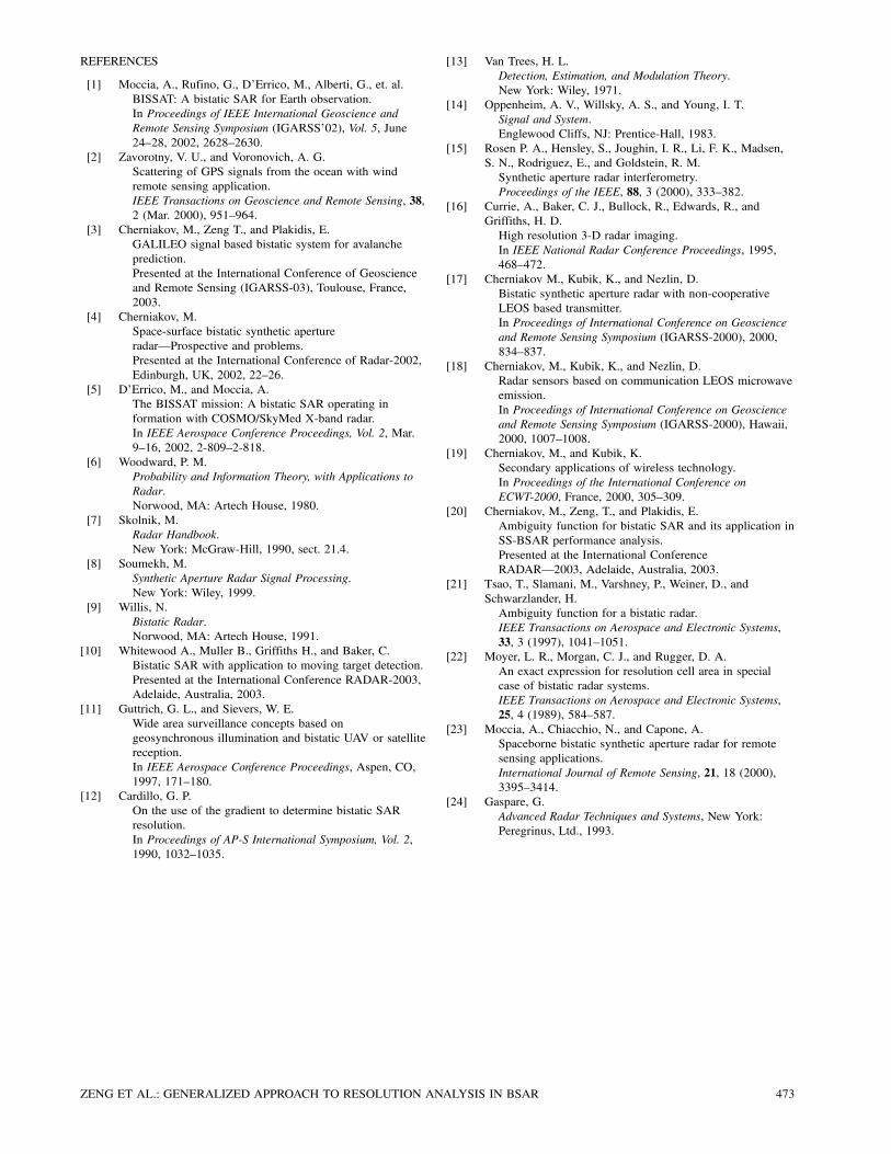
the satellite and can be ignored from an engineeringpoint of view.According to the geometry shown in Fig. 12, ±x

is determined mainly by the azimuth resolution and±y determined by the range resolution. As a result,the variation of ±y is much more dramatic than thevariation of ±x, as shown in Fig. 15 and Fig. 16. Wealso notice in Fig. 16 that ±y is much larger than therange resolution when the target is near the positivehalf Y axis; this is due to the angle between Y axisand that the direction of the range resolution is quitesizeable in this region.

V. CONCLUSION

In this paper, the GAF of bistatic SAR isintroduced. Through the study of the amplitude ofthe AF, the equations of the resolution of BSAR arepresented. Here, we also point out that the phase ofAF plays a key role in the interferometry. In futurework, the performance of the interferometric bistaticSAR will be studied by the usage of the phase of theGAF.Using this basic approach, two sets of equations

are deduced to characterize resolution in terms ofdelay-Doppler and space coordinates. The resolutionwas specified as range and azimuth resolutions, as

Fig. 15. Resolution in X direction (±x).

Fig. 16. Resolution in Y direction (±y).

Fig. 17. Ground resolution area (Sg).

well as the resolution cell area. Moreover, it wasderived from appropriate equations that specifyresolution in basic and arbitrary planes. The proposedmethod can be viewed as a universal and powerfultool for BSAR systems analysis. On the other hand,by using SS-BSAR as a test case, it was demonstratedhow resolution analysis of any particular BSARconfiguration can easily be done. The correctnessof the proposed generalized method is verified bythe results in comparison to particular configurationsobtained by other approaches to the resolution study.


REFERENCES

[1] Moccia, A., Rufino, G., D’Errico, M., Alberti, G., et. al.BISSAT: A bistatic SAR for Earth observation.In Proceedings of IEEE International Geoscience andRemote Sensing Symposium (IGARSS’02), Vol. 5, June24—28, 2002, 2628—2630.

[2] Zavorotny, V. U., and Voronovich, A. G.Scattering of GPS signals from the ocean with windremote sensing application.IEEE Transactions on Geoscience and Remote Sensing, 38,2 (Mar. 2000), 951—964.

[3] Cherniakov, M., Zeng T., and Plakidis, E.GALILEO signal based bistatic system for avalancheprediction.Presented at the International Conference of Geoscienceand Remote Sensing (IGARSS-03), Toulouse, France,2003.

[4] Cherniakov, M.Space-surface bistatic synthetic apertureradar–Prospective and problems.Presented at the International Conference of Radar-2002,Edinburgh, UK, 2002, 22—26.

[5] D’Errico, M., and Moccia, A.The BISSAT mission: A bistatic SAR operating information with COSMO/SkyMed X-band radar.In IEEE Aerospace Conference Proceedings, Vol. 2, Mar.9—16, 2002, 2-809—2-818.

[6] Woodward, P. M.Probability and Information Theory, with Applications toRadar.Norwood, MA: Artech House, 1980.

[7] Skolnik, M.Radar Handbook.New York: McGraw-Hill, 1990, sect. 21.4.

[8] Soumekh, M.Synthetic Aperture Radar Signal Processing.New York: Wiley, 1999.

[9] Willis, N.Bistatic Radar.Norwood, MA: Artech House, 1991.

[10] Whitewood A., Muller B., Griffiths H., and Baker, C.Bistatic SAR with application to moving target detection.Presented at the International Conference RADAR-2003,Adelaide, Australia, 2003.

[11] Guttrich, G. L., and Sievers, W. E.Wide area surveillance concepts based ongeosynchronous illumination and bistatic UAV or satellitereception.In IEEE Aerospace Conference Proceedings, Aspen, CO,1997, 171—180.

[12] Cardillo, G. P.On the use of the gradient to determine bistatic SARresolution.In Proceedings of AP-S International Symposium, Vol. 2,1990, 1032—1035.

[13] Van Trees, H. L.Detection, Estimation, and Modulation Theory.New York: Wiley, 1971.

[14] Oppenheim, A. V., Willsky, A. S., and Young, I. T.Signal and System.Englewood Cliffs, NJ: Prentice-Hall, 1983.

[15] Rosen P. A., Hensley, S., Joughin, I. R., Li, F. K., Madsen,S. N., Rodriguez, E., and Goldstein, R. M.Synthetic aperture radar interferometry.Proceedings of the IEEE, 88, 3 (2000), 333—382.

[16] Currie, A., Baker, C. J., Bullock, R., Edwards, R., andGriffiths, H. D.High resolution 3-D radar imaging.In IEEE National Radar Conference Proceedings, 1995,468—472.

[17] Cherniakov M., Kubik, K., and Nezlin, D.Bistatic synthetic aperture radar with non-cooperativeLEOS based transmitter.In Proceedings of International Conference on Geoscienceand Remote Sensing Symposium (IGARSS-2000), 2000,834—837.

[18] Cherniakov, M., Kubik, K., and Nezlin, D.Radar sensors based on communication LEOS microwaveemission.In Proceedings of International Conference on Geoscienceand Remote Sensing Symposium (IGARSS-2000), Hawaii,2000, 1007—1008.

[19] Cherniakov, M., and Kubik, K.Secondary applications of wireless technology.In Proceedings of the International Conference onECWT-2000, France, 2000, 305—309.

[20] Cherniakov, M., Zeng, T., and Plakidis, E.Ambiguity function for bistatic SAR and its application inSS-BSAR performance analysis.Presented at the International ConferenceRADAR–2003, Adelaide, Australia, 2003.

[21] Tsao, T., Slamani, M., Varshney, P., Weiner, D., andSchwarzlander, H.Ambiguity function for a bistatic radar.IEEE Transactions on Aerospace and Electronic Systems,33, 3 (1997), 1041—1051.

[22] Moyer, L. R., Morgan, C. J., and Rugger, D. A.An exact expression for resolution cell area in specialcase of bistatic radar systems.IEEE Transactions on Aerospace and Electronic Systems,25, 4 (1989), 584—587.

[23] Moccia, A., Chiacchio, N., and Capone, A.Spaceborne bistatic synthetic aperture radar for remotesensing applications.International Journal of Remote Sensing, 21, 18 (2000),3395—3414.

[24] Gaspare, G.Advanced Radar Techniques and Systems, New York:Peregrinus, Ltd., 1993.


Tao Zeng received his Ph.D. degree in 1999 from the Department of ElectronicEngineering, Beijing Institute of Technology, China.He joined the teaching staff of the same university in 1999. His research

interests include SAR imaging technology and real time radar signal processing.

Mikhail Cherniakov received the M.Eng. (1974), Ph.D. (1980), and D.Sc. (1992)in the Technical University, Moscow Institute of Electronics Engineering (Russia,MIEE).After 1974 he was with the Department of Microwave Systems at MIEE. In

1981 he became the founding head of the Microwave Systems R&D Laboratory.In 1992 he accepted an appointment as professor in MIEE. In 1994 he was avisiting professor in Cambridge University, UK. From 1995 he was with theDepartment of Information Technology and Electrical Engineering, Universityof Queensland, Australia. He joined the Communications Engineering Groupat the University of Birmingham, UK, in April 2000. The area of his researchactivity is system aspect of radar and mobile communications and in particularultra-wideband radar, multisite and forward scattering sensoring, and systemswith active phased array as well as selected problems of digital signal processing.Dr. Cherniakov is the author of more than 100 papers, 10 patents, and one

monograph.

Teng Long was born in 1968, in the Province of Fujing, P.R. China. He graduatedwith a degree in radio electronics from the University of Science and Technologyof China in 1989. He received his Ph.D. electronic engineering from the BeijingInstitute of Technology (BIT) in 1995.He became a lecturer in the Electronic Engineering Department of BIT

and now is a full professor there. From January to August of 1999, he was avisiting associate professor at Stanford University, Stanford, CA. From Marchto September of 2002, he was a visiting scholar at the University College ofLondon. His research is mainly about digital signal processing, with applicationsto radar and communication systems.


Generalized approach to resolution analysis in BSAR

Documents

Transcript of Generalized approach to resolution analysis in BSAR