General non-linear finite element analysis of thick plates and ...

International Journal of Solids and Structures 43 (2006) 2209–2242

www.elsevier.com/locate/ijsolstr

General non-linear finite element analysis of thick platesand shells

George Z. Voyiadjis *, Pawel Woelke

Department of Civil and Environmental Engineering, Louisiana State University, Baton Rouge, LA 70803-6405, USA

Received 23 December 2004; received in revised form 12 July 2005Available online 30 August 2005

Abstract

A non-linear finite element analysis is presented, for the elasto-plastic behavior of thick shells and plates including theeffect of large rotations. The shell constitutive equations developed previously by the authors [Voyiadjis, G.Z., Woelke,P., 2004. A refined theory for thick spherical shells. Int. J. Solids Struct. 41, 3747–3769] are adopted here as a base for theformulation. A simple C0 quadrilateral, doubly curved shell element developed in the authors� previous paper [Woelke,P., Voyiadjis, G.Z., submitted for publication. Shell element based on the refined theory for thick spherical shells] isextended here to account for geometric and material non-linearities. The small strain geometric non-linearities are takeninto account by means of the updated Lagrangian method. In the treatment of material non-linearities the authors adopt:(i) a non-layered approach and a plastic node method [Ueda, Y., Yao, T., 1982. The plastic node method of plastic anal-ysis. Comput. Methods Appl. Mech. Eng. 34, 1089–1104], (ii) an Iliushin�s yield function expressed in terms of stressresultants and stress couples [Iliushin, A.A., 1956. Plastichnost�. Gostekhizdat, Moscow], modified to investigate thedevelopment of plastic deformations across the thickness, as well as the influence of the transverse shear forces on plasticbehaviour of plates and shells, (iii) isotropic and kinematic hardening rules with the latter derived on the basis of theArmstrong and Frederick evolution equation of backstress [Armstrong, P.J., Frederick, C.O., 1966. A mathematicalrepresentation of the multiaxial Bauschinger effect. (CEGB Report RD/B/N/731). Berkeley Laboratories. R&DDepartment, California.], and reproducing the Bauschinger effect. By means of a quasi-conforming technique, shearand membrane locking are prevented and the tangent stiffness matrix is given explicitly, i.e., no numerical integrationis employed. This makes the current formulation not only mathematically consistent and accurate for a variety of appli-cations, but also computationally extremely efficient and attractive.� 2005 Elsevier Ltd. All rights reserved.

Keywords: Thick plates and shells; Elasto-plastic analysis; Kinematic hardening; Large displacements

0020-7683/$ - see front matter � 2005 Elsevier Ltd. All rights reserved.doi:10.1016/j.ijsolstr.2005.07.012

* Corresponding author. Tel.: +1 225 578 8668; fax: +1 225 578 9176.E-mail address: [email protected] (G.Z. Voyiadjis).

mailto:[email protected]

2210 G.Z. Voyiadjis, P. Woelke / International Journal of Solids and Structures 43 (2006) 2209–2242

1. Introduction

Many approaches are used in the elasto-plastic analysis of plates and shells. The finite element methodhas been successful in modeling the linear behaviour of shells and it is therefore natural to apply the samemethod to the non-linear analysis of these technically important structures. Non-linear computations arebased on incremental and/or iterative algorithms, which are computationally expensive. The efforts ofmany authors are not only directed to accuracy and wide applicability of their formulations, but also tocomputational efficiency. The objective of the present work is to develop a general, accurate and very effi-cient procedure for the analysis of thick/thin plates and shells, including geometric and material non-linear-ities with isotropic and kinematic hardening rules and an explicit form of the tangent stiffness matrix.

Many investigators avoid the problem of shell constitutive equations by following a layered approach,also referred to as �through-the-thickness integration�, (Dvorkin and Bathe, 1984; Flores and Onate, 2001;Kebari and Cassell, 1992; Kollmann and Sansour, 1997; Onate, 1999; Parish, 1981). This procedure,although accurate, requires sometimes prohibitively large storage of the computer. For the case of anon-layered finite element, a general and accurate shell theory is of crucial importance. Following the workof Voyiadjis and Shi (1991), Voyiadjis and Woelke (2004) presented a refined theory for thick shells, basedon analytical closed form solutions for thick containers. This theory proves to be very efficient in the treat-ment of both thin and thick shells of general shape. It accounts for the effect of transverse shear deforma-tion, distribution of radial stresses, as a very important feature for thick shells and the initial curvatureeffect. This not only contributes to the stress resultants and stress couples, but also results in a non-lineardistribution of the in-plane stresses across the thickness of the shell. The resulting constitutive relations givevery good results for extremely thick (R/t = 3), and very thin shells of general shape, as well as plates andbeams. A brief outline of the theory is provided in subsequent sections.

The C0 finite element given in Woelke and Voyiadjis (submitted for publication), based on the aforemen-tioned theory, and the quasi-conforming technique, provides a very effective tool for elastic analysis ofstructures. The quasi-conforming technique given in Tang et al. (1980, 1983) is an extension of the assumedstrain fields method (Ashwell and Gallagher, 1976; Huang and Hinton, 1984; Park and Stanley, 1986), andit has been successfully applied to overcome the locking phenomena (Shi and Voyiadjis, 1990, 1991). Thebiggest advantage of this technique, when compared with the most widely used selective integration method(Hughes, 1987; Stolarski and Belytschko, 1983; Stolarski et al., 1984; Yang et al., 2000; Zienkiewicz, 1978),is the fact that the stiffness matrix of the element is given explicitly. Thus, this method is very attractive fornon-linear analysis where the element matrices are calculated many times during the analysis. Moreover,selective integration requires explicit segregation of transverse shear terms from bending and membraneterms, which is not possible when they are coupled, as is mostly the case for non-linear analysis. This prob-lem was solved by a generalization of the selective integration procedure (Hughes, 1980). The quasi-conforming technique is however chosen here for its simplicity and low computational cost. As a resultof this choice and the application of a non-layered approach, numerical integration will not be performedin the present procedure at any stage of the analysis. All the integrals are calculated analytically with theresults later introduced into a computer code. This makes the current formulation consistent mathemati-cally and extremely efficient from the point of view of computer time and power.

The strain fields are interpolated directly here, rather than obtained from the assumed displacement fieldproviding the adequate representation of the rigid body modes. The spurious energy mode, which can be aproblem in finite elements with reduced integration, is avoided here by the appropriate choice of the strainfields. The compatibility equations of the displacements can also be satisfied in the assumed strain fields.This results in a more complicated formulation of the element stiffness matrix, and therefore compatibilityis not enforced. The element adopted in this work is unified for both curved and flat configurations, satisfiesthe Kirchhoff–Love hypothesis in the case of thin plates and shells, exhibits neither shear nor membranelocking and is free from spurious zero energy modes.

G.Z. Voyiadjis, P. Woelke / International Journal of Solids and Structures 43 (2006) 2209–2242 2211

In elasto-plastic, finite element analysis of shells, large rotations and translations can play an importantrole. Displacements at the regions of the structure, which undergo inelastic deformations, can be very large.Thus, to achieve the desired accuracy, geometric non-linearities must be considered. The updated Lagrang-ian description, which has proven to be a very effective method (Bathe, 1982; Flores and Onate, 2001; Hor-rigmoe and Bergan, 1978; Kebari and Cassell, 1992) is adopted here. The element local coordinates and thelocal reference frame are continuously updated during the deformation. We consider large rotations andrigid translations here, but small strains with the total rotations decomposed into large rigid rotationsand moderate relative rotations are also considered. The relative rotations and the derivatives of the in-plane displacements from two consecutive configurations can be considered small, (Shi and Atluri, 1988;Shi and Voyiadjis, 1991). Consequently, the quadratic terms of the derivatives of the in-plane displacementare negligible. We therefore have a non-linear analysis with large displacements and rotations but smallstrains. The transformation matrix given in Argyris (1982) is employed to handle large rigid rotations.The assumed strain finite element with an explicit form of the stiffness matrix, as described above, providesthe linear part of the element tangent stiffness matrix.

Very many reliable �layered models� for elasto-plastic analysis of shells have been published. In this ap-proach, a plate or a shell is divided into layers where stresses are calculated and the yield condition ischecked for each layer separately. The forces and moments are then calculated by integration throughthe thickness. Although this method can give very accurate results, it can also be very demanding in termsof computational power. If on the other hand a �non-layered� approach is adopted, the yield function isintegrated through the thickness of the plate or shell and therefore expressed in terms of stress resultantsand couples. Numerical integration of the stresses is not necessary in this case, which makes the �non-lay-ered� formulation much cheaper computationally. The approximation of the yield criterion expressed interms of forces and moments is expected to result in a loss of accuracy. This is however not the case aswas shown by many authors comparing the two methods (Bieniek and Funaro, 1976; Owen and Hinton,1980; Shi and Voyiadjis, 1992). Both models compare very well with the analytical solutions available inHodge (1959), Olszak and Sawczuk (1977), Sawczuk (1989) and Sawczuk and Sokol-Supel (1993).

The non-layered model is employed in the current work with the yield function in terms of stress resul-tants and couples. In this case, the accuracy of the yield criterion is very important. A comparison of dif-ferent yield surfaces can be found in Robinson (1971). A modified Iliushin�s yield function is adopted in thiswork (Iliushin, 1956). Several modifications will be made to the original Iliushin�s yield function.

The first modification allows for capturing the progressive development of the plastic curvatures acrossthe thickness of the shell, as shown in Crisfield (1981) and Shi and Voyiadjis (1992). The model presentedhere very accurately reproduces the first yield point and tracks the growth of plastic curvatures until a plas-tic hinge is developed.

The transverse shear forces may significantly affect the plastic behaviour of both thick and, for certainloading conditions, thin shells. Shear becomes even more important in the case of anisotropic materials. Yetthe influence of transverse shear forces on the plastic behaviour of plates and shells has been covered in theliterature to a much lesser extent than in the case of elastic analysis, (Basar et al., 1992, 1993; Kratzig, 1992;Kratzig and Jun, 2003; Niordson, 1985; Noor and Burton, 1989; Palazotto and Linnemann, 1991; Reddy,1989; Reissner, 1945). This effect is investigated here and it is shown that transverse shears influencestrongly the plastic behaviour of considered structures.

Isotropic hardening as given in Shi and Atluri (1988) is also incorporated into the yield function in thepresent formulation. More importantly however, a kinematic hardening rule capable of capturing theBauschinger effect is defined. It is well known that when a material or a structure is loaded in tension intoa plastic zone, and subsequently the load is reversed, the yielding in compression will occur at a reducedvalue of stress. This anisotropy in the material is induced by plastic deformation. Relatively few hardeningrules for non-layered plates and shells have been published that are capable of correctly representing thisphenomenon. As first recognized by Wempner (1973), the stress resultants and couples of the classical


theory are not sufficient to describe accurately the state of stress in plastic shells. Bieniek and Funaro (1976)introduced �hardening parameters�, in the form of residual bending moments, allowing for the descriptionof a Bauschinger effect. However, Bieniek and Funaro recognized that the �hardening parameters� definedby them do not provide a full representation of kinematic hardening. For the appropriate representation ofthe rigid translation of the yield surface during non-elastic deformation in the stress resultant space, oneneeds not only the residual bending moments, but also residual shear and normal forces. These are equiv-alent parameters to the backstress in the stress space. We will therefore present a new kinematic hardeningrule for non-layered plates and shells here, explicitly derived from the evolution of the backstress given byArmstrong and Frederick (1966). It is shown later that the approach presented here is very accurate, yetsimple and efficient, which makes it very important form a practical engineering point of view.

Modeling of the elasto-plastic behaviour of structural elements based on the mathematical theory ofplasticity involves analysis of spread of plastic deformations in the regions where the yield condition is sat-isfied. Alternatively, the inelastic deformations may be considered concentrated in the plastic hinges. Theformer method originates from the analytical limit analysis of structures performed under the assumptionof elastic-perfectly plastic behaviour of the material (Hodge, 1959, 1963; Olszak and Sawczuk, 1977; Saw-czuk and Sokol-Supel, 1993). Using the finite element method and the concept of the plastic hinges Uedaand Yao (1982) developed a �plastic node method� for the plastic analysis of structures. In their formulation,the yield function is expressed in terms of stresses, as in the �layered model�. Shi and Voyiadjis (1992) pre-sented a non-layered plate element with the yield function in terms of forces and moments, adopting theconcept of concentration of plastic deformations in the plastic hinges. A similar approach is adopted in thiswork, saving again computer time, yet giving very accurate results, as will be shown later.

This paper is divided into eight sections. After Section 1, the shell constitutive equations are briefly intro-duced. In Section 3, we present the shell kinematics. Section 4 is devoted to the linear element stiffness ma-trix. Section 5 gives a description of material non-linearities, with the definition of yield surface, flow andhardening rules. The elasto-plastic stiffness matrix of the element is derived in Section 6. In Section 7, wepresent an outline of a numerical procedure and a series of discriminating examples, demonstrating that thecurrent computational model provides very good results for a variety of problems in elasto-plastic largedisplacement analysis of both thick and thin shells, plates and beams. Finally, in Section 8, we summarizethe results and draw the conclusions.

2. Shell constitutive equations

Voyiadjis and Woelke (2004) presented a detailed derivation of the shell constitutive equations adoptedfor the finite element formulation. Only the final set of relations is given here for self-completeness. Therefined theory accounts for the effect of transverse shear deformation, the distribution of radial stressesand the initial curvature of the shell, which results in a non-linear distribution of the in-plane stresses acrossthe thickness of the shell.

The main features of the shell equations are the following:

(1) Assumed out of plane stress components that satisfy given traction boundary conditions. These aredue to a closed form elasticity solution for thick walled spherical containers under internal and/orexternal uniform pressure, obtained by Lame (1852).

(2) Three-dimensional elasticity equations with an integral of the equilibrium equations.(3) Stress resultants and stress couples acting on the middle surface of the shell together with average dis-

placements along a normal of the middle surface of the shell and the average rotations of the normal(Voyiadjis and Baluch, 1981).


The membrane strains and curvatures in a rectangular coordinate system (x,y,z) are given by Eqs. (1)–(6).

ex ¼ouox

þ wR; ð1Þ

ey ¼ovox

þ wR; ð2Þ

exy ¼1

2

ouoy

þ ovox

� �; ð3Þ

jx ¼o/x

ox¼ o

oxowox

� cxz �uR

� �; ð4Þ

jy ¼o/y

oy¼ o

oyowoy

� cyz �vR

� �; ð5Þ

jxy ¼1

2

o/x

oyþo/y

ox

� �; ð6Þ

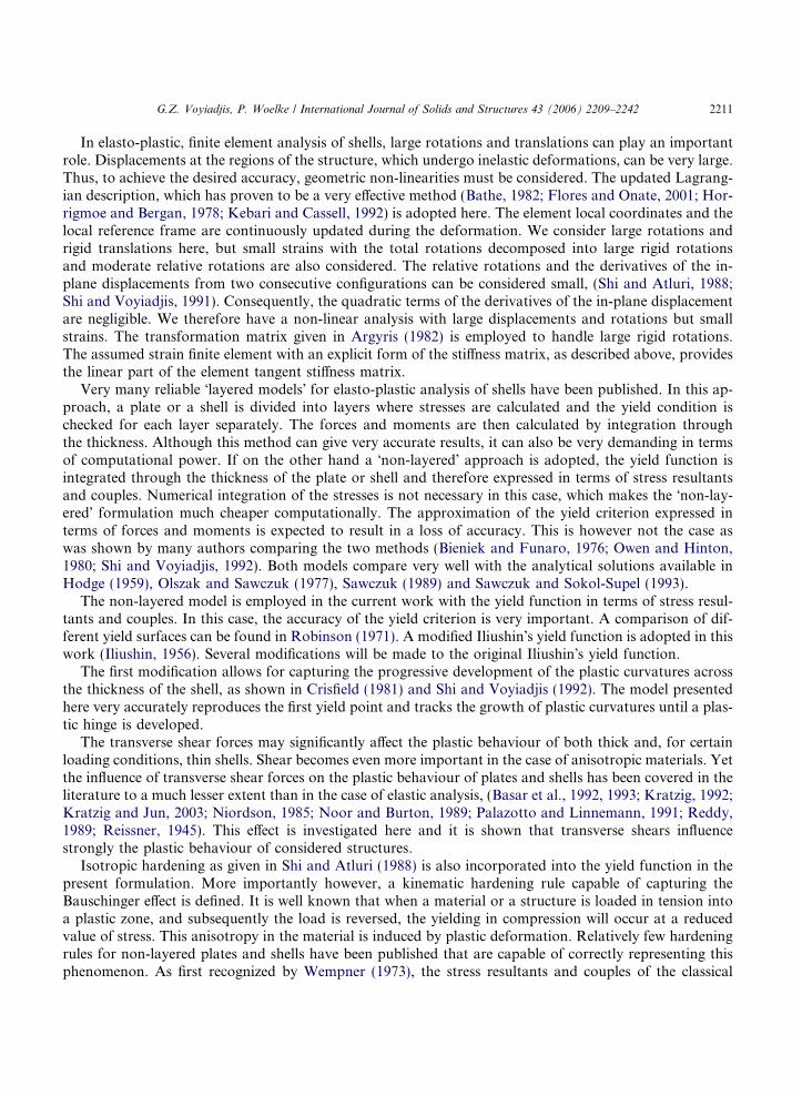
where ex, ey, exy are normal and shear strains and jx, jy, jxy are curvatures at the mid-surface in planesparallel to the xz, yz and xy planes respectively; u, v, w are the displacements along x, y, z axes respectively(Figs. 2 and 3); cxz, cyz are transverse shear strains in xz and yz planes (Fig. 1); /x, /y are angles of rotationsof the cross-sections that were normal to the mid-surface of the undeformed shell (Figs. 1 and 4); R is aradius of the shell.

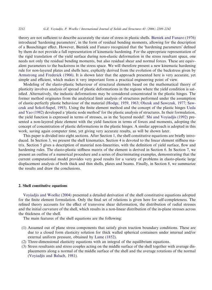
The stress resultants and couples Mx, My, Mxy, Nx, Ny, Nxy, Qx, Qy shown in Fig. 2, can be expressed interms of the strains given above

Mx ¼ D½jx þ mjy �; ð7ÞMy ¼ D½jy þ mjx�; ð8ÞMxy ¼ Dð1� mÞjxy ; ð9ÞNx ¼ S½ex þ mey �; ð10ÞNy ¼ S½ey þ mex�; ð11ÞNxy ¼ Sð1� mÞexy ; ð12ÞQx ¼ T cxz; ð13ÞQy ¼ T cyz; ð14Þ

Fig. 1. Angle of rotation with transverse shear strains.

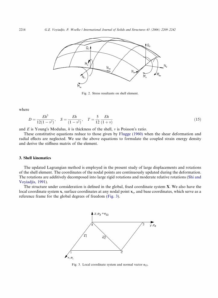
Fig. 2. Stress resultants on shell element.


where

D ¼ Eh3

12ð1� m2Þ ; S ¼ Ehð1� m2Þ ; T ¼ 5

12

Ehð1þ mÞ ð15Þ

and E is Young�s Modulus, h is thickness of the shell, m is Poisson�s ratio.These constitutive equations reduce to those given by Flugge (1960) when the shear deformation and

radial effects are neglected. We use the above equations to formulate the coupled strain energy densityand derive the stiffness matrix of the element.

3. Shell kinematics

The updated Lagrangian method is employed in the present study of large displacements and rotationsof the shell element. The coordinates of the nodal points are continuously updated during the deformation.The rotations are additively decomposed into large rigid rotations and moderate relative rotations (Shi andVoyiadjis, 1991).

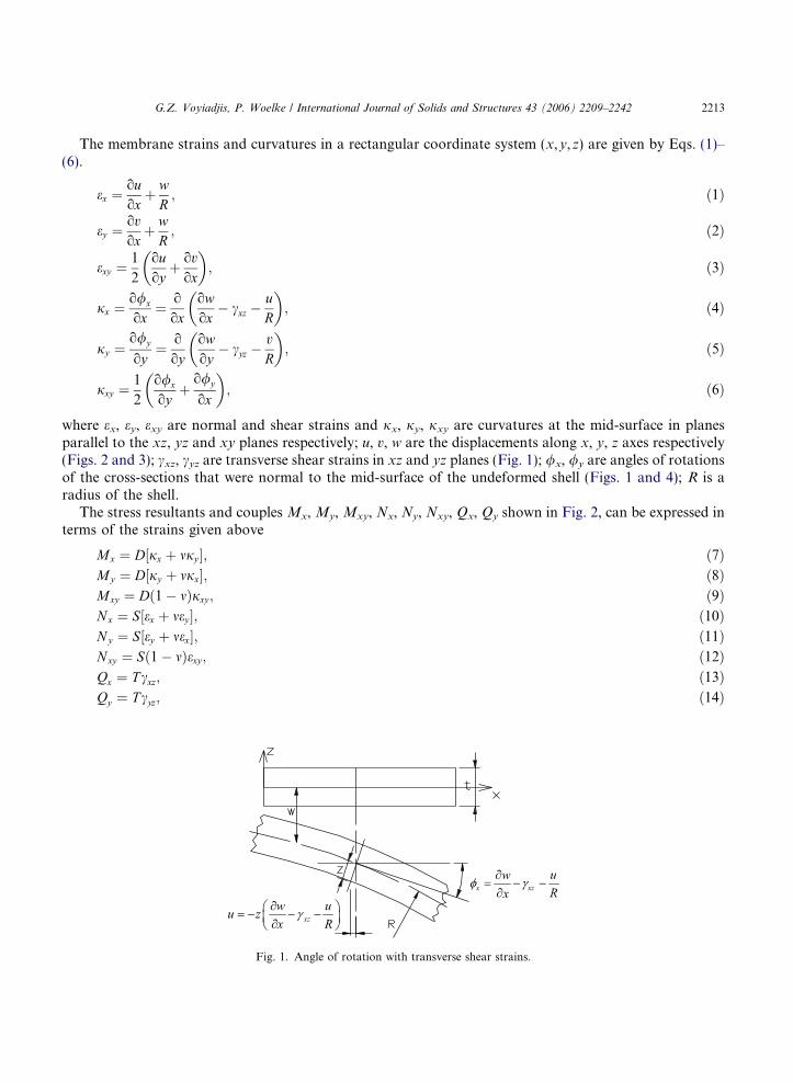
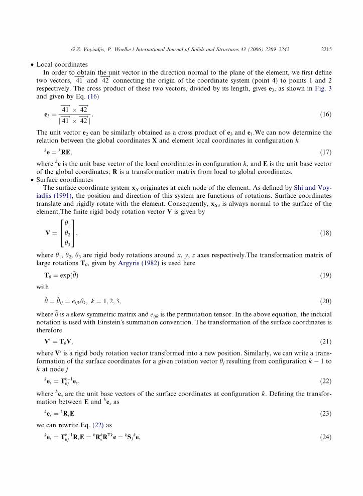
The structure under consideration is defined in the global, fixed coordinate system X. We also have thelocal coordinate system x, surface coordinates at any nodal point xs, and base coordinates, which serve as areference frame for the global degrees of freedom (Fig. 3).

Fig. 3. Local coordinate system and normal vector eS3.


• Local coordinatesIn order to obtain the unit vector in the direction normal to the plane of the element, we first define

two vectors, 41�!

and 42�!

connecting the origin of the coordinate system (point 4) to points 1 and 2respectively. The cross product of these two vectors, divided by its length, gives e3, as shown in Fig. 3and given by Eq. (16)

e3 ¼41�!� 42

�!j 41�!� 42

�!j: ð16Þ

The unit vector e2 can be similarly obtained as a cross product of e3 and e1.We can now determine therelation between the global coordinates X and element local coordinates in configuration k

ke ¼ kRE; ð17Þ
where ke is the unit base vector of the local coordinates in configuration k, and E is the unit base vectorof the global coordinates; R is a transformation matrix from local to global coordinates.
• Surface coordinatesThe surface coordinate system xS originates at each node of the element. As defined by Shi and Voy-

iadjis (1991), the position and direction of this system are functions of rotations. Surface coordinatestranslate and rigidly rotate with the element. Consequently, xS3 is always normal to the surface of theelement.The finite rigid body rotation vector V is given by

V ¼h1h2h3

264

375; ð18Þ

where h1, h2, h3 are rigid body rotations around x, y, z axes respectively.The transformation matrix oflarge rotations Th, given by Argyris (1982) is used here

Th ¼ expð~hÞ ð19Þ
with
~h ¼ ~hij ¼ eijkhk; k ¼ 1; 2; 3; ð20Þ

where ~h is a skew symmetric matrix and eijk is the permutation tensor. In the above equation, the indicialnotation is used with Einstein�s summation convention. The transformation of the surface coordinates istherefore

V0 ¼ ThV; ð21Þ
where V 0 is a rigid body rotation vector transformed into a new position. Similarly, we can write a trans-formation of the surface coordinates for a given rotation vector hj resulting from configuration k � 1 tok at node j
kes ¼ Tk�1hj es; ð22Þ

where kes are the unit base vectors of the surface coordinates at configuration k. Defining the transfor-mation between E and kes as

kes ¼ kRsE ð23Þ
we can rewrite Eq. (22) as
kes ¼ Tk�1hj RsE ¼ kRk

sRTke ¼ kSj

ke; ð24Þ

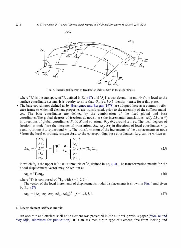
Fig. 4. Incremental degrees of freedom of shell element in local coordinates.


where kRT is the transpose of kR defined in Eq. (17) and kSj is a transformation matrix from local to thesurface coordinate system. It is worthy to note that 0Rs is a 3 · 3 identity matrix for a flat plate.

• The base coordinates defined as by Horrigmoe and Bergan (1978) are adopted here as a common refer-ence frame to which all element properties are transformed, prior to the assembly of the stiffness matri-ces. The base coordinates are defined by the combination of the fixed global and basecoordinates.The global degrees of freedom at node j are the incremental translations: DUj, DVj, DWj

in directions of global coordinates X, Y, Z and rotations Hxj, Hyj around xS, yS. The local degrees offreedom at node j are the incremental translations Duj, Dvj, Dwj in directions of local coordinates x, y,z and rotations /xj, /yj around x, y. The transformation of the increments of the displacements at nodej from the local coordinate system Dqej, to the corresponding base coordinates, Dqbj can be written as

Dqbj ¼

DUj

DV j

DW j

Hxj

Hyj

8>>>>><>>>>>:

9>>>>>=>>>>>;

¼kRT 0

0 ksj

� � DujDvjDwj

/xj

/yj

8>>>>><>>>>>:

9>>>>>=>>>>>;

¼ kTbjDqej ð25Þ

in which ksj is the upper left 2 · 2 submatrix of kSj defined in Eq. (24). The transformation matrix for thenodal displacement vector may be written as

Dqb ¼ kTbDqe; ð26Þ
where kTb is composed of kTbj with j = 1,2,3,4.
The vector of the local increments of displacements nodal displacements is shown in Fig. 4 and givenby Eq. (27)

Dqej ¼ fDuj;Dvj;Dwj;D/xj;D/yjgT j ¼ 1; 2; 3; 4: ð27Þ

4. Linear element stiffness matrix

An accurate and efficient shell finite element was presented in the authors� previous paper (Woelke andVoyiadjis, submitted for publication). It is an assumed strain type of element, free from locking and


spurious energy modes. The quasi-conforming technique (Tang et al., 1983) was used which gives an expli-cit form of the stiffness matrix as integrations are carried out directly. A detailed derivation is given inWoelke and Voyiadjis (submitted for publication).

In order to overcome the problem of shear locking, the Kirchhoff–Love assumption must be satisfied forthe case of thin shells. Since the shear forces Qx, Qy are generally finite, the shear deformations cxz and cyzmust vanish when the shear rigidity T approaches infinity. Hu (1984) point out that in order to satisfy thisrequirement the interpolation formulas must contain the ratio of the flexural and shear rigidities. We usehere the approximation of the displacement w and rotations / for the straight beam of length l given by Hu

w ¼ 1

21� nþ k

2ðn3 � nÞ

� �wi þ

1

4½1� n2 þ kðn3 � nÞ� l

2/i þ

1

21þ n� k

2ðn3 � nÞ

� �wj

þ 1

4½�1þ n2 þ kðn3 � nÞ� l

2/j; ð28Þ

/ ¼ � 3

2lk½1� n2�wi þ

1

4½2� 2n� 3kð1� n2Þ�/i þþ 3

2lk½1� n2�wj þ

1

4½2þ 2n� 3kð1� n2Þ�/j; ð29Þ

where

n ¼ 2xl� 1 6 n 6 1; k ¼ 1

1þ 12 DTl2

� � : ð30Þ

D and T denote the flexural and shear rigidity of the shell respectively. In equation, (30) the parameterD/Tl2 accounts for the shear deformation effect. We notice that when shear rigidity is very large and(h/l)2 ! 0, then k ! 1, and w in Eq. (28) reduces to a Hermite function and the Kirchhoff–Love assumptionis satisfied. When the shear rigidity is very small on the other hand, k = 0, and Eq. (28) reduces to Cook�s(1972) interpolation formula. The interpolation formulas given by Eqs. (28)–(30) are therefore suitable forboth the classical theory of shells, as well as the thick shell theory based on which the present element isformulated.

The problem of membrane locking is avoided by the appropriate choice of the strain fields as well as athird order approximation of the membrane displacements u,v. Approximation of the strains independentlyof the displacements allows satisfying the inextensibility condition for very thin curved shells and thus anyserious membrane locking is not experienced. Further details regarding overcoming shear and membranelocking may by found in Woelke and Voyiadjis (submitted for publication).

In the quasi-conforming technique, the displacement and strain fields are interpolated independently andthe compatibility equations are only satisfied in a weak sense i.e., under the integral sign. The strain fields inthe element are interpolated as follows:

• Linear bending strain field:

eb ¼jx

jy

2jxy

8>><>>:

9>>=>>; ¼

o/x

oxo/y

oy

o/x

oyþo/y

ox

8>>>>>>>><>>>>>>>>:

9>>>>>>>>=>>>>>>>>;

¼1xyxy 0

1xyxy

0 1xy

2664

3775

a1

a2

a3

. . .

a10

a11

8>>>>>>>>>><>>>>>>>>>>:

9>>>>>>>>>>=>>>>>>>>>>;

¼ Pbab: ð31Þ


• Stretch strain field:

em ¼exey2exy

8><>:

9>=>; ¼

ouox

þ wR

ovoy

þ wR

ouoy

þ ovox

8>>>>>><>>>>>>:

9>>>>>>=>>>>>>;

¼1 y 0 0 0

0 0 1 x 0

0 0 0 0 1

264

375

a12a13a14a15a16

8>>>>>><>>>>>>:

9>>>>>>=>>>>>>;

¼ Pmam: ð32Þ

• Constant transverse shear strain:

es ¼cxzcyz

( )¼

owox

� /x �uR

owoy

� /y �vR

8>><>>:

9>>=>>; ¼

1 0

0 1

� �a17a18

� ¼ Psas; ð33Þ

where a1,a2, . . . ,a18, are the undetermined strain parameters.

Let P be the trial function for the assumed strain field i.e.,

e ¼ Pa ð34Þ
and N—the corresponding test function. We multiply both sides by the test function and integrate over theelement domain Z Z
XNTedX ¼ a

Z ZXNTPdX: ð35Þ

The strain parameter a is determined from the quasi-conforming technique as follows:

a ¼ A�1Cq; ð36Þ

where q is the element nodal displacement vector given by Eq. (27), and

A ¼Z Z

XNTPdX and Cq ¼

Z ZXNTedX: ð37Þ

The details of the evaluation of the A, C matrices are given in Shi and Voyiadjis (1990), Shi and Voyiadjis(1991), Tang et al. (1983) and Woelke and Voyiadjis (submitted for publication). We may now express thestrain field in terms of the nodal displacements as follows:

e ¼ Pa ¼ PA�1Cq ¼ Bq: ð38Þ
In most cases, it is convenient to take P = N in order to obtain a symmetric stiffness matrix. This is the casein this work. Both matrices A and C may be easily evaluated explicitly. Illustration of this procedure isgiven in Tang et al. (1983) and Woelke and Voyiadjis (submitted for publication). We therefore obtain
eb ¼ PbA�1b Cbq ¼ Bbq ð39Þ

em ¼ PmA�1m Cmq ¼ Bmq ð40Þ

es ¼1

XCbq ¼ Bsq; ð41Þ

where Bb, Bm, Bs are the strain displacement matrices related to bending, stretch, transverse shear deforma-tion respectively.


In order to determine the stiffness matrix of the element we make use of the strain energy density, ex-pressed as follows:

U ¼ 1

2ðMxjx þMyjy þ 2Mxyjxy þ Nxex þ Nyey þ 2Nxyexy þ Qxcxz þ QycyzÞ: ð42Þ

Substituting Eqs. (1)–(14) into the above expression and integrating over the element domain we obtain thefollowing total strain energy Pe in the element domain X

Pe ¼1

2

Z ZXðeTbDeb þ eTmSem þ eTs TesÞdX; ð43Þ

or using (39)–(41)

Pe ¼1

2qTZ Z

XðBT

bDBb þ BTmSBm þ BT

s TBsÞdXq; ð44Þ

which leads to

Pe ¼1

2qT½Kb þ Km þ Ks�q; ð45Þ

where Kb, Km, Ks are the element stiffness matrices related to bending, stretch and transverse shear defor-mation, given by

Kb ¼Z Z

XBT

bDBb dX; ð46Þ

Km ¼Z Z

XBT

mSBm dX; ð47Þ

Ks ¼Z Z

XBT

s TBs dX: ð48Þ

The element stiffness matrix is then given by

K ¼ Kb þ Km þ Ks: ð49Þ

5. Yield criterion and hardening rule

As discussed in Section 1, a yield criterion in terms of stress resultants and couples is used here, similar toIliushin�s yield function. The yield function is modified to account for the progressive development of theplastic curvatures and shear forces, as given in Shi and Voyiadjis (1992). The Iliushin�s yield function F canbe written as

F ¼ M2

M20

þ N 2

N 20

þ 1ffiffiffi3

p jMN jM0N 0

� Y ðkÞr20

¼ 0; ð50Þ

or

F ¼ jM jM0

þ N 2

N 20

� Y ðkÞr20

¼ 0; ð51Þ


where

N 2 ¼ N 2x þ N 2

y � NxNy þ 3N 2xy ; ð52Þ

M2 ¼ M2x þM2

y �MxMy þ 3M2xy ; ð53Þ

MN ¼ MxNx þMyNy �1

2MxNy �

1

2MyNx þ 3M2

xy ; ð54Þ

M0 ¼r0h

2

4; N 0 ¼ r0h ð55Þ

and r0 is the uniaxial yield stress, Y(k) is a material parameter, which depends on isotropic hardeningparameter k; h is the thickness of the shell, and jÆj denotes absolute value.

The form of the yield condition given by Eq. (50), can be easily derived from the von Mises function andthe definition of normal stresses at top and bottom surfaces of the shell, as shown in Bieniek and Funaro(1976). We can include the transverse shear forces Qx, Qy by modifying one of the stress intensities (Shi andVoyiadjis, 1992)

N 2 ¼ N 2x þ N 2

y � NxNy þ 3ðN 2xy þ Q2

x þ Q2yÞ: ð56Þ

It is shown later, (Examples 7.1 and 7.2) that the influence of the shear forces on plastic behaviour of thickplates and shells may be very important.

For a bending dominant situation, according to Eq. (50) or (51), the structure will behave linearly untilthe whole cross-section is plastic, i.e., the plastic hinge has formed. In reality however, the plastic curvaturedevelops progressively from the outer fibers of the shell or plate and the material behaves non-linearly assoon as the outer fibers start to yield. To account for the development of plastic curvature across the thick-ness, Crisfield (1981) introduced a plastic curvature parameter að�jpÞ, into Eqs. (50) and (51)

F ¼ M2

a2M20

þ N 2

N 20

þ 1ffiffiffi3

pa

jMN jM0N 0

� Y ðkÞr20

¼ 0; ð57Þ

F ¼ jM jaM0

þ N 2

N 20

� Y ðkÞr20

¼ 0; ð58Þ

where a was chosen such that aM0 follows the uniaxial moment–plastic curvature relation:

a ¼ 1� 1

3exp � 8

3�jp

� �ð59Þ

and

�jp ¼X

D�jp ¼ Ehffiffiffi3

pr0

XððDjp

xÞ2 þ ðDjp

yÞ2 þ Djp

xDjpy þ ðDjp

xyÞ2=4Þ1=2: ð60Þ

�jp is the equivalent plastic curvature, Djpx , Dj

py and Djp

xy are the increments of the plastic curvatures. Wenote that for �jp ¼ 0, a = 2/3 and we obtain aM0 ¼ r0t2

6which represents first fiber yielding. If on the other

hand �jp ¼ 1, a = 1 and we obtain fully plastic cross-section. Therefore, through the introduction of theplastic curvature parameter a we account for progressive development of the plastic curvatures and cor-rectly predict the first yield.

To model the elasto-plastic behaviour of shells subjected to reversing loads, one needs a reliable kine-matic hardening rule. Bieniek and Funaro (1976) introduced residual bending moments (�hardening para-meters�), allowing for the description of the Bauschinger effect. These were later successfully applied fordynamic (Bieniek et al., 1976) and viscoplastic dynamic analysis of shells (Atkatsh et al., 1982, 1983).To determine correctly the rigid translation of the yield surface in the stress resultant space, we need not


only residual bending moments, but also residual normal and shear forces. These hardening parameters arerelated directly to the backstress, which represents the center of the yield surface in the stress space. We willtherefore introduce a new kinematic hardening rule for plates and shells, with residual stress resultants, de-rived directly from the evolution of the backstress given by Armstrong and Frederick (1966). The yield sur-face is expressed as

F � ¼ jM�jaM0

þ ðN �Þ2

N 20

� Y ðkÞr20

¼ 0; ð61Þ

where

ðN �Þ2 ¼ ðNx � N �xÞ

2 þ ðNy � N �yÞ

2 � ðNx � N �xÞðNy � N �

yÞ þ 3½ðNxy � N �xyÞ

2 þ ðQx � Q�xÞ

2 þ ðQy � Q�yÞ

2�;ð62Þ

ðM�Þ2 ¼ ðMx �M�xÞ

2 þ ðMy �M�yÞ

2 � ðMx �M�xÞðMy �M�

yÞ þ 3ðMxy �M�xyÞ

2; ð63Þ

where M�x ;M

�y ;M

�xy ;N

�x ;N

�y ;N

�xy ;Q

�x ;Q

�y are above described residual bending moments, normal and shear

forces respectively. We now proceed to definition of kinematic hardening parameters. For purpose of con-ciseness, we will use the indicial notation in the derivation, and only the final result will be given using engi-neering notation. The Armstrong and Frederick�s evolution of the backstress qij is given by

Dqij ¼ cDepij � aqijDepeq; ð64Þ

where a and c are constants and the equivalent plastic strain increment is

Depeq ¼ffiffiffiffiffiffiffiffiffiffiffiffiffiffiffiffiffiffi2

3DepijDe

pij

r: ð65Þ

The backstress represents the center of the transferred yield surface in the stress space. It has the dimensionof stresses. To compute the stress resultants we need to integrate the stresses over the thickness of the plate.We will use the same definition here to derive hardening parameters, which represent the center of the yieldsurface in the stress resultant space. We therefore need to integrate the backstress over the thickness of theplate, to obtain residual normal and shear forces and bending moments. The definitions of the incrementsof hardening parameters are as follows:

DN �ij ¼

Z h=2

�h=2Dqijdz; ð66Þ

DM�ij ¼

Z h=2

�h=2Dqijzdz: ð67Þ

Substituting Eq. (64) into Eq. (66) we obtain

DN �ij ¼

Z h=2

�h=2ðcDepij � aqijDe

peqÞdz: ð68Þ

The increments of plastic strains Depij in Eq. (68) are membrane strains, due to normal forces only. These areconstant across the thickness of the shell, and we thus can write

DN �ij ¼ chDepij � ahqijDe

peq: ð69Þ

Defining the hardening parameters similarly to stress resultants

hqij ¼ N �ij ð70Þ


we can rewrite Eq. (69)

DN �ij ¼ chDepij � aN �

ijDepeq: ð71Þ

Constants a and c are given similarly to Bieniek and Funaro (1976)

a ¼ c ¼ b1ð1� F Þ 1hN 0

e0; ð72Þ

where N0 and e0 are given by

N 0 ¼ r0h; e0 ¼ r0=E; ð73Þ
where F is a yield surface given in Eq. (58), h is a thickness of a plate and b1 is a constant. We thereforeobtain
DN �ij ¼ b1ð1� F ÞN 0

e0Depij �

1

hN �

ijDepeq

� �ð74Þ

Similarly, substituting Eq. (64) into Eq. (67) we determine the increments of the residual bending moments

DM�ij ¼

Z h=2

�h=2ðcDepij � aqijDe

peqÞzdz; ð75Þ

where Depij and Depeq are

Depij ¼ zDjpij; Depeq ¼

ffiffiffiffiffiffiffiffiffiffiffiffiffiffiffiffiffiDjp

ijDjpij

q: ð76Þ

Substituting Eq. (76) into Eq. (75) and integrating it we have

DM�ij ¼ c

h3

12Djp

ij � ah3

12qijDj

peq; ð77Þ

or

DM�ij ¼ c

h3

12Djp

ij � ah2M�

ijDjpeq; where qij

h2

6¼ M�

ij ð78Þ

and constants a and c are expressed similarly to those in Eq. (72)

a ¼ c ¼ b2ð1� F Þ 12h3

M0

j0

; ð79Þ

which leads to

DM�ij ¼ b2ð1� F ÞM0

j0

Djpij �

6

h2M�

ijDjpeq

� �: ð80Þ

The hardening parameters can now be rewritten in engineering notation

If F � ¼ 1 and rF � > 0 ðplastic loadingÞ

DN �x ¼ b1ð1� F ÞN 0

e0Depx �

1

hN �

xDepeq

� �;

DN �y ¼ b1ð1� F ÞN 0

e0Depy �

1

hN �

yDepeq

� �;

DN �xy ¼ b1ð1� F ÞN 0

e0Depxy �

1

hN �

xyDepeq

� �; ð81Þ

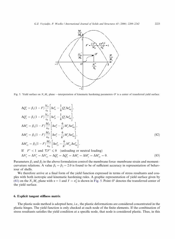
Fig. 5. Yield surface on NxMx plane —interpretation of kinematic hardening parameters O 0 is a center of transferred yield surface.


DQ�x ¼ b1ð1� F ÞN 0

e0Depxz �

1

hQ�

xDepeq

� �;

DQ�y ¼ b1ð1� F ÞN 0

e0Depyz �

1

hQ�

yDepeq

� �;

DM�x ¼ b2ð1� F ÞM0

j0

Djpx �

6

h2M�

xDjpeq

� �;

DM�y ¼ b2ð1� F ÞM0

j0

Djpy �

6

h2M�

yDjpeq

� �; ð82Þ

DM�xy ¼ b2ð1� F ÞM0

j0

Djpxy �

6

h2M�

xyDjpeq

� �;

If F � < 1 and rF �6 0 ðunloading or neutral loadingÞ

DN �x ¼ DN �

y ¼ DN �xy ¼ DQ�

x ¼ DQ�y ¼ DM�

x ¼ DM�y ¼ DM�

xy ¼ 0: ð83Þ

Parameters b1 and b2 in the above formulation control the membrane force–membrane strain and moment–curvature relations. A value b1 = b2 = 2.0 is found to be of sufficient accuracy in representation of behav-iour of shells.

We therefore arrive at a final form of the yield function expressed in terms of stress resultants and cou-ples with both isotropic and kinematic hardening rules. A graphic representation of yield surface given by(61) on the NxMx plane with a = 1 and Y ¼ r2

0 is shown in Fig. 5. Point O 0 denotes the transferred center ofthe yield surface.

6. Explicit tangent stiffness matrix

The plastic node method is adopted here, i.e., the plastic deformations are considered concentrated in theplastic hinges. The yield function is only checked at each node of the finite elements. If the combination ofstress resultants satisfies the yield condition at a specific node, that node is considered plastic. Thus, in this


method the inelastic deformations are only considered at the nodes, while the interior of the element re-mains always elastic.

When node i of the element becomes plastic, the yield function takes the form

F �i ðNi;Qi;Mi;N

�i ;Q

�i ;M

�i ; kÞ ¼ 0; ð84Þ

where

Ni ¼Nx

Ny

Nxy

8><>:

9>=>;; Qi ¼

Qx

Qy

( ); Mi ¼

Mx

My

Mxy

8><>:

9>=>;; N�

i ¼N �

x

N �y

N �xy

8><>:

9>=>;; Q�

i ¼Q�

x

Q�y

( ); M�

i ¼M�

x

M�y

M�xy

8><>:

9>=>;:

ð85Þ

At the same time the stress resultants must remain on the yield surface, i.e., the consistency condition mustbe satisfied

oF �i

oMidMi þ

oF �i

oNidNi þ

oF �i

oQidQi þ

oF �i

oM�i

dM�i þ

oF �i

oN�i

dN�i þ

oF �i

oQ�i

dQ�i þ

oF �i

okdk ¼ 0: ð86Þ

We assume an additive decomposition of strains into elastic and plastic parts

e ¼ ee þ ep: ð87Þ
The associated flow rule is used here to determine the increments of plastic strains
Djpx ¼

XNPN

i¼1

DkioF �

i

oMxi; ð88Þ

where NPN is the number of plastic nodes in the element and dki is a plastic multiplier. The remainingincrements of the plastic strains are obtained in the same way. The plastic strain fields are interpolatedas in linear elastic analysis (Eqs. (31)–(33)) rewritten here in the incremental form

Depb ¼Djp

x

Djpy

2Djpxy

8><>:

9>=>;; Depm ¼

DepxDepy2Depxy

8><>:

9>=>;; Deps ¼

DcpxzDcpyz

( ): ð89Þ

The assumption of an additive decomposition of strains may be extended to displacements, provided thatthe strains are small (Shi and Voyiadjis, 1992; Ueda and Yao, 1982). Although geometric non-linearities aretaken into account in the current work, we only consider large rigid rotations and translations, but smallstrains. Thus, we may write

q ¼ qe þ qp: ð90Þ
Following the work of Shi and Voyiadjis (1992) we approximate the increments of plastic displacements bythe increments of plastic strains. The plastic rotation D/p
x will be a function of both Djpx and Djp

xy , as can bededuced from Eq. (31). Assuming that increment of plastic nodal rotation D/p

xi is proportional to the incre-ment of elastic nodal rotation D/xi we may express the former as

D/pxi ¼ lim

dX!0

Z ZoXi

Djpx þ

D/2xi

D/2xi þ D/2

yi

2Djpxy

" #dxdy ¼ Dki

oF �i

oMxiþ 2D/2

xi

D/2xi þ D/2

yi

oF �i

oMxyi

" #; ð91Þ

where dXi represents the infinitesimal neighborhood of node i. The vector of incremental nodal plastic dis-placements of the element at node i may then be expressed as


Dqpi ¼ aiDki ð92Þ
with ai given by
aTi ¼ oF �i

oNxiþ pu

oF �i

oNxyi;oF �

i

oNyiþ pv

oF �i

oNxyi;oF �

i

oQxi

þ oF �i

oQyi

;

(

oF �i

oMxiþ p/x

oF �i

oMxyi;oF �

i

oMyiþ p/y

oF �i

oMxyi

)ð93Þ

pu ¼2Du2i

Du2i þ Dv2i; pv ¼

2Dv2iDu2i þ Dv2i

; p/x ¼2D/2

xi

D/2xi þ D/2

yi

; p/y ¼2D/2

yi

D/2xi þ D/2

yi

:

Eqs. (92) and (93) indicate that the plastic displacements at the nodes are only the functions of stress resul-tants at this node (Shi and Voyiadjis, 1992). Therefore, we can write the vector of increments of nodal plas-tic displacements, as follows:

Dqp ¼a1 0 0

0 ai 0

0 0 aNPN

264

375

Dk1

Dki

DkNPN

8><>:

9>=>; ¼ aDk: ð94Þ

In order to determine the tangent stiffness matrix of the element we define deb, dem, des as virtual elasticbending, membrane and transverse shear strains respectively (d-virtual) and M,N,Q as stress couplesand stress resultants of the element. We also make use of the linearized equilibrium equations of the systemat configuration k + 1 in the updated Lagrangian formulation, expressed by the principle of the virtualwork, which in finite element modeling takes the form
Z
X

ZðdeTbDeb þ deTmSem þ deTs TesÞdxdy

ZX

ZdhTkFhdxdy

¼ kþ1R�ZX

ZðdeTb kMþ deTm

kNþ deTskQÞdxdy; ð95Þ

where k + 1R is the total external virtual work at step k + 1 and h is the slope vector and kF is a membranestress resultant matrix at step k given by

h ¼

oDwoxoDwoy

8>><>>:

9>>=>>;; kF ¼

kNxkNxy

kNxykNy :

" #ð96Þ

The slope field h is evaluated in a similar way to the strain fields, using quasi-conforming technique (Tanget al., 1980, 1983). A bilinear interpolation is used as in Shi and Voyiadjis (1991) to approximate the slopefield 8 9

h ¼1 x y xy 0 0 0 0

0 0 0 0 1 x y xy

� � b1

b2

b3

b7

b8

>>>>>><>>>>>>:

>>>>>>=>>>>>>;

¼ Pb ð97Þ

with P denoting the trial function matrix and b is a vector of undetermined parameters, calculated in thesame way as the vectors of strain parameters a used to approximate the strain fields (Eqs. (31)–(33))


b ¼ A�1CDqe; A ¼ZX

ZPTPdxdy; CDqe ¼

ZX

ZPThdxdy: ð98Þ

The details of the evaluation of the A, C matrices are given in Shi and Voyiadjis (1990), Shi and Voyiadjis(1991), Tang et al. (1983) and Woelke and Voyiadjis (submitted for publication). The slope field h is there-fore expressed in terms of the slope–displacement matrix G

h ¼ PA�1CDqe ¼ GDqe: ð99Þ

The cubic interpolation of Dw along the boundary of the elements, given by Hu (1984) will be used here toevaluate C matrix

DwðsÞ ¼ ½1� nþ kðn� 3n2 þ 2n3Þ�Dwi þ ½n� n2 þ kðn� 3n2 þ 2n2Þ� lij2D/si

þ ½n� kðn� 3n2 þ 2n3Þ�Dwj þ ½�nþ n2 þ kðn� 3n2 þ 2n2Þ� lij2D/sj; ð100Þ

n ¼ slij

; 0 6 s 6 lij; 0 6 n 6 1; k ¼ 1

1� 12 DTL2

� � ;
where lij is the distance between nodes i and j, D/si, D/sj are tangential rotations at nodes i and j respec-tively, and D, T are flexural and transverse shear rigidities. The influence of parameter k is explained inHu (1984) and Woelke and Voyiadjis (submitted for publication).
Using Eq. (99), the virtual work principle given by (95) may now be rewritten
ZX
ZðdeTbDeb þ deTmSem þ deTs TesÞdxdy þ dDqe

T

KgDqe

¼ kþ1R�ZX

ZðdeTb kMþ deTm

kNþ deTskQÞdxdy; ð101Þ

where Kg is the initial stress matrix defined as

Kg ¼ZX

ZGTkFGdxdy ð102Þ

Substituting Eqs. (39)–(41) into the right-hand side of the above we can write
ZX
ZðdeTb kMþ deTm

kNþ deTskQÞdxdy ¼ dDqTDf; ð103Þ

where f is the internal force vector resulting from the unbalanced forces in configuration k and is expressedas follows:

f ¼ZX

ZðBT

bkMþ BT

mkNþ BT

skQÞdxdy: ð104Þ

We may now rewrite Eq. (95) using Eqs. (7)–(14), written in a matrix form, and Eqs. (87), (104) as follows:
ZX
Zdee

T

b þ depT

b

� �Mþ dee

T

m þ depT

m

� �Nþ dee

T

s þ depT

s

� �Q

h idxdy þ dDqe

T

KgDqe ¼ kþ1R� dDqTDf

ð105Þ


rearranging terms and writing the above equation in incremental form
ZX
ZdDee

T

b DMþ dDeeT

mDNþ dDeeT

s DQ� �

dxdy

þZX

ZdDep

T

b DMþ dDepT

m DNþ dDepT

s DQ� �

dxdy þ dDqeT

KgDqe ¼ kþ1R� dDqTDf. ð106Þ

Substituting Eq. (88) into Eq. (106) we obtain
ZX
ZdDee

T

b DMþ dDeeT

mDNþ dDeeT

s DQ� �

dxdy

þXNPN

i¼1

dDkioF �

i

oMidMi þ

oF �i

oNidNi þ

oF �i

oQidQi

� �þ dDqe

T

KgDqe ¼ kþ1R� dDqTDf. ð107Þ

Making use of the Eqs. (43)–(45), as well as the consistency condition given by Eq. (86), we may write

dDqeTðKþ KgÞDqe �

XNPN

i¼1

dDkioF �

i

oM�i

dM�i þ

oF �i

oN�i

dN�i þ

oF �i

oQ�i

dQ�i þ

oF �i

okdk

� �¼ kþ1R� dDqTDf; ð108Þ

where K is the linear elastic stiffness matrix given by Eq. (49).Similarly to Eq. (93) we define

aTbi ¼oF �

i

oM�i

¼ oF �i

oM�xi

;oF �

i

oM�yi

;oF �

i

oM�xyi

( );

aTmi ¼oF �

i

oN�i

¼ oF �i

oN �xi

;oF �

i

oN �yi

;oF �

i

oN �xyi

( );

aTsi ¼oF �

i

oQ�i

¼ oF �i

oQ�xi

;oF �

i

oQ�yi

( ):

ð109Þ

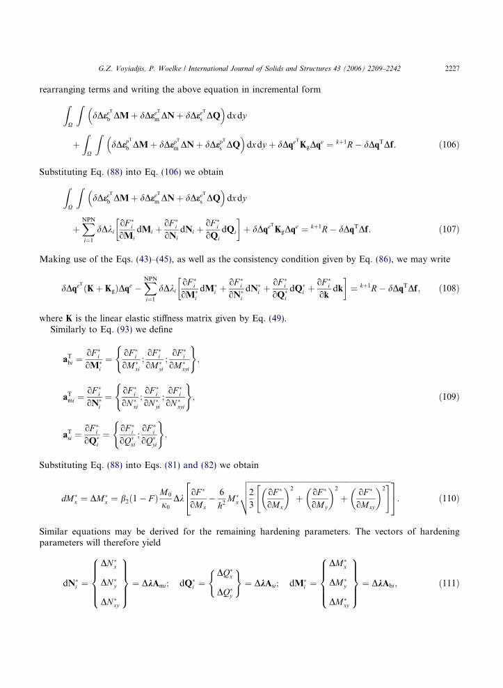
Substituting Eq. (88) into Eqs. (81) and (82) we obtain

dM�x ¼ DM�

x ¼ b2ð1� F ÞM0

j0

DkoF �

oMx� 6

h2M�

x

ffiffiffiffiffiffiffiffiffiffiffiffiffiffiffiffiffiffiffiffiffiffiffiffiffiffiffiffiffiffiffiffiffiffiffiffiffiffiffiffiffiffiffiffiffiffiffiffiffiffiffiffiffiffiffiffiffiffiffiffiffiffiffiffiffiffiffiffiffiffiffiffiffiffi2

3

oF �

oMx

� �2

þ oF �

oMy

� �2

þ oF �

oMxy

� �2" #vuut

24

35: ð110Þ

Similar equations may be derived for the remaining hardening parameters. The vectors of hardeningparameters will therefore yield

dN�i ¼

DN �x

DN �y

DN �xy

8>>><>>>:

9>>>=>>>; ¼ DkAmi; dQ�

i ¼DQ�

x

DQ�y

( )¼ DkAsi; dM�

i ¼

DM�x

DM�y

DM�xy

8>>><>>>:

9>>>=>>>; ¼ DkAbi; ð111Þ


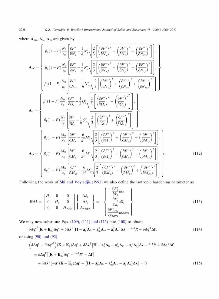
where Ami, Asi, Abi are given by

Ami ¼

b1ð1� F ÞN 0

e0

oF �

oNx� 1

hN �

x

ffiffiffiffiffiffiffiffiffiffiffiffiffiffiffiffiffiffiffiffiffiffiffiffiffiffiffiffiffiffiffiffiffiffiffiffiffiffiffiffiffiffiffiffiffiffiffiffiffiffiffiffiffiffiffiffiffiffiffiffiffiffiffiffiffiffiffiffiffiffiffiffi2

3

oF �

oNx

� �2

þ oF �

oNy

� �2

þ oF �

oNxy

� �2" #vuut

24

35;

b1ð1� F ÞN 0

e0

oF �

oNy� 1

hN �

y


3

oF �

oNx

� �2

þ oF �

oNy

� �2

þ oF �

oNxy

� �2" #vuut

24

35;

b1ð1� F ÞN 0

e0

oF �

oNxy� 1

hN �

xy


3

oF �

oNx

� �2

þ oF �

oNy

� �2

þ oF �

oNxy

� �2" #vuut

24

35

8>>>>>>>>>>>>>><>>>>>>>>>>>>>>:

9>>>>>>>>>>>>>>=>>>>>>>>>>>>>>;

;

Asi ¼

b1ð1� F ÞN 0

e0

oF �

oQx

� 1

hQ�

x

ffiffiffiffiffiffiffiffiffiffiffiffiffiffiffiffiffiffiffiffiffiffiffiffiffiffiffiffiffiffiffiffiffiffiffiffiffiffiffiffiffiffiffiffiffiffiffiffiffi2

3

oF �

oQx

� �2

þ oF �

oQy

!224

35

vuuut264

375;

b1ð1� F ÞN 0

e0

oF �

oQy

� 1

hQ�

y

ffiffiffiffiffiffiffiffiffiffiffiffiffiffiffiffiffiffiffiffiffiffiffiffiffiffiffiffiffiffiffiffiffiffiffiffiffiffiffiffiffiffiffiffiffiffiffiffiffi2

3

oF �

oQx

� �2

þ oF �

oQy

!224

35

vuuut264

375

8>>>>>>>>><>>>>>>>>>:

9>>>>>>>>>=>>>>>>>>>;;

Abi ¼

b2ð1� F ÞM0

j0

oF �

oMx� 6

h2M�

x


3

oF �

oMx

� �2

þ oF �

oMy

� �2

þ oF �

oMxy

� �2" #vuut

24

35;

b2ð1� F ÞM0

j0

oF �

oMy� 6

h2M�

x


3

oF �

oMx

� �2

þ oF �

oMy

� �2

þ oF �

oMxy

� �2" #vuut

24

35;

b2ð1� F ÞM0

j0

oF �

oMxy� 6

h2M�

x


3

oF �

oMx

� �2

þ oF �

oMy

� �2

þ oF �

oMxy

� �2" #vuut

24

35

8>>>>>>>>>>>>>><>>>>>>>>>>>>>>:

9>>>>>>>>>>>>>>=>>>>>>>>>>>>>>;

: ð112Þ

Following the work of Shi and Voyiadjis (1992) we also define the isotropic hardening parameter as

HDk ¼H 1 0 0

0 Hi 0

0 0 HNPN

264

375 Dk1

DkiDkNPN

8><>:

9>=>; ¼ �

oF �1

ok1dk1

oF �i

okidki

oF �NPN

okNPN

dkNPN

8>>>>>><>>>>>>:

9>>>>>>=>>>>>>;: ð113Þ

We may now substitute Eqs. (109), (111) and (113) into (108) to obtain

dDqeTðKþ KgÞDqe þ dDkT H� aTbAb � aTmAm � aTs As

� �Dk ¼ kþ1R� dDqTDf; ð114Þ

or using (90) and (92)

dDqT � dDqpT

� �ðKþ KgÞDqe þ dDkT H� aTbAb � aTmAm � aTs As

� �Dk� kþ1Rþ dDqTDf

¼ dDqT ðKþ KgÞDqe � kþ1R� þ Df� �

þ dDkT �aTðKþ KgÞDqe þ H� aTbAb � aTmAm � aTs As

�Dk

� �¼ 0 ð115Þ


with

kþ1R ¼ kþ1R�dDq: ð116Þ

By the virtue of the variational method Eq. (115) gives

ðKþ KgÞDqe � kþ1R� þ Df ¼ 0

� aTðKþ KgÞDqe þ H� aTbAb � aTmAm � aTs As

�Dk ¼ 0:

ð117Þ

Substituting (90) and (92) into the above equations, we get

ðKþ KgÞDqe � kþ1R� þ Df ¼ ðKþ KgÞðDq� aDkÞ ¼ kþ1R� � Df; ð118Þ

�aTðKþ KgÞðDq� aDkÞ þ H� aTbAb � aTmAm � aTs As

�Dk ¼ 0: ð119Þ

Eq. (119) leads to

Dk ¼ aTðKþ KgÞaþ H� aTbAb � aTmAm � aTs As

�� 1aTðKþ KgÞDq: ð120Þ

Eq. (118) becomes

KepgDq ¼ kþ1R� � Df; ð121Þ

where Kepg is the elasto-plastic, large displacement stiffness matrix of the element, given by

Kepg ¼ ðKþ KgÞ I� a aTðKþ KgÞaþ H� aTbAb � aTmAm � aTs As

�� 1aTðKþ KgÞ

n o: ð122Þ

The tangent stiffness matrix given by Eq. (122) is similar to the one presented by Shi and Voyiadjis (1992).The present formulation accounts for large displacements and consequently the stiffness matrix of the ele-ment contains the initial stress matrix Kg. More importantly however, the above derived stiffness matrixdescribes not only isotropic hardening, by means of parameter H, but also kinematic hardening, throughparameters Ab, Am, As, which are not determined by curve fitting, but derived explicitly from the evolutionequation of backstress given by Armstrong and Frederick (1966). We therefore have a non-layered finiteelement formulation with shell constitutive equations, yield condition, flow and hardening rules expressedin terms of membrane and shear forces and bending moments. All the variables used here, namely the stressresultants and couples, as well as the residual stress resultants and couples, representing the center of theyield surface, are derived from stresses and back-stresses in a very rigorous manner.

A very important feature of the derived tangent stiffness is its explicit form. The linear elastic stiffnessmatrix and initial stress matrix are determined by a quasi-conforming technique, which allows all the inte-grations to be performed analytically. The hardening parameters are also given explicitly. It is also notedthat through the thickness integration is not employed here either, since the current model is the non-lay-ered model with the yield condition expressed in terms of stress couples and resultants.

7. Numerical examples

For the purpose of the implementation of the model, a finite element code is developed in the program-ming language Fortran 90. A modified Newton–Raphson technique is employed to solve a system of non-linear incremental equations. To overcome a singularity problem appearing at the limit point, thearc-length method (Crisfield, 1991) is adopted to determine the local load increment for each iteration.The return to the yield surface algorithm (Crisfield, 1991) is also implemented. The results delivered by


the current model are computed using a personal computer with AMD Athlon Processor, 1.8 GHz and1.5 GB of RAM. Some of the reference solutions obtained with the layered approach (ABAQUS) weredetermined using a Silicon Graphics Onyx 3200 workstation.

The accuracy of the present formulation is verified through a series of discriminating examples. Since thispaper is a continuation of the previous work of the authors (Woelke and Voyiadjis, submitted for publica-tion), in which the linear elastic behavior of shells is examined, we will only solve non-linear examples here.The problems are chosen to challenge and demonstrate the most important features of the current model:

• Representation of the progressive development of plastic deformation until the plastic hinge is formed.• The influence of the transverse shear forces on the plastic behavior of thick plates beams and shells ofgeneral shape.

• Elasto-plastic behaviour of structures of interest upon reversal of loading (representation of Bauschingereffect through kinematic hardening).

• Description of large displacements and rotations.

The performance of the proposed procedure is compared with other formulations available in the liter-ature. Table 1 lists the references used here, and their corresponding abbreviations used later in the text.

7.1. Simply supported elasto-plastic beam

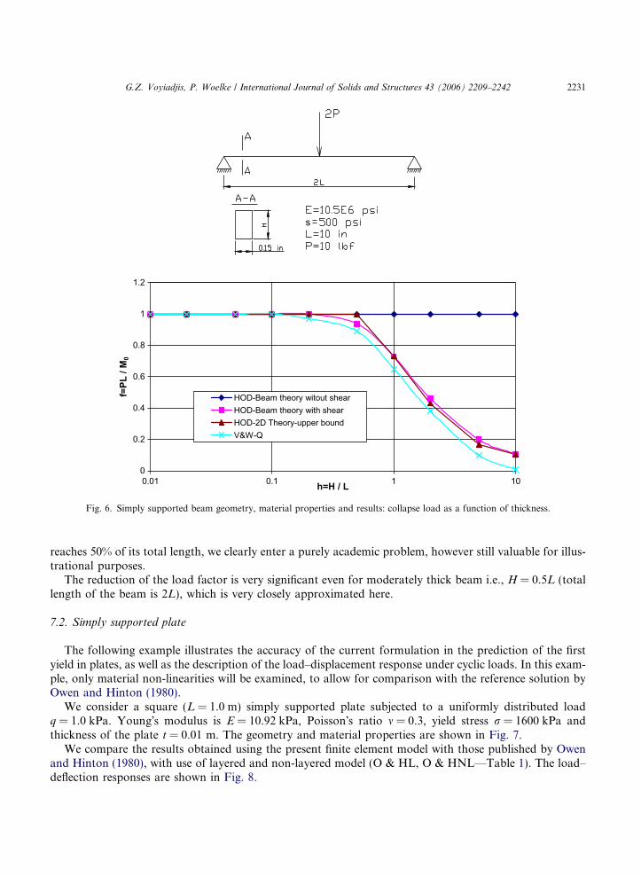
The importance of the transverse shear forces in the approximations of the collapse load of thick beams,plates and shells is known to be significant. Neglecting transverse shears in assessments of the maximumload carrying capacity of the structures may lead to predictions that are not conservative. Accurate andsafe approximations should result in a decreasing value of the maximum load factor with increasing thick-ness. To test the accuracy of the current formulations in accounting for the shear deformation, we considera simply supported beam of length 2L = 20 in subjected to a concentrated load 2P = 20 lbf at its mid-point.The Young�s modulus is E = 10.5E6 psi, yield stress r = 500 psi, and width of the beam is b = 0.15 in. Wecompute the load factor of the beam as a function of thickness. The analytical solution of this problemgiven by Hodge (1959) serves here as a reference solution.

As seen in Fig. 6, the current formulation agrees very well with analytical results of this problem byHodge (1959). As expected we observe a substantial drop in the load factor for thick beams. We note, thatfor practical purposes only a certain range of H is significant. When the thickness of the beam, plate or shell

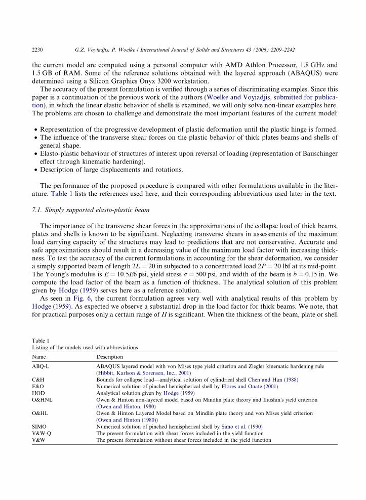
Table 1Listing of the models used with abbreviations

Name Description

ABQ-L ABAQUS layered model with von Mises type yield criterion and Ziegler kinematic hardening rule(Hibbit, Karlson & Sorensen, Inc., 2001)

C&H Bounds for collapse load—analytical solution of cylindrical shell Chen and Han (1988)F&O Numerical solution of pinched hemispherical shell by Flores and Onate (2001)HOD Analytical solution given by Hodge (1959)O&HNL Owen & Hinton non-layered model based on Mindlin plate theory and Iliushin�s yield criterion

(Owen and Hinton, 1980)O&HL Owen & Hinton Layered Model based on Mindlin plate theory and von Mises yield criterion

(Owen and Hinton (1980))SIMO Numerical solution of pinched hemispherical shell by Simo et al. (1990)V&W-Q The present formulation with shear forces included in the yield functionV&W The present formulation without shear forces included in the yield function

s

0

0.2

0.4

0.6

0.8

1

1.2

0.01 0.1 1 10h=H / L

f=PL

/ M

0

HOD-Beam theory witout shearHOD-Beam theory with shearHOD-2D Theory-upper boundV&W-Q

Fig. 6. Simply supported beam geometry, material properties and results: collapse load as a function of thickness.


reaches 50% of its total length, we clearly enter a purely academic problem, however still valuable for illus-trational purposes.

The reduction of the load factor is very significant even for moderately thick beam i.e., H = 0.5L (totallength of the beam is 2L), which is very closely approximated here.

7.2. Simply supported plate

The following example illustrates the accuracy of the current formulation in the prediction of the firstyield in plates, as well as the description of the load–displacement response under cyclic loads. In this exam-ple, only material non-linearities will be examined, to allow for comparison with the reference solution byOwen and Hinton (1980).

We consider a square (L = 1.0 m) simply supported plate subjected to a uniformly distributed loadq = 1.0 kPa. Young�s modulus is E = 10.92 kPa, Poisson�s ratio m = 0.3, yield stress r = 1600 kPa andthickness of the plate t = 0.01 m. The geometry and material properties are shown in Fig. 7.

We compare the results obtained using the present finite element model with those published by Owenand Hinton (1980), with use of layered and non-layered model (O & HL, O & HNL—Table 1). The load–deflection responses are shown in Fig. 8.

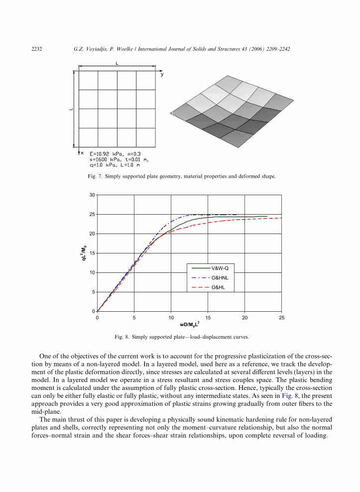
Fig. 7. Simply supported plate geometry, material properties and deformed shape.

0

5

10

15

20

25

30

0 5 10 15 20 25wD/MpL2

qL2 /M

p

V&W-Q

O&HNL

O&HL

Fig. 8. Simply supported plate—load–displacement curves.


One of the objectives of the current work is to account for the progressive plasticization of the cross-sec-tion by means of a non-layered model. In a layered model, used here as a reference, we track the develop-ment of the plastic deformation directly, since stresses are calculated at several different levels (layers) in themodel. In a layered model we operate in a stress resultant and stress couples space. The plastic bendingmoment is calculated under the assumption of fully plastic cross-section. Hence, typically the cross-sectioncan only be either fully elastic or fully plastic, without any intermediate states. As seen in Fig. 8, the presentapproach provides a very good approximation of plastic strains growing gradually from outer fibers to themid-plane.

The main thrust of this paper is developing a physically sound kinematic hardening rule for non-layeredplates and shells, correctly representing not only the moment–curvature relationship, but also the normalforces–normal strain and the shear forces–shear strain relationships, upon complete reversal of loading.


We therefore need to show the importance of all hardening parameters N*, Q*, M*. The simply sup-ported plate under a uniformly distributed load is a problem in which the normal forces are negligible.The residual forces N* will then also be negligible. The influence of these is investigated in the followingexamples.

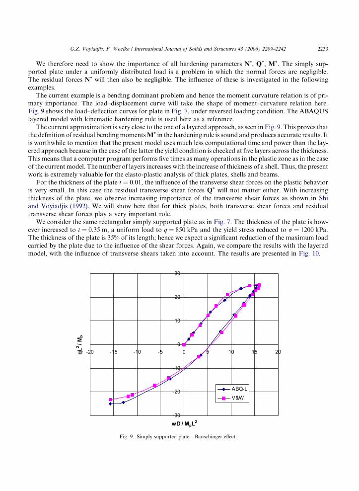
The current example is a bending dominant problem and hence the moment curvature relation is of pri-mary importance. The load–displacement curve will take the shape of moment–curvature relation here.Fig. 9 shows the load–deflection curves for plate in Fig. 7, under reversed loading condition. The ABAQUSlayered model with kinematic hardening rule is used here as a reference.

The current approximation is very close to the one of a layered approach, as seen in Fig. 9. This proves thatthe definition of residual bendingmomentsM* in the hardening rule is sound and produces accurate results. Itis worthwhile to mention that the present model uses much less computational time and power than the lay-ered approach because in the case of the latter the yield condition is checked at five layers across the thickness.This means that a computer program performs five times as many operations in the plastic zone as in the caseof the current model. The number of layers increases with the increase of thickness of a shell. Thus, the presentwork is extremely valuable for the elasto-plastic analysis of thick plates, shells and beams.

For the thickness of the plate t = 0.01, the influence of the transverse shear forces on the plastic behavioris very small. In this case the residual transverse shear forces Q* will not matter either. With increasingthickness of the plate, we observe increasing importance of the transverse shear forces as shown in Shiand Voyiadjis (1992). We will show here that for thick plates, both transverse shear forces and residualtransverse shear forces play a very important role.

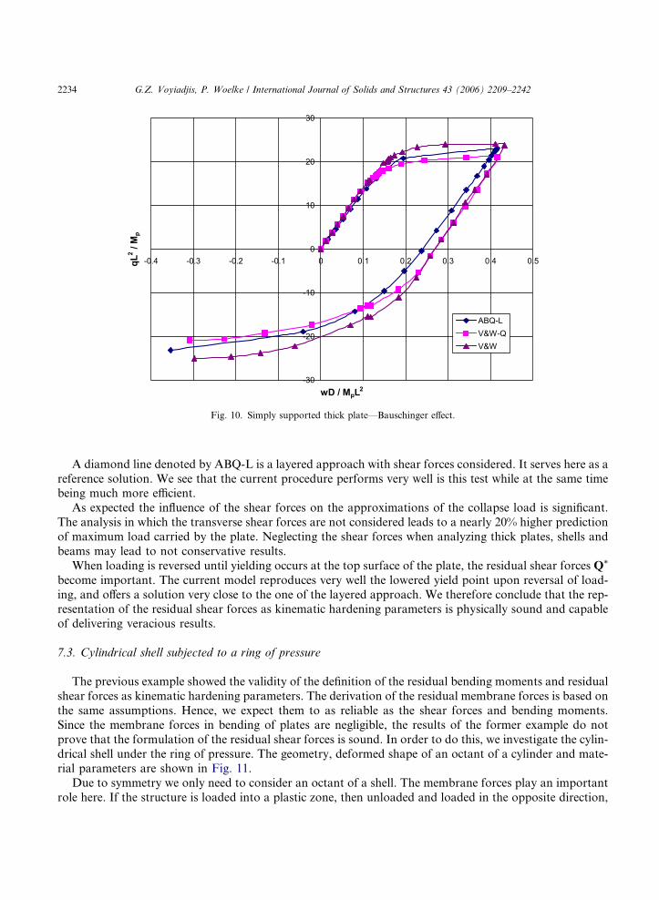
We consider the same rectangular simply supported plate as in Fig. 7. The thickness of the plate is how-ever increased to t = 0.35 m, a uniform load to q = 850 kPa and the yield stress reduced to r = 1200 kPa.The thickness of the plate is 35% of its length; hence we expect a significant reduction of the maximum loadcarried by the plate due to the influence of the shear forces. Again, we compare the results with the layeredmodel, with the influence of transverse shears taken into account. The results are presented in Fig. 10.

-30

-20

-10

0

10

20

30

-20 -15 -10 -5 0 5 10 15 20

wD / MpL2

qL2/ M

p

ABQ-L

V&W

Fig. 9. Simply supported plate—Bauschinger effect.

-30

-20

-10

0

10

20

30

-0.4 -0.3 -0.2 -0.1 0 0.1 0.2 0.3 0.4 0.5

wD / MpL2

qL2 /

Mp

ABQ-LV&W-QV&W

Fig. 10. Simply supported thick plate—Bauschinger effect.


A diamond line denoted by ABQ-L is a layered approach with shear forces considered. It serves here as areference solution. We see that the current procedure performs very well is this test while at the same timebeing much more efficient.

As expected the influence of the shear forces on the approximations of the collapse load is significant.The analysis in which the transverse shear forces are not considered leads to a nearly 20% higher predictionof maximum load carried by the plate. Neglecting the shear forces when analyzing thick plates, shells andbeams may lead to not conservative results.

When loading is reversed until yielding occurs at the top surface of the plate, the residual shear forces Q*

become important. The current model reproduces very well the lowered yield point upon reversal of load-ing, and offers a solution very close to the one of the layered approach. We therefore conclude that the rep-resentation of the residual shear forces as kinematic hardening parameters is physically sound and capableof delivering veracious results.

7.3. Cylindrical shell subjected to a ring of pressure

The previous example showed the validity of the definition of the residual bending moments and residualshear forces as kinematic hardening parameters. The derivation of the residual membrane forces is based onthe same assumptions. Hence, we expect them to as reliable as the shear forces and bending moments.Since the membrane forces in bending of plates are negligible, the results of the former example do notprove that the formulation of the residual shear forces is sound. In order to do this, we investigate the cylin-drical shell under the ring of pressure. The geometry, deformed shape of an octant of a cylinder and mate-rial parameters are shown in Fig. 11.

Due to symmetry we only need to consider an octant of a shell. The membrane forces play an importantrole here. If the structure is loaded into a plastic zone, then unloaded and loaded in the opposite direction,

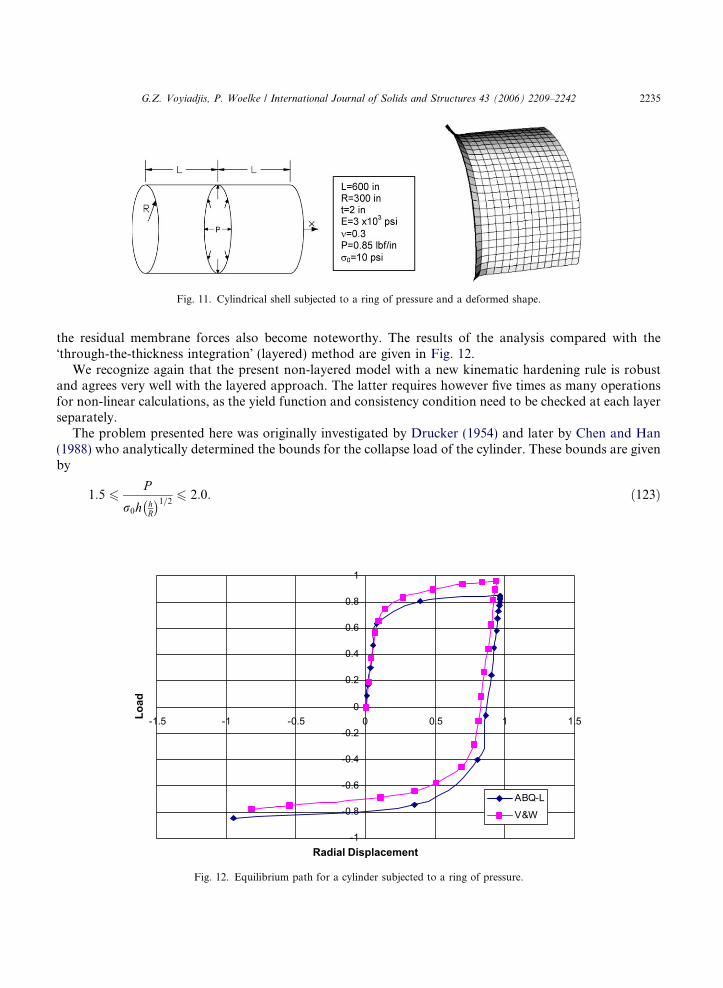
Fig. 11. Cylindrical shell subjected to a ring of pressure and a deformed shape.


the residual membrane forces also become noteworthy. The results of the analysis compared with the�through-the-thickness integration� (layered) method are given in Fig. 12.

We recognize again that the present non-layered model with a new kinematic hardening rule is robustand agrees very well with the layered approach. The latter requires however five times as many operationsfor non-linear calculations, as the yield function and consistency condition need to be checked at each layerseparately.

The problem presented here was originally investigated by Drucker (1954) and later by Chen and Han(1988) who analytically determined the bounds for the collapse load of the cylinder. These bounds are givenby

1:5 6P

r0h hR

�1=2 6 2:0: ð123Þ

-1

-0.8

-0.6

-0.4

-0.2

0

0.2

0.4

0.6

0.8

1

-1.5 -1 -0.5 0 0.5 1 1.5

Radial Displacement

Load

ABQ-L

V&W

Fig. 12. Equilibrium path for a cylinder subjected to a ring of pressure.


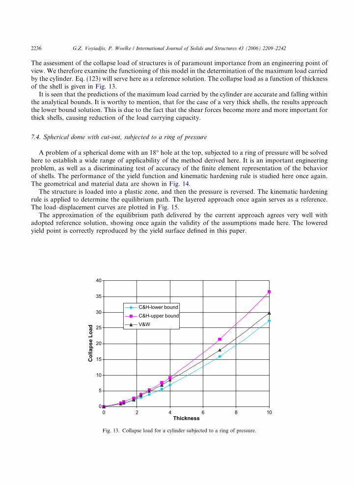
The assessment of the collapse load of structures is of paramount importance from an engineering point ofview. We therefore examine the functioning of this model in the determination of the maximum load carriedby the cylinder. Eq. (123) will serve here as a reference solution. The collapse load as a function of thicknessof the shell is given in Fig. 13.

It is seen that the predictions of the maximum load carried by the cylinder are accurate and falling withinthe analytical bounds. It is worthy to mention, that for the case of a very thick shells, the results approachthe lower bound solution. This is due to the fact that the shear forces become more and more important forthick shells, causing reduction of the load carrying capacity.

7.4. Spherical dome with cut-out, subjected to a ring of pressure

A problem of a spherical dome with an 18� hole at the top, subjected to a ring of pressure will be solvedhere to establish a wide range of applicability of the method derived here. It is an important engineeringproblem, as well as a discriminating test of accuracy of the finite element representation of the behaviorof shells. The performance of the yield function and kinematic hardening rule is studied here once again.The geometrical and material data are shown in Fig. 14.

The structure is loaded into a plastic zone, and then the pressure is reversed. The kinematic hardeningrule is applied to determine the equilibrium path. The layered approach once again serves as a reference.The load–displacement curves are plotted in Fig. 15.

The approximation of the equilibrium path delivered by the current approach agrees very well withadopted reference solution, showing once again the validity of the assumptions made here. The loweredyield point is correctly reproduced by the yield surface defined in this paper.

0

5

10

15

20

25

30

35

40

0 2 4 6 8Thickness

Col

laps

e Lo

ad

10

C&H-lower bound

C&H-upper bound

V&W

Fig. 13. Collapse load for a cylinder subjected to a ring of pressure.

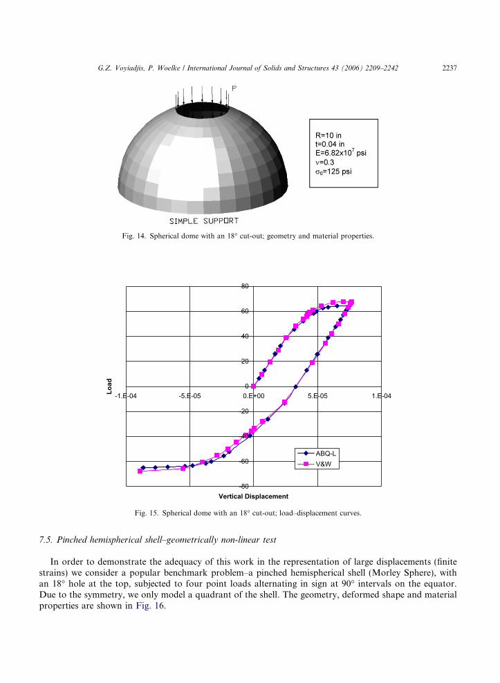
Fig. 14. Spherical dome with an 18� cut-out; geometry and material properties.

-80

-60

-40

-20

0

20

40

60

80

-1.E-04 -5.E-05 0.E+00 5.E-05 1.E-04

Vertical Displacement

Load

ABQ-LV&W

Fig. 15. Spherical dome with an 18� cut-out; load–displacement curves.


7.5. Pinched hemispherical shell–geometrically non-linear test

In order to demonstrate the adequacy of this work in the representation of large displacements (finitestrains) we consider a popular benchmark problem–a pinched hemispherical shell (Morley Sphere), withan 18� hole at the top, subjected to four point loads alternating in sign at 90� intervals on the equator.Due to the symmetry, we only model a quadrant of the shell. The geometry, deformed shape and materialproperties are shown in Fig. 16.

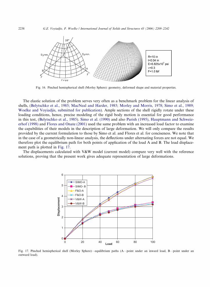
Fig. 16. Pinched hemispherical shell (Morley Sphere): geometry, deformed shape and material properties.


The elastic solution of the problem serves very often as a benchmark problem for the linear analysis ofshells, (Belytschko et al., 1985; MacNeal and Harder, 1985; Morley and Morris, 1978; Simo et al., 1989;Woelke and Voyiadjis, submitted for publication). Ample sections of the shell rigidly rotate under theseloading conditions, hence, precise modeling of the rigid body motion is essential for good performancein this test, (Belytschko et al., 1985). Simo et al. (1990) and also Parish (1995), Hauptmann and Schweiz-erhof (1998) and Flores and Onate (2001) used the same problem with an increased load factor to examinethe capabilities of their models in the description of large deformation. We will only compare the resultsprovided by the current formulation to those by Simo et al. and Flores et al. for conciseness. We note thatin the case of a geometrically non-linear analysis, the deflections under alternating forces are not equal. Wetherefore plot the equilibrium path for both points of application of the load A and B. The load displace-ment path is plotted in Fig. 17.

The displacements calculated with V&W model (current model) compare very well with the referencesolutions, proving that the present work gives adequate representation of large deformations.

0

1

2

3

4

5

6

0 20 40 60 80Load

Dis

plac

emen

t

100

SIMO-ASIMO- BF&O-AF&O-BV&W-AV&W-B

Fig. 17. Pinched hemispherical shell (Morley Sphere)—equilibrium paths (A—point under an inward load, B—point under anoutward load).


8. Conclusions

A mathematically consistent finite element model for elasto-plastic, large rotations analysis of thin/thickshells is presented here. An accurate set of shell constitutive equations, previously developed by the sameauthors is adopted. The theory treats both thick and thin shells, with transverse shear deformation, radialstresses and initial curvature effects taken into account, which makes it accurate and reliable for a variety ofapplications.

A numerical implementation of the shell constitutive equations, by means of the �quasi conforming tech-nique�, leads to the development of a finite element free from common deficiencies, i.e., shear and mem-brane locking and spurious energy modes. Moreover, integration is performed analytically, which ismore precise from a mathematical point of view, and features an explicit form of the stiffness matrix.Numerical integration is not necessary which makes this formulation very efficient and attractivecomputationally.

The most important feature of the paper is the non-layered yield surface with a new kinematic hardeningrule. Iliushin�s yield function expressed in terms of stress resultants and couples, and modified to accountfor the progressive development of the plastic deformation and transverse shear forces is used. The kine-matic hardening rule representing the rigid motion of the yield surface during loading, in the stress resultantspace is also derived. It is capable of correctly determining the load–displacement response including theBauschinger effect. Residual forces and bending moments are related to backstress using a similar definitionto that of primary forces and moments. All the integrals are calculated analytically, which makes the cur-rent formulation extremely effective, as numerical integration is not employed at any stage of the compu-tations. Thus, the kinematic hardening rule outlined here simplifies and speeds up the analysis, without anysubstantial loss of accuracy.

Large rotations and displacements are often associated with inelastic deformation. An updated Lagrang-ian method is utilized to describe the geometric non-linearities. We decompose rotations into large rigidrotations and moderate relative rotations. The strains are assumed to be small.

The reliability of the presented concept is numerically evaluated through a series of benchmark prob-lems. In all the cases results are very close to the reference solutions, which demonstrates that the modelis well grounded.

The effect of the shear forces on the plastic behavior and maximum load carrying capacity is correctlyrecognized. As expected, the results show a reduction of the limit load for thick plates, shells and beams,owing to the increasing significance of transverse shears.

The progressive plastification of the cross-section is also closely approximated. Typically, in the non-lay-ered approach, the load displacement relation is linear until the plastic hinge is developed. Any yieldingoccurring before the section becomes fully plastic is neglected. Through a modification introduced byCrisfield (1981), the first yield of the outer fibers may be predicted as is also proven here.

The Bauschinger effect may only be numerically observed if the method employed features a veraciouskinematic hardening rule. The one proposed here is defined in a stress resultant space, which is very effectivefrom a structural analysis viewpoint. The lowered yield point upon reversal of load is correctly determinedhere for both plates and shells proving that the definition of the �hardening parameters� is sound and capa-ble of delivering very accurate results.

Example 7.5 evaluates the ability of the model to handle large rigid rotations. The solution offered here isonce again precise demonstrating validity of large rotation formulation.

We note that although presented framework is robust for plates and shells of general shape, it performsbest in the case of spherical shells. This is expected since the shell constitutive equations used here arederived by means of spherical strains, and later generalized through the finite element method.

The elastic analysis of shells by means of three-dimensional �brick� elements is sometimes prohibitive dueto the complexity of the problem. Shell elements are �degenerated�; hence, they require a vastly reduced


number of operations executed by the computer. It allows engineers to predict the internal forces ofcomplicated structures, which would have been difficult or impossible otherwise. Yet in the elasto-plasticconsiderations, most shell elements follow the layered approach, which is a concept similar to three dimen-sional �brick� elements. While in the case of composite laminates, multi-layered shells give more accuratedescription of interlaminar effects, they lose their advantages in the analysis of isotropic homogenous shells.A non-layered method seems to be a natural consequence of the shell elements� development because thesystem of non-linear equations is expressed in terms forces and bending moments, and solved without dis-cretization of the shell through the thickness. It allows taking the full advantage of shell elements in inves-tigation of elasto-plastic behavior. A non-layered computational model consisting of a reliable shell elementand a sound definition of the yield surface, isotropic and kinematic hardening rules capable of accuratedescription of elasto-plastic equilibrium path of shells under cyclic loading, is a great advancement.

The current work presents a complete and consistent formulation with redundant shell constitutive equa-tions, finite element implementation in the elastic zone, yield surface and new kinematic hardening rule inthe stress resultant space (non-layered method). It delivers very precise results of non-linear analysis ofshells under cyclic loading, being at the same time simple and extremely effective.

The present model is also suitable for further enhancement leading to incorporation of damage effects,which will be shown in the next paper of the authors.

Acknowledgement

The authors gratefully acknowledge the help of Dr. P. Kattan who offered numerous valuablesuggestions.

References

Argyris, J., 1982. An excursion into large rotations. Comput. Meth. Appl. Mech. Eng. 32, 85–155.Armstrong, P.J., Frederick, C.O., 1966. A Mathematical Representation of the Multiaxial Bauschinger Effect. (CEGB Report RD/B/

N/731). Berkeley Laboratories, R&D Department, California.Ashwell, D.G., Gallagher, R.H. (Eds.), 1976. Finite Elements for Thin Shells and Curved Membranes. Wiley, New York.Atkatsh, R.S., Bieniek, M.P., Sandler, I.S., 1982. Theory of viscoplastic shells for dynamic response. Technical report DNA-TR-81-50,

Weidlinger Associates, New York.Atkatsh, R.S., Bieniek, M.P., Sandler, I.S., 1983. Theory of viscoplastic shells for dynamic response. J. Appl. Mech. 50, 131–136.Basar, Y., Ding, Y., Schultz, R., 1993. Refined shear-deformation models for composite laminates with finite rotations. Int. J. Solids

Struct. 30 (19), 2611–2638.Basar, Y., Ding, Y., Schultz, R., 1992. Shear-deformation models for the finite-rotation analysis of multilayered shell structures.

Modeling of shells with non-linear behaviour, Euromech Colloquium 292, 2–4 September 1992, Munich, Germany.Bathe, K.J., 1982. Finite Element Procedures in Engineering Analysis. Prentice-Hall, Englewood Cliffs, NJ.Belytschko, T., Stolarski, H., Liu, W.K., Carpenter, N., Ong, J.S.-J., 1985. Stress projection for membrane and shear locking in shell

finite elements. Comput. Methods Appl. Mech. Eng. 51, 221–258.Bieniek, M.P., Funaro, J.R., 1976. Elasto-plastic behaviour of plates and shells. Technical report DNA 3584A, Weidlinger Associates,

New York.Bieniek, M.P., Funaro, J.R., Baron, M.L. 1976. Numerical analysis of the dynamic response of elasto-plastic shells. Technical report

no. 20, November 1976, Weidlinger Associates, New York.Chen, W., Han, D., 1988. Plasticity for Structural Engineers. Springer-Verlag, Berlin.Cook, R.D., 1972. Two hybrid elements for analysis of thick and thin sandwich plates. Int. J. Numer. Methods Eng. 5, 277.Crisfield, M.A., 1981. Finite element analysis for combined material and geometric nonlinearities. In: Wunderlich, W. (Ed.), Nonlinear

Finite Element Analysis in Structural Mechanics. Springer-Verlag, New York, pp. 325–338.Crisfield, M.A., 1991Non-linear Finite element Analysis of Solids and Structures, vol. 1. John Wiley & Sons Ltd., New York.Drucker, D.C., 1954. Limit analysis of cylindrical shells under axially symmetric loading. In: Proc. 1st Midwestern Conf. Solid Mech.,

Urbana, Illinoi, pp. 158–163.


Dvorkin, E.N., Bathe, K.J, 1984. A continuum mechanics based four-node shell element for general non-linear analysis. Eng. Comput.1, 77–88.

Flores, F.G., Onate, E., 2001. A basic thin shell triangle with only translational DOFs for large strain plasticity. Int. J. Numer.Methods Eng. 51, 57–83.

Flugge, W., 1960. Stresses in Shells. Springer, New York.Hauptmann, R., Schweizerhof, K., 1998. A systematic development of �solid-shell� element formulations for linear and non-linear

analyses employing only displacement degrees of freedom. Int. J. Numer. Methods Eng. 42, 49–69.Hibbit, Karlson & Sorensen, Inc. Abaqus, Theory Manual, Pawtucket, RI, USA.Horrigmoe, G., Bergan, P.G., 1978. Nonlinear analysis of free form shells by flat elements. Comput. Methods Appl. Mech. Eng. 16,

11–35.Hu, H.-C., 1984. Variational Principles of Theory of Elasticity with Applications. Scientific Publisher, Beijing, China.Huang, H.C., Hinton, E., 1984. A nine-node Lagrangian plate element with enhanced shear interpolation. Eng. Comput. 1, 369–379.Hughes, T.J.R., 1980. Generalization of selective integration procedures to anisotropic and nonlinear media. Int. J. Numer. Methods

Eng. 15, 1413–1418.Hughes, T.J.R., 1987. The Finite Element Method. Prentice-Hall, Englewood-Cliffs, NJ.Hodge, P.G., 1959. Plastic Analysis of Structures. McGraw-Hill, NY.Hodge, P.G., 1963. Limit Analysis of Rotationally Symmetric Plates and Shells. Prentice-Hall, Inc., Englewood Cliffs, NJ.Iliushin, A.A., 1956. Plastichnost. Gostekhizdat, Moscow.Kebari, H., Cassell, A.C., 1992. A stabilized 9-node non-linear shell element. Int. J. Numer. Methods Eng. 35, 37–61.Kollmann, F.G., Sansour, C., 1997. Viscoplastic shells. Theory and numerical analysis. Arch. Mech. 49, 477–511.Kratzig, W.B., 1992. �Best� transverse shearing and stretching shelll theory for nonlinear finite element simulations. Comput. Methods

Appl. Mech. Eng. 103, 135–160.Kratzig, W.B., Jun, D., 2003. On �best� shell models—From classical shells, degenerated and multi-layered concepts to 3D. Arch. Appl.

Mech. 73, 1–25.Lame, 1852. Lecons sur la theorie de l�elasticite. Paris, 1852.MacNeal, H.R., Harder, R.L., 1985. A proposed standard set of problems to test finite element accuracy. Finite Element Anal. Des. 1,

3–20.Morley, L.S.D., Morris, A.J., 1978. Conflict between finite elements and shell theory. Royal Aircraft Establishment Report, London.Niordson, F.I., 1985. Shell Theory. North-Holland, Amsterdam.Noor, A.K., Burton, W.S., 1989. Assessment of shear deformation theory for multilayered composite plates. Appl. Mech. Rev. 42 (1),

1–13.Olszak, W., Sawczuk, A., 1977. Inelastic Behaviour in Shells. P. Noordhoff Ltd., Groningen, The Netherlands.Onate, E., 1999. A review of some finite element families for thick and thin plate and shell analysis. In: Hughes, T.J.R., Onate, E.,

Zienkiewicz, O.C. (Eds.), Recent Developments in FE Analysis. CIMNE, Barcelona.Owen, D.R.J., Hinton, E., 1980. Finite Elements in Plasticity: Theory and Practice. Pineridge Press, Swansea, UK.Palazotto, A.N., Linnemann, P.E., 1991. Vibration and buckling characteristics of composite cylindrical panels incorporating the

effects of a higher order shear theory. Int. J. Solids Struct. 28 (3), 341–361.Parish, H., 1981. Large displacement of shells including material nonlinearties. Comput. Methods Appl. Mech. Eng. 27, 183–214.Parish, H., 1995. A continuum-based shell theory for non-linear applications. Int. J. Numer. Methods Eng. 38, 1855–1883.Park, K.C., Stanley, G.M., 1986. A curved C0 shell element based on assumed natural coordinate strains. J. Appl. Mech. 53, 278–290.Reddy, J.N., 1989. On refined computational models composite laminates. Int. J. Numer. Methods Eng. 27, 361–382.Reissner, E., 1945. The effects of transverse shear deformation on the bending of elastic plates. J. Appl. Mech. ASME 12, 66–77.Robinson, M., 1971. A comparison of yield surfaces for thin shells. Int. J. Mech. Sci. 13, 345–354.Sawczuk, A., 1989. Mechanics and Plasticity of Structures. Polish Scientific Publishers, Warszawa.Sawczuk, A., Sokol-Supel, J., 1993. Limit Analysis of Plates. Polish Scientific Publishers, PWN, Warszawa.Shi, G., Atluri, S.N., 1988. Elasto-plastic large deformation analysis of space frames: a plastic-hinge and stress-based explicit

derivation of tangent stiffnesses. Int. J. Numer. Methods Eng. 26, 589–615.Shi, G., Voyiadjis, G.Z., 1990. A simple C0 quadrilateral thick/thin shell element based on the refined shell theory and the assumed

strain fields. Int. J. Solids Struct. 27 (3), 283–298.Shi, G., Voyiadjis, G.Z., 1991. Simple and efficient shear flexible two node arch/beam and four node cylindrical shell/plate finite

element. Int. J. Numer. Methods Eng. 31, 759–776.Shi, G., Voyiadjis, G.Z., 1991. Efficient and accurate four-node quadrilateral C0 plate bending element based on assumed strain fields.

Int. J. Numer. Methods Eng. 32, 1041–1055.Shi, G., Voyiadjis, G.Z., 1991. Geometrically nonlinear analysis of plates by assumed strain element with explicit tangent stiffness.

Comput. Struct. 41, 757–763.Shi, G., Voyiadjis, G.Z., 1992. A simple non-layered finite element for the elasto-plastic analysis of shear flexible plates. Int. J. Numer.

Methods Eng. 33, 85–99.


Simo, J.C., Fox, D.D., Rifai, M.S., 1989. On a stress resultant geometrically exact shell model. Part II: The linear Theory. Comput.Methods Appl. Mech. Eng. 73, 53–92.

Simo, J.C., Fox, D.D., Rifai, M.S.., 1990. On a stress resultant geometrically exact shell model. Part III: Computational Aspects of theNonlinear Theory. Comput. Methods Appl. Mech. Eng. 79, 21–70.

Stolarski, H., Belytschko, T., 1983. Shear and membrane locking in curved C0 elements. Comput. Methods Appl. Mech. Eng. 41, 279–296.

Stolarski, H., Belytschko, T., Carpenter, N., Kennedy, J.M., 1984. A simple triangular curved shell element. Eng. Comput. 1, 210–218.Tang, L., Chen, W., Liu, Y., 1980. Quasi conforming elements for finite element analysis. J. DIT 19 (2).Tang, L., Chen, W., Liu, Y., 1983. String net function applications and quasi conforming technique. In: Hybrid Mixed Finite Element

Methods. Wiley, NY.Ueda, Y., Yao, T., 1982. The plastic node method of plastic analysis. Comput. Methods Appl. Mech. Eng. 34, 1089–1104.Voyiadjis, G.Z., Baluch, H.M., 1981. Refined theory for flexural motions of isotropic plates. J. Sound Vib. 76, 57–64.Voyiadjis, G.Z., Shi, G., 1991. Refined two-dimensional theory for thick cylindrical shells. Int. J. Solids Struct. 27, 261–282.Voyiadjis, G.Z., Woelke, P., 2004. A refined theory for thick spherical shells. Int. J. Solids Struct. 41, 3747–3769.Wempner, G.A., 1973. Nonlinear theory of shells. ASCE National Environmental Engineering Meeting, New York.Woelke, P., Voyiadjis, G.Z., submitted for publication. Shell element based on the refined theory for thick spherical shells.Yang, H.T.Y., Saigal, S., Masud, A., Kapania, R.K., 2000. A survey of recent shell finite elements. Int. J. Numer. Meth. Engng. 47,

101–127.Zienkiewicz, O.C., 1978. The Finite Element Method. McGraw-Hill, NY.

General non-linear finite element analysis of thick plates and ...

Documents

Transcript of General non-linear finite element analysis of thick plates and ...