arX

iv:a

stro

-ph/

0309

186v

1 5

Sep

200

3

Mon. Not. R. Astron. Soc. 000, 000–000 (0000) Printed 2 February 2008 (MN LATEX style file v1.4)

GALICS I: A hybrid N-body/semi-analytic model ofhierarchical galaxy formation

Steve Hatton1, Julien E. G. Devriendt1,2⋆, Stephane Ninin1, Francois R. Bouchet1,

Bruno Guiderdoni1, & Didier Vibert1

1Institut d’Astrophysique de Paris, 98bis Boulevard Arago, 75014 Paris, France.2Oxford University, Astrophysics, Keble Road, Oxford OX1 3RH, United Kingdom.

2 February 2008

ABSTRACT

This is the first paper of a series that describes the methods and basic results of thegalics model (for Galaxies In Cosmological Simulations). galics is a hybrid model forhierarchical galaxy formation studies, combining the outputs of large cosmological N-body simulations with simple, semi-analytic recipes to describe the fate of the baryonswithin dark matter halos. The simulations produce a detailed merging tree for thedark matter halos including complete knowledge of the statistical properties arisingfrom the gravitational forces. We intend to predict the overall statistical propertiesof galaxies, with special emphasis on the panchromatic spectral energy distributionemitted by galaxies in the UV/optical and IR/submm wavelength ranges.

In this paper, we outline the physically motivated assumptions and key free pa-rameters that go into the model, comparing and contrasting with other parallel efforts.We specifically illustrate the success of the model in comparison to several datasets,showing how it is able to predict the galaxy disc sizes, colours, luminosity functionsfrom the ultraviolet to far infrared, the Tully–Fisher and Faber–Jackson relations, andthe fundamental plane in the local universe. We also identify certain areas where themodel fails, or where the assumptions needed to succeed are at odds with observations,and pay special attention to understanding the effects of the finite resolution of thesimulations on the predictions made. Other papers in this series will take advantage ofdifferent data sets available in the literature to extend the study of the limitations andpredictive power of galics, with particular emphasis put on high-redshift galaxies.

Key words: galaxies: evolution – galaxies: formation

1 INTRODUCTION

In the last five years, the discovery of the Cosmic InfraredBackground (Puget et al. 1996; Guiderdoni et al. 1997;Fixsen et al. 1998; Hauser et al. 1998) and the faintgalaxy counts with ISO at 15µm (Elbaz et al. 1999)and 175µm (Puget et al. 1999), SCUBA at 850µm(Smail, Ivison, & Blain 1997) and MAMBO at 1.3 mm(Carilli et al. 2000) have shown that about two-thirds ofthe luminosity budget of galaxies is emitted by dust inthe IR/submm range. Whilst the nature of the sourcethat heats up the dust is still uncertain, it now seemsincreasingly plausible that the contribution of AGNs toheating is not dominant, and that most of the energyis powered by starbursts due to gas inflows triggered by

⋆ devriend@iap.fr

close encounters and merging. The IR/submm wavelengthrange is actually tracking the star formation rate historyof the Universe more accurately than the UV range, withstrong sensitivity to the merging phenomenon that is thesignpost of hierarchical galaxy formation. The luminousand ultra-luminous infrared galaxies that contribute tothe CIB are thought to be the progenitors of the bulgesand elliptical galaxies in the local Universe. The goal ofgalics is to get a consistent panchromatic description ofthis process and of the luminosity budget of galaxies as itappears, for instance, through the faint galaxy counts atvarious wavelengths in the optical, IR and submm.

Various pieces of work have converged to build up a con-sistent description of galaxy formation within the paradigmof hierarchical clustering. Initial density perturbationsare gravitationally amplified and collapse to form almostrelaxed, virialized structures called dark matter halos. In all

2 Hatton et al.

variants of the Cold Dark Matter scenario (Peebles 1982;Blumenthal et al. 1984), smaller halos form first, and biggerhalos form continuously from the collapse of smaller halos.Gas radiates and cools down in the potential wells of the ha-los (White & Rees 1978). Halos have little angular momen-tum, and dissipative collapse stops when the cold gas settlesin rotationally-supported discs (Fall & Efstathiou 1980;Dalcanton, Spergel, & Summers 1997;Mo, Mao, & White 1998). Star formation at galaxyscales can be reasonably described with Schmidt lawsor more sophisticated recipes (Kennicutt 1989). Modelsof spectrophotometric evolution of the stellar popula-tions produce luminosities, spectra, and colours from thestar formation rate histories and initial mass function(Bruzual 1981; Guiderdoni & Rocca-Volmerange 1987;Bruzual & Charlot 1993), and are now extendedto the modelling of dust thermal emission(Mazzei, Xu, & de Zotti 1992; Silva et al. 1998;Devriendt, Guiderdoni, & Sadat 1999, hereafter DGS).When they die, stars eject gas, heavy elements andenergy into their environment. The energy feedbackheats up the remaining gas and can produce galac-tic winds in the shallower potential wells that depletethe galaxies and quench subsequent star formation(Dekel & Silk 1986). Finally, spheroids form from ma-jor mergers (Toomre & Toomre 1972; Kent 1981). If thespheroid can still be a centre for gas cooling, a new discforms around this bulge. As a result, the morphologicaland spectral types of galaxies are not fixed once for all, butrather evolve as star formation, gas accretion and mergingoccur.

These ingredients can be put together with somesuccess within a fully semi-analytic model (hereafter SAM)that starts from the power spectrum of linear fluctuations,and follows the various processes right up to spectral energydistributions of stellar populations. For instance, underthe assumption that each newly-collapsed peak producesa halo where a new galaxy forms, therefore neglectingthe classical ‘cloud-in-cloud’ problem, it is possible toreproduce at least qualitatively the main statistical prop-erties of galaxies (Lacey & Silk 1991; Lacey et al. 1993;Guiderdoni et al. 1998; Devriendt & Guiderdoni 2000).The Extended Press–Schechter prescription (EPS,Press & Schechter 1974; Bond et al. 1991; Bower 1991;Lacey & Cole 1993) is a more efficient tool to describegravitational collapse and estimate the merging historytrees of dark matter halos. The fate of the stars, gas andheavy elements can also be followed within the hierar-chy of merging halos with an implementation of theseingredients in the EPS formalism (White & Frenk 1991).However it is only through Monte–Carlo realizations ofhalo merging history trees (Kauffmann & White 1993;Lacey & Cole 1994; Somerville & Kolatt 1999) that galaxymerging can be followed and hierarchical galaxy formationcan be addressed. Implementing a simple recipe for dy-namical friction of satellite galaxies in the potential wellsof halos enabled Kauffmann, White, & Guiderdoni (1993)and Kauffmann, Guiderdoni, & White (1994) to followthe galaxy merging history. Though the ‘block model’ forhierarchical structure formation has been used for sometime (Cole et al. 1994), most studies now involve this typeof random realization based on the EPS for the merging

history (Somerville & Primack (1999), hereafter SP99;Cole et al. (2000), hereafter CLBF, and papers of theseseries). In addition to the cosmological parameters (H0, Ω0,ΩΛ, ΩB , the shape of the power spectrum and its normal-ization σ8), the semi-analytic method introduces a limitedset of free parameters because some of the processes have tobe addressed phenomenologically: in the most general casethey can be reduced to a star formation efficiency, a stellarfeedback efficiency for the ISM/IGM, and a parameterthat describes our ignorance on the complicated mergingprocesses. These parameters are determined by requiringthe results to fit certain datasets, commonly includingthe K-band luminosity density in the local Universe, thenumber of dwarf galaxies (which are the most sensitiveobjects to stellar feedback) and the number of ellipticalgalaxies (which only form from major mergers in thesimplest hierarchical scenario). Once the free parametersare fixed, many predictions can be produced and comparedto data.

A large number of papers have been devoted to var-ious aspects of galaxy formation and evolution, rangingfrom the Butcher–Oemler effect (Kauffmann 1995), the for-mation of discs and bulges (Kauffmann 1996a), dampedLyman-α systems (Kauffmann 1996b), Lyman-break galax-ies (Baugh et al. 1998; Somerville, Primack, & Faber 2001),and the parallel evolutions of quasars and galaxies(Kauffmann & Haehnelt 2000).

However, this approach still suffers from a number ofshortcomings. First, even if the EPS agrees with N-bodysimulations (Efstathiou et al. 1988; Lacey & Cole 1993;Kauffmann & White 1993; Lacey & Cole 1994;Somerville et al. 2000), it is clearly a limiting simplifi-cation of the complex dynamical processes that actuallyoccur. The non-linear dynamics is computed with thetop-hat model that assumes sphericity and homogeneity,and it overestimates the number of halos on galactic andgroup scales (Gross et al. 1998). The only pieces of spatialand dynamical information that are stored in the halomerging history trees are the virial radii and circular ve-locities. There is no information on the spatial distributionand peculiar velocities of halos. As a consequence, theoutputs of SAM cannot be used for synthesizing realisticmock catalogues and images that take into account spatialcorrelations, whereas there is an increasing need for thesecatalogues and images to analyse current and forthcomingobservations and to test data processing techniques.

It is tantalizing to bypass some of these limits by us-ing merging history trees produced from large cosmologicalN-body simulations. The basic idea is to get a descriptionof the dark matter halo merging history trees, which canbe computed accurately from simulations, and to keep theusual semi-analytic approach to model the more uncertainphysics of baryons. This model rests on the assumption thatbaryons do not alter significantly the dynamics of the darkmatter, except on the smallest scales. Hence the name ‘hy-brid model’. The result is a more realistic merging historyfor halos, which necessarily reflects on galaxy formation andevolution. The drawback is a loss of flexibility since the val-ues of the cosmological parameters H0, Ω0, and ΩΛ, as wellas the choice of the power spectrum P (k) and normalizationσ8, are built in the N-body simulation. However, the valueΩB , the physics of baryons, and the associated free param-

galics I 3

eters can be changed ad libitum, very much as in classicalsemi-analytic models.

The first attempts at a hybrid model were proposed byWhite et al. 1987 and Roukema et al. 1997. Less than tensnapshots of N-body simulations were considered at thattime, and this crude time resolution had a heavy impacton the results. Moreover, it is also obvious that any numer-ical simulation has a finite mass resolution, and that theunknown fate of baryons in systems below this threshold isgoing to propagate over the threshold in the picture of hier-archical clustering. A partial solution of this problem is touse the spatial information of a numerical simulation, butto build halo merging history trees from Monte–Carlo real-izations of the EPS (Kauffmann, Nusser, & Steinmetz 1997;Benson et al. 2000; Governato et al. 2001). Unfortunately,it becomes impossible to follow the evolution of galaxiesbackwards in the structures, and the merging trees arenot consistent with the merging histories of the individ-ual halos in the simulation. Only fully hybrid models keepthis record and have fully-consistent merging history trees(Kauffmann et al. 1999, hereafter KCDW, and following pa-pers). Moreover, only most recent hybrid models, taking ad-vantage of very high resolution N-body simulations to dy-namically follow substructure within dark matter halos, arecapable of accurately tracking properties of individual galax-ies within clusters (Springel et al. 2001).

Here we propose the galics model of hierarchicalgalaxy formation which is intended to provide a fullypanchromatic description of the galaxy merging history, sim-ilar in spirit to that implemented by Granato et al. 2000 ina pure semi-analytic model. For that purpose, we will followchemical and spectrophotometric evolution in a consistentway, estimate dust extinction and radiation transfer, andcompute spectral energy distributions of dust thermal emis-sion, following the lines of the stardust model (DGS).

Our main goals are to:

• present an original hybrid model that is entirely inde-pendent of previous attempts, and study its successes andfailures compared to other models.

• present an overall view of galaxy evolution by producinga host of predictions from a ‘standard’ reference model tocompare with observed galaxy properties locally and at highredshift.

• produce a panchromatic picture, which is closely linkedto the hierarchical formation of structure, as galaxy mergersare bright in the infrared.

• implement the effects of observational selection criteriathat follow as closely as possible the actual observationalprocesses.

• study the effect of mass and time resolution constraintson these predictions.

This paper (the first in a series) proposes an overall pre-sentation of the model and the basic predictions for thosestatistical properties of galaxies in the local Universe thatcan be more easily compared with other works. In section 2we describe the procedure that has been developed to findthe halos and build the halo merging history trees from theseries of output snapshots. Section 3 presents the ‘recipes’for cooling of hot gas in the halos. In section 4, we intro-duce a simple, standard implementation of the dissipativephysics of baryons, and the construction of the galaxy merg-

ing history trees. Section 5 describes the modelling of merg-ing events, and how these events are assumed to drive galaxymorphologies. In section 6 we present our methods for deter-mining galaxy luminosities, which are largely based on thestardust model of DGS. Section 7 briefly summarizes thefew free parameters that go into the models. In section 8, weshow results for the z = 0 properties of galaxies in our ref-erence model, including sizes, colours, luminosity functions,and structural relations (Tully–Fisher, Faber–Jackson, Fun-damental plane). In section 9 we investigate in detail theeffect that the finite spatial, mass and time resolution ofour simulations has on the predictions of galaxy properties.Section 10 presents a discussion of these first results. Ap-pendix A describes the parallelized treecode that we use forlarge cosmological N-body simulations.

Four other papers will complete this description of themodel. In paper II (Devriendt et al. in preparation), we willexplore the sensitivity of our reference model to changesin some of the modelling assumptions, and study the in-fluence of variations in the choice of cosmology, recipes forthe baryonic processes, and astrophysical free parameters.This paper will also discuss the evolution of galaxy prop-erties. In paper III (Blaizot et al. in preparation) we willfocus more specifically on predicted properties for Lyman-break galaxies at redshift 3. In paper IV (Devriendt et al. inpreparation), we will give faint galaxy counts, source counts,and angular correlation functions in the UV, optical, IR andsubmm ranges. Finally, in paper V (Blaizot et al. in prepara-tion), we will focus on the redshift distributions of differentclasses of galaxy, the redshift evolution of the spatial correla-tion function, ξ(r), and statistical bias, b, and the influenceof environment on galaxy properties. Forthcoming papers ofthe series will address several other issues with an improvedmodelling of the baryonic processes.

2 DARK MATTER HALOS

We have used for the simulation a parallel tree-code writ-ten and optimized for the Cray T3E. This code, based onhierarchical methods, is described in detail in Ninin (1999).We assume that, initially, the baryon density field tracesthat of the dark matter, and thus that galaxy formationoccurs at local maxima of the underlying density distribu-tion. For a given cosmology it can be shown that there isa certain turn-around density contrast, above which mat-ter has collapsed into gravitationally bound systems whichhave separated from the expansion of the Universe. The pre-cise density contrast at which to define a ‘virialized’ halo is amatter of some debate (White 2001), and in general dependson cosmology. A physically sensible definition is that withinthe virial radius of an object the dark matter is virialized,and external to it material is infalling. This is found to occurat around 200 times the critical density, regardless of cos-mology. It is this latter definition we will use in this work.We refer to regions attaining this overdensity as dark matterhalos, and it is assumed that all galaxy formation processestake place within these halos, and furthermore that there isno communication between these halos.

4 Hatton et al.

Box size L [Mpc] 150.0Particle mass[1011M⊙] 0.08272Omega matter Ω0 0.333Omega lambda ΩΛ 0.667Omega curvature Ωc 0.0Hubble parameter h 0.667Variance σ8 0.88Γ = Ω0h 0.22Initial redshift 35.59Number of timesteps 19269Number of outputs 100Spatial resolution (kpc) 29.29Work time (103 h) 56.

Table 1. Simulation parameters used in our standard (ΛCDM,Npart = 2563) simulation.

2.1 Simulation details

We outline the details of the treecode approach in ap-pendix A. We have initially simulated a spatially flat, low-density model (ΛCDM) with a cosmological constant, in acube of comoving size LBOX = 100h−1 Mpc. The amplitudeof the power spectrum was set by demanding an approx-imate agreement with the present day abundance of richclusters (Eke, Cole, & Frenk 1996). Initial conditions wereobtained with the grafic code (Bertschinger 1995). A loga-rithmic spacing in the expansion parameter, a, was used forthe output file times: we finally had around 100 output files.

The simulation contains Npart = 2563 particles. Weran additional simulations at lower resolution (Npart =1283, 643), which we will use to test for convergence in theproperties of our dark matter halos and galaxies (see sec-tion 9). The full details of our standard simulation are sum-marised in table 1.

2.2 Detection of the halos in the simulation

Many algorithms exist for detecting halos of dark matter inN-body simulations. Examples include denmax, the spheri-cal overdensity algorithm, and the ‘hop’ algorithm. None ofthem, in spite of their complexity, has proved to be clearlysuperior to the simplest of all, the ‘friend-of-friend’ (fof)algorithm (Davis et al. 1985). This algorithm links two par-ticles in the same group if their distance is less than a certainlinking length. fof is very simple, and has the advantage ofdepending on only one parameter, the linking length. Thisis usually expressed as a fraction of the mean inter-particleseparation. Groups of particles are thus identified which arebound by a density contrast

δthresh ≈ 3/(2πb3) (2.1)

For the case where the agglomeration is well-modelled byan isothermal sphere, the average density is three times thethreshold density, so picking a link-length parameter b = 0.2identifies groups that are at average densities approximately180 times the mean density (Cole & Lacey 1996). So, as afirst step, we detect halos in every output timestep of thesimulation with this algorithm and create a linked list of par-ticles in each detected halo. In practice, we allow b to evolvewith time such that the fof picks up structures at overden-sity around 200 times the critical density. It has been shown

(KCDW) that the minimum size of groups that are actu-ally dynamically stable in numerical simulations is aroundten particles. We employ, in our fiducial model, a more con-servative minimum particle number of twenty. This resultsin fof groups of minimum mass 1.65 1011M⊙. We find atotal of 23 000 such groups in our final simulation output‘snapshot’, of which 3000 are not dynamically stable (seesection 2.5).

2.3 Properties

For each halo, we compute and record:

• the virial mass of the halo, M200 which is assumed tobe equal to the group mass, i.e. the number of particlesmultiplied by the particle mass.

• the position of the centre of mass of the halo, and itsnet velocity.

• a, b, c, the principal axis lengths of the mass distribu-tion.

• the thermal energy of the halo. This is simply the sumof the squares of the particle velocities relative to the netvelocity of the halo, multiplied by the halo mass.

• the potential energy. This is computationally expensiveto measure, since it involves a sum over particle pairs. Inappendix B we explain and justify our approximation formeasuring this quantity.

• the virial radius R200, which is deduced from themeasured mass and potential energy, assuming a singularisothermal sphere density profile for the halo.

• the circular velocity of the halo, V200.

V 2200 = GM200/R200. (2.2)

• the halo spin parameter, λ, defined by

λ =J |E|1/2

GM5/2

fof

, (2.3)

where J,E,and Mfof are the total angular momentum, en-ergy and fof group mass respectively.

2.3.1 Halo spin distribution

In the top left panel of Fig. 1 we show the distribution ofthe spin parameter, for halos in our ΛCDM, Npart = 2563

simulation. We also plot the empirical lognormal distribu-tion used by Mo, Mao, & White (1998), which is found tobe a good approximation to the distributions obtained fromseveral other investigations (eg. Barnes & Efstathiou 1987;Cole & Lacey 1996). Our distribution is slightly skewed rel-ative to this model, with a tail down to low spin parameter,but it is peaked at λ ≈ 0.04, close to the ‘fiducial’ medianvalue of 0.05. Our median value of λ is 0.038 for bound halos(see section 2.5), and the dispersion in ln λ is 0.52. This issimilar to results in these other investigations.

2.3.2 Halo mass function

In the top right panel of Fig. 1 we show the halo mass func-tion, ie. the number of halos as a function of virial mass. Wecompare this measurement with two analytic predictions.The Press–Schechter approach (Press & Schechter 1974)

galics I 5

Figure 1. Distributions of several halo properties. In each plot, the solid black line is for all groups identified by the friends-of-friendsmethod, the dotted line is for halos with negative binding energy (ie. bound objects), and the dashed line is for unbound systems. Thetop left panel shows the dimensionless spin parameter, compared to the empirical (log-normal) function of Mo, Mao, & White (1998)(dashed line, with average λ = 0.04, with arbitrary normalization). On the top right is the mass function (ie. distribution of halo virialmasses), compared to Press–Schechter and Peaks model predictions (short- and long-dashed lines). Bottom left shows the formationtime, defined in 2.4. Bottom right shows the dependence of formation time on the halo mass, showing the median and ±1-σ spread ofthe distribution.

uses a model for spherical collapse of initial perturbationsto predict the final distribution of halo masses in a givencosmology. This is plotted as a short-dashed line in Fig. 1.

The peaks formalism of Bardeen et al. (1986) uses thegeneral properties of Gaussian random fields, assuming ini-tial peaks will be associated with future halos. Predictionsfor the number density of peaks, as a function of peak height(Lacey & Silk 1991; Guiderdoni et al. 1998), thus translateto a number density of halos as a function of virial mass.The prediction from this model is shown by the long-dashedline in Fig. 1.

It can be seen that neither these two models provides anaccurate fit over the whole range of halo masses, with Press–Schechter overpredicting the number of massive halos, andthe peaks formalism overpredicting the mass function at thelight end, below 1012 solar masses.

2.4 Building the merger tree

In hierarchical models of structure formation, small objectsform first, then merge together into more massive ones, oraccrete matter from the background. These processes can be

6 Hatton et al.

Figure 2. An example merging history for a dark matter halo with mass 1.9 1014M⊙ at redshift zero. We show all the progenitors ofthe halo as circles with radii representing their virial radii on the same scale as the axes.

represented with a tree, the merging tree of the dark matterhalos. Our aim is to follow the evolution of halos detectedwith the group finder in the simulation outputs, and to savein a tree structure all the processes of accretion and mergingbetween those objects, before subsequently modelling semi-analytically the evolution of baryons within these halos. Thishybrid approach has the advantage that it allow us to useall the spatial information from the simulations as inputs toour models.

Considering a halo h1 at one timestep, we will identifya halo h2 at the previous timestep as a progenitor if at leastone particle is common to both halos.

Having compiled a progenitor list for each halo, we com-pute the mass fraction of the halo coming from each pro-genitor. This gives the basic structure of the tree. This is anon-binary tree, in the sense that each halo can have several

‘sons’. In this general case, the sum of the masses of a halo’sprogenitors can be greater than the mass of the halo itself(fragmentation, evaporation, tidal stripping of a progenitor)and differs from the implementation of KCDW as each halocan have more than one descendent.

It should be noted that an alternative method has beenemployed by other groups (SP99; CLBF). They have cre-ated a merger tree using random realizations of the Press–Schechter formalism. Their approach has theoretically infi-nite resolution, as the merging history can always be fol-lowed back to arbitrarily small progenitors. Our method,although resolution limited, has the advantage that we havefull spatial information about the halos and their progeni-tors, and we can look at the ‘genuine’ history of a halo ratherthan a statistical realization of that history.

Having defined a list of progenitors for each halo, we

galics I 7

can start to examine the history of how each halo acquiredits present day mass. One particularly simple statistic thathas been employed to parametrize this history is the forma-tion redshift, zf of the halo, defined as the time at whichone half the halo’s mass was present in a single object(Lacey & Cole 1993). In practice this is calculated by re-cursively following the largest progenitor of the halo backthrough the tree, until it has one half the present-day mass.If a halo has formed by fragmentation of another halo ofmass greater than the current mass, we equate the frag-mentation time with the formation time. In the bottom lefthand panel of Fig. 1 we plot the distribution of formationtimes, for halos in the final (z = 0) output of our ΛCDMsimulation.

In the bottom right panel of this figure, we show themedian and scatter (±1-σ) of the formation time as a func-tion of halo mass, for only those halos with negative bindingenergy. There is a clear trend that more massive halos tendto have formed more recently, as expected given the resultsof Lacey & Cole (1993) and others. This relationship breaksdown below ≈ 3 1011M⊙, showing that, although we resolvehalos of this size, we cannot resolve their progenitors withhalf this mass, so the formation time becomes the time whenthe halo crossed the mass threshold to become detectable.

In Fig. 2 we present the merging history of a typicalmassive halo in the final simulation output. We show the lo-cations and sizes of all the halo’s progenitors in the preced-ing timesteps. This clearly shows how virialized halos startto form in filaments, and then fall down these structurestowards the centre, feeding the central massive halo.

2.5 False halo identification

No group finder is totally accurate, as it is always possibleto miss groups or to identify systems that are not in factbound. Having determined the energy of our halos, we findthat many, especially the lighter ones, have positive totalenergy, ie. they are not bound systems. Leaving these ha-los in the sample can seriously skew the spin distribution,away from its usual log-normal behaviour. This effect is il-lustrated in the top left panel of Fig. 1, where we plot thedistribution for all the halos, and separately for those withpositive and negative binding energies. It can be seen thatexcluding halos with positive energy immediately leads toan huge improvement in the symmetry of the distributionfor high spins.

From the other panels of this figure, we can see that themass function of these halos is steeper than that of ‘good’halos, and that the majority of them have extremely re-cent formation time. The recent formation time in particu-lar suggests that the majority of halos with positive bindingenergies are transient collections of particles that have beenmisidentified as bound systems by the group finder. Thiscould possibly be remedied by using a different group-finder(for instance so, the spherical overdensity algorithm), or byrejecting the ‘unbound’ particles which contribute most tothe halo thermal energy.

However, it must be remembered that some of thesehalos could be made from pairs of similarly-sized objectsthat are currently going through a merger event and havenot yet relaxed to virialization. In this case, we expect thekinetic energy to be rather higher than the virial theo-

rem would predict, and the halo may have positive bind-ing energy. We would not want to reject these halos. Thoseobjects with a longer formation time may be smaller ha-los in high-density regions that appear disrupted due tostrong tidal forces, probably shortly before they merge witha more massive companion. Clustering studies of these ob-jects (Blaizot et al. 2002) show that they are highly clus-tered, and concentrated in the densest regions of the simu-lation.

2.6 Baryon tree

Although we preserve all the information about particlesshared, and hence can reconstruct the halo merging treein full detail, for practical purposes we will be interestedin following only the bulk of the dark matter. Two-body(resolution) effects on small scales imply that the exchangeof one or two particles is not a guarantee that two halosare physically related – in a higher resolution simulation,this exchange might not occur. For tracing the baryons andgalaxies between timesteps, we will use a restricted versionof the tree where we only consider merging between halos(i.e. objects with more than 20 particles). Ideally, one wouldlike all the mergers to be binary (as in Monte-Carlo gener-ated merging trees), because the order in which halos mergemight slightly change the properties of the final halo. Inpractice, due to finite time resolution, it is not possible toavoid multiple mergers between two outputs of the simula-tion, especially for the most massive halos at low redshifts.However, we find that most of our halos do not undergo amerger between timesteps, and of the merger events that dotake place, those where three or more progenitors can beidentified in the preceding timestep are less numerous by afactor ten than the number of binary mergers (Ninin 1999).We will return to a more detailed study of time resolutioneffects in section 9.2, but in the mean time we assume, forsimplicity, that halo mergers always take place exactly inthe middle of two timesteps.

When considering a halo, we sort the list of all its pro-genitors in decreasing order of contribution to its mass. Foreach of these halos, we then see whether our halo is themain (ie. most massive) son. If it is, it is assumed that thewhole baryonic component (discussed in the next section)of the father is transferred to the son. In this simplified de-scription, then, each halo has zero (it just formed) or severalprogenitors, and zero or one descendent. We note that thissimple tree is very similar to KCDW’s as their halos are alsoallowed to have many progenitors but only one descendent.

3 BARYON COOLING IN HALOS

Having compiled a list of halo properties based on their darkmatter content, and constructed a merger tree from the ex-change of N-body particles, we come to the point wherewe use semi-analytic recipes to add a baryon component tothese dark matter halos. The key assumption is that theoverall behaviour of the matter distribution is determinedby the dark matter density field, and that the baryon fieldthus represents only a small perturbation to the total den-sity. Secondly, it is assumed that gravity is the only forceoperating between halos, so at a given timestep, each halo

8 Hatton et al.

identified in the dark matter field can be considered com-pletely independent from all other halos in the simulation.

3.1 Keeping track of baryons

When a halo is first identified in the N-body simulation, weassign it a mass of hot gas consistent with the primordialbaryon fraction of the Universe, ie.

Mhot = M200ΩB

Ω0(3.1)

ΩB is a free parameter in our model, as the power spec-trum used to construct the simulations has no dependenceon the baryon fraction. For the results presented in this pa-per, we adopt a value of ΩB = 0.02h−2, suggested by ob-servations of the deuterium abundance in QSO absorptionlines (Tytler, Fan, & Burles 1996).

As the halo subsequently accretes mass, we increase itsstock of hot gas, assuming that the new mass accreted hasthe same primordial baryon fraction. If the halo loses mass,for example through evaporation of dark matter due to two-body effects, or from fragmentation (when the halo’s prin-cipal ‘son’ is less massive than its progenitor), we discardsome of its hot gas, based on the current baryon fraction ofthe hot gas in the halo.

We will see in section 4.2 that galaxy formation pro-cesses can also lead to the ejection of gas and metals fromthe halo. Whilst the physical processes are difficult to model,it seems reasonable to assume that a certain portion of thismaterial will remain in the local environment of the halo,and may later be re-accreted. For this reason, we keep trackof the mass of gas, metals and dark matter that have beenlost from the halo through these processes, storing them in ahalo ‘reservoir’. It will be assumed that, when the halo subse-quently accretes dark matter from the background, some ofthis dark matter will be ‘primordial’ (ie. with baryon frac-tion ΩB , and zero metallicity), and the rest will have thesame baryon fraction and metal content as that of the haloreservoir, up to the point where the reservoir is fully used up.We parametrize this effect with the halo recycling efficiency,ζ, where ζ = 0 implies permanent loss of ejected material,and ζ = 1 is maximally efficient re-accretion, where all thereservoir is used up before the accreted dark matter is as-sumed to be primordial.

There have been previous attempts to deal with thisissue. Benson et al. (2000) and KCDW both compare thestandard model of CLBF in which gas is re-accreted afterthe parent halo has doubled in mass, with a model in whichre-accretion is immediate (enriched gas can cool back ontothe disk immediately after it has been ejected). Both of thesemodels lack strong physical or observational support. SP99adopt the extreme case where ejected material is forever lostfrom the halo. This corresponds to our model with ζ = 0.For the rest of this paper, we will adopt a standard modelof ζ = 0.3.

3.2 Cooling the hot gas

At each time step we allow the hot intra-halo medium tocool onto a disc at the centre of each halo. As described insection 2.5, there are some halos which have positive bindingenergy, either due to false identification by the group-finding

algorithm, or extreme tidal disruption. We do not allow cool-ing in these halos, or in halos with spin parameter λ > 0.5,the threshold for complete rotational support.

The characteristic cooling time for the hot gas, as afunction of radius, is given by

tc(r) =3

2

µmpkT (r)

ρhot(r)Λ(T ), (3.2)

where µmp is the molecular mass of the gas, ρhot the hotgas mass density, and Λ(T ) is the cooling function, whichdepends on the metallicity and temperature of the gas. Weuse the model of Sutherland & Dopita (1993) to find Λ forour halos. We will make the assumption that the gas hasthe same temperature throughout, which is known to be agood approximation for clusters, at least outside the centralcooling flow region (eg. David, Jones, & Forman 1996). Thisisothermal approximation, applied to the equation of hydro-static equilibrium, results in halo temperature (in Kelvin);

T =µmp

2kV 2

c = 35.9(

Vc

kms−1

)2

. (3.3)

This latter result comes from fixing µ by assuming the gas istotally ionized, consisting of one part helium to three partshydrogen (by mass). We will also assume that the dark mat-ter distribution follows an isothermal profile, in which caseVc, the halo circular velocity, is identical to V200, defined insection 2.3.

Given the cooling rate, we can calculate the mass of gascooled during a time interval ∆t:

mcool =

∫ rmax

0

ρhot(r)d3r (3.4)

In equation 3.4, rmax is the minimum between the infall ra-dius rinf , the cooling radius rcool, (defined respectively asthe radii beyond which the gas has not had enough timeto fall/cool onto the central galaxy in ∆t), and the virialradius R200. We now need a model for the distribution ofthe hot gas in the halo. Observationally, measurements ofprofiles of X-ray gas are often translated into a β-model(Cavaliere & Fusco-Femiano 1976), where the density fol-lows

ρhot(t) = ρ0(t)

(

1 +r2

r2c

)−3β/2

. (3.5)

Several numerical studies (Eke, Navarro, & Frenk 1998;Navarro, Frenk, & White 1995b) suggest that clusters arewell fit by a profile with β = 2/3, ie. a non-singular isother-mal sphere with core radius rc. Here, we assume that thehot gas is in hydrostatic equilibrium within the virial radiusof our isothermal dark matter haloes, which yields a hot gasdistribution very similar to that of the β-model. The cen-tral density ρ0 of the gas is computed at each timestep byintegrating over the density profile given by the hydrostaticsolution and equating the result to the current mass of hotgas in the halo (it is therefore time dependent). We can alsodefine a ’time integrated cooling radius’, rint

cool, as the radiusthat would contain the current cold mass of gas, if all thegas (hot and cold) were distributed according to this profile.This radius is close to the one used in pure semi-analyticmodels to compute the quantity of gas which has cooledsince a halo has formed.

galics I 9

3.3 Overcooling

A key problem with semi-analytic models is the overpredic-tion of the bright end of the galaxy luminosity function. Inthe hierarchical framework, this can be interpreted as mean-ing that the central galaxies in massive dark matter halos aregenerally too luminous, either because they have too much‘fuel’ for star formation, or because the merger rate in thehalo is too high. A number of methods have been employedor suggested to remedy this situation:

• The approach of KCDW has been to prevent gas fromcooling altogether in halos with circular velocity greaterthan a certain limiting value. Unfortunately, this very sim-ple assumption, introduced to account for the observationalfact that disc galaxies with rotational velocities in excess of350kms−1 are extremely rare, has no physical justification.

• CLBF point out that large halos are formed from smallhalos that have already undergone cooling, and thus theywill lack the low entropy gas that cools most easily, so oneshould expect the hot gas profile to be rather broader thanthat of small halos, and cooling will be suppressed. Althoughthis model has some theoretical basis, there seems to be noobservational evidence that large clusters have flatter gasdensity profiles.

• Nulsen & Fabian (1995) point out that if the coolingtime of some gas is longer than its freefall time to the centreof the halo, a cooling flow may occur, in which case the gasmay remain in a compact cold cloud without forming stars,or it may form stars with a non-standard IMF, producingan excess of brown dwarfs that will not be visible.

• Wu, Fabian, & Nulsen (2000) show that the energy inthe hot X-ray gas is such that there needs to be signifi-cant non-gravitational (feedback, AGN) heating of this gas.In other words, if we do not include these heat sources wemay be significantly underestimating the temperature fromwhich our hot gas must cool. However, it seems that theimportance of this effect is likely to diminish with the massof the halo, so this may not in itself solve the problem.

• Competitive cooling, whereby satellite galaxies can ac-crete cold gas as well as the central galaxy in a halo, is gen-erally neglected in semi-analytic models, and would againhelp to prevent the assembly of over-luminous galaxies inthe centres of halos. However, numerical simulations of satel-lites moving in a hot intra-cluster medium strongly suggestthat RAM pressure stripping is the dominant effect (eg.Quilis, Moore, & Bower (2000)).

• SP99 point out that mergers of halos may shock heatthe gas within, again resulting in the suppression of coolingonto the central galaxy.

The failure to reach a consensus between these dif-ferent approaches, and the absence of one well-motivated,observationally and theoretically justified model, must re-grettably be regarded as one of the failings of the semi-analytic treatment, even though it probably finds its rootsin a poor theoretical understanding of cooling flows. There-fore, in what follows, we simply decide to take advantageof the observed correlation between AGN and bulge mass(Magorrian et al. 1998), and prevent gas from cooling in ahalo when the bulge mass locked in its host galaxies becomesequal to 1011 M⊙.

We defer a more detailed modelling and investigationof the observational consequences of some of the previouslymentioned models to future work, as this is clearly beyondthe scope of the present paper.

4 GALAXIES

As hot gas cools and falls to the centre of its dark matterhalo, it settles in a rotationally supported disc. If the spe-cific angular momentum of the accreted gas is conserved andstarts off with the specific angular momentum of the darkmatter halo (Mo, Mao, & White 1998), we assume it formsan exponential disc with scale length rD given by:

rD =λ√2R200. (4.1)

As gas builds up over a period of time to form a massivecentral disc we recompute its scale length at each timestep,by taking the mass-weighted average gas profile of the discand that of the new matter arriving, whose scale-length isalso given by 4.1. However, the half-mass radius of thedisc (see definition below) is never allowed to exceed thevirial radius of the halo, or to become smaller than the half-mass radius of the bulge, provided a bulge is present. Wedo not recompute the disc scale-length of galaxies whichbecome satellites. We also obtain the circular velocity ofthe disc, Vc by enforcing rotational equilibrium at the dischalf-mass radius, including all the mass enclosed within, i.e.baryons and dark matter core. We assume that the DM coreis depleted and/or flattened by a rapidly rotating disc aswe would otherwise overestimate the amount of dark mat-ter present within Milky-Way discs (Binney & Evans 2001).More specifically the fraction of dark matter within the half-mass radius of a pure disc fDM is taken to be:

fDM = 1 −(

Vc

500 km/s

)2

, (4.2)

so that a typical Milky-Way disc only has 80 % of its DMcore left. This correction should be considered as a first at-tempt to model the complex issue of interaction betweendark matter and baryons, which we plan to address in moredetail in future work. Finally, we point out that this deriva-tion of disc velocity differs from that of CLBF as these au-thors use a NFW profile for the density of the dark matterhalo and include fully self-consistent disc gravity.

We will be concerned with a number of properties ofgalaxies, including their sizes, and we will generally use theradius containing one half the galaxy mass to define a size,since this is more physically relevant than the scale-length.For an exponential disc, the half-mass radius is given by

r1/2 = 1.68 rD. (4.3)

Galaxies remain pure discs if their disc is globally stable(i.e. Vc < 0.7×Vtot where Vtot is the circular velocity of thedisk-bulge-halo system ; see e.g. van den Bosch (1998)), andthey do not undergo a merger with another galaxy. In thecase where the latter of these two events occurs, we employa recipe which will be described in section 5 to distributethe stars and gas in the galaxy between three components inthe resulting, post-merger galaxy, that is the disc, the bulge,and a starburst. In the case of a disc instability, we simply

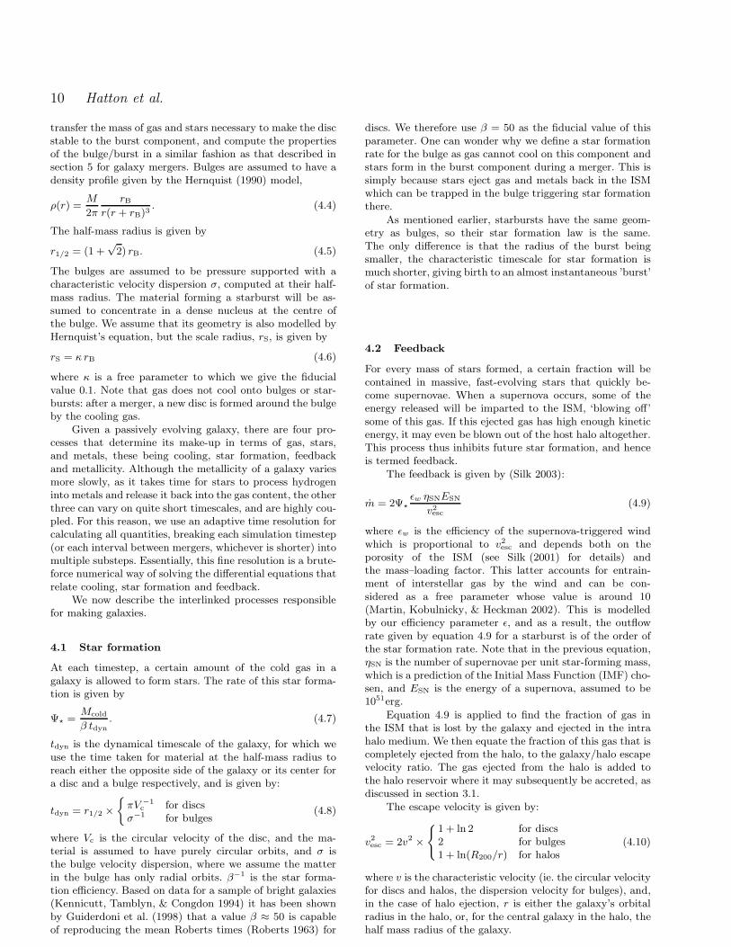
10 Hatton et al.

transfer the mass of gas and stars necessary to make the discstable to the burst component, and compute the propertiesof the bulge/burst in a similar fashion as that described insection 5 for galaxy mergers. Bulges are assumed to have adensity profile given by the Hernquist (1990) model,

ρ(r) =M

2π

rBr(r + rB)3

. (4.4)

The half-mass radius is given by

r1/2 = (1 +√

2) rB. (4.5)

The bulges are assumed to be pressure supported with acharacteristic velocity dispersion σ, computed at their half-mass radius. The material forming a starburst will be as-sumed to concentrate in a dense nucleus at the centre ofthe bulge. We assume that its geometry is also modelled byHernquist’s equation, but the scale radius, rS, is given by

rS = κ rB (4.6)

where κ is a free parameter to which we give the fiducialvalue 0.1. Note that gas does not cool onto bulges or star-bursts: after a merger, a new disc is formed around the bulgeby the cooling gas.

Given a passively evolving galaxy, there are four pro-cesses that determine its make-up in terms of gas, stars,and metals, these being cooling, star formation, feedbackand metallicity. Although the metallicity of a galaxy variesmore slowly, as it takes time for stars to process hydrogeninto metals and release it back into the gas content, the otherthree can vary on quite short timescales, and are highly cou-pled. For this reason, we use an adaptive time resolution forcalculating all quantities, breaking each simulation timestep(or each interval between mergers, whichever is shorter) intomultiple substeps. Essentially, this fine resolution is a brute-force numerical way of solving the differential equations thatrelate cooling, star formation and feedback.

We now describe the interlinked processes responsiblefor making galaxies.

4.1 Star formation

At each timestep, a certain amount of the cold gas in agalaxy is allowed to form stars. The rate of this star forma-tion is given by

Ψ⋆ =Mcold

β tdyn. (4.7)

tdyn is the dynamical timescale of the galaxy, for which weuse the time taken for material at the half-mass radius toreach either the opposite side of the galaxy or its center fora disc and a bulge respectively, and is given by:

tdyn = r1/2 ×

πV −1c for discs

σ−1 for bulges(4.8)

where Vc is the circular velocity of the disc, and the ma-terial is assumed to have purely circular orbits, and σ isthe bulge velocity dispersion, where we assume the matterin the bulge has only radial orbits. β−1 is the star forma-tion efficiency. Based on data for a sample of bright galaxies(Kennicutt, Tamblyn, & Congdon 1994) it has been shownby Guiderdoni et al. (1998) that a value β ≈ 50 is capableof reproducing the mean Roberts times (Roberts 1963) for

discs. We therefore use β = 50 as the fiducial value of thisparameter. One can wonder why we define a star formationrate for the bulge as gas cannot cool on this component andstars form in the burst component during a merger. This issimply because stars eject gas and metals back in the ISMwhich can be trapped in the bulge triggering star formationthere.

As mentioned earlier, starbursts have the same geom-etry as bulges, so their star formation law is the same.The only difference is that the radius of the burst beingsmaller, the characteristic timescale for star formation ismuch shorter, giving birth to an almost instantaneous ’burst’of star formation.

4.2 Feedback

For every mass of stars formed, a certain fraction will becontained in massive, fast-evolving stars that quickly be-come supernovae. When a supernova occurs, some of theenergy released will be imparted to the ISM, ‘blowing off’some of this gas. If this ejected gas has high enough kineticenergy, it may even be blown out of the host halo altogether.This process thus inhibits future star formation, and henceis termed feedback.

The feedback is given by (Silk 2003):

m = 2Ψ⋆ǫw ηSNESN

v2esc

(4.9)

where ǫw is the efficiency of the supernova-triggered windwhich is proportional to v2

esc and depends both on theporosity of the ISM (see Silk (2001) for details) andthe mass–loading factor. This latter accounts for entrain-ment of interstellar gas by the wind and can be con-sidered as a free parameter whose value is around 10(Martin, Kobulnicky, & Heckman 2002). This is modelledby our efficiency parameter ǫ, and as a result, the outflowrate given by equation 4.9 for a starburst is of the order ofthe star formation rate. Note that in the previous equation,ηSN is the number of supernovae per unit star-forming mass,which is a prediction of the Initial Mass Function (IMF) cho-sen, and ESN is the energy of a supernova, assumed to be1051erg.

Equation 4.9 is applied to find the fraction of gas inthe ISM that is lost by the galaxy and ejected in the intrahalo medium. We then equate the fraction of this gas that iscompletely ejected from the halo, to the galaxy/halo escapevelocity ratio. The gas ejected from the halo is added tothe halo reservoir where it may subsequently be accreted, asdiscussed in section 3.1.

The escape velocity is given by:

v2esc = 2v2 ×

1 + ln 2 for discs2 for bulges1 + ln(R200/r) for halos

(4.10)

where v is the characteristic velocity (ie. the circular velocityfor discs and halos, the dispersion velocity for bulges), and,in the case of halo ejection, r is either the galaxy’s orbitalradius in the halo, or, for the central galaxy in the halo, thehalf mass radius of the galaxy.

galics I 11

4.3 Metallicity

The baryonic gas in halos and galaxies, initially composedsolely of hydrogen and helium, acquires a metal content dueto the processing of these light elements by the stellar popu-lation, and the subsequent release of the heavy elements syn-thesized to the inter-stellar medium at the end of a star’slife. To track the metallicity, we need two components: amodel for the rate at which metals are produced inside thestars, and a model for the amount of material released by agiven stellar population.

Using these models, we are able to use the tree to trackthe metals ejected by stars at each time step, over the wholemerging history of the galaxy, and let new stars form outof the enriched gas, assuming instantaneous mixing in theISM. This is in contrast to the assumption of instantaneousrecycling, the approach generally used in semi-analytic mod-elling (CLBF, KCDW, SP99). Correct modelling of the ejec-tion is likely to be especially important for elements such asiron, nitrogen and possibly carbon, for which the productiondelay can be significant (eg. 1 Gyr for Fe produced by SNIa).

Given a mass M of stars formed at some time t0, wecan calculate the current contribution to the stellar ejectionduring a timestep from t1 to t2 as

∆M⋆ = −M∫ m(t2)

m(t1)

[m− w(m)]φ(m)dm (4.11)

where m(t) is the mass of a star having lifetime t, w(m)is the mass of the remnant left after the star has died,and φ(m) is the IMF. Our fiducial model uses a KennicuttIMF, and in Paper II we will explore the effects of using aScalo or Salpeter IMF (see Kennicutt 1983; Salpeter 1955;Scalo 1986). For all IMFs considered, we form no starslighter than 0.1M⊙ or heavier than 120M⊙.

This formula can be extended to include the entire starformation history, producing a rate of increase in the gasmass due to ejection from the stellar population,

E(t) =

∫

∞

m(t)

Ψ⋆(t− tm)[m−w(m)]φ(m)dm (4.12)

where tm is the lifetime of a star of mass m (ie. the inverseof m(t)).

Equation 4.12 can be adapted to predict the amount ofmetals produced, by making the replacement:

[m− w(m)] −→ [m− w(m)]Zcold(t− tm) +mYZ(m) (4.13)

where the first term on the right hand side represents the re-introduction of the metals that were originally in the starswhen they formed, and YZ(m) is the fraction of the ini-tial stellar mass transformed via stellar nucleosynthesis intometals, known as the stellar yield. Our models for the rem-nant mass and the yield come from the stardust code ofDGS, and are calculated self-consistently with the modelsfor spectral evolution we will discuss in section 6.

Throughout this work, we assume chemical homogene-ity (instantaneous mixing), such that outflows caused byfeedback processes are assumed to have the same metallicityas the inter-stellar medium, though in reality the materialin the outflow could be metal-enhanced (Pagel 1998).

5 MERGING

In the hierarchical picture of structure formation, mergersare clearly crucial in understanding the properties of galax-ies observed at the present day. In our models, mergers areresponsible for the formation of massive spheroids, and areassumed to trigger starburst activity. The detailed modellingof the physics of individual mergers between galaxies is cur-rently beyond the scope of what can be achieved in a cos-mological simulation. Only the highest resolution N-bodysimulations of Springel et al. (2001) are able to dynamicallyfollow the merger of 0.2 L⋆ dark matter sub-halos withina single cluster. Therefore, the best we can hope for is toapproximately model the rate and effects of merging in aglobal sense. To deal with the rate of merging, we modeltwo effects, the gradual tendency of satellite galaxies to loseorbital energy and sink towards the centre of the clusterpotential well, and the likelihood of occasional encountersbetween satellite galaxies in a cluster, based on probabilis-tic, cross-section arguments.

5.1 Halo mergers

We identify mergers between dark matter halos using thehalo tree, as described in section 2.4. When a merger occurs,the properties of the dark matter itself are obtained directlyfrom the properties of the new halo in the N-body simula-tion. We apply recipes, however, to deal with the baryoniccomponent. Firstly, the ICM, ie. the hot cluster gas, of theprogenitors are added together proportionally to the darkmatter mass which ends up in the descendent halo (the con-stant of proportionality being the current baryon fractionof each progenitor), and given the virial temperature of thenew halo. Then, the properties of the two halo reservoirsare simply added. Note that the new halo contains all thegalaxies that were present in its progenitors (even if frag-mentation occurs and the halo is less massive than all/someof its progenitors) and that the fraction of the progenitors’ICM which does not end up in the new halo is put in itsreservoir, ensuring conservation of metals.

When two halos merge (sometime in between two out-put times), there is a discontinuity between the centre of thenew halo and the centres of mass of the progenitors (linearlyextrapolated from their positions and velocities in the pre-vious timestep). We measure this ‘jumping’ distance, Rj, foreach of the progenitors directly from the N-body simulationsand use it to assign each galaxy an orbital radius in the newhalo, using the cosine law:

rnew =√

r2old +R2j − 2roldRj cos θ, (5.1)

where rold is the orbital radius of the galaxy in the progeni-tor halo and rnew is its orbital radius in the new halo. Thisassumes that the galaxy was initially at an angle θ to thevector joining the centres of the two halos. We select cos θrandomly from a flat probability distribution between −1and 1, taking account of the spherical symmetry.

To illustrate how this works in practice, we consider twocases. The first is a merger between a small halo and a muchlarger halo. It is clear that the centre of mass of the largehalo is perturbed only slightly by the encounter. Rj is thussmall, and the galaxies that were previously in the large halo

12 Hatton et al.

have rnew ≈ rold. For the small halo, Rj is close to the virialradius of the large halo. Thus rnew ≈ Rj for the galaxiesthat were in this halo, in other words they are placed closeto the virial radius of the new halo. For a collision betweenequal mass halos, Rj is approximately the progenitor virialradius, so the central galaxies are placed at this distance,while non-central ones are placed randomly throughout thenew halo.

Any galaxy whose orbital radius after the merger isless than its own half-mass radius becomes the new cen-tral galaxy of the halo. If there is more than one of theseobjects, they are merged with each other in order of de-scending mass. It may well happen that there is no centralgalaxy after a merger, in which case we cool gas onto thegalaxy closest to the halo centre. Although this scheme isreally only a naıve geometrical model, we use it to approx-imately replicate the sort of scatter in galaxy positions weexpect to see when halos collide. It has the advantage thatit reproduces the desired behaviour for the extreme cases ofequal or very unequal mass mergers in a natural, continuousway without free parameters.

5.2 Dynamical friction

Dynamical friction causes satellite galaxies to sink gradu-ally to the centre of their host halo, resulting in a mergerif there is already a galaxy at the centre. After a mergerbetween halos, the galaxies are given orbits as prescribed insection 5.1. In subsequent timesteps, the radii of the orbitsare decreased by an amount obtained from the differentialequation (Binney & Tremaine 1987):

rdr

dt= −0.428

Gmsat

VclnΛ (5.2)

where r is the orbital radius, msat the mass of the satellite(including its tidally stripped dark matter core, see nextsection), Vc the circular velocity of the halo and ln Λ theCoulomb logarithm, approximated by

Λ = 1 +(

mhalo

msat

)

(5.3)

(see eg. Mamon 1995). Calculating the amount of orbitaldecay at each timestep seems far more natural than theapproach favoured by other authors (CLBF, KCDW) whoassign each galaxy a dynamical friction timescale, and as-sume the merger occurs after that fixed time, unless a majormerger occurs, at which point this timescale is recomputed.By modelling the true radial coordinate, albeit in a naıveway, we automatically take into account possible evolutionof the halo properties, and avoid having to differentiate be-tween ‘major’ and ‘minor’ mergers.

As soon as the orbital distance of a galaxy becomeslower than the sum of its half-mass radius and the half-mass radius of the central galaxy in the halo, it is assumedto merge with this central galaxy.

Other workers (CLBF, KCDW, SP99) have taken intoaccount the fact that galaxy orbits are not in general cir-cular. This fact alters the extent of dynamical friction, andNavarro, Frenk, & White (1995a) have shown that applyingthe formula for circular orbits results an average overpredic-tion by a factor two of the time taken for an infalling galaxyto reach the centre. A proper consideration of this effect re-

quires a modified form of the dynamical friction as a functionof orbit eccentricity (Lacey & Cole 1993), and an assump-tion for the distribution of ellipticities. However, carefulexamination of Navarro, Frenk, & White 1995a (especiallytheir figure 8), shows that one can obtain the true dynami-cal friction time more accurately by simply halving the timefor circular orbits, than by using the actual orbital eccentric-ity and applying the modified form of Lacey & Cole 1993.We thus take into account the effect of non-circular orbits bymultiplying the right hand side of equation 5.2 by a factortwo.

5.3 Tidal stripping

When a merger between halos occurs, the new satellitegalaxies will, to some extent, retain the dark-matter coresof their previous host halos, and this dark matter will con-tinue to dominate their dynamics. However, as the galaxyslowly descends to the centre of the new host this sub-halowill be stripped by tidal interactions. Eventually, as themass of the remnant becomes comparable to the baryonicmass of the galaxy itself, it will no-longer dominate over theeffects of the self-gravity of the galaxy, and the dynamicsmay undergo a serious change. Following SP99, we assumethat the sub-halo is stripped down to a radius rt such thatρc(rt) = ρh(r0), where ρc is the core density and ρh(r0) isthe halo density at the orbital radius of the remnant (forisothermal spheres this density is simply proportional to themean density inside the same radius). Note that we do notattempt to model the stripping of baryons by tidal effects,only that of the dark matter.

5.4 Satellite-satellite mergers

Satellite mergers are assumed to occur through direct colli-sions between galaxies in clusters. In the absence of detailednumerical simulation of the precise positions and velocitiesof the galaxies within a halo, it is appropriate that some sortof cross-section argument be used to determine the mergingrate. There is no detailed study of how such cross-sectionsbehave in a realistic halo environment; a first analyticalestimate by Mamon (1992) has been followed numericallyby Makino & Hut (1997), with Mamon (2000) showing thatthese results are in good agreement. We assume the proba-bility of a galaxy having a merger in time ∆t is given by:

P =∆t

τ, (5.4)

where τ is the merger timescale, whose dependenceon galaxy and halo characteristics is parametrized byMakino & Hut as:

τ−1 = ψ(Ng − 1)( r1/2

R200

)3 (vgalVc

)3(

vgalr1/2

)

. (5.5)

In this formula, Ng is the number of galaxies in the halo,and vgal is taken to be a mass-weighted average of the discrotation speed and the bulge dispersion velocity. A directtransformation of the results of Makino & Hut (1997) leadsto a value of ψ = 0.017 sGyr−1km−1Mpc, which is the valuewe shall take for our fiducial model. However, their work as-sumes all galaxies are spheroids of the same size and mass,which is not the case in our models, and in Paper II we

galics I 13

Figure 3. Our algorithm for calculating the fraction of disc ma-terial remaining in the disc after a merger, as a function of themass ratio of the two progenitors.

will investigate the effect of altering ψ from this standardvalue. We are aware that our extrapolation of these authors’results is quite crude and should be, in the best of casestaken as a rough estimate of the importance of satellite-satellite mergers. Finally we note that the results obtainedby Springel et al. (2001) for sub-halo merging in dark mat-ter clusters support the view that this kind of mergers isnegligible in such environments.

5.5 Post-merger morphology

In our model, mergers and disc instabilities are both respon-sible for creating galaxy bulges, and as such are drivers ofmorphological evolution. In the case of a disc instability,the mass transfer between galaxy components has alreadybeen discussed in section 4, and therefore we will only beconcerned by mergers in this section. The standard methodfor modelling a merger-driven morphology (SP99, CLBF,KCDW) has been to take the ratio of the masses of thetwo objects merging, and add the stars of the lighter galaxyto the disc of the heavier one if the mass ratio is less thanfbulge ≈ 0.3, or destroy the disc and form a bulge if the ratiois higher.

It has been shown (Walker, Mihos, & Hernquist 1996)that a galactic disc can be completely disrupted by an en-counter even when the interloper is rather less massive thanthe disc itself, and this simple method reproduces this be-haviour. However, it does not allow for any intermediatebehaviour – there is a sharp cut-off at fbulge between totallydisrupting, or not disrupting, the morphology of the galaxy,which seems quite false.

Our model is constructed in terms of the function X. Ingeneral, this can be any function of the ratio of progenitormasses that maps the range one to infinity onto the space 0to 1. The step function used be other workers is one example

of such a function, but we will consider a smoother function,drawing inspiration from Fermi-Dirac statistics, and defining

X(R) =[

1 +(

χ− 1

R− 1

)χ]−1

(5.6)

This function is shown in Fig. 3, for the value χ = 3.333.In equation 5.6, R represents the mass ratio of the heavierto the lighter progenitor, and χ is the critical value of thatratio, ie. the value that gives X = 0.5. Since step functionswith fbulge ≈ 0.3 have been found to give good results in thepast, we set χ = 1/0.3 as our fiducial value. In Paper II wewill explore the effects of varying χ.

We then define two matrices,

Astar =

(

X 0 00 1 0

1 −X 0 1

)

(5.7)

Agas =

(

X 0 00 0 0

1 −X 1 1

)

(5.8)

Considering the vector V = (D,B, S) where D,B, S referto the mass in the disc, bulge and starburst respectively, wehave:

Vnewgas = AgasV

1gas + AgasV

2gas (5.9)

and similarly for the stars.In other words, during a merger a fraction X of gas and

stars originally sitting in the disc remain in the disc. Therest of the gas from the disc goes into the starburst, as wellas its stars. Any stars that were already in the bulge stayin the bulge, but all its gas is put in the starburst. All thematerial (gas and stars) that was originally in a starburstremains in that starburst. Note that gas is never added tothe bulge in this process, but that a small amount of gas isgenerally present in the bulges, coming from the evolutionof its stellar content.

5.6 Properties of merger remnant

Having ascertained how much mass goes where, we mustdecide on the properties of the resulting galaxy after thecollision, ie. its rotation/dispersion speed and size. For this,we adopt a similar model to that of CLBF.

Under the virial theorem, the total internal energy isgiven by E = −T where T is the internal kinetic energy.Applying conservation of energy,

Tnew = T1 + T2 − Eint, (5.10)

where Eint is the interaction energy of the collision. For a dy-namical friction encounter as well for satellite-satellite merg-ers, we use the total orbital energy,

Eint = −Gm1m2

r1 + r2(5.11)

(r1 and r2 are the half-mass radii of the two progenitors).Note that m1 and m2 stand for all the mass (dark mattercore and baryons) contained in each progenitor respectively.

These energy considerations, coupled to mass conserva-tion enable us to obtain rnew, the half mass radius of themerger product:

14 Hatton et al.

rnew =(m1 +m2)

2

− Eint

0.4G+

m2

1

r1+

m2

2

r2

, (5.12)

where the factor 0.4 depends (not sensitively) on the exactdensity profile (Hernquist in our case). As for the pure disccase, we do not allow rnew to become bigger than R200. Wethen assume that rnew is the half mass radius of the bulgeand hypothesize that the largest disc is the most likely tosurvive the merger. Following the method presented in sec-tion 4, we can calculate the characteristic velocities of ourgalaxy components. In particular, we use equation 4.6 tocalculate the radius of the starburst after merging and as-sume the starburst has the same velocity dispersion as thebulge.

In the case of a satellite-satellite merger, the orbitalradius of the merger remnant is obtained through a simplemass-weighting of the orbital radii of the two progenitors.

6 GALAXY LUMINOSITIES

Having decided where the baryons are, and what their phys-ical properties are, we apply a set of models to calculatethe amount of light they produce. Luminosities in visualand near-infrared (rest-frame) wavelengths are calculatedfrom stellar synthesis models, which take into account themetallicity and age of the stellar population. We then addgeometry- and metallicity-dependent models for the absorp-tion and re-emission of this light by the dust and gas in theinter-stellar medium.

6.1 Stellar Spectra

For each time output of the simulation, we compute thestellar contribution F ⋆

λ (t) to the galactic flux at time t, whichcan be written:

F ⋆λ (t) =

∫ t

0

∫

∞

m=0

Ψ⋆(t− τ )φ(m)fλ(m, τ, Z⋆)dmdτ , (6.1)

where fλ(m, τ, Z⋆) is the flux at wavelength λ of a starwith initial mass m, initial metallicity Z⋆, and age τ (ie.τ = 0 corresponds to the zero age main sequence, andfλ(m, τ, Z⋆) = 0 if τ > t(m)). φ(m) is once more the IMF.We neglect the nebular component. For fλ(m,τ, Z⋆) we usethe stardust model of DGS, and full details can be foundin that paper.

We use the full merging history of the galaxy to com-pute the stellar spectrum, summing up the contribution tothe present day spectrum from all the stars formed in theprevious timesteps in all the progenitors of the galaxy.

6.2 Dust Absorption

To estimate the stellar flux absorbed by the interstellarmedium in a galaxy, one first needs to compute its opticaldepth. As in Guiderdoni & Rocca-Volmerange 1987, we as-sume that the mean perpendicular optical depth of a galaxyat wavelength λ is:

τ zλ =

(

Aλ

AV

)

Z⊙

(

Zg

Z⊙

)s( 〈NH〉2.1 1021atoms cm−2

)

, (6.2)

where the mean H column density (accounting for the pres-ence of helium) is given by:

〈NH〉 =Mcold

1.4mpπ(ar1/2)2atoms cm−2, (6.3)

and a is calculated such that the column density representsthe average (mass-weighted) column density of the compo-nent, and is 1.68 for discs, 1.02 for bulges and starbursts. Theextinction curve depends on the gas metallicity Zg accord-ing to power-law interpolations based on the Solar neigh-bourhood and the Large and Small Magellanic Clouds, withs = 1.35 for λ < 2000A and s = 1.6 for λ > 2000A (seeGuiderdoni & Rocca-Volmerange 1987 for details). The ex-tinction curve for solar metallicity (Aλ/AV)Z⊙

is taken fromMathis, Mezger, & Panagia 1983.

For the spherical components we use the generaliza-tion given by Lucy et al. (1989) for the analytic formulagiving obscuration as a function of optical depth τ sph

λ

(Osterbrock 1989) to the case where scattering is takeninto account via the dust albedo, ωλ (we use the model ofDraine & Lee 1984 for the albedo):

Aλ(τ ) = −2.5 log10

[

aλ

1 − ωλ + ωλaλ

]

, (6.4)

where

aλ(τ ) =3

4τλ

[

1 − 1

2τ 2λ

+

(

1

τλ+

1

2τ 2λ

)

exp(−2τλ)

]

. (6.5)

We assume dust and stars are distributed together uni-formely and thus there is no need to average over inclinationangle, since the bulge is spherically symmetric.

For discs, the situation is more involved, dueto inclination effects. We use a uniform slab model(Guiderdoni & Rocca-Volmerange 1987) for the extinctionas a function of the inclination angle, θ:

Aλ(τ, θ) = −2.5 log10

[

1 − exp(−aλ sec θ)

aλ sec θ

]

, (6.6)

where aλ =√

1 − ωλτzλ . To calculate this quantity, we pick

a random inclination of the galactic disc to the observer’sline of sight. For comparisons of the same galaxy at differ-ent epochs, and for examining inclination-corrected statis-tics (eg. the Tully–Fisher relation), we also compute andstore the face-on magnitudes of the discs (sec θ = 1).

Our final result is the extinguished stellar spectrum:

Fλ = F ⋆λ × dex[−0.4Aλ]. (6.7)

6.3 Dust Emission

Dust absorption in bulges is spherically symmetric, so theemission is trivially calculated, but for discs it is anisotropic,so to calculate the total energy budget available for infraredemission by dust one must include contributions from all di-rections. We use the angle-averaged version of equation 6.6,

Aλ(τ ) = −2.5 log10

[∫ 1

0

1 − exp(−aλ/x)

aλ/xdx

]

. (6.8)

The value of the integral on the right hand side of this equa-tion is:

1

2aλ

[

1 + (aλ − 1) exp(−aλ) − a2λ E1(aλ)

]

, (6.9)

galics I 15

where E1 is the first-order exponential integral.Given an unextinguished stellar spectrum F ⋆

λ , the totalbolometric infrared luminosity of the galaxy is:

LIR =

∫

F ⋆λ × (1 − dex[−0.4Aλ]) dλ. (6.10)

We assume the emission is isotropic, since dust it-self is generally optically thin to infrared light (exceptin heavily obscured starbursts). To compute the IR emis-sion spectrum, one needs to model both the size distribu-tion and the chemical composition of dust grains in theISM. The model we use is based upon the MW model ofDesert, Boulanger, & Puget (1990), which includes contri-butions from polycyclic aromatic hydrocarbons, very smallgrains and big grains. Our chief refinement to this modelis to allow a second population of big grains, closer to thestar forming region, to be in thermal equilibrium at a highertemperature for galaxies undergoing massive starbursts. Ouremission model makes use of the colour/luminosity correla-tions observed by IRAS, and is detailed in DGS. We stressthat a key weakness of this model is that it is based on alocal sample and therefore assumes that dust properties donot evolve with time.

7 FREE PARAMETERS

The semi-analytic recipes described here contain a numberof free parameters that will affect our results. We detail themin this section.

• ΩB is the baryon fraction of the Universe. Whilst a highbaryon fraction can have a serious effect on both the shapeof the initial power spectrum of density perturbations (eg.Sugiyama 1995) and the internal dynamics of halos, provid-ing it remains small it can be treated as a free parameter ofthe galaxy formation recipes. Increasing ΩB results in morefuel for the star formation process, and should thus producebrighter galaxies.

• β−1 is the star formation efficiency. This is the param-eter that appears in equation 4.7. Increasing β will clearlyresult in less cold gas being turned into stars, moving thepeak in the star formation history closer to the present day.

• ǫ−1 represents the efficiency of mass–loading during thetrigerring of a galactic wind by SN explosions (section 4.2).Decreasing ǫ produces more feedback, heating more cold gas,ejecting more hot gas from halos, and thus reducing theamount of gas that can potentially form stars.

• ψ is the normalization for satellite–satellite merginglaw, equation 5.5. From (Makino & Hut 1997) we expectits value to be around 0.017, but as stated in section 5.4,we will treat it as a free parameter. Satellite–satellite merg-ing competes with dynamical friction merging (especially formassive galaxies, see Mamon 2000), and energetics of thesecollisions are different, so increasing ψ produces more diffusegalaxies, slowing the global star formation rate.

• χ parametrizes our merging law in equation 5.6, it isthe critical mass ratio, ie. the one at which half the disc isdisrupted. Our fiducial value is 1/0.3, raising χ means that alarger disc will be disrupted by a smaller interloper. It there-fore affects the morphological mix of our galaxy population.

• ζ is the efficiency with which gas stored in the haloreservoir is admitted back to the halo during accretion, as

name meaning fiducial value range

ΩB Baryon fraction 0.02h−2 0.01–0.03h−2

β Inverse star formation efficiency 50 10–100ǫ Inverse of mass–loading for feedback 0.1 0.01–1.0ψ S-S merging normalization 0.017 0.01–0.03χ galaxy merger power-law 3.333 2.0–5.0ζ recycling efficiency 0.3 0.0–1.0κ ratio of burst to bulge radius 0.1 0.05–0.2

Table 2. Summary of free parameters in the models

explained in section 3.1. Turning ζ right down will meanthat metals and gas ejected from a halo are only returnedvery slowly, restricting the supply of metals to the coolinggas.

• κ is used to determine the starburst radius from thebulge radius, as shown in equation 4.6. Smaller κ producessmaller starburst regions, where star formation is thereforefaster, brighter, and more heavily extinguished.

These parameters are summarised in table 2. In addi-tion, there are various other inputs to the models, includingcosmology, initial stellar mass function (our fiducial modeluses the Kennicutt (1983) IMF), and dust recipe, that willhave an impact. We will consider the impact of changingsome of these inputs, and varying the above free parameterswithin the range quoted in table 2, in paper II.

8 RESULTS

In order to test our models against observations, we will usea number of constraints in the literature. These fall into twomain categories; intrinsic properties, ie. relationships thatapply for individual galaxies such as the Tully–Fisher rela-tion or the dependence of metallicity on galaxy mass; andglobal properties, such as luminosity functions and cluster-ing statistics. In this paper we will just present work con-cerning the local (ie. low-redshift) Universe, and we will notuse any spatial information. Paper II will include resultsfrom higher redshift, and the effect on the results of changesin the parameters described in section 7. Papers III and IVwill be concerned with the evolution of many of the statis-tics presented here, including the luminosity function andpredictions of faint galaxy counts. We will also employ thespatial information from the dark matter simulations to in-vestigate the clustering properties of our galaxies in paperV.

In Fig. 4 we present a slice through the simulation atits final output time, with the dark matter density shownas a grey-scale. The slice is of side length 100h−1 Mpc, thewhole simulation box, but is 10h−1 Mpc in thickness. Weoverplot the locations of bright (MB < −19.5) galaxies,with the sizes of the points representing the galaxy B-bandmagnitudes. One can clearly see the way that the galaxiestrace the high-density regions of the simulation, with most ofthe light concentrated in filaments and clusters. The powerof the hybrid approach is immediately apparent when oneconsiders that state-of-the-art attempts to model the sub-grid physics with smoothed particle hydrodynamics producearound 2000 galaxies in a cube with one-third the volume of

16 Hatton et al.

Figure 4. A slice through our simulation at redshift 0. Dark matter density is represented by a grey-scale, whilst white circles markgalaxies, with their sizes depending on the B-band luminosity. Only bright galaxies (MB < −19.5) are shown. The slice is 100h−1 Mpcon a side (the entire simulation cube) and 10h−1 Mpc in thickness.

ours (Pearce et al. 2001), when we have 30 000 galaxies intotal in our final timestep, thus giving us access to a muchbroader range of galaxy mass and merging history.

8.1 Effect of resolution

The identification of halos with a given cut-off mass pro-duces an effective resolution limit on our results. We definethe galaxy resolution limit as the smallest halo mass timesthe baryon fraction of the Universe. Galaxies of baryonicmass less than this exist in our models, but no galaxy ofmass greater than this could exist in unresolved halos. This

is thus a ‘safe’ limit for completeness in our sample, and pro-duces a formal completeness limit of galaxy baryonic massmgal = 2.2 1010M⊙ for the ΛCDM simulation.

In Fig. 5 we show the dependence of galaxy luminosityon total baryonic mass for galaxies in our fiducial model, de-fined in section 7. The tight relationship between these twoquantities allows us to estimate the magnitude complete-ness limit corresponding to the mass completeness limit wejust defined. For each waveband, we perform a linear fit ofmagnitude on luminosity, and take the intercept of this fitwith the line mgal = 2.2 1010M⊙. The results of this treat-ment for a number of optical and near-infrared filters are

galics I 17

Figure 5. Galaxy absolute magnitudes as a function of totalbaryonic mass in the I-band and B-band. The solid vertical lineshows the effective completeness limit as defined in section 8.1.Results for the completeness limit in a number of wavebands arepresented in table 3.

Waveband Completeness limit

U −18.8 magB −18.9 magV −19.7 magR −20.4 magI −20.9 magJ −21.6 magH −22.2 magK −22.7 mag

12 µm 0.41 109L⊙

25 µm 0.25 109L⊙

60 µm 0.79 109L⊙

100µm 1.34 109L⊙

Table 3. Resolution limits in a variety of optical and infrared

bands (magnitudes for Johnson–Mould filters, λLλ in solar lu-minosities for the IRAS bands). Magnitudes are absolute, in theVega system, and calculated using the process described in sec-tion 8.1.

presented in table 3. It will be noted that, in the B-bandthe resolution limit is about 1.5 magnitude fainter than thevalue of M⋆ = −20.5 (assuming our value of H0) from theStromlo–APM survey (Loveday et al. 1992). We are there-fore complete to galaxies around one-fourth as luminous asan M⋆ galaxy.

Although we are effectively complete down to thesemagnitude limits, we do not fully resolve the merging historyof the faintest objects. This is an advantage of the methodemployed by Benson et al. (2000), where halos identified ina dark matter simulation have their merging histories com-puted with the Press–Schechter formalism with theoreticallyinfinite resolution, so even the smallest objects have a fullyresolved history. The smallest galaxies in our models are in

halos that have only recently been identified in the simula-tions, and hence have a high gas content and star formationrate, but low metal and stellar content, and an inevitablespiral morphology. We expect the effects of this lack of in-formation to propagate over the formal mass completenesslimit. We consider resolution effects in rather more detail insection 9.

8.2 The halo ICM

Before examining the galaxies themselves, we will look at theoverall behaviour of the baryons in the dark matter halos.In the left panel of Fig. 6, we show the ratio of hot gasto total baryonic mass for dark matter halos as a functionof their circular velocity. Note that for isothermal spheresthere is a one-to-one mapping from circular velocity to halodark-matter mass, Vc ∝M1/3.

We notice that:

• the most massive objects have around seventy per centof their baryonic mass in the form of hot intra-clustermedium (ICM), with a weak dependence on circular velocity.

• for objects with lower circular velocity, Vc <300 kms−1, the gas fraction starts to fall off rapidly as thehalo mass decreases, this scale defining the difference be-tween a galaxy and a cluster.

• finally, around 100 kms−1, the scatter becomes verylarge. This is due to the finite resolution of our approach, inthat the smallest objects do not have well-resolved merginghistories, so cooling does not start until the timestep theyare discovered, resulting in an overestimate of the hot gasfraction. The cooling in these objects is rapid enough, how-ever, that by the time the mass has increased slightly, theyhave joined the main locus on the plot.

In the right hand panel of Fig. 6 we show the behaviourof the metallicity (defined as the mass in metals relative tothe mass in gas) of the hot ICM. The resolution effects areclearly obvious again at low halo mass, with many objectsof extremely low metallicity, since their stars are very youngand have not had time to contribute via nucleosynthesis andejection. Above 100 kms−1, the metallicity is a decreasingfunction of halo mass, suggesting that larger halos have ahigher proportion of primordial gas, and galactic winds areless important in clusters than in galaxies. This result isin contrast to the observational results of Renzini (1999),who finds for the largest clusters (Vc > 1000 kms−1) thatthe metallicity, as measured from the iron abundance, hasa constant value of around one third solar. This is betweenfive and ten times more metals than the amount we find inour halos.

We will show in section 8.4 that our galaxy metallicitiesappear quite accurate. Could the missing metals be hidingin the galaxies, or possibly in the halo reservoir? We havedone the same analysis as in Fig. 6, but added to the ICM allthe metals contained in the halo reservoir, and all the metalslocked up in the cold gas inside galaxies. This thus representsthe maximum metallicity we can attain without somehowlowering the mass of non-metals in the ICM. Although thishas a large effect for small halos, there is little change in themetallicity of the largest clusters. We conclude that we arenot simply ‘misplacing’ the heavy elements.

18 Hatton et al.

Figure 6. Baryonic properties of halos, as a function of halo circular velocity. On the left we show the ratio of hot gas in the halo tothe total mass of baryons. On the right, the metallicity of this hot phase.

There are several potential explanations for this dis-crepancy:

• observations measure only the abundance at the centreof the cluster, assuming the hot gas is chemically homoge-neous. In fact, metallicity gradients have been observed inmany clusters (eg. Koyama, Takano, & Tawara 1991 for theVirgo cluster, White et al. 1994 for several cooling flow clus-ters), and the observations thus yield an upper limit on thetotal metallicity.

• the metallicity is measured using the iron abundance,whereas the metallicity we quote is the total mass of metalsin the cluster. In fact, our models pay no attention to theenergy injected to the ISM from type Ia supernovae (thoughthese supernovae do contribute to the metallicity). The over-all contribution of these objects is likely to be small, but,since these stars contain an iron core, the relative abundanceof iron can be strongly enhanced, especially from evolved,gas-poor, early-type galaxies, such as are found in clusters.Thus the simple assumption used to convert Fe abundanceto total metallicity, Z/Z⊙ = ZFe/ZFe

⊙ , may be invalid inclusters, and will produce an upper limit on the total metal-licity.

• one should also consider the existence of population IIIstars in the early Universe which may have reionized theUniverse homogeneously and likewise introduced metals intothe primordial gas. This could be simulated by allowing anon-zero primordial metal abundance in our models.

• the yields we use could be too low especially if the IMFis biased towards massive stars in the early stages of clusterformation.

• Although these effects could all play a role in the metal-licity underestimate, it seems more likely that the majorcontribution we are unable to model comes from objects be-low our resolution limit. Indeed, it is sensible to argue thatthe majority of metals seen in the ICM today came fromold dwarf galaxies (Renzini 1999; Renzini 2000), in shallow

Figure 7. Mass to light ratios of our halos, in units of the solarmass to light ratio. The upper line is for the B-band, the lower forthe K-band. The lines are the medians, with error bars showingthe ±1-σ scatter. We only include contributions from galaxieswith baryonic mass greater than the formal completeness limit(section 8.1).

potential wells, and we are a long way from achieving theresolution needed to see these galaxies.

8.3 Mass to light ratios

The mass to light ratio of dark matter halos tells us impor-tant information about measuring the dark mass from ob-servations, and about which environments are most efficientat producing energy. In Fig. 7 we show mass to light ratios,

galics I 19

in solar units, for our halos. We only include contributionsto the luminosity from galaxies above our resolution limit.We compare results in two wavebands, the B-band, wherethe energy is dominated by young stars, and the K-band,which has been shown to reliably estimate the total stel-lar content (Kauffmann & Charlot 1998). One can see thatthe distributions are qualitatively similar in shape and thatlow mass, galactic halos are brighter per unit mass than thelarger, cluster-sized objects. In the B-band, MW type ha-los have a mass-to-light ratio of around 60, rising to 300 forthe biggest clusters in the sample whereas in the K-bandthemass-to-light ratio is rather constant around 30 for galaxysize halos (Vc < 300 kms−1) and rises to 60 for the biggestobjects.

Our failure to fully resolve the merging history of haloswith circular velocity less than 100 kms−1 makes it difficultto draw any firm conclusions about the shape of the mass-to-light ratio at the low-mass end.

8.4 Assorted galaxy properties

In Fig. 8 we show scatter plots for some of the intrinsicproperties of our galaxies as a function of galaxy char-acteristic velocity. This is the circular velocity for discs,three-dimensional dispersion velocity for bulges, and a mass-weighted average of the two for objects of mixed morphology.

Firstly, we show the total mass of baryons, ie. cold gasplus stars, for our galaxies. The main locus of these points isseen to approximately follow the relationship Mbar ∝ V

5/2GAL,

although there is a substantial scatter to low baryon mass forgalaxies with low velocity. This is another example of reso-lution effects entering our results, in that these are galaxiesin small halos that have not yet had time to cool. Com-pared to halos, whose virial masses go as the cube of thecircular velocity, we already see a difference for galaxies: thebaryonic mass depends more weakly on the velocity. We canalready see the effects of the cooling and merging, in that thegalaxy mass and velocity are obviously not scaling linearlywith those of its parent halo.

Secondly, we present the metallicity of the cold gas inthe galaxy. This is a slowly varying function of circular veloc-ity. One can contrast this with the results for the halo metal-licity presented in Fig.6: although the metallicity of the clus-ter ICM decreases with increasing cluster mass, the metal-licity of the central object in the cluster increases. Thereis also a clear upper cut-off in metallicity around twice thesolar value, which corresponds to galaxies having consumedalmost all their gas and therefore having a very low, if anystar formation rate at all, and the very few metal rich youngstars produced fail to enrich the ISM much more. It is worthnoting that the main locus of our points is around a flat linewith Z ≈ Z⊙, indicating that for our mass resolution themetallicity of the Milky–way is quite typical.

In the bottom left panel, we show the star formationrate as a function of characteristic velocity. We note that themajority of galaxies lie close to the line defined by the starformation rate being proportional to the velocity squared,but that there is a small population with very high starformation rates of up to 100 solar masses per year, pre-sumably representing galaxies which are undergoing merger-driven starbursts. There is also considerable scatter at the

property actual MW reference range adopted

mgas/mbar 0.10 1 ±0.05MK −23.7mag 2 ±0.3magVc 220 km s−1 3 ±20 kms−1

Table 4. Observed parameters of the Milky Way, used todefine a MW type galaxy in the simulation. The referencesare: 1. Prantzos & Aubert 1995; 2. Kent, Dame, & Fazio 1991 ;3. Binney & Tremaine 1987.

property actual MW reference Simulation

mbar 0.6 1011M⊙ 4 (0.5 ± 0.1) 1011M⊙

Ψ⋆ 2–4M⊙yr−1 1 (1.5 ± 0.4)M⊙yr−1

rD 4–5 kpc 2 (2.8 ± 0.6) kpcZISM 0.016 5 (0.012 ± 0.002)

Table 5. Observed properties of the Milky Way compared withour predictions from a set of galaxies derived by applying theconditions presented in table 4. The references are as that tableexcept: 4. Binney & Evans 2001 and 5. Pagel 1998. The uncer-tainties in the fourth column are the ±1-σ limits of the distribu-tions.

low and high circular velocity end, due to galaxies that haveexhausted their gas supply.

We leave a detailed consideration of galaxy sizes (bot-tom right panel) to the next section.

8.4.1 Predictions for the Milky Way

To provide a consistency check for our models, we will com-pare MW-like galaxies in our simulations with the knownproperties of our galaxy. On each panel of Fig. 8 we showa grey hexagon for the approximate location of the MilkyWay itself. The values adopted for the Milky Way are pre-sented in tables 4 and 5. We also select MW candidatesfrom our galaxies by applying the selection criteria shownin table 4, and requiring that the galaxy have spiral (or Sb)morphology (defined in section 8.6). Selection of this kindproduces around six hundred MW galaxies in the simula-tion. The properties of these galaxies are shown in table 5,where we quote the median and one standard deviation ofthe distributions, and compare to data for the Milky Wayitself. We find a generally good agreement, in that applyingthe selection of table 4 produce galaxies that do look a lotlike the Milky Way. For most of the properties considered,the Milky Way would fall within 1- or 2-σ from the median.

8.5 Galaxy sizes

In the final panel of Fig. 8, we show the galaxy half-massradius. This is obtained from a mass-weighted average of thedisc and bulge half mass radii. The straight line is the radiusof a galactic disc with the same velocity as its parent halo, ifthe radius is given by 1.68 λR200/

√2, ie. equation 4.1 with

λ = 0.04.In Fig. 9 we examine the sizes of field disc galaxies (ie.

galaxies which are alone in their halos) emerging from our

20 Hatton et al.

Figure 8. Key galaxy properties, as a function of characteristic velocity, which is a mass-weighted average of the disc circular velocityand the bulge dispersion velocity. The top-left panel shows the total baryonic mass of the galaxy, ie. stars plus cold gas. Top right is themetallicity of the interstellar medium, the ratio of the mass in heavy elements to the total gas mass. In the lower-left panel we show thestar formation rate, and in the lower-right the galaxy radius, defined as the mass-weighted average of the disc, bulge and burst radii. Forclarity, on this last figure we also plot the half mass radius of a disc forming in a halo with velocity Vgal if its spin parameter were equalto 0.04 (equation 4.1). In each panel, the grey hexagon shows the approximate location of the Milky Way, from data given in tables 4and 5.

model. We compare our predictions with the observed bivari-ate space density distribution of de Jong and Lacey (2000)derived from a sample containing more than a thousandfield spiral galaxies. As stressed by these authors, the mainadvantage of using this data is that it should be quite in-sensitive to surface brightness incompleteness effects. Notethat in the model we included all the spirals with bulge-to-total-light-ratio less than 0.33, i.e. morphological typeslater than Sab, whereas the data does not contain typeslater than Sd. Indeed these very late type galaxies cannotbe excluded from the model sample as the only morpho-

logical information we are able to compute is a bulge todisc ratio. We would therefore expect an overprediction ofthe total number of galaxies, especially in the faint magni-tude bins and for small disc sizes. However, we do not seethis excess of small faint galaxies but rather an excess ofbright small galaxies with respect to the data. Moreover, aspointed out by de Jong & Lacey (2000) the model distribu-tion is (only slightly in our case) broader than the observedone. As we assume specific angular momentum conservationduring disc formation, the obvious culprit is the too broadinitial spin distribution of the dark matter halos. However,

galics I 21

Figure 9. Bivariate density distribution of field spiral galaxiesas a function of effective disc radii in different I-band absolutemagnitude bins. Magnitude cuts are indicated in the top cornerof each panel. The solid histogram represents results from thehybrid model, and the solid line the best fit to the data of de

Jong and Lacey (2000) (their eq. 7). The horizontal dashed linesin each panel represent our volume resolution.

we would like to draw the attention of the reader to thefact that unlike the CLBF model which overpredicts quite alot the density of small discs, we seem to predict about theright number of small-sized bright galaxies. Although ourmass resolution biases us against small-sized galaxies, weestimate (see table 3) that our sample is almost completefor galaxies with absolute magnitudes brighter than -20.9 inthe I band. Therefore the results displayed in the first threepanels of figure 9 should not be too sensitive to an increasein resolution.

Once again we emphasize that our recipe for discsizes depends crucially on the assumption of specific an-gular momentum conservation, and it has been shown(eg. Navarro, Frenk, & White 1995a) that disspative ef-fects can play a part in destroying some of the an-gular momentum of the gas, producing smaller discs.Dominguez-Tenreiro, Tissera, & Saiz (1998) show that thisloss is less important for gas cooling onto ’evolved’ galaxieswith stellar bulges, so these effects are likely to preferentiallyreduce the size of the smaller, less resolved galaxies in ourmodel.

8.6 Morphologies

We predict galaxy morphologies based on the ratio ofB-band luminosities of the disc and the bulge compo-nents. It has been found (Simien & de Vaucouleurs 1986)that this ratio correlates well with Hubble type. We de-fine a morphology index, I = exp(−LB/LD), such thata pure bulge has value 0, a pure disc 1. FollowingBaugh, Cole, & Frenk (1996), we translate this index into

a morphology by assuming ellipticals have I < 0.219, S0shave 0.219 < I < 0.507, and spirals have I > 0.507.

We first consider the morphological mix of galaxies inour simulation. Using the APM Bright Galaxy Catalogue(BGC, Loveday 1996), Baugh, Cole, & Frenk (1996) pointout that in the local Universe, the ratio E : S0 : SP + Irr =13 : 20 : 67. In fact, one cannot directly compare this tothe ratio arising in our simulations, since the catalogue is aflux-limited sample of the Universe, whereas our samples areeffectively volume limited, containing an entire simulationcube at z = 0. If there is any correlation between B-bandluminosity and morphological type, some types may be seenover a larger volume in the BGC than others.

For a better comparison, we take the Stromlo–APMredshift survey (Loveday et al. 1996) and construct from ita volume limited sample of galaxies containing all thosewith well-measured morphology, down to the absolute mag-nitude limit of our models, MB < −18.8. We obtainE : S0 : SP + Irr = 13 : 11 : 76 (the sample contains just 120galaxies, so the Poisson errors are ±3 : 3 : 8). Thus it ap-pears that, since S0’s are intrinsically brighter objects thanspirals, the ratio from the BGC overestimates their abun-dance when this selection is made. We compare to the ratiofound for our models with a similar magnitude limit. Wefind 17 : 16 : 67 for a sample of twenty thousand galaxies,with a total number density around twenty per cent higherthan that measured in the volume limited Stromlo–APMsample. Thus it seems that for these galaxies we slightlyover-represent Es and S0s and under-represent spirals, al-though it must be remembered that the statistics from thereal data are poor.

If we apply a more conservative limit, going 0.75 mag-nitudes brighter (ie. a factor two in luminosity), we findthe Stromlo–APM data give 14 : 13 : 73 (250 galaxies inthe sample, since the volume probed has increased, whichimplies Poisson errors 2 : 2 : 5), and 21 : 17 : 61 from ourmodels. Again our number density is around twenty per centhigher than in the real data. In other words, as we increasethe absolute magnitude of the selected objects, the quanti-tative comparison with the data remains quite stable. Thiseffect is unsurprising, since in section 8.1 we stated that ourmagnitude for completion in the B-band is around -18.9.

It is worth noting that, with more complete surveys suchas 2dF and SDSS, volume limited samples of the local Uni-verse with much better statistics will be available, and thesenumbers can be checked more accurately. As it is, we arethus broadly confident that our methods produce approxi-mately the correct morphological mix at low-redshift. How-ever, it must be appreciated that we are comparing a simplerecipe for determining morphologies with what is observa-tionally a sophisticated and subjective process (ie. assuminga one-to-one mapping between bulge-to-disc ratios and Hub-ble type), and one should not place too much emphasis onthese results.

8.7 Colours

We next consider the dependence of colour on galaxy mor-phology. Fig. 10 presents B−V colours as a function of mor-phology for our galaxies. The solid line represents data takenfrom Buta et al. 1994. Our spiral galaxies closely follow thedata both in average value and scatter, but more important

22 Hatton et al.

Figure 10. B − V colours as a function of morphology for ourgalaxies brighter (than -18.8 in the B-band) seen face-on. Thesolid triangles show the median of the distribution, with thedashed error bars giving the 1-σ range. The solid line shows themeasurements of Buta et al. 1994 (converted to a bulge-to-discratio index according to Simien & de Vaucouleurs 1986) with theobserved 1-σ dispersion (dot-dashed lines). The short-dash verti-cal lines show where the divisions are drawn between elliptical,

lenticular and spiral morphologies.

is the dependence of colour on morphological type for earlytype galaxies which is not as strong as observed, leading toelliptical/SO galaxies which are too blue with too stronglyscattered colors, independently of the exact criterion used todefine these morphological types. We will come back to thisimportant issue in paper II, but we mention that this is dueto recent overcooling leading to late star formation in earlytype galaxies. Indeed, if we remove ellipticals and S0s withmore than 1 % of gas in mass still present at z = 0 our colors(and dispersions) are in good agreement with the observa-tions, although more than half of our early-type galaxiesdrop out of the sample. Finally, we note that even thoughthis discrepancy is problematic, our median colors are stillwithin 1-2 σ of the observations, whatever the morpholog-ical type considered. Furthermore, RAM pressure strippingcould help redden the colours of S0s and cluster ellipticals.

8.8 Luminosity functions

The luminosity function, ie. the number density of objectsas a function of magnitude, is a commonly measured obser-vational statistic. In Fig. 11 we show the results for the lumi-nosity functions arising from our models in different wave-bands. We compare these with data coming from several dif-ferent sources. For the optical and near infrared (B-band andK-band) we use recent data from the 2dF galaxy redshiftsurvey (Cross et al. 2001 for the B-band, Cole et al. 2001for the K-band). For the IRAS wavebands (25 and 100µm),we compare with results from Soifer & Neugebauer (1991).

As noted in section 8.1, the finite mass resolution of

our simulations produces a lower bound to the galaxy lu-minosity to which we are complete in any given waveband.Although we have galaxies fainter than this limit, there willbe galaxies of similar luminosity in halos that we do notresolve, and hence we expect to see some depletion of thecounts lower than this limit. We plot the magnitude limitcorresponding to the mass limit with a vertical dashed linein each of the four plots in Fig. 11. The resolution effect, ie.the depletion of counts faintwards of this line, is apparent inall four wavebands. For the optical and near infrared, thisdepletion seems to occur quite close to the resolution limit,starting 0.5 – 1.0 mag brighter. This suggests that this isan accurate estimate of the resolution limit in these bands.In the IRAS bands, the turnover in the counts occurs at aluminosity of around 0.5 dex (roughly 1 mag) brigther thanthe formal limit.

On the whole, the plots show quite good agreementwith observed galaxy number densities over two orders-of-magnitude in wavelength. In the B-band, the counts agreereasonably well with the shape and normalization of the 2dFdata. This is a significant improvement on the hybrid modelresults of KCDW who found a fairly flat, power-law slope forthe B-band luminosity function in a ΛCDM Universe. Ourresults are similar to those of CLBF, although they are ableto get a slightly better amplitude of the luminosity functionbecause they have a free parameter to control the fractionof stars forming brown dwarfs (which of course do not con-tribute to the luminosity function), that they fix using theB-band number density at MbJ

− 5 log10 h = −19.8.

In the K-band, we get a good (although on the highside) overall number density, and fit the data quite well atthe ‘knee’ of the luminosity function, representing most ofthe old stellar mass in the Universe. Moreover, we note thatour overprediction of intermediate luminosity galaxies withrespect to the 2dF data might not be so much of a problemsince a more recent survey with similar number statistics(Huang et al. 2003) seems to also find a higher number den-sity of these galaxies. Our luminosity function has an overallappearance which is similar to the Schechter function thatwell describes the data ie. we reproduce the exponential cut-off at the bright end that is present in the data. This be-haviour is due both to the prescription we employ to solvethe overcooling problem (see section 3.3) and the more ef-ficient feedback we implemented (see section 4.2). KCDW,with their different prescriptions for both these effects, ob-tain a power-law shaped K-band luminosity function whichoverestimates the number of bright objects. CLBF obtain abetter fit to the data, which is insensitive to dust emissionand absorption but once again relies on the free parameter tocontrol the number of brown dwarfs formed. The conclusionis that overpredicting the bright end of the K-band luminos-ity function seems a rather natural feature of semi-analyticmodels and one has to invoke at least a rather strong feed-back (from supernovae and/or AGNs) to get rid of stars inthe the brightest galaxies.

For the IRAS number densities, we again find fairlygood agreement with available data except at the faint endwhere resolution effects dominate. In both wavebands theagreement is of excellent quality over the whole range ofluminosities above the formal resolution limit.

On the whole, we find the broad agreement with obser-vations over several orders-of-magnitude in galaxy luminos-

galics I 23

Figure 11. Galaxy luminosity functions. Top left: the B-band luminosity function (points with error bars), with data from the 2dFgalaxy redshift survey (Cross et al. 2001) (connected, lighter curve with error bars). Top right: the K-band luminosity function, withdata from 2dF (Cole et al. 2001). The error bars are Poisson errors, and the magnitudes are given in the AB system. Bottom left: IRAS

25µm luminosity function. Bottom right: IRAS 100µm luminosity function. IRAS data comes from Soifer & Neugebauer 1991. In eachpanel, the dashed vertical line is the formal resolution limit defined in section 8.1, and the dashed horizontal line is the volume limit. (ie.one galaxy per magnitude bin).

ity and two orders-of-magnitude in wavelength, a good con-firmation of our models both for the semi-analytic recipes ofthe physics of galaxy formation, the determination of spec-tra, and the modelling of extinction effects.

8.9 Optical–IR colour magnitude relation

In Fig. 12 we examine the behaviour of the optical–IR‘colour’, ie. the difference in luminosity between these wave-length ranges, as a function of galaxy luminosity. We includeall galaxies with baryonic masses greater than the formalmass limit, as defined in section 8.1. Soifer et al. (1987) find

that the colours of bright galaxies in the IRAS sample areclosely related to their total IR luminosities, but have nocorrelation with the optical luminosity, implying that galax-ies have similar optical properties no matter what their IRemission is. It can be seen from Fig. 12 that our galaxiesfollow a similar trend. On the left hand side we show thedependence of the ratio of bolometric IR luminosity to B-band luminosity against the IR emission. For low to moder-ate luminosities, this relationship is close to linear. A linearregression reveals that the slope of this correlation is 0.70.Fitting a linear relationship “by eye” to the data of Soiferet al. (their fig. 5a) yields a slope of 0.75, so the results

24 Hatton et al.

Figure 12. The relationship between the optical–IR colour, defined as the ratio of infrared to blue luminosity, and the absolute bolometricluminosity in the infrared (left) and B-band (right). All galaxies with baryonic masses greater than the formal mass limit are plotted(section 8.1). Solid lines represent lines excluding about 1 σ of the data plotted in figs 5a and 5b of Soifer et al. 1987.

are quite comparable. Our distribution is somewhat skewed,with a population of galaxies of quite high IR flux densi-ties and extremely red colours, departing from the slopethat fits the rest of the galaxies quite well. Since galaxiesin Soifer’s plot need both IR and B-band luminosities tobe measurable, galaxies that are intrinsically faint in theB-band are discriminated against in this sample. It is thuslikely that many of the galaxies in the upper part of our dis-tribution would not be included when this sort of selectionis applied. This is especially clear in the right hand panelof Fig. 12 where we plot the colour against the B-band lu-minosity. No correlation is visible, except for the handful ofextremely red galaxies, which all have B-band luminositiesless than 3 × 109L⊙. Note that in Soifer et al. 1987 (theirfig. 5b) there are very few galaxies indeed with B-band lu-minosities this low. Furthermore, the IRAS sample is fluxlimited whereas ours is volume limited, and therefore theobservations should be biased towards IR bright and dis-tant objects, which partly explains why our population ofgalaxies seem to populate the low-IR part of both diagrams.The other, and more fundamental reason is that althoughwe only plot galaxies above the formal mass resolution limit,we do not satisfactorily resolve the star formation history ofgalaxies just above this threshold, which obviously leads tobluer colors and lower IR emission because according to thesimulation, most of them have formed very recently.

Bearing these limitations in mind, we conclude that ourmodel is fairly successful at reproducing the observed cor-relations between luminosity and colour in the infrared andblue wavebands.

8.10 Tully–Fisher relation

There is a well-established empirical relationship be-tween the luminosity and rotation velocity of galacticdiscs. This effect is known as the Tully–Fisher relation(Tully & Fisher 1977). In the top left hand corner of Fig. 13

we present a scatter plot for the I-band magnitude againstcircular velocity for all spiral galaxies in our simulation. Thedashed line on the plot represents the best fit to the I-band Tully–Fisher relation found by Giovanelli et al. (1997),where we have assumed that the 21cm line width is simplytwice the galaxy circular velocity. We plot the relation onlyfor the range of velocities over which Giovanelli et al. havedata. We note that the value of the Hubble constant derivedfrom this dataset is h = 0.69±0.05, which is consistent withour value of 2/3. It is clear from this plot that the major-ity of galaxies in our sample do indeed fall in a single locuson these axes, although there is significant scatter in therelation and a population of galaxies with rather lower lu-minosities for a given circular velocity. The main locus itselfis close to the relation of Giovanelli et al. (1997) althoughour galaxies appear to be somewhat fainter, and the slopeof the correlation is shallower.

We proceed to perform a more detailed analysis by split-ting our galaxy sample into three subsamples. These are:

• ‘field’ galaxies, that are the sole occupants of their dark-matter halos,

• ‘cD’ galaxies, which are defined as central galaxies inhalos with more than one occupant,

• ‘satellites’, all non-central inhabitants of multi-memberhalos.

In the other three panels of Fig. 13 we show the Tully–Fisher relation for each of these subsamples. In each case,we plot the line connecting the median of the binned distri-bution, and add error bars to show the ±1-σ range. We againcompare to the line from Giovanelli et al. (1997). It can beseen from the plots that our cD galaxies follow the observedTully–Fisher relation quite well, although these galaxies areslightly too faint (or rotate too fast).

It is clear that the observational Tully–Fisher relation isnot followed nearly so well by our field and satellite galaxies(the solid lines in the panels of Fig. 13). The median mag-

galics I 25

Figure 13. The Tully–Fisher relation in the I-band for all our spiral galaxies above the resolution limit (top left). The other three panelsshow the same data split into subsamples by galaxy environment, with the median and ±1-σ scatter. In each panel, the dashed diagonalline is the observational Tully–Fisher relation derived by Giovanelli et al. (1997). We also show the distribution both before (dashed line)and after (grey solid line) making the gas column density selection of equation 8.1.

nitude as a function of circular velocity is well below theobserved trend, and the 1-σ scatter is very large comparedto that for the cD galaxies. Also the satellite galaxies arelargely responsible for the large scatter in the plot in the topleft. This is especially interesting because the sample usedby Giovanelli et al. 1997 to measure this relation is actuallya sample of spiral galaxies in 24 galaxy clusters, ie. corre-sponding to our satellites. There are two key reasons for thisdiscrepancy: first is that satellites or galaxies with massivebulges are no longer being ‘fed’ with hot gas cooling ontothe discs, with the result that they use up their store of coldgas, and consequently have low star formation rates and lu-minosities. In other words, galaxies that have been satellitesfor different lengths of time can therefore have quite differ-

ent gas fractions, and this is responsible for the large scatterin the relation. Second, and more fundamental is that thecircular velocity of a galaxy results from the complex inter-action between baryons and dark matter, and as a result oursimple treatment of the disc dynamics is probably too crude,especially for the fast rotating (massive) systems which arealso likely to have a complex merging history.

As pointed out by CLBF, the data in fact are subjectto a strong selection effect in that galaxy rotation velocitiesare measured using HI or optical emission lines, and a sig-nificant column density of interstellar gas must be presentin order to make those measurements. In fact, many of oursatellite spirals are gas-poor, and so would not be includedin the Giovanelli et al. dataset. To briefly demonstrate this

26 Hatton et al.

selection effect, we applying a cut-off mimicking that whichmust exist in the data,

Mcold/πr21/2 > 107M⊙kpc−2, (8.1)

which corresponds to a column density of approximatelyNH = 1.25 1021atoms cm−2. This selects only the satellitesthat still have a significant amount of gas, and the effectis clearly visible on the Tully–Fisher relation (solid line inFig. 13). The median now has similar behaviour to that ofthe field galaxies, although the satellites are still between0.25 and 0.5 magnitude fainter than field galaxies dependingon circular velocity. The scatter has been vastly diminished,although it is still larger than that of the field galaxies. Thisalso reduces the number of satellite spirals by about a fac-tor of 2.5, in keeping with a number of observational results(eg. Solanes et al. 2001) demonstrating that spirals in clus-ter environments are often gas-depleted.

We can also compare the scatter in the Tully–Fisherrelation with the intrinsic scatter estimated from the ob-servations of Giovanelli et al.. We compare the scatter fora MW-type galaxy with circular velocity 220km s−1, usingtheir equation 11. Their prediction is a scatter of ǫint = 0.22magnitudes. We find a slightly higher scatter for our fieldgalaxies, by interpolating a spline fit to the error bars shownin Fig. 13, ǫint = 0.33. The ‘cD’ galaxies have a similar scat-ter, ǫint = 0.24, and the cluster spirals have much largerscatter than the observations predict, ǫint = 0.97 for thewhole sample and ǫint = 0.49 after applying the columndensity selection of equation 8.1. Whilst it is encouragingthat our cD galaxies have similar scatter than the data, itseems that even with selection, our model predicts a widervariety of spirals in cluster environments than are observed.These results imply that, in reality, either gas cooling playsthe dominant role in determining the properties of spirals inboth cluster and field environments, and our suppression ofcooling onto satellite and massive field galaxies is responsiblefor their variety, or our estimates of galaxy velocities are sys-tematically offset towards higher values and more dispersedthan in reality.

8.11 Faber–Jackson relation

Analogous to the Tully–Fisher relation for spiral galaxies,observations show a correlation between the luminositiesand dispersion velocities for elliptical and S0 galaxies, knownas the Faber–Jackson relation (Faber & Jackson 1976). InFig. 14 we show the Faber–Jackson relation for our galaxies,and compare with that found by Forbes & Ponman (1999)for cluster ellipticals (shown by the solid line). We mimicthe observational selection by plotting only elliptical and S0cluster (i.e. halos containing more than 10 galaxies) galaxiesbut note that the match is qualitatively similar if we use allthe galaxies we classify as elliptical or S0s.

It will be seen that the galaxies sit around a line whichis slightly fainter (or at a slightly higher velocity dispersion)than that of Forbes & Ponman, once again consistent withtoo high velocity dispersion estimates. However we considerthis a fairly good imitation of the observed Faber–Jacksonrelation for our galaxies because of the scatter in the rela-tion, which is shown as an inset on this figure. This has beenobtained from the differences between the straight line andthe individual velocities as a function of B-band magnitude.

Figure 14. The Faber–Jackson relation for our elliptical andS0 cluster galaxies. We only plot galaxies above our resolu-tion limit MB = -18.8. The solid line shows the fit found byForbes & Ponman (1999) for local ellipticals. The inset shows thescatter of our galaxies from the observed relation.

We have shaded the central area containing 68.3 per cent ofthe data, and we can thus read off the 1-σ limit as +0.12 and−0.15 dex on each side of the observed relation, correspond-ing to approximately ±0.13 dex of scatter if we were to definea Faber-Jackson relation directly from our model galaxies.Estimates of the scatter by Forbes & Ponman yields a 1-σlimit of ±0.10 dex, so we are confident that even though ourrelation looks slightly offset from the data our models stillare in fairly good agreement with observations.

8.12 Fundamental plane

It has been found observationally that the scatter in theFaber–Jackson relation is rather larger than what would beexpected simply from measurement errors, leading to theidea (Djorgovski & Davis 1987; Dressler et al. 1987) thatthere is a further variable involved. The so-called Funda-mental Plane relates the galaxy luminosity, velocity disper-sion, and radius, and is found to apply to elliptical galaxies,and, to some extent, the bulges of spirals as well.

Following a similar procedure to that employed by ob-servers, we assume that the plane is of the form:

logRe = a log σ + bµe + c (8.2)

In this equation, Re is the effective radius of the spheroid,defined as the radius that contains one-half the galaxieslight when viewed in projection (for our bulges this is Re =1.815 rB, see Hernquist 1990). σ is the one-dimensional ve-locity dispersion, and µe is the average surface brightnesswithin Re.

We determine the coefficients (a, b, c) in equation 8.2 byminimizing the total absolute deviation of all our ellipticaland S0 galaxies above the formal resolution limit from thisplane. In order to do this, the variables are first transformed

galics I 27

Figure 15. The fundamental plane for our elliptical and lenticular galaxies, in the B-band (left) and I-band (right), above our resolutionlimit. The coefficients on the y-axis are found by minimizing the absolute deviation from the line y = x, as explained in the text. Theinsets show the distribution of the residuals about the plane.

into a ‘normalized’ co-ordinate system by subtracting offtheir mean value and dividing by the standard deviation, ie.

σ1 = (σ − σ)/√

〈σ2〉 (8.3)

We show our Fundamental Plane relation in Fig. 15, inboth the B-band and the I-band. There is clear evidence fora fairly tight correlation of these three bulge properties, inboth wave-bands, with the relation given by:

(a, b) =

(1.47, 0.38) B-band(1.48, 0.36) I-band

(8.4)

For a sample of 74 early-type galaxies towards the Comacluster, Scodeggio et al. (1998) find that the fundamentalplane that minimizes the absolute deviation is given by(their table 6):

(a, b) =

(1.40, 0.35) B-band(1.70, 0.33) I-band

(8.5)

These results for the coefficients (a, b) are in good agree-ment with those we find (and reasonable agreement withother observations, eg. Pahre & Djorgovski 1997). It will benoted that we also succeed in replicating a trend that existin the data as well, namely that the parameter b is quiteindependent of the waveband. The steepening of the slopea of the dependence on the velocity dispersion as a functionof increasing wavelength, is not so marked in our simulatedgalaxies.

In the insets to the two panels in Fig. 15 we show thedistributions of the residuals about the plane, ie. the differ-ences between the actual logRe values and the predictionfrom the derived FP relation. The width of these distribu-tions are approximately ±0.15 and ±0.12 for the B-bandand I-band respectively. An estimate from Scodeggio et al.fig. 7 shows the 1-σ scatter in the data to be approximately±0.10 dex in both the B-band and the I-band. Thus we notonly produce fundamental planes with a similar tilt to thatobserved, but also obtain a good match for the residuals.

This also suggests that much of the scatter in the observedFP relation is intrinsic, due to the different merging histo-ries of the objects examined, rather than being caused bymeasurement errors.

This is the first time that semi-analytic models havebeen pushed as far as looking at the fundamental plane,and we find the results an encouraging vindication of ourmethodology.

9 RESOLUTION TESTS

The issue of resolution enters our models in several ways,and it is important to check that we understand how reso-lution affects the results presented here. In this section, wewill endeavour to show that our results are quite stable to anincrease in resolution. This will generally be done by com-paring with a simulation of slightly worse resolution, andshowing that the results have already converged.

In the following sections, we consider the effects of fi-nite force, time, and mass resolution. We will use the ab-breviations HTR and LTR to stand for high and low timeresolution, and HMR and LMR for high and low mass res-olution. Thus the HTR (or HMR) is generally the original,high resolution simulation.

9.1 Spatial resolution

Initially, in the N-body simulations, there is a spatial res-olution set by the softening length used in computing thesmoothed gravitational potential. In our code, this softeninglength is set at one twentieth the mean interparticle sepa-ration. For our ΛCDM simulation, at redshift zero, this isaround 30 kpc. We identify halos with a density contrast of200 relative of the critical density, which thus have an aver-age particle-particle separation length of the mean separa-tion divided by (200/Ωt)

1/3, where Ωt is the ratio of matter

28 Hatton et al.

density to critical density as a function of time. The meandistance between particles inside halos at z = 0 is thus twicethe softening length. Improved resolution may then have aneffect on the central, dense regions of halos, where the sep-aration length is smaller than the softening length, but isunlikely to influence the virial mass itself. Thus, attemptsto fit density profiles to these inner regions would be af-fected by the softening, but we do not do this, measuringonly virial masses and energies, and assuming an isothermalprofile for all our halos. The spatial resolution limit set bygravitational softening is thus not a relevant concern for thiswork.

9.2 Time resolution

To calculate the particle trajectories in the N-body simula-tions, we use around twenty thousand timesteps (table 1),equally spaced in expansion factor from z ≈ 35 to thepresent day. To construct the halo merging tree, a subsam-ple of these steps is used, spaced logarithmically in expan-sion factor. This produces seventy timesteps between thepresent day and the first identification of a virialized objectwith twenty particles, at redshift z ≈ 10. The spacing be-tween the penultimate and the final timesteps correspondsto sixty of the simulation timesteps. It is thus the choiceof output times for constructing the merging tree that re-ally dictates time resolution. This especially has an effecton the baryon cooling tree described in section 2.4, since wewill only be interested in binary mergers in this section. Ifa massive halo has accreted two smaller halos in the courseof one timestep, we only follow the galaxies in the larger ofthe two halos. The occurrence of more-than-binary mergersobviously increases with the length of the timestep, so moregalaxies are lost with worse resolution.

To check our sensitivity to this timestep resolution, wecompare results with those from a tree made using only onehalf the number of simulation outputs (ie. with a factor twoworse time resolution). There is a one-to-one correspondencebetween halos (but not galaxies) in the final timestep of thetwo trees, so we can look to see how resolution has had aneffect on the properties of individual halos.

Fig. 16 shows a halo-by-halo comparison for several keyhalo properties. The solid line shows the number of objectswith a given fractional difference between their cold gasmasses in the full simulation and in the low time resolutionversion. It can be seen that there is a very small systematicoffset between halos in the two simulations, with halos inthe HTR having slightly more cold gas, and there is somescatter (the curve has a FWHM of the order ±20 per cent).

For hot gas, the picture is rather different. Althoughthere is a sharp peak at zero difference, this is due to halosthat have just been discovered in the final timestep, andso have not cooled at all in either version. For the rest ofthe halos, the peak in the distribution occurs when halos inthe HTR run have around forty per cent more hot gas thanthose in the LTR. However, the total amounts of hot gas inthe two simulations are similar, with the HTR run havingaround eight per cent more gas than the LTR. This impliesthat the halos containing large amounts of the hot gas arethe same in the two simulations, but that a large number ofhalos containing small amounts of gas are discrepant, andtheir precise hot gas mass is sensitive to the time resolution

Figure 16. The difference between several halo properties (com-puted on an individual basis) between halos in the full resolution(HTR) run and halos in the run only using half the number oftimesteps (LTR), as explained in section 9.2.

Figure 17. Differences inB-band magnitudes for individual halosin the full and half time resolution runs. The upper (solid) line isthe magnitude difference of the brightest halo member (BCG) forhalos with mass less than 3 1012M⊙. The middle (dotted) line isthe same statistic for the other, more massive halos. The lower(dashed) line is the difference in satellite magnitude (ie. summedover all galaxies in the halo excluding the brightest one) for eachhalo having more than one member galaxy. A vertical line hasbeen plotted at zero difference to guide the eye.

galics I 29

chosen. It is interesting to note that this effect does not havea noticeable impact on the metallicity of the hot gas, shownby the short-dashed line in Fig. 16: the metallicity differenceis peaked close to zero, showing that whatever mechanism isresponsible for losing gas in the LTR run also loses a similarfraction of metals. With the long-dashed line, we show thedifference in total stellar mass for each halo. Happily, thisis peaked close to zero, so it seems that time resolution haslittle effect on the total stellar masses.

In Fig. 17 we present three curves comparing luminosi-ties between the two runs. The upper curve is the B-bandmagnitude difference between the brightest galaxy in thehalo (BCG) in the two different runs, for halos of virial massless than 3 1012M⊙, although the majority of halos in thismass range in fact only contain a single galaxy. It can beseen that this is peaked to the left of zero, implying brighterBCG’s (by around 0.2 magnitudes) in the HTR run. This isdespite the fact that we know from above there is no offsetin the total mass of stars between the two runs. Since it isthe B-band magnitudes we are comparing, which are domi-nated by contributions from the youngest stars, this impliesthat the long timestep in the LTR smoothes out the starformation over too long a period. The second (dotted) curvecompares the BCG’s in the other, more massive halos. Theoffset is reduced (≈ 0.1 magnitudes) so this effect is less im-portant for massive halos. In the lower curve, we show thedifference in total halo magnitude when summed over allgalaxies in the halo except the brightest one. Again, there ismore luminosity in the HTR run. In fact, the final timestepin the HTR run contains a total of 6355 satellite galaxies,as opposed to 5096 in the LTR. This is because galaxies arelost due to more-than-binary merging in the LTR run, asexplained in at the beginning of this section. This twentyper cent difference in galaxy numbers is largely responsiblefor the ten per cent difference in satellite luminosity in thisplot.

In summary, there would have been little difference hadwe run our simulation with worse time resolution, except forthe depletion of low-mass satellites and slightly fainter fieldgalaxies. Since these effects are all of order 0.1–0.2 mag-nitudes, which is quite small compared to the systematicerrors due to uncertainties in the modelling techniques, weconclude that our time resolution is close to convergence.Full convergence could be achieved with better time reso-lution, though we have chosen in the previous parts of thispaper to gain improvement by allowing the code to copewith multiple merging of halos.

9.3 Mass resolution

There are two ways in which mass resolution enters our re-sults. Initially, in the N-body simulations, there is a res-olution limit set by the finite mass of each particle. Sub-sequently, when identifying dark matter halos, there is aminimum number of particles needed. We will consider theimpact of both these effects.

9.3.1 N-body resolution

To investigate the effect of N-body resolution, one would ide-ally run two simulations of different resolution and compare

the results. Although we have runs of 643 and 1283 particlesfor the same box size and initial conditions as the standard(2563) simulation, there is very little overlap in the halomass function between them, making a direct comparisonrather unproductive. Instead of comparing the simulations,we degrade the resolution of the HMR run by selecting, atrandom, one half the particles, assigning them double theiroriginal mass. We then run the halo-finding, tree-buildingand galaxy formation codes on this LMR (degraded) sim-ulation. In Fig. 18 we show how the luminosity functions(in the B-band and IRAS 60µm filter) of these simulationsdiffer. For faint galaxies, the LMR run underestimates thenumber density by a factor ≈ 2.5. For bright galaxies, theestimates converge. It is the behaviour between these tworegimes that is especially interesting. The vertical line in theplot is the formal resolution limit (MB − 5 log10 h < −18.8or M60 µm − 5 log10 h < 22.9, see section 8.1) of the LMRrun, and it will be seen that it is right in the middle of thetransition between these two regimes, and that the LMRsimulation does not fully converge with the HMR until ap-proximately three-quarters of a magnitude brighter than thislimit. As stated in section 8.1, we expect to have problemsfor slightly brighter galaxies than this limit, since we can-not accurately follow the merging histories of the lightestobjects.

Assuming that this behaviour is similar whatever theresolution limit, we have therefore shown that our galaxy‘selection’ is complete for galaxies around three-quarters of amagnitude brighter than the formal resolution limit. Hence,our results are reliable for galaxies down to one magnitudefainter than L⋆.

This is not a direct test of the effects of N-body res-olution, since we have compared with a degraded versionof the same simulation rather than a simulation actuallyrun with fewer particles. In order to check the validity ofthis degrading approach, we sample the 2563 simulation ata much lower rate, selecting one particle in 43, thus giving itthe same resolution as the 643 simulation. Making a similarcomparison, we find no significant differences in the lumi-nosity functions. Having verified this approach with a factorof 64, it is reasonable to expect that sampling with a factortwo will produce a good imitation of a simulation run withhalf the mass resolution.

9.3.2 Minimum particle number

Increasing the minimum particle number for halos will meanthat the building blocks of our galaxy formation processare more massive, so the effect should be similar to that ofdegrading the mass resolution of the simulation. However,the halos will be better resolved in this new case, so theremay be some differences. To investigate this, we compare theLMR (degraded) simulation of section 9.3.1 with the HMRsimulation when the minimum particle number is increasedfrom twenty to forty. In Fig. 19 we compare the B-bandluminosity functions of galaxies in these two runs. As canbe seen, there is no significant difference between the two.

The overall conclusion is that the limit of our resolution,in terms of noticeable effects in the local Universe, dependsonly on the mass of the smallest halos identified, and is notindividually sensitive to the actual numerical resolution ofthe simulation or the number of particles per halo.

30 Hatton et al.

Figure 18. Differences in the B-band (left panel) and IRAS 60µm (right panel) luminosity functions for the full resolution and halfresolution runs. The vertical line is plotted at the estimated resolution limit of the LMR simulation (approximately 0.75 magnitudesbrighter than values for the HMR simulation quoted in table 3).

Figure 19. As Fig. 18, but this time we compare the luminosityfunction from a run with a minimum particle number per halo offorty, with that of the half-resolution sampled run.

This also suggests that it would be valid to improve theresolution of these runs by extending the treatment to haloswith less than twenty particles in them, for example goingdown to as few as seven, the limit quoted by KCDW fordynamical stability. This alone should result in roughly aone magnitude improvement in resolution.

10 DISCUSSION

10.1 Summary

In this paper, we have presented our N-body/semi-analytichybrid model for studying galaxy formation, and demon-strated its application to a reference model within a ΛCDMcosmology. Here, we summarize the assumptions and weak-nesses of the model, emphasize some of its results, and com-ment on several aspects of the programme.

10.1.1 Implementing new recipes

At root, our approach is entirely independent of pre-existingwork as we use different N-body codes and different methodsfor tracing the history of dark matter halos. However, mostof the recipes used to model physical processes (eg. gas cool-ing, star formation, feedback, dynamical friction) are similarto those that have appeared elsewhere. We include a numberof innovations that have not previously been used in hybridmodels:

• We have measured the halo properties directly fromgroups identified in the N-body simulation, rather than as-suming distributions eg. for the spin parameter.

• We have noticed that the friend-of-friend group finderidentifies a number of (mainly low-mass) halos that are notbound systems. We have dealt with these objects by sup-pressing cooling in them. If they are simply random collec-tions of particles, misidentified, they will thus not affect ourresults.

• In general, we have endeavoured to use ‘natural’, con-tinuous models as opposed to the all-or-nothing methodsapplied by other workers. Examples include the model forhalo reservoirs, where metals and hot gas ejected from thehalo are retained in the local environment and gradually re-accreted, and the recipe for merging, where the effects are a

galics I 31

smooth function of the mass ratio of the progenitors, ratherthan the discontinuous step function.

• We have modelled disc instability as another possiblemechanism for the formation of bulges.

• We allow for mergers between satellite galaxies in clus-ters, and gradual tidal stripping of dark matter cores of sub-halos. These follow schemes that have been applied to puresemi-analytic models by SP99.

• We use the detailed chemical and stellar evolution mod-els described in DGS, giving us self-consistent, metallicity-dependent spectra and cooling. We do not make the commonassumption of instantaneous recycling of metals.

A few key weaknesses of our recipes present themselves:

• The process used to subdue cooling in massive halos,and in small halos after recent mergers, is critical to avoidovercooling on to the central object, and hence overly brightcentral galaxies. Our approach has been to treat this prob-lem phenomenologically but to point out in details where itaffects our final results. The main reason behind this choicebeing that whilst an approach like that of CLBF can bequalitatively justified, and is perhaps more reasonable thanthe simple approximation of forgetting about cooling in ha-los above a certain circular velocity (KCDW), there is noquantitative or observational justification for it.

• The treatment of the interactions between dark mat-ter and baryons is simplistic. Clearly this problem needs tobe tackled by high resolution hydrodynamical plus N-bodysimulations. We plan to undertake a detailed study of theimpact of various astrophysics processes on this interactionin the future. In particular, this will affect our predictionsfor correlations involving the dynamics of galaxies (Tully–Fisher, Faber–Jackson and fundamental plane).

• The modelling of dynamical friction relies on Chan-drasekhar’s formula, which is correct on average but doesnot reflect the diversity of cases that appear in numericalsimulations (Springel et al. 2001).

• Whilst we estimate the radial positions of galaxies in-side halos, the angular coordinates are not determined inthis model.

In particular, these points call attention to the need for moredetailed/accurate modelling of what actually occurs to bothgas and galaxies within cluster environments.

10.1.2 Addressing the optical/IR luminosity budget ofgalaxies

We have introduced an efficient technique for modellingthe distribution, composition and effects of dust in or-der to provide a full, panchromatic view of galaxy for-mation and evolution processes. For this purpose, we usethe ingredients of the stardust model of chemical andspectrophotometric evolution of stellar populations (DGS).This model was specifically designed to be implementedwithin a semi-analytic model of galaxy formation and evo-lution (Devriendt & Guiderdoni 2000). The star formationrate and cold gas metallicity histories are followed along themerging history trees of galaxies, and, once an IMF is cho-sen, the model gives theoretical spectra of the stellar pop-ulations. Given the galaxy radius and column density, theextinction and the IR/submm spectral energy distribution

are computed without additional free parameters. Comput-ing the IR properties of galaxies is particularly important inthe picture of hierarchical galaxy formation since observa-tions show that mergers radiate mostly in the IR.

10.1.3 Studying resolution effects

We provide some simple tests of the sensitivity of our re-sults to time and mass resolution. This enables us to putconfident bounds on the regime where the results should betrusted. This is a very important step in the development ofhybrid modelling, and resolution effects should be studied inmore detail. The actual limit due to the baryonic mass of thelightest halos makes us incomplete fainter than MB = −18.8at z = 0. This limitation is well understood and we simplyhave to appreciate that our predictive power is restrictedto volume limited samples above this magnitude. However,the inability to resolve merging histories of small galaxieswithin this limit is a subtler problem, and requires morework to deal with. For instance, we attribute the underes-timate of the metallicity of the intra cluster medium to theabsence of dwarf galaxies. Morover, the results of section 9.3suggest that we are only completely accurate down to galax-ies around three-quarters of a magnitude brighter than thisMB = −18.8 limit.

10.1.4 Mimicking selection effects

Our models produce a wide diversity of galaxies, but obser-vational data only probe the emerging part of this iceberg.We have stressed several times in this paper the need tounderstand observational selection effects when comparingmodels to data. Examples include the Malmquist bias in us-ing the APM catalogue to measure the relative abundance ofdifferent galaxy types, and the surface brightness selectionthat is generally present in all astrophysical datasets. Wehave roughly tested the influence of these selection effectson the comparison of the theoretical and observational sam-ples in these two cases. As a result, we manage to imitatethe datasets in a plausible way. This deserves more work,and will be addressed in forthcoming papers.

10.2 Main results

While we have the flexibility to alter the free parametersgoverning the star formation rate, feedback efficiency, etc,we find that our observationally motivated initial choice ofreference parameters is well able to match a number of ob-servational constraints:

• We find a wide variety of galaxy properties, amongwhich the Milky Way appears to have ‘normal’ properties forits circular velocity, in terms of baryonic mass, ISM metal-licity, star formation rate and size.

• The luminosity functions in the optical and IR are wellreproduced by the model, above the resolution limit.

• The optical/IR luminosity budget in z = 0 galaxiesis well reproduced by the model, as it appears from thefit of the luminosity functions around L⋆ at various opti-cal/IR wavelengths, and from the existence of an increasingIR/optical luminosity ratio with IR luminosity as observed

32 Hatton et al.

in the IRAS data. This is particularly interesting as the opti-cal/IR properties of galaxies are closely linked to the processof hierarchical galaxy formation, since mergers radiate mostof their luminosity in the IR. These first results are thusvery encouraging.

• Because the definition of morphological types in usualcatalogues of bright galaxies lies on a mix of ‘objective’ andsomewhat ‘subjective’ classification criteria, it is not easyto compare the predictions of this kind of model with data.With our simple choice of the bulge–to–disc luminosity ratioas a tracer of the type, we fairly reproduce the type fractionsin a volume-limited sample. We also reproduce the overallbehaviour of the colour-type correlation, and find that theB − V colour monotonically reddens from the late to theearly types. However we predict too slow an evolution whengoing from a morphological type to another, and thereforeB−V colours which are too blue for the S0s/ellipticals. Weare also unable to model the transition of the low-luminosityspirals to the ‘dwarfs’, that is expected to occur aroundMB = −17, which is well below our resolution limit.

• The sizes of high surface-brightness discs are in thesame range as the observational data, but we predict slightlytoo many large bright discs than are observed. We recallthat the sizes are computed under the assumption of spe-cific angular momentum conservation during the dissipativecollapse of baryons, and in the absence of dynamical effectsof the feedback mechanism on the structure of the galax-ies. Given the crudeness of the recipes which are used, weconsider that this fit is still quite satisfying.

• We obtain an arguably decent match of fundamentalstructural properties: the Tully–Fisher relation for the spi-ral galaxies, and the Faber–Jackson relation for the ellipti-cals. We compute the dispersion in these relations, and findgood agreement for the TF of cD galaxies, but the scatteris too high and the slope of the relation itself too shallowfor cluster satellites and field galaxies. The FJ scatter andslope for cluster early-type galaxies are in better agreementwith those obtained from the data.

• Finally, we obtain a fair fit to the fundamental plane intwo wavebands, reproducing the observed parameters andthe scatter. This is the first time semi-analytic models havebeen applied to look at this important observational test.

Thus the impression that emerges from this first set ofresults confirms the overall robustness of the main statisticalfeatures predicted for local galaxies, with respect to previ-ous works involving semi-analytic models or the hybrid ap-proach, although the details of the current implementationin galics are fully new and original. Hierarchical galaxy for-mation does provide us with a natural explanation of manypatterns of our local universe, at least qualitatively : therough percentage of each morphological type along the Hub-ble sequence, the fact that early-type galaxies are redder onan average, the correlation between luminosity and a char-acteristic internal velocity, the existence of an upper limitfor the luminosities of galaxies, and the overall luminositybudget between the optical and the IR. These patterns ap-pear very naturally from the interplay of a limited numberof physical processes.

The quantitative fit to local galaxies is generally satis-factory, given the crudeness of the assumptions, but somefailures remain. More interesting perhaps is the inner con-

sistency of these successes and failures. The massive galaxiesseem to rotate too fast and be too blue, with a lot of ellipti-cals still having discs. This can be attributed to an impropermodelling of cooling and/or to possible changes in the IMF,but it can be anticipated that a modification of the recipeswill have simultaneous consequences on these three features.More work is needed from our reference model to clarify thispoint.

The well-known influence of selection effects on the ob-served properties of galaxies receives a new emphasis fromhierarchical galaxy formation. This theory generically pre-dicts that galaxies scatter within a wide range of proper-ties, and that observations always unveil only the tip of theiceberg. Such a pattern considerably complicates the com-parison of predictions with published data for which theexact observational selection criteria are not always fullydocumented. Large galaxy samples produced by extensivesurveys, with a careful control of selection effects, shouldprovide us with a better basis for the comparison with thepredictions of the models.

Other papers in the series will continue to detail thesuccesses and failures of the current model at higher red-shifts, so that a consistent view on the evolution of most ofthe patterns can be obtained.

11 CONCLUSIONS

The semi-analytic approach has often been criticized for thenumber of free parameters it implies, and the differencesbetween the various models. The impression after this fullyoriginal work here, when it is compared eg. to KCDW, isthe overall robustness of many results, despite differences inthe details of the recipes that are used to model the astro-physical processes, and to handle halos and galaxies.

After a brief description of the N-body simulation, andthe way we build halo merging history trees, we have detailedthe semi-analytic recipes that are used to model the baryons.We have then shown a series of predictions for galaxy proper-ties in the local Universe coming from a reference model. Themodel produces a wide range of properties of the local galaxypopulation, and gives reasonable fits to the optical/IR lumi-nosity functions, the correlation of the IR/optical luminosityratio with IR luminosity, the morphological fractions, andthe colour-morphology relation. Satisfactory fits of the discsizes, the Tully–Fisher and Faber–Jackson relations, and thefundamental plane, are also obtained. We have tried to testthe influence of various selection effects on the comparisonof predictions to data. We have also shown that the influenceof time and mass resolution on the results can be estimated,and should not affect our conclusions.

One of the ambitions of the galics research programmeis to make predictions for a full set of observational data, atvarious redshifts. Clearly such a programme will produce ahost of results that will be covered by several papers in thisseries. Consequently, it is too early to form a full judgementof the ability of the model to capture the main statisticalproperties of galaxies, and their time evolution. In this firstpaper, we have presented our galics hybrid model for thestudy of galaxy formation. Forthcoming papers will comple-ment the picture given here. In paper II, we will study theinfluence of the cosmological and astrophysical parameters

galics I 33

on our results, and we will predict the redshift evolution of aset of statistical galaxy properties. Paper III will be devotedto Lyman-break galaxies. Paper IV will present multiwave-length faint counts and angular correlation functions, as wellas the construction of mock images that are the most funda-mental basis for the study of selection effects. In paper V, wewill study the 3D correlation function, and examine the be-haviour of the bias parameter for a variety of galaxy samplesas a function of scale and time. After this global overview,subsequent papers will address more specific issues.

ACKNOWLEDGEMENTS

The authors gratefully acknowledge the support extended bythe IFCPAR under contract 1710-1. They thank J. Blaizot,B. Lanzoni, G. Mamon and F. Stoehr for help and criti-cism all along this project as well as the anonymous ref-eree and Simon White for their very careful reading of thismanuscript and their constructive remarks. The N-bodysimulation used in this work was run on the Cray T3E atthe IDRIS supercomputing facility. SJH acknowledges sup-port of the EU TMR network ‘Formation and Evolution ofGalaxies’. The research of JEGD at Oxford has been sup-ported by a major grant from the Leverhulme Trust.

REFERENCES

Appel A., 1981, Ph.D. thesis, Princeton UniversityAppel A., 1985, SIAM J. Sci. Stat. Comput., 6, 85Bardeen J., Bond J., Kaiser N., Szalay A., 1986, ApJ, 304, 15Barnes J., Efstathiou G., 1987, ApJ, 319, 575

Barnes J., Hut P., 1986, Nature, 324, 446Barnes J. E., 1990, J. Comp. Phys., 87, 161Baugh C., Cole s., Frenk c., Lacey c., 1998, ApJ, 504Baugh C. M., Cole S., Frenk C. S., 1996, MNRAS, 283, 1361Benson A. J., Cole S., Frenk C. S., Baugh C. M., Lacey C. G.,

2000, MNRAS, 311, 793Bertschinger E., 1995, Cosmics: Cosmological initial conditions

and microwave anisotropy codes, astro-ph/9506070Binney J., Tremaine S., 1987, Galactic dynamics. Princeton, NJ,

Princeton University Press, 1987, 747 p.Binney J. J., Evans N. W., 2001, MNRAS, 327, L27Blaizot J., Colombi S., Hatton S., Devriendt J. E. G., Bouchet

F. R., Guiderdoni B., 2002, in prepBlumenthal G. R., Faber S. M., Primack J. R., Rees M. J., 1984,

Nature, 311, 517Bond J. R., Kaiser N., Cole S., Efstathiou G., 1991, ApJ, 379,

440Bouchet F. R., Hernquist L., 1988, ApJ Supp, 68, 521Bower R. G., 1991, MNRAS, 248, 332Bruzual A. G., Charlot S., 1993, ApJ, 405, 538Bruzual G., 1981, Spectral evolution of galaxies. Berkeley: Uni-

versity of California, 1981/82Buta R., Mitra S., de Vaucouleurs G., Corwin H. G., 1994, AJ,

107, 118

Carilli C. L. et al., 2000, ApJ Lett, 533, L13Cavaliere A., Fusco-Femiano R., 1976, A&A, 49, 137Cole S., Aragon-Salamanca A., Frenk C., Navarro J., Zepf S.,

1994, MNRAS, 271, 781Cole S., Lacey C., 1996, MNRAS, 281, 716Cole S., Lacey C. G., Baugh C. M., Frenk C. S., 2000, MNRAS,

319, 168 (CLBF)Cole S., Norberg P., Baugh C. M., Frenk C. S., The 2dF GRS

Team , 2001, MNRAS, submitted, astro-ph/0012429

Cross N., Driver S., Couch W., The 2dF GRS Team , 2001, MN-

RAS, Accepted, astro-ph/0012165Dalcanton J. J., Spergel D. N., Summers F. J., 1997, ApJ, 482,

659

David L. P., Jones C., Forman W., 1996, ApJ, 473, 692Davis M., Efstathiou G., Frenk C. S., White S. D. M., 1985, ApJ,

292, 371

de Jong R. S., Lacey C., 2000, ApJ, 545, 781Dekel A., Silk J., 1986, ApJ, 303, 39

Desert F. X., Boulanger F., Puget J. L., 1990, A&A, 237, 215Devriendt J. E. G., Guiderdoni B., 2000, A&A, 363, 851

Devriendt J. E. G., Guiderdoni B., Sadat R., 1999, A&A, 350,381 (DGS)

Djorgovski S., Davis M., 1987, ApJ, 313, 59

Dominguez-Tenreiro R., Tissera P. B., Saiz A., 1998, ApJ Lett,508, L123

Draine B. T., Lee H. M., 1984, ApJ, 285, 89Dressler A., Lynden-Bell D., Burstein D., Davies R. L., Faber

S. M., Terlevich R., Wegner G., 1987, ApJ, 313, 42

Efstathiou G., Frenk C. S., White S. D. M., Davis M., 1988, MN-RAS, 235, 715

Eke V. R., Cole S., Frenk C. S., 1996, MNRAS, 282, 263

Eke V. R., Navarro J. F., Frenk C. S., 1998, ApJ, 503, 569Elbaz D. et al., 1999, A&A, 351, L37

Faber S. M., Jackson R. E., 1976, ApJ, 204, 668Fall S. M., Efstathiou G., 1980, MNRAS, 193, 189

Fixsen D. J., Dwek E., Mather J. C., Bennett C. L., Shafer R. A.,1998, ApJ, 508, 123

Forbes D. A., Ponman T. J., 1999, MNRAS, 309, 623

Giovanelli R., Haynes M. P., Herter T., Vogt N. P., da CostaL. N., Freudling W., Salzer J. J., Wegner G., 1997, AJ, 113,53

Governato F., Ghigna S., Moore B., Quinn T., Stadel J., Lake G.,2001, ApJ, 547, 555

Granato G. L., Lacey C. G., Silva L., Bressan A., Baugh C. M.,Cole S., Frenk C. S., 2000, ApJ, 542, 710

Gross M. A. K., Somerville R. S., Primack J. R., Holtzman J.,Klypin A., 1998, MNRAS, 301, 81

Guiderdoni B., Bouchet F. R., Puget J., Lagache G., Hivon E.,1997, Nature, 390, 257

Guiderdoni B., Hivon E., Bouchet F. R., Maffei B., 1998, MN-RAS, 295, 877

Guiderdoni B., Rocca-Volmerange B., 1987, A&A, 186, 1

Hauser M. G. et al., 1998, ApJ, 508, 25Hernquist L., 1987, ApJ Supp, 64, 715

Hernquist L., 1990, ApJ, 356, 359

Hernquist L., Bouchet F. R., Suto Y., 1991, ApJ Supp, 75, 231Huang J.-S., Glazebrook K., Cowie L. L., Tinney C., 2003, ApJ,

584, 203

Jernigan J. G., 1985, IAU Symposia, 113, 275Kauffmann G., 1995, MNRAS, 274, 153

Kauffmann G., 1996a, MNRAS, 281, 487Kauffmann G., 1996b, MNRAS, 281, 475

Kauffmann G., Charlot S., 1998, MNRAS, 297, L23Kauffmann G., Colberg J. M., Diaferio A., White S. D. M., 1999,

MNRAS, 303, 188 (KCDW)

Kauffmann G., Guiderdoni B., White S. D. M., 1994, MNRAS,267, 981

Kauffmann G., Haehnelt M., 2000, MNRAS, 311, 576Kauffmann G., Nusser A., Steinmetz M., 1997, MNRAS, 286, 795

Kauffmann G., White S., Guiderdoni B., 1993, MNRAS, 264, 201Kauffmann G., White S. D. M., 1993, MNRAS, 261, 921

Kennicutt J., R. C., Tamblyn P., Congdon C. E., 1994, ApJ, 435,22

Kennicutt R. C., 1983, ApJ, 272, 54

Kennicutt R. C., 1989, ApJ, 344, 685Kent S. M., 1981, ApJ, 245, 805

Kent S. M., Dame T. M., Fazio G., 1991, ApJ, 378, 131

34 Hatton et al.

Koyama K., Takano S., Tawara Y., 1991, Nature, 350, 135

Lacey C., Cole S., 1993, MNRAS, 262, 627

Lacey C., Cole S., 1994, MNRAS, 271, 676

Lacey C., Guiderdoni B., Rocca-Volmerange B., Silk J., 1993,ApJ, 402, 15

Lacey C., Silk J., 1991, ApJ, 381, 14

Loveday J., 1996, MNRAS, 278, 1025

Loveday J., Peterson B. A., Efstathiou G., Maddox S. J., 1992,ApJ, 390, 338

Loveday J., Peterson B. A., Maddox S. J., Efstathiou G., 1996,ApJS, 107, 201

Lucy L. B., Danziger I. J., Gouiffes C., Bouchet P., 1989, in Su-pernovae. Springer–Verlag, p. 82

Magorrian J. et al., 1998, AJ, 115, 2285

Makino J., 1990, J. Comp. Phys., 87, 148

Makino J., Hut P., 1997, ApJ, 481, 83

Mamon G. A., 1992, ApJ Lett, 401, L3

Mamon G. A., 1995, in de Vega H., N. S., eds, 3rd Paris Cos-mology Colloquium. Singapore: World Scientific, p. 95, astro-ph/9511101

Mamon G. A., 2000, in ASP Conf. Ser. 197: Dynamics of Galaxies:from the Early Universe to the Present, p. 377

Martin C. L., Kobulnicky H. A., Heckman T. M., 2002, ApJ, 574,663

Mathis J. S., Mezger P. G., Panagia N., 1983, A&A, 128, 212

Mazzei P., Xu C., de Zotti G., 1992, A&A, 256, 45

Mo H. J., Mao S., White S. D. M., 1998, MNRAS, 295, 319

Navarro J. F., Frenk C. S., White S. D. M., 1995a, MNRAS, 275,56

Navarro J. F., Frenk C. S., White S. D. M., 1995b, MNRAS, 275,720

Ninin S., 1999, Ph.D. thesis, Universite Paris 11

Nulsen P. E. J., Fabian A. C., 1995, MNRAS, 277, 561

Osterbrock D. E., 1989, Astrophysics of Gaseous Nebulae andActive Galactic Nuclei. University Science Books

Pagel B. E., 1998, Nucleosynthesis and chemical evolution ofGalaxies. Cambridge University Press

Pahre M. A., Djorgovski S. G., 1997, in ASP Conf. Ser. 116: TheNature of Elliptical Galaxies; 2nd Stromlo Symposium, p. 154

Pearce F. R., Jenkins A., Frenk C. S., White S. D. M., Thomas

P. A., Couchman H. M. P., Peacock J. A., Efstathiou G., 2001,MNRAS, submitted, astro-ph/0010587

Peebles P., 1982, ApJ, 263, L1

Porter D. H., 1985, Ph.D. thesis, California Univ., Berkeley.

Prantzos N., Aubert O., 1995, A&A, 302, 69

Press W. H., Schechter P., 1974, ApJ, 187, 425

Press W. H., Teukolsky S. A., Vetterling W. T., Flannery B. P.,1992, Numerical Recipes in FORTRAN, 2nd edition. Cam-bridge University Press, Cambridge

Puget J. ., Abergel A., Bernard J. ., Boulanger F., Burton W. B.,Desert F. ., Hartmann D., 1996, A&A, 308, L5

Puget J. L. et al., 1999, A&A, 345, 29

Quilis V., Moore B., Bower R., 2000, Science, 288, 1617

Renzini A., 1999, in Chemical evolution from zero to high red-shift : proceedings of the ESO workshop held at Garching,Germany, 14-16 October 1998 / Jeremy R. Walsh, MichaelR. Rosa (eds.). Berlin ; New York : Springer, c1999. (ESOastrophysics symposia), p.185, p. 185, ”astro-ph/9902361”

Renzini A., 2000, in Large Scale Structure in the X-ray Uni-verse, Proceedings of the 20-22 September 1999 Workshop,Santorini, Greece, eds. Plionis, M. & Georgantopoulos, I., At-lantisciences, Paris, France, p.103, p. 103

Roberts M. S., 1963, ARA&A, 1, 149

Roukema B. F., Peterson B. A., Quinn P. J., Rocca-VolmerangeB., 1997, MNRAS, 292, 835

Salpeter E. E., 1955, ApJ, 121, 161

Scalo J. M., 1986, Fundamentals of Cosmic Physics, 11, 1

Scodeggio M., Gavazzi G., Belsole E., Pierini D., Boselli A., 1998,

MNRAS, 301, 1001Silk J., 2001, MNRAS, 324, 313Silk J., 2003, MNRAS, submittedSilva L., Granato G. L., Bressan A., Danese L., 1998, ApJ, 509,

103Simien F., de Vaucouleurs G., 1986, ApJ, 302, 564Smail I., Ivison R. J., Blain A. W., 1997, ApJ Lett, 490, L5

Soifer B. T., Neugebauer G., 1991, AJ, 101, 354Soifer B. T., Sanders D. B., Madore B. F., Neugebauer G., Daniel-

son G. E., Elias J. H., Lonsdale C. J., Rice W. L., 1987, ApJ,320, 238

Solanes J., Garcia-Gomez C., Gonzalez-Casado G., Giovanelli R.,Haynes M., 2001, ApJ, 97

Somerville R. S., Kolatt T. S., 1999, MNRAS, 305, 1Somerville R. S., Lemson G., Kolatt T. S., Dekel A., 2000, MN-

RAS, 316, 479Somerville R. S., Primack J. R., 1999, MNRAS, 310, 1087 (SP99)

Somerville R. S., Primack J. R., Faber S. M., 2001, MNRAS, 320,504

Springel V., White S. D. M., Tormen G., Kauffmann G. A. M.,2001, MNRAS, 328, 726

Steinmetz M., Bartelmann M., 1995, MNRAS, 272, 570

Suginohara T., Suto Y., Bouchet F. R., Hernquist L., 1991, ApJSupp, 75, 631

Sugiyama N., 1995, ApJ Supp, 100, 281Sutherland R. S., Dopita M. A., 1993, ApJ Supp, 88, 253

Toomre A., Toomre J., 1972, ApJ, 178, 623Tully R. B., Fisher J. R., 1977, A&A, 54, 661Tytler D., Fan X.-M., Burles S., 1996, Nature, 381, 207

van den Bosch F. C., 1998, ApJ, 507, 601Walker I. R., Mihos J. C., Hernquist L., 1996, ApJ, 460, 121White M., 2001, A&A, submitted, astro-ph/0011495

White R. E., Day C. S. R., Hatsukade I., Hughes J. P., 1994, ApJ,433, 583

White S. D. M., Davis M., Efstathiou G., Frenk C. S., 1987, Na-ture, 330, 451

White S. D. M., Frenk C. S., 1991, ApJ, 379, 52

White S. D. M., Rees M. J., 1978, MNRAS, 183, 341Wu K. K. S., Fabian A. C., Nulsen P. E. J., 2000, MNRAS, 318,

889

APPENDIX A: THE TREECODE

A1 The hierarchical approach

When computing the gravitational potential acting on aparticle, it is possible to ignore the details of the internalstructure of a group of distant particles. Replacing severalparticle-particle interactions by one particle-distant groupinteraction is much more efficient than a particle-particlecode, and one can still control the accuracy of the com-putations. This is the key simplification of the hierarchicalapproach.

The first codes of this kind were written by Appel(1981; 1985), Jernigan (1985), and Porter (1985), whowere trying to follow the spatial distribution of mass asclosely as possible. Barnes & Hut (1986) used a simpleralgorithm, employing an hierarchical decomposition ofspace, allowing them to measure the accuracy of the forceestimation. This code was vectorized by Hernquist (1987),Makino (1990), and Barnes (1990) and checked on vec-torial architectures like Cray X-MP. The adaptationfor cosmological cases, especially the adding of peri-odic boundary conditions (using the Ewald summation

galics I 35

method) was performed by Bouchet & Hernquist (1988),Hernquist, Bouchet, & Suto (1991), andSuginohara et al. (1991).

The tree-code uses a multi-polar expansion to computethe interaction of a particle and a group of particles. We cando this if the size of the group is small enough comparedto the distance of the particle to this group: a variety ofdifferent criteria are in practice used for that condition.

This concept is implemented by a hierarchical divisionof space, usually called a tree, which, in our case is a binarytree. The tree is constructed by starting from the entire boxand dividing the space along one direction (say x first) intwo equal cells. Each of those cells is divided along anotherdirection (y), and this process (division along x, y, z, al-ternately) continues until each cell has one or zero particlesinside.

The computation of the force for one particle starts fromthe ‘root’ (that is the entire simulation box) of the tree. Theselection criterion depending on the size of the cell as com-pared to the particle-cell distance is applied, to determinewhether we can replace the cell by its centre of mass. If so,we add to the ‘interaction list’ the term corresponding tothis interaction. If not, the same check is done, recursively,on sub-cells, until each term of the force is computed.

This is the basic idea for the ‘sequential’ version of thecode. We now describe the implementation of our parallelapproach.

A2 Parallelization

Our code is written specifically for a T3D or T3E Cray ar-chitecture, which has a distributed memory type. Fast Craylibraries like ShMem allow us to use shared memory rou-tines, like remote reads or remote writes, which are ratherfaster than the usual message passing routines of PVM oreven MPI. The code could be easily translated into MPI-2

routines.At each timestep, a global sort of particles is performed

on all processors. This global sort is based on four keys,which are defined by interleaving the binary digits of thex-, y-, and z-positions of particles, in such a way that twophysically close particles are, most probably, on the sameprocessor, except for particles at the borders. This sortingoperation thus amounts to a ‘pre-building’ of the tree, andalso helps to decrease communications between processorsduring the force computation. The tree is then built, simul-taneously on all processors. The binary tree is a shared one,with root on processor 0. To decrease communications, cellsthat contain particles on the same processor will also be onthis processor, most of the time; that is to say, going downalong branches of the tree, we find that cells tend to be onthe same processors as the particles they ‘control’.

The code also takes into account periodic boundary con-ditions by using the Ewald summation method, and copyingthe grid of periodic replicas onto each processor.

The force computation is finally done in a parallel wayusing the shared memory library of the Cray T3E. Onceforces are computed, we can derive accelerations, and thenupdate particle velocities and positions, using a standardintegration scheme.

We describe a few finer details of the code below.

• Sharing of particles on nodes. First of all, to bal-ance load, each processor is assigned approximately the samenumber of particles. More precisely, if Npart is the total num-ber of particles, and Nprocs the number of processors, weperform the Euclidean division:

Npart = qNprocs + r (A1)

Each processor has at least q particles, and the first r pro-cessors have an additional one.

• Sorting particles. Each particle is then assigned akey, composed of four integer numbers. Those keys are basedon the idea of the bijection between R3 and R. For com-puters, this is actually a bijection between N3 and N , be-cause of the limited precision of real numbers. The build-ing and sorting of particles is essentially based on Can-tor’s construction of this bijection, which we briefly reviewhere. We obtain the first three integers by interleaving thebinary digits of the three spatial coordinates of the par-ticles, where all the coordinates are normalized between0 and 1. Let those coordinates be written as, for exam-ple: x = 0.x1x2x3x4x5x6x7x8x9, y = 0.y1y2y3y4y5y6y7y8y9,z = 0.z1z2z3z4z5z6z7z8z9. The first three integer keys willbe: k1 = x1y1z1x2y2z2x3y3z3, k2 = x4y4z4x5y5z5x6y6z6,k3 = x7y7z7x8y8z8x9y9z9. The fourth number used is justthe original particle number, such that in the rare event thattwo particles have the same position, they will not have thesame keys.

The keys are used to sort particles on the processors inincreasing lexicographic order. This is a global sort: aftersorting, particles on processor number n + 1 will all havekeys greater than those of the particles on processor n.

• Building the tree. A global binary tree shared onall processors is then built. The entire box is the root of thetree. We then divide recursively all cells of the tree alter-nately along the (x, y, z) directions, until each cell is eitherempty or contains only one particle. As the tree is shared onall nodes, the top of the tree is divided on all processors. So,the beginning of the tree-building process requires a certainamount of communication between them. But, as the treebuilding proceeds, most of the sub-cells of a cell will be onthe same processor (as the one controlling the cell), and thiswill finally decrease considerably inter-processor communi-cation.

• Tree properties. We compute the mass and centreof mass positions of each cell. This is done by starting fromthe lowest cells in the tree, just above the particle level. Asynchronisation of the computation is made between eachlevel of the tree, because the results of the previous level arerequired to compute the mass and centre of mass positionof this level.

• Force computation. The force computation is doneby starting from the top of the tree, going down recursivelyuntil each term of the force has been computed: each cellis either ‘opened’ or accepted in the interaction list, if theopening criterion is satisfied.

• Particles update. A conventional leapfrog algorithm,taking into account the expansion of the Universe, is usedto update positions and velocities of particles.

• Optimisation. Several tricks have been used to opti-mize the code. Firstly we ‘derecursified’ most of the routinesof the code. A copy of the top of the tree (the first N ≈ 12levels), is also saved on each node, thus decreasing commu-

36 Hatton et al.

nications in the tree descent. To decrease cache misses, wealso modify the tree, so that the right pointer previouslyused for the ‘right child’ is instead used, in the force com-putation, as a ‘sibling pointer’: this modification goes withthe derecursification of the tree descent.

APPENDIX B: HALO POTENTIAL ENERGIES

As mentioned in section 2.3, the potential energy oflarge dark matter halos is computationally expensive us-ing a simple sum over pairs. We compare the measuredpotential with that from applying the formula used bySteinmetz & Bartelmann (1995) for the potential energy ofan ellipsoid,

W = −3

5GM2RF(a2, b2, c2), (B1)

where RF is Carlson’s form for the elliptic integral of thefirst kind (see eg. Press et al. 1992),

RF(x, y, z) =1

2

∫

∞

0

dt√

(t+ x)(t+ y)(t+ z). (B2)

This procedure does not correct for the non-inverse squarenature of the softened gravitational potential in the simula-tions, but, as shown in figure B1, there is a good correlationbetween the true potential energy and the energy estimatedin this way. We note from this figure that the scatter in therelation is fairly small, of order five per cent. It will alsobe seen that the median depends on the number of parti-cles in the halo. It ranges from being a slight overestimateof the true potential energy at low halo mass, to a directcorrespondence at around 25 particles, before flattening offtowards large particle number with an underestimate of themagnitude of the potential energy of around fifteen per cent.

In order to use an unbiased recipe, whilst still speed-ing up the computation, we apply this formula, to halos ofmore than one thousand particles, using the full double-summethod for smaller halos. The potential energies of thesehalos are then accurate only to five per cent. Since the spinparameter depends on the square root of the total energy,this additional scatter will have little effect on the distribu-tion of spin parameters.

It should be noted that this cut-off means that the en-ergies are computed properly (ie. without this approxima-tion) for the majority of halos (given the mass distributionof Fig. 1), and for almost all the halos that were found tohave positive total energy (since their mass function has asteeper slope).

Figure B1. Relationship between the true, measured potentialenergy from pair counting and that found by applying equa-tion B1 to the mass distribution. The faint dots show the relationfor each halo, while the solid line is the median and the dottedlines the scatter at plus and minus one standard deviation.