arX

iv:1

309.

5556

v1 [

astr

o-ph

.CO

] 2

2 Se

p 20

13

Mon. Not. R. Astron. Soc. 000, 000–000 (0000) Printed 24 September 2013 (MN LATEX style file v2.2)

Galaxy And Mass Assembly (GAMA): improved cosmicgrowth measurements using multiple tracers of large-scalestructure

Chris Blake1⋆, I.K.Baldry2, J.Bland-Hawthorn3, L.Christodoulou4, M.Colless5,

C.Conselice6, S.P.Driver7,8, A.M.Hopkins9, J.Liske10, J.Loveday11, P.Norberg12,

J.A.Peacock13, G.B.Poole14, A.S.G.Robotham7,8

1 Centre for Astrophysics & Supercomputing, Swinburne University of Technology, P.O. Box 218, Hawthorn, VIC 3122, Australia2 Astrophysics Research Institute, Liverpool John Moores University, IC2, Liverpool Science Park, 146 Brownlow Hill, Liverpool, L3 5RF, U.K.3 Sydney Institute for Astronomy, School of Physics, University of Sydney, NSW 2006, Australia4 Institute of Cosmology & Gravitation, Dennis Sciama Building, University of Portsmouth, Portsmouth, PO1 3FX, U.K.5 Research School of Astronomy and Astrophysics, The Australian National University, Canberra, ACT 2611, Australia6 School of Physics & Astronomy, University of Nottingham, University Park, Nottingham, NG7 2RD, U.K.7 International Centre for Radio Astronomy Research (ICRAR), University of Western Australia, Crawley, WA 6009, Australia8 SUPA, School of Physics and Astronomy, University of St Andrews, North Haugh, St Andrews, KY16 9SS, U.K.9 Australian Astronomical Observatory, P.O. Box 915, North Ryde, NSW 1670, Australia10 European Southern Observatory, Karl-Schwarzschild-Str. 2, 85748 Garching, Germany11 Astronomy Centre, University of Sussex, Falmer, Brighton BN1 9QH, U.K.12 Institute for Computational Cosmology, Department of Physics, Durham University, South Road, Durham DH1 3LE, U.K.13 Institute for Astronomy, University of Edinburgh, Royal Observatory, Blackford Hill, Edinburgh EH9 3HJ, U.K.14 School of Physics, University of Melbourne, Parkville, VIC 3010, Australia

24 September 2013

ABSTRACT

We present the first application of a ‘multiple-tracer’ redshift-space distortion (RSD)analysis to an observational galaxy sample, using data from the Galaxy and MassAssembly survey (GAMA). Our dataset is an r < 19.8 magnitude-limited sampleof 178,579 galaxies covering redshift interval z < 0.5 and area 180 deg2. We obtainimprovements of 10-20% in measurements of the gravitational growth rate comparedto a single-tracer analysis, deriving from the correlated sample variance imprinted inthe distributions of the overlapping galaxy populations. We present new expressionsfor the covariances between the auto-power and cross-power spectra of galaxy samplesthat are valid for a general survey selection function and weighting scheme. We findno evidence for a systematic dependence of the measured growth rate on the galaxytracer used, justifying the RSD modelling assumptions, and validate our results usingmock catalogues from N-body simulations. For multiple tracers selected by galaxycolour, we measure normalized growth rates in two independent redshift bins fσ8(z =0.18) = 0.36± 0.09 and fσ8(z = 0.38) = 0.44± 0.06, in agreement with standard GRgravity and other galaxy surveys at similar redshifts.

Key words: surveys, large-scale structure of Universe, cosmological parameters

1 INTRODUCTION

The large-scale structure of the Universe is one of the mostvaluable probes of the cosmological model, enabling mea-surements to be performed of the cosmic distance-scale andexpansion rate, the constituents of the Universe, and the

⋆E-mail: cblake@astro.swin.edu.au

gravitational forces which drive the growth of structure withtime. In particular, the ‘gravitational growth rate’ is acces-sible through the imprint of redshift-space distortion (RSD)in the pattern of structure. RSD describes the apparentanisotropic clustering induced by the small shifts in galaxyredshifts that result from the correlated peculiar velocitiesthat galaxies possess in addition to the underlying Hubble-flow expansion.

c© 0000 RAS

2 Blake et al.

This cosmic structure has been mapped out by a se-quence of galaxy redshift surveys such as the 2-degree FieldGalaxy Redshift Survey (2dFGRS, Colless et al. 2001), the6-degree Field Galaxy Survey (6dFGS, Jones et al. 2009),the Sloan Digital Sky Survey (SDSS, York et al. 2000), theWiggleZ Dark Energy Survey (Drinkwater et al. 2010) andthe Baryon Oscillation Spectroscopic Survey (BOSS, Daw-son et al. 2013). The accuracy of cosmological measurementsare often limited by ‘sample variance’, the inherent fluctu-ations between different portions of the Universe. In orderto obtain more precise measurements, the scientific progressof galaxy redshift surveys has emphasized mapping ever-greater cosmic volumes, often targetting a relatively sparsedistribution of a single type of galaxies (with number density∼ 10−4 h3 Mpc−3, where h = H0/(100 km s−1 Mpc−1) pa-rameterizes Hubble’s constantH0), chosen by considerationsof observational efficiency. For example, the WiggleZ Surveyobtained spectra of Emission Line Galaxies (Drinkwater etal. 2010), whereas BOSS has instead focused on LuminousRed Galaxies (Dawson et al. 2013). Although these ‘single-tracer’ surveys have allowed increasingly precise tests of thecosmological model – recent examples of RSD growth-rateanalyses include Blake et al. (2011), Reid et al. (2012), Beut-ler et al. (2012), Samushia, Percival & Raccanelli (2012),Contreras et al. (2013) and de la Torre et al. (2013) – thereare a number of potential advantages of multiple-tracer sur-veys which we explore in this study.

First, surveying multiple populations of galaxies allowsthe key assumptions needed to extract cosmological mea-surements to be examined in an empirical way. A funda-mental systematic-error test is that our cosmological con-clusions should not depend on the galaxy population usedto trace the large-scale structure. We flag in particular theimportance of modelling the galaxy bias which describes howgalaxy tracers populate the underlying large-scale structure.When using redshift-space distortions to measure the growthrate of structure, f = d ln δm/d ln a in terms of the rate ofchange in amplitude of a density perturbation δm with cos-mic scale factor a, it is common to assume that galaxy biasis linear and deterministic, described by a single parameter bwhich links the galaxy and matter overdensities at position~x, δg(~x) = b δm(~x). In this case the clustering anisotropy inredshift-space, i.e. the difference in the amplitude of galaxyclustering as a function of the angle to the line-of-sight, onlydepends on f/b. However, in reality galaxy bias is non-linear,scale-dependent and stochastic (e.g. Dekel & Lahav 1999,Wild et al. 2005, Swanson et al. 2008, Cresswell & Perci-val 2009, Marin 2011, Marin et al. 2013), and depends onthe detailed manner in which galaxies populate dark mat-ter halos. Comparison of growth-rate measurements basedon different galaxy tracers provides a strict test of the mod-elling assumptions.

Secondly, a number of authors have pointed out thatthe availability of multiple galaxy tracers across a volumeof space allows improved statistical errors in the measure-ments of certain cosmological parameters (McDonald & Sel-jak 2009, Seljak 2009, White, Song & Percival 2009, Gil-Marin et al. 2010, Bernstein & Cai 2011, Hamaus, Seljak& Desjacques 2012, Abramo & Leonard 2013). These im-provements derive from the fact that, under the assumptionof linear galaxy bias, the tracers encode a common sam-ple variance. The simplest example of this effect is to con-

sider the overdensities in two different galaxy populationswhich trace a single matter overdensity: δg,1(~x) = b1 δm(~x),δg,2(~x) = b2 δm(~x). Neglecting all other forms of noise, theratio of these measured galaxy overdensities allows the pre-cise determination of b2/b1 independently of the sample vari-ance contained in δm.

The next-simplest illustration, of particular relevancefor our analysis, is to consider measurements of the complexFourier amplitudes δg,1(~k) and δg,2(~k) of the overdensity of

two tracers for the same wavevector ~k, which has some angleto the line-of-sight whose cosine is denoted by µ. In a linearmodel of redshift-space distortions (Kaiser 1987):

δg,1(~k) = (b1 + fµ2) δm(~k)

δg,2(~k) = (b2 + fµ2) δm(~k) (1)

where δm(~k) is the corresponding (unknown) Fourier ampli-tude of the underlying matter overdensity field, which en-codes the contribution of sample variance. The ratio of thesemeasurements

δg,1(~k)

δg,2(~k)=

1 + fb1

µ2

b2b1

+ fb1

µ2(2)

in which we divide quantities on the right-hand side of theequation by b1 to clarify the observable combinations, doesnot contain the unknown quantity δm(~k), and is exactlyknown in this idealized case. By comparing measurements ofthis ratio at different values of µ, the quantities b2/b1, f/b1and f/b2 may be precisely determined.

There are a number of practical obstacles to realizingthe advantages outlined in the previous paragraph. First,there is an additional stochastic error component to equation(1), for example due to galaxy ‘shot noise’, that imposes afloor to the potential gains. Hence multiple-tracer techniquesdemand high number-density galaxy surveys in order to beeffective. Secondly, the expected gains scale rapidly with thedifference in galaxy bias factors, through the strength of thevariation of equation (2) with µ (with no gain if b2 = b1).The realization of this benefit conflicts somewhat with thehigh number-density requirement, given that the numberdensity of dark matter halos rapidly diminishes with in-creasing bias. Also, although magnitude-limited galaxy sur-veys span a wide range of galaxy luminosities (hence biasfactors), there is typically a strong luminosity-redshift cor-relation such that at a given redshift the range of overlap-ping luminosities may be relatively small. Thirdly, equation(1) is only a good description of galaxy clustering in thelarge-scale limit. At smaller scales, non-linear processes be-come increasingly important, weakening the shared imprintof sample variance. Fourthly, realistic survey geometries ren-der it impossible to measure directly the quantities of equa-tion (1): the underlying Fourier modes are convolved with asurvey selection function, such that measured power at somewavevector depends on the underlying power at a range ofdifferent wavevectors.

With all this said, the potential benefits of multiple-tracer surveys are such that they are worth exploring in de-tail. Indeed, although there have been a number of studies ofthe theoretical implications of the multiple-tracer technique,no analysis of data has yet been presented. In this studywe remedy this gap by applying a multiple-tracer power-spectrum analysis to one of the only high number-density

c© 0000 RAS, MNRAS 000, 000–000

GAMA Survey: RSD with multiple tracers 3

galaxy surveys at intermediate redshifts, the Galaxy andMass Assembly (GAMA) survey (Driver et al. 2011). Weexplore the resulting improvements in growth-rate measure-ments, and search for systematic differences between resultsbased on different galaxy populations.

Our paper is structured as follows: section 2 providesan overview of our implementation of the multiple-tracermethod, explaining how it differs from the illustrative equa-tion (2) above. Section 3 describes the GAMA survey data,the determination of the selection function, the clusteringmeasurements of different tracers and their covariances. Insection 4 we fit redshift-space distortion models to thesemeasurements and compare the parameter fits resultingfrom single-tracer and multiple-tracer analyses. In section5 we validate our investigations using mock catalogues de-rived from N-body simulations, and in section 6 we test ourconclusions and compare with other survey designs usingFisher matrix forecasts. Section 7 summarizes our results.

2 OVERVIEW OF ANALYSIS METHOD FOR

CORRELATED TRACERS

Before proceeding, we present an overview of our practi-cal implementation of the original insight of McDonald &Seljak (2009). First, rather than base our analysis on the 1-point statistics of the density illustrated by equation (1), it ismore convenient to employ 2-point clustering statistics (weuse the density power spectrum). In a Fisher-matrix sense,the 1-point statistics of (δg,1, δg,2) and the 2-point statis-tics described by the auto-power spectra and cross-powerspectrum of the two tracers (P1, P2, Pc) contain identical in-formation. Moreover, Fourier density modes may be binnedwhen measuring the power spectra, rendering the computa-tion of a model likelihood using the covariance matrix of thedata tractable, given the complicating effects of the realisticsurvey selection function.

Secondly, we avoid taking a ratio of observables suchas equation (2), even though this explicitly illustrates theremoval of sample variance. Using a ratio in practice canlead to larger and non-Gaussian errors, and the effects ofthe survey selection function imply that the sample vari-ance would not precisely cancel. We instead model the cor-relations between the tracer power spectra, induced by thecommon sample variance, in the full covariance matrix ofthe observables.

As a pedagogical illustration of our analysis method (seealso Bernstein & Cai 2011) we consider auto-power spectrummeasurements of two tracers in a Fourier bin containing Mmodes:

P1 = (b1 + fµ2)2 Pm (1 + α) + ǫ1

P2 = (b2 + fµ2)2 Pm (1 + α) + ǫ2 (3)

where Pm is the theoretical mean matter power spectrum inthe bin, which is assumed to be known exactly, α is the (sin-gle) fluctuation from sample variance, which has a varianceσ2 = 1/M , and (ǫ1, ǫ2) represent independent measurementerrors (e.g. from shot noise) such that 〈ǫ1〉 = 〈ǫ2〉 = 〈ǫ1ǫ2〉 =0. By analogy with equation (2) we consider estimating thequantities A = (b1+fµ2)2 and B = (b2+fµ2)2. Noting thatP1/Pm is equal to the true value of A, plus the independent

fluctuations Atrueα+ ǫ1/Pm (with zero mean), the varianceand covariance of the estimates of A and B are

σ2A = A2σ2 + 〈ǫ21〉/P 2

m

σ2B = B2σ2 + 〈ǫ22〉/P 2

m

σ2AB = ABσ2 (4)

In the limit of small measurement error (〈ǫ2i 〉 → 0) the frac-tional variances in A and B are both the sample variance σ2

– but in this limit, the correlation coefficient between A andB, σAB/

√σAσB , tends to unity. The variance in the ratio

A/B is then

Var(A/B) = (A/B)2[

〈ǫ21〉/A2P 2m + 〈ǫ22〉/B2P 2

m

]

(5)

This contains no contribution from sample variance (is in-dependent of α), reproducing the McDonald-Seljak result.

By using the power spectrum, rather than the densitymodes, we have thrown away phase information. But thereason that the McDonald-Seljak method allows us to evadethe sample variance limit is that both tracers follow the samestructure: thus a key aspect of the method is that the phaseof a given Fourier mode will be the same, independent oftracer. Since the power spectrum does not use this fact, itmay seem that we have not used the method properly andmay not suppress sample variance in the desired way. In fact,the phase adds no extra information to this particular anal-ysis since it is part of the sample variance that is cancelledin any case when forming the original ratio in equation (2).

In the equations above we have just considered the twoauto-power spectra, P1 = |δ1|2 and P2 = |δ2|2. What is therole of the cross-power spectrum Pc = Reδ1 δ∗2? In ourabove model, this would be:

Pc = (b1 + fµ2) (b2 + fµ2)Pm (1 + α) + ǫc (6)

When the measurement errors are small, Pc =√P1 P2 and

there is no extra information in the cross-power spectrum.However, determination of the cross-power spectrum doesprovide some independent validation of the underlying as-sumption of close correlation between the two tracers (e.g.,scrambling the phases of δ1 and δ2 would leave the auto-power spectrum measurements unchanged, but yield zerocross-power) and, furthermore, serves to test the assump-tion of linear galaxy bias. We note that for datasets wherethe measurement errors ǫ are not negligible, the cross-powerspectrum adds information to the parameter determina-tions. In section 6 we use a full Fisher matrix analysis toconsider this point further.

The measurement errors for the GAMA dataset ana-lyzed in this study are sufficiently small that the cross-powerspectrum adds negligible information (improving the deter-mination of the growth rate by only 0.2% according to theFisher matrix forecasts presented in section 6 below). In-deed, its inclusion in the primary analysis causes technicaldifficulties with inverting the relevant covariance matrices,which are nearly singular. Therefore, although for complete-ness we present full derivations of the covariances includingthe cross-power spectrum, we restrict our parameter fits tothe auto-power spectra of the two tracers, and use the cross-power spectrum solely for validation of the method.

c© 0000 RAS, MNRAS 000, 000–000

4 Blake et al.

3 POWER SPECTRUM DATA

3.1 GAMA survey

The Galaxy and Mass Assembly (GAMA) project (Driveret al. 2011) is a multi-wavelength photometric and spectro-scopic survey. The redshift survey, which has been carriedout with the Anglo-Australian Telescope (AAT), has pro-vided a dense, highly-complete sampling of large-scale struc-ture up to redshift z ∼ 0.5. The primary target selection isr < 19.8 (where r is an extinction-corrected SDSS Petrosianmagnitude).

In this study we analyzed a highly-complete subsam-ple of the latest survey dataset, known as the GAMA IIequatorial fields. This subsample covers three 12× 5 deg re-gions centred at 09h, 12h and 14h30m which we refer to asG09, G12 and G15, respectively. The GAMA I target selec-tion is described by Baldry et al. (2010) and GAMA II inLiske et al. (in preparation). For GAMA II, the fields werewidened by 1 degree and the r-band selection magnitudewas changed from SDSS DR6 to DR7 (updated to uber-calibration, Abazajian et al. 2009). We restricted the inputcatalogue to r < 19.8 and only included targets that satis-fied the r-band star-galaxy separation; this excluded someJ − K selection because the near-IR photometry had sig-nificant missing coverage. We obtained the GAMA II datafrom TilingCatv41, selecting 185052 targets (SURVEY CLASS

≥ 5).Papers based on GAMA I data had used red-

shifts obtained from a semi-automatic code, runz, involv-ing some user interaction. The redshifts for GAMA II(TilingCatv41), used here, have been updated using a fullyautomatic cross-correlation code that can robustly mea-sure absorption and emission line redshifts (Baldry et al.in preparation). This significantly improved the reliabilityof the measured redshifts from the AAT. We restricted theredshift catalogue to galaxies with ‘good’ redshifts (NQ ≥ 3)in the range 0.002 < z < 0.5. In the (G09, G12, G15) regionswe utilized (57194, 61278, 60107) galaxies in our analysis. K-corrections were calculated with kcorrect v4.2 (Blanton &Roweis 2007) using SDSS model magnitudes (see Loveday etal. 2012 for more details). Fig. 1 displays the average numberdensity of these GAMA galaxies as a function of redshift, il-lustrating the high values available for our analysis, whichexceed 10−2 h3 Mpc−3 in the range z < 0.25.

We performed clustering measurements of galaxies intwo independent redshift ranges 0 < z < 0.25 and 0.25 <z < 0.5. For each redshift range we split the data into twosubsamples in order to apply multiple-tracer techniques. Weconsidered splits by colour and luminosity. First, we dividedgalaxies into two colour classes, ‘red’ and ‘blue’, using aredshift-dependent division in the observed colour

g − i = 0.8 + 3.2 z (7)

which traces a clear bimodality in the observed GAMAcolour distribution at all redshifts. Here, g and i are modelmagnitudes in the appropriate bands. Alternatively, we ex-plored splitting galaxies into two luminosity classes basedon the rest-frame absolute magnitude in the r-band. For theredshift ranges (0 < z < 0.25, 0.25 < z < 0.5) we take theseluminosity divisions at Mr − 5 log10h = (−21,−22). Fig.2 illustrates the luminosity-redshift distribution of GAMA

Figure 1. The average number density of GAMA galaxies as afunction of redshift. This plot is constructed by combining datain the three survey regions.

Figure 2. The distribution of absolute magnitudes Mr and red-shifts z for the GAMA galaxies used in our analysis, which sat-isfy the selection criteria described in the text. The blue and redcolour subsamples are plotted as crosses and open circles, respec-tively, and illustrated by appropriate colouring of the data points.The ‘high-L’ and ‘low-L’ subsamples are shown by the ranges indi-cated on the figure. In this plot, the galaxies have been randomlysubsampled by a factor of 20, for clarity.

galaxies, colour-coded to indicate galaxies selected as ‘red’and ‘blue’.

3.2 Survey selection function

In order to quantify the GAMA galaxy clustering, we mustfirst define the survey selection function which describes theexpected galaxy distribution in the absence of clustering. Weseparated this selection function into independent angularand radial components.

The angular selection function for each GAMA re-gion describes the exact sky coverage of the input targetimaging catalogues, together with the small fluctuations inthe redshift completeness of the spectroscopic follow-up.We used the masks and software available in the survey

c© 0000 RAS, MNRAS 000, 000–000

GAMA Survey: RSD with multiple tracers 5

Figure 3. The angular completeness maps for each of the GAMAregions analyzed in this study. The x- and y-axes correspond toR.A. and Dec. co-ordinates, respectively, in degrees.

database, completeness maps:software:mask redshift r

and completeness maps:software:mask sdss, to produceangular completeness maps in (R.A., Dec.) on a fine pixelgrid. These maps are displayed in Fig. 3, in which we notethe very high level of redshift completeness across each sur-vey region, with a mean value of 97%.

We determined the radial selection function of a givencolour or luminosity subsample using an empirical smoothfit to the observed galaxy redshift distribution N(z) of thatsubsample. Measurements of N(z) in individual GAMA re-gions contain significant fluctuations; we reduced this bycombining the 3 regions. We found that the model

N(z) ∝(

z

z0

)α

e−(z/z0)β

(8)

provided a good fit to all the relevant redshift distributions

Figure 4. Determination of the radial selection function for allGAMA galaxies in our sample in the redshift interval 0 < z <0.5. The figure shows the redshift distributions within each ofthe three GAMA regions (black circles, red triangles and greensquares) together with the combined N(z) (jagged blue solid line)and fitted model (smooth blue solid line). The y-axis is normal-ized such that

∫

N(z) dz = 1. The plotted error bars are doublethe Poisson error predicted from the number of counts in eachbin, noting that this is sub-dominant to the region-to-region fluc-tuations. At higher redshifts z > 0.35 the extra available cosmicvolume results in these fluctuations becoming less significant.

in terms of the 3 parameters (z0, α, β). Fig. 4 displays anexample of this model fitted to all GAMA galaxies in oursample (normalized such that

∫

N(z) dz = 1).

Using the survey selection function we can visualize thegalaxy overdensity field within each region. For the purposesof this calculation we binned the galaxy distribution andnormalized selection function in a 3D co-moving co-ordinategrid, denoting these gridded distributions as D and R, andthen determined the overdensity field δ by smoothing these

distributions with a Gaussian kernelG(~x) = e−(~x.~x)/2λ2

suchthat δ = smooth(D)/smooth(R)− 1 and 〈δ〉 = 0.

Using the 0 < z < 0.25 redshift interval of the G09 re-gion for illustration, Fig. 5 compares the smoothed galaxydensity fields determined from the blue and red galaxy sub-samples for λ = 2 and 5h−1 Mpc, illustrating that qualita-tively these two populations are tracing the same underly-ing large-scale structure. Fig. 6 quantifies this observationby measuring the cross-correlation coefficient between thered and blue galaxy overdensity fields r = 〈δ1δ2〉/

√

〈δ21〉〈δ22〉as a function of the smoothing scale λ. We again ana-lyzed a 0 < z < 0.25 redshift slice, computing the cross-correlation coefficient over all 3 survey regions. The er-rors in the measurements were determined by jack-knifemethods (using 100 jack-knife partitions per survey region).The cross-correlation coefficient rises to r > 0.9 on scalesλ > 5h−1 Mpc, dropping on smaller scales due to the effectsof shot noise and the manner in which different classes ofgalaxy populate dark matter halos (scale-dependent and/orstochastic galaxy bias). These analyses illustrate the stronglevel of correlated sample variance in the multiple GAMAgalaxy populations; in the next section we quantify theseeffects using power-spectrum measurements.

c© 0000 RAS, MNRAS 000, 000–000

6 Blake et al.

Figure 5. The galaxy overdensity field within the G09 region, determined from the gridded data and selection function, and projectedonto a 2D plane parallel to the line-of-sight (such that the x-, y- and z-axes are oriented in the redshift, right ascension and declinationdirections, respectively). The left-hand and right-hand panels show the measurements for blue and red galaxies, respectively. The topand bottom rows illustrate two choices of smoothing scale, 2 and 5h−1 Mpc. Qualitatively, it can be seen that the different galaxysubsamples are tracing the same underlying large-scale structure.

Figure 6. The cross-correlation coefficient in configuration spacebetween the red and blue galaxy overdensity fields, as a functionof the smoothing length λ of a Gaussian kernel. These measure-ments correspond to a redshift interval 0 < z < 0.25 combiningall 3 GAMA regions, and illustrate the high level of correlatedsampled variance in the GAMA galaxy subsamples.

3.3 Power spectrum measurements

We measured the power spectra of GAMA galaxies withineach separate survey region, fitted models to these measure-ments, and combined the results of the fits assuming each re-gion was independent. Our measurements of the auto-powerand cross-power spectra of galaxies within each GAMA re-gion were based on the optimal-weighting estimation schemeof Feldman, Kaiser & Peacock (FKP; 1994), which we gen-eralized to cross-power spectra (also see Smith 2009).

First we converted the galaxy distribution in a par-ticular region to co-moving co-ordinates, assuming a fidu-

cial flat ΛCDM cosmology with matter density Ωm = 0.27.We then enclosed the survey cone within the relevant red-shift interval by a cuboid of sides (Lx, Ly , Lz) with volumeV = LxLyLz, and gridded the galaxy catalogue in cells num-bering (nx, ny , nz) using nearest grid point assignment toproduce distributions N1(~x) and N2(~x) for the two tracers.The cell dimensions were chosen such that the Nyquist fre-quencies in each direction (e.g. kNyq,x = πnx/Lx) exceededthe maximum frequency of measured power by a factor ofat least four.

We then applied a Fast Fourier transform to the griddeddata, weighting each pixel by factors w1(~x) and w2(~x) forthe two tracers, respectively:

FFT(Nw,α) ≡ Nw,α(~k) =∑

~x

wα(~x)Nα(~x) ei~k.~x (9)

where α = 1 or 2 labels the galaxy population in all equa-tions in this section, and the weighting factors are given by

wα(~x) =1

1 +Wα(~x)Nc nα P0(10)

In equation (10), Nc = nxnynz is the total number of gridcells, nα is the mean number density of each set of tracers,and P0 = 5000 h−3 Mpc3 is a characteristic value of thepower spectrum at the scales of interest (k ∼ 0.1 h Mpc−1;we note that this can be generalized as a function of luminos-ity following Percival, Verde & Peacock (2004), which is be-yond the scope of the current study). Wα(~x) is proportionalto the survey selection function at each grid cell determinedin section 3.2, normalized such that

∑

~x Wα(~x) = 1.We note that the application of FKP weighting to

multiple-tracer analyses requires caution: this weighting isdesigned to minimize the error in the measured power spec-trum by balancing the effects of sample variance and shotnoise, and yet (in the ideal case) the sample variance error issuppressed by the combination of the two tracers. However,

c© 0000 RAS, MNRAS 000, 000–000

GAMA Survey: RSD with multiple tracers 7

for realistic surveys with a selection function and shot noise,the sample variance is only partially suppressed. We re-peated our analyses for different choices of P0: for no weight-ing (P0 = 0) we found that the error in the measured growthrate in the various cases increased by 30-40%, whereas dou-bling the characteristic power to P0 = 10,000 h−3 Mpc3

produced a result almost identical to the fiducial choice ofP0 = 5000 h−3 Mpc3. We may also be concerned that theslightly different weights (w1 6= w2) applied to each sub-sample, owing to their different selection functions in equa-tion (10), may undermine the correlated sample varianceand weaken the eventual growth rate determination. In or-der to test this concern we repeated the power spectrummeasurements applying an identical weight to each subsam-ple equal to (w1+w2)/2. We found that the error in the finalgrowth rate was unchanged compared to our default imple-mentation. Finally, we note that more sophisticated mass-dependent weighting schemes have been proposed by someauthors (Seljak, Hamaus & Desjacques 2009; Cai, Bernstein& Sheth 2011); these will be considered in future work.

We measured the complex Fourier amplitudes of the twotracers as

δα(~k) = Nw,α(~k)−Nα Ww,α(~k) (11)

where Nα is the total number of galaxies for populationα, and Ww,α is the Fast Fourier transform of the weightedselection function

FFT(Ww,α) ≡ Ww,α(~k) =∑

~x

wα(~x)Wα(~x) ei~k.~x (12)

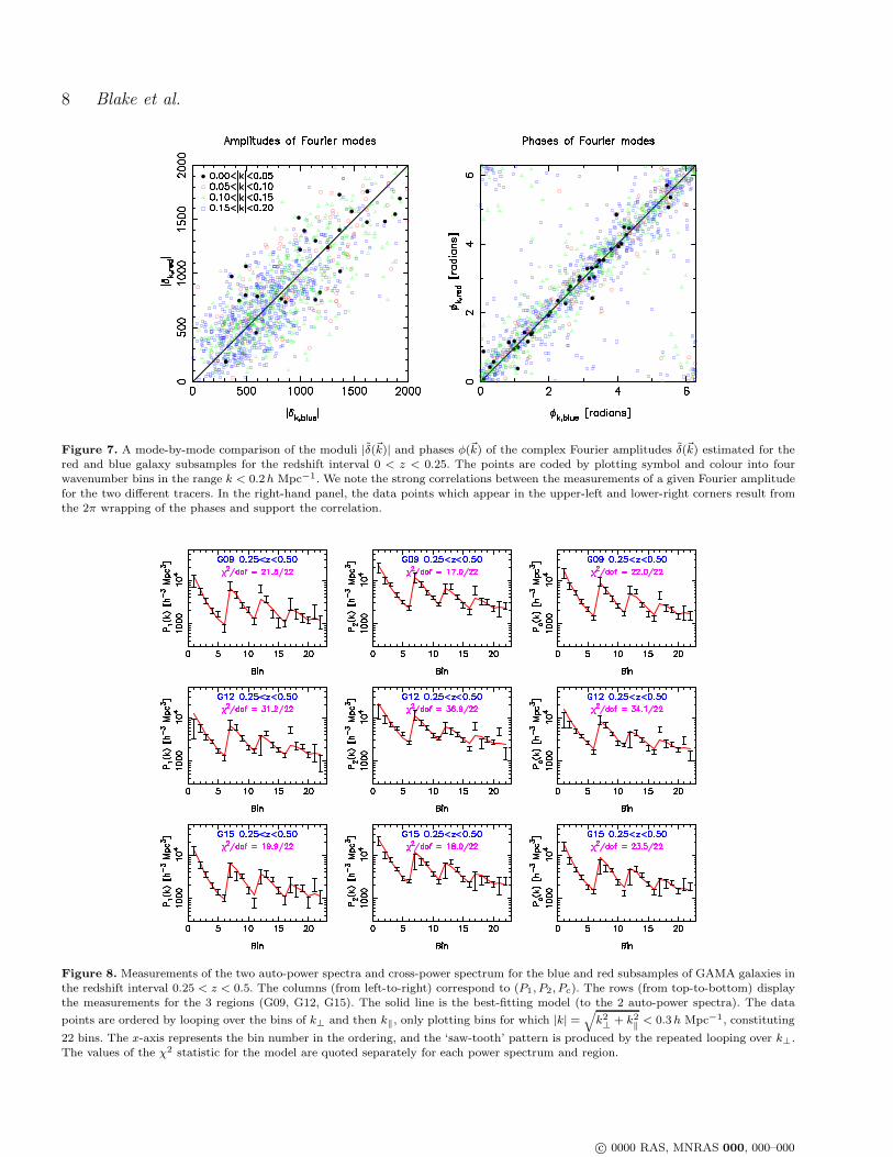
Fig. 7 compares the moduli |δα| and phases φα of the com-plex Fourier amplitudes δα = |δα| eiφα for the red and bluegalaxy subsamples for the 0 < z < 0.25 redshift interval.The common sample variance induces clear correlations be-tween the moduli and phases of the different populations.

In the Appendix we derive the estimators of the twoauto-power spectra, P1(~k) and P2(~k), and cross-power spec-

trum Pc(~k). The final expressions are:

Pα(~k) =V

[

|δα(~k)|2 −Nα

∑

~x Wα w2α

]

Nc N2α

∑

~x W2α w2

α

Pc(~k) =V Re

δ1(~k) δ∗2(~k)

Nc N1 N2

∑

~x W1 w1 W2 w2(13)

We note that the expectation values of the estimators inequation (13) are a convolution of the underlying modelpower spectra:

〈Pα(~k)〉 = V 3

(2π)3

∫

Pα(~k′) |nw,α(δ~k)|2 d3~k′

〈Pc(~k)〉 =V 3

(2π)3

∫

Pc(~k′) Re

nw,1(δ~k) n∗w,2(δ~k)

d3~k′

(14)

where nw,α = Nα Ww,α and δ~k = ~k′ − ~k. We averaged thepower spectrum amplitudes for the different Fourier modesin bins of wavevector perpendicular and parallel to the line-of-sight, (k⊥, k‖). Since in our analysis we orient the x-axisparallel to the line-of-sight to the centre of each survey re-gion, and each region has a narrow and deep geometry,we can make the flat-sky approximation k⊥ =

√

k2y + k2

z ,

k‖ = |kx| (noting that any resulting systematic distor-tion is negligible compared with the sample-variance errorin our measurements). We used wavevector bins of width∆k⊥ = ∆k‖ = 0.05 h Mpc−1 in the analysis, only consider-

ing bins for which |k| =√

k2⊥ + k2

‖ < 0.3 h Mpc−1 because

of concerns over modelling non-linearities in the power spec-trum at smaller scales, which are explored further in sec-tion 4. We also excluded the largest-scale (lowest) bin in k‖,0 < k‖ < 0.05 h Mpc−1, whose measured power is proneto systematic effects from the radial selection function fits.The final result was a total of 22 bins. Fig. 8 displays thebinned auto-power and cross-power spectrum measurementsfor the blue and red galaxy subsamples in the redshift inter-val 0.25 < z < 0.5, for each of the three GAMA regions.

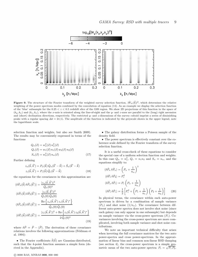
Fig. 9 displays an example of the structure of the Fouriertransform of the weighted selection function, |Ww(~k)|2,which determines the relative weighting of the power spec-trum modes combined by the convolution of equation (14).As expected, this function contains a series of diminishingpeaks along each axis spaced by ∆k = 2π/L, in accordancewith the dimension L of the survey cuboid parallel to thataxis. These peaks are hence particularly widely-spaced par-allel to the narrow, declination direction of the survey ge-ometry. This structure was fully modelled in our parameterfits. When fitting models, we re-cast the convolution inte-grals of equation (14) as matrix multiplications for reasonsof numerical speed:

〈Pα(i)〉 =∑

j

(Mα)ij Pmod,α(j)

〈Pc(i)〉 =∑

j

(Mc)ij Pmod,c(j) (15)

where (Pmod,1, Pmod,2, Pmod,c) are the model auto-power andcross-power spectra for the 2 populations, evaluated at thecentres of the Fourier bins. We determined the convolutionmatrices (M1,M2,Mc) by evaluating the full integrals givenin equation (14) for a set of unit model vectors, and testedthat this produced a negligible change in results comparedto implementing the full convolution.

We defined the effective redshift of each power spectrummeasurement by weighting each pixel in the 3D selectionfunction by its contribution to the power spectrum error:

zeff(k) =∑

~x

z ×[

n(~x)P (k)

1 + n(~x)P (k)

]2

(16)

We evaluated this relation at k = 0.1 h Mpc−1 (although theresults do not depend strongly on this choice). The effectiveredshifts of the measurements in the redshift intervals (0 <z < 0.25, 0.25 < z < 0.5 are zeff = (0.18, 0.38), with a veryweak dependence on galaxy type.

3.4 Covariance matrix

The survey selection functions and correlated sample vari-ance induce covariances between the estimates of the twoauto-power and cross-power spectra of the galaxy popula-tions for two Fourier modes ~k and ~k′. These covariances arederived in the Appendix; the expressions for the auto-powerspectrum follow Feldman et al. (1994), to our knowledgethe other formulae are new (regarding the inclusion of the

c© 0000 RAS, MNRAS 000, 000–000

8 Blake et al.

Figure 7. A mode-by-mode comparison of the moduli |δ(~k)| and phases φ(~k) of the complex Fourier amplitudes δ(~k) estimated for thered and blue galaxy subsamples for the redshift interval 0 < z < 0.25. The points are coded by plotting symbol and colour into fourwavenumber bins in the range k < 0.2h Mpc−1. We note the strong correlations between the measurements of a given Fourier amplitude

for the two different tracers. In the right-hand panel, the data points which appear in the upper-left and lower-right corners result fromthe 2π wrapping of the phases and support the correlation.

Figure 8. Measurements of the two auto-power spectra and cross-power spectrum for the blue and red subsamples of GAMA galaxies inthe redshift interval 0.25 < z < 0.5. The columns (from left-to-right) correspond to (P1, P2, Pc). The rows (from top-to-bottom) displaythe measurements for the 3 regions (G09, G12, G15). The solid line is the best-fitting model (to the 2 auto-power spectra). The data

points are ordered by looping over the bins of k⊥ and then k‖, only plotting bins for which |k| =√

k2⊥ + k2‖< 0.3h Mpc−1, constituting

22 bins. The x-axis represents the bin number in the ordering, and the ‘saw-tooth’ pattern is produced by the repeated looping over k⊥.The values of the χ2 statistic for the model are quoted separately for each power spectrum and region.

c© 0000 RAS, MNRAS 000, 000–000

GAMA Survey: RSD with multiple tracers 9

Figure 9. The structure of the Fourier transform of the weighted survey selection function, |Ww(~k)|2, which determines the relativeweighting of the power spectrum modes combined by the convolution of equation (14). As an example we display the selection functionof the ‘blue’ subsample for the 0.25 < z < 0.5 redshift slice of the G09 region. We show 2D projections of this function in the space of(ky , kx) and (kz , kx), where the x-axis is oriented along the line-of-sight and the y- and z-axes are parallel to the (long) right ascensionand (short) declination directions, respectively. The restricted y- and z-dimensions of the survey cuboid imprint a series of diminishingpeaks with a regular spacing ∆k = 2π/L. The amplitude of the function is indicated by the greyscale shown in the upper legend, notethe logarithmic scale.

selection function and weights, but also see Smith 2009).The results may be conveniently expressed in terms of thefunctions

Qα(~x) = w2α(~x)n

2α(~x)

Qc(~x) = w1(~x)n1(~x)w2(~x)n2(~x)

Sα(~x) = w2α(~x)nα(~x) (17)

Further defining

zα(~k,~k′) = Pα(~k) Qα(~k

′ − ~k) + Sα(~k′ − ~k)

zc(~k,~k′) = Pc(~k) Qc(~k

′ − ~k) (18)

the equations for the covariances in this approximation are

〈δPα(~k) δPα(~k′)〉 = |zα(~k,~k′)|2

Qα(0)2

〈δP1(~k) δP2(~k′)〉 = |zc(~k,~k′)|2

Q1(0) Q2(0)

〈δPα(~k) δPc(~k′)〉 =

Re

zα(~k,~k′) zc(~k,~k

′)∗

Qα(0) Qc(0)

〈δPc(~k) δPc(~k′)〉 =

|zc(~k,~k′)|2 +Re

z1(~k,~k′) z2(~k,~k

′)∗

2 Qc(0)2

(19)

where δP = P − 〈P 〉. The derivation of these covariancerelations involves the following approximations (Feldman etal. 1994):

• The Fourier coefficients δ(~k) are Gaussian-distributed,such that the 4-point function assumes a simple form (de-rived in the Appendix).

• The galaxy distribution forms a Poisson sample of thedensity field.

• The power spectrum is effectively constant over the co-herence scale defined by the Fourier transform of the surveyselection function.

It is a useful cross-check of these equations to considerthe special case of a uniform selection function and weights.In this case Qα = n2

α, Qc = n1n2 and Sα = nα, and theequations simplify to:

〈δPα δPα〉 =(

Pα +1

nα

)2

〈δP1 δP2〉 = P 2c

〈δPα δPc〉 = Pc

(

Pα +1

nα

)

〈δPc δPc〉 = 1

2

[

P 2c +

(

P1 +1

n1

)(

P2 +1

n2

)]

(20)

In physical terms, the covariance within each auto-powerspectrum is driven by a combination of sample variance(Pα) and shot noise (1/nα). The covariance between dif-ferent auto-power spectra does not involve shot noise (sinceeach galaxy can only appear in one subsample) but dependson sample variance via the cross-power spectrum (Pc). Co-variances involving the cross-power spectrum are more com-plicated, involving both sample variance and shot noise con-tributions.

We note an important technical difficulty that ariseswhen inverting the full covariance matrices for the two autopower-spectra and cross power-spectrum. In the approxi-mation of linear bias and common non-linear RSD damping(see section 4), the cross-power spectrum is a simple geo-metric mean of the two auto-power spectra: Pc =

√P1 P2.

c© 0000 RAS, MNRAS 000, 000–000

10 Blake et al.

In the limit of high galaxy number density, such that shotnoise is negligible, the cross-power spectrum measurementthen adds no information to that already present in the twoauto-power spectra. We can verify this mathematically bytaking the limit of equation (20) as nα → ∞. The covari-ance matrix for the measurement of (P1, P2, Pc) for a singleFourier mode becomes:

C(~k) =

P 21 P 2

c P1 Pc

P 2c P 2

2 P2 Pc

P1 Pc P2 Pc12

(

P 2c + P1 P2

)

(21)

which, given that P 2c = P1 P2, implies that |C| = 0 and the

matrix is singular. (The fact that the cross-power spectrumadds no information as nα → ∞ is also demonstrated laterby the Fisher matrix calculations in section 6).

The number densities of the GAMA multiple-tracerpopulations are well within the regime where the contri-bution of the cross-power spectrum to the parameter con-straints is negligible, and in fact we found that the full co-variance matrix was not always positive definite (even forfinite n1 and n2). We traced the cause of this issue as theapproximation made in equations (A23) and (A38) whichresults in the covariance matrix of equation (19); evaluatinginstead the exact expressions in equations (A22) and (A37)produced a positive-definite covariance matrix but was sig-nificantly more time-consuming. We therefore restricted ourfits to the two GAMA auto-power spectra and excluded thecross-power spectrum; the growth-rate error predicted bythe Fisher matrix is worsened by only 0.2% for the GAMAsurvey specifications. We note that, as justified by the Fishermatrix forecasts below, the cross-power spectrum does addsignificant information for galaxy samples with lower num-ber densities (n < 3× 10−4 h3 Mpc−3).

We instead used the measured cross-power spectrum toprovide some independent validation of the modelling as-sumptions. As an example, the right-hand column of Fig.8 compares the cross-power spectrum measurements to themodel fitted to the two auto-power spectra, finding satisfac-tory agreement as judged by the values of the χ2 statistic.

For model-fitting we defined a total data vector inwhich the measurements of the two auto-power spectrawere concatenated into a longer vector yi ≡ [P1(i), P2(i)]

(for the binned measurements) and y(~k) ≡ [P1(~k), P2(~k)](for the original Fourier modes). Given that the binnedestimates of power are averages within each Fourier binyi = (1/mi)

∑

~k y(~k), where the sum is over the mi Fourier

modes ~k lying in bin i, then the covariance of the binnedestimates is

Cij = 〈δyi δyj〉 =1

mi mj

∑

~k,~k′

〈y(~k) y(~k′)〉 (22)

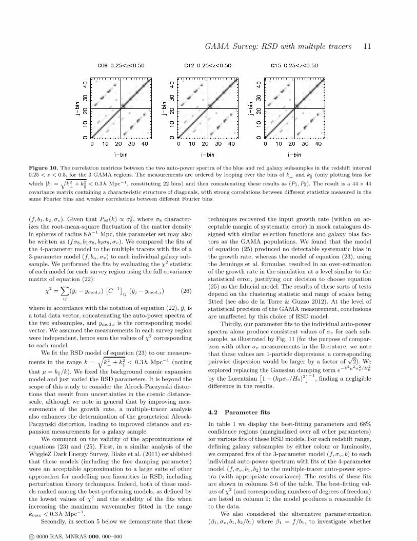
We evaluated these covariance relations over the FFT gridsfor each GAMA region, using equation (19). Fig. 10 illus-trates the structure of the resulting covariance matrices forthe 0.25 < z < 0.5 auto-power spectrum measurements,with each displayed as a correlation matrix Cij/

√

Cii Cjj .We note the characteristic structure of diagonals, withstrong correlations between different statistics measured inthe same Fourier bins, and weaker correlations between dif-ferent Fourier bins.

We tested our determination of the covariance matrixusing a large ensemble of lognormal realizations. For each re-

alization, two (correlated) populations of galaxies were cre-ated by Poisson-sampling the same underlying density fieldusing the GAMA survey selection functions. The diagonaland off-diagonal amplitudes of the lognormal and analyticcovariance matrices were in good agreement, with the nu-merical values of the matrix elements differing by less than10%.

4 MODEL FITS

4.1 RSD modelling

We fit the power spectrum measurements in each GAMAregion using a standard model for the redshift-space powerspectrum as a function of the cosine of the angle of theFourier wavevector to the line-of-sight, µ:

Pα(k, µ) =[

b2αPδδ(k) + 2bαfµ2Pδθ(k) + f2µ4 Pθθ(k)

]

× e−k2µ2σ2

v/H2

0 (23)

(Scoccimarro 2004) where, in terms of the divergence of thepeculiar velocity field θ, Pδδ(k), Pδθ(k) and Pθθ(k) are theisotropic density-density, density-θ and θ-θ power spectra.This model combines the large-scale ‘Kaiser limit’ ampli-tude correction with a heuristic damping of power on smallerscales that describes a leading-order perturbation theorycorrection. Here, the free parameter σv has units of kms−1 and H0 = 100 h km s−1 Mpc−1. When fitting multi-ple tracers, we make the approximation that all populationsof galaxies trace the same value of σv on large scales, aspredicted by linear theory:

σ2v =

f2H20

6π2

∫

Pθθ(k) dk (24)

although, as stated above, we treat σv as a free parame-ter to allow for non-linearities in the matter clustering. Onlarge scales, we neglect the contribution to equation (24)from virialized galaxy motions within dark matter halos.Approximating Pθθ as a linear power spectrum, the predic-tion of equation (24) in our fiducial cosmology is σv = 334km s−1.

We generated the matter power spectrum Pδδ in equa-tion (23) using the ‘halofit’ model (Smith et al. 2003) as im-plemented by the CAMB software package (Lewis, Challinor& Lasenby 2000) with the cosmological parameters fixed atvalues inspired by fits to the CMB fluctuations measured byWMAP (Komatsu et al. 2011): matter density Ωm = 0.27,Hubble parameter h = 0.719, spectral index ns = 0.963,baryon fraction Ωb/Ωm = 0.166 and normalization σ8 = 0.8.We considered two different choices for producing the modelvelocity power spectra Pδθ and Pθθ. In our fiducial model,we used the large-scale limits of the velocity power spec-tra Pδθ = Pθθ = Pδδ, such that the model of equation (23)simplified to:

Pα(k, µ) = Pδδ(k)(

bα + fµ2)2

e−k2µ2σ2

v/H2

0 (25)

Secondly, we investigated whether our results changed sig-nificantly if we used the fitting formulae for Pδθ and Pθθ interms of Pδδ, calibrated by N-body simulations, proposed byJennings et al. (2011).

Our model is hence characterized by four parameters

c© 0000 RAS, MNRAS 000, 000–000

GAMA Survey: RSD with multiple tracers 11

Figure 10. The correlation matrices between the two auto-power spectra of the blue and red galaxy subsamples in the redshift interval0.25 < z < 0.5, for the 3 GAMA regions. The measurements are ordered by looping over the bins of k⊥ and k‖ (only plotting bins for

which |k| =√

k2⊥ + k2‖< 0.3h Mpc−1, constituting 22 bins) and then concatenating these results as (P1, P2). The result is a 44 × 44

covariance matrix containing a characteristic structure of diagonals, with strong correlations between different statistics measured in thesame Fourier bins and weaker correlations between different Fourier bins.

(f, b1, b2, σv). Given that Pδδ(k) ∝ σ28 , where σ8 character-

izes the root-mean-square fluctuation of the matter densityin spheres of radius 8h−1 Mpc, this parameter set may alsobe written as (fσ8, b1σ8, b2σ8, σv). We compared the fits ofthe 4-parameter model to the multiple tracers with fits of a3-parameter model (f, bα, σv) to each individual galaxy sub-sample. We performed the fits by evaluating the χ2 statisticof each model for each survey region using the full covariancematrix of equation (22):

χ2 =∑

ij

(yi − ymod,i)[

C−1]

ij(yj − ymod,j) (26)

where in accordance with the notation of equation (22), yi isa total data vector, concatenating the auto-power spectra ofthe two subsamples, and ymod,i is the corresponding modelvector. We assumed the measurements in each survey regionwere independent, hence sum the values of χ2 correspondingto each model.

We fit the RSD model of equation (23) to our measure-

ments in the range k =√

k2⊥ + k2

‖ < 0.3 h Mpc−1 (noting

that µ = k‖/k). We fixed the background cosmic expansionmodel and just varied the RSD parameters. It is beyond thescope of this study to consider the Alcock-Paczynski distor-tions that result from uncertainties in the cosmic distance-scale, although we note in general that by improving mea-surements of the growth rate, a multiple-tracer analysisalso enhances the determination of the geometrical Alcock-Paczynski distortion, leading to improved distance and ex-pansion measurements for a galaxy sample.

We comment on the validity of the approximations ofequations (23) and (25). First, in a similar analysis of theWiggleZ Dark Energy Survey, Blake et al. (2011) establishedthat these models (including the free damping parameter)were an acceptable approximation to a large suite of otherapproaches for modelling non-linearities in RSD, includingperturbation theory techniques. Indeed, both of these mod-els ranked among the best-performing models, as defined bythe lowest values of χ2 and the stability of the fits whenincreasing the maximum wavenumber fitted in the rangekmax < 0.3 h Mpc−1.

Secondly, in section 5 below we demonstrate that these

techniques recovered the input growth rate (within an ac-ceptable margin of systematic error) in mock catalogues de-signed with similar selection functions and galaxy bias fac-tors as the GAMA populations. We found that the modelof equation (25) produced no detectable systematic bias inthe growth rate, whereas the model of equation (23), usingthe Jennings et al. formulae, resulted in an over-estimationof the growth rate in the simulation at a level similar to thestatistical error, justifying our decision to choose equation(25) as the fiducial model. The results of these sorts of testsdepend on the clustering statistic and range of scales beingfitted (see also de la Torre & Guzzo 2012). At the level ofstatistical precision of the GAMA measurement, conclusionsare unaffected by this choice of RSD model.

Thirdly, our parameter fits to the individual auto-powerspectra alone produce consistent values of σv for each sub-sample, as illustrated by Fig. 11 (for the purpose of compar-ison with other σv measurements in the literature, we notethat these values are 1-particle dispersions; a correspondingpairwise dispersion would be larger by a factor of

√2). We

explored replacing the Gaussian damping term e−k2µ2σ2

v/H2

0

by the Lorentzian[

1 + (kµσv/H0)2]−1

, finding a negligibledifference in the results.

4.2 Parameter fits

In table 1 we display the best-fitting parameters and 68%confidence regions (marginalized over all other parameters)for various fits of these RSD models. For each redshift range,defining galaxy subsamples by either colour or luminosity,we compared fits of the 3-parameter model (f, σv, b) to eachindividual auto-power spectrum with fits of the 4-parametermodel (f, σv, b1, b2) to the multiple-tracer auto-power spec-tra (with appropriate covariance). The results of these fitsare shown in columns 3-6 of the table. The best-fitting val-ues of χ2 (and corresponding numbers of degrees of freedom)are listed in column 9; the model produces a reasonable fitto the data.

We also considered the alternative parameterization(β1, σv, b1, b2/b1) where β1 = f/b1, to investigate whether

c© 0000 RAS, MNRAS 000, 000–000

12 Blake et al.

Table 1. Fits of RSD models in single-tracer and multiple-tracer analyses of subsamples of GAMA galaxies in two different redshiftintervals 0 < z < 0.25 and 0.25 < z < 0.5, with effective redshifts z = 0.18 and 0.38, respectively. Columns 3-6 display the results offitting the 4-parameter model (f, σv , b1, b2). Columns 7-8 are the fits of an alternative parameterization (β1, σv, b1, b2/b1). Column 9provides the best-fitting values of χ2 and corresponding numbers of degrees-of-freedom.

Redshift Sample f σv [km/s] b1 b2 β1 b2/b1 χ2/dof

0.0 < z < 0.25 Blue 0.49± 0.14 277 ± 59 0.891± 0.038 - 0.56 ± 0.17 - 41.6/63Red 0.35± 0.15 246 ± 57 - 1.377± 0.041 - - 53.9/63Joint 0.49± 0.12 285 ± 41 0.894± 0.038 1.348± 0.038 0.57 ± 0.15 1.509 ± 0.030 163.1/128

0.0 < z < 0.25 low-L 0.45± 0.15 267 ± 59 1.066± 0.039 - 0.43 ± 0.15 - 41.9/63high-L 0.35± 0.15 211 ± 62 - 1.480± 0.043 - - 78.1/63Joint 0.33± 0.13 192 ± 65 1.071± 0.038 1.467± 0.039 0.32 ± 0.13 1.371 ± 0.020 175.5/128

0.25 < z < 0.5 Blue 0.68± 0.10 269 ± 34 1.074± 0.034 - 0.64 ± 0.10 - 90.4/63Red 0.48± 0.11 256 ± 31 - 1.707± 0.035 - - 79.0/63Joint 0.66± 0.09 286 ± 23 1.105± 0.031 1.664± 0.030 0.60 ± 0.09 1.508 ± 0.027 167.7/128

0.25 < z < 0.5 low-L 0.63± 0.09 294 ± 31 1.283± 0.020 - 0.49 ± 0.07 - 75.6/63high-L 0.47± 0.12 224 ± 37 - 1.789± 0.041 - - 75.7/63Joint 0.57± 0.08 265 ± 28 1.283± 0.020 1.780± 0.026 0.45 ± 0.07 1.388 ± 0.018 147.5/128

Figure 11. Fits for the RSD parameters (f, σv), marginalized over galaxy bias, for different redshift ranges and multiple-tracer subsamples(split by both colour and luminosity). In each case we compare the fits to the individual subsamples (blue dashed and red dotted contoursfor the low-bias (‘tr-1’) and high-bias (‘tr-2’) sample, respectively) and the joint sample (black solid contours). The likelihood contoursare all 68% confidence regions. The captions quote the 1D marginalized measurements of the growth rate.

the multiple-tracer analysis allows the combinations of pa-rameters f/b1 or b2/b1 to be determined with any additionalaccuracy. These results are shown in columns 7-8. We foundthat the ratio of the galaxy bias factors of the multiple pop-ulations, b2/b1, was measured significantly more accuratelyfor the multiple-tracer fits than would be obtained by a naivepropagation of the errors in the individual bias factors in the

single-tracer fits, but the fractional errors in measuring β1

were similar to those in determining f . We note that the pre-cision afforded by a multiple-tracer analysis for measuringbias ratios (which can be carried out using the 1D monopolepower spectra) could provide a valuable test of models whichpredict the trend of bias with galaxy luminosity or colour.

Fig. 11 shows likelihood contours in the space of (f, σv)

c© 0000 RAS, MNRAS 000, 000–000

GAMA Survey: RSD with multiple tracers 13

Figure 12.Marginalized measurements of the normalized growthrate fσ8(z) fit to multiple-tracer GAMA galaxy subsamples splitby colour. The prediction of a flat ΛCDM model with matter den-sity Ωm = 0.27 and normalization σ8 = 0.8 is also shown as thesolid line. The open squares display the results of RSD analyses ofa series of other galaxy surveys in a similar redshift range, takenfrom 6dFGS (z = 0.067, Beutler et al. 2012), 2dFGRS (z = 0.17,Hawkins et al. 2003), the SDSS Luminous Red Galaxy sample(z = 0.25 and z = 0.37, Samushia et al. 2012) and the WiggleZSurvey (z = 0.22 and z = 0.41, Blake et al. 2011).

marginalized over the bias parameter(s), comparing thesingle-tracer and multiple-tracer fits. In all cases we foundthat the parameter measurements from different tracerswere mutually consistent, and that the fit to the combineddata produced a significant shrinkage in the size of the 68%confidence region. In terms of the width of the 68% confi-dence interval for the posterior probability distribution off , the multiple-tracer fits produced reductions in the range10-20%. In section 6 we will demonstrate in a Fisher ma-trix analysis that truly large improvements in the accuracyof determination of the growth rate require higher galaxynumber densities (n > 10−2 h3 Mpc−3).

Fig. 12 displays the marginalized measurements of thenormalized growth rate fσ8(z) for the GAMA multiple-tracer analysis split by colour, compared to the predictionof a flat ΛCDM model with matter density Ωm = 0.27and normalization σ8 = 0.8. The measurements of fσ8(z)in redshift slices (0 < z < 0.25, 0.25 < z < 0.5) are(0.36 ± 0.09, 0.44 ± 0.06), respectively. We compared theGAMA measurements with the published RSD analyses ofa series of other galaxy surveys in a similar redshift range,which are plotted as the open squares in Fig. 12. Thesemeasurements were taken from 6dFGS (z = 0.067, Beutleret al. 2012), 2dFGRS (z = 0.17, Hawkins et al. 2003), theSDSS Luminous Red Galaxy sample (z = 0.25 and z = 0.37,Samushia et al. 2012) and the WiggleZ Survey (z = 0.22 andz = 0.41, Blake et al. 2011). Our GAMA measurements areconsistent with the results of these other surveys at similarredshifts.

5 VALIDATION USING N-BODY

SIMULATIONS

We tested the validity of the non-linear RSD model of equa-tion (23), in particular the amplitude of any systematic mod-elling error that may impact the growth-rate measurements,by fitting it to power spectrum measurements of dark mat-ter halo catalogues generated from N-body simulations. Wecarried out these tests using the GiggleZ N-body simulation(Poole et al. in preparation), a 21603 particle dark mattersimulation run in a 1h−1 Gpc box (with resulting particlemass 7.5 × 109 h−1M⊙). Bound structures were identifiedusing Subfind (Springel et al. 2001), which uses a friends-of-friends (FoF) scheme followed by a sub-structure analysisto identify bound overdensities within each FoF halo. Weemployed each halo’s maximum circular velocity Vmax as aproxy for mass, and used the centre-of-mass velocities foreach halo when introducing redshift-space distortions.

We divided the GiggleZ simulation into 8 non-overlapping realizations of the GAMA survey for the red-shift range 0.25 < z < 0.5, where each realization consistsof the 3 survey regions. (We note that since we are justusing one simulation there will be low-level correlations be-tween these realizations deriving from common large-scalemodes, hence the scatter in results between the realizationsmay be slightly under-estimated). In each region we selectedtwo populations of halos which approximately reproduce thebias factors of the blue and red GAMA populations, a ‘low-bias’ set with 80 < Vmax < 135 km s−1 and a ‘high-bias’ setwith 135 < Vmax < 999 km s−1, and subsampled these halosusing the full survey selection functions. We note that ourintention here was not to produce full mock GAMA cata-logues, since we incorporated no information about colour,luminosity or halo occupation distribution, but rather tovalidate that the RSD model of equation (23) was able toreproduce the input growth rate of the N-body simulationon quasi-linear scales, with minimal systematic error.

We measured the auto-power spectra of the two popu-lations in each survey region for each realization and fittedthe RSD model of equation (25), using the same techniqueswe applied when analyzing the real data (using the rangek < 0.3 h Mpc−1). Fig. 13 shows the marginalized measure-ments of (f, σv) for each of the 8 realizations, with the 68%confidence region displayed as the dotted (coloured) lines.The solid black contours are the 68% and 95% confidenceregions obtained by combining these 8 measurements, as-suming that they were independent. The vertical dashed lineindicates the predicted growth rate f = 0.69 based on theinput cosmological parameters of the N-body simulation (atz = 0.408); the fits reveal no evidence for systematic mod-elling errors. The average best-fitting χ2 for the 8 realiza-tions is 91.4 for 128 degrees of freedom.

With the caveat that we only used 8 realizations, wecompared the errors in the measured growth rates of thesimulations and data. The average error in the growth ratein the fits to the mock catalogues was ∆f = 0.11, comparedto ∆f = 0.09 for the data, and the standard deviation inthe best-fitting values for each realization was σf = 0.07.Given that these mock catalogues do not match the galaxypopulations of the data sample exactly, we consider the moreconservative value obtained from the data covariance matrixto be the more reliable estimate.

c© 0000 RAS, MNRAS 000, 000–000

14 Blake et al.

Figure 13. Growth-rate fits to multiple-tracer power spectrameasured in 8 different realizations of the GAMA survey ex-tracted from a large N-body simulation. In each realization, twohalo catalogues were extracted with bias factors close to twoGAMA populations, and were subsampled in three survey regionsusing the appropriate selection functions for the 0.25 < z < 0.5redshift range. The 8 sets of dotted coloured contours representthe 68% confidence region of (f, σv) fits (marginalized over biasparameters) to each of the 8 realizations, using the same RSDmodel and fitting range as applied to the GAMA data. The solidblack contours are 68% and 95% confidence regions obtained bycombining these 8 measurements, assuming that they were inde-pendent. The vertical dotted line is the growth rate deduced fromthe input cosmological parameters of the simulation.

6 FISHER MATRIX FORECASTS

We compared our measurements with Fisher matrix fore-casts, which also indicate how our results would extend tosurveys with a different design (also see McDonald & Seljak2009, White et al. 2009, Abramo 2012). In this section weadopt the notation Pij to describe the auto-power spectrabetween tracers (with j = i) and cross-power spectra (withj 6= i). We assume that the covariance matrix for the mea-surement of (P11, P22, P12) using an individual Fourier mode~k = (k, µ) can be written following equation (20) as

C(~k) =

Q21 P1P2 Q1

√P1P2

P1P2 Q22 Q2

√P1P2

Q1

√P1P2 Q2

√P1P2

12(P1P2 +Q1Q2)

(27)where we have written Pi = Pii and Qi = Pi + 1/ni, whereni is the number density of the tracers. The RSD powerspectrum model (using equation (25) for simplicity) is then

Pij(k, µ) = (bi + fµ2) (bj + fµ2)Pm(k) e−k2µ2σ2

v/H2

0 (28)

where bi are the bias factors of the tracers. The derivativeswith respect to the parameters are

∂Pij

∂f=

[

(bi + bj)µ2 + 2fµ4

]

Pm(k) e−k2µ2σ2

v/H2

0

∂Pii

∂bi=

2Pii

bi + fµ2

∂Pii

∂bj= 0 (j 6= i)

∂Pij

∂bi=

Pij

bi + fµ2(j 6= i)

∂Pij

∂σ2v

= −k2µ2

H20

Pij (29)

The Fisher matrix of the parameter vector pα =(f, σ2

v, b1, b2) is written

Fαβ =∑

k,µ

m(k, µ)∑

i,j

∂Pij(k, µ)

∂pα

[

C(k, µ)−1]

ij

∂Pij(k, µ)

∂pβ

(30)where m(k, µ) is the number of modes in a (k, µ) bin ofwidth (∆k,∆µ), which we deduce from the survey volumeV as

m(k, µ) =V

(2π)32π k2 ∆k∆µ (31)

We considered 5 bins in µ in the range 0 < µ < 1 and 6bins in k in the range 0 < k < 0.3 h Mpc−1, although ourresults were not sensitive to the bin widths. The covariancematrix of the parameters follows as Cαβ = (F−1)αβ, and wefocused in particular on the forecast error in the growth ratemeasurement, ∆f =

√C11 = (F−1)11.

In our fiducial model of the GAMA II survey we fixedthe RSD parameters (f, σv) = (0.59, 300), number densitiesni = 5 × 10−3 h3 Mpc−3, bias factors (b1, b2) = (1.0, 1.4)and volume V = 6.42×106 h−3 Mpc3. These values are rep-resentative of the two-sample dataset for 0 < z < 0.25. Theforecast marginalized error in the growth rate for this caseis ∆f = 0.096 for the multiple-tracer fits, and ∆f = 0.124and 0.156 for the low-bias and high-bias single-tracer fits, re-spectively (such that the multiple-tracer analysis produces a≈ 20 per cent improvement compared to the low-bias case).These forecasts are a little better than, although comparableto, the measurements quoted in table 1, and we note thatthe Fisher matrix forecast assumes a perfect-cuboid surveywith no correlations between different Fourier modes.

We then considered two sets of variations which allowus to explore other survey designs:

• Varying the bias factor of the second tracer in the range1 < b2 < 4 for different choices of n2, fixing b1 = 1 andn1 = 5× 10−3 h3 Mpc−3.

• Varying the number density of both tracers in the range1× 10−4 < ni < 5× 10−2 h3 Mpc−3 for different choices ofb2, fixing b1 = 1.

The results are displayed in Fig. 14, with the solid circlesindicating the fiducial GAMA case quoted above.

The upper panel of Fig. 14 indicates the improvementin the multiple-tracer growth rate measurement that re-sults as the difference between the bias factors of the galaxypopulations increases. For n2 = n1 = 5 × 10−3 h3 Mpc−3

and b1 = 1, the growth rate measurement improves by

c© 0000 RAS, MNRAS 000, 000–000

GAMA Survey: RSD with multiple tracers 15

Figure 14. Fisher matrix forecasts for the error in the growthrate, ∆f , marginalized over the other RSD parameters. We con-sider two-tracer survey configurations varying the bias parameters(b1, b2) and number densities (n1, n2), fixing the survey volumeV = 6.42 × 106 h−3 Mpc3 and b1 = 1 for all cases. In the upperpanel we fix n1 = 5× 10−3 h3 Mpc−3 and plot ∆f as a functionof b2 for various choices of n2. In the lower panel we plot ∆f as afunction of n = n1 = n2 for various choices of b2. The dash-triple-dotted black curve in the lower panel, compared to the solid blackcurve, shows the effect of dropping the cross-power spectrum in-formation. The solid circles in the panels indicate the fiducialGAMA values of these parameters. Changing the survey volumeV will simply scale the results by ∆f ∝ V −1/2.

(8, 22, 35, 44, 51)% for b2 = (1.2, 1.4, 1.6, 1.8, 2.0). These fore-cast gains will be impacted by the practical difficulty ofmaintaining a high target number density as galaxy biasincreases, as described by the set of lines for different valuesof n2 in the upper panel of Fig. 14.

The lower panel of Fig. 14 displays the increasing ef-ficacy of the multiple-tracer method as the number den-sity of the galaxy populations increases. For n > 10−3 h3

Mpc−3 the gains from single-tracer RSD saturate (as indi-cated by the solid black line); but the growth rate measure-ment from multiple-tracers improves by (12, 22, 37, 53, 66)%for n = (0.23, 0.5, 1.1, 2.4, 5.2) × 10−2 h3 Mpc−3 assuming(b1, b2) = (1.0, 1.4). The black dash-triple-dotted line inFig. 14, which should be compared with the black solidline, illustrates the effect of dropping the information fromthe cross-power spectrum. For low values of number den-sity n < 10−3 h3 Mpc−3 the cross-power spectrum adds

some information due to shot noise. For high number den-sity n > 10−3 h3 Mpc−3 the cross-power spectrum may beentirely predicted from the two auto-power spectrum (underthe assumption of linear galaxy bias) and hence its inclusiondoes not improve the growth-rate measurements within theassumed RSD model.

7 SUMMARY

In this study we have presented the first observationalmultiple-tracer analysis of redshift-space distortions usingdata from the Galaxy and Mass Assembly survey. We per-formed a Fourier analysis of the two auto-power spectra ofgalaxy populations split by both colour and luminosity, de-riving new expressions for the covariances between thesemeasurements in terms of a general survey selection func-tion and weighting scheme, and verified our results by alsomeasuring the cross-power spectrum. We fit models to theredshift-space power spectra in terms of the gravitationalgrowth rate, f , linear galaxy bias factors and an empiricalnon-linear damping parameter. We find that, in the case ofGAMA, the multiple-tracer analysis produces an improve-ment in the measurement accuracy of f by 10-20% (de-pending on the sample). The growth rates determined fromthe separate populations, split by colour and luminosity, areconsistent, showing no evidence for strong systematic mod-elling errors. The precision of our measurements is similarto a Fisher matrix forecast, which indicates how our anal-yses would extend to surveys with a different design: forsamples with higher number densities or bias factor differen-tials, much stronger improvements in the accuracy of growthrate determination are expected. We tested our methodol-ogy using mock catalogues from N-body simulations, demon-strating that the systematic error in the measured growthrate was much smaller than the statistical error. The nor-malized gravitational growth rate determined in two inde-pendent redshift slices, fσ8(z = 0.18) = 0.36 ± 0.09 andfσ8(z = 0.38) = 0.44 ± 0.06 using multiple-tracer subsam-ples selected by colour, is consistent with results from otherRSD surveys in a similar redshift range, and with standardΛ Cold Dark Matter models.

ACKNOWLEDGMENTS

CB acknowledges the support of the Australian ResearchCouncil through the award of a Future Fellowship, and isgrateful for useful feedback from Yan-Chuan Cai and FelipeMarin.

GAMA is a joint European-Australasian projectbased around a spectroscopic campaign using the Anglo-Australian Telescope. The GAMA input catalogue is basedon data taken from the Sloan Digital Sky Survey and theUKIRT Infrared Deep Sky Survey. Complementary imagingof the GAMA regions is being obtained by a number of in-dependent survey programs including GALEX MIS, VSTKiDS, VISTA VIKING, WISE, Herschel-ATLAS, GMRTand ASKAP providing UV to radio coverage. GAMA isfunded by the STFC (UK), the ARC (Australia), the AAO,and the participating institutions. The GAMA website ishttp://www.gama-survey.org/.

c© 0000 RAS, MNRAS 000, 000–000

16 Blake et al.

REFERENCES

Abazajian, K., et al., 2009, ApJS, 182, 543

Abramo, L.R., 2012, MNRAS, 420, 2042

Abramo, L.R., Leonard, K., 2013, MNRAS, 432, 318

Baldry, I., et al., 2010, MNRAS, 404, 86

Baldry, I., et al., in preparation

Bernstein, G., Cai., Y.-C., 2011, MNRAS, 416, 3009Beutler, F., et al., 2012, MNRAS, 423, 3430

Blake, C., et al., 2011, MNRAS, 415, 2876

Blanton, M., Roweis, S., 2007, AJ, 133, 734

Cai, Y.-C., Bernstein, G., Sheth, R., 2011, MNRAS, 412, 995

Colless, M., et al., 2001, MNRAS, 328, 1039

Contreras, C., et al., 2013, MNRAS, 430, 924

Cresswell, J., Percival, W., 2009, MNRAS, 392, 682

Dawson, K., et al., 2013, AJ, 145, 10

Dekel, A., Lahav, O., 1999, ApJ, 520, 24de la Torre, S., Guzzo, L., 2012, MNRAS, 427, 327

de la Torre, S., et al., 2013, A&A accepted

Drinkwater, M., et al., 2010, MNRAS, 401, 1429

Driver, S., et al., 2011, MNRAS, 413, 971

Feldman, H., Kaiser, N., Peacock, J., 1994, ApJ, 426, 23

Gil-Marin, H., Wagner, C., Verde, L., Jimenez, R., Heavens, A.,2010, MNRAS, 407, 772

Hamaus, N., Seljak, U., Desjacques, V., 2012, PhRvD, 86, 3513

Hawkins, E., et al., 2003, MNRAS, 346, 78

Jennings, E., Baugh, C.M., Pascoli, S., 2011, MNRAS, 410, 2081

Jones, D.H., et al., 2009, MNRAS, 399, 683Kaiser, N., 1987, MNRAS, 227, 1

Komatsum E., et al., 2011, ApJS, 192, 18

Lewis, A., Challinor, A., Lasenby, A., 2000, ApJ, 538, 473

Liske, J., et al., in preparation

Loveday, J., et al., 2012, MNRAS, 420, 1239

Marin, F., 2011, ApJ, 737, 97

Marin, F., et al., 2013, MNRAS, 432, 2654

McDonald, P., Seljak, U., 2009, JCAP, 10, 7

Percival, W.J., Verde, L., Peacock, J., 2004, MNRAS, 347, 645Poole, G., et al., in preparation

Reid, B., et al., 2012, MNRAS, 426, 2719

Samushia, L., Percival, W.J., Raccanelli, A., 2012, MNRAS, 420,2102

Scoccimarro, R., 2004, PhRvD, 70, 83007

Seljak, U., 2009, PhRvL, 102, 1302

Seljak, U., Hamaus, N., Desjacques, V., 2009, PhRvL, 103, 1303

Smith, R.E., et al., 2003, MNRAS, 341, 1311

Smith, R.E., 2009, MNRAS, 400, 851

Springel, V., White, S., Tormen, G., Kauffmann, G., 2001, MN-RAS, 328, 726

Swanson, M., Tegmark, M., Blanton, M., Zehavi, I., 2008, MN-RAS, 385, 1635

White, M., Song, Y.-S., Percival, W., 2009, MNRAS, 397, 1348

Wild, V., et al., 2005, MNRAS, 356, 247

York, D., et al., 2000, AJ, 120, 1579

APPENDIX A: DERIVATION OF

AUTO-POWER AND CROSS-POWER

SPECTRUM ESTIMATORS AND

COVARIANCES

A1 Fourier conventions

First we note our conventions for Fourier transforms andinverse Fourier transforms:

FT(y) = y(~k) =1

V

∫

y(~x) ei~k.~x d3~x (A1)

IFT(y) = y(~x) =V

(2π)3

∫

y(~k) e−i~k.~x d3~k (A2)

where V is the Fourier volume. Some useful relations involv-ing the Dirac delta-function δD and its transform are:

∫

ei~k.~x d3~x = V δD(~k) (A3)

∫

ei~k.~x d3~k =

(2π)3

VδD(~x) (A4)

∫

δD(~x− ~x0) δ3~x = V (A5)

∫

y(~x) δD(~x− ~x0) δ3~x = V y(~x0) (A6)

∫

δD(~k − ~k0) δ3~k =

(2π)3

V(A7)

∫

y(~k) δD(~k − ~k0) δ3~k =

(2π)3

Vy(~k0) (A8)

It is also useful to list our conventions for evaluating FastFourier Transforms, which we will employ in practice forimplementing these calculations:

FFT(y) =∑

~xi

y(~xi) ei~k.~xi (A9)

IFFT(y) =∑

~ki

y(~ki) e−i~ki.~x (A10)

Noting the equivalences (1/V )∫

d3~x ≡ (1/Nc)∑

~x and

[V/(2π)3]∫

d3~k ≡ ∑

~k, we deduce that FFT(y) = Nc FT(y)and IFFT(y) = IFT(y), where Nc is the total number ofFFT cells.

A2 Estimator for auto-power spectrum

We first develop the estimator for the auto-power spec-trum of a galaxy number density distribution n(~x), given anunderlying selection function 〈n(~x)〉 describing the averageover many realizations, and allowing for a general weightingfunction w(~x). This derivation follows Feldman, Kaiser &Peacock (1994) and Smith (2009); we will then provide theextension to the galaxy cross-power spectrum and the var-ious covariances. The normalization of the number densityin terms of the total number of galaxies N is such that

∫

n(~x) d3~x = N (A11)

First we define the weighted galaxy overdensity

δ(~x) = w(~x) [n(~x)− 〈n(~x)〉] (A12)

and consider the Fourier transform of this expression, δ(~k).In order to perform this evaluation it is convenient to splitthe sample volume into many small cells i at positions ~xi

with infinitesimal volumes δVi, such that the number ofgalaxies Ni in the ith cell is 0 or 1, and we can write thenumber density distribution as

n(~x) =1

V

∑

i

Ni δD(~x− ~xi) (A13)

c© 0000 RAS, MNRAS 000, 000–000

GAMA Survey: RSD with multiple tracers 17

which satisfies∫

n(~x) d3~x =∑

i Ni = N . Writing theweighted number density nw(~x) ≡ w(~x)n(~x), we find that

nw(~k) =1

V

∫

nw(~x) ei~k.~x d3~x =

1

V

∑

i

wi Ni ei~k.~xi (A14)

hence

δ(~k) = nw(~k)− 〈nw(~k)〉 =1

V

∑

i

wi (Ni − 〈Ni〉) ei~k.~xi

(A15)Then, using the fact that

〈(Ni − 〈Ni〉) (Nj − 〈Nj〉)〉 = 〈Ni Nj〉 − 〈Ni〉〈Nj〉 (A16)

we find that

〈δ(~k) δ∗(~k′)〉 =1

V 2

∑

i,j

wi wj (〈Ni Nj〉 − 〈Ni〉〈Nj〉) ei(~k.~xi−~k′.~xj) (A17)

We evaluate this double sum by splitting it into two parts,with j = i and j 6= i. The part of the sum with j = i can besimplified using

〈N2i 〉 − 〈Ni〉2 = 〈Ni〉 = 〈ni〉 δVi (A18)

which holds given that N2i = Ni (for Ni = 0 or 1) and

〈Ni〉2 ∝ (δVi)2 is negligible. We can express the part of the

sum with j 6= i in terms of the galaxy correlation functionξ using

〈Ni Nj〉 − 〈Ni〉〈Nj〉 = (〈ni〉δVi) (〈nj〉δVj) ξ(~xi, ~xj) (A19)

Making these substitutions,

〈δ(~k) δ∗(~k′)〉 =1

V 2

∑

i6=j

wi wj 〈ni〉 〈nj〉 δVi δVj ξ(~xi, ~xj) ei(~k.~xi−~k′.~xj)

+1

V 2

∑

i

w2i 〈ni〉 δVi e

i(~k−~k′).~xi (A20)

Now we transform the sums into integrals and substitute therelation

ξ(~x, ~x′) =1

(2π)3

∫

P (~k′′) e−i~k′′.(~x−~x′) d3~k′′ (A21)

between the correlation function and auto-power spectrumP (~k) in volume units. After some algebra we find:

〈δ(~k) δ∗(~k′)〉 =1

(2π)3

∫

P (~k′′) nw(~k − ~k′′) n∗w(~k

′ − ~k′′) d3~k′′

+1

V 2

∫

w(~x)2 n(~x) ei(~k−~k′).~x d3~x (A22)

where for clarity we have dropped the angled brackets inthe symbols n and nw in this and all subsequent equations.If P (~k) varies sufficiently slowly compared to the width of

nw(δ~k), we can approximate the first term as

1

(2π)3P (~k)

∫

nw(~k − ~k′′) n∗w(~k

′ − ~k′′) d3~k′′ (A23)

where writing nw(~k) = (1/V )∫

nw(~x) ei~k.~x d3~x we find that

∫

nw(~k − ~k′′) n∗w(~k

′ − ~k′′) d3~k′′ =

(2π)3

V 2

∫

n2w(~x) e

i(~k−~k′).~x d3~x (A24)

Hence we derive the final expression

〈δ(~k) δ∗(~k′)〉 ≈ 1

V

[

P (~k) Q(~k − ~k′) + S(~k − ~k′)]

(A25)

in terms of

Q(~x) = n2w(~x) ≡ n2(~x)w2(~x) (A26)

S(~x) = n(~x)w2(~x) (A27)

Considering the special case ~k′ = ~k we see that an estimatorfor the auto-power spectrum is

P (~k) =V |δ(~k)|2 − S(0)

Q(0)(A28)

such that

〈P (~k)〉 = V 〈|δ(~k)|2〉 − S(0)

Q(0)≈ P (~k) (A29)

where we note that the exact expression is the convolution

〈P (~k)〉 = V 3

(2π)3

∫

P (~k′) |nw(~k − ~k′)|2 d3~k′ (A30)

We note the special case of a constant selection functionn(~x) = n0 = N/V and weights w(~x) = 1. In this case,Q = N2/V 2 and S = N/V , such that

P (~k) = V

[

V 2 |δ(~k)|2 −N

N2

]

(A31)

Converting these relations to an FFT-based estimator, wegrid the galaxy number distribution into the FFT cellsand write this number distribution as N(~x). Imposing thenormalization that

∑

~x N(~x) = N , we find that N(~x) =(V/Nc)n(~x). We define the selection function grid as W (~x),adopting the normalization convention that

∑

~x W (~x) = 1.In this case, W (~x) = (V/NcN)〈n(~x)〉. Writing Nw(~x) =w(~x)N(~x) and Ww(~x) = w(~x)W (~x), we have

δ(~k) =1

V

[

Nw −N Ww

]

(A32)

where Nw ≡ FFT(Nw) and Ww ≡ FFT(Ww). The powerspectrum estimator becomes

P (~k) = V

[ |Nw −N Ww|2 −N∑

W (~x)w(~x)2

Nc N2∑

W (~x)2 w(~x)2

]

(A33)

A3 Estimator for cross-power spectrum

The development of the cross-power spectrum estimator fol-lows a similar course, where we consider the two galaxy over-density fields

δ1(~x) = w1(~x) [n1(~x)− 〈n1(~x)〉] (A34)

δ2(~x) = w2(~x) [n2(~x)− 〈n2(~x)〉] (A35)

The generalization of equation (A17) is

〈δ1(~k) δ∗2(~k′)〉 =1

V 2

∑

i,j

w1,i w2,j (〈N1,i N2,j〉 − 〈N1,i〉〈N2,j〉) ei(~k.~xi−~k′.~xj)

(A36)

The terms with j = i now vanish, and the equivalent ofequations (A19) and (A21) now involve the cross-correlation

c© 0000 RAS, MNRAS 000, 000–000

18 Blake et al.

function ξc(~x, ~x′) and cross-power spectrum Pc(~k). We ob-

tain

〈δ1(~k) δ∗2(~k′)〉 =1

(2π)3

∫

Pc(~k′′) nw,1(~k − ~k′′) n∗

w,2(~k′ − ~k′′) d3~k′′ (A37)

with the approximation, which again holds if Pc(~k) varies

sufficiently slowly compared to the width of nw,α(δ~k),

〈δ1(~k) δ∗2(~k′)〉 ≈ Pc(~k)

V 2

∫

nw,1(~x)nw,2(~x) ei(~k−~k′).~x d3~x

(A38)We define

Qc(~x) = nw,1(~x)nw,2(~x) = w1(~x)n1(~x)w2(~x)n2(~x) (A39)

such that

〈δ1(~k) δ∗2(~k′)〉 ≈ 1

VPc(~k) Qc(~k − ~k′) (A40)

The estimator for the cross-power spectrum is then written

Pc(~k) =V Re

δ1(~k) δ∗2(~k)

Qc(0)

=V

[

δ1(~k) δ∗2(~k) + δ∗1(~k) δ2(~k)

]

2 Qc(0)(A41)

such that it is symmetric in the two indices, and

〈Pc(~k)〉 =V

[

〈δ1(~k) δ∗2(~k)〉+ 〈δ∗1(~k) δ2(~k)〉]

2 Qc(0)≈ Pc(~k)

(A42)with the exact expression

〈Pc(~k)〉 = V 3

(2π)3

∫

Pc(~k′′) nw,1(~k − ~k′′) n∗

w,2(~k′ − ~k′′) d3~k′′

(A43)The FFT-based estimator is

Pc(~k) =V Re[Nw,1 −N1 Ww,1][Nw,2 −N2 Ww,2]

∗Nc N1 N2

∑

W1(~x)w1(~x)W2(~x)w2(~x)(A44)

A4 Covariance between estimators

We now consider the covariance between the estimators forthe auto-power spectra of the two galaxy populations, P1

and P2, and the estimator for the cross-power spectrum Pc.Defining δP (~k) ≡ P (~k) − 〈P (~k)〉, these covariances can be

written

〈δP1(~k) δP1(~k′)〉 = V 2 〈δ1(~k) δ∗1(~k) δ1(~k′) δ∗1(~k

′)〉Q1(0)2

(A45)

〈δP1(~k) δP2(~k′)〉 = V 2 〈δ1(~k) δ∗1(~k) δ2(~k′) δ∗2(~k

′)〉Q1(0) Q2(0)

(A46)

〈δP1(~k) δPc(~k′)〉 = V 2

2 Q1(0) Qc(0)×

[〈δ1(~k) δ∗1(~k) δ1(~k′) δ∗2(~k′)〉

+〈δ1(~k) δ∗1(~k) δ∗1(~k′) δ2(~k′)〉] (A47)

〈δPc(~k) δPc(~k′)〉 = V 2

4 Qc(0)2×

[〈δ1(~k) δ∗2(~k) δ1(~k′) δ∗2(~k′)〉

+〈δ1(~k) δ∗2(~k) δ∗1(~k′) δ2(~k′)〉

+〈δ∗1(~k) δ2(~k) δ1(~k′) δ∗2(~k′)〉

+〈δ∗1(~k) δ2(~k) δ∗1(~k′) δ2(~k′)〉] (A48)

Taking the first expression as an example, these relations

may be evaluated by substituting δ(~k) =∑

~x δ(~x) ei~k.~x. We

can then write the product 〈δ(~k) δ∗(~k) δ(~k′) δ∗(~k′)〉 as

∑

~x1,~x2,~x3,~x4

〈δ(~x1)δ(~x2)δ(~x3)δ(~x4)〉 ei[~k.(~x1−~x2)+~k′.(~x3−~x4)]

(A49)Expectation values of individual terms in the product satisfy〈δ(~x)〉 = 0; non-zero terms are those in which the indices ofthe sum satisfy (1 = 2, 3 = 4), (1 = 3, 2 = 4) or (1 =4, 2 = 3). Splitting the sum into these combinations, it canbe expressed as

∑

~x,~x′

〈δ(~x)δ(~x)〉〈δ(~x′)δ(~x′)〉

+ 〈δ(~x)δ(~x)〉〈δ(~x′)δ(~x′)〉 ei(~k−~k′).(~x−~x′)

+ 〈δ(~x)δ(~x)〉〈δ(~x′)δ(~x′)〉 ei(~k+~k′).(~x−~x′) (A50)

We obtain

〈δP1(~k) δP1(~k′)〉 = V 2 |〈δ1(~k) δ∗1(~k′)〉|2

Q1(0)2(A51)

〈δP1(~k) δP2(~k′)〉 = V 2 |〈δ1(~k) δ∗2(~k′)〉|2

Q1(0) Q2(0)(A52)

〈δP1(~k) δPc(~k′)〉 =

V 2 Re

〈δ1(~k) δ∗1(~k′)〉 〈δ1(~k) δ∗2(~k′)〉

Q1(0) Qc(0)(A53)

〈δPc(~k) δPc(~k′)〉 = V 2

2 Qc(0)2|〈δ1(~k) δ∗2(~k′)〉|2+

Re

〈δ1(~k) δ1(~k′)〉〈δ2(~k) δ2(~k′)〉

(A54)

c© 0000 RAS, MNRAS 000, 000–000

GAMA Survey: RSD with multiple tracers 19

Writing δ~k = ~k − ~k′ and using the approximate relations inequations (A25) and (A40) gives

〈δP1(~k) δP1(~k′)〉 = |P1(~k) Q1(δ~k) + S1(δ~k)|2

Q1(0)2(A55)

〈δP1(~k) δP2(~k′)〉 = |Pc(~k) Qc(δ~k)|2

Q1(0) Q2(0)(A56)

〈δP1(~k) δPc(~k′)〉 =

Re[

P1(~k) Q1(δ~k) + S1(δ~k)]

Pc(~k)Q∗c(δ~k)

Q1(0) Qc(0)(A57)

〈δPc(~k) δPc(~k′)〉 = 1

2 Qc(0)2|Pc(~k) Qc(δ~k)|2

+Re[

P1(~k) Q1(δ~k) + S1(δ~k)] [

P2(~k) Q2(δ~k) + S2(δ~k)]∗

(A58)

For a uniform selection function the equations simplify to:

〈δP1 δP1〉 =(

P1 +1

n1

)2

(A59)

〈δP1 δP2〉 = P 2c (A60)

〈δP1 δPc〉 = Pc

(

P1 +1

n1

)

(A61)

〈δPc δPc〉 = 1

2

[

P 2c +

(

P1 +1

n1

)(

P2 +1

n2

)]

(A62)

where n1 = N1/V and n2 = N2/V .

c© 0000 RAS, MNRAS 000, 000–000