
G Gyulai PLANT GENETICS BIOTECHNOLOGY and ...
114
G Gyulai Editor PLANT GENETICS BIOTECHNOLOGY and FORESTRY 2 nd Edition Selected Chapters for University Courses of Agricultural Biotechnology (BSc and MSc) Forest Genetics and Biotechnology (MSc) Environmental Genetics (MSc) Ecological Genetics (MSc) Plant Cell Genetics and In Vitro Breeding (PhD) St. ISTVÁN UNIVERSITY FACULTY of AGRICULTURAL and ENVIRONMENTAL SCIENCES GÖDÖLLŐ 2017
-
Upload
khangminh22 -
Category
Documents
-
view
1 -
download
0
Transcript of G Gyulai PLANT GENETICS BIOTECHNOLOGY and ...

G Gyulai Editor
PLANT GENETICS
BIOTECHNOLOGY and
FORESTRY
2nd Edition
Selected Chapters for University Courses of
Agricultural Biotechnology (BSc and MSc) Forest Genetics and Biotechnology (MSc)
Environmental Genetics (MSc) Ecological Genetics (MSc)
Plant Cell Genetics and In Vitro Breeding (PhD)
St. ISTVÁN UNIVERSITY FACULTY of AGRICULTURAL and ENVIRONMENTAL SCIENCES
GÖDÖLLŐ 2017

Language Consulting Editor Gabor Zs Gyulai
Eszterházy Károly University, Eger, Hungary
© St. ISTVÁN UNIVERSITY PRESS
Dedicated
to Professor E Lehoczki (Szeged; 1979 - 1983)
and Professor Gy Heltai (Gödöllő; 1983 - 1986)
and Professor L Heszky (Gödöllő; 1986 - 1995)
Copyright © St István University Press
2100 Gödöllő, Páter Károly u 1 ISBN: 978-963-269-580-8
Preface
The purpose of this University Textbook (‘Egyetemi jegyzet’ in Hungarian) is to collect the
most significant scientific information available in Plant Genetics, Biotechnology and Forestry
edited for University Students (BSc, MSc, and PhD), Researchers, and the General Public. Take and use this book with the best wishes and regards from the
Editor, Authors, and Publishers
2017 January 1
G Gyulai, DSc Professor
St. István University, Gödöllő (Hungary, Europe)

CONTENTS
(A) PLANT GENETICS
1. Nucleic acids (DNA and RNA), and the Replication of DNA (by G Gyulai and J Marticsek) ..................... 5
2-3. RNA transcription, and Protein translation (by G Gyulai and L Füle) ..................................................... 10
4. DNA methylation – Epigenetics of gene expression through DNA methylation in Human and plant
genomes (by AM Alzohairy, G Gyulai, II Amin, MH Elazma, H Elsawy, K Youssef, AR Elhamamsy,
HMM Ibrahim,, and A Bahieldin) ................................................................................................................ 14
5. Molecular markers, Genotyping, and Next generation nucleic acids Sequencing
(by AM Alzohairy, G Gyulai, MA Ali, and A Bahieldin) ............................................................................. 21
6. LTR-retrotransposons based markers (by AM Alzohairy, G Gyulai, and A Bahieldin) ................................ 32
7. Plant molecular systematics (by Al Hemaid FMA, G Gyulai, MA Ali) ........................................................ 37
8. Molecular metabolomics – Tomato carotenoids (Solanum lycopersicum) (by WG Foshee, G Gyulai, J Lau,
HG Daood, L Waters Jr, WD Goff, L Helyes, and Z Pék) ........................................................................... 43
(B) PLANT BIOTECHNOLOGY
9. Plant cell, tissue and organ cultures of plants – Basics of plant biotechnology
(by G Gyulai and RP Malone) .................................................................................................................... 50
10. Ammonium (NH4+) metabolism of plants (by T Kőmíves, A Bittsánszky, and G Gyulai) ......................... 56
11. Chemical plant protection (by T Kőmíves and P Röder) ............................................................................ 62
12. Genetically modified (GM) plants I. qRT-PCR, and gene upregulation (by A Bittsánszky, G Gyulai,
G Gullner, T Kőmíves, and H Rennenberg) ................................................................................................. 68
13. Genetically modified (GM) plants II. Environmental risk assessment (by A Szénási and Z Pálinkás) 76
(C) FORESTRY - TREE BIOTECHNOLOGY
14. C4 photosynthetic trees (by Z Szabó, G Gyulai, and LY Murenetz) ............................................................ 79
15. Monoecious vs. Dioecious trees – Digital Seed Morphometry I. (by B Kerti, G Gyulai,
I Rovner, Sz Vinogradov, and A York) ......................................................................................................... 85
16. Pecan (Carya illinoinensis Wang.; K. Koch) – Breeding in the southern United States
(by WG Foshee, J Lau, JL Sibley, and G Gyulai) ....................................................................................... 91
17. Legume Trees (order Fabales) – Conservation genetics
(by Z Tóth, G Gyulai, and R Láposi) ........................................................................................................... 94
18. Woody grasses – Temperate bamboos (genus Phyllostachys) – Digital Seed Morphometry II.
(by A Neményi, Shibata S, K Horváth, R Higashiguchi, S Vinogradov, I Rovner, and G Gyulai) ......... 101
19. Roles of forest buffer zones and hedgerows in agro-ecosystems (by F Tóth and FT Bogdányi) ............. 105
20. Stock estimation and environmental monitoring of a fish population with reserve area (by Z Varga) .... 109

Authors (of the 1st and 2nd Editions) Ajmal, M Ali. Department of Botany and Microbiology, College of Science, King Saud University, Riyadh 11451,
Saudi Arabia Alzohairy, M Ahmed. Genetics Department, Faculty of Agriculture, Zagazig University, Zagazig 44511, Egypt Amin, Islam Ibrahim. Institute of Statistical Studies and Researches, Cairo University, Giza, Egypt Bahieldin, Ahmed. King Abdulaziz University, Faculty of Science, Department of Biological Sciences, Genomics and
Biotechnology Section, Jeddah 21589, Saudi Arabia; Genetics Department, Faculty of Agriculture, Ain Shams University, Cairo 11241, Egypt
Bittsánszky, András. Plant Protection Institute, CAR, Hungarian Academy of Sciences, Herman O 15, 1022 Budapest, Hungary
Bogdányi, T Franciska. Plant Protection Institute, Szent István University, Páter K 1, 2103 Gödöllő, Hungary Daood, G Hussein. Regional Knowledge Center, Szent István University, 2100 Gödöllő, Hungary Elhamamsy, Amr Rafat. Clinical Pharmacy department, Faculty of Pharmacy, Tanta University, Egypt Elsawy, Hany. Chemistry Department, Faculty of Science, Tanta University, Tanta, Egypt Füle, Loránd. Institute of Genetics and Plant Breeding, Szent István University, Páter K 1, 2103 Gödöllő, Hungary Foshee, G Wheeler. Department of Horticulture, College of Agriculture, Auburn University, Alabama 36849, USA Goff, Bill. Department of Horticulture, College of Agriculture, Auburn University, Alabama 36849, USA Gullner, Gábor. Plant Protection Institute, CAR, Hungarian Academy of Sciences, Herman O 15, 1022 Budapest,
Hungary Gyulai, Gábor. Institute of Genetics and Plant Breeding, Szent István University, Páter K 1, 2103 Gödöllő, Hungary Helyes, Lajos. Institute of Horticulture, Szent István University, Gödöllő, Páter K 1, 2103 Gödöllő, Hungary Hemaid Al MA Fahad. Department of Botany and Microbiology, College of Science, King Saud University, Riyadh
11451, Saudi Arabia Higashiguchi, Ryo. Graduate School of Agriculture, Division of Forest and Biomaterials Science, Laboratory of
Landscape Architecture, Faculty of Agriculture Main Building, Kitashirakawa-Oiwakecho, Sakyo-ku, Kyoto University 606-8502 Kyoto, Japan
Ibrahim, MM Heba. Biotechnology Department, Faculty of Agriculture, Cairo University, Egypt Horváth, Kitti. Institute of Horticulture, Szent István University, Páter K 1, 2103 Gödöllő, Hungary Kömíves, Tamás. Plant Protection Institute, CAR, Hungarian Academy of Sciences, Herman O 15, 1022 Budapest,
Hungary. - and - Department of Environmental Science, Eszterházy Károly University, 3200 Gyöngyös, Hungary Lau, Jeekin. Department of Horticulture, College of Agriculture, Auburn University, Alabama 36849, USA Lehoczky, Péter. Institute of Genetics and Plant Breeding, Szent István University, Páter K 1, 2103 Gödöllő, Hungary Malone, P Renée. Institute of Technology, School of Food Science and Environmental Health, Dublin 1, Ireland Marticsek, Kózsef. Institute of Genetics and Plant Breeding, Szent István University, Páter K 1, 2103 Gödöllő, Hungary Elazma, H Marwa. National Research Center, Medical Division, Medical physiology department, Cairo, Egypt Murenetz, Y Lilja. Bioorganic Chem., Russian Acad Sci. 6 Science Avenue, 142290 Pushchino, Moscow region, Russia Pálinkás, Zoltán. Plant Protection Institute, Szent István University, Páter K 1, 2103 Gödöllő, Hungary Pék, Zoltán. Institute of Horticulture, Szent István University, Gödöllő, Páter K 1, 2103 Gödöllő, Hungary Peter Schröder, Peter. Helmholtz Zentrum München, German Research Centre for Environmental Health, GmbH
Research Unit Environmental Genomics, Ingolstaedter Landstrasse 1, 85764 Neuherberg, Germany Rennenberg, Heinz. Albert-Ludwigs-Universitat, Inst. Forstbotanik und Baumphysiologie, Freiburg, 79085, Germany Rowner, Irwin. 3214 Greensview Dr. Cary, NC 27518, USA Shibata, Shozo. Graduate School of Global Environmental Studies, Kyoto University, 606-8502, Kyoto, Japan Sibley, JL. Department of Horticulture, College of Agriculture, Auburn University, Alabama 36849, USA Szénási, Ágnes. Plant Protection Institute, Szent István University, Páter K 1, 2103 Gödöllő, Hungary Szabó, Zoltán. Agricultural Biotechnology Center, Szent Györgyi A 1, 2100 Gödöllő, Szent-Györgyi A, 4. Hungary Tót, Ferenc. Plant Protection Institute, Szent István University, Páter K 1, 2103 Gödöllő, Hungary Tóth, Zoltán. Agricultural Biotechnology Center, Szent Györgyi A 1, 2100 Gödöllő, Szent-Györgyi A, 4. Hungary Varga, Zoltán. Institute of Mathematics and Informatics, Szent István University, Páter K. u. 1., H-2103 Godollo,
Hungary. Vinogradov, Szergej. Economics, Law and Methodology, Páter K 1, 2100 Gödöllő, Hungary Waters Jr, Luther. Department of Horticulture, College of Agriculture, Auburn University, Alabama 36849, USA York, Alan. Purdue University, Department of Entomology, 915 West State Street, West Lafayette, 47907-2054 IN,
USA Youssef, Khaled. Department of Agronomy, Faculty of Agriculture, Zagazig University, Egypt. / Centro de
Investigacíones Biológicas (CSIC); Madrid, Spain

Chapter 1. Nucleic acids (DNA and RNA), and the replication of DNA
5
Nucleic acids (DNA and RNA), and the replication of DNA (A) Introduction Landmarks of Genetics 1819. FESTETICS, Imre (Keszthely, Hungary), Published the first
formulation of 'genetic laws', ‘mutation’, and ‘F2 segregation’ in sheep (Ovis aries) breeding for wool fineness, 50 years before G Mendel.
1965. MENDEL G (Brno, Moravia) published the crossing experiments with green peas (Phaseolus vulgaris), and described the main principals of heredity.
1919. EREKY, KÁROLY (Budapest, Hungary), a Hungarian engineer, coins the term ‘biotechnology’, with meaning of the production of beer, cheese, bread etc., with the help of living organisms (i.e., microbes) at industrial volumes.
1861. SEMMELWEISZ, Ignác MD (Budapest, Hungary) indroduced Ca- hypochlorite against childbed fever and maternal mortality.
1869. MIESCHER F (Switzerland, Europe) isolated a phosphor-containing material from the cells nuclei found in pus from discarded surgical bandages, and called it nuclein. It was also found later in salmon sperm.
1920. EREKY, Károly (Budapest, Hungary) coined the term ‘biotechnology’ for high throughput agricultural technologies
1927. MULLER HJ (USA) demonstrated that X-rays are mutagenic in Drosophila.
1937. SZENT-GYÖRGYI, Albert (Hungary, UK, USA) Nobel Prize (1937) Nobel Lecture, December 11, 1937. ‘Oxidation, Energy Transfer, and Vitamins’.
1941. BEADLE GW and EL TATUM (USA) propose the one gene - one enzyme (polypeptide) concept.
1944. AVERY OT, CM MACLEOD and M MCCARTY (Canada, USA) published the paper on ‘Studies on the chemical nature of the substance inducing transformation of Pneumococcal’ types (J. Exp. Med. 79, 137-158), which was the first report on the chemical identification of DNA. They proved that DNA was the ‘hereditary material’ in the F Griffith’s (1928) Pneuomococcus experiments.
1946. LEDERBERG J and EL TATUM (USA) demonstrated genetic recombination (conjugation) of bacteria (Nobel Prize, 1958).
1950. CHARGAFF E (Hungary, Bukovina; Austro-Hungarian, USA) demonstrated that the numbers of adenine and thymine (A=T) are always equal similar to guanine and cytosine (G≡C).
1952. SANGER F et al., (England; UK) have sequenced the amino acid sequences of insulin. (Nobel Prize, 1958).
1953. WATSON D, and FHC CRICK (Chicago, USA; UK). On the basis of Chargaff's chemical data (1950; numbers of A and T, and C and G are the same in DNA), and Wilkins and Franklin's available X-ray diffraction data, James D WATSON and Francis HC CRICK described the DNA's double helix structure (Nature 171, 737-738) (Nobel prize, 1962).
1956. TIJO JH and A LEVAN (Sweden, USA, China) showed that the diploid chromosome number of humans are 46 (which was not obvious that far).
1957. FRANKEL-CONRAT H, A GIERER and G SCHRAMM (Tübingen, Germany) independently demonstrated that the genetic information of tobacco mosaic virus is stored not in DNA rather in RNA (i.e., discovery of RNA viruses).
1958. MESELSON MS and FW STAHL (USA) demonstrated that DNA replication is semiconservative (in E. coli), which means that DNA replication goes on both DNA strand.
1968. OKAZAKI RT et al., (Japan) reportd the discontinuous synthesis of the lagging DNA strand (i.e.. Okazaki fragments).
1968. KIMURA M (Japan) proposed the Neutral (and not the Darwinian Natural) selection and Gene Theory of Molecular Evolution.
1978. GILBERT W (USA) coined the terms intron (non coding DNA) and exon (coding DNA).
1984. JEFFREYS A (Oxford, UK) developed the term genetic fingerprinting (today syn., barcoding).
1986. SAIKI RK and KB MULLIS et al. (USA) described the polymerase chain reaction (PCR) (Nobel prize, 1993).
2004. A HERSKO (born.:Karcag, Hungary - Izrael). Nobel Prize in Chemistry for his discovery with Aaron Ciechanover and Irwin Rose, of ubiquitin-mediated protein degradation.
2006. FIRE, AZ, CC MELLO (2006) Nobel Prize for their discovery of RNA interference - gene silencing by double-stranded RNA
2015. LINDAHL T, P MODRICH, A SANCER (USA) - finalized the molecular background of DNA repair (Nobel Prize, 2015).
2016. OHSUMI, Y. The Nobel Prize awarded to for his discoveries of mechanisms for autophagy.
(B) Molecular structures of nucleic acids
DNA (Deoxyribo Nucleic Acid) (Fig. 1a) is made up of two antipararell strands forming a twin molecule. Biochemically, each strand is a very simple bio-‘polymer’ (hence the term polymerization, syn., DNA replication) as it is made up of molecular units (i.e., nucleotides), which include the row of deoyribose (a sugar) and the covalently bonded (i.e., phospho-diester bond) phosphate (PO4
3-) between adjacent sugars (which forms the ‘DNA backbone’).
The four nitrogenous bases (A, C, G, and T) (Fig. 1b) join to deoxyribose by glycosidic bond* (Fig. 1a).
The nucleic acid backbone is unique as in it an inorganic molecule (the phosphor) joins an organic (the sugar) molecule. (To compare: in the biopolymers of cellulose, starch, and glycogen the sugar units -; and, in the proteins, the amino acid units join together without bridges of inorganic elements).
Figure 1a. Molecular structure of the double stranded DNA (dsDNA). The three differnt chemical bonds are indicated (*)

Chapter 1. Nucleic acids (DNA and RNA), and replication of the DNA
6
The two DNA strands are held together by hydrogen bonds* stretching between the complementary bases (Adenine bonds to Thymine, and Guanine bonds to Cytosine; A═T and G≡C). In total, DNA is made up of only six kinds of molecules (Fig. 1c).
DNA strands are labeled by the numbers of carbon atoms of deoxyribose (1 to 5) and goes from 5’-end toward 3’-end (Fig. 1a,c).
The strands run in opposite directions (i.e., antiparallel), one strand runs in a 5'-3' direction and the other runs in a 3'-5' direction.
The functional helical DNA (i.e., double helix) forms a minor and major grooves (Fig. 1e) (see later the intercalating fluorescent DNA dyes), and is wrapped around proteins (histones, which have 8-subunits), giving the structure of nucleosome. Nucleosomes help DNA supercoiling and packaging to chromosomes (prior to cell division); and they also play important role in DNA replication, RNA transcription, and ultimately the gene expression.
(C) Biosynthesis of nucleotides
De novo synthesis of pyrimidines and purines are carried out by several enzymatic steps in the cytoplasm of the cells. In animals the liver is the major organ of de novo synthesis of all four nucleotides (IUPAC - International Union of Pure and Applied Chemistry). The synthesis of the pyrimidines starts with the formation of carbamoyl phosphate from amino acid (aa) glutamine and CO2.The atoms of purine nucleotides come from several sources from organic acids (aspartic acid and formate), amino acids (glycine and glutamine), and (HCO3
-) (Fig. 1f).
Figure 1c. The chemical difference between the sugar molecules of deoxyribose (DNA), and ribose (RNA).
Figure 1f. The biosynthetic origins of the atoms of purine ring (Adenine and Guanine).
Figure 1d. Direct metabolic changes among nucleotides of DNA and RNA(including the 5mCitosine; see in gene silencing). Enzymatic reactions of (a)deaminations, (a’) amination, (b) methylation and (b’) demethylation areindicated by arrows (see Chapter 4. Fig.1b, Chapter 12.Fig.3)
Figure 1b. Molecular structures of the four DNA nucleotides. See the contradiction in the terms of Cytosine (without sugar) vs. Cytidine (with sugar), and Thymine (without sugar) vs. Thymidine (with sugar) (which may follow the term of Pyrimidines); and compared to Adenine / Adenosine –Guanine / Guanosine (which indicate the deoxirobose).
Figure 1e. The helical structure ofDNA forms two grooves (indicated*)
Chapter 1. Nucleic acids (DNA and RNA), and replication of the DNA
7
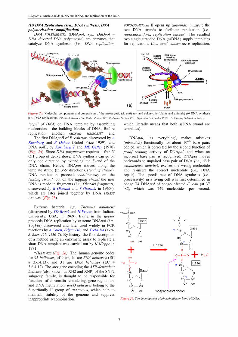
(D) DNA Replication (syn.: DNA synthesis, DNA polymerization / amplification)
DNA POLYMERASEs (DNApol; syn. DdDpol – DNA directed DNA polymerase) are enzymes that catalyze DNA synthesis (i.e., DNA replication,
‘copy’ of DNA) on DNA template by assembling nucleotides - the building blocks of DNA. Before replication, another enzyme HELICASE* and
TOPOISOMERASE II opens up (unwinds, ‘unzips’) the two DNA strands to facilitate replication (i.e., replication fork, replication bubble). The resulted two single stranded DNA (ssDNA) supply templates for replications (i.e., semi conservative replication,
which literally means that both ssDNA strand are templates).
The first DNApolI of E. coli was discovered by A Kornberg and S Ochoa (Nobel Prize 1959); and DNA polII, by Kornberg T and ME Gefter (1970) (Fig. 2a). Since DNA polymerase requires a free 3' OH group of deoxyribose, DNA synthesis can go on only one direction by extending the 3'-end of the DNA chain. Hence, DNApol moves along the template strand (in 3'-5' direction), (leading strand). DNA replication proceeds continuously on the leading strand, but on the lagging strand the new DNA is made in fragments (i.e., Okazaki fragments; discovered by R Okazaki and T Okazaki in 1960s), which are later joined together by DNA LIGASE ENZYME. (Fig. 2b).
DNApol, ‘as everything’, makes mistakes (mismatch) functionally for about 106th base pairs copied, which is corrected by the second function of proof reading activity of DNApol, and when an incorrect base pair is recognized, DNApol moves backwards to unpaired base pair of DNA (i.e., 3'-5' exonuclease activity), excises the wrong nucleotide and re-insert the correct nucleotide (i.e., DNA repair). The speed/ rate of DNA synthesis (i.e., processivity) in a living cell was first determined in phage T4 DNApol of phage-infected E. coli (at 37 °C), which was 749 nucleotides per second.
Extreme bacteria, e.g., Thermus aquaticus
(discovered by TD Brock and H Freeze from Indiana University, USA, in 1969), living in the geyser proceeds DNA replication by extreme DNApol (i.e., TaqPol) discovered and later used widely in PCR reactions by A Chien, Edgar DB, and Trela JM (1976, J. Bact. 127: 1550–7). By history, the first description of a method using an enzymatic assay to replicate a short DNA template was carried out by K Kleppe in 1971.
*HELICASE (Fig. 2a). The, human genome codes for 95 helicases, of them, 64 are RNA helicases (EC # 3.6.4.13), and 31 are DNA helicases (EC # 3.6.4.12). The atrx gene encoding the ATP-dependent helicase (also known as XH2 and XNP) of the SNF2 subgroup family, is thought to be responsible for functions of chromatin remodeling, gene regulation, and DNA methylation. RecQ helicases belong to the Superfamily II group of HELICASES, which help to maintain stability of the genome and suppress inappropriate recombination. Figure 2b. The development of phosphodiester bond of DNA.
(a) (b)
Figure 2a. Molecular components and comparison of the prokaryotic (E. coli) (a), and eukaryotic (plants and animals) (b) DNA synthesis (i.e., DNA replication). SSB - Single-Stranded DNA Binding Protein. RFC - Replication FaCtors. RPA – Replication Proteins A1-5. PCNA – Proliferating Cell Nuclear Antigen

Chapter 1. Nucleic acids (DNA and RNA), and replication of the DNA
8
RNA HELICASES are essential for ribosome biogenesis, pre-mRNA splicing, and translation initiation. RNA helicases are involved in the mediation of antiviral immune response
because they can identify foreign RNAs in vertebrates (about 80% of all viruses are RNA viruses, and they carries their own RNA helicases).
REVERSE TRANSCRIPTASE (RT) enzymes of retroviruses can transcribe (replicate) DNA on RNA template, hence the name RdDpol – RNA directed DNA polymerase (e.g., EC# 2.7.7.49). RdDpol was discovered by H Temin, and independently, by D Baltimore in 1970 (isolated from RNA tumor viruses of R-MLV and RSV), and shared the Nobel Prize in 1975 (Fig. 3).
(E) The RNA RNA (Ribo Nucleic Acid) is a single stranded nucleic
acid (ssRNA) containing ribose instead of deoxyribose (as in DNA) (Fig. 1c), and uracil instead of thymidine (Fig. 1d). The chemical structure of RNA is very similar to that of DNA, with only three differences, such as (1) RNA is a single-stranded molecule with much shorter chain than the DNA. However, RNA can also from parts of double stranded helix by complementary base pairing. (2) The
sugar component of RNA is ribose (which has no hydroxyl group in the 2' position as in ribose), which structure makes RNA less stable than DNA for it is more prone to hydrolysis (see: self splicing of RNA). (3) In RNA the thymine is demethylated (i.e., uracil) (Fig. 1d). Functionally and structurally RNAs are very divers molecules (Table 1a,b,c,d) https://en.wikipedia.org/wiki/RNA.
Table 1a. Types of RNAs involved in protein synthesis
Abbreviation RNA Types Functions Distribution
mRNA messenger RNA Codes for protein
All organisms rRNA ribosomal RNA Structural RNA of ribosomes
tRNA transfer RNA Translation
SRP RNA (7SL RNA) Signal recognition particle RNA Membrane integration
tmRNA Transfer-messenger RNA Rescuing stalled ribosomes Bacteria
Table 1b. Types of RNAs involved in post-transcriptional modification, and DNA replication Abbreviation RNA Types Functions Distribution
snRNA Small nuclear RNA Splicing and other series of functions Eukaryotes and archaea
snoRNA Small nucleolar RNA Nucleotide modification of RNAs Eukaryotes and archaea
SmY SmY RNA mRNA trans-splicing Nematodes
scaRNA Small Cajal body-specific RNA Type of snoRNA; Nucleotide modification of RNAs
gRNA Guide RNA mRNA nucleotide modification Kinetoplastid mitochondria
RNase P Ribonuclease P tRNA maturation All organisms
RNase MRP Ribonuclease MRP rRNA maturation, DNA replication Eukaryotes
yRNA Y RNA RNA processing, DNA replication Animals
TERC Telomerase RNA Component Telomere synthesis Eukaryotes
SL RNA Spliced Leader RNA mRNA trans-splicing, RNA processing
Table 1c. Types of regulatory RNAs
Abbr. RNA Types Functions Distribution
asRNA Antisense RNA Transcriptional attenuation / mRNA degradation / mRNA stabilization / Translation block
All organisms
cis-NAT Cis-natural antisense transcript Gene regulation
Figure 3. The function of Reverse Transcriptase, which turned back the “Central Dogma” (H Temin and D Baltimore, 1970; Nobel Prize, 1975).

Chapter 1. Nucleic acids (DNA and RNA), and replication of the DNA
9
Table 1c. Types of regulatory RNAs
crRNA CRISPR RNA Resistance to parasites, probably by targeting their DNA Bacteria and archaea
lncRNA Long noncoding RNA Regulation of gene transcription, epigenetic regulation Eukaryotes
miRNA MicroRNA Gene regulation Most eukaryotes
piRNA Piwi-interacting RNA Transposon defense Animals
siRNA Small interfering RNA Gene regulation Eukayotes
tasiRNA Trans-acting siRNA Gene regulation Plants
rasiRNA Repeat associated siRNA Type of piRNA; transposon defense Drosophyla
7SK 7SK RNA negatively regulating CDK9/cyclin T complex
Table 1d. Types of parasitic RNAs Type Function Distribution
Retrotransposon Self-propagation Eukaryotes and bacteria
Viral genome Information carrier dsRNA viruses, (+)ssRNA viruses, (-)SSRNA viruses, and RT viruses
Viroid Self-propagation Infected plants
Satellite RNA Self-propagation Infected cells
(F) Artificial DNA; DNA analogs
Phosphorothioates. Changes of phosphodiester bond to phosphorothioate bond makes the DNA resistant to
digestion by nucleases. The technology was already used for Human medicine (VITRAVENE, 2007) (Fig 4a).
Morpholino. Morpholinos are nonionic DNA analogs (available from Gene Tools LLC), with altered backbone linkages. Morpholinos bind to complementary nucleic acid sequences by Watson-Crick base-pairing. The backbone makes morpholinos resistant to digestion by nucleases. Also, because the backbone lacks negative charge, it is thought that morpholinos are less likely to interact nonselectively with cellular proteins. Relatively long
25-base morpholinos are frequently used for antisense gene inhibition (DR Corey and JM Abrams, 2001) (Fig. 4b).
PNA (Protein Nucleic Acids). Backbone of proteins (N-C-C bonds) can also provide backbone for DNA (i.e., PNA – protein nucleic acid), which also can hybridize to natural ssDNA strand (Fig. 4c).
(E) UV absorbance and fluorescence of nucleic acids
Due to the double bonds of DNA nucleotides (Adenine, Thymine, Guanine, Cytosine) DNA absorb UV (ultraviolet) light with a maximum peak at 260 nm (A260). Due to aromatic amino acids (TYR, TRP, PHE) proteins also absorb UV light with a maximum peak at 280 nm (A280) (Fig. 5). Therefore, UV absorbance is used for quantification of nucleic acids (and proteins). Absorbance A = 1.0 corresponds to a concentration of 50 μg/ml dsDNA. Surprisingly, ssDNA absorb more UV light than that of dsDNA (i.e., hypochromic effect). By the application of fluorescence dyes, which can be intercalated into DNA strands, the intensity of fluorescence after UV light excitation can also be used for quantification of DNA, e.g., during melting point analysis. The melting temperature (Tm) is the temperature at which half of the DNA is in double stranded form and half is single stranded. The Tm depends greatly on base composition. Since G≡C bases pair with three Hydrogen bonds, DNA with high G≡C content have a higher Tm than that of DNA with higher A=T content. Figure 5. UV spectrogram of DNA samples
measured by NanoDrop UV-vis spectrophotometer.
Figure 4b. Molecular structure of morpholino DNA (oligonucleotides) compared to natural DNA.
Figure 4c. The structure of PNA:DNA.
Figure 4a. Molecular structure of phosphorothioates (see the change of O to S)

Chapter 2-3. RNA transcription, and Protein translation
10
RNA transcription, and Protein translation
(A) RNA transcription
Eukaryotic transcription is the biochemical process of mRNA synthesis copied from DNA template catalyzed by enzyme RNA polymerase (DdRpol – DNA directed RNA polymerase). This is the first step of gene expression processed in the cell nucleus (Fig. 1).Transcription proceeds through main steps of (1) Sigma factor proteins binding to DdRpol to catalyze its binding to promoter site of the gene (e.g., TATA box); (2) DdRpol creates the transcription bubble, which separates the two strands of the DNA helix, by breaking the hydrogen bonds between complementary DNA nucleotides, similar to the reaction during DNA replication; (3) DdRpol adds matching RNA nucleotides to the complementary nucleotides, and binds the sugar-phosphate backbone of RNA; (4) Hydrogen bonds of the untwisted RNA-DNA helix break, and the newly synthesized pre-mRNA strand releases; (5) The pre-mRNA is further processed in the cell nucleus through polyadenylation, capping, and splicing. After these steps, the edited (mature) mRNA exit to the cytoplasm through the nuclear membrane pore
complexes. The transcribed gene may encode for protein-coding-, and non-coding RNAs (e.g., microRNA), ribosomal RNA (rRNA), transfer RNA (tRNA), and other enzymatic RNA molecules called ribozymes (Fig. 2a,b,c).
The transcribed gene (transcription unit) contains
not only the coding sequence, which will be translated into the protein, but the regulatory sequences, which direct and regulate the protein synthesis. This regulatory sequence before
(upstream) the coding sequence is called the five prime untranslated region (5'UTR), and the sequence after (downstream) the coding sequence is called the three prime untranslated region (3'UTR).
The eukaryotic a gene has some functionally
important gene sequences. The initiation site regulates the gene and helps transcription factors (TF
proteins) to bind for starting the mRNA synthesis. Exons are the coding sequences, which are interrupted by introns that are removed during mRNA
Figure 1. Compartmentalization of the three main genetic processes of (1) DNA replication, (2) RNA transcription, and (3) Protein translation.
Figure 2a. Schematic (left), and detailed (right) molecular steps of ‘mRNA processing’, which includes the transcription of RNA from DNA, capping of the pre-mRNA, excision of introns and splicing of exons, and polyadenilation of the mature mRNA.

Chapter 2-3. RNA transcription, and Protein translation
11
processing (excision of introns, and spicing of exons). Before splicing, the pre-mRNA is capped with a 7-methylquanosine (i.e., cap) at
the 5’ end, and ffter splicing, poly adenylation takes place at the 3’end of mRNA (Fig. 2abc, 3).
The mature mRNA leaves cell nucleus and reaches ribosomes in the cell cytoplasm and the protein synthesis starts. The amino acid sequence of a protein is determined by the base sequence of the CDS of the mRNA. Starting with the start codon (AUG), the sequence of the mRNA is read three bases at a time (one codon). tRNA molecules bring (transfer) amino acids, and amino acids form a peptide bound with each other to form the protein (Fig. 1).
By 1989, it turned out that RNA can be both a coding genetic material (like DNA), and a biological catalyst (like enzymes), and the term ribozyme (ribonucleic acid enzyme) was coined (S Altman and TR Cech, Nobel Prize, 1989). These results also led to the RNA world hypothesis, which postulated that self-replicating and splicing (Fig. 2c) ribonucleic acid (RNA) may had been developed before DNA based life (i.e., ‘RNA World’).
In the function of ribosyme the point is that, as ribose also has an -OH group on the second carbon atom, it can react with phosphate group of the RNA backbone, and RNA breaks (i.e., splicing), without catalysis of any enzyme
Some amino acids (aa) may undergo post-translational modification. Glycosylation (addition of sugar molecules) and phosphorylation (the addition of phosphate molecules) are two common aa modifications. Only methionine and tryptophan have one codon. All the other aa have redundant codes. Some organisms may use some codons preferentially over others (i.e., code preference) (Fig. 4). By history, G Gamow postulated that sets of three bases of DNA must be involved to encode the 21 amino acids (Table 1). Quantitative PCR
The mRNA content can be easily determined by quantitative PCR, which uses poly-T primer that fish out the total mRNA molecules of tissue studied. The former technique of Northern blot is also useful for it.
Figure 3. Schematic (a), and molecular structure (b) of the mature eukaryotic mRNA
Stop
(a)
(b)
Figure 2b. The evolutionarily highly conserved DNA nucleotide sequences of the IEJ (Intron Exon Junction) region (see the % values).
Figure 2c. The molecular mechanism of ribosyme (the self-cutting RNA)
Figure 4. Sample of code preference of the six synonym triplet coding for serine amino acid compared in six different organisms
Code preference
TCAAGTTCG
AGC
TCTTCC
0
10
20
30
40
50
60
E. coli S. cerevisiae D. melanogaster Z. mays H. sapiens
%

Chapter 2-3. RNA transcription, and Protein translation
12
(B)Protein translation During translation, the mRNA sequence, as a
template, is "translated / read" to the amino acid sequence of proteins. Each group of three bases in mRNA constitutes a codon, and each codon specifies a particular amino acid (hence, it is a triplet code) (Table 1). Protein translation takes
place in the cell cytoplasm on the surfaces of ribosomes
(Fig. 1). When the mRNA binds to ribosomes the UTR sequences play crucial role, for 5’UTR, as the leader sequence, carries ribosome-binding site.
Shortly, the translation includes four steps. (a) Initiation: The ribosome assembles around the target mRNA. The first tRNA (Fig. 5) is attached at the start codon. (b) Elongation: The tRNA transfers an amino acid to the tRNA corresponding to the next codon. Aminoacyl tRNA synthetases enzymes catalyze the bonding between specific tRNAs and the amino acids resulting in an
aminoacyl-tRNA. This aminoacyl-tRNA is carried to the ribosome, where mRNA codons are matched
through complementary base pairing to specific tRNA anticodons. (c) Translocation: The ribosome then moves (translocates) to the next codon along the mRNA to continue the process, and creating amino acid chain. (d) Termination: When a stop codon is reached along the mRNA, the ribosome releases the polypeptide.
tRNAs are short (up to 93 nt) molecules. The most abundant is the methionine tRNAmet with partial double stranded forms (dsRNA) which makes with loops. The 3'-terminal group of tRNAs is the special sequence of the amino acid binding site (Fig. 5).
Table 1. The genetic codes (aa-s are indicated with three- and single letter codes) (see degenerated codes, e.g., N for ‘aNy’) Amino acid Codons Compressed Amino acid Codons Compressed
Ala/A GCU, GCC, GCA, GCG GCN Leu/L UUA, UUG, CUU, CUC, CUA, CUG YUR, CUN
Arg/R CGU, CGC, CGA, CGG, AGA, AGG CGN, MGR Lys/K AAA, AAG AAR
Asn/N AAU, AAC AAY Met/M AUG
Asp/D GAU, GAC GAY Phe/F UUU, UUC UUY
Cys/C UGU, UGC UGY Pro/P CCU, CCC, CCA, CCG CCN
Gln/Q CAA, CAG CAR Ser/S UCU, UCC, UCA, UCG, AGU, AGC UCN, AGY
Glu/E GAA, GAG GAR Thr/T ACU, ACC, ACA, ACG I
Gly/G GGU, GGC, GGA, GGG GGN Trp/W UGG
His/H CAU, CAC CAY Tyr/Y UAU, UAC UAY
Ile/I AUU, AUC, AUA AUH Val/V GUU, GUC, GUA, GUG GUN
START AUG STOP UAA, UGA, UAG UAR, URA
The translated proteins, and they amino acid compositions
are responsible for enzymatic function, even in extreme sample of the extremely heat tolerant protein of Taq DNApol (Fig. 6a).
The amino acids of human muscle also shows extreme compositions with high BCAAs (Branched-Chain Amino Acids) content of leucine (Leu), isoleucine (Ile) and valine (Val), which are among the nine essential amino acids for humans, and which account for 35% of the muscle proteins (Fig. 6b) (BCAAs are used frequently for body building) (Appendix).
Figure 6a. Sample for amino acid composition of proteins (e.g., Taq)
Figure 6b. Molecular structures of the three BCAAs (Branched-Chain Amino Acids).
Figure 5. Sample for molecular structure of a tRNA (Met-tRNA; 76 nt)

Chapter 2-3. RNA transcription, and Protein translation
13
Appendix
Chemical structures of the L-amino acids (AAs) (jn total 21). Significant, and unique (Se-Cys; and Pro) AAs are indicated, and also the two smallest AAs (Gly, Ala); the two S-containing AAs (Cys, Met); the AAs with amino (NH2) group at the end of side chain, including Lys, used for Human virus infections; the tree aromatic AAs (Phe, Tyr, Trp) which provide precursors for plant hormone auxins; and the three BCAA (Branched Chained Amino Acids; Leu, Ile, Val), which are the main AAs of the Human muscles proteins (see Mickey Hargitay, 1955, and recently, Arnold Swarzenegger)
MMiicckkeeyy ((MMiikkllóóss)) HHaarrggiittaayy ((HH--UUSSAA))((11992266,, BBuuddaappeesstt –– 22000066,, LLooss AAnnggeelleess)) the First Mr. Universe in the World, 1955. And recently, A. Swarzenegger

Chapter 4. DNA methylation - Epigenetics of gene expression through DNA methylation in Human and plant genomes
14
DNA methylation - Epigenetics of gene expression through DNA methylation in human and plant genomes (A) Summary
Mechanisms of epigenetic control of DNA methylation, covalent histone modifications, and involvement of histone variants in the chromatin structure as a universal phenomenon in Human and plants are reviewed. These factors, together with chromatin remodeling, and non-coding RNAs, play key role in the determination of chromatin structure. These molecular processes interact with the chromatin in order to attain nuclear compartmentalization, as well as to establish euchromatic (gene-rich chromosome regions where nucleosomes are spaced apart and DNA is relatively accessible), and heterohromatic regions (gene-poor genomic regions where densely packed nucleosomes restrict DNA access). Crucial role of DNA methylation was observed in distinct human population phenotypes, physical appearance, social behavior, drug metabolism, sensory perception, response to environmental stimuli, and disease susceptibility. It was also shown that DNA methylation contributes to the biodiversity of natural populations. In plants, recent reports have demonstrated that different environmental stresses alter the DNA methylation pattern, and by this way, the stress response related gene expressions. Here we give a review of the molecular reasons and consequences of DNA methylation as a universal phenomenon in both human and plant genomes. (B) Introduction
Although originally defined in a different context, the term epigenetics is currently used to describe the heritable changes in the DNA structure and its associated histone proteins, which is independent from the DNA sequence information (Feinberg et al., 2010).
Epigenetic control has been shown to be involved in all biological processes, which vary from embryogenesis and cellular differentiation to learning, memory and aging. Epigenetics also play crucial role in the development of various diseases, e.g., cancer, neurodegenerative disorders, ect. Since epigenetics are more versatile in comparison to the genetic code, it is important to understand the mechanisms involved in the formation and upholding of these codes, in order to be able to reverse such errors by means of epigenetic therapy. (C) Chemical background of DNA methylation
DNA methylation is a natural enzymatic process of TGS (Transcriptional Gene Silencing) catalyzed by DNA methyltransferases (MTases), which results in the meiotically heritable methylation pattern i.e., ’genetic imprints’ (Park et al., 1996).
Methylated DNA bases mainly include N6-methyladenine, C5-methylcytosine, and N4-methylcytosine. These methylated bases are natural components of DNA, which distinguish them from a large variety of chemically modified bases that can be formed by enzymatic alkylation or oxidative damage of the DNA. All these enzymes use S-adenosyl-L-methionine (AdoMet) as the donor of an activated methyl group, and modify the DNA in a sequence-specific
manner, usually at palindromic sites, producing methylated DNA and S-adenosyl-L-homocysteine (AdoHcy) (Jeltsch, 2002) (Appendix3).
Biochemically, there are two types of DNA methylations: C-MTases, which form a C-C bond (cytosine-C5 MTases); and N-MTases, which form a C-N bond (adenine-N6 and cytosine-N4 MTases) (Fig. 1a). Different C5-cytosine MTases have been characterized in prokaryotes and eukaryotes. The methylation of C5-cytosine is the most prevalent DNA modification in eukaryotic genomes (Fig. 1b).
Figure 1a. Types of the three plant AdoMet directed (syn., SAM) MTs (C-, N-, and O-MethylTransferases)
(Alzohairy, Kovács L, Gyulai et al., 2016)
In the human genome, most of the CpG (Cytosine-phosphodiesther-Guanine) dinucleotides (CpG islands of the genome) are methylated at the C5 position of cytosine base. About 50 % of the CpG dinucleotides are concentrated in gene gene promoter regions, as well as in the 5’ untranslated regions of genes, and the remaining 50 % is located in the intragenic regions or in the genes (Delcuve et al., 2009).
DNA methylation, which occurs in the CpG islands of gene promoters results in gene silencing, in contrast to the DNA methylation in gene bodies, which might be involved in transcriptional activation (Hellman et al., 2007).
Additionally, methylated CpG islands were also observed in repetitive DNA sequences and transposable elements, which may play role in preventing translocations (Esteller, 2007).
Figure 1b. Molecular pathways of enzymatic methylation, demethylation, and spontaneous deamination of DNA
nucleotides (5-mC - C5-cytosine; MTase - DNA methyltransferase) (see Ch.1.Fig.1d, Ch..12. Fig.3.)

Chapter 4. DNA methylation - Epigenetics of gene expression through DNA methylation in Human and plant genomes
15
(D) Covalent histone modifications DNA is wrapped around octameric protein structures,
which consist of the four core histones H2A, H2B, H3 and H4. The histone octamer has a globular domain, which functions in packaging the DNA, as well as free tail structures, which protrude out from the N-terminal ends of histone proteins. These tail regions of histones are particularly of interest, due to the importance of diverse sets of covalent modifications that they can be subjected to. At least eight different types of such modifications have been described in no less than 60 different modification sites, which include: acetylation of lysines, methylation of lysine and arginines, phosphorylation of serine and threonines, ubiquitylation and sumoylation of lysines, deimination of arginines, ADP ribosylation of glutamic acids, and proline isomerization, which processes are all associated with certain biological roles (Kouzarides, 2007; Wang et al., 2007). Among these modifications, the best studied ones are the acetylations, methylations and phosphorylations.
Covalent histone modifications were shown to get involved in biological processes through two mechanisms. The first mechanism is interfering with nucleosome contacts, which results in disentanglement of the chromatin structure. The second, and better characterized mechanism, involves interacting with and recruiting certain proteins to the nucleosome, or oppositely, detaching certain proteins from the nucleosome. Hence, histone modifications are key players of the determination of the accessibility of the chromatin, and their involvement in cancer pathogenesis.
Methylation of lysine and/or arginine of histon H3 and H4 on specific sites, such as methylation of H3-K4, K36, K79, H3-R17, H3-R 26 and H4-R3, associates with the repression or activation of transcriptions (Huang et al., 2005). Methylation of lysine and arginine of H3 and H4 on other sites results in transcriptional deactivation, such as H3-K9, H3K27 H3K64 H4K20, H1.4K26, H3-R8, H3-R2, and H4K20 (Appendix3).
Figure 1c. Turning the gene transcription "on" and "off" by histone de/acetylations and DNA methylations
Although methylation of specific lysine and arginine has the same effect on transcriptional process, they vary in their functional responses for specific function.
Methylation of H3-K9 and H4-K16, which are considered as an important modifications for gene silencing, has effect on the euchromatic and heterochromatic state of the gene and results in silencing of gene expression (Stewart, et al., 2005).
Methylation of H3K27 participates in the X chromosome inactivation by suppression of HOX genes (Izzo and Schneider, 2011).
H4K20me1 is involved in M phase of the cell cycle and in chromosomal condensation (Huen et al., 2008). These processes show that there is a strong relationship between histone modifications and DNA methylation. Despite the fact that each of these modifications is carried out by similar chemical reactions, each of them have its own molecular pathway in the regulation mechanism of transcription and gene expression (Fig. 1a,c, d,e).
Figure 1d. Methylation (CH3-) of amino acid Lysine of histon proteins catalysed by KPMTs (K - stands for the single letter aa code of Lys) of Lysine-specific protein MethylTrasferases; and Acetylation (CH3-CO-) of Lysine catalyzed by HATs (Histone Acetyl Transferases). Both reactions increase the gene expression levels by neutralizing the strong positive charge of MH3
+ group, which strongly binds to the negatively charged DNA (due to phospahete group of the DNA backbome). In the opposite reactions catalyzed by KPdMTs (Lysine Protein de-MethylTransferases), and HdACs (Histone deACetylases) genes are silenced as RNApol can not catalyze the transcription of mRNAs by opening the histon-DNA complexes (the symbols of the joined –N–C–C– backbones of AAs are indicated by three dots) (Appendix3)
Cont. Figure 1d. Methylation of Agrinine aa of the Histon proteins (MMA – Mono Methyl Arginine; ADMA – Asymmetric DiMethyl Arg., SDMA – Symmetric DMA) (Esse er al., 2012) (Appendix 3)

Chapter 4. DNA methylation - Epigenetics of gene expression through DNA methylation in Human and plant genomes
16
(E) DNA methylation An emerging aspect of epigenetic play crucial role in
the environment - genome interactions (Jaenisch & Bird, 2003; Bonasio et al., 2010). Recently, many genome-wide association studies (GWAS) have established for genetic association with differences among human population phenotypes, physical appearance, social behavior, drug metabolism, sensory perception, response to environmental stimuli, and disease susceptibility (Lachance et al., 2012). Heyn et al. (2013) identified DNA methylation differences that extricate three main human ethnic populations (Caucasian-American, African-American, and Han Chinese-American).
Two-thirds of population-specific CpG sites were associated directly with genetic background, showing the evolutionary genetic context of DNA methylation on the phenotype variation. Changes in CpG region density over the time were found to be responsible for DNA methylation levels observed among species (Feinberg & Irizarry, 2010). DNA methylation pattern showed differences between an African and an European population by studying 27.000 CpG sites (Fraser et al., 2012), suggesting the linkage of population-specific methylation sites variance and the natural human variations (Bell et al., 2012). Thus, DNA methylation is a likely contributor to the different phenotypic characterisrics.
A recent genome-wide epigenetic analysis of honeybees also showed that, despite being genetically identical, the social behavior of the bees is strongly associated with their epigenetic profile, as DNA methylation significantly differ between nurse and forager bees (Herb et al., 2012). (I.) Plant DNA methylation and its environmental stress response-specificity (Appendix1,2)
DNA methylation is not universal, as in the insect fruit fly Drosophyla has not been detected (Hirochika et al., 2000). In Arabidopsis, there are at least three classes of DNA methyltransferases (METases) catalyzing asymmetric DNA methylation. These are METs (maintenance methyltranferase), CMTs (chromomethylase3) and DRMs (de novo domains rearranged DNA methylases) (Finnegan & Kovac, 2000).
In plants, levels of cytosine methylation was found to associate with elevated MET genes expression levels in both the symmetrical CG dinucleotide sites and the asymmetric CHH (H is A or T or C) sites. There are different enzymes, which are essential for the de novo and maintenance of DNA methylations. MET1 (DNA
Methyltransferase1) and CMT1 (Chromomethylase1) are involved in the de novo cytosine methylation, and DRM2 (Domains Rearranged Methylase 2) maintains the symmetric DNA methylation (Aufsatz et al., 2004, Gehring & Henikoff, 2007). These enzymes accomplish a dynamic interchange between methylation and demethylation resulting in different gene expression levels (Law & Jacobsen, 2010).
Plant MET1 genes are similar in sequences and functions to mammalian Dnmt1, however, CMT3 is specific to the plant kingdom containing a chromo domain (Henikoff & Comai, 1998).
CMTs transfer a methyl group (CH3) mainly from S-adenosyl methionine (AdoMet-dependent methyltransferases) mainly to the position of cytosine-C5 (EC 2.1.1.73), and also of cytosine-N4 (E.C. 2.1.1.13) (Pósfai et al., 1989; Cheng & Roberts, 2001), and adenine-N6 by adenine DNA methyltransferases (E.C. 2.1.2.72). The first eukaryotic adenine DNA methyltransferase was isolated from plants (wheat) and were found mainly responsible for the methylation of mitochondrial DNA (Fedoreyeva & Vanyushin, 2002).
The DRM class of METases includes DRM1 (624 aa) and DRM2 (626 aa) (syn. DNA-METase) (both EC 2.1.1.37) and contain catalytic domains which shows sequence similarity to mammalian de novo Dnmt3 (Cao & Jacobsen, 2002). In Arabidopsis, the same enzyme (DRM2) can methylate both cytosine and adenine nucleotides (Vanyushin, 2006).
A process of RdDM (siRNA and micro-RNA directed DNA methylation) also occurs in eukaryotes, which was also observed first in plants (Wassenegger, 2000).
The chromatin regulation through epigenetic modifications is important to the environmental responses. DNA methylation have a crucial impact on the plant response mechanism to biotic and abiotic stresses, which is crucial in the plant adaptation mechanisms. (I.a) DNA methylation contributes to plant abiotic stress response
A number of recent reports have demonstrated that, different environmental stresses alter the DNA methylation status, and the levels of stress response related gene expressions. In pea and tobacco, the correlation between osmotic stress (water deficit) and the DNA methylation status was studied, and hypermethylation pattern was found due to osmotic stress (Labra et al., 2002). DNA methylation deficient mutant MET1-3 was found hypersensitive to salt stress as a massive loss of cytosine methylation (Baek et al., 2011). Of the Glyma11g02400 promoter of soybean (Glycine max), exposed to salt stress, most of the cytosines (from position 518 bp to -272 bp) were demethylated (Song et al., 2012).
Methylated DNA can be demethylated by exogenously applied DNA demethylating agent DHAC (5,6-dihydro-5'-azacytidine hydrochloride) as it was used in poplar (Populus) tree at the concentration of 10-4 M for 7 days, in aseptic tissue culture (Gyulai et al., 2012). In these study, DHAC treatments unregulated the endogenous poplar gene gsh1 by 19.7-fold, and
Figure 1e. Epigenetically important DNA bases of cytosine (C), 5-methylcytosine (mC), and 5-
hydroxymethylcytosine (hmC).

Chapter 4. DNA methylation - Epigenetics of gene expression through DNA methylation in Human and plant genomes
17
reactivated the 35S-gshI transgene (cloned from E. coli) by 8.7-fold increment in the transgenic poplar.
Down regulation of MET1 expression caused hypomethylation in maize roots exposed to cold stress, which affected Ac/Ds transposon region, coupled with demethylation level of ZmMEI1 (Zea mays DNA methyltransferase1) (Steward et al., 2000) Consequently, demethylation of CG sites in the coding region caused an abiotic stress-induced gene activation. DNA methylation to demethylation shift was aslo found in rice grown under drought condition (Wang et al., 2011). All these reports support the hypothesis that plant abiotic stress response mechanisms and adaptivity are crucially regulated by the genomic methylation status.
(I.b) DNA methylation contributes to plant biotic stress response
DNA methylation dynamics, as an ‘immune’ system to defense against biotic stresses have devolved in Plants. Many reports predicted a correlation between biotic stress induced defense-related genes and the levels of DNA methylation. Dowen et al. (2012) found a significant level of DNA hypomethylation of Arabidopsis thaliana exposed to bacterial pathogenes, which influenced elevated defense-related gene expressions. Xa21G R, the R-gene of rice, at demethylated level showed increased resistance to Xanthomonas oryzae pv. Oryzae. Both, hypomethylation level and resistance traits were stable inherited (Akimoto et al., 2007). NtAlix1, a tobacco mosaic virus (TMV) responsive gene, was expressed at elevated level and associated with high levels of DNA methyltransferase transcripts NtMET activity (Wada et al., 2004).
However, mungbean yellow mosaic India virus (MYMIV) resistance of soybean was linked to a higher level of Intergenic Region (IR)-specific DNA methylation (Yadav & Chattopadhyay, 2011). Increased methylation level of IR cytosines coupled with Tomato yellow leaf curl virus (TYLCV) resistance was also reported in transgenic tobacco (Bian et al., 2006).
Useful plant DNA methylation data analysis was developed to identify the actual status of DNA methylation influenced by different experimental conditions (Amin et al., 2014).
All these results revealed that plant genome regulates gene-related pathogen defense mechanisms through the DNA methylation dynamics. Hence, epigenetic modifications through DNA methylation contribute critically to plant biotic stress defense mechanisms. The knowledge of this phenomenon will enhance the possibility of diminution of the diseases and pathogens stimuli on susceptible economic plants. (II.) DNA methylation and human cancer development
Cancer development involves two type of DNA methylation processes of hypermethylation and hypomethylation. DNA hypermethylation was found in the promoter regions of several tumor suppressor genes, which silenced of those genes. This process is important for escaping apoptosis, loss of cell adhesion and angiogenesis, which are common features of tumors (Herceg, 2007).
Figure 2. Implications of DNA methylation on Neurodevelopmental and Neurodegenerative Disorders
In contrast, hypomethylation was observed in almost
all types of cancers, which may act through loss of imprinting, inappropriate cell type expression, genome vulnerability, and the activation of endoparasitic loci (Esteller, 2007). Studies have revealed that promoter hypermethylation of tumor suppressor genes is an early event in hepatocellular carcinogenesis of liver tissues including genes of p16INK4a, DLC1, E-Cadherin and PTEN (Wong et al., 2007)
Figure 3a. Intellectual disability, milder learning problems, autism, and anxiety are associated with CGG repeat expansion and methylation of the 5’UTR region of FMR1 gene resulting in Fragile X syndrome (II) DNA Methylation in Neurodevelopmental and Neurodegenerative Disorders
In mammalian neuronal system, DNA methylation has been implicated in the regulation of neural stem cell fate determination, brain development, cognitive function, neurodevelopmental disorders, and neurodegenerative diseases (Fig. 2).
However, the number of neurodevelopmental disorders that have so far been associated with epigenetic aberrations is very limited (Fuso, 2013)
During the early embryo development, two major stages of epigenetic programming control the fate of embryonic cells. The first stage involves DNA demethylation/remethylation and reprogramming of histone PTMs (PostTranslational Modifications) in somatic cells.
The second stage involves the erasure and reestablishment of parental imprints by DNA methylation during embryo development. DNA methylation of neuron-restrictive silencer element also takes a part in preventing the non-neuronal cells from

Chapter 4. DNA methylation - Epigenetics of gene expression through DNA methylation in Human and plant genomes
18
differentiating into neurons by keeping proneural genes in an inactive state.
A part of chromosome n21 of people with Down syndrome associates with neurological changes and pathological aging due to DNA methylation. (II.b) DNA methylation is associated with repeat instability
Expansion of trinucleotide repeats (TNRs) of a gene, either in the coding or non coding regions (Fig. 3b), during the formation of gametes can cause mutations and gene silencing.
Fragile X syndrome (FRAXA) is an X-chromosome-linked TNR disease (structurally a more then 200 CGG repeat expansion of the 5’UTR of FMR1 gene) (Fig. 3a,b), which affects the early neurodevelopment, and cause intellectual disability, milder learning problems, autism, and anxiety. Heterozygote females are not of high risk due to the presence of a non-expanded FMR1 allele. FMR1 (Fragile X Mental Retardation 1) is associated with aberrant CpG methylation pattern (Fig. 4). Unmethylated CGG repeats produce overexpression of the FMR1 gene, which results in a toxic gain-of-function RNA that gives rise to the phenotypically distinct disorder called fragile X tremor/ataxia syndrome (FXTAS) (Jacquemont et al., 2003) (II.c) DNA methylation and Human neurodegenerative disorders
Human neurodegenerative disorders are difficult to study. These diseases, such as Parkinson's disease (PD), Alzheimer's disease (AD), Huntington’s disease (HD), Frontotemporal lobar degeneration (FTLD), amyotrophic lateral sclerosis (ALS), Rett syndrome, and imprinting disorders, are a group of disorders characterized by a progressive and specific loss of neurons. These diseases trigger neuronal cell death through endogenous suicide
pathways. The neuronal death occurs relatively late in the degenerative process
Figure 3b. Partial structure of the FMR1 (Fragile X mental retardation 1) gene. FMR1 is associated with the number and methylation level of trinucleotide repeat CGG (cytosine-guanine-guanine). Non-FMR1 (regular) people have unmethylated CGG within the 5'-untrunslated (5’-UTR) region of exon 1 with repeat number of 6 to 50. Fragile X carriers show repeat expansion with repeat number of 50 to 200. Fragile X syndrome patients show further repeat expansion over 200 CGG coupled with cytosine methylations of cgg repeats. Here, methylation also extends into the promoter region, which results in a silenced transcription of the FMR1 gene (after Robertson and Wolffe, 2000). (d) Tissue specific DNA methylation patterns
DNA methylation patterns show high tissue specificity. In fact, different methylation levels were observed even across neuroanatomical regions within the brain. DNA methylation also plays a role in long-term memory formation and learning, although these mechanisms are not yet fully understood. Inactivation of DNA methylases was found to block contextual fear formation in rats, and genes such as PP1, RELN and the cell death itself may occur relatively late in the degenerative process of BDNF (brain-derived neurotrophic factor), which undergo changes in methylation during memory formation (Liu et al., 2009).
Alzheimer’s disease (AD) is a neurological disorder and is the most prevalent form of age-related dementia in the modern societies. AD causes synaptic loss in specific brain regions, such as in the cortex and hippocampus (Furuya et al., 2012).
AD is characterized by neurofibrillary tangles, dystrophic neuritis, amyloid precursor protein, amyloid-β deposits coupled with increased activation of apoptosis pathways, impaired energy metabolism, mitochondrial dysfunction; oxidative stress, and DNA damage that lead to synaptic defects resulting in neuronal death (Suzanne, 2008). DNA hypomethylation and specific gene hypermethylation pattern were found among AD case studies. The methylation modification involved in a number of AD related genes such as Tau genes, which encodes proteins that stabilize microtubules. Aggregation of TAU protein in the brain is associated with a class of neurodegenerative diseases known as tauopathies. FK506- (an immunosuppressants) binding protein FKBP51, 51 kDa, forms a mature chaperone complex with Hsp90 (heat shock protein 90) that prevents TAU degradation. The decrease of DNA methylation in FKBP5 increased the expression of FKBP51, and high FKBP51 levels were associated with AD progression.
The conversion of 5-methylcytosine to 5-hydroxymethylcytosine (Fig. 1e) was discovered recently in mammalian DNA.
Figure 4. The epigenetic modifications of the DNA affect the gene functions through histone modifications, nucelosome positioning and DNA methylation
Huntington disease (HD) is a hereditary
neurodegenerative disorder characterized by loss of
Exon 1 ATG
(CGG)6‐50Regular
FMR1 gene (Xq27.3)
Carrier
Fragile X syndrome
CGG repeat metCGG repeat
(CGG)50‐200
(metCGG)200<
5’‐UTR
Epigenetic modifications Histone
modifications
Nucleosome positioning
DNA methylation

Chapter 4. DNA methylation - Epigenetics of gene expression through DNA methylation in Human and plant genomes
19
striatal neurons, and with motor, cognitive and psychiatric features that generally manifest in middle age. The huntingtin (HTT) gene (HTT) are large, spanning 180 kb and consisting of 67 exons (the large protein is 3144 aa, 13.7 Kb) (NCBI # NP_002102.4) (Fig. 5). Epigenetic mechanisms trigger apoptosis of motor neuron in HD through increasing DNA methylation, and upregulation of DNA methyltransferases (DNMT) (Chestnut et al., 2011). HD is caused by a CAG expansion in exon 1 of the huntingtin gene, which results in a poly-Q (polyglutamine) expansion in the huntingtin protein (HTT). There is an inverse correlation between CAG repeat length and age of onset with large expansions (Evans-Galea et al., 2013).
Figure 5. (a) Sample of amino acid (aa, indicated with single letter codes) sequence alignment of a domain (90 aa) (encoded by exon1 of HTT gene) of the HD patient (Homo sapiens) (first row), which shows #53 of the observed 51-57 polyQ; and the regular Huntingtin protein (HTT) with regular number (#23) of polyQ (poly-Glutamine; NCBI # NP_002102.4) (second row). (b) BLAST of the human HTT (NCBI #NP_002102.4) to other mammalian HTTs shows highly conserved regions of HTTs (dot indicates aa identical to the first row, and dash indicates aa absence). The polyP (P - Proline) stretches are also indicated (in blue)
Altered patterns of DNA methylation in cells expressing polyglutamine-expanded HTT (HunTingTin protein) was observed as compared with those of wild-type protein. The affected genes showed substantial overlap with genes that had been found to be deregulated in the presence of mutant HTT, which resulted in a changed gene expression in HD patients, which were partly attributable to DNA methylation (Wood, 2013). AP-1 and SOX2, the transcriptional regulators, are also associated with DNA methylation changes (Ng et al., 2013).
Parkinson disease (PD) is a multifactorial neurodegenerative and age related disorder, where environmental and genetic factors are involved in its etiology. Deregulation of DNA methylation was found to be associated with PD (Masliah et al., 2013). There is a significant decrease of DNA methylation levels in the frontal cortex of PD patients, and associated with the retention of DNMT1 (DNA cytosine-5-methyltransferase 1) in the cytoplasm (Desplats et al., 2011).
Detection of DNA methylation status of CpG islands of gene promoter regions of SNCA (SyNuclein Alpha) and LRRK2 (Leucine-Rich Repeat Kinase 2) showed that SNCA CpG-2 is hypomethylated in PD patients, and the methylation level is decreased in the early-onset PD
patients. The methylation level of SNCA CpG-2 may use as a useful PD biomarker (Tan al., 2014).
The level of sulphur-containing amino acid homocysteine (Hcy), which is produced in S-adenosyl methionine cycle, showed increase in Parkinson’s patients (Doherty, 2013).
Dr. Rett (the disorder was identified by A Rett) syndrome (originally termed as cerebroatrophic hyperammonemia) is caused by mutations in a methyl-CpG binding domain (MBD) protein (MeCP2) that causes loss of cognitive, motor and social skills, ending in severe mental retardation. MeCP2 participates in chromatin remodeling by recruiting key proteins to the methylated DNA sequences, which was characterized by mutations in genes coding for proteins involved in the
regulation of DNA methylation (Fuso, 2013).
Ataxia-telangiectasia (A-T) is characterized as a neurodegeneration caused by protein deficiency of ATM (Ataxia Telangiectasia Mutated), and coupled with the accumulation of histone deacetylase-4 and the increase of
trimethylation of histone H3 on Lsy27 (Li et al., 2013). Frontotemporal lobar degeneration (FTLD) is a
heterogeneous neurodegenerative disorder associated with personality changes and progressive dementia. It is due to methylation in the promoter region of progranulin gene, which may be a novel risk factor for the development of FTLD.
Mitochondrial DNA has an epigenetic regulation in normal and pathological conditions, particularly in neurodegeneration and aging. Changes in the level of 5mC and DNMTs are detected in neuronal mitochondria from patients with amyotrophic lateral sclerosis (ALS), which suggests that the motor neurons can engage epigenetic mechanisms involving DNMT upregulation and increased DNA methylation to drive apoptosis (Iacobazzi et al., 2013).
Since Recent studies have shed some light on the relationship between epigenetic alterations, neurodegenerative diseases (Portela and Esteller, 2010) and neurodevelopmental disorders (Gapp et al., 2014) new tools of genetics and methods of post-mortem brain tissue dissection would help in studying the relationship between epigenetics and cognitive decline (Jones et al., 2013). Reference (for all paper cited): Alzohairy AM, II Amin, MH Elazma, H Elsawy, KY Kamal, AR
Elhamamsy, G Gyulai, HMM Ibrahim, A Bahieldin, and MF Ramadan (2017) Universal Epigenetic Regulation of Gene expression through DNA methylation in Human and plant (in press)

Chapter 4. DNA methylation - Epigenetics of gene expression through DNA methylation in Human and plant genomes
20
500 bp
600 bp
(a) (b) (c) (d)
(e)
500 bp
600 bp
(a) (b) (c) (d)(a) (b) (c) (d)
(e)
Appendix1. M-SAP (Methylation-Sensitive Amplification
Polymorphism) (Reyna-L et al., 1997, MGG 253: 703-710) analysis of five apple varieties (Malus domestica) grown in Hungary of cv. ‘Jonathan’ (a), ‘Jonathan-M41’ (b), ‘Jonathan-Szatmarcseke’ (c), and ‘Jonathan’-Watson’ (d).
Total DNA were isolated in each case, DNAs were digested with EcoRI and methylation sensitive DNA restriction endonuclease HpaII, followed by selective PCR amplification with primer pairs of EcoRI-AGC (GACTGCGTACCAATTCAGC) and HpaII/MspI-TCAA (ATCATGAGTCCTGCTCGGTCAA).
Fragments were separated on silver stained PAGE gel (8%). Mw. sizes are indicated. The missing fragment is indicated with arrow (from experiments of Szőke Antal et al., 2016). Appendix2.
Protein Phylogram (NJ – Neigubor Joining) of plant DNA MTs (cytosine-5)-MethylTransferases) aligned to DNMT3 of Zea mays (915 aa). The ID numbers (NCBI NP_001105167.1), branch length (MEGA7), relative genetic distance (scale 0.1), and the most significant plants are indicated (Gyulai, 2016) Appendix3 (see Fig.1d).
(A) Methylation of aa Arginine of Histons. Molecular structure of Arginine, and the mono- and di-methylarginines are indicated. Type I and II Protein Arginine MethylTransferases catalyze the asymmetric and symmetric dimethylations, respectively.
(B) Methylation of aa Lysine of Histons. Molecular structures of Lysine methylated to mono-, di-, and tri-methyl-lysine (Zhang and Reinberg, 2001, Genes Dev.15:2343-2360).
PRMTs (Protein arginine methyltransferases): The sequences used in the alignment include human PRMT1 (Q99873), human PRMT2 (P55345), human PRMT3 (O60678), mouse PRMT4 (AF117887), and human PRMT5 (AF015913).
HMTs (Histone MethylTransferases). AdoMet (s-ADenOsyl-l-METhionine). AdoHcy (s-ADenOsyl-l-HomoCYsteine).

Chapter 5. Molecular markers, Genotyping, and (Next generation) Nucleic acids Sequencing
21
Molecular markers, Genotyping, and (‘Next generation’) nucleic acids Sequencing Introduction
The molecular markers based on PCR (Polymerase Chain Reaction) have been developed extensively for studies of molecular genetics, population genetics, genotype identifications and protection, monitoring of seed purity and hybrid quality, gene tagging, germplasm evaluation, phylogenetic studies, kinship studies, diagnostics, conservation genetics, forensic genetics, and molecular barcoding.
Molecular markers target different regions of the genomes (DNA) either at loci of coding vs. non-coding, nuclear vs. organelle (cp, and mt), dominant vs. co-dominant, or linked to genes or QTLs (Quantitative Trait Loci). Next to the biochemical (i.e. protein) markers such as IP (Izoenzyme Polymorphism) (Hunter and Merkert, 1957), there have been developed genetic (i.e. DNA) markers, such as RFLP (Restriction Fragment Length Polymorphism; Grodzicker et al., 1974), and the numerous PCR-based (Saiki et al., 1985; Mullis and Faloona, 1987) marker systems (Table 1). These markers are important and feasible tools to compare robust number of individuals, species and
populations. Technically, these markers can be divided into five technical generations (Table 1).
Before application, all of these techniques need primer design (e.g. Primer3) at the first technical step including analyses for hairpin, self and heterodimer formations, and the suitable annealing temperatures (Alzohairy et al., 2015). The primer specificity should also be analyzed by BLAST (Basic Local Alignment Search Tool; Altschul et al., 1997) and MSA (Multiple Sequence Alignments) (Fig. 1) in silico with the software programs of either BioEdit (Sequence Alignment Editor; North Carolina State University, USA) (Hall, 1999), MULTALIN (Combet et al., 2000), CLUSTAL W (Thompson et al., 1994), MEGA4 (Tamura et al., 2007), or FastPCR (Kalendar et al., 2009). Useful servers are also available such as NCBI (National Center for Biotechnology Information), EMBL (European Molecular Biology Laboratory), IDT (Integrated DNA Technologies), GGB (Grape Genome Browser; http://www.genoscope.cns.fr), CGD (Chloroplast Genome Database; http://chloroplast.cbio.psu.edu/index.html), and in-silico PCR (http://insilico.ehu.es/PCR/).
.
(1) Nested-PCR and Nested qRT-PCR. Nested PCR involves two subsequent uniplex PCR reactions, in which the first PCR product (i.e. the nest) is used for the second set of primers, which amplifies a secondary target site within the first PCR product. One of the principal of this method is that if a wrong locus were amplified first by mistake the probability is very low to
amplify it by the second time with the second primer pair. The other advantage is in the case of very low concentration of target sequence (e.g. viral infections). Based on qRT-PCR, nested qRT-PCR was found unique diagnostic tool to detect RNA viruses in the Human genome with the resolution rate of single tumor cell of 106 white blood cells.
(2) Multiplex PCR. Compared to uniplex PCR, which amplifies single nucleic acid sequence of the genome, multiplex PCR (mPCR) is performed with more than one primer pairs in the same reaction mix, which amplify more than one target sequences. Several mPCR assays were suggested by research groups for microbiological quality control of food, water, clinical
samples and pharmaceutical raw materials and products. An alternative PCR strategy can be applied by using gradient thermocyclers, which allow the use of primers of different annealing temperatures (Tann) for simultaneous amplification of different targets in the same run.
Figure 1. Sequence alignments (70 nt) of the MybR2R3 TF gene (transcription factor genes of nuDNA), which play crucial roles in the fruit color development including Vitis (Vitaceae) and Prunus (Rosaceae) species. Sequences were downloaded from the servers of NCBI, and GGB following the sequence alignments by BioEdit. Consensus nucleotides (.), deletions (-), SNPs (letters) and accession numbers (NCBI) are indicated.

Chapter 5. Molecular markers, Genotyping, and (Next generation) Nucleic acids Sequencing
22
Table 1. PCR-based DNA marker methods in sections and alphabetical orders (Alzohairy, Gyulai et al., 2015). References Methods Year Acronym
(1) 1st Generation Markers Saiki et al. (1986) Allele Specific Oligonucleotides 1986 ASO Landegren et al. (1988) Allele Specific Polymerase chain Reaction 1988 AS-PCR Beckmann (1988) Oligonucleotide Polymorphism 1988 OP Saiki et al. (1985) Polymerase Chain Reaction 1985 PCR Orita et al. (1989) Single Stranded Conformational Polymorphism 1989 SSCP Olsen et al. (1989) Sequence Tagged Site 1989 STS Jeffreys et al. (1985) Variable Number Tandem Repeats 1985 VNTR
(2) 2nd Generation Markers Welsh and McClelland (1990) Arbitrarily Primed Polymerase Chain Reaction 1990 AP-PCR Newton et al. (1989) Amplification Refractory Mutation System PCR 1992 ARMS Akopyanz et al. (1992) Cleaved Amplified Polymorphic Sequence 1992 CAPS Telenius (1992) Degenerate Oligonucleotides Primer - PCR 1992 DOP-PCR Weining and Langridge (1991) Intron-Exon Splice Junction PCR 1991 ISJ-PCR Zietkiewicz et al. (1994) Inter Simple Sequence Repeats 1994 ISSR Caetano-Anolles et al. (1993) Multiple Arbitrary Amplicon Profiling 1993 MAAP Williams et al. (1990) Randomly Amplified Polymorphic DNA 1990 RAPD Klein-Lankhorst et al. (1991) RAPD by using two primers 1991 Double-RAPD Hatada et al. (1991) Restriction Landmark Genome Scanning 1991 RLGS Morgante and Vogel (1994) Selective Ampl. MicroSatellite Polymorph. Loci 1994 SAMPL Paran and Michelmore (1993) Sequence Characterized Amplified Region 1993 SCAR Akkaya et al. (1992) Simple Sequence Repeats 1992 SSR Beckmann and Soller (1990) Sequence Tagged Micro Satellite Sites 1990 STMS Ye et al. (1992) Allele specific amplification by tetra-primer PCR 1992 Tetra-PCR
(3) 3rd Generation Markers Vos et al. (1995) Amplified Fragment Length Polymorphism 1995 AFLP Gu et al. (1995) Allele Specific Associated Primers 1995 ASAP Brow (1996) Cleavage Fragment Length Polymorphism 1996 CFLB Bebeli et al. (1997) Directed Ampl. of Mini Satellite DNA-PCR 1997 DAMD-PCR Reyna-Lopez et al. (1997) Methylation-Sensitive Amplified Polymorphism 1997 M-SAP Chang et al. (2001) Inter-MITE Polymorphism 2001 IMP Kalendar et al. (1999) Inter- Retrotransposon Amplified Polymorphism 1999 IRAP Rohde (1996) Inverse Sequence-Tagged Repeats 1996 ISTR Casa et al. (2000) Miniature Inverted-Repeat Transposable Element 2000 MITE Heid et al. (1996) quantitative Real Time PCR 1996 qRT-PCR Flavell et al. (1998) Retrotransposon Based Insertional Polymorphism 1998 RBIP Kalender et al. (1999) Retrotransposon-MicroSatellite Ampl. Polym. 1999 REMAP Ye et al. (2005) Combinations of RAPD-ISSR and RAPD-SSR 2005 R-ISSR Puskás and Bottka (1995) Restricted-PCR 1995 R-PCR Higuchi et al. (1993) Real-Time PCR 1993 RT-PCR Jordan and Humphries (1994) Single Nucleotide Polymorphisms 1994 SNP Li and Quiros (2001) Sequence Related Ampl. Polymorphism 2001 SRAP Waugh et al. (1997) Sequence Specific Ampl. Polymorphism 1997 SSAP Van der Wurff et al. (2000) Three Endonuclease AFLP 2000 TE-AFLP Mansour et al. (2008) Triple RAPD by using three primers, or more 2008 Triple-RAPD
(4) New Generation Markers Jaccoud et al. (2001) Diversity ARrays Technology 2001 DArT Uitdewilligen et al. (2013) Kompetitive Allele Specific PCR 2013 KASP Baurens et al. (2003) Methylation Sensitive Ampl. Polymorphism 2003 MSAP Pellionisz (2008) Recursive Genome Function 2008 RGF Várkonyi-G and Hellens (2010) Small RNA qRT-PCR 2010 sRNA-qRT-PCR
(5) Genome Sequencing (First- and Next Generation Sequencing) Fodor et al. (1991, 2008) DNA and RNA Microarrays / Chip 1991 AFFYMETRIX Sanger et al. (1980) Dideoxynucleotide Sequencing (ABI) 1980 ddNTPs in: Bentley (2006) The first Short Read Sequencer / bridgePCR 2008/2006 ILLUMINA / SOLEXA Pennisi (2010) Proton sequencing (Portable sequencer) / emPCR 2010 Ion Torrent Hayden (2012) Nanopore genome sequencer 2015/1995 NanoPorSeq (?) Ronaghi et al. (1996, 1999) Pyrosequencing (the 1st Next Gen. Seq.) / emPCR 1996 ROCHE454 http://pacbiodevnet.com Single Molecule Real Time seq./ PACBIOSCI 2013/2010 RT-SEQ (SMRT) in: Tang et al. (2009) Seq. by Oligonucl. Ligation and Detection / emPCR 2006 SOLiD/ABI in: Glenn et al. (2011) Single-molecule sequencing with quantum dots 2015 StarLight (?)

Chapter 5. Molecular markers, Genotyping, and (Next generation) Nucleic acids Sequencing
23
(3) ARMS-PCR (Amplification Refractory Mutation System PCR). It is a multiplex type PCR by using tetra primers, which provides a fast SNP (Single Nucleotide Polymorphic) analysis coupled with sequencing or
melting point analysis. Through the combinations of two outer primers and two allele-specific inner primers the genotyping requires regular PCR and fragment separations by electrophoresis.
(4) SSR (Simple Sequence Repeats) PCR.
In all prokaryotes and eukaryotes SSRs (syn.: microsatellites) are found universally with core sequence of SSR with 1 to 6 nucleotides (Gupta et al., 1994). The length polymorphism between individuals occurs due to the change in the number of this core repeats. Dinucleotide core repeats like (CA)n and (GA)n are the most abundant repeats. In humans, (CA)n repeat occurs once in every 30 kb. PCR primer pairs are designed to the sequences of flanking regions of the SSRs, and after the PCR amplification, fragment polymorphism is visualized on agarose or polyacrylamide gels (Fig. 3a,b,c). SSR PCR provides co-dominant and highly reproducible markers.
Microsatellite markers were found very useful for population genetics, variety identification and protection, monitoring of seed purity and hybrid quality, gene tagging, germplasm evaluation, genome mapping and phylogenetic studies (Lavin et al., 2003) with or without bootstrap
analysis (Fig. 4). In the case of hierarchical cluster analysis the Maximum Likelihood (ML) method was suggested to be the most comprehensive method (Hillis et al., 1994).
(5) ALF-SSR.
The SSR analysis can be automated and multiplexing by labeling the primers with fluorescent dye (Fig. 3b). A very sensitive and automated method is ALF-SSR PCR (Automatic Laser
Fluorometer). In this method, one primer of each primer pair is labeled with Cy5 (Phosphoramidite), a cyanine type fluorescent dye, at the 5’-end (Sigma) according to Röder et al. (1998).
The Cy5 labeled ALF-SSR fragments are excited
by helium/neon microlaser at 643 nm, and the emitted fluorescent signal of the Cy5 is detected at 667 nm by ALFexpress II DNA Analyser (Amersham Bioscience, Uppsala, Sweden - AP Budapest, Hungary). The ALF-SSR fluorograms are analyzed by computer program of ALFwin Fragment Analyser Version 1.00 (Pharmacia – Amersham Bioscience, Uppsala, Sweden. AP-Hungary, Budapest) according to Röder et al. (1998), Huang et al. (2002). After sequencing, SSR fragments show a repetitions of the core nucleotide sequence (Fig. 3c).
Figure 3a. Principle of the microsatellite (SSR) based barcoding inthe case of a (CA)n repeat (Alzohairy, Gyulai et al., 2015).
Figure 3b. Schematic flow chart of the ALF-SSR fragment separation by using ALF method (AutomaticLaser Fluorometer; Amersham Bioscience) (a). One strand of the PCR primer pair is labeled by Cy5 fluorescent die (b). The outputs of gel image (c) and the real fluorograms (d) are shown. DNA loading lanes (1-40), electric current (poles + and -), Mw standards (Mw1 and Mw2), DNA fragments, and the data analyzing computer program (ALFwin Fragment Analyser) are indicated (Alzohairy, Gyulai et al., 2015).
Figure 3c. Sample of the fluorogram of an SSR (TC)n repeat (68 to 100 nt) of watermelon (Citrullus lanatus) microsatellite amplified and sequenced by ABI PRISM 3100 (Szabó and Gyulai, 2005)
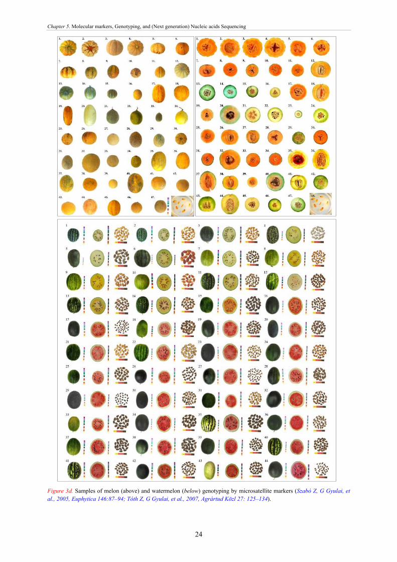
Chapter 5. Molecular markers, Genotyping, and (Next generation) Nucleic acids Sequencing
24
Figure 3d. Samples of melon (above) and watermelon (below) genotyping by microsatellite markers (Szabó Z, G Gyulai, et al., 2005, Euphytica 146:87–94; Tóth Z, G Gyulai, et al., 2007, Agrártud Közl 27: 125–134).

Chapter 5. Molecular markers, Genotyping, and (Next generation) Nucleic acids Sequencing
25
(6) Inter-simple sequence repeats (ISSR). ISSR amplifies target DNA regions located between two
identical microsatellite repeats (SSRs) (Zietkiewicz et al., 1994). ISSR was used extensively for producing molecular markers in several crops and horticultural plants (Lágler et al., 2005) (Fig. 4).
(7) RAPD-ISSR. RAPD-PCR combines RAPD (discussed below) and
ISSR primer pairs in PCR reactions, which are able to reveal new genomic loci that could not be detected with either of the primer alone. Further combinations of the different markers also suggest new possibilities in DNA barcoding. (8) R-PCR (Restricted PCR).
For reduction of nonspecific PCR amplifications, which is caused by mispriming during PCR reactions, besides the standard pair of primers, 3'-dideoxy-terminated competitor oligonucleotides were applied in the R-PCR reactions (Puskás and Bottka, 1995). By this way an enhanced specificity of target site amplification was achieved. The competitor oligonucleotides act by masking the possible sites of nonspecific primer-template interaction, thus excluding undesired PCR extensions. This technique is generally applicable when highly degenerate primers are used. (9) DGGE-RAPD (Denaturing Gradient Gel Electrophoresis RAPD).
The detection of DNA polymorphism in self-pollinating species was found to be difficult. To facilitate, DGGE (Denaturing Gradient Gel Electrophoresis) was used for RAPD analysis. In DGGE gel (12% acryalmide in TAE buffer with denaturant gradient, 10-50%, of 7 M urea and 40% formamide) the two alleles of a locus (if different) run separately. This method greatly improved the detection of reproducible DNA polymorphism among closely related plant species and lines. It was used first to estimate pedigree relationships among plant materials in wheat (Triticum), barley (Hordeum) and oat (Avena) (Dweikat et al., 1993). DDGE-RAPD was also found highly discriminative for the identification of barley (Hordeum) cultivars with different pedigree, and proved that DGGE-RAPD is a superior method for detecting DNA polymorphism when compared to agarose-RAPD, or polyacrylamide-RAPD methods (Fig. 5).
(10) Single-, Double-, and Triple-Primed RAPD. RAPD (Random Amplified Polymorphic DNA) assay
was one of the earliest and widely used PCR PCR by using single primer of arbitrary nucleotide sequence of 10 nt (Williams et al., 1990). The potential of the original RAPD assay was further increased by combining two and three primers (Fig. 6) in the same PCR reaction. This technique was extensively used for barcoding of economically important crops. Figure 6. RAPD PCR. Principles of the Single- (A), Double- (A, B), and Triple- (A, B, and C) primed RAPD (a) with indications of hypothetical band patterns (b). Only a single locus (band) per primers is indicated. Extra bands amplified with double and triple primers are indicated with asterisk (Alzohairy, Gyulai et al., 2008).
Figure 4. ISSR analysis. Samples of ISSR PCR with monomorphic (a) and polymorphic (b) band patterns on agarose gel (0.8 %), which were amplified by primers of FV835 [(AG)8YC] (a), and FV811 [ (GA)8C] (b), in common millet (P. miliaceum) cultivars (1 to 20) compared to an ancient medieval (15th CENT.) sample (indicated as 15.c). Mw – 100 bp DNA ladder. Asterisk indicates a missing ISSR fragment (Lágler, Gyulai et al., 2005).
Figure 5. RAPD. Comparison of fragment patterns of agarose-RAPD (a), (c) and (e); and compared to DGGE-RAPD (b), (d) and (f) generated by Operon RAPD primers of OP-A12 (a) and (b); OP-B09 (c)and (d); and OP-B15 (e) and (f) used for genotyping six barley (A. s.) cultivars (Bahieldin et al., 2006).

Chapter 5. Molecular markers, Genotyping, and (Next generation) Nucleic acids Sequencing
26
(11) Retrotransposon based PCR markers. Retrotransposons (RTs) are major constituents of
most eukaryotic genomes; they are ubiquitous, dispersed throughout the genome, and their
abundance correlates with the host genome sizes, which provides unique possibilities for molecular barcoding (see Chapter 6).
(12) Organelle (Chloroplast and Mitochondria) specific PCR markers.
DNAs of chloroplast (cpDNA) and mitochondria (mtDNA) have been used very frequently in plant systematic and phylogenetic studies (Ali et al., 2014). Both organelle DNAs are circular molecules ranging in size of 120 Kbp to 500 Kbp (Fig. 7), with unique exception of green alga Floydiella terrestris with huge cpDNA of 521.168 bp (NCBI# NC_014346); and Cucumis melo (Alverson et al., 2010) with giant mtDNA (2,900,000 bp).
Size correlations between cpDNA and mtDNA genomes of plants and algae show a shift (Fig. 7) from green algae (Chara vulgaris) with high cpDNA/mtDNA ratio (2.73) through mosses of Physcomitrella patens (1.16) and Marchantia polymorpha (0.65) towards flowering plants of dicots to monocots with exception of Vitis.
The decreasing ratio of cpDNA/mtDNA indicates an enlargening mtDNA during the evolution: Spirodela polyrhiza (0,74); Brassica napus (0,69); Daucus carota (0,55); Helianthus annuus (0,50); Arabidopsis thaliana (0,42); Lotus japonicus (0,40); Vaccinium macrocarpon (0,38); Glycine max (0,38); Vigna radiata (0,38); Huperzia lucidula (0,37); Ricinus communis (0,32); Sorghum bicolor (0,30); Triticum aestivum (0,29); Liriodendron tulipifera (0,29); Oryza sativa Japonica (0,274); Oryza sativa Indica (0,273); Zea mays (0,25); Oryza rufipogon (0,24); Phoenix dactylifera (0,22); and Vitis vinifera (0,21). NCBI data were plotted by XY plot of Microsoft Windows Xcel program (Ali et al., 2015).
There are about 100 functional genes encoded in the chloroplast genomes, which contains, with few exceptions (IRL vs. IRless), two duplicate regions of inverted repeats (IR) in reverse orientation (from 10- to 76 kb). They divide the chloroplast genome into large (LSC) and small single-copy (SSC) regions.
The structural organization of chloroplast genome is highly conserved, i.e., relatively free of large deletions, insertions, transpositions, inversions and SNPs (single nucleotide polymorphism), which make it advantageous for phylogenetic studies. Chloroplast DNA is abundant (generally, 50 chloroplasts are in a plant cells, and a single chloroplast have 50 cpDNA copy, which results 2.500 cpDNA copy per cell) compared nuclear DNA (which is generally 2n).
Organelle DNAs are usually uniparentally inherited (paternally in gymnosperms, and maternally in angiosperms, in general, with some exceptions), which facilitate to determine the maternal parent in hybrids and allopolyploids. Some chloroplast regions like psbA-trnH, and rps16 evolve relatively rapidly. There are a number of noncoding cpDNA regions which are also useful target of study such as the intergenic spacer of atpB-rbcL.
Due to the evolutionary high AT-content of cpDNA and mtDNA of higher plants compared to nuDNA (Fig. 8) lower temperatures are used for PCR reactions (Demesure et al., 1995; Dane et al., 2004).
(13) SNP (Single Nucleotide Polymorphism) analysis
Single nucleotides of DNA (A, T, C, or G) in the genome sequence is altered among individuals of the same species, which together give an individual-specific SNP pattern. SNPs can be determined either by melting pint analysis of qPCR, or by fragment or total genome sequencing (Table 1). SNPs occur approximately once every 100 to 300 bases of the genomes.
Besides that, e.g. the SNaPshot® Multiplex System (ThermoFisher Sci) was developed for the analysis of SNPs based on a primer extension method. Through its multiplexing capability, up to 10 SNPs can be analyzed in a single reaction, regardless of their positions on the chromosome or the amount of separation from neighboring SNP loci. The ability to use unlabeled user-defined primers allows researchers to incorporate SNPs of interest cost-
Figure 7. Size correlations between genomes of cpDNA (i.e., plastom) and mtDNA (i.e., mitom) of algae and higher plants (Gyulai et al., 2015).

Chapter 5. Molecular markers, Genotyping, and (Next generation) Nucleic acids Sequencing
27
effectively. The Multiplex Ready Reaction Mix helps ensure robust, reproducible analyses of multiplexed samples. Researchers can analyze more than 23,000 SNP genotypes per day.
CAPS (Table 1), and ITS markers (Chapter 7) are also frequently used.
(14) Total Genome Sequencing The new generation markers, and
the total genome sequencing (Table 2), such as the ddNTP technology (Sanger et al., 1980), the Chip technologies (Fodor et al., 1991), and the second- and new generation sequencing, and the newest proton- and nanopore sequencing have revolutionized genomics (Table 2). Total nuclear (nuDNA), mitochondrial (mtDNA) and chloroplast DNS (cpDNA) have been sequenced. The results provide basic knowledge for phylogenetisc (Fig. 9, 10; and Appendix 1).
The phylogram of 23S rRNA gene of cpDNA of grapevine (Vitis vinifera) was compared recently (Fig. 9) to the evolutionarily first land plant of ferns Selaginella uncinata (Seun); the ancient higher plant of gymnosperm Pinus thunbergii (Pinth) and Pinus koraiensis (Pinko); evolutionarily the first
angiosperms tree Amborella trichopoda (Amtr) of the basal angyosperm ANITA (Amborella, Nymphaeales, Illiciales, Trimeniaceae and Austrobaileya) group,
Figure 8. Nucleotide compositions of sequences of coding vs. non coding, and nuclear vs. organelle (cp and mt) DNAs. Total genomes (nuDNA, gDNA, cpDNA, and mtDNA) are compared to coding gene sequences (gsh1; psbA and nad1). Accession numbers of NCBI are NC_003070; NC_008402.1; NC_003076.5; X03954; AJ508916; Y09944; AF017983; AF128455; AF128454; NC_010093.1; NC_009963.1; NC_009766.1; NC_001568.1; NC_006050; EF380354; AB237912; DQ383815; AJ400848; AP000423; NC_007886.1; NC001284.2; NC_007982.1; NC_007579.1; NC_008362.1; NC_008360.1; NC_006581.1; NC_008285; NC_007886; NC_001284; and NC_007982 (Gyulai et al., 2015).
Figure 9. Bootstrap (1000 replicates) radial ML phylogram of plant 23S rRNA genes of cpDNA of significant plant species (Gyulai et al., 2015).

Chapter 5. Molecular markers, Genotyping, and (Next generation) Nucleic acids Sequencing
28
which plant (a dwarf tree) by xylotomy still resembles to gymnosperms (with homoxylon trunk tissues), but by flowers do it to angiosperms. Vitis
vinifera (Vivi) and two poplars (Poal - Populus alba, and Poptr - P. trichocarpa) were also included.
Total genome sequencing (Table 2).
(1) Maxam-Gilbert DNA sequencing (1977). A Maxam and W Gilbert DNA sequencing method (1977) is based on chemical synthesis of DNA (i.e. chemical sequencing) by using radioactive labeling at one 5' end of the DNA. Chemical treatment then generates breaks at a small proportion of one or two of the four nucleotide bases in each of four reactions (G, A+G, C, C+T). The fragments in the four reactions are electrophoresed side by side in denaturing acrylamide gels for size separation. To visualize the fragments, the gel is exposed to X-ray film for autoradiography.
(2) Sanger sequencing (Chain-termination DNA sequencing) (1977). The method was developed by F. Sanger and coworkers and soon became the most frequently used method, owing to its reliability. When invented, the chain-termination method used fewer toxic chemicals and lower amounts of radioactivity than the Maxam and Gilbert method. Sanger method was soon automated (by ABI) and was the method used in the first generation of DNA sequencers. Over the period, great advances were made in the technique, such as the usage of
fluorescent labeling, capillary electrophoresis, and general automation. F Sanger is a double Nobel prized scientist (1958, for sequencing the insulin), and (1980) for DNA sequencing.
(3) Shotgun sequencing (Staden, 1979). It is a sequencing method designed for analysis of DNA sequences longer than 1000 base pairs, up to entire chromosomes. This method requires the target DNA to be broken into random fragments. After sequencing individual fragments, the sequences can be reassembled on the basis of their overlapping regions.
(4) Bridge PCR (Illumina). The method is used for in vitro clonal amplification by bridge PCR. Fragments are amplified by primers attached to a solid surface. This method is used in the Illumina Genome Analyzer sequencers. The Helicos Bridge PCR uses a single-molecule methods developed by Stephen Quake's laboratory (and later commercialized by Helicos), by using bright fluorophores and laser excitation to detect base addition events from individual DNA molecules fixed to a surface.
First generation sequencing.
These methods are applied to genome sequencing, genome resequencing, transcriptome profiling (RNA-Seq), DNA-protein interactions (ChIP-sequencing), and epigenome characterization. Resequencing is necessary, because the genome of a single individual of a species will not indicate all of the genome variations among other individuals of the same species.
(5) Massively parallel signature sequencing (MPSS). It was the first of the next-generation sequencing technologies, developed in the 1990s at Lynx Therapeutics, a company founded in 1992 by Sydney Brenner and Sam Eletr. MPSS is a bead-based method that uses an adapter ligation followed by adapter decoding, and reading the sequence in increments of the four nucleotides. Because the technology was so complex, MPSS was only performed in-house by Lynx Therapeutics and no DNA sequencing machines were sold to independent laboratories. Lynx Therapeutics merged with Solexa (later acquired by Illumina) in 2004, leading to the development of sequencing-by-synthesis, a simpler
approach acquired from Manteia Predictive Medicine, which rendered MPSS obsolete. However, the essential properties of the MPSS output were typical of later next-generation data types, including hundreds of thousands of short DNA sequences. In the case of MPSS, these were typically used for sequencing cDNA for measurements of gene expression levels.
(6) Colony sequencing (SOLiD). The method was developed in the laboratory of George M Church at Harvard Univ., and used to sequence a full E. coli genome in 2005. The method combines an in vitro paired-tag library with emulsion PCR, an automated microscope, and ligation-based sequencing chemistry at an accuracy of >99.9999% and a cost approximately 1/9th that of Sanger sequencing. The technology was licensed to Agencourt Biosciences, subsequently spun out into Agencourt Personal Genomics, and eventually incorporated into the Applied Biosystems SOLiD platform. Applied Biosystems was later acquired by Life Technologies, now part of Thermo Fisher Scientific.
Next generation sequencing.
(7) Pyrosequencing (Roche 454). The methodwas developed by 454 Life Sciences, which has since been acquired by Roche Diagnostics. The method amplifies DNA inside water droplets in an oil solution (emulsion PCR), with each droplet containing a single DNA template attached to a single primer-coated bead that then forms a clonal colony. The sequencing machine contains picoliter-
volume wells, each containing a single bead and sequencing enzymes. Pyrosequencing uses luciferase enzyme to generate light for detection of the individual nucleotides added to the nascent DNA. This technology provides intermediate read length and price per base compared to Sanger sequencing.
(8) Illumina HiSeq 2500 (Solexa Inc.) sequencing (1988). Solexa, now part of Illumina, was founded by

Chapter 5. Molecular markers, Genotyping, and (Next generation) Nucleic acids Sequencing
29
S Balasubramanian and D Klenerman, and developed a sequencing method based on reversible dye-terminators technology, and engineered polymerases. The technology was invented in 1997 by P Mayer and L Farinelli, which is based on DNA clusters or DNA colonies, which involves the clonal amplification of DNA on a surface. The cluster technology was co-acquired with Lynx Therapeutics of California. Solexa Ltd. later merged with Lynx to form Solexa Inc. In the cluster technology, DNA molecules and primers are first attached on a slide or
flow cell and amplified with polymerase so that local clonal DNA colonies (later coined DNA clusters) are formed. To determine the sequence, four types of reversible terminator bases (RT-bases) are added and non-incorporated nucleotides are washed away. A camera takes images of the fluorescently labeled nucleotides. Then the dye, along with the terminal 3' blocker, is chemically removed from the DNA, allowing for the next cycle to begin. There is an Illumina MiSeq sequencer also.
(9) SOLid Sequencing. Applied Biosystems' SOLiD technology (now a Life Technologies brand) employs sequencing by ligation. A pool of all possible oligonucleotides of a fixed length is labeled according to the sequenced position. Oligonucleotides are annealed and ligated; the preferential ligation by DNA ligase for matching sequences results in a signal, which is informative of the nucleotide at that position. Before sequencing, the DNA is amplified by emulsion PCR. The resulting beads, each containing single copies of the same DNA molecule, are deposited on a glass slide.
(10) Proton sequencing (Ion Torrent semiconductor sequencing). Ion Torrent Systems Inc. (now owned by Life Technologies) developed a system based on using standard sequencing chemistry, but with a novel, semiconductor based detection system. This method of sequencing is based on the detection of hydrogen ions that are released during the polymerisation of DNA. A microwell containing a template DNA strand to be sequenced is flooded with a single type of nucleotide. If the introduced nucleotide is complementary to the leading template nucleotide it is incorporated into the growing complementary strand. This causes the release of a hydrogen ion that triggers a hypersensitive ion sensor, which indicates that a reaction has occurred.
As the results of the function ligase enzyme during both the natural process of DNA replication and the DNA synthesis during sequencing, pyrophosphate molecule releases which is detected by Pyrosequencing. A H ion (proton) also releases every step of DNA elongation, which proton is detected by Proton sequencing (Fig. 10). New generation sequencing under development (for information only).
(11) DNA nanoball sequencing. The method is a type of high throughput sequencing technology used to determine the entire genomic sequence of an organism. The company Complete Genomics uses this technology to sequence samples submitted by researchers. The method uses rolling circle replication to amplify small fragments of genomic DNA into DNA nanoballs. Unchained sequencing by ligation is then used to determine the nucleotide sequence. The method allows large numbers of DNA nanoballs to be sequenced per run and at low reagent costs compared to other next generation sequencing platforms.
(12) Heliscope single molecule fluorescent sequencing. It is a
method of single-molecule sequencing developed by Helicos Biosciences. It uses DNA fragments with added poly-A tail adapters which are attached to the flow cell surface. The next steps involve extension-based sequencing with cyclic washes of the flow cell with fluorescently labeled nucleotides (one nucleotide type at a time, as with the Sanger method). The reads are performed by the Heliscope sequencer. The reads are short, averaging 35 bp. In 2009 a human genome was sequenced using the Heliscope, however in 2012 the company went bankrupt.
(13) SMRT (Single Molecule Real Time) sequencing (PacBio).
SMRT sequencing is based on the sequencing by synthesis approach. The DNA is synthesized in zero-mode wave-guides (ZMWs) – small well-like containers with the capturing tools located at the bottom of the well. The sequencing is performed with use of unmodified polymerase (attached to the ZMW bottom)
and fluorescently labelled nucleotides flowing freely in the solution. The wells are constructed in a way that only the fluorescence occurring by the bottom of the well is detected. According to Pacific Biosciences (PacBio), the SMRT technology developer, this methodology allows detection of nucleotide modifications (such as cytosine methylation). This happens through the observation of polymerase kinetics. This approach allows reads of 20,000 nucleotides or more, with average read lengths of 5 kilobases. In 2015, Pacific Biosciences announced the launch of a new sequencing instrument called the Sequel System, with 1 million ZMWs compared to 150,000 ZMWs in the PacBio RS II instrument.
(14) Nanopore DNA sequencing (Oxford Nanopore
Technologies, UK). This method is based on the readout of electrical signals occurring at nucleotides passing by alpha-hemolysin pores covalently bound with cyclodextrin. The DNA passing through the nanopore changes its ion current, which depends on the shape, size and length of the DNA molecule. Each type of the nucleotide blocks the ion flow through the pore for a different period of time. Two main areas of nanopore sequencing are in development, the solid state-, and protein based nanopore sequencing. Protein nanopore sequencing utilizes membrane protein complexes Hemolysin and MspA (Mycobacterium Smegmatis Porin A), which show great promise given their ability to distinguish between individual and groups of nucleotides. In contrast, solid-state nanopore sequencing utilizes synthetic materials such as silicon nitride and aluminum
Figure 10. The release of Hydrogenion (i.e., proton) and pyrophosphate molecule during DNA synthesis.

Chapter 5. Molecular markers, Genotyping, and (Next generation) Nucleic acids Sequencing
30
oxide and it is preferred for its superior mechanical ability and thermal and chemical stability. The concept originated from the idea that single stranded DNA or RNA molecules can be electrophoretically driven in a strict linear sequence through a biological pore that can be less than eight nanometers, and can be detected given that the molecules release an ionic current while moving through the pore. The MinION equipment (not yet available, need further development) has a handheld sequencer capable of generating more than 150 megabases of sequencing data in one run.
(15) Tunnelling currents DNA sequencing. Another approach uses measurements of the electrical tunnelling currents across single-stranded DNA as it moves through a channel. Depending on its electronic structure, each base affects the tunnelling current differently, allowing differentiation between different bases. The use of tunnelling currents has the potential to sequence orders of magnitude faster than ionic current methods. (IV.16) Sequencing by hybridization (under development). It would be a non-enzymatic method that uses a DNA microarray. A single pool of DNA whose sequence is to be determined is fluorescently labeled and hybridized to an array containing known sequences. Strong hybridization signals from a given spot on the array identifies its sequence in the DNA being sequenced. This method utilizes the binding characteristics of a library of short single stranded DNA molecules (oligonucleotides, also called DNA probes), to reconstruct a target DNA sequence. Non-specific hybrids are removed by washing and the target DNA is eluted. The benefit of this sequencing type is its ability to capture a large number of targets. (IV.17) MALDI-TOF MS Sequencing. Mass spectrometry, i.e. Matrix-Assisted Laser Desorption Ionization Time-of-Flight Mass Spectrometry (MALDI-TOF MS), has specifically been investigated as an alternative method to gel electrophoresis for visualizing DNA fragments. With this method, DNA fragments generated by chain-termination sequencing reactions are compared by mass rather than by size. The mass of each nucleotide is different from the others and this difference is detectable by mass
spectrometry. Single-nucleotide mutations in a fragment can be more easily detected with MS than by gel electrophoresis alone. MALDI-TOF MS can more easily detect differences between RNA fragments, so researchers may indirectly sequence DNA with MS-based methods by converting it to RNA first. The higher resolution of DNA fragments permitted by MS-based methods is of special interest to researchers in forensic science, as they may wish to find single-nucleotide polymorphisms in human DNA samples to identify individuals. These samples may be highly degraded so forensic researchers often prefer mitochondrial DNA for its higher stability and applications for lineage studies. MS-based sequencing methods have been used to compare the sequences of human mitochondrial DNA from samples in a Federal Bureau of Investigation database and from bones found in mass graves of World War I soldiers. (IV.18) Microfluidic Sanger sequencing. The entire thermocycling amplification of DNA fragments as well as their separation by electrophoresis is done on a single glass wafer (approximately 10 cm in diameter), or use of microchips. Research will still need to be done in order to make this use of technology effective. (IV.19) Transmission electron microscopy DNA sequencing. This approach directly visualizes the sequence of DNA molecules using electron microscopy. (IV.20) RNAP (RNA polymerase) sequencing. In this method RNA polymerase (RNAP) is attached to a polystyrene bead, and one end of DNA to be sequenced is attached to another bead, with both beads being placed in optical traps. RNAP motion during transcription brings the beads in closer and their relative distance changes, which can then be recorded at a single nucleotide resolution. (IV.21) In vitro virus high-throughput sequencing. A method has been developed to analyze full sets of protein interactions using a combination of 454 pyrosequencing and an in vitro virus mRNA display method. Specifically, this method covalently links proteins of interest to the mRNAs encoding them, and then detects the mRNA pieces using reverse transcription PCRs. The mRNA may then be amplified and sequenced. The combined method was titled IVV-HiTSeq and can be performed under cell-free conditions.
Table 2. Comparison of automated sequencing methods.
Method Read length (nt)
Accuracy Reads per run Time per run Cost per 1 million nt
Advantages Disadvantages
1. Chain termination (Sanger Seq) (ABI)
400 - 900 99.9% N/A 20 min. – 3 hours
$ 2400 Long individual reads. Useful.
Expensive and impractical for larger sequencing projects.
2. Pyrosequencing (Roche 454)
700 99.9% 1 million 24 hours $ 10 Long read size. Fast.
Expensive. Homopolymer errors.
3. Sequencing by synthesis (Illumina)
50 - 300 99.9% (Phred30)
up to 6 billion 1 - 11 days, $ 0.15 Potential for high sequence yield
Equipment can be very expensive. Requires high conc. of DNA.
4. Single-molecule real-time sequencing (PacBio)
10,000- 15,000 > 40,000
87% single-read accuracy
50,000 per SMRT cell, or 500–1000 megabases
30 minutes- 4 hours
$ 0.40 Longest read length. Fast. Detects methylations: 4mC, 5mC, 6mA.
Moderate throughput. Equipment can be very expensive.
5. Sequencing by ligation (SOLiD)
50+35 50+50
99.9% 1.2 to 1.4 billion 1 - 2 weeks $ 0.13 Low cost per base. Slower than other methods
6. Proton Seq (Ion Torrent)
up to 400 bp
98% up to 80 million 2 hours $ 1 Less expensive equipment. Fast.
Homopolymer errors.
References (for all paper cited) Alzohairy AM, G Gyulai, H Ohm, Z Szabó, SM Ragheb, M Ajmal Ali, H Elsawy, A Bahieldin (2015) Nuclear and Organelle
Specific PCR Markers. In. Ali MA, G Gyulai, F Al-Hemaid (Eds) Plant DNA barcoding and phylogenetics. LAP Lambert Academic Publ. Germany. Chapter 4. pp. 53-78. ISBN-13: 978-3-659-28095-5.

Chapter 5. Molecular markers, Genotyping, and (Next generation) Nucleic acids Sequencing
31
Pachycladon cheesemanii
Theobro
ma cacao
96
Prunus persica
Prinsepia utilis
100
Fragaria virginiana
100
Castanea mollissima
Quercus rubra
100
99
Ricinus communis
Populus alba
100
95
Francoa sonchifolia
64
Taiwania flousiana
Taiwania cryptomerioides
72
Taxus mairei
91
Cunninghamia lanceolata
Geranium palmatum
100
Monsonia speciosa
97 Silene vulgaris
Spinacia oleracea
10097 Ni
cotina tabacum
Atropa belladonna
100 Solanu
m lyco
persic
um
Solanu
m tube
rosum
100
100
Olea w
oodian
a subs
p wood
iana
100Cath
aranthus
roseus
100 Ipomoea
purpurea
61 Utriculari
a gibba
61Daucus
carota
Ardisia polysticta
Cathaya argyrophylla
Picea morrisonicola
100
Picea abies
100
Pinus thunbergii
98
Pinus massoniana
100
Pinus taeda
100
Pinus korainensis
100
Pinus lambertiana
86
Pinus gerardiana
100
Pinus krempfii
98
Pinus monophylla
100
Pinus nelsonii
100
Pinus contorta
100
Picea sitchensis
100
Cedrus deodara
100
Podocarpus totara
100
Gnetum montanum
Nothoceros aenigmaticus
100
75
Cuscuta obtusiflora
Cuscuta gronovii
100
75
Cuscuta reflexa
Vaccinium macrocarpon
Neottia_nidus-avis
100
Cicer arietinum
Glycine soja
100
Vigna angularis
100Phaseolus vulgaris
100
Cistanche des
erticola
100
Epifagus virginiana
100
Oen
othe
ra g
lazi
ovia
na100
100
Partheniu
m ar
gent
atum
Artemis
ia frigi
da10
0
Cephalotaxus oliveri
Cephalotaxus wilsoniana
100
59
Trifolium subterraneumPh
arus latifolius
Rhynchoryza subulata
Oryza sativa Japonica
Leersia tisserantii
95
100
Lolium perenne
Festuca pratensis
Triticum monococcum
Triticum urartu
100
Hordeum vulgare subsp vulgare
59
Secale cereale
85
Triticum aestivum
100
92
100
Zea mays
Ferrocalamus rimosivaginus
Indocalamus longiauritus
100100
62
70
100
92
60Nandin
a dome
stica
Drimys
grana
densis
Liriod
endron
tulip
ifera 100
Trocho
dendro
n aral
ioides
Tetracen
tron sin
ense 100
Nelumbo nu
cifera
Platanus occ
identalis 98
100
99
100
Nymphea albaCeratophyllu
m demersumAcorus calamus
Piper cenocladum
Ranunculus macranthus
Erodium carvifolium
93
93
Elodea canadensis
Najas flexilis
100
Corallorhiza stiata var vreelandii
Phalaenopsis aphrodite
Oncidium gower ramsey
Cymbidium mannii
10096
100
Smilax china
Xiphidium caeruleum
Alpinia zerumbet
Zingiber spectabile
100
Heliconia collinsiana
Musa acuminata subsp malaccensis
100
100
Typha latifolia
Kingia australis
Dasypogon bromeliifolius
Calectasia narragara100
100
Calamus caryotoides
Chamaedorea seifrizii
Pseudophoenix vinifera
Bismarckia nobilis100100100
82
100
100
100100
100
100
89
68
89
93
92
96
0.05
Appendix 1 Total cpDNA genomes comparisons. ML (Maximum Likelihood) cladogaram of the total cpDNA genomes with 1000x bootstrap values (MEGA4). Monocots (○) show three cpDNA lineages including the individual Acorus. Of them, Triticum species are labeled (●). Gymnosperm trees (green) which show three lineages (also indicated), the (1) Gnetales (▼) – Pinaceae of Coniferales-I. It does indicate the most ancient family of Podocarpaceae (Podocarpus, ●), the Pinaceae species of Pinus, Picea, Abies, Cathaya (▲), and Cedrus. Cathaya (NC_014589) has the smallest cpDNA genome (107.122 bp) of Coniferales. This clad shows the closest similarity to the bryophyte Nothoceros. (2) Taxodiaceae of Coniferales-II: Taiwania, Taxus, and Cunninghamia. (3) The evolutionarily youngest Cepahlotaxaceae (i.e., Cephalotaxus) of Coniferales-III. Water submerged Angiosperm plants (Elodea ◊, and Ceratophyllum, ◊); and parasite plants with reduced cpDNA genomes (Cuscuta and Epifagus, ●) are also labeled. Scale (0.05) shows the relative genetic distance. Accession #s are available at NCBI and CGP. For computing the about 21 million nucleotides, an eight core computer with 24 GB RAM was used (Gyulai, Kerti, Katona M, and Hidvégi, 2015; in: Ali MA, G Gyulai, N Hidvégi, B Kerti, FMA Al Hemaid, AK Pandey, J Lee (2014) Saudi J Biol Sci 21: 204–231)
Secale cereale
Hordeum vulgare subsp vulgare
Triticum urartu
Triticum monococcum
Triticum aestivum
Festuca pratensis
Lolium perenne
Zea mays
Ferrocalamus rimosivaginus
Indocalamus longiauritus
Rhynchoryza subulata
Oryza sativa Japonica
Leersia tisserantii
Pharus latifolius
95100
10059
85100
92100
100100
62
70
Sub-clade of total cpDNA analysis, with indications of the closest relatives of Secale, Hordeum and Triticum, except T. aestivum. See also the Zea clade.

Chapter 6. LTR-Retrotransposon based markers
32
LTR-Retrotransposon based markers (A) Introduction
Retrotransposons (RTs) are major components of most eukaryotic genomes; they are ubiquitous, dispersed throughout the genome, and their abundance correlates with the host genome sizes (Fig. 1a). Copy-and-paste life style of the RTs consists of three molecular steps, which involve transcription of an RNA copy from the genomic RT, followed by reverse transcription to cDNA, and finally a reintegration event into a new locus of the genome. This process leads to new genomic insertions without excision of the original RT (Kalendar and Schulman, 2006).
The target sites of insertions are relatively random and independent for different plant taxa; however, some elements cluster together in ‘repeat seas’ or have a tendency to cluster around the chromosome centromers and telomeres. The structure and copy number of retrotransposon types (i.e. families) are strongly influenced by the evolutionary history of the host genome (Fig. 1b).
Molecular barcoding of RTs play an essential role in all fields of genetics and genomics, and represent a powerful tool for molecular barcoding. To detect RT polymorphisms, marker systems generally based on the amplification of sequences between the ends of the retrotransposon sequences, such as long terminal repeats (LTR) of LTR-retrotransposons (LTR-RTs) and the flanking genomic DNA.
Interspersed repetitive DNA sequences comprise a large fraction of the eukaryotic genomes. They predominantly consist of transposable elements (TEs) with two main families, Retrotransposons (Class I) and DNA transposons (Class II) (McClintock, 1984). Retrotransposons (RTs) are the most abundant class of TEs.
There are two major groups of RTs depending on the presence vs. absence of long terminal repeats (LTRs) the LTR-retrotransposons (LTR-RTs) and non-LTR-retrotransposons. LTR-RTs comprise two main subgroups, copia (with high copy number) and gypsy (with high transposing activity) (Fig. 1c).
8.0 pg
5.0 pg
3.5 pg3.4 pg
0.2 pg0.1 pg0.012
0.0046
77%
60%
45%40%
22%
12%5%
0.3%
0
1
2
3
4
5
6
7
8
E. coli S. cerevisiae C. elegans Drosophila m. Musmusculus
Homo s. Zea mays Ranaesulenta
DN
A (p
g)
0
10
20
30
40
50
60
70
80
90
TE (%
)
Genomes (pg)TEs (%)
Figure 1a. Correlation between levels of transposable elements (TE, %)dispersed in the genome, and the sizes (DNA pg) of host genomes of the species at different stages of evolution (Alzohairy,Gyulai et al., 2013, Plasmid 69:1–15).
Figure 1b. Types, families, molecular structures, and estimated length of transposons (i.e., jumping genes) (Casacuberta and Santiago, 2003). GAG(gag) - Group-specifikus AntiGene. CP - Coat Protein of a type of transit peptide(TP). Ihe three domains of GAG are the matrix (MA), capsid (CA), and the nucleocapsid (NC) proteins, which form the whole capsid protein (CP). EN/ENV -ENVelop protein with two domains of SU (surface) and TM (TransMembrane) proteins (syn. MP - Movement Protein). INT (int) - INTegráz. LARD - Large Retrotraspozon Derivatives. LINE - Long Interspersed Nuclear Elements. LTR -Long Terminal Repeat, which ends up in short (1-5 nt) IR (inverted repeat), i.e., TIR, Terminal Inverted Repeat. MITE - Miniature Inverted-repeat Transposable Elements. pol: mRNA-polymerase comprising domains of ap-pr (aspartic proteáz), rt (reverz transzkriptáz), RH-H Ribonukleáz-H, and rarely INT. PBS - Primer Binding Site (18 bp) for tRNAs. PPT - PoliPurin Tract (with high adenine and guanine content of 7-18 bp), which supply the primer site for the viral +cDNA synthesis. PR - PRoteáz, which is rich in Aspartic Acid aa (AP – aspartic protease). RH - RNAase-H. RT - Reverse Transcriptase (RdDpol). SINE - Short Interspersed Nuclear Elements. solo-LTR -solo-LTR, composed of the two LTRs ‘only’. TRIM - Terminal repeat Retrotransposons In Miniature. TIR - Terminal Inverted Repeat. Transposase – DNA endonuclease with Ligase activity.

Chapter 6. LTR-Retrotransposon based markers
33
Both, copia and gypsy LTR-RTs, carry regulatory sequences of gene promoters such as CAAT box (e.g., CCATT), TATA box (e.g., TGGCTATAAATAG), transcription start (e.g., CCCATGG), polyadenylation signal (e.g., AATAAG), and polyadenylation start (e.g., TAGT) (Ramallo et al., 2008). All these domains are required for replication and integration of RTs. The long internal domain (Gag-Pol Region) of the LTR-RTs encodes the structural proteins of the virus-like particle (which encapsulate the RNA copy of the RT), and the enzymes Reverse Transcriptase and Integrase (Fig. 1b).
The size of LTR-RTs varies from long (e.g., Bare1 copia LTR-RT; 13,271 bp; #NCBI Z17327) to short (e.g., Bare1 copia solo-LTR-RT; 3,130 bp; #NCBI AB014756; and the truncated RLC_Lara copia RT; 735 bp; NCBI #EF067844, # TREP2298). In plants, LTR-RTs are more plentiful and active than non-LTR-RTs (AGI, Arabidopsis Genome Initiative, 2000).
Due to the recombinational processes of chromosome during the meiotic prophase, active retrotransposons tend to lose their activity due to sequence breakage, and recombination resulting in recombinant LTR-RTs, which lost the transposition activity (i.e. non-autonomous), such
as derivatives of LARD (Large Retrotransposon Derivatives), TRIM (Terminal Repeat Retrotransposon in Miniature) and solo-LTR (sequence carrying 5’ and 3’ LTRs only).
Here we review the utility of some main PCR-based molecular barcoding methods of LTR-RTs, including
RBIP (Retrotransposon-Based Insertion Polymorphism), IRAP (Inter Retrotransposon Amplified Polymorphism), IPBS (Inter Primer Binding Sequence), REMAP (Retrotransposon-Microsatellite Amplified Polymorphism), and SSAP (Sequence-Specific Amplified Polymorphism) (Schulman, 2007).
(B) Utilization of retrotransposons as molecular markers Molecular barcoding methods (Schulman, 2007) based
on RTs are based on PCR technology, and detect large portions of the genome (Poczai et al., 2013). Retrotransposon-based markers follow Mendelian inheritance (i.e. dominant vs. recessive) with high levels of genetic variability (Manninen et al., 2000). In the genome, three different orientations of RTs are possible (i.e. head-to-head, tail-to-tail, and head-to-tail), either at a single locus, or inserted next to or within each other (nested RTs). This feature increases the variation available for revealing polymorphism within and among species. If the RT sequence and the adjacent genomic sequences are known, then all types of PCR-based molecular techniques can detect RT polymorphisms.
As the new cDNA copy of RT integrate into a new locus of the genome the old copy persist in the genome across generations, new sequence variations between ancestral and derived RT loci are generated. The presence of a given retrotransposon suggests its orthologue integration, while the absence indicates the plesiomorphic condition prior to integration. The presence vs. absence of RTs can be utilized to construct phylogenetic trees of species due to the distribution of retrotransposons across the organism. This is the reason why RTs have been suggested to provide powerful phylogenetic markers with little if any homoplasy (Schulman, 2007).
(C) Primer design for detection LTR-RTs For PCR amplification, the LTR regions of the LTR-
RTs are chosen to minimize the size of the target DNA to be amplified. A primer facing outward from the 5’-en LTR will necessarily face inward to a 3’ LTR of a neighboring LTR-RT, in the case of direct repeats (head-to-tail position). The long sequences of LTRs may also interfere with the production of amplicons within the size range of standard PCR. The conservative regions of LTR sequences are also used for designing inverted primers for Long-PCR, which can be used for cloning entire RTs. Primers, in
REMAP, one primer is designed from the LTR and another from a nearby simple sequence repeats (microsatellites, syn.: SSRs). RBIP detects both the presence and absence of the LTR-RT insertion using three primers to generate single-locus codominant markers. In SSAP, two primers are designed to produce amplification between RTs and adaptors ligated to a restriction site (usually MseI or PstI). In IPBS, primers are designed to match and amplify the conserved regions of the primer binding sequences (PBS).
LTR-RT genotyping (1) RBIP (Retrotransposon-Based Insertion Polymorphism) (Flavell et al., 1998).
This method detects retrotransposons in the genome using one primer binding to the flanking genomic site at the LTR-RT insertion, and ananother primer binds to the LTR-RT at either sites of 3`- or 5`-end of LTRs (Fig. 1a). Unfortunately, an alternative reaction can also take place between the left and right flanks in the case of empty (RT-unoccupied) site (Fig. 1b). The basic RBIP was developed for studying the PDR1 retrotransposon in Pisum sativum (Flavell et al., 1998). One of the disadvantages of this method is its high costs compared to other methods. RBIP
also allows the dot blot approach used in microarrays (Flavell et al., 1998). RBIP requires information on the sequences of the 5’ and 3’ flanking regions of the LTR-RT insertions. A further limitation of RBIP is due to its large size range compared to standard PCR (about 3-5 Kbp). By using three primers, RBIP can detect both the presence and absence of the TE insertions.
PBS GAG INT RT PPT LTR 3’
Gag-Pol Coding Region
PBS GAG RT RH INT PPT 3’ LTR
Internal Domain
AP
AP
RH 3’ LTR
5’ LTR
5’ LTR
(a)
(b)
PBS GAG INT RT PPT LTR 3’
Gag-Pol Coding Region
PBS GAG RT RH INT PPT 3’ LTR
Internal Domain
AP
AP
RH 3’ LTR
5’ LTR
5’ LTR
(a)
(b)
Figure 1c. Structural differences between Copia (a) and Gypsy (b) type LTR-Retrotransposon families. 5`LTR - 5`-end of long terminal repeat; PBS -primer binding site; GAG - group-specific antigen (syn.: capsid protein gene); AP - aspartic protease gene; INT - integrase gene; RT - reverse transcriptase gene; RH - ribonuclease-H gene; 3`LTR - 3`-end of the long terminal repeat; PPT - polypurine tract (Alzohairy,Gyulaiet al., 2014).
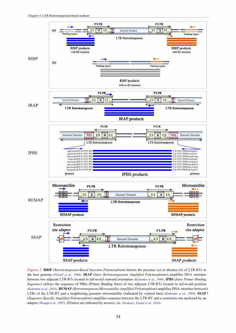
Chapter 6. LTR-Retrotransposon based markers
34
(2) IRAP (Inter-Retrotransposons Amplified Polymorphisms) (Kalendar et al., 1999). This method is based on the fact that LTR-
retrotransposons generally cluster together in ‘repeat seas’ surrounded by ‘genome islands’, and may be nested within each other. By this way, IRAP detects
insertional polymorphisms by amplifying the DNA sequences of two neighboring LTR-RTs (Kalendar et al., 1999) (Fig. 2).
REMAP
RBIP
IRAP
IPBS
SSAP
Flanking regionU3 R U5 Internal Domain U3 R U5
RBIP productswith RE insertion
LTR RetrotransposonFlanking region
Flanking regionFlanking region
RBIP productswith no RE insertion
(b)
(a)
RBIP products with RE insertion
CATG CATG
5’LTR 3’LTR
PBS
Flanking regionU3 R U5 Internal Domain U3 R U5
RBIP productswith RE insertion
LTR RetrotransposonFlanking region
Flanking regionFlanking region
RBIP productswith no RE insertion
(b)
(a)
RBIP products with RE insertion
CATG CATG
5’LTR 3’LTR
PBS
PBS
U3 R U5 Internal Domain U3 R U5
REMAP products
Microsatellite
LTR Retrotransposon
CA
Microsatellite
TG
REMAP products
CA TG
5’LTR 3’LTR
PBSU3 R U5 Internal Domain U3 R U5
REMAP products
Microsatellite
LTR Retrotransposon
CA
Microsatellite
TG
REMAP products
CA TG
5’LTR 3’LTR
PBSU3 R U5 Internal Domain U3 R U5
REMAP products
Microsatellite
LTR Retrotransposon
CA
Microsatellite
TG
REMAP products
CA TG
5’LTR 3’LTR
PBS
PBS
U3 R U5 Internal Domain U3 R U5
SSAP products SSAP products
Restriction site adaptor
Restriction site adaptor
LTR RetrotransposonCATG CATG
5’LTR 3’LTR
PBSU3 R U5 Internal Domain U3 R U5
SSAP products SSAP products
Restriction site adaptor
Restriction site adaptor
LTR RetrotransposonCATG CATG
5’LTR 3’LTR
PBS
PBS
Internal DomainInternal Domain U5 R
IRAP products
LTR Retrotransposon
U3 R U5
LTR Retrotransposon
AC GTU3 TG CA
5’LTR5’LTR
PBS
PBS Internal DomainInternal Domain U5 R
IRAP products
LTR Retrotransposon
U3 R U5
LTR Retrotransposon
AC GTU3 TG CA
5’LTR5’LTR
PBS
PBS Internal DomainInternal Domain U5 R
IRAP products
LTR Retrotransposon
U3 R U5
LTR Retrotransposon
AC GTU3 TG CA
5’LTR5’LTR
PBS
PBS
PBS
PBS
IPBS products
LTR Retrotransposon LTR Retrotransposon
Internal DomainU5RU3Internal Domain U5 R U3
5’LTR
PBS PBS
CA-NNN-TGGtatcagagcctCA-NNN-TGGttccattgccaCA-NNN-TGGtatcggcaaggCA-NNN-TGGcatcgtgagctCA-NNN-TGGcatcatgagccCA-NNN-TGGcgccgttgccaCA-NNN-TGGcgactccgctgCA-NNN-TGGtatcagagcat
aggctctgataCCA-NNN-TGgggctctgataCCA-NNN-TGtggcaatggaaCCA-NNN-TGccttgccgataCCA-NNN-TGagctcacgatgCCA-NNN-TGggctcatgatgCCA-NNN-TG
tggcaacggcgCCA-NNN-TGcagcggagtcgCCA-NNN-TG
CAGTAC TG
primers primers
5’LTR
Figures 2. RBIP (Retrotransposon-Based Insertion Polymorphism) detects the presence (a) or absence (b) of LTR-RTs inthe host genome (Flavell et al., 1998). IRAP (Inter Retrotransposons Amplified Polymorphisms) amplifies DNA stretches between two adjacent LTR-RTs located in tail-to-tail outward orientation (Kalendar et al., 1999). IPBS (Inter Primer Binding Sequence) utilizes the sequence of PBSs (Primer Binding Sites) of two adjacent LTR-RTs located in tail-to-tail position (Kalendar et al., 2010). REMAP (Retrotransposon-Microsatellite Amplified Polymorphism) amplifies DNA stretches between LTRs of the LTR-RT and a neighboring genomic microsatellite (indicated by vertical bars) (Kalendar et al., 1999). SSAP (Sequence-Specific Amplified Polymorphism) amplifies sequence between the LTR-RT and a restriction site anchored by an adaptor (Waugh et al., 1997). (Primers are indicated by arrows). (In: Alzohairy, Gyulai et al., 2014)

Chapter 6. LTR-Retrotransposon based markers
35
(2) IRAP (Inter Retrotransposons Amplified Polymorphisms) amplifies DNA stretches between two adjacent LTR-RTs located in tail-to-tail outward orientation (Kalendar et al., 1999).
IRAP does not require restriction enzyme digestion or ligation. Different retrotransposon insertions increase the number of sites amplified and sizes of inter-RT fragments, which can be used as marker to detect genotype polymorphism. The primers should be pointing outwards from the LTRs of LTR-RTs to amplify the region between two RTs (Kalendar et al., 2011). The two primers could be designed to either the same or different RT families.
IRAP can be also carried out with a single primer, which matches either the 5’ or 3’ end of the LTRs but pointing outwards from the LTR itself. IRAP may produce too many fragments to give good resolution on gels, or no products because target amplification sites are too far apart to generate amplicons. Yet, IRAP overcomes some of the drawbacks of other techniques, such in the case of SSAP, where either radioactive or fluorescent labeled primers are needed. The method was used widely for BARE-1 LTR-RT (Hordeum vulgare), and for genotyping Oryza sativa, Musa, Brassica, Spartina, Triticum and Solanum species.
(3) IPBS (Inter Primer Binding Sequence) (Kalendar et al., 2010) The method is frequently used for displaying
retrotransposon polymorphisms (Fig. 2). The need for sequence information is a prerequisite to design LTR-RT-based molecular barcodes. IPBS tends to overcome this problem as the primer binding sequence (PBS) of the LTR region is part of the internal domain of retrotransposons (Fig. 1), which is highly conserved region for duplexing with tRNAs during the reverse transcription of the life cycle of retrotransposons. PCR amplification occurs between two nested PBSs of two neighboring LTR-RTs (Fig. 2). While the process of reverse transcription is conserved among all retroviruses, the specific tRNA capture varies for different retroviruses and retrotransposons. Thus, the IPBS amplification
method can be useful for all retroviruses that contain conservative PBS sites for tRNAiMet, tRNALys, tRNAPro, tRNATrp, tRNAAsn, tRNASer, tRNAArg, tRNAPhe, tRNALeu or tRNAGln (Kalendar et al., 2010). As plant LTR-RTs are frequently nested, mixed, inverted or truncated in the geneome, LTR-RTs can be easily amplified using conservative IPBS primers. IPBS sequences can also be used for detecting other retrotransposons when the retrotransposon density is high within the genome. Retrotransposon movements and recombinations can also be monitored because new inserts or recombinations will be polymorphic, which will appear only in plant lines in which the insertions or recombinations took place.
(4) REMAP (Retrotransposon-Microsatellite Amplified Polymorphism) (Kalendar et al., 1999) REMAP combines one primer binding to LTRs of
LTR-RTs, and the other primer binding to neighbouring (if so) locus-specific simple sequence repeats (SSRs) of the genome. This technique is applicable only when SSR locates near the retrotransposons (Fig. 2). Amplification between retrotransposon and a nearby SSR requires neither
digestion with restriction enzymes, nor adaptor ligation to generate the marker bands. This protocol can be completed in 1-2 days, and has been used to scale diversity, similarity and cladistic relationships in many genotypes of Oryza sativa, rice pathogens (Magnaporthe grisea), Spartina sp. and Avena sativa.
(5) SSAP (Sequence-Specific Amplified Polymorphism) (Waugh et al., 1997) The method was one of the first retrotransposon-
based barcoding technology based on the technical steps used first in AFLP (Amplified Fragment Length Polymorphism) (Vos et al., 1995) (Fig. 2). SSAP uses one primer matching the end of an LTR (e.g., 3’ end) and the other primer matches to a restriction site (usually MseI or PstI) adaptor as in AFLP. Primer pairs (labeled either 32P- or fluorescently) contains two or three selective nucleotides. Non-selective primer pair can also be useful when restriction enzymes have a long recognition site sequence, or when the copy number of the LTR-RTs is low.
SSAP primers are often designed to the LTR region, but could also match to an internal sequence of the RTs, like the polypurine tract (PPT), which is located to the internal part the 3'-LTR (Ellis et al., 1998). The number of selected bases may be increased in the case of high-copy-number RT families. The use of single or double enzyme digestions (or infrequently cutting enzymes) allow the survey of all insertion sites for a given RT, which method can be considered as a variant of anchored PCR. Primers that give highly polymorphic, clear, and reproducible SSAP banding patterns are candidate primers for subsequent work.
References (for all paper cited) Alzohairy AM, G Gyulai, MF Ramadan, S Edris, JSM Sabir, RK Jansen, HF Eissa, A Bahieldin (2014) Retrotransposon-
based molecular markers for assessment of genomic diversity. Func Plant Biol 41(8): 781-789. Alzohairy AM, G Gyulai, RK Jansen, A Bahieldin (2013) Transposable elements domesticated and neofunctionalized by
eukaryotic genomes. Plasmid 69:1–15. Kalendar R, AH Schulman (2006) IRAP and REMAP for retrotransposon-based genotyping and fingerprinting. Nature
Protocols 1: 2478-2484. Schulman AH (2007) Molecular markers to assess genetic diversity. Euphytica 158: 313-321.

Chapter 6. LTR-Retrotransposon based markers
36
Appendix – Samples for the transpositions (‘jumping’) of RetroTransposons, which resulted in several very important achievements for the Agriculture. (A) The wild tomato (Solanum pennellii) (a), growing in South America (with small leaves and small green fruits), is the ancestor of the cultivated tomato (S. lycopersicum) (b), in which an LTR-RetroTransposon ‘Rider’ got activated, and ‘jumped further in the genome’ into ‘IQD12’ locus, and, as it’s resulted, a new from of oval tomato fruits developed (Lisch, 2013; Lookhart, 2013; Gyulai et al., 2017)
(D) DNA sequence identificication of a transposition (‘jumping’) of ‘Cila-1’ (298 nt) TRIM type Retrotranszpozon (underlined) into a Seed Nucellus-Specific Protein (WM403) gene (AF008925) in watermelon (Citrullus_lanatus) (2.726 nt). NCBI# EU009625, Kalendar R, Gyulai G, Tóth Z, Schulman AH (2007) Citrullus lanatus var. lanatus transposon ’Cila-1’, partial sequence. gi|152926315|gb|EU009625.1|[152926315]
1GGATCTTTTTAAGTGTTGGGGCTGGTTTTTATTTTGTTTACGAGTTTCAAAATGTTACCTAATTTAGTATTTCAGTTTCAAAATATTACAATTTTACTATTTAAATTTGAATTTTGTTTTAATATGGTCACTAGGTTTCAACGTTTTATATTTTTAACCTTAATTTTTCATTAAATACTCATCTTCAATCGTTGACGTTAATGTCTATTAATTAATTAAAATTAATTATAAAGTGAGATTTCAAAAGTGATGAAAATCTGTGAAACTTAATTAATTATAGTTTTTTTAATTAATTTAAATTTATTAACATACATTAACATTGAAAATGAAAAAATGAATATTTAGTAAAAAATCGAGGTTAAATGTGTAAATATTGAAACTTGGGGACCAAATTAAAATAAAGCTCAAATGTCAATTCATAACAAAGTTCAAATGAATTTCGTTGTTTGTTATGGTAGGAAAGAGAATAACTTTAAAATACGAAATGATTTCAAATCCTGTTTTTACTTTAAAAAAACCTTCCCAACCAAAATGCTCGGATTTTGCAGAATTTCATAGGATTTAAAAATAAATTACCTAGTCGACCTTGTCATATTCTAATTTTCAATTAACAGTAAATTTTTAACTTTTTTTTTTCTCTTTTTCTGTTAACATCCAAACACAATTTTAAATACATTCATTCAAATCTTTCTCGTTCCAAATAAAATAATTAATTTTAAATCATTTTTTAAATTTCAAATTACAAAATTTAAAATCATTTGTTCAAATTTGTTAAATCTATATTTAGGGTAAAAATTCTAAAAGTTACCGAAAGTTGAGCAAACCATTTTGTTGTCTCCTTTCTTATATTAGTCCACCTTTTTGTTTGAAAGACATTTATGCAATTCACGAAATAATTAAATTAGAAATCCAACTAAGATCTACGTTGATGCAATTTTGAACTTACCTTGTTCGGGTCCACCACATTGTATTATTAAAAAACAAATTAAGAACATCTTGGTATATGAACAATTCGAGTACTCACTTCAAGATGAGATACAACAATTACCTATAAGTTATACTAATTTAAAAAGTGGTCCCAATTCATAACTTTGTTTGTTGTTTAATTTCCGTAATCATAATGAATTGTAGGACCCGCTTGTAAATCTGTAATCAAAACGCGTAATTTGATTGAAGAACGAAGGATGTTCAATCTAATTGTAGTTGAAAATTGTGTGAGATCCACTACATTTACCGTTAGTGTTATAGATATTGTTGCTATAACGGTACGAATGTTATGAATCTGTCACATTTATTTTTTACGTTTATTATTACCATTCGGGTTAAACAGTAACGGTGACGATAACGATAATAATAAAATGTGACAAATTCATAATTTTAAGTAAACGTGATCAAAAGTAATCCAATTACA<TGTTGGAATGCCTTGAATCATAACCTAATTAAAATTGGTATCTTATATATTTAATTATTTAATTTTTTTCCTTCTCCACTTAGGGTTTAAAAAGTGCACTATATAAACTCTTTAATTCTATAGACTTTATTCATTTTGTGGTATTATATAATTTTATAACATTCTCTCTAATAAAATTGTTATCCCTCTATCTCGTGGACGTAACTAACACATTGTTAGTGCACAACGTAAATTTGTGTGTCGATCTTTATTTCTATTTTTTACGTTATTTTGTATTATTTAATTGTCGATTTCATAAC>ATTATATTG...CTCTCG2726
Domestication
(a) (b)
1 cm
1 cm
1 cm 1 cm
(c)
(B) The activity of (1) LTR-RetroTransposon ‘Rider’and a further partial excision (‘jumping further’ in the DNA out from gene ‘Ruby’) resulted in a new orange (Citrus x sinensis) flesh colors of ‘red/bood oranges’of cv. ‘Navalia’, ‘Tarocco’ and ‘Maro(I)’ (Lisch, 2013; Lookhart, 2013; Gyulai et al., 2017)
(C) The activity of of the ’Gret1’ LTR-RT has developed several new grape colors of Vitis vinifera by ‘just jumping’ (about 6.000 years ago) into the anthocyaine-related gene Vvmby1A (which is related with the black grape color - notice; all wild, and ancient grapes have black color only), and ‘had braked’ it, so new grape colors had developed (Kobayashi et al., 2004, Science 304:98; Lisch, 2013, Nature Reviews Genetics 14: 49–61; Gyulai et al., 2017).

Chapter 7. Plant molecular systematics
37
Plant molecular systematics (A) Introduction – Plant Systematics
Systemetics/Taxonomy of plant/animal morphology (i.e. Linnaean systematics) (Table 1, 2) are based on morphological characterization of the specimen, and uses binomial names, which was introduced first by Gaspar Bauhin in his book of Pinax Theatri Botanici (1623). Linnaeus (1753) also based his classification on morphological characters, e.g., for birds, the shape of the bill; and for plants, the structure of flowers, which are the evolutionarily most conserved plant organ including the stamens, pistils, sepals and petals (Linnaeus, C: Sytema nature; and Systema plantarum; describing about 8000 species). JB de Lamarck (1744–1829) (e.g., heritability of acquired characteristic); and later A Wallace and Ch. Darwin (1858, 1859) gave a theory of evolution (e.g., in: On the origin of species by means of natural selection), which was also based on morphological traits which are changing by selection
and adaptation. Darwin also introduced the principle of common descent into the classification.
Recently, molecular systematics provided several genetic tools for the identification, classification and description of (new) species. The rapid development in molecular technologies has resulted in three main fields of techniques of the isoenzyme (IP, Izoenzyme Polymorphism; Hunter and Merkert, 1957), RFLP (Botstein et al., 1980), and PCR-based (Mullis and Faloona, 1987) methods. For systematics, PCR based methods and whole genome sequencings were found to have distinctive resolutions. Some of the first PCR-based technologies of RAPD (Williams et al., 1990), SSR (Gupta et al., 1994), ISSR (Zietkiewicz et al., 1994), and ISJ-PCR (Weining and Langridge, 1991) were followed by numerous new approaches (see Chapter 5).
Table 1. Plant systematics based on morphology – From the Antiquity to the modern periods
- Before Linnaeus THEOPHRASTUS (BC 350 – BC 287): Historia Plantarum. PLINIUS, Gaius Secundus (AD 23 – AD 79): Historia
Naturalis. DIOSCORIDES, Pedanius (about AD 70): De Materia
Medica. AL-AWWAM Ibn (1158) Libro de agricultura. Madrid FUCHS, L (1542): De historia stirpium. Basel. CESALPINO, Andrea (1583). De plantis libri XVI. BAUHIN, Caspar (1596): Phytopinaxí. and Pinax theatri
botanici (1623). CLUSIUS, Carolus (1526–1609): Histoire des plante
(1557). Fungorum in Pannonis observatorium brevis historia (1601).
BENTHAM G and JD HOOKER (1863) Genera Plantarum. RAY, JOHN (1686): Historia Plantarum. - After Linnaeus LINNAEUS, Carolus (1707–1778): Species Plantarum
(1753). ADANSON, Michel (1763): Familles des plantes. DE JUSSIEU, ANTOINE LAURENT (1789): Genera
Plantarum, secundum ordines naturales disposita juxta methodum in Horto Regio Parisiensi exaratam.
DE CANDOLLE, AP, et al. (1824–1873): Prodromus systemati naturalis regni vegetabilis sive enumeratio contracta ordinum, generum specierumque plantarum huc usque cognitarum, juxta methodi naturalis normas digesta.
LINDLEY, John (1846): The Vegetable Kingdom. DARWIN Ch. and A. WALLACE (1858). Ch. DARWIN
(1859): Origin of Species.
ENGLER A. (1844–1930) and K.A.E. PRANTL (1849–1893): Die Naturlichen Pflanzenfamilien (1887–1915).
BESSEY, E. Charles (1845–1915): Synopsis of Plant Phyla (1907).
SOÓ, Rezső: Fejlődéstörténeti növényrendszertan – Evolutionary plant systematic. Budapest (1947, 1953).
CRONQUIST, A (1919–1992) The Evolution and Classification of Flowering Plants (1957, 1968) (2nd edition, 1988). and An Integrated System of Classification of Flowering Plants (1981).
TAKHTAJAN, A. (1910–2009) Flowering plants: origin and dispersal (1954, 1969).
THORNE, R.F. (1920–1915) A phylogenetic classification of the Angiospermae (1976).
BORHIDI, Attila (1995) A zárvatermők fejlődéstörténeti rendszertana – Evolutionary systematic of Angiosperms. Budapest (1932–).
PODANI, János (2003, 2007) A szárazföldi növények evolúciója és rendszertana – Evolution and systematic dry land plants. Budapest (1952–).
APG III system (Angiosperm Phylogeny Group III system) (2009).
Some important further references: Halley (1912), Bessey (1915), Troll (1944), Busch (1944), Grossheim (1946), Gundersen (1950), Pulle (1952), Hutchinson (1959), Meeuse (1961) and Melville (1962).
In Hungary, there is a long list of famous
botanists working in plant systematics, floristics, lichenology,
mycology, palinology, pomology, physiology, and dendrology of Hungary from the Middle Ages (Table 2).
Chapter 8. Plant molecular systematics
38
Table 2. Plant systematics in Hungary
16th CENT. MÉLIUSZ JUHÁSZ, Péter (1532–1572) BEYTHE, István (1532–1612) 17th CENT. LIPPAI, JÁNOS (1606–1666) 18th CENT. BRASSAI, Sámuel (1797–1897) CSAPÓ, József (1734–1799) DIÓSZEGI, Sámuel (1760–1813) HABERLE, Károly (1764–1832) KITAIBEL, Pál (1757–1817) SADLER, József (1791–1849) SCOPOLI, J Antal (1723–1788) WALDSTEIN-W., F. Ádám (1759–1823) 19th CENT. AMBRÓZY, István (1869–1933) ANDREÁNSZKY, Gábor (1895–1967) BAROSS, László (1865–1938) BERNÁTSKY, Jenő (1873–1944) BORBÁS, Vincze von (1844–1905) BUDAI, József (1851–1939) CHOLNOKY, László (1899–1967) CSAPODY, Vera (1890–1985) CSEREY, Adolf (1851–1918) CSERHÁTI, Sándor (1852–1909) DEGEN, Árpád (1866–1934) DEININGER, Imre (1844–1918) DOBY, Géza (1877–1968) ENDLICHER, L István (1804–1849) ENTZ, Ferenc (1805–1877) FEHÉR, Dániel (1890–1955) FILARSZKY, Nándor (1858–1941) FLEISCHMANN, Rudolf (1879–1950) GOMBOCZ, Endre (1882–1945) GRABNER, Emil (1878–1955) GREGUSS, Pál (1889–1984) GYÖRFFY, István (1880–1958) HAYNALD, Lajos (1816–1891) HAZSLINSZKY, Á Frigyes (1818–1896) HERMAN, Ottó (1835 – 1914) HOLLÓS, László (1859–1940) ISTVÁNFFI, Gyula (1860–1930) JANKA, Viktor (1837–1890) JÁVORKA, Sándor (1883–1961) JURÁNYI, Lajos (1837–1897) KABAY, János (1896–1936) KUBACSKA, András (1871–1942) LEGÁNY, Ödön (1876–1944) MÁGÓCSY-DIETZ, Sándor (1855–1945) MAGYAR, Gyula (1884–1945) MOESZ, Gusztáv (1873–1946) MOKRY, Sámuel (1832–1909) NATTER-NÁD, Miksa (1893–1982) PAÁL, Árpád (1889–1943) PÉNZES, Antal (1895–1984) RAPAICS, Rajmund (1885–1954) SIMONKAI, Lajos (1851–1910) SZABÓ, Zoltán (1882–1944) SZATALA, Ödön (1889–1958) THAISZ, Lajos (1867–1937)
TUZSON, János (1870–1943) WÁGNER, János (1870–1955) 20th - 21st CENT. BARABÁS, Zoltán (1926–1993) BARTHA, Dénes (1956–) BODROGKÖZY, György (1924–) BORHIDI, Attila (1932–) BOROS, Ádám (1900–1973) DEBRECZY, Zsolt (1941–) FACSAR, Géza (1941–) FALUDI, Béla (1909–1984) FARKAS, Gábor (1925–1986) FEKETE, Gábor (1930–) FELFÖLDY, Lajos (1920–) FRIDVALDSZKY, Loránd (1923–1994) GULYÁS, Sándor (1933–1996) GYŐRFFY, Barna (1911–1970) GYULAI, Gábor (1953–) HARASZTY, Árpád (1907–1987) HORÁNSZKY, András (1928–2015) HORTOBÁGYI, Tibor (1912–1990) HORVÁTH, Imre (1926–1979) ISÉPY, István (1942–) JAKUCS, Pál (1928–2000) JÁNOSSY, Andor (1908–1975) JEANPLONG, József (1919–2006) JUHÁSZ, Miklós (1938 –) JUHÁSZ-NAGY, Pál (1935–1993) KÁRPÁTI, Zoltán (1909–1972) KEDVES, Miklós (1933–2003) KOMLÓDI, Magda (1931–) LEHOCZKY, Endre (1941–) MAJER, Antal (1910–1996) MÁNDY, György (1913–1976) MÁTHÉ, Imre (1911–1993) MILKOVITS, István (1937–) ORBÁN, Sándor (1947–) ORSÓS, Ottó (1911–1939) PENKSZA, Károly (1963–) PÓCS, Tamás (1933–) PODANI, János (1952–) PRÉCSÉNYI, István (1926–2007) PRISZTER, SZANISZLÓ (1917–2011) RÁSKY, M Klára (1908–1971) SEREGÉLYES, Tibor (1949–2005) SIMON, Tibor (1926–) SIMONCICS, Pál (1918-2002) SOÓ, Rezső (1903–1980) SUBA, János (1929–) SZELÉNYI, Gusztáv (1904–1982) SZERDAHELYI, Tibor (1953–) TERPÓ, András (1925–2015) TUBA, Zoltán (1951–2009) UBRIZSY, Gábor (1919–1973) UHERKOVICH, Gábor (1912–2002) UJHELYI, József (1910–1979) UJVÁROSI, Miklós (1913–1981) VIDA, Gábor (1935–) ZÓLYOMI, Bálint (1908–1997)
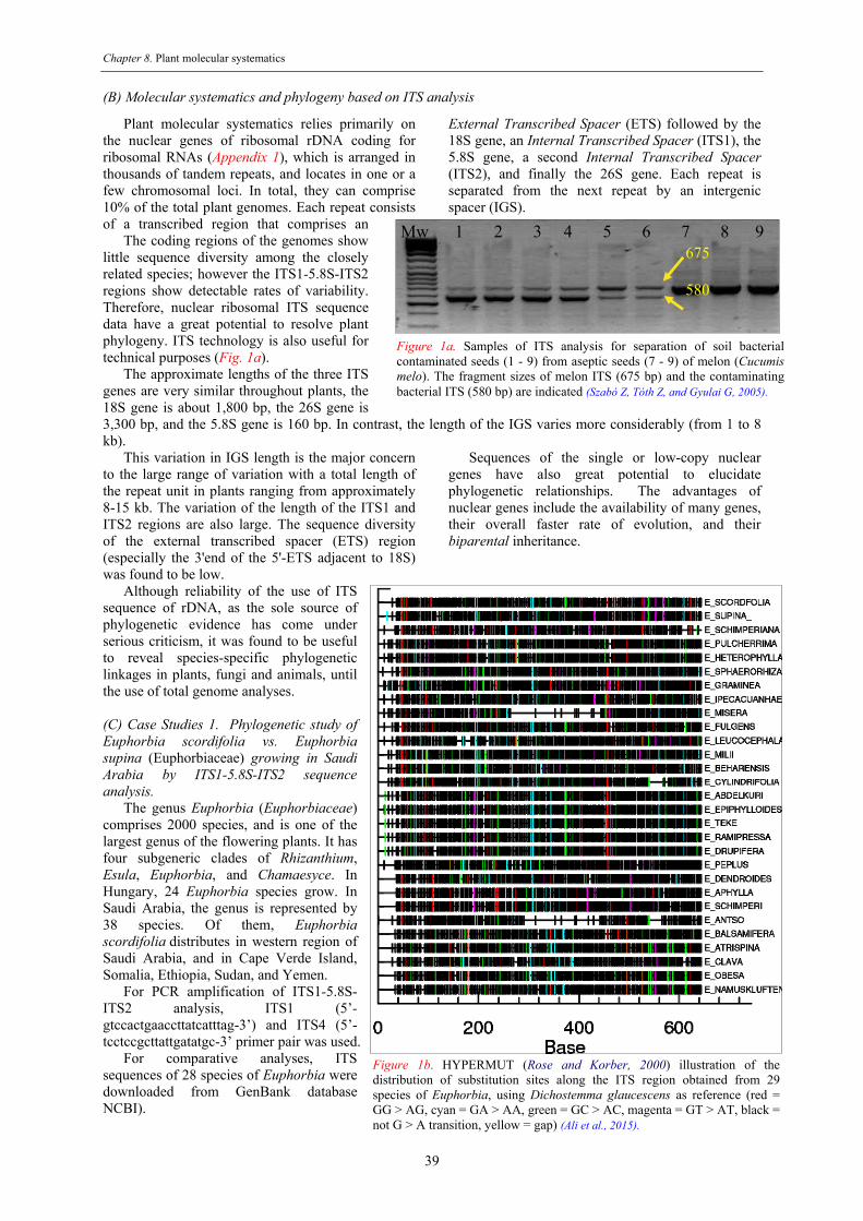
Chapter 8. Plant molecular systematics
39
(B) Molecular systematics and phylogeny based on ITS analysis
Plant molecular systematics relies primarily on the nuclear genes of ribosomal rDNA coding for ribosomal RNAs (Appendix 1), which is arranged in thousands of tandem repeats, and locates in one or a few chromosomal loci. In total, they can comprise 10% of the total plant genomes. Each repeat consists of a transcribed region that comprises an
External Transcribed Spacer (ETS) followed by the 18S gene, an Internal Transcribed Spacer (ITS1), the 5.8S gene, a second Internal Transcribed Spacer (ITS2), and finally the 26S gene. Each repeat is separated from the next repeat by an intergenic spacer (IGS).
The coding regions of the genomes show little sequence diversity among the closely related species; however the ITS1-5.8S-ITS2 regions show detectable rates of variability. Therefore, nuclear ribosomal ITS sequence data have a great potential to resolve plant phylogeny. ITS technology is also useful for technical purposes (Fig. 1a).
The approximate lengths of the three ITS genes are very similar throughout plants, the 18S gene is about 1,800 bp, the 26S gene is 3,300 bp, and the 5.8S gene is 160 bp. In contrast, the length of the IGS varies more considerably (from 1 to 8 kb).
This variation in IGS length is the major concern to the large range of variation with a total length of the repeat unit in plants ranging from approximately 8-15 kb. The variation of the length of the ITS1 and ITS2 regions are also large. The sequence diversity of the external transcribed spacer (ETS) region (especially the 3'end of the 5'-ETS adjacent to 18S) was found to be low.
Sequences of the single or low-copy nuclear genes have also great potential to elucidate phylogenetic relationships. The advantages of nuclear genes include the availability of many genes, their overall faster rate of evolution, and their biparental inheritance.
Although reliability of the use of ITS sequence of rDNA, as the sole source of phylogenetic evidence has come under serious criticism, it was found to be useful to reveal species-specific phylogenetic linkages in plants, fungi and animals, until the use of total genome analyses. (C) Case Studies 1. Phylogenetic study of Euphorbia scordifolia vs. Euphorbia supina (Euphorbiaceae) growing in Saudi Arabia by ITS1-5.8S-ITS2 sequence analysis.
The genus Euphorbia (Euphorbiaceae) comprises 2000 species, and is one of the largest genus of the flowering plants. It has four subgeneric clades of Rhizanthium, Esula, Euphorbia, and Chamaesyce. In Hungary, 24 Euphorbia species grow. In Saudi Arabia, the genus is represented by 38 species. Of them, Euphorbia scordifolia distributes in western region of Saudi Arabia, and in Cape Verde Island, Somalia, Ethiopia, Sudan, and Yemen.
For PCR amplification of ITS1-5.8S-ITS2 analysis, ITS1 (5’-gtccactgaaccttatcatttag-3’) and ITS4 (5’-tcctccgcttattgatatgc-3’ primer pair was used.
For comparative analyses, ITS sequences of 28 species of Euphorbia were downloaded from GenBank database NCBI).
Figure 1b. HYPERMUT (Rose and Korber, 2000) illustration of the distribution of substitution sites along the ITS region obtained from 29 species of Euphorbia, using Dichostemma glaucescens as reference (red = GG > AG, cyan = GA > AA, green = GC > AC, magenta = GT > AT, black = not G > A transition, yellow = gap) (Ali et al., 2015).
Mw 1 2 3 4 5 6 7 8 9 675
580
Figure 1a. Samples of ITS analysis for separation of soil bacterial contaminated seeds (1 - 9) from aseptic seeds (7 - 9) of melon (Cucumis melo). The fragment sizes of melon ITS (675 bp) and the contaminating bacterial ITS (580 bp) are indicated (Szabó Z, Tóth Z, and Gyulai G, 2005).

Chapter 8. Plant molecular systematics
40
After cloning, and sequencing, the combined length of ITS1-5.8S-ITS2 region in Euphorbia scordifolia was found to be 642 bp, including the ITS1 region (266 bp, 53% GC content), the 5.8S gene (162 bp, 56% GC content), and the ITS2 region (213 bp, 58% GC content). Molecular taxonomy of ITS sequences revealed that E. scordifolia belongs to the subgenus Chamaesyce with the closest genetic distance to E. supine. The morphological characters
of E. scordifolia are very similar with E. supina. The distribution and pattern of nucleotide substitution was investigated by using HYPERMUT program (Rose and Korber, 2000) (Fig. 1b).
(D) Case study 2. Molecular taxonomy of Astragalus collenettae (Fabaceae) an endemic legume species to Saudi Arabia by ITS1-5.8S-ITS2 sequence analysis.
Term endemism refers to the unique geographic area/habitat (e.g. island, mount, cave, or country, etc.) of a species which is indigenous to only that geographical region.
Literally, the most unique endemism is the relictum endemism, which refers to those endemic species which survived the last Ice Age at the same geographical location. To our knowledge, there are only three plant relictum endemisms in the World, the gymnosperm Welwitschia mirabilis growing in the Kalahari Desert, the Hawaii Argyroxiphium (Asteraceae); and the Linum dolomiticum, (Linaceae) growing in Hungary (personal communication of I. Milkovits and J Suba, 1978).
In Saudi Arabia, due to the extreme climatic and soil conditions, there are a high numbers of plant endemism with a total of 50 species. Astragalus collenettae is one of the three legume endemism of Saudi Arabia along with Astracantha echinus ssp. arabica, and Indigofera rubromarginata var. longipedunculata. A detailed literature survey revealed that the taxonomic status of Astragalus collenettae is unknown.
Astragalus (family Fabaceae, subfamily Faboideaea) is the largest genus of the higher plants by comprising the largest numbers of species (about 2,500 - 3,000) of a genus (with 703 entries of NCBI), which are herbs and small shrubs.
This genus was found to be a remarkable example of studying speciation through adaptive radiation (i.e. increase in genetic diversity and consequently in species numbers) on a global scale. Astragalus species distributed primarily around the northern hemisphere, and also around South America, and spread mainly in the cool temperate semiarid and arid continental regions of southwest and central Asia (with about 1500 species) and the Sino-Himalayan region (500 species), to western North America (400–450 species) and along the Andes in South America (with about 100 species).
A recent phylogenetic analyses of the ITS cladogram (Fig. 2) revealed that two species of Astragalus filicaulis and A. arpilobus show the closest sequence similarities to Astragalus collenettae. This result may indicate the putative ancestors of A. collenettae, and also shows the genetic background of plant speciation through irradiation and environmental/geographical isolation.
Astragalus collenettae*
A.filicaulis
A.arpilobus
A.sp. Kh118
A.devesae
A.allochrous
A.vagus
A.johnstonii
A.edmondstonei
A.monticola
A.pehuenches
A.curvicaulis
A.darumbium
A.lentiginosus
A.toquimanus
A.l.palans
A.arnottianus
A.berteroanus
A.cryptobotrys
A.uniflorus
A.amatus
A.nivicola
A.pagsonii
A.congdonii
A.agnicidus 2
A.agnicidus
A.peckii
A.umbraticus
A.misellus
A.arthurii
A.oniciformis
A.howellii
A.schizopterus
A.alvordensis
54
71
7061
62
83
56
50
0.002
Figure 2. Consensus ITS ML-phylogram of Astragalus species. Bootsrap values above 50% (1000 replication) are indicated (Ali et al., 2016). For orientation, photo of A. bisulcatus is included

Chapter 8. Plant molecular systematics
41
(E) Case Study 3. Phylogenetic study of Euryops jaberiana vs. Europs arabicus (Asteraceae), growing in Saudi Arabia, by ITS1-5.8S-ITS2 sequence analysis.
Euryops jaberiana (#KU577443) (tribe Senecioneae, family Asteraceae) is an endemic plant to northern Saudi Arabia. Its taxonomic status was revealed recently by using internal transcribed spacer (ITS) sequence of nuclear ribosomal DNA (nrDNA).
The genus Euryops comprises approximately 100 species and displays a restricted distribution in Africa to Arabia and Socotra. Species of Euryops are perennial shrubs (except E. annuus), with coriaceous leaves and yellow or orange-flowered capitula on simple peduncles, and usually devoid of leaves or
bracts. Despite the genus was divided into six sections of Euryops, Angustifoliae, Brachypus, Chrysops, Euryops, Leptorrhiza and Psilosteum, based on morphology, its phylogeny and phytogeography, based on molecular data, remained poorly understood.
In Saudi Arabia, the genus Euryops is represented by only two species of E. arabicus and E. jaberiana. E. arabicus is the only species found outside of Africa and is endemic to Arabian Peninsula, while E. jaberiana is endemic to northern Saudi Arabia.
Morphologically E. jaberiana is very
closely resembles with E. arabiucs and difficult to distinguish the two species. The key morphological features which differentiate E. jaberiana from E. arabicus are the 3-lobed leaves at the tips, pappus hairs transparent or rarely dull while, and achenes glabrescent, while the leaves of E. arabicus are unlobed, pappus hairs are dull white, and achene densely lanate hairy.
For PCR amplification ITS1 and ITS4 primers were used. For phylogenetic analysis the sequences (645 bp) ITS of E. jaberiana (#KU577443) was aligned with a total number of 17 representative sequences belonging to sections of the genus Euryops with an outgroup of Gymnodiscus capillaries (#EU667515).
For sequence alignment CLUSTAL X version 1.81 program was used, followed by manual adjustment of the aligned sequence using BioEdit. The Neighbor Joining (NJ), Maximum Parsimony (MP), and Maximum Likelihood (ML) dendrogram analyses were carried out using PAUP and MEGA5 programs.
Of the length of ITS region (ITS1-5.8S-ITS2) of E. jaberiana was found to comprise the ITS1 region (260 bp, with 43% GC content), the 5.8S gene (154 bp, 54% GC content), and the ITS2 region (231 bp, 50% GC content).
A total of eight specific nucleotide differences i.e. at the alignment position 93 (A T), 116 (G C), 201 (T C), 443 (C G), 461 (T G), 531 (T C), 573 (C T) and 611 (T C) were detected between E. jaberiana and E. arabicus.
The phylogenetic tree constructed by the NJ (and also by Maximum Parsimony and Maximum Likelihood) analyses showed a clear resolution, which nested within the clade of the section Angustifoliae, and showing the closest genetic relationship to E. arabicus (# EU667464) (Fig. 3).
Figure 3. The NJ tree of ITS sequence of nuclear ribosomal DNA of 18 species of Euryops including E. jaberiana The bootstrap (MP/ML) support greater than 50% in 1000 replicates is indicated (Ali et al., 2016). For orientation, photo of E. pectinatus is included.

Chapter 8. Plant molecular systematics
42
References Abedin S, Chaudhary S. 2000. Euryops. In: Chaudhary, S. (Ed.), Flora of
Saudi Arabia II(3): 191–192. Ministry of Agriculture and Water, National Herbarium, National Agriculture and Water Research Center, Riyadh, Saudi Arabia.
Ali MA, Al-Hemaid FM, Lee J, Hatamleh AA, Gyulai G, Rahman MO. 2015. Unraveling systematic inventory of Echinops (Asteraceae) with special reference to nrDNA ITS sequence based molecular typing of Echinops abuzinadianus. Genet Mol Res 14(4): 11752–11762.
Ali MA, Gyulai G, Al-Hemaid F. 2015. Plant DNA Barcoding and Phylogenetics. LAP Lambert Academic Publishing, Germany.
Ali MA, Gyulai G, Hídvégi N, Kerti B, Al-Hemaid FMA, Pandey AK, Lee J. 2014. The changing epitome of species identification - DNA barcoding. Saudi J Biol Sci 21(3): 204–231.
Altschul SF, Gish W, Miller W, Myers EW, Lipman DJ. 1990. Basic local alignment search tool. J. Mol. Biol. 215: 403–410.
Alvarez I, Wendel JF. 2003. Ribosomal ITS sequences and plant phylogenetic inference. Mol Phyl Evol 29: 417–434.
APG III 2009. An update of the angiosperm phylogeny group classification for the orders and families of flowering plants. Bot J Linn Soc 161: 105-121.
Baldwin BG, Sanderson MJ, Porter JM, Wojciechowski MF, Campbell CS, Donoghue MJ. 1995. The ITS region of nuclear ribosomal DNA: a valuable source of evidence on angiosperm phylogeny. Ann. Miss. Bot. Gard. 82: 247–277.
Botstein, D., Hite, R. L., Skonic, M., David, R. W. (1980): Construction of a genetic linkage map in man using restriction fragment length polymorphisms. Am J Hum Genet, 32: 314-331.
Carlquist S 2001 Comparative Wood Anatomy. (2nd ed.) Springer-Verlag, Berlin
Crawford DJ and ME Mort. 2003 New trends in plant systematics. Taxon 52: 3-10
Cronquist A 1981 An Integrated System of Classification of Flowering Plants. Columbia University, New York.
Devos, N, Barker NP, Nordenstam B, Mucina L. 2010. A multi-locus phylogeny of Euryops (Asteraceae, Senecioneae) augments support for the "Cape to Cairo" hypothesis of floral migrations in Africa. Taxon 59(1): 57–67.
Gupta M, Chyi YS, Severson JR, Owen JL. 1994. Amplification of DNA markers from evolutionarily diverse genomes using single primers of simple sequence repeats. Theor Appl Genet 89: 998-10Mv L2.
Hall TA 1999. BioEdit: a user-friendly biological sequence alignment editor and analysis program for Windows 95/98/ NT. Nucleic Acids Sym Ser 41: 95–98.
Henning W. 1966. Phylogenetic Systematics. University of Illinois Press, Urbana, Illinois.
Markert CL, Moller F. 1959. Multimeric forms of enzymes: tissue, ontogenic, and species specific patterns. Proc Natl Acad Sci USA 45: 753-763.
Mullis, K. B., Faloona, F. A. (1987): Specific synthesis of DNA in vitro via a polymerase-catalyzed chain reaction. Methods Enzymol 155: 335-350.
Nordenstam B, Clark VR, Devos N, Barker NP. 2009. Two new species of Euryops (Asteraceae: Senecioneae) from the Sneeuberg, Eastern Cape Province, South Africa. S African J Bot 75: 144–152.
Poczai P, Hyvönen J. 2010. Nuclear ribosomal spacer regions in plant phylogenetics: problems and prospects. Mol. Biol. Rep. 37(4): 1897–1912.
Rose PP, Korber BT. 2000. Detecting hypermutations in viral sequences with an emphasis on G A hypermutation. Bioinformatics 16: 400-401.
Simpson MG. 2010. Plant Systematics. Elsevier, Amstardam. Stuessy TF. 2003. Morphological data in plant systematics. In: Deep
Morphology: Toward a Renaissance of Morphology in Plant Systematics. Stuessy TF, Mayer V and Hörandle E (eds.) AR Gantner Liechtenstein. 299-316.
Stuessy TF. 2009. Plant Taxonomy: The Systematic Evaluation of Comparative Data. Columbia University Press, New York.
Stuessy TF, Crawford DJ, Soltis DE and Soltis PS. 2014. Plant Systematics: The Origin, Interpretation, and Ordering of Plant Biodiversity. Koeltz Scientific Books, Knigstein, Germany.
Szabó Z, Gyulai G, Humphreys M, Horvath L, Bittsánszky A, Lagler R, Heszky L. 2005. Genetic variation of melon (C. melo) compared to an extinct landrace from the Middle Ages (Hungary) I. rDNA, SSR and SNP analysis of 47 cultivars. Euphytica 146: 87–94.
Takhtajan A. 1997. Diversity and Classification of Flowering Plants. Columbia University Press, New York.
Tamura K, Peterson D, Peterson N, Stecher G, Nei M, Kumar S. 2011. MEGA5: molecular evolutionary genetics analysis using maximum likelihood, evolutionary distance, and maximum parsimony methods. Mol Biol Evol 28(10): 2731–2739.
Thompson JD, Gibson TJ, Plewniak F, Jeanmougin F, Higgins DG. 1997. The Clustal X windows interface: flexible strategies for multiple sequence alignment aided by quality analysis tools. Nucleic Acids Res. 24: 4876–4882
Williams JGK, Kubelik AR, Rafalski KJ, Tingey SV. 1990. DNA polymorphisms amplified by arbitrary primers are useful as genetic markers. Nucleic Acids Res 18: 6531-6535.
Zietkiewicz E, Rafalski A, Labuda D. 1994. Genome fingerprinting by simple sequence repeat (SSR)-anchored polymerase chain reaction amplification. Genomics 20: 176-183.
Appendix 1. Organization of the rDNA genes and subunits including ITS-1 and 2, by organisms and organs (Gyulai, 2015)

Chapter 8. Molecular metabolomics – Tomato carotenoids (Solanum lycopersicum)
43
Molecular metabolomics – Tomato carotenoids (Solanum lycopersicum) Introduction
Cultivated tomato (Solanum lycopersicum; chromosome number 2n = 24; genome size 0.9x10⁹ bp) (TGC, 2012; SGN, 2014) has twelve wild relative tomato species, which are divided into two complexes, the Peruvianum complex with two self-incompatible species (S. chilense and S. peruvianum), and the Esculentum complex, which includes the intercrossable species of S. arcanum, S. chmielewskii, S. corneliomuelleri, S. habrochaites, S. huaylasense; S. neorickii, S. pennellii, S. pimpinellifolium, and the two endemic species of S. cheesmaniae and S. galapagense (Peralta et al., 2005).
Tomato occupies the top position of the total World production of the ten major fleshy fruits with 28% (about 108 MT), followed by banana (20%, 7.6×10⁷ MT); apple and grapes (about 15% and 5.6%, respectively, a total of 5.9×10⁷ MT); pear and pineapple (about 5%, 1.9%, respectively, a total of 1.8×10⁷ MT), and papaya and strawberry (2% and 1%; 7×10⁶MT and 3.4×10⁶MT, respectively). Carotenoids and Chlorophylls
More than 700 carotenoids (including the annotated 281 molecules) have been identified from different plant sources (Appendix 1). Carotenoids are divided into non-oxygenated carotenoids, the Carotenes; and oxygenated carotenoids, the Xanthophylls. Carotenes are divided by Acyclic-carotenes (e.g., phytoene, phytofluene, ζ-carotene, neurosporene, and lycopene), and Cyclic-carotenes (e.g., δ- and γ carotene, α- and β-zeacarotene with one ring; and α- and β carotene with double rings).
Xanthophylls (syn. carotenols or hydroxycarotenoids) are also divided as acyclic (e.g., lycoxanthin and lycophyll) and cyclic groups (e.g., rubixanthin with one ring; and α- and β-cryptoxanthin, zeinoxanthin, zeaxanthis and lutein). A third group of xanthophylls includes Epoxy-carotenoids (e.g., antheraxanthin, auroxanthin, neoxanthin, luteoxanthin, violaxanthin, lutein-5-6-epoxyde, and β-carotene-5,6-epoxide). The fourth group of xanthophylls comprises some Unique carotenoids (e.g., capsanthin, capsorubin, crocetin and bixin). In the whole carotenoid biosynthesis the phytoene (C40H64) synthase (PSY) is the rate-limiting enzyme.
Colour of tomato fruit skin and flesh is one of the most important quality components of the tomato. The colors slightly depend on the elution solvents used for the analyses. The main acyclic carotenoids of ζ-carotene (its colour is light-yellow), neurosporine (yellow-orange) and lycopene (red-orange); and cyclic-carotenoids of γ-carotenes (pink-orange), and β-carotene (orange) are the main tomato fruit colorant. The main carotenoids of β-carotene and lycopene cause red-to-orange coloration, which are the predominant tomato pigments.
Chlorophylls, the green pigments of unripe fruits, breaks down during ripening, except in cultivars with
‘black’ coloured fruits, where persistent chlorophyll content gives a purplish-brown colour. This colour is regulated by gf (green flesh) gene that encodes a Stay-Green senescence-related regulator, and finally results in the mix of red and green colour, which seems black-brown-chocolate colour.
Functionally, carotenoids, especially β-carotene, primarily act as accessory and photo protective pigments for chlorophyll a and b of LHCs (Light Harvesting Complex) of Photosystem I, and II (PSI and PSII) during photosynthesis in leaves, fruits and flowers. Carotenoids absorb the sunlight in a broader range of the blue spectrum (400-500 nm) than chlorophylls, and they transfer this absorbed energy to chlorophyll a of the photosynthetic reaction center. Carotenoids also supply substrates for the biosynthesis of the plant growth regulator abscisic acid (ABA). All carotenoids can be crystallized in chromoplasts of the flowers during the transition of chloroplast to chromoplast, or transported and accumulated in lipid bodies.
In animals, ceto-carotenoid type astaxanthin
(Appendix 1) is responsible for the orange colour of salmon meat and lobster shell. Feather colours of the bird’s also came from carotenoids. Chicken egg yolks are rich in lutein and zeaxanthin. In human nutrition and health, carotenoids act as anti-aging and anti-cancer substances, and provide provitamin-A (e.g., β-carotene, β-cryptoxanthin and α-carotene). Carotenoids of algae, fungi and bacteria have also been identified and characterized.
Genes (Table 1) of enzymes involved in carotenoids synthesis are encoded in plant nuclear genomes, and gene products are transported either to the cytoplasm (including mitochondria) (i.e.,, mevalonate pathway) or to the plastids (i.e.,, non-mevalonate pathway) where they are post-translationally modified and activated.
Tomato fruits are also rich in phenols and polyphenols (like gallic acid, catechin, rutin, ferulic acid, etc.) and vitamin E (α-, and γ-tocopherol), which are also responsible for the antioxidant capacity of the soluble phase of fruit sap.
As the monoculture of tomatoes (i.e., less then ten cultivars are cultivated in the World), the unique heirloom tomato genotypes may provide basal material for new feeding experiments and medical studies. E.g., eggs of carotenoid-fed female birds (Larus fuscus) contained high carotenoid but low Ig contents (i.e.,, passive immunity), whereas control females produced eggs contained low carotenoid but high Ig content, which results indicated a carotenoid-mediated effects on phenotype for ecological fitness in mother birds and their offspring.
Lutein- and zeaxanthin supplemented male zebra finch birds (Taeniopygia guttata) an elevated blood carotenoid levels were found with increased cell mediated and humoral immune responses than control birds, and with brighter beak coloration,

Chapter 8. Molecular metabolomics – Tomato carotenoids (Solanum lycopersicum)
44
which results suggested that carotenoids-based colour signals in birds may directly signal male health via the immunostimulatory action of ingested and circulated carotenoids.
In an experiments with depletion of carotenoids of nineteen healthy adult human that were fed at low carotenoids diets for 10 weeks, of the six major human serum carotenoids of lycopene, β-carotene, α-carotene, lutein, zeaxanthin and β-cryptoxanthin, the lycopene concentration showed sharp decrease compared to other carotenoids. This result indicated that lycopene appears to be the physiologically most important antioxidant of human body (Appendix 1). Plant materials. A greenhouse study was conducted in the summer (June 1 to Sept 31) of 2014 at the spring at Experiment Station, Szent István University, Hungary, Europe. Tomatoes were seeded into Canadian Growing Mix 2 (Conrad Fafard Inc.,
Agawan, MA) in 72-cell flats and transplanted into trade gallon pots after five weeks in accordance with standard transplant production (Peat Brown OPM Multipack 025W; Kekkila) (Fig. 1).
Transplants were fertilized once a week with a 20N-4.4P-16.6K water soluble fertilizer (Peter’s Water Soluble Plant Food 20-10-20) (Scotts Co, Marysville, OH) at a rate of 265 mg/L of N. Plants were allowed to grow for three weeks and then potted into three-gallon (24.13 cm tall, 27.94 cm diameter, 11.36 L) containers.
Plants were watered twice daily and fertigated weekly with 20N-4.4P-16.6K water soluble fertilizer (Peter’s Water Soluble Plant Food 20-10-20) (Scotts Co, Marysville, OH) at a rate of 265 mg/L of N. Tomato plants were staked with three foot bamboo stakes attached with twist ties. All suckers below the first flower cluster were removed.
Table 1. Tomato genes encoding for fruit colors (TFM, 2014; TGC, 2012).
Gene Symbols
Gene Names
Description
Abg Aubergine Purple fruit epidermis particularly on shoulder Af Anthocyanin fruit Anthocyanin in green and ripe fruit (absent when shaded) ant aurantia (ant1) Short thick stems, light green pinnae; light orange fruit with colourless pericarp at apricot (yellow) Yellow-pink colour of fruit flesh aur aurantiaca (aur1) Small, pointed, yellowish light-green pinnae, and orange fruit B β-carotene High β-carotene, low lycopene in ripe fruit Bc crimson (ogc) Increased fruit lycopene content, phenotype similar to Bog Bm minutum High β-carotene, low lycopene in ripe fruit Bog old gold (og) Corolla tawny orange; increased fruit lycopene del Delta Reddish-orange fruit, due to inhibition of lycopene, and increase of δ-carotene dg dark green Darker green colour appears as fruit develops, then persists until onset of ripening, high
chlorophyll compared to normal or hp dps diospyros Fruit tissue is dusky orange gdf Gold Fleck Small dark green spots on immature fruit, which turn yellow on ripe fruit gf green flesh Persistent chlorophyll giving ripe fruit purplish-brown colour glu glutinosa (glu1) Dark green, shiny fruit with sticky epidermis; poor germination gr green ripe (gr) Resembles gf, except that center of fruit turns red gs green stripe Radical green stripes in epidermis of unripe fruit; golden in ripe fruit hp-1 high pigment (hp2) Chlorophyll, carotenoids, ascorbic acid content of fruit intensified r- yellow flesh Yellow colour of ripe fruit flesh r(1s) yellow flesh (1s) Yellow colour of ripe fruit flesh. r(2s) yellow flesh (2s) Yellow fruit flesh; lighter yellow flowers rprov4 yellow flesh Yellow colour of ripe fruit flesh rprov5 yellow flesh Yellow colour of ripe fruit flesh ry yellow flesh Reddish yellow: Likely allele of r with reddish flesh tones in ripe fruit sh sherry Fruit flesh yellow with reddish tinge t tangerine Fruit flesh and stamens orange coloured vo virescent orange Fruit flesh orange, redder in outer walls y colourless fruit epidermis Fruit epidermis lacks pigmentation (clear skin)
Treatments consisted of the following selected American heirloom tomatoes: ‘Aunt Ruby’s German Green’; ‘Black from Tula’, ‘Cherokee Purple’ and German Johnson Regular Leaf’; and ‘Kellogg’s Breakfast’, and ‘Yellow Brandywine Platfoot Strain’ (Fig. 2).
The germination vigor was found the strongest in ‘Kellogg’s Breakfast’ followed by ‘Yellow Brandywine Platfoot Strain’, ‘Cherokee Purple’, ‘German Johnson Regular Leaf’, ‘Aunt Ruby’s German Green’ and ‘Black from Tula’ heirloom. The
‘Cherokee Purple’ (3rd heirloom) was found to be a ‘potato leaved’ type (Fig. 1).
All heirlooms showed ‘indeterminate’ growing habit. Nearly a century ago, a spontaneous mutation in sp (self pruning) gene family spawned the ‘determinate’ tomato development, which now dominate the tomato market being beneficial for mechanical harvesting (TGC, 2012)
By fruit shape, all heirlooms showed extremely puffy fruits with hollow locules (i.e., fruit cavity with seeds), which suggest the presence of spf2 genes (superpuff) with bell pepper shaped fruit. Fruits of

Chapter 8. Molecular metabolomics – Tomato carotenoids (Solanum lycopersicum)
45
‘Aunt Ruby’s German Green’ showed serious radial crakes, which phenomenon is regulated by two dominant genes of CE and RA. All the other tomatoes showed some radial crack resistance, which is controlled by recessive alleles of cr and ra; however ‘Black from Tula’ was found susceptible to fruit bursting, which is regulated by dominant gene BT (burst types). The first three American heirlooms (1-3) may also carry Abg (Aubergine) gene, which cause purple fruit epidermis particularly on shoulder, and the ‘Yellow Brandywine Platfoot Strain’ (6th heirloom) probably carries fs (fruit stripe) gene, which causes dark green radial stripes at the opposite locules (Fig. 2, Table 1).
Treatments were randomly assigned to six individual plants in a completely randomized design with three replications. Data gathered included germination vigor (Fig. 1) and fruit quality characteristics. The first six ripened fruit (Fig. 2) grown on the same vine nodes were collected and processed for HPLC analysis.
Extraction of carotenoids. Lipids and fat soluble pigments collected from the raw tomatoes were extracted according to a previously described procedure with slight modification. Five-gram samples from tomato fruits were taken from each variety in four replicates (6 varieties x 4 replicates = 24 samples), and disintegrated in a crucible mortar with quartz sand. The water was removed by adding 20 mL methanol. The mixture was then transferred quantitatively to a 100 mL conical flask, and 70 mL of a 6:1 dichloroethanemethanol solution was added.
The mixture was shaken for 15 min by a mechanical shaker. Distilled water was with hand shaking till the dichloroethane phase was clearly separated from the polar phase (water + methanol). The two phases were separated into different funnels, and the lower layer containing lipids in dichloroethane was dried over anhydrous sodium sulphate. Finally, the organic solvent was evaporated under vacuum by rotary evaporator at not higher than 40°C. The residues were re-dissolved in HPLC acetone, as the best organic solvent that ensures high solubility of most of carotenoids before injection onto HPLC column (Fig. 3).
HPLC analysis. For Reverse Phase (RP) High-Performance Liquid Chromatography (HPLC) a Chromaster Hitachi HPLC instrument was used, couple with diode-array detector (Model 5430), an autosampler (Model 5210) and a gradient pump (Model 5110). The instrument and analyses was operated by EZchrom Elite software (version 3.3.2.SP2) and the separation of carotenoids was performed on Accucore (Thermo Scientific) C-30, 2.7 µ, 150 x 4.0 mm column with gradient elution of (a) tetra-butyl-methyl-ether (TBME) and (b) methanol (MetOH).
The gradient elution started with 100% TBME, and changed to 30% TBME in MetOH for 25 min, stayed isocratic for 5 min, and finally turned to 100% TBME for 5 min. Peak identification was based on the comparison of spectral properties and retention time of carotenoids with those of available standard materials like lycopene, β-carotene and zeaxanthin, which were purchased from (Sigma-Aldrich, Budapest, Hungary).
In case of compounds with no available standards, the peaks were tentatively identified according to their spectral characteristics and chromatographic retention as compared to references. The cis isomers of lycopene were identified on the basis of appearance of an extra absorption wavelength at 340 nm and 361 nm. The 9-Z and 13-Z cis lycopene isomers were identified according to II-value, which equals to absorbance at 361 nm over absorbance at the maximum wavelength of cis lycopeneThe column effluents were detected and integrated at their maximum absorption wavelength for quantitative determinations. They were quantified as either lycopene- or β-carotene-equivalent (μg g-1, equal to g kg-1) according to their spectral characteristics (Fig. 3, Table 1).
Figure 1. Germination vigor of the six American heirloom tomatoes (Solanum lycopersicum) (three pots each). (1) ‘Aunt Ruby’s German Green’; (2) ‘Black from Tula’; (3) ‘Cherokee Purple’; (4) ‘German Johnson Regular Leaf’; (5) ‘Kellogg’s Breakfast’; and (6) ‘Yellow Brandywine Platfoot Strain’.
1 2 3 4 5 6
Figure 2. Fruit samples of the six American heirloom tomatoes (Solanum lycopersicum). (1) ‘Aunt Ruby’s German Green’; (2)‘Black from Tula’; (3) ‘Cherokee Purple’; (4) ‘German Johnson Regular Leaf’; (5) ‘Kellogg’s Breakfast’; and (6) ‘Yellow Brandywine Platfoot Strain’.

Chapter 8. Molecular metabolomics – Tomato carotenoids (Solanum lycopersicum)
46
Table. 2. Carotenoids components of the fruits of six American heirloom tomatoes (Solanum lycopersicum)
Carotenoids contents (μg g-1 FW)
Mol. Formulas
MW
Aun
t Rub
y's
Ger
man
Gre
en
(1
)
Bla
ck fr
om T
ula
(2)
Che
roke
e Pu
rple
(3
)
Ger
man
John
son
(4)
Kel
log’
s Bre
akfa
st
(5)
Yel
low
B
rand
ywin
e
(6)
ζ-carotene C40H60 540.904 0 0 0 0 19.14±15.39 32.65±22.21ζ-carotene like C40H60 540.904 0 0 0 0 1.68±1.58 3.33±3.21 Neurosporene C40H58 538.890 0 0 0 0 1.55±0.59 1.42±0.38 Neurosporene-epoxide C40H58O 549.449 0 0 0 0 2.49±1.76 3.68±2.33 Prolycopene C40H56 536.889 0 0 0 0 100.87±51.4 70.99±15.27Neochrome C41H58O3 598.8974 0 0 0 0 3.1±1.54 2.26±0.41 α-cryptoxanthin C40H56O 552.872 0 0 0 0 5.33±3.12 5.96±1.29 Violaxanthin C40H56O4 600.870 0 0 0 0 2.92±1.17 1.89±0.65 Lycopene C40H56 536.873 0.23±0.26 13.33±7.48 19.25±14.25 17.93±6.29 0 0 β-carotene C40H56 536.873 1.15±1.98 23.56±9.17 11.51±3.32 12.2±3.34 0 0 9-Cis-lycopene C40H56 536.873 1.35±2.31 2.2±3.82 4.5±5.39 7.84±2.24 0 0 13-Cis-lycopene C40H56 536.873 0.08±0.02 5.04±13.06 3.68±3.15 5.28±2.77 0 0 Lycopene-epoxide 1 C40H56O 552.433 0 1.45±0.74 2.55±2.63 0.81±0.36 0 0 Lycopene-epoxide 2 C40H56O 552.433 0 0.81±0.74 2.83±5.61 0.76±0.18 0 0 β-cryptoxanthin C40H56O 552.872 0 0.35±0.22 0.96±1 0.67±0.19 0 0 Lycoxanthin C40H56O 552.872 0 7.13±13.3 0 0.77±0.29 0 0 Lycopene-diepoxide_1 C40H56O2 568.428 0.2±0.28 0.77±0.7 1.1±0.07 1.04±0.35 0 0 Lycopene-diepoxide_2 C40H56O2 568.428 0.2±0.28 1.06±1.27 1.03±0.14 1.09±0.13 0 0 Lutein C40H56O2 568.871 1.77±1.99 2.93±2.87 0.99±1.2 0.19±0.04 0 0 Mutatoxanthin C40H56O3 584.871 0 1.62±0.74 0.75±0.28 1.25±0.27 0 0 Neoxanthin C40H56O4 600.870 0 2.11±2.41 1.52±1.05 2.69±0.5 0 0 TOTAL 4.98 62.36 50.67 52.52 137.08 122.08
Figure 3. HPLC profiles of carotenoids of the six American heirlooms tomatoes (Solanum lycopersicum) studied AR - ‘Aunt Ruby’s German Green’.: 1 - Lutein, 2 - Chlorophyllid B, 3 - Chlorophyll B, 4 - Chlorophyll B, 5 - Neoxanthin, 6 - β-carotene, 7- 13-cis-lycopene, 8 - Rubixanthin, 9 - Lycopene, 10 - γ-carotene. BF - ‘Black from Tula’: 1 - Lutein, 2 - Chlorophyll B, 3 - Lycopene diepoxide, 4 -Mutatoxanthin, 5 - Neoxanthin, 6 - cis-neoxanthin, 7 - Lycopene-epoxide 1, 8 - cis-β-carotene, 9 - β-carotene, 10 - Lycoxanthin, 11 - 13-cis-lycopene, 12 - Rubixanthin, 13 - 9-cis-lycopene, 14 - Lycopene. CP - ‘Cherokee Purple’: 1 - Lutein, 2 - Chlorophyll B, 3 - Lycopene diepoxide, 4 - Mutatoxanthin, 5 - Neoxanthin, 6 - Cis-neoxanthin, 7 - Lycopene-epoxide 1, 8 - Lycoxanthin, 9 - β-carotene, 10 - 15-Cis-lycopene, 11 - 13-Cis-lycopene, 12 - Rubixanthin, 13 - 9-Cis-lycopene, 14 - Lycopene. GJ - ‘German Johnson Regular Leaf’: 1 - Lutein, 2 -Lycopene diepoxide, 3 - Mutatoxanthin, 4 - Neoxanthin, 5 - Cis-neoxanthin, 6 - Lycopene-epoxide 1, 7 - Lycoxanthin, 8 - β-carotene, 9 -15-Cis-lycopene, 10 - 13-Cis-lycopene, 11 - Rubixanthin, 12 - 9-Cis-lycopene, 13 - Lycopene. KB - ‘Kellogg’s Breakfast’: 1 - Prolycopene epoxide, 2 - Mutatoxanthin, 3 - Neoxanthin, 4 - Cis-neoxanthin, 5 - Neochrome, 6 - Prolycopene, 7 - Proneurosporene, 8 - Violaxanthin, 9 -β-carotene, 10 - 13-Cis-lycopene, 11 - 9-Cis-lycopene, 12 - Lycopene; YB - ‘Yellow Brandywine Platfoot Strain’: 1 - Prolycopene epoxide, 2 - Neochrome, 3 - Prolycopene, 4- Proneurosporene, 5 - ζ -carotene, 6 - α-cryptoxanthin; Photos of the meshed fruit saps prepared for HPLC analysis are indicated.

Chapter 8. Molecular metabolomics – Tomato carotenoids (Solanum lycopersicum)
47
Statistical analysis. Mean values of four (n=4) HPLC measurements and 95 % Confidence Interval for Mean (CI95% = x ± d) confidence intervals were calculated at P 95% confidence level by SPSS program package. For Dendrogram (using Average Linkage Within Group) - and Canonical Discriminant Functions Analyses also the SPSS program package was used.
Tomato fruit carotenoids The synthesis of plant carotenoids links
genetically with the processes of fruit ripening (i.e., cell wall softening), which is regulated by about 50 genes in tomato. Regulation/modulation of fruit ripening of all fleshy fruit plant species has profound agronomic importance
Recently, the fresh market tomatoes include only ‘long shelf-life’ varieties, which are natural mutants, and carry ripening inhibitor (RIN) genes. Another unique natural tomato mutants is a dwarf type ‘Micro-Tom’. The main RIN genes are the rin (ripening-inhibitor MADS-box gene), nor (non-
ripening transcription factor gene), nr (never-ripe ethylene signaling), nr-2 (never-ripe 2) / gr (green-ripe), and cnr (coulorless non-ripening). Of them, one of the earliest tomato fruit ripening mutants was the dominant Nr (Never-ripe) mutation. This mutation was shown to be the consequence of a single amino acid change in one of the seven ethylene receptors (LeTR1-7).
The first registered RIN tomato, the ‘Daniela’ (FA144) an indeterminate long-self life hybrid, was released in about 1992 by the BonTom Tomato Breeding Group (Faculty of Agriculture, Hebrew University of Jerusalem, Israel). Green-Ripe (Gr) and its allele, Nr-2, were also found to be dominant nonripening mutant.
During the transgenic GM programs, the first FDA-approved transgenic food of Flavr-Savr tomato was released in 1994, followed by another delayed ripening tomatoes (DNAP) by Zeneca/Peto and Monsanto.
By visual observation of fruits (Fig. 2), none of
the heirloom tomatoes showed the expression of RIN genes, as the fruits were ripened and softened very quickly in some days after total fruit size development. These fruit characters obviously suggested these heirlooms for fresh consumption or for tinned juice.
The fruit pigment composition of the heirlooms showed three main groups (Table 2, Fig. 4). In the first group, on the contrary of the extremely low carotenoids compositions (Fig. 4), ‘Aunt Ruby’s German Green’ (1st heirloom) was found with delicious taste due probably to its tasty compositions
Figure 4. Cumulative carotenoids components of the six American heirloom tomatoes (Solanum lycopersicum). The main metabolic steps (numbers 1 to 4), and molecular formulas from the non-cyclic carotenoids ζ-carotene (C40H60) (1), → prolycopene (C40H56) (2), → lycopene (C40H56) (3), to → cyclic carotenoid β-carotene (C40H56) (4), are indicated (syn. of prolycopine are: cis-lycopene; all-trans-lycopine) (Pék, Helyes, Gyulai et al., 2016)
9-Cis-lycopene
13-Cis-lycopene
13-Cis-lycopene
Prolycopine
Prolycopine
ζ-carotene
ζ-carotene
α-cryptoxanthin
α-cryptoxanthin
β-caroteneβ-carotene β-carotene
Lycopene
Lycopene Lycopene
Lycoxanthin9-Cis-lycopene
0
20
40
60
80
100
120
140
160
Aunt Ruby'sGer Green
Black fromTula
CherokeePurple
GermanJohnson
Kellog’sBreakfast
YellowBrandywine
g kg
-1 FW
Neurosporineα-cryptoxanthinζ-carotene likeζ-caroteneProlycopineNeurosporene-epoxideNeochromeViolaxanthinLycopene-diepoxide_2Lycopene-diepoxide_113-Cis-lycopene9-Cis-lycopeneLycoxanthinLycopene-epoxide_2Lycopene-epoxide_1LycopeneNeoxanthinMutatoxanthinβ-criptoxanthinβ-caroteneLutein
2 1
3
4

Chapter 8. Molecular metabolomics – Tomato carotenoids (Solanum lycopersicum)
48
of other organic fruit components such as carbohydrates and organic acids.
In the second group, ‘Black from Tula’ (2nd heirloom) showed the highest content of β-carotene (23.56 ug g-1 FW). This β-carotene content showed higher level compared tomato cv. ‘Strombolino’ (3.27±0.17 ug g-1 FW) measured in our lab using the same technology. The highest lycopene content (19.25 ug g-1 FW) was found in the ‘Cherokee Purple’(3) and ‘German Johnson’(4) (17.93±6.29 ug g-1 FW) tomatoes. These lycopene contents showed slower levels then in tomato cv. ‘Strombolino’ (62.6±2.77 ug g-1 FW), however it was higher levels compared to a vine-ripened tomato ’Lemance F1’, which yielded 4.5±1.40 ug g-1 FW (Pék et al., 2010).
The third group comprised the two yellow fruited tomatoes of ‘Kellogg’s Breakfast’(5) and ‘Yellow Brandywine Platfoot Strain’(6) with extremely high level of prolycopene content (100.87 and 70. 99 ug g-
1 FW, respectively). As the later stages of main
metabolic desaturation steps of the synthesis of plant acyclic carotenoids (C40H60), which goes through ζ-carotene → neurosporene → prolycopene (and → lycopene), we may suggest that these two heirloom tomatoes may be metabolically ‘economic’ by blocking the further enzymatic reactions (and saving metabolic energy by this way), which would have been included the cyclizations of lycopene either to α-zeacarotene → δ-carotene → ε-carotene, or to β-zeacarotene → γ-carotene → α- and β-carotene (Fig. 4, Appendix 1)
Dendrogram- (Fig. 5a) and Discriminant Analysis (Fig. 5b) of carotenoids contents (Table 2) revealed that ‘Aunt Ruby’s German Green’ shows the most homogenous clade (Clade 1 of Fig. 5a) and is close to ‘Kellogg’s Breakfast’ and ‘Yellow Brandywine Platfoot Strain’(Clade 2 of Fig. 5b). Heirlooms of ‘Black from Tula’, ‘Cherokee Purple’, and ‘German Johnson Regular Leaf’ showed separate carotenoids compositions (Fig. 5b).
In conclusion, as a result of high prolycopene and
ζ-carotene contents, the two yellow fruited heirloom tomatoes ‘Kellogg’s Breakfast’(5) and ‘Yellow Brandywine Platfoot Strain’(6) are suggested to be involved in a breeding program to identify further gene markers for yellow fruit coloration. Due to good
fruit taste of ‘Aunt Ruby’s German Green’(1); and for high lycopene and β-carotene contents the red-fruited ‘Black from Tula’(2), ‘Cherokee Purple’(3), and ‘German Johnson’(4) tomatoes have high potential for recultivation.
References (for all papers cited) Pék Z, Helyes L, Gyulai G, Foshee WG, Daood HG, Lau J, Vinogradov Sz, Bittsánszky A, Goff W, Waters L Jr (2016) Molecular Profiling -
Fruit carotenoids components of six American heirloom tomatoes (Solanum lycopersicum). J Forensic Biomed, 7:2. 1000130. SGN (2014) Sol Genomics Network website: http://solgenomics.net TFM (2014) Tomato Fruit Mutation website: http://kdcomm.net/~tomato/Tomato/mutant.html TGC (2012) Tomato Genome Consortium. Nature 485, 635–641.
1
2
3
(a) (b)
Figure 5. Dendrogram (a) and Canonical Discriminant Functions (b) analysis of the carotenoids contents of six American heirloom tomatoes (Solanum lycopersicum) studied. AR – (1) ‘Aunt Ruby’s German Green’. BF – (2) ‘Black from Tula’. CP – (3) ‘Cherokee Purple’. GJ – (4) ‘German Johnson Regular Leaf’. KB – (5) ‘Kellogg’s Breakfast’. YB – (6)‘Yellow Brandywine Platfoot Strain’. The level of dissimilarity (i.e. Squared Euclidean Distances) (0 to 25), the three main clades, and the number of four measurements of each heirloom (1 to 24) are indicated.

Chapter 8. Molecular metabolomics – Tomato carotenoids (Solanum lycopersicum)
49
Appendix 1. Molecular structures of:
(A) Acyclic Carotenes (the increasing number of double bounds are indicated by arrows) (B) Cyclic Carotenes (C) Xanthophylls (Hydroxycarotenoids, Carotenols,) (D) Epoxy-Carotenoids (E) Unique plant carotenoids (F) Unique animal carotenoid Astaxanthin The most important carotenoids are indicated with asterisk (*).
(F)
*
*
*
*
(B)
*
(E)*
(C)**
(A)*

Chapter 9. Plant Cell, Tissue, and Organ Cultures – Basics of plant biotechnology
50
Plant Cell, Tissue, and Organ Cultures – Basics of plant biotechnology Introduction Basics of Plant Tissue Cultures of Plant Biotechnology includes several laboratory techniques and processes at cell and organ levels, and apply in vitro cultures under aseptic conditions with using artificial nutritive media (Table 1) supplemented with plant hormones. Biotechnology is a very broad term and is not new. The term biotechnology, first was coined in 1919 by a Hungarian engineer EREKY K (1878-1952) (Appendix 1).
Regular plant tissue culture lab is equipped with Laminar air flow cabinets, Autoclaves, Water purification systems, and several types of Glasswares (Fig. 1, 6-8, 11a, 14ab; Appendix). The most important advantage of these techniques is the capability of the production of 10 million plants per year developed from a single cell (or explant), and to keep and treat one million plants in a flask at ‘cell level’.
(A) Main fields of Plant tissue cultures 1. Seed culture. Similar to agriculture, seeds, after surface sterilization (after using sodium- or calcium hypochlorite; which was used first in human medication by the Hungarian medical doctor Ignác Semmelweis, Budapest, 1818-1865) (Fig. 2b,c) can be used in vitro for whole plant development (Fig. 3) for further mass propagation (Fig. 8). 2a. Explants. Micropropagation (micro – propagation). It is a laboratory processes of whole plant developments, which applies small (i.e., micro) parts (i.e., explants) of a plant, and carried out under aseptic conditions, in vitro (i.e., in ‘bottle’). The most frequently used explants are the shoots (i.e., Shoot culture - Fig. 1, 6); roots (i.e., Root culture - Fig. 1); buds (i.e., both apical and axillary Bud cultures) (Fig. 4); leaves (i.e., Leaf-, and Leaf disc cultures - Fig. 1); and Petioles (e.g., of poplar leaves) (Fig. 6). These techniques also called as ‘basic plant organ cultures’, or simply ‘cloning’. Cloning means vegetative (syn., axexual) propagation. 2b. Meristem culture. Mericlones. Virus elimination. Meri(stem)-cloning uses not the whole buds (Fig. 4) for plant development, rather the excised meristems (Fig. 10) of both roots or buds (Fig. 9). As meristems are free of pathogenes, mericloning is a unique technique to produce virus-free lines for crop production. 3. Embryo, Embryo rescue, Ovary and Ovulum cultures. Seed organs having the whole embryo (Fig. 1), and female sexual organs of ovary and ovulum, or the single egg cell also can be excised from both mature or immature vs. fertilized or unfertilized seeds for further manipulation. Sexually incompatible parents also can be hybridized by embryo saving (i.e., embryo rescue), and develop the hybrid plants in vitro. 3b. Anther and Pollen cultures. Male sexual organs of the whole anther (full with undeveloped pollens – i.e., anther culture) (Fig. 11a,b), or the excised pollens (i.e., pollen culture) (Fig. 11c, 12) can also be used for whole plant development (Fig. 13) with ‘half genome’ (n) in vitro either in suspension or agar culture (Fig. 11a).
3c. Haploid cultures, DH breeding. Twin embryos. Sex cells of both egg-, and pollen cells are haploids (carrying only half of the genome) (n), so when plants develop from them, the whole plant will be also haploid (n). Through colchicines treatment, the genome can be diploidized and the developed diploid (2n) plants will be completely homozygous (i.e., DiHaploid, DH). Besides fixed meiotic recombinants (syn., sexual ‘clones’), DH-breeding also uses DH-plants for further hybridization to use up the phenomenon of hybrid vigor (i.e., hybrid produce more yield then either parent lines alone). Conventional Twin embryo technology (Fig. 11d), and haploid marker systems, also can produce haploid plants. 3d. Pollination and fertilization in vitro. Direct pollination and fertilization can be carried out in vitro for breaking down the sexual incompatibility prior to embryo rescue technology. 4. Callus cultures. Totipotency. Cell suspensions. Organogenesis. Embryogenesis. Somatic embryos. Totipotency. Somaclones. Somaclonal variation. Artificial seeds.
All plant organs cultured in vitro (summarized above) can be turned to an undifferentiated developmental way by stimulating them with plant hormones (Fig. 17), which produce clumps of undifferentiated cells (i.e., callus), either on the surface of agar-solidified media (Fig. 2a), or in liquid (Fig. 3), media (i.e., cell suspension).
Whole plants can develope from these single callus cells through either organogenesis (root develops first and later the shoot does), or through embryogenesis (not organs rather full embryo develops directly; i.e., somatic embryos) (i.e., somaclones).
Plants, developed from somatic embryos (Fig. 2a) are identical to the original plants (i.e., all cells are totipotent for they carry the same DNA), however, with slight genetic differences (i.e., somaclonal variation) due to the effects of in vitro conditions and mainly to the plant hormones (Fig. 18) applied. Somatic embryos can be coated with special compounds (e.g., graphite, and calcium alginate), and can sow (!) directly in the field (i.e., artificial seeds).

Chapter 9. Plant Cell, Tissue, and Organ Cultures – Basics of plant biotechnology
51
Figure 1-15. Basic technologies of Plant tissue and organ cultures (1). VEGETATIVE ORGANS. Somatic embryos of dicot Aesculus trees (2a) (Gyulai, Jekkel, and J. Kiss, 1998), developed in vitro, after surface sterilization of explants by Ca/Na-hypochlorite, which was used first in human medical sciences (against childbed fever and maternal mortality) (2c), by the Hungarian MD Semmelweis, Ignác (1818-1865) (2b). Seed germination of wheat (Triticum) under aseptic conditions (3). Bud explants for bud cultures (4). Samples of cloning (i.e., grafting) used in horticulture (5). Cloning in vitro: shoot culture of poplar tree in agar-solidified media (6), or in aseptic suspension culture incubated in liquid medium (7). Mass propagation of poplar in shoot cultures (8) (Bittsánszky and Gyulai, 2005). Seed meristems (of shoot and root) (9), excised for meristem cultures. Shoot apical meristem (10) excised for mericloning. GENERATIVE ORGANS. Anthers excised for anther culture (11a), close up of anthers (11b), which release pollens (12) onto the surface of agar medium (11c) (Gyulai et al., 1986). Haploid plantlet can develop from twin embryos (e.g., germinating maize) (11d), or developed from pollen (13) in anther culture of paprika (Capsicum) (Gyulai and Gémesné, 2000). Protoplasts (14) isolation from parental tobacco (Maliga P, L Márton, P Medgyesy, M Czakó, et. al., 1973) plants (14a, and 14b), and cell fusion (14c) (Gyulai and Malone, 1986) of tobacco; and carrot (NICA) (NIcotiana x Daucus/CArrot) (Dudits D, M Deák, A Páy, et al., 1987).
1
2b 2c 3 4 5
6 7 8 9 10
11a 11b 11c 12 13
14a 14c 14b
14
15
2a
11d

Chapter 9. Plant Cell, Tissue, and Organ Cultures – Basics of plant biotechnology
52
5. Protoplast. Cell immobilization. Protoclone. Cybrid.
Callus cells, after treating with cell wall digesting enzymes of cellulase, hemicellulase, and pectinase (etc.), develop to protoplast (i.e., plant cell without cell wall, only with cell membrane) (Fig. 14), which can either directly grow to protoplast originated plant (i.e., protoclone), or can be fused (i.e., cell fusion) in the case of two parental populations of protoplasts (Fig. 14c), which produce cybrids (i.e., CYtoplamic hyBRIDS). Immobilization of protoplasts with embedding them in low melting
agar, or calcium alginate (similar to artificial seeds, or enzyme immobilization for ‘champagne production’) can protect cells from bursting. (B) Plant tissue culture media
Plant tissue culture applies ‘artificial soils’ (i.e., nutritive media), which is composed of mineral elements (Table 1; Fig. 16), chelated iron for Fe-uptake (EDTA-Fe), vitamins for helping sugar digestion, plant hormones (Fig. 17, 18) to help organs development, and the solidifying agents of agar, agarose, gerlite, etc.
(a) The main physiological functions of the Major plant nutritive elements
(Ca2+): Calcium is a co-factor of several enzymes and is particularly important in plant cell wall development. (PO4
3-): Phosphorus is an integral part of nucleic acids (DNA and RNA) and other structural compounds (e.g., ATP). It is added to culture medium as phosphate (PO4
3-) salt. (K+): Potassium is the major cation in plants, its positive charge balances negative ions. (Mg2+): Magnesium is critical (i.e., cofactor) for the functioning of several enzymes, it is an integral component of the chlorophyll molecule, and is a cation that balances negative ions. Mg2+ is the central atoms of chlorophyll molecules, which molecule is the basis of Life in the earth by sunlight harvesting!
(SO4
2-): Sulfur is a part of two S-containing amino acids (cysteine and methionine) and has an important
function in protein structure by sulphur bridge bounds. It is applied as SO4
2- salts. (b) Chelating agents
EDTA (Ethylene Diamine Tetraacetic Acid) is a complexing (chelating) compounds, which chelate metal ions. It is an polyprotonic acid containing four carboxylic acid groups and two amine groups, with lone pair electrons (EDTA is synthesized on an industrial scale from ethylenediamine, formaldehide, and a source of cyanide either HCN or NaCN).
EDDHA (Ethylene Diamine DihHdroxy phenylacetic Acid) is also a powerful complexing (chelating) molecule with an additional rooting effect due to the phenylacetic acid (i.e., it is a natural auxin) component.
In molecular biology, ion depletion is commonly used to deactivate metal-dependent enzymes e.g., to suppress the damage to DNA or proteins. EDTA forms especially strong complexes with Mn(II), Cu(II), Fe(III), Pb(II), and Co(III).
As Human medicine, EDTA is used to bind metal ions in the practice of chelation therapy, e.g., for treating mercury and lead poisoning. It is used in a similar manner to remove excess iron from the body.
Figure 16. Periodic table of elements (pre-edited first by DI Mendelejev, 1837-1907; in 1875). The most important plant nutritive elements, and the two elements of Hf and Te, which were discovered by Hungarian chemists (Tellurium - by Ferenc Müller, 1782; and Hafnium by György Hevesi, 1911, Nobel Prize, 1943) are indicated.

Chapter 9. Plant Cell, Tissue, and Organ Cultures – Basics of plant biotechnology
53
Table 1. Mineral compositions of the main tissue culture media
White (1943)
MS (1962)
B5 (1968)
SH (1972)
N6 (1975)
WPM (1980)
AA (1985)
Gyulai (1992)
(I) MAJOR ELEMENTS Mw KNO3 101.1 0.08 1.90 2.5 2.5 2.83 - - - NH4NO3 80.4 - 1.65 - - - 0.4 - 0.956 KCl 74.6 0.065 - - - - - 2.95 - CaCl2 x 2H2O 147.0 - 0.44 0.15 0.2 0.166 0.096 0.15 0.096 MgSO4 x 7H2O 246.5 0.737 0.37 0.25 0.4 0.185 0.37 0.25 0.37 KH2PO4 136.1 - 0.17 - - 0.4 0.17 - 1.16 NaH2PO4 x H2O 138.0 0.0165 - 0.15 - - - 0.15 - (NH4)2SO4 132.1 - - 0.134 - 0.463 - - - Na2SO4 142.0 0.2 - - - - - - - Ca(NO3)2 x 4H2O 236.2 0.288 - - - - 0.556 - - (NH4)H2PO4 115.3 - - - 0.3 - - - - K2SO4 174.3 - - - - - 0.99 - - TTOOTTAALL ((gg LL--11)) 11..44 44..55 33..22 33..44 44..00 22..66 33..55 22..66 (II) MINOR ELEMENTS Mw MnSO4 x 4H2O 223.1 6.65 22.3 13.5 13.5 4.4 22.3 13.5 22.3 ZnSO4 x 7H2O 287.4 2.67 8.6 2.0 1.0 1.5 8.6 2.0 8.6 H3BO3 61.8 1.50 6.2 3.0 5.0 1.6 6.2 3.0 6.2 KI 166.0 0.75 0.83 0.75 1.0 0.8 - 0.75 0.83 Na2MoO4 x 2H2O 242.0 0.1 0.25 0.25 0.1 - 0.25 0.25 0.25 CuSO4 Xx5H2O 249.7 0.1 0.025 0.025 0.2 - 0.25 0.025 0.025 CoCl2 x 6H2O 237.9 - 0.025 0.025 0.025 - - 0.025 0.025 TTOOTTAALL ((mmgg LL--11)) 11.8 38.2 57.8 20.8 8.3 37.6 19.3 38.2(III) VITAMINS (mg L-1) Mw Myo-Inositol 180.2 - 100.0 100.0 1000.0 - 100.0 20.0 100.0 Tiamin (B1) 337.3 0.1 0.1 10.0 5.0 1.0 1.0 0.4 2.0 Nicotinic acid (B3) 123.1 0.5 0.5 1.0 5.0 0.5 0.5 0.5 1.0 Pyridoxine (B6) 169.2 0.1 0.1 1.0 0.5 0.5 0.5 0.1 0.5 Glycin 77.1 - 2.0 - - 2.0 2.0 7.5 2.0 Glutamine 146.2 - - - - - - 876.0 - Asparagine 132.1 - - - - - - 266.0 - Arginin 174.2 - - - - - - 174.0 - (IV) IRON (mg L-1))
Mw
FFee22((SSOO44))33 400.1 2.5 - - - - - - -
FFeeSSOO44 xx 77HH22OO 278.0 27.80EEDDTTAA ((--NNaa22)) 373.2 37.30 References AA (1985) - Amino Acid containing medium – Müller and Gráfe, 1978, Mol Gen Genet 161:67-76; and Toriyama and Hinata 1985, Plant Sci 41:179-183. B5 (1968) – Gamborg et al., Exp Cell Res 50:151-158. Gyulai G et al., F-medium – Plant Cell Rep 1992 11:266-169. MS (1962) – Murashige and Skoog, Physiol Plant 15:473-497. N6 (1975) – Chu et al., Scientica Sinic. 18:659-668. SH (1972) – Schenk and Hildebrandt, Can J Bot. 50:199-204. White (1933) – White medium; in.: Protoplasma 19:97-116; and Hoagland medium – Proc. Am. Soc. Hort. Sci. 30:288-296. WPM (1980) – Woody plant medium, Lloyd and McCown, Com.Proc.Int.Plant Prop. Soc.,30:421-427. Semmelweis I (1861) Die Ätiologie, der Begriff und die Prophylaxis des Kindbettfiebers. And. Semmelweis's 1862 Open Letter to all Professors of Obstetrics

Chapter 9. Plant Cell, Tissue, and Organ Cultures – Basics of plant biotechnology
54
(c) Plant hormones
Major plant hormones (and their functions) are the (1) Abscisic acid (closes of stomata; and initiate seed dormancy); (2) Auxins (elongate roots and shoots; and regulate phototropism – plant turn to light, and gravitropism – roots grow downward); (3) Cytokinins (promote sprouting of lateral buds, and
delay plant aging/senescence); (4) Ethylene (ripens of fruits; and accelerates blooming and flowering, and seed germination); (5) Gibberellins (initiate seed germination, and sprouting of buds; elongate of shoots, and enlarge fruits) (Fig.18).
Figure 18. The main groups of plant hormones with indications of the main physiological functions, and molecular structures.
Ethylene Abscisic Acids Gibberellins Cytokinins Auxins
Leaf / Fruit falling t
Ripening Dorming Elongating Shooting Rooting
Main groups of Plant Hormones and they main physiological functions
Figure 17. Molecular structures of chelating agents of EDTA (a) with FeIII-EDTA (b); and EDDHA (c) withFeIII-EDDHA (d).
(a)
(b)
(c)
(d)
|

Chapter 9. Plant Cell, Tissue, and Organ Cultures – Basics of plant biotechnology
55
Appendix 1. Biographic data of Károly EREKY Reference: M HOFMAN (Belgium), 2002: “Károly EREKY, a famous Hungarian economist, engineer, biotechnologist,and politician”:
• Born: 1878.Oct.20, Esztergom, Hungary (Europe) • Graduated: Technical University of Budapest • Machinery engineer worked as a mechanical engineer in Vienna • Research travels (1907-1910) through Europe and USA to study Agriculture: He was extremely satisfied about
Danish Agricultural Cooperatives, next to the Belgian and French organizations. • 1905: Senior lecturer at the Technical University of Budapest • 1911: Founded of the “Animal Trade Society” (`Állatértékesítő Egyesület`) • 1912: Developed and launched a huge pig farm at Nagytétény, suburb of Budapest (about 15 km South of
Budapest), (Dr. G Gyulai was grown up in that region, and the people there were very proud of this pig farm that was the` biggest of Central Europe`, even if they were ‘less pleased by its flies and smell’
• Served 22 months in World War I. • 1919: Minister of Social Affairs (`Népélelmezési Miniszter`) of the Friedrich’s Government • 1920-22: Senator in the Hungarian Parliament • Later: retired from politics and was consulting expert of the Hungarian National Bank. • Later his interest turned to sugar industry, and the reconstruction of the Hungarian Agriculture. • 1952: Killed in kommunist’s prison: 1952. June. 17., Budapest, Hungary.
Appendix 2. The main labwares (glasswares, plasticwares, and equipments) used in labs of biotechnology and genetics

Chapter 10. Plant ammonium (NH4+) metabolism
56
Plant ammonium (NH4+) metabolism
Summary Most of the plant nutritive elements (molecules
and ions) are taken up from the soil as anions and cations of inorganic salts. However, oxygen (O2) is taken up directly from the atmosphere to run respiration and synthesis of metabolites. The major carbon (C) source has also been fixing as atmospheric CO2 during the last three billion years through Calvin-cycle (CO2); nevertheless, vast non-photosynthetic carbon fixation (CO2/HCO3
-) also accrues from the soil solution. Nitrogen (N2) also has two main uptake sources, one is from the N-containing soil inorganic salts as nitrate (NO3
-) and ammonium (NH4
+); and the other is from the atmosphere. Plants can not metabolite inert nitrogen gas (N2), only it’s physically generated (e.g. by lightings) gaseous NOx forms of NO and NO2; and the microbiologically fixed ammonium (NH4
+) converted from N2. Whatever N-sources enter plants only NH4
+ can incorporate metabolically, first into amino acids. Next to exogenous ammonium, endogenous ammonium also releases metabolically in the living plant cells, which may lead to tissue damage, if there were no several routes of detoxification / reassimilation reactions catalyzed by enzymes and transporters. This chapter provides an overview of these enzymes based on data collected from Plant Metabolic Network (PMN), Genevestigator and The Arabidopsis Information Resource (TAIR). 1. Introduction
Availability of nitrogen as a plant mineral nutrient is the strongest limiting factor (up to 50%) to plant growth and yield. Ammonia/ammonium (NH3/NH4
+), nitrate (NO3-), and NOx (NO and NO2)
are the N-sources of plants. Nitrogen fertilizers contain ammonium and nitrate and applied primarily as KNO3, NH4NO3, (NH4)2SO4, (NH4)3PO4 in solid form or in solution.
Ammonia gas can also be injected into the soil, which rapidly diffuses from the injection point and dissolves in the soil solution as ammonium ion. Urea, the worldwide leading N-fertilizer, also releases ammonia.
Whatever N-sources enter plants only NH4+ (Fig.
1) can incorporate into amino acids and amides. NO3
- ion also turns to ammonia through reductions catalyzed by nitrate- and nitrite reductases. Forms of atmospheric nitrogen (N2) fixed and turned to NH4
+ by N-fixing bacteria (e.g. Rhizobium, Frankia, etc., see Chapter 15), and NOx gases (NO and NO2) are also taken up by plants (see Chapter 17).
As a result of global warming, ammonium will become increasingly important nutrient in the future, because under the globally elevated levels of CO2 the nitrate assimilation was found to be inhibited in sea algae.
In the opposite, both ammonium and nitrate, are strongly phytotoxic at high concentrations, especially when the rate of the conversion of ammonium into amino acids and amides becomes lower than the rate of its uptake and assimilation. Surprisingly, plant ammonium toxicity was first demonstrated by Ch. Darwin in 1882, when described the inhibition of growth of Euphorbia peplus by ammonium carbonate.
The question addressed is: is it possible to reduce or eliminate ammonium phytotoxicity? In theory, toxic action of a chemical can be counterbalanced at different levels. First, at the stage of uptake and translocation. At later stages, toxicant can be converted into less toxic or nontoxic derivatives (i.e., detoxification), and/or excreted out of the plant or by compartmentalization (deposition into an organelle where it harmless). There are well-demonstrated examples for all these processes, most of them discovered by studying the selective phytotoxicity of herbicides (Fig. 2). In cases of ammonium, several detoxifying pathways were observed including amino acid catabolism, nitrate reduction, phenylpropanoid metabolism, proteolysis, and photorespiration, etc. (Fig. 3).
For studying all these ammonium related plant metabolic reactions (Fig. 1) data were collected from Plant Metabolic Network (PMN), Genevestigator and The Arabidopsis Information Resource (TAIR). First, terms of “ammonia” and “ammonium” were searched in the Compound Search of PMN that listed the reactions and pathways. Then, using the tabulated reactions, the catalyzing enzymes, and the protein-coding genes in Arabidopsis thaliana were analyzed. Later, changes of the expressions of the Arabidopsis genes under different N-supply and stress were collected from Genevestigator. Finally,
Figure 1. Key pathways of ammonium metabolism in plants. Transaminase enzymes of GS (glutamine synthase, EC 6.3.1.2; syn.: GLUL - glutamate-ammonia ligase) and GOGAT (glutamine oxoglutarate aminotransferase; EC 1.4.1.13; syn.: glutamate synthase) localized in the chloroplasts (cp); and reversible enzyme GDH (glutamate dehydrogenase, EC 1.4.1.3) in the mitochondria (mt) are indicated (Kömíves et al,. 2015; Bittsánszky et al., 2015).

Chapter 10. Plant ammonium (NH4+) metabolism
57
TAIR (The Arabidopsis Information Resource) searched to identify enzymes and transporters in mutants. In total, 92 enzymes were found being coupled to plant ammonia metabolism. 2. Uptake and translocation of exogenous ammonium in plants
Uptake of ammonium from the soil solution and its translocation within the plant tissues are carried out by highly selective plasma membrane-located transporters of the AMT (AMmonium Transporter) enzyme family (Fig. 3). AMTs are characterized by the presence of a conserved hydrophobic molecular pore through which ammonium moves. Cellular ammonium concentrations depend on the phosphorylation levels of AMTs. This reaction protects plants against ammonium toxicity. External, and not internal, ammonium levels as low as 50 µM were found to trigger the phosphorylation of AtAMT1.1 at the conserved threonine amino acid (T460) in the C-terminus. As a result, ammonium uptake stops as soon as its cellular level reaches the optimum
The expression of AMT gene (amt1) of Arabidopsis was shown to be down-regulated by glutamine, rather than ammonium itself, which result indicates a feedback regulation, for glutamine is the first metabolite of ammonium assimilation (Fig. 1). Further regulation of ammonium uptake may involve the proteolysis of the transporters.
The discovery that bacterial and fungal transporters act as receptors as well, the term was coined transceptors. AtAMT1;3, which carries a phosphomimic residue in its C terminus, is a candidate of plant ammonium transceptors for it has the ability to regulate lateral root branching in response to localized ammonium supply. Ammonium-induced plastid-derived retrograde signaling (chloroplast to nucleus) was also detected. 3. Biochemical processes leading to the production vs. consumption of ammonium
Ammonium production and consumption are catalyzed by oxidoreductases, transferases, hydrolases, C-N bond lyases and ligases, and proteases identified here (Plant Metabolic Network).
Photorespiration, coupled to Calvin cycle, is considered the major route of metabolic ammonium production in C3 plants (see Chapter 14.) when the oxidative decarboxilation of glycine to serine releases NH3. The production of the photorespiratory
ammonium exceeded by about 10-fold of the primary nitrate reduction in the vegetative leaves of nonleguminous C3 plants.
Eexcess of ammonia generated by photophosphorylation was found excreted through the leaves as a volatile NH3 gas in rice (Oryza).
Large amount of ammonium is also producing during protein hydrolysis especially in the senescing leaves. All endogenous ammonium should be reassimilated immediately to escape toxicity.
Detoxification of ammonium in plants involves the formation of C-N bonds. There are several anaplerotic reactions in response to ammonium stress as they can provide the necessary C for the assimilation of N.
Ammonium conjugation to amino acid glutamate (Glu) to form glutamine (Gln) and the synthesis of glutamate from 2-oxoglutaric acid (2oG) are considered, not only the main way of ammonia assimilation, but the critical pathways to protect cells from ammonium toxicity (Fig. 1). These processes are catalyzed by enzymes of GS (glutamine synthase, EC 6.3.1.2; syn.: GLUL - glutamate-ammonia ligase), and GOGAT (glutamine oxoglutarate aminotransferase; EC 1.4.1.13; syn.: glutamate synthase) located in chloroplast, and GDH (glutamate dehydrogenase, EC 1.4.1.3) in the mitochondria (Fig. 1, 3).
The importance of these enzymes in the ammonium detoxification is clearly indicated by the powerful phytotoxicity of the herbicide glufosinate (2-amino-4-phosphonobutanoic acid) (Fig. 2a), the ingredients of Finale, Liberty Basta, Rely, Ignite, and Challenge. Glufosinate (as structural analog of glutamate, is a cosubstrate in the GS-catalyzed reactions) kills plants by inhibiting GS, which results in no ammonia incorporation to glutamate, consequently no glutamine synthesis. Furthermore, less glutamine content will not facilitate glutamate synthase catalyzed by GOGAT as well, with the final consequences of a rapid accumulation of ammonium in the cells, which led total plant death. For a protective clue for crops in agriculture, an increased levels of external potassium cation (K+) was found to decrease ammonium toxicity by stimulating the activities of the GS and also PEPC (phosphoenolpyruvate carboxylase; EC 4.1.1.31).
An alternative pathway in the mitochondria is the reversible reaction of ammonia with 2-oG, which also results glutamate synthesis, catalyzed by GDH (glutamate dehydrogenase, EC 1.4.1.3) (Fig. 1).
Although the most important N-containing endogenous compounds usually are generated from amino acids, there are some notable exceptions requiring ammonium as an intermediate.
There were found several enzymes, which release ammonia during amino acid synthesis: e.g., in the cysteine synthesis (cystathionine γ-lyase, 4.4.1.1); in methionine synthesis (cystathionine γ-synthase, 2.5.1.48) and methionine metabolism (cystathionine β-lyase, 4.4.1.8); in
Figure 2a. Chemical structures of amino acid glutamic acid, herbicide glufosinate, and the bacterial toxin tabtoxinine-β-lactam (Komíves et al., 2016).

Chapter 10. Plant ammonium (NH4+) metabolism
58
glutamine synthesis (glutamate-ammonia ligase, 6.3.1.2) and glutamate dehydrogenase (1.4.1.2, 1.4.1.3, 1.4.1.4, 1.4.1.13, 1.4.1.14); in proline synthesis (citrullinase, 3.5.1.20); and in the seleno-amino acid degradation. Further enzymes were also identified in the general amino acid catabolism, like L-amino acid oxidase (1.4.3.2); D-amino-acid oxidase (1.4.3.3); monoamine oxidase (1.4.3.4); putrescine oxidase (1.4.3.10); asparaginase (3.5.1.1); L-glutaminase (3.5.1.2); amidase (3.5.1.4); arginine deiminase (3.5.3.6); aspartate ammonia lyase (4.3.1.1); D-serine ammonia lyase (4.3.1.18); threonine ammonia lyase (4.3.1.19); methionine γ-lyase (4.4.1.11); D-cysteine desulfhydrase (4.4.1.15); Proteases; enzymes of polyamine synthesis of N-carbamoylputrescine amidase (3.5.1.53); and ornithine cyclodeaminase (4.3.1.12).
Ammonia monooxygenase (AMO; EC 1.14.99.39) was identified in the prokaryotic ammonia oxidation to nitrite in single enzymatic step of nitrifying bacteria (e.g., Nitrosomonas) and Archaea (Fig. 2b).
Arginase (EC 3.5.3.1, syn.: arginine amidinase, canavanase, L-arginase, arginine transamidinase) is a manganese-containing enzyme, and catalyzes the reaction of arginine + H2O → ornithine + urea, which reaction is the final step in the urea cycle (Fig. 4a,b). Similar to fishes, plants lack the excretion system of urea cycle.
Xanthine oxidoreductases (XOR; EC 1.17.3.2), a type of enzyme that generates reactive oxygen species when produce urate. Most of the enzymatic reactions of ammonia metabolism are irreversible; however transaminases (aminotransferases) catalyze reversible reactions, including GS, GDH, and probably Fd-GOGAT (Fd-glutamate synthase, EC 1.4.1.7) and NADH-GOGAT (NADH-glutamate synthase, EC 1.4.1.14). Histidine ammonia-lyase (EC 4.3.1.3), which catalyze the elimination of ammonia from L-histidine, was also reported as a reversible reaction.
The multi-ion model of potassium channel showed that the single channel current carried by potassium or ammonium ions is a nonmonotonic function of the mole fraction of these two ions in the same solution. Tests also showed that low-affinity NH4
+ influx may be mediated by both K+ and non-selective cation channels.
As compared to roots, shoot tissues of Arabidopsis thaliana are hypersensitive to exposure to ammonium. Therefore, compartmentalization of ammonium in the vacuoles of root cells could serve as an effective strategy to avoid ammonium toxicity in the more sensitive shoot, when in direct contact with ammonia, however, in vtc1-1 and hsn1-1 mutants shoots, unlike roots, did not show enhanced sensitivity to NH4
+. Both observations may connect with the auxin transport and gradient from apical buds through shoot to the roots, and the ethylene production in shoots and not in roots 5. Detoxification of ammonium
Although several direct effects of ammonium on cell biochemistry were described, the exact mechanisms responsible for its toxic action have not been fully clarified. Ammonium toxicity typically occurs at high concentrations (mM), or alternatively, when plant cells themselves overproduce ammonium
by increased proteolytic activity as a result of environmental stresses. Plants can consume ammonia at low (μM) concentrations. To compare, in in vitro aseptic conditions, ammonia is applied at 10 – 20 mM concentrations as NH4NO3 to the nutritive agar media, however prior to 20 min. autoclaving (see Chapter 9).
Mechanisms proposed to explain the toxic action of ammonium to plants are the depletion of carbon supply, damaged chloroplast ultrastructure, deficiency of mineral cations, disruptions in hormonal homeostasis and in photosynthesis, energy-demanding, futile transmembrane ammonium cycling, increased proton efflux, oxidative stress, shifting the cellular pH to intolerable levels, and uncoupling of photo- and oxidative phosphorylation.
Exogenously applied NH4Cl is able to ‘uncouple’ electron transport chains from the ATP synthesis (no oxidative- and photophosphorylation) by abolishing the proton gradient in the chloroplast and mitochondria. 4. Compartmentalization
In plant cells, several toxic metabolites and pollutants are converted to non-toxic derivatives (e.g., phytochelatin complexes and conjugates with glutathione or sugar), which are sequestered into the vacuoles catalyzed by membrane bound ATP-driven pumps. Since the pH in the plant cell vacuoles are more acidic than in the cytosol, the vacuole may contain about 100-fold higher ammonium concentrations without the necessity of an active transport. A similar mechanism was detected in barley roots which are capable to actively extrude ammonium in order to reduce its cellular concentration. A respiratory increase is associated with the extrusion process results in intensive cycling of ammonium across the plasma membrane.
An ammonium-dependent increase of O2 uptake was found to linked to the up-regulation of ATP-coupling cytochrome pathway, which may be related
Figure 2b. Metabolic reactions of ommonia-oxydizing Bacteria and Archaea with indications of the catalyzing enzymes.

Chapter 10. Plant ammonium (NH4+) metabolism
59
to the ATP consumption by plasma-membrane H+-ATPase. The importance of this mechanism is supported by the observation that increased external potassium cation (K+) concentrations can protect ammonia sensitivity in rice (Oryza) by diminishing the excessive rates of ammonia flux.
6. Detoxification of reactive oxygen species induced by ammonium
Stunted root growth, and a not iron-deplated leaf chlorosis are the main phenotypic markers of NH4
+ toxicity in plants.
Millimolar concentrations of ammonium were found to induce oxidative stress response reactions in leaf tissues of the aquatic plant Myriophyllum mattogrossense. A 24-hour treatment of tobacco (Nicotiana) with ammonium elicited the generation of reactive oxygen species. Interestingly, oxidative stress itself generated by hydrogen peroxide
increased the level of cellular ammonium concentrations by inducing protease activity, which is putatively responsible for the degradation of oxidatively damaged proteins. Long-term ammonium nutrition of Arabidopsis increased the extrachloroplastic NADPH / NADP+ ratio and the
level of the mitochondrial reactive oxygen species in leaves but did not impaired with photosynthetic capacity (Podgorska et al., 2013). 7. Ammonium production under environmental stress
Ammonium accumulates in foliar tissues exposed to biotic (e.g., nematode infection) and abiotic (e.g., water and salinity) stresses, which observations indicate the possibility of an ammonium bioassay for monitoring environmentally induced stresses in plants. High level of irradiation
Figure 3. Metabolic pathways of plant photorespiration. Flow-chart of reactions constituting the core reaction of the C2 cycle(blue), the photorespiratory nitrogen cycle (black), and several associated reactions (grey and light blue). The enzymes involved are CAT - catalase; ComplexI - NADH:ubiquinone reductase of the mitochondrial electron transport chain; GDC -glycine decarboxylase; GLYK - glycerate 3-kinase; GOGAT - ferredoxin-dependent glutamate synthase; GOX - glycolate oxidase; GGT - glutamate:glyoxylate aminotransferase; GS - glutamine synthetase; HPR1 - peroxisomal hydroxypyruvate reductase; HPR2 - cytosolic hydroxypyruvate reductase; MDH - malate dehydrogenase; NDAin - internal NADH:ubiquinone reductase; PGP - 2PG phosphatase; SGT - serine:glyoxylate aminotransferase; and SHMT - serine hydroxymethyltransferase. N-containing substances, Calvin-cycle reactions (with multiple arrows from 3PGA to RubP) are indicated. (Bauwe et al., 2010. Photorespiration: players, partners and origin. Trends in Plant Sci 5:330–336).

Chapter 10. Plant ammonium (NH4+) metabolism
60
increased ammonia tolerance in Pisum sativum. Inner content of plant ammonium showed increment when ammonium concentration increased in the outside, which result indicates an ammonium efflux at high external concentration, which wastes metabolic energy of the plant (Britto and Kronzucker, 2001).
The stress-induced production of ammonium is controversial for ammonium which may be the stressor and may be the part of defense mechanism, which induces enzyme activities of protease, phenylalanine ammonia lyase (PAL, EC 4.3.1.24) (Tanaka et al., 1989); and asparagine synthetase isozymes.
PAL catalyzes the non-oxidative deamination of L-phenylalanine yielding ammonia and producing trans-cinnamic acid (Fig. 5), which is the precursor of N-containing secondary metabolites (lignin, alkaloids, amides, etc.) that were found to accumulated in the stressed plants. In cases of biotic
stress, AtAMT1.1 was found as a negative regulator
in plant defenses against pathogens. Plant pathogens also generate ammonium stress.
The necrotrophic tomato pathogen Colletotrichum coccodes secrete ammonium into the fruit tissues during ripening, and induces host programmed cell death. Ammonium initiated programmed cell death was also observed, yeast, and mammals.
Plant-microbe interactions can also interact with ammonium toxicity. Numerous plant species live in symbiosis with bacterial and fungal microorganism. Roles of Rhizobium bacteria and mycorrhiza fungi in plant nitrogen uptake have been extensively studied, however very little information is available how these microorganisms influence plant ammonium toxicity. Symbiotic plant hemoglobines (symHbs) found in the root nodules carry oxygen to the N-fixing bacteria (’legHbs’), and may also contribute to the ammonia transportation (Seregélyes et al., 2000).
Plants infected by Agrobacterium tumefaciens and A. rhizogenes highly express the ammonium-producing enzyme ornithine cyclodeaminase (EC 4.3.1.12). Pseudomonas syringae pv. tabaci produces tabtoxinine-ß-lactam, a potent inhibitor of the enzyme GS (glutamine synthase, EC 6.3.1.2; syn.: GLUL - glutamate-ammonia ligase) (Fig. 1), which leads to the accumulation of ammonium at phytotoxic concentrations.
8. Selection and Breeding for ammonium tolerance
A combination of physiological and genomic analysis (including structural and functional genomics, proteomics and metabolomics) leads to the optimization of the traits in new crops. Marker assisted breeding and selection for ammonium tolerance is viable option for selection enzyme mutants with ammonium tolerance. Enzymes linked to glutamate synthesis (GOGAT) were found to be upregulated by the effect of ammonia either to short or long exposure.
Rice cultivar-dependent volatile gas ammonia excretion generated by photophosphorylation, showed correlation with GS activities of the cultivars, which indicates the possibility to select new crop cultivars with high GS activity. Some mutant plants were found slightly more resistant to methylammonium than the wild type. Methylammonium, a non metabolizing structural analogue of ammonium used for studying endogenous ammonia transport, was used to select resistant plants (meaR).
Figure 4b. The synthesis of urea in the Urea cycle of terrestrial animals (the enzymatic reactions are numbered).
Figure 4a. Animals excrete excess nitrogen arising from metabolic breakdown of amino acids in one of three ways: (a) fishes and all aquatic animals excrete ammonia; (b) most terrestrial vertebrates excrete urea, syn.: Carbamide (a bound from of ammonia); and (c) birds and terrestrial reptiles excrete uric acid (Komives, Gyulai et al.,2016).
Figure 5. The catalytic activity of the enzyme PAL (Phenylalanine Ammonia Lyase) that converts phenylala-nine to trans-Cinnamic acid (which is the precursor of lignin, and alkaloids), and release ammonia (Komives et al., 2016).

Chapter 10. Plant ammonium (NH4+) metabolism
61
NRT1.1 mutants showed enhanced tolerance to concentrated ammonium as sole N-source in Arabidopsis.
As the opposite, Arabidopsis with reduced ammonium transporter activity usually show normal growth (TAIR germplasm names: AMT1;1-1, CS6168, AMT1;2-1, AMT1;2-2, AMT1;3-1, AMT2;1-1), and the ascorbic acid-deficient Arabidopsis thaliana mutant (vtc1-1), which is defective for GDP-mannose pyrophosphorylase (GMPase), showed conditional hypersensitivity to ammonium.
Morphological responses of Arabidopsis mutants lacking the gene of the ammonium producing enzyme S-(hydroxymethyl)glutathione dehydrogenase (EC: 1.1.1.284; TAIR germplasm names: FUG1-2. CS66011, CS66011, CS66012, CS67832, CS67833, FLAG_298F11, GABI_315D11) were found sensitive to heat stress, and showed reduced fertility, short stamens and shriveled small petals.
Arabidopsis plants deficient in glutamate dehydrogenase (GLDH; EC: 1.4.1.4; TAIR germplasms: CS8606, CS8611, CS8612, CS6376) show chlorosis and reduced growth (carbon dioxide restores normal growth and appearance), and glutamate synthase (GOGAT) activity is also reduced in these mutants.
Plants with genetically reduced glutamate synthase (GOGAT) activity (EC 1.4.7.1) show similar phenotype (TAIR germplasms: CS6376, CS8606, CS8611, CS8612), which underline the close functional relations between these enzymes.
Arabidopsis mutants for formyltetrahydrofolate deformylase (EC: 3.5.1.10) (TAIR germplasm: CS860079) are small, pale, delayed in flowering, infertile, the mature seeds are shriveled and carrying colorless embryos with low amounts of accumulated lipids, and fail to germinate.
Plants lacking serine endopeptidases activity (EC 3.4.21) (TAIR germplasms: SALK_004770C, SALK_099162) are susceptible to high light intensity.
Ammonium sensitivity of plant species living in sea water, fresh water and terrestrial ecosystems are different, and can indicate evolutionary lineages by sequence analysis of ammonium related proteins and genes. AMTs of a gymnosperm Pinus pinaster, two monocots (Os – Oryza sativa, Zm – Zea mays); and three dicots of Cruciferae (At – Arabidopsis thaliana), Solanaceae (Le – Solanum lycopersicum) and Rosids (Malus hupehensis) revealed two main clades (Fig. 6). AMTs of tomato (Le), and maize (Zm) clustered in a single clade, and AMTs of all the other species were found in both. AtAMT1.3, -1.5, and -1.1 showed the closest sequence similarity,
which may predict shared functional similarity in transceptor functions (Fig. 6).
The approach of using genetically modified (GM) plants is more promising. Transgenic plants expressing the bacterial GDH (glutamate dehydrogenase) enzyme showed increased tolerance to drought. GM plants with either overexpressed enzymes responsible for ammonium assimilation and detoxification, or with silenced enzyme gene technology may result in immediate ammonium tolerance. 9. Conclusions
Plant ammonium metabolism including sensing, uptake, short and long-distance transport, assimilation and detoxification, and exudation by the roots and leaves, are equally important enzymatic reactions. Detailed research is necessary to clarify genetic regulations of all these steps to improve ammonium-uptake to increasing yield and to escape metabolic ammonium loss and toxicity.
Reference (for all paper cited). Bittsánszky A, K Pilinszky, G Gyulai, T Komives (2015) Overcoming ammonium toxicity. Plant Sci 231:184-190.
AtAMT1.3_498aa AtAMT1.5_496aa
AtAMT1.1_501aaCruciferae
Malus_h_AMT1.2_504aa Malus_h_AMT1.6_4666
Rosids 1
LeAMT1.1_490aa AtAMT1.4_504aa
Malus_h_AMT1.5_466aa LeAMT1.2_514aa
AtAMT1.2_514aa Malus_h_AMT1.1_505aa(2) Malus_h_AMT1.4_494aa
Rosids 2
OsAMT1.1_498aa ZmAMT1.1a_498
ZmAMT1.1b_489aa ZmAMT1.3_488a OsAMT1.3_496aa
OsAMT1.2_498aa
Monocots
Pinus_p_AMT1.1_527aa Pinus_p_AMT1.3_512aa
Gymnosperm
Pinus_p_AMT1.2_487aa Malus_h_AMT1.1_505aa Malus_h_AMT1.2_504aa(2)
LeAMT1.3_460aa
Clade I
OsAMT2.1_486aa OsAMT2.3_501aa
OsAMT2.2_497aaMonocots
Malus_h_AMT2a_490aa Malus_h_AMT2b_490aa
Rosids 3
AtAMT2.1_475aa Pinus_p_AMT2.1_486aa Pinus_p_AMT2.3_481aa
OsAMT3.3_480aa OsAMT3.1_498aa
OsAMT3.2_479aa
Gymn.-Monoc.
Clade II
100
85
60
92
86
50
100
96
99
100
100
100
52
93
91
68
59
94
93
92
82
68
57
56
52
0.1
Figure 6. In silico protein phylogram (ML – maximum likelihood; Hillis etal., 1994) of plant AMTs (ammonium transporters of membrane channel proteins) edited by MEGA5 program (Tamura et al., 2004). Plant species are indicated from gymnosperm Pinus pinaster, through monocots (Os – Oryza sativa, Zm – Zea mays), to dicots of Cruciferae (At – Arabidopsis thaliana), Solanaceae (Le – Solanum lycopersicum) and Rosids (Malus hupehensis). Substitution rate (aa per site, scale 0.1), and bootsrap values (% of the 1000 times computer running replicates) are indicated at the branch nodes (sequences were downloaded from websites of http://aramemnon.botanik.uni-koeln.de/, and http://www.uniprot.org) (Gyulai et al., 2016).

Chapter 11. Chemical plant protection
62
Chemical plant protection Moore's Law: the number of transistors in a dense integrated circuit doubles approximately every two years (Moore, 1965). Eroom's Law (spelled as Moore's Law backwards): drug discovery is slowing down and the cost of developing a new drug doubles every nine years (Scanwell et al., 2012). (1) Insecticide DDT
After the discovery (1938) and huge commercial and popular success of the insecticide DDT (DichloroDiphenylTrichloroethane) (Fig. A), (Nobel Prize for its discoverer Paul Herman Müller in 1948) a number of chemical companies started to develop new pesticide active ingredients. The demand for such chemicals was high: they were inexpensive and highly efficient replacements for earlier labor-intensive crop protection practices. As a result, the number of newly developed pesticides increased continuously and their use spread out to almost all areas of human activities from household crop production to households, and forestry, etc.
This upward curve was broken suddenly by an alarming number of reports published on the negative effects of pesticides on human health and the environment (summarized by Rachel Carson in her exceptionally influential book “Silent Spring”) (Carson, 1962). As a consequence, DDT was banned (first in Hungary, 1968) and increasingly higher standards of pest control ability and environmental toxicity were demanded by the regulatory agencies for the registration and use of pesticides.
Figure A. The molecular structure of DDT
Pesticide research and development (R&D) has been at the crossroads ever since then. Pesticide producers had to realize that commercial success is more and more difficult to achieve and the R&D methods used earlier (based on trial and error: testing random chemicals for phenotypic pesticidal effects) are not satisfactory any longer. In a bold move, the agrochemical giant Monsanto shifted away from the chemical approach in 1981 and set biotechnology as the company's strategic research focus. At the same time, for the companies that remained in the agrochemical arena, R&D costs of new pesticide active ingredients increased dramatically (similarly to pharmaceuticals: cf.
Eroom’s Law), and the success rate to find a marketable one dropped sharply. Companies responded by increasing their R&D expenditures, introduced combinatorial chemistry to generate a larger number of test compounds and applied high-throughput screening to detect phenotypic responses.
In the practice of plant protection, pesticides remained indispensable but more and more efforts were taken to apply them in the framework of integrated pest management (IPM). IPM was formulated in 1972 on the prevention, monitoring and rapid identification of the pest(s) and disease(s) and their effective control by a coordinated use of all accessible technologies. IPM requires a systematic knowledge on crop biology and the biology of their pests and diseases, as well the existing plant protection procedures (Owen et al., 2015).
In pesticide R&D the phenotype approach changed with the accumulation of knowledge in biochemistry and molecular biology, and research shifted toward a target-based one in order to take advantage of various new technologies, such as next-generation sequencing, transcriptomics, metabolomics, and proteomics. These methods are known to generate a huge number of data (“big data”), the interpretation of which is a new challenge for the science.
Up until very recently, mining of the “big data” generated by the so-called “-omics” methods did not lead to breathtaking results: the number of new pesticide active ingredients has been declining continuously. A recent announcement by Syngenta, the largest pesticide manufacturer in the world, indicates that this evident trend may change in the near future: the company has ca. 50 new crop protection innovations in the U.S. pipeline, including 19 new active ingredients (Syngenta, News Release on March 30, 2016). These numbers are remarkably high, well in the range in the “golden era” of the industry - even if only a fraction of the new active ingredients in the pipeline will actually reach commercialization. Still, it is very worrisome that discovery of compounds characterized with a new biochemical mode of action has been extremely rare during the last decades.
Nevertheless, the current R&D approach served well the largest chemical companies: they managed to increase their market share by mergers and acquisitions (cf. the merger of Dow Chemical and DuPont as well as Monsanto’s and ChemChina’s recent multibillion dollar bids to take over Syngenta) (Kaskey, 2015).
Other negative consequence of the current prevalence of Eroom’s Law in pesticide R&D is that today generic products account for 70% of the pesticide market share. Needless to say, this situation is detrimental in many ways: it hurts not only the producers, but also the users who have to deal with the reoccurrence of pest resistance, and even the environment suffers from the accumulation of overused old compounds.
Now, is there a “chemical” way out? There are two interesting paths to be explored.
(1) Designing pesticides that fit in the concept of “Ecological plant protection” (EPP, coined in 1957:

Chapter 11. Chemical plant protection
63
Nagy, 2008) – an almost 60 years old idea, preceding IPM with more than a decade. EPP is a close analogy to the recently introduced “Systems biology” approach in the R&D and practical use of pharmaceuticals. Unfortu-nately, agro-ecosystems are so complex, that there are no “big data” systems developed yet for their description. Still, the combination of the continuously increasing capacity of data collection (and evaluation, cf. Moore’s Law) with target site (“-omics”) pesticide R&D may bring us pleasant surprises in the near future.
(2) We should be aware of the “-omics” technologies opening new insights into the chemical kingdom of nature: plants and microorganisms produce hundreds of thousands of metabolites, many of them “designed” to be bioactive (e.g., for signal and defense). These may be major sources for new pesticides.
In addition, it is interesting to speculate on how the newly developed gene editing technologies, e.g., the CRISPR (Clustered Regularly Interspaced Short Palindromic Repeats) – Cas (CRISPR-Associated Protein; i.e., enzyme, which is an RNA-guided DNA endonuclease) systems (Fig. B) can serve the chemical plant protection by (1) reversing pesticide resistance in insects and weeds (n.b., this may change agro-ecosystems), and (2) increasing the production of natural pesticides in plants (in addition to their known possible roles in breeding stress-tolerant and disease-resistant crops) (Wright et al., 2016).
In summary, in the light of the most recent develop-
ments, 2017 could be a most interesting year for chemical plant protection research and for the pesticide industry. Appendix (Fig. B)
The CRISP Repeats (CRISPR) are prokaryotic DNAs, and provide an immune system that confers resistance to foreign invading genetic elements such as plasmids and phages. Each repeat is followed by short sequence of spacer DNA. Spacer sequences from invading viruses are incorporated at CRISPR loci within the bacterial genome and serve as a memory of previous infection. Re-infection triggers the complementary mature CRISPR RNA (crRNA) to find a matching sequence – which provides the CRISPR-associated (Cas) nuclease the specificity to form a double-strand break at specific foreign DNA sequences. CRISPR spacers recognize and cut the exogenous genetic elements in a manner analogous to RNA interference in eukaryotic organisms. CRISPRs are found in approximately 40% of sequenced bacterial genomes and 90% of sequenced archaea.
The recent discovery of the CRISPR/Cas9 complex has provided useful tool to target and modify any genomic sequence with high levels of specificity. The system, consisting of an RNA-guided nuclease (Cas9) and guide RNA (gRNA) complementary to a target sequence, allows for sequence-specific cleavage of target loci across the genome.
Figure B. Camparison of CRISPR and RNAi. CRISPR systems and RNAi recognize long RNA precursors that are processed into small RNAs, which act as sequence-specific guides for targeting complementary nucleic acids. In CRISPR systems, foreign DNA is integrated into the CRISPR locus, and long transcripts from these loci are processed by a CRISPR-associated (Cas) or RNase III family nuclease. The short CRISPR-derived RNAs (crRNAs) assemble with Cas proteins into large surveillance complexes that target destruction of invading genetic material. In some eukaryotes, long double-stranded RNAs are recognized as foreign, and a specialized RNase III family endoribonuclease (Dicer) cleaves these RNAs into short-interfering RNAs (siRNAs) that guide the immune system to invading RNA viruses. PIWI-interacting RNAs (piRNAs) are transcribed from repetitive clusters in the genome that often contain many copies of retrotransposons and primarily act by restricting transposon mobility. The biogenesis of piRNAs is not yet fully understood. MicroRNAs (miRNAs) are also encoded on the chromosome, and primary miRNA transcripts form stable hairpin structures that are sequentially processed (shown by red triangles) by two RNase III family endoribonucleases (Drosha and Dicer). miRNAs do not participate in genome defense but are major regulators of endogenous gene expression. Like crRNAs, eukaryotic piRNAs, siRNAs and miRNAs associate with proteins that facilitate complementary interactions with invading nucleic acid targets. In eukaryotes, the Argonauteproteins pre-order the 5′ region of the guide RNA into a helical configuration, reducing the entropy penalty of interactions with target RNAs. This high-affinity binding site, called the 'seed' sequence, is essential for target sequence interactions. Recent studies indicate that the CRISPR system may use a similar seed-binding mechanism for enhancing target sequence interactions. (Wiedenheft et al., 2012. Nature 482: 331–338).
Procaryotic

Chapter 11. Chemical plant protection
64
(2) Herbicide Glyphosate, Gluphosinate (syn., Phosphinothricin)
- “In nature nothing exists alone.” (Rachel Carson in “Silent Spring”) (Carson, 1962) - „Alle Dinge sind Gift, und nichts ist ohne Gift; allein die Dosis machts, daß ein Ding kein Gift sei. (All things are poison, and nothing is without poison: the dose alone makes a thing not poison)”. Paracelsus in ‚Sieben Verteidigungsreden‘ (von Hohenheim, 1538)
(a) Brief history Glyphosate (N-[PhosphonoMethyl]Glycine), as a
glycine analogue, is a widely applied synthetic, non-selective, systemic herbicide (JE Franz, 1970) has became the most controversial herbicide ever used.
Glyphosate is an aminophosphonic analogue of the natural amino acid glycine, and like all amino acids, exists in different ionic states depending on pH, both the phosphonic acid and carboxylic acid moieties can be ionised and the amine group can be protonated and the substance exists as a series of zwitterions (i.e., dipolar ion) (viz., gly-phos-ate - glycine and a phosphonate). The molecule is very simple, and shows rather unique chemical structure (Fig. 1a). Unlike most of other herbicides, it is highly water soluble and, and depending on the soil properties, it may be very strongly bound to soil matrices.
Figure 1a. Chemical structure of glyphosate compared to amino acid glycine, AMPA (AminoMethylPhosphonic
Acid), and gluphosinate (see Fig. 5)
The chemical structure (that was named as glyphosate decades later) was first synthesized in 1950 at the Swiss company CILAG (Franz et al., 1997). About ten years later the herbicide
manufacturer Stauffer Chemical Company patented it as a chelator (complexing agent for metals such as magnesium, copper, and zinc) (Fon and Uhing, 1964). To their later deep regret, researchers of the company missed to identify the molecule as a potential herbicide because of the short duration of the company's standardized biological assays (only five days, while the first, glyphosate-induced phytotoxic symptoms usually appear after about one week) (FM Pallos, personal communication in 1982).
It took another ten years until the molecule’s herbicidal properties were discovered at Monsanto Chemical Company (Irani, 1969). The molecule was patented, obtained “glyphosate” as the common name, and the production of the first glyphosate-based commercial herbicide ("RoundUp") began in 1974 (Székács and Darvas, 2012). In 2002, glyphosate was additionally patented by Monsanto as an antibiotic (Abraham, 2010).
At first, as a non-selective, so-called total herbicide, glyphosate had a narrow market, although its unique properties (low price, low mammalian toxicity, high efficacy due to a unique systemic action via basipetal and acropetal translocation) were rapidly acknowledged. Glyphosate linked to the phytotoxic activity when contacted with the soil attributed to rapid degradation of the active ingredient to non-phytotoxic metabolites, but later explained by the binding of glyphosate molecules to soil particles (Duke et al., 2012).
Unlike glyphosate, glufosinate (Fig. 1a) (syn., phosphinothricin) is a naturally-occurring broad-spectrum systemic herbicide produced by Streptomyces soil bacteria (and later synthesized first by scientists at Hoechst in the 1970s).
For many years, glyphosate has been considered as a ‘virtually ideal’ herbicide (Duke and Powles, 2008). Nota bene, as it turned out later, the mechanism of binding of glyphosate to soil particles is very similar to that of phosphate. Thus, as a result of a displacement reaction, the leaching of soil-bound glyphosate to the groundwater is increased by phosphate fertilizers (Munira et al., 2016). (b) GM crops
The real breakthrough for glyphosate came only with the nenefits of the genetically modified (GM) crops: a field in which Monsanto pioneered (in: Kőmíes, 2016). Glyphosate resistance of transgenic crops (GM) was achieved by introducing non-sensitive EPSPS enzyme gene (from Agrobacterium) (Pollegioni et al., 2011), which was resistant to glyphosate inhibition. (Agrobacterium strain called CP4 was found surviving in a waste-fed column at a glyphosate production facility. This CP4 EPSPS gene was cloned and transfected into soybeans. In 1996, genetically modified soybeans were made commercially available. Current glyphosate-resistant crops include soy ("RoundUp Ready"), maize,

Chapter 11. Chemical plant protection
65
canola, alfalfa, sugar beets, and cotton, with wheat still under development.
Glyphosate-resistant GM crops have been in production for twenty years by now, and their planting area is still increasing – making glyphosate the most-used pesticide in the world with a predicted annual sale of 1.35 million metric tons in 2017 (Newman et al., 2016).
However, the use of an glyphosate-insensitive EPSPS implies that glyphosate itself remains unmetabolized in the tissues of resistant plants – in contrast to glufosinate-tolerant GM plants, in which the resistance is due to their ability to chemically modify (by the introduced bacterial enzyme gene GAT (Fig. 1b), which made it much less toxic to plants and to the environment (Muller et al., 2001).
Figure 1b. The function of the prokaryotic GAT enzyme gene (Glyphosate-N-AcetylTransferase) in the deactivation
of herbicide glyphosate by acetilation
(c) Biological ‘mode of action’ of glyphosate Jaworski (1972) suggested that the phytotoxic
action of glyphosate is due to an interference with the biosynthesis of L-phenylalanine (Fig, 2) and, in particular, with the metabolism of chorismic acid (Fig. 2), the key metabolite in the biosynthesis of the so-called aromatic amino acids (L-phenylalanine, L-tyrosine, and L-tryptophan; Fig. 2). An inhibition of the formation of aromatic amino acids certainly leads to toxic symptoms, since it leads to a halt of protein de-novo synthesis of the production of the natural plant growth hormone indole-3-acetic acid (a derivative of amino acid L-tryptophan).
Figure 2. Chemical structures of chorismic acid and the aromatic amino acids L-phenylalanine, L-tyrosine, and L-
tryptophan An alternative mode of action was suggested by Duke and Hoagland (1978), as they found an elevated levels of phenolic secondary metabolites and also of the key enzyme of phenolic biosynthesis Phenyllanine Ammonia-Lyase, PAL (# EC 4.3.1.5) in the roots of dark-grown, glyphosate-treated maize
seedlings. They concluded that the phytotoxic action of glyphosate might be due to a stimulation of the biosynthesis of growth-inhibiting phenolics (Duke and Hoagland, 1978).
The subsequent lack of aromatic amino acids in glyphosate-treated plants with time (but not immediately, the results in pleiotropic effects on the physiology of plants were observed in reduced photosynthesis, growth retardation, oxidative stress, etc. (Gomes et al., 2014).
The proper biochemical mechanism of action of glyphosate was identified by Steinrücken and Amrhein (1980) by identifying the specific inhibition of 5-enolPyruvylShikimate-3-phosphate synthasee (EPSPS) (#EC 2.5.1.19; Fig. 3a,b), by confirming the first findings of Jaworski (1972).
It was also suggested that part of the phytotoxic effects of glyphosate may be due to the accumulation of shikimic acid and shikimic acid-3-phosphate (Fig. 3a,b) as a result of the inhibition of EPSP synthase (de Maria et al., 2006). (d) Effects of the secondary metabolism on plants
Aromatic amino acids are precursors of a large number of chemicals of plants synthesized. These chemicals are called secondary metabolites and they have important functions in plant life affecting responses to biotic and abiotic environmental stresses, interactions with other (beneficial or harmful) organisms, and normal growth and development (Vogt, 2010). However, deriving from chorismate, a key metabolite originated from the shikimic acid cycle (Fig. 4), it multiples other metabolic pathways can also be influenced by glyphosate.
Figure 3a. Phytotoxic mechanism of action of glyphosate
by inhibiting the enzyme EPSP synthase in the synthesis of the aromatic amino acids (Phe, Tyr, Try) (see Fig.3b)
Early mode of action studies suggested an
induction of the phenolic biosynthesis. In contrast,

Chapter 11. Chemical plant protection
66
later investing the anions confirmed that synthesis of phenolic compounds originated from phenylalanine was blocked by glyphosate in plants (Carbonari et al., 2014).
Figure 3b. Glyphosate kills plants by inhibiting the enzyme 5-EnolPyruvylShikimate-3-Phosphate Synthase (EPSPS),
which catalyzes the reaction of shikimate-3-phosphate (S3P) and phosphoenolpyruvate to form 5-enolpyruvyl-
shikimate-3-phosphate (EPSP) (see Fig.3a) It was also proved that the levels of some
phenolic compounds (e.g., hydroxybenzoic acids) not directly synthesized by the shikimic acid pathway were induced by glyphosate in several plant species. The authors concluded that hydroxybenzoic acids can overflows metabolites of the shikimic acid pathway. (Lydon and Duke, 1988).
Figure 4. Synthetic routes of the major classes of plant metabolites derived from chorismic acid
A recent study reported a response of adventitious
root cultures of Echinacea purpurea to glyphosate-induced starvation as glyphosate reduced the tissue growth and the levels of phenolic secondary metabolites.
Feeding of L-tryptophan and, to a less extent L-phenylalanine counteracted the phytotoxic effects of the herbicide and led to the accumulation of higher levels of secondary metabolites (Mobin et al., 2015). The authors concluded that in Echinacea purpurea plants the phytotoxicity of glyphosate affects the indolic pathway significantly stronger than the phenolic pathway.
The main building blocks of lignins are produced from L-phenylalanine via the phenolic biosynthesis pathway. Lignins are cross-linked structural polymers in plant tissues. They are important components of cell walls, and protect the cells against physical injury and also against pathogen
attack. Glyphosate strongly inhibits lignification, making the plants physically weaker and also prone to infections by pathogens (Zobiole et al., 2010).
Further studies indicated a glyphosate-induced disturbances in the biosynthesis of glucosinolate phytoalexins (Pedras and Yaya, 2014), flavonoids (Margna et al., 1988), cocaine (Casale and Lydon, 2007), and other secondary metabolites derived from aromatic amino acids (Tzin and Galili, 2010). (e) Fate in the environment; and side effects
Sprays the leaves with glyphosate are rapidly taken up and translocated into the newly developing plant parts (Klier et al., 2008), and appreciable amounts are exuded from the roots into the soil solution (Coupland and Caseley, 1979). In many soils, glyphosate is not readily decomposed and may remain there for a long period of time unchanged, or chelated with soil cations.
Saska et al. (2016) found that population parameters of the aphid Metopolophium dirhodum were significantly negatively affected by applications of sub-lethal doses of glyphosate.
Not surprisingly, the continuous use of very large amounts of glyphosate led to environmental problems: first, glyphosate-resistant weeds started to appear in the fields (Nandula, 2010). At the same time, residues of glyphosate and its primary metabolite aminomethyl-phosphonic acid (AMPA, Fig. 5) were detected in the soil, in freshwater, and in the organisms that live there (Perez et al., 2011), in the crop products, and in the animals that were fed with them, and in humans, too. Therefore, studies were initiated to determine whether continuous exposure to glyphosate leads to unwanted effects to the environment, such as soil microorganisms (Kremer and Means, 2009), insects (Saska et al., 2016), fish (Giannini, 2013), and to humans. Results of these studies were presented in a number of papers (Székács and Darvas, 2012; Myers et al., 2016) and discussed in books (e.g., Nandula, 2010).
Most pesticides contain substances in addition to the active ingredient(s) that are referred to as inerts, adjuvants or co-formulants, e.g., increasing the penetration of the active molecule. Nota bene, the science of toxicology does not know about “inert” chemicals: this would be against the law of Paracelsus (in: von Hohenheim, 1538). Consequently, those adjuvants and their glyphosate formulations have gone under secrutiny (Mesnage et al. 2013), also in conjunction with parallel exposure to Bacillus thuringiensis toxins (Mesnage et al. 2013). As regards to glyphosate-based herbicides, it is still not clear how many or what percentage of its side effects described in the scientific literature are due to those “inert” components (Defarge et al., 2016). However, a certain group of adjuvants, the frequently used tallow amines, have been banned recently (AgriLand, 2016).
Unfortunately, the results of studies on the side effects of glyphosate led to a number of conflicting conclusions. For example, nephropathy, cancer, etc., was attributed to glyphosate.
Figure 5. Chemical structure of AminoMethylPhosphonic Acid (AMPA), the breakdown of glyphosate which has so far only been
detected in soil bacteria

Chapter 11. Chemical plant protection
67
Recently, glyphosate was shown to induce birth defects in rats (Schimpf et al., 2016) and was suggested (without experimental evidence) to produce DNA and epigenetic effects (Nardemir et al., 2015), and was suggested to act as the analogue of the amino acid glycine to replace it in diverse proteins (Samsel and Seneff, 2016).
In contrast, glyphosate and its AMPA metabolite were found to inhibit the proliferation, and promote the apoptosis of cancer cells (but not normal ones), leading to a suggestion that they may be lead molecules to new anticancer therapies (Li et al., 2013). (f) Effects on plant-pathogen interactions
Another intriguing subject is the very complex influence of glyphosate may exert on plant-pathogen interactions.
First, glyphosate has antimicrobial effect per se (Samac and Foster-Hartnett, 2012).
Second: glyphosate may alter the chemical, physical, and biochemical mechanisms plants use to fend off to pathogens. Some of the protection barriers are constitutive, such as the cell walls and wax epidermal cuticles of the leaves. Furthermore, plant cells are capable of detecting attacking pathogens and react with inducible responses, e.g., the production of toxic chemicals (hydrogen peroxide and other reactive oxygen species; e.g., phytoalexins, etc.), pathogen-degrading enzymes, and deliberate cell suicide (hypersensitive reaction, HR) (Barna et al., 2012).
Glyphosate, by blocking the synthesis of chorismic acid (and though the aromatic amino acids; Fig. 3) may negatively influence virtually all of the induced defense plant responses. To mention a few: 1) Higher levels of the natural antimicrobial products (called phytoalexins) are synthesized at infection sites (Mhlongo et al., 2016). 2) New lignin (built from hydroxylated benzoic acids) in cell walls and localized at the point of infection keeps the pathogen isolated and blocked its spread in the plant tissues. 3) Salicylic acid (a signal compound in plant response to pathogen infection) is produced by two parallel routes, both of which need intermediates (i.e., chorismic acid and L-phenylalanine) from the shikimic acid pathway. It is interesting to note that salicylic acid antagonizes the biological activity of glyphosate (Akbulut, 2014). 4) Naturally, the synthesis of pathogenesis-related proteins is important for plant resistance depending on the availability of the aromatic amino acid building blocks (Johal and Huber, 2009).
Since most phytoalexins are synthesized from L-phenylalanine, their levels are strongly reduced in glyphosate-treated plants (Keen et al., 1982) leading to a synergistic toxic action between the herbicide and the pathogen (Descalzo et al., 1996). In fact, herbicidal activity of glyphosate on bean seedlings was partly attributed to parasitization of plants by soilborne fungi (Johal and Huber, 2009). This suggestion was confirmed in a later investigation by Schafer et al. (2013), by concluding that rhizosphere interactions play a major role in the phytotoxic action of glyphosate and might be involved in the evolution of weed tolerance and resistance to glyphosate in the field.
A practical application of the phenomenon of synergistic phytotoxic action between pathogens and glyphosate was invented by Sharon et al. (1992), and they increased the weed controlling ability of the Alternaria crassicae-based mycoherbicide by adding very low (non-phytotoxic) concentrations of glyphosate. Unexpectedly, glyphosate did not influence the pathogenicity of Fusarium solani f. sp. pisi to pea seedlings (Kawate et al., 1992), although pisatin (the key phytoalexin of pea) is also a
product of the phenolic biosynthesis pathway (Kőmíves and Casida, 1983).
Hypersensitive response (HR) was considered for a long time as a key process of plant disease resistance until Király et al. (1972) who showed that HR is a consequence, and not the cause of plant resistance to infections. Interestingly, glyphosate had no effect on the hypersensitive responses of the host cells in leaves infected with incompatible bacteria (Holliday and Keen, 1982). Bacterial counts showed that inhibition of the biosynthesis of the phytoalexin glyceollin by glyphosate only partially prevented the expression of resistance to bacteria. In contrast, glyphosate-treated plants, fed with amino acids phenylalanine and tyrosine, were capable to synthesize and accumulate glyceollin, and were also resistant to incompatible bacteria. These results were interpreted on the basis that glyceollin accumulation is only a component of the complex mechanism of resistance to bacteria (Holliday and Keen, 1982).
In addition to their roles as phytoalexins, phenolic stress metabolites may contribute to plant resistance to pathogens via taking part in complex redox reactions that lead to the formation of antimicrobial reactive oxygen species and quinines (Boeck et al., 2015). Since glyphosate inhibits only the formation of phenols originated from intermediates after chorismic acid, phenols derived from earlier steps (such as hydroxybenzoic acids) may be important for the production of reactive oxygen species.
Salicylic acid plays a central role in plant defense signaling by regulating multiple biochemical pathways (Wang, 1014). Since glyphosate blocks both synthetic routes leading to salicylic acid, some of its effects on plant pathogen interactions may be due to the absence of this key molecule. Unfortunately, no study was published yet on the salicylic acid levels in glyphosate-treated plants. (g) Future prospects
Although, there are significant arguments to ban glyphosate, most probably it will remain in use in the foreseeable future. It seems that further, thorough and rather expensive investigations are necessary to determine the environmental and human health risks of the use of glyphosate, its by-products and formulations. In this respect “omics” studies, such as those of Martyniuk and Simmons (2016), could be the most promising. Additional research is also needed on the biological functions and the regulation of the individual steps in the biosynthesis of secondary plant metabolites in order to elucidate the antagonistic (and possibly synergistic) interactions of different metabolites derived from the shikimic acid pathway.
A further but not less important challenge for future research is the identification of key mechanisms by which residues of glyphosate may affect ecosystems and ecological cycles. Acknowledgements
We sincerely thank Professors Z Király and B Barna of the Plant Protection Institute of Agricultural Research Centre of the Hungarian Academy of Sciences for helpful discussions and their valuable suggestions. We also thank two unknown referees for a number of helpful remarks on GM crops. References (for all paper cited):
Kömives T (2016) Chemical plant protection. Past. Present. Future? Ecocycles 2(1): 1-2.
Kőmíves T, P Schröder (2016) On glyphosate Ecocycles 2(2):1-8

Chapter 12. Genetically modified (GM) plants I. qRT-PCR, and gene upregulation
68
Genetically modified (GM) plants I. qRT-PCR, and gene upregulation (A) Introduction
The Biological Research Centre (Szeged, Hungary) is considered as one of the Genius Loci (Smil, 2001) of the current plant biotechnology since methodologies of plant cell line selections for chloroplast mutants (Maliga et al., 1973; Garab et al., 1974), cell fusion (Dudits et al., 1976), genetic transformation (Márton et al., 1979; Koncz et al., 1984), bacterial nitrogen fixation (Kiss et al., 1980), and artificial chromosomes (Hadlaczky, 2001) were either fundamentally developed or highly improved there.
The first stable higher plant mutant, the antibiotic (i.e. streptomycin, SR) resistant (i.e. mutant) tobacco (SR1) was selected (Maliga et al., 1973) in vitro, followed by the selection (Maliga et al., 1975) and identification of SR1A15 (Sváb and Maliga, 1986) the first double mutant of higher plants, the albino (chloroplast) tobacco (Maliga et al., 1975; Páy and Smith, 1988).
Later, as the early forms of gene transfer, plants developed from protoplast cell fusions (i.e. cybrids) were developed in several laboratories (Kao and Michayluk, 1974; Melchers and Labib, 1974; Power et al., 1976; Dudits et al., 1977; Medgyesi et al., 1985).
Alternatives to the conventional haploid genome transfer (i.e. pollination), the technologies of single and pyramided gene transfers resulted in stable transgenic crops (i.e. GM - Genetically Modified, or GMO - Genetically Modified Organism), were developed in four labs at the same time in 1983: GM Nicotiana plumbaginifolia (resistant to the antibiotic kanamycin) (Bevan et al., 1983), other tobacco lines resistant to kanamycin and
methotrexate (a drug used to treat cancer and rheumatoid arthritis) (Herrera-Estrella et al., 1983), GM petunia resistant to kanamycin (Fraley et al., 1983), and GM sunflower transformed by phaseolin gene isolated from bean (Murai et al., 1983).
The first field trial of GM plants, a GM cotton was carried out in 1990, followed by the first FDA-approved (Food and Drug Administration of the Unites States) transgenic food of Flavr-Savr tomato in 1994 (in: Bruening and Lyons, 2000). A series of further GM crops were released in 1995, such as the canola oil seed rape (Brassica napus) with modified oil composition (Calgene), Bt (Bacillus thuringiensis) corn (Ciba-Geigy) resistant to the herbicide bromoxynil (Calgene), Bt cotton (Monsanto), GM soybeans resistant to herbicide glyphosate (Monsanto); virus-resistant squash (Asgrow), and a delayed ripening tomatoes (DNAP, Zeneca/Peto and Monsanto) (in: Conner et al., 2003). Later, a series of woody plants were also bred by genetic transformation (Arisi et al., 1997; Noctor et al., 1998; Bittsánszky et al., 2005; Gyulai et al., 2012, 2014) (Table 1).
Transgenes incorporated in the host genome represent genetic markers of GMOs (Genetically Modified Organisms) and also in its vegetative and sexual progenies. Here we show a case study of detection and monitoring of CaMV-35S-gshI transgene of poplar (Populus x canescens), with a study which may be useful for both developing GM plants and for anti-GM controls.
(B) PCR amplification of CaMV-35S-gshI transgene expressed in GM poplar (P. x canescens).
Double strand breaks (DSBs) of DNA as the initial events of recombination can occur not only in the meiotic but also in the somatic cells, which can cause transgene
(Fig. 1b) elimination from the host genome. In this study,
the gshI transgene was found to be stably incorporated in the tested poplar lines (ggs11 and lgl6), and no transgene elimination or segregation was detected, which can occur during cycles of micropropagation in vitro (Fig. 1c).
The phytoextraction and remediative capacity of poplars was improved significantly by genetic transformation of Populus x canescens (P. tremula x P. alba) to overexpress the bacterial gene coding for γ-glutamylcysteine synthetase (# EC 3.2.3.3), which is the rate-limiting regulatory enzyme in the biosynthesis of the ubiquitous tripeptide thiol compound glutathione (GSH, γ-L-glutamyl-L-cysteinyl-glycine). Here we show how gshI transgene is detected by using gshI-specific PCR primers (Koprivova et al., 2002). The sequence differences between the eukaryotic plant gsh1 gene and the prokaryotic gshI
transgene of E. coli (Fig. 1a) made it feasible to design transgene specific PCR primers.
MSA (Multiple Sequence Alignments) for primer design. Nucleotide sequences of genes gsh1 were downloaded from the NCBI (National Center for Biotechnology Information) databases (Altschul et al., 1997). MSA were applied in silico with the software programs of BioEdit Sequence Alignment Editor (North Carolina State University, USA) (Hall, 1999), MULTALIN (Combet et al., 2000), CLUSTAL W (Thompson et al.,
Table 1. Samples of insect resistant transgenic GM poplars (Populus ssp.)
Poplar Species and Hybrids Transgenes Target Insects References
P. alba × P. grandidentata cryIA(a) o Malacosoma disstria o Lymantria dispar
MCCown et al., 1991.
P. alba × P. grandidentata pinII o Lymantria dispar Heuchelin et al., 1997.
[P. alba × (P. davidiana + P. simonii)] × P. tomentosa cryIA(cI)
o Lymantria dispar o Clostera anachoreta
Yang et al., 2003.
P. nigra cryIA(c) o Lymantria dispar o Apochemia cinerarius
Wang et al., 1996.
(P. tomentosa × P. bolleana) × P. tomentosa CpTI o Lymantria dispar o Malacosoma disstria o Stilpnotia candida
Zhang et al., 2005.
P. tremula × P. tremuloides cryIIIA o Chrysomela tremulae Cornu et al., 1996. P. tremula × P. tremuloides ocI o Chrysomela tremulae Leple et al., 1995. P. tremula × P. grandidentata pinII o Plagiodera versicolora Klopfenstein et al., 1997.

Chapter 12. Genetically modified (GM) plants I. qRT-PCR, and gene upregulation
69
1994), FastPCR (Kalendar et al., 2009), and computer program MEGA4 (Tamura et al., 2007).
DNA extraction. Total DNA samples of 0.1 g leaf tissue in each case are extracted in CTAB buffer (cethyltrimethylammonium bromide) followed by RNase-A treatment (extracted from bovine pancreas, Sigma, R-4875) for 30 min at 37 °C. DNA samples of ten individuals of each line were pooled in one bulk and subjected to PCR analysis.
Barcoding of transgene. The gshI-transgene (E. coli, NCBI #X03954) in the transformed poplar clones is amplified by the gshI specific primer pair of 5’-ATCCCGGACGTATCACAGG-3’ (position from 341 to 359 bp of gshI) and its reverse 3’-GATGCACCAAACAGATAAGG-5’ (position from 939 to 920 of gshI) (Fig. 1b,c).
Hot Start PCR is combined with Touchdown PCR by using AmpliTaq GoldTM DNA Polymerase (0.5 U). Reactions are carried out in a total volume of 25 µl (transgene detection) containing 50 ng of genomic DNA
diluted in 1 x PCR buffer (with 2.5 mM MgCl2), dNTPs (200 µM each) and 20 pmol of each primer.
Touchdown PCR is performed by decreasing steps of the annealing temperature from 66 oC to 56 oC by 0.7 oC / 30 s increments per cycle in each of the initial 12 cycles (PE 9700, Applied Biosystems), followed by a ‘touchdown’ annealing temperature for the remaining 25 cycles at 56 oC for 30 s with a final cycle of 60 oC for 45 min with a final hold at 4 oC. A minimum of three independent DNA preparations of each sample are used. PCR amplifications are assayed by agarose (1.8 %, SeaKem LE, FMC) gel electrophoresis (Owl system), stained with ethidium bromide (0.5 ng/µl) after running at 80 V in 1 X TAE buffer. Each successful reaction with scorable bands is repeated at least twice. Transilluminated gels are also analyzed by the ChemilImager v 5.5 computer program (Alpha Innotech). A negative control which contained all the necessary PCR components except template DNA is included in the PCR runs as negative control.
(C) Gene activation through DNA demethylation DNA methylation of genes is a general process of gene
silencing catalyzed by a nuclear enzyme family MTases (DNA methyltransferases). These enzymes transfer a methyl group (CH3) mainly from S-adenosyl methionine (AdoMet-dependent methyltransferases) either to the position of cytosine-C5 (EC 2.1.1.73), cytosine-N4 (E.C. 2.1.113) or adenine-N6 of DNA (E.C. 2.1.2.72). The
cytosine methylation to 5-methylcytosine (5mC) is the most frequent, and it results in down regulation of genes (Fig. 3). Different methylation patterns are associated with different types of silencing. For example, methylation of symmetrical sequences of cytosines (e.g. CpG and CpNpG)
in the promoter region is often associated with transcriptional gene silencing (TGS), while symmetrical methylation in the coding region is often associated with post-transcriptional silencing (PTGS).
The function of DNA methylation can be blocked by MTase-inhibitors, which act via covalent complex formation when present either in the cytosol or when
incorporated into genomic DNA results in gene reactivation. (A demethylation independent gene reactivation through the application of thymidine analogues can also occur).
(D) Functional analyses of the genes (i.e. gene expression analyses; RT-PCR; qRT-PCR) Methods of RT-PCR (Reverse Transcriptase PCR), and
qRT-PCR (Quantitative Real-Time PCR) combine RTase (Reverse Transcriptase) enzymes (Baltimore, 1970; Temin and Mizutani, 1970), which transcribe cDNA copy from mRNA template, and the real-time PCR (RT-PCR) (Holland et al., 1991; Higuchi et al., 1993; Heid et al., 1996). It detects the actual level of mRNA of the target
gene studied, and detects the amplifying PCR fragment cycle by cycles. The qRT-PCR replaced the Northern blot analysis (Alwine et al., 1977) which basically follows the DNA blot of Southern blot analysis (Southern, 1975) leading to the Western blot analysis of proteins.
490 500 510 HIGHER PLANTS ... .|. ... |.. ..| ... .|. ... |.. ..| Populus trichocarpa (gsh1) 426 GGC ATC AAT TTG TTG TCG CCG CAA GCC CTC Gly His Gln Phe Val Val Ala Ala Ser Pro Brassica juncea (gsh1) 261 .T. ... .G. .GA ... .T. .G. ... .T. ... Gly His Gln Leu Ile Val Ala Ala Ser Pro Solanum lycopersicum (gsh1) 444 .AG .C. TGA CAA ... .A. .T. ... .T. ... Gly Asp Leu Thr Ile Val Ala Ala Ser Pro Phaseolus vulgaris (gsh1) 348 .CG G.A G.G .GA ... .T. .T. .G. ... ... PROKARYOTES Gly Gly Arg Val Ile Val Ala Ala Ser Pro E. coli (gshI) 429 T.. G.G TTA A.. C.. AT. G.A ..C TGG .AA Cys Val Leu Met Leu Met Ala His Trp Gln
Figure 1a. Samples for sequence diversity of four orthologous plant gsh1 genes (stretches of 30 nt) and their amino acid translates (10 aa) of GSH proteins (Glutathione synthase), compared to the non-orthologous prokaryotic gshI and aa of GSHI of E. coli. Synonymous and non-synonymous nucleotide substitutions, and the translated aa (by BioEdit; Hall, 1999) changes are indicated in boxes in different colors. (gsh1; NCBI # EF148665) (Gyulai et al., 2005)

Chapter 12. Genetically modified (GM) plants I. qRT-PCR, and gene upregulation
70
In qRT-PCR, the isolated RNA templates of either mRNA or small RNA are first converted to complementary DNA (cDNA) using a RTase enzymes, and then the transcribed cDNA is used as a template for regular-, semi quatitative (Fig. 2a) or quantitative PCR (Fig. 2b). It depends on the ways of fragment analysis, which may
conducted by end-point detection on agarose gel (i.e. semi quantitative PCR), or by qPCR equipments (qPCR). In qPCR, to follow the amplifying qRT-PCR products cycles by cycles, DNA staying fluorescent dyes (EtBr, EvaGeen, SybrGreed, etc.) are applied either in single or combined (e.g. TaqMan; LifeTechnologies) forms.
(E) Gene expression analysis of gshI-transgene by RT-qPCR – Determination of gsh1-mRNA. The relative expression of genes (and transgenes) can
be easily triggered in vitro by both down-regulation (syn.: gene silencing, and hypomethylation), and up-regulation (syn.: reactivation, hypermethylation, and demethylation). The DNA hypermethylating drug 3-aminobenzamide has been used for down-regulation a series of genes. For gene up-regulation MTase-inhibitors, such as the structurally modified cytosine analogues zebularine, 5-azacytidine (5-azaC), 5-aza-2’-deoxycytidine and the heat-stable form of DHAC (5,6-dihydro-5'-azacytidine hydrochloride) (10-4 M for 7 days) are used. In the samples here, gene expression levels of gshI-transgene (E. coli) and endogenous poplar gsh1 gene were analyzed. For control, constitutively expressed housekeeping poplar gene a-tubulin is used. The effects of DNA demethylating agent DHAC and herbicide paraquat on the expression of gsh1 and gshI were also studied.
Reverse transcription (RT) of gsh1-mRNA followed by quantitative real time polymerase chain reaction (qPCR) analysis (RT-qPCR) has proven to be an exceptionally sensitive method for both absolute and relative quantification of gene expression levels. Relative quantification is more relevant to compare expression levels of different treatments rather then absolute quantification.
Total RNA is extracted from 0.05 g leaf disc tissues by using the Absolutely RNA Miniprep Kit (# 400800, Stratagene, USA - Biomedica, Hungary) following the manufacture’s protocol. The quality and quantity of extracted total RNA samples (2 μl) are measured by NanoDrop ND-1000 UV-Vis spectrophotometer (NanoDrop Technologies, Montchanin, DE, USA – BioScience, Budapest, Hungary).
cDNA synthesis. Reverse transcription of first strand cDNA was synthesized on the templates of total mRNA by RT (reverse transcriptase of Moloney Murine Leukemia Virus: M-MuLV) with oligo(dT)18 (0.5 µg) primer following the manufacturer’s protocol (# K1622; Fermentas – Biocenter, Szeged, Hungary).
Gene expression analysis. First strand cDNA samples (2.5 μl) were directly applied in qRT-PCR (in 25 µl vol.) and probed by gshI gene specific primer pair (400 nM) designed by ‘Primer3’ computer program (Rozen and Skaletsky, 1997), with the application of DyNAmo HS SybrGreen I qPCR kit. Reactions were performed in forty cycles (95 °C/20sec, 60 °C/20sec, 72 °C/20sec) prior to a hold at 95 °C for 10 min, and closed by a final hold at 4°C. Reactions were run either by Rotor Gene 6000 (Corbett Res., Australia – Izinta, Hung.) (Fig. 2a,b).
Data analysis. For both calibration and quantification of reactions, ten-fold serial dilutions (1x, 10x, 102x, 103x cDNAs) were applied including controls of NTC (Non DNA-Template Control) and ddH2O (Fig. 2a,b). Data were analyzed by relative quantification of the 2−ΔΔCt method (Livak and Schmittigen, 2001).
Ct values (threshold Cycles). The threshold of fluorescence value (dR) of the amplified PCR products was determined manually above the background of fluorescence signals. Standard curve correlating Ct values to log amount of DNA were plotted at high R2-ratio (0.987) (Fig. 2a,b).
ΔCt. ΔCt valaues were calculated as CtgshI-E.coli – Ctα-
tubulin and Ctgsh1-poplar – Ctα-tubulin. ΔΔCt values. ΔΔCt values were determined as mean of Ctuntreated – mean CtDHAC-treated.
Figure 1b. Binary vector construct used for Agrobacteriumtumefaciens mediated transformation of poplar (Populus x canescens)tree to overexpress gshI transgene (γ-glutamylcysteine synthetase;syn.: γ-ECS, EC 3.2.3.3) either in the cytosol (ggs11) (A) or in thechloroplast (lgl6) (B). LB/RB – left/right border of Agrobacterium T-DNA; P-p70 - 35S promoter of CaMV (Cauliflower mosaic virus) withdouble-enhancers; gshI - γ-glutamylcysteine synthetase gene; T-35S -terminator sequence; nptII - neomycin phosphotransferase gene; P-nos- 5' promoter of nopaline synthase gene, T-nos - 3' terminal signal ofnopaline synthase gene; rbcS – RUBISCO transit peptide gene of pea(Koprivova et al., 2002; Bittsánszky, Gyulai et al., 2005).
Mw ggs11 lgl6 WT
500 bp
Figure 1c. PCR amplification of partial sequence (598 bp) (arrows)of the CaMV-35S-gshI transgene cloned from E. coli (NCBI #X03954) in poplar (Populus x canescens) clones of ggs11 (cyt-ECS) and lgl6 (chl-ECS), and in the non-transformed (WT) clone(1.8% agarose gel). Primer pair used was: 5’-ATCCCGGACGTATCACAG G-3’ (341-359 nt of gshI) and 3’-GATGCACCAAACAGATAA GG-5’ (939-920 nt of gshI)(Bittsánszky, Gyulai et al., 2006).
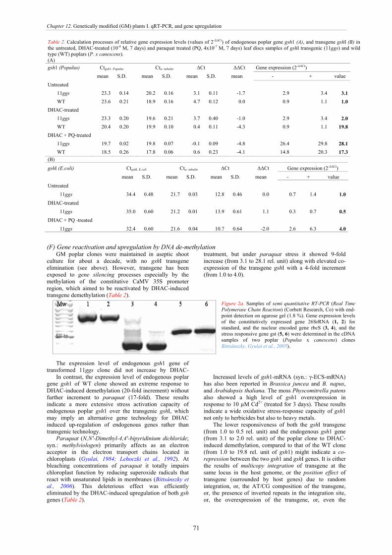
Chapter 12. Genetically modified (GM) plants I. qRT-PCR, and gene upregulation
71
(F) Gene reactivation and upregulation by DNA de-methylation
GM poplar clones were maintained in aseptic shoot culture for about a decade, with no gshI transgene elimination (see above). However, transgene has been exposed to gene silencing processes especially by the methylation of the constitutive CaMV 35S promoter region, which aimed to be reactivated by DHAC-induced transgene demethylation (Table 2).
The expression level of endogenous gsh1 gene of transformed 11ggs clone did not increase by DHAC-
treatment, but under paraquat stress it showed 9-fold increase (from 3.1 to 28.1 rel. unit) along with elevated co-expression of the transgene gshI with a 4-fold increment (from 1.0 to 4.0).
In contrast, the expression level of endogenous poplar gene gsh1 of WT clone showed an extreme response to DHAC-induced demethylation (20-fold increment) without further increment to paraquat (17-fold). These results indicate a more extensive stress activation capacity of endogenous poplar gsh1 over the transgenic gshI, which may imply an alternative gene technology for DHAC induced up-regulation of endogenous genes rather than transgenic technology.
Paraquat (N,N'-Dimethyl-4,4'-bipyridinium dichloride; syn.: methylviologen) primarily affects as an electron acceptor in the electron transport chains located in chloroplasts (Gyulai, 1984; Lehoczki et al., 1992). At bleaching concentrations of paraquat it totally impairs chloroplast function by reducing superoxide radicals that react with unsaturated lipids in membranes (Bittsánszky et al., 2006). This deleterious effect was efficiently eliminated by the DHAC-induced upregulation of both gsh genes (Table 2).
Increased levels of gsh1-mRNA (syn.: γ-ECS-mRNA) has also been reported in Brassica juncea and B. napus, and Arabidopsis thaliana. The moss Physcomitrella patens also showed a high level of gsh1 overexpression in response to 10 µM Cd2+ (treated for 3 days). These results indicate a wide oxidative stress-response capacity of gsh1 not only to herbicides but also to heavy metals.
The lower responsiveness of both the gshI transgene (from 1.0 to 0.5 rel. unit) and the endogenous gsh1 gene (from 3.1 to 2.0 rel. unit) of the poplar clone to DHAC-induced demethylation, compared to that of the WT clone (from 1.0 to 19.8 rel. unit of gsh1) might indicate a co-repression between the two gsh1 and gshI genes. It is either the results of multicopy integration of transgene at the same locus in the host genome, or the position effect of transgene (surrounded by host genes) due to random integration, or, the AT/CG composition of the transgene, or, the presence of inverted repeats in the integration site, or, the overexpression of the transgene, or, even the
Table 2. Calculation processes of relative gene expression levels (values of 2-ΔΔCt) of endogenous poplar gene gsh1 (A), and transgene gshI (B) in the untreated, DHAC-treated (10-4 M, 7 days) and paraquat treated (PQ, 4x10⁻⁷ M, 7 days) leaf discs samples of gshI transgenic (11ggs) and wild type (WT) poplars (P. x canescens). (A) gsh1 (Populus) Ctgsh1. Populus Ctα- tubulin ΔCt ΔΔCt Gene expression (2-ΔΔCt)
mean S.D. mean S.D. mean S.D. mean - + value Untreated
11ggs 23.3 0.14 20.2 0.16 3.1 0.11 -1.7 2.9 3.4 3.1WT 23.6 0.21 18.9 0.16 4.7 0.12 0.0 0.9 1.1 1.0
DHAC-treated 11ggs 23.3 0.20 19.6 0.21 3.7 0.40 -1.0 2.9 3.4 2.0WT 20.4 0.20 19.9 0.10 0.4 0.11 -4.3 0.9 1.1 19.8
DHAC + PQ-treated 11ggs 19.7 0.02 19.8 0.07 -0.1 0.09 -4.8 26.4 29.8 28.1WT 18.5 0.26 17.8 0.06 0.6 0.23 -4.1 14.8 20.3 17.3
(B)
gshI (E.coli) CtgshI. E.coli Ctα- tubulin ΔCt ΔΔCt Gene expression (2-ΔΔCt)
mean S.D. mean S.D. mean S.D. mean - + value
Untreated 11ggs 34.4 0.48 21.7 0.03 12.8 0.46 0.0 0.7 1.4 1.0
DHAC-treated 11ggs 35.0 0.60 21.2 0.01 13.9 0.61 1.1 0.3 0.7 0.5
DHAC + PQ -treated 11ggs 32.4 0.60 21.6 0.04 10.7 0.64 -2.0 2.6 6.3 4.0
Figure 2a. Samples of semi quantitative RT-PCR (Real Time Polymerase Chain Reaction) (Corbett Research, Co) with end-point detection on agarose gel (1.8 %). Gene expression levels of the constitutively expressed gene 26SrRNA (1, 2) for standard, and the nuclear encoded gene rbcS (3, 4), and the stress responsive gene gst (5, 6) were determined in the cDNA samples of two poplar (Populus x canescens) clonesBittsánszky, Gyulai et al., 2005).

Chapter 12. Genetically modified (GM) plants I. qRT-PCR, and gene upregulation
72
environmental conditions played role. Nevertheless, under PQ stress the high expression level of poplar gsh1 (9-fold increment from 3.1 to 28.1 rel. unit) and transgene gshI (4-fold from 1.0 to 4.0 rel. unit) of 11ggs clone exposed to the
combined treatment of DHAC and PQ may indicate an elevated co-expressions of the two genes (Table 2).
To conclude, by means of molecular barcoding the transgenes, either coding or reporter genes, can be detected in the genetically modified GMO plants for both GM and anti-GM purposes. The sequence differences between the foreign gene and the resident genes make it feasible to
design GMO-specific barcodes. These results also imply an alternative gene technology of DHAC induced up-regulation in poplars (Appendix 1) rather than any transgenic technology (Appendix 2).
References (for all papers cited:
Bittsánszky A, G Gyulai, I Bock, LY Murenets, M Czakó, T Kömíves, H Rennenberg (2015) Barcoding of transgenes in GM plants. In. Ali MA, G Gyulai, F Al-Hemaid (Eds) Plant DNA barcoding and phylogenetics. LAP Lambert Academic Publ. Germany. Chapter 17. pp. 269-278. ISBN-13: 978-3-659-28095-5 Appendix 1. Lists of sections (I - VI), and distribution of Populus species (1 - 24). I. section Populus - aspens and white poplar. Circumpolar subarctic and cool temperate)
1. Populus tremula (Common Aspen, Trembling Aspen or Eurasian Aspen) (Europe, northern Asia) 2. Populus tremuloides (Quaking Aspen or Trembling Aspen) (North America) 3. Populus grandidentata (Bigtooth Aspen) (Eastern North America) 4. Populus adenopoda (Chinese Aspen) (Eastern Asia) 5. Populus sieboldii (Japanese Aspen) (Eastern Asia) 6. Populus alba (White Poplar) (Southern Europe to central Asia) (warm temperate) 7. Populus × canescens (P. alba × P. tremula) (Grey Poplar)
II. section Aegiros - black poplars or cottonwoods. North America, Europe, western Asia; temperate 8. Populus nigra (Black Poplar) (Europe 9. Populus × canadensis (P. nigra × P. deltoides) (Hybrid Black Poplar) 10. Populus deltoides (Eastern Cottonwood) (Eastern North America) 11. Populus fremontii (Fremont Cottonwood) (Western North America) 12. Populus petrowskyana (Russian Poplar) (Europe/Asia)
III. section Tacamahaca balsam poplars. North America, Asia; cool temperate
Figure 2b. Samples for quantitative RT-PCR(quantitative Real Time PolymeraseChain Reaction) measurements(Corbett Res., Co) of the expressionof plant gsh1 genes in three poplar(Populus x canescens) clones(11ggs, 6Lgl, and Wild Type - WT),and compared to the concentrationseries of control DNAs (1 to 1000times dilution series) and NTC (NonTemplate Control). Relativefluorescence (dR) and PCR cyclenumbers are indicated (Bittsánszky,Gyulai et al., 2006; Gyulai et al.,2012).
Figure 3. Molecular pathways of enzymatic methylation, demethylation, and spontaneous deamination of DNA nucleotides (5-mC = C5-methyl cytosine, MTase = DNA methyltransferase) (Alzohairy, Gyulai et al., 2016) (see Chapter 1. Fig.1d., Chapter 4. Fig.1b).

Chapter 12. Genetically modified (GM) plants I. qRT-PCR, and gene upregulation
73
13. Populus angustifolia (Willow-leaved Poplar or Narrowleaf Cottonwood) (Central North America) 14. Populus balsamifera (Ontario Balsam Poplar) (Northern North America) 15. Populus trichocarpa (Western Balsam Poplar or Black Cottonwood) (Western North America) 16. Populus laurifolia (Laurel-leaf Poplar) (Central Asia) 17. Populus simonii (Simon's Poplar) (Northeast Asia) 18. Populus maximowiczii (Maximowicz' Poplar) (Northeast Asia)
IV. section Leucoides necklace poplars or bigleaf poplars. E-N America, eastern Asia; (warm temperate) 19. Populus heterophylla (Swamp Cottonwood) (Southeastern North America) 20. Populus lasiocarpa (Chinese Necklace Poplar) (Eastern Asia) 21. Populus wilsonii (Wilson's Poplar) (Eastern Asia)
V. section Turanga subtropical poplars. Southwest Asia, east Africa; subtropical to tropical 22. Populus euphratica (Euphrates Poplar) (Southwest Asia) (highly tolerant to soil salinity!) 23. Populus ilicifolia (Tana River Poplar) (East Africa)
VI. section Abaso Mexican poplars. Mexico; subtropical to tropical 24. Populus mexicana (Mexico Poplar) (Mexico)
Illustrations
Appendix 2. Owen Paterson: ‘Anti-GMO stance of Green Blob, Greenpeace condemn poor to starvation, death Owen Patterson | February 24, 2015 http://geneticliteracyproject.org/2015/02/24/owen-paterson-anti-gmo-stance-of-green-blob-greenpeace-condemn-poor-to-starvation-death/
Speaking Tuesday in Pretoria, South Africa, former UK environment secretary Owen Paterson accused the European Union and Greenpeace of condemning millions of people in developing countries to economic dependency on aid, starvation and death by their refusal to accept the science behind genetically modified crops and other life saving advances in plant sciences. Owen denounced what he called the “green blob” of officials and gullible media that misrepresent the consensus science, likening Greenpeace to the Luddites who smashed textile machinery in the nineteenth century. He accused the EU of “neo-colonialism at its worst” by restricting food production within its own borders. Paterson said the world is on the cusp of a green revolution of the kind that fed a billion people in the 1960s and 1970s as the world’s population soared–but that revolution is threatened by well-meaning Westerners who he maintains are imposing their food “fetishes” on the developing world. Here is the full text of Paterson’s speech to the International Service for the Acquisition of Agri-biotech Applications (ISAAA): Thank you all very much.
Thank you, Doctor Obokoh for that kind introduction. It’s a great pleasure to be able to speak at the Annual South African agricultural biotechnology industry/ISAAA media conference. You are all doing so much important – indeed life-saving – work to bring the benefits of modern agricultural technology to this continent.
This is a time of extraordinary opportunity for Africa. Progress in the plant sciences is opening up the promise of a second Green Revolution, one that can not only feed the 9 to 10 billion people that will inhabit our planet in 2050, but feed them well – one that can finally end the shame of the nearly one billion who still go to bed every night hungry and malnourished.
It is a revolution, powered by cutting-edge science, that can drive economic development from the bottom up. I’m talking about authentic, indigenous growth – the only kind that really takes root that empowers individuals that breaks the cycle of aid and dependency and can make every nation on this Earth a strong, competitive player in global economic growth.
No place on Earth holds more promise in this respect than Africa. With its vast, and as yet underutilized resources of land, soil, water and sun, Africa
is wonderfully situated to match or exceed the success of Brazil – a nation that agricultural development helped catapult into the front ranks of world trade – but it will only happen if African countries embrace farming systems based on modern technologies. The Green Blob
This is also a time, however, of great mischief, in which many individuals and even governments are turning their backs on progress. It’s a strange time, really, in which the privileged classes increasingly fetishize their food and seek to turn their personal preferences into policy proscriptions for the rest of us.
Not since the original Luddites smashed cotton mill machinery in early 19th century England, have we seen such an organized, fanatical antagonism to progress and science. These enemies of the Green Revolution call themselves “progressive,” but their agenda could hardly be more backward-looking and regressive.
They call themselves humanitarians and environmentalists. But their policies would condemn billions to hunger, poverty and underdevelopment. And their insistence on
mandating primitive, inefficient farming techniques would decimate the Earth’s remaining wild spaces, devastate species and biodiversity, and leave our natural ecology poorer as a result.
I call them the “Green Blob” – a reference to a 1950s Sci-Fi movie starring Steve McQueen in which a blob-like alien attacks Earth and swallows everything in its path: the environmental pressure groups, renewable energy companies and some public officials who keep each other well supplied with lavish funds, scare stories and green tape. This tangled triangle of unelected busybodies claims to have the interest of the planet and the countryside at heart, but it is increasingly clear that it is focusing on the wrong issues and doing real harm while profiting handsomely.
The Blob operates on two levels. First, by a pernicious grab for funding dollars with literally hundreds of them orbiting the honey pot of Europe. Secondly, with an ideological belief that Europe should abdicate its fundamental responsibility to feed its own people.
Neo-colonialism at its worst, Europe sits on some of the most fertile land on the planet, and yet imports food from the rest of the world which requires the equivalent of 35m hectares of farmland to produce.
There are many impediments standing between the vision of agricultural progress and Africa, of course, but none is more pernicious than the Blob. It is supported by massive funding provided by the EU itself, as well as numerous church and humanitarian groups, and the well-meaning but misguided generosity of the privileged classes in Europe and elsewhere. It has undue influence in the media, government and international institutions. Unfortunately, few question either its credentials or motives. I will be speaking more about the Green Blob and how we need to push back and reassert the fundamental primacy of science. But first I want to talk about the good news – and there is a lot of good news to talk about. The Good News About Biotech
As you know, the International Service for the Acquisition of Agri-biotech Applications, ISAAA, has just come out with its latest report on the worldwide adoption of genetically modified crops. As before, it records a remarkable success story. 2014 was the 19th year of successful commercialization of biotech crops, 18 million farmers, of which 90 per cent were small and resource-poor, planted a record 181 million hectares of biotech crops in 28 countries. GMO-versions of food staples like potato in the United States and eggplant in Bangladesh have been approved for planting. The United States continues to lead the way and saw a 5.5-fold increase in hectares of drought tolerant maize planted.
Biotech continues to be the most rapidly adopted agricultural technology in history. During the 19 years GMO crops have been commercialized, we have seen a more than 100-fold increase in the area planted. The facts also completely belie the propaganda that GMOs are only for the wealthy nations. In fact, more than 90 per cent of the farmers planting biotech are smallholder farmers in nations in the developing world. For the third year in a row, less developed countries planted more biotech hectares than the entire developed world.
Farmers are famously risk-averse. They know that the misapplication of resources can spell the difference between a bumper harvest and total crop failure. That’s why it’s even more remarkable that nearly 100 per cent of all those farmers who plant biotech
III./ 13.
I./ 6.
II./ 10.
I./ 3.
III./ 15.
IV./ 19. VI./ 24. V./ 22.

Chapter 12. Genetically modified (GM) plants I. qRT-PCR, and gene upregulation
74
crops have yet to go back to the old ways. They continue to choose to plant biotech year after year because biotech plants work. It’s really that simple.
ISAAA report a number of very heartening breakthroughs. The drought-tolerant maize technology donated to Africa by Monsanto is expected to begin commercial planting in 2017.
Field trials have been given the go-ahead in Cameroon, Egypt, Ghana, Kenya, Malawi, Nigeria and Uganda while trials have been conducted on a broad range of new crops, from biotech bananas to maize to cotton and cowpeas. One can certainly hope that as the trials reveal the dramatic benefits of GMO, these countries too will make them available to all their famers.
They can certainly look to the success in South Africa, which is still the leader on this continent, with 2.7 million biotech hectares planted. But they might also take in the dramatic example of insect resistant Bt cotton in Burkina Faso, where farmers are rapidly and overwhelmingly embracing the efficiencies and improved yields represented by the GMO variety.
By 2013, in fact, almost 70 per cent of all cotton grown in Burkina Faso was Bt, which increased farmers’ yields on average 20 per cent over non-GMO cotton. It has also dramatically decreased pesticide applications – which in Africa are often done by hand, a 40 to 80 pound backpack filled with older pesticides strapped to one’s back. Bt-cotton has cut those applications from 6 to 2 or fewer and delivers a solution that is eminently more effective.
Within one season, Bt can transform the life of smallholder farmers, turning their farms into profit-making enterprises that allow them to send their children to school rather than out into the fields, and to buy their families enough to eat – and of course with better nutrition comes better health.
Even where farmers have voted overwhelmingly for a choice of GM technology and the benefits have been tested and demonstrated in numerous studies, the Green Blob has been tireless in myth making and misinformation. Take the allegations of Indian farmer suicides. Anti-GM green groups stated that the introduction of GM crops had brought about an increase of suicides among India’s farmers. It is imperative in the case of such tragedy to be accurate about causes if you are to help people driven to suicide.
Professor Ian Plewis from the University of Manchester clarifies that farmer suicide rates in India are similar to the best estimates of the rates in Scotland and France, around 30 per 100,000 farmers. While these rates are still tragic, they existed at the same level prior to the introduction of GM cotton to India. He states, “In fact, the available data does not support the view that farmer suicides have increased following the introduction of Bt cotton. Taking all states together, there is evidence to support the hypothesis that the reverse is true. And in the global context, over 80 per cent of the world’s cotton crop has been GM for several years. The success of insect protected GM cotton has given Burkina Faso, one of the poorest countries in the world, a new tool to boost their main economic activity: cotton production. Farmers have seen at least 66 per cent less pesticide applied, 20 per cent increase in yield, and at least $87 per hectare increase in their profit.
Green Blob myths like “GM Indian Farmer Suicide” are retarding the adoption of new science in the developing world. Yet Africa is showing Europe the way. In 2014 the 28 member states of the EU recorded 12 field trials of GM crops. This compares with 13 projects in Uganda, Kenya and Nigeria. These three countries are doing more active biotech field research than the entire rich continent of Europe. Four Anti-GMO Myths and the Truth About Biotech
Around the globe, in fact, the increasingly widespread adoption of biotech is exploding the myths of the anti-GMO campaigners. It is worth taking a moment to examine four of these myths, taking them one at a time:
Myth #1 is their recurrent implication that farmers are stupid, fooled by biotech companies into paying more for GMO seeds when they would be far better off without them. Well, I tend to think farmers have a pretty good understanding of their bottom line, and I can’t imagine any farmer – in my own country or in the developing world – spending one extra dollar, euro, pound, or rand that he absolutely didn’t have to spend.
As it happens, the most current and extensive research on the subject bears that out. A recent analysis of previous major studies – conducted by researchers at Germany’s Göttingen University, found that globally since their introduction almost two decades ago, biotech crops have increased crop yield overall by 22 per cent, increased farmer profits by 68 per cent, and reduced chemical pesticide use by 37 per cent. They also found that these yield and profit gains are the highest in less developed countries, not the industrialised countries. In other words, the supposedly dumb farmer of Blob mythology is actually a lot smarter than the Green Blob itself.
Myth #2 is that forsaking modern agricultural technology – going organic – will benefit the environment. The opposite is actually the truth.
A few years ago, another group of researchers at Stanford University in the United States found that without the advances in agricultural technology since 1960, we would need more than twice as much land to grow all the food we produce today. That’s almost two billion more hectares of ploughed land than today, more than the entire landmass of Russia, the largest nation on the globe spreading over nine time zones. Two billion hectares is more than twice the entire area of the United States. The equivalent of three Amazon rain forests.
I can remember as a child seeing traumatic news bulletins with images of starving people on the Indian subcontinent. The father of the Green Revolution, Norman Borlaug – “The man who fed the world” and Nobel Peace Prize Laureate in 1970 – changed that by transferring wheat with new genetics from the Americas to the Indian sub-continent in the 1960s. India is now a major food exporter.
Borlaug and others harnessed innovation to completely change the way we farm. For example, it has been estimated that the production of a given quantity of a crop now requires 65 per cent less land than it did in 1961. Between 1967 and 2007 world food production increased by 115 per cent but land use only increased by eight per cent. Indur Goklany has calculated that if we tried to support today’s population using the production methods of the 1950s, instead of farming 38 per cent of all land, we would need to use 82 per cent.
As Borlaug said, “There are 6.6 billion people on the planet today, with organic farming we could only feed 4 billion of them. Which two billion would volunteer to die?” Agriculture always needs to balance our demands for more food whilst improving the environment and biodiversity. It is clear that sustainable intensive agriculture produces more food on less land, and therefore protects wild lands for wild life, for recreation, for urban development.
There is less pressure on land that is being used for wildlife and recreation. And the whole huge area generates tourism cash and employment for local economies. In other
words, modern agriculture – with its GMOs, nitrogen fertilizer and modern pesticides – has probably done more to save natural habitat, support biodiversity, and save endangered species than all the other environmental, NGO and UN conservation activities put together. The Keystone Alliance, a collaborative effort of industry and conservation groups in the United States, has demonstrated the environmental benefits of modern agriculture on the micro-level as well. In each of the major crops studied, inputs of water, fertilizer and energy have been slashed and the environmental impact dramatically diminished at the same time that yields have skyrocketed. Maize yields, for instance, increased by 64 per cent in the 31 years between 1980 and 2011. Land use, however, decreased by 30 per cent, soil erosion by 67 per cent, irrigation water by 53 per cent, and energy use by 44 per cent.
The revolution in no-till farming, was invented in the later 1960s a long time before GMOs. Modern herbicides and GMO crops have significantly extended its scope because farmers in many locations no longer have to plough the land to manage weeds. Tractor fuel is saved and topsoil is increasingly returning to its original structure and beneficial microorganism content and, in the United States, rivers and streams are spared the soil run-off that the EPA used to define as one of the top environmental problems in that country.
And the most widely used herbicide in no-till – the glyphosate that NGOs so love to criticize – is enormously healthier for the environment and the humans and animals that live there than the chemistries it replaced. While glyphosate is indeed bad for weeds, its toxicity to animals is less than, not equivalent, but significantly less than, vinegar. Something to think about next time you dresses your salad.
Which brings me to Myth #3: the insistence by anti-GMO campaigners that biotech crops are somehow unsafe to eat. It’s a claim they continue to hang onto in the face of many hundreds of studies testifying to GMO safety – the overwhelming majority of all the studies that have been conducted, a large number of them sponsored by governments and completely independent of industry.
It’s a claim they persist in despite the universal opinion of every independent scientific institution globally, (including the European Commission!) that GMOs are as safe as any other food, and the fact that people in the United States have been consuming diets replete with GMOs for over 15 years now without one documented adverse health effect – not so much as a sniffle or a tummy ache. Even in Europe, overwhelmingly all the animal products produced – meat, milk, cheese, eggs – come from animals fed on imported GM maize and GM soya meal. Most European farmers have, for the last almost two decades, not been permitted to grow these crops – with the one exception of a single strain of maize. But European livestock farmers import millions of tons annually – without these imports currently the European livestock market would have collapsed.
In a rational world, a recent study out of the University of California Davis (one of the leading agricultural universities in the United States) would end the call for ‘animal studies’ of GMOs once and for all. The study compared health outcomes in over 100 billion cattle and other livestock before GMOs were introduced in 1996 and after – when quite quickly GMOs accounted for approximately 90 per cent of all animal feed. In effect, US livestock production has amounted to the largest animal feeding study ever conducted. And what was the difference in health outcomes found by the researchers? Zero. None. The animals were just as healthy after GMOs were introduced as before. Of course, as with the other myths, the myth of GMOs’ adverse health effects isn’t just wrong – it’s the inverse of the truth.
Generally ignored, for instance, is the widespread problem of mycotoxin contamination, often the result of insect chewing and especially boring into the growing crop, which allows the entry into the plant of fungal pathogens. The problem afflicts a wide range of foods and feed, such as maize, sorghum and peanuts. Without doubt, many mycotoxins are most effectively controlled by planting GMO crops engineered with Bt insect resistance.
The FAO estimates that up to half of some food crops are affected. Globally, it is estimated that more than five billion people in the developing world are exposed to these naturally occurring toxins, which can suppress the immune system, retard growth and cause cancer and liver disease in both livestock and humans. In Africa, the rural poor are chronically exposed to unsafe levels of these poisons. In 2003, 120 people died in Kenya after eating maize with very high aflatoxin levels.
In the industrialized nations, organic growers have long sprayed with spores of the whole Bt bacterium to control for insects. This organism occurs naturally in the soil, after all, and has proved safe for mammals and humans. But when scientists engineered a plant that produced one protein found in the Bt cells as a part of its built-in defenses, the Blob fought tooth and nail to deprive the developed world of its benefits.
In a nationally funded trial conducted at the respected University of Milan, two varieties of maize were involved. Compared with conventional maize, Bt-maize not only increased yield by 28-34 per cent, but reduced the fungal toxin fumonisin from 6,000 parts per billion in the non-GMO maize to 60 parts per billion or less in the Bt-maize. The conventional maize containing over 6,000 parts per billion was unfit for human consumption under both Italian and European law. Despite the health implications, these results were shamelessly suppressed by the activist influenced Italian government which organized it. Once again, the myth is turned on its head: it’s not GMOs, but the anti-GMO Green Blob that is the real danger to human health.
Myth #4 is that biotech is only good for farmers and has no consumer benefits. Once again an inverse of the truth. I count increased protection of wild lands by focusing production sustainably, and cheaper food, as being fundamentally important “consumer benefits”. There are more specific examples too.
Biotechnology has already given us soybeans with higher oleic acid that don’t produce cholesterol-elevating trans fats when heated. Currently, a new biotech tomato is being tested that mimics good cholesterol. Tomatoes are coming with high concentrations of cancer-fighting anthocyanins. Non-browning apples have recently been approved by US regulators, which should potentially greatly reduce waste through less spoilage. Healthier GMO potatoes have also been approved and peanuts are currently under development that lack two of the most intense allergens that pose such a danger to so many of our children.
Only ten days ago, I was in Canberra and saw real progress on oilseed crops that will provide a sustainable source of long chain omega-3 fatty acids providing better nutrition to humans and farmed fish. This could stop the obscenity of feeding huge numbers of farmed fish with wild fish.
In addition, in future, it might be possible to have the oil yields of oil palm replicated and even exceeded from GM
broad acre crops that contain oil in their leaves and stems. So GM developments in oil producing plants could help save vulnerable orangutan habitats encroached by palm oil plantations.
Few people know that the first biotechnology product approved for food was rennet, an enzyme used to make cheese. Today, 90 per cent of the cheeses we eat use GMO rennet because it’s safer and more effective. GMO-enzymes are routinely used in the production of bread, wine and beer.
All the insulin routinely used to keep diabetics alive is from GMO-bacteria. Previously insulin was produced from the pancreases of cattle and pigs. A single diabetic
would require the pancreases of 50 pigs for a year’s supply. Before GMO-bacteria produced insulin, one major industrial insulin producer processed eleven tons of pig’s pancreases every day – from a daily slaughter of 100,000 animals. Unfortunately, hugely promising GMO techniques that could protect yoghurt starter cultures from infection have been kept off the market due to fear of consumer backlash. Perhaps the most promising development, however, is biofortification, especially for the developing world, where so many lack the nutrients essential for health and well-being. Golden Rice, Greenpeace and the Anti-Humanitarians

Chapter 12. Genetically modified (GM) plants I. qRT-PCR, and gene upregulation
75
The flagship biofortified technology was developed 15 years ago by two German Professors Ingo Potrykus and Peter Beyer. Called Golden Rice, it is a miracle grain enhanced with vitamin-A-producing beta-carotene. In 2001 the inventors donated the technology as a potential additional intervention for vitamin A deficiency, for development and deployment by the public sector in developing countries so that it could benefit the poor of the world.
Absence of a source of vitamin A in the diet, vitamin A deficiency, is the principal cause of childhood blindness globally, affecting 500,000 children annually of which half die within a year or two. Vitamin A deficiency is also a nutritionally acquired immune deficiency syndrome, so common diseases which should be survivable are lethal. Two million young children die as a result every year.
So let’s be clear. Although these deaths are preventable, 6,000 children alive today will be dead tomorrow. (By comparison Ebola has tragically killed about 9,000 in the last year: about 25 a day). Many of those millions of lives could have been saved if Golden Rice had been available in their diet, and it could have been already for several years, but for the on-going opposition of well-financed anti-GMO activist groups and their ceaseless campaign to frighten people and pressure governments to keep Golden Rice off the market.
The leader of that opposition, with a combined global war chest estimated to exceed US $500 million, has been Greenpeace, with its combination of highly sophisticated PR and un-scientific scaremongering. Greenpeace originally claimed Golden Rice wouldn’t work, but once its efficacy had been proven beyond a shadow of a doubt, they switched to saying that the poor should simply buy vitamin supplements and eat fresh vegetables instead – as if families living on less than $2 a day can afford such luxuries.
But Greenpeace doesn’t content itself with mere PR. In 2013, an organization in the Philippines who lists Greenpeace amongst its partners, used a tactic that has been used all over the world by Greenpeace – violently attacking and destroying agricultural research they oppose. The group, known as MASIPAG, claims to be a “farmer-led network,” destroyed a field trial of Golden Rice. But local officials reported that the thugs who attacked the fields had been bused in from the city.
Shamefully, Greenpeace isn’t alone in its support for the MASIPAG anti-GMO eco- terrorists. MASIPAG’s list of supporters reads like a directory of misguided European church and government sponsored social justice and development groups. Perhaps one should put the words “so-called” before social justice. A short list of MASIPAG’s funding sources include: (1) The Swiss Catholic pastoral development group known as The Fastenopfer Catholic Lenten Fund; (2) Misereor, the German Catholic Bishops’ Organization for Development Cooperation, which receives financial support from the German government; (3) The Swedish Society for Nature Conservation, which is funded by the Swedish Ministry for Foreign Affairs; (5) Trocaire, the official development agency of the Catholic Church in Ireland, which receives funding from the Irish, UK and EU governments; It should be stressed that MASIPAG is just one of a proliferating network of anti- GMO groups and assorted activists that are operating in the developing world, often with NGO and EU support.
In 2011 Greenpeace attacked GM wheat in Australia which was part of exciting research to enhance the health benefits of this staple food crop. It was heartening to observe the very widespread backlash and condemnation by the Australian community against this criminal vandalism of trusted research. On 14 July 2011, the CSIRO Experimental Station at Ginninderra in Canberra was broken into and research plants were cut down. Some of the GM crop trial plots were partially destroyed. Greenpeace admitted liability. This incident was investigated by the Australian Federal Police and two Sydney women were charged in relation to the incident, and both women later pleaded guilty to charges of damaging Commonwealth property. On 1 August 2012, CSIRO received a reparation payment of $282,560 from Greenpeace. In November 2012 the two women received a 9 month suspended sentence, to be of good behaviour for 12 months with $1,000 security, for each defendant. The question must be asked, when did so many of our “humanitarian” organizations become so disdainful about the lives of the desperately poor, whom they are supposed to be helping? How long have they been putting ideology over humanity? Do Greenpeace supporters understand that the conduct of the organization that they give to has been truly wicked? Patrick Moore, one of the early leaders of Greenpeace in the 1970’s when it took account of science and respected human life, has broken with his old organization for just this reason. He now works to expose Greenpeace’s actions in the developing world and has joined with Golden Rice inventor Ingo Potrykus in calling for the organization to be tried for crimes against humanity. So I say to my friends in Europe and in the United States: next time some young volunteer stops you on the street to ask for money for Greenpeace, ask them about Golden Rice. They’ll want to talk about all the polar bears and whales they claim to have saved, but ask them instead about the millions of children that their organization is helping condemn to blindness and early death. It should also be recognized, however, that there are some humanitarian and environmental groups that are coming to recognize the important role that biotech can play in alleviating human suffering and spurring development. I’m thinking particularly of organizations such as Oxfam and the Nature Conservancy, whose initial opposition to GMOs has softened in the light of the overwhelming scientific evidence of their efficacy and safety. It’s time for these organizations to step up and show leadership on this urgent humanitarian issue.
Where also are the UN organisations WHO, FAO, UNICEF – all with nutritional improvement and development mandates? They have recognized the scourge of vitamin A deficiency as a very major – and cheap to control – problem for the last 25 years. Undoubtedly current interventions have saved millions of lives. But VAD (Vitamin A Deficiency) induced preventable deaths continue, and now, as a result of Golden Rice, the half of the world where rice is the staple could benefit from a free nutritional trait. But, cowed by activist polemic, these huge and capable institutions have chosen not to believe in science.Here is my plea to them: You have rejected the world of activist myth for scientific fact. Now use your moral authority to appeal to your colleagues in the NGO community. Convince them to do the right thing and support giving the developing world the GM tools it needs to feed its growing, and too often malnourished, population. The EU’s Retreat from Science
Of course, the greatest offender of all is the European Union itself, which in a twisted version of neo-colonialism has imposed its affluent organic affectations and anti-scientific policies on Africa. The Kenyan-born Calestous Juma, professor of the practice of international development at Harvard Kennedy School, is a former executive secretary of the UN Convention on Biological Diversity, who has repeatedly slammed the EU for strong-arming African nations not to grow GM crops and threatening to cut off imports if they dare to assert their independence. I am proud that when I served as the Secretary of State for Environment, Food and Rural Affairs, we were able to convince the European Council of Ministers to change European policy so that now individual countries can decide for themselves whether to plant GMOs or not. This is a significant reform. I hope that when we look back over these years it will prove to have been a watershed moment, as nation after nation in Europe seizes the enormous opportunity offered by this exciting technology. But we shouldn’t fool ourselves into thinking that one reform will solve the problem. The EU’s retreat from science has become more like a rout. Just last November,
the incoming president, Jean-Claude Juncker, refused to renew the contract for the professor of cell biology, Anne Glover, who had been so ably filling the role of the Commission President’s scientific advisor. For months, Greenpeace and other NGOs had been conducting a concerted campaign against Professor Glover, largely because of her outspoken, science- based support of GMOs. In response, some forty leading scientific organizations and over 770 individuals sent a letter in support of Professor Glover and her position. It is emblematic of Europe today – once the birthplace of modern science and home to many of its greatest achievements – that the anti-science know-nothings won the day. And to think that the Lisbon treaty was meant to ensure that Europe developed a knowledge-based economy! No chance when scientific evidence is only merited with the same influence as public opinion, which as we have seen, is so easily influenced by political activists.
The European retreat from science is often dressed up as the precautionary principle, which has the advantage of sounding “sciency,” but is in fact neither science-based nor by any legitimate definition a “principle.” It’s more like an impulse, or reflex, as clichéd and inept when it comes to the serious work of regulation as saying “better safe than sorry.” No one can really define it adequately. The best its advocates can do is say that if something could possibly cause harm, ban it. Former Greenpeace UK director Stephen Tindale now urges Europe to “move on from the theological dispute with respect to GMO crops”. Everyday, activists warn us of “risks”. But everything, everywhere and always, could cause harm. You can drown in an inch of water. Coffee in large enough doses causes cancer. And let’s not get started on cell phones. The EU finds itself in the ridiculous position that, according to its own pesticide regulations, it would have to ban coffee – and beer, and a thousand other consumer items – if they were sprayed on fields rather than sold in grocery stores.
The precautionary principle is so broad it effectively gives regulators the cover to ban or restrict anything at whim or according to whomever is exerting the most pressure. In other words, it replaces science-based regulation with politics. This drives the limits on the amount of pesticides in tap water, set at 0.1 parts per billion – the equivalent of one paracetamol tablet in an Olympic-sized swimming pool. We also saw the precautionary principle in action with startling clarity in the battle over neonicotinoids, or neonics, which activists accused of causing a “bee- pocalypse,” an imminent extinction of bees. Large-scale field studies and massive real-world science do not back up this claim. The EU’s own science didn’t back it up. Even at its most basic level, it was faulty: bee populations aren’t falling at a rapid rate. They’re not falling at all. For the last two decades that neonics have been on the market, bee populations have been rising, both in the EU and around the world. But the Green Blob was fierce on this one. I myself personally received 85,000 emails; very few of them were complimentary. Insisting, as we did at DEFRA, that policies be based on science – and the science did not support a ban – wasn’t a popular position. Nor was it, as we know, the winning position. The EU Commission, as is its habit, caved in to the activists. Working with allies, I ensure that they couldn’t muster a qualified majority for a ban among the member states, despite holding two votes on the issue. But democracy only goes so far in Brussels. So EU officials simply took it on themselves to make the final decision. They overrode their own scientists and banned neonics starting at the end of 2013. The result was predictable. I say that because it was indeed predicted by farmers and others who said the ban would remove their best defence against insect pests and force them to use older, less effective pesticides that are worse for bees. Which is precisely what has happened: despite multiple sprayings with pyrethroid, England’s oil seed rape crop has been devastated, with losses over 40 per cent in some counties. Europe as a whole is looking at a 15 per cent reduction in rapeseed this year as a result of the ban. Another example of the precautionary principle creating realised risks.
Just recently this scandal developed further – some have called it Beegate – when a blogger in Brussels by the name of David Zaruck uncovered a memo that had mistakenly been left on the web by one of the scientists who was most vocal in pushing for a ban. That memo – the minutes of a meeting held back in 2010 – detailed in their own words how he and other leading scientists working for the EU-funded “Task Force” on neonics conspired to manufacture studies to support a ban. Perhaps one should put the word “scientists” here in quotes. Deciding on the outcome of your research before you even conduct it is not how science is supposed to be done. But we have apparently entered a brave new world in the EU where everything is backward.
For instance, there’s the startling fact that the “technologically advanced” EU, which boasts incredibly fertile soils and extremely friendly climates for agriculture, cannot even feed itself and has been reduced to becoming a net importer of food. What that means, of course, is that we simply export our environmental footprint elsewhere. It also means Europe is not only not contributing, we are a net drag on humanity’s foremost imperative in the 21st century – growing enough food to feed everyone on this planet, and to feed them well.
Today, nearly 805 million people do not have enough to eat, about one out of every nine people in the world. The majority of them are children, who will never have the same chance at a good life as others because hunger will stunt their development, shrink their innocent capacity for hope, and leave their small bodies prey to any number of terrible illnesses.One in three children in many developing nations today has been stunted by hunger. Sixty-six million attend school classes hungry every day. Poor nutrition causes nearly half of all the deaths of children less than five years of age – over three million children every year. This is the state of affairs that the EU’s precautionary principle would effectively preserve. The world population is seven billion today and will burst through the ten billion mark by 2050 or sometime soon after. Not long ago, one of our English celebrities was delivering a petition to our Prime Minister protesting against genetically modified foods. Being a famous and wealthy fashion designer, apparently, has given her particular insight into this field. In the process she was asked by a BBC interviewer what she would say to those who can’t afford to eat the high-priced organic food she recommends. Her answer was simple. They should simply “eat less.”
Too many of our fellow human beings are already eating less. I don’t believe that we, as Europeans, can really say that we belong to a humane society, a decent society, until every single one of them has access to good, nutritious food. Until every human being on this planet has enough to eat. That means that somehow we have to get right again with science. We need every possible tool available to meet this challenge. We simply cannot afford to take the most promising plant technologies off the table and keep them locked away in the regulatory drawer while children continue to go hungry.
Many centuries ago, science pulled the European continent out of the Dark Ages and established a whole new concept – one of on-going human progress. In our own time, the extraordinary science promoted by one-man, Norman Borlaug, accelerated that progress in the plant sciences just in time to save over a billion people from mass starvation in the 1960s and 70s. That was called the Green Revolution. We stand today at the beginning of a second Green Revolution – a period of extraordinary breakthroughs that can do the job if we let them.
We must let them. Despite the flack. Despite the propaganda. Despite the political setbacks we sometimes encounter. We must all push forward.
Myth versus fact; Green Blob versus Green Revolution. There is literally no challenge today that is more important. I commend African Nations for showing Europe the way. I am sure that science will overcome superstition. I am confident that together we will all succeed. Thank you very much!

Chapter 13. Genetically modified (GM) plants II. Environmental risk assessment
76
Genetically modified (GM) plants II. Environmental risk assessment (A) Introduction
Genetically modified organisms (GMO) interact with the environment through abiotic and biotic factors via trophic interactions. Herbivores are feeding on GM plants (direct effect), and are preyed by different predators (indirect effect) such as spiders (e.g., Theridion impressum), ladybirds (e.g., Coccinella septempunctata), and rove beetles (e.g., Tachyporus hypnorum).
The European Union (EU) and its member States are facing new challenges concerning the GM crop. According to the EU regulations, GM plants should be environmentally risk assessed before use (EFSA, 2010a,b). One of the key areas of risk assessment of GM plants is to assess its adverse effects on the non-target organisms (primarily the arthropods) (Wolt et al., 2010), in which processes the principal step is the so-called ‘tiered approach’ (USEPA, 1998, Romeis et al., 2006, 2008). It is based on the consideration of insecticidal protein producing
plants, and their tests in laboratory, glass-houses, and semi-field and field conditions (Poppy, 2000; Wilkinson et al., 2003; Garcia-Alonso et al., 2006; Rose, 2007). Ecotoxical tiered approach comprises the assessment of intended effects of GM plants based on three steps: Tier1: Laboratory studies (in vitro and in planta) for the worst case scenario; Tier 2: Semi-field studies in glass houses an cages which are close to real conditions; and Tier 3: Field studies under natural conditions. GM plants carry several points of economic, coexistence, environmental, animal feeding and food security, ethical, personal, and emotional concerns. This Chapter reflects a general scientific approach and is independent from concrete growing, economic, political and sociological relations and is exclusively to contribute to the scientific risk assessment.
(B) The environmental risk assessment (step-by-step approach) of GM plants
GM plants are capable of causing potential adverse effects to the environment. An important step in the problem formulation is to identify the aspects of the environment that need to be protected from hazardous factors. Nature needs of environmental protection concerning conservation of natural habitats of wild fauna and flora, and natural resources of biodiversity (EFSA, 2010ab). In the case of GM plants, the environment is
exposed to transgene(s), which may spread and initiate seven main sources of risks such as Plant-to-plant gene flow (vertical gene transfer); Plant-to-microorganisms gene flow (horizontal gene transfer); Interactions of the GM plant with target organisms; Interactions of the GM plant with non-target organisms; Impacts of the specific management techniques; Effects on biogeochemical processes; and Effects on human and animal health.
1. Plant-to-plant gene flow (vertical gene transfer)
In vertical gene transfers (VGT) the DNA flows from parent to offspring. In the case of a GM organism, potential adverse effects of vertical gene flow are: (a) Increased fitness of GM plant or of the transgenic (introgressed) wild relatives may make them more persistent, exacerbating weed problems which may need to be controlled by more complex weed control strategies causing environmental
harm. (b) The increased fitness of transgenic feral plants or of transgenic (introgressed) wild relatives in semi-natural or natural habitats may reduce the diversity/abundance of valued flora and fauna. Native plant species may be displaced, which in turn, might affect species that use those plants as food, shelter, etc. (EFSA 2010b).
2. Plant- to-microorganisms gene flow (horizontal gene transfer) During the horizontal gene transfer (HGT) an organism
incorporates its genetic material from another organism without being the ancestors/offspring of that organism. The evaluation of the effect of this HGT contains analysis of the transfer of recombinant plant DNA to initially receiving
micro-organisms and potential transfer to other organisms (microorganisms, or plants) and the potential consequences of such a gene transfer for the environment and human and animal health (EFSA, 2010b).
3. Interactions of the GM plant with target organisms Target organisms (TO) are those on which a GM plant
are intended to act and are usually plant pests or pathogens. All other organisms are considered as non-target
organisms. The investigation/analysis of resistance developed by the target organisms is very important (EFSA, 2010b).
4. Interactions of the GM plant with non-target organisms ERA considers the possible immediate and/or delayed
environmental impact resulting from direct and indirect interactions of GM plants with non-target organisms
(NTOs) (EFSA 2010b). Examples of non-target invertebrate organisms occurring in agro-ecosystems detailed by their ecological role are listed in Table 1.
5. Impacts of the specific management techniques The introduction of GM plants for cultivation may require specific management and cultivation
6. Effects on biogeochemical processes Biogeochemical processes are connected with the
movement, transformation and storage of energy, water, carbon, nitrogen and other elements in the ecosystems. Problem formulation should cover principally two scales, the production site, for example a field, in which the GM plant is grown; and the wider environment with which the field interacts through exchanges of energy, elements and materials. With respect to biogeochemical processes in the production site, the evaluation should address the potential impact of GM plants through factors such as:
(a) Release of recombinant gene products or GM specific metabolites into the plant-soil system, which may
directly influence the soil fertility, nutrient transformations and food webs; (b) Altered movement of other compounds from roots to soil, which may directly influence soil fertility, nutrient transformations and soil food webs; (c) Altered plant litter that decomposes differently from that of non-GM plants due to either the presence of specific compounds (e.g., toxic metabolites), or altered concentration of substances resistant to decomposition; (d) Altered uptake and cycling of plant nutrients within the plant-soil system, including the fixation of atmospheric nitrogen (see Chapters 10 and 17) (EFSA, 2010b).

Chapter 13. Genetically modified (GM) plants II. Environmental risk assessment
77
7. Effects on human and animal health
In the case of GMO risk assessment, it is required to assess whether the GM plant and its products might be harmful for human and animal health. If a potential hazard
has been detected, the risk to persons working with the GM plant, coming into contact with it or exposed to products from processed plants should be assessed (EFSA, 2010b).
(C) Post-Market Environmental Monitoring Plan
The monitoring plan should be targeted rather than considering every possible environmental aspect. The aims of environmental monitoring of the GM plant are: (1) to study any possible adverse effects of the GM plant identified in the formal risk assessment procedure, and (2) to identify the occurrence of adverse unforeseen effects of the GM plant or its use which were not anticipated in the ERA (EFSA, 2010b).
In the field (Tier 3), for instance in a maize stand (Fig. 1a) target organisms (TO) and non-target organisms (NTO)
can be monitored by different sampling methods. Arthropods occurring on plant surface can be observed visually (Fig. 1b). Flying insects (aphids, thrips, leafhoppers, flea beetles, predatory flies etc.), can be collected by yellow sticky card (Fig. 1d). Soil dwelling arthropods (ground beetles, rove beetles, mites, spiders) can be sampled by pitfall trap (Fig. 1c), or by litterbag method (Fig. 1e). The arthropods collected by litter bag can be retrieved using Berlese-funnel (Fig. 1f).
Figure 1. Sampling methods of target and non-target arthropods occurring on maize (Zea mays) (a): Visual observations (b), pitfall trap (c), yellow sticky card (d), litterbag method (e), and Berlese-funnels (f).
References EFSA (2010a) Scientific opinion on the assessment of potential impacts of
genetically modified plants on non-target organisms. EFSA Journal 8, 1877: 1–73.
EFSA (2010b) Guidance on the environmental risk assessment of genetically modified plants. EFSA Journal 8, 1879: 1–111.
Garcia-Alonso M, et al., (2006) A tiered system for assessing the risk of genetically modified plants to non-target organisms. Environmental Biosafety Research, 5: 57–65.
Poppy G, (2000) GM crops: environmental risks and non-target effects. Trends in Plant Science, 5: 4–6.
Romeis J, et al., (2008) Assessment of risk of insect-resistant transgenic crops to nontarget arthropods. Nature Biotechnology, 26(2): 203–208.
Romeis J, et al., (2006) Transgenic crops expressing Baccillus thuringiensis toxins and biological control. Nature Biotechnology, 24(1): 63–71.
Rose RI (2007) White paper on tier-based testing for the effects of proteinaceous insecticidal plant-incorporated protectants on non-target invertebrates for regulatory risk assessment. USDA-APHIS and US Environmental Protection Agency, Washington, DC, http://www.epa.gov/pesticides/biopesticides/pips/non-target-arthropods.pdf
USEPA. United States Environmental Protection Agency (1998) Guidelines for ecological risk assessment. Risk Assessment Forum and Office of Research and Development. Washington, DC. EPA/630/R-95/002F.
Wilkinson MJ, et al., (2003) Preventing the regulatory log jam; the tiered approach to risk assessments. Trends in Plant Science 8: 208–212.
Wolt JD, et al., (2010) Problem formulation in the environmental risk assessment for genetically modified plants. Transgenic Research, 19: 425–436.
Table 1. Examples of functional groups of different organisms (EFSA, 2010a) (see Appendix) 1, 2) Functional group Examples of taxonomic groups Herbivores Phloem-feeders: aphids (Hemiptera: Aphididae), leafhoppers (e.g., Hemiptera:
Cicadellidae) Cell-content feeders: thrips (Thysanoptera: Thripidae), spider mites (Acarina) Chewing: leaf beetles (Coleoptera: Chrysomelidae), Lepidoptera larvae, Diptera larvae
Natural enemies
Predators Beetles: Coleoptera (e.g., Coccinellidae, Carabidae, Staphilinidae) Predatory bugs: Heteroptera (e.g., Nabidae, Anthocoridae) Predatory flies: Diptera (e.g., Syrphidae) Lacewings: Neuroptera (e.g., Chrysopidae, Hemerobidae) Spiders: Araneae Mites: Acarina (e.g., Phytoseiidae)
Parasitoids Hymenoptera (e.g., Ichneumonidae, Braconidae, Aphelinidae) Parasites and Pathogens Bacteria, fungi, viruses Entomopathogenics Nematoda (e.g. Heterorhabditidae, Steinernematidae), pathogenic microorganisms
Pollinators Solitary and social bees (Hymenoptera: Apidae), hover flies (Diptera: Syrphidae); Coleoptera (e.g., Curculionidae, Scarabaeidae)
Decomposers Diptera larvae (e.g,. Phoridae, Sciaridae), Nematoda (e.g., Rhabditidae, Dorylaimidae), springtails (Collembola), mites (Acarina), earthworms (Haplotaxida: Lumbricidae), Isopoda, microorganisms
Plant symbionts Rhizobacteria, mycorrhiza
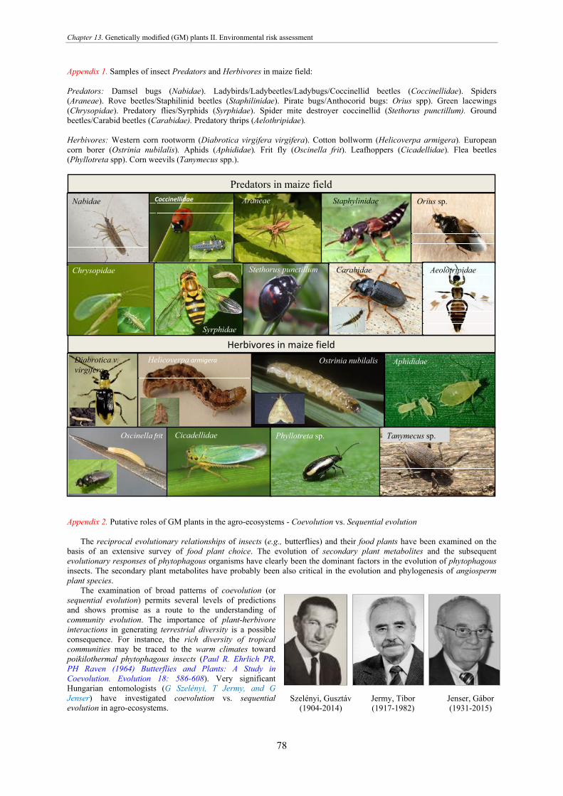
Chapter 13. Genetically modified (GM) plants II. Environmental risk assessment
78
Szelényi, Gusztáv (1904-2014)
Jenser, Gábor (1931-2015)
Jermy, Tibor (1917-1982)
Appendix 1. Samples of insect Predators and Herbivores in maize field: Predators: Damsel bugs (Nabidae). Ladybirds/Ladybeetles/Ladybugs/Coccinellid beetles (Coccinellidae). Spiders (Araneae). Rove beetles/Staphilinid beetles (Staphilinidae). Pirate bugs/Anthocorid bugs: Orius spp). Green lacewings (Chrysopidae). Predatory flies/Syrphids (Syrphidae). Spider mite destroyer coccinellid (Stethorus punctillum). Ground beetles/Carabid beetles (Carabidae). Predatory thrips (Aelothripidae). Herbivores: Western corn rootworm (Diabrotica virgifera virgifera). Cotton bollworm (Helicoverpa armigera). European corn borer (Ostrinia nubilalis). Aphids (Aphididae). Frit fly (Oscinella frit). Leafhoppers (Cicadellidae). Flea beetles (Phyllotreta spp). Corn weevils (Tanymecus spp.).
Appendix 2. Putative roles of GM plants in the agro-ecosystems - Coevolution vs. Sequential evolution
The reciprocal evolutionary relationships of insects (e.g., butterflies) and their food plants have been examined on the
basis of an extensive survey of food plant choice. The evolution of secondary plant metabolites and the subsequent evolutionary responses of phytophagous organisms have clearly been the dominant factors in the evolution of phytophagous insects. The secondary plant metabolites have probably been also critical in the evolution and phylogenesis of angiosperm plant species.
The examination of broad patterns of coevolution (or sequential evolution) permits several levels of predictions and shows promise as a route to the understanding of community evolution. The importance of plant-herbivore interactions in generating terrestrial diversity is a possible consequence. For instance, the rich diversity of tropical communities may be traced to the warm climates toward poikilothermal phytophagous insects (Paul R. Ehrlich PR, PH Raven (1964) Butterflies and Plants: A Study in Coevolution. Evolution 18: 586-608). Very significant Hungarian entomologists (G Szelényi, T Jermy, and G Jenser) have investigated coevolution vs. sequential evolution in agro-ecosystems.
Herbivores in maize field
Predators in maize fieldNabidae CoccinellidaeCoccinellidae Staphylinidae Orius sp.
Chrysopidae
Syrphidae
Stethorus punctillum Carabidae
Ostrinia nubilalisHelicoverpa armigeraDiabrotica v. virgifera
Aphididae
Oscinella frit Cicadellidae Tanymecus sp.Phyllotreta sp.
Araneae
Aeolotripidae

Chapter 14. C4 photosynthetic trees
79
C4 photosynthetic trees Introduction
C4 type of plant carbon uptake (‘fixation’ from the air) (e.g. sugarcane) is one of the three sub-types of photosynthesis including C3 (Calvin cycle) and CAM (Crassulacean Acid Metabolism) (e.g., pineapple). It is named for the 4-carbon molecules (e.g. malate) present in the first molecular product of the biochemical process, in contrast to the 3-carbon
molecule products (glycerate-3-P) in C3 plants. Both, C4 and CAM types of photosynthesis also ends in the C3 photosynthesis (Calvin cycle), so we may refer them as ‘C4-C3’ and ‘CAM-C3’ photosynthesis, and just use the short forms (C4 and CAM) (Table 1).
Table 1. The main characteristics of the three types of photosynthesis (C3; C4, and CAM)
Characteristics C3 plants C4-C3 plants CAM-C3 plants
The % of plant species 85 % 3 % 8 %
Types of Photosynthesis C3 C4-C3 CAM-C3
CO2 fixation pathway via C3 cycle only
C4 in the mesophyll cells then C3 in the bundle sheath cells. Mainly C4 grasses and sedges, about 79% of all C4 plants.
Temporally C4 at night, C3 at day time. Mostly succulents.
Leaf anatomy Large air spaces bordered by loosely arranged spongy mesophyll cells.
Leaf veins are surrounded by thick-walled BSC (Bundle Sheet Cells) and surrounded by thin-walled Mesophyll Cells (kranz/wreath/koszorú leaf anatomy).
Mesophyll cells have large, water-filled vacuoles.
Stomatal movement Stomata open at daytime, close at night.
Inverted stomatal cycle (open at night, close in the day).
Environmental effect Temperate Zone. Tropical or semi-tropical zones, high light intensity,
high temperature, drought conditions. Desert or arid (xeric) habitats.
About 7,600 plant species (only angiosperm) use C4 carbon fixation, which represents about 3% of all terrestrial plant species (C4 photosynthesis has not been developed ’yet’ in Gymnosperms) (Table 1).
C4 carbon fixation dominates in monocots (40% of monocot species follows C4), compared to only 4.5% of dicots. However, species of only 3 monocot families utilize C4 carbon fixation compared to 15 of dicots (Table 2). About 46% percent of grasses are C4. These include the food crops of maize, sugar cane, millet, and sorghum.
Of the dicots, the order Caryophyllales contains the most species; of them Chenopodiaceae use C4 carbon fixation the most, with 550 out of 1,400 species of the family. About 250 of the 1000 species of the related Amaranthaceae also use C4 (Table 2).
Biochemistry of C4 photosynthesis
C4 photosynthesis is the most efficient form of plant photosynthesis on the terrestrial Earth, due to its ability to concentrate CO2, delivered to the enzyme ribulose-1,5-bisphosphate carboxylase/oxygenase (RuBisCo), which is responsible for "fixing" CO2.
During this biochemical process,
Table 2. List of the angiosperm plant families / orders having C4-species (Sage, 2001).
Plant Family Orders MONOCOTS ( # of C4 species / genera), (% of C4 species / % of the Family) 1 Cyperaceae (1300/289), (18/27)
Poales 2 Poaceae (4600/372), (61/46) 3 Hydrocharitaceae (1/1), (0.1/1) Alismatales DICOTS ( # of C4 species / genera), (% of C4 species / % of the Family) 1 Acanthaceae (80/1)
Lamiales 2 Scrophulariaceae (14/1) 3 Chenopodiaceae (550/45), (7/39)
Caryophyllales
4 Amaranthaceae (250/11), (3/25) 5 Aizoaceae (30/5) 6 Caryophyllaceae (50/1) 7 Molluginaceae (3/1) 8 Nyctaginaceae (25/3) 9 Polygonaceae (80/1) 10 Portulacaceae (70/2), (1/16) 11 Asteraceae (150/8) (2/1.3) Asterales 12 Boraginaceae (40/1) Boraginales 13 Capparidaceae (2/1) Brassicales 14 Euphorbiaceae (250/1), (3/5) Malpighiales 15 Zygophyllaceae (50/4) Zygophyllales

Chapter 14. C4 photosynthetic trees
80
the oxygenation of ribulose 1,5-bisphosphate (RuBP) is suppressed (this is the photorespiration, catalyzed by enzyme RuBisCo, which can effectively fix O2 also, instead of CO2).
Technically, the first experiments (in 1950s) indicated that some plants do not use only the C3 carbon fixation, instead, they produce malate and aspartate in the first step of carbon fixation (Karpilov, 1960) and (Kortschak et al., 1965). The C4 pathway was finally elucidated by MD Hatch and CR Slack in Australia in 1966 (‘Hatch-Slack pathway’)
(Fig. 1a). As C4 photosynthesis is an adaptation to warm temperature and low atmospheric CO2 concentration, C4 evolution has been seen as a consequence of past atmospheric CO2 decline, as it happened about 32–25 million years ago (Mya) in the Oligocene period. The first transition from C3 to C4 photosynthesis may have occurred in the Chloridoideae subfamily of Poaceae. C4 plants also have higher water use efficiency (WUE) and nitrogen use efficiency (NUE) that are typically 1.3–4 times greater than in C3 plants.
Leaf anatomy generally is associated with the C4
photosynthesis, called kranz leaf anatomy, which is characterized by rings of Bundle Sheath Cells (BSC) cells round the vascular cells, and surrounded by Mesophyll Cells (MC) (Fig. 2). Some C4 species have no distinct bundle sheath tissue (e.g., Suaeda aralocaspica, Bienertia cycloptera, B. sinuspersici and B. kavirense, all chenopods).
During C4-photosynthesis, atmospheric CO2 reaches MC cells via the plant stomata and is converted into HCO3
−, which molecule is then fixed on phosphoenolpyruvate (PEP) by PEPC (PhosphoEnolPyruvate Carboxylase) into oxaloacetate
(OAA). This four-carbon organic acid is then transported to the BS cells via a biochemical path that varies among C4 plants. Therein, decarboxylating enzymes NADP‐ME release CO2 from the four-carbon compound, which can then enter the Calvin Cycle as in all photosynthetic plants through its fixation by RuBisCo (Ribulose-1,5-Bisphosphate Carboxylase/Oxygenase). RuBisCo is the main enzyme that catalyzes the reaction that incorporates (‘fixes’) CO2 (carbon dioxide) into the Calvin Cycle. The 560 kilo Dalton (kDa) enzyme consists of two protein subunits, large chain (55 kDa) and small chain (13 kDa).
Figure 1a. C4-photosynthesis in the mesophyll and bundle-sheath leaf cells. The CO2‐concentrating mechanism in an NADP-ME type C4 (NADP‐Malic Enzyme) plant such as sugar cane (Saccharum ssp.): PEPC (PhosphoEolPyruvate carboxylase) inthe cytosol of mesophyll celles fixes bicarbonate from CO2 by CA (Carbonic Anhydrase) and produces OAA (OxaloAcetAte).OAA is reduced to malate in the mesophyll chloroplasts by NADP‐MDH (NADP‐Malate DeHydrogenase). Malate istransported to the bundle‐sheath via the plasmodesmata and is decarboxylated in the bundle‐sheath chloroplasts byNADP‐ME. Finally, the released CO2 is fixed by enzyme RuBisCo (Ribulose-1,5-Bisphosphate Carboxylase/Oxygenase) inthe Benson–Calvin cycle. PEP is regenerated from pyruvate by PPDK (Pyruvate Pi DiKinase) in the mesophyll chloroplast(combined actions of PPDK and adenylate kinase). Glycerate‐3‐P from the Calvin Cycle is shuttled to the mesophyll cells forreduction to triose‐P (membrane transporters are indicated by filled circles). (Leegood, 2002, J Exp Bot 53:581-590).

Chapter 14. C4 photosynthetic trees
81
(a) C4 pathway: NADP-ME type
(b) C4 pathway: NAD-ME type
(c) C4 pathway: PEPCK type
Figure 1b. The three types of C4 photosynthesis (for details see Fig.1a) https://en.wikipedia.org/wiki/C4_carbon_fixation.

Chapter 14. C4 photosynthetic trees
82
The large chain is coded by the chloroplast rbcL gene, and the small chain is encoded in the cell nucleus. The RuBisCo enzyme can form large-small-, and also large-large subunit dimers.
Three types of biochemical pathways of the C4 photosynthesis were identified based on the decarboxylating enzymes: NADP–ME (Nicotinamide Adenine Dinucleotide Phosphate–Malic Enzyme), NAD–ME (Nicotinamide Adenine Dinucleotide–Malic Enzyme), and PCK (Phosphonolpyruvate CarboxyKinase) (Fig. 1b) (Mol Biol Evol, 2009, 26: 1909-1919). C4 genes
In the C4 photosynthesis, PEPC is responsible for the initial fixation of atmospheric CO2 into organic compounds. However, PEPC-encoding genes (ppc genes) form a ubiquitous multigene family not restricted to C4 plants. These genes encode different enzymes responsible for various functions, mainly anaplerotic (Latzko and Kelly, 1983).
One of the first ppc gene sequences of Cyperaceae (EMBL # AB085948) was available in public databases. Besides grasses, ppc genes of eudicot C4 systems have also been investigated, e.g., in the genus Flaveria (Asteraceae) and Alternanthera (Amaranthaceae). The sedge family (Cyperaceae) is the second most important C4 family with approximately 1,500 C4 species (more than 20% of all C4 plants).
Primers were developed recently amplify a long ppc-1 cDNA segment in monocots (2000 bp) ppc-850F (CAG TTC TCY TCY TGG ATG GG) and ppc-2872R (GCR GCR ATR CCC TTC ATG GT). Based on ppc sequences isolated from Cy. eragrostis (EMBL # FM208065 and FM208066) and E. vivipara (AB085948), primer pair was designed: ppc-1336F (TTT GGT CTC TCT YTT GTG CGT C) and ppc-2727R (GTT SGG GTC CCT GAT YCT TTT G).
Table 3. List of CAM plant families/orders MONOCOTS 1. Alismataceae Alismatales 2. Hydrocharitaceae 3. Araceae 4. Agavaceae Asparagales 5. Asphodelaceae 6. Orchidaceae 7. Ruscaceae 8. Bromeliaceae Poales 9. Cyperaceae 10. Commelinaceae Commelinales
DICOCOTS 1. Apiaceae Apiales 2. Asteraceae Asterales 3. Moringaceae Brassicales 4. Aizoaceae
Caryophyllales 5. Cactaceae 6. Didiereaceae 7. Portulacaceae 8. Cucurbitaceae Cucurbitales 9. Apocynaceae
Gentianales 10. Rubiaceae 11. Ebenaceae Ericales 12. Geraniaceae Geraniales 13. Clusiaceae
Malpighiales 14. Euphorbiacea 15. Passifloraceae 16. Gesneriaceae
Lamiales 17. Lamiaceae 18. Oxalidaceae Oxalidales 19. Piperaceae Piperales 20. Celastraceae Rosids 21. Crassulaceae Saxifragales 22. Sapindaceae Sapindales 23. Convolvulaceae Solanales 24. Vitaceae Vitales
Figure 2. Cross section of a leaf of C4 photosynthetic plant ttp://www.majordifferences.com.

Chapter 14. C4 photosynthetic trees
83
C4 trees C4 photosynthesis has developed in the woody species, e.g., Chamissoa (an Amaranthaceae genus of woody
shrubs and lianas of wet forests in the neotropics). However, there is only one ‘robust tree’ with C4 photosynthesis, the only C4 species that forms a tree in the sense of high apical dominance from an early age is Chamaesyce forbesii (Euphorbiaceae) a rare understory tree from Hawaii that is less than 5 m tall. The unusual nature of C. forbesii is attributed to its evolution on a novel island habitat with low competitive pressure. Because it has evolved a tree-like growth habit, it demonstrates that C4 species are capable of evolving true arborescence.
In total, there are 5 to 10 species of sub-trees and arborescent shrubs of genera Haloxylon and Calligonum; and there are further 500 species of shrubs and sub-shrubs, all xerophytic, and many halophytic. The woody species of Haloxylon aphyllum grows in Central Asia. Woody Atriplex canescens grows in Nevada (USA).
The capacity for secondary growth of woody species demonstrates the potential to evolve the arborescent life form, since the key difference between shrubs and trees is the degree of apical dominance. However, only limited numbers C4 species approach arborescence, most are desert shrubs that only become short stature trees with advanced age.
The best examples are black saxaul (Haloxylon aphyllum) and white saxaul (Haloxylon persicum), which are halophytic xerophytes from the hot, sandy deserts of Central Asia (Fig. 3). No of C4 species evolved also among vines (e.g., Vitis).
CAM photosynthesis Plants using full CAM the stomata in the leaves
remain shut during the day to reduce evapotranspiration, but open at night to collect carbon dioxide (CO2). The CO2 is stored in the four-carbon acid malate in vacuoles at night, and then in the daytime, the malate is transported to chloroplasts where it releases CO2 for photosynthesis. This metabolism was first studied in plants of the
Crassulaceae family of succulents (Table 3). In CAM, the carbon dioxide is fixed in the cytoplasm of mesophyll cells by a PEP reaction similar to that of C4 pathway. But, unlike the C4 mechanism, the resulting organic acids are stored in vacuoles for later use; that is, they are not immediately passed on to the Calvin cycle.
C4 crops
Below 30° latitude, annual biomass production lists only one C3 species producing over 44 t ha−1 year−1. In contrast, 12 C4 species with annual biomass yields over 50 t ha−1; seven of these C4 species produce over 60 t ha−1 of biomass.
Only C4 species (like maize) have been recorded as producing over 80 t ha−1, and as the top, the record yield for plant production per year is near 100 t ha−1 by tropical C4 grasses such as Echinochloa polystachya and Pennisetum purpureum (Napier grass) (Table 4).
Table 4. The photosynthetic pathway of the most valuable crops in the world with product values (US$ billion) (FAOstat, 2011).
C3 crop C4 crops o Rice, paddy (136) • Maize • (40) o Wheat (83) o Sugarcane o (35)o Soybeans (47) • Sorghum o Potatoes (38) • Pearl millet (Pennisetum glaucum) (100) o Cotton, lint (34) • Foxtail millet (Setara italica) o Tomatoes (32) • Proso millet (Panicum miliaceum) o Grapes (31) • Finger millet (Eluasine coracana) o Apples (20) • Tef (Eragrostis tef) o Peanuts (18) • Fonio (Digitaria exilis) o Cassava (16) o Amaranth (Amaranthus spp.)
Figure 3. Woody species with C4 photosynthesis. (A) Euphorbia(Chamaesyce) forbesii (Euphorbiaceae) (Hawai). (B) black saxaul (Haloxylonaphyllum) and (C) white saxaul (Haloxylon persicum) (Central Asia).
(A)
(B) (C)

Chapter 14. C4 photosynthetic trees
84
J Sheehy at IRRI predicted that “converting” rice into a C4 plant could produce sufficient yield increases to meet the needs of Asia by 2050. Global
warming also generates new considerations for C3 vs. C4 plants (Fig. 4, 5).
In Antarctica, near the South Pole, scientists are
drilling into the ice to recover the atmospheric compositions of the past 600,000 years (Fig. 5). These ice core data show that levels of greenhouse gases is low in glacial periods and increase in interglacial periods as Earth moved in and out of ice ages. These repeated glacial cycles reflect the absorption of carbon dioxide into the oceans during glacial periods, and its release to the atmosphere during interglacial periods.
As a result of burning fossil fuels, atmospheric
carbon dioxide levels have increased. Fossil-fuel consumption rates have accelerated since the 1950s, resulting in atmospheric carbon dioxide levels today that greatly exceed the levels recorded in the ice core records, which also show that temperature and atmospheric carbon dioxide levels are tightly correlated with each other.
References • Hatch MD (2002) C4 photosynthesis: discovery and resolution. Photosynthesis Research 73: 251–256, 2002. • Hatch MD, Slack CR (1966) Photosynthesis in sugarcane leaves: a new carboxylation reaction and the pathways of sugar formation. Biochem J 101: 103-111. • Karpilov YS (1960) The distribution of radioactive carbon 14 amongst the products of photosynthesis of maize. Trudy Kazansk Sel’shokoz Institute 41:15–24 • Kortschak HP, Hartt CE and Burr GO (1965) Carbon dioxide fixation in sugarcane leaves. Plant Physiol 40: 209–213 • Sage RF (2001) Environmental and evolutionary preconditions for the origin and diversification of the C4 photosynthetic syndrome. Plant Biol 3: 202-213.
Figure 5. Changes of the concentration of greenhouse gases CH4 (up) and CO2 (down) of the ancient airtrapped as ice bubbles for the past 600,000 years. The middle line represents the hydrogen isotope ratioof the ice which is a good proxy for the air temperature record
Figure 4. Distribution of C3 and C4 plant of the World. (Ehleringer and Forseth, 1980). Solartracking by plants. Science 210: 1094–1098. http://6e.plantphys.net/topic09.03.html).

Chapter 15. Monoecious vs. Dioecious trees - Basics of Digital Seed Morphometry
85
Monoecious vs. Dioecious trees - Basics of Digital Seed Morphometry (A) Introduction
None of the gymnosperm species (all the extant of about 860 ‘coniferous-like’ species) has bisexual (syn.: hermaphrodite) flower, they have only unisexual - either staminate (male: ♂) or pistillate (female: ♀) flower that develop either on the same plant, i.e., monoecious species (e.g., Pinus), or on separate plants, i.e., dioecious species (e.g., Taxus, Ginkgo). This indicates the ancestral property of the unisexual flowers over bisexual flower, however,
angiosperms with bisexual flowers tend to ‘mutate back’ during the evolution towards monoecy and dioecy coupled with sex chromosome development to promote outcrossing and for escaping inbreeding. In the opposite, of the total Salix (300 species) and Populus (30 species) of the Dioecious Salicaceae, two species (S. maritima and P. lasiocarpa) ‘tend’ to change to Monoecious (Field et al., 2012. Evolution 67-3:661-672).
All gymnosperm species are trees (there is no ‘herbaceous gymnosperm’), wind pollinated, and all of them are either Dioecious or Monoecious (the bisexual flower has not been evolved yet in Gymnosperms). Angiosperms mostly have bisexual flowers, but there are also Dioecious and Monoecious species among them (Fig. 1).
Dioecious plant species account for 6% (14,620) of the total 240,000 (< 300,000) flowering plant
species in 7.1% (959 of 13,500) of genera, and 43% (157 of 365) of families (Table 1).
Several Dioecious crops gained huge agronomical importance; e.g., all-male Asparagus with higher yield then female; female Phoenix produced date; female Taxus bearing red ‘berries’ (arils) for ornamental use; and female Cannabis which gives flower used for brewing beer, etc.
Table 1. List of some Dioecious & Monoceous Trees 1. Dioecious Trees 1a. Gymnosperms
1 Araucaria (Norfolk Island Pine) 2 Cephalotaxus (Plum Yew) 3 Ginkgo biloba (Ginkgo) 4 Juniperus (Juniper) 5 Podocarpus (Podocarp) 6 Taxus (Yew) 7 Torreya (Nutmeg Yew) (Taxaceae)
1b. Angiosperm
8 Acer negundo (Box Elder) 9 Actinidia (Kiwi Fruit Vine) 10 Ailanthus (Tree of Heaven) 11 Aucuba (Non Hardy Dogwood) 12 Broussonetia (Paper Mulberry) 13 Celastrus (Bittersweet Vine) 14 Cercidiphyllum (Kadsura Tree) 15 Chionanthus (Fringe Tree) 16 Cotinus (Smoke Tree) 17 Comptonia (in Bayberry Family) 18 Diospyros (Persimmon) 19 Eucommia (Hardy Rubber Tree) 20 Fraxinus (Ash Trees) 21 Gleditsia (Honey Locust) 22 Hippophae (Sea Buckthorn) 23 Ilex (Holly) 24 Lindera (Spicebush) 25 Maclura (Osage Orange) 26 Morus (Mulberry) 27 Myrica (Bayberry) 28 Nemopanthus (Mountain Holly) 29 Palm trees 30 Phellodendron (Amur Cork Tree) 31 Populus (Poplar or Aspen) 32 Salix (Willow)
33 Shepherdia (Buffalo Berry) 34 Zanthoxylum (Prickly Ash)
2. Monoecious Trees 2a. Gymnosperm
35 Abies (Fir) 36 Cedrus (Cedar) 37 Chamaecyparis (False Cypress) 38 Cryptomeria 39 Cunninghamia 40 Cupressus (Cypress) 41 Keteleeria 42 Larix (Larch) 43 Picea (Spruce) 44 Pinus (Pine) 45 Pseudolarix (Golden Larch) 46 Pseudotsuga (Douglas Fir) 47 Sciadopitys (Umbrella Pine) 48 Sequoia (Coastal Redwood) 49 Sequoiadendrom (Giant Redwood) 50 Taxodium (Bald Cypress) 51 Thuja (Arborvitae) 52 Tsuga (Hemlock)
2b. Angiosperm
53 Alnus (Alder) 54 Betula (Birch) 55 Carpinus (Hornbeam, Ironwood) 56 Castanea (Chestnut) 57 Carya (Hickory) 58 Corylus (Hazelnut) 59 Fagus (Beech) 60 Ficus (Fig) 61 Juglans (Walnut) 62 Ostrya (Hop Hornbeam) 63 Platanus (Sycamore, Plane Tree) 64 Quercus (Oak)

Chapter 15. Monoecious vs. Dioecious trees - Basics of Digital Seed Morphometry
86
(B) Terminology The complexity of the morphology of flowers and
its variation within populations has led to a rich terminology: • Androdioecious have male flowers on some plants, and
bisexual ones on the others. • Androecious have only male flowers producing pollen
but no seed. • Androgynous is syn. of bisexual. • Andromonoecious have both bisexual and male flowers
on the same plant. • Bisexual (syn.: androgynous, perfect, or hermaphroditic).
Each flower of each individual has both male (stamen) and female (pistil) organs.
• Dichogamous have sexes developing at different times; producing pollen when the stigmas are not receptive, either protandrous or protogynous. This promotes outcrossing by limiting self-pollination. Some dichogamous plants have bisexual flowers, others have unisexual flowers.
• Dioecious have either only male or only female flowers on the individuals. No individual plant of the population produces both pollen and ovules.
• Gynodioecious have hermaphrodite flowers and female flowers on separate plants.
• Gynoecious having only female flowers (the female of a dioecious population); producing seed but not pollen.
• Gynomonoecious have both bisexual and female flowers on the same plant.
• Hermaphroditic is syn. of bisexual. • Imperfect is syn. of unisexual. • Polygamous have male, female, and bisexual flowers on
the same plant. Also called polygamomonoecious or trimonoecious.
• Protandrous (of dichogamous plants) have male parts of flowers developed before female parts, e.g., having flowers that function first as male and then change to female or producing pollen before the stigmas of the same plant are receptive.
• Protogynous (of dichogamous plants) have female parts of flowers developed before male parts, e.g., having flowers that function first as female and then change to male or producing pollen after the stigmas of the same plant are receptive.
• Subandroecious have mostly male flowers, with a few
female or bisexual flowers. • Subdioecious have some individuals in otherwise
dioecious populations with flowers that are not clearly male or female. The population produces normally male or female plants with unisexual flowers, but some plants may have bisexual flowers, some both male and female flowers, and others some combination thereof, such as female and bisexual flowers. This is thought to represent a transition between bisexuality and dioecy.
• Subgynoecious have mostly female flowers, with a few male or bisexual flowers.
• Unisexual have either functionally male or functionally female flowers. This is also called diclinous, incomplete or imperfect.
(C) Physiology, Ecology and Genetics
In a population, the ratio between pistillate (♀) and staminate (♂) plants is not necessarily 50% : 50%, as male and female individuals are differentially affected by biotic and abiotic environmental stresses, which deviates equilibrium expectation of 1:1 sex ratio.
Gender-specific physiological responses of Dioecious plants to environmental stresses, like rising air temperature and CO2 concentration of global climate change, are different. It may lead to dramatic changes in sex ratio and consequently the ranges of distribution and growth pattern. In general, male plants show higher level of photosynthetic carbon fixation, and consequently higher fresh mass production. Male Salix arctica had a significantly higher photosynthetic rate than females at elevated CO2 temperature. Male Populus tremuloides trees also showed higher photosynthesis activity than
females throughout the growing season, regardless of CO2 concentrations. Moreover, male Populus cathayana trees showed higher drought and chilling tolerance then females, which results in the change of the ratio of female to male trees in a population. It was also observed in Populus tremuloides populations on the Front Range in Colorado, where the ratio of female to male was 1.27 below 2450 m of elevation, but it was only 0.56 above 2900 m.
The growth form, clonality, fleshy fruits, pollen and seed dispersal vector, and the possession of sex chromosomes also affect sex-ratio bias, and results in male-biased sex ratios, which were found twice as much as female-biased ratios. Female-bias was found associated with herbaceous species, and abiotic pollen dispersal. There are species with extreme female-biased sex ratios; e.g., seagrasses (Phyllospadix sp.) were the even sex ratio among
Figure 1. Parts and structures of bisexual flower (a), andcompared to unisexual flowers of Monoecious (e.g., maize)(b), and Dioecious (e.g., hemp) (c) species
(b) (c)
♀ ♂ ♂ ♀
(a)

Chapter 15. Monoecious vs. Dioecious trees - Basics of Digital Seed Morphometry
87
seedlings became female-biased to 90% at later life stages, which was driven by male-biased mortality.
The other reason of sex ratio bias is that there are plant species with more complex sex pattern including gynodioecious vs. gynomonoecious, androdioecious vs. andromonoecious, and tridioecious vs. trimonoecious plants (see point B. Terminology). In a populations of Asparagus (2n = 20) there may be four different individuals (i.e., genotypes): the homogametic females (XX), the heterogametic males (XY), the andromonoecious males (also XY), and the supermales (YY). The crossing experiments revealed that when an andromonoecious (XY) plant is selved (XY x XY), it gives a segregation of 1 XX (with berries) : 2 XY : 1 YY progeny. When a supermale (YY) plant was
crossed with a female (XX) plant (YY x XX) only male (XY) plants werew found in the progeny. Both observations indicate Mendelian single dominant gene segregation. For cultivation, male and supermale plants are desired because of higher yield and longevity. Breeders use difficult testcrosses to identify these genotypes, however molecular barcoding by PCR technology and, probably, the new digital seed morphometry may provide powerful tools to identify these genotypes at seedling stage.
When Asparagus seed populations of our study were re-analyzed by K-Means Cluster Analysis (IBM SPSS) setting not two, rather four putative clusters for the four possible Asparagus genotypes, the results was difficult to interpret with seed numbers of 1:48:56:44 in the four clusters (Gyulai et al., 2015a).
(D) Digital seed morphometry (by Fovea Pro 4.0 program)
Seed parameters (in total 20 of the 33 measured) can be analyzed by digital morphometry, and used to decide whether seeds carrying pistillate (♀) plant can be discriminated from seeds carrying staminate (♂) plants, which question has not been raised. In a study (Gyulai et al., 2015a), presented in this Chapter, seeds of four dioecious plants of the gymnosperm tree Taxus baccata (153 seeds) grown in Gödöllő, Hungary; the angiosperm dicot shrub Hippophae rhamnoides (268 seeds) (grown in Veresegyháza, Hungary) and tree Diospyros virginiana (103 seeds) (grown in Gödöllő, Hungary, after transplantation from Purdue University Camp, Indiana, USA) were compared to the angiosperm herbaceous monocot Asparagus officinalis (149 seeds). In total, 673 seeds were analyzed (Fig. 2).
Based on the analyses, new index of Seed Diversity Index (SDI), based on the mean values of the Relative Standard Deviation (%RSD) of measured values of seed parameters, and Seed Morphological Distances (SMD), based on Group Centroids of DA (Discriminant Analysis) were
formulated. CRT (Classification and Regression Trees) diagram was found to reveal the most discriminative seed parameters. Histogram analysis was used to determine the ‘levels of domestication’ of the species by estimating the variations (‘Force of Mutation’; X-axis) vs. selection (‘Force of Selection’; Y-axis).
Previous studies, contrary to the expectations, revealed that Nature is not always ‘natural’ (‘normal’) statistically as histograms of seed parameters in wild taxa consistently show a pattern of multimodal (syn.: non-Gaussian, non-bell-shaped) and unpredictable distributions. On the contrary, domestic crop seeds, as the result of continuous human selection, show ‘normal’ (syn.: bell-shaped, unimodal) distributions, which are distinct and more predictable, and coupled with comparatively narrow range of variation.
The PCA (Principal Component Analysis) revealed 20 of the measured 33 seed parameters, which were grouped in the first three Principal Components, and used for the further analyses
List of the main digital seed characteristics (see Chapter 18)
Area(cm2): the area of a seeds determined by counting the
connected thresholded pixels. Aspect_Ratio: Length / Breadth. Breadth(cm): the minimum caliper dimension. Circum.Rad.(cm): radius of the circle around the seed
(Circumscribed Radius). Convex_Area(cm2): a shape is convex if there are no
‘dents’ or indentations in it. Convex_Perim(cm): perimeter of the convex bounding
polygon of the seed. Convexity: Perimeter / Convex_Perimeter(cm). Elongation: Area / ConvexHull Area. Equiv.Diam(cm): the diameter of a circle with the same
area as the seed. External_Perimeter(cm): distances between the centres of
pixels on the outer side of the boundary.
Filled_Area(cm2): measures the presence of internal gaps
or voids (seeds that contain internal holes have area fractions less than unity).
FormFactor: 4π • Area / Perimeter2. Inscrib.Rad.(cm): radius of the inscribed circle of seed. Length(cm): maximum caliper dimension. Perimeter(cm): distances between the centres of pixels on
the seed side of the boundary. Radius_Ratio: Inscribed Radius / Circum.Rad.(cm). Roundness: 4 • Area / π • Max Dimension. Skeleton_Length(cm): total lineal distance down the centre
line of seed. Solidity: Area(cm2) / Convex_Area(cm2). Symmetry: the symmetry of a shape encoded in the Fourier
transform of its boundary.

Chapter 15. Monoecious vs. Dioecious trees - Basics of Digital Seed Morphometry
88
Relative Standard Deviations (%RSD) of seed parameters were calculated and plotted. Of them, the first three main %RSD parameters of seed Area(cm2), Filled_Area(cm2) and Convex_Area(cm2) showed the highest levels in the Hippophae seed population (14.6 %, 14.6 % and 14.5 %, respectively). %RSD of seed parameter Elongation was the highest in Taxus seeds (19.4 %).
To scale homo/heterogeneity of seed populations, the mean values of the Relative Standard Deviations (%RSDs) of all the twenty seed parameters was calculated species by species, which results provided a general index coined SDI (Seed Diversity Index).
Statistically, the level of %RSD
below 10% indicates homogenous (seed) populations with low morphological diversity, and it is taken as heterogeneous with higher morphological diversity above 30 %. The %RSD of seed Elongation was the highest in Taxus (19.4 %) and Diospyros (18.6 %) above 10 %, however below
30 %. Seed Area(cm2), Filled_Area(cm2) and Convex_Area(cm2) showed levels also above 10% in Hippophae (14.6 %, 14.6 % and 14.5 %, respectively).
(2a)
(3a)
(1a) (1b) (2b)
(3b) (4a) (4b)
Figure 2. Digital (a) (pdf) and BitMap photos (b) of seed samples of the four dioecious plant species prepared for digital seed morphometry analysis with scales (mm) at the same magnification. Leaf and fruit samples of (1)Asparagus officinalis, (2) Diospyros virginiana, (3) Hippophae rhamnoides,and (4) Taxus baccata are indicated (Gyulai et al., 2015a).
Figure 3a. Histogram analysis (with ten ranks on the X-axis, and the same scale on the Y-axis) (MS Xcel) of the three maindiscriminative seed parameters identified by CRT analysis of Inscrib.Rad (cm) (up); Length (cm) (middle); and Area (cm2)(down) of the four Dioecious plants (Asparagus, Disopyros, Hippophae and Taxus) (Gyulai et al., 2015a).

Chapter 15. Monoecious vs. Dioecious trees - Basics of Digital Seed Morphometry
89
Histograms of the three most discriminative seed parameters determined by CRT analysis - Inscrib.Rad(cm), Length(cm), and Area(cm2) - revealed that Asparagus shows the closest to natural unimodal distribution in all of the three parameters by using ten histogram ranks (along axis-X). All parameters of Diospyros, Hippophae and Taxus show histogram bias especially in the parameter of Inscrib.Rad(cm) of Diospyros, which is exactly multimodal. The Y-values of histograms showed the lowest levels in Diospyros and the highest levels in Taxus with Inscrib.Rad(cm), and Are(cm2) (Fig. 3a,b).
Values of X- and Y-axis of histograms of seed
parameters were also postulated to reflect ranks of X-axis (i.e., width of diversity) as measuring the ‘Force of Mutation’; and the Y-axis (with high/low protrusions) as the ‘Force of Selection’. In the study of Dioecious plants, when automatically adjusted ten ranks were set, Taxus showed the highest Y-values (i.e., ‘Force of Selection’) in two - Inscrib.Rad(cm) and Area(cm2) - of the three most discriminative CRT parameters (Fig. 3a). This results may indicate a tendency of narrowing the variations of Taxus (as a type of overspecialization of a preferred type of seed), which, consequently, increases the vulnerability of this species to environmental changes.
Recent ecological reports have indicated that the
areas of Taxus, as a species of cold preferred gymnosperms, dramatically narrowing and tend to move north around the Mediterranean Sea. Small and isolated populations of Taxus were also found to be exposed to genetic drift (with a potential extinction) by the loss of genetic variation (i.e., diversity) as it was observed by DNA markers. Moreover, isolated populations of dioecious plants tends to show a female bias of sex ratio (i.e., higher fitness of female plants) due probably to the seed sets as it was also observed in Taxus. However, male plants show higher levels of fresh mass production (discussed above).
When the histogram analysis was repeated with higher resolution by using twenty ranks, with setting the same size ranges along the X-axis and percentages on Y-axis, the results revealed that the close to normal distribution of Asparagus seeds (Fig. 3a) show more detailed pattern (Fig. 3b). The multimodality of Disopyros showed the highest ranges of diversity along the X-axis (‘Force of Mutation’) and the lowest protrusions (selections) along Y-axis (‘Force of Selection’), which result consequently indicates the most adaptability (i.e.,
ecological fitness) of this species to the environmental changes.
This result seems to contradict the SDI-indexes, which indicated Hippophae to having the most divers seed populations with DSI 8.10, compared to Dyospiros (7.16). However, SDI-indexes show an average of all twenty parameters, and histograms reflect single seed parameters. Methodologically it can conclude that, of the two types of histogram analyses, histograms with higher (i.e., twenty) ranks reveals more reliable seed diversity pattern then the regular, automatically ranked type of histograms with ten ranks.
K-means Cluster analysis used to separate the two (putative male and female) seed populations revealed that none of the K-means Cluster analysis of the twenty parameters of seed populations of the four plant species separated two seed subpopulations with ratio of 50 % (♀) : 50% (♂) for the putative male and female plant carrying seed populations. However, K-Means Cluster Analysis, by setting for two clusters, revealed the possibility to determine whether seeds carrying pistillate (♀) plant can be separated from seeds carrying staminate (♂) plant. When Asparagus seed populations were re-analyzed by K-Means
Figure 3b. Histogram analysis (with twenty ranks and setting the same scale on axis-X and -Y) (IBM SPSS) of the three maindiscriminative seed parameters of Inscrib.Rad(cm), Length(cm), and Area(cm2) of the four dioecious plants studied (Gyulai etal., 2015a).

Chapter 15. Monoecious vs. Dioecious trees - Basics of Digital Seed Morphometry
90
Cluster Analysis (IBM SPSS) setting not two, but rather four putative clusters for the four possible Asparagus genotypes (see point C. above), the results
was difficult to interpret with the obtained seed numbers of 1:48:56:44 in the four clusters.
(E) Molecular markers used for male vs. female plants Some dioecious plants, similar to animals, show
differences not only in DNA fragments (i.e., markers) but also in sex chromosomes (Tale 2; Fig. 4a,b). For molecular determination, numerous sex-linked DNA have been developed (in Gyulai et al., 2015b).
Plant sex chromosomes are not as rare as previously assumed. By families of angiosperms, Amaranthaceae, Aracaceae, Asparagaceae, Cannabaceae, Caricaceae, Caryophyllaceae, Cucurbitaceae, Polygonaceae, Rosaceae and Santalaceae comprise species with sex chromosomes.
Evolutionarily, plant sex chromosomes may evolved some million years ago, e.g., in Silene, it might have developed about 5–10 Mya ago, however, in papaya (Carica papaya) it may have evolved more recently. To compare, sex chromosomes in mammals may developed 300 Mya ago, and were discovered only about a century ago in human (XX diploid
homomorphic sex-chromosomes for females, and XY diploid heteromorphic sex chromosome for males). To compare, flowering plants may began appearing in fossil records at about of 124.6 million years ago (Mya), however angiosperms show about 158-179 Mya evolution based on DNA data.
Heteromorphic sex chromosomes for males (XY) and homomorphic for females (XX) were described, for e.g., Cannabis, Humulus, Silene, and Coccinia. Some of them have a dosage compensation system, e.g., in Humulus. Homomorphic sex chromosomes were characterized cytologically in Actinidia, Asparagus, Antennaria, Carica, Vasconcellea, Silene, Spinacia, Bryonia, Ecballium, Dioscorea, Thalictrum, and in Vitis. Female-bias mainly occurs in species with sex chromosomes and there is some evidence for a greater degree of bias in those with heteromorphic sex chromosomes (in Gyulai et al., 2015b).
References (for all papers cited) Gyulai G. et al., (2015a) Digital seed morphometry of
wild and crop dioecious plants - development and usefulness of the seed diversity index. Seed Sci & Technol 43(3): 492-506.
Gyulai G, B Kerti, M Ajmal Ali (2015b) Molecular
barcoding of sex-linked DNA markers of dioecious plants. In. Ali MA, G Gyulai, F Al-Hemaid (Eds) Plant DNA barcoding and phylogenetics. Lambert Academic Publ. Germany. pp. 279-298.
Table 2. Samples of sex-linked (male/staminate/♂ vs. female/pistillate/♀) PCR based DNA markers of Dioecious trees (Gyulai et al., 2015b
Primer sequences (5’–3’)
Fragm. Size (bp)
Gender (♂ or ♀)
References
Actinidia deliciosa RAPD CAGGCCCTTC (OPA-01)
1031 ♀ Shirkot
et al. (2002)
AATCGGGCTG (OPA-02) 2000 GTGACGTAGG (OPA-08) 700 CAATCGCCGT (OPA-11) 2800 AGCCAGCGAA (OPA-16) 3000 GTTTCGCTCC (OPB-01) 2000 GATGACCGCC (OPC-05) 350 ♂
CTCACGTTGG (OPN-01) 600 RAPD-SCAR TCTCGCCTACCTTTTACCA TCTCGCCTACAGGAACAACA
500
Li et al. (2010)
Carica papaya RAPD ACGGCGTATG (OPE-19)
2180 ♀ Niroshini
et al. (2000)
GAGGATCCCT (OPF-02) 800 ♂
Parasnis et al.
(2000) ISSR (GATA)4
5kb
Parasnis et al.
(1999)
Figure 4a. Male-specific RAPD OPC-20 DNA marker (500bp) (Sharma et al., 2010) identified in common sea-buckthorn(Hippophae rhamnoides ssp. Carpathica) population. Females♀ (L 1-8) and males ♂ (L 9-16) are indicated. M1 - Mw 100 bpDNA size marker. M2 - FastRuler Low Range DNA ruler. Seethe male specific OPC / 20 / 911 bp DNA band in each maleplant (L 9-16) (Kerti, Gyulai et al., 2015).
Figure 4b. Molecular sex-linked marker identification at seedling stage in common sea-buckthorn (Hippophae rhamnoides ssp. Carpathica) population (Kerti, Gyulai et al., 2015).

Chapter 16. Pecan (Carya illinoinensis Wang.; K. Koch) - Breeding in the southern United States
91
Pecan (Carya illinoinensis Wang.; K. Koch) - Breeding in the southern United States (A) Introduction
Pecan (Fig. 1) is the most economically important nut species native to North America (Molnar et al., 2013). The native range of pecan extends from the southeastern part of the United States (U.S.), Southwest as far as Oaxaca, Mexico, with native stands surviving winters into the central Midwestern states like Illinois, Iowa, and Kansas (Molnar et al., 2013; Radford et al., 1981; Smith, 1929). While the native range covers parts of 13 states, pecan production in the U.S. is primarily located in the Deep South, with the state of Georgia being the largest producer (USDA, 2009). Other states like Alabama, Mississippi, Louisiana, and Texas also have thousands of acres of viable commercial pecan orchards.
Family Juglandaceae includes nine main genera with several species of Alfaroa (7 species), Annamocarya (1), Carya (19), Cyclocarya (1), Engelhardia (8), Juglans (20), Oreomunnea (2), Platycarya (1), and Pterocarya (6).
The most limiting factor for obtaining marketable yields from pecan production in the humid southeastern U.S. from a pest management standpoint is pecan scab (Cladosporium caryigenum) (Demaree, 1924). Crop losses in unsprayed orchards can be as high as 50 to 100 percent (Goff, 1996). A pecan scab epidemic in the early 1900s was attributed to the widespread introduction of susceptible cultivars ‘San Saba’ and ‘Georgia Giant’ (Goff, 1996). By 1956 all common cultivars (13 total) were susceptible to pecan scab.
Pecan scab will attack leaves, leaf petioles, and nut shuck tissue, reducing photosynthesis and defoliating trees very prematurely. Yields can be reduced by 100% in many orchards. Pecan tissues are most susceptible to scab when young and actively growing (Goff, 1996).
Pecan scab is a fungus that overwinters on shucks, leaf petioles, and stems infected the previous season (Goff, 1996). Spores will be released in early February and March, but most spores are released in mid-April, at pecan bud-break. Pecan scab spores are spread by rain, wind, and leaf wetness over long distances. Relative humidity plays a major role in development of this disease. Spores are released as humidity decreases during the morning as dew evaporates (Goff, 1996). Air temperature that favors pecan scab sporulation is from 19 to 29 C. During hot dry weather very few spores are released.
Pecans are monoecious with a long juvenility period ranging from 5 to 10 years (Beedanagri, et al., 2005). The staminate flowers are produced on three-stalked catkins that emerge in the spring (Goff, 1996). The pistillate flowers appear toward the end of new shoots with three to seven clusters (Goff, 1996). Pecans are dichogamous, meaning that pollen shed and stigma receptivity are not synchronized.
There are two types of flowering in pecans: protandrous and protogynous. The protandrous
cultivars, whereby pollen is released ahead of stigma receptivity are called Type I flowering (Goff, 1996). Conversely the protogynous or Type II trees have stigma receptivity before pollen shed. Therefore, pecans need to be planted in with a mixed stand of Type I and Type II to ensure pollination (Goff, 1996). This phenomenon of dichogamy also decreases selfing of pecans since very few cultivars have periods of adequate overlap of Type I and Type II.
Pecans grown in the southeastern U.S. for commercial production have a tendency to alternate bear. This means that a heavy yield one year is most often followed by a much lower yield the following year (Goff, 1996). Much research has been conducted on reducing alternate bearing. Alternate bearing is attributed to a lack of stored carbohydrates in the off-year (Goff, 1996). In other words, the trees assimilated food reserves are used up to produce the heavy on-crop year yields, thus depleting carbohydrate reserves that are stored in the roots for the following year. When the pecans come out of dormancy the following spring, this lack of carbohydrate reserves reduces flower production and thus the lower yields in the off-crop year.
As trees age and yields increase, alternate bearing becomes more pronounced (Goff, 1996). Prevention comes in many forms, but Goff (1996) recommends maintaining healthy foliage until November (when most trees lose leaves) to store as much carbohydrate assimilates as possible. Recent research has evaluated mechanically thinning the crop in the heavy load year, which has been shown to reduce alternate bearing (Smith and Gallott, 1990 and Reid et al., 1993). Figure. 1. Pecan nut (Carya illinoinensis) is a new tree crop in Hungary (Gödöllő) transplanted from Auburn University, AL, USA, in 2005, by WG Foshee, WD Goff, and G Gyulai. (see the tree, leaves – up; and the young and old husks, and nuts - down)

Chapter 16. Pecan (Carya illinoinensis Wang.; K. Koch) - Breeding in the southern United States
92
(B) Accessions to cultivars Since the 1920s top-working trees with resistant
cultivars was recommended as the best control for scab. Unfortunately, resistance was quickly overcome by scab leading growers to depend on preventative fungicide sprays starting at budbreak and spraying on 2-week intervals throughout the growing season (Goff, 1996).
Demand for resistant cultivars to pecan scab has been a priority for commercial growers and homeowners in the southeastern U.S. Dr. Bill Goff set out in the 1990s to identify superior seedling trees that displayed excellent scab resistance. In search for scab resistance, he traveled the swampy bottom lands of Louisiana and Mississippi, the center of origin of pecans where the most genetic variation can be found. During this discovery phase, trees would be marked and evaluated for pecan scab resistance and nut quality in the following spring and fall. This approach along with collaboration from producers allowed Dr. Goff and his research team to make several selections for grafting and further evaluations.
Of these wild selections over 25 were grafted onto seedling rootstocks at the EV Smith Research Center in central Alabama (latitude 32°30'N, longitude 85°40'W). The orchard selected for evaluations (referred to as the Headquarters orchard) was established for pecan scab screening. This orchard had never received any fungicide sprays and was planted with ‘Cheyenne’, which is very susceptible to pecan scab, creating an environment with high scab pressure.
Goff (2015) updated his recommendations based on two consecutive rainy years (2014 and 2015) which increased pecan scab pressure. The recommendations include three cultivars that were rated excellent for pecan scab resistance, ‘Gafford’ located in southwest Alabama (Butler County, Alabama) and ‘Headquarters’ a cultivar that was discovered in the Headquarters orchard in Macon County, Alabama and ‘Miss L’ a seedling selected by Dr. Goff from Pointe Coupee Parish, Louisiana (Goff, 2015). Other cultivars recommended for the southeastern U.S. were ‘McMillan’ (Baldwin County, Alabama native) with a good rating on pecan scab resistance and ‘Zinner’ (Baldwin County, Alabama native) with a mediocre pecan scab resistance rating (Goff, 2015).
The selection of native trees with inherent pecan scab resistance has been a successful approach for evaluating cultivars suited for the harsh conditions of the southeastern U.S. To date, this method of discovering scab resistance has been quite successful, however introgressing these new found traits into commercial cultivars must be done via conventional breeding to create pecan trees with good yield, nut quality, and disease resistance.
Pecans are clonally propagated asexually by taking a scion from a source tree during dormancy for grafting onto seedling rootstocks that are about 1 to 2 inches in diameter when the cambium layer is in
a stage of rapid growth and the bark is slipping. Pecan nuts are borne in the fall in temperate zones in the U.S. and must be stratified (placed into a cooler at 35 to 45 °F for two months) to germinate (Goff, 1996). Fallen nuts generally have a high germination rate following natural stratification. Following stratification, nuts are then planted in early March into seedbeds or containers. Grown properly, seedlings can be whip grafted when they are 9 to 11 months old (Goff, 1996).
(C) Conventional Breeding Programs in the U.S.
Pecans are diploid 2n=2x=32. Sexual crosses made via conventional breeding involve first bagging pistillate flowers to avoid cross pollination from unwanted pollen sources (Conner, 2012).
Catkins from the male parent are collected and dried releasing the pollen which is then collected to be applied via bulbs and syringes into the bagged pistillate flowers. Breeding is very labor intensive and pecans require several years to reach a reproductive phase. The breeding cycle from cross to releasing of cultivar is on average 25 years (Thompson and Grauke, 1994).
Currently all pecan (‘Carya illinoinensis’) cultivars are sold on seedling rootstocks which can have high variability (Grauke and Gel, 1983; Smith, 1929). Several techniques have been used to try to produce clonal rootstocks for pecans but most have failed. Rooting of pecan trees has shown marginal success for juvenile cuttings but has been very limited for adult-phase wood (Smith, 1980; Sparks and Porkorney, 1966). Grauke and Gel (1983) tried to propagate adult-phase pecans by air-layering three cultivars (Candy, Desirable, and Moreland).
All three cultivars formed roots but none survived after being transplanted. Brutsch et al. (1966) were successful in getting juvenile pecan cuttings to live, but non-juvenile cuttings did not survive. As a result of mediocre success with rooted cuttings, all pecan cultivars in the U.S. in commercial use continue to be budded or grafted on seedlings grown from open-pollinated flowers (Goff, 1996). Because open-pollinated seedlings are so variable there is a need for breeding cultivars for rootstocks via recurrent selection methods due to inbreeding depression (Thompson and Conner, 2012). Currently, there is no known breeding program developing rootstocks.
Most of the World’s production of pecans comes from the U.S. (Pena, 2007). Most pecans were spread across the southern U.S. by seedlings from mother trees. Since pecans are highly heterozygous and exhibit inbreeding depression, clonal propagation was started as a way to obtain cultivars (Thompson and Conner, 2012). Scab resistance was serendipitously discovered by homeowners in this manner. ‘Stuart’, a seedling from Alabama, was the first cultivar propagated back in the late 1800’s (Thompson, 1990; Thompson and Conner, 2012).
Louis Romberg, a pecan breeder, began a pecan and hickory collection in Brownwood, Texas in the

Chapter 16. Pecan (Carya illinoinensis Wang.; K. Koch) - Breeding in the southern United States
93
1930s (Thompson and Conner, 2012). In 1984, this orchard was designated as the National Clonal Germplasm Repository for Pecans and Hickories.
Another orchard similar to this was later established at College Station, Texas. Currently, the National Repository has over 300 pecan cultivars. Georgia established a Pecan Breeding Program in 1989 (Conner, 2016).
Pecans, like many other domesticated crops, are bred conventionally using a pedigree method, introgressing useful traits found in the wild, such as resistance to diseases, into commercial cultivars. However, because of the long juvenility phase of pecans delaying reproduction (5 to 10 years), the release of a pecan cultivar can be upwards of 25 years from the initial cross, where other crops such as peaches only take 10 years (Thompson and Grauke, 1994). With the recent reduction in price of high-throughput genotyping, marker assisted selection is being utilized by breeders to help make selections in some species earlier through the use of molecular markers that have been identified for traits such as resistance to certain pathogens.
Markers developed for traits such as nut quality or precocity can significantly reduce the time it takes to select for these phenotypic traits observed in the reproductive stage while the plant is still a young seedling in a juvenile state (Grauke et al., 2015).
The United States Department of Agriculture, Agricultural Research Service (USDA-ARS) is in charge of a national pecan breeding program in College Station and Brownwood, Texas (Thompson and Conner, 2012). Two selection cycles are used: the first one being the Basic Breeding Program (BBP) where up to 4000 seedlings per year are evaluated for primarily scab resistance along with yield, precocity, and other insect and disease resistance. Subsequently, these seedlings are clonally propagated via grafting to evaluate the same genotype in both College Station and Brownwood.
The second selection cycle is the National Pecan Advanced Clone Testing System (NPACTS) where only one or two per thousand clones from the Basic Breeding Program make it to national testing of the clones across the southeastern United States pecan belt to look at the same genotype in differing environments. It is estimated that the USDA releases a new cultivar every 2-5 years using this system. The University of Georgia has the only other active breeding program for pecans and is very similar to the USDA program. References Beedanagari, S.R., S.K. Dove, B.W. Wood, and P.J. Coner.
2005. A first linage map of pecan culitvars based in RAPD and AFLP marker. Theor. Appl. Genet 110:1127-1137.
Brutsch, M.O., P. Allan, and B.N. Wolstenholme. 1966. Dept. Horticultural Science, Univ. Natal, Pietermaritzburg, South Africa. In: The Pecan Quarterly 2(1):15-16.
Conner, P.J. 2012. UGA pecan breeding program. Pecan Breeding Overview – Part 1.
http://www.caes.uga.edu/commodities/fruits/pecanbreeding/papers/documents/PecanBreedingOverview-Part1.pdf Accessed 21 August 2016. Univ. of Georgia.
Conner, P.J. 2016. UGA pecan breeding program. http://www.caes.uga.edu/commodities/fruits/pecanbreeding/. Accessed 13 June 2016. Univ. of Georgia.
Demaree, J.B. 1924. Pecan scab with special reference to sources of the early spring infections. J. Agr. Res. 28(4):321–333.
Goff, W.D. 1996. Pecan production. Second Edition. Ala. Coop. Ext. Serv. Circ. ANR-54, Auburn Univ. AL.
Goff, W.D. 2015. Pecan cultivar recommendations for the southeast – 2014-15 Update. http://www.alabamapecangrowers.com/cultivars.html. Accessed 13 June 2016. Auburn Univ., AL.
Grauke L.J. and M. Gel. 1983. Clonal propagation of pecan. Louisiana State University Agricultural Center, Agricultural Experiment Station, Fall, V. 27(1):3,24.
Grauke, L.J. and T.E. Thompson. 1996. Pecans and hickories. In: Janick, J.A. and J.N. Moore (ed.). Fruit Breeding –III Nuts. Pp. 185-239. John Wiley and Sons, Inc.
Grauke, L.J., R.R. Klein, M.A. Grusak, and P. Klein, 2015. The forest and the trees: Applications for molecular markers in the Pecan Breeding Program. Acta Horticulturae 1070:109-126.
Molnar, T.J., P.C. Kahn, T.M. Ford, C.J. Funk and C.R. Funk. 2013. Tree Crops, a Permanent Agriculture: Concepts from the Past for a Sustainable Future. Resources 2(4):457-488. doi:10.3390/resources2040457.
Pena, J.G. 2007. Trends in pecan production, consumption and trade. Texas Pecan Handbook. L.A. Stien and G.R. McEachern, (ed). Texas A&M Univ. College Station.
Radford, A.E., H.E. Ahles, and C.R. Bell. 1981 (Eighth Printing). Manual of the Vascular Flora of the Carolinas. pp. 362-366. Univ. North Carolina Press, Chapel Hill.
Reid, W., S.M. Huslig, M.W. Smith, N.O. Maness, and J.M. Whitworth. 1993. Fruit removal time influences returen bloom in pecan. HortScience 28:800-802.
Smith, J.R. 1929. Tree Crops: A Permanent Agriculture. Copyright 1950 by The Devin-Adair Company. Originally published: New York: Harcourt, Brace. c1929.
Smith, Michael W. 1980. Seasonal changes in the rooting of juvenile and adult pecan cuttings. HortScience 15:594-505.
Smith M.W. and J.C. Gallott. 1990. Mechanical thinning of pecan fruit. HortScience 24:414-416.
Sparks, D. and F.A. Porkorny. 1966. Investigations into the development of a clonal rootstock of pecans by terminal cuttings. Proc. Southeastern Pecan Grower’s Assoc. 59:51-56.
Thompson, T.E. and Grauke, L.J. 1994. Genetic resistance to scab disease in pecan. HortScience 29:1078-1080.
Thompson, T.E. and P.J. Conner. Pecan. 2012. Pecan. Chapter 20. In: M.L. Badenes and D.H. Byrne (eds.), Fruit Breeding. Handbook of Plant Breeding Vol 8. Springer-Science 771-801.
Thompson, T.E. 1990. Update pecan cultivars: current use and recommendations. Pecan South 24(1):12-20.
USDA. 2009. 2007 Census of Agriculture. Natl. Agri. Stat. Ser., Washington, DC.

Chapter 17. Legume trees (order Fabales) – Conservation genetics
94
Legume trees (order Fabales) – Conservation genetics (A) Introduction
Order Fabales comprises huge numbers of 20.055 species of 754 genera of 4 families (Fabaceae, Polygalaceae, Quillajaceae, and Surianaceae). Of them, family Fabaceae comprises the most numerous woody species (240 – 253) of a
plant family! Genus Astragalus of family Fabaceae, is also unique being the largest plant genus, which comprises the largest numbers of species (about 2,500 species) of a genus (with 703 entries in the NCBI).
Fabaceae is divided into three subfamilies
(Faboideae, Caeasalpinoideae, and Mimosoideae) (Fig. 1a), and comprises 11 genera (Hebestigma, Lennea), (Gliricidia, Poitea) and (Olneya, Robinia, Poissonia, Coursetia, Peteria,
Genistidium, and Sphinctospermum). The ITS DNA region used for phylogey (Lavin et al., 2003) is estimated at 3.1–3.5 x 10⁻⁹ substitutions/site/year.
The small genus Robinia comprises a limited numbers (about 30) of species and hybrids, such as R. boyntonii, R. elliottii, R. hartwigii, R. hispida (bristly locust; 2n = 30), R. kelseyi, R. luxurians, R. nana, R. neomexicana (New Mexican locust), R. pseudoacacia (black locust, false acacia), R. viscosa (clammy locust; 2n = 20); and the hybrids: Robinia × ambigua (R. pseudoacacia × R. viscosa) (Idaho locust), Robinia × holdtii (R. neomexicana × R. pseudoacacia), Robinia × longiloba (R. hispida × R. viscosa) and Robinia × margarettiae (R. hispida × R. pseudoacacia) (Table 1).
Legume trees Fabaceae have several endemic genera with unique genome constitutions such as the Caribbean endemic Hebestigma and Poitea, and the Australian Castaneospermum australe. Castaneospermum (Moreton Bay Chestnut or Blackbean) is already on the market as an ornamental indoor plant.
(a) (b)
(c) (d)
Figure 2. Samples of the oldest European black locust (Robinia) trees. (a)the Royal Herbal Garden Paris, France, planted in 1602 by Jean Robin(1550-1629). (b) Doorwerth, Hollandia, planted in 1678. (c) Bábolna tree,Hungary, planted in 1710 by Count Szapáry at city Bábolna (Fig. 6.b,c).(d) Kew’s ‘Old Lions’, London, UK, planted in 1762 (Gyulai et al., 2015).
Rob
inia
pse
udoa
caci
a
Rob
inia
pse
udoa
c ac i
aR
obin
ia p
seud
oaca
cia
Rob
inia
pse
udoa
cacia
Robin
ia ps
eudo
acac
ia
Robini
a pse
udoa
cacia
Robinia pseudoacacia
Robinia pseudoacacia
Robinia pseudoacacia
Robinia pseudoacacia
Robinia pseudoacacia
Robinia viscosa
Robinia hispidaRobinia hispida
Robinia hispida
Robinia neomexicana
Robinia neomexicanaRobinia neomexicanaRobinia neomexicanaRobinia neomexicana
Robinia neomexicana
Robinia neomexicana
Robinia neom
exicana
0.002
Figure 1. In silico ITS1-5.8S-ITS2 (683 bp) ML phylogram (Maximum Likelihood; Hillis et al., 1994) (MEGA4; Tamura etal., 2007) of legume trees of the three Fabaceae subfamilies (Faboideae, Caeasalpinoideae, and Mimosoideae) growing inHungary (a) and including the main four Robinia species (b). NCBI accession numbers are: Albizia julibrissin (FJ572041), Amorphafruticosa (AFU59890), Caragana arborescens (FJ537262), Caragana frutex (FJ537285), Caragana turkestanica (FJ537256), Cerationiasiliqua (AJ245576, AJ245575), Cercis chinensis (FJ432284), Cercis griffithii (FJ432280), Cercis siliquastrum (FJ432281), Coluteaarborescens (CAU56010, CAU56009), Hyppocrepis (Coronilla) emerus (AF450240), Genista tinctoria (AF330664), Gleditsia triacanthos(AF509969), Glycyrrhiza lepidota (U50759, U50758), Gymnocladus dioica (AF510032), Laburnum anagyroides (AY263679), Lespedeza(GU572199), Robinia hispida (AF398819), Robinia neomexicana (AF537351), Robinia pseuodoacacia (AF450153), Robinia viscosa(AF398821), Sophora japonica (FJ528289), Wisteria sinensis (EU424072) (Gyulai and Láposi,, 2010).

Chapter 17. Legume trees (order Fabales) – Conservation genetics
95
(B) Black locust (Robinia pseudoacacia) The most important legume trees in Hungary is
the black locust (R. pseudoacacia) (2n = 20 and 22; 2,4 pg DNA) (http://ccdb.tau.ac.il/countsByMatchedName/Robinia%20pseudoacacia/), which is native to the southeastern United States, but has been widely planted and naturalized elsewhere in the temperate North America, Europe, Southern Africa and Asia. It was introduced into Europe in 1602 (France) (Fig. 2.), however it was native to European flora as Robinia fossils were found in Germany from Miocene (14.3 to 3.8 million years BP) but later became extinct.
Fossilized Robinia-like trees (Robinia zirkelii) (syn.: Cercidoxylon/Robinoxylon z.; Robinia/Robinoxylon brewerii; and Paleo-Robinoxylon z.) were also found in several sites in
North America from Late Eocene (Chadronian; 38 – 33.9 million years BP) Nebraska, USA. Petrified woods of Robinia alexanderi, and R. breweri were also identified, but all of these samples are considered today to be R. pseudoacacia, which indicate the genome stability of Robinia without morphological changes during the last ten millions years of evolution.
Further Legume trees were also introduced to Europe such as Gleditsia triacanthos (honey locust) (in 1600s), Robinia hispida (in 1743), and Robinia viscosa (in 1797). The ITS analysis of the four main Robinia species introduced and grown in Hungary indicated that R. viscosa is genetically the closest relative to R. pseudoacacia (Fig. 1b).
Table 1. Species and hybrids of genus Robinia Species 1. R. albicans 2. R. boyntonii 3. R. breviloba. 4. R. cubense 5. R. elliottii 6. R. fertilis 7. R. grandiflora 8. R. hartwegii 9. R. hispida L. (2n = 30)
a. R. hispida var. hispida b. R. hispida var. rosea c. R. hispida var. fertilis d. R. hispida var. nana e. R. hispida var. kelseyi
10. R. kelseyi 11. R. leucantha 12. R. luxurians 13. R. nana 14. R. neomexicana
a. R. neomexicana var. neomexicana b. R. neomexicana var. luxurians c. R. neomexicana var. subvelutina d. R. neomexicana var. rusbyi
15. R. pallida 16. R. pedunculata 17. R. pseudoacacia L. (2n = 20 and 22)
a. R. p. f. inermis b. R. p. var. pyramidalis c. R. p. var. rectissima d. R. p. var. globosa
18. R. rusbyi 19. R. speciosa 20. R. viscosa (2n = 20)
a. R. viscosa. var. hartwegii b. R. viscosa var. viscose
Hybrids 21. R. × ambigua [pseudoacacia × viscosa] 22. R. × ambigua var. bella-rosea 23. R. × dubia 24. R. × holdtii [neomexicana × pseudoacacia] 25. R. × coloradensis 26. R. × longiloba [hispida × viscosa] 27. R. × margarettiae [hispida × pseudoacacia] 28. R. × slavinii
Black locust is the major honey plant in
Europe, its spreading area exceeded 464.000 ha in Hungary in 2012, which is 24,1% of the total forests of Hungary. It is the source of the unique Hungarian acacia honey. Its wood is extremely hard, resistant to rot, and durable, making it prized for furniture, flooring and paneling, and also for firewood. On its root system it has nitrogen-fixing bacteria, which are able to fix the aerial nitrogen (N2) from the atmosphere, so it can grow on poor soils.
By leaf type, black locust has at least four pinnate type, the monophylla (syn.: unifolia), triphylla, oligophylla (regular) and the polyphylla (microphylla up to 25 leaflets) types. These leaf type varieties showed different hybrid patterns in crossings. Seed pods have 4 to 8 seeds. By tree shape, new forms of pyramidalis, rectissima and globosa were selected (Table 1).
Figure 3. Thorny (up), and thornless (down) plant types. Thornlessblack locust (Robinia pseudoacacia f. inermis) (left); thornlessgleditsia (Gleditsia triacanthos f. inermis) (middle); and thornlessblack berry (Rubus fruticosus f. inermis) (Rosales!) (right).

Chapter 17. Legume trees (order Fabales) – Conservation genetics
96
(C) Thornlessness Several thornless (‘inermis’) Robinia clones
were developed and selected such as Robinia pseudoacacia f. inermis, also in Hungary (Fig. 3). Thornlessness is caused mainly epigenetically by epidermis mutation in shoot meristems, and
considered as chimera. Certain thornless varieties from other thorny species such as blackberry (Rubus laciniatus/fruticosus cv. ‘thornless evergreen’) were identified (in 1939), and also developed from tissue cultures after gamma irradiation (Fig. 3).
Thornlessness can be linked to morphological characters like in thornless Rubus fruticosus, where cotyledon marginal hairs of the seedlings are absent. Thornless honey locust (Gleditsia triacanthos) trees were also selected and grafted (Fig. 3).
Genetic markers linked to thornlessness can help the selection during breeding at seedling stage. In thornless Robinia a 262 bp long DNA fragment was found at the scu10 locus compared to 252 bb of the regular thorny trees (Fig. 4).
Thornless lemons (Citrus x limon) e.g., cv. ‘Eureka’, and limes (Citrus aurantifolia) e.g., cv. ‘Mexican’ were identified. “Every rose has a thorn”, however thornless and near-thornless Roses (1960) were also selected and cultivated.
(D) Clonal propagation
Black locust trees mainly spread clonally through root sprouts. A recent analysis revealed that the genetic diversity of 31 black locust biotypes grown in Hungary, based on 170 DNA fragments of 28 alleles at three (scu7, scu10 and ITS1-5.8S-ITS2) loci of the genomes, follows a strict clonal propagation strategy (Fig. 5). Figure 5. ML (Maximum Likelihood; Hillis et al., 1994) phylogram (MEGA4; Tamura et al., 2009) of Robinia pseudoacacia clones growing at different habitats of Hungary. The oldest Hungarian black locust (Robinia pseudoacacia cv. ‘Bábolna-1710’; (●) and its in vitro clones (○), and further 31 samples from natural black locust populations sampled in Hungary (names of cities are indicated) are compared to the oldest European clone ‘Paris-1602’ (France) (■), and two subspecies of R. p. rectissima (▲) and R. p. unifolia (♦). The phylogram was based on the patterns of 170 PCR fragments of 28 alleles at six SSR loci. Relative genetic distance (scale 0.1) and bootstrap values over 50% are indicated at the nodes (Gyulai et al., 2010).
Figure 4. Molecular marker for thornlessness (Robinia p. inermis) at the nuDNA scu10 (262 bp) locus compared to ‘Bábolna-1710’ clone. PCR amplified ALF fluorograms (15-300 nt) of four Robinia clones were compared. Mw standards (150- and 300 bp), and the amplified DNA fragments (200-, 252-, and 262 bp) are indicated (Gyulai et al., 2010)
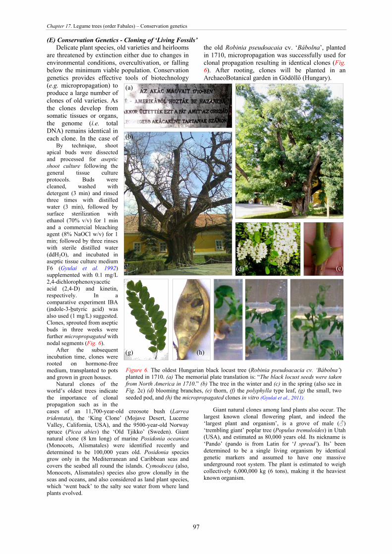
Chapter 17. Legume trees (order Fabales) – Conservation genetics
97
(E) Conservation Genetics - Cloning of ‘Living Fossils’ Delicate plant species, old varieties and heirlooms
are threatened by extinction either due to changes in environmental conditions, overcultivation, or falling below the minimum viable population. Conservation genetics provides effective tools of biotechnology (e.g. micropropagation) to produce a large number of clones of old varieties. As the clones develop from somatic tissues or organs, the genome (i.e. total DNA) remains identical in each clone. In the case of
the old Robinia pseudoacaia cv. ‘Bábolna’, planted in 1710, micropropagation was successfully used for clonal propagation resulting in identical clones (Fig. 6). After rooting, clones will be planted in an ArchaeoBotanical garden in Gödöllő (Hungary).
By technique, shoot apical buds were dissected and processed for aseptic shoot culture following the general tissue culture protocols. Buds were cleaned, washed with detergent (3 min) and rinsed three times with distilled water (3 min), followed by surface sterilization with ethanol (70% v/v) for 1 min and a commercial bleaching agent (8% NaOCl w/v) for 1 min; followed by three rinses with sterile distilled water (ddH2O), and incubated in aseptic tissue culture medium F6 (Gyulai et al. 1992) supplemented with 0.1 mg/L 2,4-dichlorophenoxyacetic acid (2,4-D) and kinetin, respectively. In a comparative experiment IBA (indole-3-butyric acid) was also used (1 mg/L) suggested. Clones, sprouted from aseptic buds in three weeks were further micropropagated with nodal segments (Fig. 6).
After the subsequent incubation time, clones were rooted on hormone-free medium, transplanted to pots and grown in green houses.
Natural clones of the world’s oldest trees indicate the importance of clonal propagation such as in the cases of an 11,700-year-old creosote bush (Larrea tridentata), the ‘King Clone’ (Mojave Desert, Lucerne Valley, California, USA), and the 9500-year-old Norway spruce (Picea abies) the ‘Old Tjikko’ (Sweden). Giant natural clone (8 km long) of marine Posidonia oceanica (Monocots, Alismatales) were identified recently and determined to be 100,000 years old. Posidonia species grow only in the Mediterranean and Caribbean seas and covers the seabed all round the islands. Cymodocea (also, Monocots, Alismatales) species also grow clonally in the seas and oceans, and also considered as land plant species, which ‘went back’ to the salty see water from where land plants evolved.
Giant natural clones among land plants also occur. The largest known clonal flowering plant, and indeed the ‘largest plant and organism’, is a grove of male (♂) ‘trembling giant’ poplar tree (Populus tremuloides) in Utah (USA), and estimated as 80,000 years old. Its nickname is ‘Pando’ (pando is from Latin for ‘I spread’). Its’ been determined to be a single living organism by identical genetic markers and assumed to have one massive underground root system. The plant is estimated to weigh collectively 6,000,000 kg (6 tons), making it the heaviest known organism.
(a)
(a) (c)
(b)
(h) (g) (i)
(d) (e)
Figure 6. The oldest Hungarian black locust tree (Robinia pseudoacacia cv. ‘Bábolna’) planted in 1710. (a) The memorial plate translation is: “The black locust seeds were taken from North America in 1710.” (b) The tree in the winter and (c) in the spring (also see in Fig. 2c) (d) blooming branches, (e) thorn, (f) the polyphylla type leaf, (g) the small, two seeded pod, and (h) the micropropagated clones in vitro (Gyulai et al., 2011).

Chapter 17. Legume trees (order Fabales) – Conservation genetics
98
(F) Nitrogen fixation Not only Legumes live in symbiosis with N2-
fixing soil bacteria. Elaeagnus (Elaeagnaceae of Rosales) and several other plant species are also able to grow in symbiosis with the N2-fixing bacteria Frankia. This symbiosis results in nitrogen fixing nodules developing on the roots. Due to this symbiotic association, the growth of plants is independent from the soluble nitrogen nutrient content of the soil (see Chapter 10). The detailed N2-fixation is summarized below:
(a) INF - Inorganic Nitrogen Fixation. Inorganic nitrogen fixation occurs at lightning in the atmosphere at terrestrial combustions, and during the industrial ammonia production (i.e. Haber - Bosch process) for manufacturing artificial fertilizers (e.g. NH4NO3).
(b) BNF - Biological (Organic/Prokaryotic) Nitrogen Fixation. BNF was discovered in 1901 (Beijerinck, 1901), which is the biological conversion of atmospheric nitrogen gas (N2, dinitrogen) to ammonia (NH3) catalyzed by the prokaryotic enzymes NITOGENAZE (EC 1.18.6.1, EC 1.19.6.1) of diazotroph organisms (N2 → NH3). As the result, the fixed aerial nitrogen is reduced to ammonia (NH3) and became available not only to other prokaryotes in the soil or water but to the plants and finally to the animals.
BNF has been detected in various microorganisms e.g. in aerobic, phototrophic Cyanobacteria, anaerobic purple-sulfur bacteria (e.g.
Chromatium), anaerobic green-sulfur bacteria (e.g., Chlorobium), chemolithotroph bacteria (e.g., Alcaligenes, Thiobacillus, Methanosarcina, and Azospirillum) and in the heterotroph bacteria (e.g. the anaerobe Clostridium, and microaerophile Herbaspirillum), and aerobe Azotobacter. In total, there are about 38 genera of Bacteria, 20 genera of Cyanobacteria and 87 species of Archaea, which are able to fix atmospheric nitrogen, and classified as diazotrophs.
N2-fixation is a high energy consuming process, which needs at least 8 mol ATP per mol NH4
+ produced. This high energy consumption is due to the very unique, triple chemical bond of dinitrogen molecules (N≡N), with high bond energy of 945 kJ/mol.
Both processes are catalyzed by enzyme nitrogenases, which are encoded by nif (nitrogen fixation) genes. The highly conserved sequences of the nif make it an ideal molecular tool to determine the BNF potential of agro/ecosystems and soils.
Structurally, the enzyme nitrogenase is a complex of two protein complexes of nitrogenase Mo-Fe (Nase; a tetramer, α2β2, Mo-Fe protein, encoded by NifDK), and nitrogenase reductase Fe-S (NRase; a homodimer, α2, Fe-S protein, encoded by NifH) (Fig. 7). Basically, Nase, which is a very large enzyme with Mw about 240 kD, catalyzes the reduction of N2 to NH3, and NRase donates two high potential electrons at a time to Nase.
150 160 170 180 190 200 210 ....|....|....|....|....|....|....|....|....|....|....|....|....|....| P08925 Frankia alni 97 AGRGVITSITYLEEAGAYEN-LDFVTYDVLGDVVCGGFAMPIRQGKAQEIYIVTSGEMMAMYAANNIARG 165 Q8KQ04 Frankia sp 97 R..................D-................................................. 165 F8B5Q3 Frankia sp 97 .......A..F...N....D-................................................. 165 P0A3S2 Anabaena azollae 102 ....I..A.NF...N...QD-....S.................E.......................... 170 A8CIG7 Anabaena siamensis 102 ....I..A.NF...N...TD-....S.................E.......................... 170 Q3M5S8 Anabaena variabilis 102 ....I..A.NF...N...QD-V...S.................E.......................... 170 D4H6V6 Denitrovibrio acetiphil. 99 .......A.NF...E....ED....S.................E.......................SK. 168 G6FYF2 Fischerella sp 101 ....I..A.NF...N...QD-....S.................E.......................... 169 D7E3U2 Nostoc azollae 103 ....I..A.NF...N...TD-....S.................E.......................... 171 Q47917 Mastigocladus laminosus 101 ....I..A.NF...N...QD-....S.................E.......................... 169 D8G542 Oscillatoria sp 102 ....I..A.NF...N....D-....S.................E.......................... 170
Figure 7. Consensus sequence alignments (BioEdit; Hall, 1999) of the highly conserved prokaryotic NifH (nitrogenase reductase Fe-S) proteins (stretches of 140 aa to 210 aa) of Frankia ssp., and related N-fixing bacteria. Amino acids (single capital letters of the possible 21 aa), consensus aa (dots), and accession numbers (UniProt) are indicated.
Molybdenum in the Mo-Fe protein, (nitrogenise-1) may be substituted by vanadium resulting in vnfDK and vnfH (nitrogenise-2), or by iron in anfDK and anfH (nitrogenise-3). Genes for nitrogenase Mo-
Fe (nifDK) and nitrogenase reductase Fe-S (nifH) contain highly conserved regions with strait phylogenetic resolutions especially in the case of nifH.
● N-fixation by free-living soil bacteria. These species are Azotobacter, Bacillus, Clostridium, and Klebsiella. Because nitrogenase can be inhibited by oxygen, free-living organisms are anaerobes.
● Associative N-fixation. Bacterium species of Azospirillum are able to form close associations with roots of grasses and cereal crops (Poaceae) such as wheat, corn, oats, barley and rice; and by this way, they release nitrogen (as ammonia NH3) in the rizosphere. The optimal soil pH for Azospirillum growth is pH 6.8-7.8, and at temperature above 15 ºC with the optimum 32-40 ºC.
● Cyanobacterial N-fixation (Symbiosis I). Cyanobacteria (e.g. species of Anabena and Nostoc) fix nitrogen in their specialized cells called heterocysts. Anabaena azollae colonizes cavities which are formed at the base of fronds of Azolla, an aquatic fern, which is the only fern that can fix nitrogen by symbiotic association. Species of Nostoc, another genus of cyanobacteria, can fix nitrogen by symbiotic association with Porella navicularis, a liwerwort. Cyanobacteria can also live on the leaf surface of Angiosperms such as rain forest palm Welfia regia, and provide nitrogen to the host plant.

Chapter 17. Legume trees (order Fabales) – Conservation genetics
99
(F.1.) N-fixation by root nodule bacteria of Rhizobium and Frankia (Symbiosis II)
• Rhizobial N-fixation. Soil bacteria became specialized for developing and living in root nodules of only legume (Fabaceae) species of both woody and herbaceous, and fix aerial N2. These species are Rhizobium legumninosarum of beans (Phaseolus) and peas (Pisum); Sinorhizobium melilotii of alfalfa (Medicago), Mesorhizobium loti of bird's-foot trefoil (Lotus), Bradyrhizobium japonicum of
soybean (Glycine), and Azorhizobium caulinodans of sesbania (Sesbania ssp).
• Frankial N-fixation. Filamentous Actinomycete of Frankia strains, similar to legume Rhizobia, also fix nitrogen by living in root hair nodules (Fig 8).
The genus Frankia was described first as filamentous fungus and named by J. Brunchorst (1886) to honor the biologist AB Frank, and only recently (1970), and it was classified to prokaryotic Actinobacteria (syn.: Actinomycetales). Complete circular genome sequences of Frankia strains are available with size rage from 5.433.628 bp (NCBI # CP000249.1) to 8.982.042 bp (NCBI # CP000820), with very high GC ratio (72.8 %), low gene (6.782) and protein numbers (6.707) (NCBI # CP000249.1). In total, three main Frankia strains were isolated from species of three plant orders of Fagales (all Alnus species, some species of Casuarina, Allocasuarina, Coriaria, Morella, Myrica, Gymnostoma), two genera of Cucurbitales (Coriaria and Datisca), and numerous genera of Rosales (Elaeagnus, Hippophae, Shepherdia, Colletia, Discaria, Kentrothamnus, Retanilla, Trevoa, Caenothus, Dryas, Purshia, Chamaebatia and Cercocarpus). The 16S ribosomal DNA sequences of the root nodules of these species indicated that the nodules are formed by Frankia. (F.2.) Plant ammonification
As plants are not able to fix atmospheric N2, they take up inorganic N-salts of NH3/NH4
+ and NO3- are fixed by bacteria
(summarized above). When NH3 is taken up, enzyme GS (glutamine synthases; EC 6.3.1.2; syn: gln-synthase) transfer it to amino acid (aa) glutamate, which became glutamine (this process is called ammonification) (Fig. 9a,b). The reverse reaction is catalyzed by enzyme GOGAT (glutamate synthase; EC 1.4.1.14). The 2-oxoglutarate can also bind NH3, which transamination is catalyzed by enzyme GDH (glutamate dehydrogenases) (GDH1, EC 1.4.1.3), which reaction also produce glutamate aa (Fig. 9b). When plants take up anionic NO3
- (from NH4NO3 or KNO3) the process is catalyzed by NR (nitrate reductase; EC 1.7.99.4) (NO3
- → NO2-) followed by NiR
(nitrite reductase; EC 1.7.2.1), which catalyzes the reaction of NO2
- → NH3, and finally closed up also by GS. (F.3.) N-loss
Plant N-loss releases the nitrogen-monoxide (NO). NO is produced not
Figure 8. Frankia root nodules (left and middle) on seabuckthorn (Hippophae rhamnoidesssp. Carpatica) (Rosales!) (right). Plotting mm-paper for sizing (Photo by BG Kerti).
Figure 9a. The metabolic function of GS (glutaminesynthase enzyme; EC 6.3.1.2)
cp mt
Figure 9b. Key metabolic routes of ammonium in plants. The reversible transaminase GS (glutamine synthase, EC 6.3.1.2; syn.: GLUL - glutamate-ammonia ligase), and GOGAT (glutamine oxoglutarate aminotransferase; EC 1.4.1.13; syn.: glutamate synthase) in the chloroplasts (cp); and the reversible enzyme GDH (glutamate dehydrogenase, EC 1.4.1.3) located in the mitochondria (mt) are indicated (Kőmíves et al., 2015 in Bittsánszky et al., 2015).

Chapter 17. Legume trees (order Fabales) – Conservation genetics
100
only from nitrite NO2- → NO (catalyzed by FdCo-
NiR; the FerredoxinCopper-NiR; # EC 1.7.7.1) but also from the amino acid L-arginine (L-Arg), which is the main substrate for NO-synthesis through the reaction of arginine + O2 → citrulline + NO (Fig. 9c); and catalyzed by NOSs (nitric oxide synthases, 1433 aa; # EC 1.14.13.39).
The NO released (Gyulai et al., 2014) has several vital functions in animals (vasodilatator, see Viagra) and in plants. In the in vitro plant experiments, NaNP (Na-nitroferricyanide III, Na2Fe(CN)5NO × 2H2O, is used (10-7 to 10-4 M) to release NO.
(G) Samples of other legume trees Next to Robinia, there are several other important legume trees and shrubs growing in the Northern Hemisphere (Fig. 10). Next to Gleditsia triacanthos (2n = 28), there are several other Gleditsia species e.g. Gleditsia amorphoides, G. aquatica, G. caspia, G. ferox, G. japonica, G. sinensis, G. fera, G. melanacantha, G. macrantha, G. heterophylla, and G. horrida. The evergreen, legume, thorny gorse (Ulex europaeus), with yellow flowers, is the main hedge bushes in England and Wales. References Bittsánszky A, Pilinszky G, Gyulai G,
Kömíves T (2015) Overcoming ammonium toxicity. Plant Sci 231:184-190.
Gyulai G, A Bittsánszky, Z Szabó, L Waters Jr, G Gullner, Gy Kampfl, Gy Heltai, T Kőmíves (2014) Phytoextraction potential of wild type and 35S-gshI transgenic poplar trees (Populus × canescens) for environmental pollutants herbicide paraquat, salt sodium, zinc sulfate and nitric oxide in vitro. Int J Phytoremediation 16:379–396.
Gyulai G, Láposi R, Rennenberg H, Veres A, Herschbach C, Fábián Gy, Waters L Jr (2010) Conservation genetics (1710 - 2010). Cloning of living fossils: micropropagation of the oldest Hungarian black locust tree (Robinia pseudoacacia) planted in 1710 (Bábolna, Hungary. In. Plant Archaeogenetics. Ed. G. Gyulai. Nova Science Publishers, Inc. USA. ISBN 978-1-61122-644-7. Ch.10:117–127.
Keresztesi B (1983) Breeding and cultivation of black locust (Robinia pseudoacacia L) in Hungary. Forest Ecology and Management 6:217–244.
Láposi R (2011) Black locust (Robinia pseudoacacia L.) and related species compared by SSR, ITS and cpDNA analyses. PhD Dissertation, SzIE, Gödöllő.
Lavin M Wojciechowski MF, Gasson P, Hughes C, Wheeler E (2003) Phylogeny of robinioid legumes (Fabaceae) revisited: Coursetia and Gliricidia recircumscribed, and a biogeographical appraisal of the Caribbean endemics. Systematic Botany 28:387–409.
Stolp H (2008) Microbial Ecology: organisms, habitats, activities. New York, Cambridge University Press.
(1) (2) (3) (4)
(5) (7) ((6)
(8) (9)( (10)
(11) Figure 10. Samples of legume trees growing in the Northern Hemisphereincluding Hungary (except the 4th sample). (1) Albizia julibrissin (Persian silktree); (2) Amorpha fruticosa (Desert false indigo; a dangerously invasive plantin Hungary); (3) Caragana arborescens (Siberian pea shrub); (4) Ceratoniasiliqua (Carob tree, syn. St. John’s bread); (5) Cercis siliquastrum (Judas tree);(6) Colutea arborescens (Bladder senna); (7) Coronilla (Hippocrepis) emerus(Scorpion senna); (8) Gymnocladus dioicus (Kentucky coffeetree); (9)Laburnum anagyroides (Golden rain); (10) Sophora japonica (Japanesepagoda tree); (11) Wisteria sinensis (Chinese Wisteria) (Láposi and Gyulai, 2011).
Figure 9c. Diagram of the urea cycle. Reactions taking place in themitochondria are indicated in red rectangle. Enzymes including CPS-I(Carbamoil Phosphate Synthetase-I) and OTC (Ornithine Transcarbamoylase)are indicated.

Chapter 18. Woody grasses - Temperate bamboos (genus Phyllostachys)
101
Woody grasses - Temperate bamboos (genus Phyllostachys) (A) Introduction
Bamboos are woody grasses of family Poaceae, comprising six tribes of Bambuseae, Buergersiochloeae, Guaduelleae, Olyreae, Parianeae and Puelieae with about 111 genera and over 1,600 species, with sizes from small herbaceous to giant timber bamboos. Genus Phyllostachys, with about 50 species (Fig. A), belongs to subtribe Shibateinae. Bamboos are the fastest-growing woody plants in the world, they can grow up to one meter a day (3.8-5.0 centimetres per hr).
Phyllostachys edulis
Phyllostachys iridescens
Pleioblastus maculosoides
Phyllostachys prominens
Phyllostachys parvifolia
Phyllostachys dulcis
Phyllostachys angusta
Bambusa oldhamii
Zea mays
Triticum aestivum
Oryza sativa Indica Group
Oryza sativa Japonica Group
Hordeum vulgare subsp. vulgare
0.02 Figure (A) Genetic phylogram (Fast Minimum Evolution) of Phyllostachys species and the closest relatives of monocots based on the sequence PAL1 gene (Phenylalanine Ammonia-Lyase) (complete cds; NCBI Sequence ID: FJ594468.1; Length: 2260 nt). There is a rising global interest in the use of bamboos as they are regarded as renewable resources with strong regeneration potential. Phyllostachys is a temperate bamboo genus belonging to Poaceae, (subfamily Bambusoideae, tribe Bambuseae, subtribe Shibataeinae), and its species are mainly native in warm temperate regions of SE China (Ma et al., 2014). Since centuries they have additionally been grown in neighbouring countries including Korea and Japan (Wang and Stapleton, 2006), where they have become naturalised. There are a total of 60 species growing in China alone. The natural distribution of bamboos is greatly affected by the amount and yearly distribution of precipitation. Sufficient and evenly distributed precipitation during the spring-summer-autumn growing season is extremely important for bamboos (Kleinhenz and Midmore, 2001). They are characterised by high canopy transpiration regardless of culm age (Tsuruta et al., 2016), which is comparable to coniferous forests. Phyllostachys edulis (syn. P. pubescens) is the most important species covering 30% of bamboo forests covering a total area of over 7.2 million hectares in China.
Similarly to other monocarpic, monopodial genera of Bambuseae (Abe and Shibata, 2012, 2014a,b; Matsuo et al., 2014) Phyllostachys are also classified as monocarpic (some taxa proven to be polycarpic), and reproduce mainly vegetatively (Isagi et al., 2016) from nodal shoots developing from the underground rhizome system, which
comprises 39-57 % of the total biomass. This means there is an underground rhizome system with buds on each node, which have the capability to develop into either above ground culms or continue as a side branch of the underground rhizome system (Ueda, 1960).
Phyllostachys species are among the fastest growing plants. Ueda (1960) reported 119 cm and 121 cm of longitudinal growth in 24 hours of culms of P. edulis (syn. P. pubescens) and P. bambusoides (syn. P. reticulata) respectively in Kyoto, Japan.
Phyllostachys species are greatly versatile in their agricultural use, and as such are important in the agriculture of East-Asian countries.
In Europe they are important mainly in ornamental horticulture, but their agricultural potential other than as ornamentals has not been fully investigated and exploited.
Japan’s long history of bamboo usage is evidenced by bamboo’s appearance in ancient literature. People in Japan have traditionally used naturally growing species of the genus Phyllostachys and other genera. Their usage has been handed down to the present day in the form of traditional products the creation of which requires skillful techniques. Some of the many historical and new modern uses of bamboo in Japan include (Shibata, 2015) as:
Sacred plants. Bamboo came to be regarded as a highly sacred plant under the influence of Chinese culture. Culms and/or branches of bamboo are used as god lodging parts in religious services and as tools in religious ceremonies.
Materials for primary industry. Bamboo culms are ideal material for use as poles and similar in agriculture, aquaculture and other primary industries.
Materials for woven products. Some bamboo species are easy to split, which makes them useful for the manufacture of woven baskets, sieves, blinds and the like.
Materials for tools used in the tea ceremony and ikebana (Japanese art of flower arrangement). Without bamboo these typical Japanese cultural activities would not have been established. Particularly it would have not been possible to produce the tea whisk - Chasen.
Materials for musical instruments. Some traditional Japanese flutes and some castanets.
Materials for traditional and everyday application:Due to bamboo’s excellent material characteristics precise rulers, knitting needles, and rubbing pads.
Materials for food and wrapping: Bamboo shoots are very important as vegetables, and suitable for fermentation and drying. Bamboo leaves and culm sheaths have long been known for their antibacterial properties, and have environmentally been used in Japan to wrap a variety of food types. Such usage continues today for traditional foods like sushi and Japanese cakes. Bamboo leaves are also used in Japan to make tea, alcohol and other beverages. As the green surface part of bamboo culm is considered to have a stronger antibacterial effect, it is sold today as a high quality product.
Materials for modern application: The bamboo filaments facilitated Thomas Edison’s invention of the light bulb around 136 years ago. The use of bamboo in the construction of reinforced-concrete buildings as the alternative to steel is still regarded as important today in some developing countries.
Horticultural usage. In Japan, bamboo is regarded as a sacred plant due to the Chinese cultural influence, so is an important material in gardening. Bamboo’s temperate climate zone preference and growth vigor make it ideal even in tight spaces. The large number of species of various sizes (from 0.5 m to 20 m tall) and ornamental characteristics (culm shape, leaf variegation, culm color etc.), all adds to its versatility.
Woody materials resources. Lamination techniques must be applied to process the bamboo material for use in construction. In Japan, kitchens and other parts of houses prone to water exposure have laminated bamboo timber flooring for its antibacterial and deodorant properties. Split bamboo is used in the construction of wind-resistant greenhouses.

Chapter 18. Woody grasses - Temperate bamboos (genus Phyllostachys)
102
Charcoal resources. Bamboo charcoal is as a high-quality, versatile material, due to its high density very fine pores creates high absorbency, making it suitable for a variety of applications including under floor humidity control and deodorization. Bamboo charcoal powder is also extensively used in soil improvement, cosmetics, audio equipment, an energy resource in industry and bamboo active charcoal for use in water purification.
Fiber resources. Bamboo fiber is known for its high quality, with usages depending on its fineness. Coarse fiber is used for purposes such as making compost and road pavement materials, while fine fiber from bamboo culms and sheaths is regarded as a superior material for the production of traditional Japanese paper (Washi). Bamboo culms are today used industrially for pulp in Japan, while fine fiber is also used for clothes, food, industrial product reinforcement and efforts have recently been made toward its use on a nanoparticle level, also with potential for use in the production of bio-plastics and bio-glass.
Extract resources. In Asia some Phyllostachys taxa have long been used in phytotherapy due to their phytochemical content and antioxidant properties. Bamboo shoots contain dietary fiber, protein, carbohydrates, amino acids, minerals, flavonoids, phenolic compounds, and sterols. Shoot or culm extracts have high antioxidant, anti-inflamatory, anti-hypertensive, antibacterial and anti-malassezia properties. Shoot or culm extracts have also been shown to have immuno-stimulating, anticarcinogenic, in ischemic injury treatment anti-apoptotic properties. Other beneficial health effects include: use as a source of dietary fiber improving lipid profile and bowel function, as therapeutic agent for atopic dermatitis, allergic airway diseases including asthma, for the prevention of hypercholesterolemia, high blood pressure, pulmonary inflammation and lung injury, and to relieve lipotoxicity (Neményi et al., 2015). The herba of leaves have high antioxidant properties and contain flavonoids, phenolic acids, chlorogenic acid derivatives, phenolic and flavone glycosides. Leaf extracts have been shown to have anticarcinogenic, cardioprotective effects, relieve lipotoxicity, protect against
oxidative stress-induced glaucoma. Leaf extracts can synergistically be used in combination with other compounds in the treatment of immune/allergic diseases related to mast cells, in the treatment of leukaemia, in the prevention and treatment of diabetic complications and autoimmunity. Bamboo leaves are also used as food additives, and bamboo leaf extracts also exhibit antimicrobial activity during food storage (Neményi et al., 2014).
Energy resources. Bamboo charcoal has traditionally been used as an energy resource in Japan producing more heat than common timber charcoal. The use of woody resources including bamboo in pellet form as an energy source is currently being reviewed in Japan. The combined combustion of bamboo chips at electric power plants and the use of bamboo chips for bio-gas power generation has been implemented and trials involving the use of bamboo for bio-ethanol production is also ongoing.
Environmental capital resources. Bamboo forests account for less than 1% of forest area in Japan, but they are regarded as important in the resolution of global warming issues. They are recognized as supporting specific biodiversity and helping to maintain favorable environmental conditions. Plans are in place to evaluate these properties toward environmental capital resumption in bamboo forest management in many parts of Japan.
The first plants were introduced to Europe in the United Kingdom in 1720. From 1856 Eugéne Mazel played an important role in introducing several taxa from Japan and China to his park in Prafrance, Anduze, France, propagules of which were distributed to other countries including Hungary, where Phyllostachys aurea, P. bambusoides, P. flexuosa, P. nigra var. nigra and P. viridiglaucescens were growing in Botanical Gardens, mansion and Royal palace parks in the 1880-ties. From the beginning of the 20th century vegetative propagating material of many taxa have been imported from Japan and more recently from China and redistributed in Europe
(B) Perclinal chimeric mutations in many taxa produce similar culm forms
Many Phyllostachys taxa have phenotypically similar culm variations which appeared as spontaneous mutations in groves of the basic species. They were described as either varietas, forma or cultivar and are propagated vegetatively.
They include green core with yellow surface periclinal chimera mutation type of culm (g’GG) where LI turns yellow and LII and LIII remains green creating a yellow culm with green stripe in the canal or sulcus (Okamura and Tanaka, 1986). This is characteristic of Phyllostachys aurea f. koi, P. aureosulcata f. spectabilis, P. bambusoides f. castillonis, P. edulis f. bicolor, while P. edulis f. nabeshimana, and P. vivax f. viridivittata have a high ratio of the mutable yellow gene (g’) in LI and also a mutable green gene (G’) creating many green longitudinal stripes on the yellow culm surface.
The other is a yellow core green surface periclinal mutation type of culm (Gg’g’), where LI remains green and LII and LIII turns yellow, creating a green culm with
yellow stripe in the canal or sulcus (Okamura and Tanaka, 1986). This is typical of Phyllostachys aurea f. flavescens-inversa, P. aureosulcata var. aureosulcata, P.angusta f. flavosulcata, P. arcane f. luteosulcata, P. bambusoides f. castilloni-inversa, P. edulis f. luteosulcata, P. hirtivagina f. luteovittata, P. nidularia f. mirabilis, P. sulphurea f. houzeauana, P. violascens f. notata, and P. vivax f. huangwenzhu.
The third is when there is a mutable yellow gene (g’) in each germlayer (LI, LII, LIII) creating an almost purely yellow culm (g’g’g’) with very few occasional green stripes (Okamura and Tanaka, 1986). This type of mutation characterizes Phyllostacys aurea f. holochrysa, P. aureosulcata f. aureocaulis, P. bambusoides f. holochrysa, P. edulis f. holochrysa, P. sulphurea var. sulphurea, and P. vivax f. aureocaulis. There are also other mutants with distorted internodes (P. edulis f. heterocycla, P. edulis f. subconvexa) or anthocyanin pigmentation (P. nigra var. nigra, and P. nigra f. boryana) (Fig. 1).
(C) Single clone, no seedling regeneration in the wild
Phyllostachys species reproduce sexually every 60-120 years depending on species, two clones of P. edulis (syn., P. pubescens) have been determined to have flowering intervals of 67 to 69 years in Japan (Shibata, 2002). Though flowering plants are greatly depleted by the successive flowering event lasting 2-3 years, they probably do not die under natural forest conditions, but regenerate vegetatively from the rhizome system similar to which was observed in the case of P. bambusoides (syn., P. reticulata, Madake) and P. nigra var. henonis (Hachiku) in Japan. When available Phyllostachys taxa can be propagated in nurseries from seeds, but there is a long nursery raising period of 4 years (often under greenhouse conditions
depending on local climate), before seedlings can be transplanted out into the field and one to two decades to reach maximum mature size. Isagi et al., (2016) studied, the genetic diversity of P. edulis (syn., P. pubescens) for the entire distribution range of the species in Japan to a vast area of its range in China. They used 16 microsatellite markers for the analysis. They used 246 leaf samples of adult P. edulis (syn., P pubescens) collected from 28 populations spanning the entire ranges in Japan (n = 20) and a large area in SE China (n = 8).
They also analyzed the patterns of pollination (selfing or outcrossing) from leaf samples that were collected from seedlings (32 and 30 for each flowering event respectively)

Chapter 18. Woody grasses - Temperate bamboos (genus Phyllostachys)
103
resulting from the flowering events in 2005 and 2006, planted in the Wakayama Farm, Tochigi Prefecture, Japan. Among these, they found that 12 loci fixed by a single allele, whereas they detected only 2 alleles for each of the remaining 4 loci. The observations indicated that all samples they collected from Japan and China are ofsspring of an identical single clone. This clone distributed over more than 2,800 km and they estimated its biomass to be approximately 6.6 × 10¹¹ kg, which is exceptionally large (Isagi et al., 2016). They also report that 20 different genets were generated among seedlings from flowering events of 2005 and 2006, by recombination through selfing of a single flowering genet/colony. (term genet refers for a colony of plants, fungi or bacteria that come from a single genetic source). Isagi et al., (2016) reported that the diverse composition of genets among seedlings and the predominance of a single clone in the wild suggest that the intermittent flowering of P. edulis (syn., P. pubescens) in the wild has possibly produced a variety of clones through recombination, but the single clonality caused the breeding system to perform selfing, but in the wild, they did not find any adult plants with genotypes generated by selfing of the dominant clone. Inbreeding depression might be one of the reasons for the low viability of P. edulis seedlings in the wild. Also, according to their theory the resulting seedlings possibly cannot compete with other tree species or adult P. edulis (syn., P. pubescens). So, sexual reproduction does not contribute to the remarkable expansive range of this species for almost all adult P. edulis (syn., P. pubescens) plants growing in Japan and China, whivh are likely the vegetative offspring of a single clone propagated by human transplantation, and its subsequent expansion through the rhizome-culm system (Isagi et al., 2016). The flowering pattern of P. edulis, which was characterized by partial flowering of a clone (polycarpic), was similar to that of the Sasa species. Thus, they suggest it is unlikely that all culms of the single genet distributed in Japan and China flower and die simultaneously. In their opinion the relatively small size of the flowering area and rapid reproduction of culms has led to the stability of P. edulis (syn., P. pubescens) communities (by polycarpy). Genetic diversity contributes to disease tolerance, evolutionary potential, ecosystem function, and adaptation to the changing environment. So,
the very low genetic diversity is an important consideration for the long-term management of this widely distributed temperate bamboo species (Isagi et al., 2016).
(D) Bamboo seed morphometric analysis Computer-assisted digital morphometry (Fig. 2)
provides a new powerful array of objective measurements of size, shape, tomography, texture, fractals, etc. of significantly large populations of objects rapidly, with accuracy and precision (Rovner and Gyulai, 2007; Gyulai et al., 2015). Bellow we present, an analysis of bamboo seeds of P. edulis (syn. P. pubescens) by using Fovea Pro 4.0 Computer Program coupled with Adobe Photoshop and IBM SPSS data analyses (18 parameters of 33 measured were used).
We also aimed to determine the evolutionary stage of the bamboo plant by estimating the levels of variation (driven by ‘Force of Mutation’) vs. selection (driven by ‘Force of Selection’) based on histogram analysis (MS Excel) of digital seed parameters.
Phyllostachys edulis (syn. P. pubescens) seed lots commercially available in 2013, 2014 and 2015 from China were analysed. For the analysis 200 seeds per lot were used.
The following 18 seed morphometric parameters were analysed: Area (cm2): If pixels are interpreted as little squares, the area of a feature is determined by counting the connected thresholded pixels and applying a calibration factor based on the size of the pixels. Convex Area (cm2): a shape is convex if there are no "dents" or indentations in it. Length (cm): maximum caliper dimension. Breadth (cm): minimum caliper dimension. Equiv.Diam (cm): the diameter of a circle with the same area as the feature. Inscrib.Rad. (cm): Radius of the inscribed circle. Circum.Rad. (cm): Radius of the circumscribed circle. Perimeter (cm): distances between the centres of pixels on the object side of the boundary. Convex Perim (cm): perimeter of the convex bounding polygon. FormFactor: 4π•Area / Perimeter. Roundness: 4 • Area / π • Max Dimension. Aspect Ratio: Length / Breadth. Solidity: Area / Convex Area. Convexity: Perimeter / Convex Perimeter. Symmetry: The symmetry of a shape is encoded in the Fourier transform of its boundary. Radius Ratio: Inscribed Radius / Circumscribed Radius. Elongation: Area / ConvexHull Area. Skeleton Length (cm): total lineal distance down the centre line of an object (see Chapter 15).
Figure 1. P. edulis f. bicolor in Japan (top). Middle (left to right): P. nigra f. boryana; P. aurea; P. edulis f.nabeshimana; P. nigra var. henonis; P. edulis f. bicolor;and P. edulis f. heterocycla. Bottom (left to right): P. nigravar. nigra; P. violascens; P. vivax; P. vivax f. viridivittata;P. vivax f. huangwenzhou; and P. aureosulcata f.aureocaulis

Chapter 18. Woody grasses - Temperate bamboos (genus Phyllostachys)
104
0,00
0,10
0,20
0,30
0,40
0,50
0,60
0,70
0,80
0,90
1,00
Equiv.D
iam.(m
m)
Area(m
m^2)
Inscrib
.Rad.(mm
)
Breadt
h(mm)
Extern
al Perim.(mm)
Conve
x Perim .(mm )
Circum
.Rad.(mm
)
Length
(mm)
Perime
ter(mm)
Roundne
ss
Radius Ratio
Aspect
Ratio
Form factor
Symme
try
Elonga
t ion
Conve
xity
Skeleton Lengt
h(mm)Solidit
y
PC3
PC2
PC1
Figure 2. Principal Component Analysis (PCA) (IBM SPSS) of the first two principal components of seed parameters of the three seed lots (2013 - blue, 2014 - green, 2015 - red of P. edulis (syn. P. pubescens) (left). Shares of variances (%) explained by the first three Principal Components (IBM SPSS) for 18 seed parameters of the of the three seed lots of P. edulis (syn., P. pubescens) studied. Seed ‘Solidity’ was found not correlative (right).
Area Length Breadth Equiv.Diam Skeleton Length Figure 3. Samples of histogram analysis (MS Excel) for five of the 18 seed parameters (Y-axis) based on digital seed morphometry data of the three seed lots (2013, 2014, 2015) of P. edulis (syn., P. pubescens).
Histograms of the seed parameters from the analysis, revealed that P. edulis (syn., P. pubescens) seeds show a close distribution to a normal distribution for the 18 parameters (Fig. 3). Histogram statistics (by SPSS) proved the visual observations of histograms (Fig. 3). In histogram statistics, skewness shows the level of symmetry (i.e., the lack of symmetry), and its value is zero in the case of normal distribution. Negative skewness indicates right-modal distribution, which is the result of high number of seeds with higher seed parameters than the mean, and with small number of seeds with lower parameters than the mean; and vice versa in positive skewness. Most of the distributions showed statistically normal distribution, however, the measures of skewness for Solidity confirmed significant negatively skewed distributions.
The Radius Ratio, Roundness, Formfactor and Symmetry of seeds showed significant positively skewed distributions. In the case of kurtosis, only three parameters (Skeleton Length, Elongation, and Convexity) of P.edulis (syn., P. pubescens) seeds showed significantly peaked and skewed distribution with high values. The following 8 parameters do not deviate from a normal distribution: Area, Breadth, Equiv. Diam., Inscrib. Rad., Perimeter, External Perim., Convex Perim., and Aspect Ratio. The study of Rovner and Gyulai (2007) revealed that, unlike previous assumptions, seed parameters of wild plant species are not normally distributed. Rather, they typically show a multimodal distribution, and the cultivated plants show normal (unimodal)
distribution. Values of X- (i.e., skewness) and Y-axis (i.e., kurtosis) of histograms of seed parameters were also postulated as the level of diversity (along X-axis), which shows the level ‘Force of Mutation’; and the level of selection (along Y-axis with high/low protrusions), which shows the ‘Force of Selection’ (Gyulai et al., 2015).
In our study here, P. edulis showed high Y-values (i.e., ‘Force of Selection’) in three - Inscrib. Rad, Length and Area - of the previously determined three most discriminative CRT parameters (Gyulai et al., 2015). Seed Diversity Index (SDI) of the three seed lots of P. edulis, calculated as mean values of the Relative Standard Deviations (RSD%) of the 18 seed parameters were as follows: 12.9 (2013), 14.39 (2014), 16.56 (2015), and total sample (3 seed lots) 15.75. This result may indicate a tendency of narrowing variation which, consequently, increases the vulnerability of this species to environmental change. This is confirmed in practice by the authors since the single clone of P. edulis (syn., P. pubescens) imported from Japan is the least adaptable, observed among the more than 60 Phyllostachys taxa under trial in the Gödöllö Botanical Garden of Szent István University, Hungary. Also an observation of the seedlings derived from the sowing of the 3 seed lots showed 3-5% of seedlings were affected by albinism which can also be regarded as a sign of the selfing of the single clone of P. edulis (syn., P. pubescens).
(E) Conclusions
Phyllostachys taxa are vegetatively propagated for centuries, and as such, globally distributed, resulting in mainly single clonal plants with low genetic diversity. There is no natural regeneration of seedlings in groves of P. edulis and P. bambusoides as a possible result of competition with other plants, and the vegetatively growing ‘mother’ plants from rhizomes. A single clone of P. edulis planted over centuries ago in Japan and SE China was proven by DNA analysis. Seed morphometry also shows low variability of seed morphometric characters in P. edulis (syn., P. pubescens). Annual generative propagation from seeds is only possible in the case of P. edulis (syn., P. pubescens), but it is a result of selfing of the single clone which produces seedlings with limited genetic diversity. Efforts should be made during the establishment of new bamboo forests to use generative planting material (seedlings) to improve genetic diversity of the species. References Abe Y, Shibata S (2012). Ecological Research 27: 625-632. Abe Y, Shibata S (2014a). J Forest Research 19: 268-275. Abe Y, Shibata S (2014b) J Forest Research 19: 166-173. Gyulai G, Rovner I, Vinogradov S, et al. (2015) Seed science & Technology 43: 1-15. Isagi Y, Oda T, Fukushima K, Lian C, Yokogawa M, Kaneko S (2016) J Plant Research 129: 21-27. Kleinhenz V, Midmore DJ (2001) Advances in Agronomy 74: 99-145. Ma N, La G, Yang L (2014) The genus Phyllostachys in China. Zhejiang Science and Technology Publishing House, Hangcsou, China. Matsuo A, Tomimatsu H, Suzuki J-., Saitoh T, Shibata S, Makita A, Suyama Y (2014) Annals of Botany 114: 1035-1041. Neményi A et al. (2014). Notulae Botanicae Horti Agrobotanici Cluj-Napoca 42(1): 43-50. Neményi A et al. Notulae Botanicae Horti Agrobotanici Cluj-Napoca 43(1): 64-69. Okamura, H., Tanaka Y (1986) The horticultural bamboo species in Japan. Takanawa Printing Co., Ltd., Kobe, Japan. Rovner I, Gyulai F (2007) Economic Botany 61(2): 154-172. Shibata S (2002) In: Bamboo for Sustainable Development. Eds.: A. Kumar, I.V. Ramanuja Rao and Ch. Sastry, VSP) 324-365. Shibata S (2015) Proceedings of the 10th World Bamboo Congress, Damyang, Korea. Tsuruta K et al. (2016) Hydrological Research Letters 10(1): 1-7. Ueda K (1960) Bulletin of the Kyoto University Forests 30: 1-169. Wang Z, Stapleton C (2006) Phyllostachys. In: Flora of China Editorial Commitee, Zhengi, W. and Raven, P. (Eds)

Chapter 19. Forest buffer zones, and hedgerows in agro-ecosystems
105
Forest buffer zones, and hedgerows in agro-ecosystems
Industrialized agriculture has become more and more dominant during the second half of the 20th century, and the trend keeps going on into the 21st century as well. One of the most prominent consequences of this change is the unfavourably altering landscape. Diversity, which once was a general characteristic across vast areas, has diminished with the spread of industrialized production. Patches of forests and shrubs, hedgerows were and are being eliminated, and the small arable plots are merged into huge blocks of homogenous fields measuring well over hundreds of hectares. However, it is not monotony and repetitiveness that makes us worry. The increase in field size on the long run contributes to decreasing soil fertility: the lack of hedges means the lack of protective shields against the erosive effects of wind. Abolishing hedges also means taking away habitats of beneficial organisms; those are arthropods, birds, and mammals that control pests. 1. The pros and cons of hedgerows: facts and myths 2. Planting and maintaining hedges 1. The pros and cons of hedgerows: facts and myths
The possibility of droughts is lower where there are forest strips or rows of bushes scattered within the field, as opposed to large, tree-less areas. The reason behind this general experience is not only that hedges slow the speed of winds. Hedges are also able to trap the various forms of aerial moisture such as mist, fog, hoarfrost or rime. Hedges, masses of organic material, are able to store the excess water of melting snow or downpours. Trees and bushes are also able to drain water from depth unavailable for herbs. In dry periods, the moisture evaporated by the forest patches reappears as morning dew on the surfaces of arable lands. Therefore fields bordered by hedges are less prone to desiccation.
Hedges buffer pesticide drift and it is extremely important in organic production. There is no need to explain the importance of keeping an area pesticide free: when the yield is no longer certified organic, the farmer can sell it only as conventional, that is, at a much lower price.
On the long run, forest patches offer additional products such as firewood, timber material, forest fruits, edible mushrooms, herbs and game. The collection, processing and management of these special side products are usually labour-intensive, but due to the immense demand, are highly marketable.
Hedges reduce production area, but there can be some other, less obvious disadvantages, too.
If not properly planned, hedges may leave crooked corners, small irregular pieces of land and thus present an obstacle to machinery. When planning and planting ignore local ventilation conditions, hedges can also create pockets of frost or heat.
Where the low level of shrubs and herbs is missing, the patch of trees rises immediately beside the field. These trees not only cast shadow on the field, but create an unfortunate whirl of wind as well,
and these combined decrease the yield along the edges of the field.
All these disadvantages are avoidable with careful planning. And these are the reasons an already existent hedge should be reconstructed, replanted or removed.
Let us take a closer look on the role of hedges from the pest management point of view. There are some issues labelled by experts as ‘disadvantages’, but when inspected thoroughly, most of these concerns can be dismissed.
One of the most important among them is weeds. Between the hedge and the field there is, inevitably, a strip of herbaceous plants. Although many express their worries about this strip increasing the number of weeds within the field, this is relevant only when the edge and the strip are being disturbed on a regular basis, that is, when machinery repeatedly treads the strip, or when the soil of the strip is broken up time and again. Ragweed (Ambrosia artemisiifolia), redroot pigweed (Amaranthus retroflexus) and lamb’s quarters (Chenopodium album), weeds so characteristic of arable fields not only tolerate, but require trampling and disturbance. Ragweed for example that thrives the next year after the soil has been disturbed will continue proliferating for a couple of years, but eventually, if the area is left unharmed, other herbaceous plants will take over the space. With proper weed management, these weed species are not viable within the field, nor they are on the undisturbed herb strips.
Tree hedges are often accused of providing overwintering (hibernation) sites and shelter for arthropod pests. Apart from a few confirmed cases, these assumptions lack proof. The larvae of the most important pests of cereals, eg., cereal ground beetle (Zabrus tenebriodes), turnip moth (Agrotis segetum), wheat chafers (Anisoplia spp.), and the pupae and larvae of cereal flies (Chloropidae) and cereal midges (Haplodiplosis marginata and Mayetiola destructor) overwinter within the soil of the field. These pests do not need margins or hedgerows for their survival. The same applies to some of the major pests of the corn as well. The maize leaf weevil (Tanymecus dilaticollis), the grubs (Melolonthidae larvae) and wireworms (Elateridae larvae) find underground shelters within the field, the eggs of the western corn rootworm (Diabrotica virgifera virgifera) are positioned into the soil of the field, and the leftover stalks of corn provide overwintering habitat for the larvae of the European corn borer (Ostrinia nubilalis).
Wheat bugs (Eurygaster and Aelia spp.) on the other hand, are worth mentioning among the species that seek overwintering shelters within the leaf litter on the southern, warmer slopes of forest hedges (Fig. 3). A thorough examination of the litter however reveals, that the majority of arthropods dwelling there are either predators (ground beetles - Carabidae, spiders - Araneae and rove beetles - Staphylinidae) or neither predators nor pests of any importance of arable production. But to see the whole picture about wheat bugs we have to note that being exceptionally good in

Chapter 19. Forest buffer zones, and hedgerows in agro-ecosystems
106
the air, they fly, search and find any cereal field regardless of the distance between the field and the soil of the forest patch.
Tree hedges are perfect refuges for the black bean aphid (Aphis fabae), a major pest of sugar beet (Beta vulgaris subsp. vulgaris. var. altissima), sunflower (Helianthus annuus), poppyseed (Papaver somniferum) and beans (Phaseolus spp.). To lay the overwintering eggs, female aphids seek the branches of the spindle tree (Euonymus europaeus), and this shrub is almost omnipresent in any hedgerow.
The extent tree hedges contribute to the proliferation of chafer grubs is still a matter of debate. We believe in the benefits of diversity, that is, the more diverse the composition of sylvan species, the higher the chance of having a large spectrum of birds and small rodents within the tree hedgerow to control the outbreak of chafer grubs.
While some argue that hedges contribute to the escalation of populations of the common vole (Microtus arvalis), this small rodent, being outnumbered by sylvan rodents, avoids bushy or forest patches, and prefers cultivated fields of alfalfa and grasses, where the soil is rich in nutrients due either to manure or fertilizers. Vole control should be based on making the habitat suitable for birds of prey (owls – Strigidae, and buzzards - Acciptridae), and predatory mammals (fox – Vulpes vulpes, polecats and weasels – Mustela spp.). A complex canopy of various trees and a dense undergrowth of bushes at the lower level are ideal, but until that phase is reached, at least some high standing observation and plucking poles should be erected for the birds.
Tree hedges however, also provide shelter for a range of beneficial arthropods, that is, natural predators of agricultural pests, including, but not limited to ladybugs (Coccinellidae), hover flies (Syrphidae), lacewings (Chrysopidae), and parasitoid wasps (Aphidiidae). The proximity of overwintering habitats is more important for these organisms than it is for the aphid community, because riding the wind, aphids can easily spread between host fields even in the lack of hedges.
The flowering patches of smaller herbaceous plants within hedges not only provide complex food sources for beneficial arthropods and pollinators, parasitoid wasps for example are unable to reproduce without them. These wasps lay their eggs inside the body of the larvae of adults of other arthropods (for example aphids). As the wasp larva hatches within, it consumes its host to pupate and develop into an adult individual. Beneficial wasps need to feed on nectars and pollens of wild flowers to lay viable eggs. Herbs also supply pests (click beetles and noctuid moths) with food, but as with overwintering, pests do not rely on hedgerows as heavily as beneficial arthropods do.
Fruits are a valuable source of food for predatory mammals, rodents and songbirds, so there should be endemic, fruit-bearing bushes such as blackthorn (Prunus spinosa), elder (Sambucus spp.), cornelian cherry (Cornus mas), rosehip (Rosa canina), hawthorn (Crataegus spp.), blackberry (Rubus spp.) and
hazelnut (Corylus spp.) planted within the hedgerows. The fruit of these bushes attract certain rodents (eg., wood mouse, Apodemus sylvaticus) that generally do not forage on the fields, but their presence lures a range of predators. 2. Planting and maintaining hedges
The ideal hedgerow fits into the landscape smoothly. The concept of ideal however, varies from location to location, depending on the actual landscape: exposure to sun and wind, slopes, the presence of wet or extremely dry habitats, the natural species composition of the flora and fauna of the region, to name a few conditions.
Where there is a hedge, or a system of hedges already present, the best a farmer can do is to examine the system and leave it as it is. Apart from a few exceptional cases, there are no reasons to reconstruct, replant or completely remove a useful and functional, endemic hedgerow.
The ideal hedge does not allow for the creation of frost or heat pockets, nor does it block everyday transport or field operations. On slopes, hedges are following the level lines. A hedge oriented north to south casts the smallest portion of shadows on the valuable arable field. An ideal hedge is connected to another hedge or at least to a patch of natural landscape, and that is connected to another hedge and so on, so as to provide for the undisturbed movement and safe shelter of game. At some locations, the local fauna is adjusted to certain heights of trees and are intimidated by higher ones. For the safety and preservation of wildlife, these are places for shrubs-only hedgerows with a maximum height of 3 m. An ideal hedge resembles the natural landscape and consists of groups of bushes, groups of trees and irregular patches of herbaceous areas as well in a relatively random fashion. On the contrary, a continuous single file of bushes or shrubs is not as valuable.
This simplified drawing of a cross section of a hedge is a suggestion, a draft, not a blueprint (Fig. 1).
The core of the hedge is the row or rows of trees. This zone is a fairly undulating strip of trees interrupted here and there by nearby bushes and patches of herbaceous plants (Fig. 2).
There are as many kinds of tree species in an ideal hedge as possible. The best arrangement is planting the same species in a smaller group, which is followed by another group of another species. When planting a new hedge, the farmer should look for using endemic species and trees that are commonly found in that particular area. Among fruitless species, some of the best suggestions are oaks (Quercus spp.), maples (Acer spp.), elms (Ulmus spp.) and poplars (Populus spp.).
A man-made hedge preferably should not include invasive and non-native species, but should have trees that attract bees and other pollinators (Fig. 3). These insectary trees may include endemic and non-endemic species as well. Lindens (Tilia spp.), black locust (Robinia pseudoacacia) and hackberry (mayday tree)

Chapter 19. Forest buffer zones, and hedgerows in agro-ecosystems
107
(Celtis spp.) are some of the most important nectar producing trees.
The most important elements of the sylvan part of
the hedgerows are those who bear fruits. Diversity is the key factor in selecting the species for a newly established hedgerow. Mulberries (Morus spp.), walnuts (Juglans spp.), filbert (Corylus maxima), common hackberry (Celtis occidentalis), rowans (Sorbus spp.), wild pear (Pyrus pyraster), wild apple (Malus sylvestris), Mirabelle plums (Prunus domestica), wild cherries (Prunus avium), common dogwood (Cornus sanguinea), and local conditions permitting, even almond (Amygdalus communis) or chestnut (Castanea sativa) are all suitable for hedges. These species are all easily available for propagation by the collection of seeds or by planting seedlings.
Adjusted to the specific conditions of the region, there should be local, resistant varieties of cultivated fruit species (plums, peaches – Prunus persica and apricots – Prunus armeniaca, cherries and sour cherries – Prunus cerasus, apples – Malus spp., pears – Pyrus spp. and medlar – Mespilus germanica) included in the hedge by sowing their seeds.
There is an ongoing debate about the nature of planting. While obtaining fruit of various wild trees and local varieties is relatively easy, and so is sowing the seeds, young seedlings require a lot of protection. The advantage of sowing fruit bearing trees by seeds, that is, by their fruit, is that the seedlings usually develop healthy, strong and resistant. Their life expectancy is high. Since only a minimum percent of seeds germinate, this procedure requires lots of propagation material. Small seedlings compete with herbaceous plants and once they have a shoots with a diameter of a human finger, deer (Cervus spp.) and hares (Lepus spp.) will find them attractive.
Hedges created with nursery raised seedlings lack the initial hardships, but the need for protection against game is inevitable, thus piles of trimmings of shoots of thorny trees and bushes is needed to ward off the hungry animals around the groups of freshly planted seedlings. These trimmings not only shield young trees, they also provide shelter for smaller mammals and insects (Fig. 3, 4), and over time, they decompose to increase the organic content of the soil, and thus fertilize the hedge area.
Beside the zone of trees within an ideal hedge, stretch a strip of shrubs, with about 30 % of thorny bushes and shrubs as a shelter for the smaller birds. The principle of selecting species and positioning
individuals is the same as with trees. Some of the most common shrubs of the Carpathian basin and Europe include rosehip, blackthorn, fly honeysuckle (Lonicera canadensis), bramble (Rubus fruticosus), dogwood and hazelnut.
The strip of shrubs is surrounded by a wavy, somewhat smaller section of undisturbed taller herbaceous plants for an ideal hedge formation, where umbellifers such as hemlock (Conium maculatum) rough chervil (Chaerophyllum temulum), wild carrot chervil (Anthriscus cerefolium), and cow parsley (Anthriscus sylvestris) are to attract parasitoid wasps. Patches of stinging nettle (Urtica dioica), false mayweed (Tripleurospermum inodorum), a couple of white mulleins (Verbascum lychnitis), wormwood (Artemisia absinthium), annual fleabane (Erigeron annuus) or yellow melilot (Melilotus officinalis) are sown to prevent the spreading of invasive pioneer species such as ragweed, common milkweed (Asclepias syriaca), cannabis (Cannabis spp.) and Canadian goldenrod (Solidago canadensis).
And finally, the hedge joins the field with a narrow strip of grass, clovers and trefoils (Trifolium spp.) or even, alfalfa (Medicago sativa). Depending actual precipitation, this section is mowed 1 to 3 times a year, so as not maintain the habitat for smaller organisms (e.g., certain web builder spiders) that are sensitive to trampling and disturbance.
Conclusion Monotonous species composition, monoculture is favourable for pests,
whereas diversity, a mixture of multi-species habitats favours the natural enemies of pests. To obtain the advantages of these semi-natural habitats, only 5-7 % of the territory of the farm should be converted into hedgerows. When tailored to the needs and conditions of the actual land, an ideal hedge not only serves the purposes of the farmer by reducing the possibility of a potential pest outbreak, but the advantages outweigh the disadvantages.
The gains on the short term are higher yields, decreased pest control costs and a landscape that is more pleasing to the eye (Fig. 2). These are significant justifications, when compared to that sacrifice of 5-7 % of acreage. But on the long run, our grandchildren may be able to thank us for preventing desertification, for inserting and maintaining fruitful and flowery patches into the already thick and heavily industrialized fabric of modern life. References Boller EF, Häni F, and Poehling H-M (2004) Ecological Infrastructures: Ideabook on
Functional Biodiversity at the Farm Level Shistar T: Hedgerows for biodiversity
http://www.beyondpesticides.org/assets/media/documents/infoservices/pesticidesandyou/documents/HedgerowsFall2014.pdf
The Royal Society for the Protection of Birds: Hedgerow management https://www.rspb.org.uk/Images/Englishhedgerows1_tcm9-133255.pdf
Figure 1. Recommended structure of protective hedgerows
Figue 2. Protective hedgerows bordering smaller production areas in Hungary (Photo by F. Tóth)

Chapter 19. Forest buffer zones, and hedgerows in agro-ecosystems
108
Figure 4. Hedges provide shelter for beneficial arthropods as well: 1. Bombardier Beetle (Brachinus crepitans), 2. Crab spider (Xysticus kochi), 3. Rove beetle (Staphylinus caesareus), 4. Seven-spot ladybird (Coccinella septempunctata) adult, 5. Seven-spot ladybird (Coccinella septempunctata) larva feeding on aphids, 6. Common banded hoverfly (Syrphus ribesii), 7. Marmalade hover fly (Episyrphus balteatus), 8. Common green lacewing (Chrysoperla carnea) adult and egg, 9. Common green lacewing (Chrysoperla carnea) larva, 10. Parasitic wasp (Aphidius ervi) adult parasiting an aphid
Figure 3. Insect Pests and Invasive Weeds. (A) Some of the most important pests were observed overwinter in the soil of the cultivated field or within the leftover crop residues on the surface of the field (1-13): 1. Cereal ground beetle (Zabrus tenebrioides), 2. Turnip moth (Agrotis segetum) larva, 3. Wheat chafer (Anisoplia austriaca), 4. Frit fly (Oscinella frit), 5. Saddle gall midge (Haplodiplosis marginata) larva, 6. Hessian fly (Mayetiola destructor) adult, 7. Hessian fly (Mayetiola destructor) pupa, 8. Maize leaf weevil (Tanymecus dilaticollis), 9. Western corn rootworm (Diabrotica virgiferavirgifera) adult, 10. Western corn rootworm (Diabrotica virgifera virgifera) larvae, 11. European cockchafer (Melolontha melolontha) grub, 12. Wireworms (Elateridae larvae), 13. European corn borer (Ostrinia nubilalis), larva. (B) Certain pests of cereals and other major crops including sugar beet, sunflower and beans overwinter outside the field, within the leaf litter of warmer southern slopes of hedges (14-16): 14. Bishop Mitre’s Shieldbug (Aelia acuminata), 15. Tortoise bug (Eurygaster maura), 16. Black bean aphid (Aphis fabae). (C) Some pests feed on the pollen of herbs (17-19): 17. Click beetle (Agriotes lineatus), 18. Noctuid moth (Helicoverpa armigera) adult, 19. Noctuid moth (Helicoverpa armigera) larva. (D) Invasive Weeds (20-25): 20. Common milkweed (Asclepias syriaca), 21. Ragweed (Ambrosia artemisiifolia), 22. Redroot pigweed (Amaranthus retroflexus), 23. Lamb’s quarters (Chenopodium album) 24. Cannabis (Cannabis spp.) 25. Canadian goldenrod (Solidago canadensis)

Chapter 20. Stock estimation and environmental monitoring of a fish population with reserve area
109
Stock estimation and environmental monitoring of a fish population with reserve area Abstract
For sustainable exploitation of renewable resources, the separation of a reserve area is a natural idea. In particular, in fishery management of such systems, dynamic modelling, monitoring and control has gained major attention in recent years. In this Chapter, based on the known dynamic model of a fish population with reserve area, the methodology of mathematical systems theory and optimal control is applied. In most cases, the control variable is fishing effort in the
unreserved area. Working with illustrative data, first a deterministic stock estimation is proposed using an observer design method. A similar approach is also applied to the estimation of the effect of an unknown environmental change.
Keywords: stock estimation, fishery resource management, reserve area, observer system, ecosystem monitoring
1. Introduction
Recently, also qualitative properties of population systems, such as controllability and observability have been studied, see e.g., Shamandy (2002,) López et al. (2004), (2007a, b). For an overview of the applications of mathematical systems theory in this context, we refer the reader to the review Varga (2008).
Over the last decades, the problem of sustainability of marine fisheries, the study the effects of a reserve area has played an important role in the management of fish resources. In fact, the the protection of a portion of the fishery stocks agains future overfishing, can be realized in a reserve (or no-take) area where fishing is prohibited, see e.g., Agardy (1997), Pauly et al. (2002) and a recent overview of the ecological effects of marine reserves a Lester et al. (2009). For a survey of criticism of reserve areas we refere to Sale et al. (2005).
To our knowledge, Dubey et al. (2003) was the first paper where the effect of a reserve area on the exploitation of a fishery resource has been modelled and analyzed in terms of a continuous-time logistic dynamics. The authors derive sufficient conditions for the existence of equilibrium in the dynamic model, and they also analyze its stability properties. In Bischi and Lamantia (2007), based on a single-species discrete time logistic model with reserve area, the game-theoretic conflict of several fishing agents is studied, where the harvested fish is sold on a Cournot-type oligopolistic market. Cartigny et al. (2008) analyze the problem of designing the access of small- and large-scale fishermen to a protected fishing reproductive area.
In our paper, the stock estimation and monitoring of the considered population system will be based on the observability theory of nonlinear systems of Lee and Markus (1971), and on the observer design methodology of Sundarapandian (2002). We call the attention to the fact that the observer system also provides a deterministic stock estimation method for the reserved area, as well; see Guiro et al. (2009). In the latter a global observer was constructed for the same model of Dubey et al. (2003), with a different methodology, and a compact survey of observer design methods was also given. Although our observer is only local, i.e., provides stock estimates only near the equilibrium state, it may be more efficient than the global one, as shown in
Gámez et al. (2011). In the latter paper the monitoring problem in the fishing effort model with reserve area has been studied, in particular, observer has been also constructed for the system under the effect of a seasonal change in the abiotic environment. In the present work we complete this with the estimation of an unknown environmental parameter, using the same observer design methodology.
The paper is organized as follows: In Section 2 first, from Dubey et al. (2003) we recall the dynamic model of a fish population with reserve area, and sufficient conditions for the stable coexistence of both subpopulations under the effect of a constant fishing effort. Then, based on a systems theoretical approach, a deterministic stock estimation method is proposed. Section 3 is devoted to the estimation of the effect of an unknown environmental change, applying the same observer design methodology of the previous section.
A Discussion section completes the paper. For the reader’s convenience, certain concepts and theorems of mathematical systems theory applied in the main body of the paper are shortly summarized in the Appendix.
2. Deterministic stock estimation by observation in the fishing area
First, from Dubey et al. (2003) we recall the dynamics of the fish population moving between two areas, an unreserved one (1) where fishing is allowed, and a reserved one (2) where fishing is prohibited. At time t, let x1(t) and x2(t) be the respective biomass densities of the same fish species inside the unreserved and reserved areas, respectively. Assume that the fish subpopulation of the unreserved area migrates into
reserved area at a rate m12, and there is also an inverse migration at rate m21. Let E be the fishing effort applied to harvesting in the unreserved area and let us assume that in each area the growth of the fish population follows a logistic model. The dynamics of the fish subpopulations in the unreserved and reserved areas are then assumed to be governed by the following system of differential equations (2.1)-(2.2):
Sample of marine reserve: Milford Sound, New Zealand is a marine reserve. https://en.wikipedia.org/wiki/Marine_protected_area

Chapter 20. Stock estimation and environmental monitoring of a fish population with reserve area
110
12211121
1111 1 qExxmxm
Kxxrx −+−⎟⎟⎠
⎞⎜⎜⎝
⎛−=& (2.1)
2211122
2222 1 xmxm
Kxxrx −+⎟⎟
⎠
⎞⎜⎜⎝
⎛−=& , (2.2)
where r1 and r2 are the intrinsic growth rates of the corresponding sub-populations, K1 and K2 are the carrying capacities for the fish species in the unreserved and reserved areas, respectively; q is the catchability coefficient of in the unreserved area. All parameters r1, r2, q, m12, m21, K1 and K2 are positive
constants. In Dubey et al. (2003), it is checked that for a unique positive equilibrium ),( 21
∗∗∗ = xxx of the
dynamic model (2.1)-(2.2) the following set of inequalities are sufficient:
1
1212
212
21212 )()(
Krmr
mKqEmrr −
<−−
(2.3a)
2112121212 ))(( mmqEmrmr <−−− (2.3b)
.1211
11 qEmrKxr
−−>∗
(2.3c)
Furthermore, the Lyapunov function
⎟⎟⎠
⎞⎜⎜⎝
⎛−−+⎟⎟
⎠
⎞⎜⎜⎝
⎛−−= *
2
2*2
*22
12*1
21*2
*1
1*1
*11 lnln:)(
xxxxx
mxmx
xxxxxxV
also implies asymptotic stability of equilibrium ∗x for system (2.1)-(2.2), globally with respect to the positive orthant of R2. Throughout the paper we shall suppose conditions (2.3a)-(2.3c) to guarantee the stable coexistence of the system applying a constant reference fishing effort.
Now, let us consider the problem of stock estimation in the reserve area on the basis of the biomass harvested in the free area. (For technical reason, its difference from the equilibrium value is supposed to be observed.) To this end, in addition to dynamics (2.1)-(2.2) we introduce an observation equation
(2.4) ),(:)( *11 xxqExhy −==
representing the observation of the biomass harvested in the free fishing area. Then linearizing observation
system (2.1)-(2.2)-(2.4) near the equilibrium, we get the Jacobian of the right-hand side of (2.1)-(2.2)
,2
2:
212
*2
2212
21121
*1
11
⎥⎥⎥⎥
⎦
⎤
⎢⎢⎢⎢
⎣
⎡
−−
−−−=
mKxrrm
mqEmKxrr
A
and the observation matrix
( ).0)(: * qExhC =′=
Now, for the linearized system we obviously have .2]|rank[ =TCAC Hence Theorem A.2 of
Appendix implies local observability of the system near the equilibrium in the sense of Definition A.1 of Appendix. In other words, in principle, the whole system state (in particular the stock of the species in
the reserve area) as function of time can be uniquely recovered, observing the biomass harvested per unit time. In the following illustrative example we will see how the state of the system (and hence the total stock) can be effectively calculated from the catch realized in the fishing area, applying the methodology of Sundarapandian (2002), see Appendix.
Example 2.1. For a possible comparison, in this numerical example we use the same parameters as
Guiro et al. (2009): r1=0.7, r2=0.5, K1=10, K2=2.2, m12=0.2, m21=0.1, q=0.25 and E=0.9,

Chapter 20. Stock estimation and environmental monitoring of a fish population with reserve area
111
.1.02.02.2
15.0
9.025.01.02.010
17.0
212
22
1211
11
xxxxx
xxxxxx
−+⎟⎠⎞
⎜⎝⎛ −=
⋅−+−⎟⎠⎞
⎜⎝⎛ −=
&
& (2.5)
Now the positive equilibrium is )12.3,85.4(=*x and with
,100
: ⎟⎟⎠
⎞⎜⎜⎝
⎛=K
matrix KCA − is Hurwitz; therefore by Theorem A.4 of Appendix we have the following observer system
)].(9.025.0[101.02.02.2
15.0
9.025.01.02.010
17.0
*1121
222
1211
11
xzyzzzzz
zzzzzz
−⋅−+−+⎟⎠⎞
⎜⎝⎛ −=
⋅−+−⎟⎠⎞
⎜⎝⎛ −=
&
&(2.6)
If we take an initial condition )120,30(:0 =x for system (2.5), and similarly, we consider another nearby initial condition )100,35(:0 =z for the observer system (2.6), then the corresponding solution z of the observer approaches the solution x of the original
system, as shown in Figure 1. We note that in this particular case the convergence is much faster than that of the global observer constructed in Guiro et al. (2009).
Figure 1. Solution of observer (2.6), approaching the solution of system (2.5) 3. Estimation of the effect of an unknown environmental change
Assume that the considered ecosystem consists, on the one hand, of a system of several interacting populations living in the given habitat, and the abiotic environment on the other. The latter may also be exposed to climatic (e.g., seasonal) changes and/or human intervention, such as e.g., pollution, described by certain abiotic parameters (e.g., temperature or concentration). In this section, considering the model (2.1)-(2.2), we suppose that the reference values of certain abiotic parameters change to unknown constant values. The effect of this change will be described by a
small additive term (disturbance) R∈w in certain model parameters. In our illustrative numerical example it will be shown how we can recover the whole state process of the population system and estimate the unknown disturbance at the same time, by constructing and solving the corresponding observer system. Let us suppose, for example, that a disturbance takes place in the migration rates. Let us consider first the corresponding fishery system, completed with a trivial equation for the unknown constant parameter w,

Chapter 20. Stock estimation and environmental monitoring of a fish population with reserve area
112
(3.3) ,0
(3.2) )()(1
(3.1) )()(1
222111122
2222
1222111121
1111
=
+−++⎟⎟⎠
⎞⎜⎜⎝
⎛−=
−+++−⎟⎟⎠
⎞⎜⎜⎝
⎛−=
w
xwcmxwcmKx
xrx
qExxwcmxwcmKxxrx
&
&
&
where c1 and c2 are positive constants. Since equilibrium ),( 21
∗∗∗ = xxx is asymptotically stable for system (2.1)-(2.2), it is not hard to prove that
equilibrium )0,,( 21∗∗ xx is Lyapunov stable for system
(3.1)-(3.3). Therefore Theorem A.5 of Appendix can be applied for the observer design.
Let us suppose that, similarly to Section 2, the biomass harvested in unit time is observed:
).(:),( *11 xxqEwxhy −== (3.4)
Now the linearization of observation system (3.1)-(3.4) gives
( )00)(:;
000
2
2
*22
*1121
2
*2
2212
*22
*112112
1
*1
11
qExhCxcxcmKxrrm
xcxcmqEmKxrr
A =′=
⎟⎟⎟⎟⎟⎟⎟
⎠
⎞
⎜⎜⎜⎜⎜⎜⎜
⎝
⎛
−−−
+−−−−
= ∗ . (3.5)
Hence we easily obtain
that 3]||[rank 2 =TCACAC , if *22 2xK ≠ and
*22
*11 xcxc ≠ . Therefore, by Theorem A.2 (see
Appendix), the system is locally observable near the
equilibrium, and applying the method of Sundarapandian (2002) we can construct a corresponding observer system, as shown in the following
Example 3.1. Using the same system parameters as in Example 2.1, with the presence of an unknown environmental disturbance w and coefficients c1=0.1, c2=0.3, we have
0
)3.01.0()1.02.0(2.2
15.0
9.025.0)3.01.0()1.02.0(10
17.0
212
22
1211
11
=
+−++⎟⎠⎞
⎜⎝⎛ −=
⋅−+++−⎟⎠⎞
⎜⎝⎛ −=
w
xwxwxxx
xxwxwxxx
&
&
&
(3.6)
System (3.6) has a nonnegative equilibrium )0,12.3,85.4(=x , and with
⎟⎟⎟
⎠
⎞
⎜⎜⎜
⎝
⎛=
10000
:K
matrix KCA − is Hurwitz, therefore by Theorem A.5 of Appendix we can construct the following observer system:
.)]85.4(9.025.0[100
)3.01.0()1.02.0(2.2
15.0
9.025.0)3.01.0()1.02.0(10
17.0
13
23132
22
123131
11
−⋅−=
+−++⎟⎠⎞
⎜⎝⎛ −=
⋅−+++−⎟⎠⎞
⎜⎝⎛ −=
zyz
zzzzxxz
zzzxzzzz
&
&
&
If we suppose that environmental perturbation
corresponds to the value 2.0=w and we take an
initial condition )2.0,5,10(:),( 00 =wx , of system (3.6), and similarly, we consider another nearby initial

Chapter 20. Stock estimation and environmental monitoring of a fish population with reserve area
113
condition, )3.0,10,15(:0 =z for the observer system (3.7). Figure 2 shows that the corresponding solution z approaches the solution x of the original system,
and also correctly estimates the “unknown” parameter w.
Figure 2. Simultaneous state and parameter estimation in system (3.6) with its observer (3.7). For a better scaling, in the graphical representation the graph of z3 is plotted only after the relatively large transient values 4. Discussion
Over the last decade, tools of mathematical systems theory has been successfully applied to both density-dependent multi-species and structured single-species dynamic population models, for a survey of our results on the subject see Varga (2008). The majority of stock assessment methods use a statistical approach, see Cadrin et al. (2005).
Recently Guiro et al. (2009) used a global observer system for deterministic stock estimation. Our observer system method proposed in this paper is local, but can not only perform better near equilibrium, but it also turned out to
be able to estimate stock and environmental parameters simultaneously. This method can be also extended to general spatially structured populations, as well as to stage-, age- or size structured populations. For example, in a size-structured model only fish of cachable size are harvested and therefore observed, and the total state vector containing all size classes are estimated. Similarly, the state of a population system in time-dependent environment can be also estimated with an appropriate observer system.
Acknowledgements. The research has been supported by the Hungarian Scientific Research Fund OTKA (K81279). The valuable comments of the anonymous referees are acknowledged.
References Agardy, T.S. 1997, Marine Protected Areas and Ocean Conservation, R.G. Landes Co Bischi, G.I., Lamantia F. 2007, Harvesting Dynamics in protected and unprotected areas. Journal of Economic Behavior and
Organization, vol. 62, 348-370. Cadrin S. X., Friedland K. D., Waldman J. R. (Eds.) 2005. Stock Identification Methods: Applications in Fishery Science. New York
(NY): Academic Press Cartigny, P., Gómez, W., Salgado, H. 2008, The spatial distribution of small- and large-scale fisheries in a marine protected area.
Ecological Modelling, 212, 513–521 Dubey, B., Chandra, P. and Sinha, P. 2003. A model for fishery resource with reserve area. Nonlinear Analysis. Real World
Applications. 4, 625-637. Gámez, M., López, I., Garay, J. and Varga, Z. 2009, Observation and control in a model of a cell population affected by radiation.
Biosystems 96 (2009) 172–177. Gámez, M., López, I., Garay, J. and Varga, Z. 2011, Monitoring and control in a spatially structured population model. In: B.
Murgante, O. Gervasi, A. Iglesias, D. Taniar, B. O. Apduhan (Eds.), Computational Science and Its Applications Vol. V, pp. 511–520, "Lecture Notes in Computer Science" 6786, Springer-Verlag Berlin Heidelberg
Guiro, A., Iggidr, A., Ngom, D. and Touré, H. 2009. On the stock estimation for some fishery systems, Review in fish biology and fisheries, 19, 313-327.
Lee, E.B. and Markus, L. 1971. Foundations of Optimal Control Theory. Wiley New York. Lester, S.E., Halpern, B.S., Grorud-Colvert, K., 3, Lubchenco, J., Ruttenberg, B.I., Gaines, S.D., Airamé, S., Warner, R.R. 2009,
Biological effects within no-take marine reserves: A global synthesis. Mar Ecol Prog Ser, 384, 33–46. López, I., Gámez, M. and Carreño, R. 2004. Observability in dynamic evolutionary models. Biosystems, 73, 99-109. López I, Gámez M, Molnár. 2007a. Observability and observers in a food web. Applied Mathematics Letters 20 (8): 951-957. López, I., Gámez, M., Garay, J. and Varga, Z. 2007b. Monitoring in a Lotka-Volterra model. Biosystems, 83, 68-74. Pauly, D., Christensen V., Guénette S., Pitcher T.J., Sumaila U.R., Walters C.J., Watson R., Zeller D. 2002, Towards sustainability in
world fisheries. Nature 418, 689–695 Rafikov, M., Balthazar, J.M., Bremen, H.F. von, 2008. Mathematical Modelling and Control of Population Systems: Applications in
Biological Pest Control. Applied Mathematics and Computation, 2008, No. 2, 557-573. Sale, P. F., Cowen, R. K., Danilowicz, B. S., Jones, G. P., Kritzer, J. P., Lindeman, K. C., Planes, S., Polunin, N. V.C., Russ, G.R.,
Sadovy, Y. J. and Steneck, R.S. 2005, Critical science gaps impede use of no-take fishery reserves. Trends in Ecology and Evolution, 20:74-80.
Shamandy, A. Monitoring of trophic chains. 2002. Biosystems, Vol. 81, Issue 1, 43-48. 2005. Sundarapandian, V. Local Observer Design for Nonlinear Systems. Mathematical and Computer Modelling 35 (2002) 25-36 Varga, Z. On observability of Fisher's model of selection. Pure Math. and Appl. Ser. B, 1, 15-25. 1992. Varga, Z. Applications of mathematical systems theory in population biology. Periodica Mathematica Hungarica , Vol. 56 (1), (2008)
157-168.

Chapter 20. Stock estimation and environmental monitoring of a fish population with reserve area
114
Appendix A.1. Observability and observer of nonlinear systems Given positive integers m, n, let
mnnn hf RRRR →→ :,:
be continuously differentiable functions and for some nx R∈*
we have that 0)( * =xf and 0)( * =xh . We consider the following observation system
)(xfx =& (A.1)
)(xhy = , (A.2)
where y is called the observed function.
Definition A.1. Observation system (A.1)-(A.2) is called locally observable near equilibrium *x , over a given time interval ],0[ T , if there
exists 0>ε , such that for any two different solutions x and x of system (A.1) with ε<− |)(| *xtx and
)],0[(|)(| * Ttxtx ∈<− ε , the observed functions xh o and xh o are different. ( o denotes the composition of functions. For
brevity, the reference to ],0[ T is often suppressed). For the formulation of a sufficient condition for local observability consider the linearization of the observation system (A.1)-(A.2), consisting in the calculation of the Jacobians
)(: *xfA ′= and )(: *xhC ′= . Theorem A.2 (Lee and Markus, 1971). Suppose that
.]|...|||[ 12 nCACACACrank Tn =− (A.3)
Then system (A.1)-(A.2) is locally observable near ∗x .
Now, we recall the construction of an observer system will be based on Sundarapandian (2002). Let us consider observation system (A.1)-(A.2).
Definition A.3. Given a continuously differentiable functionnmnG RRR →×: , system
),( yzGz =& (A.4) is called a local asymptotic (respectively, exponential) observer for observation system (A.1)-(A.2) if the composite system (A.1)-(A.2), (A.4) satisfies the following two requirements. i) If )0()0( zx = , then )()( tztx = , for all 0≥t .
ii) There exists a neighbourhood V of the equilibrium*x of
nR such that for all Vzx ∈)0(),0( , the estimation error )()( txtz − decays asymptotically (respectively, exponentially) to zero. Theorem A.4 (Sundarapandian, 2002). Suppose that the observation system (A.1)-(A.2) is Lyapunov stable at equilibrium, and that there exists
a matrix K such that matrix KCA − is Hurwitz (i.e., its eigenvalues have negative real parts), where )( *xfA ′= and
)( *xhC ′= . Then dynamic system defined by
)]([)( zhyKzfz −+=& is a local exponential observer for observation system (A.1)-(A.2). Now, for the estimation of a change in the dynamical parameters of an ecosystem, we recall that Sundarapandian (2002) also considered the possibility of an “input generator” determined by an external system called exosystem )(wsw =′ , in terms of which we can form a composite (nonlinear) system with inputs of the form
),()(
))(,(
xhywsw
wuxFx
===
&
&
(A.5)
where we suppose that kknkn sF RRRRR →→× : ,: are continuously differentiable and
0)( ,0)( ,0)0,( *** === wswuxF . Variable u is interpreted as a time-dependent vector of system parameters of the original
system (A.1), corresponding to right-hand side f . For the construction of an observer for the composite system we can apply the following Theorem A.5 (Sundarapandian, 2002). Suppose that observation system (A.5) is Lyapunov stable at equilibrium. If system (A.5) has a local
exponential observer, and that there exists a matrix K such that matrix KCA − is stable (its eigenvalues have negative real parts), where
),( ** wxFA ′= and )( *xhC ′= . Then dynamic system defined by
)]([))(,( zhyKwuzFz −+=& is a local exponential observer for observation system (A.5).