ISA Transactions 48 (2009) 24–31

Contents lists available at ScienceDirect

ISA Transactions

journal homepage: www.elsevier.com/locate/isatrans

Fuzzy-model-based hybrid predictive control

Alfredo Núñez a, Doris Sáez a,∗, Simon Oblak b, Igor Škrjanc ba Electrical Engineering Department, University of Chile, Santiago, Chileb Faculty of Electrical and Computer Engineering, University of Ljubljana, Ljubljana, Slovenia

a r t i c l e i n f o

Article history:Received 20 August 2007Received in revised form2 October 2008Accepted 16 October 2008Available online 22 November 2008

Keywords:Fuzzy modelHybrid systemsPredictive controlGenetic algorithm

a b s t r a c t

In this paper we present a method of hybrid predictive control (HPC) based on a fuzzy model.The identification methodology for a nonlinear system with discrete state–space variables based oncombining fuzzy clustering and principal component analysis is proposed. The fuzzy model is usedfor HPC design, where the optimization problem is solved by the use of genetic algorithms (GAs). Anillustrative experiment on a hybrid tank system is conducted to demonstrate the benefits of the proposedapproach.

© 2008 ISA. Published by Elsevier Ltd. All rights reserved.

1. Introduction

Most industrial processes contain continuous and discretecomponents, for example, discrete valves, discrete pumps, on/offswitches or logical overrides. These hybrid systems can be definedas hierarchical systems given by continuous components and/ordiscrete logic [1]. The mixed continuous–discrete nature rendersit impossible for a designer to use conventional identification andcontrol techniques. Thus, in the case of industrial-process controlnew tools for hybrid-system identification and control design needto be developed.Hybrid systems have received much attention from computer

science and from the control community; nevertheless, thereis as yet no general design methodology for the identificationof hybrid systems [2]. In recent years, some hybrid-fuzzy-identification methods, based on fuzzy clustering, have beenproposed. Palm and Driankov [3] presented a hierarchical black-box identification of the resulting fuzzy switched systems.Girimonte and Babuška [4] described two structure-selectingmethods for nonlinearmodels withmixed discrete and continuousinputs. However, the drawbacks of these methods are lack ofgeneralization and the increase in computation time resulting fromthe increase in the search horizon.Regarding hybrid predictive-control (HPC) design, Slupphaug

et al. [5,6] described a predictive controller with continuous

∗ Corresponding author. Tel.: +56 2 9784 207; fax: +56 2 6720 162.E-mail addresses: alfnunez@ing.uchile.cl (A. Núñez), dsaez@ing.uchile.cl

(D. Sáez), simon.oblak@fe.uni-lj.si (S. Oblak), igor.skrjanc@fe.uni-lj.si (I. Škrjanc).

0019-0578/$ – see front matter© 2008 ISA. Published by Elsevier Ltd. All rights reservdoi:10.1016/j.isatra.2008.10.007

and integer-input variables that is tuned using nonlinear mixed-integer programming. They showed that it performs better than apredictive control strategy with the separation of continuous andinteger variables. Bemporad and Morari [7] presented a predic-tive control scheme for hybrid systems including operational con-straints. In this case, the problem is solved using mixed-integerquadratic programming (MIQP). Themain problemofMIQP is com-putational complexity, which increases the time to find the solu-tion. To reduce the computation time, Thomas et al. [8] proposedpartitioning in the state–space domain, and Potočnik et al. [9]proposed building and pruning an evolution tree of an HPC algo-rithm with a discrete input based on a reachability analysis. Sáezet al. [10] and Cortés et al. [11] introduced a hybrid-predictive-adaptive-control scheme for solving the dynamic multi-vehiclepick-up and delivery problem.All the previous works related to HPC are based on linear mod-

els. However, the majority of industrial processes are nonlinear innature. Karer et al. [12] introduced a compact formulation of a hy-brid fuzzy model and used it for model-predictive control (MPC).In our work we tackle the problems of nonlinearity and the hybridnature of the system by the inherent use of a fuzzy model in HPC.As the optimization of the objective function in the case of the hy-brid fuzzy-predictive control (HFPC) is a highly nonlinear problem,the genetic optimization algorithm was employed [13]. The ideaof using genetic algorithms (GAs) in fuzzy predictive control is notnew. Vander Lee et al. [14] presented a generalized automated tun-ing algorithm for MPCs combining GA with multi-objective fuzzydecision-making. Na and Upadhyaya [15] applied a combination ofMPC, GA optimization and fuzzy identification to the design of thethermoelectric power control. Sarimveis and Bafas [16] used the

ed.

A. Núñez et al. / ISA Transactions 48 (2009) 24–31 25

GA in fuzzy-predictive control without discrete variables to pro-vide reasonable solutions in a reduced computation time. One ofthe strong points of the approach is that the feasibility of the opti-mization solution in each time sample is guaranteed, in contrast tothe conventional optimization techniques, which can potentiallyfail due to the complexity of the optimization problem. The prob-lem that we deal with in this paper is even more complex becauseof the discrete states, so that the use of a GA is fully justified as itreduces the computational load substantially.The outline of the paper is as follows. In Section 2 the fuzzy

modelling, based on fuzzy clustering and principal-componentanalysis (PCA), of a switching hybrid system with discrete statesis presented. In Section 3 the HFPC design based on the GA isdiscussed. Section 4 gives the simulation results of the control ofa hybrid tank system, and Section 5 concludes the paper.

2. Hybrid fuzzy modelling

In the paper we deal with hybrid discrete-time models thathave mixed continuous and discrete states. We consider systemswhere the continuous states remain continuous even when thediscrete states are changed. The transition of a system state occurswhen one or more continuous states satisfy the conditions definedfor each transition. This type of hybrid system is known as theWitsenhausen type [17]. It is described in general form as

xk+1 = fqk(xk, uk)qk = g(xk, qk−1)

(1)

where xk ∈ Rn is the state vector, uk ∈ Rm is the input vector,and qk ∈ Q where Q = {1, . . . , s} is the switching-region statevector. This means that the hybrid-system states are describedat any time instant by the set of states (xk, qk) in the domainRn × Q. In general the switching state (discrete state) qk dependson the state xk and the previous switching state qk−1. The localbehaviour of the system is described by the function fqk , and gis the transition function of the discrete switching-region states.This type of system can be represented by the following two-levelfuzzy system, whichwas described by Tanaka et al. [18]. These twolevels are the switching-region level and the local-fuzzy level. Theclassical form of the system is described as

xk+1 =s∑i=1

Ri∑j=1

υi(qk)βij(zk)(aijxk + bijuk + rij

)υi(qk) =

{1, qk ∈ Si0, otherwise

βij(zk) =

p∏r=1Aij,r(zk,r)

Ri∑j=1

p∏r=1Aij,r(zk,r)

(2)

where s is the number of switching regions, ri is the number of rulesin the ith switching region Si, υi(qk) is a crisp switching-regionweighting function,which is defined by the current switching stateqk and defines the current switching region, and βj(zk) is a localfuzzy-membership value defined by the local premise vector zk =[zk,1 zk,2 . . . zk,p

]T, Aij,r (r = 1, . . . , p) are the local fuzzy sets, andAij,k(zk,j) is the membership degree of the premise variable (zk,j) tothe membership set Aij,k.The two-level fuzzy form is very appealing in the case when the

switching regions are exactly or very precisely known. However,we are dealing with the case where the switching regions are notknown in advance and have to be estimated from input–outputmeasurements. Therefore, the model will be structured as a

one-level fuzzy model with a modified membership-functiondistribution. The model can be described as

xk+1 =s·Ri∑i=1

µi(zk) (aixk + biuk + ri)

µi(zk) =

p∏r=1Bi,r(zk,r)

s·Ri∑i=1

p∏r=1Bi,r(zk,r)

(3)

where µi(zk) stands for the membership degree of the productbetween the crisp switching-region membership value and thelocal fuzzy membership value. This mixed nature of the systembehaviour requires more attention in terms of the membership-function arrangement. The criterion for the arrangement isbased on analyzing the eigenvalues and the eigenvectors ofthe covariance matrices of the clusters, obtained by clusteringalgorithms. Let the centers of the clusters be vi, the eigenvaluesof the clusters be

{λi,1, λi,2, . . . , λi,k

}, and the eigenvectors be{

φi,1, φi,2, . . . , φi,k}, where the eigenvalues and the corresponding

eigenvectors are arranged in descending order of the eigenvalues,and k denotes the dimension of the data. By analyzing the mostimportant eigenvectors (the principal vectors or the principalcomponents in which directions the most information is given),the switching region can be detected. In its ‘‘inverse’’ form, thecriterion is known as the procedure to merge the clusters, and inour case it can be usefully applied to detect the switching regions:

• An experiment should be designed to obtain the informationabout all the possible clusters (behaviours of the system).• The ratio between the principal-eigenvector elements iscalculated for each cluster:

di =∣∣∣∣φi,2φi,1

∣∣∣∣ . (4)

• Consecutive ratios are compared to each other. Normally, theincrements are small. However, around the switching regionthere occurs an abrupt change of ratio. These changes aredetected by a predefined limit-value test, e.g., di ≥ d.• Around the point where an abrupt change occurs, we distributea designated number of membership functions. The purposeof this is to increase the density of the membership-spacesegmentation, so that the model is able to approximate theswitching effect.

3. Hybrid fuzzy predictive control based on genetic algorithms

3.1. Hybrid fuzzy predictive control

The HFPC strategy is a generalization of model-predictivecontrol (MPC), where the prediction model includes both dis-crete/integer and continuous variables. Here we propose an HPCbased on a fuzzy model, described in Section 2.In general, the HPCminimizes the following objective function:

min J = min{u(k),u(k+1),...,u(k+Nu−1)}

(J1 + λJ2),

J1 =Ny∑j=N1

(y (k+ j)− r (k+ j)

)2, J2 =

Nu∑j=N1

∆u (k+ j− 1)2(5)

where J is the objective function, y (k+ j) corresponds to thej-step-ahead prediction for the controlled variable, r (k+ j) isthe reference, ∆u (k+ j− 1) is the increment of the controlaction, and λ is the weighting factor. N1, Ny and Nu are the

26 A. Núñez et al. / ISA Transactions 48 (2009) 24–31

prediction horizons and the control horizon, respectively. Themodel predictions are given by the fuzzy model of the process, i.e.,

y (k+ j) = f(y (k+ j− 1) , . . . , u (k+ j− 1) , . . .

)(6)

where f is the nonlinear function defined by the fuzzy model. Theoptimization results in a control sequence {u(k), . . . , u(k+Nu−1)}.As we assume that the HPC problem includes discrete input

variables, the optimization could be solved by explicitly evaluatingfor all the possible feasible solutions (EE), Branch & Bound (BB) andother algorithms [19]. Next, we will present an efficient optimizerbased on the GA in detail.

3.2. Optimization based on the genetic algorithm

The genetic algorithm is used to solve the optimizationof an objective function because it can efficiently cope withmixed-integer nonlinear problems. Another advantage is that theobjective-function gradient does not need to be calculated, whichreduces the computational effort.A potential solution of the genetic algorithm is called an

individual. The individual can be represented by a set ofparameters related to the genes of a chromosome and can bedescribed in binary or integer form. The individual represents apossible control-action sequence

si =

ui(k)ui(k+ 1)

...

ui(k+ Nu − 1)

(7)

where an element ui(k+ j), j ∈ [0,Nu− 1] is a gene, i denotes theith individual from the population of possible individuals, and theindividual length corresponds to the control horizon Nu.Using genetic evolution, the fittest chromosome is selected

to ensure the best offspring. The best parent genes are selected,mixed and recombined for the production of an offspring in thenext generation. For the recombination of the genetic population,two fundamental operators are used: crossover and mutation.For the crossover mechanism, the portions of two chromosomesare exchanged with a certain probability in order to produce theoffspring. The mutation operator alters each portion randomlywith a certain probability [13].In the paper the control-law derivation will be based on the

simple genetic algorithm (SGA) [13]. We assume that the range ofthe manipulated variable is [u, u], quantized by steps of size q, sothat there are q possible inputs at each time instant. Therefore, theset of feasible control actions is

U = {u | u = n · (umax − umin)/q+ umin}, n ∈ {1, 2, . . . , q}. (8)

Furthermore, we assume the probability that two selected parentindividuals si and sl undergo a crossover is pc , and for mutationthe probability is pm. The control strategy, shown in Fig. 1, can berepresented by the following steps:1. Set the iteration counter to 1, and initialize a randompopulationof P individuals, i.e., create P random integer feasible solutionsof the manipulated variables for the HFPC problem. As thecontrol horizon is Nu, there are qNu possible individuals.

2. Evaluate the objective function (5) for all the initial individualsof the population.

3. Select random parents from the population P (different vectorsof the future control actions).

4. Generate a random number between 0 and 1. If the number islower than the probability pc , choose an integer 0 < cp < Nu−1(cp denotes the crossover point) and apply the crossover to theselected individuals in order to generate an offspring. Fig. 2describes the crossover operation for two individuals, si and sl,resulting in sicross and s

lcross.

Fig. 1. The SGA-based control strategy.

Fig. 2. Crossover of two individuals from cpth place forward.

A. Núñez et al. / ISA Transactions 48 (2009) 24–31 27

Fig. 3. Mutation of an individual in cmth place.

Table 1Parameters of the two-tank model.

R1 25 cm V1 0.5 cm2/sR2 15 cm V2 0.65 cm3/sH1 100 cm H1min 5 cmKCP 1 cm3/s H2min 20 cmKONOFF1 4 cm3/s H1max 50 cmKONOFF2 4 cm3/s H2max 90 cm

5. Generate a random number between 0 and 1. If the number islower than the probability pm, choose an integer 0 < cm <Nu− 1 (cm denotes the mutation point) and apply the mutationto the selected parent in order to generate an offspring. Selecta value uim ∈ U and replace the value in the cmth position inthe chromosome. Fig. 3 describes themutation operation for anindividual si resulting in simut .

6. Evaluate the fitness given by the objective function (5) of all theindividuals of the offspring population.

7. Select the best individuals according to the objective function.Replace the weakest individuals from the previous generationwith the strongest individuals of the new generation.

8. If the objective-function value reaches the defined tolerance orthemaximumgeneration number is reached (stopping criteria),then stop. In other cases, go to step 3.

The tuning parameters of the GA method are the number ofindividuals, the number of generations, the crossover probabilitypc , the mutation probability pm and the stopping criteria.

Remark 1. The genetic-algorithm approach in HFPC provides asub-optimal discrete control law close to the optimal one. Whenthe best solution ismaintained in the population, it was shown [20,16] that the GA converges to the optimal solution. However, dueto the limited time between the sampling instances reaching theglobal optimum is not guaranteed. Nevertheless, the probabilisticnature of the algorithm ensures that it finds an approximatelyoptimal solution. In contrast to that, following the Remark 5.3in [16], the application of traditional optimization techniques tosolve the same problem cannot guarantee even the calculation ofa feasible solution because of the complexity of the optimizationproblem. Since in this case we are dealing with a complexmixed integer and nonlinear programming (MINLP), using the GAoptimization is justified.

Remark 2. Using the GA optimization makes it easy to includethe input and output constraints in the calculation of the controlvariable. The procedure is described in [16]; in general, it means anarrowing of the space for feasible solutions in each optimizationstep. However, this case is beyond the scope of this work.

Fig. 4. The tank-system plant.

4. Tank system

4.1. Process description

The behaviour of the tank system, shown in Fig. 4, is defined bythe following nonlinear differential and algebraic equations, whichdefine the switching regions:

dh1dt· π ·

R21H21h21 = KCP · u+ φONOFF2 −

φV1︷︸︸︷V1h1−φONOFF1

dh2dt· π · R22 =

φV1︷︸︸︷V1h1+φONOFF1 −

φV2︷︸︸︷V2h2−φONOFF2

(9)

if (h2 ≥ H2min) and (h1 < H1max) then φONOFF2 = KONOFF2if (h1 ≥ H1max) and (h2 < H2max) then φONOFF1 = KONOFF1 (10)

where h1 and h2 stand for the level of the liquid in the first andthe second tank, and H1min, H1max, H2min, and H2max stand forthe switching levels. The controlled variable in our case will bethe level in the first tank h1, and the manipulated variable is thevoltage of the pump at the inlet u, which has discrete levels. It isalso assumed that both levels, h1 and h2, are measured, and themeasurements are corrupted with white noise that has a varianceequal to 1. The excitation and the output signals of the plant areshown in Figs. 5 and 6. The signals were sampled with Ts = 10 s.Note that the rules in Eq. (10) represent the switching or hybridbehaviour of the system. The parameters used in the model aregathered in Table 1.

4.2. Fuzzy modelling of the hybrid system

The behaviour of the hybrid system will be modelled by thefuzzy-model structure from (3). The design of the membership-function distribution is the key element of the modellingprocedure. In our case it is obtained by analyzing the principaleigenvectors of the covariance matrices of the clusters. Theclusters are obtained from the data matrix, which is composedof measurements (the variables h1 and h2). The analysis of theprincipal eigenvectors for all the clusters is presented in Fig. 7,where the eigenvector-element ratio corresponds to its owncluster. It is clear that around the level of h2 = 50 cm thereis an abrupt change of the eigenvector ratio. This change impliesa change in the system’s behaviour and potentially indicatesthe switching region of the system. The idea is to put two

28 A. Núñez et al. / ISA Transactions 48 (2009) 24–31

Fig. 5. The input signal u.

Fig. 6. The output signal h1 .

membership functions around each local extremum (theminimumand maximum of the eigenvector ratios). This is done becausethe switching region cannot be exactly defined (especially in thecase of noisy data). This idea involves a tolerance band aroundthe switching regions. In Fig. 7 the corresponding membershipfunctions are also shown.The structure of the fuzzy model follows the definition in

Eq. (3), where the variable in the premise is zk = h1,k and theconsequent vector is equal to xc =

[h1,k uk 1

]T. The parameters ofthe fuzzy model (θi = [ai bi ri]), obtained by a linear least-squaresestimation, are given in Table 2. The validation of the designedfuzzy model is shown in Fig. 8. The proposed model gives a verygood estimation of the process output, and inherently incorporatesthe hybrid (switching) nature of the system.

4.3. Hybrid predictive control based on the fuzzy model (HFPC)

The tuning parameters of the objective function in (5) are givenby N1 = 1, N = Ny = Nu = 3, and λ = 0.001. The totalcomputation time required for the HFPC will be evaluated usinga Intel r© Core(TM) 2 CPU, 2.40 GHz processor and 3.25 GB of RAM.The sampling time is 10 s and the total simulation time is 6000s. We will compare the results of the proposed method to theresults obtained by using a branch-and-bound method (HFPC-BB)and explicit enumeration (HFPC-EE). The latter evaluates all thefeasible control actions at every instant, while the HFPC-GA and

Fig. 7. The analysis of the eigenvectors and the corresponding membershipfunctions.

Table 2Parameters of the fuzzy model.

i ai bi ri

1 0.8376 0.3403 0.03862 0.9764 0.0522 0.05113 0.9873 0.0290 0.03054 0.9747 0.0196 0.76565 0.9933 0.0125 −0.01366 0.9946 0.0091 0.02657 0.9987 0.0066 −0.21638 1.0015 0.0045 −0.4334

Fig. 8. Validation of the fuzzy model.

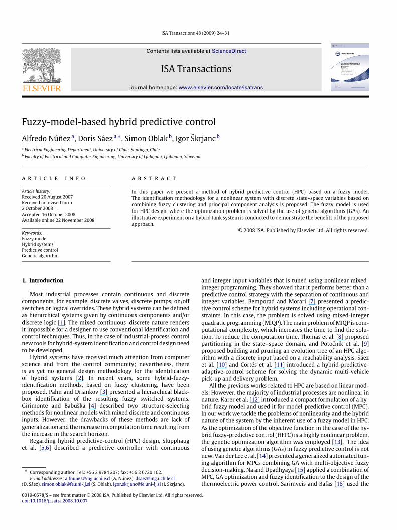
HFPC-BB consider only a reduced space search. The parametersfor HFPC-GA are as follows: mutation probability pm = 0.001,crossover probability pc = 0.7 and for the stopping criterion weused the maximum number of generations, which we obtain byfurther analyses.Fig. 9 shows the objective function as a function of the

generation number for different numbers of individuals. Basedon this figure, 30 generations with 14 individuals are selected inour example. Fig. 10 shows how this selection brings a tradeoffbetween the computation time and the value of the objectivefunction. Fig. 11 presents the computation time as a function ofthe number of generations for different numbers of individuals.

A. Núñez et al. / ISA Transactions 48 (2009) 24–31 29

Fig. 9. Evolution of the objective function.

Fig. 10. Computation time vs. the objective function.

The computation time is linearly dependent on the generationnumber, and its slope increases slightly with the number ofindividuals. It is clear that the time needed to calculate the solutionin each sampling time is shorter than the sampling time for allthe cases. This means that all the proposed control strategies aresuitable for real-time control in the sense of time consumption.For 30 generations with 14 individuals, the computation time wasapproximately 84.3 s (1.41% of the total simulation time), andthe calculation time during each iteration was smaller than thesampling time.With optimal values of 30 generation with 14 individuals, the

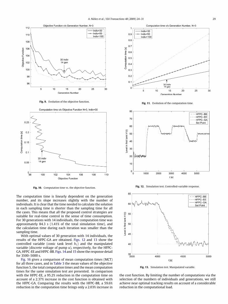
results of the HFPC-GA are obtained. Figs. 12 and 13 show thecontrolled variable (conic tank level h1) and the manipulatedvariable (discrete voltage of pump u), respectively, for the HFPC-GA, HFPC-EE andHFPC-BB. Figs. 14 and 15 show the response detailfor 3500–5000 s.Fig. 16 gives a comparison of mean computation times (MCT)

for all three cases, and in Table 3 the mean values of the objectivefunction 5, the total computation times and themean computationtimes for the same simulation test are presented. In comparisonwith the HFPC-EE, a 95.2% reduction in the computation time onaccount of a 2.37% increase in the cost function is obtained withthe HFPC-GA. Comparing the results with the HFPC-BB, a 59.6%reduction in the computation time brings only a 2.03% increase in

Fig. 11. Evolution of the computation time.

Fig. 12. Simulation test. Controlled-variable response.

Fig. 13. Simulation test. Manipulated variable.

the cost function. By limiting the number of computations via theselection of the numbers of individuals and generations, we stillachieve near optimal tracking results on account of a considerablereduction in the computational load.

30 A. Núñez et al. / ISA Transactions 48 (2009) 24–31

Table 3Mean values of the objective function and the computation times.

N2 = 3, Nu = 3, λ = 0.001 J1 J2 J Total computation time (s) Mean computation time (s)

HFPC-EE 96.69 432.4 97.12 1741.7 2.898HFPC-GA (30, 14) 98.93 488.64 99.48 84.3 0.140HFPC-BB 97.03 427.9 97.46 208.9 0.348

Fig. 14. Simulation test. Controlled variable response. Detail of Fig. 12.

Fig. 15. Simulation test. Controlled-variable response. Detail of Fig. 13.

Fig. 16. Comparison of computation times.

Table 4Mean values and standard deviations of |y− r| and |∆u|.

N2 = 3, Nu = 3,λ = 0.001

Mean(|y−r|) Mean(|∆u|) Std(|y−r|) Std(|∆u|)

HFPC-EE 2.0910 7.1500 4.8468 9.7999HFPC-GA (30, 14) 2.2161 8.5502 4.8619 9.7494HFPC-BB 2.1113 7.1833 4.8539 9.6983

Table 4 presents the statistics for the controlled and manipu-lated variables.

5. Conclusion

This work presents a new approach to the control of nonlinearsystems with mixed integer and continuous states and inputs.Using a predictive strategy based on a fuzzy model, the problemsof the mixed discrete and continuous variables and nonlinearitycan be solved together. The key element of the fuzzy-modelidentification in the case of hybrid systems is the detectionand estimation of the switching regions, which is realized by acombination of fuzzy clustering and principal eigenvector analysis.The optimization of the predictive objective function is an NP-hard problem in the case of hybrid nonlinear systems, whichcan be efficiently solved by genetic algorithms. The proposedHFPC-GA control algorithm was successfully tested on the hybridtank system in terms of accuracy and computation time. In acomparison with an optimal explicit-enumeration method andthe branch-and-bound method we showed that the proposedmethod gives comparable reference-tracking results on account ofa considerable reduction of the computational load.In summary, the main contribution of the paper is the

combination of using PCA analysis in fuzzy modelling and geneticalgorithms in obtaining the HPC law. Future work will be focusedon generalizing the methodology of fuzzy identification for hybridnonlinear systems. Other evolutionary algorithms such as PSOcould also be investigated. It is also planned to apply HFPC-GA tothe real-time control of a tank system.

Acknowledgements

This work was supported in part by Fondecyt grants #1061156and #7070293 (Chile) and by the Ministry of Science, HigherEducation and Technology of the Republic of Slovenia. The authorsgratefully acknowledge this support.

References

[1] Bemporad A, Morari M. Control of systems integrating logic, dynamics andconstraints. Automatica 1999;35:407–27.

[2] Bemporad A, Heemels W, De Schutter B. On hybrid systems and closed-loopMPC systems. IEEE Transactions on Automatic Control 2002;47:863–9.

[3] Palm R, Driankov D. Fuzzy switched hybrid systems—Modeling and identifica-tion. In: Proc. of the 1998 IEEE ISCI/CIRA/SAS joint conf. 1998. p. 130–5.

[4] Girimonte D, Babuska R. Structure for nonlinear models with mixed discreteand continuous inputs: A comparative study. In: Proc. of IEEE internationalconf. on systems, man and cybernetics. 2004. p. 2392–7.

[5] Slupphaug O, Vada J, Foss B. MPC in systems with continuous and discretecontrol inputs. In: Proc. of American control conference. 1997.

[6] Slupphaug O, Foss B. Model predictive control for a class of hybrid systems. In:Proc. of European control conference. 1997.

[7] Bemporad A, Morari M. Predictive control of constrained hybrid systems.Automatica 2000;71–8.

A. Núñez et al. / ISA Transactions 48 (2009) 24–31 31

[8] Thomas J, Dumur D, Buisson J. Predictive control of hybrid systems undera multi-MLD formalism with state space polyhedral partition. In: Proc. ofAmerican control conference. 2004.

[9] Potočnik B, Mušič G, Zupančič B. Model predictive control systems withdiscrete inputs. In: Proc. 12th IEEEMediterranean electrotechnical conference.2004. p. 383–6.

[10] Sáez D, Cortés CE, Núñez A. Hybrid adaptive predictive control forthe multi-vehicle dynamic pick-up and delivery problem based on ge-netic algorithms and fuzzy clustering. Computers & Operations Research.http://dx.doi.org/10.1016/j.cor.2007.01.025.

[11] Cortés CE, Sáez D, Núñez A. Hybrid adaptive predictive control for a dynamicpickup and delivery problem including traffic congestion. InternationalJournal of Adaptive Control and Signal Processing 2008;22(2):103–23.

[12] Karer G, Mušič G, Škrjanc I, Zupančič B. Hybrid fuzzy model-based predictivecontrol of temperature in a batch reactor. Computers and ChemicalEngineering 2007;31:1552–64.

[13] Man K, Tang K, Kwong S. Genetic algorithms, concepts and designs. Springer;1998.

[14] van der Lee JH, SvrcekWY, Young BR. A tuning algorithm for model predictivecontrollers based on genetic algorithms and fuzzy decision making. ISATransactions 2008;47:53–9.

[15] Na MG, Upadhyaya BR. Application of model predictive control strategy basedon fuzzy identification to an SP-100 space reactor. Annals of Nuclear Energy2006;33(17–18):1467–78.

[16] Sarimveis H, Bafas G. Fuzzy model predictive control of non-linear processesusing genetic algorithms. Fuzzy Sets and Systems 2003;139:59–80.

[17] Witsenhausen HS. A class of hybrid-state continuous time dynamic systems.IEEE Transactions on Automatic Control 1966;11(2):161–7.

[18] Tanaka K, Iwasaki M, Wang HO. Switching control of an R/C Hovercraft:Stabilization and smooth switching. IEEE Transactions Systems Man andCybernetics 2001;31:853–63.

[19] Floudos C. Non-linear and mixed integer optimization. Oxford UniversityPress; 1995.

[20] Rudolph G. Convergence analysis of canonical genetic algorithms. IEEETransactions on Neural Networks 1994;5(1):96–101.