
Hybrid adaptive predictive control for the multi-vehicle dynamic pick-up and delivery problem based...
27
Computers & Operations Research 35 (2008) 3412 – 3438 www.elsevier.com/locate/cor Hybrid adaptive predictive control for the multi-vehicle dynamic pick-up and delivery problem based on genetic algorithms and fuzzy clustering Doris Sáez a , ∗ , Cristián E. Cortés b , Alfredo Núñez a a Electrical Engineering Department , Universidad de Chile, Av. Tupper 2007, Santiago, Chile b Civil Engineering Department, Universidad de Chile, Blanco Encalada 2002, Santiago, Chile Available online 9 February 2007 Abstract In this paper, we develop a family of solution algorithms based upon computational intelligence for solving the dynamic multi- vehicle pick-up and delivery problem formulated under a hybrid predictive adaptive control scheme. The scheme considers future demand and prediction of expected waiting and travel times experienced by customers. In addition, this work includes an analytical formulation of the proposed prediction models that allow us to search over a reduced feasible space. Predictive models consider relevant state space variables as vehicle load and departure time at stops. A generic expression of the system cost function is used to measure the benefits in dispatching decisions of the proposed scheme when solving for more than two-step ahead under unknown demand. The demand prediction is based on a systematic fuzzy clustering methodology, resulting in appropriate call probabilities for uncertain future. As the dynamic multi-vehicle routing problem considered is NP-hard, we propose the use of genetic algorithms (GA) that provide near-optimal solutions for the three, two and one-step ahead problems. Promising results in terms of computation time and accuracy are presented through a simulated numerical example that includes the analysis of the proposed fuzzy clustering, and the comparison of myopic and new predictive approaches solved with GA. 2007 Elsevier Ltd. All rights reserved. Keywords: Dynamic pick-up and delivery problem; Predictive control; Fuzzy clustering; Genetic algorithms 1. Introduction and background The pick-up and delivery problem (PDP), with or without time windows, has been widely studied in the field-related literature by many researchers, from where various formulations as well as solution methods have been proposed to deal with different versions of the PDP [1]. Most exact and heuristic methods have been developed to solve real instances of static and dynamic problems under either stochastic or deterministic demand. In most dynamic versions of the PDP, (with demand that appears in real-time) it is assumed that the dispatcher manages reliable advanced information with regard to service requests. However, it is not very usual to find real-time routing decision rules considering ∗ Corresponding author. Tel.: +56 2 9784207; fax: +56 2 6720162. E-mail addresses: [email protected] (D. Sáez), [email protected] (C.E. Cortés). 0305-0548/$ - see front matter 2007 Elsevier Ltd. All rights reserved. doi:10.1016/j.cor.2007.01.025
-
Upload
independent -
Category
Documents
-
view
0 -
download
0
Transcript of Hybrid adaptive predictive control for the multi-vehicle dynamic pick-up and delivery problem based...

Computers & Operations Research 35 (2008) 3412–3438www.elsevier.com/locate/cor
Hybrid adaptive predictive control for the multi-vehicle dynamicpick-up and delivery problem based on genetic algorithms and
fuzzy clustering
Doris Sáeza,∗, Cristián E. Cortésb, Alfredo Núñeza
aElectrical Engineering Department , Universidad de Chile, Av. Tupper 2007, Santiago, ChilebCivil Engineering Department, Universidad de Chile, Blanco Encalada 2002, Santiago, Chile
Available online 9 February 2007
Abstract
In this paper, we develop a family of solution algorithms based upon computational intelligence for solving the dynamic multi-vehicle pick-up and delivery problem formulated under a hybrid predictive adaptive control scheme. The scheme considers futuredemand and prediction of expected waiting and travel times experienced by customers.
In addition, this work includes an analytical formulation of the proposed prediction models that allow us to search over a reducedfeasible space. Predictive models consider relevant state space variables as vehicle load and departure time at stops. A genericexpression of the system cost function is used to measure the benefits in dispatching decisions of the proposed scheme when solvingfor more than two-step ahead under unknown demand. The demand prediction is based on a systematic fuzzy clustering methodology,resulting in appropriate call probabilities for uncertain future.
As the dynamic multi-vehicle routing problem considered is NP-hard, we propose the use of genetic algorithms (GA) that providenear-optimal solutions for the three, two and one-step ahead problems. Promising results in terms of computation time and accuracyare presented through a simulated numerical example that includes the analysis of the proposed fuzzy clustering, and the comparisonof myopic and new predictive approaches solved with GA.� 2007 Elsevier Ltd. All rights reserved.
Keywords: Dynamic pick-up and delivery problem; Predictive control; Fuzzy clustering; Genetic algorithms
1. Introduction and background
The pick-up and delivery problem (PDP), with or without time windows, has been widely studied in the field-relatedliterature by many researchers, from where various formulations as well as solution methods have been proposed to dealwith different versions of the PDP [1]. Most exact and heuristic methods have been developed to solve real instancesof static and dynamic problems under either stochastic or deterministic demand. In most dynamic versions of thePDP, (with demand that appears in real-time) it is assumed that the dispatcher manages reliable advanced informationwith regard to service requests. However, it is not very usual to find real-time routing decision rules considering
∗ Corresponding author. Tel.: +56 2 9784207; fax: +56 2 6720162.E-mail addresses: [email protected] (D. Sáez), [email protected] (C.E. Cortés).
0305-0548/$ - see front matter � 2007 Elsevier Ltd. All rights reserved.doi:10.1016/j.cor.2007.01.025
D. Sáez et al. / Computers & Operations Research 35 (2008) 3412–3438 3413
potential future requests entering the system while vehicles are in operation. In this paper, we focus on developingefficient algorithms to solve dynamic multi-vehicle routing problems for passengers by considering future information(prediction) into the current vehicle dispatch decisions. The algorithms are developed based on a hybrid predictivecontrol (HPC) framework for the dynamic PDP formulated by the authors in a previous work.
Over the last few years, the interest in studying the dynamic and stochastic versions of the PDP (associated withdial-a-ride systems) has rapidly grown, mainly due to the access to communication and information technologies,as well as the current interest in real-time dispatching and routing. According to Gendreau et al. [2], stochastic ve-hicle routing problems are characterized by stochastic demands [3–6], stochastic customers [7] or a mix of both[2,3,8,9]. In the case of dynamic versions of the vehicle routing problem, our analysis focuses on the dynamic pick-upand delivery problem (DPDP), whose final output is a set of routes for all vehicles, which are dynamically chang-ing over time [10–13]. In addition, some applications to real problems of such systems have been implemented[14,15].
Regarding the use of future information to improve dispatching decisions, mainly in the context of the DPDP, thereare just few examples of research on this area. Powell and his team solve the problem of dynamically assigning driversto loads that arise randomly over time motivated from long-haul truckload trucking applications [16]. Ichoua et al.[17] develop a strategy based on probabilistic knowledge about future request arrivals to manage the fleet of vehiclesfor real-time vehicle dispatching. Their strategy introduces forecasted customers in vehicle routes to provide a goodcoverage of the territory. Solution approaches found in this research line are diverse, with formulations based upondynamic network models [18], dynamic and stochastic programming schemes [19,20], etc.
Recently, Cortés and Jayakrishnan [21] postulated that the problem could be modeled under a hybrid adaptivepredictive control (HAPC) scheme, considering that potential rerouting of vehicles could affect the current dispatchdecisions, through the extra cost of inserting real-time service requests into predefined vehicle routes while vehiclesare moving. Cortés et al. [22] describe a formal formulation of the DPDP as an HAPC problem, based on state spacevariables. The system state is defined in terms of departure time and vehicle loads at stops (stochastic state spacevariables), the system inputs (control actions) are routing decisions, the system outputs are effective departure time tostops, and the demand requests are modeled as disturbances. The authors use discrete model with variable step size,with a dispatch objective function incorporating the predictive effect via probabilities computed from historical dataregarding typical demand patterns.
Cortés et al. [22] test their model via simulated data, concluding that the inclusion of predictive power improvesthe performance of system customers, mainly through savings in effective waiting times, when compared with amyopic dispatch decision model. With regard to the predictive model, the authors use a classic clustering tech-nique (classic zoning) in order to estimate the spatial–temporal probabilities to forecast future pick-up and deliverypoints.
We recognize that the sophistication of both, solution algorithms and clustering techniques, is crucial to obtain op-timal results under more realistic scenarios. Thus, by developing efficient algorithms to solve the problem, a moregeneral cost function formulation can be tested and calibrated via sensitivity analysis. In addition, other model-specific parameters (associated with spatial zoning and probability computations) can also be estimated by using betteralgorithms.
Therefore, in this paper we develop efficient solution algorithms (based on genetic algorithm heuristic techniques,GA) as well as more accurate trip pattern prediction method based on historical data (fuzzy zoning). Broadly speaking,the major contributions of this paper are threefold. First, we develop formal analytical formulations of the state spacemodels, which allow the modeler directly use a variety of numerical optimization methods to face different problemconditions. Second, fuzzy zoning is a generic method that computes trip patterns and their probabilities from historicaldata, so we can have more accurate trip patterns predictions under more realistic scenarios. Finally, and based on suchan analytical approach, GA are proposed and tested based upon a simulated example.
Next, and for the sake of completeness, we review recent literature in the use of heuristic and metaheuristic methodsfor solving different kinds of vehicle routing problems (VRP), either dynamic or static [23–27].
Over the last few years, several modifications of the well-known Tabu search method have been developed to solveVRP variants, such as granular Tabu search and adaptive memory-based on Tabu search [12,25,28]. Another heuristicmethod for the dynamic VRP is a priority-based solver proposed by Tighe et al. [29].
As VRP is NP-hard, GA based on evolutionary techniques have been analyzed in the specialized literature. Specif-ically, GA have been applied to different versions of the VRP, considering various chromosome representations and

3414 D. Sáez et al. / Computers & Operations Research 35 (2008) 3412–3438
genetic operators according to the particular problem. Skrlec et al. [30] propose a GA optimization approach withhandy heuristic techniques for the single VRP that allows further reducing the computation time by using a cer-tain selection of the initial population. In addition, in [31] the same approach was applied to a multi-vehicle routingproblem.
Moreover, Zhu [32] describes specialized GA based on adaptive parameters to solve the static VRP with timewindows that prevents the solution search from a premature convergence and improves the results when comparedwith the typical GA method. Tong et al. [33] considers a GA method for the static VRP with time windows underuncertain fleet size. To solve this problem, a special gene codification associated with the number of vehicles and routesis considered. Recently, Haghani and Jung [34] applied a GA optimization method for the multi-vehicle dynamic VRPwith time-dependent travel time and soft time windows. This method provides promising results in terms of computationtimes.
Jih and Yung-Jen [35] and Osman et al. [36] present a successful comparison of GA against dynamic programming interms of computation time. The former method is used to solve the DVRP with time windows and capacity constraintswhile the latter one is addressed to solve a multiobjective VRP. Moreover, a hybrid method including both algorithmsis described, from which accurate results are obtained in reasonable computation time.
With regard to other heuristics used in the context of the dynamic VRP, new metaheuristics inspired by the behaviorof real ant colonies (ant colony optimization) have been applied to solve such problems [37,38]. These methods areespecially appropriate to efficiently solve combinatorial optimization problems, and are characterized by the combina-tion of a constructive and a memory-based approach on learning mechanisms [39]. Montemanni et al. [37] also applyant colony optimization to a realistic case study that obtains promising results. Dréo et al. [38] present good results fora static VRP by optimizing the fleet size as well as the vehicle route plans.
The two general metaheuristics described above (GA and ant colony optimization) have been applied only on myopicdynamic VRP formulations without considering future demand scenarios for improving current dispatch decisions. Inthis paper, we show an application of GA on a non-myopic formulation for the dynamic VRP, based upon an HAPCscheme.
The structure of the paper is as follows. In the next section, a formal analytical formulation of the HAPC state spacemodel for DPDP is presented. Next, in Section 3, the fuzzy zoning model to deal with the flexible and systematic useof historical demand patterns is shown and calibrated. In Section 4, we propose and test the use of GA to solve theanalytical model presented in Section 2. Finally, the advantages when using the new fuzzy HAPC-based GA schemeof solution are quantified by conducting simulation experiments.
2. Analytical formulation: hybrid adaptive predictive control (HAPC) approach
In this section, we formalize the DPDP under a HAPC scheme. The system is formalized in terms of state spacevariables and the objective function. The fleet size is assumed known, and the cost function does not include timewindows on either pick-up or delivery points. The operational cost is approximated by the total vehicle time traveled(see Section 2.2 for details) and the user cost considers both waiting and travel time.
The service consists of picking up (from) and delivering passengers (to) specific spatial coordinates, which are knownonly after the corresponding real-time request is received by the dispatcher. Vehicles have to be quickly rerouted (fromtheir original sequence of tasks) in order to schedule the new requests into predefined vehicle routes while vehicles are inmovement. Routing decisions are taken based on the minimization of an objective function that depends on state spacevariables associated with the real-time status of vehicles. These state variables should include all the important featuresof vehicles, which are in our case, the expected departure time and the expected vehicle load at stops. In addition, weassume that historical data are available, regarding pick-up and delivery positions (in terms of coordinates) as well asoccurrence time of the call. This information feed the predictive model as explained next.
In Section 2.1 the stricter dynamic model, as an extension of the proposal by Cortés et al. [22], is formulated forthe specific problem of routing a fleet of F vehicles for serving real-time demand, distributed over a delimited urbanarea. Travel time conditions and network structure are simplified by considering a constant vehicle average speedwhen moving from one stop to another. Next in Section 2.2, the general objective function formulation is summarized,adding the special case of three-step ahead prediction. Finally, an operational policy is modeled through an analyticalformulation to show the general problem structure and visualize its advantages.
D. Sáez et al. / Computers & Operations Research 35 (2008) 3412–3438 3415
2.1. Dynamic model formulation and logical feasibility constraints
In the context of control theory, hybrid systems are characterized by both continuous and discrete/integer variables.Specifically, hybrid systems can be expressed as a non-linear state space system given by
x(k + 1) = f (x(k), u(k)),
y(k) = g(x(k)), (1)
where x(k) are the continuous and/or discrete (integer) state space variables, u(k) are the continuous and/or discreteinput or manipulated variables and y(k) define the continuous and/or discrete system outputs. In general, a HPC designminimizes the following generic objective function [40]:
min{u(k),u(k+1),...,u(k+N−1)} J (u(k), . . . , u(k + N − 1), x(k + 1), . . . , x(k + N), y(k + 1), . . . , y(k + N)), (2)
where J is an objective function, k is the current time, N the prediction horizon, x(k + t), y(k + t) are the expected statespace vector and the expected system output at instant k + t , respectively, and {u(k), . . . , u(k + N − 1)} representsthe control sequence, which corresponds to the vector of optimization variables. Once expression (2) is optimized,only the first element of the control vector is used to update the system conditions, based upon the receding horizonmethodology.
The DPDP modeling requires a variable stepsize (�), unlike traditional HPC approaches in which stepsizes arenormally fixed. In this case, system events are triggered by specific actions, justifying a variable stepsize as a proxy ofexpected time interval between calls.
At any instant k, each vehicle that belongs to the dispatch fleet has associated with it a sequence of tasks (stops). Ana-lytically, Sj (k) represents the sequence of stops assigned to vehicle j at instant k. As introduced in the previous section,the state space variables considered here are the estimated departure time and load after vehicles leave each stop belong-ing to their assigned sequence. In short, T i
j (k) and Lij (k) represent the estimated departure time and load when vehicle
j leaves stop i, computed at instant time k, respectively. The set of sequences S(k) = {S1(k), . . . , Sj (k), . . . , SF (k)}associated with vehicles corresponds to the manipulated variable u(k) and the requests asking for service are the modeldisturbances.
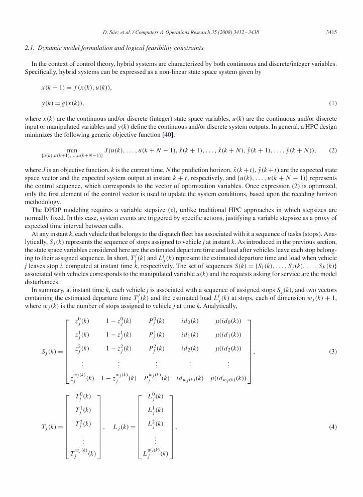
In summary, at instant time k, each vehicle j is associated with a sequence of assigned stops Sj (k), and two vectorscontaining the estimated departure time T i
j (k) and the estimated load Lij (k) at stops, each of dimension wj(k) + 1,
where wj(k) is the number of stops assigned to vehicle j at time k. Analytically,
Sj (k) =
⎡⎢⎢⎢⎢⎢⎢⎢⎢⎢⎢⎣
z0j (k) 1 − z0
j (k) P 0j (k) id0(k) �(id0(k))
z1j (k) 1 − z1
j (k) P 1j (k) id1(k) �(id1(k))
z2j (k) 1 − z2
j (k) P 2j (k) id2(k) �(id2(k))
......
......
...
zwj (k)
j (k) 1 − zwj (k)
j (k) Pwj (k)
j (k) idwj (k)(k) �(idwj (k)(k))
⎤⎥⎥⎥⎥⎥⎥⎥⎥⎥⎥⎦
, (3)
Tj (k) =
⎡⎢⎢⎢⎢⎢⎢⎢⎢⎢⎢⎣
T 0j (k)
T 1j (k)
T 2j (k)
...
Twj (k)
j (k)
⎤⎥⎥⎥⎥⎥⎥⎥⎥⎥⎥⎦
, Lj (k) =
⎡⎢⎢⎢⎢⎢⎢⎢⎢⎢⎢⎣
L0j (k)
L1j (k)
L2j (k)
...
Lwj (k)
j (k)
⎤⎥⎥⎥⎥⎥⎥⎥⎥⎥⎥⎦
, (4)
3416 D. Sáez et al. / Computers & Operations Research 35 (2008) 3412–3438
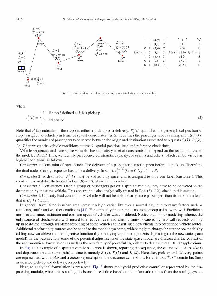
Fig. 1. Example of vehicle 1 sequence and associated state space variables.
where
zij (k) =
{1 if stop i defined at k is a pick-up,
0 otherwise.(5)
Note that zij (k) indicates if the stop i is either a pick-up or a delivery, P i
j (k) quantifies the geographical position ofstop i assigned to vehicle j in terms of spatial coordinates, idi(k) identifies the passenger who is calling and �(idi(k))
quantifies the number of passengers to be served between the origin and destination associated to request idi(k). P 0j (k),
L0j , T 0
j represent the vehicle conditions at time k (spatial position, load and reference clock time).Vehicle sequences and state space variables have to satisfy a set of constraints that depend on the real conditions of
the modeled DPDP. Thus, we identify precedence constraints, capacity constraints and others, which can be written aslogical conditions, as follows:
Constraint 1: Constraint of precedence. The delivery of a passenger cannot happen before its pick-up. Therefore,
the final node of every sequence has to be a delivery. In short, zwj (k)
j (k) = 0, ∀j : 1 . . . F .
Constraint 2: A destination P ij (k) must be visited only once, and is assigned to only one label (customer). This
constraint is analytically treated in Eqs. (8)–(12), ahead in this section.Constraint 3: Consistency. Once a group of passengers get on a specific vehicle, they have to be delivered to the
destination by the same vehicle. This constraint is also analytically treated in Eqs. (8)–(12), ahead in this section.Constraint 4: Capacity load constraint. A vehicle will not be able to carry more passengers than its maximum load,
that is Lij (k)�Lmax.
In general, travel time in urban areas present a high variability over a normal day, due to many factors such asaccidents, traffic and weather conditions [41]. For simplicity, in our applications a conceptual network with Euclideannorm as a distance estimator and constant speed of vehicles was considered. Notice that, in our modeling scheme, theonly source of stochasticity with regard to effective travel and waiting times is caused by new call requests comingup in real-time, through real-time rerouting of some vehicles to insert such new clients into predefined vehicle routes.Additional stochasticity sources can be added to the modeling scheme, which imply to change the state space model (byadding new variables) and the objective function (by modifying certain components depending on the new state spacemodel). In the next section, some of the potential adjustments of the state space model are discussed in the context ofthe new analytical formulations as well as the new family of powerful algorithms to deal with real DPDP applications.
In Fig. 1 an example of a specific vehicle sequence is shown, reporting the sequence, the estimated load (pax/veh)and departure time at stops (min) at time k, namely S1(k), T1(k) and L1(k). Hereafter, pick-up and delivery pointsare represented with a plus and a minus superscript on the customer id. In short, for client r, r+, r− denote his (her)associated pick-up and delivery, respectively.
Next, an analytical formulation is presented. Fig. 2 shows the hybrid predictive controller represented by the dis-patching module, which takes routing decisions in real-time based on the information it has from the routing system
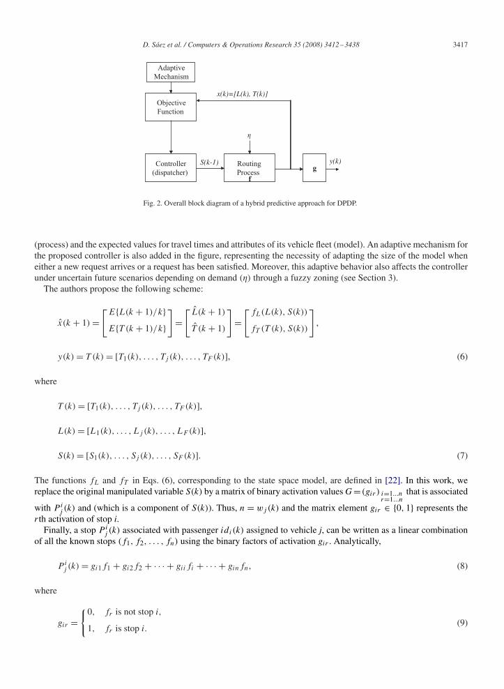
D. Sáez et al. / Computers & Operations Research 35 (2008) 3412–3438 3417
Controller
(dispatcher)
Objective
Function
Adaptive
Mechanism
Routing
Process g
x(k)=[L(k), T(k)]
f
S(k-1) y(k)
�
Fig. 2. Overall block diagram of a hybrid predictive approach for DPDP.
(process) and the expected values for travel times and attributes of its vehicle fleet (model). An adaptive mechanism forthe proposed controller is also added in the figure, representing the necessity of adapting the size of the model wheneither a new request arrives or a request has been satisfied. Moreover, this adaptive behavior also affects the controllerunder uncertain future scenarios depending on demand (�) through a fuzzy zoning (see Section 3).
The authors propose the following scheme:
x(k + 1) =[
E{L(k + 1)/k}E{T (k + 1)/k}
]=[
L(k + 1)
T (k + 1)
]=[
fL(L(k), S(k))
fT (T (k), S(k))
],
y(k) = T (k) = [T1(k), . . . , Tj (k), . . . , TF (k)], (6)
where
T (k) = [T1(k), . . . , Tj (k), . . . , TF (k)],
L(k) = [L1(k), . . . , Lj (k), . . . , LF (k)],
S(k) = [S1(k), . . . , Sj (k), . . . , SF (k)]. (7)
The functions fL and fT in Eqs. (6), corresponding to the state space model, are defined in [22]. In this work, wereplace the original manipulated variable S(k) by a matrix of binary activation values G= (gir ) i=1...n
r=1...nthat is associated
with P ij (k) and (which is a component of S(k)). Thus, n = wj(k) and the matrix element gir ∈ {0, 1} represents the
rth activation of stop i.Finally, a stop P i
j (k) associated with passenger idi(k) assigned to vehicle j, can be written as a linear combinationof all the known stops (f1, f2, . . . , fn) using the binary factors of activation gir . Analytically,
P ij (k) = gi1f1 + gi2f2 + · · · + giifi + · · · + ginfn, (8)
where
gir ={0, fr is not stop i,
1, fr is stop i.(9)
3418 D. Sáez et al. / Computers & Operations Research 35 (2008) 3412–3438
Therefore, the stop position vector Pj (k), excluding the initial condition P 0j (k), can be written as follows:
Pj (k) =
⎡⎢⎢⎢⎢⎢⎢⎢⎢⎢⎢⎢⎢⎢⎢⎣
P 1j (k)
P 2j (k)
...
...
P n−1j (k)
P nj (k)
⎤⎥⎥⎥⎥⎥⎥⎥⎥⎥⎥⎥⎥⎥⎥⎦
=
⎡⎢⎢⎢⎢⎢⎢⎢⎢⎢⎢⎢⎢⎢⎣
g11 g12 · · · · · · g1(n−1) g1n
g21 g22 · · · · · · g2(n−1) g2n
......
......
......
......
......
......
g(n−1)1 g(n−1)2 · · · · · · g(n−1)(n−1) g(n−1)n
gn1 gn2 · · · · · · gn(n−1) gnn
⎤⎥⎥⎥⎥⎥⎥⎥⎥⎥⎥⎥⎥⎥⎦
·
⎡⎢⎢⎢⎢⎢⎢⎢⎢⎢⎢⎢⎢⎢⎣
f1
f2
...
...
fn−1
fn
⎤⎥⎥⎥⎥⎥⎥⎥⎥⎥⎥⎥⎥⎥⎦
= G · f . (10)
From this modeling framework, the constraint 2 above can be written in terms of logical constraints. Thus, the followingnew constraints in terms of the gir values are generated:
gi1 + gi2 + · · · + gin = 1, ∀i = 1, . . . , n, (11)
g1r + g2r + · · · + gnr = 1, ∀r = 1, . . . , n. (12)
Among the set of stops, we know which one is either a pick-up or a delivery. By respecting the precedence stops aswell as all other logical constraints defined above in this section, we can state analytical relations between elements ofthe G matrix in order to satisfy such constraints (a pick-up has to happen before the associated delivery, etc.). Whenmatrix G is used as the optimization variable instead of the sequence, the expected load can be expressed as the sum ofthe initial load plus all the activations of the previous pick-ups less the activations of all previous deliveries, as shownin (13):
Lj (k + 1) =[L0
j (k) · · · L0j (k) +
i∑m=1
(∑r∈P
�(idr (k))gmr −∑r∈D
�(idr (k))gmr
)· · · · · · 0
]T
, (13)
where �(idr (k)) equals the number of passenger at stop fr (this value depends on the request) and P = {r :fr is a pick-up}, D = {r : fr is a delivery}.
By using (13), the capacity load constraint (constraint 4) can be written based on the activation factors of the matrixG. Analytically,
L0j (k) +
i∑m=1
(∑r∈P
�(idr (k))gmr −∑r∈D
�(idr (k))gmr
)�Lmax, i = 2, . . . , n − 1. (14)
In addition, and to complete the state space model, the departure time vector can be expressed as function of the matrixG. In short,
T (k + 1) =[T 0(k) T 0(k) + G1Q(k)G2T · · · T 0(k) +
i−1∑r=1
GrQ(k)Gr+1T · · · T 0(k)
+n−1∑r=1
GrQ(k)Gr+1T
]T
(15)
with Gr denotes the rth row of G, Q(k) is a matrix containing the network and transfer times computed between stops(from estimations based on Euclidean distance and constant speed).
In this model, an expansion and reduction matrix size technique is developed (adaptive behavior) to capture thedynamic effect caused by the real operation. The idea is to either increase or reduce the stop position vector shown inEq. (10), resulting in changes on the load and time vectors as well. For example, when certain vehicle accepts a newservice request, the dimension of the position vector increases in two rows, accounting for the customer pick-up and
D. Sáez et al. / Computers & Operations Research 35 (2008) 3412–3438 3419
delivery stops. Additionally, when a vehicle reaches any stop, that point has to be removed from the original positionvector, reducing its dimension in two rows.
2.2. Reduction of feasible search space: no-swapping case
In this application, the optimization is performed over a reduced space of solutions that satisfy the no-swappingconstraint. This criterion provides sequences that locate the pick-up and delivery of the last call within the previoussequence (the order of previous stops does not change).
There are practical reasons for considering the no-swapping case in the model instead of exploring over a largerfeasible search space. First, any other re-optimization strategy is very time-consuming for our algorithm, and not neededin most cases as discussed next. In fact, in all dynamic systems, it is necessary to use the previous information in order totake real-time decisions. Therefore, the configuration of the previous sequences (those scheduled before the insertion)must be considered as a relevant input to the optimization process. Additionally, in most pick-up and delivery problemconfigurations, the optimal solution of inserting a new request does not alter the order of previous sequences, as shownfrom simulation experiments by Cortés [42]. He found that the no-swapping strategy was optimal in more than 70%of the cases, and in the remainder not-optimal cases, the gap to optimality was negligible.
The global optimum of the dynamic routing problem in terms of the new optimization matrix G can be obtained byoptimally choosing the activation factors gir , for each vehicle in the fleet. Indeed, G determines an optimal sequenceof stops Pj (k) for each vehicle j that minimizes the objective function defined in the next section, whenever a newreal-time request has to be inserted into some previous sequence. Explicitly, the optimal Pj (k) vector is given by
Pj (k) =
⎡⎢⎢⎢⎢⎢⎢⎢⎢⎢⎢⎢⎢⎢⎢⎣
P 1j (k)
P 2j (k)
...
...
P n−1j (k)
P nj (k)
⎤⎥⎥⎥⎥⎥⎥⎥⎥⎥⎥⎥⎥⎥⎥⎦
=
⎡⎢⎢⎢⎢⎢⎢⎢⎢⎢⎢⎢⎢⎢⎣
g11 g12 · · · · · · g1(n−1) g1n
g21 g22 · · · · · · g2(n−1) g2n
......
......
......
......
......
......
g(n−1)1 g(n−1)2 · · · · · · g(n−1)(n−1) g(n−1)n
gn1 gn2 · · · · · · gn(n−1) gnn
⎤⎥⎥⎥⎥⎥⎥⎥⎥⎥⎥⎥⎥⎥⎦
·
⎡⎢⎢⎢⎢⎢⎢⎢⎢⎢⎢⎢⎢⎢⎣
f1
f2
...
...
fn−1
fn
⎤⎥⎥⎥⎥⎥⎥⎥⎥⎥⎥⎥⎥⎥⎦
= G · f , (16)
where f is a vector containing the list of scheduled stops in the whole system at time k. In the no-swapping case, newcalls are inserted directly in previous assigned sequences; by keeping the order of previously scheduled stops (onlyinsertions on previous segments are allowed). As previous sequences hold, (f1, f2, . . . , fn−2), the new insertion addedto the f vector at the bottom (pick-up, delivery), and denoted by (fn−1, fn), imposes the following conditions on relation(16). Analytically,
Pi(k) =
⎧⎪⎪⎪⎪⎪⎪⎪⎪⎪⎪⎪⎨⎪⎪⎪⎪⎪⎪⎪⎪⎪⎪⎪⎩
g11f1 + g1,n−1fn−1 = (x1, y1) if i = 1,
g21f1 + g22f2 + g2,n−1fn−1 + g2,nfn = (x2, y2) if i = 2,
gi,i−2fi−2 + gi,i−1fi−1 + gi,ifi + gi,n−1fn−1 + gi,mfn = (xi, yi) if i = 3, . . . , (n − 2),
gn−1,n−3fn−3 + gn−1,n−2fn−2 + gn−1,n−1fn−1
+gn−1,nfn = (xn−1, yn−1) if i = n − 1,
gn,n−2fn−2 + gn,nfn = (xn, yn) if i = n,
(17)
where (xi, yi) are the spatial coordinates of the i-stop. For example, the first term of (17) (i = 1) represents the firstcomponent of the stop sequence that must be either the new pick-up or the first stop of the previous sequence. Thesecond term (i = 2) represents the second component of the stop sequence that has more options, either the first stopof the previous sequence, the second stop of the previous sequence, the new pick-up stop request or the new deliverystop, and so on.

3420 D. Sáez et al. / Computers & Operations Research 35 (2008) 3412–3438
Eq. (17) can also be written in the form of general expression (16), obtaining the following sparse G matrix (opti-mization decision matrix):
G =
⎡⎢⎢⎢⎢⎢⎢⎢⎢⎢⎢⎢⎢⎢⎢⎢⎢⎢⎢⎢⎢⎢⎢⎢⎢⎢⎢⎢⎢⎢⎢⎢⎢⎢⎢⎢⎢⎢⎢⎢⎢⎢⎢⎢⎢⎢⎢⎣
g11 0 0 0 0 0 . . . . . . . . . . . . 0 0 0 g1(n−1) 0
g21 g22 0 0 0 0 . . . . . . . . . . . . 0 0 0 g2(n−1) g2n
g31 g32 g33 0 0 0 . . . . . . . . . . . . 0 0 0 g3(n−1) g3n
0 g42 g43 g44 0 0 . . . . . . . . . . . . 0 0 0 g4(n−1) g4n
0 0 g53 g54 g55 0 . . . . . . . . . . . . 0 0 0 g5(n−1) g5n
0 0 0 g64 g65 g66 . . . . . . . . . . . . 0 0 0 g6(n−1) g6n
.
.
.
.
.
.
.
.
. 0...
.
.
.
.
.
.
.
.
.
.
.
.
.
.
.
.
.
.
.
.
.
.
.
.
.
.
.
.
.
.
.
.
.
.
.
.
.
.
.
.
.
.
.
.
.
.
.
.
.
.
.
.
.
.
.
.
.
.
.
.
.
.
.
.
.
.
.
.
.
.
.
.
.
.
.
.
.
.
.
.
.
.
.
.
.
.
.
.
.
.
.
.
.
.
.
.
.
.
. g(n−4)(n−6) g(n−4)(n−5) g(n−4)(n−4) 0 0 g(n−4)(n−1) g(n−4)n
.
.
.
.
.
.
.
.
.
.
.
.
.
.
.
.
.
.
.
.
.
.
.
. 0 g(n−3)(n−5) g(n−3)(n−4) g(n−3)(n−3) 0 g(n−3)(n−1) g(n−3)n
0 0 0 0 0 0 . . . . . . 0 0 g(n−2)(n−4) g(n−2)(n−3) g(n−2)(n−2) g(n−2)(n−1) g(n−2)n
0 0 0 0 0 0 . . . . . . 0 0 0 g(n−1)(n−3) g(n−1)(n−2) g(n−1)(n−1) g(n−1)n
0 0 0 0 0 0 . . . . . . 0 0 0 0 gn(n−2) 0 gnn
⎤⎥⎥⎥⎥⎥⎥⎥⎥⎥⎥⎥⎥⎥⎥⎥⎥⎥⎥⎥⎥⎥⎥⎥⎥⎥⎥⎥⎥⎥⎥⎥⎥⎥⎥⎥⎥⎥⎥⎥⎥⎥⎥⎥⎥⎥⎥⎦
.
This analytical problem formulation allows us to generalize the N-step ahead optimization criteria defined in the nextsection and to evaluate different non-linear mixed integer optimization methods, as the GA method described in Section4. If the no-swapping operational constraint is relaxed, the search space for optimization increases, resulting in a lesssparse matrix G, allowing the optimization procedure to obtain a solution closer to a less restrictive global optimum.An intermediate case (partial swapping) is currently being studied as discussed in Section 6.
Once the state space variables are analytically defined in Section 2.1 (Eqs. (13) and (15)), and the search spaceconditions are stated (Section 2.2), the objective function of such an optimization procedure is needed, in order tocomplete the description of the model. Moreover, the two state space models defined in Section 2.1 along with theobjective function, permit the prediction at one, two and more step ahead, which are necessary for implementing theHAPC control strategy. Next, the objective function is presented and discussed.
2.3. Objective function
In Section 2.1, the problem-specific state space formulation was analytically developed. Here, the concept of costfunction is added in order to have a performance measure for deciding the optimal predicted vehicle routes by thecontroller. In this case, we consider both total expected waiting and travel time for passengers. The idle travel time(vehicles moving around without passengers) is also included in the formulation, as explained next.
The major issue in the definition of the objective function is to define a reasonable horizon for prediction N, whichdepends on the studied problem, and also on the intensity of the unknown events entering the system in real-time. Incases where the decision is taken at instant k, but considering a predictive horizon greater than one, the decision maker(controller) adds the predictive feature into the formulation, since decisions made in k+1 will depend on possible events(new service requests) occurring in future instants (k + 2, k + 3, . . . , etc.). Thus, the central dispatcher (controller)computes the decisions for the entire control horizon N, i.e., {S(k), . . . , S(k + N − 1)}, and applies just the next stepsequence S(k), based on receding horizon control. The routing decisions will depend on how well the system predictsthe impact of rerouting passengers due to unknown insertions.
The objective function for a generic prediction horizon N, can be written as follows:
Min{S(k),S(k+1),...,S(k+N−1)} J =N∑
t=1
F∑j=1
hmax(k+t)∑h=1
p�T (k+t)h · ((Cj (k + t) − Cj (k + t − 1))|Sj (k+t−2),h), (18)
D. Sáez et al. / Computers & Operations Research 35 (2008) 3412–3438 3421
Cj (k + t)|Sj (k+t−2),h =wj (k+t)∑
i=1
⎧⎪⎨⎪⎩[Li−1
j (k + t) + 1](T ij (k + t) − T i−1
j (k + t))︸ ︷︷ ︸J travel time
+ zij (k + t − 1)�(T i
j (k + t) − T 0j (k + t))︸ ︷︷ ︸
J waiting time
⎫⎪⎪⎬⎪⎪⎭∣∣∣∣∣∣∣∣Sj (k+t−2),h
, (19)
where k + t is the instant at which the t th request enters the system, measured from time interval k. hmax(k + t) is thenumber of probable requests at instant k+t , p�T (k+t)
h is the probability of occurrence of the hth request type (associatedwith a specific pair of zones, as discussed before in this paper) during time interval �T (k + t), noting that �T (k + t)
specifies the time interval to which time step k + t belongs. Cj (k + t)|Sj (k+t−2),h in (19) is the cost function of vehiclej at instant k + t , which depends on the previous sequence at k + t − 1, Sj (k + t − 2) and a new potential request h
with probabilityp�T (k+t)h , wj(k + t) is the number of stops estimated for vehicle j at instant k + t , Sj (k + t − 2), h is
the new sequence provided that h occurs. Notice that a variable time step is considered and determined by interval timebetween two consecutive requests and this step will be tuned using a sensitivity analysis. For the sake of flexibility andeconomic consistency, the waiting cost component is weighted by a coefficient �.
As mentioned before, the cost function Cj (k + t) as shown in (19), can be split into two pieces: a waiting time anda travel time component. Both of them are written as function of the load and departure time and they are computed asthe departure time between consecutive stops times.
In addition, expression (19) depends on the sequence matrix S(k), which also can be expressed in terms of the matrixG and its components. Analytically,
Cj (k + t)|Sj (k+t−2),h
=wj (k+t)∑
i=1
[1 + L0
j (k + t − 1) +i∑
m=1
(∑r∈P
�(idr (k + t − 1))gmr −∑r∈D
�(idr (k + t − 1))gmr
)]
× [G(i−1)Q(k + t − 1)GiT ] + � · zij (k + t − 1)
(i−1∑r=1
GrQ(k + t − 1)Gr+1T
). (20)
The probabilities of occurrence associated with each scenario are parameters in the objective function, and they couldbe computed based on either real-time data, historical data, or a combination of both. In this particular application, wepropose a fuzzy zoning to compute systematically these probabilities from historical data (off line implementation) asSection 3 describes.
The one-step ahead strategy means that the prediction horizon is N=1, and hmax(k+1)=1 since the new requirementis one and known, and therefore its probability is equal to 1, obtaining the following expression for the objective function,by using (18),
J =F∑
j=1
(Cj (k + 1) −known constant︷ ︸︸ ︷
Cj (k) )|Sj (k−1). (21)
The difference (Cj (k + 1) − Cj (k))|Sj (k−1),1 means that the cost is evaluated considering the control action at theprevious instant, represented by Sj (k −1). Conceptually, J represents the insertion cost when the system accepts a newcall, computed in real-time and considering the entire vehicle fleet. Note that there are many possible alternatives toinsert the new request. Thus, the vehicle sequence finally chosen by the controller is obtained by solving (21).
The two-step ahead prediction cost function is slightly different from the previous one, in that now a computation ofa closed expression for Jj is not straightforward as before, since we do not know with certainty the position of the callthat will enter the system two-steps ahead. However, in the formulation we postulate that the decision for the imminentassignment must depend on the potential future insertions. A probabilistic approach is used in order to incorporate
3422 D. Sáez et al. / Computers & Operations Research 35 (2008) 3412–3438
4 probable Callhmax(k+2)=41 New Call
Instant k Instant k+2Instant k-1 one-step ahead two-step ahead three-step ahead
(S(k),2),4
(S(k)),2
S(k-1),1
(S(k)),1
(S(k),2),3
(S(k),2),2
(S(k),2),1
(S(k),1),4
(S(k),1),3
(S(k),1),2
(S(k),1),1
S(k + 2),C(k + 3)
S(k + 1),C(k + 2)
S(k),C(k + 1)S(k-1),C(k)
S(k + 1),C(k + 2)
S(k + 2),C(k + 3)
S(k + 2),C(k + 3)
S(k + 2),C(k + 3)
S(k + 2),C(k + 3)
S(k + 2),C(k + 3)
S(k + 2),C(k + 3)
S(k + 2),C(k + 3)
>p
4(k+3)
>p
2(k+2)
>p
1(k+1)=1
>p
1(k+2)
>p
3(k+3)
>p
2(k+3)
>p
1(k+3)
>p
4(k+3)
>p
3(k+3)
>p
2(k+3)
>
>
2 probable Callhmax(k+1)=2Instant k+1
>>p
1(k+3)
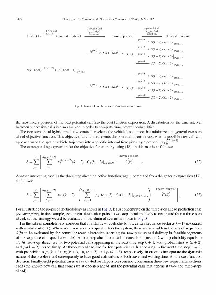
Fig. 3. Potential combinations of sequences at future.
the most likely position of the next potential call into the cost function expression. A distribution for the time intervalbetween successive calls is also assumed in order to compute time interval probabilities.
The two-step ahead hybrid predictive controller selects the vehicle’s sequence that minimizes the general two-stepahead objective function. This objective function represents the potential insertion cost when a possible new call willappear near to the spatial vehicle trajectory into a specific interval time given by a probabilityp
�T (k+2)h .
The corresponding expression for the objective function, by using (18), in this case is as follows:
J =F∑
j=1
⎡⎣hmax(k+2)∑
h=1
p�T (k+2)h (k + 2) · Cj (k + 2)|Sj (k),h −
known constant︷︸︸︷C(k)
⎤⎦ . (22)
Another interesting case, is the three-step ahead objective function, again computed from the generic expression (17),as follows:
J =F∑
j=1
⎡⎣hmax(k+2)∑
h2=1
ph2(k + 2) ·⎛⎝hmax(k+3)∑
h3=1
ph3(k + 3) · Cj (k + 3)|Sj (k),h2,h3
⎞⎠−
known constant︷︸︸︷C(k)
⎤⎦ . (23)
For illustrating the proposed methodology as shown in Fig. 3, let us concentrate on the three-step ahead prediction case(no-swapping). In the example, two origin–destination pairs at two-step ahead are likely to occur, and four at three-stepahead, so, the strategy would be evaluated in the chain of scenarios shown in Fig. 3.
For the sake of completeness, consider that at instant k−1, vehicles follow certain sequence vector S(k−1) associatedwith a total cost C(k). Whenever a new service request enters the system, there are several feasible sets of sequencesS(k) to be evaluated by the controller (each alternative inserting the new pick-up and delivery in feasible segmentsof the sequence of a specific vehicle). At one-step ahead, one call is considered (instant k with probability equals to1). At two-step ahead, we fix two potential calls appearing in the next time step k + 1, with probabilities p1(k + 2)
and p2(k + 2), respectively. At three-step ahead, we fix four potential calls appearing in the next time step k + 2,with probabilities p1(k + 3), p2(k + 3), p3(k + 3) and p4(k + 3), respectively, in order to incorporate the dynamicnature of the problem, and consequently to have good estimations of both travel and waiting times for the cost functiondecision. Finally, eight potential cases are evaluated for all possible scenarios, containing three new sequential insertionseach (the known new call that comes up at one-step ahead and the potential calls that appear at two- and three-stepsahead).

D. Sáez et al. / Computers & Operations Research 35 (2008) 3412–3438 3423
In order to perform a good estimation of future scenarios in the objective function expressions, we analyze thehistorical data through a systematic methodology for determining the future trip patterns and their correspondingoccurrence probabilities. In the next section, a fuzzy clustering approach is proposed to deal with this issue.
3. FUZZY ZONING
In this section, a systematic zoning methodology is developed to split the space into conceptual regions for a betterrepresentation of historical demand patterns, which can be obtained from demand data associated with a representativeoperation day. This proposal turns out to be an alternative a typical classic zoning approach where the total area isdivided into homogeneous and not overlapping-areas. The classic zoning approach could perform badly in cases wheretypical origin–destination patterns do not match any of the predefined pair of zones according to the classic method. Infact, a wrong zoning methodology could impact the computation of probabilities in the objective function for more thantwo-step ahead predictions. The systematic zoning proposed here is based on a fuzzy clustering method that allows usto classify the typical origin–destinations calls in representative and flexible clusters. For simplicity and consideringthe problem features, we adopt the fuzzy C-means to model such a spatial classification.
3.1. Fuzzy DPDP for probability calculation
The fuzzy C-means (FCM) method proposed by Bezdek [43] is a data clustering technique where each data pointbelongs to a cluster with a unique membership degree. In other words, the FCM shows how to split the space into aspecific number of representative clusters. The FCM considers fuzzy partitioning, such that a data point on the spacecan belong to more than one cluster, but with different membership degree (which varies from 0 to 1). FCM is aniterative algorithm that allows the modeler to find cluster centers (centroids) that minimize the following objectivefunction:
S(c) =n∑
k=1
c∑i=1
(�ik)m‖xk − vi‖2, (24)
where n is the data number, c is the number of clusters, uik is the fuzzy partition between 0 and 1, vi represents thecenter of cluster i and m ∈ [1, ∞] is a weighting factor. The details of the FCM algorithm are found in Babuska[44]. In this application, the FCM method is used to determine the representative centers associated with historicalorigin–destination patterns, which will allow us to calculate the corresponding predictive probabilities.
We explicitly propose to compute the probability of each cluster associated with a given origin–destination pair, byfollowing the procedure stated below:
Step 1: The fuzzy clusters are obtained from historical demand data by using the FCM method.Step 2: Membership degrees associated with each call from the historical database are computed for every fuzzy
cluster obtained in Step 1.Step 3: Each call is associated with only one fuzzy cluster, corresponding to that with the biggest membership degree.Step 4: Calls with a membership degree smaller than a chosen threshold are not considered in the process.Step 5: A probability of occurrence of a new request on a specific origin–destination pair is computed as the number
of calls that belong to a fuzzy cluster divided by the total number of calls (after removing the negligible data as explainedin Step 4).
Step 6: Perform a FCM recalculation of cluster center position from historical demand data without considering thenegligible data removed in Step 4.
Notice that the optimal number of clusters determines the number of trip patterns for each time period. The numberof potential calls (each one occurring with certain probability) for the n-step ahead will depend on the time period towhich the n instant belongs, according to the aforementioned clustering method.
In summary, the FCM method permits the modeler to obtain more realistic origin–destination patterns from historicaldata, and consequently, allows him (her) to systemize and improve the probability calculations. This procedure couldimprove the prediction power of future uncertainty resulting from the unknown future calls asking for service oncethey appear, in models with control horizons longer than one-step.

3424 D. Sáez et al. / Computers & Operations Research 35 (2008) 3412–3438
Fig. 4. Single vehicle requests in a certain period of time.
9
8
12
4
3
10
75
9
6
4.5
Del
iver
y [k
m]
Pickup [km]
0 4.5 9
Fig. 5. Pick-up–delivery coordinates of historical demand over a certain time period.
For example, the FCM model performs quite well for jumbled up trip patterns, in which representative zones couldbe spatially overlapped. Next, a one-dimensional example is shown to illustrate the application of the method in thecontext of the DPDP.
3.2. Illustrative example of the FCM method application
A simple example for a single-vehicle dynamic routing problem is presented in Fig. 4 in order to clarify the applicationof the FCM for zoning classification as previously described in Section 3.1. Let us assume door-to-door requestsoccurring on a one-dimensional path of nine kilometers, for pick-up and delivery positions. In the example, supposethat 10 call requests occur over certain time-period (Fig. 4), and suppose that all stops are considered to determine theoptimal zoning and the corresponding probabilities associated with such a partition.
Fig. 5 shows a two-dimensional representation of pick-up and delivery coordinates, for those requests shown inFig. 4. By looking at Fig. 5, trip patterns could be identified just by looking at the points and identify those thatare close by, since the problem is defined on a one-dimensional path. However, when the problem is defined on atwo-dimensional path, the analysis needs an automatic methodology as fuzzy clustering proposed.
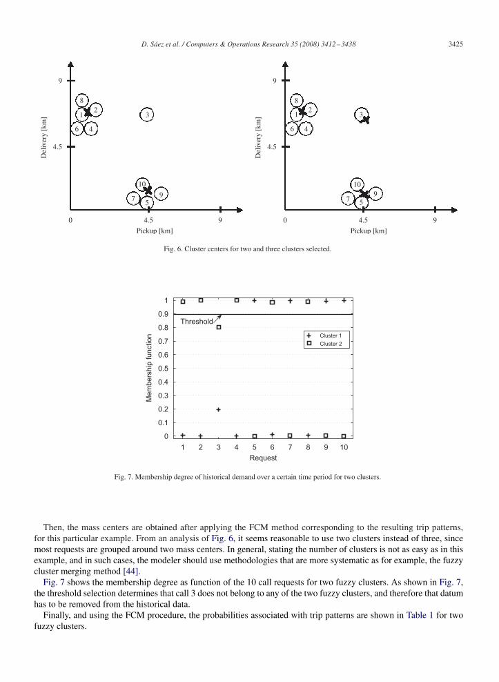
From the historical data shown in Fig. 5, the FCM is used in order to obtain the optimal zoning associated with sucha database. To do this, a fixed number of fuzzy clusters are selected and thus, Fig. 6 shows the results of FCM for twoand three fuzzy clusters, respectively. As explained in Section 3.1, the cluster centers are obtained and denoted by “x”marks in the figure.
D. Sáez et al. / Computers & Operations Research 35 (2008) 3412–3438 3425
9
4.5
8
12
46
3
10
75
9
8
12
109
7 5
3
46
4.5 90
Del
iver
y [k
m]
9
4.5
Del
iver
y [k
m]
Pickup [km]
4.5 90
Pickup [km]
Fig. 6. Cluster centers for two and three clusters selected.
1 2 3 4 5 6 7 8 9 10
0
1
Cluster 1
Cluster 2
Threshold
Mem
bers
hip
function
0.9
0.8
0.7
0.6
0.5
0.4
0.3
0.2
0.1
Request
Fig. 7. Membership degree of historical demand over a certain time period for two clusters.
Then, the mass centers are obtained after applying the FCM method corresponding to the resulting trip patterns,for this particular example. From an analysis of Fig. 6, it seems reasonable to use two clusters instead of three, sincemost requests are grouped around two mass centers. In general, stating the number of clusters is not as easy as in thisexample, and in such cases, the modeler should use methodologies that are more systematic as for example, the fuzzycluster merging method [44].
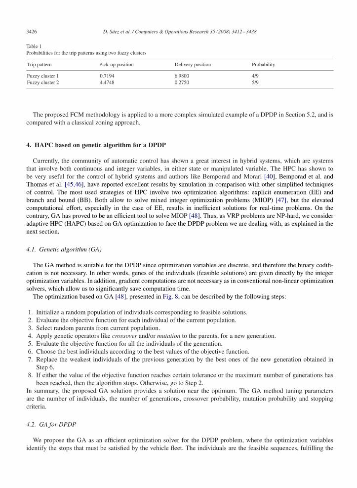
Fig. 7 shows the membership degree as function of the 10 call requests for two fuzzy clusters. As shown in Fig. 7,the threshold selection determines that call 3 does not belong to any of the two fuzzy clusters, and therefore that datumhas to be removed from the historical data.
Finally, and using the FCM procedure, the probabilities associated with trip patterns are shown in Table 1 for twofuzzy clusters.
3426 D. Sáez et al. / Computers & Operations Research 35 (2008) 3412–3438
Table 1Probabilities for the trip patterns using two fuzzy clusters
Trip pattern Pick-up position Delivery position Probability
Fuzzy cluster 1 0.7194 6.9800 4/9Fuzzy cluster 2 4.4748 0.2750 5/9
The proposed FCM methodology is applied to a more complex simulated example of a DPDP in Section 5.2, and iscompared with a classical zoning approach.
4. HAPC based on genetic algorithm for a DPDP
Currently, the community of automatic control has shown a great interest in hybrid systems, which are systemsthat involve both continuous and integer variables, in either state or manipulated variable. The HPC has shown tobe very useful for the control of hybrid systems and authors like Bemporad and Morari [40], Bemporad et al. andThomas et al. [45,46], have reported excellent results by simulation in comparison with other simplified techniquesof control. The most used strategies of HPC involve two optimization algorithms: explicit enumeration (EE) andbranch and bound (BB). Both allow to solve mixed integer optimization problems (MIOP) [47], but the elevatedcomputational effort, especially in the case of EE, results in inefficient solutions for real-time problems. On thecontrary, GA has proved to be an efficient tool to solve MIOP [48]. Thus, as VRP problems are NP-hard, we consideradaptive HPC (HAPC) based on GA optimization to face the DPDP problem we are dealing with, as explained in thenext section.
4.1. Genetic algorithm (GA)
The GA method is suitable for the DPDP since optimization variables are discrete, and therefore the binary codifi-cation is not necessary. In other words, genes of the individuals (feasible solutions) are given directly by the integeroptimization variables. In addition, gradient computations are not necessary as in conventional non-linear optimizationsolvers, which allow us to significantly save computation time.
The optimization based on GA [48], presented in Fig. 8, can be described by the following steps:
1. Initialize a random population of individuals corresponding to feasible solutions.2. Evaluate the objective function for each individual of the current population.3. Select random parents from current population.4. Apply genetic operators like crossover and/or mutation to the parents, for a new generation.5. Evaluate the objective function for all the individuals of the generation.6. Choose the best individuals according to the best values of the objective function.7. Replace the weakest individuals of the previous generation by the best ones of the new generation obtained in
Step 6.8. If either the value of the objective function reaches certain tolerance or the maximum number of generations has
been reached, then the algorithm stops. Otherwise, go to Step 2.In summary, the proposed GA solution provides a solution near the optimum. The GA method tuning parametersare the number of individuals, the number of generations, crossover probability, mutation probability and stoppingcriteria.
4.2. GA for DPDP
We propose the GA as an efficient optimization solver for the DPDP problem, where the optimization variablesidentify the stops that must be satisfied by the vehicle fleet. The individuals are the feasible sequences, fulfilling the

D. Sáez et al. / Computers & Operations Research 35 (2008) 3412–3438 3427
Create Initial
Population
Evaluate Fitness
Selection
Crossover
Mutation
Select Next
Generation
Stoping
Criteria
Check
No
Yes
Return the Best Solution
Fig. 8. GA flowchart.
load, precedence and no-swapping constraints defined in Section 2.1. The gene of an individual considers the followingthree components: the vehicle j used for the new insertion and the sequence position of the new call (for both pick-upand delivery) within the previous sequence, assuming the no-swapping policy.
To explain the gene codification, a simple example for one individual is presented. Let us assume thefollowingvector Pj (k − 1), as defined in Section 2.1, associated with the sequence at the previous instant k − 1(Sj (k − 1)):
Pj (k − 1) =
⎡⎢⎢⎢⎢⎢⎢⎣
P 1j
P 2j
P 3j
P 4j
⎤⎥⎥⎥⎥⎥⎥⎦=
⎡⎢⎢⎢⎢⎢⎣
1 0 0 0
0 1 0 0
0 0 1 0
0 0 0 1
⎤⎥⎥⎥⎥⎥⎦
︸ ︷︷ ︸G
·
⎡⎢⎢⎢⎢⎢⎣
b(1+)
b(2+)
b(1−)
b(2−)
⎤⎥⎥⎥⎥⎥⎦
︸ ︷︷ ︸f
, (25)
where b(x) denotes the position of stop x. For this example, a new customer labeled as 3 enters the system, andhas to be inserted. The new optimization variable can be represented in terms of Pj (k)as shown in the follow-ing matrix equation system, by adding the request in the last two rows of vector f, increasing the dimension of

3428 D. Sáez et al. / Computers & Operations Research 35 (2008) 3412–3438
matrix G.
Pj (k) =
⎡⎢⎢⎢⎢⎢⎢⎢⎢⎢⎢⎢⎢⎢⎣
P 1j
P 2j
P 3j
P 4j
P 5j
P 6j
⎤⎥⎥⎥⎥⎥⎥⎥⎥⎥⎥⎥⎥⎥⎦
=
⎡⎢⎢⎢⎢⎢⎢⎢⎢⎢⎢⎢⎣
g11 0 0 0 g15 0
g21 g22 0 0 g25 g26
g31 g23 g33 0 g35 g36
0 g24 g34 g36 g45 g46
0 0 g35 g37 g55 g56
0 0 0 g38 0 g66
⎤⎥⎥⎥⎥⎥⎥⎥⎥⎥⎥⎥⎦
︸ ︷︷ ︸G
·
⎡⎢⎢⎢⎢⎢⎢⎢⎢⎢⎢⎢⎣
b(1+)
b(2+)
b(1−)
b(2−)
b(3+)
b(3−)
⎤⎥⎥⎥⎥⎥⎥⎥⎥⎥⎥⎥⎦
︸ ︷︷ ︸f
. (26)
Due to the precedence and no-swapping constraints, the previous sequence is held, and the decision variables are givenby the last two columns of matrix G. By using the proposed gene codification, a feasible population of seven individualsfor vehicle j is presented by considering the previous sequence (given by expression (25)) and the new call request:
Population ⇔
⎛⎜⎜⎜⎜⎜⎜⎜⎜⎜⎜⎜⎜⎜⎜⎝
Individual 1
Individual 2
Individual 3
Individual 4
Individual 5
Individual 6
Individual 7
⎞⎟⎟⎟⎟⎟⎟⎟⎟⎟⎟⎟⎟⎟⎟⎠
⇔
⎛⎜⎜⎜⎜⎜⎜⎜⎜⎜⎜⎜⎜⎜⎜⎝
(j, 1, 4)
(j, 1, 6)
(j, 5, 6)
(j, 3, 5)
(j, 4, 6)
(j, 1, 6)
(j, 2, 4)
⎞⎟⎟⎟⎟⎟⎟⎟⎟⎟⎟⎟⎟⎟⎟⎠
⇔
⎛⎜⎜⎜⎜⎜⎜⎜⎜⎜⎜⎜⎜⎜⎜⎜⎜⎜⎜⎜⎜⎜⎜⎜⎜⎜⎜⎜⎜⎝
j, 3+ → 1+ → 2+ → 3− → 1− → 2−
j, 3+ → 1+ → 2+ → 1− → 2− → 3−
j, 1+ → 2+ → 1− → 2− → 3+ → 3−
j, 1+ → 2+ → 3+ → 1− → 3− → 2−
j, 1+ → 2+ → 1− → 3+ → 2− → 3−
j, 3+ → 1+ → 2+ → 1− → 2− → 3−
j, 1+ → 3+ → 2+ → 3− → 1− → 2−
⎞⎟⎟⎟⎟⎟⎟⎟⎟⎟⎟⎟⎟⎟⎟⎟⎟⎟⎟⎟⎟⎟⎟⎟⎟⎟⎟⎟⎟⎠
.
(27)
For example, the individual (j, 1, 4) in terms of Pj (k) can be written as
Individual 1 ⇔ Pj (k) =
⎡⎢⎢⎢⎢⎢⎢⎢⎢⎢⎢⎢⎢⎢⎣
P 1j
P 2j
P 3j
P 4j
P 5j
P 6j
⎤⎥⎥⎥⎥⎥⎥⎥⎥⎥⎥⎥⎥⎥⎦
=
⎡⎢⎢⎢⎢⎢⎢⎢⎢⎢⎢⎢⎣
0 0 0 0 1 0
1 0 0 0 0 0
0 1 0 0 0 0
0 0 0 0 0 1
0 0 1 0 0 0
0 0 0 1 0 0
⎤⎥⎥⎥⎥⎥⎥⎥⎥⎥⎥⎥⎦
︸ ︷︷ ︸G
·
⎡⎢⎢⎢⎢⎢⎢⎢⎢⎢⎢⎢⎣
b(1+)
b(2+)
b(1−)
b(2−)
b(3+)
b(3−)
⎤⎥⎥⎥⎥⎥⎥⎥⎥⎥⎥⎥⎦
︸ ︷︷ ︸f
. (28)
In short, the last two columns of matrix G are the new optimization variables associated with the sequence at instant k.As the individuals of a generation are randomly selected, the same individuals can be repeated in the next population.For example, individuals 2 and 6 are the same in (27), (j, 1, 6).

D. Sáez et al. / Computers & Operations Research 35 (2008) 3412–3438 3429
HYBRID PREDICTIVE CONTROLLER (HPC)
GENETIC ALGORITHMOPTIMIZATION METHOD
NO
YES
SYSTEM
State SpaceVariables
New callrequest
Historical O-DData
Fuzzy C-Mean O-D andprobabilities predictor Step size predictor
HorizonPrediction
N° IndividualN° Generations
Stop criteriumMaximum generation number
ManipulatedVariable S(k)
Optimal S(k)
FLEET-CLIENTS
Fig. 9. Overall block diagram of an HAPC for DPDP.
Note that as GA considers random generation of individuals, the genetic operators (mutation or crossover) couldprovide infeasible solutions that have to be removed (typically through the capacity constraint). In order to have at leastone feasible solution of the population, an always feasible individual, such as (j, wj − 1, wj ) must be used (wj is thenumber of stops including the last call). The number of individuals for each population has to be smaller than the totalnumber of feasible combinations in order to avoid solving the EE method. The crossover operator is not applied heresince the no-swapping constraint has to be satisfied.
Fig. 9 presents the proposed HAPC system scheme. The real system of fleet-clients assigns the sequences using theHAPC controller based on the state space variables, on a call prediction model and on the new call request information.
Next, an example of the application of GA in the context of DPDP is summarized, to visualize the advantages ofthat method when compared with EE, mainly in computation time saving.
4.3. Example
In this section, illustrative tests using EE and GA methods are conducted to evaluate the performance through theproposed objective function (see Section 2.3) and the corresponding computation times.
A DPDP system with four vehicles and an objective function of two-step ahead with six potential calls areconsidered. Vehicles cover an urban service area of around 81 km2, traveling at an average speed of 20 kilometers perhour [22].
The simulations tests considered are:
(i) dynamic vehicle routing under high demand conditions;(ii) dynamic vehicle routing under normal demand conditions and
(iii) dynamic vehicle routing considering a mixed solution (combining GA and EE methods).
As mentioned before, the GA method considers the number of individuals and generations, and mutation probabilityas tuning parameters. Results for three different cases of tuning parameters are presented. The first genetic solution G1
3430 D. Sáez et al. / Computers & Operations Research 35 (2008) 3412–3438
0 10 20 30 40 50 60
0
100
200
300
400
500
600
700
800
0 10 20 30 40 50 60
0
1000
2000
3000
4000
5000
6000
7000
EE
G1
G2
G3
EE
G1
G2
G3
Computation time Objective Function
Com
puta
tion tim
e [s]
Obje
ctive F
unction
Instant k Instant k
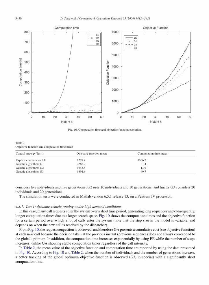
Fig. 10. Computation time and objective function evolution.
Table 2Objective function and computation time mean
Control strategy Test 1 Objective function mean Computation time mean
Explicit enumeration EE 1297.4 1536.7Genetic algorithms G1 2288.2 1.4Genetic algorithms G2 1945.8 13.9Genetic algorithms G3 1694.6 49.7
considers five individuals and five generations, G2 uses 10 individuals and 10 generations, and finally G3 considers 20individuals and 20 generations.
The simulation tests were conducted in Matlab version 6.5.1 release 13, on a Pentium IV processor.
4.3.1. Test 1: dynamic vehicle routing under high demand conditionsIn this case, many call requests enter the system over a short time period, generating long sequences and consequently,
longer computation times due to a larger search space. Fig. 10 shows the computation times and the objective functionfor a certain period over which a lot of calls enter the system (note that the step size in the model is variable, anddepends on when the new call is received by the dispatcher).
From Fig. 10, the request congestion is observed, and therefore GA presents a cumulative cost (see objective function)at each new call because the decision taken at the previous instant (previous sequence) does not always correspond tothe global optimum. In addition, the computation time increases exponentially by using EE while the number of stopsincreases, unlike GA showing stable computation times regardless of the call intensity.
In Table 2, the mean value of the objective function and computation time are reported by using the data presentedin Fig. 10. According to Fig. 10 and Table 2, when the number of individuals and the number of generations increase,a better tracking of the global optimum objective function is observed (G3, in special) with a significantly shortcomputation time.

D. Sáez et al. / Computers & Operations Research 35 (2008) 3412–3438 3431
0 20 40 60 80 1000
1
2
3
4
5
0 20 40 60 80 1000
50
100
150
200
250
Instant k
EE
G1
G2
G3
EE
G1
G2
G3
Computation time Objective Function
Com
puta
tion tim
e [s]
4.5
3.5
2.5
1.5
0.5
Instant k
Obje
ctive F
unction
Fig. 11. Computation time and objective function evolution.
Table 3Objective function and computation time mean
Control strategy Test 2 Objective function mean Computation time mean
Explicit enumeration EE 94.5 1.1Genetic algorithms G1 110.9 0.5Genetic algorithms G2 95.4 1.1Genetic algorithms G3 94.5 1.8
4.3.2. Test 2: dynamic vehicle routing under normal demand conditionsIn this case, few call requests enter the system over the studied time period. The selection of sub-optimal solutions
is not very relevant due to the existence of short sequences since most stops are reached while the system is working.Fig. 11 and Table 3 show computation times and objective function values. By looking at the objective function
evolution in Fig. 11, the GA behavior looks similar to the optimal one (EE), while a non-significant computation timeeffort is observed using GA. Table 3 shows that as the number of individuals and generations increase, the solutionconverges to the optimal global solution (EE). Notice that the G3 solution is the same as that provided by EE, becauseG3 computes almost all possible solutions, consuming a longer computation time though.
4.3.3. Test 3: dynamic vehicle routing considering a mixed solution (combining GA and EE methods)This case is similar to Test 1, but here the previous sequences for the GA method are calculated by EE, that is to say,
at any instant optimization, a good initial solution is used. Fig. 12 and Table 4 show the objective function evolutionand its corresponding error with respect to the optimal solution obtained by the EE method. Although the sequence islonger, the GA objective function error is not significantly increased.
According to Fig. 12 and Table 4, dispatch decisions obtained by GA are very similar to EE, regardless of the numberof planned stops.
In the next section, an illustrative simulated example is presented, including all policies studied in this paper (FCMand GA for one-, two- and three-step ahead problems).

3432 D. Sáez et al. / Computers & Operations Research 35 (2008) 3412–3438
0 10 20 30 40 50 60
0
500
1000
1500
2000
2500
3000
0 10 20 30 40 50 60
0
10
20
30
40
50
60
70
80
90
100
Instant k
G1
G2
G3
EE
G1
G2
G3
Objetive function
Instant k
Objective function error
Fig. 12. Computation time and objective function evolution.
Table 4Objective function and error mean
Control strategy Test 3 Objective function mean Error mean
Explicit eumeration EE 1297.4 –Genetic algorithms G1 1324.0 26.6Genetic algorithms G2 1315.1 17.7Genetic algorithms G3 1309.3 11.9
5. Simulation tests
5.1. Problem statement
A discrete-event system simulation for a two-hour period is conducted in order to evaluate the performance of bothfuzzy zoning and GA method by using a no-swapping operational policy. A transportation fleet of nine vehicles, withcapacity for four passengers each, is considered. As before, the simulation tests are implemented in Matlab version6.5.1 release 13 running on a Pentium IV processor.
We assume that the future origin–destination trip patterns are unknown. However, historical demand obtained fromthe average demand measured over a week before or so, is available. This scenario is not real. However, the demandpatterns follow a heterogeneous distribution inspired on real data from the Origin–Destination Survey in Santiago,Chile, 2001.
We consider an urban service area of approximately 81 km2. Vehicles are assumed to travel straight between stopsat an average speed of 20 km/hr within the region. All simulations are performed over two representative hours(14:00–14:59,15:00–15:59) of a working day.
The historical data generated via simulation follows the trips patterns shown in Fig. 13 with arrows.For the simulation test, 120 calls were generated over the whole simulation period of two hours according to a spatial
and temporal distribution following the same behavior as that of the historical data. Regarding the temporal dimension,

D. Sáez et al. / Computers & Operations Research 35 (2008) 3412–3438 3433
0 1 2 3 4 5 6 7 8 9
0
1
2
3
4
5
6
7
8
9
Km.
Historical demand data
Km
.
Zone 2
Zone 4Zone 3
pickupdeliveryZone 1
Fig. 13. Origin–destination trip patterns.
0 20 40 60 80 100 120
0
1
Request
Cluster 1
Cluster 2
Cluster 3
Cluster 4
Threshold
Mem
bers
hip
function
0.9
0.8
0.7
0.6
0.5
0.4
0.3
0.2
0.1
Fig. 14. Membership degree for call requests.
we assume a negative exponential distribution for time intervals between calls with rate of 1 (call/minute) for boththe first and second hour of simulation. In terms of spatial distribution, pick-up and delivery points were generatedrandomly within each corresponding zone. A reasonable warm up period was considered to avoid boundary distortions(10 calls at the beginning and 10 at the end). Fifty replications of each experiment were conducted to obtain globalstatistics. With regard to the cost function, a weight � = 1 was used, which means that travel time is as important aswaiting time in the cost function expression.
5.2. Fuzzy zoning application
In order to compare the performance of the fuzzy zoning proposed with classic zoning (the four squared areas shownin Fig. 13), two-step algorithms were tested and EE results were considered for benchmarking.
Fig. 14 shows an application of the procedure described in Section 3.1. In fact, four fuzzy clusters are obtained(Step 1), next their membership degrees are depicted (Step 2). Each call is associated with the biggest membershipdegree (Step 3). In addition, the threshold is fixed and equal to 0.6 in order to consider just the data associated with the

3434 D. Sáez et al. / Computers & Operations Research 35 (2008) 3412–3438
Table 5Pick-up and delivery coordinates and probabilities: fuzzy zoning
X pick-up Y pick-up X delivery Y delivery Probability
4.5540 5.7155 2.9218 4.7514 0.12823.7514 4.4812 5.2293 6.2232 0.20514.7989 6.6121 3.0751 4.4972 0.25645.2595 6.5057 4.3494 5.5161 0.4103
Table 6Pick-up and delivery coordinates and probabilities: classic zoning
X pick-up Y pick-up X delivery Y delivery Probability
6.75 6.75 6.75 6.75 0.09682.25 6.75 2.25 6.75 0.21516.75 6.75 2.25 2.25 0.31186.75 6.75 2.25 6.75 0.3763
0 1 2 3 4 5 6 72620
2640
2660
2680
2700
2720
2740
2760
2780
2800
2820
0 1 2 3 4 5 6 72620
2640
2660
2680
2700
2720
2740
2760
2780
2800
2820
Fuzzy C–Means Zoning Classic Zoning
Global Optimaltau=5
Global Optimaltau=5
Effective O
bje
ctive F
unction
Effective O
bje
ctive F
unction
Tau [min] Tau [min]
Fig. 15. Sensitivity analysis for � (classic and fuzzy zonings).
relevant trip patterns (Step 4). Next the corresponding probabilities are computed (Step 5) and the fuzzy cluster centersare obtained again using FCM (Step 6).
Table 5 shows the coordinates of fuzzy cluster centers for pick-up and delivery points of relevant trip patterns and thecorresponding probabilities. On the other hand, Table 6 shows the classic zoning based upon four origin–destinationpairs.
One fine-tuning parameter is the predicted interval between successive calls, �, which is relevant when evaluatingthe performance function of more than one-step ahead algorithms. We found the optimal value of such a parameter byconducting a sensitivity analysis around the observed interarrival times from the historical data report. Fig. 15 showsthe effective objective function (considering user as well as operation cost) using different � values for both classicand fuzzy zonings. Ten replications for each considered � value were used in order to obtain optimal values. For bothzoning methods, the resulting optimal � = 5.
Using the obtained optimal values of �, 50 replications of the two-step ahead algorithm based on EE were conductedin order to compare the performance of both zoning methods. Table 7 presents the mean and standard deviations of the

D. Sáez et al. / Computers & Operations Research 35 (2008) 3412–3438 3435
Table 7Passenger costs
Two-step ahead algorithm Waiting time (min) Travel time (min) Total time (min)
Mean Std Mean Std Mean Std
Classic zoning 6.1437 0.87 10.2358 0.71 16.3795 1.44Fuzzy zoning 5.9370 0.72 10.1629 0.76 16.0999 1.36Savings 0.2067 0.0729 0.2796Improv. (%) 3.36% 0.71% 1.71%
Table 8Vehicle and passenger operational costs
Two-step ahead algorithm Operational costs (min) Total effective costs (min)
Mean Std Mean Std
Classic zoning 117.9 8.81 2699.4 122.84Fuzzy zoning 115.7 8.12 2651.1 112.86Savings 2.2618 48.3163Improv. (%) 1.92% 1.79%
Table 9Performance comparison for one-, two- and three-step ahead problems
Waiting time (min) Travel time (min) Total time (min)
Mean Std Mean Std Mean Std
One-step ahead 6.969 0.82 10.877 0.89 17.847 1.46Two-step ahead 5.921 0.67 10.238 0.79 16.159 1.42Three-step ahead 5.415 0.53 10.687 0.65 16.102 1.35Savings 2 step 1.048 0.639 1.688Improv. (%) 15.04% 5.87% 9.45%Savings 3 step 1.554 0.190 1.745Improv. (%) 22.30% 1.75% 9.78%
waiting, travel and total time for users. The comparison of fuzzy zoning with respect to classic zoning is shown in thesame table. We observed that waiting time is significantly reduced (3.36%) while travel time remains almost constantand consequently, total time also decreases (1.71%).
Operational costs (mean and std) for the entire vehicle fleet are presented in Table 8. In addition, the total costincluding user and operational cost (as in the objective function) is also shown in Table 8. A moderate improvementis observed for both components. However, the proposed fuzzy zoning methodology is a systematic alternative thatallows to determine trip patterns and their corresponding probabilities over a more realistic dynamic dial-a-ride systemwith jumbled up trip patterns.
5.3. Fuzzy HAPC based on GA experiments
In order to analyze and evaluate the performance of both the proposed fuzzy zoning and the HAPC based on GA,simulation tests were conducted for one-, two- and three-step ahead problems under the same conditions described inSection 5.2. We present the results of 50 replications with GA solver by using 20 individuals and 20 generations. Wealso assume the same trip patterns and probabilities obtained in Section 5.2 for the two- and three-step ahead scenarios.
Table 9 shows the effective waiting, travel and total times of passengers, by using the fuzzy HAPC based on GA fordifferent prediction horizons.

3436 D. Sáez et al. / Computers & Operations Research 35 (2008) 3412–3438
Table 10Vehicle and passenger operational costs
Operational costs (min) Effective total costs (min)
Mean Std Mean Std
One-step ahead 105.04 9.76 2730.0 127.832Two-step ahead 105.87 11.68 2568.7 114.516Three-step ahead 110.86 11.18 2608.0 112.444Savings 2 step −0.84 161.27Improv. (%) −0.79% 5.90%Savings 3 step −5.82 122.05Improv. (%) −5.54% 4.47%
We observe that waiting time is significantly reduced by using the two-step ahead method (15.04%) and even morefrom the three-step ahead (22.30%), when compared with the myopic one-step ahead method. In addition, a moderateimprovement in travel time is observed. An interesting case is the comparison between the two-step ahead with thethree-step ahead predictive method in terms of travel time. In fact, savings in travel time are greater for the two-stepahead method, mainly due to the greater uncertainty as the prediction horizon increases, affecting the reliability of theestimated probabilities. Due to this compensatory fact, the total time saving obtained with the three-step ahead methodis almost the same as that of the two-step ahead (9.78% and 9.45%, respectively).
Table 10 describes the operational costs (mean and std) for the entire vehicle fleet. In addition, total effective costis also reported in the table. We observe that vehicle operational costs increase with the two- and three-step aheadmethods, however, total effective costs are still reduced by running both the two-step ahead (5.9%) and the three-stepahead (4.47%) methods. From the results, we can say that the two-step ahead method seems better than the three-stepahead algorithm, because the longer the prediction horizon, the less reliable the estimated probabilities are.
6. Conclusions and further research
In this paper, an analytical formulation for the DPDP based on a HAPC approach is developed considering historicaldemand information for a systematic future prediction to improve current dispatch decisions. There are three majorcontributions of this paper. First, we develop formal analytical formulations of the state space models. Second, fuzzyzoning is utilized to compute probabilities and trip patters from historical data under more realistic scenarios. Third,based on such an analytical approach, GA are proposed and tested based upon a simulated example.
One major contribution of this formulation is the use of artificial intelligence methods to find better dynamicdispatching decisions under non-myopic scenarios (more than one-step ahead prediction). Particularly, GA is presentedas an efficient solver in computation times for this DPDP based upon a detailed analytical formulation. We proved thatunder certain conditions, a scenario of more than two-step ahead can be solved by using GA in reasonable computationtime. The analytical formulation developed in this research can be potentially utilized to fit other numerical methodsto solve the DPDP optimization process.
We conclude that EE works quite well for small problems (for instance, few planned stops and few vehicles). However,as the problem size increases (for example, under more realistic systems), GA becomes an attractive alternative to solvesuch problems in manageable computation time. We believe that GA applied to this specific problem is a good optionto face more complex problems (such as the use of longer sequences, more sophisticated objective functions, relaxedconstraint problems, etc.). Note that choosing the number of individuals and generations is a critical point to getreasonable computation time as well as accurate results.
Moreover, we propose a zoning method based on fuzzy clustering to systematically estimate origin–destinationpatterns from historical data, and consequently, obtain more reliable computations of the corresponding predictionprobabilities. The proposed fuzzy zoning methodology improves the performance of predictive algorithms, mainlyunder more realistic historical data characterized by jumbled up trip patterns.
The integrated methodology (fuzzy HAPC based on GA) allows solving for more than two-step ahead prediction todeal with uncertain and heterogeneous demand pattern scenarios.
D. Sáez et al. / Computers & Operations Research 35 (2008) 3412–3438 3437
In a further application, we propose to combine historical data (offline) with online information in a more elaboratemodel able to capture imminent events that could affect the system performance. Second, a more complete rigorousexpression for the objective function must be used. That should explore the inclusion of time windows (hard and soft),and a better consideration of operational costs. A sensitivity analysis with regard to both parameters � and � is plannedto be also investigated, for two- and three-step ahead problems. We claim that it is possible to improve the estimationof tuning variables, such as number of probable calls, future step time prediction (�) which is unknown, predictionhorizon (N), service policy, search over different feasible solutions structures, etc.
In addition, we plan to relax the no-swapping operational policy to test less restrictive dispatching rules, for whichthe analytical formulation approach would be useful. The incorporation of the network speed within the state spacemodel would allow a better stochastic representation of a real traffic system.
Acknowledgments
This research was partially financed by Fondecyt, Chile, Grants 1061156 and 1061261, and the Millennium Nucleus“Complex Engineering Systems”.
References
[1] Savelsbergh M, Sol M. The general pickup and delivery problem. Transportation Science 1995;29(1):17–29.[2] Gendreau M, Laporte G, Séguin R. Stochastic vehicle routing. European Journal of Operational Research 1996;88:3–12.[3] Gendreau M, Laporte G, Séguin R. An exact algorithm for the vehicle routing problem with stochastic customers and demands. Transportation
Science 1995;29:143–55.[4] Yang W, Mathur K, Ballou R. Stochastic vehicle routing problem with restocking. Transportation Science 2000;34(1):99–112.[5] Secomandi N. Exact and heuristics dynamic programming algorithms for the vehicle routing problem with stochastic demands. PhD dissertation,
College of Business Administration, University of Houston; 1998.[6] Secomandi N. Comparing neuro-dynamic programming algorithms for the vehicle routing problem with stochastic demands. Computers &
Operations Research 2000;27:1201–25.[7] Waters C. Vehicle routing problems with uncertainty and omitted customers. Journal of the Operational Research Society 1989;40:1099–108.[8] Bertsimas D. A vehicle routing problem with stochastic demand. Operations Research 1992;40:574–85.[9] Bertsimas D, Jaillet P, Odoni A. A priori optimization. Operations Research 1990;38(6):1019–33.
[10] Psaraftis H. Dynamic vehicle routing problems. In: Golden BL, Assad AA, editors. Vehicle routing methods and studies. 1998. p. 223–48.[11] Psaraftis H. A dynamic programming solution to the single many-to-many immediate request dial-a-ride problem. Transportation Science
1980;14(2):130–54.[12] Gendreau M, Guertin F, Potvin J, Taillard E. Parallel tabu search for real-time vehicle routing and dispatching. Transportation Science
1999;33:381–90.[13] Kleywegt A, Papastavrou J. The dynamic and stochastic knapsack problem. Operations Research 1998;46:17–35.[14] Madsen O, Raven H, Rygaard J. A heuristics algorithm for a dial-a-ride problem with time windows, multiple capacities, and multiple objectives.
Annals of Operations Research 1995;60:193–208.[15] Dial R. Autonomous dial a ride transit—introductory overview. Transportation Research, Part C 1995;3:261–75.[16] Spivey M, Powell WB. The dynamic assignment problem. Transportation Science 2004;38(4):399–419.[17] Ichoua S, Gendreau M, Potvin JY. Exploiting knowledge about future demands for real-time vehicle dispatching. Transportation Science
2006;40(2):211–25.[18] Powell WB. A comparative review of alternative algorithms for the dynamic vehicle allocation problem. In: Golden BL, Assad AA, editors.
Vehicle routing methods and studies. 1988.[19] Godfrey G, Powell WB. An adaptive dynamic programming algorithm for stochastic resource allocation problems I: single period travel times.
Transportation Science 2002;36:21–39.[20] Topaloglu H, Powell WB. A distributed decision-making structure for dynamic resource allocation using non-linear functional approximations.
Operations Research 2005;53(2):281–97.[21] Cortés CE, Jayakrishnan R. Analytical modeling of stochastic rerouting delays for dynamic multi-vehicle pick-up and delivery problems.
Proceedings of the triennial symposium on transportation analysis (TRISTAN) V, Guadeloupe, French West Indies; 2004.[22] Cortés CE, Sáez D, Núñez A, Muñoz-Carpintero D. Hybrid adaptive predictive control for a dynamic pick-up and delivery problem,
Transportation Science 2007, under review.[23] Le Bouthillier A, Crainic T. A cooperative parallel meta-heuristic for the vehicle routing problem with time windows. Computers & Operations
Research 2005;32:1685–708.[24] Tarantilis C, Ioannou G, Prastacos G. Advanced vehicle routing algorithms for complex operations management problems. Journal of Food
Engineering 2005;70:455–71.[25] Tarantilis C. Solving the vehicle routing problem with adaptive memory programming methodology. Computers & Operations Research
2005;32:2309–27.
3438 D. Sáez et al. / Computers & Operations Research 35 (2008) 3412–3438
[26] Li F, Golden B, Wasil E. Very large-scale vehicle routing: new test problems, algorithms and results. Computers & Operations Research2005;32:1165–79.
[27] Bianchessi N, Righini G. Heuristic algorithms for the vehicle routing problem with simultaneous pick-up and delivery. Computers & OperationsResearch 2007;34(2):578–94.
[28] Toht P, Vigo D. The granular Tabu search and its application to the vehicle-routing problem. INFORMS Journal on Computing 2003;15(4):0333–46.
[29] Tighe A, Smith F, Lyons G. Priority based solver for a real-time dynamic vehicle routing. IEEE international conference on systems, man andcybernetics. 2004. p. 6237–42.
[30] Skrlec D, Filipec M, Krajcar S. A heuristic modification of genetic algorithm used for solving the single depot capacited vehicle routingproblem. In: Proceedings of intelligent information systems, IIS ’97. 1997. p. 184–8.
[31] Filipec M, Skrlec D, Slavko K. An efficient implementation of genetic algorithms for constrained vehicle routing problem. In: Proceedings ofIEEE international conference on system, man and cybernetics, SMC’98. 1998.
[32] Zhu K. A diversity-controlling adaptive genetic algorithm for the vehicle routing problem with time windows. In: 15th IEEE internationalconference on tools with artificial intelligence. November 3–5 2003. p. 176–83.
[33] Tong Z, Ning L, Debao S. Genetic algorithm for vehicle routing problem with time window with uncertain vehicle number. Proceedings of thefifth world congress on intelligent control and automation, June 15–19, Hangzhou, PR China; 2004. p. 2846–49.
[34] Haghani A, Jung S. A dynamic vehicle routing problem with time-dependent travel times. Computers & Operations Research 2005;32:2959–86.
[35] Jih W, Yun-Jen J. Dynamic vehicle routing using hybrid genetic algorithms. Proceedings of the IEEE international conference on robotics &automation, Detroit, MI; 1999. p. 453–8.
[36] Osman M, Abo-Sinna M, Mousa A. An effective genetic algorithm approach to multiobjective routing problems (MORPs). Applied Mathematicsand Computation 2005;163:769–81.
[37] Montemanni R, Gambardella L, Rizzoli A, Donati A. Ant colony system for a dynamic vehicle routing problem. Journal of CombinatorialOptimization 2005;10(4):327–43.
[38] Dréo J, Pétrowski A, Siarry P, Taillard E. Metaheuristics for hard optimization methods and case studies. Berlin: Springer; 2006.[39] Dorigo M, Stützle T. Ant colony optimization. Cambridge, MA: The MIT Press; 2004.[40] Bemporad A, Morari M. Control of systems integrating logic, dynamics and constraints. Automatica 1999;35:407–27.[41] Ceylan H, Bell M. Traffic signal timing optimization based on genetic algorithm approach, including drivers’ routing. Transportation Research
B 2004;38:329–42.[42] Cortés CE. High coverage point-to-point transit (HCPPT): a new design concept and simulation–evaluation of operational schemes. PhD
dissertation, Civil Engineering Department, University of California at Irvine. 2003.[43] Bezdek J. Fuzzy mathematics in pattern classification. PhD thesis, Applied Mathematics Center, Cornell University, Ithaca; 1973.[44] Babuska R. Fuzzy modeling for control. Dordrecht: Kluwer Academic Publishers; 1999.[45] Bemporad A, Heemels W, De Schutter B. On hybrid systems and closed-loop MPC systems. IEEE Transaction on Automatic Control
2002;47:863–9.[46] Thomas J, Dumur D, Buisson J. Predictive control of hybrid systems under a multi-MLD formalism with state space polyhedral partition.
Proceedings of American control conference, Boston, MA, USA; 2004.[47] Floudas C. Non-linear and mixed integer optimization. Oxford: Oxford University Press; 1995.[48] Man K, Tang K, Kwong S. Genetic algorithms, concepts and designs. Berlin: Springer; 1998.