Katholieke Universiteit LeuvenDepartement Elektrotechniek ESAT-SISTA/TR 1998-91Predictive Control Using Fuzzy Models-ComparativeStudy 1Jairo J. Espinosa, Mohamed Hadjili, Vincent Wertz and Joos Vandewalle2October 1998Submitted to the European Control Conference 19991This report is available by anonymous ftp from ftp.esat.kuleuven.ac.be in thedirectory pub/SISTA/espinosa/reports/ECC99.ps.Z2K.U.Leuven, Dept. of Electrical Engineering (ESAT), Research group SISTA,Kardinaal Mercierlaan 94, 3001 Leuven, Belgium, Tel. 32/16/32 18 03,Fax 32/16/32 19 70, WWW: http://www.esat.kuleuven.ac.be/sista. E-mail:jairo.espinosa@esat.kuleuven.ac.be. This work is supported by several insti-tutions: the Flemish Government: Concerted Research Action GOA-MIPS(Model-based Information Processing Systems), the FWO (Fund for Scien-ti�c Research - Flanders) project G.0262.97 ;Learning and Optimization: anInterdisciplinary Approach, The FWO Research Communities: The BelgianState, Prime Minister's O�ce - Federal O�ce for Scienti�c, Technical andCultural A�airs - Interuniversity Poles of Attraction Programme (IUAP P4-02 (1997-2001): Modeling, Identi�cation, Simulation and Control of ComplexSystems SCIENCE-ERNSI (European Research Network for System Identi�-cation): SC1-CT92-0779 Interuniversity Attraction Poles (IUAP P4-02 (1997-2001): Modeling, Identi�cation, Simulation and Control of Complex Systems;and IUAP P4-24 (1997-2001): Intelligent Mechatronic Systems (IMechS) )andV.C.S.T. and the Flemish Institute for Scienti�c and Technological Researchin Industry (I.W.T.). The scienti�c responsibility is assumed by its authors.

Predictive Control Using Fuzzy Models-Comparative StudyJairo J. Espinosa, Mohamed L. Hadjili, Vincent Wertz and Joos VandewalleDepartement Elektrotechniek -K.U.LeuvenKardinaal Mercierlaan 94,B-3001 Heverlee-BelgiumCESAME Universit�e Catholique de LouvainBatiment Euler 4B-1348 Louvain La Neuve-BelgiumDRAFT-VERSIONOctober 1, 1998AbstractFuzzy control and predictive control techniques are two modern control strategies that have been ac-cepted by the industry to solve complex problems. Everyday the industry demands control strategiesthat can deliver better performance for several operating points and these requirements have motivatedthe development of the theory of Nonlinear Model Predictive Control. This type of controllers can beimplemented using fuzzy models. The present paper presents 4 algorithms to construct the controllers.The comparison between the algorithms includes complexity, computational load, model representation,quality of the solution. The controllers are compared using a model of a chemical process (ContinuousStirred Tank Reactor).1 IntroductionThe Model Predictive Control (MPC) strategy has received particular attention in the areas of processcontrol [3], [5], [2]. This strategy is specially attractive because of its reduced number of tuning parametersand high performance [1]. New processes demand higher performance in multiple operating points. Thismeans that new predictive controllers based on nonlinear models are desirable. Fuzzy modeling is a welldeveloped and attractive nonlinear modeling technique due to its capability to capture expert knowledge.In recent years many algorithms have been developed to generate fuzzy models starting from Input-Output data [12], [10], [7]. Nowadays new algorithms permit the combination of numerical and expertinformation in the same framework [6]. Also a framework for non-linear system identi�cation using fuzzymodels has been proposed in [15], [16]. The wide acceptance of these two strategies motivated theformulation of a control strategy using the theory of Model Predictive Control based on Fuzzy Models.Recently di�erent methods for Model Predictive Control based on Fuzzy Models have been presented[18],[21],[22]. This paper compares these control strategies taking into account not only the performanceof the response but also the complexity and the computational e�ort that each strategy requires. Theexperiment used for the comparison is a a chemical process (Continuous Stirred Tank Reactor). Thedistribution of the paper is as follows: Section 2 describes the plant model. Section 3 shows the modelsobtained by means of identi�cation. Section 4 describes brie y the di�erent control strategies. Section 5presents the comparative results and section 6 shows the conclusions and some future perspectives.2 Plant DescriptionThe benchmark plant represents a Continuous-Stirred Tank Reactor. The model was presented in [17]and is described by the following di�erential equations:_Ca(t) = qV (Ca0 � Ca(t))� k0Ca(t)e� ERT (t) (1)_T (t) = qV (T0 � T (t))� k1Ca(t)e� ERT(t) + k2qc(t)�1� e� k3qc(t) �(Tc0 � T (t)) (2)1

2The process consists of an irreversible, exothermic reaction, A ! B, in a constant volume reactor cooledby a single coolant stream. The product concentration is represented by Ca(t) and this concentration iscontrolled by manipulating the coolant ow rate qc(t). The temperature of the mixture is represented byT (t). The heat generated acts to slow the reaction. Ca0 is the inlet feed concentration, q is the process ow rate, T0 and Tc0 the inlet feed and coolant temperatures. All these values are assumed constant atnominal values. In the same way, k0, E=R, V , k1, k2 and k3 are thermodynamic and chemical constants.The numerical values of these parameters are given in table 1.Table 1: The CSTR ParametersParameter Description Nominal Valueq process ow-rate 100 l/minV reactor volume 100 lk0 reaction rate constant 7:2� 1010min�1E=R activation energy 1� 104KT0 feed temperature 350 KTc0 inlet coolant temp. 350 K�H heat of reaction �2� 105 cal/molCp, Cpc speci�c heats 1 cal/g/K�, �c liquid densities 1� 103 g/lha heat transfer coe�. 7� 105 cal/min/KCa0 inlet feed concentration 1 mol/lk1 = ��Hk0�Cp k2 = �cCpc�Cpv k3 = ha�cCpcThe nominal conditions for a product concentration Ca = 0:1 mol/l are:T = 438:54K qc = 103:41 l/min3 Identi�cation using fuzzy modelsFor the present purpose two kind of models were identi�ed. One model uses singleton consequences, socalled \Mamdani model" and the other uses dynamic description as a consequence, so called \Takagi-Sugeno model". For the identi�cation procedure a sampling time Ts = 6 sec. was chosen. A sequence of7500 samples was generated, the �rst 5000 samples were used as training set and 2500 as validation set.Figure 1 shows the input and the output signals used for the identi�cation.3.1 Mamdani modelSeveral structures can be implemented using fuzzy models as was shown in [16]. But perhaps the mostimportant structures are the NARMAX (Non-linear Auto Regressive Moving Average with eXogenousinput) and the NOE (Non-linear Output Error). The NARMAX is a structure which is very easy to tunebecause the parameter �tting problem is a static optimization problem. Unfortunately this is not the casefor the NOE structure. This structure is a recursive structure which demands the solution of a dynamicoptimization problem with many local minima. A practical solution is to calculate �rst the NARMAXmodel and then use its consequences as the initial consequences of the NOE model. A further re�nementis obtained by using Recursive Least Squares (RLS). Of course the solution will be biased, but most ofthe time the bias is small.The NARMAX model is suitable for short term prediction in the presence of noise and the NOE is moresuitable for simulation and long term prediction.For the present case a NOE model was �tted to simulate the future behavior of the plant. The regressorswere selected using the regularity criterion for GMDH and the structure of the modelis:Ca(k + 1) = f(Ca(k); Ca(k � 1); Ca(k � 2); qc(k � 1)) (3)

30 100 200 300 400 500 600 700

0.06

0.08

0.1

0.12

0.14

0.16

time(min)

Con

cent

ratio

n m

ol/l

0 100 200 300 400 500 600 70085

90

95

100

105

110

115

time(min)

Coo

lant

Flo

w l/

min

Figure 1: Identi�cation ExperimentThe identi�ed fuzzy model has 3 triangular membership functions on each input distributed regularly onthe universes of discourse. The number of rules is then 3 � 3 � 3 � 3 = 81 rules. The structure of therules is as follows:if Ca(k) is Small AND Ca(k � 1) is Big AND Ca(k � 2) is Small AND qc(k � 1) is Small THENCa(k + 1) = 0:03737 mol/l.The membership functions can be observed in �gure 2 and the results of the validation in �gure 3.0.07 0.08 0.09 0.1 0.11 0.12 0.13 0.14 0.15

0

0.2

0.4

0.6

0.8

1

Membership functions for Ca(k)

Small Medium Big

0.07 0.08 0.09 0.1 0.11 0.12 0.13 0.14 0.150

0.2

0.4

0.6

0.8

1

Membership functions for Ca(k−1)

Small Medium Big

0.07 0.08 0.09 0.1 0.11 0.12 0.13 0.14 0.150

0.2

0.4

0.6

0.8

1

Membership functions for Ca(k−2)

Small Medium Big

92 94 96 98 100 102 104 106 108 1100

0.2

0.4

0.6

0.8

1

Membership functions for qc(k−1)

Small Medium BigFigure 2: Membership function of the fuzzy model.3.2 Takagi Sugeno ModelsAs the Mamdani fuzzy models, Takagi-Sugeno (TS) fuzzy models are based on a set of IF-THEN rules: IFantecedent THEN consequent. The consequents are usually (linear) functions of the antecedents variables.We focus on a special case of the Takagi-Sugeno (TS) fuzzy model where the o�sets are zeros.The one-step-ahead TS fuzzy model is described by a set of Nc fuzzy rules as follows:Ri : IF Y is Ai

40 50 100 150 200 250

0.06

0.08

0.1

0.12

0.14

0.16

time(min)

Con

c. m

ol/l

Validation−real system (green −−) estimation (blue −)

0 50 100 150 200 250−3

−2

−1

0

1

2

3x 10

−3

time(min)

erro

r. m

ol/l

Validation error

Figure 3: Validation experimentTHEN Cai(k + 1) = �Ti Y (4)where Y = fCa(k); Ca(k � 1); qc(k)g is the set of premise values, Ai = fA1;i; A2;i; B1;ig is the set ofmembership functions associated to the ith rule and �Ti = [ai;1 ai;2 bi;1] is the parameter vector of theith LTI sub-model.To identify such a fuzzy model, we use subtractive clustering to parameterize membership functions anda least squares algorithm to identify linear sub-models parameters. The complexity of the obtained TSfuzzy models depends on two points:� Structure of consequent regressors, which include information about variables used in sub-modelsand the number of parameters.� Number of clusters estimated by the subtractive clustering algorithm. This number is inverselyproportional to the neighborhood radius[20]. Adjusting this radius, the number of fuzzy rules inthe constructed TS fuzzy model can be modi�ed.Based on some experiments on a glass furnace process [19] and the CSTR process, we can conclude thatif the objective is to have good validation, one must decrease the neighborhood radius in the subtractivealgorithm. However the complexity of the TS fuzzy model increases signi�cantly. If the objective ismodel-based control design, a model with few rules, with second order sub-models, gives good closedloop performances. Two TS fuzzy models are identi�ed for the CSTR process with the same consequentregressors but with a di�erent number of rules.Model TS-1 The fuzzy model TS-1 is identi�ed using the following regressor:Ca(k + 1) = f(Ca(k); Ca(k � 1); qc(k � 1)) (5)where f(:) is a linear function. With the radius of neighborhood ra = 0:15, the subtractive clusteringalgorithm estimates 8 fuzzy clusters. The membership functions are described in �gure 4. The validationresults are given in �gure 5.Model TS-2 This fuzzy model is constructed in order to design a model-based controller. With a fewfuzzy rules, good closed loop performances can be obtained. TS-2 is described by 5 fuzzy rules with thesame regressors as TS-1. Figure 6 presents the membership functions learned by subtractive clusteringwith a radius of neighborhood ra = 0:2. The validation results are given in �gure 7.

50.04 0.05 0.06 0.07 0.08 0.09 0.1 0.11 0.12 0.13 0.140

0.1

0.2

0.3

0.4

0.5

0.6

0.7

0.8

0.9

1

Ca(k)

Deg

ree

of m

embe

rshi

p

A11A12A13 A14A15 A16 A17A18

0.04 0.05 0.06 0.07 0.08 0.09 0.1 0.11 0.12 0.13 0.140

0.1

0.2

0.3

0.4

0.5

0.6

0.7

0.8

0.9

1

Ca(k−1)

Deg

ree

of m

embe

rshi

p

A21A22A23 A24A25 A26 A27A28

85 90 95 100 105 110 1150

0.1

0.2

0.3

0.4

0.5

0.6

0.7

0.8

0.9

1

qc(k)

Deg

ree

of m

embe

rshi

p

B11B12B13 B14B15 B16 B17B18

Figure 4: Membership function of the fuzzy model TS-1.0 50 100 150 200 250

0.06

0.08

0.1

0.12

0.14

0.16

time/min

Con

c. m

ol/l

Validation: real Process(−−), TS fuzzy model(−)

0 50 100 150 200 250−0.01

−0.005

0

0.005

0.01

0.015

time/min

erro

r m

ol/l

Validation error

Figure 5: Validation experiment of TS-10.04 0.05 0.06 0.07 0.08 0.09 0.1 0.11 0.12 0.13 0.140

0.1

0.2

0.3

0.4

0.5

0.6

0.7

0.8

0.9

1

Ca(k)

Deg

ree

of m

embe

rshi

p

A11 A12A13 A14 A15

0.04 0.05 0.06 0.07 0.08 0.09 0.1 0.11 0.12 0.13 0.140

0.1

0.2

0.3

0.4

0.5

0.6

0.7

0.8

0.9

1

Ca(k−1)

Deg

ree

of m

embe

rshi

p

A21 A22A23 A24 A25

90 95 100 105 110 1150

0.1

0.2

0.3

0.4

0.5

0.6

0.7

0.8

0.9

1

qc(k)

Deg

ree

of m

embe

rshi

p

B11 B12B13 B14 B15

Figure 6: Membership function of the fuzzy model TS-2.3.3 Model comparisonTable 2 shows a comparison between the di�erent models.

60 50 100 150 200 250

0.06

0.08

0.1

0.12

0.14

0.16

time/min

conc

. mol

/l

Validation: real Process(−−), TS fuzzy model(−)

0 50 100 150 200 250−0.02

−0.01

0

0.01

0.02

time/min

erro

r m

ol/l

Validation error

Figure 7: Validation experiment of TS-2Table 2: Model ComparisonModel No of Rules Param. per rule Simulation error inthe validation setMamdani Model 81 1 2.1205 e-7Takagi-Sugeno Model-1 8 3 4.2200 e-6Takagi-Sugeno Model-2 5 3 9.0306 e-6The simulation error was calculated as:Error = 12500 7500Xk=5001(Ca(k)� Ca(k))2:4 The Predictive Control StrategiesIn this section we discuss four di�erent predictive control strategies based on fuzzy models, the �rst onemakes use of the Mamdani model (but can also use Takagi Sugeno Models). The other three strategiesuse the Takagi Sugeno model to generate the solution. It is important to remark that all the strategiesgenerate a sub-optimal solution in a very e�cient way close to the optimal solution of the Non-LinearQuadratic Program which is always present when the model of the plant is non-linear. The main ideasof the algorithms are discussed in the following sections, a more extensive discussion can be found in[21], [22], [18].4.1 Strategy 1This strategy makes use of the classical solution of the Generalized Predictive Control (GPC) [1] strategy,where the optimal sequence �U is�U = (GTG+ �I)�1GT (W � Yfree) (6)where G is a matrix where the entries are the step response parameters of the system, � is a term in thecost function which penalizes the variations in the input, W is a vector containing the sequence of futurereferences and Yfree is the predicted free response of the system if the plant keeps the current input. The

7main change with the strategy presented in [21] and in [22], is that the terms are time varying and thetime variation is dependent on the state and the amplitude of the inputs. The optimal sequence �U(t) is�U(t) = (G(xt; �u(tjt� 1))TG(xt; �u(tjt� 1))+ �I)�1G(xt; �u(tjt� 1))T (W (t)�Yfree(xt; u(t� 1))) (7)where G(xt; �u(tjt � 1)) is the matrix with the step response coe�cients of the nonlinear plant for thecurrent state xt and with a step amplitude given by �u(tjt � 1) which is the estimated value for �u(t)at time t � 1, the Yfree(xt; u(t � 1)) is the vector of the free response of the plant. Observe that the Gmatrix and the Yfree vector are both estimated from the fuzzy model at each sampling time.4.2 Strategy 2A straightforward extension of predictive control based on fuzzy models is di�cult, because the combina-tion of the N LTI sub-models is an LTV model. In this strategy we compute the control action for eachrule using a linear GPC technique based on the considered LTI sub-model. The control action computedfor each rule minimizes, independently of the degree of ful�llement �i of this rule, the associated quadraticcriterion. The global control action is the convex combination of the control actions computed for eachfuzzy rule.4.3 Strategy 3Firstly construct the LTV model by convex combination of the Nc LTI sub-models. Compute the controlaction that minimizes directly the GPC criterion on the global LTV model. Assume however that thetime variations over the prediction horizon can be neglected, so that the J-step ahead predictions can becomputed using classical Diophantine equations.4.4 Strategy 4Another approach consists in constructing a fuzzy model that directly involves multiple predictions overthe full prediction horizon:Ca(k + 1 + j) = fj( Ca(k); Ca(k � 1); qc(k); : : : ; qc(k + j) ) for j = 1; :::; Ny: (8)The control law can then be obtained by minimizing the GPC criterion with respect to the convexcombination of these multiple predictions.5 Implementation of the controller and performance resultsThe predictive controllers were implemented using the following parameters: prediction horizon Ny = 10,control horizon Nu = 2, � = 0, C(z�1) = 1 and D(z�1) = 1� z�1. Figure 8 shows a \stair" referencesignal used to evaluate the response of the controlled systems, each step having a duration of 10 minand an amplitude of 0.005 mol/l. The reference starts on 0.08 mol/l and it goes up to 0.12 mol/l.Perturbation steps of 0.005 mol/l are applied in the middle of each step. To compare the performance ofthe designed controllers the optimal input sequence was calculated by solving the Non-linear QuadraticProgram (NLQP) using a Branch and Bound algorithm with local search using Newton method. TheNLQP uses the exact model of the plant. The response to this optimal control strategy can be observedin �gure 9. The results of the evaluated control strategies are shown in �gures 10, 11, 12 and 13. Table3 shows a numerical comparison between the algorithms and the optimal solution. The table shows thecost of the solutions and the execution time measured on a workstation SUN-ULTRA-2 creator 200 Mhz.with the algorithms running on MATLAB. The results are shown in �gures 11, 12, 13.Figure 14 shows details of the performance comparison.The cost was calculated as: J = 900X1 [(w(t) � y(t))2 + �(�u(t))2]From the �gures and the cost values it is clear that Strategy-1 behaves is very close to the optimalone. But strategy-1 has more oscillations when the concentration is increased. Strategies 2 and 3 havethe same behavior with only minor di�erences. Strategies 2 to 4 have very good disturbance rejection

80 10 20 30 40 50 60 70 80 90

0.08

0.09

0.1

0.11

0.12

Minutes

Con

c.−

mol

/l

Reference

0 10 20 30 40 50 60 70 80 90

−0.06

−0.04

−0.02

0

0.02

Minutes

Con

c.−

mol

/l

Perturbation

Figure 8: Reference and Perturbation0 10 20 30 40 50 60 70 80 90

0.07

0.08

0.09

0.1

0.11

0.12

0.13

Time (min)

Con

c m

ol/l

Predictive Control Optimal Strategy

0 10 20 30 40 50 60 70 80 9096

98

100

102

104

106

108

110

Time (min)

Coo

lant

Flo

w l/

min

Control Effort− Optimal Strategy

Figure 9: Optimal StrategyTable 3: Performance ComparisonStrategy Exec. Time (sec.) CostOptimal BB 5 (aprox.) 3.0546 e-31 7.41e-2 3.2149e-32 3.38e-2 7.8400 e-23 5.93e-2 7.0102 e-24 5.41e-2 6.0075 e-2properties in the low concentration part but this property is only kept by strategies 2 and 3 for the highconcentration part. The four strategies present good tracking properties for small steps but for the casewhere the step is big (�rst seconds) strategies 2 to 4 generate a big overshoot. It is important to remark

90 10 20 30 40 50 60 70 80 90

0.07

0.08

0.09

0.1

0.11

0.12

0.13

Time (min)

Con

c m

ol/l

Predictive Fuzzy Control Strategy 1

0 10 20 30 40 50 60 70 80 9096

98

100

102

104

106

108

110Control Effort Strategy 1

Time (min)

Coo

lant

Flo

w l/

min

Figure 10: Fuzzy predictive control using strategy 10 10 20 30 40 50 60 70 80 90

0.07

0.08

0.09

0.1

0.11

0.12

Predictive fuzzy control−strategy 2

time/min

Con

c. m

ol/l

0 10 20 30 40 50 60 70 80 90

85

90

95

100

105

110

115

time/min

Coo

lant

flow

l/m

in

Control effort−strategy 2

Figure 11: Fuzzy predictive control using strategy 2that the di�erence in cost between strategy-1 and the other three strategies can be observed when thecontrol e�ort is compared. The control e�ort of strategies 2 to 4 is very di�erent to the control e�ort ofstrategy-1 which seems more smooth when a reference change or a disturbance step is present.Regarding the speed of the algorithms we can observe that strategy 2 is the fastest and the reason forthat is that the controller is fully pre-calculated such that the only calculation on the controller is theinference process of the fuzzy controller. It is important to observe that the di�erence in execution timebetween strategy 2 and strategy 3 is signi�cant but their di�erences in performance are not that big,meaning that strategy 2 can generate a fast suboptimal solution similar to the one generated by solution3. In fact it is possible that the use of a �ner model for strategy 2 can improve the performances withoutany sacri�ce on speed. It is clear that strategy 1 is the slowest but still it can control systems with asampling frequency of 12 Hz, being fast enough to solve control problems in the process control area anddriving the system closer to the optimal behaviour. Strategy 2 can work with a frequency sampling nearto 30 Hz making it suitable to control even some mechanical systems.

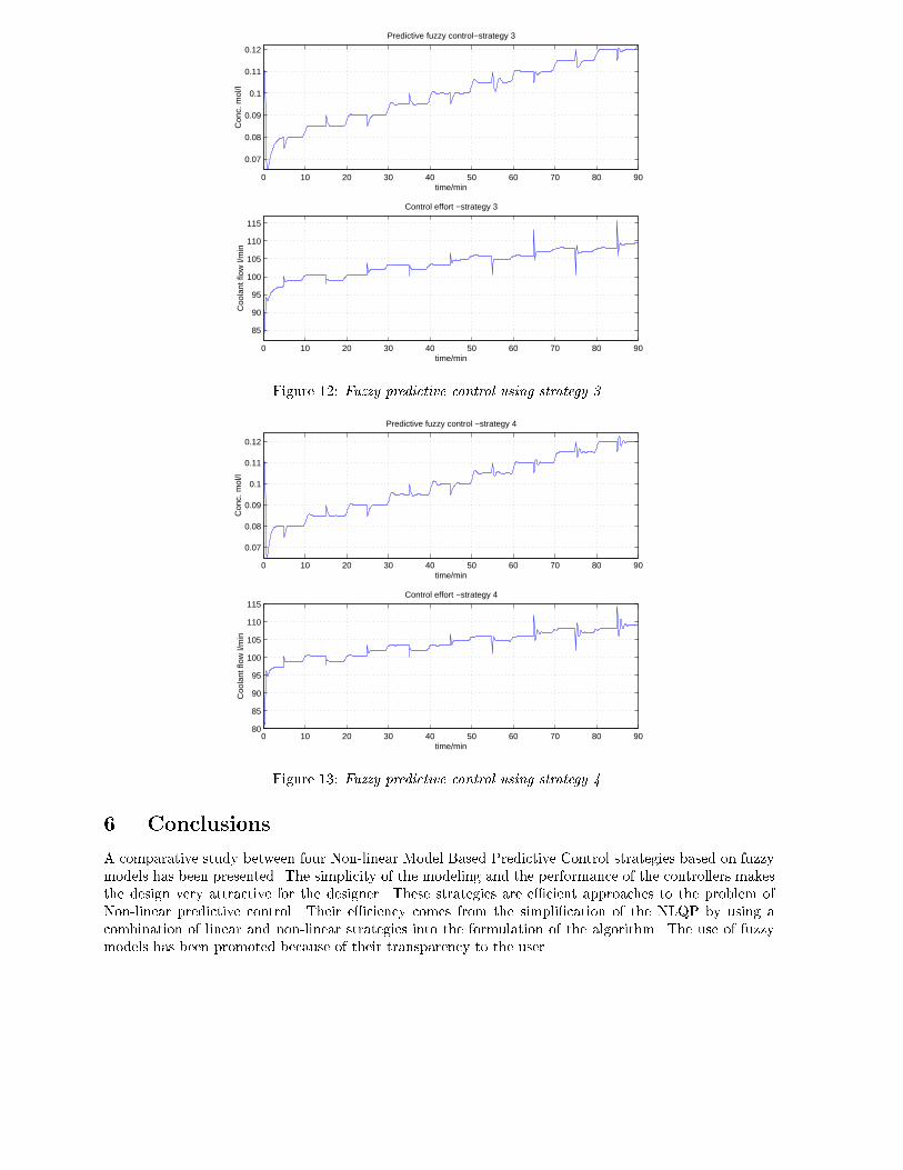
100 10 20 30 40 50 60 70 80 90

0.07

0.08

0.09

0.1

0.11

0.12

time/min

Con

c. m

ol/l

Predictive fuzzy control−strategy 3

0 10 20 30 40 50 60 70 80 90

85

90

95

100

105

110

115

time/min

Coo

lant

flow

l/m

in

Control effort −strategy 3

Figure 12: Fuzzy predictive control using strategy 30 10 20 30 40 50 60 70 80 90

0.07

0.08

0.09

0.1

0.11

0.12

time/min

Con

c. m

ol/l

Predictive fuzzy control −strategy 4

0 10 20 30 40 50 60 70 80 9080

85

90

95

100

105

110

115

time/min

Coo

lant

flow

l/m

in

Control effort −strategy 4

Figure 13: Fuzzy predictive control using strategy 46 ConclusionsA comparative study between four Non-linear Model Based Predictive Control strategies based on fuzzymodels has been presented. The simplicity of the modeling and the performance of the controllers makesthe design very attractive for the designer. These strategies are e�cient approaches to the problem ofNon-linear predictive control. Their e�ciency comes from the simpli�cation of the NLQP by using acombination of linear and non-linear strategies into the formulation of the algorithm. The use of fuzzymodels has been promoted because of their transparency to the user.

118 10 12 14 16 18

0.078

0.08

0.082

0.084

0.086

0.088

0.09Optimal strategy (−) Strategy 1 (+) Strategy 2 (−.) Strategy 3 (−−) Strategy 4 (.)

Minutes

Con

c m

ol/l

8 10 12 14 16 1898

98.5

99

99.5

100

100.5

101Control Effort Optimal strategy (−) Strategy 1 (+) Strategy 2 (−.) Strategy 3 (−−) Strategy 4 (.)

Minutes

Coo

lant

Flo

w l/

min

78 80 82 84 86 88 90

0.114

0.116

0.118

0.12

0.122

0.124

Optimal strategy (−) Strategy 1 (+) Strategy 2 (−.) Strategy 3 (−−) Strategy 4 (.)

Minutes

Con

c m

ol/l

78 80 82 84 86 88 90

106

108

110

112

114

116

Control Effort Optimal strategy (−) Strategy 1 (+) Strategy 2 (−.) Strategy 3 (−−) Strategy 4 (.)

Minutes

Coo

lant

Flo

w l/

min

Figure 14: Detailed comparison for two di�erent operating pointsReferences[1] Clarke D.W., Mohtadi C., Tu�s P.S., 1987, Generalized Predictive Control-Parts I - II, Automatica,23, 137-160.[2] Garcia C.E., Prett D.M.,Morari M., 1989, Model Predictive Control: Theory and Practice-a Survey,Automatica, 25, 335-348.[3] Richalet J., 1993, Industrial Applications of Model Based Predictive Control, Automatica, 29,1251-1274,[4] De Keyser R.M.C., Van de Velde Ph.G.A., Dumortier F.A.G., 1988, A Comparative Study of Self-Adaptive Long-range Predictive, Control Methods, Automatica, 24, 149-163.[5] Camacho E.F.,Bordons C., 1995, Model Predictive Control in the Process Industry, Springer Verlag,London.[6] Espinosa J.,Vandewalle J., 1998, Constructing Fuzzy Models with Linguistic Integrity, InternalReport,SISTA, Electrothecnik Departement, Katholieke Universiteit Leuven, Belgium.

12[7] Zhao J.,Wertz V., Gorez R. 1994, A Fuzzy Clustering Method for the Identi�cation of Fuzzy Mod-els for Dynamic Systems, Proceedings of the 9th International Symposium on Intelligent ControlCongress ISIC-94, Columbus, Ohio, USA,, pp.172-177.[8] Tan S.,Vandewalle J., 1995, An On-line Structural and Parametric Scheme for Fuzzy Modelling,Proceeding of the 6th International Fuzzy Systems Association World Congress IFSA-95, Sao Paulo,Brazil, July, pp.189-192.[9] Pedrycz W., 1994, Why Triangular Membership Functions?, Fuzzy Sets and Systems, 64, 21-30,[10] Jang J.-S.R., 1992,Neuro-Fuzzy Modeling: Architectures, Analyses and Applications, Phd. disserta-tion, University of Berkeley, California, USA.[11] Sugeno M.,Yasukawa T., 1993, A Fuzzy Logic Based Approach to Qualitative Modeling IEEE Trans.on Fuzzy Systems, 1, 7-31.[12] Wang L.X. 1994, Adaptive Fuzzy Systems and Control, Prentice Hall, USA.[13] Yager R.R.,Filev D., 1994, Essentials of fuzzy modeling and control, John Wiley & Sons, USA.[14] Ljung L., 1987, System Identi�cation. Theory for the User, Prentice Hall, USA.[15] Bossley K.M., 1997, Neurofuzzy Modelling Approaches in System Identi�cation, Ph.D. Dissertation,University of Southampton, U.K.[16] Espinosa J., Vandewalle J., 1997, Fuzzy Modeling and Identi�cation, A guide for the user, Proceedingsof the IEEE Singapore International Symposium on Control Theory and Applications, Singapore,July, pp.437-443.[17] Lightbody G., Irwin G.W., 1997, Nonlinear Control Structures Based on Embedded Neural SystemModels, IEEE Trans. on Neural Networks, 8, 553-567.[18] Hadjili M. L., Wertz V., Scorletti G. 1998, Fuzzy Model-based Predictive Control, Accepted in IEEEConference on Control and Decision, Tampa, Florida, USA, Dec.[19] Hadjili M. L., Landasse A., Wertz V., Yurkovich S., 1998, Identi�cation of Fuzzy Models for a GlassFurnace Process, Proceedings of the Conference on Control Applications, Trieste, Italy, Sep.[20] Chiu S. L., 1994,Fuzzy Model Identi�cation Based on Cluster Estimation, J. Intel. and Fuzzy Syst,2, 267-278.[21] Espinosa J., Vandewalle J., 1998, Predictive Control Using Fuzzy Models, Accepted for publicationin Advances in Soft Computing in Engineering Design and Manufacturing.[22] Espinosa J., Vandewalle J., 1998, Predictive Control Using Fuzzy Models Applied to a SteamGenerating Unit, Proceedings of the Third International FLINS Workshop , Antwerp, Sep, pp.151-160.