Proceedings of the International Multiconference on ISSN 1896-7094 Computer Science and Information Technology, pp. 327 – 336 © 2007 PIPS

Advantages of an Easy to Design Fuzzy Predictive Algorithm: Application to a Nonlinear Chemical Reactor1

Piotr M. Marusak

Institute of Control and Computation Engineering, Warsaw University of Technology,Nowowiejska 15/19, 00–665 Warsaw, Poland

P.Marusak@ia.pw.edu.pl

Abstract. Advantages of a fuzzy predictive control algorithm are discussed in the paper. The discussed fuzzy predictive algorithm is a combination of a DMC (Dynamic Matrix Control) algorithm and Takagi–Sugeno fuzzy modeling inheriting advantages of both techniques. The algorithm is numerically effective. Moreover, information about measured disturbance can be included in it in an easy way. A simple and easy to apply method of fuzzy predictive control algorithms synthesis is presented. The advantages of the fuzzy predictive control algorithm are demonstrated in the example control system of a control plant with difficult dynamics – a nonlinear chemical reactor with inverse response.

1 Introduction

Model predictive control (MPC) algorithms are widely used in practice due to the control performance they offer. They are usually used in an advanced control layer of the multilayer control system structure; see e.g. [1, 8, 10]. Basic formulations of the MPC algorithms are based on the linear control plant models. The advantage of these algorithms is that they are formulated as easy to solve, linear–quadratic optimization problems. However, application of the MPC algorithm based on a linear plant model to a nonlinear plant, if control in a wide range of set point values is needed, may bring unsatisfactory results or the results can be improved using the algorithm based on a nonlinear model.

Unfortunately, a direct usage of a nonlinear model to design the MPC algorithm leads to its formulation as a nonlinear, and in general, non–convex optimization problem that is hard to solve and computationally demanding. Thus, in practice, suboptimal algorithms that use approximate process models generated from the nonlinear model at each algorithm iteration are used; see e.g. [6, 10]. In these algorithms the nonlinear and the approximated models are used in such a way that the standard linear–quadratic optimization problem is formulated and solved at each algorithm iteration. Various kinds of nonlinear models can be used in such algorithms. However, the usage of Takagi–Sugeno (TS) fuzzy models [9] makes them especially efficient [6, 7, 10].

The DMC algorithm is practically a standard in the industrial applications; see e.g. [1, 2, 3, 5, 8, 10]. It can be relatively easily designed, because it is based on an easy to

1 This work was supported by the Polish national budget funds for science 2005-2007 as a research project.

327

328 Piotr Marusak

obtain control plant model in the form of the step response. The fuzzy DMC (FDMC) algorithm used in the paper is an easy to design fuzzy predictive algorithm based on DMC technique and Takagi–Sugeno fuzzy models [6, 7, 10]. It uses a TS fuzzy model with step responses used as the local models. Such Takagi–Sugeno fuzzy models can be obtained relatively easy using the expert knowledge and/or simulation experiments.

As the FDMC algorithm is based on the nonlinear control plant model, it usually works well in a wide range of operating point changes, offering better control performance than the algorithms based on linear process models – the feature important when it operates in a hierarchical control system structure.

The discussed FDMC algorithm was applied to a nonlinear chemical plant – an isothermal CSTR in which a van de Vusse reaction takes place. The control plant is a difficult process because except it is nonlinear, it has also an inverse response. The experiments performed in two control systems: the first one – with DMC algorithm based on a linear process model and the second one – with FDMC algorithm, demonstrate the superiority of the fuzzy algorithm over the one based on the linear model.

The organization of the paper is as follows. In Sect. 2 the idea of predictive control algorithms is discussed, the DMC and easy to design FDMC algorithms used during the test are described. In Sect. 3 the control plant and algorithms used during the experiments are detailed. Sect. 4 contains description of experiments and discussion of obtained results. The paper is summarized in Sect. 5.

2. Predictive Controllers

In the MPC algorithms future behavior of the control plant is predicted many time steps ahead, using a dynamic control plant model and all available knowledge about conditions of control system operation. The future control values are then derived in such a way that the future behavior of the control system fulfills assumed criteria. Typically, the minimization of a performance function is demanded subject to the constraints put on manipulated and controlled variables; in the MPC algorithms based on input–output models usually the following optimization problem is solved at each iteration:

( ) ( )

∆⋅+−= ∑∑−

=+

=+

1

0

2

|1

2

| λmins

ikik

p

ikikkMPC uyyJ

uΔ

subject to: ∆umin ≤ ∆u ≤ ∆umax, umin ≤ u ≤ umax, ymin ≤ y ≤ ymax,

(1)

where y k is a set–point value (in the classical multilayer control system structure it

is obtained from the economic optimization layer), y ki∣k is an output value for (k+i)th time step predicted at kth time step using control plant model, it depends on past and future control values, Δu ki∣k are future changes in the manipulated

variables, λ ≥ 0 is a weighting coefficient, p and s denote prediction and control

Advantages of an Easy to Design Fuzzy Predictive Algorithm 329

horizons, respectively; y=[ y k1∣k, , y

k p∣k ]T

, Δu=[ Δuk ∣k

, , Δuks−1∣k ]T ,

u=[uk ∣k ,, uks−1∣k ]

T, ∆umin, ∆umax, umin, umax, ymin, ymax are vectors of lower

and upper bounds of changes and values of the control signals and of the output variable values, respectively. As a solution to the optimization problem (1) the optimal vector of changes of the manipulated variables is obtained. From this vector, the Δu k∣k element is taken and applied in the control system. Then optimization is repeated at the next time instant.

The way the predicted output values y ki∣k are derived depends on the dynamic control plant model exploited by the algorithm. If the linear model is used then the optimization problem (1) is a standard linear–quadratic programming problem. The conventional (non–fuzzy) DMC algorithm is based on a process model in the form of the control plant step responses.

2.1. Standard DMC Algorithm

The classical (non–fuzzy) DMC algorithm uses the control plant model in the form of its step response; see e.g. [2, 3, 5, 8, 10]:

,~1

1dd

d

pkp

p

iikik uauay −

−

=− ⋅+∆⋅= ∑ (2)

where y k is the output of the control plant model at the kth time instant, Δu k is a change of the manipulated variable at the kth time instant, ai (i=1,…,pd) are step response coefficients of the control plant, pd is equal to the number of time instants

after which the coefficients of the step response can be assumed as settled, uk− pdis

a value of the manipulated variable at the (k–pd)th time instant.The predicted output values are then calculated using the following formula:

y ki∣k=∑n=1

i

an⋅Δuk−n i ∑n=i1

pd −1

an⋅Δu k−nia pd⋅uk− pdid k , (3)

where d k=y k− yk−1 is assumed to be the same at each time instant in the

prediction horizon (it is a DMC–type disturbance model). Thus (3) can be transformed into the following form:

yki∣k

= yk ∑

n=i1

pd−1

an⋅Δu

k−nia pd

∑n= pd

pdi−1

Δu k−ni

−∑n=1

pd−1

an Δuk−n∑n=1

i

an Δuk−ni∣k .

(4)

330 Piotr Marusak

In (4) only the last component depends on future manipulated variable changes. Thus the vector of predicted output values y can be decomposed into the following components:

y = yfr+A⋅∆u, (5)

where [ ] ,,,T

||1fr

kpkfr

kkfr yy ++= y is a vector of length p and is called a free

response of the plant, because it contains future output values calculated assuming that the control signal does not change in the prediction horizon (describes influence of the manipulated variable values applied to the control plant in previous iterations):

yfr = yl+Ap⋅∆up, (6)

where Δu p=[ Δuk−1 , , Δu

k− pd1 ]T

, yl= [ yk , , y k ]T

and

.

122211

122413

1212312

−−−−

−−−−−−−−

=

−−++

−−

−−−

dddd

dddd

dddd

pppppp

pppp

pppp

p

aaaaaaaa

aaaaaaaa

aaaaaaaa

A (7)

A is a matrix of dimensionality p×s, called the dynamic matrix and is composed of the control plant step response coefficients:

.00

000

121

12

1

=

+−+−− spsppp aaaa

aa

a

A (8)

Using the prediction (5) one can formulate the optimization problem (1), solution of which contains the future changes in the manipulated variables. The details concerning formulation of the DMC algorithm can be found, e.g. in [2, 3, 5, 8, 10].

Disturbance measurement can be taken into consideration in an easy way. Despite that, it can offer significant control system performance improvement. In order to take the disturbance measurement into consideration in the DMC algorithm the control plant model (2) should be supplemented by terms describing influence of the disturbance on the output variable:

,~1

1

1

1zz

z

dd

d

pkp

p

iikipkp

p

iikik zbzbuauay −

−

=−−

−

=− ⋅+∆⋅+⋅+∆⋅= ∑∑ (9)

Advantages of an Easy to Design Fuzzy Predictive Algorithm 331

where Δz k is a change of the manipulated variable at the kth time instant, bi (i=1,…,pz) are disturbance step response coefficients, pz is equal to the number of time instants after which the coefficients of the disturbance step response can be assumed

as settled, zk− pd is a value of the manipulated variable at the (k–pz)th time instant.

If there is no information available about future disturbance, the future changes of disturbance are assumed equal to 0. The influence of past changes of the disturbance should be included in the free response. Thus, this time, the free response is described by the following formula:

yfr = yl+Ap⋅∆up+Az⋅∆zp, (10)

where Δz p=[ Δzk−1 , , Δz

k− p z1 ]T

and

.

122211

122413

1212312

−−−−

−−−−−−−−

=

−−++

−−

−−−

zzzz

zzzz

zzzz

pppppp

pppp

pppp

z

aaaaaaaa

aaaaaaaa

aaaaaaaa

A (11)

2.2. Easy to Design Fuzzy DMC Algorithm

The FDMC algorithm used in the paper exploits TS models with local models in the form of step responses. Thanks to such an approach each iteration of the algorithm is simple. Moreover, the local models are easy to obtain. The FDMC algorithm is thus based on TS fuzzy models described by the set of the following rules:

Rule j: if

yk

is B1

j and and yk−n

P1

is Bn

P

j and uk is C

1

j and and uk−m

P1

is Cm

P

j

antecedent

then y k1

j=∑

i=1

pd−1

aij⋅Δu

k− ia

pd

j uk− p

dconsequent

,

(12)

where yk is an output variable value of the control plant model at the kth time instant,

uk is a manipulated variable value at the kth time instant, B1j ,…, BnP

j, C1

j ,…,

CmP

j are fuzzy sets, ai

j are the coefficients of step responses in jth local model,

j=1,…,l, l – number of rules.

332 Piotr Marusak

If measured disturbance is taken into consideration, the local model has the following form:

yk1j = ∑

i=1

pd−1

a ij⋅Δuk−ia pd

j⋅u k− pd

∑i=1

p z−1

bij⋅Δz k−ib p z

j⋅zk− p z

, (13)

where bij are the coefficients of step responses in jth local model.

The design process of the TS model (12) can be simplified to a large extent. It is because instead of obtaining a complicated local models (as e.g. difference equations) it is sufficient to obtain a few step responses of the control plant (from the environs of a few operating points). The membership functions can be chosen using expert knowledge, simulation experiments, fuzzy neural networks or all these techniques combined.

In the basic FDMC algorithm, the TS model (12) is used, at each iteration, in the following way:

1. A linear model for current time instant is derived using current values of process variables, the TS fuzzy model (12) and fuzzy reasoning. The output value of the model is calculated using the following formula (in the case when a measured disturbance is taken into consideration):

.~~~~~

1

1

1

1zz

z

dd

d

pkp

p

iikipkp

p

iikik zbzbuauay −

−

=−−

−

=− ⋅+∆⋅+⋅+∆⋅= ∑∑ (14)

where ai=∑j=1

l

w j⋅a ij , bi=∑

j=1

l

w j⋅bij and w i are the normalized weights

calculated using standard fuzzy reasoning, see e.g. [9].In fact (14) is the step response control plant model valid for the current values of

process variables. Thus, next steps of the FDMC algorithm are the same as in the conventional DMC algorithm (Sect. 2.1), i.e.

2. The obtained step response coefficients are used to generate the dynamic matrix.3. The step response model (14) is used to generate the plant free response.4. The free response and the dynamic matrix are used to formulate the quadratic

optimization problem.5. The optimization problem is solved and, using the obtained solution, the

manipulated variable value is generated. Then the controller passes to the next iteration.

3. Control systems

The considered control plant is an isothermal CSTR in which a van de Vusse reaction carries out (Fig. 1 a) [4]. Its steady–state characteristics are shown in Fig. 1 b.

Advantages of an Easy to Design Fuzzy Predictive Algorithm 333

a)

V, CA,CB

F, CAf

F, CB

DA

CBA

→→→

2

b)

Fig. 1. Isothermal CSTR with van de Vusse reaction; a) diagram of the plant, b) steady–state characteristics of the plant

The reaction scheme is as follows

.2

,

DA

CBA

→→→

(15)

The process model contains composition balance equations for both components

.

),(

21

231

BBAB

AAfAAA

CV

FCkCk

dt

dC

CCV

FCkCk

dt

dC

−−=

−+−−= (16)

where CA, CB are the concentrations of components A and B, respectively, F is the inlet flow rate (equal to the outlet flow rate), V is the volume in which the reaction is carried out (it is assumed constant and V =1 l), CAf is the concentration of component A in the inlet flow stream (if it is not stated differently it is assumed that CAf0

=10 mol/l). The values of the kinetic parameters are: k1 =50 1/h, k2 =100 1/h, k3

=10 l/h ⋅ mol. The output variable is the concentration CB of substance B, the manipulated

variable is the inlet flow rate F of the raw substance, the disturbance variable is the concentration of component A in the inlet flow stream CAf.

It was assumed that the manipulated variable is constrained

maxmin FFF ≤≤ (17)

where Fmin =0 l/h, Fmax =60 l/h. For the presented control plant two controllers were designed: the first one – a

DMC controller based on a linear model and the second one – an FDMC controller based on a Takagi–Sugeno fuzzy model. The sampling period of both controllers was assumed equal to 3.6 s. The following tuning parameters of both algorithms were assumed: p =70, s =35, λ =0.001.

334 Piotr Marusak

The DMC algorithm is based on a step response taken in environs of the operating point: CB0 =1.12 mol/l, CA0 = 3 mol/l, F=34.3 l/h [4]. In the case of an FDMC algorithm, two additional step responses are used (the conventional DMC algorithm was in fact extended): the first one from environs of the point CB0 =0.91 mol/l, CA0 = 2.18 mol/l, F =20 l/h, and the second one – from environs of the point CB0=1.22 mol/l, CA0=3.66 mol/l, F =50 l/h. Thus, the TS control plant model used by the FDMC controller is composed of three rules. The assumed membership functions are shown in Fig. 2.

CB,k–1

µ(CB,k–1)

0.91 1.12

0

1 ZP1 ZP2 ZP3

1.22

Fig. 2. Membership functions of the fuzzy DMC controller

4. Simulation Experiments

During the experiments the operation of both control systems (the first one – with DMC and the second one – with FDMC algorithms) was compared. First, the set–point value C B was changed towards high values of the concentration CB, to 1.22 mol/l, precisely. The response obtained in the control system with the FDMC algorithm (solid lines in Fig. 3) is better than the one acquired by the conventional DMC algorithm (dashed lines in Fig. 3) – the output variable much faster reaches the demanded set–point value.

Fig. 3. Responses of the control system with: DMC algorithm (dashed line), FDMC algorithm

(solid line) to the change of CB set–point to CB=1 .22 ; left – output variable CB, right –

manipulated variable F

Advantages of an Easy to Design Fuzzy Predictive Algorithm 335

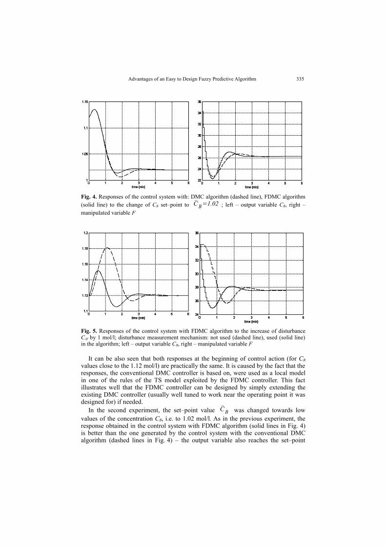
Fig. 4. Responses of the control system with: DMC algorithm (dashed line), FDMC algorithm (solid line) to the change of CB set–point to CB=1.02 ; left – output variable CB, right – manipulated variable F

Fig. 5. Responses of the control system with FDMC algorithm to the increase of disturbance CAf by 1 mol/l; disturbance measurement mechanism: not used (dashed line), used (solid line) in the algorithm; left – output variable CB, right – manipulated variable F

It can be also seen that both responses at the beginning of control action (for CB

values close to the 1.12 mol/l) are practically the same. It is caused by the fact that the responses, the conventional DMC controller is based on, were used as a local model in one of the rules of the TS model exploited by the FDMC controller. This fact illustrates well that the FDMC controller can be designed by simply extending the existing DMC controller (usually well tuned to work near the operating point it was designed for) if needed.

In the second experiment, the set–point value C B was changed towards low values of the concentration CB, i.e. to 1.02 mol/l. As in the previous experiment, the response obtained in the control system with FDMC algorithm (solid lines in Fig. 4) is better than the one generated by the control system with the conventional DMC algorithm (dashed lines in Fig. 4) – the output variable also reaches the set–point

336 Piotr Marusak

value faster in the case of the control system with the fuzzy algorithm. Moreover, the overshoot is significantly lower in the control system with the FDMC algorithm. The obtained results clearly show the profits gained thanks to the usage of the fuzzy approach.

There was also performed an experiment with the change of disturbance CAf – concentration of component A in the inlet stream. In the case when there was a disturbance measurement used (solid lines in Fig. 5) the obtained settling time is smaller than in the case without disturbance measurement (dashed lines in Fig. 5). Moreover, in the first case there is much smaller overshoot. Similar results were obtained in the case of operation near other operating points. In such cases the further the original operating point the system operates, the bigger difference of operation between DMC and FDMC algorithm is, with advantage of the latter one.

5. Summary

Application of the FDMC algorithm to the example control plant brought improvement of the control system operation comparing to the case when the algorithm based on the linear model was used. It was achieved despite relatively little effort needed to design a fuzzy algorithm. It was possible because model the FDMC algorithm is based on (a Takagi–Sugeno fuzzy model with step responses used as local models) can be obtained in an easy way. The mechanism of taking measured disturbance into consideration in the algorithm (also relatively simple to apply), brought further improvement of algorithm performance.

References

1. Blevins T. L., McMillan G. K., Wojsznis W. K., Brown M. W.: Advanced Control Unleashed, ISA (2003).

2. Camacho E. F., Bordons C.: Model Predictive Control, Springer–Verlag (1999).3. Cutler C. R., Ramaker B. L.: Dynamic Matrix Control – a computer control algorithm,

Proc. Joint Automatic Control Conference, San Francisco, CA, USA (1979).4. Doyle F., Ogunnaike B. A., Pearson R. K.: Nonlinear model-based control using second-

order Volterra models, Automatica, 31 (1995), 697–714.5. Maciejowski J. M.: Predictive control with constraints, Prentice Hall, Harlow (2002).6. Marusak P.: Predictive control of nonlinear plants using dynamic matrix and fuzzy

modeling (in Polish). PhD Thesis, Warsaw, Poland (2002).7. Marusak P., Tatjewski P.: Fuzzy Dynamic Matrix Control algorithms for nonlinear plants,

Proc. 6th International Conference MMAR 2000, Miedzyzdroje, Poland (2000) 749–754.8. Rossiter J. A.: Model-Based Predictive Control, CRC Press, Boca Raton (2003).9 . Takagi T., Sugeno M.: Fuzzy identification of systems and its application to modeling and

control, IEEE Trans. on Systems, Man and Cybernetics 15 (1985) 116–132. 10. Tatjewski P.: Advanced Control of Industrial Processes; Structures and Algorithms,

Springer–Verlag, London (2007).