Fusional method of MPS and FEM through tetrahedral mesh generation

V International Conference on Particle-based Methods – Fundamentals and Applications PARTICLES 2017

J. Imamura

FUSIONAL METHOD OF MPS AND FEM THROUGH TETRAHEDRAL MESH GENERATION

JUNYA IMAMURA¹

¹imi Computational Engineering Laboratory Wako-shi, Honcho 31-9-803, 351-0114 Saitama, Japan

E-mail: jimamura@ra2.so-net.ne.jp

Key words: Improved Helmholtz-decomposition, MPS, FEM, Non-equidistant FDM

Abstract. The moving-particle semi-implicit (MPS) method is used as a density method for moving surfaces. The main disadvantage of previous density methods was that mass conservation was difficult to achieve because the mean density varied due to elemental diffusion; in contrast, MPS satisfies mass conservation. The density method is also very suitable as a finite element method (FEM), thus leading to the concept of an MPS-FEM fusion method. The MPS method especially incorporates a weight function for calculating the particle number density. Because the weight function is a Kernel function, the MPS-FEM fusion method includes a novel Kernel function similar to the weight function of MPS. The masses (particles) occupy positions on the vertex nodes of the tetrahedral elements, and the mesh must be recomposed for the time step advance by using a mesh generation technique. The masses are distributed in the control volume (CV) according to the Karnel function, and mass conservation must be satisfied by mesh regeneration using the apparent new density . The method is composed of FEM and a conceptual Helmholtz decomposition (H-d) using uL- and uT-elements for displacement u = uL + uT (where L: Lateral and T: Transverse). Nevertheless, an improved Helmholtz decomposition method (iH-d) is applied here to satisfy the conservation laws.

1 INTRODUCTION

I present a numerical calculation model of an incompressible flow field with free surfaces. The model is based primarily on the moving-particle semi-implicit (MPS) method, but calculation is performed by the finite element method (FEM) to include not only scalar potential flow but also vorticity flow. Thus, I apply Helmholtz decomposition (H-d) to represent the velocities.

Moreover, I consider the scalar potential term of H-d inappropriate to represent dilatational components. For this reason, I propose an improved Helmholtz decomposition (iH-d). The objective of the present study is to build a route for applying iH-d to free surface flow problems.

MPS is the best method for such free surface problems, because it conserves mass perfectly and is the only method disregarding surfaces. In addition, MPS allows nonlinear mechanisms, and it can therefore be used to solve contact problems. In the flow problem, the free surface implies mechanism nonlinearity, i.e., changes from the Dirichlet boundaries to the Neumann boundaries or the reverse.

In the free-surface MPS problem, the compressible flow plays an important role because this is apparently a compressible flow problem. Therefore, FEM is required for the compressible

471

J. Imamura

2

flow calcuation. The iH-d method allows compressibility by representing the velocity vector separately, i.e.,

with the dilatational term and the rotational term. The iH-d rotational term is incompressible at any time (automatically solenoidal). However,

not only vorticity but also the shear strains in the fluid must be incompressible. Normal strains induce volume changes, whereas shear strains induce shape changes but no

volume changes. This is the basic assumption for applying iH-d to free-surface problems. In reverse, MPS causes high discretization (example discretization model shown in Fig. 1).

Figure 1: Nodal model (continua Frame work)

This problem can be explained by Kondo’s indication [3] that the original MPS formulation lacks angular momentum terms. For the equilibrium equations of the above framework model, ∑Mi=0 is required in addition to ∑Ni=0 on the nodes. This problem is automatically resolved when we use FEM, in which distributed rigidity and re-reduced particle density is assumed.

2 REDUCING AND RE-REDUCING: FINITE ELEMENTS PARTICLES

2.1 Initial setting The numerical scheme is constructed by FEM, generating tetrahedral elements by joining

two particles with a straight line. This process is called grid generation in initial setting. The particles include inner mass particles and boundary particles, and the boundary particles

include zero-mass particles on the Dirichlet boundary and nonzero–mass particles on the Neumann boundary; nonequal masses are allowed.

At the time of the initial setting, the system is divided into sub-domains, and all particles are set on the centre of gravity, with the exception of the particles on the Neumann boundary. Overall, the following steps are executed:

(1) Setting the nodes on the Dirichlet boundaries without mass (zero-mass) (2) Setting the nodes on the Neumann boundaries with mass (3) Dividing the system to sub-domains for particles with mass infinite number and

mass (4) Constructing the tetrahedral elements (by any existent scheme) nonequally

masses are allowed (5) Adaptive element generation for isolated (flying) particles (in future work)

The above steps are illustrated in Fig. 2.

472

J. Imamura

3

Figure 2: Initial setting procedure

2.2 Re-reducing particle mass to density To apply FEM, density is indispensable. mi is the mass of the concerned particle i, Vj,i is the

control volume (CV) of the j-th element that shares a node with i, and the mass mi is distributed to the individual CV in the inverse ratio following Eq. (1).

niiii VVVV ,3,2,1,

1::1:1:1

(1)

Figure 3: Re-reducing of particle mass to

has a positive physical value, so it is represented by the exponent of the r-variable, i.e., =exp(r). is constant in CV, but discontinuous in the element; consequently, mass conservation is shown in (2) without advection terms.

0divtr0div

DtD

UU (2)

3 IMPROVED HELMHOLTZ DECOMPOSITION

3.1 Helmholtz decomposition According to the Helmholtz theorem, an arbitrary vector field u can be represented in Eq.

(3) using a scalar potential ∇ and a vector potential under the restriction of the Coulomb gauge.

Diri

chle

tbou

ndar

y Neumann boundary

473

J. Imamura

4

)( 0divcurl u (3)

Let us think about the displacement vector u in a solid. The simplest example is the cantilever, which is statically deterministic and can neglect the shearing strain, i.e., u=∇.

However, we cannot obtain the numerical result expected by FEM using ∇.

3.2 Improved Helmholtz decomposition Therefore, I proposed the improved Helmholtz decomposition represented in Eq. (4).

minimize)means(),()(:solid

)(:fluid00div shr

shrdiag

curldiag

0

uu

(4)

The novel operator used in Eq. (4) is defined as follows:

The expression for the fluid in the definition assumes that the Navier–Stokes (N.S.) equation

is represented in rotational form. When the N.S. equation is represented in shearing form, the expression in the second row (using ∇shr ) is the same as for the solid.

The dilatational component in iH-d is represented by the orthogonal component of the rotational components and modified with ∇, which is constrained by the gauge.

3.3 Strain potential and chain low According to the Helmholtz theorem, the arbitrary vector field should be decomposed. By

analogy to the numerical formula, iH-d can be applied to the strain vector shown in Eq. (5).

),()(

)(:"" 0divΦ

ΦΦ

potentialstrain shrshrdiag

curldiag

0

ii

iiwhere

(5)

iH-d decomposes also the vector potential shown in Eq. (6).

),()( 0div0 curlcurldiag (6)

I call the above the “low chain of the Helmholtz decomposition”. The low chain can be endlessly developed, and, therefore, iH-d can only be represented numerically.

1,1

3

2

1

3

2

1

,,,

,2,

iii

12

13

23

12

13

23

curl

shr

diag

,,

,

,γ,γγ,,γγ,γ,

where

uu

Def. of novel operator：

)12,())()((

ii1i2i3,1,21i2,3,11i1,2,3i

curlcurl

shrshr

diagdiag

curl

shr

diag

2

2

2

474

J. Imamura

5

3.4 Scoop up residuals of an equation to ∇

The scalar potential and the pressure P function have the same spatial effects. The dilatational component modified by ∇∇diag, represents the volumetric ratio divuL=div∇diag. The conceptual function of ∇ is illustrated in Fig. 4. The numerical scheme for minimizing (∇ ⇒0) consists of two steps. First, ∇ scoops up the residual of an equation represented by u, e.g., A+divuL ∇ (Eq. (7)), and then ∇ gives the offset values of u which are explained later (in the section 4.7).

0ddivuA

})({ (7)

Figure 4: Conceptual function of ∇

3.5 iH-d elements

I propose the iH-d elements in Fig. 5, in which shows an example of ∇. This element shape is applied for ∇i, ∇, nd ∇P. ({ }k: on vertex, { }COG: on the center of gravity)

Figure 5: iH-d elements ∇ for 2D and 3D

The element function is expressed in the finite Taylor series, and the adopted terms are represented in Fig. 5 with the coefficient terms for 2D in the left part of the figure (no notice for 3D). The functions for 2D and 3D are incomplete 3rd order functions. Both functions have a zero interceptor { (00)}0=0.

compressible case

xu L *

2

Deviation of the volumetric ratio

dilatationrepresentcannotx

y

22

22

)( 2 0

yvL *

0)13()03(

)12()02(

)31()21()11()01(

)30()20()10()00(0

)(

}

{}{

lm k}

{:)11()01(

)10(

:)2( Delement

COG}{: )01()10(

!!}{: 0

)(),( ml

yxfunctionml

lmyx :)3( Delement

k}

{:)011()110()010(

)101()001()100(

COG

0

}

{:)001()010(

)100(

!!!}{: 0

)(),,( nml

zyxfunctionnml

lmnzyx

475

J. Imamura

6

4 NUMERICAL SCHEME

4.1 Navier–Stokes equation The mass conservation equation is shown in Eq. (2). The Navier–Stokes equation used in

this paper is shown in Eq. (8) in the rotational form, where U is the velocity vector, is the density, g is the gravity, P is the pressure, and is the viscosity.

0divPdivDtD

)34()( UUgUUU 2

curl (8)

4.2 Time axially central FDM I apply the central difference method to the time axis shown in Eq. (9), where u is the

displacement vector, t is the time pitch, and n is the time step (n=0,1,2,3,…).

2

1111 2}{,2 Δt

uuut

UΔt

uuUni

ni

nini

ni

nin

i

(9)

The states are known for n-1 and n , and unknown for n-1, and the displacements uL,n+1 and uT,n+1 are used as variables, i.e., unknown parameters {∇}k

n+1 , {∇}COGn+1

, ∇, ∇, and ∇P are the elements used here. For n-1 and n+1, I use the grid generated at n, but using the corresponding data for each

spatial position shown in Fig. 6

Figure 6 Grid usage

4.3 Initial setting of ∇P element

The gravity acceleration gz and the density 0 are known, and so the node parameter {P(001)}k can be determined algebraically, using Eq. (10).

zk gP 0)001( }{ (10)

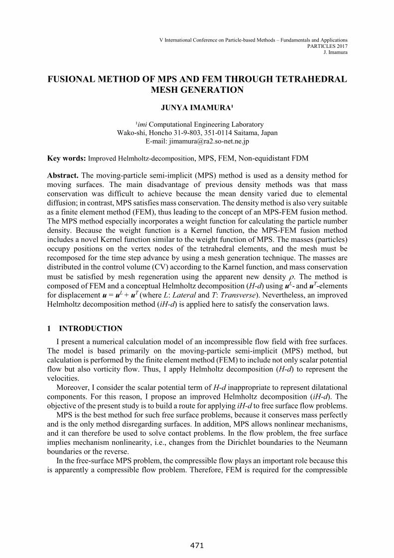
By this initial setting, the system is maintained stable, and ∇P triggers the dam breaking problem, as is shown for example in Fig. 7.

time step n

n-1

n+1

calc. by central FDM applying in n generated grid

476

J. Imamura

7

Figure 7 Dam breaking and discharge

4.4 Momentum conservation excluding source and charge The Navier–Stokes equation is resolved on the time step n-section by iteration, through the

weighted residual method. The scheme can be explained better by dividing it into step groups. In the first step group,

elements ∇, , ∇P, ∇ are calculated, and in the second step group, element ∇ is calculated.

The concept of the proposed scheme is explained by Eq. (11) and Eq. (12), where 1≡{1,1,1}.

0divt

L )( 2 UU

0ΦdivPt

Tcurl

L })(

34{})({ 2

0 U1UggUUU

(11)

(12)

Both equations mean to conserve the momentum excluding sourcing and charging into the system.

Eq. (11) excludes sourcing through a continuity equation using ∇. Eq. (12) excludes external force sourcing using ∇P and internal force sourcing using ∇.

The solenoidal term is unrelated to sourcing.

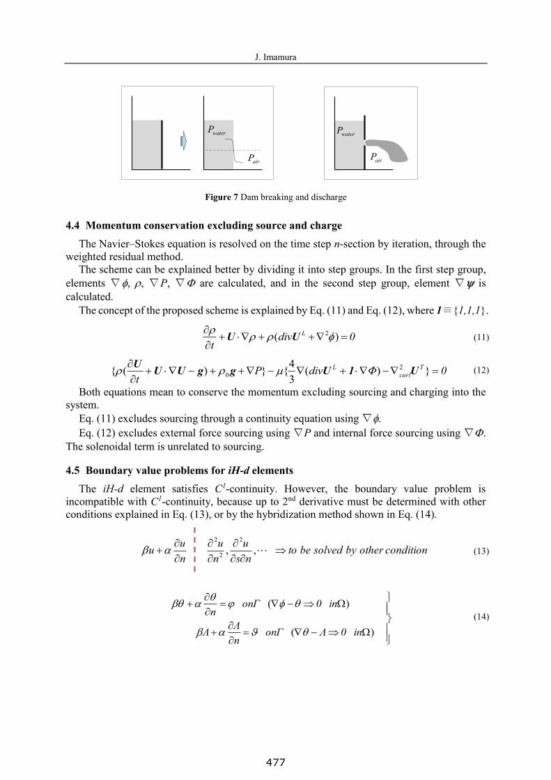
4.5 Boundary value problems for iH-d elements The iH-d element satisfies C1-continuity. However, the boundary value problem is

incompatible with C1-continuity, because up to 2nd derivative must be determined with other conditions explained in Eq. (13), or by the hybridization method shown in Eq. (14).

conditionotherbysolvedbetons

unu

nuu

,,2

2

2

(13)

)(

)(

in0ΛonΓnΛΛ

in0onΓn

(14)

waterP

airP

waterP

airP

477

J. Imamura

8

Figure 8 The boundary value problem

Thus (according to the former), the twist parameter is varied on the vertex in order to minimize the twist value in the element shown in Eq. (15) ({(11)}k : free on the boundary).

0dk

}{ )11(

)11()11(

(15)

Eq. (15) is represented in the 2D case. Up to the 2nd derivative can be varied, but the constraint condition is represented as ((11)⇒0) for simplicity.

4.6 The first group step

The node parameters {∇}k, , {∇P}k and {∇}kare obtained from Eq. (16).

)0(})}({

)0(}})({

})}({:

)0(}})({

)11(

)11(0

)11(22

Φ0dΦΦdivΦ

P0dPPDt

DP

inCV0drdivtrr

0ddivtr

TL

L

L

CV

diagdiagTL

1u

ggU

U

1U

④

③

②

①

(16)

4.7 The second step

The node parameters {∇}k are obtained from Eq. (17) and the accompanying constraint condition is shown in the 2nd row.

The incremental {∇}k : U are unknown parameters in the simultaneous equation.

)(

)(})(34)(1{

)}34()({

1

)11(

20

0,1,2,3,mΔwhere

00dΦΔΔΔt

ddivPDt

D

mm

iL

diagL

Tcurl

L

UUU

UU

UUggU

⑤

(17)

Boundary value given along the boundary curve S

Region governedby a differential equation ∇2u=-f

boundaryRobinelse

boundaryNeumann0

boundaryDirichlet0

onSunu

：③

：②

：①

478

J. Imamura

9

①〜⑤ are iterated until converged.

4.8 Gauge for iH-d scheme

∇ have ninedegrees of freedom. Therefore, nine equations are needed to obtain iH-d parameters. (Notice; Using the cubic interpolation procedure (CIP), ∇(N.S. eq.) = 0 is solved to obtain ∇u. )

I call the relationship between ∇curl and ∇shr “conjugate”. ∇curl is a conjugate variable of ∇shr and vice versa.

The Eq. (9) supplement constraint condition (∇shr⇒0) stabilizes the numerical calculation. I call this conditions also “gauge”.

To calculate divu, a gauge (∇imiu⇒0) is necessary, as seen in Eq. (18) and Eq. (19); a novel operator ∇imi is defined in Eq. (19).

)()()()(22xu

zw

zw

yv

yv

xu

zw

yv

xudiv

u

)()()(xu

zw

zw

yv

yv

xu

imi

u1

(18)

(19)

5 PARTICULARITY OF 2D MODEL To ensure the above 2D scheme is necessary condition to ensure the 3D calculations. The Helmholtz decomposition (Eq. (3)) for < x−y > 2D can be represented in Eq. (20) using

the suffices (i = 1, 2, 3), (i + 1 = 2, 3, 4), and (i−1 = 3, 1, 2); also, for < y−z > 2D it is shown in Eq. (21).

122

211

1

1

1

11

1

1

3

3

2

2

i

i

ii

i

i

ii

i

i

ii

i

i

ii

xxu

xxu

yzw

yyv

Dzy

xxu

xxu

xyv

yxu

Dyx

(20)

(21)

We can express it in the same way also for < z−x > 2D. 3D can be expressed by summation of these equations. Thus, it is sufficient by the explanation for 2D.

However, in 2D, ∇diag cannot be applied, because 1 and2 are lacking in ∇curl. It must be remembered that the 2D model calculates 3D, and the axisymmetric 1D model do

also 3D. Accordingly, the 2D model can be used to represent 3D by introducing the z-axis shown in

Eq. (22).

479

J. Imamura

10

),,(2),,(12

),,(2),,(11

yxyx

yxyx

hzhgzg

(22)

Nevertheless, it must also be remembered that the integrals of the odd functions z∙g2’ are zeros.

The vertex stretching terms also appear by introducing the z-axis; theoretically, these stretching terms are zeros in 2D. This means that the iH-d scheme using Eq. (22) satisfies [stretching terms=0], numerically.

6 CONCLUSIONS AND FUTURE WORKS - The biggest merits of MPS are that it conserves mass perfectly, and is not affected by

the existence of surfaces. Conversely, these are the week points of FEM. - One of the characteristics of FEM is that it can be used for calculations without angular

momentum terms. - I proposed in this paper an MPS-FEM fusion method that incorporates the advantages

of both models. - I interpret MPS as a sort of density method for a moving surface. - Accordingly, the fusion method may be used for compressible flow calculations. - I apply here the iH-d elements and scheme. - Going further, in my future work, I am going to finish developing an adoptive scheme

for maintaining a tetrahedral element by sub-division of a particle. - The numerical verifications are also going to be conducted in the near future. - The forced cavity must be chosen as a benchmark test problem to verify the results of

this paper.

REFERENCES [1] K. Sugihara and J. Imamura, Stress analysis by non-equidistant finite difference method (4th paper),

Transaction of AIJ, vol.178, pp. 17-24, (1970). [2] J. Imamura and T. Tanahashi, Improved HSMAC method: An improvement based on Helmholtz-

Hodge theorem, Transaction of JSCES, Paper No. 20100010, (2010). [3] M. Kondo, Angular momentum conserving particle method for high viscos fluid calculation,

Proceedings of the conference on computational engineering and science, vol. 22, JSCES, 2017 [4] J. Imamura, Proposal of improved Helmholtz-decomposition and the finite element, and application

to fluid and solid, vol. 22, JSCES, 2017 [5] J. Imamura, Helmholtz-decomposition of solid, and study on Eulerian solution, vol. 22, JSCES,

2017 [6] J. Imamura, Concept of fusional method of MPS and FEM through non-equidistant finite difference

method, vol. 22, JSCES, 2017 [7] A.E.H. Love, A treatise on the mathematical theory of elasticity, Dover Publications, 1926 [8] Y.C. Fung, Foundation of solid mechanics, Prentice-Hall, 1965

480