Fundamentals of Communication Systems

Solution Manual

Fundamentals of Communication Systems

John G. Proakis Masoud Salehi

Second Edition

2013

Chapter 2

Problem 2.1

1. Π (2t + 5) = Π(2(t + 5

2

)). This indicates first we have to plot Π(2t) and then shift it to left by

52 . A plot is shown below:

6

−114 −9

4

- t

Π (2t + 5)

1

2.∑∞n=0Λ(t−n) is a sum of shifted triangular pulses. Note that the sum of the left and right side

of triangular pulses that are displaced by one unit of time is equal to 1, The plot is given below

✲

✻

t

x2(t)

−1

1

3. It is obvious from the definition of sgn(t) that sgn(2t) = sgn(t). Therefore x3(t) = 0.

4. x4(t) is sinc(t) contracted by a factor of 10.

−1 −0.8 −0.6 −0.4 −0.2 0 0.2 0.4 0.6 0.8 1−0.4

−0.2

0

0.2

0.4

0.6

0.8

1

3

Problem 2.2

1. x[n] = sinc(3n/9) = sinc(n/3).

−20 −15 −10 −5 0 5 10 15 20−0.4

−0.2

0

0.2

0.4

0.6

0.8

1

2. x[n] = Π( n

4−13

). If −1

2 ≤n4−1

3 ≤ 12 , i.e., −2 ≤ n ≤ 10, we have x[n] = 1.

−20 −15 −10 −5 0 5 10 15 200

0.1

0.2

0.3

0.4

0.5

0.6

0.7

0.8

0.9

1

3. x[n] = n4u−1(n/4)− (n4 − 1)u−1(n/4− 1). For n < 0, x[n] = 0, for 0 ≤ n ≤ 3, x[n] = n

4 and

for n ≥ 4, x[n] = n4 −

n4 + 1 = 1.

4

−5 0 5 10 15 200

0.1

0.2

0.3

0.4

0.5

0.6

0.7

0.8

0.9

1

Problem 2.3

x1[n] = 1 and x2[n] = cos(2πn) = 1, for all n. This shows that two signals can be different but

their sampled versions be the same.

Problem 2.4

Let x1[n] and x2[n] be two periodic signals with periods N1 and N2, respectively, and let N =LCM(N1, N2), and define x[n] = x1[n]+x2[n]. Then obviously x1[n+N] = x1[n] and x2[n+N] =x2[n], and hence x[n] = x[n+N], i.e., x[n] is periodic with period N .

For continuous-time signals x1(t) and x2(t) with periods T1 and T2 respectively, in general we

cannot find a T such that T = k1T1 = k2T2 for integers k1 and k2. This is obvious for instance if

T1 = 1 and T2 = π . The necessary and sufficient condition for the sum to be periodic is that T1T2

be a

rational number.

Problem 2.5

Using the result of problem 2.4 we have:

1. The frequencies are 2000 and 5500, their ratio (and therefore the ratio of the periods) is

rational, hence the sum is periodic.

2. The frequencies are 2000 and 5500π . Their ratio is not rational, hence the sum is not periodic.

3. The sum of two periodic discrete-time signal is periodic.

4. The fist signal is periodic but cos[11000n] is not periodic, since there is no N such that

cos[11000(n+N)] = cos(11000n) for all n. Therefore the sum cannot be periodic.

5

Problem 2.6

1)

x1(t) =

e−t t > 0

−et t < 0

0 t = 0

=⇒ x1(−t) =

−e−t t > 0

et t < 0

0 t = 0

= −x1(t)

Thus, x1(t) is an odd signal

2) x2(t) = cos(120πt + π

3

)is neither even nor odd. We have cos

(120πt + π

3

)= cos

(π3

)cos(120πt)−

sin(π3

)sin(120πt). Therefore x2e(t) = cos

(π3

)cos(120πt) and x2o(t) = − sin

(π3

)sin(120πt).

(Note: This part can also be considered as a special case of part 7 of this problem)

3)

x3(t) = e−|t| =⇒ x3(−t) = e−|(−t)| = e−|t| = x3(t)

Hence, the signal x3(t) is even.

4)

x4(t) =

t t ≥ 0

0 t < 0=⇒ x4(−t) =

0 t ≥ 0

−t t < 0

The signal x4(t) is neither even nor odd. The even part of the signal is

x4,e(t) =x4(t)+ x4(−t)

2=

t2 t ≥ 0−t2 t < 0

= |t|2

The odd part is

x4,o(t) =x4(t)− x4(−t)

2=

t2 t ≥ 0t2 t < 0

= t2

5)

x5(t) = x1(t)− x2(t) =⇒ x5(−t) = x1(−t)− x2(−t) = x1(t)+ x2(t)

Clearly x5(−t) ≠ x5(t) since otherwise x2(t) = 0 ∀t. Similarly x5(−t) ≠ −x5(t) since otherwise

x1(t) = 0 ∀t. The even and the odd parts of x5(t) are given by

x5,e(t) = x5(t)+ x5(−t)2

= x1(t)

x5,o(t) = x5(t)− x5(−t)2

= −x2(t)

6

Problem 2.7

For the first two questions we will need the integral I =∫eax cos2 xdx.

I = 1a

∫cos2 x deax = 1

aeax cos2 x + 1

a

∫eax sin 2x dx

= 1aeax cos2 x + 1

a2

∫sin 2x deax

= 1aeax cos2 x + 1

a2 eax sin 2x − 2

a2

∫eax cos 2x dx

= 1aeax cos2 x + 1

a2 eax sin 2x − 2

a2

∫eax(2 cos2 x − 1) dx

= 1aeax cos2 x + 1

a2 eax sin 2x − 2

a2

∫eax dx − 4

a2 I

Thus,

I = 14+ a2

[(a cos2 x + sin 2x)+ 2

a

]eax

1)

Ex = limT→∞

∫ T2

− T2x2

1(t)dx = limT→∞

∫ T2

0e−2t cos2 tdt

= limT→∞

18

[(−2 cos2 t + sin 2t)− 1

]e−2t

∣∣∣∣ T20

= limT→∞

18

[(−2 cos2 T

2+ sinT − 1)e−T + 3

]= 3

8

Thus x1(t) is an energy-type signal and the energy content is 3/8

2)

Ex = limT→∞

∫ T2

− T2x2

2(t)dx = limT→∞

∫ T2

− T2e−2t cos2 tdt

= limT→∞

∫ 0

− T2e−2t cos2 tdt +

∫ T2

0e−2t cos2 tdt

But,

limT→∞

∫ 0

− T2e−2t cos2 tdt = lim

T→∞18

[(−2 cos2 t + sin 2t)− 1

]e−2t

∣∣∣∣0

− T2

= limT→∞

18

[−3+ (2 cos2 T

2+ 1+ sinT)eT

]= ∞

since 2+ cosθ + sinθ > 0. Thus, Ex = ∞ since as we have seen from the first question the second

integral is bounded. Hence, the signal x2(t) is not an energy-type signal. To test if x2(t) is a

power-type signal we find Px .

Px = limT→∞

1T

∫ 0

− T2e−2t cos2 dt + lim

T→∞1T

∫ T2

0e−2t cos2 dt

7

But limT→∞1T∫ T

20 e−2t cos2 dt is zero and

limT→∞

1T

∫ 0

− T2e−2t cos2 dt = lim

T→∞1

8T

[2 cos2 T

2+ 1+ sinT

]eT

> limT→∞

1TeT > lim

T→∞1T(1+ T + T 2) > lim

T→∞T = ∞

Thus the signal x2(t) is not a power-type signal.

3)

Ex = limT→∞

∫ T2

− T2x2

3(t)dx = limT→∞

∫ T2

− T2sgn2(t)dt = lim

T→∞

∫ T2

− T2dt = lim

T→∞T = ∞

Px = limT→∞

1T

∫ T2

− T2sgn2(t)dt = lim

T→∞1T

∫ T2

− T2dt = lim

T→∞1TT = 1

The signal x3(t) is of the power-type and the power content is 1.

4)

First note that

limT→∞

∫ T2

− T2A cos(2πft)dt =

∞∑k=−∞

A∫ k+ 1

2f

k− 12f

cos(2πft)dt = 0

so that

limT→∞

∫ T2

− T2A2 cos2(2πft)dt = lim

T→∞12

∫ T2

− T2(A2 +A2 cos(2π2ft))dt

= limT→∞

12

∫ T2

− T2A2dt = lim

T→∞12A2T = ∞

Ex = limT→∞

∫ T2

− T2(A2 cos2(2πf1t)+ B2 cos2(2πf2t)+ 2AB cos(2πf1t) cos(2πf2t))dt

= limT→∞

∫ T2

− T2A2 cos2(2πf1t)dt + lim

T→∞

∫ T2

− T2B2 cos2(2πf2t)dt +

AB limT→∞

∫ T2

− T2[cos2(2π(f1 + f2)+ cos2(2π(f1 − f2)]dt

= ∞+∞+ 0 = ∞

Thus the signal is not of the energy-type. To test if the signal is of the power-type we consider two

cases f1 = f2 and f1 ≠ f2. In the first case

Px = limT→∞

1T

∫ T2

− T2(A+ B)2 cos2(2πf1)dt

= limT→∞

12T(A+ B)2

∫ T2

− T2dt = 1

2(A+ B)2

8

If f1 ≠ f2 then

Px = limT→∞

1T

∫ T2

− T2(A2 cos2(2πf1t)+ B2 cos2(2πf2t)+ 2AB cos(2πf1t) cos(2πf2t))dt

= limT→∞

1T

[A2T

2+ B

2T2

]= A

2

2+ B

2

2

Thus the signal is of the power-type and if f1 = f2 the power content is (A+B)2/2 whereas if f1 ≠ f2

the power content is 12(A

2 + B2)

Problem 2.8

1. Let x(t) = 2Λ(t2

)−Λ(t), then x1(t) =

∑∞n=−∞ x(t − 4n). First we plot x(t) then by shifting

it by multiples of 4 we can plot x1(t). x(t) is a triangular pulse of width 4 and height 2

from which a standard triangular pulse of width 1 and height 1 is subtracted. The result is a

trapezoidal pulse, which when replicated at intervals of 4 gives the plot of x1(t).

✲

✻

t

x1(t)

1

2−2 6−6

2. This is the sum of two periodic signals with periods 2π and 1. Since the ratio of the two

periods is not rational the sum is not periodic (by the result of problem 2.4)

3. sin[n] is not periodic. There is no integer N such that sin[n+N] = sin[n] for all n.

Problem 2.9

1)

Px = limT→∞

1T

∫ T2

−T2

A2∣∣∣ej(2πf0t+θ)

∣∣∣2dt = lim

T→∞1T

∫ T2

−T2

A2dt = limT→∞

1TA2T = A2

Thus x(t) = Aej(2πf0t+θ) is a power-type signal and its power content is A2.

2)

Px = limT→∞

1T

∫ T2

−T2

A2 cos2(2πf0t + θ)dt = limT→∞

1T

∫ T2

−T2

A2

2dt + lim

T→∞1T

∫ T2

−T2

A2

2cos(4πf0t + 2θ)dt

As T →∞, the there will be no contribution by the second integral. Thus the signal is a power-type

signal and its power content is A2

2 .

9

3)

Px = limT→∞

1T

∫ T2

−T2

u2−1(t)dt = lim

T→∞1T

∫ T2

0dt = lim

T→∞1TT2= 1

2

Thus the unit step signal is a power-type signal and its power content is 1/2

4)

Ex = limT→∞

∫ T2

−T2

x2(t)dt = limT→∞

∫ T2

0K2t−

12dt = lim

T→∞2K2t

12

∣∣∣∣T/20

= limT→∞

√2K2T

12 = ∞

Thus the signal is not an energy-type signal.

Px = limT→∞

1T

∫ T2

−T2

x2(t)dt = limT→∞

1T

∫ T2

0K2t−

12dt

= limT→∞

1T

2K2t12

∣∣∣∣T/20= limT→∞

1T

2K2(T/2)12 = lim

T→∞

√2K2T−

12 = 0

Since Px is not bounded away from zero it follows by definition that the signal is not of the power-type

(recall that power-type signals should satisfy 0 < Px <∞).

Problem 2.10

Λ(t) =

t + 1, −1 ≤ t ≤ 0

−t + 1, 0 ≤ t ≤ 1

0, o.w.

u−1(t) =

1 t > 0

1/2 t = 0

0 t < 0

Thus, the signal x(t) = Λ(t)u−1(t) is given by

x(t) =

0 t < 0

1/2 t = 0

−t + 1 0 ≤ t ≤ 1

0 t ≥ 1

=⇒ x(−t) =

0 t ≤ −1

t + 1 −1 ≤ t < 0

1/2 t = 0

0 t > 0

The even and the odd part of x(t) are given by

xe(t) = x(t)+ x(−t)2

= 12Λ(t)

xo(t) = x(t)− x(−t)2

=

0 t ≤ −1−t−1

2 −1 ≤ t < 0

0 t = 0−t+1

2 0 < t ≤ 1

0 1 ≤ t

10

Problem 2.11

1) Suppose that

x(t) = x1e (t)+ x1

o(t) = x2e (t)+ x2

o(t)

with x1e (t), x2

e (t) even signals and x1o(t), x1

o(t) odd signals. Then, x(−t) = x1e (t)− x1

o(t) so that

x1e (t) = x(t)+ x(−t)

2

= x2e (t)+ x2

o(t)+ x2e (−t)+ x2

o(−t)2

= 2x2e (t)+ x2

o(t)− x2o(t)

2= x2

e (t)

Thus x1e (t) = x2

e (t) and x1o(t) = x(t)− x1

e (t) = x(t)− x2e (t) = x2

o(t)

2) Let x1e (t), x2

e (t) be two even signals and x1o(t), x2

o(t) be two odd signals. Then,

y(t) = x1e (t)x2

e (t) =⇒ y(−t) = x1e (−t)x2

e (−t) = x1e (t)x2

e (t) = y(t)z(t) = x1

o(t)x2o(t) =⇒ z(−t) = x1

o(−t)x2o(−t) = (−x1

o(t))(−x2o(t)) = z(t)

Thus the product of two even or odd signals is an even signal. For v(t) = x1e (t)x1

o(t) we have

v(−t) = x1e (−t)x1

o(−t) = x1e (t)(−x1

o(t)) = −x1e (t)x1

o(t) = −v(t)

Thus the product of an even and an odd signal is an odd signal.

3) One trivial example is t + 1 and t2t+1 .

Problem 2.12

1) x1(t) = Π(t)+Π(−t). The signal Π(t) is even so that x1(t) = 2Π(t)

. . . . . . . . . . . . . . . . . .1

2

12

12

11

2)

x2(t) = Λ(t) ·Π(t) =

0, t < −1/2

1/4, t = −1/2

t + 1, −1/2 < t ≤ 0

−t + 1, 0 ≤ t < 1/2

1/4, t = 1/2

0, 1/2 < t

. . . . . . . . .

.

.

.

.

.

.

.

.

.

.14

−12

12

1

3) x3(t) =∑∞n=−∞Λ(t − 2n)

... ...

−3 −1 31

1

4) x4(t) = sgn(t)+ sgn(1− t). Note that x4(0) = 1, x4(1) = 1

.

.

.

.

.

.

.

.

.0

2

1

5) x5(t) = sinc(t)sgn(t). Note that x5(0) = 0.

12

-1

-0.8

-0.6

-0.4

-0.2

0

0.2

0.4

0.6

0.8

1

-4 -3 -2 -1 0 1 2 3 4

Problem 2.13

1) The value of the expression sinc(t)δ(t) can be found by examining its effect on a function φ(t)through the integral

∫∞−∞φ(t)sinc(t)δ(t) = φ(0)sinc(0) = sinc(0)

∫∞−∞φ(t)δ(t)

Thus sinc(t)δ(t) has the same effect as the function sinc(0)δ(t) and we conclude that

x1(t) = sinc(t)δ(t) = sinc(0)δ(t) = δ(t)

2) sinc(t)δ(t − 3) = sinc(3)δ(t − 3) = 0.

3)

x3(t) = Λ(t) ?∞∑

n=−∞δ(t − 2n)

=∞∑

n=−∞

∫∞−∞Λ(t − τ)δ(τ − 2n)dτ

=∞∑

n=−∞

∫∞−∞Λ(τ − t)δ(τ − 2n)dτ

=∞∑

n=−∞Λ(t − 2n)

13

4)

x4(t) = Λ(t) ? δ′(t) =∫∞−∞Λ(t − τ)δ′(τ)dτ

= (−1)ddτΛ(t − τ)

∣∣∣∣τ=0

= Λ′(t) =

0 t < −112 t = −1

1 −1 < t < 0

0 t = 0

−1 0 < t < 1

−12 t = 1

0 1 < t

5) x5(t) = cos(2t + π

3

)δ(3t) = 1

3 cos(2t + π

3

)δ(t) = 1

3 cos(π3

)δ(t). Hence x5(t) = 1

6δ(t).

6)

x6(t) = δ(5t) ? δ(4t) =15δ(t) ?

14δ(t) = 1

20δ(t)

7) ∫∞−∞

sinc(t)δ(t)dt = sinc(0) = 1

8) ∫∞−∞

sinc(t + 1)δ(t)dt = sinc(1) = 0

Problem 2.14

The impulse signal can be defined in terms of the limit

δ(t) = limτ→0

12τ

(e−

|t|τ

)

But e−|t|τ is an even function for every τ so that δ(t) is even. Since δ(t) is even, we obtain

δ(t) = δ(−t) =⇒ δ′(t) = −δ′(−t)

Thus, the function δ′(t) is odd. For the function δ(n)(t) we have∫∞−∞φ(t)δ(n)(−t)dt = (−1)n

∫∞−∞φ(t)δ(n)(t)dt

where we have used the differentiation chain rule

ddtδ(k−1)(−t) = d

d(−t)δ(k−1)(−t) d

dt(−t) = (−1)δ(k)(−t)

14

Thus, if n = 2l (even) ∫∞−∞φ(t)δ(n)(−t)dt =


and the function δ(n)(t) is even. If n = 2l+ 1 (odd), then (−1)n = −1 and∫∞−∞φ(t)δ(n)(−t)dt = −


from which we conclude that δ(n)(t) is odd.

Problem 2.15

x(t) ? δ(n)(t) =∫∞−∞x(τ)δ(n)(t − τ) dτ

The signal δ(n)(t) is even if n is even and odd if n is odd. Consider first the case that n = 2l. Then,

x(t) ? δ(2l)(t) =∫∞−∞x(τ)δ(2l)(τ − t) dτ = (−1)2l

d2l

dτ2lx(τ)∣∣∣∣τ=t= dn

dtnx(t)

If n is odd then,

x(t) ? δ(2l+1)(t) =∫∞−∞x(τ)(−1)δ(2l+1)(τ − t) dτ = (−1)(−1)2l+1 d2l+1

dτ2l+1x(τ)∣∣∣∣τ=t

= dn

dtnx(t)

In both cases

x(t) ? δ(n)(t) = dn

dtnx(t)

The convolution of x(t) with u−1(t) is

x(t) ? u−1(t) =∫∞−∞x(τ)u−1(t − τ)dτ

But u−1(t − τ) = 0 for τ > t so that

x(t) ? u−1(t) =∫ t−∞x(τ)dτ

Problem 2.16

1) Nonlinear, since the response to x(t) = 0 is not y(t) = 0 (this is a necessary condition for linearity

of a system, see also problem 2.21).

2) Nonlinear, if we multiply the input by constant −1, the output does not change. In a linear system

the output should be scaled by −1.

15

3) Linear, the output to any input zero, therefore for the input αx1(t)+ βx2(t) the output is zero

which can be considered as αy1(t)+ βy2(t) = α× 0+ β× 0 = 0. This is a linear combination of the

corresponding outputs to x1(t) and x2(t).4) Nonlinear, the output to x(t) = 0 is not zero.

5) Nonlinear. The system is not homogeneous for if α < 0 and x(t) > 0 then y(t) = T[αx(t)] = 0

whereas z(t) = αT[x(t)] = α.

6) Linear. For if x(t) = αx1(t)+ βx2(t) then

T[αx1(t)+ βx2(t)] = (αx1(t)+ βx2(t))e−t

= αx1(t)e−t + βx2(t)e−t = αT[x1(t)]+ βT[x2(t)]

7) Linear. For if x(t) = αx1(t)+ βx2(t) then

T[αx1(t)+ βx2(t)] = (αx1(t)+ βx2(t))u(t)

= αx1(t)u(t)+ βx2(t)u(t) = αT[x1(t)]+ βT[x2(t)]

8) Linear. We can write the output of this feedback system as

y(t) = x(t)+y(t − 1) =∞∑n=0

x(t −n)

Then for x(t) = αx1(t)+ βx2(t)

y(t) =∞∑n=0

(αx1(t −n)+ βx2(t −n))

= α∞∑n=0

x1(t −n)+ β∞∑n=0

x2(t −n))

= αy1(t)+ βy2(t)

9) Linear. Assuming that only a finite number of jumps occur in the interval (−∞, t] and that the

magnitude of these jumps is finite so that the algebraic sum is well defined, we obtain

y(t) = T[αx(t)] =N∑n=1

αJx(tn) = αN∑n=1

Jx(tn) = αT[x(t)]

where N is the number of jumps in (−∞, t] and Jx(tn) is the value of the jump at time instant tn,

that is

Jx(tn) = limε→0(x(tn + ε)− x(tn − ε))

For x(t) = x1(t)+ x2(t) we can assume that x1(t), x2(t) and x(t) have the same number of jumps

and at the same positions. This is true since we can always add new jumps of magnitude zero to the

already existing ones. Then for each tn, Jx(tn) = Jx1(tn)+ Jx2(tn) and

y(t) =N∑n=1

Jx(tn) =N∑n=1

Jx1(tn)+N∑n=1

Jx2(tn)

so that the system is additive.

16

Problem 2.17

Only if ( =⇒)

If the system T is linear then

T [αx1(t)+ βx2(t)] = αT [x1(t)]+ βT [x2(t)]

for all α, β and x(t)’s. If we set β = 0, then

T [αx1(t)] = αT [x1(t)]

so that the system is homogeneous. If we let α = β = 1, we obtain

T [x1(t)+ x2(t)] = T [x1(t)]+T [x2(t)]

and thus the system is additive.

If (⇐= )Suppose that both conditions 1) and 2) hold. Thus the system is homogeneous and additive. Then

T [αx1(t)+ βx2(t)]

= T [αx1(t)]+T [βx2(t)] (additive system)

= αT [x1(t)]+ βT [x2(t)] (homogeneous system)

Thus the system is linear.

Problem 2.18

1. Neither homogeneous nor additive.


3. Homogeneous and additive.



6. Homogeneous but not additive.




17






Problem 2.19

We first prove that

T [nx(t)] = nT [x(t)]

for n ∈N . The proof is by induction on n. For n = 2 the previous equation holds since the system

is additive. Let us assume that it is true for n and prove that it holds for n+ 1.

T [(n+ 1)x(t)]

= T [nx(t)+ x(t)]= T [nx(t)]+T [x(t)] (additive property of the system)

= nT [x(t)]+T [x(t)] (hypothesis, equation holds for n)

= (n+ 1)T [x(t)]

Thus T [nx(t)] = nT [x(t)] for every n. Now, let

x(t) =my(t)

This implies that

T[x(t)m

]= T [y(t)]

and since T [x(t)] = T [my(t)] =mT [y(t)] we obtain

T[x(t)m

]= 1mT [x(t)]

Thus, for an arbitrary rational α = kλ we have

T[kλx(t)

]= T

[k(x(t)λ

)]= kT

[x(t)λ

]= kλT [x(t)]

Problem 2.20

Clearly, for any α

y(t) = T[αx(t)] =

α2x2(t)αx′(t) x′(t) ≠ 0

0 x′(t) = 0=

αx2(t)x′(t) x′(t) ≠ 0

0 x′(t) = 0= αT[x(t)]

18

Thus the system is homogeneous and if it is additive then it is linear. However, if x(t) = x1(t)+x2(t)then x′(t) = x′1(t)+ x′2(t) and

(x1(t)+ x2(t))2

x′1(t)+ x′2(t)≠x2

1(t)x′1(t)

+ x22(t)x′2(t)

for some x1(t), x2(t). To see this let x2(t) = c (a constant signal). Then

T[x1(t)+ x2(t)] =(x1(t)+ c)2x′1(t)

= x21(t)+ 2cx1(t)+ c2

x′1(t)

and

T[x1(t)]+ T[x2(t)] =x2

1(t)x′1(t)

Thus T[x1(t)+ x2(t)] ≠ T[x1(t)]+ T[x2(t)] unless c = 0. Hence the system is nonlinear since the

additive property has to hold for every x1(t) and x2(t).As another example of a system that is homogeneous but non linear is the system described by

T[x(t)] =

x(t)+ x(t − 1) x(t)x(t − 1) > 0

0 otherwise

Clearly T[αx(t)] = αT[x(t)] but T[x1(t)+ x2(t)] ≠ T[x1(t)]+ T[x2(t)]

Problem 2.21

Any zero input signal can be written as 0 · x(t) with x(t) an arbitrary signal. Then, the response

of the linear system is y(t) = L[0 · x(t)] and since the system is homogeneous (linear system) we

obtain

y(t) = L[0 · x(t)] = 0 · L[x(t)] = 0

Thus the response of the linear system is identically zero.

Problem 2.22

For the system to be linear we must have

T [αx1(t)+ βx2(t)] = αT [x1(t)]+ βT [x2(t)]

for every α, β and x(t)’s.

T [αx1(t)+ βx2(t)] = (αx1(t)+ βx2(t)) cos(2πf0t)

= αx1(t) cos(2πf0t)+ βx2(t) cos(2πf0t)

= αT [x1(t)]+ βT [x2(t)]

Thus the system is linear. In order for the system to be time-invariant the response to x(t − t0)should be y(t − t0) where y(t) is the response of the system to x(t). Clearly y(t − t0) = x(t −t0) cos(2πf0(t − t0)) and the response of the system to x(t − t0) is y′(t) = x(t − t0) cos(2πf0t).Since cos(2πf0(t − t0)) is not equal to cos(2πf0t) for all t, t0 we conclude that y′(t) ≠ y(t − t0)and thus the system is time-variant.

19

Problem 2.23

1) False. For if T1[x(t)] = x3(t) and T2[x(t)] = x1/3(t) then the cascade of the two systems is

the identity system T[x(t)] = x(t) which is known to be linear. However, both T1[·] and T2[·] are

nonlinear.

2) False. For if

T1[x(t)] =

tx(t) t ≠ 0

0 t = 0T2[x(t)] =

1tx(t) t ≠ 0

0 t = 0

Then T2[T1[x(t)]] = x(t) and the system which is the cascade of T1[·] followed by T2[·] is time-

invariant , whereas both T1[·] and T2[·] are time variant.

3) False. Consider the system

y(t) = T[x(t)] =

x(t) t ≥ 0

1 t < 0

Then the output of the system y(t) depends only on the input x(τ) for τ ≤ t This means that the

system is causal. However the response to a causal signal, x(t) = 0 for t ≤ 0, is nonzero for negative

values of t and thus it is not causal.

Problem 2.24

1) Time invariant: The response to x(t − t0) is 2x(t − t0)+ 3 which is y(t − t0).2) Time varying the response to x(t − t0) is (t + 2)x(t − t0) but y(t − t0) = (t − t0 + 2)x(t − t0),obviously the two are not equal.

3) Time-varying system. The response y(t − t0) is equal to x(−(t − t0)) = x(−t + t0). However the

response of the system to x(t − t0) is z(t) = x(−t − t0) which is not equal to y(t − t0)

4) Time-varying system. Clearly

y(t) = x(t)u−1(t) =⇒ y(t − t0) = x(t − t0)u−1(t − t0)

However, the response of the system to x(t − t0) is z(t) = x(t − t0)u−1(t) which is not equal to

y(t − t0)

5) Time-invariant system. Clearly

y(t) =∫ t−∞x(τ)dτ =⇒ y(t − t0) =

∫ t−t0−∞

x(τ)dτ

The response of the system to x(t − t0) is

z(t) =∫ t−∞x(τ − t0)dτ =

∫ t−t0−∞

x(v)dv = y(t − t0)

20

where we have used the change of variable v = τ − t0.

6) Time-invariant system. Writing y(t) as∑∞n=−∞ x(t −n) we get

y(t − t0) =∞∑

n=−∞x(t − t0 −n) = T[x(t − t0)]

Problem 2.25

The differentiator is a LTI system (see examples 2.19 and 2.1.21 in book). It is true that the output of

a system which is the cascade of two LTI systems does not depend on the order of the systems. This

can be easily seen by the commutative property of the convolution

h1(t) ? h2(t) = h2(t) ? h1(t)

Let h1(t) be the impulse response of a differentiator, and let y(t) be the output of the system h2(t)with input x(t). Then,

z(t) = h2(t) ? x′(t) = h2(t) ? (h1(t) ? x(t))

= h2(t) ? h1(t) ? x(t) = h1(t) ? h2(t) ? x(t)

= h1(t) ? y(t) = y′(t)

Problem 2.26

The integrator is is a LTI system (why?). It is true that the output of a system which is the cascade

of two LTI systems does not depend on the order of the systems. This can be easily seen by the

commutative property of the convolution

h1(t) ? h2(t) = h2(t) ? h1(t)

Let h1(t) be the impulse response of an integrator, and let y(t) be the output of the system h2(t)with input x(t). Then,

z(t) = h2(t) ?∫ t−∞x(τ)dτ = h2(t) ? (h1(t) ? x(t))

= h2(t) ? h1(t) ? x(t) = h1(t) ? h2(t) ? x(t)

= h1(t) ? y(t) =∫ t−∞y(τ)dτ

Problem 2.27

The output of a LTI system is the convolution of the input with the impulse response of the system.

Thus,

δ(t) =∫∞−∞h(τ)e−α(t−τ)u−1(t − τ)dτ =

∫ t−∞h(τ)e−α(t−τ)dτ

21

Differentiating both sides with respect to t we obtain

δ′(t) = (−α)e−αt∫ t−∞h(τ)eατdτ + e−αt d

dt

[∫ t−∞h(τ)eατdτ

]= (−α)δ(t)+ e−αth(t)eαt = (−α)δ(t)+ h(t)

Thus

h(t) = αδ(t)+ δ′(t)

The response of the system to the input x(t) is

y(t) =∫∞−∞x(τ)

[αδ(t − τ)+ δ′(t − τ)

]dτ

= α∫∞−∞x(τ)δ(t − τ)dτ +

∫∞−∞x(τ)δ′(t − τ)dτ

= αx(t)+ ddtx(t)

Problem 2.28

For the system to be causal the output at the time instant t0 should depend only on x(t) for t ≤ t0.

y(t0) =1

2T

∫ t0+Tt0−T

x(τ)dτ = 12T

∫ t0t0−T

x(τ)dτ + 12T

∫ t0+Tt0

x(τ)dτ

We observe that the second integral on the right side of the equation depends on values of x(τ) for

τ greater than t0. Thus the system is non causal.

Problem 2.29

Consider the system

y(t) = T[x(t)] =

x(t) x(t) ≠ 0

1 x(t) = 0

This system is causal since the output at the time instant t depends only on values of x(τ) for τ ≤ t(actually it depends only on the value of x(τ) for τ = t, a stronger condition.) However, the response

of the system to the impulse signal δ(t) is one for t < 0 so that the impulse response of the system

is nonzero for t < 0.

Problem 2.30

1. Noncausal: Since for t < 0 we do not have sinc(t) = 0.

22

2. This is a rectangular signal of width 6 centered at t0 = 3, for negative t’s it is zero, therefore

the system is causal.

3. The system is causal since for negative t’s h(t) = 0.

Problem 2.31

The output y(t) of a LTI system with impulse response h(t) and input signal u−1(t) is

y(t) =∫∞−∞h(τ)u−1(t − τ)dτ =

∫ t−∞h(τ)u−1(t − τ)dτ +

∫∞th(τ)u−1(t − τ)dτ

But u−1(t − τ) = 1 for τ < t so that∫ t−∞h(τ)u−1(t − τ)dτ =

∫ t−∞h(τ)dτ

Similarly, since u−1(t − τ) = 0 for τ < t we obtain∫∞th(τ)u−1(t − τ)dτ = 0

Combining the previous integrals we have

y(t) =∫∞−∞h(τ)u−1(t − τ)dτ =

∫ t−∞h(τ)dτ

Problem 2.32

Let h(t) denote the the impulse response of a differentiator. Then for every input signal

x(t) ? h(t) = ddtx(t)

If x(t) = δ(t) then the output of the differentiator is its impulse response. Thus,

δ(t) ? h(t) = h(t) = δ′(t)

The output of the system to an arbitrary input x(t) can be found by convolving x(t) with δ′(t). In

this case

y(t) = x(t) ? δ′(t) =∫∞−∞x(τ)δ′(t − τ)dτ = d

dtx(t)

Assume that the impulse response of a system which delays its input by t0 is h(t). Then the

response to the input δ(t) is

δ(t) ? h(t) = δ(t − t0)However, for every x(t)

δ(t) ? x(t) = x(t)so that h(t) = δ(t − t0). The output of the system to an arbitrary input x(t) is

y(t) = x(t) ? δ(t − t0) =∫∞−∞x(τ)δ(t − t0 − τ)dτ = x(t − t0)

23

Problem 2.33

The response of the system to the signal αx1(t)+ βx2(t) is

y1(t) =∫ tt−T(αx1(τ)+ βx2(τ))dτ = α

∫ tt−Tx1(τ)dτ + β

∫ tt−Tx2(τ)dτ

Thus the system is linear. The response to x(t − t0) is

y1(t) =∫ tt−Tx(τ − t0)dτ =

∫ t−t0t−t0−T

x(v)dv = y(t − t0)

where we have used the change of variables v = τ − t0. Thus the system is time invariant. The

impulse response is obtained by applying an impulse at the input.

h(t) =∫ tt−Tδ(τ)dτ =

∫ t−∞δ(τ)dτ −

∫ t−T−∞

δ(τ)dτ = u−1(t)−u−1(t − T)

Problem 2.34

1)

e−tu−1(t) ? e−tu−1(t) =∫∞−∞e−τu−1(τ)e−(t−τ)u−1(t − τ)dτ =

∫ t0e−tdτ

=

te−t t > 0

0 t < 0

2)

x(t) = Π(t) ?Λ(t) =∫∞−∞Π(θ)Λ(t − θ)dθ =

∫ 12

− 12

Λ(t − θ)dθ =∫ t+ 1

2

t− 12

Λ(v)dv

t ≤ −32

=⇒ x(t) = 0

−32< t ≤ −1

2=⇒ x(t) =

∫ t+ 12

−1(v + 1)dv = (1

2v2 + v)

∣∣∣∣t+ 12

−1= 1

2t2 + 3

2t + 9

8

−12< t ≤ 1

2=⇒ x(t) =

∫ 0

t− 12

(v + 1)dv +∫ t+ 1

2

0(−v + 1)dv

= (12v2 + v)

∣∣∣∣0

t− 12

+ (−12v2 + v)

∣∣∣∣t+ 12

0= −t2 + 3

4

12< t ≤ 3

2=⇒ x(t) =

∫ 1

t− 12

(−v + 1)dv = (−12v2 + v)

∣∣∣∣1

t− 12

= 12t2 − 3

2t + 9

8

32< t =⇒ x(t) = 0

24

Thus,

x(t) =

0 t ≤ −32

12t

2 + 32t +

98 −3

2 < t ≤ −12

−t2 + 34 −1

2 < t ≤12

12t

2 − 32t +

98

12 < t ≤

32

0 32 < t

Problem 2.35

The output of a LTI system with impulse response h(t) is

y(t) =∫∞−∞x(t − τ)h(τ)dτ =

∫∞−∞x(τ)h(t − τ)dτ

Using the first formula for the convolution and observing that h(τ) = 0, τ < 0 we obtain

y(t) =∫ 0

−∞x(t − τ)h(τ)dτ +

∫∞0x(t − τ)h(τ)dτ =

∫∞0x(t − τ)h(τ)dτ

Using the second formula for the convolution and writing

y(t) =∫ t−∞x(τ)h(t − τ)dτ +

∫∞tx(τ)h(t − τ)dτ

we obtain

y(t) =∫ t−∞x(τ)h(t − τ)dτ

The last is true since h(t − τ) = 0 for t < τ so that∫∞t x(τ)h(t − τ)dτ = 0

Problem 2.36

In order for the signals ψn(t) to constitute an orthonormal set of signals in [α,α+ T0] the following

condition should be satisfied

〈ψn(t),ψm(t)〉 =∫ α+T0

αψn(t)ψ∗m(t)dt = δmn =

1 m = n0 m ≠ n

But

〈ψn(t),ψm(t)〉 =∫ α+T0

α

1√T0ej2π

nT0t 1√T0e−j2π

mT0tdt

= 1T0

∫ α+T0

αej2π

(n−m)T0

tdt

If n =m then ej2π(n−m)T0

t = 1 so that

〈ψn(t),ψn(t)〉 =1T0

∫ α+T0

αdt = 1

T0t∣∣∣∣α+T0

α= 1

25

When n ≠m then,

〈ψn(t),ψm(t)〉 =1

j2π(n−m)ex∣∣∣∣j2π(n−m)(α+T0)/T0

j2π(n−m)α/T0

= 0

Thus, 〈ψn(t),ψn(t)〉 = δmn which proves that ψn(t) constitute an orthonormal set of signals.

Problem 2.37

1) Since (a− b)2 ≥ 0 we have that

ab ≤ a2

2+ b

2

2

with equality if a = b. Let

A = n∑i=1

α2i

12

, B = n∑i=1

β2i

12

Then substituting αi/A for a and βi/B for b in the previous inequality we obtain

αiAβiB≤ 1

2

α2iA2 +

12

β2iB2

with equality if αiβi =AB = k or αi = kβi for all i. Summing both sides from i = 1 to n we obtain

n∑i=1

αiβiAB

≤ 12

n∑i=1

α2iA2 +

12

n∑i=1

β2iB2

= 12A2

n∑i=1

α2i +

12B2

n∑i=1

β2i =

12A2A

2 + 12B2B

2 = 1

Thus,

1AB

n∑i=1

αiβi ≤ 1⇒n∑i=1

αiβi ≤ n∑i=1

α2i

12 n∑i=1

β2i

12

Equality holds if αi = kβi, for i = 1, . . . , n.

2) The second equation is trivial since |xiy∗i | = |xi||y∗i |. To see this write xi and yi in polar

coordinates as xi = ρxiejθxi and yi = ρyiejθyi . Then, |xiy∗i | = |ρxiρyiej(θxi−θyi)| = ρxiρyi =

|xi||yi| = |xi||y∗i |. We turn now to prove the first inequality. Let zi be any complex with real and

imaginary components zi,R and zi,I respectively. Then,

∣∣∣∣∣∣n∑i=1

zi

∣∣∣∣∣∣2

=

∣∣∣∣∣∣n∑i=1

zi,R + jn∑i=1

zi,I

∣∣∣∣∣∣2

= n∑i=1

zi,R

2

+ n∑i=1

zi,I

2

=n∑i=1

n∑m=1

(zi,Rzm,R + zi,Izm,I)

26

Since (zi,Rzm,I − zm,Rzi,I)2 ≥ 0 we obtain

(zi,Rzm,R + zi,Izm,I)2 ≤ (z2i,R + z2

i,I)(z2m,R + z2

m,I)

Using this inequality in the previous equation we get∣∣∣∣∣∣n∑i=1

zi

∣∣∣∣∣∣2

=n∑i=1

n∑m=1

(zi,Rzm,R + zi,Izm,I)

≤n∑i=1

n∑m=1

(z2i,R + z2

i,I)12 (z2

m,R + z2m,I)

12

= n∑i=1

(z2i,R + z2

i,I)12

n∑m=1

(z2m,R + z2

m,I)12

= n∑i=1

(z2i,R + z2

i,I)12

2

Thus ∣∣∣∣∣∣n∑i=1

zi

∣∣∣∣∣∣2

≤ n∑i=1

(z2i,R + z2

i,I)12

2

or

∣∣∣∣∣∣n∑i=1

zi

∣∣∣∣∣∣ ≤n∑i=1

|zi|

The inequality now follows if we substitute zi = xiy∗i . Equality is obtained ifzi,Rzi,I =

zm,Rzm,I = k1 or

∠zi = ∠zm = θ.

3) From 2) we obtain ∣∣∣∣∣∣n∑i=1

xiy∗i

∣∣∣∣∣∣2

≤n∑i=1

|xi||yi|

But |xi|, |yi| are real positive numbers so from 1)

n∑i=1

|xi||yi| ≤ n∑i=1

|xi|2 1

2 n∑i=1

|yi|2 1

2

Combining the two inequalities we get

∣∣∣∣∣∣n∑i=1

xiy∗i

∣∣∣∣∣∣2

≤ n∑i=1

|xi|2 1

2 n∑i=1

|yi|2 1

2

From part 1) equality holds if αi = kβi or |xi| = k|yi| and from part 2) xiy∗i = |xiy∗i |ejθ . Therefore,

the two conditions are |xi| = k|yi|∠xi −∠yi = θ

which imply that for all i, xi = Kyi for some complex constant K.

4) The same procedure can be used to prove the Cauchy-Schwartz inequality for integrals. An easier

approach is obtained if one considers the inequality

|x(t)+αy(t)| ≥ 0, for all α

27

Then

0 ≤∫∞−∞|x(t)+αy(t)|2dt =

∫∞−∞(x(t)+αy(t))(x∗(t)+α∗y∗(t))dt

=∫∞−∞|x(t)|2dt +α

∫∞−∞x∗(t)y(t)dt +α∗

∫∞−∞x(t)y∗(t)dt + |a|2

∫∞−∞|y(t)|2dt

The inequality is true for∫∞−∞ x∗(t)y(t)dt = 0. Suppose that

∫∞−∞ x∗(t)y(t)dt ≠ 0 and set

α = −∫∞−∞ |x(t)|2dt∫∞

−∞ x∗(t)y(t)dt

Then,

0 ≤ −∫∞−∞|x(t)|2dt + [

∫∞−∞ |x(t)|2dt]2

∫∞−∞ |y(t)|2dt

|∫∞−∞ x(t)y∗(t)dt|2

and ∣∣∣∣∫∞−∞x(t)y∗(t)dt

∣∣∣∣ ≤ [∫∞−∞|x(t)|2dt

] 12[∫∞−∞|y(t)|2dt

] 12

Equality holds if x(t) = −αy(t) a.e. for some complex α.

Problem 2.38

1)

ε2 =∫∞−∞

∣∣∣∣∣∣x(t)−N∑i=1

αiφi(t)

∣∣∣∣∣∣2

dt

=∫∞−∞

x(t)− N∑i=1

αiφi(t)

x∗(t)− N∑j=1

α∗j φ∗j (t)

dt=

∫∞−∞|x(t)|2dt −

N∑i=1

αi∫∞−∞φi(t)x∗(t)dt −

N∑j=1

α∗j

∫∞−∞φ∗j (t)x(t)dt

+N∑i=1

N∑j=1

αiα∗j

∫∞−∞φi(t)φ∗j dt

=∫∞−∞|x(t)|2dt +

N∑i=1

|αi|2 −N∑i=1

αi∫∞−∞φi(t)x∗(t)dt −

N∑j=1

α∗j

∫∞−∞φ∗j (t)x(t)dt

Completing the square in terms of αi we obtain

ε2 =∫∞−∞|x(t)|2dt −

N∑i=1

∣∣∣∣∫∞−∞φ∗i (t)x(t)dt

∣∣∣∣2

+N∑i=1

∣∣∣∣αi − ∫∞−∞φ∗i (t)x(t)dt

∣∣∣∣2

The first two terms are independent of α’s and the last term is always positive. Therefore the

minimum is achieved for

αi =∫∞−∞φ∗i (t)x(t)dt

28

which causes the last term to vanish.

2) With this choice of αi’s

ε2 =∫∞−∞|x(t)|2dt −

N∑i=1

∣∣∣∣∫∞−∞φ∗i (t)x(t)dt

∣∣∣∣2

=∫∞−∞|x(t)|2dt −

N∑i=1

|αi|2

Problem 2.39

1) Using Euler’s relation we have

x1(t) = cos(2πt)+ cos(4πt)

= 12

(ei2πt + e−j2πt + ej4πt + e−j4πt

)Therefore for n = ±1,±2, x1,n = 1

2 and for all other values of n, x1,n = 0.

2) Using Euler’s relation we have

x2(t) = cos(2πt)− cos(4πt +π/3)

= 12

(ei2πt + e−j2πt − ej(4πt+π/3) − e−j(4πt+π/3)

)= 1

2ei2πt + 1

2e−j2πt + 1

2e−j2π/3ej4πt + 1

2ej2π/3e−j4πt

from this we conclude that x2,±1 = 12 and x2,2 = x∗2,−2 =

12e−j2π/3, and for all other values of n,

x2,n = 0.

3) We have x3(t) = 2 cos(2πt)− sin(4πt) = 2 cos(2πt)+ cos(4πt +π/2). Using Euler’s relation as

in parts 1 and 2 we see that x3,±1 = 1 and x3,2 = x∗3,−2 = j, and for all other values of n, x3,n = 0.

4) The signal x4(t) is periodic with period T0 = 2. Thus

x4,n = 12

∫ 1

−1Λ(t)e−j2π

n2 tdt = 1

2

∫ 1

−1Λ(t)e−jπntdt

= 12

∫ 0

−1(t + 1)e−jπntdt + 1

2

∫ 1

0(−t + 1)e−jπntdt

= 12

(jπn

te−jπnt + 1π2n2 e

−jπnt)∣∣∣∣0

−1+ j

2πne−jπnt

∣∣∣∣0

−1

−12

(jπn

te−jπnt + 1π2n2 e

−jπnt)∣∣∣∣1

0+ j

2πne−jπnt

∣∣∣∣1

0

1π2n2 −

12π2n2 (e

jπn + e−jπn) = 1π2n2 (1− cos(πn))

When n = 0 then

x4,0 =12

∫ 1

−1Λ(t)dt = 1

2

29

Thus

x4(t) =12+ 2

∞∑n=1

1π2n2 (1− cos(πn)) cos(πnt)

5) The signal x5(t) is periodic with period T0 = 1. For n = 0

x5,0 =∫ 1

0(−t + 1)dt = (−1

2t2 + t)

∣∣∣∣1

0= 1

2

For n ≠ 0

x5,n =∫ 1

0(−t + 1)e−j2πntdt

= −(j

2πnte−j2πnt + 1

4π2n2 e−j2πnt

)∣∣∣∣1

0+ j

2πne−j2πnt

∣∣∣∣1

0

= − j2πn

Thus,

x5(t) =12+

∞∑n=1

1πn

sin 2πnt

6) The signal x6(t) is real even and periodic with period T0 = 12f0

. Hence, x6,n = a8,n/2 or

x6,n = 2f0

∫ 14f0

− 14f0

cos(2πf0t) cos(2πn2f0t)dt

= f0

∫ 14f0

− 14f0

cos(2πf0(1+ 2n)t)dt + f0

∫ 14f0

− 14f0

cos(2πf0(1− 2n)t)dt

= 12π(1+ 2n)

sin(2πf0(1+ 2n)t)∣∣ 1

4f01

4f0

+ 12π(1− 2n)

sin(2πf0(1− 2n)t)∣∣ 1

4f01

4f0

= (−1)n

π

[1

(1+ 2n)+ 1(1− 2n)

]

Problem 2.40

It follows directly from the uniqueness of the decomposition of a real signal in an even and odd part.

Nevertheless for a real periodic signal

x(t) = a0

2+

∞∑n=1

[an cos(2π

nT0t)+ bn sin(2π

nT0t)]

30

The even part of x(t) is

xe(t) = x(t)+ x(−t)2

= 12

a0 +∞∑n=1

an(cos(2πnT0t)+ cos(−2π

nT0t))

+bn(sin(2πnT0t)+ sin(−2π

nT0t)))

= a0

2+

∞∑n=1

an cos(2πnT0t)

The last is true since cos(θ) is even so that cos(θ)+cos(−θ) = 2 cosθ whereas the oddness of sin(θ)provides sin(θ)+ sin(−θ) = sin(θ)− sin(θ) = 0.

The odd part of x(t) is

xo(t) = x(t)− x(−t)2

−∞∑n=1

bn sin(2πnT0t)

Problem 2.41

1) The signal y(t) = x(t − t0) is periodic with period T = T0.

yn = 1T0

∫ α+T0

αx(t − t0)e−j2π

nT0tdt

= 1T0

∫ α−t0+T0

α−t0x(v)e−j2π

nT0 (v + t0)dv

= e−j2πnT0t0 1T0

∫ α−t0+T0

α−t0x(v)e−j2π

nT0vdv

= xne−j2π n

T0t0

where we used the change of variables v = t − t0

2) For y(t) to be periodic there must exist T such that y(t + mT) = y(t). But y(t + T) =x(t + T)ej2πf0tej2πf0T so that y(t) is periodic if T = T0 (the period of x(t)) and f0T = k for some

k in Z. In this case

yn = 1T0

∫ α+T0

αx(t)e−j2π

nT0tej2πf0tdt

= 1T0

∫ α+T0

αx(t)e−j2π

(n−k)T0

tdt = xn−k

31

3) The signal y(t) is periodic with period T = T0/α.

yn = 1T

∫ β+Tβ

y(t)e−j2πnT tdt = α

T0

∫ β+ T0α

βx(αt)e−j2π

nαT0tdt

= 1T0

∫ βα+T0

βαx(v)e−j2π

nT0vdv = xn

where we used the change of variables v = αt.

Problem 2.42

1T0

∫ α+T0

αx(t)y∗(t)dt = 1

T0

∫ α+T0

α

∞∑n=−∞

xnej2πnT0

t∞∑

m=−∞y∗me

− j2πmT0tdt

=∞∑

n=−∞

∞∑m=−∞

xny∗m1T0

∫ α+T0

αej2π(n−m)

T0tdt

=∞∑

n=−∞

∞∑m=−∞

xny∗mδmn =∞∑

n=−∞xny∗n

Problem 2.43

a) The signal is periodic with period T . Thus

xn = 1T

∫ T0e−te−j2π

nT tdt = 1

T

∫ T0e−(j2π

nT +1)tdt

= − 1

T(j2π nT + 1

)e−(j2π nT +1)t∣∣∣∣T

0= − 1

j2πn+ T[e−(j2πn+T) − 1

]

= 1j2πn+ T [1− e

−T ] = T − j2πnT 2 + 4π2n2 [1− e

−T ]

If we write xn = an−jbn2 we obtain the trigonometric Fourier series expansion coefficients as

an =2T

T 2 + 4π2n2 [1− e−T ], bn =

4πnT 2 + 4π2n2 [1− e

−T ]

b) The signal is periodic with period 2T . Since the signal is odd we obtain x0 = 0. For n ≠ 0

xn = 12T

∫ T−Tx(t)e−j2π

n2T tdt = 1

2T

∫ T−T

tTe−j2π

n2T tdt

= 12T 2

∫ T−Tte−jπ

nT tdt

= 12T 2

(jTπn

te−jπnT t + T 2

π2n2 e−jπ nT t

)∣∣∣∣T−T

= 12T 2

[jT 2

πne−jπn + T 2

π2n2 e−jπn + jT

2

πnejπn − T 2

π2n2 ejπn

]

= jπn

(−1)n

32

The trigonometric Fourier series expansion coefficients are:

an = 0, bn = (−1)n+1 2πn

c) The signal is periodic with period T . For n = 0

x0 =1T

∫ T2

− T2x(t)dt = 3

2

If n ≠ 0 then

xn = 1T

∫ T2

− T2x(t)e−j2π

nT tdt

= 1T

∫ T2

− T2e−j2π

nT tdt + 1

T

∫ T4

− T4e−j2π

nT tdt

= j2πn

e−j2πnT t∣∣∣∣ T2− T2+ j

2πne−j2π

nT t∣∣∣∣ T4− T4

= j2πn

[e−jπn − ejπn + e−jπ

n2 − e−jπ

n2

]= 1

πnsin(π

n2) = 1

2sinc(

n2)

Note that xn = 0 for n even and x2l+1 = 1π(2l+1)(−1)l. The trigonometric Fourier series expansion

coefficients are:

a0 = 3, , a2l = 0, , a2l+1 =2

π(2l+ 1)(−1)l, , bn = 0, ∀n

d) The signal is periodic with period T . For n = 0

x0 =1T

∫ T0x(t)dt = 2

3

If n ≠ 0 then

xn = 1T

∫ T0x(t)e−j2π

nT tdt = 1

T

∫ T3

0

3Tte−j2π

nT tdt

+ 1T

∫ 2T3

T3

e−j2πnT tdt + 1

T

∫ T2T3

(− 3Tt + 3)e−j2π

nT tdt

= 3T 2

(jT

2πnte−j2π

nT t + T 2

4π2n2 e−j2π nT t

)∣∣∣∣ T30

− 3T 2

(jT

2πnte−j2π

nT t + T 2


)∣∣∣∣T2T3

+ j2πn

e−j2πnT t∣∣∣∣ 2T

3

T3

+ 3TjT

2πne−j2π

nT t∣∣∣∣T2T

3

= 32π2n2 [cos(

2πn3)− 1]

33


a0 =43, an =

3π2n2 [cos(

2πn3)− 1], bn = 0, ∀n

e) The signal is periodic with period T . Since the signal is odd x0 = a0 = 0. For n ≠ 0

xn = 1T

∫ T2

− T2x(t)dt = 1

T

∫ T4

− T2−e−j2π

nT tdt

+ 1T

∫ T4

− T4

4Tte−j2π

nT tdt + 1

T

∫ T2

T4

e−j2πnT tdt

= 4T 2

(jT

2πnte−j2π

nT t + T 2


)∣∣∣∣ T4− T4

− 1T

(jT

2πne−j2π

nT t)∣∣∣∣− T4− T2+ 1T

(jT

2πne−j2π

nT t)∣∣∣∣ T2T

4

= jπn

[(−1)n −

2 sin(πn2 )πn

]= jπn

[(−1)n − sinc(

n2)]

For n even, sinc(n2 ) = 0 and xn = jπn . The trigonometric Fourier series expansion coefficients are:

an = 0, ∀n, bn =

−1πl n = 2l

2π(2l+1)[1+

2(−1)lπ(2l+1)] n = 2l+ 1

f) The signal is periodic with period T . For n = 0

x0 =1T

∫ T3

− T3x(t)dt = 1

For n ≠ 0

xn = 1T

∫ 0

− T3(

3Tt + 2)e−j2π

nT tdt + 1

T

∫ T3

0(− 3Tt + 2)e−j2π

nT tdt

= 3T 2

(jT

2πnte−j2π

nT t + T 2


)∣∣∣∣0

− T3

− 3T 2

(jT

2πnte−j2π

nT t + T 2


)∣∣∣∣ T30

+ 2TjT

2πne−j2π

nT t∣∣∣∣0

− T3+ 2TjT

2πne−j2π

nT t∣∣∣∣ T3

0

= 3π2n2

[12− cos(

2πn3)]+ 1πn

sin(2πn

3)


a0 = 2, an = 2[

3π2n2

(12− cos(

2πn3))+ 1πn

sin(2πn

3)], bn = 0, ∀n

34

Problem 2.44

1) H(f) = 10Π(f4 ). The system is bandlimited with bandwidth W = 2. Thus at the output of the

system only the frequencies in the band [−2, 2] will be present. The gain of the filter is 10 for all fin (−2, 2) and 5 at the edges f = ±2.

a) Since the period of the signal is T = 1 we obtain

y(t) = 10[a0

2+ a1 cos(2πt)+ b1 sin(2πt)]

+5[a2 cos(2π2t)+ b2 sin(2π2t)]

With

an =2

1+ 4π2n2 [1− e−1], bn =

4πn1+ 4π2n2 [1− e

−1]

we obtain

y(t) = (1− e−1)[

20+ 201+ 4π2 cos(2πt)+ 40π

1+ 4π2 sin(2πt)

+ 101+ 16π2 cos(2π2t)+ 40π

1+ 16π2 sin(2π2t)]

b) Since the period of the signal is 2T = 2 and an = 0, for all n, we have

x(t) =∞∑n=1

bn sin(2πn2t)

The frequencies n2 should satisfy |n2 | ≤ 2 or n ≤ 4. With bn = (−1)n+1 2

πn we obtain

y(t) = 20π

sin(2πt

2)− 20

2πsin(2πt)

+ 203π

sin(2π3t

2)− 10

4πsin(2π2t)

c) The period of the signal is T = 1 and

a0 = 3, , a2l = 0, , a2l+1 =2

π(2l+ 1)(−1)l, , bn = 0, ∀n

Hence,

x(t) = 32+∞∑l=0

a2l+1 cos(2π(2l+ 1)t)

At the output of the channel only the frequencies for which 2l+ 1 ≤ 2 will be present so that

y(t) = 1032+ 10

2π

cos(2πt)

35

d) Since bn = 0 for all n, and the period of the signal is T = 1, we have

x(t) = a0

2+

∞∑n=1

an cos(2πnt)

With a0 = 43 and an = 3

π2n2 [cos(2πn3 )− 1] we obtain

y(t) = 203+ 30π2 (cos(

2π3)− 1) cos(2πt)

+ 154π2 (cos(

4π3)− 1) cos(2π2t)

= 203− 45π2 cos(2πt)− 45

8π2 cos(2π2t)

e) With an = 0 for all n, T = 1 and

bn =

−1πl n = 2l

2π(2l+1)[1+

2(−1)lπ(2l+1)] n = 2l+ 1

we obtain

y(t) = 10b1 sin(2πt)+ 5b2 sin(2πt2t)

= 102π(1+ 2

π) sin(2πt)− 5

1π

sin(2πt2t)

f) Similarly with the other cases we obtain

y(t) = 10+ 10 · 2[

3π2 (

12− cos(

2π3)+ 1

πsin(

2π3)]

cos(2πt)

+5 · 2[

34π2 (

12− cos(

4π3)+ 1

2πsin(

4π3)]

cos(2π2t)

= 10+ 20

[3π2 +

√3

2π

]cos(2πt)+ 10

[3

4π2 −√

34π

]cos(2π2t)

2) In general

y(t) =∞∑

n=−∞xnH(

nT)ej2π

nT t

The DC component of the input signal and all frequencies higher than 4 will be cut off.

36

a) For this signal T = 1 and xn = 1−j2πn1+4π2n2 (1− e−1). Thus,

y(t) = 1− j2π1+ 4π2 (1− e

−1)(−j)ej2πt + 1− j2π21+ 4π24

(1− e−1)(−j)ej2π2t

+1− j2π31+ 4π29

(1− e−1)(−j)ej2π3t + 1− j2π41+ 4π216

(1− e−1)(−j)ej2π4t

+1+ j2π1+ 4π2 (1− e

−1)je−j2πt + 1+ j2π21+ 4π24

(1− e−1)je−j2π2t

+1+ j2π31+ 4π29

(1− e−1)je−j2π3t + 1+ j2π41+ 4π216

(1− e−1)je−j2π4t

= (1− e−1)4∑n=1

21+ 4π2n2 (sin(2πnt)− 2πn cos(2πnt))

b) With T = 2 and xn = jπn(−1)n we obtain

y(t) =8∑n=1

jπn

(−1)n(−j)ejπnt +−1∑n=−8

jπn

(−1)njejπnt

=8∑n=1

(−1)n

πnejπnt +

−1∑n=−8

− 1πn

(−1)njejπnt

c) In this case

x2l = 0, x2l+1 =1

π(2l+ 1)(−1)l

Hence

y(t) = 1π(−j)ej2πt + 1

3π(−1)(−j)ej2π3t

+ 1−π (−1)je−j2πt + 1

−3πje−j2π3t

= 12π

sin(2πt)− 16π

sin(2π3t)

d) x0 = 23 and xn = 3

2πn2 (cos(2πn3 )− 1). Thus

y(t) =4∑n=1

32πn2 (cos(

2πn3)− 1)(−j)ej2πnt

+−1∑n=−4

32πn2 (cos(

2πn3)− 1)jej2πnt

e) With xn = jπn((−1)n − sinc(n2 )) we obtain

y(t) =4∑n=1

1πn

((−1)n − sinc(n2))+

−1∑n=−4

−1πn

((−1)n − sinc(n2))

37

f) Working similarly with the other cases we obtain

y(t) =4∑n=1

[3

π2n2

(12− cos(

2πn3))+ 1πn

sin(2πn

3)](−j)ej2πnt

+−1∑n=−4

[3

π2n2

(12− cos(

2πn3))+ 1πn

sin(2πn

3)]jej2πnt

Problem 2.45

Using Parseval’s relation (Equation 2.2.38), we see that the power in the periodic signal is given by∑∞n=−∞ |xn|2. Since the signal has finite power

1T0

∫ α+T0

α|x(t)|2dt = K <∞

Thus,∑∞n=−∞ |xn|2 = K <∞. The last implies that |xn| → 0 as n→∞. To see this write

∞∑n=−∞

|xn|2 =−M∑n=−∞

|xn|2 +M∑

n=−M|xn|2 +

∞∑n=M

|xn|2

Each of the previous terms is positive and bounded by K. Assume that |xn|2 does not converge to

zero as n goes to infinity and choose ε = 1. Then there exists a subsequence of xn, xnk , such that

|xnk| > ε = 1, for nk > N ≥ M

Then∞∑n=M

|xn|2 ≥∞∑n=N

|xn|2 ≥∑nk|xnk|2 = ∞

This contradicts our assumption that∑∞n=M |xn|2 is finite. Thus |xn|, and consequently xn, should

converge to zero as n→∞.

Problem 2.46

1) Using the Fourier transform pair

e−α|t|F-→ 2αα2 + (2πf)2 =

2α4π2

1α2

4π2 + f 2

and the duality property of the Fourier transform: X(f) = F[x(t)]⇒ x(−f) = F[X(t)] we obtain

(2α

4π2

)F 1α2

4π2 + t2

= e−α|f |With α = 2π we get the desired result

F[

11+ t2

]= πe−2π|f |

38

2)

F[x(t)] = F[Π(t − 3)+Π(t + 3)]

= sinc(f )e−j2πf3 + sinc(f )ej2πf3

= 2sinc(f ) cos(2π3f)

3) F[Π(t/4)] = 4 sinc(4f), hence F[4Π(t/4)] = 16 sinc(4f). Using modulation property of FT we

have F[4Π(t/4) cos(2πf0t)] = 8 sinc(4(f − f0))+ 8 sinc(4(f + f0)).

4)

F[tsinc(t)] = 1πF[sin(πt)] = j

2π

[δ(f + 1

2)− δ(f − 1

2)]

The same result is obtain if we recognize that multiplication by t results in differentiation in the

frequency domain. Thus

F[tsinc] = j2π

ddfΠ(f ) = j

2π

[δ(f + 1

2)− δ(f − 1

2)]

5)

F[t cos(2πf0t)] = j2π

ddf

(12δ(f − f0)+

12δ(f + f0)

)= j

4π(δ′(f − f0)+ δ′(f + f0)

)

Problem 2.47

x1(t) = −x(t)+x(t) cos(2000πt)+x(t) (1+ cos(6000πt)) or x1(t) = x(t) cos(2000πt)+x(t) cos(6000πt).Using modulation property, we have X1(f ) = 1

2X(f −1000)+ 12X(f +1000)+ 1

2X(f −3000)+ 12X(f +

3000). The plot is given below:

1000 3000

2

39

Problem 2.48

F[12(δ(t + 1

2)+ δ(t − 1

2))] =

∫∞−∞

12(δ(t + 1

2)+ δ(t − 1

2))e−j2πftdt

= 12(e−jπf + e−jπf ) = cos(πf)

Using the duality property of the Fourier transform:

X(f) = F[x(t)] =⇒ x(f) = F[X(−t)]

we obtain

F[cos(−πt)] = F[cos(πt)] = 12(δ(f + 1

2)+ δ(f − 1

2))

Note that sin(πt) = cos(πt + π2 ). Thus

F[sin(πt)] = F[cos(π(t + 12))] = 1

2(δ(f + 1

2)+ δ(f − 1

2))ejπf

= 12ejπ

12δ(f + 1

2)+ 1

2e−jπ

12δ(f − 1

2)

= j2δ(f + 1

2)− j

2δ(f − 1

2)

Problem 2.49

a) We can write x(t) as x(t) = 2Π( t4)− 2Λ( t2). Then

F[x(t)] = F[2Π( t4)]−F[2Λ( t

2)] = 8sinc(4f)− 4sinc2(2f)

b)

x(t) = 2Π(t4)−Λ(t) =⇒ F[x(t)] = 8sinc(4f)− sinc2(f )

c)

X(f) =∫∞−∞x(t)e−j2πftdt =

∫ 0

−1(t + 1)e−j2πftdt +

∫ 1

0(t − 1)e−j2πftdt

=(j

2πft + 1

4π2f 2

)e−j2πft

∣∣∣∣0

−1+ j

2πfe−j2πft

∣∣∣∣0

−1

+(j

2πft + 1

4π2f 2

)e−j2πft

∣∣∣∣1

0− j

2πfe−j2πft

∣∣∣∣1

0

= jπf(1− sin(πf))

d) We can write x(t) as x(t) = Λ(t + 1)−Λ(t − 1). Thus

X(f) = sinc2(f )ej2πf − sinc2(f )e−j2πf = 2jsinc2(f ) sin(2πf)

40

e) We can write x(t) as x(t) = Λ(t + 1)+Λ(t)+Λ(t − 1). Hence,

X(f) = sinc2(f )(1+ ej2πf + e−j2πf ) = sinc2(f )(1+ 2 cos(2πf)

f) We can write x(t) as

x(t) =[Π(

2f0(t −1

4f0))−Π

(2f0(t −

14f0

))]

sin(2πf0t)

Then

X(f) =[

12f0

sinc

(f

2f0

)e−j2π

14f0f − 1

2f0sinc

(f

2f0))ej2π

14f0f]

?j2(δ(f + f0)− δ(f + f0))

= 12f0

sinc

(f + f0

2f0

)sin

(πf + f0

2f0

)− 1

2f0sinc

(f − f0

2f0

)sin

(πf − f0

2f0

)

Problem 2.50

(Convolution theorem:)

F[x(t) ? y(t)] = F[x(t)]F[y(t)] = X(f)Y(f)

Thus

sinc(t) ? sinc(t) = F−1[F[sinc(t) ? sinc(t)]]

= F−1[F[sinc(t)] · F[sinc(t)]]

= F−1[Π(f )Π(f )] = F−1[Π(f )]

= sinc(t)

Problem 2.51

F[x(t)y(t)] =∫∞−∞x(t)y(t)e−j2πftdt

=∫∞−∞

(∫∞−∞X(θ)ej2πθtdθ

)y(t)e−j2πftdt

=∫∞−∞X(θ)

(∫∞−∞y(t)e−j2π(f−θ)tdt

)dθ

=∫∞−∞X(θ)Y(f − θ)dθ = X(f) ? Y(f)

41

Problem 2.52

1) Clearly

x1(t + kT0) =∞∑

n=−∞x(t + kT0 −nT0) =

∞∑n=−∞

x(t − (n− k)T0)

=∞∑

m=−∞x(t −mT0) = x1(t)

where we used the change of variable m = n− k.

2)

x1(t) = x(t) ?∞∑

n=−∞δ(t −nT0)

This is because

∫∞−∞x(τ)

∞∑n=−∞

δ(t − τ −nT0)dτ =∞∑

n=−∞

∫∞−∞x(τ)δ(t − τ −nT0)dτ =

∞∑n=−∞

x(t −nT0)

3)

F[x1(t)] = F[x(t) ?∞∑

n=−∞δ(t −nT0)] = F[x(t)]F[

∞∑n=−∞

δ(t −nT0)]

= X(f)1T0

∞∑n=−∞

δ(f − nT0) = 1

T0

∞∑n=−∞

X(nT0)δ(f − n

T0)

Problem 2.53

1) By Parseval’s theorem

∫∞−∞

sinc5(t)dt =∫∞−∞

sinc3(t)sinc2(t)dt =∫∞−∞Λ(f )T(f)df

where

T(f) = F[sinc3(t)] = F[sinc2(t)sinc(t)] = Π(f ) ?Λ(f )

But

Π(f ) ?Λ(f ) =∫∞−∞Π(θ)Λ(f − θ)dθ =

∫ 12

− 12

Λ(f − θ)dθ =∫ f+ 1

2

f− 12

Λ(v)dv

42

For f ≤ −32=⇒ T(f) = 0

For −32< f ≤ −1

2=⇒ T(f) =

∫ f+ 12

−1(v + 1)dv = (1

2v2 + v)

∣∣∣∣f+ 12

−1= 1

2f 2 + 3

2f + 9

8

For −12< f ≤ 1

2=⇒ T(f) =

∫ 0

f− 12

(v + 1)dv +∫ f+ 1

2

0(−v + 1)dv

= (12v2 + v)

∣∣∣∣0

f− 12

+ (−12v2 + v)

∣∣∣∣f+ 12

0= −f 2 + 3

4

For12< f ≤ 3

2=⇒ T(f) =

∫ 1

f− 12

(−v + 1)dv = (−12v2 + v)

∣∣∣∣1

f− 12

= 12f 2 − 3

2f + 9

8

For32< f =⇒ T(f) = 0

Thus,

T(f) =

0 f ≤ −32

12f

2 + 32f +

98 −3

2 < f ≤ −12

−f 2 + 34 −1

2 < f ≤12

12f

2 − 32f +

98

12 < f ≤

32

0 32 < f

Hence, ∫∞−∞Λ(f )T(f)df =

∫ − 12

−1(12f 2 + 3

2f + 9

8)(f + 1)df +

∫ 0

− 12

(−f 2 + 34)(f + 1)df

+∫ 1

2

0(−f 2 + 3

4)(−f + 1)df +

∫ 1

12

(12f 2 − 3

2f + 9

8)(−f + 1)df

= 4164

2) ∫∞0e−αtsinc(t)dt =

∫∞−∞e−αtu−1(t)sinc(t)dt

=∫∞−∞

1α+ j2πf Π(f )df =

∫ 12

− 12

1α+ j2πf df

= 1j2π

ln(α+ j2πf)∣∣1/2−1/2 =

1j2π

ln(α+ jπα− jπ ) =

1π

tan−1 πα

3) ∫∞0e−αt cos(βt)dt =

∫∞−∞e−αtu−1(t) cos(βt)dt

= 12

∫∞−∞

1α+ j2πf (δ(f −

β2π)+ δ(f + β

2π))dt

= 12[

1α+ jβ +

1α− jβ] =

αα2 + β2

43

Problem 2.54

Using the convolution theorem we obtain

Y(f) = X(f)H(f) = ( 1α+ j2πf )(

1β+ j2πf )

= 1(β−α)

1α+ j2πf −

1(β−α)

1β+ j2πf

Thus

y(t) = F−1[Y(f)] = 1(β−α)[e

−αt − e−βt]u−1(t)

If α = β then X(f) = H(f) = 1α+j2πf . In this case

y(t) = F−1[Y(f)] = F−1[(1

α+ j2πf )2] = te−αtu−1(t)

The signal is of the energy-type with energy content

Ey = limT→∞

∫ T2

− T2|y(t)|2dt = lim

T→∞

∫ T2

0

1(β−α)2 (e

−αt − e−βt)2dt

= limT→∞

1(β−α)2

[− 1

2αe−2αt

∣∣∣∣T/20− 1

2βe−2βt

∣∣∣∣T/20+ 2(α+ β)e

−(α+β)t∣∣∣∣T/2

0

]

= 1(β−α)2 [

12α+ 1

2β− 2α+ β] =

12αβ(α+ β)

Problem 2.55

xα(t) =

x(t) α ≤ t < α+ T0

0 otherwise

Thus

Xα(f ) =∫∞−∞xα(t)e−j2πftdt =

∫ α+T0

αx(t)e−j2πftdt

Evaluating Xα(f ) for f = nT0

we obtain

Xα(nT0) =

∫ α+T0

αx(t)e−j2π

nT0tdt = T0xn

where xn are the coefficients in the Fourier series expansion of x(t). Thus Xα( nT0) is independent of

the choice of α.

44

Problem 2.56

∞∑n=−∞

x(t −nTs) = x(t) ?∞∑

n=−∞δ(t −nTs) =

1Tsx(t) ?

∞∑n=−∞

ej2πnTs t

= 1TsF−1

[X(f)

∞∑n=−∞

δ(f − nTs)]

= 1TsF−1

[ ∞∑n=−∞

X(nTs

)δ(f − n

Ts)]

= 1Ts

∞∑n=−∞

X(nTs

)ej2π

nTs t

If we set t = 0 in the previous relation we obtain Poisson’s sum formula

∞∑n=−∞

x(−nTs) =∞∑

m=−∞x(mTs) =

1Ts

∞∑n=−∞

X(nTs

)

Problem 2.57

1) We know that

e−α|t|F-→ 2αα2 + 4π2f 2

Applying Poisson’s sum formula with Ts = 1 we obtain

∞∑n=−∞

e−α|n| =∞∑

n=−∞

2αα2 + 4π2n2

2) Use the Fourier transform pair Π(t)→ sinc(f ) in the Poisson’s sum formula with Ts = K. Then

∞∑n=−∞

Π(nK) = 1K

∞∑n=−∞

sinc(nK)

But Π(nK) = 1 for n = 0 and Π(nK) = 0 for |n| ≥ 1 and K ∈ {1,2, . . .}. Thus the left side of the

previous relation reduces to 1 and

K =∞∑

n=−∞sinc(

nK)

3) Use the Fourier transform pair Λ(t)→ sinc2(f ) in the Poisson’s sum formula with Ts = K. Then

∞∑n=−∞

Λ(nK) = 1K

∞∑n=−∞

sinc2(nK)

Reasoning as before we see that∑∞n=−∞Λ(nK) = 1 since for K ∈ {1,2, . . .}

Λ(nK) =

1 n = 0

0 otherwise

Thus, K =∑∞n=−∞ sinc2(nK )

45

Problem 2.58

Let H(f) be the Fourier transform of h(t). Then

H(f)F[e−αtu−1(t)] = F[δ(t)] =⇒ H(f)1

α+ j2πf = 1 =⇒ H(f) = α+ j2πf

The response of the system to e−αt cos(βt)u−1(t) is

y(t) = F−1[H(f)F[e−αt cos(βt)u−1(t)]

]But

F[e−αt cos(βt)u−1(t)] = F[12e−αtu−1(t)ejβt +

12e−αtu−1(t)e−jβt]

= 12

1

α+ j2π(f − β2π )

+ 1

α+ j2π(f + β2π )

so that

Y(f) = F[y(t)] = α+ j2πf2

1

α+ j2π(f − β2π )

+ 1

α+ j2π(f + β2π )

Using the linearity property of the Fourier transform, the Convolution theorem and the fact that

δ′(t)F-→ j2πf we obtain

y(t) = αe−αt cos(βt)u−1(t)+ (e−αt cos(βt)u−1(t)) ? δ′(t)

= e−αt cos(βt)δ(t)− βe−αt sin(βt)u−1(t)

= δ(t)− βe−αt sin(βt)u−1(t)

Problem 2.59

1) Using the result of Problem 2.50 we have sinc(t) ? sinc(t) = sinc(t).2)

y(t) = x(t) ? h(t) = x(t) ? (δ(t)+ δ′(t)

= x(t)+ ddtx(t)

With x(t) = e−α|t| we obtain y(t) = e−α|t| −αe−α|t|sgn(t).

3)

y(t) =∫∞−∞h(τ)x(t − τ)dτ

=∫ t

0e−ατe−β(t−τ)dτ = e−βt

∫ t0e−(α−β)τdτ

46

If α = β⇒ y(t) = te−αtu−1(t)

α ≠ β⇒ y(t) = e−βt 1β−αe

−(α−β)t∣∣∣∣t

0u−1(t) =

1β−α

[e−αt − e−βt

]u−1(t)

Problem 2.60

Let the response of the LTI system be h(t) with Fourier transform H(f). Then, from the convolution

theorem we obtain

Y(f) = H(f)X(f) =⇒ Λ(f ) = Π(f )H(f)

However, this relation cannot hold since Π(f ) = 0 for 12 < |f | whereas Λ(f ) ≠ 0 for 1 < |f | ≤ 1/2.

Problem 2.61

1) No. The input Π(t) has a spectrum with zeros at frequencies f = k, (k ≠ 0, k ∈ Z) and the

information about the spectrum of the system at those frequencies will not be present at the output.

The spectrum of the signal cos(2πt) consists of two impulses at f = ±1 but we do not know the

response of the system at these frequencies.

2)

h1(t) ?Π(t) = Π(t) ?Π(t) = Λ(t)h2(t) ?Π(t) = (Π(t)+ cos(2πt)) ?Π(t)

= Λ(t)+ 12F−1

[δ(f − 1)sinc2(f )+ δ(f + 1)sinc2(f )

]= Λ(t)+ 1

2F−1

[δ(f − 1)sinc2(1)+ δ(f + 1)sinc2(−1)

]= Λ(t)

Thus both signals are candidates for the impulse response of the system.

3) F[u−1(t)] = 12δ(f) +

1j2πf . Thus the system has a nonzero spectrum for every f and all the

frequencies of the system will be excited by this input. F[e−atu−1(t)] = 1a+j2πf . Again the spectrum

is nonzero for all f and the response to this signal uniquely determines the system. In general the

spectrum of the input must not vanish at any frequency. In this case the influence of the system will

be present at the output for every frequency.

47

Problem 2.62

F[ A sin(2πf0t + θ)] = −jsgn(f )A[− 1

2jδ(f + f0)e

j2πf θ2f0 + 1

2jδ(f − f0)e

−j2πf θ2f0

]

= A2

[sgn(−f0)δ(f + f0)e

j2πf θ2f0 − sgn(−f0)δ(f − f0)e

−j2πf θ2f0

]= −A

2

[δ(f + f0)e

j2πf θ2f0 + δ(f − f0)e

−j2πf θ2f0

]= −AF[cos(2πf0t + θ)]

Thus, A sin(2πf0t + θ) = −A cos(2πf0t + θ)

Problem 2.63

Taking the Fourier transform of ej2πf0t we obtain

F[ej2πf0t] = −jsgn(f )δ(f − f0) = −jsgn(f0)δ(f − f0)

Thus,

ej2πf0t = F−1[−jsgn(f0)δ(f − f0)] = −jsgn(f0)ej2πf0t

Problem 2.64

F ddtx(t)

= F[ x(t) ? δ′(t)] = −jsgn(f )F[x(t) ? δ′(t)]

= −jsgn(f )j2πfX(f) = 2πfsgn(f )X(f)

= 2π|f |X(f)

Problem 2.65

We need to prove that x′(t) = (x(t))′.

F[x′(t)] = F[ x(t) ? δ′(t)] = −jsgn(f )F[x(t) ? δ′(t)] = −jsgn(f )X(f)j2πf

= F[x(t)]j2πf = F[(x(t))′]

Taking the inverse Fourier transform of both sides of the previous relation we obtain, x′(t) = (x(t))′

48

Problem 2.66

1) The spectrum of the output signal y(t) is the product of X(f) and H(f). Thus,

Y(f) = H(f)X(f) = X(f)A(f0)ej(θ(f0)+(f−f0)θ′(f )|f=f0)

y(t) is a narrowband signal centered at frequencies f = ±f0. To obtain the lowpass equivalent

signal we have to shift the spectrum (positive band) of y(t) to the right by f0. Hence,

Yl(f ) = u(f + f0)X(f + f0)A(f0)ej(θ(f0)+fθ′(f )|f=f0) = Xl(f )A(f0)ej(θ(f0)+fθ′(f )|f=f0)

2) Taking the inverse Fourier transform of the previous relation, we obtain

yl(t) = F−1[Xl(f )A(f0)ejθ(f0)ejfθ

′(f )|f=f0]

= A(f0)xl(t +1

2πθ′(f )|f=f0)

With y(t) = Re[yl(t)ej2πf0t] and xl(t) = Vx(t)ejΘx(t) we get

y(t) = Re[yl(t)ej2πf0t]

= Re[A(f0)xl(t +

12πθ′(f )|f=f0)e

jθ(f0)ej2πf0t]

= Re[A(f0)Vx(t +

12πθ′(f )|f=f0)e

j2πf0tejΘx(t+1

2π θ′(f )|f=f0)

]= A(f0)Vx(t − tg) cos(2πf0t + θ(f0)+Θx(t +

12πθ′(f )|f=f0))

= A(f0)Vx(t − tg) cos(2πf0(t +θ(f0)2πf0

)+Θx(t +1

2πθ′(f )|f=f0))

= A(f0)Vx(t − tg) cos(2πf0(t − tp)+Θx(t +1

2πθ′(f )|f=f0))

where

tg = −1

2πθ′(f )|f=f0 , tp = −

12πθ(f0)f0

= − 12πθ(f)f

∣∣∣∣f=f0

3) tg can be considered as a time lag of the envelope of the signal, whereas tp is the time

corresponding to a phase delay of 12π

θ(f0)f0

.

Problem 2.67

1) We can write Hθ(f ) as follows

Hθ(f ) =

cosθ − j sinθ f > 0

0 f = 0

cosθ + j sinθ f < 0

= cosθ − jsgn(f ) sinθ

Thus,

hθ(t) = F−1[Hθ(f )] = cosθδ(t)+ 1πt

sinθ

49

2)

xθ(t) = x(t) ? hθ(t) = x(t) ? (cosθδ(t)+ 1πt

sinθ)

= cosθx(t) ? δ(t)+ sinθ1πt? x(t)

= cosθx(t)+ sinθx(t)

3) ∫∞−∞|xθ(t)|2dt =

∫∞−∞| cosθx(t)+ sinθx(t)|2dt

= cos2 θ∫∞−∞|x(t)|2dt + sin2 θ

∫∞−∞|x(t)|2dt

+ cosθ sinθ∫∞−∞x(t)x∗(t)dt + cosθ sinθ

∫∞−∞x∗(t)x(t)dt

But∫∞−∞ |x(t)|2dt =

∫∞−∞ |x(t)|2dt = Ex and

∫∞−∞ x(t)x∗(t)dt = 0 since x(t) and x(t) are orthogonal.

Thus,

Exθ = Ex(cos2 θ + sin2 θ) = Ex

Computer Problems

Computer Problem 2.1

1) To derive the Fourier series coefficients in the expansion of x(t), we have

xn = 14

∫ 1

−1e−j2πnt/4 dt

= 1−2jπn

[e−j2πn/4 − ej2πn/4

](2.1)

= 12

sinc(n2

)(2.2)

where sinc(x) is defined as

sinc(x) = sin(πx)πx

(2.3)

2) Obviously, all the xn’s are real (since x(t) is real and even), so

an = sinc(n2

)bn = 0

cn =∣∣∣∣sinc

(n2

)∣∣∣∣θn = 0, π

(2.4)

50

-2 -1.5 -1 -0.5 0 0.5 1 1.5 2

-0.2

0

0.2

0.4

0.6

0.8

1

1.2

n=0

n=1

n=3

n=5

n=7

n=9

t

x(t)

x(t)

buraFigure 2.1: Various Fourier series approximations for the rectangular pulse

Note that for even n’s, xn = 0 (with the exception of n = 0, where a0 = c0 = 1 and x0 = 12). Using

these coefficients, we have

x(t) =∞∑

n=−∞

12

sinc(n2

)ej2πnt/4

= 12+

∞∑n=1

sinc(n2

)cos

(2πt

n4

)(2.5)

A plot of the Fourier series approximations to this signal over one period for n = 0,1,3,5,7,9 is

shown in Figure 2.1.

3) Note that xn is always real. Therefore, depending on its sign, the phase is either zero or π . The

magnitude of the xn’s is 12

∣∣∣sinc(n2

)∣∣∣ . The discrete and phase spectrum are shown in Figure 2.2.


51

−20 −15 −10 −5 0 5 10 15 200

0.05

0.1

0.15

0.2

0.25

0.3

0.35

0.4

0.45

0.5

n

x(n)

−20 −15 −10 −5 0 5 10 15 200

0.5

1

1.5

2

2.5

3

3.5

n

∠x(n)

Figure 2.2: The discrete and phase spectrum of the signal

52

−10 −5 0 5 100

0.05

0.1

0.15

0.2

0.25

0.3

0.35

0.4

0.45

0.5

x n

n

Figure 2.3: The discrete spectrum of the signal

1) We have

xn = 1T0

∫ T0/2

−T0/2x(t)e−j2πnt/T0dt (2.6)

= 12

∫ 1

−1Λ(t)e−jπntdt (2.7)

= 12

∫ +∞−∞

Λ(t)e−jπntdt (2.8)

= 12F[Λ(t)]f=n/2 (2.9)

= 12

sinc2(n2) (2.10)

(2.11)

where we have used the facts that Λ(t) vanishes outside the [−1,1] interval and that the Fourier

transform of Λ(t) is sinc2(f ). This result can also be obtained by using the expression for Λ(t) and

integrating by parts. Obviously, we have xn = 0 for all even values of n except for n = 0.

2) A plot of the discrete spectrum of x(t) is presented in Figure 2.3

3) A plot of the discrete spectrum {yn} is presented in Figure 2.4

The MATLAB script for this problem is given next.

% MATLAB script for Computer Problem 2.2.echo onn=[−20:1:20];

53

−20 −15 −10 −5 0 5 10 15 200

0.05

0.1

0.15

0.2

0.25

0.3

0.35

0.4

0.45

0.5

y n

n

Figure 2.4: The discrete spectrum of the signal

% Fourier series coefficients of x(t) vector

x=.5*(sinc(n/2)).^2;

% sampling interval

ts=1/40;

% time vector

t=[−.5:ts:1.5];

% impulse response 10

fs=1/ts;

h=[zeros(1,20),t(21:61),zeros(1,20)];

% transfer function

H=fft(h)/fs;

% frequency resolution

df=fs/80;

f=[0:df:fs]−fs/2;

% rearrange H

H1=fftshift(H);

y=x.*H1(21:61); 20

% Plotting commands follow.


The common magnitude spectrum is presented in Figure 2.5. The two phase spectrum of the two

signals plotted on the same axes are given in Figure 2.6.

54

−5 0 50

0.2

0.4

0.6

0.8

1

1.2

1.4

1.6

mag

nitu

de

f

Figure 2.5: The common magnitude spectrum of the signals x1(t) and x2(t)

−0.1 −0.05 0 0.05 0.1 0.15−4

−3

−2

−1

0

1

2

3

4

phas

e in

rad

ians

∠ X1(f)

∠ X2(f)

f

Figure 2.6: The phase spectrum of the signals ∆x1(t) and ∆x2(t)

55

The MATLAB script for this problem follows.

% MATLAB script for Computer Problem 2.3.df=0.01;fs=10;ts=1/fs;t=[−5:ts:5];x1=zeros(size(t));x1(41:51)=t(41:51)+1;x1(52:61)=ones(size(x1(52:61)));x2=zeros(size(t));x2(51:71)=x1(41:61); 10

[X1,x11,df1]=fftseq(x1,ts,df);[X2,x21,df2]=fftseq(x2,ts,df);X11=X1/fs;X21=X2/fs;f=[0:df1:df1*(length(x11)−1)]−fs/2;plot(f,fftshift(abs(X11)))figureplot(f(500:525),fftshift(angle(X11(500:525))),f(500:525),fftshift(angle(X21(500:525))),’--’)


The Fourier transform of the signal x(t) is

11+ j2πf

Figures 2.7 and 2.8 present the magnitude and phase spectrum of the input signal x(t).2) The fourier transform of the output signal y(t) is

y(f) =

1

1+j2πf |f | ≤ 1.5

0 otherwise

The magnitude and phase spectrum of y(t) is given in Figures 2.9 and 2.10, respectively.

3) The inverse Fourier transform of the output signal is parented in Figure 2.11

The MATLAB script for this problem is given next

% MATLAB script for Computer Problem 2.4.df= 0.01;f = −4:df:4;x f = 1./(1+2*pi*i*f);plot(f, abs(x f));figure;plot(f, angle(x f));indH = find(abs(f) <= 1.5);H f = zeros(1, length(x f));H f(indH) = cos(pi*f(indH)./3); 10

y f = x f.*H f;figure;

56

−4 −3 −2 −1 0 1 2 3 40

2

4

6

8

10

12

14

16

f

|x(f)|

Figure 2.7: Magnitude spectrum of x(t)

plot(f,abs(y f));axis([−1.5 1.5 0 16]);figure;plot(f, angle(y f));

y f(401) = 10^30;y t = ifft(y f, ’symmetric’);figure; 20

plot(y t)


Choosing the sampling interval to be ts = 0.001 s, we have a sampling frequency of fs = 1/ts = 1000

Hz. Choosing a desired frequency resolution of df = 0.5 Hz, we have the following.

1) Plots of the signal and its magnitude spectrum are given in Figures 2.12 and 2.13, respectively.

Plots are generated by Matlab.

2) Choosing f0 = 200 Hz, we find the lowpass equivalent to x(t) by using the loweq.m function.

Then using fftseq.m, we obtain its spectrum; we plot its magnitude spectrum in Figure 2.14. The

MATLAb functions loweq.m and fftseq.m are given next.

57

−4 −3 −2 −1 0 1 2 3 4−2

−1.5

−1

−0.5

0

0.5

1

1.5

2

f

∠x(f)

Figure 2.8: Phase spectrum of x(t)

function [M,m,df]=fftseq(m,ts,df)% [M,m,df]=fftseq(m,ts,df)% [M,m,df]=fftseq(m,ts)%FFTSEQ generates M, the FFT of the sequence m.% The sequence is zero-padded to meet the required frequency resolution df.% ts is the sampling interval. The output df is the final frequency resolution.% Output m is the zero-padded version of input m. M is the FFT.fs=1/ts;if nargin == 2

n1=0; 10

elsen1=fs/df;

endn2=length(m);n=2^(max(nextpow2(n1),nextpow2(n2)));M=fft(m,n);m=[m,zeros(1,n−n2)];df=fs/n;

function xl=loweq(x,ts,f0)% xl=loweq(x,ts,f0)%LOWEQ returns the lowpass equivalent of the signal x% f0 is the center frequency.% ts is the sampling interval.

58

−1.5 −1 −0.5 0 0.5 1 1.50

2

4

6

8

10

12

14

16

f

|y(f)|

Figure 2.9: Magnitude spectrum of y(t)

%t=[0:ts:ts*(length(x)−1)];z=hilbert(x);xl=z.*exp(−j*2*pi*f0*t);

It is seen that the magnitude spectrum is an even function in this case because we can write

x(t) = Re[sinc(100t)ej×400πt] (2.12)

Comparing this to

x(t) = Re[xl(t)ej2π×f0t] (2.13)

we conclude that

xl(t) = sinc(100t) (2.14)

which means that the lowpass equivalent signal is a real signal in this case. This, in turn, means that

xc(t) = xl(t) and xs(t) = 0. Also, we conclude thatV(t) = |xc(t)|

Θ =

0, xc(t) ≥ 0

π, xc(t) < 0

(2.15)

Plots of xc(t) and V(t) are given in Figures 2.15 and 2.16, respectively. Note that choosing f0 to be

the frequency with respect to which X(f) is symmetric result in these figures.

59

−4 −3 −2 −1 0 1 2 3 4−2

−1.5

−1

−0.5

0

0.5

1

1.5

2

f

∠y(f)

Figure 2.10: Phase spectrum of y(t)


The Remez algorithm requires that we specify the length of the FIR filter M , the passband edge

frequency fp, the stopband edge frequency fs , and the ratio δ2/δ1. Here, δ1 and δ2 denote passband

and stopband ripples, respectively. The filter length M can be approximated using

M = −20 log10

√δ1δ2 − 13

14.6∆f+ 1

where ∆f is the transition bandwidth ∆f = fs − fp1) Figure 2.17 shows the impulse response coefficients of the FIR filter.

2) Figures 2.18 and 2.19 show the magnitude and phase of the frequency response of the filter,

respectively.


% MATLAB script for Computer Problem 2.6.

fp = 0.4;

fs = 0.5;

df = fs−fp;

Rp = 0.5;

As = 40;

60

0 100 200 300 400 500 600 700 800 900−2.5

−2

−1.5

−1

−0.5

0

0.5

1

1.5

2

2.5x 10

27

(f ) Figure 2.11: Inverse Fourier transform

−2 −1.5 −1 −0.5 0 0.5 1 1.5 2−0.8

−0.6

−0.4

−0.2

0

0.2

0.4

0.6

0.8

1

time

x(t)

Figure 2.12: The signal x(t)

61

−500 0 5000

1

2

3

4

5

6x 10

−3

frequency

|X(f

)|

Figure 2.13: The magnitude spectrum of x(t)

−500 0 5000

0.002

0.004

0.006

0.008

0.01

0.012

frequency

|Xl(f

)|

Figure 2.14: The magnitude spectrum of xl(t)

62

−2 −1.5 −1 −0.5 0 0.5 1 1.5 2−0.4

−0.2

0

0.2

0.4

0.6

0.8

1

time

x c(t)

Figure 2.15: The signal xC(t)

−2 −1.5 −1 −0.5 0 0.5 1 1.5 20

0.1

0.2

0.3

0.4

0.5

0.6

0.7

0.8

0.9

1

time

V(t

)

Figure 2.16: The signal V(t)

63

0 5 10 15 20 25 30 35 40−0.1

0

0.1

0.2

0.3

0.4

0.5

0.6

n

h(n)

Figure 2.17: Impulse response coefficients of the FIR filter

delta1=(10^(Rp/20)−1)/(10^(Rp/20)+1);delta2=(1+delta1)*(10^(−As/20));%Calculate approximate filter length

Mhat=ceil((−20*log10(sqrt(delta1*delta2))−13)/(14.6*df)+1); 10

f=[0 fp fs 1];m=[1 1 0 0];w=[delta2/delta1 1];h=remez(Mhat+20,f,m,w);[H,W]=freqz(h,[1],3000);db = 20*log10(abs(H));% plot results

stem(h);figure;plot(W/pi, db) 20

figure;plot(W/pi, angle(H));


1) The impulse response coefficients of the filter is presented in Figure 2.20.

2) The magnitude of the frequency response of the filter is given in Figure 2.21.

64

0 0.2 0.4 0.6 0.8 1−160

−140

−120

−100

−80

−60

−40

−20

0

20

w/π

|H|

ind

ecib

els

Figure 2.18: Magnitude of the frequency response of the FIR filter


% MATLAB script for Computer Problem 2.7.f=[0 0.01 0.1 0.5 0.6 1];m=[0 0 1 1 0 0];delta1 = 0.01;delta2 = 0.01;df = 0.1 − 0.01;Mhat=ceil((−20*log10(sqrt(delta1*delta2))−13)/(14.6*df)+1);w=[1 delta2/delta1 1];h=remez(Mhat+20,f,m,w,’hilbert’);

10

[H,W]=freqz(h,[1],3000);db = 20*log10(abs(H));% plot resultsstem(h);figure;plot(W/pi, db)figure;plot(W/pi, angle(H));

20

65

0 0.2 0.4 0.6 0.8 1−4

−3

−2

−1

0

1

2

3

4

w/π

∠H

Figure 2.19: Phase of the frequency response of the FIR filter


1) The impulse response of the filter is given in Figure 2.22.

2) The magnitude of the frequency response of the filter is presented in Figure 2.23.

3) The filter output y(n) and x(n) are presented in Figure 2.24. It should be noted that y(n) is the

derivative of x(n).

66

0 5 10 15 20 25 30 35 40 45−0.4

−0.3

−0.2

−0.1

0

0.1

0.2

0.3

0.4

n

h(n)

Figure 2.20: The impulse response coefficients of the filter

67

0 0.2 0.4 0.6 0.8 1−120

−100

−80

−60

−40

−20

0

20

w/π

|H|

Figure 2.21: The magnitude of the frequency response of the filter

68

0 5 10 15 20 25 30−0.5

−0.4

−0.3

−0.2

−0.1

0

0.1

0.2

0.3

0.4

0.5

n

|h(n)|

Figure 2.22: Impulse response of the filter

69

0 0.2 0.4 0.6 0.8 1−60

−50

−40

−30

−20

−10

0

10

w/π

|H|indecibels

Figure 2.23: Magnitude of the frequency response of the filter

70

0 20 40 60 80 100−6

−4

−2

0

2

4

6

n

y(n)

x(n)

Figure 2.24: Signals x(n) and y(n)

71

Chapter 3

Problem 3.1

The modulated signal is

u(t) = m(t)c(t) = Am(t) cos(2π4× 103t)

= A[

2 cos(2π200πt)+ 4 sin(2π

250πt + π

3)]

cos(2π4× 103t)

= A cos(2π(4× 103 + 200π)t)+A cos(2π(4× 103 − 200

π)t)

+2A sin(2π(4× 103 + 250π)t + π

3)− 2A sin(2π(4× 103 − 250

π)t − π

3)

Taking the Fourier transform of the previous relation, we obtain

U(f) = A[δ(f − 200

π)+ δ(f + 200

π)+ 2

jej

π3 δ(f − 250

π)− 2

je−j

π3 δ(f + 250

π)]

?12[δ(f − 4× 103)+ δ(f + 4× 103)]

= A2

[δ(f − 4× 103 − 200

π)+ δ(f − 4× 103 + 200

π)

+2e−jπ6 δ(f − 4× 103 − 250

π)+ 2ej

π6 δ(f − 4× 103 + 250

π)

+δ(f + 4× 103 − 200π)+ δ(f + 4× 103 + 200

π)

+2e−jπ6 δ(f + 4× 103 − 250

π)+ 2ej

π6 δ(f + 4× 103 + 250

π)]

The next figure depicts the magnitude and the phase of the spectrum U(f).. . . . . . . . . . . . . . . . . . . . . .

. . . . . . . . . . . . . . . . . . . . . . .

. . . . . . . . . . . . . . . . . . . . . . . . . . . . .

. . . . . . . . . . . . . . . . . . . . . . . . . . . . .

✻

✻ ✻

✻ ✻

✻✻

✻|U(f)|

∠U(f)

−fc−250π −fc−

200π −fc+

200π −fc+

250π fc−

250π fc−

200π fc+

200π fc+

250π

−π6

π6

A/2

A

To find the power content of the modulated signal we write u2(t) as

u2(t) = A2 cos2(2π(4× 103 + 200π)t)+A2 cos2(2π(4× 103 − 200

π)t)

+4A2 sin2(2π(4× 103 + 250π)t + π

3)+ 4A2 sin2(2π(4× 103 − 250

π)t − π

3)

+terms of cosine and sine functions in the first power

72

Hence,

P = limT→∞

∫ T2

− T2u2(t)dt = A

2

2+ A

2

2+ 4A2

2+ 4A2

2= 5A2

Problem 3.2

u(t) =m(t)c(t) = A(sinc(t)+ sinc2(t)) cos(2πfct)

Taking the Fourier transform of both sides, we obtain

U(f) = A2[Π(f )+Λ(f )] ? (δ(f − fc)+ δ(f + fc))

= A2[Π(f − fc)+Λ(f − fc)+Π(f + fc)+Λ(f + fc)]

Π(f − fc) ≠ 0 for |f − fc| < 12 , whereas Λ(f − fc) ≠ 0 for |f − fc| < 1. Hence, the bandwidth of the

bandpass filter is 2.

Problem 3.3

The following figure shows the modulated signals for A = 1 and f0 = 10. As it is observed

both signals have the same envelope but there is a phase reversal at t = 1 for the second signal

Am2(t) cos(2πf0t) (right plot). This discontinuity is shown clearly in the next figure where we

plotted Am2(t) cos(2πf0t) with f0 = 3.

-1

-0.8

-0.6

-0.4

-0.2

0

0.2

0.4

0.6

0.8

1

0 0.2 0.4 0.6 0.8 1 1.2 1.4 1.6 1.8 2

73

-1

-0.8

-0.6

-0.4

-0.2

0

0.2

0.4

0.6

0.8

1

0 0.2 0.4 0.6 0.8 1 1.2 1.4 1.6 1.8 2

-1

-0.8

-0.6

-0.4

-0.2

0

0.2

0.4

0.6

0.8

0 0.2 0.4 0.6 0.8 1 1.2 1.4 1.6 1.8 2

Problem 3.4

y(t) = x(t)+ 12x2(t)

= m(t)+ cos(2πfct)+12

(m2(t)+ cos2(2πfct)+ 2m(t) cos(2πfct)

)= m(t)+ cos(2πfct)+

12m2(t)+ 1

4+ 1

4cos(2π2fct)+m(t) cos(2πfct)

74

Taking the Fourier transform of the previous, we obtain

Y(f) = M(f)+ 12M(f) ?M(f)+ 1

2(M(f − fc)+M(f + fc))

+14δ(f)+ 1

2(δ(f − fc)+ δ(f + fc))+

18(δ(f − 2fc)+ δ(f + 2fc))

The next figure depicts the spectrum Y(f)

1/4

-2fc -fc -2W 2W fc 2fc

1/8

1/2

Problem 3.5

u(t) = m(t) · c(t)= 100(2 cos(2π2000t)+ 5 cos(2π3000t)) cos(2πfct)

Thus,

U(f) = 1002

[δ(f − 2000)+ δ(f + 2000)+ 5

2(δ(f − 3000)+ δ(f + 3000))

]?[δ(f − 50000)+ δ(f + 50000)]

= 50[δ(f − 52000)+ δ(f − 48000)+ 5

2δ(f − 53000)+ 5

2δ(f − 47000)

+δ(f + 52000)+ δ(f + 48000)+ 52δ(f + 53000)+ 5

2δ(f + 47000)

]A plot of the spectrum of the modulated signal is given in the next figure

. . . . . . . . . . . . . . . . . . . . . . . .

. . . . . . . . . . . . . . . . . . . . . . . . . . . . . . . . . . . . . . . . .

✻

✻ ✻

✻ ✻

✻

✻

✻

125

50

0-53 -52 -48 -47 47 48 52 53 KHz

Problem 3.6

The mixed signal y(t) is given by

y(t) = u(t) · xL(t) = Am(t) cos(2πfct) cos(2πfct + θ)

= A2m(t) [cos(2π2fct + θ)+ cos(θ)]

75

The lowpass filter will cut-off the frequencies above W , where W is the bandwidth of the message

signal m(t). Thus, the output of the lowpass filter is

z(t) = A2m(t) cos(θ)

If the power of m(t) is PM , then the power of the output signal z(t) is Pout = PM A2

4 cos2(θ). The

power of the modulated signal u(t) = Am(t) cos(2πfct) is PU = A2

2 PM . Hence,

Pout

PU= 1

2cos2(θ)

A plot of PoutPU for 0 ≤ θ ≤ π is given in the next figure.

0

0.05

0.1

0.15

0.2

0.25

0.3

0.35

0.4

0.45

0.5

0 0.5 1 1.5 2 2.5 3 3.5

Theta (rad)

Problem 3.7

1) The spectrum of u(t) is

U(f) = 202[δ(f − fc)+ δ(f + fc)]

+24[δ(f − fc − 1500)+ δ(f − fc + 1500)

+δ(f + fc − 1500)+ δ(f + fc + 1500)]

+104[δ(f − fc − 3000)+ δ(f − fc + 3000)

+δ(f + fc − 3000)+ δ(f + fc + 3000)]

The next figure depicts the spectrum of u(t).

76

......................................

............................

. . . . . . . . . . . . . . . . . . . . . . .✻

✻

✻

✻

✻

✻

✻

✻

✻ ✻

-1030-1015-1000 -985 -970 970 985

X 100 Hz

1000 103010150

5/2

1/2

10

2) The square of the modulated signal is

u2(t) = 400 cos2(2πfct)+ cos2(2π(fc − 1500)t)+ cos2(2π(fc + 1500)t)

+25 cos2(2π(fc − 3000)t)+ 25 cos2(2π(fc + 3000)t)

+ terms that are multiples of cosines

If we integrate u2(t) from −T2 to T2 , normalize the integral by 1

T and take the limit as T →∞, then

all the terms involving cosines tend to zero, whereas the squares of the cosines give a value of 12 .

Hence, the power content at the frequency fc = 105 Hz is Pfc =400

2 = 200, the power content at

the frequency Pfc+1500 is the same as the power content at the frequency Pfc−1500 and equal to 12 ,

whereas Pfc+3000 = Pfc−3000 = 252 .

3)

u(t) = (20+ 2 cos(2π1500t)+ 10 cos(2π3000t)) cos(2πfct)

= 20(1+ 110

cos(2π1500t)+ 12

cos(2π3000t)) cos(2πfct)

This is the form of a conventional AM signal with message signal

m(t) = 110

cos(2π1500t)+ 12

cos(2π3000t)

= cos2(2π1500t)+ 110

cos(2π1500t)− 12

The minimum of g(z) = z2 + 110z −

12 is achieved for z = − 1

20 and it is min(g(z)) = −201400 . Since

z = − 120 is in the range of cos(2π1500t), we conclude that the minimum value of m(t) is −201

400 .

Hence, the modulation index is

α = −201400

4)

u(t) = 20 cos(2πfct)+ cos(2π(fc − 1500)t)+ cos(2π(fc − 1500)t)

= 5 cos(2π(fc − 3000)t)+ 5 cos(2π(fc + 3000)t)

The power in the sidebands is

Psidebands =12+ 1

2+ 25

2+ 25

2= 26

77

The total power is Ptotal = Pcarrier + Psidebands = 200+ 26 = 226. The ratio of the sidebands power to

the total power isPsidebands

Ptotal= 26

226

Problem 3.8

1)

u(t) = m(t)c(t)

= 100(cos(2π1000t)+ 2 cos(2π2000t)) cos(2πfct)

= 100 cos(2π1000t) cos(2πfct)+ 200 cos(2π2000t) cos(2πfct)

= 1002[cos(2π(fc + 1000)t)+ cos(2π(fc − 1000)t)]

2002[cos(2π(fc + 2000)t)+ cos(2π(fc − 2000)t)]

Thus, the upper sideband (USB) signal is

uu(t) = 50 cos(2π(fc + 1000)t)+ 100 cos(2π(fc + 2000)t)

2) Taking the Fourier transform of both sides, we obtain

Uu(f ) = 25 (δ(f − (fc + 1000))+ δ(f + (fc + 1000)))

+50 (δ(f − (fc + 2000))+ δ(f + (fc + 2000)))

A plot of Uu(f ) is given in the next figure.. . . . . . . . . . . . . . . . . . . . . . . . . . . . . . . . . . . . . . . . . . . . . .

. . . . . . . . . . . . . . . . . . . . . . . . . . . . . . . . .✻ ✻

✻✻

-1002 -1001 1001 1002

50

25

0 KHz

Problem 3.9

If we let

x(t) = −Πt + Tp

4Tp2

+Πt − Tp

4Tp2

then using the results of Problem 2.56, we obtain

v(t) = m(t)s(t) =m(t)∞∑

n=−∞x(t −nTp)

= m(t)1Tp

∞∑n=−∞

X(nTp)ej2π

nTp t

78

where

X(nTp) = F

−Πt + Tp

4Tp2

+Πt − Tp

4Tp2

∣∣∣∣f= n

Tp

= Tp2

sinc(fTp2)(e−j2πf

Tp4 − ej2πf

Tp4

)∣∣∣∣f= n

Tp

= Tp2

sinc(n2)(−2j) sin(n

π2)

Hence, the Fourier transform of v(t) is

V(f) = 12

∞∑n=−∞

sinc(n2)(−2j) sin(n

π2)M(f − n

Tp)

The bandpass filter will cut-off all the frequencies except the ones centered at 1Tp , that is for n = ±1.

Thus, the output spectrum is

U(f) = sinc(12)(−j)M(f − 1

Tp)+ sinc(

12)jM(f + 1

Tp)

= − 2πjM(f − 1

Tp)+ 2

πjM(f + 1

Tp)

= 4πM(f) ?

[12jδ(f − 1

Tp)− 1

2jδ(f + 1

Tp)]

Taking the inverse Fourier transform of the previous expression, we obtain

u(t) = 4πm(t) sin(2π

1Tpt)

which has the form of a DSB-SC AM signal, with c(t) = 4π sin(2π 1

Tp t) being the carrier signal.

Problem 3.10

Assume that s(t) is a periodic signal with period Tp, i.e. s(t) =∑n x(t −nTp). Then

v(t) = m(t)s(t) =m(t)∞∑

n=−∞x(t −nTp)

= m(t)1Tp

∞∑n=−∞

X(nTp)ej2π

nTp t

= 1Tp

∞∑n=−∞

X(nTp)m(t)ej2π

nTp t

where X( nTp ) = F[x(t)]|f= nTp

. The Fourier transform of v(t) is

V(f) = 1TpF[ ∞∑n=−∞

X(nTp)m(t)ej2π

nTp t]

= 1Tp

∞∑n=−∞

X(nTp)M(f − n

Tp)

79

The bandpass filter will cut-off all the frequency components except the ones centered at fc = ± 1Tp .

Hence, the spectrum at the output of the BPF is

U(f) = 1TpX(

1Tp)M(f − 1

Tp)+ 1

TpX(− 1

Tp)M(f + 1

Tp)

In the time domain the output of the BPF is given by

u(t) = 1TpX(

1Tp)m(t)ej2π

1Tp t + 1

TpX∗(

1Tp)m(t)e−j2π

1Tp t

= 1Tpm(t)

[X(

1Tp)ej2π

1Tp t +X∗( 1

Tp)e−j2π

1Tp t]

= 1Tp

2Re(X(1Tp))m(t) cos(2π

1Tp

t)

As it is observed u(t) has the form a modulated DSB-SC signal. The amplitude of the modulating

signal is Ac = 1Tp 2Re(X( 1

Tp)) and the carrier frequency fc = 1

Tp .

Problem 3.11

1) The spectrum of the modulated signal Am(t) cos(2πfct) is

V(f) = A2[M(f − fc)+M(f + fc)]

The spectrum of the signal at the output of the highpass filter is

U(f) = A2[M(f + fc)u−1(−f − fc)+M(f − fc)u−1(f − fc)]

Multiplying the output of the HPF with A cos(2π(fc +W)t) results in the signal z(t) with spectrum

Z(f) = A2[M(f + fc)u−1(−f − fc)+M(f − fc)u−1(f − fc)]

?A2[δ(f − (fc +W))+ δ(f + fc +W)]

= A2

4(M(f + fc − fc −W)u−1(−f + fc +W − fc)

+M(f + fc − fc +W)u−1(f + fc +W − fc)+M(f − 2fc −W)u−1(f − 2fc −W)+M(f + 2fc +W)u−1(−f − 2fc −W))

= A2

4(M(f −W)u−1(−f +W)+M(f +W)u−1(f +W)

+M(f − 2fc −W)u−1(f − 2fc −W)+M(f + 2fc +W)u−1(−f − 2fc −W))

The LPF will cut-off the double frequency components, leaving the spectrum

Y(f) = A2

4[M(f −W)u−1(−f +W)+M(f +W)u−1(f +W)]

The next figure depicts Y(f) for M(f) as shown in Fig. P-3.11.

80

Y(f)

-W W

2) As it is observed from the spectrum Y(f), the system shifts the positive frequency components to

the negative frequency axis and the negative frequency components to the positive frequency axis.

If we transmit the signal y(t) through the system, then we will get a scaled version of the original

spectrum M(f).

Problem 3.12

The modulated signal can be written as

u(t) = m(t) cos(2πfct +φ)= m(t) cos(2πfct) cos(φ)−m(t) sin(2πfct) sin(φ)

= uc(t) cos(2πfct)−us(t) sin(2πfct)

where we identify uc(t) =m(t) cos(φ) as the in-phase component and us(t) =m(t) sin(φ) as the

quadrature component. The envelope of the bandpass signal is

Vu(t) =√u2c(t)+u2

s (t) =√m2(t) cos2(φ)+m2(t) sin2(φ)

=√m2(t) = |m(t)|

Hence, the envelope is proportional to the absolute value of the message signal.

Problem 3.13

1) The modulated signal is

u(t) = 100[1+m(t)] cos(2π8× 105t)

= 100 cos(2π8× 105t)+ 100 sin(2π103t) cos(2π8× 105t)

+500 cos(2π2× 103t) cos(2π8× 105t)

= 100 cos(2π8× 105t)+ 50[sin(2π(103 + 8× 105)t)− sin(2π(8× 105 − 103)t)]

+250[cos(2π(2× 103 + 8× 105)t)+ cos(2π(8× 105 − 2× 103)t)]

81

Taking the Fourier transform of the previous expression, we obtain

U(f) = 50[δ(f − 8× 105)+ δ(f + 8× 105)]

+25

[1jδ(f − 8× 105 − 103)− 1

jδ(f + 8× 105 + 103)

]

−25

[1jδ(f − 8× 105 + 103)− 1

jδ(f + 8× 105 − 103)

]+125

[δ(f − 8× 105 − 2× 103)+ δ(f + 8× 105 + 2× 103)

]+125

[δ(f − 8× 105 − 2× 103)+ δ(f + 8× 105 + 2× 103)

]= 50[δ(f − 8× 105)+ δ(f + 8× 105)]

+25[δ(f − 8× 105 − 103)e−j

π2 + δ(f + 8× 105 + 103)ej

π2

]+25

[δ(f − 8× 105 + 103)ej

π2 + δ(f + 8× 105 − 103)e−j

π2

]+125

[δ(f − 8× 105 − 2× 103)+ δ(f + 8× 105 + 2× 103)

]+125

[δ(f − 8× 105 − 2× 103)+ δ(f + 8× 105 + 2× 103)

]

. . . . . . . . . . . . . . . . . . . . . . . . . . . . . . . . . .

. . . . . . . . . . . . . . . . . . . . . . . . . . . . . . . . . .

. . . . . . . . . . . . . . . . . . . . . .

. . . . . . . . . . . . . . . . . . . . . . . . . . . . . . . . . . . . . .. . . . . . . . . . . . . . . . . . . . . . . . . . . ✻✻

✻ ✻ ✻✻

✻ ✻ ✻✻

|U(f)|

∠U(f)

−π2

π2

fc+2×103fc−2×103 fc−2×103

fc−103 fc+103

−fc fc fc+2×103

2550

125

2) The average power in the carrier is

Pcarrier =A2c

2= 1002

2= 5000

The power in the sidebands is

Psidebands =502

2+ 502

2+ 2502

2+ 2502

2= 65000

3) The message signal can be written as

m(t) = sin(2π103t)+ 5 cos(2π2× 103t)

= −10 sin(2π103t)+ sin(2π103t)+ 5

As it is seen the minimum value of m(t) is −6 and is achieved for sin(2π103t) = −1 or t =3

4×103 + 1103k, with k ∈ Z . Hence, the modulation index is α = 6.

82

4) The power delivered to the load is

Pload =|u(t)|2

50= 1002(1+m(t))2 cos2(2πfct)

50

The maximum absolute value of 1 +m(t) is 6.025 and is achieved for sin(2π103t) = 120 or t =

arcsin( 120 )

2π103 + k103 . Since 2× 103 � fc the peak power delivered to the load is approximately equal to

max(Pload) =(100× 6.025)2

50= 72.6012

Problem 3.14

1)

u(t) = 5 cos(1800πt)+ 20 cos(2000πt)+ 5 cos(2200πt)

= 20(1+ 12

cos(200πt)) cos(2000πt)

The modulating signal is m(t) = cos(2π100t) whereas the carrier signal is c(t) = 20 cos(2π1000t).

2) Since −1 ≤ cos(2π100t) ≤ 1, we immediately have that the modulation index is α = 12 .

3) The power of the carrier component is Pcarrier = 4002 = 200, whereas the power in the sidebands is

Psidebands = 400α2

2 = 50. Hence,Psidebands

Pcarrier= 50

200= 1

4

Problem 3.15

1) The modulated signal is written as

u(t) = 100(2 cos(2π103t)+ cos(2π3× 103t)) cos(2πfct)

= 200 cos(2π103t) cos(2πfct)+ 100 cos(2π3× 103t) cos(2πfct)

= 100[cos(2π(fc + 103)t)+ cos(2π(fc − 103)t)

]+50

[cos(2π(fc + 3× 103)t)+ cos(2π(fc − 3× 103)t)

]Taking the Fourier transform of the previous expression, we obtain

U(f) = 50[δ(f − (fc + 103))+ δ(f + fc + 103)

+ δ(f − (fc − 103))+ δ(f + fc − 103)]

+ 25[δ(f − (fc + 3× 103))+ δ(f + fc + 3× 103)

+ δ(f − (fc − 3× 103))+ δ(f + fc − 3× 103)]

83

The spectrum of the signal is depicted in the next figure

. . . . . . . . . . . . . . . . . . . . . . . . . . . . . .

. . . . . . . . . . . . . . . . . . . .✻

✻ ✻

✻ ✻

✻✻

✻25

50

−1003 −1001 −999 −997 997 999 1001 1003 KHz

2) The average power in the frequencies fc + 1000 and fc − 1000 is

Pfc+1000 = Pfc−1000 =1002

2= 5000

The average power in the frequencies fc + 3000 and fc − 3000 is

Pfc+3000 = Pfc−3000 =502

2= 1250

Problem 3.16

1) The Hilbert transform of cos(2π1000t) is sin(2π1000t), whereas the Hilbert transform ofsin(2π1000t)is − cos(2π1000t). Thus

m(t) = sin(2π1000t)− 2 cos(2π1000t)

2) The expression for the LSSB AM signal is

ul(t) = Acm(t) cos(2πfct)+Acm(t) sin(2πfct)

Substituting Ac = 100, m(t) = cos(2π1000t) + 2 sin(2π1000t) and m(t) = sin(2π1000t) −2 cos(2π1000t) in the previous, we obtain

ul(t) = 100 [cos(2π1000t)+ 2 sin(2π1000t)] cos(2πfct)

+ 100 [sin(2π1000t)− 2 cos(2π1000t)] sin(2πfct)

= 100 [cos(2π1000t) cos(2πfct)+ sin(2π1000t) sin(2πfct)]

+ 200 [cos(2πfct) sin(2π1000t)− sin(2πfct) cos(2π1000t)]

= 100 cos(2π(fc − 1000)t)− 200 sin(2π(fc − 1000)t)

3) Taking the Fourier transform of the previous expression we obtain

Ul(f ) = 50 (δ(f − fc + 1000)+ δ(f + fc − 1000))

+ 100j (δ(f − fc + 1000)− δ(f + fc − 1000))

= (50+ 100j)δ(f − fc + 1000)+ (50− 100j)δ(f + fc − 1000)

Hence, the magnitude spectrum is given by

|Ul(f )| =√

502 + 1002 (δ(f − fc + 1000)+ δ(f + fc − 1000))

= 10√

125 (δ(f − fc + 1000)+ δ(f + fc − 1000))

84

Problem 3.17

The input to the upper LPF is

uu(t) = cos(2πfmt) cos(2πf1t)

= 12[cos(2π(f1 − fm)t)+ cos(2π(f1 + fm)t)]

whereas the input to the lower LPF is

ul(t) = cos(2πfmt) sin(2πf1t)

= 12[sin(2π(f1 − fm)t)+ sin(2π(f1 + fm)t)]

If we select f1 such that |f1 − fm| < W and f1 + fm > W , then the two lowpass filters will cut-off the

frequency components outside the interval [−W,W], so that the output of the upper and lower LPF

is

yu(t) = cos(2π(f1 − fm)t)yl(t) = sin(2π(f1 − fm)t)

The output of the Weaver’s modulator is

u(t) = cos(2π(f1 − fm)t) cos(2πf2t)− sin(2π(f1 − fm)t) sin(2πf2t)

which has the form of a SSB signal since sin(2π(f1 − fm)t) is the Hilbert transform of cos(2π(f1 −fm)t). If we write u(t) as

u(t) = cos(2π(f1 + f2 − fm)t)

then with f1+f2−fm = fc+fm we obtain an USSB signal centered at fc , whereas with f1+f2−fm =fc − fm we obtain the LSSB signal. In both cases the choice of fc and f1 uniquely determine f2.

Problem 3.18

The signal x(t) is m(t)+ cos(2πf0t). The spectrum of this signal is X(f) = M(f)+ 12(δ(f − f0)+

δ(f + f0)) and its bandwidth equals to Wx = f0. The signal y1(t) after the Square Law Device is

y1(t) = x2(t) = (m(t)+ cos(2πf0t))2

= m2(t)+ cos2(2πf0t)+ 2m(t) cos(2πf0t)

= m2(t)+ 12+ 1

2cos(2π2f0t)+ 2m(t) cos(2πf0t)

The spectrum of this signal is given by

Y1(f ) = M(f) ?M(f)+12δ(f)+ 1

4(δ(f − 2f0)+ δ(f + 2f0))+M(f − f0)+M(f + f0)

85

and its bandwidth is W1 = 2f0. The bandpass filter will cut-off the low-frequency components

M(f)?M(f)+ 12δ(f) and the terms with the double frequency components 1

4(δ(f−2f0)+δ(f+2f0)).Thus the spectrum Y2(f ) is given by

Y2(f ) = M(f − f0)+M(f + f0)

and the bandwidth of y2(t) is W2 = 2W . The signal y3(t) is

y3(t) = 2m(t) cos2(2πf0t) =m(t)+m(t) cos(2πf0t)

with spectrum

Y3(t) = M(f)+12(M(f − f0)+M(f + f0))

and bandwidth W3 = f0 +W . The lowpass filter will eliminate the spectral components 12(M(f −

f0)+M(f + f0)), so that y4(t) =m(t) with spectrum Y4 = M(f) and bandwidth W4 = W . The next

figure depicts the spectra of the signals x(t), y1(t), y2(t), y3(t) and y4(t).

. . . . . .

. . . . . . . . . . . . .

✻

✻ ✻

✻ ✻14

12

−W W

−W W f0+Wf0−W−f0+W−f0−W

−f0+W−f0−W f0−W f0+W

−2f0 −f0−W −f0+W −2W 2W f0−W f0+W 2f0

−W W−f0 f0

Y4(f )

Y3(f )

Y2(f )

Y1(f )

X(f)

86

Problem 3.19

1)

y(t) = ax(t)+ bx2(t)

= a(m(t)+ cos(2πf0t))+ b(m(t)+ cos(2πf0t))2

= am(t)+ bm2(t)+ a cos(2πf0t)

+b cos2(2πf0t)+ 2bm(t) cos(2πf0t)

2) The filter should reject the low frequency components, the terms of double frequency and pass

only the signal with spectrum centered at f0. Thus the filter should be a BPF with center frequency

f0 and bandwidth W such that f0 −WM > f0 − W2 > 2WM where WM is the bandwidth of the message

signal m(t).

3) The AM output signal can be written as

u(t) = a(1+ 2bam(t)) cos(2πf0t)

Since Am =max[|m(t)|] we conclude that the modulation index is

α = 2bAma

Problem 3.20

1) When USSB is employed the bandwidth of the modulated signal is the same with the bandwidth of

the message signal. Hence,

WUSSB = W = 104 Hz

2) When DSB is used, then the bandwidth of the transmitted signal is twice the bandwidth of the

message signal. Thus,

WDSB = 2W = 2× 104 Hz

3) If conventional AM is employed, then

WAM = 2W = 2× 104 Hz

4) Using Carson’s rule, the effective bandwidth of the FM modulated signal is

Bc = (2β+ 1)W = 2

(kf max[|m(t)|]

W+ 1

)W = 2(kf +W) = 140000 Hz

87

Problem 3.21

1) The lowpass equivalent transfer function of the system is

Hl(f ) = 2u−1(f + fc)H(f + fc) = 2

1W f +

12 |f | ≤ W

2

1 W2 < f ≤ W

Taking the inverse Fourier transform, we obtain

hl(t) = F−1[Hl(f )] =∫W−W2Hl(f )ej2πftdf

= 2∫ W

2

−W2(

1Wf + 1

2)ej2πftdf + 2

∫WW2

ej2πftdf

= 2W

(1

j2πtfej2πft + 1

4π2t2ej2πft

)∣∣∣∣W2−W2+ 1j2πt

ej2πft∣∣∣∣W2−W2+ 2j2πt

ej2πft∣∣∣∣WW

2

= 1jπt

ej2πWt + jπ2t2W

sin(πWt)

= jπt

[sinc(Wt)− ej2πWt

]

2) An expression for the modulated signal is obtained as follows

u(t) = Re[(m(t) ? hl(t))ej2πfct]

= Re[(m(t) ?

jπt(sinc(Wt)− ej2πWt))ej2πfct

]= Re

[(m(t) ? (

jπt

sinc(Wt)))ej2πfct + (m(t) ? 1jπt

ej2πWt)ej2πfct]

Note that

F[m(t) ? 1jπt

ej2πWt] = −M(f)sgn(f −W) = M(f)

since sgn(f −W) = −1 for f < W . Thus,

u(t) = Re[(m(t) ? (

jπt

sinc(Wt)))ej2πfct +m(t)ej2πfct]

= m(t) cos(2πfct)−m(t) ? (1πt

sinc(Wt)) sin(2πfct)

Problem 3.22

a) A DSB modulated signal is written as

u(t) = Am(t) cos(2πf0t +φ)= Am(t) cos(φ) cos(2πf0t)−Am(t) sin(φ) sin(2πf0t)

88

Hence,

xc(t) = Am(t) cos(φ)

xs(t) = Am(t) sin(φ)

V(t) =√A2m2(t)(cos2(φ)+ sin2(φ)) = |Am(t)|

Θ(t) = arctan

(Am(t) cos(φ)Am(t) sin(φ)

)= arctan(tan(φ)) = φ

b) A SSB signal has the form

uSSB(t) = Am(t) cos(2πf0t)∓Am(t) sin(2πf0t)

Thus, for the USSB signal (minus sign)

xc(t) = Am(t)

xs(t) = Am(t)

V(t) =√A2(m2(t)+ m2(t)) = A

√m2(t)+ m2(t)

Θ(t) = arctan(m(t)m(t)

)For the LSSB signal (plus sign)

xc(t) = Am(t)

xs(t) = −Am(t)V(t) =

√A2(m2(t)+ m2(t)) = A

√m2(t)+ m2(t)

Θ(t) = arctan(−m(t)m(t)

)

c) If conventional AM is employed, then

u(t) = A(1+m(t)) cos(2πf0t +φ)= A(1+m(t)) cos(φ) cos(2πf0t)−A(1+m(t)) sin(φ) sin(2πf0t)

Hence,

xc(t) = A(1+m(t)) cos(φ)

xs(t) = A(1+m(t)) sin(φ)

V(t) =√A2(1+m(t))2(cos2(φ)+ sin2(φ)) = A|(1+m(t))|

Θ(t) = arctan

(A(1+m(t)) cos(φ)A(1+m(t)) sin(φ)

)= arctan(tan(φ)) = φ

89

Problem 3.23

1) If SSB is employed, the transmitted signal is

u(t) = Am(t) cos(2πf0t)∓Am(t) sin(2πf0t)

Provided that the spectrum of m(t) does not contain any impulses at the origin PM = PM =12 and

PSSB =A2PM

2+ A

2PM2

= A2PM = 40012= 200

The bandwidth of the modulated signal u(t) is the same with that of the message signal. Hence,

WSSB = 10000 Hz

2) In the case of DSB-SC modulation u(t) = Am(t) cos(2πf0t). The power content of the modulated

signal is

PDSB =A2PM

2= 200

12= 100

and the bandwidth WDSB = 2W = 20000 Hz.

3) If conventional AM is employed with modulation index α = 0.6, the transmitted signal is

u(t) = A[1+αm(t)] cos(2πf0t)

The power content is

PAM =A2

2+ A

2α2PM2

= 200+ 200 · 0.62 · 0.5 = 236

The bandwidth of the signal is WAM = 2W = 20000 Hz.

4) If the modulation is FM with kf = 50000, then

PFM =A2

2= 200

and the effective bandwidth is approximated by Carson’s rule as

Bc = 2(β+ 1)W = 2(

50000W

+ 1)W = 120000 Hz

Problem 3.24

1) The next figure illustrates the spectrum of the SSB signal assuming that USSB is employed and

K = 3. Note, that only the spectrum for the positive frequencies has been plotted.

K=3

KHz211713 181410

90

2) With LK = 60 the possible values of the pair (L,K) (or (K, L)) are {(1,60), (2,30), (3,20), (4,15), (6,10)}.As it is seen the minimum value of L+K is achieved for L = 6, K = 10 (or L = 10, K = 6).

3) Assuming that L = 6 and K = 10 we need 16 carriers with frequencies

fk1 = 10 KHz fk2 = 14 KHz




fk9 = 42 KHz fk10 = 46 KHz

and

fl1 = 290 KHz fl2 = 330 KHz

fl3 = 370 KHz fl4 = 410 KHz

fl5 = 450 KHz fl6 = 490 KHz

Computer Problems


1) Figures 3.1 and 3.2 present the message and modulated signals, respectively.

2) Spectrum of m(t) and u(t) are given in Figures 3.3 and 3.4, respectively.

3) Figures 3.5, 3.6, 3.7 and 3.8 present the message signal, modulated signal, spectrum of the message

signal and the spectrum of the modulated signal for t0 = 0.4.


% MATLAB script for Computer Problem 3.1.% Matlab demonstration script for DSB-AM modulation. The message signal% is m(t)=sinc(100t).echo offt0=.4; % signal durationts=0.0001; % sampling intervalfc=250; % carrier frequencysnr=20; % SNR in dB (logarithmic)fs=1/ts; % sampling frequencydf=0.3; % required freq. resolution 10

t=[0:ts:t0]; % time vectorsnr lin=10^(snr/10); % linear SNRm=sinc(100*t); % the message signalc=cos(2*pi*fc.*t); % the carrier signalu=m.*c; % the DSB-AM modulated signal[M,m,df1]=fftseq(m,ts,df); % Fourier transform

91

0 0.02 0.04 0.06 0.08 0.1−0.4

−0.2

0

0.2

0.4

0.6

0.8

1

Time

m(t)

Figure 3.1: The message signal m(t)

M=M/fs; % scaling[U,u,df1]=fftseq(u,ts,df); % Fourier transformU=U/fs; % scalingf=[0:df1:df1*(length(m)−1)]−fs/2; % frequency vector 20

% plot the message signalfigure;plot(t,m(1:length(t)))xlabel(’Time’)% plot the modulated signal.figure;plot(t,u(1:length(t)))xlabel(’Time’)% plot the magnitude of the message and the% modulated signal in the frequency domain. 30

figure;plot(f,abs(fftshift(M)))xlabel(’Frequency’)axis([−1000 1000 0 9*10^(−3)]);figure;plot(f,abs(fftshift(U)))xlabel(’Frequency’)axis([−1000 1000 0 4.5*10^(−3)]);

92

0 0.02 0.04 0.06 0.08 0.1−1

−0.8

−0.6

−0.4

−0.2

0

0.2

0.4

0.6

0.8

1

Time

u(t)

Figure 3.2: The modulated signal u(t)


The message signal m(t) and the modulated signal u(t) are presented in Figures 3.9 and 3.10,

respectively.

2)The spectrum of the message signal is presented in Figure 3.11. Figure 3.12 presents the spectrum

of the modulated signal u(t).3) Figures 3.13, 3.14, 3.15 and 3.16 present the message signal, modulated signal, spectrum of the

message signal and the spectrum of the modulated signal for t0 = 0.4.


% MATLAB script for Computer Problem 3.2.t0=.1; % signal durationn=0:1000;ts=0.0001; % sampling intervaldf=0.2; % frequency resolutionfs=1/ts; % sampling frequencyfc=250; % carrier frequencya=0.8; % modulation indext=[0:ts:t0]; % time vectorm = sinc(100*t); % message signal 10

c=cos(2*pi*fc.*t); % carrier signalm n=m/max(abs(m)); % normalized message signal[M,m,df1]=fftseq(m,ts,df); % Fourier transformM=M/fs; % scalingf=[0:df1:df1*(length(m)−1)]−fs/2; % frequency vector

93

−1000 −500 0 500 10000

1

2

3

4

5

6

7

8

9x 10

−3

Frequency

|M(f)|

Figure 3.3: The spectrum of the message signal

94

−1000 −500 0 500 10000

0.5

1

1.5

2

2.5

3

3.5

4

4.5x 10

−3

Frequency

|U(f)|

Figure 3.4: The message of the modulated signal

95

0 0.05 0.1 0.15 0.2 0.25 0.3 0.35 0.4−0.4

−0.2

0

0.2

0.4

0.6

0.8

1

Time

m(t)

Figure 3.5: The message signal m(t) for t0 = 0.4

0 0.05 0.1 0.15 0.2 0.25 0.3 0.35 0.4−1

−0.8

−0.6

−0.4

−0.2

0

0.2

0.4

0.6

0.8

1

Time

u(t)

Figure 3.6: The modulated signal u(t) for t0 = 0.4

96

−1000 −500 0 500 10000

1

2

3

4

5

6

7

8

9x 10

−3

Frequency

|M(f)|

Figure 3.7: The spectrum of the message signal for t0 = 0.4

97

−1000 −500 0 500 10000

0.5

1

1.5

2

2.5

3

3.5

4

4.5x 10

−3

Frequency

|U(f)|

Figure 3.8: The spectrum of the modulated signal for t0 = 0.4

98

0 0.02 0.04 0.06 0.08 0.1−0.4

−0.2

0

0.2

0.4

0.6

0.8

1

Time

m(t)


0 0.02 0.04 0.06 0.08 0.1

−2

−1.5

−1

−0.5

0

0.5

1

1.5

2

Time

u(t)


99

−1000 −500 0 500 10000

0.001

0.002

0.003

0.004

0.005

0.006

0.007

0.008

0.009

0.01

Frequency

|M(f)|

Figure 3.11: The spectrum of the message signal

u=(1+a*m n).*c; % modulated signal[U,u,df1]=fftseq(u,ts,df); % Fourier transformU=U/fs; % scalingfigure;plot(t,m(1:length(t))) 20

xlabel(’Time’)figure;plot(t,u(1:length(t)))axis([0 t0 −2.1 2.1])xlabel(’Time’)figure;plot(f,abs(fftshift(M)))xlabel(’Frequency’)axis([−1000 1000 0 0.01]);figure; 30

plot(f,abs(fftshift(U)))xlabel(’Frequency’)axis([−1000 1000 0 0.06]);


1) Figures 3.17 and 3.18 present the message signal and its Hilbert transform, respectively. The

modulated signal is presented in Figure 3.19.

100

−1000 −500 0 500 10000

0.01

0.02

0.03

0.04

0.05

0.06

Frequency

U(f)

Figure 3.12: The spectrum of the modulated signal

2) The spectrum of the message signal m(t) and the modulated LSSB signal u(t) are presented in

Figures 3.20 and 3.21, respectively.

3) Figures 3.22, 3.23, 3.24, 3.25 and 3.26 present the message signal, its Hilbert transform, modulated

signal, spectrum of the message signal and the spectrum of the modulated signal for t0 = 0.4,

respectively.


% MATLAB script for Computer Problem 3.3.t0=.4; % signal durationn=0:1000;ts=0.0001; % sampling intervaldf=0.2; % frequency resolutionfs=1/ts; % sampling frequencyfc=250; % carrier frequencyt=[0:ts:t0]; % time vectorm = sinc(100*t); % message signalc=cos(2*pi*fc.*t); % carrier signal 10

udsb=m.*c; % DSB modulated signal[UDSB,udssb,df1]=fftseq(udsb,ts,df); % Fourier transformUDSB=UDSB/fs; % scalingf=[0:df1:df1*(length(udssb)−1)]−fs/2; % frequency vectorn2=ceil(fc/df1); % location of carrier in freq. vector% Remove the upper sideband from DSB.UDSB(n2:length(UDSB)−n2)=zeros(size(UDSB(n2:length(UDSB)−n2)));

101

0 0.05 0.1 0.15 0.2 0.25 0.3 0.35 0.4−0.4

−0.2

0

0.2

0.4

0.6

0.8

1

Time

m(t)

Figure 3.13: The message signal m(t) for t0 = 0.4

0 0.05 0.1 0.15 0.2 0.25 0.3 0.35 0.4

−2

−1.5

−1

−0.5

0

0.5

1

1.5

2

Time

u(t)

Figure 3.14: The modulated signal u(t) for t0 = 0.4

102

−1000 −500 0 500 10000

0.001

0.002

0.003

0.004

0.005

0.006

0.007

0.008

0.009

0.01

Frequency

|M(f)|

Figure 3.15: The spectrum of the message signal for t0 = 0.4

ULSSB=UDSB; % Generate LSSB-AM spectrum.

[M,m,df1]=fftseq(m,ts,df); % Fourier transform

M=M/fs; % scaling 20

u=real(ifft(ULSSB))*fs; % Generate LSSB signal from spectrum.

%Plot the message signal

figure;

plot(t,m(1:length(t)))

xlabel(’Time’)

%Plot the Hilbert transform of the message signal

figure;

plot(t, imag(hilbert(m(1:length(t)))))

xlabel(’Time’);

%plot the LSSB-AM modulated signal 30

figure;

plot(t, u(1:length(t)))

xlabel(’Time’)

% Plot the spectrum of the message signal

figure;

plot(f,abs(fftshift(M)))

xlabel(’Frequency’)

axis([−1000 1000 0 0.009]);

% Plot the spectrum of the LSSB-AM modulated signal 40

figure;

plot(f,abs(fftshift(ULSSB)))

103

−1000 −500 0 500 10000

0.01

0.02

0.03

0.04

0.05

0.06

Frequency

|U(f)|

Figure 3.16: The spectrum of the modulated signal for t0 = 0.4

xlabel(’Frequency’)axis([−1000 1000 0 0.005]);


1) The message signal m(t) and the modulated signal u(t) are presented in Figures 3.27 and 3.28,

respectively.

2) The demodulation output is given in Figure 3.29 for φ = 0, π/8, π/4, and π/2.



% MATLAB script for Computer Problem 3.4.t0=.1; % signal durationn=0:1000;ts=0.001; % sampling intervaldf=0.2; % frequency resolutionfs=1/ts; % sampling frequency

104

0 0.02 0.04 0.06 0.08 0.1−0.4

−0.2

0

0.2

0.4

0.6

0.8

1

Time

m(t)

Figure 3.17: Message signal m(t)

0 0.02 0.04 0.06 0.08 0.1−2

−1.5

−1

−0.5

0

0.5

1

Time

m(t)

Figure 3.18: Hilbert transform of the message signal m(t)

105

0 0.02 0.04 0.06 0.08 0.1−0.5

−0.4

−0.3

−0.2

−0.1

0

0.1

0.2

0.3

0.4

Time

u(t)

Figure 3.19: Modulated signal

fc=250; % carrier frequency

t=[0:ts:t0]; % time vector

m = sinc(100*t); % message signal

c = cos(2*pi*fc.*t); 10

u=m.*c; % modulated signal


M=M/fs; % scaling


xlabel(’t’)

figure;

plot(t,u(1:length(t)))

xlabel(’t’)

% design the filter 20

fs = 0.16;

fp = 0.0999;

f=[0 fp fs 1];

m=[1 1 0 0];

delta1 = 0.0875;

delta2 = 0.006;

df = fs − fp;

w=[delta2/delta1 1];

h=remez(31,f,m,w);

30

f cutoff=100;

106

−1000 −500 0 500 10000

1

2

3

4

5

6

7

8

x 10−3

Frequency

|M(f)|

Figure 3.20: Spectrum of the message signal

107

−1000 −500 0 500 10000

0.5

1

1.5

2

2.5

3

3.5

4

4.5

5x 10

−3

Frequency

|U(f)|

Figure 3.21: The spectrum of the modulated signal

108

0 0.05 0.1 0.15 0.2 0.25 0.3 0.35 0.4−0.4

−0.2

0

0.2

0.4

0.6

0.8

1

Time

m(t)

Figure 3.22: Message signal m(t) for t0 = 0.4

0 0.05 0.1 0.15 0.2 0.25 0.3 0.35 0.4−2

−1.5

−1

−0.5

0

0.5

1

Time

m(t)

Figure 3.23: Hilbert transform of the message signal for t0 = 0.4

109

0 0.05 0.1 0.15 0.2 0.25 0.3 0.35 0.4−0.5

−0.4

−0.3

−0.2

−0.1

0

0.1

0.2

0.3

0.4

Time

u(t)

Figure 3.24: Modulated signal u(t) for t0 = 0.4

for i = 1:4

fi = [0 pi/8 pi/4 pi/2];

tit = [’a’, ’b’, ’c’, ’d’];

y=u.*cos(2*pi*fc.*t+fi(1));

dem = filter(h, 1, y);

figure(3);

subplot(2,2,i);

plot(t,dem(1:length(t)))

xlabel(’t’) 40

title(’a’);

[Y,y,df1]=fftseq(y,ts,df);

n cutoff=floor(f cutoff/df1);

f=[0:df1:df1*(length(y)−1)]−fs/2;

H=zeros(size(f));

H(1:n cutoff)=2*ones(1,n cutoff);

H(length(f)−n cutoff+1:length(f))=2*ones(1,n cutoff);

Y=Y/fs;

DEM=H.*Y;

dem=real(ifft(DEM))*fs; 50

figure(4);

subplot(2,2,i);

plot(t,dem(1:length(t)))

xlabel(’t’);

title(tit(i));

end

110

−1000 −500 0 500 10000

1

2

3

4

5

6

7

8

x 10−3

Frequency

|M(f)|

Figure 3.25: Spectrum of the message signal for t0 = 0.4

111

−1000 −500 0 500 10000

0.5

1

1.5

2

2.5

3

3.5

4

4.5

5x 10

−3

Frequency

|U(f)|

Figure 3.26: Spectrum of the modulated signal for t0 = 0.4

112

0 0.02 0.04 0.06 0.08 0.1−0.4

−0.2

0

0.2

0.4

0.6

0.8

1

m(t)

t



1) The message signal m(t), the modulated signal u(t) and the Hilbert transform of the message

signal m(t) are presented in Figures 3.31, 3.32 and 3.33, respectively.




% MATLAB script for Computer Problem 3.5.t0=.1; % signal durationts=0.001; % sampling intervaldf=0.1; % frequency resolutionfs=1/ts; % sampling frequencyfc=250; % carrier frequencyt=[0:ts:t0]; % time vectorm = sinc(100*t); % message signalm h = imag(hilbert(m));

10

u = m.*cos(2*pi*fc*t) + m h .*sin(2*pi*fc*t);

113

0 0.02 0.04 0.06 0.08 0.1−1

−0.8

−0.6

−0.4

−0.2

0

0.2

0.4

0.6

0.8

1

u(t)

t



xlabel(’t’)

figure;

plot(t,m h(1:length(t)))

xlabel(’t’)

figure;


xlabel(’t’) 20

% design the filter

fs = 0.16;

fp = 0.0999;

f=[0 fp fs 1];

m=[1 1 0 0];

delta1 = 0.0875;

delta2 = 0.006;

df = fs − fp;

w=[delta2/delta1 1]; 30

h=remez(31,f,m,w);

f cutoff=100;

for i = 1:4

fi = [0 pi/8 pi/4 pi/2];

tit = [’a’, ’b’, ’c’, ’d’];

y=u.*cos(2*pi*fc.*t+fi(1));

114

0 0.05 0.1−0.2

0

0.2

0.4

0.6

0 0.05 0.1−0.2

0

0.2

0.4

0.6

0 0.05 0.1−0.1

0

0.1

0.2

0.3

0 0.05 0.1−2

−1

0

1

2x 10

−16

φ = 0 φ = π/8

φ = π/4 φ = π/2

tt

tt

Figure 3.29: The demodulation output

115

0 0.05 0.1−0.5

0

0.5

1

0 0.05 0.1−0.5

0

0.5

1

0 0.05 0.1−0.5

0

0.5

1

0 0.05 0.1−0.5

0

0.5

1

φ = 0 φ = π/8

φ = π/4 φ = π/2

tt

tt


116

0 0.02 0.04 0.06 0.08 0.1−0.4

−0.2

0

0.2

0.4

0.6

0.8

1

m(t)

t


dem = filter(h, 1, y);figure(4);subplot(2,2,i); 40

plot(t,dem(1:length(t)))xlabel(’t’)title(’a’);[Y,y,df1]=fftseq(y,ts,df);n cutoff=floor(f cutoff/df1);f=[0:df1:df1*(length(y)−1)]−fs/2;H=zeros(size(f));H(1:n cutoff)=2*ones(1,n cutoff);H(length(f)−n cutoff+1:length(f))=2*ones(1,n cutoff);Y=Y/fs; 50

DEM=H.*Y;dem=real(ifft(DEM))*fs;figure(5);subplot(2,2,i);plot(t,dem(1:length(t)))xlabel(’t’);title(tit(i));

end

117

0 0.02 0.04 0.06 0.08 0.1−1

−0.8

−0.6

−0.4

−0.2

0

0.2

0.4

0.6

0.8

1

u(t)

t



1) The message signal and modulated signal are presented in Figures 3.36 and 3.37

2) The demodulated received signal is presented in Figure 3.38

3) In the demodulation process above, we have neglected the effect of the noise-limiting filter, which

is a bandpass filter in the first stage of any receiver. In practice, the received signal is passed

through the noise-limiting filter and then supplied to the envelope detector. In this example, since

the message bandwidth is not finite, passing the received signal through any bandpass filter will

cause distortion on the demodulated message, but it will also decrease the amount of noise in the

demodulator output.



t0=.1; % signal duration

n=0:1000;

a = 0.8;

ts=0.0001; % sampling interval

df=0.2; % frequency resolution

fs=1/ts; % sampling frequency


t=[0:ts:t0]; % time vector

m = sinc(100*t); % message signal 10

c=cos(2*pi*fc.*t); % carrier signal

m n=m/max(abs(m)); % normalized message signal

118

0 0.02 0.04 0.06 0.08 0.1−1

−0.8

−0.6

−0.4

−0.2

0

0.2

0.4

0.6

m(t)

t

Figure 3.33: The Hilbert transform of the message signal

[M,m,df1]=fftseq(m,ts,df); % Fourier transformf=[0:df1:df1*(length(m)−1)]−fs/2; % frequency vectoru=(1+a*m n).*c; % modulated signal[U,u,df1]=fftseq(u,ts,df); % Fourier transformenv=env phas(u, a); % Find the envelope.dem1=2*(env−1)/a; % Remove dc and rescale.

% plot the message signal 20

plot(t,m(1:length(t)))xlabel(’Time’)

% plot the modulated signalfigure;plot(t,u(1:length(t)))xlabel(’Time’)

% plot the demodulated signalfigure; 30

plot(t,dem1(1:length(t)))xlabel(’Time’)

119

0 0.05 0.1−0.2

0

0.2

0.4

0.6

0 0.05 0.1−0.2

0

0.2

0.4

0.6

0 0.05 0.1−0.2

0

0.2

0.4

0.6

0 0.05 0.1−0.2

0

0.2

0.4

0.6φ = 0φ = 0

φ = 0φ = 0

tt

tt


120

0 0.05 0.1−0.5

0

0.5

1

0 0.05 0.1−0.5

0

0.5

1

0 0.05 0.1−0.5

0

0.5

1

0 0.05 0.1−0.5

0

0.5

1

φ = 0 φ = π/8

φ = π/4 φ = π/2

tt

tt


121

0 0.02 0.04 0.06 0.08 0.1−0.4

−0.2

0

0.2

0.4

0.6

0.8

1

Time

m(t)

Figure 3.36: Message signal

0 0.02 0.04 0.06 0.08 0.1−2

−1.5

−1

−0.5

0

0.5

1

1.5

2

Time

u(t)

Figure 3.37: Modulated signal

122

0 0.02 0.04 0.06 0.08 0.1−0.5

0

0.5

1

1.5

2

2.5

3

3.5

Time

dem

od

ula

ted

sig

nal

Figure 3.38: Demodulated signal

123

Chapter 4

Problem 4.1

1) Since F[sinc(400t)] = 1400Π(

f400), the bandwidth of the message signal is W = 200 and the

resulting modulation index

βf =kf max[|m(t)|]

W=kf10

W= 6 =⇒ kf = 120

Hence, the modulated signal is

u(t) = A cos(2πfct + 2πkf∫ t−∞m(τ)dτ)

= 100 cos(2πfct ++2π1200∫ t−∞

sinc(400τ)dτ)

2) The maximum frequency deviation of the modulated signal is

∆fmax = βfW = 6× 200 = 1200

3) Since the modulated signal is essentially a sinusoidal signal with amplitude A = 100, we have

P = A2

2= 5000

4) Using Carson’s rule, the effective bandwidth of the modulated signal can be approximated by

Bc = 2(βf + 1)W = 2(6+ 1)200 = 2800 Hz

Problem 4.2

1) The maximum phase deviation of the PM signal is

∆φmax = kp max[|m(t)|] = kp

The phase of the FM modulated signal is

φ(t) = 2πkf∫ t−∞m(τ)dτ = 2πkf

∫ t0m(τ)dτ

=

2πkf∫ t0 τdτ = πkf t2 0 ≤ t < 1

πkf + 2πkf∫ t1 dτ = πkf + 2πkf (t − 1) 1 ≤ t < 2

πkf + 2πkf − 2πkf∫ t2 dτ = 3πkf − 2πkf (t − 2) 2 ≤ t < 3

πkf 3 ≤ t

124

The maximum value of φ(t) is achieved for t = 2 and is equal to 3πkf . Thus, the desired relation

between kp and kf is

kp = 3πkf

2) The instantaneous frequency for the PM modulated signal is

fi(t) = fc +1

2πddtφ(t) = fc +

12πkpddtm(t)

For the m(t) given in Fig. P-4.2, the maximum value of ddtm(t) is achieved for t in [0,1] and it is

equal to one. Hence,

max(fi(t)) = fc +1

2π

For the FM signal fi(t) = fc + kfm(t). Thus, the maximum instantaneous frequency is

max(fi(t)) = fc + kf = fc + 1

Problem 4.3

For an angle modulated signal we have x(t) = Ac cos(2πfct+φ(t)), therefore The lowpass equivalent

of the signal is xl(t) = Acejφ(t) with Envelope Ac and phase π(t) and in phase an quadrature

components Ac cos(φ(t)) and Ac sin(φ(t)), respectively. Hence we have the following

PM

Ac envelope

kpm(t) phase

Ac cos(kpm(t)

)in-phase comp.

Ac sin(kpm(t)

)quadrature comp.

FM

Ac envelope

2πkf∫ t−∞m(τ)dτ phase

Ac cos(2πkf

∫ t−∞m(τ)dτ

)in-phase comp.

Ac sin(2πkf

∫ t−∞m(τ)dτ

)quadrature comp.

Problem 4.4

1) Since an angle modulated signal is essentially a sinusoidal signal with constant amplitude, we have

P = A2c

2=⇒ P = 1002

2= 5000

The same result is obtained if we use the expansion

u(t) =∞∑

n=−∞AcJn(β) cos(2π(fc +nfm)t)

along with the identity

J20(β)+ 2

∞∑n=1

J2n(β) = 1

125

2) The maximum phase deviation is

∆φmax =max |4 sin(2000πt)| = 4

3) The instantaneous frequency is

fi = fc +1

2πddtφ(t)

= fc +4

2πcos(2000πt)2000π = fc + 4000 cos(2000πt)

Hence, the maximum frequency deviation is

∆fmax =max |fi − fc| = 4000

4) The angle modulated signal can be interpreted both as a PM and an FM signal. It is a PM signal

with phase deviation constant kp = 4 and message signal m(t) = sin(2000πt) and it is an FM signal

with frequency deviation constant kf = 4000 and message signal m(t) = cos(2000πt).

Problem 4.5

The modulated signal can be written as

u(t) =∞∑

n=−∞AcJn(β) cos(2π(fc +nfm)t)

The power in the frequency component f = fc + kfm is Pk = A2c

2 J2n(β). Hence, the power in the

carrier is Pcarrier = A2c

2 J20(β) and in order to be zero the modulation index β should be one of the

roots of J0(x). The smallest root of J0(x) is found from tables to be equal 2.404. Thus,

βmin = 2.404

Problem 4.6

1) If the output of the narrowband FM modulator is,

u(t) = A cos(2πf0t +φ(t))

then the output of the upper frequency multiplier (×n1) is

u1(t) = A cos(2πn1f0t +n1φ(t))

126

After mixing with the output of the second frequency multiplier u2(t) = A cos(2πn2f0t) we obtain

the signal

y(t) = A2 cos(2πn1f0t +n1φ(t)) cos(2πn2f0t)

= A2

2(cos(2π(n1 +n2)f0 +n1φ(t))+ cos(2π(n1 −n2)f0 +n1φ(t)))

The bandwidth of the signal is W = 15 KHz, so the maximum frequency deviation is ∆f = βfW =0.1× 15 = 1.5 KHz. In order to achieve a frequency deviation of f = 75 KHz at the output of the

wideband modulator, the frequency multiplier n1 should be equal to

n1 =f∆f

= 751.5

= 50

Using an up-converter the frequency modulated signal is given by

y(t) = A2

2cos(2π(n1 +n2)f0 +n1φ(t))

Since the carrier frequency fc = (n1 +n2)f0 is 104 MHz, n2 should be such that

(n1 +n2)100 = 104× 103 =⇒ n1 +n2 = 1040 or n2 = 990

2) The maximum allowable drift (df ) of the 100 kHz oscillator should be such that

(n1 +n2)df = 2 =⇒ df =2

1040= .0019 Hz

Problem 4.7

The modulated PM signal is given by

u(t) = Ac cos(2πfct + kpm(t)) = AcRe[ej2πfctejkpm(t)

]= AcRe

[ej2πfctejm(t)

]The signal ejm(t) is periodic with period Tm = 1

fm and Fourier series expansion

cn = 1Tm

∫ Tm0ejm(t)e−j2πnfmtdt

= 1Tm

∫ Tm2

0eje−j2πnfmtdt + 1

Tm

∫ TmTm2

e−je−j2πnfmtdt

= − ej

Tmj2πnfme−j2πnfmt

∣∣∣∣ Tm20− e−j

Tmj2πnfme−j2πnfmt

∣∣∣∣TmTm2

= (−1)n − 12πn

j(ej − e−j) =

0 n = 2l2

π(2l+1) sin(1) n = 2l+ 1

127

Hence,

ejm(t) =∞∑

l=−∞

2π(2l+ 1)

sin(1)ej2πlfmt

and

u(t) = AcRe[ej2πfctejm(t)

]= AcRe

ej2πfct ∞∑l=−∞

2π(2l+ 1)

sin(1)ej2πlfmt

= Ac∞∑

l=−∞

∣∣∣∣ 2 sin(1)π(2l+ 1)

∣∣∣∣ cos(2π(fc + lfm)t +φl)

where φl = 0 for l ≥ 0 and φl = π for negative values of l.

Problem 4.8

1) The instantaneous frequency is given by

fi(t) = fc +1

2πddtφ(t) = fc +

12π

100m(t)

A plot of fi(t) is given in the next figure

. . .

. . . . .

. . . . . . . . . . . . . . . .

fc −5002π

fc +5002π

fc

0

fi(t)

t

2) The peak frequency deviation is given by

∆fmax = kf max[|m(t)|] = 1002π

5 = 250π

Problem 4.9

1) The modulation index is

β =kf max[|m(t)|]

fm= ∆fmax

fm= 20× 103

104 = 2

The modulated signal u(t) has the form

u(t) =∞∑

n=−∞AcJn(β) cos(2π(fc +nfm)t +φn)

=∞∑

n=−∞100Jn(2) cos(2π(108 +n104)t +φn)

128

The power of the unmodulated carrier signal is P = 1002

2 = 5000. The power in the frequency

component f = fc + k104 is

Pfc+kfm =1002J2

k(2)2

The next table shows the values of Jk(2), the frequency fc + kfm, the amplitude 100Jk(2) and the

power Pfc+kfm for various values of k.

Index k Jk(2) Frequency Hz Amplitude 100Jk(2) Power Pfc+kfm0 .2239 108 22.39 250.63

1 .5767 108 + 104 57.67 1663.1

2 .3528 108 + 2× 104 35.28 622.46

3 .1289 108 + 3× 104 12.89 83.13

4 .0340 108 + 4× 104 3.40 5.7785

As it is observed from the table the signal components that have a power level greater than

500 (= 10% of the power of the unmodulated signal) are those with frequencies 108 + 104 and

108 + 2 × 104. Since J2n(β) = J2

−n(β) it is conceivable that the signal components with frequency

108 − 104 and 108 − 2× 104 will satisfy the condition of minimum power level. Hence, there are four

signal components that have a power of at least 10% of the power of the unmodulated signal. The

components with frequencies 108 + 104, 108 − 104 have an amplitude equal to 57.67, whereas the

signal components with frequencies 108 + 2× 104, 108 − 2× 104 have an amplitude equal to 35.28.

2) Using Carson’s rule, the approximate bandwidth of the FM signal is

Bc = 2(β+ 1)fm = 2(2+ 1)104 = 6× 104 Hz

Problem 4.10

1)

βp = kp max[|m(t)|] = 1.5× 2 = 3

βf =kf max[|m(t)|]

fm= 3000× 2

1000= 6

2) Using Carson’s rule we obtain

BPM = 2(βp + 1)fm = 8× 1000 = 8000

BFM = 2(βf + 1)fm = 14× 1000 = 14000

3) The PM modulated signal can be written as

u(t) =∞∑

n=−∞AJn(βp) cos(2π(106 +n103)t)

129

The next figure shows the amplitude of the spectrum for positive frequencies and for these compo-

nents whose frequencies lie in the interval [106 − 4× 103,106 + 4× 103]. Note that J0(3) = −.2601,

J1(3) = 0.3391, J2(3) = 0.4861, J3(3) = 0.3091 and J4(3) = 0.1320.

. . . . .

. . . . . . . .

✛ ✲

✛✲

✻✻✻

✻✻✻✻

✻✻0

AJ4(3)2

AJ2(3)2

8×103

f Hz103

106

In the case of the FM modulated signal

u(t) = A cos(2πfct + βf sin(2000πt))

=∞∑

n=−∞AJn(6) cos(2π(106 +n103)t +φn)

The next figure shows the amplitude of the spectrum for positive frequencies and for these compo-

nents whose frequencies lie in the interval [106 − 7× 103,106 − 7× 103]. The values of Jn(6) for

n = 0, . . . ,7 are given in the following table.

n 0 1 2 3 4 5 6 7

Jn(6) .1506 -.2767 -.2429 .1148 .3578 .3621 .2458 .1296

✲✛

. . . . . . . . . .

✻✻

✻✻

✻✻✻

✻✻

✻✻

✻✻✻

✻

14× 103

AJ5(6)2

f106

4) If the amplitude of m(t) is decreased by a factor of two, then m(t) = cos(2π103t) and

βp = kp max[|m(t)|] = 1.5

βf =kf max[|m(t)|]

fm= 3000

1000= 3

The bandwidth is determined using Carson’s rule as

BPM = 2(βp + 1)fm = 5× 1000 = 5000

BFM = 2(βf + 1)fm = 8× 1000 = 8000

The amplitude spectrum of the PM and FM modulated signals is plotted in the next figure for positive

frequencies. Only those frequency components lying in the previous derived bandwidth are plotted.

Note that J0(1.5) = .5118, J1(1.5) = .5579 and J2(1.5) = .2321.

130

✲✛

✻✻

✻

✻✻

✻

✻✻✻

✛ ✲

✻ ✻

✻ ✻✻

AJ4(3)2

AJ2(3)2

8×103

106 f Hz

5×103

AJ2(1.5)2

AJ1(1.5)2

f Hz106

5) If the frequency of m(t) is increased by a factor of two, then m(t) = 2 cos(2π2× 103t) and

βp = kp max[|m(t)|] = 1.5× 2 = 3

βf =kf max[|m(t)|]

fm= 3000× 2

2000= 3

The bandwidth is determined using Carson’s rule as

BPM = 2(βp + 1)fm = 8× 2000 = 16000

BFM = 2(βf + 1)fm = 8× 2000 = 16000

The amplitude spectrum of the PM and FM modulated signals is plotted in the next figure for positive

frequencies. Only those frequency components lying in the previous derived bandwidth are plotted.

Note that doubling the frequency has no effect on the number of harmonics in the bandwidth of the

PM signal, whereas it decreases the number of harmonics in the bandwidth of the FM signal from 14

to 8.

✛✲

✻ ✻✻

✻✻

✻

✻

✻✻

✛ ✲

2×103

f Hz106

16×103

AJ2(3)2

AJ4(3)2

131

Problem 4.11

1) The PM modulated signal is

u(t) = 100 cos(2πfct +π2

cos(2π1000t))

=∞∑

n=−∞100Jn

(π2

)cos(2π(108 +n103)t)

The next table tabulates Jn(β) for β = π2 and n = 0, . . . ,4.

n 0 1 2 3 4

Jn(β) .4720 .5668 .2497 .0690 .0140

The total power of the modulated signal is Ptot = 1002

2 = 5000. To find the effective bandwidth of

the signal we calculate the index k such that

k∑n=−k

1002

2J2n

(π2

)≥ 0.99× 5000 =⇒

k∑n=−k

J2n

(π2

)≥ 0.99

By trial end error we find that the smallest index k is 2. Hence the effective bandwidth is

Beff = 4× 103 = 4000

In the the next figure we sketch the magnitude spectrum for the positive frequencies.

✻ ✻

✻

✛✲

✻

✻

✻

✻

f Hz

103

108

1002 J1(

π2 )

2) Using Carson’s rule, the approximate bandwidth of the PM signal is

BPM = 2(βp + 1)fm = 2(π2+ 1)1000 = 5141.6

As it is observed, Carson’s rule overestimates the effective bandwidth allowing in this way some

margin for the missing harmonics.

Problem 4.12

1) Assuming that u(t) is an FM signal it can be written as

u(t) = 100 cos(2πfct + 2πkf∫∞−∞α cos(2πfmτ)dτ)

= 100 cos(2πfct +kfαfm

sin(2πfmt))

132

Thus, the modulation index is βf =kfαfm = 4 and the bandwidth of the transmitted signal

BFM = 2(βf + 1)fm = 10 KHz

2) If we double the frequency, then

u(t) = 100 cos(2πfct + 4 sin(2π2fmt))

Using the same argument as before we find that βf = 4 and

BFM = 2(βf + 1)2fm = 20 KHz

3) If the signal u(t) is PM modulated, then

βp = ∆φmax =max[4 sin(2πfmt)] = 4

The bandwidth of the modulated signal is

BPM = 2(βp + 1)fm = 10 KHz

4) If fm is doubled, then βp = ∆φmax remains unchanged whereas

BPM = 2(βp + 1)2fm = 20 KHz

Problem 4.13

1) If the signal m(t) = m1(t) +m2(t) DSB modulates the carrier Ac cos(2πfct) the result is the

signal

u(t) = Acm(t) cos(2πfct)

= Ac(m1(t)+m2(t)) cos(2πfct)

= Acm1(t) cos(2πfct)+Acm2(t) cos(2πfct)

= u1(t)+u2(t)

where u1(t) and u2(t) are the DSB modulated signals corresponding to the message signals m1(t)and m2(t). Hence, AM modulation satisfies the superposition principle.

2) If m(t) frequency modulates a carrier Ac cos(2πfct) the result is

u(t) = Ac cos(2πfct + 2πkf∫∞−∞(m1(τ)+m2(τ))dτ)

≠ Ac cos(2πfct + 2πkf∫∞−∞m1(τ)dτ)

+Ac cos(2πfct + 2πkf∫∞−∞m2(τ)dτ)

= u1(t)+u2(t)

where the inequality follows from the nonlinearity of the cosine function. Hence, angle modulation is

not a linear modulation method.

133

Problem 4.14

The transfer function of the FM discriminator is

H(s) = RR + Ls + 1

Cs=

RL s

s2 + RL s +

1LC

Thus,

|H(f)|2 =4π2

(RL

)2f 2(

1LC − 4π2f 2

)2+ 4π2(RL )2f 2

As it is observed |H(f)|2 ≤ 1 with equality if

f = 1

2π√LC

Since this filter is to be used as a slope detector, we require that the frequency content of the signal,

which is [80− 6,80+ 6] MHz, to fall inside the region over which |H(f)| is almost linear. Such a

region can be considered the interval [f10, f90], where f10 is the frequency such that |H(f10)| =10% max[|H(f)|] and f90 is the frequency such that |H(f10)| = 90% max[|H(f)|].

With max[|H(f)| = 1, f10 = 74× 106 and f90 = 86× 106, we obtain the system of equations

4π2f 210 +

50× 103

L2πf10[1− 0.12]

12 − 1

LC= 0

4π2f 290 +

50× 103

L2πf90[1− 0.92]

12 − 1

LC= 0

Solving this system, we obtain

L = 14.98 mH C = 0.018013 pF

Problem 4.15

The case of φ(t) = β cos(2πfmt) has been treated in the text, the modulated signal is

u(t) =∞∑

n=−∞AcJn(β) cos(2π(fc +nfm))

=∞∑

n=−∞100Jn(5) cos(2π(103 +n10))

The following table shows the values of Jn(5) for n = 0, . . . ,5.

n 0 1 2 3 4 5

Jn(5) -.178 -.328 .047 .365 .391 .261

134

In the next figure we plot the magnitude and the phase spectrum for frequencies in the range

[950,1050] Hz. Note that J−n(β) = Jn(β) if n is even and J−n(β) = −Jn(β) if n is odd.

. . . . . . .

✻

✻

. . . . . . . .

✻

✻

✻✻

✻✻

✻

✻✻

f Hz950 10501000

π

∠U(f)

|U(f)|

f Hz1000 1050950

1002 J4(5)

The Fourier Series expansion of ejβ sin(2πfmt) is

cn = fm∫ 5

4fm

14fm

ejβ sin(2πfmt)e−j2πnfmtdt

= 12π

∫ 2π

0ejβ cosu−jnuej

nπ2 du

= ejnπ2 Jn(β)

Hence,

u(t) = AcRe

[ ∞∑n=−∞

cnej2πfctej2πnfmt]

= AcRe

[ ∞∑n=−∞

ej2π(fc+nfm)t+nπ2

]

The magnitude and the phase spectra of u(t) for β = 5 and frequencies in the interval [950,1000]Hz are shown in the next figure. Note that the phase spectrum has been plotted modulo 2π in the

interval (−π,π].

135

. . . . . . . . . . . . . . . . . . .

. . . . . . . . . . . . . . . . . .

.

.

.

.

.

. . . . . . .

✻

✻

. . . . . . . .

✻

✻

✻✻

✻✻

✻

✻✻

−π2

π

f Hz950 10501000

π2

∠U(f)

|U(f)|

f Hz1000 1050950

1002 J4(5)

Problem 4.16

The frequency deviation is given by

fd(t) = fi(t)− fc = kfm(t)

whereas the phase deviation is obtained from

φd(t) = 2πkf∫ t−∞m(τ)dτ

In the next figure we plot the frequency and the phase deviation when m(t) is as in Fig. P-4.16 with

kf = 25.

.................

...............

. . . . .

. . . . . . . . . . . . .

. . . . . . . . . .

. . . . . . . . . . .

−25π

25π

50π

5

41 3 6 t

φd(t)

−50

−25

25

50

t

fd(t)

1 3 4 5 6

Problem 4.17

136

Using Carson’s rule we obtain

Bc = 2(β+ 1)W = 2(kf max[|m(t)|]

W+ 1)W =

20020 kf = 10

20200 kf = 100

22000 kf = 1000

Problem 4.18

The modulation index is

β =kf max[|m(t)|]

fm= 10× 10

8= 12.5

The output of the FM modulator can be written as

u(t) = 10 cos(2π2000t + 2πkf∫ t−∞

10 cos(2π8τ)dτ)

=∞∑

n=−∞10Jn(12.5) cos(2π(2000+n8)t +φn)

At the output of the BPF only the signal components with frequencies in the interval [2000 −32,2000+ 32] will be present. These components are the terms of u(t) for which n = −4, . . . ,4. The

power of the output signal is then

102

2J2

0(12.5)+ 24∑n=1

102

2J2n(12.5) = 50× 0.2630 = 13.15

Since the total transmitted power is Ptot = 102

2 = 50, the power at the output of the bandpass filter is

only 26.30% of the transmitted power.

Problem 4.19

1) The instantaneous frequency is

fi(t) = fc + kfm1(t)

The maximum of fi(t) is

max[fi(t)] =max[fc + kfm1(t)] = 106 + 5× 105 = 1.5 MHz

2) The phase of the PM modulated signal is φ(t) = kpm1(t) and the instantaneous frequency

fi(t) = fc +1

2πddtφ(t) = fc +

kp2π

ddtm1(t)

The maximum of fi(t) is achieved for t in [0,1] where ddtm1(t) = 1. Hence, max[fi(t)] = 106 + 3

2π .

137

3) The maximum value of m2(t) = sinc(2× 104t) is 1 and it is achieved for t = 0. Hence,

max[fi(t)] =max[fc + kfm2(t)] = 106 + 103 = 1.001 MHz

Since, F[sinc(2 × 104t)] = 12×104Π(

f2×104 ) the bandwidth of the message signal is W = 104. Thus,

using Carson’s rule, we obtain

B = 2(kf max[|m(t)|]

W+ 1)W = 22 KHz

Problem 4.20

Since 88 MHz < fc < 108 MHz and

|fc − f ′c| = 2fIF if fIF < fLO

we conclude that in order for the image frequency f ′c to fall outside the interval [88,108] MHZ, the

minimum frequency fIF is such that

2fIF = 108− 88 =⇒ fIF = 10 MHz

If fIF = 10 MHz, then the range of fLO is [88+ 10,108+ 10] = [98,118] MHz.

138

Computer Problems


1) Figures 4.1 and 4.2 present the message signal and its integral, respectively.

2) A plot of u(t) is shown in Figure 4.3.

3) Using MATLAB’s Fourier transform routines, we obtain the expression for the spectrum of message

and modulated signals shown in Figures 4.4 and 4.5.

4)In this question, the bandwidth of the message signal is not finite, therefore to define the index of

modulation, an approximate bandwidth for the message should be used in the expression

β =kf max |m(t)|

W(4.16)

defining the bandwidth as the width of the main lobe of the spectrum of m(t) results in

W = 20 Hz

and so

β = 50× 220

= 10


% MATLAB script for Computer Problem 4.1.% Demonstration script for frequency modulation. The message signal% is +1 for 0 < t < t0/3, -2 for t0/3 < t < 2t0/3, and zero otherwise.echo ont0=.15; % signal durationts=0.0001; % sampling intervalfc=200; % carrier frequencykf=50; % modulation indexfs=1/ts; % sampling frequencyt=[0:ts:t0-ts]; % time vector 10

df=0.25; % required frequency resolution% message signalm=[ones(1,t0/(3*ts)),−2*ones(1,t0/(3*ts)),zeros(1,t0/(3*ts)+2)];int m(1)=0;for i=1:length(t)−1 % integral of m

int m(i+1)=int m(i)+m(i)*ts;echo off ;

endecho on ;[M,m,df1]=fftseq(m,ts,df); % Fourier transform 20

M=M/fs; % scalingf=[0:df1:df1*(length(m)−1)]−fs/2; % frequency vectoru=cos(2*pi*fc*t+2*pi*kf*int m); % modulated signal.[U,u,df1]=fftseq(u,ts,df); % Fourier transformU=U/fs; % scalingpause % Press any key to see a plot of the message and the modulated signal.subplot(2,1,1)plot(t,m(1:length(t)))

139

0 0.05 0.1 0.15

−2

−1.5

−1

−0.5

0

0.5

1

1.5

2

Time

m(t)

Figure 4.1: The message signal for Computer Problem 4.1

axis([0 0.15 −2.1 2.1])

xlabel(’Time’) 30

title(’The message signal’)

subplot(2,1,2)


axis([0 0.15 −2.1 2.1])

xlabel(’Time’)

title(’The modulated signal’)

pause % Press any key to see plots of the magnitude of the message and the

% modulated signal in the frequency domain.

subplot(2,1,1)

plot(f,abs(fftshift(M))) 40


title(’Magnitude spectrum of the message signal’)

subplot(2,1,2)

plot(f,abs(fftshift(U)))

title(’Magnitude spectrum of the modulated signal’)



1) Figures 4.6 and 4.7 present the message signal and its integral, respectively.

2) A plot of u(t) is shown in Figure 4.8.

140

0 0.02 0.04 0.06 0.08 0.1 0.12 0.14 0.16−0.06

−0.04

−0.02

0

0.02

0.04

0.06

Time

inte

gra

lofm(t)

Figure 4.2: The integral of the message signal for Computer Problem 4.1

0 0.05 0.1 0.15

−2

−1.5

−1

−0.5

0

0.5

1

1.5

2

Time

u(t)

Figure 4.3: The modulated signal for Computer Problem 4.1

141

−5000 0 50000

0.02

0.04

0.06

0.08

0.1

0.12

Frequency

|M(f)|

Figure 4.4: The magnitude spectrum of the message signal for Computer Problem 4.1

−5000 0 50000

0.005

0.01

0.015

0.02

0.025

0.03

Frequency

|U(f)|

Figure 4.5: The magnitude spectrum of the modulated signal for Computer Problem 4.1

142

−0.1 −0.05 0 0.05 0.1−0.4

−0.2

0

0.2

0.4

0.6

0.8

1

Time

m(t)

Figure 4.6: The message signal for Computer Problem 4.2

−0.1 −0.05 0 0.05 0.1−1

−0.8

−0.6

−0.4

−0.2

0

0.2

0.4

0.6

0.8

1

Time

inte

gra

lofm(t)

Figure 4.7: The integral of the message signal for Computer Problem 4.2

143

−0.1 −0.05 0 0.05 0.1−2

0

2

4

6

8

10

12x 10

−3

Time

u(t)

Figure 4.8: The modulated signal for Computer Problem 4.2

3) The spectrum of the message and the modulated signals are shown in Figures 4.9 and 4.11,

respectively.

4) The plot of the demodulated signal is shown in Figure 4.11. As you can see, the demodulated

signal is quite similar to the message signal.



% Demonstration script for frequency modulation. The message signal

% is m(t)=sinc(100t).

echo on

t0=.2; % signal duration

ts=0.0001; % sampling interval


snr=20; % SNR in dB (logarithmic)

fs=1/ts; % sampling frequency

df=0.3; % required freq. resolution 10

t=[−t0/2:ts:t0/2]; % time vector

kf=100; % deviation constant

df=0.25; % required frequency resolution

m=sinc(100*t); % the message signal

int m(1)=0;

for i=1:length(t)−1 % integral of m

int m(i+1)=int m(i)+m(i)*ts;

echo off ;

144

−5000 0 50000

0.002

0.004

0.006

0.008

0.01

0.012

Frequency

|M(f)|

Figure 4.9: The magnitude spectrum of the message signal for Computer Problem 4.2

−5000 0 50000

0.01

0.02

0.03

0.04

0.05

0.06

0.07

0.08

0.09

0.1

Frequency

|U(f)|

Figure 4.10: The magnitude spectrum of the modulated signal for Computer Problem 4.2

145

−0.1 −0.05 0 0.05 0.1−0.4

−0.2

0

0.2

0.4

0.6

0.8

1

Time

dem

od

ula

ted

sig

nal

Figure 4.11: The demodulated signal for Computer Problem 4.2

end

echo on ; 20


M=M/fs; % scaling

f=[0:df1:df1*(length(m)−1)]−fs/2; % frequency vector

u=cos(2*pi*fc*t+2*pi*kf*int m); % modulated signal

[U,u,df1]=fftseq(u,ts,df); % Fourier transform

U=U/fs; % scaling

[v,phase]=env phas(u,ts,250); % demodulation, find phase of u

phi=unwrap(phase); % Restore original phase.

dem=(1/(2*pi*kf))*(diff(phi)/ts); % demodulator output, differentiate and scale phase

pause % Press any key to see a plot of the message and the modulated signal. 30

subplot(2,1,1)


xlabel(’Time’)

title(’The message signal’)

subplot(2,1,2)


xlabel(’Time’)

title(’The modulated signal’)

pause % Press any key to see plots of the magnitude of the message and the

% modulated signal in the frequency domain. 40

subplot(2,1,1)

plot(f,abs(fftshift(M)))


title(’Magnitude spectrum of the message signal’)

146

subplot(2,1,2)plot(f,abs(fftshift(U)))title(’Magnitude-spectrum of the modulated signal’)xlabel(’Frequency’)pause % Press any key to see plots of the message and the demodulator output with no

% noise. 50

subplot(2,1,1)plot(t,m(1:length(t)))xlabel(’Time’)title(’The message signal’)subplot(2,1,2)plot(t,dem(1:length(t)))xlabel(’Time’)title(’The demodulated signal’)

function [v,phi]=env phas(x,ts,f0)% [v,phi]=env phas(x,ts,f0)% v=env phas(x,ts,f0)%ENV PHAS returns the envelope and the phase of the bandpass signal x% f0 is the center frequency.% ts is the sampling interval.%if nargout == 2

z=loweq(x,ts,f0);phi=angle(z); 10

endv=abs(hilbert(x));

function xl=loweq(x,ts,f0)% xl=loweq(x,ts,f0)%LOWEQ returns the lowpass equivalent of the signal x% f0 is the center frequency.% ts is the sampling interval.%t=[0:ts:ts*(length(x)−1)];z=hilbert(x);xl=z.*exp(−j*2*pi*f0*t);


Similar to Computer Problems 4.2 and 4.3.

147

Chapter 5

Problem 5.1

Let us denote by rn (bn) the event of drawing a red (black) ball with number n. Then

1. E1 = {r2, r4, b2}2. E2 = {r2, r3, r4}3. E3 = {r1, r2, b1, b2}4. E4 = {r1, r2, r4, b1, b2}5. E5 = {r2, r4, b2} ∪ [{r2, r3, r4} ∩ {r1, r2, b1, b2}]

= {r2, r4, b2} ∪ {r2} = {r2, r4, b2}

Problem 5.2

Solution:

Since the seven balls equally likely to be drawn, the probability of each event Ei is proportional to its

cardinality.

P(E1) =37, P(E2) =

37, P(E3) =

47, P(E4) =

57, P(E5) =

37

Problem 5.3

Solution:

Let us denote by X the event that a car is of brand X, and by R the event that a car needs repair

during its first year of purchase. Then

1)

P(R) = P(A,R)+ P(B,R)+ P(C,R)= P(R|A)P(A)+ P(R|B)P(B)+ P(R|C)P(C)

= 5100

20100

+ 10100

30100

+ 15100

50100

= 11.5100

2)

P(A|R) = P(A,R)P(R)

= P(R|A)P(A)P(R)

= .05.20.115

= .087

148

Problem 5.4

Solution:

If two events are mutually exclusive (disjoint) then P(A ∪ B) = P(A) ∪ P(B) which implies that

P(A ∩ B) = 0. If the events are independent then P(A ∩ B) = P(A) ∩ P(B). Combining these two

conditions we obtain that two disjoint events are independent if

P(A∩ B) = P(A)P(B) = 0

Thus, at least on of the events should be of zero probability.

Problem 5.5

Let us denote by nS the event that n was produced by the source and sent over the channel, and by

nC the event that n was observed at the output of the channel. Then

1)

P(1C) = P(1C|1S)P(1S)+ P(1C|0C)P(0C)= .8 · .7+ .2 · .3 = .62

where we have used the fact that P(1S) = .7, P(0C) = .3, P(1C|0C) = .2 and P(1C|1S) = 1− .2 = .82)

P(1S|1C) = P(1C,1S)P(1C)

= P(1C|1S)P(1S)P(1C)

= .8 · .7.62

= .9032

Problem 5.6

1) X can take four different values. 0, if no head shows up, 1, if only one head shows up in the four

flips of the coin, 2, for two heads and 3 if the outcome of each flip is head.

2) X follows the binomial distribution with n = 3. Thus

P(X = k) =

3

k

pk(1− p)3−k for 0 ≤ k ≤ 3

0 otherwise

3)

FX(k) =k∑

m=0

3

m

pm(1− p)3−mHence

FX(k) =

0 k < 0

(1− p)3 k = 0

(1− p)3 + 3p(1− p)2 k = 1

(1− p)3 + 3p(1− p)2 + 3p2(1− p) k = 2

(1− p)3 + 3p(1− p)2 + 3p2(1− p)+ p3 = 1 k = 3

1 k > 3

149

. . . . . . . . . . . . .

. . . . . . . . .

. . . . .

CDF1

(1−p)3

43210-1

4)

P(X > 1) =3∑k=2

3

k

pk(1− p)3−k = 3p2(1− p)+ (1− p)3

Problem 5.7

1) The random variables X and Y follow the binomial distribution with n = 4 and p = 1/4 and 1/2respectively. Thus

P(X = 0) =

4

0

(14

)0 (34

)4

= 34

28 P(Y = 0) =

4

0

(12

)4

= 124

P(X = 1) =

4

1

(14

)1 (34

)3

= 33428 P(Y = 1) =

4

1

(12

)4

= 424

P(X = 2) =

4

2

(14

)2 (34

)2

= 33228 P(Y = 2) =

4

2

(12

)4

= 624

P(X = 3) =

4

3

(14

)3 (34

)1

= 3 · 428 P(Y = 3) =

4

3

(12

)4

= 424

P(X = 4) =

4

4

(14

)4 (34

)0

= 128 P(Y = 4) =

4

4

(12

)4

= 124

Since X and Y are independent we have

P(X = Y = 2) = P(X = 2)P(Y = 2) = 33228

624 =

811024

2)

P(X = Y) = P(X = 0)P(Y = 0)+ P(X = 1)P(Y = 1)+ P(X = 2)P(Y = 2)

+P(X = 3)P(Y = 3)+ P(X = 4)P(Y = 4)

= 34

212+ 33 · 42

212+ 34 · 22

212+ 3 · 42

212+ 1

212= 886

4096

150

3)

P(X > Y) = P(Y = 0) [P(X = 1)+ P(X = 2)+ P(X = 3)+ P(X = 4)]+P(Y = 1) [P(X = 2)+ P(X = 3)+ P(X = 4)]+P(Y = 2) [P(X = 3)+ P(X = 4)]+P(Y = 3) [P(X = 4)]

= 5354096

4) In general P(X + Y ≤ 5) =∑5l=0

∑lm=0 P(X = l −m)P(Y = m). However it is easier to find

P(X + Y ≤ 5) through P(X + Y ≤ 5) = 1 − P(X + Y > 5) because fewer terms are involved in the

calculation of the probability P(X + Y > 5). Note also that P(X + Y > 5|X = 0) = P(X + Y > 5|X =1) = 0.

P(X + Y > 5) = P(X = 2)P(Y = 4)+ P(X = 3)[P(Y = 3)+ P(Y = 4)]+P(X = 4)[P(Y = 2)+ P(Y = 3)+ P(Y = 4)]

= 1254096

Hence, P(X + Y ≤ 5) = 1− P(X + Y > 5) = 1− 1254096

Problem 5.8

1) Since limx→∞ FX(x) = 1 and FX(x) = 1 for all x ≥ 1 we obtain K = 1.

2) The random variable is of the mixed-type since there is a discontinuity at x = 1. limε→0 FX(1−ε) =1/2 whereas limε→0 FX(1+ ε) = 1

3)

P(12< X ≤ 1) = FX(1)− FX(

12) = 1− 1

4= 3

4

4)

P(12< X < 1) = FX(1−)− FX(

12) = 1

2− 1

4= 1

4

5)

P(X > 2) = 1− P(X ≤ 2) = 1− FX(2) = 1− 1 = 0

151

Problem 5.9

1)

x < −1 ⇒ FX(x) = 0

−1 ≤ x ≤ 0 ⇒ FX(x) =∫ x−1(v + 1)dv = (1

2v2 + v)

∣∣∣∣x−1= 1

2x2 + x + 1

2

0 ≤ x ≤ 1 ⇒ FX(x) =∫ 0

−1(v + 1)dv +

∫ x0(−v + 1)dv = −1

2x2 + x + 1

21 ≤ x ⇒ FX(x) = 1

2)

p(X >12) = 1− FX(

12) = 1− 7

8= 1

8

and

p(X > 0∣∣X < 1

2) =

p(X > 0, X < 12)

p(X < 12)

=FX(1

2)− FX(0)1− p(X > 1

2)= 3

7

3) We find first the CDF

FX(x∣∣X > 1

2) = p(X ≤ x

∣∣X > 12) =

p(X ≤ x, X > 12)

p(X > 12)

If x ≤ 12 then p(X ≤ x

∣∣X > 12) = 0 since the events E1 = {X ≤ 1

2} and E1 = {X > 12} are disjoint. If

x > 12 then p(X ≤ x

∣∣X > 12) = FX(x)− FX(

12) so that

FX(x∣∣X > 1

2) =

FX(x)− FX(12)

1− FX(12)

Differentiating this equation with respect to x we obtain

fX(x∣∣X > 1

2) =

fX(x)

1−FX( 12 )

x > 12

0 x ≤ 12

4)

E[X∣∣X > 1/2] =

∫∞−∞xfX(x|X > 1/2)dx

= 11− FX(1/2)

∫∞12

xfX(x)dx

= 8∫∞

12

x(−x + 1)dx = 8(−13x3 + 1

2x2)

∣∣∣∣1

12

= 23

152

Problem 5.10

In general, if X is a Gaussian RV with mean m and variance σ2, we have,

P(X > α) = Q(α−mσ

)Therefore,

P(X > 7) = Q(

7− 43

)= Q(1) = 0.158

and using the relation P(0 < X < 9) = P(X > 0)− P(X > 9), we have

P(0 < X < 9) = Q(

0− 43

)−Q

(9− 4

3

)= 1−Q(1.33)−Q(1.66) ≈ 0.858

Problem 5.11

1) The random variable X is Gaussian with zero mean and variance σ2 = 10−8. Thus P(X > x) =Q( xσ ) and

P(X > 10−4) = Q(

10−4

10−4

)= Q(1) = .159

P(X > 4× 10−4) = Q(

4× 10−4

10−4

)= Q(4) = 3.17× 10−5

P(−2× 10−4 < X ≤ 10−4) = 1−Q(1)−Q(2) = .8182

2)

P(X > 10−4∣∣X > 0) = P(X > 10−4, X > 0)

P(X > 0)= P(X > 10−4)

P(X > 0)= .159

.5= .318

3) y = g(x) = xu(x). Clearly fY (y) = 0 and FY (y) = 0 for y < 0. If y > 0, then the equation

y = xu(x) has a unique solution x1 = y . Hence, FY (y) = FX(y) and fY (y) = fX(y) for y > 0.

FY (y) is discontinuous at y = 0 and the jump of the discontinuity equals FX(0).

FY (0+)− FY (0−) = FX(0) =12

In summary the PDF fY (y) equals

fY (y) = fX(y)u(y)+12δ(y)

The general expression for finding fY (y) can not be used because g(x) is constant for some interval

so that there is an uncountable number of solutions for x in this interval.

153

4)

E[Y] =∫∞−∞yfY (y)dy

=∫∞−∞y[fX(y)u(y)+

12δ(y)

]dy

= 1√2πσ2

∫∞0ye−

y2

2σ2 dy = σ√2π

5) y = g(x) = |x|. For a given y > 0 there are two solutions to the equation y = g(x) = |x|, that is

x1,2 = ±y . Hence for y > 0

fY (y) = fX(x1)|sgn(x1)|

+ fX(x2)|sgn(x2)|

= fX(y)+ fX(−y)

= 2√2πσ2

e−y2

2σ2

For y < 0 there are no solutions to the equation y = |x| and fY (y) = 0.

E[Y] = 2√2πσ2

∫∞0ye−

y2

2σ2 dy = 2σ√2π

Problem 5.12

1) y = g(x) = ax2. Assume without loss of generality that a > 0. Then, if y < 0 the equation

y = ax2 has no real solutions and fY (y) = 0. If y > 0 there are two solutions to the system, namely

x1,2 =√y/a. Hence,

fY (y) = fX(x1)|g′(x1)|

+ fX(x2)|g′(x2)|

= fX(√y/a)

2a√y/a

+ fX(−√y/a)

2a√y/a

= 1√ay

√2πσ2

e−y

2aσ2

2) The equation y = g(x) has no solutions if y < −b. Thus FY (y) and fY (y) are zero for y < −b.

If −b ≤ y ≤ b, then for a fixed y , g(x) < y if x < y ; hence FY (y) = FX(y). If y > b then

g(x) ≤ b < y for every x; hence FY (y) = 1. At the points y = ±b, FY (y) is discontinuous and the

discontinuities equal to

FY (−b+)− FY (−b−) = FX(−b)

and

FY (b+)− FY (b−) = 1− FX(b)

The PDF of y = g(x) is

fY (y) = FX(−b)δ(y + b)+ (1− FX(b))δ(y − b)+ fX(y)[u−1(y + b)−u−1(y − b)]

= Q(bσ

)(δ(y + b)+ δ(y − b))+ 1√

2πσ2e−

y2

2σ2 [u−1(y + b)−u−1(y − b)]

154

3) In the case of the hard limiter

P(Y = b) = P(X < 0) = FX(0) =12

P(Y = a) = P(X > 0) = 1− FX(0) =12

Thus FY (y) is a staircase function and

fY (y) = FX(0)δ(y − b)+ (1− FX(0))δ(y − a)

4) The random variable y = g(x) takes the values yn = xn with probability

P(Y = yn) = P(an ≤ X ≤ an+1) = FX(an+1)− FX(an)

Thus, FY (y) is a staircase function with FY (y) = 0 if y < x1 and FY (y) = 1 if y > xN . The PDF is a

sequence of impulse functions, that is

fY (y) =N∑i=1

[FX(ai+1)− FX(ai)]δ(y − xi)

=N∑i=1

[Q(aiσ

)−Q

(ai+1

σ

)]δ(y − xi)

Problem 5.13

The equation x = tanφ has a unique solution in [−π2 ,π2 ], that is

φ1 = arctanx

Furthermore

x′(φ) =(

sinφcosφ

)′= 1

cos2φ= 1+ sin2φ

cos2φ= 1+ x2

Thus,

fX(x) =fΦ(φ1)|x′(φ1)|

= 1π(1+ x2)

We observe that fX(x) is the Cauchy density. Since fX(x) is even we immediately get E[X] = 0.

However, the variance is

σ2X = E[X2]− (E[X])2

= 1π

∫∞−∞

x2

1+ x2dx = ∞

155

Problem 5.14

1)

E[Y] =∫∞

0yfY (y)dy ≥

∫∞αyfY (y)dy

≥ α∫∞αyfY (y)dy = αP(Y ≥ α)

Thus P(Y ≥ α) ≤ E[Y]/α.

2) Clearly P(|X − E[X]| > ε) = P((X − E[X])2 > ε2). Thus using the results of the previous question

we obtain

P(|X − E[X]| > ε) = P((X − E[X])2 > ε2) ≤ E[(X − E[X])2]

ε2 = σ2

ε2

Problem 5.15

The characteristic function of the binomial distribution is

ψX(v) =n∑k=0

ejvk

nk

pk(1− p)n−k

=n∑k=0

nk

(pejv)k(1− p)n−k = (pejv + (1− p))nThus

E[X] = m(1)X = 1

jddv(pejv + (1− p))n

∣∣∣∣v=0

= 1jn(pejv + (1− p))n−1pjejv

∣∣∣∣v=0

= n(p + 1− p)n−1p = np

E[X2] = m(2)X = (−1)

d2

dv2 (pejv + (1− p))n

∣∣∣∣v=0

= (−1)ddv

[n(pejv + (1− p)n−1pjejv

]∣∣∣∣v=0

=[n(n− 1)(pejv + (1− p))n−2p2e2jv +n(pejv + (1− p))n−1pejv

]∣∣∣∣v=0

= n(n− 1)(p + 1− p)p2 +n(p + 1− p)p= n(n− 1)p2 +np

Hence the variance of the binomial distribution is

σ2 = E[X2]− (E[X])2 = n(n− 1)p2 +np −n2p2 = np(1− p)

156

Problem 5.16

The characteristic function of the Poisson distribution is

ψX(v) =∞∑k=0

ejvkλk

k!e−k =

∞∑k=0

(ejv−1λ)k

k!

But∑∞k=0

akk! = ea so that ψX(v) = eλ(e

jv−1). Hence

E[X] = m(1)X = 1

jddvψX(v)

∣∣∣∣v=0

= 1jeλ(e

jv−1)jλejv∣∣∣∣v=0

= λ

E[X2] = m(2)X = (−1)

d2

dv2ψX(v)∣∣∣∣v=0

= (−1)ddv

[λeλ(e

jv−1)ejvj]∣∣∣∣v=0

=[λ2eλ(e

jv−1)ejv + λeλ(ejv−1)ejv]∣∣∣∣v=0

= λ2 + λ

Hence the variance of the Poisson distribution is

σ2 = E[X2]− (E[X])2 = λ2 + λ− λ2 = λ

Problem 5.17

For n odd, xn is odd and since the zero-mean Gaussian PDF is even their product is odd. Since the

integral of an odd function over the interval [−∞,∞] is zero, we obtain E[Xn] = 0 for n even. Let

In =∫∞−∞ xnexp(−x2/2σ2)dx with n even. Then,

ddxIn =

∫∞−∞

[nxn−1e−

x2

2σ2 − 1σ2x

n+1e−x2

2σ2

]dx = 0

d2

dx2 In =∫∞−∞

[n(n− 1)xn−2e−

x2

2σ2 − 2n+ 1σ2 xne−

x2

2σ2 + 1σ4x

n+2e−x2

2σ2

]dx

= n(n− 1)In−2 −2n+ 1σ2 In +

1σ4 In+2 = 0

Thus,

In+2 = σ2(2n+ 1)In − σ4n(n− 1)In−2

with initial conditions I0 =√

2πσ2, I2 = σ2√

2πσ2. We prove now that

In = 1× 3× 5× · · · × (n− 1)σn√

2πσ2

The proof is by induction on n. For n = 2 it is certainly true since I2 = σ2√

2πσ2. We assume that

the relation holds for n and we will show that it is true for In+2. Using the previous recursion we

have

In+2 = 1× 3× 5× · · · × (n− 1)σn+2(2n+ 1)√

2πσ2

−1× 3× 5× · · · × (n− 3)(n− 1)nσn−2σ4√

2πσ2

= 1× 3× 5× · · · × (n− 1)(n+ 1)σn+2√

2πσ2

Clearly E[Xn] = 1√2πσ2

In and

E[Xn] = 1× 3× 5× · · · × (n− 1)σn

157

Problem 5.18

1) fX,Y (x,y) is a PDF so that its integral over the support region of x, y should be one.

∫ 1

0

∫ 1

0fX,Y (x,y)dxdy = K

∫ 1

0

∫ 1

0(x +y)dxdy

= K[∫ 1

0

∫ 1

0xdxdy +

∫ 1

0

∫ 1

0ydxdy

]

= K[

12x2∣∣∣∣1

0y∣∣1

0 +12y2∣∣∣∣1

0x∣∣1

0

]= K

Thus K = 1.

2)

P(X + Y > 1) = 1− P(X + Y ≤ 1)

= 1−∫ 1

0

∫ 1−x

0(x +y)dxdy

= 1−∫ 1

0x∫ 1−x

0dydx −

∫ 1

0dx

∫ 1−x

0ydy

= 1−∫ 1

0x(1− x)dx −

∫ 1

0

12(1− x)2dx

= 23

3) By exploiting the symmetry of fX,Y and the fact that it has to integrate to 1, one immediately sees

that the answer to this question is 1/2. The “mechanical” solution is:

P(X > Y) =∫ 1

0

∫ 1

y(x +y)dxdy

=∫ 1

0

∫ 1

yxdxdy +

∫ 1

0

∫ 1

yydxdy

=∫ 1

0

12x2∣∣∣∣1

ydy +

∫ 1

0yx

∣∣∣∣1

ydy

=∫ 1

0

12(1−y2)dy +

∫ 1

0y(1−y)dy

= 12

4)

P(X > Y |X + 2Y > 1) = P(X > Y,X + 2Y > 1)/P(X + 2Y > 1)

158

The region over which we integrate in order to find P(X > Y,X + 2Y > 1) is marked with an A in the

following figure.

....x

y

1/3

(1,1)

x+2y=1

A

Thus

P(X > Y,X + 2Y > 1) =∫ 1

13

∫ x1−x

2

(x +y)dxdy

=∫ 1

13

[x(x − 1− x

2)+ 1

2(x2 − (1− x

2)2)]dx

=∫ 1

13

(158x2 − 1

4x − 1

8

)dx

= 49108

P(X + 2Y > 1) =∫ 1

0

∫ 1

1−x2

(x +y)dxdy

=∫ 1

0

[x(1− 1− x

2)+ 1

2(1− (1− x

2)2)]dx

=∫ 1

0

(38x2 + 3

4x + 3

8

)dx

= 38× 1

3x3∣∣∣∣1

0+ 3

4× 1

2x2∣∣∣∣1

0+ 3

8x∣∣∣∣1

0

= 78

Hence, P(X > Y |X + 2Y > 1) = (49/108)/(7/8) = 14/27

5) When X = Y the volume under integration has measure zero and thus

P(X = Y) = 0

6) Conditioned on the fact that X = Y , the new p.d.f of X is

fX|X=Y (x) =fX,Y (x,x)∫ 1

0 fX,Y (x,x)dx= 2x.

In words, we re-normalize fX,Y (x,y) so that it integrates to 1 on the region characterized by X = Y .

The result depends only on x. Then P(X > 12 |X = Y) =

∫ 11/2 fX|X=Y (x)dx = 3/4.

159

7)

fX(x) =∫ 1

0(x +y)dy = x +

∫ 1

0ydy = x + 1

2

fY (y) =∫ 1

0(x +y)dx = y +

∫ 1

0xdx = y + 1

2

8) FX(x|X + 2Y > 1) = P(X ≤ x,X + 2Y > 1)/P(X + 2Y > 1)

P(X ≤ x,X + 2Y > 1) =∫ x

0

∫ 1

1−v2

(v +y)dvdy

=∫ x

0

[38v2 + 3

4v + 3

8

]dv

= 18x3 + 3

8x2 + 3

8x

Hence,

fX(x|X + 2Y > 1) =38x

2 + 68x +

38

P(X + 2Y > 1)= 3

7x2 + 6

7x + 3

7

E[X|X + 2Y > 1] =∫ 1

0xfX(x|X + 2Y > 1)dx

=∫ 1

0

(37x3 + 6

7x2 + 3

7x)

= 37× 1

4x4∣∣∣∣1

0+ 6

7× 1

3x3∣∣∣∣1

0+ 3

7× 1

2x2∣∣∣∣1

0= 17

28

Problem 5.19

1)

FY (y) = P(Y ≤ y) = P(X1 ≤ y ∪X2 ≤ y ∪ · · · ∪Xn ≤ y)

Since the previous events are not necessarily disjoint, it is easier to work with the function 1 −[FY (y)] = 1− P(Y ≤ y) in order to take advantage of the independence of Xi’s. Clearly

1− P(Y ≤ y) = P(Y > y) = P(X1 > y ∩X2 > y ∩ · · · ∩Xn > y)= (1− FX1(y))(1− FX2(y)) · · · (1− FXn(y))

Differentiating the previous with respect to y we obtain

fY (y) = fX1(y)n∏i≠1

(1− FXi(y))+ fX2(y)n∏i≠2

(1− FXi(y))+ · · · + fXn(y)n∏i≠n(1− FXi(y))

2)

FZ(z) = P(Z ≤ z) = P(X1 ≤ z,X2 ≤ z, · · · , Xn ≤ z)= P(X1 ≤ z)P(X2 ≤ z) · · ·P(Xn ≤ z)

160

Differentiating the previous with respect to z we obtain

fZ(z) = fX1(z)n∏i≠1

FXi(z)+ fX2(z)n∏i≠2

FXi(z)+ · · · + fXn(z)n∏i≠nFXi(z)

Problem 5.20

E[X] =∫∞

0xxσ2 e

− x2

2σ2 dx = 1σ2

∫∞0x2e−

x2

2σ2 dx

However for the Gaussian random variable of zero mean and variance σ2

1√2πσ2

∫∞−∞x2e−

x2

2σ2 dx = σ2

Since the quantity under integration is even, we obtain that

1√2πσ2

∫∞0x2e−

x2

2σ2 dx = 12σ2

Thus,

E[X] = 1σ2

√2πσ2 1

2σ2 = σ

√π2

In order to find VAR(X) we first calculate E[X2].

E[X2] = 1σ2

∫∞0x3e−

x2

2σ2 dx = −∫∞

0xd[e−

x2

2σ2 ]

= −x2e−x2

2σ2

∣∣∣∣∞0+∫∞

02xe−

x2

2σ2 dx

= 0+ 2σ2∫∞

0

xσ2 e

− x2

2σ2 dx = 2σ2

Thus,

VAR(X) = E[X2]− (E[X])2 = 2σ2 − π2σ2 = (2− π

2)σ2

Problem 5.21

Let Z = X + Y . Then,

FZ(z) = P(X + Y ≤ z) =∫∞−∞

∫ z−y−∞

fX,Y (x,y)dxdy

Differentiating with respect to z we obtain

fZ(z) =∫∞−∞

ddz

∫ z−y−∞

fX,Y (x,y)dxdy

=∫∞−∞fX,Y (z −y,y)

ddz(z −y)dy

=∫∞−∞fX,Y (z −y,y)dy

=∫∞−∞fX(z −y)fY (y)dy

161

where the last line follows from the independence of X and Y . Thus fZ(z) is the convolution of

fX(x) and fY (y). With fX(x) = αe−αxu(x) and fY (y) = βe−βxu(x) we obtain

fZ(z) =∫ z

0αe−αvβe−β(z−v)dv

If α = β then

fZ(z) =∫ z

0α2e−αzdv = α2ze−αzu−1(z)

If α ≠ β then

fZ(z) = αβe−βz∫ z

0e(β−α)vdv = αβ

β−α[e−αz − e−βz

]u−1(z)

Problem 5.22

1) fX,Y (x,y) is a PDF, hence its integral over the supporting region of x, and y is 1.∫∞0

∫∞yfX,Y (x,y)dxdy =

∫∞0

∫∞yKe−x−ydxdy

= K∫∞

0e−y

∫∞ye−xdxdy

= K∫∞

0e−2ydy = K(−1

2)e−2y

∣∣∣∣∞0= K1

2

Thus K should be equal to 2.

2)

fX(x) =∫ x

02e−x−ydy = 2e−x(−e−y)

∣∣∣∣x0= 2e−x(1− e−x)

fY (y) =∫∞y

2e−x−ydy = 2e−y(−e−x)∣∣∣∣∞y= 2e−2y

3)

fX(x)fY (y) = 2e−x(1− e−x)2e−2y = 2e−x−y2e−y(1− e−x)≠ 2e−x−y = fX,Y (x,y)

Thus X and Y are not independent.

4) If x < y then fX|Y (x|y) = 0. If x ≥ y , then with u = x −y ≥ 0 we obtain

fU(u) = fX|Y (x|y) =fX,Y (x,y)fY (y)

= 2e−x−y

2e−2y = e−x+y = e−u

162

5)

E[X|Y = y] =∫∞yxe−x+ydx = ey

∫∞yxe−xdx

= ey[−xe−x

∣∣∣∣∞y+∫∞ye−xdx

]= ey(ye−y + e−y) = y + 1

6) In this part of the problem we will use extensively the following definite integral∫∞0xν−1e−µxdx = 1

µν(ν − 1)!

E[XY] =∫∞

0

∫∞yxy2e−x−ydxdy =

∫∞0

2ye−y∫∞yxe−xdxdy

=∫∞

02ye−y(ye−y + e−y)dy = 2

∫∞0y2e−2ydy + 2

∫∞0ye−2ydy

= 2123 2!+ 2

122 1! = 1

E[X] = 2∫∞

0xe−x(1− e−x)dx = 2

∫∞0xe−xdx − 2

∫∞0xe−2xdx

= 2− 2122 =

32

E[Y] = 2∫∞

0ye−2ydy = 2

122 =

12

E[X2] = 2∫∞

0x2e−x(1− e−x)dx = 2

∫∞0x2e−xdx − 2

∫∞0x2e−2xdx

= 2 · 2!− 2123 2! = 7

2

E[Y 2] = 2∫∞

0y2e−2ydy = 2

123 2! = 1

2

Hence,

COV(X,Y) = E[XY]− E[X]E[Y] = 1− 32· 1

2= 1

4

and

ρX,Y =COV(X,Y)

(E[X2]− (E[X])2)1/2(E[Y 2]− (E[Y])2)1/2 =1√5

Problem 5.23

163

E[X] = 1π

∫ π0

cosθdθ = 1π

sinθ∣∣π

0 = 0

E[Y] = 1π

∫ π0

sinθdθ = 1π(− cosθ)

∣∣π0 =

2π

E[XY] =∫ π

0cosθ sinθ

1πdθ

= 12π

∫ π0

sin 2θdθ = 14π

∫ 2π

0sinxdx = 0

COV(X,Y) = E[XY]− E[X]E[Y] = 0

Thus the random variables X and Y are uncorrelated. However they are not independent since

X2 + Y 2 = 1. To see this consider the probability p(|X| < 1/2, Y ≥ 1/2). Clearly p(|X| < 1/2)p(Y ≥1/2) is different than zero whereas p(|X| < 1/2, Y ≥ 1/2) = 0. This is because |X| < 1/2 implies

that π/3 < θ < 5π/3 and for these values of θ, Y = sinθ >√

3/2 > 1/2.

Problem 5.24

1) Clearly X > r , Y > r implies that X2 > r2, Y 2 > r2 so that X2 + Y 2 > 2r2 or√X2 + Y 2 >

√2r .

Thus the event E1(r) = {X > r,Y > r} is a subset of the event E2(r) = {√X2 + Y 2 >

√2r∣∣X,Y > 0}

and P(E1(r)) ≤ P(E2(r)).

2) Since X and Y are independent

P(E1(r)) = P(X > r, Y > r) = P(X > r)P(Y > r) = Q2(r)

3) Using the rectangular to polar transformation V =√X2 + Y 2, Θ = arctan Y

X it is proved (see text

Eq. 4.1.22) that

fV,Θ(v, θ) =v

2πσ2 e− v2

2σ2

Hence, with σ2 = 1 we obtain

P(√X2 + Y 2 >

√2r∣∣X,Y > 0) =

∫∞√

2r

∫ π2

0

v2πe−

v2

2 dvdθ

= 14

∫∞√

2rve−

v2

2 dv = 14(−e−

v2

2 )∣∣∣∣∞√

2r

= 14e−r

2

Combining the results of part 1), 2) and 3) we obtain

Q2(r) ≤ 14e−r

2or Q(r) ≤ 1

2e−

r2

2

164

Problem 5.25

The following is a program written in Fortran to compute the Q function

REAL*8 x,t,a,q,pi,p,b1,b2,b3,b4,b5

PARAMETER (p=.2316419d+00, b1=.31981530d+00,

+ b2=-.356563782d+00, b3=1.781477937d+00,

+ b4=-1.821255978d+00, b5=1.330274429d+00)

C-

pi=4.*atan(1.)

C-INPUT

PRINT*, ’Enter -x-’

READ*, x

C-

t=1./(1.+p*x)

a=b1*t + b2*t**2. + b3*t**3. + b4*t**4. + b5*t**5.

q=(exp(-x**2./2.)/sqrt(2.*pi))*a

C-OUTPUT

PRINT*, q

C-

STOP

END

The results of this approximation along with the actual values of Q(x) (taken from text Table 4.1)

are tabulated in the following table. As it is observed a very good approximation is achieved.

x Q(x) Approximation

1. 1.59× 10−1 1.587× 10−1

1.5 6.68× 10−2 6.685× 10−2

2. 2.28× 10−2 2.276× 10−2

2.5 6.21× 10−3 6.214× 10−3

3. 1.35× 10−3 1.351× 10−3

3.5 2.33× 10−4 2.328× 10−4

4. 3.17× 10−5 3.171× 10−5

4.5 3.40× 10−6 3.404× 10−6

5. 2.87× 10−7 2.874× 10−7

Problem 5.26

165

The joint distribution of X and Y is given by

fX,Y (x,y) =1

2πσ2 exp

−12

(X Y

) σ2 0

0 σ2

XY

The linear transformations Z = X + Y and W = 2X − Y are written in matrix notation as Z

W

= 1 1

2 −1

XY

= A XY

Thus,

fZ,W (z,w) =1

2πdet(M)1/2exp

−12

(Z W

)M−1

Z

W

where

M = A

σ2 0

0 σ2

At = 2σ2 σ2

σ2 5σ2

= σ2

Z ρZ,WσZσW

ρZ,WσZσW σ2W

From the last equality we identify σ2

Z = 2σ2, σ2W = 5σ2 and ρZ,W = 1/

√10

Problem 5.27

f X|Y(x|y) = fX,Y (x,y)fY (y)

=√

2πσY2πσXσY

√1− ρ2

X,Y

exp[−A]

where

A = (x −mX)2

2(1− ρ2X,Y)σ2

X+ (y −mY )2

2(1− ρ2X,Y)σ2

Y− 2ρ

(x −mX)(y −mY )2(1− ρ2

X,Y)σXσY− (y −mY )2

2σ2Y

= 1

2(1− ρ2X,Y)σ2

X

((x −mX)2 +

(y −mY )2σ2Xρ2

X,Y

σ2Y

− 2ρ(x −mX)(y −mY )σX

σY

)

= 1

2(1− ρ2X,Y)σ2

X

[x −

(mX + (y −mY )

ρσXσY

)]2

Thus

f X|Y(x|y) = 1√

2πσX√

1− ρ2X,Y

exp

{− 1

2(1− ρ2X,Y)σ2

X

[x −

(mX + (y −mY )

ρσXσY

)]2}

which is a Gaussian PDF with mean mX + (y −mY )ρσX/σY and variance (1 − ρ2X,Y)σ

2X . If ρ = 0

then f X|Y(x|y) = fX(x) which implies that Y does not provide any information about X or X, Y are

independent. If ρ = ±1 then the variance of f X|Y(x|y) is zero which means that X|Y is deterministic.

This is to be expected since ρ = ±1 implies a linear relation X = AY + b so that knowledge of Yprovides all the information about X.

166

Problem 5.28

1) Z and W are linear combinations of jointly Gaussian RV’s, therefore they are jointly Gaussian too.

2) Since Z and W are jointly Gaussian with zero-mean, they are independent if they are uncorrelated.

This implies that they are independent if E[ZW] = 0. But E[ZW] = E[XY](cos2 θ − sin2 θ) where

we have used the fact that since X and Y are zero-mean and have the same variance we have

E[X2] = E[Y 2], and therefore, (E(Y 2)− E(X2)) ∼ θ cosθ = 0. From above, in order for Z and W to

be independent we must have

cos2 θ − sin2 θ = 0 =⇒ θ = π4+ kπ

2, k ∈ Z

Note also that if X and Y are independent, then E[XY] = 0 and any rotation will produce independent

random variables again.

Problem 5.29

1) fX,Y (x,y) is a PDF and its integral over the supporting region of x and y should be one.∫∞−∞

∫∞−∞fX,Y (x,y)dxdy

=∫ 0

−∞

∫ 0

−∞

Kπe−

x2+y2

2 dxdy +∫∞

0

∫∞0

Kπe−

x2+y2

2 dxdy

= Kπ

∫ 0

−∞e−

x2

2 dx∫ 0

−∞e−

y2

2 dx + Kπ

∫∞0e−

x2

2 dx∫∞

0e−

y2

2 dx

= Kπ

[2(

12

√2π)2

]= K

Thus K = 1

2) If x < 0 then

fX(x) =∫ 0

−∞

1πe−

x2+y2

2 dy = 1πe−

x2

2

∫ 0

−∞e−

y2

2 dy

= 1πe−

x2

212

√2π = 1√

2πe−

x2

2

If x > 0 then

fX(x) =∫∞

0

1πe−

x2+y2

2 dy = 1πe−

x2

2

∫∞0e−

y2

2 dy

= 1πe−

x2

212

√2π = 1√

2πe−

x2

2

Thus for every x, fX(x) = 1√2π e

−x2

2 which implies that fX(x) is a zero-mean Gaussian random

variable with variance 1. Since fX,Y (x,y) is symmetric to its arguments and the same is true for the

region of integration we conclude that fY (y) is a zero-mean Gaussian random variable of variance 1.

167

3) fX,Y (x,y) has not the same form as a binormal distribution. For xy < 0, fX,Y (x,y) = 0 but a

binormal distribution is strictly positive for every x, y .

4) The random variables X and Y are not independent for if xy < 0 then fX(x)fY (y) ≠ 0 whereas

fX,Y (x,y) = 0.

5)

E[XY] = 1π

∫ 0

−∞

∫ 0

−∞XYe−

x2+y2

2 dxdy + 1π

∫∞0

∫∞0e−

x2+y2

2 dxdy

= 1π

∫ 0

−∞Xe−

x2

2 dx∫ 0

−∞Ye−

y2

2 dy + 1π

∫∞0Xe−

x2

2 dx∫∞

0Ye−

y2

2 dy

= 1π(−1)(−1)+ 1

π= 2π

Thus the random variables X and Y are correlated since E[XY] ≠ 0 and E[X] = E[Y] = 0, so that

E[XY]− E[X]E[Y] ≠ 0.

6) In general fX|Y (x,y) = fX,Y (x,y)fY (y) . If y > 0, then

fX|Y (x,y) =

0 x < 0√2π e−x

2

2 x ≥ 0

If y ≤ 0, then

fX|Y (x,y) =

0 x > 0√2π e−x

2

2 x < 0

Thus

fX|Y (x,y) =√

2πe−

x2

2 u(xy)

which is not a Gaussian distribution.

Problem 5.30

fX,Y (x,y) =1

2πσ2 exp

{−(x −m)

2 +y2

2σ2

}With the transformation

V =√X2 + Y 2, Θ = arctan

YX

we obtain

fV,Θ(v, θ) = vfX,Y (v cosθ,v sinθ)

= v2πσ2 exp

{−(v cosθ −m)2 + v2 sinθ

2σ2

}

= v2πσ2 exp

{−v

2 +m2 − 2mv cosθ2σ2

}

168

To obtain the marginal probability density function for the magnitude, we integrate over θ so that

fV (v) =∫ 2π

0

v2πσ2 e

− v2+m2

2σ2 emv cosθσ2 dθ

= vσ2 e

− v2+m2

2σ21

2π

∫ 2π

0emv cosθσ2 dθ

= vσ2 e

− v2+m2

2σ2 I0(mvσ2 )

where

I0(mvσ2 ) =

12π

∫ 2π

0emv cosθσ2 dθ

With m = 0 we obtain

fV (v) =

vσ2 e

− v2

2σ2 v > 0

0 v ≤ 0

which is the Rayleigh distribution.

Problem 5.31

1) Let Xi be a random variable taking the values 1, 0, with probability 14 and 3

4 respectively. Then,

mXi =14 ·1+

34 ·0 =

14 . The weak law of large numbers states that the random variable Y = 1

n∑ni=1Xi

has mean which converges to mXi with probability one. Using Chebychev’s inequality (see Problem

4.13) we have P(|Y −mXi| ≥ ε) ≤σ2Yε2 for every ε > 0. Hence, with n = 2000, Z =

∑2000i=1 Xi, mXi =

14

we obtain

P(|Z − 500| ≥ 2000ε) ≤ σ2Yε2 ⇒ P(500− 2000ε ≤ Z ≤ 500+ 2000ε) ≥ 1− σ

2Yε2

The variance σ2Y of Y = 1

n∑ni=1Xi is 1

nσ2Xi , where σ2

Xi = p(1−p) =316 (see Problem 4.13). Thus, with

ε = 0.001 we obtain

P(480 ≤ Z ≤ 520) ≥ 1− 3/162× 10−1 = .063

2) Using the C.L.T. the CDF of the random variable Y = 1n∑ni=1Xi converges to the CDF of the random

variable N(mXi ,σ√n). Hence

P = p(

480n≤ Y ≤ 520

n

)= Q

480n −mXiσ

−Q 520

n −mXiσ

With n = 2000, mXi =

14 , σ2 = p(1−p)

n we obtain

P = Q(

480− 500√2000p(1− p)

)−Q

(520− 500√

2000p(1− p)

)

= 1− 2Q(

20√375

)= .682

169

Problem 5.32

The random variable X(t0) is uniformly distributed over [−1 1]. Hence,

mX(t0) = E[X(t0)] = E[X] = 0

As it is observed the mean mX(t0) is independent of the time instant t0.

Problem 5.33

mX(t) = E[A+ Bt] = E[A]+ E[B]t = 0

where the last equality follows from the fact that A, B are uniformly distributed over [−1 1] so that

E[A] = E[B] = 0.

RX(t1, t2) = E[X(t1)X(t2)] = E[(A+ Bt1)(A+ Bt2)]= E[A2]+ E[AB]t2 + E[BA]t1 + E[B2]t1t2

The random variables A, B are independent so that E[AB] = E[A]E[B] = 0. Furthermore

E[A2] = E[B2] =∫ 1

−1x2 1

2dx = 1

6x3∣∣1−1 =

13

Thus

RX(t1, t2) =13+ 1

3t1t2

Problem 5.34

Since X(t) = X with the random variable uniformly distributed over [−1 1] we obtain

fX(t1),X(t2),··· ,X(tn)(x1, x2, . . . , xn) = fX,X,··· ,X(x1, x2, . . . , xn)

for all t1, . . . , tn and n. Hence, the statistical properties of the process are time independent and by

definition we have a stationary process.

Problem 5.35

1) f(τ) cannot be the autocorrelation function of a random process for f(0) = 0 < f(1/4f0) = 1.

Thus the maximum absolute value of f(τ) is not achieved at the origin τ = 0.

2) f(τ) cannot be the autocorrelation function of a random process for f(0) = 0 whereas f(τ) ≠ 0

for τ ≠ 0. The maximum absolute value of f(τ) is not achieved at the origin.

170

3) f(0) = 1 whereas f(τ) > f(0) for |τ| > 1. Thus f(τ) cannot be the autocorrelation function of a

random process.

4) f(τ) is even and the maximum is achieved at the origin (τ = 0). We can write f(τ) as

f(τ) = 1.2Λ(τ)−Λ(τ − 1)−Λ(τ + 1)

Taking the Fourier transform of both sides we obtain

S(f ) = 1.2sinc2(f )− sinc2(f )(e−j2πf + ej2πf

)= sinc2(f )(1.2− 2 cos(2πf))

As we observe the power spectrum S(f) can take negative values, i.e. for f = 0. Thus f(τ) can not

be the autocorrelation function of a random process.

Problem 5.36

The random variable ωi takes the values {1,2, . . . ,6} with probability 16 . Thus

EX = E[∫∞−∞X2(t)dt

]= E

[∫∞−∞ω2i e−2tu2

−1(t)dt]= E

[∫∞0ω2i e−2tdt

]

=∫∞

0E[ω2

i ]e−2tdt =

∫∞0

16

6∑i=1

i2e−2tdt

= 916

∫∞0e−2tdt = 91

6(−1

2e−2t)

∣∣∣∣∞0

= 9112

Thus the process is an energy-type process. However, this process is not stationary for

mX(t) = E[X(t) = E[ωi]e−tu−1(t) =216e−tu−1(t)

is not constant.

Problem 5.37

1) We find first the probability of an even number of transitions in the interval (0, τ].

pN(n = even) = pN(0)+ pN(2)+ pN(4)+ · · ·

= 11+ατ

∞∑l=0

(ατ

1+ατ

)2

= 11+ατ

1

1− (ατ)2(1+ατ)2

= 1+ατ1+ 2ατ

171

The probability pN(n = odd) is simply 1− pN(n = even) = ατ1+2ατ . The random process Z(t) takes

the value of 1 (at time instant t) if an even number of transitions occurred given that Z(0) = 1, or if

an odd number of transitions occurred given that Z(0) = 0. Thus,

mZ(t) = E[Z(t)] = 1 · p(Z(t) = 1)+ 0 · p(Z(t) = 0)

= p(Z(t) = 1|Z(0) = 1)p(Z(0) = 1)+ p(Z(t) = 1|Z(0) = 0)p(Z(0) = 0)

= pN(n = even)12+ pN(n = odd)

12

= 12

2) To determine RZ(t1, t2) note that Z(t + τ) = 1 if Z(t) = 1 and an even number of transitions

occurred in the interval (t, t + τ], or if Z(t) = 0 and an odd number of transitions have taken place

in (t, t + τ] (we are assuming τ > 0). Hence,

RZ(t + τ, t) = E[Z(t + τ)Z(t)]= 1 · p(Z(t + τ) = 1, Z(t) = 1)+ 0 · p(Z(t + τ) = 1, Z(t) = 0)

+0 · p(Z(t + τ) = 0, Z(t) = 1)+ 0 · p(Z(t + τ) = 0, Z(t) = 0)

= p(Z(t + τ) = 1, Z(t) = 1) = p(Z(t + τ) = 1|Z(t) = 1)p(Z(t) = 1)

= 12

1+ατ1+ 2ατ

As it is observed RZ(t + τ, t) depends only on τ and thus the process is stationary. The above is for

τ > 0, in general we have

RZ(τ) =1+α|τ|

2(1+ 2α|τ|)

Since the process is WSS its PSD is the Fourier transform of its autocorrelation function, finding the

Fourier transform of the autocorrelation function is not an easy task. We can use integral tables to

show that

SZ(f ) =12δ(f)+ 1

4αsgn(f )

[sin

(πfα

)− cos

(πfα

)]+ π

4αcos

(πfα

)− 1

2αsin

(πfα

)Si(πfα

)− 1

2αcos

(πfα

)Ci(πfα

)where

Si(x) =∫ x

0

sin(t)t

dt

Ci(x) = γ + ln(x)+∫ x

0

cos(t)− 1t

dt

Finding the power content of the process is much easier and is done by substituting τ = 0 in the

autocorrelation function resulting in PZ = RZ(0) = 12 .

3) Since the process is stationary

PZ = RZ(0) =12

172

Problem 5.38

1)

mX(t) = E[X(t)] = E[X cos(2πf0t)]+ E[Y sin(2πf0t)]

= E[X] cos(2πf0t)+ E[Y] sin(2πf0t)

= 0

where the last equality follows from the fact that E[X] = E[Y] = 0.

2)

RX(t + τ, t) = E[(X cos(2πf0(t + τ))+ Y sin(2πf0(t + τ)))(X cos(2πf0t)+ Y sin(2πf0t))]

= E[X2 cos(2πf0(t + τ)) cos(2πf0t)]+E[XY cos(2πf0(t + τ)) sin(2πf0t)]+E[YX sin(2πf0(t + τ)) cos(2πf0t)]+E[Y 2 sin(2πf0(t + τ)) sin(2πf0t)]

= σ2

2[cos(2πf0(2t + τ))+ cos(2πf0τ)]+

σ2

2[cos(2πf0τ)− cos(2πf0(2t + τ))]

= σ2 cos(2πf0τ)

where we have used the fact that E[XY] = 0. Thus the process is stationary for RX(t + τ, t) depends

only on τ .

3) The power spectral density is the Fourier transform of the autocorrelation function, hence

SX(f ) =σ2

2[δ(f − f0)+ δ(f + f0)] .

4) If σ2X ≠ σ

2Y , then

mX(t) = E[X] cos(2πf0t)+ E[Y] sin(2πf0t) = 0

173

and

RX(t + τ, t) = E[X2] cos(2πf0(t + τ)) cos(2πf0t)+E[Y 2] sin(2πf0(t + τ)) sin(2πf0t)

= σ2X

2[cos(2πf0(2t + τ))− cos(2πf0τ)]+

σ2Y

2[cos(2πf0τ)− cos(2πf0(2t + τ))]

= σ2X − σ2

Y2

cos(2πf0(2t + τ)+

σ2X + σ2

Y2

cos(2πf0τ)

The process is not stationary for RX(t + τ, t) does not depend only on τ but on t as well. However

the process is cyclostationary with period T0 = 12f0

. Note that if X or Y is not of zero mean then the

period of the cyclostationary process is T0 = 1f0

.

Problem 5.39

RXY (t1, t2) = E[X(t1)Y(t2)] = E[Y(t2)X(t1)] = RYX(t2, t1)

If we let τ = t1 − t2, then using the previous result and the fact that X(t), Y(t) are jointly stationary,

so that RXY (t1, t2) depends only on τ , we obtain

RXY (t1, t2) = RXY (t1 − t2) = RYX(t2 − t1) = RYX(−τ)

Taking the Fourier transform of both sides of the previous relation we obtain

SXY (f ) = F[RXY (τ)] = F[RYX(−τ)]

=∫∞−∞RYX(−τ)e−j2πfτdτ

=[∫∞−∞RYX(τ′)e−j2πfτ

′dτ′

]∗= S∗YX(f )

Problem 5.40

1) SX(f ) = N02 , RX(τ) = N0

2 δ(τ). The autocorrelation function and the power spectral density of the

output are given by

RY (t) = RX(τ) ? h(τ) ? h(−τ), SY (f ) = SX(f )|H(f)|2

With H(f) = Π( f2B ) we have |H(f)|2 = Π2( f2B ) = Π(f2B ) so that

SY (f ) =N0

2Π(f2B)

174

Taking the inverse Fourier transform of the previous we obtain the autocorrelation function of the

output

RY (τ) = 2BN0

2sinc(2Bτ) = BN0sinc(2Bτ)

2) The output random process Y(t) is a zero mean Gaussian process with variance

σ2Y(t) = E[Y 2(t)] = E[Y 2(t + τ)] = RY (0) = BN0

The correlation coefficient of the jointly Gaussian processes Y(t + τ), Y(t) is

ρY(t+τ)Y(t) =COV(Y(t + τ)Y(t))

σY(t+τ)σY(t)= E[Y(t + τ)Y(t)]

BN0= RY (τ)BN0

With τ = 12B , we have RY ( 1

2B ) = sinc(1) = 0 so that ρY(t+τ)Y(t) = 0. Hence the joint probability

density function of Y(t) and Y(t + τ) is

fY(t+τ)Y(t) =1

2πBN0e−

Y2(t+τ)+Y2(t)2BN0

Since the processes are Gaussian and uncorrelated they are also independent.

Problem 5.41

The impulse response of a delay line that introduces a delay equal to ∆ is h(t) = δ(t − ∆). The

output autocorrelation function is

RY (τ) = RX(τ) ? h(τ) ? h(−τ)

But,

h(τ) ? h(−τ) =∫∞−∞δ(−(t −∆))δ(τ − (t −∆))dt

=∫∞−∞δ(t −∆)δ(τ − (t −∆))dt

=∫∞−∞δ(t′)δ(τ − t′)dt′ = δ(τ)

Hence,

RY (τ) = RX(τ) ? δ(τ) = RX(τ)

This is to be expected since a delay line does not alter the spectral characteristics of the input

process.

175

Problem 5.42

The converse of the theorem is not true. Consider for example the random process X(t) =cos(2πf0t)+X where X is a random variable. Clearly

mX(t) = cos(2πf0t)+mX

is a function of time. However, passing this process through the LTI system with transfer function

Π( f2W ) with W < f0 produces the stationary random process Y(t) = X.

Problem 5.43

1) Y(t) = ddtX(t) can be considered as the output process of a differentiator which is known to be a

LTI system with impulse response h(t) = δ′(t). Since X(t) is stationary, its mean is constant so that

mY (t) =mX′(t) = [mX(t)]′ = 0

To prove that X(t) and ddtX(t) are uncorrelated we have to prove that RXX′(0)−mX(t)mX′(t) = 0

or since mX′(t) = 0 it suffices to prove that RXX′(0) = 0. But,

RXX′(τ) = RX(τ) ? δ′(−τ) = −RX(τ) ? δ′(τ) = −R′X(τ)

and since RX(τ) = RX(−τ) we obtain

RXX′(τ) = −R′X(τ) = R′X(−τ) = −RXX′(−τ)

Thus RXX′(τ) is an odd function and its value at the origin should be equal to zero

RXX′(0) = 0

The last proves that X(t) and ddtX(t) are uncorrelated.

2) The autocorrelation function of the sum Z(t) = X(t)+ ddtX(t) is

RZ(τ) = RX(τ)+ RX′(τ)+ RXX′(τ)+ RX′X(τ)

If we take the Fourier transform of both sides we obtain

SZ(f ) = SX(f )+ SX′(f )+ 2Re[SXX′(f )]

But, SXX′(f ) = F[−RX(τ) ? δ′(τ)] = SX(f )(−j2πf) so that Re[SXX′(f )] = 0. Thus,

SZ(f ) = SX(f )+ SX′(f )

3) Since the transfer function of a differentiator is j2πf , we have SX′(f ) = 4π2f 2SX(f ), hence

SZ(f ) = SX(f )(1+ 4π2f 2)

176

Problem 5.44

1) The impulse response of the system is h(t) = L[δ(t)] = δ′(t)+ δ′(t − T). It is a LTI system so

that the output process is a stationary. This is true since Y(t + c) = L[X(t + c)] for all c, so if X(t)and X(t + c) have the same statistical properties, so do the processes Y(t) and Y(t + c).

2) SY (f ) = SX(f )|H(f)|2. But, H(f) = j2πf + j2πfe−j2πfT so that

SY (f ) = SX(f )4π2f 2∣∣∣1+ e−j2πfT

∣∣∣2

= SX(f )4π2f 2[(1+ cos(2πfT))2 + sin2(2πfT)]

= SX(f )8π2f 2(1+ cos(2πfT))

3) The frequencies for which |H(f)|2 = 0 will not be present at the output. These frequencies are

f = 0, for which f 2 = 0 and f = 12T +

kT , k ∈ Z, for which cos(2πfT) = −1.

Problem 5.45

1) Y(t) = X(t) ? (δ(t)− δ(t − T)). Hence,

SY (f ) = SX(f )|H(f)|2 = SX(f )|1− e−j2πfT |2

= SX(f )2(1− cos(2πfT))

2) Y(t) = X(t) ? (δ′(t)− δ(t)). Hence,

SY (f ) = SX(f )|H(f)|2 = SX(f )|j2πf − 1|2

= SX(f )(1+ 4π2f 2)

3) Y(t) = X(t) ? (δ′(t)− δ(t − T)). Hence,

SY (f ) = SX(f )|H(f)|2 = SX(f )|j2πf − e−j2πfT |2

= SX(f )(1+ 4π2f 2 + 4πf sin(2πfT))

Problem 5.46

Using Schwartz’s inequality

E2[X(t + τ)Y(t)] ≤ E[X2(t + τ)]E[Y 2(t)] = RX(0)RY (0)

177

where equality holds for independent X(t) and Y(t). Thus

|RXY (τ)| =(E2[X(t + τ)Y(t)]

) 12 ≤ R1/2

X (0)R1/2Y (0)

The second part of the inequality follows from the fact 2ab ≤ a2 + b2. Thus, with a = R1/2X (0) and

b = R1/2Y (0) we obtain

R1/2X (0)R1/2

Y (0) ≤ 12[RX(0)+ RY (0)]

Problem 5.47

1)

RXY (τ) = RX(τ) ? δ(−τ −∆) = RX(τ) ? δ(τ +∆)= e−α|τ| ? δ(τ +∆) = e−α|τ+∆|

RY (τ) = RXY (τ) ? δ(τ −∆) = e−α|τ+∆| ? δ(τ −∆)= e−α|τ|

2)

RXY (τ) = e−α|τ| ? (−1τ) = −

∫∞−∞

e−α|v|

t − v dv

RY (τ) = RXY (τ) ?1τ= −

∫∞−∞

∫∞−∞

e−α|v|

s − v1

τ − s dsdv

(5.17)

The case of RY (τ) can be simplified as follows. Note that RY (τ) = F−1[SY (f )] where SY (f ) =SX(f )|H(f)|2. In our case, SX(f ) = 2α

α2+4π2f 2 and |H(f)|2 = π2sgn2(f ). Since SX(f ) does not

contain any impulses at the origin (f = 0) for which |H(f)|2 = 0, we obtain

RY (τ) = F−1[SY (f )] = π2e−α|τ|

3) The transfer function is H(f) = 1α+j2πf . Therefore

SY (f ) = SX(f )|H(f)|2 = SX(f )1

α2 + 4π2f 2 =2α

(α2 + 4π2f 2)2

Since 2αα2+4π2f 2 a e−α|τ|, applying the differentiation in the frequency domain result we have

ddf

2αα2 + 4π2f 2 a

2πjτe−α|τ|

resulting in(j2πf)2α

(α2 + 4π2f 2)2a −τ

2e−α|τ|

178

Now we can apply integration in the time domain result to conclude that

2α(α2 + 4π2f 2)2

a −12

∫ τ−∞ue−α|u| du

Integration of the right hand side is simple and should be carried out considering τ < 0 and τ > 0

separately. If we do this we will have

RY (τ) = F−1

[2α

(α2 + 4π2f 2)2

]= 1

2α|τ|e−α|τ| + 1

2α2 e−α|τ|

For SXY (f ) we have

SXY (f ) = SX(f )H∗(f ) =2α

(α2 + 4π2f 2)(α− j2πf) =2α(α+ j2πf)(α2 + 2π2f 2)2

or

RXY (τ) = F−1

[2α2

(α2 + 4π2f 2)2

]+F−1

[j2πf(2α)

(α2 + 4π2f 2)2

]The inverse Fourier transform of the first term we have already found, for the second term we apply

the differentiation property of the Fourier transform. We have

RXY (τ) =1

2αe−α|τ| + 1

2|τ|e−α|τ| + d

dτ

(1

2α2 e−α|τ| + 1

2α|τ|e−α|τ|

)This simplifies to

RXY (τ) =12e−α|τ|

(1α+ |τ| − τ

)

4) The system’s transfer function is H(f) = −1+j2πf1+j2πf . Hence,

SXY (f ) = SX(f )H∗(f ) =2α

α2 + 4π2f 2

−1− j2πf1− j2πf

= 4α1−α2

11− j2πf +

α− 11+α

1α+ j2πf +

1+αα− 1

1α− j2πf

Thus,

RXY (τ) = F−1[SXY (f )]

= 4α1−α2 e

τu−1(−τ)+α− 11+αe

−ατu−1(τ)+1+αα− 1

eατu−1(−τ)

For the output power spectral density we have SY (f ) = SX(f )|H(f)|2 = SX(f )1+4π2f 2

1+4π2f 2 = SX(f ).Hence,

RY (τ) = F−1[SX(f )] = e−α|τ|

5) The impulse response of the system is h(t) = 12TΠ(

t2T ). Hence,

RXY (τ) = e−α|τ| ?1

2TΠ(−τ2T) = e−α|τ| ? 1

2TΠ(τ

2T)

= 12T

∫ τ+Tτ−T

e−α|v|dv

179

If τ ≥ T , then

RXY (τ) = −1

2Tαe−αv

∣∣∣∣τ+Tτ−T

= 12Tα

(e−α(τ−T) − e−α(τ+T)

)If 0 ≤ τ < T , then

RXY (τ) = 12T

∫ 0

τ−Teαvdv + 1

2T

∫ τ+T0

e−αvdv

= 12Tα

(2− eα(τ−T) − e−α(τ+T)

)The autocorrelation of the output is given by

RY (τ) = e−α|τ| ?1

2TΠ(τ

2T) ?

12TΠ(τ

2T)

= e−α|τ| ?1

2TΛ(τ

2T)

= 12T

∫ 2T

−2T

(1− |x|

2T

)e−α|τ−x|dx

If τ ≥ 2T , then

RY (τ) =e−ατ

2Tα2

[e2αT + e−2αT − 2

]If 0 ≤ τ < 2T , then

RY (τ) =e−2αT

4T 2α2

[e−ατ + eατ

]+ 1Tα

− τ2T 2α2 − 2

e−ατ

4T 2α2

Problem 5.48

Consider the random processes X(t) = Xej2πf0t and Y(t) = Yej2πf0t , where X and Y are iid random

variables uniformly distributed on [0,1]. Clearly

RXY (t + τ, t) = E[X(t + τ)Y∗(t)] = E[XY]ej2πf0τ

However, both X(t) and Y(t) are nonstationary for E[X(t)] = E[X]ej2πf0t = E[Y(t)] = E[Y]ej2πf0t =12ej2πf0t are not constant, hence X(t) and Y(t) cannot be stationary.

Problem 5.49

1. The power is the area under the power spectral density, which has a triangular shape with a

base of 2× 105 and height of 4× 10−5. Therefore

Px =∫∞−∞SX(f )df =

12× 2× 105 × 4× 10−5 = 4 W

180

2. The range of frequencies are [−105,105], hence the bandwidth is 105 Hz or 100 kHz.

3. The transfer function of the ideal lowpass filter is H(f) = Π(f

105

), therefore,

SY (f ) = SX(f )|H(f)|2 = 4× 10−5Λ(f

105

)Π(f

105

)=

4× 10−5Λ(f

105

), |f | < 0.5× 105

0, otherwise

and the total power is the area under SY (f ). Plot of SY (f ) is shown below

f

SY (f )

−0.5× 105

4× 10−5

0.5× 105

Therefore,

PY =∫∞−∞SY (f )df = 105 × 2× 10−5 + 1

2× 105 × 2× 10−5 = 3 W

4. Since X(t) is Gaussian, X(0) is a Gaussian random variable. Since X(t) is zero-mean, X(0) has

mean equal to zero. The variance in X(0) is E[X2(0)

]which is equal to RX(0), i.e, the power in

X(t) which is 4. Therefore, X(0) is a Gaussian random variable with mean m = 0 and variance

σ2 = 4. The desired PDF is

fX(0)(x) =1√8π

e−x2/8

5. Since for Gaussian random variables independence means uncorrelated, we need to find the

smallest t0 such that RX(t0) = 0. But

RX(τ) = F−1[SX(f )

]= 4 sinc2(105τ)

and its first zero occurs at 105t0 = 1 or t0 = 10−5.

Problem 5.50

1. The power is PX = RX(0) = 4 Watts.

2. We have

SX(f ) = F [RX(τ)] = 4× 10−4Λ(f

104

)

181

3. SX(f ) occupies the frequency range [−104,104], therefore the bandwidth is 104 Hz or 10 kHZ.

4. We have

SY (f ) = SX(f )|H(f)|2 = 4× 10−4Λ(f

104

)Π(f

104

)=

4× 10−4Λ(f

104

)|f | < 5× 103

0 otherwise

and PY is the area under SY (f ). The plot of SY (f ) is shown below

f

SY (f )

−0.5× 104

4× 10−4

0.5× 104

and PY =∫∞−∞SY (f )df = 104 × 2× 10−4 + 1

2 × 104 × 2× 10−4 = 3 W

5. Since X(t) is Gaussian and zero-mean, all random variables are zero-mean Gaussian with

variances E[X2(0)

], E[X2(10−4)

], and E

[X2(1.5× 10−4)

]. But all these variances are equal to

RX(0) =∫∞−∞SX(f )df = 4, hence all random variables are distributed according a N (0,4)

PDF.

6. The covariance between X(0) and X(10−4) is RX(10−4) = 0, therefore these random variables

are uncorrelated, and since they are jointly Gaussian, they are also independent. For X(0)and X(1.5× 10−4) the covariance is RX(1.5× 10−4) = 4 sinc2(1.5) 6= 0, hence the two random

variables are correlated and hence dependent.

Problem 5.51

1. The impulse response of the system is obtained by putting x(t) = δ(t). The output, which is

h(t) is h(t) = δ(t − 1)+ 12δ′(t − 1). The transfer function is

H(f) = F [h(t)] =(

1+ 12× j2πf

)e−j2πf = (1+ jπf)e−j2πf

We can use mY =mXH(0) = 2(1+ 0)× 1 = 2.

2. SY (f ) = SX(f )|H(f)|2 = SX(f )(1+π2f 2) =

10−3(1+π2f 2

), |f | ≤ 200

0, otherwise

182

3. We have

PY =∫∞−∞SY (f )df = 2×

∫ 200

010−3 × (1+π2f 2)df = 400+ 16π2

3× 106 ≈ 52638.3 W

4. Y(t) is the result of passing a WSS process through an LTI system, therefore it is WSS.

5. Y(t) is the result of passing a Gaussian process through an LTI system, therefore it is Gaussian.

6. Y(1) is a zero-mean Gaussian random variable with variance E[Y 2(1)

]= RY (0) =

∫∞−∞ SY (f )df ≈

52638.3.

Problem 5.52

1. The transfer function from X(t) to Y(t) is the Fourier transform of the impulse response h(t) =δ(t)+ 2δ′(t), i.e., H(f) = 1+ j4πf . Hence mY =mXH(0) = 0 and SY (f ) = SX(f )|H(f)|2 =(1+ 16π2f 2)N0

2 .

2.

SZ(f ) = SY (f )Π(f

2W

)=

N02 (1+ 16π2f 2), |f | ≤ W

0,otherwise

3. Since X(t) is WSS and system is LTI, Z(t) is also WSS.

4. Since Z(t) is zero mean, its variance is E[Z2(t)

]= RZ(0) =

∫∞−∞ SZ(f )df . Hence,

σ2Z = 2

∫ 4

0

N0

2(1+ 16π2f 2)df ≈ 3372.8N0

5. The power in Y(t) is the integral of SY (f )over all frequencies which is infinite.

Problem 5.53

1)

E[X(t)] = 4π

∫ π4

0A cos(2πf0t + θ)dθ

= 4Aπ

sin(2πf0t + θ)∣∣∣∣π4

0

= 4Aπ[sin(2πf0t +

π4)− sin(2πf0t)]

Thus, E[X(t)] is periodic with period T = 1f0

.

183

RX(t + τ, t) = E[A2 cos(2πf0(t + τ)+Θ) cos(2πf0t +Θ)]

= A2

2E[cos(2πf0(2t + τ)+Θ)+ cos(2πf0τ)]

= A2

2cos(2πf0τ)+

A2

2E[cos(2πf0(2t + τ)+Θ)]

= A2

2cos(2πf0τ)+

A2

24π

∫ π4

0cos(2πf0(2t + τ)+ θ)dθ

= A2

2cos(2πf0τ)+

A2

π(cos(2πf0(2t + τ))− sin(2πf0(2t + τ)))

which is periodic with period T ′ = 12f0

. Thus the process is cyclostationary with period T = 1f0

. Using

the results of Problem 4.48 we obtain

SX(f ) = F[ 1T

∫ T0RX(t + τ, t)dt]

= F[A2

2cos(2πf0τ)+

A2

Tπ

∫ T0(cos(2πf0(2t + τ))− sin(2πf0(2t + τ))dt

]

= F[A2

2cos(2πf0τ)

]

= A2

4(δ(f − f0)+ δ(f + f0))

2)

RX(t + τ, t) = E[X(t + τ)X(t)] = E[(X + Y)(X + Y)]= E[X2]+ E[Y 2]+ E[YX]+ E[XY]= E[X2]+ E[Y 2]+ 2E[X][Y]

where the last equality follows from the independence of X and Y . But, E[X] = 0 since X is uniform

on [−1, 1] so that

RX(t + τ, t) = E[X2]+ E[Y 2] = 13+ 1

3= 2

3

The Fourier transform of RX(t + τ, t) is the power spectral density of X(t). Thus

SX(f ) = F[RX(t + τ, t)] =23δ(f)

Problem 5.54

h(t) = e−βtu−1(t) ⇒ H(f) = 1β+j2πf . The power spectral density of the input process is SX(f ) =

F[e−α|τ|] = 2αα2+4π2f 2 . If α = β, then

SY (f ) = SX(f )|H(f)|2 =2α

(α2 + 4π2f 2)2

184

If α ≠ β, then

SY (f ) = SX(f )|H(f)|2 =2α

(α2 + 4π2f 2)(β2 + 4π2f 2)

Problem 5.55

1) Let Y(t) = X(t)+N(t). The process X(t) is the response of the system h(t) to the input process

Y(t) so that

RYX(τ) = RY (τ) ? h(−τ)= [RX(τ)+ RN(τ)+ RXN(τ)+ RNX(τ)] ? h(−τ)

Also by definition

RYX(τ) = E[(X(t + τ)+N(t + τ))X(t)] = RXX(τ)+ RNX(τ)= RXX(τ)+ RN(τ) ? h(−τ)+ RNX(τ) ? h(−τ)

Substituting this expression for RYX(τ) in the previous one, and cancelling common terms we obtain

RXX(τ) = RX(τ) ? h(−τ)+ RXN(τ) ? h(−τ)

2)

E[(X(t)− X(t))2

]= RX(0)+ RX(0)− RXX(0)− RXX(0)

We can write E[(X(t)− X(t))2

]in terms of the spectral densities as

E[(X(t)− X(t))2

]=

∫∞−∞(SX(f )+ SX(f )− 2SXX(f ))df

=∫∞−∞

[SX(f )+ (SX(f )+ SN(f )+ 2Re[SXN(f )])|H(f)|2

−2(SX(f )+ SXN(f ))H∗(f )]df

To find the H(f) that minimizes E[(X(t)− X(t))2

]we set the derivative of the previous expression,

with respect to H(f), to zero. By doing so we obtain

H(f) = SX(f )+ SXN(f )SX(f )+ SN(f )+ 2Re[SXN(f )]

3) If X(t) and N(t) are independent, then

RXN(τ) = E[X(t + τ)N(t)] = E[X(t + τ)]E[N(t)]

Since E[N(t)] = 0 we obtain RXN(τ) = 0 and the optimum filter is

H(f) = SX(f )SX(f )+ N0

2

185

The corresponding value of E[(X(t)− X(t))2

]is

Emin

[(X(t)− X(t))2

]=∫∞−∞

SX(f )N0

2SX(f )+N0df

4) With SN(f ) = 1, SX(f ) = 11+f 2 and SXN(f ) = 0, then

H(f) =1

1+f 2

1+ 11+f 2

= 12+ f 2

Problem 5.56

1) Let X(t) and X(t) be the outputs of the systems h(t) and g(t) when the input Z(t) is applied.

Then,

E[(X(t)− X(t))2] = E[(X(t)− X(t)+ X(t)− X(t))2]= E[(X(t)− X(t))2]+ E[(X(t)− X(t))2]+E[(X(t)− X(t)) · (X(t)− X(t))]

But,

E[(X(t)− X(t)) · (X(t)− X(t))]= E[(X(t)− X(t)) · Z(t) ? (h(t)− g(t))]

= E[(X(t)− X(t))

∫∞−∞(h(τ)− g(τ))Z(t − τ)dτ

]=

∫∞−∞E[(X(t)− X(t))Z(t − τ)

](h(τ)− g(τ))dτ = 0

where the last equality follows from the assumption E[(X(t)− X(t))Z(t − τ)

]= 0 for all t, τ . Thus,

E[(X(t)− X(t))2] = E[(X(t)− X(t))2]+ E[(X(t)− X(t))2]

and this proves that

E[(X(t)− X(t))2] ≤ E[(X(t)− X(t))2]

2)

E[(X(t)− X(t))Z(t − τ)] = 0⇒ E[X(t)Z(t − τ)] = E[X(t)Z(t − τ)]

or in terms of crosscorrelation functions RXZ(τ) = RXZ(τ) = RZX(−τ). However, RZX(−τ) =RZ(−τ) ? h(τ) so that

RXZ(τ) = RZ(−τ) ? h(τ) = RZ(τ) ? h(τ)

3) Taking the Fourier of both sides of the previous equation we obtain

SXZ(f ) = SZ(f )H(f) or H(f) = SXZ(f )SZ(f )

186

4)

E[ε2(t)] = E[(X(t)− X(t))((X(t)− X(t))

]= E[X(t)X(t)]− E[X(t)X(t)]

= RX(0)− E[∫∞−∞Z(t − v)h(v)X(t)dv

]= RX(0)−

∫∞−∞RZX(−v)h(v)dv

= RX(0)−∫∞−∞RXZ(v)h(v)dv

where we have used the fact that E[(X(t)− X(t))X(t)] = E[(X(t)− X(t))Z(t) ? h(t)] = 0

Problem 5.57

the noise equivalent bandwidth of a filter is

Bneq =∫∞−∞ |H(f)|2df

2H2max

If we have an ideal bandpass filter of bandwidth W , then H(f) = 1 for |f − f0| < W where f0 is the

central frequency of the filter. Hence,

Bneq =12

∫ −f0+W2

−f0−W2df +

∫ f0+W2

f0−W2df

= W

Problem 5.58

1) The power spectral density of the in-phase and quadrature components is given by

Snc(f ) = Sns (f ) =

Sn(f − f0)+ Sn(f + f0) |f | < 7

0 otherwise

If the passband of the ideal filter extends from 3 to 11 KHz, then f0 =7 KHz is the mid-band

frequency so that


N0 |f | < 7

0 otherwise

The cross spectral density is given by

Sncns (f ) =

j[Sn(f + f0)− Sn(f − f0) |f | < 7

0 otherwise

However Sn(f + f0) = Sn(f − f0) for |f | < 7 and therefore Sncns (f ) = 0. It turns then that the

crosscorrelation Rncns (τ) is zero.

187

2) With f0=6 KHz


N02 3 < |f | < 5

N0 |f | < 3

0 otherwise

The cross spectral density is given by

Sncns (f ) =

−jN0

2 −5 < f < 3

jN02 3 < f < 5

0 otherwise

Hence,

Rncns (τ) = F−1[−jN0

2Π(t + 4

2)+ jN0

2Π(t − 4

2)]

= −jN0

22sinc(2τ)e−j2π4τ + jN0

22sinc(2τ)ej2π4τ

= −2N0sinc(2τ) sin(2π4τ)

Problem 5.59

The in-phase component of X(t) is

Xc(t) = X(t) cos(2πf0t)+ X(t) sin(2πf0t)

=∞∑

n=−∞Anp(t −nT) cos(2πf0(t −nT))

+∞∑

n=−∞Anp(t −nT) sin(2πf0(t −nT))

=∞∑

n=−∞An

(p(t −nT) cos(2πf0(t −nT))+ p(t −nT) sin(2πf0(t −nT))

)=

∞∑n=−∞

Anpc(t −nT)

where we have used the fact pc(t) = p(t) cos(2πf0t)+ p(t) sin(2πf0t). Similarly for the quadrature

component

Xs(t) = X(t) cos(2πf0t)−X(t) sin(2πf0t)

=∞∑

n=−∞Anp(t −nT) cos(2πf0(t −nT))

−∞∑

n=−∞Anp(t −nT) sin(2πf0(t −nT))

=∞∑

n=−∞An

(p(t −nT) cos(2πf0(t −nT))− p(t −nT) sin(2πf0(t −nT))

)=

∞∑n=−∞

Anps(t −nT)

188

Problem 5.60

The envelope V(t) of a bandpass process is defined to be

V(t) =√X2c (t)+X2

s (t)

where Xc(t) and Xs(t) are the in-phase and quadrature components of X(t) respectively. However,

both the in-phase and quadrature components are lowpass processes and this makes V(t) a lowpass

process independent of the choice of the center frequency f0.

Problem 5.61

1) The power spectrum of the bandpass signal is

Sn(f ) =

N02 |f − fc| < W0 otherwise

Hence,


N0 |f | < W0 otherwise

The power content of the in-phase and quadrature components of n(t) is Pn =∫W−W N0df = 2N0W

2) Since Sncns (f ) = 0, the processes Nc(t), Ns(t) are independent zero-mean Gaussian with variance

σ2 = Pn = 2N0W . Hence, V(t) =√N2c (t)+N2

s (t) is Rayleigh distributed and the PDF is given by

fV (v) =

v2

2N0W e− v2

4N0W v ≥ 0

0 otherwise

3) X(t) is given by

X(t) = (A+Nc(t)) cos(2πf0t)−NS(t) sin(2πf0t)

The processA+Nc(t) is Gaussian with meanA and variance 2N0W . Hence, V(t) =√(A+Nc(t))2 +N2

s (t)follows the Rician distribution (see Problem 4.31). The density function of the envelope is given by

fV (v) =

v

2N0W I0(Av

2N0W )e− v

2+A2

4N0W v ≥ 0

0 otherwise

where

I0(x) =1

2π

∫ π−πex cosudu

189

Problem 5.62

1) The power spectral density Sn(f ) is depicted in the following figure. The output bandpass process

has non-zero power content for frequencies in the band 49 × 106 ≤ |f | ≤ 51 × 106. The power

content is

P =∫ −49×106

−51×10610−8

(1+ f

108

)df +

∫ 51×106

49×10610−8

(1− f

108

)df

= 10−8x∣∣∣∣−49×106

−51×106+ 10−16 1

2x2∣∣∣∣−49×106

−51×106+ 10−8x

∣∣∣∣51×106

49×106− 10−16 1

2x2∣∣∣∣51×106

49×106

= 2× 10−2

−5·107 5·107

10−8

108

2) The output process N(t) can be written as

N(t) = Nc(t) cos(2π50× 106t)−Ns(t) sin(2π50× 106t)

where Nc(t) and Ns(t) are the in-phase and quadrature components respectively, given by

Nc(t) = N(t) cos(2π50× 106t)+ N(t) sin(2π50× 106t)

Ns(t) = N(t) cos(2π50× 106t)−N(t) sin(2π50× 106t)

The power content of the in-phase component is given by

E[|Nc(t)|2] = E[|N(t)|2] cos2(2π50× 106t)+ E[|N(t)|2] sin2(2π50× 106t)

= E[|N(t)|2] = 2× 10−2

where we have used the fact that E[|N(t)|2] = E[|N(t)|2]. Similarly we find that E[|Ns(t)|2] =2× 10−2.

3) The power spectral density of Nc(t) and Ns(t) is

SNc(f ) = SNs (f ) =

SN(f − 50× 106)+ SN(f + 50× 106) |f | ≤ 50× 106

0 otherwise

SNc(f ) is depicted in the next figure. The power content of SNc(f ) can now be found easily as

PNc = PNs =∫ 106

−10610−8df = 2× 10−2

190

10−8

10−6 106

4) The power spectral density of the output is given by

SY (f ) = SX(f )|H(f)|2 = (|f | − 49× 106)(10−8 − 10−16|f |) for 49× 106 ≤ |f | ≤ 51× 106

Hence, the power content of the output is

PY =∫ −49×106

−51×106(−f − 49× 106)(10−8 + 10−16f)df

+∫ 51×106

49×106(f − 49× 106)(10−8 − 10−16f)df

= 2× 104 − 43

102

The power spectral density of the in-phase and quadrature components of the output process is

given by

SYc(f ) = SYs (f ) =((f + 50× 106)− 49× 106

)(10−8 − 10−16(f + 50× 106)

)+(−(f − 50× 106)− 49× 106

)(10−8 + 10−16(f − 50× 106)

)= −2× 10−16f 2 + 10−2

for |f | ≤ 106 and zero otherwise. The power content of the in-phase and quadrature component is

PYc = PYs =∫ 106

−106(−2× 10−16f 2 + 10−2)df

= −2× 10−16 13f 3∣∣∣∣106

−106+ 10−2f

∣∣∣∣106

−106

= 2× 104 − 43

102 = PY

Computer Problems


We first generate the uniformly distributed random variable ui by using matlab function rand, then

we generate the random variable X by using

xi = 2√(ui) (5.18)

191

Figure 5.1 presents the plot of the histogram of the 10000 randomly generated samples. It should be

noted that this histogram of the random variables is similar to linear probability density function

f(x).The MATLAB script for this question is given next.

% MATLAB script for Computer Problem 5.1

S = 10000; % Number of samples

u = rand(1,S); %Generate uniformly dist. random numbers

x = 2.*sqrt(u);

N = HIST(x,20);

x a = 0:0.1:1.9;

plot(x a, N);


1) The MATLAB function that implements the method given in the question is given as

function [gsrv1,gsrv2]=gngauss(m,sgma)

% [gsrv1,gsrv2]=gngauss(m,sgma)

% [gsrv1,gsrv2]=gngauss(sgma)

0 0.5 1 1.5 20

200

400

600

800

1000

1200

Figure 5.1: Histogram of the random variable X in Computer Problem 5.1

192

−6 −4 −2 0 2 4 60

500

1000

1500

2000

2500

3000

3500

Figure 5.2: Histogram of the random variable X in Computer Problem 5.2

% [gsrv1,gsrv2]=gngauss% GNGAUSS generates two independent Gaussian random variables with mean% m and standard deviation sgma. If one of the input arguments is missing,% it takes the mean as 0.% If neither the mean nor the variance is given, it generates two standard% Gaussian random variables.if nargin == 0, 10

m=0; sgma=1;elseif nargin == 1,

sgma=m; m=0;end;u=rand; % a uniform random variable in (0,1)z=sgma*(sqrt(2*log(1/(1−u)))); % a Rayleigh distributed random variableu=rand; % another uniform random variable in (0,1)gsrv1=m+z*cos(2*pi*u);gsrv2=m+z*sin(2*pi*u);

2) Figure 5.2 presents the plot of the histogram of the 10000 randomly generated samples. It should

be noted that this histogram of the random variables is similar to the Gaussian probability density

function fX(x).


1) Figure 5.3 presents the plot of RX(m).

193

0 10 20 30 40 50−0.01

0

0.01

0.02

0.03

0.04

0.05

0.06

0.07

0.08

0.09

m

Rx(m)

Figure 5.3: The autocorrelation function in Computer Problem 5.3

2) Figure 5.4 presents the plot of SX(f ).The MATLAB script that implements the generation of the sequence {Xn}, the computation of the

autocorrelation, and the computation of the power spectrum Sx(f ) is given next. We should note

that the estimates of the autocorrelation function and the power spectrum exhibit a significant

variability. Therefore, it is necessary to average the sample autocorrelation over several realizations.

Rx(m) and Sx(f ) presented in Figures 5.3 and 5.4 are obtained by running this program using the

average autocorrelation over ten realizations of the random process.

% MATLAB script for Computer Problem 5.3.echo onN=1000;M=50;Rx av=zeros(1,M+1);Sx av=zeros(1,M+1);for j=1:10, % Take the ensemble average over ten realizations

X=rand(1,N)−1/2; % N i.i.d. uniformly distributed random variables% between -1/2 and 1/2.

Rx=Rx est(X,M); % autocorrelation of the realization 10

Sx=fftshift(abs(fft(Rx))); % power spectrum of the realizationRx av=Rx av+Rx; % sum of the autocorrelationsSx av=Sx av+Sx; % sum of the spectrumsecho off ;

end;echo on ;

194

−0.5 0 0.50

0.02

0.04

0.06

0.08

0.1

0.12

0.14

f

Sx(m)

Figure 5.4: The power spectrum in Computer Problem 5.3

Rx av=Rx av/10; % ensemble average autocorrelation

Sx av=Sx av/10; % ensemble average spectrum

% Plotting comments follow

function [Rx]=Rx est(X,M)

% [Rx]=Rx est(X,M)

% RX EST estimates the autocorrelation of the sequence of random

% variables given in X. Only Rx(0), Rx(1), . . . , Rx(M) are computed.

% Note that Rx(m) actually means Rx(m-1).

N=length(X);

Rx=zeros(1,M+1);

for m=1:M+1,

for n=1:N−m+1,

Rx(m)=Rx(m)+X(n)*X(n+m−1); 10

end;

Rx(m)=Rx(m)/(N−m+1);

end;


195

−2 −1.5 −1 −0.5 0 0.5 1 1.5 20

0.1

0.2

0.3

0.4

0.5

0.6

0.7

0.8

0.9

1

f

Sy(f)

Figure 5.5: Plot of Sy(f ) in Computer Problem 5.4

1)The frequency response of the filter is easily shown to be

H(f) = 11+ j2πf (5.19)

Hence,

Sy(f ) = |H(f)|2

= 11+ (2πf)2 (5.20)

The graph of Sy(f ) is illustrated in Figure 5.5.

2) Figure 5.5 presents the plot of the autocorrelation function of the filter output y(t).The MATLAB script for this question is given next.

% MATLAB script for Computer Problem 5.4.echo ondelta=0.01;F min=−2;F max=2;f=F min:delta:F max;Sx=ones(1,length(f));H=1./(1+(2*pi*f).^2);Sy=Sx.*H.^2;

196

0 10 20 30 40 500

0.1

0.2

0.3

0.4

0.5

0.6

0.7

0.8

0.9

1

m

Ry(m)

Figure 5.6: Plot of the autocorrelation function of the filter output y(t) in Computer Problem 5.4

plot(f, Sy); 10

N=256; % number of samplesdeltaf=0.1; % frequency separationf=[0:deltaf:(N/2)*deltaf, −(N/2−1)*deltaf:deltaf:−deltaf];

% Swap the first half.Sy=1./(1+(2*pi*f).^2); % sampled spectrumRy=ifft(Sy); % autocorrelation of Y% Plotting command follows.figure;plot(fftshift(real(Ry)));


The MATLAB scripts for all computations are given next. Figures 5.7, 5.8, 5.9 and 5.10 illustrate

the estimates of the autocorrelation functions and the power spectra. We note that the plots of the

autocorrelation function and the power spectra are averages over ten realizations of the random

process.

% MATLAB script for Computer Problem 5.5.N=1000; % the maximum value of nM=50;Rxav=zeros(1,M+1);

197

0 10 20 30 40 50−0.01

0

0.01

0.02

0.03

0.04

0.05

0.06

0.07

0.08

0.09

m

Rx(m)

Figure 5.7: The autocorrelation function RX(m) in Computer Problem 5.5

0 10 20 30 40 500

0.05

0.1

0.15

0.2

0.25

0.3

0.35

0.4

0.45

0.5

m

Ry(m)

Figure 5.8: The autocorrelation function RY (m) in Computer Problem 5.5

198

−0.5 0 0.50.075

0.08

0.085

0.09

0.095

0.1

0.105

f

Sx(f)

Figure 5.9: The power spectra SX(f ) in Computer Problem 5.5

Ryav=zeros(1,M+1);

Sxav=zeros(1,M+1);

Syav=zeros(1,M+1);

for i=1:10, % Take the ensemble average over ten realizations.

X=rand(1,N)−(1/2); % Generate a uniform number sequence on (-1/2,1/2).

Y(1)=0; 10

for n=2:N, Y(n)=0.9*Y(n−1)+X(n); end; % Note that Y(n) means Y(n-1).

Rx=Rx est(X,M); % autocorrelation of {Xn}

Ry=Rx est(Y,M); % autocorrelation of {Yn}

Sx=fftshift(abs(fft(Rx))); % power spectrum of {Xn}

Sy=fftshift(abs(fft(Ry))); % power spectrum of {Yn}

Rxav=Rxav+Rx;

Ryav=Ryav+Ry;

Sxav=Sxav+Sx;

Syav=Syav+Sy;

echo off ; 20

end;

echo on ;

Rxav=Rxav/10;

Ryav=Ryav/10;

Sxav=Sxav/10;

Syav=Syav/10;


199

−0.5 0 0.50

0.5

1

1.5

2

2.5

3

3.5

4

4.5

5

f

Sy(f)

Figure 5.10: The power spectra SY (f ) in Computer Problem 5.5


Figures 5.11, 5.12, and 5.13 present RXc(m), RXs (m), and RX(m), respectively. SXc(f ), SXs (f ), and

SX(f ) are presented on Figures 5.14, 5.15, and 5.16, respectively.

The MATLAB script for these computations is given next. For illustrative purposes we have

selected the lowpass filer to have transfer function

H(z) = 11− 0.9z−1

% MATLAB script for Computer Problem 5.6.N=1000; % number of samplesfor i=1:2:N,

[X1(i) X1(i+1)]=gngauss;[X2(i) X2(i+1)]=gngauss;

end; % standard Gaussian input noise processesA=[1 −0.9]; % lowpass filter parametersB=1;Xc=filter(B,A,X1);Xs=filter(B,A,X2); 10

fc=1000/pi; % carrier frequencyfor i=1:N,

200

0 20 40 60 80 100−1

0

1

2

3

4

5

m

RXc(m)

Figure 5.11: The autocorrelation of Xc(m)

band pass process(i)=Xc(i)*cos(2*pi*fc*i)−Xs(i)*sin(2*pi*fc*i);end; % T=1 is assumed.% Determine the autocorrelation and the spectrum of the bandpass process.M=100;bpp autocorr=Rx est(band pass process,M);bpp spectrum=fftshift(abs(fft(bpp autocorr)));

bpp autocorr=Rx est(band pass process,M); 20

bpp spectrum=fftshift(abs(fft(bpp autocorr)));

Xc autocorr=Rx est(Xc,M);Xc spectrum=fftshift(abs(fft(Xc)));

Xs autocorr=Rx est(Xs,M);Xs spectrum=fftshift(abs(fft(Xs)));% Plotting commands follow.

201

0 20 40 60 80 100−1

0

1

2

3

4

5

6

m

RXs(m)

Figure 5.12: The autocorrelation of Xs(m)

0 20 40 60 80 100−4

−3

−2

−1

0

1

2

3

4

5

6

m

RX(m)

Figure 5.13: The autocorrelation of X(m)

202

−0.5 0 0.50

50

100

150

200

250

300

350

400

450

500

f

SXc(f)

Figure 5.14: The power spectrum of Xc(m)

203

−0.5 0 0.50

100

200

300

400

500

600

700

800

f

SXs(f)

Figure 5.15: The power spectrum of Xs(m)

204

−0.5 0 0.50

5

10

15

20

25

30

35

f

SX(f)

Figure 5.16: The power spectrum of X(m)

205

Chapter 6

Problem 6.1

The spectrum of the signal at the output of the LPF is Ss,o(f ) = Ss(f )|Π( f2W )|2. Hence, the signal

power is

Ps,o =∫∞−∞Ss,o(f )df =

∫W−W

P0

1+ (f/B)2df

= P0B arctan(fB)∣∣∣∣W−W= 2P0B arctan(

WB)

Similarly, noise power at the output of the lowpass filter is

Pn,o =∫W−W

N0

2df = N0W

Thus, the SNR is given by

SNR =2P0B arctan(WB )

N0W= 2P0

N0

arctan(WB )WB

In the next figure we plot SNR as a function of WB and for 2P0N0= 1.

0.1

0.2

0.3

0.4

0.5

0.6

0.7

0.8

0.9

1

0 1 2 3 4 5 6 7 8 9 10

W/B

SNR

206

Problem 6.2

1) The transfer function of the RC filter is

H(s) = R1Cs + R

= RCs1+ RCs

with s = j2πf . Hence, the magnitude frequency response is

|H(f)| =(

4π2(RC)2f 2

1+ 4π2(RC)2f 2

) 12

This function is plotted in the next figure for f in [−10,10] and 4π2(RC)2 = 1.

0

0.1

0.2

0.3

0.4

0.5

0.6

0.7

0.8

0.9

1

-10 -8 -6 -4 -2 0 2 4 6 8 10

f

|H(f

)|

2) The overall system is the cascade of the RC and the LPF filter. If the bandwidth of the LPF is W ,

then the transfer function of the system is

V(f) = j2πRCf1+ j2πRCf Π(

f2W)

The next figure depicts |V(f)| for W = 5 and 4π2(RC)2 = 1.

207

0

0.1

0.2

0.3

0.4

0.5

0.6

0.7

0.8

0.9

1

-10 -8 -6 -4 -2 0 2 4 6 8 10

f

|V(f

)|

3) The noise output power is

Pn =∫W−W

4π2(RC)2f 2

1+ 4π2(RC)2f 2

N0

2df

= N0W −N0

2

∫W−W

11+ 4π2(RC)2f 2df

= N0W −N0

21

2πRCarctan(2πRCf)

∣∣∣∣W−W

= N0W −N0

2πRCarctan(2πRCW)

The output signal is a sinusoidal with frequency fc and amplitude A|V(fc)|. Since fc < W we

conclude that the amplitude of the sinusoidal ouput signal is

A|H(fc)| = A

√√√√ 4π2(RC)2f 2c

1+ 4π2(RC)2f 2c

and the output signal power

Ps =A2

2

4π2(RC)2f 2c

1+ 4π2(RC)2f 2c

Thus, the SNR at the ouput of the LPF is

SNR =A2

24π2(RC)2f 2

c1+4π2(RC)2f 2

c

N0W − N02πRC arctan(2πRCW)

=A2

N0

πRCf 2c

1+4π2(RC)2f 2c

2πRCW − arctan(2πRCW)

In the next figure we plot

G(W) = 12πRCW − arctan(2πRCW)

as a function of x = 2πRCW , when the latter varies from 0.1 to 0.5.

208

0

500

1000

1500

2000

2500

3000

3500

0.1 0.15 0.2 0.25 0.3 0.35 0.4 0.45 0.5

x

G

Problem 6.3

The noise power content of the received signal r(t) = u(t)+n(t) is

Pn =∫∞−∞Sn(f )df =

N0

2× 4W = 2N0W

If we write n(t) as

n(t) = nc(t) cos(2πfct)−ns(t) sin(2πfct)

then,

n(t) cos(2πfct) = nc(t) cos2(2πfct)−ns(t) cos(2πfct) sin(2πfct)

= 12nc(t)+

12nc(t) cos(2π2fct)−ns(t) sin(2π2fct)

The noise signal at the output of the LPF is 12nc(t) with power content

Pn,o =14Pnc =

14Pn =

N0W2

If the DSB modulated signal is u(t) =m(t) cos(2πfct), then its autocorrelation function is Ru(τ) =12RM(τ) cos(2πfcτ) and its power

Pu = Ru(0) =12RM(0) =

∫∞−∞Su(f )df = 2WP0

From this relation we find RM(0) = 4WP0. The signal at the output of the LPF is y(t) = 12m(t) with

power content

Ps,o =14E[m2(t)] = 1

4RM(0) = WP0

209

Hence, the SNR at the output of the demodulator is

SNR = Ps,oPn,o

= WP0N0W

2

= 2P0

N0

Problem 6.4

First we determine the baseband signal to noise ratio ( SN )b. With W = 1.5× 106, we obtain

(SN

)b= PRN0W

= PR2× 0.5× 10−14 × 1.5× 106 =

PR108

1.5

Since the channel attenuation is 90 db, then

10 logPTPR= 90 =⇒ PR = 10−9PT

Hence, (SN

)b= PR108

1.5= 108 × 10−9PT

1.5= PT

15

1) If USSB is employed, then(SN

)o,USSB

=(SN

)b= 103 =⇒ PT = 15× 103 = 15 KWatts

2) If conventional AM is used, then (SN

)o,AM

= η(SN

)b= ηPT

15

where, η = α2PMn1+α2PMn

. Since, max[|m(t)| = 1, we have

PMn = PM =∫ 1

−1

12x2dx = 1

3

and, therefore

η =0.25× 1

3

1+ 0.25× 13

= 113

Hence, (SN

)o,AM

= 113PT15= 103 =⇒ PT = 195 KWatts

3) For DSB modulation (SN

)o,DSB

=(SN

)b= PT

15= 103 =⇒ PT = 15 KWatts

210

Problem 6.5

1) Since |H(f)| = 1 for f = |fc ± fm|, the signal at the output of the noise-limiting filter is

r(t) = 10−3[1+α cos(2πfmt +φ)] cos(2πfct)+n(t)

The signal power is

PR = limT→∞

∫ T2

− T210−6[1+α cos(2πfmt +φ)]2 cos2(2πfct)dt

= 10−6

2[1+ α

2

2] = 56.25× 10−6

The noise power at the output of the noise-limiting filter is

Pn,o =12Pnc =

12Pn =

12N0

2× 2× 2500 = 25× 10−10

2) Multiplication of r(t) by 2 cos(2πfct) yields

y(t) = 10−3

2[1+α cos(2πfmt)]2+

12nc(t)2

+ double frequency terms

The LPF rejects the double frequency components and therefore, the output of the filter is

v(t) = 10−3[1+α cos(2πfmt)]+nc(t)

If the dc component is blocked, then the signal power at the output of the LPF is

Po =10−6

20.52 = 0.125× 10−6

whereas, the output noise power is

Pn,o = Pnc = Pn = 2N0

22000 = 40× 10−10

where we have used the fact that the lowpass filter has a bandwidth of 1000 Hz. Hence, the output

SNR is

SNR = 0.125× 10−6

40× 10−10 = 31.25 14.95 db

Problem 6.6

1) In the case of DSB, the output of the receiver noise-limiting filter is

r(t) = u(t)+n(t)= Acm(t) cos(2πfct +φc(t))+nc(t) cos(2πfct)−ns(t) sin(2πfct)

211

The power of the received signal is Ps = A2c

2 Pm, whereas the power of the noise

Pn,o =12Pnc +

12Pns = Pn

Hence, the SNR at the output of the noise-limiting filter is(SN

)o,lim

= A2cPm

2Pn

Assuming coherent demodulation, the output of the demodulator is

y(t) = 12[Acm(t)+nc]

The output signal power is Po = 14A

2cPm whereas the output noise power

Pn,o =14Pnc =

14Pn

Hence, (SN

)o,dem

= A2cPmPn

and the demodulation gain is given by

dem. gain =

(SN

)o,dem(

SN

)o,lim

= 2

2) In the case of SSB, the output of the receiver noise-limiting filter is

r(t) = Acm(t) cos(2πfct)±Acm(t) sin(2πfct)+n(t)

The received signal power is Ps = A2cPm, whereas the received noise power is Pn,o = Pn. At the output

of the demodulator

y(t) = Ac2m(t)+ 1

2nc(t)

with Po = 14A

2cPm and Pn,o = 1

4Pnc =14Pn. Therefore,

dem. gain =

(SN

)o,dem(

SN

)o,lim

=A2cPmPnA2cPmPn

= 1

3) In the case of conventional AM modulation, the output of the receiver noise-limiting filter is

r(t) = [Ac(1+αmn(t))+nc(t)] cos(2πfct)−ns(t) sin(2πfct)

The total pre-detection power in the signal is

Ps =A2c

2(1+α2PMn)

212

In this case, the demodulation gain is given by

dem. gain =

(SN

)o,dem(

SN

)o,lim

= 2α2PMn1+α2PMn

The highest gain is achieved for α = 1, that is 100% modulation.

4) For an FM system, the output of the receiver front-end (bandwidth Bc) is

r(t) = Ac cos(2πfct +φ(t))+n(t)

= Ac cos(2πfct + 2πkf∫ t−∞m(τ)dτ)+n(t)

The total signal input power is Ps,lim = A2c

2 , whereas the pre-detection noise power is

Pn,lim =N0

22Bc = N0Bc = N02(βf + 1)W

Hence, (SN

)o,lim

= A2c

2N02(βf + 1)W

The output (post-detection) signal to noise ratio is

(SN

)o,dem

=3k2fA

2cPM

2N0W3

Thus, the demodulation gain is

dem. gain =

(SN

)o,dem(

SN

)o,lim

=3β2fPM2(βf + 1)

(max[|m(t)|])2 = 6β2f (βf + 1)PMn

5) Similarly for the PM case we find that

(SN

)o,lim

= A2c

2N02(βp + 1)W

and (SN

)o,dem

=k2pA2

cPM2N0W

Thus, the demodulation gain for a PM system is

dem. gain =

(SN

)o,dem(

SN

)o,lim

=β2pPM2(βp + 1)(max[|m(t)|])2 = 2β2

p(βp + 1)PMn

213

Problem 6.7

1) Since the channel attenuation is 80 db, then

10 logPTPR= 80 =⇒ PR = 10−8PT = 10−8 × 40× 103 = 4× 10−4 Watts

If the noise limiting filter has bandwidth B, then the pre-detection noise power is

Pn = 2∫ fc+ B2fc− B2

N0

2df = N0B = 2× 10−10B Watts

In the case of DSB or conventional AM modulation, B = 2W = 2× 104 Hz, whereas in SSB modulation

B = W = 104. Thus, the pre-detection signal to noise ratio in DSB and conventional AM is

SNRDSB,AM =PRPn= 4× 10−4

2× 10−10 × 2× 104 = 102

and for SSB

SNRSSB =4× 10−4

2× 10−10 × 104 = 2× 102

2) For DSB, the demodulation gain (see Problem 5.7) is 2. Hence,

SNRDSB,o = 2SNRDSB,i = 2× 102

3) The demodulation gain of a SSB system is 1. Thus,

SNRSSB,o = SNRSSB,i = 2× 102

4) For conventional AM with α = 0.8 and PMn = 0.2, we have

SNRAM,o =α2PMn

1+α2PMnSNRAM,i = 0.1135× 2× 102

Problem 6.8

1) For an FM system that utilizes the whole bandwidth Bc = 2(βf + 1)W , therefore

2(βf + 1) = 1004

=⇒ bf = 11.5

Hence, (SN

)o,FM

= 3A2c

2

(βf

max[|m(t)|]

)2PMN0W

= 3A2c

2β2fPMnN0W

For an AM system (SN

)o,AM

= A2cα2PMn2N0W

214

Hence, (SN

)o,FM(

SN

)o,AM

=3β2f

α2 = 549.139 ∼ 27.3967 dB

2) Since the PM and FM systems provide the same SNR

(SN

)o,PM

=k2pA2

c

2PMN0W

=3k2fA

2c

2W2

PMN0W

=(SN

)o,FM

ork2p

3k2f= 1W2 =⇒

β2p

3β2fW2

= 1W2

Hence,BWPM

BWFM= 2(βp + 1)W

2(βf + 1)W=√

3βf + 1

βf + 1

Problem 6.9

1) The received signal power can be found from

10 logPTPR= 80 =⇒ PR = 10−8PT = 10−4 Watts

(SN

)o= α2PMn

1+α2PMn

(SN

)b= α2PMn

1+α2PMn

PRN0W

Thus, with PR = 10−4, PMn = 0.1, α = 0.8 and

N0W = 2× 0.5× 10−12 × 5× 103 = 5× 10−9

we find that (SN

)o= 1204 30.806 db

2) Using Carson’s rule, we obtain

Bc = 2(β+ 1)W =⇒ 100× 103 = 2(β+ 1)5× 103 =⇒ β = 9

We check now if the threshold imposes any restrictions.(SN

)b,th

= PRN0W

= 20(β+ 1) = 10−4

10−12 × 5× 103 =⇒ β = 999

Since we are limited in bandwidth we choose β = 9. The output signal to noise ratio is(SN

)o= 3β20.1

(SN

)b= 3× 92 × 0.1× 105

5= 486000 56.866 db

215

Problem 6.10

1) First we check whether the threshold or the bandwidth impose a restrictive bound on the modula-

tion index. By Carson’s rule

Bc = 2(β+ 1)W =⇒ 60× 103 = 2(β+ 1)× 8× 103 =⇒ β = 2.75

Using the relation (SN

)o= 60β2(β+ 1)PMn

with(SN

)o= 104 and PMn = 1

2 we find

104 = 30β2(β+ 1) =⇒ β = 6.6158

Since we are limited in bandwidth we choose β = 2.75. Then,(SN

)o= 3β2PMn

(SN

)b=⇒

(SN

)b= 2× 104

3× 2.752 = 881.542

Thus, (SN

)b= PRN0W

= 881.542 =⇒ PR = 881.542× 2× 10−12 × 8× 103 = 1.41× 10−5

Since the channel attenuation is 40 db, we find

PT = 104PR = 0.141 Watts

2) If the minimum required SNR is increased to 60 db, then the β from Carson’s rule remains the

same, whereas from the relation (SN

)o= 60β2(β+ 1)PMn = 106

we find β = 31.8531. As in part 1) we choose β = 2.75, and therefore(SN

)b= 1

3β2PMn

(SN

)o= 8.8154× 104

Thus,

PR = N0W8.8154× 104 = 2× 10−12 × 8× 103 × 8.8154× 104 = 0.0014

and

PT = 104PR = 14 Watts

3) The frequency response of the receiver (de-emphasis) filter is given by

Hd(f ) =1

1+ j ff0

216

with f0 = 12π×75×10−6 = 2100 Hz. In this case,

(SN

)o,PD

=(Wf0)3

3(Wf0− arctan W

f0

) ( SN

)o= 106

From this relation we find (SN

)o= 1.3541× 105 =⇒ PR = 9.55× 10−5

and therefore,

PT = 104PR = 0.955 Watts

Problem 6.11

1) In the next figure we plot a typical USSB spectrum for K = 3. Note that only the positive frequency

axis is shown.

USSB

f3W2WW0

2) The bandwidth of the signal m(t) is Wm = KW .

3) The noise power at the output of the LPF of the FM demodulator is

Pn,o =∫Wm−Wm

Sn,o(f )df =2N0W3

m3A2

c= 2N0W3

3A2cK3

where Ac is the amplitude of the FM signal. As it is observed the power of the noise that enters the

USSB demodulators is proportional to the cube of the number of multiplexed signals.

The ith message USSB signal occupies the frequency band [(i−1)W, iW]. Since the power spectral

density of the noise at the output of the FM demodulator is Sn,o(f ) = N0

A2cf 2, we conclude that the

noise power at the output of the ith USSB demodulator is

Pn,oi =14Pni =

14

2∫ iW−(i−1)W

N0

A2cf 2df = N0

2A2c

13f 3∣∣∣∣iW−(i−1)W

= N0W3

6A2c(3i2 − 3i+ 1)

Hence, the noise power at the output of the ith USSB demodulator depends on i.

4) Using the results of the previous part, we obtain

Pn,oiPn,oj

= 3i2 − 3i+ 13j2 − 3j + 1

217

5) The output signal power of the ith USSB demodulator is Psi =A2i

4 PMi . Hence, the SNR at the output

of the ith demodulator is

SNRi =A2i

4 PMiN0W3

6A2c(3i2 − 3i+ 1)

Assuming that PMi is the same for all i, then in order to guarantee a constant SNRi we have to select

A2i proportional to 3i2 − 3i+ 1.

Problem 6.12

1) The power is given by

P = V2

RHence, with R = 50, P = 20, we obtain

V2 = PR = 20× 50 = 1000 =⇒ V = 100012 = 31.6228 Volts

2) The current through the load resistance is

i = VR= 31.6228

50= 0.6325 Amp

3) The dBm unit is defined as

dBm = 10 log(

actual power in Watts10−3

)= 30+ 10 log(actual power in Watts)

Hence,

P = 30+ 10 log(50) = 46.9897 dBm

Problem 6.13

1) The overall loss in 200 Km is 200× 20 = 400 dB. Since the line is loaded with the characteristic

impedance, the delivered power to the line is twice the power delivered to the load in absence of line

loss. Hence, the required power is 20+ 400 = 420 dBm.

2) Each repeater provides a gain of 20 dB, therefore the spacing between two adjacent receivers can

be up to 20/2 = 10 Km to attain a constant signal level at the input of all repeaters. This means that

a total of 200/10 = 20 repeaters are required.

218

Problem 6.14

1) Since the noise figure is 2 dB, we have

10 log(

1+ Te290

)= 2

and therefore Te = 169.62◦ K.

2) To determine the output power we have

Pno = GkBneq(T +Te)

where 10 logG = 35, and therefore, G = 103.5 = 3162. From this we obtain

Pno = 3162× 1.38× 10−23 × 10× 106(169.62+ 50) = 9.58× 10−11 Watts ∼ −161.6 dBm

Problem 6.15

Using the relation Pno = GkBneq(T +Te) with Pno = 108kT0, Bneq = 25× 103, G = 103 and T = T0,

we obtain

(108 − 25× 106)T0 = 25× 106Te =⇒ Te = 3T0

The noise figure of the amplifier is

F =(

1+ TeT

)= 1+ 3 = 4

Problem 6.16

The proof is by induction on m, the number of the amplifiers. We assume that the physical

temperature T is the same for all the amplifiers. For m = 2, the overall gain of the cascade of the

two amplifiers is G = G1G2, whereas the total noise at the output of the second amplifier is due to

the source noise amplified by two stages, the first stage noise excess noise amplified by the second

stage, and the second stage excess noise. Hence,

Pn2 = G1G2Pns +G2Pni,1 + Pni,2= G1G2kT Bneq +G2(G1kBneqTe1)+G2kBneqTe2

The noise of a single stage model with effective noise temperature Te, and gain G1G2 is

Pn = G1G2kBneq(T +Te)

Equating the two expressions for the output noise we obtain

G1G2(T +Te) = G1G2T +G1G2Te1 +G2Te2

219

or

Te = Te1 +Te2

G1

Assume now that if the number of the amplifiers is m− 1, then

T ′e = Te1 +Te2

G1+ · · · Tem−1

G1 · · ·Gm−2

Then for the cascade of m amplifiers

Te = T ′e +TemG′

where G′ = G1 · · ·Gm−1 is the gain of the m− 1 amplifiers and we have used the results for m = 2.

Thus,

Te = Te1 +Te2

G1+ · · · Tem−1

G1 · · ·Gm−2+ TemG1 · · ·Gm−1

Proof of Fries formula follows easily with the substitution Fk =(1+ Tek

T0

)into the above equation.

Computer Problems


The plot of the message signal m(t) and the modulated signal u(t) are shown in Figures 6.1 and

6.2. Also Figures 6.3, 6.4 and 6.5 illustrate the modulated signal {r(n)}with various channel noise

values of σ : σ = 0.1, σ = 1, and σ = 2, respectively.

We design a linear lowpass filter with 31 taps, cutoff frequency (-3 dB) of 100 Hz and a stopband

attenuation of at least 30 dB. The frequency responce of the filter is given in Figure 6.6. The

demodulated signals for different values of noise are shown in Figures 6.7, 6.8 and 6.9.

The FIR filter introduces a short delay on demodulated signal. Therefore, and in order to

determine the signal to noise ratio at the output of the demodulator, one must consider this delay.

The signal to noise ratio for different values of the σ : σ = 0.1, σ = 1, and σ = 2 are SNR=−3.8027

dB, −7.6224 dB and −11.842 dB, respectively.

The MATLAB script for this question is given next.

% MATLAB script for Computer Problem 6.1.% Matlab demonstration script for DSB-AM modulation. The message signal% is m(t)=sinc(100t).echo ont0=.1; % signal durationts=0.0001; % sampling intervalfc=250; % carrier frequencyfs=1/ts; % sampling frequency

t=[0:ts:t0−ts]; % time vector 10

m=sinc(100*t); % the message signal

220

c=cos(2*pi*fc.*t); % the carrier signal

u=m.*c; % the DSB-AM modulated signal

Wc=randn(1, 1000);

Ws=randn(1, 1000);

sgma = 0.1;

r 01 = u+sgma*(Wc.*cos(2*pi*fc*t)− Ws.*sin(3*pi*fc*t));

sgma = 1;

r 1 = u+sgma*(Wc.*cos(2*pi*fc*t)− Ws.*sin(3*pi*fc*t)); 20

sgma = 2;

r 2 = u+sgma*(Wc.*cos(2*pi*fc*t)− Ws.*sin(3*pi*fc*t));

f cutoff=100; % the desired cutoff frequency

f stopband=555; % the actual stopband frequency

fs=10000; % the sampling frequency

f1=2*f cutoff/fs; % the normalized passband frequency

f2=2*f stopband/fs; % the normalized stopband frequency

N=32; % This number is found by experiment.

F=[0 f1 f2 1]; 30

M=[1 1 0 0]; % describes the lowpass filter

B=remez(N−1,F,M); % returns the FIR tap coefficients

[H,W]=freqz(B);

0 0.01 0.02 0.03 0.04 0.05 0.06 0.07 0.08 0.09 0.1−0.4

−0.2

0

0.2

0.4

0.6

0.8

1

m(t)

t

Figure 6.1: The message signal

221

0 0.01 0.02 0.03 0.04 0.05 0.06 0.07 0.08 0.09 0.1−1

−0.8

−0.6

−0.4

−0.2

0

0.2

0.4

0.6

0.8

1

u(t)

t


222

0 0.01 0.02 0.03 0.04 0.05 0.06 0.07 0.08 0.09 0.1−1.5

−1

−0.5

0

0.5

1

r(t)

t

Figure 6.3: The modulated signal with noise σ = 0.1

223

0 0.01 0.02 0.03 0.04 0.05 0.06 0.07 0.08 0.09 0.1−4

−3

−2

−1

0

1

2

3

4

r(t)

t

Figure 6.4: The modulated signal with noise σ = 1

224

0 0.01 0.02 0.03 0.04 0.05 0.06 0.07 0.08 0.09 0.1−8

−6

−4

−2

0

2

4

6

8

r(t)

t

Figure 6.5: The modulated signal with noise σ = 2

225

0 0.05 0.1 0.15 0.2 0.25 0.3 0.35 0.4 0.45 0.5−80

−70

−60

−50

−40

−30

−20

−10

0

10

|H(f)|

f

Figure 6.6: Frequency response of the linear lowpass filter

226

0 0.01 0.02 0.03 0.04 0.05 0.06 0.07 0.08 0.09 0.1−0.2

−0.1

0

0.1

0.2

0.3

0.4

0.5

0.6

mr(t)

t

Figure 6.7: The demodulated signal with noise σ = 0.1

227

0 0.01 0.02 0.03 0.04 0.05 0.06 0.07 0.08 0.09 0.1−0.5

0

0.5

1

mr(t)

t

Figure 6.8: The demodulated signal with noise σ = 1

228

0 0.01 0.02 0.03 0.04 0.05 0.06 0.07 0.08 0.09 0.1−1

−0.5

0

0.5

1

1.5

mr(t)

t


229

H in dB=20*log10(abs(H));

r m 01 = filter(B, 1, r 01.*c);r m 1 = filter(B, 1, r 1.*c);r m 2 = filter(B, 1, r 2.*c);

delayed u = filter(B, 1, u); 40

p01=10*log10(spower(delayed u)/spower(r m 01−delayed u));p1 =10*log10(spower(delayed u)/spower(r m 1−delayed u));p2 =10*log10(spower(delayed u)/spower(r m 2−delayed u));% Plotting command follows.


The message signal m(t) is similar to the message signal in previous problem, which is shown in

Figure 6.1. The modulated signal u(t) is shown in Figure 6.10. Also Figures 6.11, 6.12 and 6.13

illustrate the modulated signal {r(n)}with various channel noise values of σ : σ = 0.1, σ = 1, and

σ = 2, respectively.

We design a linear lowpass filter with 31 taps, cutoff frequency (-3 dB) of 100 Hz and a stopband

attenuation of at least 30 dB. The frequency responce of the filter is given in Figure 6.6. The

demodulated signals for different values of noise are shown in Figure 6.14.

The FIR filter introduces a short delay on demodulated signal. Therefore, and in order to

determine the signal to noise ratio at the output of the demodulator, one must consider this delay.

The signal to noise ratio for different values of the σ : σ = 0.1, σ = 1, and σ = 2 are SNR=−3.8027

dB, −7.6224 dB and −11.842 dB, respectively.


% MATLAB script for Computer Problem 6.2.% Matlab demonstration script for SSB-AM modulation. The message signal% is m(t)=sinc(100t).echo ont0=.1; % signal durationts=0.0001; % sampling intervalfc=250; % carrier frequencyfs=1/ts; % sampling frequencydf=1;t=[0:ts:t0−ts]; % time vector 10

m=sinc(100*t); % the message signalc=cos(2*pi*fc.*t); % the carrier signaludsb=m.*c; % DSB modulated signal[UDSB,udssb,df1]=fftseq(udsb,ts,df); % Fourier transformUDSB=UDSB/fs; % scalingf=[0:df1:df1*(length(udssb)−1)]−fs/2; % frequency vectorn2=ceil(fc/df1); % location of carrier in freq. vector% Remove the upper sideband from DSB.UDSB(n2:length(UDSB)−n2)=zeros(size(UDSB(n2:length(UDSB)−n2)));ULSSB=UDSB; % Generate LSSB-AM spectrum. 20

[M,m,df1]=fftseq(m,ts,df); % Fourier transformM=M/fs; % scaling

230

0 0.01 0.02 0.03 0.04 0.05 0.06 0.07 0.08 0.09 0.1−0.5

−0.4

−0.3

−0.2

−0.1

0

0.1

0.2

0.3

0.4

u(t)

t

Figure 6.10: The modulated signal u(t) for SSB-AM signal

231

0 0.01 0.02 0.03 0.04 0.05 0.06 0.07 0.08 0.09 0.1−0.8

−0.6

−0.4

−0.2

0

0.2

0.4

0.6

r(t)

t

Figure 6.11: The SSB-AM modulated signal with noise σ = 0.1

232

0 0.01 0.02 0.03 0.04 0.05 0.06 0.07 0.08 0.09 0.1−4

−3

−2

−1

0

1

2

3

4

r(t)

t

Figure 6.12: The SSB-AM modulated signal with noise σ = 1

233

0 0.01 0.02 0.03 0.04 0.05 0.06 0.07 0.08 0.09 0.1−8

−6

−4

−2

0

2

4

6

8

r(t)

t

Figure 6.13: The SSB-AM modulated signal with noise σ = 2

234

0 200 400 600 800 1000 1200 1400 1600 1800 2000−1.5

−1

−0.5

0

0.5

1

1.5σ=0.1σ=1σ=2

mr(t)

t

Figure 6.14: The SSB-AM demodulated signals with noise σ = 0.1, σ = 1 and σ = 2

235

u1=real(ifft(ULSSB))*fs; % Generate LSSB signal from spectrum.u=u1(1:length(t));signal power=spower(udsb(1:length(t)))/2;Wc=randn(1, 1000);Ws=randn(1, 1000);sgma = 1;r 1 = u+sgma*(Wc.*cos(2*pi*fc*t)− Ws.*sin(3*pi*fc*t));y1=r 1.*cos(2*pi*fc*[0:ts:ts*(length(u)−1)]); 30

[Y1,y1,df1]=fftseq(y1,ts,df); % spectrum of the output of the mixerY1=Y1/fs; % scalingf cutoff=150; % Choose the cutoff freq. of the filter.n cutoff=floor(150/df); % Design the filter.H=zeros(size(f));H(1:n cutoff)=4*ones(1,n cutoff);% spectrum of the filter outputH(length(f)−n cutoff+1:length(f))=4*ones(1,n cutoff);DEM1=H.*Y1; % spectrum of the filter outputdem1=real(ifft(DEM1))*fs; % filter output 40


Figures 6.15 and 6.16 show the message signal m(t) and the modulated signal u(t). Also Fig-

ures 6.17, 6.18 and 6.19 illustrate the modulated signals {r(n)}with various channel noise values

of σ : σ = 0.1, σ = 1, and σ = 2, respectively.

The demodulated signals for different values of noise are shown in Figures 6.20, 6.21 and 6.22.


% MATLAB script for Computer Problem 6.3.% Demonstration script for DSB-AM modulation. The message signal% is sinc(100t) for 0 < t < t0 and zero otherwise.echo ont0=.1; % signal durationts=0.0001; % sampling intervalfc=250; % carrier frequencya=0.80; % modulation indexfs=1/ts; % sampling frequencyt=[0:ts:t0−ts]; % time vector 10

% message signalm=sinc(100*t);m n=m/max(abs(m)); % normalized message signalc=cos(2*pi*fc.*t); % carrier signalu=(1+a*m n).*c; % modulated signalfigure;plot(t, m);xlabel(’Time’);figure;plot(t, u);xlabel(’Time’);

Wc=randn(1, 1000);Ws=randn(1, 1000); 20

sgma = 1;r 1 = u+sgma*(Wc.*cos(2*pi*fc*t)− Ws.*sin(3*pi*fc*t));e 1 = sqrt((1+ a.*m+ sgma.*Wc).^2 + (sgma.*Ws).^2);

236

0 0.01 0.02 0.03 0.04 0.05 0.06 0.07 0.08 0.09 0.1−0.4

−0.2

0

0.2

0.4

0.6

0.8

1

m(t)

t


237

0 0.01 0.02 0.03 0.04 0.05 0.06 0.07 0.08 0.09 0.1−2

−1.5

−1

−0.5

0

0.5

1

1.5

2

u(t)

t

Figure 6.16: The AM modulated signal u(t)

238

0 0.01 0.02 0.03 0.04 0.05 0.06 0.07 0.08 0.09 0.1−2

−1.5

−1

−0.5

0

0.5

1

1.5

2

Th

eA

Mm

od

ula

ted

sig

nal

wit

hσ=

0.1

t

Figure 6.17: The AM modulated signal with noise σ = 0.1

239

0 0.01 0.02 0.03 0.04 0.05 0.06 0.07 0.08 0.09 0.1−6

−5

−4

−3

−2

−1

0

1

2

3

4

Th

eA

Mm

od

ula

ted

sig

nal

wit

hσ=

1

t

Figure 6.18: The AM modulated signal with noise σ = 1

240

0 0.01 0.02 0.03 0.04 0.05 0.06 0.07 0.08 0.09 0.1−12

−10

−8

−6

−4

−2

0

2

4

6

8

Th

eA

Mm

od

ula

ted

sig

nal

wit

hσ=

2

t

Figure 6.19: The AM modulated signal with noise σ = 2

241

0 0.01 0.02 0.03 0.04 0.05 0.06 0.07 0.08 0.09 0.10.5

1

1.5

2

Time

Th

ed

em

od

ula

ted

sig

nal

wit

hσ=

0.1

t

Figure 6.20: The demodulated signal with noise σ = 0.1

242

0 0.01 0.02 0.03 0.04 0.05 0.06 0.07 0.08 0.09 0.10

0.5

1

1.5

2

2.5

3

3.5

4

4.5

Th

ed

em

od

ula

ted

sig

nal

wit

hσ=

1

t


243

0 0.01 0.02 0.03 0.04 0.05 0.06 0.07 0.08 0.09 0.10

1

2

3

4

5

6

7

8

Th

ed

em

od

ula

ted

sig

nal

wit

hσ=

2

t


244

[M,m,df1]=fftseq(m,ts,df); % Fourier transformM=M/fs; % scalingf=[0:df1:df1*(length(m)−1)]−fs/2; % frequency vector[U,u,df1]=fftseq(u,ts,df); % Fourier transformU=U/fs; % scalingsignal power=spower(u(1:length(t))); % power in modulated signal% power in normalized message 30

pmn=spower(m(1:length(t)))/(max(abs(m)))^2;eta=(a^2*pmn)/(1+a^2*pmn); % modulation efficiencynoise power=eta*signal power/snr lin; % noise powernoise std=sqrt(noise power); % noise standard deviationnoise=noise std*randn(1,length(u)); % Generate noise.r=u+noise; % Add noise to the modulated signal[R,r,df1]=fftseq(r,ts,df); % Fourier transform.R=R/fs; % scalingpause % Press a key to show the modulated signal power.signal power 40

pause % Press a key to show the modulation efficiency.etapause % Press any key to see a plot of the message.subplot(2,2,1)plot(t,m(1:length(t)))axis([0 0.15 −2.1 2.1])xlabel(’Time’)title(’The message signal’)pausepause % Press any key to see a plot of the carrier. 50

subplot(2,2,2)plot(t,c(1:length(t)))axis([0 0.15 −2.1 2.1])xlabel(’Time’)title(’The carrier’)pause % Press any key to see a plot of the modulated signal.subplot(2,2,3)plot(t,u(1:length(t)))axis([0 0.15 −2.1 2.1])xlabel(’Time’) 60

title(’The modulated signal’)pause % Press any key to see plots of the magnitude of the message and the% modulated signal in the frequency domain.subplot(2,1,1)plot(f,abs(fftshift(M)))xlabel(’Frequency’)title(’Spectrum of the message signal’)subplot(2,1,2)plot(f,abs(fftshift(U)))title(’Spectrum of the modulated signal’) 70

xlabel(’Frequency’)pause % Press a key to see a noise sample.subplot(2,1,1)plot(t,noise(1:length(t)))title(’Noise sample’)xlabel(’Time’)pause % Press a key to see the modulated signal and noise.

245

subplot(2,1,2)plot(t,r(1:length(t)))title(’Signal and noise’) 80

xlabel(’Time’)pause % Press a key to see the modulated signal and noise in freq. domain.subplot(2,1,1)plot(f,abs(fftshift(U)))title(’Signal spectrum’)xlabel(’Frequency’)subplot(2,1,2)plot(f,abs(fftshift(R)))title(’Signal and noise spectrum’)xlabel(’Frequency’) 90


Figures 6.23 and 6.24 show the message signalm(t) and it’s integral signal and Figure 6.25 illustrates

the FM modulated signal. Using MATLABŠs Fourier transform routine, we plot the spectra of m(t)and u(t) on Figures 6.26 and 6.27.

The impact of the channel noise on the modulated signals {r(n)} for two channel noise values of

σ = 0.1 and σ = 1 are shown in Figure 6.28. The demodulated signal are also shown in Figure 6.29.


% MATLAB script for Computer Problem 6.4.% Demonstration script for frequency modulation. The message signal% is m(t)=sinc(100t).echo ont0=.1; % signal durationts=0.0001; % sampling intervalfc=250; % carrier frequencyfs=1/ts; % sampling frequencyt=[0:ts:t0−ts]; % time vectorkf=10000; % deviation constant 10

df=0.25; % required frequency resolutionm=sinc(100*t); % the message signal

int m(1)=0;for i=1:length(t)−1 % integral of m

int m(i+1)=int m(i)+m(i)*ts;echo off ;

endecho on ;

20

figure;plot(t, m);xlabel(’Time’);ylabel(’y’);figure;plot(t, int m);xlabel(’Time’);ylabel(’y’);

246

0 5 10 15 20 25 30−0.05

0

0.05

0.1

0.15

0.2

n

m(t)

t


247

0 0.01 0.02 0.03 0.04 0.05 0.06 0.07 0.08 0.09 0.10

1

2

3

4

5

6x 10

−3

∫ t −∞m(τ)dτ

t

Figure 6.24: The integral of the message signal

248

0 0.01 0.02 0.03 0.04 0.05 0.06 0.07 0.08 0.09 0.1−1

−0.8

−0.6

−0.4

−0.2

0

0.2

0.4

0.6

0.8

1

u(t)=cos

( 2πfct+

2πkf

∫ t −∞m(τ)dτ

)

t

Figure 6.25: The FM modulated signal

249

−500 −400 −300 −200 −100 0 100 200 300 400 5000

1

2

3

4

5

6

7

8

x 10−3 Magnitude spectrum of the message signal

|M(f)|

f

Figure 6.26: The Fourier transform of M(f)

250

−500 −400 −300 −200 −100 0 100 200 300 400 5000

0.005

0.01

0.015

0.02

0.025

0.03

0.035

0.04

0.045

|U(f)|

f

Figure 6.27: The Fourier transform of U(f)

251

0 0.01 0.02 0.03 0.04 0.05 0.06 0.07 0.08 0.09 0.1−1.5

−1

−0.5

0

0.5

1

1.5

0 0.01 0.02 0.03 0.04 0.05 0.06 0.07 0.08 0.09 0.1−6

−4

−2

0

2

4

6

u(t)

wit

hn

ois

eσ=

0.1

u(t)

wit

hn

ois

eσ=

1

t

Figure 6.28: The FM modulated signals with noise of σ = 0.1 and σ = 1

252

0 100 200 300 400 500 600 700 800 900 1000−0.5

0

0.5

0 100 200 300 400 500 600 700 800 900 1000−0.5

0

0.5

u(t)

wit

hn

ois

eσ=

0.1

u(t)

wit

hn

ois

eσ=

1

t

Figure 6.29: The demodulated signals with noise of σ = 0.1 and σ = 1

253

[M,m,df1]=fftseq(m,ts,df); % Fourier transformM=M/fs; % scalingf=[0:df1:df1*(length(m)−1)]−fs/2; % frequency vector 30

u=cos(2*pi*fc*t+2*pi*kf*int m); % modulated signalfigure;plot(u);xlabel(’Time’);ylabel(’y’);

Wc=randn(1, 1000);Ws=randn(1, 1000);sgma = 1;r 1 = u+sgma*(Wc.*cos(2*pi*fc*t)− Ws.*sin(2*pi*fc*t));[U,u pad,df1]=fftseq(u,ts,df); % Fourier transform 40

U=U/fs; % scaling

[v,phase]=env phas(u,ts,250); % demodulation, find phase of uphi=unwrap(phase); % Restore original phase.dem=(1/(2*pi*kf))*(diff(phi)/ts); % demodulator output, differentiate and scale phase

[v 1,phase 1]=env phas(r 1,ts,250); % demodulation, find phase of uphi 1=unwrap(phase 1); % Restore original phase.dem 1=(1/(2*pi*kf))*(diff(phi 1)/ts); % demodulator output, differentiate and scale phasefigure; plot(dem 1); 50

% pause % Press any key to see a plot of the message and the modulated signal.subplot(2,1,1)plot(t,m(1:length(t)))xlabel(’Time’)title(’The message signal’)subplot(2,1,2)plot(t,u(1:length(t)))xlabel(’Time’)title(’The modulated signal’)% pause % Press any key to see plots of the magnitude of the message and the 60

% modulated signal in the frequency domain.subplot(2,1,1)plot(f,abs(fftshift(M)))xlabel(’Frequency’)title(’Magnitude spectrum of the message signal’)subplot(2,1,2)plot(f,abs(fftshift(U)))title(’Magnitude-spectrum of the modulated signal’)xlabel(’Frequency’)pause % Press any key to see plots of the message and the demodulator output with no 70

% noise.subplot(2,1,1)plot(t,m(1:length(t)))xlabel(’Time’)title(’The message signal’)subplot(2,1,2)plot(t,dem(1:length(t)))xlabel(’Time’)title(’The demodulated signal’);

80

254

Chapter 7

Problem 7.1

1. Since the maximum frequency in X(f) is is 40 KHz, the minimum sampling rate is fs = 2W = 80

KHz.

2. Here fs = 2W +WG = 2× 40+ 10 = 90 KHz.

3. X1(f ) = 12X(f−40000)+1

2X(f+40000), the maximum frequency in X1(f ) is 40000+40000=80000

Hz, and the minimum sampling rate is fs = 2 × 80000 = 160000. From this the maximum

sampling interval is Ts = 1/fs = 1/160000 = 6.25µ sec.

Problem 7.2

For no aliasing to occur we must sample at the Nyquist rate

fs = 2 · 6000 samples/sec = 12000 samples/sec

With a guard band of 2000

fs − 2W = 2000 =⇒ fs = 14000

The reconstruction filter should not pick-up frequencies of the images of the spectrum X(f). The

nearest image spectrum is centered at fs and occupies the frequency band [fs −W,fs +W]. Thus

the highest frequency of the reconstruction filter (= 10000) should satisfy

10000 ≤ fs −W =⇒ fs ≥ 16000

For the value fs = 16000, K should be such that

K · fs = 1 =⇒ K = (16000)−1

Problem 7.3

x(t) = Asinc(1000πt) =⇒ X(f) = A1000

Π(f

1000)

Thus the bandwidth W of x(t) is 1000/2 = 500. Since we sample at fs = 2000 there is a gap between

the image spectra equal to

2000− 500−W = 1000

255

The reconstruction filter should have a bandwidth W ′ such that 500 < W ′ < 1500. A filter that satisfy

these conditions is

H(f) = TsΠ(f

2W ′

)= 1

2000Π(f

2W ′

)and the more general reconstruction filters have the form

H(f) =

1

2000 |f | < 500

arbitrary 500 < |f | < 1500

0 |f | > 1500

Problem 7.4

1)

xp(t) =∞∑

n=−∞x(nTs)p(t −nTs)

= p(t) ?∞∑

n=−∞x(nTs)δ(t −nTs)

= p(t) ? x(t)∞∑

n=−∞δ(t −nTs)

Thus

Xp(f ) = P(f) · F[x(t)

∞∑n=−∞

δ(t −nTs)]

= P(f)X(f) ?F[ ∞∑n=−∞

δ(t −nTs)]

= P(f)X(f) ?1Ts

∞∑n=−∞

δ(f − nTs)

= 1TsP(f)

∞∑n=−∞

X(f − nTs)

2) In order to avoid aliasing 1Ts > 2W . Furthermore the spectrum P(f) should be invertible for

|f | < W .

3) X(f) can be recovered using the reconstruction filter Π( f2WΠ ) with W < WΠ < 1

Ts −W . In this case

X(f) = Xp(f )TsP−1(f )Π(f

2WΠ)

256

Problem 7.5

1)

x1(t) =∞∑

n=−∞(−1)nx(nTs)δ(t −nTs) = x(t)

∞∑n=−∞

(−1)nδ(t −nTs)

= x(t)

∞∑l=−∞

δ(t − 2lTs)−∞∑

l=−∞δ(t − Ts − 2lTs)

Thus

X1(f ) = X(f) ?

12Ts

∞∑l=−∞

δ(f − l2Ts

)− 12Ts

∞∑l=−∞

δ(f − l2Ts

)e−j2πfTs

= 12Ts

∞∑l=−∞

X(f − l2Ts

)− 12Ts

∞∑l=−∞

X(f − l2Ts

)e−j2πl

2Ts Ts

= 12Ts

∞∑l=−∞

X(f − l2Ts

)− 12Ts

∞∑l=−∞

X(f − l2Ts

)(−1)l

= 1Ts

∞∑l=−∞

X(f − 12Ts

− lTs)

2) The spectrum of x(t) occupies the frequency band [−W,W]. Suppose that from the periodic

spectrum X1(f ) we isolate Xk(f ) = 1TsX(f −

12Ts −

kTs ), with a bandpass filter, and we use it to

reconstruct x(t). Since Xk(f ) occupies the frequency band [2kW,2(k+ 1)W], then for all k, Xk(f )cannot cover the whole interval [−W,W]. Thus at the output of the reconstruction filter there will

exist frequency components which are not present in the input spectrum. Hence, the reconstruction

filter has to be a time-varying filter. To see this in the time domain, note that the original spectrum

has been shifted by f ′ = 12Ts . In order to bring the spectrum back to the origin and reconstruct x(t)

the sampled signal x1(t) has to be multiplied by e−j2π1

2Ts t = e−j2πWt . However the system described

by

y(t) = ej2πWtx(t)

is a time-varying system.

3) Using a time-varying system we can reconstruct x(t) as follows. Use the bandpass filter TsΠ(f−W2W )

to extract the component X(f − 12Ts ). Invert X(f − 1

2Ts ) and multiply the resultant signal by e−j2πWt .Thus

x(t) = e−j2πWtF−1[TsΠ(

f −W2W

)X1(f )]

Problem 7.6

1) The linear interpolation system can be viewed as a linear filter where the sampled signal

257

x(t)∑∞n=−∞ δ(t −nTs) is passed through the filter with impulse response

h(t) =

1+ t

Ts −Ts ≤ f ≤ 0

1− tTs 0 ≤ f ≤ Ts

0 otherwise

To see this write

x1(t) =[x(t)

∞∑n=−∞

δ(t −nTs)]?h(t) =

∞∑n=−∞

x(nTs)h(t −nTs)

Comparing this with the interpolation formula in the interval [nTs , (n+ 1)Ts]

x1(t) = x(nTs)+t −nTsTs

(x((n+ 1)Ts)− x(nTs))

= x(nTs)[

1− t −nTsTs

]+ x((n+ 1)Ts)

[1+ t − (n+ 1)Ts

Ts

]= x(nTs)h(t −nTs)+ x((n+ 1)Ts)h(t − (n+ 1)Ts)

we observe that h(t) does not extend beyond [−Ts , Ts] and in this interval its form should be the

one described above. The power spectrum of x1(t) is SX1(f ) = |X1(f )|2 where

X1(f ) = F[x1(t)] = F[h(t) ? x(t)

∞∑n=−∞

δ(t −nTs)]

= H(f)[X(f) ?

1Ts

∞∑n=−∞

δ(f − nTs)]

= sinc2(fTs)∞∑

n=−∞X(f − n

Ts)

2) The system function sinc2(fTs) has zeros at the frequencies f such that

fTs = k, k ∈ Z− {0}

In order to recover X(f), the bandwidth W of x(t) should be smaller than 1/Ts , so that the whole

X(f) lies inside the main lobe of sinc2(fTs). This condition is automatically satisfied if we choose

Ts such that to avoid aliasing (2W < 1/Ts ). In this case we can recover X(f) from X1(f ) using the

lowpass filter Π( f2W ).

Π(f

2W)X1(f ) = sinc2(fTs)X(f)

or

X(f) = (sinc2(fTs))−1Π(f

2W)X1(f )

If Ts � 1/W , then sinc2(fTs) ≈ 1 for |f | < W and X(f) is available using X(f) = Π( f2W )X1(f ).

258

Problem 7.7

1) W = 50Hz so that Ts = 1/2W = 10−2sec. The reconstructed signal is

x(t) =∞∑

n=−∞x(nTs)sinc(

tTs−n)

= −−1∑n=−4

sinc(tTs−n)+

4∑n=1

sinc(tTs−n)

With Ts = 10−2 and t = 5 · 10−3 we obtain

x(.005) = −4∑n=1

sinc(12+n)+

4∑n=1

sinc(12−n)

= −[sinc(32)+ sinc(

52)+ sinc(

72)+ sinc(

92)]

+[sinc(−12)+ sinc(−3

2)+ sinc(−5

2)+ sinc(−7

2)]

= sinc(12)− sinc(

92) = 2

πsin(

π2)− 2

9πsin(

9π2)

= 169π

where we have used the fact that sinc(t) is an even function.

2) Note that (see Problem 7.8)

∫∞−∞

sinc(2Wt −m)sinc∗(2Wt −n)dt = 12Wδmn

with δmn the Kronecker delta. Thus,

∫∞−∞|x(t)|2dt =

∫∞−∞x(t)x∗(t)dt

=∞∑

n=−∞x(nTs)x∗(mTs)

∫∞−∞

sinc(2Wt −m)sinc∗(2Wt −n)dt

=∞∑

n=−∞|x(nTs)|2

12W

Hence ∫∞−∞|x(t)|2dt = 1

2W

−1∑n=−4

1+4∑n=1

1

= 4W= 8 · 10−2

Problem 7.8

259

1) Using Parseval’s theorem we obtain

A =∫∞−∞

sinc(2Wt −m)sinc(2Wt −n)dt

=∫∞−∞F[sinc(2Wt −m)]F[sinc(2Wt −n)]dt

=∫∞−∞(

12W)2Π2(

f2W)e−j2πf

m−n2W df

= 14W2

∫W−We−j2πf

m−n2W df = 1

2Wδmn

where δmn is the Kronecker’s delta. The latter implies that {sinc(2Wt −m)} form an orthogonal set

of signals. In order to generate an orthonormal set of signals we have to weight each function by

1/√

2W .

2) The bandlimited signal x(t) can be written as

x(t) =∞∑

n=−∞x(nTs)sinc(2Wt −n)

where x(nTs) are the samples taken at the Nyquist rate. This is an orthogonal expansion relation

where the basis functions {sinc(2Wt −m)} are weighted by x(mTs).

3)

∫∞−∞x(t)sinc(2Wt −n)dt =

∫∞−∞

∞∑m=−∞

x(mTs)sinc(2Wt −m)sinc(2Wt −n)dt

=∞∑

m=−∞x(mTs)

∫∞−∞

sinc(2Wt −m)sinc(2Wt −n)dt

=∞∑

m=−∞x(mTs)

12Wδmn =

12Wx(nTs)

Problem 7.9

1) From Table 7.1 we find that for a unit variance Gaussian process, the optimal level spacing for a 16-

level uniform quantizer is .3352. This number has to be multiplied by σ to provide the optimal level

spacing when the variance of the process is σ2. In our case σ2 = 10 and ∆ =√

10 · 0.3352 = 1.060.

260

The quantization levels are

x1 = −x16 = −7 · 1.060− 12· 1.060 = −7.950

x2 = −x15 = −6 · 1.060− 12· 1.060 = −6.890

x3 = −x14 = −5 · 1.060− 12· 1.060 = −5.830

x4 = −x13 = −4 · 1.060− 12· 1.060 = −4.770

x5 = −x12 = −3 · 1.060− 12· 1.060 = −3.710

x6 = −x11 = −2 · 1.060− 12· 1.060 = −2.650

x7 = −x10 = −1 · 1.060− 12· 1.060 = −1.590

x8 = −x9 = −12· 1.060 = −0.530

The boundaries of the quantization regions are given by

a1 = a15 = −7 · 1.060 = −7.420

a2 = a14 = −6 · 1.060 = −6.360

a3 = a13 = −5 · 1.060 = −5.300

a4 = a12 = −4 · 1.060 = −4.240

a5 = a11 = −3 · 1.060 = −3.180

a6 = a10 = −2 · 1.060 = −2.120

a7 = a9 = −1 · 1.060 = −1.060

a8 = 0

2) The resulting distortion is D = σ2 · 0.01154 = 0.1154.

3) Substituting σ2 = 10 and D = 0.1154 in the rate-distortion bound, we obtain

R = 12

log2σ2

D= 3.2186

5) The distortion of the 16-level optimal quantizer is D16 = σ2 · 0.01154 whereas that of the 8-level

optimal quantizer is D8 = σ2 · 0.03744. Hence, the amount of increase in SQNR (db) is

10 log10SQNR16

SQNR8= 10 · log10

0.037440.01154

= 5.111 db

261

Problem 7.10

With 8 quantization levels and σ2 = 400 we obtain

∆ = σ.5860 = 20 · 0.5860 = 11.72

Hence, the quantization levels are

x1 = −x8 = −3 · 11.72− 12

11.72 = −41.020

x2 = −x7 = −2 · 11.72− 12

11.72 = −29.300

x3 = −x6 = −1 · 11.72− 12

11.72 = −17.580

x4 = −x5 = −12

11.72 = −5.860

The distortion of the optimum quantizer is

D = σ2 · 0.03744 = 14.976

As it is observed the distortion of the optimum quantizer is significantly less than that of Example

7.2.1.

Problem 7.11

Using Table 7.2 we find the quantization regions and the quantized values for N = 16. These values

should be multiplied by σ = P1/2X =

√10, since Table 6.3 provides the optimum values for a unit

variance Gaussian source.

a1 = −a15 = −√

10 · 2.401 = −7.5926

a2 = −a14 = −√

10 · 1.844 = −5.8312

a3 = −a13 = −√

10 · 1.437 = −4.5442

a4 = −a12 = −√

10 · 1.099 = −3.4753

a5 = −a11 = −√

10 · 0.7996 = −2.5286

a6 = −a10 = −√

10 · 0.5224 = −1.6520

a7 = −a9 = −√

10 · 0.2582 = −0.8165

a8 = 0

262

The quantized values are

x1 = −x16 = −√

10 · 2.733 = −8.6425

x2 = −x15 = −√

10 · 2.069 = −6.5428

x3 = −x14 = −√

10 · 1.618 = −5.1166

x4 = −x13 = −√

10 · 1.256 = −3.9718

x5 = −x12 = −√

10 · 0.9424 = −2.9801

x6 = −x11 = −√

10 · 0.6568 = −2.0770

x7 = −x10 = −√

10 · 0.3881 = −1.2273

x8 = −x9 = −√

10 · 0.1284 = −0.4060

The resulting distortion is D = 10 · 0.009494 = 0.09494. From Table 7.2 we find that the minimum

number of bits per source symbol is H(X) = 3.765.

Problem 7.12

1) The area between the two squares is 4 × 4 − 2 × 2 = 12. Hence, fX,Y (x,y) = 112 . The marginal

probability fX(x) is given by fX(x) =∫ 2−2 fX,Y (x,y)dy . If −2 ≤ X < −1, then

fX(x) =∫ 2

−2fX,Y (x,y)dy =

112y∣∣∣∣2

−2= 1

3

If −1 ≤ X < 1, then

fX(x) =∫ −1

−2

112dy +

∫ 2

1

112dy = 1

6

Finally, if 1 ≤ X ≤ 2, then

fX(x) =∫ 2

−2fX,Y (x,y)dy =

112y∣∣∣∣2

−2= 1

3

The next figure depicts the marginal distribution fX(x).. . . . . . . . .

1/6

1/3

-2 -1 1 2

Similarly we find that

fY (y) =

13 −2 ≤ y < −116 −1 ≤ y < −113 1 ≤ y ≤ 2

2) The quantization levels x1, x2, x3 and x4 are set to −32 , −1

2 , 12 and 3

2 respectively. The resulting

263

distortion is

DX = 2∫ −1

−2(x + 3

2)2fX(x)dx + 2

∫ 0

−1(x + 1

2)2fX(x)dx

= 23

∫ −1

−2(x2 + 3x + 9

4)dx + 2

6

∫ 0

−1(x2 + x + 1

4)dx

= 23

(13x3 + 3

2x2 + 9

4x)∣∣∣∣−1

−2+ 2

6

(13x3 + 1

2x2 + 1

4x)∣∣∣∣0

−1

= 112

The total distortion is

Dtotal = DX +DY =1

12+ 1

12= 1

6

whereas the resulting number of bits per (X, Y) pair

R = RX + RY = log2 4+ log2 4 = 4

3) Suppose that we divide the region over which p(x,y) ≠ 0 into L equal subregions. The case of

L = 4 is depicted in the next figure.

For each subregion the quantization output vector (x, y) is the centroid of the corresponding

rectangle. Since, each subregion has the same shape (uniform quantization), a rectangle with width

equal to one and length 12/L, the distortion of the vector quantizer is

D =∫ 1

0

∫ 12L

0[(x,y)− (1

2,122L)]2

L12dxdy

= L12

∫ 1

0

∫ 12L

0

[(x − 1

2)2 + (y − 12

2L)2]dxdy

= L12

[12L

112+ 123

L3

112

]= 1

12+ 12L2

If we set D = 16 , we obtain

12L2 =

112

=⇒ L =√

144 = 12

Thus, we have to divide the area over which p(x,y) ≠ 0, into 12 equal subregions in order to

achieve the same distortion. In this case the resulting number of bits per source output pair (X, Y)is R = log2 12 = 3.585.

264

Problem 7.13

1) The joint probability density function is fXY (x,y) = 1(2√

2)2 =18 . The marginal distribution fX(x)

is fX(x) =∫y fXY (x,y)dy . If −2 ≤ x ≤ 0,then

fX(x) =∫ x+2

−x−2fX,Y (x,y)dy =

18y∣∣x+2−x−2 =

x + 24

If 0 ≤ x ≤ 2,then

fX(x) =∫ −x+2

x−2fX,Y (x,y)dy =

18y∣∣−x+2x−2 = −x + 2

4

The next figure depicts fX(x).

−2 2

12

From the symmetry of the problem we have

fY (y) =

y+2

4 −2 ≤ y < 0−y+2

4 0 ≤ y ≤ 2

2)

DX = 2∫ −1

−2(x + 3

2)2fX(x)dx + 2

∫ 0

−1(x + 1

2)2fX(x)dx

= 12

∫ −1

−2(x + 3

2)2(x + 2)dx + 1

2

∫ 0

−1(x + 1

2)2(−x + 2)dx

= 12

(14x4 + 5

3x3 + 33

8x2 + 9

2x)∣∣∣∣−1

−2+ 1

2

(14x4 + x3 + 9

8x2 + 1

2x)∣∣∣∣0

−1

= 112

The total distortion is

Dtotal = DX +DY =1

12+ 1

12= 1

6

whereas the required number of bits per source output pair

R = RX + RY = log2 4+ log2 4 = 4

3) We divide the square over which p(x,y) ≠ 0 into 24 = 16 equal square regions. The area of each

265

square is 12 and the resulting distortion

D = 168

∫ 1√2

0

∫ 1√2

0

[(x − 1

2√

2)2 + (y − 1

2√

2)2]dxdy

= 4∫ 1√

2

0

∫ 1√2

0(x − 1

2√

2)2dxdy

= 4√2

∫ 1√2

0(x2 + 1

8− x√

2)dx

= 4√2

(13x3 + 1

8x − 1

2√

2x2)∣∣∣∣ 1√

2

0

= 112

Hence, using vector quantization and the same rate we obtain half the distortion.

Problem 7.14

X = Xxmax

= X/2. Hence,

E[X2] = 14

∫ 2

−2

X2

4dx = 1

16 · 3x3∣∣∣∣2

−2= 1

3

With ν = 8 and X2 = 13 , we obtain

SQNR = 3 · 48 · 13= 48 = 48.165(db)

Problem 7.15

1)

σ2 = E[X2(t)] = RX(τ)|τ=0 =A2

2Hence,

SQNR = 3 · 4νX2 = 3 · 4νX2

x2max

= 3 · 4νA2

2A2

With SQNR = 60 db, we obtain

10 log10

(3 · 4q

2

)= 60 =⇒ q = 9.6733

The smallest integer larger that q is 10. Hence, the required number of quantization levels is ν = 10.

2) The minimum bandwidth requirement for transmission of a binary PCM signal is BW = νW . Since

ν = 10, we have BW = 10W .

266

Problem 7.16

1)

E[X2(t)] =∫ 0

−2x2(x + 2

4

)dx +

∫ 2

0x2(−x + 2

4

)dx

= 14

(14x4 + 2

3x3)∣∣∣∣0

−2+ 1

4

(−1

4x4 + 2

3x3)∣∣∣∣2

0

= 23

Hence,

SQNR =3× 4ν × 2

3

x2max

=3× 45 × 2

3

22 = 512 = 27.093(db)

2) If the available bandwidth of the channel is 40 KHz, then the maximum rate of transmission is

ν = 40/5 = 8. In this case the highest achievable SQNR is

SQNR =3× 48 × 2

3

22 = 32768 = 45.154(db)

3) In the case of a guard band of 2 KHz the sampling rate is fs = 2W + 2000 = 12 KHz. The highest

achievable rate is ν = 2BWfs = 6.6667 and since ν should be an integer we set ν = 6. Thus, the

achievable SQNR is

SQNR =3× 46 × 2

3

22 = 2048 = 33.11(db)

Problem 7.17

Let X = X −Q(X). Clearly if |X| > 0.5, then p(X) = 0. If |X| ≤ 0.5, then there are four solutions to

the equation X = X −Q(X), which are denoted by x1, x2, x3 and x4. The solution x1 corresponds to

the case −2 ≤ X ≤ −1, x2 is the solution for −1 ≤ X ≤ 0 and so on. Hence,

fX(x1) =x1 + 2

4= (x − 1.5)+ 2

4fX(x3) =

−x3 + 24

= −(x + 0.5)+ 24

fX(x2) =x2 + 2

4= (x − 0.5)+ 2

4fX(x4) =

−x4 + 24

= −(x + 1.5)+ 24

The absolute value of (X −Q(X))′ is one for X = x1, . . . , x4. Thus, for |X| ≤ 0.5

fX(x) =4∑i=1

fX(xi)|(xi −Q(xi))′|

= (x − 1.5)+ 24

+ (x − 0.5)+ 24

+ −(x + 0.5)+ 24

+ −(x + 1.5)+ 24

= 1

267

Problem 7.18

1)

RX(t + τ, t) = E[X(t + τ)X(t)]= E[Y 2 cos(2πf0(t + τ)+Θ) cos(2πf0t +Θ)]

= 12E[Y 2]E[cos(2πf0τ)+ cos(2πf0(2t + τ)+ 2Θ)]

and since

E[cos(2πf0(2t + τ)+ 2Θ)] = 12π

∫ 2π

0cos(2πf0(2t + τ)+ 2θ)dθ = 0

we conclude that

RX(t + τ, t) =12E[Y 2] cos(2πf0τ) =

32

cos(2πf0τ)

2)

10 log10 SQNR = 10 log10

(3× 4ν × RX(0)

x2max

)= 40

Thus,

log10

(4ν

2

)= 4 or ν = 8

The bandwidth of the process is W = f0, so that the minimum bandwidth requirement of the PCM

system is BW = 8f0.

3) If SQNR = 64 db, then

ν′ = log4(2 · 106.4) = 12

Thus, ν′ − ν = 4 more bits are needed to increase SQNR by 24 db. The new minimum bandwidth

requirement is BW′ = 12f0.

Problem 7.19

1. The power spectral density ofthe process is SX(f ) = F [RX(τ)] = 2× 10−4Λ(f

104

), from wich

the bandwidth of the process isW = 104 Hz. Therefore, fs = 2W+WG = 2×104+2500 = 22500

samples/sec. and the rate is R = νfs = 22500× log2 128 = 22500× 7 = 157500 bits/sc. We

also observe that PX = RX(0) = 2 and xmax = 10, hence

SQNR(dB) = 4.8+ 6ν + 10 log10PXx2

max= 4.8+ 6× 7+ 10 log10

2100

≈ 29.8 dB

and BT = R/2 = 78750 Hz.

2. Here we need to improve the SQNR by 56− 29.8 = 26.2 dB. Since each doubling of N improves

SQNR by 6 dB, we have to double N at least 26.2/6 or 5 times, i.e., the new N is 25 = 32 times

the old N , i.e., N = 128×32 = 4096. The resulting SQNR is 5×6 = 30 dB more than the original

SQNR, i.e., 29.8+ 30 = 59.8 dB.

268

3. Using BT = R/2 = νfs/2 = ν(W +WG/2) we want to find the largest integer ν that satisfies

93000 = ν(10000 +WG/2) Clearly ν = 9 is the answer which gives WG = 6000/9 ≈ 667 Hz.

Since ν = 9 is an increase of 2 bits/sample compared to ν = 7 the resulting SQNR is 12 dB

higher or 12 + 29.8 = 41.8 dB. For this system N = 29 = 512 and fs = 2W +WG ≈ 20667

samples/sec.

Problem 7.20

1. PX = RX(0) = 4 Watts.

2. SX(f ) = F [RX(τ)] = 4× 10−4Λ(f

104

).

3. From SX(f ) the range of frequencies are [−104,104], hence, W = 104.

4. SY (f ) = SX(f )|H(f)|2 = SX(f )Π(f

104

)=

10−4Λ(f

104

), |f | ≤ 5000

0, otherwise. The plot of SY (f ) is

shown below

f

SY (f )

−0.5× 104

4× 10−4

0.5× 104

and the power is the area under the power spectral density

PY =∫∞−∞

SY (f )df = 104 × 2× 10−4 + 12× 104 × 2× 10−4 = 3 W

5. Since X(t) is Gaussian and zero-mean, all random variables are zero-mean Gaussian with

variances E[X2(0)

], E[X2(10−4)

], and E

[X2(1.5× 10−4)

]. But all these variances are equal to

RX(0) =∫∞−∞SX(f )df = 4, hence all random variables are distributed according a N (0,4)

PDF.

6. The covariance between X(0) and X(10−4) is RX(10−4) = 0, therefore these random variables

are uncorrelated, and since they are jointly Gaussian, they are also independent. For X(0)and X(1.5× 10−4), the covariance is RX(1.5× 10−4) = 4 sinc2(1.5) 6= 0, hence the two random

variables are correlated and hence dependent.

269

Problem 7.21

1. fs = 2W+WG = 2×5000+2000 = 12000 samples/sec. and R = νfs = 12000×log2 128 = 84000

bps.

2. From fX(d) we find the power as

PX = E[X2(t)

]=∫ 0

−2

13x2 dx +

∫ 2

0

16x2 dx = 4

3

and SQNR(dB) = 4.8+ 6ν + 10 log10PXx2

max= 4.8+ 42+ 10 log10

4/34 ≈ 42.

3. BT = R/2 = 84000/2 = 42000 Hz.


70000 = ν(5000+WG/2) Clearly ν = 14 is the answer which gives WG = 0 Hz. Since ν = 14

is an increase of 7 bits/sample compared to ν = 7 the resulting SQNR is 42 dB higher or

42+ 42 = 84 dB.

Problem 7.22

1. The power is the integral of the power spectral density or the area below it, i.e., PX = 12 × 2×

(4000+ 6000) = 10000 W.

2. ν = log2 512 = 9, hence, SQNR= 4.8 + 6ν + 10 log10PXx2

max= 4.8 + 6 × 9 + 10 log10

100002002 =

4.8 + 54 − 6 = 52.2 dB. We also have fs = 2W + WG = 2 × 3000 + 1000 = 7000 Hz, then

R = νfs = 9× 7000 = 63000 and BT = R/2 = 31500 Hz.


47000 = ν(3000+WG/2) Clearly ν = 15 is the answer which gives WG = 4000/15 ≈ 267 Hz.

Since ν = 15 is an increase of 6 bits/sample compared to ν = 9 the resulting SQNR is 36 dB

higher or 36+ 52.2 = 88.2 dB.

Problem 7.23

1. PX = 1π∫ 200−200

11+f 2 df = 1

π tan−1 f]200

−200≈ 1 where we have used the approximations tan−1 200 =

π2 and tan−1(−200) = −π2 . To find the SQNR, we have SQNRdB = 6 × 8 + 4.8 + 10 log 1

100 =48+ 4.8− 20 = 32.8 dB.

270

2. To increase the SQNR by 20 dB, we need at least 4 more bits per sample (each bit improved

the SQNR by 6 dB). The new number of bits per sample is 8+4=12 bits and the new number of

levels is 212 = 4096.

3. The minimum transmission bandwidth is obtained from BW = νW = 12× 200 = 2400 Hz.

Problem 7.24

1. Any probability density function satisfies∫∞−∞ f(x)dx = 1 here the area under the density

function has to be one. This is the area of the left triangle plus the area of the right rectangle

in the plot of f(x). Therefore, we should have∫∞−∞f(x)dx = 2a

2+ 2a = 3a = 1⇒ a = 1

3

2. The equation for f(x) is

f(x) =

x6 +

13 , −2 ≤ x < 0

13 , 0 ≤ x ≤ 2

0, otherwise.

Here the density function is given therefore the power can be obtained from E[X2(t)] =∫∞−∞ x2f(x)dx. We have

PX =∫ 0

−2x2(

x6+ 1

3)dx +

∫ 2

0x2 1

3dx

=[

124x4 + 1

9x3]0

−2+[

19x3]2

0

= 29+ 8

9= 10

9

3. Here xmax = 2, and N = 2ν = 32, therefore ν = 5, and

SQNR|dB = 4.8+ 6ν + 10 log10PXx2

max

= 4.8+ 30+ 10 log1010/9

4

= 34.8+ 10 log105

18

= 34.8− 5.56 = 29.24 dB

4. BT = νW = 5× 12000 = 60000 Hz.

5. Each extra bit improves SQNR by 6 dB, since we need an extra 20 dB, we need at least 4 more

bits (3 more bits can improve the performance by only 18 dB), therefore the new ν will be

5+4=9 and the new bandwidth will be BT = 9× 12000 = 108000 Hz . Compared to the previous

required bandwidth of 60000 Hz, this is an increase of eighty per cent.

271

Problem 7.25

1. SX(f ) is a triangle of height one extending from −5000 to 5000. Therefore the area under it

which is the power in the process is PX = 5000 Watts.

2. fs = 2W +WG = 2× 5000+ 2000 = 12000 samples [er second.

3. 256 = 2ν , hence ν = 8. We have

SQNRdB = 4.8+ 6ν + 10 log10PXx2

max= 4.8+ 48+ 10 log10

5000360000

= 34.23 dB

4. R = νfs = 8× 12000 = 96000 bits/sec.

5. BWT = R2 = 48000 Hz.

6. Since each extra bit increases the SNR by 6 dB’s, for at least 25 dB’s we need at least 5 extra bits.

The new value of nu is 8+5=13, and we have N = 2ν = 213 = 8192, SQNRdB = 34.23+ 6× 5 =64.23, and BWT = νfs

2 = 78000.

Problem 7.26

Suppose that the transmitted sequence is x. If an error occurs at the ith bit of the sequence, then the

received sequence x′ is

x′ = x+ [0 . . .010 . . .0]

where addition is modulo 2. Thus the error sequence is ei = [0 . . .010 . . .0], which in natural binary

coding has the value 2i−1. If the spacing between levels is ∆, then the error introduced by the channel

is 2i−1∆.

2)

Dchannel =ν∑i=1

p(error in i bit) · (2i−1∆)2

=ν∑i=1

pb∆24i−1 = pb∆2 1− 4ν

1− 4

= pb∆2 4ν − 13

3) The total distortion is

Dtotal = Dchannel +Dquantiz. = pb∆2 4ν − 13

+ x2max

3 ·N2

= pb4 · x2

max

N2

4ν − 13

+ x2max

3 ·N2

272

or since N = 2ν

Dtotal =x2

max

3 · 4ν(1+ 4pb(4ν − 1)) = x

2max

3N2 (1+ 4pb(N2 − 1))

4)

SNR = E[X2]

Dtotal= E[X2]3N2

x2max(1+ 4pb(N2 − 1))

If we let X = Xxmax

, then E[X2]x2

max= E[X2] = X2. Hence,

SNR = 3N2X2

1+ 4pb(N2 − 1)= 3 · 4νX2

1+ 4pb(4ν − 1)

Problem 7.27

The sampling rate is fs = 44100 meaning that we take 44100 samples per second. Each sample is

quantized using 16 bits so the total number of bits per second is 44100× 16. For a music piece of

duration 50 min = 3000 sec the resulting number of bits per channel (left and right) is

44100× 16× 3000 = 2.1168× 109

and the overall number of bits is

2.1168× 109 × 2 = 4.2336× 109

Computer Problems


The following MATLAB script finds the quantization levels as (−5.1865,−4.2168,−2.3706,0.7228,−0.4599,1.5101,3.2827,5.1865).


echo on ;a=[−10,−5,−4,−2,0,1,3,5,10];for i=1:length(a)−1

y(i)=centroid(’normal’,a(i),a(i+1),0.001,0,1);echo off ;

end

In this MATLAB script the MATLAB function centroid.m given next finds the centroid of a region.

273

function y=centroid(funfcn,a,b,tol,p1,p2,p3)% CENTROID Finds the centroid of a function over a region.% Y=CENTROID(’F’,A,B,TOL,P1,P2,P3) finds the centroid of the% function F defined in an m-file on the [A,B] region. The% function can contain up to three parameters, P1, P2, P3.% tol=the relative error.

args=[ ];for n=1:nargin−4

args=[args,’,p’,int2str(n)]; 10

endargs=[args,’)’];funfcn1=’x_fnct’;y1=eval([’quad(funfcn1,a,b,tol,[],funfcn’,args]);y2=eval([’quad(funfcn,a,b,tol,[]’,args]);y=y1/y2;

MATLAB functions xfunct.m and normal.m that arse used in centroid.m are given next

function y=x fnct(x,funfcn,p1,p2,p3)% y=x fnct(x,funfcn,p1,p2,p3)% Returns the function funfcn(x) times x

args=[ ];for nn=1:nargin−2

args=[args,’,p’,int2str(nn)];endargs=[args,’)’] ;y=eval([funfcn,’(x’,args,’.*x’ ]); 10

function y=normal(x,m,s)% FUNCTION y=NORMAL(x,m,s)% Gaussian distribution% m=mean% s=standard deviationy=(1/sqrt(2*pi*s^2))*exp(−((x−m).^2)/(2*s^2));


1) By the symmetry assumption the boundaries of the quantization regions are 0,±1,±2,±3,±4, and

±5.

2) The quantization regions are (−∞,−5], (−5,−4], (−4,−3], (−3,−2], (−2,−1], (−1,0], (0,1],(1,2], (2,3], (3,4], (4,5], and (5,+∞).3) The MATLAB function uq_dist.m is used to find the distortion of a uniform quantizer (it is assumed

that the quantization levels are set to the centroids of the quantization regions). uq_dist.m and the

function mse_dist.m called by uq_dist.m are given next

274

function [y,dist]=uq dist(funfcn,b,c,n,delta,s,tol,p1,p2,p3)%UQ DIST returns the distortion of a uniform quantizer% with quantization points set to the centroids% [Y,DIST]=UQ DIST(FUNFCN,B,C,N,DELTA,S,TOL,P1,P2,P3)% funfcn=source density function given in an m-file% with at most three parameters, p1,p2,p3.% [b,c]=The support of the source density function.% n=number of levels.% delta=level size.% s=the leftmost quantization region boundary. 10

% p1,p2,p3=parameters of the input function.% y=quantization levels.% dist=distortion.% tol=the relative error.

if (c−b<delta*(n−2))error(’Too many levels for this range.’); return

endif (s<b)

error(’The leftmost boundary too small.’); return 20

endif (s+(n−2)*delta>c)

error(’The leftmost boundary too large.’); returnendargs=[ ];for j=1:nargin−7

args=[args,’,p’,int2str(j)];endargs=[args,’)’];a(1)=b; 30

for i=2:na(i)=s+(i−2)*delta;

enda(n+1)=c;[y,dist]=eval([’mse_dist(funfcn,a,tol’,args]);

function [y,dist]=mse dist(funfcn,a,tol,p1,p2,p3)%MSE DIST returns the mean-squared quantization error.% [Y,DIST]=MSE DIST(FUNFCN,A,TOL,P1,P2,P3)% funfcn=The distribution function given% in an m-file. It can depend on up to three% parameters, p1,p2,p3.% a=the vector defining the boundaries of the% quantization regions. (Note: [a(1),a(length(a))]% is the support of funfcn.)% p1,p2,p3=parameters of funfcn. 10

% tol=the relative error.

args=[ ];for n=1:nargin−3

args=[args,’,p’,int2str(n)];end

275

args=[args,’)’];for i=1:length(a)−1

y(i)=eval([’centroid(funfcn,a(i),a(i+1),tol’,args]);end 20

dist=0;for i=1:length(a)−1

newfun = ’x_a2_fnct’ ;dist=dist+eval([’quad(newfun,a(i),a(i+1),tol,[],funfcn,’, num2str(y(i)), args]);

end

In uq_dist.m function we can substitute b = −20, c = 20, ∆ = 1, n = 12 , s = −5, tol = 0.001, p1 = 0,

and p2 = 2. Substituting these values into uq_dist.m, we obtain a squared error distortion of 0.0851

and quantization values of ±0.4897, ±1.4691, ±2.4487, ±3.4286, ±4.4089, and ±5.6455.


In order to design a a Lloyd-Max quantizer, the m-file lloydmax.m given next is used

function [a,y,dist]=lloydmax(funfcn,b,n,tol,p1,p2,p3)%LLOYDMAX returns the the Lloyd-Max quantizer and the mean-squared% quantization error for a symmetric distribution% [A,Y,DIST]=LLOYDMAX(FUNFCN,B,N,TOL,P1,P2,P3).% funfcn=the density function given% in an m-file. It can depend on up to three% parameters, p1,p2,p3.% a=the vector giving the boundaries of the% quantization regions.% [-b,b] approximates support of the density function. 10

% n=the number of quantization regions.% y=the quantization levels.% p1,p2,p3=parameters of funfcn.% tol=the relative error.

args=[ ];for j=1:nargin−4

args=[args,’,p’,int2str(j)];endargs=[args,’)’]; 20

v=eval([’variance(funfcn,-b,b,tol’,args]);a(1)=−b;d=2*b/n;for i=2:n

a(i)=a(i−1)+d;enda(n+1)=b;dist=v;[y,newdist]=eval([’mse_dist(funfcn,a,tol’,args]);while(newdist<0.99*dist), 30

for i=2:na(i)=(y(i−1)+y(i))/2;

end

276

dist=newdist;[y,newdist]=eval([’mse_dist(funfcn,a,tol’,args]);

end

1) Using b = 10, n = 10, tol = 0.01, p1 = 0, and p2 = 1 in lloydmax.m, we obtain the quantization

boundaries and quantization levels vectors a and y as

a = ±10,±2.16,±1.51,±0.98,±0.48,0

y = ±2.52,±1.78,±1.22,±0.72,±0.24

2) The mean squared distortion is found (using lloydmax.m) to be 0.02.


The m-file u_pcm.m given next takes as its input a sequence of sampled values and the number

of desired quantization levels and finds the quantized sequence, the encoded sequence, and the

resulting SQNR (in decibels).

function [sqnr,a quan,code]=u pcm(a,n)%U PCM uniform PCM encoding of a sequence% [SQNR,A QUAN,CODE]=U PCM(A,N)% a=input sequence.% n=number of quantization levels (even).% sqnr=output SQNR (in dB).% a quan=quantized output before encoding.% code=the encoded output.

amax=max(abs(a)); 10

a quan=a/amax;b quan=a quan;d=2/n;q=d.*[0:n−1];q=q−((n−1)/2)*d;for i=1:n

a quan(find((q(i)−d/2 <= a quan) & (a quan <= q(i)+d/2)))=. . .q(i).*ones(1,length(find((q(i)−d/2 <= a quan) & (a quan <= q(i)+d/2))));b quan(find( a quan==q(i) ))=(i−1).*ones(1,length(find( a quan==q(i) )));

end 20

a quan=a quan*amax;nu=ceil(log2(n));code=zeros(length(a),nu);for i=1:length(a)

for j=nu:−1:0if ( fix(b quan(i)/(2^j)) == 1)

code(i,(nu−j)) = 1;b quan(i) = b quan(i) − 2^j;

endend 30

endsqnr=20*log10(norm(a)/norm(a−a quan));

277

0 2 4 6 8 10−1

−0.8

−0.6

−0.4

−0.2

0

0.2

0.4

0.6

0.8

18−level16−level

t

am

pli

tud

e

Figure 7.1: Uniform PCM for a sinusoidal signal using 8 and 16 levels

1) We arbitrarily choose the duration of the signal to be 10 s. Then using the u_pcm.m m-file, we

generate the quantized signals for the two cases of 8 and 16 quantization levels. The plots are shown

in Figure 7.1.

2) The resulting SQNRs are 18.8532 dB for the 8-level PCM and 25.1153 dB for the 16-level uniform

PCM.

A MATLAB script for this problem is shown next.


echo on

t=[0:0.1:10];

a=sin(t);

[sqnr8,aquan8,code8]=u pcm(a,8);

[sqnr16,aquan16,code16]=u pcm(a,16);

pause % Press a key to see the SQNR for N = 8.

sqnr8

pause % Press a key to see the SQNR for N = 16.

sqnr16 10

278

0 100 200 300 400 500−3

−2

−1

0

1

2

3

m

inp

ut

seq

uen

ce

Figure 7.2: The plot of input sequence for 64 quantization levels

pause % Press a key to see the plot of the signal and its quantized versions.

plot(t,a,’-’,t,aquan8,’-.’,t,aquan16,’-’,t,zeros(1,length(t)))


1) The plot of 500 point sequence is given in Figure 7.2

2) Using the MATLAB function u_pcm.m given in Computer Problem 7.4, we find the SQNR for the

64-level quantizer to be 31.66 dB.

3) Again by using the MATLAB function u_pcm.m, the first five values of the sequence, the corre-

sponding quantized values, and the corresponding PCM codewords are given as

279

0 100 200 300 400 500−0.05

−0.04

−0.03

−0.02

−0.01

0

0.01

0.02

0.03

0.04

0.05

m

qu

an

tizati

on

err

or

Figure 7.3: Quantization error in uniform PCM for 64 quantization levels

Input = [−0.4326,−1.6656,0.1253,0.2877,−1.1465] (7.21)

Quantized values = [−0.4331,−1.6931,0.1181,0.2756,−1.1419] (7.22)

Codewords =

0 1 1 0 1 0

0 0 1 0 1 0

1 0 0 0 0 1

1 0 0 0 1 1

0 1 0 0 0 1

(7.23)

4) Plot of the quantization error is shown in Figure 7.3


1) This question is solved by using the m-file mula_pcm.m, which is the equivalent of the m-file

u_pcm.m when using a µlaw PCM scheme. This file is given next

function [sqnr,a quan,code]=mula pcm(a,n,mu)

280

%MULA PCM mu-law PCM encoding of a sequence% [SQNR,A QUAN,CODE]=MULA PCM(A,N,MU).% a=input sequence.% n=number of quantization levels (even).% sqnr=output SQNR (in dB).% a quan=quantized output before encoding.% code=the encoded output.

[y,maximum]=mulaw(a,mu); 10

[sqnr,y q,code]=u pcm(y,n);a quan=invmulaw(y q,mu);a quan=maximum*a quan;sqnr=20*log10(norm(a)/norm(a−a quan));

The two m-files mulaw.m and invmulaw.m given below implement µ-law nonlinearity and its

inverse. signum.m function that finds the signum of a vector is also given next.

function [y,a]=mulaw(x,mu)%MULAW mu-law nonlinearity for nonuniform PCM% Y=MULAW(X,MU).% X=input vector.

a=max(abs(x));y=(log(1+mu*abs(x/a))./log(1+mu)).*signum(x);

function x=invmulaw(y,mu)%INVMULAW the inverse of mu-law nonlinearity%X=INVMULAW(Y,MU) Y=normalized output of the mu-law nonlinearity.

x=(((1+mu).^(abs(y))−1)./mu).*signum(y);

function y=signum(x)%SIGNUM finds the signum of a vector.% Y=SIGNUM(X)% X=input vector

y=x;y(find(x>0))=ones(size(find(x>0)));y(find(x<0))=−ones(size(find(x<0)));y(find(x==0))=zeros(size(find(x==0)));

10

Let the vector a be the vector of length 500 generated according toN (0,1); that is, let

a = randn(1,500)

Then by using

[dist,a_quan,code] =mula_pcm(a,16,255)

281

we can obtain the quantized sequence and the SQNR for a 16-level quantization. Plots of the

input–output relation for the quantizer and the quantization error are given in Figures 7.4, 7.5, and

7.6.

Using mula_perm.m, the SQNR is found to be 13.96 dB. For the case of 64 levels we obtain SQNR =

26.30 dB, and for 128 levels we have SQNR = 31.49 dB.

282

0 100 200 300 400 500−1

−0.8

−0.6

−0.4

−0.2

0

0.2

0.4

0.6

0.8

m

qu

an

tizati

on

err

or

−3 −2 −1 0 1 2 3−2.5

−2

−1.5

−1

−0.5

0

0.5

1

1.5

2

2.5

quantizer input

qu

an

tizer

ou

tpu

t

Figure 7.4: Quantization error and quantizer input–output relation for a 16-level µ-law PCM283

0 100 200 300 400 500−0.4

−0.3

−0.2

−0.1

0

0.1

0.2

0.3

m

qu

an

tizati

on

err

or

−3 −2 −1 0 1 2 3−3

−2

−1

0

1

2

3

quantizer input

qu

an

tizer

ou

tpu

t


0 100 200 300 400 500−0.2

−0.15

−0.1

−0.05

0

0.05

0.1

0.15

m

qu

an

tizati

on

err

or

−3 −2 −1 0 1 2 3−3

−2

−1

0

1

2

3

quantizer input

qu

an

tizer

ou

tpu

t


Chapter 8

Problem 8.1

1) To show that the waveforms ψn(t), n = 1,2,3 are orthogonal we have to prove that∫∞−∞ψm(t)ψn(t)dt = 0, m ≠ n

Clearly,

c12 =∫∞−∞ψ1(t)ψ2(t)dt =

∫ 4

0ψ1(t)ψ2(t)dt

=∫ 2

0ψ1(t)ψ2(t)dt +

∫ 4

2ψ1(t)ψ2(t)dt

= 14

∫ 2

0dt − 1

4

∫ 4

2dt = 1

4× 2− 1

4× (4− 2)

= 0

Similarly,

c13 =∫∞−∞ψ1(t)ψ3(t)dt =

∫ 4

0ψ1(t)ψ3(t)dt

= 14

∫ 1

0dt − 1

4

∫ 2

1dt − 1

4

∫ 3

2dt + 1

4

∫ 4

3dt

= 0

and

c23 =∫∞−∞ψ2(t)ψ3(t)dt =

∫ 4

0ψ2(t)ψ3(t)dt

= 14

∫ 1

0dt − 1

4

∫ 2

1dt + 1

4

∫ 3

2dt − 1

4

∫ 4

3dt

= 0

Thus, the signals ψn(t) are orthogonal.

2) We first determine the weighting coefficients

xn =∫∞−∞x(t)ψn(t)dt, n = 1,2,3

x1 =∫ 4

0x(t)ψ1(t)dt = −

12

∫ 1

0dt + 1

2

∫ 2

1dt − 1

2

∫ 3

2dt + 1

2

∫ 4

3dt = 0

x2 =∫ 4

0x(t)ψ2(t)dt =

12

∫ 4

0x(t)dt = 0

x3 =∫ 4

0x(t)ψ3(t)dt = −

12

∫ 1

0dt − 1

2

∫ 2

1dt + 1

2

∫ 3

2dt + 1

2

∫ 4

3dt = 0

286

As it is observed, x(t) is orthogonal to the signal waveforms ψn(t), n = 1,2,3 and thus it can not

represented as a linear combination of these functions.

Problem 8.2

1) The expansion coefficients {cn}, that minimize the mean square error, satisfy

cn =∫∞−∞x(t)ψn(t)dt =

∫ 4

0sinπt4ψn(t)dt

Hence,

c1 =∫ 4

0sinπt4ψ1(t)dt =

12

∫ 2

0sinπt4dt − 1

2

∫ 4

2sinπt4dt

= − 2π

cosπt4

∣∣∣∣2

0+ 2π

cosπt4

∣∣∣∣4

2

= − 2π(0− 1)+ 2

π(−1− 0) = 0

Similarly,

c2 =∫ 4

0sinπt4ψ2(t)dt =

12

∫ 4

0sinπt4dt

= − 2π

cosπt4

∣∣∣∣4

0= − 2

π(−1− 1) = 4

π

and

c3 =∫ 4

0sinπt4ψ3(t)dt

= 12

∫ 1

0sinπt4dt − 1

2

∫ 2

1sinπt4dt + 1

2

∫ 3

2sinπt4dt − 1

2

∫ 4

3sinπt4dt

= 0

Note that c1, c2 can be found by inspection since sin πt4 is even with respect to the x = 2 axis and

ψ1(t), ψ3(t) are odd with respect to the same axis.

2) The residual mean square error Emin can be found from

Emin =∫∞−∞|x(t)|2dt −

3∑i=1

|ci|2

Thus,

Emin =∫ 4

0

(sinπt4

)2

dt −(

4π

)2

= 12

∫ 4

0

(1− cos

πt2

)dt − 16

π2

= 2− 1π

sinπt2

∣∣∣∣4

0− 16π2 = 2− 16

π2

287

Problem 8.3

1) As an orthonormal set of basis functions we consider the set

ψ1(t) =

1 0 ≤ t < 1

0 o.wψ2(t) =

1 1 ≤ t < 2

0 o.w

ψ3(t) =

1 2 ≤ t < 3

0 o.wψ4(t) =

1 3 ≤ t < 4

0 o.w

In matrix notation, the four waveforms can be represented as

s1(t)

s2(t)

s3(t)

s4(t)

=

2 −1 −1 −1

−2 1 1 0

1 −1 1 −1

1 −2 −2 2

ψ1(t)

ψ2(t)

ψ3(t)

ψ4(t)

Note that the rank of the transformation matrix is 4 and therefore, the dimensionality of the

waveforms is 4

2) The representation vectors are

s1 =[

2 −1 −1 −1

]s2 =

[−2 1 1 0

]s3 =

[1 −1 1 −1

]s4 =

[1 −2 −2 2

]

3) The distance between the first and the second vector is

d1,2 =√|s1 − s2|2 =

√∣∣∣∣[ 4 −2 −2 −1

]∣∣∣∣2

=√

25

288


d1,3 =√|s1 − s3|2 =

√∣∣∣∣[ 1 0 −2 0

]∣∣∣∣2

=√

5

d1,4 =√|s1 − s4|2 =

√∣∣∣∣[ 1 1 1 −3

]∣∣∣∣2

=√

12

d2,3 =√|s2 − s3|2 =

√∣∣∣∣[ −3 2 0 1

]∣∣∣∣2

=√

14

d2,4 =√|s2 − s4|2 =

√∣∣∣∣[ −3 3 3 −2

]∣∣∣∣2

=√

31

d3,4 =√|s3 − s4|2 =

√∣∣∣∣[ 0 1 3 −3

]∣∣∣∣2

=√

19

Thus, the minimum distance between any pair of vectors is dmin =√

5.

Problem 8.4

As a set of orthonormal functions we consider the waveforms

ψ1(t) =

1 0 ≤ t < 1

0 o.wψ2(t) =

1 1 ≤ t < 2

0 o.wψ3(t) =

1 2 ≤ t < 3

0 o.w

The vector representation of the signals is

s1 =[

2 2 2

]s2 =

[2 0 0

]s3 =

[0 −2 −2

]s4 =

[2 2 0

]Note that s3(t) = s2(t)− s1(t) and that the dimensionality of the waveforms is 3.

Problem 8.5

Case 1: fc = k2Tb , where k is a positive integer:

E1 = E2 =∫ Tb

0s2

1(t)dt =2EbTb

∫ Tb0

cos2(2πfct)dt

= EbTb

∫ Tb0

[1+ cos

(4π

k2Tb

t)]dt

= EbTb

[Tb +

[Tb

2πksin

(4π

k2Tb

t)]Tb

0

]= Eb

289

Case 2: fc 6= k2Tb , but fcTb � 1:

E1 = E2 =∫ Tb

0s2

1(t)dt =2EbTb

∫ Tb0

cos2(2πfct)dt

= EbTb

∫ Tb0[1+ cos (4πfct)] dt

= EbTb

Tb +[

14πfc

sin (4πfct)]Tb

0

= Eb +

Eb2πfcTb

sin (4πfcTb)

Noting that∣∣sin (4πfcTb)

∣∣ ≤ 1 and fcTb � 1, we conclude that teh seconfd term is negligible

compared to the first term; hence E1 = E2 ≈ Eb.

Problem 8.6

Proof of the energy part in this problem is the same as the solution of problem 8.5. For the

orthogonality, we have

∫ Tb0s1(t)s2(t)dt =

2EbTb

∫ Tb0

cos (2πf1t) cos (2πf2t) dt

= 2Eb2Tb

∫ Tb0[cos 2π (f1 + f2) t + cos 2π (f1 − f2) t] dt

= 2Eb2Tb

[1

2π(f1 + f2)sin 2π

(k1 + k2

2Tb

)t + 1

2π(f1 − f2)sin 2π

(k1 − k2

2Tb

)t]Tb

0

= 0

The proof for the case where f1Tb � 1 and f2Tb � 1 is similar to the proof of case 2 in the solution

of Problem 8.5.

Problem 8.7

1) The impulse response of the filter matched to s(t) is

h(t) = s(T − t) = s(3− t) = s(t)

where we have used the fact that s(t) is even with respect to the t = T2 =

32 axis.

290

2) The output of the matched filter is

y(t) = s(t) ? s(t) =∫ t

0s(τ)s(t − τ)dτ

=

0 t < 0

A2t 0 ≤ t < 1

A2(2− t) 1 ≤ t < 2

2A2(t − 2) 2 ≤ t < 3

2A2(4− t) 3 ≤ t < 4

A2(t − 4) 4 ≤ t < 5

A2(6− t) 5 ≤ t < 6

0 6 ≤ t

A sketch of y(t) is depicted in the next figure

. . . . . . . . . . . . . . . .

. . . . . .

2A2

A2

1 3 5 642

3) At the output of the matched filter and for t = T = 3 the noise is

nT =∫ T

0n(τ)h(T − τ)dτ

=∫ T

0n(τ)s(T − (T − τ))dτ =

∫ T0n(τ)s(τ)dτ

The variance of the noise is

σ2nT = E

[∫ T0

∫ T0n(τ)n(v)s(τ)s(v)dτdv

]

=∫ T

0

∫ T0s(τ)s(v)E[n(τ)n(v)]dτdv

= N0

2

∫ T0

∫ T0s(τ)s(v)δ(τ − v)dτdv

= N0

2

∫ T0s2(τ)dτ = N0A2

4) For antipodal equiprobable signals the probability of error is

P(e) = Q[√(

SN

)o

]

291

where(SN

)o

is the output SNR from the matched filter. Since

(SN

)o= y

2(T)E[n2

T ]= 4A4

N0A2

we obtain

P(e) = Q√4A2

N0

Problem 8.8

1. Since s3(t) = −s1(t), it is sufficient to consider just s1(t), s2(t) and s4(t). By inspection, we can

choose φ1(t) =

1, 0 ≤ t < 1

0, otherwise, φ2(t) = φ1(t − 1), and φ3(t) = φ1(t − 2). With this selection

s1 = (1,−1,0), s2 = (2,1,1), s3 = (−1,1,0), and s4 = (0,0,2).

2. The constellation is shown below

φ2φ1

φ3

s1 = (1,−1,0) s3 = (−1,1,0)

s2 = (2,1,0)

s4 = (0,0,2)

292

3. The matrix representation of the four vectors is

1 −1 0

2 1 0

−1 1 0

0 0 2

The three columns are clearly linearly independent, hence the rank of the matrix is 3. Therefore

the dimensionality of the signal space is 3.

4. We know that in general Em = ‖sm‖2, hence, E1 = ‖s1‖2 = 2, E2 = ‖s2‖2 = 5, E3 = ‖s3‖2 = 2,

and E4 = ‖s4‖2 = 4. Therefore, Eavg = 14(2+ 5+ 2+ 4) = 13

4 and Ebavg =Eavg

log2M= 13

8 .

Problem 8.9

1) Taking the inverse Fourier transform of H(f), we obtain

h(t) = F−1[H(f)] = F−1

[1

j2πf

]−F−1

[e−j2πfT

j2πf

]

= sgn(t)− sgn(t − T) = 2Π

t − T2

T

2) The signal waveform, to which h(t) is matched, is

s(t) = h(T − t) = 2Π

T − t − T2

T

= 2Π

T2 − tT

= h(t)where we have used the symmetry of Π

(t− T2T

)with respect to the t = T

2 axis.

Problem 8.10

If gT (t) = sinc(t), then its matched waveform is h(t) = sinc(−t) = sinc(t). Since, (see Problem 2.17)

sinc(t) ? sinc(t) = sinc(t)

the output of the matched filter is the same sinc pulse. If

gT (t) = sinc(

2T

(t − T

2

))293

then the matched waveform is

h(t) = gT (T − t) = sinc(

2T

(T2− t

))= gT (t)

where the last equality follows from the fact that gT (t) is even with respect to the t = T2 axis. The

output of the matched filter is

y(t) = F−1[gT (t) ? gT (t)]

= F−1

[T 2

4Π(T2f)e−j2πfT

]

= T2

sinc(

2T(t − T)

)= T

2gT

(t − T

2

)Thus the output of the matched filter is the same sinc function, scaled by T

2 and centered at t = T .

Problem 8.11

1) The output of the integrator is

y(t) =∫ t

0r(τ)dτ =

∫ t0[si(τ)+n(τ)]dτ

=∫ t

0si(τ)dτ +

∫ t0n(τ)dτ

At time t = T we have

y(T) =∫ T

0si(τ)dτ +

∫ T0n(τ)dτ = ±

√EbTT +

∫ T0n(τ)dτ

The signal energy at the output of the integrator at t = T is

Es =±

√EbTT

2

= EbT

whereas the noise power

Pn = E[∫ T

0

∫ T0n(τ)n(v)dτdv

]

=∫ T

0

∫ T0E[n(τ)n(v)]dτdv

= N0

2

∫ T0

∫ T0δ(τ − v)dτdv = N0

2T

Hence, the output SNR is

SNR = EsPn= 2EbN0

294

2) The transfer function of the RC filter is

H(f) = 11+ j2πRCf

Thus, the impulse response of the filter is

h(t) = 1RCe−

tRCu−1(t)

and the output signal is given by

y(t) = 1RC

∫ t−∞r(τ)e−

t−τRC dτ

= 1RC

∫ t−∞(si(τ)+n(τ))e−

t−τRC dτ

= 1RCe−

tRC

∫ t0si(τ)e

τRC dτ + 1

RCe−

tRC

∫ t−∞n(τ)e

τRC dτ

At time t = T we obtain

y(T) = 1RCe−

TRC

∫ T0si(τ)e

τRC dτ + 1

RCe−

TRC

∫ T−∞n(τ)e

τRC dτ

The signal energy at the output of the filter is

Es = 1(RC)2

e−2TRC

∫ T0

∫ T0si(τ)si(v)e

τRC e

vRC dτdv

= 1(RC)2

e−2TRCEbT

(∫ T0eτRC dτ

)2

= e−2TRCEbT

(eTRC − 1

)2

= EbT

(1− e−

TRC)2

The noise power at the output of the filter is

Pn = 1(RC)2

e−2TRC

∫ T−∞

∫ T−∞E[n(τ)n(v)]dτdv

= 1(RC)2

e−2TRC

∫ T−∞

∫ T−∞

N0

2δ(τ − v)e

τ+vRC dτdv

= 1(RC)2

e−2TRC

∫ T−∞

N0

2e

2τRC dτ

= 12RC

e−2TRCN0

2e

2TRC = 1

2RCN0

2

Hence,

SNR = EsPn= 4EbRC

TN0

(1− e−

TRC)2

3) The value of RC that maximizes SNR, can be found by setting the partial derivative of SNR with

respect to RC equal to zero. Thus, if a = RC , then

ϑSNRϑa

= 0 = (1− e−Ta )− T

ae−

Ta = −e−

Ta

(1+ T

a

)+ 1

295

Solving this transcendental equation numerically for a, we obtain

Ta= 1.26 =⇒ RC = a = T

1.26

Problem 8.12

1) The matched filter is

h1(t) = s1(T − t) =

−1T t + 1, 0 ≤ t < T

0 otherwise

The output of the matched filter is

y1(t) =∫∞−∞s1(τ)h1(t − τ)dτ

If t ≤ 0, then y1(t) = 0, If 0 < t ≤ T , then

y1(t) =∫∞

0

τT

(− 1T(t − τ)+ 1

)dτ

=∫ t

0τ(

1T− tT 2

)dτ + 1

T 2

∫ t0τ2dτ

= − t3

6T 2 +t2

2T

If T ≤ t ≤ 2T , then

y1(t) =∫ Tt−τ

τT

(− 1T(t − τ)+ 1

)dτ

=∫ Tt−ττ(

1T− tT 2

)dτ + 1

T 2

∫ Tt−ττ2dτ

= (t − T)36T 2 − t − T

2+ T

3

For 2T < 0, we obtain y1(t) = 0. In summary

y1(t) =

0 t ≤ 0

− t36T2 + t2

2T 0 < t ≤ T(t−T)3

6T2 − t−T2 + T

3 T < t ≤ 2T

0 2T < t

A sketch of y1(t) is given in the next figure. As it is observed the maximum of y1(t), which is T3 , is

achieved for t = T .

296

T/3

T 2T

2) The signal waveform matched to s2(t) is

h2(t) =

−1, 0 ≤ t ≤ T2

2, T2 < t ≤ T


y2(t) =∫∞−∞s2(τ)h2(t − τ)dτ

If t ≤ 0 or t ≥ 2T , then y2(t) = 0. If 0 < t ≤ T2 , then y2(t) =

∫ t0(−2)dτ = −2t. If T2 < t ≤ T , then

y2(t) =∫ t− T2

04dτ +

∫ T2

t− T2(−2)dτ +

∫ t− T2dτ = 7t − 9

2T

If T < t ≤ 3T2 , then

y2(t) =∫ T

2

t−T4dτ +

∫ t− T2T2

(−2)dτ +∫ Tt− T2

dτ = 19T2− 7t

For, 3T2 < t ≤ 2T , we obtain

y2(t) =∫ Tt−T(−2)dτ = 2t − 4T

In summary

y2(t) =

0 t ≤ 0

−2t 0 < t ≤ T2

7t − 92T

T2 < t ≤ T

19T2 − 7t T < t ≤ 3T

2

2t − 4T 3T2 < t ≤ 2T

0 2T < t

A plot of y2(t) is shown in the next figure

297

. . . . . . . .

T

5T2

−T

2T

3) The signal waveform matched to s3(t) is

h3(t) =

2 0 ≤ t ≤ T2

0 T2 < t ≤ T


y3(t) = h3(t) ? s3(t) =

4t − 2T T2 ≤ t < T

−4t + 6T T ≤ t ≤ 3T2

In the next figure we have plotted y3(t).

. . . . . . . . . .

3T2TT

2

2T

Problem 8.13

Since the rate of transmission is R = 105 bits/sec, the bit interval Tb is 10−5 sec. The probability of

error in a binary PAM system is

P(e) = Q[√

2EbN0

]where the bit energy is Eb = A2Tb. With P(e) = P2 = 10−6, we obtain√

2EbN0

= 4.75 =⇒ Eb =4.752N0

2= 0.112813

Thus

A2Tb = 0.112813 =⇒ A =√

0.112813× 105 = 106.21

298

Problem 8.14

1) For a binary PAM system for which the two signals have unequal probability, the optimum detector

is

r

s1><s2

N0

4√Eb

ln1− pp

= α∗

Here√Eb/N0 = 10 and p = 0.3. Substituting in the above gives α∗ = 0.025× ln 7

3 ≈ 0.02118.

2) The average probability of error is

P(e) = P(e|s1)P(s1)+ P(e|s2)P(s2)= pP(e|s1)+ (1− p)P(e|s2)

= p∫ α∗−∞f(r |s1)dr + (1− p)

∫∞α∗f(r |s1)dr

= p∫ α∗−∞

1√πN0

e−(r−√Eb)2

N0 dr + (1− p)∫∞α∗

1√πN0

e−(r+√Eb)2

N0 dr

= p1√2π

∫ α∗1−∞e−

x2

2 dx + (1− p) 1√2π

∫∞α∗2e−

x2

2 dx

where

α∗1 = −√

2EbN0

+α∗√

2N0

α∗2 =√

2EbN0

+α∗√

2N0

Thus,

P(e) = pQ[√

2EbN0

−α∗√

2N0

]+ (1− p)Q

[√2EbN0

+α∗√

2N0

]

If p = 0.3 and EbN0= 10, then

P(e) = 0.3Q[4.3774]+ 0.7Q[4.5668]

= 3.5348× 10−6

If the symbols are equiprobable, then we have

P(e) = Q[√

2EbN0] = Q[

√20] = 3.8721× 10−6

Problem 8.15

299

Assuming that E[n2(t)] = σ2n, we obtain

E[n1n2] = E[(∫ T

0s1(t)n(t)dt

)(∫ T0s2(v)n(v)dv

)]

=∫ T

0

∫ T0s1(t)s2(v)E[n(t)n(v)]dtdv

= σ2n

∫ T0s1(t)s2(t)dt

= 0

where the last equality follows from the orthogonality of the signal waveforms s1(t) and s2(t).

Problem 8.16

1) The optimum threshold is given by

α∗ = N0

4√Eb

ln1− pp

= N0

4√Eb

ln 2

2) The average probability of error is (α∗ = N04√Eb ln 2)

P(e) = p(am = −1)∫∞α∗

1√πN0

e−(r+√Eb)2/N0dr

+p(am = 1)∫ α∗−∞

1√πN0

e−(r−√Eb)2/N0dr

= 23Q[α∗ +

√Eb√

N0/2

]+ 1

3Q[√Eb −α∗√N0/2

]

= 23Q[√

2N0/Eb ln 24

+√

2EbN0

]+ 1

3Q[√

2EbN0

−√

2N0/Eb ln 24

]

3) Here we have Pe = 23Q

[√2N0/Eb ln 2

4 +√

2EbN0

]+ 1

3Q[√

2EbN0−√

2N0/Eb ln 24

], substituting Eb = 1 and

N0 = 0.1 we obtain

Pe =23Q[√

0.2× ln 24

+√

20

]+ 1

3

[√20+

√0.2× ln 2

4

]= 2

3Q(4.5496)− 1

3Q(4.3946)

The result is Pe = 3.64× 10−6.

300

Problem 8.17

1) The optimal receiver (see Problem 8.11) computes the metrics

C(r, sm) =∫∞−∞r(t)sm(t)dt −

12

∫∞−∞|sm(t)|2dt +

N0

2lnP(sm)

and decides in favor of the signal with the largest C(r, sm). Since s1(t) = −s2(t), the energy of the

two message signals is the same, and therefore the detection rule is written as

∫∞−∞r(t)s1(t)dt

s1><s2

N0

4lnP(s2)P(s1)

= N0

4lnp2

p1

2) If s1(t) is transmitted, then the output of the correlator is∫∞−∞r(t)s1(t)dt =

∫ T0(s1(t))2dt +

∫ T0n(t)s1(t)dt

= Es +n

where Es is the energy of the signal and n is a zero-mean Gaussian random variable with variance

σ2n = E

[∫ T0

∫ T0n(τ)n(v)s1(τ)s1(v)dτdv

]

=∫ T

0

∫ T0s1(τ)s1(v)E[n(τ)n(v)]dτdv

= N0

2

∫ T0

∫ T0s1(τ)s1(v)δ(τ − v)dτdv

= N0

2

∫ T0|s1(τ)|2dτ =

N0

2Es

Hence, the probability of error P(e|s1) is

P(e|s1) =∫ N0

4 lnp2p1−Es

−∞

1√πN0Es

e−x2

N0Es dx

= Q[√

2EsN0

− 14

√2N0

Eslnp2

p1

]


P(e|s2) = Q[√

2EsN0

+ 14

√2N0

Eslnp2

p1

]The average probability of error is

P(e) = p1P(e|s1)+ p2P(e|s2)

= p1Q[√

2EsN0

− 14

√2N0

Esln

1− p1

p1

]+ (1− p1)Q

[√2EsN0

+ 14

√2N0

Esln

1− p1

p1

]

301

3) In the next figure we plot the probability of error as a function of p1, for two values of the

SNR = 2EsN0

. As it is observed the probability of error attains its maximum for equiprobable signals.

0

0.02

0.04

0.06

0.08

0.1

0.12

0.14

0.16

0 0.1 0.2 0.3 0.4 0.5 0.6 0.7 0.8 0.9 1

P(e)

Probability p

SNR=1 (0 db)

0

1

2

3

4

5

6

7

8x10-24

0 0.1 0.2 0.3 0.4 0.5 0.6 0.7 0.8 0.9 1

P(e)

Probability p

SNR=100 (20 db)

Problem 8.18

1) The two equiprobable signals have the same energy and therefore the optimal receiver bases its

decisions on the rule


s1><s2


2) If the message signal s1(t) is transmitted, then r(t) = s1(t)+n(t) and the decision rule becomes

∫∞−∞(s1(t)+n(t))(s1(t)− s2(t))dt

=∫∞−∞s1(t)(s1(t)− s2(t))dt +

∫∞−∞n(t)(s1(t)− s2(t))dt

=∫∞−∞s1(t)(s1(t)− s2(t))dt +n

s1><s2

0

302

where n is a zero mean Gaussian random variable with variance

σ2n =

∫∞−∞

∫∞−∞(s1(τ)− s2(τ))(s1(v)− s2(v))E[n(τ)n(v)]dτdv

=∫ T

0

∫ T0(s1(τ)− s2(τ))(s1(v)− s2(v))

N0

2δ(τ − v)dτdv

= N0

2

∫ T0(s1(τ)− s2(τ))2dτ

= N0

2

∫ T0

∫ T0

(2AτT−A

)2

dτ

= N0

2A2T

3

Since ∫∞−∞s1(t)(s1(t)− s2(t))dt =

∫ T0

AtT

(2AtT−A

)dt

= A2T6

the probability of error P(e|s1) is given by

P(e|s1) = P(A2T

6+n < 0)

= 1√2π A

2TN06

∫ −A2T6

−∞exp

− x2

2A2TN0

6

dx= Q

√A2T6N0


P(e|s2) = Q√A2T

6N0

and since the two signals are equiprobable, the average probability of error is given by

P(e) = 12P(e|s1)+

12P(e|s2)

= Q

√A2T6N0

= Q[√ Es2N0

]

where Es is the energy of the transmitted signals.

Problem 8.19

For binary phase modulation, the error probability is

P2 = Q[√

2EbN0

]= Q

√A2TN0

303

With P2 = 10−6 we find from tables that√A2TN0

= 4.74 =⇒ A2T = 44.9352× 10−10

If the data rate is 10 Kbps, then the bit interval is T = 10−4 and therefore, the signal amplitude is

A =√

44.9352× 10−10 × 104 = 6.7034× 10−3

Similarly we find that when the rate is 105 bps and 106 bps, the required amplitude of the signal is

A = 2.12× 10−2 and A = 6.703× 10−2 respectively.

Problem 8.20

The energy of the two signals s1(t) and s2(t) is

Eb = A2T

The dimensionality of the signal space is one, and by choosing the basis function as

ψ(t) =

1√T 0 ≤ t < T

2

− 1√T

T2 ≤ t ≤ T

we find the vector representation of the signals as

s1,2 = ±A√T +n

with n a zero-mean Gaussian random variable of variance N02 . The probability of error for antipodal

signals is given by, where Eb = A2T . Hence,

P(e) = Q(√

2EbN0

)= Q

√2A2TN0

Problem 8.21

Plots of s(t) and h(t) are shown on left and right, respectively.

T

1

0 T

1

304


y(t) =∫∞−∞s(τ)h(t − τ)dτ

For t < 0, there is no overlap and the integral is zero. For 0 < t ≤ T we have the following figure,

where the the product of the two signals in the overlapping region is s(τ)h(t−τ) = e−τ×e−(T−t+τ) =et−T−2τ and the integral is the area of the shaded region.

0 Tt

For this case we have

y(t) = et−T∫ t

0e−2τ dτ

= et−T[−1

2e−2τ

]t0

= 12e−T

(et − e−t

)For T < t ≤ 2T we have the following figure

0 T t

and

y(t) = et−T∫ Tt−Te−2τ dτ

= et−T[−1

2e−2τ

]Tt−T

= 12e−t+T − 1

2et−3T

Therefore

y(t) =

12e−T (et − e−t) 0 < t ≤ T

12e−t+T − 1

2et−3T T < t ≤ 2

0 otherwise

305

Problem 8.22

We have Pav = REb = 2× 106Eb, hence

Pb = Q(√

2EbN0

)= Q

(√2PavRN0

)= 10−6

Using the Q-function table (page 220) we have Q(4.77) ≈ 10−6, therefore√2PavRN0

=√

2Pav2× 106N0

= Q(4.77)⇒ Pav106N0

= 4.772

From this we have PavN0= 22.753× 106.

Problem 8.23

a) The received signal may be expressed as

r(t) =

n(t) if s0(t) was transmitted

A+n(t) if s1(t) was transmitted

Assuming that s(t) has unit energy, then the sampled outputs of the crosscorrelators are

r = sm +n, m = 0,1

where s0 = 0, s1 = A√T and the noise term n is a zero-mean Gaussian random variable with variance

σ2n = E

[1√T

∫ T0n(t)dt

1√T

∫ T0n(τ)dτ

]

= 1T

∫ T0

∫ T0E [n(t)n(τ)]dtdτ

= N0

2T

∫ T0

∫ T0δ(t − τ)dtdτ = N0

2

The probability density function for the sampled output is

f(r |s0) = 1√πN0

e−r2

N0

f(r |s1) = 1√πN0

e−(r−A

√T)2

N0

Since the signals are equally probable, the optimal detector decides in favor of s0 if

PM(r, s0) = f(r |s0) > f(r |s1) = PM(r, s1)

306

otherwise it decides in favor of s1. The decision rule may be expressed as

PM(r, s0)PM(r, s1)

= e(r−A

√T)2−r2

N0 = e−(2r−A

√T)A

√T

N0

s0><s1

1

or equivalently

r

s1><s0

12A√T

The optimum threshold is 12A√T .

b) The average probability of error is

P(e) = 12P(e|s0)+

12P(e|s1)

= 12

∫∞12A√Tf(r |s0)dr +

12

∫ 12A√T

−∞f(r |s1)dr

= 12

∫∞12A√T

1√πN0

e−r2

N0 dr + 12

∫ 12A√T

−∞

1√πN0

e−(r−A

√T)2

N0 dr

= 12

∫∞12

√2N0A√T

1√2πe−

x2

2 dx + 12

∫ − 12

√2N0A√T

−∞

1√2πe−

x2

2 dx

= Q[

12

√2N0A√T]= Q

[√SNR

]where

SNR =12A

2TN0

Thus, the on-off signaling requires a factor of two more energy to achieve the same probability of

error as the antipodal signaling.

Problem 8.24

1) The impulse response of the matched filter is

s(t) = u(T − t) =

AT (T − t) cos(2πfc(T − t)) 0 ≤ t ≤ T0 otherwise

307

2) The output of the matched filter at t = T is

g(T) = u(t) ? s(t)∣∣t=T =

∫ T0u(T − τ)s(τ)dτ

= A2

T 2

∫ T0(T − τ)2 cos2(2πfc(T − τ))dτ

v=T−τ= A2

T 2

∫ T0v2 cos2(2πfcv)dv

= A2

T 2

[v3

6+(

v2

4× 2πfc− 1

8× (2πfc)3

)sin(4πfcv)+

v cos(4πfcv)4(2πfc)2

]∣∣∣∣T0

= A2

T 2

[T 3

6+(

T 2

4× 2πfc− 1

8× (2πfc)3

)sin(4πfcT)+

T cos(4πfcT)4(2πfc)2

]

3) The output of the correlator at t = T is

q(T) =∫ T

0u2(τ)dτ

= A2

T 2

∫ T0τ2 cos2(2πfcτ)dτ

However, this is the same expression with the case of the output of the matched filter sampled at

t = T . Thus, the correlator can substitute the matched filter in a demodulation system and vise

versa.

Problem 8.25

1) The signal r(t) can be written as

r(t) = ±√

2Ps cos(2πfct +φ)+√

2Pc sin(2πfct +φ)

=√

2(Pc + Ps) sin

(2πfct +φ+ an tan−1

(√PsPc

))

=√

2PT sin

(2πfct +φ+ an cos−1

(√PcPT

))

where an = ±1 are the information symbols and PT is the total transmitted power. As it is observed

the signal has the form of a PM signal where

θn = an cos−1

(√PcPT

)

Any method used to extract the carrier phase from the received signal can be employed at the

receiver. The following figure shows the structure of a receiver that employs a decision-feedback PLL.

The operation of the PLL is described in the next part.

308

✲✲

✻✲

✲✲ × Threshold

t = Tb∫ Tb0 (·)dt

cos(2πfct +φ)DFPLL

v(t)

2) At the receiver the signal is demodulated by crosscorrelating the received signal

r(t) =√

2PT sin

(2πfct +φ+ an cos−1

(√PcPT

))+n(t)

with cos(2πfct + φ) and sin(2πfct + φ). The sampled values at the output of the correlators are

r1 = 12

[√2PT −ns(t)

]sin(φ− φ+ θn)+

12nc(t) cos(φ− φ+ θn)

r2 = 12

[√2PT −ns(t)

]cos(φ− φ+ θn)+

12nc(t) sin(φ−φ− θn)

where nc(t), ns(t) are the in-phase and quadrature components of the noise n(t). If the detector

has made the correct decision on the transmitted point, then by multiplying r1 by cos(θn) and r2 by

sin(θn) and subtracting the results, we obtain (after ignoring the noise)

r1 cos(θn) = 12

√2PT

[sin(φ− φ) cos2(θn)+ cos(φ− φ) sin(θn) cos(θn)

]r2 sin(θn) = 1

2

√2PT

[cos(φ− φ) cos(θn) sin(θn)− sin(φ− φ) sin2(θn)

]e(t) = r1 cos(θn)− r2 sin(θn) =

12

√2PT sin(φ− φ)

The error e(t) is passed to the loop filter of the DFPLL that drives the VCO. As it is seen only the

phase θn is used to estimate the carrier phase.

3) Having a correct carrier phase estimate, the output of the lowpass filter sampled at t = Tb is

r = ±12

√2PT sin cos−1

(√PcPT

)+n

= ±12

√2PT

√1− Pc

PT+n

= ±12

√2PT

(1− Pc

PT

)+n

where n is a zero-mean Gaussian random variable with variance

σ2n = E

[∫ Tb0

∫ Tb0n(t)n(τ) cos(2πfct +φ) cos(2πfcτ +φ)dtdτ

]

= N0

2

∫ Tb0

cos2(2πfct +φ)dt

= N0

4

309

Note that Tb has been normalized to 1 since the problem has been stated in terms of the power of

the involved signals. The probability of error is given by

P(error) = Q[√

2PTN0

(1− Pc

PT

)]

The loss due to the allocation of power to the pilot signal is

SNRloss = 10 log10

(1− Pc

PT

)When Pc/PT = 0.1, then

SNRloss = 10 log10(0.9) = −0.4576 dB

The negative sign indicates that the SNR is decreased by 0.4576 dB.

Problem 8.26

1) If the received signal is

r(t) = ±gT (t) cos(2πfct +φ)+n(t)

then by crosscorrelating with the signal at the output of the PLL

ψ(t) =√

2Eggt(t) cos(2πfct + φ)

we obtain∫ T0r(t)ψ(t)dt = ±

√2Eg

∫ T0g2T (t) cos(2πfct +φ) cos(2πfct + φ)dt

+∫ T

0n(t)

√2Eggt(t) cos(2πfct + φ)dt

= ±√

2Eg

∫ T0

g2T (t)2

(cos(2π2fct +φ+ φ)+ cos(φ− φ)

)dt +n

= ±√Eg2

cos(φ− φ)+n

where n is a zero-mean Gaussian random variable with variance N02 . If we assume that the signal

s1(t) = gT (t) cos(2πfct +φ) was transmitted, then the probability of error is

P(error|s1(t)) = P

√Eg2

cos(φ− φ)+n < 0

= Q

√√√√Eg cos2(φ− φ)

N0

= Q√√√√2Es cos2(φ− φ)

N0

where Es = Eg/2 is the energy of the transmitted signal. As it is observed the phase error φ − φreduces the SNR by a factor

SNRloss = −10 log10 cos2(φ− φ)

310

2) When φ− φ = 45o, then the loss due to the phase error is

SNRloss = −10 log10 cos2(45o) = −10 log1012= 3.01 dB

Problem 8.27

1) The bandwidth of the bandpass channel is

W = 3000− 600 = 2400 Hz

Since each symbol of the QPSK constellation conveys 2 bits of information, the symbol rate of

transmission is

R = 24002

= 1200 symbols/sec

Thus, for spectral shaping we can use a signal pulse with a raised cosine spectrum and roll-off factor

α = 1, that is

Xrc(f ) =T2[1+ cos(πT |f |)] = 1

2400cos2

(π|f |2400

)If the desired spectral characteristic is split evenly between the transmitting filter GT (f ) and the

receiving filter GR(f ), then

GT (f ) = GR(f ) =√

11200

cos(π|f |2400

), |f | < 1

T= 1200

A block diagram of the transmitter is shown in the next figure.

×✲ ✲

✻

✲ to Channel

cos(2πfct)

GT (f )QPSK

an

2) If the bit rate is 4800 bps, then the symbol rate is

R = 48002

= 2400 symbols/sec

In order to satisfy the Nyquist criterion, the the signal pulse used for spectral shaping, should have

the spectrum

X(f) = TΠ(fW

)Thus, the frequency response of the transmitting filter is GT (f ) =

√TΠ

(fW

).

311

Problem 8.28

The constellation of Fig. P-10.9(a) has four points at a distance 2A from the origin and four points at

a distance 2√

2A. Thus, the average transmitted power of the constellation is

Pa =18

[4× (2A)2 + 4× (2

√2A)2

]= 6A2

The second constellation has four points at a distance√

7A from the origin, two points at a distance√3A and two points at a distance A. Thus, the average transmitted power of the second constellation

is

Pb =18

[4× (

√7A)2 + 2× (

√3A)2 + 2A2

]= 9

2A2

Since Pb < Pa the second constellation is more power efficient.

Problem 8.29

The optimum decision boundary of a point is determined by the perpendicular bisectors of each line

segment connecting the point with its neighbors. The decision regions for the V.29 constellation are

depicted in the next figure.

312

Problem 8.30

The following figure depicts a 4-cube and the way that one can traverse it in Gray-code order (see

John F. Wakerly, Digital Design Principles and Practices, Prentice Hall, 1990). Adjacent points are

connected with solid or dashed lines.

0000 0001

0011

0010

0110

0111

01010100

1100 1101

11111110

10101011

10001001

One way to label the points of the V.29 constellation using the Gray-code is depicted in the next

figure. Note that the maximum Hamming distance between points with distance between them as

large as 3 is only 2. Having labeled the innermost points, all the adjacent nodes can be found using

the previous figure.

0000

0001

0101

0100

1100

1101

1010

01100010

00111001

1000

1011

01111111

1110

11

11

1 1

1

1

11

1

1

2

2

1

21

2

2

1 2

1

313

Problem 8.31

1) Consider the QAM constellation of Fig. P-10.12. Using the Pythagorean theorem we can find the

radius of the inner circle as

a2 + a2 = A2 =⇒ a = 1√2A

The radius of the outer circle can be found using the cosine rule. Since b is the third side of a triangle

with a and A the two other sides and angle between then equal to θ = 75o, we obtain

b2 = a2 +A2 − 2aA cos 75o =⇒ b = 1+√

32

A

2) If we denote by r the radius of the circle, then using the cosine theorem we obtain

A2 = r2 + r2 − 2r cos 45o =⇒ r = A√2−√

2

3) The average transmitted power of the PSK constellation is

PPSK = 8× 18×(

A√2−√

2

)2

=⇒ PPSK =A2

2−√

2

whereas the average transmitted power of the QAM constellation

PQAM =18

(4A2

2+ 4(1+

√3)2

4A2

)=⇒ PQAM =

[2+ (1+

√3)2

8

]A2

The relative power advantage of the PSK constellation over the QAM constellation is

gain =PPSKPQAM

= 8

(2+ (1+√

3)2)(2−√

2)= 1.5927 dB

Problem 8.32

1) Although it is possible to assign three bits to each point of the 8-PSK signal constellation so that

adjacent points differ in only one bit, this is not the case for the 8-QAM constellation of Figure

P-10.12. This is because there are fully connected graphs consisted of three points. To see this

consider an equilateral triangle with vertices A, B and C. If, without loss of generality, we assign the

all zero sequence {0,0, . . . ,0} to point A, then point B and C should have the form

B = {0, . . . ,0,1,0, . . . ,0} C = {0, . . . ,0,1,0, . . . ,0}

where the position of the 1 in the sequences is not the same, otherwise B=C. Thus, the sequences of

B and C differ in two bits.

2) Since each symbol conveys 3 bits of information, the resulted symbol rate is

Rs =90× 106

3= 30× 106 symbols/sec

314

3) The probability of error for an M-ary PSK signal is

PM = 2Q[√

2EsN0

sinπM

]

whereas the probability of error for an M-ary QAM signal is upper bounded by

PM = 4Q[√

3Eav(M − 1)N0

]

Since, the probability of error is dominated by the argument of the Q function, the two signals will

achieve the same probability of error if

√2SNRPSK sin

πM=√

3SNRQAM

M − 1

With M = 8 we obtain

√2SNRPSK sin

π8=√

3SNRQAM

7=⇒ SNRPSK

SNRQAM= 3

7× 2× 0.38272 = 1.4627

4) Assuming that the magnitude of the signal points is detected correctly, then the detector for the

8-PSK signal will make an error if the phase error (magnitude) is greater than 22.5o. In the case of

the 8-QAM constellation an error will be made if the magnitude phase error exceeds 45o. Hence, the

QAM constellation is more immune to phase errors.

Problem 8.33

The channel bandwidth is W = 4000 Hz.

(1) Binary PSK with a pulse shape that has α = 12 . Hence

12T(1+α) = 2000

and 1T = 2667, the bit rate is 2667 bps.

(2) Four-phase PSK with a pulse shape that has α = 12 . From (a) the symbol rate is 1

T = 2667 and the

bit rate is 5334 bps.

(3) M = 8 QAM with a pulse shape that has α = 12 . From (a), the symbol rate is 1

T = 2667 and hence

the bit rate 3T = 8001 bps.

(4) Binary FSK with noncoherent detection. Assuming that the frequency separation between the two

frequencies is ∆f = 1T , where 1

T is the bit rate, the two frequencies are fc + 12T and fc − 1

2T . Since

W = 4000 Hz, we may select 12T = 1000, or, equivalently, 1

T = 2000. Hence, the bit rate is 2000 bps,

and the two FSK signals are orthogonal.

(5) Four FSK with noncoherent detection. In this case we need four frequencies with separation of 1T

between adjacent frequencies. We select f1 = fc − 1.5T , f2 = fc − 1

2T , f3 = fc + 12T , and f4 = fc + 1.5

T ,

where 12T = 500 Hz. Hence, the symbol rate is 1

T = 1000 symbols per second and since each symbol

315

carries two bits of information, the bit rate is 2000 bps.

(6) M = 8 FSK with noncoherent detection. In this case we require eight frequencies with frequency

separation of 1T = 500 Hz for orthogonality. Since each symbol carries 3 bits of information, the bit

rate is 1500 bps.

Problem 8.34

The three symbols A, 0 and −A are used with equal probability. Hence, the optimal detector uses

two thresholds, which are A2 and −A2 , and it bases its decisions on the criterion

A : r >A2

0 : −A2< r <

A2

−A : r < −A2

If the variance of the AWG noise is σ2n, then the average probability of error is

P(e) = 13

∫ A2

−∞

1√2πσ2

n

e− (r−A)

2

2σ2n dr + 1

3

1−∫ A

2

−A2

1√2πσ2

n

e− r2

2σ2n dr

+1

3

∫∞−A2

1√2πσ2

n

e− (r+A)

2

2σ2n dr

= 13Q[A

2σn

]+ 1

32Q

[A

2σn

]+ 1

3Q[A

2σn

]= 4

3Q[A

2σn

]

Problem 8.35

1) The PDF of the noise n is

f(n) = λ2e−λ|n|

The optimal receiver uses the criterion

f(r |A)f(r | −A) = e

−λ[|r−A|−|r+A|]

A><

−A

1 =⇒ r

A><

−A

0

316

The average probability of error is

P(e) = 12P(e|A)+ 1

2P(e| −A)

= 12

∫ 0

−∞f(r |A)dr + 1

2

∫∞0f(r | −A)dr

= 12

∫ 0

−∞λ2e−λ|r−A|dr +

12

∫∞0λ2e−λ|r+A|dr

= λ4

∫ −A−∞e−λ|x|dx + λ

4

∫∞Ae−λ|x|dx

= λ4

1λeλx

∣∣∣∣−A−∞+ λ

4

(−1λ

)e−λx

∣∣∣∣∞A

= 12e−λA

2) The variance of the noise is

σ2n = λ

2

∫∞−∞e−λ|x|x2dx

= λ∫∞

0e−λxx2dx = λ 2!

λ3 =2λ2

Hence, the SNR is

SNR = A2

2λ2

= A2λ2

2

and the probability of error is given by

P(e) = 12e−√λ2A2 = 1

2e−√

2SNR

For P(e) = 10−5 we obtain

ln(2× 10−5) = −√

2SNR =⇒ SNR = 58.534 = 17.6741 dB

If the noise was Gaussian, then

P(e) = Q[√

2EbN0

]= Q

[√SNR

]where SNR is the signal to noise ratio at the output of the matched filter. With P(e) = 10−5 we find√

SNR = 4.26 and therefore SNR = 18.1476 = 12.594 dB. Thus the required signal to noise ratio is 5

dB less when the additive noise is Gaussian.

Problem 8.36

The points in the constellation are at distance ±d,±3d,±5d, . . . ,±(M − 1)d from the origin. Since

the square of the distance of a point in the constellation from the origin is equal to the energy of the

317

signal corresponding to that point, we have two signals with energy d2, two signals with energy 9d2,

two signals with energy 25d2,...., and two signals with energy (M − 1)2d2. The average energy is

Eav =1M

∑iEi =

2d2

M

(1+ 9+ 25+ · · · + (M − 1)2

)Using the well known relation

12 + 22 + 32 + · · · +M2 = M(M + 1)(2M + 1)6

we have (note that M = 2k is even)

22 + 42 + · · · + (M)2 = 4

(12 + 22 + · · · +

(M2

)2)= M(M + 1)(M + 2)

6

subtracting the latter two series gives

12 + 32 + · · · + (M − 1)2 = M(M + 1)(2M + 1)6

− M(M + 1)(M + 2)6

= M(M2 − 1

)6

Therefore,

Eav =2d2

M× M

(M2 − 1

)6

= d2(M2 − 1)

3

Problem 8.37

The optimal receiver bases its decisions on the metrics

PM(r, sm) = f(r|sm)P(sm)

For an additive noise channel r = sm + n, so

PM(r, sm) = f(n)P(sm)

where f(n) is the N-dimensional PDF for the noise channel vector. If the noise is AWG, then

fn) = 1

(πN0)N2

e−|r−sm|2N0

Maximizing f(r|sm)P(sm) is the same as minimizing the reciprocal e|r−sm|2N0 /P(sm), or by taking the

natural logarithm, minimizing the cost

D(r, sm) = |r− sm|2 −N0P(sm)

This is equivalent to the maximization of the quantity

C(r, sm) = r · sm −12|sm|2 +

N0

2lnP(sm)

318

If the vectors r, sm correspond to the waveforms r(t) and sm(t), where

r(t) =N∑i=1

riψi(t)

sm(t) =N∑i=1

sm,iψi(t)

then, ∫∞−∞r(t)sm(t)dt =

∫∞−∞

N∑i=1

riψi(t)N∑j=1

sm,jψj(t)dt

=N∑i=1

N∑j=1

rism,j∫∞−∞ψi(t)ψj(t)dt

=N∑i=1

N∑j=1

rism,jδi,j =N∑i=1

rism,i

= r · sm

Similarly we obtain ∫∞−∞|sm(t)|2dt = |sm|2 = Esm

Therefore, the optimal receiver can use the costs

C(r, sm) =∫∞−∞r(t)sm(t)dt −

12

∫∞−∞|sm(t)|2dt +

N0

2lnP(sm)

=∫∞−∞r(t)sm(t)dt + cm

to base its decisions. This receiver can be implemented usingM correlators to evaluate∫∞−∞ r(t)sm(t)dt.

The bias constants cm can be precomputed and added to the output of the correlators. The structure

of the receiver is shown in the next figure.

❄

❄

❄

✲

✲

✲

✲

✲

✲

✲

✲

✲

✲

✲

✲

✲

✲

✻

✻

✻

....................................................

....................................................

....................................................

.

.

.

.

.

.largest

the

Select

cM

c2

c1r · s1

r · sM

r · s2

∫(·)dt

∫(·)dt

∫(·)dt

sM(t)

s2(t)

s1(t)

r(t)

Parallel to the development of the optimal receiver using N filters matched to the orthonormal

functions ψi(t), i = 1, . . . ,N, the M correlators can be replaced by M equivalent filters matched to

319

the signal waveforms sm(t). The output of the mth matched filter hm(t), at the time instant T is

∫ T0r(τ)hm(T − τ)dτ =

∫ T0r(τ)sm(T − (T − τ))dτ

=∫ T

0r(τ)sm(τ)dτ

= r · sm

The structure of this optimal receiver is shown in the next figure. The optimal receivers, derived

in this problem, are more costly than those derived in the text, since N is usually less than M , the

number of signal waveforms. For example, in an M-ary PAM system, N = 1 always less than M .

❘

❘

❘

✲

✲

✲

❄

❄

❄

✲

✲

✲

✲

✲

✲

✲

✲

t = T

t = T

t = T

hM(t)=sm(T−t)

h2(t)=s2(T−t)

h1(t)=s1(T−t)

.largest

the

Select

cM

c2

c1r · s1

r · sM

r · s2

r(t)

.

...

Problem 8.38

The bandwidth required for transmission of an M-ary PAM signal is

W = Rb2 log2M

Hz

Since,

Rb = 8× 103 samplessec

× 8bits

sample= 64× 103 bits

sec

we obtain

W =

16 KHz M = 4

10.667 KHz M = 8

8 KHz M = 16

Problem 8.39

320

The vector r = [r1, r2] at the output of the integrators is

r = [r1, r2] = [∫ 1.5

0r(t)dt,

∫ 2

1r(t)dt]

If s1(t) is transmitted, then∫ 1.5

0r(t)dt =

∫ 1.5

0[s1(t)+n(t)]dt = 1+

∫ 1.5

0n(t)dt

= 1+n1∫ 2

1r(t)dt =

∫ 2

1[s1(t)+n(t)]dt =

∫ 2

1n(t)dt

= n2

where n1 is a zero-mean Gaussian random variable with variance

σ2n1= E

[∫ 1.5

0

∫ 1.5

0n(τ)n(v)dτdv

]= N0

2

∫ 1.5

0dτ = 1.5

and n2 is is a zero-mean Gaussian random variable with variance

σ2n2= E

[∫ 2

1

∫ 2

1n(τ)n(v)dτdv

]= N0

2

∫ 2

1dτ = 1

Thus, the vector representation of the received signal (at the output of the integrators) is

r = [1+n1, n2]

Similarly we find that if s2(t) is transmitted, then

r = [0.5+n1, 1+n2]

Suppose now that the detector bases its decisions on the rule

r1 − r2

s1><s2

T

The probability of error P(e|s1) is obtained as

P(e|s1) = P(r1− r2 < T |s1)= P(1+n1 −n2 < T) = P(n1 −n2 < T − 1)

= P(n < T)

where the random variable n = n1 −n2 is zero-mean Gaussian with variance

σ2n = σ2

n1+ σ2

n2− 2E[n1n2]

= σ2n1+ σ2

n2− 2

∫ 1.5

1

N0

2dτ

= 1.5+ 1− 2× 0.5 = 1.5

321

Hence,

P(e|s1) =1√

2πσ2n

∫ T−1

−∞e− x2

2σ2n dx


P(e|s2) = P(0.5+n1 − 1−n2 > T)

= P(n1 −n2 > T + 0.5)

= 1√2πσ2

n

∫∞T+0.5

e− x2

2σ2n dx

The average probability of error is

P(e) = 12P(e|s1)+

12P(e|s2)

= 1

2√

2πσ2n

∫ T−1

−∞e− x2

2σ2n dx + 1

2√

2πσ2n

∫∞T+0.5

e− x2

2σ2n dx

To find the value of T that minimizes the probability of error, we set the derivative of P(e) with

respect to T equal to zero. Using the Leibnitz rule for the differentiation of definite integrals, we

obtainϑP(e)ϑT

= 1

2√

2πσ2n

[e− (T−1)2

2σ2n − e

− (T+0.5)2

2σ2n

]= 0

or

(T − 1)2 = (T + 0.5)2 =⇒ T = 0.25

Thus, the optimal decision rule is

r1 − r2

s1><s2

0.25

Problem 8.40

1) For n repeaters in cascade, the probability of i out of n repeaters to produce an error is given by

the binomial distribution

Pi =

ni

pi(1− p)n−iHowever, there is a bit error at the output of the terminal receiver only when an odd number of

repeaters produces an error. Hence, the overall probability of error is

Pn = Podd =∑i=odd

ni

pi(1− p)n−i322

Let Peven be the probability that an even number of repeaters produces an error. Then

Peven =∑

i=even

ni

pi(1− p)n−iand therefore,

Peven + Podd =n∑i=0

ni

pi(1− p)n−i = (p + 1− p)n = 1

One more relation between Peven and Podd can be provided if we consider the difference Peven − Podd.

Clearly,

Peven − Podd =∑

i=even

ni

pi(1− p)n−i − ∑i=odd

ni

pi(1− p)n−ia=

∑i=even

ni

(−p)i(1− p)n−i + ∑i=odd

ni

(−p)i(1− p)n−i= (1− p − p)n = (1− 2p)n

where the equality (a) follows from the fact that (−1)i is 1 for i even and −1 when i is odd. Solving

the system

Peven + Podd = 1

Peven − Podd = (1− 2p)n

we obtain

Pn = Podd =12(1− (1− 2p)n)

2) Expanding the quantity (1− 2p)n, we obtain

(1− 2p)n = 1−n2p + n(n− 1)2

(2p)2 + · · ·

Since, p� 1 we can ignore all the powers of p which are greater than one. Hence,

Pn ≈12(1− 1+n2p) = np = 100× 10−6 = 10−4

Problem 8.41

The overall probability of error is approximated by

P(e) = KQ[√EbN0

]

323

Thus, with P(e) = 10−6 and K = 100, we obtain the probability of each repeater Pr = Q[√Eb

N0

]= 10−8.

The argument of the function Q[·] that provides a value of 10−8 is found from tables to be√EbN0= 5.61

Hence, the required EbN0

is 5.612 = 31.47

Problem 8.42

The one-sided noise equivalent bandwidth is defined as

Beq =∫∞0 |H(f)|2df|H(f)|2max

It is usually convenient to substitute |H(f)|2f=0 for |H(f)|2max in the denominator, since the peaking

of the magnitude transfer function may be high (especially for small ζ) creating in this way anomalies.

On the other hand if ζ is less, but close, to one, |H(f)|2max can be very well approximated by

|H(f)|2f=0. Hence,

Beq =∫∞0 |H(f)|2df|H(f)|2f=0

and since

|H(f)|2 =ω2n + j2πf

(2ζωn − ω2

nK

)ω2n − 4π2f 2 + j2πf2ζωn

we find that |H(0)| = 1. Therefore,

Beq =∫∞

0|H(f)|2df

For the passive second order filter

H(s) =s(2ζωn − ω2

nK )+ω2

n

s2 + 2ζωn +ω2n

τ1 � 1, so that ω2nK =

1τ1≈ 0 and

H(s) = s2ζωn +ω2n

s2 + 2ζωn +ω2n

The Beq can be written as

Beq =1

4πj

∫ j∞−j∞

H(s)H(−s)ds

Since, H(s) = KG(s)/s1+KG(s)/s we obtain lim|s|→∞H(s)H(−s) = 0. Hence, the integral for Beq can be taken

along a contour, which contains the imaginary axis and the left half plane. Furthermore, since G(s)

324

is a rational function of s, the integral is equal to half the sum of the residues of the left half plane

poles of H(s)H(−s). Hence,

Beq = 12

[(s + ζωn +ωn

√ζ2 − 1)H(s)H(−s)

∣∣∣∣s=−ζωn−ωn

√ζ2−1

+(s + ζωn −ωn√ζ2 − 1)H(s)H(−s)

∣∣∣∣s=−ζωn+ωn

√ζ2−1

]

= ωn8(4ζ + 1

ζ) = 1+ 4ζ2

8ζ/ωn

=1+ω2

nτ22 + (

ωnK )

2 + 2ω2nτ2K

8ζ/ωn

≈ 1+ω2nτ

22

8ζ/ωn

where we have used the approximation ωnK ≈ 0.

Problem 8.43

1) The closed loop transfer function is

H(s) = G(s)/s1+G(s)/s =

G(s)s +G(s) =

1

s2 +√

2s + 1

The poles of the system are the roots of the denominator, that is

ρ1,2 =−√

2±√

2− 42

= − 1√2± j 1√

2

Since the real part of the roots is negative, the poles lie in the left half plane and therefore, the

system is stable.

2) Writing the denominator in the form

D = s2 + 2ζωns +ω2n

we identify the natural frequency of the loop as ωn = 1 and the damping factor as ζ = 1√2.

Problem 8.44

1) The closed loop transfer function is

H(s) = G(s)/s1+G(s)/s =

G(s)s +G(s) =

Kτ1s2 + s +K =

Kτ1

s2 + 1τ1s + K

τ1

The gain of the system at f = 0 is

|H(0)| = |H(s)|s=0 = 1

325

2) The poles of the system are the roots of the denominator, that is

ρ1,2 =−1±

√1− 4Kτ1

2τ1=

In order for the system to be stable the real part of the poles must be negative. Since K is greater

than zero, the latter implies that τ1 is positive. If in addition we require that the damping factor

ζ = 12√τ1K

is less than 1, then the gain K should satisfy the condition

K >1

4τ1

Problem 8.45

The transfer function of the RC circuit is

G(s) =R2 + 1

Cs

R1 + R2 + 1Cs= 1+ R2Cs

1+ (R1 + R2)Cs= 1+ τ2s

1+ τ1s

From the last equality we identify the time constants as

τ2 = R2C, τ1 = (R1 + R2)C

Problem 8.46

Assuming that the input resistance of the operational amplifier is high so that no current flows

through it, then the voltage-current equations of the circuit are

V2 = −AV1

V1 − V2 =(R1 +

1Cs

)i

V1 − V0 = iR

where, V1, V2 is the input and output voltage of the amplifier respectively, and V0 is the signal at the

input of the filter. Eliminating i and V1, we obtain

V2

V1=

R1+ 1Cs

R

1+ 1A −

R1+ 1Cs

AR

If we let A→∞ (ideal amplifier), then

V2

V1= 1+ R1Cs

RCs= 1+ τ2s

τ1s

Hence, the constants τ1, τ2 of the active filter are given by

τ1 = RC, τ2 = R1C

326

Problem 8.47

In the non decision-directed timing recovery method we maximize the function

Λ2(τ) =∑my2m(τ)

with respect to τ . Thus, we obtain the condition

dΛ2(τ)dτ

= 2∑mym(τ)

dym(τ)dτ

= 0

Suppose now that we approximate the derivative of the log-likelihood Λ2(τ) by the finite difference

dΛ2(τ)dτ

≈ Λ2(τ + δ)−Λ2(τ − δ)2δ

Then, if we substitute the expression of Λ2(τ) in the previous approximation, we obtain

dΛ2(τ)dτ

=∑my2

m(τ + δ)−∑my2

m(τ − δ)2δ

= 12δ

∑m

[(∫r(t)u(t −mT − τ − δ)dt

)2

−(∫r(t)u(t −mT − τ + δ)dt

)2]

where u(−t) = gR(t) is the impulse response of the matched filter in the receiver. However, this

is the expression of the early-late gate synchronizer, where the lowpass filter has been substituted

by the summation operator. Thus, the early-late gate synchronizer is a close approximation to the

timing recovery system.

Problem 8.48

1) r is a Gaussian random variable. If√Eb is the transmitted signal point, then

E(r) = E(r1)+ E(r2) = (1+ k)√Eb ≡mr

and the variance is

σ2r = σ2

1 + k2σ22

The probability density function of r is

f(r) = 1√2πσr

e− (r−mr )

2

2σ2r

327

and the probability of error is

P2 =∫ 0

−∞f(r)dr

= 1√2π

∫ −mrσr−∞

e−x2

2 dx

= Q

√√√√m2

r

σ2r

where

m2r

σ2r= (1+ k)

2Ebσ2

1 + k2σ22

The value of k that maximizes this ratio is obtained by differentiating this expression and solving for

the value of k that forces the derivative to zero. Thus, we obtain

k = σ21

σ22

Note that if σ1 > σ2, then k > 1 and r2 is given greater weight than r1. On the other hand, if σ2 > σ1,

then k < 1 and r1 is given greater weight than r2. When σ1 = σ2, k = 1. In this case

m2r

σ2r= 2Ebσ2

1

2) When σ22 = 3σ2

1 , k = 13 , and

m2r

σ2r=(1+ 1

3)2Eb

σ21 +

19(3σ

21 )= 4

3

(Ebσ2

1

)

On the other hand, if k is set to unity we have

m2r

σ2r= 4Ebσ2

1 + 3σ21

= Ebσ2

1

Therefore, the optimum weighting provides a gain of

10 log43= 1.25 dB

Computer Problems

328


Figure 8.1 illustrates the results of this simulation for the transmission of N = 10000 bits at several

different values of SNR. Note the agreement between the simulation results and the theoretical value

of P2. We should also note that a simulation of N = 10000 data bits allows us to estimate the error

probability reliably down to about P2 = 10−3. In other words, with N = 10000 data bits, we should

have at least ten errors for a reliable estimate of Pe. MATLAB scripts for this problem are given next.


echo on

SNRindB1=0:1:12;

SNRindB2=0:0.1:12;

for i=1:length(SNRindB1),

% simulated error rate

smld err prb(i)=smldPe81(SNRindB1(i));

echo off ;

end;

echo on ; 10

for i=1:length(SNRindB2),

SNR=exp(SNRindB2(i)*log(10)/10);

% theoretical error rate

0 2 4 6 8 10 1210

−5

10−4

10−3

10−2

10−1

100

SimulationTheoretical

P2

10 log10Eb/N0

Figure 8.1: Error probability from Monte Carlo simulation compared with theoretical error probability

for orthogonal signaling

329

theo err prb(i)=Qfunct(sqrt(SNR));echo off ;

end;echo on;% Plotting commands follow.

semilogy(SNRindB1,smld err prb,’*’);hold 20

semilogy(SNRindB2,theo err prb);

function [p]=smldPe81(snr in dB)% [p]=smldPe54(snr in dB)

% SMLDPE81 finds the probability of error for the given

% snr in dB, signal-to-noise ratio in dB.

E=1;SNR=exp(snr in dB*log(10)/10); % signal-to-noise ratio

sgma=E/sqrt(2*SNR); % sigma, standard deviation of noise

N=10000;% generation of the binary data source

for i=1:N, 10

temp=rand; % a uniform random variable over (0,1)

if (temp<0.5),dsource(i)=0; % With probability 1/2, source output is 0.

else

dsource(i)=1; % With probability 1/2, source output is 1.

end

end;% detection, and probability of error calculation

numoferr=0;for i=1:N, 20

% matched filter outputs

if (dsource(i)==0),r0=E+gngauss(sgma);r1=gngauss(sgma); % if the source output is “0”

else

r0=gngauss(sgma);r1=E+gngauss(sgma); % if the source output is “1”

end;% Detector follows.

if (r0>r1), 30

decis=0; % Decision is “0”.

else


end;if (decis˜=dsource(i)), % If it is an error, increase the error counter.

numoferr=numoferr+1;end;

end;p=numoferr/N; % probability of error estimate

330

0 2 4 6 8 1010

−6

10−5

10−4

10−3

10−2

10−1


P2

10 log10Eb/N0


for antipodal signals


Figure 8.2 illustrates the results of this simulation for the transmission of 10000 bits at several

different values of SNR. The theoretical value for P2 is also plotted in Figure 8.2 for comparison.

The MATLAB scripts for this problem are given next.

% MATLAB script for Computer Problem 8.2.echo onSNRindB1=0:1:10;SNRindB2=0:0.1:10;for i=1:length(SNRindB1),

% simulated error ratesmld err prb(i)=smldPe82(SNRindB1(i));echo off;

end;echo on; 10

for i=1:length(SNRindB2),SNR=exp(SNRindB2(i)*log(10)/10);% theoretical error ratetheo err prb(i)=Qfunct(sqrt(2*SNR));echo off;

end;echo on;% Plotting commands follow.

331

semilogy(SNRindB1,smld err prb,’*’);hold 20

semilogy(SNRindB2,theo err prb);

function [p]=smldPe82(snr in dB)% [p]=smldPe82(snr in dB)% SMLDPE82 simulates the probability of error for the particular% value of snr in dB, signal-to-noise ratio in dB.E=1;SNR=exp(snr in dB*log(10)/10); % signal-to-noise ratiosgma=E/sqrt(2*SNR); % sigma, standard deviation of noiseN=10000;% Generation of the binary data source follows.for i=1:N, 10

temp=rand; % a uniform random variable over (0,1)if (temp<0.5),

dsource(i)=0; % With probability 1/2, source output is 0.else

dsource(i)=1; % With probability 1/2, source output is 1.end

end;% The detection, and probability of error calculation follows.numoferr=0;for i=1:N, 20

% the matched filter outputsif (dsource(i)==0),

r=−E+gngauss(sgma); % if the source output is “0”else

r=E+gngauss(sgma); % if the source output is “1”end;% Detector follows.if (r<0),

decis=0; % Decision is “0”.else 30

decis=1; % Decision is “1”.end;if (decis˜=dsource(i)), % If it is an error, increase the error counter.




Figure 8.3 illustrates the estimated error probability based on 10000 binary digits. The theoretical

error rate P2 is also illustrated in this figure.



332

0 5 10 1510

−5

10−4

10−3

10−2

10−1

100


P2

10 log10Eb/N0


for on-off signals

333

echo onSNRindB1=0:1:15;SNRindB2=0:0.1:15;for i=1:length(SNRindB1),

smld err prb(i)=smldPe83(SNRindB1(i)); % simulated error rateecho off;

end;echo on;for i=1:length(SNRindB2), 10

SNR=exp(SNRindB2(i)*log(10)/10); % signal-to-noise ratiotheo err prb(i)=Qfunct(sqrt(SNR/2)); % theoretical error rateecho off;

end;echo on;% Plotting commands follow.semilogy(SNRindB1,smld err prb,’*’);holdsemilogy(SNRindB2,theo err prb);

function [p]=smldPe83(snr in dB)% [p]=smldPe83(snr in dB)% SMLDPE83 simulates the probability of error for a given% snr in dB, signal-to-noise ratio in dB.

E=1;alpha opt=1/2;SNR=exp(snr in dB*log(10)/10); % signal-to-noise ratiosgma=E/sqrt(2*SNR); % sigma, standard deviation of noiseN=10000; 10

% Generation of the binary data source follows.for i=1:N,


dsource(i)=0; % With probability 1/2, source output is 0.else

dsource(i)=1; % With probability 1/2, source output is 1.end

end;% detection, and probability of error calculation 20

numoferr=0;for i=1:N,


r=gngauss(sgma); % if the source output is “0”else

r=E+gngauss(sgma); % if the source output is “1”end;% Detector follows.if (r<alpha opt), 30

decis=0; % Decision is “0”.else


334

end;if (decis˜=dsource(i)), % If it is an error, increase the error counter.




The results of the Monte Carlo simulation are shown in Figure 8.4. Note that at a low noise power

level (σ small) the effect of the noise on performance (error rate) of the communication system is

small. As the noise power level increases, the noise components increase in size and cause more

errors.

The MATLAB script for this problem for σ = 0.5 is given next.

% MATLAB script for Computer Problem 8.4.echo onn0=.5*randn(100,1);n1=.5*randn(100,1);n2=.5*randn(100,1);n3=.5*randn(100,1);x1=1.+n0;y1=n1;x2=n2;y2=1.+n3; 10

plot(x1,y1,’o’,x2,y2,’*’)axis(’square’)


Figure 8.5 illustrates the results of the simulation for the transmissions of N = 10000 symbols at

different values of the average bit SNR. Note the agreement between the simulation results and the

theoretical values of P4 computed from

P4 =32Q(√

2Eav

5N0

)(8.24)



echo onSNRindB1=0:1:12;SNRindB2=0:0.1:12;for i=1:length(SNRindB1),

% simulated error ratesmld err prb(i)=smldPe85(SNRindB1(i));

335

σ = 0.1

σ = 0.3

σ = 0.5

Figure 8.4: Received signal points at input to the detector for orthogonal signals (Monte Carlo

simulation)

336

0 2 4 6 8 10 1210

−4

10−3

10−2

10−1

100

P4

10 log10Eavb/N0

Figure 8.5: Probability of symbol error for four-level PAM

337

echo off;end; 10

echo on;for i=1:length(SNRindB2),

% signal-to-noise ratioSNR per bit=exp(SNRindB2(i)*log(10)/10);% theoretical error ratetheo err prb(i)=(3/2)*Qfunct(sqrt((4/5)*SNR per bit));echo off;

end;echo on;% Plotting commands follow. 20

semilogy(SNRindB1,smld err prb,’*’);holdsemilogy(SNRindB2,theo err prb);

function [p]=smldPe85(snr in dB)% [p]=smldPe85(snr in dB)% SMLDPE85 simulates the probability of error for the given% snr in dB, signal to noise ratio in dB.d=1;SNR=exp(snr in dB*log(10)/10); % signal to noise ratio per bitsgma=sqrt((5*d^2)/(4*SNR)); % sigma, standard deviation of noiseN=10000; % number of symbols being simulated% Generation of the quaternary data source follows.for i=1:N, 10


dsource(i)=0; % With probability 1/4, source output is “00.”elseif (temp<0.5),

dsource(i)=1; % With probability 1/4, source output is “01.”elseif (temp<0.75),

dsource(i)=2; % With probability 1/4, source output is “10.”else

dsource(i)=3; % With probability 1/4, source output is “11.”end 20

end;% detection, and probability of error calculationnumoferr=0;for i=1:N,


r=−3*d+gngauss(sgma); % if the source output is “00”elseif (dsource(i)==1),

r=−d+gngauss(sgma); % if the source output is “01”elseif (dsource(i)==2) 30

r=d+gngauss(sgma); % if the source output is “10”else

r=3*d+gngauss(sgma); % if the source output is “11”end;% Detector follows.if (r<−2*d),

338

decis=0; % Decision is “00.”elseif (r<0),

decis=1; % Decision is “01.”elseif (r<2*d), 40

decis=2; % Decision is “10.”else

decis=3; % Decision is “11.”end;if (decis˜=dsource(i)), % If it is an error, increase the error counter.




Figure 8.6 illustrates the measured symbol error rate for 10000 transmitted symbols and the

theoretical symbol error rate given by

PM =2(M − 1)M

Q(√

6(log2M)Eavb(M2 − 1)N0

)(8.25)

where M = 16.The MATLAB scripts for this problem are given next.

% MATLAB script for Computer Problem 8.6.echo onSNRindB1=5:1:25;SNRindB2=5:0.1:25;M=16;for i=1:length(SNRindB1),

% simulated error ratesmld err prb(i)=smldPe86(SNRindB1(i));echo off;

end; 10

echo on ;for i=1:length(SNRindB2),

SNR per bit=exp(SNRindB2(i)*log(10)/10);% theoretical error ratetheo err prb(i)=(2*(M−1)/M)*Qfunct(sqrt((6*log2(M)/(M^2−1))*SNR per bit));echo off;

end;echo on;% Plotting commands follow.semilogy(SNRindB1,smld err prb,’*’); 20

holdsemilogy(SNRindB2,theo err prb);

function [p]=smldPe86(snr in dB)

339

5 10 15 20 2510

−8

10−7

10−6

10−5

10−4

10−3

10−2

10−1

100


/N0Figure 8.6: Error rate from Monte Carlo simulation compared with the theoretical error probability

for M = 16 PAM

340

% [p]=smldPe86(snr in dB)% SMLDPE86 simulates the error probability for the given% snr in dB, signal-to-noise ratio in dB.M=16; % 16-ary PAMd=1;SNR=exp(snr in dB*log(10)/10); % signal-to-noise ratio per bitsgma=sqrt((85*d^2)/(8*SNR)); % sigma, standard deviation of noiseN=10000; % number of symbols being simulated% generation of the data source 10

for i=1:N,temp=rand; % a uniform random variable over (0,1)index=floor(M*temp); % The index is an integer from 0 to M-1, where

% all the possible values are equally likely.dsource(i)=index;


% matched filter outputs 20

% (2*dsource(i)-M+1)*d is the mapping to the 16-ary constellation.r=(2*dsource(i)−M+1)*d+gngauss(sgma);% the detectorif (r>(M−2)*d),

decis=15;elseif (r>(M−4)*d),


decis=13;elseif (r>(M−8)*d), 30












decis=1;else

decis=0;

341

end;

if (decis˜=dsource(i)), % If it is an error, increase the error counter.

numoferr=numoferr+1;

end;

end; 60

p=numoferr/N; % probability of error estimate


Figure 8.7 illustrates the eight waveforms for the case in which fc = 6/T . The MATLAB script for this

computation is given next.


echo on

T=1;

M=8;

Es=T/2;

fc=6/T; % carrier frequency

N=100; % number of samples

delta T=T/(N−1);

t=0:delta T:T;

u0=sqrt(2*Es/T)*cos(2*pi*fc*t); 10

u1=sqrt(2*Es/T)*cos(2*pi*fc*t+2*pi/M);







% plotting commands follow

subplot(8,1,1);

plot(t,u0); 20

subplot(8,1,2);

plot(t,u1);

subplot(8,1,3);

plot(t,u2);

subplot(8,1,4);

plot(t,u3);

subplot(8,1,5);

plot(t,u4);

subplot(8,1,6);

plot(t,u5); 30

subplot(8,1,7);

plot(t,u6);

subplot(8,1,8);

plot(t,u7);

342

0 0.2 0.4 0.6 0.8 1−1

01

0 0.2 0.4 0.6 0.8 1−1

01

0 0.2 0.4 0.6 0.8 1−1

01

0 0.2 0.4 0.6 0.8 1−1

01

0 0.2 0.4 0.6 0.8 1−1

01

0 0.2 0.4 0.6 0.8 1−1

01

0 0.2 0.4 0.6 0.8 1−1

01

0 0.2 0.4 0.6 0.8 1−1

01

t

Figure 8.7: M = 8 constant-amplitude PSK waveforms

343


For convenience we set T = 1. The following figure illustrates the correlator outputs over the entire

signal interval for the four possible transmitted phases. Note that the double frequency terms

average out to zero, as best observed in the case where σ2 = 0. Secondly, we observe the effect of

the additive noise on the correlator outputs as σ2 increases.

The MATLAB script for the problem is given below.


M = 4;Es = 1; % Energy per symbolT = 1;Ts = 100/T;fc = 30/T;t = 0:T/100:T;l t = length(t);g T = sqrt(2/T)*ones(1,l t); 10

si 1 = g T.*cos(2*pi*fc*t);si 2 = −g T.*sin(2*pi*fc*t);for m = 0 : 3

% Generation of the transmitted signal:s mc = sqrt(Es) * cos(2*pi*m/M);s ms = sqrt(Es) * sin(2*pi*m/M);u m = s mc.*si 1 + s ms.*si 2;var = [ 0 0.05 0.5]; % Noise variance vectorif (m == 2)

figure 20

endfor k = 1 : length(var)

% Generation of the noise components:n c = sqrt(var(k))*randn(1,l t);n s = sqrt(var(k))*randn(1,l t);% The received signal:r = u m + n c.*cos(2*pi*fc*t) − n s.*sin(2*pi*fc*t);% The correlator outputs:y c = zeros(1,l t);y s = zeros(1,l t); 30

for i = 1:l ty c(i) = sum(r(1:i).*si 1(1:i));y s(i) = sum(r(1:i).*si 2(1:i));

end% Plotting the results:subplot(3,2,2*k−1+mod(m,2))plot([0 1:length(y c)−1],y c,’.-’)holdplot([0 1:length(y s)−1],y s)title([’\sigma^2 = ’,num2str(var(k))]) 40

xlabel([’n (m=’,num2str(m),’)’])axis auto

endend

344

0 10 20 30 40 50 60 70 80 90 100−50

0

50

100

150σ2 = 0, Φ = 0°

yc(n

)

n0 10 20 30 40 50 60 70 80 90 100

−20

0

20

40

60

80

100σ2 = 0, Φ = 90°

ys(n

)

n

0 10 20 30 40 50 60 70 80 90 100−150

−100

−50

0

50σ2 = 0, Φ = 180°

yc(n

)

n0 10 20 30 40 50 60 70 80 90 100

−150

−100

−50

0

50σ2 = 0, Φ = 270°

ys(n

)

n

0 10 20 30 40 50 60 70 80 90 100−50

0

50

100

150σ2 = 0.05, Φ = 0°

yc(n

)

n0 10 20 30 40 50 60 70 80 90 100

−50

0

50

100

150σ2 = 0.05, Φ = 90°

ys(n

)

n

0 10 20 30 40 50 60 70 80 90 100−150

−100

−50

0

50σ2 = 0.05, Φ = 180°

yc(n

)

n0 10 20 30 40 50 60 70 80 90 100

−100

−80

−60

−40

−20

0

20σ2 = 0.05, Φ = 270°

ys(n

)

n

0 10 20 30 40 50 60 70 80 90 100−50

0

50

100

150σ2 = 0.5, Φ = 0°

yc(n

)

n0 10 20 30 40 50 60 70 80 90 100

−50

0

50

100

150σ2 = 0.5, Φ = 90°

ys(n

)

n

0 10 20 30 40 50 60 70 80 90 100−100

−80

−60

−40

−20

0

20σ2 = 0.5, Φ = 180°

yc(n

)

n0 10 20 30 40 50 60 70 80 90 100

−100

−80

−60

−40

−20

0

20σ2 = 0.5, Φ = 270°

ys(n

)

nFigure 8.8: Correlator outputs in Computer Problem 8.8

345

Simulated bit-error rate

Simulated symbol-error rate

Theoretical bit-error rate

0 1 2 3 4 5 6 7 8 9 1010

-6

10-5

10-4

10-3

10-2

10-1

100

Eb/N0 in dB

Figure 8.9: Performance of a four-phase PSK system from the Monte Carlo simulation


Figure 8.9 illustrates the results of the Monte Carlo simulation for the transmission of N=10000

symbols at different values of the SNR parameter Eb/N0, where Eb = Es/2 is the bit energy. Also

shown in Figure 8.9 is the bit-error rate, which is defined as Pb ≈ PM/2, and the corresponding

theoretical error probability, given by

PM ≈ 2Q(√

2EsN0

sinπM

)

≈ 2Q(√

2kEbN0

sinπM

)(8.26)

The MATLAB scripts for this Monte Carlo simulation are given next.


[pb,ps]=cm sm32(SNRindB1(i)); % simulated bit and symbol error rates

346

smld bit err prb(i)=pb;smld symbol err prb(i)=ps;echo off ;

end; 10

echo on;for i=1:length(SNRindB2),

SNR=exp(SNRindB2(i)*log(10)/10); % signal-to-noise ratiotheo err prb(i)=Qfunct(sqrt(2*SNR)); % theoretical bit-error rateecho off ;

end;echo on ;% Plotting commands follow.semilogy(SNRindB1,smld bit err prb,’*’);hold 20

semilogy(SNRindB1,smld symbol err prb,’o’);semilogy(SNRindB2,theo err prb);

function [pb,ps]=cm sm32(snr in dB)% [pb,ps]=cm sm32(snr in dB)% CM SM32 finds the probability of bit error and symbol error for the% given value of snr in dB, signal-to-noise ratio in dB.N=10000;E=1; % energy per symbolsnr=10^(snr in dB/10); % signal-to-noise ratiosgma=sqrt(E/snr)/2; % noise variance% the signal mappings00=[1 0]; 10

s01=[0 1];s11=[−1 0];s10=[0 −1];% generation of the data sourcefor i=1:N,

temp=rand; % a uniform random variable between 0 and 1if (temp<0.25), % With probability 1/4, source output is “00.”

dsource1(i)=0;dsource2(i)=0;

elseif (temp<0.5), % With probability 1/4, source output is “01.” 20


elseif (temp<0.75), % With probability 1/4, source output is “10.”dsource1(i)=1;dsource2(i)=0;

else % With probability 1/4, source output is “11.”dsource1(i)=1;dsource2(i)=1;

end;end; 30

% detection and the probability of error calculationnumofsymbolerror=0;numofbiterror=0;for i=1:N,

% The received signal at the detector, for the ith symbol, is:

347

n(1)=gngauss(sgma);n(2)=gngauss(sgma);if ((dsource1(i)==0) & (dsource2(i)==0)),

r=s00+n;elseif ((dsource1(i)==0) & (dsource2(i)==1)), 40

r=s01+n;elseif ((dsource1(i)==1) & (dsource2(i)==0)),

r=s10+n;else

r=s11+n;end;% The correlation metrics are computed below.c00=dot(r,s00);c01=dot(r,s01);c10=dot(r,s10); 50

c11=dot(r,s11);% The decision on the ith symbol is made next.c max=max([c00 c01 c10 c11]);if (c00==c max),

decis1=0; decis2=0;elseif (c01==c max),

decis1=0; decis2=1;elseif (c10==c max),

decis1=1; decis2=0;else 60

decis1=1; decis2=1;end;% Increment the error counter, if the decision is not correct.symbolerror=0;if (decis1˜=dsource1(i)),

numofbiterror=numofbiterror+1;symbolerror=1;

end;if (decis2˜=dsource2(i)),

numofbiterror=numofbiterror+1; 70

symbolerror=1;end;if (symbolerror==1),

numofsymbolerror = numofsymbolerror+1;end;

end;ps=numofsymbolerror/N; % since there are totally N symbolspb=numofbiterror/(2*N); % since 2N bits are transmitted




shown in Figure 8.10 is the theoretical value of the symbol error rate based on the approximation

that the term nkn∗k−1 is negligible. We observe from Figure 8.10 that the approximation results in an

upper bound to the error probability.

348

0 2 4 6 8 10 1210

-5

10-4

10-3

10-2

10-1

100

Eb/N0 in dB

Figure 8.10: Performance of four-phase DPSK system from Monte Carlo simulation (the solid curve is

an upper bound based on approximation that neglects the noise term nln∗k−1)

349

The MATLAB scripts for this Monte Carlo simulation are given next.


smld err prb(i)=cm sm34(SNRindB1(i)); % simulated error rateecho off ;

end;echo on ;for i=1:length(SNRindB2), 10

SNR=exp(SNRindB2(i)*log(10)/10); % signal-to-noise ratiotheo err prb(i)=2*Qfunct(sqrt(SNR)); % theoretical symbol error rateecho off ;

end;echo on ;% Plotting commands followsemilogy(SNRindB1,smld err prb,’*’);holdsemilogy(SNRindB2,theo err prb);

function [p]=cm sm34(snr in dB)% [p]=cm sm34(snr in dB)% CM SM34 finds the probability of error for the given% value of snr in dB, signal-to-noise ratio in dB.N=10000;E=1; % energy per symbolsnr=10^(snr in dB/10); % signal-to-noise ratiosgma=sqrt(E/(4*snr)); % noise variance% Generation of the data source follows.for i=1:2*N, 10

temp=rand; % a uniform random variable between 0 and 1if (temp<0.5),

dsource(i)=0; % With probability 1/2, source output is “0.”else.

dsource(i)=1; % With probability 1/2, source output is “1.”end;

end;% Differential encoding of the data source follows.mapping=[0 1 3 2];M=4; 20

[diff enc output] = cm dpske(E,M,mapping,dsource);% Received signal is thenfor i=1:N,

[n(1) n(2)]=gngauss(sgma);r(i,:)=diff enc output(i,:)+n;

end;% detection and the probability of error calculationnumoferr=0;prev theta=0;for i=1:N, 30

350

theta=angle(r(i,1)+j*r(i,2));

delta theta=mod(theta−prev theta,2*pi);

if ((delta theta<pi/4) | (delta theta>7*pi/4)),

decis=[0 0];

elseif (delta theta<3*pi/4),

decis=[0 1];

elseif (delta theta<5*pi/4)

decis=[1 1];

else

decis=[1 0]; 40

end;

prev theta=theta;

% Increase the error counter, if the decision is not correct.

if ((decis(1)˜=dsource(2*i−1)) | (decis(2)˜=dsource(2*i))),

numoferr=numoferr+1;

end;

end;

p=numoferr/N;

function [enc comp] = cm dpske(E,M,mapping,sequence);

% [enc comp] = cm dpske(E,M,mapping,sequence)

% CM DPSKE differentially encodes a sequence.

% E is the average energy, M is the number of constellation points,

% and mapping is the vector defining how the constellation points are

% allocated. Finally, ‘‘sequence’’ is the uncoded binary data sequence.

k=log2(M);

N=length(sequence);

% If N is not divisible by k, append zeros, so that it is. . .

remainder=rem(N,k); 10

if (remainder˜=0),

for i=N+1:N+k−remainder,

sequence(i)=0;

end;

N=N+k−remainder;

end;

theta=0; % Initially, assume that theta=0.

for i=1:k:N,

index=0;

for j=i:i+k−1, 20

index=2*index+sequence(j);

end;

index=index+1;

theta=mod(2*pi*mapping(index)/M+theta,2*pi);

enc comp((i+k−1)/k,1)=sqrt(E)*cos(theta);

enc comp((i+k−1)/k,2)=sqrt(E)*sin(theta);

end;

351


The position of the eight signal points are (1,1), (1,−1), (−1,1), (−1,−1), (1+√

3,0), (−1,−√

3,0),(0,1+

√3), and (0,−1−

√3). For convenience, we set T = 1. Figure 8.11 illustrates the correlator

outputs over the signal interval when the transmitted symbol is (1,−1). Note that the double

frequency terms average out to zero, as best observed in the case where σ2 = 0. Furthermore, we

observe the effect of the additive noise on the correlator output as σ2 increases.



M = 8;

Es = 1; % Energy oer symbol

T = 1;

Ts = 100/T;

fc = 30/T;

t = 0:T/100:T;

l t = length(t);

A mc = 1/sqrt(Es); % Signal Amplitude 10

A ms = −1/sqrt(Es); % Signal Amplitude

g T = sqrt(2/T)*ones(1,l t);

phi = 2*pi*rand;

si 1 = g T.*cos(2*pi*fc*t + phi);

si 2 = g T.*sin(2*pi*fc*t + phi);

var = [ 0 0.05 0.5]; % Noise variance vector

for k = 1 : length(var)

% Generation of the noise components:

n c = sqrt(var(k))*randn(1,l t);

n s = sqrt(var(k))*randn(1,l t); 20

noise = n c.*cos(2*pi*fc+t) − n s.*sin(2*pi*fc+t);

% The received signal

r = A mc*g T.*cos(2*pi*fc*t+phi) + A ms*g T.*sin(2*pi*fc*t+phi) + noise;

% The correlator outputs:

y c = zeros(1,l t);

y s = zeros(1,l t);

for i = 1:l t

y c(i) = sum(r(1:i).*si 1(1:i));

y s(i) = sum(r(1:i).*si 2(1:i));

end 30

% Plotting the results:

subplot(3,1,k)

plot([0 1:length(y c)−1],y c,’.-’)

hold

plot([0 1:length(y s)−1],y s)

title([’\sigma^2 = ’,num2str(var(k))])

xlabel(’n’)

axis auto

end

352

0 20 40 60 80 100−100

0

100

σ2 = 0

n

0 20 40 60 80 100−100

0

100

σ2 = 0.05

n

0 20 40 60 80 100−100

0

100

σ2 = 0.5

n

Figure 8.11: Correlator outputs in Computer Problem 8.11.

353

0 5 10 1510

-7

10-6

10-5

10-4

10-3

10-2

10-1

100

Eb/N0 in dB

Figure 8.12: Performance of M = 16-QAM system from the Monte Carlo simulation.




shown in Figure 8.12 is the theoretical value of the symbol-error probability given by (8.27) and

(8.28).

P√M = 2(

1− 1√M

)Q(√

3M − 1

Eav

N0

)(8.27)

where Eav/N0 is the average SNR per symbol. Therefore, the probability of a symbol error for the

M-ary QAM is

PM = 1−(1− P√M

)2(8.28)


% MATLAB script for Computer Problem 8.12.echo onSNRindB1=0:2:15;SNRindB2=0:0.1:15;M=16;k=log2(M);for i=1:length(SNRindB1),

smld err prb(i)=cm sm41(SNRindB1(i)); % simulated error rateecho off;

354

end; 10

echo on ;for i=1:length(SNRindB2),

SNR=exp(SNRindB2(i)*log(10)/10); % signal-to-noise ratio% theoretical symbol error ratetheo err prb(i)=4*Qfunct(sqrt(3*k*SNR/(M−1)));echo off ;

end;echo on ;% Plotting commands follow.semilogy(SNRindB1,smld err prb,’*’); 20

holdsemilogy(SNRindB2,theo err prb);

function [p]=cm sm41(snr in dB)% [p]=cm sm41(snr in dB)% CM SM41 finds the probability of error for the given% value of snr in dB, SNR in dB.N=10000;d=1; % min. distance between symbolsEav=10*d^2; % energy per symbolsnr=10^(snr in dB/10); % SNR per bit (given)sgma=sqrt(Eav/(8*snr)); % noise varianceM=16; 10

% Generation of the data source follows.for i=1:N,

temp=rand; % a uniform R.V. between 0 and 1dsource(i)=1+floor(M*temp); % a number between 1 and 16, uniform

end;% Mapping to the signal constellation follows.mapping=[−3*d 3*d;

−d 3*d;d 3*d;

3*d 3*d; 20

−3*d d;−d d;d d;

3*d d;−3*d −d;−d −d;d −d;

3*d −d;−3*d −3*d;−d −3*d; 30

d −3*d;3*d −3*d];

for i=1:N,qam sig(i,:)=mapping(dsource(i),:);

end;% received signalfor i=1:N,

[n(1) n(2)]=gngauss(sgma);

355

r(i,:)=qam sig(i,:)+n;end; 40

% detection and error probability calculationnumoferr=0;for i=1:N,

% Metric computation follows.for j=1:M,

metrics(j)=(r(i,1)−mapping(j,1))^2+(r(i,2)−mapping(j,2))^2;end;[min metric decis] = min(metrics);if (decis˜=dsource(i)),

numoferr=numoferr+1; 50

end;end;p=numoferr/(N);


Figure 8.13 illustrates the correlator outputs for different noise variances. The MATLAB script for

the computation is given next


% Initialization:K=20; % Number of samplesA=1; % Signal amplitudel=0:K;s 0=A*ones(1,K);% Signal waveformr 0=zeros(1,K); % Output signal

% Case 1: noise˜N(0,0) 10

noise=random(’Normal’,0,0,1,K);% Sub-case s = s 0:s=s 0;r=s+noise; % received signalfor n=1:K

r 0(n)=sum(r(1:n).*s 0(1:n));end% Plotting the results:subplot(3,2,1)plot(l,[0 r 0]) 20

set(gca,’XTickLabel’,{’0’,’5Tb’,’10Tb’,’15Tb’,’20Tb’})axis([0 20 0 25])xlabel(’(a) \sigma^2= 0 & S_{0} is transmitted ’,’fontsize’,10)

% text(15,3,’\fontsize{10} r {0}: - & r {1}: –’,’hor’,’left’)% Sub-case s = s 1:s=−s 0;r=s+noise; % received signalfor n=1:K

r 0(n)=sum(r(1:n).*s 0(1:n));

356

0 5Tb 10Tb 15Tb 20Tb0

5

10

15

20

25

(a) σ2= 0 & S

0 is transmitted

0 5Tb 10Tb 15Tb 20Tb−25

−20

−15

−10

−5

0

(b) σ2= 0 & S

1 is transmitted

0 5Tb 10Tb 15Tb 20Tb0

5

10

15

20

25

(c) σ2= 0.1 & S

0 is transmitted

0 5Tb 10Tb 15Tb 20Tb−25

−20

−15

−10

−5

0

(d) σ2= 0.1 & S

1 is transmitted

0 5Tb 10Tb 15Tb 20Tb

0

10

20

(e) σ2= 1 & S

0 is transmitted


−20

−10

0

(f) σ2= 1 & S

1 is transmitted

Figure 8.13: Correlator outputs in Computer Problem8.13.

357

end 30

% Plotting the results:subplot(3,2,2)plot(l,[0 r 0])set(gca,’XTickLabel’,{’0’,’5Tb’,’10Tb’,’15Tb’,’20Tb’})axis([0 20 −25 0])xlabel(’(b) \sigma^2= 0 & S_{1} is transmitted ’,’fontsize’,10)

% Case 2: noise˜N(0,0.1)noise=random(’Normal’,0,0.1,1,K);% Sub-case s = s 0:s=s 0; 40

r=s+noise; % received signalfor n=1:K

r 0(n)=sum(r(1:n).*s 0(1:n));end% Plotting the results:subplot(3,2,3)plot(l,[0 r 0])set(gca,’XTickLabel’,{’0’,’5Tb’,’10Tb’,’15Tb’,’20Tb’})axis([0 20 0 25])xlabel(’(c) \sigma^2= 0.1 & S_{0} is transmitted ’,’fontsize’,10) 50

% Sub-case s = s 1:s=−s 0;r=s+noise; % received signalfor n=1:K

r 0(n)=sum(r(1:n).*s 0(1:n));end% Plotting the results:subplot(3,2,4)plot(l,[0 r 0])set(gca,’XTickLabel’,{’0’,’5Tb’,’10Tb’,’15Tb’,’20Tb’}) 60

axis([0 20 −25 0])xlabel(’(d) \sigma^2= 0.1 & S_{1} is transmitted ’,’fontsize’,10)

% Case 3: noise˜N(0,1)noise=random(’Normal’,0,1,1,K);% Sub-case s = s 0:s=s 0;r=s+noise; % received signalfor n=1:K

r 0(n)=sum(r(1:n).*s 0(1:n));end 70

% Plotting the results:subplot(3,2,5)plot(l,[0 r 0])set(gca,’XTickLabel’,{’0’,’5Tb’,’10Tb’,’15Tb’,’20Tb’})axis([0 20 −5 25])xlabel(’(e) \sigma^2= 1 & S_{0} is transmitted ’,’fontsize’,10)% Sub-case s = s 1:s=−s 0;r=s+noise; % received signalfor n=1:K 80

r 0(n)=sum(r(1:n).*s 0(1:n));end% Plotting the results:

358

subplot(3,2,6)plot(l,[0 r 0])set(gca,’XTickLabel’,{’0’,’5Tb’,’10Tb’,’15Tb’,’20Tb’})axis([0 20 −25 5])xlabel(’(f) \sigma^2= 1 & S_{1} is transmitted ’,’fontsize’,10)


Figure 8.14 illustrates the correlator outputs for different noise variances when s1(t) is sent. The

MATLAB script for the computation is given next

T=20;

s1=zeros(1,T);

s1(1:T/2)=1;

s2=zeros(1,T); >> s2(T/2+1:T)=1;

n1=sqrt(0.1)*randn(1,20);

n2=sqrt(0.5)*randn(1,20);

n3=randn(1,20);

r1=s1+n1;

r2=s1+n2;

r3=s1+n3;

for k=1:20

y11(k)=0;y12(k)=0;y13(k)=0;

y21(k)=0;y22(k)=0;y23(k)=0;

for n=1:k

y11(k)=y11(n)+0.05*r1(n)*s1(n);

y12(k)=y12(n)+0.05*r2(n)*s1(n);

y13(k)=y13(n)+0.05*r3(n)*s1(n);

y21(k)=y21(n)+0.05*r1(n)*s2(n);

y22(k)=y22(n)+0.05*r2(n)*s2(n);

y23(k)=y23(n)+0.05*r3(n)*s2(n);

end

end

subplot(3,2,1), stem(y11)






A similar script gives the outputs when s2(t) is transmitted. The resulting plots are shown in

Figure 8.15.

359

0 5 10 15 200

0.5

1

1.5

0 5 10 15 20−0.05

0

0.05

0.1

0.15

0 5 10 15 200

0.5

1

1.5

0 5 10 15 20−0.4

−0.3

−0.2

−0.1

0

0 5 10 15 200

0.5

1

1.5

0 5 10 15 20−0.4

−0.3

−0.2

−0.1

0

Figure 8.14: Correlator outputs in Computer Problem8.14 when s1(t) is transmitted. Left column

is the result of correlation with s1(t) and right column is the output of correlator with s2(t). Rows

one to three correspond to σ2 = 0.1,0.5,1, respectively. Note that vertical scales in left and right

columns are different.

360

0 5 10 15 200

0.05

0.1

0.15

0.2

0 5 10 15 200

0.5

1

0 5 10 15 20−0.05

0

0.05

0.1

0.15

0 5 10 15 20−0.5

0

0.5

1

0 5 10 15 200

0.2

0.4

0.6

0.8

0 5 10 15 200

0.2

0.4

0.6

0.8

Figure 8.15: Correlator outputs in Computer Problem8.14 when s2(t) is transmitted. Left column

is the result of correlation with s1(t) and right column is the output of correlator with s2(t). Rows

one to three correspond to σ2 = 0.1,0.5,1, respectively. Note that vertical scales in left and right

columns are different.

361

-1 -0.8 -0.6 -0.4 -0.2 0.2 0.4 0.6 0.8 1 x 10-3

-0.2

0.2

0.4

0.6

1

Figure 8.16: The raised-cosine signal


The plot of x(t) is given in Figure 8.16.

From Figure 8.16 it is clear that, for all practical purposes, it is sufficient to consider only the

interval |t| ≤ 0.6 × 10−3, which is roughly [−3T ,3T]. Truncating the raised-cosine pulse to this

interval and computing the autocorrelation function result in the waveform shown in Figure 8.17.

In the MATLAB script given next, the raised-cosine signal and the autocorrelation function are

first computed and plotted. In this particular example the length of the autocorrelation function is

1201 and the maximum (i.e., the optimum sampling time) occurs at the 600th component. Two cases

are examined: one when the incorrect sampling time is 700 and one when it is 500. In both cases the

early-late gate corrects the sampling time to the optimum 600.

% MATLAB script for Computer Problem 8.15echo onnum=[0.01 1];den=[1 1.01 1];[a,b,c,d]=tf2ss(num,den);dt=0.01;u=ones(1,2000);x=zeros(2,2001);for i=1:2000

x(:,i+1)=x(:,i)+dt.*a*x(:,i)+dt.*b*u(i); 10

y(i)=c*x(:,i);echo off;

endecho on;t=[0:dt:20];plot(t(1:2000),y)

362

-1 -0.5 0.5 1 x 10-3

Figure 8.17: The autocorrelation function of the raised-cosine signal

363

Chapter 9

Problem 9.1

1) The first set represents a 4-PAM signal constellation. The points of the constellation are {±A,±3A}.The second set consists of four orthogonal signals. The geometric representation of the signals is

s1 = [ A 0 0 0 ] s3 = [ 0 0 A 0 ]

s2 = [ 0 A 0 0 ] s4 = [ 0 0 0 A ]

This set can be classified as a 4-FSK signal. The third set can be classified as a 4-QAM signal

constellation. The geometric representation of the signals is

s1 = [ A√2

A√2] s3 = [ − A√

2− A√

2]

s2 = [ A√2− A√

2] s4 = [ − A√

2A√2]

2) The average transmitted energy for sets I, II and III is

Eav,I = 14

4∑i=1

‖si‖2 = 14(A2 + 9A2 + 9A2 +A2) = 5A2

Eav,II = 14

4∑i=1

‖si‖2 = 14(4A2) = A2

Eav,III = 14

4∑i=1

‖si‖2 = 14(4× (A

2

2+ A

2

2)) = A2

3) The probability of error for the 4-PAM signal is given by

P4,I =2(M − 1)M

Q[√

6Eav,I(M2 − 1)N0

]= 3

2Q

√6× 5×A2

15N0

= 32Q

√2A2

N0

4) When coherent detection is employed, then an upper bound on the probability of error is given by

P4,II,coherent ≤ (M − 1)Q[√

EsN0

]= 3Q

√A2

N0

If the detection is performed noncoherently, then the probability of error is given by

P4,II,noncoherent =M−1∑n=1

(−1)n+1

M − 1

n

1n+ 1

e−nρs/(n=1)

= 32e−

ρs2 − e−

2ρs3 + 1

4e−

3ρs4

= 32e−

A2

2N0 − e−2A2

3N0 + 14e−

3A2

4N0

364

5) It is not possible to use noncoherent detection for the signal set III. This is because all signals have

the same square amplitude for every t ∈ [0,2T].

6) The following table shows the bit rate to bandwidth ratio for the different types of signaling and

the results for M = 4.

Type R/W M = 4

PAM 2 log2M 4

QAM log2M 2

FSK (coherent) 2 log2MM 1

FSK (noncoherent) log2MM 0.5

To achieve a ratio RW of at least 2, we have to select either the first signal set (PAM) or the second

signal set (QAM).

Problem 9.2

The correlation coefficient between the mth and the nth signal points is

γmn =sm · sn|sm||sn|

where sm = (sm1, sm2, . . . , smN) and smj = ±√EsN . Two adjacent signal points differ in only one

coordinate, for which smk and snk have opposite signs. Hence,

sm · sn =N∑j=1

smjsnj =∑j≠ksmjsnj + smksnk

= (N − 1)EsN− EsN= N − 2

NEs

Furthermore, |sm| = |sn| = (Es)12 so that

γmn =N − 2N

The Euclidean distance between the two adjacent signal points is

d =√|sm − sn|2 =

√∣∣∣±2√Es/N

∣∣∣2=√

4EsN= 2

√EsN

Problem 9.3

365

The energy of the signal waveform s′m(t) is

E′ =∫∞−∞

∣∣s′m(t)∣∣2 dt =∫∞−∞

∣∣∣∣∣∣sm(t)− 1M

M∑k=1

sk(t)

∣∣∣∣∣∣2

dt

=∫∞−∞s2m(t)dt +

1M2

M∑k=1

M∑l=1

∫∞−∞sk(t)sl(t)dt

− 1M

M∑k=1

∫∞−∞sm(t)sk(t)dt −

1M

M∑l=1

∫∞−∞sm(t)sl(t)dt

= E + 1M2

M∑k=1

M∑l=1

Eδkl −2ME

= E + 1ME − 2

ME =

(M − 1M

)E

The correlation coefficient is given by

γmn =∫∞−∞ s′m(t)s′n(t)dt[∫∞

−∞ |s′m(t)|2dt] 1

2[∫∞−∞ |s′n(t)|2dt

] 12

= 1E′

∫∞−∞

sm(t)− 1M

M∑k=1

sk(t)

sn(t)− 1M

M∑l=1

sl(t)

dt= 1

E′

∫∞−∞sm(t)sn(t)dt +

1M2

M∑k=1

M∑l=1

∫∞−∞sk(t)sl(t)dt

− 1E′

1M

M∑k=1

∫∞−∞sn(t)sk(t)dt +

1M

M∑l=1

∫∞−∞sm(t)sl(t)dt

=

1M2ME − 1

ME −1ME

M−1M E

= − 1M − 1

Problem 9.4

The biorthogonal signal set has the form

s1 = [√Es ,0,0,0] s5 = [−

√Es ,0,0,0]

s2 = [0,√Es ,0,0] s6 = [0,−

√Es ,0,0]

s3 = [0,0,√Es ,0] s7 = [0,0,−

√Es ,0]

s4 = [0,0,0,√Es] s8 = [0,0,0,−

√Es]

For each point si, there are M − 2 = 6 points at a distance

di,k = |si − sk| =√

2Es

366

and one vector (−si) at a distance di,m = 2√Es . Hence, the union bound on the probability of error

P(e|si) is given by

PUB(e|si) =M∑

k=1,k≠iQ[di,k√2N0

]= 6Q

[√EsN0

]+Q

[√2EsN0

]

Since all the signals are equiprobable, we find that

PUB(e) = 6Q[√

EsN0

]+Q

[√2EsN0

]

With M = 8 = 23, Es = 3Eb and therefore,

PUB(e) = 6Q[√

3EbN0

]+Q

[√6EbN0

]

Problem 9.5

It is convenient to find first the probability of a correct decision. Since all signals are equiprobable

P(C) =M∑i=1

1MP(C|si)

All the P(C|si), i = 1, . . . ,M are identical because of the symmetry of the constellation. By translating

the vector si to the origin we can find the probability of a correct decision, given that si was

transmitted, as

P(C|si) =∫∞−d2f(n1)dn1

∫∞−d2f(n2)dn2 . . .

∫∞−d2f(nN)dnN

where the number of the integrals on the right side of the equation is N , d is the minimum distance

between the points and

f(ni) =1πN0

e−n2iN0

Hence,

P(C|si) =(∫∞−d2f(n)dn

)N=1−

∫ −d2−∞f(n)dn

N

=(

1−Q[

d√2N0

])Nand therefore, the probability of error is given by

P(e) = 1− P(C) = 1−M∑i=1

1M

(1−Q

[d√2N0

])N

= 1−(

1−Q[

d√2N0

])N

367

Note that since

Es =N∑i=1

s2m,i =

N∑i=1

(d2)2 = Nd

2

4

the probability of error can be written as

P(e) = 1−(

1−Q[√

2EsNN0

])N

Problem 9.6

Consider first the signal

y(t) =n∑k=1

ckδ(t − kTc)

The signal y(t) has duration T = nTc and its matched filter is

g(t) = y(T − t) = y(nTc − t) =n∑k=1

ckδ(nTc − kTc − t)

=n∑i=1

cn−i+1δ((i− 1)Tc − t) =n∑i=1

cn−i+1δ(t − (i− 1)Tc)

that is, a sequence of impulses starting at t = 0 and weighted by the mirror image sequence of {ci}.Since,

s(t) =n∑k=1

ckp(t − kTc) = p(t) ?n∑k=1

ckδ(t − kTc)

the Fourier transform of the signal s(t) is

S(f) = P(f)n∑k=1

cke−j2πfkTc

and therefore, the Fourier transform of the signal matched to s(t) is

H(f) = S∗(f )e−j2πfT = S∗(f )e−j2πfnTc

= P∗(f )n∑k=1

ckej2πfkTce−j2πfnTc

= P∗(f )n∑i=1

cn−i+1e−j2πf(i−1)T−c

= P∗(f )F[g(t)]

Thus, the matched filter H(f) can be considered as the cascade of a filter,with impulse response

p(−t), matched to the pulse p(t) and a filter, with impulse response g(t), matched to the signal

368

y(t) =∑nk=1 ckδ(t − kTc). The output of the matched filter at t = nTc is

∫∞−∞|s(t)|2 =

n∑k=1

c2k

∫∞−∞p2(t − kTc)dt

= Tcn∑k=1

c2k

where we have used the fact that p(t) is a rectangular pulse of unit amplitude and duration Tc .

Problem 9.7

1) The inner product of si(t) and sj(t) is

∫∞−∞si(t)sj(t)dt =

∫∞−∞

n∑k=1

cikp(t − kTc)n∑l=1

cjlp(t − lTc)dt

=n∑k=1

n∑l=1

cikcjl∫∞−∞p(t − kTc)p(t − lTc)dt

=n∑k=1

n∑l=1

cikcjlEpδkl

= Epn∑k=1

cikcjk

The quantity∑nk=1 cikcjk is the inner product of the row vectors Ci and Cj . Since the rows of the

matrix Hn are orthogonal by construction, we obtain

∫∞−∞si(t)sj(t)dt = Ep

n∑k=1

c2ikδij = nEpδij

Thus, the waveforms si(t) and sj(t) are orthogonal.

2) Using the results of Problem 8.30, we obtain that the filter matched to the waveform

si(t) =n∑k=1

cikp(t − kTc)

can be realized as the cascade of a filter matched to p(t) followed by a discrete-time filter matched

to the vector Ci = [ci1, . . . , cin]. Since the pulse p(t) is common to all the signal waveforms si(t),we conclude that the n matched filters can be realized by a filter matched to p(t) followed by ndiscrete-time filters matched to the vectors Ci, i = 1, . . . , n.

369

Problem 9.8

1) The optimal ML detector selects the sequence Ci that minimizes the quantity

D(r, Ci) =n∑k=1

(rk −√EbCik)2

The metrics of the two possible transmitted sequences are

D(r, C1) =w∑k=1

(rk −√Eb)2 +

n∑k=w+1

(rk −√Eb)2

and

D(r, C2) =w∑k=1

(rk −√Eb)2 +

n∑k=w+1

(rk +√Eb)2

Since the first term of the right side is common for the two equations, we conclude that the optimal

ML detector can base its decisions only on the last n−w received elements of r. That is

n∑k=w+1

(rk −√Eb)2 −

n∑k=w+1

(rk +√Eb)2

C2

><

C1

0

or equivalently

n∑k=w+1

rk

C1

><

C2

0

2) Since rk =√EbCik +nk, the probability of error P(e|C1) is

P(e|C1) = P

√Eb(n−w)+ n∑k=w+1

nk < 0

= P

n∑k=w+1

nk < −(n−w)√Eb

The random variable u =

∑nk=w+1nk is zero-mean Gaussian with variance σ2

u = (n−w)σ2. Hence

P(e|C1) =1√

2π(n−w)σ2

∫ −√Eb(n−w)−∞

exp(− x2

2π(n−w)σ2 )dx = Q√Eb(n−w)

σ2

370

Similarly we find that P(e|C2) = P(e|C1) and since the two sequences are equiprobable

P(e) = Q√Eb(n−w)

σ2

3) The probability of error P(e) is minimized when Eb(n−w)σ2 is maximized, that is for w = 0. This

implies that C1 = −C2 and thus the distance between the two sequences is the maximum possible.

Problem 9.9

Consider the following waveforms of the binary FSK signaling:

u1(t) =√

2EbT

cos(2πfct)

u2(t) =√

2EbT

cos(2πfct + 2π∆ft)

The correlation of the two signals is

γ12 = 1Eb

∫ T0u1(t)u2(t)dt

= 1Eb

∫ T0

2EbT

cos(2πfct) cos(2πfct + 2π∆ft)dt

= 1T

∫ T0

cos(2π∆ft)dt + 1T

∫ T0

cos(2π2fct + 2π∆ft)dt

If fc � 1T , then

γ12 =1T

∫ T0

cos(2π∆ft)dt = sin(2π∆fT)2π∆fT

To find the minimum value of the correlation, we set the derivative of γ12 with respect to ∆f equal

to zero. Thus,ϑγ12

ϑ∆f= 0 = cos(2π∆fT)2πT

2π∆fT− sin(2π∆fT)(2π∆fT)2

2πT

and therefore,

2π∆fT = tan(2π∆fT)

Solving numerically the equation x = tan(x), we obtain x = 4.4934. Thus,

2π∆fT = 4.4934 =⇒ ∆f = 0.7151T

and the value of γ12 is −0.2172. Note that when a gradient method like the Gauss-Newton is used to

solve the equation f(x) = x − tan(x) = 0, then in order to find the smallest nonzero root, the initial

value of the algorithm x0 should be selected in the range (π2 ,3π2 ).

371

The probability of error can be expressed in terms of the distance d12 between the signal points,

as

pb = Q

√√√√ d2

12

2N0

The two signal vectors u1, u2 are of equal energy

‖u1‖2 = ‖u2‖2 = Eb

and the angle θ12 between them is such that

cos(θ12) = γ12

Hence,

d212 = ‖u1‖2 + ‖u2‖2 − 2‖u1‖‖u2‖ cos(θ12) = 2Es(1− γ12)

and therefore,

pb = Q[√

2Es(1− γ12)2N0

]= Q

[√Es(1+ 0.2172)

N0

]

Problem 9.10

1) If the transmitted signal is

u0(t) =√

2EsT

cos(2πfct), 0 ≤ t ≤ T

then the received signal is

r(t) =√

2EsT

cos(2πfct +φ)+n(t)

In the phase-coherent demodulation of M-ary FSK signals, the received signal is correlated with each

of the M-possible received signals cos(2πfct + 2πm∆ft + φm), where φm are the carrier phase

estimates. The output of the mth correlator is

rm =∫ T

0r(t) cos(2πfct + 2πm∆ft + φm)dt

=∫ T

0

√2EsT

cos(2πfct +φ) cos(2πfct + 2πm∆ft + φm)dt

+∫ T

0n(t) cos(2πfct + 2πm∆ft + φm)dt

=√

2EsT

∫ T0

12

(cos(2π2fct + 2πm∆ft + φm +φ)+ cos(2πm∆ft + φm −φ)

)+n

=√

2EsT

12

∫ T0

cos(2πm∆ft + φm −φ)dt +n

where n is a zero-mean Gaussian random variable with variance N02 .

372

2) In order to obtain orthogonal signals at the demodulator, the expected value of rm, E[rm], should

be equal to zero for every m 6= 0. Since E[n] = 0, the latter implies that

∫ T0

cos(2πm∆ft + φm −φ)dt = 0, ∀m 6= 0

The equality is true when m∆f is a multiple of 1T . Since the smallest value of m is 1, the necessary

condition for orthogonality is

∆f = 1T

Problem 9.11

The noise components in the sampled output of the two correlators for the mth FSK signal, are given

by

nmc =∫ T

0n(t)

√2T

cos(2πfct + 2πm∆ft)dt

nms =∫ T

0n(t)

√2T

sin(2πfct + 2πm∆ft)dt

Clearly, nmc , nms are zero-mean random variables since

E[nmc] = E

∫ T0n(t)

√2T

cos(2πfct + 2πm∆ft)dt

=

∫ T0E[n(t)]

√2T

cos(2πfct + 2πm∆ft)dt = 0

E[nms] = E

∫ T0n(t)

√2T

sin(2πfct + 2πm∆ft)dt

=

∫ T0E[n(t)]

√2T

sin(2πfct + 2πm∆ft)dt = 0

Furthermore,

E[nmcnkc] = E[∫ T

0

∫ T0

2Tn(t)n(τ) cos(2πfct + 2πm∆ft) cos(2πfct + 2πk∆fτ)dtdτ

]

= 2T

∫ T0

∫ T0E[n(t)n(τ)] cos(2πfct + 2πm∆ft) cos(2πfct + 2πk∆fτ)dtdτ

= 2TN0

2

∫ T0

cos(2πfct + 2πm∆ft) cos(2πfct + 2πk∆ft)dt

= 2TN0

2

∫ T0

12(cos(2π2fct + 2π(m+ k)∆ft)+ cos(2π(m− k)∆ft))dt

= 2TN0

2

∫ T0

12δmkdt =

N0

2δmk

373

where we have used the fact that for fc � 1T∫ T

0cos(2π2fct + 2π(m+ k)∆ft)dt ≈ 0

and for ∆f = 1T ∫ T

0cos(2π(m− k)∆ft)dt = 0, m 6= k

Thus, nmc , nkc are uncorrelated for m ≠ k and since they are zero-mean Gaussian they are

independent. Similarly we obtain

E[nmcnks] = E[∫ T

0

∫ T0

2Tn(t)n(τ) cos(2πfct + 2πm∆ft) sin(2πfct + 2πk∆fτ)dtdτ

]

= 2T

∫ T0

∫ T0E[n(t)n(τ)] cos(2πfct + 2πm∆ft) sin(2πfct + 2πk∆fτ)dtdτ

= 2TN0

2

∫ T0

cos(2πfct + 2πm∆ft) sin(2πfct + 2πk∆ft)dt

= 2TN0

2

∫ T0

12(sin(2π2fct + 2π(m+ k)∆ft)− sin(2π(m− k)∆ft))dt

= 0

E[nmsnks] = N0

2δmk

Problem 9.12

1) The noncoherent envelope detector for the on-off keying signal is depicted in the next figure.

✛✲✲

✻

❄

❄

❄

✻

✲

✲

✲

✲

✲ r

rs

rc

(·)2

(·)2

t = T

t = T

√2T cos(2πfct)

DeviceThreshold

VT

×

−π2

×

+

r(t)

∫ t0(·)dτ

∫ t0(·)dτ

2) If s0(t) is sent, then the received signal is r(t) = n(t) and therefore the sampled outputs rc , rsare zero-mean independent Gaussian random variables with variance N0

2 . Hence, the random variable

r =√r2c + r2

s is Rayleigh distributed and the PDF is given by

p(r |s0(t)) =rσ2 e

− r2

2σ2 = 2rN0e−

r2

N0

If s1(t) is transmitted, then the received signal is

r(t) =√

2EbTb

cos(2πfct +φ)+n(t)

374

Crosscorrelating r(t) by√

2T cos(2πfct) and sampling the output at t = T , results in

rc =∫ T

0r(t)

√2T

cos(2πfct)dt

=∫ T

0

2√EbTb

cos(2πfct +φ) cos(2πfct)dt +∫ T

0n(t)

√2T

cos(2πfct)dt

= 2√EbTb

∫ T0

12(cos(2π2fct +φ)+ cos(φ))dt +nc

=√Eb cos(φ)+nc

where nc is zero-mean Gaussian random variable with variance N02 . Similarly, for the quadrature

component we have

rs =√Eb sin(φ)+ns

The PDF of the random variable r =√r2c + r2

s =√Eb +n2

c +n2s is (see Problem 4.31)

p(r |s1(t)) =rσ2 e

− r2+Eb2σ2 I0

(r√Ebσ2

)= 2rN0e−

r2+EbN0 I0

(2r√Eb

N0

)

that is a Rician PDF.

3) For equiprobable signals the probability of error is given by

P(error) = 12

∫ VT−∞p(r |s1(t))dr +

12

∫∞VTp(r |s0(t))dr

Since r > 0 the expression for the probability of error takes the form

P(error) = 12

∫ VT0p(r |s1(t))dr +

12

∫∞VTp(r |s0(t))dr

= 12

∫ VT0

rσ2 e

− r2+Eb2σ2 I0

(r√Ebσ2

)dr + 1

2

∫∞VT

rσ2 e

− r2

2σ2 dr

The optimum threshold level is the value of VT that minimizes the probability of error. However,

when EbN0� 1 the optimum value is close to

√Eb2 and we will use this threshold to simplify the

analysis. The integral involving the Bessel function cannot be evaluated in closed form. Instead of

I0(x) we will use the approximation

I0(x) ≈ex√2πx

which is valid for large x, that is for high SNR. In this case

12

∫ VT0

rσ2 e

− r2+Eb2σ2 I0

(r√Ebσ2

)dr ≈ 1

2

∫ √Eb2

0

√r

2πσ2√Ebe−(r−

√Eb)2/2σ2

dr

This integral is further simplified if we observe that for high SNR, the integrand is dominant in the

vicinity of√Eb and therefore, the lower limit can be substituted by −∞. Also√

r2πσ2

√Eb≈√

12πσ2

375

and therefore,

12

∫ √Eb2

0

√r

2πσ2√Ebe−(r−

√Eb)2/2σ2

dr ≈ 12

∫ √Eb2

−∞

√1

2πσ2 e−(r−

√Eb)2/2σ2

dr

= 12Q[√

Eb2N0

]

Finally

P(error) = 12Q[√

Eb2N0

]+ 1

2

∫∞√Eb2

2rN0e−

r2

N0 dr

≤ 12Q[√

Eb2N0

]+ 1

2e−

Eb4N0

Problem 9.13

(a) Four phase PSK

If we use a pulse shape having a raised cosine spectrum with a rolloff α, the symbol rate is determined

from the relation1

2T(1+α) = 50000

Hence,1T= 105

1+αwhere W = 105 Hz is the channel bandwidth. The bit rate is

2T= 2× 105

1+α bps

(b) Binary FSK with noncoherent detection

In this case we select the two frequencies to have a frequency separation of 1T , where 1

T is the symbol

rate. Hence

f1 = fc −1

2T

f2 = f + c +1

2Twhere fc is the carrier in the center of the channel band. Thus, we have

12T= 50000

or equivalently1T= 105

Hence, the bit rate is 105 bps.

(c) M = 4 FSK with noncoherent detection

In this case we require four frequencies with adjacent frequencies separation of 1T . Hence, we select

f1 = fc − |1.5T, f2 = fc −

12T, f3 = fc +

12T, f4 = fc +

1.5T

376

where fc is the carrier frequency and 12T = 25000, or, equivalently,

1T= 50000

Since the symbol rate is 50000 symbols per second and each symbol conveys 2 bits, the bit rate is

105 bps.

Problem 9.14

We assume that the input bits 0, 1 are mapped to the symbols -1 and 1 respectively. The terminal

phase of an MSK signal at time instant n is given by

θ(n; a) = π2

k∑k=0

ak + θ0

where θ0 is the initial phase and ak is ±1 depending on the input bit at the time instant k. The

following table shows θ(n; a) for two different values of θ0 (0, π ), and the four input pairs of data:

{00,01,10,11}.

θ0 b0 b1 a0 a1 θ(n; a)

0 0 0 -1 -1 −π0 0 1 -1 1 0

0 1 0 1 -1 0

0 1 1 1 1 π

π 0 0 -1 -1 0

π 0 1 -1 1 π

π 1 0 1 -1 π

π 1 1 1 1 2π

Problem 9.15

1) The envelope of the signal is

|s(t)| =√|sc(t)|2 + |ss(t)|2

=√

2EbTb

cos2

(πt2Tb

)+ 2EbTb

sin2(πt2Tb

)

=√

2EbTb

Thus, the signal has constant amplitude.

377

2) The signal s(t) has the form of the four-phase PSK signal with

gT (t) = cos(πt2Tb

), 0 ≤ t ≤ 2Tb

Hence, it is an MSK signal. A block diagram of the modulator for synthesizing the signal is given in

the next figure.

✛✛

❄

✻

❄

✻

❄❄

✲

✻

❄

✲✲

✲✲

✲ s(t)+cos(2πfct)cos( πt2Tb

)

×

×

˜˜

−π2

×

−π2

×

a2n+1

a2n

DemuxParallelSerial /

data an

Serial

3) A sketch of the demodulator is shown in the next figure.

✲

✲

❄

❄

✻✛

❄

❄

✻✛

✲❄

✻

✲

✲

✲

✲

✲

t = 2Tb

t = 2Tb

−π2

˜

×

×

cos( πt2Tb)cos(2πfct))

×

−π2

×

˜r(t)

∫ 2Tb0 (·)dt

∫ 2Tb0 (·)dt

Threshold

Threshold

Parallel toSerial

Problem 9.16

Since p = 2, m is odd (m = 1) and M = 2, there are

Ns = 2pM = 8

phase states, which we denote as Sn = (θn, an−1). The 2p = 4 phase states corresponding to θn are

Θs ={

0,π2, π,

3π2

}and therefore, the 8 states Sn are{

(0,1), (0,−1),(π2,1),(π2,−1

), (π,1), (π,−1),

(3π2,1),(

3π2,−1

)}Having at our disposal the state (θn, an−1) and the transmitted symbol an, we can find the new

phase state as

(θn, an−1)an-→ (θn +

π2an−1, an) = (θn+1, an)

378

The following figure shows one frame of the phase-trellis of the partial response CPM signal.

. . . . . . . . . . . . . . . .

.........................

. . . . . . . . . . . . . . . .

. . . . . . . . . . . . . . . . . . .

. . . . . . . . . . . . . . . .

. . . . . . . . . . . . . . . . . . .

.............................

. . . . . . . . . . . . . . . . . . .

(0,1)

(0,−1)

(π2 ,1)

(π2 ,−1)

(π,1)

(π,−1)

(3π2 ,1)

(3π2 ,−1)(3π

2 ,−1)

(3π2 ,1)

(π,−1)

(π,1)

(π2 ,−1)

(π2 ,1)

(0,−1)

(0,1)

(θn+1, an)(θn, an−1)

The following is a sketch of the state diagram of the partial response CPM signal.

❑

✮

❯

✐

❯

✶

❯

☛❯

❑

❑

❑

✮

q✶

✣

-1

1 -1

1

-1

-11

-1

-1

1

-1

1

11

1

(π2 ,−1)

(π,−1)

( 3π2 ,−1)

( 3π2 ,1)

(π,1)

(π2 ,1)

(0,−1)(0,1)

Problem 9.17

1) For a full response CPFSK signal, L is equal to 1. If h = 23 , then since m is even, there are p

terminal phase states. If h = 34 , the number of states is Ns = 2p.

2) With L = 3 and h = 23 , the number of states is Ns = p22 = 12. When L = 3 and h = 3

4 , the number

of states is Ns = 2p22 = 32.

379

0 2 4 6 8 1010

−6

10−5

10−4

10−3

10−2

10−1

100


Pb

10 log10Eb/N0

Figure 9.1: Bit-error probability forM = 4 orthogonal signals from a Monte Carlo simulation compared

with theoretical error probability

Computer Problems


Figure 9.1 illustrates the results of the simulation for the transmission of 20000 bits at several

different values of the SNR Eb/N0. Note the agreement between the simulation results and the

theoretical value of Pb given by

Pb =2k−1

2k − 1PM (9.29)


% MATLAB script for Computer Problem 9.1.echo onclear all;tolerance=1e−8; % Tolerance used for the integrationminus inf=−100000000; % This is practically -infinityplus inf=100000000; % This is practically infinitySNRindB=0:1:10;for i=1:length(SNRindB),

380

% simulated error ratesmld err prb(i)=smldP87(SNRindB(i)); 10

echo off;end;for i=1:length(SNRindB),

snr=10^(SNRindB(i)/10);% theoretical error ratetheo err prb(i)=(2/3)*quad8(’bdt_int’,minus inf,plus inf,tolerance,[ ],snr,4);echo off;

end;

echo on; 20

% Plotting commands followsemilogy(SNRindB,smld err prb,’*’);hold

semilogy(SNRindB,theo err prb);legend(’Simulation’,’Theoretical’);

function [p]=smldP87(snr in dB)% [p]=smldP87(snr in dB)% SMLDP87 simulates the probability of error for the given% snr in dB, signal-to-noise ratio in dB.M=4; % quaternary orthogonal signalingE=1;SNR=exp(snr in dB*log(10)/10); % signal-to-noise ratio per bitsgma=sqrt(E^2/(4*SNR)); % sigma, standard deviation of noiseN=10000; % number of symbols being simulated% generation of the quaternary data source 10

for i=1:N,temp=rand; % a uniform random variable over (0,1)if (temp<0.25),


elseif (temp<0.5),dsource1(i)=0;dsource2(i)=1;

elseif (temp<0.75),dsource1(i)=1; 20

dsource2(i)=0;else


end


% matched filter outputs 30

if ((dsource1(i)==0) & (dsource2(i)==0)),r0=sqrt(E)+gngauss(sgma);r1=gngauss(sgma);r2=gngauss(sgma);

381

r3=gngauss(sgma);elseif ((dsource1(i)==0) & (dsource2(i)==1)),

r0=gngauss(sgma);r1=sqrt(E)+gngauss(sgma);r2=gngauss(sgma);r3=gngauss(sgma); 40

elseif ((dsource1(i)==1) & (dsource2(i)==0)),r0=gngauss(sgma);r1=gngauss(sgma);r2=sqrt(E)+gngauss(sgma);r3=gngauss(sgma);

else

r0=gngauss(sgma);r1=gngauss(sgma);r2=gngauss(sgma);r3=sqrt(E)+gngauss(sgma); 50

end;% the detectormax r=max([r0 r1 r2 r3]);if (r0==max r),

decis1=0;decis2=0;

elseif (r1==max r),decis1=0;decis2=1;

elseif (r2==max r), 60

decis1=1;decis2=0;

else

decis1=1;decis2=1;

end;% Count the number of bit errors made in this decision.if (decis1˜=dsource1(i)), % If it is an error, increase the error counter.

numoferr=numoferr+1;end; 70

if (decis2˜=dsource2(i)), % If it is an error, increase the error counter.numoferr=numoferr+1;

end;end;p=numoferr/(2*N); % bit error probability estimate




theoretical value of Pb given by



382

0 2 4 6 8 1010

−8

10−7

10−6

10−5

10−4

10−3

10−2

10−1

100


Pb

10 log10Eb/N0

Figure 9.2: Bit-error probability forM = 8 orthogonal signals from a Monte Carlo simulation compared

with theoretical error probability

383

clear all;tolerance=1e−15; % Tolerance used for the integrationminus inf=−60; % This is practically -infinityplus inf=60; % This is practically infinitySNRindB=0:1:10;for i=1:length(SNRindB),

% simulated error ratesmld err prb(i)=smldP88(SNRindB(i));

end; 10

for i=1:length(SNRindB),snr=10^(SNRindB(i)/10);

% theoretical error ratetheo err prb(i)=(4/7)*quad8(’bdt_int’,minus inf,plus inf,tolerance,[ ],snr,8);

end;%Plotting commands followsemilogy(SNRindB,smld err prb,’*’);hold on;semilogy(SNRindB,theo err prb);legend(’Simulation’,’Theoretical’); 20

hold on;

function [p]=smldP87(snr in dB)% [p]=smldP87(snr in dB)% SMLDP87 simulates the probability of error for the given% snr in dB, signal-to-noise ratio in dB.M=8; % quaternary orthogonal signalingE=1;numoferr = 0;SNR=exp(snr in dB*log(10)/10); % signal-to-noise ratio per bitsgma=sqrt(E^2/(6*SNR)); % sigma, standard deviation of noiseN=10000; % number of symbols being simulated 10

% generation of the quaternary data sourcefor i=1:N,

temp=rand; % a uniform random variable over (0,1)if (temp<1/8),

dsource1(i)=0;dsource2(i)=0;dsource3(i)=0;

elseif (temp<2/8),dsource1(i)=0;dsource2(i)=0; 20

dsource3(i)=1;elseif (temp<3/8),


elseif (temp<4/8),dsource1(i)=0;dsource2(i)=1;dsource3(i)=1;

elseif (temp<5/8), 30

dsource1(i)=1;

384


elseif (temp<6/8),dsource1(i)=1;dsource2(i)=0;dsource3(i)=1;

elseif (temp<7/8),dsource1(i)=1;dsource2(i)=1; 40

dsource3(i)=0;else


endend;% detection, and probability of error calculationnumoferr=0;for i=1:N, 50

% matched filter outputsif ((dsource1(i)==0) & (dsource2(i)==0) & (dsource3(i)==0)),

r0=sqrt(E)+gngauss(sgma);r1=gngauss(sgma);r2=gngauss(sgma);r3=gngauss(sgma);r4=gngauss(sgma);r5=gngauss(sgma);r6=gngauss(sgma);r7=gngauss(sgma); 60

elseif ((dsource1(i)==0) & (dsource2(i)==0) & (dsource3(i)==1)),r0=gngauss(sgma);r1=sqrt(E)+gngauss(sgma);r2=gngauss(sgma);r3=gngauss(sgma);r4=gngauss(sgma);r5=gngauss(sgma);r6=gngauss(sgma);r7=gngauss(sgma);

elseif ((dsource1(i)==0) & (dsource2(i)==1) & (dsource3(i)==0)), 70

r0=gngauss(sgma);r1=gngauss(sgma);r2=sqrt(E)+gngauss(sgma);r3=gngauss(sgma);r4=gngauss(sgma);r5=gngauss(sgma);r6=gngauss(sgma);r7=gngauss(sgma);

elseif ((dsource1(i)==0) & (dsource2(i)==1) & (dsource3(i)==1)),r0=gngauss(sgma); 80

r1=gngauss(sgma);r2=gngauss(sgma);r3=sqrt(E)+gngauss(sgma);r4=gngauss(sgma);r5=gngauss(sgma);

385

r6=gngauss(sgma);r7=gngauss(sgma);

elseif ((dsource1(i)==1) & (dsource2(i)==0) & (dsource3(i)==0)),r0=gngauss(sgma);r1=gngauss(sgma); 90

r2=gngauss(sgma);r3=gngauss(sgma);r4=sqrt(E)+gngauss(sgma);r5=gngauss(sgma);r6=gngauss(sgma);r7=gngauss(sgma);

elseif ((dsource1(i)==1) & (dsource2(i)==0) & (dsource3(i)==1)),r0=gngauss(sgma);r1=gngauss(sgma);r2=gngauss(sgma); 100

r3=gngauss(sgma);r4=gngauss(sgma);r5=sqrt(E)+gngauss(sgma);r6=gngauss(sgma);r7=gngauss(sgma);

elseif ((dsource1(i)==1) & (dsource2(i)==1) & (dsource3(i)==0)),r0=gngauss(sgma);r1=gngauss(sgma);r2=gngauss(sgma);r3=gngauss(sgma); 110

r4=gngauss(sgma);r5=gngauss(sgma);r6=sqrt(E)+gngauss(sgma);r7=gngauss(sgma);

elseif ((dsource1(i)==1) & (dsource2(i)==1) & (dsource3(i)==1)),r0=gngauss(sgma);r1=gngauss(sgma);r2=gngauss(sgma);r3=gngauss(sgma);r4=gngauss(sgma); 120

r5=gngauss(sgma);r6=gngauss(sgma);r7=sqrt(E)+gngauss(sgma);

elser0=gngauss(sgma);r1=gngauss(sgma);r2=gngauss(sgma);r3=gngauss(sgma);r4=gngauss(sgma);r5=gngauss(sgma); 130

r6=gngauss(sgma);r7=sqrt(E)+gngauss(sgma);

end;% the detectormax r=max([r0 r1 r2 r3 r4 r5 r6 r7]);if (r0==max r),

decis1=0;decis2=0;decis3=0;

386

elseif (r1==max r), 140


elseif (r2==max r),decis1=0;decis2=1;decis3=0;

elseif(r3==max r)decis1=0;decis2=1; 150

decis3=1;elseif(r4==max r)


elseif(r5==max r)decis1=1;decis2=0;decis3=1;

elseif(r6==max r) 160


elsedecis1=1;decis2=1;decis3=1;

end;% Count the number of bit errors made in this decision.if (decis1˜=dsource1(i)), % If it is an error, increase the error counter. 170

numoferr=numoferr+1;end;if (decis2˜=dsource2(i)), % If it is an error, increase the error counter.

numoferr=numoferr+1;end;if (decis3˜=dsource3(i)), % If it is an error, increase the error counter.


end;p=numoferr/(3*N); % bit error probability estimate 180


Figure 9.3 illustrates the outputs of the two correlators for different noise variances and transmitted

signals. The MATLAB script for the computation is given next.


% Initialization:

387


−20

−10

0

10

20

(a) σ2= 0 & y

0(kT

b)

20Tb 25Tb 30Tb 35Tb 40Tb

−20

−10

0

10

20

(b) σ2= 0 & y

1(kT

b)


−20

−10

0

10

20

(c) σ2= 0.1 & y

0(kT

b)


−20

−10

0

10

20

(d) σ2= 0.1 & y

1(kT

b)


−20

0

20

(e) σ2= 1 & y

0(kT

b)


−20

0

20

(f) σ2= 1 & y

1(kT

b)

Figure 9.3: Correlator outputs in Computer Problem 9.3. Solid, dashed, dotted, and dash-dotted plots

correspond to transmission of s0(t), s1(t), s2(t), and s3(t), respectively.

388

K=40; % Number of samplesA=1; % Signal amplitudem=0:K/2;n=K/2:K;% Defining signal waveforms:s 0=[A*ones(1,K/2) zeros(1,K/2)];s 1=[zeros(1,K/2) A*ones(1,K/2)]; 10

s 2=[−A*ones(1,K/2) zeros(1,K/2)];s 3=[zeros(1,K/2) −A*ones(1,K/2)];% Initializing Outputs:y 0 0=zeros(1,K);y 0 1=zeros(1,K);y 0 2=zeros(1,K);y 0 3=zeros(1,K);y 1 0=zeros(1,K);y 1 1=zeros(1,K);y 1 2=zeros(1,K); 20

y 1 3=zeros(1,K);

% Case 1: noise˜N(0,0)noise=random(’Normal’,0,0,1,K);r 0=s 0+noise; r 1=s 1+noise; % received signalsr 2=s 2+noise; r 3=s 3+noise; % received signalsfor k=1:K/2

y 0 0(k)=sum(r 0(1:k).*s 0(1:k));y 0 1(k)=sum(r 1(1:k).*s 0(1:k));y 0 2(k)=sum(r 2(1:k).*s 0(1:k)); 30

y 0 3(k)=sum(r 3(1:k).*s 0(1:k));l=K/2+k;y 1 0(l)=sum(r 0(21:l).*s 1(21:l));y 1 1(l)=sum(r 1(21:l).*s 1(21:l));y 1 2(l)=sum(r 2(21:l).*s 1(21:l));y 1 3(l)=sum(r 3(21:l).*s 1(21:l));

end% Plotting the results:subplot(3,2,1)plot(m,[0 y 0 0(1:K/2)],’-bo’,m,[0 y 0 1(1:K/2)],’--b*’,. . . 40

m,[0 y 0 2(1:K/2)],’:b.’,m,[0 y 0 3(1:K/2)],’-.’)set(gca,’XTickLabel’,{’0’,’5Tb’,’10Tb’,’15Tb’,’20Tb’})axis([0 20 −25 25])xlabel(’(a) \sigma^2= 0 & y_{0}(kT_{b})’ ,’fontsize’,10)subplot(3,2,2)plot(n,[0 y 1 0(K/2+1:K)],’-bo’,n,[0 y 1 1(K/2+1:K)],’--b*’,. . .

n,[0 y 1 2(K/2+1:K)],’:b.’,n,[0 y 1 3(K/2+1:K)],’-.’)set(gca,’XTickLabel’,{’20Tb’,’25Tb’,’30Tb’,’35Tb’,’40Tb’})axis([20 40 −25 25])xlabel(’(b) \sigma^2= 0 & y_{1}(kT_{b})’ ,’fontsize’,10) 50

% Case 2: noise˜N(0,0.1)noise=random(’Normal’,0,0.1,4,K);r 0=s 0+noise(1,:); r 1=s 1+noise(2,:); % received signalsr 2=s 2+noise(3,:); r 3=s 3+noise(4,:); % received signalsfor k=1:K/2

y 0 0(k)=sum(r 0(1:k).*s 0(1:k));y 0 1(k)=sum(r 1(1:k).*s 0(1:k));

389

y 0 2(k)=sum(r 2(1:k).*s 0(1:k));y 0 3(k)=sum(r 3(1:k).*s 0(1:k));l=K/2+k; 60

y 1 0(l)=sum(r 0(21:l).*s 1(21:l));y 1 1(l)=sum(r 1(21:l).*s 1(21:l));y 1 2(l)=sum(r 2(21:l).*s 1(21:l));y 1 3(l)=sum(r 3(21:l).*s 1(21:l));

end% Plotting the results:subplot(3,2,3)plot(m,[0 y 0 0(1:K/2)],’-bo’,m,[0 y 0 1(1:K/2)],’--b*’. . .

,m,[0 y 0 2(1:K/2)],’:b.’,m,[0 y 0 3(1:K/2)],’-.’)set(gca,’XTickLabel’,{’0’,’5Tb’,’10Tb’,’15Tb’,’20Tb’}) 70

axis([0 20 −25 25])xlabel(’(c) \sigma^2= 0.1 & y_{0}(kT_{b})’ ,’fontsize’,10)subplot(3,2,4)plot(n,[0 y 1 0(K/2+1:K)],’-bo’,n,[0 y 1 1(K/2+1:K)],’--b*’,. . .

n,[0 y 1 2(K/2+1:K)],’:b.’,n,[0 y 1 3(K/2+1:K)],’-.’)set(gca,’XTickLabel’,{’20Tb’,’25Tb’,’30Tb’,’35Tb’,’40Tb’})axis([20 40 −25 25])xlabel(’(d) \sigma^2= 0.1 & y_{1}(kT_{b})’ ,’fontsize’,10)

% Case 3: noise˜N(0,1) 80

noise=random(’Normal’,0,1,4,K);r 0=s 0+noise(1,:); r 1=s 1+noise(2,:); % received signalsr 2=s 2+noise(3,:); r 3=s 3+noise(4,:); % received signalsfor k=1:K/2

y 0 0(k)=sum(r 0(1:k).*s 0(1:k));y 0 1(k)=sum(r 1(1:k).*s 0(1:k));y 0 2(k)=sum(r 2(1:k).*s 0(1:k));y 0 3(k)=sum(r 3(1:k).*s 0(1:k));l=K/2+k;y 1 0(l)=sum(r 0(21:l).*s 1(21:l)); 90

y 1 1(l)=sum(r 1(21:l).*s 1(21:l));y 1 2(l)=sum(r 2(21:l).*s 1(21:l));y 1 3(l)=sum(r 3(21:l).*s 1(21:l));

end% Plotting the results:subplot(3,2,5)plot(m,[0 y 0 0(1:K/2)],’-bo’,m,[0 y 0 1(1:K/2)],’--b*’,. . .

m,[0 y 0 2(1:K/2)],’:b.’,m,[0 y 0 3(1:K/2)],’-.’)set(gca,’XTickLabel’,{’0’,’5Tb’,’10Tb’,’15Tb’,’20Tb’})axis([0 20 −30 30]) 100

xlabel(’(e) \sigma^2= 1 & y_{0}(kT_{b})’ ,’fontsize’,10)subplot(3,2,6)plot(n,[0 y 1 0(K/2+1:K)],’-bo’,n,[0 y 1 1(K/2+1:K)],’--b*’,. . .

n,[0 y 1 2(K/2+1:K)],’:b.’,n,[0 y 1 3(K/2+1:K)],’-.’)set(gca,’XTickLabel’,{’20Tb’,’25Tb’,’30Tb’,’35Tb’,’40Tb’})axis([20 40 −30 30])xlabel(’(f) \sigma^2= 1 & y_{1}(kT_{b})’ ,’fontsize’,10)

390

0 2 4 6 8 1010

−6

10−5

10−4

10−3

10−2

10−1

100


P4

10 log10Eb/N0

Figure 9.4: Symbol-error probability for M = 4 biorthogonal signals from Monte Carlo simulation

compared with theoretical error probability




theoretical value of P4 given by (9.30) and (9.31).

PM = 1− Pc (9.30)

where Pc is given by

Pc =∫∞

0

1√2π

∫ r0/√EN0/2

−r0/√EN0/2

e−x2/2 dx

M−1

p(r0)dr0 (9.31)


% MATLAB script for Computer Problem 9.4.echo onSNRindB=0:2:10;for i=1:length(SNRindB),

% simulated error ratesmld err prb(i)=smldP89(SNRindB(i));echo off;

end;

391

echo on ;% Plotting commands follow. 10

function [p]=smldP89(snr in dB)% [p]=smldP89(snr in dB)% SMLDP89 simulates the probability of error for the given% snr in dB, signal-to-noise ratio in dB, for the system% described in Computer Problem 9.4.M=4; % quaternary biorthogonal signalingE=1;SNR=exp(snr in dB*log(10)/10); % signal-to-noise ratio per bitsgma=sqrt(E^2/(4*SNR)); % sigma, standard deviation of noiseN=10000; % number of symbols being simulated 10

% generation of the quaternary data sourcefor i=1:N,

temp=rand; % uniform random variable over (0,1)if (temp<0.25),

dsource(i)=0;elseif (temp<0.5),

dsource(i)=1;elseif (temp<0.75),

dsource(i)=2;else 20

dsource(i)=3;end

end;% detection, and error probability computationnumoferr=0;for i=1:N,

% the matched filter outputsif (dsource(i)==0)

r0=sqrt(E)+gngauss(sgma);r1=gngauss(sgma); 30

elseif (dsource(i)==1)r0=gngauss(sgma);r1=sqrt(E)+gngauss(sgma);

elseif (dsource(i)==2)r0=−sqrt(E)+gngauss(sgma);r1=gngauss(sgma);

elser0=gngauss(sgma);r1=−sqrt(E)+gngauss(sgma);

end; 40

% detector followsif (r0>abs(r1)),

decis=0;elseif (r1>abs(r0)),

decis=1;elseif (r0<−abs(r1)),

decis=2;else

decis=3;

392

0 1000 2000 3000 4000 5000−500

0

500

1000

1500

2000

2500

3000

y1c

y1s

y2c

y2s

k

Figure 9.5: Correlator outputs for cos(2πf1t)

end; 50

if (decis˜=dsource(i)), % If it is an error, increase the error counter.numoferr=numoferr+1;

end;end;p=numoferr/N; % bit error probability estimate


Figures 9.5 and 9.6 present the correlator outputs for cos(2πf1t) and cos(2πf2t), respectively.

y1 = 6.2525e+ 006 and y2 = 1 for cos(2πf1t). y1 = 1 and y2 = 6.2525e+ 006 for cos(2πf2t).The MATLAB script for this problem is given next.

% MATLAB script for Computer Problem 9.5.Tb=1;f1=1000/Tb;f2=f1+1/Tb;phi=pi/4;N=5000; % number of samplest=0:Tb/(N−1):Tb;u1=cos(2*pi*f1*t);u2=cos(2*pi*f2*t);% Assuming that the received signa is r = cos(2*pi*f1*t) 10

sgma=1;for i=1:N,

r(i)=cos(2*pi*f1*t(i));

393

0 1000 2000 3000 4000 5000−1000

−500

0

500

1000

1500

2000

2500

3000

y1c

y1s

y2c

y2s

k

Figure 9.6: Correlator outputs for cos(2πf2t)

end;% The correlator outputs are computed next.v1=sin(2*pi*f1*t);v2=sin(2*pi*f2*t);y1c(1)=r(1)*u1(1);y1s(1)=r(1)*v1(1);y2c(1)=r(1)*u2(1); 20

y2s(1)=r(1)*v2(1);for k=2:N,

y1c(k)=y1c(k−1)+r(k)*u1(k);y1s(k)=y1s(k−1)+r(k)*v1(k);y2c(k)=y2c(k−1)+r(k)*u2(k);y2s(k)=y2s(k−1)+r(k)*v2(k);

end;% decision variablesy1=y1c(5000)^2+y1s(5000)^2y2=y2c(5000)^2+y2s(5000)^2 30

% Plotting commands follow.plot(y1c, ’-’);hold on;plot(y1s, ’-.’);hold on;plot(y2c,’--’);hold on;plot(y2s,’-.’);legend(’y_{1c}’, ’y_{1s}’, ’y_{2c}’, ’y_{2s}’);xlabel(’k’); 40

394

0 2 4 6 8 10 1210

−4

10−3

10−2

10−1

100

Eb/N0 in dB

Figure 9.7: Theoretical error probability and Monte Carlo simulation results for a binary FSK system


Figure 9.7 presents the measured error rate and compares it with the theoretical error probability.



smld err prb(i)=cm sm52(SNRindB1(i)); % simulated error rateecho off ;

end;echo on ;for i=1:length(SNRindB2), 10

SNR=exp(SNRindB2(i)*log(10)/10); % signal-to-noise ratiotheo err prb(i)=(1/2)*exp(−SNR/2); % theoretical symbol error rateecho off;

end;echo on;% Plotting commands follow.semilogy(SNRindB1,smld err prb,’*’);hold on;semilogy(SNRindB2,theo err prb);

395

function [p]=cm sm52(snr in dB)% [p]=cm sm52(snr in dB)% CM SM52 Returns the probability of error for the given% value of snr in dB, signal-to-noise ratio in dB.N=10000;Eb=1;d=1;snr=10^(snr in dB/10); % signal-to-noise ratio per bitsgma=sqrt(Eb/(2*snr)); % noise variancephi=0; 10

% Generation of the data source follows.for i=1:N,

temp=rand; % a uniform random variable between 0 and 1if (temp<0.5),

dsource(i)=0;else

dsource(i)=1;end;

end;% detection and the probability of error calculation 20

numoferr=0;for i=1:N,

% demodulator outputif (dsource(i)==0),

y0c=sqrt(Eb)*cos(phi)+gngauss(sgma);y0s=sqrt(Eb)*sin(phi)+gngauss(sgma);y1c=gngauss(sgma);y1s=gngauss(sgma);

elsey0c=gngauss(sgma); 30

y0s=gngauss(sgma);y1c=sqrt(Eb)*cos(phi)+gngauss(sgma);y1s=sqrt(Eb)*sin(phi)+gngauss(sgma);

end;% square-law detector outputsy0=y0c^2+y0s^2;y1=y1c^2+y1s^2;% Decision is made next.if (y0>y1),

decis=0; 40

elsedecis=1;

end;% If the decision is not correct the error counter is increased.if (decis˜=dsource(i)),


end;p=numoferr/(N);

396

Chapter 10

Problem 10.1

1) The following table shows the values of Eh(W)/T obtained using an adaptive recursive Newton-

Cotes numerical integration rule.

WT 0.5 1.0 1.5 2.0 2.5 3.0

Eh(W)/T 0.2253 0.3442 0.3730 0.3748 0.3479 0.3750

A plot of Eh(W)/T as a function of WT is given in the next figure

0.05

0.1

0.15

0.2

0.25

0.3

0.35

0.4

0 0.5 1 1.5 2 2.5 3 3.5

WT

Ene

rgy

/ T

2) The value of Eh(W) as W →∞ is

limW→∞

Eh(W) =∫∞−∞g2T (t)dt =

∫ T0g2T (t)dt

= 14

∫ T0

(1+ cos

2πT

(t − T

2

))2

dt

= T4+ 1

2

∫ T0

cos2πT

(t − T

2

)dt

+18

∫ T0

[1+ cos

2πT

2(t − T

2

)]dt

= T4+ T

8= 3T

8= 0.3750T

397

Problem 10.2

We have

y =

a+n− 1

2 with Prob. 14

a+n+ 12 with Prob. 1

4

a+n with Prob. 12

By symmetry, Pe = P(e|a = 1) = P(e|a = −1), hence,

Pe = P(e|a = −1) = 12P (n− 1 > 0)+ 1

4P(n− 3

2> 0

)+ 1

4P(n− 1

2> 0

)= 1

2Q(

1σn

)+ 1

4Q(

32σn

)+ 1

4Q(

12σn

)

Problem 10.3

1) If the transmitted signal is

r(t) =∞∑

n=−∞anh(t −nT)+n(t)

then the output of the receiving filter is

y(t) =∞∑

n=−∞anx(t −nT)+ ν(t)

where x(t) = h(t)?h(t) and ν(t) = n(t)?h(t). If the sampling time is off by 10%, then the samples

at the output of the correlator are taken at t = (m ± 110)T . Assuming that t = (m − 1

10)T without

loss of generality, then the sampled sequence is

ym =∞∑

n=−∞anx((m−

110T −nT)+ ν((m− 1

10)T)

If the signal pulse is rectangular with amplitude A and duration T , then∑∞n=−∞ anx((m− 1

10T −nT)is nonzero only for n =m and n =m− 1 and therefore, the sampled sequence is given by

ym = amx(−1

10T)+ am−1x(T −

110T)+ ν((m− 1

10)T)

= 910amA2T + am−1

110A2T + ν((m− 1

10)T)

The power spectral density of the noise at the output of the correlator is

Sν(f ) = Sn(f )|H(f)|2 =N0

2A2T 2sinc2(fT)

398

Thus, the variance of the noise is

σnu2 =∫∞−∞

N0

2A2T 2sinc2(fT)df = N0

2A2T 2 1

T= N0

2A2T

and therefore, the SNR is

SNR =(

910

)2 2(A2T)2

N0A2T= 81

1002A2TN0

As it is observed, there is a loss of 10 log1081100 = −0.9151 dB due to the mistiming.

2) Recall from part a) that the sampled sequence is

ym =910amA2T + am−1

110A2T + νm

The term am−1A2T10 expresses the ISI introduced to the system. If am = 1 is transmitted, then the

probability of error is

P(e|am = 1) = 12P(e|am = 1, am−1 = 1)+ 1

2P(e|am = 1, am−1 = −1)

= 1

2√πN0A2T

∫ −A2T

−∞e− ν2

N0A2T dν + 1

2√πN0A2T

∫ − 810A

2T

−∞e− ν2

N0A2T dν

= 12Q

√2A2TN0

+ 12Q

√√√( 810

)2 2A2TN0

Since the symbols of the binary PAM system are equiprobable the previous derived expression is

the probability of error when a symbol by symbol detector is employed. Comparing this with the

probability of error of a system with no ISI, we observe that there is an increase of the probability of

error by

Pdiff(e) =12Q

√√√( 810

)2 2A2TN0

− 12Q

√2A2TN0

Problem 10.4

1) Taking the inverse Fourier transform of H(f), we obtain

h(t) = F−1[H(f)] = δ(t)+ α2δ(t − t0)+

α2δ(t + t0)

Hence,

y(t) = s(t) ? h(t) = s(t)+ α2s(t − t0)+

α2s(t + t0)

2) If the signal s(t) is used to modulate the sequence {an}, then the transmitted signal is

u(t) =∞∑

n=−∞ans(t −nT)

399

The received signal is the convolution of u(t) with h(t). Hence,

y(t) = u(t) ? h(t) =( ∞∑n=−∞

ans(t −nT))?(δ(t)+ α

2δ(t − t0)+

α2δ(t + t0)

)

=∞∑

n=−∞ans(t −nT)+

α2

∞∑n=−∞

ans(t − t0 −nT)+α2

∞∑n=−∞

ans(t + t0 −nT)

Thus, the output of the matched filter s(−t) at the time instant t1 is

w(t1) =∞∑

n=−∞an

∫∞−∞s(τ −nT)s(τ − t1)dτ

+α2

∞∑n=−∞

an∫∞−∞s(τ − t0 −nT)s(τ − t1)dτ

+α2

∞∑n=−∞

an∫∞−∞s(τ + t0 −nT)s(τ − t1)dτ

If we denote the signal s(t) ? s(t) by x(t), then the output of the matched filter at t1 = kT is

w(kT) =∞∑

n=−∞anx(kT −nT)

+α2

∞∑n=−∞

anx(kT − t0 −nT)+α2

∞∑n=−∞

anx(kT + t0 −nT)

3) With t0 = T and k = n in the previous equation, we obtain

wk = akx0 +∑n≠k

anxk−n

+α2akx−1 +

α2

∑n≠k

anxk−n−1 +α2akx1 +

α2

∑n≠k

anxk−n+1

= ak(x0 +

α2x−1 +

α2x1

)+∑n≠k

an[xk−n +

α2xk−n−1 +

α2xk−n+1

]

The terms under the summation is the ISI introduced by the channel.

Problem 10.5

The pulse x(t) having the raised cosine spectrum is

x(t) = sinc(t/T)cos(παt/T)1− 4α2t2/T 2

The function sinc(t/T) is 1 when t = 0 and 0 when t = nT . On the other hand

g(t) = cos(παt/T)1− 4α2t2/T 2 =

1 t = 0

bounded t 6= 0

400

The function g(t) needs to be checked only for those values of t such that 4α2t2/T 2 = 1 or αt = T2 .

However,

limαt→ T2

cos(παt/T)1− 4α2t2/T 2 = lim

x→1

cos(π2 x)1− x

and by using L’Hospital’s rule

limx→1

cos(π2 x)1− x = lim

x→1

π2

sin(π2x) = π

2<∞

Hence,

x(nT) =

1 n = 0

0 n ≠ 0

meaning that the pulse x(t) satisfies the Nyquist criterion.

Problem 10.6

Substituting the expression of Xrc(f ) in the desired integral, we obtain

∫∞−∞Xrc(f )df =

∫ − 1−α2T

− 1+α2T

T2

[1+ cos

πTα(−f − 1−α

2T)]df +

∫ 1−α2T

− 1−α2T

Tdf

+∫ 1+α

2T

1−α2T

T2

[1+ cos

πTα(f − 1−α

2T)]df

=∫ − 1−α

2T

− 1+α2T

T2df + T

(1−αT

)+∫ 1+α

2T

1−α2T

T2df

+∫ − 1−α

2T

− 1+α2T

cosπTα(f + 1−α

2T)df +

∫ 1+α2T

1−α2T

cosπTα(f − 1−α

2T)df

= 1+∫ 0

−αTcos

πTαxdx +

∫ αT

0cos

πTαxdx

= 1+∫ αT

−αTcos

πTαxdx = 1+ 0 = 1

Problem 10.7

Let X(f) be such that

Re[X(f)] =

TΠ(fT)+U(f) |f | < 1T

0 otherwiseIm[X(f)] =

V(f) |f | < 1T

0 otherwise

401

with U(f) even with respect to 0 and odd with respect to f = 12T Since x(t) is real, V(f) is odd with

respect to 0 and by assumption it is even with respect to f = 12T . Then,

x(t) = F−1[X(f)]

=∫ 1

2T

− 1T

X(f)ej2πftdf +∫ 1

2T

− 12T

X(f)ej2πftdf +∫ 1T

12T

X(f)ej2πftdf

=∫ 1

2T

− 12T

Tej2πftdf +∫ 1T

− 1T

[U(f)+ jV(f)]ej2πftdf

= sinc(t/T)+∫ 1T

− 1T

[U(f)+ jV(f)]ej2πftdf

Consider first the integral∫ 1T− 1TU(f)ej2πftdf . Clearly,

∫ 1T

− 1T

U(f)ej2πftdf =∫ 0

− 1T

U(f)ej2πftdf +∫ 1T

0U(f)ej2πftdf

and by using the change of variables f ′ = f + 12T and f ′ = f − 1

2T for the two integrals on the right

hand side respectively, we obtain

∫ 1T

− 1T

U(f)ej2πftdf

= e−jπT t∫ 1

2T

− 12T

U(f ′ − 12T)ej2πf

′tdf ′ + ejπT t∫ 1

2T

− 12T

U(f ′ + 12T)ej2πf

′tdf ′

a=(ej

πT t − e−j

πT t)∫ 1

2T

− 12T


′tdf ′

= 2j sin(πTt)∫ 1

2T

− 12T


′tdf ′

where for step (a) we used the odd symmetry of U(f ′) with respect to f ′ = 12T , that is

U(f ′ − 12T) = −U(f ′ + 1

2T)

For the integral∫ 1T− 1TV(f)ej2πftdf we have

∫ 1T

− 1T

V(f)ej2πftdf

=∫ 0

− 1T

V(f)ej2πftdf +∫ 1T

0V(f)ej2πftdf

= e−jπT t∫ 1

2T

− 12T

V(f ′ − 12T)ej2πf

′tdf ′ + ejπT t∫ 1

2T

− 12T

V(f ′ + 12T)ej2πf

′tdf ′

402

However, V(f) is odd with respect to 0 and since V(f ′ + 12T ) and V(f ′ − 1

2T ) are even, the translated

spectra satisfy ∫ 12T

− 12T

V(f ′ − 12T)ej2πf

′tdf ′ = −∫ 1

2T

− 12T

V(f ′ + 12T)ej2πf

′tdf ′

Hence,

x(t) = sinc(t/T)+ 2j sin(πTt)∫ 1

2T

− 12T


′tdf ′

−2 sin(πTt)∫ 1

2T

− 12T


′tdf ′

and therefore,

x(nT) =

1 n = 0

0 n ≠ 0

Thus, the signal x(t) satisfies the Nyquist criterion.

Problem 10.8

The bandwidth of the channel is 1400 Hz. Since the minimum transmission bandwidth required

for baseband signaling is R/2, where R is the symbol rate, we conclude that the maximum value

of the symbol rate for the given channel is Rmax = 2800. If an M-ary PAM modulation is used for

transmission, then in order to achieve a bit-rate of 9600 bps, with maximum symbol rate of Rmax,

the minimum size of the constellation is M = 2k = 16. In this case, the symbol rate is

R = 9600k

= 2400 symbols/sec

and the symbol interval T = 1R =

12400 sec. The roll-off factor α of the raised cosine pulse used for

transmission is determined by noting that 1200(1+α) = 1400, and hence, α = 0.166. Therefore, the

squared root raised cosine pulse can have a roll-off of α = 0.166.

Problem 10.9

Since the bandwidth of the ideal lowpass channel is W = 2400 Hz, the rate of transmission is

R = 2× 2400 = 4800 symbols/sec

The number of bits per symbol is

k = 144004800

= 3

403

Hence, the number of transmitted symbols is 23 = 8. If a duobinary pulse is used for transmission,

then the number of possible transmitted symbols is 2M − 1 = 15. These symbols have the form

bn = 0,±2d,±4d, . . . ,±12d

where 2d is the minimum distance between the points of the 8-PAM constellation. The probability

mass function of the received symbols is

P(b = 2md) = 8− |m|64

, m = 0,±1, . . . ,±7

An upper bound of the probability of error is given by (see (9.3.33))

PM < 2(

1− 1M2

)Q

√√√(π4

)2 6M2 − 1

kEb,avN0

With PM = 10−6 and M = 8 we obtain

kEb,avN0

= 1.3193× 103 =⇒ Eb,av = 0.088

Problem 10.10

1) If the power spectral density of the additive noise is Sn(f ), then the PSD of the noise at the output

of the prewhitening filter is

Sν(f ) = Sn(f )|Hp(f )|2

In order for Sν(f ) to be flat (white noise), Hp(f ) should be such that

Hp(f ) =1√Sn(f )

2) Let hp(t) be the impulse response of the prewhitening filter Hp(f ). That is, hp(t) = F−1[Hp(f )].Then, the input to the matched filter is the signal s(t) = s(t) ? hp(t). The frequency response of the

filter matched to s(t) is

Sm(f ) = S∗(f )e−j2πft0 == S∗(f )H∗p (f )e−j2πft0

where t0 is some nominal time-delay at which we sample the filter output.

3) The frequency response of the overall system, prewhitening filter followed by the matched filter, is

G(f) = Sm(f )Hp(f ) = S∗(f )|Hp(f )|2e−j2πft0 =S∗(f )Sn(f )

e−j2πft0

404

4) The variance of the noise at the output of the generalized matched filter is

σ2 =∫∞−∞Sn(f )|G(f)|2df =

∫∞−∞

|S(f)|2Sn(f )

df

At the sampling instant t = t0 = T , the signal component at the output of the matched filter is

y(T) =∫∞−∞Y(f)ej2πfTdf =

∫∞−∞s(τ)g(T − τ)dτ

=∫∞−∞S(f)

S∗(f )Sn(f )

df =∫∞−∞

|S(f)|2Sn(f )

df

Hence, the output SNR is

SNR = y2(T)σ2 =

∫∞−∞

|S(f)|2Sn(f )

df

Problem 10.11

The roll-off factor α is related to the bandwidth by the expression 1+αT = 2W , or equivalently

R(1 + α) = 2W . The following table shows the symbol rate for the various values of the excess

bandwidth and for W = 1500 Hz.

α .25 .33 .50 .67 .75 1.00

R 2400 2256 2000 1796 1714 1500

Problem 10.12

The following table shows the precoded sequence, the transmitted amplitude levels, the received

signal levels and the decoded sequence, when the data sequence 10010110010 modulates a duobinary

transmitting filter.

Data seq. dn: 1 0 0 1 0 1 1 0 0 1 0

Precoded seq. pn: 0 1 1 1 0 0 1 0 0 0 1 1

Transmitted seq. an: -1 1 1 1 -1 -1 1 -1 -1 -1 1 1

Received seq. bn: 0 2 2 0 -2 0 0 -2 -2 0 2

Decoded seq. dn: 1 0 0 1 0 1 1 0 0 1 0

Problem 10.13

405

The following table shows the precoded sequence, the transmitted amplitude levels, the received

signal levels and the decoded sequence, when the data sequence 10010110010 modulates a modified

duobinary transmitting filter.

Data seq. dn: 1 0 0 1 0 1 1 0 0 1 0

Precoded seq. pn: 0 0 1 0 1 1 1 0 0 0 0 1 0

Transmitted seq. an: -1 -1 1 -1 1 1 1 -1 -1 -1 -1 1 -1

Received seq. bn: 2 0 0 2 0 -2 -2 0 0 2 0

Decoded seq. dn: 1 0 0 1 0 1 1 0 0 1 0

Problem 10.14

Let X(z) denote the Z-transform of the sequence xn, that is

X(z) =∑nxnz−n

Then the precoding operation can be described as

P(z) = D(z)X(z)

mod−M

where D(z) and P(z) are the Z-transforms of the data and precoded sequences respectively. For

example, if M = 2 and X(z) = 1+ z−1 (duobinary signaling), then

P(z) = D(z)1+ z−1 =⇒ P(z) = D(z)− z−1P(z)

which in the time domain is written as

pn = dn − pn−1

and the subtraction is mod-2.

However, the inverse filter 1X(z) exists only if x0, the first coefficient of X(z) is relatively prime

with M . If this is not the case, then the precoded symbols pn cannot be determined uniquely from

the data sequence dn.

Problem 10.15

1) The dimensionality of the signal space is two. An orthonormal basis set for the signal space is

formed by the signals

ψ1(t) =

√

2T , 0 ≤ t < T

2

0, otherwiseψ2(t) =

√

2T ,

T2 ≤ t < T

0, otherwise

406

2) The optimal receiver is shown in the next figure

❘

❘

✲

✲

✲

✲

✲

largest

the

Select

t = T

t = T2

r2

r1

ψ2(T − t)

ψ1(T2 − t)r(t)

3) Assuming that the signal s1(t) is transmitted, the received vector at the output of the samplers is

r = [√A2T

2+n1, n2]

where n1, n2 are zero mean Gaussian random variables with variance N02 . The probability of error

P(e|s1) is

P(e|s1) = P(n− 2−n1 >

√A2T

2)

= 1√2πN0

∫∞A2T

2

e−x2

2N0 dx = Q√A2T

2N0

where we have used the fact the n = n2 −n1 is a zero-mean Gaussian random variable with variance

N0. Similarly we find that P(e|s1) = Q[√

A2T2N0

], so that

P(e) = 12P(e|s1)+

12P(e|s2) = Q

√A2T2N0

4) The signal waveform ψ1(T2 − t) matched to ψ1(t) is exactly the same with the signal waveform

ψ2(T − t) matched to ψ2(t). That is,

ψ1(T2− t) = ψ2(T − t) = ψ1(t) =

√

2T , 0 ≤ t < T

2

0, otherwise

Thus, the optimal receiver can be implemented by using just one filter followed by a sampler which

samples the output of the matched filter at t = T2 and t = T to produce the random variables r1 and

r2 respectively.

5) If the signal s1(t) is transmitted, then the received signal r(t) is

r(t) = s1(t)+12s1(t −

T2)+n(t)

The output of the sampler at t = T2 and t = T is given by

r1 = A

√2TT4+ 3A

2

√2TT4+n1 =

52

√A2T

8+n1

r2 = A2

√2TT4+n2 =

12

√A2T

8+n2

407

If the optimal receiver uses a threshold V to base its decisions, that is

r1 − r2

s1><s2

V

then the probability of error P(e|s1) is

P(e|s1) = P(n2 −n1 > 2

√A2T

8− V) = Q

2

√A2T8N0

− V√N0

If s2(t) is transmitted, then

r(t) = s2(t)+12s2(t −

T2)+n(t)

The output of the sampler at t = T2 and t = T is given by

r1 = n1

r2 = A

√2TT4+ 3A

2

√2TT4+n2

= 52

√A2T

8+n2

The probability of error P(e|s2) is

P(e|s2) = P(n1 −n2 >52

√A2T

8+ V) = Q

52

√A2T8N0

+ V√N0

Thus, the average probability of error is given by

P(e) = 12P(e|s1)+

12P(e|s2)

= 12Q

2

√A2T8N0

− V√N0

+ 12Q

52

√A2T8N0

+ V√N0

The optimal value of V can be found by setting ϑP(e)

ϑV equal to zero. Using Leibnitz rule to differentiate

definite integrals, we obtain

ϑP(e)ϑV

= 0 =2

√A2T8N0

− V√N0

2

−5

2

√A2T8N0

+ V√N0

2

or by solving in terms of V

V = −18

√A2T

2

408

6) Let a be fixed to some value between 0 and 1. Then, if we argue as in part 5) we obtain

P(e|s1, a) = P(n2 −n1 > 2

√A2T

8− V(a))

P(e|s2, a) = P(n1 −n2 > (a+ 2)

√A2T

8+ V(a))


P(e|a) = 12P(e|s1, a)+

12P(e|s2, a)

For a given a, the optimal value of V(a) is found by setting ϑP(e|a)ϑV(a) equal to zero. By doing so we

find that

V(a) = −a4

√A2T

2

The mean square estimation of V(a) is

V =∫ 1

0V(a)f(a)da = −1

4

√A2T

2

∫ 1

0ada = −1

8

√A2T

2

Problem 10.16

The precoding for the duobinary signaling is given by

pm = dm pm−1

The corresponding trellis has two states associated with the binary values of the history pm−1. For

the modified duobinary signaling the precoding is

pm = dm ⊕ pm−2

Hence, the corresponding trellis has four states depending on the values of the pair (pm−2, pm−1).The two trellises are depicted in the next figure. The branches have been labelled as x/y , where

x is the binary input data dm and y is the actual transmitted symbol. Note that the trellis for the

modified duobinary signal has more states, but the minimum free distance between the paths is

dfree = 3, whereas the minimum free distance between paths for the duobinary signal is 2.

✲ ✲

❘

✕

✒

✲

✒

✕

❯

❘

❘

✲

✼✲

✲

✼

✇

✲1/1

0/-1

11

10

01

00

(pm−2, pm−1)

1

0

pm−1

0/-1

1/1

1/1

0/-1

Modified Duobinary

Duobinary

409

Problem 10.17

1) The spectrum of the baseband signal is

SV (f ) =1TSa(f )|Xrc(f )|2 =

1T|Xrc(f )|2

where T = 12400 and

Xrc(f ) =

T 0 ≤ |f | ≤ 1

4TT2 (1+ cos(2πT(|f | − 1

4T ))1

4T ≤ |f | ≤3

4T

0 otherwise

If the carrier signal has the form c(t) = A cos(2πfct), then the spectrum of the DSB-SC modulated

signal, SU(f ), is

SU(f ) =A2[SV (f − fc)+ SV (f + fc)]

A sketch of SU(f ) is shown in the next figure.

2

2AT

-fc-3/4T -fc+3/4T fcfc-3/4T fc+3/4T-fc

2) Assuming bandpass coherent demodulation using a matched filter, the received signal r(t) is first

passed through a linear filter with impulse response

gR(t) = Axrc(T − t) cos(2πfc(T − t))

The output of the matched filter is sampled at t = T and the samples are passed to the detector. The

detector is a simple threshold device that decides if a binary 1 or 0 was transmitted depending on

the sign of the input samples. The following figure shows a block diagram of the optimum bandpass

coherent demodulator.

.............❘✲✲✲

device)(Threshold

Detectort = T

r(t)

gR(t)matched filter

Bandpass

410

Problem 10.18

1) The bandwidth of the bandpass channel is

W = 3000− 600 = 2400 Hz

Since each symbol of the QPSK constellation conveys 2 bits of information, the symbol rate of

transmission is

R = 24002

= 1200 symbols/sec

Thus, for spectral shaping we can use a signal pulse with a raised cosine spectrum and roll-off factor

α = 1, that is

Xrc(f ) =T2[1+ cos(πT |f |)] = 1

2400cos2

(π|f |2400

)If the desired spectral characteristic is split evenly between the transmitting filter GT (f ) and the

receiving filter GR(f ), then

GT (f ) = GR(f ) =√

11200

cos(π|f |2400

), |f | < 1

T= 1200

A block diagram of the transmitter is shown in the next figure.

×✲ ✲

✻

✲ to Channel

cos(2πfct)

GT (f )QPSK

an

2) If the bit rate is 4800 bps, then the symbol rate is

R = 48002

= 2400 symbols/sec

In order to satisfy the Nyquist criterion, the the signal pulse used for spectral shaping, should have

the spectrum

X(f) = TΠ(fW

)Thus, the frequency response of the transmitting filter is GT (f ) =

√TΠ

(fW

).

Problem 10.19

The bandwidth of the bandpass channel is

W = 3300− 300 = 3000 Hz

In order to transmit 9600 bps with a symbol rate R = 2400 symbols per second, the number of

information bits per symbol should be

k = 96002400

= 4

411

Hence, a 24 = 16 QAM signal constellation is needed. The carrier frequency fc is set to 1800 Hz,

which is the mid-frequency of the frequency band that the bandpass channel occupies. If a pulse

with raised cosine spectrum and roll-off factor α is used for spectral shaping, then for the bandpass

signal with bandwidth WR = 1200(1+α) = 1500

and

α = 0.25

A sketch of the spectrum of the transmitted signal pulse is shown in the next figure.

-1800 -300-3300 300 33001800

1/2T

f6003000

Problem 10.20

1) The number of bits per symbol is

k = 4800R

= 48002400

= 2

Thus, a 4-QAM constellation is used for transmission. The probability of error for an M-ary QAM

system with M = 2k, is

PM = 1−(

1− 2(

1− 1√M

)Q[√

3kEb(M − 1)N0

])2

With PM = 10−5 and k = 2 we obtain

Q[√

2EbN0

]= 5× 10−6 =⇒ Eb

N0= 9.7682

2 If the bit rate of transmission is 9600 bps, then

k = 96002400

= 4

In this case a 16-QAM constellation is used and the probability of error is

PM = 1−(

1− 2(

1− 14

)Q[√

3× 4×Eb15×N0

])2

412

Thus,

Q[√

3×Eb15×N0

]= 1

3× 10−5 =⇒ Eb

N0= 25.3688

3 If the bit rate of transmission is 19200 bps, then

k = 192002400

= 8

In this case a 256-QAM constellation is used and the probability of error is

PM = 1−(

1− 2(

1− 116

)Q[√

3× 8×Eb255×N0

])2

With PM = 10−5 we obtainEbN0= 659.8922

4) The following table gives the SNR per bit and the corresponding number of bits per symbol for the

constellations used in parts a)-c).

k 2 4 8

SNR (db) 9.89 14.04 28.19

As it is observed there is an increase in transmitted power of approximately 3 dB per additional bit

per symbol.

Problem 10.21

The channel bandwidth is W = 4000 Hz.

(1) Binary PSK with a pulse shape that has α = 12 . Hence

12T(1+α) = 2000

and 1T = 2667, the bit rate is 2667 bps.

(2) Four-phase PSK with a pulse shape that has α = 12 . From (a) the symbol rate is 1

T = 2667 and the

bit rate is 5334 bps.

(3) M = 8 QAM with a pulse shape that has α = 12 . From (a), the symbol rate is 1

T = 2667 and hence

the bit rate 3T = 8001 bps.

(4) Binary FSK with noncoherent detection. Assuming that the frequency separation between the two

frequencies is ∆f = 1T , where 1

T is the bit rate, the two frequencies are fc + 12T and fc − 1

2T . Since

W = 4000 Hz, we may select 12T = 1000, or, equivalently, 1

T = 2000. Hence, the bit rate is 2000 bps,

and the two FSK signals are orthogonal.

(5) Four FSK with noncoherent detection. In this case we need four frequencies with separation of 1T

413

between adjacent frequencies. We select f1 = fc − 1.5T , f2 = fc − 1

2T , f3 = fc + 12T , and f4 = fc + 1.5

T ,

where 12T = 500 Hz. Hence, the symbol rate is 1

T = 1000 symbols per second and since each symbol

carries two bits of information, the bit rate is 2000 bps.

(6) M = 8 FSK with noncoherent detection. In this case we require eight frequencies with frequency

separation of 1T = 500 Hz for orthogonality. Since each symbol carries 3 bits of information, the bit

rate is 1500 bps.

Problem 10.22

1) The output of the matched filter demodulator is

y(t) =∞∑

k=−∞ak∫∞−∞gT (τ − kTb)gR(t − τ)dτ + ν(t)

=∞∑

k=−∞akx(t − kTb)+ ν(t)

where,

x(t) = gT (t) ? gR(t) =sin πt

TπtT

cos πtT

1− 4 t2

T2

Hence,

y(mTb) =∞∑

k=−∞akx(mTb − kTb)+ v(mTb)

= am +1πam−1 +

1πam+1 + ν(mTb)

The term 1πam−1+ 1

πam+1 represents the ISI introduced by doubling the symbol rate of transmission.

2) In the next figure we show one trellis stage for the ML sequence detector. Since there is postcursor

ISI, we delay the received signal, used by the ML decoder to form the metrics, by one sample. Thus,

the states of the trellis correspond to the sequence (am−1, am), and the transition labels correspond

to the symbol am+1. Two branches originate from each state. The upper branch is associated with

the transmission of −1, whereas the lower branch is associated with the transmission of 1.

am+1

1-1

1-1

-1

1

1

-1

1 1

1 -1

-1 1

-1 -1

(am−1, am)

414

Problem 10.23

1) The output of the matched filter at the time instant mT is

ym =∑kamxk−m + νm = am +

14am−1 + νm

The autocorrelation function of the noise samples νm is

E[νkνj] =N0

2xk−j

Thus, the variance of the noise is

σ2ν =

N0

2x0 =

N0

2

If a symbol by symbol detector is employed and we assume that the symbols am = am−1 =√Eb

have been transmitted, then the probability of error P(e|am = am−1 =√Eb) is

P(e|am = am−1 =√Eb) = P(ym < 0|am = am−1 =

√Eb)

= P(νm < −54

√Eb) =

1√πN0

∫ − 54

√Eb

−∞e−

ν2mN0 dνm

= 1√2π

∫ − 54

√2EbN0

−∞e−

ν2

2 dν = Q[

54

√2EbN0

]

If however am−1 = −√Eb, then

P(e|am =√Eb, am−1 = −

√Eb) = P(

34

√Eb + νm < 0) = Q

[34

√2EbN0

]

Since the two symbols√Eb, −

√Eb are used with equal probability, we conclude that

P(e) = P(e|am =√Eb) = P(e|am = −

√Eb)

= 12Q[

54

√2EbN0

]+ 1

2Q[

34

√2EbN0

]

2) In the next figure we plot the error probability obtained in part (a) (log10(P(e))) vs. the SNR per bit

and the error probability for the case of no ISI. As it observed from the figure, the relative difference

in SNR of the error probability of 10−6 is 2 dB.

415

-7

-6.5

-6

-5.5

-5

-4.5

-4

-3.5

-3

-2.5

-2

6 7 8 9 10 11 12 13 14

SNR/bit, dB

log(

P(e)

Problem 10.24

The frequency response of the RC filter is

C(f) =1

j2πRCf

R + 1j2πRCf

= 11+ j2πRCf

The amplitude and the phase spectrum of the filter are

|C(f)| =(

11+ 4π2(RC)2f 2

) 12

, Θc(f ) = arctan(−2πRCf)

The envelope delay is

Tc(f ) = −1

2πdΘc(f )df

= − 12π

−2πRC1+ 4π2(RC)2f 2 =

RC1+ 4π2(RC)2f 2

where we have used the formuladdx

arctanu = 11+u2

dudx

Problem 10.25

416

1) The envelope delay of the RC filter is (see Problem 9.19)

Tc(f ) =RC

1+ 4π2(RC)2f 2

A plot of T(f) with RC = 10−6 is shown in the next figure

9.99

9.991

9.992

9.993

9.994

9.995

9.996

9.997

9.998

9.999

10x10-7

0 500 1000 1500 2000 2500 3000 3500 4000 4500 5000

Frequency (f)

Tc(

f)

2) The following figure is a plot of the amplitude characteristics of the RC filter, |C(f)|. The values

of the vertical axis indicate that |C(f)| can be considered constant for frequencies up to 2000 Hz.

Since the same is true for the envelope delay, we conclude that a lowpass signal of bandwidth ∆f = 1

KHz will not be distorted if it passes the RC filter.

417

0.999

1

0 500 1000 1500 2000 2500 3000 3500 4000 4500 5000

Frequency (f)

|C(f

)|

Problem 10.26

Let GT (f ) and GR(f ) be the frequency response of the transmitting and receiving filter. Then, the

condition for zero ISI implies

GT (f )C(f)GR(f ) = Xrc(f ) =

T 0 ≤ |f | ≤ 1

4TT2 [1+ cos(2πT(|f | − 1

T )]1

4T ≤ |f | ≤3

4T

0 |f | > 34T

Since the additive noise is white, the optimum transmitting and receiving filter characteristics are

given by (see Example 8.6.1)

|GT (f )| =|Xrc(f )|

12

|C(f)|12

, |GR(f )| =|Xrc(f )|

12

|C(f)|12

Thus,

|GT (f )| = |GR(f )| =

[T

1+0.3 cos 2πfT

] 12 0 ≤ |f | ≤ 1

4T[T(1+cos(2πT(|f |− 1

T )2(1+0.3 cos 2πfT)

] 12 1

4T ≤ |f | ≤3

4T

0 otherwise

418

Problem 10.27

A 4-PAM modulation can accommodate k = 2 bits per transmitted symbol. Thus, the symbol interval

duration is

T = k9600

= 14800

sec

Since, the channel’s bandwidth is W = 2400 = 12T , in order to achieve the maximum rate of

transmission, Rmax = 12T , the spectrum of the signal pulse should be

X(f) = TΠ(f

2W

)Then, the magnitude frequency response of the optimum transmitting and receiving filter is (see

Example 9.4.1)

|GT (f )| = |GR(f )| =[

1+(f

2400

)2] 14

Π(f

2W

)=

[

1+(f

2400

)2] 1

4, |f | < 2400

0 otherwise

Problem 10.28

1) The equivalent discrete-time impulse response of the channel is

h(t) =1∑

n=−1

hnδ(t −nT) = 0.3δ(t + T)+ 0.9δ(t)+ 0.3δ(t − T)

If by {cn} we denote the coefficients of the FIR equalizer, then the equalized signal is

qm =1∑

n=−1

cnhm−n

which in matrix notation is written as0.9 0.3 0.

0.3 0.9 0.3

0. 0.3 0.9

c−1

c0

c1

=

0

1

0

The coefficients of the zero-force equalizer can be found by solving the previous matrix equation.

Thus, c−1

c0

c1

=−0.4762

1.4286

−0.4762

419

2) The values of qm for m = ±2,±3 are given by

q2 =1∑

n=−1

cnh2−n = c1h1 = −0.1429

q−2 =1∑

n=−1

cnh−2−n = c−1h−1 = −0.1429

q3 =1∑

n=−1

cnh3−n = 0

q−3 =1∑

n=−1

cnh−3−n = 0

Problem 10.29

1) The output of the zero-force equalizer is

qm =1∑

n=−1

cnxmn

With q0 = 1 and qm = 0 for m ≠ 0, we obtain the system1.0 0.1 −0.5

−0.2 1.0 0.1

0.05 −0.2 1.0

c−1

c0

c1

=

0

1

0

Solving the previous system in terms of the equalizer’s coefficients, we obtain

c−1

c0

c1

=

0.000

0.980

0.196

2) The output of the equalizer is

qm =

0 m ≤ −4

c−1x−2 = 0 m = −3

c−1x−1 + c0x−2 = −0.49 m = −2

0 m = −1

1 m = 0

0 m = 1

c0x2 + x1c1 = 0.0098 m = 2

c1x2 = 0.0098 m = 3

0 m ≥ 4

420

Hence, the residual ISI sequence is

residual ISI = {. . . ,0,−0.49,0,0,0,0.0098,0.0098,0, . . .}

and its span is 6 symbols.

Problem 10.30

The MSE performance index at the time instant k is

J(ck) = E∣∣∣∣∣∣

N∑n=−N

ck,nyk−n − ak

∣∣∣∣∣∣62

If we define the gradient vector gk as

gk =∂J(ck)2∂ck

then its lth element is

gk,l =∂J(ck)2∂ck,l

= 12E

2

N∑n=−N

ck,nyk−n − ak

yk−l

= E[−ekyk−l

]= −E

[ekyk−l

]Thus, the vector gk is

gk =

−E[ekyk+N]

...

−E[ekyk−N]

= −E[ekyk]where yk is the vector yk = [yk+N · · ·yk−N]T . Since gk = −ekyk, its expected value is

E[gk] = E[−ekyk] = −E[ekyk] = gk

Problem 10.31

If {cn} denote the coefficients of the zero-force equalizer and {qm} is the sequence of the equalizer’s

output samples, then

qm =1∑

n=−1

cnxm−n

where {xk} is the noise free response of the matched filter demodulator sampled at t = kT . With

q−1 = 0, q0 = q1 = Eb, we obtain the systemEb 0.9Eb 0.1Eb

0.9Eb Eb 0.9Eb0.1Eb 0.9Eb Eb

c−1

c0

c1

=

0

EbEb

421

The solution to the system is

(c−1 c0 c1

)=(

0.2137 −0.3846 1.3248

)

Problem 10.32

The optimum tap coefficients of the zero-force equalizer can be found by solving the system

1.0 0.3 0.0

0.2 1.0 0.3

0.0 0.2 1.0

c−1

c0

c1

=

0

1

0

Hence,

c−1

c0

c1

=−0.3409

1.1364

−0.2273

b) The output of the equalizer is

qm =

0 m ≤ −3

c−1x−1 = −0.1023 m = −2

0 m = −1

1 m = 0

0 m = 1

c1x1 = −0.0455 m = 2

0 m ≥ 3

Hence, the residual ISI sequence is

residual ISI = {. . . ,0,−0.1023,0,0,0,−0.0455,0, . . .}

Problem 10.33

422

1) If we assume that the signal pulse has duration T , then the output of the matched filter at the

time instant t = T is

y(T) =∫ T

0r(τ)s(τ)dτ

=∫ T

0(s(τ)+αs(τ − T)+n(τ))s(τ)dτ

=∫ T

0s2(τ)dτ +

∫ T0n(τ)s(τ)dτ

= Es +n

where Es is the energy of the signal pulse and n is a zero-mean Gaussian random variable with

variance σ2n = N0Es

2 . Similarly, the output of the matched filter at t = 2T is

y(2T) = α∫ T

0s2(τ)dτ +

∫ T0n(τ)s(τ)dτ

= αEs +n

2) If the transmitted sequence is

x(t) =∞∑

n=−∞ans(t −nT)

with an taking the values 1,−1 with equal probability, then the output of the demodulator at the

time instant t = kT is

yk = akEs +αak−1Es +nkThe term αak−1Es expresses the ISI due to the signal reflection. If a symbol by symbol detector is

employed and the ISI is ignored, then the probability of error is

P(e) = 12P(error|an = 1, an−1 = 1)+ 1

2P(error|an = 1, an−1 = −1)

= 12P((1+α)Es +nk < 0)+ 1

2P((1−α)Es +nk < 0)

= 12Q

√2(1+α)2EsN0

+ 12Q

√2(1−α)2EsN0

3) To find the error rate performance of the DFE, we assume that the estimation of the parameter αis correct and that the probability of error at each time instant is the same. Since the transmitted

symbols are equiprobable, we obtain

P(e) = P(error at k|ak = 1)

= P(error at k− 1)P(error at k|ak = 1, error at k− 1)

+P(no error at k− 1)P(error at k|ak = 1,no error at k− 1)

= P(e)P(error at k|ak = 1, error at k− 1)

+(1− P(e))P(error at k|ak = 1,no error at k− 1)

= P(e)p + (1− P(e))q

423

where

p = P(error at k|ak = 1, error at k− 1)

= 12P(error at k|ak = 1, ak−1 = 1, error at k− 1)

+12P(error at k|ak = 1, ak−1 = −1, error at k− 1)

= 12P((1+ 2α)Es +nk < 0)+ 1

2P((1− 2α)Es +nk < 0)

= 12Q

√2(1+ 2α)2EsN0

+ 12Q

√2(1− 2α)2EsN0

and

q = P(error at k|ak = 1,no error at k− 1)

= P(Es +nk < 0) = Q[√

2EsN0

]

Solving for P(e), we obtain

P(e) = q1− p + q =

Q[√

2EsN0

]1− 1

2Q[√

2(1+2α)2EsN0

]− 1

2Q[√

2(1−2α)2EsN0

]+Q

[√2EsN0

]A sketch of the detector structure is shown in the next figure.

✛ ✛

✻

✲✲

✲✲✲ +

Delay

rkInput

×

−

+ Output ak

device

Threshold

αEstimate

Problem 10.34

A discrete time transversal filter equivalent to the cascade of the transmitting filter gT (t), the channel

c(t), the matched filter at the receiver gR(t) and the sampler, has tap gain coefficients {ym}, where

ym =

0.9 m = 0

0.3 m = ±1

0 otherwise

The noise νk, at the output of the sampler, is a zero-mean Gaussian sequence with autocorrelation

function

E[νkνl] = σ2yk−l, |k− l| ≤ 1

424

If the Z-transform of the sequence {ym}, Y(z), assumes the factorization

Y(z) = F(z)F∗(z−1)

then the filter 1/F∗(z−1) can follow the sampler to white the noise sequence νk. In this case the

output of the whitening filter, and input to the MSE equalizer, is the sequence

un =∑kakfn−k +nk

where nk is zero mean Gaussian with variance σ2. The optimum coefficients of the MSE equalizer,

ck, satisfy (see (9.4.32))1∑

n=−1

cnRu(n− k) = Rua(k), k = 0,±1

where

Ru(n− k) = E[ul−kul−n] =1∑

m=0

fmfm+n−k + σ2δn,k

=

yn−k + σ2δn,k, |n− k| ≤ 1

0 otherwise

Rua(k) = E[anun−k] =

f−k, −1 ≤ k ≤ 0

0 otherwise

With

Y(z) = 0.3z + 0.9+ 0.3z−1 = (f0 + f1z−1)(f0 + f1z)

we obtain the parameters f0 and f1 as

f0 =

±√

0.7854

±√

0.1146, f1 =

±√

0.1146

±√

0.7854

The parameters f0 and f1 should have the same sign since f0f1 = 0.3. However, the sign itself does

not play any role if the data are differentially encoded. To have a stable inverse system 1/F∗(z−1),we select f0 and f1 in such a way that the zero of the system F∗(z−1) = f0 + f1z is inside the unit

circle. Thus, we choose f0 =√

0.1146 and f1 =√

0.7854 and therefore, the desired system for the

equalizer’s coefficients is0.9+ 0.1 0.3 0.0

0.3 0.9+ 0.1 0.3

0.0 0.3 0.9+ 0.1

c−1

c0

c1

=√

0.7854√

0.1146

0

Solving this system, we obtain

c−1 = 0.8596, c0 = 0.0886, c1 = −0.0266

425

Problem 10.35

The power spectral density of the noise at the output of the matched filter is

Sν(f ) = Sn(f )|GR(f )|2 =N0

2|X(f)| = N0

21W

cos(πf2W)

Hence, the autocorrelation function of the output noise is

Rν(τ) = F−1[Sν(f )] =N0

2

∫∞−∞

1W

cos(πf2W)ej2πfτdf

= N0

2

∫∞−∞

1W

cos(πf2W)e−j

πf2W ej2πf(τ+

14W )df

= N0

2

∫∞−∞X(f)ej2πf(τ+

14W )df

= N0

2x(τ + 1

4W)

and therefore,

Rν(0) = N0

2x(

14W) = N0

2

(sinc(

12)+ sinc(−1

2))= 2N0

π

Rν(T) = Rν(1

2W) = N0

2

(sinc(

32)+ sinc(

12))= 2N0

3π

Since the noise is of zero mean, the covariance matrix of the noise is given by

C =

Rν(0) Rν(T)

Rν(T) Rν(0)

= 2N0

π

1 13

13 1

Problem 10.36

a) Each segment of the wire-line can be considered as a bandpass filter with bandwidth W = 1200 Hz.

Thus, the highest bit rate that can be transmitted without ISI by means of binary PAM is

R = 2W = 2400 bps

b) The probability of error for binary PAM transmission is

P2 = Q[√

2EbN0

]

Hence, using mathematical tables for the function Q[·], we find that P2 = 10−7 is obtained for√2EbN0

= 5.2 =⇒ EbN0= 13.52 = 11.30 dB

426

c) The received power PR is related to the desired SNR per bit through the relation

PRN0= REb

N0

Hence, with N0 = 4.1× 10−21 we obtain

PR = 4.1× 10−21 × 1200× 13.52 = 6.6518× 10−17 = −161.77 dBW

Since the power loss of each segment is

Ls = 50 Km × 1 dB/Km = 50 dB

the transmitted power at each repeater should be

PT = PR + Ls = −161.77+ 50 = −111.77 dBW

Problem 10.37

1) The alternative expression for s(t) can be rewritten as

s(t) = Re

[∑na′nQ(t −nT)

]

= Re

[∑nanej2πfcnTg(t −nT)

[cos 2πfc(t −nT)+ j sin 2πfc(t −nT)

]]

= Re

[∑nang(t −nT)

[cos 2πfcnT + j sin 2πfcnT

] [cos 2πfc(t −nT)+ j sin 2πfc(t −nT)

]]

= Re

[∑nang(t −nT) [cos 2πfcnT cos 2πfc(t −nT)− sin 2πfcnT sin 2πfc(t −nT)

+j sin 2πfcnT cos 2πfc(t −nT)+ j cos 2πfcnT sin 2πfc(t −nT)]]

= Re

[∑nang(t −nT)

[cos 2πfct + j sin 2πfct

]]

= Re

[∑nang(t −nT)ej2πfct

]= s(t)

so indeed the alternative expression for s(t) is a valid one.

2)

427

++

anr

ani

a'nr

a'ni

q(t)

q(t)^-

e j2πfnT

q(t)

q(t)^

e-j2πfnT

+

Modulator (with phase rotator)

Demodulator (with phase derotator)

Problem 10.38

1) The impulse response of the pulse having a square-root raised cosine characteristic, is an even

function, i.e., xSQ(t) = xSQ(−t), i.e., the pulse g(t) is an even function. We know that the product of

an even function times an even function is an even function, while the product of an even function

times an odd function is an odd function. Hence q(t) is even while q(t) is odd and their product

q(t)q(t) has odd symmetry. Therefore,∫∞−∞q(t)q(t)dt =

∫ (1+β)/2T−(1+β)/2T

q(t)q(t)dt = 0

2) We notice that when fc = k/T , where k is an integer, then the rotator/derotator of a carrierless

QAM system (described in Problem 10.22) gives a trivial rotation of an integer number of full circles

(2πkn), and the carrierless QAM/PSK is equivalent to CAP.

Computer Problems


The impulse response and the frequency response of a length N = 41 FIR filter that meets these

specifications is illustrated in Figures 10.1, 10.2, and 10.3 . Since N is odd, the delay through the filter

is (N+1)/2 taps, which corresponds to a time delay of (N+1)/20 ms at the sampling rate of Fs = 10

KHz. In this example, the FIR filter was designed in MATLAB using the Chebyshev approximation

method (Remez algorithm).



428

0 5 10 15 20 25 30 35 40 45−0.1

0

0.1

0.2

0.3

0.4

0.5

0.6

m

h(m)

Figure 10.1: Impulse response of linear phase FIR filter in Computer Problem 10.1

echo onf cutoff=2000; % the desired cutoff frequencyf stopband=2500; % the actual stopband frequencyfs=10000; % the sampling frequencyf1=2*f cutoff/fs; % the normalized passband frequencyf2=2*f stopband/fs; % the normalized stopband frequencyN=41; % This number is found by experiment.F=[0 f1 f2 1];M=[1 1 0 0]; % describes the lowpass filter 10

B=remez(N−1,F,M); % returns the FIR tap coefficients% Plotting command follows.figure(1);[H,W]=freqz(B);H in dB=20*log10(abs(H));plot(W/(2*pi),H in dB);figure(2);plot(W/(2*pi),(180/pi)*unwrap(angle(H)));% Plot of the impulse response follows.figure(3); 20

plot(zeros(size([0:N−1])));hold;stem([0:N−1],B);

429

0 0.1 0.2 0.3 0.4 0.5−80

−70

−60

−50

−40

−30

−20

−10

0

10

f

|H|

Figure 10.2: Frequency response of linear phase FIR filter in Computer Problem 10.1

430

0 0.1 0.2 0.3 0.4 0.5−2000

−1800

−1600

−1400

−1200

−1000

−800

−600

−400

−200

0

f

|∠H|

Figure 10.3: Phase response of linear phase FIR filter in Computer Problem 10.1

431


For Channel 1, the received signal sequence{yn}

in the absence of noise is shown in Figure 10.4(a),

and with additive white Gaussian noise having a variance of σ2 = 0.1, the received signal sequence is

shown in Figure 10.4(b). We note that in the absence of noise, the ISI alone does not cause errors at

the detector that compares the received signal sequence{yn}

with the threshold set to zero. Hence,

the eye diagram is open in the absence of noise. However, when the additive noise is sufficiently

large, errors will occur.

In the case of Channel 2, the noise-free and noisy (σ2 = 0.1) sequence{yn}

is illustrated in

Figure 10.5. Now, we observe that the ISI can cause errors at the detector that compares the received

sequence{yn}

with the threshold set at zero, even in the absence of noise. Thus, for this channel

characteristic, the eye is completely closed.



% channel 1x ch1 = [ 0.1 −0.25 1 −0.25 0.1];% channel 2x ch2 = [−0.2 0.5 1 0.5 −0.2];

noise var=0.1;sigma=sqrt(noise var);

10

for ak=−1:2:1for i=0:15

a = dec2bin(i,4);%Output of channel 1yk1(i+1) = ak + x ch1(4)*(2*str2num(a(1))−1) + x ch1(2)*(2*str2num(a(2))−1) + . . .

x ch1(5)*(2*str2num(a(3))−1) + x ch1(1) * (2*str2num(a(4))−1);yk1 noise(i+1) = yk1(i+1) + gngauss(sigma);%Output of channel 2yk2(i+1) = ak + x ch2(4)*(2*str2num(a(1))−1) + x ch2(2)*(2*str2num(a(2))−1) + . . .

x ch2(5)*(2*str2num(a(3))−1) + x ch2(1) * (2*str2num(a(4))−1); 20

yk2 noise(i+1) = yk2(i+1) + gngauss(sigma);end

if (ak==−1)figure(1);plot(yk1, 0, ’x’)axis([−2 2 0 1]);hold on;figure(2);plot(yk1 noise, 0, ’x’)axis([−2 2 0 1]); 30

hold on;figure(3);plot(yk2, 0, ’x’)axis([−2 2 0 1]);hold on;figure(4);plot(yk2 noise, 0, ’x’)axis([−2 2 0 1]);

432

-2 -1.5 -1 -0.5 0 0.5 1 1.5 20

0.1

0.2

0.3

0.4

0.5

0.6

0.7

0.8

0.9

1

-2 -1.5 -1 -0.5 0 0.5 1 1.5 20

0.1

0.2

0.3

0.4

0.5

0.6

0.7

0.8

0.9

1

1 is transmitted-1 is transmitted


(a)

(b)

Figure 10.4: Output of channel model 1 without and with AWGN. (a) No noise. (b) Additive Gaussian

noise with σ2 = 0.1

433


-2.5 -2 -1.5 -1 -0.5 0 0.5 1 1.5 2 2.50

0.1

0.2

0.3

0.4

0.5

0.6

0.7

0.8

0.9

1

-3 -2 -1 0 1 2 30

0.1

0.2

0.3

0.4

0.5

0.6

0.7

0.8

0.9

1

1 is transmitted -1 is transmitted

(a)

(b)

Figure 10.5: Output of channel model 2 without and with AWGN. (a) No noise. (b) Additive Gaussian

noise with variance σ2 = 0.1

434

hold on;else 40

figure(1);plot(yk1, 0, ’o’)axis([−2 2 0 1]);figure(2);plot(yk1 noise, 0, ’o’)axis([−2 2 0 1]);figure(3);

plot(yk2, 0, ’o’)axis([−2 2 0 1]);figure(4); 50

plot(yk2 noise, 0, ’o’)axis([−2 2 0 1]);

endend


Figure 10.6 illustrates the impulse response of the transmitter filter gT (n− N−12 ), n = 0,1, ...,N−1 for

α = 14 and N = 31. The corresponding frequency response characteristics are shown in Figure 10.7.

Note that the frequency response is no longer zero for |f | ≥ (1+α)/T , because the digital filter has

finite duration. However, the sidelobes in the spectrum are relatively small. Further reduction in the

sidelobes may be achieved by increasing N .

Also in Figure 10.8, we compare the |GT (f )|2 and Xrc(f ). Finally we repeat the first three parts

using N = 41. Figure 10.9 illustrates the impulse response of the transmitter filter gT (n − N−12 )

for N = 41. The corresponding frequency response characteristics are shown in Figure 10.10. Note

that the sidelobes in the spectrum became smaller by increasing N from N = 31 to N = 41. In

Figure 10.11, we compare the |GT (f )|2 and Xrc(f ) and in Figure 10.12, we compare the frequency

response characteristics of the filter for different values of N .

The MATLAB script is given next.

% MATLAB script for Computer Problem 10.3.echo onN=31;T=1/1800;alpha=1/4;n=−(N−1)/2:(N−1)/2; % the indices for g T% The expression for g T is obtained next.for i=1:length(n),

g T(i)=0;for m=−(N−1)/2:(N−1)/2, 10

g T(i)=g T(i)+sqrt(xrc(4*m/(N*T),alpha,T))*exp(j*2*pi*m*n(i)/N);echo off ;

end;end;echo on ;g T=real(g T) ; % The imaginary part is due to the finite machine precision% Derive g T(n-(N-1)/2).

435

0 5 10 15 20 25 30−0.05

0

0.05

0.1

0.15

0.2

gT(n−N−

12)

n

Figure 10.6: Impulse response of truncated discrete-time FIR filter at transmitter

n2=0:N−1;% Get the frequency response characteristics.[G T,W]=freqz(g T,1); 20

% normalized magnitude responsemagG T in dB=20*log10(abs(G T)/max(abs(G T)));G T2 in dB=20*log10(abs(G T).*abs(G T)/max(abs(G T).*abs(G T)));

for l=1:length(W),X rc(l) = xrc(W(l)/(2*T), alpha, T);

end;X rc in dB = 20*log10(X rc/T);

% impulse response of the cascade of the transmitter and the receiver filters 30

g R=g T;imp resp of cascade=conv(g R,g T);% Plotting commands follow.


Figure 10.13 illustrates gT (n− N−12 ), n = 0,1, ...,N −1 for W = 1800 and N = 31. The corresponding

436

0 0.05 0.1 0.15 0.2 0.25 0.3 0.35 0.4 0.45 0.5−70

−60

−50

−40

−30

−20

−10

0

|GT(f)|

2

f

Figure 10.7: Frequency response of truncated discrete-time FIR filter at transmitter

frequency response characteristic is shown in Figure 10.14. Finally in Figure 10.15, we show the

impulse response of the cascade of the transmitter and receiver FIR filters. This impulse response

may be compared with the ideal impulse response obtained by sampling x(t) at a rate Fs = 4/T = 8W .

Note that the frequency response is no longer zero for |f | ≥ W because the digital filter has finite

duration. However, the sidelobes in the spectrum are relatively small.

The MATLAB script is given next.

% MATLAB script for Computer Problem 10.4.echo onN=31;W=1800;T=1/(2*W);n=−(N−1)/2:(N−1)/2; % the indices for g T% The expression for g T is obtained next.for i=1:length(n),

g T(i)=0;for m=−(N−1)/2:(N−1)/2, 10

if ( abs((4*m)/(N*T)) <= W ),g T(i)=g T(i)+sqrt((1/W)*cos((2*pi*m)/(N*T*W)))*exp(j*2*pi*m*n(i)/N);

end;echo off ;

437

0 0.05 0.1 0.15 0.2 0.25 0.3 0.35 0.4 0.45 0.5−140

−120

−100

−80

−60

−40

−20

0

|G(f)|X

rc(f)

|GT(f)|

vs.|Xrc(f)|

f

Figure 10.8: |GT (f )|2 and Xrc(f )

end;

end;

echo on ;

g T=real(g T) ; % The imaginary part is due to the finite machine precision

% Obtain g T(n-(N-1)/2).

n2=0:N−1; 20

% Obtain the frequency response characteristics.

[G T,Wf]=freqz(g T,1);

% normalized magnitude response

magG T in dB=20*log10(abs(G T)/max(abs(G T)));

G T2 = abs(G T).*abs(G T);

G T2 in dB = 20*log10(G T2/max(G T2));

for m=1:length(Wf),

f=4*W*m/length(Wf);

if (f<W)

X(m) = (1/W)*cos(pi*f/(2*W)); 30

else

X(m)=0;

end

end;

X=X/max(abs(X));

X= 20.* log10(abs(X));

438

0 5 10 15 20 25 30 35 40−0.05

0

0.05

0.1

0.15

0.2

0.25

0.3

gT(n−N−

12),N=

41

n

Figure 10.9: Impulse response of truncated discrete-time FIR filter at transmitter N = 41

439

0 0.05 0.1 0.15 0.2 0.25 0.3 0.35 0.4 0.45 0.5−120

−100

−80

−60

−40

−20

0

|GT(f)|

2

f

Figure 10.10: Frequency response of truncated discrete-time FIR filter at transmitter N = 41

440

0 0.05 0.1 0.15 0.2 0.25 0.3 0.35 0.4 0.45 0.5−250

−200

−150

−100

−50

0

N=41Ideal filter

|GT(f)|

2vs.

Ideal

filt

er

f

Figure 10.11: |GT (f )|2 and Xrc(f )

441

0 0.05 0.1 0.15 0.2 0.25 0.3 0.35 0.4 0.45 0.5−120

−100

−80

−60

−40

−20

0

N=31N=41

|GT(f)|

2N=

31

vs.N=

41

f

Figure 10.12: |GT (f )|2 for N = 31 and N = 41

442

0 5 10 15 20 25 30−0.02

0

0.02

0.04

0.06

0.08

0.1

0.12

0.14

gT(n−N−

12)

n

Figure 10.13: Impulse response of truncated discrete-time duobinary FIR filter at the transmitter

% impulse response of the cascade of the transmitter and the receiver filtersg R=g T;imp resp of cascade=conv(g R,g T);% Plotting commands follow. 40


The MATLAB script for this question is given below.

% MATLAB script for Computer Problem 10.5echo ond = [1 0 0 1 0 1 1 1 0 1 1 0];p(1)=0;for i=1:length(d)

p(i+1)=rem(p(i)+d(i),2);echo off ;

endecho on ;a=2.*p−1; 10

b(1)=0;

443

0 0.05 0.1 0.15 0.2 0.25 0.3 0.35 0.4 0.45 0.5−70

−60

−50

−40

−30

−20

−10

0

|GT(f)|

2

f

Figure 10.14: Frequency response of truncated discrete-time duobinary FIR filter at the transmitter

444

0 0.05 0.1 0.15 0.2 0.25 0.3 0.35 0.4 0.45 0.5−140

−120

−100

−80

−60

−40

−20

0

N=31Ideal filter

|GT(f)|

2fo

rN=

31

vs.

Ideal

filt

er

f

Figure 10.15: |GT (f )| and ideal X(f)

445

dd(1)=0;for i=1:length(d)

b(i+1)=a(i+1)+a(i);d out(i+1)=rem(b(i+1)/2+1,2);echo off ;

end

echo on ;d out=d out(2:length(d)+1);


Figure 10.16 illustrates the error probability of the receiver for different values of σ2 = 0.1, σ2 = 0.5and σ2 = 1. Inter Symbol Interference (ISI) causes degradation in the performance of the system.

0 1 2 3 4 5 6 7 8 9 1010

−4

10−3

10−2

10−1

100

with ISIno ISI

Pb

10log 1σ2

Figure 10.16: Bit Error Probability of duobinary system using binary PAM with and without ISI


% MATLAB script for Computer Problem 10.6echo onL=100000;

446

N=100;

noise var=0.1;

sigma=sqrt(noise var); % standard deviation of the noise

errors = 0;

for m=1:L,

d=zeros(1,N); 10

d( find( rand(1,N) < 0.5 ) )=1;

p(1)=0;

for i=1:length(d)

p(i+1)=rem(p(i)+d(i),2);

echo off ;

end

echo on ;

a=2.*p−1;

for i=1:N, 20

noise(i)=gngauss(0, sigma); % channel noise

echo off ;

end;

b(1)=0;

dd(1)=0;

for i=1:length(d)

b(i+1)= a(i+1) + a(i) + noise(i);

if (b(i+1) < −1) 30

b rec(i+1)=−2;

elseif(b(i+1) < 1)

b rec(i+1)=0;

else

b rec(i+1)=2;

end;

d out(i+1) = rem(b rec(i+1)/2+1,2);

echo off ;

end

40

echo on ;

d out=d out(2:length(d)+1);

errors = errors + sum(abs(d out−d));

end

[ errors , errors/(N*L) ]


The equation

q(mT) =2∑

n=−2

cnx(mT −nT2)

447

0 5 10 15 20 250

0.1

0.2

0.3

0.4

0.5

0.6

0.7

0.8

0.9

1

n

x

(b)Figure 10.17: Original pulse

may be expressed in matrix form as Xc = q, where X is a (2K + 1)× (2K + 1) matrix with elements

x(mT−nτ), c is the (2K+1) coefficient vector, and q is the (2K+1) column vector with one nonzero

element. Thus, we obtain a set of 2K + 1 linear equations for the coefficients of the zero-forcing

equalizer using following equation

copt = X−1q

Figure 10.17 illustrates the original pulse x(t). Figures 10.18, 10.19, and 10.20 present the

equalized pulse for K = 2, K = 4, and K = 6, respectively. We should emphasize that the FIR

zero-forcing equalizer does not completely eliminate ISI for K = 2. However, as K is increased, the

residual ISI is reduced.



T = 1;

Fs=2/T;

Ts=1/Fs;

t=−5*T:T/2:5*T;

x=1./(1+((2/T)*t).^2); % sampled pulse

stem(x);

for K = 2:2:6

X = zeros(2*K+1, 2*K+1);

m=−K; 10

448

0 2 4 6 8 10 12 14−0.2

0

0.2

0.4

0.6

0.8

1

1.2

n(b)

Figure 10.18: Equalized pulse for K = 2

449

0 2 4 6 8 10 12 140

0.2

0.4

0.6

0.8

1

1.2

1.4

n(b)


450

0 2 4 6 8 10 12 14−0.2

0

0.2

0.4

0.6

0.8

1

1.2

n(b)


for i=1:2*K+1n=−K;for j = 1:2*K+1

X(i,j) = 1/(1+(2*(m*T−n*(T/2))/T)^2);n= n+1;

endm = m+1;

endq = zeros(1, 2*K+1);q(K+1)=1; 20

c opt = inv(X) * q’equalized x=filter(c opt,1,[x zeros(1, K)]); % since there will be a delay of two samples at the output% to take care of the delayequalized x=equalized x(K+1:length(equalized x));% Now, let us downsample the equalizer output.for i=1:2:length(equalized x),

downsampled equalizer output((i+1)/2)=equalized x(i);end;figure;stem(downsampled equalizer output); 30

end

451


The error in MSE equalizer is defined as difference between am and the equalized symbol z(mT).The mean square error (MSE) between the actual output symbol z(mT) and the desired values am is

MSE = E|z(mT)− am|2 (10.32)

= E[∣∣∣ K∑

n=−Kcny(mT −nτ)

∣∣∣2]

(10.33)

=K∑

n=−K

K∑−KcnckRy(n− k)− 2

K∑k=−K

ckRay(k)+ E(|am|2) (10.34)

where the correlations are defined as

Ry(n− k) = E[y∗(mT −nτ)y(mT − kτ)

](10.35)

Ray(k) = E[y∗(mT − kτ)a∗m

](10.36)

and the expectation is taken with respect to the random information sequence {am} and the additive

noise.

The MSE solution is obtained by differentiating with respect to the equalizer coefficients {cn}.Thus we obtain the necessary conditions for minimum MSE as

K∑n=−K

cnRy(n− k) = Ray(k), , k = 0,±1,±2, ...,±K (10.37)

or

Ryc = Ray

copt = R−1y Ray

First we construct the matrix Ry and vector Ray , then we determine the filter coefficient using

copt = R−1y Ray . For K=2, the matrix Ry with elements Ry(n− k) is simply

Ry = XtX +N0

2I

where X is given in previous problem and I is identity matrix. The vector with elements Ray(k) is

given as

Ray =

1512

11215

452

The equalizer coefficients obtained by inverting the matrix Ry and the results are as follows

copt = X−1q =

0.0956

−0.7347

1.6761

−0.7347

0.0956

Figure 10.21 presents the equalized pulse. Note the small amount of residual ISI in the equalized

pulse. Using a MSE linear equalizer with higher number of taps, a better equalization can be achieved.

Figures 10.22 and 10.23 illustrates the equalized pulse for linear filters with K = 4 and K = 6. Note

that there is no or little residual ISI in the equalized pulse.

−4 −3 −2 −1 0 1 2 3 4−0.2

0

0.2

0.4

0.6

0.8

1

1.2

x(nT)

wit

hK=

2

n

Figure 10.21: Graph of equalized signal by MSE linear equalizer K = 2


% MATLAB script for Computer Problem 10.8.echo onT=1;K=6;N0=0.01; % assuming that N0=0.01% XX and Ry

453

−5 −4 −3 −2 −1 0 1 2 3 4 5−0.2

0

0.2

0.4

0.6

0.8

1

1.2

x(nT)

wit

hK=

4

n


for n=−K:K,

for k=−K:K,

temp=0;

for i=−K:K, temp=temp+(1/(1+(n−i)^2))*(1/(1+(k−i)^2)); end; 10

XX(k+K+1,n+K+1)=temp;

echo off ;

end;

end;

echo on;

Ry=XX+(N0/2)*eye(2*K+1);

% Riy

t=−K:K;

Riy = (1 ./ (1+(t./T).^2)).’;

20

c opt=inv(Ry)*Riy; % optimal tap coefficients

% find the equalized pulse. . .

t=−3:1/2:3;

x=1./(1+(2*t/T).^2); % sampled pulse

equalized pulse=conv(x,c opt);

% Decimate the pulse to get the samples at the symbol rate.

decimated equalized pulse=equalized pulse(1:2:length(equalized pulse));

% Plotting command follows.

454

−6 −4 −2 0 2 4 6−0.2

0

0.2

0.4

0.6

0.8

1

1.2

x(nT)

wit

hK=

6

n



The bit error probability of the adaptive equalizer for various values of σ2 versus AWGN channel

without ISI is shown is Figure 10.24.


% MATLAB script for Computer Problem 10.9T = 1;Fs=2/T;Ts=1/Fs;t=−5*T:T/2:5*T;x=1./(1+((2/T)*t).^2); % sampled pulsestem(x);for K = 2:2:6

X = zeros(2*K+1, 2*K+1);m=−K; 10

for i=1:2*K+1n=−K;

455

0 2 4 6 8 10 12 14 1610

−4

10−3

10−2

10−1

100

Adaptive LMS equalizerNo ISI

Pb

10log 1σ2

Figure 10.24: Symbol error probability of LMS adaptive equalizer for σ2 = 0.01, σ2 = 0.1 and σ2 = 1

for j = 1:2*K+1X(i,j) = 1/(1+(2*(m*T−n*(T/2))/T)^2);n= n+1;

endm = m+1;

endq = zeros(1, 2*K+1);q(K+1)=1; 20

c opt = inv(X) * q’equalized x=filter(c opt,1,[x zeros(1, K)]); % since there will be a delay of two samples at the output% to take care of the delayequalized x=equalized x(K+1:length(equalized x));% Now, let us downsample the equalizer output.for i=1:2:length(equalized x),

downsampled equalizer output((i+1)/2)=equalized x(i);end;figure;stem(downsampled equalizer output); 30

end

456

Chapter 11

Problem 11.1

The analog signal is

x(t) = 1√N

N−1∑k=0

Xkej2πkt/T , 0 ≤ t < T

The subcarrier frequencies are: Fk = k/T , k = 0,1, . . . , N , and, hence, the maximum frequency in the

analog signal is: N/T . If we sample at the Nyquist rate: 2N/T = N/T , we obtain the discrete-time

sequence:

x(n) = x(t = nT/N) = 1√N

N−1∑k=0

Xkej2πk(nT/N)/T =1√N

N−1∑k=0

Xkej2πkn/N , n = 0,10, . . . ,N − 1

which is simply the IDFT of the information sequence {Xk}.To show that x(t) is a real-valued signal, we make use of the condition: XN−k = X∗k , for

k = 1.2. . . . , N−1. By combining the pairs of complex conjugate terms, we obtain for k = 1,2, . . . , N−1

Xkej2πkt/T +X∗k e−j2πkt/T = 2|Xk| cos(

2πktT

+ θk)

where Xk = |Xk|ejθk . We also note that X0 and XN are real. Hence, x(t) is a real-valued signal.

Problem 11.2

The filter with system function Hn(z) has the impulse response h(k) = ej2πnk/N , k = 0,1, . . . . If we

pass the sequence {Xk, k = 0,1, . . . ,N − 1} through such a filter, we obtain the sequence yn(m),given as

yn(m) =m∑k=0

Xkh(m− k), m = 0,1, . . .

=m∑k=0

Xkej2πn(m−k)/N

At m = N, where yn(N) =∑Nk=0Xke−j2πnk/N =

∑N−1k=0 Xke−j2πnk/N , since XN = 0. Therefore, the

IDFT of {Xk} can be computed by passing {Xk} through the N filters Hn(z) and sampling their

outputs at m = N .

457

Problem 11.3

If T is the time duration of the symbols on each subcarrier and Tc is the ime duration of the channel

impulse response, then the cyclic prefix (or time-guard interval) must span Tc seconds. Equivalently,

if N is the number of signal samples in the time interval T and m is the number of samples in the

cyclic prefix, then:

(a) The channel bandwidth is expanded by the precentage 100m/N% or 100Tc/T%.

(b) The transmitted signal energy is expanded by the same percentage.

Problem 11.4

The DFT of x[n] is

X(k) =N−1∑n=0

e−j2πnk/N , 0 ≤ k ≤ N − 1

Define

y[n] =

x[n], for 0 ≤ n ≤ N − 1

0, for N ≤ n ≤ N + L− 1

The DFT of y[n] is

X′(k) =N+L−1∑n=0

y[n]e−j2πnk/(N+L), 0 ≤ k ≤ N + L− 1

Then, X(0) =∑N−1n=0 x[n] and X′(0) =

∑N+L−1n=0 y[n] =

∑N−1n=0 x[n] = X(0)

To determine the relationship between X(k) and X′(k), we begin by computing the Fourier

transform of x[n],

X(f) =N−1∑n=0

x[n]e−j2πfn

The DFT {X(k)} is simply the sampled version of X(f) at the frequencies fk = k/N, 0 ≤ k ≤ N − 1.

The DFT {X′(k)} is the sampled version of X(f) at the frequencies fk = k/(N+L), 0 ≤ k ≤ N+L−1.

In general, X(k) 6= X′(k), except for k = 0. Note that if L is selected as L = N, then X(k) = X′(2k),0 ≤ k ≤ N − 1.

Computer Problems

458


From Equation (11.2.1) we have U6 =√

2/TX6. Since the channel is noise free, R6 = C6U6. Y6 is

obtained by demodulation through correlating with signals given in Equation (11.2.4) and then

sampling at time T . Since ψ1(t) and ψ2(t) have the channel phase in them, the correlation and

sampling process is equivalent to multiplying R6 by√T/2e−j∠C6 . Therefore,

Y6 = R6√T/2e−j∠C6 =

√T/2e−j∠C6C6U6 = e−j∠C6C6X6 = |C6|X6

from which we have

X6 =Y6

|C6|

for this problem X6 = 3+ j and C6 = 12j, and T = 50. Hence, U6 = 1

5(3+ j) and R6 = 110(−1+ 3j).

From this we have Y6 = −5jR6 = 12(3+j) and since |C6| = 1

2 , we have Y6/|C6| = 3+j which is clearly

equal to X6.


Here K = 10 and N = 20. The plot is shown below and the MATLAB script for this problem is given

next.

0 20 40 60 80 1000

1

2

3

4

5

6

7

8

echo onK=10;N=2*K;T=100;a=rand(1,36);a=sign(a−0.5);b=reshape(a,9,4);% Generate the 16QAM pointsXXX=2*b(:,1)+b(:,2)+j*(2*b(:,3)+b(:,4));XX=XXX’;X=[0 XX 0 conj(XX(9:−1:1))];

459

xt=zeros(1,101); 10

for t=0:100

for k=0:N−1

xt(1,t+1)=xt(1,t+1)+1/sqrt(N)*X(k+1)*exp(j*2*pi*k*t/T);

echo off

end

end

echo on

xn=zeros(1,N);

for n=0:N−1

for k=0:N−1 20

xn(n+1)=xn(n+1)+1/sqrt(N)*X(k+1)*exp(j*2*pi*n*k/N);

echo off

end

end

echo on

pause % press any key to see a plot of x(t)

plot([0:100],abs(xt))

% Check the difference between xn and samples of x(t)

for n=0:N−1

d(n+1)=xt(T/N*n+1)−xn(1+n); 30

echo off

end

echo on

e=norm(d);

Y=zeros(1,10);

for k=1:9

for n=0:N−1

Y(1,k+1)=Y(1,k+1)+1/sqrt(N)*xn(n+1)*exp(−j*2*pi*k*n/N);

echo off

end 40

end

echo on

dd=Y(1:10)−X(1:10);

ee=norm(dd);


The solution is similar to the solution of Computer Problem 11.2.


Here N = 2K = 32 and Xk’s are selected from a QPSK constellation, i.e., ±1± j. Let us assume we

have selected the following values for Xk, 0 ≤ k ≤ 15, {1+ j,−1+ j,−1− j,1− j,1+ j,1+ j,−1−j,1− j,1− j,1+ j,−1+ j,−1− j,1− j,1− j,1+ j,−1+ j}. Note that here we have not assumed

that X0 = 0. Using Equation (11.3.5) we compute xn values using the following Matlab code

460

X=[1+j,-1+j,-1-j,1-j,1+j,1+j,-1-j,1-j,1-j,1+j,-1+j,-1-j,1-j,1-j,1+j,-1+j];

Xp=[real(X(1)),X(2:16),conj(X(16:-1:2)),imag(X(1))];

x(1:32)=0;

for n=1:32

for k=1:32

x(n)=x(n)+1/sqrt(32)*Xp(k)*exp(2*pi*(k-1)*(n-1)*j/32);

end

end

and then compute X(f) and plot its magnitude using the following Matlab code

f=[0:0.005:pi];

Xf=zeros(size(f));

for m=1:32

Xf=Xf+x(m)*exp(-j*2*pi*(m-1)*f);

end

plot(f,abs(Xf))

The plot is shown below

0.5 1 1.5 2 2.5 3 3.50

2

4

6

8

10

12

14

f

|X(f)|

461


In this problem K = 10 and N = 20. The signal values from the N-point DFT are x0, x1, . . . , x19. To

this sequence, we append the values x16, x17, x18, and x19 at the front end, prior to x0. Thus, the

transmitted signal sequence at the input of the D/A converter is

x16, x17, x18, x19, x0, x1, . . . , x19

The modification to the MATLAB script is given below.

echo onK=10;N=2*K;T=100;m=4;a=rand(1,36);a=sign(a−0.5);b=reshape(a,9,4);% Generate the 16QAM pointsXXX=2*b(:,1)+b(:,2)+1i*(2*b(:,3)+b(:,4));XX=XXX’;X=[0 XX 0 conj(XX(9:−1:1))]; 10

xt=zeros(1,101);for t=0:100

for k=0:N−1xt(1,t+1)=xt(1,t+1)+1/sqrt(N)*X(k+1)*exp(1i*2*pi*k*t/T);echo off

endendecho onxn=zeros(1,N+m);for n=0:N−1 20

for k=0:N−1xn(n+m+1)=xn(n+1)+1/sqrt(N)*X(k+1)*exp(1i*2*pi*n*k/N);echo off

endendxn(1:m)=xn(N−m+1:N);echo onpause % press any key to see a plot of x(t)plot([0:100],abs(xt))% Check the difference between xn and samples of x(t) 30

for n=0:N−1d(n+1)=xt(T/N*n+1)−xn(1+n+m);echo off

endecho one=norm(d);Y=zeros(1,10);for k=1:9

for n=0:N−1Y(1,k+1)=Y(1,k+1)+1/sqrt(N)*xn(n+m+1)*exp(−1i*2*pi*k*n/N); 40

echo offend

endecho on

462

dd=Y(1:10)−X(1:10);ee=norm(dd);


The Fourier transform of xk(t) =√

2/T cos 2πfkt for 0 ≤ t ≤ T may be expressed as the convolution

of G(f) with V(f) where

V(f) = 12[δ(f − fk)+ δ(f + fk)]↔ cos 2πfkt

G(f) =√

2Te−j(πfT−π/2)sinc(fT)

Hence,

|Uk(f )| =√T2

∣∣sinc(f − fk)T + sinc(f + fk)T∣∣

The plot of |Uk(f )| is shown below. Note the large spectral overlap of the main lobes of each

|Uk(f )|. Also note that the first sidelobe in the spectrum is only 13 dB down from the main lobe.

Therefore, there is a significant amount of spectral overlap among the signals transmitted on different

subcarriers. Nevertheless, these signals are orthogonal when transmitted synchronously in time.

0 0.5 1 1.5 2 2.5 3 3.5 4−180

−160

−140

−120

−100

−80

−60

−40

−20

0

20

f

|Uk(f

)| (

dB)


T = 1;k = 0 : 5;f k = k/T;f = −4/T : 0.01*4/T : 4/T;U k abs = zeros(length(k),length(f));for i = 1 : length(k)

U k abs(i,:) = abs(sqrt(T/2)*(sinc((f−f k(i))*T) + sinc((f+f k(i))*T)));end

463

plot(f,U k abs(1,:),’.-’,f,U k abs(2,:),’--’,f,U k abs(3,:),’c-’,f,U k abs(4,:),’.’,f,U k abs(5,:),f,U k abs(6,:)) 10

xlabel(’f’)ylabel(’|U_k(f)|’)


The average power of the sample {xn} is

Pav =1

200

199∑n=0

x2n

and the peak power is

Ppeak =maxn{x2n}

Hence, the PAR = Ppeak/Pav. The plot of the PAR is shown here.

2 4 6 8 10 12 14 16 18 200

2

4

6

8

10

12

Realization

PAR


T = 1;Fs = 200;t = 0 : 1/(Fs*T) : T−1/(Fs*T);K = 32;k = 1 : K−1;rlz = 20; % No. of realizationsPAR = zeros(1,rlz); % Initialization for speedfor j = 1 : rlz

theta = pi*floor(rand(1,length(k))/0.25)/2; 10

x = zeros(1,Fs); % Initialization for speedecho off;for i = 1 : Fs

464

for l = 1 : K−1x(i) = x(i) + cos(2*pi*l*t(i)/T+theta(l));

endendecho on;% Calculation of the PAR:P peak = max(x.^2); 20

P av = sum(x.^2)/Fs;PAR(j) = P peak/P av;

end% Plotting the results:stem(PAR)axis([1 20 min(PAR) max(PAR)])xlabel(’Realization’)ylabel(’PAR’)


Solution is similar to Computer Problem 11.7.


The plot of the signal distortion D is shown below

2 4 6 8 10 12 14 16 18 200

2

4

6

8

10

12

14

16

18

20

Realization

Dis

tort

ion

(D)


T = 1;Fs = 200;

465

t = 0 : 1/(Fs*T) : T−1/(Fs*T);K = 32;k = 1 : K−1;rlz = 20; % No. of realizations

% Initialization for speed:

PAR = zeros(1,rlz);PAR dB = zeros(1,rlz); 10

D = zeros(1,rlz);echo off;for j = 1 : rlz

theta = pi*floor(rand(1,length(k))/0.25)/2;x = zeros(1,Fs); % Initialization for speed

for i = 1 : Fs

for l = 1 : K−1x(i) = x(i) + cos(2*pi*l*t(i)/T+theta(l));

end

end 20

x h = x;% Calculation of the PAR:

[P peak idx] = max(x.^2);P av = sum(x.^2)/Fs;PAR(j) = P peak/P av;PAR dB(j) = 10*log10(PAR(j));% Clipping the peak:

if P peak/P av > 1.9953while P peak/P av > 1.9953

x h(idx) = sqrt(10^0.3*P av); 30

[P peak idx] = max(x h.^2);P av = sum(x h.^2)/Fs;PAR dB(j) = 10*log10(P peak/P av);

end

end

D(j) = sum((x−x h).^2)/Fs; % Distortion

end

echo on;% Plotting the results:

stem(D) 40

axis ([1 20 min(D) max(D)])xlabel(’Realization’)ylabel(’Distortion (D)’)


This is similar to Computer Problem 11.9.


The plot of the PAR is shown below.

466

5 10 15 205

5.5

6

6.5

7

7.5

8

8.5

9

Realization

PAR


T = 1;Fs = 200;t = 0 : 1/(Fs*T) : T−1/(Fs*T);K = 32;k = 1 : K−1;rlz = 20; % No. of realizationsPAR = zeros(1,rlz); % Initialization for speedecho off;for j = 1 : rlz 10

theta = pi*floor(rand(1,length(k))/0.25)/2;phi = 2*pi*rand(4,length(k));PAR phi = zeros(1,size(phi,1)); % Initialization for speedfor m = 1 : size(phi,1)

x = zeros(1,Fs); % Initialization for speedfor i = 1 : Fs

for l = 1 : K−1x(i) = x(i) + cos(2*pi*l*t(i)/T+theta(l)+phi(m,l));

endend 20

% Calculation of the PAR:P peak = max(x.^2);P av = sum(x.^2)/Fs;PAR phi(m) = P peak/P av;

end[PAR(j) idx theta]= min(PAR phi);

endecho on;

467

% Plotting the results:stem(PAR) 30

axis ([1 20 min(PAR) max(PAR)])xlabel(’Realization’)ylabel(’PAR’)


This is similar to Computer Problem 11.11.

468

Chapter 12

Problem 12.1

H(X) = −6∑i=1

pi log2 pi = −(0.1 log2 0.1+ 0.2 log2 0.2

+0.3 log2 0.3+ 0.05 log2 0.05+ 0.15 log2 0.15+ 0.2 log2 0.2)

= 2.4087 bits/symbol

If the source symbols are equiprobable, then pi = 16 and

Hu(X) = −6∑i=1

pi log2 pi = − log216= log2 6 = 2.5850 bits/symbol

As it is observed the entropy of the source is less than that of a uniformly distributed source.

Problem 12.2

If the source is uniformly distributed with size N , then pi = 1N for i = 1, . . . ,N . Hence,

H(X) = −N∑i=1

pi log2 pi = −N∑i=1

1N

log21N

= − 1NN log2

1N= log2N

Problem 12.3

H(X) = −∑ipi logpi =

∑ipi log

1pi

By definition the probabilities pi satisfy 0 < pi ≤ 1 so that 1pi ≥ 1 and log 1

pi ≥ 0. It turns out that

each term under summation is positive and thus H(X) ≥ 0. If X is deterministic, then pk = 1 for

some k and pi = 0 for all i ≠ k. Hence,

H(X) = −∑ipi logpi = −pk log 1 = −pk0 = 0

Note that limx→0 x logx = 0 so if we allow source symbols with probability zero, they contribute

nothing in the entropy.

469

Problem 12.4

1)

H(X) = −∞∑k=1

p(1− p)k−1 log2(p(1− p)k−1)

= −p log2(p)∞∑k=1

(1− p)k−1 − p log2(1− p)∞∑k=1

(k− 1)(1− p)k−1

= −p log2(p)1

1− (1− p) − p log2(1− p)1− p

(1− (1− p))2

= − log2(p)−1− pp

log2(1− p)

2) Clearly p(X = k|X > K) = 0 for k ≤ K. If k > K, then

p(X = k|X > K) = p(X = k,X > K)p(X > K)

= p(1− p)k−1

p(X > K)

But,

p(X > K) =∞∑

k=K+1

p(1− p)k−1 = p ∞∑k=1

(1− p)k−1 −K∑k=1

(1− p)k−1

= p

(1

1− (1− p) −1− (1− p)K1− (1− p)

)= (1− p)K

so that

p(X = k|X > K) = p(1− p)k−1

(1− p)K

If we let k = K + l with l = 1,2, . . ., then

p(X = k|X > K) = p(1− p)K(1− p)l−1

(1− p)K = p(1− p)l−1

that is p(X = k|X > K) is the geometrically distributed. Hence, using the results of the first part we

obtain

H(X|X > K) = −∞∑l=1

p(1− p)l−1 log2(p(1− p)l−1)

= − log2(p)−1− pp

log2(1− p)

470

Problem 12.5

H(X,Y) = H(X,g(X)) = H(X)+H(g(X)|X)= H(g(X))+H(X|g(X))

But, H(g(X)|X) = 0, since g(·) is deterministic. Therefore,

H(X) = H(g(X))+H(X|g(X))

Since each term in the previous equation is non-negative we obtain

H(X) ≥ H(g(X))

Equality holds when H(X|g(X)) = 0. This means that the values g(X) uniquely determine X, or that

g(·) is a one to one mapping.

Problem 12.6

The entropy of the source is

H(X) = −6∑i=1

pi log2 pi = 2.4087 bits/symbol

The sampling rate is

fs = 2000+ 2 · 6000 = 14000 Hz

This means that 14000 samples are taken per each second. Hence, the entropy of the source in bits

per second is given by

H(X) = 2.4087× 14000 (bits/symbol)× (symbols/sec) = 33721.8 bits/second

Problem 12.7

Consider the function f(x) = x − 1− lnx. For x > 1,

df(x)dx

= 1− 1x> 0

Thus, the function is monotonically increasing. Since, f(1) = 0, the latter implies that if x > 1 then,

f(x) > f(1) = 0 or lnx < x − 1. If 0 < x < 1, then

df(x)dx

= 1− 1x< 0

which means that the function is monotonically decreasing. Hence, for x < 1, f(x) > f(1) = 0 or

lnx < x − 1. Therefore, for every x > 0,

lnx ≤ x − 1

471

with equality if x = 0. Applying the inequality with x = 1/Npi , we obtain

ln1N− lnpi ≤

1/Npi

− 1

Multiplying the previous by pi and adding, we obtain

N∑i=1

pi ln1N−

N∑i=1

pi lnpi ≤N∑i=1

(1N− pi

)= 0

Hence,

H(X) ≤ −N∑i=1

pi ln1N= lnN

N∑i=1

pi = lnN

But, lnN is the entropy (in nats/symbol) of the source when it is uniformly distributed (see Problem

12.2). Hence, for equiprobable symbols the entropy of the source achieves its maximum.

Problem 12.8

Suppose that qi is a distribution over 1,2,3, . . . and that

∞∑i=1

iqi =m

Let vi = 1qim

(1− 1

m

)i−1and apply the inequality lnx ≤ x − 1 (see Problem 12.7) to vi. Then,

ln

[1m

(1− 1

m

)i−1]− lnqi ≤

1qim

(1− 1

m

)i−1

− 1

Multiplying the previous by qi and adding, we obtain

∞∑i=1

qi ln[

1m

(1− 1

m

)i−1]−∞∑i=1

qi lnqi ≤∞∑i=1

1m(1− 1

m)i−1 −

∞∑i=1

qi = 0

But,

∞∑i=1

qi ln[

1m

(1− 1

m

)i−1]=

∞∑i=1

qi[

ln(1m)+ (i− 1) ln(1− 1

m)]

= ln(1m)+ ln(1− 1

m)∞∑i=1

(i− 1)qi

= ln(1m)+ ln(1− 1

m)

∞∑i=1

iqi −∞∑i=1

qi

= ln(

1m)+ ln(1− 1

m)(m− 1) = −H(p)

where H(p) is the entropy of the geometric distribution (see Problem 12.4). Hence,

−H(p)−∞∑i=1

qi lnqi ≤ 0 =⇒ H(q) ≤ H(p)

472

Problem 12.9

1)

H(X) = −(.05 log2 .05+ .1 log2 .1+ .1 log2 .1+ .15 log2 .15

+.05 log2 .05+ .25 log2 .25+ .3 log2 .3) = 2.5282

2) After quantization, the new alphabet is B = {−4,0,4} and the corresponding symbol probabilities

are given by

p(−4) = p(−5)+ p(−3) = .05+ .1 = .15

p(0) = p(−1)+ p(0)+ p(1) = .1+ .15+ .05 = .3p(4) = p(3)+ p(5) = .25+ .3 = .55

Hence, H(Q(X)) = 1.4060. As it is observed quantization decreases the entropy of the source.

Problem 12.10

Using the first definition of the entropy rate, we have

H = limn→∞

H(Xn|X1, . . . Xn−1)

= limn→∞

(H(X1, X2, . . . , Xn)−H(X1, X2, . . . , Xn−1))

However, X1, X2, . . . Xn are independent, so that

H = limn→∞

n∑i=1

H(Xi)−n−1∑i=1

H(Xi)

= limn→∞

H(Xn) = H(X)

where the last equality follows from the fact that X1, . . . , Xn are identically distributed.

Using the second definition of the entropy rate, we obtain

H = limn→∞

1nH(X1, X2, . . . , Xn)

= limn→∞

1n

n∑i=1

H(Xi)

= limn→∞

1nnH(X) = H(X)

The second line of the previous relation follows from the independence of X1, X2, . . . Xn, whereas

the third line from the fact that for a DMS the random variables X1, . . . Xn are identically distributed

independent of n.

473

Problem 12.11

H = limn→∞

H(Xn|X1, . . . , Xn−1)

= limn→∞

− ∑x1,...,xn

p(x1, . . . , xn) log2 p(xn|x1, . . . , xn−1)

= lim

n→∞

− ∑x1,...,xn

p(x1, . . . , xn) log2 p(xn|xn−1)

= lim

n→∞

− ∑xn,xn−1

p(xn, xn−1) log2 p(xn|xn−1)

= lim

n→∞H(Xn|Xn−1)

However, for a stationary process p(xn, xn−1) and p(xn|xn−1) are independent of n, so that

H = limn→∞

H(Xn|Xn−1) = H(Xn|Xn−1)

Problem 12.12

H(X|Y) = −∑x,yp(x,y) logp(x|y) = −

∑x,yp(x|y)p(y) logp(x|y)

=∑yp(y)

(−∑xp(x|y) logp(x|y)

)=∑yp(y)H(X|Y = y)

Problem 12.13

1) The marginal distribution p(x) is given by p(x) =∑y p(x,y). Hence,

H(X) = −∑xp(x) logp(x) = −

∑x

∑yp(x,y) logp(x)

= −∑x,yp(x,y) logp(x)

Similarly it is proved that H(Y) = −∑x,y p(x,y) logp(y).

2) Using the inequality lnw ≤ w − 1 (see Problem 12.7) with w = p(x)p(y)p(x,y) , we obtain

lnp(x)p(y)p(x,y)

≤ p(x)p(y)p(x,y)

− 1

Multiplying the previous by p(x,y) and adding over x, y , we obtain∑x,yp(x,y) lnp(x)p(y)−

∑x,yp(x,y) lnp(x,y) ≤

∑x,yp(x)p(y)−

∑x,yp(x,y) = 0

474

Hence,

H(X,Y) ≤ −∑x,yp(x,y) lnp(x)p(y) = −

∑x,yp(x,y)(lnp(x)+ lnp(y))

= −∑x,yp(x,y) lnp(x)−

∑x,yp(x,y) lnp(y) = H(X)+H(Y)

Equality holds when p(x)p(y)p(x,y) = 1, i.e when X, Y are independent.

Problem 12.14

H(X,Y) = H(X)+H(Y |X) = H(Y)+H(X|Y)Also, from Problem 12.15, H(X,Y) ≤ H(X)+H(Y). Combining the two relations, we obtain

H(Y)+H(X|Y) ≤ H(X)+H(Y) =⇒ H(X|Y) ≤ H(X)

Suppose now that the previous relation holds with equality. Then,

−∑xp(x) logp(x|y) = −

∑xp(x) logp(x)⇒

∑xp(x) log(

p(x)p(x|y)) = 0

However, p(x) is always greater or equal to p(x|y), so that log(p(x)/p(x|y)) is non-negative. Since

p(x) > 0, the above equality holds if and only if log(p(x)/p(x|y)) = 0 or equivalently if and only if

p(x)/p(x|y) = 1. This implies that p(x|y) = p(x) meaning that X and Y are independent.

Problem 12.15

Let pi(xi) be the marginal distribution of the random variable Xi. Then,

n∑i=1

H(Xi) =n∑i=1

−∑xipi(xi) logpi(xi)

= −

∑x1

∑x2

· · ·∑xnp(x1, x2, · · · , xn) log

n∏i=1

pi(xi)

Therefore,

n∑i=1

H(Xi)−H(X1, X2, · · ·Xn)

=∑x1

∑x2

· · ·∑xnp(x1, x2, · · · , xn) log

(p(x1, x2, · · · , xn)∏n

i=1 pi(xi)

)

≥∑x1

∑x2

· · ·∑xnp(x1, x2, · · · , xn)

(1−

∏ni=1 pi(xi)

p(x1, x2, · · · , xn)

)=

∑x1

∑x2

· · ·∑xnp(x1, x2, · · · , xn)−

∑x1

∑x2

· · ·∑xnp1(x1)p2(x2) · · ·pn(xn)

= 1− 1 = 0

475

where we have used the inequality lnx ≥ 1− 1x . This inequality is obtained by substituting y = 1/x

into lny ≤ y − 1 (see Problem 12.7). Hence,

H(X1, X2, · · ·Xn) ≤n∑i=1

H(Xi)

with equality if∏ni=1 pi(xi) = p(x1, · · · , xn), i.e. a memoryless source.

Problem 12.16

1) The probability of an all zero sequence is

p(X1 = 0, X2 = 0, · · · , Xn = 0) = p(X1 = 0)p(X2 = 0) · · ·p(Xn = 0) =(

12

)n

2) Similarly with the previous case

p(X1 = 1, X2 = 1, · · · , Xn = 1) = p(X1 = 1)p(X2 = 1) · · ·p(Xn = 1) =(

12

)n

3)

p(X1 = 1, · · · , Xk = 1, Xk+1 = 0, · · ·Xn = 0)

= p(X1 = 1) · · ·p(Xk = 1)p(Xk+1 = 0) · · ·p(Xn = 0)

=(

12

)k (12

)n−k=(

12

)n

4) The number of zeros or ones follows the binomial distribution. Hence

p(k ones ) =

nk

(12

)k (12

)n−k=

nk

(12

)n

5) In case that p(Xi = 1) = p, the answers of the previous questions change as follows

p(X1 = 0, X2 = 0, · · · , Xn = 0) = (1− p)n

p(X1 = 1, X2 = 1, · · · , Xn = 1) = pn

p(first k ones, next n− k zeros) = pk(1− p)n−k

p(k ones ) =

nk

pk(1− p)n−k

476

Problem 12.17

From the discussion in the beginning of Section 12.2 it follows that the total number of sequences

of length n of a binary DMS source producing the symbols 0 and 1 with probability p and 1 − prespectively is 2nH(p). Thus if p = 0.3, we will observe sequences having np = 3000 zeros and

n(1− p) = 7000 ones. Therefore,

# sequences with 3000 zeros ≈ 28813

Another approach to the problem is via the Stirling’s approximation. In general the number of binary

sequences of length n with k zeros and n− k ones is the binomial coefficient nk

= n!k!(n− k)!

To get an estimate when n and k are large numbers we can use Stirling’s approximation

n! ≈√

2πn(ne

)nHence,

# sequences with 3000 zeros = 10000!3000!7000!

≈ 1

21√

2π30 · 701010000

Problem 12.18

1) The total number of typical sequences is approximately 2nH(X) where n = 1000 and

H(X) = −∑ipi log2 pi = 1.4855

Hence,

# typical sequences ≈ 21485.5

2) The number of all sequences of length n is Nn, where N is the size of the source alphabet. Hence,

# typical sequences# non-typical sequences

≈ 2nH(X)

Nn − 2nH(X)≈ 1.14510−30

3) The typical sequences are almost equiprobable. Thus,

p(X = x, x typical) ≈ 2−nH(X) = 2−1485.5

4) Since the number of the total sequences is 2nH(X) the number of bits required to represent these

sequences is nH(X) ≈ 1486.

477

5) The most probable sequence is the one with all a3’s that is {a3, a3, . . . , a3}. The probability of this

sequence is

p({a3, a3, . . . , a3}) =(

12

)n=(

12

)1000

6) The most probable sequence of the previous question is not a typical sequence. In general in a

typical sequence, symbol a1 is repeated 1000p(a1) = 200 times, symbol a2 is repeated approximately

1000p(a2) = 300 times and symbol a3 is repeated almost 1000p(a3) = 500 times.

Problem 12.19

1) The entropy of the source is

H(X) = −4∑i=1

p(ai) log2 p(ai) = 1.8464 bits/output

2) The average codeword length is lower bounded by the entropy of the source for error free

reconstruction. Hence, the minimum possible average codeword length is H(X) = 1.8464.

3) The following figure depicts the Huffman coding scheme of the source. The average codeword

length is

R(X) = 3× (.2+ .1)+ 2× .3+ .4 = 1.9

111

110

10

0

1

0

1

0

1

0

.6

.3

.1

.2

.3

.4

4) For the second extension of the source the alphabet of the source becomesA2 = {(a1, a1), (a1, a2), . . . (a4, a4)}and the probability of each pair is the product of the probabilities of each component, i.e. p((a1, a2)) =.2. A Huffman code for this source is depicted in the next figure. The average codeword length in

bits per pair of source output is

R2(X) = 3× .49+ 4× .32+ 5× .16+ 6× .03 = 3.7300

The average codeword length in bits per each source output is R1(X) = R2(X)/2 = 1.865.

5) Huffman coding of the original source requires 1.9 bits per source output letter whereas Huffman

coding of the second extension of the source requires 1.865 bits per source output letter and thus it

is more efficient.

478

1

01

0

1

0

1

0

1

0

1

0

1

0

1

0

1

0

1

0

1

0

1

0

1

0

111111

111110

11110

10111

10110

01111

01110

1110

1010

0110

0011

0010

110

100

010

000

(a1, a1)

(a1, a2)

(a2, a1)

(a1, a3)

(a3, a1)

(a1, a4)

(a2, a2)

(a4, a1)

(a2, a3)

(a3, a2)

(a2, a4)

(a4, a2)

(a3, a3)

(a3, a4)

(a4, a3)

(a4, a4)

.01

.02

.02

.03

.03

.04

.04

.04

.06

.06

.08

.08

.09

.12

.12

.16

Problem 12.20

The following figure shows the design of the Huffman code. Note that at each step of the algorithm

the branches with the lowest probabilities (that merge together) are those at the bottom of the tree.

479

.

.

.

.

.

.

111...11

111...10

11...10

10

0

1

0

1

0

1

0

1

01

0

12n−2

12n−1

12n−1

14

12

The entropy of the source is

H(X) =n−1∑i=1

12i

log2 2i + 12n−1 log2 2n−1

=n−1∑i=1

12ii log2 2+ 1

2n−1 (n− 1) log2 2

=n−1∑i=1

i2i+ n− 1

2n−1

In the way that the code is constructed, the first codeword (0) has length one, the second codeword

(10) has length two and so on until the last two codewords (111...10, 111...11) which have length

n− 1. Thus, the average codeword length is

R =∑x∈X

p(x)l(x) =n−1∑i=1

i2i+ n− 1

2n−1

= 2(1− (1/2)n−1

)= H(X)

Problem 12.21

The following figure shows the position of the codewords (black filled circles) in a binary tree.

Although the prefix condition is not violated the code is not optimum in the sense that it uses

more bits that is necessary. For example the upper two codewords in the tree (0001, 0011) can be

substituted by the codewords (000, 001) (un-filled circles) reducing in this way the average codeword

length. Similarly codewords 1111 and 1110 can be substituted by codewords 111 and 110.

480

?

6

1

0

Problem 12.22

The following figure depicts the design of a ternary Huffman code.

22

21

20

12

11

10

0

2

1

0

2

1

0

2

1

0

.50

.28

.05

.1

.13

.15

.17

.18

.22

The average codeword length is

R(X) =∑xp(x)l(x) = .22+ 2(.18+ .17+ .15+ .13+ .10+ .05)

= 1.78 (ternary symbols/output)

For a fair comparison of the average codeword length with the entropy of the source, we compute

the latter with logarithms in base 3. Hence,

H(X) = −∑xp(x) log3 p(x) = 1.7047

As it is expected H(X) ≤ R(X).

481

Problem 12.23

If D is the size of the code alphabet, then the Huffman coding scheme takes D source outputs and it

merges them to 1 symbol. Hence, we have a decrease of output symbols by D − 1. In K steps of the

algorithm the decrease of the source outputs is K(D − 1). If the number of the source outputs is

K(D − 1)+D, for some K, then we are in a good position since we will be left with D symbols for

which we assign the symbols 0,1, . . . ,D − 1. To meet the above condition with a ternary code the

number of the source outputs should be 2K + 3. In our case that the number of source outputs is six

we can add a dummy symbol with zero probability so that 7 = 2 · 2+ 3. The following figure shows

the design of the ternary Huffman code.

.0

.05

.1

.13

.15

.17

.4

220221220212010

2

10

2

10

2

10

Problem 12.24

1. Designing Huffman code

3

-3

0

-1

-5

1

2

0.4

0.2

0.15

0.12

0.08

0.03

0.02

0

1

0

1

0

1

0

1

0

1

0

100

1

0101

110

1110

11110

11111

0.05

0.13

0.25

0.35

0.6

0.4

1

results in

R = 0.4× 1+ 3× (0.2+ 0.15+ 0.12)+ 4× 0.08+ 5× (0.03+ 0.02) = 2.38

2. H(X) = −∑7i=1 pi log2 pi = 2.327 bits and η = H(X)

R = 0.977

482

3. We have P(X = −2) = 0.2+ 0.08 = 0.28

P(X = 0) = 0.12+ 0.15+ 0.03 = 0.3

P(X = 2) = 0.02+ 0.4 = 0.42

and H(X) = −0.28 log2 0.28− 0.3 log2 0.3− 0.42 log2 0.42 = 1.56 bits.

4. There are a total of 310000 sequences of which roughly 210000H(X) = 215600 are typical.

5. In general for the second extension we have H(X) ≤ R < H(X) + 12 and therefore 2.327 ≤

R < 2.827. But in this case since the second extension will not perform worse than the first

extension, the upper bound is the R we derived in part 1. Therefore, the tightest bounds are

2.327 ≤ R ≤ 2.38.

Problem 12.25

1.

x3, 12

x6, 14

x2, 18

x4, 116

x1, 132

x5, 132

116

18

14

12

0

1

0

1

0

1

0

1

0

1

0

10

110

1110

11110

11111

The average codeword length is R = 12 + 2× 1

4 + 318 + 4× 1

16 + 5× (2× 132) = 115

16 .

2. We first find the entropy of the source

H(X) = −12

log212− 1

4log2

14− 1

8log2

18− 1

16log2

116− 2

32log2

132= 1

1516

Since the average codeword length is already equal to the entropy no improvement is possible

3. No, in general entropy is the lower limit for the average codeword length and no improvement

for lossless coding is possible.

483

Problem 12.26

1.

H(X) = −0.1 log2 0.1−0.2 log2 0.2−0.05 log2 0.05−0.3 log2 0.3−0.35 log2 0.35 ≈ 2.064 bits/symbol

Since the entropy exceeds 2, lossless encoding of this source at 2 bits per symbol is impossible.

2. The size of the source alphabet is 5, therefore 51000 = 21000 log2 5 ≈ 22322 sequences of length

1000 are possible

3. The number of typical sequences is 21000H(X) ≈ 22064.

4. The process of merging should be done such that the entropy of the resulting sources (with

an alphabet of size 4) is less than 1.5 bits per symbol. To minimize the entropy by combining

two letters we have to combine the two letters that have the maximum contribution to the

entropy. These are a4 and a4 with probabilities of 0.3 and 0.35, respectively. Combining these

two results in a single letter b with probability of 0.65. The entropy of the resulting source

would be

H(Y) = −0.1 log2 0.1− 0.2 log2 0.2− 0.05 log2 0.05− 0.65 log2 0.65 ≈ 1.417 bits/symbol

Since the entropy is less than 1.5, it is possible to transmit this source at a rate of 1.5 bits per

symbol.

Problem 12.27

1. The minimum rate is equal to the entropy of the source, given by H(X) = −∑i pi log2 pi, and

this is given by

H(X) = −2× 0.11 log2 0.11− 0.18 log2 0.18− 0.1 log2 0.1− 0.2 log2 0.2

− 0.215 log2 0.25− 0.05 log2 0.05 = 2.66 bits/symbol

2. Following the algorithm for designing Huffman codes we have

484

0.25

0.2

0.18

0.11

0.11

0.1

0.05

0.15

0.22

0.33

0.42

0.580

1

0

1

0

1

0

1

0

1

0

1

00

10

010

110

111

0110

0111

a1

a4

a2

a5

a7

a3

a6

The average codeword length is

R =∑ipili

= 0.25× 2+ 0.2× 2+ 0.18× 3+ 0.11× 3+ 0.11× 3+ 0.1× 4+ 0.05× 4

= 0.5+ 0.4+ 0.54+ 0.33+ 0.33+ 0.4+ 0.2 = 2.7 binary symbols/source output

the inequality H(X) ≤ R < H(X)+ 1 is satisfied, as required.

3. Here P(b1) = P(a1)+ P(a2) = 0.29, P(b2) = P(a3)+ P(a4) = 0.2, P(b3) = P(a5)+ P(a6) =0.3, P(b4) = P(a7) = 0.11, and H(B) =

∑4i=1−P(bi) log2 P(bi) = 1.91 bits/symbol.

Problem 12.28

Parsing the sequence by the rules of the Lempel-Ziv coding scheme we obtain the phrases

0, 00, 1, 001, 000, 0001, 10, 00010, 0000, 0010, 00000, 101, 00001,

000000, 11, 01, 0000000, 110, 0, ...

The number of the phrases is 19. For each phrase we need 5 bits plus an extra bit to represent the

new source output.

485

Dictionary Dictionary Codeword

Location Contents

1 00001 0 00000 0

2 00010 00 00001 0

3 00011 1 00000 1

4 00100 001 00010 1

5 00101 000 00010 0

6 00110 0001 00101 1

7 00111 10 00011 0

8 01000 00010 00110 0

9 01001 0000 00101 0

10 01010 0010 00100 0

11 01011 00000 01001 0

12 01100 101 00111 1

13 01101 00001 01001 1

14 01110 000000 01011 0

15 01111 11 00011 1

16 10000 01 00001 1

17 10001 0000000 01110 0

18 10010 110 01111 0

19 0 00000

Problem 12.29

I(X;Y) = H(X)−H(X|Y)= −

∑xp(x) logp(x)+

∑x,yp(x,y) logp(x|y)

= −∑x,yp(x,y) logp(x)+

∑x,yp(x,y) logp(x|y)

=∑x,yp(x,y) log

p(x|y)p(x)

=∑x,yp(x,y) log

p(x,y)p(x)p(y)

Using the inequality lny ≤ y − 1 (see Problem 12.7) with y = 1x , we obtain lnx ≥ 1− 1

x . Applying

486

this inequality with x = p(x,y)p(x)p(y) we obtain

I(X;Y) =∑x,yp(x,y) log

p(x,y)p(x)p(y)

≥∑x,yp(x,y)

(1− p(x)p(y)

p(x,y)

)=∑x,yp(x,y)−

∑x,yp(x)p(y) = 0

lnx ≥ 1− 1x holds with equality if x = 1. This means that I(X;Y) = 0 if p(x,y) = p(x)p(y) or in

other words if X and Y are independent.

Problem 12.30

1) I(X;Y) = H(X) − H(X|Y). Since in general, H(X|Y) ≥ 0, we have I(X;Y) ≤ H(X). Also (see

Problem 12.33), I(X;Y) = H(Y)−H(Y |X) from which we obtain I(X;Y) ≤ H(Y). Combining the two

inequalities, we obtain

I(X;Y) ≤min{H(X),H(Y)}

2) It can be shown (see Problem 12.7), that if X and Z are two random variables over the same set

X and Z is uniformly distributed, then H(X) ≤ H(Z). Furthermore H(Z) = log |X|, where |X| is

the size of the set X (see Problem 6.2). Hence, H(X) ≤ log |X| and similarly we can prove that

H(Y) ≤ log |Y|. Using the result of the first part of the problem, we obtain

I(X;Y) ≤min{H(X),H(Y)} ≤min{log |X|, log |Y|}

Problem 12.31

By definition I(X;Y) = H(X)−H(X|Y) and H(X,Y) = H(X)+H(Y |X) = H(Y)+H(X|Y). Combining

the two equations we obtain

I(X;Y) = H(X)−H(X|Y) = H(X)− (H(X,Y)−H(Y))= H(X)+H(Y)−H(X,Y) = H(Y)− (H(X,Y)−H(X))= H(Y)−H(Y |X) = I(Y ;X)

Problem 12.32

1) The joint probability density is given by

p(Y = 1, X = 0) = p(Y = 1|X = 0)p(X = 0) = εpp(Y = 0, X = 1) = p(Y = 0|X = 1)p(X = 1) = ε(1− p)p(Y = 1, X = 1) = (1− ε)(1− p)p(Y = 0, X = 0) = (1− ε)p

487

The marginal distribution of Y is

p(Y = 1) = εp + (1− ε)(1− p) = 1+ 2εp − ε− pp(Y = 0) = ε(1− p)+ (1− ε)p = ε+ p − 2εp

Hence,

H(X) = −p log2 p − (1− p) log2(1− p)H(Y) = −(1+ 2εp − ε− p) log2(1+ 2εp − ε− p)

−(ε+ p − 2εp) log2(ε+ p − 2εp)

H(Y |X) = −∑x,yp(x,y) log2(p(y|x)) = −εp log2 ε− ε(1− p) log2 ε

−(1− ε)(1− p) log2(1− ε)− (1− ε)p log2(1− ε)= −ε log2 ε− (1− ε) log2(1− ε)

H(X,Y) = H(X)+H(Y |X)= −p log2 p − (1− p) log2(1− p)− ε log2 ε− (1− ε) log2(1− ε)

H(X|Y) = H(X,Y)−H(Y)= −p log2 p − (1− p) log2(1− p)− ε log2 ε− (1− ε) log2(1− ε)

(1+ 2εp − ε− p) log2(1+ 2εp − ε− p)+(ε+ p − 2εp) log2(ε+ p − 2εp)

I(X;Y) = H(X)−H(X|Y) = H(Y)−H(Y |X)= ε log2 ε+ (1− ε) log2(1− ε)−(1+ 2εp − ε− p) log2(1+ 2εp − ε− p)−(ε+ p − 2εp) log2(ε+ p − 2εp)

2) The mutual information is I(X;Y) = H(Y) −H(Y |X). As it was shown in the first question

H(Y |X) = −ε log2 ε − (1 − ε) log2(1 − ε) and thus it does not depend on p. Hence, I(X;Y) is

maximized when H(Y) is maximized. However, H(Y) is the binary entropy function with probability

q = 1+ 2εp − ε− p, that is

H(Y) = Hb(q) = Hb(1+ 2εp − ε− p)

Hb(q) achieves its maximum value, which is one, for q = 12 . Thus,

1+ 2εp − ε− p = 12=⇒ p = 1

2

3) Since I(X;Y) ≥ 0, the minimum value of I(X;Y) is zero and it is obtained for independent X and

Y . In this case

p(Y = 1, X = 0) = p(Y = 1)p(X = 0) =⇒ εp = (1+ 2εp − ε− p)p

488

or ε = 12 . This value of epsilon also satisfies

p(Y = 0, X = 0) = p(Y = 0)p(X = 0)

p(Y = 1, X = 1) = p(Y = 1)p(X = 1)

p(Y = 0, X = 1) = p(Y = 0)p(X = 1)

resulting in independent X and Y .

Problem 12.33

I(X;YZW) = I(YZW ;X) = H(YZW)−H(YZW |X)= H(Y)+H(Z|Y)+H(W |YZ)−[H(Y |X)+H(Z|XY)+H(W |XYZ)

]=

[H(Y)−H(Y |X)

]+[H(Z|Y)−H(Z|YX)

]+[H(W |YZ)−H(W |XYZ)

]= I(X;Y)+ I(Z|Y ;X)+ I(W |ZY ;X)

= I(X;Y)+ I(X;Z|Y)+ I(X;W |ZY)

This result can be interpreted as follows: The information that the triplet of random variables

(Y ,Z,W ) gives about the random variable X is equal to the information that Y gives about X plus the

information that Z gives about X, when Y is already known, plus the information that W provides

about X when Z , Y are already known.

Problem 12.34

1) Using Bayes rule, we obtain p(x,y, z) = p(z)p(x|z)p(y|x, z). Comparing this form with the one

given in the first part of the problem we conclude that p(y|x, z) = p(y|x). This implies that Y and

Z are independent given X so that, I(Y ;Z|X) = 0. Hence,

I(Y ;ZX) = I(Y ;Z)+ I(Y ;X|Z)= I(Y ;X)+ I(Y ;Z|X) = I(Y ;X)

Since I(Y ;Z) ≥ 0, we have

I(Y ;X|Z) ≤ I(Y ;X)

2) Comparing p(x,y, z) = p(x)p(y|x)p(z|x,y) with the given form of p(x,y, z) we observe that

p(y|x) = p(y) or, in other words, random variables X and Y are independent. Hence,

I(Y ;ZX) = I(Y ;Z)+ I(Y ;X|Z)= I(Y ;X)+ I(Y ;Z|X) = I(Y ;Z|X)

489

Since in general I(Y ;X|Z) ≥ 0, we have

I(Y ;Z) ≤ I(Y ;Z|X)

3) For the first case consider three random variables X, Y and Z, taking the values 0, 1 with equal

probability and such that X = Y = Z. Then, I(Y ;X|Z) = H(Y |Z)−H(Y |ZX) = 0− 0 = 0, whereas

I(Y ;X) = H(Y) − H(Y |X) = 1 − 0 = 1. Hence, I(Y ;X|Z) < I(X;Y). For the second case consider

two independent random variables X, Y , taking the values 0, 1 with equal probability and a random

variable Z which is the sum of X and Y (Z = X + Y .) Then, I(Y ;Z) = H(Y) −H(Y |Z) = 1 − 1 = 0,

whereas I(Y ;Z|X) = H(Y |X)−H(Y |ZX) = 1− 0 = 1. Thus, I(Y ;Z) < I(Y ;Z|X).

Problem 12.35

The capacity of the channel is defined as

C =maxp(x)

I(X;Y) =maxp(x)

[H(Y)−H(Y |X)]

The conditional entropy H(Y |X) is

H(Y |X) = p(X = a)H(Y |X = a)+ p(X = b)H(Y |X = b)+ p(X = c)H(Y |X = c)

However,

H(Y |X = a) = −∑kp(Y = k|X = a) logP(Y = k|X = a)

= −(0.2 log 0.2+ 0.3 log 0.3+ 0.5 log 0.5)

= H(Y |X = b) = H(Y |X = c) = 1.4855

and therefore,

H(Y |X) =∑kp(X = k)H(Y |X = k) = 1.4855

Thus,

I(X;Y) = H(Y)− 1.4855

To maximize I(X;Y), it remains to maximize H(Y). However, H(Y) is maximized when Y is a

uniformly distributed random variable, if such a distribution can be achieved by an appropriate

input distribution. Using the symmetry of the channel, we observe that a uniform input distribution

produces a uniform output. Thus, the maximum of I(X;Y) is achieved when p(X = a) = p(X = b) =p(X = c) = 1

3 and the channel capacity is

C = log2 3−H(Y |X) = 0.0995 bits/transmission

490

Problem 12.36


C =maxp(x)

I(X;Y) =maxp(x)

[H(Y)−H(Y |X)]

If the probability distribution p(x) that achieves capacity is

p(X) =

p X = 0

1− p X = 1

then,

H(Y |X) = pH(Y |X = 0)+ (1− p)H(Y |X = 1)

= ph(ε)+ (1− p)h(ε) = h(ε)

where h(ε) is the binary entropy function. As it is seen H(Y |X) is independent on p and therefore

I(X;Y) is maximized when H(Y) is maximized. To find the distribution p(x) that maximizes the

entropy H(Y) we reduce first the number of possible outputs as follows. Let V be a function of the

output defined as

V =

1 Y = E0 otherwise

Clearly H(V |Y) = 0 since V is a deterministic function of Y . Therefore,

H(Y ,V) = H(Y)+H(V |Y) = H(Y)= H(V)+H(Y |V)

To find H(V) note that P(V = 1) = P(Y = E) = pε + (1 − p)ε = ε. Thus, H(V) = h(ε), the binary

entropy function at ε. To find H(Y |V) we write

H(Y |V) = p(V = 0)H(Y |V = 0)+ p(V = 1)H(Y |V = 1)

But H(Y |V = 1) = 0 since there is no ambiguity on the output when V = 1, and

H(Y |V = 0) = −∑k=0,1

p(Y = k|V = 0) log2 p(Y = k|V = 0)

Using Bayes rule, we write the conditional probability P(Y = 0|V = 0) as

P(Y = 0|V = 0) = P(Y = 0, V = 0)p(V = 0)

= p(1− ε)(1− ε) = p

Thus, H(Y |V = 0) is h(p) and H(Y |V) = (1− ε)h(p). The capacity is now written as

C = maxp(x)

[H(V)+H(Y |V)− h(ε)]

= maxp(x)

H(Y |V) =maxp(x)

(1− ε)h(p) = (1− ε)

491

and it is achieved for p = 12 . The next figure shows the capacity of the channel as a function of ε.

1C(ε)

ε10

Problem 12.37

The overall channel is a binary symmetric channel with crossover probability p. To find p note that

an error occurs if an odd number of channels produce an error. Thus,

p =∑

k=odd

nk

εk(1− ε)n−kUsing the results of Problem 11.24, we find that

p = 12

[1− (1− 2ε)2

]and therefore,

C = 1− h(p)If n→∞, then (1− 2ε)n → 0 and p → 1

2 . In this case

C = limn→∞

C(n) = 1− h(12) = 0

Problem 12.38

Denoting ε = 1−ε, we haven! ≈√

2πnnne−n, (nε)! ≈√

2πnε(nε)nεe−nε, and (nε)! ≈√

2πnε(nε)nεe−nε(nnε

)= n!

(nε)!(nε)!

≈√

2πnnne−n√2πnε(nε)nεe−nε

√2πnε(nε)nεe−nε

= 1√2πnεεεnεεnε

From above

1n

log2

(nnε

)≈ − 1

2nlog2(2πnεε)− ε log2 ε− ε log2 ε

→ −ε log2 ε− ε log2 ε as n→∞= Hb(ε)

This shows that as n→∞,(nnε

)≈ 2nHb(ε).

492

Problem 12.39

Due to the symmetry in channel, the capacity is achieved for uniform input distribution, i.e., for

p(X = A) = p(X = −A) = 12 . For this input distribution, the output distribution is given by

p(y) = 1

2√

2πσ2e−(y+A)

2/2σ2 + 1

2√

2πσ2e−(y−A)

2/2σ2

and the mutual information between the input and the output is

I(X;Y) = 12

∫∞−∞p(y | X = A) log2

p(y | X = A)p(y)

dy

+12

∫∞−∞p(y | X = −A) log2

p(y | X = −A)p(y)

dy

= 12I1 +

12I2

where

I1 =∫∞−∞p(y | X = A) log2

p(y | X = A)p(y)

dy

I2 =∫∞−∞p(y | X = −A) log2

p(y | X = −A)p(y)

dy

Now consider the first term in the above expression. Substituting for p(y | X = A) and p(y), we

obtain,

I1 =∫∞−∞

1√2πσ2

e−(y−A)2

2σ2 log2

1√2πσ2

e−(y−A)2

2σ2

1√2πσ2

e−(y−A)2

2σ2 1√2πσ2

e−(y+A)2

2σ2

dy

=∫∞−∞

1√2πσ2

e−(y/σ−A/σ)2

2 log22

1+ e−2yA/σ2 dy

using the change of variable u = y/σ and denoting A/σ by a we obtain

I1 =∫∞−∞

1√2πe−

(u−a)22 log2

21+ e−2ua du

A similar approach can be applied to I2, the second term in the expression for I(X;Y), resulting in

I(X;Y) = 12f(Aσ

)+ 1

2f(−Aσ

)where

f(a) =∫∞−∞

1√2πe−(u−a)

2/2 log22

1+ e−2au du

493

Problem 12.40


C =maxp(x)

I(X;Y) =maxp(x)

[H(Y)−H(Y |X)]

However,

H(Y |X) =∑xp(x)H(Y |X = x) =

∑xp(x)H(R) = H(R)

where H(R) is the entropy of a source with symbols having probabilities the elements of a row of the

probability transition matrix. The last equality in the previous equation follows from the fact that

H(R) is the same for each row since the channel is symmetric. Thus

C =maxp(x)

H(Y)−H(R)

H(Y) is maximized when Y is a uniform random variable. With a symmetric channel we can always

find an input distribution that makes Y uniformly distributed, and thus maximize H(Y). To see this,

let

p(Y = y) =∑xp(x)P(Y = y|X = x)

If p(x) = 1|X| , where |X| is the cardinality of X, then

p(Y = y) = 1|X|

∑xP(Y = y|X = x)

But∑x P(Y = y|X = x) is the same for each y since the columns of a symmetric channel are

permutations of each other. Thus,

C = log |Y| −H(R)

where |Y| is the cardinality of the output alphabet.

Problem 12.41

a) The capacity of the channel is

C1 =maxp(x)

[H(Y)−H(Y |X)]

But, H(Y |X) = 0 and therefore, C1 =maxp(x)H(Y) = 1 which is achieved for p(0) = p(1) = 12 .

b) Let q be the probability of the input symbol 0, and thus (1−q) the probability of the input symbol

1. Then,

H(Y |X) =∑xp(x)H(Y |X = x)

= qH(Y |X = 0)+ (1− q)H(Y |X = 1)

= (1− q)H(Y |X = 1) = (1− q)h(0.5) = (1− q)

494

The probability mass function of the output symbols is

P(Y = c) = qp(Y = c|X = 0)+ (1− q)p(Y = c|X = 1)

= q + (1− q)0.5 = 0.5+ 0.5q

p(Y = d) = (1− q)0.5 = 0.5− 0.5q

Hence,

C2 =maxq[h(0.5+ 0.5q)− (1− q)]

To find the probability q that achieves the maximum, we set the derivative of C2 with respect to qequal to 0. Thus,

∂C2

∂q= 0 = 1−

[0.5 log2(0.5+ 0.5q)+ (0.5+ 0.5q)

0.50.5+ 0.5q

1ln 2

]

−[−0.5 log2(0.5− 0.5q)+ (0.5− 0.5q)

−0.50.5− 0.5q

1ln 2

]= 1+ 0.5 log2(0.5− 0.5q)− 0.5 log2(0.5+ 0.5q)

Therefore,

log20.5− 0.5q0.5+ 0.5q

= −2 =⇒ q = 35

and the channel capacity is

C2 = h(15)− 2

5= 0.3219

3) The transition probability matrix of the third channel can be written as

Q = 12

Q1 +12

Q2

where Q1, Q2 are the transition probability matrices of channel 1 and channel 2 respectively. We

have assumed that the output space of both channels has been augmented by adding two new

symbols so that the size of the matrices Q, Q1 and Q2 is the same. The transition probabilities to

these newly added output symbols is equal to zero. Now we show that in general, the capacity of

a channel is a convex function of the probability transition of the channel, in other words for any

two probability transition matrices Q1 and Q2 and any 0 ≤ λ ≤ 1, if we define Q = λQ1 + (1− λ)Q2,

then CQ ≤ λCQ1 + (1− λ)CQ2 , where CQi =maxp I(p; Qi) is the channel capacity when the transition

495

probability is Qi. To show this we have (note that λ = 1− λ)

I(p;λQ1 + λQ2)− λI(p; Q1)+ λI(p; Q2)

=∑x

∑yp(x)(λp1(y|x)+ λp2(y|x)) log

λp1(y|x)+ λp2(y|x)∑x p(x)(λp1(y|x)+ λp2(y|x))

−∑x

∑yp(x)λp1(y|x) log

p1(y|x)∑x p(x)p1(y|x)

−∑x


p2(y|x)∑x p(x)p2(y|x)

=∑x


[λp1(y|x)+ λp2(y|x)∑

x p(x)(λp1(y|x)+ λp2(y|x))

∑x p(x)p1(y|x)p1(y|x)

]

+∑x





]

≤∑x

∑yp(x)λp1(y|x)




− 1

]

+∑x

∑yp(x)λp2(y|x)




− 1

]

=∑y

∑x p(x)p1(y|x)∑

x p(x)(λp1(y|x)+ λp2(y|x))∑xλp(x)p1(y|x)

λp1(y|x)+ λp2(y|x))p1(y|x)

−λ∑x

∑yp(x)p1(y|x)

+∑y

∑x p(x)p2(y|x)∑

x p(x)(λp1(y|x)+ λp2(y|x))∑xλp(x)p2(y|x)

λp1(y|x)+ λp2(y|x))p2(y|x)

−λ∑x

∑yp(x)p2(y|x)

= 0

From which we conclude that CQ ≤ λCQ1 + (1− λ)CQ2 . Putting λ = 12 , we have C < 1

2(C1 + C2)(Since Q1 and Q2 are different, the inequality is strict.)

Problem 12.42

The capacity of a channel is

C =maxp(x)

I(X;Y) =maxp(x)

[H(Y)−H(Y |X)] =maxp(x)

[H(X)−H(X|Y)]

Since in general H(X|Y) ≥ 0 and H(Y |X) ≥ 0, we obtain

C ≤min{max[H(Y)],max[H(X)]}

However, the maximum of H(X) is attained when X is uniformly distributed, in which case

max[H(X)] = log |X|. Similarly max[H(Y)] = log |Y| and by substituting in the previous inequality,

496

we obtain

C ≤ min{max[H(Y)],max[H(X)]} =min{log |Y|, log |X|}= min{logM, logN}

Problem 12.43

1) Let q be the probability of the input symbol 0, and therefore (1− q) the probability of the input

symbol 1. Then,

H(Y |X) =∑xp(x)H(Y |X = x)

= qH(Y |X = 0)+ (1− q)H(Y |X = 1)

= (1− q)H(Y |X = 1) = (1− q)h(ε)

The probability mass function of the output symbols is

p(Y = 0) = qp(Y = 0|X = 0)+ (1− q)p(Y = 0|X = 1)

= q + (1− q)(1− ε) = 1− ε+ qεp(Y = 1) = (1− q)ε = ε− qε

Hence,

C =maxq[h(ε− qε)− (1− q)h(ε)]

To find the probability q that achieves the maximum, we set the derivative of C with respect to qequal to 0. Thus,

∂C∂q= 0 = h(ε)+ ε log2(ε− qε)− ε log2(1− ε+ qε)

Therefore,

log2ε− qε

1− ε+ qε = −h(ε)ε

=⇒ q = ε+ 2−h(ε)ε (ε− 1)

ε(1+ 2−h(ε)ε )

and the channel capacity is

C = h 2−

h(ε)ε

1+ 2−h(ε)ε

− h(ε)2−h(ε)ε

ε(1+ 2−h(ε)ε )

2) If ε → 0, then using L’Hospital’s rule we find that

limε→0

h(ε)ε= ∞, lim

ε→0

h(ε)ε

2−h(ε)ε = 0

and therefore

limε→0C(ε) = h(0) = 0

497

If ε = 0.5, then h(ε) = 1 and C = h(15)−

25 = 0.3219. In this case the probability of the input symbol

0 is

q = ε+ 2−h(ε)ε (ε− 1)

ε(1+ 2−h(ε)ε )

= 0.5+ 0.25× (0.5− 1)0.5× (1+ 0.25)

= 35

If ε = 1, then C = h(0.5) = 1. The input distribution that achieves capacity is p(0) = p(1) = 0.5.

3) The following figure shows the topology of the cascade channels. If we start at the input labelled

0, then the output will be 0. If however we transmit a 1, then the output will be zero with probability

p(Y = 0|X = 1) = (1− ε)+ ε(1− ε)+ ε2(1− ε)+ · · ·= (1− ε)(1+ ε+ ε2 + · · · )

= 1− ε1− εn1− ε = 1− εn

Thus, the resulting system is equivalent to a Z channel with ε1 = εn.

1− ε1− ε1− ε

εεε

111

1

0

...

1

0

4) As n→∞, εn → 0 and the capacity of the channel goes to 0.

Problem 12.44

The capacity of Channel A satisfies (see Problem 12.44)

CA ≤min{log2M, log2N}

where M , N is the size of the output and input alphabet respectively. Since M = 2 < 3 = N, we

conclude that CA ≤ log2 2 = 1. With input distribution p(A) = p(B) = 0.5 and p(C) = 0, we have a

noiseless channel, therefore CA = 1. Similarly, we find that CB = 1, which is achieved when

p(a′) = p(b′) = 0.5,

achieved when interpreting B′ and C′ as a single output. Therefore, the capacity of the cascade

channel is CAB = 1.

Problem 12.45

The SNR is

SNR = 2PN02W

= P2W

= 1010−9 × 106 = 104

498

Thus the capacity of the channel is

C = W log2(1+PN0W

) = 106 log2(1+ 10000) ≈ 13.2879× 106 bits/sec

Problem 12.46

The capacity of the additive white Gaussian channel is

C = 12

log(

1+ PN0W

)For the nonwhite Gaussian noise channel, although the noise power is equal to the noise power in

the white Gaussian noise channel, the capacity is higher, The reason is that since noise samples are

correlated, knowledge of the previous noise samples provides partial information on the future noise

samples and therefore reduces their effective variance.

Problem 12.47

The capacity of the channel of the channel is given by

C =maxp(x)

I(X;Y) =maxp(x)

[H(Y)−H(Y |X)]

Let the probability of the inputs C , B and A be p, q and 1− p − q respectively. From the symmetry

of the nodes B, C we expect that the optimum distribution p(x) will satisfy p(B) = p(C) = p. The

entropy H(Y |X) is given by

H(Y |X) =∑p(x)H(Y |X = x) = (1− 2p)H(Y |X = A)+ 2pH(Y |X = B)

= 0+ 2ph(0.5) = 2p

The probability mass function of the output is

p(Y = 1) =∑p(x)p(Y = 1|X = x) = (1− 2p)+ p = 1− p

p(Y = 2) =∑p(x)p(Y = 2|X = x) = 0.5p + 0.5p = p

Therefore,

C =maxp[H(Y)−H(Y |X)] =max

p(h(p)− 2p)

To find the optimum value of p that maximizes I(X;Y), we set the derivative of C with respect to pequal to zero. Thus,

∂C∂p= 0 = − log2(p)− p

1p ln(2)

+ log2(1− p)− (1− p)−1

(1− p) ln(2)− 2

= log2(1− p)− log2(p)− 2

499

and therefore

log21− pp

= 2 =⇒ 1− pp

= 4 =⇒ p = 15

The capacity of the channel is

C = h(15)− 2

5= 0.7219− 0.4 = 0.3219 bits/transmission

Problem 12.48

The capacity of the “product” channel is given by

C = maxp(x1,x2)

I(X1X2;Y1Y2)

However,

I(X1X2;Y1Y2) = H(Y1Y2)−H(Y1Y2|X1X2)

= H(Y1Y2)−H(Y1|X1)−H(Y2|X2)

≤ H(Y1)+H(Y2)−H(Y1|X1)−H(Y2|X2)

= I(X1;Y1)+ I(X2;Y2)

and therefore,

C = maxp(x1,x2)

I(X1X2;Y1Y2) ≤ maxp(x1,x2)

[I(X1;Y1)+ I(X2;Y2)]

≤ maxp(x1)

I(X1;Y1)+ maxp(x2)

I(X2;Y2)

= C1 + C2

The upper bound is achievable by choosing the input joint probability density p(x1, x2), in such a

way that

p(x1, x2) = p(x1)p(x2)

where p(x1), p(x2) are the input distributions that achieve the capacity of the first and second

channel respectively.

Problem 12.49

1) Let X = X1 +X2, Y = Y1 +Y2 and

p(y|x) =

p(y1|x1) if x ∈ X1

p(y2|x2) if x ∈ X2

the conditional probability density function of Y and X. We define a new random variable M taking

the values 1,2 depending on the index i of X. Note that M is a function of X or Y . This is because

500

X1 ∩X2 = � and therefore, knowing X we know the channel used for transmission. The capacity of

the sum channel is

C = maxp(x)

I(X;Y) =maxp(x)

[H(Y)−H(Y |X)] =maxp(x)

[H(Y)−H(Y |X,M)]

= maxp(x)

[H(Y)− p(M = 1)H(Y |X,M = 1)− p(M = 2)H(Y |X,M = 2)]

= maxp(x)

[H(Y)− λH(Y1|X1)− (1− λ)H(Y2|X2)]

where λ = p(M = 1). Also,

H(Y) = H(Y ,M) = H(M)+H(Y |M)= H(λ)+ λH(Y1)+ (1− λ)H(Y2)

Substituting H(Y) in the previous expression for the channel capacity, we obtain

C =maxp(x)

I(X;Y)

= maxp(x)

[H(λ)+ λH(Y1)+ (1− λ)H(Y2)− λH(Y1|X1)− (1− λ)H(Y2|X2)]

= maxp(x)

[H(λ)+ λI(X1;Y1)+ (1− λ)I(X2;Y2)]

Since p(x) is function of λ, p(x1) and p(x2), the maximization over p(x) can be substituted by a

joint maximization over λ, p(x1) and p(x2). Furthermore, since λ and 1− λ are nonnegative, we let

p(x1) to maximize I(X1;Y1) and p(x2) to maximize I(X2;Y2). Thus,

C =maxλ[H(λ)+ λC1 + (1− λ)C2]

To find the value of λ that maximizes C, we set the derivative of C with respect to λ equal to zero.

Hence,dCdλ= 0 = − log2(λ)+ log2(1− λ)+ C1 − C2 =⇒ λ =

2C1

2C1 + 2C2

Substituting this value of λ in the expression for C , we obtain

C = H(

2C1

2C1 + 2C2

)+ 2C1

2C1 + 2C2C1 +

(1− 2C1

2C1 + 2C2

)C2

= − 2C1

2C1 + 2C2log2

(2C1

2C1 + 2C2

)−(

1− 2C1

2C1 + 2C2

)log2

(2C1

2C1 + 2C2

)

+ 2C1

2C1 + 2C2C1 +

(1− 2C1

2C1 + 2C2

)C2

= 2C1

2C1 + 2C2log2(2C1 + 2C2)+ 2C2

2C1 + 2C2log2(2C1 + 2C2)

= log2(2C1 + 2C2)

Hence

C = log2(2C1 + 2C2) =⇒ 2C = 2C1 + 2C2

501

2)

2C = 20 + 20 = 2 =⇒ C = 1

Thus, the capacity of the sum channel is nonzero although the component channels have zero

capacity. In this case the information is transmitted through the process of selecting a channel.

3) The channel can be considered as the sum of two channels. The first channel has capacity

C1 = log2 1 = 0 and the second channel is BSC with capacity C2 = 1− h(0.5) = 0. Thus

C = log2(2C1 + 2C2) = log2(2) = 1

Problem 12.50

1) The entropy of the source is

H(X) = h(0.3) = 0.8813

and the capacity of the channel

C = 1− h(0.1) = 1− 0.469 = 0.531

If the source is directly connected to the channel, then the probability of error at the destination is

P(error) = p(X = 0)p(Y = 1|X = 0)+ p(X = 1)p(Y = 0|X = 1)

= 0.3× 0.1+ 0.7× 0.1 = 0.1

2) For reliable transmission we must have H(X) = C = 1 − h(ε). Hence, with H(X) = 0.8813 we

obtain

0.8813 = 1− h(ε) =⇒ ε < 0.016 or ε > 0.984

Computer Problems


1) Figure 12.1 shows the Huffman code tree

2) The average codeword length for this code is

L = 2× 0.2+ 3× (0.15+ 0.13+ 0.12+ 0.1)+ 4× (0.09+ 0.08+ 0.07+ 0.06)

= 3.1 bits per source output

502

3) The entropy of the source is given as

H(X) = −9∑i=1

pi logpi = 3.0371 bits per source output

We observe that L > H(X), as expected.

The MATLAB function entropy.m given next calculates the entropy of a probability vector p.

function h=entropy(p)% H=ENTROPY(P) returns the entropy function of% the probability vector p.if length(find(p<0))˜=0,

error(’Not a prob. vector, negative component(s)’)endif abs(sum(p)−1)>10e−10,

error(’Not a prob. vector, components do not add up to 1’)endh=sum(−p.*log2(p)); 10


1) The entropy of the source is derived via the entropy.m function and is found to be 2.3549 bits per

source symbol.

x9

x8

0.06

0.07

x6

x7

0.09

0.08

x4

x3

0.12

0.1

x1

x2

x30.13

0.15

0.2

0.13

0.17

0.22

0.26

0.32

0.42

0.58

Prob. = 1

0

1

00

01

010

011

10

11

100

101

1010

1011

110

111

1110

1111

Codewords

00

100

110

010

011

1010

1011

1110

1111

Figure 12.1: Huffman code tree

503

2) We can solve this problem using the MATLAB function huffman.m, which designs a Huffman code

for a discrete-memoryless source with probability vector p and returns both the codewords and the

average codeword length. huffman.m function is given next.

function [h,l]=huffman(p);%HUFFMAN Huffman code generator% [h,l]=huffman(p), Huffman code generator% returns h the Huffman code matrix, and l the% average codeword length for a source with% probability vector p.

if length(find(p<0))˜=0,error(’Not a prob. vector, negative component(s)’)

end 10

if abs(sum(p)−1)>10e−10,error(’Not a prob. vector, components do not add up to 1’)

endn=length(p);q=p;m=zeros(n−1,n);for i=1:n−1

[q,l]=sort(q);m(i,:)=[l(1:n−i+1),zeros(1,i−1)];q=[q(1)+q(2),q(3:n),1]; 20

endfor i=1:n−1

c(i,:)=blanks(n*n);endc(n−1,n)=’0’;c(n−1,2*n)=’1’;for i=2:n−1

c(n−i,1:n−1)=c(n−i+1,n*(find(m(n−i+1,:)==1)). . .−(n−2):n*(find(m(n−i+1,:)==1)));c(n−i,n)=’0’; 30

c(n−i,n+1:2*n−1)=c(n−i,1:n−1);c(n−i,2*n)=’1’;for j=1:i−1

c(n−i,(j+1)*n+1:(j+2)*n)=c(n−i+1,. . .n*(find(m(n−i+1,:)==j+1)−1)+1:n*find(m(n−i+1,:)==j+1));

endendfor i=1:n

h(i,1:n)=c(1,n*(find(m(1,:)==i)−1)+1:find(m(1,:)==i)*n);l1(i)=length(find(abs(h(i,:))˜=32)); 40

endl=sum(p.*l1);

Using this function, the codewords are found to be 010, 11, 0110, 0111, 00, and 10.

3) The average codeword length for this code is found to be 2.38 binary symbols per source

output. Therefore, the efficiency of this code is

η1 =2.3549

2.38= 0.9895

504

4) A new source whose outputs are letter pairs of the original source has 36 output letters of the

form {(xi, xj)}6i,j=1. Since the source is memoryless, the probability of each pair is the product of

the individual letter probabilities. Thus, in order to obtain the probability vector for the extended

source, we must generate a vector with 36 components, each component being the product of two

probabilities in the original probability vector p. This can be done by employing the MATLAB function

kron.m in the form of kron(p,p). The Huffman codewords are given by

1110000, 01110, 10110111, 1011001, 111001, 00101, 01111, 000, 011010, 00111, 1001, 1100,

11101110, 011011, 111011110, 111011111, 1110001, 001000, 1011010, 01100, 10110110, 1011000,

101110, 111110, 111010, 1010, 1110110, 101111, 11110, 0100, 00110, 1101, 001001, 111111, 0101,

1000

The average codeword length for the extended source is 4.7420. The entropy of the extended source

is found to be 4.7097, so the efficiency of this Huffman code is

η2 =4.70974.7420

= 0.9932

which shows an improvement compared to the efficiency of the Huffman code designed in part 2.


1) We use the huffman.m function to determine a Huffman code. The resulting codewords are 1, 01,

001, 0001, 00001, 000001, 0000001, 00000000, and 00000001. The figure below presents the code

tree.

505

1/256

1/256

1/32

1/128

1/64

1/16

1/128

1/64

1/32

1/16

1/8

1/4

1/2

1

1/8

1/4

1/2 1

00

0

01

001

000

0001

0000

00001

00000

000001

000000

0000001

0000000

00000001

000000002) The average codeword length is found to be 1.9922 binary symbols per source output by using

huffman.m function. If we find the entropy of the source using the entropy.m function, we see that

the entropy of the source is also 1.9922 bits per source output; hence the efficiency of this code is 1.

3) For the efficiency of the Huffman code to be equal to one, the source must have a diadic distribution,

i.e., all probabilities be powers of 12 .


1) The entropy is found to be 3.7179 using the Matlab function entropy.m introduced in Computer

Problem 12.1.

2) We design a Huffman code using the Matlab function huffman.m. that was presented in Computer

Problem 12.2. This function generates the resulting code words 1011, 100000, 00000, 10100,

010, 110011, 100001, 0001, 0111, 11000000111„ 11000001, 10101, 110010, 0110, 1001, 100010,

1100000010, 0010, 0011, 1101, 00001, 1100001, 110001, 110000000, 100011, 11000000110, 111.

3) The average code word is found to be 4.1195. In this case efficiency of the code is

η = 3.71794.1195

= 0.9025

506



A = 0.0642; B = 0.0127; C = 0.0218;

D = 0.0317; E = 0.1031; F = 0.0208;

G = 0.0152; H = 0.0467; I = 0.0575;

J = 0.0008; K = 0.0049; L = 0.0321;

M = 0.0198; N = 0.0574; O = 0.0632;

P = 0.0152; Q = 0.0008; R = 0.0484;

S = 0.0514; T = 0.0796; U = 0.0228;

V = 0.0083; W = 0.0175; X = 0.0013;

Y = 0.0164; Z = 0.0005; Space = 0.1859; 10

p = [A B C D E F G H I J K L M N O P Q R S T U V W X Y Z Space];

% Compute the entropy

H = entropy(p)

% Design a Huffman code

[h l] = huffman(p);


1. The error probability of the BPSK with optimal detection is given by

p = Q(√

2γ)

(12.38)

The corresponding plot is shown below.

-20

-10

0

10 20 0

0.05

0.1

0.15

0.2

0.25

0.3

0.35

0.4

0.45

γ (dB)

507

2. Here we use the relation

C = 1−Hb(p)

= 1−Hb(Q(√

2γ))

(12.39)

to obtain a plot of C versus γ. This plot is shown below.

-20

-10

0

10 20

0

0.2

0.4

0.6

0.8

1

C (bits/transmission)

γ (dB)


echo on

gamma db=[−20:0.1:20];gamma=10.^(gamma db./10);p error=q(sqrt(2.*gamma));capacity=1.−entropy2(p error);pause % Press a key to see a plot of error probability vs. SNR/bit.

clf

semilogx(gamma,p error)xlabel(’SNR/bit’)title(’Error probability versus SNR/bit’) 10

ylabel(’Error Prob.’)pause % Press a key to see a plot of channel capacity vs. SNR/bit.

clf

semilogx(gamma,capacity)xlabel(’SNR/bit’)title(’Channel capacity versus SNR/bit’)ylabel(’Channel capacity’)

508


Due to the symmetry in the problem, the capacity is achieved for uniform input distribution—that is,

for p(X = A) = p(X = −A) = 12 . For this input distribution, the output distribution is given by

p(y) = 1

2√

2πσ2e−(y+A)

2/2σ2 + 1

2√

2πσ2e−(y−A)

2/2σ2(12.40)

and the mutual information between the input and the output is given by

I(X;Y) = 12

∫∞−∞p(y | X = A) log2

p(y | X = A)p(y)

dy

+ 12

∫∞−∞p(y | X = −A) log2

p(y | X = −A)p(y)

dy (12.41)

Simple integration and change of variables result in

I(X;Y) = f(Aσ

)(12.42)

where

f(a) =∫∞−∞

1√2πe−(u−a)

2/2 log22

1+ e−2au du (12.43)

Using these relations we can calculate I(X;Y) for various values of A/σ and plot the result. A plot

of the resulting curve is shown below.

10-2

10-1

100

101

102

0

0.2

0.4

0.6

0.8

1

C (bits/transmission)

A/σ


echo ona db=[−20:0.2:20];a=10.^(a db/10);for i=1:201

509

f(i)=quad(’il3_8fun’,a(i)−5,a(i)+5,1e−3,[ ],a(i));

g(i)=quad(’il3_8fun’,−a(i)−5,−a(i)+5,1e−3,[ ],−a(i));

c(i)=0.5*f(i)+0.5*g(i);

echo off ;

end

echo on ; 10

pause % Press a key to see capacity vs. SNR plot.

semilogx(a,c)

title(’Capacity versus SNR in binary input AWGN channel’)

xlabel(’SNR’)

ylabel(’Capacity (bits/transmission)’)


1) The desired plot is given below.

10−2

10−1

100

101

102

103

0

200

400

600

800

1000

1200

1400

P/N0 (dB)

Cap

acity

(bi

ts/s

econ

d)

2) The capacity as a function of bandwidth is plotted here.

510

100

101

102

103

104

105

0

50

100

150

200

250

300

350

400

450

500

W (Hz)

Cap

acity

(bi

ts/s

econ

d)

As is seen in the plots, when either P/N0 or W tend to zero, the capacity of the channel also tends

to zero. However, when P/N0 or W tends to infinity, the capacity behaves differently. When P/N0

tends to infinity, the capacity also tends to infinity, as shown in the first figure. However, when Wtends to infinity, the capacity does go to a certain limit, which is determined by P/N0. To determine

this limiting value, we have

limW→∞

W log2

(1+ P

N0W

)= PN0 ln 2

(12.44)

= 1.4427PN0

(12.45)


% MATLAB script for Computer Problem 12.7.echo onpn0 db=[−20:0.1:30];pn0=10.^(pn0 db./10);capacity=3000.*log2(1+pn0/3000);pause % Press a key to see a plot of channel capacity vs. P/N0.clfsemilogx(pn0,capacity)title(’Capacity vs. P/N0 in an AWGN channel’)xlabel(’P/N0’) 10

ylabel(’Capacity (bits/second)’)clearw=[1:10,12:2:100,105:5:500,510:10:5000,5025:25:20000,20050:50:100000];pn0 db=25;pn0=10^(pn0 db/10);capacity=w.*log2(1+pn0./w);pause % Press a key to see a plot of channel capacity vs. bandwidth.clfsemilogx(w,capacity)title(’Capacity vs. bandwidth in an AWGN channel’) 20

xlabel(’Bandwidth (Hz)’)

511

ylabel(’Capacity (bits/second)’)


This figure presents the normalized capacity C/W as a function of 10 log10Eb/N0.

−5 0 5 10 15 20 250

1

2

3

4

5

6

7

8

9

10

10 log10Eb/N0

C/W


% MATLAB script for Computer Problem 12.8C W = 0.1:0.05:10; % C W= C/W;Eb No = ((2.^C W) − 1) ./C W; % Eb No = Eb/NoEb No indB = 10*log10(Eb No);plot(Eb No indB ,C W );

512

Chapter 13

Problem 13.1

The codewords of the linear code of Example 13.2.1 are

c1 = [ 0 0 0 0 0 ]

c2 = [ 1 0 1 0 0 ]

c3 = [ 0 1 1 1 1 ]

c4 = [ 1 1 0 1 1 ]

Since the code is linear the minimum distance of the code is equal to the minimum weight of the

codewords. Thus,

dmin = wmin = 2

There is only one codeword with weight equal to 2 and this is c2.

Problem 13.2

The parity check matrix of the code in Example 13.2.3 is

H =

1 1 1 0 0

0 1 0 1 0

0 1 0 0 1

The codewords of the code are

c1 = [ 0 0 0 0 0 ]

c2 = [ 1 0 1 0 0 ]

c3 = [ 0 1 1 1 1 ]

c4 = [ 1 1 0 1 1 ]

Any of the previous codewords when postmultiplied by Ht produces an all-zero vector of length 3.

For example

c2Ht = [ 1⊕ 1 0 0 ] = [ 0 0 0 ]

c4Ht = [ 1⊕ 1 1⊕ 1 1⊕ 1 ] = [ 0 0 0 ]

513

Problem 13.3

The following table lists all the codewords of the (7,4) Hamming code along with their weight. Since

the Hamming codes are linear dmin = wmin. As it is observed from the table the minimum weight is

3 and therefore dmin = 3.

No. Codewords Weight

1 0000000 0

2 1000110 3

3 0100011 3

4 0010101 3

5 0001111 4

6 1100101 4

7 1010011 4

8 1001001 3

9 0110110 4

10 0101100 3

11 0011010 3

12 1110000 3

13 1101010 4

14 1011100 4

15 0111001 4

16 1111111 7

Problem 13.4

The parity check matrix H of the (15,11) Hamming code consists of all binary sequences of length 4,

except the all zero sequence. The systematic form of the matrix H is

H = [ Pt | I4 ] =

1 1 1 0 0 0 1 1 1 0 1

1 0 0 1 1 0 1 1 0 1 1

0 1 0 1 0 1 1 0 1 1 1

0 0 1 0 1 1 0 1 1 1 1

∣∣∣∣∣∣∣∣∣∣∣∣∣∣∣∣∣∣∣∣∣∣

1 0 0 0

0 1 0 0

0 0 1 0

0 0 0 1

514

The corresponding generator matrix is

G = [ I11 | P ] =

1

1

1 0

1

1

1

1

1

0 1

1

1

∣∣∣∣∣∣∣∣∣∣∣∣∣∣∣∣∣∣∣∣∣∣∣∣∣∣∣∣∣∣∣∣∣∣∣∣∣

1 1 0 0

1 0 1 0

1 0 0 1

0 1 1 0

0 1 0 1

0 0 1 1

1 1 1 0

1 1 0 1

1 0 1 1

0 1 1 1

1 1 1 1

Problem 13.5

Let C be an (n, k) linear block code with parity check matrix H. We can express the parity check

matrix in the form

H = [ h1 h2 · · · hn ]

where hi is an n − k dimensional column vector. Let c = [c1 · · · cn] be a codeword of the code Cwith l nonzero elements which we denote as ci1 , ci2 , . . ., cil . Clearly ci1 = ci2 = . . . = cil = 1 and since

c is a codeword

cHt = 0 = c1h1 + c2h2 + · · · + cnhn

= ci1hi1 + ci2hi2 + · · · + cilhil= hi1 + hi2 + · · · + hil = 0

This proves that l column vectors of the matrix H are linear dependent. Since for a linear code the

minimum value of l is wmin and wmin = dmin, we conclude that there exist dmin linear dependent

column vectors of the matrix H.

Now we assume that the minimum number of column vectors of the matrix H that are linear

dependent is dmin and we will prove that the minimum weight of the code is dmin. Let hi1 , hi2 , . . .,hdmin be a set of linear dependent column vectors. If we form a vector c with non-zero components

at positions i1, i2, . . ., idmin , then

cHt = ci1hi1 + · · · + cidmin= 0

which implies that c is a codeword with weight dmin. Therefore, the minimum distance of a code is

equal to the minimum number of columns of its parity check matrix that are linear dependent.

515

For a Hamming code the columns of the matrix H are non-zero and distinct. Thus, no two

columns hi, hj add to zero and since H consists of all the n − k tuples as its columns, the sum

hi + hj = hm should also be a column of H. Then,

hi + hj + hm = 0

and therefore the minimum distance of the Hamming code is 3.

Problem 13.6

The generator matrix of the (n,1) repetition code is a 1 × n matrix, consisted of the non-zero

codeword. Thus,

G =[

1 | 1 · · · 1

]

This generator matrix is already in systematic form, so that the parity check matrix is given by

H =

1

1...

1

∣∣∣∣∣∣∣∣∣∣∣∣∣∣

1 0 · · · 0

0 1 0...

. . ....

0 0 · · · 1

Problem 13.7

1) The parity check matrix He of the extended code is an (n+1−k)× (n+1) matrix. The codewords

of the extended code have the form

ce,i = [ ci | x ]

where x is 0 if the weight of ci is even and 1 if the weight of ci is odd. Since ce,iHte = [ci|x]Hte = 0

and ciHt = 0, the first n− k columns of Hte can be selected as the columns of Ht with a zero added

in the last row. In this way the choice of x is immaterial. The last column of Hte is selected in such

a way that the even-parity condition is satisfied for every codeword ce,i. Note that if ce,i has even

weight, then

ce,i1 + ce,i2 + · · · + ce,in+1 = 0 =⇒ ce,i[ 1 1 · · · 1 ]t = 0

for every i. Therefore the last column of Hte is the all-one vector and the parity check matrix of the

516

extended code has the form

He =(Hte)t=

1 1 0 1

1 0 1 1

0 1 1 1

1 0 0 1

0 1 0 1

0 0 1 1

0 0 0 1

t

=

1 1 0 1 0 0 0

1 0 1 0 1 0 0

0 1 1 0 0 1 0

1 1 1 1 1 1 1

2) The original code has minimum distance equal to 3. But for those codewords with weight equal to

the minimum distance, a 1 is appended at the end of the codewords to produce even parity. Thus,

the minimum weight of the extended code is 4 and since the extended code is linear, the minimum

distance is de,min = we,min = 4.

3) The coding gain of the extended code is

Gcoding = de,minRc = 4× 37= 1.7143

Problem 13.8

If no coding is employed, we have

pb = Q[√

2EbN0

]= Q

[√PRN0

]

wherePRN0

= 10−6

104 × 2× 10−11 = 5

Thus,

pb = Q[√

5] = 1.2682× 10−2

and therefore, the error probability for 11 bits is

Perror in 11 bits = 1− (1− pb)11 ≈ 0.1310

If coding is employed, then since the minimum distance of the (15,11) Hamming code is 3,

pe ≤ (M − 1)Q[√

dminEsN0

]= 10Q

[√3EsN0

]

where EsN0= Rc

EbN0= Rc

PRN0

= 1115× 5 = 3.6667

517

Thus

pe ≤ 10Q[√

3× 3.6667]≈ 4.560× 10−3

As it is observed the probability of error decreases by a factor of 28. If hard decision is employed,

then

pe ≤ (M − 1)dmin∑

i=dmin+12

dmin

i

pib(1− pb)dmin−i

where M = 10, dmin = 3 and pb = Q[√Rc PRN0

]= 2.777× 10−2. Hence,

pe = 10× (3× p2b(1− pb)+ p3

b) = 0.0227

In this case coding has decreased the error probability by a factor of 6.

Problem 13.9

1) The encoder for the (3,1) convolutional code is depicted in the next figure.

■

✻

✲❄

.

✲

❄✲

✲ ❄

+

+ n = 3

k = 1

2) The state transition diagram for this code is depicted in the next figure.

.....................❨

.....................❥.

✛✲

✒

■✠

❘

1/101

0/010

0/011

1/1101/100

0/0011/111

0/000

01

11

10

00

3) In the next figure we draw two frames of the trellis associated with the code. Solid lines indicate

an input equal to 0, whereas dotted lines correspond to an input equal to 1.

518

. . . . . . . . .

............ . . . . . . . .. . . . . . .. . . . . . .

. . . . . . . . .

. . . . . . . . .

...........

11

10

01

00

101

010

110

001

100

011

111

000

4) The diagram used to find the transfer function is shown in the next figure.

♦

❄

❘ ✲✲

✒

✲ D2J

DNJ

DJ

D2NJ

D3NJ

DJ

Xd

Xc Xb Xa′′Xa′

Using the flow graph results, we obtain the system

Xc = D3NJXa′ +DNJXbXb = DJXc +DJXdXd = D2NJXc +D2NJXdXa′′ = D2JXb

Eliminating Xb, Xc and Xd results in

T(D,N, J) = Xa′′Xa′

= D6NJ3

1−D2NJ −D2NJ2

To find the free distance of the code we set N = J = 1 in the transfer function, so that

T1(D) = T(D,N, J)|N=J=1 =D6

1− 2D2 = D6 + 2D8 + 4D10 + · · ·

Hence, dfree = 6

5) Since there is no self loop corresponding to an input equal to 1 such that the output is the all zero

sequence, the code is not catastrophic.

Problem 13.10

The number of branches leaving each state correspond to the number possible different inputs to the

encoder. Since the encoder at each state takes k binary symbols at its input, the number of branches

leaving each state of the trellis is 2k. The number of branches entering each state is the number of

possible kL contents of the encoder shift register that have their first k(L− 1) bits corresponding to

that particular state (note that the destination state for a branch is determined by the contents of

the first k(L− 1) bits of the shift register). This means that the number of branches is equal to the

number of possible different contents of the last k bits of the encoder, i.e., 2k.

519

Problem 13.11

1.

00

00

00

10

01

11000/000 1/001

1/010

0/100

0/1111/110

1/101

0/011

2.

a a’b c

d

D2

D2

D3

D2

D D

D

we have the following equations

Xb = D2Xa +D2XcXc = D3Xb +DXdXd = DXd +DXbXa′ = D2Xc

from which we obtain

T(D) = Xa′Xa

= D6 +D7 −D8

1−D −D4 −D5 +D6

520

3. Expanding T(D) we have

T(D) = D6 + 2D7 +D8 + . . .

Therefore dfree = 6.

4.

Receivedsequence

000

101 101 101

011 011 011 011 011

101 101

2

2

010 010

001 001 001

010 010100 100 100 100?

?

? ?

? ?

4 3

3 3 4 5

5 4

4 5 5 3 5 7

53343

000

111 111 111 111 111

000 000 000 000 000

110 110 110

110 110 110 111 010 101 101

From this figure we see that there are many options, one is the sequence 0101000, in which the

two last bits are the additional two zeros to reset the memory. Therefore (one of the) most

likely transmitted sequences is 01010. Other options are 10101 and 11000. All these sequences

result in codewords that are at a Hamming distance of 7 from the received sequence.

5. In general we have to use Equation (13.3.23)

Pb ≤1k∂T2(D,N)∂N

∣∣∣∣N=1,D=

√4p(1−p)

But here p = 10−5 is very small, therefore the dominating term in the expansion on the right

side of the inequality will be the first term in expansion of T2(D,N) corresponding to dfree.

This term in T2(D,N) is D6N, since the path with weight 6 at the output corresponds to the

input sequence 100, which is of weight 1. Therefore

Pb ≤1k∂D6N∂N

∣∣∣∣∣N=1,D=

√4p(1−p)

= 13

(4× 10−5(1− 10−5)

)3≈ 2× 10−14

Problem 13.12

1.

521

00

00

00

10

01

11000/000 1/001

1/010

0/110

0/1011/100

1/111

0/011

2.

a a’b c

d

ND3

D2

D2

ND

ND

ND

D2

From the figure we have the following equations

Xb = ND3Xa +NDXcXc = D2Xb +D2XdXd = NDXd +NDXbXa′ = D2Xc

From which we obtain

T2(D,N) =ND7

1−ND −ND3

Substituting N = 1 we have T(D) = D7

1−D−D3 .

3. Expanding T2(N,D) we have

T2(N,D) = ND7 +N2D8 +N3D9 + . . .

and therefore dfree = 7. This path corresponds to the sequence 100. The path is highlighted

below

522

000

111 111 111

011

000

101

000

4. From the trellis diagram shown below

Receivedsequence

000

111 111 111

011 011 011 011

111

3

0

010 010

001 001

010110 110 110

3 3

2 4 5

2

6 2 4 5 4

3431

000

101 101 101 101

000 000 000 000

100 100

111 111 111 111 111 111

We see that the best matching path through the trellis is the highlighted path corresponding to

100100. Therefore the information sequence is 1001.

Problem 13.13

The code of Problem 13.11 is a (3,1) convolutional code with L = 3. The length of the received

sequence y is 15. This means that 5 symbols have been transmitted, and since we assume that the

information sequence has been padded by two 0’s, the actual length of the information sequence is

3. The following figure depicts 5 frames of the trellis used by the Viterbi decoder. The numbers on

the nodes denote the metric (Hamming distance) of the survivor paths. In the case of a tie of two

merging paths at a node, we have purged the lower path.

523

✲✲✸

✸❫

............ . . . . . . .. . . . . . .

. . . . . . . . .

............ . . . . . . . .

...........

X

XX

X

X

X X011

000000

001

101

110

001

111

000

111

000

6

7

3

6

4

5

1

4

4

1

3

1

2 111110011001101

11

10

01

00

The decoded sequence is {111,001,011,000,000} and corresponds to the information sequence

{1,0,0} followed by two zeros.

Problem 13.14

1) The encoder for the (3,1) convolutional code is depicted in the next figure.

✲

■

✻

✲

✲ ❄

❄✲❄

✻✲

+

+

+

n = 3

k = 1

2) The state transition diagram for this code is shown below

.....................❨

.....................❥.

✛✲

✒

■✠

❘

1/001

0/110

0/011

1/0101/100

0/1011/111

0/000

01

11

10

00

3) In the next figure we draw two frames of the trellis associated with the code. Solid lines indicate

an input equal to 0, whereas dotted lines correspond to an input equal to 1.

524

. . . . . . . . .

............ . . . . . . . .. . . . . . .. . . . . . .

. . . . . . . . .

. . . . . . . . .

...........

11

10

01

00

001

110

010

101

100

011

111

000

4) The diagram used to find the transfer function is shown in the next figure.

♦

❄

❘ ✲✲

✒

✲ D2J

DNJ

D2J

DNJ

D3NJ

D2J

Xd

Xc Xb Xa′′Xa′

Using the flow graph results, we obtain the system

Xc = D3NJXa′ +DNJXbXb = D2JXc +D2JXdXd = DNJXc +DNJXdXa′′ = D2JXb

Eliminating Xb, Xc and Xd results in


= D7NJ3

1−DNJ −D3NJ2

To find the free distance of the code we set N = J = 1 in the transfer function, so that

T1(D) = T(D,N, J)|N=J=1 =D7

1−D −D3 = D7 +D8 +D9 + · · ·

Hence, dfree = 7

5) Since there is no self loop corresponding to an input equal to 1 such that the output is the all zero

sequence, the code is not catastrophic.

Problem 13.15

Using the diagram of Figure 13.13, we see that there are only two ways to go from state Xa′ to

state Xa′′ with a total number of ones (sum of the exponents of D) equal to 6. The corresponding

transitions are:

Path 1: Xa′D2

→ Xc D→ XdD→ Xb

D2

→ Xa′′

Path 2: Xa′D2

→ Xc D→ Xb → XcD→ Xb

D2

→ Xa′′

525

These two paths correspond to the codewords

c1 = 0,0, 1,0, 1,0, 1,1, 0,0, 0,0, . . .

c2 = 0,0, 0,1, 0,0, 0,1, 1,1, 0,0, . . .

Problem 13.16

1) The state transition diagram and the flow diagram used to find the transfer function for this code

are depicted in the next figure.

.....................❨

.....................❥.

✛✲

✒

■✠

❘

1/10

0/11

0/10

1/001/11

0/011/01

0/00

01

11

10

00

♦

❄

❘ ✲✲

✒

✲ DJ

D2NJ

DJ

NJ

DNJ

DNJ

D2J

Xd

Xc Xb Xa′′Xa′

Thus,

Xc = DNJXa′ +D2NJXbXb = DJXc +D2JXdXd = NJXc +DNJXdXa′′ = DJXb

and by eliminating Xb, Xc and Xd, we obtain


= D3NJ3

1−DNJ −D3NJ2

To find the transfer function of the code in the form T(D,N), we set J = 1 in T(D,N, J). Hence,

T(D,N) = D3N1−DN −D3N

2) To find the free distance of the code we set N = 1 in the transfer function T(D,N), so that

T1(D) = T(D,N)|N=1 =D3

1−D −D3 = D3 +D4 +D5 + 2D6 + · · ·

Hence, dfree = 3

3) An upper bound on the bit error probability, when hard decision decoding is used, is given by

Pb ≤1k∂T(D,N)∂N

∣∣∣∣N=1,D=

√4p(1−p)

526

Since∂T(D,N)∂N

∣∣∣∣N=1

= ∂∂N

D3N1− (D +D3)N

∣∣∣∣N=1

= D3

(1− (D +D3))2

with k = 1, p = 10−6 we obtain

Pb ≤D3

(1− (D +D3))2

∣∣∣∣D=√

4p(1−p)= 8.0321× 10−9

Problem 13.17

1) Let the decoding rule be that the first codeword is decoded when yi is received if

p(yi|x1) > p(yi|x2)

The set of yi that decode into x1 is

Y1 ={yi : p(yi|x1) > p(yi|x2)

}The characteristic function of this set χ1(yi) is by definition equal to 0 if yi 6∈ Y1 and equal to 1 if

yi ∈ Y1. The characteristic function can be bounded as (see Problem 9.40)

1− χ1(yi) ≤(p(yi|x2)p(yi|x1)

) 12

Given that the first codeword is sent, then the probability of error is

P(error|x1) =∑

yi∈Y−Y1

p(yi|x1) =∑

yi∈Yp(yi|x1)[1− χ1(yi)]

≤∑

yi∈Yp(yi|x1)

(p(yi|x2)p(yi|x1)

) 12

=∑

yi∈Y

√p(yi|x1)p(yi|x2)

=2n∑i=1

√p(yi|x1)p(yi|x2)

where Y denotes the set of all possible sequences yi. Since, each element of the vector yi can take

two values, the cardinality of the set Y is 2n.

2) Using the results of the previous part we have

P(error) ≤2n∑i=1

√p(yi|x1)p(yi|x2) =

2n∑i=1

p(yi)

√p(yi|x1)p(yi)

√p(yi|x2)p(yi)

=2n∑i=1

p(yi)

√p(x1|yi)p(x1)

√p(x2|yi)p(x2)

=2n∑i=1

2p(yi)√p(x1|yi)p(x2|yi)

However, given the vector yi, the probability of error depends only on those values that x1 and x2

are different. In other words, if x1,k = x2,k, then no matter what value is the kth element of yi, it will

not produce an error. Thus, if by d we denote the Hamming distance between x1 and x2, then

p(x1|yi)p(x2|yi) = pd(1− p)d

527

and since p(yi) = 12n , we obtain

P(error) = P(d) = 2pd2 (1− p)

d2 = [4p(1− p)]

d2

3) Assuming codeword c is sent, let d1, d2, . . . , dM−1 denote its Hamming distance from other

codewords, then by the union bound

P(Error|c) ≤M−1∑i=1

(4p(1− p)

)di2 ≤ (M − 1)

(4p(1− p)

)dmin2

where in the last step we have used the fact that since 0 ≤ p ≤ 1, then 4p(1 − p) ≤ 1, and

for x ≤ 1 the function xp is a decreasing function of p. Therefore since dmin2 ≤ di

2 we have(4p(1− p)

)di2 ≤

(4p(1− p)

)dmin2 .

Problem 13.18

1)

Q(x) = 1√2π

∫∞xe−

v2

2 dv

v=√

2t= 1√π

∫∞x√2

e−t2dt

= 12

2π

∫∞x√2

e−t2dt

= 12

erfc(x√2

)

2) The average bit error probability can be bounded as (see (13.3.16))

Pb ≤ 1k

∞∑d=dfree

adf(d)Q[√

2RcdEbN0

]= 1k

∞∑d=dfree

adf(d)Q[√

2Rcdγb]

= 12k

∞∑d=dfree

adf(d)erfc(√Rcdγb)

= 12k

∞∑d=1

ad+dfreef(d+ dfree)erfc(√Rc(d+ dfree)γb)

≤ 12k

erfc(√Rcdfreeγb)

∞∑d=1

ad+dfreef(d+ dfree)e−Rcdγb

But,

T(D,N) =∞∑

d=dfree

adDdNf(d) =∞∑d=1

ad+dfreeDd+dfreeNf(d+dfree)

528

and therefore,

∂T(D,N)∂N

∣∣∣∣N=1

=∞∑d=1

ad+dfreeDd+dfreef(d+ dfree)

= Ddfree

∞∑d=1

ad+dfreeDdf(d+ dfree)

Setting D = e−Rcγb in the previous and substituting in the expression for the average bit error

probability, we obtain

Pb ≤1

2kerfc(

√Rcdfreeγb)eRcdfreeγb ϑT(D,N)

ϑN

∣∣∣∣N=1,D=e−Rcγb

Problem 13.19

1. For the Hamming code dmin = d1 = 3 and for the second code simple inspection shows

dmin = d2 = 4. Therefore for the product code we have dmin = d1d2 = 3× 4 = 12.

2. ec =⌊dmin−1

2

⌋= 5.

3. For Hamming code we use the result of Example 13.2.4 and for the (6,2) code use the given

generator matrix to obtain

1 1 1 1 1 1 1

1 1 1 1 1 1 1

1 1 1 1 1 1 1

0 0 0 0 0 0 0

0 0 0 0 0 0 0

1 1 1 1 1 1 1

4. The Hamming code can correct all single errors and the other code, with minimum distance of

4 can also correct all single errors. For three errors, if they are on different rows and columns,

they can obviously been corrected. If all three are in a single row, then in each column we do

not have more than one error, and the errors can all be corrected, similarly for the case when

all errors are in a single column. If two errors are in a row and two errors are in a column, like

the figure below

1 1 1 1 1 1 1

1 1 X 1 X 1 1

1 1 1 1 1 1 1

0 0 0 0 0 0 0

0 0 0 0 X 0 0

1 1 1 1 1 1 1

529

then we can first correct the single error in the fifth row, and then the single errors in the

columns. A four error pattern shown below cannot be corrected by applying hard decision to

the rows and columns separately (but can be corrected by applying the optimal hard decision

decoding to the product code)

1 1 1 1 1 1 1

1 1 X 1 X 1 1

1 1 1 1 1 1 1

0 0 0 0 0 0 0

0 0 X 0 X 0 0

1 1 1 1 1 1 1

Problem 13.20

By definition max∗{x,y} = ln(ex + ey), if x = y the conclusion is obvious, otherwise, if x > y we

have

max∗{x,y} = ln[ex(1+ ey−x)]= ln(ex)+ ln(1+ e|y−x|)=max{x,y} + ln(1+ e|y−x|)

and the result is proved, for y > x we can similarly show the result.

For the second relation, we define w = ln(ex + ey) =max∗{x,y}, then

max∗{x,y, z} = ln(ex + ey + ez)= ln(ew + ez)=max∗{w,z}=max∗{max∗{x,y}, z}

Problem 13.21

The partition of the 8-PAM constellation in four subsets is depicted in the figure below.

530

10

1

10

0

3-57-15-3-7 1

1 5-3-7 73-1-5

1 3 5 7-1-3-5-7

2) The next figure shows one frame of the trellis used to decode the received sequence. Each branch

consists of two transitions which correspond to elements in the same coset in the final partition

level.

✲

✯

✯

✒

❘

❥

❥

✲

-7,1

-5,3

-3,5

-1,7

-1,7

-3,5

-5,3

-7,1

The operation of the Viterbi algorithm for the decoding of the sequence {−.2,1.1,6,4,−3,−4.8,3.3}is shown schematically in the next figure. It has been assumed that we start at the all zero state and

that a sequence of zeros terminates the input bit stream in order to clear the encoder. The numbers

at the nodes indicate the minimum Euclidean distance, and the branches have been marked with the

decoded transmitted symbol. The paths that have been purged are marked with an X.

1 3 5 3 -5 -3 3

Transmitted sequence:

X

X

X

X

X

X

XX

X

X

X

X

X

3

14.38

-3

14.29

-5

11.09

-37.05

-1

11.05

-511.05

-5

15.45

57.05

5 11.45

1

15.053

7.05

7

6.05

5

6.05

310.45

126.45

-1

14.65

525.45

35.05

11.45

1.1

310.24

1.441

3.3-4.8-346-.2

531

Computer Problems


We derive pe for values of n from 1 to 61. The error probability is given by

pe =n∑

k=(n+1)/2

(nk

)0.3k × 0.7n−k

and the resulting plot is shown below. The MATLAB script file for this problem is given next.

echo onep=0.3;for i=1:2:61

p(i)=0;for j=(i+1)/2:i

p(i)=p(i)+prod(1:i)/(prod(1:j)*prod(1:(i−j)))*ep^j*(1−ep)^(i−j);echo off ;

endendecho on ; 10

pause % Press a key to see the plot.stem((3:2:41),p(3:2:41))xlabel(’n’)ylabel(’pe’)title(’Error probability as a function of n in simple repetition code’)

0 5 10 15 20 25 30 35 40 450

0.05

0.1

0.15

0.2

0.25

n

pe

532


In order to obtain all codewords, we have to use all information sequences of length 4 and find the

corresponding encoded sequences. Since there is a total of 16 binary sequences of length 4, there

will be 16 codewords. Let U denote a 2k × k matrix whose rows are all possible binary sequences of

length k, starting from the all-0 sequence and ending with the all-1 sequence. The rows are chosen in

such a way that the decimal representation of each row is smaller than the decimal representation of

all rows below it. For the case of k = 4, the matrix U is given by

U =

0 0 0 0

0 0 0 1

0 0 1 0

0 0 1 1

0 1 0 0

0 1 0 1

0 1 1 0

0 1 1 1

1 0 0 0

1 0 0 1

1 0 1 0

1 0 1 1

1 1 0 0

1 1 0 1

1 1 1 0

1 1 1 1

(13.46)

We have

C = UG (13.47)

where C is the matrix of codewords, which in this case is a 16× 10 matrix whose rows are the

533

codewords. The matrix of codewords is given by

C =

0 0 0 0

0 0 0 1

0 0 1 0

0 0 1 1

0 1 0 0

0 1 0 1

0 1 1 0

0 1 1 1

1 0 0 0

1 0 0 1

1 0 1 0

1 0 1 1

1 1 0 0

1 1 0 1

1 1 1 0

1 1 1 1

1 0 0 1 1 1 0 1 1 1

1 1 1 0 0 0 1 1 1 0

0 1 1 0 1 1 0 1 0 1

1 1 0 1 1 1 1 0 0 1

=

0 0 0 0 0 0 0 0 0 0

1 1 0 1 1 1 1 0 0 1

0 1 1 0 1 1 0 1 0 1

1 0 1 1 0 0 1 1 0 0

1 1 1 0 0 0 1 1 1 0

0 0 1 1 1 1 0 1 1 1

1 0 0 0 1 1 1 0 1 1

0 1 0 1 0 0 0 0 1 0

1 0 0 1 1 1 0 1 1 1

0 1 0 0 0 0 1 1 1 0

1 1 1 1 0 0 0 0 1 0

0 0 1 0 1 1 1 0 1 1

0 1 1 1 1 1 1 0 0 1

1 0 1 0 0 0 0 0 0 0

0 0 0 1 0 0 1 1 0 0

1 1 0 0 1 1 0 1 0 1

A close inspection of the codewords shows that the minimum distance of the code is

534

dmin = 2.

The MATLAB script file for this problem is given next.

% Generate U, denoting all information sequences.

k=4;

for i=1:2^k

for j=k:−1:1

if rem(i−1,2^(−j+k+1))>=2^(−j+k)

u(i,j)=1;

else

u(i,j)=0;

end

echo off ; 10

end

end

echo on ;

% Define G, the generator matrix.

g=[1 0 0 1 1 1 0 1 1 1;

1 1 1 0 0 0 1 1 1 0;

0 1 1 0 1 1 0 1 0 1;

1 1 0 1 1 1 1 0 0 1];

% Generate codewords.

c=rem(u*g,2); 20

% Find the minimum distance.

w min=min(sum((c(2:2^k,:))’));


Here

H =

1 0 0 1 1 0 1 0 1 1 1 1 0 0 0

1 1 0 0 0 1 1 1 0 1 1 0 1 0 0

0 1 1 1 0 0 1 1 1 0 1 0 0 1 0

0 0 1 0 1 1 0 1 1 1 1 0 0 0 1

(13.48)

535

and, therefore,

G =

1 0 0 0 0 0 0 0 0 0 0 1 1 0 0

0 1 0 0 0 0 0 0 0 0 0 0 1 1 0

0 0 1 0 0 0 0 0 0 0 0 0 0 1 1

0 0 0 1 0 0 0 0 0 0 0 1 0 1 0

0 0 0 0 1 0 0 0 0 0 0 1 0 0 1

0 0 0 0 0 1 0 0 0 0 0 0 1 0 1

0 0 0 0 0 0 1 0 0 0 0 1 1 1 0

0 0 0 0 0 0 0 1 0 0 0 0 1 1 1

0 0 0 0 0 0 0 0 1 0 0 1 0 1 1

0 0 0 0 0 0 0 0 0 1 0 1 1 0 1

0 0 0 0 0 0 0 0 0 0 1 1 1 1 1

(13.49)

There is a total of 211 = 2048 codewords, each of length 15. The rate of the code is 1115 = 0.733.

In order to verify the minimum distance of the code, we use a MATLAB script similar to the one used

in Computer Problem 13.2. The MATLAB script is given next, and it results in dmin = 3.

echo onk=11;for i=1:2^k

for j=k:−1:1if rem(i−1,2^(−j+k+1))>=2^(−j+k)

u(i,j)=1;else

u(i,j)=0;endecho off ; 10

endendecho on ;

g=[1 0 0 0 0 0 0 0 0 0 0 1 1 0 0;0 1 0 0 0 0 0 0 0 0 0 0 1 1 0;0 0 1 0 0 0 0 0 0 0 0 0 0 1 1;0 0 0 1 0 0 0 0 0 0 0 1 0 1 0;0 0 0 0 1 0 0 0 0 0 0 1 0 0 1;0 0 0 0 0 1 0 0 0 0 0 0 1 0 1; 20

0 0 0 0 0 0 1 0 0 0 0 1 1 1 0;0 0 0 0 0 0 0 1 0 0 0 0 1 1 1;0 0 0 0 0 0 0 0 1 0 0 1 0 1 1;0 0 0 0 0 0 0 0 0 1 0 1 1 0 1;0 0 0 0 0 0 0 0 0 0 1 1 1 1 1];

c=rem(u*g,2);w min=min(sum((c(2:2^k,:))’));

536

30


Since the minimum distance of Hamming codes is 3, we have

pe ≤(211 − 1

) [4p(1− p)

]dmin/2

= 2047

[4Q

(√1.466EbN0

)(1−Q

(√1.466EbN0

))]1.5

(13.50)

The resulting plot is shown below.

10 11 12 13 14 15 1610

−18

10−16

10−14

10−12

10−10

10−8

10−6

10−4

10−2

γb(dB)

Pe

The MATLAB function for computing the bound on message-error probability of a linear block

code when hard-decision decoding and antipodal signaling are employed is given next.

function [p err,gamma db]=p e hd a(gamma db l,gamma db h,k,n,d min)% p e hd a.m Matlab function for computing error probability in% hard-decision decoding of a linear block code% when antipodal signaling is used.% [p err,gamma db]=p e hd a(gamma db l,gamma db h,k,n,d min)% gamma db l=lower E b/N 0% gamma db h=higher E b/N 0% k=number of information bits in the code% n=code block length% d min=minimum distance of the code 10

gamma db=[gamma db l:(gamma db h−gamma db l)/20:gamma db h];gamma b=10.^(gamma db/10);

537

R c=k/n;p b=q(sqrt(2.*R c.*gamma b));p err=(2^k−1).*(4*p b.*(1−p b)).^(d min/2);

In the MATLAB script given next, the preceding MATLAB function is employed to plot error

probability versus γb.

[p err ha,gamma b]=p e hd a(10,16,11,15,3);semilogy(gamma b,p err ha)


In the problem under study, dmin = 3, Rc = 1115 , and M = 211 − 1 = 2047. Therefore, we have

Pe ≤ 2047Q(√

225EbN0

)(13.51)

The corresponding plots are shown below.

7 8 9 10 11 12 13 14 15 1610

−20

10−15

10−10

10−5

100

105

γb(dB)

Pe

Two MATLAB functions for computing the error probability for antipodal signaling when soft-

decision decoding is employed, are given next

function [p err,gamma db]=p e sd a(gamma db l,gamma db h,k,n,d min)% p e sd a.m Matlab function for computing error probability in% soft-decision decoding of a linear block code% when antipodal signaling is used.% [p err,gamma db]=p e sd a(gamma db l,gamma db h,k,n,d min)% gamma db l=lower E b/N 0% gamma db h=higher E b/N 0

538

% k=number of information bits in the code% n=code block length% d min=minimum distance of the code 10

gamma db=[gamma db l:(gamma db h−gamma db l)/20:gamma db h];gamma b=10.^(gamma db/10);R c=k/n;p err=(2^k−1).*q(sqrt(2.*d min.*R c.*gamma b));

In the MATLAB script given next, the preceding MATLAB function is employed to plot error

probability versus γb.

[p err ha,gamma b]=p e sd a(7,13,11,15,3);semilogy(gamma b,p err ha)


Here, the length of the information sequence is 17, which is not a multiple of k0 = 2; therefore, extra

zero-padding will be done. In this case it is sufficient to add one 0, which gives a length of 18. Thus,

we have the following information sequence:

1 0 0 1 1 1 0 0 1 1 0 0 0 0 1 1 1 0

Now, since we have

G =

0 0 1 0 1 0 0 1

0 0 0 0 0 0 0 1

1 0 0 0 0 0 0 1

we obtain n0 = 3 and L = 4. The length of the output sequence is, therefore,(

182+ 4− 1

)× 3 = 36

The zero-padding required to make sure that the encoder starts from the all-0 state and returns to

the all-0 state adds (L − 1)k0 0’s to the beginning and end of the input sequence. Therefore, the

sequence under study becomes

0 0 0 0 0 0 1 0 0 1 1 1 0 0 1 1 0 0 0 0 1 1 1 0 0 0 0 0 0 0

Using the function cnv_encd.m, we find the output sequence to be

0 0 0 0 0 1 1 0 1 1 1 1 1 0 1 0 1 1 1 0 0 1 1 0 1 0 0 1 0 0 1 1 1 1 1 1

The MATLAB script and the function cnv_encd.m to solve this problem is given next.

k0 = 2;g = [0 0 1 0 1 0 0 1; 0 0 0 0 0 0 0 1; 1 0 0 0 0 0 0 1];

539

input = [1 0 0 1 1 1 0 0 1 1 0 0 0 0 1 1 1];

output = cnv encd(g, k0, input)

function output=cnv encd(g,k0,input)

% cnv encd(g,k0,input)

% determines the output sequence of a binary convolutional encoder

% g is the generator matrix of the convolutional code

% with n0 rows and l*k0 columns. Its rows are g1,g2,. . .,gn.

% k0 is the number of bits entering the encoder at each clock cycle.

% input the binary input seq.

% Check to see if extra zero-padding is necessary.

if rem(length(input),k0) > 0 10

input=[input,zeros(size(1:k0−rem(length(input),k0)))];

end

n=length(input)/k0;

% Check the size of matrix g.

if rem(size(g,2),k0) > 0

error(’Error, g is not of the right size.’)

end

% Determine l and n0.

l=size(g,2)/k0;

n0=size(g,1); 20

% add extra zeros

u=[zeros(size(1:(l−1)*k0)),input,zeros(size(1:(l−1)*k0))];

% Generate uu, a matrix whose columns are the contents of

% conv. encoder at various clock cycles.

u1=u(l*k0:−1:1);

for i=1:n+l−2

u1=[u1,u((i+l)*k0:−1:i*k0+1)];

end

uu=reshape(u1,l*k0,n+l−1);

% Determine the output. 30

output=reshape(rem(g*uu,2),1,n0*(l+n−1));


The code is a (2,1) code with L = 3. The length of the received sequence y is 14. This means that

m = 7, and we have to draw a trellis of depth 7. Also note that since the input information sequence

is padded with k0(L− 1) = 2 0’s, for the final two stages of the trellis we will draw only the branches

corresponding to all-0 inputs. This also means that the actual length of the input sequence is 5,

which, after padding with two 0’s, has increased to 7. The trellis diagram for this case is shown

below.

540

a

b

c

d

00

11

01

10

00

11

00 00 00 00 00

11 11 11

01 01 01 01

10 10 1010101010

01 01 01

1111111111

00 00 00

01 10 11 11 01 00 01

1 2 3 2 3 3 4

3 2 3 3 4

2 2 3 3

1 2 3 3

?

?

?

?

??

Receivedsequence

The parsed received sequence y is also shown in this figure. Note that in drawing the trellis in

the last two stages, we have considered only the 0 inputs to the encoder (notice that in the final two

stages, there exist no dashed lines corresponding to 1 inputs). Now the metric of the initial all-0

state is set to 0 and the metrics of the next stage are computed. In this step there is only one branch

entering each state; therefore, there is no comparison, and the metrics (which are the Hamming

distances between that part of the received sequence and the branches of the trellis) are added to the

metric of the previous state. In the next stage there exists no comparison either. In the fourth stage,

for the first time we have two branches entering each state. This means that a comparison has to be

made here, and survivors are to be chosen. From the two branches that enter each state, one that

corresponds to the least total accumulated metric remains as a survivor, and the other branches are

deleted (marked by a small circle on the trellis). If at any stage two paths result in the same metric,

each one of them can be a survivor. Such cases have been marked by a question mark in the trellis

diagram. The procedure is continued to the final all-0 state of the trellis; then, starting from that

state we move along the surviving paths to the initial all-0 state. This path, which is denoted by a

heavy path through the trellis, is the optimal path. The input-bit sequence corresponding to this path

is 1100000, where the last two 0’s are not information bits but were added to return the encoder to

the all-0 state. Therefore, the information sequence is 11000. The corresponding codeword for the

selected path is 11101011000000, which is at Hamming distance 4 from the received sequence. All

other paths through the trellis correspond to codewords that are at greater Hamming distance from

the received sequence.

For soft-decision decoding a similar procedure is followed, with squared Euclidean distances

substituted for Hamming distances.

The MATLAB function viterbi.m given next employs the Viterbi algorithm to decode a channel

output. This algorithm can be used for both soft-decision and hard-decision decoding of convolutional

codes. The separate file metric.m defines the metric used in the decoding process. For hard-decision

decoding this metric is the Hamming distance, and for soft-decision decoding it is the Euclidean

distance. For cases where the channel output is quantized, the metric is usually the negative of the

log-likelihood, − logp(channel output | channel input) A number of short m-files called by viterbi.m

are also given next.

function [decoder output,survivor state,cumulated metric]=viterbi(G,k,channel output)

%VITERBI The Viterbi decoder for convolutional codes

541

% [decoder output,survivor state,cumulated metric]=viterbi(G,k,channel output)% G is a n x Lk matrix each row of which% determines the connections from the shift register to the% n-th output of the code, k/n is the rate of the code.% survivor state is a matrix showing the optimal path through% the trellis. The metric is given in a separate function metric(x,y)% and can be specified to accommodate hard and soft decision.% This algorithm minimizes the metric rather than maximizing 10

% the likelihood.

n=size(G,1);% check the sizesif rem(size(G,2),k) ˜=0

error(’Size of G and k do not agree’)endif rem(size(channel output,2),n) ˜=0

error(’channel output not of the right size’)end 20

L=size(G,2)/k;number of states=2^((L−1)*k);% Generate state transition matrix, output matrix, and input matrix.for j=0:number of states−1

for l=0:2^k−1[next state,memory contents]=nxt stat(j,l,L,k);input(j+1,next state+1)=l;branch output=rem(memory contents*G’,2);nextstate(j+1,l+1)=next state;output(j+1,l+1)=bin2deci(branch output); 30

endendstate metric=zeros(number of states,2);depth of trellis=length(channel output)/n;channel output matrix=reshape(channel output,n,depth of trellis);survivor state=zeros(number of states,depth of trellis+1);% Start decoding of non-tail channel outputs.for i=1:depth of trellis−L+1

flag=zeros(1,number of states);if i <= L 40

step=2^((L−i)*k);else

step=1;endfor j=0:step:number of states−1

for l=0:2^k−1branch metric=0;binary output=deci2bin(output(j+1,l+1),n);for ll=1:n

branch metric=branch metric+metric(channel output matrix(ll,i),binary output(ll)); 50

endif((state metric(nextstate(j+1,l+1)+1,2) > state metric(j+1,1). . .

+branch metric) | flag(nextstate(j+1,l+1)+1)==0)state metric(nextstate(j+1,l+1)+1,2) = state metric(j+1,1)+branch metric;survivor state(nextstate(j+1,l+1)+1,i+1)=j;flag(nextstate(j+1,l+1)+1)=1;

542

endend

endstate metric=state metric(:,2:−1:1); 60

end% Start decoding of the tail channel outputs.for i=depth of trellis−L+2:depth of trellis

flag=zeros(1,number of states);last stop=number of states/(2^((i−depth of trellis+L−2)*k));for j=0:last stop−1

branch metric=0;binary output=deci2bin(output(j+1,1),n);for ll=1:n

branch metric=branch metric+metric(channel output matrix(ll,i),binary output(ll)); 70

endif((state metric(nextstate(j+1,1)+1,2) > state metric(j+1,1). . .

+branch metric) | flag(nextstate(j+1,1)+1)==0)state metric(nextstate(j+1,1)+1,2) = state metric(j+1,1)+branch metric;survivor state(nextstate(j+1,1)+1,i+1)=j;flag(nextstate(j+1,1)+1)=1;

endendstate metric=state metric(:,2:−1:1);

end 80

% Generate the decoder output from the optimal path.state sequence=zeros(1,depth of trellis+1);state sequence(1,depth of trellis)=survivor state(1,depth of trellis+1);for i=1:depth of trellis

state sequence(1,depth of trellis−i+1)=survivor state((state sequence(1,depth of trellis+2−i). . .+1),depth of trellis−i+2);

enddecodeder output matrix=zeros(k,depth of trellis−L+1);for i=1:depth of trellis−L+1

dec output deci=input(state sequence(1,i)+1,state sequence(1,i+1)+1); 90

dec output bin=deci2bin(dec output deci,k);decoder output matrix(:,i)=dec output bin(k:−1:1)’;

enddecoder output=reshape(decoder output matrix,1,k*(depth of trellis−L+1));cumulated metric=state metric(1,1);

function distance=metric(x,y)if x==y

distance=0;else

distance=1;end

function [next state,memory contents]=nxt stat(current state,input,L,k)binary state=deci2bin(current state,k*(L−1));binary input=deci2bin(input,k);next state binary=[binary input,binary state(1:(L−2)*k)];

543

next state=bin2deci(next state binary);memory contents=[binary input,binary state];

function y=bin2deci(x)l=length(x);y=(l−1:−1:0);y=2.^y;y=x*y’;

function y=deci2bin(x,l)y = zeros(1,l);i = 1;while x>=0 & i<=l

y(i)=rem(x,2);x=(x−y(i))/2;i=i+1;

endy=y(l:−1:1);


The parity-check bits are given by

c(2) =[

0 1 1 1 1 1 1 0 1 0 0 0 1 1 1 1 1 1 0 0

]and the MATLAB file for the encoder is given next.

function [c sys,c pc]=RSCC 57 Encoder(u);% RSCC 57 Encoder Encoder for 5/7 RSCC% [c sys,c pc]=RSCC 57 Encoder(u)% returns c sys the systematic bits and% c pc, the parity check bits of the code% when input is u and the encoder is% initiated at 0-state.u = [0 1 1 1 0 0 1 0 0 1 1 0 0 1 0 0 1 1 1 1];L = length(u);l = 1; 10

% Initializing the values of the shift register:r1 = 0;r2 = 0;r3 = 0;while l <= L

u t = u(l);% Generating the systematic bits:c1(l) = u t;% Updating the values of the shift register:r1 t = mod(mod(r3 + r2,2) + u t,2); 20

544

r3 = r2;r2 = r1;r1 = r1 t;% Generating the parity check bits:c2(l) = mod(r1 + r3,2);l = l + 1;

endc cys=c1;c pc=c2;


ïz£The MATLAB script for the problem is given next.

function alpha=forward recursion(gamma);% FORWARD RECURSION computing alpha for 5/7 RSCC% alpha=forward recursion(gamma);% returns alpha in the form of a matrix.% gamma is a 16XN matrix of gamma i(sigma (i-1),sigm i)

N = size(gamma,2); % Assuming gamma is givenNs = 4; % Number of states% Initialization:alpha = zeros(Ns,N); 10

alpha 0 = 1;i = 1; % Time indexsimga i = [1 3]; % Set of states at i=1alpha(simga i(1),i) = gamma(1,i);alpha(simga i(2),i) = gamma(3,i);i = 2;simga i = [1 2 3 4]; % Set of states at i=2alpha(simga i(1),i) = gamma(1,i) *alpha(1,i−1);alpha(simga i(2),i) = gamma(10,i)*alpha(3,i−1);alpha(simga i(3),i) = gamma(3,i) *alpha(1,i−1); 20

alpha(simga i(4),i) = gamma(12,i)*alpha(3,i−1);for i = 3:N−2

alpha(simga i(1),i) = gamma(1,i) *alpha(1,i−1) + gamma(5,i) *alpha(2,i−1);alpha(simga i(2),i) = gamma(10,i)*alpha(3,i−1) + gamma(14,i)*alpha(4,i−1);alpha(simga i(3),i) = gamma(3,i) *alpha(1,i−1) + gamma(7,i) *alpha(2,i−1);alpha(simga i(4),i) = gamma(12,i)*alpha(3,i−1) + gamma(16,i)*alpha(4,i−1);

endi = N − 1; % Set of states at i=N-1simga i = [1 2];alpha(simga i(1),i) = gamma(1,i) *alpha(1,i−1) + gamma(5,i) *alpha(2,i−1); 30

alpha(simga i(2),i) = gamma(10,i)*alpha(3,i−1) + gamma(14,i)*alpha(4,i−1);i = N;simga i = 1; % Set of states at i=Nalpha(simga i(1),i) = gamma(1,i) *alpha(1,i−1) + gamma(5,i) *alpha(2,i−1);alpha=[[1 0 0 0]’,alpha];

545


ïz£The MATLAB script for the problem is given below.

function beta=backward recursion(gamma);% BACKWARD RECURSION computing beta for 5/7 RSCC% beta=backward recursion(gamma);% beta in the form of a matrix% gamma is a 16XN matrix of gamma i(sigma (i-1),sigm i)N = size(gamma,2); % Assuming gamma is givenNs = 4; % Number of states% Initialization:beta = zeros(Ns,N);beta(1,N) = 1; 10

i = N; % Time indexsimga i 1 = [1 2]; % Set of states at i=Nbeta(simga i 1(1),i−1) = gamma(1,i);beta(simga i 1(2),i−1) = gamma(5,i);i = N − 1;simga i 1 = [1 2 3 4]; % Set of states at i=N-1beta(simga i 1(1),i−1) = gamma(1,N)*gamma(1,i);beta(simga i 1(2),i−1) = gamma(1,N)*gamma(5,i);beta(simga i 1(3),i−1) = gamma(5,N)*gamma(10,i);beta(simga i 1(4),i−1) = gamma(5,N)*gamma(14,i); 20

for i = N−2:−1:3beta(simga i 1(1),i−1) = beta(1,i)*gamma(1,i) + beta(3,i)*gamma(3,i);beta(simga i 1(2),i−1) = beta(1,i)*gamma(5,i) + beta(3,i)*gamma(7,i);beta(simga i 1(3),i−1) = beta(2,i)*gamma(10,i) + beta(4,i)*gamma(12,i);beta(simga i 1(4),i−1) = beta(4,i)*gamma(16,i) + beta(2,i)*gamma(14,i);

endi = 2; % Set of states at i=2simga i 1 = [1 3];beta(simga i 1(1),i−1) = beta(1,i)*gamma(1,i) + beta(3,i)*gamma(3,i);beta(simga i 1(2),i−1) = beta(2,i)*gamma(10,i) + beta(4,i)*gamma(12,i); 30

i = 1;simga i 1 = 1; % Set of states at i=1beta 0(simga i 1(1)) = beta(1,i)*gamma(1,i) + beta(3,i)*gamma(3,i);


The MATLAB scripts for the problem are given next.

function [c check] = sp decoder(H,y,max it,E,EbN0 dB)%SP DECODER is the Sum-Product decoder for a linear block code code with BPSK modulation% [c check] = sp decoder(H,y,max it,N0)% y channel output% H parity-check matrix of the code% max it maximum number of iterations

546

% E symbol energy% EbN0 dB SNR/bit (in dB)% c decoder output% check is 0 if c is a codeword and is 1 otherwise 10

n = size(H,2); % Length of the codef = size(H,1); % Number of parity checksR = (n−f)/n; % RateEb = E/R; % Energy/bitN0 = Eb*10^(−EbN0 dB/10); % one-sided noise PSDL i = 4*sqrt(E)*y/N0;[j i] = find(H);nz = length(find(H));L j2i = zeros(f,n); 20

L i2j = repmat(L i,f,1) .* H;L i2j vec = L i + sum(L j2i,1);% Decision making:L i total = L i2j vec;for l = 1:n

if L i total(l) <= 0c h(l) = 1;

elsec h(l) = 0;

end 30

ends = mod(c h*H’,2);if nnz(s) == 0

c = c h;else

it = 1;while ((it <= max it) && (nnz(s)˜=0))

% Variable node updates:for idx = 1:nz

L i2j(j(idx),i(idx)) = L i2j vec(i(idx)) − L j2i(j(idx),i(idx)); 40

end% Check node updates:for q = 1:f

F = find(H(q,:));L j2i vec(q) = prod(tanh(0.5*L i2j(q,F(:))),2);

endfor idx = 1:nz

L j2i(j(idx),i(idx)) = 2*atanh(L j2i vec(j(idx)) /. . .tanh(0.5*L i2j(j(idx),i(idx))));

end 50

L i2j vec = L i + sum(L j2i,1);% Decision making:L i total = L i2j vec;for l = 1:n

if L i total(l) <= 0c h(l) = 1;

elsec h(l) = 0;

endend 60

547

s = mod(c h*H’,2);it = it + 1;

endendc = c h;check = nnz(s);if (check > 0)

check = 1;end

548

Chapter 14

Problem 14.1

1) The wavelength λ is

λ = 3× 108

109 m = 310

m

Hence, the Doppler frequency shift is

fD = ±uλ= ±100 Km/hr

310 m

= ±100× 103 × 103× 3600

Hz = ±92.5926 Hz

The plus sign holds when the vehicle travels towards the transmitter whereas the minus sign holds

when the vehicle moves away from the transmitter.

2) The maximum difference in the Doppler frequency shift, when the vehicle travels at speed 100

km/hr and f = 1 GHz, is

∆fDmax = 2fD = 185.1852 Hz

This should be the bandwidth of the Doppler frequency tracking loop.

3) The maximum Doppler frequency shift is obtain when f = 1 GHz + 1 MHz and the vehicle moves

towards the transmitter. In this case

λmin =3× 108

109 + 106 m = 0.2997 m

and therefore

fDmax =100× 103

0.2997× 3600= 92.6853 Hz

Thus, the Doppler frequency spread is Bd = 2fDmax = 185.3706 Hz.

Problem 14.2

1) Since Tm = 1 second, the coherence bandwidth

Bcb =1

2Tm= 0.5 Hz

and with Bd = 0.01 Hz, the coherence time is

Tct =1

2Bd= 100/2 = 50 seconds

2) Since the channel bandwidth W � bcb, the channel is frequency selective.

3) Since the signal duration T � Tct , the channel is slowly fading.

549

4) The ratio W/Bcb = 10. Hence, in principle up to tenth order diversity is available by subdividing

the channel bandwidth into 10 subchannels, each of width 0.5 Hz. If we employ binary PSK with

symbol duration T = 10 seconds, then the channel bandwidth can be subdivided into 25 subchannels,

each of bandwidth 2T = 0.2 Hz. We may choose to have 5th order frequency diversity and for each

transmission, thus, have 5 parallel transmissions. Thus, we would have a data rate of 5 bits per

signal interval, i.e., a bit rate of 1/2 bps. By reducing the order of diversity, we may increase the data

rate, for example, with no diversity, the data rate becomes 2.5 bps.

5) To answer the question we may use the approximate relation for the error probability given by

(11.1.32), or we may use the results in the graph shown in Figure 11.5. For example, for binary

PSK with D = 4, the SNR per bit required to achieve an error probability of 10−6 is 18 dB. This the

total SNR per bit for the four channels (with maximal ration combining). Hence, the SNR per bit per

channel is reduced to 12 dB (a factor of four smaller).

Problem 14.3

The signal bandwidth is W = 100 kHz. Therefore, the time resolution is

τr =1W= 10 µsec.

and, hence, the multipath component is resolvable. The appropriate channel model is

input signal

s(t)τr

× ×c1 c1

+

output signal

c1s(t)+ c2s(t − τr )

Problem 14.4

The signal bandwidth is W = 10 kHz. Therefore, the time resolution is

τr =1W= 100 µsec.

in this case, the multipath component is not resolvable. The appropriate channel model is

550

input signal

s(t)×

c

output signal

cs(t)

Problem 14.5

The Rayleigh distribution is

p(α) =

ασ2αe−α2/2σ2

α , α > 0

0, otherwise

Hence, the probability of error for the binary FSK and DPSK with noncoherent detection averaged

over all possible values of α is

P2 =∫∞

0

12e−c

α2EbN0

ασ2αe−α

2/2σ2αdα

= 1

2σ2α

∫∞0αe−α2

[cEbN0+ 1

2σ2α

]dα

But, ∫∞0x2n+1e−ax

2dx = n!

2an+1 , (a > 0)

so that with n = 0 we obtain

P2 = 1

2σ2α

∫∞0αe−α2

[cEbN0+ 1

2σ2α

]dα = 1

2σ2α

1

2[cEbN0+ 1

2σ2α

]= 1

2[c Eb2σ2

αN0

+ 1] = 1

2 [cρb + 1]

where ρb = Eb2σ2α

N0. With c = 1 (DPSK) and c = 1

2 (FSK) we have

P2 =

1

2(1+ρb) , DPSK1

2+ρb , FSK

Problem 14.6

1)

551

✲Matched Filter 2 ( )2

✲Matched Filter 2 ( )2×✲

×✲

✻

❄

+❄

✻

cos 2πf2t

sin 2πf2t



×✲

✻

❄

+❄

✻

cos 2πf1t

sin 2πf1t



×✲

✻

❄

+❄

✻

cos 2πf2t

sin 2πf2t



×✲

✻

❄

+❄

✻

cos 2πf1t

sin 2πf1t

✲

✲r1(t)

r2(t)

sample at t = kT

✻

❄

+❄

✻

+

✻

❄

✲

✲

Detector

selectthe larger

✲output

2) The probability of error for binary FSK with square-law combining for D = 2 is given in Figure

14.14. The probability of error for D = 1 is also given in Figure 14.14. Note that an increase in SNR

by a factor of 10 reduces the error probability by a factor of 10 when D = 1 and by a factor of 100

when D = 2.

Problem 14.7

552

1) r is a Gaussian random variable. If√Eb is the transmitted signal point, then

E(r) = E(r1)+ E(r2) = (1+ k)√Eb ≡mr

and the variance is

σ2r = σ2

1 + k2σ22

The probability density function of r is

f(r) = 1√2πσr

e− (r−mr )

2

2σ2r


P2 =∫ 0

−∞f(r)dr

= 1√2π

∫ −mrσr−∞

e−x2

2 dx

= Q

√√√√m2

r

σ2r

where

m2r

σ2r= (1+ k)

2Ebσ2

1 + k2σ22

The value of k that maximizes this ratio is obtained by differentiating this expression and solving for

the value of k that forces the derivative to zero. Thus, we obtain

k = σ21

σ22

Note that if σ1 > σ2, then k > 1 and r2 is given greater weight than r1. On the other hand, if σ2 > σ1,

then k < 1 and r1 is given greater weight than r2. When σ1 = σ2, k = 1. In this case

m2r

σ2r= 2Ebσ2

1

2) When σ22 = 3σ2

1 , k = 13 , and

m2r

σ2r=(1+ 1

3)2Eb

σ21 +

19(3σ

21 )= 4

3

(Ebσ2

1

)

On the other hand, if k is set to unity we have

m2r

σ2r= 4Ebσ2

1 + 3σ21

= Ebσ2

1

Therefore, the optimum weighting provides a gain of

10 log43= 1.25 dB

553

Problem 14.8

1) The probability of error for a fixed value of a is

Pe(a) = Q√2a2E

N0

since the given a takes two possible values, namely a = 0 and a = 2 with probabilities 0.1 and 0.9,

respectively, the average probability of error is

Pe =0.12+Q

(√8EN0

)= 0.05+Q

(√8EN0

)

As EN0→∞, Pe → 0.05

3) The probability of error for fixed values of a1 and a2 is

Pe(a1, a2) = Q

√√√√2(a2

1 + a22)E

N0

In this case we have four possible values for the pair (a1, a2), namely, (0,0), (0,2), (2,0), and (2,2),with corresponding probabilities ).01, 0.09, 0.09 and 0.81. Hence, the average probability of error is

Pe =0.01

2+ 0.18Q

(√8EN0

)+ 0.81Q

(√16EN0

)

4) As EN0→∞, Pe → 0.005, which is a factor of 10 smaller than in (2).

Problem 14.9

a)

E[c] = 1

N√Eb

N∑k=1

[c√Eb + E[n1k]+ E[n2k]

]= c

since n1k and n2k are zero-mean random variables.

554

b) In order to find the variance of the estimate we first need E[c2]. Note that

E[c2]= 1

N2EbE

N∑k=1

[c√Eb +n1k +n2k

]2

= 1N2Eb

E

Nc√Eb + N∑k=1

n1k +N∑j=1

n2j

2

= 1N2Eb

[N2c2Eb +Nσ2 +Nσ2

]= 1

N2Eb

[N2c2Eb +NN0

]= c2 + N0

NEbwhere we have used the facts that E[n1jn1k] = 0 for j 6= k because n1k and n1k are independent

and zero-mean, E[n1jn2k] = 0 for all i, j, and E[n21k] = E[n2

2k] = σ2 = N0/2. From above

Var(c] = E[c2]− (E[c])2 = c2 + N0

NEb − c2 = N0

NEb which goes to 0 as N increases.

c) σ2c = N0

NEb , therefore 1/σ2c =

NEbN0

, which increases linearly with both N and Eb

Problem 14.10

Channel bandwidth is B = 3200 Hz.

1. To achieve a rate of 4800 bps, we may use M = 4 PSK with a symbol rate of Ts = 1/2400 sec.,

which is 0.42 milliseconds. Since Tm = 5 msec., and Ts < Tm, an equalizer is needed to combat

ISI.

2. To achieve a rate of 20 nits per second, we may use BPSK with a symbol rate of Ts = 1/20 = 50

msec. Since Tm = 5 msec., and Ts � Tm, no equalizer is needed. However, a time guard band

of Tm may ne used to avoid ISI.

Problem 14.11

For a train traveling at 200 km/ht, the vehicle speed is v = 56 m/sec. At a carrier of fc = 1 GHz, the

maximum Doppler frequency is

fm = vfc/c= 56× 109/3× 108

= 186 Hz

The Doppler power spectrum is

S(f ) =

1

186π√

1−(f

186

)2, |f | ≤ 186

0, |f | > 186

555

Problem 14.12

We may select the symbol duration T = 100 µsec. to satisfy the bandwidth loss constraint. Then,

∆f = 1T =

110−4 = 10 kHz and the number of subcarriers is N = 800

10 = 80. The coherence time is

Tct = 1Bd = 100 msec. Therefore, Tct � T . The coherence bandwidth is Bc = 1

Tm = 100 kHz. To

combat signal fading in any subchannel, we may transmit the same symbol on multiple subcarriers

having a frequency separation of at least 100 kHz.

The symbol throughput rate achieved on this channel is

Rs =NTD

= 8010−4D

= 800D

k symbols/sec

where D is the order of diversity.

Problem 14.13

We have T � Tm = 1Bcn , then TW � TmW = W

Bcb � 1. Therefore, TW � 1.

Problem 14.14

The matrix G is given by

G =

s1 s2 s3 0

−s∗2 s∗1 0 s3

s∗3 0 −s∗1 s2

0 s∗3 −s∗2 −s1

To show that the code has full diversity (in this case 4) we need to show that the matrix

D = G−G′

has full rank; where G′ is similar to G but is obtained by using the triplet (s′1, s′2, s

′3) instead of

(s,s2, s3), where (s′1, s′2, s

′3) 6= (s,s2, s3). Simple substitution gives

D = G−G′ =

s1 − s′1 s2 − s′2 s3 − s′3 0

−s∗2 + s′∗2 s∗1 − s′∗1 0 s3 − s′∗3s∗3 − s′∗3 0 −s∗1 + s′∗1 s2 − s′2

0 s∗3 − s′∗3 −s∗2 + s′∗2 −s1 + s′1

To show that this matrix is full rank, we can show that its determinant is nonzero unless (s1, s2, s3) =(s′1, s

′2, s

′3). It is easily verified that

DHD =(|s1 − s′1|2 + |s2 − s′2|2 + |s3 − s′3|2

)I4

556

from which we conclude that if (s′1, s′2, s

′3) 6= (s,s2, s3), then G has full rank, and hence the code has

full diversity.

The orthogonality of code is easy to verify by computing GHG and showing that

GHG =(|s1|2 + |s2|2 + |s3|2

)I4

Problem 14.15

1) The antenna gain for a parabolic antenna of diameter D is

GR = η(πDλ

)2

If we assume that the efficiency factor is 0.5, then with

λ = cf= 3× 108

109 = 0.3 m D = 3× 0.3048 m

we obtain

GR = GT = 45.8458 = 16.61 dB

2) The effective radiated power is

EIRP = PTGT = GT = 16.61 dB

3) The received power is

PR =PTGTGR(

4πdλ

)2 = 2.995× 10−9 = −85.23 dB = −55.23 dBm

Note that

dBm = 10 log10

(actual power in Watts

10−3

)= 30+ 10 log10(power in Watts )

Problem 14.16

1) The antenna gain for a parabolic antenna of diameter D is

GR = η(πDλ

)2

If we assume that the efficiency factor is 0.5, then with

λ = cf= 3× 108

109 = 0.3 m and D = 1 m

557

we obtain

GR = GT = 54.83 = 17.39 dB

2) The effective radiated power is

EIRP = PTGT = 0.1× 54.83 = 7.39 dB

3) The received power is

PR =PTGTGR(

4πdλ

)2 = 1.904× 10−10 = −97.20 dB = −67.20 dBm

Problem 14.17

The wavelength of the transmitted signal is

λ = 3× 108

10× 109 = 0.03 m

The gain of the parabolic antenna is

GR = η(πDλ

)2

= 0.6(π100.03

)2

= 6.58× 105 = 58.18 dB

The received power at the output of the receiver antenna is

PR =PTGTGR(4π dλ )2

= 3× 101.5 × 6.58× 105

(4× 3.14159× 4×107

0.03 )2= 2.22× 10−13 = −126.53 dB

Problem 14.18

1) Since T = 3000K, it follows that

N0 = kT = 1.38× 10−23 × 300 = 4.14× 10−21 W/Hz

If we assume that the receiving antenna has an efficiency η = 0.5, then its gain is given by

GR = η(πDλ

)2

= 0.5

3.14159× 503×108

2×109

2

= 5.483× 105 = 57.39 dB

Hence, the received power level is


= 10× 10× 5.483× 105

(4× 3.14159× 108

0.15)2= 7.8125× 10−13 = −121.07 dB

2) If EbN0= 10 dB = 10, then

R = PRN0

(EbN0

)−1

= 7.8125× 10−13

4.14× 10−21 × 10−1 = 1.8871× 107 = 18.871 Mbits/sec

558

Problem 14.19

The overall gain of the system is

Gtot = Ga1 +Gos +GBPF +Ga2 = 10− 5− 1+ 25 = 29 dB

Hence, the power of the signal at the input of the demodulator is

Ps,dem = (−113− 30)+ 29 = −114 dB

The noise-figure for the cascade of the first amplifier and the multiplier is

F1 = Fa1 +Fos − 1Ga1

= 100.5 + 100.5 − 110

= 3.3785

We assume that F1 is the spot noise-figure and therefore, it measures the ratio of the available PSD

out of the two devices to the available PSD out of an ideal device with the same available gain. That

is,

F1 =Sn,o(f )

Sn,i(f )Ga1Gos

where Sn,o(f ) is the power spectral density of the noise at the input of the bandpass filter and

Sn,i(f ) is the power spectral density at the input of the overall system. Hence,

Sn,o(f ) = 10−175−30

10 × 10× 10−0.5 × 3.3785 = 3.3785× 10−20

The noise-figure of the cascade of the bandpass filter and the second amplifier is

F2 = FBPF +Fa2 − 1

GBPF= 100.2 + 100.5 − 1

10−0.1 = 4.307

Hence, the power of the noise at the output of the system is

Pn,dem = 2Sn,o(f )BGBPFGa2F2 = 7.31× 10−12 = −111.36 dB

The signal to noise ratio at the output of the system (input to the demodulator) is

SNR =Ps,demPn,dem

= −114+ 111.36 = −2.64 dB

Problem 14.20

The wavelength of the transmission is

λ = cf= 3× 108

4× 109 = 0.75 m

559

If 1 MHz is the passband bandwidth, then the rate of binary transmission is Rb = W = 106 bps.

Hence, with N0 = 4.1× 10−21 W/Hz we obtain

PRN0= Rb

EbN0

=⇒ 106 × 4.1× 10−21 × 101.5 = 1.2965× 10−13

The transmitted power is related to the received power through the relation


=⇒ PT =PRGTGR

(4πdλ

)2

Substituting in this expression the values GT = 100.6, GR = 105, d = 36× 106 and λ = 0.75 we obtain

PT = 0.1185 = −9.26 dBW

Problem 14.21

Since T = 2900 + 150 = 3050K, it follows that

N0 = kT = 1.38× 10−23 × 305 = 4.21× 10−21 W/Hz

The transmitting wavelength λ is

λ = cf= 3× 108

2.3× 109 = 0.130 m

Hence, the gain of the receiving antenna is

GR = η(πDλ

)2

= 0.55(

3.14159× 640.130

)2

= 1.3156× 106 = 61.19 dB

and therefore, the received power level is


= 17× 102.7 × 1.3156× 106

(4× 3.14159× 1.6×1011

0.130 )2= 4.686× 10−12 = −113.29 dB

If Eb/N0 = 6 dB = 100.6, then

R = PRN0

(EbN0

)−1

= 4.686× 10−12

4.21× 10−21 × 10−0.6 = 4.4312× 109 = 4.4312 Gbits/sec

Computer Problems

560


Figures 14.1 and 14.2 present |c1(n)| and |c2(n)| for W = 10 kHz, respectively. The channel output

|y(n)| for input sequence x(n) = 1 is presented in Figure 14.3 for σ2w = 0,0.5,1 for W = 10 kHz.

|c1(n)| and |c2(n)| for W = 5 kHz are presented in Figures 14.4 and 14.5, respectively. The channel

output for W = 5kHz is presented in Figure 14.6.



W = 5 * 10^3; % Signal bandwidth

Td = 10^(−3);

timeResolution = 1/W;

delaySamples = Td / timeResolution;

% generate tap weights


c1(1) = randn + j*randn;

c2(1) = randn + j*randn;

for n = 2:1000 10

c1(n) = 0.9*c1(n−1)+ randn + j*randn;

c2(n) = 0.9*c2(n−1)+ randn + j*randn;

end

x = ones(1,1000);

i = 0;

for variance = 0:0.5:1.5

i = i + 1;

c2delayed = zeros(1,n);

c2delayed(delaySamples+1:1000) = c2(1:1000−delaySamples);

y(i, :) = (x.*c1 + x.*c2delayed) + (sqrt(variance) * (randn(1,1000) + j*randn(1,1000))); 20

end



The following figure illustrates the result of the Monte Carlo simulation and the comparison with the

theoretical error probability.

561

0 200 400 600 800 10000

1

2

3

4

5

6

7

8

9

n

|c1(n)|

Figure 14.1: The tap weight sequences |c1(n|) for W = 10kHz

0 200 400 600 800 10000

1

2

3

4

5

6

7

8

9

n

|c2(n)|

Figure 14.2: The tap weight sequences |c2(n)| for W = 10kHz

562

0 200 400 600 800 10000

10

20

0 200 400 600 800 10000

10

20

0 200 400 600 800 10000

10

20

n

σ2w = 0

σ2w = 0.5

σ2w = 1

Figure 14.3: Channel outputs for σ2w = 0,0.5,1 for W = 10kHz

563

0 200 400 600 800 10000

1

2

3

4

5

6

7

8

9

n

|c1(n)|


0 200 400 600 800 10000

1

2

3

4

5

6

7

8

n

|c2(n)|


564

0 200 400 600 800 10000

10

20

0 200 400 600 800 10000

10

20

0 200 400 600 800 10000

10

20

n

σ2w = 0

σ2w = 0.5

σ2w = 1

Figure 14.6: Channel outputs for σ2w = 0,0.5,1 for W = 5kHz

0 5 10 15 20 25 30 3510

−5

10−4

10−3

10−2

10−1

100

Average SNR/bit (dB)

Err

or P

roba

bilit

y

Monte Carlo simulationTheoretical value


565

Eb = 1; % Energy per bit

EbNo dB = 0:5:35;

No over 2 = Eb*10.^(−EbNo dB/10); % Noise power

sigma = 1; % Rayleigh parameter

BER = zeros(1,length(EbNo dB));

% Calculation of error probability using Monte Carlo simulation:

for i = 1:length(EbNo dB)

no errors = 0;

no bits = 0; 10

% Assumption: m = 0 (All zero codeword is transmitted):

while no errors <= 100

u = rand;

alpha = sigma*sqrt(−2*log(u));

noise = sqrt(No over 2(i))*randn;

y = alpha*sqrt(Eb) + noise;

if y <= 0

y d = 1;

else

y d = 0; 20

end

no bits = no bits + 1;

no errors = no errors + y d;

end

BER(i) = no errors/no bits;

end

% Calculation of error probability using the theoretical formula:

rho b = Eb./No over 2;

P2 = 1/2*(1−sqrt(rho b./(1+rho b)));

% Plot the results: 30

semilogy(EbNo dB,BER,’-*’,EbNo dB,P2,’-o’)

xlabel(’Average SNR/bit (dB)’)

ylabel(’Error Probability’)

legend(’Monte Carlo simulation’,’Theoretical value’)


The figure shown below illustrates the result of the Monte Carlo simulation and a comparison with

the theoretical error probability. We note that the agreement is very good for large SNR.

566

5 10 15 20 25 30 3510

−6

10−5

10−4

10−3

10−2

10−1

100


BE

R



D = 2;sigma = 1;Eb = 1/sqrt(2);EbNo rx per ch dB = 5:5:30;EbNo rx per ch = 10.^(EbNo rx per ch dB/10);No = Eb*2*sigma^2*10.^(−EbNo rx per ch dB/10);BER = zeros(1,length(No));SNR rx per b per ch = zeros(1,length(No));% Calculation of error probability using Monte Carlo simulation: 10

for i = 1:length(No)no bits = 0;no errors = 0;P rx t = 0; % Total rxd powerP n t = 0; % Total noise powerr = zeros(2,2);R = zeros(1,2);% Assumption: m = 1 (All one codeword is transmitted):while no errors <= 100

no bits = no bits + 1; 20

u = rand(1,2); alpha = sigma*sqrt(−2*log(u)); phi = 2*pi*rand(1,2);noise = sqrt(No(i)/2)*(randn(2,2) + 1i*randn(2,2));r(1,1) = alpha(1)*sqrt(Eb)*exp(1i*phi(1))+noise(1,1);r(1,2) = noise(1,2);r(2,1) = alpha(2)*sqrt(Eb)*exp(1i*phi(2))+noise(2,1);r(2,2) = noise(2,2);R(1) = abs(r(1,1))^2 + abs(r(2,1))^2;

567

R(2) = abs(r(1,2))^2 + abs(r(2,2))^2;

if R(1) <= R(2)

m h = 0; 30

else

m h = 1;

end

P n t = P n t + No(i);

P rx t = P rx t + 0.5*(abs(r(1))^2 + abs(r(2))^2);

no errors = no errors + (1−m h);

end

SNR rx per b per ch(i) = (P rx t−P n t)/P n t;

BER(i) = no errors/no bits;

end 40

% Calculation of error probability using the theoretical formula:

rho = EbNo rx per ch;

rho dB = 10*log10(rho);

rho b =D*rho;

rho b dB = 10*log10(rho b);

K D = factorial((2*D−1))/factorial(D)/factorial((D−1));

P 2 = K D./rho.^D;

% Plot the results:

semilogy(rho b dB,BER,’-*’,rho b dB,P 2,’-o’)

xlabel(’Average SNR/bit (dB)’); ylabel(’BER’) 50

legend(’Monte Carlo simulation’,’Theoretical value’)


We use the relation R =√

2σ2 ln(

11−A

)to generate the the samples from a Rayleigh distribution,

where the parameter A is generated from a uniform distribution in the interval (0,1) and σ2 may be

arbitrary selected as 1,5,10. Then the actual Rayleigh PDF is given by

f(x) = xσ2 e

−x2/σ2, x ≥ 0

The figure below illustrates the histogram and the comparison with the actual Rayleigh PDF for

σ = 5.

568

0 2 4 6 8 10 12 14 16 18 20 22 240

100

200

300

0 2 4 6 8 10 12 14 16 18 20 22 24

0.1

0.2


N=20000;

x=0:0.1:25;

u=rand(1,N);

sigma=5;

r=sigma*sqrt(-2*log(u));

r_ac=x/sigma^2.*exp(-(x/sigma).^2/2);

subplot(2,1,1)

hist(r,x)

axis([0 25 0 300])

subplot(2,1,2)

plot(x,r_ac)


The following figure illustrates the result of the Monte Carlo simulation and comparison with the

theoretical error probability for a dual diversity system (D = 2) at large SNR. We note that the

agreement is very good for large SNR.

569

]

5 10 15 20 25 3010

−6

10−5

10−4

10−3

10−2

10−1


BE

R



D = 2;sigma = 1/sqrt(2);Eb = 1;EbNo rx per ch dB = 5:5:25;EbNo rx per ch = 10.^(EbNo rx per ch dB/10);No = Eb*2*sigma^2*10.^(−EbNo rx per ch dB/10);BER = zeros(1,length(No));SNR rx per b per ch = zeros(1,length(No));% Calculation of error probability using Monte Carlo simulation: 10

for i = 1:length(No)no bits = 0;no errors = 0;% Assumption: m = 0 (All zero codeword is transmitted):while no errors <= 100

no bits = no bits + 1;u = rand(1,2);alpha = sigma*sqrt(−2*log(u));phi = 2*pi*rand(1,2);c = alpha.*exp(1i*phi); 20

noise = sqrt(No(i)/2)*(randn(1,2) + 1i*randn(1,2));r = c*sqrt(Eb) + noise;R = real(conj(c(1))*r(1)+conj(c(2))*r(2));if R <= 0

m h = 1;else

m h = 0;

570

endno errors = no errors + m h;

end 30

BER(i) = no errors/no bits;end% Calculation of error probability using the theoretical formula:rho = EbNo rx per ch;rho b = D*rho;rho b dB = 10*log10(rho b);K D = factorial((2*D−1))/factorial(D)/factorial((D−1));P 2 = K D./(4*rho).^D;% Plot the results:semilogy(rho b dB,BER,’-*’,rho b dB,P 2,’-o’) 40

xlabel(’Average SNR/bit (dB)’); ylabel(’BER’)legend(’Monte Carlo simulation’,’Theoretical value’)


ïz£The inputs to the detectors at the receive antennas are given by Equation (14.4.7), where the

channel coefficients complex-valued, independent, zero-mean Gaussian random variables with

identical variance σ2.

The MATLAB script for the problem for the case of NT = NR = 2, σ = 5 is given below.

Nt = 2; % No. of transmit antennasNr = 2; % No. of receive antennassigma = 5; % Variance of fading coefficientsH = (randn(Nr,Nt) + 1i*randn(Nr,Nt))*sigma/sqrt(2); % Channel coefficients


ïz£The elements of H are h11, h12, h21, and h22. For the Rayleigh fading channel, these parameters

are complex-valued, statistically independent, zero-mean Gaussian random variables with identical

variances σ2. Hence, the two inputs to the detectors at the two antennas are

y1 = h11s1 + h12s2 + η1

y2 = h21s1 + h22s2 + η2

where s1 and s2 are the transmitted symbols from the two transmit antennas and (η1, η2) are the

statistically independent additive Gaussian noise terms with zero mean and equal variances σ2n.

The MATLAB script for the problem when σ2 = 5 and σ2n = 1 is given below.

Nt = 2; % No. of transmit antennasNr = 2; % No. of receive antennas

571

sigma = 5; % Variance of fading coefficientsNo = 1; % Noise variances = 2*randi([0 1],Nt,1) − 1; % Binary transmitted symbolsH = (randn(Nr,Nt) + 1i*randn(Nr,Nt))*sigma/sqrt(2); % Channel coefficientsnoise = sqrt(No/2)*(randn(Nr,1) + 1i*randn(Nr,1)); % AWGN noisey = H*s + noise; % Inputs to the detectorsdisp([’The inputs to the detectors are: ’, num2str(y’)]) 10


ïz£The MATLAB script for the computations in each of the three detectors is given below.

Nt = 2; % No. of transmit antennasNr = 2; % No. of receive antennasS = [1 1 −1 −1; 1 −1 1 −1]; % Reference codebookH = (randn(Nr,Nt) + 1i*randn(Nr,Nt))/sqrt(2); % Channel coefficientss = 2*randi([0 1],Nt,1) − 1; % Binary transmitted symbolsNo = 0.1; % Noise Noiancenoise = sqrt(No/2)*(randn(Nr,1) + 1i*randn(Nr,1)); % AWGN noisey = H*s + noise; % Inputs to the detectorsdisp([’The transmitted symbols are: ’,num2str(s’)]) 10

% Maximum Likelihood Detector:mu = zeros(1,4);for i = 1:4

mu(i) = sum(abs(y − H*S(:,i)).^2); % Euclidean distance metricend[Min idx] = min(mu);s h = S(:,idx);disp([’The detected symbols using the ML method are: ’,num2str(s h’)])

20

% MMSE Detector:w1 = (H*H’ + No*eye(2))^(-1) * H(:,1); % Optimum weight vector 1w2 = (H*H’ + No*eye(2))^(-1) * H(:,2); % Optimum weight vector 2W = [w1 w2];s h = W’*y;for i = 1:Nt

if s h(i) >= 0s h(i) = 1;

elses h(i) = −1; 30

endenddisp([’The detected symbols using the MMSE method are: ’,num2str(s h’)])

% Inverse Channel Detector:s h = H\y;for i = 1:Nt

if s h(i) >= 0s h(i) = 1;

572

else 40

s h(i) = −1;end

enddisp([’The detected symbols using the ICD method are: ’,num2str(s h’)])


ïz£The graph for the estimated error rates as a function of SNR is shown below.

5 10 15 2010

−4

10−3

10−2

10−1

100

SNR (dB)

Sym

bol E

rror

Rat

e (S

ER

)

Alamouti: 4−PSK


Nt = 2; % No. of transmit antennasNr = 1; % No. of receive antennascodebook = [1+1i 1−1i −1+1i −1−1i]; % Reference codebookEs = 2; % Energy per symbolSNR dB = 5:5:20; % SNR in dBNo = Es*10.^(−1*SNR dB/10); % Noise variance% Preallocation for speed:Dist1 = zeros(1,4); % Distance vector for s1Dist2 = zeros(1,4); % Distance vector for s1 10

BER = zeros(1,length(SNR dB));% Maximum Likelihood Detector:echo off;for i = 1:length(SNR dB)

573

no errors = 0;no symbols = 0;while no errors <= 100

s = 2*randi([0 1],1,2)−1 + 1i*(2*randi([0 1],1,2)−1);no symbols = no symbols + 2;% Channel coefficients 20

h = 1/sqrt(2) * (randn(1,2) + 1i*randn(1,2));% Noise generation:noise = sqrt(No(i))*(randn(2,1) + 1i*randn(2,1));% Correlator outputs:y(1) = h(1)*s(1) + h(2)*s(2) + noise(1);y(2) = −h(1)*conj(s(2)) + h(2)*conj(s(1)) + noise(2);% Estimates of the symbols s1 and s2:s h(1) = y(1)*conj(h(1)) + conj(y(2))*h(2);s h(2) = y(1)*conj(h(2)) − conj(y(2))*h(1);% Maximum-Likelihood detection: 30

for j = 1 : 4Dist1(j) = abs(s h(1)−codebook(j));Dist2(j) = abs(s h(2)−codebook(j));

end[Min1 idx1] = min(Dist1);[Min2 idx2] = min(Dist2);s t(1) = codebook(idx1);s t(2) = codebook(idx2);% Calculation of error numbers:if s t(1) ˜= s(1) 40

no errors = no errors + 1;endif s t(2) ˜= s(2)

no errors = no errors + 1;end

endBER(i) = no errors/no symbols;

endecho on;semilogy(SNR dB,BER) 50

xlabel(’SNR (dB)’)ylabel(’Symbol Error Rate (SER)’)legend(’Alamouti: 4-PSK’)


ïz£Figures 14.7 and 14.8 illustrate the binary error rate (BER) for binary PSK modulation with

(NT , NR) = (2,2) and (NT , NR) = (2,3), respectively. In both cases, the variances of the channel

gains are identical and their sum is normalized to unity; that is,∑n,m

E[|hmn|2] = 1 (14.52)

The BER for binary PSK modulation is plotted as a function of the average SNR per bit. With the

normalization of the variances in the channel gains {hmn} as given by Equation (14.52), the average

received energy is simply the transmitted signal energy per symbol.

574

0 5 10 15 20 25 3010

−7

10−6

10−5

10−4

10−3

10−2

10−1

100


BE

R

MLMMSEICD

Figure 14.7: Performance of MLD, MMSE, and ICD (detectors) with NR = 2 receiving antennas

0 5 10 15 20 25 3010

−6

10−5

10−4

10−3

10−2

10−1

100


BE

R

MLMMSEICD

Figure 14.8: Performance of MLD and MMSE detectors with NR = 3 receiving antennas

575

The performance results in Figures 14.7 and 14.8 illustrate that the MLD exploits the full diversity

of order NR available in the received signal and, thus, its performance is comparable to that of

a maximal ratio combiner (MRC) of the NR received signals, without the presence of interchannel

interference; that is, (NT , NR) = (1, NR). The two linear detectors, the MMSE detector and the ICD,

achieve an error rate that decreases inversely as the SNR raised to the (NR − 1) power for NT = 2

transmitting antennas. Thus, when NR = 2, the two linear detectors achieve no diversity, and when

NR = 3, the linear detectors achieve dual diversity. We also note that the MMSE detector outperforms

the ICD, although both achieve the same order of diversity. In general, with spatial multiplexing (NTantennas transmitting independent data streams), the MLD detector achieves a diversity of order NRand the linear detectors achieve a diversity of order NR −NT + 1, for any NR ≥ NT . In effect, with

NT antennas transmitting independent data streams and NR receiving antennas, a linear detector

has NR degrees of freedom. In detecting any one data stream, in the presence of NT − 1 interfering

signals from the other transmitting antennas, the linear detectors utilize NT − 1 degrees of freedom

to cancel the NT − 1 interfering signals. Therefore, the effective order of diversity for the linear

detectors is NR − (NT − 1) = NR −NT + 1.The MATLAB script for the problem is given below.

Nt = 2; % No. of transmit antennasNr = 2; % No. of receive antennasS = [1 1 −1 −1; 1 −1 1 −1]; % Reference codebookEb = 1; % Energy per bitEbNo dB = 0:5:30; % Average SNR per bitNo = Eb*10.^(−1*EbNo dB/10); % Noise varianceBER ML = zeros(1,length(EbNo dB)); % Bit-Error-Rate InitializationBER MMSE = zeros(1,length(EbNo dB)); % Bit-Error-Rate InitializationBER ICD = zeros(1,length(EbNo dB)); % Bit-Error-Rate Initialization 10

% Maximum Likelihood Detector:echo off;for i = 1:length(EbNo dB)

no errors = 0;no bits = 0;while no errors <= 100

mu = zeros(1,4);s = 2*randi([0 1],Nt,1) − 1;no bits = no bits + length(s); 20

H = (randn(Nr,Nt) + 1i*randn(Nr,Nt))/sqrt(2*Nr);noise = sqrt(No(i)/2)*(randn(Nr,1) + 1i*randn(Nr,1));y = H*s + noise;for j = 1:4

mu(j) = sum(abs(y − H*S(:,j)).^2); % Euclidean distance metricend[Min idx] = min(mu);s h = S(:,idx);no errors = no errors + nnz(s h−s);

end 30

BER ML(i) = no errors/no bits;endecho on;

576

% Minimum Mean-Sqaure-Error (MMSE) Detector:echo off;for i = 1:length(EbNo dB)


s = 2*randi([0 1],Nt,1) − 1; 40

no bits = no bits + length(s);H = (randn(Nr,Nt) + 1i*randn(Nr,Nt))/sqrt(2*Nr);noise = sqrt(No(i)/2)*(randn(Nr,1) + 1i*randn(Nr,1));y = H*s + noise;w1 = (H*H’ + No(i)*eye(Nr))^(-1) * H(:,1); % Optimum weight vector 1w2 = (H*H’ + No(i)*eye(Nr))^(-1) * H(:,2); % Optimum weight vector 2W = [w1 w2];s h = W’*y;for j = 1:Nt

if s h(j) >= 0 50

s h(j) = 1;else

s h(j) = −1;end

endno errors = no errors + nnz(s h−s);

endBER MMSE(i) = no errors/no bits;

endecho on; 60

% Inverse Channel Detector:echo off;for i = 1:length(EbNo dB)


s = 2*randi([0 1],Nt,1) − 1;no bits = no bits + length(s);H = (randn(Nr,Nt) + 1i*randn(Nr,Nt))/sqrt(2*Nr); 70

noise = sqrt(No(i)/2)*(randn(Nr,1) + 1i*randn(Nr,1));y = H*s + noise;s h = H\y;for j = 1:Nt

if s h(j) >= 0s h(j) = 1;

elses h(j) = −1;

endend 80

no errors = no errors + nnz(s h−s);endBER ICD(i) = no errors/no bits;

endecho on;% Plot the results:semilogy(EbNo dB,BER ML,’-o’,EbNo dB,BER MMSE,’-*’,EbNo dB,BER ICD)

577

xlabel(’Average SNR/bit (dB)’,’fontsize’,10)ylabel(’BER’,’fontsize’,10)legend(’ML’,’MMSE’,’ICD’) 90


ïz£The MATLAB script for the problem is given below.

no bits = 10; % Determine the length of input vectorinput = randi([0 3],1,no bits); % Define the input as a random vectorif mod(no bits,2) ˜= 0

input = [input 0];endL = size(input,2);st 0 = 0; % Initial statest c = st 0; % Initialization of the current stateant 1 = [ ]; % Output of antenna 1 10

ant 2 = [ ]; % Output of antenna 2% Update the current state as well as outputs of antennas 1 and 2:for i = 1:L

st p = st c;if input(i) == 0

st c = 0;elseif input(i) == 1

st c = 1;elseif input(i) == 2

st c = 2; 20

elsest c = 3;

endant 1 = [ant 1 st p];ant 2 = [ant 2 st c];

endif st c ˜= 0

st p = st c;st c = 0;ant 1 = [ant 1 st p]; 30

ant 2 = [ant 2 st c];end% Display the input vector and outputs of antennas 1 and 2:disp([’The input sequence is: ’, num2str(input)])disp([’The transmitted sequence by antenna 1 is: ’, num2str(ant 1)])disp([’The transmitted sequence by antenna 2 is: ’, num2str(ant 2)])

578

Chapter 15

Problem 15.1

The probability of error for DS spread spectrum with binary PSK may be expressed as

P2 = Q(√

2W/RbPJ/PS

)

where W/R is the processing gain and PJ/PS is the jamming margin. If the jammer is a broadband,

WGN jammer, then

PJ = WJ0

PS = Eb/Tb = EbRb

Therefore,

P2 = Q(√

2EbJ0

)

which is identical to the performance obtained with a non-spread signal.

Problem 15.2

We assume that the interference is characterized as a zero-mean AWGN process with power spectral

density J0. To achieve an error probability of 10−5, the required Eb/J0 = 10 . Then, by using the

relation in (11.3.33) and (11.3.37), we have

W/RPN/PS = W/R

Nu−1 =EbJ0

W/R =(EbJ0

)(Nu − 1)

W = R(EbJ0

)(Nu − 1)

where R = 104bps, Nu = 30 and Eb/J0 = 10. Therefore,

W = 2.9× 106 Hz

The minimum chip rate is 1/Tc = W = 2.9× 106 chips/sec.

579

Problem 15.3

To achieve an error probability of 10−6, we require(EbJ0

)dB= 10.5dB

Then, the number of users of the CDMA system is

Nu = W/RbEb/J0

+ 1

= 100011.3 + 1 = 89 users

If the processing gain is reduced to W/Rb = 500, then

Nu =50011.3

+ 1 = 45users

Problem 15.4

We are given a system where(PJ/PS

)dB = 20 dB,R = 1000 bps and (Eb/J0)dB = 10 dB. Hence, using

the relation in (11.3.33) we obtain

(WR

)dB

=(PJPS

)dB+(EbJ0

)dB= 30 dB

WR = 1000

W = 1000R = 106Hz

Problem 15.5

The radio signal propagates at the speed of light, c = 3× 108m/ sec . The difference in propagation

delay for a distance of 300 meters is

Td =300

3× 108 = 1µ sec

The minimum bandwidth of a DS spread spectrum signal required to resolve the propagation paths

is W = 1 MHz. Hence, the minimum chip rate is 106 chips per second.

580

Problem 15.6

1. We have Nu = 15 users transmitting at a rate of 10,000 bps each, in a bandwidth of W =1 MHz. The Eb/J0 is

EJ0

= W/RNu−1 =

106/104

14 = 10014

= 7.14 (8.54 dB)

1. The processing gain is 100.

2. With Nu = 30 and Eb/J0 = 7.14, the processing gain should be increased to

W/R = (7.14) (29) = 207

Hence, the bandwidth must be increased to W = 2.07MHz.

Problem 15.7

1. The length of the shift-register sequence is

L = 2m − 1 = 215 − 1

= 32767 bits

For binary FSK modulation, the minimum frequency separation is 2/T , where 1/T is the symbol

(bit) rate. The hop rate is 100 hops/ sec . Since the shift register has N = 32767 states and

each state utilizes a bandwidth of 2/T = 200 Hz, then the total bandwidth for the FH signal is

6.5534 MHz.

2. The processing gain is W/R. We have,

WR= 6.5534× 106

100= 6.5534× 104 bps

3. If the noise is AWG with power spectral density N0, the probability of error expression is

P2 = Q(√

EbN0

)= Q

(√W/RPN/PS

)

581

Problem 15.8

The processing gain is given asWRb= 500 (27 dB)

The (Eb/J0) required to obtain an error probability of 10−5 for binary PSK is 9.5 dB. Hence, the

jamming margin is (PJPS

)dB

=(WRb

)dB−(EbJ0

)dB

= 27− 9.5

= 17.5 dB

Problem 15.9

Without loss of generality, let us assume that L1 < L2. Then, the period of the sequence obtained by

forming the modulo-2 sum of the two periodic sequences is

L3 = kL2

where k is the smallest integer multiple of L2 such that kL2/L1 is an integer. For example, suppose

that L1 = 15 and L2 = 63. Then, we find the smallest multiple of 63 which is divisible by L1 = 15,without a remainder. Clearly, if we take k = 5 periods of L2, which yields a sequence of L3 = 315,and divide L3 by L1, the result is 21. Hence, if we take 21L1 and 5L2, and modulo-2 add the resulting

sequences, we obtain a single period of length L3 = 21L,= 5L2 of the new sequence.

Problem 15.10

1. The period of the maximum length shift register sequence is

L = 210 − 1 = 1023

Since Tb = LTc , then the processing gain is

L = TbTc= 1023 (30dB)

2. The jamming margin is

582

(PJPS

)dB

=(WRb

)dB−(EbJ0

)dB

= 30− 10

= 20dB

where Jav = J0W ≈ J0/Tc = J0 × 106

Problem 15.11

At the bit rate of 270.8 Kbps, the bit interval is

Tb =10−6

.2708= 3.69µsec

a) For the suburban channel model, the delay spread is 7 µsec. Therefore, the number of bits affected

by intersymbol interference is at least 2. The number may be greater than 2 if the signal pulse

extends over more than one bit interval, as in the case of partial response signals, such as CPM.

b) For the hilly terrain channel model, the delay spread is approximately 20 µ sec. Therefore, the

number of bits affected by ISI is at least 6. The number may be greater than 6 if the signal pulse

extends over more than one bit interval.

Problem 15.12

In the case of the urban channel model, the number of RAKE receiver taps will be at least 2. If the

signal pulse extends over more than one bit interval, the number of RAKE taps must be further

increased to account for the ISI over the time span of the signal pulse. For the hilly terrain channel

model, the minimum number of RAKE taps is at least 6 but only three will be active, one for the first

arriving signal and 2 for the delayed arrivals.

If the signal pulse extends over more than one bit interval, the number of RAKE taps must be

further increased to account for the ISI over the same span of the signal pulse. For this channel,

in which the multipath delay characteristic is zero in the range of 2 µsec to 15 µsec, as many as

3 RAKE taps between the first signal arrival and the delayed signal arrivals will contain no signal

components.

Problem 15.13

For an automobile traveling at a speed of 100 Km/hr,

fm =vf0

c= 105

3600× 9× 108

38 = 83.3Hz

583

For a train traveling at a speed of 200 Km/hr,

fm = 166.6Hz

The corresponding spread factors are

TmBd = Tmfm =

5.83× 10−4, automobile

1.166× 10−3, train

The plots of the power spectral density for the automobile and the train are shown below

-200 -150 -100 -50 0 50 100 150 200 0

0.01

0.02

0.03

0.04

0.05

0.06

0.07

0.08

train automobile

fm (Hz)

Problem 15.14

The expression for the received signal power is

PRdB = PTdB − LsdB +GTdB

where LsdB is the free-space path loss and GTdB is the antenna gain. The path loss is

LsdB = 20 log(

4πd2

)where the wavelength λ = 100 meters. Hence,

LsdB = 20× log(8π × 104) = 108 dB

584

Therefore,

PTdB = PRdB + 108− 20

= PRdB + 88

The received power level can be obtained from the condition PR/PN = 10−2. First of all, PN = WN0,

where N0 = kT = 4× 10−21 W/Hz and W = 105 Hz. Hence,

PN = 4.1× 10−16 W

and

PR = 4.1× 10−18 W

or, equivalently, PRdB = −174 dBW. Therefore,

PTdB = PRdB + 99 = −86 dBW

or, equivalently, PT = 2.5× 10−9 W. The bit rate is R = W/Lc = 105/103 = 100 bps.

Problem 15.15

(a) The coding gain is

RcdHmin =12× 10 = 5 (7dB)

(b) The processing gain is W/R, where W = 107Hz and R = 2000bps. Hence,

WR= 107

2× 103 = 5× 103 (37dB)

(c) The jamming margin given by (10.3.43) is

(PJPs

)dB

=(WR

)dB+ (CG)dB −

(EbJ0

)dB

= 37+ 7− 10 = 34dB

Problem 15.16

(a) If the hopping rate is 2 hops/bit and the bit rate is 100 bits/sec, then, the hop rate is 200

hops/sec. The minimum frequency separation for orthogonality 2/T = 400Hz. Since there

are N = 32767 states of the shift register and for each state we select one of two frequencies

separated by 400 Hz, the hopping bandwidth is 13.1068 MHz.

585

(b) The processing gain is W/R, where W = 13.1068 MHz and R = 100bps. Hence

WR= 0.131068MHz

(c) The probability of error in the presence of AWGN is given by (10.3.61) with N = 2 chips per

hop.

Problem 15.17

a) The total SNR for three hops is 20 ∼ 13 dB.Therefore the SNR per hop is 20/3. The probability of a

chip error with noncoherent detection is

p = 12e−

Ec2N0

where Ec/N0 = 20/3. The probability of a bit error is

Pb = 1− (1− p)2

= 1− (1− 2p + p2)

= 2p − p2

= e−Ec

2N0 − 12e−

EcN0

= 0.0013

b) In the case of one hop per bit, the SNR per bit is 20, Hence,

Pb = 12e−

Ec2N0

= 12e−10

= 2.27× 10−5

Therefore there is a loss in performance of a factor 57 AWGN due to splitting the total signal energy

into three chips and, then, using hard decision decoding.

Problem 15.18

(a) We are given a hopping bandwidth of 2 GHz and a bit rate of 10 kbs. Hence,

WR= 2× 109

104 = 2× 105 (53dB)

(b) The bandwidth of the worst partial-band jammer is α∗W, where

α∗ = 2/ (Eb/J0) = 0.2

586

Hence

α∗W = 0.4GHz

(c) The probability of error with worst-case partial-band jamming is

P2 = e−1

(Eb/J0) =e−1

10

= 3.68× 10−2

Computer Problems


The results of Monte Carlo simulation are shown in Figure 15.1 for three different values of amplitude

of the sinusoidal interference with Lc = 20.

The Matlab script for the simulation program is given next.

% MATLAB script for Computer Problem 15.1.echo onLc=20; % number of chips per bitA1=3; % amplitude of the first sinusoidal interferenceA2=10; % amplitude of the second sinusoidal interferenceA3=12; % amplitude of the third sinusoidal interferenceA4=0; % fourth case: no interferencew0=1; % frequency of the sinusoidal interference in radiansSNRindB=0:2:30;for i=1:length(SNRindB), 10

% measured error ratessmld err prb1(i)=ss Pe(SNRindB(i),Lc,A1,w0);smld err prb2(i)=ss Pe(SNRindB(i),Lc,A2,w0);smld err prb3(i)=ss Pe(SNRindB(i),Lc,A3,w0);echo off ;

end;echo on ;SNRindB4=0:1:8;for i=1:length(SNRindB4),

% measured error rate when there is no interference 20

smld err prb4(i)=ss Pe(SNRindB4(i),Lc,A4,w0);echo off ;

end;echo on ;% Plotting commands follow.

587

function [p]=ss Pe(snr in dB, Lc, A, w0)% [p]=ss Pe(snr in dB, Lc, A, w0)% SS PE finds the measured error rate. The function% that returns the measured probability of error for the given value of% the snr in dB, Lc, A and w0.snr=10^(snr in dB/10);sgma=1; % Noise standard deviation is fixed.Eb=2*sgma^2*snr; % signal level required to achieve the given

% signal-to-noise ratioE chip=Eb/Lc; % energy per chip 10

N=100000; % number of bits transmitted% The generation of the data, noise, interference, decoding process and error% counting is performed all together in order to decrease the run time of the% program. This is accomplished by avoiding very large sized vectors.num of err=0;for i=1:N,

% Generate the next data bit.temp=rand;if (temp<0.5),

data=−1; 20

elsedata=1;

end;% Repeat it Lc times, i.e. divide it into chips.for j=1:Lc,

repeated data(j)=data;end;% pn sequence for the duration of the bit is generated nextfor j=1:Lc,

temp=rand; 30

if (temp<0.5),pn seq(j)=−1;

elsepn seq(j)=1;

end;end;% the transmitted signal istrans sig=sqrt(E chip)*repeated data.*pn seq;% AWGN with variance sgma^2noise=sgma*randn(1,Lc); 40

% interferencen=(i−1)*Lc+1:i*Lc;interference=A*sin(w0*n);% received signalrec sig=trans sig+noise+interference;% Determine the decision variable from the received signal.temp=rec sig.*pn seq;decision variable=sum(temp);% making decisionif (decision variable<0), 50

decision=−1;else

decision=1;end;

588

0 5 10 15 20 2510

−4

10−3

10−2

10−1

100

SNR in dB

Measu

red

err

or

pro

bab

ilit

y

A = 0

A = 3

A = 10

Figure 15.1: The results of Monte Carlo simulation

% If it is an error, increment the error counter.if (decision˜=data),

num of err=num of err+1;end;

end;% then the measured error probability is 60

p=num of err/N;


The results of Monte Carlo simulation are shown in Figure 15.2.


% MATLAB script for Computer Problem 15.2snrMin = 1;snrMax = 14;numOfUsers = 4;N = 10000; % Number of simulation bits% Assign the gold sequencesgs{1} = [1 0 0 1 1 0 0 0 0 0 0 1 0 0 1 1 1 1 0 0 1 1 0 0 1 1 1 1 0 1 1];gs{2} = [1 0 0 0 1 0 1 0 1 0 1 0 0 0 1 1 0 0 1 0 1 0 1 0 0 0 0 0 1 1 0];gs{3} = [1 0 1 0 1 1 1 1 1 1 0 0 0 0 1 0 1 1 1 0 0 1 1 1 1 1 1 1 1 0 0];gs{4} = [1 1 1 0 0 1 0 1 0 0 0 0 0 0 0 1 0 1 1 1 1 1 0 0 0 0 0 1 0 0 0]; 10

589

for i=1:4gs{i} = 2*gs{i}−1;

endchip = length(gs{1});err = zeros(numOfUsers, (snrMax − snrMin)+1);j = 0;for SNR = snrMin:snrMax

j = j + 1;std dev = sqrt(chip/((10^(SNR/10))*2));for inData=1:N 20

channelOutput = zeros(1, chip);for i =1:numOfUsers

infoData(i) = 2.*(round(rand(1))) − 1;channelOutput = channelOutput + gs{i}*infoData(i);

endnoise = std dev * randn(1,chip);channelOutput = channelOutput + noise;for i = 1:numOfUsers

hardDec = sign(sum(channelOutput .* gs{i}));if hardDec ˜= infoData(i); 30

err(i, j) = err(i, j) + 1;end

endend

end% Plotting commands follow.ber = err./N;snr = snrMin:snrMax;semilogy(snr, ber(1,:), ’--’);hold on; 40

semilogy(snr, ber(2,:), ’-.’);semilogy(snr, ber(3,:), ’:’);semilogy(snr, ber(4,:), ’-’);legend(’User 1’, ’User 2’, ’User 3’, ’User 4’);


The results of Monte Carlo simulation are shown in Figure 15.3.


% MATLAB script for Computer Problem 15.3snrMin = 1;snrMax = 14;numOfUsers = 4;N = 10000;% Assign the gold sequencesgs{1} = [1 0 0 1 1 0 0 0 0 0 0 1 0 0 1 1 1 1 0 0 1 1 0 0 1 1 1 1 0 1 1];gs{2} = [1 0 0 0 1 0 1 0 1 0 1 0 0 0 1 1 0 0 1 0 1 0 1 0 0 0 0 0 1 1 0];gs{3} = [1 0 1 0 1 1 1 1 1 1 0 0 0 0 1 0 1 1 1 0 0 1 1 1 1 1 1 1 1 0 0];gs{4} = [1 1 1 0 0 1 0 1 0 0 0 0 0 0 0 1 0 1 1 1 1 1 0 0 0 0 0 1 0 0 0]; 10

for i=1:4

590

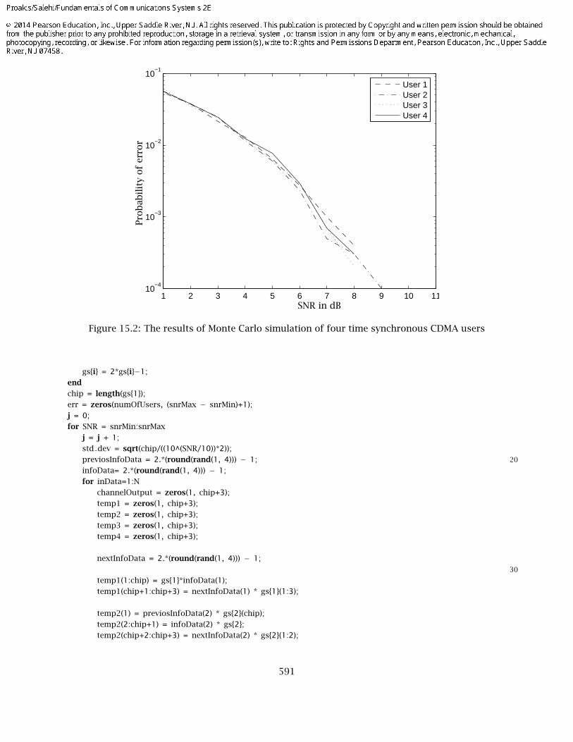
1 2 3 4 5 6 7 8 9 10 1110

−4

10−3

10−2

10−1

User 1User 2User 3User 4

SNR in dB

Pro

bab

ilit

yof

err

or

Figure 15.2: The results of Monte Carlo simulation of four time synchronous CDMA users

gs{i} = 2*gs{i}−1;

end

chip = length(gs{1});

err = zeros(numOfUsers, (snrMax − snrMin)+1);

j = 0;

for SNR = snrMin:snrMax

j = j + 1;

std dev = sqrt(chip/((10^(SNR/10))*2));

previosInfoData = 2.*(round(rand(1, 4))) − 1; 20

infoData= 2.*(round(rand(1, 4))) − 1;

for inData=1:N

channelOutput = zeros(1, chip+3);

temp1 = zeros(1, chip+3);




nextInfoData = 2.*(round(rand(1, 4))) − 1;

30

temp1(1:chip) = gs{1}*infoData(1);

temp1(chip+1:chip+3) = nextInfoData(1) * gs{1}(1:3);

temp2(1) = previosInfoData(2) * gs{2}(chip);

temp2(2:chip+1) = infoData(2) * gs{2};

temp2(chip+2:chip+3) = nextInfoData(2) * gs{2}(1:2);

591

temp3(1:2) = previosInfoData(3) * gs{3}(chip−1: chip);temp3(3:chip+2) = infoData(3) * gs{3};temp3(chip+3) = nextInfoData(3) * gs{3}(1); 40

temp4(1:3) = previosInfoData(4) * gs{4}(chip−2: chip);temp4(4:chip+3) = infoData(4) * gs{4};

noise = std dev * randn(1,chip+3);channelOutput = temp1 + temp2 + temp3 + temp4+ noise;

for user = 1:4hardDec = sign(sum(channelOutput(user:(chip+(user−1))).*gs{user})); 50

if hardDec ˜= infoData(user);err(user, j) = err(user, j) + 1;

endendpreviousInfoData = infoData;infoData = nextInfoData;

end

end 60

% Plotting commands follow.ber = err./N;snr = snrMin:snrMax;semilogy(snr, ber(1,:), ’--’);hold on;semilogy(snr, ber(2,:), ’-.’);semilogy(snr, ber(3,:), ’:’);semilogy(snr, ber(4,:), ’-’);legend(’User 1’, ’User 2’, ’User 3’, ’User 4’);


The period of the sequence is

L = 2m − 1 = 4095

The periodic autocorrelation function of the equivalent bipolar sequence is presented in Fig-

ure 15.4

The Matlab script for this problem is given next.

% MATLAB script for Computer Problem 15.4connections=zeros(1,12);m = 12;L = 2^m −1;connections(1) = 1;connections(7) = 1;

592

1 2 3 4 5 6 7 8 910

−4

10−3

10−2

10−1

User 1User 2User 3User 4

SNR in dB

Pro

bab

ilit

yof

err

or

Figure 15.3: The results of Monte Carlo simulation of four time asynchronous CDMA users

connections(9) = 1;connections(12) = 1;sequence=ss mlsrs(connections);c = 2.* sequence − 1; 10

Rc = zeros(1, L);for m=1:L

for n=1:L

Rc(m) = Rc(m)+ c(n)*c(n+m−1);end

end% Plotting commands follow.

plot(Rc); 20

axis([−500 4500 −500 4500]);

function [seq]=ss mlsrs(connections);% [seq]=ss mlsrs(connections)% SS MLSRS generates the maximal length shift-register sequence when the% shift-register connections are given as input to the function. A “zero”% means not connected, whereas a “one” represents a connection.m=length(connections);L=2^m−1 % length of the shift register sequence requestedregisters=[1 zeros(1,m−1)]; % initial register contentsseq(1)=registers(1); % first element of the sequence

593

−500 0 500 1000 1500 2000 2500 3000 3500 4000 4500−500

0

500

1000

1500

2000

2500

3000

3500

4000

4500

m

Rc(m)

Figure 15.4: The autocorrelation of the bipolar sequence

for i=2:2*L, 10

new reg cont(m)=mod(sum(registers.*connections), 2);for j=m−1:−1:1,

new reg cont(j)=registers(j+1);end;registers=new reg cont; % current register contentsseq(i)=registers(1); % the next element of the sequence

end;


The figure shown below illustrates the result of this crosscorrelation of {rk} with {ck}. Although

the signal component is not observable in the high-level noise, the signal is clearly detectable at the

output of the correlator.


N = 1000; % Number of samplesM = 50; % Length of the autocorrelation functionp = [0.9 0.99]; % Pole positionsw = 1/sqrt(2)*(randn(1,N) + 1i*randn(1,N)); % AWGN sequence% Preallocation for speed:c = zeros(length(p),N);

594

0 200 400 600 800 1000

−10

−8

−6

−4

−2

0

2

4

6

8

10

k

r k

0 200 400 600 800 1000

100

200

300

400

500

600

700

800

900

1000

n

y n

Rx = zeros(length(p),M+1);Sx = zeros(length(p),M+1);for i = 1:length(p) 10

for n = 3:Nc(i,n) = 2*p(i)*c(n−1) − power(p(i),2)*c(n−2) + power((1−p(i)),2)*w(n);

end% Calculation of autocorrelations and power spectra:Rx(i,:) = Rx est(c(i,:),M);Sx(i,:)=fftshift(abs(fft(Rx(i,:))));

end% Plot the results:subplot(3,2,1)plot(real(c(1,:))) 20

axis([0 N −max(abs(real(c(1,:)))) max(abs(real(c(1,:))))])title(’\it{p} = 0.9’)xlabel(’\it{n}’)ylabel(’\it{c_{nr}}’)subplot(3,2,2)plot(real(c(2,:)))axis([0 N −max(abs(real(c(2,:)))) max(abs(real(c(2,:))))])title(’\it{p} = 0.99’)xlabel(’\it{n}’)ylabel(’\it{c_{nr}}’) 30

subplot(3,2,3)plot(imag(c(1,:)))axis([0 N −max(abs(imag(c(1,:)))) max(abs(imag(c(1,:))))])title(’\it{p} = 0.9’)xlabel(’\it{n}’)ylabel(’\it{c_{ni}}’)subplot(3,2,4)plot(imag(c(2,:)))axis([0 N −max(abs(imag(c(2,:)))) max(abs(imag(c(2,:))))])title(’\it{p} = 0.99’) 40

xlabel(’\it{n}’)ylabel(’\it{c_{ni}}’)subplot(3,2,5)plot(abs(c(1,:)))axis([0 N 0 max(abs(c(1,:)))])title(’\it{p} = 0.9’)

595

xlabel(’\it{n}’)ylabel(’\it{|c_n |}’)subplot(3,2,6)plot(abs(c(2,:))) 50

axis([0 N 0 max(abs(c(2,:)))])title(’\it{p} = 0.99’)xlabel(’\it{n}’)ylabel(’\it{|c_n |}’)

figuresubplot(2,2,1)plot(abs(Rx(1,:)))axis([0 M 0 max(abs(Rx(1,:)))])title(’\it{p} = 0.9’) 60

xlabel(’\it{n}’); ylabel(’\it{|R_{c}(n)|}’)subplot(2,2,2)plot(abs(Rx(2,:)))title(’\it{p} = 0.99’)xlabel(’\it{n}’); ylabel(’\it{|R_{c}(n)|}’)axis([0 M 0 max(abs(Rx(2,:)))])subplot(2,2,3)plot(Sx(1,:))title(’\it{p} = 0.9’)xlabel(’\it{f}’); ylabel(’\it{S_{c}(f)}’) 70

axis([0 M 0 max(abs(Sx(1,:)))])subplot(2,2,4)plot(Sx(2,:))title(’\it{p} = 0.99’)xlabel(’\it{f}’); ylabel(’\it{S_{c}(f)}’)axis([0 M 0 max(abs(Sx(2,:)))])


Figure 15.5 presents the frequency selection pattern for the first ten bit interval.

The Matlab script for this problem is given next.

% MATLAB script for Computer Problem 15.6W = 127; % frequency band of widthDf = 2; % frequency seperation for fskm=7;L=2^m−1 % length of the shift register sequence requestedconnections=zeros(1,7);connections(1) = 1;connections(7) = 1;registers=[1 zeros(1,m−1)]; % initial register contentsseq(1)=registers(1); % first element of the sequence 10

frequency(1) = bin2dec(num2str(registers)); % first frequency% select the first two frequenciesf0(1) = frequency(1) − Df/2;f1(1) = frequency(1) + Df/2;for i=2:2*L,

596

1 2 3 4 5 6 7 8 9 100

20

40

60

80

100

120

140

time

Fre

qu

en

cy

Figure 15.5: Frequency selection pattern

new reg cont(m)=mod(sum(registers.*connections), 2);for j=m−1:−1:1,

new reg cont(j)=registers(j+1);end;registers=new reg cont; % current register contents 20

seq(i)=registers(1); % the next element of the sequence

frequency(i) = bin2dec(num2str(registers)); % select the frequency

% select two frequencies

f0(i) = frequency(i) − Df/2;f1(i) = frequency(i) + Df/2;

end;plot(frequency(1:10), ’*’);


Figure 15.6 illustrates the error rate that results from the Monte Carlo simulation. Also shown in the

figure is the theoretical value of the probability of error.

The MATLAB scripts for the simulation program are given next.

echo on

rho b1=0:5:35; % rho in dB for the simulated error rate

rho b2=0:0.1:35; % rho in dB for theoretical error rate computation

for i=1:length(rho b1),

597

0 5 10 15 20 25 30 3510

-4

10-3

10-2

10-1

100

ρb

Figure 15.6: Error-rate performance of FH binary FSK system with partial-band interference—Monte

Carlo simulation

smld err prb(i)=ss pe96(rho b1(i)); % simulated error rateecho off ;

end;echo on ;for i=1:length(rho b2),

temp=10^(rho b2(i)/10); 10

if (temp>2)theo err rate(i)=1/(exp(1)*temp); % theoretical error rate if rho>2

elsetheo err rate(i)=(1/2)*exp(−temp/2);% theoretical error rate if rho<2

end;echo off ;

end;echo on ;% Plotting commands follow.

function [p]=ss Pe96(rho in dB)% [p]=ss Pe96(rho in dB)% SS PE96 finds the measured error rate. The value of% signal per interference ratio in dB is given as an% input to the function.rho=10^(rho in dB/10);Eb=rho; % energy per bitif (rho>2),

598

alpha=2/rho; % optimal alpha if rho>2else 10

alpha=1; % optimal alpha if rho<2end;sgma=sqrt(1/(2*alpha)); % noise standard deviationN=10000; % number of bits transmitted% generation of the data sequencefor i=1:N,

temp=rand;if (temp<0.5)

data(i)=1;else 20

data(i)=0;end;

end;% Find the received signals.for i=1:N,

% the transmitted signalif (data(i)==0),

r1c(i)=sqrt(Eb);r1s(i)=0;r2c(i)=0; 30

r2s(i)=0;else

r1c(i)=0;r1s(i)=0;r2c(i)=sqrt(Eb);r2s(i)=0;

end;% The received signal is found by adding noise with probability alpha.if (rand<alpha),

r1c(i)=r1c(i)+gngauss(sgma); 40

r1s(i)=r1s(i)+gngauss(sgma);r2c(i)=r2c(i)+gngauss(sgma);r2s(i)=r2s(i)+gngauss(sgma);

end;end;% Make the decisions and count the number of errors made.num of err=0;for i=1:N,

r1=r1c(i)^2+r1s(i)^2; % first decision variabler2=r2c(i)^2+r2s(i)^2; % second decision variable 50

% Decision is made next.if (r1>r2),

decis=0;else

decis=1;end;% Increment the counter if this is an error.if (decis˜=data(i)),

num of err=num of err+1;end; 60

end;% measured bit error rate is then

599

p=num of err/N;

600

Fundamentals of Communication Systems

Documents

Transcript of Fundamentals of Communication Systems