Modeling Advanced Collective CommunicationAlgorithms on Cell-based Systems ∗

Qasim Ali, Samuel P. Midkiff and Vijay S. PaiSchool of Electrical and Computer Engineering, Purdue University

{qali, smidkiff, vpai}@purdue.edu

AbstractThis paper presents and validates performance models for a vari-ety of high-performance collective communication algorithms forsystems with Cell processors. The systems modeled include a sin-gle Cell processor, two Cell chips on a Cell Blade, and a cluster ofCell Blades. The models extend PLogP, the well-known point-to-point performance model, by accounting for the unique hardwarecharacteristics of the Cell (e.g., heterogeneous interconnects andDMA engines) and by applying the model to collective communi-cation. This paper also presents a micro-benchmark suite to accu-rately measure the extended PLogP parameters on the Cell Bladeand then uses these parameters to model different algorithms forthe barrier, broadcast, reduce, all-reduce, and all-gather collectiveoperations. Out of 425 total performance predictions, 398 of themsee less than 10% error compared to the actual execution time andall of them see less than 15%.

Categories and Subject Descriptors D.1.3 [Programming Tech-niques]: Concurrent Programming

General Terms Algorithms, Performance, Measurement

Keywords Collective communication, Algorithms, Modeling

1. IntroductionCollective communication is critical in many high performance ap-plications. Recent advances in high performance microprocessorslike the Cell processor and GPUs, as well as advances in on-chipand off-chip network technology, require improved design of col-lective communication algorithms to effectively utilize the new ar-chitecture [4]. Such systems also require new modeling techniquesfor collective communication to accurately predict performanceand to intelligently select among various choices of algorithmsand implementations for any given operation, as many system andworkload parameters can affect the performance of any particu-lar algorithm. Among existing models, the best known and stud-ied model for point-to-point communication is LogP, which char-acterizes communication performance in terms of message latency,

∗This work is supported in part by the National Science Foundationunder Grant Nos. CCF-0325603, CNS-0509390, CCF-0532448 andCNS-0751153, CCF-0916901, CCF-0833115, CNS-0707931.

Permission to make digital or hard copies of all or part of this work for personal orclassroom use is granted without fee provided that copies are not made or distributedfor profit or commercial advantage and that copies bear this notice and the full citationon the first page. To copy otherwise, to republish, to post on servers or to redistributeto lists, requires prior specific permission and/or a fee.PPoPP’10, January 9–14, 2010, Bangalore, India.Copyright c© 2010 ACM 978-1-60558-708-0/10/01. . . $10.00

message overhead, inter-message gap time, and the number of pro-cesses in the system [9, 10]. Extensions to LogP include PLogP,which makes the overhead and gap measures functions of the mes-sage size, and LoGPC, which includes a term for network con-tention [13, 15]. Other parameters that can shape the performanceof a collective communication operation include the number of pro-cesses involved in the particular communication, the size of the databuffers to be communicated, the pattern of communication, and thescheduled order of data transfers.

Combining system parameters to accurately predict communi-cation performance is difficult. The situation is worse for accelera-tors such as the Cell processor because of its complex and uniquearchitecture. The on-chip Element Interconnect Bus (EIB), which isthe heart of the Cell processor’s communication infrastructure, cansupport three concurrent DMA transfers on each of its four rings.The off-chip broadband interface (BIF), which connects two Cellprocessors on a Cell Blade, has an order of magnitude less band-width than the EIB and thus can only handle a limited number ofmessages without being overloaded. Modeling the contention re-sulting from these limits is an issue for communication operationsthat create large numbers of messages, such as broadcast or all-reduce. Addressing these limits requires additional effort, as previ-ous models have either ignored contention effects or considered theeffect of contention as it arises on a single uniform network.

This paper makes the following contributions:

• Modifies the PLogP model by adding a contention term, andsimplifies the model for Cell-based systems.

• Presents a novel suite of micro-benchmarks and a methodologyto accurately determine the parameters of the extended PLogPmodel accounting for the unique characteristics of the Cellprocessor and Cell Blades.

• Introduces basic collective communication patterns which areused as building blocks for various collective communicationalgorithms and develops models for them, in the context of theCell processor and its hardware features, using the parametersdetermined above.

• Uses the above parameters to model advanced and efficientcollective communication algorithms for a single Cell processorand the Cell Blade.

• Shows that the models can easily be plugged into existingcluster-based models for collective communication

We claim and show that performance modeling of an indi-vidual Cell processor and a Cell blade is different from othersystems because of their novel architectures. Generic models donot work in the aforementioned systems as we show in our ex-perimental section. We expand the abstract PlogP model to ac-count for architecture-specific details of the Cell. We also show

������������������� ������������������

���

�����

���

���� ���� ���� ����

���� ��� ���! ���"

��#

��$

�

�

�

" � % ��

� � �

��

�

�

!

���& ��'��(����)�*��������

���&������)���+,���������

���&��,-.,�-���*)���)���+,�

��$&��,-.,�-�)���+,�

������

/��

��0��

��������

�0��

��,-��

��1�

Figure 1: Cell architecture overview.

how this modeling can be extended to a cluster of Cell Blades orRoadrunner-like systems by adapting the cluster-level models andtechniques previously proposed by Dongarra et al. and Kielmann etal. [13, 17].

Empirical data shows that our models perform well: 94% of our425 performance predictions show errors of less than 10% and allof the predictions show errors less than 15%. The errors are smallenough that these predictions can be used to make correct decisionsabout which algorithm to choose for a particular operation beforeimplementing the operation. This capability is particularly valuablefor systems, such as the Cell, that require architecture-specificprogramming efforts. In contrast, using previous non-Cell-specificmethods to capture the inter-message gap parameter or ignoringBIF contention would lead to large and highly variable errors,ranging from no difference at all up to 140% error. Consequently,these predictions cannot guide proper algorithm choices, furthervalidating the need for a new model and new methods to capturethe model parameters.

2. Cell Architecture and CommunicationOverview

This section describes the Cell and features that are germane to thedesign and modeling of efficient collective communication. Fig-ure 1 gives a simplified illustration of the Cell architecture. TheCell processor is a heterogeneous multicore chip consisting of onegeneral-purpose 64-bit Power processor element (PPE), eight spe-cialized SIMD coprocessors called synergistic processor elements(SPEs), a high-speed memory controller, and a high-bandwidth businterface, all integrated on-chip. Each SPE consists of a synergis-tic processor unit (SPU) and a memory flow controller (MFC).The MFC includes a DMA controller, a memory management unit(MMU) to allow the SPEs to use virtual addresses when perform-ing DMAs, a bus interface unit, and an atomic unit for synchroniza-tion with other SPEs and the PPE. Each SPU includes a 256 Kbytelocal-store (LS) memory to hold its program’s instructions anddata; the SPU does not have any hardware-managed cache. TheSPU cannot access main memory directly, but it can issue DMAcommands to the MFC to bring data into local store or write com-putation results to main memory.

The PPE and SPEs communicate through an on-chip high-speedinterconnect called the Element Interconnect Bus (EIB). The EIBhas a vast amount of data bandwidth (204.8 GB/s) and is the com-munication path for commands and data between all processor el-

ements and the on-chip controllers for memory and I/O. It consistsof a shared command bus and a point-to-point data interconnect.The command bus distributes commands, sets up end-to-end trans-actions, and handles coherency. The data interconnect consists offour 16-byte-wide rings, with two used for clockwise data transfersand two for counter-clockwise data transfers. Each ring potentiallyallows up to three concurrent data transfers, as long as their pathsdo not overlap. Therefore the EIB can support up to 12 concurrenttransfers. To initiate a data transfer, bus elements must request databus access. The EIB data bus arbiter processes these requests anddecides which ring will handle each request.

Each processor element has one on-ramp and one off-ramp tothe EIB. Processor elements can transmit and receive data simulta-neously. Figure 1 shows the unit ID numbers of each element andthe order in which the elements are connected to the EIB. The con-nection order is important to programmers seeking to minimize thelatency of transfers on the EIB, as transfers can range from nearest-neighbor (e.g., SPE6 to SPE4) to 6-hop latencies (e.g., SPE1 toSPE6).

The on-chip Cell Broadband Engine interface (BEI) unit pro-vides two interfaces for external communication. One supportsonly a non-coherent I/O interface (IOIF) protocol, suitable for I/Odevices. The other is the Broadband interface (BIF), used for com-munication between two Cell processors on the same blade. TheBIF multiplexes its bandwidth over four rings of the EIB. The band-width of the BIF is 80% less than the EIB, so inter-chip commu-nications are much slower than intra-chip communications. Moredetails about the Cell can be found in [14].

3. Performance Modeling for the CellPerformance models are a basis for the design and analysis of par-allel algorithms. A good model includes a small number of param-eters but can express the complexity of the underlying runtime andhardware across a wide range of different scenarios. Since the col-lective communication algorithms used are based on point-to-pointmessages, we extend the standard PLogP model to model the Cell-targeted collective communication algorithms we previously pre-sented by carefully analyzing the communication characteristics ofeach algorithm [4]. Since some of the collectives have both a com-munication and computation part (e.g., all-reduce), we model boththe network and computation aspects of the Cell system.

3.1 The PLogP model and our extensionsTo model the communication part of a collective, we extend thepopular PLogP model [13]. PLogP characterizes the network interms of latency L, send and receive overheads os and or , gap re-quired between messages g, and the number of nodes (processors)in the system, p. The latency, gap and overheads are dependent onmessage size. In PLogP, the time to send a message between twonodes is given by L + g(m).

As in other collective communication models (e.g., Dongarraet al. [17]), we modify the p parameter to represent the numberof processors in a particular communication. The algorithms wemodel only use SPE-to-SPE communication, so p is the number ofSPEs in the collective. Following the LoGPC model, we add a con-gestion/contention term, C [15]. In our model, this is used only torepresent contention on the lower-bandwidth BIF and the method-ology to measure it is different than LoGPC. Our C parameter de-pends on the message size m and number of messages crossing theBIF n. The parameters of our model are summarized as below:

• p: the number of SPEs participating in a collective opertaion;• L: Communication delay (upper bound on the latency with no

contention from LS of one SPE to LS of another SPE);

0 1 32

0 1 32

0 1 32

0123

Round 1

Round 2

Round 3

Tim

e

Address written in current

round

Address written in

previous rounds

Nothing written-

Zero Value

ADDR

1

23

Ack written in

current round

Ack written in

previous rounds

Dma_put(Addr)

Dma_get(data)Dma_put(Ack)

ACK

0123 0123 0123

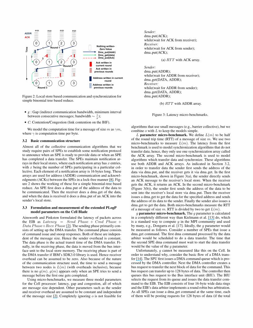
Figure 2: Local store based communication and synchronization forsimple binomial tree based reduce.

• g : Gap (indirect communication bandwidth, minimum intervalbetween consecutive messages; bandwidth ∼ 1

g);

• C: Contention/Congestion (link contention on the BIF).

We model the computation time for a message of size m as γm,where γ is computation time per byte.

3.2 Basic communication structureAlmost all of the collective communication algorithms that westudy require pairs of SPEs to establish some notification protocolto announce when an SPE is ready to provide data or when an SPEhas completed a data transfer. The SPEs maintain notification ar-rays in their local stores, where each notification array has x entries,with x being the number of SPEs participating in a particular col-lective. Each element of a notification array is 16 bytes long. Thesearrays are used for address (ADDR) communication and acknowl-edgments (ACKs) between the SPEs in a lock-free manner [8]. Fig-ure 2 shows the working of these for a simple binomial-tree basedreduce. An SPE first does a dma put of the address of the data tobe communicated. Then the receiver does a dma get of the data,and when the data is received it does a dma put of an ACK into thesender’s local store.

3.3 Formulation and measurement of the extended PLogPmodel parameters on the Cell Blade

Ainsworth and Pinkston formulated the latency of packets acrossthe EIB as Latency = Send Phase + Cmd Phase +Data Phase+Recv Phase [2]. The sending phase primarily con-sists of setting up the DMA transfer. The command phase consistsof command issue and snoop responses. Both of these are indepen-dent of the message size. Hence the sender overhead is constant.The data phase is the actual transit time of the DMA transfer. Fi-nally, in the receiving phase, the data is moved from the bus inter-face unit to the local store memory. The receiving phase is part ofthe DMA transfer if IBM’s SDK3.0 library is used. Hence receiveroverhead can be assumed to be zero. Also because of the natureof the communication structure used, the time to send a messagebetween two nodes is L(m) (with overheads inclusive), becausethere is no g(m). g(m) appears only when an SPE tries to send amessage before the first one gets completed.

Using micro-benchmarks, we measure three model parametersfor the Cell processor: latency, gap and congestion, all of whichare message size dependent. Other parameters such as the senderand receiver overhead are assumed to be constant and independentof the message size [2]. Completely ignoring o is not feasible for

Sender:dma put(ACK);while(wait for ACK from receiver);Receiver:while(wait for ACK from sender);dma put(ACK);

(a) RTT with ACK array.

Sender:dma put(ADDR);while(wait for ADDR from receiver);dma get(DATA, ADDR);Receiver:while(wait for ADDR from sender);dma get(DATA, ADDR);dma put(ADDR);

(b) RTT with ADDR array.

Figure 3: Latency micro-benchmarks.

algorithms that use small messages (e.g., barrier collective), but wecombine o with L to keep the models simple.

L parameter micro-benchmark. We define L(m) to be halfof the round trip time (RTT) of a message of size m. We use twomicro-benchmarks to measure L(m). The latency from the firstbenchmark is used to model synchronization algorithms that do nottransfer data; hence, they only use one synchronization array calledthe ACK array. The second micro-benchmark is used to modelalgorithms which transfer data and synchronize. These algorithmsuse both ADDR and ACK arrays. As indicated in Section 3.2,in order to transfer data the sender first sends the address of thedata via dma put, and the receiver gets it via dma get. In the firstmicro-benchmark, shown in Figure 3(a), the sender directly sendsan ACK message to the receiver’s local store. When the receivergets the ACK, it returns an ACK. In the second micro-benchmark(Figure 3(b)), the sender first sends the address of the data to besent into the receiver’s local store via dma put. Then the receiverissues a dma get to get the data for the specified address and sendsthe address of its data to the sender. Finally the sender also issues adma get to get the data. Both micro-benchmarks measure the RTTof a message of size m. RTT is divided by two to get L(m).

g parameter micro-benchmark. The g parameter is calculatedin a completely different way than Kielmann et al. [13] do, whichis a standard way to compute g in the MPI community and usedby many, e.g., Dongarra et al. [17]. Ideally, the g parameter wouldbe measured as follows. Consider a number of SPEs that issue adma get command. The first dma command processed by the dataarbiter would be scheduled to do a data transfer. The time thatthe second SPE dma command must wait to start the data transferwould be the value of the g parameter.

Unfortunately, g cannot be measured like this on the Cell. Inorder to understand why, consider the basic flow of a DMA trans-fer [14]. The SPU first issues a DMA command queue which is pro-cessed by the DMA controller. Next the DMA controller creates abus request to transfer the next block of data for the command. Thisbus request can transfer up to 128 bytes of data. The controller thenqueues this bus request to the Bus interface unit (BIU). The BIUselects the request from its queue and issues the data transfer com-mand to the EIB. The EIB consists of four 16-byte wide data ringsand the EIB’s data arbiter implements a round robin bus arbitration.As all SPEs can issue a dma get command at the same time, eachof them will be posting requests for 128 bytes of data (if the total

requested data is equal to or more than 128 bytes, and less than 128bytes if the requested data is less).

Because we cannot change the data arbiter policy, we employthe following technique to measure the gap parameter. We desig-nate one SPE as the root which has the data. All other (non-root)SPEs issue a dma get of data from this root SPE. The time taken byeach SPE is measured, and these times are averaged over the num-ber of SPEs issuing the dma get command. The value of g obtainedin this manner would be similar to what the value of g would be ifwe changed the data arbiter policy to “first-come, first-served” andlet the bus requests issued by one SPE finish before the bus requestof another SPE is serviced. For two Cell processors on a blade,there are two g parameters, the intra-chip g1 and inter-chip g2. Weonly use the single g when a single Cell processor is involved in thecommunication.

C parameter micro-benchmark. The congestion parame-ter is calculated by the butterfly communication pattern micro-benchmark, i.e., each SPE sends and receives data from anotherdistinct SPE. When two SPEs are engaged in the data transfer (bothsending and receiving) across the BIF, we denote this as BIF-2.Thus, BIF-16 means 16 messages are crossing the BIF. BIF-2 la-tency is the average of the time taken by the two SPE DMAs. Weuse BIF-2 as the baseline since we have observed that BIF-1 equalsBIF-2; that is, the BIF can support two simultaneous messageswithout any observable contention. We define the C parameter, fora given message size m and number of BIF-crossing messages n,as the excess latency observed by a BIF-n butterfly communicationpattern when compared to a BIF-2 pattern. As the values of n andm increase, the congestion also increases.

Some other notation used in our models is L1(1) and L1(m),which are the intra-chip latencies. The “1” inside the parenthesesindicates that the message size is a small constant; more specifi-cally, it is 16 bytes long as this is the smallest DMA transfer possi-ble on Cell and m is the message size in bytes. Similarly L2(1) andL2(m) are latencies for inter-chip transfers. gAck is used to denotethe gap for ACKs.

4. Building Blocks for Collective CommunicationModels

This section presents an overview of the three basic collective com-munication patterns that serve as building blocks for the algorithmsused in this paper. We will briefly explain these patterns and de-velop models for them in the context of the Cell processor and itsDMA engine. In Figure 4 the numbers in circles represent nodes,and the arrows (both dotted and dark) represent communication.

0 1 32

0 1 32

0 1 32

0

21 3

(a) Simple One-to-all(c) Recursive Distance

doubling (rdb)

0

1

3

2

Longest latency

path

Acks

High priority Nodes

1 2

1

(b) DMA Ordered Tree

Figure 4: Different communication patterns and techniques.

Figure 4(a) shows a one-to-all (OTA) communication pattern inwhich all nodes receive data from just one node. If all the nodessimultaneously do a dma get, then a communication gap will arisethat depends on g. Let q be the number of inter-message gaps (g)required. This value is based on the maximum out-degree of a node

at each level of the tree and is given by the following equation:

q =

h∑k=1

(dk − 1)

where dk is the maximum out-degree of a node at level k and his the height of the tree. In the example of Figure 4(a), h is 1 andd1 = 3, so there will be two gaps (q = 2).

Similarly, in the case of inter-chip SPE communication, two q’swill be used, q1 for the number of g1 (on-chip gap) terms and q2

for the number g2 (inter-chip gap) terms given below:

q1 =

h∑k=1

(dk − nk2 − 1)

q2 =

h∑k=1

(dk − nk1 − 1)

where nk1 and nk2 are the number of messages at level k betweenchips and across chips, respectively.

The second pattern is the optimized ordered tree pattern shownin Figure 4(b). The gap parameter which arises in Figure 4(a)can be eliminated by inserting ACKs to order the DMAs. TheACKs are depicted in Figure 4 (b). To do this, the root nodefirst does a dma put into the dark colored node, because it is onthe longest latency path, and then into the white colored node.The cost of the communication pattern shown in Figure 4(b) is2× (L(m) + L(1)). If the DMAs were not ordered the cost wouldhave been 2×L(m) + g(m): one g term in the first level and no gterm in the second level of the tree.

The third pattern shown in Figure 4(c) is based on an efficientalgorithm known as recursive distance doubling or the butterfly al-gorithm [19]. Figure 4(c) shows the butterfly algorithm in action.Each node sends to, and receives from, a different partner node ateach stage of the algorithm: first with distance 1, then with dis-tance 2, then 4, and so forth. At the end of the last stage all nodeshave received (reduction and gather operations) and, if necessary,processed the data (reduction operations). When applied to all-reduce, this algorithm specifically exploits full-duplex communica-tion links to collapse a reduce and broadcast into a single operation.Each round of the butterfly pattern requires L(m)+L(1) time (dataplus ACK) based on the interconnect parameters. If, however, theBIF is the network used at any stage, sending too many messagesacross it may lead to poor performance. In particular, if the numberof BIF messages is greater than two and the data size is greater than256 bytes, the network starts to become congested and becomes abottleneck. We model the congestion on the BIF by a parameter C.These thresholds were determined experimentally.

If the number of SPEs involved is not a power of 2, the firststage communicates from the higher-numbered SPEs to the lower-numbered SPEs within the next lower power of 2 [18]. The SPEswithin the next lower power of 2 proceed using the butterfly algo-rithm. After that, the lower-numbered SPEs feed information backto the higher-numbered SPEs, for a total of 2 + blog2 pc steps forp numbers of SPEs in the all-reduce.

5. Modeling Collective CommunicationAlgorithms

Using the communication flow of each algorithm, the point-to-point messages modeled using the standard PLogP parameters, ourmodeling extensions described in Section 3 and the three basiccommunication patterns discussed and modeled in Section 4, wehave developed models for different algorithms for the barrier, re-duce, all-reduce, broadcast and all-gather collectives. All the algo-

rithms used in this paper are based on inter-SPE communicationand the data to be communicated resides in the local store, similarto the Cell Messaging Library, which is an MPI implementation forthe Cell [16]. We will explain a few representative algorithms toexplain how the models are developed. The details of all the algo-rithms can be found in our previous work [4].

For one-to-all (OTA) models (barrier and broadcast), the rootnode is assumed to be on the first chip, without loss of generality.

5.1 Barrier modelsWe use the results of the micro-benchmark in Figure 3(a) to modelthe barrier algorithms because they transfer no message data andonly use an ACK array. Note that if more than eight SPEs are in-volved in a particular collective, the first eight SPEs are on thefirst Cell processor and the rest are on the second. This arrange-ment minimizes the number of BIF crossings. The cost of recur-sive doubling follows from Section 4, except that the actual costof a recursive doubling round is only L(1), not L(m) + L(1),because there is no data transfer. In Bruck, step k of the collec-tive has an SPE of rank r sending a message to an SPE of rank(r+2k) and receiving a message from an SPE of rank (r-2k) withwrap around [7, 17]. Bruck always needs dlog2 pe rounds for pnodes. In Bruck, 2round num inter-chip messages are exchanged ateach round, leading to higher latencies in higher numbered rounds.round num is the total number of communication rounds/phases.As there are at least two messages crossing the BIF in each round,the overall latency in each round is max(L1(1), L2(1)), i.e., themaximum of the inter-chip and intra-chip latency. Because thereare dlog2 pe steps, the overall communication time for two chips ismodeled as dlog2 pe × (max[L1(1), L2(1)]).

In a one-to-all barrier, the root node sends (p − 1) messages.The first message reaches the first non-root SPE in time L(1), thesecond message arrives in time g(1) because it has to wait g(1)amount of time, and so on. Thus it takes a total of g(1)× (p−2)+L(1) time to broadcast a message to p − 1 SPEs, thus the valueof q is p − 2. After all p − 1 SPEs get their messages, they sendan ACK back to the root node. In this phase, the time will be atleast L(1) plus some gap experienced by the ACKs. The total gapis given by 0 ≤ g ≤ ((p − 2) × gAck(1)). Some of these ACKswill be overlapped with the original messages in the first phase.Other barrier algorithms were modeled similarly and are shown inTable 1.

5.2 Broadcast modelsWe use the second latency micro-benchmark shown in Figure 3 tomodel different broadcast algorithms and the other algorithms pre-sented in the remainder of this paper. The “simple” suffix in Table 2denotes a broadcast in which nodes do not wait for ACKs at theend of each communication round, allowing later communicationrounds to complete their data transfers before earlier ones.In thesimple version of the binomial tree algorithm, the root node sendsthe address of the data to be broadcast to all of its children and theyissue a dma get at approximately the same time. Because the DMArequests are 128 bytes in length, each child will get 128 bytes ofdata initially rather than SPE 1 getting all the data. The result ofthis is that SPE 1 will get the data after L(m) + q × g(m) time,not L(m) time. This in turn delays the children of SPE 1. Hence ateach level there is an additional delay, which we model by g(m).We call such behavior a priority inversion.

We refer to an optimized version of broadcast that preventspriority inversion of messages by ordering DMAs as “opt”. Thisis the second communication pattern discussed in Section 4. Toavoid the priority inversion problem in the simple broadcast, ouroptimized broadcast uses address-data-ACK phases at each roundas described in Section 3.2. Each round takes L(m)+L(1) time. By

0

21

3 65

7

4

Figure 5: First phase of the segmented binomial algorithm.

using such ordered DMAs, the overall latency will not have g(m)terms in the case of a power-of-two number of SPEs.

A segmented binomial tree has a two-phase broadcast process.In the first phase, the nodes in the left half of the tree get the lefthalf of the data and the nodes in the right half of the tree get theright half. This step takes (log2 p − 1) × L(m/2) + L(1) time.In the second phase, the left and right half nodes exchange theirdata, which takes L(m/2) + L(1) time. (All of our segmentedtrees assume the DMA ordering optimization.) In Figure 5, theleft half of the data is shown as a dark color (blue) and the righthalf is shown as a light color (red). In the 16 SPE case, thispolicy results in 14 inter-chip data exchanges in the last phase,causing substantial congestion when larger messages are used. Thisis shown by the C(m > 256) term in the segmented-binomialmodel since sending more than two large messages across theBIF will result in some congestion and delay, which is accuratelycaptured by our congestion micro-benchmark.

To reduce the number of BIF-crossing messages in the 16 SPEcase, we implemented a hybrid version of the segmented binomial,where the root node sends all data to one representative node in thesecond chip. This takes L2(m) for the data message and L2(1) forthe ACK, after which the two-phase broadcast times are all on-chipand thus based on L1.

5.3 All-gather ModelsIn recursive distance doubling for all-gather, p messages are ex-changed in each communication round and the data being commu-nicated doubles at each stage. For the two chip scenario, in the firstlog2 p − 1 rounds, data communication will take place on the EIBand the communication cost in each round is L1(messagesize) +L1(1). In the last round, all the data traffic will be on the BIF. Be-cause the number of messages crossing the BIF interface is morethan two, the congestion C term is needed in the final equationshown in Table 3.

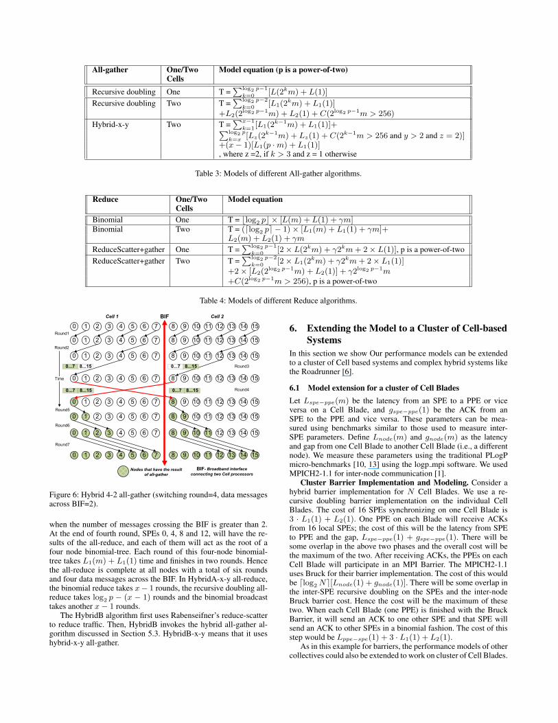
Consider the hybrid algorithm called hybrid-x-y (shown in Fig-ure 6) that seeks to find an ideal compromise between the concur-rency of recursive doubling and the low traffic of gather followedby broadcast. x is the round number where the switch to recursivedoubling occurs and y is the number of data messages crossing theBIF. For simplicity, consider the case of p nodes where p is a powerof 2. This algorithm starts by performing x− 1 rounds of binomialgather, leaving p

2x−1 evenly-spaced node IDs in the communica-tion structure. The cost of each step is L1(messagesize)+L1(1),where the message size depends on the round number, and is2round number ×messagesize bytes. At this point, the algorithmswitches to recursive doubling until all p

2x−1 nodes have the re-sults of the all-gather. This takes log2 p − (x − 1) rounds and re-sults in p

2x−1 messages across the BIF when the lower half andupper half of the nodes are on separate chips. The cost of each

Barrier One/TwoCells

Model equation

Recursive doubling One T = log2 p × L(1), p is a power-of-twoT = (blog2 pc+ 2)× L(1), otherwise

Recursive doubling Two T = (log2 p − 1)× L1(1) + L2(1), p is a power-of-twoT = (blog2 pc+ 1)× L1(1) + L2(1), otherwise

Bruck One T = dlog2 pe × L(1)Bruck Two T = dlog2 pe × (max[L1(1), L2(1)])Gather-Broadcast One T = 2× dlog2 pe × L(1)Gather-Broadcast Two T = max[2× (dlog2 pe − 1)× L1(1),

2× [L2(1) + (dlog2 pe − 1)× L1(1)]]One-to-all One T = q × g(1) + L(1) + L(1) + X,

0 ≤ X ≤ (q × gAck(1)) and q = p − 2One-to-all Two T = 2× (L1(1) + L2(1)) + q1 × g1(1) + q2 × g2(1) + X,

0 ≤ X ≤ q1 × g1Ack(1) + q2 × g2Ack(1) and q1 = 6, q2 = p − 9

Table 1: Models of different Barrier algorithms.

Broadcast One/TwoCells

Model equation

One-to-all One T = q × g(m) + L(m) + L(1) + X,0 ≤ X ≤ (q × gAck(1)) and q = p − 2

One-to-all Two T = L1(m) + q1 × g1(m) + L2(m) + q2 × g2(m)+L1(1) + L2(1) + X, 0 ≤ X ≤q1 × g1Ack(1) + q2 × g2Ack(1), p > 8 and q1 = 6, q2 = p − 9

Binomial-Tree-simple One T = blog2 pc × [L(m) + L(1)] + q×g(m) + X , 0 ≤ X ≤ q × gAck(1)), and q = 3

Binomial-Tree-opt One T = log2 p × [L(m) + L(1)], where p is power-of-twoBinomial-Tree-simple Two T = (blog2 pc − 1)× [L1(m) + L1(1)] + L2(m) + L2(1)

+q1 × g1(m) + X , 0 ≤ X ≤ q×g1Ack(1)), and q1 = 7, q2 = 0

Binomial-Tree-opt Two T = (dlog2 pe − 1)× [L1(m) + L1(1)] + L2(m) + L2(1)Segmented-Binomial-opt One T = (log2 p + 1)× [L(m/2) + L(1)], p is a power-of-twoSegmented-Binomial-opt Two T = (log2 p − 1)× [L1(m/2) + L1(1)]+

2× [L2(m/2) + L2(1)] + C(m/2 > 256), p is a power-of-twoHybrid-Seg-Binomial-opt Two T = log2 p × [L1(m/2) + L1(1)] + [L2(m) + L2(1)], p is a power-of-two

Table 2: Models of different Broadcast algorithms.

round would be the same as above, except that the cost should beL2(messagesize)+L2(1) for rounds that cross the BIF. A C termis added if the messages crossing the BIF are large and more thantwo in number. Now, each of the p

2x−1 nodes with the result act asthe root of binomial broadcast trees, requiring x − 1 more roundsto give the result to all nodes. The cost of each of these steps is alsoL1(messagesize) + L1(1). Thus, the total number of rounds arelog2 p + (x − 1) and there are p

2x−1 BIF-crossing data messages.In Table 3, m is the starting size of the send buffer and p · m is thesize of the final receive buffer.

5.4 Reduce ModelsThe binomial reduce is the opposite of binomial broadcast. In thiscase, however, there is a computation term γ included in the mod-els. For large data sizes, we studied Rabenseifner’s reduce, whichis based on reduce-scatter and gather [19]. Reduce-scatter effec-tively decreases the aggregate bandwidth requirement by givingeach node only a subset of the reduced data. The amount of datato be communicated is halved at each stage along a binomial treeand computation is performed on the communicated data. Thecost of each stage k is L(mk) + γmk + L(1), where the mes-sage size mk depends on the round number k as (2log2p−k). Inthe gather phase, the amount of data is doubled at each stage,

and the root node contains the total reduced data, with the costbeing L(messagesize) + L(1) for each stage. Thus the result-ing overall time for reduce-scatter plus gather based reduction is∑log2 p−1

k=0[2L(2km) + γ2km + 2L(1)]. For 16 SPEs, the con-

gestion (C) term is added since in the first round of reduce-scatterthere will be 16 messages crossing the BIF. In Table 4, the reduce-scatter model assumes that the total size of the reduced data is p·m,with m being the size of the data at each node when the reduce-scatter is done.

5.5 All-reduce ModelsThe Reduce-scatter plus recursive distance doubling all-gather issimilar to reduce-scatter plus gather-based reduce with the additionof another congestion term (C). When 16 SPEs are participating inthe all-reduce, the reduce-scatter phase has 16 messages crossingthe BIF and so does the all-gather phase.

HybridA-3-4 switches to recursive doubling in the third com-munication round (x− 1 = 2). HybridA-3-4 starts with x− 1 = 2rounds of binomial reduce with the cost of each round beingL1(m) + L1(1) + γ · m and then switches to recursive doublingall-reduce in round x = 3. The number of data messages cross-ing the BIF is 4. The cost of each round is the same as above,but L2(messagesize) + L2(1), if x > 3 and a C term added

All-gather One/TwoCells

Model equation (p is a power-of-two)

Recursive doubling One T =∑log2 p−1

k=0[L(2km) + L(1)]

Recursive doubling Two T =∑log2 p−2

k=0[L1(2

km) + L1(1)]+L2(2

log2 p−1m) + L2(1) + C(2log2 p−1m > 256)

Hybrid-x-y Two T =∑x−1

k=1[L1(2

k−1m) + L1(1)]+∑log2 p

k=x[Lz(2

k−1m) + Lz(1) + C(2k−1m > 256 and y > 2 and z = 2)]+(x − 1)[L1(p · m) + L1(1)], where z =2, if k > 3 and z = 1 otherwise

Table 3: Models of different All-gather algorithms.

Reduce One/TwoCells

Model equation

Binomial One T = blog2 pc × [L(m) + L(1) + γm]Binomial Two T = (dlog2 pe − 1)× [L1(m) + L1(1) + γm]+

L2(m) + L2(1) + γm

ReduceScatter+gather One T =∑log2 p−1

k=0[2× L(2km) + γ2km + 2× L(1)], p is a power-of-two

ReduceScatter+gather Two T =∑log2 p−2

k=0[2× L1(2

km) + γ2km + 2× L1(1)]+2× [L2(2

log2 p−1m) + L2(1)] + γ2log2 p−1m+C(2log2 p−1m > 256), p is a power-of-two

Table 4: Models of different Reduce algorithms.

0 1 3 4 762 5 8 9 11 12 151410 13

0 1 3 4 762 5 8 9 11 12 151410 13

0 1 3 4 762 5 8 9 11 12 151410 13

0 1 3 4 762 5 8 9 11 12 151410 13

0 1 3 4 762 5 8 9 11 12 151410 13

0 1 3 4 762 5 8 9 11 12 151410 13

0 1 3 4 762 5 8 9 11 12 151410 13

Time

Round1

Round2

Round3

Round4

Round5

Round6

BIFCell 1 Cell 2

Nodes that have the result

of all-gather

BIF- Broadband interface

connecting two Cell processors

0 1 3 4 762 5 8 9 11 12 151410 13

Round7

0...7 8...15 0...7 8...15

0...7 8...15 0...7 8...15

Figure 6: Hybrid 4-2 all-gather (switching round=4, data messagesacross BIF=2).

when the number of messages crossing the BIF is greater than 2.At the end of fourth round, SPEs 0, 4, 8 and 12, will have the re-sults of the all-reduce, and each of them will act as the root of afour node binomial-tree. Each round of this four-node binomial-tree takes L1(m) + L1(1) time and finishes in two rounds. Hencethe all-reduce is complete at all nodes with a total of six roundsand four data messages across the BIF. In HybridA-x-y all-reduce,the binomial reduce takes x− 1 rounds, the recursive doubling all-reduce takes log2 p − (x − 1) rounds and the binomial broadcasttakes another x − 1 rounds.

The HybridB algorithm first uses Rabenseifner’s reduce-scatterto reduce traffic. Then, HybridB invokes the hybrid all-gather al-gorithm discussed in Section 5.3. HybridB-x-y means that it useshybrid-x-y all-gather.

6. Extending the Model to a Cluster of Cell-basedSystems

In this section we show Our performance models can be extendedto a cluster of Cell based systems and complex hybrid systems likethe Roadrunner [6].

6.1 Model extension for a cluster of Cell BladesLet Lspe−ppe(m) be the latency from an SPE to a PPE or viceversa on a Cell Blade, and gspe−ppe(1) be the ACK from anSPE to the PPE and vice versa. These parameters can be mea-sured using benchmarks similar to those used to measure inter-SPE parameters. Define Lnode(m) and gnode(m) as the latencyand gap from one Cell Blade to another Cell Blade (i.e., a differentnode). We measure these parameters using the traditional PLogPmicro-benchmarks [10, 13] using the logp mpi software. We usedMPICH2-1.1 for inter-node communication [1].

Cluster Barrier Implementation and Modeling. Consider ahybrid barrier implementation for N Cell Blades. We use a re-cursive doubling barrier implementation on the individual CellBlades. The cost of 16 SPEs synchronizing on one Cell Blade is3 · L1(1) + L2(1). One PPE on each Blade will receive ACKsfrom 16 local SPEs; the cost of this will be the latency from SPEto PPE and the gap, Lspe−ppe(1) + gspe−ppe(1). There will besome overlap in the above two phases and the overall cost will bethe maximum of the two. After receiving ACKs, the PPEs on eachCell Blade will participate in an MPI Barrier. The MPICH2-1.1uses Bruck for their barrier implementation. The cost of this wouldbe dlog2 Ne[Lnode(1) + gnode(1)]. There will be some overlap inthe inter-SPE recursive doubling on the SPEs and the inter-nodeBruck barrier cost. Hence the cost will be the maximum of thesetwo. When each Cell Blade (one PPE) is finished with the BruckBarrier, it will send an ACK to one other SPE and that SPE willsend an ACK to other SPEs in a binomial fashion. The cost of thisstep would be Lppe−spe(1) + 3 · L1(1) + L2(1).

As in this example for barriers, the performance models of othercollectives could also be extended to work on cluster of Cell Blades.

All-reduce One/TwoCells

Model equation (p is power-of-two)

Recursive doubling One T = log2 p × [L(m) + 2× L(1) + γm]Recursive doubling Two T = (log2 p − 1)× [L1(m) + 2× L1(1) + γm]+

L2(m) + 2× L2(1) + γm + C(m > 256)

ReduceScatter+rd-allgather One T =∑log2 p−1

k=0[2× L(2km) + γ2km + 2× L(1)]

ReduceScatter+rd-allgather Two T =∑log2 p−2

k=0[2× L1(2

km) + γ2km + 2× L1(1)]+2× [L2(2

log2 p−1m) + L2(1)] + γ2log2 p−1m+2× C(2log2 p−1m > 256)

ReduceScatter+gather+Bcast One T =∑log2 p−1

k=0[2× L(2km)+

γ2km + 2× L(1)] + log2 p × [L(m) + L(1)]

ReduceScatter+gather+Bcast Two T =∑log2 p−2

k=0[2× L1(2

km)+γ2km + 2× L1(1)]+2× [L2(2

log2 p−1m) + L2(1)] + γ2log2 p−1m+C(2log2 p−1m > 256) + (log2 p − 1)× [L1(m) + L1(1)]+L2(m) + L2(1)

HybridA-x-y Two T = 2× (x − 1)[L1(m) + L1(1)] + (x − 1)× γm∑log2 p

k=x[Lz(m) + Lz(1)+

γm + C(m > 256 and y > 2 and z = 2)], where z =2, if k > 3 and z = 1 otherwise

HybridB-x-y Two T =∑log2 p−2

k=0[L1(2

km) + γ2km + L1(1)]+L2(2

log2 p−1m) + L2(1) + γ2log2 p−1mC(2log2 p−1m > 256) + Hybridall-gather-x-y

Table 5: Models of different All-reduce algorithms.

6.2 Model extension for Cell-based hybrid systemsSimilarly these models can be extended to work on hybrid systemslike the Roadrunner, by accounting for the additional levels of hier-archy and interconnect. Roadrunner has a deep communication hi-erarchy, including an Element Interconnect Bus (EIB), BIF (Broad-band interface), PCI Express, Hypertransport, and Infiniband. Eachof these interconnects has a different latency. Define L3(m) andg3(m) as the latency and gap from a Cell blade to an Opteronblade on the triblade Roadrunner node (over PCIe) and L4(m)and g4(m) as the latency and gap from one Opteron to anotherOpteron (different node). Note that the third and fourth level pa-rameters could be benchmarked using the traditional LogP/PlogPmeasures as these are more appropriate for conventional networks.

Roadrunner Barrier Modeling. Consider a recursive doublingbarrier for N triblade nodes. The cost of 16 SPEs synchronizingon one Cell Blade is 3 · L1(1) + L2(1). One PPE on each Bladewill receive ACKs from 16 local SPEs; the cost of this will be thelatency from SPE to PPE and 15 times the gap. There will be someoverlap in the above two phases and the overall cost will be themaximum of the two. After receiving ACKs, the two PPEs willsend an ACK to the Opteron in approximately L3(1) time, becauseeach Cell blade has an independent PCI Express link. Finally theOpterons will engage in the global recursive doubling phase andthis step will take log2 N steps when N is a power of two. Each stepwill have a cost of L4(1). When each Opteron blade is be done withrecursive doubling, it will send ACKs to two PPEs (one per Cellblade), costing another L3(1)+g3(1). Each PPE will then forwardthe ACK to one representative SPE and that SPE will do a one-to-all broadcast or binomial broadcast of the ACKs to all other SPEs.The model for this is already covered in the previous section 6.1.As in this example for barriers, the performance models of othercollectives can be extended to account for the additional levels ofhierarchy and interconnect in the Roadrunner.

7. Experimental EvaluationAll experiments reported here were performed on the IBM Blade-Centers QS20 and QS22 at Georgia Tech. The QS2x organizes two3.2Ghz Cell processors into an SMP configuration, connected bythe BIF inter-chip interconnect. All code shown here uses IBM’sSDK3.0 and were compiled using 64-bit gcc with optimizationlevel -O3. Timings are measured using the fine-grained decrement-ing register provided by the Cell blade. All latency numbers wereaveraged over 100,000 iterations. These results are compared withthe predictions of the performance models of Section 5.

7.1 Model parameters.We measured the parameters L(m) and g(m) using our micro-benchmarks. We calculated RTT across both the EIB and the BIFby averaging the RTT for communications between SPE0 and allother SPEs. Recall that for 16 SPEs (Cell Blade), there are two gapparameters: one for EIB messages, g1 and one for BIF messages,g2. Figure 7 shows the gap parameter values for various messagesizes. The g1 value is different from g because there are additionalSPEs across the BIF posting bus requests to the data arbiter. There-fore the waiting time for each SPE request is increased, Recall thatwe use g when only one Cell processor is involved in the commu-nication.

The congestion parameter (C), is calculated by the butterflycommunication pattern micro-benchmark, with each SPE sendingand receiving data from another distinct SPE. Note that in Figure 8,there is almost no congestion up to a data size of 256 bytes. Thelatency starts to climb as the data size increases above 256 bytesand as the number of data messages crossing the BIF increasesabove two. The latency increase caused by congestion is up to218% of the latency when there is no contention.

1

10

100

1000

10000

16 32 64 128 256 512 1K 2K 4K 8K 16K 32K

DataSize(Bytes)

Late

ncy(n

secs)

g2

g1

g

Figure 7: Gap micro-benchmark results.

1

10

100

1000

16 32 64 128 256 512 1K 2K 4K 8K 16K 32K

DataSize (Bytes)

La

ten

cy

(T

ick

s)

BIF-2

BIF-4

BIF-8

BIF-16

Figure 8: BIF Contention micro-benchmark results.

7.2 Analysis of Collective Communication performancemodels

All of the execution times predicted by the performance modelsare very close to the experimental results. Figure 9 shows the ex-perimentally measured and predicted values of each barrier imple-mentation. In the gather-broadcast barrier, the actual performanceis slightly worse than the model because of some control code inthe implementation; in the Bruck barrier, the actual performance isslightly better due to message pipelining effects not captured by themodel. These errors are small enough that these predictions can beused to make correct decisions about which algorithm to choose.

Figure 10 shows the error rate for different algorithms forall-gather, broadcast, reduce and all-reduce. Considering all algo-rithms, implementations, and data sizes, we have a total of 425 datapoints. Of those, 398 (94%) have a discrepancy between the modeland the actual execution of less than 10% and all of them see er-rors less than 15%. The algorithms not shown in this figure haveerror rates less than 5%. All of the error rate graphs show data sizesfrom 64 bytes to 32 KB. Performance of data sizes less than 64bytes is the same as the performance at 64 bytes. Again, the er-rors are small enough that the predictions can still be used to makecorrect decisions when selecting algorithms. We also modeled andtested Barrier and Broadcast up to 64 SPEs (4 Cell Blades) to showthat our models can be easily plugged into cluster-based collectivecommunication models. The error rates were within 13%.

We attribute the general accuracy of the models to two factors:first, the accurate micro-benchmarks and methodology we devel-

0

0.2

0.4

0.6

0.8

1

1.2

1.4

1.6

1.8

8 16

NUM_SPES

Late

ncy (

usecs)

Rdb-exp

Rdb-pred

Bruck-exp

Bruck-pred

One-to-all-exp

One-to-all-pred

Gather-broadcast-exp

Gather-broadcast-pred

Figure 9: Performance predictions and actual latencies for variousbarrier implementations.

oped to capture latency, gap and congestion parameters on the Cell;and second, the breaking down of each algorithm into fundamen-tal components that could be represented using 3 basic and easilymodeled communication patterns. Almost all the algorithm predic-tions are very accurate, with a correlation factor of over 0.98 acrossall algorithms and implementations.

Figure 11 shows the error rates using non-Cell-specific model-ing representative of the prior state-of-the-art. These models do notincorporate BIF contention, and they use non-Cell-specific micro-benchmarks for defining and measuring g, following the methodsof Kielmann et al. [13]. For some of the algorithms and data sizesshown, errors are below 1%. However, in other cases, errors go ashigh as 140% as a result of using the old gap parameters or 56%from ignoring BIF contention. Because the errors are both largeand variable, these models cannot be used to select appropriate al-gorithms before implementing the collective operations.

0.1

1

10

100

1000

Bcast-One-to-all-

8SPEs-old-g

Bcast-One-to-all-

16SPEs-old-g

Bcast-Segmented-

Binomial-Opt-

16SPEs-no-C

Allgather-Rdb-

16SPEs-no-C

Err

orR

ate

(%)

64 128 256 512

1K 2K 4K 8K

16K 32K

Figure 11: Error rates when using non-Cell-specific models.

8. Related workSeveral approaches have been proposed in the literature to modelcollective communication, especially in the context of MPI collec-tive communication.

Kielmann et al. have presented work on modeling hierarchi-cal collective communication and discussed the limitations in ex-isting performance models that motivated their new model called

0

2

4

6

8

10

12

Bcast-

One-to-a

ll-8SPEs

Bcast-

Two-to-a

ll-opt-8

SPEs

Bcast-

Binomial-o

pt-8SPEs

Bcast-

Binomial-s

imple-8

SPEs

Bcast-

Segmente

d-opt-8

SPEs

Bcast-

One-to-a

ll-16SPEs

Bcast-

Two-to-a

ll-opt-1

6SPEs

Bcast-

Binomial-o

pt-16SPEs

Bcast-

Binomial-s

imple-1

6SPEs

Bcast-

Hybrid

-Segm

ented-B

inomial-o

pt-16SPEs

Bcast-

Segmente

d-Binom

ial-opt-1

6SPEs

Reduce-B

inomial-8

SPEs

Reduce-B

inomial-1

6SPEs

Reduce-R

educeSca

tter+

Gather-1

6SPEs

All-Reduce

-Barri

er-8SPEs

AllReduce

-Reduce

Scatte

r+rd

b-allg

ather-8

SPEs

AllReduce

-Hyb

ridB-3

-4

AllReduce

-Hyb

ridB-2

-8

Err

orR

ates

(%)

64 128 256 512 1K

2K 4K 8K 16K 32K

Figure 10: Predictions of various algorithms.

PLogP [13]. Our work is similar in that our models must accountfor the interconnect characteristics of the design and the ways inwhich algorithms use that interconnect; however, the Cell Bladeis a unique design and thus requires a different approach than themodeling of clusters on a LAN or WAN.

Besides LogP and PLogP, several other performance modelsexist, such as LogGP and the Hockney model [3, 12]. Thakur etal. use the Hockney model to analyze the performance of variouscollective communication algorithms [20, 21]. Moritz et al. usethe LoGPC model to model contention in message passing pro-grams [15]. Unfortunately, its complexity makes it hard to applysuch a model in practical situations. It also assumes k-ary n-cubenetworks which might not be true in some cases, such as the BIFin Cell Blades. Barchet et al. use PlogP to model all-to-all commu-nication and extend it to include a congestion parameter [5] similarto what we do. Our methods to capture gap and contention are dif-ferent from all of the above methods. Pjesivac-grbovic et al. haveevaluated the Hockney, LogP, LogGP, and PLogP standard mod-els for collective communication [17]. Their approach consists ofmodeling each collective communication using many different al-gorithms, and they give an optimal/optimized algorithm for differ-ent communication models. They all ignore contention, and thismay lead to inaccurate results in environments, such as the Cellblade, that heavily stress the interconnect.

Faraj et al. propose an automatic generation and tuning of MPIcollective communication routines using the Hockney model [11].Their modeling accounts for network contention but also requires alarge number of parameters, many of which are difficult to measurefor some networks and processor architectures.

Despite the various related efforts, there is currently no commu-nication model in the literature that targets collective communica-tion on accelerator-based processors such as the Cell.

9. ConclusionsThis paper presents performance models for some advanced col-lective communication algorithms that exploit features of the Cellarchitecture. In particular we provide an extension to the PLogPperformance model to predict the performance of various collectivecommunication operations. This modeling is achieved by break-ing down the collective communication algorithms into three basiccommunication patterns that can be analyzed and modeled directly.Expressing and modeling collectives in this fashion enables the ex-tension of this work to incorporate other algorithms that can alsobe built on top of those three primitives. The predictions from theseperformance models are accurate and the errors are within 10% fornearly all of the algorithms modeled, both within a single Cell chipand across Cell chips that are part of a blade. We show how thesemodels can be extended for a system that consists of a cluster ofCell Blades. We also discuss how these models can be extended forRoadrunner-like systems.

The future of HPC depends on efficient communication algo-rithms and the models presented in this paper will serve as a guide-line for future developers of any collective communication patternfor Cell-based systems. There exists a myriad of algorithms for anygiven collective communication operation, and selecting, tuning,and coding the best algorithm for a given platform requires sub-stantial development time. Using the model equations to predictperformance and communication efficiency allows developers tofocus on the design of an algorithm rather than going through thetedious process of implementing the algorithm. Although this istrue of modeling in general, it is even more so for modeling theCell since Cell programming is often substantially different from,and more complicated than, general-purpose programming. Mod-eling can thus play an important role in bridging the gap betweenalgorithm design and performance programming.

10. AcknowledgmentsWe acknowledge Georgia Institute of Technology, its Sony-Toshiba-IBM Center of Competence, and the National ScienceFoundation, for the use of Cell Broadband Engine resources thathave contributed to this research. We would also like to thankScott Pakin at LANL for explaining collective communicationalgorithms in CML and providing valuable feedback regardingCell/Roadrunner.

References[1] http://www.mcs.anl.gov/research/projects/mpich2.

[2] T. Ainsworth and T. Pinkston. On characterizing performance of theCell broadband engine element interconnect bus. Networks-on-Chip,2007. NOCS 2007. First International Symposium on, pages 18–29,May 2007.

[3] A. Alexandrov, M. F. Ionescu, K. E. Schauser, and C. Scheiman.Loggp: Incorporating long messages into the logp model — one stepcloser towards a realistic model for parallel computation. Technicalreport, Santa Barbara, CA, USA, 1995.

[4] Q. Ali, S. P. Midkiff, and V. S. Pai. Efficient high performancecollective communication for the cell blade. In ICS ’09: Proceedingsof the 23rd International Conference on Supercomputing, pages 193–203, New York, NY, USA, 2009. ACM.

[5] L. Barchet-Steffenel and G. Mounie. Total exchange performancemodelling under network contention. In Proceedings of the 6thInternational Conference on Parallel Processing and AppliedMathematics, LNCS Vol. 3911, pages 100–107, 2005.

[6] K. Barker, K. Davis, A. Hoisie, D. J. Kerbyson, M. Lang, S. Pakin,and J. C. Sancho. Entering the petaflop era: The architecture andperformance of Roadrunner. In IEEE/ACM Supercomputing (SC08),November 2008.

[7] J. Bruck, C. tien Ho, S. Kipnis, E. Upfal, and D. Weathersby. Efficientalgorithms for all-to-all communications in multi-port message-passing systems. In IEEE Transactions on Parallel and DistributedSystems, pages 298–309, 1997.

[8] D. Buntinas, G. Mercier, and W. Gropp. Data transfers betweenprocesses in an SMP system: Performance study and application toMPI. Parallel Processing, International Conference on, 0:487–496,2006.

[9] D. Culler, R. K. Y, D. Patterson, A. Sahay, R. Subramonian, and T. V.Eicken. LogP: Towards a realistic model of parallel computation. InIn Fourth ACM SIGPLAN Symposium on Principles and Practice ofParallel Programming, pages 1–12, 1993.

[10] D. E. Culler, L. T. Liu, R. P. Martin, and C. O. Yoshikawa. Assessingfast network interfaces. IEEE Micro, 16(1):35–43, 1996.

[11] A. Faraj and X. Yuan. Automatic generation and tuning of MPIcollective communication routines. In ICS ’05: Proceedings of the19th annual international conference on Supercomputing, pages 393–402, New York, NY, USA, 2005. ACM.

[12] R. W. Hockney. The communication challenge for MPP: IntelParagon and Meiko CS-2. Parallel Computing, 20(3):389–398,1994.

[13] T. Kielmann, H. E. Bal, and S. Gorlatch. Bandwidth-efficientcollective communication for clustered wide area systems. In InProc. International Parallel and Distributed Processing Symposium(IPDPS 2000), Cancun, pages 492–499, 2000.

[14] M. Kistler, M. Perrone, and F. Petrini. Cell multiprocessorinterconnection network: Built for speed. IEEE Micro, 26(3), May-June 2006.

[15] C. A. Moritz and M. I. Frank. LoGPC: Modeling network contentionin message-passing programs. IEEE Transactions on Parallel andDistributed Systems, 12(4):404–415, 2001.

[16] S. Pakin. Receiver-initiated message passing over RDMA networks.In 22nd International Parallel and Distributed Processing Symposium(IPDPS 2008).

[17] J. Pjesivac-Grbovic, T. Angskun, G. Bosilca, G. E. Fagg, E. Gabriel,and J. Dongarra. Performance analysis of MPI collective operations.In IPDPS, 2005.

[18] J. Pjesivac-Grbovic, T. Angskun, G. Bosilca, G. E. Fagg, E. Gabriel,and J. J. Dongarra. Performance analysis of MPI collectiveoperations. Cluster Computing Journal, 10:127–143, 2007.

[19] R. Rabenseifner. Optimization of Collective Reduction Operations.In Proceedings of the International Conference on ComputationalScience, June 2004.

[20] R. Thakur and W. Gropp. Improving the performance of collectiveoperations in MPICH. In Recent Advances in Parallel VirtualMachine and Message Passing Interface. Number 2840 in LNCS,Springer Verlag (2003) 257267 10th European PVM/MPI UsersGroup Meeting, pages 257–267. Springer Verlag, 2003.

[21] R. Thakur, R. Rabenseifner, and W. Gropp. Optimization of collectivecommunication operations in MPICH. International Journal of HighPerformance Computing Applications, 19(1):49–66, February 2005.