Functional Nanostructured Materials as Matrices for ... - FloRE

Functional Nanostructured Materialsas Matrices for Controlled Drug Release

PhD Thesis by Benedetta Castroflorio

Tutor: Prof.ssa Debora Berti Coordinator: Prof. Andrea Goti

Functional Nanostructured Materialsas Matrices for Controlled Drug Release

PhD Thesis by Benedetta Castroflorio

Tutor: Prof.ssa Debora Berti Coordinator: Prof. Andrea Goti

Università degli Studi di Firenze

Dipartimento di Chimica Dottorato di Ricerca in Scienze Chimiche

Ciclo XXVII Settore Scientifico Disciplinare CHIM/02 – Chimica Fisica

Functional Nanostructured Materials as Matrices for Controlled Release

Materiali Funzionali Nanostrutturati come Matrici

per Rilascio Controllato

Ph. D. Thesis

DOTTORANDABenedetta Castroflorio

TUTORE CORDINATORE Prof.ssa Debora Berti Prof. Andrea Goti

Anni 2012˗2014

Contents Abstract………………………………………………………………... 1 Chapter 1 – Introduction 1 Introduction…………………………………………………………... 5

1.1 Nanotechnology and Nanomedicine……………………………... 6

1.2 Drug Delivery……………………………………………………. 7

1.3 Inorganic Nanoparticles………………………………………...... 9

1.3.1 Calcium Phosphate Nanoparticles………………………..... 10 1.3.2 Magnetic Nanoparticles…………………………………..... 13

1.3.2.1 Magnetic Nanoparticles for drug delivery…………. 15 1.3.2.2 Gold coated magnetic nanoparticles (core/shell

system)…………………………………………....... 16

1.4 Liposomes and Magnetoliposomes………………………………. 17

1.4.1 Magnetoliposomes for drug delivery………………………. 20

1.5 Cubosomes and Magnetocubosomes…………………………...... 22

1.5.1 Magnetocubosomes for drug delivery……………………... 27

1.6 Bibliography……………………………………………………... 30 Chapter 2 – Inorganic Nanoparticles 2 Inorganic Nanoparticles……………………………………………… 39

2.1 Synthesis and characterization of CaP NPs……………………… 39

2.1.1 Discussions………………………………………………… 50

2.2 Synthesis and characterization of bimetallic core-shell hydrophilic Au@Fe3O4 NPs……………………………………... 53

2.2.1 Discussions………………………………………………… 67

2.3 Synthesis and characterization of bimetallic core-shell hydrophobic Au@Fe3O4 NPs……………………………………. 70

2.3.1 Discussions………………………………………………… 75

2.4 Bibliography……………………………………………………... 77

Chapter 3 – Magnetoliposomes for controlled drug release 3 Magnetoliposomes for controlled drug release………………………. 81

3.1 Synthesis and characterization of magnetic iron-oxide nanoparticles……………………………………………………... 82

3.1.1 Citrate-coated Fe3O4 nanoparticles………………………… 82 3.1.2 Oleic acid-coated γ-Fe2O3 nanoparticles…………………... 82 3.1.3 DLS and Zeta Potential…………………………………….. 83 3.1.4 SAXS measurements………………………………………. 83

3.2 Synthesis and characterization of Liposomes and Magnetoliposomes……………………………………………….. 85

3.2.1 DLS measurements………………………………………… 87 3.2.2 Optical microscopy………………………………………… 91 3.2.3 SAXS measurements………………………………………. 92

3.3 Release study with carboxyfluorescein………………………….. 97

3.4 Final Remark…………………………………………………….. 106

3.5 Bibliography……………………………………………………... 108 Chapter 4 – Magnetocubosomes for controlled drug release 4 Magnetocubosomes for controlled drug release……………………... 113

4.1 Bulk Cubic Phase………………………………………………… 114

4.1.1 Synthesis…………………………………………………… 114 4.1.2 Characterization……………………………………………. 115

4.2 Cubosomes and Magnetocubosomes…………………………….. 122

4.2.1 Synthesis…………………………………………………… 122 4.2.2 Characterization……………………………………………. 123

4.3 Release from bulk cubic phase…………………………………... 126

4.4 Release from magnetocubosomes………………………………... 131

4.5 Final Remark…………………………………………………….. 133

4.6 Bibliography……………………………………………………... 134 Chapter 5 – Experimental methods 5 Experimental methods……………………………………………….. 139

5.1 Small Angle Scattering (SAS)…………………………………… 139

5.1.1 Dynamic Light Scattering (DLS)…………………………... 140

5.1.1.1 Basic principles…………………………………….. 140 5.1.1.2 Instrumentation…………………………………….. 142 5.1.1.3 Data analysis……………………………………….. 143

5.1.2 Small Angle X-ray Scattering (SAXS)…………………….. 146

5.1.2.1 Basic principles…………………………………….. 146 5.1.2.2 Instrumentation…………………………………….. 150

5.2 Zeta Potential…………………………………………………….. 151

5.3 Microscopy………………………………………………………. 153

5.3.1 Atomic Force Microscopy (AFM)…………………………. 154

5.3.1.1 Basic principles…………………………………….. 154 5.3.1.2 Operating modes…………………………………… 156 5.3.1.3 Instrumentation…………………………………….. 158

5.3.2 Scanning Electron Microscopy (SEM)…………………….. 158


5.3.3 Transmission Electron Microscopy (TEM)………………... 162


5.4 Fluorescence Spectroscopy………………………………………. 164

5.4.1 Basic principles…………………………………………….. 164 5.4.2 Instrumentation…………………………………………….. 166

5.5 Fluorescence Correlation Spectroscopy (FCS)…………………... 167

5.5.1 Confocal Microscopy………………………………………. 167 5.5.2 Autocorrelation analysis…………………………………… 168

5.6 Magnetic Field…………………………………………………… 171

5.7 Bibliography……………………………………………………... 173 Chapter 6 – Conclusions 6 Conclusions…………………………………………………………... 179 Publications……………………………………………………………. 183

1

Abstract Nanostructured drug delivery systems (DDS) have drawn great attention in these last years due to the improvement of the efficacy of therapeutic principle, by enhancing their biocompatibility, bioavailability and targeting. Particular interest was focused on the design and development of multifunctional architectures for the delivery of different therapeutics and diagnostic agents and their spatially and temporally controlled release. In this study we report the design, synthesis and characterization of two main categories of nanostructured functional materials for drug delivery: simple DDS based on inorganic and magnetic nanoparticles (MNPs) and more complex hybrid responsive platforms based on lipids and MNPs. Calcium Phosphate NPs decorated with oligonucleotide single and double strands as nanocarriers for gene delivery endowed of high biodegradability and biocompatibility, were synthesized and characterized by DLS and Atomic Force Microscopy. Moreover, magnetic core-shell hydrophobic and hydrophilic nanoparticles of magnetite (Au@Fe3O4) were prepared and characterized through DLS and SAXS. These MNPs, having suitable sizes to be incorporated in the lipid bilayers and in the aqueous core of liposomes (magnetoliposomes), were used as actuators for the magnetic triggered release of Carboxyfluorescein from the core of liposomes dispersed in biological fluids (serum 10% and 55% in protein concentration), in order to study the effects of the serum proteins on the release behavior. The design, preparation and characterization of another hybrid lipid/MNPs DDS, where hydrophobic Fe3O4 NPs are embedded in the bilayer of bicontinuous cubic lipid phase of Glyceryl Monooleate (GMO), either in bulk phase and in dispersed cubic lipid nanoparticles (magnetocubosomes), were performed. Furthermore, for the first time Fluorescence Correlation Spectroscopy was employed to investigate the magnetoliposomes’ ability to encapsulate simultaneously both hydrophilic and hydrophobic drugs and also to study their diffusion inside the bicontinuous cubic phase domains. Finally, with the same technique a magnetically triggered release of a hydrophilic model drug toward an aqueous environment from aqueous channels of both bulk cubic phase, doped with MNPs, and magnetoliposomes was monitored highlighting that a low-frequency alternating magnetic field (LF-AMF) can act as an external trigger to boost the release of a model drugs confined in the cubic phase.

Chapter 1

Introduction

5

1 Introduction

Nanostructured materials exhibit several physical and chemical properties which have made them an integral part of research in the nanoscience and nanomedicine fields. Nanostructured systems (inorganic, metallic, lipidic or mixed systems) show a wide potential applications range, one of which is their use as nano-carriers for the confinement and delivery of therapeutic molecules. Biocompatible and responsive nanostructured drug delivery systems (DDS) are of great interest for the development of smart, efficient and non-toxic vectors for therapeutic agents. The design and development of therapeutic vectors for drugs and/or diagnostic imaging agents, characterized by a controlled size in the submicron range, able to interact and be internalized by cells without toxic side effects, are among the main goals of research in this field.1,2 These carriers should promote therapeutic efficacy, by enhancing the circulation time of active principles inside the organism, by protecting them from degradation, and by targeting them to the designed biological objective. In addition, it is of utmost importance that, once the target is reached, the payloads are released with spatial and temporal control. But a main issue in the design of such biomedical devices is biocompatibility. For all these reasons this research work was focused on the design, synthesis and characterization of drug delivery systems based on inorganic and magnetic nanoparticles (MNPs) in a first time and, subsequently, on hybrid lipid/MNPs DDS in order to improve their biocompatibility. In fact, inorganic nanostructured systems are intrinsically characterized by a high surface energy: therefore they show robust interactions with biological fluids and interfaces, possibly causing toxic effects on cells and organisms.3,4 In this regard, lipid nanostructured assemblies are completely safe and non-toxic, and can be easily employed as scaffolds for the development of multifunctional devices. Lipid self-assembly in aqueous media gives rise to a multitude of architectures, characterized by the coexistence of separate hydrophobic and hydrophilic regions within the same nanosized structure, that can spontaneously host both hydrophilic and hydrophobic drugs. This feature provides a multifunctional integrated platform, where drugs or imaging agents with different water affinity can be stored and delivered to the same target and eventually released simultaneously in a controlled way.

1 – Introduction

6

1.1 Nanotechnology and Nanomedicine

Nanotechnology is the engineering and manufacturing of functional materials at the atomic and molecular scale. The first use of the term “Nanotechnology” was in “There is Plenty of Room at the Bottom”5 a talk given by physicist Richard Feynman at an American Physical Society meeting in 1959 in which Feynman described the possibility of manipulating individual atoms and molecules, using one set of precise tools to build and operate another proportionally smaller set, and so on down to the needed scale. Nanotechnology and nanoscience got started in the early 1980s with two major developments: the birth of cluster science and the invention of the scanning tunneling microscopy (STM). This development led to the discovery of fullerenes, carbon nanotubes, semiconductor nanocrystals and to a fast increasing number of metal and metal oxide nanoparticles and quantum dots. Generally, with nanotechnologies refer to structures sized between 1 and 100 nm, in at least one dimension, but it is also commonly referred to structures that are up to several hundred nanometers in size.6 Current nanotechnology progresses in chemistry, physics, materials science and biotechnology have created novel materials that have unique properties due to their sub-micron scaled structures. Moreover, nanotechnology has also found important application in the healthcare and disease diagnosis and treatment, giving rise to the specific branch of Nanomedicine. It is the medical application of nanotechnology and it has two main goals: 1) understand how the biological machinery inside living cells is built and operates at the nanoscale and 2) use this information to re-engineer these structures and develop new technologies that could be applied to disease diagnosis and treatment. Nanomedicine is based on the applications of nanomaterials and the current problems in nanomedicine involve understanding the toxicity and environmental impact of these nanoscaled materials toward the biological tissues. The size of nanomaterials is comparable to that of most biological molecules and structures, so they can be used as a tool for biomedical research and applications. In this way, through the integration of nanomaterials with biology, diagnostic devices, contrast agents, analytical tools, physical therapy applications and drug delivery vehicles are developed.7 Today artificial bone implants already benefit from nanotechlogical materials, nanostructured surfaces are used for controlled tissue growth,8,9 antibacterial surfaces incorporating photocatalytic or biocidal nanoparticles10 have reduced the risk of infections. Moreover, all kinds of medical devices profit from the miniaturization of electronic

1– Introduction

7

components as they move beyond micro to nano. Nanoparticulate pharmaceutical agents can penetrate cells more effectively and, stimulated from outside the body, they can destroy the tumor cells. New contrast agents (MRI, Magnetic Resonance Imaging) and visualization tools provide a closer look at cellular processes by using nanoparticles.11 Portable testing kits allow for self-monitoring and speedy diagnosis.12 Nanoparticles can be used for separation and purification of biological molecules and cells or for protein detection.13 These are only some examples of nanomaterials applications to medicine and biology, but many others can be found in several reports on the prospects and promises of nanomedicine.

1.2 Drug Delivery

In the medicine field, one of the most promising applications of nanotechnology is to achieve selective delivery of pharmaceutical agents to specific area in the body in order to maximize drug action and minimize toxic side effects. The application of nanotechnology to drug delivery has been able to change the landscape of pharmaceutical and biotechnology industries.14 The development of nanotechnology products has played an important role in the introduction of new tools useful in several fields in the research medicine and biology area. The development of drug delivery started with the idea of Paul Ehrlich (1854-1915), who proposed the use of a “magic bullet” capable to target specificity disease cells in the body. Using nanotechnology it is possible to achieve:

• Improved delivery of poorly water-soluble drugs; • Improved oral bioavailability; • Improved the stability of therapeutic agents against enzymatic

degradation (nucleases and proteases); • Targeted delivery of drugs in a cell- or tissue-specific manner; • Transcytosis of drug across tight epithelial and endothelial barriers; • Delivery of large macromolecule drugs to intracellular sites of action; • Co-delivery of two or more drugs or therapeutic modality for

combination therapy; • Visualization of sites of drug delivery by combining therapeutic

agents with imaging modalities; • Real-time read on the in vivo efficacy of a therapeutic agent.15

1 – Introduction

8

Nanotechnology for drug delivery focuses on formulating therapeutic agents (as proteins, peptides, DNA, genes, etc.) in biocompatible nanocomposites such as nanoparticles, nanospheres (matrix-type nanodevices), nanocapsules (reservoir-type nanodevices), micellar systems and conjugates. Moreover, the distribution of these nanosystems and their loads through the body depends on many physico-chemical factors: size, toxicity, surface charge, capacity for protein absorption, drug loading and release kinetics, stability, degeneration of carrier systems, hydration behavior, electrophoretic mobility, porosity, surface characteristics, density and molecular weight. The nanometer size-ranges of these delivery systems allow them to penetrate deep into tissues through fine capillaries, cross the fenestration present in the epithelial lining (e.g. liver) and are generally taken up efficiently by the cells. This provides efficient delivery of therapeutic agents to target sites in the body. Furthermore, by modulating the characteristic of the nanosystems (e.g. with magnetic materials, specific polymeric chain or with a biospecific ligand) it is possible to achieve a controlled (temporally and/or spatially) or triggered release of a drug in target tissue for an optimal therapeutic efficacy. Among the first drug delivery systems were liposomes,1 subsequently a variety of organic and inorganic biomaterials were developed for drug delivery systems. In 1976 the first polymeric nanosystems for delivery was described,16 while more complex DDS able to responding to changes in pH were described about 1980. The development of nanodevices based on biocompatible/biodegradable polymers has emerged with the discoveries of albumin, polyalkylcyanoacrylate, polylactate-co-glycolate, and later, solid lipid or chitosan nanoparticles.17 Others examples of DDS are inorganic nanoparticles constituted by several kind of inorganic materials as calcium phosphate, carbon nanotubes, silica, gold, magnetite, quantum dots, strontium phosphate, magnesium phosphate and double hydroxides.18

The increase of therapeutic index, that is the margin between the doses resulting in a therapeutic efficacy and toxicity to the other organ of the body, is needed for the preparation of long-lived and target-specific nanodevices: in fact, one of the problem in the use of nanoparticulate drug carriers is their entrapment in the reticuloendothelial system (RES), mainly in the liver and spleen, which can drastically reduce the time of permanence in the bloodstream. Circulating mononuclear phagocytes (monocytes) clear the nanoparticles to the liver, spleen and bone where residence cells capture and expel them. In general, the larger the particles are, the shorter their plasma half-life period is. Surface coatings play an essential role in retarding clearance by the RES. For this purpose polyethylene glycol (PEG), a

1– Introduction

9

hydrophilic and flexible polymer, is the most widely used coating that inhibits recognition and phagocytosis by the RES due to its protein-resistant feature, preventing opsonization and subsequent liver capture and so increasing circulation time.19 However, the “immunostealthing” function provided by PEG is frequently concurrent with the loss of biomolecular targeting capabilities. The nature of the coating is also important where the surface functionalization might cause hydrogen bonding and agglomeration of nanoparticles, reducing their stability in body fluids.20 Finally, the fate and toxicity of the nanocarrier also depend strongly on the dose and administration route (oral, intravenous, pulmonary, transdermal, ocular, etc.). Despite the progresses in the DDS field, only a few medicine-loaded nanodevices have reached the market (e.g. Abraxane® and Endorem® for imaging application) due to poor drug loading and too rapid release. Therefore, it appeared necessary to have better and safer (bio)materials for drug delivery purposes which can provide a more efficient loading and controlled release. The focus was so on the multifunctional drug delivery nanodevices that can possibly provide simultaneously personalized patient treatment and diagnosis (“Nanotheragnostics”).21

Finally, most of innovations in the drug delivery area were centered on producing of DDS able to release therapeutics payload on-demand. Responsive DDS were designed in order to mimic the biological behavior in which external stimuli or changes in local environment can trigger a change in property like conformation, charge, shape, solubility and size. Therefore, drug release from responsive nanodevice-carriers can be regulated both spatial manner through targeting and temporal manner when the external stimuli are applied. For this purpose several kind of chemical (as pH and ionic strength), physical (as temperature, light, electricity, magnetic field, ultrasound, mechanical stress, etc.) and biological (like enzymes and proteins) signals were employed as triggering stimuli.22

1.3 Inorganic Nanoparticles

In this research work a study on calcium phosphate nanoparticles as nanocarriers for oligonucleotides delivery was first of all performed in order to highlight the possibility to use a highly biocompatible and biodegradable inorganic material to build DNA delivery nanosystems. The subsequent part of work has been focused on the synthesis and characterization of magnetic nanoparticles in order to obtain a responsive

1 – Introduction

10

DDS to an external magnetic stimulus and with the purpose to use them like triggers in the more complex lipid/magnetic nanoparticles DDS, which will be discussed further on.

1.3.1 Calcium Phosphate Nanoparticles One of the most relevant challenges in biotechnology in the last years has been the possibility to modify the cell genome and therefore to influence the synthesis of defined proteins for therapeutic purposes. Through the transfection, in fact, it is possible to introduce into eukaryotic cells foreign nucleic acids, DNA or RNA, in order to control intracellular processes, like the expression of the desirable proteins and the silencing of chosen genes. But, nucleic acids itself are not able to penetrate the cell wall, thus efficient carriers and protectors are needed to internalize nucleic acids.23 Many carriers were investigated and applied but few of them showed satisfactory results in terms of toxicity or transfection efficiency. Generally, gene-delivery systems can be divided in two categories: viral and non-viral carriers. The viral systems are the most effective for transfection but dangerous because of the risk of immunogenicity, inflammatory response and carcinogenicity.24 Among non-viral systems cationic compounds, recombinant proteins and inorganic nanoparticles are the most important. Although they show smaller transfection efficiency than that the viral systems, they possess some advantages: they are no subject to microbial attack, can be easily prepared, they have low toxicity and good storage stability. Inorganic materials generally used to built nano-carriers were silica, magnetite, carbon nanotubes, magnesium, manganese and calcium phosphate.25-27 Nanoparticles of noble metals as gold, silver, palladium and platinum were also explored.28 Among all of these inorganic materials, Calcium Phosphate (CaP) has special properties: in fact, as constituent of biological hard tissue (bone and teeth) it possesses an excellent biocompatibility, biodegradability and moreover it is involved in the regulation of many cellular processes. For these features together to its adsorptive capacity for DNA, Calcium Phosphate Nanoparticles (CaP NPs) are widely used as non-viral vectors for transfection of a variety of cells. Another advantage is that these CaP NPs can also be suitably functionalized with fluorescent dyes, polymeric agents, pro-drugs or activators. Moreover, the small CaP monodisperse NPs only mildly influence the intracellular calcium level and so are non-toxic for the cells. It is very important to notice that, the transfection efficiency of the CaP NPs is strongly dependent on preparation parameters, such as pH, reagents’

1– Introduction

11

concentration, temperature and size of the nanoparticles. Many efforts have been made to prepare CaP NPs with appropriate and controlled size and good monodispersity. The first precipitation method for transfection with CaP NPs was described by Graham and var der Eb in 1973.29 The precipitation occurs in situ and consists in a subsequent mixing of calcium chloride solution, DNA and phosphate buffer saline solution to obtain CaP/DNA precipitates, then this dispersion can be added to a cell culture and the agglomerate will be taken from the cells.

Figure 1.1 Cartoon sketching of calcium phosphate NPs with an oligonucleotide stabilizing agent and its possible pathway across a membranes.

Another methods of nanoparticles’ preparation were then described, taking in to account that the concentration of calcium, phosphate and DNA are parameters that must be controlled to ensure supersaturation but avoiding precipitation. In order to prevent precipitation is necessary a stabilizing agent which could furthermore facilitate its penetration through vessel epithelium or cell membrane. It was early clear that to obtain a reproducible method a high control of nanoparticles size and morphology are essential. Wezel et al. developed a method of controlled precipitation of spherical CaP NPs functionalized with DNA.30 Sokolova et al. developed a multi-shell particles in which DNA was protected against nuclease attack.31 Bisht et al. prepared instead CaP NPs from microemulsions with DNA encapsulated into the CaP NPs core and so protected from the degradation by nucleases.32 Through the functionalization with DNA the growth of calcium phosphate crystals is

1 – Introduction

12

inhibited and also elements such as magnesium and aluminum have inhibitory effect respect to the growth of calcium phosphate crystals. CaP NPs may also be used as a template for more complex structures where e.g. a core of CaP is used for the synthesis of polymeric nanocapsules through layer-by-layer technique. Therefore, it is possible to use these nanocapsules loaded with a drug for drug delivery in vivo. CaP NPs have been also prepared with polymer to obtain porous nanospheres in order to increase the gene loading.38,39 In the first part of this research work, inorganic Ca3(PO4)2 NPs decorated with single and double strand oligonucleotides were prepared and were characterized by Dynamic Light Scattering (DLS), Zeta Potential (ζ-Pot) and Atomic Force Microscopy (AFM). The aim of the work was to develop one-pot synthetic process through the rapid and highly controlled mixing of the reagents in order to obtain a stable, monodisperse and size controlled calcium phosphate nanoparticles’ dispersion stabilized by an oligonucleotide. The precursors used to achieve CaP NPs’ dispersion were only an aqueous solution of calcium and phosphate with an aqueous solution of an oligonucleotide of 50 pairs of bases (that we called d(AT)-50 mers), both single and double strands. In this study oligonucleotide has two important roles: it is the stabilizing agent that inhibits the CaP crystals growth and it prevents the subsequent aggregation by steric and electrostatic repulsion. But at the same time, it is also the therapeutic agent which can be potentially carried and delivered from CaP NPs in a target tissues. The purpose of this oligonucleotide functionalization was to avoid the use of another stabilizing agent (e.g. polymer) that could affect the biocompatibility and biodegradability of the nanosystem and so to use the same drug present on the surfaces to achieve colloidal stabilization of the nanoparticles’ dispersion. This is was possible thanks to the electrostatic interaction between partially positively charged calcium phosphate nanoparticle’s surface and negatively charged phosphate backbone of the oligonucleotide. The presence of the nucleic acid on the CaP NPs surface was demonstrated by the negative values of the zeta potential. Moreover, the high control of the preparation method has allowed obtaining a control of size, distribution size and stability of the nanoparticles. These results were highlighted by also morphological investigation, which has showed nanoparticles with dimensions comparable with those obtained by the DLS measurements (Chapter 2, Section 2.1).

1– Introduction

13

1.3.2 Magnetic Nanoparticles The first application of magnetism in medicine was reported in a pioneering work of the physician U. Hafeli.41 More recently, the miniaturization of electromagnets, the development of superconducting electromagnets and the introduction of permanent magnets have stimulated the medical use of magnets in several fields such as in cardiology, oncology and radiology area. Magnetic Nanoparticles (MNPs) have been commonly used in many technological applications especially for biomedical applications such as magnetic separation, cell labeling, drug targeting and delivery, hyperthermia treatment of solid tumors, contrast agents for magnetic resonance imaging (MRI), biosensors and bioimaging.42-45 All these applications require an high magnetization values of these MNPs and size smaller than 100 nm with overall narrow particle size distribution, in order to have homogeneity in physical and chemical properties. Moreover, their ability to distally control the position of the particles in a certain media to induce accumulation or separation from similar structures constitute a powerful application in innovative medicine.46 Despite the low toxicity and the suitability of MNPs for in vivo applications, many efforts have been done in order to modulate surface features and to improve the biocompatibility of the magnetic materials. Thanks to their magnetic properties a magnetic field would pull the MNPs to target specific organ or tissue, where the carrier would subsequently break down and so release drugs into surrounding environment, resolving the problem in drug therapy of the non-specific concentration of drugs.47 Magnetic nanoparticles are more properly indicated as “superparamagnetic” nanoparticles (Superparamagnetic Iron-Oxide Nanoparticles-SPIONs) referring to their magnetization ability upon exposure to a magnetic field without permanent magnetization; so, after removing the magnetic field, the particles no longer show magnetic interaction, this make them very usable for the previous mentioned applications.48 Among nanosized magnetic nanoparticles, the iron-oxides maghemite NPs γ-Fe2O3 and magnetite Fe3O4 NPs are the most investigated in the magnetic nanoparticles field in which the magnetite is a very promising candidate since its biocompatibility has already proven. Magnetite, Fe3O4, has a cubic inverse spinel structure with oxygen forming a fcc closed packing and Fe cations occupying interstitial tetrahedral sites and octahedral sites. With proper surface coating, these MNPs can be dispersed into suitable solvents, forming homogeneous suspensions, called ferrofluids.49,50

1 – Introduction

14

Much work has been dedicated to the synthesis of iron-oxides nanoparticles because the synthesis process has a great influence on particles composition, size distribution and morphology from which physical properties depend. In addition, the inorganic or polymeric coating layers of magnetic nanoparticles can enhance desirable properties such as colloidal dispersion stability and biocompatibility. Usually, iron-oxide nanoparticles are coated by compatible materials such as polysaccharides, synthetic polymers, lipid, but also by noble metal obtaining a nano-composite morphology referred to as a core-shell structure. In the literature, a lot of synthetic methods for the preparation of iron-oxides MNPs are reported. But the most used are the co-precipitation and the thermal decomposition methods.51 The first is based on a protocol introduced by Massart that consists in a co-precipitation of Fe3+ and Fe2+ aqueous chloride solutions by addition of a base.52 The main advantage of this synthetic pathway is the large quantities of nanoparticles obtained, however with a limited control of their size, shape and generally crystallinity, mainly due to kinetic factors that control the growth of the crystal; in fact, the co-precipitation method consists of two stages, a short burst of nucleation followed by a slow growth of the nuclei by diffusion of the solutes to the surface of the crystal. MNPs prepared by this process tend to be rather polydispersed and the addition of chelating anions (carboxylate ions, such as citric, gluconic or oleic acid) or polymer surface complexing agents (dextran or polyvinyl alcohol) during the formation of magnetic core could help to the size control of the nanoparticles. Moreover, the parameters of this process are strongly influenced by the base (NH3 or NaOH), pH value, by the cations (N(CH3)4

+, CH3NH3+, Na+, K+ and NH4

+) and by the temperature. Through co-precipitation method, by modulating these parameters, it is possible to obtain particles with a size ranging from 2 to 20 nm. While, a higher control of the size and shape (with high monodispersity) of the MNPs, can be achieved by thermal decomposition of a metal-organic precursor in high-boiling organic solvents. Sun et al were the first to prepare Fe3O4 MNPs by pyrolyzing Fe3+ acetylacetonate (Fe(acac)3) in the presence of oleic acid, oleylamine and 1,2-hexadecanediol.53 However, in this case the formed MNPs are soluble in organic solvents and a crucial step is a ligand exchange procedure needed to transform the prepared MNPs into water soluble nanoparticles. It is important to remember that the size and the composition of the MNPs may affect their physical characteristic and so their relaxivity.

1– Introduction

15

1.3.2.1 Magnetic Nanoparticles for drug delivery

The first application of magnetic micro and nano-particles for drug delivery were proposed by Widder et al, in the late 1970s, who described the targeting of magnetic albumin microsphere encapsulating an anticancer drug (doxorubicin) in animal models.54 Ideally, magnetic nanoparticles could bear on their surface or in their bulk a pharmaceutical drug that could be directly driven and released into a specific site of the body by an external magnetic force. For these applications, the size, charge and surface chemistry of the MNPs are particularly important and the blood circulating time as well as bioavailability of the particles within the body is strongly affected by MNPs’ features. Moreover, the nanoparticle’s size influences also their internalization capacity. In fact, nanoparticles with 200 nm of diameters are generally sequestrated by the spleen as a result of mechanical filtration. But, MNPs with a less than 10 nm are rapidly removed through renal clearance. Thus, nanoparticles with 10 to 100 nm diameters range are optimal for intravenous injection, being able to evade the RES of the body as well as penetrate the small capillaries in the body tissues. It is possible to increase the blood circulation time by minimizing or eliminating the protein adsorption on the particle’s surface by covering it with amphiphilic polymeric surfactant such as poloxamers and PEG.55 As a result, a functional magnetic drug carrier should consist of a magnetic core, a protective coating and an active drug. Magnetically mediated hyperthermia is a particular application of magnetic nanoparticles in drug delivery. MNPs exposed to an external magnetic field are heated through either hysteresis loss or relaxation loss depending on their size and properties. Because cancer cells are killed at temperature over 44°C, whereas normal cells survive at these higher temperatures, magnetically mediated hyperthermia, induced by magnetic field, can be used to selectively destroy cancer cells in which MNPs have been accumulated.56 Magnetic nanoparticles can be also used as carriers of therapeutic genes. The cellular entry of DNA is hindered by several barriers, including enzymatic degradation operated by nucleases and the high molecular weight and charge density of nucleic acids that prevent cellular uptake. It is possible to employ MNPs in Gene Therapy, by functionalization with DNA molecules, increasing their stability and circulation time, to avoid fast degradation and to overcome the barriers represented by the cell membranes. By employing magnetic properties of the MNPs the controlled release could be occur by the exposure to an external magnetic field. Magnetofection, i.e. magnetically

1 – Introduction

16

enhanced nucleic acid delivery method, provides a triggered delivery method by using magnetic force to release a nucleic acid from the magnetic nanoparticles into a target cell.57

1.3.2.2 Gold-coated magnetic nanoparticles (core/shell system)

Iron oxides, maghemite or magnetite, are magnetic nanostructures that combine their high magnetic susceptibilities with very low toxicity. But, the extent of biomedical applicability of these nanoparticles depends strongly upon their stability at physiological pH and as well as the degree to which their surfaces may be chemically functionalized. The most important limits that hinder their biomedical applications are the oxidizable surface of iron oxide nanoparticles and the magnetostatic interactions that generally lead to aggregation and so precipitation. Both limitations could be resolved through an extensive stabilizing coating layer, this strategy comprises grafting or coating with organic species such as surfactant or polymer or inorganic layer such as silica or gold. This latter, is widely used in biomedical application because of its biocompatibility, well defined synthesis routes, resistance to oxidation and flexible conjugation possibilities with different molecules. It is well established that Au nanoparticles can be functionalized with thiolated organic molecules.58,59 Thus, gold coating on the magnetic nanoparticles surface could prevent aggregation due to magnetostatic interaction improving the colloidal stability and could protect the iron oxide nanoparticle surfaces from oxidation. Finally, the Au coating allows a widely versatility of functionalization thanks to the thiol-gold chemistry. Mirkin et al have worked with success on coordination of thiol-modified DNA molecules to Au particles.60 So, it is possible to use the ability to tune chemical functionality based on alkanethiolate adsorption onto Au surfaces, when combined with magnetically susceptible Fe oxide cores, providing nanocomposite core-shell systems Au-Fe oxide that allow to integrate magnetic properties to a plasmonic materials, for drug an gene delivery. In this study we report the synthesis and characterization of hydrophilic and hydrophobic magnetic nanoparticles of magnetite Fe3O4, with a gold coating layer in order to obtain a core-shell nanosystem. The hydrophilic citrate-coated Fe3O4 MNPs were prepared according to the Massart protocol.61

Whereas the hydrophobic oleic acid-coated Fe3O4 MNPs were synthesized by employing the protocol introduced by Wang et al,62 modified for the preparation of two different gold shell thickness. The gold coating formation

1– Introduction

17

on the Fe3O4 surface was obtaining through the Au3+ reduction on the surfaces of the nanoparticles by using as oxidant agents citrate and oleylamine and 1,2-hexadecanediol, respectively in the two synthetic pathways above mentioned (Chapter 2, Section 2.2 and 2.3). The first aim of this part of work was to obtain a simple, versatile and responsive drug delivery systems so constituted by a magnetic core, stabilized with citrate or oleic acid, coated with a different gold shell thickness that could be subsequently functionalized with thiolated-DNA molecules, with a specific biological function. Moreover, the subsequent chemical-physical characterization, performed on these magnetic nanoparticles by DLS, Zeta Potential and SAXS, has highlighted magnetic nanoparticles with suitable size, charge and polydispersity for to embed both hydrophilic and hydrophobic MNPs inside the aqueous core of liposomes (called “magnetoliposomes”) and inside the lipid bilayer of the cubosomes (obtaining that is “magnetocubosomes”), in order to use them like a triggers for spatially and temporally controlled drug release upon external magnetic field exposure.

1.4 Liposomes and Magnetoliposomes

Liposomes are colloidal systems constituted of lipid vesicles characterized by one or more lipid bilayers arranged around an aqueous core. Lipid vesicles are classified in function of their size and physical structure in: Multilamellar Lipid Vesicles (MLV) that are usually larger than 500 nm and consist of several concentric bilayers; Unilamellar Vesicles that are instead formed by a single bilayer and can be classified as: Small (SUV) for size range between 20 and 100 nm, Large (LUV) for ranging from 100 to 1 μm and Giant (GUV) for larger than 1 μm vesicles. The presence of an aqueous domain (the aqueous pool) and a hydrophobic domain (lipid bilayer) together with a chemically tunable surface makes liposomes attractive vectors for the delivery of drugs, that can be both hydrophilic and thus encapsulated in the aqueous core, and hydrophobic and so interacting with the membrane. Alternatively the drug can chemically bound on liposomes’ surface. The simultaneous presence of different compartments within liposomes provides multifunctional carriers based on liposomes, able to encapsulate different species, depending on the affinity of the drug for the different domains of the liposome: pool, membrane or surface.68,69 For instance, the drugs can be inserted in the lipid chain bilayer region, intercalated in the polar head group

1 – Introduction

18

region, adsorbed on the membrane surface, anchored by hydrophobic tail or easily entrapped in the aqueous pool. Moreover, it is also possible to opportunely functionalize liposomes’ surface in order to have a specific targeted delivery, allowing the reduction of the drug doses and of side effects on the other tissues. Another advantages related to the liposomes are their high biocompatibility and biodegradability due to the possibility to prepare them with naturally occurring phospholipids, that are the main constituent of biological membranes, as well as synthetic lipids characterized by low toxicity and high biodegradability. All these properties have make liposomes valuable candidates for several applications in biomedical field such as the use of them as models for biological membranes and as multifunctional nanosized non-toxic vectors for in in vivo administration of drugs, vaccines, DNA, antibodies and other therapeutic molecules.70-72 Relevant requisites in the preparation of liposomes for drug delivery are a good control of particle size, stability, encapsulation rates and leakage kinetics of the entrapped substances. Liposomes are prepared by spontaneously self-assembling of amphiphilic molecules that contain both hydrophobic (non-polar tail) and hydrophilic (polar head) moieties. These molecules aggregate spontaneously in water, due to the energetically unfavorable contact between the non-polar tails and water (hydrophobic interactions), giving rise to assemblies of different size and geometries depending on both hydrophobic and polar head properties such as tail length, multiple chains, charge and size of polar head. Moreover, temperature, pH, concentration and solvent can affect the size, geometry and stability of the aggregates. The packing parameter (P) contains information about the geometrical shape and curvature of the aggregate obtained with a specific amphiphilic molecule; it is given by P = ν/la0 where ν is the molecular volume, l is the molecular length and a0 is the cross sectional area of the polar head of the lipid.73 Spontaneous reorganization of certain amphiphilic lipids in aqueous environment can led to the formation of liquid crystals with different kind of three-dimensional structures, such as lamellar (Lα), hexagonal (H) and cubic phase.74 By varying water content and temperature, different mesophases may form in which the order of the formed structure depends on the lipid used.75 A hypothetical sequence is shown in Fig. 1.2. The lamellar phase is characterized by a linear arrangement of alternating lipids bilayers and water channels, with zero mean curvature (P=1). Natural and synthetic phospholipids used for the preparation of liposomes are constituted from two acyl chains, usually saturated or unsaturated long fatty

1– Introduction

19

acids, linked to a head group, generally choline, serine or ethanolamine. Phosphatidylcholines are the most widely used lipids in liposomes works; they are zwitterionic at all relevant pH and can therefore form lamellar structures independently of the pH of the solution.

Figure 1.2 Hypothetical lipid/water phase diagram in which the phase transition depends on the water content. The regions indicated with a, b, c and d represent the intermediate phases, many of which are cubic.75

Lipid vesicles can be prepared by different methods, the most common are: hydration for multilamellar vesicles, sonication for small unilamellar vesicles, extrusion for large unilamellar vesicles and electroformation for giant unilamellar vesicles. In this work the liposomes were prepared through hydration followed by sequential extrusion. This method consists on lipiddissolution in an organic solvent (chloroform or chloroform-methanol mixture) that then is removed giving rise to a lipid film. After, the lipid film is dried to remove residual organic solvent under vacuum and then hydrated with an aqueous solution. The temperature of the hydrating medium should be above the gel-liquid crystal transition temperature (Tm) of the lipid and should be maintained during the entire hydration period. Swelling of the lipid film under vigorous agitation leads to the formation of a milky suspension of heterogeneous large MLV (with size around several microns). MLV are structures in which each lipid bilayer is separated by water layer and the spacing between lipid bilayers is dependent by the composition and charge of the lipid. These multilamellar vesicles can be reduced in size by providing

1 – Introduction

20

energy input via sonicating or by mechanical energy, i.e. extrusion. This latter is a technique in which lipid dispersion is forced through a filter with a specific pore size in order to obtain particles having a specific diameter that will depend from the pore size of the filter chosen. Several freeze-thaw cycles and several prefiltering steps through larger pore size filter must be done before the extrusion through the final pore size in order to disrupt MLV suspension. As with all procedures for downsizing vesicle dispersions, the extrusion should be done at a temperature above the Tm of the lipid used. Extrusion through filters with 100 nm pore size usually yields large unilamellar vesicles with a mean diameter of 120-140 nm. Mean particle size also depends on lipid composition and it is quite monodisperse and reproducible from batch to batch.

1.4.1 Magnetoliposomes for drug delivery One of the most important features of a drug carrier is the release of the encapsulated drug selectively at the target site with an efficient rate.76 The diffusion of a drug can occur spontaneously through liposome membrane, but the drug release rate could be enhanced by an external stimulus, such as pH,77 temperature,78 and mechanical ablation, for example, using low frequency ultrasounds.79,80 Drug release rate from liposomes could be also increased by encapsulating magnetic nanoparticles either in their lipid membrane or in their aqueous core, giving rise to the so-called magnetoliposomes (MLs). The combination of liposomes with magnetic iron-oxide nanoparticles provides valuable hybrid lipid/MNPs drug carriers in which the versatility and the high biocompatibility of liposomes as drug delivery vehicles can be combined with the possibility to remotely control their accumulation in the body through exposure to an external static or alternating magnetic field.81,82 When magnetic nanoparticles are embedded in liposomes, the application of an alternating magnetic field induces thermally activated processes, that typically result in the leakage of the drug contained in the lipid bilayer or in the aqueous pool, through enhancement of the bilayer permeability or alteration of diffusivity in the bilayer itself. Moreover, the encapsulated magnetic nanoparticles can also be used to direct the drug loaded magnetoliposome to targeted sites by means of an external magnetic stimulus.83,84 Generally, high-frequency alternating magnetic field (HF-AMF, 50-400 kHz) has been used to promote local heating of magnetic nanoparticles (hyperthermia), placed in proximity of cancer cells, causing their thermal disruption with a high reduction of the damage to the healthy

1– Introduction

21

tissues.78,81,85-87 Recently, it has been shown that a low-frequency alternating magnetic field (LF-AMF, 0.01-10 kHz) can also be applied to promote triggered release of drugs from magnetic nanosystems.88 In previous works, the effect of LF-AMF on magnetoliposome permeability in the presence of both hydrophilic and hydrophobic cobalt ferrite (CoFe2O4) NPs embedded in the aqueous pool and in the lipid bilayer respectively, was investigated.82,89,90 Despite the promising results obtained from these multifunctional integrated soft matter architectures doped with superparamagnetic nanoparticles, that allow spatial and temporal responsivity with remote control, the behavior in biologically relevant fluids and the interaction with biological barriers for their in vivo application should also be addressed. It is known that in biological fluids nanosurfaces are modified by the adsorption of biomolecules such as proteins and lipids forming a biomolecular protein corona.91 Several factors may affect the formation of this protein corona on the surface of NPs such as, surface curvature, size, chemical composition and protein concentration.92,93 In general, both hydrophobic and electrostatic interactions are the responsible force for the protein adsorption on liposome membrane.94 It is thought that the protein corona determines the fate of the NPs in vivo, regulating interactions with cells and causing their removal from bloodstream. For example, adsorption of opsonins like fibrinogen, IgG, complement factor is believed to promote phagocytosis with removal of the NPs from the bloodstream,95 while binding of dysopsonins like human serum albumin (HSA), apolipoproteins, etc. promotes prolonged circulation time in blood.96 Furthermore, corona proteins can physically mask the NP surface, potentially affecting the function of molecules, antibodies, DNA oligomers, etc. bound to the NP surface and responsible of the therapeutic effect. Interestingly, recent studies have shown that in some case the presence of a protein corona enhances the ability of the NP to work as a drug delivery system, promoting high payloads. In fact, in a work of Cifuentes-Rius at al.97

was found that it was possible to manipulate DNA release from NPs bearing protein coronas by varying the surrounding environment. They showed that the payload release profile of pre-formed NP-protein corona complexes (nanorods, gold nanobones, and carbon nanotubes) could be tuned placing them in different biological environments. In particular, fluids rich of hard corona proteins promoted a faster release of the payload than those bearing soft corona proteins. In this work the synthesis and characterization of magnetoliposomes, formed by 1-palmitoyl-2-oleoyl-sn-glycero-3-phosphocholine (POPC), loaded either

1 – Introduction

22

with hydrophobic magnetic nanoparticles (oleic acid-coated γ-Fe2O3 NPs) and hydrophilic magnetic nanoparticles (citrate-coated Fe3O4 NPs) embedded in the lipid bilayer and in the aqueous core respectively, were performed (Chapter 3). First of all, we studied the different magnetically triggered drug release behavior of the two kinds of magnetoliposomes: those with MNPs encapsulated in the aqueous core and those with MNPs embedded in the lipid bilayer. But, this part of work was especially focused on the study of the drug release behavior from magnetoliposomes dispersed in biological fluids upon exposure to a LF-AMF, in order to understand how the serum-proteins affect the magnetic triggered drug release. In particular, the magnetically-actuated drug release from magnetoliposomes dispersed in bovine serum at different protein concentrations (10% and 55% v/v related to the in vitro and in vivo protein concentrations) was measured as self-quenching decrease of the fluorescent molecule Carboxyfluorescein (CF) entrapped in the liposome aqueous pool to mimic a hydrophilic drug. The leakage of CF was monitored as a function of the exposure time to 5.7 kHz alternating magnetic field. Control experiments were also performed for the same magnetoliposomes samples in aqueous physiological buffer (PBS, pH 7.4) and for empty liposomes as references. A structural characterization of both magnetic nanoparticles and magnetoliposomes was performed by Dynamic Light Scattering (DLS) and Small Angle X-ray Scattering (SAXS) in physiological buffer and in bovine serum, before and after LF-AMF exposure.

1.5 Cubosomes and Magnetocubosomes

Liposomes are the most popular and widely employed lipid carriers for therapeutics,98 while there are comparatively less studies on dispersions of cubic lipid nanoparticles. Cubosomes are dispersed non-lamellar lipid nanoparticles characterized by an internal cubic liquid crystalline structure, where a lipid bilayer folds in a tridimensional architecture forming a bicontinuous phase of lipid bilayered regions and aqueous channels.99-103 Liquid crystalline phases share features of both a crystal and a melt, showing a partial order/disorder of atomic species.104 Because of this intermediate state they are also called as “mesophases”.105 Liquid crystalline phases can be distinguished into lyotropic, when the mesophase is obtained by adding specific solvent in certain concentration range and thermotropic when instead the liquid crystal is formed by varying the temperature. Thus, amphiphilic molecules, which contain a hydrophilic head-group and a hydrophobic

1– Introduction

23

hydrocarbon chain region, self-assemble upon addition to water giving rise to different structures with long-range order, called lyotropic liquid crystalline phases. The driving force of the self-assembly that lies behind the formation of lyotropic liquid crystalline mesophases is the hydrophobic effect, which acts in order to minimize interactions between the hydrophobic tails and the aqueous environment.106 In the Figure 1.3 some of the possible liquid crystalline phases structures, which can be formed by amphiphilic molecules, are reported with the corresponding packing parameter (P, see parag. 1.4).73

Figure 1.3 Different liquid crystalline phases with the corresponding packing parameters (P = ν/la0). Cryo-TEM images of dispersed reversed hexagonal phase (b); dispersed bicontinuous cubic phase (c); vesicles obtained from dispersed lamellar phase (liposomes) (d) and micelles (e).73

Some of these structures, when prepared with very low aqueous soluble amphiphilic molecule, can be dispersed by several energy input methods in order to obtain dispersed liquid-crystalline nanoparticles which retain the internal order of the bulk “parent” material.101 But, unlike the liposomes which can form colloidally stable dispersions, for non-lamellar liquid-crystalline dispersions is needed to use a stabilizing agent to avoid the aggregation and flocculation, obtaining in this way nanoparticles of diameter ranging from 100 to 400 nm. As previously mentioned (section 1.4), the lamellar phase (Lα) is characterized by a linear arrangement of alternating lipid bilayers and water channels and the liposomes are its corresponding dispersed phase. The

1 – Introduction

24

reversed hexagonal phase (HII) consists in cylindrical micelles each of which surrounded by six cylindrical micelles. The order of the cylindrical micelles is two-dimensional and they are separated by lipid bilayers. In the reverse hexagonal phase, the polar heads of the amphiphilic lipids point toward the inner part of the micelles, whereas in the normal hexagonal phase (HI) the polar heads are on the outside. The dispersed nanoparticles of hexagonal phase are called hexosomes. Also the reverse discontinuous micellar cubic phase (L2) (i.e. cubic phase consisting of ordered packing of micelles) can be dispersed giving rise to micellosomes or micellar cubosomes. Finally, the bicontinuous cubic phase (V2) characterized by curved three-dimensional bicontinuous lipid bilayers separated by two interpenetrating but not-connected similar networks of water channels, when dispersed forms the so-called cubosomes.74,75,106,107 In particular, there are three different types of cubic phase identified in lipid systems with different structural features and they are based on the double-Diamond (D), Primitive (P) and on Gyroid (G) minimal surface. Moreover, they are denoted as QII

D phase (crystallographic space group Pn3m), QII

P phase (crystallographic space group Im3m) and QIIG

phase (crystallographic space group Ia3d), respectively. The three possible networks of water or chain-filled channels generated by the three structures are showed in the Fig. 1.4.73,108,109

Figure 1.4 Labyrinth networks in the (a) Primitive, (b) double-Diamond and (c) Gyroid phase. These channels are water-filled or chain-filled depending of the normal or inverse phase.109

Lipid-based colloid nanoparticles’ dispersions can be prepared by several emulsification methods that generally consist in the application of high-energy input (such as ultrasonication, microfluidization and homogenization) to fragment bulk cubic phase; this is the typical top-down approach. Another synthesis process can be the application of mechanical stirring during the hydration of a dry lipid/stabilizer film or a dilution process of lipids in the presence of ethanol or the application of microfluidization followed by a heat treatment at 125 °C that allows the formation of dispersions (of cubosomes or

1– Introduction

25

hexosomes) with narrow particle size distributions and a good colloidal stability.101 The two most common type of lipids used in the preparation of non-lamellar lyotropic liquid-crystalline dispersions are glyceryl monooleate (GMO, also called monoolein) and phytantriol. Monoolein has been extensively studied since it acts as a model lipid for several trivial or challenging studies. It is a non-ionic polar lipid composed of a hydrocarbon chain (oleic acid) which is attached to a glycerol backbone by an ester bond. The remaining two hydroxyl groups of the glycerol moiety confer polar characteristics to this part of the molecule, constituting the polar-head, that is responsible for the hydrogen bonds with water in aqueous solution. Instead, the C18 hydrocarbon chain (referred as tail) featuring a cis double bond at the 9,10 position is the hydrophobic part, rendering monoolein an amphiphilic molecule, with an overall hydrophilic lipophilic balance value (HLB) of 3.8. It is non-toxic, biodegradable and biocompatible material classified as GRAS (generally recognized as safe), and is included in the FDA Inactive Ingredients Guide and in non-parental medicines licensed in the UK. Its biodegradability is due to the fact that monoolein is the substrate of the lipase.110,111

Figure 1.5 Chemical structure of monoolein.

Figure 1.6 Glyceryl monooleate phase diagram adapted from Qiu and Caffrey.112

1 – Introduction

26

Monoolein-water is one of the most well characterized lipid-water systems, GMO is able to self-assemble into different liquid-crystalline structures depending on the water content and temperature. A transition from the lamellar phase to the gyroid cubic phase then to the double-diamond cubic phase results by increasing the water content. All these cubic phases can coexist in equilibrium with excess water. A very detailed phase diagram of the GMO-water system (Fig. 1.6) was reported in a work of Qiu and Caffrey.112 Other lipids that have been shown cubic phase structure are phosphatidylcholines, phosphatidylethanolamines, PEG-ylated phospholipids and various monoglycerides. In order to gain a stable aqueous dispersion of nanoparticles with a cubic liquid-crystalline inner structure, it is need to employ a dispersing/stabilizing agent will participate in the lipid-water assembly without disrupting the cubic inner structure. Aqueous dispersions of cubosomes have been prepared by using bile salts,113 amphiphilic proteins114 or amphiphilic block copolymers115 as stabilizing agents. The stabilizer most used for the preparation of lyotropic cubic liquid-crystalline particles is the Pluronic® F-127 (Polaxamer 407) that is a non-ionic tri-block copolymer composed of polyethylene oxide (PEO) - polypropylene oxide (PPO) – polyethylene oxide (PEO) with PEO chains of 100 units and 65 units of PPO (Fig. 1.7). The hydrophobic PPO domain is thought to anchor to the cubosomes’ surface imparting long-term stabilitywhilst the hydrophilic PEO blocks extend to cover the surface providing steric stabilization.116

Figure 1.7 Chemical structure of Pluronic® F-127.

The cubosomes due to their three-dimensional inner cubic structure exhibit several advantages over liposomes as DDS such as a high internal interfacial surface that allows to encapsulate and protect a higher amount of both hydrophilic and hydrophobic drugs, with respect to liposomes. They are also characterized by high heat stability, relatively high mechanical rigidity and structural stability, capability to affect compound release rate and thermodynamic stability in excess of water.106,117 Moreover, the structure of

1– Introduction

27

the assemblies improves the ability of the DDS to interact with the lipid bilayer of the cell membrane, and therefore reach the designed biological targets inside the cells.118 Several applications in these last years have been demonstrated that GMO bulk cubic phase is able to form sustained-release drug carriers for the delivery of small and protein drugs via different routes and it was found that the proteins encapsulated in the cubic phase appear to retain their native conformation and biological activity.74 Cubic phase with protein encapsulated have been used in different applications such as, tissue engineering, biosensors, medical diagnostic: as carriers for imaging agents and as filtering membranes by channel size control.108,119 Thus, bulk cubic phase offers many advantages as potential drug delivery systems but its high viscosity complicate the direct application for the pharmaceutical purposes. For this reason, cubosomes have attracted great interest for new potential applications as DDS. The production and use of cubosomes were first proposed by Larsson and co-workers.105,120,121 In contrast to the success of liposomes as DDS, relatively limited progresses have been made on developing of nanodispersed cubic liquid-crystalline based drug delivery vehicles; for instance, the loading of rifampicin,122 the encapsulation and release of somatostatin123 and the efficiency of oral administration of loaded insulin124 have been studied. In this regard, it should be done further advances on the effective loading and the controlled delivery of bioactive materials such as proteins, poorly water-soluble drugs and foods. But, whilst there is an increasing volume of research on loading of compounds into dispersed lyotropic liquid-crystalline phases, few data exist about the release of drugs from dispersed phases.

1.5.1 Magnetocubosomes for drug delivery As already mentioned, one of the main goals in the development of DDS is to control the temporal (i.e., at a given time after administration) and spatial (i.e., in proximity of a selected tissue or cell) drug release profile from the vector, with the aim to improve the efficacy and the selectivity of the drug, and to limit its side effects on healthy tissues. To this purpose, many examples of responsive systems have been proposed, employing specific responsive features of the lipids with respect to the environment of the biological target, i.e. variations in temperature,125 pH126 or molecular composition of the media,127 as triggers for drug release.

1 – Introduction

28

As already seen in the previous section (1.4.1) a different approach to address this point is also to make use of an external trigger, such as an alternating magnetic field, by exploiting the magnetic properties of super-paramagnetic iron oxide nanoparticles (SPIONs) embedded in the delivery device. Aqueous ferrofluids composed of iron oxide nanoparticles have obtained clinical approval as contrast agents for magnetic resonance imaging (MRI), as iron substitute products for intravenous therapy.128,129 Like in the previous section we have viewed examples concerning magnetoliposomes, i.e. lipid vesicles containing SPIONs in their aqueous pool or in the bilayer, as responsive DDS which have been proposed and widely study.130 In this work the potential of hybrid SPION/lipid systems is extended to cubosomes by incorporating magnetic nanoparticles in the lipid bilayer of the inner cubic structure of the cubosomes. In particular, this last part of research work was focused on the design, preparation and characterization of magnetocubosomes as lipid DDS endowed with magnetic responsiveness. This study highlights that magnetocubosomes are able to release a model hydrophilic drug upon application of a low frequency alternating magnetic field (LF-AMF). To the best of our knowledge, only one recent study reports on the preparation of hybrid cubosomes/SPION from iron oxide NPs,131 which where designed for MRI purposes.

(a) (b)

Figure 1.8 Chemical structure of Rhodamine 110 (a) and Octadecyl Rhodamine B (b).

The goals of this part of work are to include hydrophobic MNPs within the bilayer and to use them as an internal trigger to actuate the release of both hydrophobic and hydrophilic active principles. So, a bulk cubic phase of fully hydrated GMO was prepared and characterized in the absence and in the presence of hydrophobic magnetite nanoparticles (oleic acid-coated Fe3O4 NPs) through Small Angle X-ray Scattering (SAXS). With Fluorescence

1– Introduction

29

Correlation Spectroscopy (FCS) we investigated the encapsulation both of model hydrophilic and hydrophobic molecules within the cubic phase, and their diffusion behavior was monitored within the liquid crystalline structure, respectively inside the aqueous channels and in the lipid bilayer. As hydrophilic model drug was used Rhodamine 110 (λex=488 nm and λem=500-530 nm) while as hydrophobic model drug was employed the Octadecyl Rhodamine B (λex=561 nm and λem=607-683 nm), shown in the Fig. 1.8. Then, cubosomes and magnetocubosomes by dispersing the bulk cubic phase with Pluronic F-127, in the presence and in the absence of MNPs were prepared. Cubosomes and magnetocubosomes were fully characterized through SAXS, Dynamic Light Scattering (DLS) and Zeta Potential to assess the physicochemical features of the designed DDS and their stability in time. Finally, FCS was employed to monitor the ability of both the bulk cubic phase and of cubosomes loaded with MNPs, to release a model drug in aqueous environment upon application of a LF-AMF (Chapter 4).

1 – Introduction

30

1.6 Bibliography

1. T.M. Allen, P.R. Cullis, Adv. Drug Deliv. Rev., 65 (2013) 36-48. 2. V. P. Torchilin, Adv. Drug Deliv. Rev., 64 (2012) 302-315. 3. K. A. Dawson, A. Lesniak, F. Fenaroli, M.P. Monopoli, A. Christoffer,

A. Salvati, ACS Nano, (2012) 5845-5857. 4. A. Nel, T. Xia, H. Meng, X. Wang, S. Lin, Z. Ji, et al., Acc. Chem.

Res., 46 (2013) 607–621. 5. There is Plenty of Room at the Bottom, R. Feynman in The Pleasure of

Finding Things Out, (Ed.: J. Robbins), Perseus Books, 1999. 6. O. C. Farokhzad, R. Langer, ACS Nano, vol 3, NO 1 (2009) 16-20. 7. V. Wagner, A. Dullaart, AK Bock, A. Zweck, Nat. Biotechnol., 24 (10)

(2006) 1211-1217. 8. A. de la Isla, W. Brostow, B. Bujard, M. Estevez, J. R. Rodriguez, S.

Vargas, V. M. Castano, Materials Research Innovations, 7 (2003) 110-114.

9. J. Ma, H. F. Wong, L. B. Kong, K. W. Peng, Nanotechnology, 14 (2003) 619-623.

10. E. Falletta, M. Bonini, E. Fratini, A. Lo Nostro, G. Pesavento, A. Becheri, P. Lo Nostro, P. Canton, P. Baglioni, J. Phys. Chem. C, 112 (2008) 11758-11766.

11. R. Weissleder, G. Elizondo, J. Wittenberg, C. A. Rabito, H. Bengele, L. Josephson, Radiology, 175 (1990) 489-493.

12. M. Mohammed and M. P. Y. Desmulliez, Lab Chip, 11 (2011) 569-595.

13. J. M. Nam, C. S. Thaxton, C. A. Mirkin, Science, 301 (2003) 1884-1886.

14. R. Langer, “Drug Delivery and Targeting”, Nature, 392 (1998) 5-10. 15. M. Ferrart, “Cancer Nanotechnology: Opportunities and Challenges”,

Nat. Rev. Cancer, 5 (2005), 161-171. 16. R. Langer, J. Folkman, Nature, 263 (1976) 797-800. 17. P. Couvreur, Advanced Drug Delivery Reviews, 65 (2013) 21-23. 18. E. Bourgeat-Lami, Journal of Nanoscience and Nanotechnology, 2

(2002) 1-24. 19. R. Gref, Y. Minamitake, M. T. Peracchia, V. Trubetskoy, V. Torchilin,

R. Langer, Science, 263 (1994) 1600-1603. 20. Q. Dai, C. Walkey, Warren C. W. Chan, Angew. Chem. Int. Ed., 53

(2014) 5093-5096.

1– Introduction

31

21. G. Bao, S. Mitragori, S. Tong, Annual Review of Biomedical Engineering, 15 (2013) 253-282.

22. S. Kim, J. H. Kim, O. Jeon, I. C. Kwon, K. Park, Eur. J. Pharm., Biopharm., 71 (2009) 420-430.

23. V. Sokolova and M. Epple, Angw. Chem. Int. Ed., 47 (2008) 1382-1395.

24. N. Bessis, F. J. GarciaCozar, M. C. Boissier, Gene Ther., 11 (2004) 10-17.

25. R. A. Gemeinhart, D. Luo and W. M. Saltzman, Biotechnol. Progr., 21 (2005) 532-537.

26. E. H. Chowdhury, M. Kunou, M. Nagaoka, A. K. Kundu, T. Hoshiba, T. Akaike, Gene, 341 (2004) 77-82.

27. Z. Liu, M. Winters, M. Holodnyi and H. Dai, Angew. Chem., 119 (2007) 2069-2073.

28. G. Schmid, Nanoparticles. From Theory to Application, Wiley-VCH, Weinheim, 2004.

29. F. L. Graham and A. J. van der Eb, Virology, 52 (1973) 456-467. 30. T. Welzel, I. Radtke, W. Meyer-Zaika, R. Heumann, M. Epple, J.

Mater. Chem., 14 (2004) 2213-2217. 31. V. V. Sokolova, O. Prymak, W. Meyer-Zaika, H. Colfen, H. Rehage,

A. Shukla, M. Epple, Materials Science and Engineering Technology, 37 (2006) 441-445.

32. S. Bisht, G. Bhakta, S. Mitra, A. Maitra, Int. J. Pharm., 288 (2005) 157-168.

33. V. Uskokovic, D. P. Uskokovic, Journal of Biomedical Materials Research B: Applied Biomaterials, 96B (2011) 152-191.

34. M. Epple, K. Ganesan, R. Heumann, J. Klesing, A. Kovtun, S. Neumann and V. Sokolova, J. Mater. Chem., 20 (2010) 18-23.

35. Q. Hu, H. Ji, Y. Liu, M. Zhang, X. Xu and R. Tang, Biomed. Mater., 5 (2010) 1-8.

36. Y. Liu, T. Wang, F. He, Q. Liu, D. Zhang, S. Xiang, S. Su, J. Zhang, International Journal of Nanomedicine, 6 (2011) 721-727.

37. S. V. Dorozhkin and M. Epple, Angew. Chem. Int. Ed., 41 (2002) 3130-3146.

38. K. W. Wang, Y. Zhu, F. Chen, S. Cao, Materials Letters, 64 (2010) 2299-2301.

39. K.W. Wang, L.Z. Zhou, Y. Sun, G.J. Wu, H.C. Gu, Y.R. Duan, F. Chen, Y.J. Zhu, J. Mater. Chem., 20 (2010) 1161-1166.

1 – Introduction

32

40. T. T. Morgan, H. S. Muddana, E. I. Altinoglu, S. M. Rouse et al., Nano Letters, 8 (2008) 4108-4115.

41. U. Hafeli, Magnetism in medicine: A handbook, 1998. 42. Q. A. Pankhurst, N. K. T. Thanh, S. K. Jones and J. Dobson, J. Phys.

D: Appl. Phys., 42 (2009) 224001-224015. 43. C. C. Berry and A. S. G. Curtis, J. Phys. D: Appl. Phys., 36 (2003)

R198-R206. 44. A. K. Gupta and M. Gupta, Biomaterials, 26 (2005) 3995-4021. 45. H-Y. Park, MJ Schadt, L. Wang, I-IS. Lim, PN. Njoki, SH Kim, M-Y.

Jang, J. Luo, C-J. Zhong, Langmuir, 23 (2007) 9050-9056. 46. J. Corchero, A. Villaverde, Trends in Biotechnology, 27 (2009) 468-

476. 47. A. Kumar, P. K. Jena, S. Behera, R. F. Lockey, S. Mohapatra, S.

Mohapatra, Nanomedicine: Nanotechnology, Biology and Medicine, 6 (2010) 64-69.

48. T. Neuberger, B. Schopf, H. Hofmann, M. Hofmann, B. Rechenberg, Journal of Magnetism and Magnetic Materials, 293 (2005) 483-496.

49. U. Schwertmann, RM. Cornell, Iron oxides in the laboratory: preparation and characterization, Weinheim, Cambridge: VCH, 1991.

50. G. H. Kwei, R. B. von Dreele, A. Williams, J. A. Goldstone, A. C. Lawson, W. K. Warburton, J. Molecul. Struct., 223 (1990) 383-406.

51. S. Laurent, D. Forge, M. Port, A. Roch, C. Robic, L. Vander Elst, R. N. Muller, Chem. Rev., 108 (2008) 2084-2110.

52. R. Massart, IEEE Trans. Magn., 17 (1981) 1247-1248. 53. S. H. Sun, H. Zeng, Journal of American Chemical Society, 124 (2002)

8205-8294. 54. M. A. Rettenmaier, J. A. Stratton, M. L. Berman, A. Senyei, K.

Widder, D. B. White, P. J. Disaia, Gynecologic Oncology, 27 (1987) 34-43.

55. G. Storm, S. O. Belliot, T. Daemen, D. D. Lasic, Adv. Drug Del. Rev., 17 (1995) 31-48.

56. Y. Cohen and S. Y. Shoushan, Current Opinion in Biotechnology, 24 (2013) 672-681.

57. C. Plank, U. Schillinger, F. Scherer, C. Bergemann, J. S. Remy, F. Krotz, M. Anton, J. Lausier, J. Rosenecker, Biological Chemistry, 384 (2003) 737-747.

58. M. Brust, M. Walker, D. Bethell, D. Schiffrin, R. J. Whyman, Chem. Soc. Chem. Comm., (1994) 801-802.

1– Introduction

33

59. A. Templeton, S. Chen, S. Gross, R. W. Murray, Langmuir, 15 (1999) 66-67.

60. J. J. Storhoff, R. Elghanian, R. C. Mucic, C. A. Mirkin, R. L. Letsinger, Journal of American Chemical Society, 120 (1998) 1959-1964.

61. H. Zhou, J. Lee, T. J. Park, S. J. Lee, J. Y. Park, J. Lee, Sensors and Actuators B, 163 (2012) 224-232.

62. L. Wang, J. Luo, Q. Fan, M. Suzuki, I. S. Suzuki, M. H. Engelhard, Y. Lin, N. Kim, J. Q Wang and C-J. Zhong, J. Phys. Chem., 109 (2005) 21593-21601.

63. W. Brullot, V. K. Valev, T. Verbiest, Nanomedicine: Nanotechnology, Biology and Medicine, 8 (2012) 559-568.

64. J. L. Lyon, D. A. Fleming, M. B. Stone, P. Schiffer and M. E. Williams, Nano Letters, 4 (2004) 719-723.

65. I. Robinson, L. D. Tung, S. Maenosono, C. Wälti and N. T. K. Thanh, Nanoscale, 2 (2010) 2624-2630.

66. S. Park and K. H. Schifferli, Current Opinion in Chemical Biology, 14 (2010) 616-622.

67. J. Lim and S. A. Majetich, Nano Today, 8 (2013) 98-113. 68. J. A. Kloepfer, N. Cohen and J. L. Nadeau, J. Phys. Chem., 108 (2004)

17042-17049. 69. W. T. Al-Jamal, K. T. Al-Jamal, P. H. Bomans, P. M. Frederick and K.

Kostarelos, Small, 4 (2008) 1406-1415. 70. T. M. Allen and P. R. Cullis, Drug Delivery Systems: entering the

mainstream, Science, 303 (2004) 1818-1822. 71. M. C. Woodle, Adv. Drug Deliv. Rev., 16 (1995) 249-265. 72. V. P. Torchilin, Nat. Rev. Drug Discov., 4 (2005) 145-160. 73. L. Sagalowicz, M. E. Leser, H. J. Watzke, M. Michel, Trends Food

Sci. Technol., 17 (2006) 204-214. 74. J. Shah, Y. Sadhale, D. M. Chilukuri, Adv. Drug Deliv. Rev., 47 (2001)

229-250. 75. J. M. Seddon, R. H. Templer, Polymorphism of lipid-water systems,

Handbook of Biological Physics, Vol.1; Structure and dynamics of membranes: From cells to vesicles, 1995, 97-160.

76. D. Needham and M. W. Dewhirst, Adv. Drug Deliv. Rev., 53 (2001) 285-305.

77. J. K. Mills, G. Eichenbaum and D. Needham, J. Liposome Res., 9 (1999) 275-290.

78. P. C. M Babincová, Bioelectrochemistry Amst. Neth., 55 (2002) 17-19.

1 – Introduction

34

79. H-Y. Lin and J. Thomas, Langmuir, 19 (2003) 1098-1105. 80. A. Schroeder et al., Langmuir, 23 (2007) 4019-4025. 81. S. Lesieur et al., J. Am. Chem. Soc., 125 (2003) 5266-5267. 82. S. Nappini, F. B. Bombelli, M. Bonini, M. Nordèn and P. Baglioni,

Soft Matter, 6 (2009) 154-162. 83. S. Laurent et al., Chem. Rev., 108 (2008) 2064-2110. 84. N. Kohler, C. Sun, J. Wang and M. Zhang, Langmuir, 21 (2005) 8858-

8864. 85. H. S. Ekapop Viroonchatapan, J. Controlled Release, 46 (1997) 263-

271. 86. R. E. Rosensweig, J. Magn. Magn. Mater., 252 (2002) 370-374. 87. G. Beaune, C. Ménager and V. Cabuil, J. Phys. Chem. B, 112 (2008)

7424-7429. 88. V. M. De Paoli et al., Langmuir ACS J. Surf. Colloids, 22 (2006) 5894-

5899. 89. S. Nappini, M. Bonini, F.B. Bombelli, F. Pineider, C. Sangregorio, P.

Baglioni et al., Soft Matter, 7 (2011) 1025-1037. 90. S. Nappini, M. Bonini, F. Ridi, P. Baglioni, Soft Matter, 7 (2011)

4801-4811. 91. T. Cedervall et al., Proc. Natl. Acad. Sci., 104 (2007) 2050-2055. 92. M. P. Monopoli et al., J. Am. Chem. Soc., 133 (2011) 2525-2534. 93. D. Walczyk, F. B. Bombelli, M. P. Monopoli, I. Lynch and K. A.

Dawson, J. Am. Chem. Soc., 132 (2010) 5761-5768. 94. G. Caracciolo et al., Appl. Phys. Lett., 99 (2011) 33702-33703. 95. D. E. Owens III and N. A. Peppas, Int. J. Pharm., 307 (2006) 93-102. 96. P. Camner et al., J. Appl. Physiol., 92 (2002) 2608-2616. 97. A. Cifuentes-Rius, H. de Puig, J. C. Y. Kah, S. Borros and K. Hamad-

Schifferli, ACS Nano, 7 (2013) 10066-10074. 98. W.T. Al-Jamal, K. Kostarelos, Acc. Chem. Res., 44 (2011) 1094–1104. 99. C. Caltagirone, A. M. Falchi, S. Lampis, V. Lippolis, V. Meli, M.

Monduzzi et al., Langmuir, 30 (2014) 6228-6236. 100. S. Murgia, A. M. Falchi, M. Mano, S. Lampis, R. Angius, A. M.

Carnerup, et al, J. Phys. Chem. B., 114 (2010) 3518–3525 101. A. Yaghmur, O. Glatter, Adv. Colloid Interface Sci., 147-148 (2009)

333–342. 102. A. J. Tilley, C. J. Drummond, B. J. Boyd, J. Colloid Interface Sci., 392

(2013) 288–296. 103. P. T. Spicer, Curr. Opin. Colloid Interface Sci., 10 (2005) 274–279.

1– Introduction

35

104. P. V. Patel, J. B. Patel, R. D. Dangar, K. S. Patel and K. N. Chauhan, International Journal of Pharmaceutical and Applied Science, 1 (2010) 118-123.

105. K. Larsson, J. Phys. Chem, 93 (1989) 7301-7314. 106. X. Mulet, B. J. Boyd, C. J. Drummond, J. Colloid Interface Sci., 393

(2013) 1-20. 107. D. Yang, B. Armitage and S. R. Marder, Angew. Chem. Int. Ed., 43

(2004) 4402-4409. 108. C. E. Conn and C. J. Drummond, Soft Matter, 9 (2013) 3449-3464. 109. S. T. Hyde, Identification of Lyotropic Liquid Crsystalline

Mesophases, Handbook of Applied Surface and Colloid Chemistry, Wiley, 2001.

110. A. Ganem-Quintanar, D. Quintanar-Guerrero and P. Buri, Drug Development and Industrial Pharmacy, 26 (2000) 809-820.

111. C. V. Kulkarni, W. Wachter, G. Iglesias-Salto, S. Engelskirchen and S. Ahualli, Phys. Chem. Chem. Phys., 13 (2011) 3004-3021.

112. H. Qiu, M. Caffrey, Biomaterials, 21 (2000) 223-234. 113. J. Gustafsson, T. Nylander, M. Almgren, H. Ljusberg-Wahren, J.

Colloid Interface Sci., 211 (1999) 326-335. 114. W. Bucheim, K. Larsson, J. Colloid Interface Sci., 117 (1987) 582-

583. 115. P. Alexandridis, Curr. Opin. Colloid Interface Sci., 1 (1997) 490-501. 116. J. Y. T. Chong, X. Mulet, L. J. Waddington, B. J. Boyd, C. J.

Drummond, Soft Matter, 7 (2011) 4768-4777. 117. C. Guo, J. Wang, F. Cao, R J. Lee, G. Zhai, Drug Discovery Today, 15

(2010) 1032-1040. 118. P. Vandoolaeghe, A. R. Rennie, R. A. Campbell, R. K. Thomas, F.

Höök, G. Fragneto et al., Soft Matter, 4 (2008) 2267-2277. 119. R. Negrini and R. Mezzenga, Langmuir, 28 (2012) 16455-16462. 120. J. Gustafsson, H. Ljusberg-Wahren, M. Almgren, K. Larsson,

Langmuir, 12 (1996) 4611-4613. 121. J. Gustafsson, H. Ljusberg-Wahren, M. Almgren, K. Larsson,

Langmuir, 13 (1997) 6964-6971. 122. J. S. Kim, H. Kim, H. Chung, Y. T. Sohn, I. C. Kwon, S. Y. Jeong,

Proc. Int. Symp. Control. Rel. Bioact. Mat., 27 (2000) 1118-1119. 123. S. Engstrom, B. Ericsson, T. Landh, Proc. Int. Symp. Control. Rel.

Bioact. Mat., 23 (1996) 89-90. 124. H. Chung, J. Kim, J. Y. Um, I. C. Kwon, S. Y. Jeong, Diabetology, 45

(2002) 448-451.

1 – Introduction

36

125. K. Kono, S. Nakashima, D. Kokuryo, I. Aoki, H. Shimomoto, S. Aoshima, et al., Biomaterials, 32 (2011) 1387–1395.

126. R. Negrini, R. Mezzenga, Langmuir, 27 (2011) 5296–5303. 127. D. Lee, J. W. Hong, C. Park, H. Lee, J. E. Lee, T. Hyeon, et al., ACS

Nano, (2014) 8887–8895. 128. Y. X. Wang, S. M. Hussain, G. P. Krestin, Eur. Radiol., 11 (2001)

2319–2331. 129. M. Lu, M. H. Cohen, D. Rieves, R. Pazdur, Am. J. Hematol., 85 (2010)

315–319. 130. M. Bonini, D. Berti, P. Baglioni, Curr. Opin. Colloid Interface Sci., 18

(2013) 459–467. 131. D.P. Acharya, B. A. Moffat, A. Polyzos, L. Waddington, G. Coia, D.

K. Wright, et al., RSC Adv., 2 (2012) 6655-6662. 132. D. Prashar and D. Sharma, Asian J. Res. Pharm. Sci., 1 (2011) 59-62. 133. S. B. Rizwan, W. T. McBurney, K. Yong, T. Hanley, B. J. Boyd, T.

Rades and S. Hook, Journal of Controlled Release, 165 (2013) 16-21. 134. A. Angelova, B. Angelov, R. Mutafchieva, S. Lesieur and P. Couvreur,

Accounts of Chemical Research, 44 (2011) 147-156.

Chapter 2

Results and Discussions:

Inorganic Nanoparticles

39

2 Inorganic Nanoparticles

The first part of this research work has been focused on the synthesis and characterization of two different inorganic nanosystems: Calcium Posphate nanoparticles (CaP NPs) decorate with single and double strand oligonucleotide and magnetic nanoparticles of Magnetite (FeO Fe2O3 Fe3O4 NPs). Fe3O4 nanoparticles with a gold shell were also synthesized in order to obtain a composite core-shell system, more biocompatible and more suitable for the subsequent relative ease of biofunctionalization.

2.1 Synthesis and Characterization of CaP NPs

Chemicals: Calcium nitrate tetrahydrate Ca(NO3)2 4H2O ≥99% and NaOH ≥97% in pellets were purchased from Sigma Aldrich (St Louis MO) and di-ammonium hydrogen phosphate (NH4)2HPO4 ≥99% from Fluka. The DNA d(AT)-50 mers purified by HPLC was purchased from ATDbio- University of Southampton. Ultrapure Milli-Q (from Milli-Q Merk-Millipore system) water was employed for the synthesis of the nanoparticles. A simple, flexible and reproducible synthetic method has been developed to prepare aqueous dispersions of CaP nanoparticles by using the nucleation from homogeneous phase method.1 This method consists in a rapid and controlled mixing, in aqueous phase, of the Ca(NO3)2 and (NH4)2HPO4 aqueous salts. Subsequently, the dispersion obtained is added to the oligonucleotide aqueous solution, both single and double strand. The electrostatic interaction, between the oligonucleotidic chains negatively charged and the surface partially positively charged, was employed to functionalize the CaP nanoparticles with DNA. This is the stabilizing agent that is very useful during the synthetic phase because it limits the growth and the following aggregation of the nanoparticles. But, at the same time it is itself the therapeutic agent that it must been carried.2 Therefore, its selection is crucial and especially it is determinated univocally by the particular therapeutic purpose. Like therapeutic agent a model oligonucleotide constituted by an alternated and palindromic sequence of 50 bases, of adenine and thymine, has been chosen, called d(AT)50-mers, single and double strand.

2 – Inorganic Nanoparticle

40

d(AT)-functionalized calcium phosphate nanoparticles (d(AT)-CaP NPs) were prepared by using an apparatus as that shown in Fig. 2.1. In order to have a high rate control of the mixing of the reagents a peristaltic pump has been used and the additional rate was 5 μl/sec. An aqueous solution (0.75 ml) of Ca(NO3)2 (12.5 mM and pH 9) and 0.75 ml of (NH4)2HPO4 (7.48 mM and pH 9) were pumped at rate seen above into a glass vial at room temperature. The pH of both solutions was adjusted beforehand to 9 with NaOH (0.1 M). After 30 seconds, whole the nanoparticles dispersion was rapidly pumped at the same rate of 5 μl/sec into a glass vial containing 0.250 ml of a aqueous solution of d(AT) 63 μM at room temperature. The resulting dispersion of d(AT)-CaP NPs was colourless and slightly cloudy and it can be stored in fridge at 6°C.

Figure 2.1 Schematic setup of the apparatus used to prepare d(AT)-CaP NPs. Two solutions containing calcium nitrate and ammonium hydrogen phosphate, respectively, are mixed in a glass vessel to form CaP NPs dispersion. This dispersion, after 30 sec, is pumped into a d(AT) solution.

The same process was repeated both for the d(AT)-single strand-CaP NPs(d(AT)ss-CaP NPs) and for d(AT)-double strand-CaP NPs (d(AT)ds-CaP NPs). The d(AT) double strand has been prepared by thermal annealing of the d(AT) single strand aqueous solution. This process consists in to warm up the d(AT) single strand aqueous solution at 65°C (melting temperature) for 15 minutes into a thermal block. In this step, the DNA sequence single strand from its random configuration with hydrogen bonds between nucleotidic bases in the same filament gets on to a completely freedom configuration without hydrogen bonds and so it became ready to anneal to another complementary filament. Therefore, after the heating it was cooled very slowly at room temperature in order to allow the pairing of the

2 – Inorganic Nanoparticles

41

complementary sequence. The concentration of the two oligonucleotidic solutions (single and double strand), in terms of monomeric concentration, was the same. DLS Measurements DLS measurements were carried out on a Brookhaven Instrument 200 SM goniometer. The light source was the second harmonic of a diode Nd:YAG laser, λ= 532 nm Coherent DPY315M-100. The d(AT)-single/double-strand-CaP NPs dispersed in water were characterized by DLS to obtain size and polydispersity degree of the system. To avoid multiple scattering, the samples were diluted 10 times with water milli-Q. Moreover, the samples were filtered through a sterile syringe filter with a 0.200 μm cellulose acetate membrane (single use syringe filter, Sartorius) to remove larger aggregates. Measurements were performed at 25 °C on 1 ml of sample. Each single measurement was repeated 3 times and standard deviation was calculated. The autocorrelation function obtained soon after the synthesis (t0) of the d(AT)-single and double strand is showed in the Fig.2.2 below.

Figure 2.2 Autocorrelation functions of the scattering intensity obtained from the samples d(AT)ss-CaP NPs t0 and d(AT)ds-CaP NPs t0 diluted 1:10.

As it possible to see from the autocorrelation functions of the two samples in Fig. 2.2 there are no very pronounced differences of the decay time between the samples functionalized with single or double strand. The Fig. 2.3 shows the autocorrelation functions of the same samples but at different times, after 24h, 48h, 72h and 144h from the synthesis. In the Fig. 2.3 (c) the differences between the single and double strand functionalized samples are more marked because the d(AT)ds-CaP NPs samples start to aggregate before than the d(AT)ss-CaP NPs samples. Instead, the ACFs showed in the Fig. 2.3 (d)


42

highlight the lost of the colloidal stabilization of the system due to aggregation of the nanoparticles.

(a) (b)

(c) (d)

Figure 2.3 Autocorrelation functions of the scattering intensity obtained from the samples d(AT)ss-CaP NPs and d(AT)ds-CaP NPs diluted 1:10 at different times; after 24h (a); after 48h (b); after 72h (c) and after 144h (d).

(a) (b)

Figure 2.4 Autocorrelation functions of the scattering intensity obtained from the samples d(AT)ss-CaP NPs and d(AT)ds-CaP NPs diluted 1:10 in the time; (a) for the d(AT)ss-CaP NPs from 0 to 144h; (b) for the d(AT)ds-CaP NPs from 0 to 144h.


43

From the comparison between all ACFs in the time (Fig. 2.4) for the functionalized d(AT)ss and d(AT)ds nanoparticles it is possible to state that the d(AT)ss-CaP NPs samples are more stable than the CaP nanoparticles decorated with double strand d(AT) during the 144h. The hydrodynamic diameter values (Dh) and the polydispersity were obtained by analyzing the autocorrelation functions through a cumulant analysis stopped to the second order. For the samples with more polydispersity (> 0.2) the algorithm CONTIN was used for the interpretation of the autocorrelation functions. In the Table 2.1 the average of Dh values are showed.

Table 2.1 Average hydrodynamic diameter and polydispersity indexes of the d(AT)ss-CaP NPs and d(AT)ds-CaP NPs samples.

d(AT)ss-CaP NPs d(AT)ds-CaP NPs

<Dh> (nm)

polydispersity <Dh> (nm)

polydispersity

t0 162 ± 18 0.21 178 ± 10 0.28

24 h 162 ± 20 0.26 180 ± 20 0.29

48 h 176 ± 18 0.27 190 ± 18 0.28

72 h 178 ± 16 0.26 315 ± 16 0.25

144 h 640 ± 80 0.5 570 ± 80 0.4

In the Fig. 2.5 are reported the Dh values showed in Table 2.1. From this graph is possible to observe the trend of the hydrodynamic values for the two samples in the time.

Figure 2.5 Schematic representation of Dh trend of the d(AT)ss-CaP NPs and d(AT)ds-CaP NPs samples in the time.


44

Zeta-Potential Zeta potential determinations were performed with a Zeta Plus-system by Brookhaven Instruments. Measurements were carried out at 25 °C on 1.6 ml of sample and analyzed by the Smoluchowki approximation (see 5.2 section) The samples were dialyzed before the measurements in order to remove the salt’s excess that could compromise the measure of the zeta potential. The dialysis was carried out against milli-Q water for 8 h through a cellulose dialysis bag (avg. flat width 23 mm, MCWO 12400, 99.99% retention). The samples inside the membrane were analyzed by DLS before and after dialysis in order to control the particle size variation due to the dialysis process. The Fig. 2.6 illustrates the autocorrelation functions obtained from this experiments on the d(AT)ss-CaP NPs and d(AT)ds-CaP NPs samples before and after dialysis.

(a) (b)

Figure 2.6 Autocorrelation functions of the scattering intensity obtained from the samples d(AT)ss-CaP NPs (a) and d(AT)ds-CaP NPs (b), diluted 1:10 before and after 2h, 4h, 6h and 22h of dialysis.

It can be seen that after only two hours of dialysis the autocorrelation functions of the nanoparticles change, that is the size and distribution size are modified showing aggregation of the nanosystems. This behavior is probably due to fact that with the dialysis ionic species, that could have a stabilizing effect on the colloidal system, are removed, leading to aggregation. The zeta potential values before and after dialysis that are reported as average from 5 measurements on each sample are reported in the Table 2.2. The standard deviations of each measurement are also showed.


45

Table 2.2 Zeta potential data of the d(AT)ss-CaP NPs and d(AT)ds-CaP NPs before and after dialysis at room temperature.

d(AT)ss-CaP NPs d(AT)ds-CaP NPs

Zeta Potential (mV)

Conductance (μS)

Zeta Potential (mV)

Conductance (μS)

Before dialysis -30 ± 2 419 -28 ± 3 419

2h -37 ± 1 210 -33 ± 2 229 4h -32 ± 2 102 -34 ± 2 179 6h -30 ± 2 112 -31 ± 3 140

22h -37 ± 2 103 -31 ± 3 76 Atomic Force Microscopy The calcium phosphate nanoparticles functionalized with single and double strand oligonucleotide, d(AT)ss-CaP NPs and d(AT)ds-Ca NPs diluted 1:10, were investigated by atomic force microscopy in order to study their morphologic features. 20 μl of the each dispersion were deposited on a substrate of mica through spin coating that is a procedure generally used to deposit uniform thin films to flat substrates. Atomic force microscopic images were taken in air under non-contact mode. The AFM images of the CaP nanoparticles with single and double strand d(AT) diluted 1:10 are reported respectively in Fig. 2.7 and 2.9. The dimensional analysis of the images obtained through AFM for the CaP nanoparticles with single strand d(AT) shows nanoparticles having a height about 3-5 nm and a diameter, measured as width at half height, between 40 and 50 nm. In the following picture (Fig. 2.8) are reported AFM images and dimensional analysis of the same samples but with a lower scan size of 0.5 μm.


46

(a) (b)

(c)

Figure 2.7 Representative atomic force microscopic images (obtained with a 1μm of scan size x-y) of the d(AT)ss-CaP NPs samples diluted 1:10 few hours after the synthesis; (a) 3D image; (b) image in grey gradation; (c) dimensional analysis of the nanoparticles.


47

(a) (b)

(c)

Figure 2.8 Representative atomic force microscopic images (obtained with a 0.5 μm of scan size x-y) of the d(AT)ss-CaP NPs samples diluted 1:10 few hours after the synthesis; (a) 3D image; (b) image in grey gradation; (c) dimensional analysis of the nanoparticles.

The AFM images of the d(AT)ss-CaP nanoparticles at 0.5 μm of scan size confirm the previous dimensional analysis, i.e. on the surface there were nanoparticles with a height about 4 nm and a diameter of 40-50 nm. The same dimensions are evident in the AFM images of the CaP nanoparticles samples functionalized with double strand d(AT) represented in the Fig. 2.9 and 2.10 below.


48

(a) (b)

(c) (d)

(e)

Figure 2.9 Representative atomic force microscopic images of the d(AT)ds-CaP NPs samples diluted 1:10 few hours after the synthesis; (a) AFM image and (b) image in grey gradation at 2 μm scan size; (c) 3D image, (d) image in grey gradation and (e) dimensional analysis at 1 μm scan size.


49

(a) (b)

(c)

Figure 2.10 Representative atomic force microscopic images (obtained with a 0.5 μm of scan size x-y) of the d(AT)ds-CaP NPs samples diluted 1:10 few hours after the synthesis; (a) 3D image; (b) image in grey gradation; (c) dimensional analysis of the nanoparticles.

The system d(AT)ss-CaP NPs was investigated also 10 days after the synthesis and similar dimensional features of the nanoparticles were observed (Fig. 2.11). Finally, the sample CaP NPs with d(AT) single strand after 4 hours of dialysis was studied (Fig. 2.12) through AFM. In this case, the surface appears uniformly covered by nanoparticles with a height about 4 nm, as those revealed in the previous analysis, but the diameter was slightly larger than the nanoparticles before dialysis. This result confirms the aggregation


50

noted in DLS investigation, where an increment of dimensions was observed, see Fig. 2.6 (a).

(a) (b)

Figure 2.11 Representative atomic force microscopic images (obtained with a 1 μm of scan size x-y) of the d(AT)ss-CaP NPs samples diluted 1:10, 10 days after the synthesis; (a) 3D image and (b) dimensional analysis of the nanoparticles.

(a) (b)

Figure 2.12 Representative atomic force microscopic images (obtained with a 1 μm of scan size x-y) of the d(AT)ss-CaP NPs samples diluted 1:10 after 4h of dialysis. (a) 3D image and (b) dimensional analysis of the nanoparticles.

2.1.1 Discussions Calcium phosphates are very attractive for many biomedical applications due to their good biocompatibility, biodegradability and bioactivity. Calcium phosphate nanoparticles, for this reason, are good candidates as efficient and safe carriers to deliver nucleic acid or another therapeutic macromolecule in to living systems. In fact, they can be surface-functionalized in many


51

different ways and they are able to penetrate the cell wall via endocytosis, thus CaP NPs can be used like a DNA-nanovectors. For all these reasons, the aim of this part of work was to develop a rapid, easy, reproducible, low-cost synthetic method and to study the chemical-physics characteristics of the nanosystems obtained. An easy method highly controlled, in terms of rate of addition of the reagents, that consists in the rapid mixing of aqueous solutions followed by addition of dispersion to the oligonucleotidic solution was carried out. We expect that, like DNA, negatively charged oligonucleotide interacts with the positively charged calcium phosphate surface.3,4 Another possible reason for the good absorption is the chemical similarity between the phosphate backbone of the oligonucleotide and the phosphate of the nanoparticles surface. The relatively high negative zeta potential values of the nanoparticles (Table 2.2) recorded demonstrate a high degree of absorption. From a previous work, a positive zeta potential of CaP nanoparticles of about +7 mV has been achieved.5 Therefore, it is possible state that the oligonucleotide probably stabilize the dispersions both by electrostatic repulsion and by steric stabilization. Similar results were obtained both the single strand and double strand functionalized nanoparticles. An aggregation of the nanosystems begins after the first hours of the dialysis process (Fig.2.6 a and b) probably due to the decrease of the ionic species in solution, evidenced by the lower conductance values (Table 2.2). This could affect the interaction forces between oligonucleotide and nanoparticles, resulting in a solubilization of some oligonucleotide molecules and consequently in a destabilization of the system. In fact, the characteristic peak of an oligonucleotide in aqueous solution was revealed in the UV-Vis spectra of the external water during the dialysis process (Fig. 2.13).

Figure 2.13 UV-VIS spectrum of the external water after 22h of dialysis of the sample d(AT)ss-CaP NPs.


52

Nevertheless, the zeta potential values after the dialysis were still negative and about -30 mV more or less like the zeta potential before the dialysis. This could mean that despite alteration of the forces of interaction between DNA and CaP nanoparticles, the surface charge negative density of the nanoparticles does not undergo a significant change. So, maybe the contribution to the stabilization due to steric hindrance lower because some molecules of oligonucleotide solubilize, but a part of stabilizing effect related to the electrostatic repulsion persists, in fact precipitation of the colloids was not identified. The DLS investigation performed have revealed a hydrodynamic diameter about 170-180 nm for the single strand and double strand functionalized calcium phosphate nanoparticles until about 72 hours. In particular, the double strand decorated nanoparticles showed an increment in the diameter already at 72h; so the d(AT)ds-CaP NPs are less stable than the d(AT)ss-CaPNPs that exhibit loss of stability after 72h (Fig. 2.5). But on the other hand, the AFM study has shown that the nanosystems, both single and double strand functionalized, have two dimensions (see Fig. 2.7 and Fig. 2.9): an height about 4-7 nm and a diameter between 40-50 nm. Therefore, this result suggests that the nanosystems prepared are not real sphere-particles but rather the calcium phosphate nanoparticles studied have a disk-like shape.

(2.1)

where, if we consider a schematic disk-like shape:

Figure 2.14 Schematic representation of a disk-like shape.

(2.2)

The relation 2.1 allows to determine a hypothetic hydrodynamic radius by the two dimensions observed through dimensional analysis of the images


53

performed by AFM.6 This value can be compared to the hydrodynamic diameter found by DLS study. It is possible to state that in our system , that is the thickness or the height of the disk, is 4 nm and that is the radius of the disk is 25 nm, see Fig. 2.14. Thus, replacing the value of in the equation (2.1) we can achieve 19.5 nm that corresponds to a diameter of 39 nm. From the comparison between this diameter value and that obtained by DLS measurement (about 170 nm) it is possible to conclude by stating that clusters of 3 or 4 primary nanoparticles are formed and these clusters with a hydration layer have been revealed through DLS investigation.

2.2 Synthesis and Characterization of bimetallic core-shell hydrophilic Au@Fe3O4NPs

Chemicals: Ferric (III) Chloride FeCl3 6H2O, Ferrous Chloride (II) FeCl2 4H2O and NH3 were purchased from Sigma-Aldrich. Sodium Citrate and Hydrogen tetrachloroaurate(III) were purchased from Fluka. Ultrapure Milli-Q water (18.2mΩ/cm) was used in all experiments (Milli-Q Merk-Millipore system). Iron oxide nanoparticles were synthesized according to the Massart protocol.7 It consists in a co-precipitation method in alkaline medium that is probably the simplest and most efficient chemical pathway to obtain magnetic nanoparticles. Usually, metal oxides are prepared by a stoichiometric mixing of metal salts in aqueous medium. In the case of Fe3O4 nanoparticles, they have been prepared by mixing ferrous and ferric salt solutions. 1.622 g of FeCl3 6H2O and 0.994 g of FeCl2 4H2O were dissolved in 40 mL of water milli-Q under constant mechanical stirring. When the reagents were completely dissolved, 5 ml of NH3 solution (28% w/v) were added to the reaction mixture. A color change of the mixture from yellowish to black was observed (see Fig. 2.13 a and b). After 10 minutes, 4.4 g of sodium citrate were added and the temperature of the system was brought to 90°C. The mechanical stirring was maintained for 30 minutes at this temperature, obtaining sharp color black dispersion. Later, the reaction mixture was cooling to room temperature (25°C) and a black precipitate was achieved. In order to separate the precipitate (i.e. the nanoparticles) from supernatant the sample was left on a permanent magnet over night. The next day, the precipitate was separated from the supernatant and thoroughly rinsed


54

with water; during rinsing it was always separated from the rest by using the same permanent magnet. Finally, dialysis was performed employing a cellulose dialysis bag (avg. flat width 23 mm, MWCO 12400, 99.99% retention) to remove the excess of non-absorbed citrate. In the Fig. 2.15 several steps of the synthetic process are represented.

(a) (b) (c)

Figure 2.15 Reaction mixture before the addition of NH3 28% (a), after the addition (b) and the mixture inside the membrane for dialysis (c).

The concentration of the Fe3O4/citrate dispersion was demonstrated to be 0.972 μM. We have done different tests to found a satisfying protocol to covering the Fe3O4 nanoparticles with a gold shell (covered nanoparticles that we’ll indicate from now like Au@Fe3O4) following the Grabar’s method.8 Thus, 1 mL of the Fe3O4 suspension (0.972 μM) was transferred into 100 mLof 1 mM sodium citrate aqueous solution and it was heated until boiling under continuous stirring. 10 mL of 10 mM HAuCl4 were heated until boiling and were rapidly added to the hot dispersion under stirring that was maintained for 30 minutes. A continuous color change from brown to burgundy was denoted. Stirring was maintained for another 10 minutes. The mixture turned deep red indicating the presence of metallic gold. The colloidal suspension was cooled to room temperature leaving it continually under magnetic stirring. The Au@Fe3O4 nanoparticles were precipitated using the permanent magnet over night (see Fig. 2.16). The day after, the nanoparticles (red-Au@Fe3O4) were separated from the supernatant and washed with ultrapure water by centrifugation and re-suspended. The suspension was centrifuged at 10.000 rpm for 10 minutes and supernatant containing very small particles, excess surfactant and reaction by-products such as salts were decanted away. The process was repeated until that the supernatant, after the application of permanent magnet, appeared colorless. In order to obtain a different gold shell thickness a slight variation of the


55

concentration of the reagents was employed. In particular, 10 mL of the Fe3O4 suspension were added to 100 mL of 1 mM sodium citrate aqueous solution, like before. It was heated until boiling under continuously stirring. After that, 5 mL of 5 mM HAuCl4 boiling were added to the dispersion. The stirring was maintained for several minutes and then the dispersion was left cool at room temperature still under stirring. The purple precipitate (purple-Au@Fe3O4 NPs) was separated from the supernatant as previously described.

Figure 2.16 Au@Fe3O4 dispersion with the permanent magnet.

The stability of the Fe3O4 citrate dispersion is due to the presence of citrate on the particles’ surface. It interacts with them through the coordination of the carboxylate functionalities. That way it hinders the aggregation of nanoparticles through steric and electrostatic repulsion allowing colloidal stability to the system (see Fig. 2.17).

Figure 2.17 Schematic representation of Fe3O4 nanoparticle with citrate ion on its surface.

But at the same time, the citrate of Fe3O4 NPs surfaces is the reducing agent that reduces the gold salt (Au3+) in solution to metallic Au and therefore a homogeneous gold covering of the nanoparticle’s surface should be formed. In the Fig. 2.18 the schematic representation of the covering process is showed.


56

Figure 2.18 Schematic representations of reaction steps and images of the nanoparticle dispersions of Fe3O4 (Fe3O4 NPs), red-Au@Fe3O4 NPs and purple-Au@Fe3O4.

A possible reaction mechanism has already been postulated in order to explain the gold layer formation on the Fe3O4 NPs surfaces through reduction of Au3+ by sodium citrate, which was based on the experimental evidence and the existing literature.9-11 DLS Measurements The Fe3O4-citrate and Au@Fe3O4 nanoparticles were characterized in terms of dimensions and size distribution through DLS investigation, by using the 90Plus/BI-MAS system by Brookhaven Instruments apparatus, with a 15 mW solid state laser λ= 635 nm as light source.

Figure 2.19 Autocorrelation functions of the scattering intensity obtained from the samples Fe3O4 NPs (black), Red-Au@Fe3O4 NPs (red) and Purple-Au@Fe3O4 NPs (green) diluted 100 times.


57

The measurements were carried out at 25 °C on 1.5 ml of sample previously transferred into cells. The autocorrelation functions achieved for the dispersions were analyzed with Cumulant analysis stopped to the second order. To avoid multiple scattering, the samples were diluted 100 times with ultrapure water. Each measurement was repeated 5 times and the standard deviation was calculated. In the Fig. 2.19 the autocorrelation functions of the Fe3O4 and Fe3O4 Au coated nanoparticles are reported. The hydrodynamic diameters and polydispersity indexes are showed in Table 2.3.

Table. 2.3 Average hydrodynamic diameters (<Dh>) and polydispersity indexes of the Fe3O4 NPs, Red-Au@Fe3O4 NPs and Purple-Au@Fe3O4 NPs.

Fe3O4 Red-Au@Fe3O4 Purple-Au@Fe3O4

<Dh> (nm) 395 ± 6 258 ± 8 213 ± 3

Polydispersity 0.24 ± 0.08 0.15 ± 0.05 0.21 ± 0.10

The results of DLS investigation evidence that the dimension of the Fe3O4-citrate nanoparticles are larger than red and purple Au@Fe3O4 NPs. In the DLS technique, the mean Dh value is given by the core together with hydration layer and if there is by stabilizing agent too. Whereas, the Fe3O4 NPs are stabilized with citrate, no stabilizing agent on the surface of Au@Fe3O4 is present. Thus, the Dh of the latter is smaller than the Dh of the Fe3O4 nanoparticles. Moreover, due to the magnetic features of the nanoparticles, when they interact with the magnetic component of the incident radiation they tend to align themselves, resulting in a bigger value of the Dh obtained from the analysis of the autocorrelation function. Furthermore, like reported in a previous work of Wang et al.12 the magnitude of the magnetization for Au coated Fe3O4 NPs is much smaller than that of Fe3O4 nanoparticles. The coercivity showed a clear increase for Au@Fe3O4 reflecting the fact that coercivity in a superparamagnetic nanoparticles is related to a change in dipolar coupling or a change in the magnetic core size.13 The decrease coupling of the magnetic moments is a result of the increased interparticle spacing of the magnetic cores by gold shell.14 In addition, the larger size of Au@Fe3O4 causes a less-effective coupling of the magnetic dipole moments, increasing coercivity. According to this, the interpretation of the ACFs of the gold coated nanoparticles leads to diameters


58

smaller than those uncoated. Finally, it is well known that the magnetic susceptibility provides a further contribution to the attractive component of the DLVO interaction. Zeta Potential The zeta potential of the superparamagnetic Fe3O4 and Au@Fe3O4 red and purple was determinated by using the zeta potential analyzer Zeta-Plus Brookhaven Instrument. The values of zeta potential have been acquired according to Smoluchowski method15 and are reported in Table 2.4. Each measurement was repeated 5 times and the standard deviation on these results was calculated.

Table 2.4 Average Zeta Potential values of the Fe3O4 NPs and Au@Fe3O4 red and purple nanoparticles.


<ζ- Pot>

(mV) -45.9 ± 0.6 -28.1 ± 1.7 -17.2 ± 0.6

The results obtained suggest that the magnetic nanoparticles Fe3O4 are rather stable also for electrostatic repulsion. The decrease of the zeta potential value of the coated nanoparticles respect those uncoated is due to loss of the citrate’s stabilizing effect leading to smaller surface charge density of the core/shell nanoparticles. SAXS Measurements The dimensional features of the Fe3O4 NPs and of core-shell red-Au@Fe3O4 and purple-Au@Fe3O4 have been also studied with Small Angle X-ray Scattering (SAXS). In particular, through this technique it was possible to determinate gold shell thickness too. SAXS spectra were recorded at 25°C by using a glass capillary with 1 mm of diameter for the samples. For the uncoated citrate-Fe3O4 nanoparticles the scattering intensity was modelled according to the formalism introduced by Barlett and Ottewill for polydisperse spherical particles.16 In this approach, the particles are described as spherical objects with a Schulz distribution of radii.17,18 In particular, the model accounts for a polydispersed population of spheres with uniform scattering length density. Structure factors are not included in this model because, due to the low concentration of particles in the dispersion, the inter-


59

particle interference effects can be neglected. The Schulz model-fitting analysis is represented by the eq. 2.3:

(2.3)

where is the total number of the spheres for unit volume, is the difference in the scattering length density, is the scattering amplitude for a sphere and is the Schulz distribution of the radii, given from eq. 2.4:

(2.4)

where is the mean radius, is the variance of distribution related to polydispersity and is the gamma function. For the sample core-shell Au@Fe3O4 the scattering intensity was investigated according to polyCore form model.16 In this approach the spherical particles have a polydisperse core with a constant shell thickness. The form factor is normalized by the average particle volume such that:

(2.5)

where is the single particle scattering amplitude, appropriately averaged over the Schulz distribution of radii. SAXS spectra of the samples uncoated Fe3O4 nanoparticles and Au@Fe3O4 NPs red and purple, corrected for the solvent, are showed in the following Fig. 2.20. The fitting results for the core average radius, the shell thickness and the polydispersity index of the magnetic nanoparticles uncoated and coated are reported in Table 2.5.


60

(a) (b)

(c)

Figure 2.20 SAXS spectra measured for the Fe3O4-citrate NPs (green markers) (a), red-Au@Fe3O4 NPs (red markers) (b), purple-Au@Fe3O4 NPs (violet markers) (c). Fitting curves of the experimental data according to the model chosen is showed by the black solid line.

Table 2.5 Average hydrodynamic radius of the cores, polydispersity and shell thickness values by SAXS experiments.


core <Rh> (nm) 3.1 ± 0.2 3.2 ± 0.2 3.1 ± 0.6

shell thickness

(nm) / 3.4 6.2

core

polydispersity 0.5 0.3 0.6


61

Morphological studies: SEM and TEM Morphological studies of the magnetic nanoparticles citrate-Fe3O4 and the gold coated nanoparticles Au@Fe3O4 red and purple were performed through Scanning Electron Microscopy (SEM) and Transmission Electron Microscopy (TEM). In particular SEM (see section 5.3.2) coupled with energy dispersive X-rays spectroscopy like qualitative detection system (EDS) was employed for the composition valuation of the nanosystems. In fact, the analysis of characteristic X-rays emitted from the sample gives quantitative and qualitative elemental information on the sample. Moreover, it was possible to use the fact that such X-ray analysis can be confined to a very low analytical area. The electron beam can be focused over the particles projection area during the X-ray acquisition for the particles’ compositional analysis. SEM images were collected by using a working distance of 9 mm, optimizing the voltage at 5 kV on aluminum substrate, upon which the samples were deposited and dried under vacuum. The estimation of the structural features and composition was done on these same substrates. A better evaluation of the Fe3O4 sizes has been done by using TEM, because SEM images not highlights primary particles, due to the drying process during the sample pretreatment that leads to their aggregation. Nevertheless, good SEM images were obtained which reveal a surface covered by monodisperse nanoparticles. SEM images of citrate-Fe3O4 NPs with its compositional analysis and the respective EDX spectrum are reported in Fig. 2.21.

Element Weight

%

Atomic

%

C (K) 12.85 29.19

O (K) 24.07 41.04

Fe (L) 60.11 29.36

Au (M) 2.98 0.41

(a)

(b)


62

(c)

Figure 2.21 SEM image of citrate-Fe3O4 NPs sample diluted 30 times in the left (a), in the right the percentage of elements with the line of emission for each of them (b) and in the bottom its spectrum EDX (c).

EDX analysis reveals an atomic percentage of Fe and O with a ratio of 3 to 4, and carbon according to citrate-Fe3O4 NPs composition. In the following picture (Fig. 2.22) TEM images of the same sample are showed and the mean radius about 4 nm was disclosed.

(a) (b)

Figure 2.22 TEM images of citrate stabilized Fe3O4 NPs.

SEM images of the red-Au@Fe3O4 sample (that is the sample with the smaller shell thickness of gold) with its compositional analysis and spectrum EDX, related on a brighter spot, are reported in Fig. 2.23. Brighter globular particles appear clearly in the picture due to the higher electron density of the gold. As it is possible to see from the image, the surface results to be homogeneous in size of nanoparticles.


63

Element Weight

%

Atomic

%

C (K) 21.44 50.95

O (K) 16.51 29.45

Fe (L) 28.95 14.80

Au (M) 33.11 4.80

(a)

(b)

(c) (d)

Figure 2.23 SEM image of red-Au@Fe3O4 NPs sample diluted 10 times in the left (a), in the right the percentage of elements with the line of emission for each of them (b) and in the bottom its spectrum EDX (c) obtained from analysis on the brighter spot (d).

The average diameter is about 20 nm with about 5 nm of shell thickness. The EDX analysis was performed on several spots, both on brighter sphere and on darkest area. In all of these spots the EDX investigation has revealed presence of gold. Moreover, as it is possible to see in the table (Fig. 2.23 b) the atomic percentage of Fe and O is in a ratio equal 2 to 3 respectively, accounting for the presence of the γ-Fe2O3 NPs. This highlights the role of HAuCl4 as an oxidizing agent at high temperature in the coating process. The Fig. 2.24 shows the SEM image and the compositional analysis on a darkest spot. The same analysis was performed on the purple-Au@Fe3O4 NPs samples diluted 10 times, both on darkest and brighter spots (Fig. 2.25 and Fig. 2.26 respectively) and as expected it reveals a greater percentage of gold respect to red-Au@Fe3O4 NPs. In addition, from the SEM image it is possible to disclose that the dispersion appears clearly characterized by monodisperse and shaped spheres, with diameters of about 40-50 nm.


64

Element Weight

%

Atomic

%

C (K) 29.28 56.12

O (K) 19 31 7.78

Fe (L) 34.19 14.06

Au (M) 17.21 2.01

(a)

(b)

(c)

Figure 2.24 SEM image of red-Au@Fe3O4 NPs sample diluted 10 times in the left (a), in the right the percentage of elements with the line of emission for each of them (b) and in the bottom its spectrum EDX (c) obtained from analysis on the darkest spot (a).

Element Weight

%

Atomic

%

C (K) 15.21 43.81

O (K) 14.86 32.13

Fe (L) 26.55 16.44

Au (M) 43.38 7.62

(a)

(b)


65

(c) (d)

Figure 2.25 SEM image of purple-Au@Fe3O4 NPs sample diluted 10 times in the left (a), in the right the percentage of elements with the line of emission for each of them (b) and in the bottom its spectrum EDX (c) obtained from analysis on the darkest spot (d).

Element Weight

%

Atomic

%

C (K) 13.41 47.64

O (K) 9.67 25.81

Fe (L) 18.05 13.80

Au (M) 58.87 12.76

(a)

(b)

(c)

Figure 2.26 SEM image of purple-Au@Fe3O4 NPs sample diluted 10 times in the left (a), in the right the percentage of elements with the line of emission for each of them (b) and in the bottom its spectrum EDX (c) obtained from analysis on the brighter spot (a).

The EDX results highlight a higher percentage of gold in the purple-Au@Fe3O4 than the red-Au@Fe3O4 NPs sample, showing an atomic gold percentage of about 10% respect to the only 3% in the two different samples.


66

UV-Vis Spectroscopy study Nanoparticles of noble metal display a strong optical absorbance when the incident photon frequency is in resonance with the collective excitation of the conduction electrons, setting up the condition of localized surface plasmon resonance (LSPR). The plasmon mode in pure Au nanoparticles produces an absorption peak in the visible region of the electromagnetic spectrum.19 The LSPR gives the distinct ruby red color to many gold colloid suspensions. Normally, the position of this peak lies in the range between 515-530 nm and its resonant frequency is strongly dependent on the nanoparticle size20,21 shape,22 stabilizing ligand, as well as the local dielectric properties of the surrounding medium.23 On the basis of Mie theory is possible to investigate the factors that affect the position of the SP peak.24 The SP absorbance peak would undergo significant broadening and red shift due to the aggregation of the Au nanoparticles correlated to a collective interaction of the electrons of the interconnected sub-micron particles. Moreover, the core-shell nanocomposite systems have a tunable plasmon resonance that depends on the ratio of the core radius respect to the total radius. In a work of Brullot et al.25 was disclosed that in the Au core-shell nanospheres for equal core radius a thinner shell exhibits a greater red shift in comparison with a thicker shell that shows a blue shift of the SP peak.26-29 This effect is explained in terms of the domination of Drude-like electrons that participate in the collective plasmon resonance based on Mie scattering theory and quasi-scattering calculations. The UV-Vis spectra of the citrate-Fe3O4, red and purple Au@Fe3O4 nanoparticles are reported in the Fig. 2. 27.

Figure 2.27 UV-Vis spectra of as synthesized citrate-Fe3O4, red-Au@Fe3O4 and purple-Au@Fe3O4 nanoparticles. The samples were diluted 15 times.


67

The spectrum of the Fe3O4 dispersion would display an absorbance peak in the UV region. This peak may be suppressed both in red and purple Au@Fe3O4 samples due to the Au character increasing for which the Fe oxide becomes buried beneath the Au shell, thus resulting in a change of the optical properties of the nanosystems. Mutually, the electronic properties induced by the presence of Fe core may also affect the Au SP peak position. However, probably the red shift of the purple-Au@Fe3O4 NPs accounts for an increased dimension of the particles. Moreover, the lack of a uniform Au shell around the cores may have also an effect on SP peak position, meaning that the second iteration, besides increase the thickness of already formed shell, may start the nucleation on cores (or on a area of the same core just covered) that remain uncoated from the first iteration. In fact, in the absorbance curve of the red-sample a weak shoulder near 400 nm is disclosed. It seems a typical peak of γ-Fe2O3 NPs that decreases or disappears in the purple-sample, and the bandwidth of the SP peak changes in terms of a peak broadness caused by a non-uniform shell around the Fe3O4 cores.

2.2.1 Discussions Iron oxide-gold nanoparticles exhibit both magnetic and plasmonic behaviors that have great potential for biomedical application. Composite magnetic-plasmonic nanoparticles have advantages in two areas. First, the ability to remotely control the spatial position of a nanoparticle in a real time without perturbing the biological system (as would occur with a large electric field). Second, the magnetic-gold NPs could be used for increased range in selective binding. Moreover noble-metal surfaces are beneficial for their relative ease of biofunctionalization, high chemical stability, biocompatibility, but also for “plasmonic” biosensing, i.e. the detection of biomolecular targets through shift in LSPR spectrum. The gold layer on the surface of the magnetic nanoparticles has also the rule to stabilize the dispersion, because ferri- or ferromagnetic NPs require an extensive stabilizing hydrophilic coating layer in aqueous environments to prevent precipitation due to the magnetostatic interactions.30 In this part of work, a rapid and effective rout to synthesis magnetic core-shell nanoparticles soluble in aqueous medium was performed. Two different thicknesses of gold shell were obtained on nanoparticle’s surfaces, by modulating the respective concentration of NPs and HAuCl4. On these nanosystems gained DLS, SAXS, TEM and SEM investigations were employed to a chemical-physical characterization. Furthermore, the intensity


68

and position of the plasmon resonance was accounted to control the growth of the gold shell on the nanoparticles surfaces. The results obtained for the magnetic and magnetic core/shell, with two different thicknesses, are summarized in the Table 2.6. The values display that the size of nanoparticles is usually different in each of employed techniques; this is due to the different parameters involving in the size estimation in each of them. If we consider the reaction steps, reported in the Fig. 2.18, it is possible to estimate the thickness of the growing gold shell simply by knowing the quantity of added HAuCl4 (that is 10 mM for the red-Au@Fe3O4 and 5 mM fore the purple-Au@Fe3O4), the mean radius of the citrate-Fe3O4 NPs (that is 4 nm from TEM analysis) and the number of the magnetic nanoparticles used in the aliquot for the step reaction. It was calculated that 1 ml of Fe3O4 dispersion contains 4.45 1015 NPs; this number was obtained by weighting 1 mL of SPIONs dispersion previously dried in the stove and since the Fe3O4 nanoparticles have a mean radius and a density noted, through them the mass value and then the number of the NPs in the dried aliquot were achieved. The shell thickness values expected were 0.5 nm for red-Au@Fe3O4 NPs and 1.3 nm for the purple-Au@Fe3O4 NPs.

Table 2.6 Values of hydrodynamic diameter from DLS experiments, Zeta Potential, core diameter and shell thickness from SAXS, sizes from SEM and TEM of citrate-Fe3O4 and red and purple-Au@Fe3O4.


<Dh> (nm) 395 ± 6 258 ± 8 213 ± 3

<ζ-Pot>

(mV) -45.9 ± 0.6 -28.1 ± 1.7 -17.2 ± 0.6

<Rsaxs> core (nm) 3.1 ± 0.2 3.2 ± 0.2 3.1 ± 0.6

shell (nm)

thickness / 3.4 6.2

TEM/SEM (nm) 8 20 40-50

shell (nm) thickness / 5 8-10


69

The results of the measurements reported in the table are rather far than those calculated. As already mentioned, DLS measures are affected by the hydration layer and by magnetic susceptibility that provides a further contribution to the interaction of particles in solution, leading to aggregation. Instead, the SAXS data are close enough to those achieved from morphological investigation. The deviation from expected thickness lies on the presence of Fe3O4 clusters of primary nanoparticles that decreases the number of free SPIONs and therefore it leads to a less free surface available for the coverage. From the UV-Vis investigation the broad absorption peaks in the 500 nm to 600 nm range indicate the presence of Au shell in the samples. Instead the absorbance peak in the UV region highlights the SPION presence. As previously mentioned, the two components of the composite core-shell nanosystem influence the intensity and the position of respective peaks each other. A red shift and broadening of the SP peak of the purple-sample was noticed probably due to the increased dimension of the purple nanoparticles compared to the red core-shell nanoparticles. Another important remark is that, during the first coverage could occur an inhomogeneous and/or incomplete coating of the nanoparticles surfaces. This phenomenon may lead to two consequences during the second iteration: a thickening of the previous formed gold shell or a growth of new coating on the surface areas still available. But this means that, during the first iteration there could be Fe3O4 nanoparticles, or better parts of their surfaces, still uncoated. For this reason in the absorbance spectrum of red-Au@Fe3O4 NPs appears a weak shoulder around 400 nm that seems to be typical peak of γ-Fe2O3 that decreases or disappears in the absorbance of purple-sample in which the whole surface should be covered by Au layer. Thus, that shoulder in the spectrum could demonstrate the γ-Fe2O3 presence in the red-Au@Fe3O4

samples. The evidence of the maghemite presence was found also in the SEM-EDX investigation on the sample red-Au@Fe3O4 (see Fig. 2.23 b). The formation of γ-Fe2O3 is due to the presence of HAuCl4 at high temperature, necessary for the Au shell coverage step. The gold in the ionic form AuCl4

- is a strong oxidizing agent and it during the gold coating step at high temperature leads to the oxidation of the magnetite (oxide of Fe2+ and Fe3+) to the maghemite (oxide of Fe3+). However, Fleming et al. demonstrate that either γ-Fe2O3 or Fe3O4 may be used as cores, because the magnetic properties are maintained.28 The oxidation of Fe3O4 to γ-Fe2O3 occurs in aqueous solutions, exposed to air also at room temperature, even if much


70

more slowly. Once oxidized to γ-Fe2O3, the magnetic fluid is remarkably stable, lasting for years in acidic or alkaline medium. They also reported that the Fe3O4 are more resistant to Au deposition than are γ-Fe2O3, suggesting that Au3+ reduction may preferentially occur at more oxidized sites, but the cause for this difference in deposition behavior in unclear.

2.3 Synthesis and Characterization of bimetallic core-shell hydrophobic Au@Fe3O4 NPs

Chemicals: Iron(III) acetylacetonate (Fe(acac)3, 99.9%), 1,2-hexadecanediol (C14H29CH(OH)CH2(OH), 90%), oleylamine (OAM, C9H18=C9H17NH2, 70%), oleic acid (OA, C9H18=C8H15-COOH, 99%), phenyl ether (C12H10O, 99%), hexane and ethanol employed for the synthesis were purchased from Sigma Aldrich (St Louis MO). Gold acetate (Au(OOCCH3)3 99%) from Fluka. Ultrapure Milli-Q water (18.2mΩ/cm) was used in all experiments (Milli-Q Merk-Millipore system). The citrate stabilized Fe3O4 nanoparticles described in the previous section have given good results in terms of size and gold covering. But, on the other hands the polydispersity indexes of these nanosystems (coated and uncoated) have not showed a good monodispersity of the nanoparticles’ dispersions (see Table 2.5). So, since the ability to control the size and the monodispersity is very important for the properties of the nanoscale core, shell and their combination in the subsequent technological applications, a different synthetic pathway based on thermal decomposition of a metal complex was performed. This process is able to provide a very good control of the formation of the gold’s shell at the iron oxide nanocrystal cores with high monodispersity and controllable surface capping properties, which facilitates the following control and manipulation of the interparticle interactions and rectivities. Hydrophobic iron oxide nanoparticles were synthesized according to the protocol reported by Wang et al.13 Substantially, 0.71 g Fe(acac)3 (2 mmol) were dissolved in 20 mL of phenyl ether with 2 mL of oleic acid (~ 6 mmol) and 2 mL of oleylamine (~ 4 mmol) under argon atmosphere and vigorous stirring. 1,2-hexadecanediol (2.58 g, 10 mmol) was added into the solution. The solution was heated to 210 °C, refluxed for 2 h and then cooled to room temperature. Ethanol was added to the solution and the precipitate collected, washed with ethanol and re-dispersed in 20 mL of hexane in the presence of


71

~ 75 mM each of oleic acid and oleylamine. A stable black dispersion of the magnetic nanoparticles with a hydrophobic coating of oleic acid and oleylamine in hexane was thus obtained. The synthesis of the hydrophobic Fe3O4 NPs with a gold shell (HF-Au@Fe3O4) involve the previous initial preparation of Fe3O4 NPs that will be used as seeds and a subsequent reduction of Au3+ (thanks to oleylamine and 1,2-hexadecanediol) in the presence of the seeds. Thus, 10 mL of the phenyl ether reaction solution of Fe3O4 NPs (~ 0.33 mmol Fe3O4), 0.83 g (2.2 mmol) of Au(OOCCH3)3, 3.1 g (12 mmol) of 1,2-hexadecanediol, 0.5 mL (~ 1.5 mmol) of oleic acid, 3 mL (~ 6 mmol) of oleylamine were added into 30 mL of phenyl ether, under argon atmosphere and vigorous stirring. The reaction solution was heated to 190 °C slowly and was kept at this temperature for 1.5 h. After cooling at room temperature, ethanol was added into the solution. A dark-purple precipitate was collected and separated by centrifuging. Then it was washed with ethanol and re-dispersed in hexane in the presence of ~ 75 mM each of oleic acid and oleylamine. A stable dark-purple dispersion of hydrophobic SPIONs gold covered in hexane was gained.

Figure 2.28 Cartoon sketching of the process involved in the synthesis of the HF-Fe3O4 and HF-Au@Fe3O4 nanoparticles.

DLS Measurements The samples achieved HF-Fe3O4 and HF-Au@Fe3O4 were analyzed through dynamic light scattering by using 90Plus/BI-MAS system by Brookhaven Instrument apparatus (with a 15 mW solid state laser, λ= 635 nm like light source) in order to obtain dimensional features of the nanosystems. The measurements were carried out at 25 °C on 1.5 ml of sample. The autocorrelation functions, reported in the Fig. 2.29, were fitted with cumulant


72

analysis. While, the size distributions of the nanoparticles have been extracted from CONTIN analysis. Each measurement was repeated 5 times.

(a)

(b)

Figure 2.29 Autocorrelation functions of the scattering intensity obtained from the samples HF-Fe3O4 NPs and HF-Au@Fe3O4 NPs (a) and size distribution for HF-Fe3O4 NPs (grey bars) and HF-Au@Fe3O4 NPs (white bars), obtained with CONTIN analysis.

In particular, CONTIN analysis was calculated in function of the number of nanoparticles and it has shown a higher population around 7 nm and smaller populations with lower diameters for the Fe3O4 NPs. Instead data analysis, performed by using the same model, has displayed a population of the coated nanoparticles with 11 nm of diameter. The diameters obtained from DLS study, are summarized in Table 2.7. Only the diameter value of the population with higher number is reported in table, i.e. the higher frequent value (modal value).


73

Table 2.7 Hydrodynamic diameter values (modal value) and polydispersity indexes for the samples HF-Fe3O4 and HF-Au@Fe3O4 nanoparticles.

HF-Fe3O4 NPs HF-Au@Fe3O4 NPs

core Dh (nm) 7 11

SAXS Measurements The sizes of the samples HF-Fe3O4 and HF-Au@Fe3O4 NPs with its gold’s shell thickness were studied through Small Angle X-ray Scattering. SAXS spectra were recorded at 25 °C by using a sealed glass capillary of 1 mm of diameter. Each measurement was collected for 2 h. The data analysis for the uncoated Fe3O4 nanoparticles have been done applying the SchulzSphere model-fit (see eq. 2.3 in the previous section). Whilst for the study of the experimental data of the gold coated Fe3O4 nanoparticles polyCore model-fit (see eq. 2.5) has been used. The SAXS spectrum recorded for the HF-Fe3O4 NPs sample is reported in Fig. 2.30.

Figure 2.30 SAXS spectrum measured for the sample HF-Fe3O4 NPs in hexane, black markers. Curve Fit of the experimental data according to a fitting model is showed with a red continuous line.

The size, polydispersity index and shell thickness values achieved through the model fit used are reported in Table 2.8.


74

Table 2.8 Mean core radius, shell thickness and polydispersity index values obtained from the experimental data according to the models fit used.


core <Rh> (nm) 2.7 ± 0.3 2.5 ± 0.2

shell thickness (nm) / 0.8

polydispersity 0.17 0.15

The SAXS investigation displays a nanoparticles’ dispersion of core radius of 2-3 nm with high monodispersity. The thickness of the gold shell on the Fe3O4 NPs is 0.8 nm. Morphological study: TEM The synthesized SPIONs, gold coated and uncoated, were also studied with TEM microscopy in order to obtain the sizes of the sub-micron particles and so compare them with the values achieved from SAXS investigation. The figure 2.31 shows representative TEM images for the Fe3O4 NPs with hydrophobic coating of oleic acid and oleylamine.

Figure 2.31 TEM micrographs for HF-Fe3O4 nanoparticles with hydrophobic coating of oleic acid and oleylamine.


75

TEM micrographs show highly monodisperse nanoparticles with 6 nm of diameter according to the SAXS data. From the representative picture, shown above, the monodispersity of the system studied is very highlighted. Likewise, the same high monodispersity is displayed from the TEM images of the Fe3O4 gold covered reported in the Fig. 2.32.

Figure 2.32 TEM micrographs for HF-Au@Fe3O4 nanoparticles with hydrophobic coating of oleic acid and oleylamine and dimensional analysis.

The dimensional analysis of the TEM images for the gold-coated nanoparticles shows high monodispersity, as expected, with total diameter about 7 nm. If we consider the diameter found in the previous micrographs (~6 nm) we can state that the gold’s shell thickness obtained from the TEM analysis is about 1 nm, this is a result one more time in agreement with the SAXS studies.

2.3.1 Discussions The importance to synthesize magnetic nanoparticles and core-shell SPIONs with high monodispersity and with a good shell thickness control is relevant for their further technological applications, like magnetic resonant imaging for medical diagnosis, biological targeting or separation, catalysis and controlled drug delivery.31-35 In particular, in this work a good size control of


76

the synthesized magnetic nanoparticles is required because these nanoparticles with hydrophobic coating of oleic acid and oleylamine will subsequently be used in the mixed systems lipid based for a controlled release triggered through application of a magnetic field. Since, these triggers will be embedded in a bilayered lipid channels of specific dimensions, it is very important that the nanoparticles size is highly controlled. For this reason, a synthesis procedure that provides small and monodisperse magnetic nanocores, through thermal decomposition in organic solvent at high temperature of the ferric metal complex, has been performed. Moreover, a good control of the thickness of the gold's covering was also achieved. In this case, the molar ratio of the Au precursor to the iron oxide nanoparticles was approximately 7:1. The structural features of the synthesized nanosystems are summarized in Table 2.9 following showed.

Table 2.9 Hydrodynamic diameter, shell thickness and polydispersity indexes of the HF-Fe3O4 and HF-Au@Fe3O4 nanoparticles.


DLS core Dh (nm)

7

11

SAXS

core <Rh> (nm) 2.7 ± 0.3 2.5 ± 0.2

shell thickness (nm) / 0.8


TEM 6 7

Thus, from this synthetic procedure based on the thermal decomposition of a ferric complex it was possible to achieve SPIONs of about 7 nm of diameter and a gold shell with about 1 nm of thickness. The monodispersity reached was very high. Furthermore, the results obtained with the different techniques used are very much agreed between them.


77

2.4 Bibliography

1. V. Sokolova, A. Kovtun, O. Prymak, W. Meyer-Zaika, E. A. Kubareva, E. A. Romanova, T. S. Oretskaya, R. Heumann and M. Epple, Journal of Materials Chemistry, 17 (2007) 721-727.

2. V. Sokolova and M. Epple, Angewandte Chemie, 47 (2008) 1382-1395.

3. S. V. Dorozhkin and M. Epple, Angew. Chem. Int. Ed., 41 (2002) 3130-3146.

4. M. Okazaki, Y. Yoshida, S. Yamaguchi, M. Kaneno and J. C. Elliot, Biomaterials, 22 (2001) 2459-2464.

5. T. Welzel, W. Meyer-Zaika and M. Epple, Chem. Commun., (2004) 1204-1205.

6. M. Johnsson and K. Edwards, Biophysical Journal, 85 (2003) 3839-3847.

7. C. R. Massart, IEEE Trans. Magn., 17 (1981) 1247-1248. 8. K. C. Grabar, R. G. Freeman, M. B. Hommer, M. J. Natan, Analytical

Chemistry, 67 (1995) 735-743. 9. I. Ojea-Jimenez, F. M. Romero, N. G. Bastus, V. Puntes, Journal of

Physical Chemistry C, 114 (2010) 1800-1804. 10. V. Soni, R. S. Sindal, R. N. Mehrotra, Inorganica Chimica Acta, 360

(2007) 3141-3148. 11. X. M. Wu, P. L. Redmond, H. T. Liu, Y. H. Chen, M. Steigerwald, L.

Brus, J. Am. Chem. Soc., 130 (2008) 9500-9506. 12. L. Y. Wang, H. Y. Park, S. I. I. Lim, M. J. Schadt, D. Mott, J. Luo, X.

Wang, C J. Zhong, J. Mater. Chem., 18 (2008) 2629-2635. 13. L. Wang, J. Luo, Q. Fan, M. Suzuki, I. S. Suzuki, M. H. Engelhard, Y.

Lin, N. Kim, J. Q Wang and C-J. Zhong, J. Phys. Chem. B, 109 (2005) 21593-21601.

14. A. K. Boal, B. L. Frankamp, O. Uzun, M. Tuominen, V. M. Rotello, Chem. Mater., 16 (2004) 3252-3256.

15. A. Sze, D. Erickson, L. Ren and D. Li, Journal of Colloid and Interface Science, 261 (2003) 402-410.

16. P. Barlett and R. H. Ottewill, J. Chem. Phys., 96 (1992) 3306-3318. 17. G. V. Schulz, J. Phys. Chem., 25 (1935). 18. J. B. Hayter and J. Penfold, Mol. Phys., 42 (1981) 109-118. 19. J. A. Creighton and D. G. Eadon, J. Chem. Soc., Faraday Trans., 87

(1991) 3881-3891. 20. S. Link, M. A. El-Sayed, Int. Rev. Phys. Chem., 19 (2000) 409-453.


78

21. S. Link, M. A. El Sayed, J. Phys. Chem. B, 103 (1999) 4212. 22. A. J. Haes, C. L. Haynes, A. D. McFarland, G. C. Schatz, R. P. Van

Duyne, S. Zou, MRS Bull., 30 (2005) 368-375. 23. A. D. McFarland, R. P. Van Duyne, Nanoletter, 3 (2003) 1057-1062. 24. G. Mie, Ann. Phys. (Leipzig), 25 (1908) 377-445. 25. W. Brullot, V. K. Valev, T. Verbiest, Nanomedicine: Nanotechnology,

Biology and Medicine, 8 (2012) 559-568. 26. T. Hienpham, C. Cao, S. Sim, J. Magn. Magn. Mater., 320 (2008)

2049-2055. 27. P. K. Jain, Y. Xiao, R. Walsworth, A. E. Cohen, Nano Lett., 9 (2009)

1644-1650. 28. J. L. Lyon, D. A. Fleming, M. B. Stone, P. Schiffer, M. E. Williams,

Nano Lett., 4 (2004) 719-723. 29. J. Lim, A. Eggeman, F. Lanni, R. D. Tilton, S. A. Majetich, Adv.

Mater., 20 (2008) 1721-1726. 30. C. Bergemann, D. Mueller-Schulte, J. Oster, L. A. Brassard, A. S.

Luebbe, J. Magn. Magn. Mater, (1999) 19445-19452. 31. P. Tartaj, M. D. Morales, S. Veintemillas-Verdaguer, T. Gonzalez-

Carreno, C. J. Serna, J. Phys. D, 36 (2003) 182-197. 32. B. Bonnemain, J. Drug Targeting, 6 (1998) 167-174. 33. K. Woo, J. Hong, S. Choi, H. W. Lee, J. P. Ahn, C. S. Kim, S. W. Lee,

Chem. Mater., 16 (2004) 2814-2818. 34. C. Wilhelm, F. Gazeau, J. Roger, J. N. Pons, J. C. Bacri, Langmuir, 18

(2002) 8148-8155. 35. D. Wang, J. He, N. Rosenzweig, Z. Rosenzweig, Nano Lett., 4 (2004)

409-413.

Chapter 3


Magnetoliposomes for controlled drug release

81

3 Magnetoliposomes for controlled drug release

A part of my research project was dealt on the synthesis and characterization of lipid based nanosystems containing hydrophobic (oleic acid-coated γ-Fe2O3) and hydrophilic (citrate-coated Fe3O4) SPIONs (nanocomposite systems called magnetoliposomes, MLs) in order to obtain a highly biocompatible, flexible, responsive and very stable nanometer-scaled systems for drug delivery. Moreover, the release behavior of a model drug from magnetoliposomes under magnetic field and either in aqueous physiological buffer and in bovine serum at two different concentrations was investigated. The aim of this study was to understand the release’s kinetics and understand how the magnetically triggered drug release is influenced by the interaction with the serum proteins. The magnetic nanoparticles and MLs were characterized by Dynamic Light Scattering and Small Angle X-ray Scattering in physiological buffer and in bovine serum. Finally, the leakage of a model drug fluorescent molecule (Carboxyfluorescein) was monitored in order to study the liposomes and magnetoliposome’s permeability upon external alternating magnetic field. Chemicals: Iron(III) chloride hexahydrate (97%), Iron(II) sulfate heptahydrate (99%), Iron pentacarbonyl Fe(CO)5, octyl ether (purity grade, 99%), oleic acid (99%), trimethylamine N-oxide (98%), cyclohexane (>99.9%), ethyl alcohol (>99.8%), hydroxide solution 33%, hydrogen chloride solution 37%, tetramethylammonium hydroxide 25% wt solution in water (TMAOH), sodium chloride minimum (99.5%), tri-Sodium citrate dehydrate (>99%), citric acid monohydrate (>99.5%), 5(6)-carboxyfluorescein (>>95% HPLC, CF), chloroform (99.9% HPLC grade), ethylenediaminetetraacetic acid (EDTA, 99.5%), TritonX-100 were purchased from Sigma Aldrich (St Louis, MO). 1-palmitoyl-2-oleoyl-sn-glycero-3-phosphocholine (POPC) was purchased from Avanti Polar Lipids. Concentrated nitric acid (90%) was purchased from Fluka. Methanol (99.8%) was purchased from Panreac Quimica Sau and Sephadex G-25 Superfine from Pharmacia Fine Chemicals. Fetal bovine serum was purchased from HyClone. All the reagents were used as supplied, except for trimethylamine N-oxide that was dehydrated immediately before using it. Ultrapure Milli-Q water (18.2mΩ/cm) was used in all experiments (Milli-Q Merk-Millipore system).

3 – Magnetoliposomes for controlled drug release

82

3.1 Synthesis and Characterization of magnetic Iron-Oxide nanoparticles

3.1.1 Citrate-coated Fe3O4 nanoparticles Magnetite nanoparticles (Fe3O4 NPs) were prepared introducing minor modifications to a method described elsewhere.1 Briefly, a solution of 1 M FeCl3 (1 mL) in 2 M HCl was added to 4 mL of 2 M Fe2SO4 solution in 2 M HCl. An aqueous solution of NH3 was added dropwise to the mixture under vigorous agitation. A black precipitated of magnetite was formed immediately. The particles obtained were separated by magnetic decantation, washed with water and re-dispersed in 10 mL of 2 M HCl solution and stirred for 5 minutes. The precipitate was again separated through magnetic decantation and washed several times with water. The citrate coating of the nanoparticles was done by dispersing the precipitate in 20 mL of 100 mM citric acid solution and stirring for 1 h at room temperature. After recollecting the precipitate by using the permanent magnet, NPs were dispersed in 20 mM tri-sodium citrate (20 ml) and kept under stirring for 45 minutes. The achieved nanoparticles were separated again by magnetic decantation and washed several times with water and acetone in order to remove any excess of citric acid. The citrate-coated NPs were with care dried under a nitrogen gas flux, dispersed in the buffer solution (10 mM PBS, 150 mM NaCl, pH 7.4) and kept under slight stirring for 24h. Finally the dispersion was centrifuged at 1000 g for 2 minutes and the supernatant was dialyzed against water for 24 h through a cellulose dialysis bag (avg. flat width 23 mm, MWCO 12400, 99.99% retention) in order to remove the non-adsorbed citrate species.

3.1.2 Oleic acid-coated γ-Fe2O3 nanoparticles Maghemite nanoparticles (γ-Fe2O3 NPs) were prepared according to the previous protocol described by Hyeon.2 Substantially, oleic acid (1.197 g, 6 mmol) was added to 15 mL of octyl ether and the solution heated up to 100 °C. Iron pentacarbonyl Fe(CO)5 (260 μl, 2 mmol) was then added and the resulting mixture kept refluxing for 1 h, during which the color of the solution changed from orange to brown-black. At the end of this step, the black dispersion of NPs was cooled at room temperature and purged with nitrogen. Still under nitrogen atmosphere, the previously dehydrated


83

trimethylamine N-oxide (447 g, 6 mmol) was added and the dispersion was heated to 130 °C and kept to this temperature for 2 h. The nitrogen flux was then removed and the temperature was slowly increased up (3 °C/min) to the boiling point. After refluxing for 2 h, the dispersion was cooled to room temperature. The NPs were then collected adding ethanol (50 ml) and the dispersion was centrifuged at 6000 rpm. The precipitate was washed twice with 20 mL of ethanol and then the dried precipitate was finally dissolved in cyclohexane to obtain a stable magnetic fluid.

3.1.3 DLS and Zeta Potential Both citrate-coated Fe3O4 and oleic acid-coated γ-Fe2O3 in PBS buffer were investigated through Dynamic Light Scattering in order to obtain their size. The measurements were carried out by using 90Plus/BI-MAS system by Brookhaven Instrument apparatus (with a light source constituted by a 15 mW solid state laser, λ= 635 nm). The measurements were performed at 25 °C on 1.5 mL of sample previously transferred into cells. In DLS experiments, the normalized time autocorrelation function of the intensity of the scattered light is measured. The autocorrelation functions were analyzed through a cumulant analysis stopped to the second order.

Table 3.1 Average hydrodynamic diameters from DLS analysis and surface charge by Z-Potential analysis of the hydrophilic and hydrophobic magnetic nanoparticles.

Citrate-Fe3O4 Oleic acid γ-Fe2O3

<Dh> (nm) 178.4 ± 3.7 116.8 ± 5.6

Z-pot (mV) -16.4 ± 1.7 -0.5 ± 0.1

Z-potential determination on the same samples was also performed. The measurements have been done at 25 °C on 1.6 mL of sample. In Table 3.1 the average hydrodynamic diameters and Z-potential values are reported.

3.1.4 SAXS measurements The magnetic nanoparticles both citrate-coated Fe3O4 and oleic acid-coated γ-Fe2O3 were also characterized by means of Small Angle X-ray Scattering. In the Fig. 3.1 SAXS spectra of both nanoparticles with their fitting curve are reported.


84

Figure 3.1 SAXS spectra of citrate-coated Fe3O4 NPs in PBS (gray markers, ) and oleic acid-coated γ-Fe2O3 NPs in cyclohexane (black markers, Δ).

The SAXS spectrum of citrate coated-Fe3O4 NPs dispersed in PBS was modelled according to the formalism introduced by Barlett and Ottewill for polydispersed spherical particles.3 As previously seen (paragraph 2.2, equations 2.3-2.5) in this approach the particles are described as spherical objects with a Schulz distribution of radii.4,5 No structure factors were included in this model as, due to the low concentration of particles in the dispersion, the inter-particles interference effects can be neglected. Moreover, no aggregates are visible al low q value and the experimental data interpretation, through Schulz sphere model, leads to diameter value of the magnetite nanoparticles about 15 nm. While, SAXS spectrum of γ-Fe2O3 NPs dispersed in cyclohexane were analyzed according to the “pearl necklace” model.6 This model was developed to describe the scattering pattern produced by a string of micelles (i.e. spherical objects) distributed along a polypeptide chain, therefore nick-named as “pearl necklace” model.7 The model is analogous to that used for the SAXS spectra of the magnetoliposomes, that it is showed in detail ahead (paragraph 3.2.3). The only difference lies in the fact that, owing to the low concentration of NPs in the dispersion, the inter-particle structure factor S(Q) in equation 3.5 is set equal to 1 and so it becomes:

(3.1)

where is the particle volume fraction and is the form factor. Thus, apart from that, the fitting procedure and model are the same.


85

Table 3.2 Structural features of the citrate coated-Fe3O4 NPs and oleic acid-coted γ-Fe2O3 NPs obtained from SAXS measurements.

Citrate-Fe3O4 Oleic acid γ-Fe2O3

model fit Schulz sphere Pearl necklace model

core <R> (nm) 7.7 ± 0.2 3.3 ± 0.2

shell (nm) − 1.2


Fractal dimension, D − 2.8

NP correlation length ξ (nm) − 31.1

The optimal fitting was obtained for nanoparticles having a diameter of about 9 nm, in particular a core of 6.6 nm of diameter and a shell of 1.2 nm. The resulting fractal dimension was 2.8, not close to 1, indicating that γ-Fe2O3

NPs are not arranged into linear chains, but rather into more compact structures. The correlation length value obtained indicates that probably the aggregates are constituted by a few units around 3 or 4 nanoparticles. The structural parameters extracted by the fitting of the experimental SAXS data are reported in Table 3.2. The corresponding scattering length densities (SLD), necessary for the model’s application, were calculated from the X-ray scattering lengths of the atoms. SLD of each component was kept constant during the fitting of the experimental data.8

3.2 Synthesis and Characterization of Liposomes and Magnetoliposomes

Liposomes and magnetoliposomes were prepared by the extrusion method, which is based on lipid film hydration followed by sequential extrusion (section 1.4).9-14 In particular, the lipid suspension is forced through a polycarbonate filter with a defined pore size to yield particles having a diameter near the pore size of the filter used. Prior to extrusion through the final pore size, the multilamellar vesicles (MLV) suspensions were disrupted by several freeze-thaw cycles and by prefiltering the suspension through a


86

larger pore size filter. The amphiphilic molecule used for the liposomes and magnetoliposomes synthesis is represented in the Fig. 3.2.

Figure 3.2 Chemical structure of 1-palmitoyl-2-oleoyl-sn-glycero-3-

phosphocholine (POPC).

Magnetoliposomes with hydrophilic magnetic nanoparticles (citrate coated-Fe3O4 NPs) embedded in the aqueous pool were prepared by evaporation of the solvent from a CHCl3/MeOH solution of the lipid POPC. Then, the dry lipid film was hydrated with a buffer solution of carboxyfluorescein (30 mM CF, 10 mM PBS, 130 mM NaCl, 94 mM NaOH, 1 mM EDTA, pH 7.4) and Fe3O4 nanoparticles to have a lipid concentration of 20 mM. Magnetoliposomes with hydrophobic magnetic nanoparticles (oleic acid coated γ-Fe2O3 NPs) entrapped in the lipid bilayer of the vesicles were prepared by evaporation of the solvent from a CHCl3/MeOH solution of the lipid (POPC) and an aliquot of maghemite NPs coated with oleic acid in cyclohexane. Then, the dry film was hydrated with the buffer solution of CF to have a lipid concentration of 20 mM. Finally, control liposomes (i.e. without magnetic nanoparticles) were prepared by adding CF in buffer to the dry POPC lipid film.

Figure 3.3 Schematic representations of magnetoliposomes with embedded oleic acid-coated γ-Fe2O3 NPs (on the left) and with citrate coated-Fe3O4 NPs (on the right).15

The three dispersions were homogenized by vortex mixing and then freeze-thaw for six times was done. Multilamellar polydispersed vesicles were then


87

downsized by sequentially extrusion at room temperature through polycarbonate membranes of 0.8 μm, 0.4 μm and 0.2 μm pore size (Whatman). Each step of extrusion was repeated 21 times. Non-entrapped nanoparticles and carboxyfluorescein were removed by gel exclusion chromatography (GEC) with Sephadex G-25 micro-column (1 mL syringe) saturated with 20 mM POPC solution so that the three liposome samples were recovered without dilution. Under these conditions, liposome dispersions (300 μl) were eluted by centrifugation at 2000 g for 3 minutes without loss or dilution of material. The collected fractions were investigated by DLS and SAXS.

3.2.1 DLS measurements The fractions of purified liposomes and magnetoliposomes were collected and investigated by Dynamic Light Scattering in order to obtain their size distributions. The analysis was carried out by using 90Plus/BI-MAS system by Brookhaven Instrument apparatus (with a light source constituted by a 15 mW solid state laser, λ= 635 nm). The measurements were performed at 25 °C on 1.5 mL of sample previously transferred into cells. Data analysis has been performed according to the standard procedure; the field autocorrelation functions were analyzed through a cumulant analysis stopped to the second order. Moreover, in order to obtain a distribution of the decay rates (Γi) a Non-Negatively constrained Least-Squares (NNLS)16 algorithm was used to invert the experimental data. Liposomes and magnetoliposomes were characterized in PBS buffer, in 10% serum and 55% serum, in order to observe the stability of the system, in terms of size distribution, with the different media employed. Hydrodynamic diameters, Dh, of the vesicles in PBS were obtained by fitting the autocorrelation functions with a cumulant analysis. In particular, the obtained diameters range between 100 nm and 250 nm with a polydispersity between 0.10 e 0.30. The size distributions of the liposomes and magnetoliposomes (MLs) with citrate coated-Fe3O4 NPs and oleic acid-coated γ-Fe2O3 NPs in PBS buffer, obtained by NNLS analysis are reported in Fig. 3.4. This investigation showed that, empty liposomes and MLs loaded with citrate Fe3O4 NPs are characterized by a single population (monomodal distribution) centered at the Dh values obtained by the cumulant analysis. Instead, MLs with embedded oleic acid-coated γ-Fe2O3 NPs show the presence of two populations, probably due to some free nanoparticles clusters. Although the size of the smaller population is larger than of isolated single nanoparticle.


88

This might indicate that free oleic acid-coated γ-Fe2O3 NPs could remove some lipids from the bilayer to coat their surface and improve their stability in the aqueous solution. This process probably leads to the formation of larger aggregates in PBS, explaining the presence of the two populations: magnetoliposomes and agglomerates of free lipid-coated NPs.

Figure 3.4 Representative size distributions of liposomes (empty grey bars), magnetoliposomes with citrate-coated Fe3O4 NPs (empty black bars) and magnetoliposomes with oleic acid-coated γ-Fe2O3 NPs (grey bars) dispersed in PBS from NNLS analysis, before LF-AMF exposure.

DLS analysis was also performed on the same samples immediately after 15 minutes exposure to the low-frequency alternating magnetic field (LF-AMF) at a frequency of 5.7 kHz (LF-AMF features are explained in the section 5.6). This frequency was chosen according to previous results.9,10,11 The exposure of the samples to the LF-AMF for 15 minutes increase the temperature to 42 °C independently of their composition, due to over-heating of the magnetic equipment. DLS analysis of the magnetic-treated samples did not show large variations in magnetoliposomes size distributions, except for MLs loaded with oleic acid-coated γ-Fe2O3 NPs, as shown in the Fig. 3.5. The presence of hydrophobic NPs into the liposome bilayer seems to promote a strong vesicle aggregation during the LF-AMF exposure, more likely due to local hyperthermic effects of the magnetic NPs. In a previous work,9 was demonstrated that on MLs embedded with CoFe2O4 NPs, for field frequency higher than 10 kHz the local hyperthermia is the main destabilizing element of the tested system. Thus, in the case of γ-Fe2O3 MLs, exposure to 5.7 kHz LF-AMF causes a local temperature increase in proximity of the magnetic


89

NPs localized into the phospholipid membrane, inducing destabilization of the bilayer and subsequent formation of aggregates.

Figure 3.5 Representative size distributions of liposomes (empty grey bars), magnetoliposomes with citrate-coated Fe3O4 NPs (empty black bars) and magnetoliposomes with oleic acid-coated γ-Fe2O3 NPs (grey bars) dispersed in PBS from NNLS analysis, after magnetic treatment at 5.7 kHz for 15 min.

DLS analysis was also performed on the samples dispersed in serum at protein concentration of 10% and 55% v/v. But, in this case it was very difficult to evaluate the size distribution of protein-liposomes complexes in serum through DLS measurements due to the high background signal from the free proteins, as it can be possible to see in the Fig. 3.6.

(a) (b)

Figure 3.6 Representative size distributions of pure (a) serum 10% v/v and (b) serum 55% v/v, from NNLS analysis.


90

Because of this limitation, as it is possible to see in the Fig. 3.7 where are showed only the DLS results on liposome samples, we could detect the presence of a main population, not found in pure serum, of hydrodynamic size of about 500 nm in serum 10% and of about 700 nm in serum 55%. The same behavior was observed with both magnetoliposomes loaded with hydrophobic and hydrophilic nanoparticles (data are not showed).

Figure 3.7 Representative size distributions of liposomes in serum 10% (grey bars) and liposomes in serum 55% (empty black bars), from NNLS analysis.

DLS measurements were also carried out on the samples in serum 10% and 55% after of 5.7 kHz LF-AMF exposure for 15 minutes. In Fig. 3.8 the comparison between the size distributions of the liposomes and both MLs before and after LF-AMF exposure are reported, only for the measurements performed in serum 10%. From this DLS analysis, we could not extract any definitive conclusions but the results obtained suggest that magnetoliposomes form agglomerates in the presence of the environmental proteins and this behavior is even more enhanced after the LF-AMF application. In particular, in the MLs samples the vesicles’ agglomeration was so extensive to form objects that tended to sediment over time. Obviously, this behavior was more emphasized for the MLs samples in serum 55%.


91

Figure 3.8 Representative size distributions of (a) liposomes, (b) magnetoliposomes with oleic acid-coated γ-Fe2O3 NPs and (c) magnetoliposomes with citrate-coated Fe3O4 NPs in serum 10% v/v before (empty black bars) and after LF-AMF exposure (grey bars).

3.2.2 Optical microscopy The aggregation of the liposomes and magnetoliposomes in the biological fluids after the magnetic treatment has been also detected by using optical microscope. The images of the liposomes and MLs with oleic acid-coated γ-Fe2O3 NPs in serum 55% before and after LF-AMF exposure are showed in Fig. 3.9 and 3.10. The images related to the magnetically treated samples show large aggregates ranging from 0.2 to 3 μm for the liposomes and from 1 to 9 μm for the magnetoliposomes. These results clearly confirm that the local heating due to the 5.7 kHz of LF-AMF exposure promotes the formation of large protein-vesicle agglomerates probably enhanced by the local heating of the magnetic nanoparticles located in the lipid bilayer of the magnetoliposomes, for which a higher aggregation and sedimentation was revealed.


92

(a) (b)

Figure 3.9 Optical microscopy images of liposomes in serum 55% v/v (a) before LF-AMF and (b) after LF-AMF exposure.

(a) (b)

Figure 3.10 Optical microscopy images of magnetoliposomes with oleic acid-coated γ-Fe2O3 NPs in serum 55% v/v (a) before LF-AMF and (b) after LF-AMF exposure.

3.2.3 SAXS measurements SAXS measurements were done to obtain insights on the local structure of the lipid membrane as a function of nanoparticles encapsulation, LF-AMF exposure and serum incubation. SAXS spectra of liposomes and magnetoliposomes loaded with citrate coated-Fe3O4 NPs and oleic acid-coated γ-Fe2O3 NPs dispersed in PBS were reported with the corresponding best fittings in Fig. 3.11.


93

Figure 3.11 SAXS spectra of liposomes (�), magnetoliposomes with citrate coated-Fe3O4 NPs (Δ) and oleic acid-coated γ-Fe2O3 NPs ( ) in PBS. The curves fit are reported as solid line.

Data analysis has been done using two fitting models, one for liposomes and another one for magnetoliposomes. In particular, the SAXS spectrum of liposomes (control sample) were analyzed according to a model proposed by Nallet et al.17 for lamellar phases of amphiphilic bilayer, through the following equation:

(3.2)

where the form factor is given by:

(3.3)

and is the head group thickness, is the tail length, and are the scattering length density contrast, where , and are the scattering length density of head group, tail and solvent, respectively. In the fitting, the scattering length densities corresponding to the theoretical atomic compositions were used. In this model no inter-lamellar structure factor S(Q) is included. Magnetoliposomes were modelled taking in account both scattering intensity arising from liposomes (amphiphilic bilayer) and that arising from


94

nanoparticles arranged in fractal clusters. Thus, SAXS spectrum of magnetoliposomes has been modelled according to the following equation:

(3.4) where is the scattering intensity from the liposomes, while is the scattering intensity arising from magnetic nanoparticles arranged in fractal clusters and modelled according to pearl necklace model.7 This model was previously used to describe polydispersed spherical nanoparticles with a core-shell structure, arranged into fractal clusters.6 The spherical particles have a constant shell thickness and a core with a Schulz distribution of radii.18 The contribution to the total scattering intensity arising from these objects was calculated according to the follow relationship:

(3.5) where is the particle volume fraction, is the form factor and is the inter-particle structure factor accounting for the inter-particle correlations. The form factor was modelled as:

(3.6)

(3.7)

(3.8)

(3.9)

where is the core radius, is the shell thickness, is the particle volume, and , and are the scattering length densities (SLDs) of the core, shell and solvent respectively. In the fitting, the scattering length densities corresponding to the theoretical atomic compositions were used. The function is the normalized probability of finding a particle with a core radius between and , and it accounts for the polydispersity of the cores according to a Schulz distribution (eq. 3.10).19,20


95

(3.10)

where is the gamma function and the parameter is related to the polydispersity of the core radius by the expression 3.11:

(3.11)

The interparticle structure factor describes how the scattering intensity is modulated by interference effects between radiations scattered by different scattering objects. In our case, it should account for the aggregation of the magnetic nanoparticles, in analogy with the distribution of the micelles along the polypeptide backbone. Therefore, we used the same expression derived by Chen and Teixeira:7

(3.12)

where is the mean radius of the particles as resulting from the sum of the core radius and the shell thickness , is the gamma function and is the correlation length, i.e. a cut-off factor related to the dimensions of the aggregates that are eventually formed by the particles. is the fractal dimension that describes the spatial distribution of the individual scatters and it is related to their number within a sphere of radius through the equation 3.13:

(3.13) Corresponding scattering length densities (SLDs) were calculated from the X-ray scattering lengths of the atoms, considering the molecular volumes of phospholipid fragments evaluated by Armen at al..21 SLD of each component was kept constant during the fitting of the experimental data. The results from the data analysis are reported in Table 3.3. It is possible to observe that citrate coated-Fe3O4 NPs not affects the structure of the lipid bilayer, confirming their presence only in the aqueous pool of the liposomes. While, the slight change of the lipid tail length in the presence of oleic acid-


96

coated γ-Fe2O3 NPs indicates the direct interaction of nanoparticles with the lipid bilayer. This can schematically correspond to either a physi-sorption of these nanoparticle aggregates onto the liposome surface or an insertion of the nanoparticles in the lipid bilayer (see Fig. 3.3).

Table 3.3 Structural parameters of liposomes and both MLs by SAXS analysis.

Liposomes MLs with citrate Fe3O4

MLs with oleic acid γ-Fe2O3

Lipid head group thickness,

(nm) 0.36 0.35 0.38

Lipid tail length, (nm) 1.71 1.70 1.91

NPs shell thickness,

(nm) - 0.12 0.96

NPs core polydispersity,

- 0.98 0.30

NP mean core radius, <R>

(nm) - 6.90 3.48

NP fractal dimension, D - 3.01 2.90

NP correlation length, (nm) - 15.91 14.72

In fact, given that γ-Fe2O3 NPs have diameters exceeding the thickness of the lipid bilayer, POPC membrane can distort to accommodate NPs both inside and/or on the surface of the lipid membrane. This result can be consistent with the ability of cell membrane to accommodate transmembrane proteins.22 No changes of lipid structure were observed by SAXS analysis after magnetic treatments. Finally, SAXS spectra of liposomes in serum (10% and 55%) were also recorded, but liposome signal is completely covered by serum as shown in the graph reported Fig. 3.12.


97

Figure 3.12 SAXS spectra of liposomes in ( ) PBS, ( ) serum 10% and (Δ) serum 55%. SAXS spectra of (blue markers) pure serum 10% and (green markers) 55% are also reported.

3.3 Release study with carboxyfluorescein

The carboxyfluorescein (CF) fluorescence of the magnetically untreated samples and of the samples exposed to the LF-AMF for 15 minutes was measured over time in order to obtain a kinetics release study. The release behavior was checked as a function of the LF-AMF exposure time by measuring the fluorescence intensity of CF at regular time intervals. Fluorescence experiments were also performed on liposomes and MLs kept at the highest temperature reached during the magnetic treatment (42 °C) for the same exposure time, in order to evaluate the contribution to the release due to heating caused by the exposure of the sample to the 5.7 kHz of LF-AMF for 15 minutes. Release experiments were performed on all the samples dispersed in the three different investigated fluids (PBS, 10% v/v serum and 55% v/v serum). The CF release was monitored by measuring the fluorescence emission increase. In fact, CF inside the aqueous pool of the liposomes or magnetoliposomes is confined and so highly concentrated. In this condition it forms a non-fluorescent dimer, giving rise to self-quenching.23 For this reason the leakage of CF was studied like an increment of the fluorescence intensity of the probe. Fluorescence emission was continuously monitored during the first 1000 minutes (about 16 h) at time points of 10 min and eventually, single measurements were performed at 18, 24 and 40 h after the LF-AMF exposure. The emission fluorescence spectra of CF were recorded


98

between 500 and 610 nm in the corrected spectrum mode with excitation wavelength set at 492 nm and 2.5 nm slit. At least 5 scans were averaged for each spectrum. Liposome and magnetoliposome samples were diluted 1:67 with PBS and bovine serum 10% and 55% v/v respectively, before and after LF-AMF. All samples were then diluted to the measurement concentration with a solution of TritonX-100 to achieve complete release of CF through vesicles disruption. The release percentage was calculated from the fluorescence intensity through the following equation:

(3.14)

where is the measured fluorescence intensity, is the fluorescence intensity of the untreated sample and is the maximum fluorescence emission after TritonX-100 addition. However, the interaction of TritonX-100 with serum makes impossible the direct measurements of

in biological medium; for this reason the theoretical value of for MLs dispersed in biological fluid was extrapolated from the calibration curves of CF in serum 10% and 55% v/v using the experimental value of

obtained for MLs in PBS as reference. Calibration curves of the carboxyfluorescein in PBS and serum 10% and 55% is reported in the Fig. 3.13.

Figure 3.13 Calibration curves of the Carboxyfluorescein (CF) in (red) PBS, (blue) serum 10% v/v and (green) serum 55% v/v.


99

The experimental data obtained were fitted using the Ritger-Peppas equation (eq. 3.15),24,25 a semi-empirical equation used to describe drug release kinetics from polymeric systems:

(3.15)

where is the drug fraction released at time , is the kinetic constant that include the structural and geometric characteristics of the system, and n is the diffusion exponent which is related to the drug transport mechanism. The power-law equation can be seen as the superposition of a Fickian diffusion and a zero order kinetics:24,26-28 n values around 0.5 indicate pure Fickian diffusion, while n value around 1.0 indicates that erosion or relaxation processes lead the release process (zero-order release, case II transport). Intermediate n values between 0.5 and 1.0 suggest that diffusion and erosion contribute to the overall release mechanism (anomalous transport). Occasionally, values of n>>1 have been observed and considered as kinetics dominated by disruption processes of the matrix (supercase II transport). The kinetics of the CF release from empty liposomes (i.e. without nanoparticles) was investigated and the results are shown in Fig. 3.14. The kinetic parameters (n and k) related to the CF’s release obtained from the experimental data by using the Ritger-Peppas model for the liposomes without NPs are reported in Table 3.4.

Table 3.4 Kinetic parameters related to the CF release from empty liposomes obtained from the fitting of the kinetic curves with the Ritger-Peppas model (eq. 3.15).

PBS Serum 10% Serum 55%

No-field n 0.55±0.01 0.46±0.01 0.44±0.02

k 5.01 10-3±0.48 10-3 1.17 10-2±0.12 10-2 1.57 10-3±0.01 10-3

LF-AMF n 0.85±0.02 1.10±0.02 0.79±0.07

k 5.09 10-4±0.36 10-4 9.89 10-5±0.44 10-3 1.57 10-3±0.01 10-3


100

Figure 3.14 Release kinetics of empty liposomes during the first 16h, (red) untreated samples, (blue) samples heated at 42 °C for 15 minutes and (green) samples exposed to LF-AMF for 15 minutes at 5.7 kHz of frequency, in (a) PBS, (b) serum 10% v/v and (c) serum 55% v/v. Solid curves (in black) are the best fittings obtained by means of equation 3.15. Single measurements of the release in (a’) PBS, (b’) serum 10% v/v and (c’) serum 55% v/v were taken within 40 hours.

In the Fig. 3.15 and 3.16 the kinetics of CF release from MLs containing citrate coated-Fe3O4 NPs and oleic acid-coated γ-Fe2O3 NPs are showed, respectively.


101

Figure 3.15 Release kinetics of citrate coated-Fe3O4 NPs embedded-magnetoliposomes during the first 16h, (red) untreated samples and (green) samples exposed to LF-AMF for 15 minutes at 5.7 kHz of frequency, in (a) PBS, (b) serum 10% v/v and (c) serum 55% v/v. Solid curves (in black) are the best fittings obtained by means of equation 3.15, except for the samples in serum 55% (c), where it was no possible to use the Ritger-Peppas model for the data analysis. Single measurements of the release in (a’) PBS, (b’) serum 10% v/v and (c’) serum 55% v/v were taken within 40 hours.


102

Figure 3.16 Release kinetics of oleic acid-coated γ-Fe2O3 NPs embedded-magnetoliposomes during the first 16h, (red) untreated samples and (green) samples exposed to LF-AMF for 15 minutes at 5.7 kHz of frequency, in (a) PBS, (b) serum 10% v/v and (c) serum 55% v/v. Solid curves (in black) are the best fittings obtained by means of equation 3.15. Single measurements of the release in (a’) PBS, (b’) serum 10% v/v and (c’) serum 55% v/v were taken within 40 hours.

The kinetic parameters obtained from the experimental data analysis by applying Ritger-Peppas model for both MLs are reported in Table 3.5.


103

Table 3.5 Kinetic parameters related to the CF release from both MLs in PBS, in serum 10% and serum 55% obtained from the fitting of the kinetic curves with the Ritger-Peppas model (eq. 3.15).

MLs-citrate Fe3O4 NPs MLs-oleic acid γ-Fe2O3 NPs

PBS No-field

n 0.71±0.01 0.55±0.01 k 1.16 10-3±0.07 10-3 8.67 10-3±0.88 10-3

LF-AMF n 0.82±0.01 0.87±0.01 k 7.21 10-4±0.37 10-4 4.66 10-4±0.26 10-4 Serum 10% v/v

No-field n 0.44±0.01 0.44±0.01 k 8.5 10-3±0.03 10-3 2.47 10-2±0.20 10-2

LF-AMF n 0.68±0.01 0.63±0.01 k 1.06 10-3±0.01 10-3 1.70 10-5±0.16 10-3 Serum 55% v/v

No-field n 0.45±0.11 0.66±0.01 k 2.59 10-2±0.54 10-2 3.13 10-3±0.03 10-3

LF-AMF n - 0.99±0.01 k - 1.69 10-4±0.02 10-3

All the samples, included empty liposomes, show a lower release of CF in serum than in PBS (see Fig. 3.15 and 3.16), indicating a typical trend of anomalous transport and zero-order kinetics of perturbed systems likely due to the formation of protein-vesicle complexes. In fact, these complexes display to aggregate after exposure to LF-AMF strongly hindering the CF leakage from the surface of the MLs. Specifically, as shown in Fig. 3.16, the kinetic profiles of MLs loaded with oleic acid-coated γ-Fe2O3 NPs in buffer and serum differ mainly for the fluorescence intensity, which decreases with protein concentration. Moreover, the release of the magnetically treated MLs in serum is higher at short times after application, while after 15 h is comparable to that of untreated MLs. This suggests that the release is mostly promoted by the application of the magnetic field and is higher during the


104

magnetic exposure. Once the field was removed, the leakage decreases probably because of the aggregation process favored by the formation of protein-ML complexes. This was also strengthening by behavior in PBS, where the release after magnetic exposure was still higher with respect to the untreated MLs even after 40 h. This is an indication that the magnetic field acts as trigger that actuates the release of CF from the magnetoliposomes. The analysis of the kinetic curves reveals different mechanisms of release for each of the cases considered above. LF-AMF treated-MLs showed anomalous transport mechanism in PBS and in serum 10%, while a case II transport mechanism (zero kinetic order) in serum 55% is associated to the formation of larger protein-ML complexes. Protein-ML complexes and aggregates were likely induced by the local temperature increase, driven mainly by the exposure to the LF-AMF (hyperthermia) that lead to lateral aggregation of the vesicles.

Figure 3.17 Schematic representation of protein- γFe2O3 MLs complexes.15

Similarly, MLs loaded with citrate coated-Fe3O4 NPs have exhibit lower releases in serum than in PBS, as shown in Fig. 3.15. On the other side, the release of both LF-AMF treated and untreated samples, is comparable for the entire monitored period. These results suggest that the LF-AMF does not provide any improvement to the drug release from MLs loaded with citrate coated-Fe3O4 NPs in serum. So, it is possible to state that the presence of the oleic acid-coated γ-Fe2O3 NPs in the lipid bilayer boosts the CF release in the LF-AMF presence thanks to the local heating due to the friction of the NPs in the lipid bilayer that destabilizes the lipid membrane and thus promotes the CF release. In fact, the CF leakage from MLs with oleic acid-coated γ-Fe2O3 NPs is higher than the release upon LF-AMF application on the citrate coated-Fe3O4 NPs magnetoliposomes.


105

Figure 3.18 Schematic representation of protein-citrate Fe3O4 MLs complexes.15

Kinetic data analysis of the release by Ritger-Peppas equation highlights that the mechanism in 10% serum after magnetic exposure corresponds to anomalous transport process as well as for the untreated sample. MLs in 55% serum gave a very noisy release curve with a shape that could not be analyzed by Ritger and Peppas equation, so kinetic parameters are not showed in Table 3.5. The low response to the alternating magnetic field of MLs loaded with citrate coated-Fe3O4 NPs dispersed in serum is also likely due to the presence of a high concentration of NPs (13 times higher than MLs loaded with oleic acid-coated γ-Fe2O3 NPs). Nanoparticles can promote a stronger serum protein adsorption on ML’s membrane and the formation of larger serum-ML aggregates (not detectable by DLS measurements because too large). The huge amount of serum proteins adsorbed on ML surface hinders completely the CF release, resulting in a low release-response even to the magnetic field. Since DLS, SAXS and microscope analysis of MLs loaded with hydrophobic and hydrophilic nanoparticles have shown similar structure, the different kinetic behavior might be related to the local perturbation of the magnetoliposome bilayer permeability, which is not detectable by anyone of the above mentioned techniques because of their experimental limits. It is important to consider that the two systems differ for many variables making difficult a comparison. First, γ-Fe2O3 and Fe3O4 NPs are two distinct iron oxides having also different diameters that can strongly influence their magnetic properties. Secondly, the two ML samples differ for NP loading: the concentration is 13 times higher in MLs loaded with citrate coated-Fe3O4 NPs. Finally, the two investigated nanoparticles have different coatings that lead to different interactions with MLs and the environment.


106

On the basis of these considerations, the local increase of the temperature and the alteration of the ML membrane can be influenced by several parameters. The release took place according to various paths on different portions of the lipid vesicles, giving rise to distinct release processes for oleic acid-coated and citrate-coated magnetic nanoparticles.

3.4 Final Remark

In this part of work, the drug release behavior of two different MLs (oleic acid-coated γ-Fe2O3 NPs and citrate-coated Fe3O4 NPs embedded MLs) and liposomes upon exposure to a LF-AMF was studied. Their release behavior in PBS and in biological fluids was also investigated in order to evaluate how the release of a drug model is influenced by the interaction of phospholipid vesicles with serum proteins. Both MLs and liposomes, dispersed in serum 10% and 55% v/v have displayed a weak CF release with respect to the same samples dispersed in PBS. Although the release is triggered by thermal and magnetic treatments, the percentage of release does not change significantly. In particular, it is possible to state that probably the local heating induced by the LF-AMF exposure in the presence of magnetic nanoparticles (hyperthermia) promotes the interaction of the ML phospholipids with the proteins of serum, resulting in the formation of protein-liposome complexes and micro-sized aggregates, which obstruct the drug leakage. However, we demonstrated that the CF release from magnetoliposomes with magnetic NPs in the lipid bilayer is higher than that from magnetoliposomes with magnetic NPs in the aqueous pool after LF-AMF exposure. This experimental result highlights that the application of the LF-AMF to the magnetoliposomes endowed of MNPs in the lipid bilayer boosts the CF leakage, so the magnetic field can be considered as a trigger to the release of a hydrophilic model drug. Considering the obtained results, it is clear the importance of testing nano-systems designed for biomedical applications in biological fluids, in order to understand their behavior in the presence of proteins and biomolecules that can interact with them. However, here it still remains unclear if the major destabilization observed after magnetic exposure in the biological fluids is directly bound to the protein adsorption or to a combined effect of a first destabilization of the membrane due to the presence of magnetic nanoparticles, that leads to a further extensive agglomeration. A strategy to


107

reduce the protein adsorption without affecting the magnetic responsivity of the system could be the use of PEGylated magnetoliposomes.


108

3.5 Bibliography

1. P. Berger, N. B. Adelman, K. J. Beckman, D. J. Campbell and A. B. Ellis, J. Chem. Educ., 76 (1999) 943-948.

2. T. Hyeon, Chem. Commun., (2003) 927-934. 3. P. Barlett and R. H. Ottewill, J. Chem. Phys., 96 (1992) 3306-3318. 4. G. V. Schulz, J. Phys. Chem., 25 (1935). 5. J. B. Hayter and J. Penfold, Mol. Phys., 42 (1981) 109-118. 6. M. Bonini, E. Fratini and P. Baglioni, Mater. Sci. Eng. C, 27 (2007)

1377-1381. 7. S. H. Chen and J. Teixeira, Phys. Rev. Lett., 57 (1986) 2583-2586. 8. M. Kotlarchyk and S-H. Chen, J. Chem. Phys., 79 (1983) 2461-2469. 9. S. Nappini, M. Bonini, F.B. Bombelli, F. Pineider, C. Sangregorio, P.

Baglioni et al., Soft Matter, 7 (2011) 1025-1037. 10. S. Nappini, M. Bonini, F. Ridi and P Baglioni, Soft Matter, 7 (2011)

4801-4811. 11. S. Nappini, F. B. Bombelli, M. Bonini, M. Nordèn and P. Baglioni,

Soft Matter, 6 (2009) 154-162. 12. S. Lesieur, C. Gabrielle-Madelmont, C. Ménager, V. Cabuil, D. Dadhi,

P. Pierrot and K. Edwards, J. Am. Chem. Soc., 125 (2003) 5266-5267. 13. M. S. Martina, J. P. Fortin, C. Ménager, O. Clement, G. Barratt, C.

Gabrielle-Madelmont, F. Gazeau, V. Cabuil, S. Lesieur, J. Am. Chem. Soc., 127 (2005) 10676-10685.

14. R. Sabaté, R. Barnadas-Rodriguez, J. Callejas-Fernández, R. Hidalgo-Alvarez and J. Estelrich, Int. J. Pharm., 347 (2008) 156-162.

15. S. Nappini, S. Fogli, B. Castroflorio, M. Bonini, F. Baldelli Bombelli and P. Baglioni, Soft Matter, manuscript in preparation.

16. I. D. Morrison, E. F. Grabowski and C. A. Herb, Langmuir, 1 (1985) 496-501.

17. F. Nallet, R. Laversanne and D. Roux, J. Phys. II, 3 (1993) 487-502. 18. S. R. Kline, J. Appl. Cryst., 39 (2006) 895-900. 19. J. B. Hayter and J. Penfold, Mol. Phys., 42 (1981) 109. 20. J. B. Hayter, Edited by V. DeGiorgio & M. Corti, Amsterdam: North

Holland, (1983) 59-93. 21. R. S. Armen, O. D. Uitto and S. E. Feller, Biophys. J., 75 (1998) 734-

744. 22. G. D. Bothun, J. Nanobiotechnology, 6 (2008) 13. 23. R. F. Chen and J. R. Knutson, Analytical Biochemistry, 172 (1988) 61-

77.


109

24. D. Y. Arifin, L. Y. Lee and C-H. Wang, Adv. Drug Deliv. Rev., 58 (2006) 1274-1325.

25. L. Serra, J. Doménech and N. A. Peppas, Biomaterials, 27 (2006) 5440-5441.

26. P. L. Ritger and N. A. Peppas, J. Control. Release, 5 (1987) 23-36. 27. P. L. Ritger and N. A. Peppas, J. Control. Release, 5 (1987) 37–42. 28. N. A. Peppas, J. J. Sahlin, Int. J. Pharm., 57 (1989) 169–172.

Chapter 4


Magnetocubosomes for controlled drug release

113

4 Magnetocubosomes for controlled drug release

The last part of my research work has been focused on the study of a responsive and biocompatible drug delivery systems (DDS) constituted by a bulk cubic phase or a dispersed cubic phase (called cubosomes) as efficient and non-toxic vectors for therapeutics. The design, preparation and characterization of bulk cubic phase and magnetocubosomes as lipid DDS endowed with a magnetic responsiveness were investigated. The aim of this part of work was to include hydrophobic nanoparticles within bilayer and to use them as an internal trigger to actuate the release of both hydrophobic (Octadecyl Rhodamine B) and hydrophilic (Rhodamine 110) drug models. The encapsulation and the diffusion behavior of both model hydrophilic and hydrophobic molecules were monitored inside the aqueous channels and in the lipid bilayer respectively, through Fluorescence Correlation Spectroscopy (FCS). Moreover, the ability of both bulk cubic phase and cubosomes loaded with oleic acid-coated Fe3O4 NPs, to release a model drug in the aqueous environment upon external magnetic field application was investigated, in order to demonstrate that this kind of DDS constitute a useful responsive hybrid lipid/MNPs platform for the delivery and controlled release of therapeutics. Chemicals: Iron(III) acetylacetonate (Fe(acac)3, 99.9%), 1,2-hexadecanediol (C14H29CH(OH)CH2(OH), 90%), oleylamine (OAM, C9H18=C9H17NH2, 70%), oleic acid (OA, C9H18=C8H15-COOH, 99%), phenyl ether (C12H10O, 99%), hexane and ethanol employed for the synthesis of the NPs were purchased from Sigma Aldrich (St Louis MO), the same for the glyceryl monooleate (Monoolein, GMO) and Pluronic F-127. GMO is a polar lipid included in the FDA Inactive Ingredients Guide, used as a food additive and classified as “generally recognized as safe”, (GRAS).1 Rhodamine 110 Chloride and Octadecyl Rhodamine B Chloride employed for the Fluorescence Correlation Spectroscopy experiments were purchased respectively from Sigma Aldrich (St Louis MO) and from Invitrogen (Heidelberg, Germany). The same for Alexa 568 employed for FCS calibration. Ultrapure Milli-Q water (18.2mΩ/cm) was used in all experiments (Milli-Q Merk-Millipore system).

4 – Magnetucubosomes for controlled drug release

114

The synthesis and characterization of the oleic acid-coated Fe3O4 NPs, that have been embedded in the lipid bilayers of both bulk cubic phase and cubosomes, are described in the section 2.3. The amphiphilic molecule that was used for the preparation of the cubic phase and cubosomes is the Glyceryl monooleate (GMO), that featuring a polar head group and a non-polar hydrocarbon chain clearly it shows amphiphilic properties (section 1.5) that provide different structural geometry due to thermic treatment or solvent addition. In our case, a proper amount of water was added to the GMO in order to obtain a specific self-assembly geometry: bicontinuous cubic phase, with a double diamond Pn3m symmetry.

4.1 Bulk Cubic Phase

4.1.1 Synthesis 30 mg of GMO were weighted in a glass vial and a small volume of hexane was added to completely dissolve the powder. The solvent was then evaporated under a stream of nitrogen and kept under vacuum overnight. Subsequently, the proper amount of H2O (50% w/w or more) was added to obtain a fully hydrated paste. The samples were homogenized with ten cycles centrifugation (1000 rpm, 5’ each, alternating one cycle with the glass vial upward and the following the other way round). For the preparation of the cubic phases loaded with nanoparticles, first the proper amount of NPs’ dispersion in hexane was weighted in a glass vial, in order to have 6 mg of NPs, the solvent was then evaporated under a stream of nitrogen obtaining a dry film of NPs on the walls of the vials. Then, 30 mg of GMO were added and the previously described protocol adopted. For the preparation of the cubic phases for the FCS experiments a similar procedure was followed. For the addition of the lipophilic fluorescent tag, Octadecyl Rhodamine B, a proper amount of the solution of the probe was added to the GMO solution in hexane, in order to obtain a 0.01% mol:mol amount of the probe with respect to the total lipid quantity. For the addition of the hydrophilic drug, a 1 µM (for the study on the diffusion of Rhodamine 110 inside the cubic phase channels) or 10 µM (for the study on the release of Rhodamine 110 from the cubic phase channels) aqueous solution of Rhodamine 110 was employed to hydrate the GMO or GMO-NPs films, instead of H2O.


115

(a) (b)

Figure 4.1 Schematic representations of the (a) Pn3m cubic phase structure and (b) Pn3m cubic phase structure with hydrophobic magnetic NPs within the lipid bilayer.

4.1.2 Characterization Fully hydrated GMO bulk cubic phase was characterized in the absence and in the presence of oleic acid-coated Fe3O4 NPs through SAXS and FCS, in order to investigate the inner structural features of the studied systems. Figure 4.2 reports the SAXS spectra of the bulk cubic phase prepared as described in previous section (4.1.1), in the absence of NPs. As expected, the Bragg reflections of a Pn3m cubic phase can be detected. The cubic lattice parameter a can be obtained through the linear fit of the plot of qhkl vs (h2+k2+l2)1/2 (4.2, inset), according to the crystallographic relation a=2π/qhkl(h2+k2+l2)1/2 , being qhkl the measured position of each peak defined by hkl Miller indices. The resulting value a = 95.4 ± 0.9 Å is in agreement with the data reported in the literature for the same system.2-4 The structure of the Pn3m cubic phase, sketched in the Fig. 4.1, is characterized by a continuous curved lipid bilayer region, which forms a complex three-dimensional cubic structure separating two continuous non-intersecting water channels.5 The radius of the inner water channels rw can be calculated according to the following relation:

(4.1) where l is the lipid length (17 Å) and σ and χ are topological constants, characteristic of a given cubic phase, equal to 1.919 and -2 for the Pn3m structure, respectively.2 The obtained value is 20.3 Å, which is consistent with the literature data.2 The structure of the cubic phase is able to host at the same time, embedded in separated compartments, hydrophobic and hydrophilic drugs. However, the open structure of the cubic phase, with the channels connected to the surface and the aqueous medium, determines a


116

non-permanent encapsulation of the hydrophilic drugs, which can diffuse spontaneously inside the channels and reach the surface.

Figure 4.2 SAXS profile of the GMO bulk cubic phase without NPs.

Several studies have addressed this issue both in terms of diffusion of model drugs inside the structure of the cubic phase (e.g. through NMR Self-Diffusion experiments and theoretical studies),6-8 and in terms of release rate of a model drug from the cubic phase inside an aqueous environment.9 However, this point still stirs debate. In this regard, fluorescence correlation spectroscopy (FCS) provides spatially resolved information on the diffusion both of hydrophilic and hydrophobic molecules inside the cubic phase. This technique monitors fluctuations of fluorescence emission in the confocal volume; the time autocorrelation of these fluctuations provides information on the diffusion coefficient of the fluorescent species. FCS provides spatial selectivity with the resolution provided by a confocal geometry and chemical selectivity, since only the fluorescent species are detected and their behavior in a complex matrix can be singled out. In order to characterize the encapsulation of model drugs and their dynamics when confined in the DDS, an amphiphilic (Octadecyl Rhodamine B,

Pn3m


117

carrying an extended highly hydrophobic lipid chain) and a hydrophilic (Rhodamine 110) fluorescent tag, as drug models, were inserted in the cubic phase and their diffusion monitored through FCS. Very few studies10-12 have been performed on the diffusion of fluorescent probes inside mesophases. These investigations demonstrated that the diffusion mode of the probes (in terms of dimensionality of diffusion environment), as well as the normal or anomalous time dependence of the mean square displacement of a species, provide information on the viscosity, size and structure of the medium.

(a)

(b)

Figure 4.3 Confocal microscopy image of the GMO bulk cubic phase, prepared in the presence of the fluorescently-labeled lipid Octadecyl Rhodamine B (red), representative FCS curve acquired for Octadecyl Rhodamine B inside the cubic phase (red markers) and curve fit of the experimental data according to a 3D normal diffusion model (continuous line) (eq. 4.3, i=1) (a); confocal microscopy image of the GMO bulk cubic phase, prepared in the presence of the water soluble fluorescent probe Rhodamine 110 (green), representative FCS curve acquired for Rhodamine 110 in pure water (black markers) inside the cubic phase (green markers) and curve fit of the experimental data according to a 3D normal diffusion model (continuous lines) (eq. 4.3, i=1) (b).

Figure 4.3a reports representative FCS curves acquired for the lipophilic Octadecyl Rhodamine B (red markers). The curves can be analyzed


118

according to a 3D normal diffusion mode (eq. 4.3, i=1, the fitting curve is reported as a continuous red line), which provides a value of 4.7 ± 0.5 μm2s-1 for the 3D diffusion coefficient of the probe within the lipid structure. The analysis of the motion of an amphiphilic probe diffusing along the tridimensional bilayered structure of a cubic phase is not straightforward. Generally, the diffusion of a fluorescently-labeled lipid in a lipid bilayer (i.e. a Supported Lipid Bilayer or a Giant Unilamellar Vesicle (GUV) or a lamellar liquid crystalline phase)13,14 is analyzed according to 2D diffusion, since the curvature of the lipid membrane is significantly lower with respect to the single molecule size and to the FCS detection volume. The motion can be then described as confined in the bilayer plane. Conversely, the cubic phase is characterized by a bilayered structure with a high local curvature, since the radius of the aqueous channels is generally around 2 nm, three orders of magnitude lower than the radius of a typical GUV, in the range of several microns. A 3D diffusion mode can be consistent with the structure of the diffusing environment experienced by the fluorescent probe. However, the FCS investigation of the motion of a hydrophobic molecule embedded in a complex liquid crystalline structure is a complex issue, that will require further modeling. Figure 4.3b compares the FCS curves of the hydrophilic probe Rhodamine 110 freely diffusing in water (black markers) and inside the aqueous channels of the GMO cubic phase (green markers). Also in this case the curves were analyzed according to a 3D normal diffusion mode, with the diffusion coefficient of the free diffusing Rhodamine 110 (in water) at 25°C equal to 430 μm2s-1.15 Interestingly, the diffusion of the Rhodamine 110 inside the cubic phase can still be analyzed as a 3D diffusion inside the aqueous channels, but its diffusion rate is slowed down of more than one order of magnitude (11 ± 1 μm2s-1). This effect could be related to the restricted mobility of water confined into the water channels16,17 of the cubic phase and/or to the possible interaction of the probe molecules onto the internal surface of the aqueous channels. The hydrodynamic size of Rhodamine 110, evaluated through the Stokes-Einstein equation, considering the diffusion coefficient of the molecule in pure water, yields a value of 1 nm. Therefore, the molecular hydrodynamic size, comparable with the size of the channels (around 4.6 nm), might suggest a hampered 3D diffusion of the molecule, due to confinement cage effects.9,18,19


119

As already stated, the overall structure of the cubic phase is characterized by the communication of the aqueous channels with the external aqueous environment, thus, hydrophilic guest molecules are spontaneously released from the cubic phase. From FCS data it is possible to see that the spontaneous diffusion towards the surface is two orders of magnitude slower with respect to the normal diffusion in the bulk phase. Therefore the hydrophilic fluorescent molecules are efficiently retained inside the cubic phase, possibly due to confinement effects. Concerning the hydrophobic molecules embedded within the lipid structure of the cubic phase, FCS data show that they exhibit a relatively free mobility inside the lipid bilayered structure. It can then be expected that they are released only upon interaction with a lipid bilayer20 through fusion of the cubic phase with the lipid membrane of the target cells, while an external trigger can be used to boost the release of the hydrophilic drug, accelerating its diffusion from the aqueous internal channels to the external aqueous environment. The control over release of a model hydrophilic drug can be provided by incorporation of magnetic nanoparticles inside the lipid structure of the cubic phase. Very few examples have been presented concerning the incorporation of superparamagnetic iron oxide nanoparticles (SPIONs) inside a cubic phase. In particular, it has been reported that ferrite NPs can be synthesized in situ inside the water channels of the cubic phase;21 in addition, pre-synthesized NPs were incorporated in the cubic phase, to build-up a new class of MRI contrast agents.22 In this work, for the first time, the inclusion of hydrophobic magnetic NPs in the bilayer of the bicontinuous structure as a responsive system for drug release is reported. It has been proved that magnetic NPs encapsulated inside liposomes lead, upon application of a low frequency-alternating magnetic field (LF-AMF), a structural destabilization of the bilayer with the formation of pores, which can allow the escape of drugs from the aqueous pool of liposomes, thus acting as a release trigger (section 3.3).23-25 Moreover, previous studies, performed on magnetic NPs clusters connected through pairing of complementary DNA strands, have demonstrated that the effect of local heating, generated by the application of a LF-AMF, can be employed to reach the melting temperature of the ds-DNA and release a single-stranded DNA in the aqueous environment.26 In this study the SPIONs as an internal responsive component to actuate, thanks to the application of a LF-AMF, the release of a hydrophilic molecule confined within the aqueous channel of the cubic phase were employed.


120

(a) (b)

Figure 4.4 TEM micrography of oleic acid-coated Fe3O4 NPs (a); SAXS spectrum measured for the oleic acid-coated Fe3O4 NPs (black markers) in hexane and curve fit (in red) of the experimental data according to the Schulz-spheres fitting model (b) (see paragraph 2.3).

The hydrophobic Fe3O4 NPs were synthesized according to the procedure described in the paragraph 2.3, yielding a stable hexane dispersion of SPIONs passivated by oleic acid and oleylamine. The NPs were characterized in terms of size and size-distribution through TEM and SAXS measurements. Figure 4.4a shows a representative TEM image acquired for the NPs, which yields a size of 6 ± 1 nm diameter and provides evidence of the presence of monodisperse and non-aggregated particles. The SAXS data acquired on the same sample are displayed in Figure 4.4b (black markers). A model-free analysis in the low-q range according to the Guinier asymptotic law provides a value for the diameter of gyration equal to 6.9 nm. Alternatively, the data were interpreted with a spherical form factor and a Schulz polydispersity model (Figure 4.4b, red continuous line). From the fitting of the experimental curves, a value of 5.4 nm for the diameter of the spheres and 0.17 as polydispersity index, which are in agreement with the TEM data, was obtained. Taking into account that the bilayer has a thickness of around 3.5-4 nm, the hydrophobic nanoparticles have a suitable size to be inserted inside the lipid bilayer, causing only a local destabilization of the lipid structure. The fully hydrated GMO cubic phases were prepared with incorporated hydrophobic nanoparticles, to monitor the effect of the NPs on the structure of the cubic phase. SAXS experiments on the cubic phase loaded with the NPs were performed, as shown in Fig. 4.5. The presence of a low-q small


121

angle contribution (highlighted by a red ellipse), can be ascribed to the structure factor deriving from the spatial correlation of the NPs inside the cubic structure. The effect of the presence of NPs on the structure of the cubic phase is modest, i.e., all the six Bragg reflections observed for the cubic phase in the absence of NPs (Figure 4.2) are still detectable, highlighting that the order on the mesoscale is not disrupted by the inclusion of the NPs. From the linear fit of qhkl vs (h2+k2+l2)1/2 (Fig. 4.5, inset) a lattice parameter a = 86.4 ± 0.8 Å was obtained. Apparently, the incorporation of the nanoparticles in the cubic phase results in the shrinkage of the structure, with a decrease of the lattice parameter of about 1 nm.

Figure 4.5 SAXS profile of the GMO bulk cubic phase loaded with hydrophobic oleic acid-coated Fe3O4 NPs within the lipid bilayer.

Taking into account the tortuosity of the cubic phase, which determines an interfacial area of about 400 m2/g, the number of NPs per surface unit can be estimated. Considering the cross section of each nanoparticle (calculated as πr2, with r the radius of the NPs’core, obtained from TEM and SAXS measurements) and the density of bulk magnetite, it is possible to estimate the number of particles included in the cubic phase and hence the total interacting surface of the nanoparticles. By comparing this value with the

Pn3m-MNPs


122

inner surface of the cubic phase, one obtains that the nanoparticles are covering around 2.5% of the inner surface of the cubic phase structure, with an average nanoparticles' distance of 12.5 nm, which nicely matches the structure factor position in the scattering vector space. This amount determines a clearly detectable effect on the lattice parameters of the cubic phase (i.e. the shrinkage of the lattice parameter), without disrupting the overall symmetry.

4.2 Cubosomes and Magnetocubosomes

The main limitations in the employment of the cubic phases as drug delivery systems, are their rheological properties (they are highly viscous systems, which are not suitable e.g. for injection) and their irritating effect on the tissues. Discrete cubic nanoparticles (cubosomes), obtained by dispersion of the bulk phase, have been developed, in order to overcome these drawbacks. 27

4.2.1 Synthesis We prepared cubosomes with a well-established “top-down” approach, by hydrating the cubic phase in the presence of a stabilizing agent (the block copolymer PEO/PPO/PEO Pluronic F-127) and then providing an energy input by heating, vortexing and sonicating in order to obtain a stable dispersion, stabilized by a surface cushion of the triblock copolymer. In more detail, first a GMO or GMO with oleic acid-coated Fe3O4 NPs dry film was obtained, as previously described in the paragraph 4.1.1. Subsequently, 8 mg of Pluronic F-127 were added to the dry films and the mixture was put in a water bath at 70°C for 5’ to melt the Pluronic F-127 and then vortexed for 5’. Five cycles of heating-vortexing were carried out and then 500 µL of preheated H2O at 70°C were added. The dispersion was then sonicated in a bath-sonicator for 6h, to homogenize the system. For the preparation of fluorescently-labeled cubosomes and magnetocubosomes the same preparation protocol was employed. The proper amount of Octadecyl Rhodamine B (0.01% with respect to total GMO amount) was added to the GMO solution, as previously described for the preparation of the cubic phase. 500 µL of preheated Rhodamine 110 solution was employed instead of pure water to hydrate the GMO-(NPs)-Pluronic F-127 hot paste, in order to insert the fluorescent probe Rhodamine 110 inside the cubosomes. The excess of


123

Rhodamine was eliminated by purification through a size exclusion column, by using a column of Sephadex G-25 (from Sigma-Aldrich).

4.2.2 Characterization SAXS spectra obtained for the cubosomes as prepared (black line) and loaded with Fe3O4 NPs (red line) are reported in Fig. 4.6. Clearly, the Bragg peaks of the inner cubic phase are superimposed to a form factor due to the dispersed nature of the lipid nanoparticles, and only four peaks can be recognized (q=6.66x10-2Å-1; q=8.14x10-2Å-1; q=9.39x10-2Å-1; q=1.15x10-1Å-

1). By indexing the peaks according to a Pn3m cubic structure, the lattice parameter results 133 Å, which is considerably higher than that of the bulk cubic phase. It is known that the presence of solutes can affect the internal structure of cubosomes, both concerning the lattice parameter and in terms of cubic phase nature.

Figure 4.6 SAXS profile of the cubosomes in the absence (black line) and in the presence (red line) of oleic acid-coated Fe3O4 NPs in the lipid bilayers.

For instance, it has been proved28 that high percentages of Pluronic with respect to the GMO amount, leads to an increase of the Pn3m lattice parameter and even to a structural variation, where the penetration of Pluronic inside the water channels shifts the equilibrium towards a cubic structure of Im3m geometry. Interestingly, the Im3m phase is also compatible


124

with the SAXS pattern that is observed for cubosomes. However, the quality of the data does not allow discriminating between the two cubic phases, since the fingerprint for the Pn3m geometry, the second peak at q=8.14x10-2Å-1, is barely distinguishable from the background noise. In the presence of the NPs, the form factor of the lipid nanoparticles covers almost completely the cubosomes' internal structure factor; however, the fourth peak of the Pn3m (or the third peak of the Im3m) is still very visible, confirming that the nanoparticles are indeed incorporated in the cubosomes without affecting their liquid-crystalline structure. Figure 4.7, instead, shows some representative DLS curves of the cubosomes (black line and markers) and of magnetocubosomes (red line and markers). It is possible to notice a slight increase of the decay time in the presence of nanoparticles; however, this effect is limited and no destabilization or occurrence of multiple size populations is detected.

Figure 4.7 Representative normalized DLS curves obtained for the cubosomes as prepared (black line) and cubosomes loaded with oleic acid-coated Fe3O4 NPs (red line).

Table 4.1 summarizes the DLS and zeta potential data acquired on the cubosomes, whose hydrodynamic size is about 200 nm both in the absence and in the presence of nanoparticles and is stable in time (24h). The slightly negative charge of the cubosomes (see zeta potential data, Table 4.1) can provide an additional contribution to their stability against aggregation, which sums up to the steric stabilization due to Pluronic F-127.


125

Table 4.1 Hydrodynamic diameter (Dh) and polydispersity index (PDI) of cubosomes’ dispersions, in the absence (Cubosomes) and in the presence (Magnetocubosomes) of oleic acid-coated Fe3O4 NPs, obtained from the analysis of DLS measurements carried out just after and after 24h from samples preparation; zeta potential values (ζ-potential) measured for cubosomes in the absence and in the presence of NPs.

Cubosomes Magnetocubosomes

Dh (nm) PDI Dh (nm) PDI

t = 0 210 ± 30 0.08 ± 0.05 230 ± 50 0.09 ± 0.05 t = 24 h 250 ± 40 0.12 ± 0.05 240 ± 50 0.13 ± 0.05

ζ- Potential (mV) -16 ± 4 -14 ± 3 The magnetocubosomes containing the fluorescent tag Octadecyl Rhodamine B in the lipid bilayer were also characterized through FCS. In Fig. 4.8 a representative FCS curve obtained for labeled magnetocubosomes is reported (black markers). The curve was analyzed according to a simple 3D diffusion model (see eq. 4.2 an 4.3), obtaining for the diffusion coefficient a value of 2.4 ± 0.4 μm2s-1, consistent, according to the Stokes-Einstein equation, with a

Figure 4.8 Representative FCS curve measured for cubosomes loaded with oleic acid-coated Fe3O4 NPs, containing an Octadecyl Rhodamine B tag within the lipid region.

hydrodynamic diameter of 180 nm. The diffusion coefficient obtained is related to the translational motion of the entire magnetocubosome in the water. Considering that the FCS analysis does not take into account any


126

polydispersity for the particles and the size distribution range of the z-averaged values for the hydrodynamic diameters (see Table 4.1) we can consider the agreement between the sizes obtained for the batches as satisfying.

4.3 Release from bulk cubic phases

Finally, the release of a model hydrophilic drug from the aqueous channels of the hybrid lipid/SPION DDS cubic phase was investigated upon application of a LF-AMF, as external trigger with space and time control. Both the release from the bulk cubic phase and from the magnetocubosomes through FCS was investigated. Fluorescence Correlation Spectroscopy offers a unique opportunity to study spatially resolved phenomena in situ. In this work samples were monitored during the application of the LF-AMF. As described in the previous section, a solution of the hydrophilic fluorescent probe Rhodamine 110 was employed to hydrate the dried GMO-NPs mixture. The fluorescent probe is confined inside the aqueous channels of the cubic phase and its diffusion is slowed down with respect to the free diffusion in water. However, it can be expected that upon addition of an excess of water to the bulk cubic phase, the fluorescent molecules partition, due to the concentration gradient, to the surface of the cubic phase in the aqueous environment. The leakage of the dye can be investigated in situ through FCS, which provides, through the intercept of the correlation function, a quantitative measurement of the average concentration of the fluorescent molecule in the observation volume (see eq. 4.2 and 4.3). Therefore, thanks to the spatial resolution of the technique, if this volume is selected in the excess water solution which hydrates the cubic phase, it is possible to directly determine the dye concentration, the dimensionality of its diffusion motion, and the diffusion coefficient. These two latter pieces of information are important to rule out any presence of mixed lipid/Rhodamine assemblies. The models employed for the analysis of the autocorrelation functions (ACFs) take into account the shape and the exact size of the detection volume, which is approximated as 3D-ellipsoidal Gaussian shape with axial ( ) and lateral ( ) defining parameters, determined through a calibration performed with a reference fluorescent dye with known diffusion coefficient (50 nM standard solutions of Rhodamine 110 and Alexa 568, with respectively D = 430 µm2s-1 and D = 332 µm2s-1 in water at 25°C). For a


127

three-dimensional Brownian diffusion mode in a 3D Gaussian volume shape, the ACFs profiles can be analyzed according to the equation 4.2:29,30

(4.2)

with the averaged fluorophore concentration, the diffusion coefficient of the probe (μm2s-1). In the case of a multicomponent system the measured autocorrelation function is a weighted sum of the autocorrelation function of each component.31 The general expression for the analysis of the autocorrelation function of the fluorescence intensity due to the 3D diffusion contribution of different i diffusing entities, is given by the relation 4.3:

(4.3)

being the average fluorophore concentration and the weight factor of each i diffusing component characterized by diffusion coefficient .

Figure 4.9 FCS curves acquired for Rhodamine 110 released from GMO bulk cubic phase to the surrounding aqueous medium spontaneously (a) and upon application of a LF-AMF (b). Curves measured at t = 0; 10’; 20’; 30’ after the addition of water to the measurement chamber containing the bulk cubic phase (markers); curve fitting of the experimental data (continuous lines) by using eq. 4.3 with i=1.

Figure 4.9a displays some representative FCS curves acquired in the excess aqueous phase of the measurement well containing the cubic phase, just after


128

the addition of the excess water (t = 0') and every 10 minutes for thirty minutes. The same experiment was performed by applying to the measurement chamber a LF-AMF (Figure 4.9b). The main parameters characterizing a FCS curve are the decay time, which corresponds to the τ value of the inflection point and is connected to the diffusion coefficient of the fluorescent species, and the intercept value G(0), which is inversely proportional to the concentration of the fluorescent molecule. The diffusion coefficient of Rhodamine 110 in water at 25°C is, as already stated, known (430 μm2s-1). Conversely, the concentration of the probe inside the aqueous phase of the well is the unknown quantity and should increase with time due to the diffusion of Rhodamine 110 from the cubic bulk phase to the excess water. This effect is clear from the progression of the profiles of the FCS curves acquired for increasing elapsed times, which exhibit a steady decrease of the ACF intercept value, i.e. an increase of the probe concentration in solution. In the presence of the applied magnetic field this effect is however much more pronounced, (Figure 4.9b) with respect to the “spontaneous”, i.e. driven by thermal equilibrium, process (Figure 4.9a). All the curves were analyzed according to a 3D diffusion of the dye (equation 4.3, i = 1), with the diffusion coefficient of Rhodamine 110 kept constant, to obtain a more robust estimate of the dye concentration. The Fig. 4.10a displays the time progression (monitored for 60 minutes) of Rhodamine 110 concentration in the excess solution, obtained from the analysis of the FCS curves in the absence (black markers) and in the presence (red markers) of the magnetic field. The concentration values are normalized with respect to the concentration measured at t = 0 minutes (C/C0) and a linear fit of the experimental points is included as a guide for the eye. As already visible from the comparison of the original ACFs profiles, the application of the LF-AMF determines a strong increase in the rate of dye release from the cubic phase. This is a clear indication the magnetic field acts as trigger that actuates the release of the model drug included in the aqueous channels of the cubic phase, boosting the spontaneous leakage and providing spatial (since the LF-AMF is applied in a defined region of space) and a temporal control. In a previous study on magnetoliposomes, it was verified that upon application of an alternating magnetic field, the local heating provoked by the relaxation of the nanoparticles determines the formation of temporary pores in the lipid membrane surrounding the aqueous pool of liposomes, thus determining the release of the molecules encapsulated inside the aqueous pool in the surrounding medium.23


129

(a) (b)

Figure 4.10 Release of Rhodamine 110 from the aqueous channels of the bulk cubic phase to the aqueous environment; spontaneous release (black lines and markers) and release upon application of a LF-AMF (red lines and markers). Trend of the normalized concentration of Rhodamine 110 (reported as concentration at time t C divided for to the initial concentration C0), with time (a). Trend of the released amount of Rhodamine 110 (reported as concentration at time t Mt divided for the concentration at infinite time Minf) with time (black and red markers), curve fit of the curves according to the Ritger-Peppas model (black and red continuous lines) (b).

Since the cubic phase, unlike liposomes, is characterized by the presence of open aqueous compartments, which are connected to the external surface, it can be expected that small molecules are able to migrate towards the surface of the cubic phase, under a concentration gradient.

Figure 4.11 Schematic representation of the Rhodamine 110 release from aqueous channels of the cubic phase into external aqueous environment in the presence and in the absence of the LF-AMF.


130

Thus as evident from the displayed data (Figure 4.9a and 4.10a) Rhodamine 110 molecules are spontaneously and slowly released from the cubic phase. The increase in the release rate in the presence of an applied LF-AMF can be due to an additional contribution to the release kinetics, which is much more effective with respect to the spontaneous migration, due to the formation of pores in the lipid bilayered structure of the cubic phase, allowing the hydrophilic solutes present in the aqueous channels to overcome the tortuous pathway of the cubic phase to be rapidly released in the aqueous environment. In order to investigate the release kinetics, the Ritger-Peppas model to define the solute transport process in the presence and in the absence of applied LF-AMF, was employed. Figure 4.10b reports the concentration of the solute (Rhodamine 110) at time ( ) normalized for the concentration of solute at infinite time (the theoretical concentration for quantitative release as was chosen) in the absence (black markers) and in the presence (red markers) of the LF-AMF. The Ritger-Peppas model describes the general release kinetic process (as already mentioned in section 3.3) as:32-34

(4.4)

being thus the solute fraction released at time , the kinetics constant and n the diffusion exponent, which is related to the transport mechanism. From the fitting of the experimental data according to the Ritger-Peppas model, it was found n = 0.78 concerning the spontaneous release of Rhodamine 110 from the cubic phase, while n increases up to 1 upon application of the LF-AMF. Classically, values of n comprised between 0.4 and 0.5 are due to a purely Fickian transport mechanism (case-I), while case-II transport occurs when n = 1 and a so-called "anomalous transport" is observed when the two processes are coupled. It is known9 that the release from a bicontinuous cubic phase is expected as purely Fickian, while in our case a higher value of n is obtained. This effect could be possibly due to the very slow release observed in our system (so we are able to investigate only the very early stage of the release process) and to the experimental setup, where the bulk cubic phase is deposited on the bottom of the measurement well as a semispherical paste exposed to the solvent, with a limited control on the actual surface exposed to the external medium and, moreover, the extended application of a laser beam to the system could cause a local slight


131

increase in the temperature, that could affect the release process. These factors could lead to an anomalous behavior of the diffusion from the cubic phase to the aqueous environment. However, the application of the magnetic field changes the transport process, which follows a case-II transport kinetics, which can be attributed to the destabilization of the lipid membrane and to the formation of pores, similarly to what previously observed on magnetoliposomes (paragraph 3.3).24

4.4 Release from magnetocubosomes

To the best of our knowledge, no studies have addressed the issue of a triggered release of a drug from cubosomes or magnetocubosomes. In this work, for the first time the release of the fluorescent tag from magnetocubosomes, prepared as described in the previous section, is reported. The retention of a hydrophilic drug inside the cubosomes' aqueous channels and the control of its release is much more challenging with respect to the cubic phase, since the small size of cubosomes determines a strong decrease in the tortuous pathway of the encapsulated molecules to reach the surface and thus facilitates a lot the spontaneous release of a hydrophilic drug embedded in the aqueous channels.

Figure 4.12 Representative FCS curves acquired for cubosomes loaded with magnetic oleic acid-coated Fe3O4 NPs containing both Octadecyl Rhodamine B and Rhodamine 110 tags, respectively in the lipid region and in the aqueous channels, before (a) and ten minutes after (b) the application of a LF-AMF. Curve fit carried out according to a 3D one component diffusion model (for Octadecyl Rhodamine B diffusion, 4.3 with i=1) and to a two-components 3D diffusion model (eq. 4.3 i=2), being the diffusion coefficients of the two components (Rhodamine 110 inside cubosomes and free Rhodamine 110) kept fixed at 2.4 µm2s-1 and 430 µm2s-1, respectively.


132

The diffusion of magnetocubosomes containing both the Octadecyl Rhodamine B tag embedded in the lipid structure and the hydrophilic Rhodamine 110 in the aqueous channels was studied through FCS investigation. Figure 4.12a displays representative ACFs acquired for the same magnetocubosomes' sample by monitoring at the same time the diffusion of the Octadecyl Rhodamine B lipid tag (red markers) and of the Rhodamine 110 (green markers). The diffusion of Octadecyl Rhodamine B is attributable to the solely relaxation of the molecules present inside the cubosomes (see Figure 4.8 and discussion) and is thus analyzed according to a one diffusing component 3D diffusion model (eq. 4.3, i=1, Figure 4.12 red continuous lines). Conversely, the diffusion of Rhodamine 110 is due to the combination of the contribution of the free Rhodamine in solution (with D1 = 430 μm2s-1) and the contribution of the Rhodamine inside cubosomes. This latter diffusion coefficient can be assumed equal to that of the Octadecyl Rhodamine B inside cubosomes, determined by the translational motion of the entire cubosomes (D2 = 2.4 μm2s-1). A two component 3D diffusion was thus employed to analyze the motion of magnetocubosomes labeled with Rhodamine 110 (eq. 4.3 i=2, Figure 4.12 green continuous lines), keeping fixed the diffusion coefficient values (D1 = 430 μm2s-1, D2 = 2.4 μm2s-1) and obtaining, as a result, the relative percentage of each contribution (free Rhodamine 110 and Rhodamine 110 embedded inside cubosomes) to the overall autocorrelation function. Before the application of the LF-AMF to the cubosomes' dispersion the two-components analysis of the Rhodamine 110 diffusion leads to an evaluation of the retained percentage of Rhodamine 110 inside cubosomes of 17.2%. This percentage can be considered low, however, it has to be considered that Rhodamine 110 is a small molecule, compared to possible drugs, and that cubosomes were prepared 24h before the measurements. The measured concentration of Rhodamine 110 found free outside the cubosomes (82.8%) can be considered as that spontaneously released in a long time. Moreover, it can be expected that the size exclusion column employed for the elimination of the Rhodamine110 excess is not able to completely purify the sample from the free Rhodamine 110, especially taking into account the high sensitivity of the FCS technique. After ten minutes application of the LF-AMF (Figure 4.12b) the percentage of Rhodamine 110 retained inside cubosomes decreases to 7.8%, thus a 9.4% release of Rhodamine 110 in solution is observed as a direct consequence of the application of the LF-AMF. This experimental result highlights that the application of a LF-AMF to magnetocubosomes can be effective as a trigger to the release of a model hydrophilic drug from magnetocubosomes.


133

4.5 Final remark

The last part of my research work has been focused on a new biocompatible multifunctional and responsive drug delivery system where glyceryl-monooleate (GMO) cubosomes are loaded with magnetic oleic acid-coated Fe3O4 nanoparticles. These magnetocubosomes are able to host both hydrophilic and hydrophobic therapeutics in separated compartments, and to release the payload in a space and time controlled manner, upon application of a low frequency alternating magnetic field (LF-AMF). The encapsulation of hydrophobic magnetite nanoparticles in the lipid bilayer of the GMO cubic phase was characterized, proving that small nanoparticles, featuring a diameter of the core comparable with the lipid bilayer thickness of the cubic phase, are efficiently embedded in the lipid region of the cubic structure, without disrupting the overall symmetry of the liquid crystalline phase. Moreover, a stable and monodisperse cubosomes and magnetocubosomes by swelling the bulk cubic phase, both in the absence and in the presence of nanoparticles, by means of the stabilizing agent Pluronic F-127 were obtained. For the first time, Fluorescence Correlation Spectroscopy (FCS) was employed to investigate the diffusing behavior of model hydrophilic and hydrophobic drugs encapsulated inside the cubic phase, proving that they are efficiently retained inside the cubic phase, which can thus efficiently act as a vector for therapeutics with different molecular characteristics and water affinity. Finally, for the first time FCS was employed to investigate both the spontaneous and the LF-AMF actuated release of a model hydrophilic drug from the aqueous channels of a cubic phase and of magnetocubosomes. It was proved that the application of the LF-AMF dramatically increases the release of the hydrophilic molecules from the water channels of the Fe3O4 nanoparticles loaded cubic phase and of magnetocubosomes, acting as a proper external trigger to the release. Both components of these multifunctional devices are biocompatible. Thus, it is possible to believe that this novel hybrid platform, endowed with responsiveness to an external mild stimulus can represent an extremely interesting and flexible device for the targeted delivery of multiple therapeutic and or/diagnostic agents.


134

4.6 Bibliography

1. A. Ganem-Quintanar, D. Quintanar-Guerrero, P. Buri, Drug Dev. Ind. Pharm., 26 (2000) 809–820.

2. S. Murgia, S. Bonacchi, A. M. Falchi, S. Lampis, V. Lippolis, V. Meli, et al., Langmuir, 29 (2013) 6673–6679.

3. B. Angelov, A. Angelova, V. M. Garamus, S. Lesieur, M. Ollivon, S. Funari, et al., J. Am. Chem. Soc., 129 (2007) 13474–13479.

4. D. S. Khvostichenko, J. J. D. Ng, S. L. Perry, M. Menon, P. J. Kenis, Biophys. J., 105 (2013) 1848–1859.

5. S. Fraser, F. Separovic, A. Polyzos, Eur. Biophys. J., 39 (2009) 83–90. 6. D. M. Anderson, H. Wennerstroem, J. Phys. Chem., 94 (1990) 8683–

8694. 7. L. Sagalowicz, M. E. Leser, H. J. Watzke, M. Michel, Trends Food

Sci. Technol., 17 (2006) 204–214. 8. S. Murgia, G. Palazzo, M. Mamusa, S. Lampis, M. Monduzzi, Phys.

Chem. Chem. Phys., 13 (2011) 9238–9245. 9. R. Negrini, R. Mezzenga, Langmuir, 28 (2012) 16455–16462. 10. J. Hohlbein, M. Steinhart, C. Schiene-Fischer, A. Benda, M. Hof, C. G.

Hübner, Small, 3 (2007) 380–385. 11. A. W. Kirkeminde, T. Torres, T. Ito, D. A. Higgins, J. Phys. Chem. B.,

115 (2011) 12736–12743. 12. C. Montis, P. Baglioni, D. Berti, Soft Matter, 10 (2014) 39-43. 13. R. Machan, M. Hof, Biochim. Biophys. Acta-Biomembranes, 1798

(2010) 1377–1391. 14. A. J. García-Sáez, P. Schwille, Biochim. Biophys. Acta, 1798 (2010)

766–776. 15. P.-O. Gendron, F. Avaltroni, K. J. Wilkinson, J. Fluoresc., 18 (2008)

1093–1101. 16. D. Liu, Y. Zhang, Y. Liu, J. Wu, C.-C. Chen, C.-Y. Mou, et al., J.

Phys. Chem. B, 112 (2008) 4309–4312. 17. M. C. Bellissent-Funel, Eur. Phys. J. E. Soft Matter, 12 (2003) 83–92. 18. R. Raccis, A. Nikoubashman, M. Retsch, U. Jonas, K. Koynov, H.-J.

Butt, et al., ACS Nano, 5 (2011) 4607–4616. 19. S. Tanaka, Soft Matter, 8 (2012) 8936-8943. 20. P. Vandoolaeghe, A. R. Rennie, R. A. Campbell, R. K. Thomas, F.

Höök, G. Fragneto, F. Tiberg and T. Nylander, Soft Matter, 4 (2008) 2267-2277.


135

21. S. K. Hong, J. Y. Ma, J.-C. Kim, J. Ind. Eng. Chem., 18 (2012) 1977–1982.

22. D. P. Acharya, B. A. Moffat, A. Polyzos, L. Waddington, G. Coia, D. K. Wright, et al., RSC Adv., 2 (2012) 6655-6662.

23. S. Nappini, T. Al Kayal, D. Berti, B. Norden, P. Baglioni, J. Phys. Chem. Lett., 2 (2011) 713–718.

24. S. Nappini, M. Bonini, F. B. Bombelli, F. Pineider, C. Sangregorio, P. Baglioni, et al., Soft Matter, 7 (2011) 1025–1037.

25. S. Nappini, M. Bonini, F. Ridi, P. Baglioni, Soft Matter, 7 (2011) 4801–4811.

26. M. Banchelli, S. Nappini, C. Montis, M. Bonini, P. Canton, D. Berti, et al., Phys. Chem. Chem. Phys., 16 (2014) 10023–10031.

27. C. Guo, J. Wang, F. Cao, R. J. Lee, G. Zhai, Drug Discov. Today, 15 (2010) 1032–1040.

28. M. Nakano, A. Sugita, H. Matsuoka, T. Handa, Langmuir, 17 (2001) 3917–3922.

29. K. Koynov, H.-J. Butt, Curr. Opin. Colloid Interface Sci., 17 (2012) 377–387.

30. J. Ries, P. Schwille, BioEssays, 34 (2012) 361–368. 31. S. Milani, F. Baldelli Bombelli, A. S. Pitek, K. A. Dawson and J.

Rädler, ACS Nano, 6 (2012) 2532-2541. 32. P. L. Ritger, N. A. Peppas, J. Control. Release, 5 (1987) 37–42. 33. P. L. Ritger, N. A. Peppas, J. Control. Release, 5 (1987) 23–36. 34. N. A. Peppas, J. J. Sahlin, Int. J. Pharm., 57 (1989) 169–172.

Chapter 5

Experimental Methods

139

5 Experimental methods

5.1 Small Angle Scattering (SAS)

Small Angle Scattering (SAS) is a powerful technique used to study large-scale structure from 10 Å up to several tens of thousands of angstroms. The SAS collects three different techniques: small angle neutron (SANS), X-ray (SAXS) and light (LS) scattering. Each of these is based on the elastic scattering of a radiation after its interaction with structures much larger than the wavelength of the radiation. The angle of deflection of the scattered radiation is low (0.1-10°), so for this reason the name small angle. The scattering pattern obtained supply information about the size, shape and orientation of some components of the sample. Therefore, with the SAS method the analysis of the inner structure of disordered systems with random arrangement of density inhomogeneities is possible. The type of the sample that can be investigated depends from the nature of the radiation employed. All three techniques are based by the same basic relations that can be used to analyze data, excluding some minor adjustments dependent on the radiation used. In the Table 5.1 the main features of these methods are shown and it is possible to see that each one is sensible to different aspects of the investigated molecules. In fact, they study different sizes of the sample.

Table 5.1 Small angle scattering techniques.

Radiation X-ray Neutron Light (laser)

Wavelength 1-50 nm 10-150 nm 100-1000 nm

Sensible to Electron density Nuclear density Refractive index

Technique SAXS SANS LS

Sample thick 1-2 mm 1-2 mm 1-10 mm

In a SAS experiment, a collimated beam radiation strike the sample and it is illuminated a volume V. A part of this radiation is absorbed, another part is transmitted and scattered by the sample. The detector reveals the intensity of the radiation scattered I(q) from uniform nanoparticles constituting the sample. The scattering patterns are usually presented as function of the

5 – Experimental methods

140

scattering vector or momentum transfer (q or Q) that is the resultant scattering vector between the incident and scattering (final) wavevectors (Ki and Kf), and it is given by:

(5.1)

where is the half of the scattering angle and is the solution refractive index. The standard unit for is Å-1 or nm-1.

Figure 5.1 Schematic representation of the scattering vector.

In this work Dynamic Light Scattering (DLS) and Small Angle X-ray Scattering (SAXS) have been employed to characterize the prepared nanosystems.

5.1.1 Dynamic Light Scattering (DLS)

5.1.1.1 Basic principles

Dynamic Light Scattering (DLS), or also known as Photon Correlation Spectroscopy (PCS) or Quasi-Elastic Light Scattering (QELS), is a method relied on the variation of the scattered intensity with scattering angle to measure the size distribution of sub-micron particles suspended in a fluid. The DLS method is based on two common characteristics of colloids, i.e., the Tyndall effect (scattering) and Brownian motion. The basic principle is that a laser beam (monochromatic and coherent light source) hits a sample and scattered light is probed by a detector allocated at an angle respect to the incident beam direction. Most of the light passes through the particle unscattered and the scattered light is much weaker with its phase inverted on scattering. The intensity of scattered light from a colloidal suspensions depends on the scattering angle


141

( ) and the observation time (t). For this reason two type of experiments are possible: static light scattering (SLS) in which the time averaged scattering intensity at various scattering angles is measured (it can produce thermodynamic data like molecular weight) and the dynamic light scattering in which the rapid fluctuations in the scattered intensity signal in the time is measured. These fluctuations arise from the fact that, at ambient conditions, colloidal particles are not stationary in the medium, rather they move in a random way by the Brownian motion process, so the distance between the scatters in the solution is constantly changed with the time. When a laser beam impinges on collection of particles, each particle acts as secondary source for the scattering of the radiation. But, since the particles move randomly in the space, due to the interference of scattered waves from particles, the net intensity fluctuates randomly in time as the relative positions of the particles changes.1

Figure 5.2 Scattering geometry and intensity fluctuation at detector.

In DLS experiment, the characteristic time of fluctuations in the scattering intensity is measured and it depends on the diffusion coefficient of the particles undergoing Brownian motions. The speed of these is influenced by particle size, sample viscosity and temperature. Smaller particles have more fast Brownian motion than larger particles and higher temperatures lead to more rapid Brownian motions. There are several approaches to describe the scattering of the particles and to derive dynamic information about particles’ movements in solution by Brownian motions. They are the rigorous solution or Mie theory and three theories derived from it, which are approximations of scattering from particles with size smaller o larger compared to wavelength of the light.2,3 The most important are Rayleigh theory that is applicable for small particles


142

whose diameters are less than 1/10th of the laser wavelength and the Mie theory that is an exact description of how spherical particles of all sizes and optical properties scatter light. The intensity of the scattering light is influenced by the direction of the incident light, scattering angle and refractive index ratio between the molecules and the medium. According to the Rayleigh approximation, valid for molecules of size much smaller than the wavelength of the light, the scattering intensity, , is inversely proportional to the fourth power of the wavelength ( ) and directly proportional to the sixth power of the dimensions of the particles:

(5.2)

(5.3)

Instead the Mie solution is applicable for particles with sizes larger and almost equivalent to the wavelength. This theory can be applied in the case of spherical, homogeneous, isotropic and non-magnetic particles in non-absorbing medium.4

5.1.1.2 Instrumentation

The DLS instrumentation consists of several components. A light source generates a laser beam that passes through optics devices to be transmitted and focused on a scattering volume of the sample. The latter is contained in a glass cuvette immerged in a “toluene” bath in order to avoid reflexes and control accurately the temperature. The scattering light from a defined volume is collected by collecting optics and then detected at an angle θ by a photomultiplier or photodiodes, that convert a variation of intensity into a variation of voltage, transferring the signal to a PC. The attenuator, that reduces the intensity of the laser and the scattering light, have the purpose to protect the detector from a too high photon flux. A time correlation function of the scattering intensity is computed through an autocorrelator to extract useful information from the signal. The autocorrelator is a computer provided of special boards in order to allow a rapid real-time calculation of the scattered intensity time correlation function. Substantially, the output of the photomultiplier is then digitized by a photon counting system and the output sent to an autocorrelator, in which these counts are used to produce the autocorrelation function.5


143

Commercial “particle sizing” systems mostly operate at only one angle (90°) and use red light (675 nm).

Figure 5.3 Schematic representation of DLS instrument set-up.6

DLS measurements were carried out on a Brookhaven Instruments apparatus, New York, USA (BI 9000 AT correlator and BI 200 SM goniometer). The signal was detected by an EMI 9863B/350 photomultiplier. The light source was the second harmonic of a diode Nd:YAG laser (λ= 532 nm, 20 mW) Coherent DPY315M-100, linearly polarized in the vertical direction. It was also used a JDS Uniphase He-Ne laser (λ= 635 nm, 5 mW). The laser long term power stability was ± 0.5 %. Self-beating detection was recorded by using decahydronaphtalene (thermostated by a water circulating system) as index matching liquid. Measurements have been performed at 25°C on 0.6 mL or 1.5 mL samples previously transferred into cylindrical Hellma scattering cells. The time autocorrelation functions of the intensity of the scattered light were measured at the scattering angle θ= 90° and analyzed according to the Siegert relationship (eq. 5.5). For each sample at least three separate measurements were performed and generally data analysis has been done according to standard procedure by analyzing the field autocorrelation functions through a cumulant analysis stopped to second order.

5.1.1.3 Data analysis

The autocorrelation is a signal processing technique that provides quantitative information regarding the time scale of the fluctuations in the scattered intensity. The autocorrelation function (ACF) determines in which extent two dynamical properties are correlated over a period of time. The essence of DLS method lies in analyzing the ACF to obtain the particle size information. The variable in the ACF can be considered either the electric field or the light intensity. In the latter case the ACF is called the scattered


144

intensity time autocorrelation function and it is a second-order autocorrelation function indicated as G(2)(τ) is the correspondent normalized intensity autocorrelation function, as it is shown follow:

(5.4)

The upper equation represents the normalized ACF of the scattered intensity obtained from the scattered intensity of the signal at an arbitrary time as and those after a delay time as . At short time delays (when tends to 0) the signal is perfectly correlated and so the correlation function is high, when instead tends to infinity it is perfectly uncorrelated and the ACF decays exponentially to zero, there is no correlation between the scattered intensity of the initial and final states. The eq. 5.5 relates the two autocorrelation functions (intensity ACF and electric field ACF) and is rarely violated. The validity of this relation rests on the assumption that e.g. the scattered electric field of the particles undergoes Brownian motions. It is called Siegert relation:

(5.5)

where is the delay time, is the baseline as determined by the infinite (calculated) delay-time point, is a constant less or equal to one determined by the specific experimental setup (like the temporal and spatial coherence properties of the laser beam and the detector optics) and is the normalized first-order or scattered electric field time autocorrelation function. For a dilute solutions of monodisperse and spherical molecules undergoing Brownian diffusion, the normalized electric field ACF can be described by a simple exponential decay, as showed follow:

(5.6) where is the decay constant or relaxation rate and for dilute systems where the decay is entirely due to translational and diffusive motion of the center of mass of the scatterer, it can be shown that:

(5.7)


145

where is the translational self-diffusion coefficient of the particles and is the magnitude of the scattering wave vector (eq. 5.1). The diffusion coefficient is the variable measured by DLS instrument and it provides the value of the hydrodynamic radius of isotropic and spherical particles in dilute solutions by using the Stokes-Einstein relationship:

(5.8)

where is the Boltzmann’s constant, is the bulk viscosity of the liquid in which the particle moves and is the absolute temperature. The dependence of the diffusion coefficient ( ) on the concentration ( ) of the particles can be expressed by follow equation:

(5.9) where is a virial coefficient, which regards the particles-particles interactions and the multiple interactions. However, for very dilute samples,

tends to that is given by the Stokes-Einstein relation. The values determined by DLS measurements are larger than those obtained by using direct imaging methods (like SEM or TEM). The reason is that when the particles undergo Brownian motion a layer of medium, which is part of electrical double layer, moves with them resulting in a larger diameter determined by DLS.7 In many real systems the nanoparticles dispersions are often polydisperse that is there exists a distribution of particle sizes and scattering, which leads to deviation from expected single exponential decay of correlation function. In fact, these particles have different translational self-diffusion coefficients. In this case for a dilute solution, is given by a sum of the single exponential decays corresponding to each of the particles with a specific diffusion coefficient (denoted by i) and so characterized by a different decay constant, so that

(5.10)

where i represents a population of particles with the same characteristic decay constant, , and is the scattering vector.


146

There are different algorithms that are able to extract the decay constant and so the particle size (see eq. 5.7 and 5.8) information from the measured data in polydisperse samples. One of the most common methods to fit the ACF is the method of cumulants.8 It consists in to calculate the mean and the variance of the distribution, without considering the higher moments and is applicable only for narrow monomodal distribution. In this case in addition to the sum of the exponentials more information can be derived about the polydispersity of the system as follow:

(5.11)

where is the second order polydispersity index.

Finally, one can also obtain the full distribution by performing an inversion of the Laplace Integral equation. Some of the commonly used methods, under this category, are Non-Negatively constrained Least-Squares (NNLS), exponential sampling and CONTIN,6 according to the specific case. CONTIN analysis is the most widely applied Laplace Integral transform algorithm, developed by Provencher, and it is ideal for polydisperse and multimodal systems.

5.1.2 Small Angle X-Ray Scattering (SAXS)


The SAXS is a X-ray technique in which the elastic scattered radiation by the sample is revealed at low angles (generally 0.1-10°). In this angular range this method provides information on the structural features of the materials such as shape, size, mass and intermolecular spacing, on a scale from 1 to 100 nm. The analyzed materials can be solid or liquid and include all types of colloids, metals, cements, oils, polymers, proteins etc. In particular, SAXS is one of the most powerful techniques for the determination of the liquid crystal phase. This method is accurate, non destructive and requires only a minimum preparation of the sample. X-rays are scattered by the electrons, for this reason the Small Angle X-ray Scattering method observes the elastic (or coherent) scatterings of X-rays produced by samples with inhomogeneities in the electron densities. When a monochromatic beam of X-rays hits the sample electrons start to oscillate with same frequency and amplitude as the original beam and produce


147

secondary waves with the same wavelength of the X-ray beam but 180° out of phase. So, the electron scatters the radiation and the measured scattering at the angle of 2θ is proportional to (1+2cos22θ) and reaches a maximum when 2θ is equal to zero. It decreases at large angles. Periodical electron density fluctuations in the sample may give rise to constructive interferences between the scattered X-rays intensity giving a diffraction pattern collected by a detector situated behind the sample perpendicular to the direction of the primary beam. Likewise the others SAS techniques, the relevant parameter to analyze the interaction is the momentum transfer or scattering vector, which was discussed in the section 5.1 (see eq. 5.1). The scattering pattern contains the information on the structure of the sample. The major problem that must be overcome in SAXS instrumentation is the separation of the weak scattered intensity from the strong main beam. The smaller the angle desired, the more difficult this becomes. In substance, the non-scattered beam that merely travels through the sample must be blocked without blocking the closely adjacent scattered radiation. Most available X-say sources produce divergent beams and this complicates the problem. For this reason in most laboratories small angle devices rely on collimated beams. The difference between the incident and the scattered waves is the phase difference (φ), which is given by the scattering vector multiplied by 2π. It is also related to the distance between the scatterers (Δ) by the relation of φ = q Δ.9 If the scattering object has an ordered structure, constructive interference of the out-coming X-rays may occur, giving rise to peaks in the scattering profile as described by Bragg’s Law (eq. 5. 12); the wavevector is related to the lattice spacing by the eq. 5.13:

(5.12)

(5.13)

where is an integer, is a wavelength of the incoming X-rays and is the angle between the incoming X-rays and the scattering planes.


148

Figure 5.4 Bragg’s description diffraction.

The limit of the resolution which is the minimum distance at which two objects can be detected is defined by one the properties of the X-rays: dmin=λ/2.10 Each point generates a secondary wave with amplitude defined by the term and the sum of amplitudes derived by N number of electrons is described by the Fourier distribution (eq. 5.14):

(5.14)

where is the scattering amplitude (or scattering factor). However, considering the huge number of electrons, it is more convenient to consider the electron density, which is defined as the number of electrons per unit volume and it is indicated by .11 Therefore, for a small volume , at a position r, there will be electrons. The summation can be replaced by the integration of the volume V irradiated by the incident beam (eq. 5.15), so the amplitude is:

(5.15)

In SAXS experiments, the measured intensity of the radiation, I(q), scattered by a collection of uniform particles is given by:12

(5.16) where is the amplitude accounting for the instrumental factor, is the particle volume fraction, is the particles form factor (intra-particle structure factor), is the inter-particle structural factor accounting for the interparticle correlations and is the incoherent background.


149

Table 5.2 Peak spacing ratio (Bragg peaks) and corresponding Miller indices for lamellar (Lα), hexagonal (H2), Gyroid cubic (Ia3d), Diamond cubic (Pn3m) and Primitive cubic (Im3m).13,14,15

Liquid crystal phase

Symmetry (dimensionality)

Peaks Spacing

ratio

Miller Indices (h, k , l)

Lattice parameter

Lamellar Smetic (1D)

110 220

300

Hexagonal 2(D)

100

110 200 210 300

Cubic

Gyroid Ia3d (3D)

221

220

Diamond Pn3m (3D)

110

111

200

211

220

221

300

Primitive Im3m (3D)

110 200 211 220 221

The “contrast term” is the difference of scattering length density (SLD) values between the part of the sample and the surrounding medium, and in SAXS it arises out of the differences in electron density. The form factor,

, is a function that describes how the scattering vector, q, is modulated by interference effects between radiation scattered by different parts of the same scattering body; consequently it is very dependent on the shape of the scatterer. Several analytic expressions exist for most common shapes and expressions for more complexes topologies can usually be deduced from these. The inter-particles structure factor, , is a function that describes how q is modulated by interference effects between radiation scattered by different scattering bodies; consequently it depend on the degree of local


150

order in the sample and on the sample concentration. Generally, for diluted system, can be discarded and considered equal to 1. Peaks can arise also from non crystalline structure, such as microemulsion and micellar systems, but in this case, broad peaks are commonly observed. The SAXS technique is the most recognized method to study the structural features of the lyotropic liquid-crystalline mesophase, both in their bulk or dispersed form. In the diffraction pattern, the small angle region identifies the symmetry and long range organization of the phase, whereas the wide angle region gives information on the molecular packing. The position of the peaks of the plot I(q) vs q, can be used to characterize the structure in terms of space groups and the unit cell dimensions of the single liquid crystal phases. The space groups are obtained by comparing the Bragg peaks and the Miller indices (h, k, l) for different phases. Usually, three or more peaks are necessary for an unequivocal identification. The relationship between the Bragg peaks and the Miller indices is summarized in Table 5.2.


The basic components of the SAXS instrument are shown in Fig. 5.5. It consists of a source, a collimation system, the beam stop and the detector. The source can be an X-ray tube or tube with rotating anode, but synchrotrons can also be used. The advantage of synchrotrons is the production of highly collimated, low divergent and focused X-ray beam. The collimation system is required to reduce the divergence of the incoming beam before hitting the sample. The collimation system constitutes of a series of slits or pinholes, which reduce the intensity of the beam and produce a parasitic scattering.11 The beam stop prevents the beam to hit the detector.16

Figure 5.5 Schematic representation of the components of a SAXS instrument.9

SAXS measurements were carried out on a S3-MICRO SAXS/WAXS instrument (HECUS X-ray Systems GmbH, Graz, Austria) which consists of a GeniX microfocus X-ray sealed CuKα source (Xenocs, Grenoble, France)


151

power 50 W which provides a detector focused X-ray beam with λ = 0.1542 nm CuKα line. The instrument is equipped with two one-dimensional (1D) position sensitive detectors (HECUS 1D-PSD-50 M system), each detector is 50 mm long (spatial resolution 54 μm/channel, 1024 channels) and cover the SAXS Q-range (0.003 < Q < 0.6 Å−1) and the WAXS Q-range (1.2 < Q < 1.9 Å−1). SAXS measurements of the liposomes, magnetoliposomes and magnetic nanoparticles were carried out instead with a HECUS SWAX-camera (Kratky) equipped with a position sensitive detector (OED 50 M) containing 1024 channels of width 54 μm. X-ray generator (Seifert ID-3003), operating at a maximum power of 2 kW, provides CuKα radiation of wavelength 1.524 Å. A 10 μm thick nickel filter was used to remove the CuKβ radiation. The temperature was controlled by means of a Peltier TCCS-3 Hecus. SAXS spectra were recorded at 25°C with an accuracy of ± 0.1°C, with an acquisition time of 2 hours. The volume between the sample and the detector was kept under vacuum (P < 1 mBar) during measurements to minimize scattering from air. The liquid samples (magnetic nanoparticles, liposomes’ and cubosomes’ dispersions) were filled into 1 mm glass capillary an then sealed. While, the paste (cubic phase) was loaded in a solid sample-holder constituted by two windows of kapton® which absorbs at 4e-1 Å (or 700 number of channel). All scattering curves were corrected for the solvent contribution (ultrapure water) in the liquid-sample case. Instead, in the solid-sample study the correction has been done for the kapton® contribution of the sample-holder. The liquid crystalline phases were identified by using the software 3D-View (Hecus, Graz).

5.2 Zeta Potential

Zeta Potential (usually denoted as ζ-potential) is the electric potential in the interfacial double layer that is located at the slipping plane relative to a point away from the interface in the bulk fluid. In other words, the zeta potential is the potential difference between the dispersion medium and the stationary layer of fluid attached to the dispersed particles which moves together to them. Thus the zeta potential is not equal to the Stern potential or electric surface potential in the double layer, because these are defined at different locations. Nevertheless, ζ-potential is often the only available path for the double-layer properties determination. The zeta potential value is not measurable directly and so several techniques exist, for measuring this


152

quantity, based on one of the three electrokinetic effects: electrophoresis, electroosmosis and streaming potential.17 In the electrophoresis method the zeta potential is determined from the experimentally-determined electrophoretic mobility. Substantially, an electric field is applied across the dispersion and the particles within the dispersion will migrate toward the electrode of opposite charge with a velocity proportional to the magnitude of their charge (their zeta potential).18 The particles mobility is measured as the frequency or phase shift of an incident laser beam caused by the moving particles . This mobility (μ) is converted to the zeta potential at which is related by the Smoluchowski equation (eq. 5.17):

(5.17)

where and are the electrical permittivity of a vacuum and the relative dielectric constant respectively, is the solution viscosity, is the particle radius and is the Debye-Hükel parameter defined by the equation 5.18:

(5.18)

where is the bulk ionic concentration, is the valence of the ion, is the charge of an electron, is the Boltzmann constant and is the absolute temperature. Smoluchowski’s theory is powerful because it is valid for dispersed particles of any shape and any concentration. However it has a limitation: this theory is valid only for a sufficiently thin double layer. The instrument that measures zeta potential is based on one of the two different experimental techniques: microelectrophoresis and electrophoresis light scattering. The latter is based on dynamic light scattering method. This kind of measuring technique may require dilution of the sample, but sometimes this dilution might affect properties of the sample and change the zeta potential. Thus, this method makes it possible determine the surface charge of submicron structures in solution and it provides indication on the stability of colloidal dispersions. Usually, the absolute value of the zeta potential is correlated to the colloid’s stability with respect to the flocculation and aggregation.


153

The zeta potential magnitude in fact indicates the degree of electrostatic repulsion between adjacent similarly charged particles in a dispersion. For small particles a high value of zeta potential (negative or positive) will confer stability and so the dispersion will resist to aggregation and flocculation and it will be electrically stabilized. Instead, lower values of zeta potential indicate attractive forces that exceed the repulsion and the nanoparticles of the dispersion will tend to aggregation and precipitation. Generally a zeta potential value in the range between ± 30 and ± 60 is correlated to a good colloidal stability. For the inorganic nanoparticles the surface charge is a very fundamental parameter because a negative charge surface makes nanoparticles more biocompatible, while a positive charge increase the interaction between them and cell but is more toxic too. Zeta potential measurements were taken using a zeta potential analyzer (Zeta Plus system, Brookhaven Instruments Corporation, Holtsville, NY). A laser beam (35 mW solid state laser, λ= 635 nm) passes through the sample placed in a cell containing two electrodes to provide an electric field. Zeta potential values were obtained from the electrophoretic mobility , according to Helmholtz–Smoluchowski equation (eq. 5.19), also represented as:

(5.19) with being the viscosity of the medium and the dielectric permittivity of the dispersing medium. The measurements were performed at 25 °C on 1.6 mL of sample. The zeta potential values are reported as averages from 5 measurements on each sample.

5.3 Microscopy

Microscopy is the technical field of using microscopes to view samples or objects that cannot be seen with the unaided eye (objects that are not within the resolution range of the normal eye). There are three well-known branches of microscopy: optical, electron, and scanning probe microscopy. Optical and electron microscopy involve the diffraction, reflection, or refraction of electromagnetic radiation/electron beams interacting with the subject of study, and the subsequent collection of this scattered radiation in order to


154

build up an image. This process may be carried out by wide-field irradiation of the sample (for example standard light microscopy and transmission electron microscopy) or by scanning of a fine beam over the sample (for example confocal laser scanning microscopy and scanning electron microscopy).

5.3.1 Atomic Force Microscopy (AFM)


The Atomic Force Microscopy (AFM) is one of the Scanning Probe Microscopy (SPM) techniques. The SPMs are a class of instrumentations based on short range interactions from which is possible to have a surface's microscopy. To obtain the images are not used lenses but sensors that consist of sharp tips intimately interacting with the surface of the sample. The sequential manner to achieve the image is similar for the whole this family of microscopes, the main differences are the nature of the probe and the corresponding interaction with the sample (electromagnetic field, the tunneling current, van der Waals force, etc.). The resolution depends on the type of interaction, the shape and size of the probe and the specific structure of the sample, but it is free by the diffraction limits. The AFM is currently the most popular technique among them. It allows to perform non-destructive analysis of surfaces, with a resolution lower than a nanometer. The main AFM application is the determination of high-resolution images of different materials such as metals, polymers and biomolecules. For ultra-flat and stiff surfaces the technique is able to obtain images with atomic resolution. Moreover, through the existence of different experimental variants, several structural properties of the sample’s surface such as composition, friction, elasticity, electrical and magnetic features can be analyzed. The atomic force microscope consists of a flexible arm (called cantilever) to the end of which is located a sharp tip, generally composed of silicon oxide or nitride and with a radius typically between 4 and 60 nm.19,20 The tip, which constitutes the physical probe that scans the sample along the x and y directions, is placed in close proximity to the sample surface. It must be very sharp to allow a high lateral resolution. On the other hand, the cantilever must have an appropriate resonant frequency and flexibility for the selected operative mode. When the tip is located at interatomic distances from the surface, it compresses the electron clouds of the atoms of the sample


155

producing a repulsive force which varies with the profile of the surface. This force between the tip and the sample causes a deflection of the cantilever. The recordable cantilever’s deflection is in the order of fractions of the nanometer and it is due to forces of the order of nanonewtons. Generally, an optical system is used to record and amplify these displacements: a laser beam hits the top of the cantilever and the reflected beam reaches a photodiode array detector which produces an output signal depending on the position of the reflected beam on its surface. This makes it possible to detect vertical and torsion displacements of the probe. A feedback system (feedback circuit) based on the signal coming from the photodiode regulates the sample surface-tip distance according to the selected acquisition mode so as to avoid that the tip can collide with the surface damaging it. All the sample movements are realized through a piezoelectric guide which ensures high accuracy (typically lower than a nanometer) along the three axes. Furthermore, the variations of the applied voltage to this piezoelectric guide are also electronically translated in a topographic image of the surface. Generally, the sample is placed on a piezoelectric tube which can move it in a perpendicular direction (z direction) in order to maintain a specific tip-surface distance and in the plane (x and y direction) to analyze the surface. The resulting map represents the topography of the sample surface. Regarding the resolution, there is no currently an accepted general definition but it is clear that the tip plays an important role with its shape and its dimensions, so the analyzed surface is deformed by the pressure of the tip and the resolution can be consequently affected. In reality, it must be also evaluate that, according to the tip-surface distance, the interacting forces may also be attractive, therefore the overall interaction tip-surface can be described by the Lennard-Jones potential:

(5.20)

where A and B are the constants which depend by the constituting materials of the tip and sample surface while r is the distance between them. The first term represents the short range repulsive forces due to the interaction between the electrons of the tip and the surface. The second term represents the attractive component generated by the interaction between the dipoles of the tip and the sample.


156

5.3.1.2 Operating modes

Over the years, several operating methods have been developed for the atomic force microscopy. The main operative modes are: contact mode, non-contact mode and dynamic mode whose main technique is the tapping mode.21 Contact mode This is the simplest operative method in AFM, in which the tip is always in physical contact with the sample surface. So, it is possible obtain topographical images of the surface through the deflection of the cantilever. The contact mode can be used in the scanning of hard and stable samples that do not suffer the friction forces due to the constant contact between tip and surface. The applied forces are usually in the order of nN. The repulsive forces of Van der Waals are responsible of the deflection of the lever. It is required a small elastic constant of the lever in order to avoid an excessive pressure on the sample. In general, besides to the topographic image, the processor generates an image related to the tip-surface friction, through the deflection of the cantilever, dependent on topography and composition. The image of friction allows to distinguish chemically different regions on the same surface. Moreover, this method allows another kind of determination. In fact, the direct contact tip-surface leads to lateral torsions of the cantilever in the xy plane. These torsions depend once again from the properties of friction of the surface and may be monitored by the photodiode. The variant of the contact mode in which these torsions are determined is called Lateral Force Mode (LFM). If the tip is chemically modified with a hydrophobic or hydrophilic functional group, this approach allows to determine hydrophobic and hydrophilic areas of the surface. It is not always necessary to change the tip to obtain information on the composition of the surface. Non-contact mode The effects of lateral forces and the strong interactions that cause damage to soft samples can be reduced by keeping the tip distant few nanometers from the sample surface. The tip vibrates close to its natural resonance frequency and it is preferable a high elastic constant. In these conditions, the attractive forces of Van der Waals are involved and as they are weakly dependent on the distance, do not allow a high lateral resolution (10 nm). The variations in the oscillation frequency are used to reconstruct the image.


157

Tapping mode This method allows an improvement of the resolution because a sweeter interaction between tip and sample surface is involved. The lever oscillates at its resonance frequency or close, so that the tip has only a transient contact with the surface. Thus, no lateral forces of friction which may damage the sample, alter the data, or to slow down the tip are exercised on the sample. The force applied by the tip can be absorbed by the majority of the samples without damage. However, a high elastic constant is required, so that the lever has the necessary potential energy to retract itself from the sample after touching the surface. When the tip touches the surface, it loses energy and the oscillation amplitude decreases: a piezoelectric guide then moves the sample along the z axis maintaining a constant oscillation amplitude of the cantilever. The "phase imaging" is an extension of the "tapping" which provides information on the nanoscaled surface’s structure. By tracing the map of the oscillation phase of the lever during the scan, besides the surface topography also other characteristics such as viscosity, elasticity and changes in chemical composition can be revealed. The "phase imaging" can be carried out simultaneously with the "tapping mode". It has been highlighted that in the sample surface-tip interaction a large number of forces are involved simultaneously. But the capillarity and atomic repulsive forces are dominant for the operating mode in the air, both in contact and tapping mode. In fact, there is always a thin layer of water on the surface of the sample, which generates an attractive capillary force of a few hundred of nN. A humidity control can reduce this force to 10 nN. In contact mode the capillary force fixes the tip to the surface perturbing the net interaction tip-surface. Instead, in tapping mode this undesired contribution determines the lower limit to the required oscillation amplitude to prevent blocking of the tip.22 The AFM provides a broad spectrum of values for the resolution and different operative modes to obtain the image. For low resolution (on large areas) it can be used as a supplementary technique to the optical microscopy with the advantages of a better vertical resolution and a more simple preparation of the samples. The mechanical parameters of a lever (elastic constant, resonance frequency and its physical dimensions) play an important role in determining the sensitivity and resolution of the technique. The optimal value of elastic constant depends on the operative mode (contact or non-contact) and the physical characteristics of the tested sample.23


158


AFM images were collected using a Park XE-100 microscope (Park Systems) operating in non-contact mode. The probes used were Park NCHR probes, nominal resonant frequency 300 kHz, radius of curvature about 5 nm.

Figure 5.6 Schematic representation of the AFM instrumentation.

The instrumentation is placed on an anti-vibration table in order to avoid that even slight vibrations may affect the acquisition. When the tip is suspended in air, the laser will hit the center of the quadrant photodetector. If the tip encounters a feature on the surface, the tip deflects and the laser will move on the quadrant photodetector. This is relayed to a motor controlling the tip which adjusts the tip’s vertical position until the laser is aimed in the center of the quadrant photodetector once again. Effectively, this keeps the tip at a constant distance from the sample surface. By recording the position of the motor height, it possible to know the topography of the sample surface. In this set-up the tip works according to the “non contact” mode and so rather than relying on physical contact with the surface, the cantilever/tip is oscillated at a given frequency above the sample surface, and interactive forces from the surface lead to changes in the amplitude/phase of this oscillation.

5.3.2 Scanning Electron Microscopy (SEM)


Scanning Electron Microscopy (SEM) is a method for high resolution imaging of surfaces. The SEM focuses an electron beam over a surface to create an image, much as a light microscope uses visible light. The electrons in the beam interact with the sample, producing various signals that can be used to obtain information about the surface topography and composition.


159

The advantages of SEM over light microscopy include much higher magnification (>100,000 X) and greater depth of field up to 100 times that of light microscopy. The resolving power of the microscope is not only limited by the number and quality of the lenses but also by the wavelength of the light used for illumination. The electron microscope was developed when the wavelength became the limiting factor in light microscope. In fact, electrons have much shorter wavelengths, enabling better resolution. The SEM produces magnified images by scanning the sample with a high-energy beam of electrons. When the electron beam hits the surface of the sample, it penetrates the sample to the depth of a few microns, depending on the accelerating voltage and the density of the sample. The interaction of the electron beam with the surface or bulk of a sample produces a wide variety of signals: secondary electrons (SE), backscattered electrons (BE), characteristic X-rays and Auger electrons (AE), which can provide a signature of the sample, specially information on its structure and chemical composition. In particular, secondary electrons provide information on the surface topography producing a high-resolution imaging of the surface. They are emitted lower-energy electrons, from the near sample’s surface, resulting from the inelastic electron scattering caused by the interaction between the sample’s electrons and the incident electrons. The topography of surface features influences the number of electrons that reach the secondary electron detector from any point on the scanned surface. This local variation in electron intensity creates the image contrast that reveals the surface morphology. The energy of SEs is typically 50eV or less. The backscattered electrons are high-energy electrons that are produced by the elastic collision of incident electron typically with a sample atom’s nucleus. The energy of BE will be comparable to that of the incident electrons. These high-energy electrons can escape from much deeper than secondary electrons, so surface topography is not as accurately resolved as for secondary electron imaging. The backscattering electron yield depends on the average atomic number (Z) of the atoms present in the sample, which results in image contrast as a function of composition, i.e., higher atomic number appears brighter than low atomic number material in a backscattered electron image. Regarding X-rays, they are produced by the interaction of the incident primary electrons with the inner-shell electrons of the atoms present in the sample. Characteristic X-rays are emitted by the de-energization of the specimen atom after a secondary electron is produced. The incident electrons eject electrons from one of the inner shell (usually K-shell) during the secondary electron process and create a vacancy. Electrons from higher


160

energy shells drop into the lower energy shell, filling the vacancy and emitting energy, usually X-rays. The energy of the X-rays is unique and characteristic of the element with which the primary electron is interacting; this allows elemental identification. Emitted X-rays can be used to obtain both qualitative and quantitative chemical information about the atoms present in the sample. Finally, Auger electrons are produced also by the de-energization of the specimen atom after a secondary electron is produced. The vacancy in the inner shell (usually K-shell), generated by the incident electrons, is once again filled by an electron from the outer higher shell. The energy difference is transferred to a third outer electron, which is an Auger electron. These electrons are emitted from an atom with a characteristic energy, which is unique to each element, and which provides chemical compositional information about the sample. The electron-sample interaction volume is a function of the electron-beam energy and the atomic number of the sample (Z). Most of the primary incident electrons penetrate deeply into a low-Z specimen and are absorbed. For high-Z materials, a significant scattering occurs near the surface and, hence, a large fraction of incident primary electrons is backscattered. Moreover, elemental analysis (qualitative and quantitative) can be performed on any feature observed with an integrated Energy Dispersive X-ray Spectroscopy (EDS or EDX) detector. EDS is a technique based on the collection and energy dispersion of X-rays created when high-energy electrons bombard a sample. The X-rays have energies that are characteristic of the elements in the sample. The instrument’s electronics process the signals to give histograms of energy vs signal strength, the latter being related to relative concentration. EDS analysis can also provide elemental maps of the sample that can be compared to the electron micrographs and it is able to detect all elements except for H, He, Li, and Be in areas as small as one micrometer in diameter.24,25

With a SEM it is possible to obtain microscopic feature measurements, fracture characterization, microstructure studies, thin coating evaluation and surface contamination examination and other possible applications. Backscattered electron imaging can be performed on conductive or nonconductive samples. For secondary electron imaging, samples must be electrically conductive. Non-conductive materials can be coated by depositing through evaporation a thin film of carbon, gold or other conductive material to obtain conductivity without significantly affecting observed surface morphology.


161


The SEM generates a beam of incident electrons in a top of an electron column above the sample chamber. The electrons can be produced in three commonly types of electron sources: tungsten filament source that consists of an inverted V-shaped wire of tungsten, about 100 mm long, which is heated resistively to produce electrons. This is the most basic type of electron source. Lanthanum hexaboride (LaB6) or Cerium hexaboride (CeB6) are instead thermionic emission gun. It is the most common high-brightness source. This solid state crystal source offers about 5-10 times the brightness and a much longer lifetime than tungsten. Field emission gun (FEG) is another type of electron source that consists in a wire of tungsten with a very sharp tip, less than 100 nm. It uses field electron emission to produce the electron beam. The small tip radius improves emission and focusing ability. The energy of the incident electrons can be as low as 100 eV or as high as 30 keV depending on the evaluation objectives. The beam then follows a vertical path in the column where the electromagnetic lenses steer the beam to a fine focused spot onto the sample's surface, which is located on a movable stage. Scanning coils near the end of the column are used to deflect the beam in the x and y axes so that it scans in a raster fashion over the surface of the sample. The beam can also be focused at a single point or scanned along a line for X-ray analysis and it can be focused to a final probe diameter as small as about 10 Å. So, the emitted electrons are detected for each position in the scanned area by an electron detector. The intensity of the emitted electron signal is displayed as brightness on a cathode ray tube (CRT). By synchronizing the CRT scan to that of the scan of the incident electron beam, the CRT display represents the morphology of the sample surface area scanned by the beam. Magnification of the CRT image is the ratio of the image display size to the sample area scanned by the electron beam. Two electron detector types are predominantly used for SEM imaging. Scintillator type detectors (Everhart-Thornley) are used for secondary electron imaging. This detector is charged with a positive voltage to attract electrons to the detector for improved signal to noise ratio. Detectors for backscattered electrons can be scintillator types or a solid-state detector. The SEM column and sample chamber are at a moderate vacuum to allow the electrons to travel freely from the electron beam source to the sample and then to the detectors. Samples must be compatible with at least a moderate vacuum. For high-resolution secondary electron imaging, the sample environment is at a pressure of 1 10-5 to 10-7 Torr. Imaging of nonconductive,


162

volatile, and vacuum-sensitive samples can be performed at higher pressures (2 Torr). SEM experiments were carried out with a Field Emission Gun (FEG)-SEM, mod. ΣIGMA by Carl Zeiss, working at different acceleration potentials (generally, values are reported in the images). Images were acquired by collecting Secondary Electrons (SE) with a conventional SE detector (when working at high accelerating potentials) or with an In-Lens detector (when working at lower potentials). X-ray fluorescence profiles were acquired through an Oxford EDX system.

5.3.3 Transmission Electron Microscopy (TEM)


Transmission Electron Microscopy (TEM) provides highly magnified images and with a high resolution, like SEM. Both are techniques that refer to electron microscopy and so also TEM uses electron beams to illuminate the specimen and thus creates an image. However, SEM and TEM also share some differences. The method used in SEM is based on scattered electrons while TEM is based on transmitted electrons. The scattered electrons in SEM are classified as backscattered or secondary electrons. Nevertheless, there is no other classification of electrons in TEM. In TEM, electrons are directly pointed toward the sample. The electrons that pass through the sample are the parts that are illuminated in the image. The focus of analysis is also different. SEM focuses on the sample’s surface and its composition. On the other hand, TEM seeks to see what is inside or beyond the surface. SEM also shows the sample bit by bit while TEM shows the sample as a whole. SEM also provides a three-dimensional image while TEM delivers a two-dimensional picture. In terms of magnification and resolution, TEM has an advantage compared to SEM. TEM has up to 50 million magnification level while SEM only offers 2 million as a maximum level of magnification. The resolution is 0.5 Å while SEM has 4 Å nm. However, SEM images have a better depth of field compared to TEM produced images. Another point of differences is the sample thickness, “staining” and preparation. In SEM, the sample is prepared on specialized aluminum stubs and placed on the bottom of the chamber of the instrument. The image of the sample, then is projected onto the CRT. On the other hand, TEM requires the sample to be prepared in a TEM grid and


163

placed in the middle of the specialized chamber of the microscope. Moreover, the image is produced by the microscope via fluorescent screens. TEMs provide topographical, morphological, compositional and crystalline information, allowing to view samples on a molecular level, making it possible to analyze structure and texture. A source at the top of the microscope emits the electrons that travel through vacuum in the column of the microscope. Electromagnetic lenses focus the electrons into a very thin beam. The electron beam then travels through the sample. Depending on the density of the material present, some of the electrons are scattered and disappear from the beam. At the bottom of the microscope the unscattered electrons hit a fluorescent screen, which gives rise to a "shadow image" of the specimen with its different parts displayed in varied darkness according to their density. The image can be studied directly by the operator or photographed with a camera.

26,27


The main components of a TEM are: an electron source, electromagnetic lenses, sample stage and an imaging system. The electron source is an electron gun which consists of a tungsten filament. This filament emits electrons when it is heated. Electrons are emitted from a metal by two possible methods. Thermionic emission in which the electrons are emitted from the metals by heating them or field emission where instead the electrons are emitted from metals under strong electric fields. The latter gives much higher source brightness than thermionic guns, but requires a very good vacuum. Once emitted by the source, the electron beam passes through multiple electromagnetic lenses. These solenoids are tubes with coil wrapped around them. Air needs to be pumped out of the vacuum chamber, creating a space where electrons are able to move. In this way, the electrons are focused on the sample. The beam of electron that has been partially transmitted through the very thin specimen carries information about the structure of the sample. The spatial variation in this information (the "image") is then magnified by a series of magnetic lenses until it is recorded by hitting a fluorescent screen, photographic plate, or light sensitive sensor like CCD (charge-coupled device) camera. The image detected by the CCD may be displayed in real time on a monitor or computer. The image can be manipulated by adjusting the voltage of the gun to accelerate or decrease the speed of electrons as well as chancing the electromagnetic wavelength via the solenoids. The lighter areas of the image represent the places where a greater number of electrons


164

were able to pass through the sample and the darker areas reflect the dense areas of the object. These differences provide information on the structure, texture, shape and size of the sample. To obtain a TEM analysis, samples need to have certain properties. They need to be sliced thin enough for electrons to pass through, a property known as electron transparency. Samples need to be able to withstand the vacuum chamber and often require special preparation before viewing. In this work TEM images were acquired with a STEM CM12 Philips electron microscope. The nanoparticle samples dispersed in hexane solution were cast onto a carbon-coated copper grid sample holder, followed by evaporation at room temperature.

5.4 Fluorescence Spectroscopy

5.4.1 Basic principles Fluorescence spectroscopy is a spectrochemical method of analysis where the molecules of the analyte are excited by irradiation at a certain wavelength and emit radiation of a different wavelength. The usual option is an ultraviolet light that is used to excite electrons in the molecules. This leads to production of a light emitting phenomenon of lower energy, which can be within the visible and non-visible light spectra. The emission spectrum provides information for both qualitative and quantitative analysis. It has a wide area of applications such as in pharmaceutical sciences, chemistry, molecular biology, biotechnology etc. Fluorescence spectroscopy involves the electronic and vibrational states of the sample molecules. Fluorimetry and spectrofluorimetry are other names for fluorescence spectroscopy. The device used for the fluorescence analysis is known as spectrofluorimeter and it work by measuring the amount of light that has been emitted from the material from longer wavelengths of light. When light of an appropriate wavelength is absorbed by a molecule (i.e., excitation), the electronic state of the molecule changes from the ground state to one of many vibrational levels in one of the excited electronic states. The excited electronic state is usually the first excited singlet state, S1. Once the molecule is in this excited state, relaxation can occur via several processes. Fluorescence is one of these processes and results in the emission of light. It corresponds to the relaxation of the molecule from the singlet excited state to


165

the singlet ground state with emission of light. Fluorescence has short lifetime (~10-8 sec) so that in many molecules it can compete favorably with collisional deactivation, intersystem crossing and phosphorescence. The wavelength (and thus the energy) of the light emitted is dependent on the energy gap between the ground state and the singlet excited state. An overall energy balance for the fluorescence process could be written as:

(5.21) where is the energy of the emitted light,

is the energy of the light

absorbed by the molecule during excitation, and is the energy lost by the molecule from vibrational relaxation. The term arises from the need for the solvent cage of the molecule to reorient itself in the excited state and then again when the molecule relaxes to the ground state. As can be seen from equation (5.21), fluorescence energy is always less than the absorption energy for a given molecule. Thus the emitted light is observed at longer wavelengths than the excitation. Moreover, fluorescence intensity may also be reduced or eliminated if the luminescent molecule forms ground or excited state complexes (quenching). The quantum yield or quantum efficiency for fluorescence is the fraction of the number of molecules that give luminescence respect to the total number of excited molecules. According to the previous discussion, the quantum yield ( ) for a compound is determined by the following relation:

(5.22)

and it depends from the relative rate constants ( ) for the processes which deactivate the lowest excited singlet states, namely, fluorescence ( , intersystem crossing ( , external conversion ( , internal conversion ( ), pre-dissociation ( ) and dissociation ( . Fluorescence spectroscopy can yield low detection limits, high sensitivity and high specificity. The high specificity is largely due to the fact that fluorophores exhibit specific excitation (absorption) and emission (fluorescence) wavelengths. These wavelengths can be determined via the collection of two spectra, an excitation spectrum and an emission spectrum. Although the approximate excitation and emission wavelengths for many


166

molecules are known, these wavelengths should generally be optimized for the specific conditions employed.28,29

5.4.2 Instrumentation Spectrofluorimeter uses a light source that is excited and passed through either the filter or the monochromator and lands on the sample. The sample absorbs a portion of the incident light and the fluorescent molecules in the sample emit the light. A detector is attached at a viewing angle (usually around 90 degrees), which prevents that the incident light can affect the detected fluorescent light. The sample can be excited through different light sources to measure the produced fluorescence. The most common types of light sources are: lasers, photodiodes, lamps, Xenon Arcs and Mercury vapor. Different light sources are used simply because they offer different levels of irradiation due to the wavelength of light that is causing the excitation. Filters and monochromators can be used in a spectrofluorimeter device. Monochromators allow wavelength adjustment, which makes it possible to get the right amount of stimuli into the materials to provide the fluorescence and data necessary when testing samples. The primary filters that excite the sample provide the appropriate wavelength necessary, while the secondary filters monochromate the emitted light when sent to the detector. Another reason for using a filter or monchromator is to remove “pollution” or stray light from the wavelength that is used to excite the sample. This improves the reading and data’s accuracy that the sample provides. For this reason, detectors in the setup are often positioned at a 90 degree angle in order to receive less stray light from the reading by only allowing scattered light that comes from the sample as stray light to have a lowered signal to noise ratio, which is better for detecting the intended emitted wavelengths rather than the stray light. The 90 degree detector also makes it possible to measure samples from the front when they are opaque or turbid by measuring the emitted light. Fluorescence spectroscopy detectors may have a single channel or multiple channels. Single channeled detectors only detect a single wavelength from a sample at a time. Multiple channeled detectors are much more suited for getting multiple wavelength intensity readings at the same time. When using a multiple channel detector, it is possible to reduce the need to use a monochromator or filter in the excitation/emission of the samples. In this research work fluorescence spectroscopy has been used to investigate the release behavior of a fluorescent molecule Carboxyfluorescein (CF) through its de-quenching process when it is released from the aqueous pool


167

of magnetoliposomes. Steady-state fluorescence was measured with a LS50B Spectrofluorimeter (Perkin Elmer, Italy). The emission fluorescence spectra of CF were recorded between 500 and 610 nm in the corrected spectrum mode with excitation wavelength set at 492 nm and 2.5 nm slit. At least 5 scans were averaged for each spectrum. The release behavior was checked in time-drive modality by measuring the fluorescence intensity every 10 minutes during 16 hours, and checking the fluorescence intensity value after 18, 24 and 40 h after the LF-AMF exposure. The samples were diluted 1:67 with PBS and bovine serum (10% and 55%). The data were analyzed by calculating the release percentage and by using the Ritger-Peppas equation for the kinetic release analysis (see paragraph 3.3).

5.5 Fluorescence Correlation Spectroscopy (FCS)

Fluorescence Correlation Spectroscopy (FCS) is an experimental technique (introduced by Magde et al in 1972) based on the analysis of the time fluctuations of the fluorescent intensity of a selected fluorescent probe, due to concentration temporal fluctuations inside a small defined detection volume. It allows the measurement of diffusion coefficients and concentrations for fluorescent systems providing information about the size and weight of the moving particle. FCS is usually performed on a confocal microscope and may be applied to any fluorescently labeled molecules in solution (generally water or buffer solution), on membranes and even inside living cells.29

5.5.1 Confocal Microscopy In FCS the small focal volume is achieved by using a confocal microscope and it is on the order of 1 fl = 10-15 l = 1 μm3. The experimental optical setup can be described as represented in Fig. 5.7.30 A high numerical aperture microscope objective (typically water or oil immersion) is used to focus the laser beam (an incident excitation blue light) to a diffraction limited spot into the sample. The emitted fluorescent light is collected by the same objective. After passing through a dichroic mirror and an emission filter, it is imaged onto a confocal pinhole, which blocks the fluorescent light not originating from the focal region. In this way a very small observation volume V of less than 1 μm3 is created. The detection is performed by a fast and sensitive detector, typically a single photon counting avalanche photodiode (ADP).


168

Figure 5.7 Schematic representation of a typical confocal FCS setup and its principle of operation. Reprinted from reference.30

By plugging a laser-scanner that deflects the laser beam in two directions directly in front of the objective lens, it is possible to convert the confocal microscope into a laser-scanning confocal microscope (LSCM), which may also be used to do fluorescence imaging of the sample. With such a LSCM it is also possible to freely select the location for the FCS measurement inside the sample.

5.5.2 Autocorrelation analysis In a FCS experiment the samples are maintained at thermal equilibrium so that all of the processes under analysis are in fact statistical fluctuations around equilibrium. Like the name Fluorescence Correlation Spectroscopy states, the data that at the end of each FCS measure we obtain is the autocorrelation function of the particles fluctuating in the confocal volume. The temporal fluctuations in the detected fluorescence intensity, caused by the diffusion of the fluorescent species inside and outside the observation volume, are recorded and analyzed through their autocorrelation function (equation 5.23) that it is calculated as a function of the fluctuations of the signal from the averaged value:

(5.23)


169

where the intensity temporal fluctuations are evaluated by comparison of the signal obtained at the time with the signal at the time ; the fluctuations of the signal from the averaged value are expressed as:

(5.24) with the averaged signal defined as:31

(5.25)

The models employed for the analysis of the ACFs take into account the shape and the exact size of the detection volume, that generally it is approximated as 3D-ellipsoidal Gaussian shape with axial (z0) and lateral (w0 or r0), defining parameters. These parameters can be determined through calibration, by employing a reference fluorescent dye with well known diffusion coefficient. Several artifacts and physical processes, not specifically correlated to the phenomena under investigation have to be considered, which could critically contribute to the ACFs profiles and bias the data. Optical aberration, due to incorrect coverslip thickness, refractive index mismatch, disactivation of the fluorescent probe due to the decay to a triplet fluorescently silent state, photobleaching i.e. the irreversible photoinduced destruction of the fluorophore, especially critical for slow diffusing molecules and high laser powers,31 are the main limitations. They have to be known in advance and possibly prevented by e.g. low laser excitation power, careful choice of the fluorescent probe and of the experimental set up, as well as the previously mentioned accurate calibration procedure. This latter step can be avoided if more advanced calibration-free techniques are employed.31 The diffusion coefficient D (units μm2s-1) describes the diffusive motion of the particles in a specific volume. The higher the diffusion coefficient is, the faster the particle moves. The trajectory may be characterized by its so called mean square displacement (MSD) , which describes the area that the particle covers in a certain time, it is linear in time and the proportionality is given by the diffusion coefficient. The general scaling law, which expresses the MSD of the molecule as a function of the time is so given by the eq. 5.26:

(5.26)


170

where is the diffusion coefficient of the molecule, is the dimensionality of the diffusing medium and α the anomalous (α ≠ 1) or normal (α = 1) diffusion parameter. For purely diffusive fluctuations, this relationship is used to mode the ACF that describes the fluctuation of fluorescence intensity.32 The case of a 3D (z = 3) normal diffusion (α = 1) with a 3D Gaussian volume shape, is described by the ACF expression as (eq. 5.27):

(5.27)

where is the aspect ratio of the detection volume and is connected to the experimental setup and and contain the information on the sample. is the average number of particles in the effective detection volume and the diffusion time is given by:

(5.28)

with as lateral parameter of the confocal volume and diffusion coefficient of the probe. The potentially accurate evaluation of these parameters with nM concentration range of the fluorescent probe, makes FCS an almost single-molecule technique with spatially resolved diffusion/concentration measurements.33,34 Moreover, physical or chemical processes producing fluorescence fluctuations inside the observation volume due to changes in fluorescence quantum efficiency can be investigated through FCS to obtain information on the kinetics of these processes and the corresponding rate constants.35-37 Finally, FCS allows the specific investigation of selected phenomena within complex environments, thus making it interesting for the study of a host of processes related to biologically relevant systems.38 A specifically growing field of interest relies in the investigation of diffusion in confined environments, in particular lipid membranes, where the motion of a fluorescent unit covalently attached to a lipid molecule is defined by the 2D dimensionality of membrane leaflet. Many efforts have been devoted to the technical implementation of 2D diffusion within lipid membranes measurement.39 A few studies have considered the effect of confinement and crowding in the free diffusion of fluorescent probes, and have addressed the issue of environment dimensionality on the probe diffusion.40-43


171

In our study, we use FCS by employing the fluorescent molecules Octadecyl Rhodamine B and Rhodamine 110, in order to investigate their diffusion in a lipid region and in aqueous domain respectively, of the bulk cubic phase, cubosomes and magnetocubosomes, thus obtaining structural and dimensional information, already investigated through SAXS study. FCS experiments were also performed to study the release kinetics of the Rhodamine 110 from the aqueous channels of both bulk cubic phase and magnetocubosomes in the external aqueous environment, thus demonstrating the possibility to employ them as drug delivery systems of hydrophilic drugs. FCS experiments were carried out with a laser scanning confocal microscope Leica TCS SP2 (Leica Microsystems GmbH, Wetzlar, Germany) equipped with a 63x water immersion objective instrument by using the 561 nm and 488 nm laser lines, respectively for Octadecyl Rhodamine B and Rhodamine 110. The fluorescence emission was acquired with a ISS module (ISS, Inc.1602 Newton Drive Champaign, IL, USA) equipped with two APD with 500-530 nm (where the fluorescence emission of Rhodamine 110 was acquired) and 607-683 nm (where the fluorescence emission of Octadecyl Rhodamine B was acquired) band pass, respectively.

5.6 Magnetic Field

A sinusoidal magnetic field was generated in the gap of a broken toroidal magnet (ferrite) carrying a solenoid through which an alternating electric current (AC) from a tone generator was led. The samples to be treated with low-frequency alternating magnetic field (LF-AMF) were placed in the middle of the gap, within 1 cm cylindrical quartz cells (Fig. 5.8). Due to the design of the experimental apparatus, the magnetic field inside the cell is not isotropic.44

Figure 5.8 Broken toroidal magnet used to apply the LF-AMF. The position of the sample during the LF-AMF treatment is indicated by the red arrow.


172

The operating conditions and magnetic field values at different positions of the broken toroidal magnet used to apply the LF-AMF, as measured by means of a GM-07 Gaussmeter (HIRST Magnetic Instruments Ltd, UK), are reported in Fig. 5.9. Since the measured magnetic fields are different depending on the sample positioning, the sample undergoes magnetic field gradients that cannot be avoided. During the release experiments, the field frequency was set at 5.7 kHz.

Figure 5.9 Operating conditions and magnetic field values at different positions of the broken toroidal magnet used to apply the LF-AMF.


173

5.7 Bibliography

1. H. C. van de Hulst, Light scattering by small particles, Dover Publications, 1981.

2. B. R. Jennings, H. G. Jerrard, Journal of Colloid Science, 20 (1965) 448-452.

3. H. Horvath, Journal of Quantitative Spectroscopy and Radiative Transfer, 110 (2009) 783-786.

4. R. Hu, Particle characterization: light scattering methods, Kluwer Academic Publisher, 2002.

5. R. Pecora, Journal of Nanoparticle Research, 2 (2000) 123-131. 6. P. A. Hassan, S. Rana and G. Verma, “Making Sense of Brownian

Motion: Colloid Characterization by Dynamic Light Scattering”, Langmuir, 2014.

7. R. Xu, Langmuir, 14 (1998) 2593-2597. 8. D. E. Koppel, Journal of Chemical Physics, 57 (1972) 4814-4820. 9. M. H. J. Koch, P. Vachette, D. I. Svergun, Quarterly Reviews of

Biophysics, 36 (2003) 147-227. 10. C. D. Putnam, M. Hammel, G. L. Hura, J. A. Tainer, Quarterly

Reviews of Biophysics, 40 (2007) 191-285. 11. O. Glatter, O. Kratky, Small Angle X-ray Scattering, Academic Press,

1982. 12. S. H. Chen, J. Teixeira, Journal of Physical Review Letters, 57 (1986)

2583-2597. 13. N. Garti, P. Somasundaran, R. Mezzegna, Self-Assembled

Supramolecular Archtectures: Lyotropic Liquid Crystals, Wiley, John & Sons, Incorporated, 2012.

14. E. Venugopal, S. K. Bhat, J. J. Vallooran, R. Mezzegna, Langmuir, 27 (2011) 9792-9800.

15. P. Garteski, R. Hoayst, Langmuir, 18 (2002) 2529-2537. 16. W. Bras, A. J. Ryan, Advances in Colloid and Interface Science, 75

(1998) 1-43. 17. D. F. Evans, H Wennerström, The Colloidal Domain: Where Physics,

Chemistry, Biology, and Technology Meet, Wiley-VCH, New York, 1999.

18. R. J. Hunter, Zeta Potential in Colloid Science, Academic Press, New York, 1981.

19. T. R. Abrecht, S. Ackamine, T. E. Carver and C. F. Quate, Journal of Vacuum Science and Technology A, 8 (1990) 3386-3396.


174

20. O. Wolter, T. H. Bayer and J. Greschner, Journal of Vacuum Science and Technology B, 9 (1991) 1353-1357.

21. J. Tamayo and R. García, Langmuir, 12 (1996) 4430-4435. 22. G. Binnig, C. F. Quate and Ch. Gerber, Phys. Rev. Lett., 56 (1986)

930-933. 23. Y. Ebenstein, Eyal Nahum and U. Banin, Nano Letters, 2 (2002) 945-

950. 24. A. Nabok, Organic and Inorganic Nanostructure, Artech house, 2005. 25. R. Marassi and F. Nobili, Reference Module in Chemistry, Molecular

Sciences and Chemical Engineering, Encyclopedia of Electrochemical Power Sources, (2009) 758-768.

26. D. B. Williams and C. B. Carter, Transmission Electron Microscopy, 2009, Springer.

27. Z. L. Wang, J. Phys. Chem. B, 104 (2000) 1153-1175. 28. J. R. Lakowicz and C. D. Geddes, Topics in fluorescence spectroscopy,

1991, Springer. 29. J. Krieger, K. Tóth and J. Langowski, Practical Course Biophysics:

Absorption and Fluorescence Spectroscopy, Fluorescence Correlation Spectroscopy, Biophysics of Macromolecules (B040).

30. K. Koynov and H. Butt, Current Opinion in Colloid Interface Science, 17 (2012) 377-387.

31. J. Ries and P. Schwille, BioEssays, 34 (5, SI) (2012) 361-368. 32. C. Seebacher, C. Hellriegel, F. Deeg, C. Brauchle, S. Altmaier, P.

Behrens and K. Mullen, Journal of Physical Chemistry B, 106 (2002) 5591-5595.

33. S. Berezhna, S. Schaefer, R. Heintzmann, M. Jahnz, G. Boese, A. Deniz and P. Schwille, Biochimica et Biophysica Acta-Biomembranes, 1669 (2005) 193-207.

34. A. J. Garcia-Saez and P. Schwille, FEBS Letters, 584 (2010) 1653-1658.

35. S. Hess, S. Huang, A. Heikal and W. Webb, Biochemistry, 41 (2002) 697-705.

36. E. L. Elson, Biophysical Journal, 101 (2011) 2855-2870. 37. O. Krichevsky and G. Bonnet, Reports on Progress in Physics, 65

(2002) 251-297. 38. L. Wawrezinieck, H. Rigneault, D. Marguet and P. Lenne, Biophysical

Journal, 89 (2005) 4029-4042. 39. R. Machan and M. Hof, Biochimica et Biophysica acta-Biomembranes,

1798 (2010) 1377-1391.


175

40. J. Szymanski, A. Patkowski, J. Gapinski, A. Wilk and R. Holyst, Journal of Physical Chemistry B, 110 (2006) 7367-7373.

41. R. Raccis, A. Nikoubashman, M. Retsch, U. Jonas, K. Koynov, H.-J. Butt, C. N. Likos and G. Fytas, ACS Nano, 5 (2011) 4607-4616.

42. J. Hohlbein, M. Steinhart, C. Schiene-Fischer, A. Benda, M. Hof and C. G. Huebner, Small, 3 (2007) 380-385.

43. L. Petit, C. Barentin, J. Colombani, C. Ybert and L. Bocquet, Langmuir, 25 (2009) 12048-12055.

44. M. Banchelli, S. Nappini, C. Montis, M. Bonini, P. Canton, D. Berti et al., Phys. Chem. Chem. Phys., 16 (2014) 10023-10031.

Chapter 6

Conclusions

179

6 Conclusions

Biocompatible multifunctional nanostructures have focused increasing interest in the biomedical area as drug delivery systems, due to their ability to improve the biocompatibility, bioavailability and targeting of therapeutic molecules, in order to enhance their therapeutic efficacy and to reduce, at the same time, drug doses and side effects on other tissues. Many efforts have been done in this direction over the past years by employing several kinds of nanocarriers, belonging to soft and hard matter, able to load and carry drug molecules protecting them against degradation and inactivation thus extending also their circulation time. In literature different studies report the effect of this drug delivery systems on the pharmacokinetics, pharmacodynamics and active intracellular uptake of several therapeutic drugs, such as peptide, proteins or nucleic acids. Among various nanostructured drug vectors studied large interest was focused on nanosystems endowed of high efficacy of confinement and selectivity of transport characterized also by low toxicity and relatively easy synthesis processes. These features combined with a high control of the therapeutic principle release make nanostructured functional matrices highly valuable for drug delivery systems. The aim of this work was focused on the design, synthesis and characterization of nanostructured materials for drug delivery of therapeutic molecules and nucleic acids. In particular inorganic and magnetic nanoparticles were studied during the first part of work and subsequently they were employed to create highly biocompatible hybrid platform constituted by lipid moiety combined with magnetic nanoparticles in order to obtain responsive systems for spatially and temporally controlled release upon low frequency-alternating magnetic field exposure (LF-AMF). The first part of this thesis was dedicated to a study on physical-chemical characteristics of inorganic Calcium Phosphate nanoparticles Ca3(PO4)2 (CaP NPs). The main advantage related to CaP NPs is their high biocompatibility and biodegradability, but on the other hand they require the presence of a stabilizing agent to ensure the colloidal stability of the system. We have report an easy and low-cost strategy to obtain aqueous CaP NPs dispersion stabilized by a short oligonucleotide interacting with NPs’ surface. Therefore, the oligonucleotide is the colloidal stabilizing agent and also the therapeutic molecule allowing to use the designed inorganic CaP NPs like nanocarriers

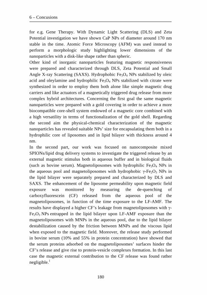
6 – Concusions

180

for e.g. Gene Therapy. With Dynamic Light Scattering (DLS) and Zeta Potential investigation we have shown CaP NPs of diameter around 170 nm stable in the time. Atomic Force Microscopy (AFM) was used instead to perform a morphologic study highlighting lower dimensions of the nanoparticles with a disk-like shape rather than spheric. Other kind of inorganic nanoparticles featuring magnetic responsiveness were prepared and characterized through DLS, Zeta Potential and Small Angle X-ray Scattering (SAXS). Hydrophobic Fe3O4 NPs stabilized by oleic acid and oleylamine and hydrophilic Fe3O4 NPs stabilized with citrate were synthesized in order to employ them both alone like simple magnetic drug carriers and like actuators of a magnetically triggered drug release from more complex hybrid architectures. Concerning the first goal the same magnetic nanoparticles were prepared with a gold covering in order to achieve a more biocompatible core-shell system endowed of a magnetic core combined with a high versatility in terms of functionalization of the gold shell. Regarding the second aim the physical-chemical characterization of the magnetic nanoparticles has revealed suitable NPs’ size for encapsulating them both in a hydrophilic core of liposomes and in lipid bilayer with thickness around 4 nm. In the second part, our work was focused on nanocomposite mixed SPIONs/lipid drug delivery systems to investigate the triggered release by an external magnetic stimulus both in aqueous buffer and in biological fluids (such as bovine serum). Magnetoliposomes with hydrophilic Fe3O4 NPs in the aqueous pool and magnetoliposomes with hydrophobic γ-Fe2O3 NPs in the lipid bilayer were separately prepared and characterized by DLS and SAXS. The enhancement of the liposome permeability upon magnetic field exposure was monitored by measuring the de-quenching of carboxyfluorescein (CF) released from the aqueous pool of the magnetoliposomes, in function of the time exposure to the LF-AMF. The results have displayed a higher CF’s leakage from magnetoliposomes with γ-Fe2O3 NPs entrapped in the lipid bilayer upon LF-AMF exposure than the magnetoliposomes with MNPs in the aqueous pool, due to the lipid bilayer destabilization caused by the friction between MNPs and the viscous lipid when exposed to the magnetic field. Moreover, the release study performed in bovine serum (10% and 55% in protein concentration) have showed that the serum proteins adsorbed on the magnetoliposomes’ surfaces hinder the CF’s release and give rise to protein-vesicle complexes formation. In this last case the magnetic external contribution to the CF release was found rather negligible.1

6 – Conclusions

181

In the last part, a novel hybrid platform endowed of two different environments able to host simultaneously both hydrophilic and hydrophobic molecules was studied and for the first time on bulk cubic phase and cubosomes were performed release study through Fluorescence Correlation Spectroscopy (FCS). First step was to encapsulate oleic acid-coated Fe3O4 NPs in the lipid bilayer of both bulk cubic phase and cubosomes, obtaining so-called magnetocubosomes and so exploiting the responsiveness of these nanoparticles to make versatile drug delivery systems with the possibility to remotely control their accumulation in the body and their responsivity to an alternating magnetic field. Bulk cubic phase with SPIONs and magnetocubosomes were characterized by SAXS, DLS and Zeta Potential. FCS was employed to investigate the diffusion behavior of a hydrophilic model drug (Rhodamine 110) inside the aqueous channels and of a hydrophobic model drug (Octadecyl Rhodamine B) in the lipid domains of both bulk cubic phase and magnetocubosomes, demonstrating that the model drugs are efficiently retained inside the aqueous or lipid domain where they can diffuse. By this experiment we can state that cubic phase and magnetocubosomes can act as a vector for therapeutics with different chemical affinities, which can be confined in the inner cubic structure. With the same technique the release of a hydrophilic model drug (Rhodamine 110) from the aqueous channels of the bulk cubic phase and magnetoliposomes was investigated. It was possible to monitor both the spontaneous release and the release triggered by the alternating magnetic field exposure of 5.7 kHz. The FCS investigation have highlighted that the LF-AMF application increase dramatically the amount of hydrophilic drug released in the external aqueous environment from both DDS containing Fe3O4 NPs, demonstrating that the external magnetic field acts as a proper external trigger to the release. The results achieved make it possible to state that this novel hybrid nanostructured architectures endowed with magnetic responsiveness provide a new multifunctional and flexible scaffold for the encapsulation and targeted delivery of different therapeutic and/or diagnostic molecules.2

6 – Concusions

182

6.1 Bibliography

1. Silvia Nappini, Silvia Fogli, Benedetta Castroflorio, Massimo Bonini, Francesca Baldelli Bombelli and Piero Baglioni, “Magnetic field responsive drug release from magnetoliposomes in biological fluids”, Soft Matter, manuscript in preparation.

2. Costanza Montis, Benedetta Castroflorio, Marco Mendozza, Annalisa Salvatore, Debora Berti and Piero Baglioni, “Magnetocubosomes for the delivery and controlled release of therapeutics”, Journal of Colloid and Interface Science, (2014) article in press - http://dx.doi.org/10.1016/j.jcis.2014.11.056.

Publications

185

1. Peter Sandin, Francesca Baldelli Bombelli, Benedetta Castroflorio, Christoph Müller, Jürgern Obermeier, Göran Karlsson, K. Edwards, Piero Baglioni and Debora Berti, “Diastereoselective self-assembly of clofarabine lipids”, New Journal of Chemistry, 38 (2014) 5247-5253.

2. Costanza Montis, Benedetta Castroflorio, Marco Mendozza, Annalisa

Salvatore, Debora Berti and Piero Baglioni, “Magnetocubosomes for the delivery and controlled release of therapeutics”, Journal of Colloid and Interface Science, (2014) article in press - http://dx.doi.org/10.1016/j.jcis.2014.11.056.

3. Silvia Nappini, Silvia Fogli, Benedetta Castroflorio, Massimo

Bonini, Francesca Baldelli Bombelli and Piero Baglioni, “Magnetic field responsive drug release from magnetoliposomes in biological fluids”, Soft Matter - manuscript in preparation.

This journal is©The Royal Society of Chemistry and the Centre National de la Recherche Scientifique 2014 New J. Chem., 2014, 38, 5247--5253 | 5247

Cite this: NewJ.Chem., 2014,

38, 5247

Diastereoselective self-assembly ofclofarabine lipids

Peter Sandin,†ab Francesca Baldelli Bombelli,†acd Benedetta Castroflorio,a

Christoph Muller,e Jurgen Obermeier,e Goran Karlsson,f Katarina Edwards,f

Piero Baglionia and Debora Berti*a

Clofarabine is a nucleosidic chemotherapeutic approved for the treatment of acute lymphoblastic leukemia,

currently undergoing clinical trials for the treatment of solid tumors. Like for many others, lipidic derivatization

of this drug improves pharmacokinetics and relieves the heavy side effects. Since the self-assembly pattern

can modulate the bioactivity profile, a precise knowledge of the aggregation behavior of these nucleolipids

and of the microstructure of the aggregates is central to design formulations that efficiently provide sufficient

bioavailability. In this contribution we investigate the self-assembly behavior of two Clofarabine dioxy-ether

derivatives, the diastereomers (1-2S and 1-2R). These clofarabine lipid derivatives showed an unexpected

diastereoselective self-assembly effect, which we have monitored by observing the time evolution of self-

assemblies and their microstructural response to thermal treatment. Dynamic Light Scattering and Circular

Dichroism provide an ensemble of results which correlate with the occurrence of a hierarchical association of

wormlike aggregates, imaged using Electron Microcopy. A strikingly different behavior for the two

diastereomers was observed. This behavior can be crucial for the different bioavailability observed in vivo.

Introduction

Clofarabine is a cytotoxic deoxyadenosine analogue that receivedaccelerated approval in 2004 from FDA1 and recently from EMEA2

for the treatment of pediatric acute lymphoblastic leukemia,currently under clinical trials for some adult solid tumors.3

A dose-dependent severe myelosuppression represents its mostserious side-effect.4 Like for many other nucleosidic chemothera-peutics, a pro-nucleotide approach,5 with a specific lipid carrierlinked to the nucleoside via a covalent phosphodiester bond, canreduce these effects, improve pharmacokinetic behavior and over-come or decrease the development of resistance against the drug.

Recently we have synthesized a specific conjugate of clofarabinewith a synthetic dialkyl lipid phosphate, (1, Fig. 1), which showedimproved pharmacokinetic, pharmacodynamic and toxicologicproperties compared to free clofarabine.6

In vivo 1 is activated by membrane associated specifichydrolases, releasing the free clofarabine into the respectivecells. Since 1 is a 1 : 1 mixture of two diastereomers (1-2S and1-2R, Fig. 1), the question arose whether the two diastereomerswould differ with regard to biological activity, with the 1-2R,sterically similar to natural phospholipids, expected to be themost active. For this reason we synthesized 1-2S and 1-2R.Remarkably, 1-2S, with the ‘‘unnatural’’ S configuration atcarbon SN2 in the lipid part, showed higher bioavailabilityand anti-tumor activity in vivo.6 The stereochemical differenceinvolves a portion of the molecule, which is cleaved away fromthe active clofarabine part, and should in principle have littleeffect on biological properties. The reasons for the observeddifference in bioactivity must therefore lay elsewhere. Theamphiphilic properties of 1-2R and 1-2S suggest the possibilityof aggregation and formation of ordered supramolecular structuresin solution. Amphiphilic self-assemblies display a rich phasebehavior, characterized by a large structural diversity, in termsof size, shape and flexibility of the aggregates. The typicalindependent parameters of the amphiphilic phase diagramare surfactant volume fraction, temperature and ionic strength:subtle variations of local microstructure can lead to cascadeeffects with dramatic morphological transitions on the mesoscale.7

This effect is particularly important for biologically-inspiredfunctional surfactants, such as peptide-amphiphiles andoligonucleotide-amphiphiles,8–11 where a biological recognitionunit is incorporated in the amphiphile molecular architecture.

a Department of Chemistry, University of Florence and CSGI, Via della Lastruccia 3,

Sesto Fiorentino, 50019 Florence, Italy. E-mail: [email protected] Department of Chemistry - BMC, Uppsala University, Box 579, S-75123 Uppsala,

Swedenc Centro Europeo di Nanomedicina c/o Dipartimento di Chimica,

Materiali e Ingegneria Chimica G. Natta, Politecnico di Milano, Via Mancinelli 7,

20131 Milano, Italyd School of Pharmacy, University of East Anglia, Norwich, NR47TJ, UKe Heidelberg Pharma GmbH, Schriesheimer Strasse 101, 68526 Ladenburg, Germanyf Department of Physical and Analytical Chemistry, Uppsala University, Box 579,

S-75123 Uppsala, Sweden

† These authors have contributed equally to this work.

Received (in Montpellier, France)24th May 2014,Accepted 29th August 2014

DOI: 10.1039/c4nj00856a

www.rsc.org/njc

NJC

PAPER

Publ

ishe

d on

01

Sept

embe

r 20

14. D

ownl

oade

d by

Uni

vers

ity o

f W

inds

or o

n 30

/10/

2014

17:

59:3

4.

View Article OnlineView Journal | View Issue

5248 | New J. Chem., 2014, 38, 5247--5253 This journal is©The Royal Society of Chemistry and the Centre National de la Recherche Scientifique 2014

This work investigates the self-assembly behavior displayedby clofarabine lipid diastereomers reported in Fig. 1, whichcould influence their biological activity.

A diastereoselective assembly is by no means obvious forionic amphiphiles, because predictions on the morphology ofthe aggregate are based on the balance of molecular packingparameters and excluded volume or electrostatic repulsiveinteractions between the polar heads. Therefore, a differentstereochemistry at the C2 should in principle play little or norole in the structural properties of the aggregates.

On the other side, lipophilic nucleosides are known to giverise to interesting and extremely rich phase behavior in aqueoussolutions. Clofarabine is a derivative of adenosine and we havepreviously studied the aggregation behavior of phosphatidyl-nucleosides, where a natural RNA nucleotide is conjugated to adouble-chain glycerol lipid skeleton. These derivatives self-organizein aqueous solution as assemblies of various size, shape andinterfacial curvature, according to the length of the two hydropho-bic portions.12,13 The nucleic motif imparts molecular recognitioncapability to self-assemblies. A coarse-grained mapping of the phasebehavior in aqueous solutions can be predicted by comparison withthe corresponding phosphatidylcholine precursors:14 as the hydro-phobic double chain is lengthened, the dimensionless surfactantpacking parameter p = v/a0lc, with v the volume of the alkyl chain, a0the cross section of the polar head and lc the fully extended lengthof the hydrophobic portion, increases until it reaches anasymptotic value. In this progression, we observed the usualphase evolution, from positively curved surfactant films

(globular micelles) to flat assemblies (bilayers). However, sincethe geometry of spontaneous self-assembly and interfacial filmproperties are the result of a delicate balance between hydrophobicforces and polar head interactions, the properties of nucleolipidself-assemblies is further modulated by base–base interactionsthat are triggered by aggregation.15 Their self-assemblies show astrong dependence on subtle changes of molecular details of themonomer, such as the syn or anti conformation of the nucleo-side. Some reports on amphiphiles with functional polar headshave shown that, when a complex interaction pattern at the intra-and inter-aggregate level can occur at the interface, variations in thestereochemistry of the polar head, of the counterions, or slightchanges in the experimental conditions, can promote drastic altera-tions of the aggregate morphology.16–19 An illuminating example isprovided by dilauroyl-phosphatidyl-N (DLPN), with N either adeno-sine or uridine, whose aggregation properties have been studied indetail, to better highlight the contribution of the functional polarhead to local and mesoscopic properties of the aggregates. Freshlyprepared dilauroyl-phosphatidyl-adenosine solutions are mostlycomposed of threadlike flexible micelles whose cross-section size isabout 5 nm. The observed time evolution of the aggregate morphol-ogy results in twisted superstructures, which account for the appear-ance of an ultraslow relaxation in quasielastic light scattering.Conversely DLPU forms wormlike flexible micelles, whose structureis stable with time and which do not associate into superstructures.DLPA superstructures arise from the hierarchical aggregation ofwormlike structures identical to dilauroyl-phosphatidyl-uridinemicelles. The higher stacking constant of the former nucleotide isresponsible for the different self-assembly behavior, which is alsostrictly dependent on the thermal history of the samples, whichalters the syn–anti distribution of conformers of the adenosineheadgroups. The syn–anti redistribution is then retained when thesample is brought back to room temperature, due to the intermo-lecular constraints present in the self-assembled structure.20

In this contribution we focus on an even subtler aspect, i.e.the stereochemistry of the polar head at the SN2 carbon. Ifbase–base associative interactions at the polar head level areoperative, then despite the same charge of the headgroups, thestereochemical details may have a deep influence on the self-assembly and on the hierarchical assembly of associated units.

To address this issue, we compare the microstructure of theaggregates formed by 1-2R and 1-2S.

We expect the local structure to be similar to the DLPN case, i.e.that the amphiphiles will assemble into locally cylindrical micelles.Any difference of the flexibility of the aggregates, and the associationof simpler associated units into hierarchical super-twisted superstructures, should be ascribed to the specificity of the polar head andto the effect that the stereochemistry of the SN2 Carbon has on theinteraction pattern.

Materials and methodsSynthesis and characterization of the diastereomers

The preparation of [2-chloro-9-(2 0-deoxy-20-fluoro-b-D-arabino-furanosyl)adenine]-50-phosphoric acid-(2R-decyloxy-3-dodecyloxy)-propyl ester (1-2R) is shown in Scheme 1.

Fig. 1 Chemical structures of 1 and its diastereomers 1-2R and 1-2S.

Paper NJC

Publ

ishe

d on

01

Sept

embe

r 20

14. D

ownl

oade

d by

Uni

vers

ity o

f W

inds

or o

n 30

/10/

2014

17:

59:3

4.

View Article Online


All the reagents, chemicals and solvents have been purchasedfrom Sigma Aldrich and used without further purification.

4.41 g (9.17 mmol) of enantiomerically pure phosphoricacid-(2R-decyloxy-3-dodecyoxo-)propyl ester, synthesised from(S)-(+)-1,2-isopropylideneglycerol as previously described,21 aretreated twice with 50 ml of anhydrous pyridine and concen-trated by evaporation. The residue is dissolved in 180 ml ofanhydrous pyridine at room temperature, treated with 5.56 g(18.35 mmol) of 2,4,6-triisopropylbenzenesulfonyl chlorideunder nitrogen and stirred at 20–25 1C for 1 hour. Then4.18 g (13.76 mmol = 1.5 eq.) of 2-chloro-9-(20-deoxy-20-fluoroarabinofuranosyl)adenine (clofarabine) are added at once, andthe mixture is stirred under nitrogen for 20 hours. Hydrolysis isperformed by adding 100 ml of saturated sodium hydrogencarbonate solution; the mixture is stirred for another 0.5 hourat room temperature until evolution of carbon dioxide stopsand it is freed from the solvent under vacuum at 40 1C. Acetone(150 ml) is added to the solid residue vigorously stirred for anadditional hour. The resulting suspension is filtrated withsuction and the residual salt is washed with 50 ml acetone.The combined acetone filtrate and washings are concentratedand the residue is purified by HPLC on Lichrospher 60 RPselectB with methanol/aqueous 40 mM sodium acetate 85 : 15 as theeluent. The product containing fractions is evaporated. Theresidue is distributed between 200 ml of tert-butylmethyletherand 60 ml of 2 N hydrochloric acid. The organic layer isevaporated, the residue is dissolved in a mixture of 20 ml ofmethanol and the pH is adjusted to pH 7 by addition of sodiummethanolate (30% in methanol). The solvent is stripped off andthe residual sodium salt dissolved in 25 ml acetone anddropped at 0 1C to 50 ml acetonitrile. The resulting suspensionis stirred for 1 h at 0 1C, the precipitate is filtered off withsuction and washed with 50 ml ice cold acetonitrile and driedin vacuum: 5.50 g (76%) sodium salt of 1-2R as a whiteamorphous powder.

1H NMR (300 MHz, DMSO-d6): 8.2 (s, 1H, H8), 8.0, (s (br), 1H,NH2), 6.6, (s, 1H, 30-OH), 6.3 (dd, 1H, H10), 5.2 (dt, 1H, H20), 4.5,(dt, 1H, H30), 3.9–4.0, (m, 3H, H40, POCH2), 3.6, (m, 1H, –H5a0),3.6 (m, 1H, H5b0), 3.2–3.5 (m, 7H, 4CHOCH2–, –CH2OCH2),1.1–1.4 (m, 32H, –(CH2)9–, –(CH2)7–), 0.8 (m, 6H, CH2–CH3);3J10-H,20-H E 3J20-H,30-H E 3J30-H,40-H E 4.6 Hz, 3J10-H,F = 13.2 Hz,2J20-H,F = 52.7 Hz, 3J30-H,F = 19.4 Hz.

13C NMR (75.0 MHz, DMSO-d6): 156.6, 153.1, 150.0 (C-2, C-4,C-6), 139.7 (C-8), 117.2 (C-5), 95.8 + 93.9 (C-20), 82.0 (C-40), 81.2

(C-10), 77.7 (O-CHo), 73.1 (C-30), 70.7, 70.4 (CH2–CH2O–CH2–),69.1 (CH2–CH2O–CHo), 63.6 (C-50), 63.3 (50-O-P(O)2OCH2),21.8–31.1 (–(CH2)9–, –(CH2)7–), 13.6 (2 � CH3).

31P NMR (121.5 MHz, DMSO-d6): 0.23 ppm (singlet).19F NMR (282 MHz, DMSO-d6): �199.5 ppm (singlet – 1H-

decoupled).Mass spec. (FAB–): m/z = 764.39 [M-Na+]The preparation of [2-chloro-9-(20-deoxy-20-fluoro-b-D-arabino-

furanosyl)adenine]-50-phosphoric acid-(2S-decyloxy-3-dodecyloxy)-propyl ester (1-2S) is similar to that reported for 1-2R, except forthe use of enantiomerically pure phosphoric acid-(2S-decyloxy-3-dodecyloxoy)propyl ester (synthesised from (R)-(�)-1,2-isopro-pylideneglycerol as in WO 96/06620). 1-2S is obtained as asodium salt in 28% yield.

19F NMR (282 MHz, DMSO-d6): �198.5 ppm (singlet –1H-decoupled).

Dynamic Light Scattering (DLS)

DLS experiments were carried out on a Brookhaven Instrumentapparatus, New York, USA (BI 9000AT correlator card and BI200 SM goniometer). The signal was detected using an EMI9863B/350 photomultiplier. The light source was the doubledfrequency of a Coherent Innova diode pumped Nd-YAG laser(l = 532 nm, 20 mW). The laser long term power stability was�0.5%. Self-beating detection was recorded using decahydro-naphthalene (thermostated by a water circulating system) asthe index matching liquid. A temperature probe was inserted inthe sample to monitor T while simultaneously recording auto-correlation functions. Measurements have been performed at20 1C on 0.5 ml samples previously transferred into cylindricalHellma scattering cells. For each sample at least three separatemeasurements were performed at different angles (i.e. 701, 901,1201) corresponding to three different scattering vectors; n isthe refractive index of the medium equal to 1.33. In DynamicLight Scattering experiments, the normalized time autocorrela-tion function g2(q,t) of the scattered intensity is measuredaccording to:

g2ðq; tÞ ¼ I�ðq; 0ÞIðq; tÞh iIðq; 0Þ2

D E (1)

For ergodic systems, this function can be expressed in terms of thefield autocorrelation function g1(q,t) through the Siegert relation:

g2(q,t) = A[1 + b2g1(q,t)2] (2)

where A is the baseline and b2 is the coherence factor dependenton the scattering geometry and details of the detection system.

Data analysis has been performed by fitting the field auto-correlation functions through a double exponential decay,yielding two distinct decay rates, labeled as ‘‘fast’’ and ‘‘slow’’decay modes. The analytical expression used to fit the fieldautocorrelation functions was:

g1ðq; tÞ ¼ A Pe�G1t þ ð1� PÞe�G2t� �þ B (3)

where A is the total amplitude of the correlation function, P isthe contribution of the first mode to the total amplitude, B isScheme 1 Synthetic pathway to the diastereomer 1-2R.

NJC Paper

Publ

ishe

d on

01

Sept

embe

r 20

14. D

ownl

oade

d by

Uni

vers

ity o

f W

inds

or o

n 30

/10/

2014

17:

59:3

4.

View Article Online


the baseline. The extracted decay modes have a typical diffusivescaling: it is commonly agreed that a linear dependence of thedecay rate on the square scattering vector, q2, indicates adiffusive origin (Fig. 2). The line slope is the translationaldiffusion coefficient Dt of that population. The diffusion coefficientsprovide access to the hydrodynamic correlation lengths RH forisotropic particles through the Stokes–Einstein relationship

Dt ¼ kBT

6pZsRH(4)

where Zs is the solvent viscosity and kB the Boltzmann constant.Although such hydrodynamic sizes cannot be related to anystructural parameter of anisotropic particles, as they refer to theradius of the equivalent diffusing spheres, they can qualitativelyindicate the order of magnitude of the size of the diffusing self-assemblies.

Circular Dichroism Spectroscopy (CD)

Circular Dichroism spectra were collected on a J-715 Jascospectro-polarimeter. Hellma quartz cylindrical cells with vari-able path-length, selected not to exceed 0.8 optical density,were used. The observed Circular Dichroism was converted intoMolar Ellipticity, normalizing for pathlength and dichroicchromophore concentration.

Cryo-transmission electron microscopy (Cryo-TEM)

The preparation of the samples for Cryo-TEM was performed asfollows: a small droplet of the solution was placed undercontrolled conditions on a pretreated 20 mm thick Cu grid,coated with a perforated cellulose acetate butyrate film. Theexcess material was removed by gently wiping off with a filterpaper. The specimen was vitrified by a rapid transfer into liquidethane close to its freezing temperature. The examination of

the sample was then performed using a Zeiss 902A electronmicroscope operating at 80 kV and 100 K. The temperature ofthe specimen was kept below �165 1C both during the transferto the microscope and the examination. Images were recordedat under focus settings of about 2–3 mm to enhance the imagecontrast.

Results and discussions

We studied the microstructure of 0.5 mM clofarabine lipidsdissolved in 50 mM PBS, as a function of time and of the thermalhistory of the sample, by DLS, CD and Cryo-TEM investigations.The samples were prepared by dissolving the dry powder in thebuffer, through mild vortex-mixing. After having obtained atransparent solution, no further stirring was applied.

Time evolution of the lipidic self-assembly

Fig. 3 shows the time evolution of the Dynamic Light Scattering(DLS) and Circular Dichroism (CD) data for the two diastereomersfreshly dissolved in PBS. The autocorrelation functions (Fig. 3A andB) can be fitted with a double exponential decay. Both modes arediffusive, as the linear trend of the decay rates vs. the squared

Fig. 2 Decay modes, extracted from the field autocorrelation functionsthrough eqn (3), are reported as a function of the squared scattering vectorq. G1 and G2 are the fast and slow decay mode, respectively. The lineardependence of the decay rate on the squared scattering vector, q2,indicates a diffusive nature of both decays. The values of the diffusioncoefficients are shown in Table 1.

Fig. 3 Time evolution of DLS field autocorrelation functions and CD for1-2S and 1-2R micellar solution. DLS field autocorrelation functions for(A) 1-2S and (B) 1-2R fresh micellar solutions (&), sample aged at 25 1C forone day (J) and four days (,). Solid curves are the best double-exponential fittings (eqn 3) from which we extracted the characteristicdecay modes (see text and Table 1). While the autocorrelation functions ofthe two fresh samples are very similar, 1-2S show a dramatic changealready after one day whereas for 1-2R the change is less pronounced.(C) and (D) The time evolution of the CD spectra of 1-2S and 1-2R,respectively, fresh micellar solution (dashed curve), sample aged one (&)and four (K) days at 25 1C. 1-2S shows a gradual change from fresh to fourdays while 1-2R shows no change over the same time interval. Allmeasurements were carried out at 0.5 mM in 50 mM PBS buffer at25 1C, the DLS measurements were made at y = 90.

Paper NJC

Publ

ishe

d on

01

Sept

embe

r 20

14. D

ownl

oade

d by

Uni

vers

ity o

f W

inds

or o

n 30

/10/

2014

17:

59:3

4.

View Article Online


scattering vector, reported in Fig. 2, reveals. These contributions aredue to centre-of-mass motion of the aggregates.

The fast decay mode corresponds to a diffusion coefficient,which is identical for the two derivatives within experimentaluncertainty (D E 1.2 � 10�7 cm2 s�1, RH E 178 Å). The slowdecay mode, due to larger aggregates, is different for the twodiastereomers even in the freshly prepared samples (D E 4.5 �10�8 cm2 s�1, RH E 476 Å and D E 2.6 � 10�8 cm2 s�1, RH E824 Å for 1-2S and 1-2R, respectively).

The hydrodynamic sizes inferred from the diffusion coefficientsindicate that, even for the faster decay, the aggregates cannot beaccounted for by spherical micellar aggregates, (considering amonomer size of B20 Å), but rather suggest the presence ofelongated structures.

Surprisingly, 1-2S aggregates show a noticeable evolutiontoward larger aggregates already after 24 hours and are thenstable, while 1-2R has a much slower evolution, involving onlythe long-time decay, as reported in Fig. 3 and Table 1.

CD offers insight into the base–base interaction pattern asthe CD signal is sensitive to mutual interactions of the nucleobaseanalogs. The CD spectra of 1-2S (Fig. 3C) reveal a significant changeover time, which suggests that the structural evolution observed inDLS is accompanied by a change in the base–base interactionpattern. Conversely, 1-2R does not show any significant change inthe CD spectra over the time course of the experiment.

Thermal effects on the self-assembly

The effects of thermal cycles on the self-assembling propertiesof these derivatives were also investigated. In previous studieson the nucleolipid dilauroyl-phosphatidyl-adenosine (DLPA) wehave shown that the thermal history of the sample has a dramaticeffect on the resulting superstructures,17 since the temperature canpromote the formation of long-lived non-equilibrium states.Incubation at 45 1C for 48 hours drastically alters the structuralfeatures of 1-2S assemblies, as revealed both by DLS and CD (Fig. 4),

Table 1 Results obtained from the fitting of the field autocorrelation functionsusing eqn (3) for fresh and aged samples of the two diastereoisomers at 25 1C

Sample D1 (cm2 s�1) A1 (%) D2 (cm

2 s�1) Rh1a (Å) Rh2

a (Å)

1-2S-fresh 1.2 � 10�7 87 4.5 � 10�8 178.3 475.51-2R-fresh 1.2 � 10�7 77 2.6 � 10�8 178.3 823.71-2S-2days 7.6 � 10�8 33 9.0 � 10�9 281.6 2377.81-2R-2days 1.0 � 10�7 70 2.4 � 10�8 214.0 891.71-2S-4days 7.6 � 10�8 33 9.0 � 10�9 178.3 2377.81-2R-4days 1.1 � 10�7 72 1.54 � 10�8 195.8 1389.2

a Hydrodynamic radii are only indicative since they were calculatedusing the Stokes–Einstein relationship (eqn (4)), which gives thehydrodynamic radius of the equivalent diffusing sphere. Recall thecomplex structures of these self-assemblies, it is not possible to relatethem to structural parameters.

Fig. 4 Time evolution of DLS field autocorrelation functions and CD for1-2S and 1-2R micellar solution after four days of aging at 25 1C and twodays of incubation at 45 1C. DLS field autocorrelation functions for (A) 1-2Sand (B) 1-2R after four days at 25 1C (dashed lines), directly after incubationat 25 1C for two days (J), after one day at 25 1C after incubation (n), aftertwo days at 25 1C after incubation (&) and seven days at after 25 1C afterincubation (+). CD spectra of (C) 1-2S and (D) 1-2R after four days at 25 1C(dashed lines), directly after incubation at 25 1C for two days (J), after oneday at 25 1C after incubation (+), after two days at 25 1C after incubation(n). The incubation at 45 1C has a strong affect on 1-2S as seen in thesignificant changes in both DLS and CD. Although the DLS and the CDchanges also for 1-2R after incubation the effect is significantly lesspronounced. All measurements were carried out at 0.5 mM in 50 mMPBS buffer at 25 1C, the DLS measurements were made at y = 90.

Fig. 5 Representative Cryo-TEM micrographs of 1-2S, 0.5 mM in 50 mMPBS, before (A) and after (B) incubation (48 h incubation at 45 1C). In bothcases there are elongated threads, characterized by certain stiffness,occasionally aggregated through side-by-side interactions. In the agedsamples before incubation smaller wormlike micelles are observed, whilethe incubated sample shows a higher supraorganization of these fibers toform stacked superstructures through side–side interactions. The lengthof the scale bar is 100 nm.

NJC Paper

Publ

ishe

d on

01

Sept

embe

r 20

14. D

ownl

oade

d by

Uni

vers

ity o

f W

inds

or o

n 30

/10/

2014

17:

59:3

4.

View Article Online


i.e. of those aggregates which, under ambient conditions, show astronger structural evolution. CD and DLS also change for1-2R, but in a much less dramatic way when compared to 1-2S.To summarize, DLS highlights a complex self-assembly pattern,different time evolution of the structures and different thermalhistory behaviour.

Cryo-TEM investigation

Information on the morphology, flexibility and super-organizationcan be obtained by direct imaging of the aqueous aggregates by

Cryo-TEM. Representative Cryo-TEM micrographs of 1-2S and1-2R, both aged and incubated samples, are shown in Fig. 5 and6, respectively. 1-2S (Fig. 5A and B) shows extremely elongatedthreads, characterized by a notable stiffness, often associatedthrough side-by-side interactions. The characteristic size of thethinner fibers is consistent with the monomer size, thusindicating that the primary aggregates are formed by cylindricalmicelles. There are also small wormlike micelles visible inthe background. Incubation increases the side-associationin superaggregates, while it does not appear to reduce thestiffness. These results support the size variation observed inDLS as well as the change in the base–base interaction patternwhen the ‘‘primary’’ flexible wormlike micelles hierarchicallyorganize into superaggregated structure. This structural tran-sition is accompanied by a change in base–base interactions,as the variation of CD patterns indicates for this derivative.Fig. 6 shows a completely different behavior for 1-2R.The structures are characterized by a much higher degree offlexibility of the aggregates (Fig. 6A and B), which can even-tually wind around each other to form helicoidal superstruc-tures with locally cylindrical curvature. Incubated samplesdisplay, in addition to twisted structures, elongated andapparently stiff, bilayer bands (Fig. 6C). The large degree ofdiversity in this sample makes both DLS and CD much moredifficult to be interpreted.

Conclusions

The two nucleolipid diastereomers of 1 give rise to complexsuperstructures with different aggregation morphologies andsometimes resulting in distinct interfacial curvatures. It is clearthat, on the molecular scale, a different bending rigidity of theamphiphilic film is responsible of the meso-scale behaviour.The different stereochemistry of the polar head results in adifferent flexibility of the aggregates, which in turn causes acompletely different structural behaviour on a much higherlength scale. These findings can be correlated with the differ-ence in bioavailability and anti-tumor activity for the twodiastereomers, administered at similar concentrations andconditions as those investigated in this study. In particular,the complex twisted aggregates formed by the 1-2R derivative(Fig. 6A and B) give rise to a lesser oral bioavailability and anti-tumor activity with respect to the more rigid structures formedby the 1-2S derivative. We hypothesize that the differentmorphologies, resulting from diastereoselective self-assemblycan definitely play a role and practically account for thedifferent bioavailability. It is clear that a deeper investigationis needed to completely understand the chemical and biologicalmechanisms behind this effect.

This study highlights that a successful application oflipid pro-drugs as a means of drug delivery demands specialattention to the self-aggregation behavior since very subtlestructural features of the monomer can play a crucial role atthe mesoscopic scale which may seriously affect the therapeuticefficiency.

Fig. 6 Representative Cryo-TEM micrographs of 1-2R, 0.5 mM in 50 mMPBS buffer, before (A, B) and after (C) incubation (48 h incubation at 45 1C).1-2R shows a very different self-assembling behaviour with respect to 1-2S:the cylindrical curvature is maintained but the fibers are much more flexibleand tend to wound each other to form helicoidally superstructures whichcoexist with the starting structures. The increase in temperature inducessignificant changes in the self-assembling behaviour with the coexistence ofdifferent superstructures such as twisted structures, fibers and elongatedand apparently stiff bilayer bands. The length of the scale bar is 100 nm.

Paper NJC

Publ

ishe

d on

01

Sept

embe

r 20

14. D

ownl

oade

d by

Uni

vers

ity o

f W

inds

or o

n 30

/10/

2014

17:

59:3

4.

View Article Online


Acknowledgements

P. Sandin thanks the Knut and Alice Wallenberg foundation forfinancial support; K. Edwards gratefully acknowledges financialsupport from the Swedish Research Council and the Swedish CancerSociety. This work was supported by a grant of the ItalianMinistry ofResearch (PRIN 2010–2011). B.C. acknowledges funding from CSGI.

Notes and references

1 http://www.accessdata.fda.gov/scripts/cder/ob/default.cfm.2 http://www.ema.europa.eu/ema/.3 E. Lech-Maranda, A. Korycka and T. Robak, Mini-Rev. Med.

Chem., 2009, 9, 805–812.4 H. M. Kantarjian, V. Gandhi, P. Kozuch, S. Faderl, F. Giles,

J. Cordes, S. O’Brien, N. Ibrahim, F. Khuri, M. Du, M. B. Rios,S. Jeha, P. McLaughlin, W. Plunkett and M. Keating, J. Clin.Oncol., 2003, 21, 1167–1173.

5 G. I. Neil, P. F. Wiley, R. C. Manak and T. E. Moxeley, CancerRes., 1970, 30, 1047–1054.

6 J. Obermeier, G. Heckl-Oestreicher, C. Mueller, M. Kulke,R. Wehr, J. Anderl, Proceedings of the 100th Annual Meetingof the American Association for Cancer Research; 2009, Denver,CO: AACR 2009. Abstract nr 4522; G. Heckl-Oestreicher,C. Mueller, C. Lutz, M. Kulke, J. Obermeier, A. Minchinton,R. Wehr, J. Anderl, Proceedings of the 100th Annual Meeting ofthe American Association for Cancer Research; 2009 Denver, CO:AACR 2009. Abstract nr 4523.

7 D. Berti, Curr. Opin. Colloid Interface Sci., 2006, 11, 74.8 D. Berti, C. Montis and P. Baglioni, Self-assembly of

designer biosurfactants, Soft Matter, 2011, 7, 7150–7158.

9 M. Schade, D. Berti, D. Huster, A. Herrmann andA. Arbuzova, Adv. Colloid Interface Sci., 2014, 208,235–251.

10 M. Banchelli, F. Betti, D. Berti, G. Caminati, F. BaldelliBombelli, T. Brown, L. M. Wilhelmsson, B. Norden andP. Baglioni, J. Phys. Chem. B, 2008, 112, 10942.

11 A. Gissot, M. Camplo, M. W. Grinstaff and P. Barthelemy,Org. Biomol. Chem., 2008, 6, 1324.

12 D. Berti, F. Baldelli Bombelli, M. Fortini and P. Baglioni,Amphiphilic Self-assemblies Decorated by Nucleobases,J. Phys. Chem. B, 2007, 111(40), 11734–11744.

13 P. Baglioni and D. Berti, Curr. Opin. Colloid Interface Sci.,2003, 8, 55.

14 H. Hauser, Biochim. Biophys. Acta, Biomembr., 2000, 1508(1–2),164–181.

15 F. Baldelli Bombelli, D. Berti, U. Keiderling and P. Baglioni,J. Phys. Chem. B, 2002, 106, 11613–11621.

16 J. D. Hartgerink, E. Beniash and S. I. Stupp, Science, 2001,294, 1684–1688.

17 H. Cui, T. Muraoka, A. G. Cheetham and S. I. Stupp, NanoLett., 2009, 9, 945–951.

18 R. Oda, I. Huc, M. Schmutz, S. J. Candau andF. C. MacKintosh, Nature, 1999, 399, 566–569.

19 A. Brizard, C. Aime, T. Labrot, I. Huc, D. Berthier, F. Artzner,B. Desbat and R. Oda, J. Am. Chem. Soc., 2007, 129,3754–3769.

20 F. Baldelli Bombelli, D. Berti, S. Milani, M. Lagi, P. Barbaro,G. Karlsson, A. Brandt and P. Baglioni, Soft Matter, 2008, 4,1102–1113.

21 K. S. Ishaq, L. S. Kucera and S. L. Morris-Natschke, PCTWO1996006620 A2, 1996.

NJC Paper

Publ

ishe

d on

01

Sept

embe

r 20

14. D

ownl

oade

d by

Uni

vers

ity o

f W

inds

or o

n 30

/10/

2014

17:

59:3

4.

View Article Online

Magnetocubosomes for the delivery and controlled releaseof therapeutics

Costanza Montis, Benedetta Castroflorio, Marco Mendozza, Annalisa Salvatore, Debora Berti ⇑,Piero Baglioni ⇑Department of Chemistry and CSGI, University of Florence, via della Lastruccia 3, Sesto Fiorentino, 50019 Florence, Italy

a r t i c l e i n f o

Article history:Received 2 November 2014Accepted 21 November 2014Available online xxxx

Keywords:CubosomesCubic phasesMagnetic nanoparticlesDrug deliveryFluorescence Correlation Spectroscopy

a b s t r a c t

The design of nanostructured drug delivery systems (DDS) that improve the efficacy of therapeutic prin-ciples by enhancing their biocompatibility, bioavailability and targeting, has been the focus of extensiveresearch over the past years. Of particular relevance in this field is the development of multifunctionalarchitectures that can deliver different therapeutics or diagnostic agents and release them in a controlledway. In this study we report on the design, preparation and characterization of a DDS where hydrophobicFe3O4 magnetic nanoparticles (NPs) are included in the bilayer of bicontinuous cubic lipid nanoparticlesof Glyceryl Monooleate (GMO). The ‘‘magnetocubosomes’’ are characterized and investigated in terms oftheir ability to encapsulate and release both hydrophilic and hydrophobic model drugs. For the first timeFluorescence Correlation Spectroscopy (FCS) is used to study the diffusion of encapsulated moleculesinside the bicontinuous cubic phase and to monitor their release from the matrix towards the aqueousphase. In addition, we show with the same technique that magnetocubosomes are responsive to a lowfrequency alternating magnetic field (LF-AMF), which acts as an external trigger to boost the release ofmodel drugs confined in the cubic phase. Magnetocubosomes, reported for the first time in this paper,represent a novel biocompatible, multifunctional and responsive DDS.

� 2014 Elsevier Inc. All rights reserved.

1. Introduction

Responsive biocompatible drug delivery systems (DDS) are ofgreat interest for the development of smart, efficient and non-toxicvectors for therapeutics. The design and development of therapeu-tic vectors for drugs and/or diagnostic imaging agents, character-ized by a controlled size in the submicron range, able to interactand be internalized by cells without toxic side effects, are amongthe main goals of research in this field [1,2]. These carriers shouldpromote therapeutic efficacy, by enhancing the circulation time ofactive principles inside the organism, by protecting them fromdegradation, and by targeting them to the designed biologicalobjective. In addition, it is of utmost importance that, once the tar-get is reached, the payloads are released with spatial and temporalcontrol.

A main issue in the design of such biomedical devices is bio-compatibility. For instance inorganic nanostructured systems areintrinsically characterized by a high surface energy: therefore they

show robust interactions with biological fluids and interfaces, pos-sibly causing toxic effects on cells and organisms [3,4]. In thisregard, lipid nanostructured assemblies are completely safe andnon-toxic, and can be easily employed as scaffolds for the develop-ment of multifunctional devices. Lipid self-assembly in aqueousmedia gives rise to a multitude of architectures, characterized bythe coexistence of separate hydrophobic and hydrophilic regionswithin the same nanosized structure, that can spontaneously hostboth hydrophilic and hydrophobic drugs. This feature provides amultifunctional integrated platform, where drugs or imagingagents with different water affinity can be stored and deliveredto the same target and eventually released simultaneously in acontrolled way.

Liposomes are the most popular and widely employed lipidcarriers for therapeutics [5], while there are comparatively lessstudies on dispersions of cubic lipid nanoparticles. Cubosomesare dispersed lipid nanoparticles characterized by a cubic liquidcrystalline internal structure, where a lipid bilayer folds in a tridi-mensional architecture forming a bicontinuous phase of lipidbilayered regions and aqueous channels [6–10]. The main advanta-ges of cubosomes with respect to liposomes as DDS, lie in this innercubic structure, which determines a high interfacial surface, able toencapsulate and protect a higher amount of both hydrophilic and

http://dx.doi.org/10.1016/j.jcis.2014.11.0560021-9797/� 2014 Elsevier Inc. All rights reserved.

⇑ Corresponding authors.E-mail addresses: [email protected] (C. Montis), [email protected]

(B. Castroflorio), [email protected] (M. Mendozza), [email protected](A. Salvatore), [email protected] (D. Berti), [email protected] (P. Baglioni).

Journal of Colloid and Interface Science xxx (2014) xxx–xxx

Contents lists available at ScienceDirect

Journal of Colloid and Interface Science

www.elsevier .com/locate / jc is

Please cite this article in press as: C. Montis et al., J. Colloid Interface Sci. (2014), http://dx.doi.org/10.1016/j.jcis.2014.11.056

hydrophobic drugs, with respect to liposomes [11,12]. Moreover,the structure of the assemblies improves the ability of the DDSto interact with the lipid bilayer of the cell membrane, and there-fore reach the designed biological targets inside the cells [13].

As already mentioned, one of the main goals in the develop-ment of DDS is to control the temporal (i.e., at a given time afteradministration) and spatial (i.e., in proximity of a selected tissueor cell) drug release profile from the vector, with the aim toimprove the efficacy and the selectivity of the drug, and to limitits side effects on healthy tissues. To this purpose, many examplesof responsive systems have been proposed, employing specificresponsive features of the lipids with respect to the environmentof the biological target, i.e. variations in temperature [14], pH[15] or molecular composition of the media [16], as triggers fordrug release.

A different approach to address this point is to make use of anexternal trigger, such as an alternating magnetic field, by exploit-ing the magnetic properties of super-paramagnetic iron oxidenanoparticles (SPIONs) embedded in the delivery device.

Aqueous ferrofluids composed of iron oxide nanoparticles haveobtained clinical approval as contrast agents for magnetic reso-nance imaging (MRI), as iron substitute products for intravenoustherapy [17,18]. Several examples concerning magnetoliposomes,i.e. lipid vesicles containing SPIONs in their aqueous pool or inthe bilayer, have been reported in the recent past [19].

This work extends the potential of hybrid SPION/lipid systemsto cubosomes. We report on the design, preparation and character-ization of magnetocubosomes as lipid DDS endowed with mag-netic responsiveness. We show that magnetocubosomes are ableto release a model hydrophilic drug upon application of a low fre-quency alternating magnetic field (LF-AMF).

To the best of our knowledge, only one recent study reports onthe preparation of hybrid cubosomes/SPION from iron oxide NPs[20], which where designed for MRI purposes. In this work we havea different goal, that is, to include hydrophobic NPs within thebilayer and to use them as an internal trigger to actuate the releaseof both hydrophobic and hydrophilic active principles.

A bulk cubic phase of fully hydrated GMO was prepared andcharacterized in the absence and in the presence of hydrophobicmagnetite nanoparticles (NPs) through Small Angle X-ray Scatter-ing (SAXS). With Fluorescence Correlation Spectroscopy (FCS) weinvestigated the encapsulation both of model hydrophilic andhydrophobic molecules within the cubic phase, and their diffusionbehavior was monitored within the liquid crystalline structure,respectively inside the aqueous channels and in the lipid bilayer.Then, we prepared cubosomes and magnetocubosomes by dispers-ing the bulk cubic phase with Pluronic F-127, in the presence andin the absence of NPs. Cubosomes and magnetocubosomes werefully characterized through SAXS, Dynamic Light Scattering (DLS)and zeta potential to assess the physicochemical features of thedesigned DDS and their stability in time. Finally, we monitoredthrough FCS the ability of both the bulk cubic phase and of cubo-somes loaded with NPs, to release a model drug in aqueous envi-ronment upon application of a LF-AMF.

2. Materials and methods

2.1. Chemicals

Fe(III)acetylacetonate, 1,2-hexadecanediol, oleylamine, oleicacid, diphenylether, ethanol and hexane employed for the synthe-sis of the NPs, were purchased from Sigma Aldrich (St. Louis MO),the same for the Glyceryl Monooleate (GMO) and Pluronic F-127.GMO is a polar lipid included in the FDA Inactive IngredientsGuide, used as a food additive and classified as ‘‘generally

recognized as safe, (GRAS) [21]. Rhodamine 110 Chloride and Octa-decyl Rhodamine B Chloride employed for the Fluorescence Corre-lation Spectroscopy experiments were purchased respectivelyfrom Sigma Aldrich (St. Louis MO) and from Invitrogen (Heidel-berg, Germany). The same for Alexa 568 employed for FCScalibration.

2.2. Synthesis of magnetite nanoparticles

Iron oxide nanoparticles were synthesized according to the pro-tocol reported by Wang et al. [22]. Briefly, 0.71 g Fe(acac)3(2 mmol) were dissolved in 20 mL of phenyl ether with 2 mL ofoleic acid (�6 mmol) and 2 mL of oleylamine (�4 mmol) underargon atmosphere and vigorous stirring. 1,2-hexadecanediol(2.58 g, 10 mmol) was added into the solution. The solution washeated to 210 �C, refluxed for 2 h and then cooled to room temper-ature. Ethanol was added to the solution and the precipitate col-lected, washed with ethanol and redispersed in 20 mL of hexanein the presence of�75 mM each of oleic acid and oleylamine. A sta-ble dispersion of the magnetic NPs with a hydrophobic coating ofoleic acid and oleylamine in hexane was thus obtained.

2.3. Preparation of cubic phases

30 mg of GMO were weighted in a glass vial and a small volumeof hexane was added to completely dissolve the powder. The sol-vent was then evaporated under a stream of nitrogen and keptunder vacuum overnight. Subsequently, the proper amount ofH2O (50% w/w or more) was added to obtain a fully hydrated paste.The samples were homogenized with ten cycles centrifugation(1000 rpm, 50 each, alternating one cycle with the glass vialupward and the following the other way round). For the prepara-tion of the cubic phases loaded with nanoparticles, first the properamount of NPs’ dispersion in hexane was weighted in a glass vial,in order to have 6 mg of NPs, the solvent was then evaporatedunder a stream of nitrogen obtaining a dry film of NPs on the wallsof the vials. Then, 30 mg of GMO were added and the previouslydescribed protocol adopted. For the preparation of the cubic phasesfor the FCS experiments a similar procedure was followed. For theaddition of the lipophilic fluorescent tag, octadecyl Rhodamine B, aproper amount of the solution of the probe was added to the GMOsolution in hexane, in order to obtain a 0.01% mol:mol amount ofthe probe with respect to the total lipid quantity. For the additionof the hydrophilic drug, a 1 lM (for the study on the diffusion ofRhodamine 110 inside the cubic phase channels) or 10 lM (forthe study on the release of Rhodamine 110 from the cubic phasechannels) aqueous solution of Rhodamine 110 was employed tohydrate the GMO or GMO-NPs films, instead of H2O.

2.4. Preparation of cubosomes

For the preparation of cubosomes, first a GMO or GMO-NPs dryfilm was obtained, as previously described. 8 mg of Pluronic F-127were added to the dry films and the mixture was put in a waterbath at 70 �C for 50 to melt the Pluronic F-127 and then vortexedfor 50. Five cycles of heating-vortexing were carried out and then500 lL of preheated H2O at 70 �C were added. The dispersionwas then sonicated in a bath-sonicator for 6 h, to homogenizethe system. For the preparation of fluorescently-labeled cubo-somes and magnetocubosomes the same preparation protocolwas employed. The proper amount of Octadecyl Rhodamine B(0.01% with respect to total GMO amount) was added to theGMO solution, as previously described for the preparation of thecubic phase. 500 lL of preheated Rhodamine 110 solution wasemployed instead of pure water to hydrate the GMO-(NPs)-Pluron-ic F-127 hot paste, in order to insert the fluorescent probe

2 C. Montis et al. / Journal of Colloid and Interface Science xxx (2014) xxx–xxx


Rhodamine 110 inside the cubosomes. The excess of Rhodaminewas eliminated by purification through a size exclusion column.

2.5. Small-angle X-ray scattering

SAXS measurements were carried out on a S3-MICRO SAXS/WAXS instrument (HECUS GmbH, Graz, Austria) which consistsof a GeniX microfocus X-ray sealed Cu Ka source (Xenocs, Greno-ble, France) power 50 W which provides a detector focused X-raybeam with k = 0.1542 nm Cu Ka line. The instrument is equippedwith two one-dimensional (1D) position sensitive detectors,(HECUS 1D-PSD-50 M system) each detector is 50 mm long(spatial resolution 54 lm/channel, 1024 channels) and coverthe SAXS Q-range (0.003 < Q < 0.6 Å�1) and the WAXS Q-range(1.2 < Q < 1.9 Å�1). The temperature was controlled by means of aPeltier TCCS-3 Hecus. SAXS spectra were recorded at 25 �C. SAXSspectra were recorded in a glass capillary for cubosomes’ disper-sions and NPs dispersions and in a solid sample-holder for thecubic phases.

2.6. Dynamic light scattering

DLS measurements were carried out on a Brookhaven Instru-ments apparatus (BI 9000AT correlator and BI 200 SM goniometer).The signal was detected by an EMI 9863B/350 photomultiplier. Thelight source was the second harmonic of a diode Nd:YAG laser,k = 532 nm Coherent DPY315M-100, linearly polarized in the verti-cal direction. The normalized electrical field time autocorrelationfunctions of the normalized intensity time autocorrelation of thescattered light were measured at 90� and analyzed according tothe Siegert relationship (Eq. (1)), which connects the first orderor field normalized autocorrelation function g1(q, s) to the mea-sured normalized time autocorrelation function g2(q, s):

g2ðq; sÞ ¼ 1þ bjg1ðq; sÞj2 ð1Þ

with b being the spatial coherence factor which depends on thegeometry of the detection system. The functions (b|g1(q, s)|2)1/2)were also normalized to vary between 0 and 1 for display purposes.The field autocorrelation functions were analyzed through a cumu-lant analysis stopped to the second order.

2.7. Zeta potential

Zeta potential measurements were taken using a zeta potentialanalyzer (Zeta Plus, Brookhaven Instruments Corporation, Holts-ville, NY). Zeta potentials were obtained from the electrophoreticmobility u, according to Helmholtz–Smoluchowski equation(Eq. (2)):

f ¼ g=e� u ð2Þ

with g being the viscosity of the medium and e the dielectric per-mittivity of the dispersing medium. The zeta potential values arereported as averages from 5 measurements on each sample.

2.8. Transmission electron microscopy

Transmission Electron Microscopy (TEM) images were acquiredwith a STEM CM12 Philips electron microscope. The nanoparticlesamples dispersed in hexane solution were cast onto a carbon-coated copper grid sample holder, followed by evaporation at roomtemperature.

2.9. Fluorescence Correlation Spectroscopy

FCS experiments were carried out with a laser scanning confo-cal microscope Leica TCS SP2 (Leica Microsystems GmbH, Wetzlar,Germany) equipped with a 63� water immersion objective instru-ment by using the 561 nm and 488 nm laser lines, respectively forOctadecyl Rhodamine B and Rhodamine 110. The fluorescenceemission was acquired with a ISS module (ISS, Inc. 1602 NewtonDrive Champaign, IL, USA) equipped with two APD with 500–530 nm (where the fluorescence emission of Rhodamine 110 wasacquired) and 607–683 nm (where the fluorescence emission ofOctadecyl Rhodamine B was acquired) band pass, respectively.The autocorrelation function of the fluorescence intensity, G(s), isevaluated as a function of the fluctuations of the signal from theaverage value, as:

GðsÞ ¼ dIðtÞdIðt þ sÞhIðtÞi2

ð3Þ

The models employed for the analysis of the autocorrelationfunctions (ACFs) take into account the shape and the exact sizeof the detection volume, which is approximated as 3D-ellipsoidalGaussian shape with axial (z0) and lateral (w0) defining parameters,determined through a calibration performed with a reference fluo-rescent dye with known diffusion coefficient (50 nM standardsolutions of Rhodamine 110 and Alexa 568, with respectivelyD = 430 lm2 s�1 and D = 332 lm2 s�1 in water at 25 �C). For athree-dimensional Brownian diffusion mode in a 3D Gaussian vol-ume shape, the ACFs profiles can be analyzed according to theequation [23,24]:

GðsÞ ¼ 1< c > p3=2w0z0

1þ 4Dsw2

0

� ��1

1þ 4Dsz20

� ��1=2

ð4Þ

With hci the averaged fluorophore concentration, D the diffusioncoefficient of the probe (lm2 s�1).

The general expression for the analysis of the autocorrelationfunction of the fluorescence intensity due to the 3D diffusion con-tribution of different i diffusing entities, is:

GðsÞ ¼ 1< c > p3=2w0z0

Xi

f i 1þ 4Disw2

0

� ��1

1þ 4Disz20

� ��1=2

ð5Þ

Being hci the average fluorophore concentration and fi the weightfactor of each i diffusing component characterized by diffusion coef-ficient Di.

2.10. Magnetic field

A sinusoidal magnetic field was generated in the gap of a brokentoroidal magnet carrying a solenoid through which an alternatingelectric current (AC) from a tone generator was led, as describedin a previous publication. The samples to be treated with LF-AMFwere placed in the middle of the gap. Due to the design of theexperimental apparatus, the magnetic field inside the cell is notisotropic [25]. During the release experiments, the field frequencywas set at 6 kHz.

3. Results and discussion

3.1. Bulk cubic phase

Fig. 1a reports the SAXS spectra of the bulk cubic phase pre-pared as described in the experimental section, in the absence ofNPs. As expected, the Bragg reflections of a Pn3m cubic phasecan be detected. The cubic lattice parameter a can be obtainedthrough the linear fit of the plot of qhkl vs (h2 + k2 + l2)1/2 (1a, inset),

C. Montis et al. / Journal of Colloid and Interface Science xxx (2014) xxx–xxx 3


according to the crystallographic relation a = 2p/qhkl(h2 + k2 + l2)1/2,being qhkl the measured position of each peak defined by hkl Millerindices. The resulting value a = 95.4 ± 0.9 Å is in agreement withthe data reported in the literature for the same system [26–28].The structure of the Pn3m cubic phase, sketched in the inset ofFig. 1a, is characterized by a continuous curved lipid bilayer region,which forms a complex three-dimensional cubic structure separat-ing two continuous non-intersecting water channels [29]. The

radius of the inner water channels rw can be calculated accordingto the relation rw = [(�r/2pv)1/2a] � l with l the lipid length(17 Å) and r and v topological constants, characteristic of a givencubic phase, equal to 1.919 and �2 for the Pn3m structure, respec-tively [26]. The obtained value is 20.3 Å, which is consistent withthe literature data [26]. The structure of the cubic phase is ableto host at the same time, embedded in separated compartments,hydrophobic and hydrophilic drugs. However, the open structureof the cubic phase, with the channels connected to the surfaceand the aqueous medium, determines a non-permanent encapsu-lation of the hydrophilic drugs, which can diffuse spontaneouslyinside the channels and reach the surface.

Several studies have addressed this issue both in terms of diffu-sion of model drugs inside the structure of the cubic phase (e.g.through NMR Self-Diffusion experiments and theoretical studies[30–32]), and in terms of release rate of a model drug from thecubic phase inside an aqueous environment [33]. However, thispoint still stirs debate. In this regard, Fluorescence CorrelationSpectroscopy (FCS) provides spatially resolved information on thediffusion both of hydrophilic and hydrophobic molecules insidethe cubic phase.

This technique monitors fluctuations of fluorescence emissionin the confocal volume; the time autocorrelation of these fluctua-tions provides information on the diffusion coefficient of the fluo-rescent species. FCS provides spatial selectivity with the resolutionprovided by a confocal geometry and chemical selectivity, sinceonly the fluorescent species are detected and their behavior in acomplex matrix can be singled out.

In order to characterize the encapsulation of model drugs andtheir dynamics when confined in the DDS, an amphiphilic (Octa-decyl Rhodamine B, carrying an extended highly hydrophobic lipidchain) and a hydrophilic (Rhodamine 110) fluorescent tag, as drugsmodels, were inserted in the cubic phase and their diffusion mon-itored through FCS. Very few studies [34–36] have been performedon the diffusion of fluorescent probes inside mesophases. Theseinvestigations demonstrated that the diffusion mode of the probes(in terms of dimensionality of diffusion environment), as well asthe normal or anomalous time dependence of the mean square dis-placement of a species, provide information on the viscosity, sizeand structure of the medium. Fig. 1b reports representative FCScurves acquired for the lipophilic Octadecyl Rhodamine B (redmarkers). The curves can be analyzed according to a 3D normal dif-fusion mode (Eq. (5), i = 1, the fitting curve is reported as a contin-uous red line), which provides a value of 4.7 ± 0.5 lm2 s�1 for the3D diffusion coefficient of the probe within the lipid structure.

The analysis of the motion of an amphiphilic probe diffusingalong the tridimensional bilayered structure of a cubic phase isnot straightforward. Generally, the diffusion of a fluorescently-labeled lipid in a lipid bilayer (i.e. a Supported Lipid Bilayer or aGiant Unilamellar Vesicle (GUV) or a lamellar liquid crystallinephase) [37,38] is analyzed according to 2D diffusion, since the cur-vature of the lipid membrane is significantly lower with respect tothe single molecule size and to the FCS detection volume. Themotion can be then described as confined in the bilayer plane. Con-versely, the cubic phase is characterized by a bilayered structurewith a high local curvature, since the radius of the aqueous chan-nels is generally around 2 nm, three orders of magnitude lowerthan the radius of a typical GUV, in the range of several microns.A 3D diffusion mode can be consistent with the structure of the dif-fusing environment experienced by the fluorescent probe. How-ever, we are aware that the FCS investigation of the motion of ahydrophobic molecule embedded in a complex liquid crystallinestructure is a complex issue, that will require further modeling.

Fig. 1c compares the FCS curves of the hydrophilic probe Rhoda-mine 110 freely diffusing in water (black markers) and inside theaqueous channels of the GMO cubic phase (green markers). Also

Fig. 1. SAXS profile of the bulk cubic phase of GMO (a); confocal microscopy imageof the GMO bulk cubic phase, prepared in the presence of the fluorescently-labeledlipid Octadecyl Rhodamine B (red), representative FCS curve acquired for OctadecylRhodamine B inside the cubic phase (red markers) and curve fit of the experimentaldata according to a 3D normal diffusion model (continuous line) (Eq. (5), i = 1) (b);confocal microscopy image of the GMO bulk cubic phase, prepared in the presenceof the water soluble fluorescent probe Rhodamine 110 (green), representative FCScurve acquired for Rhodamine 110 in pure water (black markers) inside the cubicphase (green markers) and curve fit of the experimental data according to a 3Dnormal diffusion model (continuous lines) (Eq. (5), i = 1) (c). (For interpretation ofthe references to colour in this figure legend, the reader is referred to the webversion of this article.)



in this case the curves were analyzed according to a 3D normal dif-fusion mode, with the diffusion coefficient of the free diffusingRhodamine 110 at 25 �C equal to 430 lm2 s�1 [39]. Interestingly,the diffusion of the Rhodamine 110 inside the cubic phase can stillbe analyzed as a 3D diffusion inside the aqueous channels, but itsdiffusion rate is slowed down of more than one order of magnitude(11 ± 1 lm2 s�1). This effect could be related to the restrictedmobility of water confined into the water channels [40,41] of thecubic phase and/or to the possible interaction of the probe mole-cules onto the internal surface of the aqueous channels. The hydro-dynamic size of Rhodamine 110, evaluated through the Stokes–Einstein equation, considering the diffusion coefficient of the mol-ecule in pure water, yields a value of 1 nm. Therefore, the molecu-lar hydrodynamic size, comparable with the size of the channels(around 4.6 nm), might suggest a hampered 3D diffusion of themolecule, due to confinement cage effects [33,42,43].

As already stated, the overall structure of the cubic phase ischaracterized by the communication of the aqueous channels withthe external aqueous environment, thus, hydrophilic guest mole-cules are spontaneously released from the cubic phase. From FCSdata we see that the spontaneous diffusion towards the surfaceis more than one order of magnitude slower with respect to thenormal diffusion in the bulk phase. Therefore the hydrophilic fluo-rescent molecules are efficiently retained inside the cubic phase,possibly due to confinement effects. Concerning the hydrophobicmolecules embedded within the lipid structure of the cubic phase,FCS data show that they exhibit a relatively free mobility inside thelipid bilayered structure. It can then be expected that they arereleased only upon interaction with a lipid bilayer [44] throughfusion of the cubic phase with the lipid membrane of the targetcells, while an external trigger can be used to boost the releaseof the hydrophilic drug, accelerating its diffusion from the aqueousinternal channels to the external aqueous environment.

The control over release of a model hydrophilic drug can be pro-vided by incorporation of magnetic nanoparticles inside the lipidstructure of the cubic phase. Very few examples have been pre-sented concerning the incorporation of superparamagnetic ironoxide nanoparticles (SPIONs) inside a cubic phase. In particular, ithas been reported that ferrite NPs can be synthesized in situ insidethe water channels of the cubic phase [45]; in addition, presynthe-sized NPs were incorporated in the cubic phase, to build-up a newclass of MRI contrast agents [20].

In this paper we report for the first time on the inclusion ofhydrophobic magnetic NPs in the bilayer of the bicontinuous struc-ture as a responsive system for drug release. It has been provedthat magnetic NPs encapsulated inside liposomes lead, upon appli-cation of a LF-AMF, a structural destabilization of the bilayer withthe formation of pores, which can allow the escape of drugs fromthe aqueous pool of liposomes, thus acting as a release trigger[46–48]. Moreover, previous studies, performed on magnetic NPsclusters connected through pairing of complementary DNAstrands, have demonstrated that the effect of local heating, gener-ated by the application of a LF-AMF, can be employed to reach themelting temperature of the ds-DNA and release a single-strandedDNA in the aqueous environment [25]. In this study we employthe SPIONs as an internal responsive component to actuate, thanksto the application of a LF-AMF, the release of a hydrophilic mole-cule confined within the aqueous channel of the cubic phase.

The hydrophobic Fe3O4 NPs were synthesized according to theprocedure described in the experimental section, yielding a stablehexane dispersion of SPIONs passivated by oleic acid and oleyl-amine. The NPs were characterized in terms of size and size-distri-bution through TEM and SAXS measurements. Fig. 2a shows arepresentative TEM image acquired for the NPs, which yields a sizeof 6 ± 1 nm diameter and provides evidence of the presence ofmonodisperse and non aggregated particles. The SAXS data

acquired on the same sample are displayed in Fig. 2b (black mark-ers). A model-free analysis in the low-q range according to the Gui-nier asymptotic law provides a value for the diameter of gyrationequal to 6.9 nm. Alternatively, the data were interpreted with aspherical form factor and a Schultz polydispersity model (Fig. 2b,red continuous line). From the fitting of the experimental curves,we obtained a value of 5.4 nm for the diameter of the spheresand 0.17 as polydispersity index, which are in agreement withthe TEM data. Taking into account that the bilayer has a thicknessof around 3.5–4 nm, the hydrophobic nanoparticles have a suitablesize to be inserted inside the lipid bilayer, causing only a localdestabilization of the lipid structure.

The fully hydrated GMO cubic phases were prepared with incor-porated hydrophobic nanoparticles, to monitor the effect of theNPs on the structure of the cubic phase. We performed SAXS exper-iments on the cubic phase loaded with the NPs, as shown in Fig. 2c.The presence of a low-q small angle contribution (highlighted by ared ellipse), can be ascribed to the structure factor deriving fromthe spatial correlation of the NPs inside the cubic structure. Theeffect of the presence of NPs on the structure of the cubic phaseis modest, i.e., all the six Bragg reflections observed for the cubicphase in the absence of NPs (Fig. 1a) are still detectable, highlight-ing that the order on the mesoscale is not disrupted by the inclu-sion of the NPs. From the linear fit of qhkl vs (h2 + k2 + l2)1/2

(Fig. 2c, inset) we obtain a lattice parameter a = 86.4 ± 0.8 Å.Apparently, the incorporation of the nanoparticles in the cubicphase results in the shrinkage of the structure, with a decrease ofthe lattice parameter of about 1 nm.

Taking into account the tortuosity of the cubic phase, whichdetermines an interfacial area of about 400 m2/g, we can estimatethe number of NPs per surface unit. Considering the cross sectionof each nanoparticle (calculated as pr2, with r the radius of theNPs’core, obtained from TEM and SAXS measurements) and thedensity of bulk magnetite, it is possible to estimate the numberof particles included in the cubic phase and hence the total inter-acting surface of the nanoparticles. By comparing this value withthe inner surface of the cubic phase, one obtains that the nanopar-ticles are covering around 2.5% of the inner surface of the cubicphase structure, with an average nanoparticles’ distance of12.5 nm, which nicely matches the structure factor position inthe scattering vector space. This amount determines a clearlydetectable effect on the lattice parameters of the cubic phase (i.e.the shrinkage of the lattice parameter), without disrupting theoverall symmetry.

3.2. Cubosomes and magnetocubosomes

The main limitations in the employment of the cubic phases asdrug delivery systems are their rheological properties (they arehighly viscous systems, which are not suitable e.g. for injection)and their irritating effect on the tissues. Discrete cubic nanoparti-cles (cubosomes), obtained by dispersion of the bulk phase, havebeen developed, in order to overcome these drawbacks [11].

We prepared cubosomes with a well-established top-downapproach, by hydrating the cubic phase in the presence of a stabi-lizing agent (the block copolymer PEO/PPO/PEO Pluronic F-127)and then providing an energy input by heating, vortexing and son-icating in order to obtain a stable dispersion, stabilized by a surfacecushion of the triblock copolymer (see the experimental section fordetails).

Fig. 3a reports the SAXS spectra obtained for the cubosomes asprepared (black line) and loaded with NPs (red line). Clearly, theBragg peaks of the inner cubic phase are superimposed to a formfactor due to the dispersed nature of the lipid nanoparticles,and only four peaks can be recognized (q = 6.66 � 10�2 Å�1;q = 8.14 � 10�2 Å�1; q = 9.39 � 10�2 Å�1; q = 1.15 � 10�1 Å�1). By



indexing the peaks according to a Pn3m cubic structure, the latticeparameter results 133 Å, which is considerably higher than that ofthe bulk cubic phase. It is known that the presence of solutes canaffect the internal structure of cubosomes, both concerning the lat-tice parameter and in terms of cubic phase nature. For instance, ithas been proved [49] that high percentages of Pluronic withrespect to the GMO amount, leads to an increase of the Pn3mlattice parameter and even to a structural variation, where thepenetration of Pluronic inside the water channels shifts the

equilibrium towards a cubic structure of Im3m geometry. Interest-ingly, the Im3m phase is also compatible with the SAXS pattern weobserve for cubosomes. However, the quality of the data doesnot allow discriminating between the two cubic phases, sincethe fingerprint for the Pn3m geometry, the second peak atq = 8.14 � 10�2 Å�1, is barely distinguishable from the backgroundnoise. In the presence of the NPs, the form factor of nanoparticlescovers almost completely the cubosomes’ internal structure factor;however, the fourth peak of the Pn3m (or the third peak of the

Fig. 2. TEM micrography of the Fe3O4-oleate NPs (a); SAXS spectrum measured for the Fe3O4-oleate NPs (black markers) in hexane and curve fit of the experimental dataaccording to the Schultz-spheres fitting model (b); SAXS profile of the bulk cubic phase of GMO loaded with magnetite NPs (c).

Fig. 3. SAXS profile of the cubosomes in the absence (black line) and in the presence (red line) of Fe3O4-oleate NPs (a); representative normalized DLS curves obtained for thecubosomes as prepared (black line) and loaded with Fe3O4-oleate NPs (red line) (b); representative FCS curve measured for cubosomes loaded with NPs containing aOctadecyl Rhodamine B tag within the lipid region (c). (For interpretation of the references to colour in this figure legend, the reader is referred to the web version of thisarticle.)



Im3m) is still very visible, confirming that the nanoparticles areindeed incorporated in the cubosomes without affecting theirliquid–crystalline structure.

Fig. 3b shows some representative DLS curves of the cubosomes(black line and markers) and of magnetocubosomes (red line andmarkers). We notice a slight increase of the decay time of theACF in the presence of nanoparticles; however, this effect is limitedand no destabilization or occurrence of multiple size populations isdetected. Table 1 summarizes the DLS and zeta potential dataacquired on the cubosomes, whose hydrodynamic size is about200 nm both in the absence and in the presence of nanoparticlesand is stable in time (24 h). The slightly negative charge of thecubosomes (see zeta potential data, Table 1) can provide an addi-tional contribution to their stability against aggregation, whichsums up to the steric stabilization due to Pluronic F-127.

Fig. 3c reports a representative FCS curve obtained for magneto-cubosomes containing the fluorescent tag Octadecyl Rhodamine Bin the lipid bilayer (black markers). The curve was analyzedaccording to a simple 3D diffusion model, obtaining for the diffu-sion coefficient a value of 2.4 ± 0.4 lm2 s�1, consistent, accordingto the Stokes–Einstein equation, with a hydrodynamic diameterof 180 nm. Considering that the FCS analysis does not take intoaccount any polydispersity for the particles and the size distribu-tion range of the z-averaged values for the hydrodynamic diame-ters (see Table 1) we can consider the agreement between thesizes obtained for the batches as satisfying.

3.3. Release from bulk cubic phases

Finally, the release of a model hydrophilic drug from the aque-ous channels of the hybrid lipid/SPION DDS cubic phase was inves-tigated upon application of a LF-AMF, as external trigger withspace and time control. We studied both the release from the bulkcubic phase and from the magnetocubosomes through FCS.

Fluorescence Correlation Spectroscopy offers a unique opportu-nity to study spatially resolved phenomena in situ. In this worksamples were monitored during the application of the LF-AMF.

As described in the experimental section, a solution of thehydrophilic fluorescent probe Rhodamine 110 was employed tohydrate the dried GMO-NPs mixture.

The fluorescent probe is confined inside the aqueous channelsof the cubic phase and its diffusion is slowed down with respectto the free diffusion in water. However, it can be expectedthat upon addition of an excess of water to the bulk cubic phase,the fluorescent molecules partition, due to the concentrationgradient, to the surface of the cubic phase in the aqueousenvironment.

The leakage of the dye can be investigated in situ through FCS,which provides, through the intercept of the correlation func-tion, a quantitative measurement of the average concentrationof the fluorescent molecule in the observation volume (seeEqs. (4) and (5)).

Therefore, thanks to the spatial resolution of the technique, ifthis volume is selected in the excess water solution which hydratesthe cubic phase, it is possible to directly determine the dye concen-tration, the dimensionality of its diffusion motion, and the diffu-sion coefficient. These two latter pieces of information areimportant to rule out any presence of mixed lipid/Rhodamineassemblies.

Fig. 4a displays some representative FCS curves acquired in theexcess aqueous phase of the measurement well containing thecubic phase, just after the addition of the excess water (t = 00)and every 10 min for thirty minutes. The same experiment wasperformed by applying to the measurement chamber a LF-AMF(Fig. 4b).

The main parameters characterizing a FCS curve are the decaytime, which corresponds to the s value of the inflection pointand is connected to the diffusion coefficient of the fluorescent

Table 1Hydrodynamic diameter (Dh) and polydispersity index (PDI) of cubosomes’ disper-sions, in the absence (cubosomes) and in the presence (magnetocubosomes) of Fe3O4-oleateNPs, obtained from the analysis of DLS measurements carried out just after andafter 24 h from samples preparation; zeta potential values (f-potential) measured forcubosomes in the absence and in the presence of NPs.

Cubosomes Magnetocubosomes

f-potential �16 ± 4 mV �14 ± 3 mVDh (t = 0) 210 ± 30 nm 230 ± 50 nmPDI (t = 0) 0.08 ± 0.05 0.09 ± 0.05Dh (t = 24 h) 250 ± 40 nm 240 ± 50 nmPDI (t = 24 h) 0.12 ± 0.05 0.13 ± 0.05

Fig. 4. FCS curves acquired for Rhodamine 110 released from GMO cubic phase tothe surrounding aqueous medium spontaneously (a) and upon application of anAMF (b). Curves measured at t = 0; 100; 200; 300 after the addition of water to themeasurement chamber containing the cubic phase (markers); curve fitting of theexperimental data (continuous lines). (For interpretation of the references to colourin this figure legend, the reader is referred to the web version of this article.)



species, and the intercept value G(0), which is inversely propor-tional to the concentration of the fluorescent molecule.

The diffusion coefficient of Rhodamine 110 in water at 25 �C is,as already stated, known (430 lm2 s�1). Conversely, the concentra-tion of the probe inside the aqueous phase of the well is theunknown quantity and should increase with time due to the diffu-sion of Rhodamine 110 from the cubic bulk phase to the excesswater. This effect is clear from the progression of the profiles ofthe FCS curves acquired for increasing elapsed times, which exhibita steady decrease of the ACF intercept value, i.e. an increase of theprobe concentration in solution.

In the presence of the applied magnetic field this effect is how-ever much more pronounced, (Fig. 4b) with respect to the ‘‘sponta-neous’’, i.e. driven by thermal equilibrium, process (Fig. 4a).

All the curves were analyzed according to a 3D diffusion of thedye (Eq. (5), i = 1), with the diffusion coefficient of Rhodamine 110kept constant, to obtain a more robust estimate of the dyeconcentration.

Fig. 5a displays the time progression (monitored for 60 min) ofRhodamine 110 concentration in the excess solution, obtainedfrom the analysis of the FCS curves in the absence (black circles)and in the presence (red triangles) of the magnetic field. The con-centration values are normalized with respect to the concentrationmeasured at t = 0 min (C/C0) and a linear fit of the experimentalpoints is included as a guide for the eye. As already visible fromthe comparison of the original ACFs profiles, the application ofthe LF-AMF determines a strong increase in the rate of dye releasefrom the cubic phase.

This is a clear indication the magnetic field acts as trigger thatactuates the release of the model drug included in the aqueouschannels of the cubic phase, boosting the spontaneous leakageand providing spatial (since the LF-AMF is applied in a definedregion of space) and a temporal control.

In a previous study on magnetoliposomes, we verified that uponapplication of an alternating magnetic field, the local heating pro-voked by the relaxation of the nanoparticles determines the forma-tion of temporary pores in the lipid membrane surrounding theaqueous pool of liposomes, thus determining the release of themolecules encapsulated inside the aqueous pool in the surround-ing medium [50]. Since the cubic phase, unlike liposomes, is char-acterized by the presence of open aqueous compartments, whichare connected to the external surface, it can be expected that small

molecules are able to migrate towards the surface of the cubicphase, under a concentration gradient. Thus as evident from thedisplayed data (Figs. 4a and 5a) Rhodamine 110 molecules arespontaneously and slowly released from the cubic phase. Theincrease in the release rate in the presence of an applied AMFcan be due to an additional contribution to the release kinetics,which is much more effective with respect to the spontaneousmigration, due to the formation of pores in the lipid bilayeredstructure of the cubic phase, allowing the hydrophilic solutes pres-ent in the aqueous channels to overcome the tortuous pathway ofthe cubic phase to be rapidly released in the aqueous environment.In order to investigate the release kinetics, we employed the Rit-ger–Peppas model to define the solute transport process in thepresence and in the absence of applied AMF. Fig. 5b reports theconcentration of the solute (Rhodamine 110) at time t (Mt) normal-ized for the concentration of solute at infinite time (we chose thetheoretical concentration for quantitative release as Minf) inthe absence (black markers) and in the presence (red markers) ofthe LF-AMF. The Ritger–Peppas model describes the general releasekinetic process as [51–53]:

Mt

Minf¼ ktn ð6Þ

for Mt/Minf < 0.6, being thus Mt/Minf the solute fraction released attime t, k the kinetics constant and n the diffusion exponent, whichis related to the transport mechanism. From the fitting of the exper-imental data according to the Ritger–Peppas model, we find n = 0.78concerning the spontaneous release of Rhodamine 110 from thecubic phase, while n increases up to 1 upon application of theAMF. Classically, values of n comprised between 0.4 and 0.5 aredue to a purely Fickian transport mechanism (case-I), while case-II transport occurs when n = 1 and a so-called ‘‘anomalous trans-port’’ is observed when the two processes are coupled. It is known[33] that the release from a bicontinuous cubic phase is expected aspurely Fickian, while in our case a higher value of n is obtained. Thiseffect could be possibly due to the very slow release observed in oursystem (so we are able to investigate only the very early stage of therelease process) and to the experimental setup, where the bulkcubic phase is deposited on the bottom of the measurement wellas a semispherical paste exposed to the solvent, with a limited con-trol on the actual surface exposed to the external medium and,moreover, the extended application of a laser beam to the system

Fig. 5. Release of Rhodamine 110 from the aqueous channels of the cubic phase to the aqueous environment; spontaneous release (black lines and circles) and release uponapplication of an AMF (red lines and triangles). Trend of the normalized concentration of Rhodamine 110 (reported as concentration at time t C divided for to the initialconcentration C0), with time (a). Trend of the released amount of Rhodamine 110 (reported as concentration at time t Mt divided for the concentration at infinite time Minf)with time (black and red markers), curve fit of the curves according to the Ritger–Peppas model (black and red continuous lines) (b). (For interpretation of the references tocolour in this figure legend, the reader is referred to the web version of this article.)



could cause a local slight increase in the temperature, that couldaffect the release process. These factors could lead to an anomalousbehavior of the diffusion from the cubic phase to the aqueous envi-ronment. However, the application of the magnetic field changesthe transport process, which follows a case-II transport kinetics,which can be attributed to the destabilization of the lipid mem-brane and to the formation of pores, similarly to what previouslyobserved on magnetoliposomes [47].

3.4. Release from magnetocubosomes

To the best of our knowledge, no studies have addressed theissue of a triggered release of a drug from cubosomes or magneto-cubosomes. We report here for the first time the release of the fluo-rescent tag from magnetocubosomes, prepared as described in theexperimental section. The retention of a hydrophilic drug insidethe cubosomes’ aqueous channels and the control of its release ismuch more challenging with respect to the cubic phase, sincethe small size of cubosomes determines a strong decrease in thetortuous pathway of the encapsulated molecules to reach the sur-face and thus facilitates a lot the spontaneous release of a hydro-philic drug embedded in the aqueous channels. We studied withFCS the diffusion of magnetocubosomes containing both the Octa-decyl Rhodamine B tag embedded in the lipid structure and thehydrophilic Rhodamine 110 in the aqueous channels. Fig. 6a dis-plays representative ACFs acquired for the same magnetocubo-somes’ sample by monitoring at the same time the diffusion ofthe Octadecyl Rhodamine B lipid tag (red triangles) and of the Rho-damine 110 (green circles). The diffusion of Octadecyl RhodamineB is attributable to the solely relaxation of the molecules presentinside the cubosomes (see Fig. 3c and discussion) and is thus ana-lyzed according to a one diffusing component 3D diffusion model(Eq. (5), i = 1, Fig. 6 red continuous lines). Conversely, the diffusionof Rhodamine 110 is due to the combination of the contribution ofthe free Rhodamine in solution (with D1 = 430 lm2 s�1) and thecontribution of the Rhodamine inside cubosomes. This latter diffu-sion coefficient can be assumed equal to that of the Octadecyl Rho-damine B inside cubosomes, determined by the translationalmotion of the entire cubosomes (D2 = 2.4 lm2 s�1). A two compo-nent 3D diffusion was thus employed to analyze the motion ofmagnetocubosomes labeled with Rhodamine 110 (Eq. (5) i = 2,Fig. 6 green continuous lines), keeping fixed the diffusion coeffi-cient values (D1 = 430 lm2 s�1, D2 = 2.4 lm2 s�1) and obtaining,as a result, the relative percentage of each contribution (free Rho-damine 110 and Rhodamine 110 embedded inside cubosomes) tothe overall autocorrelation function. Before the application of theAMF to the cubosomes’ dispersion the two-components analysisof the Rhodamine 110 diffusion leads to an evaluation of theretained percentage of Rhodamine 110 inside cubosomes of17.2%. This percentage can be considered low, however, it has tobe considered that Rhodamine 110 is a small molecule, comparedto possible drugs, and that cubosomes were prepared 24 h beforethe measurements. The measured concentration of Rhodamine110 found free outside the cubosomes (82.8%) can be consideredas that spontaneously released in a long time. Moreover, it canbe expected that the size exclusion column employed for the elim-ination of the Rhodamine 110 excess is not able to completely pur-ify the sample from the free Rhodamine 110, especially taking intoaccount the high sensitivity of the FCS technique. After ten minutesapplication of the AMF (Fig. 6b) the percentage of Rhodamine 110retained inside cubosomes decreases to 7.8%, thus a 9.4% release ofRhodamine 110 in solution is observed as a direct consequence ofthe application of the AMF. This experimental result highlights thatthe application of a LF-AMF to magnetocubosomes can be effectiveas a trigger to the release of a model hydrophilic drug frommagnetocubosomes.

4. Conclusions

In this work we present a new biocompatible multifunctionaland responsive drug delivery system where glyceryl-monooleate(GMO) cubosomes are loaded with magnetic Fe3O4 nanoparticles.These magnetocubosomes are able to host both hydrophilic andhydrophobic therapeutics in separated compartments, and torelease the payload in a space and time controlled manner, uponapplication of a low frequency alternating magnetic field (LF-AMF).

We characterized the encapsulation of hydrophobic magnetitenanoparticles in the lipid bilayer of the GMO cubic phase, provingthat small nanoparticles, characterized by a diameter of the corecomparable with the lipid bilayer thickness of the cubic phase,are efficiently embedded in the lipid region of the cubic structure,without disrupting the overall symmetry of the liquid crystallinephase. Moreover, we obtained stable and monodisperse cubosomes

Fig. 6. Representative FCS curves acquired for cubosomes loaded with magneticNPs containing both Octadecyl Rhodamine B and Rhodamine 110 tags, respectivelyin the lipid region and in the aqueous channels, before (a) and ten minutes after (b)the application of an AMF. Curve fit carried out according to a 3D one componentdiffusion model (for Octadecyl Rhodamine B diffusion, Eq. (5) i = 1) and to a two-components diffusion model (Eq. (5) i = 2), being the diffusion coefficients of thetwo components (Rhodamine 110 inside cubosomes and free Rhodamine 110) keptfixed at 2.4 lm2 s�1 and 430 lm2 s�1, respectively. (For interpretation of thereferences to colour in this figure legend, the reader is referred to the web version ofthis article.)



and magnetocubosomes by swelling the bulk cubic phase, both inthe absence and in the presence of nanoparticles, by means of thestabilizing agent Pluronic F-127.

For the first time, Fluorescence Correlation Spectroscopy (FCS)was employed to investigate the diffusing behavior of modelhydrophilic and hydrophobic drugs encapsulated inside the cubicphase, proving that they are efficiently retained inside the cubicphase, which can thus efficiently act as a vector for therapeuticswith different molecular characteristics and water affinity. Finally,for the first time FCS was employed to investigate both the sponta-neous and the LF-AMF actuated release of a model hydrophilicdrug from the aqueous channels of a cubic phase and of magneto-cubosomes. We prove that the application of the LF-AMF dramati-cally increases the release of the hydrophilic molecules from thewater channels of the Fe3O4 nanoparticles loaded cubic phaseand of magnetocubosomes, acting as a proper external trigger tothe release.

Both components of this multifunctional devices are biocom-patible. We believe that this novel hybrid platform, endowed withresponsiveness to an external mild stimulus can represent anextremely interesting and flexible device for the targeted deliveryof multiple therapeutic and or/diagnostic agents.

Acknowledgments

This work was funded by CSGI, the Italian Ministry of Researchthrough the PRIN 2010–2011 (grant 2010BJ23MN) and Ente Cassadi Risparmio di Firenze.

References

[1] T.M. Allen, P.R. Cullis, Adv. Drug Deliv. Rev. 65 (2013) 36–48, http://dx.doi.org/10.1016/j.addr.2012.09.037.

[2] V.P. Torchilin, Adv. Drug Deliv. Rev. 64 (2012) 302–315, http://dx.doi.org/10.1016/j.addr.2012.09.031.

[3] K.A. Dawson, A. Lesniak, F. Fenaroli, M.P. Monopoli, A. Christoffer, A. Salvati,ACS Nano (2012) 5845–5857.

[4] A. Nel, T. Xia, H. Meng, X. Wang, S. Lin, Z. Ji, et al., Acc. Chem. Res. 46 (2013)607–621, http://dx.doi.org/10.1021/ar300022h.

[5] W.T. Al-Jamal, K. Kostarelos, Acc. Chem. Res. 44 (2011) 1094–1104, http://dx.doi.org/10.1021/ar200105p.

[6] C. Caltagirone, A.M. Falchi, S. Lampis, V. Lippolis, V. Meli, M. Monduzzi, et al.,Langmuir 12 (2014).

[7] S. Murgia, A.M. Falchi, M. Mano, S. Lampis, R. Angius, A.M. Carnerup, et al., J.Phys. Chem. B 114 (2010) 3518–3525, http://dx.doi.org/10.1021/jp9098655.

[8] A. Yaghmur, O. Glatter, Adv. Colloid Interface Sci. 147–148 (2009) 333–342,http://dx.doi.org/10.1016/j.cis.2008.07.007.

[9] A.J. Tilley, C.J. Drummond, B.J. Boyd, J. Colloid Interface Sci. 392 (2013) 288–296, http://dx.doi.org/10.1016/j.jcis.2012.09.051.

[10] P.T. Spicer, Curr. Opin. Colloid Interface Sci. 10 (2005) 274–279, http://dx.doi.org/10.1016/j.cocis.2005.09.004.

[11] C. Guo, J. Wang, F. Cao, R.J. Lee, G. Zhai, Drug Discov. Today 15 (2010) 1032–1040, http://dx.doi.org/10.1016/j.drudis.2010.09.006.

[12] A. Salonen, S. Guillot, O. Glatter, Determination of water content in internallyself-assembled monoglyceride-based dispersions from the bulk phase (2007)9151–9154.

[13] P. Vandoolaeghe, A.R. Rennie, R.a. Campbell, R.K. Thomas, F. Höök, G. Fragneto,et al., Soft Matter 4 (2008) 2267, http://dx.doi.org/10.1039/b801630e.

[14] K. Kono, S. Nakashima, D. Kokuryo, I. Aoki, H. Shimomoto, S. Aoshima, et al.,Biomaterials 32 (2011) 1387–1395, http://dx.doi.org/10.1016/j.biomaterials.2010.10.050.

[15] R. Negrini, R. Mezzenga, Langmuir 27 (2011) 5296–5303, http://dx.doi.org/10.1021/la200591u.

[16] D. Lee, J.W. Hong, C. Park, H. Lee, J.E. Lee, T. Hyeon, et al., ACS Nano (2014)8887–8895.

[17] Y.X. Wang, S.M. Hussain, G.P. Krestin, Eur. Radiol. 11 (2001) 2319–2331, http://dx.doi.org/10.1007/s003300100908.

[18] M. Lu, M.H. Cohen, D. Rieves, R. Pazdur, Am. J. Hematol. 85 (2010) 315–319,http://dx.doi.org/10.1002/ajh.21656.

[19] M. Bonini, D. Berti, P. Baglioni, Curr. Opin. Colloid Interface Sci. 18 (2013) 459–467, http://dx.doi.org/10.1016/j.cocis.2013.07.007.

[20] D.P. Acharya, B.a. Moffat, A. Polyzos, L. Waddington, G. Coia, D.K. Wright, et al.,RSC Adv. 2 (2012) 6655, http://dx.doi.org/10.1039/c2ra20135f.

[21] A. Ganem-Quintanar, D. Quintanar-Guerrero, P. Buri, Drug Dev. Ind. Pharm. 26(2000) 809–820.

[22] L. Wang, J. Luo, Q. Fan, J. Phys. Chem. B 109 (2005) 21593–21601.[23] K. Koynov, H.-J. Butt, Curr. Opin. Colloid Interface Sci. 17 (2012) 377–387,

http://dx.doi.org/10.1016/j.cocis.2012.09.003.[24] J. Ries, P. Schwille, Bioessays 34 (2012) 361–368, http://dx.doi.org/10.1002/

bies.201100111.[25] M. Banchelli, S. Nappini, C. Montis, M. Bonini, P. Canton, D. Berti, et al., Phys.

Chem. Chem. Phys. 16 (2014) 10023–10031, http://dx.doi.org/10.1039/c3cp55470h.

[26] S. Murgia, S. Bonacchi, A.M. Falchi, S. Lampis, V. Lippolis, V. Meli, et al.,Langmuir 29 (2013) 6673–6679, http://dx.doi.org/10.1021/la401047a.

[27] B. Angelov, A. Angelova, V.M. Garamus, S. Lesieur, M. Ollivon, S. Funari, et al., J.Am. Chem. Soc. 129 (2007) 13474–13479.

[28] D.S. Khvostichenko, J.J.D. Ng, S.L. Perry, M. Menon, P.J. Kenis, Biophys. J. 105(2013) 1848–1859, http://dx.doi.org/10.1016/j.bpj.2013.09.009.

[29] S. Fraser, F. Separovic, A. Polyzos, Eur. Biophys. J. 39 (2009) 83–90, http://dx.doi.org/10.1007/s00249-009-0493-2.

[30] D.M. Anderson, H. Wennerstrom, Self-Dlff usion in Bicontinuous Cubic Phases,L3 Phases, and Microemulsions (1990) 8683–8694.

[31] L. Sagalowicz, M.E. Leser, H.J. Watzke, M. Michel, Trends Food Sci. Technol. 17(2006) 204–214, http://dx.doi.org/10.1016/j.tifs.2005.12.012.

[32] S. Murgia, G. Palazzo, M. Mamusa, S. Lampis, M. Monduzzi, Phys. Chem. Chem.Phys. 13 (2011) 9238–9245, http://dx.doi.org/10.1039/c1cp20209j.

[33] R. Negrini, R. Mezzenga, Langmuir 28 (2012) 16455–16462.[34] J. Hohlbein, M. Steinhart, C. Schiene-Fischer, a Benda, M. Hof, C.G. Hübner,

Small 3 (2007) 380–385, http://dx.doi.org/10.1002/smll.200600398.[35] A.W. Kirkeminde, T. Torres, T. Ito, D.A. Higgins, J. Phys. Chem. B 115 (2011)

12736–12743, http://dx.doi.org/10.1021/Jp208234b.[36] C. Montis, P. Baglioni, D. Berti, Soft Matter. 10 (2014) 39, http://dx.doi.org/

10.1039/c3sm52254g.[37] R. Machan, M. Hof, Biochim. Biophys. Acta-Biomembranes 1798 (2010) 1377–

1391, http://dx.doi.org/10.1016/j.bbamem.2010.02.014.[38] A.J. García-Sáez, P. Schwille, Biochim. Biophys. Acta 1798 (2010) 766–776,

http://dx.doi.org/10.1016/j.bbamem.2009.09.016.[39] P.-O. Gendron, F. Avaltroni, K.J. Wilkinson, J. Fluoresc. 18 (2008) 1093–1101,

http://dx.doi.org/10.1007/s10895-008-0357-7.[40] D. Liu, Y. Zhang, Y. Liu, J. Wu, C.-C. Chen, C.-Y. Mou, et al., J. Phys. Chem. B 112

(2008) 4309–4312, http://dx.doi.org/10.1021/jp710331k.[41] M.-C. Bellissent-Funel, Eur. Phys. J. E. Soft Matter 12 (2003) 83–92, http://

dx.doi.org/10.1140/epje/i2003-10023-9.[42] R. Raccis, A. Nikoubashman, M. Retsch, U. Jonas, K. Koynov, H.-J. Butt, et al., ACS

Nano 5 (2011) 4607–4616, http://dx.doi.org/10.1021/nn200767x.[43] S. Tanaka, Soft Matter 8 (2012) 8936, http://dx.doi.org/10.1039/c2sm00045h.[44] P. Vandoolaeghe, A.R. Rennie, R.a. Campbell, R.K. Thomas, F. Höök, G. Fragneto,

et al., Soft Matter 4 (2008) 2267, http://dx.doi.org/10.1039/b801630e.[45] S.K. Hong, J.Y. Ma, J.-C. Kim, J. Ind. Eng. Chem. 18 (2012) 1977–1982, http://

dx.doi.org/10.1016/j.jiec.2012.05.016.[46] S. Nappini, T. Al Kayal, D. Berti, B. Norden, P. Baglioni, J. Phys. Chem. Lett. 2

(2011) 713–718, http://dx.doi.org/10.1021/Jz2000936.[47] S. Nappini, M. Bonini, F.B. Bombelli, F. Pineider, C. Sangregorio, P. Baglioni,

et al., Soft Matter 7 (2011) 1025–1037, http://dx.doi.org/10.1039/C0sm00789g.

[48] S. Nappini, M. Bonini, F. Ridi, P. Baglioni, Soft Matter 7 (2011) 4801–4811,http://dx.doi.org/10.1039/C0sm01264e.

[49] M. Nakano, A. Sugita, H. Matsuoka, T. Handa, Langmuir 17 (2001) 3917–3922,http://dx.doi.org/10.1021/la010224a.

[50] S. Nappini, T. Al Kayal, D. Berti, B. Nord Èn, P. Baglioni, J. Phys. Chem. Lett. 2(2011) 713–718, http://dx.doi.org/10.1021/jz2000936.

[51] P.L. Ritger, N.A. Peppas, J. Control Release 5 (1987) 37–42.[52] P.L. Ritger, N.A. Peppas, J. Control Release 5 (1987) 23–36.[53] N.A. Peppas, J.J. Sahlin, Int. J. Pharm. 57 (1989) 169–172.



Ringraziamenti Vorrei prima di tutto ringraziare Debora Berti che mi ha accolto nel suo gruppo di ricerca e che col suo supporto ha reso possibile la realizzazione di questo lavoro. Ringrazio anche il Prof. Piero Baglioni per avermi concesso la possibilità di lavorare all’interno del CSGI. Un ringraziamento particolare vorrei anche rivolgere al Prof. Giovanni Marletta, che mi ha sempre incoraggiato e ha reso possibile la mia esperienza e il mio contributo per la ricerca. Inoltre vorrei ringraziare anche Costanza Montis, Silvia Nappini e Annalisa Salvatore con le quali ho avuto il piacere di collaborare durante i miei tre anni di dottorato. Un grazie davvero speciale vorrei rivolgere a Yareli Jáidar e Marcia Arroyo che, oltre ad essere state colleghe di lavoro, sono state e sono per me carissime amiche su cui poter sempre contare, vorrei ringraziarle per il loro eterno supporto e per la loro amicizia. Ringrazio inoltre tutti i dottorandi, strutturati e segretari del CSGI, che hanno reso davvero interessante e piacevole la mia permanenza durante questi tre anni al CSGI. Vorrei ringraziare moltissimo Eva Cenghiaro, il suo contributo è stato fondamentale per la grafica di questo lavoro. Ringrazio infine la mia famiglia, in particolar modo Mamma e Papà per essermi stati sempre vicini in questi tortuosi anni con il loro affetto e il loro aiuto.

Firenze, Gennaio 2015

University of Florence Department of Chemistry – CSGI Dottorato in Scienze ChimicheCiclo XXVII January 2015

UNIVERSITÀDEGLI STUDI

FIRENZE

Functional Nanostructured Materials as Matrices for ... - FloRE

Documents

Transcript of Functional Nanostructured Materials as Matrices for ... - FloRE