Full–Field Quantitative Phase Imaging

Full–Field Quantitative Phase Imaging

Charles A. DiMarzioDepartment of Electrical and Computer Engineering

440 Dana Research CenterNortheastern University360 Huntington Avenue

Boston, Massachusetts [email protected]

ABSTRACT

Full–field quantitative phase imaging provides useful endogenous contrast in a variety of biological specimenswhere contrast from other natural sources is small and the use of exogenous materials is undesirable. Whilethe concepts of interferometric microscopy are simple and have long been known, difficulties in implementationhave prevented this imaging modality from being exploited to its fullest capability. In recent years, as a resultof improvements in lasers and light–delivery systems, cameras, and computational ability, new technologies havebeen developed to bring this capability within reach of a large number of users.

Phase imaging presents some unique issues. For example ambiguities between amplitude and phase andambiguities within a cycle of phase (eg. the cosine is an even function) require two measurements per pixel.Ambiguities in the number of cycles require phase unwrapping. More fundamentally, ambiguity between refractiveindex and thickness requires multiple views.

Furthermore, coherent images tend to contain artifacts caused by multiple reflections from optical components,which require special attention to image processing. They also are more likely than incoherent images to includesignificant energy at high spatial frequencies, which can interact in complex ways with realistic optical transferfunctions and discrete sampling.

Different full–field quantitative phase imaging hardware and software are discussed, with attention to thepractical limitations imposed by these considerations.

1. INTRODUCTION

Phase imaging offers a number of advantages over amplitude imaging in microscopy. Most obvious is the abilityto examine transparent specimens in which the only contrast is index of refraction. In a two–dimensional phaseimage, it is possible to observe variations in index of refraction such as those caused by the arrangement of cellsin an embryo, and even to count the number of cells.1 It is also possible to obtain the “dry mass” of the specimenby integrating the phase images over area.2, 3 If the specimen thickness is known, the index of refraction can becomputed from a single image, for example in thin slices of tissue.4

Thus phase imaging offers the opportunity to examine biomedical specimens without the use of toxic stains orfluorophores. Furthermore, coherent detection of phase and amplitude can approach quantum–limited imagingwith lower irradiance, because the quantum noise results from the reference wave. Provided that the referencewave follows a separate path, it can be increased in power, resulting in enhanced signals and quantum noise,without increasing other sources of noise. Generally phase imaging can be done at any wavelength at whichthe specimen is transparent. Red or near–infrared wavelengths generally have less photo–toxicity, and are verysuitable for phase imaging. Thus phase imaging provides a low–toxicity approach to imaging.

Phase imaging is also critical to many types of three–dimensional imaging. Projection tomography basedon multiple views (for example by rotating the specimen) can produce useful results in partially–absorbingspecimens under the assumption that the wavelength is small compared to the structures in the object beingimaged. However many objects of biomedical interest have features of size comparable to optical wavelengthsand can not be reconstructed well without using a model based on wave propagation. In order to invert a wave–based model, it is important to have complete field information: amplitude and phase. With sufficient views, the

Three-Dimensional and Multidimensional Microscopy: Image Acquisition and Processing XVedited by Jose-Angel Conchello, Carol J. Cogswell, Tony Wilson, Thomas G. Brown

Proc. of SPIE Vol. 6861, 686107, (2008) · 1605-7422/08/$18 · doi: 10.1117/12.764190

Proc. of SPIE Vol. 6861 686107-1

ability to apply wave–propagation calculations to an image may enable reconstruction of the three–dimensionaldistribution of the index of refraction.5

Another advantage of being able to apply wave–propagation calculations is that it allows computationalfocusing. This means that (1) it is possible to do lensless microscopy, imaging in the pupil plane and computa-tionally reconstructing the image,6 (2) an image can be refocused after it has been collected,7 auto–focusingcan be done after data collection,8 and (4) aberrations can be corrected more easily and completely than inimages of amplitude alone.

Nevertheless, phase imaging is fraught with difficulty. In contrast to radio frequencies and acoustic waves,optical wave amplitudes can not be measured directly. All optical detectors measure power, which is proportionalto the squared magnitude of the field amplitude, so phase can only be measured indirectly, by mixing the signalwith some reference wave. The resulting image suffers from ambiguities, some of which can be resolved by the useof multiple reference waves or by careful configuration of a single reference wave, combined with some knowledgeof the specimen.

Here we explore various concepts for generating the reference wave, producing the offset, and reconstructingthe phase image. Section 2 discusses the basic concepts, Section 3 discusses specific techniques which havebeen documented in the literature, and Section 4 shows examples of the performance of the various techniques,followed by a brief summary in Section 5.

2. CONCEPTS

Phase measurement provides a sensitive measure of the optical path length,

OPL =∫

n (x, y, z)d�, (1)

where n is the index of refraction, and d� is an increment of path length along a ray of light. The phase is

α =2π

λ× OPL, (2)

where λ is the wavelength of the light. In OPL measurements accuracy is difficult to achieve because of thedifficulty of determining absolute path lengths, but precision can be achieved with much less difficulty. Thus itmakes sense to consider the optical path difference with respect to some known index of refraction, n0, as

OPD =∫

[n (x, y, z) − n0] d�. (3)

With sufficient light, phase can be measured to small fractions of a degree, and thus OPDs much smaller thana wavelength can be determined very precisely. However, because optical detectors are incapable of measuringphase directly, it is necessary to infer the phase through indirect measurements, such as interferometry.

As is well known, an interferogram formed by mixing a signal field which has passed through, or reflectedfrom, a specimen,

Esig = E0 exp iωtA exp iα (4)

with a reference beam (sometimes called the “local oscillator” or LO, by analogy with the heterodyne radioreceiver) which has, at least ideally, not been modified by the specimen,

ELO = B exp iβE0 exp iωt. (5)

Because optical detectors are sensitive only to the irradiance, the resulting signal is

C = |Esig + ELO|2 =(E∗

sig + E∗LO

)(Esig + ELO) (6)

C = |Esig |2 + |ELO|2 + E∗LOEsig + ELOE∗

sig = S + R + M. (7)


In these equations E0 is the field incident on the specimen. The specimen then reduces the field amplitude by afactor A, and introduces a phase α. The LO field amplitude is modified by a factor B, which can account forbeamsplitters and other optical losses in the interferometer. The goal is to examine the resulting interferogramand from it reconstruct the complex transmission

A exp iα. (8)

Traditional interferometric imaging is troubled by a number of ambiguities. If β = 0,

M0 = E∗LOEsig + ELOE∗

sig = E0AB cosα. (9)

Several ambiguities arise. First, variations in amplitude, A can not be distinguished from variations in phase, α.Second, the cosine is an even function, so there are two phases within a cycle that yield the same cosine. Third,variations in amplitude of either the signal or LO affect the first two terms in Equation 6. Fourth, the cosineis periodic, resulting in a “wrapping” of the phase data into a single cycle, say −π to π. Finally, with regardto interpretation of the phase images, a single measurement can not invert Equation 3 to recover the index ofrefraction. The first three problems can be addressed by varying the phase of the LO. If β = −π/2,

M1 = E∗LOEsig + ELOE∗

sig = E0AB sin α. (10)

The first two ambiguities are readily resolved with the combination of Equations 9 and 10. The third ambiguitycan be resolved by making separate measurements of S and R, or by making separate measurements with threeor more values of β.

The original work on phase–shifting holography was done by Gabor in the early 1960s.9 The idea was tocollect multiple images with different LO phases, and produce an image without a second image in a differentposition, which is often called the ghost image. Given an image from the mixing described in Equation 6, ahologram can be generated by making a film with transmission proportional to the irradiance, C, and illuminatedwith a “playback” wave, P , with the result PE∗

LOEsig . If P is equal to ELO, the first and second terms producetransmitted copies of the LO, ELO |ELO|2 and ELO |Esig |2, the third produces the desired image, |ELO|2 Esig ,and the fourth produces the ghost image. Recently, photo–refractive crystals have been used in place of filmto produce dynamic holograms.10 Alternatively, the images can be collected with an electronic camera, andprocessed digitally. In any case, removal of the unwanted images is a key to quantitative imaging. Removingthe ghost images or removing the fourth term of Equation 6, is equivalent to resolving the phase ambiguities bytechniques such as using Equations 9 and 10 in combination.

The problem of the ghost image can readily be understood in spectral terms. We consider a signal in whicha carrier modulated by a function of time, Esig, is mixed with a LO, ELO. Figure 1 illustrates the situation.In the top left panel, two signals are shown, shifted to opposite sides of the optical–frequency carrier. Thisconcept was originally used to describe Doppler radar or laser radar signals, where the goal is to determine thesign of the velocity vector. It may be used here to describe an image that has temporal variations describedby their frequency spectrum. Below, we will see that the use of a frequency–offset LO removes the ambiguitiesbetween positive and negative frequencies. Likewise, the concept may be used with images that have spatialvariations described by their spectra in spatial frequency. The ambiguities between positive and negative spatialfrequencies can be resolved by using a LO offset in spatial frequency. In the figure, the frequency differencesare exaggerated for clarity. The LO is at the same frequency as the carrier. Mixing of the fields is modeled byadding and squaring the fields as functions of time and space. Thus in the frequency domain, we add the signaland LO, and then convolve the result with itself. The negative–frequency LO and positive–frequency signalcombine to produce a positive–frequency copy of the signal shifted down to baseband. The positive–frequencyLO and negative–frequency signal combine to produce a negative–frequency copy of the signal, also shifted downto baseband. Thus the resulting spectrum is symmetric, and independent of whether the original signal frequencywas above or below the source laser frequency. Thus, in a Doppler radar, the mixed signal can be explained byeither a positive or negative Doppler shift. Likewise in imaging, the signal on the correct side reconstructs theoriginal object and the one on the incorrect side reconstructs its ghost. In the right panel, the local oscillator isoffset in frequency by an amount greater than any possible signal bandwidth, and the two detected signals are


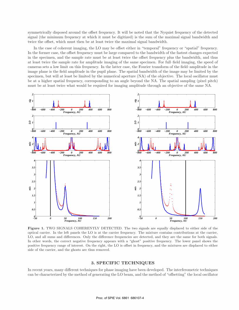
symmetrically disposed around the offset frequency. It will be noted that the Nyquist frequency of the detectedsignal (the minimum frequency at which it must be digitized) is the sum of the maximal signal bandwidth andtwice the offset, which must then be at least twice the maximal signal bandwidth.

In the case of coherent imaging, the LO may be offset either in “temporal” frequency or “spatial” frequency.In the former case, the offset frequency must be large compared to the bandwidth of the fastest changes expectedin the specimen, and the sample rate must be at least twice the offset frequency plus the bandwidth, and thusat least twice the sample rate for amplitude imaging of the same specimen. For full–field imaging, the speed ofcameras sets a low limit on this frequency. In the latter case, the Fourier transform of the field–amplitude in theimage plane is the field amplitude in the pupil plane. The spatial bandwidth of the image may be limited by thespecimen, but will at least be limited by the numerical aperture (NA) of the objective. The local oscillator mustbe at a higher spatial frequency, corresponding to an angle beyond the NA. The spatial sampling (pixel pitch)must be at least twice what would be required for imaging amplitude through an objective of the same NA.

−800 −600 −400 −200 0 200 400 600 8000

2

4

mix

Frequency, AU

−800 −600 −400 −200 0 200 400 600 8000

1

2

sig

Frequency, AU

−800 −600 −400 −200 0 200 400 600 8000

1

2

LO

Frequency, AU

−50 0 50 100 150 2000

0.5

1

1.5

2

2.5

3

3.5

4

mix

Frequency, AU

−800 −600 −400 −200 0 200 400 600 8000

2

4m

ix

Frequency, AU

−800 −600 −400 −200 0 200 400 600 8000

1

2

sig

Frequency, AU

−800 −600 −400 −200 0 200 400 600 8000

1

2

LO

Frequency, AU

−50 0 50 100 150 2000

0.5

1

1.5

2

2.5

3

3.5

4

mix

Frequency, AU

Figure 1. TWO SIGNALS COHERENTLY DETECTED. The two signals are equally displaced to either side of theoptical carrier. In the left panels the LO is at the carrier frequency. The mixture contains contributions at the carrier,LO, and all sums and differences. Only the difference frequencies are detected, and they are the same for both signals.In other words, the correct negative frequency appears with a “ghost” positive frequency. The lower panel shows thepositive frequency range of interest. On the right, the LO is offset in frequency, and the mixtures are displaced to eitherside of the carrier, and the ghosts are thus removed.

3. SPECIFIC TECHNIQUES

In recent years, many different techniques for phase imaging have been developed. The interferometric techniquescan be characterized by the method of generating the LO beam, and the method of “offsetting” the local oscillator


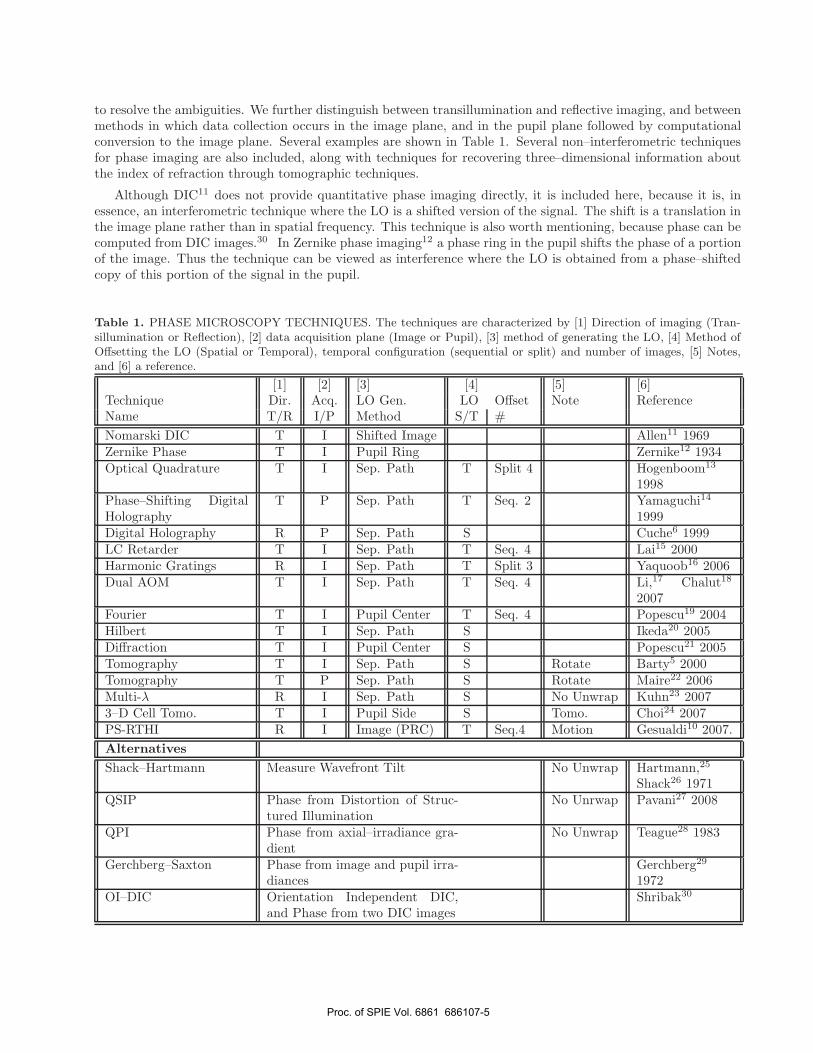
to resolve the ambiguities. We further distinguish between transillumination and reflective imaging, and betweenmethods in which data collection occurs in the image plane, and in the pupil plane followed by computationalconversion to the image plane. Several examples are shown in Table 1. Several non–interferometric techniquesfor phase imaging are also included, along with techniques for recovering three–dimensional information aboutthe index of refraction through tomographic techniques.

Although DIC11 does not provide quantitative phase imaging directly, it is included here, because it is, inessence, an interferometric technique where the LO is a shifted version of the signal. The shift is a translation inthe image plane rather than in spatial frequency. This technique is also worth mentioning, because phase can becomputed from DIC images.30 In Zernike phase imaging12 a phase ring in the pupil shifts the phase of a portionof the image. Thus the technique can be viewed as interference where the LO is obtained from a phase–shiftedcopy of this portion of the signal in the pupil.

Table 1. PHASE MICROSCOPY TECHNIQUES. The techniques are characterized by [1] Direction of imaging (Tran-sillumination or Reflection), [2] data acquisition plane (Image or Pupil), [3] method of generating the LO, [4] Method ofOffsetting the LO (Spatial or Temporal), temporal configuration (sequential or split) and number of images, [5] Notes,and [6] a reference.

[1] [2] [3] [4] [5] [6]Technique Dir. Acq. LO Gen. LO Offset Note ReferenceName T/R I/P Method S/T #Nomarski DIC T I Shifted Image Allen11 1969Zernike Phase T I Pupil Ring Zernike12 1934Optical Quadrature T I Sep. Path T Split 4 Hogenboom13

1998Phase–Shifting DigitalHolography

T P Sep. Path T Seq. 2 Yamaguchi14

1999Digital Holography R P Sep. Path S Cuche6 1999LC Retarder T I Sep. Path T Seq. 4 Lai15 2000Harmonic Gratings R I Sep. Path T Split 3 Yaquoob16 2006Dual AOM T I Sep. Path T Seq. 4 Li,17 Chalut18

2007Fourier T I Pupil Center T Seq. 4 Popescu19 2004Hilbert T I Sep. Path S Ikeda20 2005Diffraction T I Pupil Center S Popescu21 2005Tomography T I Sep. Path S Rotate Barty5 2000Tomography T P Sep. Path S Rotate Maire22 2006Multi-λ R I Sep. Path S No Unwrap Kuhn23 20073–D Cell Tomo. T I Pupil Side S Tomo. Choi24 2007PS-RTHI R I Image (PRC) T Seq.4 Motion Gesualdi10 2007.AlternativesShack–Hartmann Measure Wavefront Tilt No Unwrap Hartmann,25

Shack26 1971QSIP Phase from Distortion of Struc-

tured IlluminationNo Unrwap Pavani27 2008

QPI Phase from axial–irradiance gra-dient

No Unwrap Teague28 1983

Gerchberg–Saxton Phase from image and pupil irra-diances

Gerchberg29

1972OI–DIC Orientation Independent DIC,

and Phase from two DIC imagesShribak30


The most direct techniques for phase imaging use a separate path for the LO, and are divided into twodistinct groups: Phase–shifting techniques (temporal frequency offset) and tilted–reference techniques (spatialfrequency offset). These are distinguished in Column 4 of Table 1. Temporal offset can be implemented withthe images obtained sequentially in time, as in phase–shifting interferometry14 (A recent technique, for example,uses a liquid crystal retarder15). More rapid temporal variations can be obtained by shifting the LO frequencyand collecting images at the difference frequency,17 which was implemented in a microscope recently.18 Inthese cases, it is important that the object not have temporal variations at frequencies higher than half the totalsample rate. Alternatively, images can be collected simultaneously using beamsplitters and polarizing optics, asin our optical quadrature microscope (OQM),31 or harmonically related gratings.16 These techniques do notimpose limitations on either the spatial or temporal frequencies of the object, but require multiple cameras.

Digital Holographic Microscopy6 offsets the LO in spatial frequency. This results in a tilted wavefront, andif the tilt is sufficient to eliminate any aliasing effects, the phase can be recovered from a single image. Thecamera is in the pupil plane and the object is reconstructed computationally. Hilbert Phase Microscopy20 alsouses a tilted reference wavefront, but images directly. The spatial sampling must be sufficiently dense to preventaliasing of the frequency–shifted data as discussed in Section 2.

The separate path for the local oscillator adds a certain amount of complexity to the microscope design.Mismatches in optical path can lead to reduced coherence, and may lead to instability in the fringe pattern. Ifsequential images are collected with temporal frequency offset, the instability may lead to unpredictable changesin the phase shifts. In OQM, care was taken to ensure that all four cameras collect data at exactly the sametime.

To avoid the instabilities that can occur with a separate reference path, an alternative is to generate the LOfrom a portion of the signal itself. Both DIC and Zernike phase imaging microscopes do this in different ways,as mentioned above. Fourier Phase Microscopy19 uses a different approach, by generating the LO from a centralportion of the signal in the center of the pupil. Thus it is inherently coherent with the signal. Because it is in thecenter, it includes only the low spatial frequencies of the signal. Thus it provides very stable phase imaging ofobjects that consist mostly of high spatial frequencies. Diffraction Phase Microscopy21 combines this approachwith Hilbert Phase Microscopy.

It is worth mentioning that there are some more indirect approaches to phase imaging. One is QuantitativePhase Imaging (QPI), which computes phase from the axial–irradiance gradient.28 This technique effectivelymeasures wavefront shape, and thus measures optical path length independently of wavelength and without thewrapping that occurs in direct phase measurement. The technique requires measuring the irradiance at twoclosely spaced planes and performing a computation to obtain the phase. Another example uses two irradianceimages, but one in the image plane and one in the pupil. The complex amplitudes in both planes are calculatediteratively using Fourier transforms, and comparing the resulting amplitudes to the measurements.29

Another phase imaging technique measures deformations of structured illumination27 to compute wavefrontvariations and then thee optical path length. Shack–Hartmann25, 26 imaging measures direction of wavefronts,which is related to the derivative of phase.

Three–dimensional reconstruction of the index of refraction has been accomplished using rotation of thespecimen,5, 22 and by rotation of the input light direction.24 The latter approach recovers the axial informationthat is lost to the small numerical aperture of illumination that is inherent to coherent imaging.

The cyclic ambiguity in phase can be removed by using multiple wavelengths,23 which increases the ambiguityinterval to 1/λeff = 1/λ2 − 1/λ2, without degrading the resolution.

4. PERFORMANCE MODELS

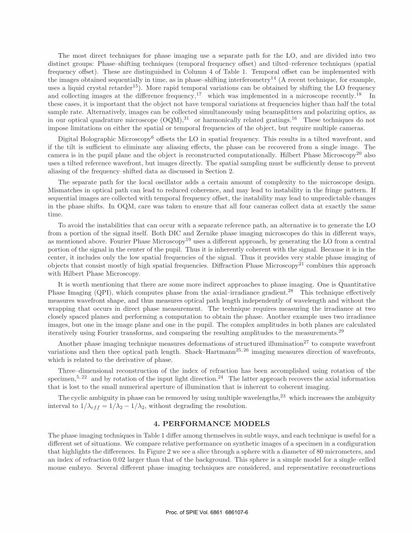
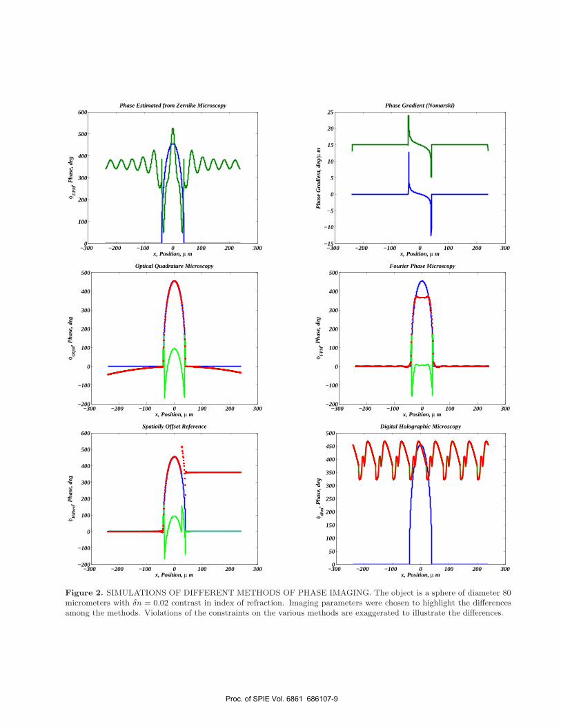
The phase imaging techniques in Table 1 differ among themselves in subtle ways, and each technique is useful for adifferent set of situations. We compare relative performance on synthetic images of a specimen in a configurationthat highlights the differences. In Figure 2 we see a slice through a sphere with a diameter of 80 micrometers, andan index of refraction 0.02 larger than that of the background. This sphere is a simple model for a single–celledmouse embryo. Several different phase–imaging techniques are considered, and representative reconstructions


are shown, along with the phase obtained by integrating the index of refraction along straight rays through thespecimen. The object and the microscope parameters have been carefully chosen, and generally exaggerated, toshow the differences among the techniques. In most cases, one would anticipate better agreement among thetechniques, and better agreement with the actual phase than shown here. The top two panels show Zernikephase microscopy and DIC. The second row shows OQM on the left and Fourier Phase Microscopy on the right.The curves show the phase computed by projection, the reconstructed phase from the image, and the unwrappedreconstructed phase. The major limitation on OQM is the need for a well defined reference wave. The exampleshows what happens if the reference is assumed flat while in fact it is slightly curved. In addition, errors causedby imperfections in the optical system can lead to artifacts, as with any coherent imaging technique. FourierPhase Microscopy shows some errors in the low spatial frequencies on this extremely large specimen. The errorswill be much smaller on smaller objects, which are typically imaged with this technique. Limiting the LO tolower spatial frequencies could improve the performance for larger objects with a reduced LO power. Curvatureerrors and artifacts will be reduced by the common optical paths. The bottom row in the figure shows imagingwith a spatially offset LO. In the left panel, the camera is focused on the image plane. The parameters weredeliberately chosen so that some aliasing occurs, because of under–sampling of the data. On the right, the camerais focused on the pupil plane, and the image is computed. In this case, sampling in the pupil plane causes theimage to be periodic in the image plane. Provided that the sampling is sufficiently dense to accommodate thedesired field of view, this is not a problem.

5. SUMMARY AND CONCLUSIONS

Phase useful in biomedical imaging, because it can provide contrast at low light levels, without the need forpotentially toxic markers or high levels of light. Ambiguities that arise in interferograms can be resolved throughthe use of a reference wave that is offset in temporal or spatial frequency. Here we have considered varioustechniques for generating the reference wave, and the required frequency offset. Each method has advantagesand disadvantages, depending on the spatial and temporal characteristics of the specimen, the ability to samplethe image with sufficient density, and the numerical aperture and field of view. Furthermore, phase imagingcan be combined with specimen or beam rotation, to produce tomographic images in three dimensions. Asimple model has been constructed to illustrate the behavior of each technique, and some sample results havebeen shown. With the success of so many techniques in recent years, phase imaging shows promise for morebiomedical applications in the future.

6. ACKNOWLEDGMENTS

This work was supported in part by CenSSIS, the Gordon Center for Subsurface Sensing and Imaging Systems,under the Engineering Research Centers Program of the National Science Foundation (award number EEC-9986821).

REFERENCES1. W. C. Warger, II, J. A. Newmark, C. M. Warner, and C. A. DiMarzio, “Phase subtraction cell counting

method for live mouse embryos beyond the eight–cell stage,” Journal of Biomedical Optics , 2008. in Press.2. H. G. Davies and M. H. F. Wilkins, “Interference microscopy and mass determination,” Nature 169, 1952.3. G. A. Dunn and D. Zicha, “Using the drimaps system of interference microscopy to study cell behavior,” in

Cell Biology: A Laboratory Handbook, 2nd edition, E. Celis, ed., 3, pp. 44–53, Academic Press Inc., 1998.4. N. Lue, J. Bewersdorf, M. D. Lessard, K. Badizadegan, R. R. Dasari, M. S. Feld, and G. Popescu, “Tissue

refractometry using hilbert phase microscopy,” Opt. Lett. 32(24), pp. 3522–3524, 2007.5. A. Barty, K. A. Nugent, A. Roberts, and D. Paganin, “Quantitative phase tomography,” Optics Communi-

cations 175, pp. 329–336, March 2000.6. E. Cuche, F. Bevilacqua, and C. Depeursinge, “Digital holography forquantitative phase-contrast imaging,”

Optics Letters 24, pp. 291–293, Mar. 1999.7. F. Dubois, C. Yourassowsky, O. Monnom, J.-C. Legros, O. Debeir, P. V. Ham, R. Kiss, and C. Decaestecker,

“Digital holographic microscopy for the three-dimensional dynamic analysis of in vitro cancer cell migration,”Journal of Biomedical Optics 11(5), p. 054032, 2006.


8. P. Langehanenberg, B. Kemper, and G. von Bally, “Autofocus algorithms for digital-holographic mi-croscopy,” Biophotonics 2007: Optics in Life Science 6633(1), p. 66330E, SPIE, 2007.

9. D. Gabor and W. P. Goss, “Interference microscope with total wavefront reconstruction,” J. Opt. Soc.Am. 56(7), p. 849, 1966.

10. M. R. R. Gesualdi, M. Mori, M. Muramatsu, E. A. Liberti, and E. Munin, “Phase-shifting real-time holo-graphic interferometry applied to load transmission evaluation in dried human skull,” Appl. Opt. 46(22),pp. 5419–5429, 2007.

11. R. Allen, G. David, and G. Nomarski, “The Zeiss-Nomarski differential interference equipment fortransmitted-light microscopy,” Zeitschrift fur Wissenschaftliche Mikroskopie und Mikroskopische Tech-nike 69(4), pp. 193–221, 1969.

12. F. Zernike, “Beugungstheorie des schneidenverfahrens und seiner verbesserten form, der phasenkontrast-methode,” Physica 1, pp. 689–704, 1934.

13. D. Hogenboom, C. A. DiMarzio, T. J. Gaudette, A. J. Devaney, and S. C. Lindberg, “Three-dimensionalimages generated by quadrature interferometry,” Optics Letters 23(10), pp. 783 – 785, 1998.

14. I. Yamaguchi and T. Zhang, “Phase-shifting digital holography,” Opt. Lett. 22(16), pp. 1268–1270, 1997.15. S. Lai, B. King, and M. A. Neifeld, “Wave front reconstruction by means of phase-shifting digital in-line

holography,” Optics Communications 173, pp. 155–160, January 2000.16. Z. Yaqoob, J. Wu, X. Cui, X. Heng, and C. Yang, “Harmonically-related diffraction gratings-based inter-

ferometer for quadrature phase measurements,” Optics Express 14(18), pp. 8127 – 8128, 2006.17. E. Li, J. Yao, D. Yu, J. Xi, and J. Chicharo, “Optical phase shifting with acousto-optic devices,” Opt.

Lett. 30(2), pp. 189–191, 2005.18. K. J. Chalut, W. J. Brown, and A. Wax, “Quantitative phase microscopy with asynchronous digital holog-

raphy,” Opt. Express 15(6), pp. 3047–3052, 2007.19. G. Popescu, L. P. Deflores, J. C. Vaughan, K. Badizadegan, H. Iwai, R. R. Dasari, and M. S. Feld, “Fourier

phase microscopy for investigation of biological structures and dynamics,” Optics Letters 29(21), pp. 2503– 2505, 2004.

20. T. Ikeda, G. Popescu, R. R. Dasari, and M. S. Feld, “Hilbert phase microscopy for investigating fast dynamicsin transparent systems,” Opt. Lett. 30(10), pp. 1165–1167, 2005.

21. G. Popescu, T. Ikeda, C. A. Best, K. Badizadegan, R. R. Dasari, and M. S. Feld, “Erythrocyte structureand dynamics quantified by hilbert phase microscopy,” Journal of Biomedical Optics 10(6), p. 060503, 2005.

22. G. Maire, G. Pauliat, and G. Roosen, “Homodyne detection readout for bit-oriented holographic memories,”Opt. Lett. 31(2), pp. 175–177, 2006.

23. J. Kuhn, T. Colomb, F. Montfort, F. Charriere, Y. Emery, E. Cuche, P. Marquet, and C. Depeursinge,“Real-time dual-wavelength digital holographic microscopy with a single hologram acquisition,” OpticsExpress 15(12), pp. 7231 – 7242, 2007.

24. W. Choi, C. Fang-Yen, K. Badizadegan, S. Oh, N. Lue, R. R. Dasari, and M. S. Feld, “Tomographic phasemicroscopy,” Nature Methods 4, pp. 717 – 719, 2007.

25. Hartmann, “Bemerkungen uber den bau und die justirung von spektrographen,” Z. Instrumentenkunde 20,pp. 2–27, Jan 1900.

26. R. V. Shack and B. C. Platt, “Production and use of a lenticular hartmann screen,” Journal of the OpticalSociety of America 61, 1971. (Abstract of a talk to be presented at the OSA Annual Meeting, Tuscon, AZ.in April 1971).

27. S. R. P. Pavani, A. R. Libertun, S. V. King, and C. J. Cogswell, “Quantitative structured-illumination phasemicroscopy,” Appl. Opt. 47(1), pp. 15–24, 2008.

28. M. R. Teague, “Deterministic phase retrieval: a green’s function solution,” J. Opt. Soc. Am. 73(11), p. 1434,1983.

29. R. W. Gerchberg and W. . Saxton, “A practical algorithm for the determination of phase from image anddiffraction plane,” Optik 35, pp. 227–246, 1972.

30. M. Shribak and S. Inoue, “Orientation-independent differential interference contrast microscopy,” Appl.Opt. 45(3), pp. 460–469, 2006.

31. D. Hogenboom, C. DiMarzio, T. Gaudette, A. Devaney, and S. Lindberg, “Three-dimensional images gen-erated by quadrature interferometry,” Optics Letters 23, pp. 783–785, 1998.


−300 −200 −100 0 100 200 3000

100

200

300

400

500

600Phase Estimated from Zernike Microscopy

x, Position, µ m

φ FP

M, P

hase

, deg

−300 −200 −100 0 100 200 300−200

−100

0

100

200

300

400

500Optical Quadrature Microscopy

x, Position, µ m

φ OQ

M, P

hase

, deg

−300 −200 −100 0 100 200 300−200

−100

0

100

200

300

400

500

600Spatially Offset Reference

x, Position, µ m

φ Hilb

ert, P

hase

, deg

−300 −200 −100 0 100 200 300−15

−10

−5

0

5

10

15

20

25Phase Gradient (Nomarski)

x, Position, µ m

Pha

se G

radi

ent,

deg/

µ m

−300 −200 −100 0 100 200 300−200

−100

0

100

200

300

400

500Fourier Phase Microscopy

x, Position, µ m

φ FP

M, P

hase

, deg

−300 −200 −100 0 100 200 3000

50

100

150

200

250

300

350

400

450

500Digital Holographic Microscopy

x, Position, µ m

φ dhm

, Pha

se, d

eg

Figure 2. SIMULATIONS OF DIFFERENT METHODS OF PHASE IMAGING. The object is a sphere of diameter 80micrometers with δn = 0.02 contrast in index of refraction. Imaging parameters were chosen to highlight the differencesamong the methods. Violations of the constraints on the various methods are exaggerated to illustrate the differences.


Full–Field Quantitative Phase Imaging

Documents

Transcript of Full–Field Quantitative Phase Imaging