Quantitative imaging of lung function using hyperpolarised ...

Quantitative imaging of lung function using

hyperpolarised gas MRI

Thesis submitted for the degree of Doctor of Philosophy

Felix Clemens Horn

Academic Unit of Radiology

Department of Cardiovascular Science

School of Medicine

The University of Sheffield

Supervisors: Jim Wild, Juan Parra-Robles

Examiners: Jan Wolber, Peter Thelwall

e-thesis submission (edited version)

January 2015

1

Acknowledgements

First and foremost I owe greatest gratitude to my supervisor Jim Wild, who has supported me and

given me patient guidance throughout this thesis whilst allowing me the room to work my own

way and develop. I thank him for all the effort he put into training me and for sending me to

numerous conferences. With Jim’s scientific thinking, his dedication to the topic and his social

attitude towards us as a group he’s a person I look up to.

Equally I’d like to express my gratitude towards my second supervisor Juan Parra-Robles. It’s

been an amazing pleasure to learn from Juan. I thank him for his thoughtful advice and his

eagerness to explain and discuss with me.

I’m thankful to have done this work together with great colleagues/friends from my group in

Sheffield. I’m thankful to Helen, who’s been incredibly helpful, without whom I could not have

accomplished all this. Graham, who’s supported me during the first months after arriving in

Sheffield. Equally I’d like to thank Guilhem, General, Neil and Madhwesha, who have had

contribution towards accomplishing this work. Finally I’d also like to acknowledge Martin Deppe

for introducing me into my project during his last weeks in Sheffield and who’s laid the

foundations of the work that I’ve been doing here in Sheffield. Last but not least thanks to Peggy

Xu, the best person to share a desk with (when you like chocolate).

I am grateful to Alex Horsley and Laurie Smith who have taught me on pulmonary function

testing, taught me acquiring pulmonary function data on my own and both have contributed to

this work.

I would like to thank Leanne Armstrong, Yvonne Steel and the whole Academic Unit of

Radiology for all their help and amazing company in the coffee room. I’d like to thank in

particular the radiographers of our unit for their great help with scanning patients.

I would also like to express my appreciation to the organiser of the pulmonary imaging network

(PI-net) Jesus Ruiz-Cabello and all contributors. It’s been an honour to be part of this European

training network and meeting people from all over Europe for focused scientific exchanges and

friendship.

I’d like to express my gratitude towards my former supervisor from Technischer Hochschule

Nürnberg, Prof. Florian Steinmeyer, an admirable scientist, who’s introduced me to MRI and

awakened the fascination thereof. Equally I’d like to thank my former supervisors from Siemens

Healthcare, Dr. Dieter Ritter and Matthias Gebhardt.

But all this would have been impossible without the support from family and friends. A special

thanks to my oldest and best friend here, Jenny for the countless evenings discussing all matters

of life. Thanks to Helen, Kevin, General and Carolyn for the great time together climbing inside,

2

outside as well as the after climbing social sessions. Thanks to my friends Nico and Simon for

amazing times together at the Matrix. And thanks to my flatmate Dani, the one who had to bear

me most of all. Thanks also to my German friends, who came here so many times to explore

Britain together with me, to Christoph and Stephan. Cheers also to my old colleague Martin for

all the advice he’s given me over the years.

Finally thanks to my dear family. Thanks to my parents Beatrice and Ulrich, without whom I

would not be where I’m today. I’d also like to thank my beloved sisters Ina, Susanne, Elisabeth,

Maria, and Cornelia for all their support, love and their countless visits.

And last but not least a great thanks to my girlfriend Fabiola, for her continuous support,

encouragement and for coping with me during writing up. Thanks for the countless times you

were coming to Sheffield when I was not able to come visit you.

This thesis was funded by European framework 7 – PI-net.

3

Abstract

This thesis describes methods for Magnetic Resonance Imaging (MRI) of hyperpolarised noble

3He and 129Xe gas to quantitatively measure lung ventilation and changes thereof in humans.

Three different methods are proposed and tested:

1. Percentage ventilated lung volume derived from functional (hyperpolarised gas imaging)

and anatomical (proton imaging) imaging acquired in a single breath-hold is compared to

images from two separate breath-holds. The single breath technique is shown to be

significantly more reliable and can help to reduce statistical noise.

2. Treatment response mapping is developed as a quantitative measure of lung ventilation

response to intervention. The measured signal difference between ventilation images

acquired before and after treatment (provocation) is used to calculate changes in gas

regional distribution. The technique is validated in an asthma cohort and preliminary

findings indicate the method is thought to be more sensitive to changes than existing

hyperpolarised gas techniques as existing pulmonary function tests.

3. With multiple breath washout imaging a method is developed and investigated to derive

quantitative functional information from images by monitoring regional signal decay

during tracer gas washout. The technique is extended to produce regional quantitative

information of ventilation in 3D. Reproducibility of the technique is tested and its errors

are systematically investigated. Furthermore, image acquisition is optimised using bSSFP

imaging. The method is applied to a CF and an asthma cohort.

Finally, preliminary results are presented comparing multiple breath washout measured

at the mouth in the pulmonary function lab to a predicted global washout as modelled

from regional functional information derived from the imaging technique.

4

Contents

Acknowledgements ...................................................................................................................... 1

Abstract ........................................................................................................................................ 3

List of abbreviations .................................................................................................................... 8

Chapter 1 Introduction ............................................................................................................... 9

1.1. Motivation ..................................................................................................................... 9

1.2. Thesis outline ................................................................................................................. 9

Chapter 2 Background .............................................................................................................. 11

2.1. Principles of nuclear magnetic resonance.................................................................... 11

2.1.1. Spin angular momentum and magnetisation ........................................................ 11

2.1.2. Thermal polarisation ............................................................................................ 13

2.1.3. Excitation ............................................................................................................. 14

2.1.4. Relaxation and signal detection ........................................................................... 15

2.2. Imaging using magnetic resonance .............................................................................. 16

2.2.1. Encoding k-space with magnetic field gradients ................................................. 16

2.2.2. Discrete sampling ................................................................................................ 20

2.2.3. The SPGR pulse sequence ................................................................................... 21

2.2.4. The bSSFP sequence ........................................................................................... 22

2.3. Lung imaging using proton MRI ................................................................................. 23

2.4. Imaging hyperpolarised gases in the lung ................................................................... 24

2.4.1. Introduction ......................................................................................................... 24

2.4.2. Optical pumping .................................................................................................. 25

2.4.3. Imaging hardware ................................................................................................ 27

2.4.4. Sequence considerations ...................................................................................... 27

2.4.5. Flip angle calibration ........................................................................................... 29

2.4.6. Ventilation imaging ............................................................................................. 29

2.4.7. Diffusion weighted imaging ................................................................................ 30

2.4.8. Imaging of partial oxygen pressure ..................................................................... 31

2.4.9. Conclusion ........................................................................................................... 32

2.5. Pulmonary Function Testing ....................................................................................... 33

2.5.1. Pulmonary structure ............................................................................................. 33

2.5.2. Pulmonary volumes ............................................................................................. 34

2.5.3. Lung function ...................................................................................................... 35

5

2.5.4. Lung disease ........................................................................................................ 35

2.5.5. Measuring respiratory function ........................................................................... 37

2.6. Multiple breath washout models - modelling gas mixing ........................................... 43

Chapter 3 Lung ventilation volumetry with same breath acquisition of hyperpolarised gas

and proton MRI ........................................................................................................................ 46

3.1. Introduction ................................................................................................................. 46

3.2. Materials and methods ................................................................................................ 48

3.2.1. Participant selection ............................................................................................ 48

3.2.2. Imaging protocol ................................................................................................. 48

3.2.3. Image analysis ..................................................................................................... 50

3.3. Results ......................................................................................................................... 53

3.4. Discussion ................................................................................................................... 57

3.5. Conclusions ................................................................................................................. 59

Chapter 4 A method for quantitative mapping in lung ventilation in response to treatment

using hyperpolarised 3He MRI demonstrated in asthma patients ........................................ 61

4.1. Introduction ................................................................................................................. 61


4.2.1. Patient recruitment .............................................................................................. 62

4.2.2. MRI acquisition................................................................................................... 63

4.2.3. Image analysis ..................................................................................................... 64

4.3. Results ......................................................................................................................... 71

4.3.1. Baseline variability ............................................................................................. 71

4.3.2. Treatment response mapping .............................................................................. 72

4.4. Discussion ................................................................................................................... 76

4.4.1. Baseline variability thresholding......................................................................... 77

4.4.2. Treatment response ............................................................................................. 78

4.4.3. Conclusion .......................................................................................................... 78

Chapter 5 Quantification of regional fractional ventilation in human subjects by

measurement of hyperpolarised 3He washout with 2D and 3D MRI ................................... 80

5.1. Introduction ................................................................................................................. 80


5.2.1. Human subjects ................................................................................................... 81

5.2.2. Multiple breath washout protocols ...................................................................... 82

5.2.3. 2D washout acquisition protocol (2D-WO) ........................................................ 83

5.2.4. 3D washout acquisition protocol (3D-WO) ........................................................ 83

5.2.5. Flow measurement during washout imaging experiments .................................. 84

6

5.2.6. 3He MR hardware and pulse sequences ............................................................... 84

5.2.7. Calculation of fractional ventilation from washout imaging data ....................... 85

5.2.8. Specific details of image processing.................................................................... 87

5.2.9. Gravitational evaluation of fractional ventilation ................................................ 89

5.2.10. Comparison of imaging and pneumotachograph measurements of ventilation ... 89

5.2.11. Comparison of fractional ventilation from 2D and 3D protocols ........................ 89

5.2.12. Reproducibility .................................................................................................... 90

5.3. Results ......................................................................................................................... 90

5.3.1. Gravitational effects of fractional ventilation ...................................................... 92

5.3.2. Comparison of imaging and pneumotachograph measurements of ventilation ... 93

5.3.3. Comparison of fractional ventilation from 2D and 3D protocols ........................ 95

5.3.4. Repeatability of washout measurements ............................................................. 95

5.4. Discussion .................................................................................................................... 97

5.4.1. Repeatability ........................................................................................................ 98

5.4.2. Gravitational evaluation of fractional ventilation ................................................ 98

5.4.3. Conclusion ........................................................................................................... 98

Chapter 6 Error analysis of fractional ventilation from MBW-imaging ........................... 100

6.1. Introduction ............................................................................................................... 100

6.2. Errors derived from volume changes ......................................................................... 100

6.3. Errors associated with the signal correction factor .................................................... 103

6.4. Influence of SNR on fractional ventilation ................................................................ 108

6.5. Total combined error analysis ................................................................................... 111

6.6. Conclusions ............................................................................................................... 113

Chapter 7 Advances in multiple breath washout imaging acquisition methods ................ 114

7.1. Introduction ............................................................................................................... 114

7.2. Methods ..................................................................................................................... 115

7.3. Results ....................................................................................................................... 117

7.4. Discussion and future work ....................................................................................... 122

7.5. Conclusions ............................................................................................................... 124

Chapter 8 Linking regional ventilation heterogeneity from hyperpolarised gas MR

imaging to MBW in obstructive airways disease .................................................................. 125

8.1. Introduction ............................................................................................................... 125

8.2. Methods ..................................................................................................................... 125

8.2.1. Subjects .............................................................................................................. 125

8.2.2. Pulmonary function tests ................................................................................... 127

8.2.3. Washout imaging ............................................................................................... 127

7

8.2.4. Image analysis ................................................................................................... 128

8.3. Results ....................................................................................................................... 129

8.3.1. Correlations ....................................................................................................... 130

8.3.2. Analysis of variances ........................................................................................ 130

8.4. Discussion ................................................................................................................. 134

8.5. Conclusions ............................................................................................................... 136

Chapter 9 Future work - linking multiple breath washout imaging to global multiple

breath washout tests with modelling ..................................................................................... 137

9.1. Introduction ............................................................................................................... 137

9.2. Methods..................................................................................................................... 138

9.2.1. MBW-imaging .................................................................................................. 138

9.2.2. MBW ................................................................................................................. 140

9.3. Results ....................................................................................................................... 141

9.4. Discussion ................................................................................................................. 142

9.5. Conclusions ............................................................................................................... 143

Chapter 10 Conclusions .......................................................................................................... 144

List of figures ........................................................................................................................... 146

List of tables............................................................................................................................. 155

List of publications .................................................................................................................. 157

References ................................................................................................................................ 161

8

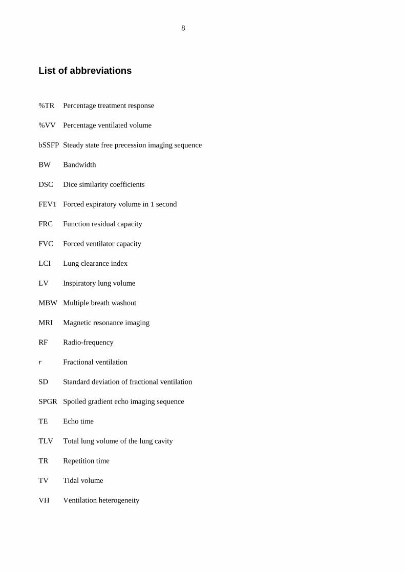
List of abbreviations

%TR Percentage treatment response

%VV Percentage ventilated volume

bSSFP Steady state free precession imaging sequence

BW Bandwidth

DSC Dice similarity coefficients

FEV1 Forced expiratory volume in 1 second

FRC Function residual capacity

FVC Forced ventilator capacity

LCI Lung clearance index

LV Inspiratory lung volume

MBW Multiple breath washout

MRI Magnetic resonance imaging

RF Radio-frequency

r Fractional ventilation

SD Standard deviation of fractional ventilation

SPGR Spoiled gradient echo imaging sequence

TE Echo time

TLV Total lung volume of the lung cavity

TR Repetition time

TV Tidal volume

VH Ventilation heterogeneity

9

Chapter 1 Introduction

1.1. Motivation

2014 year it has been 20 years since the first images from hyperpolarised 129Xe were acquired in

animals [1]. Only one year later hyperpolarised 3He was successfully used to acquire images in

human lungs [2]. In the past decades major efforts were undertaken to improve sensitivity of this

imaging technique with advances in hardware [3], sequence design [4-6] as well higher

polarisation levels of hyperpolarised gases e.g. using stronger lasers [7].

In an editorial in early 2014, Prisk and Sá emphasise the achievements of imaging hyperpolarised

gases and point out the need for quantitative numbers for better physiological interpretation of

data [8]. Those quantitative metrics and imaging markers are crucial for successful classification

of disease and early detection of change in regional lung function. The motivation of this thesis

is the development of more quantitative metrics for measuring lung ventilation with

hyperpolarised gases in human lungs.

1.2. Thesis outline

Chapter 2 serves as a very brief introduction to the background of MRI physics and pulmonary

physiology and function testing. This has deliberately been kept short.

Chapter 3 investigates the increase in reliability of percentage ventilated volume (%VV) gained

through the use of a single breath-hold imaging method: Instead of acquiring functional (3He) and

anatomical (1H) images in separate breath-holds, both images are acquired in a single breath-hold.

This is shown to significantly decrease the variability of the %VV in repeated experiments when

compared to a technique acquiring both images in separate breath-holds.

Chapter 4 introduces treatment response mapping as a method to derive quantitative information

of ventilation changes from images acquired before and after intervention. Differences of regional

changes of static ventilation weighted image signal intensity are used derive percent treatment

response (%TR). The technique is tested on an asthma cohort and compared to %VV and

spirometry.

Chapter 5 explains the methodology of multiple breath washout imaging. Images are acquired

in subjects after each breathing cycle (expiration-inspiration) over multiple breaths. Regional gas

washout is used to derive quantitative maps of fractional ventilation in 2D and 3D. The washout

imaging protocol and post-processing steps to derive fractional ventilation from images are

10

described. The method is compared to independently measured lung volume turn over and

repeatability is tested in 7 volunteers.

Chapter 6 is an error analysis of multiple breath washout imaging. Sources of error are addressed

and resulting errors are estimated using values from the literature and obtained in measurements.

Chapter 7 demonstrates further advances in multiple breath washout imaging. Balanced steady

state imaging (bSSFP) is demonstrated to use only half the dose of hyperpolarised 3He when

compared to the initial protocol (from Chapter 5) using an SPGR sequence. Quantitative fractional

ventilation maps derived from images acquired with a bSSFP sequence are compared to the SPGR

sequence as used in Chapter 5. Quantitative maps from both sequences show very good

agreement. Using the bSSFP sequence the feasibility of MBW-imaging in 3D with hyperpolarised

129Xe is also demonstrated.

Chapter 8 tests multiple breath washout imaging in two clinical studies: (1) comparing healthy

children to age matched cystic fibrosis (CF) patients with early lung disease and (2) an cohort of

moderate-severe asthmatics. An increased sensitivity of multiple breath washout derived

ventilation heterogeneity parameter SD is demonstrated compared to methods from the

pulmonary function lab such as LCI and spirometry in healthy children when compared to CF

patients. Good correlation between SD and spirometry as well as SD and LCI could be found over

the whole cohort of 47 subjects and controls.

Chapter 9 briefly introduces the theory to predictively model multiple breath washout as

measured globally at the mouth using the regional functional information from imaging. A direct

comparison in a preliminary study on 3 subjects shows the difficulties of the proposed method

and highlights the scope for future work.

11

Chapter 2 Background

2.1. Principles of nuclear magnetic resonance

Nuclear magnetic resonance (NMR) was first discovered by Bloch and Purcell, which they were

given a joint Nobel Price for in 1952 [9, 10]. Their seminal work quantifies the effect of a spin

precessing in the presence of a magnetic field setting the stage for all further developments. To

regionally differentiate soft tissues Lauterbur and Mansfield utilised imaging gradients in 1973

[11, 12]. This chapter provides a very brief overview of the basic concepts of NMR relevant to

this thesis.

2.1.1. Spin angular momentum and magnetisation

NMR is fundamentally based on the interaction of nuclear spin with external magnetic fields.

Spin (like mass) is an intrinsic property of elementary particles and atomic nuclei. The nuclear

spin ( I) possesses an magnetic moment (

) that is directly related to its spin angular moment (

S) [13]:

IS

Eq. [2.1]

Where ħ is the reduced Planck constant h/2π, I is the spin angular momentum and γ is the

gyromagnetic ratio. Nuclear spin I

takes integer or half-integer values and is non-zero for many

atomic nuclei -a requirement of NMR. The gyromagnetic ratio is the ratio of the nuclear magnetic

dipole moment to the nuclear angular momentum and is determined by a nucleus’s distribution

of charge and mass.

Table 2.1: Summary of the magnetic properties and isotopic abundance in nature of the

principal nuclei relevant to this work [14-16].

12

For a system of nuclei, the sum of microscopic magnetic moments

can be visualised as a

macroscopic magnetisation in the volume occupied by the system:

V

iV

1M

Eq. [2.2]

The spin quantum number I (and hence the total spin angular momentum) is a fixed quantity for

a nucleus in the ground state (see Table 2.1 for values of nuclei relevant to this work). Iz is the

quantum number along an arbitrary axis of quantisation (z) and can take (2I+1) different values

ranging from –I to +I. In the absence of a magnetic field the states (–I and +I) are energetically

equivalent (degenerate).

In the presence of an external magnetic field ( 0B

) the ground energy state is split. 1H for example

has a spin I=+1/2 and occupies 2 different states (corresponding to the nuclear magnetic moment

aligning parallel and anti-parallel to 0B

). The energy of interaction of the individual magnetic

moments with the external magnetic field is related to the strength of 0B

:

0BE

Eq. [2.3]

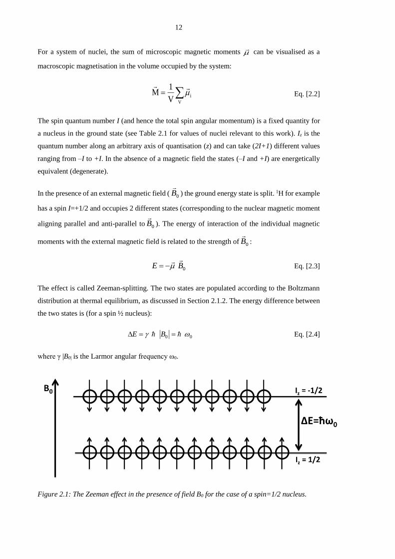
The effect is called Zeeman-splitting. The two states are populated according to the Boltzmann

distribution at thermal equilibrium, as discussed in Section 2.1.2. The energy difference between

the two states is (for a spin ½ nucleus):

00 BE Eq. [2.4]

where γ |B0| is the Larmor angular frequency ω0.

Figure 2.1: The Zeeman effect in the presence of field B0 for the case of a spin=1/2 nucleus.

13

2.1.2. Thermal polarisation

Polarisation P is defined as the ratio of the difference on number of nuclei on the lower (parallel

to 0B

) and higher (anti-parallel) energy states of a spin-½ system in the presence of magnetic

field:

NN

NNP Eq. [2.5]

Where P is a value between 0 and 1 and is usually expressed in percent.

NN , are the quantity

of spins in the lower and higher energy states calculated by the Boltzmann distribution. At body

temperature the thermal energy of the nuclei is much larger than the energy difference between

parallel and anti-parallel states (Eq. [2.4]). Hence, polarisation of a spin system at thermal

equilibrium is very small and can be approximated as:

TkP

B2

0 Eq. [2.6]

where kB is Boltzmann’s constant and T is the absolute temperature in Kelvin. The resulting

magnetisation 0M

along a magnetic field

0B

is typically denoted as Mz (assuming zBB ˆ00

)

and is proportional to polarisation P and spin density ρ:

zz PM Eq. [2.7]

From Eq. [2.6], the polarisation at body temperature, with B0= 1.5T is approximately 10-5. In most

tissues the low polarisation is compensated for by a high density of protons (spin density in tissue

~6.7x1022/cm3 [16]) resulting in sufficient magnetisation for MR-imaging. However, the

considerably lower spin density in the lung, in combination with additional compounding effects

(e.g. field inhomogeneity due to numerous tissue-air interfaces) make proton imaging in the lung

inherently challenging. Noble gases with a ½-spin (3He and 129Xe) can also be used for MR

imaging of the lung upon inhalation, but at thermal equilibrium the lower spin density of the gases

(~ 0.002x1022/cm3 at 1-bar and room temperature) and lower gyromagnetic ratios (Table 2.1)

result in a considerably smaller magnetisation. Nevertheless, through hyperpolarisation, the

polarisation levels of these noble gases can be significantly enhanced compensating for the low

spin density and enabling lung MRI with hyperpolarised 3He and 129Xe. Details of the

hyperpolarisation methods will be discussed in Section 2.4.

14

2.1.3. Excitation

Nuclear spin is an intrinsic property of a nucleus which can be described by the laws of quantum

physics. In addition, the microscopic magnetic moment

can be treated according to classical

electrodynamics and this formalism is often beneficial to visualise spin dynamics. As discussed

above, in the presence of a static magnetic field 0B

a magnetisation 0M

is created as the result

of the sum of all microscopic magnetic moments. Generally, we consider the B0-field to act along

z and hence on thermal equilibrium we can think of the magnetisation vector 0M

aligning with

the, z-axis ( zMM ˆ00

). When applying a radiofrequency pulse (RF) of frequency f0, a rotating

small magnetic field 1B

is generated perpendicular to the static field 0B

and the magnetisation

vector tilts into the transverse (x,y) plane as a result of the applied torque1BM

. Depending on

the amplitude of the field (B1, e.g. along the x-axis) and duration (T) of the RF pulse, the

magnetisation vector will be rotated away from its alignment with 0B

at a ‘flip angle’ α:

T

dttB0

1 )( Eq. [2.8]

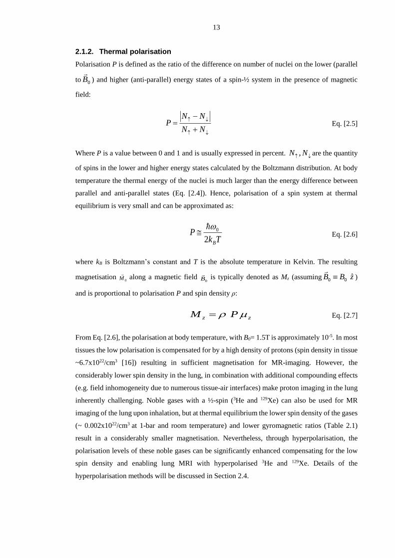
This will result in a certain magnetisation component perpendicular to the z-axis commonly

referred to as transverse magnetisation Mxy ( Mxy=M0 sinα). It is this transverse magnetisation that

is detected as the signal on an NMR experiment as discussed below. Figure 2.2 shows a

diagrammatical representation of the excitation process, showing in (A) the initial state of the

spin-system at equilibrium and in (B) the same spin-system after application of a RF pulse with

a Larmor frequency f0, resulting in a flip angle α.

Figure 2.2: (A) Magnetisation Mo in the presence of a static magnetic field B0. (B) After applying

a RF pulse B1(t) (with frequency ω0 along the x-axis for a duration T) magnetisation has tilted at

flip angle α and has two components: Mxy and Mz

15

2.1.4. Relaxation and signal detection

Immediately after the RF pulse is switched off (Figure 2.2B) the tilted magnetisation vector

transverse component (Mxy) precesses around 0B

and recovers its alignment along z over time

returning to their equilibrium state (t=0, Figure 2.2A). During this process the spin system re-

emits the energy that was absorbed from the RF pulse. During precession a time-varying magnetic

flux is produced in the xy-plane inducing an electromotive force (emf) in a receiver coil tuned to

the Larmor frequency f0 (the frequency of precession):

rdrBtrMdt

demf RF

3))(),((

Eq. [2.9]

where RFB

is the magnetic field per unit current produced at location r .The voltage measured by

the coil as a result of the time-varying flux is called the free induction decay (FID). This decay

can be described by two intrinsic processes which lead to relaxation of the magnetisation vector,

as related by the Bloch equation [9]:

xyzext MT

MMT

BMdt

Md

2

0

1

1)(

1 Eq. [2.10]

Where extB

is the 0B

field pointing in z-direction,

0M is the equilibrium magnetisation,zM

and

xyM denote the component of the magnetisation in the longitudinal direction and transversal

planes respectively. T1 and T2 are relaxation time constants discussed below. The Bloch equation

(Eq. [2.10]) fundamentally describes how the magnetisation in the longitudinal (zM

) and

transverse (xyM

) plane evolves with time. The longitudinal and transversal components can be

separated and solved in the following manner:

)(1

0

1

zz MM

Tdt

dM Eq. [2.11]

Eq. 2.11 describes the interaction of the spin system with its surrounding lattice and can be solved

as follows

11 //

0 )0(1)(Tt

z

Tt

z eMeMtM

Eq. [2.12]

where |Mz|= |M0| for t>>T1. This equation shows that there is an exponential regrowth of

longitudinal magnetisationzM

, after excitation. T1 is the so-called ‘spin-lattice’ relaxation time.

The magnetisation xyM

in the transverse plane rotates with the Larmor frequency around the z-

axis (due toextB

) and relaxes towards zero with a time constant T2. As a result of the rotation, it is

16

best to solve the Bloch equation describing magnetisation in the transverse plane in the ‘rotating

frame’ rather than the ‘laboratory frame’. In the rotating frame, the term describing the

magnetisation precession around the z-axis goes to zero. The solution can be expressed as:

20T/t

xyxy e)(M)t(M

Eq. [2.13]

where T2 is the ‘spin-spin’ relaxation resulting in a decreasing |Mxy| over time, while T1 decay is

also acting to recover Mz. As the name suggest, spin-spin relaxation concerns spins interacting

with each other, rather than the lattice. Spins exchanging energy induce a dephasing of the spin-

system coherence in the transverse direction and therefore a decay of the net-magnetisation |Mxy|.

In addition, in most real applications regional field inhomogeneities also lead to dephasing and

effectively a shortening of the time constant of transverse magnetisation decay (*T2 < T2):

'* TTT 222

111 Eq. [2.14]

Where 'T2 derives from inhomogeneity in the external field 0B

and within the sample itself

(especially in the lungs where many air-tissue interfaces are present1). Nevertheless, dephasing

induced by field inhomogeneity can be reversed using a 180° RF pulse which results in a re-

phasing of the spins and recovery of magnetisation. Sequences using this mechanism are referred

to as spin-echo sequences.

2.2. Imaging using magnetic resonance

In the previous section the excitation and relaxation of a spin system was discussed in the context

of the Bloch equations. In this section the principles of spatial encoding of the spin system to

measure regional information is introduced.

2.2.1. Encoding k-space with magnetic field gradients

To encode the 3D spatial position of the spins, gradients G in all directions (x,y,z) are used.

Gradients are magnetic fields that vary linearly with position x, y or z. Superposition of a gradient

with the principal magnetic field |B0| results in a modulation of the Larmor resonant frequency as

a function of position, according to:

1 Two adjacent areas with different magnetic susceptibility (e.g. water-air) cause small magnetic field

gradients. In the presence of susceptibility gradients spins dephase faster leading to signal attenuation via

T2*.

17

))(()()( 0 rtGBrBr

Eq. [2.15]

Where r is the position (| r

|=(x2+y2+z2)½) and G(t) is a gradient field resulting in a regionally

varying magnetic field B(r). Note that on 3D G(t) is the resultant gradient of 3 linearly varying

gradients on x,y and z. Expressed in the rotating frame, the angular frequency reduces to:

rtGtr

)(),( Eq. [2.16]

In the temporal domain, a gradient switched on for a time interval T causes a position-dependent

accumulation of phase by the spins:

rkdttGrdttrTrTT

2)(),(),(00

Eq. [2.17]

where dttGkT

0 )(2

is the spatial frequency. With this, the time-dependent MRI signal can

be expressed as:

object

tri drerts ),()()(

Eq. [2.18]

Eq. [2.18] describes the relationship of the position-dependent spin density ρ(r) to the signal s(t)

in the temporal domain. This can be re-written in terms of the spatial frequency k:

object

rki drerks

2)()( Eq. [2.19]

This equation is central to MRI and relates the signal s(k) to the function of spatial frequency (k).

Eq. [2.19] is expressed in the rotating frame after demodulation of the Larmor frequency. The

spin density ρ(r) is deducted from the detected signal by applying the inverse Fourier transform

to s(k):

dkeksksFTr

spacek

rki

)()]([)( 1 Eq. [2.20]

It is useful to introduce the concept of k-space here as the domain of spatial frequencies (Eq.

[2.17]). k varies as a function of time according to the temporal course of the magnetic field

gradient (Eq. [2.17]). Gradients are therefore used to sample k-space in 3 spatial dimensions and

k-space is the Fourier inverse (Fourier space) of the image domain. An example k-space and the

corresponding image are shown in Figure 2.3.

18

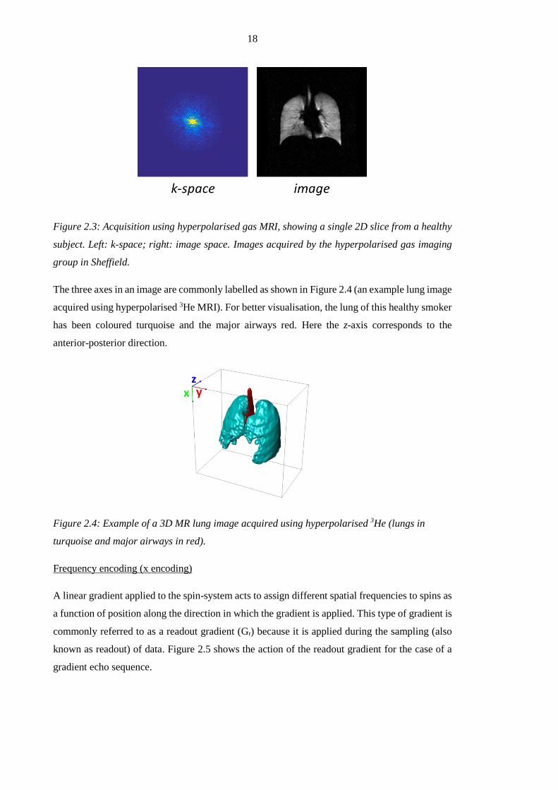
Figure 2.3: Acquisition using hyperpolarised gas MRI, showing a single 2D slice from a healthy

subject. Left: k-space; right: image space. Images acquired by the hyperpolarised gas imaging

group in Sheffield.

The three axes in an image are commonly labelled as shown in Figure 2.4 (an example lung image

acquired using hyperpolarised 3He MRI). For better visualisation, the lung of this healthy smoker

has been coloured turquoise and the major airways red. Here the z-axis corresponds to the

anterior-posterior direction.

Figure 2.4: Example of a 3D MR lung image acquired using hyperpolarised 3He (lungs in

turquoise and major airways in red).

Frequency encoding (x encoding)

A linear gradient applied to the spin-system acts to assign different spatial frequencies to spins as

a function of position along the direction in which the gradient is applied. This type of gradient is

commonly referred to as a readout gradient (Gr) because it is applied during the sampling (also

known as readout) of data. Figure 2.5 shows the action of the readout gradient for the case of a

gradient echo sequence.

19

Figure 2.5: After excitation a negative gradient is applied to dephase the spins. Immediately

afterwards in the opposite direction is applied rephasing the spins as an echo. The area of the

two regions shaded grey is equal.

Phase encoding (y encoding)

A gradient is applied such that spins accrue a phase which differs depending on their position.

The gradient is applied immediately after the RF pulse. In 2D MRI, phase encoding is applied in

one dimension (usually y). However, in 3D sequences two sets of phase encoding gradients are

applied to encode spin position in the y and z dimensions. The effect of a phase encode gradient

on an ensemble of spins is schematically shown in Figure 2.6.

Figure 2.6: Following the RF pulse all spins are aligned (neglecting B0 inhomogeneity). Spins

start to dephase according to their y position after application of the phase encoding gradient

(Gpe) in the y-direction.

Slice selection (z encoding) for 2D MRI

In 2D MRI, x and y read and phase encoding is typically used to acquire a 2D image from

particular segments (slices) of an object. To selectively excite only the spins within a certain slice,

a slice-selection gradient (Gss) is switched on in parallel with the application of a tailored RF pulse

at centre frequency ω0 with a bandwidth Δω determined by its duration τ (see Figure 2.7). The

slice select gradient causes a spatial change in resonant frequency meaning that the RF pulse

selectively excites only a certain slice of space. Only spins with an angular frequency of ω0±Δω/2

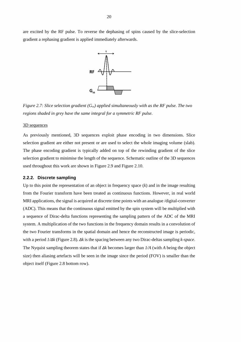
20

are excited by the RF pulse. To reverse the dephasing of spins caused by the slice-selection

gradient a rephasing gradient is applied immediately afterwards.

Figure 2.7: Slice selection gradient (Gss) applied simultaneously with as the RF pulse. The two

regions shaded in grey have the same integral for a symmetric RF pulse.

3D sequences

As previously mentioned, 3D sequences exploit phase encoding in two dimensions. Slice

selection gradient are either not present or are used to select the whole imaging volume (slab).

The phase encoding gradient is typically added on top of the rewinding gradient of the slice

selection gradient to minimise the length of the sequence. Schematic outline of the 3D sequences

used throughout this work are shown in Figure 2.9 and Figure 2.10.

2.2.2. Discrete sampling

Up to this point the representation of an object in frequency space (k) and in the image resulting

from the Fourier transform have been treated as continuous functions. However, in real world

MRI applications, the signal is acquired at discrete time points with an analogue /digital-converter

(ADC). This means that the continuous signal emitted by the spin system will be multiplied with

a sequence of Dirac-delta functions representing the sampling pattern of the ADC of the MRI

system. A multiplication of the two functions in the frequency domain results in a convolution of

the two Fourier transforms in the spatial domain and hence the reconstructed image is periodic,

with a period 1/Δk (Figure 2.8). Δk is the spacing between any two Dirac-deltas sampling k-space.

The Nyquist sampling theorem states that if Δk becomes larger than 1/A (with A being the object

size) then aliasing artefacts will be seen in the image since the period (FOV) is smaller than the

object itself (Figure 2.8 bottom row).

21

Figure 2.8: Schematic representation of sampling in 1D image space. Discrete sampling results

in a convolution (*) of the object (in this case a boxcar function) with the sampling pattern (a

series of Dirac delta functions). This can cause aliasing if the sampling frequency is less than

the Nyquist frequency (bottom row).

2.2.3. The SPGR pulse sequence

Spoiled gradient echo sequences (SPGR) are commonly used for imaging with hyperpolarised

gases. This type of sequence is also known as fast low-angle shot (FLASH) [17] and Figure 2.9

shows a schematic of the sequence diagram. The sequence employs all the above described

gradients to sample k-space: slice-selection gradient (z), a read-out gradient (x) and a phase

encoding gradient (y). The sequence diagram illustrates the gradients required for acquisition of

a single line in k-space. This sequence is repeated for different phase encode steps. The time

between two repetitions (measured from the middle of the RF pulse the middle of the next) is

called the repetition time (TR). The time from the middle of the RF pulse to the middle of the

data acquisition is the echo time (TE). The additional gradients at the end of the sequence in all

spatial directions are used to spoil (dephase) any residual magnetisation before the next repetition.

22

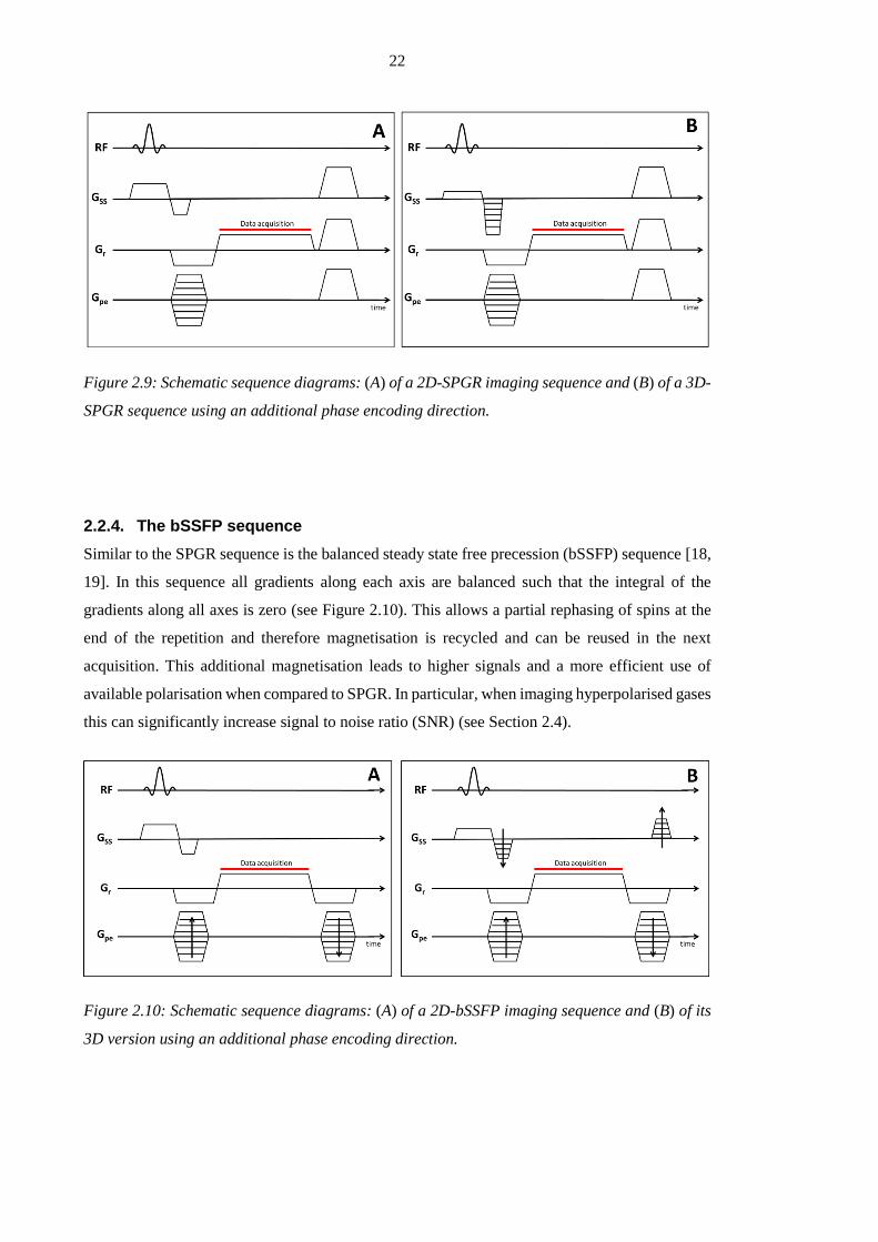
Figure 2.9: Schematic sequence diagrams: (A) of a 2D-SPGR imaging sequence and (B) of a 3D-

SPGR sequence using an additional phase encoding direction.

2.2.4. The bSSFP sequence

Similar to the SPGR sequence is the balanced steady state free precession (bSSFP) sequence [18,

19]. In this sequence all gradients along each axis are balanced such that the integral of the

gradients along all axes is zero (see Figure 2.10). This allows a partial rephasing of spins at the

end of the repetition and therefore magnetisation is recycled and can be reused in the next

acquisition. This additional magnetisation leads to higher signals and a more efficient use of

available polarisation when compared to SPGR. In particular, when imaging hyperpolarised gases

this can significantly increase signal to noise ratio (SNR) (see Section 2.4).

Figure 2.10: Schematic sequence diagrams: (A) of a 2D-bSSFP imaging sequence and (B) of its

3D version using an additional phase encoding direction.

23

2.3. Lung imaging using proton MRI

With a density of 0.1g/cm3 the 1H MR signal deriving from lung tissue is about 10 times weaker

than from the surrounding tissue [20]. In addition the numerous tissue– air interfaces in the lung

lead to magnetic susceptibility differences, which give rise to local field gradients. These

microscopic field gradients lead to short T2* relaxation times for 1H of <2ms at B0 = 1.5T. This

makes proton imaging of the lung intrinsically challenging.

Spoiled gradient echo imaging (SPGR)

SPGR imaging is fast enough to acquire whole lung coverage MR scans within a breath-hold. As

T2* in the lungs is very short partial Fourier reconstruction [21] in the frequency encoding

direction and high bandwidths (>60kHz) are typically used to ensure short TEs (~1ms) can be

achieved [20]. A specific example of SPGR is presented in Chapter 3 as a method to measure the

volume of the lung cavity. An example 1H MR image slice from a healthy volunteer using a SPGR

imaging sequence is shown in Figure 2.11A.

Balanced steady state free precession imaging (bSSFP)

bSSFP allows rephasing of magnetisation dephased by imaging gradients, however, in the

presence of field inhomogeneities so called banding artefacts can be observed [20]. bSSFP is also

associated with complex contrast behaviour (e.g. for short TRs the contrast is proportional to the

ratio T2/T1 [22]). Nevertheless, bSSFP sequences provide improved SNR over SPGR sequences

and have been shown to be useful to detect interstitial lung disease and morphologic abnormalities

in the lung [23]. An example slice acquired from a healthy volunteer using a bSSFP sequence is

shown in Figure 2.11B.

Figure 2.11: 1H Lung images from a healthy volunteer: (A) 1H lung image acquired with a SPGR

sequence. (B) Same resolution 1H lung image acquired using a bSSFP sequence. Images acquired

by the hyperpolarised gas imaging group in Sheffield.

24

Oxygen enhanced (OE) imaging

OE imaging exploits the paramagnetic properties of oxygen, which act to shorten the T1 of blood

and tissue in the lung. When breathing pure oxygen compared against breathing air, the T1-

shortening enhances the 1H MR signal [24]. Parametric maps of perfusion weighted lung

ventilation can be calculated from the difference between OE and air images. Hence T1 weighted

sequences have been facilitated to measure changes in MR signal intensity when breathing pure

oxygen, which can be used to map oxygen distribution by quantifying the T1 of lung parenchyma

[20]. Oxygen enhanced imaging has also been used to quantitatively measure lung ventilation

using signal intensity changes from images acquired during washin and washout of oxygen [25].

Despite promising results it is still not clear to what extend those images are weighted by

perfusion [20].

Fourier decomposition (FD) 1H MRI

In the FD method bSSFP images of a single slice are acquired in quick succession while subjects

are breathing freely. A Fourier frequency decomposition of the signal over time allows separation

of perfusion weighted signal (at a frequency of typically 1Hz) from ventilation weighted signal

(around 0.2Hz) caused by respiratory motion [26]. This technique has been applied to study

abnormalities in expansion of lung parenchyma in patients with cancer [27] and to deduce

ventilation weighted and perfusion weighted images in patients with pulmonary embolism and

COPD [28]. The drawback of the method is, it is currently a single slice technique.

2.4. Imaging hyperpolarised gases in the lung

2.4.1. Introduction

As briefly discussed above, proton MRI of the lungs has challenges related to available signal.

However, introducing gaseous imaging agents in the lung allows measurement of gas density and

diffusion directly in the alveolar airspaces. Hyperpolarisation of spin-½ noble gases permits

compensation of the low density of a gaseous spin system at body temperature and ambient

pressure, allowing MR imaging with high spatial and temporal resolution. This enables the

derivation of both high quality functional and structural information from images.

Most of the work presented in this thesis is based on imaging hyperpolarised 3He. This stable

isotope is chemically inert, non-toxic, and highly diffusive and has a low solubility in tissues.

However, the finite supply of 3He has caused prices to reach > $500 per litre recently [29, 30].

129Xe ($30 per litre at natural abundance) is a much cheaper alternative, although MRI with 129Xe

is more difficult since its gyromagnetic ratio is about 2.75 times lower than that of 3He (Table

25

2.1). Thus images acquired with 129Xe result in lower SNR with gas polarised to same levels as

3He, even when using 129Xe enriched xenon (129Xe isotope has a natural abundance of 26.4%).

Fluorinated gases such as sulphurhexafluoride (SF6), tetrafluorometane (CF4), and

hexafluoroethane (C2F6) can also be used for MR imaging due to the inherent 19F nuclear spin of

½. As less expensive contrast agents they can be used in a thermally polarised state. However,

imaging is therefore challenging due to the low spin-density [31]. To increase quality of images

additional averages can be acquired however, this increases scan time (and hence breath-hold).

Although most of the work presented here was done using 3He the same methods are directly

transferable to other nuclei. In fact MBW-imaging (presented in Chapter 5) is also demonstrated

using 129Xe.

2.4.2. Optical pumping

3He and 129Xe gases are hyperpolarised by optical pumping methods through the transfer of

angular momentum from circularly polarised laser light to the noble gas nucleus. There are two

commonly used methods of optical pumping to achieve high nuclear spin polarisations of 3He and

129Xe. Metastability exchange optical pumping (MEOP) is a technique of direct optical pumping

used to polarise 3He, and is capable of producing high quantities of hyperpolarised gas in a short

amount of time. Polarisation is transferred through metastability exchange collisions at low gas

pressures [32]. Spin-exchange optical pumping (SEOP) is the second method of optical pumping

and is the technique used in Sheffield for polarising both 3He and 129Xe [33]. SEOP is an indirect

method of optical pumping by which the transfer of angular momentum occurs in two steps, using

an alkali metal (usually rubidium) as an intermediate to transfer polarisation to the noble gas. The

SEOP process takes place in a glass cell heated to approximately 100°C to vaporise the rubidium

(Rb). Circularly polarised laser light at a wavelength of λ = 795nm induces a transition from the

5S1/2 ground state to the 5P1/2 state. Due to the circular polarisation of the laser light, the

electrons preferentially build up on the 5S+1/2 ground state, causing polarisation ‘↑’. The Rb

electrons can then transfer their polarisation to the noble gas nuclear spin through collisional spin

exchange [33]. The result is a net transfer of angular momentum from the circularly polarised

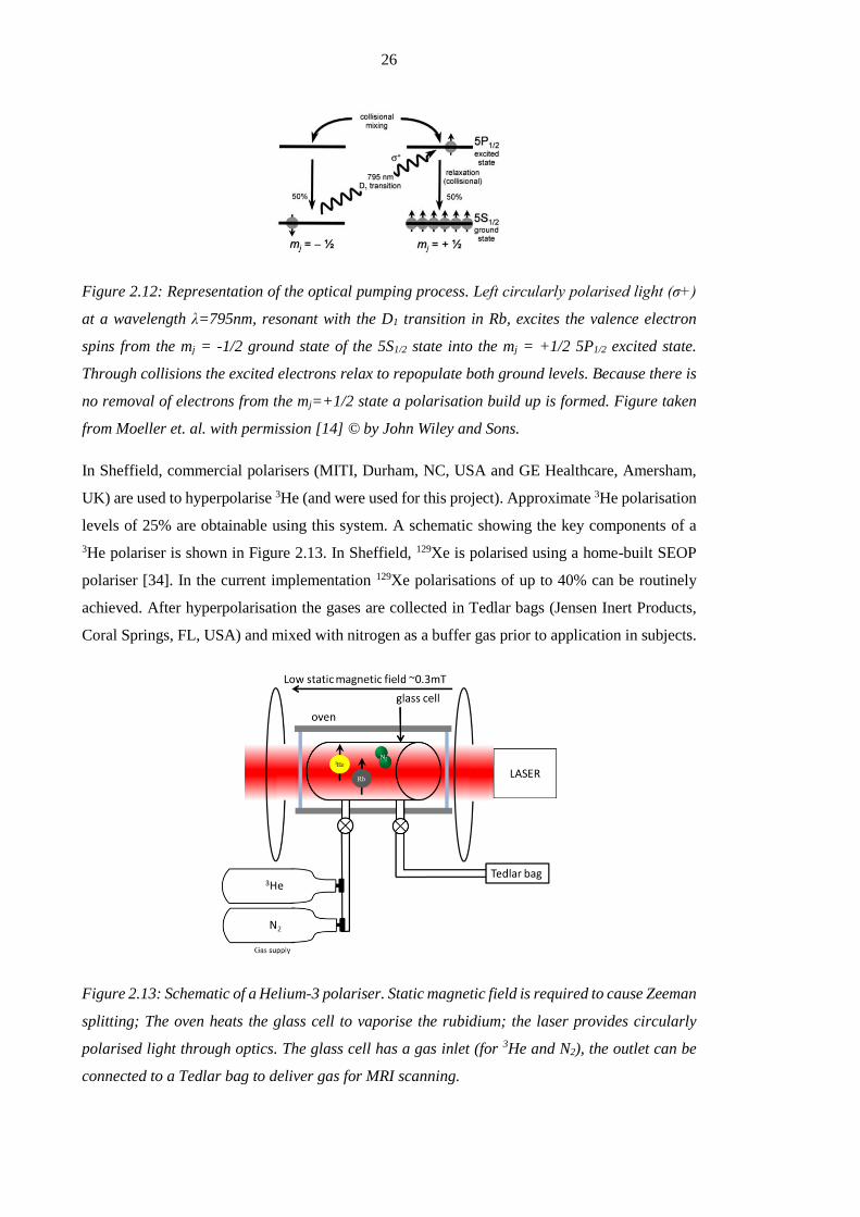
light to the nuclear spin system. This process is schematically shown in Figure 2.12 [14].

26

Figure 2.12: Representation of the optical pumping process. Left circularly polarised light (σ+)

at a wavelength λ=795nm, resonant with the D1 transition in Rb, excites the valence electron

spins from the mj = -1/2 ground state of the 5S1/2 state into the mj = +1/2 5P1/2 excited state.

Through collisions the excited electrons relax to repopulate both ground levels. Because there is

no removal of electrons from the mj=+1/2 state a polarisation build up is formed. Figure taken

from Moeller et. al. with permission [14] © by John Wiley and Sons.

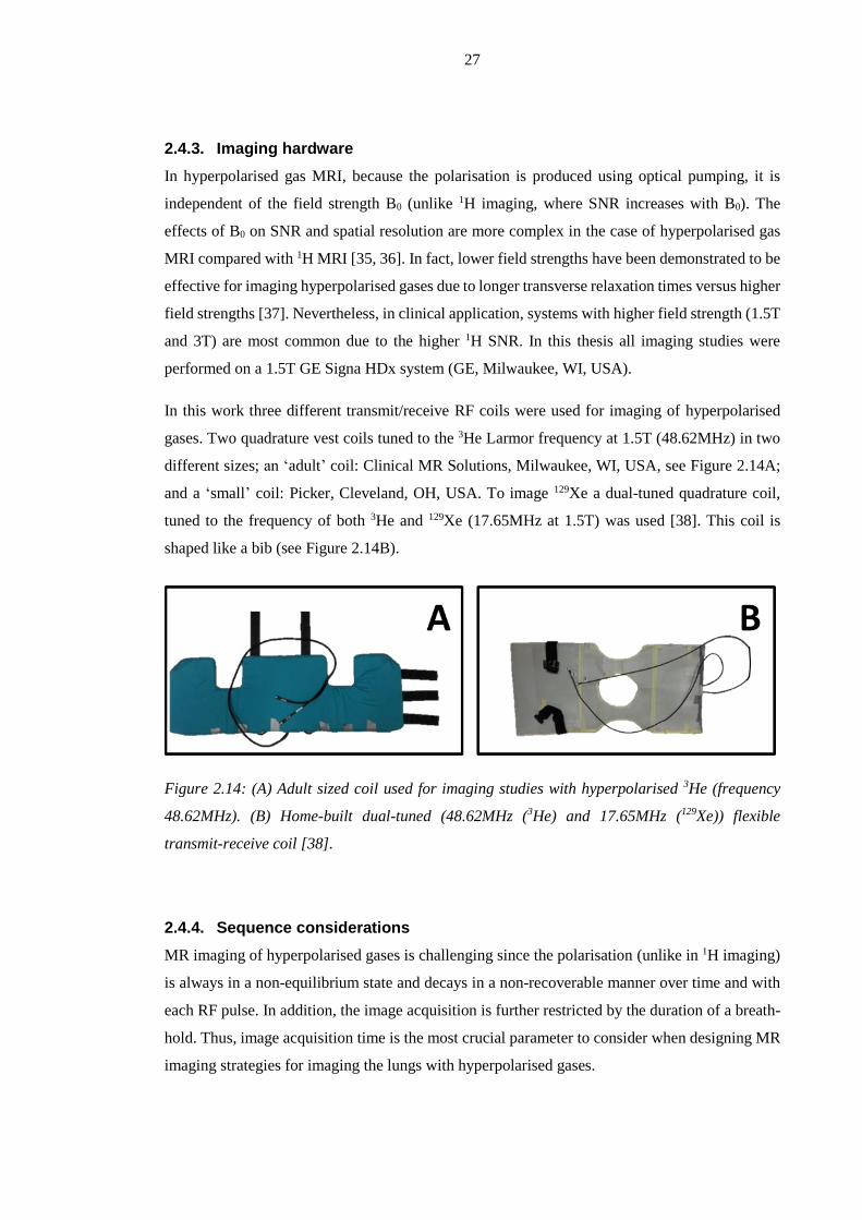
In Sheffield, commercial polarisers (MITI, Durham, NC, USA and GE Healthcare, Amersham,

UK) are used to hyperpolarise 3He (and were used for this project). Approximate 3He polarisation

levels of 25% are obtainable using this system. A schematic showing the key components of a

3He polariser is shown in Figure 2.13. In Sheffield, 129Xe is polarised using a home-built SEOP

polariser [34]. In the current implementation 129Xe polarisations of up to 40% can be routinely

achieved. After hyperpolarisation the gases are collected in Tedlar bags (Jensen Inert Products,

Coral Springs, FL, USA) and mixed with nitrogen as a buffer gas prior to application in subjects.

Figure 2.13: Schematic of a Helium-3 polariser. Static magnetic field is required to cause Zeeman

splitting; The oven heats the glass cell to vaporise the rubidium; the laser provides circularly

polarised light through optics. The glass cell has a gas inlet (for 3He and N2), the outlet can be

connected to a Tedlar bag to deliver gas for MRI scanning.

27

2.4.3. Imaging hardware

In hyperpolarised gas MRI, because the polarisation is produced using optical pumping, it is

independent of the field strength B0 (unlike 1H imaging, where SNR increases with B0). The

effects of B0 on SNR and spatial resolution are more complex in the case of hyperpolarised gas

MRI compared with 1H MRI [35, 36]. In fact, lower field strengths have been demonstrated to be

effective for imaging hyperpolarised gases due to longer transverse relaxation times versus higher

field strengths [37]. Nevertheless, in clinical application, systems with higher field strength (1.5T

and 3T) are most common due to the higher 1H SNR. In this thesis all imaging studies were

performed on a 1.5T GE Signa HDx system (GE, Milwaukee, WI, USA).

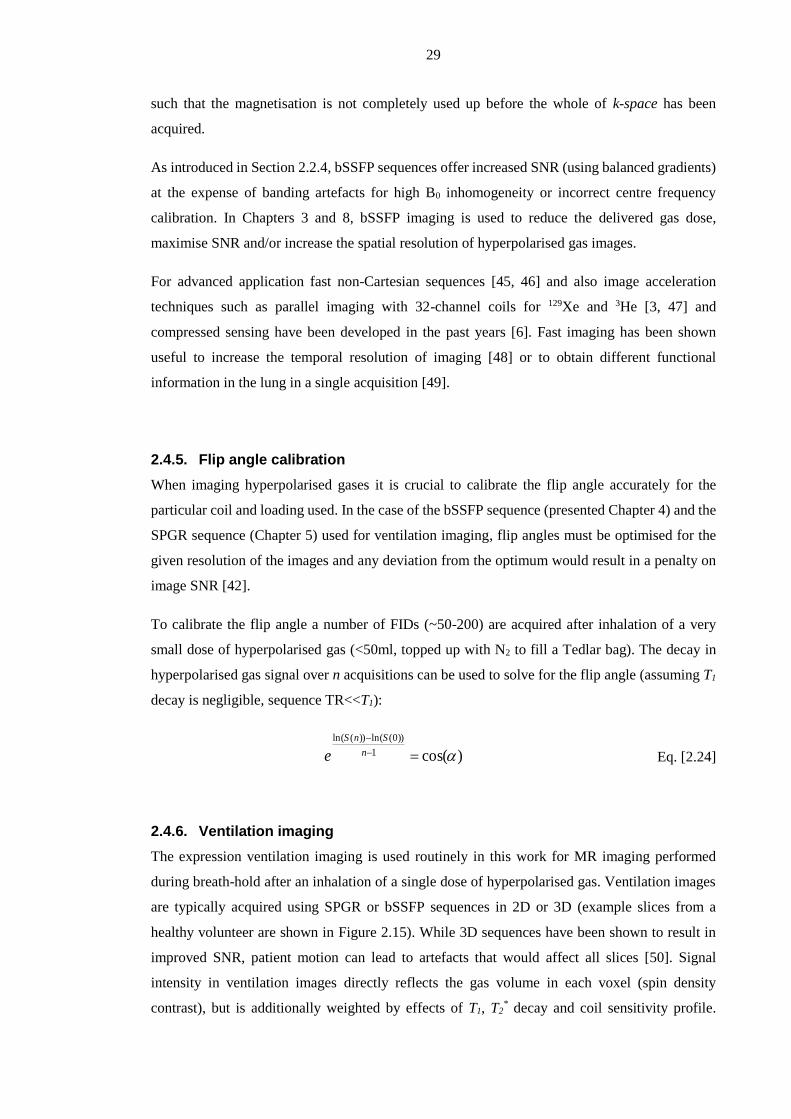
In this work three different transmit/receive RF coils were used for imaging of hyperpolarised

gases. Two quadrature vest coils tuned to the 3He Larmor frequency at 1.5T (48.62MHz) in two

different sizes; an ‘adult’ coil: Clinical MR Solutions, Milwaukee, WI, USA, see Figure 2.14A;

and a ‘small’ coil: Picker, Cleveland, OH, USA. To image 129Xe a dual-tuned quadrature coil,

tuned to the frequency of both 3He and 129Xe (17.65MHz at 1.5T) was used [38]. This coil is

shaped like a bib (see Figure 2.14B).

Figure 2.14: (A) Adult sized coil used for imaging studies with hyperpolarised 3He (frequency

48.62MHz). (B) Home-built dual-tuned (48.62MHz (3He) and 17.65MHz (129Xe)) flexible

transmit-receive coil [38].

2.4.4. Sequence considerations

MR imaging of hyperpolarised gases is challenging since the polarisation (unlike in 1H imaging)

is always in a non-equilibrium state and decays in a non-recoverable manner over time and with

each RF pulse. In addition, the image acquisition is further restricted by the duration of a breath-

hold. Thus, image acquisition time is the most crucial parameter to consider when designing MR

imaging strategies for imaging the lungs with hyperpolarised gases.

28

The longitudinal magnetisation of a hyperpolarised gas relaxes towards the thermal equilibrium

value with a time constant T1. In the absence of paramagnetic oxygen or other paramagnetic

impurities the T1 of 3He and 129Xe can be many hours [39]. However, in the presence of oxygen

the T1 shortens dramatically and upon inhalation in the lung T1 is ~20-30s. The inverse of T1 is

linearly related to partial oxygen pressure:

1

2T

pO

Eq. [2.21]

At room temperature the proportionality constant has been empirically determined to be

2.61bar∙s for 3He [40]. This low T1 value places restrictions on acquisition time. In addition, the

high self-diffusion of noble gases (D0-3He = 1.85cm2∙s-1 and D0-129Xe=0.058cm2∙s-1 [41]) compared

water protons contributes to an increased signal attenuation due to Brownian motion of the gas

atoms in the presence of magnetic field gradients.

SPGR sequences (see Section 2.2.3) are most commonly used to image hyperpolarised gases [42].

The use of low flip angles preserves non-recoverable magnetisation throughout acquisition of k-

space. Strong spoiler gradients after each data acquisition act to dephase residual transverse

magnetisation, preparing the spin-system for another data acquisition and allowing minimal TR.

This spoiling is necessary for hyperpolarised gases to avoid interference of residual magnetisation

with the subsequent acquisition (since T2* relaxation can be relatively long with ~30ms for 3He

and 129Xe at 1.5T [36, 43]). The transverse magnetisation used for imaging hyperpolarised gas

can be described as a function of acquisitions number (or RF pulse) n as follows:

1

1

10

T

TRn

n

xy eMnM

)(

)sin()cos()( Eq. [2.22]

For sequential Cartesian sampling of k-space, the optimal flip angle therefore be derived by

maximising the signal at the centre of k-space is [42]:

))12/arctan(( 2/1 Nopt Eq.[ 2.23]

for N total phase encoding steps. Nevertheless, using constant flip angle will continually deplete

the transversal magnetisation available for imaging with each data acquisition, leading to blurred

images, since the edges of k-space along phase encoding direction are acquired last [42].To

maximise the use of available magnetisation a variable flip angle (VFA) scheme can be applied

[44]. This reduces the effects of k-space filtering by maintaining a constant transverse

magnetisation for each phase encoding step. VFA requires a careful calibration of the flip angle,

29

such that the magnetisation is not completely used up before the whole of k-space has been

acquired.

As introduced in Section 2.2.4, bSSFP sequences offer increased SNR (using balanced gradients)

at the expense of banding artefacts for high B0 inhomogeneity or incorrect centre frequency

calibration. In Chapters 3 and 8, bSSFP imaging is used to reduce the delivered gas dose,

maximise SNR and/or increase the spatial resolution of hyperpolarised gas images.

For advanced application fast non-Cartesian sequences [45, 46] and also image acceleration

techniques such as parallel imaging with 32-channel coils for 129Xe and 3He [3, 47] and

compressed sensing have been developed in the past years [6]. Fast imaging has been shown

useful to increase the temporal resolution of imaging [48] or to obtain different functional

information in the lung in a single acquisition [49].

2.4.5. Flip angle calibration

When imaging hyperpolarised gases it is crucial to calibrate the flip angle accurately for the

particular coil and loading used. In the case of the bSSFP sequence (presented Chapter 4) and the

SPGR sequence (Chapter 5) used for ventilation imaging, flip angles must be optimised for the

given resolution of the images and any deviation from the optimum would result in a penalty on

image SNR [42].

To calibrate the flip angle a number of FIDs (~50-200) are acquired after inhalation of a very

small dose of hyperpolarised gas (<50ml, topped up with N2 to fill a Tedlar bag). The decay in

hyperpolarised gas signal over n acquisitions can be used to solve for the flip angle (assuming T1

decay is negligible, sequence TR<<T1):

)cos(1

))0(ln())(ln(

n

SnS

e Eq. [2.24]

2.4.6. Ventilation imaging

The expression ventilation imaging is used routinely in this work for MR imaging performed

during breath-hold after an inhalation of a single dose of hyperpolarised gas. Ventilation images

are typically acquired using SPGR or bSSFP sequences in 2D or 3D (example slices from a

healthy volunteer are shown in Figure 2.15). While 3D sequences have been shown to result in

improved SNR, patient motion can lead to artefacts that would affect all slices [50]. Signal

intensity in ventilation images directly reflects the gas volume in each voxel (spin density

contrast), but is additionally weighted by effects of T1, T2* decay and coil sensitivity profile.

30

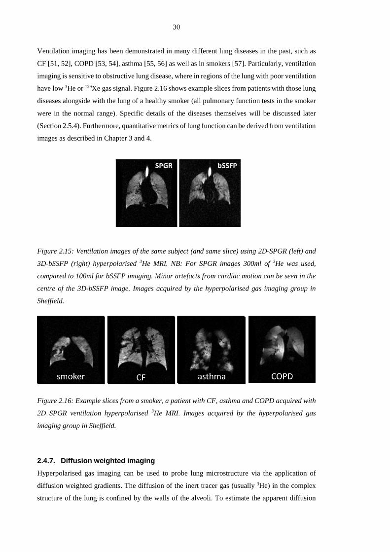
Ventilation imaging has been demonstrated in many different lung diseases in the past, such as

CF [51, 52], COPD [53, 54], asthma [55, 56] as well as in smokers [57]. Particularly, ventilation

imaging is sensitive to obstructive lung disease, where in regions of the lung with poor ventilation

have low 3He or 129Xe gas signal. Figure 2.16 shows example slices from patients with those lung

diseases alongside with the lung of a healthy smoker (all pulmonary function tests in the smoker

were in the normal range). Specific details of the diseases themselves will be discussed later

(Section 2.5.4). Furthermore, quantitative metrics of lung function can be derived from ventilation

images as described in Chapter 3 and 4.

Figure 2.15: Ventilation images of the same subject (and same slice) using 2D-SPGR (left) and

3D-bSSFP (right) hyperpolarised 3He MRI. NB: For SPGR images 300ml of 3He was used,

compared to 100ml for bSSFP imaging. Minor artefacts from cardiac motion can be seen in the

centre of the 3D-bSSFP image. Images acquired by the hyperpolarised gas imaging group in

Sheffield.

Figure 2.16: Example slices from a smoker, a patient with CF, asthma and COPD acquired with

2D SPGR ventilation hyperpolarised 3He MRI. Images acquired by the hyperpolarised gas

imaging group in Sheffield.

2.4.7. Diffusion weighted imaging

Hyperpolarised gas imaging can be used to probe lung microstructure via the application of

diffusion weighted gradients. The diffusion of the inert tracer gas (usually 3He) in the complex

structure of the lung is confined by the walls of the alveoli. To estimate the apparent diffusion

31

coefficient (ADC) of 3He, two sets of ventilation images are required with the exact same timing:

one with diffusion weighting gradients, and one without. From the difference in measured signal

intensity between the two sets of images and knowledge of the gradient waveform and duration

(b-value), ADC values can be calculated. Hence ADC maps of the lungs can be generated; this

has enabled quantification of tissue destruction in emphysema for example, on regions where the

ADC is large [58]. In the literature mathematical models have been proposed to draw conclusions

about lung microstructure from measurements of different diffusion length scales. The so-called

cylinder model treats the alveolar ducts as infinitely long cylinders isotropically oriented in space

[59]. Application of this model to 3He ADC data permits estimation of lung microstructural

parameters e.g. alveolar duct diameter. However, it has been shown that acinar branching and the

finite length of the airways have a significant influence upon the 3He diffusivity [37] and recently

a method based solely on fractal exponential analysis (independent of modelling) has been

developed [60].

Figure 2.17: ADC maps of a healthy volunteer (left) and a COPD patient (right). High ADC

values indicate structural damage to the lung tissue/alveolar walls in the COPD patient as shown

in the schematic on top. Images acquired by the hyperpolarised gas imaging group in Sheffield.

2.4.8. Imaging of partial oxygen pressure

As presented in Section 2.4.4, Saam. et. al. discovered an inverse linear dependence of T1 with

partial oxygen pressure pO2 (see Eq. [2.21]) as mentioned before [20]. Therefore measurement of

the T1 of hyperpolarised 3He allows determination of alveolar pO2. In order to properly calculate

the pO2, RF depolarisation of the hyperpolarised gas signal must be separated from the oxygen

32

induced signal decay. A minimum of three subsequent imaging acquisitions is therefore

necessary. The time evolution of alveolar pO2 can be followed over multiple time points using a

method of acquiring two series of images as first demonstrated by Deninger et al.[61]. More

recent methods use only one single breath-hold to obtain regional maps of pO2 [62, 63]. These

methods require the assumption that pO2 decay in the lung is linear with time. This might be true

for short breath-holds, but recent work has suggested an exponential fitting of the 3He signal

decay might be more accurate for longer breath-holds [64].

Figure 2.18: Map of regional pO2 measured in the lungs of a healthy volunteer obtained with

hyperpolarised 3He MRI. Average pO2 is 150mbar, in agreement with literature values [65].

Images acquired by the hyperpolarised gas imaging group in Sheffield.

2.4.9. Conclusion

Over the past 20 years hyperpolarised gas MRI has become established as a comprehensive tool

with a multitude of methods to probe different functional and structural aspects of the lung.

Despite major improvements in sequence design and of polarisation technology expectations of

bringing this technique into the clinical routine have yet to be fulfilled. In parts this might be

attributed to the cost of 3He, but future research must also focus on the definition of new

quantitative measurement methods and metrics that underline the additional value that the

increased sensitivity and regional insight into disease processes offered by hyperpolarised gas

imaging can add to standard pulmonary function tests.

Finally, a wide variety of methods and derived metrics have been developed over the past few

years. Methods such as phase contrast velocimetry to measure flow [66] or chemical shift

saturation recovery of 129Xe to measure alveolar wall thickness [67] are just two examples of the

broad spectrum of promising applications using hyperpolarised gas MRI, and there are many more

that cannot be covered in this thesis.

33

2.5. Pulmonary Function Testing

2.5.1. Pulmonary structure

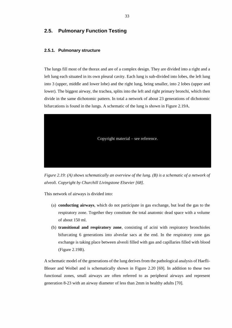
The lungs fill most of the thorax and are of a complex design. They are divided into a right and a

left lung each situated in its own pleural cavity. Each lung is sub-divided into lobes, the left lung

into 3 (upper, middle and lower lobe) and the right lung, being smaller, into 2 lobes (upper and

lower). The biggest airway, the trachea, splits into the left and right primary bronchi, which then

divide in the same dichotomic pattern. In total a network of about 23 generations of dichotomic

bifurcations is found in the lungs. A schematic of the lung is shown in Figure 2.19A.

Figure 2.19: (A) shows schematically an overview of the lung. (B) is a schematic of a network of

alveoli. Copyright by Churchill Livingstone Elsevier [68].

This network of airways is divided into:

(a) conducting airways, which do not participate in gas exchange, but lead the gas to the

respiratory zone. Together they constitute the total anatomic dead space with a volume

of about 150 ml.

(b) transitional and respiratory zone, consisting of acini with respiratory bronchioles

bifurcating 6 generations into alveolar sacs at the end. In the respiratory zone gas

exchange is taking place between alveoli filled with gas and capillaries filled with blood

(Figure 2.19B).

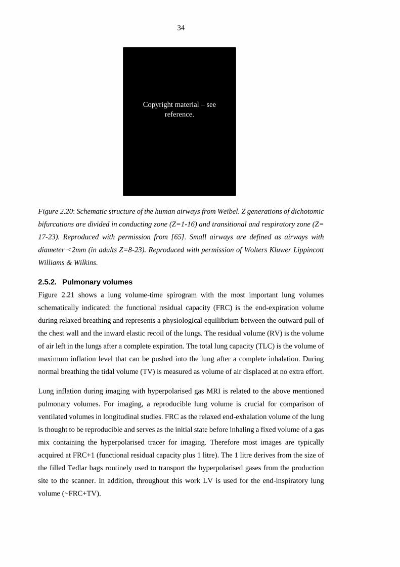
A schematic model of the generations of the lung derives from the pathological analysis of Haefli-

Bleuer and Weibel and is schematically shown in Figure 2.20 [69]. In addition to these two

functional zones, small airways are often referred to as peripheral airways and represent

generation 8-23 with an airway diameter of less than 2mm in healthy adults [70].

Copyright material – see reference.

34

Figure 2.20: Schematic structure of the human airways from Weibel. Z generations of dichotomic

bifurcations are divided in conducting zone (Z=1-16) and transitional and respiratory zone (Z=

17-23). Reproduced with permission from [65]. Small airways are defined as airways with

diameter <2mm (in adults Z=8-23). Reproduced with permission of Wolters Kluwer Lippincott

Williams & Wilkins.

2.5.2. Pulmonary volumes

Figure 2.21 shows a lung volume-time spirogram with the most important lung volumes

schematically indicated: the functional residual capacity (FRC) is the end-expiration volume

during relaxed breathing and represents a physiological equilibrium between the outward pull of

the chest wall and the inward elastic recoil of the lungs. The residual volume (RV) is the volume

of air left in the lungs after a complete expiration. The total lung capacity (TLC) is the volume of

maximum inflation level that can be pushed into the lung after a complete inhalation. During

normal breathing the tidal volume (TV) is measured as volume of air displaced at no extra effort.

Lung inflation during imaging with hyperpolarised gas MRI is related to the above mentioned

pulmonary volumes. For imaging, a reproducible lung volume is crucial for comparison of

ventilated volumes in longitudinal studies. FRC as the relaxed end-exhalation volume of the lung

is thought to be reproducible and serves as the initial state before inhaling a fixed volume of a gas

mix containing the hyperpolarised tracer for imaging. Therefore most images are typically

acquired at FRC+1 (functional residual capacity plus 1 litre). The 1 litre derives from the size of

the filled Tedlar bags routinely used to transport the hyperpolarised gases from the production

site to the scanner. In addition, throughout this work LV is used for the end-inspiratory lung

volume (~FRC+TV).

Copyright material – see

reference.

35

Figure 2.21: Volume-time curve of tidal breathing (FRC=functional residual capacity) followed

by a complete exhalation to residual volume (RV) and inhalation to total lung capacity (TLC).

Expiratory reserve volume (ERV), inspiratory capacity (IC) as well as inspiratory vital capacity

(IVC) are derived from this curve. Adapted version reproduced with permission of the European

Respiratory Society © Eur Respir J March 2013 [71].

2.5.3. Lung function

Before explaining the primary function of the lung, which is gas exchange with the blood, the

mechanism of how gas gets to the alveoli needs to be addressed. Ventilation is the process of gas

turnover via inhalation and exhalation in order to transport oxygenated air into the lung and

remove deoxygenated air. Gas turnover is the movement of air along pressure gradients generated

by volume changes of the respiratory system. Those pressure gradients are created by volume

changes of the expandable lung tissue. Volume changes are the response to the summation of

forces applied to lung and chest wall from respiratory musculature that combine to drive the air

into and out of the lung. The continuous turnover of gas in the lungs supplies the lung with oxygen

and transports air with increased carbon dioxide away. The difference of gas concentration in the

blood and alveoli creates pressure gradients leading gas to diffuse through lung tissue of

approximately 0.3µm thickness: Oxygen diffuses into the blood and CO2 into the alveoli. Under

normal conditions (tidal breathing of air) gas exchange depends on three major factors: (a) the

thickness of the alveolar-capillary wall (b) the mixture and concentration of the gases present in

the lung and (c) the volume of blood available for gas exchange. Different lung diseases can affect

these pathways individually, by different pathophysiological mechanisms resulting in a less

efficient gas exchange [65, 72].

2.5.4. Lung disease

A number of diseases influence gas exchange directly or indirectly. Thickening of the alveolar-

capillary walls leads to a prolonged gas exchange due to increased septal diffusion times (i.e.


36

from fibrogen deposition in idiopathic pulmonary fibrotic disease). Indirect effects on gas

exchange include ventilatory dysfunction and diseases involving the pulmonary vasculature,

where capillary uptake is altered by impaired cardiopulmonary circulation. The focus of this work

is on heterogeneous ventilation related to airflow obstruction.

In obstructive lung disease airflow and ventilation are regionally impaired. This causes an

inhomogeneous distribution and mixing of gas in the lung commonly referred to as ventilation

heterogeneity (VH). Ventilation is known to be heterogeneous in healthy volunteers and increase

with age [73]. VH increases considerably in obstructed lungs with airway narrowing or blockage

and resulting in an insufficient supply with fresh gas. As a result of a reduced turnover of gas, the

lack of oxygen and increased CO2 levels influence gas exchange efficiency. Therefore patients

with severe obstructive airway disease cannot supply alveoli with enough oxygen and suffer from

breathlessness. Obstructive lung diseases are the target of studies presented here and the

quantitative imaging methods discussed throughout this work are sensitive to changes in

ventilation. Techniques presented in Chapter 3, 4 and 5 are tested on an asthma and a cystic

fibrosis cohort.

Asthma

Asthma is a chronic inflammatory pulmonary disease characterised by reversible obstruction of

airways as a result of bronchial hyper-responsiveness [74]. Obstruction leading to restricted

airflow derives from reversible bronchoconstriction, inflammation of the airway walls and

chronic mucus plugging [75]. Starting in the peripheral airways, the inflammatory process can

result in remodelling of the airways, if not detected early [76, 77]. The hyper-responsiveness of

airways to different direct (histamine, methacholine) and indirect stimuli (exercise, cold or dry

air) results in bronchoconstriction as a response to inflammatory mediators [78].

Cystic fibrosis

Cystic fibrosis (CF) is a genetic disorder that affects function of liver, pancreas, intestine and the

lungs. About 1 in 2500 children is diagnosed with this life-shortening disorder in Causcasian

people [79]. CF patients do not possess a working copy of the gene for the protein cystic fibrosis

transmembrane conductance regulator that is needed to regulate components of mucus, sweat and

digestive fluids. This mutation results in build up of mucus in the lung, leading to airway blockage

and inflammation. Despite early detection through new-born screening and advances over the

past decades, life expectancy of CF patients is with a median of 36.6 years (in the UK in 2013)

much lower than healthy subjects [80]. An early detection of increased ventilation heterogeneity

is crucial to decide on treatment pathways.

37

COPD

Chronic obstructive pulmonary disease is characterised by irreversible airflow obstruction. Its

prevalence is increasing majorly caused by effects of smoking [81]. COPD is used as an umbrella

term to describe a disease encompassing chronic bronchitis and emphysema and most patients

have elements of both conditions [82]. Chronic bronchitis can derive long term exposure with

cigarette smoke or other inhaled irritants and is associated with structural narrowing of the small

airways because of chronic inflammation. Emphysema is characterised by destruction of airway

walls in the distal airways of the respiratory zone, loss of elastic recoil and rapid airway closure

on expiration [74, 83]. As late diagnosis and under-treatment are seen as one of the major causes

for high mortality from COPD an early detection and treatment is important to improve the long-

term prognosis to prevent irreversible losses of lung function [82].

2.5.5. Measuring respiratory function

Respiratory function can be directly measured using a variety of breathing tests performed at rest

and during exercise. These tests can be used to assess: (1) airflow through the respiratory tract

[71, 84]; (2) gas distribution throughout the airways [73, 85, 86]; (3) the efficiency of gas

exchange [65]; just to name the most important ones. Some measures, such as spirometry, are

well established and are commonly used in clinical practice and clinical trials. Others are less

established but have great potential to be useful in the future, such as the multiple breath washout

test (MBW), which measures behaviour of tracer gases in the lung. In the following a brief

overview is given of lung function tests used in this thesis as comparison to functional imaging

metrics.

2.5.5.1. Flow derived metrics - spirometry

Spirometry is the measurement of flow and lung volumes. Modern spirometry uses a

pneumotachograph deriving flow and volume from pressure differences measured with sensors

at the mouth. The following parameters are usually reported from spirometry [84]: FEV1, the

forced expired volume in one second, and FVC, the forced vital capacity. In addition, maximum

flow-volume loops (MFVL) are acquired for visual recognition of typical disease patterns. Two

flow-volume loops acquired during spirometry are shown in Figure 2.22. Example A of that figure

is a healthy volunteer with a predicted FEV1 of 109% [71]. Example B displays the MFVL of a

subject of similar height and weight with a significantly reduced FEV1 (25%), indicating severe

airflow limitation as found in obstructive pulmonary diseases. In addition this patient has a

severely decreased FVC (compare flow-volume loops of A and B) with a flat flow in the second

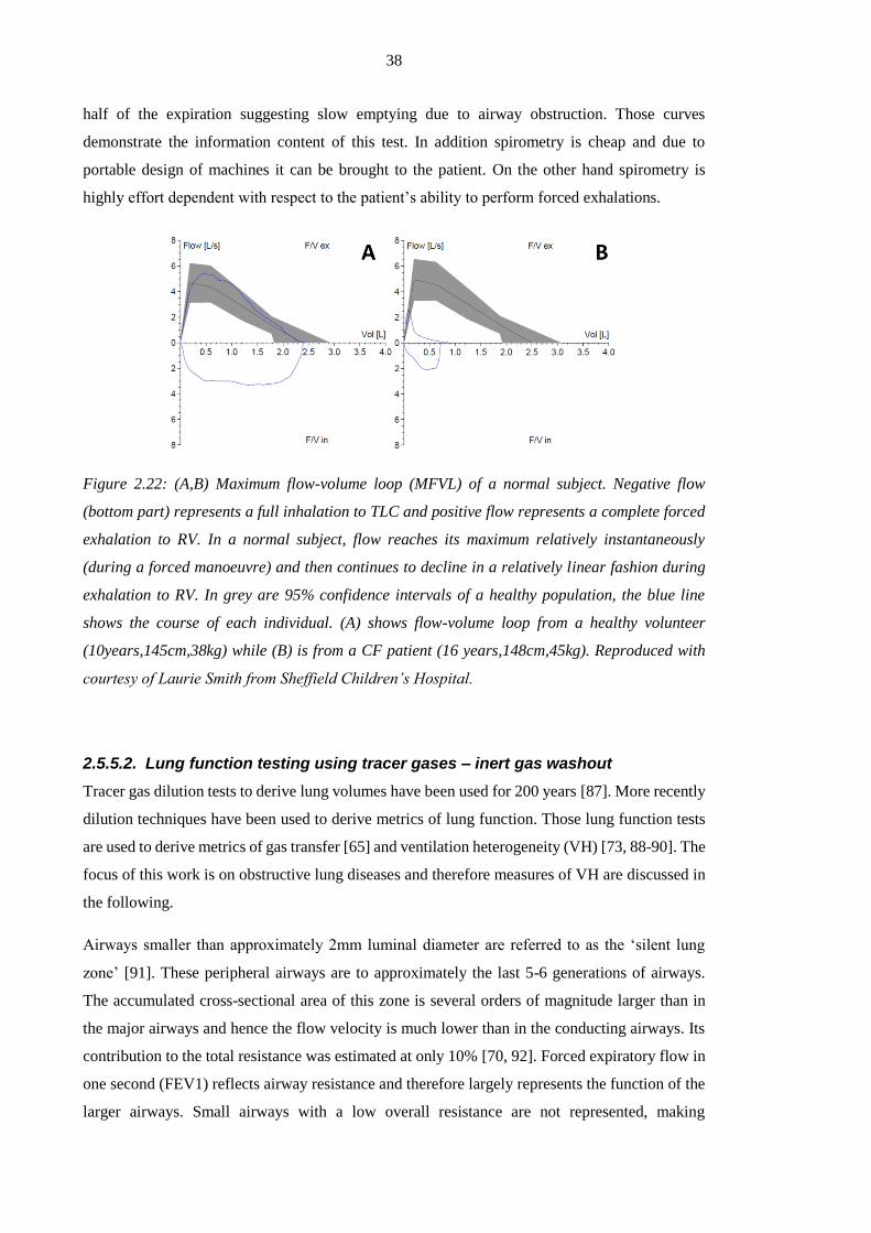
38

half of the expiration suggesting slow emptying due to airway obstruction. Those curves

demonstrate the information content of this test. In addition spirometry is cheap and due to

portable design of machines it can be brought to the patient. On the other hand spirometry is

highly effort dependent with respect to the patient’s ability to perform forced exhalations.

Figure 2.22: (A,B) Maximum flow-volume loop (MFVL) of a normal subject. Negative flow

(bottom part) represents a full inhalation to TLC and positive flow represents a complete forced

exhalation to RV. In a normal subject, flow reaches its maximum relatively instantaneously

(during a forced manoeuvre) and then continues to decline in a relatively linear fashion during

exhalation to RV. In grey are 95% confidence intervals of a healthy population, the blue line

shows the course of each individual. (A) shows flow-volume loop from a healthy volunteer

(10years,145cm,38kg) while (B) is from a CF patient (16 years,148cm,45kg). Reproduced with

courtesy of Laurie Smith from Sheffield Children’s Hospital.

2.5.5.2. Lung function testing using tracer gases – inert gas washout

Tracer gas dilution tests to derive lung volumes have been used for 200 years [87]. More recently

dilution techniques have been used to derive metrics of lung function. Those lung function tests

are used to derive metrics of gas transfer [65] and ventilation heterogeneity (VH) [73, 88-90]. The

focus of this work is on obstructive lung diseases and therefore measures of VH are discussed in

the following.

Airways smaller than approximately 2mm luminal diameter are referred to as the ‘silent lung

zone’ [91]. These peripheral airways are to approximately the last 5-6 generations of airways.

The accumulated cross-sectional area of this zone is several orders of magnitude larger than in

the major airways and hence the flow velocity is much lower than in the conducting airways. Its

contribution to the total resistance was estimated at only 10% [70, 92]. Forced expiratory flow in

one second (FEV1) reflects airway resistance and therefore largely represents the function of the

larger airways. Small airways with a low overall resistance are not represented, making

39

spirometry a less sensitive test for detecting changes in the small airways. This has systematically

been proven in animal experiments [93]. In cystic fibrosis (CF) it has been shown that the early

lung changes occur peripherally in small airways [94]. FEV1 is broadly used in CF to assess lung

function, but other methods have been suggested as more sensitive measures of early changes [92,

95]. By the time a change in FEV1 is detected the disease has already caused major damage [96-

99]. Similar peripheral airway restructuring has also been verified in asthma and chronic

obstructive lung disease (COPD) [100]. Also early emphysema related to smoking damage of the

alveoli can go undetected by spirometry. Therefore alternative lung function testing has been

suggested for early detection of those diseases [95].

Inert gas washout (IGW) as a measure of gas mixing efficiency is used to assess VH. IGW was

described as a pulmonary function test in the first half of the last century [101]. Instead of using

flow or volumes as a surrogate of ventilation efficiency, the gas composition is measured using

inert gas washout upon single or multiple exhalations. While Darling et al. [101] were interested

in the process of 100% oxygen replacing the present alveolar nitrogen their colleagues Mundt et

al. looked into the feasibility to measure the composition of alveolar gas in a single breath [102].

With those two publications, the basis of the two principal IGW tests was laid: single breath

washout (SBW) and multiple breath washout (MBW). Both lung function tests sample the

composition of exhaled gases - one over a single breath (SBW) the other over multiple breaths

(MBW). Therefore they both rely on accurate measurement of gas composition with a high

temporal resolution. The introduction of mass spectrometers into respiratory research made

precise measurement of gas concentrations feasible for clinical practice [103]. Due to the

capability to directly measure partial mass of more than one gas with a good temporal resolution,

the mass spectrometer still remains the gold standard [104, 105]. Today’s development of reliable

IGW systems with enhanced optical and acoustic sensors has increased the interest in this lung

function test. The user friendly compact systems have been validated against mass-spectrometry

using SF6 [95] and N2 [106, 107] as tracer gases. In the following SBW and MBW are described

in further detail.

Single breath washout (SBW)

Single breath washout measures concentration change of a tracer gas during a single expiration.

Most commonly nitrogen concentration is sampled over a full expiration to RV after a single

inspiration of 100% oxygen [89]. Figure 2.23 shows the result of a SBW from a healthy volunteer.

The N2 concentration is plotted against accumulated exhaled total gas volume. The curve is

divided into 4 phases: phase I, where the inhaled oxygen has completely washed out all N2 and

therefore no concentration of N2 is measured; phase II (the bronchial phase) with a fast rising N2

40

concentration leading to phase III the alveolar phase and finally phase IV of the washout referred

to as closing volume with a fast rising slope. From each phase different parameters have been

derived: phase I & II is used to calculate Fowler-dead space [108], phase III, a slope (phase III

slope) as a measure of VH [109], phase IV measuring the closing volume (CV) [110].

Figure 2.23: SBW after single inhalation of 100% oxygen. Dead space is derived from phase I,

phase II is the bronchial phase with a rising N2 concentration until phase III with a constant slope

(alveolar phase, 25-75% of exhaled volume) used to derive ventilation heterogeneity (SIII as the

dotted line) and phase IV as the fast rising end of expiration used to derive the closing volume

(CV). Reproduced with permission of the European Respiratory Society © Eur Respir J 2013

[105].

Multiple breath washout (MBW)

Multiple breath washout (MBW) was established more than 70 years ago [111] and has gained

popularity in recent years. It has been successfully tested for sensitivity to changes in disease in

different patient populations such as cystic fibrosis [95, 97, 98, 112, 113], asthma [114] as well

as chronic obstructive pulmonary disease (COPD) [115] and asymptomatic smokers [116].

Methods

MBW measures the concentration decay during gas washout over multiple breaths. The observed

tracer gas can either be naturally present in the air (e.g. N2) or an exogenous tracer gas washed in

to the lungs before MBW (e.g. SF6). Due to the easy access to oxygen, N2 washout using wash-

in of 100% oxygen is broadly used in the clinic. Nevertheless, up to this point it is still not clear

to which extent nitrogen dissolved in tissue and blood influences the outcome of a MBW


41

measurement. In recent work it has been shown to significantly alter the outcome of metrics

derived from MBW [117]. Therefore, in this thesis all MBW tests were performed using SF6

washout. MBW was performed in compliance with the ERS-ATS guidelines [105]. For the

purposes of this work MBW was performed using a modified photoacoustic analyser (Innocor,

Innovision, Glamsbjerg, Denmark) and SF6 as the tracer gas mixed with air as (0.2% SF6 in the

gas mix) [95]. The experimental setup is shown in Figure 2.24A. A gas cylinder provides air

mixed with the tracer gas (red), the analyser records flow and tracer gas concentration (blue). A

fan prevents rebreathing of tracer gas during the washout (green). Figure 2.24B shows the setup

at the patient’s mouth in greater detail. During an initial phase of the MBW, the SF6/air mix is

washed into the lungs until equilibrium is reached between the concentrations of inhaled and

exhaled gas. The difference between inspirational concentration and exspirational concentration

should be less than approximately 0.1‰. Afterwards the flowpast2 (marked with a red square,

Figure 2.24B) is removed to allow the subject to breathe air. This enables the washout of SF6 from

the lungs. The washout of SF6 continues until the SF6 concentration has fallen below 1/40th of the

concentration at the end of the tracer gas washin phase. The resulting recordings of flow and

tracer gas concentration during a MBW are shown in Figure 2.25.

Figure 2.24: (A) Setup of a MBW experiment. (B) Detailed view of system setup.

2 A flowpast is a t-piece with a tube supplying constant gas flow attached at one side, an exhaust on the

opposite side and the subject breathing from the third side (Figure 2.24B). A constant flow higher than

the maximum inspiratory flow assures that the gas mix supplied at the inlet is inhaled by subjects.

42

Figure 2.25: Recording from an SF6 MBW in a healthy volunteer. Top figure: flow-time curve

acquired during experiment to calculate accumulated exhaled volume. Bottom figure: tracer gas

concentration over time. After wash-in to equilibrium concentration, the tracer gas supply is

disconnected and the washout begins (approximately at t=33s).

The lung clearance index (LCI)

A variety of metrics have been derived from MBW to probe ventilation heterogeneity [73, 118-

120]. The most widely used is the lung clearance index (LCI). LCI is calculated as the amount of

lung turn-overs (ratio of accumulated expiratory volume to FRC) needed to reduce end tidal tracer

gas concentration (Cet3) to 1/40th of its initial values [121]:

FRC

iTV

dtFRC

tVLCI

n

i

t

t

exhale

end

1

0

)()(

Eq. [2.25]

3 Cet = end tidal concentration. End tidal concentration is referred to as the gas concentration at the end of

an exhalation.

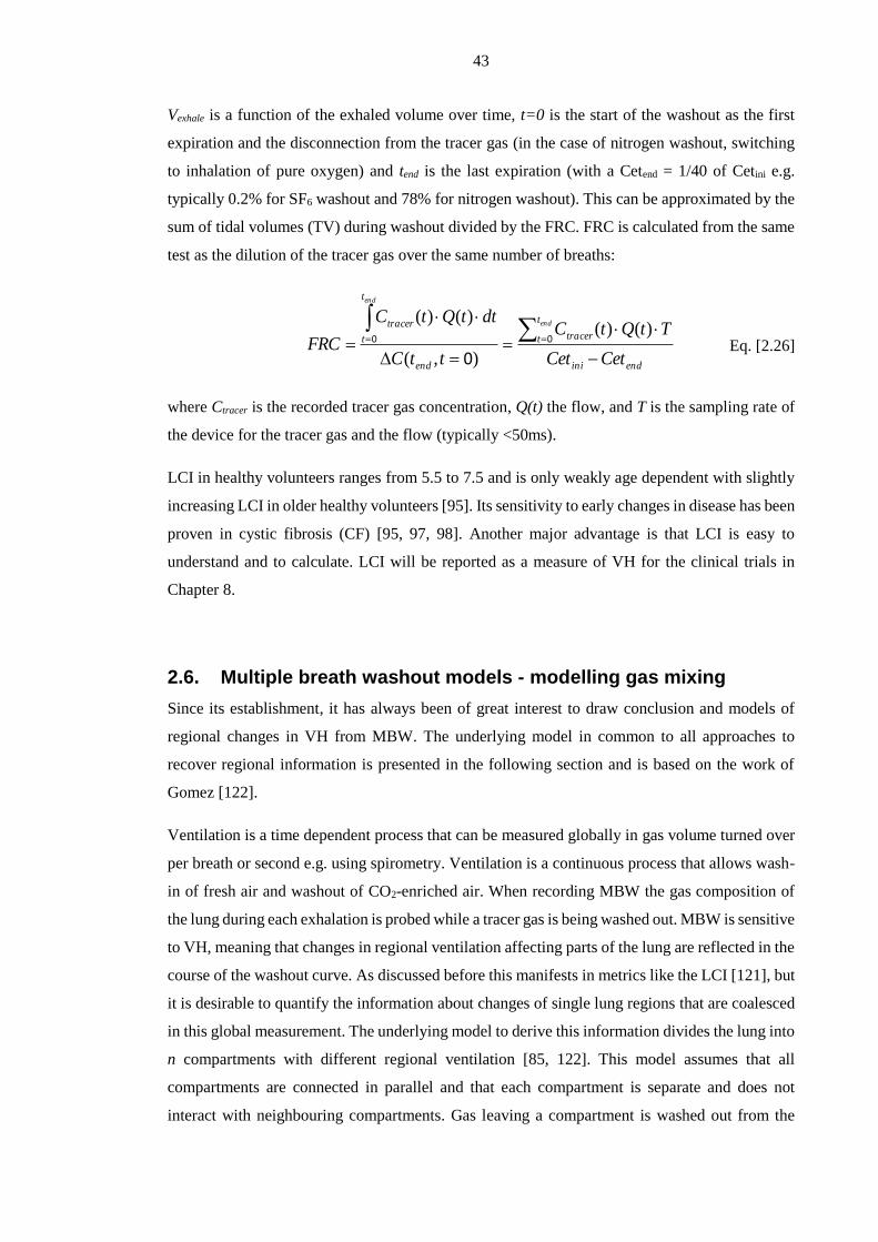
43

Vexhale is a function of the exhaled volume over time, t=0 is the start of the washout as the first

expiration and the disconnection from the tracer gas (in the case of nitrogen washout, switching

to inhalation of pure oxygen) and tend is the last expiration (with a Cetend = 1/40 of Cetini e.g.

typically 0.2% for SF6 washout and 78% for nitrogen washout). This can be approximated by the

sum of tidal volumes (TV) during washout divided by the FRC. FRC is calculated from the same

test as the dilution of the tracer gas over the same number of breaths:

endini

t

t tracer

end

t

t

tracer

CetCet

TtQtC

ttC

dttQtC

FRC

end

end

)()(

),(

)()(00

0 Eq. [2.26]

where Ctracer is the recorded tracer gas concentration, Q(t) the flow, and T is the sampling rate of

the device for the tracer gas and the flow (typically <50ms).

LCI in healthy volunteers ranges from 5.5 to 7.5 and is only weakly age dependent with slightly

increasing LCI in older healthy volunteers [95]. Its sensitivity to early changes in disease has been

proven in cystic fibrosis (CF) [95, 97, 98]. Another major advantage is that LCI is easy to

understand and to calculate. LCI will be reported as a measure of VH for the clinical trials in

Chapter 8.

2.6. Multiple breath washout models - modelling gas mixing

Since its establishment, it has always been of great interest to draw conclusion and models of

regional changes in VH from MBW. The underlying model in common to all approaches to

recover regional information is presented in the following section and is based on the work of

Gomez [122].

Ventilation is a time dependent process that can be measured globally in gas volume turned over

per breath or second e.g. using spirometry. Ventilation is a continuous process that allows wash-

in of fresh air and washout of CO2-enriched air. When recording MBW the gas composition of

the lung during each exhalation is probed while a tracer gas is being washed out. MBW is sensitive

to VH, meaning that changes in regional ventilation affecting parts of the lung are reflected in the

course of the washout curve. As discussed before this manifests in metrics like the LCI [121], but

it is desirable to quantify the information about changes of single lung regions that are coalesced

in this global measurement. The underlying model to derive this information divides the lung into

n compartments with different regional ventilation [85, 122]. This model assumes that all

compartments are connected in parallel and that each compartment is separate and does not

interact with neighbouring compartments. Gas leaving a compartment is washed out from the

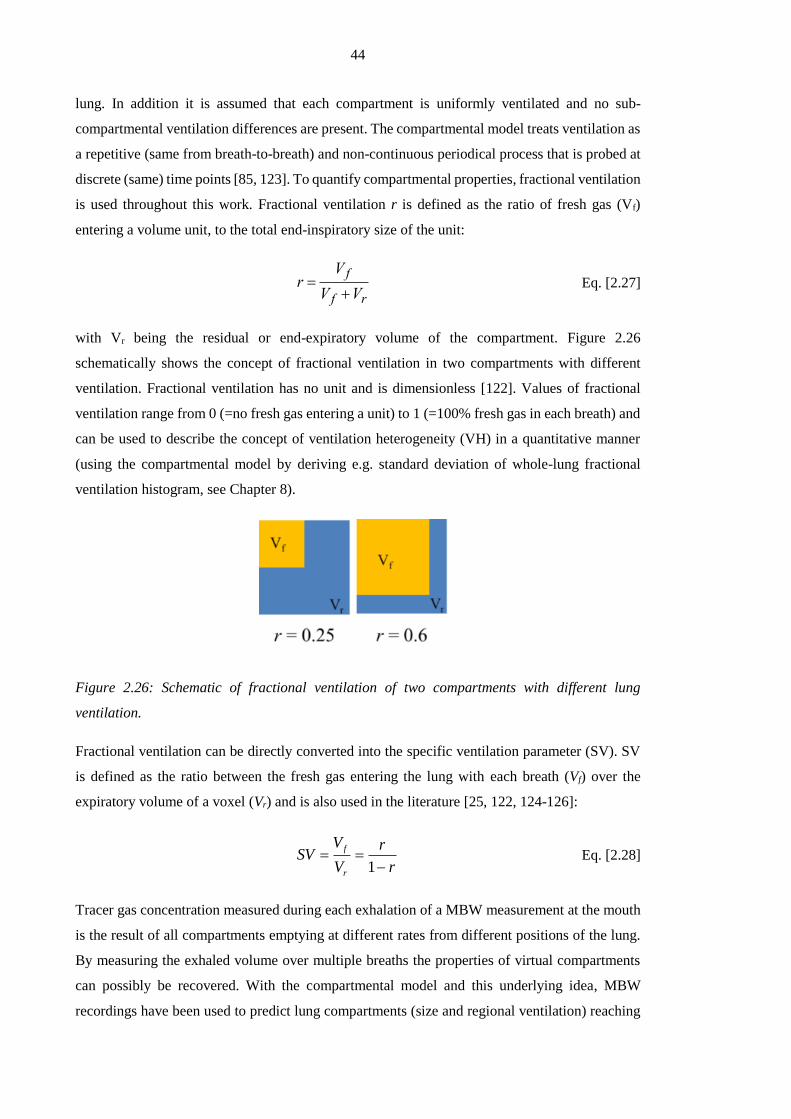
44

lung. In addition it is assumed that each compartment is uniformly ventilated and no sub-

compartmental ventilation differences are present. The compartmental model treats ventilation as

a repetitive (same from breath-to-breath) and non-continuous periodical process that is probed at

discrete (same) time points [85, 123]. To quantify compartmental properties, fractional ventilation

is used throughout this work. Fractional ventilation r is defined as the ratio of fresh gas (Vf)

entering a volume unit, to the total end-inspiratory size of the unit:

r V f

V f Vr Eq. [2.27]

with Vr being the residual or end-expiratory volume of the compartment. Figure 2.26

schematically shows the concept of fractional ventilation in two compartments with different

ventilation. Fractional ventilation has no unit and is dimensionless [122]. Values of fractional

ventilation range from 0 (=no fresh gas entering a unit) to 1 (=100% fresh gas in each breath) and

can be used to describe the concept of ventilation heterogeneity (VH) in a quantitative manner

(using the compartmental model by deriving e.g. standard deviation of whole-lung fractional

ventilation histogram, see Chapter 8).

Figure 2.26: Schematic of fractional ventilation of two compartments with different lung

ventilation.

Fractional ventilation can be directly converted into the specific ventilation parameter (SV). SV

is defined as the ratio between the fresh gas entering the lung with each breath (Vf) over the

expiratory volume of a voxel (Vr) and is also used in the literature [25, 122, 124-126]:

r

r

V

VSV

r

f

1 Eq. [2.28]

Tracer gas concentration measured during each exhalation of a MBW measurement at the mouth

is the result of all compartments emptying at different rates from different positions of the lung.

By measuring the exhaled volume over multiple breaths the properties of virtual compartments

can possibly be recovered. With the compartmental model and this underlying idea, MBW

recordings have been used to predict lung compartments (size and regional ventilation) reaching

45

from n = 2 compartments to a continuous spectrum of regional ventilation distribution [120, 125,

127, 128]. It should be noted that attributing these compartments to regional location in the lung

is not possible as there is no unique solution. In the case of MBW-imaging developed in Chapter

5, the compartmental information of concentration decay is measured as the image intensity decay

with each breath in every voxel, thus giving truly regional information of each compartment. In

addition, quantitative values can be derived from signal changes gas does not need to be washed

in to equilibrium before starting a wash-out – a prerequisite when sampling tracer gases during

MBW at the mouth.

46

Chapter 3 Lung ventilation volumetry with same breath

acquisition of hyperpolarised gas and proton MRI4

3.1. Introduction

Hyperpolarised gas (3He and 129Xe) single breath-hold lung ventilation weighted MRI has been

shown to be sensitive to disease severity in chronic obstructive pulmonary disease [129-131],

cystic fibrosis [51, 132, 133], asthma [134-137] and other obstructive lung diseases [138, 139]

(see Figure 2.16). The technique can resolve regional impairment in lung ventilation caused by

airway obstruction before changes are seen in spirometry [129, 140] and before structural

alterations of lung disease are manifested on CT [141].

With 3He lung ventilation weighted MRI, high spatial resolution gas spin density images,

(referred to as ventilation images) can be produced covering the whole of the lungs at a single

breath-hold. Initially defect size and count were used to derive a semi-quantitative parameter from

functional images acquired using this technique [55, 142]. Nevertheless, this can result in intra

observer differences and a defect count and classification according to size (e.g. small, medium,

big) represents only a semi-quantitative method. When combined with spatially registered proton

(1H) images of the lungs, a commonly used quantitative metric can be derived, such as the

percentage of lung ventilated or obstructed. This is calculated from the ratio of the ventilated lung

volume from 3He ventilation MRI to the total lung volume from the segmented 1H lung MRI

[129]. Percentage of lung volume ventilated (%VV) and its derivative, the volume of defects in

percent(VDP) are quantitative measures of lung function, which have been shown to be sensitive

to early obstructive changes in the lungs of smokers with normal spirometry [129] and in the

assessment of lung ventilation changes in response to bronchodilator therapy [143].

4 This chapter is based on an article published in NRM in Biomedicine: Lung ventilation volumetry with

same breath acquisition of hyperpolarized gas and proton MRI. 1FC Horn, 1,2BA Tahir, 1NJ Stewart, 1GJ

Collier, 1G Norquay, 1G Leung, 2RH Ireland, 1J Parra-Robles, 1H Marshall and 1JM Wild; NMR in

Biomedicine; Volume 27, Issue 12, pages 1461–1467, December 2014;

1. Academic Radiology, Department of Cardiovascular Sciences, University of Sheffield, UK

2. Academic Unit of Clinical Oncology, University of Sheffield, UK

47

Figure 3.1: Calculation of percentage ventilated volume (%VV) is ratio of ventilated volume to

total lung volume from masks of a ventilation scan and a proton scan. Example 3He ventilation

slice (left) and 1H slice (right) from a healthy smoker.

The spatial signal variation in these ventilation-weighted images can also be analysed with other

quantitative approaches such as cluster analysis or treatment response mapping (Chapter 4) [143,

144], which help quantify ventilation heterogeneity. Moreover, multi breath washout imaging

[145] provides a more quantitative measure of ventilation without losses of the regional

information (Chapter 5).

To date, all studies that have evaluated %VV and VDP with 3He ventilation MRI, and indeed

more recently with 129Xe ventilation MRI [146], have acquired anatomical 1H MRI images during

a separate breath-hold from the hyperpolarised gas ventilation MRI images [129]. To match lung

inflation levels between the separate 3He and 1H breath-holds, the same breathing manoeuvre can

be used for both scans. However, any difference in lung inflation level between the separate

breath-holds leads to an inherent error in the calculated %VV. Other studies have used

interpolation algorithms to estimate the lung boundaries from the 3He ventilation images alone

[136, 147], which may not be robust in the presence of large peripheral ventilation defects, where

the lung borders are difficult to delineate, and may therefore under or over estimate the total lung

volume. The same day and short-term reproducibility of separate breath-hold and interpolation

techniques for %VV calculation [53, 132] have been reported. However, no method currently

uses 1H MR images that are spatially and temporally registered to the hyperpolarised gas

ventilation images for more accurate calculation of the total lung volume.

48

Methods to synchronously acquire hyperpolarised gas and 1H images of the lungs have recently

been demonstrated in our group [148, 149] allowing images of gas ventilation and lung anatomy

to be acquired within the same breath-hold, thus, eliminating spatio-temporal mis-registration

between scans. The benefits of the methods are yet to be tested quantitatively for %VV

calculation. In this chapter a same breath hyperpolarised 3He and 1H 3D image acquisition

protocol is used to demonstrate increased accuracy of %VV calculations when compared to the

separate breath method. The method used is tested in a cohort of subjects scanned twice to assess

reproducibility of %VV. In the same session proton images from a separate breath are acquired

to assess reproducibility of separate breath methods and separate breath method facilitating image

registration.

3.2. Materials and methods

3.2.1. Participant selection

13 volunteers were recruited for this study; no exclusion criteria based on either pulmonary

function test results or smoking history were applied. The volunteers ranged in age from 24 to 70.

Four volunteers were former smokers, one volunteer was a current smoker and eight volunteers

were never smokers. No specific inclusion criteria were applied. The study was performed with

National Research Ethics Committee and MHRA regulatory approval with informed consent from

all volunteers.

3.2.2. Imaging protocol

Volunteers were positioned in a 3He transmit-receive quadrature vest coil (Clinical MR Solutions,

Brookfield, WI, USA). The 3He coil was fitted with passive trap circuits to isolate the coil from

the proton body coil and to block induced currents during its transmission at 63.6 MHz. For

imaging a 1.5T MRI scanner (GE HDx, Milwaukee, WI, USA) was used. Figure 3.2 shows the

timings of the imaging protocols used. In order to best replicate the lung inflation state during

imaging [129], in breath 1, proton images were acquired after inhalation of 1L air from functional

residual capacity (FRC). In breath 2, a 1L mix of hyperpolarised 3He and N2 was inhaled from

FRC and 3He images were acquired followed immediately by 1H images in the same breath-hold.

Breath 3 was a repeat of breath 2, with a maximum time interval of 10 minutes between the two

3He breaths. Before breathing hyperpolarised 3He, volunteers were trained in the breathing

49

manoeuvres using a test bag filled with air. They were instructed to exhale relaxed to functional

residual capacity (FRC) before inhaling 1L of air. A test run was performed twice, outside the

scanner to visually check the execution of instructions as well as the maneuver and once inside

the scanner before the imaging protocol was carried out.

Figure 3.2: Imaging protocol; 3He image acquisition is shown in light grey, 1H image acquisition

is shown in dark grey and black indicates the delay time taken to switch the scanner from 3He to

1H acquisition.

3He ventilation MRI

Helium was polarised on site to approximately 25% using a rubidium spin exchange polariser

(Section 2.4.2). Patients inhaled 150 ml 3He mixed with 850 ml N2 from a Tedlar bag (Jensen

Inert Products, Coral Springs, Florida, USA) from functional residual capacity (FRC). An

optimised 3D balanced steady state free precession sequence (bSSFP) [4] was used to acquire the

static ventilation weighted images (parameters shown in Table 3.1) as discussed in Section 2.2.4.

Table 3.1: Scan parameters for the helium and proton acquisitions. The number of slices was

adjusted for full lung coverage according to volunteer size but kept consistent for all scans of an

individual volunteer. The size of voxels is kept constant for all volunteers and all scans.

50

1H anatomical MRI

1H images were acquired at the same voxel size and from the same volume as the 3He ventilation

images using the scanner quadrature transmit-receive body coil with a 3D spoiled gradient echo

sequence (SPGR, parameters shown in Table 3.1). 1H images were acquired in the same breath

directly after both 3He image acquisitions (breath 2 and breath 3, Figure 3.2) and also in a separate

breath (breath 1, Figure 3.2). The SPGR sequence was used here instead of a 3D bSSFP to avoid

banding-artefacts at the lung edges in the 1H anatomical images.

3.2.3. Image analysis

All images were analysed using ScanIP (Simpleware Ltd, Exeter, UK). To calculate %VV for

each volunteer the total lung volume was determined by segmenting the 1H anatomical scans as

well as 3He functional images (Figure 3.3). Proton images were segmented in a semi-automated

way by applying a 3D region growing algorithm based on thresholds. The thresholds were

manually tuned and had to be changed individually for each dataset. Following this step, holes in

the mask were filled automatically. Resulting masks were visually inspected and manual

correction was applied wherever necessary. As a final step major airways were excluded from the

mask up to the second generation. In a similar fashion 3He ventilation images were segmented

using the same threshold-based region growing method (Figure 3.3) and by setting thresholds

manually and patient specific. Artifacts from cardiac motion, found in 3D SSFP images, and the

signal from the major airways were manually excluded. To exclude any 3He signal which fell

outside of the lung volume as defined by the proton images and to prevent an unrealistic %VV >

100%, the masks from the ventilation images were multiplied by the proton masks produced in

the previous step. This situation may arise for example if the lung inflation level in the 3He images

is greater than that in the 1H images when acquiring images in separate breath-holds. Despite the

use of same breath-hold imaging, partial volume effects may occur in voxels containing both 3He

signal and high 1H signal e.g. close to the major blood vessels.

Ventilated volume was then divided by the total lung volume in order to calculate %VVsingle and

%VVseparate for each set of scans. The appropriate proton mask was applied to the 3He masks in

each case.

51

Figure 3.3: Image segmentation workflow for 1H images and 3He images.

Image registration

To assess the effect of image registration upon the efficacy of the separate breath method the

proton images from breath 1 were registered to the 3He images from breaths 2 and 3. In contrast

to the rest of this thesis, where the Sheffield Image Registration Toolbox (SHIRT) was used, here

image registration was performed using the ANTsRegistration tool incorporated as part of the

Advanced Normalisation Tools [150]. SHIRT cannot be used with images deriving from different

imaging modalities.

Registration was designed and conducted in collaboration with Bilal Tahir who has optimised

ANTs for this purpose as part of his PhD project. The separate breath 1H images (breath 1) were

registered to the 3He ventilation images (breaths 2 and 3). The mutual information similarity

metric was used. A coarse pre-alignment rigid transform was applied to align the centres of the

image datasets. The resulting transform was then input to a rigid transform stage allowing for

rotations and translations only. An additional diffeomorphic transformation was also applied to

the resulting transform of the rigid transform pipeline. The registered proton masks were used to

calculate %VVsep-registered.

Dice overlap analysis

As an additional metric to compare single breath 3He and 1H acquisition, separate breath

acquisition and registered separate breath acquisition, Dice similarity coefficients (DSC) were

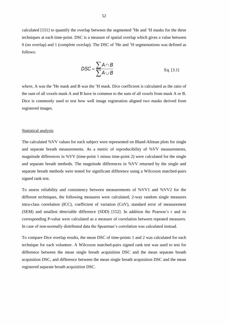
52

calculated [151] to quantify the overlap between the segmented 3He and 1H masks for the three

techniques at each time-point. DSC is a measure of spatial overlap which gives a value between

0 (no overlap) and 1 (complete overlap). The DSC of 3He and 1H segmentations was defined as

follows:

BA

BADSC Eq. [3.1]

where, A was the 3He mask and B was the 1H mask. Dice coefficient is calculated as the ratio of

the sum of all voxels mask A and B have in common to the sum of all voxels from mask A or B.

Dice is commonly used to test how well image registration aligned two masks derived from

registered images.

Statistical analysis

The calculated %VV values for each subject were represented on Bland-Altman plots for single

and separate breath measurements. As a metric of reproducibility of %VV measurements,

magnitude differences in %VV (time-point 1 minus time-point 2) were calculated for the single

and separate breath methods. The magnitude differences in %VV returned by the single and

separate breath methods were tested for significant difference using a Wilcoxon matched-pairs

signed rank test.

To assess reliability and consistency between measurements of %VV1 and %VV2 for the

different techniques, the following measures were calculated; 2-way random single measures

intra-class correlation (ICC), coefficient of variation (CoV), standard error of measurement

(SEM) and smallest detectable difference (SDD) [152]. In addition the Pearson’s r and its

corresponding P-value were calculated as a measure of correlation between repeated measures.

In case of non-normally distributed data the Spearman’s correlation was calculated instead.

To compare Dice overlap results, the mean DSC of time-points 1 and 2 was calculated for each

technique for each volunteer. A Wilcoxon matched-pairs signed rank test was used to test for

difference between the mean single breath acquisition DSC and the mean separate breath

acquisition DSC, and difference between the mean single breath acquisition DSC and the mean

registered separate breath acquisition DSC.

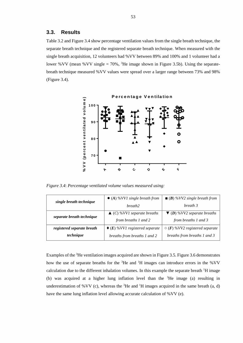
53

3.3. Results

Table 3.2 and Figure 3.4 show percentage ventilation values from the single breath technique, the

separate breath technique and the registered separate breath technique. When measured with the

single breath acquisition, 12 volunteers had %VV between 89% and 100% and 1 volunteer had a

lower %VV (mean %VV single = 70%, 3He image shown in Figure 3.5b). Using the separate-

breath technique measured %VV values were spread over a larger range between 73% and 98%

(Figure 3.4).

Figure 3.4: Percentage ventilated volume values measured using:

single breath technique ● (A) %VV1 single breath from

breath2

■ (B) %VV2 single breath from

breath 3

separate breath technique ▲ (C) %VV1 separate breaths

from breaths 1 and 2

▼ (D) %VV2 separate breaths

from breaths 1 and 3

registered separate breath

technique

♦ (E) %VV1 registered separate

breaths from breaths 1 and 2

○ (F) %VV2 registered separate

breaths from breaths 1 and 3

Examples of the 3He ventilation images acquired are shown in Figure 3.5. Figure 3.6 demonstrates

how the use of separate breaths for the 3He and 1H images can introduce errors in the %VV

calculation due to the different inhalation volumes. In this example the separate breath 1H image

(b) was acquired at a higher lung inflation level than the 3He image (a) resulting in

underestimation of %VV (c), whereas the 3He and 1H images acquired in the same breath (a, d)

have the same lung inflation level allowing accurate calculation of %VV (e).

P e rc e n ta g e V e n t ila t io n

%V

V (

pe

rc

en

t v

en

tila

ted

vo

lum

e)

A B C D E F

7 0

8 0

9 0

1 0 0

54

Figure 3.7 shows Bland-Altman plots of %VV measurements obtained by the three different

techniques. The reproducibility of %VV measured with single breath acquisition (a) is greater

than that measured with the conventional separate breath acquisition either without (b) or with

registration (c).

Figure 3.5: 3He ventilation images of the volunteers with (a) the highest single breath %VV (mean

%VV single = 97.59%) and (b) the lowest single breath %VV (mean %VV single = 70.47%).

55

Table 3.2: Percentage ventilated volume (%VV) measurements.

Figure 3.6: Example of lung inflation level differences between separate breaths, volunteer 1. (a)

3He ventilation image, breath 2, (b) separate breath 1H image, breath 1 and (c) shows (a)

superimposed on (b). (d) Single breath 1H image, breath 2 and (e) shows (a) superimposed on

(d).

Single breath compared to separate breath

The mean of magnitude %VV differences between the two sets of measurements (+ standard

deviation) for the single breath technique was 1.49 ± 1.32% whilst the mean of magnitude %VV

differences between the two sets of measurements for the separate breath technique was 4.19 ±

4.10%. A Wilcoxon matched-pairs signed rank test showed significant difference between the

reproducibility of the same-breath and separate-breath acquisition strategies (P=0.01).

Single breath compared to registered separate breath

The mean of magnitude %VV differences between the two sets of measurements for the registered

separate breath technique was 2.27 + 2.23%. A Wilcoxon matched-pairs signed rank test found

no significant difference between the reproducibility of the same breath and registered separate

breath techniques (P=0.19). There was significant difference between the reproducibility

calculated from separate breaths without registration and separate breaths with registration

(P<0.01, Wilcoxon matched-pairs signed rank test). Registration improved the reproducibility of

separate breath %VV measurement but the registered separate breath %VV still remained less

reproducible than single breath %VV (Figure 3.7).

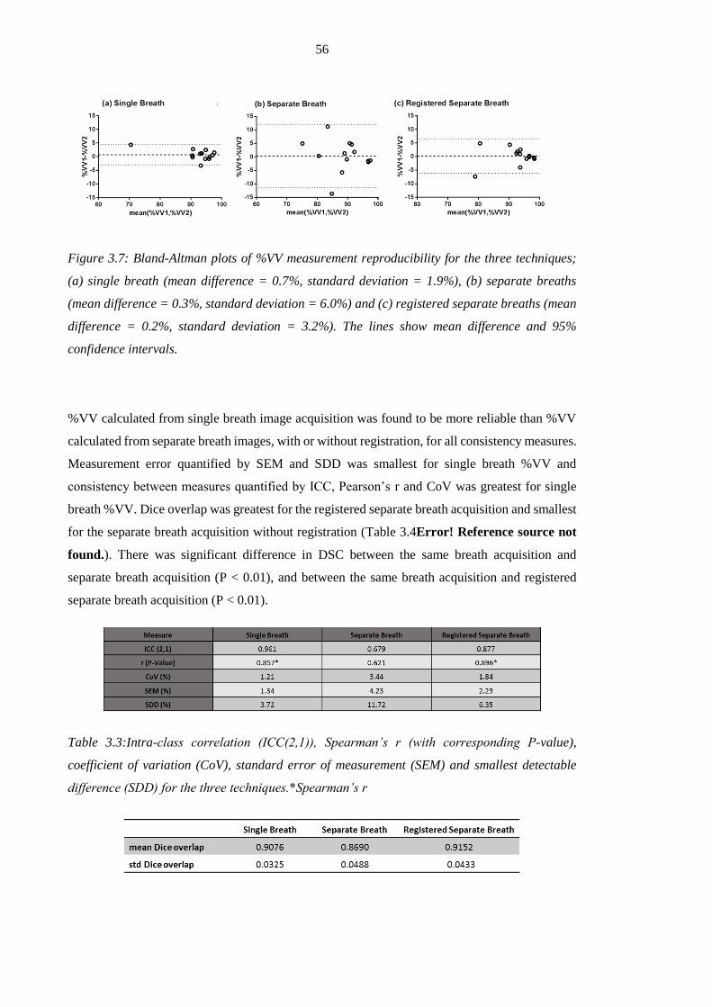
56

Figure 3.7: Bland-Altman plots of %VV measurement reproducibility for the three techniques;

(a) single breath (mean difference = 0.7%, standard deviation = 1.9%), (b) separate breaths

(mean difference = 0.3%, standard deviation = 6.0%) and (c) registered separate breaths (mean

difference = 0.2%, standard deviation = 3.2%). The lines show mean difference and 95%

confidence intervals.

%VV calculated from single breath image acquisition was found to be more reliable than %VV

calculated from separate breath images, with or without registration, for all consistency measures.

Measurement error quantified by SEM and SDD was smallest for single breath %VV and

consistency between measures quantified by ICC, Pearson’s r and CoV was greatest for single

breath %VV. Dice overlap was greatest for the registered separate breath acquisition and smallest

for the separate breath acquisition without registration (Table 3.4Error! Reference source not

found.). There was significant difference in DSC between the same breath acquisition and

separate breath acquisition (P < 0.01), and between the same breath acquisition and registered

separate breath acquisition (P < 0.01).

Table 3.3:Intra-class correlation (ICC(2,1)), Spearman’s r (with corresponding P-value),

coefficient of variation (CoV), standard error of measurement (SEM) and smallest detectable

difference (SDD) for the three techniques.*Spearman’s r

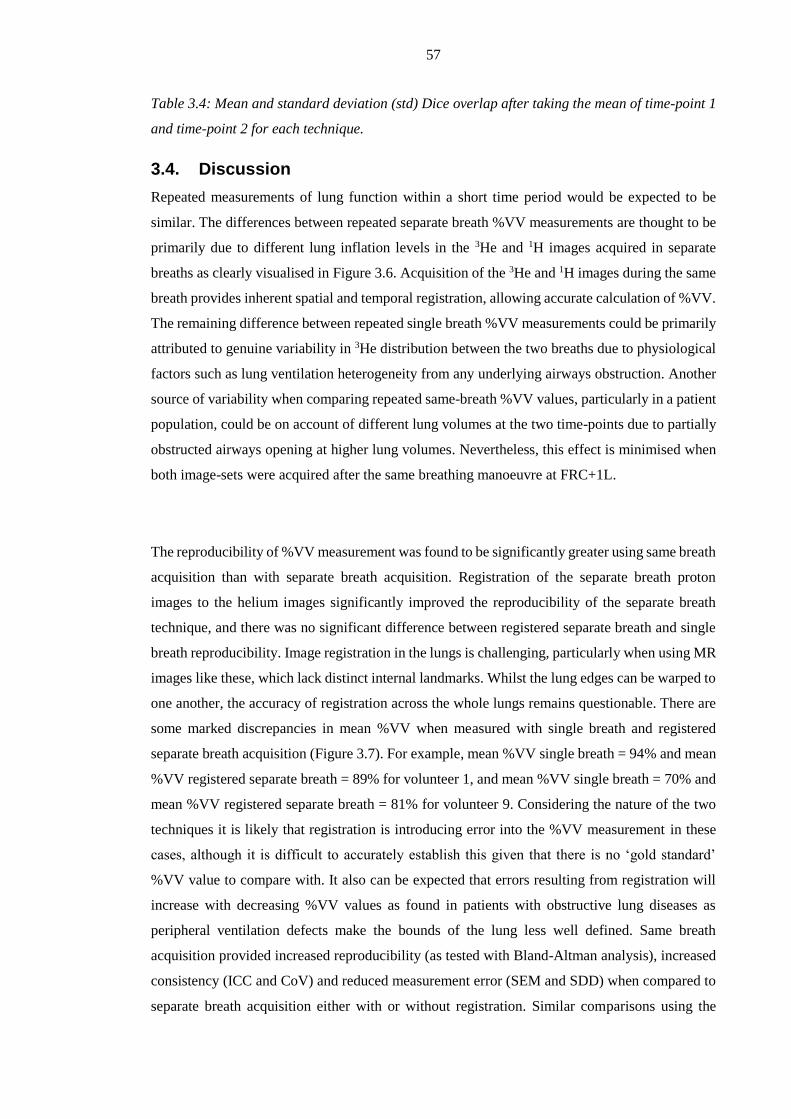
57

Table 3.4: Mean and standard deviation (std) Dice overlap after taking the mean of time-point 1

and time-point 2 for each technique.

3.4. Discussion

Repeated measurements of lung function within a short time period would be expected to be

similar. The differences between repeated separate breath %VV measurements are thought to be

primarily due to different lung inflation levels in the 3He and 1H images acquired in separate

breaths as clearly visualised in Figure 3.6. Acquisition of the 3He and 1H images during the same

breath provides inherent spatial and temporal registration, allowing accurate calculation of %VV.

The remaining difference between repeated single breath %VV measurements could be primarily

attributed to genuine variability in 3He distribution between the two breaths due to physiological

factors such as lung ventilation heterogeneity from any underlying airways obstruction. Another

source of variability when comparing repeated same-breath %VV values, particularly in a patient

population, could be on account of different lung volumes at the two time-points due to partially

obstructed airways opening at higher lung volumes. Nevertheless, this effect is minimised when

both image-sets were acquired after the same breathing manoeuvre at FRC+1L.

The reproducibility of %VV measurement was found to be significantly greater using same breath

acquisition than with separate breath acquisition. Registration of the separate breath proton

images to the helium images significantly improved the reproducibility of the separate breath

technique, and there was no significant difference between registered separate breath and single

breath reproducibility. Image registration in the lungs is challenging, particularly when using MR

images like these, which lack distinct internal landmarks. Whilst the lung edges can be warped to

one another, the accuracy of registration across the whole lungs remains questionable. There are

some marked discrepancies in mean %VV when measured with single breath and registered

separate breath acquisition (Figure 3.7). For example, mean %VV single breath = 94% and mean

%VV registered separate breath = 89% for volunteer 1, and mean %VV single breath = 70% and

mean %VV registered separate breath = 81% for volunteer 9. Considering the nature of the two

techniques it is likely that registration is introducing error into the %VV measurement in these

cases, although it is difficult to accurately establish this given that there is no ‘gold standard’

%VV value to compare with. It also can be expected that errors resulting from registration will

increase with decreasing %VV values as found in patients with obstructive lung diseases as

peripheral ventilation defects make the bounds of the lung less well defined. Same breath

acquisition provided increased reproducibility (as tested with Bland-Altman analysis), increased

consistency (ICC and CoV) and reduced measurement error (SEM and SDD) when compared to

separate breath acquisition either with or without registration. Similar comparisons using the

58

separate breath technique are reported in two publications. Investigating 24 COPD patients

Mathew et al. [53] claimed to find an ICC of 0.97 calculating the ventilation defect volume

(VDV=TLV-VV), when comparing images acquired within about 10min intervals. This shows a

very high reproducibility of VDV. Kirby et al. performed a similar analysis on a CF population

[132]. The gap between the two imaging sessions was 7 days, which was considerably longer than

in the presented study. A Bland-Altman analysis was done on ventilated defect percentage

(VDP=100%-%VV) from this population and a mean difference of -3% with a standard deviation

of 4% was found. They also reported a high correlation between repeated scans with a Spearman’s

r = 0.94. The high correlation is not a surprise, since the standard deviation found from the Bland-

Altman analysis was relatively small and the pulmonary function tests of this patient cohort were

spread out over a wide range. The high mean difference of -3% might be explained with

ventilation changes between scans. The standard deviation of the Bland-Altman analysis is

comparable to what we found (SD = 3.2%, separate breath registered, Figure 3.7 (c)) and the

much lower mean difference (MD = 0.3%) can be explained with the smaller gap between scans

(5 min versus 7 days). The slightly lower correlation (r = 0.90) in this study compared to Kirby

et al. can be explained by a much smaller range of values of %VV.

Dice overlap between the segmented 3He and 1H masks was significantly greater for single breath

acquisition than for un-registered separate breath acquisition as would be expected. The Dice

overlap of the registered separate breath technique was significantly greater than that of single

breath acquisition. This is likely to be due to the fact that the diffeomorphic registration used is

driven by a cost-function, which sought to maximise a metric similar to DSC. The different

contrasts of the source and target images, the lack of internal structures visible in the lungs in the

SPGR 1H images and partial-volume effects make registration of 1H to 3He images complicated.

Therefore it is realistic to assume that registration will introduce some level of error into %VV

calculation, even in this healthy population.

Image segmentation of the 3He ventilation images in this healthy volunteer population with an

average SNR of 33 was checked visually and masks were adjusted manually to optimise

segmentation. Automated segmentation eliminates inter- and intra-observer variability,

nevertheless, in patient data, semi-automated segmentation was shown to be highly reproducible

and more reliable than manual methods [153]. To date no reliable use of an automated algorithm

for segmenting ventilation images has been found in the literature. Simple methods using noise

level [52] are highly SNR dependent, more sophisticated segmentation using a region growing

algorithm has been demonstrated [136]. A detailed comparison of those methods with manual

segmentation is still a gap in the literature.

59

Overall there are still limitations of single breath %VV measurement. Although single breath

acquisition removes breath to breath inhalation volume discrepancy, factors such as cardiac

motion and any gradual or sudden diaphragm movement during the breath-hold are not mitigated.

In a few cases a small movement of the diaphragm occurred between the 3He and 1H images in

the same breath-hold. In a patient population it is more likely that some patients would not be

able to complete the 18s breath-hold. Further reduction of the single breath-hold duration will

help to mitigate this problem. Further work is aimed at reducing the scanner-reset time between

sequences on the system used (3s), which would then reduce the overall breath-hold time. In

previous work at 3T on another system this delay was eliminated altogether by acquiring the 1H

and 3He data in an interleaved fashion from k-space view to view [148]. The interleaved sampling

technique is not used here since a non-successful breath-hold (especially in the case of severe

patients) would result in image quality losses of both, the ventilation and anatomical scan. With

the proposed method, the important information from the ventilation images is more likely to be

acquired successfully. In addition the use of faster image acquisition acceleration methods such

as parallel imaging and compressed sensing [154, 155] could be used to substantially reduce the

breath-hold duration for synchronous 3He and 1H acquisition.

3.5. Conclusions

In conclusion, hyperpolarised 3He ventilation and 1H anatomical MRI acquisition within a single

breath-hold was shown to provide spatially and temporally registered images. These coregistered

same breath images increased the reproducibility of percentage lung ventilation calculation. The

single breath method is more consistent in measuring percentage ventilated lung volume and

minimises errors from lung inflation volume differences. The increased reliability of the

technique when compared to the separate breath approach will reduce statistical noise and should

enable subsequent studies that use this lung imaging metric of ventilation to evaluate intervention

and exacerbations to reach an appropriate power with a smaller number of participants. In addition

the image processing workflow can be further automated in major parts with the use of automated

image segmentation (e.g. using edge detection).

The major disadvantage of %VV, independent of how it is obtained, remains a complete loss of

all regional ventilation intensity information by converting images into binary masks of

ventilated/non-ventilated. Also %VV has been shown to be a sensitive measure to early changes

in disease, valuable information from images is lost. Exploiting the fact that image intensity is

proportional to gas concentration could give further insight into inhomogeneous gas distribution

as a measure of ventilation heterogeneity (VH). The following chapter presents a new approach

60

using ventilation weighted imaging to maximise the regional information to detect regional

changes in ventilation as response to treatment.

61

Chapter 4 A method for quantitative mapping of lung

ventilation in response to treatment using hyperpolarised 3He

MRI demonstrated in asthma patients5

4.1. Introduction

Functional imaging using single-breath hyperpolarised gas ventilation MRI is able to measure

ventilation as regional gas distribution. Image intensity in ventilation weighted images acquired

in a single breath is proportional to gas concentration in that voxel. Hyperpolarised gas ventilation

MR-imaging has been shown to be a sensitive measure of ventilation heterogeneity in asthma

[142, 156-159]. In addition, simple metrics such as percentage ventilated volume (%VV, Chapter

3) and percentage ventilation defect volume can be derived from these images, which have been

shown to correlate with spirometry in asthma [132, 134, 160]. These metrics which express the

percentage of the lungs ventilated, whilst commonly used, are limited by the binary classification

of lungs as non-ventilated versus ventilated as result of image segmentation process. Furthermore,

despite being derived from regionally specific imaging data, these numbers represent coalesced

metrics from the whole lung. Thus, there is scope and a need to derive better quantitative metrics

from these exquisite, sensitive and high spatial resolution images of regional lung function that

better utilise the quantitative data from all voxels. This is particularly the case when we are

interested in which parts of the lung respond to therapy.

Methods to quantify gas distribution based on ventilation image intensity have been proposed

before. Clustering has been used to subdivide image intensities into different shades of ventilation

intensity [153], and a continuous approach to normalise images using gas volumes and mean

image intensities has been used as an outcome measure to assess response to metacholine

challenge in asthma patients [158]. However, a direct comparison of images from multiple time-

points has not been performed with either of these techniques.

In this work a technique to quantitatively map treatment response of the lungs using

hyperpolarised 3He ventilation images was developed and evaluated in an asthma cohort pre and

post bronchodilator application. The motivation was to develop an algorithm sensitive to regional

5 Acknowledgements:

I would like to acknowledge Professor David Barber for his help with the image registration and Bilal

Tahir for great advice on the same topic. Ventilated volume calculation from ventilation images were

performed by John C. Kenwrothy.

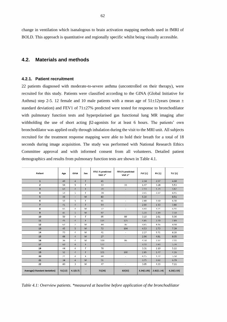
62

change in ventilation which isanalogous to brain activation mapping methods used in fMRI of

BOLD. This approach is quantitative and regionally specific whilst being visually accessible.


4.2.1. Patient recruitment

22 patients diagnosed with moderate-to-severe asthma (uncontrolled on their therapy), were

recruited for this study. Patients were classified according to the GINA (Global Initiative for

Asthma) step 2-5. 12 female and 10 male patients with a mean age of 51±12years (mean ±

standard deviation) and FEV1 of 71±27% predicted were tested for response to bronchodilator

with pulmonary function tests and hyperpolarised gas functional lung MR imaging after

withholding the use of short acting β2-agonists for at least 6 hours. The patients’ own

bronchodilator was applied orally through inhalation during the visit to the MRI unit. All subjects

recruited for the treatment response mapping were able to hold their breath for a total of 18

seconds during image acquisition. The study was performed with National Research Ethics

Committee approval and with informed consent from all volunteers. Detailed patient

demographics and results from pulmonary function tests are shown in Table 4.1.

Table 4.1: Overview patients. *measured at baseline before application of the bronchodilator

63

4.2.2. MRI acquisition

All patients were scanned at three time points. Two images were acquired before application of a

bronchodilator (baseline scans) and once more after application of the bronchodilator (post-BD

scan). The scan protocol timing is schematically shown in Figure 4.1A: the baseline scans were

both acquired within a time frame of five minutes to assess short time scale baseline physiological

variability in lung ventilation, and the scan following bronchodilator inhalation was acquired 20

minutes after administration of the drug. Each MRI scan consisted of functional images (3He

ventilation) and structural images (1H anatomy) acquired during a single breath of <18 seconds.

In addition to MRI scans, PFTs were performed during a separate visit temporally close (±3 days)

to the imaging appointments.

Six patients returned after 12 weeks for a repetition of the MRI scans as a means of assessment

of long term baseline variability; they were imaged with the same protocol as during their first

visit (dropping only one of the baseline scans).

Images were acquired after inhalation of 1 litre of gas (350 ml 3He mixed with 650 ml N2) from

functional residual capacity. Patients were trained in the breathing manoeuvre outside the MR

scanner before the each imaging session and once inside the MRI scanner before administration

of the hyperpolarised 3He. Examples of corresponding MR-images from a subject are depicted in

Figure 4.1B.

Figure 4.1: (A) Imaging protocol, including the treatment application. (B) Corresponding

example images 1H and 3He images from each time point.

Patients were imaged using a whole-body clinical 1.5 T MRI scanner (GE HDx, Milwaukee, WI,

USA) with a quadrature transmit-receive vest coil and the systems pquadrature transmit-receive

body coil for proton imaging.

64

3He Ventilation MRI

Helium was polarised on site to approximately 25% using a rubidium spin exchange polariser

(GE Healthcare, Amersham, UK). Patients inhaled 350 ml 3He mixed with 650 ml N2 from a

Tedlar bag (Jensen Inert Products, Coral Springs, Florida, USA) from functional residual capacity

(FRC) as described earlier. A multi-slice 2D spoiled gradient echo sequence was adjusted to the

patients’ thoracic size with a field of view between 38 and 42 cm and 20-24 coronal slices of

10mm thickness. Static ventilation weighted images were acquired with a fixed imaging matrix

of 128x102 resulting in a resolution of about 3x3x10mm. The echo time (TE) was set to 1.1ms

with a repetition time (TR) of 3.6 ms using a flip angle of 8° and 62.5 kHz receiver bandwidth.

1H anatomical MRI

During the same breath-hold 1H images were acquired from the same volume as the 3He

ventilation images with a multi-slice 2D balanced steady state free precession sequence with a

lower resolution matrix (128x64) to reduce the length of the breath-hold. The echo time was

0.7ms with a repetition time of 2.4ms using a flip angle of 50° and a receiver bandwidth of 167

kHz. Note that the advanced same breath 3D ventilation and anatomical imaging sequences used

in Chapter 3 were not used in this study due to the fact that the asthma imaging protocol was

defined for this study before that acquisition method had been evaluated.


Before quantitative treatment response maps could be calculated from the ventilation weighted

images, three intermediate image processing steps were first necessary:

(i) Image registration

Image registration was performed to compensate for patient movement between acquisitions

made during separate breaths and after repositioning. Despite training in the breathing manoeuver

some patients struggled to reproduce their breath-hold precisely. Image registration was then used

to correct for volume changes between images performed at different time points. Since the

chosen treatment can change gas distribution and signal intensity related to ventilation in the lung

considerably, the corresponding 3He ventilation images can show substantial regional changes in

intensity and morphology pre and post bronchodilator treatment. This makes registration of

ventilation images before and after treatment difficult. To avoid the influence of morphologic

changes in ventilation images on the deformation and translation of the registration process, the

65

temporally co-registered same breath proton images were used to facilitate registration. Since

proton images were acquired in the same breath-hold as ventilation images (Figure 4.1B), the

deformation matrix obtained from the proton anatomical image registration was applied to the

ventilation images to spatially match acquisitions from different time-points. The registration

algorithm used is part of a Matlab plugin called ShIRT (Sheffield image registration Toolbox)

and described in [161] in greater detail (compare also Section 5.2.8.

(ii) Image segmentation

Semi-automated image segmentation was performed to segment signal from 3He in ventilated

lung voxels from the background using ScanIP (Simpleware Ltd., Exeter, UK) as presented in

Section 3.2.3. A threshold-based region growing algorithm was used, followed by visual

inspection of the result and an adjustment of the threshold if necessary. In a second step the major

airways were manually excluded from the images. The results of segmenting an example slice are

shown in Figure 4.2.

Figure 4.2: Showing the results of a segmentation and extraction of the major airways until

generation 2/3 depending on visibility of the airways.

(iii) Normalisation of signal intensity

In order to compare ventilation images acquired at different time points normalisation is

necessary. Normalisation was performed in two separate steps:

In a first step images are normalised to correct for variability in number of 3He atoms dispensed

(inhaled gas) and their polarization. This approach is based on Tzeng et al. [158]:

voxel

bag

r

V

V

rI

rIrI

)(

)()(

Eq. [4.1]

)(rI

is the normalised image intensity with r =(x,y,z). Vbag is the total amount of gas inhaled,

which was in this study 1l in all cases and Vvoxel is the voxel volume. The accumulated image

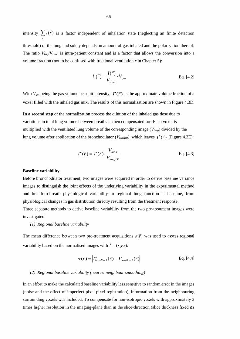
66

intensity r

rI )(

is a factor independent of inhalation state (neglecting an finite detection

threshold) of the lung and solely depends on amount of gas inhaled and the polarization thereof.

The ratio Vbag/Vvoxel is intra-patient constant and is a factor that allows the conversion into a

volume fraction (not to be confused with fractional ventilation r in Chapter 5):

gas

voxel

VV

rIrI

)()(

Eq. [4.2]

With Vgas being the gas volume per unit intensity, )(rI

is the approximate volume fraction of a

voxel filled with the inhaled gas mix. The results of this normalisation are shown in Figure 4.3D.

In a second step of the normalization process the dilution of the inhaled gas dose due to

variations in total lung volume between breaths is then compensated for. Each voxel is

multiplied with the ventilated lung volume of the corresponding image (Vlung) divided by the

lung volume after application of the bronchodilator (VlungBD), which leaves )(rI

(Figure 4.3E):

lungBD

lung

V

VrIrI )()(

Eq. [4.3]

Baseline variability

Before bronchodilator treatment, two images were acquired in order to derive baseline variance

images to distinguish the joint effects of the underlying variability in the experimental method

and breath-to-breath physiological variability in regional lung function at baseline, from

physiological changes in gas distribution directly resulting from the treatment response.

Three separate methods to derive baseline variability from the two pre-treatment images were

investigated:

(1) Regional baseline variability

The mean difference between two pre-treatment acquisitions )(r

was used to assess regional

variability based on the normalised images with r =(x,y,z):

)()()( 21 rIrIr baselinebaseline

Eq. [4.4]

(2) Regional baseline variability (nearest neighbour smoothing)

In an effort to make the calculated baseline variability less sensitive to random error in the images

(noise and the effect of imperfect pixel-pixel registration), information from the neighbouring

surrounding voxels was included. To compensate for non-isotropic voxels with approximately 3

times higher resolution in the imaging-plane than in the slice-direction (slice thickness fixed Δz

67

= 10mm) images were filtered in-plane with a [3 3] pixel kernel. The convolution matrix took

surrounding pixels equally into account (mean-filter). After filtering images, regional variability

was calculated as Eq. [4.4].

(3) Global mean difference

The baseline variability can also be defined as a global value for the whole lung. Regional baseline

variability was calculated as per Eq. [4.4] then an average value of all non-zero voxels is

calculated to obtain the mean global baseline variability, :

)()( 21 rIrI baselinebaseline

Eq. [4.5]

In the case of the subgroup that came on two occasions 12 weeks apart, the baseline variability

acquired during Visit 1 was used for both visits, since only a single pre-treatment image was

acquired during Visit 2.

For subsequent calculation of treatment response maps method (2) was used throughout.

Justification for this choice is discussed in the discussion section.

Treatment response

Having calculated the threshold for activation of treatment response for each voxel, the magnitude

of the treatment response was then calculated from the difference between ventilated volume

fraction before and after treatment over the total volume fraction in both images:

)()()( _ rIrIrI baslinemeanpostBD

Eq. [4.6]

where )(rI

represents ventilation differences due to treatment. This subtraction to

quantitatively compare the two images relies on the imaging parameters and hardware being the

same and the subject being in a similar position in the RF coil. Each voxel of the calculated )(rI

map was then compared for ‘activation’ against the threshold set by the baseline variability

)(r

. Since )(r

was defined as the absolute difference between the two normalised baseline

images it is used as a threshold for a positive or negative response effect of the difference of

)(rI

before and after treatment. For voxels where this absolute difference was smaller than the

absolute threshold )(r

, treatment response was set to zero:

68

)()(

)()(

,)(

,0%100)(

rIr

rIr

ifrI

ifrTR

Eq. [4.7]

The final result is the TR (treatment response) expressed in percent change. An example treatment

response map from a single imaging slice is shown in Figure 4.3G (bottom). The black

background represents the intersection of masks from baseline and post-treatment scans (see

bottom Figure 4.3F). Treatment response is measured in terms of difference between normalized

image signals )(rI

before and after treatment, maps show increased ventilation )(rTR

>0 in

green and decreased ventilation in red )(rTR

<0. Since )(rI

is the approximate fraction of a

voxel filled with gas (after gas volume and density normalization) changes are expressed in

percent. Figure 4.3 shows a graphical overview of all image processing workflow steps.

69

Figure 4.3: Different steps to calculated treatment response maps from ventilation weighted

images.

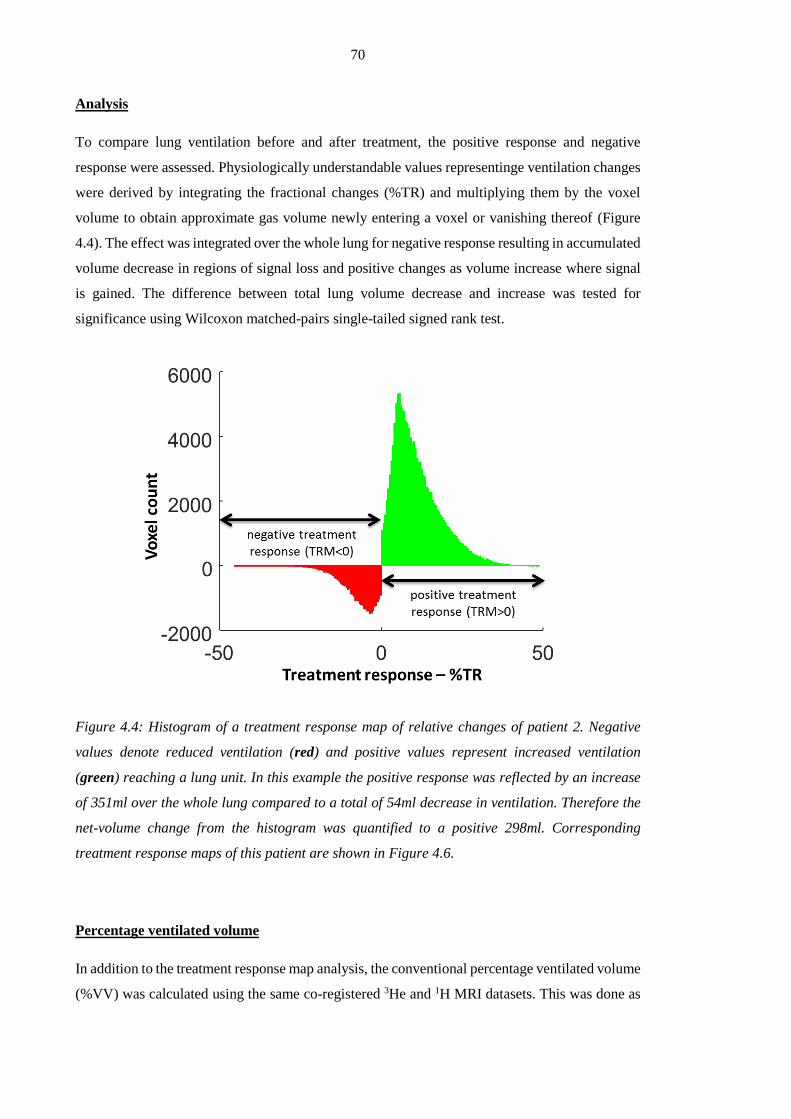
70

Analysis

To compare lung ventilation before and after treatment, the positive response and negative

response were assessed. Physiologically understandable values representinge ventilation changes

were derived by integrating the fractional changes (%TR) and multiplying them by the voxel

volume to obtain approximate gas volume newly entering a voxel or vanishing thereof (Figure

4.4). The effect was integrated over the whole lung for negative response resulting in accumulated

volume decrease in regions of signal loss and positive changes as volume increase where signal

is gained. The difference between total lung volume decrease and increase was tested for

significance using Wilcoxon matched-pairs single-tailed signed rank test.

Figure 4.4: Histogram of a treatment response map of relative changes of patient 2. Negative

values denote reduced ventilation (red) and positive values represent increased ventilation

(green) reaching a lung unit. In this example the positive response was reflected by an increase

of 351ml over the whole lung compared to a total of 54ml decrease in ventilation. Therefore the

net-volume change from the histogram was quantified to a positive 298ml. Corresponding

treatment response maps of this patient are shown in Figure 4.6.

Percentage ventilated volume

In addition to the treatment response map analysis, the conventional percentage ventilated volume

(%VV) was calculated using the same co-registered 3He and 1H MRI datasets. This was done as

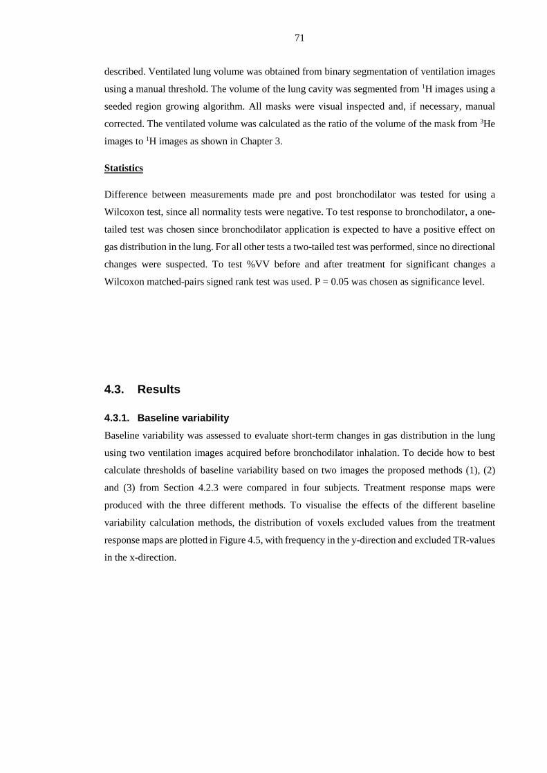
71

described. Ventilated lung volume was obtained from binary segmentation of ventilation images

using a manual threshold. The volume of the lung cavity was segmented from 1H images using a

seeded region growing algorithm. All masks were visual inspected and, if necessary, manual

corrected. The ventilated volume was calculated as the ratio of the volume of the mask from 3He

images to 1H images as shown in Chapter 3.

Statistics

Difference between measurements made pre and post bronchodilator was tested for using a

Wilcoxon test, since all normality tests were negative. To test response to bronchodilator, a one-

tailed test was chosen since bronchodilator application is expected to have a positive effect on

gas distribution in the lung. For all other tests a two-tailed test was performed, since no directional

changes were suspected. To test %VV before and after treatment for significant changes a

Wilcoxon matched-pairs signed rank test was used. P = 0.05 was chosen as significance level.

4.3. Results

4.3.1. Baseline variability

Baseline variability was assessed to evaluate short-term changes in gas distribution in the lung

using two ventilation images acquired before bronchodilator inhalation. To decide how to best

calculate thresholds of baseline variability based on two images the proposed methods (1), (2)

and (3) from Section 4.2.3 were compared in four subjects. Treatment response maps were

produced with the three different methods. To visualise the effects of the different baseline

variability calculation methods, the distribution of voxels excluded values from the treatment

response maps are plotted in Figure 4.5, with frequency in the y-direction and excluded TR-values

in the x-direction.

72

Figure 4.5: Histograms show distributions of excluded TR values using different methods to

calculate the baseline-variability thresholds:

Method 1: (red) – regional threshold as mean difference between baseline 1 & baseline 2

Method 2: (yellow) – regional baseline variability (nearest neighbour method)

Method 3: (black) – global threshold ;

Method (3) is based on a cut-off threshold and does not take regional variability of ventilation

into account but instead non-selectively excludes values. Both methods (1) and (2) allow for a

regionally sensitive cut-off and approximately follow a Gaussian distribution (Figure 4.5). In

comparison to method (1), method (2) aims to reduce the effects of noise by weighting the

prescribed baseline variability for a given voxel with weightings from the nearest neighbour

voxels. Method (2) was thus chosen as the number of voxels lost when masking treatment

response with baseline variability was minimized (see Figure 4.6). A single slice example of a

baseline variability map is shown in Figure 4.3G. The image shows regional hot-spots where

more variability between the two images was observed.

4.3.2. Treatment response mapping

Treatment response mapping was successfully performed in 20 patients. An example dataset from

patient 2 is shown in Figure 4.6, with treatment response maps and the corresponding 3He MR

images. Green areas corresponding to an increase of ventilation (TR as change of ventilated

fraction) dominate the treatment response map. In this case, increase of gas volume was quantified

as 351ml in total after treatment (green voxels) compared to a decrease of 54ml (red voxels). This

results in a net-area of 297ml from the histogram in Figure 4.4.

Figure 4.7 shows the group treatment response to bronchodilator from all 20 patients. Changes in

ventilation were measured as increased and decreased volume from integration of whole lung

histograms. Positive response over the cohort was found to be significantly greater than negative

response using a one-tailed Wilcoxon test (P<0.001). Accumulated volume increase was found

73

to be 210±68ml in comparison to a negative response of 95±31ml as graphically shown in Figure

4.7 in this cohort. The same test was used to test differences in percentage ventilated volume

(%VV), which also showed significant increase (P<0.001) after bronchodilator application. FEV1

increased significantly (P<0.001) in response to bronchodilator application as well as FVC

(P<0001). %VV was found to be 86±11% on average before treatment and elevates to 90±9%

after treatment. FEV1 was found to change from an average of 71±27% predicted to 81±28%

predicted.

Figure 4.6: Example treatment response sets from patient 2 showing all slices acquired. Top row

TR, middle row pre-treatment ventilation images, and bottom post-treatment ventilation images.

The TR is in units of litres. White areas correspond to no significant changes in ventilation above

the threshold )(r

.

Figure 4.7: Comparison of image derived parameters: (A) – TR as volume change, (B) - %VV;

and spirometry: (C) - FEV1, (D) - FVC. Response to Bronchodilator treatment was found to be

significant with all methods (one-tailed Wilcoxon signed rank test, P<0.001). Although all

methods show significant sensitivity to change the TR groups are more tightly clustered with

clearer separation and a difference >50% between the mean values.

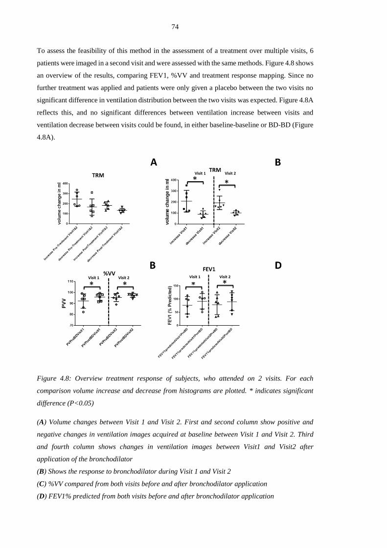
74

To assess the feasibility of this method in the assessment of a treatment over multiple visits, 6

patients were imaged in a second visit and were assessed with the same methods. Figure 4.8 shows

an overview of the results, comparing FEV1, %VV and treatment response mapping. Since no

further treatment was applied and patients were only given a placebo between the two visits no

significant difference in ventilation distribution between the two visits was expected. Figure 4.8A

reflects this, and no significant differences between ventilation increase between visits and

ventilation decrease between visits could be found, in either baseline-baseline or BD-BD (Figure

4.8A).

Figure 4.8: Overview treatment response of subjects, who attended on 2 visits. For each

comparison volume increase and decrease from histograms are plotted. * indicates significant

difference (P<0.05)

(A) Volume changes between Visit 1 and Visit 2. First and second column show positive and

negative changes in ventilation images acquired at baseline between Visit 1 and Visit 2. Third

and fourth column shows changes in ventilation images between Visit1 and Visit2 after

application of the bronchodilator

(B) Shows the response to bronchodilator during Visit 1 and Visit 2

(C) %VV compared from both visits before and after bronchodilator application

(D) FEV1% predicted from both visits before and after bronchodilator application

75

Difference between volume increase and decrease pre and post application of bronchodilator in

Visit 1 and Visit 2 were both found to be significant (P<0.05, one-tailed Wilcoxon signed rank

test). %VV derived from the same datasets showed significance between pre-and post-

bronchodilator treatment in both visits (Figure 4.8C), as did FEV1 (Figure 4.8D). These findings

are in agreement with those in the Visit 1 pre and post treatment.

Since large changes in lung volume can have an impact on the outcome of the registration, the

reproducibility of lung volumes was tested. Lung volumes from the baseline and the post-BD

scan from all 20 volunteers were tested. The total lung volume (TLV) calculated from

segmentation of the lung cavity in 1H images was compared between pre- and post-treatment

images. The Bland-Altman plot of the differences is shown in Figure 4.9Error! Reference

source not found.. A mean total volume difference of less than 40 ml was found with a standard

deviation of 389ml corresponding to -0.5%±8.3% of the mean lung volume. Findings show a

similar mean difference (0.2%) as Horn et al. with a much higher standard deviation (SD=3.2%,

[162]). This might be explained by the fact that the previous study included trained healthy

volunteers, while the current study examines asthma patients who are short of breath.

Nevertheless, the findings emphasise the necessity of image registration and lung volume

normalization step (2) in the TRM process.

Figure 4.9: Bland-Altman plot of differences between lung volumes in litres. Dotted lines show

±1.96 standard deviations and the mean difference. Mean difference between total lung volumes

-0.5% with a standard deviation of 8%.

76

4.4. Discussion

A method for treatment response mapping was developed for quantification and visualisation of

regional changes in gas distribution in the lung. The technique was demonstrated in an asthma

cohort. Single breath ventilation weighted images acquired before and after treatment were used

as a basis to calculate treatment response maps. Additionally, the baseline random variability of

the gas distribution in the lung was studied by acquiring two images before treatment. Regional

short-term baseline physiological variability was derived from those images and used to quantify

true treatment response effect.

Measuring regional ventilation changes between acquisitions caused by motion and differences

in lung volume is challenging. This problem has been addressed previously [162] in the

calculation of percent ventilated volume (%VV), where the acquisition of proton images and

ventilation images in separate breaths reduce the repeatability of %VV calculation and

registration was shown to improve reproducibility of %VV. When calculating treatment response

maps, image registration was used to overcome differences in lung volume of ventilation images

acquired at different breath-holds. Proton images, acquired during the same breath-hold as the

ventilation images were used to calculate deformation maps that were then applied to ventilation

images. This reduced registration errors introduced by morphologic changes in ventilation images

arising from response to treatment. Moreover, registration reduces misalignment resulting from

patient movement between scans and from repositioning patients in the scanner between imaging

sessions. Registered images allow comparison of ventilation changes over multiple time points.

Since the signal from lung parenchyma in 1H MRI is hard to distinguish from noise, image

registration relies on the outline of the lungs and blood vessels inside the lung. In diseased lungs,

air-trapping could result in altered lung expansion, which might cause errors in deformation maps

from image registration. Nevertheless, this error is expected to be low, since patients were aiming

for the same lung inflation and volumes changes were found to be less than 1±8%.

After registration, the image normalisation process enabled comparison of signal intensities in the

ventilation images from different acquisitions. The method proposed by Tzeng et al. was used

[158], to compensate for differences in 3He atoms reaching the lungs and polarisation levels rather

than relying solely on image intensity detected in the trachea. In a second normalisation step

change in concentration of 3He of gas in the lungs due to changes in ventilation (e.g. airway

opening or altered lung inflation) were considered.

77

Images were acquired in a similar position within the coil using the same sequence parameters

each time, allowing a comparison of relative changes in image intensity. Changes from

normalised images were calculated, allowing comparison from voxel to voxel and also

comparison of size of effect between subjects. Translated to lung physiology, a negative response

(red areas) in a certain lung unit corresponds to reduction in ventilation at approximately the value

of TR in percent. On the other hand a positive response (green areas) implies an increase in

ventilation of TR. The two effects can be converted to a volume by multiplying fractional change

within a voxel with voxel volume or summarised as net effect over the histogram (compare Figure

4.10).

It is acknowledged that lung units which show very low ventilation before and after treatment,

may represent a long time constant for gas washin and therefore, may not be captured accurately

with a single breath imaging method. Those areas in the lung are thresholded and are hence not

considered with this method. Nevertheless defects that are reflected in the %VV derived from the

same data as treatment response maps and could be assessed separately with this method to add

information about the efficacy of the treatment. The other difference to tidal breathing at rest

results from the amount of gas breathed in: the dose was fixed to a total gas volume of 1L, rather

than the individual tidal volume, and consisted of 300ml of highly diffusive 3He (D0helium_in_air

≈0.9cm 2/s compared to D0air≈0.2 cm 2/s) [149]. Considering an average total ventilated lung

volume of 4,09l, then about 7% of the gas in the lung is composed of 3He.

4.4.1. Baseline variability thresholding

Three methods were proposed to obtain the threshold for activation of TR. A global mean

difference of the two images acquired is not sensitive to regional changes. It might be a valid

method in healthy subjects where only small changes in regional ventilation from pixel-pixel can

be expected within a short time period. However, a regionally specific threshold is more sensitive

to redistribution of gas within the lung in the absence of treatment and is more suitable for patients

where some regional reversibility of baseline ventilation heterogeneity due to underlying

physiological variability at baseline is expected. It has been shown that non-ventilated regions of

the lung can change size and position between scans performed on the same day in asthma [55].

This was confirmed by the baseline variability maps produced in this study, indicating local

redistribution of gas in the lung (Figure 4.4G). It would be interesting to assess this repeatability

more than twice before treatment. Future work could assess to what extent the regional assessment

of baseline variability from two images is valid by scanning the same asthma patient multiple

times before treatment.

78

4.4.2. Treatment response

Ventilation changes in response to bronchodilator inhalation in asthma were regionally visualised

and quantified. Improvement of ventilation was found to be significant using the measures of

percentage treatment response, ventilated volume and spirometry in this asthma cohort. The

average net treatment response expressed as volume was found to be positive 115±74ml. Note

also that volume increase and decrease clusters in Figure 4.7A are tighter and better delineated

than the other measurements of %VV, FEV1 and FVC, pre- and post-bronchodilator indicating

that the method may be a more sensitive outcome measure as an endpoint measurement of change.

Mean increased volume was 55% higher than decreased volume over all 20 patients and therefore

distinguishes much clearer changes due to treatment.

In the small subgroup of patients imaged 12 weeks later, response to bronchodilator was shown

to be significant during Visit 1 and Visit 2 with all methods. Since patients were untreated during

the 12-week intermediary period it is not surprising that changes between visits are not significant.

Nevertheless, volume increase is 31% higher than volume decrease before bronchodilator

treatment comparing both visits (Figure 4.8A, columm 1&2), which suggests a small increase in

global ventilation between visits in these 6 patients. This difference is also apparent as a very

small net change of ventilated volume %VV (3.39%) and FEV1 (2.72%). An explanation for this

change might be the effect of the placebo that the patients were given or it may just be another

effect of the small sub-sample size.

Figure 4.8A visualises changes in ventilation between repeated visits (Visit 1 and Visit 2).

Nevertheless, non-zero TR suggests a redistribution of gas in the lung when measuring ventilation

under similar conditions (e.g. same time of the day, same imaging hardware) with a 3 month gap.

In comparison to %VV or clustering image intensity [153] as a quantitative metric, treatment

response mapping maximises regional information measured in each voxel by calculating a

continuous metric based on changes in image intensity for each voxel. In contrast to Tzeng et al.

[158], this method did not only compare the heterogeneity measure of ventilated volume fraction

in the lung, but registration of images from different acquisitions and visits enables a

quantification and visualisation of response to treatment or challenge on a regional basis.

4.4.3. Conclusion

Treatment response mapping enables quantitative evaluation of regional ventilation changes from

hyperpolarised gas MRI. The presented method was shown to be suitable for longitudinal studies

79

and the absence of ionising radiation makes it particularly suitable for application in paediatric

populations. Treatment response mapping can be transferred to other patient populations and

interventions than those presented here. FEV1 (as a commonly applied endpoint for studies) and

%VV (as an established parameter derived from ventilation images) show only global net changes

in ventilation. Nevertheless, this method is sensitive to regional and directional changes of gas

distribution on a continuous scale. Changes in ventilation are measured in an observed area within

the lung and are quantitatively expressed as percentage change response to treatment (TR) or as

the corresponding change of regional gas volume. Based on the same ventilation images used to

calculate %VV, the regional information is maximised by taking image intensity changes into

account and generating a single number for each measured voxel derived from pre- and post-

treatment images. For the comparison presented in this chapter, the information content from

treatment response maps reduced to two numbers (ventilation increase and decrease expressed in

a volume) in order to perform statistical analysis to test for significant changes as would be done

for global metrics such as in %VV and FEV1 in response to treatment. Nevertheless, these number

are condensed information from each measured voxel in the lung and the TR maps themselves

are indeed intended as a regional quantitative means of assessment of treatment. Condensing the

voxel information into a single index risks sacrificing the sensitivity to regional change. Figure

4.10 demonstrates in 5 example slices from different volunteers of the asthma cohort how visually

the effects of the treatment response can be seen in the maps.

Figure 4.10: Selected example slices from TR maps from different volunteers (indicated in the

maps). For each example the net-effect as a net gas-volume change and the positive and negative

volume (ventilation increase and ventilation decrease) are given.

80

Chapter 5 Quantification of regional fractional ventilation in

human subjects by measurement of hyperpolarised 3He washout

with 2D and 3D MRI6

5.1. Introduction

Following the introduction of new methods for quantitative evaluation of ventilation images in

Chapter 3 and Chapter 4, this chapter describes a new method to derive a regional quantitative

parameter of ventilation from imaging gas washout over multiple breaths [163]. The experimental

design of multiple breath washout imaging (MBW-imaging) is presented and evaluated in a

preliminary study on 7 healthy volunteers. A 2D method and a 3D method are tested. The

parameter of fractional ventilation derived from washout imaging is compared to an

independently globally measured gas turnover. The gravitational effect of ventilation gradient

from anterior to posterior when supine as described in the literature is investigated in healthy

subjects.

Different imaging modalities have been shown to be capable of regionally resolving VH; for

example 133Xe scintigraphy [124, 164], xenon-enhanced computed tomography (CT) [165, 166]

and 13N-N2 positron emission tomography (PET) [167]. However, all of these methods use

ionising radiation, thus limiting their application in paediatric patients and for repeat longitudinal

studies of lung physiology in human subjects.

MRI methods for quantitative ventilation imaging have been proposed, using both proton (1H)

lung MRI and hyperpolarised gas lung MRI. O2-enhanced 1H-MR imaging is sensitive to T1

changes of the pulmonary tissue and the perfused blood-pool in the lungs when pure oxygen is

inhaled. Physiological parameters, such as specific ventilation that is directly related to fractional

ventilation (see Section 2.6), have been derived from the signal changes that the inhaled oxygen

causes in the surrounding tissue and blood pool [25]. However, the technique is not a direct

measurement of the O2 gas distribution itself in the lung (lung ventilation) but rather the signal

enhancement it causes in 1H in tissue.

6 This chapter is based on an article published in the Journal of Applied Physiology: Quantification of

regional fractional ventilation in human subjects by measurement of hyperpolarized 3He washout with 2D

and 3D MRI. 1FC Horn, 1MH Deppe, 1 H Marshall,1 J Parra-Robles, and 1JM Wild; Journal of Applied

Physiology (1985), Volume 116, Issue 2, pages 129-139;

1. Academic Radiology, Department of Cardiovascular Sciences, University of Sheffield, UK

81

Quantitative multiple-breath imaging with hyperpolarised 3He MRI was initially proposed by

Deninger et al [168] based on the signal build-up of gas washin and demonstrated in rodent lungs.

An optimised protocol reducing the number of breaths needed has since been shown to be feasible

in mechanically ventilated large animals [169]. The requirement for large volumes of 3He, and

mechanical ventilation, mean that washin methods have been limited to animal studies at present.

In this chapter washout imaging is used to derive regional fractional ventilation as a quantitative

measure of gas turnover. The concept of fractional ventilation as the ratio of fresh gas entering a

volume unit to the total end inspiratory size of the unit is explained in Chapter 2.6 ‘Multiple breath

washout models - modelling gas mixing’.

The aim of this development work on 7 healthy subjects was to develop a technique for multiple

breath washout imaging using hyperpolarised gas MRI which is capable of producing maps of

fractional ventilation while being practical for the clinical use in human subjects. For this reason

a fast 2D imaging protocol for minimal interruption of the breathing pattern and a 3D protocol

providing full lung coverage are introduced and evaluated. The technique was compared to an

independent measure of gas turnover and is evaluated in 4 healthy volunteers.


5.2.1. Human subjects

In this initial study 7 healthy subjects were imaged, following informed consent and approval of

the national research ethics committee Table 5.1 gives an overview of the specific details of the

volunteers.

Table 5.1: Subject characteristics; *at rest, supine and outside scanner; ** Calculated according

to guidelines by Quanjer et al. [84]

82

5.2.2. Multiple breath washout protocols

MBW imaging was performed using a single dose of hyperpolarised 3He gas, which was inhaled

from a one litre bag from a starting position of functional residual capacity (FRC) similar to the

protocol used in routine single breath-hold ventilation weighted imaging with 3He. The

assumption is that the gas is washed in to equilibrium across all lung units before washout

commences on subsequent breaths. The single breath gas washin procedure does not, however,

represent a steady state of gas concentration in the presence of obstructive lung disease and

regional VH. It has been shown before that during the course of a breath-hold there is a time

dependent ventilation component of 3He in partially obstructed lungs [170]. Nevertheless, the

more dominant effect on tracer gas turnover is the washout of gas from the lungs.

During the washout, a fraction of the hyperpolarised 3He in every volume element (voxel) V =

xyz at position (x,y,z) in the lungs is replaced by air with each subsequent breathing cycle

(exhalation – inhalation) directly translating into a signal intensity decay. From this signal decay

the fractional ventilation r can be calculated independent of the initial concentration. Values range

between r = 0, meaning no gas is replaced, and r = 1 meaning all gas is completely replaced with

each breath like in conducting airways. Fractional ventilation r can only be calculated for voxels

with sufficient initial concentration of the tracer gas. Since the decay is monitored within each

voxel, fractional ventilation r is the average decay of the whole unit that might include different

smaller structures within the imaging voxel.

A schematic of the MBW imaging acquisition timing is outlined in Figure 5.1. Images are

acquired separated by a fixed delay time, denoted by Δt. The delay is sufficiently long to allow

subjects to perform a breathing cycle (exhale – inhale) between data acquisitions. The first two

images are acquired during a calibration breath-hold to account for signal losses due to gas

depolarisation that are not related to gas washout. This delay before the washout starts allows

time for the gas to achieve an equilibrium concentration and to fill airspaces that are filled at a

later stage in breath hold due to partial obstruction [170].

Prior to inhaling the hyperpolarised gas for the wash-out experiment, the whole procedure was

tested. Subjects were inside the scanner breathing instructions were given and the imaging

sequence was being played out by the scanner to mock the experiment. This allowed subject to

get used to timing and breathing during the image acquisition. The tidal volume was acquired

during those test runs and qualitative feedback was given to subjects about their breathing efforts.

After 2-3 test runs subjects were considered to be well trained for the experiment using

hyperpolarised 3He.

83

Figure 5.1 : Timing of image acquisitions and breathing manoeuvre. Images were acquired at a

fixed delay Δt. Subjects held their breath during the first two acquisitions, constituting the

calibration phase, and performed a single breathing cycle (exhale – inhale) between subsequent

acquisitions.

A 2D imaging protocol was developed for assessment of gas washout in two parallel sagittal

slices covering the central parts of both the left and right lungs. This approach was then

extended to a 3D whole lungs imaging method in a second protocol with different timings. Both

follow the schematic outlined in Figure 5.1 and are described below in further detail.

5.2.3. 2D washout acquisition protocol (2D-WO)

Subjects inhaled a mixture of 3He and N2 from FRC. The dose consisted of ~100 mℓ of 3He topped

up with N2 to match the subject's tidal volume and was delivered in a Tedlar bag. Following the

calibration breath-hold (purpose of calibration explained in Section 5.2.7), subjects were

instructed to breathe in synchronisation with the timing of the sequence for data acquisition (as

shown in Figure 5.1). The fixed delay time Δt was empirically set at 4s to ensure comfortable

breathing. This protocol was performed in all healthy subjects and repeated twice for each subject

to assess reproducibility.

5.2.4. 3D washout acquisition protocol (3D-WO)

To perform washout imaging with 3D images, a dose of 200 mℓ 3He was mixed with 800 mℓ N2

and inhaled from FRC. Similar to the 2D-WO acquisition, subjects breathed in synchronisation

with the sequence timing after a calibration breath-hold (as shown in Figure 5.1). Due to the

increased acquisition duration needed for volume coverage with the 3D sequence (2.6s) the fixed

delay Δt was increased to 5s.

84

5.2.5. Flow measurement during washout imaging experiments

During the washout phase of the experiments tidal volume, flow and pressure were monitored at

the mouth using a RSS 100HR research pneumotachograph (Hans Rudolph, Shawnee, KS) with

a series 3830/4830 linear screen sensor (Hans Rudolph, Shawnee, KS), which allows a sampling

interval of 20 ms as shown in Figure 5.2A. Recorded flow, pressure and volume are shown in

Figure 5.2B. The apparatus was tested in the MRI environment for compatibility and was not

found to reduce image quality. A disposable filter was connected to the sensor to avoid

contamination (Model 2820, Vitalograph, Buckingham, UK). The flow data were also used to

assess the reproducibility of tidal volume during the wash-out experiment.

Figure 5.2: (A) Setup of the pneumotachograph evaluation unit measuring the pressure

differences connected to the flow sensor. To calibrate setup a 3L test syringe is used. (B) Recoding

from the evaluation unit using the 3L test syringe: Flow, pressure and volume are evaluated.

5.2.6. 3He MR hardware and pulse sequences

MRI experiments were performed on a 1.5T Signa HDx scanner (GE, Milwaukee, WI, USA)

using a quadrature wrap-around transmit-receive chest RF coil tuned to 48.62 MHz (Clinical MR

Solutions, Milwaukee, WI, USA). 3He was hyperpolarised to ~25% using spin-exchange optical

pumping apparatus (GE Healthcare, Amersham, UK) under a site-specific regulatory licence.

In the case of the 2D acquisitions, the pulse sequence parameters of the spoiled gradient echo

sequence (SPGR) were: a 64 × 32 matrix (frequency × phase), 38x38 cm field-of-view, echo time

(TE) 1 ms, repetition time (TR) 3.38 ms, receiver bandwidth (RBW) 31.3 kHz, flip angle ~ 4°

and centric phase encoding order. Two sagittal slices were acquired with a slice thickness of

50mm to mitigate effects of intra-slice gas diffusion during the experiment [50] and to cover

major parts of the left and right lung. The acquisition duration for each time-point was 0.2s.

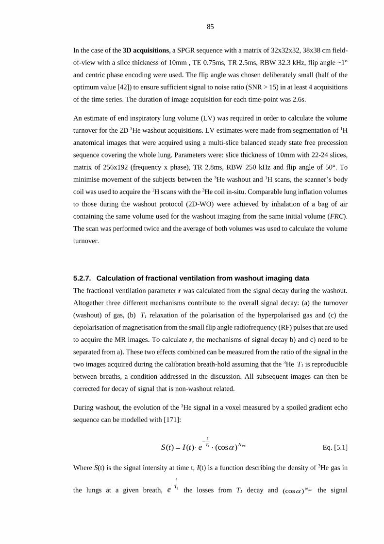
85

In the case of the 3D acquisitions, a SPGR sequence with a matrix of 32x32x32, 38x38 cm field-

of-view with a slice thickness of 10mm , TE 0.75ms, TR 2.5ms, RBW 32.3 kHz, flip angle ~1°

and centric phase encoding were used. The flip angle was chosen deliberately small (half of the

optimum value [42]) to ensure sufficient signal to noise ratio (SNR > 15) in at least 4 acquisitions

of the time series. The duration of image acquisition for each time-point was 2.6s.

An estimate of end inspiratory lung volume (LV) was required in order to calculate the volume

turnover for the 2D 3He washout acquisitions. LV estimates were made from segmentation of 1H

anatomical images that were acquired using a multi-slice balanced steady state free precession

sequence covering the whole lung. Parameters were: slice thickness of 10mm with 22-24 slices,

matrix of 256x192 (frequency x phase), TR 2.8ms, RBW 250 kHz and flip angle of 50°. To

minimise movement of the subjects between the 3He washout and 1H scans, the scanner’s body

coil was used to acquire the 1H scans with the 3He coil in-situ. Comparable lung inflation volumes

to those during the washout protocol (2D-WO) were achieved by inhalation of a bag of air

containing the same volume used for the washout imaging from the same initial volume (FRC).

The scan was performed twice and the average of both volumes was used to calculate the volume

turnover.

5.2.7. Calculation of fractional ventilation from washout imaging data

The fractional ventilation parameter r was calculated from the signal decay during the washout.

Altogether three different mechanisms contribute to the overall signal decay: (a) the turnover

(washout) of gas, (b) T1 relaxation of the polarisation of the hyperpolarised gas and (c) the

depolarisation of magnetisation from the small flip angle radiofrequency (RF) pulses that are used

to acquire the MR images. To calculate r, the mechanisms of signal decay b) and c) need to be

separated from a). These two effects combined can be measured from the ratio of the signal in the

two images acquired during the calibration breath-hold assuming that the 3He T1 is reproducible

between breaths, a condition addressed in the discussion. All subsequent images can then be

corrected for decay of signal that is non-washout related.

During washout, the evolution of the 3He signal in a voxel measured by a spoiled gradient echo

sequence can be modelled with [171]:

RFNT

t

etItS )(cos)()( 1

Eq. [5.1]

Where S(t) is the signal intensity at time t, I(t) is a function describing the density of 3He gas in

the lungs at a given breath, 1T

t

e

the losses from T1 decay and RFN)(cos the signal

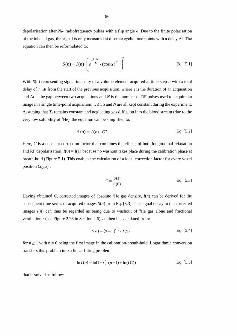
86

depolarisation after NRF radiofrequency pulses with a flip angle α. Due to the finite polarisation

of the inhaled gas, the signal is only measured at discrete cyclic time points with a delay Δt. The

equation can then be reformulated to:

n

NT

t

enInS

)(cos)()( 1

Eq. [5.1]

With S(n) representing signal intensity of a volume element acquired at time step n with a total

delay of τ+Δt from the start of the previous acquisition, where τ is the duration of an acquisition

and Δt is the gap between two acquisitions and N is the number of RF pulses used to acquire an

image in a single time-point acquisition. τ, Δt, α and N are all kept constant during the experiment.

Assuming that T1 remains constant and neglecting gas diffusion into the blood stream (due to the

very low solubility of 3He), the equation can be simplified to:

nCnInS )()( Eq. [5.2]

Here, C is a constant correction factor that combines the effects of both longitudinal relaxation

and RF depolarisation, I(0) = I(1) because no washout takes place during the calibration phase at

breath-hold (Figure 5.1). This enables the calculation of a local correction factor for every voxel

position (x,y,z) :

)0(

)1(

S

SC Eq. [5.3]

Having obtained C, corrected images of absolute 3He gas density, I(n) can be derived for the

subsequent time series of acquired images S(n) from Eq. [5.3]. The signal decay in the corrected

images I(n) can thus be regarded as being due to washout of 3He gas alone and fractional

ventilation r (see Figure 2.26 in Section 2.6)can then be calculated from:

)()( 111

IrnIn

Eq. [5.4]

for n ≥ 1 with n = 0 being the first image in the calibration-breath-hold. Logarithmic conversion

transfers this problem into a linear fitting problem:

))1(ln()1(1ln)(ln InrnI Eq. [5.5]

that is solved as follow:

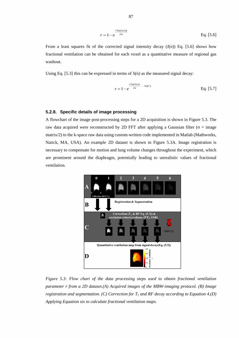
87

n

nI

er

))(ln(

1 Eq. [5.6]

From a least squares fit of the corrected signal intensity decay (I(n)) Eq. [5.6] shows how

fractional ventilation can be obtained for each voxel as a quantitative measure of regional gas

washout.

Using Eq. [5.3] this can be expressed in terms of S(n) as the measured signal decay:

)ln()(ln(

1C

n

nS

er

Eq. [5.7]

5.2.8. Specific details of image processing

A flowchart of the image post-processing steps for a 2D acquisition is shown in Figure 5.3. The

raw data acquired were reconstructed by 2D FFT after applying a Gaussian filter (σ = image

matrix/2) to the k-space raw data using custom-written code implemented in Matlab (Mathworks,

Natick, MA, USA). An example 2D dataset is shown in Figure 5.3A. Image registration is

necessary to compensate for motion and lung volume changes throughout the experiment, which

are prominent around the diaphragm, potentially leading to unrealistic values of fractional

ventilation.

Figure 5.3: Flow chart of the data processing steps used to obtain fractional ventilation

parameter r from a 2D dataset.(A) Acquired images of the MBW-imaging protocol. (B) Image

registration and segmentation. (C) Correction for T1 and RF decay according to Equation 4.(D)

Applying Equation six to calculate fractional ventilation maps.

88

All datasets were registered to the first image using an image registration algorithm as described

in greater detail by Barber et al. [161]. To account for the different intensity ranges resulting from

the washout of gas, the images are first normalised to the maximum signal of the lung volume at

each time point before applying the registration algorithm and mapped back to their original

intensities after registration. An in silico simulation using a lung virtual from the outline from a

segmented dataset was used. The virtual lung was filled with defined values of image intensity to

test the algorithm, registering two different inflation states. A comparison of original data with

the registered data showed that the registration algorithm did not affect signal intensity. The

registration algorithm is based on an adjusted sum-of-squared intensity differences as similarity

measure (SSD).

After registration, images are segmented using a threshold-based mask created from the first

image which has the highest signal to noise ratio (SNR2D >150 ; SNR3D> 200). The threshold is

established using Otsu’s method [172] as a fast method to obtain a threshold. This uses the signal

threshold level which maximises the between-class variance of the two clusters defined by the

applied threshold (foreground and background) in the histogram of an image. The images were

then filtered using a median filter with a 3x3 neighbourhood to reduce the effect of noise.

Afterwards images with SNR < 15 were excluded from further evaluation. SNR was calculated

as the ratio of mean signal intensity of the whole segmented lung to the standard deviation of the

noise. A second segmentation is then applied using a mask created from the last acquisition with

SNR≥15 of the washout cycle (Figure 5.3D). The second segmentation excluded lung regions

with no signal left after the washout (e.g. trachea) and guaranteed that the SNR in each pixel in

all voxels was at least 15. This mask is then applied to all images. The segmentation is followed

by the correction for T1 and RF depolarisation described above in Eq. [5.2] (Figure 5.3C). Finally,

Eq. [5.5] is evaluated on a pixel by pixel basis to calculate the fractional ventilation r for each

voxel using a least squares algorithm (Figure 5.3D).

As a final step the lung volumes and breathing were checked for reproducibility due to their direct

impact on the fractional ventilation (compare also Section 6.2). Recordings from the

pneumotachograph were evaluated and the mean tidal volume over the whole experiment was

calculated. Tidal volume changes ±15% of the mean value resulted in an exclusion of the two

sequential time-points to avoid major changes of fractional ventilation between breaths (due to

altered breathing efforts). In addition the lung volume (LV as segmented from the individual time-

steps) of the 3D acquisition was taken into account and for changes of LV >10% compared to the

mean LV the individual acquisition was excluded.

89

5.2.9. Gravitational evaluation of fractional ventilation

To evaluate the effects of gravity on regional ventilation, each map was divided into strips of 2cm

running length-wise in the superior-inferior direction, orthogonal to the direction of gravity when

the subject is supine in the MRI scanner, and mean r was calculated for each strip. The first and

last strips were excluded from the evaluation of gravitational slopes to omit upper and lower

borders.

5.2.10. Comparison of imaging and pneumotachograph measurements of

ventilation

The values of fractional ventilation obtained from washout imaging were compared to the total

gas volume turnover measured using the pneumotachograph and lung volume from MRI. With

knowledge of the inspiratory lung volume, LV (from the imaging data), and the tidal volume, TV,

(from the pneumotachograph), the gas volume turnover of the whole lungs with each breath can

be calculated [65, 171]:

LV

TVf Eq. [5.8]

In the case of the 3D protocol, LV , was obtained by segmenting the 3D ventilation images

acquired for each breathing cycle and taking the mean value. The images were segmented using

a threshold determined by Otsu’s method [172]. In the case of the 2D protocol the average

inspiratory lung volume was determined from manual segmentation of the signal void (air space)

in the additional proton scans acquired. This method has previously been shown to give good

estimates of LV [57]. This measurement can be considered as independent of the 3He MR

measurements of fractional ventilation. Even though the same dataset is used to calculate gas

volume turnover and fractional ventilation for the 3D protocol, the information is used in a

different way. While the binary segmented images from the calibration phase are used to return

the lung volume as part of calculation of gas turnover, for calculation of fractional ventilation, the

image intensity itself as a function of time is required.

5.2.11. Comparison of fractional ventilation from 2D and 3D protocols

To directly compare the mean fractional ventilation of the 2D maps with the 3D maps it is

assumed that the two thick slice 2D maps represent most of the lung volume. The tidal volume

during the washout phase of the experiment directly influences the values of r:

90

FRCTV

TV

VV

Vr

rf

f

global

Eq.[ 5.9]

and is dependent on the subject's voluntary breathing. However, as FRC is common to both

experiments, mean global fractional ventilation values measured with the 2D protocol are

converted using Eq. [5.9] for comparison with those measured with the 3D protocol:

FRCTV

TVr

TVr

TVTVLVFRC

WOD

WODconvglobal

WOD

measuredD

WODWOD

3

3

2

2

22

_

Eq.[ 5.10]

where TV is the tidal volume measured during washout from the 2D acquisition (2D-WO) and

the 3D acquisition (3D-WO) respectively, measuredDr 2

represents the fractional ventilation

measured with the 2D protocol, and convglobalr _ is the fractional ventilation measured with the

2D protocol scaled for comparison with the fractional ventilation measured with the 3D protocol.

5.2.12. Reproducibility

Repeatability of 2D and 3D MBW-imaging was investigated. Subjects were imaged repeatedly

with the same protocol. In case of the 3D washout acquisition the gap between scans was 5

minutes. In case of the 2D dataset only Volunteer 4 was imaged within the same scan session.

Repeatability of 3D datasets was tested by comparing the r-maps on a voxel-voxel basis and a

comparison of the histograms (Pearson’s correlation of mean values and standard deviations). In

the case of the 2D datasets voxel by voxel correlation was performed on Volunteer 4.

5.3. Results

Table 5.1 shows subject data; weight, age and sex as well as tidal volume measured in supine at

rest (TV), FEV1 and FVC in litres and % predicted [84]. All healthy volunteers had no history of

respiratory or cardiac disease and were non-smokers. All subjects tolerated the imaging protocols

well. A representative 2D dataset from one slice of a washout acquisition in the sagittal plane is

shown in the top row of Figure 5.3. The middle row displays the images after correction for RF

depolarisation and T1 decay, which are then used to obtain a fractional ventilation map from the

dataset as seen at bottom of Figure 5.3. The resulting 2D fractional ventilation maps from healthy

subjects (volunteers 1- 4) are displayed in Figure 5.4 together with the corresponding histograms

from the right and left lung r maps. Representative slices from 3D fractional ventilation maps

from subjects 1-4 are shown in the axial, coronal and sagittal planes in Figure 5.5.

91

Figure 5.4: Maps of fractional ventilation parameter r obtained with the 2D washout

acquisition protocol. Sagittal slices from left and right lung are shown for 4 healthy subjects as

well as histograms of distribution of r values for each lung slice.

Figure 5.5: Fractional ventilation maps from 3D washout from healthy subjects in the sagittal,

coronal and axial plane (Volunteer 1-4).

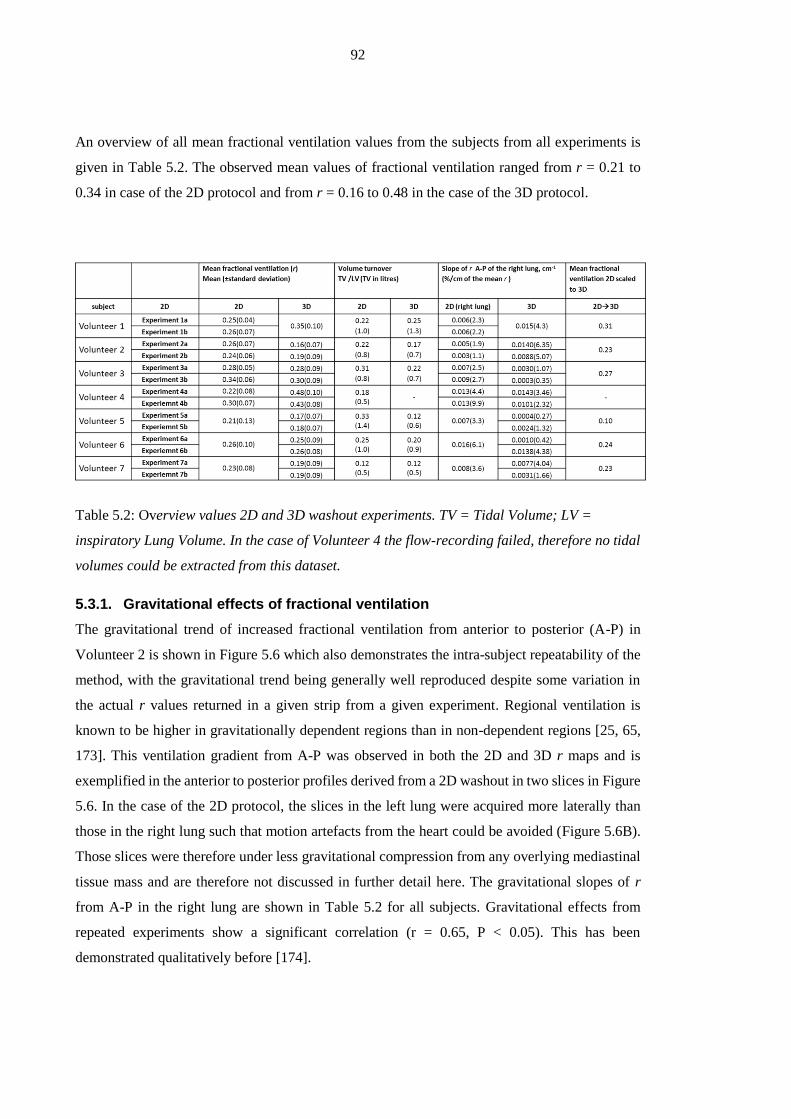
92

An overview of all mean fractional ventilation values from the subjects from all experiments is

given in Table 5.2. The observed mean values of fractional ventilation ranged from r = 0.21 to

0.34 in case of the 2D protocol and from r = 0.16 to 0.48 in the case of the 3D protocol.

Table 5.2: Overview values 2D and 3D washout experiments. TV = Tidal Volume; LV =

inspiratory Lung Volume. In the case of Volunteer 4 the flow-recording failed, therefore no tidal

volumes could be extracted from this dataset.

5.3.1. Gravitational effects of fractional ventilation

The gravitational trend of increased fractional ventilation from anterior to posterior (A-P) in

Volunteer 2 is shown in Figure 5.6 which also demonstrates the intra-subject repeatability of the

method, with the gravitational trend being generally well reproduced despite some variation in

the actual r values returned in a given strip from a given experiment. Regional ventilation is

known to be higher in gravitationally dependent regions than in non-dependent regions [25, 65,

173]. This ventilation gradient from A-P was observed in both the 2D and 3D r maps and is

exemplified in the anterior to posterior profiles derived from a 2D washout in two slices in Figure

5.6. In the case of the 2D protocol, the slices in the left lung were acquired more laterally than

those in the right lung such that motion artefacts from the heart could be avoided (Figure 5.6B).

Those slices were therefore under less gravitational compression from any overlying mediastinal

tissue mass and are therefore not discussed in further detail here. The gravitational slopes of r

from A-P in the right lung are shown in Table 5.2 for all subjects. Gravitational effects from

repeated experiments show a significant correlation (r = 0.65, P < 0.05). This has been

demonstrated qualitatively before [174].

93

Figure 5.6: (A) Gravitational effects from anterior to posterior as seen in the left and right lungs

of volunteer 2 from two 2D washout datasets. The repeatability between the two scans can be

observed. The right lung shows an increase in fractional ventilation between anterior and

posterior parts, while the slices in the left lung do not. (B) The slices in the left lung are positioned

further lateral and are therefore under less gravitational compression from overlaying

mediastinal tissue mass.

5.3.2. Comparison of imaging and pneumotachograph measurements of

ventilation

Figure 5.7 shows comparison of the mean fractional ventilation values from gas washout imaging

with the global gas volume turnover obtained from the flow measured with the pneumotachograph

at the mouth and the total inspiratory volume as segmented from the breath hold MRI volume

images. The dead-space volume of the upper airways as measured from the 3He images (NB this

was excluded from the fractional ventilation calculations) was in total 150mℓ, including the dead

space volume of the pneumotachograph and the filter (70mℓ). This total dead space volume was

subtracted from the measured tidal volume. A significant correlation of r = 0.67 (P < 0.001) was

found between the two measures. Despite this good Pearson’s correlation (of the best fit to all

points) the gas turnover is systematically lower. The assessment of LV from ventilation images

and anatomical images is not a precise measure of true LV, since it is hard to account for the exact

contribution of tissue and blood in LV.

94

Figure 5.7: Comparison between the gas volume turnover (tidal volume measured by

pneumotachograph divided by total lung volume measured by MRI) and the measured global

mean fractional ventilation from the 2D and 3D washout protocols including the Bland-Altman

plot in the top left corner. Pearson’s correlation r = 0.67 (P < 0.001, of the best fit to all points),

Bland-Altman analysis shows a mean difference = 17.2% (standard deviation = 23.7%).

Figure 5.8: Pneumotachograph recordings for subject 4 during (A) a 2D acquisition and (B) a

3D acquisition. n = 1,2,3,4,5 numbers the respiratory cycle in which the datasets were acquired.

95

5.3.3. Comparison of fractional ventilation from 2D and 3D protocols

The last column in Table 5.2 shows the fractional ventilation measured with the 2D protocol

converted to corresponding 3D fractional ventilation values using Eq. [5.8]. The comparison

accounts for the dead space of 150mℓ. A Bland-Altman analysis showed a relative mean

difference of 5.9% with standard deviation of ±27.2%. The correlation was not found to be

significant.

5.3.4. Repeatability of washout measurements

Figure 5.9A and B show the comparison of two experiments from Volunteer 4 on a pixel by pixel

basis from the 2D and the 3D protocol, respectively. Corresponding experiments were performed

within the same session and the volunteer was not moved between the acquisitions. A significant

Pearson’s correlation of r= 0.85 (P < 0.0005) was found in the case of the 2D protocol and r= 0.74

(P < 0.0005) in the case of 3D protocol. A Bland-Altman analysis of the datasets from Figure 5.9

resulted in a relative mean of difference of 2.9% (2D) and 10.9% (3D) with a standard deviation

of ±12.1% (2D) and ±13.5% (3D).

Figure 5.9: (A) Correlation on a pixel by pixel basis of two 2D washout experiments of Volunteer

4 acquired in the same session (Pearson’s correlation of r = 0.85 and P<0.005). (B) Correlation

on a pixel by pixel basis of two 3D washout experiments of Volunteer 4 acquired in the same

session (Pearson's correlation of r = 0.74 and P<0.005). Pearson’s correlation was done on the

best fit to data (continuous line).

Table 5.3 shows an overview of the repeatability test results comparing 3D MBW-imaging in 6

volunteers. All datasets show significant correlations r = 0.5 or greater. In addition a Bland-

Altman analysis was performed and the results are listed in Table 5.3. In addition fractional

ventilation maps were divided along the major axis into anterior-posterior, left-right and superior-

inferior into 8 regions of roughly equal size (Figure 5.10).

96

Figure 5.10: (A) Correlation and Bland-Altman plot of 8-region comparison from Volunteer 4.

Errorbars derive from the standard deviation of fractional ventilation in each of the regions.

Black dots show comparison of same regions in both experiments (r = 0.97, P<0.001,), the red

line is the linear fit (almost equal to unity line). A Bland-Altman analysis is shown in the top left

corner (mean difference = 10.5%, standard deviation = 3.2%). (B) Lung divided into 8 regions

of roughly equal size. Each colour represents one region.

Mean values from repeated experiments performed with the 2D washout protocol from all healthy

volunteers are reported in Table 5.2. A standard deviation of the mean values of 12.0% and a

relative average difference of 17.0% was found. A regional comparison was not possible since

data were not acquired on the same day for all volunteers. In case of a 2D slice this could account

for significant differences when matching regions or voxels from different locations in the lung.

Table 5.3: Comparison of repeated 3D MBW-imaging during the same session. Pearson’s

correlation all show highly significant correlations. In addition lungs were divided into 8 regions

of equal size for comparison (divided along the main axis). Mean fractional ventilation measured

in the all 8 regions shows high correlation for all volunteers tested.

97

5.4. Discussion

This work of methodical development has shown how quantitative maps of fractional ventilation

can be acquired in under a half minute by monitoring the washout of a single dose of

hyperpolarised 3He gas. This method was shown to work with a 2D acquisition protocol that

allows synchronised breathing close to calm tidal breathing with very small interruptions. The

same method was also extended to a 3D acquisition allowing the assessment of regional fractional

ventilation values from the whole lung.

The mean global values of fractional ventilation were compared to an independently-measured

value of whole lung gas turnover and significant agreement was found (Figure 5.7). The average

of the mean values of fractional ventilation obtained from all 7 healthy volunteers with the 2D

protocol (r = 0.26±0.04) correspond to specific ventilation (SV) of 0.35±0.04 which is

comparable to the values measured by Sá et al. (SV = 0.33±0.11) with free breathing oxygen-

enhanced 1H MRI [25]. The histograms of r (VH) shown in Figure 5.4 from the 2D fractional

ventilation maps display the same shape with the exception of Volunteer 4. The histogram

suggests a bimodal distribution of fractional ventilation in the right lung reflecting the VH in two

different lobes presumably, while the histogram shape in the left lung is similar in all volunteers.

The mean values from the 3D acquisitions from all volunteers were similar (average r =

0.25±0.08) to those derived from 2D protocol in the same volunteer, but ranged between r=0.16-

0.48. The fractional ventilation values scale with breathing volume and inhalation level. Due to

the timing of the 3D data acquisition, some volunteers (compare Volunteer 4) found it harder to

breathe in a calm fashion. The longer 3D sequence duration increases the apnoea during the first

breath-hold, which in turn can result in an altered subsequent breathing pattern in some cases with

increased TV (Figure 5.8, volunteer 4). This might explain the bigger variability in mean fractional

ventilation in the 3D protocol. While volunteers re-establish steady tidal breathing during the 2D

washout after apnoea this was not possible during a 3D washout, where only four to five

acquisitions with sufficient SNR could be acquired and longer image acquisitions considerably

interrupt the breathing pattern. Acquisition acceleration techniques like compressed sensing (CS)

[6] and k-t-BLAST [175] may help to decrease 3D acquisition times and the number of RF pulses

needed to acquire the 3D images, so that a timing similar to the one in 2D might be achievable.

Using the recorded TV in both experiments and with the assumption that FRC (the initial volume

before breathing in the hyperpolarised gas) is highly reproducible, the values acquired with the

2D protocol can be converted into whole lung fractional ventilation values (Table 5.2).

Comparison of mean whole-lung fractional ventilation from 3D image acquisition does not

significantly correlate with mean fractional ventilation from 2D slices (scaled by the difference

98

in TV).This might indicate that two sagittal slices do not represent the heterogeneity from the

whole lung as previously suggested by Sá et al [176].

5.4.1. Repeatability

The pixel by pixel comparisons of the fractional ventilation maps from repeated experiments

(Figure 5.9A and B) show significant correlations and confirm the reliability of both protocols in

the tested volunteer. Table 5.3 shows the strong correlations of all tested 3D datasets when

compared across 8 similar regions in the lung. Even a voxel-by-voxel comparison shows highly

significant Pearson’s correlations greater than 0.5.

5.4.2. Gravitational evaluation of fractional ventilation

The well-known A-P ventilation gradient in supine humans, which is usually attributed to gravity

and the spring-like compression of the lung under the weight of the overlying mediastinum [25,

65, 173], is clearly demonstrated in this work and helps confirm the validity of the method. The

comparison of 2D and 3D gravitational effects shows good agreement of the gravitational effect.

This leads to the assumption as used by Sá et al. [176], that a single sagittal slice could be

representative for VH distributed in the whole lung in healthy volunteers. In the presence of lung

disease VH is not only a function of the gravitational difference in ventilation from anterior to

posterior parts of the lung, but from inhomogeneous gas distribution related to disease patho-

physiology.

5.4.3. Conclusion

The results presented here demonstrate that it is feasible to obtain quantitative fractional

ventilation maps by MR measurements of 3He washout with only a single dose of hyperpolarised

3He. This reduces the amount of hyperpolarised 3He necessary for this type of examination

considerably when compared to previously suggested methods based on 3He washin [168, 169].

The washout approach presented here enables 3He MRI ventilation quantification for studies in

humans breathing voluntarily using ~100 mℓ doses of 3He for a 2D washout with two slices. This

compares favourably to 2ℓ of 3He used to acquire a 2D fractional ventilation map in a

mechanically-ventilated pig used as a prelude to human experiments with the equivalent washin

technique [169]. The feasibility of acquiring a fractional ventilation map of the whole lung using

200 mℓ of 3He was shown using the 3D washout protocol. Additionally, the total duration of the

examination is less than a half a minute, making it practical for routine clinical application.

Reproducibility of the technique was shown.

99

The 2D washout imaging protocol caused subjects to deviate less from a relaxed breathing pattern

than the 3D protocol. Tidal volumes approximately matched those measured at rest in a supine

position outside the scanner. This could be an advantage when trying to measure fractional

ventilation under different physiological conditions. As an example this could be used to

investigate linearity of values of fractional ventilation when subjects breathe at different tidal

volumes. It would also be an advantage for studies on patients with severely impeded lung

function, as it requires only a synchronisation of the breathing cycle with the acquisition protocol.

For patients who are able to hold their breath for longer than 10s, the 3D voluntary breathing

protocol was shown to be capable of producing fractional ventilation maps of the whole lung. In

Chapter 8 it is shown that this requirement can be met by patients with a predicted FEV1 of 30%.

After some training even a 6 year old child was tested successfully with this technique.

Furthermore, in particular for patients in the presence of ventilation heterogeneity full lung

coverage is of advantage to probe the whole lung rather than a single slice.

100

Chapter 6 Error analysis of fractional ventilation from MBW-

imaging

6.1. Introduction

In the previous chapter measurement of regional fractional ventilation as a metric of gas turnover

was introduced using hyperpolarised 3He MBW-imaging. Agreement with an independent

measure of gas turnover was shown and the gravitational gradient in lung ventilation described

in literature previously was observed [25, 65, 163, 173, 174]. The feasibility of the technique in

2D and 3D was then tested.

In this chapter measurement errors influencing fractional ventilation derived from MBW-imaging

are systematically investigated. The calculation of fractional ventilation from image intensity

decay is described in Chapter 5. The signal intensity decay, to be fitted to obtain regional

fractional ventilation can be described as follows:

)1(1)( 11SCrnI

n

Eq. [6.1]

where r is the regional fractional ventilation. C the correction factor calculated from non-washout

related signal decay and S(1) the signal intensity in the first image before the gas washout has

started. Therefore the error in I(n) can be broken down as:

222

2

S

S

IC

C

Ir

r

II Eq. [6.2]

where the random error δI of the intensity decay represents the combination of effects from

variation in tidal volume from breathing (δ r ), errors in the correction factor (δC) and due to noise

in the measured signal (δS). In the following analysis relative errors are denoted with a Δ and

expressed in percent. First the individual errors influencing I(n) are investigated alongside their

influence on fractional ventilation. Then the combined error in I(n) is used as an input to a Monte-

Carlo analysis to determine the combined effect of all errors on r.

6.2. Errors derived from volume changes

During MBW-imaging subjects breathe voluntarily and have to synchronise breathing with the

imaging sequence. The disadvantage of synchronised breathing is that the tidal volume (TV) as

well as the lung volume during breath-hold (LV) can alter considerably from breath to breath.

This is especially the case for the first image following the calibration phase of apnoea, which is

101

likely to be at higher LV than the first two images. These changes in TV and LV will directly scale

mean values of fractional ventilation accordingly (Section 5.2.10):

LV

TVr Eq. [6.3]

Figure 6.1 shows a volume curve as recorded during washout imaging. Errors resulting from

irregular breathing are schematically shown. Pneumotachograph recording and segmented lung

volumes from 3D washout images during washout in healthy volunteers (Table 5.1) were used to

evaluate volumes and the corresponding standard deviations δTV and δLV. Those standard

deviation are subject-specific and derive from intra-experimental changes of tidal volume and

lung volume (see Table 6.1).

Figure 6.1: Schematic of a multiple breath washout imaging protocol showing the volume curve

during MBW-imaging experiment as measured with a pneumotachograph. Above the curve a

segmented coronal slice is shown to visualise the volume change. The deviations of lung volume

and tidal volume are schematically shown in the volume curve.

Error propagation was used to investigate the influence of deviations in both tidal and lung

volume on the estimate of fractional ventilation.

rLV

LV

TV

TVr

22

Eq. [6.4]

102

Where r is the mean global fractional ventilation as derived from TV and LV. r is the

associated error in fractional ventilation due to volume changes during the experiment.

Results

Lung volumes (LV) were obtained from volumetric images of the 3D MBW-imaging protocol

from 7 subjects. It should be noted that the SNR is not expected to influence the outcome LV

measurements, since images with an SNR<10 were excluded from evaluation. Table 6.1 gives an

overview of the resulting volumes, the standard deviations thereof and the resulting error in global

fractional ventilation evaluating Eq. [6.4].

Table 6.1: Overview average end inspiratory lung volumes (LV) and standard deviation as

obtained from segmenting 3D image-volumes. Tidal volume (TV) and its standard deviation were

measured using a pneumotachograph during gas-washout. Resulting global fractional ventilation

( rr ) and relative error ( r ) were calculated using Eq. [6.4]. All volumes are in ml.

Figure 6.2: Demonstration of the effects of lung volume change in an example from a young CF

patient. Total volume difference from segmented 3D volumes in this example was found to be

0.5L. The same intensity window was applied to both images.

103

Discussion

The relative error of fractional ventilation related to changes in lung volumes was evaluated to be

less than 19±3% on average and was found to be 25% in the worst case scenario. It is assumed

that the relative error Δr deriving from lung volume changes during MBW-imaging is influencing

all values of fractional ventilation equally. Linear scaling of regional fractional ventilation with

global volume changes has been evaluated in the literature [177, 178] and was previously applied

in a similar method using fractional ventilation from oxygen enhanced imaging [176].

6.3. Errors associated with the signal correction factor

The correction factor to compensate for non-washout related signal decay is derived from two

images acquired during a calibration breath-hold (Eq. [5.3]) and is a function of T1 and α:

RFNT

t

eC )(cos

1 Eq. [6.5]

Where the exponential describes the T1 signal decay over a time t and the other term treats signal

decay due to RF depolarisation with NRF pulses. In the following the influence of changes in the

delivered transmit flip angle due to different lung inspiration levels during each breath-hold and

changes in T1 due to changes in the gas mix during gas washout are discussed and investigated.

In addition oxygen uptake by the blood is investigated in terms of influence on the outcome of

fractional ventilation. The error is calculated based on values from literature [61, 179]. It should

be noted, that in the presence of collateral ventilation the correction factor will also be masked by

inter-pixel gas diffusion resulting in gas movement between compartments during breath-hold.

Those effects are not taken into account in this error analysis.

The effect of RF flip angle α

Depending on the loading of the RF coil different power has to be applied to accomplish a given

flip angle in a given subject. The flip angle changes within a small margin for different inflation

levels with the coil design used and at 1.5T [180]. Lung volumes change less than ±11% (Table

6.1). Assuming isotropic expansion of each voxel in the lung this means a change of 2.2% in each

direction. The error in flip angle due to this change of inspirational level is therefore considered

as negligible in this error evaluation [180].

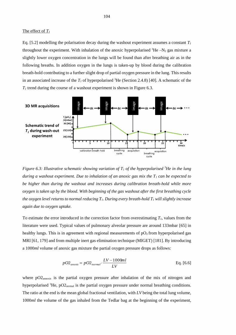
104

The effect of T1

Eq. [5.2] modelling the polarisation decay during the washout experiment assumes a constant T1

throughout the experiment. With inhalation of the anoxic hyperpolarised 3He –N2 gas mixture a

slightly lower oxygen concentration in the lungs will be found than after breathing air as in the

following breaths. In addition oxygen in the lungs is taken-up by blood during the calibration

breath-hold contributing to a further slight drop of partial oxygen pressure in the lung. This results

in an associated increase of the T1 of hyperpolarised 3He (Section 2.4.8) [40]. A schematic of the

T1 trend during the course of a washout experiment is shown in Figure 6.3.

Figure 6.3: Illustrative schematic showing variation of T1 of the hyperpolarised 3He in the lung

during a washout experiment. Due to inhalation of an anoxic gas mix the T1 can be expected to

be higher than during the washout and increases during calibration breath-hold while more

oxygen is taken up by the blood. With beginning of the gas washout after the first breathing cycle

the oxygen level returns to normal reducing T1. During every breath-hold T1 will slightly increase

again due to oxygen uptake.

To estimate the error introduced in the correction factor from overestimating T1, values from the

literature were used. Typical values of pulmonary alveolar pressure are around 133mbar [65] in

healthy lungs. This is in agreement with regional measurements of pO2 from hyperpolarised gas

MRI [61, 179] and from multiple inert gas elimination technique (MIGET) [181]. By introducing

a 1000ml volume of anoxic gas mixture the partial oxygen pressure drops as follows:

LV

mlLVpOpO normalanoxic

100022

Eq. [6.6]

where pO2annoxic is the partial oxygen pressure after inhalation of the mix of nitrogen and

hyperpolarised 3He, pO2normal is the partial oxygen pressure under normal breathing conditions.

The ratio at the end is the mean global fractional ventilation, with LV being the total lung volume,

1000ml the volume of the gas inhaled from the Tedlar bag at the beginning of the experiment,

105

describing the relative amount of residual gas in the lung. This assumes equilibrium mixing of

the resident gases in the lung a valid assumption in healthy subjects in absence of delayed

ventilation. The lung volumes, as in the previous section on volume related errors, are derived

from the volunteer datasets in Chapter 5. This allows an evaluation of the changes in T1 derived

from inhaling an anoxic gas mixture.

In addition to the change of apparent gas mix in the lung, the uptake of oxygen by the blood has

an influence on T1. To evaluate oxygen uptake a linear model is used [61, 63]:

tRpOpO initend 22 Eq. [6.7]

where pO2init is the initial partial oxygen concentration upon inhalation, R is the rate at which this

concentration decays over the time t. The initial partial oxygen pressure (pO2init) is equal to

pO2annoxic and for R a value of 2mbar/s was taken from literature [61, 179]. t is the period of

apnoea during the calibration acquisitions which is equal to the duration of the acquisition

(~2∙2.2s) plus the gap between the images (4s) acquired during calibration breath-hold and adds

up to 8.4s. pO2end therefore is the partial oxygen concentration at the end of the calibration breath-

hold.

tRLV

LVpO

T

normal

10002

11 Eq. [6.8]

where T1′ is the T1 after the combined effects of inhaling anoxic gas and oxygen uptake are both

factored in and ξ = 2.61 bar·s [61]. The results for subjects are summarised in Table 6.2.

Table 6.2: Overview of the parameters used in estimating T1’. Standard deviation of mean values

derive from inter-volunteer variations. * value from literature [61, 179];

106

The systematic error ΔCsys is calculated by substituting T1′ plugged into Eq. [6.5]:

%100)(cos1

C

eCC

RFNT

t

sys

Eq. [6.9]

In addition to the systematic overestimation of T1 the variation of T1′ is taken into account as

relative error (δT1′, Table 6.2 as the variation between volunteers). The random error in C is

derived as follows:

2

12

1

2

12

1

2

1

1

'

1

)cos(

)()(

1

TT

tCT

T

te

TT

CTC

T

t

Eq. [6.10]

With sequence parameters as shown in Chapter 5 (α=1°, acquisition matrix: 322) the error in C

was calculated.

From the systematic error ΔCsys due to T1 overestimation, the systematic error in fractional

ventilation r can be calculated as follows:

%100

r

Crrr

sys

sys Eq. [6.11]

The erroneous correction factor results in a deviation of the true slope that linearly changes

fractional ventilation r. The random error in r is calculated similarly from error propagation:

22

C

CrC

C

rr

Eq. [6.12]

This means that the random error found in C is equal to the random error in fractional ventilation

r (under the assumption that the error deriving from flip angle variations was neglected).

Results:

The resulting systematic error in the correction factor for typical values of T1 in healthy lung are

shown in Figure 6.4 including δT1′ as the inter-volunteer variability. The systematic error of the

correction factor Cerr ranges from approximately 10% to 18% for higher values of T1.

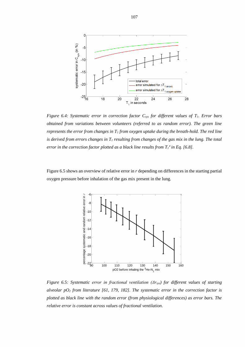
107

Figure 6.4: Systematic error in correction factor Csys for different values of T1. Error bars

obtained from variations between volunteers (referred to as random error). The green line

represents the error from changes in T1 from oxygen uptake during the breath-hold. The red line

is derived from errors changes in T1 resulting from changes of the gas mix in the lung. The total

error in the correction factor plotted as a black line results from T1′ in Eq. [6.8].

Figure 6.5 shows an overview of relative error in r depending on differences in the starting partial

oxygen pressure before inhalation of the gas mix present in the lung.

Figure 6.5: Systematic error in fractional ventilation (Δrsys) for different values of starting

alveolar pO2 from literature [61, 179, 182]. The systematic error in the correction factor is

plotted as black line with the random error (from physiological differences) as error bars. The

relative error is constant across values of fractional ventilation.

90 100 110 120 130 140 150 160-22

-20

-18

-16

-14

-12

-10

-8

-6

pO2 before inhaling the 3He-N2 mix

perc

enta

ge s

yste

matic a

nd r

andom

rela

tive e

rror

in r

108

Discussion

In summary, errors in fractional ventilation range between 7 and 22% depending on T1 (Figure

6.5) and are expected to be constant for different values of fractional ventilation in healthy

volunteers. This assumption might not apply for lungs with a very uneven distribution of gas upon

inhalation of the gas mix containing the hyperpolarised 3He, where spatial T1 mapping might be

required to estimate the effect of spatial heterogeneity.

6.4. Influence of SNR on fractional ventilation

In MRI the measured complex raw signal is influenced by Gaussian noise when Fourier

transformed and presented as magnitude images, the distribution is well represented by a Gaussian

if SNR>2 (SNR in images used here >10) [183, 184]. To simulate the effect of random noise on

the estimate of fractional ventilation a Monte Carlo simulation was performed. Typical SNR

values were taken from the images from the volunteer study of the previous chapter using a fixed

amount of 200ml 3He for each washout and are summarised in Table 6.3. The SNR was calculated

as the ratio of mean signal from the segmented lung to the standard deviation of the noise.

Table 6.3: Average SNR in each image of the washout acquisition for volunteers from Chapter 5.

Noise levels were obtained from the first slices in the absence of signal and the additive standard

deviation of the noise in regions with signal is calculated [183]:

122

22 )(

m

Eq. [6.13]

Where σ is the noise in the presence of signal, and σm the standard deviation of the noise measured

in the absence of signal. The noise is a random error in the signal term S(1) in Eq. [6.1] with δS

being equal to σ. With knowledge of the SNR as the ratio of mean signal to the standard deviation

of the noise, for the measured levels of SNR, δS=1.53σm.

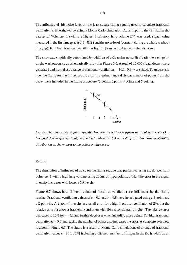
109

The influence of this noise level on the least square fitting routine used to calculate fractional

ventilation is investigated by using a Monte Carlo simulation. As an input to the simulation the

dataset of Volunteer 1 (with the highest inspiratory lung volume LV) was used: signal value

measured in the first image at S(0) ( =I(1) ) and the noise level (constant during the whole washout

imaging). For given fractional ventilation Eq. [6.1] can be used to determine the error.

The error was empirically determined by addition of a Gaussian-noise distribution to each point

on the washout curve as schematically shown in Figure 6.6. A total of 10,000 signal decays were

generated and from these a range of fractional ventilation r = [0.1 , 0.8] were fitted. To understand

how the fitting routine influences the error in r estimation, a different number of points from the

decay were included in the fitting procedure (2 points, 3 point, 4 points and 5 points).

Figure 6.6: Signal decay for a specific fractional ventilation (given as input to the code). I

(=signal due to gas washout) was added with noise (σ) according to a Gaussian probability

distribution as shown next to the points on the curve.

Results

The simulation of influence of noise on the fitting routine was performed using the dataset from

volunteer 1 with a high lung volume using 200ml of hyperpolarised 3He. The error in the signal

intensity increases with lower SNR levels.

Figure 6.7 shows how different values of fractional ventilation are influenced by the fitting

routine. Fractional ventilation values of r = 0.1 and r = 0.8 were investigated using a 3-point and

a 2-point fit. A 2 point fit results in a small error for a high fractional ventilation of 2%, but the

relative error for a lower fractional ventilation with 19% is considerably higher. The relative error

decreases to 10% for r = 0.1 and further decreases when including more points. For high fractional

ventilation (r > 0.6) increasing the number of points also increases the error. A complete overview

is given in Figure 6.7. The figure is a result of Monte-Carlo simulations of a range of fractional

ventilation values r = [0.1 , 0.8] including a different number of images in the fit. In addition an

110

approximate SNR was calculated by taking into account signal decay as measured from the

correction factor and washout.

Figure 6.7: Distribution of errors across all 10,000 simulations resulting from noise in images.

An initial SNR of 86 was assumed in the first image (value taken from Volunteer 1 with biggest

lung volume). 10,000 values were simulated for two different fractional ventilations r = 0.8 and

r = 0.1. For a very rapid signal decay (r = 0.8, high turn-over of gas) the relative error in r was

found to be 7%.

Figure 6.8: (A) shows the estimated SNR of the last image used to fit fractional ventilation. (B)

shows the resulting relative error of the fitting routine. The simulation is based on dataset of

volunteer 1 and assumes an initial SNR = 57 in the image before the gas-washout (compare Table

3).

111

Discussion

Low values of fractional ventilation show a decrease of error when adding points to the fit. The

reverse effect is observed at higher values of fractional ventilation. Including signal with low

SNR into the fitting routine introduces additional error in the fit resulting in an increase of the

total error. Low values of fractional ventilation representing slower washout of the hyperpolarised

gas are not influenced by this, but values about r = 0.5 show an increasing error when adding

points to the fit. A sudden decrease of relative error at higher fractional ventilation (e.g. 5 point

fit for r > 0.65, Figure 6.9) is explained with the use of absolute signal intensity in the fitting

routine. Therefore the absolute value of negative signal intensities resulting from noise being

bigger than signal value is taken.

By increasing the dose applied during a washout experiment SNR could be increased throughout

the washout. Nevertheless, gas amount should be scaled according to expected fractional

ventilation. For higher average fractional ventilation ( r > 0.45, Figure 6.9) more gas would be

beneficial for the fitting routine resulting in an reduction of error when including 3 or more points

to the fit. Nevertheless, the volunteer data all have a mean fractional ventilation of less than 0.35.

Setting an SNR constraint of SNR>10 with a dose of 200ml 3He in comparable or smaller lung

volumes then 4 points result in the best fit. The error deriving from signal noise is then around

5%. Especially when imaging children with considerably smaller lungs (see Chapter 8) with doses

comparable to those used with adults, the data could be fitted over up to 4 points, since the SNR

curves (Figure 6.8A) will start at a higher level.

This assumes that the flip angle is kept constant and is not adjusted to the amount of images

expected. The main aim is to acquire as many images as only possible and therefore the flip angle

should be as small as possible, since data from bad breathing manoeuvres or due to too low SNR

images might have to be excluded subsequently.

In future work it would be beneficial for the reliability of the data to not set a fixed SNR threshold

in combination with a fit over a fixed number of points, but to adjust both depending on the

actually measured regional SNR and signal decay (fractional ventilation).

6.5. Total combined error analysis

As a last step, the total error deriving from the combination of errors in SNR, T1, and volume

changes is calculated. When solving Eq. [6.2] with all errors taken into account in this analysis,

the following equation describes the propagating errors in I(n):

112

)()(

)()(

)( nInS

S

C

Cn

r

rnI

222

11

Eq. [6.14]

The first term of the equation under the square root describes the error deriving from volume

changes (δ r ), which is thought to be constant over all values of fractional ventilation r. The

second term accounts for the errors from variation in the correction factor and the last term

represents the error deriving from image noise.

The individual errors are obtained from the sections above. For δ r the error resulting from volume

changes is used and therefore the volume related error is a function of the fractional ventilation.

It is assumed that this volume change influences the range of fractional ventilation found in the

healthy volunteers in the same way. The correction factor is independent of fractional ventilation

and an average random error of 3% was used as established in the section above. In addition, the

systematic error deriving from the correction factor is considered and directly scales values of

fractional ventilation as shown in the section above. The signal intensity is a function of the breath

number with an error increasing in each breath (due to constant noise level and a decrease of

signal intensity measured). The total error including least squares fitting is investigated using

Monte-Carlo simulation of Eq. [5.7]. As input to this equation the corrected intensity decay and

the calculated associated error distribution I(n)±δI(n) were used.

Figure 6.9: Total error simulated in a Monte-Carlo analysis. Each data point consists of 10.000

experiments.

0.1 0.2 0.3 0.4 0.5 0.6 0.7 0.810

15

20

25

30

35

40

45

50

55

fractional ventilation r

random

rela

tive e

rror

of fr

actional ventila

tion

r in

%

2 point fit

3 point fit

4 point fit

5 point fit

113

Results

Figure 6.9 shows the result of the Monte Carlo simulation. The relative error decreases for higher

values of fractional ventilation. The worst case scenario of a two point fit at low fractional

ventilation results in a relative error Δr <55%. In addition, to random errors the systematic error

deriving from the correction factor between 7-22% (Figure 6.5) has to be added to the values

found in Figure 6.9. This systematic error derives from the overestimation of T1 due to the length

of the calibration breath-hold and the changed gas mix present in the lung. Due to different lung

volumes (resulting in different gas mixe from volunteer to volunteer) and different initial inflation

states it is hard to predict the contribution of this systematic error exactly for this analysis. For a

fractional ventilation r = 0.01 this means the associated error is Δr=0.0014±0.0055 in the case of

regions with high gas turnover r = 0.8 the associated error is Δr=0.11±0.16.

Discussion

Taking all investigated random errors into account at mean fractional ventilation of r = 0.2-0.4 a

bias error of ~15% due to T1 overestimation can be expected. The random error deriving due to

breathing manoeuvres and different lung physiology in the volunteer cohort was estimated to be

around ±25% for this range of fractional ventilation.

6.6. Conclusions

The impact of breathing pattern, changes of T1 due to changes in gas mix and the influence of

SNR on the fitting routing were found to be as the most important sources of error on fractional

ventilation from MBW-imaging. It is assumed that changes in B1 field due to different

inspirational lung volumes are negligible [180]. Furthermore introduced by image registration are

not discussed in this context. Image registration is used to align the lungs after each breathing

cycle. Especially non-physiological values around the diaphragm are avoided this way, since the

exact position of the diaphragm is hard to reproduce. The currently used algorithm developed by

Barber et al. seems to be well suited for the purpose and no physiological unrealistic values around

the edges of the lungs are found.

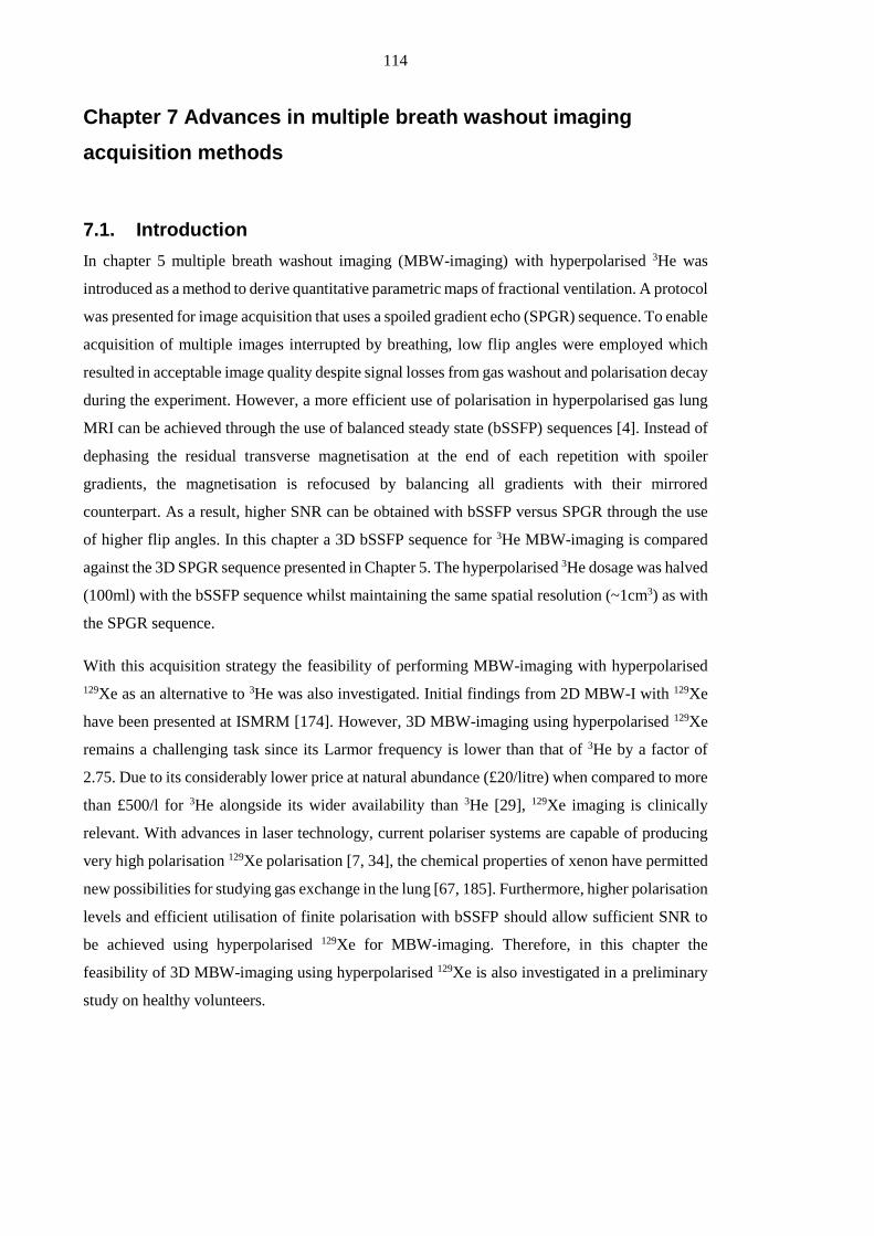
114

Chapter 7 Advances in multiple breath washout imaging

acquisition methods

7.1. Introduction

In chapter 5 multiple breath washout imaging (MBW-imaging) with hyperpolarised 3He was

introduced as a method to derive quantitative parametric maps of fractional ventilation. A protocol

was presented for image acquisition that uses a spoiled gradient echo (SPGR) sequence. To enable

acquisition of multiple images interrupted by breathing, low flip angles were employed which

resulted in acceptable image quality despite signal losses from gas washout and polarisation decay

during the experiment. However, a more efficient use of polarisation in hyperpolarised gas lung

MRI can be achieved through the use of balanced steady state (bSSFP) sequences [4]. Instead of

dephasing the residual transverse magnetisation at the end of each repetition with spoiler

gradients, the magnetisation is refocused by balancing all gradients with their mirrored

counterpart. As a result, higher SNR can be obtained with bSSFP versus SPGR through the use

of higher flip angles. In this chapter a 3D bSSFP sequence for 3He MBW-imaging is compared

against the 3D SPGR sequence presented in Chapter 5. The hyperpolarised 3He dosage was halved

(100ml) with the bSSFP sequence whilst maintaining the same spatial resolution (~1cm3) as with

the SPGR sequence.

With this acquisition strategy the feasibility of performing MBW-imaging with hyperpolarised

129Xe as an alternative to 3He was also investigated. Initial findings from 2D MBW-I with 129Xe

have been presented at ISMRM [174]. However, 3D MBW-imaging using hyperpolarised 129Xe

remains a challenging task since its Larmor frequency is lower than that of 3He by a factor of

2.75. Due to its considerably lower price at natural abundance (£20/litre) when compared to more

than £500/l for 3He alongside its wider availability than 3He [29], 129Xe imaging is clinically

relevant. With advances in laser technology, current polariser systems are capable of producing

very high polarisation 129Xe polarisation [7, 34], the chemical properties of xenon have permitted

new possibilities for studying gas exchange in the lung [67, 185]. Furthermore, higher polarisation

levels and efficient utilisation of finite polarisation with bSSFP should allow sufficient SNR to

be achieved using hyperpolarised 129Xe for MBW-imaging. Therefore, in this chapter the

feasibility of 3D MBW-imaging using hyperpolarised 129Xe is also investigated in a preliminary

study on healthy volunteers.

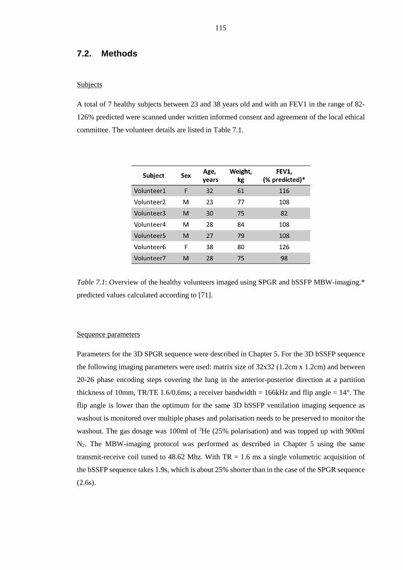
115

7.2. Methods

Subjects

A total of 7 healthy subjects between 23 and 38 years old and with an FEV1 in the range of 82-

126% predicted were scanned under written informed consent and agreement of the local ethical

committee. The volunteer details are listed in Table 7.1.

Table 7.1: Overview of the healthy volunteers imaged using SPGR and bSSFP MBW-imaging.*

predicted values calculated according to [71].

Sequence parameters

Parameters for the 3D SPGR sequence were described in Chapter 5. For the 3D bSSFP sequence

the following imaging parameters were used: matrix size of 32x32 (1.2cm x 1.2cm) and between

20-26 phase encoding steps covering the lung in the anterior-posterior direction at a partition

thickness of 10mm, TR/TE 1.6/0.6ms; a receiver bandwidth = 166kHz and flip angle = 14°. The

flip angle is lower than the optimum for the same 3D bSSFP ventilation imaging sequence as

washout is monitored over multiple phases and polarisation needs to be preserved to monitor the

washout. The gas dosage was 100ml of 3He (25% polarisation) and was topped up with 900ml

N2. The MBW-imaging protocol was performed as described in Chapter 5 using the same

transmit-receive coil tuned to 48.62 Mhz. With TR = 1.6 ms a single volumetric acquisition of

the bSSFP sequence takes 1.9s, which is about 25% shorter than in the case of the SPGR sequence

(2.6s).

116

129Xe MBW-imaging

The same 3D bSSFP sequence was optimised for hyperpolarised 129Xe MBW-imaging, with the

following parameters: matrix size and slice thickness as above; TR/TE 2.9/0.9 ms, a receiver

bandwidth = 16.1 kHz. The flip angle was chosen as 7° to ensure sufficient SNR over multiple

acquisitions during MBW-imaging. A hard pulse was used resulting in a total acquisition time of

2.4s. A total of 600ml of enriched xenon topped up with 400ml N2 was inhaled for imaging. The

hyperpolarised 129Xe had an approximate polarisation of approximately 40%. To directly compare

bSSFP 129Xe MBW-imaging with results from 3He MBW-imaging, subjects were placed in a dual

tuned coil (resonating at both 17.66Mhz, 129Xe, and 48.62Mhz, 3He) [186] so that no change in

patient position was required between scans. Both gases were dispensed within 10 minutes and

the breathing manoeuvres repeated for the repeated gas inhalations.

For a direct comparison, 3He acquisitions were repeated using the same sequence with a hard

pulse, resulting in shorter still TR/TE (1.4/0.4ms). The bandwidth was kept at 161kHz and the

flip angle at 7°. Due to reduced coil sensitivity the 3He dosage was increased to 200ml compared

with the single-tuned T/R coil.

Post-processing

To calculate fractional ventilation maps from both 3He and 129Xe images the same procedure as

described in the Methods of Chapter 5 were followed.

Comparison

To compare fractional ventilation values from different experiments, with different sequences

(bSSFP versus SPGR) and 3He versus 129Xe, Pearson’s correlation coefficient was calculated. In

addition, a Bland-Altman analysis was performed and the mean difference and the standard

deviation as percentage of the mean over all values were reported. This voxel-by-voxel analysis

was valid because volunteers were not moved between experiments performed in the dual tuned

RF coil. Therefore, inter-breath motion was assumed to be being the primary source of miss-

registration. Depending on regional SNR (masks were created using image segmentation of the

last image with mean SNR>10, see Chapter 5), parametric values could not be derived for all

regions in the comparison. This resulted in the exclusion of some voxels from the comparison

(see for example Figure 7.5).

As shown in Figure 5.10, parametric maps of fractional ventilation from the 3He bSSFP-SPGR

sequence comparison were manually divided into 8 regions of interest with similar size. The

difference of mean values from each compartment between experiments was evaluated by

calculating a Pearson’s correlation coefficient.

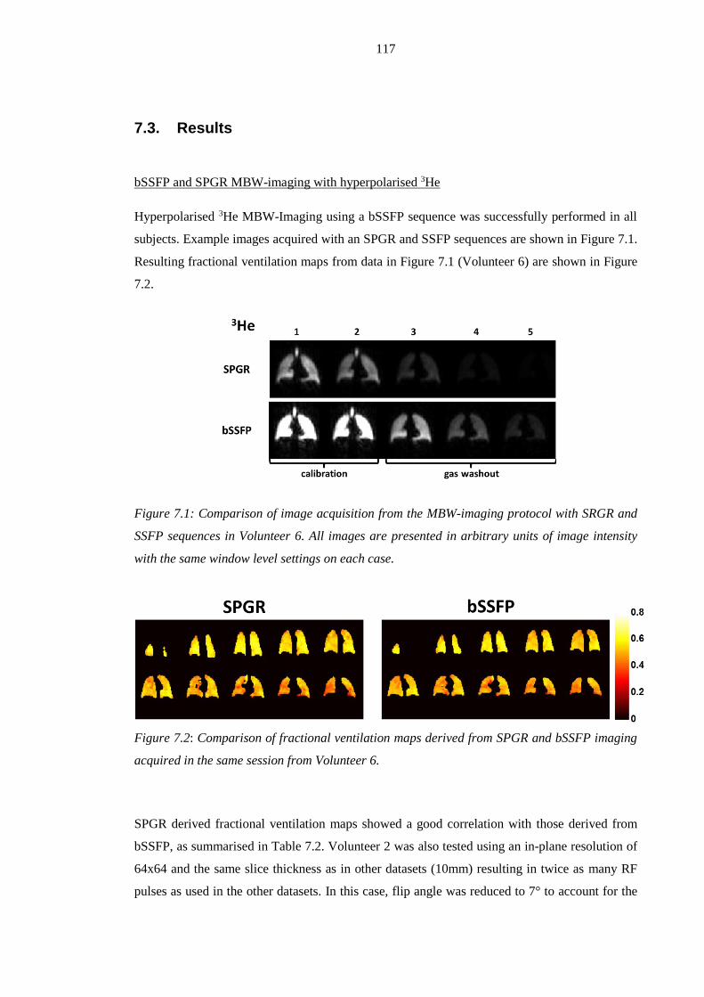
117

7.3. Results

bSSFP and SPGR MBW-imaging with hyperpolarised 3He

Hyperpolarised 3He MBW-Imaging using a bSSFP sequence was successfully performed in all

subjects. Example images acquired with an SPGR and SSFP sequences are shown in Figure 7.1.

Resulting fractional ventilation maps from data in Figure 7.1 (Volunteer 6) are shown in Figure

7.2.

Figure 7.1: Comparison of image acquisition from the MBW-imaging protocol with SRGR and

SSFP sequences in Volunteer 6. All images are presented in arbitrary units of image intensity

with the same window level settings on each case.

Figure 7.2: Comparison of fractional ventilation maps derived from SPGR and bSSFP imaging

acquired in the same session from Volunteer 6.

SPGR derived fractional ventilation maps showed a good correlation with those derived from

bSSFP, as summarised in Table 7.2. Volunteer 2 was also tested using an in-plane resolution of

64x64 and the same slice thickness as in other datasets (10mm) resulting in twice as many RF

pulses as used in the other datasets. In this case, flip angle was reduced to 7° to account for the

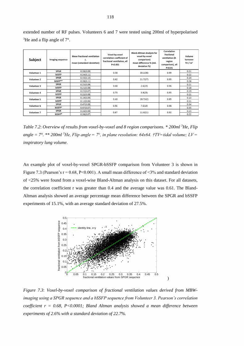
118

extended number of RF pulses. Volunteers 6 and 7 were tested using 200ml of hyperpolarised

3He and a flip angle of 7°.

Table 7.2: Overview of results from voxel-by-voxel and 8 region comparisons. * 200ml 3He, Flip

angle = 7°. ** 200ml 3He, Flip angle = 7°, in plane resolution: 64x64. †TV=tidal volume; LV =

inspiratory lung volume.

An example plot of voxel-by-voxel SPGR-bSSFP comparison from Volunteer 3 is shown in

Figure 7.3 (Pearson’s r = 0.68, P<0.001). A small mean difference of <3% and standard deviation

of <25% were found from a voxel-wise Bland-Altman analysis on this dataset. For all datasets,

the correlation coefficient r was greater than 0.4 and the average value was 0.61. The Bland-

Altman analysis showed an average percentage mean difference between the SPGR and bSSFP

experiments of 15.1%, with an average standard deviation of 27.5%.

)

Figure 7.3: Voxel-by-voxel comparison of fractional ventilation values derived from MBW-

imaging using a SPGR sequence and a bSSFP sequence from Volunteer 3. Pearson’s correlation

coefficient r = 0.68, P<0.0001; Bland Altman analysis showed a mean difference between

experiments of 2.6% with a standard deviation of 22.7%.

0 0.05 0.1 0.15 0.2 0.25 0.3 0.35 0.4 0.45 0.50

0.05

0.1

0.15

0.2

0.25

0.3

0.35

0.4

0.45

0.5

fractional ventilation values from SPGR sequcnce

fractional ventila

tion fro

m b

SS

FP

sequence

identity line, x=y

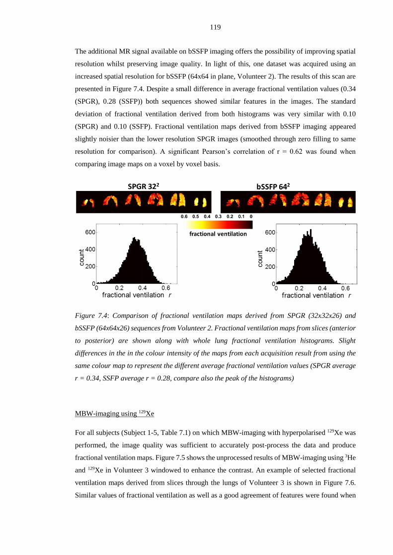
119

The additional MR signal available on bSSFP imaging offers the possibility of improving spatial

resolution whilst preserving image quality. In light of this, one dataset was acquired using an

increased spatial resolution for bSSFP (64x64 in plane, Volunteer 2). The results of this scan are

presented in Figure 7.4. Despite a small difference in average fractional ventilation values (0.34

(SPGR), 0.28 (SSFP)) both sequences showed similar features in the images. The standard

deviation of fractional ventilation derived from both histograms was very similar with 0.10

(SPGR) and 0.10 (SSFP). Fractional ventilation maps derived from bSSFP imaging appeared

slightly noisier than the lower resolution SPGR images (smoothed through zero filling to same

resolution for comparison). A significant Pearson’s correlation of r = 0.62 was found when

comparing image maps on a voxel by voxel basis.

Figure 7.4: Comparison of fractional ventilation maps derived from SPGR (32x32x26) and

bSSFP (64x64x26) sequences from Volunteer 2. Fractional ventilation maps from slices (anterior

to posterior) are shown along with whole lung fractional ventilation histograms. Slight

differences in the in the colour intensity of the maps from each acquisition result from using the

same colour map to represent the different average fractional ventilation values (SPGR average

r = 0.34, SSFP average r = 0.28, compare also the peak of the histograms)

MBW-imaging using 129Xe

For all subjects (Subject 1-5, Table 7.1) on which MBW-imaging with hyperpolarised 129Xe was

performed, the image quality was sufficient to accurately post-process the data and produce

fractional ventilation maps. Figure 7.5 shows the unprocessed results of MBW-imaging using 3He

and 129Xe in Volunteer 3 windowed to enhance the contrast. An example of selected fractional

ventilation maps derived from slices through the lungs of Volunteer 3 is shown in Figure 7.6.

Similar values of fractional ventilation as well as a good agreement of features were found when

120

comparing 3He and 129Xe MBW-imaging data. The fractional ventilation histograms (Figure 7.7)

are similarly shaped and display the same VH (ventilation heterogeneity i.e. the standard

deviation of whole lung fractional ventilation maps). Volunteer 3, whose data is presented in

Figure 7.5-Figure 7.7, exhibited the smallest value of mean differences of fractional ventilation

between 3He and 129Xe of 2.9%, as calculated from Bland-Altman analysis. Results for all 5

volunteers are summarised in Table 7.3.

Figure 7.5: Comparison of image acquisition from the MBW-imaging protocol with 3He and 129Xe

in Volunteer 3. Reduced coil sensitivity at the bottom of the posterior slices when imaging with

3He prevented calculation of fractional ventilation from those regions. All images are presented

in arbitrary units of image intensity with the same window level settings in each case.

Figure 7.6: Comparison of fractional ventilation maps from 3He and 129Xe MBW-imaging in

Volunteer 3. The second slice of both fractional ventilation maps result from raw images shown

in Figure 7.5. Every second slice from both 3D datasets is plotted, with posterior slices on the

left and anterior in the right. The second slice is calculated from raw-images in Figure 7.5.

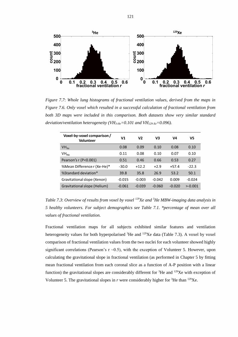
121

Figure 7.7: Whole lung histograms of fractional ventilation values, derived from the maps in

Figure 7.6. Only voxel which resulted in a successful calculation of fractional ventilation from

both 3D maps were included in this comparison. Both datasets show very similar standard

deviation/ventilation heterogeneity (VH3-He=0.101 and VH129-Xe=0.096).

Table 7.3: Overview of results from voxel by voxel 129Xe and 3He MBW-imaging data analysis in

5 healthy volunteers. For subject demographics see Table 7.1. *percentage of mean over all

values of fractional ventilation.

Fractional ventilation maps for all subjects exhibited similar features and ventilation

heterogeneity values for both hyperpolarised 3He and 129Xe data (Table 7.3). A voxel by voxel

comparison of fractional ventilation values from the two nuclei for each volunteer showed highly

significant correlations (Pearson’s r ~0.5), with the exception of Volunteer 5. However, upon

calculating the gravitational slope in fractional ventilation (as performed in Chapter 5 by fitting

mean fractional ventilation from each coronal slice as a function of A-P position with a linear

function) the gravitational slopes are considerably different for 3He and 129Xe with exception of

Volunteer 5. The gravitational slopes in r were considerably higher for 3He than 129Xe.

122

7.4. Discussion and future work

Comparison of 3He MBW-imaging using SPGR and bSSFP

The comparison of fractional ventilation values derived from 3He MBW-imaging with SPGR and

bSSFP sequences shows very good agreement in all volunteers. Considering 3He is a scarce

resource, bSSFP MBW-imaging is potentially a more economical alternative to SPGR requiring

50% less 3He gas dosage. In addition the 10% 3He : 90% N2 mix used is a better approximation

of the normal gas mix in the lung in terms of density and diffusion coefficient. Alternatively,

bSSFP with the same gas dosage as SPGR permits the use of increased spatial resolution. One

3He bSSFP MBW-imaging dataset was acquired using a 2-fold increase in voxel resolution in the

coronal plane (64x64). Despite the increased resolution, higher SNR was measured in the first

acquisition using optimised bSSFP compared to SPGR sequence at 32x32 (SNRbSSFP = 39,

SNRSPGR = 33). In this healthy volunteer the higher resolution showed significant correlation with

lower resolution SPGR-derived maps. This invariance of r distribution with voxel resolution

suggests that a resolution of ~1cm3 is sufficient to fulfil a major assumption of the washout model:

that ventilation is homogeneous within a voxel. The 3He datasets at different special resolution

suggest that this assumption may hold in healthy volunteers. However, in patients with

inhomogeneous ventilation (e.g. asthma, where ventilation heterogeneity starts with effects in the

terminal bronchioles resulting in patchy patterns of ventilation) it may be less applicable. Thus,

an increase in spatial resolution of acquired MBW-imaging data could provide greater insight into

the length scale of the VH and the underlying disease process. Alternatively, the intra-voxel

heterogeneity could be probed by measuring the deviation of fractional ventilation from a model

decay. Insight into sub-voxel heterogeneity may be afforded by treating signal decay with a

stretched exponential model rather than a mono exponential behaviour:

)(ln( nSeay Eq. [7.1]

In this case the signal decay (S(n)) measured over n breaths can be represented by combination

of mono exponential decay with a power law, with a factor α , which gives a semi quantitative

estimation of heterogeneity [60].

For the 3He SPGR-bSSFP comparison, a sequence with a Gaussian-shaped RF pulse (TR=

1.6msec) was used, but recent sequence developments have allowed a rectangular-shaped RF

pulse (width 200µs) that reduces TR to 1.4ms and the total time for a volume acquisition to 1.4s.

This configuration of the bSSFP sequence was used in the 3He-129Xe MBW-imaging comparison.

In addition, the careful optimisation of the bandwidth and flip angle in future work could result

in further improved bSSFP image quality [4]. However, a requirement of bSSFP is that the centre

123

frequency has to be carefully calibrated for each subject to avoid B0 banding artefacts.

Nevertheless, the calibration procedure is relatively simple to perform, and as a result, no major

banding artefacts were observed in any of the datasets acquired in this work. In addition the

broadening of the point spread function that results from the use of high flip angles is not expected

to influence resulting image quality at the currently used resolution as the flip angle was

deliberately kept smaller than the optimum [4] in order to preserve signal between breaths.

Finally, the error estimation presented for SPGR imaging in Chapter 6 has to be revisited for

bSSFP since diffusional dephasing of magnetisation during imaging gradients and effective T2

effects have to be considered when quantitatively modelling the magnetisation (signal) with time

in the total error function of bSSFP-derived fractional ventilation. Nevertheless, the fact that

bSSFP fractional ventilation values findings show a good agreement with SPGR derived

quantitative values is promising.

MBW-imaging of 129Xe

3D multi-nuclear MBW-imaging with 129Xe has been demonstrated. This has been made feasible

by the efficient use of polarisation afforded by bSSFP sequences and the recent improvements in

129Xe polarisation levels which have enabled high SNR images, to be obtained over 4 cycles of

tidal breathing. In our preliminary work using SPGR, MBW-imaging did not provide sufficient

SNR for multiple 3D acquisitions with 129Xe MBW-imaging [174]. Comparable functional

information was derived from MBW-I datasets from both nuclei, with similar ventilation

heterogeneity exhibited by each nucleus for most subjects. The voxel by voxel comparison of

regional fractional ventilation values resulted in a slightly lower average Pearson’s correlation

coefficient of r = 0.48 than found from comparing parametric maps from different sequences

using the same gas (mean Pearson’s r = 0.60). Nevertheless, correlations between data derived

from both nuclei were highly significant (P<0.001 in all cases). Considerably different

gravitational slopes in fractional ventilation for the two gases were found in all subjects. VH in

healthy volunteers is usually associated with the gravitational distribution of ventilation and

therefore this finding is unexpected and requires further investigation. In particular the differences

may arise from altered breathing patterns in both experiments as well as different inspiratory

levels, which will alter distribution of gases with different density throughout the lung. In the case

of 129Xe MBW-imaging the tracer gas makes about 15% of the inspired lung volume and might

have an impact on air distribution. Nevertheless, we observed no clear trend between subjects to

indicate a common alteration on breathing behaviour. Finally the properties of xenon as a much

denser (ρHe-N2=0.958kg/m3, ρXe-N2=2.905kg/m3), and less diffusive gas might have an impact on

the outcome of fractional ventilation (DHe-N2 = 0.90cm2/s, DXe-N2 = 0.12 cm2/s, [149, 187]).

124

A limitation of the current implementation of this dual MBW-imaging technique is associated

with to the coil design. The dual-tuned coil is developed similar to a bib, with high sensitivity in

the apex of the lung and drop off towards the base in posterior slices. This effect could be observed

in all subjects. In the 129Xe images this effect appears less pronounced than in 3He images (Figure

7.6). The improved homogeneity of the Xenon images might be due to the considerably higher

gas dose, resulting in higher concentration of gas throughout the lung. This has an impact on the

inhalation of the gas itself (volunteers take longer to empty the gas bag for the Xenon experiment

than for the Helium experiment) and the altered diffusivity of the gas mix in the lung might also

impact the breathing pattern.

7.5. Conclusions

Fractional ventilation values derived from 3He MBW-imaging using a 3D bSSFP sequence

showed similar quantitative values as SPGR imaging. This bSSFP sequence is promising for

future healthy volunteer and patient studies with MBW-imaging due to its efficient utilisation of

polarisation and hence a reduction in the required gas dosage by a factor of 2. In addition in a

single healthy volunteer it was shown that a resolution of 0.5x0.5x1cm resulted in comparable

fractional ventilation maps to those derived from an isotropic resolution of ~1cm3, which indicates

in healthy normal lungs’ VH is over a length scale greater than that of the voxel. In patients with

considerable regional VH, a finer spatial resolution may however, be advantageous. The

feasibility of 3D multi-nuclear MBW-I with 3He and 129Xe has been successfully demonstrated in

5 healthy volunteers for the first time. In future work, it may be possible to identify sensitivity

differences in MBW-I with 3He and 129Xe to different physiological processes symptomatic of

obstructive lung disease. Work could be taken forward with simultaneous 3He-129Xe MBW-

imaging to monitor different properties of both gases simultaneously.

125

Chapter 8 Linking regional ventilation heterogeneity from

hyperpolarised gas MR imaging to MBW in obstructive airways

disease7

8.1. Introduction

After introducing MBW-imaging as a method to measure fractional ventilation in 3D in Chapter

5 and showing reproducibility of the method, it is important to test its feasibility and sensitivity

to VH in patients. Since the developed method quantitatively measures ventilation with an

approximate resolution of 1cm3 it is expected to be a sensitive tool for the evaluation of

obstructive lung diseases. In this chapter, ventilation heterogeneity (VH) is assessed with this

imaging method and the results are compared to pulmonary function tests sensitive to VH (LCI)

[95, 109] and airflow obstruction (FEV1) [164].

The following two studies were performed in adults diagnosed with asthma and children with

cystic fibrosis (CF) with normal spirometry. The outcome of MBW-imaging is analysed and

statistically compared to pulmonary function tests including LCI from MBW with SF6.

8.2. Methods

8.2.1. Subjects

Studies were performed with the consent of patients, volunteers or the parent (in case of the

children in the CF study) and ethics committee approval. The asthma patient cohort included 30

moderate-severe patients with an FEV1 of 75±26% (mean ± standard deviation). Selected

ventilation images of subjects from this cohort are also presented in Chapter 4. The other cohort

was part of a study comparing early signs of lung disease in children with CF to heathy age-

matched subjects. Children between the age of 6 and 16, all with normal spirometry (FEV1>80%)

at recruitment, were imaged and 6 healthy subjects and 13 patients with CF have been recruited

at this point. An overview of patient and volunteer data is presented in Table 8.1.

7 The patient data acquired for this chapter were collected by the hyperpolarised gas imaging group in

collaboration with Sheffield Children’s Hospital and the Cinical Respiratory Group from the University

of Leicester. Prof. Chris Brightling and Prof. Christopher Taylor are acknowledged here as

representatives for their groups, who have recruited patients and helped with pulmonary function testing.

126

Table 8.1: Overview of patient and subject details (dark blue=healthy volunteer, red=CF patient,

turquoise = asthma patient) and imaging derived values as well as pulmonary function test

results. For the fractional ventilation – as in previous chapters – r is used as an abbreviation.

Predicted FEV1 was calculated according to Miller et al. [71].

127

8.2.2. Pulmonary function tests

All subjects underwent spirometry to obtain FVC and FEV1. Multiple breath washout (MBW)

testing was conducted using the Innocor apparatus (Innovision, Glamsbjerg, Denmark) according

to ATS/ERS guidelines [105]. A mixture of 0.2% SF6 gas and air was used in the experiments.

After washin of the tracer gas to equilibrium a washout was performed until the concentration

had dropped to less than 1/40 of its original value (equals 0.005% of SF6) for three subsequent

exhalations. The system was used as described in Chapter 2 ‘Multiple breath washout (MBW)’

[95]. The lung clearance index was derived from MBW as the lung turn-overs required to reduce

the tracer gas concentration to 1/40 of its original value.

8.2.3. Washout imaging

Washout imaging was performed as described in Chapter 5. Upon inhalation of the hyperpolarised

3He subjects held their breath for 2 calibration acquisitions, after which subjects began to breathe

independently in synchronisation with acquisitions of the scanner. The delay between breaths was

4s in the case of the CF study on children and was increased to 5s in the case of the study on

asthma patients, since children have a higher breathing frequency. Washout imaging was

performed using a 3D spoiled gradient echo sequence covering the whole lung with the specific

imaging parameters as described in Chapter 5: a 32x32 matrix and a subject dependent field of

view between 30x30 cm2 up to 42x42cm2. This resulted in a resolution in the x-y-plane between

9.3mm-13mm, making voxels almost isotropic with a slice thickness of 10mm. The number of

slices was altered between 20 and 28 slices depending upon subjects’ size. With a phase field of

view of 0.8 and an TR of 2.5ms this results in an acquisition time between 1.3s and 1.8s for each

lung volume. The bandwidth of the receiver was 32.3 kHz with an echo time TE of 0.8ms. The

flip angle was calibrated for each subject to 1°, as described in the preliminary experiments

section; this is an empirical value to preserve as much hyperpolarised magnetisation as possible

for images at later stages of the washout.

Asthma patients inhaled a fixed dose of 200ml hyperpolarised 3He, the children were given

between 100ml and 200ml (determined empirically according to predicted FRC). Doses were

topped up with N2 to 1 litre in the case of the adult asthmatic study and to 350-500ml for the CF

children. In the case of patient studies, patients were monitored closely to ensure that they did not

breathe between calibration scans or lose their breath. To monitor the steadiness of the breath-

hold during calibration the lung volume segmented from both calibration images was compared

and in addition the mean correction factor (Eq. [5.4], Chapter 5) was recorded. The mouthpiece

connected to the flow sensor was placed in the subjects’ mouth after inhalation of the gas mixture

containing the 3He from a Tedlar bag during the calibration breath-hold interval. Care was taken,

128

that patients had finished inhalation before the image acquisition began in order to avoid a delayed

inflow of hyperpolarised gas during calibration. This would cause erroneous calibration values as

gas would still be entering the lung during the acquisition of the first calibration image. To avoid

this effect, the acquisition was delayed by one second after inhalation of the gas-mix. This resulted

in a total breath-hold of 10s for the calibration followed by the subsequent exhalation-inhalation

cycles from room air.


Parametric maps of fractional ventilation were derived from MBW-images using the algorithm

described in Chapter 5. Assuming an approximately normal distribution of fractional ventilation

over the whole lung, the standard deviation (SD) and mean values were derived from fractional

ventilation maps. The histograms are used to derive skewness [188] of the distribution and

coefficient of variation (CV). In addition, the gravitational gradient in ventilation was

investigated. For each subject the average fractional ventilation for each coronal slice was

calculated and a linear slope was fitted to the result, as shown in Figure 8.1.

Figure 8.1: The average of each 10mm coronal slice in 3D fractional ventilation maps (A) was

plotted from anterior to posterior (B). A linear slope was fitted to measure influence of gravity

on fractional ventilation in supine subjects. The slope has units of fractional ventilation per slice

[Δr/cm] and can be used to evaluate ventilation changes from anterior-posterior.

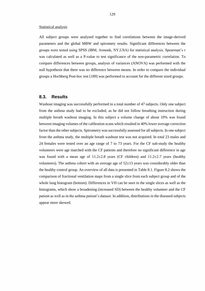
129

Statistical analysis

All subject groups were analysed together to find correlations between the image-derived

parameters and the global MBW and spiromety results. Significant differences between the

groups were tested using SPSS (IBM, Armonk, NY,USA) for statistical analysis. Spearman’s r

was calculated as well as a P-value to test significance of the non-parametric correlation. To

compare differences between groups, analysis of variances (ANOVA) was performed with the

null hypothesis that there was no difference between means. In order to compare the individual

groups a Hochberg Post-hoc test [189] was performed to account for the different sized groups.

8.3. Results

Washout imaging was successfully performed in a total number of 47 subjects. Only one subject

from the asthma study had to be excluded, as he did not follow breathing instruction during

multiple breath washout imaging. In this subject a volume change of about 10% was found

between imaging volumes of the calibration scans which resulted in 40% lower average correction

factor than the other subjects. Spirometry was successfully assessed for all subjects. In one subject

from the asthma study, the multiple breath washout test was not acquired. In total 23 males and

24 females were tested over an age range of 7 to 73 years. For the CF sub-study the healthy

volunteers were age matched with the CF patients and therefore no significant difference in age

was found with a mean age of 11.2±2.8 years (CF children) and 11.2±2.7 years (healthy

volunteers). The asthma cohort with an average age of 52±13 years was considerably older than

the healthy control group. An overview of all data is presented in Table 8.1. Figure 8.2 shows the

comparison of fractional ventilation maps from a single slice from each subject group and of the

whole lung histogram (bottom). Differences in VH can be seen in the single slices as well as the

histograms, which show a broadening (increased SD) between the healthy volunteer and the CF

patient as well as in the asthma patient’s dataset. In addition, distributions in the diseased subjects

appear more skewed.

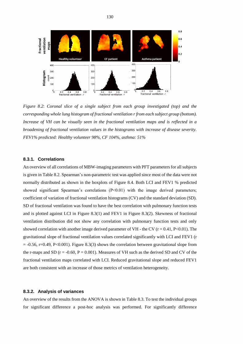
130

Figure 8.2: Coronal slice of a single subject from each group investigated (top) and the

corresponding whole lung histogram of fractional ventilation r from each subject group (bottom).

Increase of VH can be visually seen in the fractional ventilation maps and is reflected in a

broadening of fractional ventilation values in the histograms with increase of disease severity.

FEV1% predicted: Healthy volunteer 98%, CF 104%, asthma: 51%

8.3.1. Correlations

An overview of all correlations of MBW-imaging parameters with PFT parameters for all subjects

is given in Table 8.2. Spearman’s non-parametric test was applied since most of the data were not

normally distributed as shown in the boxplots of Figure 8.4. Both LCI and FEV1 % predicted

showed significant Spearman’s correlations (P<0.01) with the image derived parameters;

coefficient of variation of fractional ventilation histograms (CV) and the standard deviation (SD).

SD of fractional ventilation was found to have the best correlation with pulmonary function tests

and is plotted against LCI in Figure 8.3(1) and FEV1 in Figure 8.3(2). Skewness of fractional

ventilation distribution did not show any correlation with pulmonary function tests and only

showed correlation with another image derived parameter of VH - the CV (r = 0.41, P<0.01). The

gravitational slope of fractional ventilation values correlated significantly with LCI and FEV1 (r

= -0.56, r=0.49, P<0.001). Figure 8.3(3) shows the correlation between gravitational slope from

the r-maps and SD (r = -0.60, P = 0.001). Measures of VH such as the derived SD and CV of the

fractional ventilation maps correlated with LCI. Reduced gravitational slope and reduced FEV1

are both consistent with an increase of those metrics of ventilation heterogeneity.

8.3.2. Analysis of variances

An overview of the results from the ANOVA is shown in Table 8.3. To test the individual groups

for significant difference a post-hoc analysis was performed. For significantly difference

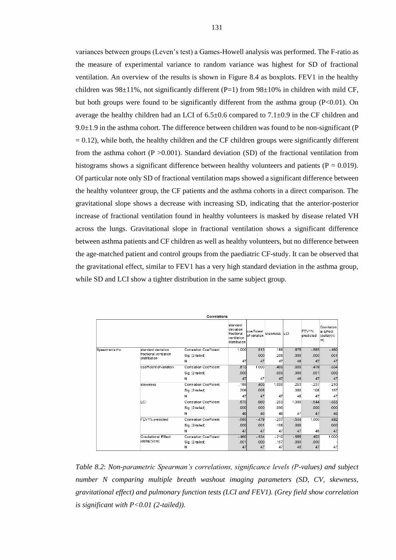
131

variances between groups (Leven’s test) a Games-Howell analysis was performed. The F-ratio as

the measure of experimental variance to random variance was highest for SD of fractional

ventilation. An overview of the results is shown in Figure 8.4 as boxplots. FEV1 in the healthy

children was 98±11%, not significantly different (P=1) from 98±10% in children with mild CF,

but both groups were found to be significantly different from the asthma group (P<0.01). On

average the healthy children had an LCI of 6.5±0.6 compared to 7.1±0.9 in the CF children and

9.0±1.9 in the asthma cohort. The difference between children was found to be non-significant (P

= 0.12), while both, the healthy children and the CF children groups were significantly different

from the asthma cohort (P >0.001). Standard deviation (SD) of the fractional ventilation from

histograms shows a significant difference between healthy volunteers and patients (P = 0.019).

Of particular note only SD of fractional ventilation maps showed a significant difference between

the healthy volunteer group, the CF patients and the asthma cohorts in a direct comparison. The

gravitational slope shows a decrease with increasing SD, indicating that the anterior-posterior

increase of fractional ventilation found in healthy volunteers is masked by disease related VH

across the lungs. Gravitational slope in fractional ventilation shows a significant difference

between asthma patients and CF children as well as healthy volunteers, but no difference between

the age-matched patient and control groups from the paediatric CF-study. It can be observed that

the gravitational effect, similar to FEV1 has a very high standard deviation in the asthma group,

while SD and LCI show a tighter distribution in the same subject group.

Table 8.2: Non-parametric Spearman’s correlations, significance levels (P-values) and subject

number N comparing multiple breath washout imaging parameters (SD, CV, skewness,

gravitational effect) and pulmonary function tests (LCI and FEV1). (Grey field show correlation

is significant with P<0.01 (2-tailed)).

132

Figure 8.3: (1) Correlation between standard deviation of fractional ventilation histograms and

the lung clearance index (LCI). Blue circles represent the healthy volunteers, green the cystic

fibrosis patients and red the asthmatics study. A significant correlation (P<0.001) of r = 0.68

was found. (2) Correlation between standard deviation of fractional ventilation histograms and

forced expiratory volume in 1 second (FEV1). A significant negative correlation (P< 0.001) of r

= -0.59 was found. FEV1 increases with decreasing ventilation heterogeneity. (3) Significant

correlation between standard deviation of fractional ventilation and gravitation effects measured

from changes of fractional ventilation from anterior-posterior coronal slices in all subjects. The

anterior-posterior change in fractional ventilation is reduced with increased ventilation

heterogeneity (r = -0.46, P <0.01). Black lines show a linear fit to all data in each of the graphs.

Figure 8.4: Boxplots of imaging-derived variables and pulmonary function tests. (A) FEV1 (B)

LCI (C) Standard deviation derived from fractional ventilation maps (SD/VH-MBWI) and (D) the

gravitational slope. *=significant difference between groups (P < 0.01).

133

Table 8.3: Overview ANOVA testing of MBW-imaging derived values and pulmonary function

tests. P<0.05 of mean differences was selected as significance level. F describes the ratio of

random variance to experimental variance. Grav. is an abbreviation for gravitational slope.

*Levenne’s test of equality of error variances P<0.01 (as a result a Games-Howell test was

performed)

In the case of the CF sub-study, MBW was performed in both a sitting position and supine in

order to mimic the imaging posture. To test the two groups for significant difference LCI derived

from sitting and supine MBW was compared. The findings are shown in Figure 8.5. An

independent samples Mann-Whitney U test was performed to test the hypothesis that both

distributions are the same. In the case of the sitting LCI- data the null hypothesis was retained (P

= 0.18) while supine data showed a significant difference between patients and healthy volunteers

(P = 0.02). There was no significant difference found when comparing LCI values supine and

sitting within the subject groups, but in both cases the average supine LCI is higher than LCI

measured sitting.

Figure 8.5: Comparison of LCI measured sitting and in supine position between heathy volunteers

and CF patients. An independent samples Mann-Whitney U Test showed no significant difference

between the two groups measured sitting, but with a significant different when MBW was recoded

in supine position (P = 0.02).

134

8.4. Discussion

3He MBW-I was used to produce fractional ventilation maps from patients and controls with

healthy lungs in order to derive parameters to quantify ventilation heterogeneity (VH). In the case

of patients with severe VH the model of each voxel being an independently ventilated

compartment of the lung might be violated. Delayed ventilation representing collateral movement

of gas between adjacent voxels in 3He MRI breath-hold imaging has been shown before in COPD

patients [170, 190] and similar effects can be found in asthma [191]. Signs of inter-voxel delayed

ventilation during the breath-hold calibration interval were also found in some patients in the

asthma cohort of this study [192]. Lung units affected by evidence of such delayed ventilation

were however excluded from fractional ventilation maps to avoid errors introduced by inter-voxel

signal increase during the calibration step. The associated signal increase would cause an

overestimation of fractional ventilation that could even result in negative values. As such, we

work on the premise that all voxels are at an equilibrium gas concentration at the endpoint of the

breath-hold calibration period (~6s after inspiration). It is not certain to what extent delayed filling

of lung units contribute to gas turnover as measured by MBW-I.

Both asthma and cystic fibrosis are obstructive lung diseases. Patients suffer from restriction to

airflow caused by airway constriction and narrowing. As a result of restricted airflow, VH is

expected to increase. VH is a term used to describe a heterogeneous ventilation of different

regions of the lung, and can be directly studied and visualised using quantitative imaging methods

like MBW-imaging. From fractional ventilation maps, regionally specific parameters can be

generated in order to better understand VH. The standard deviation (SD) of fractional ventilation

maps as a measure of VH was found to be most sensitive. The SD derived from the fractional

ventilation maps was also shown to inversely correlate with FEV1 (r = -0.61, P<0.001). Similarly

the lung clearance index (LCI) increases with rising VH and shows a positive correlation with SD

(r = 0.625, P<0.001). SD also incorporates the effect of gravity, as a well-known and described

VH found in healthy volunteers across the whole lung (see Chapter 2). The gravitational effect of

increase of ventilation from non-dependent to dependent parts of the lung is reflected in a slope

of fractional ventilation from anterior to posterior parts of the lung. Gravitational effects in lung

ventilation have previously been shown to change with disease [193-195]. It is hypothesised that

with an increase of VH the effect of gravity on ventilation becomes less apparent as it is masked

by high variation of fractional ventilation between different regions of the lung determined by the

underlying location of the disease related physiological changes. This is supported by the negative

correlation between the gravitational effect and LCI (r = -0.55, P<0.001), CV (r = -0.53, P=0.002)

and SD of fractional ventilation (r = -0.46, P<0.001) and in contrast, a positive correlation with

FEV1 (r = 0.55, P<0.001) was found, i.e. in healthy lungs with little ventilation impairment the

anterior-posterior slope in ventilation is a good indicator of healthy lung ventilation. The slightly

135

lower correlation of the gravitational slope and SD (derived from the same images) when

compared to the correlation of gravitational slope with pulmonary function tests might be

explained by the fact that in healthy volunteers an increased gravitational effect results in a higher

VH. A trend of increase in VH with increasing gravitational effect was found in both the healthy

volunteers and the CF-patients, but was not statistically significant.

The coefficient of variation (CV) was also derived from fractional ventilation maps as the

standard deviation divided by the mean value of fractional ventilation. Since the mean value of

the fractional ventilation is dependent on tidal volume, this therefore makes CV effort-dependent.

Significant correlations of CV with FEV1 (r = -0.479 P<0.01) and LCI (r = 0.660, P<0.01) were

found, similar to SD. In addition, the skewness of fractional ventilation histograms was measured

and Spearman’s correlation (r = 0.40, P <0.01) with CV was the only significant relationship

found. Skewness of the fractional ventilation distribution in the whole lung seems to be less

sensitive to changes in VH.

Significant differences in imaging-derived parameters and PFTs were found between the much

older asthma patients and the children in the CF-study (both patients + volunteers). This is not

surprising when comparing an asthma cohort with a mean age of 52 years and predicted FEV1 of

75±26% to children with mean age of 11 and predicted FEV1 > 80% in the CF study. Of particular

interest is the comparison of the heathy volunteers group with the age matched CF patients where

the MBW-imaging SD showed significant difference between groups, while LCI and FEV1

differences did not show significant differences. In Figure 8.5 a trend in difference between

heathy volunteers and CF patients was seen when looking at the LCI, which might be expected

to become significant with an increase of recruited subjects for this study.

The SF6 MBW (LCI) was routinely acquired in the upright position whilst imaging was performed

in the supine position due to the horizontal bore of the MRI scanner. Especially for patients with

CF, a change in position might alter the ventilation pattern as mucus can shift within the lung

when body position changes. This hypothesis is supported by the significantly higher LCI in CF

patients than in healthy volunteers found when performing MBW in supine position.

Unfortunately those data were not collected for the asthma study and it is questionable if similar

effects might be found in asthmatics where mucus probably plays a lesser role in lung obstruction.

LCI sitting was greater than LCI supine in healthy volunteers, although not significantly, so these

changes may be derived from differences in tissue compression (gravitational effect) when

performing MBW in supine. This result has to be tested in a bigger cohort of healthy volunteers

and patients.

136

8.5. Conclusions

It was shown that MBW-imaging is feasible with patients as young as 6 years old. Patients with

predicted FEV1 <30% were also found to be able to perform the MBW-imaging breathing

protocol as only a single long breath-hold of <11s was required before breathing in

synchronisation with image acquisition. This makes MBW-imaging a potentially useful and

promising technique to quantify regional ventilation in the whole lung in patients with lung

disease.

MBW-imaging derived parameters (SD, CV, gravitational effect) were shown to correlate

significantly with pulmonary function tests. The standard deviation of fractional ventilation maps

(SD) is a robust measure of ventilation heterogeneity (VH) that is less likely to be masked by

breathing effort than the coefficient of variation (CV) [176]. SD derived from MBW-imaging was

shown to be sensitive to the early changes in VH, whereas all other metrics did not result in

significant differences between investigated subject groups. The LCI itself is more sensitive to

early changes in CF when measured in supine position rather than upright sitting in this group of

patients with mild CF and it can be expected increasing the number of patients recruited will

result in a significant difference between mean LCI of the two groups.

The gravitational effect in healthy volunteers in the absence of ventilation defects is expected to

explain any underlying VH. However, from the data from the two patient studies it was possible

to show that with increased severity of disease (lower FEV1, higher VH) the gravitational effect

becomes less apparent, which is consistent with gravitational effects measured with other imaging

techniques in lung disease.

In future work it will be investigated how VH measured from MBW-imaging (SD) changes with

age. It is not expected to be highly age dependent since only a small change of VH sensitive LCI

has been shown before [95].

137

Chapter 9 Future work - linking multiple breath washout

imaging to global multiple breath washout tests with modelling

9.1. Introduction

In the previous chapter multiple breath washout (MBW) derived indices from whole lung tests

were compared to standard deviation of fractional ventilation maps derived from MBW-imaging.

Both metrics of ventilation heterogeneity (VH) were shown to correlate significantly. Here a basic

theoretical model is presented to directly compare exhaled tracer gas volume predicted from

functional information (MBW-imaging) and that measured by sampling concentration and flow

at the mouth with MBW. While MBW samples tracer gas with a high temporal resolution, it is a

1-D test and information on VH is inferred from the temporal course of measured gas

concentration. This information cannot provide a unique solution from a regional perspective

regarding VH. MBW-imaging on the other hand derives functional information (fractional

ventilation r) regionally for each voxel, but due to the properties of the hyperpolarised gas used

and duration of a whole lung image acquisition, currently only a single measurement is acquired

for each breathing cycle and therefore it currently lacks the temporal information.

The comparison of quantitative functional lung MRI with MBW from the pulmonary function lab

has been presented before by Sá et al. [176]. The approach uses regional signal changes from

oxygen enhanced 1H MRI washin and washout to derive specific ventilation8 maps of a single

sagittal slice. To directly compare specific ventilation histograms from imaging with MBW-

curves the most likely distribution of specific ventilation is recovered from the global values

measured at the mouth using the method from Lewis et al. [125]. VH here was assessed as the

standard deviation of the logarithmic distribution of specific ventilation and showed good

correlation with small differences (~10%) between both measurements. This comparison,

Nevertheless, is rather similar to work presented in Chapter 8 and does not atempt to model or

directly compare MBW-tracer gas decay with time.

The approach taken in this chapter to compare MBW measured from the pulmonary function lab

to 3D MBW-imaging using hyperpolarised gas MRI is novel. Instead of recovering regional

information from a global measurement, the regional functional information obtained from

MBW-imaging is used to model the global signal (tracer gas volume) washout from the whole

8 Specific ventilation definition can be found in Chapter 2 Eq. [2.28]. Specific ventilation can be directly

converted to fractional ventilation.

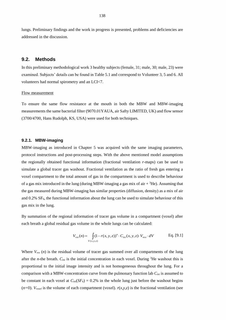
138

lungs. Preliminary findings and the work in progress is presented, problems and deficiencies are

addressed in the discussion.

9.2. Methods

In this preliminary methodological work 3 healthy subjects (female, 31; male, 30; male, 23) were

examined. Subjects’ details can be found in Table 5.1 and correspond to Volunteer 3, 5 and 6. All

volunteers had normal spirometry and an LCI<7.

Flow measurement

To ensure the same flow resistance at the mouth in both the MBW and MBW-imaging

measurements the same bacterial filter (9070.01YAUA, air Safty LIMITED, UK) and flow sensor

(3700/4700, Hans Rudolph, KS, USA) were used for both techniques.

9.2.1. MBW-imaging

MBW-imaging as introduced in Chapter 5 was acquired with the same imaging parameters,

protocol instructions and post-processing steps. With the above mentioned model assumptions

the regionally obtained functional information (fractional ventilation r-maps) can be used to

simulate a global tracer gas washout. Fractional ventilation as the ratio of fresh gas entering a

voxel compartment to the total amount of gas in the compartment is used to describe behaviour

of a gas mix introduced in the lung (during MBW-imaging a gas mix of air + 3He). Assuming that

the gas measured during MBW-imaging has similar properties (diffusion, density) as a mix of air

and 0.2% SF6, the functional information about the lung can be used to simulate behaviour of this

gas mix in the lung.

By summation of the regional information of tracer gas volume in a compartment (voxel) after

each breath a global residual gas volume in the whole lungs can be calculated:

),,(

),,()),,(1()(

zyxV

voxinin

res dVVzyxCzyxrnV Eq. [9.1]

Where Vres (n) is the residual volume of tracer gas summed over all compartments of the lung

after the n-the breath. Cini is the initial concentration in each voxel. During 3He washout this is

proportional to the initial image intensity and is not homogeneous throughout the lung. For a

comparison with a MBW-concentration curve from the pulmonary function lab Cini is assumed to

be constant in each voxel at Cini(SF6) = 0.2% in the whole lung just before the washout begins

(n=0). Vvoxel is the volume of each compartment (voxel). r(x,y,z) is the fractional ventilation (see

139

Figure 9.1A ) of a given voxel location (x,y,z). Figure 9.1B shows the modelled residual gas

volume calculated using the r maps from 4 compartments (shown in top right corner of that figure)

from Figure 9.1A (Cinitial = 0.2%).

Figure 9.1: (A) Fractional ventilation map r is used to predict the concentration washout for each

voxel from Volunteer 6. (B) Residual gas volume in 4 compartments in the lung (left-right,

posterior-anterior, compartments shown in top right corner). A uniform equilibrium gas

concentration of 0.2% tracer gas is assumed at the beginning (breath n=0) and the acquired

functional information (fractional ventilation r) is used to calculate residual gas volume after

each breath in each of the 4 compartments. The sum of all compartments is equal is total residual

tracer gas volume left in the lung measured with MBW at the mouth.

From the residual gas measured in the lung with each breath the total exhaled volume of tracer

gas exhaled after each breath can then be calculated:

)()()( nVnVnV residualresidualexhaled 1 Eq. [9.2]

140

9.2.2. MBW

MBW was performed as described in Chapter 2 and as specified in the ERS-ATS guidelines [105].

To mimic the position of subjects in the MRI, all MBW measurements were recorded supine.

Since breathing pattern during MBW-imaging was interrupted by image acquisition, the acoustic

noise of the MRI scanner was recorded and played out during the gas washout. Subjects were

encouraged to breathe in synchronisation with the recording to mimic MBW-imaging protocol.

Figure 9.2A shows recordings from the flow and gas concentration from the MBW device. In the

flow-pattern, zero flow is found after each inhalation, imitating the breath-hold during an MRI-

acquisition. With knowledge of gas concentration over time and flow-rate the accumulated

exhaled volume for each breath n can be calculated as follow:

s

nt

nt

nt

nt

exhale TtQtCdttQtCnV )()()()()()(

)(

)(

)(

2

1

2

1

Eq. [9.3]

Where C(t) is the concentration recorded during MBW and Q(t) is the flow. The start and end of

an exhalation denoted by t1(n) and t2(n) which are defined by the zero crossing from positive flow

to negative. Ts is the sampling rate of flow-gas analyser, which is in case of the Innocor system

(Innovision, Glamsbjerg, Denmark) used here 10ms. The sampled data time course from Figure

9.2A were integrated using Eq. [9.3] and the exhaled tracer gas volume is plotted over breath

number n in Figure 9.2B.

Figure 9.2: (A) MBW showing SF6 concentration and flow recordings from Volunteer 6.

Breathing was synchronised with recorded sound from MR MBW-imaging acquisition, which

explains the zero-flow following each breathing cycle after inspiration. Similar to the calibration

phase during the disconnection of the gas subjects held their breath before starting synchronised

141

breathing with breath n=0. (B) Exhaled tracer gas volume in each breath calculated from the

recordings in A.

Comparison

For a direct comparison of exhaled tracer gas volume the exhaled tracer gas volume is plotted

against the total gas exhaled of each breath. This allows a comparison despite differences in tidal

volumes between experiments.

9.3. Results

Figure 9.3 shows the preliminary results of comparison of 3He MR image based model of MBW

versus SF6 washout from three healthy volunteers. The figure shows the exhaled tracer gas volume

plotted against the total exhaled volume on the left. Error-bars are derived from standard deviation

of measurements. The result from Volunteer 3 shows a good match between both curves. Curves

from Volunteer 5 and 6 do not match as well. For Volunteer 6 the two curves do not show a good

agreement after about the 4th breath and the two curves drift apart. Important for this comparison

Table 9.1 gives an overview of functional residual capacity and tidal volume made with

pneumotachograph during experiments.

Table 9.1: Overview pulmonary volumes measured during experiments. TV is the tidal volume

measured in ml from flow-recordings.

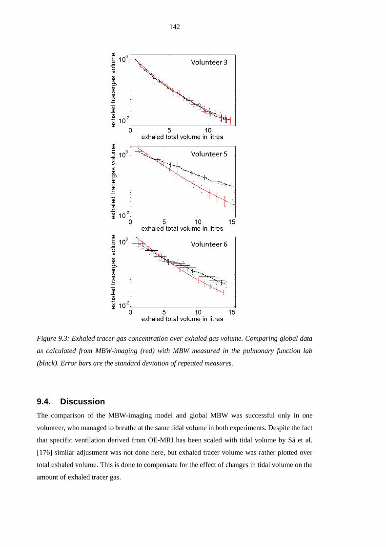
142

Figure 9.3: Exhaled tracer gas concentration over exhaled gas volume. Comparing global data

as calculated from MBW-imaging (red) with MBW measured in the pulmonary function lab

(black). Error bars are the standard deviation of repeated measures.

9.4. Discussion

The comparison of the MBW-imaging model and global MBW was successful only in one

volunteer, who managed to breathe at the same tidal volume in both experiments. Despite the fact

that specific ventilation derived from OE-MRI has been scaled with tidal volume by Sá et al.

[176] similar adjustment was not done here, but exhaled tracer volume was rather plotted over

total exhaled volume. This is done to compensate for the effect of changes in tidal volume on the

amount of exhaled tracer gas.

143

The results from this direct comparison show altered breathing pattern results in a deviation of

the curve. The assumption made by Sá et al. i. e. that SV in all units scales with TV is questionable

and might not hold for bigger changes in tidal volume [178]. Observed changes in TV between

the experiments from Voluneer 5 and 6 were about 15%. Dynamic 1H MRI or CT could help

assess the linearity of lung expansion with TV.

In addition it is assumed in the compartmental model of the lung that all functional units in the

lung are separate and gas is distributed and mixed uniformly within each compartment. This

assumption was tested in Chapter 7 (comparing two different resolutions) and holds for healthy

volunteers with an uniform distribution of fractional ventilation, as tested here.

Furthermore, two different tracer gases are used for both techniques. Both gases have different

density and diffusion (D3He-air = 0.9cm2/s [187], DSF6-air = 0.035 cm2/s [196]), but in the

concentrations of the tracer gases used for these experiments the influence can be neglected. A

single dose of 3He is inhaled during (200ml) MBW-imaging mixed with N2 (800ml) resulting in

a concentration of less than 7% 3He in air in all cases and SF6 in air is 0.2% immediately after

washin.

9.5. Conclusions

These preliminary results show promising agreement in the volunteer, who managed to match the

tidal volume in both the MBW-imaging and MBW experiments. This comparison shows the

difficulty of this direct comparison and how sensitive to changes both methods are. In the future

training volunteers in breathing procedure before each data acquisition solve those problems. An

alternative would be to record tracer gas concentration at the mouth while performing the MBW-

imaging. This would exclude mismatching derived from different breathing pattern or lung

inflation. In addition this could be done with different tracer gases used for imaging, such as SF6

(19F-imaging) which could be used together with fast gas analysers (Chapter 2, Multiple breath

washout (MBW), page 40).

144

Chapter 10 Conclusions

This thesis investigated hyperpolarised gas MRI methods to measure lung ventilation in a

quantitative fashion. Three methods were introduced and discussed. Application in patients was

successfully shown.

Chapter 3 demonstrated the use of single breath-hold hyperpolarised 3He ventilation and 1H

anatomical MRI acquisition (Figure 10.1) to increase the reproducibility of percentage ventilation

volume (%VV) calculation to provide spatially and temporally registered images. This improved

reliability when compared to a separate breath-hold technique will reduce statistical noise and

could therefore reduce the number of participants to evaluate the outcome of clinical studies with

a smaller number of participants. An optimised workflow automates process in major parts and

reduces the user variability.

Figure 10.1: Single coronal slice of superpositioned 3He image and 1H image anatomical scan of

the lungs using the single breath-hold technique from a healthy smoker.

Chapter 4 took ventilation image derived quantitative metrics one step further by using regional

intensity differences between images before and after treatment. This maximises the regional

information by taking intensity based regional and directional changes in ventilation into account.

Changes of ventilation are quantitatively expressed in percentage change to treatment (%TR,

Figure 10.2). The feasibility to monitor treatment response in longitudinal studies with this

technique, as shown in Chapter 4, could be of great advantage. In this preliminary study no

significant advantage over %VV and FEV1% predicted was demonstrated, but further studies

could show the advantage of this metric.

Figure 10.2: Treatment response showing effects of a bronchodilator in patient with asthma

(Volunteer 7, Table 4.1)

145

Chapter 5 introduced the method of multiple breath washout imaging (MBW-imaging) as a

quantitative functional imaging method, based on regional signal decay. This allows us to derive

values of fractional ventilation. An example fractional ventilation map from a 2D acquisition is

shown in Figure 10.3. Errors influencing the quantitative outcome are systematically investigated

(Chapter 6) and improvements are achieved using steady-state imaging sequences to acquire data

from MBW-imaging (Chapter 7). These improvements result in the feasibility to acquire 129Xe

MBW-imaging data.

Figure 10.3: Fractional ventilation map of a sagittal slice in a healthy volunteer superimposed

on a 1H image.

Chapter 8, MBW-imaging derived metrics were shown to correlate significantly with pulmonary

function tests. MBW-imaging is shown to be more sensitive to increased ventilation heterogeneity

in a young CF cohort than spirometry and even than its pendant in the pulmonary function lab,

LCI. Example coronal fractional ventilation maps from two patients are shown in Figure 10.4.

Figure 10.4: Example slices of fractional ventilation map from a CF and an asthma patient.

The regional information provided by MBW-imaging gives unique spatial insight into the

washout time constants of the whole lung, and may help therefore help understanding the concept

of ventilation heterogeneity in the context of clinical MBW measurements made from the whole

lung (e.g. LCI). The preliminary work presented in Chapter 9 shows that functional information

from MBW-imaging can be linked to conventional MBW, an important pre-requisite for the

subsequent regional interpretation of MBW.

146

List of figures

Figure 2.1: The Zeeman effect in the presence of field B0 for the case of a spin=1/2 nucleus. .. 12

Figure 2.2: (A) Magnetisation Mo in the presence of a static magnetic field B0. (B) After

applying a RF pulse B1(t) (with frequency ω0 along the x-axis for a duration T)

magnetisation has tilted at flip angle α and has two components: Mxy and Mz ................... 14

Figure 2.3: Acquisition using hyperpolarised gas MRI, showing a single 2D slice from a healthy

subject. Left: k-space; right: image space. Images acquired by the hyperpolarised gas

imaging group in Sheffield. ................................................................................................. 18

Figure 2.4: Example of a 3D MR lung image acquired using hyperpolarised 3He (lungs in

turquoise and major airways in red). ................................................................................... 18

Figure 2.5: After excitation a negative gradient is applied to dephase the spins. Immediately

afterwards in the opposite direction is applied rephasing the spins as an echo. The area of

the two regions shaded grey is equal. .................................................................................. 19

Figure 2.6: Following the RF pulse all spins are aligned (neglecting B0 inhomogeneity). Spins

start to dephase according to their y position after application of the phase encoding

gradient (Gpe) in the y-direction. .......................................................................................... 19

Figure 2.7: Slice selection gradient (Gss) applied simultaneously with as the RF pulse. The two

regions shaded in grey have the same integral for a symmetric RF pulse. .......................... 20

Figure 2.8: Schematic representation of sampling in 1D image space. Discrete sampling results

in a convolution (*) of the object (in this case a boxcar function) with the sampling pattern

(a series of Dirac delta functions). This can cause aliasing if the sampling frequency is less

than the Nyquist frequency (bottom row). ........................................................................... 21

Figure 2.9: Schematic sequence diagrams: (A) of a 2D-SPGR imaging sequence and (B) of a

3D-SPGR sequence using an additional phase encoding direction. .................................... 22

Figure 2.10: Schematic sequence diagrams: (A) of a 2D-bSSFP imaging sequence and (B) of its

3D version using an additional phase encoding direction. .................................................. 22

Figure 2.11: 1H Lung images from a healthy volunteer: (A) 1H lung image acquired with a

SPGR sequence. (B) Same resolution 1H lung image acquired using a bSSFP sequence.

Images acquired by the hyperpolarised gas imaging group in Sheffield. ............................ 23

Figure 2.12: Representation of the optical pumping process. Left circularly polarised light (σ+)

at a wavelength λ=795nm, resonant with the D1 transition in Rb, excites the valence

electron spins from the mj = -1/2 ground state of the 5S1/2 state into the mj = +1/2 5P1/2

excited state. Through collisions the excited electrons relax to repopulate both ground

levels. Because there is no removal of electrons from the mj=+1/2 state a polarisation build

147

up is formed. Figure taken from Moeller et. al. with permission [14] © by John Wiley and

Sons. .................................................................................................................................... 26

Figure 2.13: Schematic of a Helium-3 polariser. Static magnetic field is required to cause

Zeeman splitting; The oven heats the glass cell to vaporise the rubidium; the laser provides

circularly polarised light through optics. The glass cell has a gas inlet (for 3He and N2), the

outlet can be connected to a Tedlar bag to deliver gas for MRI scanning. ......................... 26

Figure 2.14: (A) Adult sized coil used for imaging studies with hyperpolarised 3He (frequency

48.62MHz). (B) Home-built dual-tuned (48.62MHz (3He) and 17.65MHz (129Xe)) flexible

transmit-receive coil [38]. ................................................................................................... 27

Figure 2.15: Ventilation images of the same subject (and same slice) using 2D-SPGR (left) and

3D-bSSFP (right) hyperpolarised 3He MRI. NB: For SPGR images 300ml of 3He was used,

compared to 100ml for bSSFP imaging. Minor artefacts from cardiac motion can be seen

in the centre of the 3D-bSSFP image. Images acquired by the hyperpolarised gas imaging

group in Sheffield. .............................................................................................................. 30

Figure 2.16: Example slices from a smoker, a patient with CF, asthma and COPD acquired with

2D SPGR ventilation hyperpolarised 3He MRI. Images acquired by the hyperpolarised gas

imaging group in Sheffield. ................................................................................................ 30

Figure 2.17: ADC maps of a healthy volunteer (left) and a COPD patient (right). High ADC

values indicate structural damage to the lung tissue/alveolar walls in the COPD patient as

shown in the schematic on top. Images acquired by the hyperpolarised gas imaging group

in Sheffield. ......................................................................................................................... 31

Figure 2.18: Map of regional pO2 measured in the lungs of a healthy volunteer obtained with

hyperpolarised 3He MRI. Average pO2 is 150mbar, in agreement with literature values

[65]. Images acquired by the hyperpolarised gas imaging group in Sheffield. ................... 32

Figure 2.19: (A) shows schematically an overview of the lung. (B) is a schematic of a network

of alveoli. Copyright by Churchill Livingstone Elsevier [68]. ........................................... 33

Figure 2.20: Schematic structure of the human airways from Weibel. Z generations of

dichotomic bifurcations are divided in conducting zone (Z=1-16) and transitional and

respiratory zone (Z= 17-23). Reproduced with permission from [65]. Small airways are

defined as airways with diameter <2mm (in adults Z=8-23). Reproduced with permission

of Wolters Kluwer Lippincott Williams & Wilkins. ........................................................... 34

Figure 2.21: Volume-time curve of tidal breathing (FRC=functional residual capacity) followed

by a complete exhalation to residual volume (RV) and inhalation to total lung capacity

(TLC). Expiratory reserve volume (ERV), inspiratory capacity (IC) as well as inspiratory

vital capacity (IVC) are derived from this curve. Adapted version reproduced with

permission of the European Respiratory Society © Eur Respir J March 2013 [71]. .......... 35

148

Figure 2.22: (A,B) Maximum flow-volume loop (MFVL) of a normal subject. Negative flow

(bottom part) represents a full inhalation to TLC and positive flow represents a complete

forced exhalation to RV. In a normal subject, flow reaches its maximum relatively

instantaneously (during a forced manoeuvre) and then continues to decline in a relatively

linear fashion during exhalation to RV. In grey are 95% confidence intervals of a healthy

population, the blue line shows the course of each individual. (A) shows flow-volume loop

from a healthy volunteer (10years,145cm,38kg) while (B) is from a CF patient (16

years,148cm,45kg). Reproduced with courtesy of Laurie Smith from Sheffield Children’s

Hospital................................................................................................................................ 38

Figure 2.23: SBW after single inhalation of 100% oxygen. Dead space is derived from phase I,

phase II is the bronchial phase with a rising N2 concentration until phase III with a constant

slope (alveolar phase, 25-75% of exhaled volume) used to derive ventilation heterogeneity

(SIII as the dotted line) and phase IV as the fast rising end of expiration used to derive the

closing volume (CV). Reproduced with permission of the European Respiratory Society ©

Eur Respir J 2013 [105]. ...................................................................................................... 40

Figure 2.24: (A) Setup of a MBW experiment. (B) Detailed view of system setup. ................... 41

Figure 2.25: Recording from an SF6 MBW in a healthy volunteer. Top figure: flow-time curve

acquired during experiment to calculate accumulated exhaled volume. Bottom figure:

tracer gas concentration over time. After wash-in to equilibrium concentration, the tracer

gas supply is disconnected and the washout begins (approximately at t=33s). ................... 42

Figure 2.26: Schematic of fractional ventilation of two compartments with different lung

ventilation. ........................................................................................................................... 44

Figure 3.1: Calculation of percentage ventilated volume (%VV) is ratio of ventilated volume to

total lung volume from masks of a ventilation scan and a proton scan. Example 3He

ventilation slice (left) and 1H slice (right) from a healthy smoker. ..................................... 47

Figure 3.2: Imaging protocol; 3He image acquisition is shown in light grey, 1H image

acquisition is shown in dark grey and black indicates the delay time taken to switch the

scanner from 3He to 1H acquisition. .................................................................................... 49

Figure 3.3: Image segmentation workflow for 1H images and 3He images. ................................ 51

Figure 3.4: Percentage ventilated volume values measured using: ............................................. 53

Figure 3.5: 3He ventilation images of the volunteers with (a) the highest single breath %VV

(mean %VV single = 97.59%) and (b) the lowest single breath %VV (mean %VV single =

70.47%). .............................................................................................................................. 54

Figure 3.6: Example of lung inflation level differences between separate breaths, volunteer 1.

(a) 3He ventilation image, breath 2, (b) separate breath 1H image, breath 1 and (c) shows

(a) superimposed on (b). (d) Single breath 1H image, breath 2 and (e) shows (a)

superimposed on (d). ........................................................................................................... 55

149

Figure 3.7: Bland-Altman plots of %VV measurement reproducibility for the three techniques;

(a) single breath (mean difference = 0.7%, standard deviation = 1.9%), (b) separate breaths

(mean difference = 0.3%, standard deviation = 6.0%) and (c) registered separate breaths

(mean difference = 0.2%, standard deviation = 3.2%). The lines show mean difference and

95% confidence intervals. ................................................................................................... 56

Figure 4.1: (A) Imaging protocol, including the treatment application. (B) Corresponding

example images 1H and 3He images from each time point. ................................................ 63

Figure 4.2: Showing the results of a segmentation and extraction of the major airways until

generation 2/3 depending on visibility of the airways. ....................................................... 65

Figure 4.3: Different steps to calculated treatment response maps from ventilation weighted

images. ................................................................................................................................ 69

Figure 4.4: Histogram of a treatment response map of relative changes of patient 2. Negative

values denote reduced ventilation (red) and positive values represent increased ventilation

(green) reaching a lung unit. In this example the positive response was reflected by an

increase of 351ml over the whole lung compared to a total of 54ml decrease in ventilation.

Therefore the net-volume change from the histogram was quantified to a positive 298ml.

Corresponding treatment response maps of this patient are shown in Figure 4.6. .............. 70

Figure 4.5: Histograms show distributions of excluded TR values using different methods to

calculate the baseline-variability thresholds: ...................................................................... 72

Figure 4.6: Example treatment response sets from patient 2 showing all slices acquired. Top row

TR, middle row pre-treatment ventilation images, and bottom post-treatment ventilation

images. The TR is in units of litres. White areas correspond to no significant changes in

ventilation above the threshold )(r

. ............................................................................... 73

Figure 4.7: Comparison of image derived parameters: (A) – TR as volume change, (B) - %VV;

and spirometry: (C) - FEV1, (D) - FVC. Response to Bronchodilator treatment was found

to be significant with all methods (one-tailed Wilcoxon signed rank test, P<0.001).

Although all methods show significant sensitivity to change the TR groups are more tightly

clustered with clearer separation and a difference >50% between the mean values. .......... 73

Figure 4.8: Overview treatment response of subjects, who attended on 2 visits. For each

comparison volume increase and decrease from histograms are plotted. * indicates

significant difference (P<0.05) ........................................................................................... 74

Figure 4.9: Bland-Altman plot of differences between lung volumes in litres. Dotted lines show

±1.96 standard deviations and the mean difference. Mean difference between total lung

volumes -0.5% with a standard deviation of 8%. ................................................................ 75

150

Figure 4.10: Selected example slices from TR maps from different volunteers (indicated in the

maps). For each example the net-effect as a net gas-volume change and the positive and

negative volume (ventilation increase and ventilation decrease) are given. ........................ 79

Figure 5.1 : Timing of image acquisitions and breathing manoeuvre. Images were acquired at a

fixed delay Δt. Subjects held their breath during the first two acquisitions, constituting the

calibration phase, and performed a single breathing cycle (exhale – inhale) between

subsequent acquisitions. ...................................................................................................... 83

Figure 5.2: (A) Setup of the pneumotachograph evaluation unit measuring the pressure

differences connected to the flow sensor. To calibrate setup a 3L test syringe is used. (B)

Recoding from the evaluation unit using the 3L test syringe: Flow, pressure and volume

are evaluated. ....................................................................................................................... 84

Figure 5.3: Flow chart of the data processing steps used to obtain fractional ventilation

parameter r from a 2D dataset.(A) Acquired images of the MBW-imaging protocol. (B)

Image registration and segmentation. (C) Correction for T1 and RF decay according to

Equation 4.(D) Applying Equation six to calculate fractional ventilation maps. ................ 87

Figure 5.4: Maps of fractional ventilation parameter r obtained with the 2D washout acquisition

protocol. Sagittal slices from left and right lung are shown for 4 healthy subjects as well as

histograms of distribution of r values for each lung slice. ................................................... 91

Figure 5.5: Fractional ventilation maps from 3D washout from healthy subjects in the sagittal,

coronal and axial plane (Volunteer 1-4). ............................................................................. 91

Figure 5.6: (A) Gravitational effects from anterior to posterior as seen in the left and right lungs

of volunteer 2 from two 2D washout datasets. The repeatability between the two scans can

be observed. The right lung shows an increase in fractional ventilation between anterior

and posterior parts, while the slices in the left lung do not. (B) The slices in the left lung

are positioned further lateral and are therefore under less gravitational compression from

overlaying mediastinal tissue mass. ..................................................................................... 93

Figure 5.7: Comparison between the gas volume turnover (tidal volume measured by

pneumotachograph divided by total lung volume measured by MRI) and the measured

global mean fractional ventilation from the 2D and 3D washout protocols including the

Bland-Altman plot in the top left corner. Pearson’s correlation r = 0.67 (P < 0.001, of the

best fit to all points), Bland-Altman analysis shows a mean difference = 17.2% (standard

deviation = 23.7%). ............................................................................................................. 94

Figure 5.8: Pneumotachograph recordings for subject 4 during (A) a 2D acquisition and (B) a

3D acquisition. n = 1,2,3,4,5 numbers the respiratory cycle in which the datasets were

acquired. .............................................................................................................................. 94

Figure 5.9: (A) Correlation on a pixel by pixel basis of two 2D washout experiments of

Volunteer 4 acquired in the same session (Pearson’s correlation of r = 0.85 and P<0.005).

151

(B) Correlation on a pixel by pixel basis of two 3D washout experiments of Volunteer 4

acquired in the same session (Pearson's correlation of r = 0.74 and P<0.005). Pearson’s

correlation was done on the best fit to data (continuous line). ............................................ 95

Figure 5.10: (A) Correlation and Bland-Altman plot of 8-region comparison from Volunteer 4.

Errorbars derive from the standard deviation of fractional ventilation in each of the regions.

Black dots show comparison of same regions in both experiments (r = 0.97, P<0.001,), the

red line is the linear fit (almost equal to unity line). A Bland-Altman analysis is shown in

the top left corner (mean difference = 10.5%, standard deviation = 3.2%). (B) Lung divided

into 8 regions of roughly equal size. Each colour represents one region. ........................... 96

Figure 6.1: Schematic of a multiple breath washout imaging protocol showing the volume curve

during MBW-imaging experiment as measured with a pneumotachograph. Above the

curve a segmented coronal slice is shown to visualise the volume change. The deviations

of lung volume and tidal volume are schematically shown in the volume curve. ............ 101

Figure 6.2: Demonstration of the effects of lung volume change in an example from a young CF

patient. Total volume difference from segmented 3D volumes in this example was found to

be 0.5L. The same intensity window was applied to both images. ................................... 102

Figure 6.3: Illustrative schematic showing variation of T1 of the hyperpolarised 3He in the lung

during a washout experiment. Due to inhalation of an anoxic gas mix the T1 can be

expected to be higher than during the washout and increases during calibration breath-hold

while more oxygen is taken up by the blood. With beginning of the gas washout after the

first breathing cycle the oxygen level returns to normal reducing T1. During every breath-

hold T1 will slightly increase again due to oxygen uptake. ............................................... 104

Figure 6.4: Systematic error in correction factor Csys for different values of T1. Error bars

obtained from variations between volunteers (referred to as random error). The green line

represents the error from changes in T1 from oxygen uptake during the breath-hold. The

red line is derived from errors changes in T1 resulting from changes of the gas mix in the

lung. The total error in the correction factor plotted as a black line results from T1′ in Eq.

[6.8]. .................................................................................................................................. 107

Figure 6.5: Systematic error in fractional ventilation (Δrsys) for different values of starting

alveolar pO2 from literature [61, 179, 182]. The systematic error in the correction factor is

plotted as black line with the random error (from physiological differences) as error bars.

The relative error is constant across values of fractional ventilation. ............................... 107

Figure 6.6: Signal decay for a specific fractional ventilation (given as input to the code). I

(=signal due to gas washout) was added with noise (σ) according to a Gaussian probability

distribution as shown next to the points on the curve. ...................................................... 109

Figure 6.7: Distribution of errors across all 10,000 simulations resulting from noise in images.

An initial SNR of 86 was assumed in the first image (value taken from Volunteer 1 with

152

biggest lung volume). 10,000 values were simulated for two different fractional

ventilations r = 0.8 and r = 0.1. For a very rapid signal decay (r = 0.8, high turn-over of

gas) the relative error in r was found to be 7%. ................................................................. 110

Figure 6.8: (A) shows the estimated SNR of the last image used to fit fractional ventilation. (B)

shows the resulting relative error of the fitting routine. The simulation is based on dataset

of volunteer 1 and assumes an initial SNR = 57 in the image before the gas-washout

(compare Table 3). ............................................................................................................. 110

Figure 6.9: Total error simulated in a Monte-Carlo analysis. Each data point consists of 10.000

experiments. ....................................................................................................................... 112

Figure 7.1: Comparison of image acquisition from the MBW-imaging protocol with SRGR and

SSFP sequences in Volunteer 6. All images are presented in arbitrary units of image

intensity with the same window level settings on each case. ............................................ 117

Figure 7.2: Comparison of fractional ventilation maps derived from SPGR and bSSFP imaging

acquired in the same session from Volunteer 6. ................................................................ 117

Figure 7.3: Voxel-by-voxel comparison of fractional ventilation values derived from MBW-

imaging using a SPGR sequence and a bSSFP sequence from Volunteer 3. Pearson’s

correlation coefficient r = 0.68, P<0.0001; Bland Altman analysis showed a mean

difference between experiments of 2.6% with a standard deviation of 22.7%. ................. 118

Figure 7.4: Comparison of fractional ventilation maps derived from SPGR (32x32x26) and

bSSFP (64x64x26) sequences from Volunteer 2. Fractional ventilation maps from slices

(anterior to posterior) are shown along with whole lung fractional ventilation histograms.

Slight differences in the in the colour intensity of the maps from each acquisition result

from using the same colour map to represent the different average fractional ventilation

values (SPGR average r = 0.34, SSFP average r = 0.28, compare also the peak of the

histograms) ........................................................................................................................ 119

Figure 7.5: Comparison of image acquisition from the MBW-imaging protocol with 3He and

129Xe in Volunteer 3. Reduced coil sensitivity at the bottom of the posterior slices when

imaging with 3He prevented calculation of fractional ventilation from those regions. All

images are presented in arbitrary units of image intensity with the same window level

settings in each case. .......................................................................................................... 120

Figure 7.6: Comparison of fractional ventilation maps from 3He and 129Xe MBW-imaging in

Volunteer 3. The second slice of both fractional ventilation maps result from raw images

shown in Figure 7.5. Every second slice from both 3D datasets is plotted, with posterior

slices on the left and anterior in the right. The second slice is calculated from raw-images

in Figure 7.5. ...................................................................................................................... 120

Figure 7.7: Whole lung histograms of fractional ventilation values, derived from the maps in

Figure 7.6. Only voxel which resulted in a successful calculation of fractional ventilation

153

from both 3D maps were included in this comparison. Both datasets show very similar

standard deviation/ventilation heterogeneity (VH3-He=0.101 and VH129-Xe=0.096). ......... 121

Figure 8.1: The average of each 10mm coronal slice in 3D fractional ventilation maps (A) was

plotted from anterior to posterior (B). A linear slope was fitted to measure influence of

gravity on fractional ventilation in supine subjects. The slope has units of fractional

ventilation per slice [Δr/cm] and can be used to evaluate ventilation changes from anterior-

posterior. ........................................................................................................................... 128

Figure 8.2: Coronal slice of a single subject from each group investigated (top) and the

corresponding whole lung histogram of fractional ventilation r from each subject group

(bottom). Increase of VH can be visually seen in the fractional ventilation maps and is

reflected in a broadening of fractional ventilation values in the histograms with increase of

disease severity. FEV1% predicted: Healthy volunteer 98%, CF 104%, asthma: 51% .... 130

Figure 8.3: (1) Correlation between standard deviation of fractional ventilation histograms and

the lung clearance index (LCI). Blue circles represent the healthy volunteers, green the

cystic fibrosis patients and red the asthmatics study. A significant correlation (P<0.001) of

r = 0.68 was found. (2) Correlation between standard deviation of fractional ventilation

histograms and forced expiratory volume in 1 second (FEV1). A significant negative

correlation (P< 0.001) of r = -0.59 was found. FEV1 increases with decreasing ventilation

heterogeneity. (3) Significant correlation between standard deviation of fractional

ventilation and gravitation effects measured from changes of fractional ventilation from

anterior-posterior coronal slices in all subjects. The anterior-posterior change in fractional

ventilation is reduced with increased ventilation heterogeneity (r = -0.46, P <0.01). Black

lines show a linear fit to all data in each of the graphs. .................................................... 132

Figure 8.4: Boxplots of imaging-derived variables and pulmonary function tests. (A) FEV1 (B)

LCI (C) Standard deviation derived from fractional ventilation maps (SD/VH-MBWI) and

(D) the gravitational slope. *=significant difference between groups (P < 0.01). ............ 132

Figure 8.5: Comparison of LCI measured sitting and in supine position between heathy

volunteers and CF patients. An independent samples Mann-Whitney U Test showed no

significant difference between the two groups measured sitting, but with a significant

different when MBW was recoded in supine position (P = 0.02). .................................... 133

Figure 9.1: (A) Fractional ventilation map r is used to predict the concentration washout for

each voxel from Volunteer 6. (B) Residual gas volume in 4 compartments in the lung (left-

right, posterior-anterior, compartments shown in top right corner). A uniform equilibrium

gas concentration of 0.2% tracer gas is assumed at the beginning (breath n=0) and the

acquired functional information (fractional ventilation r) is used to calculate residual gas

volume after each breath in each of the 4 compartments. The sum of all compartments is

154

equal is total residual tracer gas volume left in the lung measured with MBW at the mouth.

........................................................................................................................................... 139

Figure 9.2: (A) MBW showing SF6 concentration and flow recordings from Volunteer 6.

Breathing was synchronised with recorded sound from MR MBW-imaging acquisition,

which explains the zero-flow following each breathing cycle after inspiration. Similar to

the calibration phase during the disconnection of the gas subjects held their breath before

starting synchronised breathing with breath n=0. (B) Exhaled tracer gas volume in each

breath calculated from the recordings in A........................................................................ 140

Figure 9.3: Exhaled tracer gas concentration over exhaled gas volume. Comparing global data

as calculated from MBW-imaging (red) with MBW measured in the pulmonary function

lab (black). Error bars are the standard deviation of repeated measures. ......................... 142

Figure 10.1: Single coronal slice of superpositioned 3He image and 1H image anatomical scan of

the lungs using the single breath-hold technique from a healthy smoker. ......................... 144

Figure 10.2: Treatment response showing effects of a bronchodilator in patient with asthma

(Volunteer 7, Table 4.1) .................................................................................................... 144

Figure 10.3: Fractional ventilation map of a sagittal slice in a healthy volunteer superimposed

on a 1H image. ................................................................................................................... 145

Figure 10.4: Example slices of fractional ventilation map from a CF and an asthma patient. .. 145

155

List of tables

Table 2.1: Summary of the magnetic properties and isotopic abundance in nature of the

principal nuclei relevant to this work [14-16]. .................................................................... 11

Table 3.1: Scan parameters for the helium and proton acquisitions. The number of slices was

adjusted for full lung coverage according to volunteer size but kept consistent for all scans

of an individual volunteer. The size of voxels is kept constant for all volunteers and all

scans. ................................................................................................................................... 49

Table 3.2: Percentage ventilated volume (%VV) measurements. ............................................... 55

Table 3.3:Intra-class correlation (ICC(2,1)), Spearman’s r (with corresponding P-value),

coefficient of variation (CoV), standard error of measurement (SEM) and smallest

detectable difference (SDD) for the three techniques.*Spearman’s r ................................. 56

Table 3.4: Mean and standard deviation (std) Dice overlap after taking the mean of time-point 1

and time-point 2 for each technique. ................................................................................... 57

Table 4.1: Overview patients. *measured at baseline before application of the bronchodilator 62

Table 5.1: Subject characteristics; *at rest, supine and outside scanner; ** Calculated according

to guidelines by Quanjer et al. [84] ..................................................................................... 81

Table 5.2: Overview values 2D and 3D washout experiments. TV = Tidal Volume; LV =

inspiratory Lung Volume. In the case of Volunteer 4 the flow-recording failed, therefore no

tidal volumes could be extracted from this dataset. ............................................................ 92

Table 5.3: Comparison of repeated 3D MBW-imaging during the same session. Pearson’s

correlation all show highly significant correlations. In addition lungs were divided into 8

regions of equal size for comparison (divided along the main axis). Mean fractional

ventilation measured in the all 8 regions shows high correlation for all volunteers tested. 96

Table 6.1: Overview average end inspiratory lung volumes (LV) and standard deviation as

obtained from segmenting 3D image-volumes. Tidal volume (TV) and its standard

deviation were measured using a pneumotachograph during gas-washout. Resulting global

fractional ventilation ( rr ) and relative error ( r ) were calculated using Eq. [6.4]. All

volumes are in ml. ............................................................................................................. 102

Table 6.2: Overview of the parameters used in estimating T1’. Standard deviation of mean

values derive from inter-volunteer variations. * value from literature [61, 179]; ............. 105

Table 6.3: Average SNR in each image of the washout acquisition for volunteers from Chapter

5. ....................................................................................................................................... 108

Table 7.1: Overview of the healthy volunteers imaged using SPGR and bSSFP MBW-imaging.*

predicted values calculated according to [71]. .................................................................. 115

156

Table 7.2: Overview of results from voxel-by-voxel and 8 region comparisons. * 200ml 3He,

Flip angle = 7°. ** 200ml 3He, Flip angle = 7°, in plane resolution: 64x64. †TV=tidal

volume; LV = inspiratory lung volume. ............................................................................ 118

Table 7.3: Overview of results from voxel by voxel 129Xe and 3He MBW-imaging data analysis

in 5 healthy volunteers. For subject demographics see Table 7.1. *percentage of mean over

all values of fractional ventilation. .................................................................................... 121

Table 8.1: Overview of patient and subject details (dark blue=healthy volunteer, red=CF patient,

turquoise = asthma patient) and imaging derived values as well as pulmonary function test

results. For the fractional ventilation – as in previous chapters – r is used as an

abbreviation. Predicted FEV1 was calculated according to Miller et al. [71]. .................. 126

Table 8.2: Non-parametric Spearman’s correlations, significance levels (P-values) and subject

number N comparing multiple breath washout imaging parameters (SD, CV, skewness,

gravitational effect) and pulmonary function tests (LCI and FEV1). (Grey field show

correlation is significant with P<0.01 (2-tailed)). .............................................................. 131

Table 8.3: Overview ANOVA testing of MBW-imaging derived values and pulmonary function

tests. P<0.05 of mean differences was selected as significance level. F describes the ratio

of random variance to experimental variance. Grav. is an abbreviation for gravitational

slope. *Levenne’s test of equality of error variances P<0.01 (as a result a Games-Howell

test was performed) ........................................................................................................... 133

Table 9.1: Overview pulmonary volumes measured during experiments. TV is the tidal volume

measured in ml from flow-recordings. .............................................................................. 141

157

List of publications

Journal Papers

1. Lung ventilation volumetry with same breath acquisition of hyperpolarized gas and

proton MRI.

Felix C. Horn, Martin H. Deppe, Helen Marshall, Juan Parra-Robles, Jim M Wild

Journal of Applied Physiology (1985). 2014; 116(2):129-39.

2. Reply to Verbank and Paiva.

Jim M. Wild, Felix C. Horn

Journal Applied Physiology (1985). 2014 May; 116(9):1258.

3. Lung ventilation with same-breath acquisition of hyperpolarized gas and proton MRI.

Felix C. Horn, Bilal A. Tahir, Neil J. Stewart, Guilhem J. Collier, Graham Norquay,

General Leung, Rob H.. Ireland, Juan Parra-Robles, Helen Marshall, Jim M. Wild

NMR in Biomedicine. 2014 September; 27(12):1461-7.

4. Comparison of CT-based Lobar Ventialtion with 3He MRI Ventilation Measuments in

Asthmatics

Bilal A. Tahir, Cederic Van Holsbeke, Rob H. Ireland, Andy Swift, Felix C. Horn, Helen

Marshall, John C. Kenworthy, Juan Parra-Robles, Ruth Hartley, M Laurencin, Richard

Kay, B Chris, Jan De Backer, Wim Vos, Jim M. Wild

Radiology (accepted)

5. Quantitative treatment response mapping using hyperpolarized 3He MRI in asthma

patients

Felix C. Horn, Helen Marshall, Richard Kay, Christopher E. Brightling, Juan Parra-

Robles, Jim M. Wild

(In preparation)

6. Linking regional ventilation heterogeneity from hyperpolarised gas MRI to multiple

breath washout in obstructive lung disease

Felix C. Horn, Juan Parra-Robles, Alexander Horsley, Richard Kay, Ina Aldag, Salman

Seddiqui, Christopher E. Brightling, Christopher Taylor, Helen Marshall, Jim Wild

(In preparation)

Oral Presentation

1. Quantitative mapping of treatment response in the lungs of asthmatics using

hyperpolarized ventilation 3He MRI

Congress of the American Thoracic Society, San Diego (2014)

158

2. Multiple breath washout with hyperpolarised gas MRI

UK Respiratory and Pulmonary Vascular Imaging Meeting, Sheffield (2014)

3. Bronchodilator treatment response mapping in COPD using hyperpolarized gas

ventilation MRI

European Respiratory Society, Barcelona (2013)

4. Multiple breath washout with hyperpolarised gas MRI

Lung-From molecule to image, Bordeaux (2013)

Poster presentations

1. Visualizing regional ventilation heterogeneity by linking multiple breath washout to 3He

MRI imaging

Felix C. Horn, Alexander Horsley, Laurie Smith, Christopher Taylor, Helen Marshall,

Juan Parra-Robles, Jim M. Wild

European Respiratory Society, Munich (2014)

2. Delayed gas filling imaged in asthma patients using hyperpolarised 3He MRI

Felix C. Horn, Helen Marshall, Juan Parra-Robles, Christopher Brightling, Jim M. Wild


3. Detection of early-stage lung disease in cystic fibrosis; comparing the sensitivity of 3He

and 1H MRI, CT and LCI

Helen Marshall, David Hughes, Alexander Horsley, Felix C. Horn, Laurie Smith, Juan

Parra-Robles, Steve Cunningham, Leanne Armstrong, Ina Aldag, Christopher Taylor,

Jim M. Wild

Conference Paper, European Respiratory Society, Munich (2014)

4. Comparison of CT-based lobar ventilation models with 3He MRI ventilation

measurements in asthmatics


Marshall, Juan Parra-Robles, Ruth Hartley, Richard Kay, B Chris, Jan De Backer, Wim

Vos, Jim M. Wild


5. Linking Helium-3 MRI Washout Imaging To Multiple Breath Washout - First Steps To

Understanding Regional Lung Ventilation Heterogeneity

Felix C. Horn, Alexander Horsley, Helen Marshall, Christopher Taylor, Juan Parra-

Robles, Jim M. Wild

American Thoracic Society, San Diego (2014)

6. Assessment of Structural And Functional Changes In Early Stage CF With Helium-3

MRI, CT And Multi-Breath Washout

159

Helen Marshall, David Hughes, Alexander Horsley, Felix Horn, Laurie Smith, Juan

Parra-Robles, Leanne Armstrong, Ina Aldag, Christopher Taylor, Jim M. Wild

American Thoracic Society, San Diego (2014)

7. Comparison of global multiple breath washout measured at the mouth to imaging multiple

breath washout in healthy subjects and Cystic Fibrosis patients

Felix C. Horn, Juan Parra-Robles, Helen Marshall, Christopher J. Taylor, Alexander

Horsley, Jim M. Wild

International Society of Magnetic Resonance in Medicine, Milan (2014)

8. Hyperpolarised 3He MRI is superior to lung clearance index in detection of ventilation

abnormalities in young children with mild CF

Helen Marshall, Alexandere Horsley, Laurie Smith, David Hughes, Felix C. Horn,

Leanne Armstrong, Juan Parra-Robles, Steve Cunningham, Ina Aldag, Christopher

Taylor, Jim M. Wild

British Thoracic Society, London (2013)

9. Comparison of CT-based Lobar Ventilation with Hyperpolarized 3He MRI using image

registration


Marshall, Juan Parra-Robles, Ruth Hartley, M Laurencin, Richard Kay, B Chris, Wim

Vos, Jim M. Wild

International Workshop of Pulmonary Functional Imaging, Madison,WI (2013)

10. Comparison of CT-based lobar ventilation models with 3He MRI ventilation

measurements in asthmatics


Marshall, Juan Parra-Robles, Ruth Hartley, M Laurencin, Richard Kay, B Chris, Jan De

Backer Wim Vos, Jim M. Wild

European Respiratory Society, Barcelona (2013)

11. Registration based estimates of lung ventilation

Asmund Kjorstadt, Dominique Corteville, Felix C. Horn, Fank Zöllner, E Hodneland,

Christian Fink, Lothar R. Schad

ESMRMB, Toulouse (2013)

12. Reliable free breathing 3D multiple breath gas washout with hyperpolarized 3He lung

MRI

Felix C. Horn, Martin H. Deppe, Juan Parra-Robles, Jim M. Wild

International Society of Magnetic Resonance in Medicine, Salt Lake City, UT (2013)

13. Reproducible Multiple-breath washout imaging in 3D

Felix C. Horn, Martin H. Deppe, Juan Parra-Robles, Jim M. Wild

BCISMRM, Cambridge (2012)

160

14. Observation of gravitational dependence of regional fractional ventilation in human lungs

with 2D and 3D multiple-breath washout imaging of 3He and 129Xe

Felix C. Horn, Martin H. Deppe, Helen Marshall, Graham Norquay, Juan Parra-Robles,

Jim M. Wild

International Society of Magnetic Resonance in Medicine, Melbourne (2012)

161

References

1. Albert, M.S., et al., Biological magnetic resonance imaging using laser-polarized 129Xe.

Nature, 1994. 370(6486): p. 199-201.

2. Middleton, H., et al., MR imaging with hyperpolarized 3He gas. Magnetic resonance in medicine

: official journal of the Society of Magnetic Resonance in Medicine / Society of Magnetic

Resonance in Medicine, 1995. 33(2): p. 271-5.

3. Deppe, M.H., et al., A flexible 32-channel receive array combined with a homogeneous transmit

coil for human lung imaging with hyperpolarized (3) He at 1.5 T. Magnetic resonance in

medicine : official journal of the Society of Magnetic Resonance in Medicine / Society of

Magnetic Resonance in Medicine, 2011.

4. Wild, J.M., et al., Steady-state free precession with hyperpolarized 3He: experiments and theory.

J Magn Reson, 2006. 183(1): p. 13-24.

5. Deppe, M.H. and J.M. Wild, Variable flip angle schedules in bSSFP imaging of hyperpolarized

noble gases. Magn Reson Med, 2012. 67(6): p. 1656-64.

6. Ajraoui, S., et al., Compressed sensing in hyperpolarized 3He lung MRI. Magnetic resonance in

medicine 2010. 63(4): p. 1059-69.

7. Nikolaou, P., et al., Near-unity nuclear polarization with an open-source 129Xe hyperpolarizer

for NMR and MRI. Proc Natl Acad Sci U S A, 2013. 110(35): p. 14150-5.

8. Prisk, K.G. and R.C. Sa, It's about numbers, not pictures. J Appl Physiol (1985), 2014. 116(2):

p. 127-8.

9. Bloch, F., The Principle of Nuclear Induction. Science, 1953. 118(3068): p. 425-30.

10. Purcell, E.M., H.C. Torrey, and R.V. Pound, Resonance Absorption by Nuclear Magnetic

Moments in a Solid. Physical Review, 1946. 69(1-2): p. 37-38.

11. Lauterbur, P.C., Image formation by induced local interactions. Examples employing nuclear

magnetic resonance. 1973. Clin Orthop Relat Res, 1989(244): p. 3-6.

12. Mansfield, P. and P.K. Grannell, Nmr Diffraction in Solids. Journal of Physics C-Solid State

Physics, 1973. 6(22): p. L422-L426.

13. Levitt, M.H., Spin dynamics : basics of nuclear magnetic resonance. 2nd ed. ed. 2008, Hoboken,

N.J.: Wiley ; Chichester : John Wiley [distributor].

14. Moeller, H.E., et al., MRI of the lungs using hyperpolarized noble gases. Magnetic resonance in

medicine : official journal of the Society of Magnetic Resonance in Medicine / Society of

Magnetic Resonance in Medicine, 2002. 47(6): p. 1029-51.

15. Haacke, E.M., Magnetic resonance imaging : physical principles and sequence design. 1999,

New York: Wiley. xxvii, 914 p.

16. Kauczor, H., R. Surkau, and T. Roberts, MRI using hyperpolarized noble gases. Eur Radiol,

1998. 8(5): p. 820-7.

17. Haase, A., et al., FLASH imaging: rapid NMR imaging using low flip-angle pulses. 1986.

Journal of magnetic resonance, 1986. 213(2): p. 533-41.

18. Oppelt, A., et al., FISP-a new fast MRI sequence. electromedica, 1986. 54(1): p. 15-8.

19. Scheffler, K. and S. Lehnhardt, Principles and applications of balanced SSFP techniques. Eur

Radiol, 2003. 13(11): p. 2409-18.

20. Wild, J.M., et al., MRI of the lung (1/3): methods. Insights Imaging, 2012. 3(4): p. 345-53.

21. Noll, D.C., D.G. Nishimura, and A. Macovski, Homodyne detection in magnetic resonance

imaging. IEEE Trans Med Imaging, 1991. 10(2): p. 154-63.

22. Huang, T.Y., et al., Are TrueFISP images T2/T1-weighted? Magn Reson Med, 2002. 48(4): p.

684-8.

23. Rajaram, S., et al., Lung morphology assessment with balanced steady-state free precession MR

imaging compared with CT. Radiology, 2012. 263(2): p. 569-77.

24. Edelman, R.R., et al., Noninvasive assessment of regional ventilation in the human lung using

oxygen-enhanced magnetic resonance imaging. Nat Med, 1996. 2(11): p. 1236-9.

25. Sa, R.C., et al., Vertical distribution of specific ventilation in normal supine humans measured

by oxygen-enhanced proton MRI. Journal of applied physiology, 2010. 109(6): p. 1950-9.

26. Bauman, G., et al., Non-contrast-enhanced perfusion and ventilation assessment of the human

lung by means of fourier decomposition in proton MRI. Magn Reson Med, 2009. 62(3): p. 656-

64.

27. Kjorstad, A., et al., Quantitative lung ventilation using Fourier decomposition MRI; comparison

and initial study. MAGMA, 2014. 27(6): p. 467-76.

162

28. Capaldi, D.P., et al., Free-breathing Pulmonary H and Hyperpolarized He MRI: Comparison in

COPD and Bronchiectasis. Acad Radiol, 2014.

29. Shea, D., The Helium-3 Shortage: Supply, Demand, and Options for Congress. 2010,

Congressional Research Service: Washington, DC. p. 1-27.

30. Cho, A., Physics. NRC urges U.S. to rethink sale of helium reserve. Science, 2010. 327(5965): p.

511.

31. Kuethe, D.O., et al., Imaging lungs using inert fluorinated gases. Magn Reson Med, 1998. 39(1):

p. 85-8.

32. Colegrove, F.D., L.D. Schearer, and G.K. Walters, Polarization of He3 Gas by Optical Pumping.

Physical Review, 1963. 132(6): p. 2561-2572.

33. Walker, T.G. and W. Happer, Spin-exchange optical pumping of noble-gas nuclei. Reviews of

Modern Physics, 1997. 69(2): p. 629-642.

34. Norquay, G., et al., Optimized production of hyperpolarized 129Xe at 2 bars for in vivo lung

magnetic resonance imaging. Journal of Applied Physics, 2013. 113(4): p. -.

35. Parra-Robles, J., A.R. Cross, and G.E. Santyr, Theoretical signal-to-noise ratio and spatial

resolution dependence on the magnetic field strength for hyperpolarized noble gas magnetic

resonance imaging of human lungs. Med Phys, 2005. 32(1): p. 221-9.

36. Xu, X., et al., Hyperpolarized 129Xe gas lung MRI-SNR and T2* comparisons at 1.5 T and 3 T.

Magn Reson Med, 2012. 68(6): p. 1900-4.

37. Parra-Robles, J., et al., Theoretical prediction and experimental measurement of the field

dependence of the apparent transverse relaxation of hyperpolarized noble gases in lungs. J

Magn Reson, 2008. 192(1): p. 85-91.

38. Rao, M., R. Fraser, and J.M. Wild, Dedicated Receiver Array Coil for 1H Lung Imaging with

Synchornous Acquistion of Hyperpolarized 3He and 129Xe Gas, in ISMRM. 2014, Proc. Intl.

Soc. Mag. Reson. Med. : Milan, Italy. p. 0625.

39. Wild, J.M., et al., MR imaging of the lungs with hyperpolarized helium-3 gas transported by air.

Phys Med Biol, 2002. 47(13): p. N185-90.

40. Saam, B., W. Happer, and H. Middleton, Nuclear relaxation of 3He in the presence of O2. Phys

Rev A, 1995. 52(1): p. 862-865.

41. Acosta, R.H., et al., Controlling diffusion of 3He by buffer gases: a structural contrast agent in

lung MRI. J Magn Reson Imaging, 2006. 24(6): p. 1291-7.

42. Wild, J.M., et al., k-space filtering in 2D gradient-echo breath-hold hyperpolarized 3He MRI:

spatial resolution and signal-to-noise ratio considerations. Magnetic resonance in medicine,

2002. 47(4): p. 687-95.

43. Deppe, M.H., et al., Susceptibility effects in hyperpolarized (3)He lung MRI at 1.5T and 3T.

Journal of magnetic resonance imaging : JMRI, 2009. 30(2): p. 418-23.

44. Zhao, L. and M.S. Albert, Biomedical imaging using hyperpolarized noble gas MRI: pulse

sequence considerations. Nucl Instrum Methods Phys Res A, 1998. 402: p. 454-60.

45. Salerno, M., et al., Dynamic spiral MRI of pulmonary gas flow using hyperpolarized (3)He:

preliminary studies in healthy and diseased lungs. Magnetic resonance in medicine : official

journal of the Society of Magnetic Resonance in Medicine / Society of Magnetic Resonance in

Medicine, 2001. 46(4): p. 667-77.

46. Marshall, H., et al., K-space filter deconvolution and flip angle self-calibration in 2D radial

hyperpolarised (3) He lung MRI. NMR in biomedicine, 2011.

47. Dregely, I., et al., 32-channel phased-array receive with asymmetric birdcage transmit coil for

hyperpolarized xenon-129 lung imaging. Magn Reson Med, 2013. 70(2): p. 576-83.

48. Wild, J.M., et al., Dynamic radial projection MRI of inhaled hyperpolarized 3He gas. Magnetic

resonance in medicine : official journal of the Society of Magnetic Resonance in Medicine /

Society of Magnetic Resonance in Medicine, 2003. 49(6): p. 991-7.

49. Ajraoui, S., et al., Acquisition of (3)He ventilation images, ADC, T(2)* and B(1) maps in a single

scan with compressed sensing. NMR in biomedicine, 2012. 25(1): p. 44-51.

50. Wild, J.M., et al., Comparison between 2D and 3D gradient-echo sequences for MRI of human

lung ventilation with hyperpolarized 3He. Magnetic resonance in medicine : official journal of

the Society of Magnetic Resonance in Medicine / Society of Magnetic Resonance in Medicine,

2004. 52(3): p. 673-8.

51. McMahon, C.J., et al., Hyperpolarized 3helium magnetic resonance ventilation imaging of the

lung in cystic fibrosis: comparison with high resolution CT and spirometry. Eur Radiol, 2006.

16(11): p. 2483-90.

163

52. Woodhouse, N., et al., Assessment of hyperpolarized 3He lung MRI for regional evaluation of

interventional therapy: a pilot study in pediatric cystic fibrosis. J Magn Reson Imaging, 2009.

30(5): p. 981-8.

53. Mathew, L., et al., Hyperpolarized 3He magnetic resonance imaging of chronic obstructive

pulmonary disease: reproducibility at 3.0 tesla. Acad Radiol, 2008. 15(10): p. 1298-311.

54. van Beek, E.J., et al., Hyperpolarised 3He MRI versus HRCT in COPD and normal volunteers:

PHIL trial. Eur Respir J, 2009. 34(6): p. 1311-21.

55. de Lange, E.E., et al., Changes in regional airflow obstruction over time in the lungs of patients

with asthma: evaluation with 3He MR imaging. Radiology, 2009. 250(2): p. 567-75.

56. Tzeng, Y.S., et al., Investigation of hyperpolarized 3He magnetic resonance imaging utility in

examining human airway diameter behavior in asthma through comparison with high-resolution

computed tomography. Acad Radiol, 2008. 15(6): p. 799-808.

57. Woodhouse, N., et al., Combined helium-3/proton magnetic resonance imaging measurement of

ventilated lung volumes in smokers compared to never-smokers. Journal of magnetic resonance

imaging : JMRI, 2005. 21(4): p. 365-9.

58. Swift, A.J., et al., Emphysematous changes and normal variation in smokers and COPD patients

using diffusion 3He MRI. Eur J Radiol, 2005. 54(3): p. 352-8.

59. Yablonskiy, D.A., et al., Quantification of lung microstructure with hyperpolarized 3He

diffusion MRI. J Appl Physiol, 2009. 107(4): p. 1258-65.

60. Parra-Robles, J., et al. Mapping the microscopic distribution of acinar airway length scales

using fractal exponential analysis of helium-3 diffusion MRI. in ATS. 2014. San Diego.

61. Deninger, A.J., et al., Quantification of regional intrapulmonary oxygen partial pressure

evolution during apnea by (3)He MRI. Journal of magnetic resonance, 1999. 141(2): p. 207-16.

62. Wild, J.M., et al., Synchronous acquisition of hyperpolarised 3He and 1H MR images of the

lungs - maximising mutual anatomical and functional information. NMR in biomedicine, 2011.

24(2): p. 130-4.

63. Deninger, A.J., et al., Assessment of a single-acquisition imaging sequence for oxygen-sensitive

(3)He-MRI. Magnetic resonance in medicine, 2002. 47(1): p. 105-14.

64. Cieslar, K., et al., Measurement of nonlinear pO2 decay in mouse lungs using 3He-MRI. NMR

in biomedicine, 2007. 20(3): p. 383-91.

65. West, J.B., Respiratory physiology : the essentials. 8th ed. 2008, Philadelphia: Wolters Kluwer

Health/Lippincott Williams & Wilkins. ix, 186 p.

66. de Rochefort, L., et al., Phase-contrast velocimetry with hyperpolarized 3He for in vitro and in

vivo characterization of airflow. Magnetic resonance in medicine : official journal of the Society

of Magnetic Resonance in Medicine / Society of Magnetic Resonance in Medicine, 2006. 55(6):

p. 1318-25.

67. Stewart, N.J., et al., Experimental validation of the hyperpolarized Xe chemical shift saturation

recovery technique in healthy volunteers and subjects with interstitial lung disease. Magn Reson

Med, 2014.

68. Waugh, A., et al., Ross and Wilson anatomy & physiology in health and illness. 12th edition / ed.

2014. xii, 509 pages.

69. Haefeli-Bleuer, B. and E.R. Weibel, Morphometry of the human pulmonary acinus. Anat Rec,

1988. 220(4): p. 401-14.

70. Macklem, P.T., The physiology of small airways. American journal of respiratory and critical

care medicine, 1998. 157(5 Pt 2): p. S181-3.

71. Miller, M.R., et al., Standardisation of spirometry. Eur Respir J, 2005. 26(2): p. 319-38.

72. Cotes, J.E., D.J. Chinn, and M.R. Miller, Lung function : physiology, measurement and

application in medicine. 6th ed. 2006, Malden, Mass. ; Oxford: Blackwell Pub. xi, 636 p.

73. Verbanck, S., et al., Ventilation heterogeneity in the acinar and conductive zones of the normal

ageing lung. Thorax, 2012. 67(9): p. 789-95.

74. Barnes, P.J., et al., Asthma and COPD: Basic Mechanisms and Clinical Management. 2002:

Elsevier Science.

75. Hogg, J.C., Airway Pathology, in Asthma and COPD, P.J. Barnes, Editor. 2002, Academic

Press: London; San Diego, CA. p. 56-66.

76. Yanai, M., et al., Site of airway obstruction in pulmonary disease: direct measurement of

intrabronchial pressure. J Appl Physiol (1985), 1992. 72(3): p. 1016-23.

77. Hamid, Q., Pathogenesis of small airways in asthma. Respiration, 2012. 84(1): p. 4-11.

78. Holgate, S.T. and J. Douglass, Fast Facts: Asthma. 2006, Oxford: Health Press Limited.

79. Bush, A.A., D.M. Geddes, and M.E. Hodson, Cystic fibrosis. 3rd ed. ed. 2007, London: Hodder

Arnold.

164

80. Owen, E. and D. Bilton, Cystic Fibrosis - our focus. Annual data report 2013, in Annual Data

Report. 2013, Cystic Fibrosis Trust: Kent, United Kingdom. p. 56.

81. Lopez, A.D., et al., Chronic obstructive pulmonary disease: current burden and future

projections. Eur Respir J, 2006. 27(2): p. 397-412.

82. Price, D.J., Asthma and COPD. In clinical practice series. 2004, Edinburgh ; New York:

Churchill Livingstone. vi, 143 p.

83. Szilasi, M., et al., Pathology of chronic obstructive pulmonary disease. Pathol Oncol Res, 2006.

12(1): p. 52-60.

84. Quanjer, P.H., et al., Multi-ethnic reference values for spirometry for the 3-95-yr age range: the

global lung function 2012 equations. Eur Respir J, 2012. 40(6): p. 1324-43.

85. Wagner, P.D., Information content of the multibreath nitrogen washout. J Appl Physiol, 1979.

46(3): p. 579-87.

86. Aurora, P., W. Kozlowska, and J. Stocks, Gas mixing efficiency from birth to adulthood

measured by multiple-breath washout. Respiratory physiology & neurobiology, 2005. 148(1-2):

p. 125-39.

87. Brown, R., D.E. Leith, and P.L. Enright, Multiple breath helium dilution measurement of lung

volumes in adults. Eur Respir J, 1998. 11(1): p. 246-55.

88. Society, O.s.o.t.A.T., Single breath Carbon Monoxide Diffusing Capacity (Transfer Factor):

Recommendations for a Standard Technique. American Review of Respiratory Disease, 1987.

136(5): p. 1299-1307.

89. Fowler, W.S., Lung function studies; uneven pulmonary ventilation in normal subjects and in

patients with pulmonary disease. J Appl Physiol, 1949. 2(6): p. 283-99.

90. Larsson, A., C. Jonmarker, and O. Werner, Ventilation inhomogeneity during controlled

ventilation. Which index should be used? Journal of applied physiology, 1988. 65(5): p. 2030-9.

91. Aljassim, F., et al., A whisper from the silent lung zone. Pediatr Pulmonol, 2009. 44(8): p. 829-

32.

92. Macklem, P.T. and J. Mead, Resistance of central and peripheral airways measured by a

retrograde catheter. J Appl Physiol, 1967. 22(3): p. 395-401.

93. Brown, R., et al., Physiological effects of experimental airway obstruction with beads. J Appl

Physiol, 1969. 27(3): p. 328-35.

94. Hamid, Q., et al., Inflammation of small airways in asthma. J Allergy Clin Immunol, 1997.

100(1): p. 44-51.

95. Horsley, A.R., et al., Lung clearance index is a sensitive, repeatable and practical measure of

airways disease in adults with cystic fibrosis. Thorax, 2008. 63(2): p. 135-140.

96. Brody, A.S., et al., High-resolution computed tomography in young patients with cystic fibrosis:

distribution of abnormalities and correlation with pulmonary function tests. The Journal of

pediatrics, 2004. 145(1): p. 32-8.

97. Aurora, P., et al., Multiple breath inert gas washout as a measure of ventilation distribution in

children with cystic fibrosis. Thorax, 2004. 59(12): p. 1068-73.

98. Gustafsson, P.M., P. Aurora, and A. Lindblad, Evaluation of ventilation maldistribution as an

early indicator of lung disease in children with cystic fibrosis. The European respiratory journal

: official journal of the European Society for Clinical Respiratory Physiology, 2003. 22(6): p.

972-9.

99. Aurora, P., et al., Multiple-breath washout as a marker of lung disease in preschool children

with cystic fibrosis. Am J Respir Crit Care Med, 2005. 171(3): p. 249-56.

100. Hogg, J.C., et al., The nature of small-airway obstruction in chronic obstructive pulmonary

disease. N Engl J Med, 2004. 350(26): p. 2645-53.

101. Darling, R.C., et al., Studies on the Intrapulmonary Mixture of Gases. I. Nitrogen Elimination

from Blood and Body Tissues during High Oxygen Breathing. J Clin Invest, 1940. 19(4): p. 591-

7.

102. Mundt, E., W. Schoedel, and H. Schwarz, Ueber die Glechmaessigkeit der Lungenbelueftung.

Pflueger's Archiv fuer die gesamte Physiologie des Menschen und der Tiere, 1940. 244(1): p.

99-106.

103. Fowler, K.T. and P. Hugh-Jones, Mass spectrometry applied to clinical practice and research.

Br Med J, 1957. 1(5029): p. 1205-11.

104. Arieli, R., Mass spectrometer for respiratory research. Respir Physiol Neurobiol, 2010. 170(2):

p. 183-4.

105. Robinson, P.D., et al., Consensus statement for inert gas washout measurement using multiple-

and single- breath tests. Eur Respir J, 2013. 41(3): p. 507-22.

165

106. Singer, F., et al., A realistic validation study of a new nitrogen multiple-breath washout system.

PLoS One, 2012. 7(4): p. e36083.

107. Fuchs, S.I., et al., Multiple breath washout with a sidestream ultrasonic flow sensor and mass

spectrometry: a comparative study. Pediatr Pulmonol, 2006. 41(12): p. 1218-25.

108. Fowler, W.S., Lung function studies; the respiratory dead space. Am J Physiol, 1948. 154(3): p.

405-16.

109. Robinson, P.D., M.D. Goldman, and P.M. Gustafsson, Inert gas washout: theoretical

background and clinical utility in respiratory disease. Respiration, 2009. 78(3): p. 339-55.

110. Burger, E.J., Jr. and P. Macklem, Airway closure: demonstration by breathing 100 percent O2 at

low lung volumes and by N2 washout. J Appl Physiol, 1968. 25(2): p. 139-48.

111. Meneely, G.R. and N.L. Kaltreider, The Volume of the Lung Determined by Helium Dilution.

Description of the Method and Comparison with Other Procedures. J Clin Invest, 1949. 28(1): p.

129-39.

112. Aurora, P., Multiple-breath inert gas washout test and early cystic fibrosis lung disease. Thorax,

2010. 65(5): p. 373-374.

113. Lum, S., et al., Early detection of cystic fibrosis lung disease: multiple-breath washout versus

raised volume tests. Thorax, 2007. 62(4): p. 341-7.

114. Lutchen, K.R., et al., Respiratory impedance and multibreath N2 washout in healthy, asthmatic,

and cystic fibrosis subjects. Journal of applied physiology, 1990. 68(5): p. 2139-49.

115. Verbanck, S., et al., Conductive and acinar lung-zone contributions to ventilation inhomogeneity

in COPD. American journal of respiratory and critical care medicine, 1998. 157(5 Pt 1): p. 1573-

7.

116. Verbanck, S., et al., Noninvasive assessment of airway alterations in smokers: the small airways

revisited. American journal of respiratory and critical care medicine, 2004. 170(4): p. 414-9.

117. Nielsen, N., J.G. Nielsen, and A.R. Horsley, Evaluation of the impact of alveolar nitrogen

excretion on indices derived from multiple breath nitrogen washout. PLoS One, 2013. 8(9): p.

e73335.

118. Verbanck, S., et al., Relationships between the lung clearance index and conductive and acinar

ventilation heterogeneity. J Appl Physiol, 2012. 112(5): p. 782-90.

119. Saidel, G.M., R.B. Salmon, and E.H. Chester, Moment analysis of multibreath lung washout. J

Appl Physiol, 1975. 38(2): p. 328-34.

120. Gustafsson, P.M., et al., Slow and fast lung compartments in cystic fibrosis measured by

nitrogen multiple-breath washout. J Appl Physiol (1985), 2014. 117(7): p. 720-9.

121. Bouhuys, A., Pulmonary nitrogen clearance in relation to age in healthy males. J Appl Physiol,

1963. 18: p. 297-300.

122. Gomez, D.M., A mathematical treatment of the distribution of tidal volume throughout the lung.

Proc Natl Acad Sci U S A, 1963. 49: p. 312-9.

123. Moeller, H.E., et al., Measurements of hyperpolarized gas properties in the lung. Part III: He-3

T-1. Magnetic Resonance in Medicine, 2001. 45(3): p. 421-430.

124. Kaneko, K., et al., Regional distribution of ventilation and perfusion as a function of body

position. Journal of applied physiology, 1966. 21(3): p. 767-77.

125. Lewis, S.M., J.W. Evans, and A.A. Jalowayski, Continuous distributions of specific ventilation

recovered from inert gas washout. Journal of applied physiology: respiratory, environmental and

exercise physiology, 1978. 44(3): p. 416-23.

126. Milic-Emili, J., et al., Regional distribution of inspired gas in the lung. Journal of applied

physiology, 1966. 21(3): p. 749-59.

127. Hashimoto, T., A.C. Young, and C.J. Martin, Compartmental analysis of the distribution of gas

in the lungs. J Appl Physiol, 1967. 23(2): p. 203-9.

128. Rossing, R.G., Evaluation of a computer solution of exponential decay or washout curves. J

Appl Physiol, 1966. 21(6): p. 1907-10.

129. Woodhouse, N., et al., Combined helium-3/proton magnetic resonance imaging measurement of

ventilated lung volumes in smokers compared to never-smokers. J Magn Reson Imaging, 2005.

21(4): p. 365-9.

130. Fain, S.B., et al., Early emphysematous changes in asymptomatic smokers: detection with 3He

MR imaging. Radiology, 2006. 239(3): p. 875-83.

131. Kirby, M., et al., Chronic obstructive pulmonary disease: longitudinal hyperpolarized (3)He MR

imaging. Radiology, 2010. 256(1): p. 280-9.

132. Kirby, M., et al., Quantitative evaluation of hyperpolarized helium-3 magnetic resonance

imaging of lung function variability in cystic fibrosis. Acad Radiol, 2011. 18(8): p. 1006-13.

166

133. Donnelly, L.F., et al., Cystic fibrosis: combined hyperpolarized 3He-enhanced and conventional

proton MR imaging in the lung--preliminary observations. Radiology, 1999. 212(3): p. 885-9.

134. de Lange, E.E., et al., Evaluation of asthma with hyperpolarized helium-3 MRI: correlation with

clinical severity and spirometry. Chest, 2006. 130(4): p. 1055-62.

135. de Lange, E.E., et al., The variability of regional airflow obstruction within the lungs of patients

with asthma: assessment with hyperpolarized helium-3 magnetic resonance imaging. J Allergy

Clin Immunol, 2007. 119(5): p. 1072-8.

136. Tustison, N.J., et al., Feature analysis of hyperpolarized helium-3 pulmonary MRI: a study of

asthmatics versus nonasthmatics. Magn Reson Med, 2010. 63(6): p. 1448-55.

137. Peterson, E.T., et al., Measurement of lung airways in three dimensions using hyperpolarized

helium-3 MRI. Phys Med Biol, 2011. 56(10): p. 3107-22.

138. Ireland, R.H., et al., An image acquisition and registration strategy for the fusion of

hyperpolarized helium-3 MRI and x-ray CT images of the lung. Phys Med Biol, 2008. 53(21): p.

6055-63.

139. Lipson, D.A., et al., Pulmonary ventilation and perfusion scanning using hyperpolarized helium-

3 MRI and arterial spin tagging in healthy normal subjects and in pulmonary embolism and

orthotopic lung transplant patients. Magn Reson Med, 2002. 47(6): p. 1073-6.

140. Koumellis, P., et al., Quantitative analysis of regional airways obstruction using dynamic

hyperpolarized 3He MRI-preliminary results in children with cystic fibrosis. J Magn Reson

Imaging, 2005. 22(3): p. 420-6.

141. Gast, K.K., et al., MRI in lung transplant recipients using hyperpolarized 3He: comparison with

CT. Journal of magnetic resonance imaging, 2002. 274: p. 268-274.

142. Altes, T.A., et al., Hyperpolarized 3He MR lung ventilation imaging in asthmatics: preliminary

findings. J Magn Reson Imaging, 2001. 13(3): p. 378-84.

143. Kirby, M., et al., Chronic obstructive pulmonary disease: quantification of bronchodilator

effects by using hyperpolarized (3)He MR imaging. Radiology, 2011. 261(1): p. 283-92.

144. Horn, F.C., et al., Bronchodilator treatment response mapping in COPD using Hyperpolarised

gas ventilation MRI. 2013, ERS: Barcelona.

145. Horn, F.C., et al., Quantification of regional fractional ventilation in human subjects by

measurement of hyperpolarized 3He washout with 2D and 3D MRI. J Appl Physiol (1985),

2013. 5: p. 5.

146. Virgincar, R.S., et al., Quantitative analysis of hyperpolarized (129) Xe ventilation imaging in

healthy volunteers and subjects with chronic obstructive pulmonary disease. NMR Biomed,

2012.

147. Gast, K.K., et al., (3)He-MRI in follow-up of lung transplant recipients. Eur Radiol, 2004. 14(1):

p. 78-85.

148. Wild, J.M., et al., Synchronous acquisition of hyperpolarised 3He and 1H MR images of the

lungs - maximising mutual anatomical and functional information. NMR Biomed, 2011. 24(2):

p. 130-4.

149. Wild, J.M., et al., Simultaneous imaging of lung structure and function with triple-nuclear

hybrid MR imaging. Radiology, 2013. 267(1): p. 251-5.

150. Avants, B.B., et al., A reproducible evaluation of ANTs similarity metric performance in brain

image registration. Neuroimage, 2011. 54(3): p. 2033-44.

151. Dice, L.R., Measures of the Amount of Ecologic Association between Species. Ecology, 1945.

26(3): p. 297-302.

152. Weir, J.P., Quantifying test-retest reliability using the intraclass correlation coefficient and the

SEM. J Strength Cond Res, 2005. 19(1): p. 231-40.

153. Kirby, M., et al., Hyperpolarized 3He magnetic resonance functional imaging semiautomated

segmentation. Acad Radiol, 2012. 19(2): p. 141-52.

154. Lustig, M., D. Donoho, and J.M. Pauly, Sparse MRI: The application of compressed sensing for

rapid MR imaging. Magn Reson Med, 2007. 58(6): p. 1182-95.

155. Ajraoui, S., et al., Compressed sensing in hyperpolarized 3He lung MRI. Magn Reson Med,

2010. 63(4): p. 1059-69.

156. Aysola, R., et al., Demonstration of the heterogeneous distribution of asthma in the lungs using

CT and hyperpolarized helium-3 MRI. J Magn Reson Imaging, 2010. 32(6): p. 1379-87.

157. Fain, S.B., et al., Functional lung imaging using hyperpolarized gas MRI. Journal of magnetic

resonance imaging : JMRI, 2007. 25(5): p. 910-23.

158. Tzeng, Y.S., K. Lutchen, and M. Albert, The difference in ventilation heterogeneity between

asthmatic and healthy subjects quantified using hyperpolarized 3He MRI. J Appl Physiol, 2009.

106(3): p. 813-22.

167

159. Samee, S., et al., Imaging the lungs in asthmatic patients by using hyperpolarized helium-3

magnetic resonance: assessment of response to methacholine and exercise challenge. J Allergy

Clin Immunol, 2003. 111(6): p. 1205-11.

160. Kirby, M., et al., Hyperpolarized 3He and 129Xe MR imaging in healthy volunteers and patients

with chronic obstructive pulmonary disease. Radiology, 2012. 265(2): p. 600-10.

161. Barber, D.C., et al., Efficient computational fluid dynamics mesh generation by image

registration. Medical image analysis, 2007. 11(6): p. 648-62.

162. Horn, F.C., et al., Lung ventilation volumetry with same-breath acquisition of hyperpolarized

gas and proton MRI. NMR Biomed, 2014.

163. Horn, F.C., et al., Quantification of regional fractional ventilation in human subjects by

measurement of hyperpolarized 3He washout with 2D and 3D MRI. J Appl Physiol (1985),

2014. 116(2): p. 129-39.

164. Milic-Emili, J., Radioactive xenon in the evaluation of regional lung function. Semin Nucl Med,

1971. 1(2): p. 246-62.

165. Gur, D., et al., Dynamic computed tomography of the lung: regional ventilation measurements.

Journal of computer assisted tomography, 1979. 3(6): p. 749-53.

166. Fujimura, M., et al., A trial to measure local lung volume changes during respiration with CT.

Radiat Med, 2004. 22(2): p. 82-9.

167. Rhodes, C.G., et al., Quantification of regional V/Q ratios in humans by use of PET. II.

Procedure and normal values. Journal of applied physiology, 1989. 66(4): p. 1905-13.

168. Deninger, A.J., et al., Quantitative measurement of regional lung ventilation using 3He MRI.

Magnetic resonance in medicine : official journal of the Society of Magnetic Resonance in

Medicine / Society of Magnetic Resonance in Medicine, 2002. 48(2): p. 223-32.

169. Emami, K., et al., Improved technique for measurement of regional fractional ventilation by

hyperpolarized 3He MRI. Magnetic resonance in medicine 2010. 63(1): p. 137-50.

170. Marshall, H., et al., Direct visualisation of collateral ventilation in COPD with hyperpolarised

gas MRI. Thorax, 2012. 67(7): p. 613-7.

171. Deppe, M.H., et al., Combined Measurement of Pulmonary Inert Gas Washout and Regional

Ventilation Heterogeneity by MR of a Single Dose of Hyperpolarized (3)He. Magnetic

Resonance in Medicine, 2011. 65(4): p. 1076-1084.

172. Otsu, N., Threshold Selection Method from Gray-Level Histograms. Ieee Transactions on

Systems Man and Cybernetics, 1979. 9(1): p. 62-66.

173. Hopkins, S.R., et al., Vertical gradients in regional lung density and perfusion in the supine

human lung: the Slinky effect. Journal of applied physiology, 2007. 103(1): p. 240-8.

174. Horn, F.C., et al. Observation of Gravitational Dependence of Regional Fractional Ventilation

in Human Lungs with 2D and 3D Multi-Breath Washout Imaging of 3He and 129Xe. in

International Socienty of Magnetic Resonance in Medicine Annual Meeting. 2012. Melbourne:

International Socienty of Magnetic Resonance in Medicine.

175. Tsao, J., P. Boesiger, and K.P. Pruessmann, k-t BLAST and k-t SENSE: dynamic MRI with high

frame rate exploiting spatiotemporal correlations. Magnetic resonance in medicine 2003. 50(5):

p. 1031-42.

176. Sa, R.C., et al., Validating the distribution of specific ventilation in healthy humans measured

using proton MR imaging. J Appl Physiol (1985), 2014. 116(8): p. 1048-56.

177. Crawford, A.B., et al., Effect of lung volume on ventilation distribution. J Appl Physiol (1985),

1989. 66(6): p. 2502-10.

178. Crawford, A.B., M. Makowska, and L.A. Engel, Effect of tidal volume on ventilation

maldistribution. Respir Physiol, 1986. 66(1): p. 11-25.

179. Wild, J.M., et al., 3D volume-localized pO2 measurement in the human lung with 3He MRI.

Magnetic resonance in medicine 2005. 53(5): p. 1055-64.

180. Wild, J.M., et al., Sensitivity of Transmit Coil B1+ to Lung Inflation in Hyperpolarised 3He

MRI, in ISMRM 2011: Montreal.

181. Wagner, P.D., et al., Continuous distributions of ventilation-perfusion ratios in normal subjects

breathing air and 100 per cent O2. J Clin Invest, 1974. 54(1): p. 54-68.

182. Wagner, P.D., The multiple inert gas elimination technique (MIGET). Intensive Care Med, 2008.

34(6): p. 994-1001.

183. Gudbjartsson, H. and S. Patz, The Rician distribution of noisy MRI data. Magn Reson Med,

1995. 34(6): p. 910-4.

184. Henkelman, R.M., Measurement of signal intensities in the presence of noise in MR images.

Med Phys, 1985. 12(2): p. 232-3.

168

185. Kaushik, S.S., et al., Measuring diffusion limitation with a perfusion-limited gas--hyperpolarized

129Xe gas-transfer spectroscopy in patients with idiopathic pulmonary fibrosis. J Appl Physiol

(1985), 2014. 117(6): p. 577-85.

186. Rao, M., R. Fraser, and J.M. Wild. Dedicated Receiver Array coil for 1H lung imaging with

synchronous acquisiton of hyperpolarized 3-He and 129-Xe Gas. in ISMRM. 2014. Milan, Italy:

ISMRM.

187. Acosta, R.H., et al., Diffusion in binary gas mixtures studied by NMR of hyperpolarized gases

and molecular dynamics simulations. Phys Chem Chem Phys, 2006. 8(36): p. 4182-8.

188. Joanes, D.N. and C.A. Gill, Comparing measures of sample skewness and kurtosis. Journal of

the Royal Statistical Society: Series D (The Statistician), 1998. 47(1): p. 183-189.

189. Hochberg, Y., Some generalizations of the T-method in simultaneous inference. Journal of

Multivariate Analysis, 1974. 4(2): p. 224-234.

190. Marshall, H., et al., He pO mapping is limited by delayed-ventilation and diffusion in chronic

obstructive pulmonary disease. Magn Reson Med, 2013.

191. Andrew, D.H., et al., Dynamic Ventilation Distribution During Breath-Hold Differs By Asthma

Severity, in A19. Understanding Ventilation Distribution In Airways Disease. 2013, American

Thoracic Society. p. A1045-A1045.

192. Horn, F.C., et al., Delayed gas filling imaged in asthma patients using hyperpolarised 3He MRI,

in ERS. 2014, ERS Society: Munich.

193. Dregely, I., et al., Hyperpolarized Xenon-129 gas-exchange imaging of lung microstructure: first

case studies in subjects with obstructive lung disease. J Magn Reson Imaging, 2011. 33(5): p.

1052-62.

194. Qing, K., et al., Regional mapping of gas uptake by blood and tissue in the human lung using

hyperpolarized xenon-129 MRI. J Magn Reson Imaging, 2014. 39(2): p. 346-59.

195. Mugler, J.P., 3rd, et al., Simultaneous magnetic resonance imaging of ventilation distribution

and gas uptake in the human lung using hyperpolarized xenon-129. Proc Natl Acad Sci U S A,

2010. 107(50): p. 21707-12.

196. Boushehri, A., et al., Equilibrium and Transport-Properties of 11 Polyatomic Gases at Low-

Density. Journal of Physical and Chemical Reference Data, 1987. 16(3): p. 445-466.

Quantitative imaging of lung function using hyperpolarised ...

Documents

Transcript of Quantitative imaging of lung function using hyperpolarised ...