FUEL EFFECTS IN HOMOGENEOUS CHARGE COMPRESSION IGNITION (HCCI) ENGINES DOCTOR OF PHILOSOPHY IN...
217
FUEL EFFECTS IN HOMOGENEOUS CHARGE COMPRESSION IGNITION (HCCI) ENGINES John P. Angelos B.S., University of South Carolina - Honors College, 2004 M.S. CEP, Massachusetts Institute of Technology, 2006 Submitted to the Department of Chemical Engineering in partial fulfillment of the requirements for the degree of DOCTOR OF PHILOSOPHY IN CHEMICAL ENGINEERING PRACTICE AT THE MASSACHUSETTS INSTITUTE OF TECHNOLOGY JUNE 2009 © Massachusetts Institute of Technology 2009. All rights reserved. Author ....... Certified by.... Accepted by .................. John P. Angelos Department of Chemical Engineering August 31, 2007 William H. Green, Jr. Professor of Chemical Engineering Thesis Supervisor William M. Deen Professor of Chemical Engineering Chairman, Committee for Graduate Students ARCHIVES MASSACHUSETTS INSTITUTE OFTECHNOLOGY JUN 2 3 2009 LIBRARIES
-
Upload
independent -
Category
Documents
-
view
0 -
download
0
Transcript of FUEL EFFECTS IN HOMOGENEOUS CHARGE COMPRESSION IGNITION (HCCI) ENGINES DOCTOR OF PHILOSOPHY IN...

FUEL EFFECTS IN HOMOGENEOUS CHARGECOMPRESSION IGNITION (HCCI) ENGINES
John P. AngelosB.S., University of South Carolina - Honors College, 2004
M.S. CEP, Massachusetts Institute of Technology, 2006
Submitted to the Department of Chemical Engineering in partial fulfillment of the requirementsfor the degree of
DOCTOR OF PHILOSOPHY INCHEMICAL ENGINEERING PRACTICE
AT THEMASSACHUSETTS INSTITUTE OF TECHNOLOGY
JUNE 2009© Massachusetts Institute of Technology 2009. All rights reserved.
Author .......
Certified by....
Accepted by ..................
John P. AngelosDepartment of Chemical Engineering
August 31, 2007
William H. Green, Jr.Professor of Chemical Engineering
Thesis Supervisor
William M. DeenProfessor of Chemical Engineering
Chairman, Committee for Graduate Students
ARCHIVES
MASSACHUSETTS INSTITUTEOFTECHNOLOGY
JUN 2 3 2009
LIBRARIES

ABSTRACT
Homogenous-charge, compression-ignition (HCCI) combustion is a new method of burning fuelin internal combustion (IC) engines. In an HCCI engine, the fuel and air are premixed prior tocombustion, like in a spark-ignition (SI) engine. However, rather than using a spark to initiatecombustion, the mixture is ignited through compression only, as in a compression-ignition (CI)engine; this makes combustion in HCCI engines much more sensitive to fuel chemistry than intraditional IC engines. The union of SI- and CI-technologies gives HCCI engines substantialefficiency and emissions advantages. However, one major challenge preventing significantcommercialization of HCCI technology is its small operating range compared to traditional ICengines. This project examined the effects of fuel chemistry on the size of the HCCI operatingregion, with an emphasis on the low-load limit (LLL) of HCCI operability.
If commercialized, HCCI engines will have to operate using standard commercial fuels.Therefore, investigating the impact of fuel chemistry variations in commercial gasolines on theHCCI operability limits is critical to determining the fate of HCCI commercialization. Toexamine these effects, the operating ranges of 12 gasolines were mapped in a naturally-aspirated,single-cylinder HCCI engine, which used negative valve overlap to induce HCCI combustion.The fuels were blended from commercial refinery streams to span the range of market-typicalvariability in aromatic, ethanol, and olefin concentrations, RON, and volatility. The resultsindicated that all fuels achieved nearly equal operating ranges. The LLL of HCCI operabilitywas completely insensitive to fuel chemistry, within experimental measurement error. The high-load limit showed minor fuel effects, but the trends in fuel performance were not consistentacross all the speeds studied. These results suggest that fuel sensitivity is not an obstacle to auto-makers and/or fuel companies to introducing HCCI technology.
Developing an understanding of what causes an HCCI engine to misfire allows for estimation ofhow fuel chemistry and engine operating conditions affect the LLL. The underlying physics of amisfire were studied with an HCCI simulation tool (MITES), which used detailed chemicalkinetics to model the combustion process. MITES was used to establish the minimum ignitiontemperature (T,,ist,-) and full-cycle, steady-state temperature (T.,) for a fuel as a function ofresidual fraction. Comparison of T,i.i,- and Ts near the misfire limit showed that T,, approachesT,,,ji, quite closely (to within - 14 K), suggesting that the primary cause of a misfire isinsufficient thenrmnal energy needed to sustain combustion for multiple cycles. With thisrelationship, the effects of engine speed and fuel chemistry on the LLL were examined.Reducing the engine speed caused a reduction in T,, which allowed fuel chemistry effects to bemore apparent. This effect was also observed experimentally with 2 primary reference fuels(PRFs): PRF60 and PRF90. At 1000 RPM, PRF60 obtained a substantially lower (~30%) LLLthan PRF90, but at speeds > 1500 RPM, fuel ignitability had no effect on the LLL. Fuelchemistry was shown to influence the LLL by increasing both T,,,i.~,, and T, for more auto-ignition resistant fuels. However, the extent to which fuel chemistry affects these temperaturesmay not be equivalent. Therefore, the relative movement of each temperature determines theextent to which fuel chemistry impacts the LLL.


DEDICATION
This work is dedicated to my parents, Jimmy and Christine Angelos, and my siblings, Tim,Patrick, and Bridget Angelos. They have all be sources of constant support and encouragementthroughout my academic studies.


ACKNOWLEDGEMENTS
This thesis work would not have been possible without the help of several individuals. I wouldfirst like to thank my thesis committee: Profs. William Green, Wai Cheng, and Jeff Tester. Eachof you has contributed immensely to my work. Bill, thank you for your constant encouragementand enthusiasm for my research. Your expertise in chemical kinetics and computer software hasbeen invaluable throughout my thesis. I would like to thank Wai for his constant help with theexperimental engine. Your knowledge of engine hardware and electronics are unparalleled, and Ihave benefited greatly from your time and generosity. Jeff, thank you for keeping me focused onthe broader implications of my research. Your questions during thesis committee meetings havealways been thought provoking.
I am grateful to my collaborators at Ford Motor Company and BP for their financial andintellectual support on this project. I especially thank Tom Kenney and Simon Pitts from Ford,and Yi Xu from BP. Each of you has provided invaluable input on engine behavior and theinfluence of fuel chemistry on HCCI operation. Your constant involvement in my research wasalways encouraging and motivating.
Several former MIT personnel were a tremendous help during my time at the Institute. I wouldlike to thank Dr. Morgan Andreae for his patience in teaching me about everything from generalengine hardware to HCCI operation. Without your help during the initial phase of this project,the experimental portion of this thesis would not be possible. Dr. Mike Singer was alsoinvaluable to me at the onset of my research. Thank you, Mike, for teaching me how to program,to write technical papers, and to think independently about my research. You were an excellentmentor during your tenure at MIT, and I hope we can collaborate on projects in the future. Thankyou to Dr. John Tolsma and Dr. Glenn Ko from Numerica Technology for their help withJacobian and OPENCHEM PRO. Without your help, the HCCI simulations performed in thiswork would have been impossible.
The students in the Sloan Automotive Laboratory were always willing to help me with problemsinvolving my engine. I would like to thank especially R.J. Scaringe, Eric Senzer, StevePrzesmitzki, Vince Costanzo, and Nathan Anderson. All of you were constantly willing toanswer my barrage of questions and to lend a helping hand to change my cam timing, replace adriveline coupling, fix LabVIEW, etc., etc.
All of the Green group members have helped me tremendously during my time at MIT. Thanksgo to Sandeep Sharma for always answering my questions about n-heptane and iso-octaneoxidation and for being a constant source of comic relief. Thanks to Rob Ashcraft and FranklinGoldsmith for their help with FORTRAN and MATLAB. Also, thank you to Barb Balkwill forher help with everything in and around the office.
Lastly, I would like to thank the friends I have made while at MIT. Thanks to R.J., Eric, Vinceand Steve for constantly being sources of entertainment. A special thanks to Sohan Patel foralways encouraging me and forcing me to goof off a little. Finally, countless thanks to MelanieChin for being a clownfish. Your constant support, laughter, and encouragement have propelledme through MIT. I am forever in your debt.

TABLE OF CONTENTS
1. IN TRO D U CTION ...................................................... ... ............................... ............. 18
1.1. Background and Motivation ..................................... ............... 18
1.2. Thesis Overview by Chapter .................................................................. ... 21
1.2.1. C hapter 2 ................................................................. 2 1
1.2.2. Chapter 3 ................................................................ 22
1.2.3. Chapter 4 ................................................................ 22
1.2 .4 . C h ap ter 5 ................................................................................................... 2 3
2. EFFECTS OF VARIATIONS IN MARKET GASOLINE PROPERTIES ON HCCI
LOAD LIMITS ......................................... 25
2.1. Introduction ............................................................ 25
2.2. Experimental Setup...................... ............................ 28
2.3. T est M atrix .................................................................. 30
2 .4 . F uels..... . . . ............ ........................................................ .................................... 30
2.5. Defining the HCCI Operational Limits .................................... ........ .......... 35
2.5.1. Low Load Limit..........................................35
2.5.2. H igh Load Lim it ......................................... ....... ............................... 36
2.6. M axim izing the Operating Range....................................................... 36
2.6.1. Low Load Lim it................................................................. ...................... 37
2.6.2. H igh Load Lim it ......................................... .. ........................... ............ 37
2.7. LLL Results and Discussion............... .................. .... .............. 38
2.7.1. Effect of Ethanol on the LLL ....................................... ................... 42
2.7.2. LLL Measurement Repeatability..................... ..... ................. 43
2.7.3. Effect of Cam Timing on the LLL.............................................48
2.7.4. Phenomena Affecting the LLL .......................... .............. 49
2.8. High Load Lim it Results and Discussion .................................................................. 51
2.8.1. Effect of Ethanol on the HLL ...................................... .................... 55
2.8.2. HLL M easurement Repeatability ................................... ................... 55
2.8.3. Effect of Cam Timing on the HLL ................................. ......................... 62
2.8.4. Phenomena Affecting the HLL ..................................... 62
2.9. Conclusions... ............ ......................................... 64
3. THE EFFECT OF FUEL IGNITABILITY ON THE LOW-LOAD LIMIT
OF HCCI OPERABILITY....................................................................... .............. ...... 66
3.1. Introduction ................................................ 66
3.1.1. Motivation ........................................... 66
3.1.2. Prior Studies on HCCI Fuel Effects ................................................. 67
3.1.3. Scope of Work ..................... .................... 67
3.2. Experimental Apparatus and Operating Procedure .................... ............... 68
3.2.1. Experimental Apparatus ........................................ 68
3.2.2. Operating Procedure......... ............................... 71
3.2.3. Test Matrix ........................................ 72
3.3. Experimental Results ......................................... 72
3.4. D iscussion .............................................................................. 79
3.5. Conclusions ..................... ..................................................... .................... 8 1
4. DETAILED CHEMICAL KINETIC SIMULATIONS OF HCCI ENGINE
TRANSIENTS .................................................. 83
4.1. Introduction ............................................................................ ................... 83
4.2. Experimental Configuration ....................................... 88
4.3. HCCI Engine Simulator..................................................90
4.3.1. W A V E M odel ........................................................................... 9.........90
4.3.2. Cylinder M odel................................................................. .....................90
4.3.3. Heat Transfer M odel....... ...... ....................................................... 94
4.4. Results................... ........... ........ .......................... 96
4.4.1. Simulating Steady-state Operation ........................................ .. ......... 97
4.4.2. Fueling Transients ................................................................ ................... 103
4.4.3. Speed Transients...................................... ......... .......... 108
4.4.4. Valve Timing Transients .................... .................... ............. 113
4.4.5. Computational perform ance .................................. .................. .............. 115
4 .5. D iscu ssion ................................................................................................................ 116
4.5.1. Potential for Model Refinement .................... ..... ................... 116
4.5.2. Usefulness of MITES .................................................. 117
4.5.3. Experim ental Errors................................... ......... 118
4.6. Conclusions......................................................... 119
5. THE HCCI MISFIRE: THE CAUSE AND ITS EFFECT ON THE
LOW LOAD LIM IT ........... .............. ................................................... ....................... 121
5.1. Introduction ............................................................................................. .. 12 1
5.1. 1. M otivation ......................................... 121
5.1.2. Relevant Prior Studies......................................................................... 123
5.2. HCCI Engine Sim ulator.......................... ....... ... .................................... 124
5.2.1. W A V E M odel................................................................................................124
5.2.2. Cylinder M odel ...................... .............................. . ........... . ............... 125
5.3. N um erical Procedure ..... ................... ............................................................... 126
5.3.1. Closed-cycle Simulations .................................. ......... .................... 126
5.3.2. Full-cycle Simulations................................... .......... 128
5.3.3. Primary Reference Fuels ....................................... .................. 129
5.4. Building the Fire/Misfire Line.......................................130
5.5. Determining Steady-state In-Cylinder Temperature ............................ 135
5.6. The HCCI M isfire...................................................................................... 139
5.7. The Low-load Limit......................................... 142
5.8. Effects of Engine Speed and Fuel Ignitability on The Misfire Regime ............... 147
5.8.1. Engine Speed and the Fire/Misfire Line.......................................... 148
5.8.2. Engine Speed and the Steady-state Temperature ...................................... 148
5.8.3. Fuel Chemistry and the Fire/Misfire Temperature .................................... 151
5.8.4. Fuel Chemistry and the Steady-state Temperature...... ........... 155
5.8.5. Discussion................................ ...... .......... 157
5.8.6. Comparison with Experimental Data ............................................. 162
5.9. Modeling Uncertainties .................................... 163
5 . 10 . C onclu sions ............................................................................. ......................... 164
6. FINAL CONCLUSIONS AND RECOMMENDATIONS................... ....................... 167
6. 1. Final Conclusions ............................................................................... 167
10

6.2. Recommendations ....................... ....................... 168
7. PH.D. CEP CAPSTONE: FINANCIAL INCENTIVES TO IMPLEMENTING
DUAL-MODE SI/HCCI VEHICLES ......................................................................... 170
7.1. Executive Summary....................................................................................... 170
7.2. Background and Motivation ....................................... 171
7.2.1. What is HCCI? ........................................... 172
7.2.2. Objectives ................................................ 174
7.3. Method for Determining Payback Period ..................... ............. ........ 175
7.4. Technologies Required to Implement an SI/HCCI Dual-mode Engine .......... 176
7.4.1. Ion Current Sensors .......................... .......................... 177
7.4.2. Variable Valve Timing and Lift .............................................................. 178
7.4.3. Lean NOx After Treatment Systems......................................... 179
7.4.3.1. Selective Catalytic Reduction (SCR) ..................................... 180
7.4.3.2. Lean NOx Traps (LNTs)............................... ....... 182
7.5. Fuel Consumption Benefits of HCCI Combustion .................................... 185
7.5.1. Fully Stoichiometric Operation ........................................ 186
7.5.2. Lean HCCI with Stoichiometric SI ............................................................ 186
7.6. Estimating Future Gasoline Prices ............................................... ......... 188
7.7. Payback Period Analysis .......................................... 192
7.7.1. Summary of Technology Retail Prices........................................... 1-92
7.7.2. Vehicles Examined ........................... ....................................... 192
7.7.3. Payback Period Calculations ...................................... 193
7.7.4. R esults ............................................................................ ......................... 193
7.8. Manufacturer Cost to Improve Fuel Economy ........................................ 197
7.9. Conclusions................... ............................................ 200
7.10. A ppendix A .................. ... .. ....... ........ ...................................................... 203
G LO SSA R Y ............ ............................................................... 206
R EFE R EN C E S ............................................................................... 209
11

LIST OF FIGURES
Figure 2-1. Schematic of the experimental setup ......... ........... ....................29
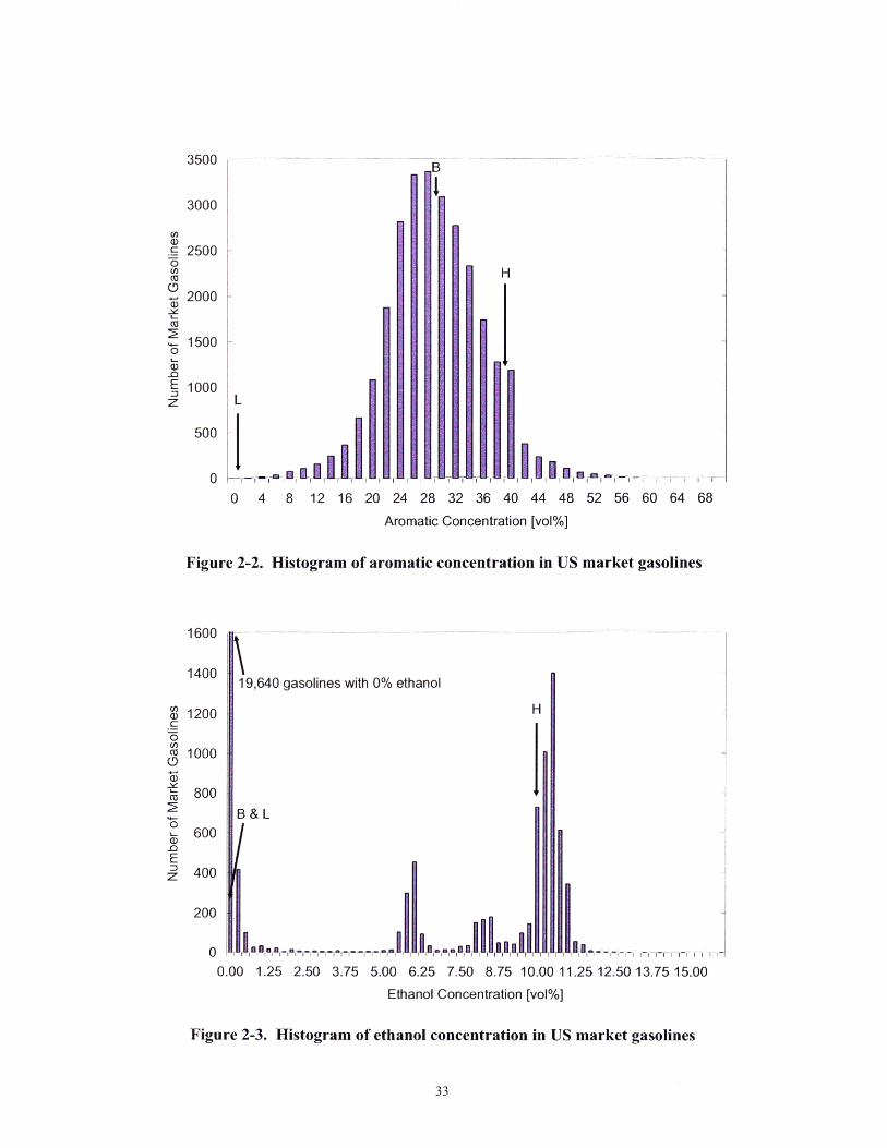
Figure 2-2. Histogram of aromatic concentration in US market gasolines ......................... 33
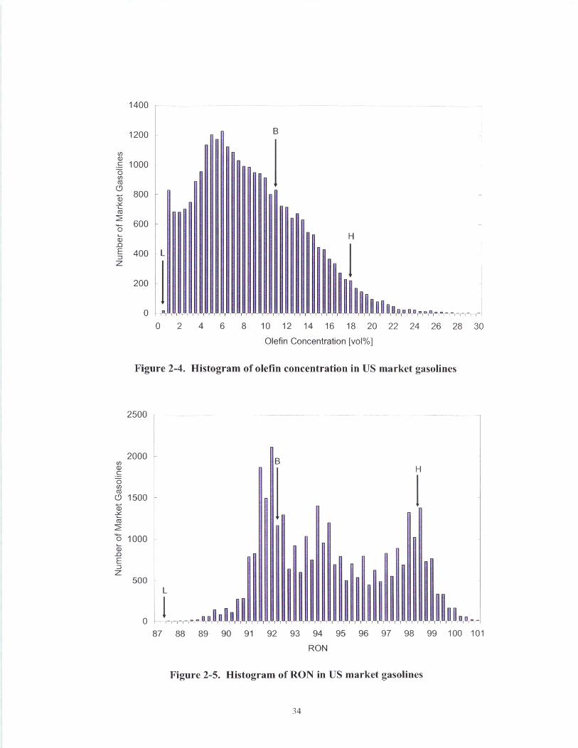
Figure 2-3. Histogram of ethanol concentration in US market gasolines...............................33
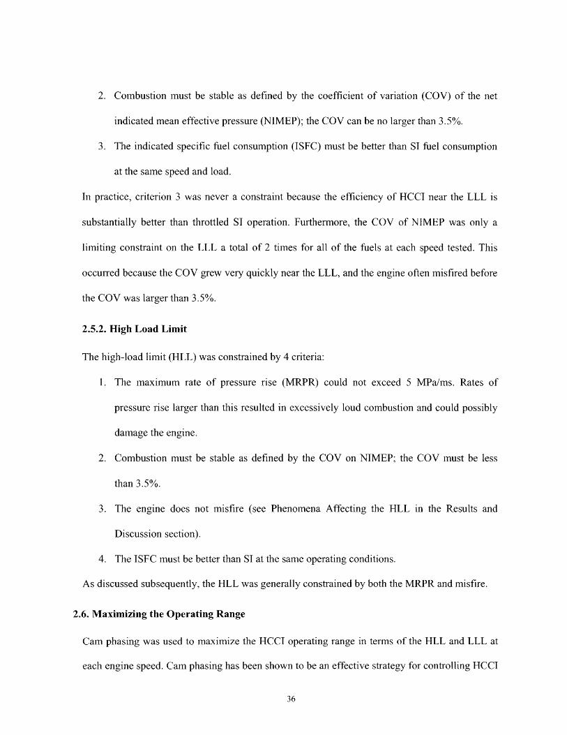
Figure 2-4. Histogram of olefin concentration in US market gasolines .............................. 34
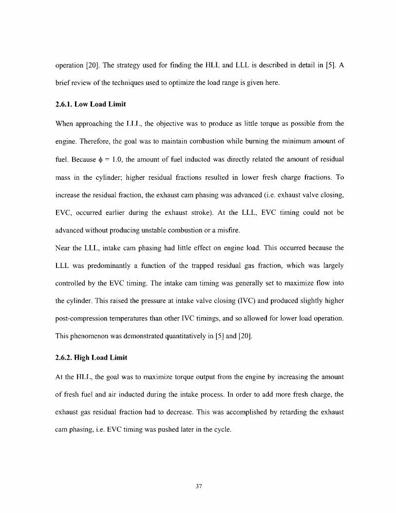
Figure 2-5. Histogram of RON in US market gasolines ..................... ..... 34
Figure 2-6. Histogram of RVP in US market gasolines...........................................35
Figure 2-7. Low Load Limit (LLL) for each fuel as a function of engine speed ................... 40
Figure 2-8. Full-cycle average pressure traces at the 1000 RPM LLL ........................... 41
Figure 2-9. Effect of ethanol on the LLL ..................................... ........... ........... 42
Figure 2-10. Single-day repeatability measurements of High RVP LLL at 1500 RPM.........43
Figure 2-1 1. 1000 RPM LLLs with 12% error bar ................................................................. 45
Figure 2-12. 1500 RPM LLLs with 12% error bar.......................................45
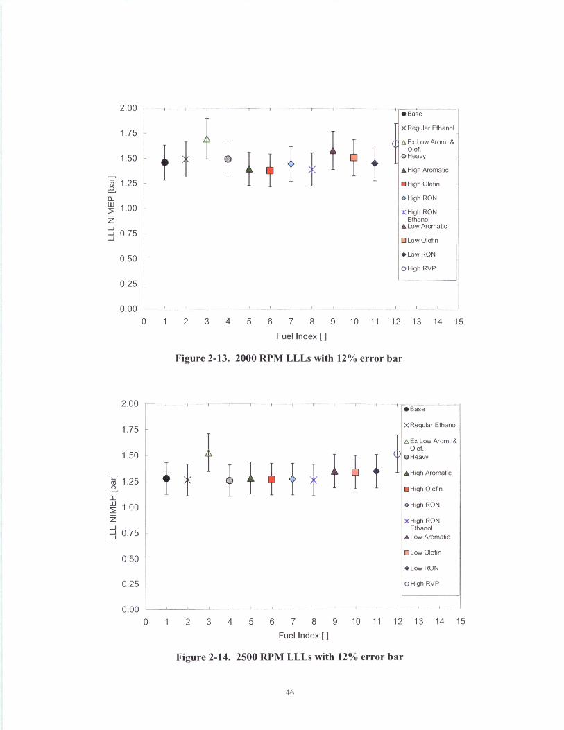
Figure 2-13. 2000 RPM LLLs with 12% error bar .......................... ................... 46
Figure 2-14. 2500 RPM LLLs with 12% error bar ................................................................. 46
Figure 2-15. Effect of exhaust valve closing (EVC) timing
on low RON load at 1000 RPM ....................................... 50
Figure 2-16. Effect of EVC timing on Ex. Low Arom. & Olef. load at 1500 RPM...........50
Figure 2-17. HLL for each fuel as a function of engine speed ........................................ 51
Figure 2-18. Average pressure traces at the HLL at 1000 RPM.......................................... 54
Figure 2-19. Effect of ethanol on the HLL ............................ ........................... 55
Figure 2-20. Single-day repeatability measurements of High RVP HLL at 1500 RPM ........ 56
Figure 2-21. 1000 RPM HLL measurements with a 3% error bar .................................... 58
Figure 2-22. 1500 RPM HLL measurements with 3% error bar .................................... 58
Figure 2-23. 2000 RPM HLL measurements with 3% error bar ...................................... 59
Figure 2-24. 2500 RPM HLL measurements with 3% error bar ................................... 59
Figure 2-25. Hydrocarbon family concentration deviations from the base fuel .................. 60

Figure 3-1. Schematic of the experimental apparatus..........................................70
Figure 3-2. Experimental LLL trajectories for PRFs 60 and 90 at 1000 RPM........................73
Figure 3-3. Experimental LLL pressure traces for PRFs 60 and 90 at 1000 RPM...............74
Figure 3-4. LLL measurement repeatability at 1000 RPM with PRF60 .............................74
Figure 3-5. Experimental LLL trajectories for PRFs 60 and 90 at 1500 RPM........................76
Figure 3-6. LLL measurement repeatability at 1500 RPM with PRF90 .............................76
Figure 3-7. Experimental LLL pressure traces for PRFs 60 and 90 at 1500 RPM..................77
Figure 3-8. Experimental LLL trajectories for PRFs 60 and 90 at 2000 RPM.....................78
Figure 3-9. LLL measurement repeatability at 2000 RPM with PRF90 ..............................78
Figure 3-10. Experimental LLL pressure traces for PRFs 60 and 90 at 2000 RPM.............79
Figure 4-1. In-cylinder pressure versus crank angle degree ........................ ............. 100
Figure 4-2. MITES simulation results en route to steady-state
for two different initial conditions (as given in Table 4-3): ..................................... 102
Figure 4-3. Engine performance while undergoing a transient
from lean (0 = 0.9) to stoichiometric ( = 1): ..........................................................105
Figure 4-4. Experimental and numerical gross indicated mean effective pressure
(GIMEP) during a speed transient from 1500 RPM to 1250 RPM. ....................... 109
Figure 4-5. Numerical pressure traces for speed transient: ....................................... 109
Figure 4-6. Combustion phasing while undergoing a speed transient.................................. 111
Figure 4-7. Experimental and numerical CA50 during an exhaust valve transient
from 1540 ATDC to 148' ATDC. ..................................... 114
Figure 5-1. Closed-cycle simulation pressure traces for a firing and misfiring cycle........ 131
Figure 5-2. Fire/misfire line at Ovc (a) and 30 CAD BTC (b) obtained from closed-cycle
simulations at 1500 RPM, Pjvc = 1.115 bar, Chang et al. heat transfer model .........132
Figure 5-3. Effect of initializing Myvc or Prvc on the PRF90 fire/misfire line at 0vc (a) and 30
CAD BTC (b) at 1500 RPM ............................................................ 134
Figure 5-4. Sensitivity of the PRF90 fire/misfire line at Ofvc (a) and 30 CAD BTC (b) to P1rc at
1500 RPM ..................................................... ................................... 136
Figure 5-5. Full-cycle simulation pressure traces for a firing and misfiring cycle.............137
Figure 5-6. Steady-state temperature at Ovc (a) and 30 CAD BTC (b) as a function residual mass
fraction from full-cycle simulations at 1500 RPM using the LLNL PRF chemistry model
................................................................................................................ .138
Figure 5-7. Steady-state Tvc over a broad range of residual fractions for PRF90 at 1500 RPM
........................................................................................................... .................. 139
Figure 5-8. Fire/misfire line and steady-state temperature at ,vrc (a) and 30 CAD BTC (b) at
1500 RPM as computed with the full-cycle, full-chemistry simulations, and the Chang et
al. heat transfer model......................................... 141
Figure 5-9. Simulated LLL trajectory for 3 PRFs at 1500 RPM ....................................... 142
Figure 5-10. Last 10 cycles leading to steady-state (i.e., Cycle 10) at approximately 64% residual
fraction for PRF90 at 1500 RPM ........................................ 144
Figure 5- 11. Last 10 cycles leading to steady-state (i.e., Cycle 10) at the LLL for PRF90 at 1500
RPM ............................................ ....................................... .......... ... 144
Figure 5-12. Simulated LLL trajectories for PRFs 60 and 90 at 1000 RPM ...................... 146
Figure 5-13. Simulated LLL pressure traces for PRFs 60 and 90 at 1000 RPM ................... 146
Figure 5-14. Fire/misfire line at OIvc (a) and 30 CAD BTC (b) for PRF90 at 2 speeds........149
Figure 5-15. Wiebe-calculated steady-state temperature at Olvc (a) and 30 CAD BTC (b) as a
function residual mass fraction for 2 engine speeds ................................................. 150
Figure 5-16. Pressure profiles of PRFs 60 and 90 at constant IVC conditions
obtained from detailed-kinetic simulations................................ 153
Figure 5-17. Experimental pressure profiles for PRFs 60 and 90 at
constant intake and exhaust cam phasing ................... ............................... 153
Figure 5-18. Cartoon showing the effect of fuel ignitability on the fire/misfire limit...........154
Figure 5-19. Cartoon showing the dependence of the fire/misfire
limit on residual fraction ............ ........................ ..... ...... 155
Figure 5-20. Wiebe-calculated steady-state temperature at Ovc (a) and 30 CAD BTC (b) as a
function of mass fraction for 3 ignition delays at 1500 RPM................................. 156
Figure 5-21. Effect of engine speed on both the fire/misfire line
and the steady-state (Tss) temperature at lvec (a) and 30 CAD BTC (b) ............. 158
Figure 5-22. Cartoon showing the shift of the steady-state temperature
and fire/misfire line due to fuel chemistry........................................................ ...... 160
Figure 5-23. Cartoon showing the effect of fuel chemistry on the
steady-state and fire/misfire temperatures .................................... .................... 160
Figure 5-24. Cartoon showing an extreme shift of the fire/misfire
line due to fuel chemistry..........................................161
Figure 5-25. Cartoon showing the relative change in the steady-state
temperature compared to the fire/misfire line due to heat transfer effects ................ 161
Figure 7-1. Typical SI and HCCI operating ranges. Figure adapted from Andreae [5]........174
Figure 7-2. Historic prices for U.S. regular conventional gasoline [99] and U.S.
spot, freight-on-board crude oil [100] ........................................... 190
Figure 7-3. Actual and predicted prices of U.S. regular conventional gasoline .................... 90
LIST OF TABLES
Table 2-1. Engine specifications ................. ......................... 29
Table 2-2. Properties of 12 test fuels ...................................... 32
Table 2-3. Average EVC and IVO [CAD after TDC] timings at the LLL .......................... 40
Table 2-4. LLL Repeatability measurements spanning several months .............................. 44
Table 2-5. Average EVC and IVO [CAD after TDC] timings at the HLL..................... 52
Table 2-6. Average CA50 [CAD after TDC] at the HLL ............................. 52
Table 2-7. HLL repeatability measurements spanning several months for base fuel.............56
Table 2-8. Variance inflation factors (VIFs) for hydrocarbon families in the test fuels ........ 61
Table 2-9. Mechanism limiting the HLL for each fuel ............................... ...... ........ 63
Table 3-1. Engine Specifications ................................... 70
Table 4-1. Parameters of the single-cylinder engine. .................................................... 97
Table 4-2. Comparison of experimental and numerical results for steady-state operation: ...98
Table 4-3. Initial conditions for two MITES simulations ...................................... 101
Table 5-1. Conditions used in closed-cycle simulations...................... ................... 128
Table 5-2. Conditions used in full-cycle simulations ........................................................... 129
Table 7-1. Average crude future prices as of July 29, 2008 and implied prices of gasoline. 191
Table 7-2. Technologies required to implement a dual-mode, SI/HCCI engine and
the resulting increase in retail price ........................................... 192
Table 7-3. Payback hurdles, fuel economy improvements, and implied payback periods.... 195
Table 7-4. Technologies required to implement a dual-mode, SI/HCCI engine and the resulting
increase in manufacturing cost ....... ................................... 198
Table 7-5. Increase in manufacturing cost for each HEV studied ................................... 199
Table 7-6. Increase in manufacturing cost, average fuel economy improvement, and
cost per mile per gallon ($/MPG) improvement for each fuel savings configuration200
Table 7-7. Average crude future prices as of December 1, 2008 and implied prices
of gasoline ................................... .............................................................. 204

Table 7-8. Payback hurdles, fuel economy improvements, and implied payback periods
for each vehicle examined based on gasoline prices as of December 11, 2008 ........ 205
1. INTRODUCTION
1.1. Background and Motivation
The concept of homogeneous-charge, compression-ignition (HCCI) combustion was first
introduced as an alternate combustion regime for two-stroke engines in 1979 [1 ]. HCCI
combustion is a combination of spark-ignition (SI, or gasoline) and compression-ignition (CI, or
Diesel) engine technologies. As in an SI engine, the fuel and air are premixed prior to
combustion. However, instead of using a spark to initiate the burning process, the fuel/air
mixture in an HCCI engine is ignited through compression only, as in a Diesel engine. The union
of these technologies allows HCCI engines to offer several advantages over traditional internal
combustion (IC) engines. Moreover, HCCI engines use standard IC engine hardware, making the
possible transition to this technology relatively easy for the automotive industry.
In SI engines, the work (i.e., the load or torque) produced during combustion is controlled by
limiting the amount of fresh fuel and air that enter the cylinder. To reduce the load to near idle,
the intake flow is significantly throttled; this throttling process greatly reduces the engine
efficiency. In HCCI engines, the load is often controlled by varying the amount of dilution:
either in the form of excess air for fuel-lean operation or excess exhaust gas residuals for
stoichiometric operation. Various experimental techniques can be used to control the dilution
level without throttling the intake flow. Consequently, HCCI engines generally operate
unthrottled and thus do not suffer the efficiency losses observed in SI engines at light loads. As a
result, HCCI engines have the potential to provide a 15 - 20% improvement in fuel economy
relative to SI engines.

In addition to fuel economy benefits, HCCI engines also have emission advantages over SI or
Diesel engines. In typical CI engines, the fuel is injected into a hot air mass, and the fuel begins
to auto-ignite shortly after (-1 ms) injection. Consequently, the fuel does not thoroughly mix
with the air, and there are regions in the cylinder that are significantly fuel-rich. These fuel-rich
regions lead to soot formation, which has recently been linked with high rates of asthma for
residents living near major highways [2]. In HCCI engines, the fuel and air are premixed prior to
combustion, and thus there are no local fuel-rich regions within the cylinder. As a result, HCCI
engines have near zero levels of soot or particulate matter (PM) emission. HCCI engines also
produce significantly less nitrogen oxides (NOx), which produce urban smog, than SI or Diesel
engines. In SI and Diesel engines, NOx are formed during combustion at the flame front. There,
temperatures are high enough to oxidize the nitrogen in air. In HCCI engines, the auto-ignition
process occurs throughout the entire combustion chamber; no flame front is present. Therefore,
fewer NO, are formed during combustion than in SI or Diesel engines. Furthermore, the high
levels of dilution present during HCCI combustion further reduce the combustion temperature,
thus driving NOx emissions even lower.
Despite the advantages of HCCI combustion, several technical hurdles must be resolved before
HCCI engines becomes mainstream technology. For example, precisely controlling combustion
phasing is difficult in the HCCI combustion regime due to the lack of an inherent control
strategy, such as spark- or injection-timing, used in traditional engines; in HCCI engines,
combustion is controlled by the chemical kinetics of the fuel/air mixture. Relying on chemical
kinetics to control the combustion event makes transient operation problematic in HCCI engines.

In addition, due to the low combustion temperatures in HCCI engines, the combustion process
often does not go to completion. Consequently, hydrocarbon (HC) emissions are generally
higher than those from SI engines [3]. Lastly, one of the greatest challenges facing HCCI
combustion is its limited operating range relative to SI or Diesel combustion [4,5]. The size and
location of the operating domain are influenced by several factors, including the engine
geometry, the method used for inducing auto-ignition, as well as the fuel used.
The primary goals of this work were to evaluate the impact of fuel chemistry on the HCCI
operating range and to establish what fundamentally causes an HCCI engine to misfire as it
approaches the low-load limit (LLL). The operating range research consisted of two studies: 1)
determining the effect of market-typical variations in commercial gasolines on the size of the
HCCI operating range, 2) examining the sensitivity of the HCCI LLL to fuels spanning a broad
range of auto-ignitability. Study I is important to the potential commercialization of HCCI
engine technology. If the sensitivity is large, commercialization will be difficult because fuel
companies may be required to blend a third fuel (alongside standard gasolines and diesels)
exclusively for HCCI engines to ensure smooth engine operation across the country/world.
Alternatively, auto-makers may have to alter significantly their engine calibration procedures to
counteract the fuel effects. However, if the sensitivity is small, HCCI engines could be
introduced with little strain on both the automotive and fuel industries. Study 2 arose to confirm
the conclusions reached during study 1.
The mechanism that limits HCCI operation near the LLL has yet to be determined in the HCCI
literature. We hypothesize that a misfire is the result of colder, in-cylinder temperatures that are
caused by falling combustion temperatures as the residual fraction increases. Cycle-to-cycle
instability could also potentially contribute to causing a misfire. If cycle-to-cycle fluctuations
grow near the LLL, perhaps a stable steady-state is unattainable beyond a critical residual
fraction. The second major objective of this work was to test these hypotheses and identify what
causes an HCCI engine to misfire when approaching the LLL. In this work, the underlying
physics of a misfire cycle were studied with a full-cycle HCCI simulation tool, which uses
detailed chemical kinetics to model the combustion process; this tool was developed as part of
the thesis project. The simulation results, along with the experimental data obtained from study
2, were used to estimate how fuel chemistry and engine operating conditions affect the LLL of
HCCI operability.
1.2. Thesis Overview by Chapter
1.2.1. Chapter 2
This chapter examines the impact of market-fuel variations on the HCCI operating range.
Twelve fuels were tested in a naturally-aspirated, single-cylinder HCCI engine in the Sloan
Automotive Laboratory at MIT. The fuels were designed to span the range of market-typical
variability in the following properties: aromatic concentration, ethanol concentration, olefin
concentration, research octane number (RON), and volatility.
HCCI combustion was achieved through residual trapping, and variable cam phasing was used to
maximize the load range at each speed tested. The load range was defined by the high-load limit
(HLL), the highest possible torque subject to the limiting criteria, and the low-load limit (LLL),
the lowest possible torque subject to the limiting criteria. All of the fuels were tested at 4 engine
speeds: 1000, 1500, 2000, and 2500 RPM.

The effects of market-typical variations in fuel composition on the operational limits were
modest; all fuels achieved nearly equal operating ranges. At the HLL, some fuel effects were
observed, but the trends in fuel performance were not consistent across all the speeds studied.
The LLL was insensitive to the changes in fuel chemistry across all the speeds examined.
1.2.2. Chapter 3
In Chapter 2, the LLL was found to be insensitive to changes in fuel chemistry observed in
market-typical gasolines. Therefore, in this chapter, the sensitivity of the LLL to a much broader
range of fuels was examined. The experiments were performed with primary reference fuels
(PRFs). These fuels are well characterized in the literature, and large changes in ignition
behavior can be accomplished simply by varying the ratio of the 2 fuel constituents: iso-octane
and n-heptane.
The LLLs of PRFs 60 and 90 were obtained at 1000, 1500, and 2000 RPM in a naturally-
aspirated, single-cylinder HCCI engine. Fuel ignitability had no effect on the obtainable LLL at
1500 or 2000 RPM. However, at 1000 RPM, PRF60 achieved a substantially lower (-30%) LLL
than PRF90. The large difference in the LLL at 1000 RPM was believed to be caused by colder
in-cylinder temperatures at lower engine speeds. The colder temperatures allowed differences in
fuel ignitability to affect combustion phasing and thus resulted in different LLL behavior
between the fuels.
1.2.3. Chapter 4
This chapter introduces the MIT engine simulator, MITES. MITES was developed during the
thesis project to model a full HCCI engine cycle using detailed chemical kinetics. To accomplish
this goal, a commercial engine simulation software package, Ricardo WAVE, was linked with a
user-written, detailed kinetic model of the engine cylinder. An in-depth discussion of the model
formulation is given, which includes information on the model equations as well as how the
detailed chemistry model was linked with WAVE to form a full-cycle simulator.
In this chapter, MITES was used to study the response of an HCCI engine to transients in fueling
rate, speed, and phasing of the exhaust valve event. Simulation results were compared to
experimental data taken from a naturally-aspirated, single-cylinder HCCI engine in Sloan
Automotive Laboratory. MITES was able to predict accurately transient time constants and
changes in the engine load for several of the transients studied. This work demonstrated the
potential for MITES to be used in HCCI design work, due to its fast computational speeds and
semi-quantitative agreement with experimental trends.
1.2.4. Chapter 5
In this chapter, the modeling tool developed in Chapter 4 was used to examine the mechanism
that causes an HCCI engine to misfire. Closed-cycle (intake valve closing to exhaust valve
opening) simulations were used to establish the minimum temperature required to induce auto-
ignition of a stoichiometric fuel/air mixture at a fixed residual fraction. The closed-cycle
simulations were performed over a range of residual fractions to build the fire/misfire line. The
fire/misfire line represented the boundary between the conditions that would and would not
allow for HCCI combustion for a single engine cycle; a reduction in temperature of I K below
the fire/misfire line resulted in a misfire.
In the closed-cycle simulations, the residual fraction and in-cylinder temperature were varied
independently. However, in the context of real engine operation, these two quantities are linked.

Thus, full-cycle simulations were used to develop the correlation between the in-cylinder
temperature and the residual fraction. Near the LLL, the in-cylinder temperature was found to
decrease as the residual fraction increased. This resulted from a reduction in the trapped fuel
mass, which reduced the combustion temperatures and consequently the residual gas
temperatures.
A comparison of the full- and closed-cycle simulation results showed that the last stable
operating temperature in the full-cycle simulations approached the fire/misfire line quite closely
(to within -14 K). These results suggest that the primary cause of an HCCI misfire was
insufficient thermal energy required to sustain combustion for multiple cycles. The full-cycle
simulations used to develop the correlations for in-cylinder temperature marked the first
simulations of the LLL for stoichiometric, residual-induced HCCI operation.
The effects of fuel chemistry and engine speed on the LLL were also examined. A reduction in
engine speed resulted in colder, steady-state in-cylinder temperatures, which caused fuel
chemistry to more strongly influence the LLL. This effect was observed experimentally, but due
to errors in the chemistry model, was not captured in the simulations. Therefore, empirical-based
combustion models (i.e., Wiebe functions) were used to study the impact of fuel chemistry on
the LLL. More auto-ignition resistant fuels exhibited hotter steady-state and misfire
temperatures. However, fuel chemistry affected each temperature to a varying extent.
Consequently, the relative movement of each temperature ultimately determined the impact of
fuel chemistry on the LLL.
2. EFFECTS OF VARIATIONS IN MARKET GASOLINE PROPERTIES ON HCCI
LOAD LIMITS
If homogenous-charge, compression-ignition (HCCI) engines are commercialized, they will
likely have to operate using standard commercial fuels. Therefore, investigating the impact of
market-typical, fuel chemistry variations on HCCI engine performance is necessary. This will
allow auto-makers and fuel companies to assess the need for new engine calibration procedures
and/or modified fuel blending processes. This chapter examines the effects of variations in
market gasoline properties, as observed in the North America market, on the HCCI operating
range.
2.1. Introduction
Research on HCCI engines has witnessed explosive growth over the last decade. The major
reasons for this boom are: 1) HCCI engines can potentially provide significant fuel consumption
benefits (- 15 - 20%) relative to spark-ignition (SI) engines, 2) the levels of NOx emissions from
HCCI engines are significantly lower than from SI or Diesel engines, 3) the particulate emissions
from HCCI engines are extremely low compared to those from Diesel engines [4]. Consequently,
HCCI engines are viewed as a possible alternative to conventional SI and/or Diesel technology
and may help automakers meet increasingly stringent emissions standards, while improving fuel
economy.
Several technical issues must be resolved before HCCI engines could become mainstream
technology. Two major problems facing HCCI engines are control of combustion phasing and a
small operating range. The difficulties in controlling combustion phasing have prompted many
researchers to investigate control methods for HCCI engines during both steady-state and
transient operation [6- 8]. The small operating range of HCCI engines makes a dedicated HCCI
engine currently impossible. Several factors influence both the size and location of the HCCI
operating region. These factors include engine geometry, the method of inducing auto-ignition
(e.g., increase compression ratio, high levels of exhaust gas residuals), and the fuel used, among
others. This chapter focuses on how fuel chemistry affects the size of the HCCI operating range.
There is a consensus that chemical kinetics are critical to HCCI combustion [4]. Consequently,
many experimenters have utilized a range of surrogate fuels (e.g. primary reference fuels, pure
chemicals such as methanol) to investigate the impact of fuel chemistry on HCCI operation [9-
16]. Yao et al. [9] tested a range of primary reference fuels (PRFs) to examine the impact of
octane number on combustion phasing and operating region size. They found that increasing the
octane number delayed ignition and that the operating range could be broadened by using
different octane fuels at different loads. Sato et al. [11 ] studied how dimethyl ether (DME) and
hydrogen functioned as ignition accelerators in methane/air mixtures. Both chemicals shortened
the ignition time; however, unlike hydrogen, which exhibits a single-stage heat release process,
the 2-stage heat release of DME made operation at high loads possible. Shibata et al. [12,13] and
Shibata and Urushihara [14] have tested a range of surrogate fuels to examine the effects of fuel
chemistry on the low temperature (LT-) and high temperature heat releases (HTHR). These
authors have developed correlations relating families of hydrocarbons (e.g. paraffins, aromatics)
to combustion phasing of the HTHR and correlations between combustion phasing of the HTHR
to the LTHR phasing and magnitude. In [14], Shibata and Urushihara extended their work to
examine the effect of intake air temperature on the LTHR. They found that increasing the intake

air temperature decreased the LTHR, which resulted in smaller but discernable differences in the
HTHR profiles.
Despite the many works that have investigated the effects of PRFs and various other surrogate
fuels on HCCI operation, very little data exist in the literature that are relevant to the important
practical question: is the operating range of a gasoline HCCI engine significantly different for
the fuel spread that exists in the market? Kalghatgi [17,18] developed an octane index (OI) to
characterize the auto-ignition quality of fuels for both SI and HCCI engine operation. The 01
was a function of the octane sensitivity, which was defined as the difference between the
Research Octane Number (RON) and the Motor Octane Number (MON) of the fuel.
Aroonrisopon et al. [ 19] used a broad range of fuels, which included a few research gasolines, to
correlate combustion phasing with the 01 defined by Kalghatgi. Oakley et al. [15] showed that 3
different fractions of a single commercial gasoline achieved virtually identical operating regions
for 2 sets of experimental conditions; each fraction had different amounts of aromatics, paraffins
and olefins. Koopmans, Stroemberg, and Denbratt [16] investigated the impact of fuel chemistry
on combustion phasing by testing 15 different fuels at a fixed operating condition. Nine of the
fuels were commercial gasolines or reference fuels. Their results indicated that the differences in
chemical composition among the fuels changed the 50% burned location (CA50) by less than 5
crank angle degrees (CAD).
In this work we aim to demonstrate how the HCCI operational region is influenced by the
variations observed in commercial gasolines. This information is vital to the potential
deployment of HCCI engine technology. This study examined the HCCI high- and low-load
limits at 4 engine speeds for 12 gasolines. The fuels were selected to have properties (e.g. RON,
aromatic content, etc.) that cover the range of variation seen in the North American market.
2.2. Experimental Setup
The experimental setup used in this work has been reported previously [20]. Briefly, the
experiments were performed on a production Mazda 2.3L, in-line, 4-cylinder, 16-valve engine,
modified for single-cylinder operation. The intake air and exhaust from the firing cylinder were
kept separate from the motoring cylinder flow to ensure accurate fuel/air ratio measurements.
Other modifications to the engine included: increasing the compression ratio from 9.7 to 11.1,
adding continuously variable cam phasing to the exhaust valve train (continuously variable
intake cam phasing was a standard feature on the production engine), and using cams with
reduced durations and lifts. The final engine configuration is presented in Table 2-1, and a
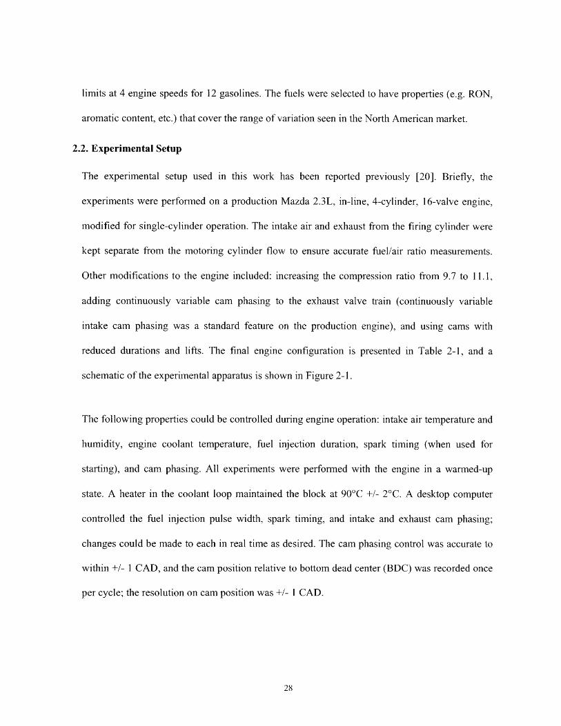
schematic of the experimental apparatus is shown in Figure 2-1.
The following properties could be controlled during engine operation: intake air temperature and
humidity, engine coolant temperature, fuel injection duration, spark timing (when used for
starting), and cam phasing. All experiments were performed with the engine in a warmed-up
state. A heater in the coolant loop maintained the block at 900 C +/- 20 C. A desktop computer
controlled the fuel injection pulse width, spark timing, and intake and exhaust cam phasing;
changes could be made to each in real time as desired. The cam phasing control was accurate to
within +/- 1 CAD, and the cam position relative to bottom dead center (BDC) was recorded once
per cycle; the resolution on cam position was +/- 1 CAD.

EXHAUST
FIRINGCYLINDER
MOTORED0CYLINDERS
** AN
-JFigure 2-1. Schematic of the experimental setup
Table 2-1. Engine specificationsDisplacement (cm3) 565
Bore (mm) 87.5
Stroke (mm) 94.0
Connecting Rod (mm) 154.8
Compression Ratio 11.1
Intake Cam Duration (o crank angle) 120
Exhaust Cam Duration (o crank angle) 120
Intake Valve Maximum Lift (mm) 2.0
Exhaust Valve Maximum Lift (mm) 2.0
Equivalence Ratio ( ) 1.0
AIR FILTER
I
HCCI combustion was induced by negative valve overlap (NVO), i.e. the exhaust valve was
closed early during the exhaust stroke to trap hot exhaust gas residuals. The thermal energy of
the exhaust gases was used to induce auto-ignition on the subsequent cycle. This procedure was
also used in [20] and is described in detail therein.
2.3. Test Matrix
For each fuel, the maximum operating range in terms of engine load was obtained; the definition
of these limits and the procedure to find these limits are discussed in the following sections. All
fuels were tested at 4 engine speeds: 1000, 1500, 2000, and 2500 RPM. For all experiments, the
intake air was dehumidified to a dew point of 40 C (corresponds to a water vapor mole fraction of
approximately 0.7%), and then reheated to 400 C before entering the engine. All experimental
data reported here were for an equivalence ratio of 1.0 as measured by a lambda meter in the
exhaust. The effect of varying the equivalence ratio of the load limits was examined previously
in [18].
2.4. Fuels
The chemical and physical composition of market gasolines vary with season and origin. To help
during cold starts, winter gasolines are often formulated to have higher Reid vapor pressures
(RVP) than summer fuels. The ASTM D4814 protocol limits the highest allowable RVP for
winter gasolines to 15 psi (103.4 kPa) and the lowest allowable RVP for summer gasolines to 7.0
psi (48.3 kPa). Other changes in gasoline properties result simply from the differences in crude
oil sources or the details of the refining process used to blend each fuel. Little research has been
done to quantify the effects of these market-typical property variations on HCCI operation. This
is, in part, due to the complexity of commercial fuels, which have 100s of compounds.
Therefore, unlike in experiments with surrogate fuels such as PRFs, attributing specific
operational effects to fuel chemistry can be difficult. Nevertheless, assessing these impacts is
crucial to the future deployment of HCCI engine technology.
For this study, a range of fuels were blended from commercial refinery streams. The blended
fuels were designed to span the market-typical variation in the select fuel properties. The
variables of interest were chosen based on two criteria: the property must show significant
variation within market gasolines, and literature data must support that the selected property has
some influence on HCCI combustion. Both criteria had to be met in order for the property to be
selected as a variable of study. The project sponsors at BP performed a fuel survey of over
27,000 different US fuels dated from 1999 to 2005 for all major US brands. Based on this fuel
survey and data from the research literature, particularly [12], [13], [15], and [17], the following
properties were selected for testing: volatility (measured by the Reid vapor pressure: RVP),
Research Octane Number (RON), aromatic content, olefin content, and ethanol content. The
Motor Octane Number (MON) was not used as an independent parameter because MON was
significantly correlated to the aromatic content of the fuels. Although RVP is a physical rather
than a chemical fuel property, (a) there is significant spread in commercial fuels; (b) RVP
correlates with lighter fuel hydrocarbon (HC) species. Therefore, RVP was a surrogate for
testing the difference between light and heavy HCs. Fuels were blended to span the range of
variability in the North American market observed for these parameters. The strategy used for
blending the fuels was first to create a base fuel, which would have properties similar to the
"average US gasoline." The properties of the average US gasoline were determined from the fuel
survey performed by BP. The other test fuels were blended as perturbations of the Base fuel in
the selected chemical/physical properties. One blending constraint was maintained for most of
the fuels: the RON for each fuel was fixed at approximately 92. However, the High RON, Low
RON, and High RON Ethanol fuels had higher or lower RONs than the fixed value. Also, the
High RVP fuel was a commercial winter gasoline with a high RVP; this fuel was not blended
exclusively for this program. The High RVP fuel had a lower T10 boiling point (390 C) than the
Base fuel (580 C), and the Heavy fuel had a higher T90 (192 0 C) than the Base fuel (172 0 C).
These fuels were used to examine the front- and back-end volatility effects on HCCI combustion.
Table 2-2 provides the properties of each fuel. Figure 2-2 to Figure 2-6 were generated from the
information in the fuel survey performed by BP. These figures show the range of market
variability for each selected property. For reference, the low, base, and high values for the
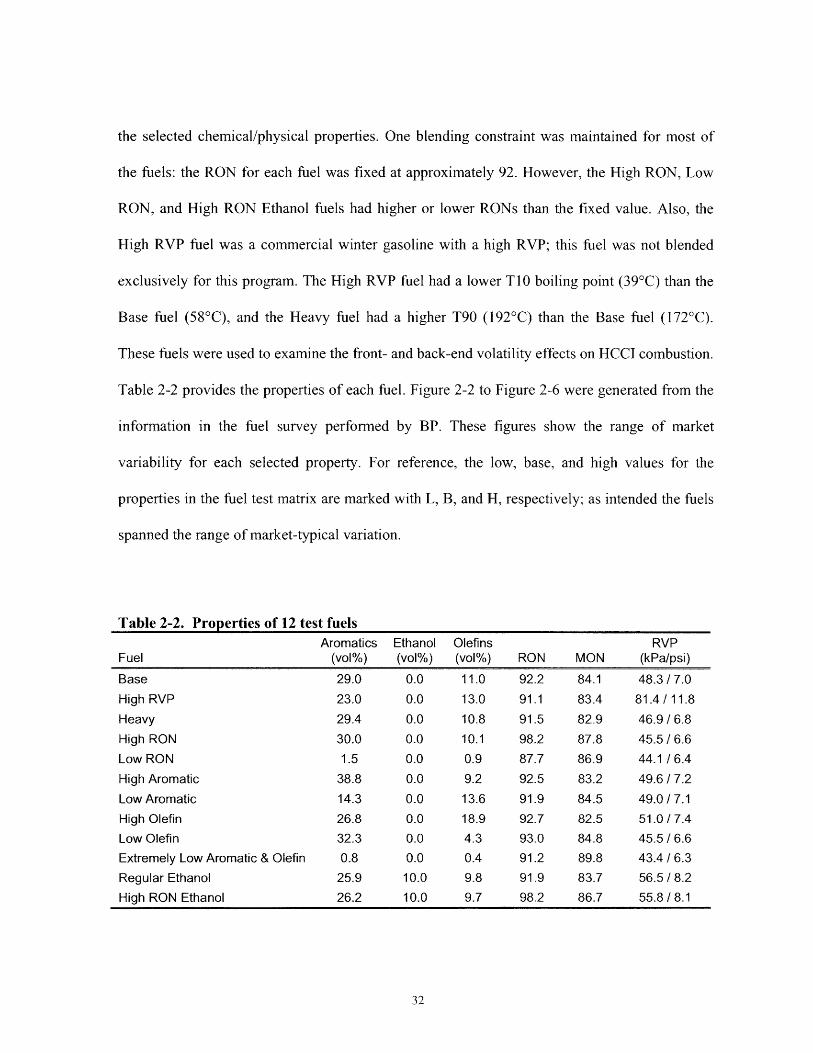
properties in the fuel test matrix are marked with L, B, and H, respectively; as intended the fuels
spanned the range of market-typical variation.
Table 2-2. Properties of 12 test fuelsAromatics Ethanol Olefins RVP
Fuel (vol%) (vol%) (vol%) RON MON (kPa/psi)
Base 29.0 0.0 11.0 92.2 84.1 48.3 / 7.0High RVP 23.0 0.0 13.0 91.1 83.4 81.4/11.8Heavy 29.4 0.0 10.8 91.5 82.9 46.9 / 6.8High RON 30.0 0.0 10.1 98.2 87.8 45.5/ 6.6Low RON 1.5 0.0 0.9 87.7 86.9 44.1 / 6.4High Aromatic 38.8 0.0 9.2 92.5 83.2 49.6 / 7.2Low Aromatic 14.3 0.0 13.6 91.9 84.5 49.0 / 7.1High Olefin 26.8 0.0 18.9 92.7 82.5 51.0 / 7.4Low Olefin 32.3 0.0 4.3 93.0 84.8 45.5 / 6.6Extremely Low Aromatic & Olefin 0.8 0.0 0.4 91.2 89.8 43.4 / 6.3Regular Ethanol 25.9 10.0 9.8 91.9 83.7 56.5 / 8.2High RON Ethanol 26.2 10.0 9.7 98.2 86.7 55.8/8.1
3500 ---
3000
.E 2500
H
2000
15000
-.Q
E 1000z L
500
0 r Y i T f-i-
0 4 8 12 16 20 24 28 32 36 40 44 48 52 56 60 64 68
Aromatic Concentration [vol%]
Figure 2-2. Histogram of aromatic concentration in US market gasolines
1600
140019,640 gasolines with 0% ethanol
2 1200 H-5
C 1000
S800
4B & L600
Ez 400
200
0.00 1.25 2.50 3.75 5.00 6.25 7.50 8.75 10.00 11.25 12.50 13.75 15.00
Ethanol Concentration [vol%]
Figure 2-3. Histogram of ethanol concentration in US market gasolines
1400
1200
1000
800
600
400
0 2 4 6 8 10 12 14 16 18 20 22 24 26 28 30
Olefin Concentration [vol%]
Figure 2-4. Histogram of olefin concentration in US market gasolines
2500 .
2000
1500
1000
500 LTL -1t-iI .I I , .T1-T'I-
87 88 89 90 91 92 93 94 95 96 97 98 99 100 101
RON
Figure 2-5. Histogram of RON in US market gasolines
t rT
200
0
H
"T ] TT"
111111110 1 T I', IT, 1 11 1 -1 I'l t 11 1

BH
45.0 53.0 61.0 69.0 77.0
RVP [kPa]
Figure 2-6. Histogram of RVP in US
2500c
O 2000(o(9
- 1000Ez
500
093.0 101.0 109.0
market gasolines
2.5. Defining the HCCI Operational Limits
The region of HCCI operability is strongly tied to the definition of the limiting behavior. In this
work, the goal was to maximize the HCCI operating range in terms of load as a function of
engine speed. The criteria used to define the HCCI operating range were similar to those
previously defined by Andrea [5] and Andrea et al. [20]. Each point reported as an operational
limit was a 100-cycle average of the last experimental conditions meeting the criteria described
below.
2.5.1. Low Load Limit
The low-load limit (LLL) was defined by 3 criteria:
1. The engine does not misfire.
3000
85.037.037.0
2. Combustion must be stable as defined by the coefficient of variation (COV) of the net
indicated mean effective pressure (NIMEP); the COV can be no larger than 3.5%.
3. The indicated specific fuel consumption (ISFC) must be better than SI fuel consumption
at the same speed and load.
In practice, criterion 3 was never a constraint because the efficiency of HCCI near the LLL is
substantially better than throttled SI operation. Furthermore, the COV of NIMEP was only a
limiting constraint on the LLL a total of 2 times for all of the fuels at each speed tested. This
occurred because the COV grew very quickly near the LLL, and the engine often misfired before
the COV was larger than 3.5%.
2.5.2. High Load Limit
The high-load limit (HLL) was constrained by 4 criteria:
1. The maximum rate of pressure rise (MRPR) could not exceed 5 MPa/ms. Rates of
pressure rise larger than this resulted in excessively loud combustion and could possibly
damage the engine.
2. Combustion must be stable as defined by the COV on NIMEP; the COV must be less
than 3.5%.
3. The engine does not misfire (see Phenomena Affecting the HLL in the Results and
Discussion section).
4. The ISFC must be better than SI at the same operating conditions.
As discussed subsequently, the HLL was generally constrained by both the MRPR and misfire.
2.6. Maximizing the Operating Range
Cam phasing was used to maximize the HCCI operating range in terms of the HLL and LLL at
each engine speed. Cam phasing has been shown to be an effective strategy for controlling HCCI
operation [20]. The strategy used for finding the HLL and LLL is described in detail in [5]. A
brief review of the techniques used to optimize the load range is given here.
2.6.1. Low Load Limit
When approaching the LLL, the objective was to produce as little torque as possible from the
engine. Therefore, the goal was to maintain combustion while burning the minimum amount of
fuel. Because < = 1.0, the amount of fuel inducted was directly related the amount of residual
mass in the cylinder; higher residual fractions resulted in lower fresh charge fractions. To
increase the residual fraction, the exhaust cam phasing was advanced (i.e. exhaust valve closing,
EVC, occurred earlier during the exhaust stroke). At the LLL, EVC timing could not be
advanced without producing unstable combustion or a misfire.
Near the LLL, intake cam phasing had little effect on engine load. This occurred because the
LLL was predominantly a function of the trapped residual gas fraction, which was largely
controlled by the EVC timing. The intake cam timing was generally set to maximize flow into
the cylinder. This raised the pressure at intake valve closing (IVC) and produced slightly higher
post-compression temperatures than other IVC timings, and so allowed for lower load operation.
This phenomenon was demonstrated quantitatively in [5] and [20].
2.6.2. High Load Limit
At the HLL, the goal was to maximize torque output from the engine by increasing the amount
of fresh fuel and air inducted during the intake process. In order to add more fresh charge, the
exhaust gas residual fraction had to decrease. This was accomplished by retarding the exhaust
cam phasing, i.e. EVC timing was pushed later in the cycle.
As load increased, the rate of pressure rise during combustion increased; eventually the rate of
pressure rise exceeded the 5 MPa/ms limiting criteria. The rate of pressure rise was strongly
influenced by combustion phasing. If combustion began before top dead center (TDC), the in-
cylinder gases expanded against a compressing cylinder, thus producing a faster rate of pressure
rise. However, if combustion began after top center, the rate of pressure rise was reduced by the
expansion of the cylinder volume. Therefore, if combustion phasing was delayed, the rate of
pressure rise could be abated. Post-TDC heat release also increases the load. However, if the
phasing was too late, the engine could misfire. Usually the highest load with acceptable MRPR
was measured near the misfire limit. Combustion phasing was retarded by adjusting the intake
cam to control the amount of fresh charge entering the cylinder. The effect of intake cam timing
on combustion phasing was previously demonstrated in [20].
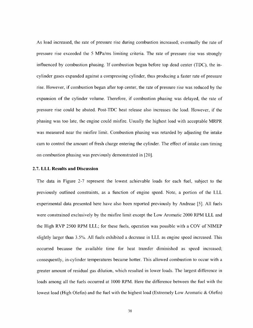
2.7. LLL Results and Discussion
The data in Figure 2-7 represent the lowest achievable loads for each fuel, subject to the
previously outlined constraints, as a function of engine speed. Note, a portion of the LLL
experimental data presented here have also been reported previously by Andreae [5]. All fuels
were constrained exclusively by the misfire limit except the Low Aromatic 2000 RPM LLL and
the High RVP 2500 RPM LLL; for these fuels, operation was possible with a COV of NIMEP
slightly larger than 3.5%. All fuels exhibited a decrease in LLL as engine speed increased. This
occurred because the available time for heat transfer diminished as speed increased;
consequently, in-cylinder temperatures became hotter. This allowed combustion to occur with a
greater amount of residual gas dilution, which resulted in lower loads. The largest difference in
loads among all the fuels occurred at 1000 RPM. Here the difference between the fuel with the
lowest load (High Olefin) and the fuel with the highest load (Extremely Low Aromatic & Olefin)
was approximately 0.74 bar. The variation in the lowest-achievable load among the fuels shrunk
to approximately 0.26 bar at 2500 RPM.
The 100-cycle average EVC and IVO timings for all the data in Figure 2-7 are given in Table
2-3. The range of IVO timings at a constant speed varied from approximately 14 CAD at 1000
RPM to approximately 2 CAD at 1500 RPM. While this variation at 1000 RPM appears large,
prior work [20] demonstrated that intake cam timing had minimal effect on the LLL; a change in
IVO timing of 35 CAD changed the NIMEP by only 0.2 bar. Across all the speeds studied, the
range of EVC timing for all the fuels was less than approximately 7 CAD. This result is
consistent with the small variations in LLL observed. At each speed the EVC timing for the
Extremely Low Aromatic & Olefin fuel and the High Olefin fuel were often at the extremes of
the range. These results are consistent with those fuels generally having one of the highest and
lowest LLLs, respectively.
Near the LLL, the combustion phasings for all of the fuels were approximately equal for a given
speed. The range of the location of the maximum rate of pressure rise among all the fuels was
less than 2.5 CAD at every speed studied. Note, in prior work [5] the authors showed that for this
engine the crank angle for 50% heat release (CA50) had a one-to-one correspondence with the
location of the maximum rate of pressure rise. Figure 2-8 is a plot showing the 400-cycle
averaged pressure traces for the 2 fuels showing the largest differences in the LLL at 1000 RPM;
the Base fuel pressure trace is also included for reference. As expected, the pressure traces for

0 Base
X Regular Ethanol
A Ex Low Arom. &Olef.
0 Heavy
A High Aromatic
0 High Olefin
I OHigh RON
X High RONEthanol
A Low Aromatic
1 Low Olefin
* Low RON
O High RVP
1500 2000Engine Speed [RPM]
2500 3000
Low Load Limit (LLL) for each fuel as a function of engine speedData presented previously by Andreae [5]
Table 2-3. Average EVC and IVO [CAD after TDCJ timings at the LLL1000 RPM 1500 RPM 2000 RPM 2500 RPM
Fuel EVC IVO EVC IVO EVC IVO EVC IVO
Base 129.5 97.8 120.5 101.8 102.3 104.9 107.0 108.8
Regular Ethanol 125.0 101.9 121.6 102.0 100.6 106.8 105.9 105.8
Ex Low Arom. & Olef. 123.2 97.0 117.5 101.9 102.9 105.8 102.9 108.3
Heavy 129.3 97.9 119.6 101.9 103.7 104.9 105.8 107.7
High Aromatic 125.3 103.0 117.6 102.0 100.6 106.8 105.9 109.4
High Olefin 129.0 109.9 121.3 102.0 104.4 105.8 107.9 109.8
High RON 122.4 98.0 118.5 102.0 99.6 105.9 105.9 109.0
High RON Ethanol 126.4 96.0 118.8 103.0 100.8 105.9 105.9 109.0
Low Aromatic 126.3 100.0 117.3 102.0 100.6 107.8 102.9 111.8
Low Olefin 126.4 97.9 117.5 101.9 101.7 106.9 102.9 108.8
Low RON 128.3 98.0 120.4 100.9 103.7 105.9 103.8 105.8
High RVP 129.3 97.0 116.5 102.9 102.6 105.0 105.9 107.8
2.50
2.25
2.00
1.75
1.50
1.25 -
n
w.
z-- 1.00 i
0.75 1-
0.50
0.25
0.00500
Figure 2-7.
1000

-.- Basea Ex. Low Arom. & Olef.
-0-High Olefin
-90 0 90 180
CAD
270 360 450 540
-30 -15 0 15 30 45
CAD
Full-cycle average pressure traces at the 1000A) full view B) zoom of A around TDC
RPM LLL
A) 30
10
5
0-180
B) 30
25
20
Figure 2-8.
the different fuels are very similar. The I bar difference in peak recompression pressure observed
between the Base/High Olefin fuel and the Extremely Low Aromatic & Olefin fuel was due to
differences in valve timing.
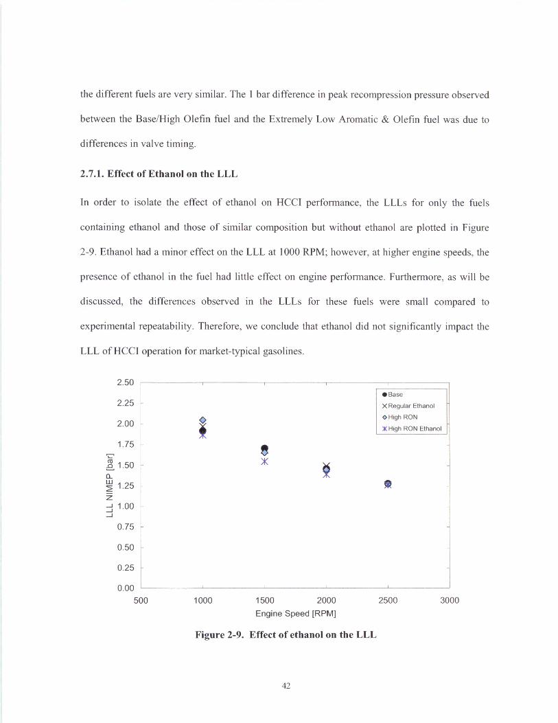
2.7.1. Effect of Ethanol on the LLL
In order to isolate the effect of ethanol on HCCI performance, the LLLs for only the fuels
containing ethanol and those of similar composition but without ethanol are plotted in Figure
2-9. Ethanol had a minor effect on the LLL at 1000 RPM; however, at higher engine speeds, the
presence of ethanol in the fuel had little effect on engine performance. Furthermore, as will be
discussed, the differences observed in the LLLs for these fuels were small compared to
experimental repeatability. Therefore, we conclude that ethanol did not significantly impact the
LLL of HCCI operation for market-typical gasolines.
2.50
2.25
2.00
1.75
1.50
1.25
1.00
0.75
0.50
0.25
0.00500
* Base
X Regular Ethanol
OHigh RON
X High RON Ethanol
1000 1500 2000 2500
Engine Speed [RPM]
Figure 2-9. Effect of ethanol on the LLL
3000

2.7.2. LLL Measurement Repeatability
2.25
2.000 0 0 0 0 0 0 0 0 O
1.75
, 1.50
n 1.25
z 1.00
0.75
0.50
0.25
0.000 1 2 3 4 5 6 7 8 9 10 11
Index []
Figure 2-10. Single-day repeatability measurements of High RVP LLL at 1500 RPMData presented previously by Andreae [51
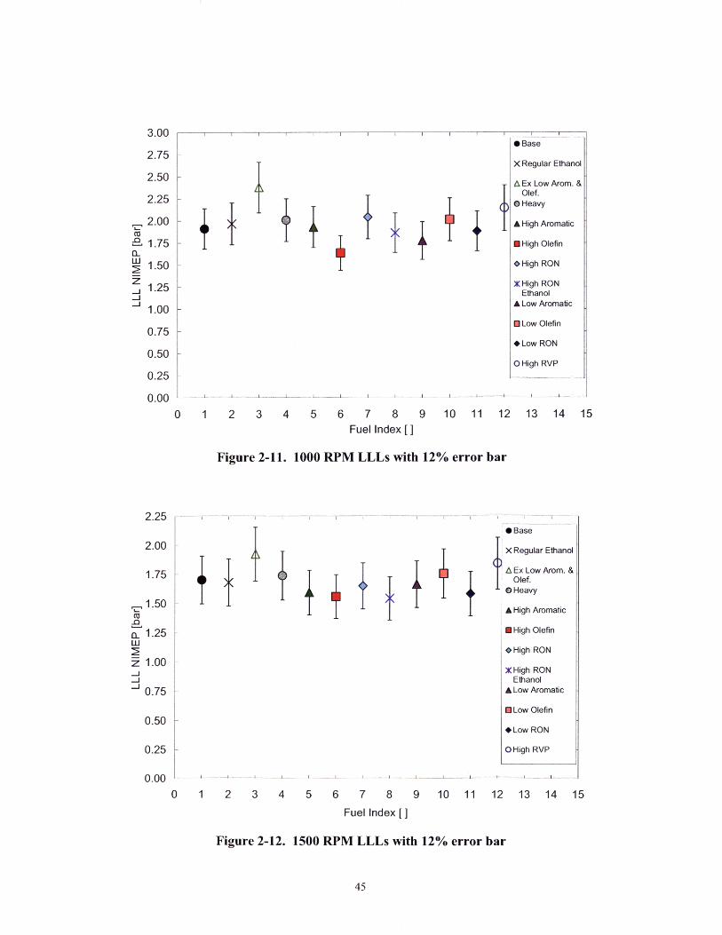
Two procedures were performed to assess the repeatability of the measured LLLs: 1) a single
fuel's LLL was measured 10 times during the course of a single day; 2) the LLLs of several fuels
were remeasured within several weeks or months of the original LLL measurements. The results
of Test 1, which was conducted with the High RVP fuel at 1500 RPM, are presented in Figure
2-10.
The LLL measurement was quite repeatable on a single day. The maximum difference in the
measured LLLs was only 0.07 bar, and the COV of the LLL NIMEPs was approximately 1.37%;
here the COV refers to the coefficient of variation of the LLL NIMEPs, not the COV of the

NIMEP on a cycle-by-cycle basis. These data demonstrated that the measurement error of the
LLL on a single day was small in comparison to the LLL.
Due to the large number of fuels examined in this study, it took several months to measure all the
LLLs. Therefore, repeatability measurements spanning several weeks or months were needed to
quantify the drift of the LLL from that measured on the original test date. The Base fuel's LLL at
1000 RPM was repeated 3 times over the course of approximately 3 months. In addition, the
Low RON fuel's LLL at 1500 RPM was remeasured 7 times over an approximate 4 month
period. The data for these measurements are given in Table 2-4. The LLL was far less repeatable
when reassessed after an extended period of time, with variations of up to 0.5 bar in NIMEP; the
fluctuations were about 12% of the LLL. A portion of this drift was due to cam timing control,
which will be discussed in Effect of Cam Timing on LLL. The time between testing the different
fuels ranged from days to months. Therefore, when comparing the LLLs of all the fuels, a 12%
error bar was placed on the LLL measurements for a given speed, as shown in Figure 2-11 to
Figure 2- 4.
Table 2-4. LLL Repeatability measurements spanning several monthsSpeed NIMEP
Fuel [RPM] [bar]
Base 1000 2.45
Low RON
2.181.91
1500 1.591.631.982.102.091.932.02
3.00
2.75
2.50
2.25
2.00
1.75
1.50
1.25
1.00
0.75
0.50
0.25
0.00
* Base
X Regular Ethanol
A Ex Low Arom. &Olef.
0 Heavy
A High Aromatic
S High Olefin
* High RON
X High RONEthanol
A Low Aromatic
• Low Olefin
* Low RON
O High RVP
I - A - - 4 - -
0 1 2 3 4 5 6 7 8 9 10 11Fuel Index []
Figure 2-11. 1000 RPM LLLs with 12% error bar
i I" I ~ I' T
0 1 2 3 4 5 6 7 8
Fuel Index []
10 11
* Base
X Regular Ethanol
A Ex Low Arom. &Olef.
0 Heavy
A High Aromatic
N High Olefin
SHigh RON
X High RONEthanol
A Low Aromatic
N Low Olefin
*Low RON
0 High RVP
12 13.... 1 . 15...
12 13 14 15
Figure 2-12. 1500 RPM LLLs with 12% error bar
12 13 14
2.25
2.00
1.75
1.50.Q
a 1.25
z 1.00.J
- 0.75
0.50
0.25
0.00
I I I I
2.00
S..
0 1 2 3 4 5 6 7 8 9 10 11
Fuel Index []
Figure 2-13. 2000 RPM LLLs with 12% error bar
S I I
4~,, x 1
If_-- i J J 1I I i I
3 4 5 6 7 8 9 10 11 12
Fuel Index []
re 2-14. 2500 RPM LLLs with 12% error bar
0 Base
X Regular Ethanol
A Ex Low Arom. &Olef.
@ Heavy
A High Aromatic
U High Olefin
OHigh RON
KHigh RONEthanol
A Low Aromatic
E Low Olefin
+ Low RON
O High RVP
13 14 15
0 Base
X Regular Ethanol
A Ex Low Arom. &Olef.
* Heavy
A High Aromatic
• High Olefin
SHigh RON
X High RONEthanol
A Low Aromatic
I Low Olefin
* Low RON
O High RVP
12 13 14 15
1.75
1.50
c 1.25-Q
2 1.00
0.75_J
0.50
0.25
0.00
2.00
1.75
1.50
8 1.25
U 1.00
-J1 0.75
0.50
0.25
0.000 1 2
Figu
I
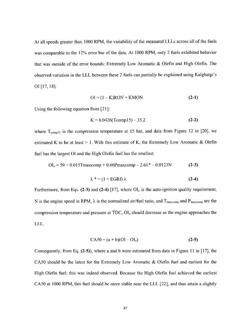
At all speeds greater than 1000 RPM, the variability of the measured LLLs across all of the fuels
was comparable to the 12% error bar of the data. At 1000 RPM, only 2 fuels exhibited behavior
that was outside of the error bounds: Extremely Low Aromatic & Olefin and High Olefin. The
observed variation in the LLL between these 2 fuels can partially be explained using Kalghatgi's
01 [17, 18].
OI= (1 - K)RON + KMON (2-1)
Using the following equation from [21]:
K = 0.0426(Tcomp 15) - 35.2 (2-2)
where T,,ompl5 is the compression temperature at 15 bar, and data from Figure 12 in [20], we
estimated K to be at least > 1. With this estimate of K, the Extremely Low Aromatic & Olefin
fuel has the largest 01 and the High Olefin fuel has the smallest.
01 = 59 + 0.015Tmaxcomp + 0.66Pmaxcomp - 2.6X* - 0.0123N (2-3)
X * = ( + EGRf) X (2-4)
Furthermore, from Eqs. (2-3) and (2-4) [17], where OI is the auto-ignition quality requirement,
N is the engine speed in RPM, X is the normalized air/fuel ratio, and Tmaxcomp and Pmaxcomp are the
compression temperature and pressure at TDC, 01o should decrease as the engine approaches the
LLL.
CA50 = (a + b)(OI - Oo1) (2-5)
Consequently, from Eq. (2-5)), where a and b were estimated from data in Figure 11 in [17], the
CA50 should be the latest for the Extremely Low Aromatic & Olefin fuel and earliest for the
High Olefin fuel; this was indeed observed. Because the High Olefin fuel achieved the earliest
CA50 at 1000 RPM, this fuel should be more stable near the LLL [22], and thus attain a slightly
lower LLL than the other fuels; conversely, the Extremely Low Aromatic & Olefin fuel should
be the least stable and achieve the highest LLL. One should note, however, that the difference in
CA50 between these 2 fuels at 1000 RPM was only approximately 2.4 CAD, and the resolution
of CA50 was +/- 1 CAD. Furthermore, the 01 explanation of the LLL variability only held for
the extreme (highest/lowest OI) fuels at 1000 RPM.
Regression analysis was used in an effort to correlate chemical properties to fuel performance at
the LLL. In this analysis, fuel chemical and physical properties were used as predictor variables,
and the LLL was used as the response variable. Due to the small variations of the LLLs at each
speed and considerable collinearity in the fuel properties, which is discussed in detail in the HLL
section to follow, no statistically significant trends were observed relating fuel properties to the
measured LLLs. Consequently, we conclude that the effects of market-typical variations in fuel
properties on the LLL could not be separated from experimental repeatability. This conclusion,
however, has only been demonstrated for NVO-induced HCCI. Controlling HCCI combustion
with alternate methods (e.g. intake air heating, variable compression ratio) may result in fuel
chemistry exhibiting greater influence on the LLL.
2.7.3. Effect of Cam Timing on the LLL
The precision of intake and exhaust cam timing control for this engine was +/- I CAD. Small
fluctuations in the exhaust cam timing that resulted from control issues impacted the residual gas
fraction for each cycle. As the residual gas fraction changed, the available volume for fresh fuel
and air varied proportionally. Changes in the amount of fresh fuel and air directly impacted the
load. Therefore, controllability of the cam timing was responsible for some of the measurement
variability observed at the LLL. To evaluate quantitatively how large of an impact cam timing
had on measurement precision near the LLL, data points along the exhaust valve trajectory to the
LLL at 1000 and 1500 RPM are shown in Figure 2-15 and Figure 2-16, respectively.
For both data sets, the intake cam timing was held constant. The slopes of the lines in these
figures provided an estimate of how much I CAD affected the load at each speed. At 1000 RPM,
a one-degree change in exhaust cam timing resulted in a change of approximately 0.08 bar in
load. Therefore, +/- 1 CAD cam control contributed approximately 0.16 bar of variability to the
LLL at 1000 RPM; this accounted for approximately 8.5% of the LLL measurement error for the
Low RON fuel. Similarly, at 1500 RPM, +/- 1 CAD exhaust cam control resulted in a change of
approximately 0.2 bar NIMEP, which was approximately 10.0% of the LLL for the Extremely
Low Aromatic & Olefin fuel. From this information, we conclude that a large portion of the
variability observed in the LLL measurements was due to cam timing control.
2.7.4. Phenomena Affecting the LLL
At the LLL, the goal was to burn as little fuel as possible while maintaining stable combustion.
As the amount of fuel burned in each cycle was decreased, the in-cylinder temperature declined.
Therefore, the likely cause of the engine misfire was insufficient thermal energy required to
induce auto-ignition. Because fuel chemistry is strongly tied to ignition behavior, fuels with
different chemical compositions should achieve different LLLs. However, our data indicate that
the differences in LLL performance were of comparable magnitude to measurement error. In
addition, the true fundamental limiting mechanisms governing the LLL are not yet well
understood.

f -'=--------T------?- ---- ~r- -'- T"~~-;~~
NIMEP [bar] = -0.08*EVC [CAD BTDC] + 12.75 [bar]R2 = 0.9955
.- -..........-..-.-.-. __.. .
122.0 122.5 123.0 123.5 124.0 124.5 125.0 125.5 126.0
EVC Timing [CAD BTDC]
Figure 2-15. Effect of exhaust valve closing (EVC) timingon low RON load at 1000 RPM
r" . . ... . ... ..T
NIMEP [bar] = -0.10*EVC [CAD BTDC] + 13.70 [bar]R2 = 0.9875
114.0 114.5 115.0 115.5 116.0 116.5 117.0 117.5 118.0
EVC Timing [CAD BTDC]
Figure 2-16. Effect of EVC timing on Ex. Low Arom. & Olef. load at 1500 RPM
2.65
2.60
2.55
. 2.50
S2.45z
2.40
2.35
2.30 1-
2.25
2.20
2.15
4 2.10
- 2.05z
2.00
1.95
1.90
r- . . 1........---. - .-..
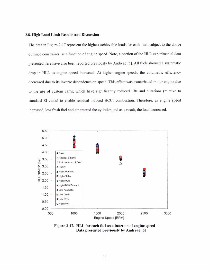
2.8. High Load Limit Results and Discussion
The data in Figure 2-17 represent the highest achievable loads for each fuel, subject to the above
outlined constraints, as a function of engine speed. Note, a portion of the HLL experimental data
presented here have also been reported previously by Andreae [5]. All fuels showed a systematic
drop in HLL as engine speed increased. At higher engine speeds, the volumetric efficiency
decreased due to its inverse dependence on speed. This effect was exacerbated in our engine due
to the use of custom cams, which have significantly reduced lifts and durations (relative to
standard SI cams) to enable residual-induced HCCI combustion. Therefore, as engine speed
increased, less fresh fuel and air entered the cylinder, and as a result, the load decreased.
5.50 ---
5.00 i
4.50 -
4.00 - 0 Base
-? 3.50 x Regular Ethanol
A Ex Low Arom. & Olef. AS3.00 O Heavy
2.50 High Aromatic
I High Olefin
I 2.00 - *High RON
1.50 X High RON Ethanol
A Low Aromatic
1.00 E Low Olefin
*Low RON0.50
0 High RVP
0.00
500 1000 1500 2000 2500 3000Engine Speed [RPM]
Figure 2-17. HLL for each fuel as a function of engine speedData presented previously by Andreae [5]

Table 2-5. Average EVC and IVO [CAD after TDC] timings at the HLL
Fuel
Base
Regular Ethanol
Ex Low Arom. & Olef.
Heavy
High Aromatic
High Olefin
High RON
High RON Ethanol
Low Aromatic
Low Olefin
Low RON
High RVP
1000 RPM
EVC IVO
78.5 69.9
71.3 68.0
85.3 98.0
80.1 66.0
77.3 66.9
78.5 62.9
73.1 75.0
78.2 75.0
76.1 69.0
79.2 71.0
80.2 91.0
71.6 70.0
Table 2-6. Average CA50 [CAD after TDC] at the HLLFuel
Base
Regular Ethanol
Ex Low Arom. & Olef.
Heavy
High Aromatic
High Olefin
High RON
High RON Ethanol
Low Aromatic
Low Olefin
Low RON
High RVP
1500
EVC
71.4
63.4
74.8
70.5
66.5
68.1
64.5
68.7
64.4
69.4
73.8
69.7
RPM
IVO
72.7
75.9
97.9
68.0
67.8
66.9
77.9
79.9
71.0
72.9
91.9
69.9
2000
EVC
65.8
54.8
74.8
61.7
60.5
59.6
56.6
60.8
61.7
63.6
69.3
55.1
RPM
IVO
91.9
104.9
107.9
93.9
87.8
89.8
100.9
103.8
98.0
96.8
102.0
103.0
2500
EVC
76.9
59.9
75.9
61.9
64.7
58.8
60.9
65.9
66.9
69.9
74.0
65.9
RPM
IVO
91.7
81.9
98.9
73.8
78.9
73.9
80.9
76.9
81.9
82.8
87.0
89.8
1000 RPM
7.6
8.9
11.1
6.5
7.2
8.4
7.4
7.5
9.1
7.4
9.8
8.2
1500 RPM
11.4
10.3
12.2
10.3
11.1
10.8
12.4
11.0
10.8
10.6
11.2
11.6
2000 RPM
13.8
12.9
9.5
14.3
12.3
12.9
13.4
14.6
13.2
12.7
13.3
13.9
2500 RPM
3.8
7.2
4.9
8.9
7.7
11.0
7.2
6.8
5.5
6.1
5.7
4.9
~III
--

As was the case for the LLLs, the largest difference observed in the HLLs occurred at 1000
RPM; the High Aromatic fuel achieved a HLL of 4.37 bar, and the Low RON fuel achieved a
HLL of 5.10 bar. At 2000 RPM, most of the fuels showed very little difference in their HLL. At
this speed, the air flow into the engine was especially restricted due to manifold dynamics.
Usually, the HLL was limited by the MRPR. However, at 2000 RPM, the MRPR limit for
several of the fuels was not a constraint on the HLL. Instead increasing the load was limited by
the amount of fresh charge that could enter the cylinder (see Phenomenon Affecting the HLL).
As residual fraction was reduced to increase the fresh charge fraction, the engine eventually
misfired (presumably because the temperature after compression was too low).
The 100-cycle average EVC and IVO timings for all the data in Figure 2-17 are given in Table
2-5. Near the HLL, the intake cam timing was advanced to retard combustion phasing and thus
combat large MRPRs. Consequently, IVO timings near the HLL were generally significantly
earlier than those at the LLL (see Table 2-3). However, at 2000 RPM the intake cam timing for
several fuels required little advancement relative to the LLL IVO timing due to the manifold
dynamics mentioned previously. Larger ranges of EVC timing were also observed at the HLL
than at the LLL for a constant speed. These results are consistent with the greater variability in
HLLs than the LLLs (see HLL Measurement Repeatability). The ranges of IVO timings at the
HLL were also larger than those at the LLL. This occurred because finding the HLL involved
varying the intake cam to control the MRPR and the exhaust cam to control the residual fraction.
The CA50s for all the HLLs at each speed are given in Table 2-6. Combustion phasing exhibited
greater variability at the HLL than at the LLL. At 2500 RPM, combustion phasing varied by
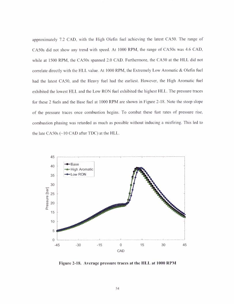
approximately 7.2 CAD, with the High Olefin fuel achieving the latest CA50. The range of
CA50s did not show any trend with speed. At 1000 RPM, the range of CA50s was 4.6 CAD,
while at 1500 RPM, the CA50s spanned 2.0 CAD. Furthermore, the CA50 at the HLL did not
correlate directly with the HLL value. At 1000 RPM, the Extremely Low Aromatic & Olefin fuel
had the latest CA50, and the Heavy fuel had the earliest. However, the High Aromatic fuel
exhibited the lowest HLL and the Low RON fuel exhibited the highest HLL. The pressure traces
for these 2 fuels and the Base fuel at 1000 RPM are shown in Figure 2-18. Note the steep slope
of the pressure traces once combustion begins. To combat these fast rates of pressure rise,
combustion phasing was retarded as much as possible without inducing a misfiring. This led to
the late CA50s (-10 CAD after TDC) at the HLL.
45
40
35
30
25
20
15
10
5
0 ---45
- -- 1 -- ---- - -~--- - --
-Base- High Aromatic-4--Low RON
- ----L- -------- -- - ------
-30 -15 0 15 30 45
CAD
Figure 2-18. Average pressure traces at the HLL at 1000 RPM

2.8.1. Effect of Ethanol on the HLL
* Base
X Regular Ethanol
*High RON
X High RON Ethanol
5.00
4.50
4.00
3.50
3.00
2.50
2.00
1.50
1.00
0.50
0.00500 3000
The HLL data for the fuels with ethanol and the fuels with similar composition but without
ethanol are presented in Figure 2-19. The addition of ethanol to the test fuels had no effect on the
HLL for all speeds below 2000 RPM. Minor differences in load were observed at 2500 RPM, but
these differences were small compared to experimental repeatability - see paragraphs below.
Therefore, we conclude that ethanol did not significantly impact the HLL of HCCI operation.
2.8.2. HLL Measurement Repeatability
Experimental repeatability was assessed at the HLL. The 2 tests used to evaluate experimental
measurement error at the LLL were used at the HLL. First, the High RVP fuel's HLL was
repeated 10 times on a single day; these data are presented in Figure 2-20. The relative error in
1500 2000 2500Engine Speed [RPM]
Effect of ethanol on the HLL
1000
Figure 2-19.
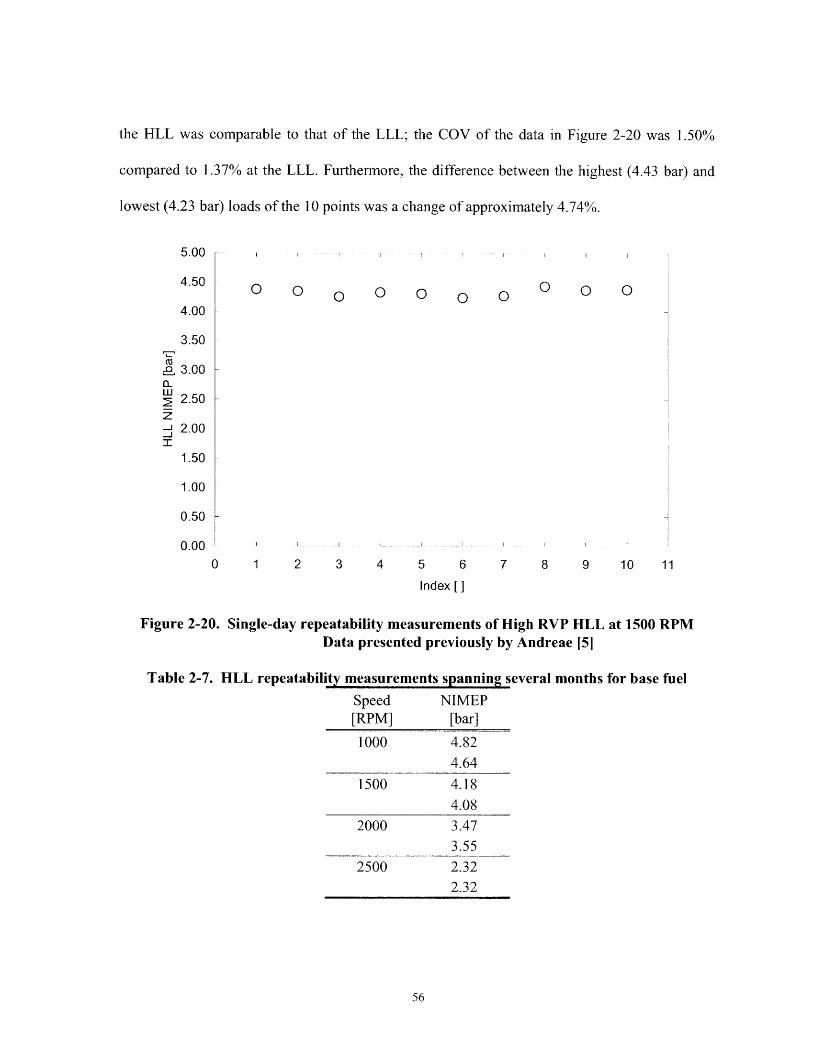
the HLL was comparable to that of the LLL; the COV of the data in Figure 2-20 was 1.50%
compared to 1.3 7 % at the LLL. Furthermore, the difference between the highest (4.43 bar) and
lowest (4.23 bar) loads of the 10 points was a change of approximately 4.74%.
5.00
4.50
4.00
3.50
3.00
2.50
2.00
1.50
1.00
0.50
0.00
0 0 0 0 0 0 0 0 0
0 1 2 3 4 5 6 7 8 9 10 11
Index []
Figure 2-20. Single-day repeatability measurements of High RVP HLL at 1500 RPMData presented previously by Andreae [51
Table 2-7. HLL repeatability measurements spanning several months for base fuel
Speed NIMEP[RPM] [bar]
1000 4.82
4.64
1500 4.18
4.08
2000 3.47
3.55
2500 2.322.32
iI~
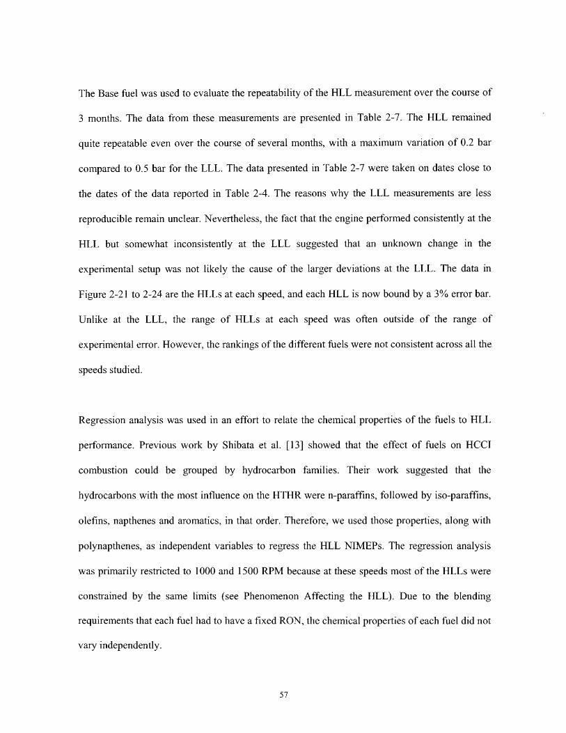
The Base fuel was used to evaluate the repeatability of the HLL measurement over the course of
3 months. The data from these measurements are presented in Table 2-7. The HLL remained
quite repeatable even over the course of several months, with a maximum variation of 0.2 bar
compared to 0.5 bar for the LLL. The data presented in Table 2-7 were taken on dates close to
the dates of the data reported in Table 2-4. The reasons why the LLL measurements are less
reproducible remain unclear. Nevertheless, the fact that the engine performed consistently at the
HLL but somewhat inconsistently at the LLL suggested that an unknown change in the
experimental setup was not likely the cause of the larger deviations at the LLL. The data in
Figure 2-21 to 2-24 are the HLLs at each speed, and each HLL is now bound by a 3% error bar.
Unlike at the LLL, the range of HLLs at each speed was often outside of the range of
experimental error. However, the rankings of the different fuels were not consistent across all the
speeds studied.
Regression analysis was used in an effort to relate the chemical properties of the fuels to HLL
performance. Previous work by Shibata et al. [13] showed that the effect of fuels on HCCI
combustion could be grouped by hydrocarbon families. Their work suggested that the
hydrocarbons with the most influence on the HTHR were n-paraffins, followed by iso-paraffins,
olefins, napthenes and aromatics, in that order. Therefore, we used those properties, along with
polynapthenes, as independent variables to regress the HLL NIMEPs. The regression analysis
was primarily restricted to 1000 and 1500 RPM because at these speeds most of the HLLs were
constrained by the same limits (see Phenomenon Affecting the HLL). Due to the blending
requirements that each fuel had to have a fixed RON, the chemical properties of each fuel did not
vary independently.

5.50
5.00
4.50
4.00
c' 3.50
3.00
Z 2.50-J
r 2.00
1.50
1.00
0.50
0.000 1 2 3 4 5 6 7
Fuel Index []
8 9 10 11 12
Figure 2-21. 1000 RPM HLL measurements with a 3% error bar
--r- . . r r
0 1 2 3 4 5 6 7
Fuel Index []
8 9
* Base
X Regular Ethanol
A Ex Low Arom. & Olef.
* Heavy
A High Aromatic
* High Olefin
*High RON
X High RON Ethanol
A Low Aromatic
N Low Olefin
+ Low RON
O High RVP10 .... 11 12 13
10 11 12 13
Figure 2-22. 1500 RPM HLL measurements with 3% error bar
0 Base
X Regular Ethanol
A Ex Low Arom. & Olef.
0 Heavy
A High Aromatic
N High Olefin
*High RON
X High RON Ethanol
A Low Aromatic
N Low Olefin
* Low RON
0 High RVPS I I I I ' I I I '
5.00
4.50
4.00
3.50
- 3.00
2 2.50
- 2.00-J
1.50
1.00
0.50
0.00

4.00
3.50
3.00
b 2.50-_
2 2.00
-J
1.50I
1.00
0.50
0.00
0 1 2 3 4 5 6 7
Fuel Index []
8 9 10 11 12
Figure 2-24. 2500 RPM HLL measurements with 3% error bar
0 Base
X Regular Ethanol
A Ex Low Arom. & Olef.
O Heavy
A High Aromatic
* High Olefin
* High RON
X High RON Ethanol
A Low Aromatic
* Low Olefin
* Low RON
OHigh RVP
0 1 2 3 4 5 6 7 8 9 10 11 12 13
Fuel Index []
Figure 2-23. 2000 RPM HLL measurements with 3% error bar
* Base
X Regular Ethanol
A Ex Low Arom. & Olef.
O Heavy
A High Aromatic
S High Olefin
*High RON
X High RON Ethanol
A Low Aromatic
* Low Olefin
* Low RON
O High RVP
3.00
2.75
2.50
2.25
2.00
1.75
1.50
1.25
1.00
0.75
0.50
0.25
0.00
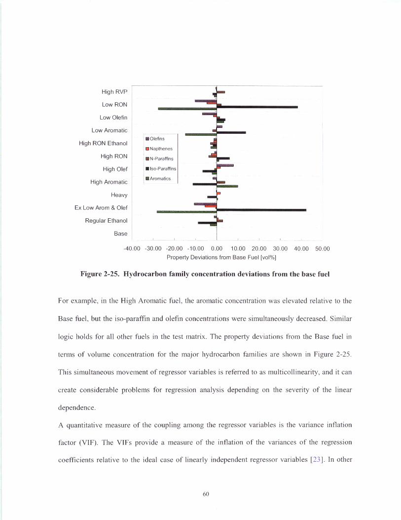
High RVP
Low RON
Low Olefin
Low Aromatic
High RON Ethanol
High RON
High Olef
High Aromatic
Heavy
Ex Low Arom & Olef
Regular Ethanol
Base
-40.00
MOle
* Nap
SN-P
MIso-
EArol
fns
thenes
araffins
Paraffins _
matics
°I
-30.00 -20.00 -10.00 0.00 10.00 20.00 30.00 40.00 50.00
Property Deviations from Base Fuel [vol%]
Figure 2-25. Hydrocarbon family concentration deviations from the base fuel
For example, in the High Aromatic fuel, the aromatic concentration was elevated relative to the
Base fuel, but the iso-paraffin and olefin concentrations were simultaneously decreased. Similar
logic holds for all other fuels in the test matrix. The property deviations from the Base fuel in
terms of volume concentration for the major hydrocarbon families are shown in Figure 2-25.
This simultaneous movement of regressor variables is referred to as multicollinearity, and it can
create considerable problems for regression analysis depending on the severity of the linear
dependence.
A quantitative measure of the coupling among the regressor variables is the variance inflation
factor (VIF). The VIFs provide a measure of the inflation of the variances of the regression
coefficients relative to the ideal case of linearly independent regressor variables [23]. In other
U
Umu
man1unsmme
U
t- - -~--
M
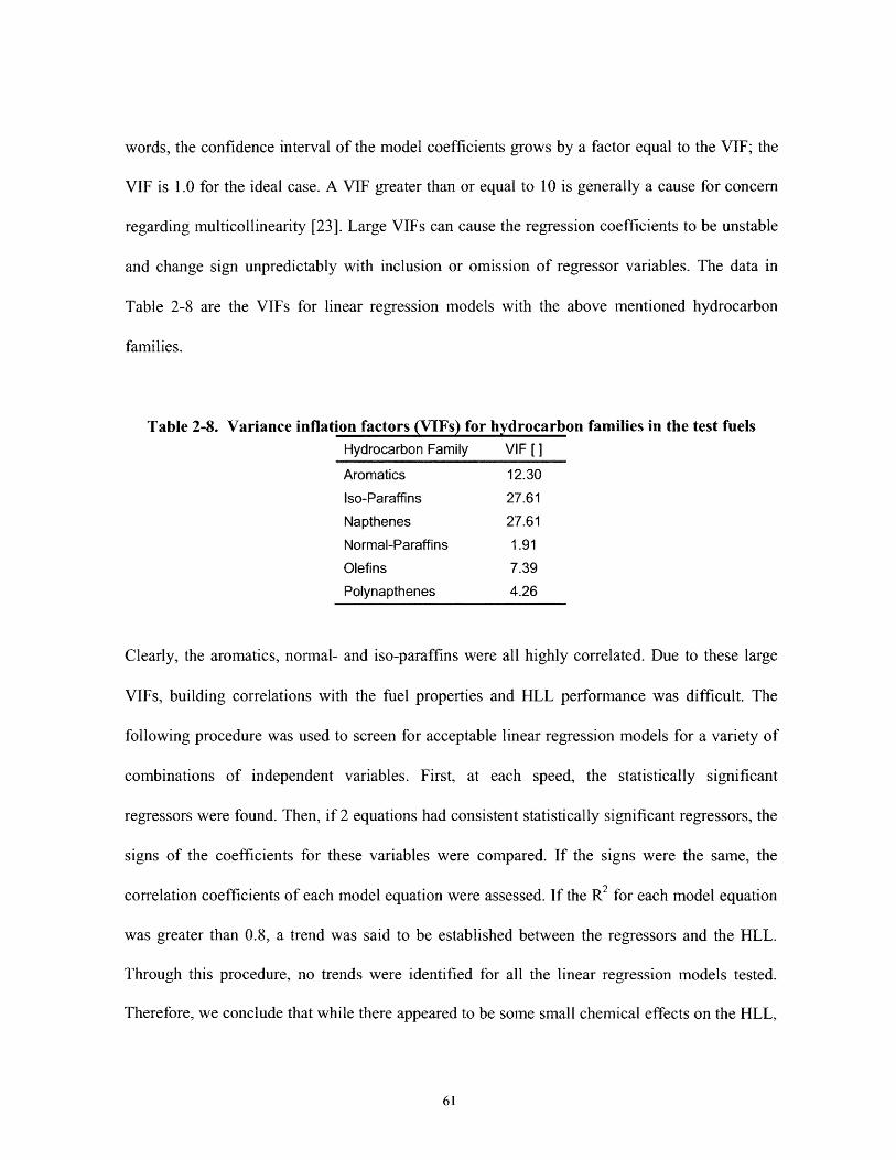
words, the confidence interval of the model coefficients grows by a factor equal to the VIF; the
VIF is 1.0 for the ideal case. A VIF greater than or equal to 10 is generally a cause for concern
regarding multicollinearity [23]. Large VIFs can cause the regression coefficients to be unstable
and change sign unpredictably with inclusion or omission of regressor variables. The data in
Table 2-8 are the VIFs for linear regression models with the above mentioned hydrocarbon
families.
Table 2-8. Variance inflation factors (VIFs) for hydrocarbon families in the test fuelsHydrocarbon Family VIF []
Aromatics 12.30Iso-Paraffins 27.61
Napthenes 27.61Normal-Paraffins 1.91
Olefins 7.39
Polynapthenes 4.26
Clearly, the aromatics, normal- and iso-paraffins were all highly correlated. Due to these large
VIFs, building correlations with the fuel properties and HLL performance was difficult. The
following procedure was used to screen for acceptable linear regression models for a variety of
combinations of independent variables. First, at each speed, the statistically significant
regressors were found. Then, if 2 equations had consistent statistically significant regressors, the
signs of the coefficients for these variables were compared. If the signs were the same, the
con-elation coefficients of each model equation were assessed. If the R2 for each model equation
was greater than 0.8, a trend was said to be established between the regressors and the HLL.
Through this procedure, no trends were identified for all the linear regression models tested.
Therefore, we conclude that while there appeared to be some small chemical effects on the HLL,

the absence of consistent trends across multiple speeds made attributing chemical properties to
engine performance impossible. As noted in the LLL section, this conclusion has only been
demonstrated for NVO-induced HCCI. Employing other controlling methods of HCCI
combustion may result in larger and more discernable fuel effects on the HLL.
2.8.3. Effect of Cam Timing on the HLL
As discussed previously, cam timing control impacted the residual gas fraction trapped during
each cycle. Fluctuations in the residual gas fraction resulted in a proportional change in the fresh
fuel and air fraction, which impacted the engine load. Data near the LLL indicated that exhaust
cam timing control contributed to variability in NIMEP of approximately 0.16 bar at 1000 RPM.
Similar results were obtained near the HLL; the repeated measurements with the Base fuel
showed variability of 0. 10 bar NIMEP. This was expected because the dominant effect of the
variations in cam timing was to change the residual gas fraction and the amount of fresh charge
entering the cylinder, and this phenomenon is largely independent of the operating conditions,
i.e. near the LLL or HLL. At 1500 RPM, the HLL variation for the Base fuel was approximately
0.10 bar NIMEP, which was consistent with a 1 CAD change in EVC timing, as demonstrated in
Figure 2-16. These results indicated that a significant fraction of the HLL variability observed
was due to cam timing control.
2.8.4. Phenomena Affecting the HLL
In general, there were at least 2 competing mechanisms controlling the HLL: the MRPR and
combustion stability. The data in Table 2-9 show which constraints limited the HLL for each fuel
at each engine speed tested. In the table, COV implies the HLL was constrained by the COV of
NIMEP, M implies the HLL was limited by misfire, and MRPR implies the HLL was limited by
the MRPR. At 1000 and 1500 RPM, almost all of the fuels were limited by combustion stability,
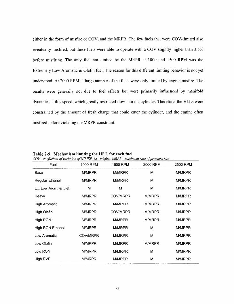
either in the form of misfire or COV, and the MRPR. The few fuels that were COV-limited also
eventually misfired, but these fuels were able to operate with a COV slightly higher than 3.5%
before misfiring. The only fuel not limited by the MRPR at 1000 and 1500 RPM was the
Extremely Low Aromatic & Olefin fuel. The reason for this different limiting behavior is not yet
understood. At 2000 RPM, a large number of the fuels were only limited by engine misfire. The
results were generally not due to fuel effects but were primarily influenced by manifold
dynamics at this speed, which greatly restricted flow into the cylinder. Therefore, the HLLs were
constrained by the amount of fresh charge that could enter the cylinder, and the engine often
misfired before violating the MRPR constraint.
Table 2-9. Mechanism limiting the HLL for each fuelCOV- coefficient of variation ofNIMEP, M- misfire, MRPR - maximum rate of pressure rise
Fuel 1000 RPM 1500 RPM 2000 RPM 2500 RPM
Base M/MRPR M/MRPR M M/MRPR
Regular Ethanol M/MRPR M/MRPR M M/MRPR
Ex. Low Arom. & Olef. M M M M/MRPR
Heavy M/MRPR COV/MRPR M/MRPR M/MRPR
High Aromatic M/MRPR M/MRPR M/MRPR M/MRPR
High Olefin M/MRPR COV/MRPR M/MRPR M/MRPR
High RON M/MRPR M/MRPR M/MRPR M/MRPR
High RON Ethanol M/MRPR M/MRPR M M/MRPR
Low Aromatic COV/MRPR M/MRPR M M/MRPR
Low Olefin M/MRPR M/MRPR M/MRPR M/MRPR
Low RON M/MRPR M/MRPR M M/MRPR
High RVP M/MRPR M/MRPR M M/MRPR
At the HLL, the rates of pressure rise in the cylinder become fast. These rates were significantly
influenced by combustion phasing. If combustion phasing was early, the gases expand in a
smaller volume leading to faster rates of pressure rise. Therefore, if the MRPR became
significant, combustion phasing was delayed. However, if combustion was delayed too far, the
engine could become unstable and misfire. Generally, at the HLL, combustion could not be
delayed without inducing a misfire, and combustion could not be advanced without violating the
MRPR criterion. These 2 competing mechanisms make studying the HLL difficult. In addition,
the 2 mechanisms lead to different requirements of the same fuel. The misfire limit requires the
fuel to auto-ignite easily, but the MRPR limit requires the fuel to burn slowly. Currently, it is not
clear which factor is more important at the HLL and how fuel chemistry influences which limit
is reached first.
2.9. Conclusions
The impact of variations in market fuel properties on the HCCI operating range was examined.
Twelve commercial-grade gasolines were tested in a single-cylinder, NVO-induced, HCCI
engine. The fuels were blended to span the market-typical range of variability in 5 properties:
aromatic concentration, ethanol content, olefin concentration, RON, and volatility. The HLL and
LLL of each fuel were obtained at 4 engine speeds: 1000, 1500, 2000, and 2500 RPM. The
following conclusions were reached:
* The HCCI operating range was not materially affected the range of variations in fuel
properties observed in the North American market; all of the fuels achieved nearly
equal operating ranges. This conclusion has only been demonstrated for NVO-
induced HCCI, though we expect it to hold for all SI-like, HCCI engines.
* The effect of adding ethanol to the test fuels was insignificant at the LLL and HLL.
* At the high-load limit, some small fuel effects on the operating range were observed;
however, the observed trends were not consistent across all the speeds studied.
* Within experimental measurement error, there was no change in the LLL among the
blends of test fuels.
The observation that the operating range of HCCI engines is not significantly affected over the
entire range of North American gasolines has huge practical implications. This suggests that fuel
sensitivity is not an obstacle to introducing HCCI engine technology commercially.
Consequently, auto-makers and fuel companies need not be overly concerned that HCCI engines
will cease to operate given the spread of fuels in the market.
3. THE EFFECT OF FUEL IGNITABILITY ON THE LOW-LOAD LIMIT
OF HCCI OPERABILITY
In Chapter 2, the effects of fuel chemistry on the HCCI operating range were examined over the
range of market-typical variability. In that study, the LLL of HCCI operability was found to be
insensitive to these variations. Therefore, the goal of this work was to test the broader
applicability of this conclusion by examining the sensitivity of the LLL to much larger changes
in fuel ignitability. This was accomplished by studying 2 well characterized primary reference
fuels (PRFs) with very different ignition characteristics: PRF60 and PRF90; PRF90 is
significantly more auto-ignition resistant than PRF60.
3.1. Introduction
3.1.1. Motivation
One of the greatest challenges facing HCCI engines is its limited operating range size relative to
ST or Diesel engines [4]. The HCCI operating range lies in the low speed, low load portion of the
SI operating range. Under these conditions, SI engines suffer large efficiency losses due to the
throttling process used to reduce the load. However, HCCI engines generally operate unthrottled,
and consequently they have significantly higher (-25%) efficiencies than SI engines at light
loads [5]. Unfortunately, the HCCI operating range does not extend down to idle operation.
Reducing the low-load limit (LLL) of HCCI operation could significantly improve the fuel
efficiency.
Developing an understanding of what factors influence the lower load limit of HCCI operability
is an important step towards maximizing the potential of HCCI efficiency advantages. This work

examines how the HCCI operating range is influenced by different ftiels and specifically focuses
on how fuel ignitability affects the lowest achievable load in the HCCI combustion regime.
3.1.2. Prior Studies on HCCI Fuel Effects
Several studies have been presented in the literature in which researchers examined how fuel
ignitability affects combustion phasing in HCCI engines [10,12,13,14]. For example, Lti et al.
[24] tested a broad range of PRF octane numbers (0 - 90) and found that the start of ignition was
more delayed for higher octane PRFs. In addition, their results showed that combustion duration
decreased with increasing PRF octane number. Other studies have focused on the effect of fuel
ignitability on the HCCI operating range [12,25]. For example, Yao et al. [9,26] examined the
effect of PRF octane number on the size of the HCCI operating range. In [9], the operating range
was defined as a function of 2 (the air/fuel equivalence ratio) and the research octane number
(RON) of the fuel. Yao et al. [9] observed that higher RON fuels could operate over a smaller
range of A than lower RON fuels at a fixed speed. In [26], Yao et al. defined the operating range
as a function of A and exhaust gas residual (EGR) fraction. They concluded that higher RON
fuels could achieve higher loads than low RON fuels, and lower RON fuels could achieve lower
loads than high RON fuels at a fixed engine speed.
3.1.3. Scope of Work
In Chapter 2, market-typical variations in commercial gasolines were shown to have little effect
on the HCCI operating range, particularly at the LLL. However, the impact of fuel chemistry on
the LLL was examined only over the range of market-typical variations in gasolines. Therefore,
in this study, the sensitivity of the LLL to a much broader range of fuels (with regards to fuel
ignitability) was investigated to examine the broader applicability of the conclusions reached in

Chapter 2. The current experiments were performed with two well-characterized fuels with very
different ignition behaviors, primary reference fuel 90 (PRF90) and PRF60.
In the literature (e.g., [15,25,26,27,28,29]), HCCI operation is generally performed fuel-lean to
take advantage of reduced fuel consumption. However, if HCCI engines are hybridized with SI
engines, stoichiometric operation will likely be required to use current catalyst technology.
Therefore, in Chapter 2 and in the current study, the HCCI operating range was determined for
stoichiometric (0 = 1.0) mixtures. Stoichiometric operation is not well studied in the literature,
and to the authors' knowledge, this work offers the first examination of the affect of large
differences in fuel ignitability on the LLL at stoichiometric fuel/air equivalence ratios.
3.2. Experimental Apparatus and Operating Procedure
3.2.1. Experimental Apparatus
The experimental setup used in this work was reported previously in Chapter 2; however, minor
changes have been made to the fuel system to reduce downtime while switching fuels. Only the
essential features of the experimental setup are described here. The experiments were performed
on a production Mazda 2.3L, 4-cylinder, 16-valve engine, modified for single-cylinder operation.
The intake and exhaust manifolds of the production engine were modified to keep the intake air
and exhaust gases of the firing cylinder separate from the motoring cylinders' flows. This was
done to ensure accurate fuel/air ratio measurements. Other modifications to the production
engine included: increasing the compression ratio from 9.7 to 11.1, using cams with reduced
durations and lifts, and adding continuously variable cam phasing to the exhaust valve train
(continuously variable intake cam phasing was a standard feature on the production engine). The
final engine configuration is presented in Table 3-1, and a schematic of the experimental
apparatus is shown in Figure 3-1.
The fuel system used in this study consisted of one fuel tank with 3 separate bladders. Each
bladder was filled with only one fuel. To reduce purging volume, each fuel was pumped from its
respective bladder via separate fuel pumps, and each fuel was sent through its own filter. Two
valves were used to select which fuel was sent to the fuel rail. To change fuels, only the volume
from the valves to the fuel rail and the fuel rail itself required purging. This greatly reduced
wasted fuel, and significantly reduced the downtime between experiments.
The following properties were controlled during engine operation: engine coolant temperature,
fuel injection duration, spark timing (when used for starting), cam phasing, and intake air
temperature and humidity. A heater and heat exchanger were included in the coolant loop to
maintain the engine block at 900 C +/- 20C throughout all the experiments. A desktop computer
controlled the fuel injection pulse width, spark timing, and intake and exhaust cam phasing;
changes to each could be made in real time as desired. The cam phasing control was accurate to
within +/- 1 CAD, and the cam position relative to bottom dead center (BDC) was recorded once
per cycle; the resolution on cam position was +/- 1 CAD.
HCCI combustion was achieved by negative valve overlap (NVO), i.e. the exhaust valve was
closed early during the exhaust stroke to trap hot exhaust gas residuals. The thermal energy of
the exhaust gases was used to induce auto-ignition on the subsequent cycle. Cam phasing was
used to vary the engine load.

PUELBLADDER
FUELBLADDER 2
FUELBLADDER 3
FUEL INJECTOR
EXHAUST FIRING
FIRING
CYLINDERSPARK PLUG
MOTOREDCYLINDERS
XFigure 3-1. Schematic of the experimental apparatus
Figure 3-1. Schematic of the experimental apparatus
Table 3-1. Engine SpecificationsDisplacement (cm3) 565
Bore (mm) 87.5
Stroke (mm) 94.0
Connecting Rod Length (mm) 154.8
Compression Ratio 11.1
Intake Cam Duration (o crank angle) 120
Exhaust Cam Duration (0 crank angle) 120
Intake Valve Maximum Lift (mm) 2.0
Exhaust Valve Maximum Lift (mm) 2.0
Equivalence Ratio (0) 1.0
AIR FILTER
01

3.2.2. Operating Procedure
The criteria used to define the LLL are similar to those reported previously in Chapter 2. Each
point reported as an operational limit is a 100-cycle average of the data from the last
experimental operating condition that meet the following 2 criteria:
1. The engine cannot misfire.
2. Combustion must be stable as defined by the coefficient of variation (COV) of the net
indicated mean effective pressure (NIMEP); the COV must be less than 3.5%.
In practice, criterion 2 was never a constraint on the LLL, because the engine always misfired
before the COV was ever greater than 3.5%.
When approaching the LLL, the objective was to produce as little torque as possible from the
engine. Therefore, the goal was to maintain combustion while burning the minimum amount of
fuel. Because the equivalence ratio was held constant, the amount of fuel inducted was directly
related to the amount of residual mass in the cylinder; higher residual fractions resulted in lower
fresh charge fractions. To increase the residual fraction, the exhaust cam phasing was advanced
(i.e. exhaust valve closing, EVC, occurred earlier during the exhaust stroke). At the LLL, the
EVC timing could not be advanced without producing unstable combustion or a misfire.
Near the LLL, intake cam phasing had only minor effects on load. This occurred because the
LLL was predominantly a function of the trapped residual gas fraction, which was largely
controlled by the EVC phasing. The intake cam phasing was generally set to the position that
maximized flow into the cylinder. This raised the pressure at intake valve closing (IVC) and
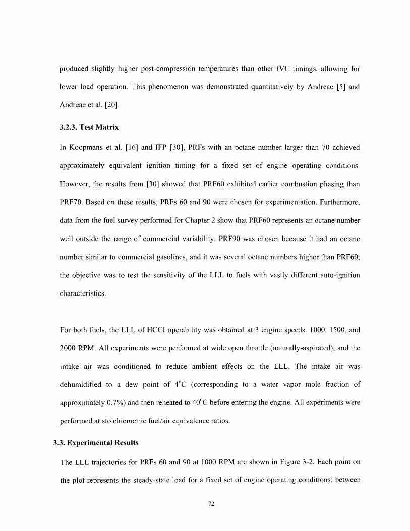
produced slightly higher post-compression temperatures than other IVC timings, allowing for
lower load operation. This phenomenon was demonstrated quantitatively by Andreae [5] and
Andreae et al. [20].
3.2.3. Test Matrix
In Koopmans et al. [16] and IFP [30], PRFs with an octane number larger than 70 achieved
approximately equivalent ignition timing for a fixed set of engine operating conditions.
However, the results from [30] showed that PRF60 exhibited earlier combustion phasing than
PRF70. Based on these results, PRFs 60 and 90 were chosen for experimentation. Furthermore,
data from the fuel survey performed for Chapter 2 show that PRF60 represents an octane number
well outside the range of commercial variability. PRF90 was chosen because it had an octane
number similar to commercial gasolines, and it was several octane numbers higher than PRF60;
the objective was to test the sensitivity of the LLL to fuels with vastly different auto-ignition
characteristics.
For both fuels, the LLL of HCCI operability was obtained at 3 engine speeds: 1000, 1500, and
2000 RPM. All experiments were performed at wide open throttle (naturally-aspirated), and the
intake air was conditioned to reduce ambient effects on the LLL. The intake air was
dehumidified to a dew point of 40C (corresponding to a water vapor mole fraction of
approximately 0.7%) and then reheated to 40'C before entering the engine. All experiments were
performed at stoichiometric fuel/air equivalence ratios.
3.3. Experimental Results
The LLL trajectories for PRFs 60 and 90 at 1000 RPM are shown in Figure 3-2. Each point on
the plot represents the steady-state load for a fixed set of engine operating conditions: between

points OEVc was advanced. The intake cam phasing at the LLL for both fuels was very similar:
On'c for PRF90 was 141 CAD before top center, and Orvc for PRF60 was 144 CAD before top
center. As the exhaust valve timing was advanced, more residual gases were trapped in the
cylinder. This decreased the available cylinder volume for fresh fuel and air, and the reduction in
fueling resulted in a lower engine load. The LLL was reached when the OEvc could not be
advanced without violating one of the previously outlined constraints. At this engine speed, the
LLL of PRF60 was approximately 1.04 bar (-30%) lower than that of PRF90.
4 ------SPRF60
3.8 PRF90
3.6 *
3.4- LLLs
S3.2
U
Z2.8 ,
2.6 +
2.4 02.2
2100 105 110 115 120 125
0EVc [CAD BTC]
Figure 3-2. Experimental LLL trajectories for PRFs 60 and 90 at 1000 RPM
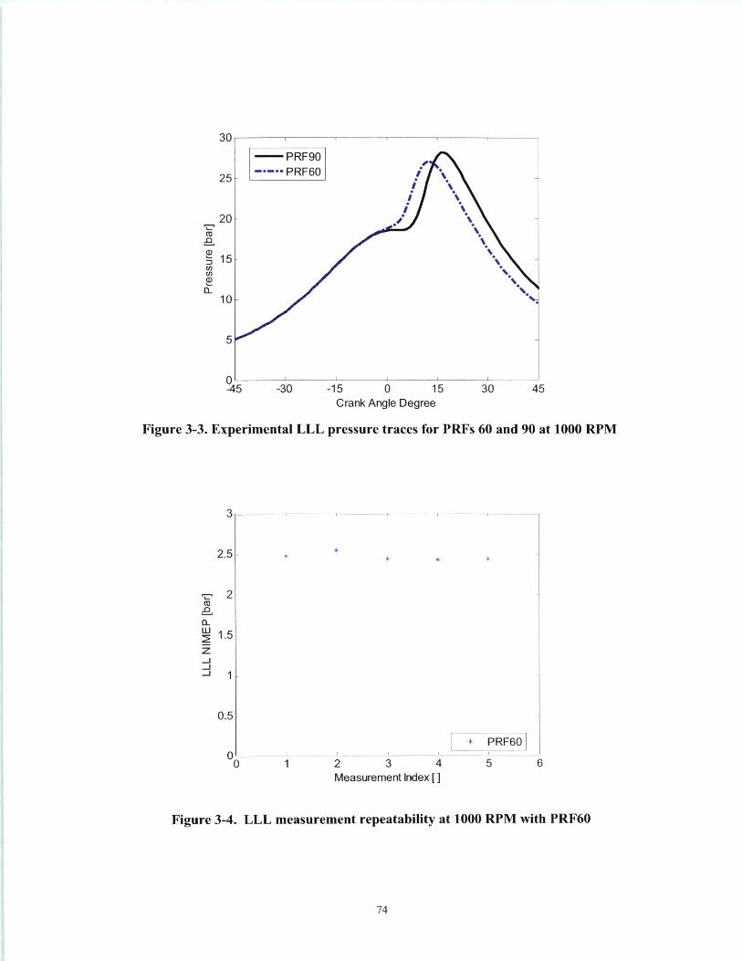
0 1 I I I-45 -30 -15 0 15 30 45
Crank Angle Degree
Figure 3-3. Experimental LLL pressure traces for PRFs 60 and 90 at 1000 RPM
0.51-
l.I .. .. I .. I_
1 2 3 4Measurement Index [ ]
* PRF60
5
Figure 3-4. LLL measurement repeatability at 1000 RPM with PRF60
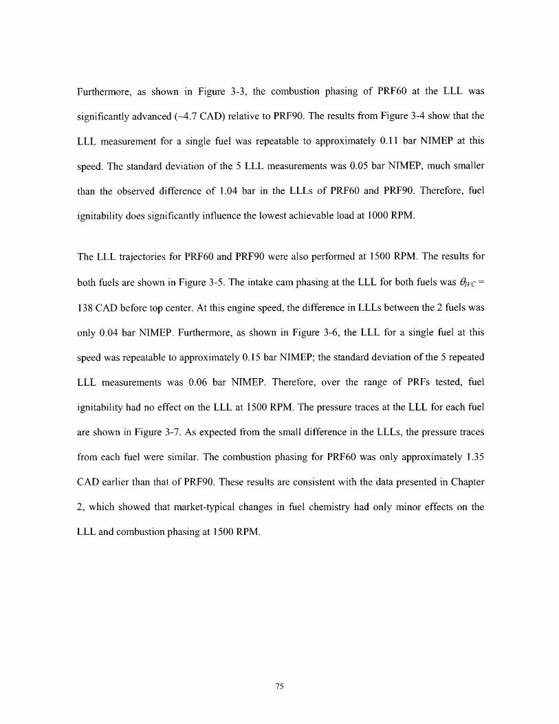
Furthermore, as shown in Figure 3-3, the combustion phasing of PRF60 at the LLL was
significantly advanced (-4.7 CAD) relative to PRF90. The results from Figure 3-4 show that the
LLL measurement for a single fuel was repeatable to approximately 0.11 bar NIMEP at this
speed. The standard deviation of the 5 LLL measurements was 0.05 bar NIMEP, much smaller
than the observed difference of 1.04 bar in the LLLs of PRF60 and PRF90. Therefore, fuel
ignitability does significantly influence the lowest achievable load at 1000 RPM.
The LLL trajectories for PRF60 and PRF90 were also performed at 1500 RPM. The results for
both fuels are shown in Figure 3-5. The intake cam phasing at the LLL for both fuels was vc =
138 CAD before top center. At this engine speed, the difference in LLLs between the 2 fuels was
only 0.04 bar NIMEP. Furthermore, as shown in Figure 3-6, the LLL for a single fuel at this
speed was repeatable to approximately 0.15 bar NIMEP; the standard deviation of the 5 repeated
LLL measurements was 0.06 bar NIMEP. Therefore, over the range of PRFs tested, fuel
ignitability had no effect on the LLL at 1500 RPM. The pressure traces at the LLL for each fuel
are shown in Figure 3-7. As expected from the small difference in the LLLs, the pressure traces
from each fuel were similar. The combustion phasing for PRF60 was only approximately 1.35
CAD earlier than that of PRF90. These results are consistent with the data presented in Chapter
2, which showed that market-typical changes in fuel chemistry had only minor effects on the
LLL and combustion phasing at 1500 RPM.

3.51
2.5
LLLs
1.5 V
111 112
OEVc [CAD BTC]
+* PRF60* PRF90
113 114 115
Figure 3-5. Experimental LLL trajectories for PRFs 60 and 90 at 1500 RPM
0 0
_L ..... .. .. ... I.. . ...... . . .
2 3 4Measurement Index []
Figure 3-6. LLL measurement repeatability at 1500 RPM with PRF90
0.5k
0919 110
2.51* 0
* PRF90
50 1
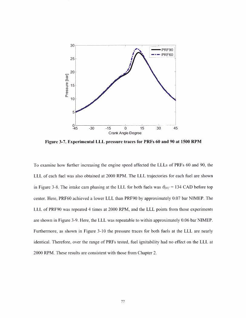
15U_
10
5
-45 -30 -15 0 15 30 45Crank Angle Degree
Figure 3-7. Experimental LLL pressure traces for PRFs 60 and 90 at 1500 RPM
To examine how further increasing the engine speed affected the LLLs of PRFs 60 and 90, the
LLL of each fuel was also obtained at 2000 RPM. The LLL trajectories for each fuel are shown
in Figure 3-8. The intake cam phasing at the LLL for both fuels was Owc = 134 CAD before top
center. Here, PRF60 achieved a lower LLL than PRF90 by approximately 0.07 bar NIMEP. The
LLL of PRF90 was repeated 4 times at 2000 RPM, and the LLL points from those experiments
are shown in Figure 3-9. Here, the LLL was repeatable to within approximately 0.06 bar NIMEP.
Furthermore, as shown in Figure 3-10 the pressure traces for both fuels at the LLL are nearly
identical. Therefore, over the range of PRFs tested, fuel ignitability had no effect on the LLL at
2000 RPM. These results are consistent with those from Chapter 2.

LLLs
2
1.5
w
0.5
09494
* PRF60* PRF90
99 100
Figure 3-8. Experimental LLL trajectories for PRFs 60 and 90 at 2000 RPM
2.5 F
0.5
1 2 3 4Measurement Index []
Figure 3-9. LLL measurement repeatability at 2000 RPM with PRF90
2.51
... . .. ... I . . . . I I.... ... ..
95 96 97 980 EVc [CAD BTC]
101
*PRF9O]
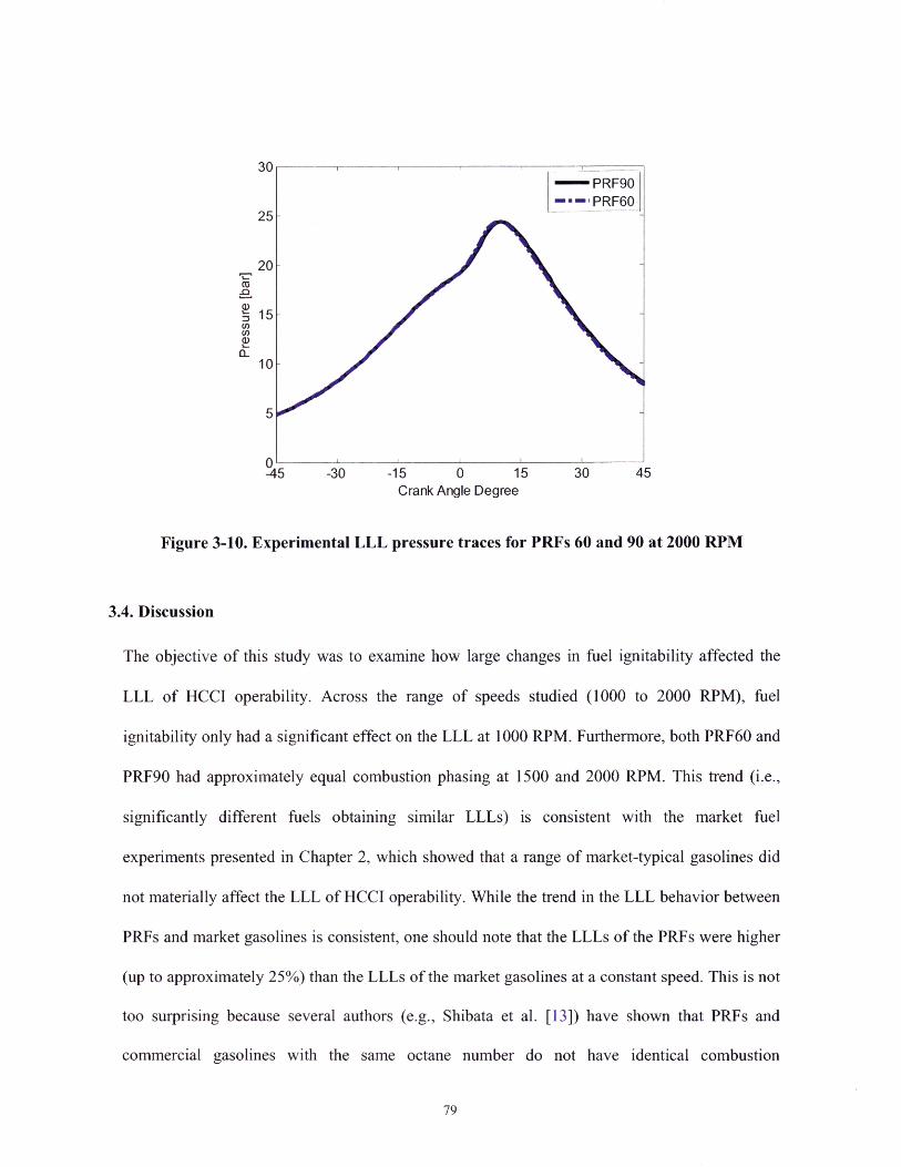
15-Cl
10 -
10
-45 -30 -15 0 15 30 45Crank Angle Degree
Figure 3-10. Experimental LLL pressure traces for PRFs 60 and 90 at 2000 RPM
3.4. Discussion
The objective of this study was to examine how large changes in fuel ignitability affected the
LLL of HCCI operability. Across the range of speeds studied (1000 to 2000 RPM), fuel
ignitability only had a significant effect on the LLL at 1000 RPM. Furthermore, both PRF60 and
PRF90 had approximately equal combustion phasing at 1500 and 2000 RPM. This trend (i.e.,
significantly different fuels obtaining similar LLLs) is consistent with the market fuel
experiments presented in Chapter 2, which showed that a range of market-typical gasolines did
not materially affect the LLL of HCCI operability. While the trend in the LLL behavior between
PRFs and market gasolines is consistent, one should note that the LLLs of the PRFs were higher
(up to approximately 25%) than the LLLs of the market gasolines at a constant speed. This is not
too surprising because several authors (e.g., Shibata et al. [13]) have shown that PRFs and
commercial gasolines with the same octane number do not have identical combustion
characteristics in an HCCI engine. In addition, the results from Chapter 2 showed that the
repeatability of the LLL over an extended period of time (-months) was poor: the variations in
some cases were as large as approximately 28%. Therefore, comparing the absolute values of the
LLLs here with the data from Chapter 2 is difficult. The cause of the large variations with time is
currently unresolved. These large variations in the absolute LLL over extended test periods point
to the importance of testing the PRFs with little downtime between the experiments. All the
LLLs reported here at a constant speed were obtained either on a single day or within a few days.
At 1000 RPM, PRF60 ignited significantly earlier (-4.7 CAD) than PRF90 leading to a much
lower LLL. At first glance, this is quite surprising: a relatively small change in engine speed
caused a large change in fuel sensitivity. A possible explanation for the observed trends in
combustion phasing and the LLLs is that at the higher engine speeds (i.e., 1500 and 2000 RPM),
the in-cylinder gases remain hot due to reduced time for heat transfer. The hotter in-cylinder
conditions would diminish the differences in ignition delays between the fuels; this would
simultaneously result in similar LLL behavior. Prior work by Fieweger, Blumenthal, and
Adomeit [31] showed that the ignition delays, as measured in a shock tube, of PRFs 60, 80, 90,
and 100 all converged at high shock temperatures. The similarities in ignition delays among the
fuels would result in similar LLL behavior.
At lower engine speeds, the available time for heat transfer between the gases and the cylinder
walls increases. Consequently the trapped charge is colder than at higher speeds. These colder
temperatures at 1000 RPM would cause fuel effects to be more apparent. This trend is observed
experimentally: PRFs 60 and 90 ignite with significantly different ignition delays at 1000 RPM,
but at 1500 and 2000 RPM, both fuels have nearly constant combustion phasing. This causes the

LLLs of the fuels to be similar at 1500 and 2000 RPM but significantly different at 1000 RPM.
The results from Chapter 2 also showed that the differences in the LLL among several market-
typical gasolines shrunk as engine speed increased. Unfortunately, the in-cylinder temperature
cannot be directly measured with the current experimental apparatus, so a direct test of this
hypothesis is presently not feasible.
3.5. Conclusions
The impact of fuel ignitability on the LLL of HCCI operability was examined. PRFs 60 and 90
were tested in a naturally-aspirated, single-cylinder HCCI engine, which used NVO to initiate
combustion. The PRFs were selected to span a large range in fuel ignitability. The LLL of each
fuel was obtained at 1000, 1500, and 2000 RPM. The experiments were performed at 0 = 1.0,
and the LLLs were obtained by varying the cam phasing. The following conclusions were
reached:
* At 1500 and 2000 RPM, fuel ignitability had no effect on the LLL or combustion
phasing. PRFs 60 and 90 achieved the equivalent LLLs to within experimental
repeatability. This trend was in agreement with the previous work using market gasolines
(see Chapter 2).
* At 1000 RPM, fuel ignitability had a significant impact on both the LLL and combustion
phasing; PRF60 achieved a lower LLL by approximately 1.0 bar (-30%) NIMEP, and its
combustion phasing was approximately 4.7 CAD earlier than PRF90.
* A possible explanation for the large change in fuel sensitivity at 1000 RPM was
proposed. The sensitivity was likely linked to the in-cylinder temperature. The hotter in-
cylinder temperatures at higher engine speeds would diminish the effects of fuel
chemistry on combustion phasing, which would simultaneously reduce the changes in the
LLL. This hypothesis is consistent with prior trends in the literature but could not be
directly tested due to the inability to measure the in-cylinder temperature with this
experimental apparatus.
The results at 1500 and 2000 RPM reaffirm the conclusions reached in Chapter 2 with the
market fuel experiments: fuel ignitability does not significantly impact the LLL of HCCI
operability. However, the results at 1000 RPM are quite surprising: a small change in engine
speed resulted in a large fuel sensitivity. Potential reasons for this sudden change in fuel
behavior are reexamined in Chapter 5.

4. DETAILED CHEMICAL KINETIC SIMULATIONS OF HCCI ENGINE
TRANSIENTS
Because HCCI combustion is controlled by chemical kinetics, this combustion regime is well
suited for studying via kinetic simulations. Developing accurate models to investigate engine
performance and the effects of various operating parameters (e.g. fuel used, valve timing), etc. is
important to the experimental community. Analyzing all these factors exclusively in the
laboratory would be expensive, inefficient, and impractical because many variables (e.g. in-
cylinder temperature) are either difficult to measure or impossible to isolate due to complex
interactions with other variables. This chapter introduces a fast, full-cycle HCCI simulation tool,
which uses detailed chemical kinetics to model the combustion process. Here, the tool is used to
investigate transient operation in HCCI engines. However, the ultimate purpose of creating this
simulator was to study the phenomenon that causes an HCCI engine to misfire (see Chapter 5).
4.1. Introduction
Despite the advantages of HCCI engines over SI and diesel engines, a number of technical issues
must be resolved before HCCI engines are significantly commercialized. Many of the
complications stem from the lack of a mechanical means to control combustion phasing in an
HCCI engine. Additionally, for negative valve overlap-induced HCCI, there is a strong
dependence of the present cycle on the previous cycle. These factors make controlling HCCI
engines during transient operation among the most prevalent issues that need to be addressed.
Under normal day-to-day usage, an automobile engine experiences numerous transients (e.g.,
during cold-start and acceleration). In an HCCI engine, responding to these transients in a
manner that is transparent to the driver is difficult due to the absence of an inherent strategy to
control the combustion event (e.g., spark timing). Furthermore, the maximum and minimum
torque range of an HCCI engine is small in comparison to an SI or diesel engine of the same
displaced volume. Consequently, the commercial application of HCCI engines may require the
hybridization with other types of engines (e.g., SI or diesel). That is, when the torque output of
the engine is within the operating range of HCCI combustion, then the engine is operated in
HCCI-mode; otherwise, the engine is operated in SI- or diesel-mode. If such a hybridization
scheme is realized, then the transitions between the different combustion modes will introduce
transients that must be controlled smoothly, so that vehicle drivability is not hindered. Hence, the
characterization and understanding of HCCI engine transients is critical for making them
practical.
HCCI engine simulators that model transient operation must be time accurate. In particular, the
modeling tools must predict accurately the thermodynamic state of the cylinder at intake valve
closing (IVC). This state of the system has direct implications on combustion phasing and
duration [32]. In a full-cycle simulation tool, the conditions at IVC for each cycle are obtained
automatically from the converged solution of the previous engine cycle. To model the detailed
chemical kinetics that govern the oxidation of automotive fuels, a full-cycle simulation tool must
be computationally efficient so that it can be used with modest computing resources.

Most research on HCCI engines, both experimental and simulation-based, is focused on steady-
state operation. Largely, this is a result of the difficulty in controlling transient operation in the
HCCI combustion regime. Experimentally, Santoso, Matthews, and Cheng [6] demonstrated the
ability to control mode switching between SI and HCCI (and vice versa) in a single-cylinder
gasoline HCCI engine by using an electromagnetic variable valve timing system. In subsequent
work [33], the authors developed a load-following controller that managed the load subject to
changes in engine speed and intake air temperature. Additional experimental work has examined
various aspects of HCCI engine operation during transients (e.g., [7,8,34]).
Ohyama [35] developed a simplistic model of a gasoline HCCI engine that contained three sub-
models: intake, combustion, and gas exchange. The combustion process was represented using a
Livengood-Wu integral, which gave information on the temperature of the burned gas and on
characteristics of the auto-ignition process. Using this model, Ohyama investigated control
strategies for transient operation of HCCI engines. Xie et al. [36] developed an engine simulator
for investigating the ability of a 4-variable valve actuating system to control HCCI (or CAI -
controlled auto-ignition) operation and to control combustion mode switching between SI and
CAI. Their model linked a commercial cycle simulation package (GT-Power) with a user-
defined, external model for heat release. The external model, however, did not use a detailed
chemical kinetics mechanism for combustion, and the authors developed their own model for
heat release. Chang et al. [37] also used GT-Power with an external, user-defined model for
combustion. They investigated the effects of the cylinder wall temperature and the residual
temperature on gasoline HCCI combustion. They also performed simulations to examine the
impact of speed and load transients on the HCCI operating range. This model, however, did not

use detailed chemistry to model the chemical kinetics of the combustion process. Agrell et al.
[38- 41] developed a transient simulation tool to study a variety of strategies to control
combustion phasing; they used a Vibe correlation to simulate the heat release. Xu et al. [42,43]
used CHEMKIN [44,45] to solve a detailed combustion model, which was "linked" with a full-
cycle engine simulation package (i.e., GESIM [42] or WAVE [43]). However, the linkage
between the programs was not automated and the results of the engine simulation package had to
be iteratively compared with those of CHEMKIN until the two programs predicted the same
ignition timing. Narayanaswamy and Rutland [46] built an automated, transient simulation tool
for a diesel HCCI engine that combined a full-cycle simulation package (GT-Power) with a
multi-zone chemistry model, which used a skeletal mechanism for n-heptane. They used their
model to examine the impact of injection timing, exhaust gas recirculation (EGR), intake gas
temperature, and IVC timing on combustion phasing. They also used their model to test control
strategies for handling speed and load transients. The model was further refined in subsequent
works [47,48] to use computational fluid dynamics (CFD) to model the mixing and combustion
processes in the cylinder. The new model was used to examine similar conditions as in [46], and
the results with the CFD showed closer agreement with experimental results. Such detailed
simulations are expensive even with skeletal chemical mechanisms; faster computational
methods capable of handling more accurate chemistry models would be quite helpful for
understanding how fuel variations affect HCCI engine transients.
Other research groups have used different methods to simulate HCCI engines, almost always
focusing on engines running steady-state. Bhave et al. [49] used a probability density function
based stochastic reactor model coupled with GT-Power to investigate the effect of octane
number on combustion, emissions, and engine performance. Good agreement was observed
between the predicted and measured values for in-cylinder pressure, auto-ignition timing, and
CO, HC, and NOx emissions. In Erlandsson et al. [50], the performance and efficiency of an
HCCI engine running on natural and landfill gases was examined. For these studies, a zero-
dimensional model of the engine, turbo, inlet and exhaust manifolds, and inlet air conditioner
was used to study the effect of compression ratio and exhaust turbine size on the maximum mean
effective pressure and efficiency. Aceves et al. [51] modeled HCCI engines by developing an
artificial neural network-based code that was integrated into a fluid mechanics code, KIVA3V
[520]. The code provided reasonable predictions for HCCI combustion and emissions at a
reduced computational cost.
This work introduces a fast full-cycle HCCI engine simulator (MITES: MIT Engine Simulator)
for gasoline engines that is fully automated, uses detailed chemical kinetic mechanisms, and is
capable of modeling engine transients. MITES is a modeling tool that combines the Ricardo
WAVE software package with a 2-zone model to represent the cylinder of an engine. When
modeling a primary reference fuel (PRF) mechanism containing over 1000 species and 4000
reactions, MITES required only 7 - 8 minutes per cycle on a desktop PC. We use MITES to
simulate transients in fueling, speed, and valve timing of a single-cylinder HCCI engine. The
model predictions are compared with experimental data obtained from a single-cylinder HCCI
engine.
4.2. Experimental Configuration
The experiments were performed using a modified, port fuel injected 2.3L in-line 4 cylinder, 16
valve, production-built, Mazda spark-ignition engine. Engine specifications are listed in Table
4-1. The modifications to the engine included: increasing the compression ratio from 9.7 to 11.1,
adding cam phasing to the exhaust valve train (continuously variable intake cam phasing is a
standard feature on the production engine), and using cams that decreased the duration and lift of
the valve events to allow for HCCI operation. In addition to the engine modifications described
above, alterations were made to both the intake and exhaust manifolds. For the intake, a custom
manifold was used so that air pressure and temperature could be measured 5 cm from the intake
port; furthermore, a chiller/condenser and an electric heater were added to the intake system to
control the humidity and temperature of the intake air. To reduce the experimental complexity,
while retaining the essential physics, tests were performed using one firing cylinder; the
remaining three cylinders were motored. Because a lambda sensor was used to monitor the
exhaust air/fuel ratio, a custom exhaust manifold was required for the firing cylinder. The
manifold was designed to keep the air from the three motored cylinders separate from the
exhaust exiting the firing cylinder so that an accurate measure of the air/fuel ratio was obtained.
The following properties were controlled during operation of the engine: intake air temperature
and humidity, engine coolant temperature, fuel injection duration, spark timing (when used for
starting), and cam phasing. All experiments were performed with the engine in a warmed-up
state. This was accomplished by adding a heater to the coolant loop of the engine. The heater
warms the coolant to 900C, and a proportional-integral controller keeps the coolant to within
+2'C. The fuel injection pulse width, spark timing, and intake and exhaust cam phasing were all
controlled with a desktop computer and changed in real time as desired. The cam phasing was
continuously variable within a range of 35 crank angle degrees (CAD). If a desired cam position
was outside of the 35 CAD range, the default position of the cam was reset manually to allow the
desired position to be reached. The control strategy was accurate to within ±1 CAD, and the
feedback on cam position was available once per cycle; the resolution on cam position
measurement was I CAD.
HCCI combustion is induced by trapping large (relative to SI operation) fractions of residual
gases in the cylinder. This trapping strategy is referred to as negative valve overlap, i.e., the
exhaust valve is closed early during the exhaust stroke. The thermal energy of the exhaust gases
are used to achieve auto-ignition. For this negative valve overlap strategy, cams with 120 CAD
durations were selected for both the exhaust and intake cams; the 120 CAD cams were designed
to maximize lift. This selection was made based on prior modeling results [53]. With the short
duration of the cams, however, the available lift (without putting undo stress on the lobes of the
cam) was only 2 mm.
Because HCCI combustion is achieved using hot residual gases, the engine was started in SI-
mode. Once the engine was running, the cam position was set to trap sufficient residual gases to
induce auto-ignition. Then, HCCI combustion was achieved by disabling the spark via the
computer controller.
4.3. HCCI Engine Simulator
4.3.1. WAVE Model
The numerical simulations were performed by combining the Ricardo WAVE engine simulator
with a 2-zone model of the engine cylinder. WAVE uses a one-dimensional fluid mechanics
description of the flow of fuel and air through the fuel injection system and the ducts that
connect to the cylinder. The configuration and dimensions of the intake and exhaust systems in
the WAVE model were derived from the actual dimensions of the experimental engine described
above. The experimental intake system is complex and consists of a chiller, an air heater, an air
filter, and duct work. The impact of these components on the intake system was modeled in
WAVE by using a boundary condition block for which pressure and temperature time profiles
were user-specified. The profiles used were the air pressure from the experimental intake
manifold and the set-point temperature of the air heater. There were, however, some
characteristics of the engine that were not represented in the WAVE model e.g., corrugation of
the exhaust pipes. Nevertheless, the essential features of the gas exchange process were captured
by the model.
4.3.2. Cylinder Model
To model accurately the CAI process, it is essential to use a detailed chemical kinetics model.
The built-in cylinder models included with WAVE use a Wiebe function to model the
combustion event: detailed kinetics models are not used. Therefore, an external, user-defined
model of the cylinder was used to model the CAI process; Ricardo WAVE was used to model
the intake/exhaust system.

The cylinder model used for this work was a 2-zone model that divides the cylinder into two
regions: a boundary layer zone and a core zone. Here, the "boundary layer" zone was not a
boundary layer in the strictest sense. Rather, it represented the mass in the colder volumes of the
cylinder (i.e., the true boundary layer and crevice volumes). The boundary layer zone contained
a user-specified fraction, Xbouiday, of the mass in the cylinder. In the present work xbo,,nda,, = 0.05:
the boundary layer zone contained 5% of the total mass. Setting xbounc,,J, = 0.05 was consistent
with prior work in the literature [54], in which the authors assigned 5% of the total cylinder mass
to the coldest 5 zones to account for boundary layer and crevice volume effects. The 5% mass
distribution in the boundary layer was maintained throughout the cycle, as in [54]. In practice,
the boundary layer and crevice volumes remain at relatively low temperatures due to heat loss to
the walls. As a result, it was assumed that no chemical reactions occurred in the boundary layer
zone. This assumption is consistent with the results in [55]. The core zone containes the
remaining mass in the cylinder and is the zone in which the combustion event (i.e., chemical
reactions) occurs. Both zones were modeled as perfectly mixed; however, the perfectly mixed
assumption for the boundary layer zone is superfluous, since no reactions occur there. The
pressure throughout the cylinder was taken to be spatially uniform.
The input variables to the 2-zone model were { Tc , Yc , m, Vc } at IVC. Here, Tc is the
temperature in the core, Yc = IYI,c ,Y2,c ,...,Y,,c} is the vector of mass fractions for the n,
chemical species in the core, m is the total mass of the mixture in the cylinder (boundary layer
and core zones), and Vc is the volume of the core. The temperature of the boundary layer (TB)
was assumed to be the average of the core temperature and the area-averaged (i.e., piston,
cylinder head, and cylinder liner) cylinder wall temperature (Tw)

T= - (4-1)
The piston, cylinder head, and cylinder liner temperatures were assumed to be constant
throughout the simulations.
The 2-zone model describes the time evolution of the combustion process by the following
system of differential-algebraic equations (DAEs):
-- = V 1 (4-2)dt
dVdT- P -V' c uZ iu4 +q
Sdt (4-3)dt (I - x,,oundarY )m Cv,c + 0.5,,oundarYin cv,
R((m T,/W)+(mc-/1Wc)P = (4-4)
Vv[
Here, vc is the specific volume of the core, 4. is the net molar production rate of species i, W is
the molecular weight of species i, P is the pressure in the cylinder, V(q is the volume of the
cylinder, ui is the specific internal energy of species i, q is the rate of heat loss to the walls of the
cylinder, c, is the specific heat at constant volume (zone denoted by subscript), R is the universal
gas constant, mc is the core mass, min is the boundary layer mass, and W = I1 , ./1 is the
effective molar mass (zone denoted by subscript). SI units were used for all quantities. The
volume of the core was computed using the ideal gas law: Vc. = mcTR/(WcP). V,, was
computed using the slider-crank relationship [56], and the rate of heat transfer (c") model are
described below. The thermodynamic quantities and molar production rates were computed
using OpenChem Pro [57]. Note that, due to the assumption of spatial homogeneity in the
cylinder, the system of equations did not contain spatial variations. Also, the ideal gas equation
of state (used to compute the pressure) was incorporated as an algebraic constraint to make the
Jacobian sparse [58].
Equation (4-3) was obtained via summation of the core and boundary layer zone energy balance
equations. Equation (4-2) was then differentiated to obtain dTl/dt, which was then substituted
into the sum of the energy balances. Solving the summation for dTc/dt resulted in Equation
(4-4).
The 2-zone model was used to compute the state of the mixture in the cylinder from IVC to
exhaust valve opening (EVO) and during the re-compression event (i.e., exhaust valve closing
(EVC) to intake valve opening (IVO)). It should be noted that building an accurate, full-cycle
simulator for an HCCI engine was difficult due to the feedback nature of the residual-induced
ignition process. The difficulty arose from the requirement for proper initial conditions for each
cycle. In MITES, the conditions at IVC were predicted by WAVE as a result of solving the one-
dimensional transport equations that model the intake system (e.g., flow across the valves, heat
transfer in the ports). This information was then passed to the 2-zone model and used as the
initial condition.
An additional difficulty arose while coupling the user-defined cylinder model with the Ricardo
WAVE software: the PRF mechanism has over 1000 chemical species, and WAVE tracks only 5
"species." WAVE's species are air, vapor fuel, burned air, burned fuel, and liquid fuel. The user-
defined model exchanges information with WAVE at every time step. However, during the
closed portions of the cycle (i.e., IVC to EVO and EVC to IVO), all thermal and physical
properties were calculated from the chemical species in the PRF mechanism. During the gas
exchange processes (i.e., EVO to EVC and IVO to IVC), WAVE calculated the state of the
cylinder from its pseudo-species. During the combustion and recompression processes, the
chemical species in the PRF mechanism were converted to the WAVE species. During the gas
exchange processes, the detailed species concentrations were assumed to be frozen and thus
remain constant. Reactions can occur during the recompression process, however. At IVC, the
WAVE-calculated residual mass fraction was set to have the concentration of the frozen detailed
species from IVO. The residual mass was then mixed with a fresh charge. The mass and
composition of the fresh charge were determined by WAVE. The fresh mass contains only air
(i.e., N2 and 02) and fuel (i.e., iso-octane and n-heptane) and was thus easily converted to the
PRF species.
Equations (4-2) to (4-4) were solved using the JACOBIAN software package [57], which
contains a specialized numerical solver, DSL48S, for sparse systems of DAEs [59]. To
accelerate the computations, analytical expressions for the Jacobians were computed a priori
using automatic differentiation [60]. Prior work by Yelvington et al. [61] demonstrated that use
of DSL48S and the analytical Jacobians can increase computational speed by more than an order
of magnitude relative to other ODE solvers (e.g., DASSL, VODE).
4.3.3. Heat Transfer Model
Due to the sensitivity of the auto-ignition process in HCCI engines, it was necessary to model
accurately the heat transfer processes between the cylinder walls and the mixture inside the
cylinder. Despite its widespread use in HCCI engine simulations, the Woschni and reduced
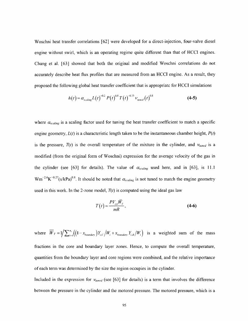
Woschni heat transfer correlations [62] were developed for a direct-injection, four-valve diesel
engine without swirl, which is an operating regime quite different than that of HCCI engines.
Chang et al. [63] showed that both the original and modified Woschni correlations do not
accurately describe heat flux profiles that are measured from an HCCI engine. As a result, they
proposed the following global heat transfer coefficient that is appropriate for HCCI simulations
h(t) = ca,,iL (t)-' P(t)os T(t)-0.73 v,,d (t)08 (4-5)
where a,,,in,,g is a scaling factor used for tuning the heat transfer coefficient to match a specific
engine geometry, L(t) is a characteristic length taken to be the instantaneous chamber height, P(t)
is the pressure, T(t) is the overall temperature of the mixture in the cylinder, and Viuned is a
modified (from the original form of Woschni) expression for the average velocity of the gas in
the cylinder (see [63] for details). The value of a,,,caig used here, and in [63], is 11.1
Wm-2.6K-0.27(s/kPa) 8. It should be noted that Aca,,, is not tuned to match the engine geometry
used in this work. In the 2-zone model, T(t) is computed using the ideal gas law
PV ,W,T(t) P ? T (4-6)
mR
where Wr = /Z;i1((1- xhou ,o),~ / +xbou,,B,,r~, is a weighted sum of the mass
fractions in the core and boundary layer zones. Hence, to compute the overall temperature,
quantities from the boundary layer and core regions were combined, and the relative importance
of each term was determined by the size the region occupies in the cylinder.
Included in the expression for Viuned (see [63] for details) is a term that involves the difference
between the pressure in the cylinder and the motored pressure. The motored pressure, which is a

function of CAD (and, therefore, time), may be measured experimentally or computed using
WAVE; the present work used motored pressures that ere computed using WAVE. Regardless of
how it is determined, values of the motored pressure are obtained at discrete crank angles. When
running a simulation in MITES, it is likely that a value of the motored pressure will be required
at a crank angle for which there is no data. In this case, linear interpolation between known
pressures is used to compute the pressure at the required crank angle.
Using Equation (4-4) for the heat transfer coefficient, the heat transfer model used in Equation
(4-2) is
= h(t)A(r, -T)+ A,, -T)+ A, (T- ))(4-7)
where A,, Ah, Ap are the areas of the cylinder liner, cylinder head, and piston, respectively:
similar subscript notation is used for the temperatures. Estimates for the piston, cylinder head,
and cylinder liner temperatures were obtained from the engine manufacturer.
4.4. Results
Experimental and numerical studies were performed using the engine parameters listed in Table
4-1. The fuel is a blend of 90 volume-percent iso-octane and 10 volume-percent n-heptane
(PRF90). The combustion chemistry was modeled using the iso-octane/n-heptane chemical
kinetics mechanism from Lawrence Livermore National Laboratory (LLNL) [64]. This full
mechanism contains 1036 species undergoing 4238 elementary reactions. No emissions data are
presented because the mechanism does not contain nitrogen chemistry, and single-zone HCCI
models give poor estimates of hydrocarbon and CO emission [54,65]. Due to the broad range of

timescales involved, this chemistry model leads to large systems of stiff differential equations. In
section 4.4.1, experimental and numerical results are compared and steady-state operation of
MITES is demonstrated. Sections 4.4.2, 4.4.3, and 4.4.4 examine the impact of fueling, speed,
and valve timing transients on the performance of the engine, respectively. Finally, section 4.4.5
discusses the computational performance of MITES and comments on the role that MITES can
play in the design of HCCI engines.
Table 4-1. Parameters of the single-cylinder engine.Abbreviations: crank angle degree (CAD), revolutions per minute (RPM), primary reference fiel (PRF)
Compression Ratio 11.1
Bore (mm) 87.5
Stroke (mm) 94.0
Cam Duration (o crank angle) 120
Maximum Valve Lift (mm) 2.0
Speed (RPM) 1250 -1500
Inlet Charge Temperature (oC) 40.0
Fuel PRF 90
Equivalence Ratio (4)) 1.0
4.4.1. Simulating Steady-state Operation
To evaluate quantitatively the predictive capability of MITES without any calibration to
experimental data, a simulation and experiment with identical operating conditions (e.g., 0, valve
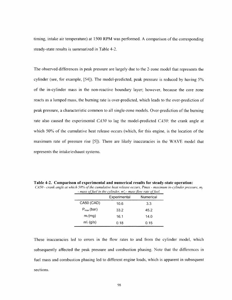
timing, intake air temperature) at 1500 RPM was performed. A comparison of the corresponding
steady-state results is summarized in Table 4-2.
The observed differences in peak pressure are largely due to the 2-zone model that represents the
cylinder (see, for example, [54]). The model-predicted, peak pressure is reduced by having 5%
of the in-cylinder mass in the non-reactive boundary layer; however, because the core zone
reacts as a lumped mass, the burning rate is over-predicted, which leads to the over-prediction of
peak pressure, a characteristic common to all single-zone models. Over-prediction of the burning
rate also caused the experimental CA50 to lag the model-predicted CA50: the crank angle at
which 50% of the cumulative heat release occurs (which, for this engine, is the location of the
maximum rate of pressure rise [5]). There are likely inaccuracies in the WAVE model that
represents the intake/exhaust systems.
Table 4-2. Comparison of experimental and numerical results for steady-state operation:CA50 - crank angle at which 50% of the cumulative heat release occurs, Pmax - maximum in-cylinder pressure, mi
- mass o fuel in the cylinder, m'f - mass flow rate of fel.
Experimental Numerical
CA50 (CAD) 10.6 3.3
Pmax (bar) 33.2 45.2
mf (mg) 16.1 14.0
m'f (g/s) 0.18 0.15
These inaccuracies led to errors in the flow rates to and from the cylinder model, which
subsequently affected the peak pressure and combustion phasing. Note that the differences in
fuel mass and combustion phasing led to different engine loads, which is apparent in subsequent
sections.

The steady-state simulation results presented here and the simulation results in all subsequent
sections were obtained without any calibration to experimental data. This is in contrast to
common practices in the literature. However, the motivation for this work was not to fit
experimental data; this can be accomplished with a much simpler model. Rather, MITES is
designed for the purpose of predicting future experiments in new engines, possibly with new
fuels, and in such cases, experimental data would not be available. Without calibration, MITES
did not currently capture the experimental combustion phasing (shown in Table 4-2). Such errors
are expected because even calibrated models can have errors as large as I to 3 CAD in
combustion phasing, and such errors are considered very acceptable [66]. However, as shown in
subsequent sections, even without calibration, MITES predicts experimental trends (e.g.,
transient time constants) fairly accurately.
The full-cycle simulation capability of MITES is demonstrated in Figure 4-1a. Here,
experimental and numerical pressure profiles for three steady-state cycles are shown. Further, to
demonstrate that MITES captured the cycle-to-cycle dynamics en route to steady-state, pressure
profiles for 4 cycles before and 3 cycles after steady-state are shown in Figure lb. From cycles
58 - 60 in Figure lb, we observe that MITES has reached steady-state and has little cycle-to-
cycle variation.
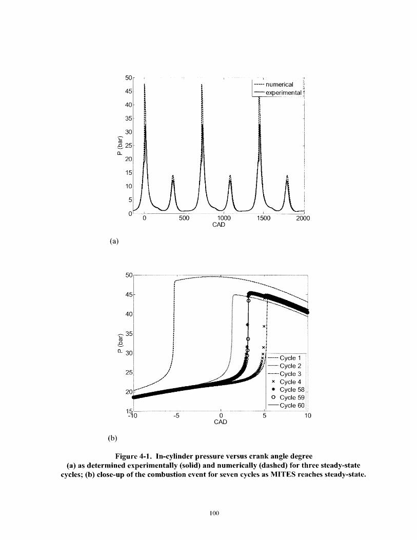
----- numerical
-0 250L
20
15
10
5
00 500 1000 1500 2000
CAD
(a)
50
45
40i
x!
S35
- 30
30-x ----- Cycle 1S/ --.......... Cycle 2
25 ------- Cycle 3x Cycle 4
20- * Cycle 580 Cycle 59
-Cycle 6015--
-5 0 5 10CAD
(b)
Figure 4-1. In-cylinder pressure versus crank angle degree(a) as determined experimentally (solid) and numerically (dashed) for three steady-state
cycles; (b) close-up of the combustion event for seven cycles as MITES reaches steady-state.
100
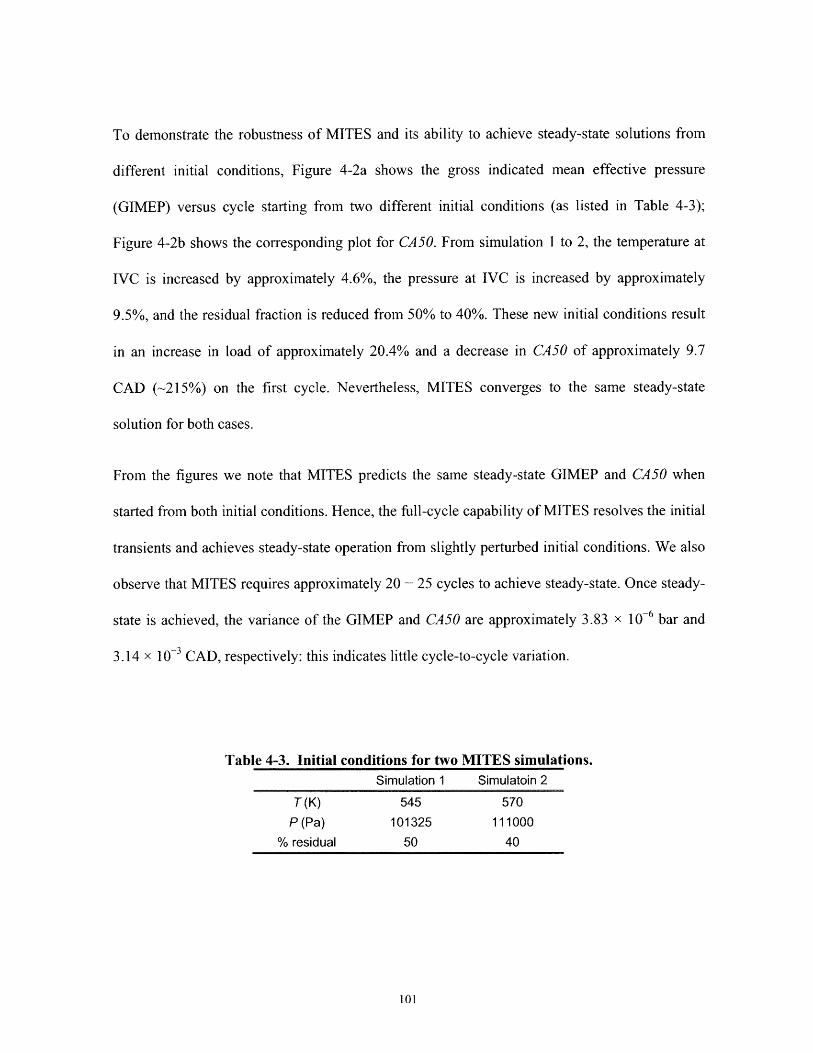
To demonstrate the robustness of MITES and its ability to achieve steady-state solutions from
different initial conditions, Figure 4-2a shows the gross indicated mean effective pressure
(GIMEP) versus cycle starting from two different initial conditions (as listed in Table 4-3);
Figure 4-2b shows the corresponding plot for CA50. From simulation 1 to 2, the temperature at
IVC is increased by approximately 4.6%, the pressure at IVC is increased by approximately
9.5%, and the residual fraction is reduced from 50% to 40%. These new initial conditions result
in an increase in load of approximately 20.4% and a decrease in CA50 of approximately 9.7
CAD (-215%) on the first cycle. Nevertheless, MITES converges to the same steady-state
solution for both cases.
From the figures we note that MITES predicts the same steady-state GIMEP and CA50 when
started from both initial conditions. Hence, the full-cycle capability of MITES resolves the initial
transients and achieves steady-state operation from slightly perturbed initial conditions. We also
observe that MITES requires approximately 20 - 25 cycles to achieve steady-state. Once steady-
state is achieved, the variance of the GIMEP and CA50 are approximately 3.83 x 10- 6 bar and
3.14 x 10- CAD, respectively: this indicates little cycle-to-cycle variation.
Table 4-3. Initial conditions for two MITES simulations.Simulation 1 Simulatoin 2
T (K) 545 570P (Pa) 101325 111000
% residual 50 40
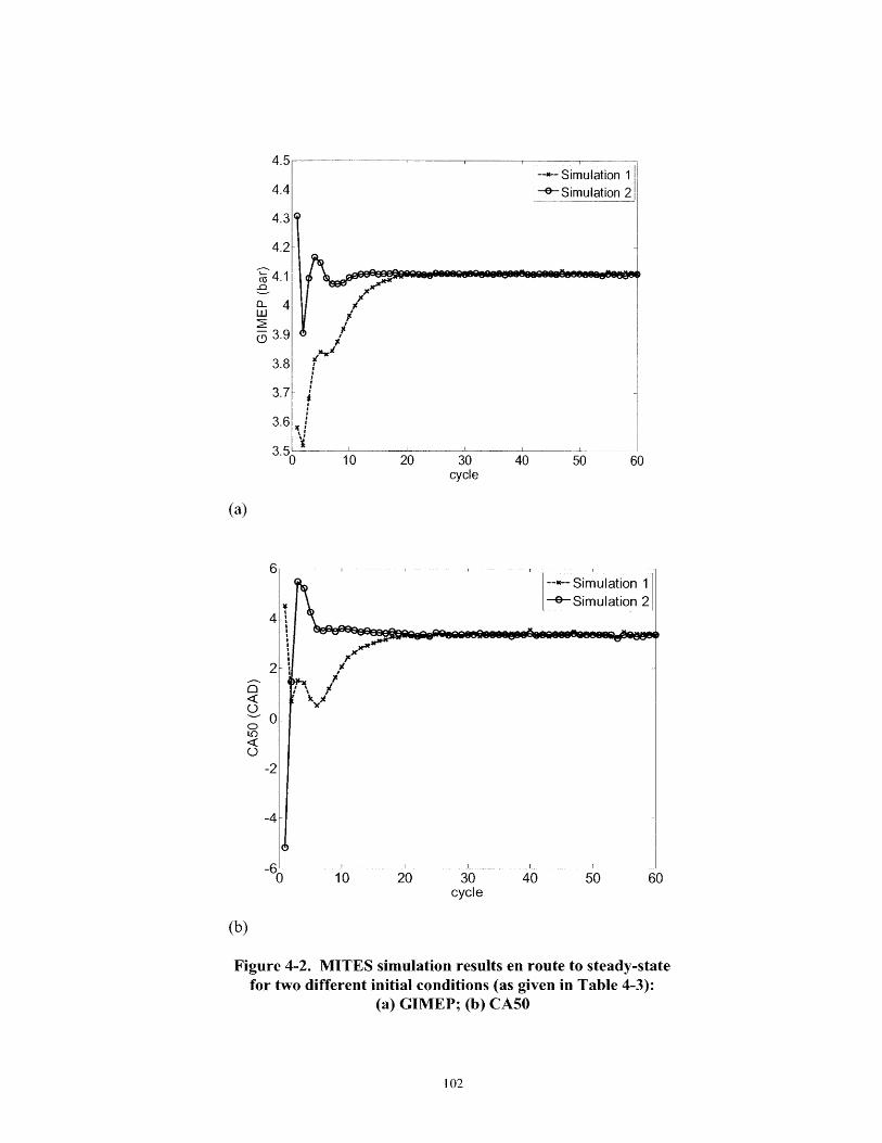
10 20 30cycle
40 50 60
(a)
--- Simulation 1-e-Simulation 2
w@860989OW16 1 ! 1 1
) 10 20 30 4(cycle
50 60
(b)
Figure 4-2. MITES simulation results en route to steady-statefor two different initial conditions (as given in Table 4-3):
(a) GIMEP; (b) CA50
102
I I I
4.4.2. Fueling Transients
To examine numerically the impact of fueling transients on performance, MITES was first run to
steady-state at an equivalence ratio (0) of 0.9 (fuel lean). The equivalence ratio is defined as the
actual fuel/air ratio divided by the stoichiometric fuel/air ratio [67]. The number of cycles
required to reach steady-state operation is dependent on the user-specified initial conditions;
however, the final steady-state is independent of the initial conditions. After a steady-state 0 =
0.9 simulation was achieved, the mass of fuel that was injected into the intake duct was increased
so that 0 = 1 (stoichiometric). This rapid increase in 0 induces a transient. In the present
configuration, the speed remains constant at 1500 revolutions per minute (RPM) throughout the
duration of the simulation.
In the experimental configuration, the engine was first run to steady-state by adjusting the fuel
injection pulse width until the lambda sensor read approximately 1.1 (i.e., = 0.9). Fueling
transients were then introduced by increasing the fuel injection pulse width so that the lambda
sensor read approximately I (i.e., 0 = 1); all other engine parameters (e.g., valve timing, speed)
were held constant.
The numerical and experimental impact of these changes in fueling on the gross indicated mean
effective pressure is shown in Figure 4-3a. Only the data near the transient are shown. The
oscillations present in the experimental data in Figure 3a (and subsequent figures) are typical
cycle-to-cycle fluctuations that occur in internal combustion engines. These fluctuations result
from (among others) variations in the mixing of the fresh charge with residual gases and
variations in the masses of fresh charge and residual [68]. These processes affect combustion
stability.
In this work, combustion was defined to be stable if the coefficient of variation (COV: the
standard deviation of the load normalized by the average load [68]) of the net indicated mean
effective pressure (NIMEP) was less than 3.5%. This limit is below the practical limit of
approximately 10%; larger COVs lead to problems in drivability [68]. The COV of the
experimental data in Figure 4-3a before the transient is approximately 1.75% and is
approximately 1.24% after the transient.
From the figure, it is clear that increasing 0 increases the GIMEP. This response is expected
because an increase in the mass of fuel undergoing combustion (resulting from an increase in 0)
results in the production of more work. In addition, there is qualitative agreement between the
experimental and modeling results and, as discussed below, the response times of the engine to
fueling transients are in good agreement.
The data in Figure 4-3b represent the numerical change in the fueling rate and combustion
phasing as a result of increasing 0. MITES predicts a reduction in CA50 of approximately 1.7
CAD as a result of the fuel transient. Experimentally, the CA50 decreases by approximately 0.7
CAD after the transient (data not shown). However, the measurement error of the experimental
CA50 is + 1 CAD, and the standard deviation of the experimental CA50 both before and after the
transient is approximately 1.9 CAD. Therefore, the model-predicted change in combustion
phasing is within the experimental uncertainty.
104
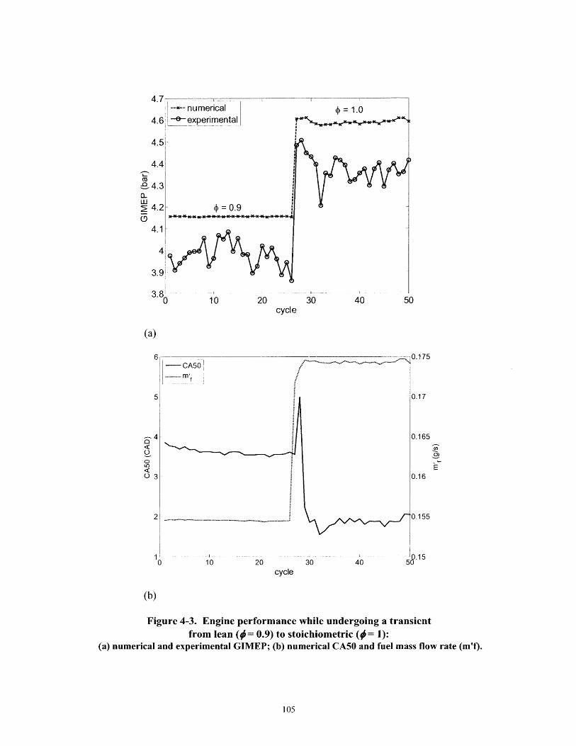
--"- numerical-e- experimental
4 = 1.0
4 = 0.9
10 20 30 40cycle
CA50.......... m f
20 30 40 0.15
cycle
(b)
Figure 4-3. Engine performance while undergoing a transient
from lean (0= 0.9) to stoichiometric (0= 1):(a) numerical and experimental GIMEP; (b) numerical CA50 and fuel mass flow rate (m't).
_ 4.3
2 4.2-0j5
3.8'0
O
03
0.17
0.165
0.16
.. ..... ... ... ... .. ..... .... ... .... .... ... ... .

During the fuel transient, all other operating conditions were fixed. Consequently, increasing the
equivalence ratio increases the mass flow rate of fuel. In the simulations, the mass flow rate of
fuel changes substantially one cycle prior to a change in the CA50. The lag of the CA50 relative
to the fueling rate is due to the definition of the starting point of each simulated cycle in MITES;
new cycles begin at IVC. Consequently, when a change in fueling rate is commanded during
cycle N, the simulation must first progress through cycle N (with the old fueling rate) to the next
intake process (that of cycle N+I) before the effects of the new fueling rate affect the trapped
charge. As a result, the change in fueling rate observed in cycle N affects the conditions at IVC
of cycle N+1. This causes the one-cycle lag in the CA50 relative to the fueling rate change. As
the fueling rate increases, the CA50 initially increases (i.e., combustion is later). As more fuel is
injected into the intake port, a larger amount of energy is required to vaporize the fuel. The heat
required to vaporize the fuel is taken from the intake charge, thus cooling it by approximately
4K. The colder charge results in later combustion phasing. When combustion phasing is later,
less energy is removed from the gases as work, which results in hotter trapped residuals. These
gases raise the temperature at IVC on the subsequent cycle (by = 10K) resulting in earlier
combustion phasing (i.e., smaller CA50). A steady-state is reached once a balance is achieved
between combustion phasing and the cooling effect of vaporizing more fuel.
The mean of the GIMEP when 0 = 0.9 for the experimentally obtained data is GIMEP = 3.98
bar; the corresponding mean for the simulation data is GIMEP = 4.16 bar. When the
equivalence ratio is increased to b = 1, the mean of the experimentally obtained load is GIMEP
- 4.34 bar; the corresponding mean for the simulation is GIMEP = 4.59 bar. Therefore, the

difference between the numerical and experimental values of the GIMEP is less than 6% for both
lean and stoichiometric operation: this is excellent agreement especially in light of the 2-zone
combustion model that is used. Furthermore, when b is increased by 10%, both the experimental
and numerical results indicate an increase in the GIMEP of approximately 9%.
In the context of real engine operation, the time required for the engine to respond to a change in
the equivalence ratio is important. This delay time may, for example, be used as part of an
engine control strategy, which determines the mode in which a hybrid HCCI engine is operated.
The experimental data shown in Figure 4-3a indicate that the GIMEP of the engine responds to
the fueling transient in one engine cycle: the transition from GIMEP = 3.98 bar when = 0.9 to
GIMEP = 4.34 bar when i = 1 takes place with no intermediate data points. This fast transient
overshoots the true = 1 steady-state. After approximately four more cycles, the engine
stabilizes at its new steady-state value of GIMEP. The results from the simulation are similar: the
GIMEP jumps up in one cycle, overshoots the steady-state value, and then settles to the new
steady-state value in approximately four more cycles. In both cases, approximately 5 - 6
complete cycles are required before steady-state operation is resumed.
Note from Figure 4-3a that the steady-state GIMEPs predicted by the model for both = 0.9 and
0 = 1.0 are greater than the corresponding experimental results. The bulk of these differences is
likely due to the use of a 2-zone model which, as discussed in section 4.4.1, over-predicts the
burning rate. Consequently, the peak pressure in the cylinder is greater than the experimental
107
value, which leads to a larger value of GIMEP (for the lean and stoichiometric conditions). In
addition, the differences in combustion phasing also contribute to the different values of GIMEP.
4.4.3. Speed Transients
During experimentation, the engine was first run to steady-state at 1500 RPM with = 1; the
engine speed was controlled using a dynamometer and an electric motor. A transient in speed
was initiated by making a step-change in the set-point of the dynamometer from 1500 to 1250
RPM. The new steady-state speed was not achieved instantaneously due to the finite time
required to slow the engine. The decrease in speed resulted in an increase in the volumetric
efficiency thereby causing an increase in the mass of trapped air at IVC. Consequently, unless
the fueling rate is increased, 0 will decrease. To combat these effects experimentally, a step-
change was also made to the fueling rate (manually) to ensure stoichiometric operation during
and after the speed transient; all other engine parameters were held constant.
The effects of a transient in engine speed were also investigated numerically. Using MITES, a
simulation was run to steady-state at 1500 RPM with A = 1.0. As done experimentally, a step-
change in RPM from 1500 to 1250 was made; however, the experimental lag-time required to
slow the engine was not accounted for numerically. In WAVE, a constant fuel/air ratio was
specified. Therefore, WAVE automatically determined the quantity of fuel to inject based on the
mass flow rate of air; thus, stoichiometric operation was maintained throughout the simulations.
The experimental and numerical results showing the change in GIMEP as the engine undergoes
the speed transient are shown in Figure 4-4. For clarity, only the data near the transient are
shown.

5.2
5
4.8
0~4.6
w2 4.4
4.2
4
3.80
--- numerical 1250 RPM
I
1500 RPM
10 20 30 40 50 60cycle
Figure 4-4. Experimental and numerical gross indicated mean effective pressure(GIMEP) during a speed transient from 1500 RPM to 1250 RPM.
x 1065
4.5
4--4--o Cycle 1
SCycle 2C----Cycle 3
3.5 > Cycle 4
3
-510 -5 0 5 10CAD
Figure 4-5. Numerical pressure traces for speed transient:one cycle before the speed transient at 1500 RPM (Cycle 1) and three
cycles immediately after the speed transient at 1250 RPM (Cycles 2 - 4).
109

In both the experimental and numerical results, decreasing the RPM increases the GIMEP. For
the experimental data, GIMEP increases from 4.09 bar at 1500 RPM to 4.54 bar at 1250 RPM:
an increase of approximately 11%.
Qualitatively similar results are obtained numerically: GIMEP = 4.46 bar at 1500 RPM and
GIMEP = 5.02 bar at 1250 RPM: an increase of approximately 12.5%. The over-prediction in
load is caused by several factors. As discussed above, the simulations overestimate the absolute
magnitude of the load, but the simulator correctly predicts both the percent increase in the load
and the timescale of the transient. The observed increase in load, when transitioning from 1500
to 1250 RPM, is largely due to the increase in volumetric efficiency that accompanies a
reduction in speed. This effect is more pronounced in the experimental engine used here due to
the short cam duration and low valve lift (see Table 4-1). As the volumetric efficiency increases,
the mass of trapped air at IVC also increases. Since the results above are obtained using a
constant fuel/air ratio, an increase in the mass of air in the cylinder also increases the mass of
fuel in the cylinder, which increases the load.
As seen in Figure 4-4, the numerical results show that the GIMEP decreases during the first
cycle at 1250 RPM. The reasons for this are as follows. When the engine speed is reduced, more
time is available for chemical reactions to occur during the compression and expansion strokes.
Therefore, combustion phasing tends to advance as the engine speed decreases. As shown in
Figure 4-1, combustion phasing at 1500 RPM is only slightly after TDC. Figure 4-5 is a plot of
the pressure traces around TDC for the last cycle at 1500 RPM (denoted Cycle 1) and the first 3
cycles at 1250 RPM (denoted Cycles 2 - 4). When the speed is first reduced, the additional time
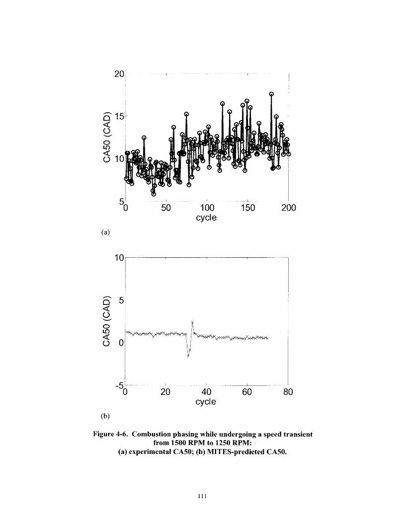
20
010
50 50 100 150 200
cycle
(a)
10
C) 5
LO '05
0 20 40 60 80cycle
(b)
Figure 4-6. Combustion phasing while undergoing a speed transientfrom 1500 RPM to 1250 RPM:
(a) experimental CA50; (b) MITES-predicted CA50.
available for chemical reactions results in earlier combustion and advances the combustion
phasing before TDC. This causes the reduction in load seen in Figure 4-4. As the first cycle at
1250 RPM simulation is completed, more time is also available for heat transfer, which cools the
charge and results in later combustion phasing. Furthermore, as mentioned previously, the
reduction in speed results in more fresh charge entering the cylinder; in other words, less (hot)
residual mass is present. This, too, has a cooling effect on the IVC temperature, which retards
combustion. As seen in Figure 4-5, the second cycle at 1250 RPM (Cycle 3) is later than Cycle
2, but the combustion phasing of Cycle 3 is before TDC. For this reason, the load in Cycle 3 is
still less than the original load in Cycle I (see Figure 4-5). As further charge cooling occurs on
the subsequent cycle, combustion phasing is pushed after TDC on Cycle 4. The load then
increases as a result of the increased mass of fuel (due to the increase in volumetric efficiency),
and post-TDC combustion phasing. The results demonstrate that MITES captures relative
changes in engine performance even in the absence of absolute accuracy in the observable (e.g.,
GIMEP). The ability to capture these relative changes is important when the model is used for
engine design work.
The data in Figure 4-6a represent the experimental change in the CA50 as a result of the speed
transient. The average CA50 before the transient is approximately 8.8 CAD, with a standard
deviation of approximately 1.4 CAD. The average CA50 after the transient is approximately 12.3
CAD, with a standard deviation of approximately 1.9 CAD. The data in Figure 4-6b represent
the change in the simulated CA50 as a result of the speed transient. Significantly less cycle-to-
cycle fluctuations are observed in MITES, because the model does not replicate turbulent
fluctuations and other sources of variability. MITES predicts a near zero change between the
pre- and post-transient CA5Os. This is presumably due to the cancellation of several factors. For
example, reducing the speed allows more time for heat transfer, which cools the charge and
delays the CA50. However, at slower speeds, there is more time for chemical reactions, which
increases the CA50. Experimentally the CA50 changes approximately 3.5 CAD, indicating that
the model does not predict accurately at least one of the off-setting effects. Even models that
have been empirically adjusted to match experimental data typically reproduce HCCI CA50's to
within 2 CAD, so the approximate 4 CAD discrepancy in a pure prediction model is not
surprising.
4.4.4. Valve Timing Transients
Valve timing is critical to maintaining combustion in residual-induced HCCI engines. Therefore,
we investigated the effects of a valve timing transient on combustion phasing. Experimentally,
the engine was first run to steady-state at 1500 RPM with #= 0.9. A transient in EVC timing was
induced by advancing the exhaust cam position by 6 CAD, i.e., the exhaust valve closes 6
degrees earlier during the exhaust stroke; the intake cam position was held constant. The change
in EVC timing was accomplished by commanding a step change in the valve timing via the
controlling computer. The cam phasing controller moves the cam at a rate of approximately one
CAD per cycle at 1500 RPM. During the valve transient, all other variables, including the fuel
pulse width, remained fixed. Consequently, the equivalence ratio increases from 0.9 to 1.0 as
more residual gas is trapped in the cylinder, decreasing the volume available for fresh charge.
The numerical simulations were performed in a consistent manner to the experiments. The
simulations were first run to steady-state with # = 0.9. Upon reaching steady-state, the EVC
timing was advanced one CAD per cycle for 6 cycles. The equivalence ratio was simultaneously

increased linearly per cycle from 0.9 to 1.0 over the duration of the valve transient. At the final
valve position and equivalence ratio, the simulations were run to a new steady-state.
The experimental and numerical impacts of the EVC timing on the CA50 are shown in Figure
4-7. For clarity, only the data near the transient are shown. From the figure it is clear that closing
the exhaust valve further from TDC results in an earlier combustion event. This change in
combustion phasing is due to an increase in the mass of hot residuals that are trapped in the
cylinder; these hot residuals increase the compression temperature of the subsequent cycle,
which causes earlier combustion phasing.
---- numerical- experimental
1540 ATDC
' 1480 ATDC
10 20 30 40 50 60 70cycle
Figure 4-7. Experimental and numerical CA50 during an exhaust valve transientfrom 1540 ATDC to 1480 ATDC.

From the model, the residual mass fraction increases by approximately 5% as the EVC timing
advances 6 CAD. For both the experimental and numerical data, the exhaust valve first moves at
cycle 31. However, neither set of data indicates that the combustion phasing changes
substantially on this cycle. The lag in combustion phasing relative to the exhaust valve
movement occurs because, on cycle 31, the residual fraction in the cylinder is determined
primarily by the EVC timing of cycle 30 (which was a steady-state cycle). However, once the
valve moves on cycle 31, the residual fraction in cycle 32 is larger than that in cycle 31.
Consequently, the combustion phasing in cycle 32 is advanced both experimentally and
numerically.
The experimental data indicate that the combustion phasing reaches a new steady-state in
approximately 5 - 6 cycles. The experimental phasing appears to under-shoot slightly the second
steady-state value. The numerical results show that the transient in combustion phasing is
complete in approximately 7 cycles, but no under-shoot is observed. Nevertheless, the predicted
time constant for the change in combustion phasing is accurate to within 1- 2 engine cycles.
4.4.5. Computational performance
All of the computations described above were performed on an Intel Pentium D processor
running at 2.0GHz. Each cycle of MITES (with the present engine configuration and chemical
mechanism) required approximately 7 - 8 minutes to complete. Therefore, each of the transient
simulations shown above was completed in less than 24 hours (including the time required for
the simulator to achieve steady-state). These rapid computational times demonstrate the potential
for MITES to be used as a design and analysis tool that is capable of testing different engine
configurations.

4.5. Discussion
4.5.1. Potential for Model Refinement
Steady-state and single-cycle simulations of HCCI combustion have shown that combustion
phasing is sensitive to temperature, residual fraction, and details of the fuel chemistry (see, for
example, [32,65,69]). Also well known is the propensity of "few-zone" models to overestimate
experimental quantities such as the peak pressure and engine load [54,65,66]. Many potential
improvements for steady-state modeling have been examined in the literature; here, we briefly
review some potential improvements for our transient simulator.
There are a number of enhancements that can be implemented to improve the quantitative
accuracy of MITES without using experimental data to calibrate the model. For example, the
assumption that no reactions occur in the boundary layer can be relaxed. However, in order to
model accurately true boundary layer and crevice volume effects, many additional zones would
be required. These intenrmediate zones would undergo some chemical reactions, but due to lower
temperatures, the rates at which the reactions proceed would be slower than in the core zone. The
presence of additional zones would decrease the amount and rate of heat release. Physically,
adding more zones is used to account for mixture inhomogeneities within the cylinder. Note that
the addition of more zones would increase the CPU time required to perform a given simulation.
Further refinement of the WAVE model used to represent the intake/exhaust system will also
improve the quantitative accuracy. In the present work, we found that MITES is sensitive to
changes in the WAVE model (especially the exhaust system). Therefore, by taking additional

measurements of the experimental engine (e.g., subtle bend angles in the exhaust ducts) and
entering that data into WAVE, a model that more accurately describes the engine could be used.
Improvements in the heat transfer model will also increase the quantitative accuracy of MITES.
In particular, the aN,tig used in the present work is that used in [63]. But, the engine
configuration used in [63] is different than the present configuration (e.g., bore, stroke,
compression ratio). A detailed study into the impact of ac,,ting on the solution accuracy (e.g., by
examining pressure profiles) may reveal a value of ca,,ting that is more appropriate for the present
engine configuration.
4.5.2. Usefulness of MITES
There are several reasons why it is difficult to simulate an HCCI engine to the high level of
accuracy that is desirable for engine design work. These include, for example, the modeling of
heat transfer, combustion chemistry, and the intake and exhaust flow patterns of the engine. All
of these factors, in addition to those described above, contribute to the differences between the
numerical and experimental results. Here we present a practical, transient HCCI engine simulator
that is capable of using detailed combustion chemistry for liquid gasoline fuels. The current
simulation results are obtained using the full LLNL PRF mechanism. There are several reasons
for using the detailed chemistry model. In future work, we plan to use MITES to study the
misfire limit in HCCI engines. When attempting to find the misfire boundary, having an accurate
chemical mechanism is crucial. Furthermore, while single-zone models do not provide accurate
estimates of emissions, such models can be used to estimate emissions limits [65]. When
studying the emissions limits, including detailed chemical kinetics are important. Finally, the
ability to capture some experimental trends (e.g., transient time constants), depends on having
accurate chemistry models. As shown in Figure 4-3, Figure 4-4, and Figure 4-6, MITES predicts
experimental transient time constants with reasonable accuracy.
Also, it should be born in mind that engine experiments are not perfect (e.g., see section 4.5.3).
At this point, the simulator is semi-quantitatively correct, with errors of 5 - 20% depending on
the quantity that is measured. But, the correct quantitative prediction of a single quantity is
equally as important as the relative change in a quantity in response to changes in the operating
conditions. The latter helps to characterize the operability of different configurations which is of
assistance to engine designers.
4.5.3. Experimental Errors
The engine experiments are complex and are prone to errors. A brief list of possible errors and
factors to reduce these is compiled here. First, the current resolution of crank angle
measurements is 1 CAD. Furthermore, the location of the valve timing events is known to within
± 1 CAD. Increasing the resolution of these two quantities would reduce noise in the pressure
traces and would allow for greater accuracy in determining the valve timing events. Second, for
the current engine configuration, the exact location of bottom dead center (BDC) is known to
within one degree. Errors in the location of BDC will cause errors in the GIMEP and other
calculated quantities. Fortunately, errors in BDC location can be minimized with proper
experimental techniques. The fuel/air equivalence ratio is controlled manually in these
experiments. Consequently, the fueling rate adjustment that occurs during the speed transient
may have allowed 0 to drift from 0 = 1.0. These errors can be reduced by inclusion of a feedback
mechanism from the lambda sensor to the controlling software. Finally, the pegging procedure
for determining the in-cylinder pressure is difficult in the current engine due to the low valve
lifts and short cam durations. As a result, the cylinder pressure is not likely to be completely
equalized with the intake manifold pressure (MAP). Nonetheless, all in-cylinder pressures are
pegged to the MAP at 3 CAD after BDC intake. This may lead to errors in the absolute value of
experimental GIMEPs, but the errors are consistent for all the data.
4.6. Conclusions
This work introduces a fast, full-cycle gasoline HCCI engine simulator (MITES) that is fully
automated, uses detailed chemical mechanisms, and is capable of modeling unsteady operation.
Here MITES was used to examine the effects of transient operation on HCCI engine
performance. However, the MITES was primarily developed to be a tool for studying LLL
behavior. This is discussed in the following chapter.
MITES uses the Ricardo WAVE software package to model the engine, excluding the cylinder.
The cylinder is represented by a 2-zone combustion model that is activated from IVC to EVO
and during the re-compression event. The state of the cylinder at IVC, which is critical for
detennrmining the auto-ignition properties of the mixture in the cylinder, is obtained automatically
from the converged solution of the previous engine cycle: no user-intervention is required.
The in-cylinder pressure traces from MITES are compared with the corresponding traces from
the experiments. As expected for a 2-zone HCCI model, MITES overpredicts the peak pressure
in the cylinder. It also overpredicts the peak pressure during re-compression by approximately
12%. The latter discrepancy, and discrepancies in the combustion physics, are likely related to
WAVE's inaccurate estimate of the valve throughput possibly compounded by inaccuracies in
the heat-loss and chemistry models.
119
The simulator was used to model the impact of changes in the equivalence ratio on the GIMEP
of the engine. Both the simulation and experiment agree that a 10% increase in the equivalence
ratio (from lean to stoichiometric) yields a 9% increase in GIMEP. It was also observed that 5 -
6 complete engine cycles are required before the engine achieves steady-state after the fueling
transient is introduced.
MITES was also used to investigate the impact of operating speed changes on the load of the
engine. The experimental data and predictions from the simulation demonstrate that decreasing
the RPM from 1500 to 1250 results in a I 1-12% increase in load.
The impact of EVC timing on combustion phasing was also examined using MITES. Here we
observed qualitative agreement with experimental data. Both the experimental and numerical
results suggest that 4 - 6 cycles are required to resume steady-state operation following a 6 CAD
advancement in EVC.
MITES is run on a conventional Intel Pentium-based desktop PC. Each cycle of the engine
requires only 7 - 8 minutes of CPU time to complete for a detailed fuel chemistry model, which
includes more than 1000 species and 4000 reactions. As such, MITES has the potential to be
used in the design phase of HCCI engine development. With further refinements to the WAVE
and 2-zone models, closer quantitative agreement between numerical and experimental results is
anticipated.

5. THE HCCI MISFIRE: THE CAUSE AND ITS EFFECT ON THE
LOW LOAD LIMIT
Developing an understanding of what causes an HCCI engine to misfire is important when
studying the LLL and provides the ability to estimate how fuel chemistry and engine operating
conditions (e.g. engine speed) affect the LLL of HCCI operability. In this work, a combination of
detailed, chemical-kinetic simulations and empirical-based models (i.e., Wiebe functions) were
used to study the underlying physics of what causes an HCCI engine to misfire. These simulation
results, along with experimental LLL data presented in Chapter 3, were used to predict fuel and
operating condition effects on the LLL.
5.1. Introduction
5.1.1. Motivation
One major challenge preventing commercialization of HCCI technology is its operating range
size. Across a speed range of 1000 to 2500 RPM, a typical operating range defined by the net
indicated mean effect pressure (NIMEP) for an SI engine is approximately 1 to 11 bar; the HCCI
operating range is approximately 1.5 to 5 bar [5]. With such a small operating range, a dedicated
HCCI engine is not competitive with conventional engines. Fortunately, the HCCI operating
range is located in the lower half of the SI operating range, where the HCCI efficiency benefits
are largest. Nevertheless, the low-load limit (LLL) of HCCI operability wastes fuel because the
engine speed cannot be reduced to idle. Therefore, developing an understanding of the limiting
mechanism for the LLL is crucial to future HCCI engine development. This work focuses on
explaining the phenomenon that cause an HCCI misfire and how this affects the HCCI LLL.
The mechanism that limits HCCI operation near the LLL has yet to be determined in the HCCI
literature. We hypothesize that near the LLL, the in-cylinder temperatures are colder with
increasing residual fraction as a result of falling combustion temperatures. Therefore, when the
residual fraction is increased to lower the engine load, the temperature drops below a critical
ignition temperature that allows for sustained operation. Cycle-to-cycle instability could also
potentially contribute to a misfire. If cycle-to-cycle fluctuations grow near the LLL, perhaps a
stable steady-state is unattainable beyond a critical residual fraction. The goals of this work are
to test these hypotheses, to identify the cause of the HCCI LLL, and to determine how fuel
chemistry and engine operating conditions can affect the misfire regime.
Studying the LLL exclusively through experimentation is difficult. During a typical experiment,
only a few in-cylinder conditions can be measured accurately: volume and pressure. Current
methods for measuring quantities, such as the in-cylinder gas temperatures and/or residual mass
fraction, are difficult to employ. Therefore, in this work, a full-cycle simulation tool of an HCCI
cylinder is used to study the misfire limit phenomenon. With such a model, estimates of
quantities such as temperature, residual mass fraction, and fuel mass fraction burned are easily
obtainable. The simulation tool is first used to establish the underlying physics of an HCCI
misfire. Then, semi-quantitative simulations are performed with Wiebe combustion models to
establish trends describing how fuel chemistry and engine speed affect the LLL of HCCI
operability. Finally, these trends are used to support experimental LLL data with primary
reference fuels.
5.1.2. Relevant Prior Studies
Dec [65] and Sjbberg and Dec [29,32] used a combination of simulations and experiments to
investigate HCCI operation at low engine loads. In [65], Dec used a single-zone kinetic model to
examine how reducing the fueling rate affected quenching of the bulk-gas reactions. In these
simulations, the fueling rate was reduced by decreasing the fuel/air equivalence ratio (0). Dec
found that HCCI combustion could not go to completion for 0 < 0.15. At these equivalence
ratios, the bulk gas reactions were quenched due to low combustion temperatures. Sj6berg and
Dec [29] investigated how fuel chemistry and engine speed affected the onset of incomplete
combustion in HCCI engines. They found that fuels with minimal cool-flame chemistry (e.g.,
iso-octane, gasoline) reach the onset of incomplete bulk-gas reactions at the same 0
independently of engine speed. However, for fuels that exhibit significant cool-flame chemistry
(e.g., n-heptane), engine speed influenced the onset of incomplete bulk-gas reactions; larger q
were required at lower engine speeds to maintain complete combustion. In a subsequent work
[32], Sj6berg and Dec examined the minimum temperature required to achieve complete CO-to-
CO 2 oxidation in an HCCI engine. They found that the temperature requirements correlated well
with the peak cycle temperature. A peak temperature of 1500 K was necessary to complete the
CO oxidation process at 1200 RPM with a compression ratio of 18. This temperature was found
to be independent of fuel type.
In the works of Dec [65] and Sjober and Dec [29,32], and several other studies in the literature
(see, for example, [19,27,28]), the lower load limit was reached by varying the equivalence ratio.
However, if HCCI engines are hybridized with SI engines, stoichiometric operation diluted with
residual will likely be required to use current catalyst technology. To the author's knowledge, no

studies exist in the literature that examine the cause of an HCCI misfire at stoichiometric
operation. Therefore, the goals of this work were to establish the mechanism that governs the
LLL of an HCCI engine operating with a stoichiometric fuel/air ratio and to understand how fuel
chemistry and engine operating conditions affect the misfire regime.
5.2. HCCI Engine Simulator
The HCCI simulator used here combines a user-defined, detailed chemistry model of the engine
cylinder with a commercial engine simulation software, Ricardo WAVE. The coupled model is
referred to as the MIT Engine Simulator, or MITES. MITES was previously used to model
transient behavior in HCCI engines (see Chapter 4). In that work, MITES was able to accurately
predict transient time constants and relative changes in engine load for experimental transients in
fueling rate and engine speed. A detailed description of MITES is given in Chapter 4, Section
4.3. However, a brief review of the model methodology is given here.
5.2.1. WAVE Model
WAVE models the flows to and from the cylinder using l-D fluid mechanics. During the gas
exchange portions of the engine cycle (i.e., exhaust valve opening, EVO, to exhaust valve
closing, EVC, and intake valve opening, IVO, to intake valve closing, IVC), WAVE models the
flows across the cylinder valves, and thus is responsible for calculating the trapped mass and
residual mass fraction. WAVE also calculates the mass of fuel to inject in order to maintain the
correct fuel/air equivalence ratio within the cylinder. Unlike in Chapter 4, the WAVE model
used here does not use experimental pressure profiles to account for the experimental intake
system. Rather, a constant pressure ambient block is used for the intake. This approach led to
greater simulation stability.

5.2.2. Cylinder Model
Modeling of the auto-ignition process requires an accurate representation of the chemical
kinetics that occur inside the engine cylinder. The commercially available version (7.0) of
Ricardo WAVE does not offer a method for using detailed chemical kinetics to model HCCI
combustion. Therefore an external cylinder model was written and linked with WAVE.
In the external model, the cylinder contents were divided into one of two regions: a boundary
layer zone and a core zone. Here, the "boundary layer" zone was not a boundary layer in the
strictest sense. Rather, it represented the mass in the colder volumes of the cylinder (i.e., the true
boundary layer and crevice volumes). The boundary layer zone contained a user-specified
fraction, Xhoundary, of the mass in the cylinder. In the present work xboun,,,,y = 0.05 (i.e., the
boundary layer zone contained 5% of the total mass). The mass in the boundary layer was
assumed to be non-reactive due to significant heat loss to the cylinder walls. Therefore, all
reactions occurred in the core zone only. Each zone was assumed to be spatially uniformn, and the
pressure in the cylinder was uniform throughout both masses.
The external model solves a system of differential-algebraic equations (DAEs). These include
equations for species conservation, energy conservation, and the ideal gas equation of state,
which was included to make the Jacobian of the model equations sparse. The model equations
are given in Section 4.3.2. The equations are solved using the JACOBIAN software package
[57], which contains a computationally efficient numerical solver, DSL48S, for sparse systems
of DAEs [60]. Additional computational speed-ups were obtained by using analytical
expressions for the Jacobians, which were obtained apriori using automatic differentiation [59].

5.3. Numerical Procedure
5.3.1. Closed-cycle Simulations
MITES was first used to determine the minimum temperature required to induce auto-ignition of
a stoichiometric' fuel/air mixture at a fixed residual fraction for one engine cycle only. Because
the conditions sought simply needed to guarantee combustion for a single cycle, only the closed-
portion of the engine cycle was simulated (i.e., from IVC to EVO). Consequently, the thermal
conditions found to ensure auto-ignition did not guarantee sustainable combustion for multiple
cycles. The procedure for finding the minimum temperature is described in the following
paragraphs.
In order to specify the thermodynamic state of the cylinder at IVC, 3 of the 4 following variables
had to be specified: pressure, temperature, total mass, and the mass fractions of N-l species,
where N was the total number of species. The volume of the cylinder was calculated from the
slider crank equation at the crank angle of IVC. For the closed-cycle simulations in this work,
total mass was not specified but was calculated from the ideal gas law and the remaining
thermodynamic quantities. As shown subsequently, specifying alternate variables, for example
the total mass and calculating the pressure, gave comparable results. The N-1 mass fractions
were derived from the specified residual mass fraction at IVC. Given the residual mass fraction,
equivalence ratio, and the molecular weight of the fuel, the composition of the in-cylinder
mixture can be determined [70]. The pressure at IVC (Psvc) was always set to 1.115 bar. This
pressure is consistent with the pressure at IVC from the full-cycle simulations. Furthermore,
All simulations were performed at a fuel/air equivalence ratio of 0.99, which is referred to as "stoichiometric."
varying the pressure at IVC in the closed-cycle simulations had little effect on the results. For all
the closed-cycle simulations, the crank angle of IVC (01vc) was set to 138' before top center
(BTC), and all the simulations were performed at 1500 RPM. The 01vc chosen was consistent
with the valve timing at the LLL in prior experimental work (see Chapter 2).
The procedure for determining the minimum temperature required to induce auto-ignition is as
follows:
1. Specify a residual mass fraction
2. Calculate the initial concentrations of the in-cylinder mixture using [70]
3. Guess a temperature at IVC (Tivc)
4. Simulate the closed portion of the engine cycle
5. Check: did the mixture auto-ignite?
a. If no, increase Tifc and repeat steps 4 and 5 until the mixture does auto-ignite,
then move to step 6
b. If yes, reduce Tivc and repeat steps 4 and 5 until the mixture does NOT auto-
ignite, then move to step 6
6. Record the first temperature that led to auto-ignition or the last temperature that allowed
for auto-ignition
7. Increase (or decrease) the residual mass fraction and repeat steps 2 - 6
Steps 1 - 7 were completed for a range of residual fractions. A summary of the conditions tested
are given in Table 5-1. Using the temperatures recorded in step 6, the fire/misfire line was
constructed. This line represents the minimum temperature required to burn a mixture with fixed
composition for a single engine cycle.
Table 5-1. Conditions used in closed-cycle simulationsParameter Value
% residual 55 - 75
Pvc (bar) 1.115
,0vc (CAD BTC) 138Equivalence ratio 0.99
(0)Speed (RPM) 1500
5.3.2. Full-cycle Simulations
In the closed-cycle simulations, the residual mass fraction and T c were allowed to vary
independently. In the context of a real engine, this is not possible; the residual fraction and in-
cylinder temperature are directly linked. Therefore, in order to gain an understanding of how the
in-cylinder temperature correlates with residual mass fraction, full-cycle simulations were
required.
The full-cycle simulations were performed in a manner consistent with the experimental
approach used to obtain the LLL (see Chapter 2). For a fixed set of operating conditions (e.g.,
0ivc, RPM, intake air temperature), a simulation was run to steady-state. Once steady-state was
achieved with the initial configuration, the exhaust valve timing (OEvc) was advanced 1 CAD
(effectively increasing the residual fraction), and the simulation was allowed to achieve steady-
state at the new valve timing. OEvc was repeatedly advanced until the simulation misfired. The
transition in valve timing occurred without terminating the original simulation. Therefore,
MITES captured the cycle-to-cycle dynamics of changing the valve timing. For all the
simulations, the following variables were fixed at the values used experimentally in Chapter 2:
engine speed (1500 RPM), fuel/air equivalence ratio (0 = 0.99), intake air temperature (Tiv =
400C), and 0ivc (138 CAD BTC). A summary of the conditions simulated is provided in Table
5-2.
Table 5-2. Conditions used in full-cycle simulationsParameter Value
OEVC (CAD BTC) 114-122
6Avc (CAD BTC) 138TIN (oC) 40
Equivalence Ratio (4) 0.99Speed (RPM) 1500
5.3.3. Primary Reference Fuels
Both the closed-cycle and full-cycle simulations were performed using the full mechanism for
primary reference fuels (PRFs) developed at the Lawrence Livermore National Laboratory [64].
The detailed chemical mechanism contains 1036 species undergoing 4238 elementary reactions.
PRFs are used to define the research [71] and motor octane numbers [72] (RON and MON,
respectively) of commercial gasolines. PRFs are binary mixtures of iso-octane and n-heptane.
Iso-octane is a highly auto-ignition resistant fuel, and n-heptane is an easily auto-ignitable fuel.
Therefore, varying the ratio of iso-octane to n-heptane in a PRF mixture adjusts the auto-
ignitability of the overall fuel blend. The octane number of a PRF is defined as the volume-
percent of iso-octane in the mixture. For example, PRF90 is composed of 90 volume-percent iso-
octane and 10 volume-percent n-heptane and has a RON and MON equal to 90. Both the closed-
cycle and full-cycle simulations were performed with PRFs 25 and 90. These were chosen to
cover a broad range of fuel ignitability. Full-cycle simulations were also performed with PRF60
to facilitate comparison with experimental data presented in Chapter 3.
5.4. Building the Fire/Misfire Line
The definition of what constitutes a misfire in a closed-cycle simulation is not well established.
Experimentally, and in full-cycle simulations, when a misfire occurs the NIMEP for that cycle is
negative because no work is produced during combustion. However, a full cycle must be
completed to calculate the NIMEP, so this definition cannot be used to define a misfire in the
closed-cycle simulations. Therefore, in this work a cycle was defined as a misfire if the first
derivative of the cylinder pressure with respect to time was never positive after top center (i.e.,
zero CAD). This definition was equivalent to inspecting the heat release profiles: firing
conditions lead to a clear HTHR, whereas misfire conditions resulted in no HTHR. Examples of
firing and misfiring pressure traces are shown in Figure 5-1. These results were obtained with
PRF90 at a constant residual mass fraction of 65%. For the misfire pressure trace, Tvc was 548
K, and Tirc was 549 K for the firing simulation.
The data in Figure 5-2a represent the minimum temperature required at fvec to induce auto-
ignition of a stoichiometric fuel/air mixture with constant residual fraction (i.e., the fire/misfire
line). A reduction in temperature of 1 K below the fire/misfire lines in the figure results in a
misfire.
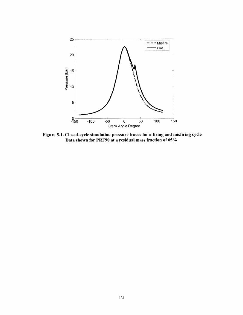
25 I....... Misfire- Fire
20
Col
15- /
0-150 -100 -50 0 50 100 150
Crank Angle Degree
Figure 5-1. Closed-cycle simulation pressure traces for a firing and misfiring cycleData shown for PRF90 at a residual mass fraction of 65%
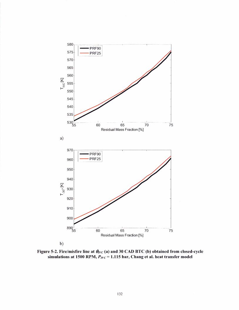
8R0
- PRF9O575 - PRF25
570
565
560
o555
550
545
540
535
530 ..55 60 65 70 75
Residual Mass Fraction [%]
a)
970i-PRF90
960 - PRF25
950
940
0 930I.-'
920
910
900
890--55 60 65 70 75
Residual Mass Fraction [%]
b)
Figure 5-2. Fire/misfire line at Ovc (a) and 30 CAD BTC (b) obtained from closed-cyclesimulations at 1500 RPM, Pwvc = 1.115 bar, Chang et al. heat transfer model
132
- 1111- 11-1- -, - - ___T___ - -
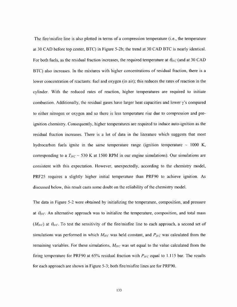
The fire/misfire line is also plotted in terms of a compression temperature (i.e., the temperature
at 30 CAD before top center, BTC) in Figure 5-2b; the trend at 30 CAD BTC is nearly identical.
For both fuels, as the residual fraction increases, the required temperature at Orc (and at 30 CAD
BTC) also increases. In the mixtures with higher concentrations of residual fraction, there is a
lower concentration of reactants: fuel and oxygen (in air); this reduces the rates of reaction in the
cylinder. With the reduced rates of reaction, higher temperatures are required to initiate
combustion. Additionally, the residual gases have larger heat capacities and lower y's compared
to either nitrogen or oxygen and so there is less temperature rise due to compression and pre-
ignition chemistry. Consequently, higher temperatures are required to induce auto-ignition as the
residual fraction increases. There is a lot of data in the literature which suggests that most
hydrocarbon fuels ignite in the same temperature range (ignition temperature - 1000 K,
corresponding to a Tivc - 530 K at 1500 RPM in our engine simulations). Our simulations are
consistent with this expectation. However, unexpectedly, according to the chemistry model,
PRF25 requires a slightly higher initial temperature than PRF90 to achieve ignition. As
discussed below, this result casts some doubt on the reliability of the chemistry model.
The data in Figure 5-2 were obtained by initializing the temperature, composition, and pressure
at 01~c. An alternative approach was to initialize the temperature, composition, and total mass
(Mvc) at 01vc. To test the sensitivity of the fire/misfire line to each approach, a second set of
simulations was performed in which Mvc was held constant, and Pec was calculated from the
remaining variables. For these simulations, MiVc was set equal to the value calculated from the
firing temperature for PRF90 at 65% residual fraction with Pvc equal to 1.115 bar. The results
for each approach are shown in Figure 5-3; both fire/misfire lines are for PRF90.
133
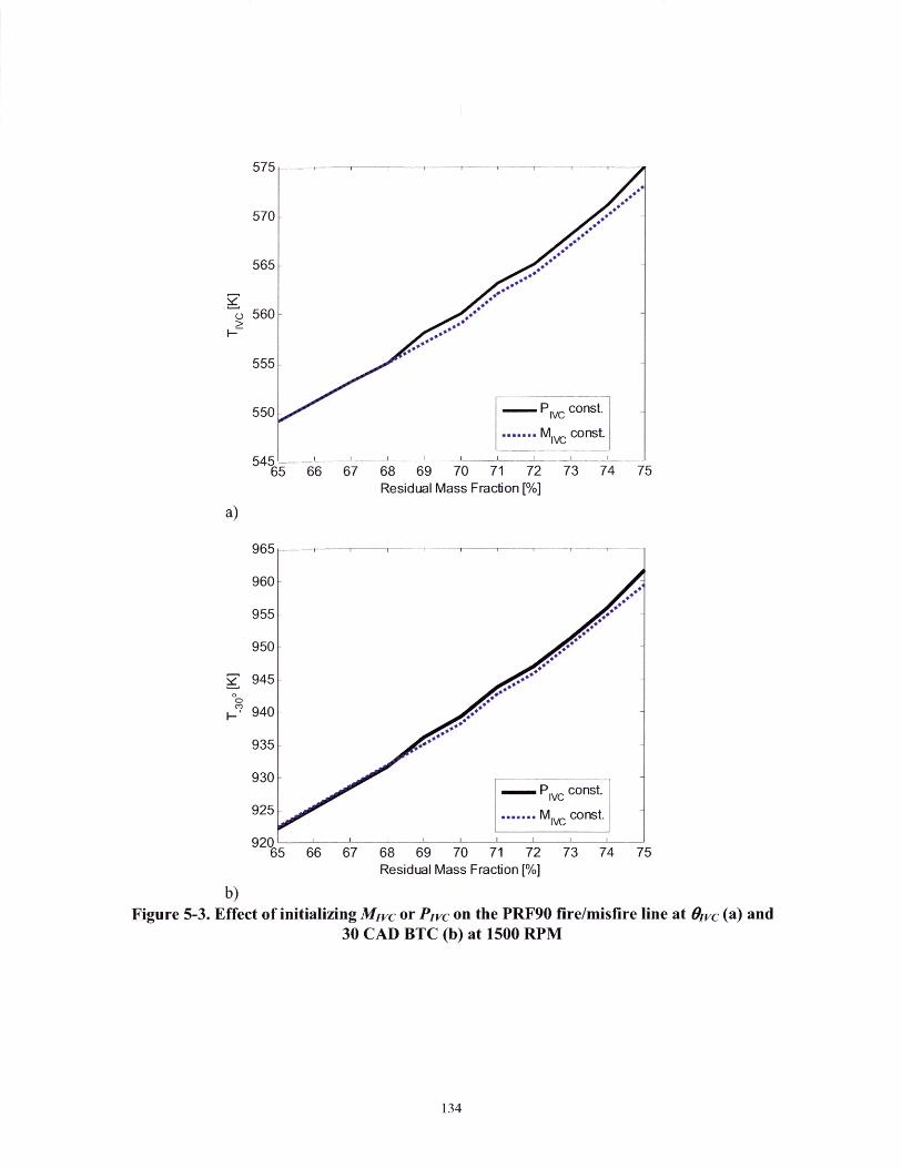
o*
Ivc*
Ivc const.Romagna MR/ const.
545 .. .. ... ....65 66 67 68 69 70 71 72 73 74
Residual Mass Fraction [%]
- Pivc const.
....... M c const.
66 67 68 69 70 71 72 73 74Residual Mass Fraction [%]
b)Figure 5-3. Effect of initializing Mrvc or Prvc on the PRF90 fire/misfire line at Owvc (a) and
30 CAD BTC (b) at 1500 RPM
575
570
565
560
555
550
965
960
955
950
945
940
935
930
925
920-65
--- T__------------I- ----
Specifying either Pivc or Mc had only a minor effect on the fire/misfire temperature at Ovc or at
30 CAD BTC. At 75% residual fraction, the minimum Tvc changed by only 2 K (approximately
0.35%); an even smaller change (2 K, or approximately 0.24%) was observed at 30 CAD BTC.
The pressure used to initialize the closed-cycle simulations was estimated from the full-cycle
simulation results. There, PiVc was approximately 1.115 bar over a broad range of operating
conditions. Therefore, the results in Figure 5-2 were obtained with PlPc equal to 1.115 bar.
In order to test the sensitivity of the results to Prvc, the procedure to build the fire/misfire line
was repeated with Prc equal to 1.05925 bar (a reduction of 5%) with PRF90. The fire/misfire
lines at OIvc and 30 CAD BTC for both pressures are shown in Figure 5-4. Reducing the pressure
causes the fire/misfire line to shift to higher temperatures. When PIc is reduced, the
concentration of the gases in the cylinder decreases; this slows the reaction rates. Also, the total
heat capacity decreases more than the heat losses, reducing the peak temperature. To
compensate, the temperature must be increased to achieve combustion. However, this increase in
temperature is minor; a 5% reduction in Ppc, requires only a 0.53% increase in Twvc or a 0.30%
change at 30 CAD BTC.
5.5. Determining Steady-state In-Cylinder Temperature
Defining a misfire cycle in the context of a fill-cycle simulation was straight forward. On cycles
that misfired, the NIMEP was negative, i.e., no work was produced from the combustion
process. Such a definition was not possible in the closed-cycle simulations because a full engine
cycle must be completed to calculate the NIMEP. In addition to the NIMEP being negative on
the misfire cycle, the pressure traces from firing and misfire cycles were clearly different.

Examples of a firing and a misfiring cycle are shown in Figure 5-5; the data in the figure are for
PRF90.
580
575
570
565
-- 560 ."
550 /=1.115 bar
.....Pvc=1.05925 bar
54565 66 67 68 69 70 71 72 73 74 75
Residual Mass Fraction [%]
a)
965
960
955
950
, 945
- 940
935 ,
930 ,°30,. Pc=1.115 barIvc925 p .. c=1.05925 bar
65 66 67 68 69 70 71 72 73 74 75Residual Mass Fraction [%]
b)
Figure 5-4. Sensitivity of the PRF90 fire/misfire line at 6,vc (a) and 30 CAD BTC (b) to Prvcat 1500 RPM

35.. **" 'Misfire30 Fire
30
25
fo20
15
10
0 .. I . .... . .. I. . I . ....... 1
-150 -100 -50 0 50 100 150Crank Angle Degree
Figure 5-5. Full-cycle simulation pressure traces for a firing and misfiring cycleData shown are for PRF90 at 1500 RPM
The firing trace is the steady-state pressure trace at the last OEvc before the simulation misfired.
The full-cycle simulations were performed to determine how the in-cylinder temperature and
residual fraction are correlated. The correlation is presented in Figure 5-6. Each data point in the
figure represents the steady-state in-cylinder temperature at Ovc and 30 CAD BTC for a fixed set
of engine operating conditions (e.g., valve timing). The steady-state temperatures for PRF25
were marginally higher than those of PRF90. This was likely a consequence of a smaller heat
capacity and larger heating value of PRF25 relative to PRF90. The residual fraction was
progressively increased by advancing OEVC by I CAD once steady-state had been reached (after
approximately 50 engine cycles) at one valve timing; all other operating conditions were held
constant. As the residual fraction increases, the temperature in the cylinder decreases.

* PRF90A PRF25
0 AA A
. * 0
600
595
590
585
PRF90PRF25
* 9
A
64 66 68 70Residual Mass Fraction [%]
b)
Figure 5-6. Steady-state temperature at Ovc (a) and 30 CAD BTC (b) as a function residualmass fraction from full-cycle simulations at 1500 RPM using the LLNL PRF chemistry
model
A
-S
64 66 68 70Residual Mass Fraction [%]
580
575
57062
990
985
980
975
970
965
960 162

600 .
595
590 ..
- 580 5
575
570
56545 50 55 60 65
Residual Mass Fraction [%]
Figure 5-7. Steady-state Tvc over a broad range of residualRPM
\ 1
70 75
fractions for PRF90 at 1500
Increasing the residual fraction has 2 competing effects. Trapping more hot combustion products
increases the temperature of the trapped mixture. Simultaneously, the mass of fuel in the cylinder
decreases, which results in colder combustion temperatures and thus cooler residuals. This
causes the in-cylinder temperature to decrease. As seen in Figure 5-7, these competing
mechanisms cause the in-cylinder temperature to go through a maximum. Each data point in
Figure 5-7 represents the steady-state Twvc for fixed valve timing; here the residual fraction
varies over a much larger range than in Figure 5-6. The dotted line in Figure 5-7 is for clarity
only.
5.6. The HCCI Misfire
The purpose of this work was to develop an understanding of what causes an HCCI engine to
misfire at it approaches the LLL. Prior work by Sjiberg and Dec [32] suggested that the misfire
limit was linked to the complete oxidation of CO to C0 2, which was governed by the peak in-

cylinder temperature. This mechanism was not the limiting factor here, because the peak
temperature for a firing cycle was always much larger (by a minimum of - 300 K) than 1500 K -
the value determined by Sj6ber and Dec necessary to complete the CO-to-CO 2 oxidation.
Comparing the closed-cycle results from section 5.4 with steady-state data from section 0
provides insight on an alternative possible limiting mechanism. The data from Figure 5-2 and
Figure 5-6 are plotted together in Figure 5-8; trend lines are drawn through the steady-state data
for clarity.
The 2 circled steady-state points represent the last stable operating point for each fuel.
Advancing OEvc by I CAD from these points caused both fuels to misfire. As evident in Figure
5-8, the steady-state solutions and the fire/misfire lines converge, with the last stable operating
point for PRF90 approaching the fire/misfire line to within 14 K at 0 -c or 20 K at 30 CAD BTC.
The 2 curves likely do not intersect because the fire/misfire line represents the minimum
temperature required to achieve auto-ignition for one cycle. Therefore, presumably a higher
initial temperature (relative to the fire/misfire temperature) is required to sustain combustion for
multiple cycles, considering the cycle-to-cycle fluctuations, and the fact that near the misfire
limit the ignition timing is not optimal for maximizing the residual temperature.
The small differences in temperature between the last stable steady-state points and the
fire/misfire line suggest that the main cause of an HCCI misfire is insufficient thermal energy to
sustain combustion for multiple cycles. Even if the temperature could be reduced to fire/misfire
line, the residual fraction could only be increased by a few percent. As shown subsequently, such
a small increase in the residual fraction would only reduce the LLL by a few percent.

SPRF90 SS- PRF90 Misfire Line
A PRF25 SS.....
PRF25 Misfire Line
545 ---. -62 64 66 68
Residual Mass
'A
70 72Fraction [%]
o
* PRF90 SS- PRF90 Misfire Line
A PRF25 SS.. "" PRF25 Misfire Line
64 66 68Residual Mass
70 72 74Fraction [%]
b)
Figure 5-8. Fire/misfire line and steady-state temperature at Orvc (a) and 30 CAD BTC (b)at 1500 RPM as computed with the full-cycle, full-chemistry simulations, and the Chang et
al. heat transfer model
595-
590
585
580
575
570
565
560
555
550
990
980
970
960
950
940
930
920 "62
I ? I
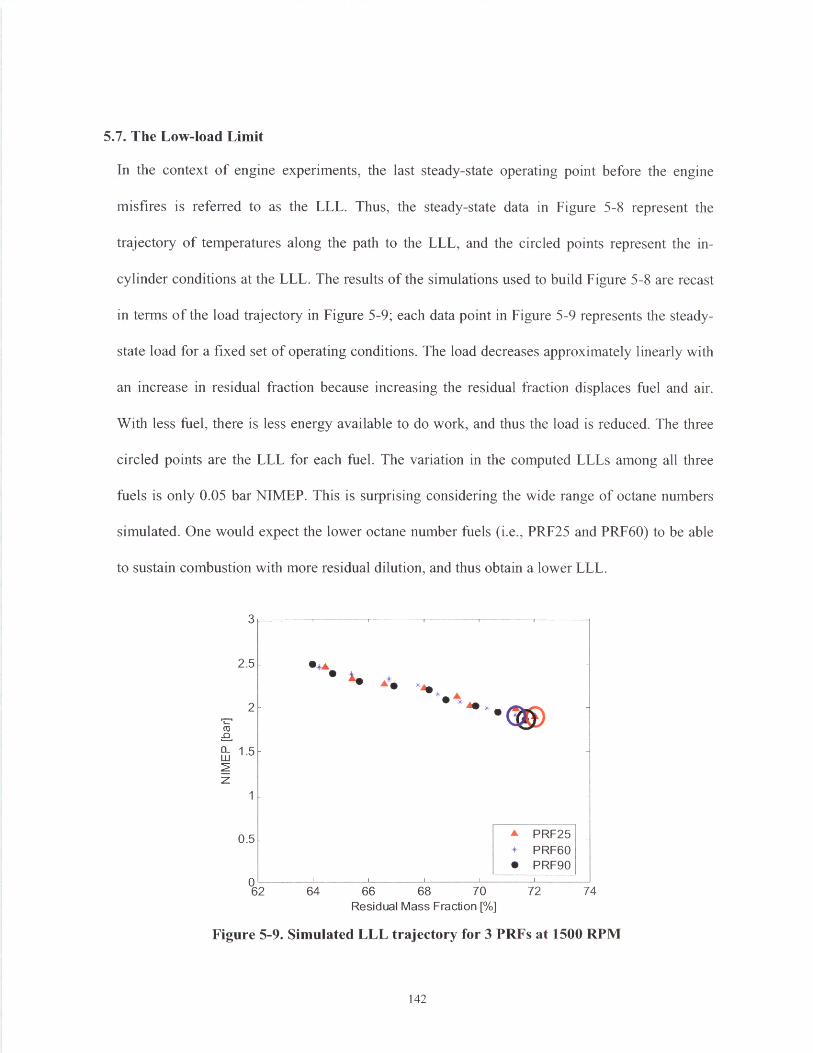
5.7. The Low-load Limit
In the context of engine experiments, the last steady-state operating point before the engine
misfires is referred to as the LLL. Thus, the steady-state data in Figure 5-8 represent the
trajectory of temperatures along the path to the LLL, and the circled points represent the in-
cylinder conditions at the LLL. The results of the simulations used to build Figure 5-8 are recast
in terms of the load trajectory in Figure 5-9; each data point in Figure 5-9 represents the steady-
state load for a fixed set of operating conditions. The load decreases approximately linearly with
an increase in residual fraction because increasing the residual fraction displaces fuel and air.
With less fuel, there is less energy available to do work, and thus the load is reduced. The three
circled points are the LLL for each fuel. The variation in the computed LLLs among all three
fuels is only 0.05 bar NIMEP. This is surprising considering the wide range of octane numbers
simulated. One would expect the lower octane number fuels (i.e., PRF25 and PRF60) to be able
to sustain combustion with more residual dilution, and thus obtain a lower LLL.
3
2.5 * e
2 A*o
0- 1.5
z1
0.5 A PRF25+ PRF60* PRF90
062 64 66 68 70 72 74
Residual Mass Fraction [%]
Figure 5-9. Simulated LLL trajectory for 3 PRFs at 1500 RPM
142
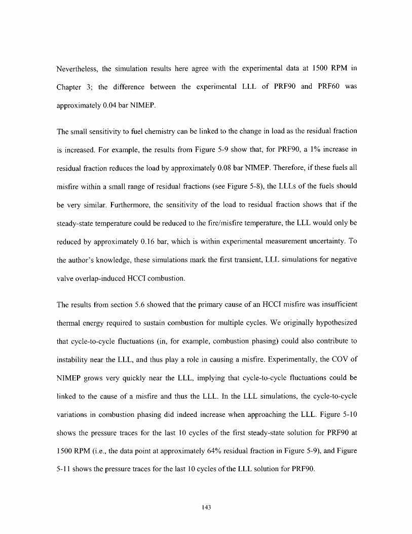
Nevertheless, the simulation results here agree with the experimental data at 1500 RPM in
Chapter 3; the difference between the experimental LLL of PRF90 and PRF60 was
approximately 0.04 bar NIMEP.
The small sensitivity to fuel chemistry can be linked to the change in load as the residual fraction
is increased. For example, the results from Figure 5-9 show that, for PRF90, a 1% increase in
residual fraction reduces the load by approximately 0.08 bar NIMEP. Therefore, if these fuels all
misfire within a small range of residual fractions (see Figure 5-8), the LLLs of the fuels should
be very similar. Furthermore, the sensitivity of the load to residual fraction shows that if the
steady-state temperature could be reduced to the fire/misfire temperature, the LLL would only be
reduced by approximately 0.16 bar, which is within experimental measurement uncertainty. To
the author's knowledge, these simulations mark the first transient, LLL simulations for negative
valve overlap-induced HCCI combustion.
The results from section 5.6 showed that the primary cause of an HCCI misfire was insufficient
thermal energy required to sustain combustion for multiple cycles. We originally hypothesized
that cycle-to-cycle fluctuations (in, for example, combustion phasing) could also contribute to
instability near the LLL, and thus play a role in causing a misfire. Experimentally, the COV of
NIMEP grows very quickly near the LLL, implying that cycle-to-cycle fluctuations could be
linked to the cause of a misfire and thus the LLL. In the LLL simulations, the cycle-to-cycle
variations in combustion phasing did indeed increase when approaching the LLL. Figure 5-10
shows the pressure traces for the last 10 cycles of the first steady-state solution for PRF90 at
1500 RPM (i.e., the data point at approximately 64% residual fraction in Figure 5-9), and Figure
5-11 shows the pressure traces for the last 10 cycles of the LLL solution for PRF90.
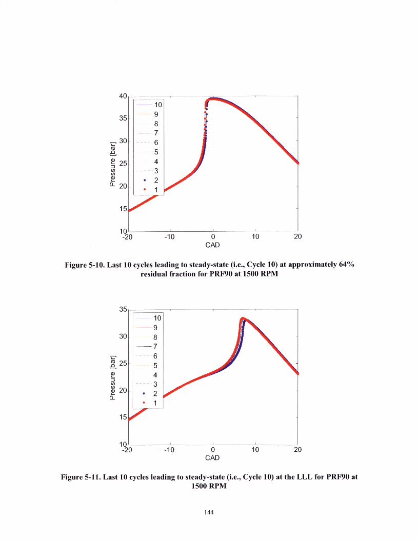
10' 1 1-20 -10 0 10 20
CAD
Figure 5-10. Last 10 cycles leading to steady-state (i.e., Cycle 10) at approximately 64%residual fraction for PRF90 at 1500 RPM
35
30
25
20
10-20 -10 0 10
CAD
Figure 5-11. Last 10 cycles leading to steady-state (i.e., Cycle 10) at the LLL for PRF90 at1500 RPM
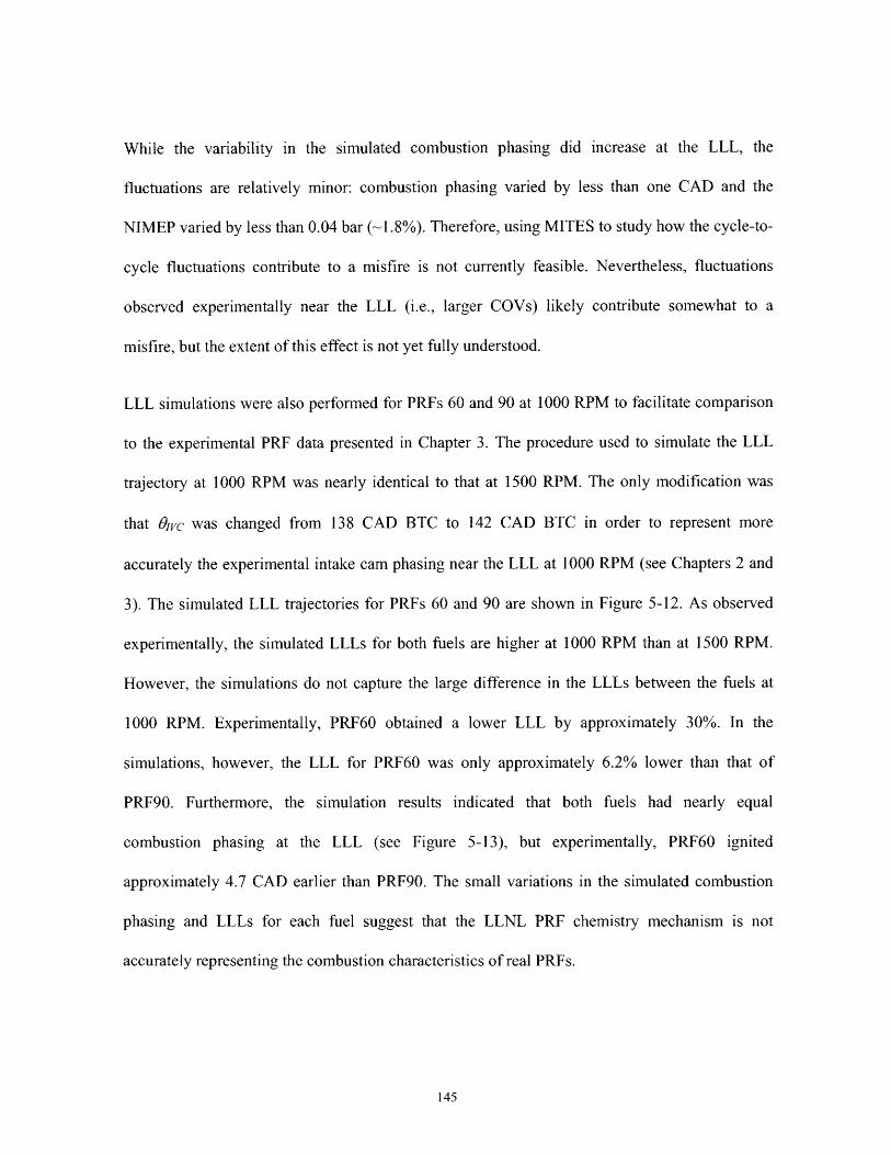
While the variability in the simulated combustion phasing did increase at the LLL, the
fluctuations are relatively minor: combustion phasing varied by less than one CAD and the
NIMEP varied by less than 0.04 bar (-1.8%). Therefore, using MITES to study how the cycle-to-
cycle fluctuations contribute to a misfire is not currently feasible. Nevertheless, fluctuations
observed experimentally near the LLL (i.e., larger COVs) likely contribute somewhat to a
misfire, but the extent of this effect is not yet fully understood.
LLL simulations were also performed for PRFs 60 and 90 at 1000 RPM to facilitate comparison
to the experimental PRF data presented in Chapter 3. The procedure used to simulate the LLL
trajectory at 1000 RPM was nearly identical to that at 1500 RPM. The only modification was
that 01vc was changed from 138 CAD BTC to 142 CAD BTC in order to represent more
accurately the experimental intake cam phasing near the LLL at 1000 RPM (see Chapters 2 and
3). The simulated LLL trajectories for PRFs 60 and 90 are shown in Figure 5-12. As observed
experimentally, the simulated LLLs for both fuels are higher at 1000 RPM than at 1500 RPM.
However, the simulations do not capture the large difference in the LLLs between the fuels at
1000 RPM. Experimentally, PRF60 obtained a lower LLL by approximately 30%. In the
simulations, however, the LLL for PRF60 was only approximately 6.2% lower than that of
PRF90. Furthermore, the simulation results indicated that both fuels had nearly equal
combustion phasing at the LLL (see Figure 5-13), but experimentally, PRF60 ignited
approximately 4.7 CAD earlier than PRF90. The small variations in the simulated combustion
phasing and LLLs for each fuel suggest that the LLNL PRF chemistry mechanism is not
accurately representing the combustion characteristics of real PRFs.
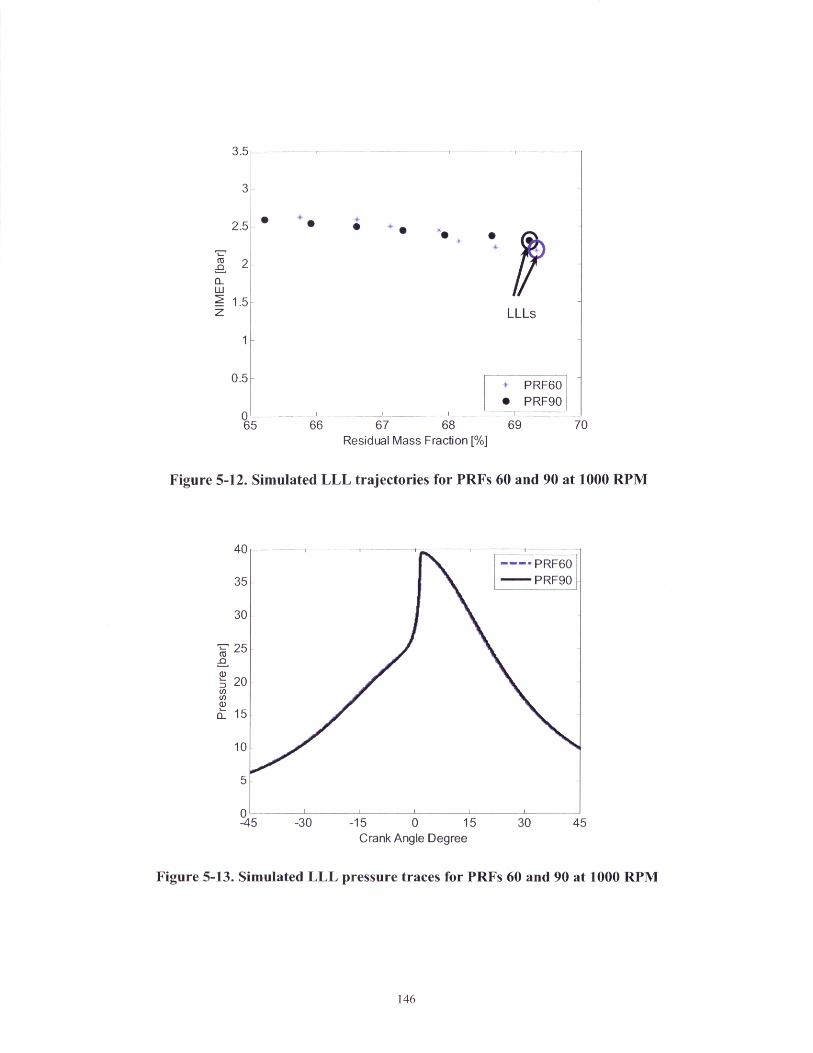
*0
Residual Mass Fraction [%]
Figure 5-12. Simulated LLL trajectories for PRFs 60 and 90 at 1000 RPM
40
35
30
S25-o
20
-15
10
5
-30 -15 0 15Crank Angle Degree
Figure 5-13. Simulated LLL pressure traces for PRFs 60 and 90 at 1000 RPM
3.5
66
66
1.5 k
0.5
LLLs
± PRF60PRF90
69
30 45

Further discussion regarding inaccuracies in the LLNL PRF chemistry model is given in sections
5.8.3 and 5.9. Because the full chemistry model cannot accurately model the LLL behavior at
1000 RPM, the effects of fuel chemistry on the LLL are discussed semi-quantitatively in the
following sections.
5.8. Effects of Engine Speed and Fuel Ignitability on The Misfire Regime
The previous analysis showed that the primary cause of an HCCI misfire was insufficient
thermal energy needed to sustain auto-ignition for multiple cycles. However, this conclusion was
reached based on data at a single engine speed and 2 fuels with similar (simulated) combustion
characteristics. In real-world operation, engines operate at multiple speeds and with a broad
range of fuels. Therefore evaluating the impact of engine speed on the in-cylinder temperature,
and the subsequent effects on the misfire limit, is important. Additionally, evaluating the impact
of changes in combustion phasing, which occur as fuel chemistry alters the ignition delay, is also
necessary.
Two variables were critical to explaining the cause of a misfire cycle in an HCCI engine. These
variables were the steady-state temperature at Ovc (or 30 CAD BTC) and the fire/misfire
temperature. Therefore, in order to understand how engine speed and fuel chemistry affect the
cause of an HCCI misfire and the subsequent impact on the LLL, the impact of each of these
variables on the steady-state and fire/misfire temperatures must be determined. The effects of
engine speed and fuel ignitability on each temperature were studied independently. In studying
these effects, the primary objective was to establish the semi-qualitative relationship, or trend,
between the variables. From these trends, the overall impact of each variable on the misfire limit
can be assessed. Finally, these trends can be compared to experimental data at the LLL.

5.8.1. Engine Speed and the Fire/Misfire Line
The effect of engine speed on the fire/misfire line for a single fuel was examined first. The
fire/misfire line was computed for PRF90 at 1000 and 1500 RPM. At both engine speeds, Prve
was held constant at 1.0 bar, and Orvc was fixed at 144 CAD before top center. The results from
these simulations are shown in Figure 5-14. As the engine speed decreases, the fire/misfire line
shifts to colder temperatures, indicating that for a fixed residual fraction, a colder temperature is
required to induce auto-ignition at slower engine speeds. There are 2 competing effects on the
fire/misfire line as the engine speed changes. At slower engine speeds, there is more time for
heat transfer, leading to colder in-cylinder conditions. This would cause the fire/misfire line to
shift up to hotter temperatures to overcome the heat transfer effects. However, the reduced
engine speed also allows more time for chemical reactions because the reactions are not
quenched as quickly by the expanding cylinder volume. This would shift the fire/misfire line
down to colder temperatures because less heating would be required to induce combustion. The
result from Figure 5-14 suggests that given the currently-available heat transfer and fuel
chemistry models, the additional time available for reactions at slower speeds has a larger impact
on the fire/misfire limit than the increased time for heat transfer.
5.8.2. Engine Speed and the Steady-state Temperature
The effect of engine speed on the steady-state, in-cylinder temperature was examined next. In
order to isolate the effect of changing engine speed on the in-cylinder temperature, Wiebe
combustion models were used. With this approach, the combustion phasing can be fixed to a
specific crank angle independently of the fuel and engine speed; this is not possible when using
the detailed-kinetic model.
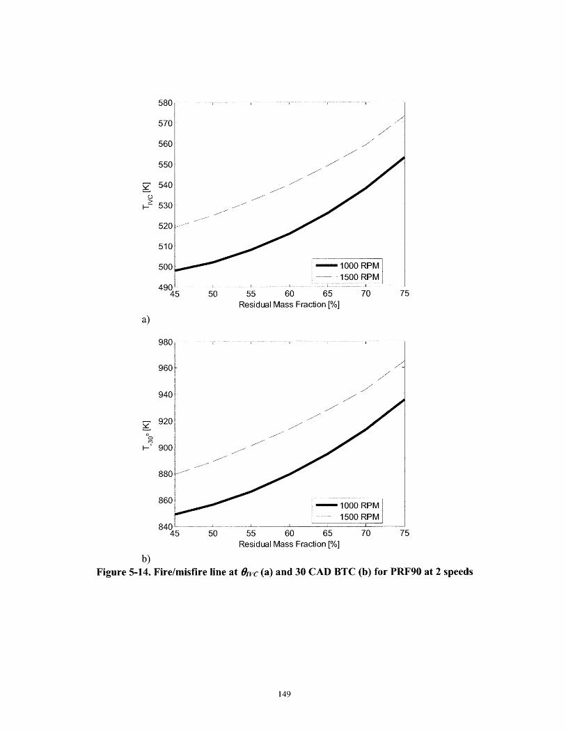
580
570
560
550
540
530
520
510
500
49045
00- 1000 RPM1500 RPM
50 55 60 65 70 75
Residual Mass Fraction [%]
b)Figure 5-14. Fire/misfire line at 0wc (a) and 30 CAD BTC (b) for PRF90 at 2 speeds
149
-~ 1000 RPM-_ 1500 RPM
50 55 60 65 70
Residual Mass Fraction [%]
980
960
940
920
900
880
860
840 -45
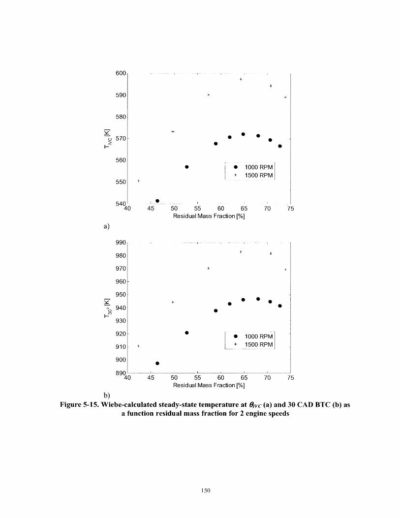
0
600
590
580
570
560
550
54040 45 50 55 60 65
Residual Mass Fraction [%]
* 1000 RPM± + 1500 RPM
45 50 55 60 65 70Residual Mass Fraction [%]
b)Figure 5-15. Wiebe-calculated steady-state temperature at Gavc (a) and 30 CAD BTC (b) as
a function residual mass fraction for 2 engine speeds
150
* 1000 RPM* 1500 RPM
990
980
970
960
950
940
930
920
910
900
89040
By holding combustion phasing constant, the change in the steady-state temperature due to
changes in heat losses can be decoupled from the effects of changes in combustion phasing that
result from changes in engine speed. Full-cycle simulations were performed in which all
parameters (e.g., intake/exhaust cam phasing, intake/exhaust pressures) were held constant, and
the speed was reduced from 1500 to 1000 RPM. The results of these simulations are shown in
Figure 5-15.
As expected, for fixed ignition timing, etc., the steady-state temperature drops as engine speed is
reduced. This occurs because there is more time available for heat transfer at slower engine
speeds, and this reduces the in-cylinder temperature. The magnitude of this drop is computed to
be slightly greater than the corresponding drop in the fuel ignition temperature. The implications
of these results are discussed in detail in section 0.5.
5.8.3. Fuel Chemistry and the Fire/Misfire Temperature
The effect of fuel chemistry on the fire/misfire line has been discussed previously. In section 5.4,
the fire/misfire lines for PRF25 and PRF90 were obtained. Quite surprisingly, the fire/misfire
lines for both fuels are nearly identical despite the vast difference in fuel ignitability between the
2 fuels in the standard octane rating tests. Furthermore, PRF25 required a slightly hotter
temperature (- 2 K) than PRF90 to induce auto-ignition. These results suggest that the chemistry
model used for building the fire/misfire line is not accurate enough to resolve the differences in
real PRFs. Further evidence of the inaccuracies in the chemistry model can be seen in Figure
5-16. In this figure, the pressure profiles for PRF90 and PRF60 at 1000 RPM are shown from
detailed-kinetic simulations in which TIvc (514 K), Pivc (0.99 bar), and the residual mass fraction
(47%) were held constant, thus isolating the effect of fuel chemistry. PRF60 exhibited later
combustion phasing by less than I CAD. A similar inaccuracy in the PRF chemistry models has
been noted before: in shock tube experiments, the PRF chemistry model overpredicts the ignition
delay for PRF 100 by approximately 25% at 1000 K for 0 = 1 mixtures in air at 40 bar [64].
Comparing the experimental pressure traces for each fuel at constant IVC conditions is difficult
because it is impossible to force the conditions at rzvc to be identical for both fuels. However, a
potential surrogate for this comparison is examining the combustion phasing of two fuels at
constant valve timing. In such a case, the conditions at Ovc will not be identical for two fuels due
to subtle variations in combustion phasing, and the subsequent effects on residual gas fraction,
etc. Nevertheless, this approach facilitates a comparison of two fuels with "similar" conditions at
Ovc.
The experimental pressure traces for PRFs 60 and 90 at 1000 RPM and equivalent valve timing
are shown in Figure 5-17. Here, OEVC was set to 105 CAD before top center, and O-vc was set to
141 CAD before top center. Both fuels exhibit significantly different combustion phasing:
PRF60 ignited significantly earlier (- 10 CAD) than PRF90, thus causing the large difference in
the peak pressure between the fuels. These results, and the 1000 RPM LLL simulations, provide
further support that the chemistry model cannot accurately capture the combustion
characteristics of real PRFs in an HCCI engine.
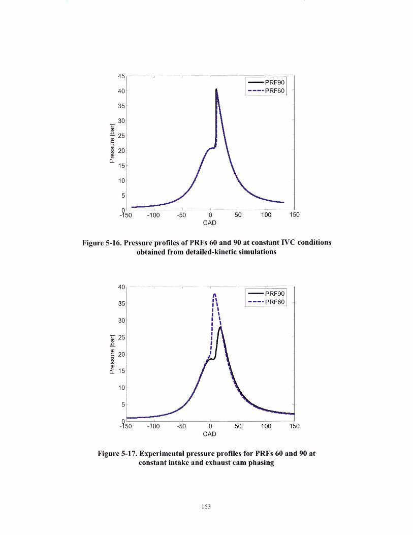
[ PRF90PRF60
-100 -50 0 50 100CAD
Figure 5-16. Pressure profiles of PRFs 60 and 90 at constantobtained from detailed-kinetic simulations
40 --
35 ---- PRF1
30 i
~' 25ca
20,
15
-100 -50 0CAD
IVC conditions
00,
50 100 150
Figure 5-17. Experimental pressure profiles for PRFs 60 and 90 atconstant intake and exhaust cam phasing
153
30[
25
20
15
10
5
0-150 150

Given the inability of the chemistry model to resolve the differences in PRFs, the effect of fuel
chemistry on the fire/misfire line is discussed here conceptually. One would expect the
fire/misfire line to shift vertically based on fuel ignitability. That is, for a fixed residual fraction,
the fire/misfire temperature should be hotter for a fuel that is more resistant to auto-ignition (e.g.,
PRF90 vs. PRF60). This trend is demonstrated in cartoon form in Figure 5-18. Additionally, one
could imagine that the effect of residual fraction on the fire/misfire line for different fuels could
vary. For example, the slope of the fire/misfire line could be altered by fuel chemistry. A more
auto-ignition resistant fuel could potentially require more relative heating at larger residual
fractions than a fuel that is more susceptible to auto-ignition. This trend is also demonstrated in
cartoon form in Figure 5-19. While these trends are merely hypothetical examples, clearly one
would expect fuel ignitability to have some impact on the fire/misfire line. These examples offer
some possible scenarios of these effects.
- easy-to-ignite fuel
---- hard-to-ignite fuel
Residual Mass Fraction [%]
Figure 5-18. Cartoon showing the effect of fuel ignitability on the fire/misfire limit
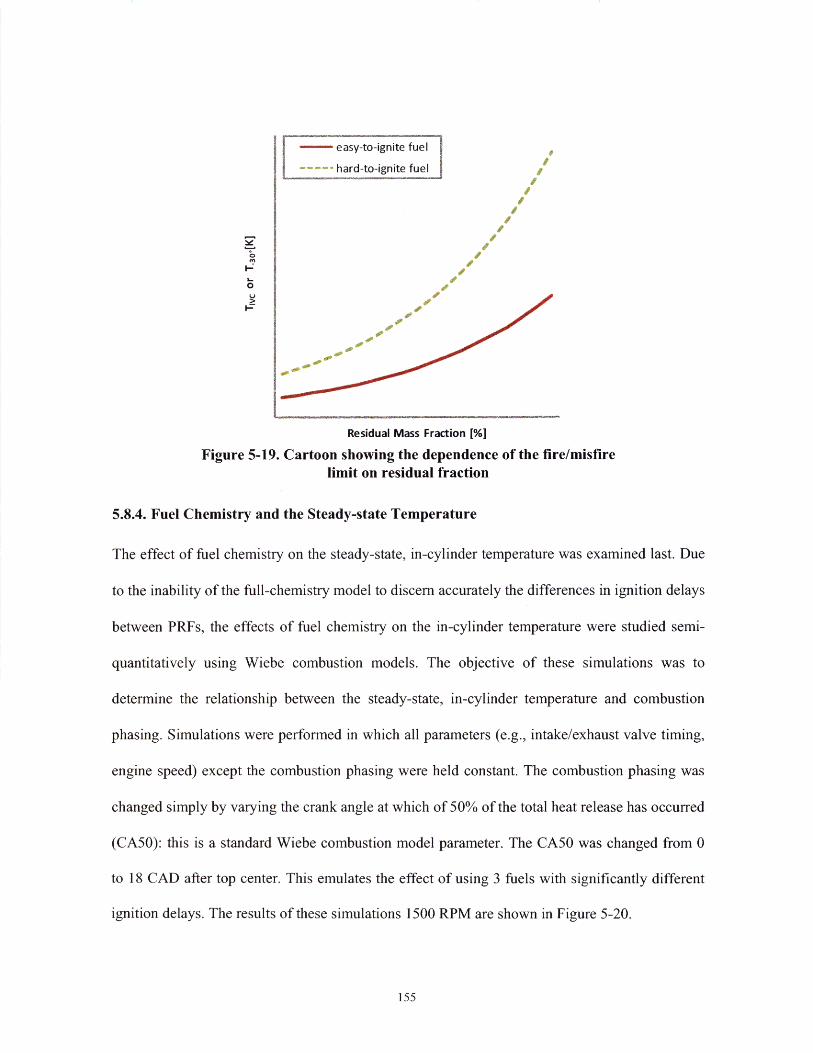
easy-to-ignite fuel
. hard-to-ignite fuel
0
Residual Mass Fraction [%]
Figure 5-19. Cartoon showing the dependence of the fire/misfirelimit on residual fraction
5.8.4. Fuel Chemistry and the Steady-state Temperature
The effect of fuel chemistry on the steady-state, in-cylinder temperature was examined last. Due
to the inability of the full-chemistry model to discern accurately the differences in ignition delays
between PRFs, the effects of fuel chemistry on the in-cylinder temperature were studied semi-
quantitatively using Wiebe combustion models. The objective of these simulations was to
determine the relationship between the steady-state, in-cylinder temperature and combustion
phasing. Simulations were performed in which all parameters (e.g., intake/exhaust valve timing,
engine speed) except the combustion phasing were held constant. The combustion phasing was
changed simply by varying the crank angle at which of 50% of the total heat release has occurred
(CA50): this is a standard Wiebe combustion model parameter. The CA50 was changed from 0
to 18 CAD after top center. This emulates the effect of using 3 fuels with significantly different
ignition delays. The results of these simulations 1500 RPM are shown in Figure 5-20.
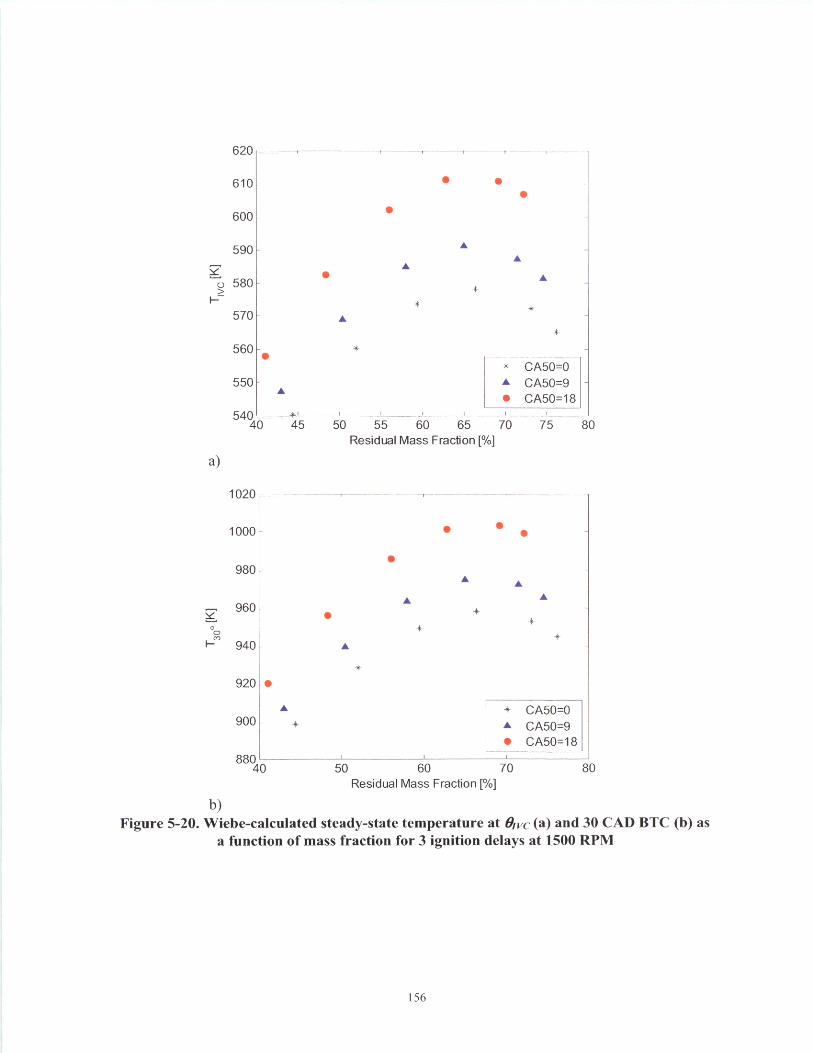
0 0
* CA50=0A CA50=9* CA50=18
_I.. ... . . I . ... II.... .... . . . .
50 55 60 65 70 75 80Residual Mass Fraction [%]
CA50=0A CA50=9* CA50=18
60 70Residual Mass Fraction [%]
b)Figure 5-20. Wiebe-calculated steady-state temperature at avc (a) and 30 CAD BTC (b) as
a function of mass fraction for 3 ignition delays at 1500 RPM
156
620
610
600
590
580
570
560 -
550 [
540' -*'40 45
1020
1000
980
960
940
920 *
900
880 -40
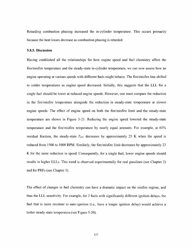
Retarding combustion phasing increased the in-cylinder temperature. This occurs primarily
because the heat losses decrease as combustion phasing is retarded.
5.8.5. Discussion
Having established all the relationships for how engine speed and fuel chemistry affect the
fire/misfire temperature and the steady-state in-cylinder temperature, we can now assess how an
engine operating at various speeds with different fuels might behave. The fire/misfire line shifted
to colder temperatures as engine speed decreased. Initially, this suggests that the LLL for a
single fuel should be lower at reduced engine speeds. However, one must compare the reduction
in the fire/misfire temperature alongside the reduction in steady-state temperature at slower
engine speeds. The effect of engine speed on both the fire/misfire limit and the steady-state
temperature are shown in Figure 5-21. Reducing the engine speed lowered the steady-state
temperature and the fire/misfire temperature by nearly equal amounts. For example, at 65%
residual fraction, the steady-state T1ic decreases by approximately 25 K when the speed is
reduced from 1500 to 1000 RPM. Similarly, the fire/misfire limit decreases by approximately 23
K for the same reduction in speed. Consequently, for a single fuel, lower engine speeds should
results in higher LLLs. This trend is observed experimentally for real gasolines (see Chapter 2)
and for PRFs (see Chapter 3).
The effect of changes in fuel chemistry can have a dramatic impact on the misfire regime, and
thus the LLL sensitivity. For example, for 2 fuels with significantly different ignition delays, the
fuel that is more resistant to auto-ignition (i.e., have a longer ignition delay) would achieve a
hotter steady-state temperature (see Figure 5-20).
157
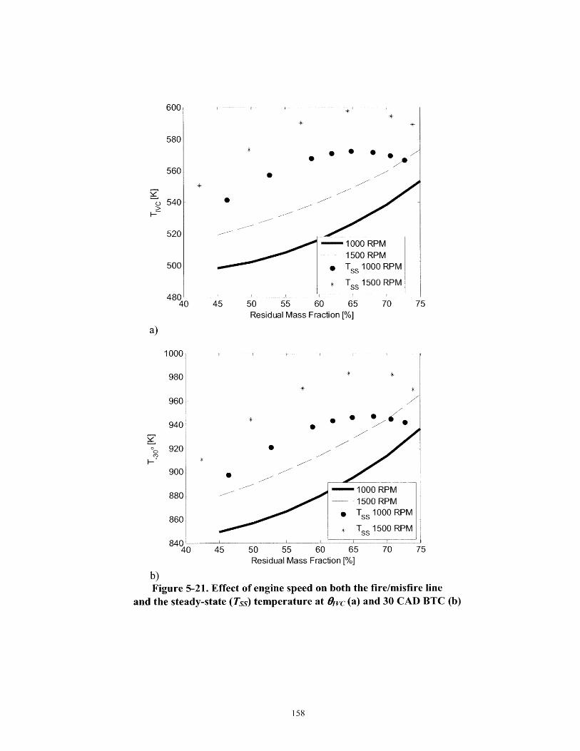
600 1 r
580
560
S540
520- 1000 RPM
1500 RPM500 * Tss 1000 RPM
Tss 1500 RPM
48040 45 50 55 60 65 70 75
Residual Mass Fraction [%]
a)
1000
980
960
* *940 *
0 920
900
- 1000 RPM880 - 1500 RPM
860 Tss 1000 RPM
* Tss 1500 RPM
840140 45 50 55 60 65 70 75
Residual Mass Fraction [%]
b)Figure 5-21. Effect of engine speed on both the fire/misfire line
and the steady-state (Tss) temperature at 0Iwc (a) and 30 CAD BTC (b)
However, the fire/misfire temperature for that fuel would also shift to hotter temperatures,
because more heating would be required to overcome the fuels auto-ignition resistance. This
could significantly alter the intersection point of the fire/misfire line and the steady-state
temperature curve. This trend is shown in cartoon form in Figure 5-22. The degree to which this
shift occurs could also potentially vary. For example, the fire/misfire line for the more auto-
ignition resistant fuel could shift relative to the steady-state temperature such that the
intersection of the 2 curves falls near the maximum in steady-state temperature. This trend is
shown in Figure 5-23.
Finally, in an extreme case, the fire/misfire curve for the more auto-ignition resistant fuel could
lie very close to the steady-state temperature curve (see Figure 5-24). Because operation near the
fire/misfire boundary cannot be sustained for multiple cycles, the fuel could potentially misfire at
significantly smaller residual fractions than the more auto-ignition resistant fuel. As the
intersection of the fire/misfire and steady-state temperature curves shifts, the change in the
residual fraction at the misfire point can be large (note the change in Ax,, from Figure 5-22 to
Figure 5-24). This would drastically alter the LLL. It is possible that the situation demonstrated
in Figure 5-24 occurs experimentally at 1000 RPM for PRF60 and PRF90. However, this trend
cannot be confirmed quantitatively due to the failure of the chemistry model to distinguish PRFs
and the inability to verify the experimental, in-cylinder temperature.
Heat transfer effects could also shift the misfire regime in similar ways as those of fuel
chemistry. For example, heat losses are expected to affect the steady-state temperature more than
fire/misfire temperature, because most of the heat losses occur after combustion.
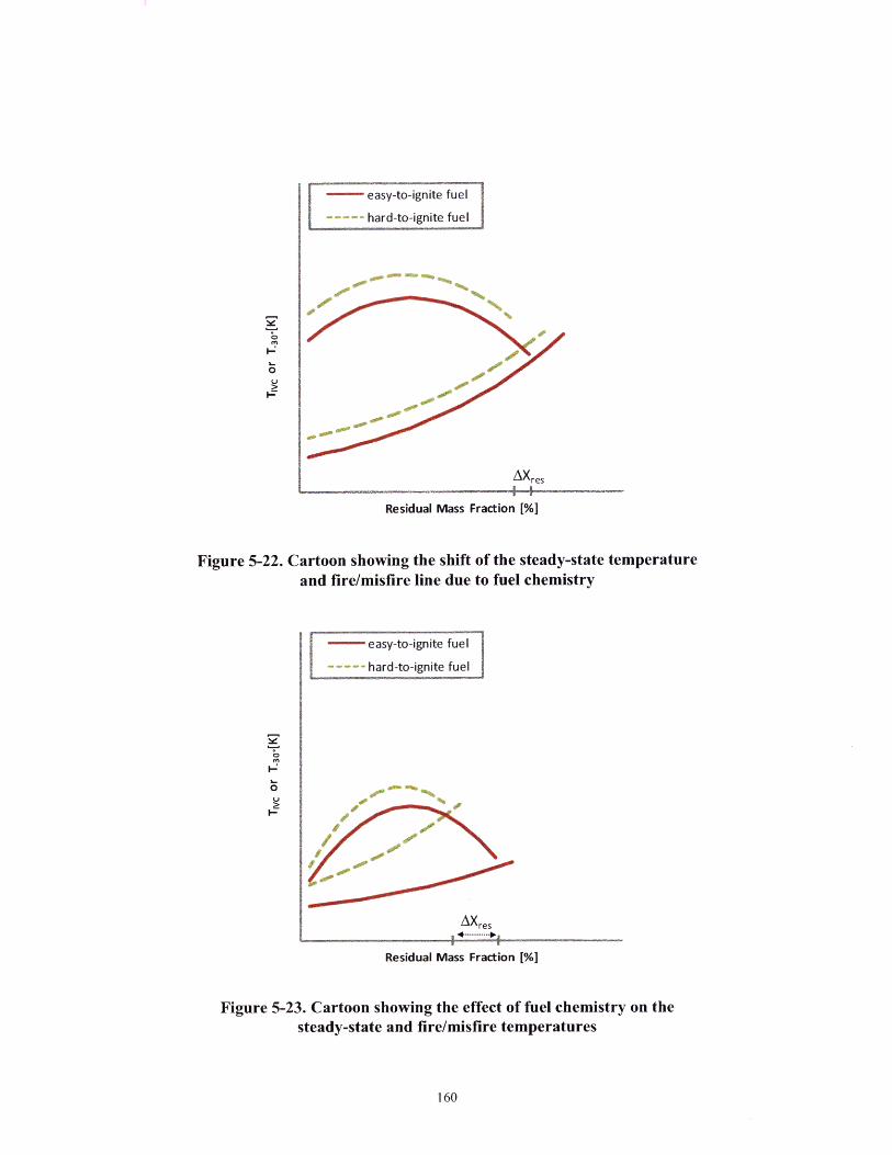
- easy-to-ignite fuel
---- hard-to-ignite fuel
AXres
Residual Mass Fraction [%]
Figure 5-22. Cartoon showing the shiftand fire/misfire line due
of the steady-state temperatureto fuel chemistry
easy-to-ignite fuel
--.- hard-to-ignite fuel
AXres
Residual Mass Fraction [%]
Figure 5-23. Cartoon showing the effect of fuel chemistry on thesteady-state and fire/misfire temperatures
160
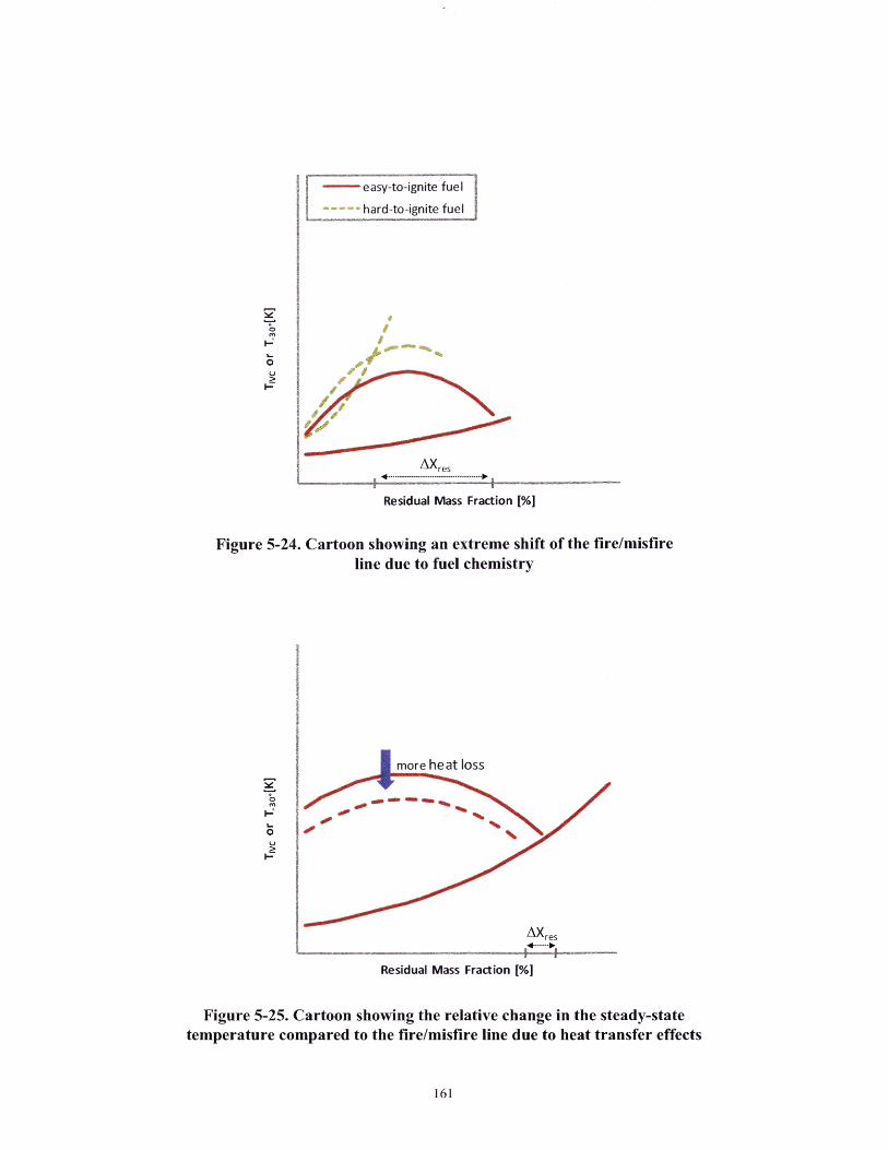
- easy-to-ignite fuel
- hard-to-ignite fuel
I-O
0.
I-
AX es
Residual Mass Fraction [%]
Figure 5-24. Cartoon showing an extreme shift of the fire/misfireline due to fuel chemistry
AXres
Residual Mass Fraction [%]Residual Mass Fraction [%]
Figure 5-25. Cartoon showing the relative change in the steady-statetemperature compared to the fire/misfire line due to heat transfer effects

Therefore, changes in the engine wall temperature or heat transfer will shift the steady-state
temperature up and down relative to fire/misfire temperature, thus causing the point of
intersection to move to different residual fractions. These effects are illustrated in cartoon form
in Figure 5-25. The impact on the change in the LLL is similar to how fuel chemistry alters the
LLL behavior.
5.8.6. Comparison with Experimental Data
The effect of fuel chemistry on the misfire regime discussed above could potentially be the cause
of the experimental trend in the LLLs of PRFs 60 and 90 at 1000 RPM, as observed in Chapter 3.
At this speed, PRF60 achieved a lower LLL by approximately 1.04 bar NIMEP (-30%) than
PRF90: even though the residual fraction, and also presumably the temperature, were more
favorable for early ignition in the PRF90 LLL operating conditions. Furthermore, PRF90 ignited
significantly later (- 5 CAD) than PRF60. As shown in Figure 5-20, this would have caused the
steady-state temperature for PRF90 to be hotter for a given residual fraction. However, as shown
in Figure 5-22 to Figure 5-24, or alternatively in Figure 5-25, the fire/misfire line (or steady-state
curve) could also have moved in such a way as to cause PRF90 to achieve a higher LLL at this
engine speed. The scenarios in these figures offer a potential explanation to the observed
experimental trend at 1000 RPM.
At 1500 and 2000 RPM, PRFs 60 and 90 achieve similar experimental LLLs (see Chapter 3).
However, at these engine speeds, both fuels have nearly equal ignition delays. This is believed to
be caused by hotter, in-cylinder conditions at higher engine speeds as a consequence of reduced
time for heat transfer. This effect was observed semi-quantitatively in Figure 5-15. The hotter in-
cylinder conditions contribute to smaller differences in ignition delays among the fuels. This

effect has been observed experimentally in shock tubes by Fieweger, Blumenthal, and Adomeit
[31 ]. The similarities in the experimental LLLs of PRFs 60 and 90 at the higher engine speeds (>
1500 RPM) are consistent with the cause of a misfire discussed in section 5.6 (i.e., 2 fuels with
similar ignition delays achieved nearly equal LLLs).
5.9. Modeling Uncertainties
Several modeling uncertainties make studying the LLL phenomenon difficult. A very brief
review of some of the large uncertainties in the modeling approach is discussed here. Methods of
reducing these errors are also outlined. The inaccuracies in the chemistry model were discussed
in detail in sections 5.4 and 5.8.3. These errors make studying fuel effects (with these
mechanisms) on the LLL difficult because the model does not accurately represent the true large
differences in fuel ignitability. However, addressing the errors in the chemistry model was
beyond the focus of this project. Accurately modeling the heat transfer from the in-cylinder
gases to the cylinder walls is also very difficult. Errors in the heat transfer model result in less
accurate estimates of the in-cylinder temperature. Fortunately, errors in the heat transfer
estimates can be minimized by using accurate heat transfer correlations, such as those of Chang
et al. [63]. However, even these most accurate heat transfer correlations have quoted
uncertainties of approximately + 20%, which could cause shifts in the computed steady-state
Trvc up to approximately 40 K. Due to the unconventional (relative to SI engines) cam phasing
(i.e., NVO) and profiles (i.e., 2 mm lift, 120 CAD durations) in the model (and experimental)
engine, WAVE struggled to simulate accurately the flows across the intake and exhaust valves.
Furthermore, the acoustics in the experimental intake port were difficult to replicate in WAVE.
These 2 factors produce significant (-5%) errors in the estimates of the in-cylinder mass and up
to 10% errors in the predicted NIMEP. The uncertainties in the mass flows and our lack of
knowledge of the temperature and compositional inhomogeneities within the cylinder make it
very difficult to infer the actual time-temperature history seen by the igniting fuel parcels in the
engine, even though we have measured detailed pressure traces. There are also some substantial
uncertainties and slow drifts in the experimental engine data (presumably due to changes in the
mass flows through the valves), which are particularly problematic when comparing data
measured months apart, as discussed in Chapters 2 and 3. For the work presented here, these
errors were not critical, because they affect absolute quantities, and this work focused on semi-
quantitative relationships (e.g., trends).
5.10. Conclusions
This work identifies the primary cause of a misfire in an HCCI engine. The conclusions reached
here were drawn from detailed-kinetic simulations of the LLL of HCCI operability. Empirically
based combustion models (i.e., Wiebe functions) were also used to establish trends describing
the effects of fuel chemistry and engine speed on the misfire regime. These results provide
researchers with a qualitative means for estimating how fuel chemistry and engine operating
conditions affect the LLL.
The LLL limiting mechanism was studied with two types of simulations: closed-cycle and full-
cycle. The closed-cycle (from IVC to EVO) simulations were performed to identify the
minimum temperature required to initiate auto-ignition for a single engine cycle at a fixed Pivc
and residual mass fraction. A series of temperatures were identified for a range of residual mass
fractions spanning 55 to 75%. This data comprised the fire/misfire line for a given fuel. A
deviation of I K below the fire/misfire line resulted in an engine misfire. The results from
MITES indicated that as residual fraction increased, the temperature required to bum the fuel
also increased. This was a consequence of lower reactant (fuel and oxygen) concentrations and
higher mixture heat capacities from the excess CO2 and H20 in the residual gases.
Full-cycle simulations were performed to identify the trends relating the steady-state residual
mass fraction to the in-cylinder temperature at Ovc (or 30 CAD BTC). Increasing the residual
fraction had 2 competing effects. Trapping more hot combustion products increased the
temperature of the trapped mixture. However, larger residual fractions led to smaller fractions of
fuel in the cylinder, which resulted in lower combustion temperatures and consequently colder
residuals. These competing effects cause the in-cylinder temperature to go through a maximum
as residual fraction is increased. Near the misfire limit, the conditions in the cylinder are such
that increasing the residual fraction cools the trapped mass.
Comparing the closed-cycle results with the data from the steady-state simulations provided
insight on the mechanism limiting HCCI misfire. As the residual fraction is increased to reach
the LLL, the in-cylinder temperatures approached the fire/misfire line quite closely (to within 14
K according to the engine model). These results suggest that the primary cause of an HCCI
misfire is insufficient thermal energy needed to sustain auto-ignition for multiple cycles. The
limiting mechanism was found to be independent of fuel ignitability at 1500 RPM. At this speed,
the variation of the computed LLLs among PRFs 25, 60, and 90 was only 0.05 bar NIMEP,
which was consistent with experimental data for PRF60 and PRF90. This, along with data from
the market fuel study (Chapter 2), confirms that at 1500 RPM the LLL is not sensitive to the
fuel.

However, at 1000 RPM the experimental LLL for PRF90 was unexpectedly high. The existing
chemistry model is not adequate to explain this observation. A similar failing of the PRF
chemistry model had been previously noted in the literature. We propose that at this low engine
speed, the in-cylinder temperature in our experiment has dropped into a range where ignition
delays of different fuels become noticeably different. Quantitative tests of this proposal will
require precise determination/modeling of several engine parameters as well as more accurate
chemistry models.
Wiebe simulations confirmed that a reduction in engine speed resulted in colder, steady-state
temperatures. Consequently, differences in fuel chemistry were more apparent at slower engine
speeds. Experimental results with PRFs 60 and 90 exhibited this trend across a speed range of
1000 to 2000 RPM. Due to the inability of the chemistry model to distinguish the combustion
characteristics of PRFs, Wiebe-based simulations were also used to examine fuel effects on the
LLL. Fuels with longer ignition delays showed hotter steady-state and misfire-limit
temperatures. However, each temperature was affected to a different degree. Consequently, the
relative shift of each temperature ultimately determined the impact of fuel chemistry on the LLL.
6. FINAL CONCLUSIONS AND RECOMMENDATIONS
6.1. Final Conclusions
Within the range of commercial variations in gasoline properties, the viable HCCI operating
range is not significantly affected by fuel chemistry. The sensitivity of the HCCI operating range
to fuel chemistry is an important aspect towards the potential commercialization of HCCI engine
technology. If large, fuel companies would potentially be forced to blend a dedicated fuel for
HCCI engines, thus placing a strain on the current liquid fuel infrastructure, or automotive
companies would possibly be required to alter significantly their current engine calibration
procedures to counteract the fuel effects. Thus, our demonstration of the insensitivity to fuel
chemistry makes the future deployment of HCCI engines more feasible.
The primary cause of a misfire cycle in an HCCI engine, and thus the limiting mechanism for the
LLL, was established through simulations. MITES was used to establish the functional
relationship for the initial, in-cylinder temperature and the residual fraction for 2 scenarios: 1)
full-cycle, steady-state conditions, 2) closed-cycle (i.e., IVC to EVO) conditions. The closed-
cycle simulations were used to determine the minimum temperature (Tmi,,,je) required to induce
auto-ignition for a single engine cycle. The results from the closed-cycle simulations were
compared with the steady-state temperatures (T,.,) from the full-cycle simulation. Near the
misfire limit, T., approached T,,,,ji, quite closely (to within - 14 K), suggesting that the primary
cause of a misfire in an HCCI engine is insufficient thermal energy need to sustain combustion
for multiple cycles.
167

The misfire regime is affected by both the engine speed and fuel chemistry. At slower engine
speeds, there is increased time for heat transfer, which reduces T,. The colder in-cylinder
conditions allow fuel effects to be more apparent. This was observed experimentally with PRFs
60 and 90. At 1000 RPM, PRF60 obtained a substantially lower (-30%) LLL than PRF90.
However, at engine speeds > 1500 RPM, both fuels obtained similar LLLs to within
experimental uncertainty. At slower speeds, when fuel effects can be important, fuel ignitability
affects both T, and T,,i,,,-e. T, increases for more auto-ignition resistant fuels (i.e., longer
ignition delays) due to reduced heat transfer as a result of retarded combustion. Unfortunately,
the effects of fuel chemistry on Ti,,sfire could not be quantitatively assessed, due to inaccuracies in
the PRF mechanism. However, fuel chemistry could potentially affect T,,,;,._ to a greater or less
degree than Ts. The relative movement of these temperatures determines the extent to which fuel
chemistry impacts the LLL.
6.2. Recommendations
In addition to testing the sensitivity of the HCCI operating range to market gasoline variations, a
secondary goal of the market-fuel experiments was to find a set of chemical properties that
expanded the HCCI operating range and to use those species to design an optimal fuel for HCCI
operation. However, the experimental results showed that the fuel ignitability did not
significantly impact HCCI operation, particularly the LLL. Therefore, if the fuel chemistry
cannot be leveraged to expand the HCCI envelope, hardware changes to the engine should be
considered. In that respect, one possibility would be to redesign the experimental setup to
include direct injection and a fully-variable valve train. Several control strategies (e.g., multiple
injections, injections during the NVO) can be used in a direct injection engine that are not
168

possible with a port fuel injection engine. Furthermore, the use of a fully-variable-valve-timing
(FVVT) mechanism (e.g., hydraulic valve train) would allow for changes in both valve-open
duration and closing angle, thus offering a greater degree of freedom for possible operating
range extension. With the current setup, only changes in closing angle are possible.
The accuracy of the LLNL PRF mechanism for HCCI simulations should be evaluated. Currently
the model cannot accurately distinguish combustion phasing trends observed in real PRFs.
However, if accurate measurements of the experimental residual fraction, in-cylinder
temperature, and heat transfer were available, it would be possible to isolate the errors in the
chemistry model in a simulation. Current simulation errors may arise from any or all of the
variables (i.e., residual fraction, temperature, and heat transfer estimates), among others. Without
experimental data to confirm any of the predicted quantities, isolating the errors to any particular
variable is impossible. Obtaining more accurate chemistry models for PRFs, and ultimately real
gasolines, will allow for a more quantitative analysis of fuel effects.
The HCCI operating range is currently too small to allow for a dedicated HCCI engine.
Therefore, future work should also focus on the potential hybridization of an HCCI engine with
an SI or Diesel engine. The hybridization process will require fast and timely switches between
combustion modes. For these switches to be made with minimal impact on drivability, accurate
sensors (e.g., knock and/or misfire sensors) and control strategies will be required. Future work
in these areas could have a significant impact on commercializing an SI/HCCI or CI/HCCI
hybrid.
169

7. PH.D. CEP CAPSTONE: FINANCIAL INCENTIVES TO IMPLEMENTING
DUAL-MODE SI/HCCI VEHICLES
7.1. Executive Summary
The objective of this work is to examine the incentives to both consumers and manufacturers for
purchasing and producing dual-mode, spark-ignition/homogenous-charge compression-ignition
(SI/HCCI) vehicles. The financial payback period for these automobiles is calculated to estimate
consumers' incentives. The results show that stoichiometric, SI/HCCI vehicles have payback
periods of 3 - 4 years, which is as short or shorter than any of the hybrid-electric vehicles (HEV)
examined. The payback period for lean, SI/HCCI hybrids is dependent upon the lean NOx after
treatment system used. Vehicles employing selective catalytic reduction (SRC) systems have
similar payback periods to stoichiometric SI/HCCI hybrids, while those using lean NOx traps
(LNTs) have payback periods ranging from 7 to 13 years, which is generally longer than HEV
paybacks. The long payback periods for LNT-dual-modes is a product of the expensive precious
metal catalysts required for LNTs. The manufacturers' incentive to produce the SI/HCCI
vehicles was estimated by calculating the increase in manufacturing cost per mile per gallon
improvement in fuel economy ($/MPG). The small increase in manufacturing cost for the
stoichiometric, dual-model vehicles meant their $/MPG improvement was the best of any fuel
savings configuration. Lean dual-mode vehicles that use SCRs are more expensive on a $/MPG
basis than their stoichiometric counterparts but are still cheaper than HEVs. Lean SI/HCCI
vehicles employing LNTs are the most expensive for the manufacturers on a $/MPG basis. The
combined results of this project demonstrate that stoichiometric and lean-SCR dual-mode,
SI/HCCI vehicles are a viable economic option for both consumers and vehicle manufactures.
7.2. Background and Motivation
In 2005, the global demand for energy reached 230 million barrels per day of oil equivalent
(MBDOE), which primarily consisted of fossil fuels. For example, approximately 87.5 MBDOE
(38%) consumed were from oil alone, and approximately 194 MBDOE (84%) were from oil,
gas, and coal combined. The total global energy demand is expected to grow by as much as 40%
by 2035 [73]. Meeting this growing demand represents a great challenge. As a means for helping
to mitigate the difficulties that lie ahead, much attention has been turned to the transportation
sector. While power generation is currently the largest consumer of energy globally,
transportation comprises approximately 20% (44 MBDOE) of global energy demand [73].
Therefore, by targeting the transportation sector as an area for reducing energy consumption, a
potentially significant dent can be placed in the global energy demand.
A major push to reduce transportation energy demand came in December 2007 when U.S.
President George W. Bush signed into law new Corporate Average Fuel Economy (CAFE)
standards as part of the Energy Independence and Security Act of 2007 [74].The new laws,
modified for the first time since 1975, require automotive companies to raise fuel economy to 35
miles per gallon by 2020. Prior to the new laws, the CAFE standard for cars was approximately
27.5 miles per gallon and slightly more than 22 miles per gallon for light trucks; the new
standard represents an approximately 40% reduction in fuel consumption over the old laws.
Automotive companies face a significant challenge in complying with the new laws. However,
they are not without some ammunition, even without considering alternative technologies, such
as hybrid electric vehicles (HEVs). The California Energy Commission [75] recently released a
report showing the cost and benefit of some technological improvements to traditional (i.e., non-
hybrid) automobiles that will improve fuel economy. For example, reducing the drag coefficient
and rolling resistance of vehicles by 10% can improve fuel economy by approximately 4.2% and
would cost only $45. Other, more complex, improvements include moving to lean, direct-
injection engines, which can improve fuel economy by 12.5% but cost more - approximately
$600. Finally, HEVs represent an option for reducing fuel consumption, but introducing the
systems required to hybridize an automobile come with a significant cost penalty; integrating a
300V system into a vehicle can cost as much as $4400.
The "magic bullet" automotive companies are seeking will be both inexpensive and highly
effective. In order to be inexpensive, the technological enhancements to traditional internal
combustion engines (ICEs) must be somewhat minor (in contrast to adding a hybrid-electric
drive system). One such technology that offers these benefits is homogenous-charge,
compression-ignition, or HCCI, combustion. The technology used to implement HCCI
combustion is largely in-use in the automotive fleet today, and HCCI has to potential to provide
up to a 15-20% improvement in fuel economy.
7.2.1. What is HCCI?
A detailed discussion of the methodology and benefits of HCCI is provided in Chapter 1, but a
brief review is provided here. HCCI is a new method (first demonstrated in the 1970s) of burning
fuel in ICEs that combines aspects of traditional spark-ignition (SI) and compression-ignition
(CI, or more commonly Diesel) engine technologies. In an SI engine, the fuel is usually injected
into the intake manifold just upstream of the cylinder. Then, when the fuel and air are drawn into
the cylinder, the fuel and air mix thoroughly. This mixing process ensures that the fuel is evenly
distributed throughout the cylinder. This mixture of fuel and air is then compressed an ignited
with a spark plug. In contrast, in a Diesel engine, the fuel is injected directly into the engine
cylinder. Prior to fuel injection, a mass consisting only of air is compressed to high temperatures
and pressures. When the fuel is then injected into this hot air mass, the fuel begins to auto-ignite
without the assistance of a spark plug. However, because the fuel does not have a lot of time to
mix with the air before ignition, there are regions within the cylinder that have very high local
fuel concentrations - these lead to the soot formation. In the HCCI process, the fuel and air are
premixed prior to combustion, like in an SI engine, but the mixture is ignited through
compression, like in a Diesel engine. This allows HCCI engines to achieve emission levels
similar to SI engines (i.e., low soot), while obtaining the fuel economy similar to Diesels (i.e.,
about 15-20% better than SI engines).
In addition to the fuel economy benefits of HCCI engines, an alternative advantage that is
attractive to automotive companies is that no radically new engine hardware is required in order
to initiate HCCI combustion. In theory, this means automotive companies can implement HCCI
combustion in their fleets for relatively low cost compared HEVs. However, HCCI technology is
not without its shortcomings. For example, the combustion process is not nearly as robust as
traditional SI or Diesel combustion, making things like speed and engine load transitions
difficult within the HCCI combustion regime. Also, cold starts are problematic in HCCI engines,
because some heat from earlier engine cycles is needed to achieve ignition. Finally, probably the
biggest hurdle HCCI technology faces for becoming a wide-spread commercial technology is its
limited operating range. As shown below in Figure 7-1, the HCCI operating range is
approximately one-eighth the size of the SI operating range. For this reason, many researchers

and automotive companies feel that HCCI technology will likely be implemented in a dual-
mode, SI/HCCI "hybrid." The engine will run in SI-mode in portions of the operating range
where HCCI is infeasible and in HCCI-mode where possible to take advantage of fuel savings.
..Q
-J
C
wL
I SI Operating RangeHCCIOperating Range
0
Figure 7-1. T3
I I I I i 1
1000 2000 3000 4000 5000 6000 7C
Engine Speed (RPM)
ypical SI and HCCI operating ranges. Figure adapted from And
7.2.2. Objectives
The focus of this paper is to determine the financial payback period for a consumer who
purchases an SI/HCCI dual-mode vehicle. Furthermore, this work examines the cost of
implementation per unit of fuel savings that an automotive company will have to invest to
implement a dual-mode SI/HCCI engine. Looking at both the payback period for consumers as
well as the cost to vehicle manufactures will allow for a better understanding of the likelihood of
)00
reae [15
implementing HCCI technology. Both the payback period and the implementation costs will be
compared to HEV values.
7.3. Method for Determining Payback Period
The payback period of an investment is equal the number of years it takes for the predicted
future cash flows to sum to the value of the initial investment. For example, if an investment
costs $1000 in year 0, and future cash flows are $200 in year 1, $700 in year 2, and $300 in year
3, then the payback period for this project is 3 years. The advantage of the payback period
calculation is that it is simple and easy to conceptualize. Projects that have a shorter payback
period are superior to projects with longer ones. There are a few disadvantages to the payback
period approach, however. First, payback calculations ignore all future cash flows past the
payback period. For example, in the short example outlined above, if the cash flow in year 4
were -$2000, the payback period would still be 3 years. The second drawback of payback
calculations is that they neglect the time value of money. However, it is precisely because of this
reason that this analysis will use the payback period and not the more rigorous approach of net
present value (NPV). The NPV approach does take into account all cash flows and the time value
of money. However, in order to account for the time value of money, a discount rate is needed.
Estimating the appropriate discount rate for a dual-mode, SI/HCCI vehicle, each of which may
be purchased by individuals with different risk appetites, is nearly impossible. Therefore, to
make this analysis tractable, the time value of money is ignored for the simpler payback period
approach. Additionally, HEVs are often evaluated based on their payback periods (see, for
example [76]), so this analysis will allow for a direct comparison between current HEVs and a
dual-mode, SI/HCCI automobile.

The first thing needed to determine the payback period is the additional cost of a dual-mode,
SI/HCCI vehicle relative to a standard SI vehicle. Therefore, the following section discusses the
technologies necessary to make a SI/HCCI dual-model engine possible and their associated
costs. Next, an estimate of the fuel savings for the automobile is required. A detailed discussion
of these estimates is provided in section 7.5. Finally, an estimate of the future cost of gasoline is
required. This is arguably the most difficult quantity to estimate, and the estimates can have
dramatic impacts on the payback period. A detailed discussion of the estimation technique for
gasoline prices is provided in section 7.6. Once all these estimates are obtained, the initial added
cost of producing a dual-mode SI/HCCI vehicle relative to a standard SI vehicle can be
compared to the fuel savings (in dollars) to determine the payback period. In all of the payback
period calculations, the dollar values are the costs to consumers who would purchase the
vehicles.
7.4. Technologies Required to Implement an SI/HCCI Dual-mode Engine
Because the HCCI process is so new relative to its SI and Diesel cousins, there is currently no
standard method of inducing HCCI combustion. For example, HCCI has been implemented with
a multitude of engine hardware: variable compression ratio mechanisms [77]; intake air heaters
[78]; and variable valve timing devices to induce negative valve overlap [20], just to name a few.
Further adding to the variability is the fuel source; HCCI research has been performed with a
vast number of fuels including gasoline, Diesel fuel, methanol, ethanol, and natural gas. Each of
these variations requires different technologies, making the evaluation of potential costs to
implement HCCI commercially difficult. Therefore, in order to make this study more tractable,
176
this work will focus on only one type of HCCI combustion: port-fuel injected, gasoline HCCI
induced via negative valve overlap. In order to run an HCCI engine in this fashion, certain
technologies are required. These technologies and their importance to the HCCI process are
reviewed in the following paragraphs.
7.4.1. Ion Current Sensors
One of the major challenges facing HCCI engines is that there is no direct control over
combustion phasing. Combustion simply occurs whenever the gases inside the cylinder reach
their auto-ignition point. Therefore, in order to have some knowledge about when combustion is
happening (if at all), a measuring device is needed inside the cylinder. In research laboratories,
researchers generally install pressure sensors inside the firing cylinders. However, these pressure
sensors are expensive, and for greater accuracy (i.e., higher crank-angle and pressure resolution),
the price quickly escalates. Vehicle manufactures would prefer a device that provides similar
information but at a fraction of the cost. Such an alternative exists in ion current sensors.
Ionization probes have been used in combustion research since 1934 [79] and are now even
being used in production models to detect misfires [80] and engine knock [81].
The ion current sensor is an electrode (i.e., a spark plug) to which a small voltage is applied; the
voltage is low enough not to induce a spark. When a flame occurs during combustion, ions are
formed, and they flow towards the electrode. The flow of the ions creates a current, which in-
turn creates a voltage drop across a serially, connected fixed resistance. The voltage drop is
recorded by a data acquisition system, and this signal can be processed to gain a host of
information about the gases inside the cylinder. Critical to HCCI combustion, ion current sensors
177
can be used to estimate the timing of combustion. Attard and Micallef [82] showed that the 50%
mass fraction burned location can be estimated to within 0.1 crank angle degree (CAD) with
99.7% confidence. Their work also demonstrated a strong correlation between the location of
50% of the cumulative ion current signal and the location of peak pressure and peak heat release.
Ion current sensors can also be used to measure the air/fuel ratio [83].
The biggest advantage of ion current sensors is their cost. The spark plug is used as the ion
current sensor, so SI vehicles already have the necessary hardware. Furthermore, automobiles
already have a CPU and power supply onboard, so no additional costs are necessary to power the
sensor. Therefore, for this project, the assumed cost for adding an ion current sensor to a dual-
model, SI/HCCI engine will be zero dollars (i.e., $0.00) [84].
7.4.2. Variable Valve Timing and Lift
In order to induce HCCI combustion via negative valve overlap, the engine must be equipped
with a mechanism to vary the valve timing. The valve timing must be varied for 2 reasons: 1) the
engine load in HCCI-mode is controlled by varying the amount of trapped residual gases, which
is accomplished through varying the valve timing, and 2) the valve timing in SI-mode is
significantly different than in HCCI-mode (i.e., there is no negative overlap). Adding to the
complications of varying the valve timing is the fact that in SI-mode, the valve profile also has a
vastly different lift than when in HCCI-mode. For example, the maximum valve lift in SI-mode
is generally on the order of 10 mm [85], whereas the maximum valve lift in HCCI-mode can be
as small as 2 mm [20].
178
Several devices exist for varying either the lift or valve timing, or both; however, the price for
each mechanism can vary considerably. For example, a camless, variable valve lift and timing
device designed by Lotus for research engines can cost over $500,000. Clearly, such an
expensive piece of hardware could not go into mass production vehicles. Alternatively, simple
devices are currently available that can vary the valve timing by as much as 30 crank angle
degrees. Andreae et al. [20] used such a device in their work, and these mechanisms cost on the
order of a few hundred dollars. However, these devices only vary the cam phasing (i.e., the lift is
fixed according the cam profile). One mechanism that can be used to vary both the valve timing
and lift is BMW's Valvetronic system. The system is fully mechanical, unlike the Lotus camless
valve actuation system. Valvetronic can vary the valve lift between 0 and 9.7 mm, and it can
cover the entire range in approximately 300 milliseconds, and the cam phasing can be varied by
up to 60 CAD [86].While the Valvetronic system might not be the optimal device for a dual-
mode, SI/HCCI engine, it is reasonable to assume a device such as the Valvetronic could be
used. In the payback period analysis to follow, the analysis will be done assuming the
Valvetronic system is used. The additional manufacturing cost of the Valvetronic system is
reasonable: approximately 100 Euros with a markup of between approximately 3- to 4-times.
Therefore, the retail price to customers would increase by approximately 300 to 400 Euros [87]
(or $460 to $613 at the exchange rates prevailing in June 2008).
7.4.3. Lean NOx After Treatment Systems
HCCI combustion has been researched under a variety of fuel/air equivalence ratios. Several
researchers study HCCI combustion under lean conditions. While this helps to improve the fuel
consumption benefits of the technology, it creates an additional problem: traditional 3-way
179
catalysts on SI engines only work at stoichiometric equivalence ratios. Therefore, one of the
biggest challenges for a lean HCCI system will be meeting the ever more stringent NOx
standards. Even though HCCI combustion is a low NO, producer, the emissions standards are
such that a lean NOx catalyst will still be required. However, if the dual-mode engine were
always run at stoichiometric ratios, then no additional catalyst technology will be necessary.
Currently it is unclear which mode of operation will survive to make it into commercial vehicles.
Consequently, this work will evaluate the payback periods for both a lean dual-mode engine,
which will require a lean NOx catalyst system, and a stoichiometric dual-mode engine, which
will incur no additional catalyst costs.
Researchers have recently been working on lean NO, catalysts for Diesel engines. The
technology developed for Diesel engines can effectively be "borrowed" for a lean, dual-mode
SI/HCCI engine. In the U.S., there is currently no standard, commercial lean NOx after treatment
system for Diesel engines. The two primary methods under consideration are: selective catalytic
reduction (SCR) and NO, absorbers (also known as lean NOx traps, or LNTs). The following
subsections describe each technology in greater detail and provide pricing information.
7.4.3.1. Selective Catalytic Reduction (SCR)
While SCR has not officially been adopted in the U.S., it is certainly the front runner and has
already been adopted in Europe. The SCR system uses urea to clean the exhaust via the
following reactions [88]:
Urea hydrolysis:

(NH2)2CO + H20 -, CO 2 + 2 NH3
NOx conversion:
4 NO + 4 NH 3 + 02 -- 4 N2 + 6 H20
6 N02 + 8 NH3 --- 7 N2 + 12 H20.
The above reactions occur with the help of the SCR catalyst: TiOz2-V20s-type.
The SCR system is heavily favored over LNTs because: 1) SCR systems have a proven 80-90%
effectiveness at reducing NOx emissions with open-loop control and up to 95% effectiveness
with closed-loop control; 2) SCRs work over a broad range of exhaust temperatures; 3) unlike
LNTs, SCRs are durable and do not easily lose effectiveness due to catalyst damage; 4) SCR
technology has decades of field experience in other combustion and engine applications; 5) most
importantly, SCRs have significantly lower initial costs than LNTs [89]. There are a few major
drawbacks of SCR systems. First, with SCRs an additional urea storage tank and delivery system
is required, and these systems can be quite complex (requiring items such as heated/insulated
urea storage tanks and cabin dashboard gauges and alarms) [89]. Further adding to the hurdle in
the U.S. is the fact that there is currently no major distribution system for urea like there is in
Europe. However, if SCRs were to become widely adopted, the latter problem would certainly
vanish.
As mentioned previously, one of the biggest advantages of SCRs is their low costs compared to
LNTs. The additional manufacturers' costs for adding an SCR system to a light-duty Diesel has
been estimated to be approximately $180 to $250 in high volume production [90,91]. These
costs will be passed on to the consumer with a markup of 2-3x [89]. The main drivers of these
costs are the urea dosing and control systems. The dosing system alone will consist of a urea
tank (and likely an accompanying tank heater), an injection system and pump, and an exhaust
mixer. The system may also require ammonia sensors to detect leaks of unreacted ammonia, also
known as ammonia slip. Lastly, additional safeguards will also likely be required to prevent
drivers from operating the vehicle without urea [92]. Because dual-mode, SI/HCCI engines will
likely be small displacement engines, the cost for consumers will likely fall in the low range of
$360 - $6452. There is also the added operating cost of using urea. The urea consumption is
generally 2% of the fuel flow volume, and the urea can cost anywhere from $2/gallon at high-
volume truck stops to $5/gallon for one-gallon containers [89]. Both the $2/gallon and $5/gallon
scenarios will be examined for the payback period calculations.
7.4.3.2. Lean NO, Traps (LNTs)
LNTs are a new and emerging technology for treating lean exhaust on Diesel engines. LNTs
work in a 2 step process by cycling between lean and rich conditions. In the first step, LNTs trap
NOx when the engine is running lean. Then in step 2, they regenerate (reduce NOx) when the
engine is running rich. LNTs use precious metal catalysts to remove NO, from the exhaust gases
via the following reactions [93]:
Oxidation:
N20 --+ NO + 02 +-* NO2
Trapping:
The low estimate of $360 equals $180 of manufacturing cost at a markup of 2x; the high estimate of $645 equals$215 of manufacturing cost (mid-range cost based on SI-engine sizes relative to Diesel engines) at a markup of 3x.
NO2 + BaO +-+ BaNO3
Reduction:
BaNO3 -- BaO + N0 2
NO2 + CO, H2, HCs - CO 2 -+ H20 + N2.
LNTs use a number of different catalyst metals: platinum (Pt) and palladium (Pd) are often used
as the oxidation catalysts, rhodium (Rh) is generally used as the reduction catalyst, and barium
oxide (BaO) is often used as the adsorbent catalyst [91]. These catalysts are generally supported
on a porous material, and the entire system is usually encased within a stainless steel canister.
This canister is then added to the exhaust system of the vehicle [93,94].
LNTs have a few advantages over SCR systems. For example, they do not require an additional
urea system for efficacy, and consequently require no additional driver intervention (like
traditional 3-way catalyst technology). LNTs are also highly effective, reaching reduction
efficiencies of nearly 99% [93]. However, LNTs are highly susceptible to catalyst poisoning by
sulfur, which drastically reduces the efficacy of the system. LNTs also result in a fuel
consumption penalty because additional fuel is used during the rich cycles of regeneration. The
fuel penalty is approximately 4% of the fuel flow volume [91]. An additional challenge facing
LNTs is that they are currently more expensive than SCRs. The high cost of LNTs is primarily a
function of the precious metal catalysts. The cost ratio between the base metal catalysts of SCRs
and "platinum group" metal (PGM) catalysts of LNTs can be as high as 2000:1 [91]. For a
SI/HCCI hybrid vehicle, however, this cost disadvantage is not so severe. All SI vehicles will
already have a 3-way catalyst onboard. The 3-way catalyst used during SI-mode can be
integrated with the LNT to reduce the amount of precious metal required; in effect, the LNT
system would perform as the 3-way catalyst during SI-mode [95]. One should not, however, that
such an integration has never been done before, so some complication may exist. For example,
the configurations between LNTs and 3-way catalysts can be different, which may present some
problems during integration [96]. Nevertheless, the assumption used here will be such that the
systems are integrated, and consequently the only cost of adding an LNT system to a SI/HCCI
hybrid would be the additional PGMs required to perform under lean conditions; this is
discussed in the following paragraph.
Bodek [91], who drew upon the work of several researchers, outlined a method for estimating the
cost of an LNT system to the vehicle manufacturer. The costs largely vary with the price of the
PGMs, which can be highly volatile. Rather than estimate the costs of all 3 precious metals (i.e.,
Pt, Rh, and Pd), the price of Pt is used as the average cost of the PGMs. This simplifying
assumption evolves from the fact that Pt and Rh prices are generally inversely related and that
most catalysts contain either only Pt or a combination of the 3 metals. The range of possible Pt
prices was estimated as the average daily Pt price [97] plus or minus one standard deviation
between January 1, 2008 and December 12, 2008: $57.02/g + $16.73/g. Again, it should be noted
that the price of platinum is highly volatile; the price has changed by over 192% in 2008 alone.
Therefore the price estimate used here will almost certainly change in the future. The amount of
PGM used in an LNT system is often expressed as a loading density (i.e., grams of PGM/L of
catalyst volume). Bodek estimated that on average the density is 2.65 g/L; a similar load density
is used for 3-way catalysts. Catalyst volume required can be expressed a ratio of swept engine
volume to catalyst volume. Based on an extensive literature review, Bodek found that the
average ratio for LNT systems is 1.6 L catalyst/L swept volume, whereas the average ratio for a
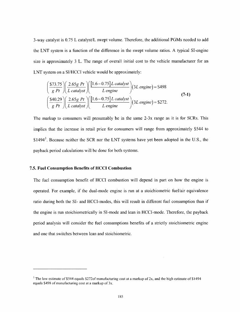
3-way catalyst is 0.75 L catalyst/L swept volume. Therefore, the additional PGMs needed to add
the LNT system is a function of the difference in the swept volume ratios. A typical SI-engine
size is approximately 3 L. The range of overall initial cost to the vehicle manufacturer for an
LNT system on a SI/HCCI vehicle would be approximately:
$73.75)( 2.65g Pt [1.6 - 0.75]L catalyst )
g Pt L catalyst L engine= $498(7-1)
$40.29 2.65g Pt [1.6-0.75]L catalyst )
g Pt L catalyst L engine (3L engine) $272.
The markup to consumers will presumably be in the same 2-3x range as it is for SCRs. This
implies that the increase in retail price for consumers will range from approximately $544 to
$14943. Because neither the SCR nor the LNT systems have yet been adopted in the U.S., the
payback period calculations will be done for both systems.
7.5. Fuel Consumption Benefits of HCCI Combustion
The fuel consumption benefit of HCCI combustion will depend in part on how the engine is
operated. For example, if the dual-mode engine is run at a stoichiometric fuel/air equivalence
ratio during both the SI- and HCCI-modes, this will result in different fuel consumption than if
the engine is run stoichiometrically in SI-mode and lean in HCCI-mode. Therefore, the payback
period analysis will consider the fuel consumptions benefits of a strictly stoichiometric engine
and one that switches between lean and stoichiometric.
3 The low estimate of $544 equals $272of manufacturing cost at a markup of 2x, and the high estimate of $1494equals $498 of manufacturing cost at a markup of 3x.
7.5.1. Fully Stoichiometric Operation
Andreae [5] examined the fuel consumption benefits of a dual-mode, SI/HCCI engine running
constantly at a stoichiometric fuel/air equivalence ratio. To do this, Andreae used a combination
of fuel consumption benefit data he obtained from an experimental HCCI engine and the Advisor
vehicle simulation software package. The Advisor program was used to simulate the urban and
highway Federal Test Procedure (FTP) drive cycles, from which fuel economy benefits were
obtained. During each step of the simulation, the engine load was calculated, and if the load was
between I and 4 bar brake mean effective pressure (BMEP), HCCI combustion was considered
feasible. The simulations assumed that perfect switching between HCCI and SI was possible and
that there was no fuel penalty for combustion-mode switching. Obviously, perfect switching
could not be realized in practice, but these results represent an upper bound for fuel consumption
benefit for a dual-mode SI/HCCI engine. The fuel consumption benefit for an engine operating
in HCCI-mode was estimated from a comparison of baseline SI data to experimental HCCI data.
The Advisor modeling results showed that fuel consumption was improved by approximately 6%
over the urban drive cycle and by approximately 10% over the highway drive cycle. These
estimates for fuel savings will be used in the payback period calculations for the scenarios with
fully stoichiometric operation.
7.5.2. Lean HCCI with Stoichiometric SI
Hardy [98]examined the fuel consumption benefits of a dual-mode, SI/HCCI engine that runs
stoichiometric in SI-mode but lean in HCCI-mode. Hardy used a proprietary vehicle simulation
software package (ESA and CVSP) developed by Ford Motor Company to determine the fuel
consumption benefits, among other things. The HCCI-mode performance characteristics were
modeled using a series of regression equations developed from experimental data collected at
Ford. These equations describe how, for example, the air/fuel ratio changes as a function of
BMEP, or how fuel consumption (in HCCI-mode) is improved as a function of BMEP. Hardy
performed a multitude of simulations under several different test conditions, but this work will
focus on only a select number of cases. Because lean HCCI requires the addition of a lean NO,
catalyst system, Hardy's simulations considered 2 scenarios with respect to catalyst
performance: 1) the "Maximum Fuel Economy" case and 2) the "Emissions Constrained" case.
In the Maximum Fuel Economy case, it is assumed that the 3-way catalyst converts all of the
hydrocarbons and CO but does not treat any NOx emissions. Then, the necessary lean NO,
conversion efficiency is calculated for the after treatment system such that the emissions are
within given regulations. For the cases of interest, the required conversion efficiency was often
between approximately 60 and 90% (depending on the regulation requirement), and SCR or LNT
systems can easily reach these efficiencies [89,93]. Therefore, for the payback period
calculations, the Maximum Fuel Economy cases will be considered; this is also consistent with
the approach of Andreae [5] in estimating an upper bound fuel consumption improvement for
HCCI.
This work will focus on 2 of Hardy's "best cases" under the Maximum Fuel Economy scenario.
Case I assumes that any time the engine load is less than 4.5 bar BMEP 4 and the engine speed is
less than 3500 RPM, the engine can run in HCCI-mode. Within HCCI-mode, the fuel
consumption benefit is estimated from the regression equations obtained from experimental data.
Case 2 incorporates a mode-transition fuel penalty for switching between SI- and HCCI-mode.
Finally, Hardy considered a 3375 lb ("heavy") and a 2375 lb ("light") vehicle in her simulations,
and to be consistent with Andreae [5], who simulated a vehicle weighing approximately 3300 lb,
this work will consider only the "heavy" vehicle results.
In the city driving cycle, the percent fuel consumption reduction for Case I (i.e., no switching
penalty) was 12.07%, and for Case 2 the reduction was 11.04%. For the highway driving cycle,
the percent fuel consumption reduction for Case I was 7.70%, and for Case 2 the reduction was
6.97%. Because the fuel consumption reduction numbers are so similar between Cases I and 2,
for the payback period analysis only the average fuel consumption savings will be used: 11.56%
for city driving and 7.34% for highway driving.
7.6. Estimating Future Gasoline Prices
Projecting the future cost of gasoline is arguably the most difficult task in determining the
payback period. However, some estimate of future gasoline costs is absolutely necessary to
project dollars saved from fuel consumption benefits of a dual-model SI/HCCI vehicle. The
method used here to project gasoline prices relies on the historical link between crude oil and
gasoline prices.
Historic crude oil prices from 1978 to the present for several countries are available from the
U.S. Department of Energy [99]. For the purposes of this study, the historic U.S. spot price
freight-on-board weighted by estimated import volume in dollars/barrel is used. The price for
each year is taken as the average price of a barrel of oil for all reported dates (usually weekly)
4 The Ford HCCI engine is capable of idle operation.
188
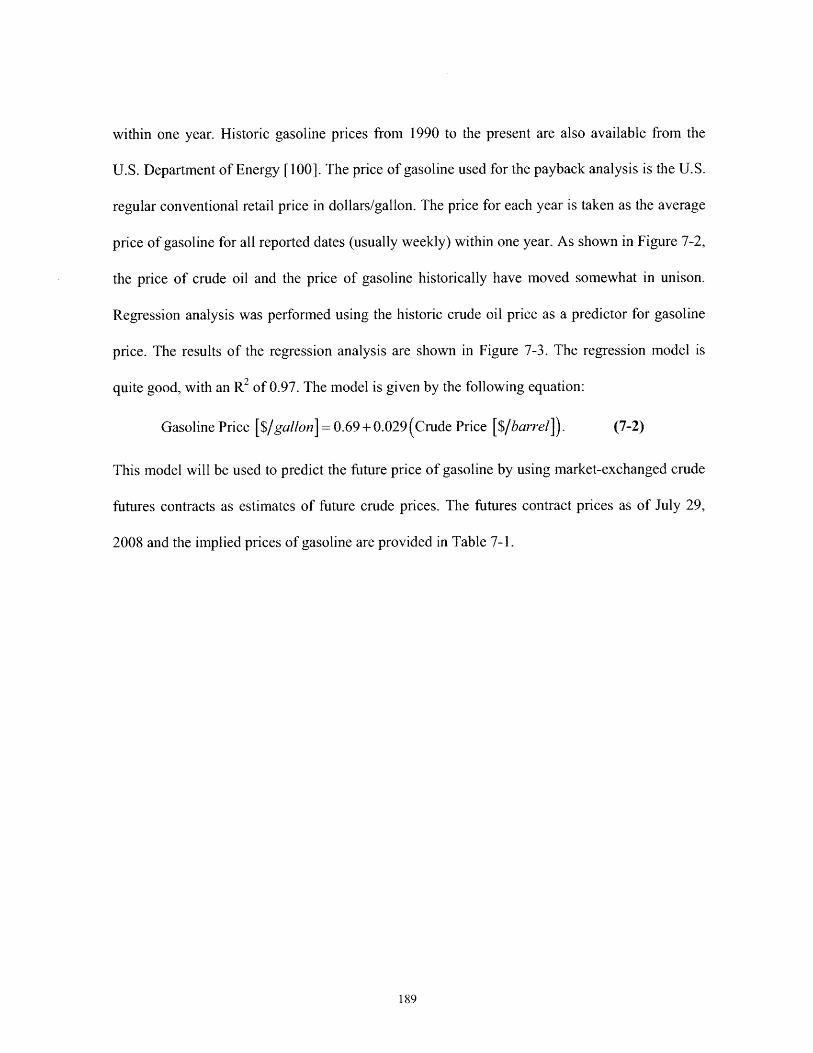
within one year. Historic gasoline prices from 1990 to the present are also available from the
U.S. Department of Energy [100]. The price of gasoline used for the payback analysis is the U.S.
regular conventional retail price in dollars/gallon. The price for each year is taken as the average
price of gasoline for all reported dates (usually weekly) within one year. As shown in Figure 7-2,
the price of crude oil and the price of gasoline historically have moved somewhat in unison.
Regression analysis was performed using the historic crude oil price as a predictor for gasoline
price. The results of the regression analysis are shown in Figure 7-3. The regression model is
quite good, with an R2 of 0.97. The model is given by the following equation:
Gasoline Price [$/gallon] = 0.69 + 0.029(Crude Price [$/barrel]). (7-2)
This model will be used to predict the future price of gasoline by using market-exchanged crude
futures contracts as estimates of future crude prices. The futures contract prices as of July 29,
2008 and the implied prices of gasoline are provided in Table 7-1.
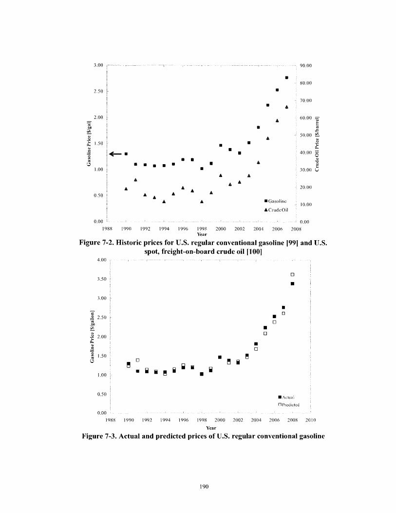
90.00
80.00
70.00
60.00
50.00
40.00
30.00 0
A . A
* Gasoline
ACrudcOil
20.00
10.00
1990 1992 1994 1996 1998 2000 2002Year
0.002004 2006 2008
Historic prices for U.S. regular conventional gasoline 1991 and U.S.spot, freight-on-board crude oil [100]
4.00
3.50
3.00
U[]2.50
2.00
1.50
1.00
0 m
0.50SActual
O Predicted
0.001988 1990 1992 1994 1996 1998 2000 2002 2004 2006 2008
Year
Figure 7-3. Actual and predicted prices of U.S. regular conventional gasoline
2.50
2.00
4f- U
a i i NU U
1.00
0.50
0.001988
Figure 7-2.
2010
3.00
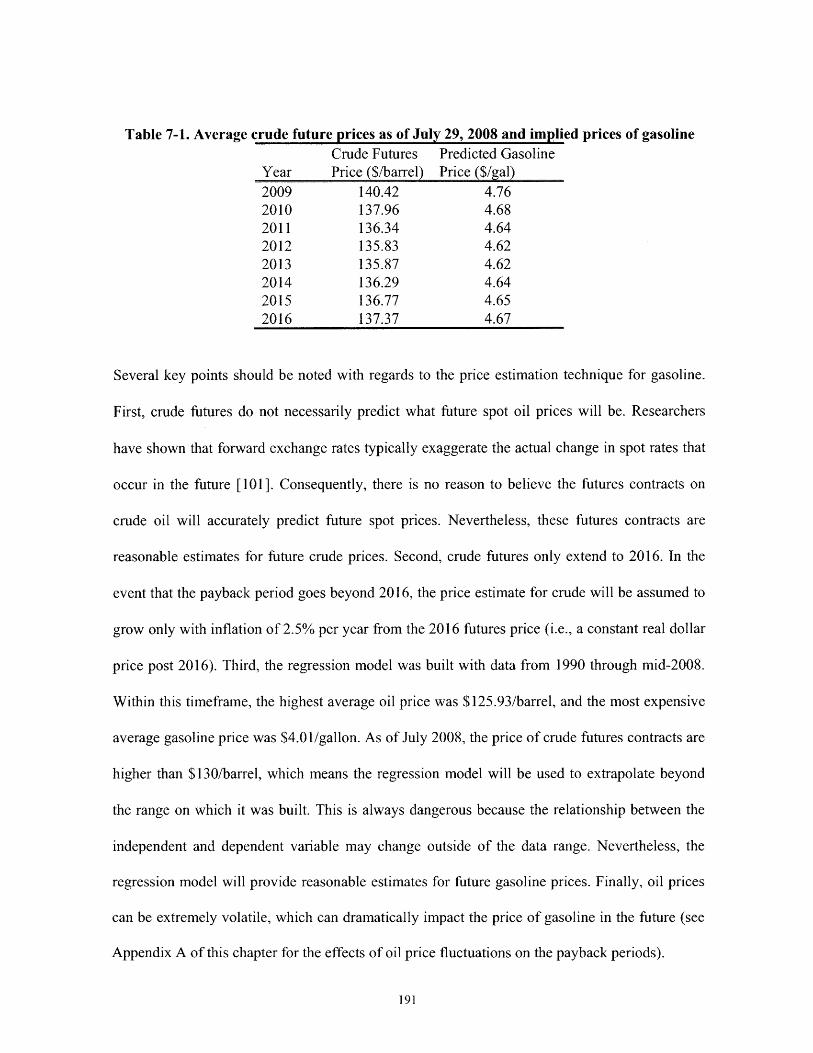
Table 7-1. Average crude future prices as of July 29, 2008 and implied prices of gasolineCrude Futures Predicted Gasoline
Year Price ($/barrel) Price ($/gal)2009 140.42 4.762010 137.96 4.682011 136.34 4.642012 135.83 4.622013 135.87 4.622014 136.29 4.642015 136.77 4.652016 137.37 4.67
Several key points should be noted with regards to the price estimation technique for gasoline.
First, crude futures do not necessarily predict what future spot oil prices will be. Researchers
have shown that forward exchange rates typically exaggerate the actual change in spot rates that
occur in the future [101]. Consequently, there is no reason to believe the futures contracts on
crude oil will accurately predict future spot prices. Nevertheless, these futures contracts are
reasonable estimates for future crude prices. Second, crude futures only extend to 2016. In the
event that the payback period goes beyond 2016, the price estimate for crude will be assumed to
grow only with inflation of 2.5% per year from the 2016 futures price (i.e., a constant real dollar
price post 2016). Third, the regression model was built with data from 1990 through mid-2008.
Within this timeframe, the highest average oil price was $125.93/barrel, and the most expensive
average gasoline price was $4.01/gallon. As of July 2008, the price of crude futures contracts are
higher than $130/barrel, which means the regression model will be used to extrapolate beyond
the range on which it was built. This is always dangerous because the relationship between the
independent and dependent variable may change outside of the data range. Nevertheless, the
regression model will provide reasonable estimates for future gasoline prices. Finally, oil prices
can be extremely volatile, which can dramatically impact the price of gasoline in the future (see
Appendix A of this chapter for the effects of oil price fluctuations on the payback periods).
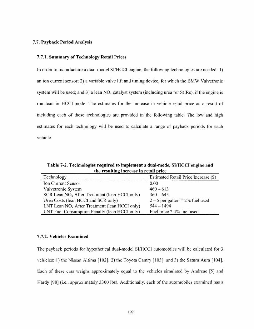
7.7. Payback Period Analysis
7.7.1. Summary of Technology Retail Prices
In order to manufacture a dual-model SI/HCCI engine, the following technologies are needed: 1)
an ion current sensor; 2) a variable valve lift and timing device, for which the BMW Valvetronic
system will be used; and 3) a lean NOx catalyst system (including urea for SCRs), if the engine is
run lean in HCCI-mode. The estimates for the increase in vehicle retail price as a result of
including each of these technologies are provided in the following table. The low and high
estimates for each technology will be used to calculate a range of payback periods for each
vehicle.
Table 7-2. Technologies required to implement a dual-mode, SI/HCCI engine andthe resulting increase in retail price
Technology Estimated Retail Price Increase ($)Ion Current Sensor 0.00Valvetronic System 460 - 613SCR Lean NO, After Treatment (lean HCCI only) 360 - 645Urea Costs (lean HCCI and SCR only) 2 - 5 per gallon * 2% fuel usedLNT Lean NOx After Treatment (lean HCCI only) 544 - 1494LNT Fuel Consumption Penalty (lean HCCI only) Fuel price * 4% fuel used
7.7.2. Vehicles Examined
The payback periods for hypothetical dual-model SI/HCCI automobiles will be calculated for 3
vehicles: 1) the Nissan Altima [102]; 2) the Toyota Camry [103]; and 3) the Saturn Aura [104].
Each of these cars weighs approximately equal to the vehicles simulated by Andreae [5] and
Hardy [98] (i.e., approximately 3300 lbs). Additionally, each of the automobiles examined has a

standard SI- and a HEV-version. Using the hybrid premium relative to the SI-version [76], the
payback period for the HEV can be compared to the dual-mode SI/HCCI version.
7.7.3. Payback Period Calculations
The payback period for each vehicle was calculated using the following procedure. First, each
vehicle was assumed to travel 15,000 miles per year, spending 45% of those miles in highway
driving and 55% of those miles in urban driving [105]. This assumption was used in conjunction
with the SI-version fuel economy to determine the baseline volume of fuel consumed each year.
This fuel volume per year was multiplied by the estimated yearly gasoline price obtained from
the regression model discussed previously; the result is the baseline fuel cost for each vehicle.
Next, the HCCI (or HEV) fuel consumption advantage is applied to the SI-version fuel economy
of each vehicle, and the yearly fuel costs are recalculated. The difference between the SI-version
and the SI/HCCI-version (or HEV-version) fuel costs represents the annual fuel savings. These
fuel savings are then added together until their sum is larger than then payback hurdle for each
vehicle. The payback hurdle was calculated directly from the technology costs for the SI/HCCI
vehicles (see Table 7-2) or was taken from Valcourt [76] for HEVs. The number of years it takes
for the fuel savings to equal to the payback hurdle is the payback period.
7.7.4. Results
Table 7-3 summarizes the results of the payback period calculations. The results show that each
stoichiometric SI/HCCI vehicle has a payback period of only 3 - 4 years. The short payback
period is primarily a product of the small increase in retail price for the added necessary
technologies to implement a stoichiometric, dual-mode vehicle. The short payback period also
comes in spite of only incremental improvements in fuel economy. For example, for the Nissan

Altima the baseline SI fuel economy is 23 MPG in the city and 32 MPG on the highway. The
dual-mode vehicle would have a fuel economy of only 24.5 MPG in the city and 35.6 MPG on
the highway. The payback periods of the dual-mode vehicles also compare very well to the HEV
payback periods; the dual-mode payback periods are at least as short as any of the HEVs, and for
the Saturn Aura the dual-mode engine has a significantly shorter payback period.
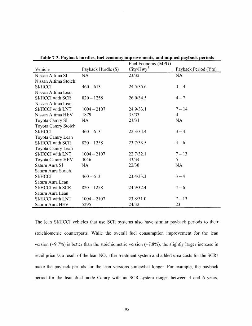
Table 7-3. Payback hurdles, fuel economy improvements, and implied payback periodsFuel Economy (MPG)
Vehicle Payback Hurdle ($) City/Hwy5 Payback Period (Yrs)Nissan Altima SI NA 23/32 NANissan Altima Stoich.SI/HCCI 460 - 613 24.5/35.6 3 - 4Nissan Altima LeanSI/HCCI with SCR 820 - 1258 26.0/34.5 4-7Nissan Altima LeanSI/HCCI with LNT 1004 - 2107 24.9/33.1 7 - 14Nissan Altima HEV 1879 35/33 4Toyota Camry SI NA 21/31 NAToyota Camry Stoich.SI/HCCI 460 -613 22.3/34.4 3 -4Toyota Camry LeanSI/HCCI with SCR 820 - 1258 23.7/33.5 4 -6Toyota Camry LeanSI/HCCI with LNT 1004 - 2107 22.7/32.1 7 - 13Toyota Camry HEV 3046 33/34 5Saturn Aura SI NA 22/30 NASaturn Aura Stoich.SI/HCCI 460 - 613 23.4/33.3 3 - 4Saturn Aura LeanSI/HCCI with SCR 820 - 1258 24.9/32.4 4-6Saturn Aura LeanSI/HCCI with LNT 1004 - 2107 23.8/31.0 7 - 13Saturn Aura HEV 5295 24/32 23
The lean SI/HCCI vehicles that use SCR systems also have similar payback periods to their
stoichiometric counterparts. While the overall fuel consumption improvement for the lean
version (-9.7%) is better than the stoichiometric version (-7.8%), the slightly larger increase in
retail price as a result of the lean NOx after treatment system and added urea costs for the SCRs
make the payback periods for the lean versions somewhat longer. For example, the payback
period for the lean dual-mode Camry with an SCR system ranges between 4 and 6 years,
195
whereas the stoichiometric version requires only 3 to 4 years. The payback periods for the lean-
versions with SCRs also compare well to HEV payback periods. For the Saturn Aura, the HEV
version actually has a longer payback period than the lean version.
The lean SI/HCCI vehicles with LNT systems have the longest payback periods of all the dual-
mode configurations, but the payback periods are still somewhat competitive nonetheless. In
general, the range of payback periods for configurations with LNTs overlaps the range of
payback periods with SCRs by a year. However, the upper range of the estimates for the systems
with LNTs is somewhat longer due to the high costs of the PGMs that make up the LNT system;
this results in a larger payback hurdle for these vehicles. In addition, the fuel consumption
penalty caused by use of the LNT weakens the HCCI advantage. These effects combined
translate into longer payback periods. For example, the payback period for the Camry with the
LNT system ranges from 7 to 13 years compared to only 4 to 6 year for the SCR-lean-version.
Also, the payback periods for the lean-versions with LNTs are typically longer than the HEV
payback periods. Consequently, the high cost of this after treatment technologies may prohibit
the lean HCCI vehicles with LNTs from making good economic sense.
In addition to the payback data presented in Table 7-3, an interesting picture also emerges from
the fuel economy data. The new CAFE laws raised the fuel efficiency standard to 35 MPG,
which must be achieved by 2020 [74]. Examining the fuel economy data in Table 7-3, none of
the automobiles have an average fuel economy over 35, including the HEVs. This implies that
these fuel savings configurations alone will not be enough to allow the automotive companies to
All fuel economy estimates for LNT-models contain a 4% fuel consumption penalty for use of the LNT system.
196

meet the new laws. Consequently, what is likely to occur is that these firms will have to employ
several strategies simultaneously. Such strategies could include, among other things: a) enticing
customers to purchase smaller and/or lower-powered cars; b) engineering new automobiles to
have lower air friction, weight and rolling resistances; c) selling a significant number of HEVs to
boost the average MPG. The SI/HCCI hybrid vehicles could be yet another option in the toolkit,
but this option alone, or any single one of the strategies outlined above, will not be sufficient.
This analysis helps shed light on some of the challenges automotive firms will face in the
coming decade.
7.8. Manufacturer Cost to Improve Fuel Economy
If dual-mode SI/HCCI vehicles are to become a reality, there must not only be an incentive for
consumers to purchase the vehicles (i.e., short payback periods), but there also must be an
incentive for auto manufactures to use the technology. Two factors could help drive these
companies to produce SI/HCCI vehicles. First, the automotive industry is highly price
competitive. Therefore, from the perspective of a single automotive company, it would want to
improve fuel economy as cheaply as possible in its fleets so that consumers will purchase its
automobiles rather than the competitors'. That is, automotive firms would like to spend less
money to improve the miles per gallon of an automobile by a given amount. Second, the new
CAFE laws require that automotive companies sell a larger quantity of higher fuel efficient
vehicles. The first stimulus goes hand-in-hand with the second: if automotive companies can
produce higher fuel efficient vehicles cheaply, then consumers will likely purchase a greater
quantity of higher fuel efficient automobiles thus helping the finns meet the new CAFE laws.
Therefore, in order to evaluate the incentive to vehicle manufacturers to use SI/HCCI hybrid
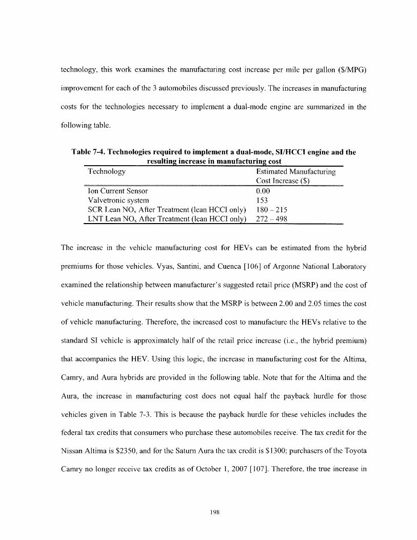
technology, this work examines the manufacturing cost increase per mile per gallon ($/MPG)
improvement for each of the 3 automobiles discussed previously. The increases in manufacturing
costs for the technologies necessary to implement a dual-mode engine are summarized in the
following table.
Table 7-4. Technologies required to implement a dual-mode, SI/HCCI engine and theresulting increase in manufacturing cost
Technology Estimated ManufacturingCost Increase ($)
Ion Current Sensor 0.00Valvetronic system 153SCR Lean NOx After Treatment (lean HCCI only) 180 - 215LNT Lean NOx After Treatment (lean HCCI only) 272 - 498
The increase in the vehicle manufacturing cost for HEVs can be estimated from the hybrid
premiums for those vehicles. Vyas, Santini, and Cuenca [106] of Argonne National Laboratory
examined the relationship between manufacturer's suggested retail price (MSRP) and the cost of
vehicle manufacturing. Their results show that the MSRP is between 2.00 and 2.05 times the cost
of vehicle manufacturing. Therefore, the increased cost to manufacture the HEVs relative to the
standard SI vehicle is approximately half of the retail price increase (i.e., the hybrid premium)
that accompanies the HEV. Using this logic, the increase in manufacturing cost for the Altima,
Camry, and Aura hybrids are provided in the following table. Note that for the Altima and the
Aura, the increase in manufacturing cost does not equal half the payback hurdle for those
vehicles given in Table 7-3. This is because the payback hurdle for these vehicles includes the
federal tax credits that consumers who purchase these automobiles receive. The tax credit for the
Nissan Altima is $2350, and for the Saturn Aura the tax credit is $1300; purchasers of the Toyota
Camry no longer receive tax credits as of October 1, 2007 [107]. Therefore, the true increase in

the MSRP for the Altima and the Aura is equal to the payback hurdle in Table 7-3 plus the
federal tax credit. Table 7-5 shows the increase in manufacturing cost for each vehicle.
Table 7-5. Increase in manufacturing cost for each HEV studiedVehicle Estimated Manufacturing
Cost Increase ($)Nissan Altima HEV 2063Toyota Camry HEV 1486Saturn Aura HEV 3217
Table 7-6 summarizes the cost to vehicle manufacturers for the incremental fuel economy
improvement achieved by implementing either SI/HCCI engines or producing HEVs. The results
show that stoichiometric, dual-mode engines are an extremely cost effective method for
improving fuel economy. Even though the fuel economy improvements for the dual-mode
engines are significantly less than the HEV, the lower cost of implementation makes them an
attractive alternative. For example, for the Altima, the stoichiometric, dual-mode engine would
improve average fuel economy by only 2.4 MPG compared to the 7.1 MPG improvement for
producing an HEV. However, the added manufacturing cost for the dual-mode engine is only
$153 compared to $2063 for the HEV. This large pricing difference is largely a result of the
expensive battery assemblies needed for an HEV as well as the additional hardware necessary to
couple an electronic drive train with the standard drive train. The additional technology for the
dual-mode engines is relatively simply by comparison and is consequently significantly less
expensive. The lean, dual-mode vehicles are more expensive on a $/MPG basis than the
stoichiometric-versions, but the SCR-versions are still attractive options compared to HEVs. For
example, the Altima SCR-version improvement ranges from $119/MPG to $132/MPG compared
199
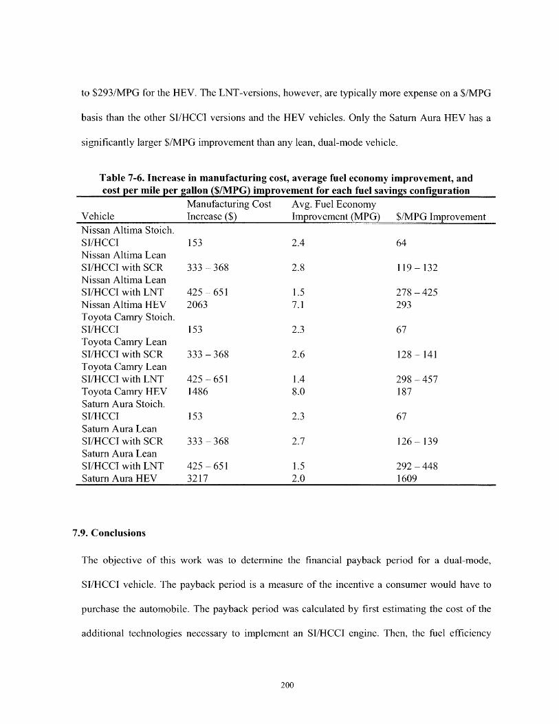
to $293/MPG for the HEV. The LNT-versions, however, are typically more expense on a $/MPG
basis than the other SI/HCCI versions and the HEV vehicles. Only the Saturn Aura HEV has a
significantly larger $/MPG improvement than any lean, dual-mode vehicle.
Table 7-6. Increase in manufacturing cost, average fuel economy improvement, andcost per mile per gallon ($/MPG) improvement for each fuel savings configuration
Manufacturing Cost Avg. Fuel EconomyVehicle Increase ($) Improvement (MPG) $/MPG ImprovementNissan Altima Stoich.SI/HCCI 153 2.4 64Nissan Altima LeanSI/HCCI with SCR 333 - 368 2.8 119 - 132Nissan Altima LeanSI/HCCI with LNT 425 - 651 1.5 278 - 425Nissan Altima HEV 2063 7.1 293Toyota Camry Stoich.SI/HCCI 153 2.3 67Toyota Camry LeanSI/HCCI with SCR 333 - 368 2.6 128 - 141Toyota Camry LeanSI/HCCI with LNT 425 - 651 1.4 298 - 457Toyota Camry HEV 1486 8.0 187Saturn Aura Stoich.SI/HCCI 153 2.3 67Saturn Aura LeanSI/HCCI with SCR 333 - 368 2.7 126 - 139Saturn Aura LeanSI/HCCI with LNT 425 - 651 1.5 292 - 448Saturn Aura HEV 3217 2.0 1609
7.9. Conclusions
The objective of this work was to determine the financial payback period for a dual-mode,
SI/HCCI vehicle. The payback period is a measure of the incentive a consumer would have to
purchase the automobile. The payback period was calculated by first estimating the cost of the
additional technologies necessary to implement an SI/HCCI engine. Then, the fuel efficiency
200

improvement resulting from the HCCI process was used to estimate the annual fuel savings from
employing the dual-mode engine. Finally, an estimate of the future price of gasoline was used in
conjunction with the fuel savings estimates to determine the dollars saved in fuel costs each year.
The following conclusions were reached:
* The increase in retail price for a stoichiometric, dual-mode vehicle over a traditional SI
model is relatively minor - on the order of $460 to $600.
* The small increase in retail price results in short payback periods (approximately 3 to 4
years) for stoichiometric, dual-mode automobiles.
* The payback periods for the stoichiometric, dual-mode vehicles are as short or shorter
than any HEV payback period.
* Lean SI/HCCI vehicles that employ SCR NOx after treatment systems are economically
viable and have payback periods of similar order to HEVs. However, lean-versions that
employ LNTs may not be economically sensible due to expensive PGMs that comprise
the catalyst bed and drive up the range of payback periods to often over 10 years.
In addition to examining the payback period for customers who may purchase a dual-mode
vehicle, this work also examined the incentive of automotive manufacturers to produce SI/HCCI
automobiles. This was done by calculating the cost increase to the manufacturer per mile per
gallon improvement in fuel economy (i.e., $/MPG). The following conclusions were reached:
* The increase in manufacturing cost for stoichiometric, dual-mode engines is less than
$70/MPG gain, which is smaller than the increase for both lean dual-mode vehicles and
HEVs.
201
* Despite the smaller increase in fuel economy of the SI/HCCI engines relative to HEVs,
the $/MPG improvement for stoichiometric, dual-mode vehicles is smaller than any other
fuel savings configuration.
* The increase in manufacturing costs per MPG gain for lean, dual-mode vehicles that
employ SCRs are typically lower or of similar order to those of an HEV.
* Employing LNT systems for lean, dual-mode SI/HCCI vehicles may make the $/MPG
improvement prohibitively expensive compared to other fuel savings configurations
available to manufacturers.
The combined results of this project demonstrate that dual-mode, SI/HCCI vehicles are a viable
economic option for both consumers and vehicle manufactures; however, two points should be
kept in mind. First, the calculations presented here are best case estimates of the benefits of a
dual-mode vehicle. At present, accurately estimating the research and development (R&D) costs
that will be incurred for developing the dual-mode process is extremely difficult because there is
no market data available on this topic. Some of the additional engineering costs include those
incurred for developing the control software and for calibrating the engine in both combustion
regimes. These costs will likely not be overwhelming large, however. The fraction of these R&D
costs passed to the consumer is currently not well-defined and consequently is not include the
calculations presented here. Second, neither SI/HCCI vehicles nor HEVs achieve a large enough
fuel economy advantage to allow automotive companies to meet the new CAFE standards by
implementing these technologies alone. This implies that these firms will have to employ several
strategies simultaneously. These strategies include, among others, reducing vehicular weight and
rolling resistance while selling smaller and/or lower-powered automobiles and larger quantities
202
of HEVs. Nevertheless, the results of this study demonstrate that SI/HCCI vehicles are a viable
economic option for both the consumer, by helping to save on fuel expenses, and the producer,
by helping to improve the fleet fuel economy.
7.10. Appendix A
This appendix examines the sensitivity of the payback period calculations to oil price
fluctuations. As discussed in the main text, the price of oil can be highly volatile, which can have
a significant impact on gasoline prices and thus payback periods. This work was originally
drafted in mid-2008 when the price of oil was at an all-time high (-$140/barrel). Now nearing
the end of 2008, the U.S. stock market and equity markets around the world have suffered
tremendously. This has caused the price of oil to drop to near-2005 levels (-$40/barrel). Using
current (i.e., end-2008) estimates for oil prices, the payback periods will be reexamined here.
The methodology used in determining the payback period will remain unchanged.
The average crude futures price as of December 11, 2008 and corresponding estimated gasoline
price (based on Equation (7-2)) are presented below in Table 7-7. Contrasting these values to
those in Table 7-1 provide a clear glimpse into how volatile oil prices can be - even within a
single year. Also, the average price of oil in 2008 has been updated from $101.33/barrel to
$96.58/barrel. The gasoline prices presented in Table 7-7 are used in the payback period
calculations presented next.
203

Table 7-7. Average crude future prices as of December 11, 2008 and implied pricesof gasoline
Crude PredictedFutures Price Gasoline
Year ($/barrel) Price ($/gal)2009 55.34 2.292010 63.40 2.532011 68.36 2.672012 71.35 2.762013 73.39 2.812014 75.20 2.872015 77.30 2.932016 78.72 2.972017 79.79 3.00
Table 7-8 summarizes the results of the payback period calculations based on the updated
gasoline prices. The results here are qualitatively similar to those presented in the main text.
Stoichiometric dual-mode vehicles have the shortest payback periods, due to their low payback
hurdles. Lean dual-mode vehicles that employ SCRs have longer payback periods, but these are
still of similar order of magnitude to those of most HEVs. For lean-models using LNTs, the
higher payback hurdles continue to result in the longest payback periods of any of the
configurations examined. Comparing the results here to those in Table 7-3 shows that with lower
gasoline prices, the payback periods for all of the vehicles are longer. This demonstrates why
automotive companies struggle to sell highly fuel efficient vehicles when gasoline prices are
low; consumers simply do not have as strong of an incentive to purchase them. Furthermore, this
analysis also demonstrates why calculating the "correct" payback period is difficult. The price of
oil (and thus gasoline), among other things, is highly uncertain, and this can drastically impact
the payback results.
204
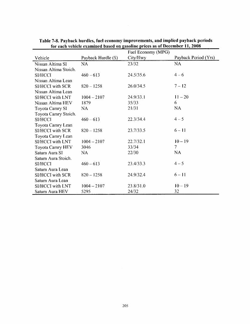
Table 7-8. Paybaclfor each vehi
c hurdles, fuel economy improvements, and implied payback periodscle examined based on gasoline prices as of December 11, 2008
Fuel Economy (MPG)Payback Hurdle ($) City/Hwy Payback Period (Yrs)NA 23/32 NA
VehicleNissan Altima SINissan Altima Stoich.SI/HCCINissan Altima LeanSI/HCCI with SCRNissan Altima LeanSI/HCCI with LNTNissan Altima HEVToyota Camry SIToyota Camry Stoich.SI/HCCIToyota Camry LeanSI/HCCI with SCRToyota Camry LeanSI/HCCI with LNTToyota Camry HEVSaturn Aura SISaturn Aura Stoich.SI/HCCISaturn Aura LeanSI/HCCI with SCRSaturn Aura LeanSI/HCCI with LNTSaturn Aura HEV
24.5/35.6
26.0/34.5
24.9/33.135/3321/31
22.3/34.4
23.7/33.5
22.7/32.133/3422/30
23.4/33.3
24.9/32.4
23.8/31.024/32
4-6
7-12
11 -206NA
4-5
6-11
10-197NA
4-5
6-11
10-1932
205
460 - 613
820 -1258
1004 -21071879NA
460 - 613
820 -1258
1004 - 21073046NA
460 -613
820 -1258
1004 - 21075295
GLOSSARY
Oscaling: prefactor of the heat transfer coefficient of Chang et al.
y: ratio of specific heat capacities
k: air/fuel equivalence ratio
d: fuel/air equivalence ratio
OEvc: crank angle of exhaust valve close
Owvc: crank angle of intake valve close
mf: mass of fuel in the cylinder
m'f: mass flow rate of fuel
Mivc: in-cylinder mass at intake valve close
Pmax: maximum in-cylinder pressure
Pwvc: in-cylinder pressure at intake valve close
T-30: in-cylinder temperature at 30 crank angle degrees before top center
TIN: intake air temperature
Tlvc: in-cylinder temperature at intake valve close
Tmisfre: in-cylinder temperature at a misfire
T,,: steady-state, in-cylinder temperature
Xboundary: mass fraction in the boundary layer
BDC: bottom dead center
BTC: before top center
CA50: crank angle at which 50% of the cumulative heat release has occurred
CAI: controlled auto-ignition
206
CAD: crank angle degree
CFD: computational fluid dynamics
CI: compression-ignition
COV: coefficient of variation
DAEs: differential-algebraic equations
EGR: exhaust gas residuals
EVC: exhaust valve close
EVO: exhaust valve open
GIMEP: gross indicated mean effective pressure
HC: hydrocarbon
HCCI: homogenous-charge compression-ignition
HLL: high-load limit
HTHR: high temperature heat release
ISFC: indicated specific fuel consumption
IVC: intake valve close
IVO: intake valve open
LLL: low-load limit
LLNL: Lawrence Livermore National Laboratory
LTHR: low temperature heat release
MAP: manifold air pressure
MITES: MIT engine simulator
MON: motor octane number
MRPR: maximum rate of pressure rise
207
NIMEP: net indicated mean effective pressure
NVO: negative valve overlap
010: auto-ignition quality requirement
01: octane index
PRF: primary reference fuel
PSI: pounds per square inch
RON: research octane number
RPM: revolutions per minute
RVP: Reid vapor pressure
SI: spark-ignition
TDC: top dead center
VIF: variance inflation factor
208
REFERENCES
1. Onishi, S., Jo, S.H., Shoda, K., Jo, P.D., Kato, S. "Active Thermo-AtmosphericCombustion (ATAC) - A New Combustion Process for Internal Combustion Engines,"SAE Technical Paper, 790501 (1979).
2. Nicolia, T., Carr, D., Weiland, S.K., Duhme, H., von Ehrenstein, O., Wagner, C., vonMutius, E. "Urban traffic and pollutant exposure related to respiratory outcomes and atopyin a large sample of children," Eur. Respir. J. 2003, 21, 956-963.
3. Dec, J.E. and Sjoeberg, M., "A Parametric Study of HCCI Combustion - the Sources ofEmissions at Low Loads and the Effects of GDI Fuel Injection," SAE 2003-01-0752, 2003.
4. Zhao, F., Asmus, T.W., Assanis, D.N., Dec, J.E., Eng, J.A., and Najt, P.M. (Eds.)Homogeneous Charge Compression Ignition Engines: Key Research and DevelopmentIssues. Society of Automotive Engineers, Incorporated, Warrendale, Pennsylvania, 2003.
5. Andreae, M.M. "Effect of ambient conditions and fuel properties on homogeneous chargecompression ignition engine operation." Ph.D. thesis, Massachusetts Institute ofTechnology, 2006.
6. Santoso, H., Matthews, J., and Cheng, W.K., "Managing SI/HCCI Dual-Mode EngineOperation," SAE Paper 2005-01-0162, 2005.
7. Koopmans, L., Dembratt, I., Stroem, H., Lundgren, S., and Backlund, O., "Demonstrating aSI-HCCI-SI Mode Change on a Volvo 5-cylinder Electronic Valve Control Engine," SAEPaper 2003-01-0753, 2003.
8. Milovanovic, N., Blundell, D., Turner, J., and Gedge, S., "Cam Profile Switching (CPS)and Phasing Strategy vs. Fully Variable Valve Train (FVVT) Strategy for Transitionsbetween Spark Ignition and Controlled Auto Ignition Modes," SAE Paper 2005-01-0766,2005.
9. Yao, M., Zhang, Z., Zhang, B., and Chen, Z., "The Effect of PRF Fuel Octane Number onHCCI Operation," SAE 2004-01-2992, 2004.
10. Dec, J. E. and Sjoeberg, M., "Isolating the Effects of Fuel Chemistry on CombustionPhasing in an HCCI Engine and the Potential of Fuel Stratification for Ignition Control,"SAE 2004-01-0557, 2004.
11. Sato, S., Jun, D., Kwoen, S., Yamashita, D. and lida, N., "Basic Research on the SuitableFuel for HCCI Engine from the Viewpoint of Chemical Reaction," SAE 2005-01-0149,2005.
209
12. Shibata, G., Oyama, K., Urushihara, T., and Nakano, T., "The Effect of Fuel Properties onLow and High Temperature Heat Release and Resulting Performance of an HCCI Engine,"SAE Paper 2004-01-0553, 2004.
13. Shibata, G., Oyama, K., Urushihara, T., and Nakano, T., "Correlation of Low TemperatureHeat Release with Fuel Composition and HCCI Engine Combustion," SAE Paper 2005-01-0138, 2005.
14. Shibata, G. and Urushihara, T., "The Interaction between Fuel Chemicals and HCCICombustion Characteristics under Heated Intake Air Conditions," SAE 2006-01-0207,2006.
15. Oakley, A., Zhao, H., Ladommatos, N., and Ma T., "Dilution Effects on the ControlledAuto-Ignition (CAI) Combustion of Hydrocarbon and Alcohol Fuels," SAE 2001-01-3606,2001.
16. Koopmans, L., Stroemberg, E., and Denbratt, I., "The Influence of PRF and CommercialFuels with High Octane Number on the Auto-Ignition Timing of an Engine Operated inHCCI Combustion Mode with Negative Valve Overlap," SAE 2004-01-1967, 2004.
17. Kalghatgi, G.T., "Auto-ignition Quality of Practical Fuels and Implications for FuelRequirements of Future SI and HCCI Engines," SAE Paper 2005-01-0239, 2005.
18. Kalghatgi, G.T., "Fuel Anti-Knock Quality - Part 1. Engine Studies," SAE Paper, 2001-01-3584, 2001.
19. Aroonsrisopon, T., Sohm, V., Werner, P., Foster, D.E., Morikawa, T., and lida, M., "AnInvestigation into the Effect of Fuel Composition on HCCI Combustion Characteristics,"SAE Paper, 2002-01-2830, 2002.
20. Andreae, M.M., Cheng, W.K., Kenney, T., and Yang, J., "Effect of Air Temperature andHumidity on Gasoline HCCI Operation in the Negative-Valve-Overlap Mode," SAE Paper2007-01-0221, 2007.
21. Kalghatgi, G.T. and Head, R.A., "The Available and Required Autoignition Quality ofGasoline-Like Fuels in HCCI Engines at High Temperatures," SAE Paper 2004-01-1969,2004.
22. Kalghatgi, G.T. and Head, R.A., "Combustion Limits and Efficiency in A HomogenousCharge Compression Ignition Engine," Int. J. Engine Res. 2006, Vol. 7, 215-236.
23. Myers, R.H. Classical and Modern Regression with Applications; Duxbury Press: Boston,MA, 1986.
210
24. Lti, X., Chen, W., Hou, Y., and Huang, Z. "Study on the Ignition, Combustion andEmissions of HCCI Combustion Engines Fueled with Primary Reference Fuels," SAETechnical Paper 2005-01-0155, 2005.
25. Farrell, J.T. and Bunting, B.G. "Fuel Composition Effecs at Constant RON and MON in anHCCI Engine Operated with Negative Valve Overlap," SAE Technical Paper 2006-01-3275, 2006.
26. Yao, M., Zhang, B., Zheng, Z., Cheng, Z., Xing, Y. "Experiment Study on the Effects ofEGR and Octane Number of PRF Fuel on combustion and Emissions Characteristics ofHCCI Engines," SAE Technical Paper 2005-01-0174, 2005.
27. Atkins, M.J. and Koch, C.R. "The Effect of Fuel Octane and Dilutent on HomogenousCharge Compression Ignition Combustion," Proc. IMechE. 2005, 219, 665-675.
28. Aroonsrisopon, T., Foster, D., Morikawa, T., and lida, M. "Comparison of HCCI OperatingRanges for Combinations of Intake Temperature, Engine Speed and Fuel Composition,"SAE Technical Paper 2002-01-1924, 2002.
29. Sj6berg, M and Dec, J.E."Combined Effects of Fuel-type and Engine Speed on IntakeTemperature Requirements and Completeness of Bulk-gas Reactions for HCCICombustion," SAE Technical Paper 2003-01-3173, 2003.
30. IFP (via Green, W.H.), Personal Communication, January 16, 2007.
31. Fieweger, K., Blumenthal, R., and Adomeit, G. "Self-Ignition of S.I. Engine Model Fuels:A Shock Tube Investigation at High Pressure," Combust. Flame, 1997, 109(4), 599-619.
32. Sjoberg, M. and Dec, J.E. "An investigation of the relationship between measured intaketemperature, BDC temperature, and combustion phasing for premixed DI HCCI engines,"SAE Paper 2004-01-1900, 2004.
33. Matthews, J., Santoso, H., and Cheng, W.K. "Load control for an HCCI engine," SAEPaper 2005-01-0150, 2005.
34. Santoso, H., Matthews, J., and Cheng, W.K. "Characteristics of HCCI engine operating inthe negative-valve-overlap mode," SAE Paper 2005-01-2133, 2005.
35. Ohyama, Y. "Engine modeling of HCCI transient operations," SAE Paper 2005-01-0158,2005.
211

36. Xie, H., Hou, S., Qin, J., Zhang, Y., Li, N., and Zhao, H. "Control strategies for steady andtransient operation of a 4-stroke gasoline engine with CAI combustion using a 4-variablevalve actuating system (4WAS)," SAE Paper 2006-01-1083, 2006.
37. Chang, K., Babajimopoulos, A., Lavoie, G.A., Filipi, Z.S., and Assanis, D.N. "Analysis ofload and speed transitions in an HCCI engine using 1-D cycle simulation and thermalnetworks," SAE Paper 2006-01-1087, 2006.
38. Agrell, F., Angstr6m, H-E, Eriksson, B., Wikander, J., Linderyd, J. "Integrated simulationand engine test of closed-loop HCCI control by aid of variable valve timings," SAE Paper2003-01-0748, 2003.
39. Agrell, F., Angstr6m, H-E., Eriksson, B., Wikander, J., and Linderyd, J. "Transient Controlof HCCI through combined intake and exhaust valve actuation," SAE Paper 2003-01-3172,2003.
40. Agrell, F., Eriksson, B., Angstr6m, H-E., Wikander, J., and Linderyd, J. "Control of HCCIduring engine transients by aid of variable valve timings through the use of model-based,non-linear compensation," SAE Paper 2005-01-0131, 2005.
41. Agrell, F. "Transient control of HCCI combustion by aid of variable valve timing throughthe use of an engine state corrected CA50-controller combined with an in-cylinder stateestimator estimating lambda," SAE Paper 2005-01-2128, 2005.
42. Xu, H., Fu, H., Williams, H., and Shilling, I. "Modeling study of combustion and gasexchanged in a HCCI (CAI) engine," SAE Paper 2002-01-0114, 2002.
43. Xu, H., Rudolph, S., Liu, Z., Wallace, S., Richardson, S., Wyszynski, M., and Megaritis, A."An investigation into the operating mode transitions of a homogeneous chargecompression ignition engine using EGR trapping," SAE Paper 2004-01-1911, 2004.
44. Kee, R.J., Miller, J.A., and Jefferson, T.H. "Chemkin: A general-purpose, problem-independent transportable, fortran chemical kinetics code package," Report No. SAND80-8003, Sandia National Laboratories, 1980.
45. Kee, R.J., Rupley, F.M., and Miller, J.A. "The Chemkin thermodynamics database,"Report No. SAND87-8215, Sandia National Laboratories, 1987.
46. Narayanaswamy, K., and Rutland, C.J. "Cycle simulation diesel HCCI modeling studiesand control," SAE Paper 2004-01-2997, 2004.
47. Narayanaswamy, K., Hellel, R.P., and Rutland, C.J. "A new approach to model DI-dieselHCCI combustion for use in cycle simulation studies," SAE Paper 2005-01-3743, 2005.
212

48. Narayanaswamy, K., and Rutland, C.J. "A modeling investigation of combustion controlvariables using DI-diesel HCCI engine transients," SAE Paper 2006-01-1084, 2006.
49. Bhave, A., Kraft, M., Montorsi, L., and Mauss, F. "Modelling a duel-fuelled, multi-cylinder HCCI engine using a PDF-based engine cycle simulator," SAE Paper 2004-01-0561, 2004.
50. Erlandsson, O., Einewall, P., Johansson, B., Amneus, P., and Mauss, F. "Simulation ofHCCI: Addressing compression ratio and turbocharging," SAE Paper 2002-01-2862, 2002.
51. Aceves, S.M., Flowers, D.L., Chen, J.-Y., and Babajimopoulos, A. "Fast prediction ofHCCI combustion with an artificial neural network linked to a fluid mechanics code," SAEPaper 2006-01-3298, 2006.
52. Amsden, A.A. "KIVA-3V: A block-structured KIVA program for engines with vertical orcanted valves," Report No. LA-13313-MS, Los Alamos National Laboratory, 1997.
53. Chesa, J.L, Andreae, M., Green, W., Cheng, W., and Cowart, J. "A modeling investigationinto the optimal intake and exhaust valve event duration and timing for a homogeneouscharge compression ignition engine," SAE Paper 2005-01-3746, 2005.
54. Aceves, S.M., Flowers, D.L., Westbrook, C.K., Smith, J.R., Dibble, R.W., Christensen, M.,Pitz, W.J., and Johansson, B. "A multi-zone model for prediction of HCCI combustion andemissions," SAE Paper 2000-01-0327, 2000.
55. Aceves, S.M., Flowers, D.L., Espinosa-Loza, F., Martinez-Fria, J., Dec, J.E., Sj6berg, M.,Dibble, R.W., and Hessel, R.P. "Spatial analysis of emissions sources for HCCIcombustion at low loads using a multi-zone model," SAE Paper 2004-01-1910, 2004.
56. Heywood, J.B. Internal Combustion Engine Fundamentals. McGraw-Hill, Incorporated,New York, New York, 1988, p. 43-44.
57. Numerica Technology, LLC, http://www.numericatech.com.
58. Schwer, D.A., Tolsma, J.E., Green, Jr., W.H., and Barton, P.I. "On upgrading the numericsof combustion chemistry codes," Combust. Flame, 2002, 128(3), 270-291.
59. Tolsma, J.E. and Barton, P.I. "DAEPACK: An open modeling environment for legacycodes," Ind. Eng. Chem. Res. 2000, 39, 1826-1839.
60. Barton, P.I., Allgor, R.J., and Feehery, W.F. "DLS48S: A large-scale differential-algebraicand parametric sensitivity solver." 1997, Department of Chemical Engineering,Massachusetts Institute of Technology, Cambridge, MA.
213

61. Yelvington, P.E., Rallo, M.B.I., Liput, S., Tester, J.W., Green, W.H., and Yang, J."Prediction of performance maps for homogeneous-charge compression-ignition engines,"Combust. Sci. and Tech., 2004, 176, 1243-1282.
62. Woschni, G. "Universally applicable equation for the instantaneous heat transfercoefficient in the internal combustion engine," SAE Paper 670931, 1967.
63. Chang, J., Giieralp, O., Filipi, Z., Assanis, D., Kuo, T., Najt, P., and Rack, R. "Heat transfercorrelation for an HCCI engine derived from measurements of instantaneous surface heatflux," SAE Paper 2004-01-2996, 2004.
64. Curran, H.J., Gaffuri, P., Pitz, W.J., and Westbrook C.K. "A comprehensive modelingstudy of iso-octane oxidation," Combust. Flame, 2002, 129(3), 253-280. Version accessedJuly 2005 from http://wwwcms.llnl.gov/combustion/combustion2.html.
65. Dec, J. "A computational study of the effects of low fuel loading and EGR on heat releaserates and combustion limits in HCCI engines," SAE Paper 2002-01-1309, 2002.
66. Fiveland, S.B., Agama, R., Christensen, M., Johansson, B., Hiltner, J., Mauss, F., andAssanis, D.N. "Experimental and simulated results detailing the sensitivity of natural gasHCCI engines to fuel composition," SAE Paper 2001-01-3609, 2001.
67. Heywood, J.B. Internal Combustion Engine Fundamentals. McGraw-Hill, Incorporated,New York, New York, 1988, p. 71.
68. Ibid, p. 413-418.
69. Kelly-Zion, P.L. and Dec. J.E. "A computational study of the effect of fuel type on ignitiontime in homogeneous charge compression ignition engines," Proc. Comb. Inst., 2000, 28,1187-1194.
70. Heywood, J.B. Internal Combustion Engine Fundamentals. McGraw-Hill, Incorporated,New York, New York, 1988, p. 106.
71. American Society of Testing and Materials Test Number D-2699.
72. American Society of Testing and Materials Test Number D-2700.
73. "The Outlook for Energy: A View to 2030." Accessed Jan 11, 2008 fromhttp://www.exxonmobil.com/Corporate/Files/energy outlook 2007.pdf.
74. "Fact Sheet: Energy Independence and Security Act of 2007." Accessed Jan 11, 2008 fromhttp://www.whitehouse.gov/news/releases/2007/12/20071219-1 .html.
214
75. "Energy and Environmental Analysis Inc. (2002). Analysis and Forecast of thePerformance and Cost of Conventional and Electric-Hybrid Vehicles." Accessed Jan 30,2008 from http://www.energy.ca.gov/fuels/petroleumdependence/documents/2002-04-09 HYBRID.PDF.
76. Valcourt, J. "Pricier Gasoline Makes Hybrids A Better Deal." The Wall Street Journal 12June 2008: D1.
77. Ryan III, T.W., Callahan, T.J., and Mehta, D. "HCCI in a Variable Compression RatioEngine-Effects of Engine Variables," SAE Technical Paper 2004-01-1971, 2004.
78. Flowers, D., Aceves, S., Martinez-Frias, J., Smith, J.R., Au, M., Girard, J., Dibble, R."Operation of a four-cylinder 1.9 1 propane-fueled homogeneous charge compressionignition engine: Basic operating characteristics and cylinder-to- cylinder effects," SAETechnical Paper 2001-01-1895, 2001.
79. Schnauffer, K. "Engine Cylinder Flame Propagation Studies by New Methods," SAE J. 1-17, 1934.
80. Lee, A. and Pyko, J. "'Engine Misfire Detection by Ionization Current Monitoring," SAETechnical Paper 950003, 1995.
81. Asano, M., Kuma, T., Kajitani, M., Takeuchi, M. "Development of New Ion CurrentCombustion Control Systems," SAE Technical Paper 980162, 1998.
82. Attard, P. and Micallef, J. "Ion Current Combustion Technology for Controlled Auto-ignition Gasoline Engines," Int. J. Engine Res. Vol. 8, 429-437, 2007.
83. Hellring, M., Rognvaldsson, T.S., Carpenter, I.J., Golunski, S.E., Carlsson, C., Hellring,M., Reinkingh, J., Larsson, M., Munther, T., Wickstrom, N. "Robust AFR EstimationUsing the Ion Current and Neural Networks," SAE Technical Paper 1999-01-1161, 1999.
84. Personal communication. H. Mack. June 15, 2008.
85. Heywood, J.B. Internal Combustion Engine Fundamental; McGraw-Hill Book Company:New York, NY, 1988; 223.
86. Kimberley, W. "BMW Improves Powertrains." Accessed June 15, 2008 fromhttp://www.autofieldguide.com/columns/0501 euro.html.
87. "Camless Valvetrains -- Helping Internal Combustion Engines Breathe Easier," Frost &Sullivan database. Published Jan. 19, 2005.
215

88. William M.R., Klein, J.T., Mueller, R., Doelling, W., and Zuerbig, J. "The Development ofUrea-SCR Technology for US Heavy Duty Trucks," SAE Technical Paper 2000-01-0190,2000.
89. Rinek, L. "US Diesel Vehicle NOx Emissions Controls: What is the Market Outlook?"Frost & Sullivan database, Published Feb. 27, 2008.
90. Hoard, J., Hammerle, R., Lambert, C., and Wu, G. "Economic Comparison of LNT VersusUrea SCR for Light Duty Diesel Vehicles in US Market." 2004 US DOE Diesel Efficiencyand Emission Reduction Conference, Coronado, CA. Accessed December 11, 2008 fromhttp://www I.eere.energy.gov/vehiclesandfuels/pdfs/deer 2004/session 11/2004 deer hoard.pdf.
91. Bodek, K. Ph.D. Thesis. Massachusetts Institute of Technology, Cambridge, MA, 2008.
92. Personal communication. A. Sappok. Aug, 28, 2008.
93. Touns, M., Menegazzi, P., and Rouchon, P. "NOx Trap Model for Lean Burn EngineControl," SAE Technical Paper 2003-01-2292, 2003.
94. "Lean NOx Catalyst (LNC)," Wrap Offroad Diesel Retrofit Guidance Document, Vol. 2,Sec. IV. Accessed June 21, 2008 from http://www.wrapair.org/forums/msf/offroad diesel.html.
95. Personal communication. T.V. Johnson. Dec 18, 2008.
96. Personal communication. W. Chang. Dec 29, 2008.
97. "Platinum Today." Accessed Dec 12, 2008 fromhttp://www.platinum.matthey.comiprices/pricecharts.html.
98. Hardy, A.J.J. Ph.D. Thesis, Massachusetts Institute of Technology, Cambridge, MA, 2007.
99. "World Crude Oil Prices," Energy Information Administration. Accessed June 28, 2008from http://tonto.eia.doe.gov/dnav/pet/pet_priwco k w.htm.
100. "U.S. Regular Weekly Retail," Energy Information Administration. Accessed June 28,2008 from http://www.eia.doe.gov/oil _gas/petroleum/data_publications/wrgp/mogas_history.html.
101. Brealey, R.A., Myers, S.C., and Allen, F. Principles qf Corporate Finance; McGraw-HillIrwin: Boston, MA, 2006, 761.
216

102. Nissan Altima specifications. Accessedhttp://www.nissanusa.com/altima/specifications.html.
June 29, 2008 from
103. Toyota Camry specifications. Accessed June 29, 2008 fromhttp://www.toyota.com/camry/specs.html.
104. Saturn Aura specifications. Accessed Junehttp://www.satumrn.com/saturn/vehicles/aura/pricing.jsp.
105. "Fuel Economy Estimation Technique." Accessedhttp://www.fueleconomy.gov/feg/findacar.htm.
106. Vyas, A., Santini, D., and Cuenca, R. "Comparison of IndirectManufacturing." Accessed July 19,http://www.transportation.anl.gov/pdfs/TA/57.pdf.
107. "Federal Incentives (United States)." Accessedhttp://www.hybridcars.com/federal-incentives.html.
29, 2008 from
June 30, 2008 from
Cost Multipliers for Vehicle2008 from
July 19, 2008 from
217