Behavioral/Cognitive

From Image Statistics to Scene Gist: Evoked Neural ActivityReveals Transition from Low-Level Natural Image Structureto Scene Category

Iris I.A. Groen,1,2 Sennay Ghebreab,2,3 Hielke Prins,2 Victor A.F. Lamme,1 and H. Steven Scholte1,2

1Cognitive Neuroscience Group, Department of Psychology, 2Amsterdam Center for Brain and Cognition, Institute for Interdisciplinary Studies, and3Intelligent Systems Laboratory Amsterdam, Institute of Informatics, University of Amsterdam, 1018 WS, Amsterdam, The Netherlands

The visual system processes natural scenes in a split second. Part of this process is the extraction of “gist,” a global first impression. It isunclear, however, how the human visual system computes this information. Here, we show that, when human observers categorize globalinformation in real-world scenes, the brain exhibits strong sensitivity to low-level summary statistics. Subjects rated a specific instanceof a global scene property, naturalness, for a large set of natural scenes while EEG was recorded. For each individual scene, we derived twophysiologically plausible summary statistics by spatially pooling local contrast filter outputs: contrast energy (CE), indexing contraststrength, and spatial coherence (SC), indexing scene fragmentation. We show that behavioral performance is directly related to thesestatistics, with naturalness rating being influenced in particular by SC. At the neural level, both statistics parametrically modulatedsingle-trial event-related potential amplitudes during an early, transient window (100 –150 ms), but SC continued to influence activitylevels later in time (up to 250 ms). In addition, the magnitude of neural activity that discriminated between man-made versus naturalratings of individual trials was related to SC, but not CE. These results suggest that global scene information may be computed by spatialpooling of responses from early visual areas (e.g., LGN or V1). The increased sensitivity over time to SC in particular, which reflects scenefragmentation, suggests that this statistic is actively exploited to estimate scene naturalness.

IntroductionThe remarkable speed at which humans can perceive naturalscenes has been studied for decades (Potter, 1975; Intraub, 1981;Thorpe et al., 1996; Fei-Fei et al., 2007). Many theories of visualprocessing propose that a global impression of the scene accom-panies (Rousselet et al., 2005; Wolfe et al., 2011) or precedes(Hochstein and Ahissar, 2002) detailed feature extraction(“coarse-to-fine” processing) (Hegde, 2008). This global perceptis often described as visual gist (Torralba and Oliva, 2003; Oliva,2005). Behavioral results confirm that global scene properties areindeed perceived very rapidly (Greene and Oliva, 2009a).

An important example of a global scene property is manifested ina difference between images with man-made versus natural content.Scene naturalness can be judged with less exposure time comparedwith other global properties (e.g., openness, depth) (Oliva and Tor-ralba, 2001; Greene and Oliva, 2009b) or basic-level categories (e.g.,

mountain vs forest) (Rousselet et al., 2005; Joubert et al., 2007;Loschky and Larson, 2010; Kadar and Ben-Shahar, 2012). In com-puter vision, it was shown that this distinction coincides with low-level regularities of natural scenes (e.g., the distribution of spatialfrequencies in an image) (Baddeley, 1997; Oliva et al., 1999), leadingto the suggestion that humans might use such “image statistics” inrapid scene recognition (Schyns and Oliva, 1994; McCotter et al.,2005; Kaping et al., 2007). It is unclear, however, to which imagestatistics the brain is sensitive and how it uses them to extract scenenaturalness: besides spatial frequency, color (Oliva and Schyns,2000; Goffaux et al., 2005), and local edge alignment (Wichmann etal., 2006; Loschky et al., 2007) are examples of image features thatmay play a role.

We propose that, to elucidate the role of image statistics inscene perception and their neural representations, we need toaddress two challenges. First, a plausible computational mecha-nism by which image statistics are extracted by the brain must bespecified. For example, estimating spatial frequency distributionsusing a global Fourier transformation is a biologically implausi-ble mechanism, given that the visual system receives localizedinformation from the retina (Graham, 1979; Field, 1987). Sec-ond, if image statistics are indeed used to extract global proper-ties, they should predict not only general differences betweenscene categories but representations of individual images. Thismeans that single-trial differences, in both neural responses andbehavior, should correlate with differences in image statistics.

Here, we addressed these problems by combining computa-tional modeling of physiologically plausible image statistics with

Received July 23, 2013; revised Oct. 7, 2013; accepted Oct. 24, 2013.Author contributions: I.I.A.G., S.G., V.A.F.L., and H.S.S. designed research; I.I.A.G. and H.P. performed research;

S.G. and H.S.S. contributed unpublished reagents/analytic tools; I.I.A.G. analyzed data; I.I.A.G., S.G., V.A.F.L., andH.S.S. wrote the paper.

This work is part of the Research Priority Program “Brain & Cognition” at the University of Amsterdam and wassupported by an Advanced Investigator Grant from the European Research Council to V.A.F.L. and the Dutch nationalpublic-private research program COMMIT to S.G.

The authors declare no competing financial interests.Correspondence should be addressed to Iris I.A. Groen, Nieuwe Achtergracht 129-131, 1018 WS, Amsterdam, The

Netherlands. E-mail: i.i.a.groen@uva.nl.DOI:10.1523/JNEUROSCI.3128-13.2013

Copyright © 2013 the authors 0270-6474/13/3318814-11$15.00/0

18814 • The Journal of Neuroscience, November 27, 2013 • 33(48):18814 –18824

single-trial EEG measurements. We approximated image statis-tics by summarizing the outputs of model receptive fields (Tor-ralba, 2003; Renninger and Malik, 2004; Ghebreab et al., 2009)using two parameters, contrast energy (CE), and spatial coher-ence (SC) that carry information about contrast strength andscene fragmentation (Scholte et al., 2009; Groen et al., 2012b).We tested whether these parameters were related to behavioralratings of scene naturalness, and examined how they affected thetime course of single-trial event-related potentials (sERPs) dur-ing naturalness categorization. Additionally, we examined howthey affected discriminability of man-made versus natural ratingsbased on EEG activity.

Materials and MethodsSubjectsSixteen subjects (age mean � SD, 26 � 6 years; 3 males) participated inthe experiment, which was approved by the Ethical Committee of thePsychology Department at the University of Amsterdam. All participantsgave written informed consent before participation and were rewarded

with study credits or financial compensation (7 euro/h). Two subjectswere excluded from analysis because their recordings were incomplete.

Visual stimuliA stimulus set of 1600 color images (bit depth 24, JPG format, 640 � 480pixels) was composed from several existing online databases. The setincluded images from a previous fMRI study on scene categorization(Walther et al., 2009), as well as images from various datasets used incomputer vision: the INRIA holiday database (Jegou et al., 2008), theGRAZ dataset (Opelt et al., 2006), ImageNet (Deng et al., 2009), and theMcGill Calibrated Color Image Database (Olmos and Kingdom, 2004).These different sources assured maximal variability of the stimulus set(Fig. 1A): it contained a wide variety of indoor and outdoor scenes,landscapes, forests, cities, villages, roads, images with and without ani-mals, objects, and people. The images were selected such that one half ofthe set contained mostly man-made, and the other mostly naturalelements.

Computational modelingGeneral approach. Natural images exhibit much statistical regularity. Oneinstance of such regularity is present in the distribution of contrast

A

B

D

C

SE

RP

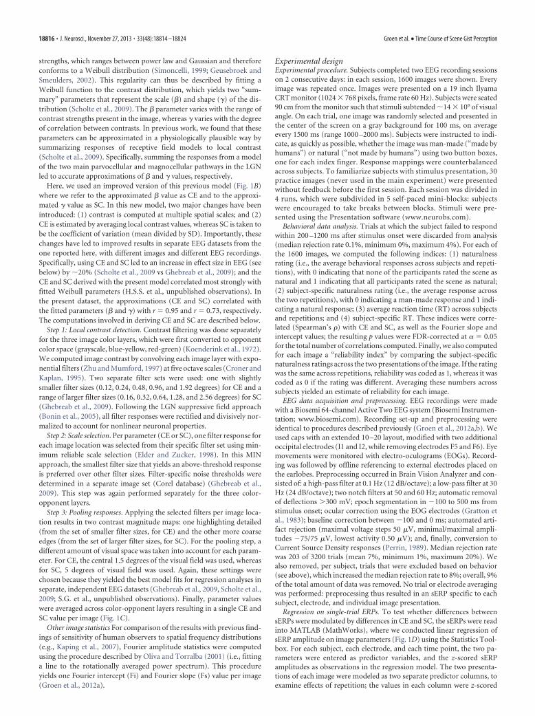
Figure 1. Stimuli, model, and methods. A, Examples of images used in the experiment. Images varied considerably in the degree to which they contained exclusively man-made (left) or natural(right) elements, and the set included images for which the distinction may be unclear (middle). B, A feedforward filtering model was used to derive two summary statistics: CE and SC. Threeopponent (grayscale, blue-yellow, red-blue) contrast magnitude maps were computed by convolving the image with multiscale filters (black circles). For CE, a range of smaller filter sizes (� �diameters in degrees) was used; for SC, a range of larger filter sizes. For each image location and parameter, a single filter response was selected (red circles) from each range using minimum reliablescale selection (see Materials and Methods). These responses were then pooled across a selection of the visual field (red dotted circles): for CE, the resulting responses were averaged; for SC, thecoefficient of variation (COV) was computed. These values were averaged across the three color-opponent maps resulting in one CE and SC value per image. C, A subset of 160 images (10% of thewhole stimulus set, randomly selected) plotted against their CE and SC values. CE (the approximation of the � parameter of the Weibull function) describes the scale of the contrast distribution: itvaries with the distribution of local contrasts strengths. SC (the approximation of the � parameter of the Weibull function) describes the shape of the contrast distribution: it varies with the amountof scene fragmentation (scene clutter). Four representative pictures are shown in each corner of the parameter space. Images that are highly structured (e.g., a street corner) are found on the left,whereas highly cluttered images (e.g., a forest) are on the right. Images with higher figure-ground separation (depth) are located on the top, whereas flat images are found at the bottom. D, sERPsto images presented at the center of the screen were computed for each subject. The resulting estimates of sERP amplitude were regressed on CE and SC at each time sample and electrode separately.The design matrix for the regression contained five columns: a constant term (c) for the intercept, two columns for CE and two for SC, each containing the same parameter values for the first andsecond image presentation (p1 and p2). These were modeled as separate predictors to examine reliability of the obtained effects across repetitions. The outcome of the analysis is a measure of modelfit (explained variance or R 2) separately over subjects, time (samples), and space (electrodes); an example is shown for one subject at electrode Oz.

Groen et al. • Time Course of Scene Gist Perception J. Neurosci., November 27, 2013 • 33(48):18814 –18824 • 18815

strengths, which ranges between power law and Gaussian and thereforeconforms to a Weibull distribution (Simoncelli, 1999; Geusebroek andSmeulders, 2002). This regularity can thus be described by fitting aWeibull function to the contrast distribution, which yields two “sum-mary” parameters that represent the scale (�) and shape (�) of the dis-tribution (Scholte et al., 2009). The � parameter varies with the range ofcontrast strengths present in the image, whereas � varies with the degreeof correlation between contrasts. In previous work, we found that theseparameters can be approximated in a physiologically plausible way bysummarizing responses of receptive field models to local contrast(Scholte et al., 2009). Specifically, summing the responses from a modelof the two main parvocellular and magnocellular pathways in the LGNled to accurate approximations of � and � values, respectively.

Here, we used an improved version of this previous model (Fig. 1B)where we refer to the approximated � value as CE and to the approxi-mated � value as SC. In this new model, two major changes have beenintroduced: (1) contrast is computed at multiple spatial scales; and (2)CE is estimated by averaging local contrast values, whereas SC is taken tobe the coefficient of variation (mean divided by SD). Importantly, thesechanges have led to improved results in separate EEG datasets from theone reported here, with different images and different EEG recordings.Specifically, using CE and SC led to an increase in effect size in EEG (seebelow) by �20% (Scholte et al., 2009 vs Ghebreab et al., 2009); and theCE and SC derived with the present model correlated most strongly withfitted Weibull parameters (H.S.S. et al., unpublished observations). Inthe present dataset, the approximations (CE and SC) correlated withthe fitted parameters (� and �) with r � 0.95 and r � 0.73, respectively.The computations involved in deriving CE and SC are described below.

Step 1: Local contrast detection. Contrast filtering was done separatelyfor the three image color layers, which were first converted to opponentcolor space (grayscale, blue-yellow, red-green) (Koenderink et al., 1972).We computed image contrast by convolving each image layer with expo-nential filters (Zhu and Mumford, 1997) at five octave scales (Croner andKaplan, 1995). Two separate filter sets were used: one with slightlysmaller filter sizes (0.12, 0.24, 0.48, 0.96, and 1.92 degrees) for CE and arange of larger filter sizes (0.16, 0.32, 0.64, 1.28, and 2.56 degrees) for SC(Ghebreab et al., 2009). Following the LGN suppressive field approach(Bonin et al., 2005), all filter responses were rectified and divisively nor-malized to account for nonlinear neuronal properties.

Step 2: Scale selection. Per parameter (CE or SC), one filter response foreach image location was selected from their specific filter set using min-imum reliable scale selection (Elder and Zucker, 1998). In this MINapproach, the smallest filter size that yields an above-threshold responseis preferred over other filter sizes. Filter-specific noise thresholds weredetermined in a separate image set (Corel database) (Ghebreab et al.,2009). This step was again performed separately for the three color-opponent layers.

Step 3: Pooling responses. Applying the selected filters per image loca-tion results in two contrast magnitude maps: one highlighting detailed(from the set of smaller filter sizes, for CE) and the other more coarseedges (from the set of larger filter sizes, for SC). For the pooling step, adifferent amount of visual space was taken into account for each param-eter. For CE, the central 1.5 degrees of the visual field was used, whereasfor SC, 5 degrees of visual field was used. Again, these settings werechosen because they yielded the best model fits for regression analyses inseparate, independent EEG datasets (Ghebreab et al., 2009, Scholte et al.,2009; S.G. et al., unpublished observations). Finally, parameter valueswere averaged across color-opponent layers resulting in a single CE andSC value per image (Fig. 1C).

Other image statistics For comparison of the results with previous find-ings of sensitivity of human observers to spatial frequency distributions(e.g., Kaping et al., 2007), Fourier amplitude statistics were computedusing the procedure described by Oliva and Torralba (2001) (i.e., fittinga line to the rotationally averaged power spectrum). This procedureyields one Fourier intercept (Fi) and Fourier slope (Fs) value per image(Groen et al., 2012a).

Experimental designExperimental procedure. Subjects completed two EEG recording sessionson 2 consecutive days: in each session, 1600 images were shown. Everyimage was repeated once. Images were presented on a 19 inch IlyamaCRT monitor (1024 � 768 pixels, frame rate 60 Hz). Subjects were seated90 cm from the monitor such that stimuli subtended �14 � 10° of visualangle. On each trial, one image was randomly selected and presented inthe center of the screen on a gray background for 100 ms, on averageevery 1500 ms (range 1000 –2000 ms). Subjects were instructed to indi-cate, as quickly as possible, whether the image was man-made (“made byhumans”) or natural (“not made by humans”) using two button boxes,one for each index finger. Response mappings were counterbalancedacross subjects. To familiarize subjects with stimulus presentation, 30practice images (never used in the main experiment) were presentedwithout feedback before the first session. Each session was divided in4 runs, which were subdivided in 5 self-paced mini-blocks: subjectswere encouraged to take breaks between blocks. Stimuli were pre-sented using the Presentation software (www.neurobs.com).

Behavioral data analysis. Trials at which the subject failed to respondwithin 200 –1200 ms after stimulus onset were discarded from analysis(median rejection rate 0.1%, minimum 0%, maximum 4%). For each ofthe 1600 images, we computed the following indices: (1) naturalnessrating (i.e., the average behavioral responses across subjects and repeti-tions), with 0 indicating that none of the participants rated the scene asnatural and 1 indicating that all participants rated the scene as natural;(2) subject-specific naturalness rating (i.e., the average response acrossthe two repetitions), with 0 indicating a man-made response and 1 indi-cating a natural response; (3) average reaction time (RT) across subjectsand repetitions; and (4) subject-specific RT. These indices were corre-lated (Spearman’s �) with CE and SC, as well as the Fourier slope andintercept values; the resulting p values were FDR-corrected at � � 0.05for the total number of correlations computed. Finally, we also computedfor each image a “reliability index” by comparing the subject-specificnaturalness ratings across the two presentations of the image. If the ratingwas the same across repetitions, reliability was coded as 1, whereas it wascoded as 0 if the rating was different. Averaging these numbers acrosssubjects yielded an estimate of reliability for each image.

EEG data acquisition and preprocessing. EEG recordings were madewith a Biosemi 64-channel Active Two EEG system (Biosemi Instrumen-tation; www.biosemi.com). Recording set-up and preprocessing wereidentical to procedures described previously (Groen et al., 2012a,b). Weused caps with an extended 10 –20 layout, modified with two additionaloccipital electrodes (I1 and I2, while removing electrodes F5 and F6). Eyemovements were monitored with electro-oculograms (EOGs). Record-ing was followed by offline referencing to external electrodes placed onthe earlobes. Preprocessing occurred in Brain Vision Analyzer and con-sisted of: a high-pass filter at 0.1 Hz (12 dB/octave); a low-pass filter at 30Hz (24 dB/octave); two notch filters at 50 and 60 Hz; automatic removalof deflections �300 mV; epoch segmentation in �100 to 500 ms fromstimulus onset; ocular correction using the EOG electrodes (Gratton etal., 1983); baseline correction between �100 and 0 ms; automated arti-fact rejection (maximal voltage steps 50 �V, minimal/maximal ampli-tudes �75/75 �V, lowest activity 0.50 �V); and, finally, conversion toCurrent Source Density responses (Perrin, 1989). Median rejection ratewas 203 of 3200 trials (mean 7%, minimum 1%, maximum 20%). Wealso removed, per subject, trials that were excluded based on behavior(see above), which increased the median rejection rate to 8%; overall, 9%of the total amount of data was removed. No trial or electrode averagingwas performed: preprocessing thus resulted in an sERP specific to eachsubject, electrode, and individual image presentation.

Regression on single-trial ERPs. To test whether differences betweensERPs were modulated by differences in CE and SC, the sERPs were readinto MATLAB (MathWorks), where we conducted linear regression ofsERP amplitude on image parameters (Fig. 1D) using the Statistics Tool-box. For each subject, each electrode, and each time point, the two pa-rameters were entered as predictor variables, and the z-scored sERPamplitudes as observations in the regression model. The two presenta-tions of each image were modeled as two separate predictor columns, toexamine effects of repetition; the values in each column were z-scored

18816 • J. Neurosci., November 27, 2013 • 33(48):18814 –18824 Groen et al. • Time Course of Scene Gist Perception

independently (Rousselet et al., 2011). This analysis thus results in ameasure of model fit (explained variance or R 2) for each subject, elec-trode, and time point separately. In addition, we read out from the re-gression results the �-coefficients assigned to each predictor column,which reflect the regression weights between the image parameters andsERP amplitude (again, separately for each subject, electrode, and timepoint). To assess the significance of these coefficients, we tested thesubject-averaged coefficient against zero using t tests (separate for eachtime point and electrode): a significant test result indicates that the asso-ciation between a predictor and evoked neural activity is reliably largerthan zero at a specific time point and electrode. To correct for multiplecomparisons (time points, electrodes and parameters), p values wereFDR-corrected at � � 0.05. The rationale of this approach is quite similarto conventional fMRI analysis (GLM); we compute the �-coefficients foreach predictor in our model and threshold using multiple-comparisoncorrected t values. By doing this for every electrode (“whole-scalp anal-ysis”), we created spatial maps that indicate which electrodes containsignificant �-coefficients.

Regression results for other image statistics. For comparison of the re-gression results for CE and SC with parameters obtained from the Fou-rier transform, we ran the regression analyses described above (Fig 1D)while replacing the predictor columns with Fi and Fs. In addition, weexamined the dependence between the two models by running a thirdregression analysis in which we entered all four parameters (CE, SC, Fi,and Fs) together as predictors, yielding a “full” model. By subtracting theR 2 values for the first two models from the full model, we obtained ameasure of “unique explained variance” by each model (Groen et al.,2012b). These values were again obtained separately per subject, elec-trode, and time point.

Linear discriminant component analysis. To identify decision-relatedactivity in the EEG signal, we used linear discrimination analysis as de-veloped by Philiastides and colleagues (Parra et al., 2002; Philiastides andSajda, 2006; Philiastides et al., 2006). Linear discriminant analysis per-forms logistic regression of binary data on multivariate EEG data toidentify spatial weighting vectors (w) across electrodes that maximallydiscriminate between conditions of interest (e.g., a face or car stimulus).Here, we used as conditions of interest the ratings made by the subjectsduring naturalness rating, by entering the trial-specific behavioral re-sponses (man-made or natural) as the binary data. The analysis outcomeis a “discriminating component” y, which is specific to activity correlatedwith one condition while minimizing activity correlated with both taskconditions (Philiastides et al., 2006); in our case, we isolated activityspecific to the decision that a scene was natural.

We used an online available regularized logistic regression algorithm(Conroy and Sajda, 2012) that allows for fast estimation of the discrim-inating components. We tested various regularization terms (� � 1ex

with x � �6:1:2), which yielded similar results to those reported here for� � 1e �1. We computed y for a number of temporal windows (windowsize � 20 ms), to estimate the temporal evolution of discriminantactivity over the course of the ERP. Per time window, discriminatorperformance (Az) across all trials was quantified using the area under thereceiver-operator characteristic curve, with a leave-one-out cross-validation approach (Duda et al., 2001). Following Blank et al. (2013),significance of performance was evaluated by bootstrapping the Az val-ues. We used 100 bootstraps per time window (epoch of 600 ms/ � 40windows) and subject (n � 14), resulting in 42,000 Az values in total. Theoverall distribution of these values was used to determine the Az valueleading to a significance level of p � 0.05. Finally, the components wereprojected back on the scalp using a forward model that multiplies thew-vector with average ERP amplitude in a specific time window (Parra etal., 2002).

Relating discriminant component activity to image statistics. After ob-taining an estimate of discriminant component activity at each trial andtime window, the y values were correlated (Spearman’s �) with the CEand SC values of the image presented at that trial, for each subject sepa-rately. To assess the significance of these correlations, we again testedthe average correlation across subjects against zero using separate ttests for each time window; the resulting p values were again correctedfor multiple comparisons using an FDR-correction at � � 0.05.

ResultsBehaviorFourteen subjects rated 1600 scene images as either man-made ornatural while EEG was recorded. We first examined how behav-ioral ratings were distributed across the entire set of images. Next,we tested how these results were related to differences in CE andSC estimated from modeled responses to local contrast.

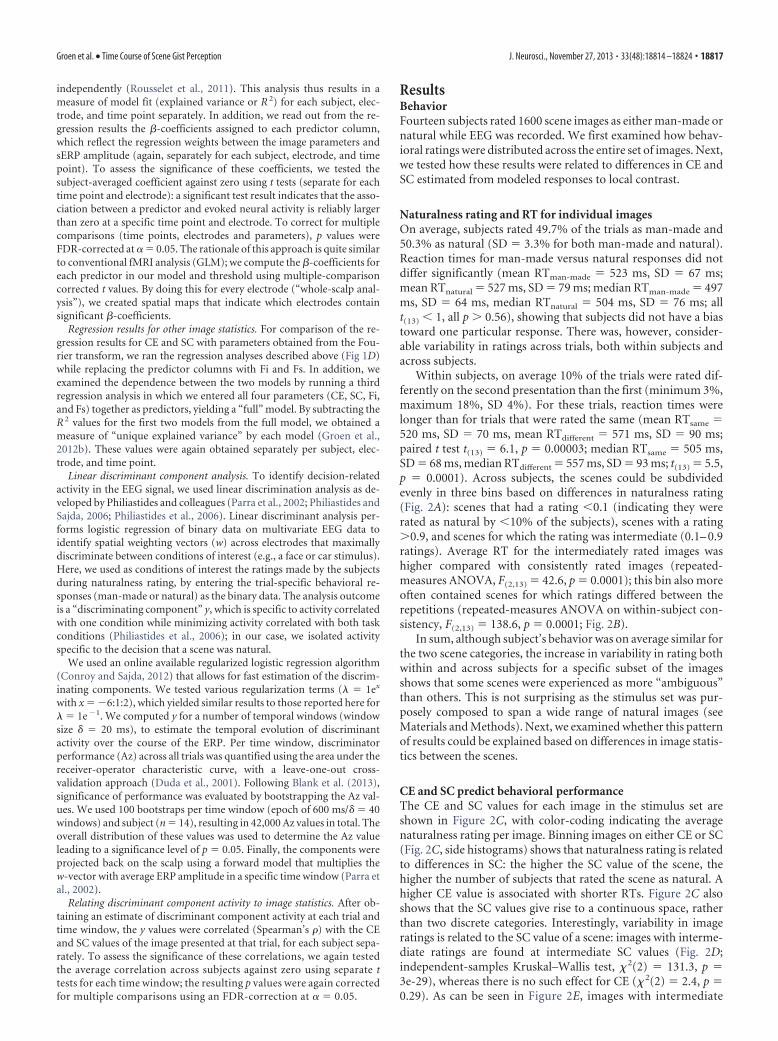
Naturalness rating and RT for individual imagesOn average, subjects rated 49.7% of the trials as man-made and50.3% as natural (SD � 3.3% for both man-made and natural).Reaction times for man-made versus natural responses did notdiffer significantly (mean RTman-made � 523 ms, SD � 67 ms;mean RTnatural � 527 ms, SD � 79 ms; median RTman-made � 497ms, SD � 64 ms, median RTnatural � 504 ms, SD � 76 ms; allt(13) � 1, all p � 0.56), showing that subjects did not have a biastoward one particular response. There was, however, consider-able variability in ratings across trials, both within subjects andacross subjects.

Within subjects, on average 10% of the trials were rated dif-ferently on the second presentation than the first (minimum 3%,maximum 18%, SD 4%). For these trials, reaction times werelonger than for trials that were rated the same (mean RTsame �520 ms, SD � 70 ms, mean RTdifferent � 571 ms, SD � 90 ms;paired t test t(13) � 6.1, p � 0.00003; median RTsame � 505 ms,SD � 68 ms, median RTdifferent � 557 ms, SD � 93 ms; t(13) � 5.5,p � 0.0001). Across subjects, the scenes could be subdividedevenly in three bins based on differences in naturalness rating(Fig. 2A): scenes that had a rating �0.1 (indicating they wererated as natural by �10% of the subjects), scenes with a rating�0.9, and scenes for which the rating was intermediate (0.1– 0.9ratings). Average RT for the intermediately rated images washigher compared with consistently rated images (repeated-measures ANOVA, F(2,13) � 42.6, p � 0.0001); this bin also moreoften contained scenes for which ratings differed between therepetitions (repeated-measures ANOVA on within-subject con-sistency, F(2,13) � 138.6, p � 0.0001; Fig. 2B).

In sum, although subject’s behavior was on average similar forthe two scene categories, the increase in variability in rating bothwithin and across subjects for a specific subset of the imagesshows that some scenes were experienced as more “ambiguous”than others. This is not surprising as the stimulus set was pur-posely composed to span a wide range of natural images (seeMaterials and Methods). Next, we examined whether this patternof results could be explained based on differences in image statis-tics between the scenes.

CE and SC predict behavioral performanceThe CE and SC values for each image in the stimulus set areshown in Figure 2C, with color-coding indicating the averagenaturalness rating per image. Binning images on either CE or SC(Fig. 2C, side histograms) shows that naturalness rating is relatedto differences in SC: the higher the SC value of the scene, thehigher the number of subjects that rated the scene as natural. Ahigher CE value is associated with shorter RTs. Figure 2C alsoshows that the SC values give rise to a continuous space, ratherthan two discrete categories. Interestingly, variability in imageratings is related to the SC value of a scene: images with interme-diate ratings are found at intermediate SC values (Fig. 2D;independent-samples Kruskal–Wallis test, 2(2) � 131.3, p �3e-29), whereas there is no such effect for CE ( 2(2) � 2.4, p �0.29). As can be seen in Figure 2E, images with intermediate

Groen et al. • Time Course of Scene Gist Perception J. Neurosci., November 27, 2013 • 33(48):18814 –18824 • 18817

ratings and SC values typically contain patches with both man-made and natural elements. This suggests that SC in particularis diagnostic of scene naturalness.

We confirmed these observations by correlating the CE andSC values directly with the behavioral measures (Table 1). SCcorrelated with naturalness rating, but not with RT, whereas CEcorrelated with RT, and to a lesser extent with rating. For com-parison, we also computed correlations with image statistics de-rived from the power spectra of the scenes (Oliva and Torralba,2001), Fi and Fs (see Materials and Methods). These correlationsare in a similar range as those with CE and SC (Table 1). For thismodel, however, the two parameters are less well dissociable, asthey both correlate significantly with accuracy as well as RT.

The behavioral results support our proposal that CE and SC,which are computed by pooling of local contrast, capture globalscene information. They predict human categorization of scenenaturalness to a similar degree as statistics obtained from a globalimage transformation (Fourier parameters). In particular, thereis a relation between SC and perceived naturalness, whereas CEseems to influence the speed of processing.

EEGsERPs were extracted from the continuous EEG data after whichwe performed linear regression of sERP amplitude on image sta-

tistics. We first examined how CE and SC affected evoked activityto individual images, again comparing them with the Fourierparameters. Next, we tested how the EEG activity itself was re-lated to the behavioral ratings, and whether this relation wasdependent on CE and/or SC.

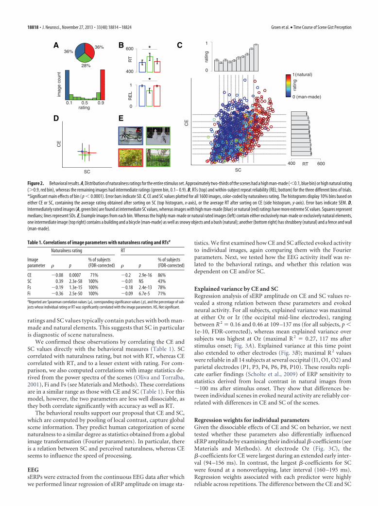
Explained variance by CE and SCRegression analysis of sERP amplitude on CE and SC values re-vealed a strong relation between these parameters and evokedneural activity. For all subjects, explained variance was maximalat either Oz or Iz (the occipital mid-line electrodes), rangingbetween R 2 � 0.16 and 0.46 at 109 –137 ms (for all subjects, p �1e-10, FDR-corrected), whereas mean explained variance oversubjects was highest at Oz (maximal R 2 � 0.27, 117 ms afterstimulus onset; Fig. 3A). Explained variance at this time pointalso extended to other electrodes (Fig. 3B); maximal R 2 valueswere reliable in all 14 subjects at several occipital (I1, O1, O2) andparietal electrodes (P1, P3, P4, P6, P8, P10). These results repli-cate earlier findings (Scholte et al., 2009) of ERP sensitivity tostatistics derived from local contrast in natural images from�100 ms after stimulus onset. They show that differences be-tween individual scenes in evoked neural activity are reliably cor-related with differences in CE and SC of the scenes.

Regression weights for individual parametersGiven the dissociable effects of CE and SC on behavior, we nexttested whether these parameters also differentially influencedsERP amplitude by examining their individual �-coefficients (seeMaterials and Methods). At electrode Oz (Fig. 3C), the�-coefficients for CE were largest during an extended early inter-val (94 –156 ms). In contrast, the largest �-coefficients for SCwere found at a nonoverlapping, later interval (160 –195 ms).Regression weights associated with each predictor were highlyreliable across repetitions. The difference between the CE and SC

A

D

B C

E

Figure 2. Behavioral results. A, Distribution of naturalness ratings for the entire stimulus set. Approximately two-thirds of the scenes had a high man-made (�0.1, blue bin) or high natural rating(�0.9, red bin), whereas the remaining images had intermediate ratings (green bin, 0.1– 0.9). B, RTs (top) and within-subject repeat reliability (REL; bottom) for the three different bins of trials.*Significant main effects of bin ( p � 0.0001). Error bars indicate SD. C, CE and SC values plotted for all 1600 images, color-coded by naturalness rating. The histograms display 10% bins based oneither CE or SC, containing the average rating obtained after sorting on SC (top histogram, x-axis), or the average RT after sorting on CE (side histogram, y-axis). Error bars indicate SEM. D,Intermediately rated images (A, green bin) are found at intermediate SC values, whereas images with high man-made (blue) or natural (red) ratings have more extreme SC values. Squares representmedians; lines represent SDs. E, Example images from each bin. Whereas the highly man-made or natural rated images (left) contain either exclusively man-made or exclusively natural elements,one intermediate image (top right) contains a building and a bicycle (man-made) as well as snowy objects and a bush (natural); another (bottom right) has shrubbery (natural) and a fence and wall(man-made).

Table 1. Correlations of image parameters with naturalness rating and RTsa

Naturalness rating RT

Imageparameter � p

% of subjects(FDR-corrected) � p

% of subjects(FDR-corrected)

CE �0.08 0.0007 71% �0.2 2.9e-16 86%SC 0.39 2.3e-58 100% �0.01 NS 43%Fs �0.19 1.3e-15 100% �0.18 2.4e-13 78%Fi �0.36 2.5e-50 100% �0.09 6.7e-5 71%aReported are Spearman correlation values (�), corresponding significance values ( p), and the percentage of sub-jects whose individual rating or RT was significantly correlated with the image parameters. NS, Not significant.

18818 • J. Neurosci., November 27, 2013 • 33(48):18814 –18824 Groen et al. • Time Course of Scene Gist Perception

effects is illustrated in Figure 3D, where sERP amplitude foreach image relative to its SC and CE value is shown for the twotime points with largest �-coefficients (113 and 184 ms, respec-tively). At the first maximum, differences in amplitude are mostlyaligned with the CE-axis of the space. At the second maximum, theamplitudes align with the SC-axis instead. Significant but smallercoefficients for SC were also found at two shorter and earlier inter-vals (78–85 ms and 117–136 ms) and one later interval (226 –242ms). Neural sensitivity to different image parameters thus dif-fers substantially over the time course of visual processing.Interestingly, these results again demonstrate dissociable ef-fects of CE and SC, but now on evoked neural activity.

Finally, for both CE and SC, regression coefficients were alsosignificant toward the end of the ERP epoch, most likely reflect-ing spill-over of effects at other electrodes. These might be elec-trodes near motor cortex, as this interval is in the RT range(minimal average RT was 436 ms, maximal average RT was 647ms); the �-coefficients at Oz are very small at this time point,indicating low sERP amplitudes. In the next section, we test towhat extent each image parameter affected responses at otherelectrodes.

Whole-scalp regression weightsThe distribution of regression coefficients across the whole scalpmirrors the effects observed at electrode Oz. Generally, the

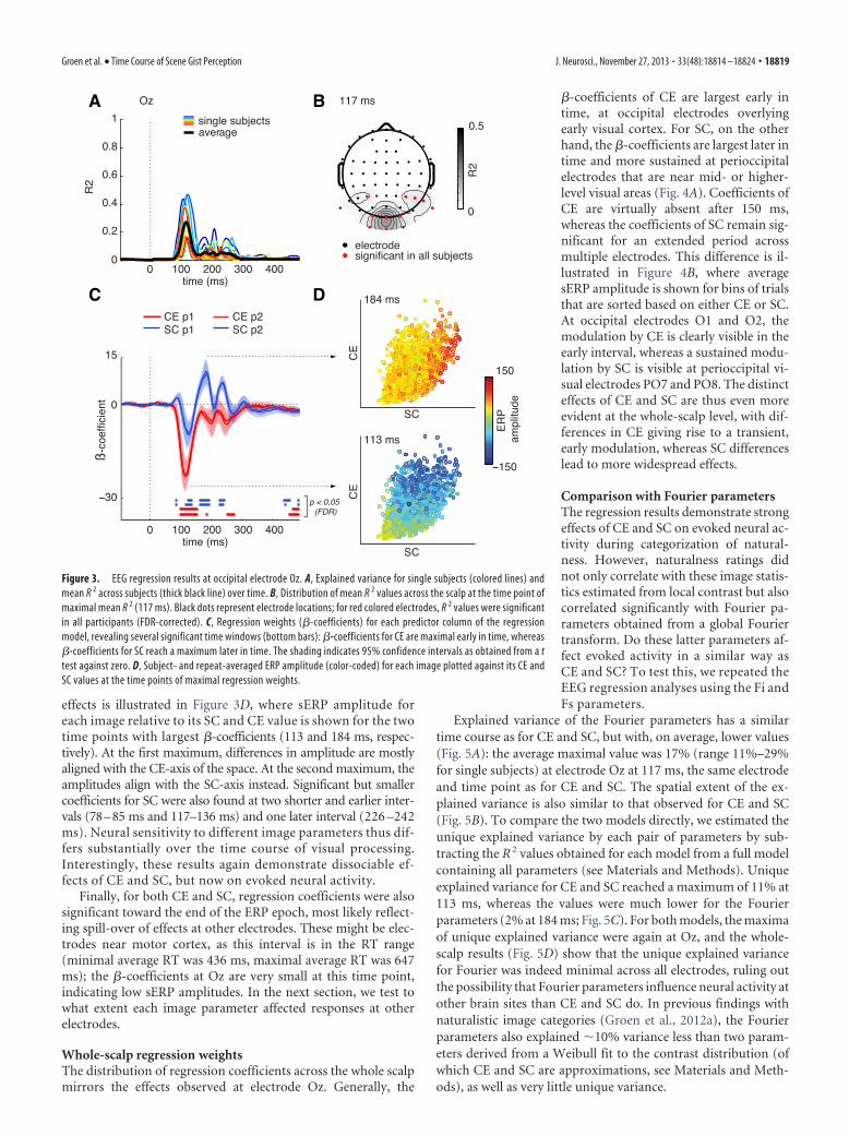
�-coefficients of CE are largest early intime, at occipital electrodes overlyingearly visual cortex. For SC, on the otherhand, the �-coefficients are largest later intime and more sustained at perioccipitalelectrodes that are near mid- or higher-level visual areas (Fig. 4A). Coefficients ofCE are virtually absent after 150 ms,whereas the coefficients of SC remain sig-nificant for an extended period acrossmultiple electrodes. This difference is il-lustrated in Figure 4B, where averagesERP amplitude is shown for bins of trialsthat are sorted based on either CE or SC.At occipital electrodes O1 and O2, themodulation by CE is clearly visible in theearly interval, whereas a sustained modu-lation by SC is visible at perioccipital vi-sual electrodes PO7 and PO8. The distincteffects of CE and SC are thus even moreevident at the whole-scalp level, with dif-ferences in CE giving rise to a transient,early modulation, whereas SC differenceslead to more widespread effects.

Comparison with Fourier parametersThe regression results demonstrate strongeffects of CE and SC on evoked neural ac-tivity during categorization of natural-ness. However, naturalness ratings didnot only correlate with these image statis-tics estimated from local contrast but alsocorrelated significantly with Fourier pa-rameters obtained from a global Fouriertransform. Do these latter parameters af-fect evoked activity in a similar way asCE and SC? To test this, we repeated theEEG regression analyses using the Fi andFs parameters.

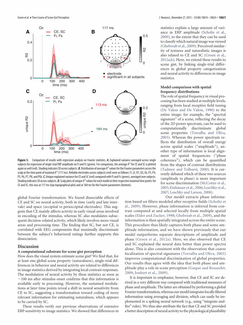
Explained variance of the Fourier parameters has a similartime course as for CE and SC, but with, on average, lower values(Fig. 5A): the average maximal value was 17% (range 11%–29%for single subjects) at electrode Oz at 117 ms, the same electrodeand time point as for CE and SC. The spatial extent of the ex-plained variance is also similar to that observed for CE and SC(Fig. 5B). To compare the two models directly, we estimated theunique explained variance by each pair of parameters by sub-tracting the R 2 values obtained for each model from a full modelcontaining all parameters (see Materials and Methods). Uniqueexplained variance for CE and SC reached a maximum of 11% at113 ms, whereas the values were much lower for the Fourierparameters (2% at 184 ms; Fig. 5C). For both models, the maximaof unique explained variance were again at Oz, and the whole-scalp results (Fig. 5D) show that the unique explained variancefor Fourier was indeed minimal across all electrodes, ruling outthe possibility that Fourier parameters influence neural activity atother brain sites than CE and SC do. In previous findings withnaturalistic image categories (Groen et al., 2012a), the Fourierparameters also explained �10% variance less than two param-eters derived from a Weibull fit to the contrast distribution (ofwhich CE and SC are approximations, see Materials and Meth-ods), as well as very little unique variance.

A

C D

B

Figure 3. EEG regression results at occipital electrode Oz. A, Explained variance for single subjects (colored lines) andmean R 2 across subjects (thick black line) over time. B, Distribution of mean R 2 values across the scalp at the time point ofmaximal mean R 2 (117 ms). Black dots represent electrode locations; for red colored electrodes, R 2 values were significantin all participants (FDR-corrected). C, Regression weights (�-coefficients) for each predictor column of the regressionmodel, revealing several significant time windows (bottom bars): �-coefficients for CE are maximal early in time, whereas�-coefficients for SC reach a maximum later in time. The shading indicates 95% confidence intervals as obtained from a ttest against zero. D, Subject- and repeat-averaged ERP amplitude (color-coded) for each image plotted against its CE andSC values at the time points of maximal regression weights.

Groen et al. • Time Course of Scene Gist Perception J. Neurosci., November 27, 2013 • 33(48):18814 –18824 • 18819

These results suggest that modulationsof single-trial evoked activity during nat-uralness categorization are also correlatedwith differences in spatial frequency con-tent (Fi and Fs). However, the effects wereweaker compared with those observed forCE and SC, and the Fourier parametersdid not explain substantial variance aboveand beyond the variance explained by CEand SC. This suggests that informationthat is contained in the Fourier parame-ters is also captured by CE and SC and thatthe latter may provide a more plausibledescription of evoked neural activity dur-ing naturalness categorization.

Role of image statistics inperceptual decision-making?The regression results suggest that CE andSC play different roles in visual processingof natural images, with CE giving rise toearly, transient effects, whereas SC differ-ences lead to sustained effects on evokedactivity. Interestingly, the modulations bySC extend into time intervals associatedwith mid-level stages of visual processing(beyond 200 ms) that are sensitive to top-down influences (Luck et al., 2000;Scholte et al., 2006) and possibly involvedin perceptual decision-making (Philias-tides et al., 2006). Task relevance of thescene parameters may thus play a role inthe differential effects of CE and SC thatwere observed here. Specifically, the latemodulation by SC could reflect an influ-ence of SC on the naturalness decision.

To test how CE and SC affected decision-related neural activ-ity, we used linear discriminant analysis to identify discriminat-ing components in the EEG (Parra et al., 2002; Philiastides andSajda, 2006; Philiastides et al., 2006; Conroy and Sajda, 2012;Blank et al., 2013). This is essentially again a single-trial regres-sion, but of behavior onto the EEG: observations correspond to the(subject-specific) man-made or natural ratings, and the predictorvariables consist of the sERP amplitudes at each electrode. Thisanalysis yields two measures: overall discrimination accuracy, sum-marized in parameter Az and trial-specific discriminant compo-nents y, reflecting evidence toward a natural versus a man-maderating at a given trial (see Materials and Methods). Both measureswere determined for consecutive time windows (see Materialsand Methods), to examine the development of discriminant ac-tivity over time. With this analysis, we aimed to address twoquestions: (1) From what point in time can we reliably predictwhether a given trial will be rated as man-made or natural? (2) Towhat extent is the strength of evidence toward the man-made orthe natural rating modulated by CE and SC?

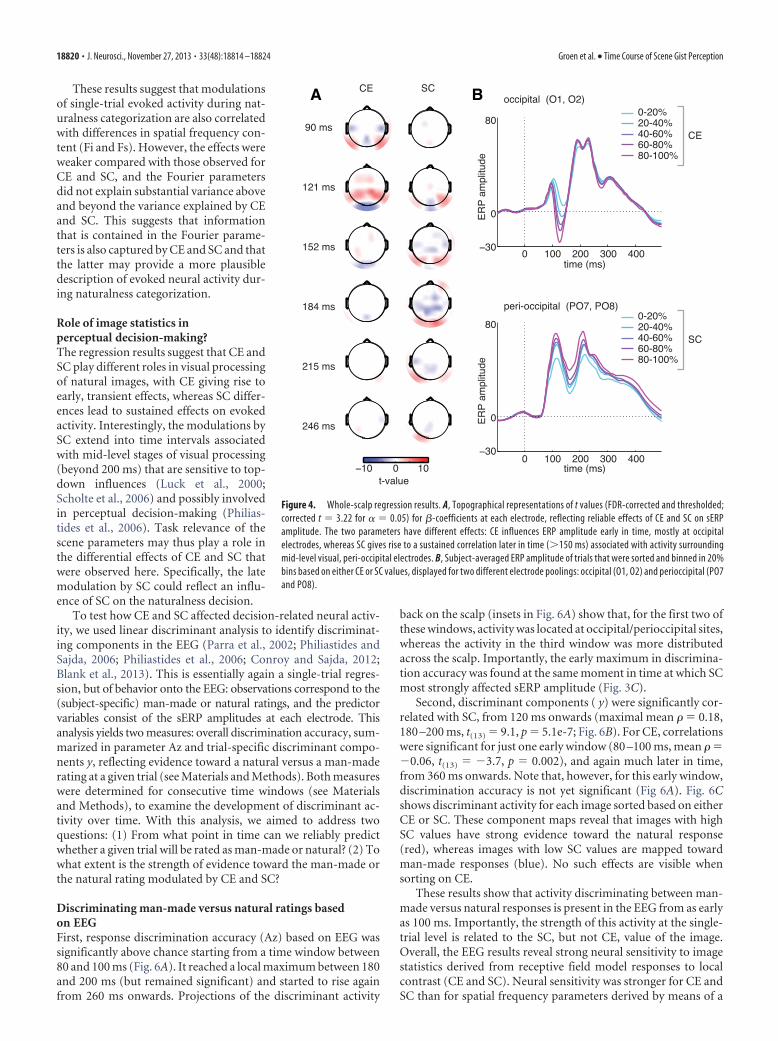
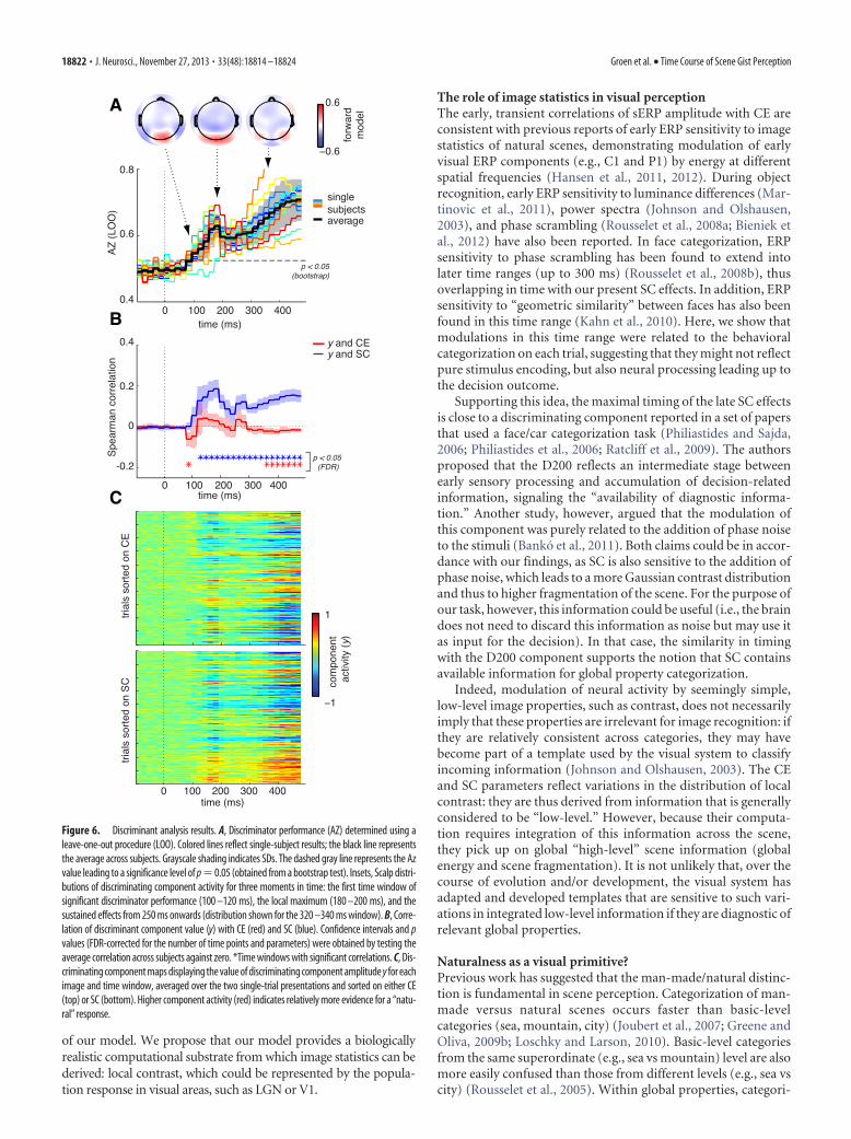
Discriminating man-made versus natural ratings basedon EEGFirst, response discrimination accuracy (Az) based on EEG wassignificantly above chance starting from a time window between80 and 100 ms (Fig. 6A). It reached a local maximum between 180and 200 ms (but remained significant) and started to rise againfrom 260 ms onwards. Projections of the discriminant activity

back on the scalp (insets in Fig. 6A) show that, for the first two ofthese windows, activity was located at occipital/perioccipital sites,whereas the activity in the third window was more distributedacross the scalp. Importantly, the early maximum in discrimina-tion accuracy was found at the same moment in time at which SCmost strongly affected sERP amplitude (Fig. 3C).

Second, discriminant components ( y) were significantly cor-related with SC, from 120 ms onwards (maximal mean � � 0.18,180 –200 ms, t(13) � 9.1, p � 5.1e-7; Fig. 6B). For CE, correlationswere significant for just one early window (80 –100 ms, mean � ��0.06, t(13) � �3.7, p � 0.002), and again much later in time,from 360 ms onwards. Note that, however, for this early window,discrimination accuracy is not yet significant (Fig 6A). Fig. 6Cshows discriminant activity for each image sorted based on eitherCE or SC. These component maps reveal that images with highSC values have strong evidence toward the natural response(red), whereas images with low SC values are mapped towardman-made responses (blue). No such effects are visible whensorting on CE.

These results show that activity discriminating between man-made versus natural responses is present in the EEG from as earlyas 100 ms. Importantly, the strength of this activity at the single-trial level is related to the SC, but not CE, value of the image.Overall, the EEG results reveal strong neural sensitivity to imagestatistics derived from receptive field model responses to localcontrast (CE and SC). Neural sensitivity was stronger for CE andSC than for spatial frequency parameters derived by means of a

A B

Figure 4. Whole-scalp regression results. A, Topographical representations of t values (FDR-corrected and thresholded;corrected t � 3.22 for � � 0.05) for �-coefficients at each electrode, reflecting reliable effects of CE and SC on sERPamplitude. The two parameters have different effects: CE influences ERP amplitude early in time, mostly at occipitalelectrodes, whereas SC gives rise to a sustained correlation later in time (�150 ms) associated with activity surroundingmid-level visual, peri-occipital electrodes. B, Subject-averaged ERP amplitude of trials that were sorted and binned in 20%bins based on either CE or SC values, displayed for two different electrode poolings: occipital (O1, O2) and perioccipital (PO7and PO8).

18820 • J. Neurosci., November 27, 2013 • 33(48):18814 –18824 Groen et al. • Time Course of Scene Gist Perception

global Fourier transformation. We found dissociable effects ofCE and SC on neural activity, both in time (early and late inter-vals) and space (occipital vs perioccipital electrodes). This sug-gests that CE mainly affects activity in early visual areas involvedin encoding of the stimulus, whereas SC also modulates subse-quent decision-related activity, which likely involves more visualareas and processing time. The finding that SC, but not CE, iscorrelated with EEG components that maximally discriminatebetween the subject’s behavioral ratings further supports thisdissociation.

DiscussionA computational substrate for scene gist perceptionHow does the visual system estimate scene gist? We find that, forat least one global scene property (naturalness), single-trial dif-ferences in behavior and neural activity are related to differencesin image statistics derived by integrating local contrast responses.The modulation of neural activity by these statistics as soon as�100 ms after stimulus onset confirms that this information isavailable early in processing. However, the sustained modula-tions at later time points reveal a shift in neural sensitivity fromCE to SC, suggesting a transformation toward coding of morerelevant information for estimating naturalness, which appearsto be carried by SC.

These results verify our previous observations of extensiveERP sensitivity to image statistics. We showed that differences in

statistics explain a large amount of vari-ance in ERP amplitude (Scholte et al.,2009), to the extent that they can be usedto classify which natural image was viewed(Ghebreab et al., 2009). Perceived similar-ity of textures and naturalistic images isalso related to CE and SC (Groen et al.,2012a,b). Here, we extend these results toscene gist, by linking single-trial differ-ences in global property categorizationand neural activity to differences in imagestatistics.

Model comparison with spatialfrequency distributionsThe role of spatial frequency in visual pro-cessing has been studied at multiple levels,ranging from local receptive field tuning(De Valois and De Valois, 1990) to theentire image: for example, the “spectralsignature” of a scene, reflecting the decayof the 2D power spectrum, can be used tocomputationally discriminate globalscene properties (Torralba and Oliva,2003). Whereas the power spectrum re-flects the distribution of overall energyacross spatial scales (“amplitude”), an-other type of information is local align-ment of spatial frequencies (“phasecoherence”), which can be quantifiedfrom the shapes of contrast distributions(Tadmor and Tolhurst, 2000). It is cur-rently debated which of these two sources(amplitude vs phase) is more importantfor scene discrimination (McCotter et al.,2005; Einhauser et al., 2006; Loschky et al.,2007; Loschky and Larson, 2008).

Our model extracts phase informa-tion based on filters modeled after receptive fields (Scholte etal., 2009). However, phase information is inferred from con-trast computed at and selected locally from multiple spatialscales (Elder and Zucker, 1998; Ghebreab et al., 2009), and theinformation is then spatially integrated across the entire scene.This procedure thus likely captures both phase and some am-plitude information, and we have shown previously that ourmodel outperforms separate descriptions of amplitude andphase (Groen et al., 2012a). Here, we also observed that CEand SC explained the neural data better than power spectraalone. This is also consistent with the observation that coarselocalization of spectral signatures (Torralba and Oliva, 2003)improves computational discrimination of global properties.Our results thus agree with the idea that both phase and am-plitude play a role in scene perception (Gaspar and Rousselet,2009; Joubert et al., 2009).

It is important to emphasize, however, that CE and SC are de-rived in a very different way compared with traditional measures ofphase and amplitude. The latter are obtained by performing a globalFourier transformation, whereas our model integrates locally filteredinformation using averaging and division, which can easily be im-plemented in a spiking neural network (e.g., using “integrate-and-fire” rules). We thus also attribute the fact that CE and SC provideda better description of neural activity to the physiological plausibility

A

C D

B

Figure 5. Comparison of results with regression analysis on Fourier statistics. A, Explained variance averaged across singlesubjects for regression of single-trial ERP amplitude on Fi and Fs (green). For comparison, the average R 2 for CE and SC is plottedagain as well (red). Shading indicates SD across subjects. B, Distribution of average R 2 values for the Fourier parameters across thescalp at the time point of maximal R 2 (117 ms). Reliable electrodes across subjects (red) were as follows: I1, I2, O1, O2, Oz, P3, P4,P5, P6, P7, P8, and POz. C, Unique explained variance for CE and SC (red) compared with Fi and Fs (green), averaged over subjects.Shading indicates SD across subjects. D, Scalp plots of unique R 2 values for each model at their respective maximal time points: forCE and SC, this was at 117 ms (top topographical plot) and at 184 ms for the Fourier parameters (bottom).

Groen et al. • Time Course of Scene Gist Perception J. Neurosci., November 27, 2013 • 33(48):18814 –18824 • 18821

of our model. We propose that our model provides a biologicallyrealistic computational substrate from which image statistics can bederived: local contrast, which could be represented by the popula-tion response in visual areas, such as LGN or V1.

The role of image statistics in visual perceptionThe early, transient correlations of sERP amplitude with CE areconsistent with previous reports of early ERP sensitivity to imagestatistics of natural scenes, demonstrating modulation of earlyvisual ERP components (e.g., C1 and P1) by energy at differentspatial frequencies (Hansen et al., 2011, 2012). During objectrecognition, early ERP sensitivity to luminance differences (Mar-tinovic et al., 2011), power spectra (Johnson and Olshausen,2003), and phase scrambling (Rousselet et al., 2008a; Bieniek etal., 2012) have also been reported. In face categorization, ERPsensitivity to phase scrambling has been found to extend intolater time ranges (up to 300 ms) (Rousselet et al., 2008b), thusoverlapping in time with our present SC effects. In addition, ERPsensitivity to “geometric similarity” between faces has also beenfound in this time range (Kahn et al., 2010). Here, we show thatmodulations in this time range were related to the behavioralcategorization on each trial, suggesting that they might not reflectpure stimulus encoding, but also neural processing leading up tothe decision outcome.

Supporting this idea, the maximal timing of the late SC effectsis close to a discriminating component reported in a set of papersthat used a face/car categorization task (Philiastides and Sajda,2006; Philiastides et al., 2006; Ratcliff et al., 2009). The authorsproposed that the D200 reflects an intermediate stage betweenearly sensory processing and accumulation of decision-relatedinformation, signaling the “availability of diagnostic informa-tion.” Another study, however, argued that the modulation ofthis component was purely related to the addition of phase noiseto the stimuli (Banko et al., 2011). Both claims could be in accor-dance with our findings, as SC is also sensitive to the addition ofphase noise, which leads to a more Gaussian contrast distributionand thus to higher fragmentation of the scene. For the purpose ofour task, however, this information could be useful (i.e., the braindoes not need to discard this information as noise but may use itas input for the decision). In that case, the similarity in timingwith the D200 component supports the notion that SC containsavailable information for global property categorization.

Indeed, modulation of neural activity by seemingly simple,low-level image properties, such as contrast, does not necessarilyimply that these properties are irrelevant for image recognition: ifthey are relatively consistent across categories, they may havebecome part of a template used by the visual system to classifyincoming information (Johnson and Olshausen, 2003). The CEand SC parameters reflect variations in the distribution of localcontrast: they are thus derived from information that is generallyconsidered to be “low-level.” However, because their computa-tion requires integration of this information across the scene,they pick up on global “high-level” scene information (globalenergy and scene fragmentation). It is not unlikely that, over thecourse of evolution and/or development, the visual system hasadapted and developed templates that are sensitive to such vari-ations in integrated low-level information if they are diagnostic ofrelevant global properties.

Naturalness as a visual primitive?Previous work has suggested that the man-made/natural distinc-tion is fundamental in scene perception. Categorization of man-made versus natural scenes occurs faster than basic-levelcategories (sea, mountain, city) (Joubert et al., 2007; Greene andOliva, 2009b; Loschky and Larson, 2010). Basic-level categoriesfrom the same superordinate (e.g., sea vs mountain) level are alsomore easily confused than those from different levels (e.g., sea vscity) (Rousselet et al., 2005). Within global properties, categori-

A

B

C

Figure 6. Discriminant analysis results. A, Discriminator performance (AZ) determined using aleave-one-out procedure (LOO). Colored lines reflect single-subject results; the black line representsthe average across subjects. Grayscale shading indicates SDs. The dashed gray line represents the Azvalue leading to a significance level of p � 0.05 (obtained from a bootstrap test). Insets, Scalp distri-butions of discriminating component activity for three moments in time: the first time window ofsignificant discriminator performance (100 –120 ms), the local maximum (180 –200 ms), and thesustained effects from 250 ms onwards (distribution shown for the 320 –340 ms window). B, Corre-lation of discriminant component value (y) with CE (red) and SC (blue). Confidence intervals and pvalues (FDR-corrected for the number of time points and parameters) were obtained by testing theaverage correlation across subjects against zero. *Time windows with significant correlations. C, Dis-criminating component maps displaying the value of discriminating component amplitude y for eachimage and time window, averaged over the two single-trial presentations and sorted on either CE(top) or SC (bottom). Higher component activity (red) indicates relatively more evidence for a “natu-ral” response.

18822 • J. Neurosci., November 27, 2013 • 33(48):18814 –18824 Groen et al. • Time Course of Scene Gist Perception

zation may occur hierarchically, starting with man-made versusnatural (Kadar and Ben-Shahar, 2012). The relation between SCand scene naturalness, as well as the influence of SC on evokedneural activity during naturalness categorization, suggests thatthe SC of the scene may drive this early primary distinction.

The fact that humans can quickly decide about naturalness,however, does not imply that the brain computes it automati-cally. Would the brain be interested in determining the natural-ness of visual input in everyday viewing? SC varies with scenefragmentation, signaling the relative presence of “chaos” versus“order,” rather than an absolute distinction between man-madeand natural. However, there is a relation because natural scenesare more likely to be chaotic because of the presence of foliage orother structure that has not been organized by humans (as urbanenvironments are).

We thus suggest that the primacy of man-made versus naturalreflects early sensitivity to the fragmentation level of visual input.Estimating the fragmentation of incoming visual informationmay be a useful step in rapid scene processing, for example toallocate attention (when presented with a highly chaotic scene,or alternatively, with a highly coherent scene containing arapidly approaching object) or cognitive control mechanisms.Future experiments can establish to what extent image prop-erties, such as CE and SC, predict recruitment of attention orcontrol networks.

In conclusion, together, these results suggest that natural im-age statistics, derived in a physiologically plausible manner, affectthe perception of at least one global property: scene naturalness.The results revealed strong neural sensitivity to image statisticswhen subjects categorized this global property, with decision-related activity specifically being modulated by SC. We proposethat, during scene categorization, the brain extracts diagnosticimage statistics from pooled responses in early visual areas.

ReferencesBaddeley R (1997) The correlational structure of natural images and the

calibration of spatial representations. Cogn Sci 21:351–372. CrossRefBanko EM, Gal V, Kortvelyes J, Kovacs G, Vidnyansky Z (2011) Dissociating

the effect of noise on sensory processing and overall decision difficulty.J Neurosci 31:2663–2674. CrossRef Medline

Bieniek MM, Pernet CR, Rousselet GA (2012) Early ERPs to faces and ob-jects are driven by phase, not amplitude spectrum information: evidencefrom parametric, test-retest, single-subject analyses. J Vis 12:1–24.CrossRef Medline

Blank H, Biele G, Heekeren HR, Philiastides MG (2013) Temporal charac-teristics of the influence of punishment on perceptual decision making inthe human brain. J Neurosci 33:3939 –3952. CrossRef Medline

Bonin V, Mante V, Carandini M (2005) The suppressive field of neurons inlateral geniculate nucleus. J Neurosci 25:10844 –10856. CrossRef Medline

Conroy B, Sajda P (2012) Fast, exact model selection and permutation test-ing for L2-regularized logistic regression. In: Proceedings of the 15thInternational Conference on Artificial Intelligence and Statistics, pp 246 –254. La Palma, Canary Islands.

Croner LJ, Kaplan E (1995) Receptive fields of P and M ganglion cells acrossthe primate retina. Vision Res 35:7–24. CrossRef Medline

Deng J, Dong W, Socher R, Li LJ, Li K, Fei-Fei L (2009) ImageNet: a large-scale hierarchical image database. IEEE Conf Comput Vis Pattern Recog-nit 248 –255.

De Valois RL, De Valois KK (1990) Spatial vision. New York: Oxford UP.Duda R, Hart P, Stork D (2001) Pattern classification. New York: Wiley.Einhauser W, Rutishauser U, Frady EP, Nadler S, Konig P, Koch C (2006)

The relation of phase noise and luminance contrast to overt attention incomplex visual stimuli. J Vis 6:1148 –1158. CrossRef Medline

Elder JH, Zucker SW (1998) Local scale control for edge detection and blurestimation. IEEE Trans Pattern Anal Mach Intell 20:699 –716. CrossRef

Fei-Fei L, Iyer A, Koch C, Perona P (2007) What do we perceive in a glanceof a real-world scene? J Vis 7:10. CrossRef Medline

Field DJ (1987) Relations between the statistics of natural images and theresponse properties of cortical cells. J Opt Soc Am 4:2379 –2394. CrossRefMedline

Gaspar CM, Rousselet GA (2009) How do amplitude spectra influencerapid animal detection? Vision Res 49:3001–3012. CrossRef Medline

Geusebroek JM, Smeulders AWM (2002) A physical explanation for naturalimage statistics. In: Paper presented at the 2nd International Workshopon Texture Analysis, Heriot-Watt University.

Ghebreab S, Smeulders AWM, Scholte HS, Lamme VAF (2009) A biologi-cally plausible model for rapid natural image identification. In: Advancesin Neural Information Processing Systems 22, pp 629 – 637.

Goffaux V, Jacques C, Mouraux A, Oliva A, Schyns PPG, Rossion B (2005)Diagnostic colours contribute to the early stages of scene categorization:behavioural and neurophysiological evidence. Vis Cogn 12:878 – 892.CrossRef

Graham N (1979) Does the brain perform a Fourier analysis of the visualscene? Trends Neurosci 2:207–208. CrossRef

Gratton G, Coles MG, Donchin E (1983) A new method for off-line removalof ocular artifact. Electroencephalogr Clin Neurophysiol 55:468 – 484.CrossRef Medline

Greene MR, Oliva A (2009a) Recognition of natural scenes from globalproperties: seeing the forest without representing the trees. Cogn Psychol58:137–176. CrossRef Medline

Greene MR, Oliva A (2009b) The briefest of glances: the time course ofnatural scene understanding. Psychol Sci 20:464 – 472. CrossRef Medline

Groen IIA, Ghebreab S, Lamme VAF, Scholte HS (2012a) Spatially pooledcontrast responses predict neural and perceptual similarity of naturalisticimage categories. PLoS Comput Biol 8:e1002726. CrossRef Medline

Groen IIA, Ghebreab S, Lamme VAF, Scholte HS (2012b) Low-level con-trast statistics are diagnostic of invariance of natural textures. Front Com-put Neurosci 6:34. CrossRef Medline

Hansen BC, Jacques T, Johnson AP, Ellemberg D (2011) From spatial fre-quency contrast to edge preponderance: the differential modulation ofearly visual evoked potentials by natural scene stimuli. Vis Neurosci 28:221–237. CrossRef Medline

Hansen BC, Johnson AP, Ellemberg D (2012) Different spatial frequencybands selectively signal for natural image statistics in the early visual sys-tem. J Neurophysiol 108:2160 –2172. CrossRef Medline

Hegde J (2008) Time course of visual perception: coarse-to-fine processingand beyond. Prog Neurobiol 84:405– 439. CrossRef Medline

Hochstein S, Ahissar M (2002) View from the top: hierarchies and reversehierarchies in the visual system. Neuron 36:791– 804. CrossRef Medline

Intraub H (1981) Rapid conceptual identification of sequentially presentedpictures. J Exp Psychol Hum Percept Perform 7:604 – 610. CrossRef

Jegou H, Douze M, Schmid C (2008) Hamming embedding and weak geo-metric consistency for large scale image search. In: Proceedings of the 10thEuropean conference on Computer Vision, pp 304 –317.

Johnson JS, Olshausen BA (2003) Timecourse of neural signatures of objectrecognition. J Vis 3:499 –512. CrossRef Medline

Joubert OR, Rousselet GA, Fize D, Fabre-Thorpe M (2007) Processing scenecontext: fast categorization and object interference. Vision Res 47:3286 –3297. CrossRef Medline

Joubert OR, Rousselet GA, Fabre-Thorpe M, Fize D (2009) Rapid visualcategorization of natural scene contexts with equalized amplitude spec-trum and increasing phase noise. J Vis. 9:2 1–16. CrossRef Medline

Kadar I, Ben-Shahar O (2012) A perceptual paradigm and psychophysicalevidence for hierarchy in scene gist processing. J Vis 12:1–17. CrossRefMedline

Kahn DA, Harris AM, Wolk DA, Aguirre GK (2010) Temporally distinctneural coding of perceptual similarity and prototype bias. J Vis 10:1–12.CrossRef Medline

Kaping D, Tzvetanov T, Treue S (2007) Adaptation to statistical propertiesof visual scenes biases rapid categorization. Vis Cogn 15:12–19. CrossRef

Koenderink JJ, van de Grind WA, Bouman MA (1972) Opponent color cod-ing: a mechanistic model and a new metric for color space. Kybernetik10:78 –98. CrossRef Medline

Loschky LC, Larson AM (2008) Localized information is necessary for scenecategorization, including the Natural/Man-made distinction. J Vis 8:1–9.CrossRef Medline

Loschky LC, Larson AM (2010) The natural/man-made distinction is madebefore basic-level distinctions in scene gist processing. Vis Cogn 18:513–536. CrossRef

Groen et al. • Time Course of Scene Gist Perception J. Neurosci., November 27, 2013 • 33(48):18814 –18824 • 18823

Loschky LC, Sethi A, Simons DJ, Pydimarri TN, Ochs D, Corbeille JL (2007)The importance of information localization in scene gist recognition.J Exp Psychol Hum Percept Perform 33:1431–1450. CrossRef Medline

Luck SJ, Woodman GF, Vogel EK (2000) Event-related potential studies ofattention. Trends Cogn Sci 4:432– 440. CrossRef Medline

Martinovic J, Mordal J, Wuerger SM (2011) Event-related potentials revealan early advantage for luminance contours in the processing of objects.J Vis 11:1–15. CrossRef Medline

McCotter M, Gosselin F, Sowden P, Schyns PG (2005) The use of visualinformation in natural scenes. Vis Cogn 12:938 –953. CrossRef

Oliva A (2005) Gist of the scene. In: Encyclopedia of neurobiology of atten-tion (Itti L, Rees G, Tsotsos JK, eds.), pp 251–256. San Diego: Elsevier.

Oliva A, Schyns PG (2000) Diagnostic colors mediate scene recognition.Cogn Psychol 41:176 –210. CrossRef Medline

Oliva A, Torralba A (2001) Modeling the shape of the scene: a holistic rep-resentation of the spatial envelope. Int J Comput Vis 42:145–175.CrossRef

Oliva A, Torralba AB, Guerin-Dugue A, Herault J (1999) Global semanticclassification of scenes using power spectrum templates. In: Proceedingsof the Challenge of Image Retrieval, Electronic Workshops in ComputingSeries. Newcastle: Springer.

Olmos A, Kingdom FA (2004) A biologically inspired algorithm for the re-covery of shading and reflectance images. Perception 33:1463–1473.CrossRef Medline

Opelt A, Pinz A, Fussenegger M, Auer P (2006) Generic object recognitionwith boosting. IEEE Trans Pattern Anal Mach Intell 28:416 – 431.CrossRef Medline

Parra L, Alvino C, Tang A, Pearlmutter B, Yeung N, Osman A, Sajda P (2002)Linear spatial integration for single-trial detection in encephalography.Neuroimage 230:223–230. Medline

Perrin F, Pernier J, Bertrand O, Echallier JF (1989) Spherical splines forscalp potential and current density mapping. Electroencephalogr ClinNeurophysiol 72:184 –187. CrossRef Medline

Philiastides MG, Sajda P (2006) Temporal characterization of the neuralcorrelates of perceptual decision making in the human brain. Cereb Cor-tex 16:509 –518. CrossRef Medline

Philiastides MG, Ratcliff R, Sajda P (2006) Neural representation of taskdifficulty and decision making during perceptual categorization: a timingdiagram. J Neurosci 26:8965– 8975. CrossRef Medline

Potter MC (1975) Meaning in visual search. Science 187:965–966. CrossRefMedline

Ratcliff R, Philiastides MG, Sajda P (2009) Quality of evidence for percep-tual decision making is indexed by trial-to-trial variability of the EEG.Proc Natl Acad Sci U S A 106:6539 – 6544. CrossRef Medline

Renninger LW, Malik J (2004) When is scene identification just texture rec-ognition? Vision Res 44:2301–2311. CrossRef Medline

Rousselet GA, Joubert OR, Fabre-Thorpe M (2005) How long to get to the“gist” of real-world natural scenes? Vis Cogn 12:852– 877. CrossRef

Rousselet GA, Husk JS, Bennett PJ, Sekuler AB (2008a) Time course androbustness of ERP object and face differences. J Vis 8:1–18. CrossRefMedline

Rousselet GA, Pernet CR, Bennett PJ, Sekuler AB (2008b) Parametric studyof EEG sensitivity to phase noise during face processing. BMC Neurosci9:98. CrossRef Medline

Rousselet GA, Gaspar CM, Wieczorek KP, Pernet CR (2011) Modelingsingle-trial ERP reveals modulation of bottom-up face visual processingby top-down task constraints (in some subjects). Front Psychol 2:1–19.CrossRef Medline

Scholte HS, Witteveen SC, Spekreijse H, Lamme VA (2006) The influence ofinattention on the neural correlates of scene segmentation. Brain Res1076:106 –115. CrossRef Medline

Scholte HS, Ghebreab S, Waldorp L, Smeulders AWM, Lamme VAF (2009)Brain responses strongly correlate with Weibull image statistics whenprocessing natural images. J Vis 9:1–15. CrossRef Medline

Schyns PG, Oliva A (1994) From blobs to boundary edges: evidence for timeand spatial-scale-dependent scene recognition. Psychol Sci 5:195–200.CrossRef

Simoncelli EP (1999) Modeling the joint statistics of images in the waveletdomain. Proc SPIE D:188 –195.

Tadmor Y, Tolhurst DJ (2000) Calculating the contrasts that retinal gan-glion cells and LGN neurones encounter in natural scenes. Vision Res40:3145–3157. CrossRef Medline

Thorpe S, Fize D, Marlot C (1996) Speed of processing in the human visualsystem. Nature 381:520 –522. CrossRef Medline

Torralba A (2003) Contextual priming for object detection. Int J ComputVis 53:169 –191. CrossRef

Torralba A, Oliva A (2003) Statistics of natural image categories. Network14:391– 412. Medline

Walther DB, Caddigan E, Fei-Fei L, Beck DM (2009) Natural scene catego-ries revealed in distributed patterns of activity in the human brain. J Neu-rosci 29:10573–10581. CrossRef Medline

Wichmann FA, Braun DI, Gegenfurtner KR (2006) Phase noise and theclassification of natural images. Vision Res 46:1520 –1529. CrossRefMedline

Wolfe JM, Vo ML, Evans KK, Greene MR (2011) Visual search in scenesinvolves selective and nonselective pathways. Trends Cogn Sci 15:77– 84.CrossRef Medline

Zhu SC, Mumford D (1997) Prior learning and Gibbs reaction-diffusion.In: IEEE Transactions on Pattern Analysis and Machine Intelligence, pp1236 –1250.

18824 • J. Neurosci., November 27, 2013 • 33(48):18814 –18824 Groen et al. • Time Course of Scene Gist Perception