PowerPoint 프레젠테이션 - GIST AI대학원

LoadsRenewable energy and microgrid

School of Integrated Technology, GIST

Prof. Yun-Su Kim

Load models

• Currently used in industry

Source: A. Arif et al., “Load modeling–A review”, IEEE TSG vol. 9, no. 6, Nov. 2018

[For steady-state analysis] [For dynamic studies – active power] [For dynamic studies – reactive power]

Static load models

• Expresses the characteristics of the load at any instant of time as

algebraic functions of bus voltage magnitude and frequency

• Exponential model

• With 𝑎𝑎 and 𝑏𝑏 = 0, 1, or 2 : constant power, constant current, or constant impedance

• For composite system loads,

• 𝑎𝑎 ranges between 0.5–1.8 and 𝑏𝑏 ranges between 1.5–6

Source: P. Kundur, “Power system stability and control”

𝑃𝑃 = 𝑃𝑃0 �𝑉𝑉 𝑎𝑎 𝑄𝑄 = 𝑄𝑄0 �𝑉𝑉 𝑏𝑏

Where �𝑉𝑉 = 𝑉𝑉𝑉𝑉0

and the subscript 0 represents the initial operating condition

Static load models

• Polynomial (ZIP) model

• Widely used model

• Frequency dependency

• Represented by multiplying the exponential model or the ZIP model by a factor as:

• Typically 𝐾𝐾𝑝𝑝𝑝𝑝 ranges between 0–3.0 and 𝐾𝐾𝑞𝑞𝑝𝑝 ranges between -2.0–0


𝑃𝑃 = 𝑃𝑃0 𝑝𝑝1 �𝑉𝑉2 + 𝑝𝑝2 �𝑉𝑉 + 𝑝𝑝3 𝑄𝑄 = 𝑄𝑄0 𝑞𝑞1 �𝑉𝑉2 + 𝑞𝑞2 �𝑉𝑉 + 𝑞𝑞3

𝑃𝑃 = 𝑃𝑃0 �𝑉𝑉 𝑎𝑎 1 + 𝐾𝐾𝑝𝑝𝑝𝑝∆𝑓𝑓 𝑄𝑄 = 𝑄𝑄0 �𝑉𝑉 𝑏𝑏 1 + 𝐾𝐾𝑞𝑞𝑝𝑝∆𝑓𝑓

𝑃𝑃 = 𝑃𝑃0 𝑝𝑝1 �𝑉𝑉2 + 𝑝𝑝2 �𝑉𝑉 + 𝑝𝑝3 1 + 𝐾𝐾𝑝𝑝𝑝𝑝∆𝑓𝑓 𝑄𝑄 = 𝑄𝑄0 𝑞𝑞1 �𝑉𝑉2 + 𝑞𝑞2 �𝑉𝑉 + 𝑞𝑞3 1 + 𝐾𝐾𝑞𝑞𝑝𝑝∆𝑓𝑓

Where ∆𝑓𝑓 = 𝑓𝑓 − 𝑓𝑓0

Dynamic load models

• Thermostatically controlled loads


Where

𝐾𝐾𝑃𝑃 : Proportional gain𝐾𝐾𝐼𝐼 : Integral gain𝐾𝐾𝑙𝑙 : Gain associated with load

model𝑇𝑇𝐶𝐶 , 𝑇𝑇𝑙𝑙 : Time constants𝜏𝜏𝑟𝑟𝑟𝑟𝑝𝑝 : Reference temperature𝜏𝜏𝐴𝐴 : Ambient temperature𝐺𝐺0 : Initial value of 𝐺𝐺𝐺𝐺𝑀𝑀𝐴𝐴𝑀𝑀 : Maximum value of 𝐺𝐺

Dynamic load models

• Thermostatically controlled loads

• Dynamic equation of a heating device may be written as:


𝐾𝐾𝑑𝑑𝜏𝜏𝐻𝐻𝑑𝑑𝑑𝑑

= 𝑃𝑃𝐻𝐻 − 𝑃𝑃𝐿𝐿

Where

𝑃𝑃𝐻𝐻 = 𝐾𝐾𝐻𝐻𝐺𝐺𝑉𝑉2 : Power from the heater𝑃𝑃𝐿𝐿 = 𝐾𝐾𝐴𝐴 𝜏𝜏𝐻𝐻 − 𝜏𝜏𝐴𝐴 : Heat loss by escape to ambient area𝜏𝜏𝐻𝐻 : Temperature of heated area𝜏𝜏𝐴𝐴 : Ambient temperature𝐺𝐺 : Load conductance

Dynamic load models

• Discharge lighting loads

• Include mercury vapour, sodium vapour, and fluorescent lamps

• Non-linear function of 𝑉𝑉


Dynamic load models

• Induction motor

• ZIP + Induction motor


Dynamic load models

• Composite loads – Complex load model

• Adopted by the Siemens PTI PSS/E program


Dynamic load models

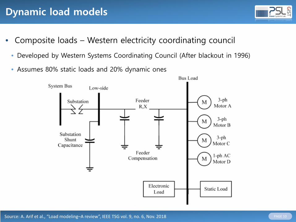
• Composite loads – Western electricity coordinating council

• Developed by Western Systems Coordinating Council (After blackout in 1996)

• Assumes 80% static loads and 20% dynamic ones


Motors

• Consumes 60 – 70% of the total energy supplied by a power system

• Induction motors

• Synchronous motors

• Exactly same as the generators

Refer to- “Electric machinery” class

Motors

• Induction machine

• Stator field rotating speed (at synchronous speed)

• Slip

𝑛𝑛𝑠𝑠 =120𝑓𝑓𝑠𝑠𝑝𝑝𝑝𝑝

[rpm]

Where 𝑝𝑝𝑝𝑝 : Number of poles (2 per 3-phase winding set)𝑓𝑓𝑠𝑠 : Frequency of 3-phase current

𝑠𝑠 =𝑛𝑛𝑠𝑠 − 𝑛𝑛𝑟𝑟𝑛𝑛𝑠𝑠

[per unit]

Where 𝑛𝑛𝑟𝑟 : Rotor speed

Motors


• Angle (see the figure) :

• Stator voltage equations:

• Rotor voltage equations:

𝜃𝜃 = 𝜔𝜔𝑟𝑟𝑑𝑑 [rad/s]

= 1 − 𝑠𝑠 𝜔𝜔𝑠𝑠𝑑𝑑 [rad/s]

𝑣𝑣𝑎𝑎 = 𝑝𝑝𝜓𝜓𝑎𝑎 + 𝑅𝑅𝑠𝑠𝑖𝑖𝑎𝑎𝑣𝑣𝑏𝑏 = 𝑝𝑝𝜓𝜓𝑏𝑏 + 𝑅𝑅𝑠𝑠𝑖𝑖𝑏𝑏𝑣𝑣𝑐𝑐 = 𝑝𝑝𝜓𝜓𝑐𝑐 + 𝑅𝑅𝑠𝑠𝑖𝑖𝑐𝑐

𝑣𝑣𝐴𝐴 = 𝑝𝑝𝜓𝜓𝐴𝐴 + 𝑅𝑅𝑟𝑟𝑖𝑖𝐴𝐴𝑣𝑣𝐵𝐵 = 𝑝𝑝𝜓𝜓𝐵𝐵 + 𝑅𝑅𝑠𝑠𝑖𝑖𝐵𝐵𝑣𝑣𝐶𝐶 = 𝑝𝑝𝜓𝜓𝐶𝐶 + 𝑅𝑅𝑠𝑠𝑖𝑖𝐶𝐶


Motors


• Flux linkages for stator phase a and rotor phase A: (similar to the other phases)

Let

With 𝑑𝑑𝑞𝑞 transformation: (where 𝐿𝐿𝑚𝑚 = 𝐿𝐿𝑎𝑎𝐴𝐴 × 3/2)

𝜓𝜓𝑎𝑎 = 𝐿𝐿𝑎𝑎𝑎𝑎𝑖𝑖𝑎𝑎 + 𝐿𝐿𝑎𝑎𝑏𝑏 𝑖𝑖𝑏𝑏 + 𝑖𝑖𝑐𝑐 + 𝐿𝐿𝑎𝑎𝐴𝐴 𝑖𝑖𝐴𝐴 cos𝜃𝜃 + 𝑖𝑖𝐵𝐵cos(𝜃𝜃 + 120°) + 𝑖𝑖𝐶𝐶cos(𝜃𝜃 − 120°)

𝐿𝐿𝑠𝑠𝑠𝑠 = 𝐿𝐿𝑎𝑎𝑎𝑎 − 𝐿𝐿𝑎𝑎𝑏𝑏

𝜓𝜓𝐴𝐴 = 𝐿𝐿𝐴𝐴𝐴𝐴𝑖𝑖𝐴𝐴 + 𝐿𝐿𝐴𝐴𝐵𝐵 𝑖𝑖𝐵𝐵 + 𝑖𝑖𝐶𝐶 + 𝐿𝐿𝑎𝑎𝐴𝐴 𝑖𝑖𝑎𝑎 cos𝜃𝜃 + 𝑖𝑖𝑏𝑏cos(𝜃𝜃 − 120°) + 𝑖𝑖𝑐𝑐cos(𝜃𝜃 + 120°)

𝐿𝐿𝑟𝑟𝑟𝑟 = 𝐿𝐿𝐴𝐴𝐴𝐴 − 𝐿𝐿𝐴𝐴𝐵𝐵

𝜓𝜓𝑎𝑎 = 𝐿𝐿𝑠𝑠𝑠𝑠𝑖𝑖𝑎𝑎 + 𝐿𝐿𝑎𝑎𝐴𝐴 𝑖𝑖𝐴𝐴 cos𝜃𝜃 + 𝑖𝑖𝐵𝐵cos(𝜃𝜃 + 120°) + 𝑖𝑖𝐶𝐶cos(𝜃𝜃 − 120°)

𝜓𝜓𝐴𝐴 = 𝐿𝐿𝑟𝑟𝑟𝑟𝑖𝑖𝐴𝐴 + 𝐿𝐿𝑎𝑎𝐴𝐴 𝑖𝑖𝑎𝑎 cos𝜃𝜃 + 𝑖𝑖𝑏𝑏cos(𝜃𝜃 − 120°) + 𝑖𝑖𝑐𝑐cos(𝜃𝜃 + 120°)

𝜓𝜓𝑑𝑑𝑠𝑠 = 𝐿𝐿𝑠𝑠𝑠𝑠𝑖𝑖𝑑𝑑𝑠𝑠 + 𝐿𝐿𝑚𝑚𝑖𝑖𝑑𝑑𝑟𝑟𝜓𝜓𝑞𝑞𝑠𝑠 = 𝐿𝐿𝑠𝑠𝑠𝑠𝑖𝑖𝑞𝑞𝑠𝑠 + 𝐿𝐿𝑚𝑚𝑖𝑖𝑞𝑞𝑟𝑟

𝜓𝜓𝑑𝑑𝑟𝑟 = 𝐿𝐿𝑟𝑟𝑟𝑟𝑖𝑖𝑑𝑑𝑟𝑟 + 𝐿𝐿𝑚𝑚𝑖𝑖𝑑𝑑𝑠𝑠𝜓𝜓𝑞𝑞𝑟𝑟 = 𝐿𝐿𝑟𝑟𝑟𝑟𝑖𝑖𝑞𝑞𝑟𝑟 + 𝐿𝐿𝑚𝑚𝑖𝑖𝑞𝑞𝑠𝑠


Motors


• Stator and rotor voltages: (where 𝑝𝑝𝜃𝜃𝑟𝑟 = 𝑠𝑠𝜔𝜔𝑠𝑠)

• Electrical power and torque:

𝑝𝑝𝑠𝑠𝑝𝑝𝑟𝑟𝑟𝑟𝑑𝑑 dividing by − 𝑝𝑝𝜃𝜃𝑟𝑟 2/𝑝𝑝𝑝𝑝 , which is the rotor speed w.r.t. 𝑑𝑑𝑞𝑞 axes, gives:

𝑣𝑣𝑑𝑑𝑠𝑠 = 𝑅𝑅𝑠𝑠𝑖𝑖𝑑𝑑𝑠𝑠 − 𝜔𝜔𝑠𝑠𝜓𝜓𝑞𝑞𝑠𝑠 + 𝑝𝑝𝜓𝜓𝑑𝑑𝑠𝑠

𝑣𝑣𝑞𝑞𝑠𝑠 = 𝑅𝑅𝑠𝑠𝑖𝑖𝑞𝑞𝑠𝑠 + 𝜔𝜔𝑠𝑠𝜓𝜓𝑑𝑑𝑠𝑠 + 𝑝𝑝𝜓𝜓𝑞𝑞𝑠𝑠

𝑣𝑣𝑑𝑑𝑟𝑟 = 𝑅𝑅𝑟𝑟𝑖𝑖𝑑𝑑𝑟𝑟 − 𝑝𝑝𝜃𝜃𝑟𝑟 𝜓𝜓𝑞𝑞𝑟𝑟 + 𝑝𝑝𝜓𝜓𝑑𝑑𝑟𝑟

𝑣𝑣𝑞𝑞𝑟𝑟 = 𝑅𝑅𝑟𝑟𝑖𝑖𝑞𝑞𝑟𝑟 + 𝑝𝑝𝜃𝜃𝑟𝑟 𝜓𝜓𝑑𝑑𝑟𝑟 + 𝑝𝑝𝜓𝜓𝑞𝑞𝑟𝑟

𝑝𝑝𝑠𝑠 =32 𝑣𝑣𝑑𝑑𝑠𝑠𝑖𝑖𝑑𝑑𝑠𝑠 + 𝑣𝑣𝑞𝑞𝑠𝑠𝑖𝑖𝑞𝑞𝑠𝑠 𝑝𝑝𝑟𝑟 =

32 𝑣𝑣𝑑𝑑𝑟𝑟𝑖𝑖𝑑𝑑𝑟𝑟 + 𝑣𝑣𝑞𝑞𝑟𝑟𝑖𝑖𝑞𝑞𝑟𝑟

𝑝𝑝𝑠𝑠𝑝𝑝𝑟𝑟𝑟𝑟𝑑𝑑 =32 𝜓𝜓𝑑𝑑𝑟𝑟𝑖𝑖𝑞𝑞𝑟𝑟 − 𝜓𝜓𝑞𝑞𝑟𝑟𝑖𝑖𝑑𝑑𝑟𝑟 𝑝𝑝𝜃𝜃𝑟𝑟 : Power associated with the speed voltage (𝑝𝑝𝜃𝜃𝑟𝑟)

𝑇𝑇𝑟𝑟 =32 𝜓𝜓𝑞𝑞𝑟𝑟𝑖𝑖𝑑𝑑𝑟𝑟 − 𝜓𝜓𝑑𝑑𝑟𝑟𝑖𝑖𝑞𝑞𝑟𝑟

𝑝𝑝𝑝𝑝2


Motors


• Acceleration equation

• Steady-state characteristics

• Under steady-state, 𝑝𝑝𝜓𝜓 terms disappear, and by using previous equations:

𝑇𝑇𝑟𝑟 − 𝑇𝑇𝑚𝑚 = 𝐽𝐽𝑑𝑑𝜔𝜔𝑚𝑚𝑑𝑑𝑑𝑑

= 𝐽𝐽𝑑𝑑2𝜃𝜃𝑑𝑑𝑑𝑑2

Where 𝐽𝐽 : the moment of inertia of the rotor and the connected load𝜔𝜔𝑚𝑚 : Angular velocity or rotor [rad/s]

�𝑉𝑉𝑠𝑠 = 𝑅𝑅𝑠𝑠𝐼𝐼𝑠𝑠 + 𝑗𝑗𝜔𝜔𝑠𝑠𝐿𝐿𝑠𝑠𝑠𝑠𝐼𝐼𝑠𝑠 + 𝑗𝑗𝜔𝜔𝑠𝑠𝐿𝐿𝑚𝑚𝐼𝐼𝑟𝑟= 𝑅𝑅𝑠𝑠𝐼𝐼𝑠𝑠 + 𝑗𝑗𝜔𝜔𝑠𝑠 𝐿𝐿𝑠𝑠𝑠𝑠 − 𝐿𝐿𝑚𝑚 𝐼𝐼𝑠𝑠 + 𝑗𝑗𝜔𝜔𝑠𝑠𝐿𝐿𝑚𝑚 𝐼𝐼𝑠𝑠 + 𝐼𝐼𝑟𝑟= 𝑅𝑅𝑠𝑠𝐼𝐼𝑠𝑠 + 𝑗𝑗𝑋𝑋𝑠𝑠𝐼𝐼𝑠𝑠 + 𝑗𝑗𝑋𝑋𝑚𝑚 𝐼𝐼𝑠𝑠 + 𝐼𝐼𝑟𝑟

where �𝑉𝑉𝑠𝑠 = 𝑣𝑣𝑑𝑑𝑠𝑠 + 𝑗𝑗𝑣𝑣𝑞𝑞𝑠𝑠 / 2

Where 𝑋𝑋𝑠𝑠 = 𝜔𝜔𝑠𝑠(𝐿𝐿𝑠𝑠𝑠𝑠 − 𝐿𝐿𝑚𝑚) : stator leakage reactance𝑋𝑋𝑚𝑚 = 𝜔𝜔𝑠𝑠𝐿𝐿𝑚𝑚 : magnetizing reactance


Motors


• Steady-state characteristics (Cont’d)

• With the rotor circuits shorted, 𝑣𝑣𝑑𝑑𝑟𝑟 = 𝑣𝑣𝑞𝑞𝑟𝑟 = 0 :

• In phasor notation:

�𝑉𝑉𝑟𝑟 =𝑅𝑅𝑟𝑟𝑠𝑠𝐼𝐼𝑟𝑟 + 𝑗𝑗𝜔𝜔𝑠𝑠𝐿𝐿𝑟𝑟𝑟𝑟𝐼𝐼𝑟𝑟 + 𝑗𝑗𝜔𝜔𝑠𝑠𝐿𝐿𝑚𝑚𝐼𝐼𝑠𝑠

=𝑅𝑅𝑟𝑟𝑠𝑠𝐼𝐼𝑟𝑟 + 𝑗𝑗𝑋𝑋𝑟𝑟𝐼𝐼𝑟𝑟 + 𝑗𝑗𝑋𝑋𝑚𝑚(𝐼𝐼𝑠𝑠 + 𝐼𝐼𝑟𝑟)

Where 𝑋𝑋𝑟𝑟 = 𝜔𝜔𝑠𝑠(𝐿𝐿𝑟𝑟𝑟𝑟 − 𝐿𝐿𝑚𝑚) : rotor leakage reactance

𝑣𝑣𝑑𝑑𝑟𝑟 = 0 = 𝑅𝑅𝑟𝑟𝑖𝑖𝑑𝑑𝑟𝑟 − 𝑠𝑠𝜔𝜔𝑠𝑠(𝐿𝐿𝑟𝑟𝑟𝑟𝑖𝑖𝑞𝑞𝑟𝑟 + 𝐿𝐿𝑚𝑚𝑖𝑖𝑞𝑞𝑠𝑠)

𝑣𝑣𝑞𝑞𝑟𝑟 = 0 = 𝑅𝑅𝑟𝑟𝑖𝑖𝑞𝑞𝑟𝑟 + 𝑠𝑠𝜔𝜔𝑠𝑠(𝐿𝐿𝑟𝑟𝑟𝑟𝑖𝑖𝑑𝑑𝑟𝑟 + 𝐿𝐿𝑚𝑚𝑖𝑖𝑑𝑑𝑠𝑠)


Motors


• Equivalent circuit (Single phase, Referred to the stator side)

• Can be derived from the phasor equations

Power transferred across the air-gap : 𝑃𝑃𝑎𝑎𝑎𝑎 = 𝑅𝑅𝑟𝑟𝑠𝑠𝐼𝐼𝑟𝑟2

Rotor resistance loss : 𝑃𝑃𝑙𝑙𝑟𝑟 = 𝑅𝑅𝑟𝑟𝐼𝐼𝑟𝑟2

Mechanical power transferred to the shaft : 𝑃𝑃𝑠𝑠𝑠 = 𝑃𝑃𝑎𝑎𝑎𝑎 − 𝑃𝑃𝑙𝑙𝑟𝑟


Load characteristics

• ZIP coefficients for electrical appliances


𝑝𝑝1 𝑝𝑝2 𝑝𝑝3 𝑞𝑞1 𝑞𝑞2 𝑞𝑞3

[R1]

[R2]

[R3]

[R1] L. G. Swan and V. I. Ugursal, “Modeling of end-use energy consumption in the residential sector: A review of modeling techniques,” Renew. Sustain. Energy Rev., vol. 13, no. 8, pp. 1819–1835, 2009.

[R2] A. Bokhari et al., “Experimental determination of the ZIP coefficients for modern residential, commercial, and industrial loads,” IEEE Trans. Power Del., vol. 29, no. 3, pp. 1372–1381, Jun. 2013.

[R3] L. M. Hajagos and B. Danai, “Laboratory measurements and models of modern loads and their effect on voltage stability studies,” IEEE Trans. Power Syst., vol. 13, no. 2, pp. 584–592, May 1998.


• Component static characteristics



• Load class static characteristics



• Dynamic characteristics

• Induction motor

(i) The composite dynamic characteristics of a feeder supplying predominantly a

commercial load:

(ii) A large industrial motor:

(iii) A small industrial motor:


where m is the load torque exponent that affects slip-dependent rotor parameters: 𝑅𝑅𝑟𝑟 and 𝑋𝑋𝑟𝑟

Modeling approach


PowerPoint 프레젠테이션 - GIST AI대학원

Documents

Transcript of PowerPoint 프레젠테이션 - GIST AI대학원