
Scene-based correction of image sensor deficiencies - DiVA
83
Scene-based correction of image sensor deficiencies Master’s thesis in image processing at Link¨ oping Institute of Technology by Petter Torle LiTH-ISY-EX-3350-2003 Abstract This thesis describes and evaluates a number of algorithms for reduc- ing fixed pattern noise in image sequences by analyzing the observed scene. Fixed pattern noise is the dominant noise component for many infrared detector systems, perceived as a superimposed pattern that is approximately constant for all image frames. Primarily, methods based on estimation of the movement between individual image frames are studied. Using scene-matching tech- niques, global motion between frames can be successfully registered with sub-pixel accuracy. This allows each scene pixel to be traced along a path of individual detector elements. Assuming a static scene, differences in pixel intensities are caused by fixed pattern noise that can be estimated and removed. The algorithms have been tested by using real image data from existing infrared imaging systems with good results. The tests in- clude both a two-dimensional focal plane array detector and a linear scanning one-dimensional detector, in different scene conditions. Keywords: Nonuniformity correction, fixed pattern noise, scene- based, motion estimation, sequence, registration. Supervisors: Ingmar Andersson and Leif Haglund, Saab Bofors Dynamics AB Examiner: Klas Nordberg Link¨oping, May 6, 2003
-
Upload
khangminh22 -
Category
Documents
-
view
4 -
download
0
Transcript of Scene-based correction of image sensor deficiencies - DiVA

Scene-based correction ofimage sensor deficiencies
Master’s thesis in image processing atLinkoping Institute of Technology by
Petter Torle
LiTH-ISY-EX-3350-2003
Abstract
This thesis describes and evaluates a number of algorithms for reduc-ing fixed pattern noise in image sequences by analyzing the observedscene. Fixed pattern noise is the dominant noise component for manyinfrared detector systems, perceived as a superimposed pattern thatis approximately constant for all image frames.
Primarily, methods based on estimation of the movement betweenindividual image frames are studied. Using scene-matching tech-niques, global motion between frames can be successfully registeredwith sub-pixel accuracy. This allows each scene pixel to be tracedalong a path of individual detector elements. Assuming a static scene,differences in pixel intensities are caused by fixed pattern noise thatcan be estimated and removed.
The algorithms have been tested by using real image data fromexisting infrared imaging systems with good results. The tests in-clude both a two-dimensional focal plane array detector and a linearscanning one-dimensional detector, in different scene conditions.
Keywords: Nonuniformity correction, fixed pattern noise, scene-based, motion estimation, sequence, registration.
Supervisors:Ingmar Andersson and Leif Haglund, Saab Bofors Dynamics AB
Examiner:Klas Nordberg
Linkoping, May 6, 2003


Acknowledgments
This master’s thesis was done at Saab Bofors Dynamics, Linkoping.I would like to thank the following people:
• The initiators to the thesis and my supervisors at Saab BoforsDynamics, Ingmar Andersson and Leif Haglund
• Mikael Lindgren and Lars Peterson at Saab Bofors Dynam-ics, Goteborg, who helped me record most of the test imagesequences
• My examiner Klas Nordberg at the Department of ElectricalEngineering, Linkopings Universitet
• The staff at the section for image processing at Saab BoforsDynamics
• My opponent Martin Ohlson.
7


Abbreviations
The following abbreviations are used in this document:
FPN Fixed Pattern NoiseIR InfraredIIR Infinite Impulse ResponseIRST Infrared Search and TrackMCA Motion Compensated AverageMSM Multispectral Measurement SystemNUC Nonuniformity CorrectionQWIP Quantum Well Infrared PhotodetectorSNR Signal to Noise Ratio
9


Contents
1 Introduction 131.1 Background . . . . . . . . . . . . . . . . . . . . . . . . 131.2 Goal of the thesis . . . . . . . . . . . . . . . . . . . . . 141.3 Guidelines and assumptions . . . . . . . . . . . . . . . 141.4 Previous work . . . . . . . . . . . . . . . . . . . . . . . 141.5 Implementation . . . . . . . . . . . . . . . . . . . . . . 141.6 Thesis overview . . . . . . . . . . . . . . . . . . . . . . 15
2 Infrared sensor technology 172.1 Thermal radiation . . . . . . . . . . . . . . . . . . . . 172.2 Sensor design . . . . . . . . . . . . . . . . . . . . . . . 182.3 Fixed pattern noise . . . . . . . . . . . . . . . . . . . . 182.4 Sensor systems . . . . . . . . . . . . . . . . . . . . . . 19
3 Nonuniformity correction 233.1 Removing fixed pattern noise . . . . . . . . . . . . . . 233.2 Basic scene-based nonuniformity correction . . . . . . 243.3 Ghosting artifacts . . . . . . . . . . . . . . . . . . . . 263.4 One-image correction . . . . . . . . . . . . . . . . . . . 263.5 Enhanced scene-based algorithms . . . . . . . . . . . . 28
4 Estimating image motion 314.1 A Fourier-based method . . . . . . . . . . . . . . . . . 314.2 Sub-pixel accuracy . . . . . . . . . . . . . . . . . . . . 334.3 Two-component motion estimation . . . . . . . . . . . 344.4 Special case: Fixed pattern noise . . . . . . . . . . . . 374.5 Evaluation . . . . . . . . . . . . . . . . . . . . . . . . . 374.6 Comments on implementation . . . . . . . . . . . . . . 38
11

5 Registration-based nonuniformity correction 415.1 Motion compensating methods . . . . . . . . . . . . . 415.2 Crossing path . . . . . . . . . . . . . . . . . . . . . . . 43
6 Evaluation 536.1 Test sequences . . . . . . . . . . . . . . . . . . . . . . 536.2 Evaluation methods . . . . . . . . . . . . . . . . . . . 536.3 Temporal noise . . . . . . . . . . . . . . . . . . . . . . 536.4 One-image correction . . . . . . . . . . . . . . . . . . . 546.5 Temporal highpass filter . . . . . . . . . . . . . . . . . 556.6 Constant statistics . . . . . . . . . . . . . . . . . . . . 556.7 Motion compensated average . . . . . . . . . . . . . . 566.8 Crossing path . . . . . . . . . . . . . . . . . . . . . . . 59
7 Results 637.1 Computational speed . . . . . . . . . . . . . . . . . . . 637.2 Reference images . . . . . . . . . . . . . . . . . . . . . 647.3 Introduced noise . . . . . . . . . . . . . . . . . . . . . 657.4 Synthetic sequences . . . . . . . . . . . . . . . . . . . 657.5 Visual inspection . . . . . . . . . . . . . . . . . . . . . 677.6 One-dimensional sensor . . . . . . . . . . . . . . . . . 697.7 Example results . . . . . . . . . . . . . . . . . . . . . . 71
8 Conclusions 798.1 Summary . . . . . . . . . . . . . . . . . . . . . . . . . 798.2 Suggestions for further work . . . . . . . . . . . . . . . 80
12

Chapter 1
Introduction
1.1 Background
The performance of any image processing system depends on thequality of the input images, which makes image enhancement andpre-processing an important field of research. Compensating for non-linear sensor optics, enhancing or suppressing different parts of theimage, and reducing disturbing noise are examples of common imagepre-processing. This thesis concerns the latter.
All image sensors consisting of an array of detector elements suffermore or less from an undesired effect called fixed pattern noise, FPN.This type of noise is caused by the fact that individual detector ele-ments respond differently to incoming irradiance, which is perceivedin images as a superimposed pattern, approximately constant fromframe to frame. Although the observed image can be quite severelydistorted, the fact that the same distortion is present in several ac-quired images should make it possible to accurately extract the truescene, a process referred to as non-uniformity correction, NUC. Tradi-tionally, this is performed by using hardware temperature referencesfor calibration. Another approach is scene-based techniques, whereinformation from the observed scene itself is used to reduce fixed pat-tern noise. For example, two different detector elements that observethe same part of the scene should produce the same output. If not,correction parameters can be slightly adjusted to compensate.
For infrared (IR) imaging systems, fixed pattern noise is usuallythe dominant noise component. It is also depending on scene irradi-ance, detector temperature and is slightly time varying, which makesit difficult to correct this problem with an initial factory calibration.
13

1.2 Goal of the thesis
The goal of this thesis is to design and evaluate scene-based nonuni-formity correction algorithms that are able to suppress fixed patternnoise without need for external hardware such as temperature ref-erence equipment. In particular, algorithms should be able to ac-curately estimate motion between images and use this knowledge toimprove performance.
1.3 Guidelines and assumptions
The correction algorithms should be developed with a future real-timehardware implementation in mind. This means for example that theresulting output must not depend on any future input signals, andthat the execution time for each input frame should be approximatelyconstant. Furthermore, the input images are assumed to be capturedfrom a static scene, and the global motion between frames is assumedto consist only of translations in the image plane. The methodsshould be designed both for a two-dimensional array detector and aone-dimensional scanning detector.
1.4 Previous work
Methods for scene-based removal of fixed pattern noise have been re-searched for some time. Yet, relatively few different correction meth-ods were found when a search for nonuniformity correction relatedarticles was conducted. The most widely used algorithms [4, 2, 3, 10]are either based on making each detector output similar to those ofthe surrounding detectors in the array, or based on statistical analysis.Some more advanced methods depending on image motion estimationwas also found [7, 8].
1.5 Implementation
The nonuniformity correction algorithms are evaluated using bothsynthetic and real image data. Image sequences have been recordedat Saab Bofors Dynamics in Goteborg as well as in Linkoping. Algo-rithms and utilities have been developed in a Matlab environment.
14

1.6 Thesis overview
Chapter 2 – Infrared sensor technologyThis chapter gives a short introduction to infrared sensor tech-nology, including a discussion on some of the factors contribut-ing to fixed pattern noise in IR images. Basic properties ofthe sensors used to acquire IR images for this thesis are alsomentioned.
Chapter 3 – Nonuniformity correctionIn this chapter, different nonuniformity correction methods arecategorized and some basic scene-based algorithms are pre-sented.
Chapter 4 – Estimating image motionFor more advanced nonuniformity correction, accurate know-ledge of the global image motion is required. A Fourier-basedmethod for motion estimation is described and evaluated.
Chapter 5 – Registration-based nonuniformity correctionIn this chapter, nonuniformity correction methods relying onknowledge of image motion are presented.
Chapter 6 – EvaluationThe proposed algorithms are evaluated individually in this chap-ter, using several test sequences. The quality of the resultingoutput data is discussed, and some methods are modified toperform better.
Chapter 7 – ResultsThe results from the previous chapter are summed up and thedifferent correction methods are compared in various ways.
Chapter 8 – ConclusionsThis chapter concludes the thesis, with comments on the resultsand suggestions for further work.
15


Chapter 2
Infrared sensor technology
2.1 Thermal radiation
Any given object emits thermal electromagnetic radiation, distributedover an entire spectrum of wavelengths. Figure 2.1 shows emittancespectrums for the temperatures T=300, 400 and 500 K.
0 2 4 6 8 10 12 14 16 18 200
50
100
150
200
250
300
350
400
450
T=500
T=300
T=400
Wavelength [µm]
Em
ittan
ce [W
/m2 µm
]
Figure 2.1: Thermal radiation for different temperatures.
17

The radiation for a specific temperature T has an intensity peakat the wavelength given by Wien’s displacement law :
λmax =k
T, k = 2.898 · 10−3
If the temperature is high enough, the radiation can be perceived bythe human eye as colored light. However, most natural objects havea much lower temperature, corresponding to an intensity peak in the0.8–30 µm wave band. These wavelengths are part of the infraredband, positioned between visible light and microwaves in the electro-magnetic spectrum. Sensors that detect photons with wavelengths inthis range thus produce an image with intensities corresponding tothe temperatures of the observed scene.
2.2 Sensor design
A widely used detector design is a focal plane array of photodiode el-ements, made of mercury-cadmium-telluride. For a two-dimensionalarray, each element represents one pixel in the output image. Thearray can also be one-dimensional, in which case the array needs toundergo a scanning motion to generate an entire image.
2.3 Fixed pattern noise
Individual elements in the detector array differ in responsivity toincoming irradiance, which is the main reason why fixed pattern noiseoccur in an image. Some pixels end up too bright, some too dark,depending on a multitude of parameters [1]. Some of these parametersmay be identified in advance and compensated for, but it is impossibleto compensate for all. The result is an image with a superimposedpattern that varies with unknown environmental parameters, leadingto a time varying fixed pattern noise.
The most common fixed pattern noise sources include:
Fabrication errorsInaccuracies in the fabrication process give rise to variationsin geometry and substrate doping quality of the detector ele-ments. This leads directly to offset and gain variations acrossthe detector array.
18

Cooling systemIn order to deliver any useful data, many sensors must be cooledto an operating temperature below 100 K. Small deviations inthe regulated temperature are hard to avoid, and may havelarge impact on detector parameters.
ElectronicsFor detector arrays, variations in the read-out electronics is acommon source of fixed pattern noise, often visible as grid andline patterns.
System 1f noise
Apart from white noise, the power spectrum of typical temporalnoise present in infrared image sequences also consists of a com-ponent proportional to the inverse of the frequency. The originof this 1
f component is not completely known, but it causes driftof system parameters, ultimately leading to time-varying fixedpattern noise.
OpticsSome fixed pattern noise is also caused by the sensor optics.This includes a decrease in signal intensity at the edges of theimage and different kinds of circular image artifacts.
2.4 Sensor systems
The sensor used to acquire most of the test sequences for this thesisis called MSM, multispectral measurement system. The MSM uses atwo-dimensional focal plane array, cooled to a temperature of about80 K to minimize disturbance from the sensor chip itself.
To illustrate the level of nonuniformity for the MSM system, figure2.2 shows six raw frames from one of the test sequences. As a previewof things to come, figure 2.3 shows what the corresponding framesmay look like when nonuniformity correction has been performed. Inthis particular case, the resulting parameters after processing all 400frames of the sequence have been used to calibrate each image.
Compared to the latest IR sensor technology, the MSM is slightlyoutdated and the produced images are severely distorted by fixedpattern noise. A somewhat more sophisticated detector based onquantum well infrared photodetector (QWIP) technology has alsobeen studied.
19

(a) Frame 25 (b) Frame 50
(c) Frame 75 (d) Frame 100
(e) Frame 200 (f) Frame 400
Figure 2.2: Raw sensor images from one of the MSM test sequences.
20

(a) Frame 25 (b) Frame 50
(c) Frame 75 (d) Frame 100
(e) Frame 200 (f) Frame 400
Figure 2.3: Corrected sequence.
21

As mentioned earlier, an alternative to a two-dimensional detectorarray is to use a one-dimensional scanning array. Saab Bofors Dy-namics has developed an IRST system (Infrared Search and Track)equipped with such a sensor. The final image is generated by hor-izontally sweeping the column of detector elements. Fixed patternnoise for this system is then visible as horizontal stripes, which canbe regarded as a special case of two-dimensional fixed pattern noise.Raw images from this sensor can be so degraded that it is difficult todiscern any scene information at all.
Typical raw images from these sensors are shown in figure 2.4.
(a) IRST-system, using a horizontallyscanning 1D detector array.
(b) A modern QWIP camera
Figure 2.4: Typical raw IRST and QWIP sensor images.
22

Chapter 3
Nonuniformity correction
3.1 Removing fixed pattern noise
Reducing fixed pattern noise to a minimum is, of course, essentialto any imaging system. Many techniques have been developed toperform such nonuniformity correction, most of which are based ona linear irradiance–voltage model:
x = z · g + o (3.1)
where the true scene value z is scaled by a gain factor g and offsetby an offset term o to produce the observed detector output x. It isalso common to model the fixed pattern noise completely as an offsetshift:
x = z + o (3.2)
The correction parameters g and o are especially straight forwardto obtain if a true scene value z is known. This can be achieved byexposing the sensor to a surface with known uniform temperature.Using more than one reference temperature, both gain and offsetcorrection parameters can be resolved. This approach is a widelyused reference-based method for nonuniformity correction. It is alsopossible to use only one uniform temperature surface, imaged withtwo different integration times. The MSM system, used to acquireinfrared image sequences in this thesis, can use both these calibrationmethods [1]. Figure 3.1 shows typical MSM gain and offset correctionparameters, obtained when applying reference based calibration.
23

(a) Offset (b) Gain
Figure 3.1: Typical MSM correction parameters.
3.2 Basic scene-based nonuniformity correc-tion
Though imaging systems with reference-based nonuniformity correc-tion are accurate, they often involve opto-mechanic components andtemperature references that are expensive and complex in design. Toovercome this problem, a lot of research has been focused on per-forming sensor calibration entirely in software. Several methods havebeen presented where the observed scene itself is used to calibratethe detector elements — scene-based nonuniformity correction.
In this section, two scene-based correction methods are presented:temporal highpass filter[2, 3] and constant statistics[4]. Both are wellknown and appears frequently in the literature.
Temporal highpass filter
Images from a sequence of infrared image data consist of scene in-formation, varying from frame to frame, and a fixed pattern noise,roughly the same in all frames. This means that when studying eachpixel individually over time, high-frequency information belongs tothe scene, while low-frequency information belongs to fixed patternnoise. An estimate of the noise is thus obtained by lowpass filter-ing the image sequence along the temporal axis. When subtractingthis estimate from an input image frame, nonuniformity correction is
24

performed. The whole process acts like a temporal highpass filter, asshown in figure 3.2. A temporal average f of the image sequence isgenerated by a recursive IIR filter and subtracted from the currentframe. The output image at time index n becomes
yn = xn − fn
wherefn =
xn + (n − 1)fn−1
n(3.3)
Lowpassfilter
fn
xn yn
Figure 3.2: Temporal highpass filter.
Constant statistics
The constant statistics algorithm is similar to the temporal highpassfilter but is extended to estimate both gain and offset parameters.The assumptions of this method are that the temporal means andvariances are identical for all pixels. For this assumption to hold, itis necessary that over time, all possible scene irradiance values willbe observed by all detector elements. This means that image motionmust exist, either from a dynamic scene or from movement of thesensor. For the linear model (3.1), the temporal mean value is
mx = E[x] = E[z · g + o] = g · E[z] + o = g · mz + o
and the mean deviation is
sx = E[|x − mx|] = E[|g · (z − mz)|] = g · sz
It is further assumed that the temporal statistics of z is constantfor all detector elements. For example, z can be assumed to havezero mean and unity mean deviation (mz = 0, sz = 1). This canbe done without losing generality since the true values of mz and sz
25

can be incorporated into the parameters o and g respectively. Theexpressions are now written
mx = o
sx = g
which allows solving (3.1) as:
z = x−mxsx
Note that this expression equals the temporal highpass filter of theprevious section when neglecting the denominator.
The estimated mean of x can be calculated recursively like before(3.3), while a recursive equation for sx is given by
sx,n =|xn − mx,n| + (n − 1)sx,n−1
n
3.3 Ghosting artifacts
If some part of the scene remains motionless for several algorithmiterations, it will be considered to be fixed pattern noise and as suchbe blended into the background. When this part eventually resumesmotion, it will leave an inverse ghost image in its place. This ghostingartifact is a problem to most scene-based nonuniformity correctionalgorithms. Ghosting may occur even when the image motion issufficient. For example, a view of the horizon may generate a ghostimage when panning the sensor horizontally.
A simple method for reducing the ghosting effect is to prohibitparameter updates if the magnitude of the change at each pixel issmaller than a fixed threshold. [5]
3.4 One-image correction
Usually, some properties and characteristics of the fixed pattern noiseis known in advance. For example, pixel intensity is generally lower atthe edges of the image, and pixel-to-pixel correlation is visible as gridand line patterns. This knowledge can be used to produce an estimateof the fixed pattern noise as an initial set of correction parametersfor further processing by the nonuniformity correction algorithms.
Figure 3.3(a) shows a close-up of an IR image, with grid noisetypical for sensors with detector arrays. It seems that every second
26

pixel is somewhat correlated. This is also evident when examining theFourier transform of the image, figure 3.3(b), where the two brightpixels located in the middle of the top and left edges correspond toa sine-shaped signal with a wavelength of 2 pixels.
(a) Grid noise (b) Fourier transform
Figure 3.3: IR image properties
Once identified, these frequency components may be filtered outto remove most of the grid noise, as shown in figure 3.4.
With the typical correction parameters of figure 3.1 in mind, thegrid noise is mostly additive in origin, while the pixel intensity de-crease at the image edges is part of a slowly varying multiplicativefixed pattern noise.
By taking the logarithm of the image, this noise will be turnedinto additive noise, which then can be reduced by applying a highpass filter. This is sometimes referred to as homomorph filtering [9].In figure 3.5, this filter is applied to the previous result from figure3.4(b).
Some artifacts are still clearly visible in the image. The sharpvertical lines are always located at the same position, probably causedby the read-out electronics. The lines can possibly be reduced bymodifying the grid noise filter or adding a mask manually, but itwould be wise not to make the initial correction procedure too sensor-specific.
27

(a) Original image (b) Filtered image
Figure 3.4: One-image correction of grid noise
(a) Original image (b) Filtered image
Figure 3.5: Homomorph filtering
3.5 Enhanced scene-based algorithms
The nonuniformity correction methods described so far assume thatmotion between the image frames exists, but no further analysis ofthis motion is performed. It is reasonable that performance wouldincrease if knowledge of the actual image movement is incorporated
28

into the algorithms. This leads to a higher level of scene-based al-gorithms, referred to as registration-based nonuniformity correction.With these methods, computational complexity and computer mem-ory demands are significantly increased.
Being able to accurately estimate the image motion is naturallyan important part of registration-based algorithms. Such a motionestimation algorithm will be described in the following chapter.
29

Chapter 4
Estimating image motion
The performance of many nonuniformity correction algorithms de-pends heavily on an accurate estimate of the global motion betweenimage frames. In this thesis, the motion is assumed to consist onlyof translation, neglecting any scaling, rotation or other warping ofthe images. A well known motion estimation method based on theFourier phase of the images [6] is presented in this chapter.
4.1 A Fourier-based method
Consider two images, f and g, related to each other by a translationvector x0 as in g(x) = f(x − x0). The Fourier shift theorem thenstates that the corresponding Fourier transforms F and G are relatedas:
G(ω) = F (ω) · e−i2πωx0
Now let
H(ω) ≡ G(ω)F (ω)
= e−i2πωx0 (4.1)
The inverse Fourier transform of H is given by
h(x) = δ(x − x0)
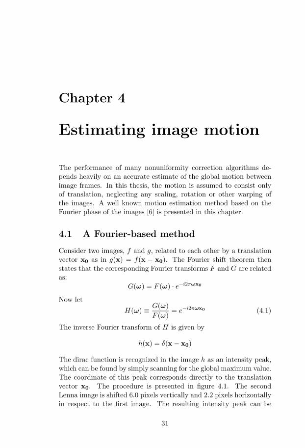
The dirac function is recognized in the image h as an intensity peak,which can be found by simply scanning for the global maximum value.The coordinate of this peak corresponds directly to the translationvector x0. The procedure is presented in figure 4.1. The secondLenna image is shifted 6.0 pixels vertically and 2.2 pixels horizontallyin respect to the first image. The resulting intensity peak can be
31

seen clearly in image 4.1(c), with coordinates corresponding to thetranslation vector.
(a) Lenna image 1 (b) Lenna image 2
0 1 2 3 4 5 6 7 8 9
0123456789
(c) h(x)
Figure 4.1: Image motion estimation. Image 2 has been shifted 6.0pixels vertically and 2.2 pixels horizontally in respect to image 1.
Note that these calculations assume that there is a one-to-onemapping of pixels in the two images. This is of course not true.Some new scene data has inevitably been introduced at the edges ofthe image, while other has been translated out of the image frameand lost. These irregularities cause noise that affect the estimationaccuracy. To overcome this problem, the magnitude of pixels at theedges of the images can be decreased by spatially filtering the twoimages with a suitable window function.
32

4.2 Sub-pixel accuracy
The translation estimates delivered by the proposed method are inte-ger values. Generally, however, sub-pixel accuracy is required. Thiscan be achieved in a number of ways. For example, finding themaximum of a second-degree polynomial surface fitted to the regionaround the intensity peak increases estimation accuracy by severaltenths of a pixel. This solution has its drawbacks though. Figure 4.2shows the translation estimates of an image shifted one pixel in stepsof 0.1 pixels. It seems that the translation estimates are weighted to-wards integer values. A reason for this may be that a second-degreesurface is not really an optimal model for the intensity peak.
0 0.2 0.4 0.6 0.8 10
0.2
0.4
0.6
0.8
1
True image shift (pixels)
Est
imat
ed im
age
shift
(pi
xels
)
Figure 4.2: Estimates are weighted towards whole pixels.
An alternative method for sub-pixel accuracy is Fourier phaseexpansion, where the phase of H is multiplied by a scaling constantC. Algebraically:
H(ω) ≡ |H(ω)| ·(
H(ω)|H(ω)|
)C
(4.2)
Using H from (4.1):H(ω) = e−i2πωx0C
Like before, this image is inverse transformed
h(x) = δ(x − x0C)
The position of the intensity peak has now been scaled by the constantC, which means that the integer coordinate of the global maximum
33

should be divided by C in order to find the translation vector x0. Thisprocedure effectively increases the estimation accuracy by a factor ofC. Naturally, this value should be chosen as large as possible. Inpractice this is limited by the size of the image and noise, whichgrows larger with increasing scale constant.
The two methods for sub-pixel accuracy can be combined to in-crease performance even more.
4.3 Two-component motion estimation
The described motion estimation method assumes only one dominantimage motion in the sequence. In this section it will be shown howthe method deals with several motion components, especially a fixedpattern superimposed on moving images.
Consider the case where two patterns undergoing different mo-tions are combined additively in each image. The images f and g canthen be written as
f(x) = a(x) + b(x)g(x) = a(x − xa) + b(x − xb)
where a and b represent two patterns, displaced in the second im-age by the vectors xa and xb. As before, the images are Fouriertransformed and divided:
F (ω) = A(ω) + B(ω)G(ω) = A(ω) · e−i2πωxa + B(ω) · e−i2πωxb
H(ω) =G(ω)F (ω)
=A
A + B(ω) · e−i2πωxa +
B
A + B(ω) · e−i2πωxb
In this case, the image data is not cancelled out. H is now a sum oftwo shifted terms, each weighted in some sense by the frequency con-tent of the corresponding image in relation to the frequency contentof the combined images. Without getting too far into signal theory, itwould be reasonable that the Fourier inverse of H now consists of notone, but two intensity peaks. The peaks should be located at xa andxb with magnitudes related to the corresponding image frequencycontent. Figure 4.3 shows the results when two motion componentsare present. Two images of flowers, related by a translation of 4.0pixels horizontally and 1.0 pixels vertically, have been added to the
34

Lenna image pair from figure 4.1. As seen in figure 4.3(c), the im-age h(x) contains two intensity peaks at the expected locations. Thebackground noise level is also higher.
(a) Lenna with flowers 1 (b) Lenna with flowers 2
0 2 4 6 8 10 12 14
02468
101214
(c) h(x)
0 2 4 6 8 10 12 14
02468
101214
(d) h(x), C = 2
Figure 4.3: Two-component motion estimation.
To achieve sub-pixel accuracy as before, the phase of H shouldbe multiplied by a scaling constant (definition 4.2). However, the ex-pression for the normalized H now involves a sum of two exponentialfunctions. Phase-expanding such an expression gives the following
35

results. For now, only the exponential functions are considered.
C = 2 H(ω) � (ei2πωxa + ei2πωxb)2 == ei2πω2xa + 2ei2πω(xa+xb) + ei2πω2xb
C = 3 H(ω) � (ei2πωxa + ei2πωxb)3 == ei2πω3xa + 3ei2πω(2xa+xb) ++ 3ei2πω(xa+2xb) + ei2πω3xb
The two exponential functions have been phase scaled properly, butsignificant noise has been introduced by the additional terms in thebinomial expansion. These terms will all be present as intensity peaksin the resulting inverse transformed image h(x), as shown in figure4.3(d). The locations of the peaks are determined by the possiblecombinations of C added original translation vectors, see figure 4.4for an example.
C = 3C = 2C = 1
Origin
xa
xb
xa
xaxb
xb
xb
xb
xb
xa
xa
xa
Origin Origin
Figure 4.4: Intensity peak positions for two-component image motionwith C=1,2,3.
Scanning for a global intensity maximum is no longer sufficientfor finding the correct translation vectors. However, all the intensitypeaks can be found by gathering C +1 local maxima. The true peaksare those with the largest in-between distance. Another method is tostart without any phase expansion and register the original positionsof the intensity peaks. For a given scale factor C, new peak positionscan be extrapolated and used as centers for smaller regions where alocal maximum search is performed.
36

So far the frequency information contributed to H(ω) by the re-mains of the image data A(ω) and B(ω) has been neglected. Thisnoise is unfortunately not insignificant. The magnitude of the in-tensity peaks in the image h(x) drops rather rapidly with increasingscale factor, and drowns completely in background noise after just afew steps.
4.4 Special case: Fixed pattern noise
Image sequences with fixed pattern noise can be considered to be aspecial case of two-component image motion. Since the noise patternis motionless, one of the resulting intensity peaks in the image h(x)is always located at the origin. This makes it easier to identify thetrue image motion.
When used in combination with a nonuniformity correction al-gorithm, the fixed pattern noise is hopefully reduced with each newframe. The undesired intensity peaks will eventually become less sig-nificant, and after some time the image motion consists essentially ofonly one component.
4.5 Evaluation
To evaluate the accuracy of this algorithm in the presence of fixed pat-tern noise, normal distributed gain and offset coefficients are appliedto an 8 bit grayscale image pair like the one in figure 4.1, related bya translation of 2.4 pixels horizontally and 1.8 pixels vertically. Therelative translation is then estimated using the described algorithmwith C = 2. The mean absolute error of the estimate is presented forseveral levels of nonuniformity in figure 4.5.
When the noise becomes too dominant in the image, no relativetranslation is detected, which results in an absolute error of about4 pixels (cut off at 1.5 pixels in the figure). For somewhat less ex-treme noise levels, the average absolute error is about 0.1 pixels. Todemonstrate the noise levels, the image shown in figure 4.6 is dis-torted by gain and offset nonuniformity with standard deviation 0.3and 25 respectively.
37

4.6 Comments on implementation
When implementing this motion estimation algorithm, the problemarises about which two images to relate in the estimation process.
010
2030
4050
00.1
0.20.3
0.40.5
0
0.5
1
1.5
Offset standard deviationGain standard deviation
Mea
n ab
solu
te e
rror
(pi
xels
)
Figure 4.5: Mean absolute error of translation estimates for variouslevels of gain and offset nonuniformity in an 8-bit grayscale image.
Figure 4.6: An 8-bit grayscale image with normal distributed gain andoffset nonuniformity, standard deviations 0.3 and 25 respectively.
38

Unless the sensor is restricted to move only a short distance from theinitial position, it will soon be impossible to relate new frames to thefirst frames since they obviously share less and less of the scene data.
A reasonable solution would be to relate each new frame to theprevious frame. This may however prove undesirable. There is alwaysa small error in each individual motion estimate, hopefully no largerthan about 0.1 pixels. When constantly using the previous frameas a reference for the new estimate, this small error is accumulatedand may well grow to several pixels — resulting in completely uselessmotion estimates.
To avoid accumulating errors, the reference frame should be keptthe same for as long as possible. This can be done by changing refer-ence frame only when the distance to the new frame is approachingthe limit of the estimation algorithm.
There are problems with this method as well, though. Chances arethat an image frame with unusually large estimation error is chosenas the reference frame. In that case, that error will be present inall the following frames. A possible solution could be to examinethe reference frame candidate more closely before actually selectingit. For example, a frame with an absolute translation vector thatdeviates rather much from the translation vectors of following andpreceding frames would not be an ideal choice as a new referenceframe.
39


Chapter 5
Registration-basednonuniformity correction
5.1 Motion compensating methods
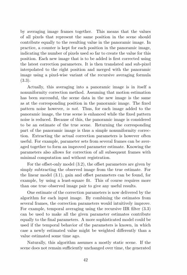
With motion estimation, each image in the sequence can be spatiallyrelated to previous images. This is an advantage for further imageprocessing. For example, the input images can be translated accord-ingly and merged together to form a new, larger image. Figure 5.1shows such a panoramic image created from one of the MSM imagesequences. The creation of a panoramic image is the first step in aregistration-based nonuniformity correction method known as motioncompensated average [8].
Figure 5.1: Panoramic image. The last inserted frame is indicated.
The word average indicates that the panoramic image is created
41
by averaging image frames together. This means that the valuesof all pixels that represent the same position in the scene shouldcontribute equally to the resulting value in the panoramic image. Inpractice, a counter is kept for each position in the panoramic image,indicating the number of pixels used so far to create the value for thisposition. Each new image that is to be added is first corrected usingthe latest correction parameters. It is then translated and sub-pixelinterpolated to the right position and merged with the panoramicimage using a pixel-wise variant of the recursive averaging formula(3.3).
Actually, this averaging into a panoramic image is in itself anonuniformity correction method. Assuming that motion estimationhas been successful, the scene data in the new image is the sameas at the corresponding position in the panoramic image. The fixedpattern noise however, is not. Thus, for each image added to thepanoramic image, the true scene is enhanced while the fixed patternnoise is reduced. Because of this, the panoramic image is consideredto be an estimate of the true scene. Returning the correspondingpart of the panoramic image is thus a simple nonuniformity correc-tion. Extracting the actual correction parameters is however oftenuseful. For example, parameter sets from several frames can be aver-aged together to form an improved parameter estimate. Knowing theparameters also allows for correction of all subsequent frames withminimal computation and without registration.
For the offset-only model (3.2), the offset parameters are given bysimply subtracting the observed image from the true estimate. Forthe linear model (3.1), gain and offset parameters can be found, forexample, by using a least-square fit. This of course requires morethan one true–observed image pair to give any useful results.
One estimate of the correction parameters is now delivered by thealgorithm for each input image. By combining the estimates fromseveral frames, the correction parameters would intuitively improve.For example, temporal averaging using the recursive IIR filter (3.3)can be used to make all the given parameter estimates contributeequally to the final parameters. A more sophisticated model could beused if the temporal behavior of the parameters is known, in whichcase a newly estimated value might be weighted differently than avalue estimated some time ago.
Naturally, this algorithm assumes a mostly static scene. If thescene does not remain sufficiently unchanged over time, the generated
42

panoramic image is not very useful. The static scene assumption iscommon for registration-based algorithms.
5.2 Crossing path
So far, knowledge of the image motion in a sequence has been used toconstruct a panoramic image for further nonuniformity processing.
The image motion can also be used to study the difference in de-tector response in a more algebraical sense. For example, if the rela-tive translation between two observed images is exactly (1,0) pixels,two detector elements with the relative distance (1,0) units have ob-served the very same scene irradiance and should ideally produce thesame output value. Of course, this reasoning assumes a static scene,as mentioned earlier. Any deviation is caused by detector nonunifor-mities. Translation vectors ending up at exactly integer pixel unitsis however rather improbable.
It has been shown by Ratliff et al. [7] that for pure horizontal orvertical sub-pixel translations, the responses of two detectors at unitydistance can be accurately related through extrapolation. An elegantnonuniformity correction method for offset-only calibration (3.2) canbe derived that unifies the offset terms to one unknown but globalvalue. Another approach to this problem is to specifically move theimage sensor according to a predetermined pattern. This is suggestedin the patent of O’Neil, described in [2], along with a method for bothgain and offset calibration (3.1).
The algorithm introduced here is called crossing path and is basedon these two methods. Both gain and offset correction parameters areestimated, and the constraint of pure horizontal or vertical motion issomewhat relaxed.
Analyzing detector movements
The main idea of this algorithm is to find all pairs of images thatare related by translation vectors with integer vertical and horizontalcomponents. When such a pair has been found, it is possible toidentify different detectors that observe the exact same scene value.
For each new input image, motion estimation delivers the corre-sponding position of the image origin relative to a previous image.This means that the distance to every previous position can easilybe calculated. If any of these distances are sufficiently close to an
43

integer value, a suitable image pair has been found. In figure 5.2, adetector path of motion is shown where the registered images 5 and10 are quite close to being separated by (1,1) pixels. However, it ishighly improbable that the distance is exactly integer valued.
0 1 2
0
1
2
Figure 5.2: A detector motion path. The distance between image 5and 10 is almost (1,1) pixels.
The probability of integer pixel distances can be increased byinterpolating the image sequence to create in-between images. Inpractice, this means that the number of image positions is increased,allowing for an improved distance match. This procedure can berepeated infinitely. Eventually, it is no longer discrete image positionsthat are compared, but continuous segments of the detector motionpath.
Finding integer valued pixel distances can be expressed as findingcrossing points between the new path segment and all the previoussegments, duplicated horizontally and vertically in unity steps, repre-senting the motion paths for all elements in the detector array. Thissearch for intersections is what gives the algorithm its name. Eachcrossing check can be performed quickly since the segments can beexpressed as linear equations with boundaries. Figure 5.3(a) showsthe detector motion path from figure 5.2 with duplicates at (0,1) and(1,1) pixels, representing three individual elements in the detectorarray. The two paths separated by (0,1) pixels gets rather close at
44

the first and fifth image respectively, indicating that the first and thefifth image recorded are related almost exactly by a translation ofone pixel vertically. Nevertheless, this is disregarded, since the pathsdo not cross each other. After another couple of frames, however, thepaths separated by (1,1) pixels do. The crossing point is shown inmore detail in figure 5.3(b), indicated by a circle. At this point, twoimages are related by a translation of exactly (1,1) pixels. Unfortu-nately, no images have been recorded at this specific point in time,but estimates can be obtained by interpolation. In this case, images5 and 6 are interpolated into one image and images 10 and 11 areinterpolated into another.
0 1 2
0
1
2
3
(a) Three motion paths
1 1.1 1.2 1.3 1.4 1.5 1.6
1.8
1.9
2
2.1
2.2
(b) Close up of crossing point
Figure 5.3: Three detector motion paths for the first 11 images.
If the length of the segment is greater than one, i.e. the relativetranslation between the two images is greater than one pixel, theinterpolation might introduce too large errors and the crossing shouldbe disregarded. The crossing should also be disregarded if too muchtime has passed between the two observations, since the assumptionof a static scene might not be valid.
Checking a new path segment for crossings with all previous seg-ments at all possible detector locations is a time consuming processthat can be simplified. Consider a square with the size of one pixel.The center of the square represents a reference origin, from which
45

a motion path is constructed. The motion path extends with onesegment for each input image, inevitably crossing the square borderat some time. When this happens, the corresponding segment is di-vided into two parts, one that reaches the border and another thatcontinues from the opposite side of the square. Thus, the motion pathis trapped inside the square, wrapping around cyclicly as it tries tocross a border. Every time the path is wrapped around, a distancevector is updated that indicates the integer horizontal and verticaldifference to the actual position of the path. Every new segment istagged with its corresponding distance vector. The resulting motionpath is then checked for crossings with itself. When a crossing isdetected, the detector element has reached a position already visitedbefore, but with an integer horizontal and vertical relative transla-tion, indicated by the difference in the distance vectors of the twocrossing segments. It is thus sufficient to perform crossing detectiononly on one motion path, as the distance vectors indicate which twooriginal motion paths that have actually crossed each other. Themotion path from figure 5.2 is built up in this manner in figure 5.4.Eventually a crossing point is detected for two segments, one createdwhen the distance vector was (0,1) and the other when the distancevector was (1,2). The difference is (1,1), which indicates that theimages are related by a translation of (1,1) pixels, just as before.
For each detected crossing point, the algorithm delivers an imagepair and a translation vector that indicates the integer horizontal andvertical translation between the images.
Correcting offset nonuniformity
The first step in this correction algorithm is to consider only offsetnonuniformity, which means that the gain parameters are assumedto be unity.
With this assumption, two pixels xa and xb in a delivered im-age pair as described above, with relative distance given by the cor-responding translation vector, can be written as xa = z + oa andxb = z + ob. The two pixels represent the same scene value z, ob-served by two detectors with additive fixed pattern noise oa and ob.Subtracting these pixel values effectively cancels out the scene value,leaving only
xa − xb = z + oa − z − ob = oa − ob (5.1)
46

−0.5 0 0.5−0.5
0
0.5
(a) Distance vector: (0,0)
−0.5 0 0.5−0.5
0
0.5
(b) Distance vector: (0,1)
−0.5 0 0.5−0.5
0
0.5
(c) Distance vector: (1,2)
−0.5 0 0.5−0.5
0
0.5
(d) Distance vector: (1,3)
Figure 5.4: A motion path constrained within a pixel-sized square.
Adding this value to the pixel xb has the effect of changing thecorresponding offset nonuniformity to that of pixel xa.
Of course, pixels xa and xb are not the only two pixels that arerelated like this. Pixel xb can in turn be related to a third pixel,xc. Using the same method, the offset nonuniformity of xc can bechanged to that of pixel xb, which again can be changed to that ofpixel xa using (5.1). This effect accumulates along the entire image.The whole procedure is shown in the following figures.
Figure 5.5 shows a pair of images related by a vertical shift oftwo pixels. Subtraction of pixels representing the same scene value
47

Z21 +O21
Z31 +O31
Z41 +O41
Z51 +O
Z61 +O61
Z71 +O71 Z72 +O72
Z62 +O62
Z52 +O52
Z42 +O42
Z32 +O32
Z22 +O22
Z +O12 Z13 +O13
Z23 +O23
Z33 +O33
Z43 +O43
Z53 +O53
Z63 +O63
Z73 +O73
51
11+O11Z 12
(a)
Z41 +O21
Z51 +O31
Z61 +O41
Z71 +O
Z81 +O61
Z91 +O71 Z92 +O72
Z82 +O62
Z72 +O52
Z62 +O42
Z52 +O32
Z42 +O22
Z +O12 Z33 +O13
Z43 +O23
Z53 +O33
Z63 +O43
Z73 +O53
Z83 +O63
Z93 +O73
51
+OZ 3231 11
(b)
Figure 5.5: An image pair with translation vector (0,2). Z representsa true value that has been distorted by an offset term O.
zyx yields the image in figure 5.6(a). No values are calculated forthe first two rows since that would require data from outside thefirst image frame. As expected, each offset term is present twice,with same relative spacing as the relative shift between the images.This is exploited by performing a cumulative sum over all elementsseparated by this relative spacing. In this case, the cumulative sum iscalculated for every second pixel value in each column. The resultingimage is shown in figure 5.6(b). This image contains offset term
O11 −O31
O21 −O41
52 −O72
O42 −O62
O32 −O52
O22 42
O −O32 O13 −O33
O23 −O43
O33 −O53
O43 −O63
O53 −O73
−O
0
0 0
0 0
0
12
O
O31 −O51
O41 −O61
O51 −O71
(a) Result after subtraction
O11 −O31
O21 −O41
11−O
O21 −O61
O11 −O71 −O72
O22 −O62
O12 −O52
O22 42
O −O32 O13−O33
O23−O43
O13−O53
O23−O63
O13−O73
51
−O
0
0 0
0 0
0
12
O
O
12
(b) Result after cumulative sum
Figure 5.6: Subimages generated by the algorithm.
differences distributed in such a way that when added to an imagefrom the sequence, the existing offset terms are replaced with one
48

of two offset terms, belonging to the two first detector elements ineach column. This means that the number of different offset termshas been reduced from N2 to 2N , a partial nonuniformity correction.The corrected version of the image in figure 5.5(a) is shown in figure5.7.
Z21
Z31
Z41
Z51
Z61
Z71 Z72
Z62
Z52
Z42
Z32
Z22
Z Z13
Z23
Z33
Z43
Z53
Z63
Z73
1211Z +O13
+O13
+O13
+O13
12
+O11
+O
+O11
11
11+O
+O21
+O21
+O21
+O12
+O12
+O12
+O
23+O
+O
+O23
23
+O22
+O22
+O22
Figure 5.7: Cumulative sum added to original image
This correction procedure is applied to all the following images inthe sequence. Furthermore, whenever new image pairs are delivered,hopefully with translation vectors in other directions, the number ofoffset parameters is even more reduced. Eventually, the entire imageshares an unknown but common offset parameter.
Correcting gain nonuniformity
The gradients of the outputs of two detector elements following thesame path between two specific scene points should be equal. Anydeviation is caused by variations in the gain parameters of thoseelements. With this knowledge it is possible to incorporate gain pa-rameter estimation in the algorithm.
The reason for involving a gradient is to eliminate the offsetnonuniformity. The ratio between the two detector gradients thengives an estimate of the gain parameter. As an example, considertwo detector elements a and b that have observed the same sceneposition on three occasions:
z1 · ga + oa z1 · gb + ob
z2 · ga + oa z2 · gb + ob
z3 · ga + oa z3 · gb + ob
49

The offset terms are eliminated by constructing gradients:
(z1 − z2) · ga (z1 − z2) · gb
(z2 − z3) · ga (z2 − z3) · gb
The scene data can be eliminated by dividing the gradients, resultingin two estimates of ga/gb. By multiplying the output of detector bwith this estimate, the corresponding gain parameter can be replacedwith that of detector a. Naturally, since all elements in the arrayare spaced equally, similar relations can be found between all theother detectors in the array, allowing for a gain parameter reductionjust like the offset term reduction described earlier, this time using acumulative product instead of a sum.
Comments on the implementation
As described, the accumulation of correction terms is performed overan entire image. Unfortunately, this means that errors in one correc-tion term may be distributed to several other terms. To overcomethis, the accumulation is allowed only for a limited number of terms,and is then reset. This can for example mean that pixels 1–20 shareone offset term, pixels 21–40 share another, and so on. Errors in oneterm is then only distributed to the other pixels in that group. Figure5.8 shows the difference. Disturbance at the top gives rise to errorsthat accumulate down over the entire image (a). When using a max-imum accumulation length of 20 pixels, the errors are only spread ashort distance (b).
As previously described, the accumulation is performed so that allpixels share the offset term of the first pixel. It is of course possibleto instead share the offset term of the last pixel, by changing the di-rection of the cumulative sum. In the implementation, this directionis swapped for each new frame to cancel out any border effects.
50

(a) No accumulation limit (b) 20 pixel limit
Figure 5.8: Error accumulation in crossing path algorithm.
51


Chapter 6
Evaluation
6.1 Test sequences
Eight different sequences of 400 frames each have been recorded inGoteborg using the MSM system. These sequences were extensivelyused for testing and tuning the algorithms during the implementationstage. Another four MSM sequences were recorded some months laterfor evaluation purposes, along with a couple of sequences from themore sophisticated QWIP camera and the one-dimensional sensor ofthe IRST system. Synthetic sequences have also been constructed forsome specific evaluation.
6.2 Evaluation methods
The nonuniformity correction performed on the sequences is not de-signed for any specific field of application other than to produce highquality images. This complicates the evaluation, since the humanvisual system and an artificial image processing system usually havedifferent opinions on what constitutes a high quality image. The eval-uation is carried out with this in consideration, using both calculatedquality measures and opinions from human observers.
6.3 Temporal noise
When evaluating the algorithms, it is useful to know the magnitudeof the temporal noise that always is present in the sequences, sincethis sets a limit for image quality in the resulting sequences.
53

This magnitude can be measured by studying the output from asingle detector element in a sequence without image motion. Unfor-tunately, none of the available sequences are completely motionless.A reasonable estimate should be possible to obtain anyway by ig-noring the low frequency signal variations in a slowly varying imagesequence. The noise level can then be estimated visually from a signalplot. Removing low-frequency information by highpass filtering maysimplify this procedure even more. Figure 6.1 shows the output froma single detector element in one of the MSM sequences, suggestingthat the temporal noise magnitude usually is below 10 units, with astandard deviation of 3-4 units.
6880
6900
6920
6940
6960
6980
(a) Original detector output
−10
−5
0
5
10
(b) Highpass filtered
Figure 6.1: The output from a single MSM detector element.
6.4 One-image correction
The one-image correction method described in section 3.4 is able toimprove image quality in the test sequences. Being a static pre-processing correction procedure, this is mainly a way of reducingthe time of convergence for the described nonuniformity correctionmethods. However, the differences between the methods also becomeharder to demonstrate, especially in print. For the following evalua-tion, this one-image correction will therefore not be performed unlessotherwise stated.
54

6.5 Temporal highpass filter
The temporal highpass method has the advantage of being very fastand easy to implement. It is however an offset-only correction algo-rithm, capably only of reducing additive noise.
The fixed pattern noise estimate that is subtracted from the im-age frames is generated by a temporal mean of the sequence. Thisgives appropriate results only when all detector elements have beenexposed to roughly the same range of scene irradiance. If, for ex-ample, some elements only observe bright parts of the scene, theircorresponding offset correction term will be too high. This meansthat until a sufficient number of frames have been processed, brightscene areas give rise to burned-in inverse patterns in the output se-quence, much like the ghosting artifacts described in section 3.3.
The number of frames needed depends on the scene and the mo-tion. Most tested sequences require several hundred frames to reducethe ghosting effects to an acceptable level. Usually, some traces werestill visible at the end of the sequences. The fixed pattern noise washowever rather quickly suppressed with good results.
Note that since the temporal mean of the sequence is constantlysubtracted, the range of intensity values in the output sequence iscentered around zero.
6.6 Constant statistics
The constant statistics algorithm is basicly an extension of the tem-poral highpass filter to include gain parameter estimation. Thereforeit is not very surprising that the two methods produce very similarresults. The pattern burn-in artifacts described above are visible hereas well, actually even more than before since the effect now is presentin both the offset and the gain parameter images. As for the conver-gence rate, the image quality at the end of the sequence is roughlythe same as for the temporal highpass method. However, the typicalresulting gain parameter image, shown in figure 6.2, is not similar atall to the expected gain variation from figure 3.1. Some patterns inthe image are actually traces of the observed scene, which indicatesthat this is not a very good gain estimate. This algorithm proba-bly needs a lot more image frames to converge than the 400 framesavailable in the test sequences — about 10000 frames are suggestedin [4].
55

Figure 6.2: Typical resulting gain parameters for constant statisticsalgorithm.
This algorithm assumes that the true mean value of the scene is0 and the mean deviation is 1. Because of this, the intensity valuesof the resulting sequences are scaled to fit the assumptions. In orderto objectively compare results from different correction methods, itmay be better to leave the range of intensity values approximatelyunchanged. This can be done by modifying the assumptions so thatthe mean gain correction becomes unity.
6.7 Motion compensated average
For the registration-based methods, motion estimation is an essentialpart of the algorithms. If motion estimation fails, or the assump-tion of a static scene is violated too much, severe distortions may beintroduced in the resulting sequences.
Since this method is based on performing a running average ofmotion compensated incoming frames, it is vulnerable to ghosting.Most of these artifacts can however be successfully suppressed by us-ing the simple deghosting principle described in section 3.3. Actually,most of the test sequences show no signs of introduced artifacts.
The offset-only version of this method is able to reduce fixed pat-tern noise very quickly, especially high-frequency spatial noise. Somelow-frequency shading effects remain visible, probably multiplicativein origin. For a human observer, such noise is however less disturbingthan high-frequency noise.
56

Estimation of the gain parameters involves a least-square fit ofobserved frames to estimated true frames. Achieving good resultswith this procedure has however proven to be difficult. For example,figure 6.3 shows a plot of the observed scene values for a specificdetector element along with the corresponding estimated true valuesfrom the panoramic image. Finding a linear relation between the twoplots is quite problematic. The gray areas indicate extreme situationswhere one plot is approximately constant while the other is varyingheavily. Trying to find a least-square fit for these plots may wellresult in zero or negative gain parameters, which in turn forces theoffset parameter to levels equal to or greater than the total irradiancevalue.
60 70 80 90 100 110 120
6900
7000
7100
7200
7300
7400
7500
7600
frame nr
irrad
ianc
e
Observed valuesEstimated true values
Figure 6.3: Observed and estimated values seem uncorrelated, espe-cially within the gray areas.
This type of problem occurs when fixed pattern noise causes shad-ing artifacts in the panoramic image. For example, signal intensityusually decreases at the edges of the source images. Because of this,a part of the scene that has been observed only at the image edgescontributes to the panoramic image with too low intensity. This isunfortunate, since the panoramic image is used as an estimate of thetrue scene. Illustrated in figure 6.4, the smiley face is observed fora long time in a shaded region (figure a). Because of this, the true
57
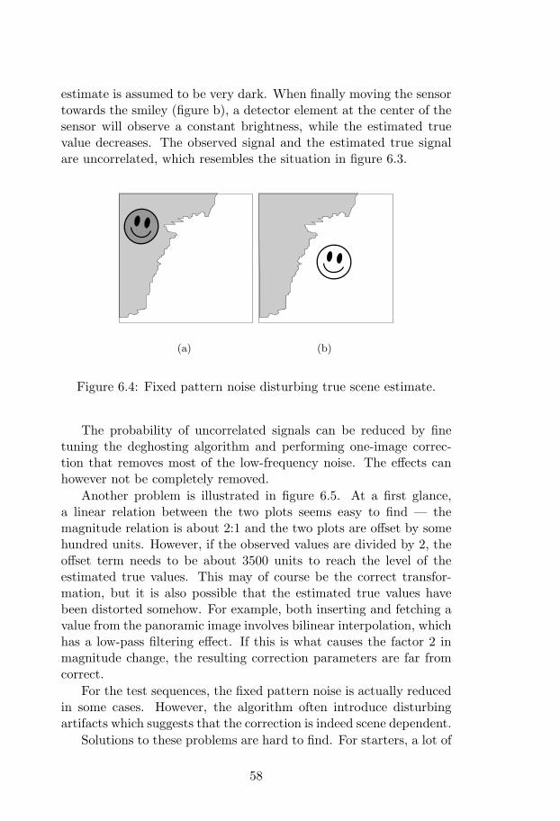
estimate is assumed to be very dark. When finally moving the sensortowards the smiley (figure b), a detector element at the center of thesensor will observe a constant brightness, while the estimated truevalue decreases. The observed signal and the estimated true signalare uncorrelated, which resembles the situation in figure 6.3.
(a) (b)
Figure 6.4: Fixed pattern noise disturbing true scene estimate.
The probability of uncorrelated signals can be reduced by finetuning the deghosting algorithm and performing one-image correc-tion that removes most of the low-frequency noise. The effects canhowever not be completely removed.
Another problem is illustrated in figure 6.5. At a first glance,a linear relation between the two plots seems easy to find — themagnitude relation is about 2:1 and the two plots are offset by somehundred units. However, if the observed values are divided by 2, theoffset term needs to be about 3500 units to reach the level of theestimated true values. This may of course be the correct transfor-mation, but it is also possible that the estimated true values havebeen distorted somehow. For example, both inserting and fetching avalue from the panoramic image involves bilinear interpolation, whichhas a low-pass filtering effect. If this is what causes the factor 2 inmagnitude change, the resulting correction parameters are far fromcorrect.
For the test sequences, the fixed pattern noise is actually reducedin some cases. However, the algorithm often introduce disturbingartifacts which suggests that the correction is indeed scene dependent.
Solutions to these problems are hard to find. For starters, a lot of
58

290 300 310 320 330 340 350 360
6400
6600
6800
7000
7200
7400
7600
7800
frame nr
irrad
ianc
e
Observed valuesEstimated true values
Figure 6.5: Observed and estimated value for a detector element.
procedures for detecting valid input data have to be included in thealgorithm, and the parameters must be updated very slowly. Still, theoffset-only version always gives better results. A possible conclusionto be drawn is that the true scene estimate is good enough only foradditive noise correction. The least-square method is considered toounstable and will not be evaluated further.
A way of improving the offset-only correction is to introduce asimple algorithm that reduces low-frequency noise and shadows. Suchan algorithm is already available — the homomorph filter of the one-image correction procedure (section 3.4). Repeating this one-imagecorrection for each input frame and averaging the resulting gain cor-rection images over time results in a method that at least improvesthe offset-only correction to some degree.
6.8 Crossing path
Theoretically, this is the fastest nonuniformity correction method,ideally requiring only two frames to remove all additive fixed pattern
59

noise. In practice, the image sequences contain temporal noise, deadpixels and moving scene objects that disturb the algorithm. Never-theless, some of the test sequences are completely cleaned from allvisible fixed pattern noise within only 50 frames.
The in-between image interpolation is assumed to be valid onlyif the two source images are related by a translation of one pixel orless. This is a drawback of the crossing path algorithm. For sequenceswhere the image-to-image translation is always more than a pixel, nocorrection at all is performed. If such problems arise, it may benecessary to modify the algorithm to find detector element overlapsin some other way, for example by checking for detector translationsclose to integer distances.
The crossing path algorithm is especially sensitive to errors inmotion estimation and violations of the static scene assumption. Ex-amples of such artifacts are showed in figure 6.6(a), where a truckdrives through the lower right part of the scene, and in figure 6.6(b),where a very hot spot in the lower part of the scene causes noise sinceit is so small that it sometimes disappears due to limited resolution.Most artifacts that are introduced by the algorithm are however can-celled out rather quickly, since the algorithm itself is adapting veryfast to new fixed pattern noise.
(a) Moving objects in scene (b) Tiny hot spot disappears
Figure 6.6: Artifacts due to violated static scene assumption.
Unfortunately, the gain parameter estimation does not work asgood as expected. As described in section 5.2, the offset terms are
60

first removed by constructing gradients of each detector output. Re-lations between gain parameters are then calculated by dividing thegradients. The results are however not easily interpreted. As anexample, consider the situation in figure 6.7, where two detector ele-ments have observed the same point of the scene on six occasions.
1 2 3 4 5 67160
7180
7200
7220
7240
7260Detector ADetector B
(a) Detector outputs
1 2 3 4 5−40
−30
−20
−10
0
10
20Gradient AGradient B
(b) Gradients
Figure 6.7: Signals from two detectors observing the same scenepoints on six occasions.
Five estimates of the gain parameter relation gA/gB can be com-puted by dividing each pair of gradient values. For this particularcase, the estimates are:
1.60 − 0.41 1.31 1.42 − 0.84
As can be seen, the uncertainty is so high that it is practically impos-sible to use this method for gain parameter estimation. Inaccuracy intranslation estimation, in-between image interpolation and changesin the scene all contribute to distortions, but even in the most idealcase, temporal noise alone can be enough to cause such variations inthe signal outputs that the gradient ratios become unreliable or evennegative. Also, when two observed values are nearly identical, thealgorithm includes a division with a value close to zero, introducinglarge numerical errors.
The method can be modified to counter some of these problems.Instead of assuming unity gain parameters for offset-only correction,the offset terms can be assumed to be zero for gain-only correction.
61

Gain correction can then be performed exactly like the offset correc-tion by changing the subtractions to divisions. The revised algorithmnow works in two steps:
• Assume that fixed pattern noise is completely additive.
• Perform offset-only correction.
• Assume that fixed pattern noise is completely multiplicative.
• Perform gain-only correction.
Hopefully, the correction procedure will converge so that multiplica-tive noise is eventually removed by the gain parameters and additivenoise by the offset parameters. If this really is the case is hard tosay. For most test sequences, the resulting gain and offset correctionimages end up very similar. There is also no visible improvement ofimage quality compared to the offset-only correction.
62

Chapter 7
Results
7.1 Computational speed
Optimizing algorithms for speed is not a specific goal for this thesis.Nevertheless, it might be interesting to see how fast the differentmethods are. Table 7.1 shows a rough average of how many framesper second the algorithms are able to process. The tests have beenperformed in Matlab on a dual Pentium 3 system using sequencesof 400 frames, each 128×128 pixels.
Method Frame rateTemporal highpass filter 36.6Constant statistics 24.2Motion compensated average 4.8Crossing path, offset only 5.3Crossing path, offset and gain 4.3
Table 7.1: Average frame rate for the NUC methods.
As expected, the registration-based methods require much moreprocessing time than the simpler ones, partly due to the need formotion estimation. It should be noted that the computation timefor the crossing path method depends on how many valid motionpath collisions that are detected. For example, the parameters wereupdated 280 times in one of the sequences and 1070 times in another.
63

7.2 Reference images
Images of a reference surface with uniform temperature, one at 0◦C andanother at 30◦C, have been recorded in conjunction with some of thetest sequences. For an ideal nonuniformity correction, all pixels inthese images should have equal values. In practice, the pixel valueshave a certain standard deviation, which can be used as a perfor-mance measure of the corresponding correction algorithm. Table 7.2shows the resulting standard deviation of the reference images foreach correction method. The temporal noise standard deviation isabout 3-4 units.
Method Standard deviationSequence 1 Sequence 20◦C 30◦C 0◦C 30◦C
Temporal highpass filter 45 186 46 181Constant statistics 264 1194 178 853MCA, offset only 227 362 169 284MCA, offset and gain 65 102 47 78Crossing path, offset only 50 193 56 190Crossing path, offset and gain 24 64 24 66Uncorrected reference image 317 457 324 458
Table 7.2: Standard deviation of uniform temperature image.
Since the fixed pattern noise is time variant, it is important thatthe test sequences and the reference images are related closely intime. Unfortunately, the sequences that are recorded along with thereference images are of rather poor quality. Compared to the othertest sequences, the range of scene irradiance is much lower and thefixed pattern noise level is much higher. Because of this, the valuesin table 7.2 are probably higher than normal.
Even though the sequence quality leaves a lot to be desired, it isclear that the crossing path algorithm produces best results. Whenusing the constant statistics algorithm, the deviation values end upvery high, sometimes even higher than the standard deviation of theuncorrected image. Obviously this method requires many more inputframes to deliver any useful results.
In these sequences, the average scene temperature is about 0◦C.This is one reason why the resulting deviation for the 0◦C image islower than for the 30◦C image.
64

7.3 Introduced noise
Although the correction algorithms are designed to remove fixed pat-tern noise, some is actually introduced as well. This is mostly causedby errors in motion estimation and image resampling. To gain someknowledge on the magnitude of this introduced noise, the nonunifor-mity correction algorithms are applied to a synthetic sequence of 400frames without any temporal or fixed pattern noise. The standarddeviation of the resulting offset calibration images is then used asa measure of the introduced noise level. Results for the offset-onlyalgorithms are showed in table 7.3.
Std.dev. RatioOriginal sequence 1174 100%Temporal highpass filter 255 22%Motion compensated average 17 2%Crossing path 20 2%
Table 7.3: Levels of introduced noise.
Not surprisingly, the level of noise introduced by the temporalhighpass filter is rather high. For a longer test sequence, this valuewould however be lower. The other two methods have somewhatmore moderate noise magnitudes.
7.4 Synthetic sequences
Comparing the correction algorithms is especially easy when workingwith synthetic sequences, where the true scene is known.
Different kinds of fixed pattern noise is added to a synthetictest sequence, an aerial view of a residential area. Sequence A fea-tures normal distributed additive noise and sine-shaped multiplica-tive noise. Sequence B is distorted by noise similar to that of theMSM sequences. Example frames from the two sequences are shownin figure 7.1
Nonuniformity correction is performed for 400 frames. The lastcorrected image is then compared to the corresponding noise freeimage. If the difference between the two images is regarded as noise,
65

(a) Sequence A (b) Sequence B
Figure 7.1: Images from the two synthetic sequences.
the signal-to-noise ratio can be calculated as
SNR =σ2
z
σ2d
where σ2z is the average squared value of the noise free image and σ2
d isthe average squared difference between the images. This is a commonSNR definition that, for example, is often used in data compressionto measure image degradation. Results are shown in table 7.4.
Method SNRSequence A Sequence B
Temporal highpass filter 6.4 6.9Constant statistics 23.5 9.0MCA, offset only 1.9 1.0MCA, offset and gain 8.7 10.3Crossing path, offset only 2.3 5.2Crossing path, offset and gain 61.2 26.6
Table 7.4: Signal-to-noise ratio for the sequences in figure 7.1. Thehigher the ratio, the more noise has been reduced.
As before, the crossing path method gives best results. Interest-ingly, constant statistics also gives very good results. The properties
66

of the synthetic sequences are clearly in parity with the statistic as-sumptions. The inability to remove low-frequency shading effectsresults in very low signal-to-noise levels for the offset-only motioncompensated average, even though most of the fixed pattern noisehas been successfully removed. As a reference, figure 7.2 shows thefinal frame from synthetic sequence B, corrected using motion com-pensated average and crossing path.
(a) Motion compensated aver-age, offset only. SNR=1.0
(b) Crossing path, offset andgain. SNR=26.6
Figure 7.2: The last frame from corrected synthetic sequence B.
7.5 Visual inspection
As seen in the previous section, computed quality measures are notalways consistent with what humans perceive as a high quality im-age. As a complement, the following questions are answered for eachcorrection method when studying the sequences visually:
1. At which frame has most of the annoying high-frequency noisebeen removed?
2. At which frame has enough fixed pattern noise been removedso that a still image is of acceptable quality?
3. When applying the final correction parameters to the entireuncorrected sequence, how can the quality of the resulting se-
67

quence be described? (1=unacceptable, 2=disturbing, 3=ac-ceptable, 4=good, 5=excellent)
Sequence Q1 Q2 Q3Synthetic 1 75 350 3MSM 1 150 350 3MSM 2 350 – 1
(a) Temporal highpass filter
Sequence Q1 Q2 Q3Synthetic 1 200 200 4MSM 1 250 350 3MSM 2 – – 1
(b) Constant statistics
Sequence Q1 Q2 Q3Synthetic 1 40 350 2MSM 1 150 150 4MSM 2 150 250 3
(c) Motion compensated average,offset only
Sequence Q1 Q2 Q3Synthetic 1 40 150 2MSM 1 150 150 5MSM 2 150 250 5
(d) Motion compensated average,offset and gain
Sequence Q1 Q2 Q3Synthetic 1 50 200 4MSM 1 80 80 3MSM 2 200 200 2
(e) Crossing path, offset only
Sequence Q1 Q2 Q3Synthetic 1 50 50 4MSM 1 50 50 5MSM 2 180 180 4
(f) Crossing path, offset and gain
Table 7.5: Test person opinions.
Comments
As can be seen for MSM sequence 2, the crossing path algorithmrequires a lot more frames to converge than usual. This is becausethe relative translation between images is larger than one pixel forthe entire first part of the sequence. The motion slows down brieflyafter about 150 frames, allowing for a acceptable correction in only 30frames. This behavior also causes some artifacts in MSM sequence 1.The image motion speeds up to more than one pixel per frame justafter some violations of the static scene assumptions introduce noiseinto the sequence, which then is left uncorrected until the motionslows down.
68

The 400 frames in these sequences are barely enough for the tem-poral highpass filter and the constant statistics method to convergeproperly. Image quality would surely increase further if more frameswere to be processed.
The offset-only variant of the motion compensated average methodhas problems with removing low-frequency shadows and variations.
7.6 One-dimensional sensor
As described earlier, the IRST system developed by Saab Bofors Dy-namics is equipped with a scanning one-dimensional sensor array.Raw images from this system are severely disturbed by fixed patternnoise, and additional pre-processing is required to make it possiblefor the registration-based algorithms to detect image motion. For ex-ample, the mean values of each pixel row can be forced to be equal byadjusting detector element offset levels. This tremendously improvesimage quality, as can be seen in figure 7.3.
(a) Original (b) Equal horizontal mean
Figure 7.3: One-dimensional sensor. Forcing the mean of each pixelrow to the same value reveals the scene.
Forcing equal horizontal mean is unnecessary for the methodsthat do not estimate image motion. Actually, a similar procedure iscarried out anyway by the temporal highpass filter, as the temporalmean is subtracted from input images, initially forcing zero meanvalues for all detector elements.
One might believe that this horizontal mean correction is in itselfan effective calibration method. However, some disturbing artifacts
69

are introduced when all rows in the image are forced to share thesame mean value. For example, bright parts of the scene are followedhorizontally by shadows to make the mean value constant. This canbe seen for the clouds in figure 7.3(b). Furthermore, most detectorelements are not corrected satisfactory with offset calibration alone,which makes horizontal stripes visible when the scene moves around.
Performing nonuniformity correction on the IRST sequences pro-duces results similar to the MSM sequences. As usual, the temporalhighpass filter and constant statistics methods introduce disturbingghosting. Surprisingly, horizontal stripes are visible during the entiresequence for all correction methods. The sequence motion is mostlyhorizontal, which may explain why the registration-based methodsare unable to completely suppress such noise. In fact, the stripes areleast visible when using the constant statistics algorithm.
In these tests, all pixels are corrected with individual correctionparameters. The fact that all pixels in a row originate from a singledetector element can be exploited by using the horizontal mean valueof the parameters to calibrate the entire row. This adaptation is thenused in conjunction with the nonuniformity correction methods.
While the registration-based methods show little or no significantimprovement, the ghosting artifacts of the temporal highpass filterand constant statistics methods are almost completely removed. Asghosting otherwise is the dominant noise component for these algo-rithms, image quality is significantly increased. The performance issimilar to, or even better than, the registration-based algorithms.Figure 7.4 shows results for the constant statistics and crossing pathmethods.
With the modifications suggested here, the algorithms first pro-duce correction parameters for a two-dimensional sensor array, whichthen are averaged horizontally to fit the assumptions of a one-dimensionalarray. It is likely that even better results can be achieved if the cor-rection algorithms are designed for a one-dimensional sensor in thefirst place. This has however not been studied in this thesis.
70

(a) Constant statistics (b) Crossing path
Figure 7.4: Corrected images from a one-dimensional sensor. Theconstant statistics method gives equal or even better results than themore sophisticated crossing path method.
7.7 Example results
The following pages show frames 25, 50, 75, 100, 200 and 400 from oneof the MSM test sequences, followed by the corresponding resultingimages for each correction method.
71
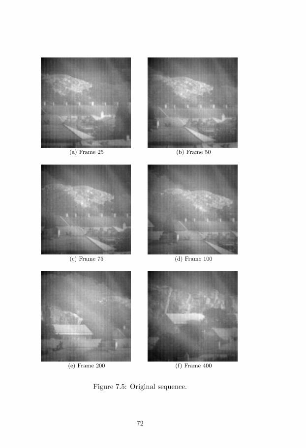
(a) Frame 25 (b) Frame 50
(c) Frame 75 (d) Frame 100
(e) Frame 200 (f) Frame 400
Figure 7.5: Original sequence.
72

(a) Frame 25 (b) Frame 50
(c) Frame 75 (d) Frame 100
(e) Frame 200 (f) Frame 400
Figure 7.6: Temporal highpass filter.
73

(a) Frame 25 (b) Frame 50
(c) Frame 75 (d) Frame 100
(e) Frame 200 (f) Frame 400
Figure 7.7: Constant statistics.
74

(a) Frame 25 (b) Frame 50
(c) Frame 75 (d) Frame 100
(e) Frame 200 (f) Frame 400
Figure 7.8: Motion compensated average, offset only.
75

(a) Frame 25 (b) Frame 50
(c) Frame 75 (d) Frame 100
(e) Frame 200 (f) Frame 400
Figure 7.9: Motion compensated average, offset and gain.
76

(a) Frame 25 (b) Frame 50
(c) Frame 75 (d) Frame 100
(e) Frame 200 (f) Frame 400
Figure 7.10: Crossing path, offset only.
77

(a) Frame 25 (b) Frame 50
(c) Frame 75 (d) Frame 100
(e) Frame 200 (f) Frame 400
Figure 7.11: Crossing path, offset and gain.
78

Chapter 8
Conclusions
8.1 Summary
Several nonuniformity correction methods are described in this thesis,each with its individual pros and cons.
Temporal highpass filter and constant statistics are two well-knownmethods that are very easy to implement and can process sequencesin real-time. Although they require many input frames before the im-age quality is acceptable, fixed pattern noise is usually reduced withgood results. The temporal highpass filter is an offset-only algorithm,while the constant statistics method estimates both gain and offsetparameters. Both methods assume that image motion exists betweenimages in the sequence.
Crossing path, a new method that is introduced in this thesis, andmotion compensated average are two somewhat more sophisticatedcorrection methods. They are referred to as registration-based meth-ods, in that they assume that the image motion can be accuratelyestimated using a motion estimation algorithm. With knowledge ofthe image motion, multiple detector elements that have observed thesame position in the scene can be found and analyzed, leading to anefficient nonuniformity correction. In general, the registration-basedmethods produce very good results, but require much more compu-tation time.
The different methods are evaluated in a number of ways usingseveral test sequences from existing IR imaging systems, as well assynthetic data. For the special case of a scanning one-dimensionaldetector array, combining correction parameters from all pixels thatoriginate from the same detector element is shown to be a way of
79

significantly improving image quality.Removing multiplicative fixed pattern noise has proven to be dif-
ficult. For both registration-based methods, the original gain param-eter estimation theory was unsuccessful when put into practice andhad to be modified. The difficulties are consistent with earlier experi-ence with sensor nonuniformities at Saab Bofors Dynamics. Yet, theoffset-only algorithms usually produce excellent results, suggestingthat for a certain scene temperature range, the lack of multiplicativecorrection can be compensated by additive correction. If the scenetemperature changes, disturbing artifacts would probably be visibleuntil the algorithm stabilizes. For a fast enough method, offset-onlycorrection might be enough for a wide temperature range. Also, eachalgorithm responds differently to violations of the initial assumptions,which should be taken into consideration when choosing a suitablecorrection method.
8.2 Suggestions for further work
The one-image correction procedure is an example of pre-processingthat improves the image quality. The simple method presented herecan surely be tweaked to perform even better, especially if it is de-signed for a specific sensor.
Since motion estimation is a key component of the registration-based algorithms, research in this field is encouraged. For example,methods can be developed to detect which parts of the scene thatare well suited for motion estimation. By neglecting areas of highuncertainty, estimation accuracy will improve. It would also be inter-esting to see what improvements can be achieved by complementingor replacing the software motion estimation with hardware positionindicators on the sensor unit.
Another improvement would be to automatically detect when anybasic assumptions are violated. The correction algorithm could thenturn itself on and off when necessary, or at least revert uncertainparameters to an earlier state.
When correcting nonuniformity for the one-dimensional sensor,the existing algorithms are modified by averaging the correction pa-rameters for pixels that originate from the same detector element. Itwould be interesting to see what improvements could be made if thealgorithms were to be designed for a one-dimensional sensor in thefirst place.
80

Finally, the correction methods described in this thesis have allbeen studied separately. It is possible that performance would in-crease if two or more methods were to be combined into one hybridalgorithm.
81


Bibliography
[1] M. Tornkvist: Nonuniformity correction and property investiga-tion of a multispectral IR camera, Diploma thesis, University ofUmea, September 1999
[2] S. Tzimopoulou, A.H. Lettington: Scene based techniques fornonuniformity correction of infrared focal plane arrays, Proc.SPIE vol. 3436, p 172-183, Infrared Technology and ApplicationsXXIV, October 1998
[3] D.A. Scribner, K.A. Sarkady, J.T. Caulfield, M.R. Kruer,G. Katz, C.J. Gridley: Nonuniformity correction for staringIR focal plane arrays using scene-based techniques, Proc. SPIEvol. 1308, p 224-233, Infrared detectors and focal plane arrays,September 1990
[4] J.G. Harris, Y-M. Chiang: Nonuniformity correction of infraredimage sequences using the constant-statistics constraint, IEEETransactions on Image Processing, vol. 8, no. 8, p 1148-1151,August 1999
[5] J.G. Harris, Y-M. Chiang: Minimizing the ghosting artifact inscene-based nonuniformity correction, Proc. SPIE vol. 3377, p106-113, Infrared Imaging Systems: Design, Analysis, Modelingand Testing IX, August 1998
[6] E. Ronnqvist: Image resolution enhancement using image se-quences, M.Sc. thesis, department of electrical engineering,Linkopings universitet, May 2000.
[7] B.M. Ratliff, M.M. Hayat, R.C. Hardie: An algebraic algorithmfor nonuniformity correction in focal-plane arrays, The Jour-nal of the Optical Society of America A, vol. 19, p 1737-1747,September 2002
83

[8] R.C. Hardie, M.M. Hayat, E. Armstrong, B. Yasuda: Scene-based nonuniformity correction with video sequences and regis-tration, Applied Optics, vol. 39, no. 8, p 1241-1250, March 2000
[9] P-E. Danielsson, O. Seger, M. Magnusson Seger: Bildbehandling2000, Image processing course litterature, Department of Sys-tems Engineering, Linkoping Institute of Technology, 2000
[10] P. Reddy, G. de Jager: Reference free nonuniformity correctionfor mercury cadmium telluride infrared focal plane arrays, Proc.COMSIG vol. 1998, p 243-248, 1998
84

På svenska Detta dokument hålls tillgängligt på Internet – eller dess framtida ersättare – under en längre tid från publiceringsdatum under förutsättning att inga extra-ordinära omständigheter uppstår.
Tillgång till dokumentet innebär tillstånd för var och en att läsa, ladda ner, skriva ut enstaka kopior för enskilt bruk och att använda det oförändrat för ickekommersiell forskning och för undervisning. Överföring av upphovsrätten vid en senare tidpunkt kan inte upphäva detta tillstånd. All annan användning av dokumentet kräver upphovsmannens medgivande. För att garantera äktheten, säkerheten och tillgängligheten finns det lösningar av teknisk och administrativ art.
Upphovsmannens ideella rätt innefattar rätt att bli nämnd som upphovsman i den omfattning som god sed kräver vid användning av dokumentet på ovan beskrivna sätt samt skydd mot att dokumentet ändras eller presenteras i sådan form eller i sådant sammanhang som är kränkande för upphovsmannens litterära eller konstnärliga anseende eller egenart.
För ytterligare information om Linköping University Electronic Press se förlagets hemsida http://www.ep.liu.se/ In English The publishers will keep this document online on the Internet - or its possible replacement - for a considerable time from the date of publication barring exceptional circumstances.
The online availability of the document implies a permanent permission for anyone to read, to download, to print out single copies for your own use and to use it unchanged for any non-commercial research and educational purpose. Subsequent transfers of copyright cannot revoke this permission. All other uses of the document are conditional on the consent of the copyright owner. The publisher has taken technical and administrative measures to assure authenticity, security and accessibility.
According to intellectual property law the author has the right to be mentioned when his/her work is accessed as described above and to be protected against infringement.
For additional information about the Linköping University Electronic Press and its procedures for publication and for assurance of document integrity, please refer to its WWW home page: http://www.ep.liu.se/ © Petter Torle