From data to insightsAn advice to improve the capacity planning

of temporary employees

Master thesis at CEVA Logistics BeneluxUniversity of Twente

Author:Bram de la Combé

Company supervisor:Maarten Borsten

Supervisor:Dr. Engin Topan

Co-Supervisor:Dr. Ipek Seyran-Topan

MSc Industrial Engineering and ManagementSeptember 22, 2019

Essentially,all models are wrong,but some are useful.

GEORGE E. P. BOX (1976)

Preface

This thesis is written as the graduation assignment for my masters degree of the study IndustrialEngineering and Management at the University of Twente. The company, CEVA Logistics Benelux,offered me a place where I could apply my passion for data analysis and my interests in logistics. Iworked at the headquarter office in Culemborg and visited various warehouses during my time at thecompany. Over there, I got the opportunity to formulate my own research as long as the focus was toprovide insights in order to improve a logistic process by data analysis. I learned to individually identifya problem, formulate a problem solving approach and to create a model from scratch in the programmingsoftware R.

First of all, I would like to thank my family, friends and girlfriend, who supported me with appreciationand understanding. And secondly, my committee members, each of whom has provided patient adviceand guidance throughout the research process. Thank you all for your unwavering support.

i

Management Summary

This research is executed at CEVA Logistics Benelux, they are a logistic service provider with multiplewarehouses across The Netherlands. Currently the warehouses facing a high outflow rate of temporaryworkers. On average, 24% of the pool of temporary workers leave every month. The cost of outflow aredefined as the cost of inflow since a temporary worker that is leaving must be replaced by a new oneif the demand is increasing. The cost of inflow includes the costs of training and the use of supportingstaff. The yearly costs of the outflow rate is approximately ranging between e2.000.000 and e3.100.000in total. A survey among 1300 temporary employees indicated that receiving less work than desired isone of the main causes a temporary worker decides to leave. In addition to this, the temporary workersare planned as on-call staff, so the temporary workers have a lot of uncertainty how much work they getoffered on a weekly base. Given these points, the problem is that it seems that receiving enough workis a very important factor for a temporary employee and currently this is not an important factor asconsidered by the capacity planning.

The capacity planning determines the amount of work a temporary employee receives on a weekly ormonthly base by determining how many temporary employees should be included in the pool. In orderto reduce the outflow rate, the capacity planning strategy must be improved such that the preferencesof the temporary workers are better represented.

The purpose of this thesis is to provide advice and insights how the capacity planning strategy can beimproved such that the outflow rate of the temporary employees can be reduced. This thesis proposed twomodels. The first model determines the relationship between the estimated outflow rate when receivingless work for a certain period of time. The result of this model is used to formulate an advice about howthe pool of temporary workers must change when the demand changes. The second model investigatesto what extent demand can be predicted using only time series data in order to adjust the pool size oftemporary workers to the forecasted demand in time. To conclude, the first model assumes that futuredemand is known and provides an advice towards a capacity planning strategy. The second model verifiesthat assumption by investigating to what extent future demand can be predicted.

The first model is called the outflow rate model. The purpose of the model is to estimate the outflow ratewhen the pool of temporary workers receive less work. The model operates by identifying the regularamount of work a temporary employee receives. The estimated outflow rate is determined by identifyingthe amount of times a temporary worker received less work within a certain period than normal, themoments the temporary worker didn’t decide to leave and the final moment a temporary worker decidedto leave are compared with each other. So, if it happens that a temporary employee left during a periodin which the temporary employee received less work than normal, the model indicates this event asoutflow due to less work. The output of the outflow rate model is used as input for a regression model.This model generalizes the relationship between the estimated outflow rate and the rate of receiving lesswork. The result is a linear regression model where the outflow rate increases more if the rate of lesswork increases. Another way to interpret this outcome is by using the overcapacity. The overcapacity isdefined as the surplus of temporary workers in the pool to fulfill demand, a high overcapacity rate meansthat temporary workers receive less work. The conclusion is that at any overcapacity level, the estimatedoutflow rate will be higher and undesired outflow of temporary workers occurs. It is assumed that anovercapacity rate between 0% to 15% does not have an influence on the outflow rate. Therefore theconclusion of the outflow rate model is that the overcapacity rate should not exceed the 15%, otherwiseundesired outflow of temporary workers occurs.

ii

The second model is called the time series forecasting model. The motivation of this model is that formost of the warehouses a demand forecast with a horizon of three months is unknown. In order to use theadvise of the outflow rate model, the three months ahead forecast must be known. The purpose of theforecasting model is to know to what extent it is possible to generate a reasonable accurate three monthsahead forecast, using only monthly time series demand data of different clients. The model provides anadvice and insights if there are time series forecasting methods that are able to generate a forecast thatis accurate enough to accept the advice provided by the outflow rate model.

The three best performing methods from an international forecasting competition are selected for theforecast model. In addition to that, a parameter is proposed in order to improve the selected forecastsmethods in case of some typical demand behavior of some clients. The model uses monthly time seriesdemand data that consist of warehouse activities such as the number of orderlines, orders or trucks. Intotal there are 177 different time series data from different clients available, each consisting of more than24 monthly observations. For each time series demand data, the model chooses the best forecast method.The forecast accuracy is summarized per client sector. The conclusion of the forecasting model is thatin general the clients within the healthcare and industrial sector have a forecast error of 14% to 16% fora three months ahead forecast. The clients within the technology and retail sector have a considerablylower forecast error ranging from 8% to 9%. The conclusion is that the outflow rate model should onlybe used for clients active in the technology or retail sector, since it is desired to have an three monthsahead forecast error of less than 9%.

To conclude the findings by the outflow rate and forecasting model, the advice is that the capacityplanning strategy determines that a maximum overcapacity of 15% is allowed, otherwise undesiredoutflow of temporary workers occur due to receiving less work. The proposed capacity planning strategyis only applicable for clients within the technology or retail sector, or a client that is able to deliver athree months ahead forecast with a forecast error of at most 9% to ensure that the pool of temporaryworkers can be adjusted in time to the forecasted demand.

For the year 2018, the total costs as a consequence of outflow by less work is estimated at a rangefrom e200.000 to e290.000. The cost savings are determined when the advice was integrated in thecapacity planning strategy. Costs can be saved as a result of preventing outflows by adjusting the poolsize in time to be within the 15% overcapacity rate. The costs savings are based on the condition thatan reasonable accurate demand forecast is available. Altogether, the potential cost savings over 2018 areestimated at a range from e110.000 - e160.000.

The most important recommendation is to incorporate the expected overcapacity level when a warehousedetermines the capacity planning of temporary workers. The expected overcapacity level can be madevisible with a key performance indicator. There are three options to implement the key performanceindicator.

1. Basic: Incorporate the actual overcapacity level in the dashboard that a warehouse (supervisor)can use when determining the capacity planning. It is up to the warehouse (supervisor) to makethe right decisions.

2. Premium: Incorporate the expected overcapacity level in a software tool that provides an adviceto the warehouse (supervisor) about the decisions to be made regarding the capacity planning.

3. Pro: Incorporate the expected overcapacity level in a programming environment where the outcomefor multiple scenario’s with different variables are simulated. This lowers the uncertainty of thecapacity planning.

This research focused on two input variables of the capacity planning, the estimated outflow rate andthe estimated forecast accuracy. The next step is to go from a strategy to implementation. Therefore amodel that incorporates these two input variables provides a warehouse with advice about the capacityplanning decisions of a live operation. To conclude, the most interesting point of further research is tobuild a proof of concept model that can be used at a live operation and convinces the warehouses of theopportunities to improve their capacity planning of temporary workers.

iii

Contents

Preface i

Management Summary ii

List of Figures vi

List of Tables viii

1 Introduction 11.1 CEVA Logistics . . . . . . . . . . . . . . . . . . . . . . . . . . . . . . . . . . . . . . . . . . 1

1.1.1 CEVA Logistics Benelux . . . . . . . . . . . . . . . . . . . . . . . . . . . . . . . . . 11.2 Problem statement . . . . . . . . . . . . . . . . . . . . . . . . . . . . . . . . . . . . . . . . 2

1.2.1 Mapping opportunities . . . . . . . . . . . . . . . . . . . . . . . . . . . . . . . . . . 21.2.2 Resource planning . . . . . . . . . . . . . . . . . . . . . . . . . . . . . . . . . . . . 31.2.3 Problem cluster . . . . . . . . . . . . . . . . . . . . . . . . . . . . . . . . . . . . . . 3

1.3 Research goal . . . . . . . . . . . . . . . . . . . . . . . . . . . . . . . . . . . . . . . . . . . 51.3.1 Main research question . . . . . . . . . . . . . . . . . . . . . . . . . . . . . . . . . . 51.3.2 Research questions . . . . . . . . . . . . . . . . . . . . . . . . . . . . . . . . . . . . 5

1.4 Research approach . . . . . . . . . . . . . . . . . . . . . . . . . . . . . . . . . . . . . . . . 61.5 Scope and assumptions . . . . . . . . . . . . . . . . . . . . . . . . . . . . . . . . . . . . . . 7

2 Current situation analysis 92.1 Introduction to warehousing and resource planning . . . . . . . . . . . . . . . . . . . . . . 9

2.1.1 Warehouse operations . . . . . . . . . . . . . . . . . . . . . . . . . . . . . . . . . . 92.1.2 Resource planning . . . . . . . . . . . . . . . . . . . . . . . . . . . . . . . . . . . . 102.1.3 Data warehousing . . . . . . . . . . . . . . . . . . . . . . . . . . . . . . . . . . . . 112.1.4 TEMP characteristics . . . . . . . . . . . . . . . . . . . . . . . . . . . . . . . . . . 12

2.2 No aligned strategy towards capacity planning of TEMPs . . . . . . . . . . . . . . . . . . 142.3 High inflow and outflow rate of TEMPs . . . . . . . . . . . . . . . . . . . . . . . . . . . . 15

2.3.1 Inflow and outflow rates . . . . . . . . . . . . . . . . . . . . . . . . . . . . . . . . . 152.3.2 Causes of outflow . . . . . . . . . . . . . . . . . . . . . . . . . . . . . . . . . . . . . 172.3.3 Cost of outflow . . . . . . . . . . . . . . . . . . . . . . . . . . . . . . . . . . . . . . 18

2.4 Proposed solution towards improving the capacity planning of TEMPs . . . . . . . . . . . 19

3 Literature review 213.1 Forecasting . . . . . . . . . . . . . . . . . . . . . . . . . . . . . . . . . . . . . . . . . . . . 21

3.1.1 Problem definition . . . . . . . . . . . . . . . . . . . . . . . . . . . . . . . . . . . . 213.1.2 Gathering information . . . . . . . . . . . . . . . . . . . . . . . . . . . . . . . . . . 213.1.3 Preliminary (exploratory) analysis . . . . . . . . . . . . . . . . . . . . . . . . . . . 223.1.4 Choosing and fitting models . . . . . . . . . . . . . . . . . . . . . . . . . . . . . . . 223.1.5 Evaluating the quality of a forecasting model . . . . . . . . . . . . . . . . . . . . . 273.1.6 Using the model . . . . . . . . . . . . . . . . . . . . . . . . . . . . . . . . . . . . . 293.1.7 Forecasting competitions to select best performing method . . . . . . . . . . . . . 29

3.2 Resource capacity planning . . . . . . . . . . . . . . . . . . . . . . . . . . . . . . . . . . . 303.2.1 Planning methodology . . . . . . . . . . . . . . . . . . . . . . . . . . . . . . . . . . 303.2.2 MILP model . . . . . . . . . . . . . . . . . . . . . . . . . . . . . . . . . . . . . . . 30

3.3 Data analytics . . . . . . . . . . . . . . . . . . . . . . . . . . . . . . . . . . . . . . . . . . 32

iv

3.3.1 Data analytics framework . . . . . . . . . . . . . . . . . . . . . . . . . . . . . . . . 323.3.2 A definition of Big data . . . . . . . . . . . . . . . . . . . . . . . . . . . . . . . . . 32

3.4 Regression analysis . . . . . . . . . . . . . . . . . . . . . . . . . . . . . . . . . . . . . . . . 333.4.1 Quantitative prediction problems . . . . . . . . . . . . . . . . . . . . . . . . . . . . 343.4.2 Qualitative prediction problems . . . . . . . . . . . . . . . . . . . . . . . . . . . . . 353.4.3 Conclusion regression analysis . . . . . . . . . . . . . . . . . . . . . . . . . . . . . . 35

3.5 Literature conclusion . . . . . . . . . . . . . . . . . . . . . . . . . . . . . . . . . . . . . . . 35

4 Model Explanation 374.1 Forecasting model . . . . . . . . . . . . . . . . . . . . . . . . . . . . . . . . . . . . . . . . 39

4.1.1 Convert warehouse data to time series data . . . . . . . . . . . . . . . . . . . . . . 424.1.2 Selection of method . . . . . . . . . . . . . . . . . . . . . . . . . . . . . . . . . . . 424.1.3 Robustness check of the model . . . . . . . . . . . . . . . . . . . . . . . . . . . . . 46

4.2 Outflow rate model . . . . . . . . . . . . . . . . . . . . . . . . . . . . . . . . . . . . . . . . 484.2.1 Approach and main assumptions . . . . . . . . . . . . . . . . . . . . . . . . . . . . 494.2.2 Data cleaning . . . . . . . . . . . . . . . . . . . . . . . . . . . . . . . . . . . . . . . 504.2.3 Data analysis . . . . . . . . . . . . . . . . . . . . . . . . . . . . . . . . . . . . . . . 51

4.3 Strategy towards improving the capacity planning of TEMPs . . . . . . . . . . . . . . . . 53

5 Model results 555.1 Forecasting model . . . . . . . . . . . . . . . . . . . . . . . . . . . . . . . . . . . . . . . . 55

5.1.1 Input data . . . . . . . . . . . . . . . . . . . . . . . . . . . . . . . . . . . . . . . . 555.1.2 Results . . . . . . . . . . . . . . . . . . . . . . . . . . . . . . . . . . . . . . . . . . 565.1.3 Robustness analysis . . . . . . . . . . . . . . . . . . . . . . . . . . . . . . . . . . . 595.1.4 Conclusion of the forecast model . . . . . . . . . . . . . . . . . . . . . . . . . . . . 64

5.2 Outflow rate model . . . . . . . . . . . . . . . . . . . . . . . . . . . . . . . . . . . . . . . . 665.2.1 Input data . . . . . . . . . . . . . . . . . . . . . . . . . . . . . . . . . . . . . . . . 665.2.2 Initial results . . . . . . . . . . . . . . . . . . . . . . . . . . . . . . . . . . . . . . . 665.2.3 Analysis of the results . . . . . . . . . . . . . . . . . . . . . . . . . . . . . . . . . . 675.2.4 Sensitivity analysis . . . . . . . . . . . . . . . . . . . . . . . . . . . . . . . . . . . . 705.2.5 Interpretation of the outflow rate model . . . . . . . . . . . . . . . . . . . . . . . . 715.2.6 Cost impact of the outflow rate model . . . . . . . . . . . . . . . . . . . . . . . . . 725.2.7 Conclusion outflow rate model . . . . . . . . . . . . . . . . . . . . . . . . . . . . . 75

5.3 Improvement of the capacity planning strategy of TEMPs . . . . . . . . . . . . . . . . . . 765.3.1 Motivation of the behaviour of a TEMP . . . . . . . . . . . . . . . . . . . . . . . . 765.3.2 How must a pool of TEMPs react on changes in demand? . . . . . . . . . . . . . . 765.3.3 Forecasting demand . . . . . . . . . . . . . . . . . . . . . . . . . . . . . . . . . . . 775.3.4 Implementation of the proposed capacity planning strategy . . . . . . . . . . . . . 78

6 Conclusions and recommendations 796.1 Conclusions . . . . . . . . . . . . . . . . . . . . . . . . . . . . . . . . . . . . . . . . . . . . 79

6.1.1 Outflow rate model . . . . . . . . . . . . . . . . . . . . . . . . . . . . . . . . . . . . 806.1.2 Time series forecast model . . . . . . . . . . . . . . . . . . . . . . . . . . . . . . . . 806.1.3 Final conclusions . . . . . . . . . . . . . . . . . . . . . . . . . . . . . . . . . . . . . 82

6.2 Recommendations . . . . . . . . . . . . . . . . . . . . . . . . . . . . . . . . . . . . . . . . 826.2.1 Implementation . . . . . . . . . . . . . . . . . . . . . . . . . . . . . . . . . . . . . . 826.2.2 Discussion . . . . . . . . . . . . . . . . . . . . . . . . . . . . . . . . . . . . . . . . . 846.2.3 Further research . . . . . . . . . . . . . . . . . . . . . . . . . . . . . . . . . . . . . 85

Glossary 87

Bibliography 88

A Pseudo-code 90

B Additional tables 91

C Additional figures 92

v

List of Figures

1.1 CEVA Logistics Benelux Contract Logistics sites and their main clients. . . . . . . . . . . 11.2 A value assessment of projects that could be explored via quantitative based based research. 21.3 The problem cluster regarding the capacity planning problem. . . . . . . . . . . . . . . . . 41.4 An overview of the research approach of this thesis. . . . . . . . . . . . . . . . . . . . . . . 7

2.1 A general overview of the logistic activities within a warehouse . . . . . . . . . . . . . . . 102.2 An overview of the data warehouse systems and the available data per system. . . . . . . 122.3 A density plot for the amount of hours worked per week and the average number of shifts

worked per week of all fixed blue collars in the year 2018. . . . . . . . . . . . . . . . . . . 132.4 Left: the ratio between the different TEMP types per site per year. Right: the total

number of TEMPs on each site per year. . . . . . . . . . . . . . . . . . . . . . . . . . . . . 142.5 An overview of the size of the pool of TEMPs and the actual needed TEMPs together

with the overcapacity for the CEVA warehouses. . . . . . . . . . . . . . . . . . . . . . . . 152.6 This figure shows that the outflow rate of TEMPs did increase over the past couple of years. 162.7 The rate of inflow and outflow of TEMPs per warehouse . . . . . . . . . . . . . . . . . . . 162.8 A highlight of a case where the inflow of TEMPs increases as well as the outflow of TEMPs. 17

3.1 An example of a Theta-model forecast and the decomposed series for theta is equal tozero and two. A forecast is provided from time is equal to 10. . . . . . . . . . . . . . . . . 27

3.2 An example of underfitting. . . . . . . . . . . . . . . . . . . . . . . . . . . . . . . . . . . . 343.3 An example of overfitting . . . . . . . . . . . . . . . . . . . . . . . . . . . . . . . . . . . . 34

4.1 An overview of the outlines of the forecast model and outflow rate model, together withthe deliverables of the model. . . . . . . . . . . . . . . . . . . . . . . . . . . . . . . . . . . 38

4.2 An detailed overview of the contents of the forecast model. . . . . . . . . . . . . . . . . . 414.3 Convert warehouse data to a monthly time series per warehouse activity per client per site. 424.4 The demand of a client where demand increases and suddenly drops. . . . . . . . . . . . . 454.5 An example of cross-validation for time series data when using a rolling horizon. . . . . . 474.6 An detailed overview of the contents of the outflow rate model. . . . . . . . . . . . . . . . 494.7 The average amount of shifts per week from period 1 (base period) is compared with that

of period 2 (review period), right before a TEMP leaves the company. . . . . . . . . . . . 504.8 The holiday cleaning procedure of a TEMP in order to determine their usual workload . . 51

5.1 The result of the forecast model per sector. . . . . . . . . . . . . . . . . . . . . . . . . . . 575.2 The result of the forecast model per warehouse activity. . . . . . . . . . . . . . . . . . . . 585.3 The amount of time a forecast method was the best of all the methods used in the forecast

model in case a forecast horizon of 3 months is used. . . . . . . . . . . . . . . . . . . . . . 595.4 An evaluation of the effectiveness of the ExtrP method compared with the original forecast

method. . . . . . . . . . . . . . . . . . . . . . . . . . . . . . . . . . . . . . . . . . . . . . . 605.5 An analysis which of the forecasting methods are prone to overfitting, a forecast horizon

of three months is applied. . . . . . . . . . . . . . . . . . . . . . . . . . . . . . . . . . . . . 615.6 A sensitivity analysis of the forecast methods by multiple forecast horizons. . . . . . . . . 625.7 The result of the forecast model (3 months ahead) when only the robust methods are

included for all activities. . . . . . . . . . . . . . . . . . . . . . . . . . . . . . . . . . . . . 635.8 The result of the forecast model (3 months ahead) with only robust forecast methods and

4 realistic activities included. . . . . . . . . . . . . . . . . . . . . . . . . . . . . . . . . . . 64

vi

5.9 The initial result of the outflow rate of Table 5.3. Run time = 7 hours . . . . . . . . . . . 685.10 Two regression model to determine the outflow rate . . . . . . . . . . . . . . . . . . . . . . 685.11 Two regression model to determine the outflow rate . . . . . . . . . . . . . . . . . . . . . . 695.12 The linear regression models of the outflow rate given a set of different lengths for period

2, in addition to that the R-squared values and p-values are given. (Run time = 35 hours) 705.13 The accumulated number of outflows for a certain less worked than usual percentage. . . 715.14 The linear regression model to determine the estimated outflow rate when a TEMP receives

less work. . . . . . . . . . . . . . . . . . . . . . . . . . . . . . . . . . . . . . . . . . . . . . 725.15 The impact of overcapacity, as determined by the outflow rate model, expressed in TEMPs

lost. . . . . . . . . . . . . . . . . . . . . . . . . . . . . . . . . . . . . . . . . . . . . . . . . 73

C.1 An example of different productivity rates per sites. . . . . . . . . . . . . . . . . . . . . . 92C.2 The costs of the estimated number of outflows due to less work for maximum overcapacity

level of 10% within the year 2018. . . . . . . . . . . . . . . . . . . . . . . . . . . . . . . . . 92C.3 An overview of the most important sections (1/3) of the outflow rate model, expressed in

R script. . . . . . . . . . . . . . . . . . . . . . . . . . . . . . . . . . . . . . . . . . . . . . 93C.4 An overview of the most important sections (2/3) of the outflow rate model, expressed in

R script. . . . . . . . . . . . . . . . . . . . . . . . . . . . . . . . . . . . . . . . . . . . . . 94C.5 An overview of the most important sections (3/3) of the outflow rate model, expressed in

R script. . . . . . . . . . . . . . . . . . . . . . . . . . . . . . . . . . . . . . . . . . . . . . 95

vii

List of Tables

1.1 Resource planning and scheduling framework [1]. . . . . . . . . . . . . . . . . . . . . . . . 3

2.1 The resource planning process at the sites. . . . . . . . . . . . . . . . . . . . . . . . . . . . 112.2 The inflow and outflow rates of TEMPs during 05-2018 till 05-2019 . . . . . . . . . . . . . 172.3 A survey of the reason of outflow during the outboarding process of TEMPs between mid

2018 and the start of 2019 over all Benelux sites. . . . . . . . . . . . . . . . . . . . . . . . 182.4 A breakdown of the costs of a new inflow of a TEMP. . . . . . . . . . . . . . . . . . . . . 19

3.1 Minimum requirements for common forecasting methods [2]. . . . . . . . . . . . . . . . . . 223.2 Comparison of forecasting model performance by different studies [3], [4]. . . . . . . . . . 233.3 The exponential smoothing methods. . . . . . . . . . . . . . . . . . . . . . . . . . . . . . . 243.4 An overview how to determine the forecast value of each of the ETS models. . . . . . . . 253.5 The parameters of the ARIMA model. . . . . . . . . . . . . . . . . . . . . . . . . . . . . . 253.6 A mathematical breakdown of the ARIMA model. . . . . . . . . . . . . . . . . . . . . . . 263.7 An overview of the Makridakis competitions. . . . . . . . . . . . . . . . . . . . . . . . . . 293.8 Analytics maturity framework [5]. . . . . . . . . . . . . . . . . . . . . . . . . . . . . . . . 323.9 The development of the size of a database which is recognized as big data [6]. . . . . . . . 33

4.1 An example of a sensitive forecast model for multiple forecast horizons. . . . . . . . . . . 47

5.1 The number of available time series data per warehouse activity for two minimum amountof observations per data set. . . . . . . . . . . . . . . . . . . . . . . . . . . . . . . . . . . . 56

5.2 The result of the robustness analysis of the forecast methods. . . . . . . . . . . . . . . . . 635.3 The likeliness of a TEMP leaving the organisation given a certain percentage of less work. 675.4 The result of two regression models to determine the outflow rate. . . . . . . . . . . . . . 685.5 The result of the improved regression models to determine the outflow rate. . . . . . . . . 695.6 The estimated number of TEMPs that left due to receiving less work, but could potentially

be retained by improving the capacity planning in 2018. . . . . . . . . . . . . . . . . . . . 745.7 A breakdown of the outflow causes to validate the result of the outflow rate model. . . . . 75

B.1 The MAPE values for a one month and three month ahead forecast per sector, using therobust forecast methods. . . . . . . . . . . . . . . . . . . . . . . . . . . . . . . . . . . . . . 91

B.2 The inflow and outflow rates of TEMPs for nine sites during 05-2018 till 05-2019 . . . . . 91

viii

1 | Introduction

The purpose of this thesis is to provide CEVA Logistics Benelux with advice how the capacity planing oftemporary employees can be improved. The approach is to perform a quantitative research for multipleCEVA warehouses in the Netherlands. These quantitative research models focuses on exploring thelong-term forecasting processes and analyzing the behaviour of temporary employees when their workpattern differs. The Benelux Innovation Team is the main client of this thesis, since they are eagerto know which insights can be derived with the current available data and to what extent this thesiscontributes with the decision making processes concerning the capacity planning of temporary employees.

1.1 CEVA LogisticsCEVA Logistics is a supply chain management companies that it present in over 160 countries worldwidewith an gross revenue of 7.4 billion dollars in the year 2018. The main sectors CEVA Logistics operateare freight management and contract logistics. The freight management sector provides a service forother companies to transport their goods via road, sea or air. The contract logistics sector consists of allthe activities concerning warehousing. CEVA Logistics is divided into 11 clusters, one of them is CEVALogistics Benelux.

1.1.1 CEVA Logistics BeneluxThe CEVA Logistics Benelux is a non-asset-based supply chain management company that has 17warehouses that cover over 600.000m2 of storage space. An overview of those location can be givenin Figure 1.1. Together with 4.000 employees they generated around e480 million revenue in the year2018. Besides the warehouses, CEVA Logistics Benelux has two control towers that are responsible forfreight management. At the time of writing, the major clients of CEVA Logistics Benelux can be foundin Figure 1.1.

Figure 1.1: CEVA Logistics Benelux Contract Logistics sites and their main clients.

1

1.2 Problem statementAround the end of the year 2018, the Benelux Innovation Board, abbreviated as BIB, is founded. Thismultidisciplinary team is looking for opportunities to innovate parts of the organisation. One of theirinterests is to explore the possibilities of a quantitative research. Nowadays companies put more effort inextracting information which could be valuable in order to improve their processes. The BIB team wantto go along with this trend, but there are some limitations regarding the capacity to analyse data andknowledge about data analysis methods. Besides, CEVA Logistics Benelux has multiple sites that workmost of the time independently for each other when analyzing certain processes. Furthermore, almost allanalysis are made in a basic Microsoft Excel worksheet. Fortunately, the current strategy is to centralizemost of the warehouse data. This increases the importance for CEVA Logistics Benelux to familiarizethemselves with analyzing big data sets. The following sections elaborate on the processes of selectingthe research topic, defining the problem formulation and defining the research approach.

1.2.1 Mapping opportunitiesThe BIB team wants to explore the opportunities regarding quantitative research for the Benelux cluster.The start of this research begun with a value assessment of potential projects that could be investigatedvia quantitative research. The value assessment is made with the heads of the IT, Customer Engagementand Solution Design departments. The result is listed in Figure 1.2, it must be mentioned that thesevalue are objective.

Figure 1.2: A value assessment of projects that could be explored via quantitative based based research.

This assessment indicates the most relevant project to investigate in terms of value creation and feasibility.A high value indicates that a certain project could have a big impact on the organisation in order tosave costs, a high feasibility indicates how complex a project can be with respect to data gathering and

2

data processing. The first impression is that the freight activities have less value and less feasibility thanthe warehousing activities. One of the main reasons why the freight management activities score low onvalue assessment is because CEVA Logistics Benelux does not own any form of modality. Optimizingthese fields would require extensive cooperation with external transport companies. Therefore, only thewarehousing activities are within the scope of this thesis.

There are two warehousing activities with a high value and high feasibility, these project are "reducetravel distance by slotting based on product combinations" and "Capacity Planning". Both project canbe applied to all Benelux warehouses and the data is available. The reason why the "slotting on productcombinations" project scores just a bit less on value is because it is only applicable for existing clients,since new clients have no data or data is outdated. The outcome of the value assessment is that a projectconcerning the capacity planning of temporary employees seem to have the highest value and the highestfeasibility of all other quantitative based projects. From this point on, this thesis focuses on the capacityplanning of temporary employees, a topic within the resource planning.

1.2.2 Resource planningThe resource planning problem concerns the decision maker’s response to a changing demand patternover time [7]. In other words, what needs to be the workforce capacity in order to meet the demandand minimize the costs if hiring and firing. In case of a warehouse, the capacity planning problem canbe formulated as how many full time equivalent hours (FTE) capacity is needed to process the demandwhile minimizing the cost of a certain size of the workforce pool.

The capacity planning problem occurs on a tactical decision level within a warehouse, that means overa time frame of a couple of months or quarters of a year as can be seen in Table 1.1. Over there thedifference between different types of levels is explained regarding planning and scheduling according toa framework of Hans et al. [1]. It is important to see the differences between the strategical, tactical andoperational level, since this thesis focuses on the tactical level.

Table 1.1: Resource planning and scheduling framework [1].

Level Resource Planning Review periodStrategic Case mix planning, capacity dimensioning YearsTactical Block planning, staffing, admission

planning and capacity planningWeeks, months,quarters

Offline Operational Workforce scheduling Day-to-dayOnline Operational Monitoring and emergency coordination Real-time

1.2.3 Problem clusterThe value assessment of section 1.2.1 indicates that the most valuable and feasible project is aboutimproving the capacity planning. In order to know what can be improved of the capacity planning, aproblem cluster is needed to identify cause-effect relationships that lead to the core problem of an activity.This methodology to solve a problem by determining it’s core problem is useful when identifying an actionproblem. An action problem is defined as that the result of something that happens differs from thedesired outcome [8]. In case of the capacity planning, there are three action problems identified by themanagement of CEVA. The first one is a high inflow of TEMPs, a TEMP is an temporary employee.The second one is a high outflow of TEMPs and the third one is a high turnover rate of the pool ofTEMPs. That means that the whole pool is refreshed at a rather high frequency. Their root-causes aredisplayed in Figure 1.3, which is called the problem cluster.

Within a warehouse, the workforce pool consists of fixed employees and temporary employees. The ideais that the pool of TEMPs deals with seasonality, if demand increases, then the pool of TEMPs increasesas well. At the CEVA warehouses, the ratio between the fixed employees and TEMPs is about 50%-50%.Therefore, the pool of TEMPs also deals with non-seasonal demand, so there are always TEMPs presentto fulfill demand. The problem that occurs is that the number of TEMPs that flow in, as well as the

3

Figure 1.3: The problem cluster regarding the capacity planning problem.

number of TEMPs that flow out, is quite high. This results in a loss of productivity, since a new TEMPneed a couple of weeks to get familiar with a new work environment. In addition to that, a high inflowof new TEMPs result in a high costs of training. Even dough the warehouse activities involve low skilledwork, a training is needed to explain the tools, processes, lean methodology and continuous improvementprogram. The root-cause of the actions problems relates all the way to the bottom of the figure, markedin a blue box. These are called the core problems.

The purpose of this thesis is to tackle the core problems, except for two core problems that are outof scope. They require a different research approach and the problem is just too big to handle in onethesis. There are five core problems identified, but only three core problems are solved. These are listedbelow, in addition to that some further explanation is given. The next section incorporates the coreproblems and rephrases the problems to questions.

1. "Absence of client forecast or forecasting software": A site depends either on a forecast that ismade by their client or by their own. However, at the moment they use often a yearly forecast.This includes the seasonalities, but is does not have a good accuracy on a monthly base. In case aclient does not provide a site with a forecast, they can make their own forecast. But this requiresa lot of effort and no support of an forecasting company is given. A site will make sure that

4

there are always enough workforce to cover demand, so in case a forecast is absent or a forecast ininaccurate, a site makes sure that there is extra workforce capacity to cover this uncertainty. Theincrease in workforce capacity causes an unaligned balance between the workforce pool size andactual workforce needed. This causes TEMPs to leave, which results in more TEMPs that needsto be hired and unnecessary costs will follow.

2. "TEMPs are planned as on-call staff": The TEMPs are hired by employment agencies, but CEVAsends a request to these employment agencies when more TEMPs need to be hired. The problem isthat in most cases, the TEMPs receive one day in advance a conformation that they can work. Inaddition to that, the TEMPs are paid per week. So when they did not work much for a couple ofconsecutive weeks, they are likely to leave when they have the opportunity to work more elsewhere.The likeliness increases given the fact that they don’t have any assurance that they can work thenext week more. Therefore the on-call planning of TEMPs is a cause of a high outflow rate.

3. "TEMPs received less work than desired": The most important reason for a TEMP to work is toearn money. Since the hourly wages are not high, it is very important for them that they can workthe amount of hours that they desired. That does not mean that every TEMP wants to work 40hours a week, since there are also part-time TEMPs. As mentioned previously, TEMPs get paidper week so if they get the feeling that they didn’t get the opportunity to work their desired hoursin the past couple of weeks, they are very likely to leave after a couple of weeks. To comparethat with employees who are paid every month, they are less sensitive to weekly changes and willprobably decide to stay or leave after a couple of months.

1.3 Research goal

1.3.1 Main research questionThe BIB teams want to improve the capacity planning of TEMPs by a quantitative analysis. Two coreproblems, that were identified in the previous section, are likely to be the cause that the workforcecapacity planning is not optimal. This section formulates the research goal that will help to developinsights to improve the capacity planning of TEMPs. The research goal is divided by multiple researchquestions that provides an answer for the main research question. The main research question is listedbelow, the answer to that question is formulated in section 6.1.3.

How can the capacity planning of temporary workers at the CEVA Logistics Benelux warehouses beimproved by an estimation of the outflow rate and a prediction of demand?

1.3.2 Research questionsThe main research question is divided in to two topics. One topic is about the prediction of demand(forecasting) and the other topic is about the estimation of the outflow rate (resource planning). First,a small section introduces the purpose of the topic and then a list of the research questions is added.

1. OrganizationCEVA Logistics has multiple warehouses throughout the Benelux, this results in a great amount ofavailable data. Furthermore, a possible solution could increase in value if it can cover all the sites.However, there are some differences among the sites regarding the capacity planning strategy. Thissection elaborates on the organisational aspect of the main research question.

(a) Section 2.1.2: How does the process of capacity planning of TEMPs currently looks like?(b) Section 2.1.4: How are the warehouses characterized in terms of size and differences between

TEMPs?(c) Section 6.2.1: How can the result of the capacity planning model and the forecasting model

be implemented within the organisation?

2. Resource planningThe capacity planning is part of the tactical planning as explained in Table 1.1. The capacityplanning indicates how many TEMPs to include or exclude to and from the pool of TEMPs on amonthly base. As indicated in section 1.2, the capacity planning can be improved by reducing thehigh outflow rate. In order to reduce high outflow rate, the relationship between the outflow rateand the size of the pool of TEMPs is investigated.

5

(a) Section 2.3.1: How many TEMPs flow out on a monthly base?(b) Section 2.3.2: What are the causes that a TEMP flows out of the organization?(c) Section 2.3.3: What are the estimated costs of outflow and what are the potential savings

regarding an improvement of the capacity planning strategy?(d) Section 2.4 & section 4.2: How can the relation between the size of the pool of TEMPs and

the outflow rate be modelled?(e) Section 3.4: What are the tools from the literature to interpret the results of the proposed

outflow rate model?(f) Section 5.2: If the relation between the size of the pool of TEMPs and the outflow rate is

known, how much could potentially be saved in the past when anticipating on this relationship?(g) Section 6.1.1: How can the result of the outflow rate model be incorporated within the strategy

towards capacity planning of TEMPs?

3. ForecastingA workforce capacity planning need a certain prediction of the workload for a certain month. Thiscan be a forecast of the demand that the TEMPs need to fulfill. An accurate forecast does notprovide the needed workforce capacity, since more variables are involved to determined the neededworkforce capacity. Nevertheless, a large amount of uncertainty is involved in this forecast. Thismakes the workforce capacity planning also uncertain. By reducing the uncertainty of the forecast,the uncertainty of the workforce capacity planning will also be reduced.

(a) Section 2.4: How does the current long-term forecasting method perform?(b) Section 2.1.3: Which data is available that could be used by a forecasting model?(c) Section 3.1: Which forecasting method or methods are capable to deliver the best results

according to the literature?(d) Section 4.1: How can the best forecasting methods or method from the literature be put into

a model to find out what the best possible forecast accuracy is, given the current input data?(e) Section 4.1.2: Is there a way to improve some proposed forecasting methods out of the

literature, by adding parameters to deal with specific demand behavior?(f) Section 5.1: How well does the proposed forecasting model perform?(g) Section 6.1.2: Is the performance of the proposed forecasting model good enough or is there

a need to search for alternative methods to determine a forecast.

1.4 Research approachThe research approach can be formulated as the problem solving approach. The core problems are alreadydefined in section 1.2.3. There is a high outflow rate of TEMPs and it is likely that the underlying corereasons are that TEMPs receive less work than desired and that TEMPs are planned as on-call staff.These two events are responsible for some part of the high outflow rate, it is assumed that an improvedcapacity planning can reduce the effect of the two events and lower the outflow rate. An overview of theresearch approach can be find in Figure 1.4.

There are two models that are key for the problem solving approach. Due to he large number of TEMPsthat leave, it is valuable to know the impact of receiving less work on the likeliness that a TEMP leaves.This is modeled as the outflow rate model. With this insight, the size of the pool of TEMPs can beadjusted in order to reduce the high outflow rate. In addition to that, if it is known how the pool ofTEMPs should change to fluctuating demand, it must be known how accurate the changes in demandcan be predicted. The main reason is that the uncertainty of a forecast influences the accuracy whendetermining the correct size of the pool of TEMPs in order to reduce the outflow rate. Altogether, theresult is a proposed strategy towards the capacity planning of TEMPs. This advises about the ideal sizeof the pool of TEMPs, under a set of assumptions what the demand forecast is going to do.

6

Figure 1.4: An overview of the research approach of this thesis.

1.5 Scope and assumptions

The scope and assumptions are written down in order to explain the conditions and expectations of thisthesis. The scope is defined as restriction that are made by the company or are necessary due to timelimitations. The assumptions are defined as presumptions that are likely to be true, but they are not100% verified within this thesis.

Scope

Forecasting• The forecast horizon will be long term, this mean the model predicts one to three months in

advance.• The forecasting model is programmed in programming language R, this open source analysis tool

comes along with a big user community to provide support during the modelling phase.• The model uses monthly time series demand data of all the warehouses located in the Benelux of

a period between the year 2015 and the year 2019.• The focus is to develop insights based on analysing literature about accurate time series forecast

models.• Building the best forecast model is out of scope, since only demand data is used as input for the

forecast. In order to create a better forecast, more data should be used such as information aboutspecial events or external influences.

Workforce capacity planning• This thesis focuses on the tactical resource planning, another word for that is workforce capacity

planning or workforce pool size planning.• A part of this thesis refers to the hiring and firing process of the TEMPs. Another way of expressing

this process is the inclusion and exclusion of TEMPs to the pool of TEMPs, since actually TEMPsare not fired, they only receive less to no work for a certain period.

• The costs of one TEMP per hour is kept secret for the reader of this report, but a range of theapproximate costs is given. It is assumed that all TEMPs have the same costs per hour.

• The workforce pool consists of fixed blue collar employees and temporary employees, only theTEMPs are considered in this thesis.

• Daily data is gathered from 01-2015 till 05-2019.• The purpose of the model is to provide insights for a month-to-month planning, the model is not

build to use for day-to-day operations.• Cost savings and improvements towards the satisfaction of TEMPs are the two points of interests.

7

• The ratio between the amount of fixed employees and the amount of TEMPs must be approximately50%/50% at a warehouse, this is considered to be a fixed constraint.

• The pool of fixed employees move along with the trend of the demand and the pool of TEMPsmove along with the seasonality or fluctuation in demand.

• It can happen that there are cost benefits to have backorders, but the proposed model in this thesisassumes that the demand a warehouse receives must be met.

• The model uses daily data about worked hours of nine warehouses located in the Netherlands.These ones are the most valuable warehouses for CEVA Logistics Benelux, below an overview ofthese locations.

– Venray 1– Venray 2– Venray 3

– Born 1– Born 2– Eindhoven

– Roosendaal– Den Haag– Maarssen

• The use of TEMPs is different between the Netherlands and Belgium, since they have differentemployee rights. Therefore the TEMPs that are located in Belgium warehouses are out of scope.

Assumptions

Forecasting• The forecasting model uses monthly time series data of different warehouse activities. The assumption

is that this aggregated monthly demand is representative enough as measure for the trend andseasonality of the workload during a year.

• Special events are not filtered out of the time series data, it is assumed that these special eventsdo not have a big impact on the overall demand behavior.

• Since all CEVA warehouses must operate according to the same standards, it’s assumed that therecommendations of this thesis can be used, in most cases, for all warehouses.

Resource planning• Some warehouse run two or three shifts a day, consisting of approximately 8 hours each.• The productivity parameters are constant.• It is assumed that the employment agencies do not share or do not have information about the

pool size of TEMPs dedicated for CEVA.• Overcapacity is defined as the difference between the total capacity of TEMPs on a certain month

and the needed amount of TEMPs at that moment.• The needed amount of TEMPs per month is defined as the actual amount of hours spend in one

month multiplied by a factor of 1.14. The reason for that is because the pool must deal with illnessand holiday, so it must be 14% higher than the actual needed amount of TEMPs. More about that14% in section 2.2.

• It is assumed that the required size of the pool of TEMPs per month is big enough to deal withdaily fluctuations, since TEMPs

• The results are either shown in a number of TEMPs or the number of FTE. The calculation areperformed in FTE, but can be converted in a number of TEMPs by a factor of 1.06. On average,1 FTE consist of 1.06 TEMP.

Conclusion

This report delivers an advice concerning the capacity planning of TEMPs of the CEVA warehouseslocated in the Netherlands. There is a high outflow of TEMPs which costs a lot of money. It is likely thatan improvement towards the capacity planning can reduce that outflow rate. Two goals are formulatedin order to develop a set of recommendations that will help to reduce the high outflow rate. The first goalis to explore the relationship between the size of the capacity planning and the behaviour of TEMPs toleave the company. The second goal is to investigate to what extent monthly demand of multiple clientscan be predicted using only the currently available data and which knowledge can be derived from theperformance of current forecasting methods. The relation between the two goals is that the first one tellshow to react when demand changes and the second one tells how much demand changes. This can besummarized to first determine an optimal strategy for the workforce capacity planning regarding certainchanges in demand, then determine to what extent the changes in demand can be predicted so that theoptimal strategy for the workforce capacity planning can be effective.

8

2 | Current situation analysis

This chapter gives an answer to several sub research questions regarding the current situation of theworkforce capacity planning of TEMPs at different warehouses. Furthermore this chapter describeswhich processes are involved in the warehouse operations and which aspects characterize both the problemdefinition and the CEVA warehouses. First the general processes are explained, then a section explainsthat their is no mutual strategy towards the capacity of the pool of TEMPs. This is followed by asection that supports the feeling that there is a high rate of inflow and outflow of TEMPs. The endof this chapter summarizes the findings and proposes a the path towards a better capacity planning ofTEMPs.

2.1 Introduction to warehousing and resource planningThe upcoming sections give an overview of the mutual processes at the different CEVA warehouses andto what extent the approach differs towards certain processes between sites. First the general warehouseactivities are listed, then the resource planning on a operational and a tactical level is discussed. At last,a description how data is gathered, stored and retrieved is written and the characteristics of TEMPs aredescribed.

2.1.1 Warehouse operationsThis section describes which processes are common in the CEVA warehouses. This involves the logisticactivities, the current process of planning TEMPs and the way how data is gathered. A general overviewof the logistic activities within a warehouse is given in Figure 2.1. CEVA Logistics is responsible forthe logistic activities of their clients. A product can be ordered from the warehouse from three differentsources. These sources can be a local decentralized warehouse, a local store or a customer of the clientwho ordered something online. CEVA makes sure that the products are picked and shipped within theagreed time.

The clients of CEVA are categorized per sector, this is based on the characteristics of the productsthat are stored within a warehouse and if a client sells their products to another company or to endconsumers. Within the Benelux area, there are four sectors present. An overview of these sectors can befound below, along with some examples of clients that belong to a certain sector.

• RetailCompanies with physical stores or e-commerce companies, most of them sell fashion items (businessto consumer)

• HealthcareCompanies with medical equipment that can be electronics or dressings (business to business andconsumer).

• TechnologyCompanies with electrical equipment (business to business and consumer).

• IndustrialCompanies with large products or spare parts (business to business).

9

Figure 2.1: A general overview of the logistic activities within a warehouse

2.1.2 Resource planningThis sections answers research question 1a: How does the process of capacity planning of TEMPs currentlylooks like?

There are two types of employees working at the CEVA warehouses, the blue collars and the whitecollars. The blue collars represent the people that are directly involved with the warehouse operations,so they often perform physical labor. The white collars represent the people that facilitate the bluecollars, this is often involved with administrative work. The blue collar employees are hired in two ways.One group that is hired directly by CEVA, they have a fixed contract. The other group is hired by anemployment agency, they do not have a fixed contract and are called a temporary blue collar employee(TEMP). Traditionally, the TEMPs are used as flexible workforce that can easily increase during a highseason peak or decrease during a period of low demand.

Each day TEMPS are used at the warehouses and that involves decisions on a operational and tacticalresource planning level. The challenge of the operational resource planning is to match the right amountof TEMPS to process all the orderlines for that day, without creating overtime. The challenge of thetactical resource planning is to create a workforce pool big enough to have enough flexibility to meet thedaily demand, but without creating a workforce pool that is too big which costs a lot of money.

Currently within CEVA there is no aligned strategy of who is responsible for the tactical capacityplanning of TEMPs. Some sites give the warehouse supervisors that responsibility, others a resourceplanner and some give the employment agencies that responsibility. The ownership of this responsibilityis important, since a new TEMP must be trained and those costs must be paid by CEVA. The thing thatmost sites have in common is that they put their focus to the operational resource planning. That consistof the day to day or weekly planning, while the recruitment process may take up to a month regardingadvertising, screening and onboarding. Therefore it is important to put also some focus to the tacticalresearch planning. The way the sites currently arrange their resource planning can be seen in Table 2.1 1.

1COP is a Centre of Planning, a company of Manpower that provides as service that they match a certain demand toa number of TEMPs.

10

Table 2.1: The resource planning process at the sites.

Site Responsible for resource planning Planning methodology tactical levelOperational level Tactical level

Born HR, Supervisor Middlemanagement

Plan based on annual forecast, weeklyforecast and one day in advance.

Den Haag HR, Supervisor Middlemanagement

Plan based on annual forecast, weeklyforecast and one day in advance.

Eindhoven HR, Supervisor HR, Supervisor,middlemanagement,COP

There is a 3 month forecast provided byclient and supervisors. This is send to theCOP and they provide the supervisors witha certain number of employees to includeor exclude from the workforce pool. Onoperational level there is a scheduling tool,but that determines the requirements perday.

Maarssen HR, Supervisor HR, Supervisor Receive forecast of client per weekand increase or decrease pool size byexperience.

Roosendaal HR, Resourceplanner,Supervisors

Middlemanagement

The addition of the resource planner is tomatch the skills via a competence matrixand to improve the resource planning onoperational level.

Venray HR, Resourceplanner,Supervisors

Middlemanagement

Determine capacity based on the busiestday of the week or month out of theforecast. The resource planner has thesame role as the resource planner ofRoosendaal.

The pool of TEMPS must flexible enough in order to minimize the probability of overtime and undertimeat the same time it is required to minimize the amount of inflow of a new TEMP. Since a new employeerequires training and is not as productive in the first couple of shifts as an experienced TEMP 2. Thechallenge to determine the optimal pool size of TEMPS can be described as the problem to know howmany TEMPs to include or exclude from the workforce pool.

2.1.3 Data warehousingThis sections answers research question 3b: Which data is available that could be used by a forecastingmodel?

CEVA has multiple systems to store warehouse data. This differs per client since a client has a differentportfolio of items, different order volumes and different preferences to store certain information. Ingeneral the information about the generic warehouse operations (WMS data) that are mentioned insection 2.1 is available of every client. Since a couple of years, a database exists that collects all the WMSdata and makes it available through a QlikView application. Unfortunately, the QlikView applicationkeeps only one year of data. To obtain data over a longer period of time, the QlikView application cannotbe used and more effort is needed.

In case more than one year of data is needed, queries are needed to withdrawal data from other servers.This process is not standardized and requires a lot of effort. An overview of the warehouse data systemscan be found in Figure 2.2 along with the contents and volume of the data. As Figure 2.2 illustrates,detailed daily data such as orders per store is only available for 90 days, this is due to the General DataProtection Regulation. Further limitations like the one year of available data of QlikView happens dueto a trade-off between application speed and application capacity.

In addition to the warehouse data, also employee data is available. This data is stored in a system2An experienced TEMP is defined as a TEMP that meets the required productivity after 20 shifts.

11

called Protime. This protime data consists of all the activities that employees performed within awarehouse. An example of this can be found in Figure 2.2, over there a table is listed with the contentsof the data tables. A warehouse employees register all their activities in the protime system. They arepaid by the hours that are stored in the protime system, so that makes the protime data reliable.

Figure 2.2: An overview of the data warehouse systems and the available data per system.

2.1.4 TEMP characteristicsThis sections answers research question 1b: How are the warehouses characterized in terms of size anddifferences between TEMPs?

This section categorizes TEMPs based on hours worked and gives an overview how these categoriesdiffer among the sites. The categories are full-time, part-time and not available. The not availableTEMPs are TEMPs that worked for less than 20 shifts at CEVA. Most of the TEMPs work five shiftsa week for a total of 40 hours a week, this is called a full-time TEMP. But unfortunately, there isno general database present in which the preferences or restrictions regarding the amount of hours apart-time TEMP want to work.

In order to provide an answer how many hours part-time TEMPs want to work in general, an analysis isperformed over the fixed employees. The reason to choose for the fixed employees is because the amountof hours that is provided to TEMPs fluctuate, therefore it is hard to determine which TEMPs work ona full-time or part-time base. Sites are focused to give fixed employees the amount of hours as agreed onthe contract, based on that it should be more clear to see which employees work on a full-time base andwhich employees work on a part-time base.

The average amount of hours worked per week and the average number of shifts per week per fixedemployee of the year 2018 are plotted in Figure 2.3. In order to determine the average amount of hoursworked or the average number of shifts worked, the holiday days must be excluded from the data. Thatmeans that if a TEMP didn’t show up for more than 7 days, that period is indicated as a holiday for theTEMP and won’t be included to calculate the averages. The days when an employee was ill or if therewas a public holiday are still included, since the assumption is that this amount is rather low and haslittle influence to the calculation of the averages. More about the way how this is calculated in section 4.2.

12

Figure 2.3: A density plot for the amount of hours worked per week and the average number of shiftsworked per week of all fixed blue collars in the year 2018.

As indicated in the figure, two area’s can be distinguished. The most upper right area are the full-timersand those employees work for around 40 hours a week with an average number of shifts between 4.5 and5 per week. This indicates that some overtime work occurs, thus TEMPs work sometimes more than 8hours a days. The area on the left are the part-timers, since they work on average between 12 hours and34 hours a week. However, this does not give an answer to the question because the range is too big.Based on the most dense area of the part-timers, it can be assumed that most part-time employees workaround 32 hours in a bit less than 4 shifts a week. Also, this indicates that overtime work does happen.To conclude the following assumption can be made, the average amount of hours full-time TEMPs workis 40 hours a week and the average amount of hours part-time TEMPs work is 32 hours a week.

Based on the this verification the TEMPs can be distinguished into three types. The third type isnot characterized by their average hours worked per week, but by their total employment period. Thereare a lot of TEMPs that won’t achieve the desired productivity after working 20 shifts or don’t have a fitwith the organisation and quit within 20 shifts. These are called the NA TEMP 3. The type of TEMPsare enumerated below.

TEMP types:• They want to work 40 hours a week: Full-time TEMP• They want to work 32 hours a week: Part-time TEMP• Worked less than 20 shifts: NA TEMP (Not Available TEMPs)

The ratio’s of the TEMP types is given in Figure 2.4, in addition to that, to indicate the size of theworkforce of each warehouse, the total number of TEMPs worked per year on a site is listed next to it.In 2018 on average it can be concluded that out of every 10 new TEMPs that were hired, 5 are full-time,2 are part-time and 3 are NA TEMPs. This ratio changes per site, but the ones who are quite similar insize have the same characteristics of the TEMP type ratio.

The smaller sites like Born, Maarssen and Venray 3 have a lot of full-timers in their pool. It is likely toassume that those sites have a non-fluctuating demand and therefore a non-fluctuating workforce pool.Interesting is the high ratio of NA TEMPs. Probably this is caused during a period of high demand.Within a short period of time, a lot of TEMPs needs to be hired. The result of that might be that thequality of TEMPs is not as high as desired. Another reason might be the case where an overreactiontakes place to counter a sudden increase in demand, more TEMPs are hired than needed and some need

3NA TEMP means a Not Available TEMP since the TEMP worked for less than 20 shifts.

13

to leave again.

To conclude, there are three TEMP types. A full-time TEMP expects to work 40 hours a week, apart-time TEMP expects to work 32 hours a week and the NA TEMPs worked less than 20 shifts intotal for a warehouse. It is not desired to have many NA TEMPs since they do not have many additivevalue in the long-term. In 2018 on average 50% were full-time TEMPs, 30% were NA TEMPs and 20%were part-time TEMPs. The smaller sites have a higher full-time TEMPs ratio, compared with thebigger sites.

Figure 2.4: Left: the ratio between the different TEMP types per site per year. Right: the total numberof TEMPs on each site per year.

2.2 No aligned strategy towards capacity planning of TEMPsThe capacity planning of TEMPs is part of the tactical workforce planning. It determines the size ofthe pool of TEMPs based on the needed amount of workforce. The pool of TEMPs must always bebigger than the amount of needed workforce, otherwise overtime occurs. The difference between the poolsize of TEMPs and the amount of needed workforce within a certain month is called overcapacity. Alot of overcapacity results in high costs, since more TEMPs are employed. On the other hand, a lot ofovercapacity gives a warehouse more flexibility and safety since more TEMPs are available when needed.The amount of overcapacity differs per site, this can be seen in Figure 2.5. Sites like Den Haag, Venray1-2-3 have relatively a bigger blue area, thus a bigger pool of available TEMPs than needed.It is desirable to minimize the overcapacity, since it is likely that a lot of overcapacity causes a TEMP towork less than desired. The constraint is that there must be enough flexibility within the workforce poolto, for example, replace the TEMPS that are ill 4. The value of the lowest overcapacity ratio possible isestimated by the following assumptions:

1. A TEMP takes on average 25 days per year off.2. A TEMP is on average ill for 12.5 days per year.3. Adding those values gives the total amount of days per year that a TEMP needs a replacement

TEMP, this results in 37.5 days.

There are 313 days per year that a CEVA warehouse is open, thus given that there are 37.5 days per yearwhere another TEMP is needed to replace another, at least 12% additional workforce is needed. All sitesseem to have always an overcapacity ratio of at least 12%, except for some periods with high demand likeautumn 20108. However the overcapacity ratio changes per site. The question to be answered is: whatshould be the optimal strategy towards the ratio of overcapacity? A high overcapacity ratio creates more

4TEMPs are also used to replace fixed blue collars when they are ill, but that value is incorporated in the actual neededamount of TEMPs.

14

Figure 2.5: An overview of the size of the pool of TEMPs and the actual needed TEMPs together withthe overcapacity for the CEVA warehouses.

flexibility and safety, but it is likely that a lot of TEMPs quit if they cannot work that much. On theother hand, a low overcapacity ratio is cost efficient only when demand is met. This requires a perfectforecasting of demand and perfect planning. The next section elaborates more on the outflow rate ofTEMPs, since that was one of the action problems as identified in section 1.2.3.

2.3 High inflow and outflow rate of TEMPsThis section quantifies the inflow and outflow rate of TEMPs. The rate differs per site since differentstrategies are used and a seasonality has also some impact to the inflow and outflow rate. It is likely thatthe a high outflow rate causes a high inflow rate. Or the other way around, a high inflow rate causes aTEMP to receive less work which could also be a reason to leave. Therefore the result of a survey thatwas held during the outboarding process gives insight in the different reasons of leaving a warehouse.This section ends with describing the cost impact of a high inflow and outflow rate.

2.3.1 Inflow and outflow ratesThis sections answers research question 2a: How many TEMPs flow out on a monthly base?

As mentioned in section 1.2.3, there is a feeling that the number of TEMPs who quitting and starting atCEVA warehouses increases. That feeling is confirmed by Figure 2.6, over there the number of inflows aswell as the number of outflows increased over the past few years. Logically speaking when a warehousewants to expand, the number of inflows increases. In this case, the inflow rate is higher than the outflowrate, so in general the warehouses grow in size but both the number of inflows and the number of outflowsincreases. Thus, Figure 2.6 gives an confirmation that there is problem concerning the high outflow rateof TEMPs.

15

Figure 2.6: This figure shows that the outflow rate of TEMPs did increase over the past couple of years.

In an ideal situation, the pool of TEMPs move along with the fluctuations of the demand. If the demandincreases more TEMPs needs to be hired and if the demand decreases the pool of TEMPs must decrease.In practice this is often not the case. The actual inflow and outflow numbers over a period starting from05-2018 til 05-2019 are given in Figure 2.7 (mind that the y-axis values change per row of graphs). Overthere it is clearly not the case that TEMPs only flow in or out of the pool.

Figure 2.7: The rate of inflow and outflow of TEMPs per warehouse

Anyway, TEMPs do flow out during the year. The reason for that might be the ending of the temporarycontract, a TEMP that want to work elsewhere or a TEMP that becomes ill for a long period. Allreasons are independent of the size of the pool of TEMPs, so independent of the inflow rate. Although,there are cases that might be conflicting in terms of the inflow and outflow rate. An example of thatcan be seen in Figure 2.8. Initially, one would expect that if demand increases, the inflow rate of TEMPmust also increase and the outflow rate decreases since more workforce is needed. The black squarewithin that figure indicates that there are situations where the inflow rate increases while the outflowrate increases as well. This case might be dependent on the size of the pool of TEMPs, more about thatwill be discussed in section 2.4.

16

Figure 2.8: A highlight of a case where the inflow of TEMPs increases as well as the outflow of TEMPs.

The exact inflow and outflow rate over the period 05-2018 and 05-2019 is given in Table 2.2. First theaverage inflow and outflow of the nine sites is calculated, followed by the total inflow and outflow ofthose nine sites. The inflow rate is slightly bigger than the outflow rate, so in general the warehousesneeded more workforce within that period. In order to calculate the ratio of the pool that is replacedby new TEMPs, the outflow rate is divided by the average pool size. The inflow rate is bigger than theoutflow rate, so in an optimal situation, every outflow is unnecessary. Therefore is outflow rate is usedin stead of the inflow rate in order to calculate the ratio of the pool that is replaced by new TEMPs.Interesting to notice is that every month, almost 25% of the entire pool of TEMPs is renewed. Thisresult in a replacement of the entire pool of TEMPs around three times a week. The inflow and outflowrates for all nine sites are listed in Table B.2. The next section elaborates on the possible reasons whyTEMPs leave, this might give an indication of the causes of the high inflow and outflow rate.

Table 2.2: The inflow and outflow rates of TEMPs during 05-2018 till 05-2019

Inflow Outflow Averagepool size

Ratio of poolreplaced

Poolreplaced

(monthly TEMPs) (monthly TEMPs) (TEMPs) (per month) (per year)

Average 23.9 23.7 100 24% 2.99 sites 215 213 905 24% 2.9

2.3.2 Causes of outflowThis sections answers research question 2b: What are the causes that a TEMP flows out of the organization?

There are various causes why a TEMP leaves a warehouse. In general an outflow can be caused bythe preference of CEVA or by the preference of a TEMP. From the perspective of CEVA, the TEMPSare the first ones to exclude from the workforce pool when demand decreases due to the easy firingprocess with negligible costs. From a perspective of a TEMP, a TEMP can leave the company quiteeasily due to the zero hour contract with the employer when another company offers better primaryor secondary working conditions. The list below summarizes likely causes of the possible outflow of aTEMP 5.

Outflow of a TEMP by a decision of CEVA:• The TEMP cannot meet the desired productivity.• A TEMP was unable to meet the standard requirements of CEVA, for example showing up on time

and working in a safe way.• There is a decrease of demand, thus the workforce pool must decrease as well.• A TEMP is promoted with a fixed contract 6.

5This has been verified with the HR coordinator responsible for the outflow of employees.6The promotion to a fixed contract means that the TEMP is hired by CEVA directly, in stead of an employment agency.

This can happen within two years of employment.

17

Outflow of a TEMP by the decision of that TEMP:• A TEMP was looking for short-term employment.• A TEMP came from abroad, like Poland or Portugal, and want to work for only one period of

time.• A TEMP can receive a higher wage elsewhere.• A TEMP is offered to work more hours elsewhere.

Since July 2018 till the start of 2019 a survey was held every time a TEMP was excluded from theworkforce pool, so for both cases when a TEMP left on own initiative or when a TEMP left on theinitiative of CEVA. This survey provides the company some insights about the most important reasonswhy a TEMP left the company. Important to mention is that CEVA does not fire TEMPs directly,CEVA just does not use a TEMP anymore since CEVA is not obliged to provide hours to a TEMP.Regarding this thesis, it would be interesting to identify the reasons of outflow that occur frequently andthat can be influenced by the workforce capacity planning. There are around 1300 respondents whichworked for at least two weeks at a site. The result of this survey is listed in Table 2.3.

Table 2.3: A survey of the reason of outflow during the outboarding process of TEMPs between mid2018 and the start of 2019 over all Benelux sites.

Reason of outflow Ratio Outflow initiated by:Attitude and behaviour 20% CompanyReceived CEVA fixed contract 9% CompanyProductivity low 8% CompanyNo zero hour contract possible anymore 4% CompanyIllness 2% CompanyTotal ratio of reasons initiated by the company: 43%Private reason 14% TEMPToo few hours 9% TEMPOther job 9% TEMPOther 8% TEMPBack to country of birth 7% TEMPBack to school 5% TEMPWorking environment 3% TEMPLow salary 2% TEMPTotal ratio of reasons initiated by the TEMPs: 57%

The observation in general about this survey is that TEMPs leave due to the initiative of CEVA or bytheir own initiative. There are maybe many more possible reasons but a survey provides a list of themost important ones. The survey was held every time a TEMP left CEVA. Around 40% of the TEMPsleft due to the initiative of CEVA and 60% of the TEMPs left due to their own initiative. The capacityplanning of TEMPs cannot influence the decisions of CEVA since they are independent of the size of theworkforce pool. The capacity planning can influence the decision made by the TEMPs since the mostfrequent reason, working less hours than desired, is based on the amount of overcapacity. Therefore, thisthesis continues to research more about the relationship between working less hours than desired andthe outflow rate. The next section elaborates on the cost aspect of the high inflow and outflow rates.

2.3.3 Cost of outflowThis sections answers research question 2c: What are the estimated costs of outflow and what are thepotential savings regarding an improvement of the capacity planning strategy?

As mentioned in section 2.3.1, per month around 213 TEMPs leave a warehouse. Since the rate ofinflow was higher in that period, the assumption is that all those 213 TEMPs needed to be replacedby a new TEMP. The costs of sourcing those new TEMPs are made by the employment agencies, butare out of scope of this thesis. Other costs that are involved are costs made during the onboardingand outboarding process. The onboarding process includes administrative tasks, training and a loss ofproductivity. The outboarding process includes only administrative tasks. An overview of the costs thatare involved when hiring a new TEMP is given in Table 2.4.

18

The costs of training is certain, but the costs of lost time due to productivity losses are estimatesby the warehouses. The costs of a lower productivity could also be incorporated in the need for extraworkforce capacity during the start of a TEMP. In that case, the costs of hiring a TEMP is estimatedat a value between e400 and e600. The extra capacity must be covered by overtime or by hiring moreTEMPs. To conclude, this thesis regards the costs of hiring a TEMP as described in Table 2.4, which isestimated at a value between e800 and e1200 per TEMP. The exact hourly tariff of a TEMP remainsa company secret, therefore a range is indicated as the costs of hiring a new TEMP.

Table 2.4: A breakdown of the costs of a new inflow of a TEMP.

Hoursspend

Type of loss Reason of loss

22.00h Lost time Estimate productivity loss in hours due to start00.50h Administration Distribution of company clothing01.25h Introduction Onboarding process, presentation01.50h Review moment By supervisor on day 1, 5 and 2008.00h Training First day01.00h Training 5Ss01.00h Training Safety02.00h Training AFS (Airfreight Security), 4 hours of training for

50% of the employees01.00h Administration Put new employee in systems (facturation,

protime, creating account etc.)02.00h Training Extra safety and quality training due to

inexperience04.00h Lost hours Productivity loss due to lack of motivation of

replacement01.00h Administration Exit interview, hand-in company clothing, final

administrationexx Hourly tariff TEMP (Company secret)45.25h A summation of the total hours invested per new TEMPe800-e1200 Range of total costs that is invested per new TEMP

In general there are 213 TEMPs per month that are leaving a CEVA warehouse and needs to be replacedby new TEMPs. In terms of costs this means that the whole pool of TEMPs needs to be replaced andtrained 2.9 times a year, which costs between e2.000.000 and e3.100.000 per year. Not every site hasthe same size of their pool of TEMPs, but on average that means that a site spends per year betweene220.000 and e340.000. If the monthly rate of outflow could be reduced with 25% by optimizing thecapacity planning of TEMPs, a total of 600 new TEMPs do not need to be hired. This results in apotential cost savings of e500.000 to e700.000 per year.

2.4 Proposed solution towards improving the capacity planningof TEMPs

This sections answers research question 2d and 3a: 2d-How can the relation between the size of the poolof TEMPs and the outflow rate be modelled? and 3a- How does the current long-term forecasting methodperform?

The problem cluster identified four core problems of which two can be tackled by this research. Theabsence of dedicated forecasting software results in a lot of uncertainty, therefore the resource capacitylevel is a lot of times higher than needed. The conclusion is that given a strategy that is not alignedover all sites, it can happen that the needed resource capacity is not aligned with the available capacityat a certain moment. In addition to that, a high rate of outflow and inflow of TEMPs is noticed. Theoutflow rate of 213 TEMPs per month costs on a yearly base between e2.000.000 to e3.100.000. It’s

19

likely that the cause of the high outflow rate is due to the overcapacity of the pool of TEMPs. WhenTEMPs get less hours offered than they usually receive, it is imaginable that they leave the organisation.If the capacity planning op TEMPs can be improved by reducing the outflow of TEMPs by 25%, a costsaving of e500.000 to e600.000 can be accomplished per year. The improvement of the capacity planningconsist of three topics, which are listed below. The purpose is that the first two topics serve as input forthe third topic.

1. Model: Estimation of the outflow rate of TEMPs when receiving less work.2. Model: Long-term forecasting with time series data.3. Strategy: How must the pool of TEMPs behave when demand changes.

The first topic verifies the assumption that receiving less work is one of the causes that a TEMP leaves.Due to seasonality or after a period of a maximum of two years employment it is inevitable to have someoutflow of TEMPs, but still a large portion of outflow could be caused by receiving less work. Anotherpurpose of the the estimation of the outflow rate model is that the size of pool of TEMPs can be adjustedwhen this estimation is known. However, this assumes that future demand is known. Therefore, thelong-term forecasting model is made to known to what extent future demand can be predicted.

The forecasting model uses time series data to predict monthly demand. The purpose of this modelis to use the best forecasting methods, these are determined in the literature section, for monthly timeseries data to get an estimate of the likely forecast error. Currently, the average forecast error for athree month ahead forecast is unknown. Some site don’t receive a demand forecast of their clients, someclient only provide a yearly forecast and some clients deliver a very inaccurate forecast. At the moment,the warehouses use the yearly forecast to anticipate towards seasonal fluctuations and determine theworkforce capacity on a weekly base. Clearly, it would be valuable if the workforce capacity can bedetermined on a monthly base since it takes a couple of weeks to source new TEMPs. In order to use theinsights of the outflow rate model, future demand needs to be known. the time series forecast model willconclude if the monthly time series data is good enough to get a reasonably accurate forecast. Otherwise,other input data variables or data cleaning methods must be used.

The analysis of the outflow rate provides an advice about the strategy towards the ideal pool size ofTEMPs when demand changes. The forecast model indicates if it is possible to predict monthly demandwith a reasonable accuracy, so this model indicates if is is feasible to use insights of the outflow ratemodel in practice.

A lot of variables are involved when determining the capacity of the pool of TEMPs. These variablescan say something about the lead time to hire a TEMP, the productivity level, the ratio between fixedemployees and temporary employees and many more. If a reasonable forecast can be generated for acouple of months ahead, a very complex planning problem exists. This planning problem can be solvedby an MILP, Mixed Integer Linear Programming, problem. The outcome of such a model result in theexact amount of TEMPs that needs to be hired or excluded to and from the current pool of TEMPs whilethe cost of hiring is minimized. Due to the outcome of the outflow rate model and the situation thatmany of those variables are fixed assumptions or out of scope regarding this thesis, no MILP model iscreated. Some useful literature about a MILP model that solves a workforce capacity planning problem isadded. This is valuable for the recommendations section to provide some guidance how further researchcan improve the capacity planning even more.

The next chapter elaborates on the theoretical aspects that is used for the two models, the first section isdedicated for the forecasting model. After discussing the literature, the way how the outflow rate modeland time series forecast model are build is explained. The solution of improving the capacity planning ofTEMPs is given in section 6.1, over there the results of both models are merged into one sentence thatprovides an answer to the main research question.

20

3 | Literature review

3.1 ForecastingThis sections answers research question 3c: Which forecasting method or methods are capable to deliverthe best results according to the literature?

Within any logistic operations it is vital to have insights in what is going to happen, otherwise processescannot be aligned and therefore efficiencies will drop. Forecasting can have a significant impact togenerate future insights. Companies typically perform a forecast by extracting historical patterns andapply those to forthcoming periods. One of the most cited researchers within this topic are Box et al.[9]. They provide knowledge about the forecasting of time series data. It means that the availableobservations of a times series at time t can be used to forecast its value at some future time t+ l. Thoseforecasts can be used for economic and business planning, production planning, inventory and productioncontrol and optimization of industrial processes.

The question that a lot of people asking is how well are we able to perform a forecasts. The answerto that depends on the forecasting technique used, the data that is used and external variables. A setof forecasting techniques will be discussed in more depth later on. There are three external variablesidentified by Hyndman and Athanasopoulos [10] that indicate the predictability of events:

1. How well are the parameters that contribute to the forecasts understood;2. How much data is available;3. Can the forecast effect the thing where the forecast is performed over.

These three major challenges can be tackled if the right forecasting procedures are executed. Severalauthors defined methods to give a structured approach regarding forecasting, but the two most mentionedare listed in "Forecasting: principles and practice." by Hyndman and Athanasopoulos [10] and "Introductionto time series and forecasting." by Brockwell et al. [11]. They provide the following steps in a forecastingtask and they will be discussed within the following subsections.

1. Problem definition;2. Gathering information;3. Preliminary (exploratory) analysis;4. Choosing and fitting models;5. Evaluating a forecasting model;6. Using the model.

3.1.1 Problem definitionThe most difficult part of forecasting is the first phase of the problem definition. This stage requiresa deep understanding what the purpose of the forecasts is, who requires the forecast and how doesthe forecasting process fit within the organisation. Especially the last point is very important, since itconsiders data gathering and data management. Those processes are often involved with high investmentcosts.

3.1.2 Gathering informationThe forecasting process can use two kinds of information: statistical data and accumulated expertise offield experts. In case of a lack of historical data, a forecast model can be build by a judgemental method.

21

These judgemental methods are often integrated to adjust the forecasts in case of unique events. Althoughit’s done often, literature that is recently written about a judgemental method is missing.

The judgemental forecasting method has the strongest link with aspects from the cognitive psychologicalliterature, a review about this topic has been done by Hogarth and Makridakis [12]. Their conclusion isthat people have limited ability to process information and people remain adaptive. In addition to that,they provide an overview of all the biases caused by human judgement related to the forecasting process.It seems that this overview is still valid today, but the need for human judgment did decrease since theintroduction of data sampling techniques [13]. The basic idea is that the statistics of a population canbe modelled by re-sampling from a limited chunk of data. As of the introduction of an improved datasampling technique called bootstrapping in 1991, the need to implement human judgemental methods toadjust forecasts decreased [14]. The data sampling techniques are accurate enough to cope with a lackof historical data.

The statistical data consist of a series of observations in time. A good forecast model uses old data tohandle evolutionary changes in the organization and uses more recent data to implement more structuralchanges in a forecast. It is important to know the structure of the time series data, since outliers orunique events can be present and must be removed from the data. There is no fixed minimum number ofobservations needed since that amount heavily depends on the occurrence of random variation accordingto Hyndman et al. [2]. Despite, Hyndman and Athanasopoulos provides a guideline of a minimumamount of observations needed for three common forecasting methods. These can also be applicable forother methods, but extra attention regarding this topic is needed. The result can be found in Table 3.1,where mt is the amount of periods in a year for t is equal to a quarter, month or week. These commonforecasting methods will be discussed in chapter 3.1.4.

Table 3.1: Minimum requirements for common forecasting methods [2].

ForecastingMethod

Parameters(Par)

MinimumPeriodsRequired

Quarter Month Week

Simple Regression 1 mt + Par + 1 6 14 54Holt-Winters 3 mt + Par + 2 9 17 57ARIMA, exampleof (1, 1, 1)(1, 1, 1)

6 mt + Par + 1 10 18 58

3.1.3 Preliminary (exploratory) analysisMost forecasting methods work for a set of data with the same characteristics. In the next section, 3.1.4,these aspects are connected to a number of forecasting models. However, first these characteristics mustbe made visible by graphing the data and look for consistent patterns, significant trends and the presenceof seasonality. Outliers need to be explained and excluded. Then the strength of the relationships betweenvariables can be researched. These steps are needed as a final preparation in order to choose the rightforecasting model.

3.1.4 Choosing and fitting modelsThis sections answers research question 1c and 1d: (1c) - To what extent can the forecast be improvedby using traditional forecasting techniques? (1d) - To what extent can the forecast be improved by usingmodern forecasting techniques?

The best model to use depends on the availability of historical data, the strength of relationships betweenthe forecast variable and any explanatory variables and the way in which the forecast is going to beused. It could be useful to compare multiple models and studies, since it is quite easy to create idealcircumstances where an improved forecast model outperforms others. In addition to that, there is nota lot of literature available regarding the relative performance of models as a standard forecasting tool.This makes it hard to select the best model according to Hyndman and Koehler [15]. An overview aboutthe findings of this paper is listed below.

22

1. The conclusions of improved forecasting methods are based on a few time series data. This raisesquestions about the statistical significance of the results and the generalizations.

2. Often, the improved forecasting methods are evaluated for short-term horizons, so one-step-ahead,instead of considering medium to long-term periods.

3. When using a machine learning forecasting model, often a benchmark lacks with statistical learningforecast models.

It is common to compare two or three potential models [3]. Nowadays there are a lot of forecastingmodels available which each excel in a specific data set. The best general method is hard to define, sincethat depends heavily on the environment to forecast on. Since those settings have external influences,it’s hard to control and often very time consuming. Therefore there is a need for a more general approachregarding forecasting. Luckily, there are two studies which compare models that are used in internationalforecasting competitions. Based on that, some generalisation of good performing forecasting methodscan be derived. More about the competitions is told in section 3.1.7. The following Table 3.2 shows alist of the best performing models, based on the studies of Makridakis et al. [3] and Crone et al. [4]. Theresults are ranked on descending order. The purpose of those forecasting competitions is to develop amodel which delivers an accurate forecast for over 3.000 different time series data (from industry, financesector, socio-demographic etc.) based on lowest sMAPE.

Table 3.2: Comparison of forecasting model performance by different studies [3], [4].

Forecasting Best reference Ranked by sMAPEMethod Typea Referred Author Year Makri-

dakis(2018)

Crone(2011)

ETS Exponential Smooting SL R. Hyndman 2002 1 -ARIMA Autoregressive Integrated MovingAverage

SL R. Hyndman 2007 2 6

Damped Exponential smoothing SL E. Gardner 1985 3 2Comb (ETS, ARIMA, Theta) SL R. Andrawis 2011 4 3Theta SL V. Assimakopoulos 2000 5 1SES Single Exponential Smoothing SL E. Gardner 1985 6 4Holt SL P. Kalekar 2004 7 5BNN Bayesian Neural Network ML D. Foresee 1997 8 10MLP Multi-layer Perceptron ML C. Bergmeir 2012 9 8Naïve RW R. Hyndman 2006 10 -SVR Support Vector Machine ML L Cao 2001 11 9RNN Recurrent Neural Network ML K Lee 1992 12 -KNN K-Nearest Neighbor Regression ML J Arroyo 2009 13 7AANN Automated Artificial Neural Network ML S. Makridakis 2000 - -a The types are listed with abbreviations, the meaning of these are SL = Statistical learning, ML = Machine Learning and

RW = Random Walk

The purpose of Table 3.2 is to create a good intuitive feeling about which methods have a good generalperformance. As mentioned before, an accurate forecast depends heavily on the data to forecast on.Therefore the competitions uses a large set of different time series data (more than 3.000 sets). Thesesets consists of yearly, quarterly, monthly or weekly observations, no daily time series data is included.Based on Table 3.2, the methods that are likely to give a good forecast result and that are useful toimplement during this thesis are the first four of the list. These methods are ETS, ARIMA, Theta andComb, the explanation of these models is given from section 3.1.4 till section 3.1.4.

The damped exponential smoothing is not implemented since this methods shares a lot of propertieswith the ETS method and the ETS method performes better. Besides, the advanced machine learningmodels are lacking performance compared with the statistical learning models. There are multiple reasonswhy that happens, but the main difference between those two types is that the machine learning modelsdon’t use the property of time series data in which the last observation is one of the most valuable ones.The implementation of the three chosen methods will be discussed in chapter 4, but first the principlesof these methods are explained in this section.

23

ETS method

The ETS method is an abbreviation of Error, Trend and Seasonal and it is based on a set of exponentialsmoothing models. This method is developed by Hyndman et al. [16] to automatically choose a goodforecast model, based on the evaluation of a set of exponential smoothing methods.

The ETS method includes an error component, a trend component or a seasonal component. The errorcomponent can be additive or multiplicative. In case of an additive component, the error componenthas a constant impact. In case of a multiplicative component the errors can increase or decrease intime when performing the forecast. The same holds for the trend and seasonal component, the can beadditive or multiplicative. In addition to that, they can be excluded from the model. To summarizethis information, Table 3.3 is made. Over there the conclusion is that 30 different forecast models (2error {Additive, Multiplicative} times 5 trend {none, additive (damped), multiplicative (damped) } times3 seasonal components {none, additive, multiplicative}) can be made with the ETS method.

Some of these models have more familiar names in the field of forecasting, these are listed below. Basicallythere are three base models which are also listed, with their abbreviation, in Table 3.3. These modelswill be explained in more detail.

• N,N Simple Exponential smoothing (SES)• A(d),N or M(d),N Holt’s linear method (Holt)• {A/M,A} or {A/M,M} Holt-Winters’ method (HW)

Table 3.3: The exponential smoothing methods.

Seasonal ComponentTrend Component N A M

None Additive MultiplicativeN None N,N (SES) N,A (HW) N,M (HW)A Additive A,N (Holt) A,A (HW) A,M (HW)Ad Additive damped Ad, N (Holt) Ad, A (HW) Ad,M (HW)M Multiplicative M,N (Holt) M,A (HW) M,M (HW)Md Multiplicative damped Md, N (Holt) Md, A (HW) Md,M (HW)

As mentioned before, a more detailed look to the ETS method is given. First the method distinguishestwo types of errors, additive errors and multiplicative errors. An additive error is calculated by thedifference between the forecast value and the actual value. A multiplicative error is calculated by thedifference between the forecast value and the actual value, divided by the forecast value. These two errorinfluence the level, base and season values and therefore the forecast as well. The two error types arelisted below.

• Additive: εt = yt − yt• Multiplicative: εt = yt−yt

yt

The performance of an ETS model depends on the use of variables. Table 3.4 gives the equations todetermine the forecast value at a certain time for a specific model, the abbreviations are listed below.

• yt The value of the forecast at time t.• lt The value of the level at time t.• bt The value of the base (trend factor) at time t.• st−m The value of the seasonal factor at the time t minus the seasonal period m.• φ A smoothing factor {0,1} to adjust the trend factor.

24

Table 3.4: An overview how to determine the forecast value of each of the ETS models.

Trend SeasonalN A M

N yt = lt−1 yt = lt−1 + st−m yt = lt−1 ∗ st−m

A yt = lt−1 + bt−1 yt = lt−1 + bt−1 + st−m yt = (lt−1 + bt−1) ∗ st−m

Ad yt = lt−1 + φ ∗ bt−1 yt = lt−1 + φ ∗ bt−1 + st−m yt = (lt−1 + φ ∗ bt−1) ∗ st−m

M yt = lt−1 ∗ bt−1 yt = lt−1 ∗ bt−1 + st−m yt = lt−1 ∗ bt−1 ∗ st−m

Md yt = lt−1 ∗ bφt−1 yt = lt−1 ∗ bφt−1 + st−m yt = lt−1 ∗ bφt−1 ∗ st−m

ARIMA method

The ARIMA method is an abbreviation of Auto Regressive Integrated Moving Average. It includes sixparameters that determine the behaviour of the model, they are linked to parts of the name of themethod which can be found in Table 3.5 [17]. The notation of this model is ARIMA(p, d, q, P,D,Q), amathematical breakdown of the model is listed in Table 3.6.

Table 3.5: The parameters of the ARIMA model.

Technique Abbreviation Non-seasonalparameter

Seasonalparameter

Auto regressive AR p PmIntegrated I d Dm

Moving Average MA q Qm

The auto regressive component determines how many past values are included in the regression model,thus parameter p indicates how may lags of the forecasted values are included in the model. A highnumber of p results in a forecast value that does not change much when performing a one-step-aheadforecast. A low number of p results in a forecast value that quickly converges to it’s mean. The integratedcomponent is used to stabilize a time series, thus parameter d indicates the degree of differencing. Ahigh number of d results in a stable time series, but observations will be lost. The moving averagecomponent indicates how many lags of the error terms are included in the model. A high value of qresults in a forecast model that does not change very much if a new observation, thus the most recenterror term, is available. As mentioned before, the mathematical model is described in Table 3.6. Overthere the variables that determine the forecast value are displayed per set of parameters. The nonseasonal parameters can range from zero to three, a value higher than three is very unlikely since a lotof data is lost. The seasonal parameters are zero or one, since there is a seasonality or not. The totalamount of combinations that are possible are: (p ∗ d ∗ q)(P ∗D ∗ Q) = (4 ∗ 4 ∗ 4)(2 ∗ 2 ∗ 2) = 512 Theabbreviations used are:

yt The forecast value at time t et Error variable, the difference between yt and ytµ The base value of the forecast, a constant yt−1 The actual time series value at time t− 1θ A coefficient for the AR terms s The seasonality variableφ A coefficient for the MA terms

25

Table 3.6: A mathematical breakdown of the ARIMA model.

Parameters(p,d,q)(P,D,Q)

Forecast formula’s

(p,0,0) yt = µ+ φ1 ∗ yt−1 + . . .+ φp ∗ yt−p(p,0,0)(1,0,0) yt = µ+ φ1 ∗ yt−1 + . . .+ φp ∗ yt−p + φs ∗ yt−s(0,d,0) yt = (yt − yt−1)− . . .− (yt−d − yt−(d+1))

(0,d,0)(0,1,0) yt = (yt − yt−1)− . . .− (yt−d − yt−(d+1))− (yt−s − yt−s−1)

(0,0,q) yt = µ− θq ∗ et−1 − . . .− θq ∗ et−q(0,0,q)(0,0,1) yt = µ− θq ∗ et−1 − . . .− θq ∗ et−q − θs ∗ et−s

The ARIMA method rely on past values and work best on long and stable series. The set of parametersis chosen according to the lowest AIC estimator (Akaike Information Criterion). Although the AICestimator will choose the best model from a set, it won’t say anything about the quality of the bestmodel since it is a relative measure. The estimator is based on choosing the model with the highestlikelihood of the fit of the model, but penalises the use of many variables. It handles the trade-offbetween the underfitting and overfitting of a model1. The AIC can be calculated in two ways, which isstated in equation (3.1) till (3.2) and their result is the same value.

AIC =2K − ln(L) (3.1)or

AIC =N ∗ Log(RSSN

) + 2K (3.2)

Where:

• N Number of observations• K Number of parameters + 1• L The maximum likelihood of obtaining a low error measure• RSS Residual Sum of Squares

Theta method

The Theta model is developed by Assimakopoulos and Nikolopoulos [18] and the idea is to break onestream of time series data down into several series that include individual components such as the trendcycle, seasonality and an error component. This is called a decomposition approach. For each of thedecomposed series, a simple exponential smoothing forecast is calculated. The final forecast value isdetermined by the average of the simple exponetial smoothing forecasts. An example of the decomposedseries can be found in Figure 3.1.

The decomposed series are called "Theta lines". These are calculated by the trend line value where thedifference is added between the trend line and the original demand is multiplied by the theta parametervalue. This is shown in equation (3.3).

Original demand =YtDecomposed line =(lt ∗ bt) + θ ∗ ((lt ∗ bt)− Yt) (3.3)

where : 0 ≤ θTrend line =lt ∗ bt

Figure 3.1 shows two decomposed series with a theta value of θ = 0 and θ = 2. A value of (0 ≤ θ ≤ 1)results in a smoothed line in order to capture the long term features, where values of (1 ≤ θ) results ina more erratic theta line in order to capture the short-term behavior. The number of "Theta lines" andthe theta parameter values is not fixed, so a Theta forecast can be optimized by changing the amountof decomposed series and changing

1The terms underfitting and overfitting are explained in chapter 3.4.1.

26

Figure 3.1: An example of a Theta-model forecast and the decomposed series for theta is equal to zeroand two. A forecast is provided from time is equal to 10.

Comb method

The Comb forecasting method is an abbreviation for the word combination, so it includes multipleforecasts models. It uses the weighted average performance of the ETS, ARIMA and Theta method.The weights are equally distributed among the three models which is used in Table 3.2. The ratio betweenthe weights can differ and selected on the lowest forecast error, as long as the sum of the weights areequal to one. The formula for the Comb forecasting method is listed in formula (3.7), .

Yt =a ∗ YETS + b ∗ YARIMA + c ∗ YTheta (3.4)where

a+ b+ c =1 (3.5)

The reason why a weighted average of multiple forecast models is used, is that it’s unlikely that onemodel performs best within a whole period. Therefore the use of multiple models makes sure that theaverage performance of the model increases. But in case one of the models performs good for a givendata set, then the Comb method will make the forecast worse by taking the weighted average of multipleforecasts. Lastly the overall performance is good, since it ended up high at the forecasting competitions,therefore it could be a useful model to implement when performing a forecast.

3.1.5 Evaluating the quality of a forecasting modelWhen the set of forecasting methods is chosen, the question rises which one performs the best? To answerthat question, multiple data sets are needed to get the best general impression. After the forecasts aremade and data about the actual performance over that forecasting period becomes available, the resultcan be evaluated. An evaluation can be generated by the differences between the forecast values and theactual values, but these can be calculated in multiple ways. Again there is a discussion which accuracymeasure should be used. The difference can be that one measure is more sensitive to outliers than others,therefore good theoretical argumentation is needed. This section will elaborate which type of accuracymeasures are available and what is recommended from a theoretical perspective.

A typical forecast error can be defined as et = Yt − Ft where Yt is the observation at time t and Ftis the forecasted value on time t. Hyndman and Koehler [15] mentioned three different type of errormeasures, an enumeration of these measures are listed in the next sections.

Scale-dependent error measures

These measures are helpful when comparing different methods applied to the same set of data, butcannot be used when the data sets have a different scale, thus have a different length [19]. The most usescale-depend error measures are listed below, along with their mathematical expression.

27

1. Mean Squared Error (MSE) = mean(e2t )

2. Root Mean Squared Error (RMSE) =√MSE

3. Mean Absolute Error (MAE) = mean(| et |)4. Median Absolute Error (MdAE) = median(| et |)5. Mean Absolute Scaled Error (MASE) = mean(| et | /(Yt − Yt−1))

Percentage error measures

To overcome the scale dependency as mentioned in previous section, a percentage error measurementcould be used. This measure is given by pt = 100 ∗ (et/Yt) and this ratio is independent of the scale.The most used measures of this type are listed below, along with their mathematical expression.

1. Mean Absolute Percentage Error (MAPE) = mean(| (pt) |)2. Symmetric Mean Absolute Percentage Error (sMAPE) = mean(200 | Yt − Ft | /(Yt + Ft)3. Median Absolute Percentage Error (MdAPE) = median(| (pt) |4. Symmetric Median Absolute Percentage Error (sMdAPE) = median(200 | Yt − Ft | /(Yt + Ft)5. Root Mean Square Percentage Error (RMSPE) =

√mean(p2

t )6. Root Median Square Percentage Error (RMdSPE) =

√median(p2

t )

A big disadvantage of the percentage error measures is the use of a ratio. If Yt is small or equal tozero, thus there is little to no demand observed at time t, than the ratio pt = 100 ∗ (et/Yt) will go toinfinity. Forecasts over intermittent demand cannot be evaluated using these measures. In addition tothat, forecasts over a temperature scale are also excluded when using this measure, due to the possiblezero value of the observed demand.

The MAPE and MdAPE have the disadvantage that they put a heavier penalty on positive errors thanon negative error, the sMAPE and aMdAPE are able to overcome this non-symmetry. Unfortunatelythe sMAPE and sMdAPE have another disadvantages, of penalizing low value forecasts more than highvalue forecasts. The percentage errors are often highly skewed, but therefore well suited for algorithmsto make them more stable [20].

Relative error measures

This method divides a forecasts error measure with another forecasts error measure, this is calledthe relative error and is expressed as rt = et/e

∗t . The other forecasts error measure is obtained by

a benchmark forecasting method in order to compare the performance of a new model with existingones. The most use measures of this type are listed below, most of them are already mentioned in thesubsections.

1. Mean Relative Absolute Error (MRAE) = mean(| rt |)2. Median Relative Absolute Error (MdRAE) = median(| rt |)3. Geometric Mean Relative Absolute Error (GMRAE) = gmean(| rt |)

Again since this measure is a ratio, there is a probability that the rate takes extreme values. The methodis more complex and requires a benchmark forecast. It could be useful if the performance of one forecastis compared to multiple ones.

Conclusion error measures

Three types of forecast error measures can be distinguished. The scale-dependent error measures aresimple to implement, but to compare them along multiple time series, the length of the time series mustcorrespond with each other. A more complex approach could be to include a relative error measure incase a benchmark forecast is available. Given that the length of the time series differ, a percentage errormeasure is best to apply. For both of the relative error measures and percentage error measures hold thatthe evaluation is expressed in a ratio, so some caution is needed since it could be sensible for extremevalues. To conclude, the forecast error measure that is going to be used depends on the characteristicsof time series data or the presence of benchmark forecasts. This will be investigated in the modellingsection 4.

28

3.1.6 Using the modelThere are also organisational issues in using and acting on the forecasts. A brief discussion of some ofthese issues is given at the beginning of this chapter regarding data gathering. The conclusion is thatenough data must be available, but when using a forecasting model in practice, numerous practical issuesarise such as how to handle missing values and outliers. An example of how to cope with that in practiceis given in chapter 4. Nowadays the best performing forecast models require a lot of human effort, sincethe performance increases with an increase in the level of detail. Therefore there could be a discussionbetween how much human input is needed to have a sufficiently accurate forecast and to what extentautomated forecasting delivers a result that is satisfied by their users.

3.1.7 Forecasting competitions to select best performing methodMost users of forecast models want to know which methods produce good forecasts. Unfortunatelyauthors of new forecasting models only compare an improved model with its predecessor, thus no answercan be given how a new forecasting model performs in general. In addition to that, most users work withdifferent time series data. So from a literature perspective it’s very difficult to conclude which modelsproduce good forecasts. Luckily forecasting competitions provide better insights, since the goal is oftento build a forecasting model that has a good performance based on many different time series data.The biggest forecasting competition is the Makridakis competition, also called the "M-Competition".The history and some properties of this competition is listed in Table 3.7. This competition is found

Table 3.7: An overview of the Makridakis competitions.

Year Numberof timeseriesused

Numberofmethodstested

Competition characterized by

M 1982 1001 15 First forecasting competition worldwide [21].M2 1993 29 29 Better simulation of real-world forecasting, therefore

less data sets and opportunaty to talk with companies[22].

M3 2000 3003 24 Replicate and extent the features of the M andM2 competition to more times series. Since 2000every proposed forecasting method must be competitiveagainst the original M3 methods, otherwise theInternational Journal of Forecasting (IJF) won’t publisha new article[23].

M4 2018 100.000 248 Replication and extension of the features of the M, M2and M3 competition on more data sets. All majormethods including traditional statistical learning (SL)ones and machine learning (ML) models were part of thecompetition. Outcome of the competition is that MLmodels lack performance compared to the traditionalSL methods [24].

by Spyros Makridakis, a professor in decision sciences and active in the field of forecasting. There arein total four competition held, started in 1982. A big advantage of these competitions is that modelsare empirically tested on a diverse data set and that the organisers require that the creators of thosemodels must write an article about it, so the information about good and bad forecasting models becomepublicly available. In addition to that, the models created during the latest M4-competition are madein Python or R and some of those models are published by their creators for academic purposes. Table3.7 is also a good representation of historical performance of forecasting models, since every competitionfigures as a benchmark.

With respect to this thesis, the results of the M3 and M4 competitions are the most relevant. Theconclusion, also mentioned in Table 3.2, is that as of today the statistical learning models outperform themachine learning models. This has two reasons and one remark. The two reasons why machine learning

29

models might not perform that good is due to the lack of computational power and the complexity ofa good working model in practice. A lack of computational power results in longer waiting times ora trade-off based on shorter waiting times and a worse results occurs. The complexity of a machinelearning model increases when a lot of factors are taken into account that influence the forecast. Forevery factor, a good estimation of the impact must be determined. This complexity increases when thetime series have different factors, thus more estimations of factors have to be made. The condition isthat the machine learning model needs this set of variables that have explanatory value of the behaviorof the time series data.

Since the start of the M3 competition, multiple forecasting competitions are organised such as theGlobal Energy Forecasting Competition (GEFCom) by Hong et al. [25]. This open competition will allowresearchers to share their models in a community to strengthen their ideas, all of this will contribute tothe development of advanced forecasting models.

3.2 Resource capacity planningResource capacity planning methodologies are designed to translate demand forecasts into a blueprintfor planning staffing for the firm over a predetermined planning horizon [26]. This is only of the manydefinitions regarding a capacity planning. In general it consists of a certain methodology and LP model.The methodology elaborates on how the strategy copes with uncertainty of a demand forecast. TheMILP, Mixed Integer Linear Programming, model explains which parameters, variables, constrains andgoal function are included. In addition to that, the way to solve such a MILP model is explained.

3.2.1 Planning methodologyThe capacity planning depends on a forecast, therefore the capacity planning must deal with theuncertainty of the forecast. There are four types of uncertainty identified by DE MEYER et al. [27].

• Variation, for example variability of customers demand.• Foreseen uncertainty, for example the risk of illness of employee, productivity loss due to breakdown

of equipment or a labor strike.• Unforeseen uncertainty, this are the risks that could not be predicted or that the probability of

occurrence is too low. Examples are a natural disaster or a trade blockade due to politics.• Chaos, this is unforeseen uncertainty, but the event also affects the core business of a company. An

example is that a natural disaster can cause a companies motivation to shift from profit orientedto a more socially responsible one.

This thesis only deals with variation and foreseen uncertainty, the other types involves more strategiclevel decisions. The planning strategies that are dealing with variation and foreseen uncertainty arebuffering, pooling or contingency planning. The buffering strategy implies that there is an excess ofresources. The pooling strategy collects multiple small buffers, therefore the variability decreases as well.The contingency planning contains a preset course of action for an anticipated scenario. Related to thisthesis, it can involve a backup pool of employees during a high peak season. In general there is no beststrategy, this depends too much on the input data of the forecasts and the given productivity of TEMPs.

3.2.2 MILP modelThe capacity planning problem can be solved near optimal by solving a MILP model formulation of theproblem. These MILP models can deal with a specific goal function which is bound to a certain set ofvariables and constraints. Therefore this literature section will deliver a generic model, that is createdby a combination of Nahmias and Olsen [26] and Silver et al. [28], which will provide guidelines to solvethe capacity planning problem for a certain set of variables and constraints. An example of such a modelcan be find below, first the equations are given then a section elaborates on the purpose of the equations.In addition to that, some extra variables are proposed to create a more realistic model of the capacityplanning problem.

30

Additions to the MILP formulation from the literature that solves the capacity planning problem• Defining the cost of undertime as the expected outflow rate according to the outflow rate model.• Using a factor to convert one FTE to a certain number of TEMPs, this is the ratio between full-time

and part-time TEMPs.

ParametersCH Cost of hiring one TEMPCF Cost of firing one TEMPCO Cost of overtime per FTECU Cost of undertime (expected outflow rate) per FTE expressed as a formulaFTE The factor to convert one FTE to X number of TEMPsK Productivity rate: the number of orderlines per FTEWt=0 Initial workforce level at t = 0 in FTEDt ∀t ∈ T The forecasted demand for TEMPs at period t in orderlines

VariablesHt ∀t ∈ T The amount of TEMPs to hire in period tFt ∀t ∈ T The amount of TEMPs to fire in period tOt ∀t ∈ T The overtime in period t in FTEUt ∀t ∈ T The undertime in period t in FTEWt ∀t ∈ T The workforce level at t = 0 in FTEMt ∀t ∈ T The variable that determine if there is over-capacity or under-capacity in period t

Objective

minT∑t=1

(CH ∗Ht + CF ∗ Ft + CO ∗Ot + CU ∗ Ut ∗ CH) (3.1)

Constraints

Dt ≤ K ∗Wt ∗+K ∗Ot ∗Mt ∀t ∈ T (3.2)Ut = (1−Mt) ∗ (K ∗Wt −K ∗Dt) ∀t ∈ T (3.3)

Wt = Wt−1 + (Ht − Ft) ∗1

FTE∀t ∈ T (3.4)

Wt, Ot, Ut ≥ 0 ∀t ∈ T (3.5)Ht, Ft ≥ 0 ∀t ∈ T (3.6)

Wt, Ht, Ft : integer ∀t ∈ T (3.7)Mt : binary ∀t ∈ T (3.8)

The objective function and constraints are explained below:(3.1) The objective function minimizes the sum of hiring, firing, undertime and overtime costs.(3.2) Constraint that makes sure that demand is met every period.(3.3) Constraint that determines the amount of estimated outflow when TEMPs receive less work

(undertime).(3.4) Constraint that determines the workforce level every period in FTE.(3.5) Constraint that defines the lower bound for the workforce level, overtime and undertime hours.(3.6) Constraint that defines that the amount of TEMPs that should be hired or fired must be bigger

than zero.(3.7) Constraint that defines that the workforce level and the amount of TEMPs to hire or fire should

be integer numbers.(3.8) Constraint that defines that either undercapacity or overcapacity could occur.

31

3.3 Data analyticsData analytics is becoming increasingly more important within companies. All companies generate dataand additional revenue or lower costs can be generated by exploring this data. The purpose is to identifyto what extent CEVA is performing based on the effort to integrate data analytics into their processes.This section will elaborate more on the current degree in which data analytics can be applied, it also givesa clear definition of big data and a description of some key methods to estimate the relation betweentwo variables.

3.3.1 Data analytics frameworkOne of the approaches of this report is to verify assumptions based on data analytics and to generatenew insights by data analysis. A framework is useful to indicate what the current level of data analysisis, then on an organisational level it will be possible to set a target which degree of data analysis isdesired in the near future. The following overview in Table 3.8 is made, it indicates multiple stages ofdata analysis. Currently CEVA is able to reflect on past events regarding resource planning, but they arelacking to know the demand for the next month. Therefore the level of data analytics of the organisationis diagnostic. In order to level up to the predictive phase, CEVA must create better insights in futuredemand and have a better understanding how multiple variables influence each other which is part ofthe sensitivity analysis. An example of the latter one is how the capacity planning is related to theinflow and outflow of TEMPs. The prescriptive and cognitive level are for now out of scope since firstthe predictive phase must be reached.

Table 3.8: Analytics maturity framework [5].

Level DecisionAutomationLevel

Question Examples

Descriptive Lowest What happend? • Reports and dashboards• Pattern-based attributes

Diagnostic Low Why did it happen? • Root Cause Analaysis• Segmentation

Predictive Medium What will happen? • Simulation• What if analysis• Forecasting• Sensitivity analysis

Prescriptive High What should I do? • Deterministic optimization• Stochastic optimization

Cognitive Highest Which new data driventechniques tell me what todo?

• Statistical learning• Machine learning• Reinforced learning

3.3.2 A definition of Big dataWithin an organisation that is able to collect lots of data, the need to analyse data is big. Big data isoften used as a buzz word within industries. Therefore to be clear, it is helpful to know which stage thecompany currently is in. Furthermore it could help to create support within the company to address theneed for a data driven approach to solve problems, since the more data is available the bigger the needto take advantage of that.

To start with a statement, there is not one worldwide accepted definition of big data. But two ofthem provide sufficient insight. The Gartner research group defines four dimensions to characterize big

32

data, these elements are Volume, Variety, Velocity and Value [29]. Another definition is defined byMckinsey. Big data considers datasets whose size is beyond the ability of typical database software toolsto capture, store, manage and analyse [30].

The last mentioned definition seems to be an robust one since our hardware became more advanced overtime. The advanced computers around the 1980s were able to store data in term of Gigabytes, nowadaysthat level of storage fits within our pockets in the form a mobile phone. Therefore the quantitativedescription of big data will change over time, while the qualitative description of Mckinsey remainsconstant over time. A brief quantitative description of big data is collected by Hu et al. [6]. Over therethe development of the size of a big data database is mentioned and can be found in Table 3.9. Currentlythe global CEVA Logistics organisation owns around five petabyte of data. By the standards of today,the global business does not posses big data, still most computers are unable to analyse this quantity ofinformation. Although it increases the importance to start looking at how data can be used to improvedecision making.

Table 3.9: The development of the size of a database which is recognized as big data [6].

Year Step From Step To Equivalent (in GB)1970 - 1980 Megabyte Gigabyte 100

1980 - 1990 Gigabyte Terabyte 103

1990 - 2000 Terabyte Petabyte 106

2010 - current Petabyte Exabyte 109

3.4 Regression analysisThis sections answers research question 2e: What are the tools from the literature to interpret the resultsof the proposed outflow rate model?

Regression analysis is a set of techniques that can help to make a generalization of observations amongvariables. Data can be classified as supervised or unsupervised data. A regression model with superviseddata involves building a statistical model for predicting or estimating an output based on one or moreinputs. Constructing a regression model with unsupervised data includes input variables but no outputvariables, so only relationships and structures between those inputs can be learned. In this section onlythe supervised models are listed, since that is aligned with the scope of this thesis. The knowledge isgathered from the book written by James et al. [31].

• Quantitative prediction problems– Linear regression– Polynomial regression– Ridge regression2

– Lasso regression2

– ElasticNet regression2

• Qualitative prediction problems– Logistic regression analysis– Linear Discriminant analysis

The purpose of this section is to introduce some popular methods out of the statistical learning area,since there is no single best approach to handle a correlation analysis. One of the mean issues are howto fit a model in such a way a model is not underfitted or overfitted. In addition to that, a couple ofperformance measurements are explained to evaluate a statistical learning model.

2only applicable in case multiple predictors are available

33

3.4.1 Quantitative prediction problemsLinear regressionLinear regression is used to model the relationship between a response variable and one or more predictors.This relationship is based on a linear function and a standard model with two predictors looks like:Y = β0 + β1 ∗X1 + β2 ∗X2 + ε. Where Y is the response, Xi the predictors, the βi are scalars and ε isan error term. Given this model, a correlation matrix is calculated. This indicates how much influencethe predictors have over the response.

The linear regression model has some disadvantage, namely that if the response value has three or morevalues, the differences between those values must be equal. In addition to that, a linear regressionmodel has difficulties to handle qualitative responses, even if they are converted into quantitativeresponses. Furthermore the model could be subjected to underfitting or overfitting, a visual example ofthe underfitting and overfitting problem can be found in Figure 3.2 and Figure 3.3. An underfitted modelis a too general representation of the data and an overfitted model is a too specific representation ofthe data. The following models provide basic techniques that can cope with underfitting and overfitting.

Figure 3.2: An example of underfitting. Figure 3.3: An example of overfitting

Overcome underfitting by Polynomial RegressionThe polynomial regression is based on the linear regression model, but now non-linearity is taken intoaccount. The model approximates the value of y as the nth degree polynomial and looks like:

Y = β0 + β1 ∗X + β2 ∗X2 + ...+ βn ∗Xn + ε

Overcome overfitting by Ridge RegressionThe standard approach for linear regression is to fit the model based on the residual sum of squares,Residual Sum of Squares, which can be find below.

RSS =n∑i=1

(εi)2 =n∑i=1

(yi − (α+ βxi))2

Using this RSS comes with some challenges, since the slope of the regression line influences the impactof the weights (β), therefore overfitting occurs. To overcome this problem, regularization techniques areneeded like ridge regression. This technique simplifies the model by penalizing large weights (λ ∗

∑β2).

The model is trained on minimizing a loss function that is shown in the following example:

L = RSS + λ ∗∑

β2

Overcome overfitting by Lasso RegressionThe ridge regression has one disadvantage and that is uses all the predictors that are included in themodel, since (λ ∗

∑β2) can shrink the coefficients towards zero, but it is unable to set them exactly to

zero. Lasso regressions overcomes that problem by changing the weight penalty to (λ ∗∑|βj |). The

result of this model is easier to interpret since the selection of variables by the lasso method. The modelslooks like:

L = RSS + λ ∗∑|βj |

34

Overcome overfitting by ElasticNet RegressionTo summarize the previous two methods, when you know that all variables are useful and want to preventoverfitting, you use ridge regression. When not all variables are useful and overfitting is an issue you uselasso regression. But in case of a lot of variables, it is maybe not clear which variables are useful. Inthat case ElasticNet regression is helpful. It combines both methods, by adding parameter α. The lossfunction looks as follow:

L = RSS

2n + λ ∗ ((1− a2 ) ∗

∑β2j + α ∗

∑|βj |)

3.4.2 Qualitative prediction problemsLogistic RegressionA logistic regression model determines the probability that Y belong to a particular category given oneor multiple variables. In this case the calculation of the output must be between 0 and 1 for all values ofX. The logistic function offers a good approximation and can be found below. The output of a logisticregression model follows a S-shape with the rate of occurrence.

p(X) = eβ0+β1X+...+βpXp

1 + eβ0+β1X+...+βpXp

The coefficients, or weights, are determined based on a maximum likelihood method. For example toestimate β0 and β1, the likelihood function becomes:

l(β0, β1) =∏i:yi=1

p(xi)∏

i′:yi′ =0(1− p(xi′))

Linear Discriminant AnalysisThere are a couple of situation where logistic regression lacks performance.

1. If the classes are well-separated, the parameter estimate becomes unstable in case of logisticregression.

2. If n is small and the predictors are normally distributed, the linear discriminant model performsbetter than logistic regression.

3. In case of more than two response classes, linear discriminant analysis performs better.

The linear discriminant analysis models the distribution of the predictors separately in each of theresponse classes, the probabilities are determined by Bayes’ theorem. What it basically does is projectthe responses in such a way that the distances between the means are maximized and the variation ofeach is minimized. This created a good distinction between variables and a better estimation of theclassification process. The formula of the LDA is not relevant for this thesis, since the many variationswhen the amount of responses classes vary.

3.4.3 Conclusion regression analysisA good regression model finds a balance between the underfitting and overfitting of a model. Severaltechniques are based to minimize the Residual Sum of Squares with some other variables. Ridgeregression penalizes large weights, lasso regression has the ability to exclude variables and ElasticNetis a combination of both with the drawback that in case of many variables prioritizing them becomeshard. The condition is that these three regression methods require multiple predictors. In case of aclassification problem, logistic regression gives a probability of belonging to a certain type. The methodof logistic regression to use depends on the spread of the observations, the number of observations andthe amount of response classes.

3.5 Literature conclusionThis chapter proposes several forecasting techniques and discusses which forecasting method delivers ingeneral the best forecasts. Subsequently, two forecasting competitions recognized three forecast methodsto generate accurate forecasts in 100.000 cases. The three selected methods are ETS, ARIMA and Theta.It is expected that these methods develop the best forecasts when only historical data is given. Moreover,

35

the mathematical properties of these methods and different error measures are given. The type of errormeasure must be able to compare forecasts with the same forecast horizon and the type of error measuremust be easy to interpreted. Given these points, the MASE measure is used to compare different forecastmethods for one time series data. The MAPE measure is used to compare the performance the selectedforecast methods for multiple time series data.

On the subject of regression analysis, multiple techniques in case of multiple situations are discussed.The right regression technique depends on the type of variables that are used. Linear regression andpolynomial regression is used in case of a quantitative prediction and logistics regression is used in caseof a qualitative prediction. Lastly, a good regression model consists always of the trade-off betweenunderfitting and overfitting of the data by a model. At last, the difficulties of an capacity planning, thecontents of an MILP model and a framework for data analysis is presented from a literature perspective.

36

4 | Model Explanation

The previous chapters described the problem situation and gave an overview of the current situation atthe different warehouses and introduced useful literature. This chapter combines that knowledge in orderto propose a solution for the main research question, which is "How can the capacity planning of TEMPsat the CEVA Benelux warehouses be improved and how does forecasting and the use of analytics helpthis process?". The following models are explained in this section:

• A model to gain insights about long-term forecasting.• A model to determine the likeliness to leave when a TEMP works less than desired.

As mentioned in the problem identification section 1.2.3 there are two core problems that were identified.The first one is that there is a lot of uncertainty in demand forecasting for the sites, this results in a highworkforce capacity level. TEMPs cannot work 40 hours a week and will leave the organisation soon, thehigh outflow rate of TEMPs support this assumption. To lower the amount of uncertainty, a forecastmodel is proposed that uses time-series data without using external variables for each client. The use ofthe forecast model should be quite simple, but this model is mainly used to give insights to the followingquestions:

Forecast model• For which type of client delivers the forecast model a good result?• For which type of warehouse activity delivers the forecast model a good result?• Which type of forecast method delivers a good result and which do not?

The second core problem is formulated as every site performs their own analysis regarding workforceplanning which leads to inconsistency among sites. The question which strategy is best, is hard toanswer. There is only a limited number of sites that use data analysis to support their resource planningdecisions. The bottom line is that a site wants to have as many TEMPs as possible, since this generatesflexibility. But this will also result in a high outflow rate since TEMPs cannot work as much as theywant to do. Therefore it is important to known at what rate TEMPs will leave to organisation to makea trade-off between flexibility and costs. Given this reason, a model is built to determine the outflowrate when TEMPs work less than desired. The questions that the outflow rate model answers is givenbelow:

Outflow rate model• If a TEMP receives less work for a given period, what is the likeliness of outflow?• How should the insights of this model be used in practice?• What are the potential cost savings?

The two models are introduced to solve the core problems, the next step is to combine the findings ofboth models. To illustrate this, Figure 4.1 is added. Over there, the input, the purpose, how it worksand the deliverables of the models are briefly mentioned. Besides the two models introduced earlier, aMILP model may be added to determine the optimal workforce pool policy based on minimizing costsand multiple variables. The decision is to not include a MILP model since the result of the outflowratio model is relatively easy to interpret and there are some hard restrictions that limit the possibilitiesfor a MILP model. That means that with the current restrictions, the (local) optimal pool size can becalculated by hand , given the capacity planning strategy as determined by this research. More aboutthe MILP model will be discussed in chapter 5 and 6.2.

A more detailed view towards the forecast model and the outflow rate model is discussed in the upcomingsections. The results and evaluation of the models are given in chapter 5, the final conclusions in section6.1 and the recommendations towards the company in section 6.2.

37

Figure 4.1: An overview of the outlines of the forecast model and outflow rate model, together with thedeliverables of the model.

38

4.1 Forecasting modelThis sections answers research question 3d: How can the best forecasting methods or method from theliterature be put into a model to find out what the best possible forecast accuracy is, given the currentinput data?

The purpose of this section is to model a forecast procedure that works with limited human input,but is accurate enough to use within the business. The reason why it has to work with a limited amountof human input is, as defined by the problem cluster Figure 1.2.3, that there is no analytics team at thesites who can clean data, adjust forecast parameters or improve forecast models. This model evaluatesa set of forecasting ideas that is based on literature section 3.1. The conclusion of that section is touse the best performing models from two international forecasting competitions. Per client the best fitwith a forecast method is determined, the aggregate forecasts of all clients per site determines the futuredemand at a site. This chapter describes the how the forecast models works, chapter 5 gives the resulthow the forecast models performs given a naive forecast and discusses the findings.

An overview of the forecast model is given in Figure 4.2. Over here, the input data, calculations and thedeliverables of the models are listed. It shows the outlines of the forecast model. The model can be splitinto three sections which are listed below. The explanation of the forecasting model is done accordingto these sections.

1. Convert warehouse data to time series data2. Forecasting model selection3. Check forecast model robustness

Convert warehouse data to time series data.This section explains how the warehouse data is converted to time series data. The time series dataconsists of monthly data, since there is a limited availability of daily data. Daily data consists of clientspecific information, so it has to comply with the General Data Protection Regulation and thereforecan only be available for at most 90 days. The assumption is that aggregated monthly data is accurateenough as long-term measure for the demand of a warehouse.

Forecasting model selection.This section explains how the model selects a good forecast method per time series data. Three existingmethods (ETS, ARIMA, Theta) are evaluated and an own method (ExtrP) is proposed to improvethe forecasting process given the characteristics of the companies warehouses. The performance of theforecasting model is evaluated by summarizing the error measures of the best forecast method per timeseries data.

Check forecast model robustness.The performance of the forecast model is tested on a large data set, but that does not guarantee a goodperformance in the future. Therefore the robustness of the forecast model is checked by an analysis tooverfitting and a sensitivity analysis.

The purpose of the forecast model is to deliver insights about which sectors and operations are suited forthe given forecasting techniques and formulates an advice on how the forecasting model can contributeto predict long-term demand under different circumstances. The series of sectors and operations thatare forecasted by the model and the set of forecast methods are described below.

Sector of client:• Retail Healthcare• Technology Industrial

Warehouse activities• Units received Shipping units• Picking units Shipping total• Picking orderlines Shipping orders

39

• Picking pallets Shipping orderlines• Inbound trucks Items returned• Outbound trucks

Forecast methods:With and without the ExtrP-parameter

• ETS (-ExtrP)• ARIMA (-ExtrP)• Theta (-ExtrP)• ETS-ARIMA (-ExtrP)• ETS-Theta (-ExtrP)• ARIMA-Theta (-ExtrP)• ETS-ARIMA-Theta (-ExtrP)

40

Figure 4.2: An detailed overview of the contents of the forecast model.

41

4.1.1 Convert warehouse data to time series dataThe first step consists of the conversion of data from the Warehouse Management System (WMS data)to time series data. It is preferred to use time series data that have many observations, since seasonalpatterns can be better distinguished. Literature section 3.1.2 mentioned that at least 18 observationsare needed when performing a monthly forecast. Still this includes only one observation in case of ayearly seasonality, thus a minimum of 24 observations would be better in theory. Therefore a minimumof 24 observations per time series data can be used, on the condition that enough time series data remainavailable. This trade-off will be discussed in chapter 5. The conversion of warehouse data to time seriesdata is listed in Figure 4.3.

The data gathering from the WMS is described in section 2.1.3. Unfortunately there are too manydifferent warehouse data management systems active. A new model must be made per different WMS,this makes it very time consuming to withdrawal data from every database. A solution is to gather dataabout the warehouse activities from somewhere else that is less time consuming.

The data that is used as input for the forecasting model is gathered from monthly reports in whichthe aggregated results per warehouse activity per client are listed. These reports are acceptable, sincemonthly data is sufficient enough for the forecast model but it is not recommended since it requires a lotof manual labor and a lot of people within the organisation are involved. In case weekly or daily data isneeded, the method as described in section 2.1.3 must be used.

Figure 4.3: Convert warehouse data to a monthly time series per warehouse activity per client per site.

4.1.2 Selection of methodAs mentioned in the literature chapter about forecasting, choosing the best model heavily depends onthe characteristics of a data set. This could potentially be very labor intensive. Therefore there is a needto see how an forecasting model performs that evaluated multiple methods. In this case, the literaturesection selected a set of potential good performing forecasting methods. In addition to that an extraparameter is added to the set of forecasting methods. It is assumed that the extra parameter will improvethe performance of forecast method, since it is designed to handle a specific type of demand behaviour.More about the extra parameter is explained in section 4.1.2.

The procedure to select the best forecasting method is already described in figure 4.2. however a more

42

detailed description is given as pseudo-code in Appendix A algorithm 6. The best forecast method isselected based on two criteria, the MASE and MAPE values. The MASE criteria is used to comparedifferent methods on the same data set. The MASE value of forecast models must be low, but the bestmethod is selected on the lowest MAPE value. The reason for that the MAPE value of methods ondifferent dataset can be compared with each other.

Among the set of forecasting methods, a combination of multiple forecasting method is possible. Inthat case, the forecast value is the average of multiple forecast values. Chapter 3.1.4 explains thatcombining the ETS, ARIMA and Theta methods results in a combination which is referred in theliterature as "Comb". By including the ExtrP method to the "comb" method, a new combination called"Combe" is created. Previously, the literature section explained how the single forecast methods work.The upcoming sections explain how these methods work in practice.

Forecast ETS

As mentioned in the literature section, the ETS method consists of an error, trend and seasonal parameter.A total of 30 different forecast models are evaluated including 2 single exponential smoothing model,8 Holt models and 20 Holt-Winters models. The best model is chosen based on the lowest AIC. Thepseudo-code can be found in algorithm 1.

Algorithm 1 Pseudo-code: ETS forecasting method1: Input: Time series data2: Output: The forecast values of the ETS method3:4: error ← parameter that is estimated by model5: trend ← parameter that is estimated by model6: season ← parameter that is estimated by model7: damped ← parameter that is estimated by model8:9: Make combinations of within the method . N = "none", A = "additive", M = "multiplicative"10: for all error ∈ error types {A,M} do11: for all trend ∈ trend types {N,A,M} do12: for all season ∈ season types {N,A,M} do13: if (error = A AND (trend = M OR season = M)) then14: Exclude non existing model15: end if16:17: if (trend = N AND season = N) then18: forecast ← Single Exponential Smoothing (SES) forecast on training data19: end if20: if (trend = {A,M} AND season = N) then21: forecast ← Holt forecast on training data22: end if23: if (trend = {A,M} AND season = {A,M}) then24: forecast ← Holt Winters forecast on training data25: end if26:27: AIClocal ← −2log(likelihood) + 2p . Determine AIC of model28: if (AIClocal < AICglobal) then29: Store model and parameters as best global model30: end if31: end for32: end for33: end for34: Return: Method parameters and the values of the MASE and MAPE.

43

Forecast ARIMA

The auto-regressive integrated moving average method uses four parameters that determine the behaviourof the model. The auto-regressive component determines how many past values to include in theregression model. The integrated component is used to stabilize the time series. The moving averagecomponent indicates how many lags of the error terms are included in the model. The best model ischosen on the lowest AIC. The pseudo-code can be found in algorithm 2.

Algorithm 2 Pseudo-code: ARIMA forecasting method1: Input: Time series data2: Output: The forecast values of the ARIMA method3:4: {p} ← {0,4} variable that indicated the number of autoregressive lags.5: {d} ← {0,4} variable that indicated the number of nonseasonal differences.6: {q} ← {0,4} variable that indicated the number of moving-average terms.7: {P} ← {0,1} variable that indicated the number of seasonal autoregressive lags.8: {D} ← {0,1} variable that indicated the number of seasonal differences.9: {Q} ← {0,1} variable that indicated the number of seasonal moving-average terms.10: Capital letters are the variables when seasonality is involved.11:12: Check on seasonality by differencing13: Determine the amount of model configurations14: for all configurations do15: Select sequentially a set of parameters.16: forecast ← ARIMA(training data,p,d,q,P,D,Q)17: AIClocal ← −2log(likelihood) + 2p18: if (AIClocal < AICglobal) then19: Store configuration and the parameters20: end if21: end for22: Return: ARIMA configuration with lowest AIC

Forecast THETA

The Theta model decomposes the time series data into multiple time series data. For each stream of timeseries data a simple exponential smoothing forecast is made. The final forecast consists of the averagevalues of the simple exponential smoothing forecasts. The pseudo-code can be found in algorithm 3.

Algorithm 3 Pseudo-code: Theta forecasting method1: Input: Time series data2: Output: The forecast values of the Theta method3: Variable: A set of theta values4:5: Determine frequency value, these are the number of "theta lines". Frequency value is determined by the

the lag value, this is a function in R6: Decompose the data into the number of theta lines, calculated by the theta values7:8: for all Theta lines do9: forecasti ← single exponential smoothing forecast10: end for11: Final forecast is the average of the sum of all forecasti.12: Return: Theta configuration and the forecast values.

44

ExtrP parameter

This sections answers research question 3e: Is there a way to improve some proposed forecasting methodsout of the literature, by adding parameters to deal with specific demand behavior?

The extra parameter, ExtrP, is implemented to improve the performance of current forecast methods.The main motivation behind this method is a frequently mentioned phrase out of the literature thatsays "the performance of a forecast model depends heavily on the characteristics of its input data". Oneof the characteristics of the input data, so the characteristics of the demand at warehouses, is that thedemand at the start of a high season increase a bit, but during the end of a high season the demandsuddenly drops. The occurrence of this increase in demand and suddenly drop can be seen in Figure 4.4.

Figure 4.4: The demand of a client where demand increases and suddenly drops.

The reason why that happens can be explained by an example from an electronic goods client. Theirhigh season period starts around August and end around January, this has a lot to do with events likeBlack Friday, Christmas and Saint Nicholas 1. During the months August, September and October aCEVA warehouse is replenished with goods from Asia until they almost reach their maximum storagecapacity, a lot of inbound activities happen at this time. During the months October, November andDecember the local warehouses of clients or the physical stores clients are replenished with goods, soa lot of outbound activities happen around that time. In addition to that, the e-commerce activitiesstarts to increase in November and December, this increases the workload since picking goods for singlecustomers is more labor intensive than picking goods to replenish a store. At the end of December or inJanuary some goods are returned by a store or online customer, but then demand drops since the marketis saturated with presents.

This sudden decrease in demand takes place somewhere in the months December, January and February.The reason why a forecast method that incorporates a seasonality factor cannot capture this suddendecrease, is because the moment when this happens is not the same every year. Therefore it mightbe reasonable that the training data consist of observations where there is a sudden demand drop atDecember and the next year in January, a forecast method will smooth this demand drop. The ExtrPparameter adjusts this smoothing and therefore supports a forecast method to generate a more accurateforecast.

The ExtrP parameter that adjust the forecasts values of other forecasting methods. If the forecastindicates that demand decreases, the ExtrP parameter decreases the forecast even more. The reasonbehind this, is that the seasonality factor of a forecast method is smoothed. Since we know that theevent described in Figure 4.4 definitely happens at some clients, it may be worth to experiment if thisaddition is successful. The pseudo-code can be found in algorithm 4.

1Saint Nicholas is a Dutch feast where gifts are bought for young children.

45

Algorithm 4 Pseudo-code: ExtrP method1: Input: A forecast that is made by the ETS, ARIMA, Theta or a combination of those methods.2: Output: The adjusted forecast values3: Variable: The ExtrP parameter value (default = 0.96)4:5: if (Forecast horizon (or length of forecast values) > 1) then6: for all Forecast values do7: if forecast went down compared to the previous observation then8: forecastvalue = forecastvalue ∗ ExtrP9: end if10: end for11: else if (Forecast horizon = 1) then12: if forecast went down compared to the previous observation then13: forecastvalue = forecastvalue ∗ ExtrP14: end if15: end if16:17: Return: the adjusted forecast values

4.1.3 Robustness check of the modelThere are two ways to verify if the forecast model is able to generate a robust result. That means that theforecast model delivers approximately the same result under different conditions. Examples of differentconditions are varying length of the training and test data set.

In case the length of the training set differs, the forecast should generate an approximately same result,because most of the observations of the training data is still the same. If the forecast accuracy dropswhen the length of the training set differs, then it is likely that the forecast overfitted the initial trainingdata set.

In case the length of the test set differs, it is expected that the forecast accuracy decreases with aconstant rate. Otherwise it can be concluded that the forecast is too sensitive for different forecasthorizons.

As previously stated, the forecast model is robust enough if the model delivers approximately the sameresults as the initial situation. A test on overfitting determines if the forecast model is robust enough whenthe length of the training data differs. A sensitivity analysis to different forecast horizons determines ifthe forecast model is robust enough when the length of the test data differs. First the test on overfittingis described, after that a section elaborates on the sensitivity analysis.

Test on overfitting by cross-validation

A good forecast model is supposed to learn from historical data and extract repetitive behaviour ofdemand in order to say something useful of future demand. A forecast model can extract repetitivebehaviour in a simple way, such that estimations of future demand are quite general. This is underfittingand results in a high forecast error. The other way around is that a forecast model captures everyrepetitive behaviour of historical demand, this includes random errors as well and results in a toocomplex model. The difference with overfitting and underfitting is that the problem of underfitting issolved by the model since that results in a high error rate, but overfitting is hard to notice. An overfittedforecast model may result in a low error rate, but the model is not robust enough for future changes inthe training data. Therefore it is important to focus on potentially overfitted forecast models in orderto ensure that the forecast method is robust enough.

A way to identify overfitting is to do to cross-validation. Normally cross-validation excludes a certainsubset of the data to generate a new data set, but this is not very common for time series data sincethe observations are dependent of each other. Therefore the way to cross-validate time series data is toevaluate a forecast with a rolling origin Tashman [32]. The condition is that sufficient observations must

46

be available.

The rolling origin is applied by using a forecast horizon of three months as the base forecast. Every stepof the rolling origin decreases the training set length with one month, but the test data set continues toconsists of three months. To clarify the rolling origin, Figure 4.5 is added in case there are 30 observationsavailable. The white cells represent the training data and the gray cells represent the test data. Thepurpose is to test to what extent a forecast method is fitted to the training data. There is an indicationof overfitting if it occurs that the forecast error rapidly increases when the step value of the rolling originchanges. If the forecast model is able to produce more or less the same forecast result with less trainingdata, there is no indication of overfitting.

Figure 4.5: An example of cross-validation for time series data when using a rolling horizon.

Sensitivity analysis for multiple forecast horizons

It is logical to assume that if the forecast horizon increases, the forecast accuracy decreases due tothe higher amount of uncertainty. Therefore the forecast error may increase when the forecast horizonincreases, but the errors cannot increase rapidly. Ideally the errors increase with a constant rate, anexample can be found in Table 4.1.

Table 4.1: An example of a sensitive forecast model for multiple forecast horizons.

Forecast horizon 1 2 3 4 5 6 Sensitive for differentforecast horizons

Error rate per horizon 5% 10% 15% 20% 25% 30% NoAverage error rate 5% 8% 10% 13% 15% 18%

Error rate per horizon 3% 7% 14% 16% 35% 45% YesAverage error rate 3% 5% 8% 10% 15% 20%

Over there, the forecast that is not sensitive to different horizons has an error rate that increases with 5%per period. In case of six forecast horizons, the error rate on period six is equal to 30%. The average errorrate for a forecast over six period is 18%, which is as expected lower than the error rate on period six.The other forecast, which is sensitive to different forecast horizons has error rates that do not increasewith a constant value.

The reason why this sensitivity reason is important can be seen when the average error rates and theerror rate per horizon are compared. It seems that the average error rates of both forecasts are quiteequal, so based on that one could conclude that the performance of both models is rather similar. Butthe sensitive forecast performs good, until period 5 and 6. In this case, the performance of both forecastslook different now and the forecast that is not sensitive is preferred over the sensitive forecast.

To conclude, a forecast can be evaluated by the average error rate. A problem occurs when a forecastmodel has a large variation between the error rates per forecast horizon. This causes an irregularperformance which is not desired. A sensitivity analysis of the error rates per horizon must determineto what extent the performance of a forecast is robust enough.

47

4.2 Outflow rate modelThis sections answers research question 2d: How can the relation between the size of the pool of TEMPsand the outflow rate be modelled?

In order to improve the tactical resource planning, some characteristics of TEMPs must be analyzed, sincethe problem cluster 1.2.3 identifies that the high outflow rate of TEMPs is one of the visible problemsthat is already identified within the company. The root-cause for this problem can be formulated as theabsence of dedicated forecasting software and the fact that each site has their own strategy regardingworkforce planning. The first problem of the absence of dedicated forecasting software is tackled by thepreviously proposed model. This section proposes a model that supports strategy making regarding theworkforce planning of TEMPs.

There is one major decisions involved when determining the workforce pool strategy. For a certainpoint in time, how big should the workforce pool be. It is obvious that a deficit of the pool of TEMPsmust be avoided, since the company must meet the demand. In addition to that, a surplus of the poolof TEMPs results in many negative consequences such as high training costs of TEMPs, a possible lowerproductivity since TEMPs work irregular and TEMPs that decide to leave to company since they cannotwork the amount of hours as desired.

To support strategic decision making, it can be helpful to perform a research to the negative consequencesof a surplus of the pool of TEMPs since these are not quantified. This section focuses on the case thatthere is a surplus of TEMPs in the workforce pool and TEMPs don’t get the opportunity to work theamount of hours that they desire to work. The result of this event is that the TEMPs are more likelyto leave to company. A high outflow rate of TEMPs occur and this affects the strategy regarding theworkforce planning.

The question that this model solves is:"If a TEMP cannot work the desired amount of hours a week, what is the likeliness of leaving?"

Since the start of 2018 some sites keep track of the reason why a TEMP leaves by making sure thatthey fill in a survey during the out-boarding process. Unfortunately the results of this survey are not100% reliable since most of the TEMPs state that a personal reason is the main factor of leaving. Apersonal reason could mean that a TEMP wanted to work more, but that cannot be verified as moreinterpretations are possible. Therefore there is a need to model the likeliness of outflow. In addition tothat, chapter 5.2.4 discusses the result of the survey and the relevance for the outflow rate model. Thestructure to answer the question of this section is as follow. First, general overview of the contents ofthe model is given in Figure 4.6. The code of some important section is given in Figure C.3, C.4 andC.5. This is followed by the model approach and main assumptions, then the data cleaning procedure,followed by the data analysis part. The results of the outflow rate model are listed in chapter 5.2.

48

Figure 4.6: An detailed overview of the contents of the outflow rate model.

4.2.1 Approach and main assumptionsTEMPs leave if they work less then the amount they desire to work. This assumption is true for sure,since TEMPs are very dependent of their income. To get that estimation of outflow, the desired amountof work (expressed in shifts) must be known for each TEMP. Then for some period, if the actual amountof work is less than the desired amount of work and the TEMP has decided to quit, it can be marked as

49

an outflow due to less work. The approach is to look at all the circumstances where the actual amountof work was less than the desired amount of work and sum all the occasions where a TEMP left or not.This procedure is repeated for multiple value of the differences between the actual and desired amountof work. The result is an overview with the outflow rates, the main assumptions are listed below:

• The protime data consists of all employees, but only observations of TEMPs are used.• No distinction is made per warehouse location or warehouse activity.• This analysis considers shifts as observations. The duration of a shift has a range from 5 till 10

hours, but most shifts have a span of around 7.8 hours (first quartile 7.7 hours and third quartile8.0 hours).

• A TEMP does not determine to leave the company after one day not working, there must be acertain period that a TEMP worked less than desired in order to make the decision to leave thecompany. The desired amount of work is determined by splitting the time a TEMP worked atCEVA in period 1 and a period 2. An overview of the definition of period 1 and period 2 is givenby Figure 4.7.

• Period 1 can be called the base period and consist of the all shifts a TEMP worked before thereview period, so before the last 10 shifts worked.

• Period 2 can be called the review period, which consist of the last 10 times a TEMP worked.• To analyze the outflow behavior, we compare the average number of shifts worked in the base

period and the review period. If a TEMP worked considerably less in the review period, than thereis an indication that a TEMP left due to receiving less work.

• This procedure is an estimation of the ratio of outflow. It is less likely that a small overcapacityrate results in outflow. Therefore the outflow ratio’s for a small overcapacity number is consideredto have other causes than a small overcapacity rate.

• It can happen that there are observations in which a TEMP worked more in period 2 than in period1. These observations are left out.

• The data analysis part returns a list of outflow rates given a set of percentages of differencesbetween actual and desired working hours. The assumption is that a regression model provides agood generalisation of estimated outflow rate given a certain decrease in work.

• The TEMPs that are hired at the beginning of a high season and flow out at the end of that highseason are likely to have little effect on the data analysis, since these TEMPs are likely to be thefirst ones to leave. The assumption is that they suddenly receive no more work in stead of slowlydecreasing the amount of work.

Figure 4.7: The average amount of shifts per week from period 1 (base period) is compared with that ofperiod 2 (review period), right before a TEMP leaves the company.

4.2.2 Data cleaningThe analysis starts with data cleaning, since not all of the observations are useful. Without data cleaningthe result could be a mismatch with the actual situation. The assumptions of the data cleaning processare listed below. Some assumptions need a further explanation, these will be discussed separately.

• The observations where TEMPs worked less than one hour a day are excluded, since that isconsidered as a mistake by the TEMP or supervisor to work on that day.

• On average a TEMP must have worked between 5 till 10 hours per shift.• Per TEMP a minimum of 40 observations is required, thus a TEMP must have worked at least 40

times in order to estimate the desired amount of work.• All the TEMPs that were working in the last full month of the protime data are excluded, in this

case that is April 2019.

50

• The periods where a TEMP is considered to be on holiday are removed from the data set. Aholiday is considered to be a period between 10 and 40 days of not showing up.

• If a TEMP does not show up after 40 days, all of the observations of that TEMP are removed.Since it could happen that a TEMP starts working again after half a year, but this makes is veryhard to determine the desired amount of work.

Holiday periods are removed.The period of time that a TEMP is not working due to a holiday influences the average number of shiftsper week for period 1 (base period) and period 2 (review period). Therefore the time that a TEMP hasa holiday must be excluded from the data. All the observations that took place after the holiday aremoved to the time just after the holiday started. This procedure is made visually in Figure 4.8. The lineon top are all the moments a TEMP worked in the year 2017. In the months Mars and July the TEMPtook a holiday and all observations after that holiday are moved in front, this results in the most bottomline.

Figure 4.8: The holiday cleaning procedure of a TEMP in order to determine their usual workload

4.2.3 Data analysisThis section elaborates on how to process the data. First, the number of outflows and the number ofoccurrences per bin are calculated. These are the observations that are used as input to determine aregression model. At last, a sensitivity analysis must determine if the default variables are robust enough.

Determine the outflow rates

To determine the outflow rate when receiving less work, we have to know if a TEMP left when the TEMPreceived less work and in addition to that, were there moments where a TEMP received less work, butdecided to stay. This determines the outflow rate, it provides an answer to the situation when a pool ofTEMPs receive less work, what is the estimated rate in which the TEMPs leave.

First a list with bins is made. The bins consist of the differences between the average amount ofshifts worked per week between period 1 (base period) and period 2 (review period), in this case the binsstart from 2.5% and end at 100% with steps of 2.5%. Per TEMP the difference between the base andreview period is determined, which is equal to the overcapacity rate at that moment. The next step isto determine the number of moments where a TEMP had the same or more difference in average shiftsper week the TEMP usually does over the whole period of time the TEMP worked at the company. Theoutflow rate is calculated by dividing the number of outflows that belongs to a certain bin by the numberof occurrences that a TEMP experienced the same or more difference of that bin for a period of time.This process is explained in procedure 5.

51

Algorithm 5 Determine the outflow rate1: procedure outflowProbability2: Load protimeData3: Remove observations if:4: A TEMP worked ≤ 1 hour per shift5: Exclude TEMP from data set if:6: A TEMP worked ≤ 5 hours or ≥ 10 hours on average per shift7: A TEMP worked ≤ 40 shift in total8: The gap between two shifts ≥ 40 days9: A TEMP worked in the last full month of the data set10: bin ← sequence of 0.025 till 1.000 with stepsize 0.02511: for all TEMP ∈ protimeData do12: period1 ← determine average shifts per week for the base period (period 1)13: period2 ← determine average shifts per week for review period (period 2)14: binValue ← reviewperiod/baseperiod15: end for16: numberOfOutflow ← sum all outflows per bin17: numberOfPeriods← Based on the number of shifts worked, determine how many period to review

of 10 shifts (70 shifts worked in total becomes 6 periods to review).18: for all bin value do19: for all TEMP ∈ protimeData do20: for all numberOfPeriods do . Of each TEMP21: difference ← determine the difference of value of the base period and this period22: if difference ≥ bin value then23: numberOfOccurence += 124: end if25: end for26: end for27: Store all numberOfOccurences per bin28: end for29: outflowProbability ← Number of outflows/Number of occurences ∀bins30: end procedure

Regression analysis

After the outflow rates are determined for a set of values for the review period, a regression analysis isperformed. The purpose of the regression analysis is to estimate the relationship between receiving lesswork and the outflow rate. The steps of this analysis can be found in Figure 4.6. The first step is todelete the observations that were determined with less than 30 occurrences, in order to exclude unreliableobservations. The check for correlation indicates only if a regression model can deliver promising results.A high correlation between the variable mean that if one variable increases, the other one increases aswell, or if one variables decreases, the other one decreases as well.

A linear and polynomial regression model are fitted on the data, since the data consists of quantitativevariables. As mentioned in literature section 3.4, the linear regression model can have one term in caseof two variables. Therefore there is only model with a certain set of parameters that maximizes theR-squared. The polynomial regression model can have multiple terms in case of two variables. A highnumber of terms (Xn

1 ) results in a model that is likely to overfit the data. Therefore only a second termand a third term are evaluated to maximize the R-squared. A threshold of a p-value less than 1% isapplied to the selection of the regression model, since that indicates that the changes of the predictor orpredictors of the model are related to the changes in the response variable. Eventually the model withthe highest R-squared value is chosen.

Sensitivity analysis

Section 4.2.1 mentioned that the model compares the average shifts worked per week over the last 10 shifts(review period) with the average shifts over the period before those last 10 shifts (base period). Figure4.6 defines the last 10 shifts as the default value, but the length of period 2 can differ since this value is

52

based on logical reasoning. The outcome of the outflow rate model could differ when the length of period2 changes from 10 shifts to, for example, 15 shifts. Therefore a sensitivity analysis is needed in order tosee those changes and determine the impact of the length of period 2 on the result of the regression model.

Hence, the sensitivity analysis is done by running the outflow rate model for multiple lengths of period2, followed by a regression analysis. These values are 7, 15 and 20 shifts. The results are plotted inone graph in order to see the differences and to be able to discuss the outcome. All results are listed inchapter 5.2.

4.3 Strategy towards improving the capacity planning of TEMPs

The previous models figure as input for the capacity planning strategy. The outflow rate model estimateshow many TEMPs are likely to leave when they are offered less work. This provides knowledge to makea decision about what to do with the capacity of TEMPs, in other words the pool of TEMPs, when thedemand changes. In case demand decreases, there is the question if the pool of TEMPs must scale downentirely, a bit or must remain the same. This question can be answered when the estimated number ofTEMPs that are leaving due to less work is known.

The outflow rate model provides knowledge about what to do with the capacity planning of TEMPswhen demand changes, but this model can only be used if the changes in demand can be predicted withan acceptable accuracy rate. Otherwise, the capacity planning decisions are done too late. The forecastmodel provides an estimate of the forecast accuracy for the demand of the clients within a sector. Thepurpose is that based on the accuracy of the forecast model per sector, it is determined if the outflowrate model can be used as input for the capacity planning of TEMPs for that sector. Another purpose isto provide knowledge about which input data of the forecast model is necessary. The forecast model usestime series data and the best time series forecasting methods, as provided in the literature section 3.1.4,are implemented. In case the accuracy of the forecast model is sufficient, than the effort to determinea forecast is kept to a minimum. In case the accuracy of the forecast model is insufficient, more effortmay be put in data cleaning or including more variables that are likely to influence demand.

Ultimately, the needed amount of TEMPs can be calculated if three conditions are met. The firstcondition is that there is an accurate demand forecast, the second condition is that the strategy towardsthe capacity planning must be clear. The last one is that the productivity rates should be known. Asmentioned in section 1.5, the assumption is that the productivity parameters are constant. Currentlythe capacity planning uses fixed productivity rates per client. The items of every client are different,that means they differ in weight and size so the productivity rates differ per client. In addition to that,the productivity rates also changes when the demand changes due to the economies of scale. Figure C.1in chapter C supports these statements. The reason why the productivity rate is mentioned, is becauseit is an important aspect in order to determine how many TEMPs needs to be hired or excluded fromthe pool. Unfortunately, a research towards a better estimation of the productivity rate given a certaindemand rate and external influences is a thesis on it’s own. Therefore, within this thesis it is assumedthat the productivity rates are known.

As mentioned previously, the outflow rate model estimates how many TEMPs are likely to leave whenthey are offered less work. This provides knowledge about how the pool of TEMPs must behave when thedemand changes. It could be the case that the outflow rate is not the leading variable that determineshow the pool of TEMPs should change. Therefore a MILP model as proposed in literature section 3.2.2could be useful. However, this is formulated as an advice towards the company, since a MILP modelis out of scope due to constraints that are applied because of strategical reasons. An example of thesestrategical reasons are a predetermined ratio between fixed blue collars and TEMPs, further researchmust provide enough support to see this ratio as a variable that can change over time.

To conclude, there is a high outflow of TEMPs which costs a lot of money. It is likely that an improvementtowards the capacity planning can reduce that outflow rate. Two models are proposed in order to developa set of recommendations that will help to improve the capacity planning. The first model explores therelationship between the size of the pool of TEMPs and likeliness that TEMPs leave the pool. The modelprovides the capacity planning with advice how the pool of TEMPs should change when demand changes

53

in order to reduce unwanted outflow of TEMPs. The second model looks into the demand forecast andadvises how accurate the forecasts can be made using only monthly time series data. The sectors thathave acceptable demand forecast are able to use the advice of the outflow rate model. Otherwise, thesectors need a different forecast model that requires different input data or extensive data cleaning.

54

5 | Model results

Two models are made in order to improve the workforce capacity planning of TEMPs. The purpose ofthis chapter is to present the results of the outflow rate model and the time series forecasting model.The result of the two models together provides an answer how the capacity planning of TEMPs can beimproved which results in a lower outflow rate.

First the performance of the forecasting model is presented and the robustness of this model is evaluatedfollowed by the conclusions. Second, the the outflow rate model is presented and a sensitivity analysisprovides the confidence that this model is robust enough. An overview of the number of outflows dueto receiving less work over previous years, as determined by the model, indicates the economic relevanceof the model. Third, a section describes how the capacity planning of TEMPs can be improved, usingthese two models. The final conclusion and recommendations can be find in respectively section 6.1 andsection 6.2.

5.1 Forecasting modelThis sections answers research question 3f: How well does the proposed forecasting model perform?

The purpose of the forecast model is to obtain reasonably accurate forecasts given a limited input of auser. The forecast model delivers insights about which sectors and operations are suited for the givenforecasting techniques and give an advice how the forecasting model can contribute to predict long-termdemand under different circumstances.

The data cleaning process could be very time consuming, due to the filtering of unique events. Thisforecast model did not exclude unique events, only when a unique event results in zero demand. Theaccuracy of the forecast models for a set of different sectors and warehouse activities are compared to anaive model as the benchmark. The naive forecast consist of an average of the past three observations.Eventually this section summarizes the findings about the extent how these forecasts can be used toimprove long-term demand prediction, which contributes to the improvement of the tactical workforceplanning of TEMPs.

5.1.1 Input dataThe aggregated volumes per month of different warehouse activities per client are used as input for theforecast model. The reason is that using more data results in a better validation of the performance ofthe forecast, as shown in literature section 3.1.7. The most recent forecasting competition uses up to100.000 different time series data to validate their models. In this case, that amount is not available.Table 5.1 lists the available different time series data per warehouse activity for two minimum numberof observations. As mentioned in literature section 3.1.2 Table 3.1, the minimum amount of requiredmonthly observations is 18 in case of the ARIMA model. Therefore Table 5.1 lists the amount ofavailable different time series in case of the required minimum of 18 and a minimum of 24 observations.The minimum of 24 observations is used to see if a desirable amount of different time series data remains.

The maximum number of different time series data that the forecast can use is equal to 219 sets in caseof a minimum of 18 observations per data set. It is preferred to use more observations if that is possible,since a model can extract seasonal patterns better. In case a minimum of 24 observations is used, atleast 2 reference values are available given a yearly seasonality. Therefore a minimum of 24 observations

55

Table 5.1: The number of available time series data per warehouse activity for two minimum amount ofobservations per data set.

Number of different time series data sets availableActivity Min 18 observations Min 24 observationsUnits received 25 20Picking units 25 20Picking orderlines 22 18Picking pallet 8 6Inbound trucks 19 14Outbound trucks 18 15Shipping units 13 10Shipping orderlines 31 26Shipping orders 19 17Shipping total 29 22Items returned 10 9Total 219 177

is desired. There are 42 different time series less when setting the criteria of the minimum amount ofobservations per set to 24. This is quite a difference, but the assumption that more observations per dataset is better is leading in this case. So further forecasting results are based on time series data with aminimum of 24 observations. To conclude, the forecast model evaluates monthly time series demand dataof 177 different clients and warehouse activities, each time series consist of a minimum of 24 observations.

5.1.2 ResultsThe overall results are listed per sector, per warehouse activity and per method. The results arebenchmarked with a naive forecast model, since no actual forecast values for those 177 time seriesdata exists. The naive forecast model uses the mean value of the last three observations as forecast.

The error measure that is used to evaluate the performance of both models is the MAPE (MeanAbsolute Percentage Error). This measure is easy to interpret and therefore good to use from a companyperspective. There are some situations where the MAPE is not a good measure. The MAPE cannotbe calculated when demand is zero. If the forecast is considerable higher than the actual value, theMAPE value will be bigger than one. To overcome this last issue, a selection of forecast models witha reasonable MASE value is chosen. From that list, the forecast with the lowest MAPE is selected. Ifthat MAPE is higher than one, that forecast will be penalized since it will unnecessary effects the overallperformance. A check is included in the forecast model to discard any time series with zero demand, butthis should not be necessary since it is expected that there is always demand within a warehouse for thegiven activities.

Forecast performance per sectorThere are four sectors in which the clients of CEVA Benelux are categorized. Figure 5.1 shows the resultof the forecasting model per sector for a forecasting horizon of three months. Overall, the forecast modelperforms better than the naive forecast. An summary of the findings of the figure is given below.

• The MAPE values of the forecast model with a forecasting horizon of three months ranges between14% and 19%.

• The MAPE values of the naive forecast with a forecasting horizon of three month ranges between18% and 25%.

• The model has more difficulties to predict demand for the industrial sector, since the accuracy ofthe naive forecast corresponds with the ones of the retail and technology sector.

• The model has the same performance for the healthcare, retail and technology sector, but thehealthcare sector does not show the same rate of improvement compared the retail and technologysectors.

• Based on improvement, the model shows the best result for the retail and technology sector.• Based on MAPE, the model has a low MAPE for the healthcare, retail and technology sectors.

56

Figure 5.1: The result of the forecast model per sector.

Forecast performance per warehouse activityAs mentioned before, it may be useful to evaluate the performance of the forecast on the individualwarehouse activities. It can be a very valuable insight if it appears that certain warehouse activities aregood to predict by the model so the amount of labor needed could be predicted with a relative highaccuracy according to the need of that activity. In case it appears that it is very difficult to forecasta certain activity, the recommendation should be that this specific activity should receive more attention.

The forecast performance per activity is listed in Figure 5.2. Overall, the model performs better thanthe naive forecast. An summary of the findings of the figure is given below.

• The MAPE values of the forecast model with a forecasting horizon of three months ranges between9% and 25%.

• The MAPE values of the naive forecast with a forecasting horizon of three month ranges between12% and 33%.

• The model performs better when predicting aggregated demand such as orders, orderlines andpallets. Individual demand, such as single units seems harder to predict.

• The demand of outbound trucks can be predicted with the highest accuracy, but this is quiteobvious since an outbound truck consists of aggregated demand and often an outbound truck hasfixed pick-up times, even if the truck is fully loaded or not.

• The demand of inbound trucks can not be predicted with a high accuracy. An explanation for this,could be that the replenishment of the warehouses for an upcoming season have no fixed month. Sofor example a fashion retailer can ship it’s cloths from Asia to Europe during July and Novemberto prepare for the upcoming winter season.

• The intensity of returned items are hard to predict. But the MAPE of the naive forecast is alsohigh, therefore the stream of returned items must fluctuate a lot without a certain pattern.

• Based on improvement, the shipped units and items returned show the biggest improvement(around 10%) between the model and the naive forecast.

• Based on improvement, the number of outbound trucks and shipping total show the smallestimprovement (around 2%) between the model and the naive forecast.

The activities where the forecast model performs good, depends on a low MAPE (lower than 15%) and asignificant improvement compared with the naive forecast (improvement bigger than 5%). The activitiesthat score good on both criteria are listed below:

• Shipping orderlines• Picking orderlines• Picking pallets

57

Figure 5.2: The result of the forecast model per warehouse activity.

The activities where the forecast model improve the benchmark method significantly (more than 10%),but does not have a low MAPE value are:

• Shipping units• Items returned

The activities where the forecast model cannot improve the benchmark method significantly (less than3%) are listed below. The number outbound trucks do not fluctuate a lot since there are agreementsabout the frequency a truck leaves a warehouse, fully loaded or partial full loaded. That is the reasonsforecast model cannot improve the benchmark a lot. The number of total units shipped does fluctuate alot over time, without a distinct demand pattern. Over here, more aggregated demand should be usedas input for the forecast model.

• Outbound trucks• Shipping orders• Shipping total

Forecast performance per methodThe forecast model evaluates different settings for all of the 14 different forecast methods and combinationof forecast methods. A group of good performing methods are chosen by having a low MASE value andthe best method is selected to have the lowest MAPE value of that set of methods per time series data.In order to know which method or combination of methods are performing good given the 177 differenttimes series data sets, Figure 5.3 is made.

According to Figure 5.3, the Theta models selected quite often and the addition of the Extra-P parameterseems to be working in most cases. Altogether, both methods are used for around 30% of all the timeseries data sets. Below, more insights are about the frequency of best selected methods are given:

• The abbreviations of the methods are as follow: ETS = E, ARIMA = A, Theta = T.• All the methods are selected at least once, that indicates that the behaviour of the time series data

is quite diverse.• The literature section suggested that a combination of methods can outperform single methods.

Based on this figure, it cannot be concluded that this occurs for this data set, since the MAPEvalues are missing. But the single methods are selected more often (70%) than a combination ofmethods (30%).

• The ExtrP model seems to be a good addition, since it is selected 96 out of the 177 times (55%).• The combe method (ETS, ARIMA, Theta and ExtrP) is selected for only 3%, so it is likely that

this method works only for a specific situations.

58

Figure 5.3: The amount of time a forecast method was the best of all the methods used in the forecastmodel in case a forecast horizon of 3 months is used.

5.1.3 Robustness analysisThe previous section described the performance of the forecast model. One way to guaranty the accuracyof the model is by using lots of time series data. Other methods to ensure the accuracy of the modelgiven different situations are performing an analysis to overfitting and sensitivity. First the addition ofthe ExtrP forecast method is evaluated, then the results of the sensitivity and overfitting analysis areshown.

Evaluation of ExtrP method

The ExtrP method, the Extra Parameter, is a method to cope with a specific demand pattern thatoccurs for some clients of the company. This pattern can be recognized by a slowly increase of demandfor four or five of months, when suddenly the demand drops within one or two months. The ExtrPmethod adds a multiplicative factor that decreases the forecast more heavier when the forecast identifiesthat the forecast goes down.

Figure 5.4 evaluates the effectiveness of the ExtrP method, by comparing the performance of the originalmethod and the performance of the original method combined with the ExtrP method. The evaluation isdone by using the 177 time series data as input, but not every time series data is used. A small differencebetween two forecasts with a high error rate has less impact than a small difference between two forecastswith a low error rate. Therefore, only the methods that produce a forecast with a reasonable error rateare included.

The result is that in three out of the seven methods, the ExtrP method is a useful addition. It seems thatthe ExtrP method does not work with the methods where multiple forecasting models are combined.To conclude, the ExtrP method does improve the performance of the ETS, ARIMA and Theta models.Although a large set of data is used and the method does result in a lower forecast error, there is noproof that overfitting of the data does not occur.

59

Figure 5.4: An evaluation of the effectiveness of the ExtrP method compared with the original forecastmethod.

Overfitting analysis by rolling origin

A good forecast model is supposed to learn from historical data and extract repetitive behaviour ofdemand in order to say something useful of future demand. A forecast model can extract repetitivebehaviour in a simple way, such that estimations of future demand are quite general. This is underfittingand results in a high forecast error. The other way around is that a forecast model captures everyrepetitive behaviour of historical demand, this includes random errors as well and results in a toocomplex model. The difference with overfitting and underfitting is that the problem of underfitting issolved by the model since that results in a high error rate, but overfitting is hard to notice. An overfittedforecast model may result in a low error rate, but the model is not robust enough for future changes inthe training data. Therefore it is important to focus on potentially overfitted forecast models in orderto ensure that the forecast method is robust enough.

The rolling origin is applied by using a forecast horizon of three months as the base forecast. Every stepof the rolling origin decreases the training set length with one month, but the test data set continuesto consists of three months. There is an indication of overfitting if it occurs that the forecast errorrapidly increases when the step value of the rolling origin changes. The forecast method has a differentperformance when small changes are applied to the training data, therefore the forecast is initially toogood fitted or adjusted to the training data.

The rolling origin cross-validation method is applied to every forecast of the 177 different time series data.The results are averaged per forecast method to indicate which methods are prone to overfitting, thesecan be find in Figure 5.5. The headers "overfitting occurs" and "extreme overfitting occurs" include themethods that are likely to overfit the data. The headers "a bit of overfitting occurs" and "robust forecastmethods" include the methods that have little to no motives to overfit the data. This can be identifiedas method who have a steady performance, so no fluctuating errors, for different forecast origins. Allmethods that may have overfitted the training data and who are likely to not have overfitted the dataare listed in Table 5.2. A total of 50 out of 177 different time series data use one of these methods. Itmust be mentioned that the methods that show signs of overfitting are selected on a subjective base.That means the methods without a steady performance are marked as overfitted.

To conclude, forecasting with a rolling origin is a method to check if a forecasting method overfitsthe training data. This is the only method to cross-validate time series data. For all forecasting methodsthat came up as best method for the 177 different time series data, a forecast using a rolling originof five steps is applied. The result is that 47 out of the 177 time series data are likely to overfit thetraining data. In addition to that, 4 out of the 7 methods where the ExtrP variable is included overfitthe data. This does not mean that the ExtrP variable is not good to use, since there are methods wherethe variable does work. Extra caution is needed, since the ExtrP method may lower a forecast error, butoften overfitting occurs.

60

Figure 5.5: An analysis which of the forecasting methods are prone to overfitting, a forecast horizon ofthree months is applied.

Sensitivity analysis by multiple forecast horizons

As mentioned in section 4.1.3, it’s logical to assume that the forecast error increase when the forecasthorizon increases since the amount of uncertainty rises. A forecast is sensitive to different forecasthorizons if that increase is not linear. In other words, a forecast is sensitive if there is a large variationbetween the error rate of multiple forecast horizons.

In order to test the forecast method if they are sensitive to multiple forecast horizon, Figure 5.6 ismade. Over there the best forecast methods for the 177 different time series data are selected, initiallythey had to compose a forecast with a horizon of three months. This figure includes the same methodon the same data set, but for a forecast horizon ranging from 1 month to six months. The methods arecategorized in four groups:

• Not sensitive, the forecast errors increase linearly with the forecast horizon.• Not sensitive, the forecast errors have a constant value over the forecast horizons.• Sensitive, since large variations of an increase or decrease occurs.• Sensitive, since small variations of an increase or decrease occurs.

The result is that 7 of the 14 methods are not likely to be sensitive to multiple forecast horizons. Thereare two methods that show a very large variation in forecast errors like the EAT-ExtrP and EAT.When a one month ahead forecast is performed, the method show an average error of 10%. When thatmethod has to forecast six months ahead, the average forecast error is equal to 50%. The one monthahead forecast could be acceptable, but the rapid increase of errors when the horizon increases is lessacceptable. Other sensitive methods are ET-ExtrP, E-ExtrP, A-ExtrP, E and AT. Over there the errorsincrease and decrease, so if the horizon increases the errors may decrease like the case of the ET-ExtrPmethod. This is not desirable, since it seems like the forecast depends too much on the test data set.

61

Figure 5.6: A sensitivity analysis of the forecast methods by multiple forecast horizons.

To conclude, a forecast can be evaluated by the average error rate but it is important that the errorsrates increase with a constant value when the forecast horizon increases. Otherwise, the result of aforecast depends too much on a certain set of test data. An overview is listed, after the next section,which summarizes the methods that are likely to be or not be robust.

Forecast performance after robustness analysis

Some forecast methods have a good performance for a certain set of data and a certain forecast horizon.It may happen that the performance of the forecast method fluctuates when the forecast horizon or thedata set slightly changes. In this case, using this forecast method is not appreciated. The previoussections identified which methods are likely to overfit the data and which methods are highly sensitiveto multiple forecast horizons. Table 5.2 summarizes the results of the test on overfitting (section 5.1.3)and the sensitivity test on multiple forecast horizons (section 5.1.3).

A total of 5 of the 14 forecast methods are robust enough to use. This means that 88 out of the177 forecasts were run with forecast methods that were not robust enough. Therefore, these forecastsare run for a second time with only the robust forecast methods. It is expected that the forecast errorincreases, since the first time only the method with the lowest error was chosen. The question is, towhat extent does the forecasting error increase when only the robust forecasting models can be chosen.If the forecast error increased a lot over initial situation and the robust methods, than the either thetime series data is hard to predict or the methods are still not good enough. Per activity the averageincrease of the forecast error is equal to 4%, so that might not be that much.

62

Table 5.2: The result of the robustness analysis of the forecast methods.

Method performance Method robustnessMethod Times used MAPE Sensitivity OverfitA 16 25% 3 3T 26 13% 3 3T-ExtrP 26 12% 3 3ET 4 21% 3 3EA-ExtrP 12 22% 3 3EA 3 19% 3 5AT-ExtrP 11 16% 3 5A-ExtrP 17 23% 5 3E 16 14% 5 3E-ExtrP 17 12% 5 5ET-ExtrP 10 21% 5 5AT 5 16% 5 5EAT 4 12% 5 5EAT-ExtrP 5 15% 5 5

The result per sector does change a lot, since the purpose is to predict the demand at a warehouse inorder to estimate the needed amount of workforce. Therefore, only the activities that are good to predictare included in the demand forecast per client. The result of the expected forecasting error per activity isgiven in Figure 5.7. The activities with a relative low forecasting error are listed below. These activitieshave the ability to contribute to a good estimation of needed workforce if they are used as input for theforecasting model.

• Picking orderlines• Picking pallets• Shipping orderlines• Shipping orders

Figure 5.7: The result of the forecast model (3 months ahead) when only the robust methods are includedfor all activities.

The forecast per sector is made using only time series data of the activities as described above and onlywith the five robust methods. The result can be found in Figure 5.8. The result is that the ratio betweenthe times that the methods were used as best forecast changed.

The initial forecast showed that the most used methods were the Theta and Theta-ExtrP. Still theTheta method remains the most used method, but after that the ARIMA method is the second mostused method. The reason for that is the MASE criteria, this creates a set of feasible forecast methods

63

based on the method with the lowest MASE. Since some methods are excluded from these forecasts, anew set of feasible forecasts is created. Therefore another method may have a lower MAPE, which is thecase for the ARIMA method.

Figure 5.8: The result of the forecast model (3 months ahead) with only robust forecast methods and 4realistic activities included.

5.1.4 Conclusion of the forecast modelThe purpose of the forecast model is to obtain reasonably accurate forecasts given a limited input ofa user. The model delivers insights about how accurate the sectors and warehouse operations can bepredicted, in addition to that various forecasting methods and an improvement for those methods areevaluated. The accuracy of these methods are compared to a benchmark method, this naive forecastconsist of an average of the past three observations.

The input of the model is chosen based on a trade-off between a minimum of 24 observations and aminimum of 18 observations as proposed by Hyndman et al. [2]. A minimum of 24 observations, 2 yearsof data, is preferred if enough time series data remain left. Since this is the case, 177 monthly time seriesdata sets from different clients and warehouses with a minimum length of 24 observations are selected.

Three forecasting methods are selected based on their performance at two international forecastingcompetitions. Over there, around 248 forecasting methods are evaluated based on the average performanceon 100.000 time series data. Surprisingly, the outcome of the competitions is that the statisticalforecasting methods perform better than the machine learning forecasting methods. It is likely thatforecasting without using external variables such as weather conditions, product promotions, region andeconomic development does not use the full potential of a machine learning model. In addition to that,when performing a forecast on time series data, the last observations are always the most important one.A machine learning model does not add more value to the last couple of observations as a statisticalforecast model does. So in case of a response variable with multiple predictors, a machine learning modelcan be the best way to predict demand. In case of time series data, a statistical forecasting methods canbe the best way to predict demand.

The selected statistical forecasting methods are ETS, ARIMA and Theta. In addition to these singlemethods, a combination of these methods (the Comb forecast method) should also generate goodforecasts. Furthermore, an own method (ExtrP) is proposed that should help to improve the forecastaccuracy in a situation where demand decreases rapidly, this occurs at some clients at the end of a season.In general, a forecast method smooths out rapid changes of demand. The ExtrP method removes thissmoothing element only when a forecast generated by the ETS, ARIMA or Theta indicated that demanddecreases. The ExtrP method is a multiplicative parameter that must be used together with a singleforecast of the ETS, ARIMA or Theta methods or with a combination of those methods.

The results of the model are focused on a three months ahead forecast. First the robustness of themethods is evaluated, this includes a test on overfitting and a sensitivity test to multiple lengths of theforecast horizon. A rolling origin, ranging between the current origin to 5 months back, is applied as

64

test on overfitting. A forecast method is overfitted when the errors fluctuate when less training data isused. Figure 5.5 indicates that seven out of the fourteen forecast methods are likely to overfit the data.Regarding the sensitivity test, the same training data is used for multiple test sets. It is expected thatthe errors of not sensitive methods increases when the test set expands in length, but does not fluctuate.Figure 5.6 identified that seven out of the fourteen forecasts methods are likely to be sensitive. The finalresult is that five of the fourteen methods are robust enough to use, their results are listed in Figure 5.8.A summation with brief conclusions is given below per topic.

Warehouse activity• The activities where demand is aggregated can be better predicted.• The activities with the lowest error thus are best suited to forecast on are:

– Picking orderlines– Picking pallets– Shipping orderlines– Shipping orders– Outbound trucks

• Range of activities with low errors ranges between 10% and 14%• Range of activities with high errors ranges between 21% and 23%.• The activities outbound trucks and returned items have one of the highest error rates. This is not

really a problem for the outbound trucks since a site knows that much better in a couple of weeksin advance and this activity does not tell much about the needed workforce. The returned itemcan be better predicted on a less aggregated level.

Sector• The forecast error with an forecast horizon of three months ranges between 8% and 16%.• The forecast error with a one month ahead horizon ranges between 6% and 16%, as indicated in

Table B.1.• The technology (8%) and retail (9%) sectors are the best predictable sectors, it is likely that the

are good to predict since they have a clear seasonality. A high demand season for the technologysector occurs around the end of the year and the high demand seasons of the retail sector movealong with the winter and summer clothing seasons.

• The clients within the healthcare and industrial sector have a forecast error of respectively 14%and 16%.

• The forecast model improves the result of the naive forecast the most at the retail and technologysector.

Method• The most used forecasting methods are Theta (35%) and ARIMA (25%)• A total of five methods came out to be robust enough to use for this dataset: Theta, ARIMA,

Theta-ExtrP, ETS-Theta and ETS-ARIMA-ExtrP• As mentioned in the literature, it is useful to combine different methods into a forecast since the

Theta-ExtrP, ETS-Theta and ETS-ARIMA-ExtrP outformed the single method forecasts togetherin 38% of the times.

• Even dough, the Comb method (ETS-ARIMA-Theta) performed well in the forecasting competition.Tough, the Comb method was not selected very often as best method and did not succeed the teston overfitting and sensitivity to multiple forecast horizons. So to conclude, in general the Combmethod may perform well, but when multiple methods are used as benchmark, it is the case thatone of those single methods outperform the Comb method. Only in case a forecasting model wantsto include one method, the Comb method might an option.

• The addition of the ExtrP method is rewarding since it improved the result of the Theta model25% of the time. However, the ExtrP variable in combination with 5 of the 7 other methods resultsin a model that overfits the data and is too sensitive for multiple forecast horizons.

65

5.2 Outflow rate modelThis sections answers research question 2f: If the relation between the size of the pool of TEMPs andthe outflow rate is known, how much could potentially be saved in the past when anticipating on thisrelationship?

There is a high rate in which TEMPs leave the company. One of the causes could be that TEMPsleave due to receiving less work than desired. Surveys that were held during the outbound process donot provide the support of a certain assumption about the chance of leaving due to receiving less workthan expected. By analyzing data about the behaviour of TEMPs, it is expected that some relation canbe found between offering less hours and the outflow rate. The steps towards this analysis are written inchapter 4.2 in which also the psuedo-code (5) is given, in this part the results are listed. The first thingto present are the settings of the model, followed by the raw outcomes of the model. Next, the results areanalyzed and the way to interpret these results is given. Furthermore a section is dedicated to sensitivityanalysis and a validation of the results. Finally the impact of the outflow rate is determined for existingoperations in terms of how many TEMPs left due to receiving less work than wanted. The amount ofmoney that is lost due to this outflow rate is determine in section 5.2.6, over there the possible savingsare determines when the resource planning is improved.

5.2.1 Input dataThe data that is used as input for the model consists of all the TEMPs that worked at the Dutchwarehouses of the company. This includes also the TEMPs that worked at different sites than mentionedin chapter 2. These different sites are relatively small, but the trustworthiness of this analysis increaseswhen more TEMPs are used as observations. The behavior of 12.273 TEMPs in total are analyzed overa period between the year 2015 and 2019. As mentioned at the description of the model in chapter 4.2,the outflow rate of a TEMP can only be analyzed when that TEMP worked for more than 20 shifts atthe company. Otherwise it is unclear how many hours a TEMP usually work and how many hours aTEMP did work during the period right before leaving the company. The pool of TEMPs is reducedfrom 12.273 TEMPs to 7.491 TEMPs, but part of this group is still active during the time of the analysis.In order to determine the behaviour of a TEMP during their last couple of shifts, a TEMPs cannot beactive anymore. When applying this filter to the TEMPs, a pool of 6.286 TEMPs is left to analyze.

5.2.2 Initial resultsThe model evaluated the outflow behaviour of 6.286 TEMPs. Bins that contain the percentage lessworked with a step size of 5% are made. The bins indicate how much a TEMP worked less, or in otherwords how overcapacity is present. What the model does is for every TEMP looking at the averageamount of shifts worked per week for the base period (period 1) and for the review period (period 2).If a TEMP worked on average less shifts per week in the review period compared with the base period,that TEMP is flagged. That difference is used to look trough the whole period that the flagged TEMPsworked at a site, if it occurs that within a period of 10 shifts a flagged temp worked less or equal thenthat difference, it is marked as an occurrence. Per bin the number of occurrences and the number ofoutflows are listed. The likeliness of outflow per bin is calculated by dividing the number of outflowsby the number of occurrences. The total run time of the model is approximately 9.5 hours on a normallaptop, the result can be seen in Table 5.3.

A first glance at the initial results show an increasing likeliness of outflow when the a TEMP receivesless work, so if the bin value increases the outflow rate increases as well. The result of Table 5.3 cannotbe used as a final answer to the outflow rate. The result of the model must be analyzed in such a waythat the expected outflow rate is determined. Therefore the next section will perform some analysis toconvert observations to expectations.

66

Table 5.3: The likeliness of a TEMP leaving the organisation given a certain percentage of less work.

Less worked than usual (%) Number ofoccurrences

Number ofoutflows

Probability ofoutflow

2.5-5 % 683 98 14%5-7.5 % 1361 87 6%

7.5-10 % 744 99 13%10-12.5 % 1291 91 7%12.5-15 % 778 124 16%15-17.5 % 1283 284 22%17.5-20 % 801 125 16%20-22.5 % 1161 216 19%22.5-25 % 761 209 27%25-27.5 % 858 385 45%27.5-30 % 826 397 48%30-32.5 % 443 212 48%32.5-35 % 531 213 40%35-37.5 % 237 120 51%37.5-40 % 234 89 38%40-42.5 % 243 60 25%42.5-45 % 163 68 42%45-47.5 % 70 60 86%47.5-50 % 64 43 67%50-52.5 % 41 9 22%52.5-55 % 22 17 77%55-57.5 % 28 3 11%57.5-60 % 7 3 43%

5.2.3 Analysis of the resultsAs mentioned before, the number of occurrences and the number of outflows of Table 5.3 are observations.In order to use the estimated outflow rate in practice, these observations must be converted to expectations.In other words, the results must be generalized that fits in a model. That model can be used in practicein order to know the expected number of TEMPs that leave the organisation when they receive less workthan desired. The section below explains the steps needed to determine that model.

Visualization of the resultsFirst, it is useful to have a visual overview of the results. As mentioned before Table 5.3 indicates thatthe likeliness of outflow increases when a TEMP receives less work. Is this the case in every situation,are there any outliers or is that increase of likeliness linear or exponential? These questions may rise andmore insights can be generated by Figure 5.9.

Regression modelFigure 5.9 shows that there is some indication for a relation between the outflow rate and the differencein receiving less work. If a regression model must be applied to this set of data, only a linear regressionor polynomial regression are applicable (as mentioned in chapter 3.4). There is one independent variable(percentage of less shifts worked per week than usual) and one dependent variable (the outflow rate), inaddition to that the variables are continuous. Therefore logistic regression cannot be used.

In order to answer the question, "is it true that if the percentage of less shifts worked increases, theoutflow rate also increases", the correlation between the two variables must be calculated.

corr(y, x) = corr(outflowrate, difference) = 43%

A correlation of only 43% means that four out of ten times the percentage of receiving less shifts increases,the outflow rate increases as well. This is rather low so a linear regression or polynomial regression modelwill not perform that good. There are two terms that indicate the performance of a regression model,the p-value and the R-squared value.

67

Figure 5.9: The initial result of the outflow rate of Table 5.3. Run time = 7 hours

The p-value can be interpreted as the value that indicates how well the changes of the independentvariable are related to the changes of the dependent variable. A low p-value means that the dependentvariable is a good addition for the model. The definition of the R-squared value is given by the percentageof the variation of the dependent variable that is explained by the regression model. A high R-squaredvalue indicates that the variability of the dependent variable is well explained by the regression model.The results are listed in Table 5.4. A plot of these results can be find in Figure 5.10, the linear regressionmodel is displayed on the left and the polynomial regression model is displayed on the right.

Table 5.4: The result of two regression models to determine the outflow rate.

Model P-value R-squaredLinear regression x : 0.034 0.151(y = c0 + c1 ∗ x)Polynomial regression x : 0.019 0.338(y = c0 + c1 ∗ x+ c2 ∗ x2) x2 : 0.014

(a) Linear regression model (b) Polynomial regression model

Figure 5.10: Two regression model to determine the outflow rate

As indicated by the correlation of only 43%, the results were not expected to be good. Therefore itis interesting to find ways to improve the models. In addition to that, currently the support of bothmodels is quite low. That means that there are some values for the independent variable with only afew observations. The support can increase if those observations are left out. More about this process isexplained in the next section.

68

Improvement of regression modelAs mentioned in literature section 3.4, a good regression model deals with the trade-off between underfittingand overfitting. The polynomial regression model is included to overcome the tendency of a linearregression model to underfit the data. A drawback of a polynomial regression model is the possibility ofoverfitting the data, but the proposed polynomial model includes only up to a second degree polynomial.If a higher number degree polynomial was proposed, the likelihood of overfitting the data increases.Since Figure 5.10(b) does not show aspects that the data is overfitted and only up to a second degreepolynomial is used, there is no need to implement models like ridge or lasso regression.

There are certain values of the input data that have a few observations. For example in Table 5.3 bin50-52.2% has 9 number of TEMPs that left because of less work. The confidence that the correspondingoutflow rate is a reliable value is low, due to the lack of observations. There is no rule of thumb toleave out data with a limited number of observations, therefore the only criteria is that the decisionmust be based on logical intuition. Table 5.3, column "number of outflows", provides the number ofobservations. The bins with less than 30 observations per bin are excluded since that is less than 1% ofall the observations. The assumption is that the input data for the regression models is more reliable.Again the correlation value is calculated to know if the exclusion of observations has the potential toimprove the regression model.

corr(y, x) = corr(outflowrate, difference) = 83%

The higher correlation indicates that 8 out of 10 times the percentage less shifts increases, the likelinessof outflow increases as well. This suggests that the linear and polynomial regression models can beimproved in terms of p-value and R-squared value. The results are listed in Table 5.5 and Figure 5.11.

Table 5.5: The result of the improved regression models to determine the outflow rate.

Improved model P-value R-squaredLinear regression x : 6.67e-05 0.64(y = c0 + c1 ∗ x)Polynomial regression x : 1.14e-04 0.64(y = c0 + c1 ∗ x+ c2 ∗ x2) x2 : 0.95

(a) Improved linear regression model (b) Improved polynomial regression model

Figure 5.11: Two regression model to determine the outflow rate

Both the p-value and the R-squared values improved, except for the second term of the polynomial model.This means that the second term of the polynomial model is not a good addition, since a high p-valueindicates that there is a high probability that there is no difference between the outflow rate variable andthe second term if the less shifts worked per week variable. Thus, the polynomial regression model doesnot meet the conditions to be statically significant. The conclusion is that the linear regression model isa good generalization of the observations between the percentage less worked than usual and the outflowrate of TEMPs. From this point, all the calculations and examples are shown with the linear regressionmodel.

69

5.2.4 Sensitivity analysisAs mentioned in section 4.2.3, there can be multiple lengths of the review period (period 2) in whichTEMPs leave. In the case of section 5.2.3, a fixed number of 10 shifts is used as input for the model.So, a sensitivity analysis shows how and if the outflow rate model changes in case of different lengths ofreview period.

In theory, if the length of period 2 increases, a TEMP works less for a longer period of time. Thisincreases the confidence that every outflow of a TEMP due to less work increases corresponds with anoutflow due to less work identified by the model. The downside is that more TEMPs are excluded fromthe data, since the length of employment increases. The model has less observations to use. The otherway around, if the length of period 2 decreases, more observations are available but the likeliness that itis just coincidence that a TEMP worked less and then leaves increases.

Figure 5.12: The linear regression models of the outflow rate given a set of different lengths for period2, in addition to that the R-squared values and p-values are given. (Run time = 35 hours)

So the desirable length of period 2 comes down to a trade-off between the number of available observationsand period 2 that is as long as possible. Therefore the outflow rate model is run for 5 different lengthswhich are 8,10,12,14,16. The sensitivity analysis shows to what extent this variable influences the outflowrate. This result can be found in Figure 4.2.3.

For each of the different lengths of period 2, a regression model is made. It looks like that this variabledoes influence the outflow rate, since the values 8,16 differ from 10,12,14. Furthermore on the right offigure 5.12, the p-values are listed. A p-value higher than 0.05 indicates that a variable has no meaningfull addition to the model. Therefore only the values 10,12,14 are suited to use as input for the model.As mentioned at the beginning of the previous paragraph, if the length of period 2 increases, the lessobservations are left. The number of TEMPs that is used to analyse the outflow rate is 2900 in caselength of p2 is 10 and 2700 in case length of p2 16. The difference of 200 TEMPs is equal to 7%, which isacceptable since it is only a small percentage of the total amount of observations. Altogether, the choiceto set the length of period 2 to 10 shifts is a good one since it has the highest R-squared value.

To conclude, a sensitivity analysis is performed for various lengths of period 2. The purpose is tocheck if the model is robust enough for different values of the variable. This period 2 consists of thelast certain number of shifts a TEMP worked before the last shift. If it occurs that the model gives avery different result per small increase or decrease of the value of period 2, than the model may not bereliable enough to use. The result of the sensitivity analysis is that the number of shifts in period 2 canchange from 10 to 14 shifts without changing the result of the outflow rate model much. This supportsthe confidence in the model that it is able to capture multiple relationships and works for not only onevalue but a set of values for a variable.

70

5.2.5 Interpretation of the outflow rate modelSection 5.2.3 indicates that the best representation of the observations where a certain rate of TEMPsleft for a given percentage of less worked than usual can be done with a linear regression model. Section5.2.4 verified that the length of the review period (period 2) is not very sensitive to small changes, thecurrent length of the review period can be used. The question that remains is how to interpreted theresults of the outflow rate model, this is explained in this section.

First, it must be known when the outflow rate model can be applied. The result of the linear regressionmodel is an indication of a certain percentage of TEMPs that are likely to leave when they work less fora week. The thing is that it is unlikely that the model is applicable for situations where TEMPs worka bit less than usual. Therefore, the threshold level must be known. This threshold level indicates thepercentages of decrease in work which starts to have an impact to the outflow of TEMPs. To formulatethis in a different way, at what percentage of less work does the number outflows of TEMPs starts toincrease. The answer to that question is given in Figure 5.13.

The conclusion of Figure 5.13 is that the number of outflow show a linear increase at the less workedthan usual percentage from 0% to 15%. From a less worked than usual percentages equal to 15%, thenumber of outflows starts to increase. Therefore the assumption is that the TEMPs starts to flow out ifthey receive less than 15% work than usual. This assumption implicates that the outflow rate model isapplicable when the percentage less worked than usual is higher than 15%. In terms of the overcapacity,it means that number of TEMPs that are likely to flow out can be determined by the outflow rate modelwhen the overcapacity is more than 15%.

Figure 5.13: The accumulated number of outflows for a certain less worked than usual percentage.

Second, the outflow rate model provides observations of the outflow rate when TEMPs receive less workthan usual. The regression model generalise those observations into estimations, so the regression modeprovides the expected outflow rate for a given rate in which TEMPs work less than usual. The resultis presented in Figure 5.14. Over there, the regression line determines that the estimated outflow rateincreases with a factor of 1.09 if the less worked rated than usual increases. In practice, the situationmight be that the pool of TEMPs suffers from an overcapacity of 20%, the expected outflow rate isdetermined by multiplying the overcapacity rate by 1.09. So the expected outflow rate is equal to 22%,which means that 22% of the TEMPs of the current pool are likely to leave due to receiving less work.To conclude, it is expected that TEMPs leave from the point when they receive 15% less work. Thatmeans that the outflow rate model is only applicable when the overcapacity of TEMPs is bigger than15%. In case this condition is met, the expected outflow rate is calculated by multiplying the overcapacityrate with the factor 1.09.

71

Figure 5.14: The linear regression model to determine the estimated outflow rate when a TEMP receivesless work.

5.2.6 Cost impact of the outflow rate modelThis section reviews the impact of the previously determined relation between the outflow rate and theperiod when a TEMP receives less work. The linear regression model, as determined in Figure 5.14 isused to calculate how many TEMPs left due to receiving less work. The period considered is the year2018 and all sites are included. For each month two variables must be known:

1. The actual amount of TEMPs that is needed to perform all the warehouse activities.2. The amount of available part-time and full-time TEMPs.

The overcapacity is calculated by dividing the number of TEMPs needed by the current pool of TEMPs,but according to section 2.2 there are at least 12% more TEMPs needed to deal with days a TEMPis ill or were on holiday. Thus the number of TEMPs needed is calculated by multiplying the actualnumber of TEMPs scheduled by a factor of 1.12. It is likely that outflow occurs on the condition thatthe overcapacity is bigger than 15%. The following formula’s summarizes how the estimated outflow rateis calculated, based on the overcapacity rate.

Number of TEMPsneeded = Actual number of TEMPs scheduled ∗ 1.12

Overcapacity = Number of TEMPsneeded

Current pool of TEMPs

where

Overcapacity ≥ 15%

Estimated outflow ratio = 1.09 ∗ overcapacity

The impact of the likeliness of outflow, given in the number of TEMPs over the year 2018, is shownin Figure 5.15. The blue line corresponds with the pool of TEMPs and the red line corresponds withthe actual amount of TEMPs needed. It could be that the amount of actual amount of TEMPs neededis bigger than the amount of available TEMPs, in that case the assumption is that the part-time orfull-time TEMPs did overwork. This won’t affect the outcome of this analysis, since this only considersthe situations where overcapacity occurs.

72

Figure 5.15: The impact of overcapacity, as determined by the outflow rate model, expressed in TEMPslost.

Figure 5.15 shows that a total of 451 TEMPs left due to receiving less work. The total number of TEMPsthat left during that period is equal to 2069 TEMPs. Therefore, the conclusion is that 21% of all TEMPsthat leaving the company is caused by giving them less work than they desire. It is estimated that theoutflow of TEMPs due to receiving less work costed in 2018 around e350.000-e530.000. An importantcomment is that these are not the total costs that could have been saved in 2018. The following sectionprovides the possible savings over 2018. There are two cases when outflow occurs due to receiving lesswork:

1. Demand increasesIt could be the case that in order to prepare a site for a seasonality, the site expands their workforcepool too early in advance. The workforce pool increases but the amount of work per TEMPdecreases.

2. Demand decreases.It could be the case that after a seasonality a site shrinks their workforce pool too slow. Thedemand decreases and a TEMP receives less work.

Costs savings when demand increasesFigure 5.15 shows that there are 240 TEMPs that left when the demand increased. An explanationfor that is that currently some sites are facing a low unemployment rate within their area, so for themit can be hard to find new TEMPs. Therefore they hire many TEMPs in advance, but forget thenegative consequences that already employed TEMPs might leave due to less work. Due to the increasein uncertainty when demand increases, the risk of having undercapacity becomes bigger. So it is notrealistic to ask from sites that they have a maximum overcapacity of 15% when demand increases.Therefore the assumption is that 50% of the outflows due to an increase in demand could be saved.

Costs savings when demand decreasesFigure 5.15 shows that there are 211 TEMPs that left when the demand decreased. Since the workforcepool must decrease when the demand decreases, the outflow of TEMPs when demand drops is not entirelyunwanted. The event that is undesirable is when more TEMPs leave than necessary. The outflow ratemodel shows that this event occurs when the overcapacity is bigger than 15%. Therefore a part of the211 TEMPs that left is undesired. The amount can be estimated by the regression model of the outflow

73

rate model results, the description is given in (5.1) and the calculation is given in equation (5.2). Theresult is that there are 27 undesired outflow of TEMPs when demand decreases, so this amount couldhave been saved in 2018 by improving the capacity planning.

Undesired outflow = current pool ∗ (outflow ratio− overcapacity rate) (5.1)Undesired outflow = pool ∗ ((overcapacity rate ∗ 1.09)− overcapacity rate) (5.2)

Total costs savings in 2018Table 5.6 summarizes the cost savings when the demand increases and decreases. In case of an increaseof demand, the potential number of TEMPs that could be saved is approximated by 50% of the totaloutflows due to an increase in demand. In case of a decrease of demand, the potential number of TEMPsthat could be saved is approximated by the undesired outflows, calculated by equation (5.1). The totalpotential cost savings for the year 2018 result in a range between e110.000 - e160.000.

Table 5.6: The estimated number of TEMPs that left due to receiving less work, but could potentiallybe retained by improving the capacity planning in 2018.

Situation 2018 Number ofTEMPs left

PotentialTEMPs saving

Potential costs saving

1: Demand increases 228 114 e91.000 - e137.0002: Demand decreases 146 21 e17.000 - e25.000

Total 374 135 e108.000 - e162.000

Sensitivity analysis for multiple values for the maximum overcapacity rate.The value of the maximum desired overcapacity is equal to 15% for the calculations made in Table5.6. Figure 5.13 indicates that from 15% less work than usual, the TEMPs are likely to flow out.The result of Figure 5.13 is an assumption, so the outcome might be different for another perspective.Therefore a sensitivity analysis of this variable is needed to indicate the impact to the estimated totalcost savings. The total costs savings in 2018 is again calculated when the maximum desired overcapacityis equal to 10%. So, the assumption is that outflow is likely to occur from 10% less work than usual.The result is given in Figure C.2, over there the total costs savings of the year 2018 ranges betweene130.000 - e200.000. The conclusion is that a sensitivity analysis of two values for the maximum desiredovercapacity does not have a big impact to the total estimated cost savings in 2018.

Validation of the cost savings by the outflow model in 2018The previous section indicates that the outflow rate model estimates that a total of 150 undesiredoutflows could been saved by making sure that the overcapacity rate does not exceed 15%. The questionis how likely is the case that the result of the model actually provides the correct outflow rate in case ofovercapacity. In other words, is there a way to validate the cost savings by the outflow model in 2018.

A way to validate the result of the cost savings by the outflow model is by looking at the total numberof outflow in 2018. By a breakdown of the potential outflow causes a certain number of outflows remainleft. This number is likely to be the amount of TEMPs that left due to overcapacity, which is equal tothe amount of potential savings. The result is presented in Table 5.7.

Most of the outflow cause ratio’s are determined based on the survey as presented in section 2.3.2.The NA TEMPs ratio is determined by section 2.1.4, the seasonality and trend cause ratio is determinedby summing all the necessary outflows if the pool of TEMPs moved perfectly along with the demandfluctuation in 2018. Since it is likely that there are no other outflow causes left, it is assumed that theremaining outflow cause is outflow due to receiving less work. As mentioned in Table 5.7, around 320TEMPs are identified as potential savings. That means the outflow of 320 TEMPs was unnecessary.

To conclude, the model identified around 140 TEMPs that could have been saved from flowing outby keeping the overcapacity to a maximum rate of 15%. A validation of this result shows that up to 320TEMPs left likely due to receiving less work. The validation method works with the average ratio of theoutflow causes, this provides an indication if the result of the proposed outflow rate model approximates arealistic results. In this case, the result of the model is very conservative, but this increases the reliabilityof the model.

74

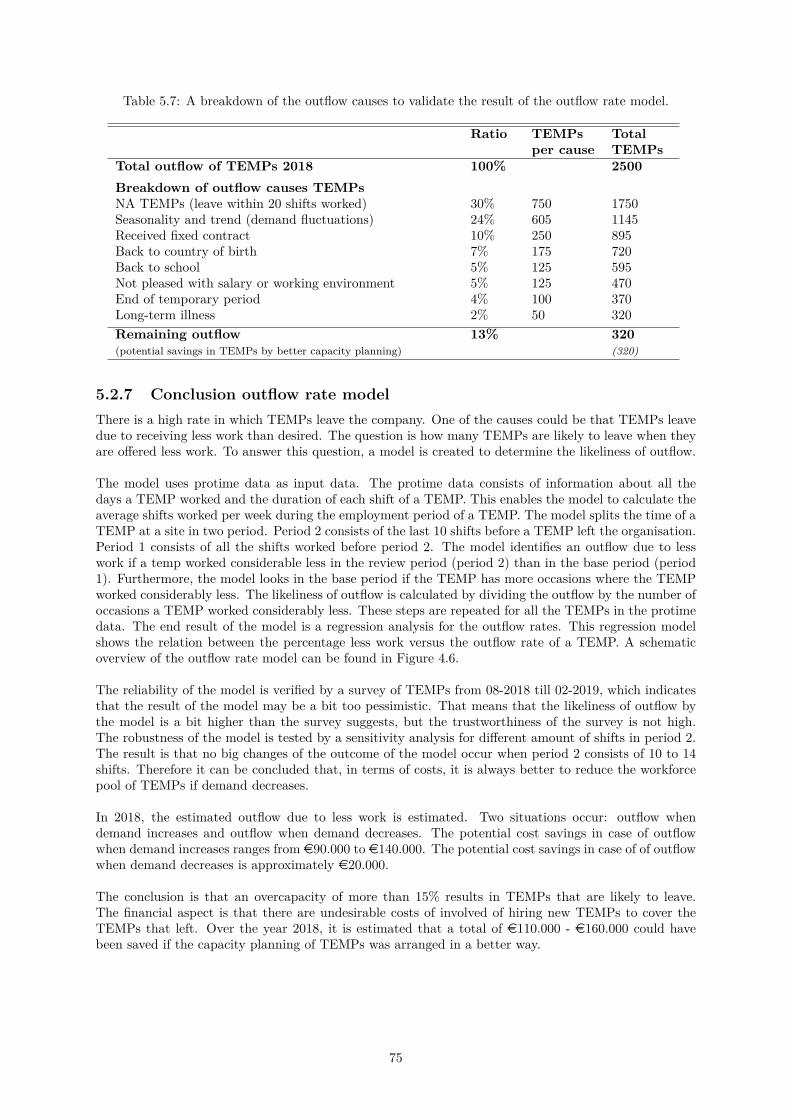
Table 5.7: A breakdown of the outflow causes to validate the result of the outflow rate model.

Ratio TEMPsper cause

TotalTEMPs

Total outflow of TEMPs 2018 100% 2500Breakdown of outflow causes TEMPsNA TEMPs (leave within 20 shifts worked) 30% 750 1750Seasonality and trend (demand fluctuations) 24% 605 1145Received fixed contract 10% 250 895Back to country of birth 7% 175 720Back to school 5% 125 595Not pleased with salary or working environment 5% 125 470End of temporary period 4% 100 370Long-term illness 2% 50 320Remaining outflow 13% 320(potential savings in TEMPs by better capacity planning) (320)

5.2.7 Conclusion outflow rate modelThere is a high rate in which TEMPs leave the company. One of the causes could be that TEMPs leavedue to receiving less work than desired. The question is how many TEMPs are likely to leave when theyare offered less work. To answer this question, a model is created to determine the likeliness of outflow.

The model uses protime data as input data. The protime data consists of information about all thedays a TEMP worked and the duration of each shift of a TEMP. This enables the model to calculate theaverage shifts worked per week during the employment period of a TEMP. The model splits the time of aTEMP at a site in two period. Period 2 consists of the last 10 shifts before a TEMP left the organisation.Period 1 consists of all the shifts worked before period 2. The model identifies an outflow due to lesswork if a temp worked considerable less in the review period (period 2) than in the base period (period1). Furthermore, the model looks in the base period if the TEMP has more occasions where the TEMPworked considerably less. The likeliness of outflow is calculated by dividing the outflow by the number ofoccasions a TEMP worked considerably less. These steps are repeated for all the TEMPs in the protimedata. The end result of the model is a regression analysis for the outflow rates. This regression modelshows the relation between the percentage less work versus the outflow rate of a TEMP. A schematicoverview of the outflow rate model can be found in Figure 4.6.

The reliability of the model is verified by a survey of TEMPs from 08-2018 till 02-2019, which indicatesthat the result of the model may be a bit too pessimistic. That means that the likeliness of outflow bythe model is a bit higher than the survey suggests, but the trustworthiness of the survey is not high.The robustness of the model is tested by a sensitivity analysis for different amount of shifts in period 2.The result is that no big changes of the outcome of the model occur when period 2 consists of 10 to 14shifts. Therefore it can be concluded that, in terms of costs, it is always better to reduce the workforcepool of TEMPs if demand decreases.

In 2018, the estimated outflow due to less work is estimated. Two situations occur: outflow whendemand increases and outflow when demand decreases. The potential cost savings in case of outflowwhen demand increases ranges from e90.000 to e140.000. The potential cost savings in case of of outflowwhen demand decreases is approximately e20.000.

The conclusion is that an overcapacity of more than 15% results in TEMPs that are likely to leave.The financial aspect is that there are undesirable costs of involved of hiring new TEMPs to cover theTEMPs that left. Over the year 2018, it is estimated that a total of e110.000 - e160.000 could havebeen saved if the capacity planning of TEMPs was arranged in a better way.

75

5.3 Improvement of the capacity planning strategy of TEMPsThe purpose of this thesis is to advice how the capacity planning of TEMPs can be improved using theresults of a quantitative analysis. This was previously identified as the main research question. The resultof the past chapters and models help to formulate an answer to that question. The strategy towards anoptimal resource capacity planning is described in this chapter. First an explanation of the perspectivefrom a TEMP towards the current pool capacity planning is given, than an advice is given how the poolof TEMPs should react to changes in demand. This is followed to what extent a forecast can help topredict the demand in case of the conditions that apply for the company. A future perspective of howthese advises could be merged into one solution based on software finalizes the content of this chapter.

5.3.1 Motivation of the behaviour of a TEMPThe first chapter identified that there is a large inflow and outflow of TEMPs. A large inflow of TEMPsmeans that a lot of costs are involved to train them. Chapter 2 gave the corresponding numbers andindicated that a cost saving of e160.000 to e240.000 may be feasible given an initial estimation.

It is assumed that the second most frequent reason why TEMPs leave is due to receiving less hoursthan they want to work 1. This assumption is supported by the following arguments why it is importantfor a TEMP to work their desired hours.

• Most employment agencies won’t give a guaranteed minimum of hours a TEMP can work.• The hourly wage is just above the minimum wage determined by law.• TEMPs receive their payment once a week. Most of them determine their budget based on their

earnings per week. So if they receive less money within a couple of consecutive weeks, they aremore likely to respond to that instead of determining a budget based on the earnings per month.

• A big part of the pool of TEMPs come from abroad. Their main purpose to work in the Netherlandsis to make money, which takes care of their family in their home country.

• TEMPs do not know the forecasts. In case of the start of a high season, the pool of TEMPs mustincrease in order to prepare a warehouse for a peak of the demand. At the beginning, the TEMPcannot work that much since the pool is too big. This is demotivating since a TEMP sees newpeople get training while he or she does not get the opportunity to work their desired amount ofhours.

5.3.2 How must a pool of TEMPs react on changes in demand?The size of the pool of TEMPs determines to a large extent the amount of hours a TEMP can work. Asmentioned in the previous part, it is very important for a TEMP to get the opportunity to work theirdesired amount of hours. From a business perspective, there is another important factor which is thecosts of the pool of TEMPs. Besides the fact that a TEMP must work from time to time in order tokeep their productivity level, a TEMP needs to be trained during the onboarding procedure which costsmoney. The question is how the pool of TEMPs should change when the demand changes based on aperspective from the TEMPs and a business perspective.

The business perspective wants to save money on training, so the priority is to reduce the numberof outflows since every outflow must be replaced by an inflow when the demand is constant. A TEMPwant to work their desired hours, since their expected weekly wage is leading. In order to combine bothperspectives, a MILP model could be used to calculate an optimal solution what to do in case thatdemand decreases in the upcoming period but increases in the period after that. Should you keep thecurrent pool of TEMPs to save training costs or should you scale down the pool of TEMPs to make surethat every TEMP can work their desired amount of hours. The outlines of a MILP model are describedin section 3.2.2, which indicates the variables, parameters and constraints in order to solve a hiring andfiring problem. One variable that is not included in that model is the amount of TEMPs that are likelyto leave the organisation, when a TEMP receives less work than desired.

The outcome of the latter one is very important, since it determines if a MILP model is needed tosolve the capacity planning problem to an optimum. If it happens that there is a smaller percentage of

1The primary reason why TEMPs leave is that TEMPs don’t successfully finish the trail period.

76

TEMPs that leave than the percentage of less work the TEMPs receive, a MILP model is needed. Inthis case, it is more cost efficient to keep a certain amount of TEMPs, since not all TEMPs will leaveif demand decreases. Therefore the threshold criteria can be formulated as: use a MILP model if theoutflow rate is lower than the percentage of less work a TEMP receives.

Consequently, a model is needed that determines the likeliness of outflow when a TEMP receives lesswork for a certain period of time. The model uses a data set consisting 12.500 TEMPs that workedbetween 2015 and 2019 for a certain period of time. The outflow rate is calculated by analyzing howmuch a TEMP usually works and how likely it is to leave every time that TEMP works less than usual.The most important outcome of the model is that the likeliness of outflow is higher than the percentageof less work a pool receives. It is estimated by the outflow rate model that the size of the pool of TEMPscan be at most 15% more than the actual needed amount of TEMPs, so the overcapacity rate is at most15%, otherwise more TEMPs will leave than desired and unnecessary training costs are applicable.

5.3.3 Forecasting demand

The next step is to identify the behavior of the demand in order to adjust the size of the pool of TEMPs.A forecast model can be used to predict demand for a certain warehouse per client. If this forecastmodel is accurate enough, the predicted amount of needed TEMPs can be calculated together with theproductivity rate of TEMPs.

First, section 3.1 explored the best forecasting methods by looking at forecasting competitions for timeseries data. This results in three methods where an additional method is proposed that may improvethe performance of those three methods. In addition to that, it may be useful to combine the averageresults of different forecasts to create a better forecast. The forecast model evaluates the performance of14 methods on 177 time series demand data. The methods that are likely to give different results whenthe forecast horizon increases and the methods that are likely to give different results when the forecastorigin changes are excluded from the set of forecasting methods. In the end five forecast methods arelikely to be robust enough, including two methods where the proposed improvement method is used.

The forecast model indicates the forecast accuracy per sector. The result is that the clients withinthe technology and retail sector have a three months ahead forecast error of respectively 8% and 9%.The clients within the healthcare and industrial sector have a forecast error of respectively 14% and 16%.The discussion is what forecast error is reasonable accurate enough such that the results of the outflowrate model can be used in order to improve the capacity planning strategy.

The outflow rate model advises that a overcapacity rate cannot exceed 15%, otherwise unnecessaryoutflow due to receiving less work occurs. This strategy towards the capacity planning is only applicableif a reasonable accurate forecast can be generated. A concrete maximum forecast error value can beapproximated by verifying a worse case scenario. If a site wants to ensure that there is always a sufficientamount of TEMPs available, a site determines the capacity of TEMPs on the forecast value plus themaximum forecast error. It can happen that it turn out that the actual demand is lower than the forecastindicated, in this case overcapacity happens. If the restriction is that the overcapacity is at most 15%,the maximum forecast error can be approximated by equation 5.3. The result is that the maximumforecast error, to ensure that the overcapacity rate does not exceed 15%, is equal to around 9%. Theassumptions are given below:

• The forecast predicts that 100 TEMPs are needed to fulfill demand. This is equal to the averagepoolsize of TEMPs at a site.

• A site wants to make sure that demand is met, so if the forecast error is equal to x than a siteincreases the capacity planning with half of forecast error. Any shortage of workforce can solvedwith overtime work, but for many cases there is enough workforce available. The capacity planningof TEMPs is equal to forecast ∗ 1

2 ∗ x.• A worse case scenario is calculate, that means that the actual demand is equal to the forecast

values minus the forecast error. The actual demand result in forecast - forecast * x.• The overcapacity is determined by capacity planning

actual demand , this must be equal to 115%.

77

Worse case scenario:(capacity planning)

(actual needed workforce) = 115%

(100 + 100 ∗ 12 ∗ x)

(100− 100 ∗ x) = 115% (5.3)

x = 9maximum forecast error = 9%

A higher forecast accuracy could be achieved by extensive data cleaning. All special promotions andevent must be removed from the data, but still the impact of future special promotions and events isunknown. Furthermore, this process will be labor intensive. Another approach is to include externalvariables in the forecasting model such as weather, social media and macro economic factors. Thisincreases the likelihood of overfitting the data, when using a forecast model based on statistical method.To overcome this problem, a forecast can be created based on a method that uses machine learning. Thehard criteria is that enough data must be available and it only works in case of many predictors. Asnoticed in section 3.1.4, a statistical model, which is based on time series data outperforms a forecastmodel that is based on a machine learning model.

5.3.4 Implementation of the proposed capacity planning strategyA site can track the current and predicts overcapacity levels via a software tool. This enable every layerof the warehouse organisation to understand the size of the optimal capacity of TEMPs for a certainperiod. The constraint is that there is enough confidence that the forecast model produces reliable resultsand that the forecast model is accurate enough. However, the accuracy of the forecast model presentedin this thesis is rather low, so there is definitely a discussion in what ways the forecast model should beimproved. In case a forecast model can predict the demand accurate enough, a software tool can convertthat forecast into the needed workforce along with additional variables and parameters. Examples ofwhat elements the software tool can include are written below:

1. Include the lead time to find and hire a TEMP.2. Define per site the percentage of TEMPs that do not succeed he trial period and include that

parameter.3. Include the increase in productivity during the first weeks since a TEMP started working.4. Include the productivity rate as a variable, in stead of a constant, since there are external factors

like the temperature inside the warehouse that influence the productivity rate.5. Incorporate the influence of an increase in hourly wage rate of competitors of CEVA on the TEMPs.

A software tool should provide the employees on a site with an advice how many TEMPs the current poolneeds to increase of decrease. Especially the warehouse supervisors will use this advice. The softwaretool creates one place where information about the capacity of the pool is visible. In addition to that,warehouse supervisors have insights to the workforce capacity of other department. Situations wherethere is a risk of under-staffing can be handled and situations where every department hires new TEMPsdue to a slight shortage will be prevented. In addition to that, a site will be able to indicate over a periodof a couple of months how many TEMPs they need towards the employment agencies. These employmentagencies can help to anticipate to a certain increase or decrease of the pool of TEMPs. Besides the factthat a software tool reduces costs, it makes sure a bigger group of TEMPs is more satisfied since theyreceive the amount of work they expect to receive.

78

6 | Conclusions and recommendations

This chapter starts by mentioning the problem solving approach. This is followed by the conclusionsabout the outflow rate model and the time series forecast model. The final conclusion advises how thestrategy towards the capacity planning of TEMPs can be improved. Since there is a set of advises,the recommendation section is added in order to provide the company with options to implement theinsights into practice. Besides the recommendations about how to implement the insights, also therecommendations about further research topics are mentioned. It could be the case that it might beinteresting to widen the scope at some points or verify some of the assumptions. First, the chapter startswith the conclusions.

6.1 ConclusionsThe motivation to explore various improvements regarding the capacity planning of TEMPs started withobserving a high inflow and outflow of TEMPs at all Dutch warehouses. Approximately around 50% ofthe warehouse blue collars are TEMPs, 50% of that work on a full-time base and 20% on a part-timebase. The rest of the TEMPs work on average less than 20 shifts in total, so they are employed for onlya short period of time. The problem that occurs can be described by the following reasoning. The inflowrate is a bit higher than the outflow rate of TEMPS, so ideally no outflow should be present. However,the outflow rate is rather high. Due to seasonality and a short-term employment preference of certainTEMPs, outflow cannot be avoided. In this case, there is a feeling that more outflow of TEMPs occursthan necessary. The question is what factors causes this high outflow rate and how can the high outflowrate be reduced.

The current outflow rate of TEMPs causes that 24% of the pool of TEMPs is renewed every month.Per year, this results in having 2.9 times a complete new pool. The costs that are involved with theinflow of a new TEMP is determined by the losses that occur during the onboarding and outboardingprocesses. Per TEMP the costs ranges between e800 and e1200, per year the total costs of outflow isestimated around e2.000.000 to e3.100.000. A TEMP flows out by the initiative of CEVA or on theirown initiative. A survey among 1300 TEMPs indicated that one of the most occurring reason for aTEMP to leave the organisation is that they receive less hours than desired, which is outflow on theirown initiative. It seems like a logical cause-effect relation, since TEMPs do not earn much. In additionto that, they are paid per week so they determine their budget on a weekly base. If a TEMP receives lesshours for a set of consecutive weeks, a TEMP is more likely to leave the organisation than a employeethat is paid per month. In order to verify this cause-effect relationship, the behavior of TEMPs whenreceiving less work than desired is analyzed. If needed, the capacity planning can change in general theamount of work a TEMP receives, therefore reducing the outflow rate.

The problem solving approach results in an advice how the capacity planning of TEMPs could beimproved, based on a quantitative analysis. This is the main research question of this thesis. The scopeof the research is limited to only use daily data generated by the TEMPs located in the Netherlands overa period between January 2015 till May 2019 and monthly aggregated data generated by the warehouseslocated in the Benelux over a period between May 2015 till May 2019.

The problem solving approach starts first by analyzing the relationship between receiving less workfor a TEMP and the likeliness of leaving the organisation. In case there is a relationship present, anadvice is formulated to what extent the pool of TEMPs should match the demand of needed workforce.This assumes that future demand is known, therefore the next step is to gain more insights to what

79

extent three month ahead demand can be predicted. The purpose is to verify if a reasonably accurateforecast can be generated with the current available data. The forecast uses only aggregated monthlytime series demand data about the warehouse activities such as the number of orderlines for differentclients. To conclude, the strategy towards the capacity planning of TEMPs is formulated by the resultsof two models. These models are listed below.

1. Outflow rate model: What is the likeliness that a TEMP leaves the organisation when theTEMP works less than desired.

2. Time series forecastmodel:

What is the best method or set of methods to perform a long-termforecast of a client using only monthly time series data and how accuratecan a long-term forecast be given a large set of time series data.

6.1.1 Outflow rate modelThis sections answers research question 2g: How can the result of the outflow rate model be incorporatedwithin the strategy towards capacity planning of TEMPs?

The outflow rate model uses protime data as input data. The protime data consists of informationabout all the days a TEMP worked and the duration of each shift of a TEMP. This enables the modelto calculate the average shifts worked per week during the employment period of a TEMP. The modelsplits the time of a TEMP at a site in two periods. Period 2, the review period, consists of the last 10shifts before a TEMP left the organisation. Period 1, the base period, consists of all the shifts workedbefore the review period. The model identifies an outflow due to less work if a temp worked considerableless in the review period than in the base period. Furthermore, the model looks in the base period ifthe TEMP has more occasions where the TEMP worked considerably less. The likeliness of outflow iscalculated by dividing the number of outflows by the number of occasions a TEMP worked considerablyless. The output of the outflow rate model is a set of observations between a estimated outflow rate anda certain rate of less worked before outflow. These observations are used as input for a linear regressionmodel to generalize the relation between the expected number of outflows for a give overcapacity rate.The overcapacity rate is the same as the rate a TEMP receives less work. The regression model is testedon robustness by experimenting with various number of shifts that determine the length of the reviewperiod. The exact formula of the regression line is: (Estimated outflow rate = 1.09 ∗ overcapacity)where (overcapacity > 15%). The minimum overcapacity rate is determined based on an estimationwhere receiving less work has an impact to likeliness of leaving the company. The conclusion is that theoutflow rate is always higher for a certain ratio of receiving less work, given a minimum receiving lesswork ratio of 15%. The interpretation of that is when for example there is an overcapacity of 20% for acertain month, so on average the pool receives 20% less work, it is expected that (1.09 ∗ 0.2 = 22%) ofthe TEMPs within that pool leaves within that month. The advice is that the capacity of TEMPs mustadapt to changes in the amount of needed workforce. The size of the pool may be up to 15% bigger thanthe actual amount of needed TEMPs 1.

For the year 2018, the cost savings are calculated if the pool of TEMPs did not cause outflows dueto receiving less work than desired. The total cost due to receiving less work ranges from e300.000 toe450.000, but this is not equal to costs that can be saved since a site needs to deal with uncertainty. Incase of an increase in demand, the assumption is that 50% of the costs due to receiving less work canbe saved by adjusting the capacity planning in time. In case of a decrease in demand, the number ofmore outflow than desired is equal to the potential cost savings. Altogether, if the pool of TEMPs wasadjusted on time to the demand, a potential cost saving of e110.000 - e160.000 could be realized.

6.1.2 Time series forecast modelThis sections answers research question 3g: Is the performance of the proposed forecasting model goodenough or is there a need to search for alternative methods to determine a forecast?

The previous model indicated how the capacity of TEMPs should change if demand changes. In order to1The actual amount of needed TEMPs is defined as amount of aggregated hours of TEMPs that is spend on the

warehouse operations multiplied by a factor 1.12 (12%) in order to deal with sickness and days off

80

know if the demand changes, a forecast model is made that predicts the demand for a set of warehouseactivities, like the number of orderlines, over a period of 3 months ahead. The model must be able togenerate a reasonable accurate long-term forecast using only time series data. The result of the modelmust deliver insights which methods deliver in general good results and how accurate a long-term timeseries forecast method(s) can predict demand for CEVA.

The literature about forecasting of time series data give many methods, most methods are build fora specific demand behaviour. Since the demand behaviour changes from time to time, this model needsa forecasting method that has in general a good performance. Unfortunately, many papers compare anew method with a set of predecessors, in stead of comparing a new method with a wide range of othermethods. The result of international forecasting competitions provides an answer to search for the bestforecasting method(s). The findings are written below:

1. Statistical learning models perform a better forecast than machine learning models when usingonly time series data.

2. A machine learning model needs at least a set of variables that has an explanatory value for changesin the demand data in order to outperform a statistical learning forecast model.

3. Three methods (ETS, ARIMA and Theta) had the best performance when forecasting on 100.000different time series data sets.

4. Using the average value of multiple forecast methods, thus creating combinations of methods, couldgenerate accurate forecasts.

About 177 monthly time series data are used as input for the model. Besides the three methods ETS,ARIMA and Theta, a fourth method is added that is expected to improve the performance of the otherthree methods. The ExtrP method tries to cope with a specific but frequently occurring situation forCEVA, where demand suddenly decreases after a high season. This sudden decreases happens somewhereafter Christmas, Cyber Monday or any event where consumer good are bought in advance. It is sometimesnot clear at what moment this decrease happens, so a seasonality factor of three mentioned forecastmethods may not adjust the demand correctly. The ExtrP method is a multiplicative parameter thatmust be used together with a single forecast of the ETS, ARIMA or Theta methods or with a combinationof those methods, the parameter intensifies a decrease in demand in order to improve the forecast.

A total of 14 methods and combinations of methods are evaluated by a test of overfitting (change intraining data length) and a sensitivity test (change in test data length). The result is that five methodsare likely to be robust enough. These five methods are implemented in the forecasting model, the resultsare written below.

1. The five robust methods or combination of methods are Theta, ARIMA, Theta-ExtrP, ETS-Thetaand ETS-ARIMA-ExtrP

2. The most used forecasting methods are Theta (35%) and ARIMA (25%)3. As mentioned in the literature, it is useful to combine different methods into a forecast since the

Theta-ExtrP, ETS-Theta and ETS-ARIMA-ExtrP outformed the single method forecasts togetherin 38% of the times.

4. The addition of the ExtrP method is rewarding, since it improved the result of the Theta model25% of the time. However, the ExtrP variable in combination with 5 of the 7 other methods resultsin a model that overfits the data and is too sensitive for multiple forecast horizons.

5. The activities with the lowest forecast error and that are representative as measure for the overalldemand in a warehouse are:

• Picking orderlines• Picking pallets• Shipping orderlines• Shipping orders

6. The forecast error (using the robust forecast methods, representative activities and a forecasthorizon of three months) ranges between 8% and 16%.

7. The sectors technology and retail have the highest forecast accuracy (8% MAPE) of all sectors.8. The forecast model does not improve the naive forecast for the clients within the healthcare sector,

so it seems like the healthcare sector does not have a distinctive demand behavior.9. The industrial sector has the highest forecast error (16%).10. The desired value of a reasonable accurate forecast, given a maximum overcapacity level of 15%,

is calculated in section 5.3.3 and equal to 9%.

81

6.1.3 Final conclusionsThis sections answers the main research question: How can the capacity planning of temporary workers atthe CEVA Logistics Benelux warehouses be improved by an estimation of the outflow rate and a predictionof demand?

Every month there are 24% of the current TEMPs that leave the company, so there is a outflow rate.This results in high costs of hiring new TEMPs and a lack of motivation among the pool of TEMPs.The yearly costs are estimated at a range from e2.000.000 to e3.100.000. The assumption is that on ofthe main reasons why TEMPs leave is because they don’t get the opportunity to work the amount ofhours that they desire, since the are very dependent of their weekly income.

The outflow rate can be reduced by determining the size of the pool of TEMPs, this is part of thecapacity planning. The capacity planning determines in general the amount of work the pool of TEMPsreceive. A model determined the relation between the reduction in work and the estimated outflow rate.The result is that unnecessary outflow due to less work can be prevented if a maximum overcapacitylevel of 15% on a monthly base is applied to the pool of TEMPs. The advice is that that the pool ofTEMPs must not be bigger than 115% of the actual amount of needed TEMPs.

In order to adjust the pool of TEMPs in time, an accurate prediction of demand is necessary. A literaturestudy determines the best methods to predict demand using only time series data. The result is thatthe clients within the technology and retail sector have an expected forecast error (MAPE) ranging from8% to 9%. The clients within the healthcare and industrial sector have an expected forecast error ofrespectively 14% and 16%. These forecasts are made with a forecast horizon of three months ahead. Acalculation in section 5.3.3 determined that a reasonably accurate forecast has a forecast error of 9%.

If the overcapacity of the pool of TEMPs was not bigger than the recommended 15% during the year2018, a possible cost saving ranging from e110.000 - e160.000 could be accomplished. The conditionis that the forecast error of a three months ahead forecast is not more than 9%, in order to the reducethe amount of uncertainty of the capacity planning. The forecast model indicated that in general theclients within the healthcare and industrial sector do not meet this condition. Therefore, the capacityplanning strategy might not be applicable for those clients. In addition to these points, it is desirablefrom a ethical perspective to reduce the amount of uncertainty a TEMP encounters if a TEMP wants toknow if he or she could work the amount shifts as desired. To conclude, the main research question canbe answered by the following sentence:

"The capacity planning of TEMPs can be improved by applying a new norm that an average monthlymaximum of 15% overcapacity is allowed for the pool of TEMPs, given that they work for a client

within the technology or retail sector or have a three months ahead forecast error of at most 9%. Theforecast model for the clients within the industrial and healthcare sectors need further research."

6.2 RecommendationsThis chapter summarizes the findings of this thesis as an advice towards the company. The advice consistsof suggestions how to implement the findings, provides the discussion points and lists further researchopportunities. As previously stated, the final conclusion of this thesis is that the capacity planning ofTEMPs can be improved by applying a new norm that the overcapacity level of TEMPs cannot exceed arate of 15% on an monthly base, given that the TEMPs work for a client within the technology or retailsector or have a forecast error less than 9%. First, the steps that needs to be taken in order to improvethe capacity planning by taking the overcapacity into account, are written below.

6.2.1 ImplementationThis sections answers research question 1c: How can the result of the capacity planning model and theforecasting model be implemented within the organisation?

As mentioned in the final conclusion, the capacity planing can be improved by having a maximumof 15% overcapacity of the pool of TEMPs. The 15% overcapacity figures as a rule of thumb, since theoutflow rate model estimates how many TEMPs are likely to leave when there is too much overcapacity.

82

The only way to use the rule of thumb properly, is that the overcapacity value must be made visible likea key performance indicator. There are three ways to implement this KPI. There is the basic option, byonly displaying the KPI on current dashboards. The second option, the premium option, is to incorporatethe KPI in a software tool that shows a prediction of the overcapacity value and advises how to react onthat certain KPI value. The last option, the pro option, consist of a software tool that solves a MILPmodel, as suggested in section 3.2.2, to near optimal. It is recommended to first have a pilot project forjust one site, this project represents a proof of concept. After a successful implementations, the scope ofthe project can be extended to more sites. These options are listed below.

Basic implementationThis KPI is relatively easy to explain, therefore there is a low threshold to implement the KPI at everysite. Warehouse supervisors can report the past overcapacity values and make an estimation of the futureovercapacity values by checking the current size of the pool of TEMPs and calculate the overcapacityusing the monthly forecasts. A dashboard will indicate the desired maximum KPI value (15%) and thecurrent KPI value. This enables the warehouse supervisors to proactively adapt the pool of TEMPs tochanges in demand.

Premium implementationA more advanced approach is to use software that reports to the warehouse supervisors the amount ofTEMPs that needs to be hired or excluded from the pool of TEMPs at a certain moment in time. Thissaves potentially a lot of time, since previously a warehouse supervisor has to calculate the predictedovercapacity value. A software tool can include more variables in order to have a better estimate of thefuture overcapacity value of the pool of TEMPs. Variables that can be included are summarized below:

• Incorporate the lead time of searching and hiring new TEMPs.• Take a lower productivity rate into account during the first 20 shifts of a new TEMP when

determining the current capacity of TEMPs.• Determine the capacity per warehouse competence, to create a risk pooling effect over all departments.• In case there is a group of TEMPs that are highly motivated and skilled, it is desirable to give

less work to other TEMPs when necessary. So the outflow rate model may not be applied to thewhole pool of TEMPs, but only the TEMPs that are not assigned to the group of good performingTEMPs.

Pro implementationThe most advanced implementation of the rule of thumb is to incorporate even more variables. Thedifference with the overview of variables of the previous section, is that variables can be included whichwere fixed parameters before. The solution space increases when more variables are incorporated, thesoftware tool must now might solve a MILP problem. The literature refers to this problem as an aggregateplanning problem, this topic is also part of the further research section since it has a high value whenimplemented. The variables that might be responsible for such an increase of the solution space, sowhich are used in case of an aggregate planning (MILP) problem are enumerated below.

• The ratio between fixed blue collars and TEMPs• The uncertainty of forecasts per demand of a client• The local unemployment rate• The influence of the hourly salary rate and the likeliness that a TEMP stays

Implementation considering the forecast accuracyThe rule of thumb of a maximum of 15% overcapacity can be used in practice as long as the forecasthas a reasonable accuracy. Otherwise, an inaccurate forecast results in an inaccurate estimation of theovercapacity. The forecast model indicated that the clients within the retail and technological sectorshave the lowest three months ahead forecast error of 8% to 9%. It is likely that the one and two monthsahead forecast error will be less than that. The clients within the other sectors might have a higherforecast error, but ideally the forecast accuracy must be determined per client in order to adjust thepool of TEMPs in time to the predicted demand. Another rule of thumb is that as long as the forecasterror does not exceed 9%, the maximum of 15% overcapacity of the pool of TEMPs rule can be used.Otherwise too much uncertainty is involved. In order to cope with that, some improvements of theforecast model are listed in section 6.2.3. The list below summarizes the recommendations.

• Implement as rule of thumb that the overcapacity of the pool of TEMPs cannot exceed the 15%.

83

• Create a new KPI that indicates the current overcapacity value and set the desired level to bewithin 15%.

• Give the task to the warehouse supervisors to predict the new overcapacity KPI value when theychange the pool size of TEMPs.

• An alternative is to outsource that task to software, which has the ability to include more variablesand is therefore better able to give a better estimation of the predicted overcapacity KPI value.The purpose is that the software advises the warehouse supervisors, they are still responsible forthe size of the pool of TEMPs.

• The forecast error per client must not exceed the 9%, otherwise too much uncertainty is involvedand the maximum of 15% overcapacity is not applicable.

6.2.2 DiscussionThe purpose of this section is to mention different points of views towards the assumptions and interpretationsof the two proposed models, since there might be some discussion if the two proposed models are 100%validated and verified. First, the section discusses the problem identification. Then the outflow ratemodel and time series forecasting model are discussed.

Problem identificationThe core problems are formulated based on observations made by the management and a first look tothe data. The following statements, that are used to formulate the core problem, can be discussed.

• A survey identified that receiving less work than desired is one of the main reasons why a highoutflow rate occurs. It could be the case that there are other reasons applicable, but the surveydoes not provide many more details reasons as an option.

• If a TEMP must leave by the company, it could be the case that the TEMP is not motivated toanswer the survey truthfully. The result of the survey might by not fully reliable.

• The initial estimate of the costs of the current outflow rate ranges from e2.000.000 to e3.100.000per year. These costs are based on the current outflow rate multiplied by the estimated costs toreplace a TEMP that leaves by a new TEMP. One part of the costs of hiring a new TEMPs isan estimation of the loss in productivity for the first couple of weeks in order to get familiar withthe warehouse operations. This estimated is made by warehouse supervisors and is not based onmeasurements.

Outflow rate modelThe discussion regarding the outflow rate model are based on how the model handles the data cleaningprocess and how the results are interpreted.

• The desired amount of work per week of a TEMP is based on what they worked on average beforeleaving the company. It could be the case that this does not correspond with the desired amountof work.

• Currently, the outflow rate is based on if a TEMP worked less during the review period (period2). It could also be the case that a certain pattern of periods, where a TEMP worked less thandesired, is one of the causes to leave the company. This is not included in the model.

• The assumption is that a TEMP is on a holiday if a TEMP didn’t work within 10 days. Thediscussion is that there are definitely TEMPs on a holiday for only one week, but those cases arehard to filter since it is also possible that a TEMP is not asked to work for a week.

• It is not filtered out of the input data if a TEMP wanted to work less instead of needed to workless. The outflow rate could be lower than actual since this event may be marked as a TEMPreceived less work but didn’t leave the company.

• Currently, the model assumes that the needed workforce per month is sufficient enough to deal withthe fluctuation on a weekly or daily base. This is not verified, since no daily or weekly demanddata is available for more than 1.5 years.

• The conclusion of the outflow rate model mentioned that an overcapacity rate of no more than15% of the pool of TEMPs is desired in order to reduce the outflow rate. The threshold of15% overcapacity is selected based on an objective interpretation of a figure, so there could be adiscussion that this percentage can differ within a small range.

Time series forecast modelThe discussion regarding the time series forecasting model is based on which data is selected and whichgeneralizations about the clients are made.

84

• The model uses only the time series data as reported. In case of special event such as the openingof a new store of a client is not included as a variable in this time series data. The accuracy of theforecast model would increase if such variables are known.

• The process how clients are categorized between the retail and technology sector is not straightforward.Most clients that produce electronic goods sell them via stores or e-commerce, therefore someclients that are categorized as a technology client could also be categorized as a retail client. Thedifferences with the industrial and healthcare sector are better distinguishable.

• The conclusion of the forecast model is that the clients within the industrial and healthcare sectorhave a low forecast accuracy. There are some clients within these sectors that have a very stabledemand. Therefore the generalization about the forecast accuracy is not applicable to every clientwithin that sector.

6.2.3 Further researchThere are assumptions that need further research, since they were out of scope for this thesis or simplifieddue to time restrictions. An overview of the assumptions and how the further research may look like isdescribed below. They are categorized per model, so one category is about the assumptions made for theoutflow rate model and the other is about the assumptions made for the time series forecasting model.

Outflow rate model:• The data cleaning process removed the dates of which a TEMP was potentially on a holiday. Right

now it is assumed that if a TEMP did not work for 10 consecutive days, the TEMP is on holiday.It could be that a TEMP went on a holiday for a shorter period of time or that one of the 10consecutive days involved a regular day off. In order to calculate the average amount of shiftsworked per week, it is useful to perform more research when and how long TEMPs were actuallyon a holiday or wanted days off.

• Right now, the outflow date is determined as the last day worked. Maybe a TEMP was availablefor a longer period of time, but did not get the opportunity to work. So it could be useful todocument the moment of outflow.

• The result of the model can be verified in a better way, if the opinion of the warehouse supervisorabout a TEMP is added to the survey when a TEMP leaves.

• The result of the model can be verified in a better way if there is a new survey with questionsspecified if they leave due to receiving less hours than desired.

• Due to a lack of temporary employees at some parts of The Netherlands, it could be interestingto include a cost-benefit analysis to pay TEMPs more if they receive less work otherwise they arelikely to leave the organisation .

• Due to a lack of temporary employees at some parts of The Netherlands, it could be interesting toinclude a cost-benefit analysis to determine if it is cost efficient to adjust the minimum requiredproductivity after 20 shifts. It may be cost efficient to not exclude a TEMP from the workforcepool when the TEMP has a lower productivity because there is already invested in the TEMP.

• The speed of the model is slow right now, it takes about 36 hours to run the full model. Optimizingthe run time will stimulate to perform more experiments, this increases the reliability of the model.

• The ratio between fixed blue collars and TEMPs is not a variable, since the company prefers tohave a fixed ratio. It could be interesting to include the fixed blue collars in the outflow rate modeland to make hire or fire decisions based on the whole workforce pool. This is called an aggregateworkforce planning in the literature. A model that incorporates the expected outflow rate togetherwith hire and fire decisions could result in potentially higher amount of savings.

Forecasting model• As mentioned before, the overall forecasting performance is reasonable for clients within two

sectors. The clients in the other sectors have a forecast error which is too high. If the forecastingperformance must increase, the following methods could be applied:

– Involve the client to make sure that they deliver an accurate demand forecast.– Use less aggregated data so use weeks in stead of months. This captures a weekly seasonality.

The three months ahead forecast uses a monthly and weekly seasonality, which is likely toincrease the forecast accuracy.

– More effort can be put in data cleaning, that means filter special events out of the time seriesdata. Special events are variables that for example determine if a new store of a client opened,

85

which product promotions a client applies for a certain period or if the site did effort to smoothout demand over a certain period in the past.

– External variables that are likely to influence the demand can be integrated. Examples ofexternal variables are: macro-economical, weather or social media influences.

– If lots of detailed demand data is available with more than 10.000 observations and consistsof a set of multiple variables, a machine learning model might be useful to increase forecastaccuracy.

• When expanding the scope to CEVA global, the amount of available data increases. There arecurrently around 4.000 clients within 11 sectors. The performance of the methods of the forecastingmodel can be verified on more data, thus making the result of the forecasting model more reliable.

• Determine the potential cost savings of a forecast model with a certain accuracy, in order to createa business case. The purpose of the business case is to verify if purchasing forecasting softwaresaves costs within a reasonable amount of time.

86

Glossary

AIC Akaike Information Criterion. 26

ARIMA Auto Regressive Integrated Moving Average. 25

BIB Benelux Innovation Board. 2

ETS A set of exponential smoothing models that includes an error, trend and seasonal component.. 24

ExtrP Extra Parameter, it is a multiplicative parameter that adjusts a forecast to some distinct demandbehaviour.. 45

GDPR General Data Protection Regulation. 11, 39

KPI Key Performance Indicator. 83

LDA Linear Discriminant Analysis. 35

MAPE Mean Absolute Percentage Error. 28, 43

MASE Mean Absolute Scaled Error. 28, 43

MILP Mixed Integer Linear Programming. 20, 30

NA TEMP Not Available TEMPs, TEMPs who worked less than 20 shifts in total.. 13

R R is a software tool and programming language for statistical and data analysis purposes.. 7

Residual Sum of Squares Error measure of linear regression model fit. 34, 35

TEMP temporary employee. 3, 10, 19

WMS Warehouse Management System. 11, 42

87

Bibliography

[1] Erwin W Hans, Willy Herroelen, Roel Leus, and Gerhard Wullink. A hierarchical approach tomulti-project planning under uncertainty. Omega, 35(5):563–577, 2007.

[2] Rob J Hyndman, Andrey V Kostenko, et al. Minimum sample size requirements for seasonalforecasting models. Foresight, 6(Spring):12–15, 2007.

[3] Spyros Makridakis, Evangelos Spiliotis, and Vassilios Assimakopoulos. Statistical and machinelearning forecasting methods: Concerns and ways forward. PloS one, 13(3):e0194889, 2018.

[4] Sven F Crone, Michele Hibon, and Konstantinos Nikolopoulos. Advances in forecasting with neuralnetworks? empirical evidence from the nn3 competition on time series prediction. InternationalJournal of forecasting, 27(3):635–660, 2011.

[5] Henry Canitz. Three checklists to build a successful supply chain analytics foundation.,2018. URL https://www.supplychain247.com/article/better_supply_chain_decisions_with_advanced_analytics.

[6] Han Hu, Yonggang Wen, Tat-Seng Chua, and Xuelong Li. Toward scalable systems for big dataanalytics: A technology tutorial. IEEE access, 2:652–687, 2014.

[7] David A Goodman. A goal programming approach to aggregate planning of production and workforce. Management Science, 20(12):1569–1575, 1974.

[8] Johannes MG Heerkens and Arnold Van Winden. Geen probleem, een aanpak voor allebedrijfskundige vragen en mysteries. Business School Nederland, 2012.

[9] George EP Box, Gwilym M Jenkins, Gregory C Reinsel, and Greta M Ljung. Time series analysis:forecasting and control. John Wiley & Sons, 2015.

[10] Rob J Hyndman and George Athanasopoulos. Forecasting: principles and practice. OTexts, 2018.

[11] Peter J Brockwell, Richard A Davis, and Matthew V Calder. Introduction to time series andforecasting, volume 2. Springer, 2002.

[12] Robin M Hogarth and Spyros Makridakis. Forecasting and planning: An evaluation. Managementscience, 27(2):115–138, 1981.

[13] Bradley Efron. Bootstrap methods: another look at the jackknife. In Breakthroughs in statistics,pages 569–593. Springer, 1979.

[14] Thomas Diciccio and Bradley Efron. More accurate confidence intervals in exponential families.Biometrika, 79(2):231–245, 1992.

[15] Rob J. Hyndman and Anne B. Koehler. Another look at measures of forecast accuracy.International Journal of Forecasting, 22(4):679 – 688, 2006. ISSN 0169-2070. doi: https://doi.org/10.1016/j.ijforecast.2006.03.001. URL http://www.sciencedirect.com/science/article/pii/S0169207006000239.

[16] Rob Hyndman, Anne B Koehler, J Keith Ord, and Ralph D Snyder. Forecasting with exponentialsmoothing: the state space approach. Springer Science & Business Media, 2008.

[17] Sangarshanan. Time series forecasting - arima models, Oct 2018. URL https://towardsdatascience.com/time-series-forecasting-arima-model.

88

[18] V Assimakopoulos and Konstantinos Nikolopoulos. The theta model: a decomposition approach toforecasting. International journal of forecasting, 16(4):521–530, 2000.

[19] J Scott Armstrong and Fred Collopy. Error measures for generalizing about forecasting methods:Empirical comparisons. International journal of forecasting, 8(1):69–80, 1992.

[20] Charles D Coleman and David A Swanson. On mape-r as a measure of estimation and forecastaccuracy. In Annual meeting of the Southern Demographic Association, Hilton Head Island, SouthCarolina, 2004.

[21] Spyros Makridakis, A Andersen, Robert Carbone, Robert Fildes, Michele Hibon, RudolfLewandowski, Joseph Newton, Emanuel Parzen, and Robert Winkler. The accuracy of extrapolation(time series) methods: Results of a forecasting competition. Journal of forecasting, 1(2):111–153,1982.

[22] Spyros Makridakis, Chris Chatfield, Michele Hibon, Michael Lawrence, Terence Mills, Keith Ord,and LeRoy F Simmons. The m2-competition: A real-time judgmentally based forecasting study.International Journal of Forecasting, 9(1):5–22, 1993.

[23] Spyros Makridakis and Michele Hibon. The m3-competition: results, conclusions and implications.International journal of forecasting, 16(4):451–476, 2000.

[24] Spyros Makridakis, Evangelos Spiliotis, and Vassilios Assimakopoulos. The m4 competition: Results,findings, conclusion and way forward. International Journal of Forecasting, 34(4):802–808, 2018.

[25] Tao Hong, Pierre Pinson, and Shu Fan. Global energy forecasting competition 2012, 2014.

[26] Steven Nahmias and Tava Lennon Olsen. Production and operations analysis. Waveland Press,2015.

[27] Arnoud Cyriel Leo DE MEYER, Christoph H Loch, and Michael T Pich. Managing projectuncertainty: from variation to chaos. MIT Sloan Management Review, 43(2):60, 2002.

[28] Edward A Silver, David F Pyke, and Douglas J Thomas. Inventory and production management insupply chains. CRC Press, 2017.

[29] Doug Laney. 3d data management: Controlling data volume, velocity and variety. META group(Gartner) research note, 6(70):1, 2001.

[30] James Manyika, Michael Chui, Brad Brown, Jacques Bughin, Richard Dobbs, Charles Roxburgh,and Angela H Byers. Big data: The next frontier for innovation, competition, and productivity.Mckinsey Global Institute, 2011.

[31] Gareth James, Daniela Witten, Trevor Hastie, and Robert Tibshirani. An introduction to statisticallearning, volume 112. Springer, 2013.

[32] Leonard J Tashman. Out-of-sample tests of forecasting accuracy: an analysis and review.International journal of forecasting, 16(4):437–450, 2000.

89

A | Pseudo-code

Algorithm 6 Pseudocode - Forecasting model1: Input: Time series data2: Output: Per time series data, the best forecast method and MAPE value3: Variable: Forecast horizon (default value = 3)4:5: Load time series data6: for all series ∈ time series data do7: if (Series has more than 24 observation) AND (no zero demand) then8: Continue with this series9: else10: Skip current iteration of loop and go to next series11: end if12:13: Create training set of the time series minus the last observations of the forecast horizon14: Create test set of the observations of the forecast horizon15:16: if (1st quantile - 3*diff) ≥ observation ≥ (3e quantile + 3*diff) then17: (the diff is defined as the difference between the 1st and 3e quantile)18: Create linear regression model for train set data19: Replace observation by value of linear regression model20: Delete the outlier in train set21: end if22:23: for all ExtrPParameter ∈ (1,0.96) do24: Compute ETS forecast25: Compute ARIMA forecast26: Compute Theta forecast27: Create all possible combinations (7 in total, a combination is the average forecast value of multiple

forecasts)28: if forecast value goes down then29: Multiply forecast with ExtrPParameter30: end if31: Merge the forecasts in one table32: end for33:34: Calculate the MASE35: Calculate the MAPE36: if Forecast MASE ≥ 10% forecast lowest MASE then37: Delete forecast38: end if39: Arrange the forecasts on descending MAPE value40: Select the forecast with the lowest MAPE value.41: end for42:43: Return: The method of the best forecast, the MAPE value and the sector of the time series.

90

B | Additional tables

Table B.1: The MAPE values for a one month and three month ahead forecast per sector, using therobust forecast methods.

Sector Forecast error (MAPE) for different horizons1 month 3 months

Retail 6.3% 8.9%Technology 7.0% 8.4%Industrial 8.3% 16.2%Healthcare 18.1% 14.1%

Table B.2: The inflow and outflow rates of TEMPs for nine sites during 05-2018 till 05-2019

Site Inflow(monthlyin TEMPs)

Outflow(monthlyin TEMPs)

Ratio of poolrefreshed permonth

Poolrefreshedper year

Born 12 9 23% 2.8Born 2 4 5 21% 2.5Den Haag 16 15 22% 2.6Eindhoven 25 25 21% 2.5Maarssen 8 8 16% 2.0Roosendaal 65 55 26% 3.1Venray 1 25 28 22% 2.7Venray 2 44 50 26% 3.1Venray 3 16 18 28% 3.4Average of all sites 23.9 23.7 24% 2.9

91

C | Additional figures

Figure C.1: An example of different productivity rates per sites.

Figure C.2: The costs of the estimated number of outflows due to less work for maximum overcapacitylevel of 10% within the year 2018.

92

Figure C.3: An overview of the most important sections (1/3) of the outflow rate model, expressed in Rscript.

93

Figure C.4: An overview of the most important sections (2/3) of the outflow rate model, expressed in Rscript.

94

Figure C.5: An overview of the most important sections (3/3) of the outflow rate model, expressed in Rscript.

95