thesis_C_Nshemereirwe.pdf - University of Twente Research ...

The Relationship Between Pre-University Schooling and University Grades in Uganda

Connie V. Nshemereirwe

Thesis committee members:

Chairperson/Secretary: Prof. Dr. Ir. A.J. Mouthaan

PhD supervisor: Prof. Dr. C.A.W. Glas

Members: Prof. Dr. J. Scheerens

Prof. A. J. Visscher

Prof. Dr. W.A.J.M. Kuiper

Prof. Dr. R.R. Meijer

Prof. Dr. J.M. Voogt

The work described in this thesis was performed at the department of Research Methodology, Measurement and Data Analysis, Institute for Innovation and Governance Studies at the Faculty of Behavioural, Management & Social Sciences , University of Twente, P.O. Box 217, 7500 AE Enschede, The Netherlands

Nshemereirwe, Connie Vivien

The Relationship Between Pre University Schooling and University Grades in Uganda

PhD Thesis University of Twente, Enschede

ISBN: 978-90-365-3738-4

Doi: 10.3990/1.9789036537384

Printed by Ipskamp Drukkers, Enschede

Copyright © 2014 C.V. Nshemereirwe. All rights reserved

THE RELATIONSHIP BETWEEN PRE-UNIVERSITY SCHOOLING AND UNIVERSITY

GRADES IN UGANDA

DISSERTATION

to obtain

the degree of doctor at the University of Twente,

on the authority of the rector magnificus,

prof.dr. H. Brinksma,

on account of the decision of the graduation committee,

to be publicly defended

on Thursday the 20th of November 2014 at 16:45

by

Connie Vivien Nshemereirwe

Born on September 18, 1974

in Nairobi, Kenya

This dissertation has been approved by the promotor:

Prof. Dr. C.A.W. Glas

He who opens a school door closes a prison Victor Hugo

Acknowledgements

They say it takes a village to raise a child, but in my case it took two villages. I owe a tremendous debt of gratitude to both my Ugandan and Dutch villages

My first thanks go to all my colleagues in the department of Research Methodology, Measurement and Data Analysis at the University of Twente, who over the last four years have patiently and tirelessly entertained every last one of my endless questions and requests for help. First and foremost, my thanks go to my supervisor, Prof. Cees Glas, who generously guided me to my own vision of the work, and who taught me so much about the process of educational measurement. For help with various conceptual and methodological issues Jean-Paul and Stephanie were always graciously helpful, and for help with data analysis Wim and Muirne kept their doors open and always had some time to assist me. That said, my first port of call for every inconsequential and consequential issue was Hanneke, who was down the hall ready to listen attentively and smilingly offer a word of encouragement. And for all the other problems under the sun one could always count on Lorette to simply wave them on their way, although straightening out the mess I made with the layout out of my thesis gave even her a run for her money! My special thanks go to Inga who took hours out of her evenings and weekends to proofread my entire thesis, and spent yet more hours helping me design the cover – my heartfelt thanks! I would also like to thank Josine who, apart from invaluable advice on the research, is singlehandedly responsible for kick-starting my social and extra-curricular life in Enschede by introducing me to Twente Toastmasters, PNUT, couchsurfing and body pump! You continue to be an inspiration.

In addition to colleagues, I have been fortunate to meet and get to know some incredible people. The Toastmasters are always a heap of fun and have been responsible for some memorable evenings. In particular my mentor Huub who was always gently looking out for my growth as a speaker and leader. Ines, our immediate past club president also modelled what it was to be a true Toastmaster: enthusiastic, curious and bold. I am also extremely grateful for her help planning all the extra stuff around my defence. I was also especially glad to meet Marcel, a fun guy who was always up for a drink and sparked a love for board and card games. Not to mention opening his home for my family to stay during my defence. Vens, who even living across the country, proved himself a true and loyal and particularly wise friend. And then of course my girls Annika, Ebtesam, Maya and Laura – life would have been perfectly dull without you. Finally my incredibly kind landlord Hans – going above and beyond to make my stay comfortable – making me eggless sweet treats and encouraging my love of baking by declaring everything lekker even when we both knew otherwise! Most of all thanks for opening his home to my friends and family to stay as long as they liked during my defence – I will never forget your kindness. I also have to thank Frances who offered her place for me to stay in the first days of my arrival – your kindness is greatly appreciated.

In Uganda, I was constantly amazed by the willingness and openness with which everyone greeted my research. It is near impossible for me to mention all the people who helped me along the way but two stand out. First is a young man in the registry department of Makerere university, Tom Mukasa, whose work ethic was truly admirable. He provided the steam that propelled the whole research forward and I can’t thank him enough. The second is Mr Dan Odongo, the head of the Secondary Education Department at the Uganda National Examinations Board (UNEB). He and his colleagues facilitated all my requests to the fullest, and showed themselves to be true men and women of science and integrity. Without the UNEB data this research would have been a completely different animal. In addition to that was all the Deputy Vice Chancellors in charge of Academic Affairs at all the universities that participated in the research, the Registrars, the Deans and Heads of Departments, the administrators and the students – my work was made very light by their cooperation and I feel deeply grateful to them. Finally, but certainly not least, is my colleagues at the Uganda Martyrs University – being part of you has been a rich and rewarding experience and I look forward to many more years of collegiality. I would like to particularly thank my colleagues in the Faculty of the Built Environment whose support and understanding have been invaluable. For my research assistants Achilles, Arthur, Conrad and Grace, and special thanks to Alex, Moreen, and Arnold who all took time out of their busy schedules to work on various iterations of the thesis cover.

Turning to my Ugandan friends and family, I find that mere words are insufficient to express myself. I am the most fortunate human on earth to have had your love and support and encouragement and advice and acceptance and – you name it – all my life. To my friend of twenty years, Jackie: your unwavering and unconditional acceptance and loyalty to me and my family does not cease to amaze me – you are truly one of a kind. To my sister and friend, Keshubi, with whom we have spent uncountable hours on Skype and in person pondering questions big and small – long may we continue. I would also like to thank a very special companion to me in the last year of my PhD studies: Anne Gert – my journey with you has been one of growth and self-discovery, and your unwavering and generous support have been invaluable. I thank you from the bottom of my heart.

And finally to my aunts and uncles and cousins and in-laws and nephews and nieces and general extended family, but most especially to you Mom, Dad, Norman, Julian and Moreen – I could not have asked for a better family. I hope you all know how much I love and treasure each one of you. You are a great inspiration, joy and comfort.

Connie V. Nshemereirwe Enschede, November 2014

TABLE OF CONTENTS

INTRODUCTION 1

CHAPTER 1 5

CHARACTERISING UNIVERSITY STUDENTS IN UGANDA 5

1.0 Introduction 5

1.1 The Ugandan pre-university education system 6

1.3 Characterizing university students – A preliminary study 18

1.4 Discussion and conclusion 27

CHAPTER 2 29

VARIATION IN ENTRY SCORES AT UNIVERSITIES IN UGANDA: A MULTILEVEL ANALYSIS 29

2.0 Introduction 29

2.1 Education in Uganda 30

2.2 Methodology 35

2.3 The data 38

2.4 Results 39

2.5 Discussion 52

2.6 Limitations of the study 53

CHAPTER 3 55

ESTIMATING THE DIFFICULTY OF A’LEVEL EXAMINATION SUBJECTS IN UGANDA 55

INTRODUCTION 56 3.0

A’Level subject choice and selection to university 56 3.1

The concept of subject difficulty 61 3.2

A methodology for estimating subject difficulty 64 3.3

IRT modelling of subject difficulty in the Uganda national A’Level examinations 72 3.4

IRT modelling of subject difficulty using registry and self-reported data 81 3.5

Discussion and conclusion 90 3.6

CHAPTER 4 91

EVALUATING THE FEASIBILITY OF USING SELF-REPORTS IN INVESTIGATING THE PREDICTIVE VALIDITY OF UNIVERSITY ENTRY GRADES IN UGANDA 91

Introduction 91 4.0

Reliability of self-reports 92 4.1

Determinants of success at university 93 4.2

Developing the instrument 98 4.3

Evaluating the credibility of self reports: A pilot study 101 4.4

Implications for using self-reports in the proposed study 111 4.5

Conclusion 113 4.6

CHAPTER 5: 115

MODELLING THE EFFECTS OF SES, ENTRY A’LEVEL PERFORMANCE AND PREVIOUS SCHOOLING ON UNIVERSITY CGPA 115

5.0 Introduction 115

5.1 A framework for investigaTing the prediction of CGPA by A’Level performance 116

5.2 The structural equation model 122

5.3 Sample characteristics and measured variables 124

5.4 Results of structural equation modelling 135

5.4.1 Measurement model 136

5.4.2 Structural model 139

5.5 Discussion and conclusion 148

5.6 Limitations of the study 149

REFERENCES 151

APPENDICES 159

SAMENVATTING 203

1

INTRODUCTION Universities are concerned with selecting students with the highest potential for successfully pursuing university education. For universities in Uganda, this potential is, apparently, sufficiently indicated by student performance in the national examinations at the end of the advanced level (A’Level) of secondary school. However, performance trends at A’Level indicate that there is a wide variation in performance between the different subjects offered at A’Level, as well as between different schools. Further, since the national examinations represent such high stakes, there are reports of a heavy emphasis on teaching and learning strategies aimed at maximising pass rates, which is further accompanied by a tendency to choose the A’Level subjects that consistently exhibit high pass rates. Since university selection depends almost solely on scores in the A’Level national examinations, it was of interest to investigate the extent to which these university entry scores predicted university grades after taking account of the various school and student level factors present in the pre-university schooling system. The main student level variables included in the study were student age and socioeconomic status (SES), while school level variables concerned ownership (public vs. private), gender balance (single-sex vs. coeducational), whether or not schools provided boarding facilities, and finally whether or not they run the Universal Secondary Education programme (USE). The USE is a government funded programme that provides tuition-free education to students, and can be accessed at selected public and private secondary schools.

The majority of university students in Uganda is enrolled at the country’s 5 public universities, with the largest public university accounting for about 30% of university enrolments nationwide. In the last 20 years, more than 30 private universities have also been established but these boast much lower enrolments, only accounting for 15% of total university enrolment (National Council for Higher Education, NCHE, 2013). Selection requirements at public and private universities are similar, but while selection into private universities is carried out at university level, selection into public universities is carried out jointly by a central body at the ministry of education. This is partly to facilitate the award of about 3,000 merit-based state sponsored scholarships which are only available to students enrolled at public universities. The availability of state scholarships at public universities has made entry highly competitive. Further, since the majority of prospective university students would like to be considered for these scholarships, the entry requirements for the academic programmes at public universities heavily influence subject choice at A’Level.

The subject requirements and associated weighting for admission into the various academic programmes offered at public universities are published every year before students sit their A’Level examinations. Table 1 shows the entry requirements for some of the more selective and some of the less selective academic programmes offered at

Introduction

2

public universities. As can be seen, the more selective programmes like Telecom Engineering and Human Medicine have specific subject requirements, while programmes like Development Studies and Law have none at all.

TABLE 1: ENTRY REQUIREMENTS FOR SELECTED DEGREE PROGRAMMES AT PUBLIC UNIVERSITIESa

Programme Essential Subjects

(Receives a weighting of three)

Relevant Subjects

(Receives a weighting of two)

Bachelor of Science in Telecom Engineering Maths, Physics One better done of Economics,

Chemistry

M.B.C.H.B (Human Medicine) Biology One better done of Chemistry,

Maths, Physics

Bachelor of Information Technology (BIT)

Two best done of Mathematics, Economics Physics, Biology, Chemistry, Literature, Geography, Entrepreneurship, Technical Drawing, Fine Art

One better done of the remaining A’Level subjects

Bachelor of Business Administration

Economics and one better done of the remaining A’Level Subjects

Next better done of the remaining A’Level Subjects

Bachelor of Development Studies Two best done of all A ’Level Subjects Third best done of all A’ Level

Subjects

Bachelor of Lawsb Two best done of all A ’Level Subjects Third best done of all A’ Level Subjects

a information valid for entry 2012/2013 b additional pre-entry examination required from 2012 onwards

More than 70% of all university students are enrolled in the humanities and social sciences, and in most cases these academic programmes make no distinction at selection between entry A’Level grades obtained in subjects which are generally poorly performed (and potentially more difficult, such as sciences), and those in subjects that are usually better performed. This may be partly responsible for the observed tendency for students to choose the Humanities and Social Science subjects at A’Level which, since they tend to have the highest pass rates, offer the best chances of being selected for university. On the other hand, the country faces a shortage of qualified science teachers, and in addition many schools also lack the proper facilities to teach science; this may partly explain why sciences are chosen less and also why they exhibit lower pass rates.

Given the high emphasis on passing examinations in the pre-university system and the possibility of an inflation effect on student scores in the national examinations, to what extent do A’Level grades really represent variability in cognitive ability? This question was addressed by setting up a study to compare the entry A’Level grades to a cognitive outcome at university, say cumulative grade point average (CGPA), while at the same time allowing for the effects of student background characteristics and pre-university schooling. This PhD thesis reports this study, and the guiding research questions and study design are presented hereafter.

Introduction

3

THE RESEARCH PROBLEM

The guiding question for the research reported here was the following:

Allowing for the effects of student SES and pre-university schooling, to what extent do A’Level grades predict university CGPA?

This question was broken down into three sub-questions:

1. To what extent do school level variables explain A’Level and University entry grades?

2. What is the difference in difficulty for subjects examined at A’Level? 3. Allowing for A’Level subject difficulty, student SES and the effect of a student’s

former school, to what extent do A’Level grades predict university CGPA? The hypothesised relationships under investigation are represented by Figure 1.

Figure 1: Investigating the effects of students’ pre-university schooling, SES and A’Level

grades on university CGPA.

STUDY DESIGN

In order to tackle these questions, the research was carried out in four stages:

a) A preliminary study to characterise university students with regard to their former A’Level schools, A’Level subject choice and A’Level performance;

b) A multilevel analysis to determine some of the student and school-level factors that account for variation in student A’Level grades;

c) An estimation of relative A’Level subject difficulty using item response theory (IRT);

d) Employing structural equation modelling (SEM) to estimate the extent to which A’Level scores predict university CGPA, given student SES and pre-university schooling effects.

UNIVERSITY CGPA

PRE-UNIVERSITY SCHOOLING

STUDENT SES

A-LEVEL GRADES

Introduction

4

ORGANISATION OF THESIS

The organisation of the thesis roughly follows the four elements of the study design. First, a characterisation of university students in Uganda is presented in chapter one, then the estimation of school effects in A’Level performance is presented in chapter two. Chapter three presents the results of estimating A’Level subject difficulty for purposes of scaling the subjects ahead of a proposed study to estimate the relationship between A’Level grades and university CGPA. Chapter four describes a pilot of the proposed study designed to investigate the feasibility of using self-reported scores, and the full scale study is reported in chapter five.

5

CHAPTER 1 CHARACTERISING UNIVERSITY STUDENTS IN UGANDA Abstract

The organization and characteristics of the Ugandan pre-university and university education system are presented in this chapter. In particular, the characteristics of students enrolled at public and private universities are investigated. This was achieved by analysing the admissions data for three of the most commonly pursued academic programmes at each of eight public and private universities in Uganda: Bachelor of Business Administration, Bachelor of Information Technology and Bachelor of Development Studies. About 14,000 university students were involved in this analysis, and the majority was found to have chosen Humanities subjects at A’Level. Further, about 50% of the students had attended just 10% of schools represented in the sample (i.e., 91 schools); of this 10%, one-fifth had attended just six schools. Mean entry grades at public universities were also found to be almost one and half grades higher than mean entry grades at private universities. Among the students at public universities, those enrolled under government sponsorship had the highest mean entry grades, although the mean entry grades of the fee-paying students were only one-tenth of a grade lower.

Keywords: Uganda, Pre-university education, University students

1.0 INTRODUCTION

The Ugandan pre-university and university systems have undergone a number of changes since the mid-1990s. With the youngest population in the world, emphasis has increasingly been placed on widening access to primary and secondary education. This has been done by implementing programmes to enable all children of school going age to access tuition-free education at primary school, and a selected number at secondary school. This has driven the growth in the university education sector as well, but the education system as a whole has not been able to adequately meet the schooling needs of the population, either in quantity or in quality. Pupil-teacher ratios are still among the highest in Sub-Saharan Africa (SSA), and even though the country is close to achieving 100% access to the first year of primary school, completion and transition rates are still low. Further, the system is still marked by high drop-out and repetition rates (Ministry of Education and Sports, MoES, 2013). In addition to this, national and regional assessments of educational achievement reveal that students in primary and lower secondary school still perform at levels below the desired minimum (Byamuisha & Ssenabulya, 2005, Uganda National Examinations Board, UNEB, 2011a, UNEB 2011b).

Chapter 1

6

The pre-university education system is divided into three parts: primary school, lower secondary and upper secondary school. Students sit centrally developed national examinations at the end of each stage, and these play a large part in determining their progress. The aim of this chapter is to provide an overview of the pre-university and university systems, and then focus further on investigating the characteristics of the students who do make it to university. Of particular interest were the schools that these university students attended at A’Level, the subjects they chose, and the differences between those who are enrolled at public universities and those at private universities.

1.1 THE UGANDAN PRE-UNIVERSITY EDUCATION SYSTEM

Uganda is a landlocked country in East Africa and had an estimated population of 37 million in 2014. 85% of this population is rural and depends mostly on small scale farming for their livelihood. The latest figures on literacy put it at 79% for men and 66% for women on average, and 88% for the urban as opposed to 69% of the rural population (Uganda Bureau of Statistics, UBOS, 2012). The majority of the working population is engaged in Agriculture (66%), although this only contributes about 22% to the national GDP. Almost half of the country’s GDP is provided by the service industry, which employs 28% of the population; the remaining 6% of the population is engaged in the manufacturing sector (UBOS, 2012).

Organisation of Education

Uganda follows a 7+4+2 pre-university education system: seven years of primary school, four years of lower or ordinary secondary school (O’Level) and two years of upper or advanced secondary school (A’Level). This is presented graphically in Figure 1.1.

The majority of children in Uganda first encounter formal schooling at the start of primary school. In 2011, there were only about 215,000 children enrolled in pre-primary school compared to 1.8 million enrolled in the first year of primary school (MoES, 2011) In order to advance from one education level to the next, students must sit and pass a national examination, the results of which determine their progress through the system. At the end of primary school, students sit examinations in a total of four subjects: Science, Mathematics, English language and Social Studies. At the end of O’Level students take between 9 and 10 subjects, and may sit the national examinations in a minimum of eight. Five of the eight subjects are compulsory: Mathematics, English, Physics, Chemistry and Biology. Upon entry to A’Level, students may choose only three subjects in which to sit examinations (until 2012 they could choose up to four subjects). It is common for students to choose a combination of Humanities subjects or a combination of Science subjects. Although some students choose combinations containing both Humanities and Sciences, timetabling challenges in arranging the classes as well as the examinations restrict the range of possible combinations. On the whole, science subjects are the most poorly performed subjects at all levels of the

Characterising University Students in Uganda

7

education system. After A’Level students are eligible for university entry, or may otherwise opt to join various technical, business and teacher training colleges. Similar options also exist at the end of primary school and O’Level.

Figure 1.1: The Ugandan Education System

The Ministry of Education and Sports is charged with the overall management of education in Uganda, and is also charged with overseeing the activities of the following semi-autonomous bodies:

a) The National Curriculum Development Centre (NCDC) – reviews existing and develops new curricula for all levels of education except university.

b) The Uganda National Examinations Board (UNEB) – develops and administers national examinations at all levels of education except university.

c) The National Council for Higher Education (NCHE) – regulates the establishment and operation of all education institutions of higher learning, including universities and technical, business and teacher colleges.

Primary School (7 Years)

Ordinary Level (O’Level)/Lower Secondary

Education (4 Years)

Junior Technical School (3 Years)

Uganda Advanced Certificate of Education National Examinations

(UACE)

Primary Leaving National Examinations

Technical, Business and Primary Teacher

Institutes (2 Years)

National Teacher, Technical and Business

Colleges (3 Years)

Advanced Level (A’Level) Secondary Education

(2 Years)

Uganda Certificate of Education National Examinations (UCE)

UNIVERSITY

Pre-School (Duration varies)

Chapter 1

8

Recent Developments in the Pre-University Education System

The seeds for the current education system were first sown by Catholic and Anglican missionaries in the late 1800s, and evolved through colonial times mainly as a vehicle for training low-level government civil servants. Upon independence in 1962, Uganda maintained the British-based education system, but made some adjustments to better meet the perceived post-colonial national human development needs. Political and economic upheaval during the 1970s and 80s, however, led to a serious deterioration in educational quality as state funding dropped. Efforts to recover from these effects in the early 1980s centred around strengthening the technical components of the primary and secondary school curriculum, teacher training and improving basic infrastructure (Odaet, 1990). These efforts notwithstanding, the 1990s still saw problems with irrelevant curricula, unemployed school leavers, and poor access to basic education. In the 30 odd years since, the education system has undergone some majors changes, targeted mainly at addressing issues of access to primary and secondary education. This in turn has had a knock-on effect on the tertiary education sector, particularly for university education.

Improving access to education

With about 50% of its population under the age of 15, Uganda has the youngest population in the world (United Nations Population Fund, UNFPA, 2013). To ensure a basic education for all children, the Uganda government introduced the Universal Primary Education (UPE) in 1997. This was a programme meant to provide tuition-free education for up to four children in each family, and was offered at all public primary schools. The introduction of UPE led to an immediate surge in enrolments, especially of over-age children who had not had the opportunity to go to school until then, and enrolments continued to rise steadily well into the mid-2000s. Unfortunately, many of the students receiving this free education dropped out at the end of primary school because they could not afford to go to secondary school. To cater for these kind of students, the Universal Secondary Education (USE) was introduced in 2007, leading to yet another of surge of enrolments. At the beginning, USE was offered at a small number of public secondary schools but has since spread to more public and some private schools.

The unprecedented growth in school enrolments at primary and secondary level saw local communities as well as the private sector become increasingly active in providing education since the state could no longer do it alone. The biggest growth of private sector involvement has been at secondary school level where private and community schools accounted for almost 70% of secondary schools in 2014. This was a significant change from the 1990s when almost all secondary school education was publically funded. Despite this expansion in the sector, the education system still lacks the capacity to absorb all the school going children. For instance, although the number of primary schools increased by more than 3,500 (26%), and that of secondary schools by about


9

1,200 (60%), between 2005 and 2009, the teacher-to-pupil and classroom-to-pupil ratios at both levels hardly changed, meaning that the demand continued to outstrip supply. (Uganda Investment Authority, UIA, 2014). In addition, students, especially at the lower education levels, have an inadequate access to textbooks, classroom space and teachers, among others. Unfortunately, the hardest hit are the schools which participate in the UPE and USE programs, and this has had an effect on the quality of education offered there.

Since there are fewer and fewer places available at each succeeding educational level, good results in the national examinations essentially serve as a ticket for progression, and have become very high stakes. In 2010, at the end of primary school, more than 500,000 children completing primary school were competing for about 300,000 places at O’Level, and less than half of these could be absorbed at A’Level in the same year. Although the number of schools in the pre-university system is growing at a tremendous rate, this is still not enough to keep up with demand. The capacity is even less at entry to university: only 35% of those completing upper secondary school in 2010 joined university, even though double that number qualified (UIA, 2014). It is no wonder, then, that the country’s national examination body reports that schools and students alike have increasingly taken on various examination passing strategies to increase the likelihood of progressing to the next level (Uganda National Examinations Board (UNEB), 2009). In such an examination oriented environment, however, students are more likely to leave with learning strategies that lend themselves best to passing examinations such as memorisation and rote learning (Kellaghan & Greaney, 2004); this could certainly have consequences at higher levels of education.

Participation in education

Participation in education can either be measured in terms of the gross enrolment ratio (GER) or in terms of the net enrolment ratio (NER). GER is computed by taking the enrolment at a given school level, regardless of age, as a percentage of all children of official age for that level. Due to over-age pupils, this percentage can be more than 100. On the other hand, NER refers to the pupils of official age enrolled at a given level as a proportion of a country’s population of official age children. With regard to GER measures, the most recent figures available from The World Bank (2014) indicate that pre-primary GER was at only 14 in 2010. This means that only a small percentage of children have access to pre-primary school, all of which is offered by the private sector. Primary school GER, on the other hand, is a lot higher. Before the introduction of Universal Primary Education (UPE) in 1997, the primary school GER stood at 70. After the introduction of UPE, this shot to 117, reaching a peak of 135 in 2003, but has since dropped off again and stood at around 110 in 2013. That said, GER measures can be misleading. While giving an indication of school participation, they are distorted by repetition and over-age children. In Uganda, only 25% of children enrolled in the first year of primary school are of official age, and yet GER stood at 158% in 2010. A more informative measure, known as transversal schooling profile, is a series of ratios that

Chapter 1

10

show the new entrants into each grade as a percentage of the population of official age children for that grade. This is a better reflection of the pupils’ transition through the school system since it reflects the dropouts at each grade level. Figure 1.2 shows the transversal schooling profile for primary and secondary school in 2010 (Ministry of Education and Sports, MoES, 2013). It shows that by the seventh and last year of primary school (indicated as P7 in Figure 1.2), the ratio of new entrants into that grade to that of 12-year olds, the official age at P7, is only 63%. At entry to the first year of secondary school (S.1), this percentage has dropped to 42%, and down to only 10% at the end of A’Level (S6).

Figure 1.2: Transversal Schooling Profile, 2010. Adapted from “Teacher issues in Uganda: A diagnosis for

a shared vision on issues and the designing of a feasible, indigenous and effective teachers’ policy” by

Ministry of Education and Sports, 2013. Kampala: Author. Copyright 2013 by Ministry of Education and

Sports. Reprinted with permission.

In addition to being associated with higher drop-out rates, being over-age is also associated with lower achievement. The UNEB carries out a periodic evaluation of student progress known as the National Assessment of Progress in Education (NAPE). This is carried out for children in their third and sixth years of primary school (P3 and P6), and also for students in their second year of secondary school (S2). The NAPE carried out in 2012 for P6 pupils found that more than 80% of the expected age group (11-year olds) were at the minimum desired proficiency in the English language, and that this percentage dropped off steadily to about 40% for 13-year-olds, and down to just 20% for 15-year-olds (UNEB , 2011a). At S2 the situation was similar, with 87% of students aged between 12 and 13 achieving the minimum proficiency; this dropped off to about 60% for 16-year olds, and down to 40% for 18-year olds. (UNEB , 2011b).

158%

63%

42% 30%

11% 10%

0%

20%

40%

60%

80%

100%

120%

140%

160%

180%

P1 P2 P3 P4 P5 P6 P7 S1 S2 S3 S4 S5 S6


11

One of the successes of the UPE is that improved access to primary school has been of highest benefit to children from low income families. Figure 1.3 shows the improvement in access before and after the introduction of UPE in 1997. Only 51% of the poorest quintile of the population was enrolled in primary school in 1992 compared to 82% of those in the richest quintile, and by 1999 these numbers were both close to 85%. (The World Bank, 2002).

Figure 1.3: Improvement in access to UPE by the poor in 1992 and in 1999. Adapted from “Achieving

Universal Primary Education in Uganda: The ‘big bang’ approach” by The World Bank, 2002. Washington:

Author. Copyright 2002 by The World Bank. Reprinted with permission.

The introduction of both the UPE and USE programmes has generally improved access but there are concerns that this has been at the expense of quality. National assessments have found that students enrolled at schools that run the UPE and USE programmes perform at lower levels than their peers (see UNEB 2011a and UNEB 2011b). Besides this, transition rates within the education system are still low. In 2010, the share of pupils enrolled in the first grade of primary school who eventually reached the last grade as a percentage of their cohort stood at just 25%. In addition to low completion rates in primary school, there was also a high dropout rate due to the high tuition fees for those who made it to secondary school. The introduction of USE helped to a certain extent but students still have to meet the other non-tuition costs like food and board.

Socioeconomic determinants of access to, and performance in, pre-university schooling

SES is one of the strongest predictors of educational achievement, and appears to be consistent across different populations. Hattie (2009) carried out a meta-analysis of 36 meta-analyses of studies investigating the influence of home environment on educational achievement. In total, these meta-analyses involved 2,211 individual studies with more than 10 million participants altogether. The unit of analysis in these studies

51.1

83.7 82.1

85.1

1992 1999

Chapter 1

12

was at both school and individual level, and on the whole, SES aggregated to the school level was found to have a higher effect on student achievement than student level SES. At student level, the results of the meta-analysis suggested that SES effects had the most influence at pre-school and the early years of schooling, with high SES students starting out ahead from the beginning. The home environment also had an impact on a student’s achievement, particularly the extent of parental involvement in the child’s learning. Parental involvement took on several forms, some positive and some negative. For instance, parental involvement in the forms of surveillance, such as limiting television time, mostly had a negative impact, while high parental expectations and aspirations tended to have a much more positive effect on student achievement.

In the particular case of Uganda, some children have a higher probability of not going to school, or of dropping out before they have completed any of the education cycles due to the social and economic conditions within their homes and communities. Community level determinants include overall poverty levels, access to basic health facilities, proximity of sources of clean water, peace and security levels, level of urbanity and distance to the nearest school. For instance, there are large regional disparities between school enrolment in the north and north-western regions compared to other regions due to the fact that these communities are largely composed of subsistence farmers, which puts them at a high poverty ratio (Japan International Cooperation Agency (JICA), 2012). Further, due to the war that was going on in the region for most of the 1990s and 2000s, development and welfare levels deteriorated even further.

Household level determinants include household size, nourishment levels and various characteristics of the house head such as gender and education level. For instance Okumu, Nakajjo and Isoke (2008) found that children with more highly educated parents were less likely to drop out of primary school. Contrary to general belief, however, they found that children from larger households were less likely to drop out, with effects being highest for girls. A possible explanation for this was that in larger households, some children could supply labour while some others could go to school, or that other household members contributed part of their earnings for the education of the younger members of the household.

Factors particular to individual children also have an impact on the likelihood of their dropping out, as well as on their academic achievement. For instance, although enrolment rates for girls and boys hardly differ, girls are much more likely to miss school or drop out altogether due to factors like early marriage, pregnancy and lack of sanitary facilities. Orphaned children are also at higher risk of dropping out, as are children with disabilities (JICA, 2012). These risks extend to other categories of vulnerable children such as children who head households, child labourers and all other children who are susceptible to exploitation. Overarching all these factors is the prevalence of HIV/AIDS, which has an effect on children, parents and teachers all together. Having HIV/AIDS may lead to absenteeism, stigma, and general cognitive difficulties, not to mention possible premature death. (JICA, 2012).


13

Curriculum overhaul

Alongside efforts to address access, the Ministry of Education set up a task force to review the primary school curriculum in 2000. This task force found that among other things, “the curriculum was overloaded, emphasized the acquisition of facts in various subjects, and the teaching and learning also focused mainly on recall and other lower cognitive skills” (p. 154, Altinyelken, 2009). This process culminated in the development and implementation of the so-called Thematic Curriculum, which rearranged content to reflect children’s experience, emphasised a more child-centred approach to education, and could be taught in the child’s local language. This curriculum was only to be implemented for the first three years of primary school to boost early literacy gains, while allowing the usual curriculum to continue over the remaining four years of primary school. Since its implementation in 2006, this curriculum has received mixed reviews. While it is agreed that it is a well-designed and relevant curriculum, there are still challenges with implementing a child-centred methodology given the large class sizes and unqualified teachers. In addition to this, there are difficulties with deciding which local language to use out of the many local languages in multi-ethnic localities. Finally, schools face a shortage of appropriate textbooks (Altinyelken, 2009). Curriculum review is continuing in a similar vein for both upper primary and secondary school.

Characteristics of Schools Within the Pre-university Education System

Primary and secondary schools in Uganda can be broadly categorised as public (government owned) and private schools. By 2011, just over 70% of primary schools were public, but these accounted for almost 90% of enrolments. This was owing to the fact that UPE was offered only at public primary schools, which resulted in higher teacher-pupil ratios than at private schools. These differences were not as stark at secondary school level since both public and private secondary schools participate in the USE programme. In 2011, about 40% of secondary schools were public, accounting for just over half of all enrolment (Ministry of Education and Sports, MoES, 2011). Further, almost 60% of all secondary school students were enrolled in the USE programme, with about one third of these at private schools. Some primary and secondary schools offer boarding facilities to their students, but the majority are day schools. Additionally, the majority of schools in Uganda are located in rural areas. Table 1.1 shows the distribution of schools by location and boarding status.

Chapter 1

14

TABLE 1.1: SCHOOLS CATEGORISED BY LOCATION AND BOARDING STATUS in 2011

Category Primary Schools Secondary Schools

Boarding Status

Day School 92% 60% Partly Boarding 7% 32% Fully Boarding 1% 8%

Location

Rural 77% 55% Peri-Urban1 14% 29% Urban 9% 16% Source: Ministry of Education and Sports (MoES), 2011

School characteristics and student achievement in the pre-university system

National and International assessments reveal that average school achievement within the Ugandan education system varies widely. This is due to a combination of both student and school characteristics, and over the last few years has become strongly linked with whether or not a school runs the UPE or USE programmes. Schools that run these programmes generally tend to be under-resourced and in many cases over crowded, with high pupil-teacher ratios and a scarcity of basic scholastic necessities. For instance, the public primary schools, most of which run the UPE programme, had an average pupil-teacher ratio of about 55 in 2012; this stood at only about 25 at private primary schools (Ministry of Education and Sports, MoES, 2012). Further, national assessments of educational achievement at both primary and secondary school reveal that UPE and USE schools lag behind the non-UPE and non-USE schools in student achievement (UNEB 2011a, UNEB 2011b). Related to this is the fact that a larger percentage of the students who attend UPE and USE schools tend to come from low income families, or are over-age, both of which are associated with lower average performance.

1 Peri-urban refers to areas on the outskirts of towns and cities


15

1.2 UNIVERSITY EDUCATION

The political and economic instability in Uganda during the 1970s and 80s also took their toll on the development of higher education. By the mid-1980s, the country’s sole public university, Makerere University Kampala (MUK), was facing severe staff shortages, outdated equipment and run-down facilities. At the same time, the demand for higher education was on the rise, but state and international support for university education was declining as attention shifted to the provision of basic education. Until the early 1990s, university education was offered completely free, but the actual amount allocated was too low to run the university – about US$ 345 per student compared to an average of US$ 2000 within the Eastern and Southern African region (Curry, 1987, in Mayanja, 1998). In order to meet the deficit, MUK introduced the “Private Sponsorship Scheme” in the early 1990s. Through this scheme, students not eligible for government funding could apply separately and pay for their own tuition and board. This development led to an explosion in the student population at MUK. For instance, between 1993 and 1999, undergraduate enrolments more than quadrupled, with 80% of the 10,000 new students being fee-paying at the end of this period (Musisi & Muwanga, 2003).

Since then, more public and some new private universities have been established, bringing the total to almost 40 in 2011. Of these, five are public universities, seven are fully accredited private universities and the rest are licenced to operate for a fixed period of time while they prepare for full accreditation (National Council for Higher Education (NCHE), 2013). The growth within the university sector over the last few decades translates to a rise in student numbers from under 10,000 in the 1990s to almost 140,000 in 2011, with about 30,000 graduating every year. With more than 30% of all university students enrolled, MUK is still the biggest university in the country (UIA, 2014; NCHE, 2013). Despite this rapid growth, however, the national tertiary GER stood at only 6.2% in 2011, which was far below the world average of 24%. Further, the NCHE reports that access to tertiary education is still generally out of reach for the lower income section of society (NCHE, 2013).

University education in Uganda is offered at three levels: bachelor, master and PhD level. The majority of students is enrolled at the bachelors level, with only about 8% enrolled at masters level and less than 1% at PhD level (Uganda National Council for Science and Technology (UNCST), 2011). About 55% percent of all university academic programmes offered in 2011 were on a full time basis, and the rest were divided between evening (30%), weekend (10%) and distance mode (5%). Slightly more males than females were enrolled at universities, and international students made up just over 10% of the total university student population. Almost 75% of all university students were enrolled in the Humanities and Arts, with the rest in Science and Technology programmes (NCHE, 2013).

Chapter 1

16

University Selection

The legal minimum requirement for university entry in Uganda is two principle passes obtained at the same sitting of the A’Level national examinations; that is to say, a score of A, B, C, D or E in at least two subjects (other possible scores are O – a subsidiary pass, and F – a fail). Until 2012, students could choose up to four subjects at A’Level but since then are limited to a maximum of three in total. Depending on the requirements for the different university academic programmes, selection is determined by applying weights to the performance in each subject so as to calculate a student’s overall score. At some universities the student’s performance at O’Level also counts towards the final weighted score, although to a much smaller extent.

Admission to public universities

Selection for public universities is the responsibility of the Public Universities Joint Admissions Board (PUJAB), which publishes the entry requirements for each of the academic programmes offered at the public universities in a given year. This includes a list of the so-called “essential” and “desirable” A’Level subjects for admission to each university academic programme (see for example PUJAB 2013(a) and PUJAB 2013 (b)). Prior to sitting the A’Level examinations, all registered candidates are required to apply to the public university of their choice. During the selection process, the examination scores in the subjects considered essential receive a weighting of 3, desirable subjects receive a weighting of 2, and the rest get a weighting of either 1 or 0.5. At public universities, the student’s performance in the O’Level national examinations also receives a small weight. The weighted scores are then aggregated, and depending on the number of places in the academic programme a cut off score is determined. Students scoring above that cut-off score are then offered admission.

The admission requirements of some of the academic programmes in the highest demand at public universities are given in Table 1.2. It can be noted that while some academic programmes, such as Engineering and Medicine, have fairly restrictive subject entry requirements, some other programme have far less restrictive subject requirements. The entry criteria for the Information Technology programme, for instance, gives the highest weighting to the student scores in up to 10 subjects; inexplicably, this list contains Fine Art. The Business Administration programme only requires students to have taken Economics, and applies the maximum weight to that and the next best performed subject out of those chosen by the student. Finally, some other academic programmes do not have any subject restrictions at all. For instance, for entry into the Development Studies or Law programmes, the highest weighting is applied to any two best done subjects of the student’s choice; as such, students choosing any combination of A’Level subjects can obtain admission if they have high enough scores in their chosen subjects.


17

TABLE 1.2: ENTRY REQUIREMENTS FOR SELECTED DEGREE PROGRAMMES AT PUBLIC UNIVERSITIESa

Programme Essential Subject (Receives a weighting of three)

Relevant Subjects (Receives a weighting of two)

Bachelor of Science in Telecom Engineering Maths, Physics One better done of Economics,

Chemistry

M.B.C.H.B (Human Medicine) Biology One better done of Chemistry,

Maths, Physics

Bachelor of Information Technology (BIT)

Two best done of Mathematics, Economics Physics, Biology, Chemistry, Literature, Geography, Entrepreneurship, Technical Drawing, Fine Arts

One better done of the remaining A’Level subjects

Bachelor of Business Administration

Economics and one better done of the remaining A’Level Subjects

Next better done of the remaining A’Level Subjects

Bachelor of Development Studies Two best done of all A ’Level Subjects Third best done of all A’ Level

Subjects

Bachelor of Lawsb Two best done of all A ’Level Subjects Third best done of all A’ Level Subjects

a information valid for entry 2012/2013 b additional pre-entry examination required from 2012 onwards Source: PUJAB 2013a

Two rounds of selection to public universities are carried out: the first for students who will be offered state scholarships and the second for those to be considered under the private sponsorship scheme. In the first round of admission, a predetermined number of state-funded scholarships is available to the students with the highest weighted scores in each academic programme offered at public universities. A total of 4,000 scholarships is available each year. 75% are offered on a country-wide basis to the best performing students admitted, and the rest are offered on a district quota basis to underprivileged but well performing students, together with students with special needs and sports talent. The quota system was put in place to address the regional inequalities in school quality, which previously resulted in the majority of students that received these scholarships being from the better resourced schools, which were often located in particular regions. Applicants who have not been selected in the first round are invited to re-apply under the private sponsorship scheme, and this second round of selection is carried out separately by the public universities. The PUJAB is only responsible for carrying out the selection in the first round. Following a similar weighting and cut-off procedure as is utilised by the PUJAB, the next best performing students are then offered admission as fee-paying students.

Chapter 1

18

Admission to private universities

Applications to programmes offered at the Private Universities are often received after the applicants have sat their A’Level examination, and are made directly to the private universities. Admission requirements and procedures at private universities vary. Some carry out additional pre-selection tests and interviews, and some also take O’Level performance into consideration. Table 1.3 gives an indication of A’Level subject requirements for some degree programmes at three private universities. On the whole, they are similar to those for public universities for comparable academic programmes. All students enrolled at private universities pay their own way since no government scholarships are tenable there. This tends to make entry into the country’s five public universities much more competitive than entry into the private universities, and on the whole results in the best performing A’Level students being enrolled at the public universities.

TABLE 1.3: UNIVERSITY ENTRY REQUIREMENTS FOR VARIOUS DEGREE PROGRAMMES AT THREE PRIVATE UNIVERSITIES

University Entry Requirements

Uganda Martyrs University (UMU)

BITa: Two principle passes at A' level in any subject BBAb: Economics and one better done of the remaining A’Level Subjects

Nkumba University (NKU)

For degree programmes, applicants should have either: At least 2 principal passes at A’Level; or, A Diploma qualification from a recognized institution of Higher Learning; or, A pass in Mature Age Examinations.

Kampala International University (KIU)

BBA: Economics and one better done of the remaining A’Level Subjects BDSc: Two principle passes at A' level in any subject BIT: Two A Level Principals in either Arts or Science Subjects LAW: Two principle passes at A' level in any subject

aBachelor of Information Technology; bBachelor of Business Administration; cBachelor of Development Studies. Sources: Kampala International University, (2014); Nkumba University (2014) and Uganda Martyrs University (2014)

1.3 CHARACTERIZING UNIVERSITY STUDENTS – A PRELIMINARY STUDY

In order to gain insight into which students successfully enter university in Uganda, a preliminary study was conducted. The main aim of this study was to investigate the character of the university student population with regard to the subjects they attempted at A’Level, the schools they attended at A’Level and their university entry grades . The findings of this preliminary study were then used to guide the design of the wider study, whose aim was to determine the link between pre-university schooling and university CGPA.


19

Methodology

Permission to access student admissions data was sought by writing letters to the Heads of Academic Affairs of all the selected Universities; that is, the 12 public and accredited private universities in Uganda. The purpose to which the data was to be put was explained, and an undertaking made to uphold the necessary ethical standards. Out of the universities contacted, it was only possible to obtain data from eight. Of the four remaining ones, one did not offer the programmes selected, two were located in rather remote areas and logistics could not allow for information to be collected from them, and one declined to participate. The Universities that participated in the study are listed in Table 1.4.

TABLE 1.4: SAMPLED UNIVERSITIES

University Affiliation Established Makerere University, Kampala (MUK) Public 1922 Mbarara University of Science & Technology (MUST) Public 1989 Uganda Martyrs University (UMU) Private (Catholic) 1992 Nkumba University (NKU) Private (for – profit) 1996 Bugema University (BU) Private (7th Day Adventist) 1997 Ndejje University (NJU) Private (Anglican) 1999 Kampala International University (KIU) Private (for – profit) 2002 Kyambogo University (KYU) Public 2002

Before the data could be collected, a visit was made to the Registry department of each university to determine the form in which the data was stored so as to decide on a strategy for retrieving it. At three of the universities, the data was not available in digital form so it was necessary to manually convert the data from the student paper files into digital form. All the other Universities had the data in digital form although to varying degrees of completeness. Where available, data was collected for up to five academic years; that is to say from the 2006/2007 academic year to the 2010/2011 academic year.

The following information was obtained on university students:

a) The school where they completed their A’Level studies

b) Subjects taken at A’Level and the scores in these subjects

c) Gender

Three degree programmes were selected at each university: Bachelor of Development Studies (BDS), Bachelor of Business Administration (BBA) and Bachelor of Information Technology (BIT). Data were available for between three and five entry cohorts at the different universities, from 2005/2006 to 2010/2011, resulting in a sample of about fourteen thousand students. Limiting the study to these programs presented two advantages: they were offered at almost all Universities and they also provided a balance between Humanities, Business and Semi-Technical studies.

Chapter 1

20

Sample characteristics

The distribution of students in the sample is shown in Table 1.5. Only three universities had the data that was requested for all the five academic years targeted. The majority of students in the sample was enrolled at MUK (42%); of these, just over a tenth had received the state-funded university scholarships within the five years under study. The rest of the public universities accounted for an additional 15% of the total sample, leaving the contribution of private universities at 43%. The academic programme with the highest number of enrolments was BBA, and that with the lowest was BDS. BDS is a relatively new academic programme on the university scene in Uganda, which might account for its lower enrolments. Overall, the number of males and females was about equal, with small variations within academic programmes. There were slightly more females than males in the BBA and BDS programmes. The situation was reversed in the BIT programme, where the number of males was substantially higher. This was not unexpected since more male students tend to enrol in more technical or science academic programmes than female students.

TABLE 1.5: STUDENTS BY UNIVERSITY AND STUDY PROGRAMME (N = 14,404)

No. of cohorts

BBA BDS BIT

University Fa Mb F M F M Total %

BU 4 116 140 47 71 0 0 374 3

KIU 5 476 869 402 465 302 790 3,304 23

KYU 2 43 62 236 115 64 114 634 4

MUK 5 1,985 1,438 506 351 851 934 6,065 42

MUST 3 284 383 138 128 293 321 1,547 11

NJU 3 176 150 76 56 30 56 544 4

NKU 2 158 171 173 107 42 101 752 5

UMU 5 277 170 234 87 180 236 1,184 8

Total 3,515 3,383 1,812 1,380 1,762 2552 14,404

% of Total 24 23 13 10 12 18 aMale; bFemale; BBA - Bachelor of Business Administration; BDS - Bachelor of Development Studies; BIT - Bachelor of Information Technology (BIT); BU - Bugema University; Kampala International University; KYU - Kyambogo University; MUK - Makerere University, Kampala; MUST - Mbarara University of Science & Technology; NJU - Ndejje University; NKU - Nkumba University; UMU - Uganda Martyrs University


21

Results

Distribution of university students by former A’Level school

There are about 1200 secondary schools at which students can enrol to do their A’Levels in Uganda. The university students sampled over the five academic years had attended 980 unique secondary schools, but almost half of them had attended one of just 91 schools. Of this half, almost 20% had attended just 6 schools, all of which were private, co-educational and partly or fully boarding schools. Table 1.6 shows the distribution of students in these 91 schools. The schools are categorised by the number of students they contributed over the five years sampled, starting with those which contributed between 40 and 59, and on up to those which contributed more than 150 students in that period.

TABLE 1.6: DISTRIBUTION OF STUDENTS FROM TOP 90 FORMER SCHOOLS

Students from Individual School

No. of Schools No. of Students

% of Total (N = 7226)

40-59 37 1,769 24.5

60-79 27 1,855 25.7

80-99 11 984 13.6

100-149 10 1,207 16.7

>150 6 1,411 19.5

Subjects chosen at A’Level

In order to determine the knowledge and skills that students bring with them to the different academic programmes at university, an analysis was performed to find out the subjects most commonly chosen at A’Level by the students sampled. Within this sample, students had chosen between combinations of three or four subjects at A’Level. Since there are two rounds of admission at public university, a distinction was made between students enrolled at public universities under government sponsorship and those enrolled under the private sponsorship scheme. These two groups of university students were in turn differentiated from those enrolled at private universities, and the subjects most commonly chosen by each group at A’Level are presented in Table 1.7. One of the private universities is not included in this analysis because the data provided only indicated A’Level grades and no subjects.

Irrespective of whether students were fee-paying or government sponsored, or enrolled at public or private universities, Economics and History appeared at the top of every list. This was as would be expected since Economics is an essential subject for some of the academic programmes included in the study at both public and private universities. History, on the other hand, is the second most popular subject chosen in the wider A’Level population and records quite high pass rates; as such, it would also be expected

Chapter 1

22

among the subjects most often chosen by students selected for university. The other subjects that made it into the top four of all the programmes at all the sampled universities were Geography and Christian Religious Education. Altogether, it is not surprising that these were the four top subjects chosen for two reasons. Firstly, the academic programmes sampled did not have highly restrictive entry subject requirements, and secondly these academic programmes could be categorised as general Humanities studies. As such, students applying to and being selected for them would be expected to have chosen mostly Humanities subjects at A’Level.

TABLE 1.7: SUBJECTS MOST OFTEN CHOSEN AT A’LEVEL BY UNIVERSITY STUDENTS SAMPLED

Sponsored Students at Public Universities (N = 1386)

Fee-Paying at Public Universities (N = 5898)

Fee-Paying at Private Universities (N = 5023)

Rank Subject N % of N Subject N % of N Subject N % of N

1 ECO 1,290 93.1 ECO 5,626 95.4 ECO 4,497 89.5 2 HIS 901 65.0 HIS 4,662 79.0 HIS 3,558 70.8 3 GEO 714 51.5 CRE 3,485 59.1 GEO 2,872 57.2 4 CRE 678 48.9 GEO 3,258 55.2 CRE 2,761 55.0 5 MAT 456 32.9 ART 1,344 22.8 ART 1,951 38.8 6 PHY 314 22.7 LIT 867 14.7 MAT 834 16.6 7 ART 257 18.5 MAT 740 12.5 ENT 657 13.1

ECO: Economics MAT: Mathematics HIS: History GEO: Geography ENT: Entrepreneurship LIT: Literature CRE: Christian Religious Education ART: Fine Art PHY: Physics

Beyond sharing the top four subjects, students enrolled under government sponsorship at public universities also chose Mathematics and Physics in reasonable numbers – at least 20% of students chose one or the other. Since Physics and Mathematics have rather low pass rates overall, and given that these are not really essential subjects for any of the academic programmes sampled, it is reasonable to suppose that the students who receive scholarships are almost as good in the science subjects as they are in the Humanities since their scores were still high enough to get them selected. The fifth most commonly chosen subject for the other two groups of students was Fine Art, and the bottom two spots were shared between Mathematics, Literature and Entrepreneurship. All in all, although the university programmes represent a spread across social, business and technical studies, the subjects done by the majority of entrants are quite similar, and science subjects are rarely chosen. On the other hand, low rates of science subjects are expected since those who would have done well in them would have been admitted to more science-based academic programmes.


23

Best Performed subjects at A’Level

Every year, the UNEB issues a report analysing the overall performance of students in the various subjects examined at the end of A’Level. The most recent report available is that for the examinations sat at the end of the year 2009, and compares performance in that year with performance in 2008 as shown in Table 1.8 (UNEB, 2009.). The second and third columns show the number and proportion of students selecting the different subjects at A’Level in 2008, and the next column shows the percentage of students obtaining the top score of A. The fifth column shows the proportion of students obtaining at least a principle pass (between A and E); students need to score at least 2 principle passes to be eligible for university entry. The sixth shows the total percentage of students scoring between A and O, or in other words scoring above F. O is known as a subsidiary pass, and is a special score awarded when a student fails a major part of the exam but passes another major part. Some examinations have a practical and a theoretical part for instance, or may be carried out over more than one sitting, each of which covers a separate part of the subject content.

TABLE 1.8: COMPARISON OF A’LEVEL EXAMINATION PERFORMANCE – 2008/2009

2008 A’Level Examinations (N=89,921) 2009 A’Level Examinations (N=98,217)

Total Students Aa A – Eb A-Oc Total Students A A-E A- O

Subject N % (%) (%) % N % (%) (%) %

Economics 67,953 75.57 2.2 44.8 72.9 73,596 74.93 3.8 45.8 72.8 History 52,235 58.09 8.2 65.8 88.2 60,843 61.95 7.7 66.9 90.5 Geography 43,806 48.72 0.5 32.5 85.0 45,357 46.18 2.2 52.4 92.3 CRE 33,815 37.61 3.2 68.7 96.4 39,227 39.94 3.8 71.0 95.9 Entrepreneurship 29,217 32.49 0.3 29.3 68.2 45,252 46.07 2.2 35.1 67.2 Fine Art 26,398 29.36 0.8 84.1 99.8 26,524 27.01 1.7 88.3 99.9 Mathematics 16,097 17.90 3.9 38.9 63.3 21,180 21.56 7.7 50.0 72.4 a Top score possible at A’Level b Scores at the level of a principle pass c Scores excluding a complete fail

In terms of subject choice, the sampled university students reflect what is in the wider population: Economics, History and Geography are also the most widely chosen subjects. In 2008, the subject which recorded the highest number of As was History, with 8% of students attempting the examinations scoring A. In 2009, Mathematics joined History in registering high scorers, with almost 8% of students who chose each subject scoring A. In terms of overall pass rates at principle level, Economics had one of the lower pass rates among the most commonly chosen subjects, with just under 50% obtaining a principle pass in both years. Geography had even lower pass rates in 2008 at just 33%, but this improved greatly in 2009 to 52%. On the other hand, the other commonly chosen subjects, Christian Religious Education (CRE) and History, both had pass rates of

Chapter 1

24

at least 65%. Fine Art is chosen by almost 30% of students at A’Level, and has the highest overall pass rates with almost 85% in 2008 and almost 90% in 2009 obtaining a principle pass. Mathematics, the only science subject that registers in the top eight subjects selected at A’Level, turns out to have pass rates comparable to Geography: 39% in 2008 and 50% in 2009. Finally, it is worth noting that a rather large proportion of students score O in some of the more commonly chosen subjects. In 2008, for instance, the percentage of students scoring A-E in Entrepreneurship was 30%, compared to almost 70% scoring A-O. In Economics, it goes from 45% to 73%, while for Geography this proportion jumps from 33% to 85%. This is an indication that a substantial number of students fail one or more major parts of these subjects.

University entry A’Level grades of sampled students

The practice at many Universities is to convert the letter grades into a number and then apply weights to pre-determined essential and desirable subjects before determining a cut-off point. As such, all scores of A receive a value of 6, B receives a value of 5, C = 4, D = 3, E = 2, O = 1 and F gets a value of 0. The average university entry A’Level scores of students within the sampled university students were calculated in a similar way, and the performance of the 12 most often chosen A’Level subjects are presented in Tables 1.9a, 1.9b and 1.9c. The entry scores of government-sponsored students at public universities are presented first, followed by the fee-paying students enrolled at public universities, and finally students enrolled at private universities. Also reported is the proportion of students that score at least a C in each of these best done subjects.

It turns out that the best performed subject for all the three groups of students was Islamic religious education. 100% of students enrolled at the public universities obtained at least a principle pass at selection, and 100% obtained at least a score of C among those who received a government scholarship. It is likely, therefore, that choosing this subject at A’Level counted heavily towards their selection. Other well performed subjects included History, Fine Art, CRE and the local languages Kiswahili and Luganda, which generally appeared in the top five best performed subjects for all three groups. These subjects also happen to be the best performed subjects in the general A’Level population, and the fact that these performance trends are consistent between the two populations points to the possibility that as far as possible, university students tend to choose subjects that are easier to pass as part of their combinations prior to university selection. That said, Economics and Geography are also often both chosen by the general A’Level student population and by those enrolled at university, but these subjects consistently landed in the bottom four worst performed subjects within the university students, alongside Physics and Mathematics.


25

TABLE 1.9a: MEAN A’LEVEL SUBJECT SCORES FOR GOVERNMENT SPONSORED STUDENTS AT PUBLIC UNIVERSITIES

Rank Subject N Mean S.D A-C % A-E %

1 Islamic Religious Educ. 57 5.44 0.732 100.0 2 Luganda 75 4.81 1.216 89.3 96.0 3 History 901 4.72 1.189 84.1 98.4 4 Entrepreneurship 123 4.44 1.605 78.9 90.2 5 Christian Religious Educ. 678 4.39 1.211 76.8 98.7 6 Kiswahili 28 4.25 1.110 82.1 96.4 7 Literature 173 4.16 1.340 66.5 97.1 8 Fine Art 257 4.04 0.965 73.5 98.8 9 Economics 1,290 3.93 1.455 62.1 92.0 10 Geography 714 3.62 1.320 54.5 92.0 11 Mathematics 456 3.57 1.202 54.2 95.4 12 Physics 314 3.26 1.160 49.4 87.3

TABLE 1.9b: MEAN A’LEVEL SUBJECT SCORES FOR FEE-PAYING STUDENTS AT PUBLIC UNIVERSITIES


1 Islamic Religious Educ. 307 4.84 1.042 88.3 100.0 2 Kiswahili 505 4.78 0.833 94.5 99.6 3 Luganda 267 4.64 1.032 86.5 99.3 4 History 4,662 4.63 1.174 84.9 97.3 5 Christian Religious Educ. 3,485 4.39 1.057 81.8 98.6 6 Fine Art 1,344 4.06 0.986 73.7 98.7 7 Literature 867 3.79 1.166 61.7 95.5 8 Entrepreneurship 717 3.71 1.406 59.8 90.7 9 Economics 5,626 3.66 1.317 58.7 91.4 10 Geography 3,258 3.44 1.248 48.9 91.6 11 Mathematics 740 1.84 1.428 13.1 46.6 12 Physics 461 1.98 1.195 11.9 54.7

Chapter 1

26

TABLE 1.9c: MEAN A’LEVEL SUBJECT SCORES FOR STUDENTS AT PRIVATE UNIVERSITIES


1 Islamic Religious Educ. 125 3.36 1.568 51.2 83.2

2 Kiswahili 131 3.26 1.238 44.3 91.6

3 Fine Art 1,951 3.17 1.118 41.3 91.4

4 History 3,558 3.11 1.470 41.9 80.9

5 Luganda 151 3.07 1.357 41.7 82.1

6 Christian Religious Educ. 2,761 2.92 1.276 33.2 83.4

7 Literature 570 2.63 1.384 27.2 75.8

8 Entrepreneurship 657 2.42 1.607 25.4 61.8

9 Economics 4,497 2.14 1.486 19.2 58.5

10 Geography 2,872 2.13 1.260 15.0 60.0

11 Physics 553 1.93 1.335 12.7 53.3

12 Mathematics 834 1.65 1.414 12.1 41.7

The choice of Economics in particular may be as a result of its being a required subject for a good number of university programmes in general, which may explain why it is chosen that often. Mathematics and Physics were not among the required subjects for the sampled academic programmes, but still a high proportion of students who received a government scholarship obtained at least a principle pass in Mathematics (95%) and Physics (87%). Further, about 50% of students who chose these subjects obtained at least a score of C, compared to about 12% of students choosing them among the fee paying students at public and private universities. This illustrates the likelihood that students who receive government scholarships at public universities are almost as good at science subjects as they are at the Arts and Humanities subjects.

To determine the extent to which the mean university entry scores differed for the three groups of students, a one-way ANOVA was carried out. The variances of the three groups turned out to be significantly different, but the Welch test still showed that the mean entry grades for the three groups were statistically different (F (2, 12,302)= 3.38, p < 0.001). The results of running the Games-Howell post-hoc test to determine which means were different revealed that the mean entry grades were significantly different for all three groups, and are reported in Table 1.10.


27

TABLE 1.10: DIFFERENCE BETWEEN MEAN ENTRY SCORES OF GOVERNMENT SPONSORED AND FEE PAYING STUDENTS AT PUBLIC UNIVERSITIES, AND STUDENTS AT PRIVATE UNIVERSITIES.

Group (I) Group (J) Mean Difference (I-J)

Sig. 95% Confidence Interval Lower Bound Upper Bound

Public - Sponsored Public - Fee Paying 0.113 .000 0.043 0.183 Private University 1.474 .000 1.403 1.545 Public - Fee Paying Private University 1.361 .000 1.320 1.402

The difference in mean entry grades at public universities for those receiving a scholarship and those not receiving a scholarship in this sample was very small but still significant – just one tenth of a letter grade. Mean entry grades at private universities, however, were more than a letter grade lower than entry at public universities, and almost one and a half lower than students receiving a scholarship at public universities. This clearly illustrates how much more competitive selection to public universities is than selection to private universities.

1.4 DISCUSSION AND CONCLUSION

One of the main aims of this chapter was to give a general introduction to the organisation of the pre-university and university education systems in Uganda, as well as to highlight the factors that relate to progress and educational achievement at both levels. One of the main changes within the pre-university education in the few decades preceding this study was the introduction of the universal primary education (UPE) and universal secondary education (USE), both of which allow students to access tuition free primary and secondary education. The introduction of these programmes has been of highest benefit to students of low SES, but due to a rapid rise in enrolments and insufficient capital and personnel investments within the sector, not all students are able to access good quality education. National and international assessments of student achievement in Uganda show that educational gains are generally lower for students enrolled in the UPE and USE programmes, for instance, and yet these are the schools where the majority of low SES students are enrolled.

The second aim of this chapter was to investigate the general characteristics of students who do get selected for university in Uganda, in terms of the subjects they select at A’Level, their performance compared to the general A’Level performance, and their distribution as far as the schools at which they complete their A’Level schooling is concerned. In order to carry out this investigation, admission data for students enrolled in three academic programmes commonly offered at universities in Uganda were collected. The programmes were the Business Administration, Information Technology and Development Studies bachelor degree programmes, and data for each of these

Chapter 1

28

programmes was collected for students enrolled at eight universities. Of these, three were public and five were accredited private universities; there are a total of 12 public and accredited private universities in Uganda. Data was collected on cohorts of entrants for at least two, and up to five, academic years – the latest being 2010/2011.

On the whole, just as is the case in the general A’Level population, it was found that most students in the sampled university academic programmes had chosen Humanities subjects at the A’Level. It was noteworthy that these Humanities subjects are also the ones with the highest pass rates, pointing to the possibility that university students tended to choose the easier subjects where possible. Further, it was found that the mean entry grades at public universities were almost one and a half letter grades higher than mean entry grades at private universities. There was also a small but significant difference in mean entry grades of students enrolled at public universities with a government scholarship and those enrolled as fee-paying students, with the latter scoring about a tenth of a letter grade lower on average. Turning to the distribution of schools at which the sampled university students completed their A’Level schooling, it was found that about 900 of the 1200 A’Level schools were represented. However, about half the university students sampled had attended just 10% of the secondary schools within the sample, of which almost a fifth came just from six schools.

The overarching aim in giving an overview of the education system and making an attempt to characterise university students in Uganda was to lay the groundwork for a study investigating the predictive validity of the university entry A’Level grades for university CGPA, given students’ pre-university schooling and SES. Clearly, the school that a university student goes to prior to being selected plays an important role, and the school effect in the A’Level performance was investigated further in chapter two. Another issue that needed attention was the apparent tendency for students to choose easier subjects at A’Level, so the comparability of A’Level subjects was also investigated using advanced statistical techniques based on Item Response Theory (IRT) (chapter three). These preliminary studies then went on to inform the final design of the predictive validity study in chapters four and five.

29

CHAPTER 2 VARIATION IN ENTRY SCORES AT UNIVERSITIES IN UGANDA: A MULTILEVEL ANALYSIS Abstract

Due to the widely differing secondary school quality in Uganda, a small handful of schools tends to outperform the rest in the national A’Level examinations, and similarly at the ensuing selection for university. The study reported here utilises a multilevel approach to investigate the magnitude and character of the school effect in the general A’Level performance as well as at selection for university. Covering a period of five years (2005-2009), it was found that allowing for annual fluctuations in average performance, 30% of the variation in student performance at the end of A’Level, and 24% within university entry grades, could be attributed to the student’s A’Level school. About 20% of the school effect at A’Level (and 13% at university entry) was explained by four school characteristics: ownership, boarding status, whether a school was coeducational or not and whether it ran the tuition-free universal secondary education (USE) programme. Mean entry grades at public universities were also significantly higher than those at private universities, while selection by a given university explained almost 50% of variation in mean performance of entrants’ former schools and over 30% of student-level variation in performance. This indicates that further stratification occurs at university entry, with the best performing students from the best performing schools being admitted to the most selective universities. However, since state-funded tuition support is only offered at the public universities (generally also the most selective), students from poor quality schools face higher challenges in accessing it.

Keywords: Multilevel Analysis; School Effect; University Selection

2.0 INTRODUCTION

Entry into university in Uganda is determined by a candidate’s performance in the national examinations at the end of the advanced level of secondary school (A’Level). Due to interventions by the Uganda government, access to education at all pre-university levels has tremendously increased over the last fifteen years, and the number of students completing the A’Level has steadily risen in this period. At the same time, the number of universities has also risen (the majority being private universities), but not at a rate that is sufficient to enable all qualified candidates to enter university. To select students from among the applicants, therefore, universities calculate cut-off points, and only select the best performing students. The competition to enter public universities is even fiercer because there are about 3000 merit-based state scholarships on offer every year. However, as result of the widely differing quality of secondary schools Uganda, most of these state scholarships are awarded to students from a relatively small number of the best performing A’Level schools. The aim of this study was to investigate the

Chapter 2

30

general characteristics of schools that could explain these differences in student performance both at the end of A’Level and at entry to university.

The data for this investigation was obtained from two sources. The first set was composed of the results of all students who sat the A’Level examinations between the years 2005 and 2009, and was obtained from the Uganda National Examinations Board (UNEB). The second data set was obtained from the registry departments of eight out of the twelve public and accredited private universities in Uganda. This was composed of the entry grades of students enrolled in three different academic programmes at each sampled university. Allowing for annual fluctuations in performance, both data sets were then submitted to a multilevel analysis. The first part of the chapter gives an overview of the determinants of educational attainment at primary and lower secondary school in Uganda. Based upon this information, various hypotheses were formulated to investigate student and school level variables that explain variation in performance at the A’Level and university entry. Multilevel analysis, the methodology used to test these hypotheses, is then described in some detail before the results of the analysis are reported. The chapter ends with a summary and discussion of the findings, and the conclusions that can be drawn about the impact of differing school quality on student access to university.

2.1 EDUCATION IN UGANDA

Determinants of learning achievement at primary and lower secondary school

Starting with the late 1990s, the Uganda government has been focused on expanding access to primary and secondary education. This has been mainly through two special programmes to provide tuition-free education: the Universal Primary Education (UPE)2 and the Universal Secondary Education (USE)3 programmes. With the increased enrolments at both levels came a strong demand for more schools, which has mostly been met by the private sector. Nevertheless, this has not been enough to meet the demand because even 2012, over 30% of primary school children still did not have adequate sitting space. The most affected were those in the first and second year of primary school, where rates were 48% and 40% respectively (Uganda Bureau of Statistics, UBOS, 2012). This has had a direct effect on student achievement. One study found that the two most significant determinants of learning achievement in primary school were that a pupil had their own place to sit, and the number of teachers in a school with the mandatory two years of teacher training (Kasirye, 2009). The situation is not as bad at secondary school where an average of 7.5% do not having adequate

2 The UPE programme gave four children from each family the opportunity to go to primary school for free 3 The USE programme enabled students who were unable to pay their tuition for secondary school to access free secondary education at schools where the programme was available, mostly in public schools.

Investigating the variation in A’Level grades

31

sitting space (all students in A’Level had adequate sitting space) (UBOS, 2012). The achievement levels of primary and lower secondary school pupils in Uganda is regularly measured in both national and international assessments.

National assessments of learning achievement

The UNEB carries out the annual National Assessment of Progress in Education (NAPE) in the third and sixth year of primary school (P.3 and P.6) in English Language Literacy and Numeracy. Reading in English and local language is also monitored at P.3. In 2011, this survey indicated that 63% of students in P.3 attained the defined levels of competency in Numeracy, 48% in English Literacy, and 46% in Reading. There were hardly any gender differences in performance but there were wide regional variations, with pupils in urban schools doing significantly better. In addition, pupils in public schools performed significantly worse than those in private schools. The possible reason for this is that all the students enrolled under the UPE scheme are enrolled in public primary schools, which leads to overcrowding and results in fewer resources to go around. In P.6, the proportion of pupils at a competent level in Numeracy was about 46%, with a higher proportion of boys attaining proficiency (49.6%) than girls (41.7%). Around 41% of students were rated competent in English Literacy; no significant gender differences were observed. The same regional trends were observed as at P.3. (see Byamugisha & Ssenabulya, 2005; UNEB, 2011a).

A special challenge in the primary school sector is the high proportion of over age children. The expected age of P.3 pupils is about 8 years but in the 2011 NAPE survey, more than 90% were over-age, raising the mean age to around 10 years of age. The age of P.6 pupils should be around 12 years but again, more than 75% were over that age. Over-age children are a result of two things: children starting school later and grade repetition. Grade repetition itself is a challenge because it increases the cost of education, in that more teachers have to be hired and more classrooms built, and yet student achievement generally does not improve. Over-age children on the whole achieve at lower levels than their peers.

The annual NAPE survey is also performed for students in their second year of lower secondary school (S.2). Student achievement is measured in Mathematics, English Language and Biology. The 2011 NAPE survey revealed that 67% of S.2 students had adequate English literacy skills, while only 38.2% obtained an adequate level in Mathematics, with an even smaller proportion (just under 20%) performing at adequate levels in Biology (see UNEB, 2011b). In all three subjects, performance had steadily declined over the previous four years. On the whole, students in urban schools did better than those in rural schools (except for Biology where they were comparable), and there were also significant regional differences. Gender differences were most pronounced in Mathematics and Biology with boys performing significantly better than girls (43.9% vs. 32.2% and 24.2% vs. 14.9% respectively); girls performed slightly better than boys in English literacy but not to a significant level. In 2011, more than 50% of students at S.2

Chapter 2

32

were found to be over-age (i.e. older than the expected 14-15 years), and as was the case for over-age primary school children, over-age S.2 students performed worse than their younger counterparts. At school level, the best performing schools at S.2 were public schools that did not run the USE programme, followed by the private schools that also did not run the USE, and then finally by both public and private schools running USE (UNEB, 2011b).

International assessments of learning achievement

Uganda participates in the international assessments carried out by the Southern and Eastern Africa Consortium for Monitoring Educational Quality (SACMEQ) for pupils in P.6. The SACMEQ was set up in 1991 and currently has fifteen members: Botswana, Kenya, Lesotho, Malawi, Mauritius, Mozambique, Namibia, Seychelles, South Africa, Swaziland, Tanzania (Mainland), Tanzania (Zanzibar), Uganda, Zambia, and Zimbabwe. There have been three cycles of assessment since its inception and Uganda has participated in the last two: SACMEQ II & SACMEQ III (data collected in 2000 and 2007 respectively). A critical difference between the NAPE and the SACMEQ surveys is that SACMEQ also collects and uses SES information in analysis, as well as extending analysis to more school factors than the NAPE.

Table 2.1 shows a summary of the pupil and school level variables for which a significant effect (p≤0.05) was found for the case of Uganda in the reading and mathematics achievement in SACMEQ III (Hungi, 2011). Effects with standardised regression values ≥|0.10| are considered important in the usual context of educational research and are underlined in Table 2.1.

The most important effects at student level turned out to be age and the amount of homework (given, corrected and explained to pupils). Indeed, similar to the findings in the NAPE, the proportion of over-age students (at least one year older than expected) among P.6 pupils in Uganda was considerable: close to three quarters. This is probably exacerbated by the practice of holding pupils back if it is thought that they will not perform well in the Primary Leaving Examinations, which they attempt at the end of P.7.; however, since grade repetition appears to have a separate effect from age nevertheless, then the effect of age may also be simply due to children having started school later, or having dropped out and started up again. On the other hand, whereas hardly any gender effects were found in the NAPE, the SACMEQ III found that overall, boys appeared to perform better than girls in both Reading and Mathematics.

At the school level, the most important variables are school resources, school location and school ownership. It is worth noting that most private schools are located in urban areas (Ministry of Education and Sports, MoES, 2009), so the effects of private schools may be confounded with those of urban location. The availability of free school meals is also an important predictor of achievement (particularly reading), as is the mean household tasks for achievement in reading; household tasks presumably take up leisure time in which the child might read. Finally, it is important to note that the information


33

collected in the SACMEQ III was able to account for a much larger percentage of between school variation, than that within schools (and therefore between individuals).

TABLE 2.1: ACCOUNTING FOR VARIATIONS IN ACHIEVEMENT OF P.6 CHILDREN IN MATHEMATICS AND READING IN UGANDA (STANDARDISED REGRESSION COEFFICIENTS, Pupil Level Variables Reading Mathematics

Age -0.10* -0.04

Gender (i.e. effect of being a girl) -0.06 -0.09

Grade Repetition -0.05 -0.04

Days Absent -0.04 -0.03

Meals per week (at home) 0.04 -

Pupil Learning Materials(notebook, pencil/pen, ruler, etc.) - 0.04

Textbook ownership 0.04

Homework (given, corrected and explained) 0.11 0.10

Percentage of within-school variance explained: 6% 4.2%

School Level Variables

Teacher days absent -0.04

Head Teacher Experience as a Teacher - 0.08

School Resources (classrooms, chalk boards, library, etc.) 0.18 0.11

School Location (0=isolated; 1=rural; 2=small town; large town or city) 0.18 0.13

School-community problems -0.08

School Inspections 0.09

Private School 0.12 0.14

Free School Meals -0.14 -0.09

Mean Household Tasks 0.09

Percentage of between-school variance explained: explained 27% 13.9%

*Effects with standardised regression values ≥|0.10| are considered important in the usual context of educational research, and are underlined in this table

Socioeconomic status (SES) and educational achievement

Zuze & Leibbrandt, (2011) carried out a multilevel analysis of the data in the SACMEQ II survey and found that the slope of SES on reading achievement was generally positive, but that it was steeper in schools with a higher average SES. That is to say: Overall achievement was higher in schools with higher average SES, but this advantaged the wealthier students the most. Adding school physical resources to this model, however, lowered the slope of SES on reading achievement. Although causal inferences from surveys are difficult to make, these findings may suggest that equipping schools better

Chapter 2

34

would lead to meaningful gains for lower SES students. Another interesting finding was that the achievement advantage experienced by private schools was partially explained by a lower average age, as well as a higher average SES. It was also found that teaching resources (the presence of a chalkboard, chalk, wall charts, teacher table, etc.) had a positive effect on pupil scores, while teacher workload (weekly teaching hours) had a negative effect. Finally, teacher workload had a negative and significant slope, indicating that heavy teaching workload had the worst effect on the performance of pupils of lower SES.

Determinants of learning achievement at A’Level and beyond

To the author’s knowledge, no national or international assessments of learning achievement have been carried out for levels beyond lower secondary in Uganda in the past, so the determinants of learning achievement are still unreported. The specific focus of this chapter, therefore, was to report on the investigation into whether the student and school level effects on student achievement observed at primary and lower secondary level continue through to A’Level, and further, at entry to university. The important student level variables at lower education levels have been found to be gender, SES, age, access to own learning materials, and the amount of homework and feedback, among others. Effects at school level have included ownership (public/private), teacher workload, school resources, location (urban/rural), among others. The multilevel analysis reported in this chapter utilised information on some of these variables at A’Level and university entry, and was guided by the research questions presented in the next section.

Research Question

To investigate the school and student level variables that explain variation within A’Level grades, the following research question was formulated:

To what extent do school level variables explain A’Level success and University entry?

This question was broken down into four sub-questions:

a) What is the school effect in the A’Level grades of all students who sit the A’Level national examinations, and what is the school effect in the A’Level grades of students who gain admission to university?

b) What characteristics of students’ former secondary schools explain the school effect at A’Level and at entry to university?

c) Do the age and gender differences in performance found at lower levels of schooling in Uganda persist to A’Level and university enrolment?

d) How much of the variation in student entry scores is due to selection by a given university?


35

2.2 METHODOLOGY

Multilevel Analysis

Multilevel analysis pays attention to the fact that a given data set has a “nested” structure. In the current research, students are nested within schools; therefore, their performance will depend on their own ability, but may also depend on factors related to the school. For instance, student performance could be influenced by factors related to the combined character of the students such as their combined socioeconomic status or the gender-ratio in a school. As a result, the patterns of performance within the same school may be different from the patterns in another school, so that the effect of being in one school rather than another is quite large. Using ordinary regression analysis instead of multilevel analysis in such a case can result in serious bias in the estimates of regression coefficients and grossly misleading conclusions (Snijders & Bosker, 2012).

To give an impression of the extent to which mean school performance can vary in Uganda, the mean performance of a random sample of 32 schools in the A’Level examinations in 2009 is presented. A’Level performance is usually reported using letter grades, and these were translated to numbers as follows: A = 6, B = 5, C = 4, D = 3, E = 2, O = 1, F = 0. The school means were computed and standard error bars plotted as shown in Figure 2.1. The number of students in each of the schools in the random sample ranges from just 12 to over 200. The best performing school (school 3) has an estimated mean performance of almost 4 or letter grade C, (N =144, SD = 1.00) while the worst performing school of comparable size (school 19) comes in at just over 1, or letter grade O (N = 113, SD = 0.85). These are quite large performance differences.

To represent the extent to which these patterns differ, a measure known as the Intra-class coefficient (ICC) can be computed. This compares the “within-school variance” (the extent to which students within a given school differ on their individual performance) to the “between-school variance” (the extent to which schools differ on their mean performance). Essentially, the ICC gives an estimate of the proportion of total variance around the population mean of student performance that can be attributed to clustering within schools, and is given by the formula:

Values of the ICC range from 0 to 1, with values very close to 0 indicating very little difference between schools, in which case the nested structure of the data would not affect the estimation of regression coefficients. However, values as low as 0.1 (or 10%) may indicate enough differences between schools as to be worth exploring (Kahn, 2011).

Chapter 2

36

Figure 2.1: ±1 SE error bars of estimated mean performance of a random sample of schools in the

2009 A’Level examinations

Predicting the student score

Multilevel analysis is a procedure that allows the relationship between the explanatory and outcome variables to vary from school to school, so that rather than resulting in a regression equation with a fixed intercept and slope for all students, there is a variable (random) intercept, and possibly even a random slope. Student scores can then be predicted by a regression equation incorporating the school level intercepts and slopes as random variables, as is shown in the general multilevel equation below:

where

= the A’Level score of an individual student i in a given school j,

= the random (school-specific) intercept,

= regression coefficient for the predictor variable x,


37

= the value of a predictor variable x for student i in school j, and

= the residual of the performance of student i around the mean performance of school j; that is, the error associated with estimating the student score (the variance of , say

, is known as the “within-school” variance).

Note: all residuals are assumed to be normally distributed with a mean of zero, and to be mutually independent; additionally, these residuals are assumed to have the same variances for all groups)

Estimating the random intercept

The intercept in multilevel analysis is random because of differences between schools, and so can be predicted by school level variables such as school size or the average socioeconomic status of students within a school. It is reasonable that such factors would affect the average performance of a school, and indirectly the individual performance of a student. As such, the random intercept in multilevel regression analysis is itself predicted by another regression equation as follows:

where

= grand mean of all school-specific intercepts,

= the first school-level predictor variable z for school j,

= the regression coefficient for the school-level predictor variable , and

= residual of school-specific intercepts around the grand mean (the variance of , say , is known as “between-school” variance).

Estimating the random slope

In some cases, in addition to the group level means or intercepts being allowed to vary, the effect of a given student or school level variable may also turn out to behave differently for different groups. Take the example of the effect of student socioeconomic status (SES) on student performance. In general, the slope of SES is expected to be positive, indicating that students with a higher value of SES have higher predicted performances. If the relationship between SES and performance is similar in all groups (such as schools), then one slope coefficient for all students can be estimated; if, however, the relationship between SES and student performance is steeper or flatter in some schools than others, then SES is said to have a random slope. This situation has been encountered in Ugandan primary schools, where in schools with lower resources, the difference in performance of students of high SES and those of low SES is much more pronounced in schools with higher resources where the slope is flatter (Zuze & Leibbrandt, 2011).

Chapter 2

38

The slope coefficient in equation (2) is now given by:

where

= the average slope of the student level variable,

= a school level predictor of the slope,

= the regression coefficient for the school level variable , and

= residual of school-specific slopes around the mean slope (the variance of is denoted by , and the covariance between slope and intercept residuals, cov ( ), is denoted by ).

There can be more predictor variables at both student and school level depending on the complexity of relationships. This is only a basic overview of multilevel analysis – for a more detailed explanation, see Bryk and Raudenbush (1992); Enders and Tofighi, (2007); Kahn, (2011); Kreeft and De Leeuw (1998); and Snijders and Bosker (2012).

2.3 THE DATA

There were two main data sets for this study. The first was university admissions data for students enrolled in the three most popular study programmes offered at university level in Uganda: Bachelor of Business Administration (BBA), Bachelor of Development Studies (BDS) and Bachelor of Information Technology (BIT). This data was obtained from the registry departments of eight public and accredited private universities, and where possible was collected for cohorts joining university between 2006 and 2010. In addition to student A’Level university entry grades, this data also contained information on entrants’ gender and former schools (where they sat their A’Level examinations). Students’ A’Level schools were characterised by ownership, whether schools were single-sex or coeducational, whether they were boarding or non-boarding schools and whether they run the USE programme or not. The second set of data was obtained from the UNEB, and contained the results of all students who attempted the A’Level national examinations country-wide over the period 2005-2009. These data also contained information on students’ A’Level schools but only included gender and age as the only student level variables because the UNEB deemed any other student level information confidential. The outcome variable in this study is the student score averaged over the grades obtained in the subjects chosen by students at A’Level. This was preferred to the total score since some students choose three subjects at A’Level while others choose four. In order to calculate the average A’Level scores, the letter grades were translated to numbers as follows: A=6; B=5; C=4; D=3; E=2; O=1; F=0.This is also the transformation that most universities use in calculating cut-off points to determine admission. Table 2.2 shows the distribution of students over secondary schools in the two samples as well as average student performance.


39

TABLE 2.2: DATA CHARACTERISTICS

No. of Unique Schools No. of Students Mean Score (SD)

A’Level Year (University

A’Level Sample

University Sample

A’Level Sample

University Sample

A’Level Sample

University Sample

2005 (2006/2007) 862 316 70,548 1,320 2.25 (1.282) 3.94 (0.896)

2006 (2007/2008) 900 306 70,574 2,749 2.10 (1.210) 3.11 (1.036)

2007 (2008/2009) 996 620 84,930 2,744 2.04 (1.254) 3.09 (1.052)

2008 (2009/2010) 1,069 614 88,377 2,414 2.08 (1.255) 3.32 (1.138)

2009 (2010/2011) 1,164 610 96,633 2,999 2.25 (1.348) 3.73 (1.274)

2.4 RESULTS

Question 1: What is the school effect in the A’Level grades of students who sit the A’Level national examinations between 2005 and 2009, and what is the school effect in the A’Level grades of students who gain admission to university from 2006 to 2010?

University entry data were available for the academic years 2006/2007 through to 2010/2011, and the A’Level data analysed were for students sitting examinations in 2005 (entering university in 2006/2007) through to 2009 (entering university in 2010/2011). It should be noted that although these are independent data sets, many of the students who enter university in a given year will have sat the A’Level examination the previous year. In order to answer the research question, it was necessary to fit the unconditional or so-called “empty” model (a model without any predictor variables in it), hereafter referred to as Model 0, to both sets of data to calculate the ICC for each data set. Model 0 is represented by equation (5).

substituting for from equation (2) leads to

The results of fitting Model 0 are reported in Table 2.3.

Chapter 2

40

TABLE 2.3: INTERCEPTS AND ICC FOR A’LEVEL PERFORMANCE AND UNIVERSITY ENTRY

A’Level Students (2005-2009)

University entry (2006-2010)

Parameter S.E Parameter S.E

Intercept 1.931*** a 0.019 2.964*** 0.024 (Within-School Variance) 1.022*** 0.0023 0.906*** 0.0119

(Between-School Variance) 0.427*** 0.0178 0.334*** 0.0222

Intra Class Correlation (ICC) 0.295 0.269

Devianceb 1,181,031 34,871

*** significant at the 0.001 level a A’Level letter grades have been transformed to a scale between 0-6, with 0 being the lowest. b Deviance is a measure of how well a model fits the data compared to random noise. In this case, the -2 Restricted Log Likelihood is reported, and the fit of further proposed models will be evaluated based upon the significance (chi-square tested) of the reduction in this value.

The unconditional school effect in the A’Level student performance is almost 30% while that at entry to university is slightly lower at almost 27%. The values of these two school effects differ slightly, which may be due to the restriction of range within the university entry data. First of all, range is restricted because universities select the best performing students out of the A’Level students, and secondly these students come mostly from a small proportion of the best performing schools – 50% of the sampled students attended only 10% of all the secondary schools represented in the university sample. The reported intercepts represent the estimated grand mean performance of students, and at 1.93, that of the A’Level population is almost equivalent to a letter grade of E, while that of the population entering university, at 2.96, is higher and equivalent to almost letter grade D.

Year effects on student A’Level performance

The A’Level data is composed of the results of students sitting examinations in different years, as is the case with the university entry sample. Figure 2.2 shows the changes in performance over a 10-year period (2001-2010) for a random sample of 30 schools, and it is clear that school mean performance varies with year. Further, it was found that the estimated school effect varied between years for the two samples. Table 2.4 shows the ICCs for the years 2005 to 2009 for A’Level and university samples. In in both cases, the ICC for the combined data sets underestimates the school effect in individual years.


41

Figure 2.2: Variation of average performance for a random sample of 30 schools between 2001-2010

TABLE 2.4: VALUES OF INTERCEPTS AND ICCS FOR DIFFERENT YEARS OF THE A’LEVEL NATIONAL EXAMINATIONS AND UNIVERSITY ENTRY

A’Level Data 2005 2006 2007 2008 2009 Combined Data Set

Grand Intercept 2.046 1.931 1.847 1.920 2.045 1.930 ICC 0.356 0.321 0.350 0.312 0.340 0.295

University Data 2006/7 2007/8 2008/9 2009/10 2010/11 Combined Data Set

Grand Intercept 3.721 2.874 2.827 3.045 3.231 2.943 ICC 0.340 0.246 0.305 0.279 0.418 0.269

In order to more accurately estimate school and student level effects on student performance, therefore, the year effect had to be explicitly modelled; as such, Year was added to Model 0 as a covariate, and this new model, Model 1, was then used as the baseline for further analysis.

Chapter 2

42

Model 1: A’Level examination year as a fixed effect on the intercept

In order to model year as a fixed effect on the intercept, year was dummy coded with the year 2009 being set to zero. The equation for the intercept is then represented as follows:

The results of fitting Model 1 are shown in Table 2.5. The intercept, , for the A’Level population represents the average mean performance of students who sat the examination in the year 2009, and that for the university sample represents the mean entry grade for students entering university the following year, 2010. The value of the ICC hardly changes between Model 0 and Model 1, and nor do the intercepts for the two samples, but model fit improves significantly for both groups. In addition, there are small but significant year effects, with the highest average performance for the A’Level population being estimated for the year 2009, and for the year 2005 for the university entry population.

TABLE 2.5: INTERCEPTS AND ICC FOR A’LEVEL PERFORMANCE AND UNIVERSITY ENTRY GRADES (MODEL 1)


University Entry (2006/2007 – 2010/2011)

Parameter S.E Parameter S.E

Intercept 2.033*** a 0.0193 3.265*** 0.0277

Fixed Effects

Exam Year 2005 (University entry 2006) -0.018*** 0.0052 0.106*** 0.0317

Exam Year 2006(University entry 2007) -0.186*** 0.0051 -0.528*** 0.0253



Random Effects

(Within-School Variance) 1.015*** 0.0022 0.847*** 0.0111

(Variance of random intercept residual) 0.428*** 0.0178 0.306*** 0.0206

Residual Intra Class Correlation 0.297 0.265

Deviance (Model 1 from Model 0)b 3113*** 814***

*** p< 0.001; ** p< 0.01; * p< 0.05. aA’Level letter grades have been transformed to a scale between 0-6, with 0 being the lowest. b Deviance is a measure of how well a model fits the data and is in this case is the difference between the -2 Restricted Log Likelihood value of the unconditional model (Model 0 in this case) and the present model. A significant positive value (chi-square tested) indicates better fit.


43

Question 2: What characteristics of students’ former secondary schools explain the school effect at A’Level and at entry to university?

The majority of students enrolled in the study programmes sampled at the eight universities was found to have come from a small proportion of schools in the country. Collected over a period of five years, the sample consisted of about 12,000 students from about 900 different secondary schools, but 10% of enrolled students came from just six secondary schools. Three of the factors that have been found to partly explain variation in student performance at lower levels of education were tested in this analysis: the first one was school ownership, where students in private schools have generally been found to perform better; the second was whether a school is boarding or non-boarding, where students in boarding schools have been found to perform better; and the third was whether a school runs the USE programme or not, where students in USE schools have been found to perform worse on average. In addition to these three factors, the gender ratio of schools was added as a factor because the general observation is that single-sex schools tend to perform better than mixed gender or coeducational schools; as such, the following hypotheses were tested:

a) Students from private schools have higher average scores than students from public and community schools.

b) Students from boarding schools have a higher average performance than students from non-boarding schools.

c) Students from schools that run the Universal Secondary Education (USE) programme perform worse than students from schools that do not run the USE programme.

d) Students in single sex schools perform better, on average, than students from co-educational schools.

Model 2: Estimating the fixed effects of school-type

The variables under consideration in this model are the following: ownership (OwnershipType) which is dummy coded as Public, Private and Community, with Private set to zero; if a school is All-boys, All-girls or Coeducational (GenderType), with Coeducational set to zero; whether a school is a day school, partly boarding or fully boarding (BoardingType) where Partly-boarding was set to zero; and whether or not the school runs the USE programme (USEType) with USE schools set to zero.

Chapter 2

44

Since all these variables are at the school level, their effects are reflected in the mean school performance, which is represented by the random intercept , which now expands from Equation 6 to:

where , , and are the effects of attending a particular type of school. Each of the school level variables has at least two levels so one level is set to zero and the effects of the other levels are reported relative to it. The results of fitting Model 2 to the two sets of data are shown in Table 2.6, and its fit was evaluated in comparison to Model 1, the baseline model. Fitting Model 2 to the A’Level and university entry data leads to a small but significant improvement in data fit. The explained variance at school and student level was computed according to Bryk and Raudenbush (1992) as follows:

student

, (8)

school level

, (9)

Accordingly, fitting Model 2 resulted in the explanation of 23% of variance within the A’Level population and about 13% within the university population.

The intercept estimated by fitting Model 2 refers to a student who attended a coeducational, privately owned, part-boarding school that runs the USE programme in 2009 and entered university in 2010. The values in the table therefore show the effect of attending a school that is different from that reflected by the intercept. For instance, the average performance at the end of A’Level for boarding schools is significantly higher than at part-boarding schools (effect size = 0.39, p<0.001). This drops slightly at entry to university (0.23, p<0.01). Further, part-boarding schools perform better on average than day schools at A’Level (0.12, p<0.05), but this effect disappears at university. The USE status of secondary schools turned out to be a particularly strong predictor of student performance at both A’Level and university entry. Students who attended a non-USE school performed almost half a grade better than students at USE schools at A’Level (effect size = 0.49, p<0.001), with the effect being slightly higher at entry to university (0.54, p<0.001). Attending a boys-only school resulted in an additional effect of 0.31 (p<0.01), while that of attending a girls-only school had an effect of 0.23 (p<0.05). However, the advantage of attending a single-sex school disappears at entry to university. Finally, contrary to expectations, public schools performed slightly better than private schools at A’Level (0.11, p<0.05), although this effect also disappeared at university. A possible explanation for this reversal may be because the USE effect is


45

modelled separately. The national assessments carried out by the UNEB annually have found that the best performing schools at lower secondary are public schools that do not run the USE programme, while the worst performing schools are private schools that run the USE programme (UNEB, 2011b).

Predicted student performance for the A’Level population can now be represented as follows:

,

and similarly for the university entry grades except with an intercept value of 3.104.

TABLE 2.6: MULTILEVEL MODEL SHOWING SCHOOL EFFECTS AT A’LEVEL AND UNIVERSITY ENTRY (MODEL 2)



Effect Parameter S.E Parameter S.E

Intercept 1.703***a 0.0519 3.104*** 0.1102

Fixed Effects

Exam Year 2005 (University entry 2006) -0.019*** 0.0052 0.102** 0.0317




Community Schools 0.135 0.0702 -0.029 0.0816

Public Schools 0.110* 0.0542 -0.114 0.0637

Boarding School 0.391*** 0.0731 0.234** 0.0777

Day School -0.119* 0.0530 -0.018 0.0629

Boys Only 0.310** 0.1097 0.148 0.1117

Girls Only 0.227* 0.0888 0.141 0.0910

Non-USE School 0.486*** 0.0465 0.538*** 0.1097

Random Effects



School-level variance explained 0.229 0.134


*** p< 0.001; ** p< 0.01; * p< 0.05. a A’Level letter grades have been transformed to a scale between 0-6, with 0 being the lowest. b Deviance is a measure of how well a model fits the data and is in this case is the difference between the -2 Restricted Log Likelihood value of the simpler model and the present model. A significant positive value (chi-square tested) indicates better fit.

Chapter 2

46

Question 3: Do the age and gender differences in performance found at lower levels of schooling in Uganda persist to A’Level and university enrolment?

National and international studies at lower levels of education in Uganda show that gender and age are significant predictors of performance. More boys than girls took the A’Level examinations during the five years in the analysis (60% compared to 40%), although the distribution within the sample of university students was about half and half. Students are expected to sit their A’Level examinations at around the age of 18. Age data were not available for the university entry sample but of the students who sat their A’Level examinations between 2005 and 2009, the majority of students was aged between 17 and 23 (96%), so analysis was restricted to that age range. The distribution of boys and girls by age for the A’Level population is shown in Table 2.7. It turns out that the girls are generally younger, with 65% aged 19 and below, compared to only 38% of boys. Secondly, mean score of students drops with increasing age.

TABLE 2.7: DISTRIBUTION OF BOYS AND GIRLS BY AGE GROUP IN THE A’LEVEL POPULATION (2005-2009)

Age Total

Gender 17 18 19 20 21 22 23

Missing 3 15 48 37 22 11 2 138 Female 3,372 41,364 64,039 38,047 13,119 4,760 1,733 166,434 Male 1,998 26,254 60,000 66,536 43,039 25,304 11,683 234,814 Total 5,373 67,633 124,087 104,620 56,180 30,075 13,418 401,386

% Females 62.76% 61.16% 51.61% 36.37% 23.35% 15.83% 12.92% 41.46% Age group as % of total 1.34% 16.85% 30.91% 26.06% 14.00% 7.49% 3.34% 100.00%

Mean Score (All) 3.037 2.740 2.308 1.973 1.806 1.682 1.612 2.141

Model 3: The fixed effects of student age and gender

Building on Model 2, Model 3 explores the additional explanatory effects of age and gender for students sitting the A’Level examinations between 2005 and 2009. At lower levels of education, males and females generally perform to a similar level except in science subjects, and older students perform worse than younger students. The hypothesis tested with Model 3, therefore, was the following:

There is no significant difference in performance between boys and girls, but performance drops with increasing student age.

The results of fitting this model are reported in Table 2.8.


47

TABLE 2.8 COMBINED EFFECT OF SCHOOL AND STUDENT LEVEL VARIABLES (MODEL 3)



Effect Parameter S.E Parameter S.E

Intercept 1.635***a 0.0508 3.079*** 0.1099

Fixed Effects

Exam Year 2005 (University entry 2006) -0.010 0.0053 0.103** 0.0317

Exam Year 2006 (University entry 2007) -0.178*** 0.0052 -0.526*** 0.0252



Community Schools 0.126 0.0677 -0.031 0.0811

Public Schools 0.097 0.0523 -0.114 0.0634

Boarding School 0.378*** 0.0705 0.232** 0.0773

Day School -0.113* 0.0511 -0.017 0.0626

Boys-Only School 0.263* 0.1058 0.169 0.1113

Girls- Only School 0.286*** 0.0856 0.110 0.0909

Non-USE School 0.449*** 0.0449 0.537*** 0.1090

Female Student -0.168*** 0.0036 0.064** 0.0193

17-year olds 0.489*** 0.0167

18-year olds 0.377*** 0.0100

19-year olds 0.224*** 0.0095

20-year olds 0.101*** 0.0095

21-year olds 0.052*** 0.0098

Random Effects



Additional student-level variance explained 0.014 0.000

Additional school-level variance explained 0.056 0.016

Overall student-level variance explained 0.014 0.000

Overall school-level variance explained 0.285 0.147


*** p< 0.001; ** p< 0.01; * p< 0.05. aA’Level letter grades have been transformed to a scale between 0-6, with 0 being the lowest. b Deviance is a measure of how well a model fits the data and is, in this case, the difference between the -2 Restricted Log Likelihood value of the simpler model and the present model. A significant positive value (chi-square tested) indicates better fit.

Chapter 2

48

The intercept in Model 3 refers to a 23-year old male student in a coeducational, privately owned, part-boarding school that runs the USE programme; female students in coeducational schools, therefore, perform worse than the male students (effect size = -0.17, p<0.001), but going to a girls-only school reverses this effect (effect size = 0.29, p<0.001). Further, the performance differences due to age are such that seventeen year-olds perform almost half a grade better on average than twenty-three-year olds (effect size = 0.49, p<0.001).

From the value of the deviance it can be concluded that Model 3 fits the A’Level data significantly better. However, although student-level variables are now being added, Model 3 explains only 1.4% of student level variance but explains an additional 7% of school-level variance. The fact that student age and gender explained more school-level variance than student-level variance points to the possibility that schools differ on average performance as a result of differences in mean student age. To investigate this possibility, a separate model (Model 4) was fitted with mean school age added as a school-level variable. On the other hand, Model 3 barely fits better than Model 2 for the university entry data. Most of the school effects remain almost unchanged, but contrary to the case in the A’Level data, the entry grades for females are slightly higher than for the male students. The predicted student performance for a student at A’Level, therefore, is given by:

and that for the university entry grades as:

.

Model 4: Effect of school mean age

In Model 3, the choice was made to include age as a categorical variable because the variation within student scores was much better partitioned then. From Table 2.8, it can clearly be seen that performance drops off quite steeply between age 17 and 18, and then more steadily down to age 22, where it flattens out so that 22 and 23-year olds perform at about the same level. For purposes of better modelling the cross-level effect of age, however, the student age variable was recoded into a continuous variable so that the school mean student age could be calculated (SchoolMeanAge). Thereafter, the student ages were centred around each school mean (StudentAgeCentred), and in this way separated the effects of age at school and student level. These two variables were normalised to keep the scale of the intercept consistent, and Model 4 was fitted to the A’Level data (note: this analysis was only carried out for the A’Level data since age is not available for the university entry data.). The changes in parameters and explained variance that result are reported in Table 2.9 – only variables whose effects changed noticeably are included.


49

The intercept in this model now indicates the predicted performance of a male student of average age in the average school. The reported school effects, therefore, apply to the case where such a school is also a boarding school (effect size = 0.38, p<0.001) or a boys only school (effect size = 0.23, p<0.05), and have a different interpretation from the effects in Model 3. Further, mean school age is negatively associated with mean school performance as indicated by the estimated slope of -0.15. This means that schools with a mean age located at 1 SD above the average school perform 0.15 points worse on average. Although this model fits slightly less well than Model 3, it results in the explanation of a much higher proportion of the overall school level variance (40% as opposed to the earlier 29%), and since interest is in the explanatory effects of school differences, Model 4 is better at partitioning between school-level and student-level variance.

TABLE 2.9. THE EFFECT OF SCHOOL MEAN STUDENT AGE ON MEAN SCHOOL PERFORMANCE AT A’LEVEL

Model 3 with Age only as a Level 1 Variable

Model 4 with Age as a Level 1 and Level 2 Variable

Effect Parameter S.E. Parameter S.E.

Intercept 1.635***a 0.0508 1.873***a 0.0462 Fixed Effects

Exam Year 2005 -0.010 0.0053 0.009 0.0054 Exam Year 2006 -0.178*** 0.0052 -0.155*** 0.0055 Exam Year 2007 -0.204*** 0.0049 -0.186*** 0.0051 Exam Year 2008 -0.163*** 0.0048 -0.149*** 0.0049 Boarding School 0.378*** 0.0705 0.355*** 0.0648 Boys-Only School 0.263* 0.1058 0.270** 0.0972 Girls- Only School 0.286*** 0.0856 0.228** 0.0787 Non-USE School 0.449*** 0.0449 0.372*** 0.0416 Female Student -0.168*** 0.0036 -0.166*** 0.0036 SchoolMeanAge (Normalised: Mean = 21.85, SD = 0.560) -0.152*** 0.0058

StudentAgeCentred -0.086*** 0.0014 Random Effects

(Within-School Variance) 1.001*** 0.0023 1.002*** 0.0023 (Variance of random intercept residual) 0.306*** 0.0129 0.258*** 0.0112

Overall student-level variance explained 0.014 0.013 Overall school-level variance explained 0.285 0.397 Deviance (Model 3 from Model 2)b 51658*** 51316*** *** p< 0.001; ** p< 0.01; * p< 0.05. aA’Level letter grades have been transformed to a scale between 0-6, with 0 being the lowest. b Deviance is a measure of how well a model fits the data and is, in this case, the comparison between the simpler model and the present model. A significant value (chi-square tested) indicates better fit.

Chapter 2

50

Question 4: How much of the variation in student entry scores is due to selection by a given university?

The university data were drawn from three study programmes each offered at a total of eight public and private chartered universities in Uganda. Where available, enrolment data were gathered for entry years 2006/2007 through to 2010/11, and Table 2.10 shows the distribution of entrants over the universities. 59% of the sample was from public universities and of these about a third had received state scholarships.

TABLE 2.10. DISTRIBUTION OF UNIVERSITY SAMPLE OVER UNIVERSITIES AND ENTRY YEARS Year

University Type 2006/2007 2007/2008 2008/2009 2009/2010 2010/2011 Total

BU PRIVATE 6 16 42 75 137 276 KIU PRIVATE 38 681 887 717 736 3,059 KYU PUBLIC - 202 431 - - 633 MUBS PUBLIC 563 536 - 442 480 2,021 MUK PUBLIC 532 586 525 741 901 3,285 MUST PUBLIC - 335 503 - 507 1,345 NJU PRIVATE - 203 122 179 - 504 UMU PRIVATE 186 201 261 286 250 1,184 % age Private 17 40 47 52 37 41 Total 1325 2760 2771 2440 3011 12,307 BU- Bugema University; KIU – Kampala International University; KYU – Kyambogo University; MUBS – Makerere Business School; MUK - Makerere University Kampala; MUST – Mbarara University of Science and Technology; NJU – Ndejje University; UMU - Uganda Martyrs University

The preceding three models have treated the university sample as homogenous; however, a further analysis of the comparability of samples from different universities revealed that the average student entry grades at public universities were significantly higher than at private universities, and that as such, students in the two populations could not be assumed to be exchangeable (See Tables 1.1 and 1.2 in Appendix A). Further, even within public and private universities, average entry grades differed significantly, and so, in order to further explore these effects, it was decided to model the university to which a student is selected as a fixed effect in the prediction of entry grades (Model 5).

Model 5: University Selection Effects

The random intercept of Model 5 is a modified version of the random intercept of Model 2, and is given by:


51

Model 5 also aims at estimating the predicted performance of a student given that they are admitted to a given public or private university, and further that if they are admitted to a public university, they receive a government scholarship. A small number of these government scholarships are awarded as part of a quota system to benefit various special categories of students, such as those from remote regions of the country, but most of them are offered to the best performing students applying to the public universities. Model 5, therefore, is represented in full as follows:

The results of fitting Model 5 are reported in Table 2.11, and for brevity of presentation, non-significant effects were left out. A number of things are immediately evident: first, from the value of the deviance (5842), model fit improves tremendously; secondly, a large amount of student and school level variance is explained by allowing for university effects. Model 3 allowed for the only student level variable available for university students, student gender, but this hardly explained any student level variance; fitting Model 5, however, results in the explanation of just over 35% of student level variance. This may partly be a reflection of the effect of the best performing students being streamed into the universities with the highest selection criteria, so that students in these universities end up being quite similar to one another. Additionally, Model 3 only accounted for up to 15% of overall school level variance (see Table 2.8), but fitting Model 5 increases this proportion to almost 75%; once again, this large effect of selection by university may be a reflection of how the selection of the best performing students by the different universities leads to the majority of students being selected from only a few of the best performing schools.

The intercept of 2.88 in Model 5 represents a male student at UMU (a private university) or MUST (a public university) who enrolled for the Bachelor of Information Technology or Development Studies in 2009, having gone to a private, part-boarding, coeducational USE school for A’Level. It turns out that entry into the Bachelor of Business Studies is more competitive than the other two (effect size = 0.28). The fixed effects of being selected by a given university show that the additional effect on predicted entry scores can be as large as one and a half grades (the difference in average entry grades between MUK and UMU = 1.699, for instance). On top of that, the difference in entry grades for students at public universities given that they receive a state scholarship is just over one third of a grade. Finally, it is worth noting that three school level effects retain significance even after allowing for university selection: the USE status of a school (effect size = 0.35), the effect of attending an all-boys’ school (effect size = 0.19), and a slight disadvantage for attending a public school (-0.09); all the other school and student level variables show no further significant effect on predicted student university entry grades.

Chapter 2

52

TABLE 2.11 UNIVERSITY SELECTION EFFECTS ON PREDICTED STUDENT UNIVERSITY ENTRY GRADES

Effect Parameter Standard Error

Intercept 2.881 a 0.0761

Fixed Effects

University entry 2006 -0.239 0.0265




Public School -0.094 0.0409

Boys-Only School 0.194 0.0689

Non-USE School 0.352 0.0675

BU (PRIVATE) -0.646 0.0525

KIU (PRIVATE) -0.528 0.0284

KYU (PUBLIC) 0.219 0.0486

MUBS (PUBLIC) 0.722 0.0306

MUK (PUBLIC) 1.053 0.0269

MUST (PUBLIC) -0.354 0.0452

NJU (PRIVATE) -0.586 0.0421

UMU (PRIVATE) -0.646 0.0525

Bachelor of Business Studies 0.283 0.0185 Government Sponsored Student at Public University 0.378 0.0306 Random Effects

(Within-School Variance) 0.537 0.0071

(Variance of random intercept residual) 0.081 0.0074

Overall student-level variance explained 0.366

Overall school-level variance explained 0.735

Devianceb (Model 5 from Model 3) 5903*** aA’Level letter grades have been transformed to a scale between 0-6, with 0 being the lowest. b Deviance is a measure of how well a model fits the data and is, in this case, the difference between the -2 Restricted Log Likelihood value of the simpler model and the present model. A significant positive value (chi-tested) indicates better fit. *** p< 0.001

2.5 DISCUSSION

National and international assessments of learning achievement at the primary and lower secondary education levels in Uganda have revealed that a significant proportion of the variation within student learning achievement can be explained by differences between schools. The study reported in this chapter extended this analysis to the A’Level, and further at entry to university.


53

Overall, the performance patterns found at lower levels of education were found to persist into the A’Level. Allowing for annual fluctuations in student performance, around 30% of the proportion of variation within the A’Level student performance could be attributed to differences between school mean performance; the magnitude of the school effect was similar at entry to university (approximately 27%). The school characteristics of ownership, gender balance, boarding status and USE status together explained about 23% and 13% of the school effect within the A’Level and university entry grades respectively. The largest effects were observed for USE status, where students in schools that did not run the USE programme performed almost half a letter grade better at A’Level and university entry than USE schools. The student level variables of age and gender at A’Level and university entry were similar to what is found at lower education levels. There was hardly any difference in performance between boys and girls, but being over-age at the end of A’Level was associated with poorer performance. This had the largest effect at school level, where higher school mean student age was associated with lower mean school performance.

The most significant finding from the multilevel analysis on the university entry sample was the additional proportion of variance that selection to a given university explained at both student and school level. Allowing for university selection effects increased the proportion of overall explained variance from almost none to more than 35% at student level, and from 15% to over 70% at school level. The main conclusion that can be drawn from this is that the selection of the best performing students at entry to university leads to the streaming of the best performing students from a small number of high performing schools into the universities with the highest entry grade requirements. It appears, then, that the school an applicant attends at A’Level makes a big difference for university selection.

2.6 LIMITATIONS OF THE STUDY

The national and international assessments on learning achievement at lower levels of the education system in Uganda reveal that student characteristics such as SES and other such student background variables play an important role in explaining student achievement; however, student-level data in the study reported here was limited. The student-level data provided by the Uganda National Examinations Board was limited for confidentiality reasons, although no SES information is collected at that level all the same. The data on university entry grades obtained from the registry departments of the various universities also lacked student level information because universities generally do not collect background information on students at enrolment; critically missing from the university data, for instance, was student age, a variable that proved to be important variable for performance at the end of A’Level. In order to get more insight into school and student level relationships with performance, therefore, a more complete analysis would require the inclusion of more student level variables at both A’Level and entry to university.

Chapter 2

54

55

CHAPTER 3 ESTIMATING THE DIFFICULTY OF A’LEVEL EXAMINATION SUBJECTS IN UGANDA Abstract

For the study to investigate the relationship between pre-university factors and university CGPA, A’Level grades had to be transformed into one or more proficiency variables that were comparable over students. Further, students choose a combination of up to four subjects out of a possible 27 at A’Level, and this freedom of choice presented a problem of incomplete data as well as the possibility of a difference in difficulty level. As such, the A’Level scores had to be scaled. This was done by estimating the dimensionality and relative difficulty of 16 commonly chosen A’Level subjects using uni- and multidimensional versions of an item response theory (IRT) model; that is, the generalised partial credit model (GPCM). Data from three populations were used: the results of all students sitting the A’Level national examinations in the years 2009 (N=98,113) and 2010 (N=101,287), data from the registry departments of six universities for the entry year 2010 (N = 3,011), and self-reported data from a sample of students at four universities (N = 1,288), for entry years 2010, 2011 and 2012. The first data set is used to obtain an overall impression of the results of all A’Level students before selection to university. The second data set consists of the university entry A’Level scores of a sample of students actually entering university while the third data set contains self-reported university entry A’Level scores from students in a study on the relationship between pre-university factors and university CGPA. The parameter estimates of the GPCM differed substantially between the first and the last two data sets, which was not unexpected and can be explained by the difference between the two populations. The results of the analyses with the second and third data sets were inconclusive: the parameter estimates of the GPCM using registry versus self-report and one versus two dimensions were similar but not identical. Therefore, it was decided to perform the analyses in the proposed follow-up study into the relationship with university CGPA using A’Level variables constructed via the GPCM in all four outlined combinations. This approach is motivated by the intention to draw conclusions that are robust against possible model violations and the effect of self-reports.

Keywords: Subject Comparability; Generalized Partial Credit Model; Multidimensional IRT; Data Imputation.

Chapter 3

56

INTRODUCTION 3.0

Subject choice at A’Level is an important consideration because it may mean the difference between getting selected for university in the academic programme of one’s choice, or failing to enter university altogether. Prior to selection, public and private universities publish the entry requirements for the different academic programmes, and students choose their A’Level subject combinations to match their university preference. Students may choose between 3 and 4 subjects at A’Level, out of the 27 available. Some of the university academic programmes have specific subject requirements, but the majority select students based on the highest grades obtained in whatever subjects students choose at A’Level. This practice, combined with the fact that the Humanities subjects have the highest pass rates at A’Level, means that the majority of students admitted in such academic programmes took the Humanities at A’Level. In the proposed study to investigate the relationship between university entry A’Level grades and CGPA, it was felt that university entry A’Level grades may not be comparable given the widely varying pass rates at A’Level. Further, subject choice patterns led to a large amount of missing data on the A’Level entry scores. Before the study could proceed, therefore, it was decided to scale the difficulty of the A’Level subjects as well as impute the unobserved subject scores. In this chapter, the exploration of the relative A’Level subject difficulty and dimensionality that was carried out to guide the process is reported.

The chapter starts with a brief overview of the A’Level examination development and administration procedures, followed by an exploration of subject choice patterns and performance at A’Level and at entry to university in Uganda. Thereafter, the general concept of subject difficulty is discussed in advance of selecting an approach to scale the difficulty of the A’Level subjects and carry out missing value imputation. This concludes with a short introduction to IRT which can be skipped by the reader already familiar with the topic). The next section reports on the estimation of the relative subject difficulty and dimensionality of the 16 most commonly chosen subjects at A’Level using the results of the national examinations of 2009 and 2010. The last section reports on the results of the same scaling procedure applied to the admissions data of students actually entering university and finally the scaling using a set of self-reported scores is reported.

A’LEVEL SUBJECT CHOICE AND SELECTION TO UNIVERSITY 3.1

Setting, Marking and Grading of A’Level Examinations in Uganda

Until 2012, students could choose up to 4 subjects at A’Level out of a possible 27 (see Table 3.1) but from 2012 onwards they can only choose 3. Students also take an additional compulsory subject called General Paper, which contributes one point at entry to university if a student passes it. The scores in the rest of the subjects contribute more points, with some receiving an additional weight depending on their relevance for the academic programme.

Estimating the difficulty of the A’Level examination subjects

57

TABLE 3.1: A’LEVEL SUBJECTS

I. GENERAL PAPER (COMPULSORY) II. HUMANITIES P210 History P220 Economics P230 Entrepreneurship Education P235 Islamic Religious Education P245 Christian Religious Education P250 Geography III. LANGUAGES P310 Literature in English P320 Kiswahili P330 French P340 German P350 Latin P360 Luganda P370 Arabic IV. MATHEMATICAL SUBJECTS P425 [Pure] Mathematics S475 [Subsidiary] Mathematics

V. SCIENCE SUBJECTS P510 Physics P515 Agriculture: Principles and Practice P525 Chemistry P530 Biology VI. CULTURAL SUBJECTS AND OTHERS P615 Art P620 Music P630 Clothing and Textiles P640 Foods and Nutrition VII. TECHNICAL SUBJECTS P710 Geometrical and Mechanical Drawing P720 Geometrical and Building Drawing P730 Woodwork P740 Engineering Metalwork

Source: UNEB, 2014.

The UNEB gives the following guidelines on making a choice of subject combination:

Candidates are advised to avoid selecting more than one subject from groups that are normally timetabled together. […] candidates are particularly advised to avoid combining Science subjects with Arts subjects, e.g. Sciences with Languages, Physics with Geography, etc. (Section 1, Entry Requirements, (f) UNEB, 2010)

From interviews with various UNEB staff, it came to light that they follow a strict procedure in the setting, marking and grading of examinations. First, experienced teachers of the different subjects are gathered in one place and trained in test item development. These teachers are then retained by the UNEB to help set examinations for a fixed period of three years, after which a new set of examiners is recruited. Once the training has been completed, teachers may then proceed with developing multiple choice and open ended test items together with marking guides. Thereafter, the developed items and marking guides are moderated by subject specialists to check for language, factual correctness, syllabus coverage and level of difficulty, after which poorly performing items are discarded. Of the test items left, the multiple choice items are pretested on selected students, and thereafter examination papers compiled.

Chapter 3

58

Examination papers are compiled according to a table of specifications which ensures that the questions included in each paper reflect a proper balance between testing both lower and higher level skills. A set of back-up examinations papers is developed to cater for cases in which the first one is compromised, and then all the papers are typeset and sent to a secure facility for printing. Examination security has long been a concern for the UNEB, and the body goes to great lengths to secure the examination papers. At present, the item bank is still in paper form but steps are being taken to transform it into an encrypted electronic bank. The examination administration process itself is tightly monitored. Examinations papers for examination centres that are distant from the UNEB headquarters are sent out in double-locked compartments a day in advance, and on the day of the examination the double-locked compartment is jointly unlocked by a policemen and an official from the UNEB in the presence of the UNEB area supervisor.

Once the examinations have been completed by the students, the scripts are immediately transported back to UNEB headquarters under heavy security, and then distributed between various subject marking centres. The so-called “conveyor belt” system of marking is employed, whereby each marker only marks one question and passes the script on to the next marker to mark the next question. Before marking begins, individuals who are responsible for marking the same question go over the marking scheme and agree on tolerance levels. Finally, after all the marking is done, a grade awarding meeting is held, where a mixture of criterion and norm referencing is employed to arrive at grade cut-offs. This is done in an effort to adjust for difficulty levels between test administration years, although no information was available on whether any adjustments are made to account for relative subject difficulty.

A’Level Subject Performance

The A’Level national examinations are conducted once a year, and candidates’ results are only valid if they are obtained at the same sitting. Examination subjects are scored with letters A (which is the highest), through B, C, D, E, O and F (the last being a fail). A score between A and E is referred to as a principle pass, while a grade of O is referred to as a subsidiary pass and is a special grade awarded to a student in a subject if they fail any of the constituent papers of a subject. Each subject is examined through at least two constituent papers, and the final subject score is an average over the scores in the constituent papers. For instance, Literature in English is examined over three sittings: Paper I (Prose and Poetry), Paper II (Plays), and Paper III (Novels and Short Stories). Failing any of these papers leads to the award of an overall grade of O even if the candidate has passed the other papers.. The minimum entry requirement for university in Uganda is at least two principle passes. Table 3.2 gives a summary of the average performance in the subjects most commonly chosen at A’Level for 2012, the latest year for which this summary was available. The last three columns report the percentage of students who received a score of A, at least a principle pass (score between A and E), and those who received at least a subsidiary pass (score between A and O).


59

TABLE 3.2: SUBJECT CHOICE AND PERFORMANCE AT A’LEVEL, 2012

No. of candidates (Total = 109,600)

Score A Scores A-E Scores A-O

Subject N % of Total % of N % of N %of N

Economics 87,719 80 1 31 59

History 63,716 58 4 84 97

Geography 54,017 50 4 58 91

Fine Art 45,122 41 1 87 100

Christian Religious Education 43,757 40 1 48 87

Entrepreneurship Education 34,519 32 6 63 91

Mathematics 26,784 25 7 54 82

Physics 18,533 17 1 43 82

Chemistry 11,528 11 4 47 80

Biology 10,957 10 2 54 87

Agriculture 8,979 8 0 29 72

Literature in English 6,507 6 5 71 94

Islamic Religious Education 5,824 5 2 56 90

Kiswahili 4,152 4 19 90 100

Source: UNEB, 2009

Table 3.2 also provides an indication of subject choice behaviour at A’Level. The majority of students choose the Humanities and Cultural Subjects, with Economics, History, Geography and Fine Art taking the top four spots. Further, with the exception of Economics, these subjects also have some of the highest pass rates of all the subjects. All students obtain at least a subsidiary pass in Fine Art, for instance, while up to 87% of students obtain at least a principle pass. Conversely, less than 50% of students obtain at least a principle pass in Physics or Chemistry, and barely 55% in Mathematics or Biology. That said, with 80% of students choosing Economics, it is the most popular subject at A’Level but also has one of the lowest pass rates, with only 31% obtaining at least a principle pass, and more than 40% receiving a grade of F. It would appear at first sight, then, that the relationship between subject choice and pass rates is a rather complicated one, so the study reported here was aimed at obtaining more insight into it. This relationship potentially bears implications first for university selection, and then also possibly for the relationship between the university entry A’Level scores and university CGPA in the proposed follow-on study.

Chapter 3

60

University Entry A’Level Subject Choice and Performance

In order to compare the subject choice behaviour of students that do get admitted to university to that of the general A’Level population, data was collected on the entry A’Level subjects and performance for a sample of university students enrolled in three academic courses at eight universities (3 public and 5 private) in 2010. This was compared to the A’Level subject choice and performance of the entire A’Level examination sitting in the previous year, 2009. The degree programmes in which the sampled university students were enrolled were Information Technology, Business Administration and Development Studies, and typically have the highest number of enrolled students in most universities. The results of the comparison for some of the most commonly chosen A’Level subjects are presented in Table 3.3.

TABLE 3.3 SUBJECT CHOICE AND PERFORMANCE AT A’LEVEL (2009) AND UNIVERSITY ENTRY (2010)

All A’Level (N = 98,113)

Public Universities (N = 1,888)

Private Universities (N = 1,123)

Subject % of N % A - E % of N % A - E % of N % A - E Economics (ECO) 76.1 45.04 97.60 93.16 89.40 62.25 History(HIS) 63.0 65.82 85.20 98.51 71.20 85.25 Geography (GEO) 47.0 51.60 57.90 99.54 54.20 63.55 Entrepreneurship (ENT) 46.8 34.55 48.00 96.58 28.20 60.57 Christian Religion Education (CRE) 40.7 69.95 26.40 91.38 49.20 87.14 Fine Art (ART) 38.5 86.05 17.40 99.09 33.70 93.92 Mathematics (MAT) 21.9 49.29 9.90 47.31 19.00 47.42 Physics (PHY) 18.1 40.07 5.80 34.86 11.10 36.80

As expected, subject pass rates within the university populations are much higher than those within the general A’Level population. Apart from that, subject choice and performance trends within university students in the sampled programmes are similar to those in the A’Level population. This is not surprising since the sampled academic programmes have fairly open subject requirements and so would be expected to reflect patterns within the general population.


61

THE CONCEPT OF SUBJECT DIFFICULTY 3.2

Current Views on Subject Comparability

Subject difficulty as a concept is rather controversial. On one hand, the observation that certain subjects generally have higher pass rates than other subjects appears to indicate that some subjects are relatively more difficult than others; on the other hand, it can be argued that pass rates may be a result of other factors intrinsic to the education system such as less qualified teachers in some of the subjects, or intrinsic to students themselves such as varying levels of motivation (i.e. more motivated students tend to choose certain subjects), rather than a characteristic of the subject itself. Additionally, there is a possibility that grading practices in some subjects are simply more stringent than in others. Finally, it can also be argued that scores in different subjects may indicate different dimensions of ability in the first place, rather than a uniform dimension that underlies all subjects, and that therefore no sensible comparison can be made between them.

Aside from comparison of subjects to one another at the same sitting, another issue of contention is comparability of examination scores across time. Public confidence in the school system is often shaped by whether performance is improving or not, judging from pass rates. Unfortunately, this sets up a situation where an increase in the proportion of students passing raises concerns that examination standards are falling (examinations are easier or have been compromised), and when pass rates drop, this raises concerns that standards in schools are falling. William (1996, in Coe, 2010) has described the dilemma that school systems and examination boards face as a result as a “heads I win, tails you lose” situation (p. 271).

In considering subject comparability, it may be useful to start with reviewing the process of grade allocation itself. In examination systems such as Uganda’s, an A’Level grade scale, such as A-F, is applied across all subjects, and the grade boundaries agreed upon by a panel of subject matter experts. Care is taken to decide on these grade boundaries in such a way as to maintain some kind of comparability between the grades from year to year. According to Newton (2005), these kinds of panels may also make use of statistical information on candidate performance in previous years, as well as technical information regarding mark distributions for the particular sitting, so as to arrive “comparable” grade boundaries. This process of judgemental grade boundary allocation or “linking” is meant to enable fair decision-making, such as university selection, for students sitting the same subjects from year to year. The purpose of national examinations, however, is not only for selection for the next level, but also to provide data to enable the monitoring of schools and education systems. In this case, it is also necessary to be able to determine the actual achievement levels of students from year to year; that is to say, the knowledge and skill levels in each subject so as to judge progress. In Uganda, the UNEB uses a combination of criterion and norm referencing to arrive at grade boundaries, and these two methods of viewing performance reflect the

Chapter 3

62

two main views on “comparability” as well, namely performance comparability and statistical comparability.

Performance comparability of any two subjects concerns judging difficulty based on the degree of challenge each subject presents students. This challenge may be in terms of complexity, skill level or knowledge required to score the same grade in each subject. The main difficulty with this conceptualisation of difficulty is the fact that complexity and skill levels cannot be directly observed and therefore must be inferred, making this comparability method problematic (Coe, 2010). Further, different knowledge and skill sets may be necessary for the different subjects, and then how can a judgement be made on which is the more “difficult”?

Statistical comparability circumvents this problem by only relying on defining a standard as the relative chances of success that candidates have in different subjects. Coe (2010) puts it as follows: “Two subjects are of comparable standard if the same grades are equally likely to be achieved by comparable candidates in each” (p275). A statistical conceptualisation of comparability, however, takes no account of the quality or content of the examinations, which, depending on the use to which the comparability is to be put, may be problematic as well.

For purposes of the current study, a statistical comparability view is appropriate because the focus is on the use of a simple (in some cases weighted) average of A’Level subject scores for selection for university. That is to say, scores in the A’Level examinations are used as a basis to qualify students by ranking them, rather than as an indication of specific skill and knowledge levels. In the next few sections, therefore, the methods used to determine statistical comparability are described in more detail.

Statistical comparability of subject scores

Coe, Searle, Barmby, Jones, & Higgins (2007) give a summary of the statistical methods employed in the comparison of subject scores. Only three will be described here: Subject Pair Analysis (SPA), Common-Examinee Linear Methods and Latent Trait Methods. SPA computes subject ”difficulty” by comparing the proportion of students obtaining a given grade in each of two subjects, for instance, using an “interval” method where letter grades are converted into numerical equivalents, and then the difference between each student’s score on the two subjects averaged over all students to produce a measure of difficulty. The other statistical method is the common-examinee linear method, of which the most well-known is Kelly’s method (1976, in Coe, Searle, Barmby, Jones, & Higgins, 2007). Kelly’s method is viewed as an improvement on the SPA in that it estimates the difficulty of a subject based on all candidates who have taken that particular subject along with any other. In this way, it overcomes the weakness within the SPA where students choosing a hard subject are likely to pair it with another hard subject. The third approach outlined by Coe, Searle, Barmby, Jones, & Higgins (2007) relies on latent variable models such as Item Response Theory (IRT) models. Korobko, Glas, Bosker and Luyten (2008) point out that these methods are superior to the more traditional


63

methods because they provide a concurrent estimate of the difficulty of all subjects and the proficiency of all students simultaneously. Latent trait models have an advantage over methods like Kelly’s in that they allow for the interval between subject scores to vary in terms of difficulty. In other words, the difference between a score of A and B need not be equal to the difference between a score of B and C; similarly, the distances between scores in different subjects need not be the same, so that the distance between a score of A and B in History can differ from the distance between a score of A and B in Chemistry. Another advantage of latent trait models is that depending on the particular model employed, it is possible to determine the extent to which scores on subjects can be represented by a single underlying dimension or more than one dimension, and to test which explanation best fits the observed data. In this way, subject comparability can be more fully explored. Before explaining the scaling of subject difficulty using IRT in more detail, some critical considerations regarding statistical comparability are summarized.

Some criticisms of statistical comparability

Coe (2008) outlines some criticisms of statistical approaches, such as the basic incomparability of subjects in general, and the fact that performance is affected by many other factors besides difficulty. Coe (2008) maintains, however, that statistical differences are still interpretable within the context of a linking construct as long as all inferences are confined to that linking construct. The important consideration, then, is the identification of a plausible linking construct. Given the assumed shortcomings of both performance and statistical views of comparability, Newton (2005) proposes a third, integrated view, which he terms as construct comparability. This view of comparability takes the position that it is inadvisable to infer any sense of equivalence based on a statistical comparison of scores on a combination of subjects; rather, comparison can only translate the scores in these different subjects to another scale which expresses the extent to which the scores measure the same construct. Inferences about the scores so linked can therefore only be made with reference to this construct. It should be noted that this construct is not identical to any of the constructs being measured by individual tests, and that no such inference should be made (Newton, 2005). Coe (2008) goes further to say that in comparing subject scores, it can only be said that a given score in a subject indicates a lower level of the linking construct than the same score in another subject. Take for instance comparing scores in Mathematics and English: while these two subjects clearly represent different abilities, it is still reasonable to say that a high score on both may be indicative of a more general academic ability. In placing the scores in these two subjects on a scale of general academic ability (the linking construct), it can then be said that a high score in one subject represents a higher level on the linking construct than the same score in the other subject. That being said, careful thought and consideration must go into defining this linking construct, and then “made explicit for all users and stakeholders” (Newton, 2005, pp 111, emphasis in original) so as to avoid invalid inferences.

Chapter 3

64

A METHODOLOGY FOR ESTIMATING SUBJECT DIFFICULTY 3.3

Item Response Theory

In carrying out an educational measurement, such as the UNEB does with the national examinations, the aim is to arrive at a judgement of the level of a person’s skill and knowledge in a given domain. The level of these skills and knowledge, however, cannot be directly observed, and must be inferred from the student responses that are observed. Since it is usually the aim of education to develop a person’s abilities in various domains, such as language and science, many education systems require students to be examined in these different domains so as not only to make a judgement of a student’s level in the different domains, but also their level aggregated over those domains to arrive at a form of general academic ability. This general academic ability is an example of what is known as a latent trait in educational measurement. A latent trait is something that one is interested in measuring but that one cannot observe directly; as such, some other measure is developed and carried out in the expectation that what is observed will give some indication of the underlying trait.

In the present study, the concern was whether or not the different subjects in which students are examined at A’Level in Uganda can be said to be exchangeable, and in that way equally difficult and predictive of their university success. In other words, whether a particular score in one subject indicates a comparable level of some underlying ability necessary for university success as the same score in another subject. Given the differences in content and performance trends for the different A’Level subjects, it was also decided to carry out a dimensionality analysis alongside the subject comparability analysis. The method chosen to carry this out was based on IRT modelling.

IRT is a general statistical theory which attempts to relate the performance of an individual on an item to the ability measured by that item (Hambleton & Jones, 1993). In contrast to traditional testing where a person’s ability is often inferred from a total score on an assessment, IRT uses the information on the individual’s responses to every item. Traditionally, IRT rests on three assumptions: a) items measure a uniform underlying trait (unidimensionality); b) a response on one item is not dependent on the response to another item on the same test (local independence); and c) that the relationship between a person’s response and their ability can be mathematically modelled, for instance by a logistic or normal ogive function (Hambleton & Jones, 1993). The first assumption is nowadays generalized to the assumption that there is a multidimensional set of latent variables underlying the observed responses (see, for instance, Reckase, 2009). In this section, the unidimensional model is outlined; the multidimensional model will be treated later.

In the present application, pertaining to examinations, the observed responses relate to subjects rather than items. Therefore, in the sequel, the terms items and individuals will be replaced by subjects and students.


65

In general, IRT modelling proceeds by analysing the scores of a large number of students on subjects to estimate the ability level ϴ (theta) associated with a given subject score pattern and to simultaneously estimate subject parameters gauging the difficulty of the subjects and the strength of the association between a subject and the ability. The latter association parameters are known as discrimination parameters. Once item parameters have been estimated, a particular subject score pattern will indicate the same ϴ value no matter who attempts the exam, which is a distinct advantage of IRT because subject parameters are not tied to a particular population - this property of IRT is known as population invariance. The ϴ scale itself runs from negative infinity to positive infinity, and is often scaled by fixing the zero point at the population mean, with each unit change in the value of theta being equal to a change in ability represented by one standard deviation in the population.

The subjects (in this case A’Level subjects) are identified by two sets of parameters, discrimination and difficulty parameters. The discrimination parameters indicate how well a given item discriminates between students with different abilities. A subject has high discrimination if it can detect a small difference in the level of ability between persons based on their subject score; in other words, if the probability of a given score was plotted against ability levels, a highly discriminating item would have a steeper slope since the difference in probability of that score at low levels of ability would be quite different from that at higher levels of the latent trait. A flatter slope would signify that the probability of a given score does not change much between students of low and high ability (Baker, 2001). It should be noted that a subject may have high discrimination only in a small part of the ability scale. For instance, a subject may be very well suited to differentiate students at the upper end of the ability scale but have little discriminatory power at the lower end since almost all the students would score low.

Besides discrimination parameters, the subjects are also identified with difficulty parameters. These parameters are closely related to the response format. Within the IRT framework, various models have been developed to deal with different test formats and to meet different assumptions. Students in Uganda may obtain a grade of A, B, C, D, E, O or F in the national A’Level examinations, with A being the highest grade and F being the lowest. Further, each student takes examinations in three or four subjects. In order to model student performance using IRT, each subject can be thought of as an item with seven score categories to represent the seven possible grades. Since there are more than two possible scores categories for each subject, modelling the relationship between student scores and subject difficulty requires a model developed for polytomously scored observations.

Chapter 3

66

IRT models for polytomously scored items are divided into two major categories – those for items where the response categories are ordered (ordinal), and those where the response categories are in no particular order (nominal). In the present case, if the ordering is certain, i.e. A>B>C>D>E>O>F, then the one of the ordinal models would be suitable; however, if this ordering cannot be assumed in advance and one wants to test the hypothesis that A>B>C>D>E>O>F, then a nominal response model is more appropriate. In the present case, the ordering was not assumed in advance; further, it was of interest to not only estimate the difficulty of items but also their discrimination, and the most suitable model for this was found to be the Generalised Partial Credit Model (GPCM) (Muraki, 1992). The GPCM is also particularly suitable for the modelling of A’Level subject difficulty because it allows subjects to have different numbers of score categories. At A’Level, there are some subjects where no one scores A, or where no one scores F, so that subjects end up with a different number of score categories.

Generalised Partial Credit Model (GPCM)

Difficulty in the GPCM is conceptualised as a set of thresholds, where the probability of scoring in two adjacent categories is equally likely; as such, threshold values are estimated for all adjacent categories so that more than one difficulty or threshold parameter is estimated for every subject. It can be imagined that as ability increases, the probability of scoring in a lower category decreases as the probability of scoring in the adjacent category increases. As such, the probability of scoring in the lowest category is always dropping with increasing ability since the probability of scoring in any other category is also rising at the same time. At some point, the probability of scoring in an adjacent category becomes higher than that of scoring in the lowest category, and the point at which these two curves cross marks the threshold ability where the chances of scoring in either category are equal.

Figure 3.1 represents the category response curves for an item with five response categories k = 0 to k = 4. The thresholds are indicated on the theta-scale as b1, b2, b3 and b4.


67

Figure 3.1: Probability of scoring in different categories for a polytomously scored item. Adapted

from "Confirmatory Factor Analysis and Item Response Theory: Two approaches for exploring

measurement invariance” by S. P. Reise, K. F. Widaman, & R. H. Pigh, 1993. Psychological Bulletin 114

(3), 552-566.

The thresholds, however, do not need to be ordered. Figure 3.2 represents the category response curves for the subjects of Biology and Luganda for the A’Level examinations of 2009. Because it was possible for a student to be awarded one out of seven possible grades, there were six thresholds: F-O, O-E, E-D, D-C, C-B, and B-A. In the case of Biology, the ϴ values represented by the threshold difficulties are ordered so that F-O< O-E< E-D< D-C< C-B< B-A; in the case of Luganda, however, the threshold difficulties are ordered so that F-O< E-D <O-E < D-C< C-B< B-A. The curve for grade category E is represented by the dotted line, and is crossed first by that of grade D (indicated by the arrow on the left) and then by that of grade O (indicated by the arrow on the right). This is a phenomenon known as reversal, and is often seen at cut-off points or pass marks. This applies to the present case since grade E can be considered a pass mark. It is the lowest grade at which a student receives a principle pass in a subject, and at least two principle passes are required for a student to obtain a secondary school-leaving certificate. It may be the case that examiners, therefore, tend to be more careful about awarding a grade of E during the marking process, or that the decision is more difficult especially where a student is a borderline case, so that examiners are more likely to award the lower O-grade or the higher D-grade instead.

Chapter 3

68

Figure 3.2: Probability of scoring in different categories for the subjects of Biology and Luganda in the

A’Level examinations of 2009

A final remark pertains to the fact that in many applications (see, for instance, OECD, 2009) it proves more convenient to represent the difficulty of an item or subject as one index number instead of a series of threshold values. The index is computed as the mean of the threshold parameters; for instance, for the example given in Figure 3.1, it is the mean of the thresholds b1, b2, b3 and b4. This index was also computed in a similar manner and utilised to compare subject difficulties in the present study.

Multidimensional Item Response theory (MIRT)

In the previous section, it was assumed that proficiency represented by the different subject scores can be represented by a unidimensional latent variable,ϴ; however, this assumption may not be valid. An indication in this direction was found in a study by Korobko, Glas, Bosker, & Luyten (2008), using data from the Central Examinations in Secondary Education in the Netherlands. Here too, students have a choice between

0.00.10.20.30.40.50.60.70.80.91.0

-5.0 -4.0 -3.0 -2.0 -1.0 0.0 1.0 2.0 3.0 4.0 5.0

F

O

E

D

C

B

A

F

O

E D

A

B C

BIOLOGY

0.0

0.1

0.2

0.3

0.4

0.5

0.6

0.7

0.8

0.9

1.0

-5.0 -4.0 -3.0 -2.0 -1.0 0.0 1.0 2.0 3.0 4.0 5.0

F

O

E

D

C

B

A

LUGANDA

O

E D C B

A

F


69

different subjects. They present methods based on uni- and multidimensional IRT and come to the conclusion that, in their case, a multidimensional IRT model gave a better fit to the data. Therefore, multidimensional IRT was also considered in the present study.

Multidimensional IRT models are structurally equivalent to factor analysis models. The model where some of the subjects are conceived to load on one dimension while some others load on another dimension, is analogous to a confirmative factor analysis model (Ackerman, Gierl, & Walker 2003) where the IRT discrimination parameters are analogous to the factor loadings. In this terminology, the IRT ϴ-values of the students are analogous to factor scores; note that if the model has Q dimensions, each student will have Q different factor scores of ϴ. One of the interesting aspects of the model is that it contains a covariance matrix of the dimensions. In fact, this covariance matrix is constrained to a correlation matrix to identify the model. High correlations between dimensions, say above 0.90, are an indication that the scores are essentially unidimensional, while very low correlations, say below 0.10, point in the direction of independence between the related sets of scores.

The model considered by Korobko, Glas, Bosker, & Luyten (2008), which is also the model considered in the present study, does not substantially differ from the GPCM discussed in the previous section. That is, the response function with its subject parameters remains unchanged, except that sets of subjects now depend on specific latent ability parameters. That is to say, there are a limited number of latent variables and each subject relates to one of them.

Missing Data and Plausible Value Imputation

One of the issues of particular concern in the proposed study to estimate the predictive power of the university entry A’Level grades for university CGPA was that of missing values. Given that students are selected based on their scores in four subjects out of a possible 27, and with students taking various different subject combinations, the entry data contain a large amount of missing data. This feature is shared with large scale educational surveys such as PISA, TIMSS and IALS; that is, an incomplete data structure where students do not respond to all items or sit examinations for all subjects. In such data collection designs, secondary analyses involving proficiency variables face two problems. The first is that most software for secondary analysis is better suited to handle complete data. IRT solves this problem because the IRT ϴ-values are defined independent of the choice of subjects by the students. However, there is a second problem. The ϴ-values of the students are not observations but estimates and estimates are endowed with measurement error. If this measurement error is ignored, estimates in secondary analyses, such as the Structural Equation Modelling considered for the present study, are seriously biased. In order to take account of this measurement error, a procedure of plausible value imputation is utilised.

Chapter 3

70

The theoretical underpinning of the imputed value methodology was developed by Rubin (1987), applied to large-scale assessment by Mislevy (1991), and studied further by Mislevy, Johnson and Muraki (1992) and Beaton and Johnson (1992). The method entails drawing ϴ-values of the students from the students’ posterior distribution; that is, a distribution of ϴ which depends on the observed data, the covariance structure of ϴ, and possible observed covariates, preferably the covariates that will also play a role in subsequent secondary analyses. Usually, five sets of plausible values are drawn and all subsequent analyses are replicated using each of the five sets of plausible values. Finally, the five analyses are averaged into an overall analysis result using a procedure developed by Little and Schenker (1995). Essentially, this procedure boils down to weighting the five analyses. This approach was also used in the present study but with one important difference: For the secondary analyses, it was considered desirable to leave the observed data intact as much as possible and to impute as little values as possible. The argument for this choice was that imputation is model-based and always has an element of noise to possible lack of model fit in it. Therefore, the observed subject scores were not changed and the missing scores were imputed. So the procedure was to draw five ϴ-values from a student’s posterior distribution, to compute the expected missing subject scores and to input these scores to obtain five complete data sets, and then to use these data sets in structural equation model analyses.

Modelling missing data mechanisms

In their study to create a model to compare examination subject combinations for the central examinations in secondary education in the Netherlands, Korobko, Glas, Bosker, and Luyten (2008) developed three models based on IRT: a model with a unidimensional representation of proficiency, a model with a multidimensional representation of proficiency, and a model which was a compound of a multidimensional IRT model for proficiency and a model which represented the stochastic nature of the choice of examination subjects. Both the multidimensional models produced acceptable model fit, but the model that explicitly took the choice process into account produced the best model fit. To explain this result, the concept of missing data needs some attention.

For purposes of statistical analysis, the mechanisms believed to underlie the occurrence of missing values in data have been classified according to a system developed by Rubin (1976) and Little and Rubin (2002; also see Baraldi & Enders, 2010). First, data may be missing completely at random (MCAR), in which case there is no systematic pattern to the missingness, or at least none that is related to any of the variables included in the analysis. If the pattern of non-response is related to some characteristic of the respondent that has been measured in the study and included in the analysis, such as age or race, but not on the unobserved missing value itself, then this is considered to be missing at random (MAR). In these two cases, the process causing the missing data can be ignored in the analyses. Finally, missingness that is dependent on the missing value itself in a way that is not completely factored out by observed values, is known as


71

missing not at random (NMAR). In the current study, for instance, the missing subject scores would be NMAR if the unobserved values were related to the students’ ability levels. For such cases, a general method to deal with non-ignorable missing data proposed by Heckman (1979) is the introduction of a selection model. Such a model is usually based on observations which can serve as proxies for the unobserved values. However, several authors (Holman & Glas, 2005; Moustaki & Knott, 2000; Moustaki & O’Muircheartaigh, 2000) have shown that selection bias can also be removed when the distribution of missing data indicators is modelled concurrently with the observed data using an IRT model. So the multidimensional IRT model for proficiency is supplemented with an IRT model for the missing data indicators to create an augmented multidimensional IRT model. This approach was also used in the study by Korobko, Glas, Bosker, and Luyten (2008) and it was investigated whether this approach could also increase the precision of the present study. Korobko, Glas, Bosker, & Luyten (2008) assume that students will choose subjects close to their proficiency level and avoid subjects that are too difficult or too easy. They translate that into the hypothesis of a latent dimension which is highly correlated with the proficiency dimensions, and where the probability of choosing a topic as a function of this latent dimension is single-peaked. So the probability of a choice of a topic is high within a certain region of the latent choice dimension and decreases to zero for extreme positions on this latent dimension.

Estimation and Model Fit

All computations were made using the public domain computer program MIRT (Glas, 2010). This program computes marginal maximum likelihood estimates of the uni- and multidimensional GPCM. The program produces two kinds of fit statistics: global fit statistics and local fit statistics. Global fit statistics evaluate the relative fit of the two models by computing the log of the likelihood of the data given the estimated parameters. In other words, for each of the two models, MIRT searches for the values of the parameters which make the data most likely through an estimation procedure known as Maximum Likelihood Estimation, and then reports the found log of this likelihood. The value of the log-likelihood is always negative, and the closer it is to zero the better the fit. The log-likelihood is then used to compare the fit of alternative models by computing a statistic known as the log-likelihood ratio, which is given by:

Log-Likelihood Ratio = 2* (log-likelihood of more complex model – log-likelihood of simpler model).

This ratio has a chi-square distribution with the degrees of freedom equal to the difference between the numbers of estimated parameters in the two models being compared. The choice for a more complex model (i.e. with more parameters estimated) is only made if it’s log-likelihood is significantly lower than that of the simpler model as indicated by the log-likelihood ratio. Global model fit indices often favour the model with more parameters, especially with high sample sizes, whereas the more parsimonious model with less

Chapter 3

72

parameters may serve just as well. Therefore, local fit indices are computed to give insight into the extent to which a model gives an acceptable representation of the data. The program MIRT evaluates the appropriateness of the GPCM response model using item-oriented fit statistics. In the present application this translates to subject-oriented fit statistics. For every subject, the observed average subject score and its expectation under the estimated GPCM model are computed in three total-score levels (lowest scoring one-third, middle third and top scoring third, where the total score is computed excluding the subject to which the fit index applies). The differences between the observed and expected subject scores give an indication of how far the predictions by the model are off. The summed squared differences between the observed and expected subject scores can be combined into a chi-square distributed fit statistic, but here too the tests will easily become significant for very large sample sizes, and are therefore less informative.

IRT MODELLING OF SUBJECT DIFFICULTY IN THE UGANDA 3.4

NATIONAL A’LEVEL EXAMINATIONS

Substantive Exploration of the Dimensionality Structure of the A’Level Scores

Before the IRT estimation process could begin, a substantive exploration of the multidimensionality structure was carried out as advised by Ackerman, Gierl, & Walker (2003). The data set used in this analysis was of the results of students who sat the A’Level examination in 2009. Initially, the possibility of up to four dimensions was investigated by categorising subjects loosely following the categories provided by UNEB; as such, subjects were categorised into pure Sciences, Language subjects, Humanities and a category for Other, which contained the subjects that were rarely selected, including languages like Latin, Arabic and German (see Table 3.4).

TABLE 3.4 CATEGORISING SUBJECTS FOR MULTIDIMENSIONALITY ANALYSIS Science Language Humanities Other

Agriculture (AGR) French (FRE) Economics (ECO) Clothing and textiles (CT) Biology (BIO) Kiswahilli (KIS) Geography (GEO) Music (MUS) Chemistry (CHE) Luganda (LUG) Literature (LIT) Food and Nutrition (FN) Mathematics (MAT) History (HIS) Arabic (ARB) Physics (PHY) Entrepreneurship (ENT) German (GER) Fine Art (ART) Latin (LAT)

Islamic Religious Education (IRE)

Geometric Mechanical Design (GMD)

Christian Religious Education (CRE)

Geometric Building Design (GBD)

In order to create a basis for comparison, a linking subject was needed. Since Economics is the most commonly chosen subject at A’Level, and also because it is often chosen in


73

combination with both Humanities and Science subjects, it was selected as a linking subject. However, retaining only students with Economics as one of their chosen subjects, the responses for the subjects categorised as Other turned out to be too low for MIRT to estimate their parameters, so these individuals were removed from the analysis as well. This reduced the sample size from 98, 113 to 74,696, and the assumed dimensions down to three. The three dimensions were now defined as follows:

a) Science orientation (at least two of the Science subjects in addition to Economics – 14%)

b) Humanities orientation (at least 2 of the Humanities subjects in addition to Economics– 74%)

c) Mixed (all the rest – 12%)

The letter grades were translated to numbers as follows: A = 6, B = 5, C = 4, D = 3, E = 2, O = 1 and F = 0, and the mean scores of all the subjects for the students in the three groupings were tabulated as shown in Table 3.5.

TABLE 3.5 MEAN SCORES IN SUBJECTS FOR THREE SUBJECT CHOICE GROUPINGS (SCIENCE, HUMANITIES AND MIXED) IN THE SAMPLE OF STUDENTS WHO SAT THE NATIONAL EXAMINATIONS IN 2009

All (N = 74,696) Science (N = 10,077) Humanities (N = 55, 839) Mixed (N = 8,780)

N Mean N Mean N Mean N Mean AGR 1,598 1.14 844 1.46 128 0.82 626 0.77 ART 19,532 3.04 2,233 3.67 13,840 2.96 3459 2.95 BIO 287 0.34 287 0.34 - - - - CHE 893 2.04 893 2.04 - - - - CRE 33,571 2.90 - - 32,989 2.91 582 2.13 ECO 74,696 1.91 10,077 2.94 55,839 1.72 8,780 1.93 ENT 35,258 1.74 5,264 2.62 24,317 1.55 5,677 1.73 FRE 445 3.53 115 4.25 269 3.19 61 3.66 GEO 37,745 2.15 496 2.33 30,678 2.10 6,571 2.39 HIS 53,616 2.97 - - 52,216 2.99 1,400 2.13 IRE 3,497 2.91 2 4.00 3,442 2.93 53 1.58 KIS 2,016 4.02 129 4.00 1,401 4.04 486 3.94 LIT 4,412 2.51 - - 4,403 2.51 9 1.67 LUG 4,533 3.40 13 4.77 2,917 3.60 1,603 3.01 MAT 15,213 1.81 9,800 2.27 20 0.60 5,393 1.00 PHY 9,543 1.48 9,534 1.48 - - 9 0.33 OVERALL MEAN 2.37 2.78 2.46 2.09 Letter grades translated onto a number scale as follows: A = 6, B = 5, C = 4, D = 3, E = 2, O = 1 and F = 0.

It turned out that the science oriented students performed better than the other two groups in a total of eleven out of the sixteen subjects (shaded in the table), and also have

Chapter 3

74

the highest overall average subject score. Additionally, the mean scores on the Science subjects were lower than the scores on Humanities and Language on the whole. The Humanities group performed best in four out of the remaining five subjects and also performed better than students taking a mixed subject combination on most of the subjects. The subject performance for the mixed group is particularly low, with most scores falling below the mean scores for the combined A’Level sample. These two observations, higher performance on most subjects by science students, and low scores on science subjects in general, points to the possibility that science students have generally higher ability, and that science subjects are more difficult respectively.

MIRT Modelling

The preliminary analysis of dimensionality within the A’Level performance pointed at the likelihood of at least two, and possibly three, dimensions to the general ability latent scale that is indicated by the scores in the A’Level examinations. Consequently, the GPCM was fitted to the results of the 2009 and 2010 A’Level examinations as a one-dimensional, two-dimensional (Science/All the rest), and three-dimensional model (Science/Arts/Languages and Fine Art) using the MIRT computer program (Glas, 2010). Shared subjects included those which students could freely choose alongside either Science or Arts subjects, such as the Economics and the Languages.

Model fit

The global fit of the three models was compared using likelihood ratio tests. For 2009, the likelihood ratio statistic for testing the one-dimensional model against the two-dimensional model had a value of 3,088.3 with one degree of freedom, while the likelihood ratio statistic for testing the two-dimensional model against the three-dimensional model had a value of 18,289.1 with two degrees of freedom. So according to this criterion, the three-dimensional model fit the data best. Similarly, for 2010, the likelihood ratio statistic for testing the one-dimensional model against the two-dimensional model had a value of 2,720.8 with one degree of freedom, while the likelihood ratio statistic for testing the two-dimensional model against the three-dimensional model had a value of 2,628.7 with two degrees of freedom. However, as argued previously, the local model fit and the correlation between theorised dimensions is also of importance. Item fit is indicated by the difference between observed and estimated student item scores, and the lower the absolute difference between the two the better the item fit. Table 3.6 gives an example of the local model fit for the 2009 data in two dimensions. The last column gives the residual, which is the absolute difference between the observed and expected scores averaged over the three score groups. Usually, a residual of 0.10*M (where M is the maximum score) is considered small (see, Glas, 1999). In this case the maximum score is between 5 and 6 depending on the subject – some subjects have no students scoring A. The largest residual was only 0.08, from which it can be concluded that the local model fit for the two-dimensional GPCM is very good.


75

TABLE 3.6: EXAMPLE OF LOCAL MODEL FIT FOR TWO-DIMENSIONAL GPCM, A’LEVEL DATA 2009 (N=98,113) Group 1a Group 2 Group 3 Subject Obs Exp Obs Exp Obs Exp Resb Agriculture (AGR) 1.16 1.14 1.80 1.76 2.66 2.72 0.04 Fine Art (ART) 2.37 2.32 2.97 3.01 3.64 3.65 0.04 Biology (BIO) 0.37 0.35 0.81 0.76 1.89 1.95 0.04 Chemistry (CHE) 0.59 0.57 1.34 1.35 2.89 2.91 0.02 Christian Religious Education (CRE) 1.53 1.53 2.82 2.81 4.21 4.22 0.00 Economics (ECO) 0.69 0.65 1.54 1.50 3.15 3.20 0.04 Entrepreneurship (ENT) 0.51 0.51 1.24 1.21 2.72 2.73 0.02 French (FRE) 2.77 2.68 3.56 3.68 4.53 4.49 0.08 Geography (GEO) 1.09 1.08 1.77 1.76 3.20 3.22 0.01 History (HIS) 1.50 1.49 2.97 2.96 4.52 4.54 0.01 Islamic Religious Education (IRE) 1.34 1.37 2.77 2.72 4.19 4.22 0.03 Kiswahili (KIS) 3.22 3.19 4.05 4.14 4.71 4.64 0.07 Literature (LIT) 1.13 1.16 2.22 2.13 3.54 3.59 0.05 Luganda (LUG) 2.13 2.09 3.16 3.19 4.32 4.32 0.03 Mathematics (MAT) 1.01 0.99 2.01 1.97 3.45 3.49 0.03 Physics (PHY) 0.52 0.59 1.37 1.35 2.87 2.81 0.05 a the observations are divided into three score categories: the lowest, middle and highest scoring third. b absolute difference between the observed and expected scores averaged over the three score groups; a value below 0.10*M, M is the maximum total score, indicates acceptable local fit.

Table 3.7 shows the values of residuals for each subject for the one, two and three-dimensional models in the two years. Note that all subjects have a very good fit for all three models. Item fit improves for some of the subjects between the one and two-dimensional models (these are highlighted in the table), but not much further improvement is observed for the three-dimensional model. The largest improvement in item fit between the one and two-dimensional models was observed for the two science subjects Mathematics and Agriculture, followed by that for French and Economics. For reasons of parsimony, the one-and two-dimensional models seemed to be proper representations of the data. This is further substantiated when inspecting the correlation between the dimensions.

The correlations between the dimensions in the two and three-dimensional models for the two examination years are presented in Table 3.8. For the two-dimensional model, the correlation between the Science dimension and all the other subjects was only 0.66 in 2009 and 0.68 in 2010, which provides evidence of the two being separate dimensions. However, the correlation between the additional dimension representing Fine Art and the Languages as separate from the Humanities was greater than 0.95in the three-dimensional model for both years, making the two dimensions almost indistinguishable. With this additional information on subject fit and dimensional correlation, the two-dimensional solution was evaluated as the best fitting model over all.

Chapter 3

76

TABLE 3.7: COMPARISON OF MODEL FIT BETWEEN 1, 2 AND 3-DIMENSIONAL GPCM USING RESIDUALS

2009 (N=98113) 2010 (N=101,287)

Subject 1-DIM 2-DIM 3-DIM 1-DIM 2-DIM 3-DIM Agriculture (AGR) 0.11 0.04 0.04 0.11 0.03 0.02 Fine Art (ART) 0.05 0.04 0.04 0.06 0.05 0.05 Biology (BIO) 0.04 0.04 0.04 0.08 0.07 0.06 Chemistry (CHE) 0.02 0.02 0.02 0.01 0.00 0.00 Christian Religious Education (CRE) 0.01 0.00 0.00 0.01 0.01 0.01 Economics (ECO) 0.07 0.04 0.04 0.07 0.05 0.04 Entrepreneurship (ENT) 0.03 0.02 0.02 0.05 0.02 0.01 French (FRE) 0.13 0.08 0.08 0.06 0.05 0.01 Geography (GEO) 0.04 0.01 0.01 0.03 0.03 0.03 History (HIS) 0.02 0.01 0.01 0.02 0.01 0.02 Islamic Religious Education (IRE) 0.03 0.03 0.03 0.02 0.02 0.02 Kiswahili (KIS) 0.06 0.07 0.07 0.03 0.03 0.04 Literature (LIT) 0.02 0.05 0.05 0.01 0.03 0.05 Luganda (LUG) 0.03 0.03 0.03 0.04 0.05 0.07 Mathematics (MAT) 0.14 0.03 0.03 0.11 0.03 0.04 Physics (PHY) 0.01 0.05 0.05 0.01 0.03 0.02 TABLE 3.8: CORRELATION BETWEEN THEORISED DIMENSIONS IN 2 AND 3-DIMENSIONAL GPCM A’Level 2009

2-Dimensional GPCM Humanities

Science 0.659

3-Dimensional GPCM Humanities Fine Art & Languages

Science 0.600 0.718 Fine Art & Languages 0.957

A’Level 2010

2-Dimensional GPCM Humanities

Science 0.679

3-Dimensional GPCM Humanities Fine Art & Languages

Science 0.619 0.755 Fine Art & Languages 0.970


77

Discrimination parameters

Attention now turns to the estimated discrimination parameters. Figure 3.3 shows a plot of the discrimination or a-parameters for each of the 16 subjects analysed under the theorised one-, two- and three-dimensional models for the data from 2010. From the plot, it can be observed that the estimated a-parameters vary only very slightly in the three scenarios. That said, the sciences had the highest discrimination values in all three of the theorised dimensional scenarios (with the exception of Mathematics and Agriculture). The three language subjects together with Fine Art were located at the lower end of the discrimination scale, indicating that a score on them does not give as much information about the ability of students on the latent scale measured by the rest of the subjects. The Humanities were located in the middle of the scale, with Geography and Christian Religious Education offering the highest discrimination among them. Estimated discrimination parameters behaved similarly for the examination year 2009.

Figure 3.3: Subject Loadings (as indicated by subject discrimination or a-parameters) for the 1, 2 and

3-dimensional models.

Difficulty parameters

Figure 3.4 shows a comparison of subject threshold difficulties for the examination years 2009 and 2010 for 16 subjects. A low threshold difficulty indicates that the probability

0.0

0.5

1.0

1.5

2.0

2.5

3.0

a-pa

ram

eter

s

Subject loadings on different dimensions, 2010

1-DIM

2-DIM

3-DIM

Chapter 3

78

of being awarded that grade in that subject was high, and a high threshold difficulty value means that the probability of being awarded that grade in that subject was low. This is the information that is used to determine the relative difficulty of the subjects. For instance, in 2009 the threshold difficulty of receiving grade C in Fine Art was estimated at about -1.8, but that of receiving the same grade in Economics was about 0.8 (each unit increase on the ability scale represents one standard deviation from the overall mean. Note that the overall mean is located at the zero-point). This can be taken as an indication that obtaining grade C in Art was relatively easier than obtaining the same grade in Economics. The subjects are ordered from the one with the lowest difficulty value for the F-O threshold to the subject with the highest value for the F-O threshold. In 2009 the F-O threshold was lowest for Luganda and highest for Biology, while in 2010, Kiswahili had the lowest F-O threshold and Chemistry had the highest.

In interpreting Figure 3.4, it is important to remember that values of threshold difficulty do not have an inherent scale but only indicate the relative standing for that particular sample of students. Secondly, since the two data sets (2009 and 2010) are independent, the estimated threshold difficulties are not on the same scale. The fact that the threshold difficulty of obtaining at least a grade of O in Kiswahili in 2010 appears to be lower than obtaining it in 2009 does not mean that in reality Kiswahili was relatively easier in 2010. The scale for each year is determined by fixing zero at the mean performance of the students in that examination year, but the mean performance indicated by this zero may represent a higher general ability level in one year than in the next. The only way the relative difficulties of subjects in the two years could be compared would be if they were linked through a set of students sitting both examinations, or if some of the examinations given in one year had been given again to the set of students sitting examinations the following year

The plots in Figure 3.4 illustrate another advantageous aspect of IRT modelling, which is that it is possible to model the “distance” between grade categories. In examination year 2010, for instance, the difference between the F-O and the O-E thresholds for subjects like Economics, Mathematics and Physics was very small, indicating that the abilities of students who score in these adjacent categories is quite similar; in the case of Mathematics, these two points are almost indistinguishable. On the other hand, for subjects like Kiswahili and Art the distance is quite large, indicating that the difference between the ability of students who score E and those who score O in these subjects is much greater. In the particular case of Kiswahili in 2010, the very high probability that students were awarded at least a grade of O (i.e. the presence of students who were very poor in Kiswahilli relative to the rest of the students who chose Kiswahili) accounts for the scale going to almost -10.000, indicating that the ability level required for the award of a grade of O was almost 10 standard deviations below the average performance of the students sitting the national examinations in 2010. While such observations may indicate levels of severity within the marking process, they nevertheless reflect the “ease” or “difficulty” with which certain scores are obtained, and therefore the relative ability reflected by those scores.


79

Figure 3.4: Comparison of subject threshold difficulties, A’Level National Examinations 2009 and

2010.

-10.0

-8.0

-6.0

-4.0

-2.0

0.0

2.0

4.0Th

resh

old

Diffi

culti

es

Subject Threshold Difficutlies, 2009

F-O

O-E

E-D

D-C

C-B

B-A

-10.0

-8.0

-6.0

-4.0

-2.0

0.0

2.0

4.0

Thre

shol

d Di

fficu

lties

Subject threshold difficulty values, 2010

F-O

O-E

E-D

D-C

C-B

B-A

Chapter 3

80

A third advantage of fitting the GPCM was that it enabled the free estimation of grade thresholds without the restriction that A>B>C>D>E>O>F. As it turned out, this was an appropriate model because it allowed the observation of the phenomenon of reversal for various grade categories in different subjects. Grade reversal is particularly consistent for the thresholds between grade of O and grade E (thick broken line) and that of grade E and grade D (thick solid line). In some cases, the O-E threshold is even higher than the D-C threshold (see Kiswahili and History, 2009, and Mathematics 2010) or even the C-B threshold (see Kiswahili and French, 2010). This indicates that the middle grade categories do not reflect a consistent ordering of ability levels, and that these trends also vary between years.

A final advantage of fitting the GPCM is that it allows us to observe the differences between grade thresholds for different subjects. For instance, although the F-O threshold difficulties of subjects like Art and Kiswahili are the some of the lowest in both examination years, their B-A thresholds are also some of the highest. The ability level associated with being awarded grade A in Art, for instance, is comparable to being awarded A in Chemistry. On the other hand, a grade of C in Chemistry (i.e. the D-C threshold) in 2009 was associated with an ability level almost as high as that of grade of A in History. Since the grade threshold difficulties differ so much between and within subjects, a comparison of subject difficulty based upon threshold difficulties is rather difficult. In large scale surveys such as the PISA, this is solved by computing a single index for each subject by averaging the threshold difficulties. In Figure 3.5 a plot of the average subject difficulties as indicated by their index values is shown for the two examination years.

Figure 3.5: Relative subject difficulty, A’Level national examinations, 2009 and 2010.

-2.5-2.0-1.5-1.0-0.50.00.51.01.52.02.5

Aver

age

of T

hres

hold

Di

fficu

lties

Relative Subject Difficulty 2009 and 2010

RelativeDifficulty,2009

RelativeDifficulty,2010


81

The general trend was that the local languages Kiswahilli and Luganda had the lowest relative difficulty, while the four science subjects Mathematics, Physics, Chemistry and Biology had the highest relative difficulty. Entrepreneurship and Economics turned out to have the highest relative difficulties out of the Humanities and Cultural subjects, while History and the two religious studies had the lowest. French, Geography and Literature were located in the mid- range.

Ignorability of Missing Data

The ignorability of the missing data for the A’Level examination results in Uganda was tested by creating a dummy variable to indicate whether or not a student chose a given subject (1 if chosen; 0 if not chosen). This variable was assumed to load on a single peaked latent choice dimension while all the other subject scores loaded on another general ability dimension. An IRT analysis was run for the two examination years 2009 and 2010, and the correlation between the choice dimension and the general ability dimension estimated. For 2009 the correlation was 0.222 (SE = 0.088) and for 2010 the correlation was -0.145 (SE = 0.072). In the latter case, the correlation 0.00 was included in the 99% confidence region. Also in the first case, the point 0.0 was not too far outside this region. Therefore, it was concluded that choice behaviour in the Uganda A’Level examinations had little to do with student proficiency, and that missingness can be assumed to be at random. This result diverges substantially from the results by Korobko, Glas, Bosker, & Luyten (2008), who showed that ignorability cannot be maintained for the missing data structure for the Dutch examinations in secondary education. The contrary finding in the Ugandan A’Level has two possible explanations. Firstly, the conditions in the secondary schooling system are such that schools cannot always offer students a real choice between Sciences and Humanities. Science teachers are scarce, and the quality of science facilities is often lacking. Secondly, the choice of Humanities may be more motivated by the fact that students’ main aim is getting into university, and so they purposely choose subjects in which it is most likely to obtain the highest possible scores, which would give them an advantage at university entry. In this way, both high and low ability students may choose strategically rather than out of interest or ability. Nevertheless, missingness in the university entry A’Level subject scores to be used in the proposed validity study was also investigated using a similar procedure, and is reported in next section.

IRT MODELLING OF SUBJECT DIFFICULTY USING REGISTRY AND 3.5

SELF-REPORTED DATA

The preceding IRT analysis was concerned with investigating the dimensionality and subject comparability within the whole A’Level population. The main purpose was to obtain an overall impression of the students from which universities select students, and also to act as a guide for a similar analysis for the A’Level students who do get selected

Chapter 3

82

for university. A study was proposed to investigate the relationship between university entry grades and CGPA, and a scaling process such as the one carried out on the general A’Level population was considered necessary to turn the university entry grades into comparable proficiency variables. Two sets of university entry A’Level data were available for the proposed study. The first set was obtained through the self-reports of students who had enrolled at four universities between 2010 and 2012, and the second set was admissions data obtained from the registry departments of six universities for the academic year 2010. Registry data is usually verified by registry staff from students’ official A’Level examination records before being entered into their databases, and so was assumed to contain less error than the self-reported data. The distribution of students represented in the two separate sets of data is shown in Table 3.9.

TABLE 3.9: CHARACTERISTICS OF QUESTIONNAIRE AND REGISTRY DATA USED FOR DATA IMPUTATION OF MISSING A’LEVEL SCORES

Registry (Entry 2010)

Self-Reports (Entry 2010-2012)

Universities Academic Programmes N N KIU (Private) BBAa 315 107 BDSb 196 35 BITc 225 85 MUBS (Public) BBA 480 125 MUK (Public) BDS 693 53 BIT 208 78 LAW - 300 NKU (Private) BBA - 91 BDS - 135 BIT - 72 LAW - 43 UMU (Private) BBA 115 70 BDS 29 51 BIT 106 43 OTHER UNIVERSITIES BBA 362 - BDS 33 - BIT 249 - Year of University Enrolment N N

2010 3,011 209 2011 - 794 2012 - 285 Total 3,011 1,288 KIU – Kampala International University; MUBS – Makerere University Business School; NKU – Nkumba University; UMU – Uganda Martyrs University a Bachelor of Business Administration; b Bachelor of Development Studies; c Bachelor of Information Technology


83

The universities in the registry data set included all but one of the universities at which the self-reported data was collected, and was available for three out of four academic programmes for which self-reported data had been collected. Due to the nature of the academic programmes sampled for the proposed study, most of the observed student scores were in the Humanities subjects, and very few in the hard Sciences like Chemistry and Biology. An initial IRT analysis revealed that only nine subjects had enough observations to enable stable parameter estimates, and so the cases without any observations on these nine subjects were deleted from the data. This led to a 5% reduction in sample size, which was considered an acceptable loss. Differences between selection procedures at public and private universities mean that differences can also be expected between the characteristics of students enrolled at the two, so the two samples are treated separately. Subject choices and mean A’Level performance in the nine remaining subjects for the registry and the self-reported data sets for the two types of universities are reported in Tables 3.10(a) and 3.10(b).

TABLE 3.10 (a) MEAN PERFORMANCE OF STUDENTS ENROLLED AT PUBLIC UNIVERSITIES WITHIN THE SELF-REPORT AND REGISTRY SAMPLES

Self-Reported Data (N = 556) Registry Data (N = 1,888)

% Mean S.D. % Mean S.D. ART 10.3 4.74 1.078 17.4 4.25 0.951 CRE 63.7 5.12 0.955 57.9 4.81 0.948 ECO 91.7 4.53 1.236 97.6 4.18 1.375 ENT 26.8 4.67 1.136 26.4 3.79 1.409 GEO 36.3 4.70 1.255 48.0 4.21 1.244 HIS 89.6 5.09 0.836 85.2 5.01 1.029 LIT 34.9 5.14 0.910 13.1 3.87 1.195 MAT 2.5 3.43 1.910 9.9 1.83 1.486 PHY 2.2 3.42 1.730 5.8 1.51 1.111 TABLE 3.11 (b) MEAN PERFORMANCE OF STUDENTS ENROLLED AT PRIVATE UNIVERSITIES WITHIN THE SELF-REPORT AND REGISTRY SAMPLES

Self-Reported Data (N = 732) Registry Data (N = 1,123)

% Mean S.D. % Mean S.D. ART 24.3 3.90 1.173 33.7 3.22 1.097 CRE 40.3 3.79 1.273 49.2 3.12 1.284 ECO 70.8 3.13 1.454 89.4 2.32 1.579 ENT 31.3 3.52 1.471 28.2 2.30 1.515 GEO 40.3 3.38 1.304 54.2 2.37 1.368 HIS 57.4 4.11 1.233 71.2 3.38 1.444 LIT 6.6 3.88 1.482 11.5 2.83 1.511 MAT 15.2 2.90 1.471 19.0 1.87 1.530 PHY 9.3 2.66 1.462 11.1 1.58 1.369

Chapter 3

84

Looking at the self-reported data, it can be seen that students enrolled at public universities were slightly more homogeneous with regard to subject choice, with the majority choosing Economics (92%), History (90%) and Christian Religious Education (64%). Conversely, less than 3% of students chose either Mathematics or Physics. At private universities, on the other hand, subject choice is slightly more spread out, although the majority still choose the non-science subjects; nevertheless, at least 15% of students chose Mathematics and almost 10% chose Physics at A’Level.

The registry data depicts a more heterogeneous sample with regard to subject choice. Further, mean performance of the registry sample on the different subjects is lower than that in the self-report sample on the whole. Similar to the self-report sample, however, the majority of students in the registry sample chose non-science subjects, with only 10% choosing Mathematics and only around 6% choosing Physics at public universities, for instance. These proportions are higher at private universities, where 20% of students chose Mathematics at A’Level, and about 11 % chose Physics. At any rate, the subject choice and performance trends observed within the two university data sets match those observed within the general A’Level student population. Students chose predominantly non-science subjects, and the mean performance in the non-science subjects is higher than that of the science subjects on the whole. However, given that the sampled university programmes have almost no subject restrictions upon entry, the similarity in these trends is not surprising.

MIRT Modelling

Similar to the procedure with the A’Level data for all students sitting the national examinations in 2009 and 2010, the dimensionality and relative difficulty of the nine subjects chosen by university students were investigated by fitting the one and two-dimensional GPCM to both the self-reported and registry data. The first ability dimension was represented by the subjects of Mathematics and Physics (science dimension), and the second by the all the rest of the subjects (non-science dimension). The model fit and estimated discrimination and difficulty parameters are discussed in the sections below.

Model fit

The global fit of the one dimensional GPCM compared to the two-dimensional GPCM as indicated by the likelihood ratio test was 864.1 for one degree of freedom for the self-reported, and 1,291.1 for one degree of freedom for the registry data. In both cases, the two-dimensional models showed better global fit. The local fit for the two data sets as indicated by the residuals for observed and estimated scores for each subject are as shown in Tables 3.11(a) and 3.11(b).


85

The subjects are scored on a scale of 0-6, and all subjects show acceptable fit as all residuals are below 0.10*M, where M is the maximum possible score. Further, for most of the subjects local fit either improves or stays the same between the one- and two-dimensional models in both data sets. The exceptions are Christian Religious Education and Geography, whose fit slightly worsens under the two-dimensional model for the self-reported data; similarly, the fit of Geography worsens slightly for the registry data. Not surprisingly, Mathematics and Physics show the most improvement in local fit going from the one to the two-dimensional model, especially so for the registry data.

TABLE 3.11(a): LOCAL MODEL FIT SELF REPORT DATA N = 1288 Group 1a Group 2 Group 3 1 Dimension Obs Exp Obs Exp Obs Exp Resb Fine Art (ART) 3.78 3.67 3.86 4.04 4.56 4.48 0.12 Christian Religious Education (CRE) 3.71 3.69 4.57 4.63 5.40 5.37 0.04 Economics (ECO) 2.90 2.90 3.78 3.82 4.83 4.78 0.03 Entrepreneurship (ENT) 3.22 3.22 4.11 4.09 4.77 4.79 0.01 Geography (GEO) 3.03 2.96 3.67 3.75 4.85 4.82 0.06 History (HIS) 3.98 3.97 4.73 4.73 5.23 5.24 0.01 Literature (LIT) 4.50 4.37 4.68 4.90 5.53 5.45 0.15 Mathematics (MAT) 2.93 2.70 2.73 2.80 3.26 3.42 0.16 Physics (PHY) 2.81 2.51 2.29 2.60 3.19 3.22 0.22 Group 1 Group 2 Group 3 2 Dimensions Obs Exp Obs Exp Obs Exp Res Fine Art (ART) 3.80 3.69 3.86 4.04 4.56 4.48 0.12 Christian Religious Education (CRE) 3.71 3.69 4.57 4.64 5.40 5.36 0.05 Economics (ECO) 2.90 2.90 3.78 3.83 4.83 4.77 0.03 Entrepreneurship (ENT) 3.22 3.21 4.11 4.11 4.77 4.78 0.00 Geography (GEO) 3.05 2.99 3.67 3.77 4.85 4.80 0.07 History (HIS) 3.98 3.96 4.73 4.74 5.23 5.24 0.01 Literature (LIT) 4.50 4.37 4.68 4.90 5.53 5.45 0.14 Mathematics (MAT) 2.93 2.73 2.73 2.84 3.26 3.33 0.13 Physics (PHY) 2.79 2.53 2.29 2.61 3.19 3.19 0.19 a the observations are divided into three score categories: the lowest, middle and highest scoring third. b absolute difference between the observed and expected scores averaged over the three score groups; a value below 0.10*M, M is the maximum total score, indicates acceptable local fit.

Chapter 3

86

TABLE 3.11(b): LOCAL MODEL FIT REGISTRY DATA N = 3011 Group 1a Group 2 Group 3 1 Dimension Obs Exp Obs Exp Obs Exp Resb Fine Art (ART) 3.26 3.27 3.52 3.61 4.32 4.23 0.07 Christian Religious Education (CRE) 3.08 3.17 4.65 4.49 4.97 5.02 0.10 Economics (ECO) 2.59 2.55 3.59 3.60 4.33 4.37 0.02 Entrepreneurship (ENT) 2.07 2.18 3.46 3.34 4.16 4.16 0.08 Geography (GEO) 2.45 2.48 3.74 3.73 4.33 4.31 0.02 History (HIS) 3.47 3.52 4.80 4.75 5.15 5.16 0.04 Literature (LIT) 2.66 2.79 3.93 3.68 4.06 4.17 0.17 Mathematics (MAT) 2.03 1.61 1.69 1.78 1.80 2.20 0.30 Physics (PHY) 1.62 1.42 1.34 1.52 1.69 1.76 0.15 Group 1 Group 2 Group 3 2 Dimensions Obs Exp Obs Exp Obs Exp Res Fine Art (ART) 3.26 3.30 3.52 3.60 4.32 4.21 0.07 Christian Religious Education (CRE) 3.08 3.17 4.65 4.49 4.97 5.02 0.10 Economics (ECO) 2.59 2.57 3.59 3.58 4.33 4.36 0.02 Entrepreneurship (ENT) 2.08 2.18 3.46 3.34 4.16 4.17 0.08 Geography (GEO) 2.47 2.52 3.74 3.72 4.33 4.30 0.03 History (HIS) 3.47 3.53 4.80 4.75 5.15 5.15 0.04 Literature (LIT) 2.66 2.79 3.93 3.68 4.06 4.18 0.17 Mathematics (MAT) 2.03 1.75 1.69 1.85 1.80 1.97 0.20 Physics (PHY) 1.60 1.49 1.34 1.42 1.69 1.77 0.09 a the observations are divided into three score categories: the lowest, middle and highest scoring third. b absolute difference between the observed and expected scores averaged over the three score groups; a value below 0.10*M, M is the maximum total score, indicates acceptable local fit.

Finally, for the proposed study to investigate the relationship between university entry grades and university CGPA, there was a choice of imputing missing values based on parameter estimates from fitting the GPCM to self-reported data only or using parameters estimated by fitting the GPCM to the registry data only. As such, it was of interest to find out how much the observed scores in the self-reported data compared to the expected subject scores estimated using only the registry data. The difference between these for each subject was used as an indicator for the suitability of using the parameter estimates from the registry data set as the basis for missing value imputation, and this fit is shown in Table 3.12. Overall, all subjects have acceptable fit for both one- and two-dimensional models. Further, except for Geography, all the subjects show either the same or improved local improved fit between the one- and two-dimensional models This result is inconclusive either way, so the study investigating the relationship between university entry grades and CGPA was carried out using imputations from both the self-reported data and the registry data under both the one- and two-dimensional solutions.


87

TABLE 3.12: LOCAL MODEL FIT SELF REPORT DATA (N=1,288) WITH SUBJECT PARAMETERS ESTIMATED FROM REGISTRY DATA (N=3,011) Group 1a Group 2 Group 3 1 Dimension Obs Exp Obs Exp Obs Exp Resb Fine Art (ART) 3.78 3.57 3.86 3.92 4.56 4.40 0.14 Christian Religious Education (CRE) 3.71 3.83 4.57 4.68 5.40 5.35 0.09

Economics (ECO) 2.90 3.03 3.78 3.94 4.83 4.86 0.10 Entrepreneurship (ENT) 3.22 2.89 4.11 3.70 4.77 4.45 0.35 Geography (GEO) 3.03 2.98 3.67 3.74 4.85 4.81 0.05 History (HIS) 3.98 4.05 4.73 4.82 5.23 5.34 0.09 Literature (LIT) 4.50 3.87 4.68 4.40 5.53 5.14 0.43 Mathematics (MAT) 2.93 2.27 2.73 2.29 3.26 2.69 0.55 Physics (PHY) 2.81 2.14 2.29 2.20 3.19 2.70 0.42 Group 1 Group 2 Group 3 2 Dimensions Obs Exp Obs Exp Obs Exp Res Fine Art (ART) 3.80 3.58 3.86 3.90 4.56 4.35 0.16 Christian Religious Education (CRE) 3.71 3.80 4.57 4.66 5.40 5.32 0.09

Economics (ECO) 2.90 2.99 3.78 3.91 4.83 4.82 0.07 Entrepreneurship (ENT) 3.22 2.85 4.11 3.67 4.77 4.40 0.39 Geography (GEO) 3.05 2.96 3.67 3.72 4.85 4.75 0.08 History (HIS) 3.98 4.02 4.73 4.81 5.23 5.31 0.07 Literature (LIT) 4.50 3.86 4.68 4.37 5.53 5.11 0.46 Mathematics (MAT) 2.93 2.53 2.73 2.69 3.26 3.16 0.18 Physics (PHY) 2.79 2.42 2.29 2.55 3.19 3.09 0.24 a the observations are divided into three score categories: the lowest, middle and highest scoring third. b absolute difference between the observed and expected scores averaged over the three score groups; a value below 0.10*M, M is the maximum total score, indicates acceptable local fit

Discrimination parameters

Turning to the estimation of discrimination parameters for the self-reported and the registry data, Figure 3.6 shows a comparison between the one- and two-dimensional GPCM for the two data sets. Subjects are ordered from lowest to highest discrimination on the one-dimensional GPCM. In contrast to the general A’Level population, the Sciences have the lowest estimated discrimination out of the nine subjects. Geography, CRE and Economics have the highest discrimination in both data sets, and for the self-reported data this discrimination rises under the 2-dimensional model. The subject discrimination for Physics rises sharply under the two-dimensional model for both data sets, but the discrimination of Mathematics only rises as sharply for the self-reported data and not the registry data. The fact that the discrimination parameters sharply rise in the two-dimensional solution for the self-report data is an indication for multidimensionality: if the two science subjects are given their own dimension, they

Chapter 3

88

tend to load highly on it, while their loading vanishes when they are forced to load on one overall dimension with the other topics. So this is an indication that the two-dimensional solution should at least be considered in subsequent analyses. For the registry data, the result is less clear: only Physics gets a high loading. So in this sense, recollection through the self-reports and hard facts from the registry give a different picture. Whether this is attributable to the difference between the two samples of students or to an effect of recollection cannot be disentangled and might motivate further research.

Figure 3.6: Discrimination Parameters for the 1 and 2-dimensional GPCM for the self-report and registry data

0.0

0.2

0.4

0.6

0.8

1.0

1.2

1.4

MAT PHY ART LIT ENT HIS ECO CRE GEO

Disc

rimin

atio

n pa

ram

eter

s

Self-report data

1-DimensionalGPCM

2-DimensionalGPCM

0.0

0.2

0.4

0.6

0.8

1.0

1.2

1.4

1.6

MAT PHY ART LIT ENT HIS ECO CRE GEO

Disc

rimin

atio

n pa

ram

eter

s

Registry Data

1-DimensionalGPCM

2-DimensionalGPCM


89

Difficulty parameters

The estimated difficulty parameters for the two data sets were similarly compared, and found to be similar for both registry and self-reported data. Plots of the averaged threshold difficulty parameters for the two data sets are presented in Figure 3.7. Similar to the general A’Level population, the Sciences are relatively the most difficult subjects at entry to university. For the self-reported data, the estimated difficulties for the one-dimensional scale are slightly lower than those for the two-dimensional models. Hardly any differences are observed for the registry data, but the bottom line is that after IRT scaling, Mathematics and Physics appear as the most difficult subjects.

Figure 3.7: Difficulty Parameters for the 1 and 2-dimensional GPCM for the self-report and registry data

-2.0

-1.5

-1.0

-0.5

0.0

0.5

1.0

1.5

ART HIS CRE LIT GEO ECO ENT MAT PHY

Diffi

cutly

par

amet

ers

Self-Report Data

1-DimensionalGPCM

2-DimensionalGPCM

-2.0

-1.5

-1.0

-0.5

0.0

0.5

1.0

1.5

2.0

ART HIS CRE LIT GEO ECO ENT PHY MAT

Diffi

culty

par

amet

ers

Registry Data

1-DimensionalGPCM

2-DimensionalGPCM

Chapter 3

90

Ignorability of Missing Data

As was done in the case of the general A’Level population, the ignorability of missing data was investigated by creating dummy choice variables for each subject, and the correlation between the choice and ability dimensions computed. For the registry data this correlation was -0.01(SE = 0.188), and that for the self-reported data was 0.051 (SE = 0.201); as such, the hypothesis of ignorability of missing data, that is, the hypothesis of a zero correlation, could not be rejected for university entry A’Level grades either. So the process causing the missing data was not explicitly modelled in the analyses in the sequel.

DISCUSSION AND CONCLUSION 3.6

Overall, the A’Level examination grades for both the general A’Level population and the students that are selected for university could be scaled to an acceptable extent using IRT as all models showed good global and local fit. However, while the parameter estimates obtained by fitting the GPCM to the registry and self-reported data were comparable, they were both substantially different from the estimates for the general A’Level population. This is not unreasonable since the two populations are differently defined. In the first place, the university population sampled is that mostly entering academic programmes in the Humanities, and would be expected to be different from the general A’Level population. Secondly, the majority of university students are selected from a small proportion of the A’Level schools, are generally of a higher socioeconomic status, and are also the best performing out of their peers at A’Level.

The main purpose of the IRT scaling carried out in this chapter was to aid in transforming the university entry grades into comparable proficiency variables to enable the investigation of their relationship with university CGPA. Both the one and two-dimensional models presented reasonable solutions so it was decided to try both in the proposed study. Further, estimates using both the self-reported and the registry data were comparable, and since none of the models emerged as clearly superior in fit, it was decided to carry out the investigation under both scenarios. Finally, the present analysis ruled out the necessity of a selection model for choice behaviour since choice was demonstrated to be unrelated to ability. The outcome of the study for which the current scaling was carried out is reported in chapter five.

91

CHAPTER 4 EVALUATING THE FEASIBILITY OF USING SELF-REPORTS IN INVESTIGATING THE PREDICTIVE VALIDITY OF UNIVERSITY ENTRY GRADES IN UGANDA

Abstract

As a preliminary investigation for a larger survey regarding the effect of university entry A’Level performance and previous schooling on university cumulative grade point average (CGPA), a pilot was carried out to pretest measures of SES, university preparedness and student learning approaches. A major problem with the planned survey was that information from possible sources such as the university admissions departments was not available, so information on the background variables, A’Level performance and CGPA was collected using self-reports. The pilot reported in this chapter involved 95 students and was carried out in April 2012 at 3 universities in Uganda. The aim was to determine whether self-reports produced credible patterns of relations between the background variables, A’Level performance and CGPA. Due to the small sample size, the relations found were not significant, but the direction of the relations was as expected so it was concluded that since alternatives were lacking, the self-reports were a promising approach. Going forward, it was decided to strengthen the measurement of SES with additional items as well as extend measurement of student pre-university academic performance to the Ordinary Level (O’Level) of secondary school. Further, alongside the university preparedness measure, attention would also be paid to educational practices at students’ previous A’Level schools that could have had an impact on their performance at both A’Level and university.

Keywords: Predictive Validity; Instrument Development and Testing; University Selection; Uganda.

INTRODUCTION 4.0

University entry in Uganda is based almost solely on student performance in the national examinations at the end of the advanced level (A’Level) of secondary school. However, given the large variation in the mean A’Level performance of different schools in Uganda, as well as the effect of SES on performance and progress all through the education system, there are concerns that the A’Levels have lost most of their utility in selecting students for university education. In order to investigate this, a survey was planned to compare university entry grades to university cumulative grade point average (CGPA), while at the same time allowing for the effects of background variables like SES and prior schooling. There were two viable sources of information for the data needed in such a study: the admission and registry departments of universities on one hand and the university students themselves on the other. However, it turned out that

Chapter 4

92

most universities in Uganda do not collect background information beyond age and gender during the selection process, nor were they willing to release student CGPA records. This left the university students themselves as the only other viable source of information. However, one of the biggest challenges in using self-reports in surveys is their reliability. Before a large scale survey was carried out, therefore, measures for the various variables of interest were developed, and a pilot carried out to evaluate the credibility of using self-reports to investigate the relationships between these variables. The chapter begins by highlighting the general concerns surrounding the use of self-reports in research and ways in which these can be addressed. This is followed by an overview of the state of research on the effects of various student characteristics on university academic performance, which informed the development of a conceptual model for the survey. The chapter goes on with a description of the development and piloting of the proposed instrument, and ends with some conclusions on the viability of using self-reports in the planned survey.

RELIABILITY OF SELF-REPORTS 4.1

Concerns about the reliability of self-reported data centre around the systematic and random error introduced by respondents either not being able to accurately recall the information being requested, or deliberately giving what they perceive as socially acceptable responses. Some degree of random error is an inherent part of measurement, and is generally believed to cancel out, although it may lead to the attenuation of estimates of relationships. On the other hand, systematic error in self-reported scores is of concern because it may lead to spurious relationships (Kuncel, Credé & Thomas, 2005). The main difficulty with such bias is that patterns vary: over-reporting is much more common than under-reporting for instance, so there is a bias towards higher scores being reported; secondly, lower performing students tend to over-report more than higher performing students. Some authors believe that the motivation to give false information may stem from a fear of perceived possible consequences, for instance if the information given incriminates the subject, or a desire to project a favourable impression, such as happens with low performing students who report inflated test scores (Cole & Gonyea 2010). Unfortunately, it is not known if these patterns of reporting are associated with gender or other demographic or individual characteristics; nevertheless, self-reported grades appear to predict student outcomes to a similar extent as actual grades would (Kuncel, Credé & Thomas, 2005). According to Carini, Kuh, & Klein (2006), self-reports are valid and reliable under the following conditions:

(1) the information requested is known to the respondents, (2) the questions are phrased clearly and unambiguously, (3) the questions refer to recent activities, (4) the respondents think the questions merit a thoughtful response, (5) the information requested is potentially verifiable, and (6) the question asks for information that is known to those answering the questions and does not threaten, embarrass, or violate their privacy or encourage the respondent to respond in socially desirable ways. (p. 2)

Evaluating the feasibility of using self-reports

93

In the current research, the relationship between prior educational attainment and current university performance was investigated; however, both of these performances were going to be self-reported. As such, specific measures were taken to address reliability concerns in the pilot reported here such as anonymising responses, keeping questions non-threatening and confining them to information personally known to the respondent, and finally requesting for more than one measure of a given indicator where possible. Cole and Gonyea (2010) found that reports of summed scores were generally more reliable than scores for individual subjects or courses, and suggested that researchers favour the former over the latter. Both the scores in individual subjects and the sum scores were requested in the current study. Further, knowing that lower performing students were more likely to over report their scores, Cole and Gonyea (2010) also recommend that researchers be cautious about creating groups based on self-reported scores, as there would be much more error in the lower performing bands. Finally, they advised researchers to exercise caution when using self-reported scores as covariates to control for prior learning since covariates were usually assumed to be measured with minimum error and so were meant to explain existing variance not introduce more unexplained variance. On the whole, however, the relationship between self-reported and actual scores has been found to be good enough so that if the proper precautions are taken, self-reported scores could still yield dependable results (Cole and Gonyea, 2010).

Instrument Development

The process of developing the instrument to be piloted started with a search of the literature to identify the variables that are important in the prediction of university success. This fed into the development of a conceptual model to guide the planned survey, after which indicators for each of the variables to be included in the survey were developed, and the instrument to be piloted finalised.

DETERMINANTS OF SUCCESS AT UNIVERSITY 4.2

Most of the research on the determinants of success at university is carried out on students who are already enrolled at university. This clearly presents a range restriction problem but the findings in this kind of research can nevertheless be useful in informing selection procedures. In particular, it can be useful in evaluating the importance of various university entry criteria in selecting the students that are most likely to succeed at university. Richardson, Abraham and Bond (2012) carried out a meta-analysis of studies on antecedents of university grade point average (GPA). The majority of the studies included in this meta-analysis were carried out in the US (186 studies), and the rest in Europe (55 studies). Combined, the studies represented the investigation of 50 separately identifiable correlates of university GPA, of which 41 were found to have significant weighted correlations after being subjected to the meta-analysis. The 50 measures were broadly categorised under demographic, cognitive and non-cognitive factors.

Chapter 4

94

Demographic factors

Studies investigating the effects of cognitive and non-cognitive factors on university GPA often include demographic factors like age, sex and socioeconomic status (SES) as control variables. The correlations of demographic factors with GPA were found to be the lowest out of all the measures identified in the meta-analysis, but found to be consistent with findings in other studies where older students, females and students from higher SES backgrounds had higher GPAs. The low relative importance of factors like SES was attributed to the fact that university students are already a rather select group, and that SES had probably already played the bigger role at selection (Richardson, Abraham and Bond, 2012).

At the pre-university level, the effects of SES on student achievement are also related to the fact that low SES students are generally more likely to attend schools of low quality, further lowering their academic performance. In Uganda, the student and school level effects of SES on achievement are well documented for the primary and lower secondary school levels (see Hungi, 2011; Zuze & Leibbrandt, 2011). Recent studies on the effects of SES at higher levels of education in Uganda are scarce, but in an earlier study by Mayanja (1999), high SES students were found to make up a disproportionate number of students enrolled at the biggest public university in Uganda. More than 40% of those enrolled at the time belonged to the top 1% of the population by income. The over-representation of high SES students at university is often attributed to the use of measures like the national A’Level examinations as the main selection criteria, which are seen as perpetuating the disadvantages faced by low SES students, such as the high likelihood of having attended a poor quality school. Geiser & Santelices (2007) suggest, instead, that less emphasis be put on such ability indicators and more on measures like high school GPA, which, being an aggregate of observed student performance on several occasions, provide a better estimate of ability.

In a study involving almost 80,000 freshmen enrolling between 1996 and 1999 at the University of California (UC) in the US, Geiser & Santelices (2007) found that high school GPA was not only a better predictor than the Scholastic Aptitude Test (SAT) of first year student GPA, for instance, but also of long term university performance, accounting for an even greater amount of variance in the cumulative GPA in the fourth year of university than in the first year. Further, they found that at entrance, student scores in the SAT were much more stratified along SES lines than their high school GPA scores. They demonstrated this by ranking students by entry high school GPA and SAT scores, and found that 45% of the minority students enrolled ranked in the bottom 10% in the SAT scores, while only 28% of them ranked in the bottom 10% of high school GPA scores. Conversely, only 4% of the enrolled minority students ranked in the top 10% by SAT score, while 9% of the minority students ranked in the top 10% of high school GPA. The minority students, of which a disproportionate part came from low SES backgrounds, made up about 17% of students enrolled at the UC (Geiser & Santelices, 2007). It should be kept in mind, however, that this observation may be partly the result


95

of the fact that high school GPA scores are tied to score distributions in each high school, and low quality schools tend to be more lenient in their scoring. The SATs, on the other hand, reflect the wider population of high schoolers (Zwick and Himelfarb, 2011).

That said, the predictive validity of the SATs has also been found to vary between low SES students and high SES students in the US; that is to say, they both consistently over-predict the performance of African American and Latino students at university, while under-predicting the performance of whites (Zwick and Himelfarb, 2011). The “underperformance” of African American and Latino students is often put down to factors like unfriendly university environments, possible financial problems or low aspirations. However, Zwick and Himelfarb suggest that this underperformance could also be linked to the fact that these students are more likely to go to schools with lower resources. Surprisingly, this over-prediction was found to be even more severe if only high school GPA was used, even though high school GPA would be expected to be a more reliable measure. Once again, this was related to the fact that high school GPA was tied to the score distribution of a student’s former school, and if that school is under-resourced then the predicted first year university GPA is likely to be misleadingly high. Adding SAT to the prediction model mitigates the effect of high school GPA since it has the same meaning across high schools. The relationship between student SES and university entry criteria based on aptitude tests like the SATs as well as more long-term achievement measures like high school GPA, therefore, can be quite complicated.

Cognitive factors

Richardson, Abraham and Bond (2012) found that the cognitive factors most often investigated in connection with predicting university GPA were scores in the SAT, the test of academic reasoning (ACT), A’Level scores, high school GPA and intelligence tests. The SAT and ACT are aptitude tests that are often used in conjunction with high school GPA to make university selection decisions in the US. Although the effect of intelligence tests on university GPA has also been separately investigated, intelligence tests have been found to have a considerable conceptual and empirical overlap with the SAT and ACT. This may explain why their combined effect is hardly investigated. The effects of A’Level scores on university GPA, on the other hand, were investigated mainly in the U.K. where they play a central role in student selection for university. A’Level scores play a similar role in Uganda, as well as in a number of other former British colonies in Africa such as Kenya and Tanzania. Of the three broad categories of predictors investigated in the meta-analysis, cognitive factors were found to have the highest correlations with GPA. Studies investigating the predictive validity of the A’Levels in particular found further that these varied for subjects in which the examination was taken, being higher for Science than for Arts subjects. This was put down to the resemblance of the content in the Science subjects to that in the degree programmes for which Sciences are relevant, whereas the content in Arts and Social Science degree programmes tends to differ from that in the Arts subjects at A’Level to a greater extent (Richardson, Abraham and Bond, 2012). While the studies in this meta-analysis found that the predictive validity of

Chapter 4

96

measures like the A’levels is generally low, other authors separate the suitability of A’Level grades as a selection mechanism from that of prediction. As a selection mechanism, it was viewed as performing the task of keeping low performers out of university, whereas prediction may depend on a lot more factors than just A’Level performance, rendering the contribution of A’Level grades smaller in comparison (McDonald, Newton, Whetton & Benefield, 2001).

Non-cognitive Factors

University selection procedures, especially those based solely on prior academic achievement, apparently tend to result in a reduced variation in cognitive ability at the university level so that other individual differences take on a bigger role (McDonald, Newton, Whetton & Benefield, 2001). In the UK, for instance, A’Levels only accounted for about 8% of variation in the class of university degree. Similarly, Richardson, Abraham and Bond (2012) found that the prediction of performance turned out to be more accurate if both cognitive and non-cognitive aspects were taken into account. Table 4.1 shows the non-cognitive factors that were investigated in the studies included in their meta-analysis.

TABLE 4.1: NON-INTELLECTIVE CORRELATES OF GPA GROUPED BY DISTINCT RESEARCH DOMAINS

Personality traits Motivation factors Self-regulatory learning strategies

Students’ approach to learning

Psychosocial contextual influences

Conscientiousness Procrastination Openness Neuroticism Agreeableness Extraversion Need for cognition Emotional intelligence

Locus of control Pessimistic attributional style Optimism Academic self- efficacy Performance self-efficacy Self-esteem Academic intrinsic motivation Academic extrinsic motivation Learning goal orientation Performance goal orientation Performance avoidance goal orientation Grade goal

Test anxiety Rehearsal Organization Elaboration Critical thinking Metacognition Effort regulation Help seeking Peer learning Time/study management Concentration

Deep Surface Strategic

Social integration Academic integration Institutional integration Goal commitment Social support Stress (in general) Academic stress Depression

Note. Retrieved from “Psychological Correlates of University Students' academic performance: a systematic review and meta-analysis” by M. Richardson, C. Abraham, & R. Bond, 2012, Psychological Bulletin, 138, p. 355. Copyright 2012 by the American Psychological Association. Reprinted with permission.


97

In the Ugandan context, the learning approaches that students apply to their university studies is one of the bigger concerns. These learning approaches are believed to stem from the high emphasis that schools place on passing the national examinations at both the O’Level and A’Level. The Uganda National Examination Board (UNEB) indeed reports that schools increasingly apply specific strategies to increase pass rates, sometimes at the expense of completing the curriculum (UNEB, 2009). Students leaving such schools may therefore have become accustomed to applying surface learning approaches within the learning context, and may continue to do so at university. Surface learning approaches are those that are associated with an extrinsic motivation to learn (such as grades), as well as employing strategies like memorisation for the purpose of reproducing the material in the examinations. It can be contrasted with a deep learning approach where students are intrinsically motivated to learn, and apply strategies such as synthesis and critical analysis as part of their learning process. It must be noted, however, that these learning approaches are not intrinsic traits. Students strategically use one or the other depending on the task; that said, it is not always clear if the choice of learning approach on the part of a student is a remnant of the pre-university education or a response to current learning conditions at university. Studies have found that this choice can be moderated by the assessment methods used by the university. Indeed, Diseth, Pallesen, Brunborg, and Larsen (2010) found that learning approaches were mediators between course experience and university academic performance. Keeping this in mind, it was decided to request students to indicate the learning approaches they were using for their current university studies, and then find out what relationship they had with variables measured at pre-university and university level.

Measures of University Student Success

In studies investigating the determinants of success at university, the idea of student success itself is perceived in different ways. For instance, Kuh, Kinzie, Buckley, Bridges, & Hayek (2006) point out that it could refer simply to a student completing their studies and receiving a certain class of degree, or it could include more encompassing variables such as how well a student is able to adjust to university life and thrive in their new social environment, how well a student negotiates administrative and organisational structures, their personal wellbeing and motivation, cultural awareness and intelligence, and even further to the ultimate economic returns on the cost of pursuing a university education. The most widely used measure of university success, however, is GPA, although it presents the challenge of the differences in grading practices at different universities. Nevertheless, given the difficulties associated with obtaining measures of non-cognitive factors such as learning approaches, GPA is still preferred because it shows good internal reliability, is used for further study and employment decisions, and is meaningful to students and other relevant stakeholders (Richardson, Abraham & Bond, 2012).

Chapter 4

98

Implications for the present study: a conceptual model

The current study was conceived to investigate the extent to which A’Level grades predict university CGPA given various demographic and non-cognitive characteristics. Based on what has been found on the determinants of success at university elsewhere, as well as on the particular circumstances in the Ugandan system, the conceptual model shown in Figure 4.1 was developed to guide the investigation. The main demographic factor investigated was SES, and the two non-cognitive factors included were university preparedness and learning approaches. The motivation for and development of each factor is presented in the next section.

DEVELOPING THE INSTRUMENT 4.3

The development of the measures proposed for the planned survey is presented in this section. In particular, the survey would investigate the influence of the following factors in addition to university entry grades:

a) Socioeconomic status (SES),

b) university preparedness, and

c) current learning approaches.

The motivation for each factor is discussed in more detail in the sections that follow.

Figure 4.1: A Conceptual Model of the Determinants of University CGPA in Uganda

SES

UNIVERSITY CGPA

UNIVERSITY ENTRY (A’LEVEL)

GRADES

STUDENT FACTORS

?

Learning Approaches

University Preparedness


99

Socioeconomic status (SES)

The measurement of SES differs across contexts. For such measurement to make sense, it has to be able to differentiate between people in a society to a reasonable extent. In large international assessments such as the PISA and TIMSS, SES is usually measured using indicators such as parental education and occupation, income and household possessions. However, depending on the society under investigation, asking if a household has a television set or not may not differentiate between respondents if almost all of them have a television set, or if almost none of them have a television set. Items on parental education, on the other hand, appear to have more potential to better differentiate between respondents of different SES in a context like Uganda. These have been used successfully in regional educational assessments such as the Southern and Eastern Africa Consortium for Monitoring Educational Quality (SACMEQ). Another potentially important measure of SES in the Ugandan context is the language spoken at home. At lower levels of education, it has been found that if this is different from the language of instruction (English in this case), then it is associated with lower performance (Hungi, 2011).


University preparedness was hypothesised as the extent to which students’ prior academic experiences, particularly those at A’Level, had prepared them for university studies. This was envisaged as being made up of two aspects:

a) the extent to which activities besides academics are emphasised in their prior education, and

b) students’ perception of the extent to which the knowledge and skills needed to succeed at university had been developed during their prior educational experiences.

As a measure, university preparedness was aimed at exploring the extent to which educational practices and experiences at A’Level imparted the knowledge and skills needed for navigating university education. These skills would presumably be necessary for success at university, and be the skills that universities aim at building upon and developing further. As such, the measure for university preparedness was developed by adapting items from university student experience surveys such as the Australian University Student Engagement Survey (AUSSE), through which universities often attempt to measure the extent to which desirable knowledge and skills are being developed.

Chapter 4

100

Learning Approaches

In this study, it was decided to include an investigation of learning approaches as one of the non-cognitive factors that may explain differences in university CGPA. However, measures for constructs like these are very difficult to develop and require extensive validation; therefore, part of an existing scale, the revised study process questionnaire (R-SPQ-2F) developed by Biggs, Kember, & Lueng (2001) was used for this study. This scale characterises students’ approaches to learning tasks as being either primarily a surface or deep approach. The main distinction between these two is that a deep approach aims at understanding the material, while a surface approach aims at gathering facts and numbers without much effort to create or understand the connections between them. Depending on the learning event, students will find that they are intrinsically motivated to engage with the material (deep motivation), or will be motivated by the extrinsic reward of a grade, or the corresponding fear of failure (surface motivation). The strategies that students then employ to achieve their desired result may either be surface strategies, such as rote learning, or deep strategies such as reading widely and trying to make connections. This results in four sub-scales within the R-SPQ-2F: deep motive, deep strategy, surface motive and surface strategy. It should be noted that these are not indicators of stable and unchangeable traits, but can be seen more as “preferred, ongoing, and contextual approaches to learning” (Biggs, Kember & Leung, p. 137). The R-SPQ-2F contains 20 questions, with five questions for each subscale. For purposes of the pilot, only the first 12 were selected, resulting in three items for each subscale, although a production error led to only 11 being piloted.

Structuring the Instrument

The full instrument that was piloted can be found in Appendix B, and was divided into three parts:

Part I – Student background and personal information

The main purpose of this part of the questionnaire was to gather information on student background variables like age, gender and SES. SES was measured using items on parental education, home language and home location.

Part II : Student A’Level performance and university preparedness

In this section, students were asked to provide information on their scores in the national examinations at the end of A’Level, and also to indicate whether or not they had repeated any part of their A’Level studies, or if they attempted the national examinations more than once. The purpose of the additional two questions was to determine if repeating part of their A’Level studies or attempting the national examinations more than once made a difference to their individual performance at A’Level. It should be noted that research at lower levels of education in Uganda had previously found that repeating a class was generally associated with poorer performance. The second part of this section asked students to respond to a series of


101

questions meant to elicit information on the extent to which they felt their A’Level education had prepared them for university, a measure labelled university preparedness.

Part III –Student university educational experience: learning approaches and CGPA scores

Finally, students were requested to provide information on their ongoing university studies. This included information on the degree programme in which they were enrolled, their year of study, whether or not they were the recipients of the government scholarships offered to the best performing students, and their CGPA at that point in time. Secondly, students were presented with a shortened version of the revised study process questionnaire (R-SPQ-2F) (Biggs, Kember & Lueng, 2001), in order to measure their approaches to learning at university.

EVALUATING THE CREDIBILITY OF SELF REPORTS: A PILOT 4.4STUDY

This section describes the sampling, data collection and results of piloting the developed instrument.

Sampling and Data Collection

Three out of the twelve public and chartered private universities in Uganda were selected to provide samples for the pilot: Makerere University which is the largest and oldest public university (opened in 1970) and two private universities – Uganda Martyrs University (opened in 1992) and Nkumba University (opened in 1996). Three degree programmes were selected at each university: the Bachelor of Business Administration (BBA), Bachelor of Development Studies (BDS) and Bachelor of Information Technology (BIT). These particular programmes were selected because all three are offered at almost all the 12 public and chartered private universities in Uganda, and were thought to be fairly representative. In order to secure participants for the pilot, a request was made to the Faculty Deans, who then asked students to volunteer. These students met the researcher at a prearranged time and place, filled in the questionnaire and immediately handed their completed questionnaires back. A guided feedback session then followed, where students were asked to comment on both the content and experience of responding to the different items.

Results

Part I: Student background and personal information

The questionnaire was piloted in April 2012 through administration to 95 students enrolled in their second year of study in the selected degree programmes. The spread of respondents across universities and degree programmes was as shown in Table 4.2, and the age and gender characteristics were as shown in Table 4.3. The majority of students in the sample were enrolled in the BDS programme, and more than half the respondents

Chapter 4

102

were enrolled at the public university, Makerere. This reflects the distribution of university students in Uganda since more than half of all university students in the country are enrolled at public universities. There were slightly more males than females represented in the sample (53 and 42 respectively), which also reflects the gender balance at universities, since estimates put the total enrolment of females at university at about 45% (Uganda National Council for Science and Technology (UNCST), 2011). Finally, the majority of students was aged between 18 and 21, which is about the expected age for university.

TABLE 4.2: UNIVERSITIES AND DEGREE PROGRAMMES OF RESPONDENTS IN THE PILOT

Not Indicated BBA BDS BIT Total

Makerere University (Public; Set up in 1922 - achieved University Status in 1970) 0 0 30 15 45

Nkumba University (Private, Anglican; set up in 1996) 15 11 11 0 37

Uganda Martyrs University (Private, Catholic; set up in 1992) 0 5 4 4 13

Total 15 16 45 19 95

TABLE 4.3: AGE AND GENDER OF RESPONDENTS

Age Gender

Category N % University N

Less than 18 0 0.0 Makerere University Female 23 18-19 14 14.7 Male 22 20-21 48 50.5 Nkumba University Female 17 22-23 17 17.9 Male 20

24+ 9 9.5 Uganda Martyrs University Female 2

Missing 7 7.4 Male 11 Total 95 100 Total 95

In addition to requesting information on the respondents’ date of birth and gender, this part of the instrument also contained four items on student SES. The summary of the sample characteristics on parental education is reported in Table 4.4, and shows that the parents of the majority of students in the sample had attained at least a secondary school education, with almost 40% of fathers and more than 20% of mothers having attained at least a university education. This is high compared to the general population where less than 5% has more than a secondary school education (Uganda Bureau of Statistics, UBOS, 2010).


103

TABLE 4.4: REPONSE PATTERN ON PARENTAL EDUCATION ITEMS

Father Education Mother Education N % N % No School 2 2.1 6 6.3 Primary School 11 11.6 11 11.6 Secondary School 22 23.2 24 25.3 Vocational/Technical College 12 12.6 16 16.8 University Degree/Diploma 27 28.4 18 18.9 Post Graduate Degree/Diploma 11 11.6 5 5.3 Not Sure 7 7.4 5 5.3 Missing Response 3 3.2 10 10.5 Total 95 100.0 95 100.0

The home location and home language of the university students in the sample is presented in Table 4.5. Most students in the sample came from urban centres (66%), but only 22% had English as the main language spoken at home. Since more than 30 native languages are spoken in Uganda, this indicates that most of the students came from fairly affluent homes since English is an indication of higher education levels.

TABLE 4.5: UNIVERSITY STUDENTS’ HOME LOCATION AND LANGUAGE SPOKEN AT HOME

Home Location N % Home Language N %

Outside Uganda 1 1.1 ENGLISH 21 22.1 Kampala (Capital city) 30 31.6 OTHER 72 75.8 Small Town 33 34.7 Missing Response 2 2.1 Village Settlement 24 25.3 Total 95 100.0 Other 6 6.3 Missing Response 1 1.1 Total 95 100.0

Table 4.6 shows the correlations between the four SES indicators. Mother and father education level correlated quite highly (0.67, p<0.01). Home location was scored on a scale of one to five, with living outside Uganda or in the big city being scored high, and living in a village settlement receiving the lowest score. Living outside Uganda was scored higher than living in the capital city because it was assumed that such students were effectively studying abroad, which was assumed to be associated with a high SES. Home location was significantly correlated with both mother and father education (0.37, p< 0.01 and 0.33, p< 0.01 respectively). The language spoken at home was scored on a binary scale, with English scored 1 and any other language scored 0. Home language correlated positively and significantly with home location (0.33, p<0.01) and mother education (0.37, p<0.01) but not with father education.

Chapter 4

104

TABLE 4.6: CORRELATIONS BETWEEN THE DIFFERENT SES INDICATORS

Father Education Mother Education Home Language Home Location

Father Education 1 Mother Education 0.674** 1 Home Language 0.153 0.231* 1 Home Location 0.328** 0.365** 0.326** 1 *Correlation is significant at the 0.05 level (2-tailed); **Correlation is significant at the 0.01 level (2-tailed).

Part II: Student A’Level performance and university preparedness

The items in this part of the piloted instrument collected data on the following:

a) A’Level subjects chosen and scores in the national examinations;

b) length of A’Level studies (Min = 2 Years) and number of attempts at national examinations;

c) university preparedness.

A’Level subjects chosen and scores in the national examination

Until 2011, students could choose a minimum of three, and a maximum of four subjects at A’Level (from 2012 onwards they can only choose three). The national examinations at A’Level are scored using letter grades A, B, C, D, E, O and F, where A is the highest and F the lowest. Respondents were asked to provide information on the scores in the subjects that they had taken at A’Level upon which their university selection had been based. The scores were then translated to a number scale so that A = 6, B = 5, C = 4, D = 3, E = 2, O = 1 and F = 0. The mean scores in the subjects chosen by the students in the sample are reported in Table 4.7. As is generally the case within the general A’Level population, the majority of students took Arts and Humanities subjects at A’Level; further, mean performance in Science subjects was generally lower than that in the Arts subjects, which is also the trend in the general A’Level population. Finally, mean entry grades at the one public university were on average higher (4.48, SD = 0.660) than at the two private universities (3.97, SD. 0.810 and 3.29, SD 0.833). This also reflects the general university entry trends.


105

TABLE 4.7: A’LEVEL SUBJECT CHOICES AND MEAN UNIVERSITY ENTRY SCORES OF SAMPLED STUDENTS

Subject AR CH EC EN FR GE HI IR KI LI LU M P ND

No. Students 30 60 86 35 1 48 84 1 2 10 4 7 4 8

% 32 63 91 37 1 51 88 1 2 11 4 7 4 8

Av. Gradea 4.3 4.5 3.5 3.4 6.0 3.4 4.6 5.0 4.0 4.0 4.1 3.3 2.8 NAb

AR – Art; CH – Christian Religious Education; EC – Economics; EN- Entrepreneurship; FR – French; GE – Geography; HI – History; IR – Islamic Religious Education; KI – Kiswahili; LI – Literature; LU – Luganda; M – Mathematics; P – Physics; ND – not declared; ameasured on a scale of 0-6; bnot applicable.

Length of A’Level studies and number of attempts at national examinations

At lower levels of education in Uganda, repeating a year of study is generally associated with lower overall performance. This relationship was also explored within the pilot group and the results are reported in Table 4.8.

TABLE 4.8: THE EFFECT OF REPEATING A’LEVEL ON MEAN A’LEVEL PERFROMANCE

N Mean A-Level Grade

Mean Difference t df Sig.

(2-tailed)

Attempted A-Level Exam More than Once

Yes 5 3.79 No 85 3.94 0.16 0.369 88 0.713

Spent Longer than 2 Years (Minimum) in A-Level

Yes 13 3.40 No 77 4.03 0.63 2.274 88 0.025

It turned out that spending longer than the minimum 2 years in A’Level was associated with significantly lower average scores in the A’Level Examinations (p < 0.05). This was only to be expected since it is likely that weaker students would repeat in the first place. There was no significant difference in A’Level performance between those students who attempted the A’Level examinations once and those who attempted them more than once; given the sample size, however, it was not possible to draw any hard conclusions from this finding.

University preparedness

The items on the first part of this scale asked respondents to indicate the extent to which various intellectual and social activities were emphasised at their former schools, and these were scored on a 4-point scale (not at all, very little, some, and very much). The mean scores for these items are reported in Table 4.9. The items spending significant amounts of time studying and on academic work and providing the support needed to succeed academically had the highest mean score, while using computers in academic work had the lowest score. The overall reliability of this scale as expressed by Cronbach’s alpha was 0.66, which, given the sample size and number of items, could be judged as good.

Chapter 4

106

TABLE 4.9: EMPHASIS OF INTELLECTUAL, SOCIAL AND EXTRA-CURRICULAR ASPECTS IN THE A’LEVEL SCHOOL Item N Min Max Mean SD Spending significant amounts of time studying and on academic work 94 1 4 3.72 0.576

Providing the support needed to help you succeed academically 93 2 4 3.56 0.598

Encouraging participation in Extracurricular Activities such as sports, music, debate, etc. 94 1 4 3.17 0.851

Providing the support you need to socialise 92 1 4 2.92 0.880 Using computers in academic work 93 1 4 2.13 1.055 Providing support in case of personal difficulties 93 1 4 2.89 0.938

The second part of university preparedness collected information on students’ perceptions of the extent to which given knowledge, attitudes and skills needed for university study, such as communication skills and team work, had been developed during their A’Level studies. These were also measured on a four-point scale (not at all, very little, some, and very much). The reliability of this scale, estimated at α = 0.80, was relatively high, although some items had relatively low item-total correlations. The results are reported in Table 4.10. The item on the extent to which ICT skills had been developed had a particularly low item-total correlation at 0.20. This could be due to the fact that ICT facilities in most Ugandan secondary schools are generally poor, and so ICT skills would not have been developed to any consistent degree. The other item that had a low item-total correlation (0.45) was the one investigating the extent to which students’ A’Level educational experiences had allowed them to develop a personal code of ethics. This is not an issue that receives much attention at secondary school level.

TABLE 4.10: RELIABILITY STATISTICS OF THE SCALE MEASURING EXTENT OF DEVELOPMENT OF KNOWLEDGE, SKILLS AND ATTITUDES NECESSARY FOR UNIVERSITY

Scale Mean if Item Deleted

Corrected Item-Total Correlation

Cronbach's Alpha if Item Deleted

1. Acquiring a broad general knowledge 24.76 0.652 0.761 2. Writing clearly and effectively 25.00 0.500 0.777

3. Speaking clearly and effectively 24.82 0.601 0.764

4. Analysing real life problems 25.00 0.548 0.771

5. Using computing and information technology 26.18 0.198 0.827

6. Working effectively with others 24.85 0.561 0.770

7. Learning effectively on your own 24.70 0.507 0.777

8. Developing a personal code of ethics 24.79 0.436 0.785 9. Overall extent to which A-Level studies prepared you for your current University programme of study?

24.78 0.537 0.772

Cronbach’s Alpha = 0.80


107

Part III: Student university educational experience: learning approaches and CGPA scores

This part of the instrument contained items on:

a) University, academic programme, year of study and year of commencement (+ University registration number – optional),

b) Learning approaches, and

c) GPA

The data collected under this section revealed that there were differences in mean CGPA scores at the three universities sampled, which was partly explained by the fact that universities generally practise different assessment practices. In addition to that, the National Council for Higher Education (NCHE) had previously made an attempt to streamline the award of grades by issuing a directive that all universities were to institute the same 5-point CGPA system. However, at the time of data collection some universities were still transitioning from reporting student grades using percentages, which made the comparison of grades even more difficult. Table 4.11 shows the mean GPA of respondents by university, university degree programme and gender. The grades that were reported by the participants in the form of percentages were translated to the 5-point scale recommended by the NCHE.

TABLE 4.11: GPA OF RESPONDENTS BY GENDER AND UNIVERSITY/UNIVERSITY PROGRAMME

University Degree Programme

Gender Freq. Mean CGPA by Gender Degree University

Makerere University (Public; Set up in 1922 - achieved University Status in 1970)

Development Studies

F 17 3.94 4.00 4.02

M 13 4.08 Information Technology

F 6 4.33 4.03 M 9 3.83

Nkumba University (Private, Anglican; set up in 1996)

Missing F 9 3.50 3.81

3.66

M 6 4.17 Business Studies

F 6 3.80 3.78 M 5 3.75 Development Studies

F 2 3.50 3.40 M 9 3.38

Uganda Martyrs University (Private Catholic; set up in 1992)

Business Studies

M 5 3.60 3.60

3.49

F 0 - Development Studies

M 4 3,63 3.63 F 0 - Information Technology

M 2 3,00 3.25 F 2 3,50

Chapter 4

108

Due to the differences in grading practices at the three universities, no attempt is made to compare the CGPA in the present chapter. That said, it was observed that the students with the highest CGPA among those who volunteered to participate in the pilot were enrolled at the public university, having at least 4.00 on the 5-point CGPA scale. Females performed slightly better in Development Studies but males performed better in Information Technology at the public university. On the other hand, students enrolled at the two private universities had a CGPA of about 3.50 on average, with the highest CGPA being obtained by students enrolled in Business Studies. Females at the private universities generally had lower CGPAs than males, except for those taking Information Technology, where females scored slightly higher.

Learning approaches

Finally, students’ learning approaches were investigated using the first 11 items of the 20-item revised study process questionnaire (R-SPQ-2F) (Biggs, Kember, & Lueng, 2001). Items 3, 4, 7, 8, 10 and 11 which represented surface learning were reverse coded, and the reliability of this scale turned out to be fairly good (α = 0.66). The details of the reliability analysis are presented in Table 4.12. Even though the reliability of the whole scale was fairly good, one item had an item-total correlation as low as 0.14 (Item 3 - my aim is to pass the course while doing as little work as possible ). This item was also the only one whose removal would result in an improvement of alpha. Since this item asked about whether students aimed at only doing as much work as was necessary to pass and no more, it is possible that it elicited socially desirable responses. The items with the highest item-total correlations were Items 5 (I feel that virtually any topic can be highly interesting once I get into it ) and 10 (I test myself on important topics until I understand them completely – reversed) at 0.40 and 0.45 respectively. The two subscales containing items representing surface and deep learning approaches each also had a relatively good reliability of at least 0.6. Given that this scale contained just under half the items on the R-SPQ-2F, it performed quite well over all.


109

TABLE 4.12: RELIABILITY STATISTICS OF THE SCALE MEASURING STUDENT LEARNING APPROACHES AT UNIVERSITY

Scale Mean if Item Deleted



1. I find that at times studying gives me a feeling of deep personal satisfaction 31.38 .314 .638

2. I find that I have to do quite a bit of work on a topic so that I can form my own conclusions before I am satisfied

31.54 .290 .642

3. My aim is to pass the course while doing as little work as possible 32.66 .141 .675

4. I only study seriously what is given out in class or in the course outlines 32.37 .302 .641

5. I feel that virtually any topic can be highly interesting once I get into it 31.24 .401 .622

6. I find most topics interesting and often spend extra time trying to obtain more information about them

31.40 .280 .644

7. I do not find my course very interesting so I keep my work to a minimum 33.45 .245 .649

8. I learn some things by rote, going over and over them until I know them by heart even if I do not understand them

32.32 .355 .630

9. I find that studying academic topics can at times be as exciting as a good novel or movie. 31.52 .308 .639

10. I test myself on important topics until I understand them completely 31.24 .446 .618

11. I find that I can get by in most assessments by memorising key sections rather than trying to understand them

32.34 .397 .622

Cronbach’s Alpha = 0.66

Predicting CGPA

The aim of this study was to pilot an instrument that used self-reports to investigate the extent to which university entry A’Level grades predicted CGPA given various student demographic and non-cognitive characteristics. The strength of the conceptualised relationships was mainly explored through a correlation analysis, the result of which is presented in Table 4.13. SES was represented by parental education, and university preparedness and learning approaches were computed by summing up the scores on their indicators.

Chapter 4

110

TABLE 4.13: CORRELATIONS BETWEEN PARENTAL EDUCATION, UNIVERSITY PREPARATION, LEARNING APPROACHES, AVERAGE UNIVERSITY ENTRY A’LEVEL GRADES AND CGPA

Father Education

Mother Education


Learning Approaches

Average A’Level Grade

Father Education 1

Mother Education .674** 1

University Preparedness .034 .103 1

Learning Approaches .157 -.025 .212* 1

Average A’Level Grade .129 .208 .099 -.028 1

CGPA .107 .053 .194 .164 .137 *Correlation is significant at the 0.05 level (2-tailed). **Correlation is significant at the 0.01 level (2-tailed).

Student performance at A’Level had a low and non-significant positive correlation with CGPA; however, estimating the strength of this relationship may have been complicated by the different grading systems at the universities in the sample. An analysis with the universities separated was also carried out, but this did not show any significant correlations either. On the other hand, separating the universities lowered the power of the analysis even further so this finding was altogether inconclusive.

Similarly, none of the rest of the variables was found to correlate significantly with either CGPA or A’Level grades, but this was to be expected given the sample size. Noteworthy, however, was that the directions of association between CGPA and all the other variables were positive. This was also the case for associations with A’Level grades except for learning approaches which was slightly negatively correlated with A’Level grades. Learning approaches was also slightly negatively correlated with mother education, but positively with father education. As might be expected, however, father and mother education were positively and significantly correlated (r = 0.674, p<0.01). The only other pair of variables that was significantly correlated with each other was learning approaches and university preparedness (0.212, p< 0.01). A possible explanation for this is that students who perceive themselves as well prepared for university study may also be the ones who engage with learning tasks at university to a deeper level. The low and non-significant effect of SES could also be put down to the fact that university students being such a select group, SES would likely have had an effect at earlier selection points so that there was little residual effect beyond A’Level.


111

IMPLICATIONS FOR USING SELF-REPORTS IN THE PROPOSED 4.5STUDY

On the whole, the pilot study appeared to provide sufficient evidence for the utility of self-reports in the planned survey. Given the sample size, strong effects were unlikely to be found but in most cases the direction of association was as would be expected. The findings and feedback during the pilot were used as input to modify the different parts of the piloted instrument, and these modifications are discussed below.

Part I : Student Background and Personal Information

The associations between self-reported measures of SES and the other major variables in the instrument were positive, which is what would normally be expected to be the case. These were promising findings, and going forward it was decided to strengthen the measurement of SES even further by including more indicators. In cognisance of context, additional measures of SES were adapted from the regional assessment carried out by the Southern and Eastern Africa Consortium for Monitoring Educational Quality (SACMEQ). The items added would ask respondents about aspects like household energy supply, building materials and number of books in the home.

Part II: Student A’Level performance and University Preparedness

A’Level performance

The self-reported A’Level subjects and grades showed patterns similar to those in the general A’Level population, and mean entry grades at public universities were higher than those at private universities, which is also the case in general. This gives some initial credibility to the self-reported A’Level grades. Secondly, A’Level grades were found to be weakly but positively correlated with CGPA which is also what would be expected. A’Level grades represented one of the possible cognitive predictors of CGPA, but the predictive power of performance in one-shot national examinations like the A’Levels is usually low. Conversely, student performance at the O’Level has been found to be a better predictor of CGPA than A’Levels in comparable education systems (McDonald, Newton, Whetton & Benefield, 2001; Kirkup, Wheater, Morrison, Durbin & Pomati, 2010). Going forward, therefore, it was decided to include the measurement of student O’Level performance as an additional measure of the effects of student cognitive ability on CGPA. Since the O’Level examinations are on average two years further back than the A’Level examinations, it was possible that self-reports of these scores may contain more random error. To improve their reliability, therefore, two measures would be requested: the sum scores over the subjects they chose (at least eight in number), as well as individual scores in Mathematics and English. For the same reason, respondents would be asked to provide their sum score in the A’Level examinations in addition to the individual subject scores that were requested in the pilot.

Chapter 4

112

University preparedness

The university preparedness measure represented the extent to which students perceived that their A’Level educational experience had prepared them for university study. In the form piloted, university preparedness correlated positively but non-significantly with both CGPA and A’Level performance. This gave some indication of its possible importance for predicting both, so it was decided to retain it as a measure.

Part III: Student university educational experience: learning approaches and CGPA scores

Learning approaches

A shortened version of the revised study process questionnaire (R-SPQ-2F), developed by Biggs, Kember, & Lueng (2001) was used to measure learning approaches in this pilot. It is often not easy to determine if measures of learning approaches taken of university students represent behaviour that is due to conditions at university or if it is a reflection of habits developed before university. Perhaps that accounts for the mixed pattern of relationship that was observed between this variable and both student SES and achievement measures. For instance, its estimated correlation with A’Level performance was slightly negative, as was its correlation with mother education, while its correlation with CGPA was positive, as was its correlation with father education (all non-significant). On the other hand, it was found to correlate positively and significantly with university preparedness. This may be an indication that in this case, learning approaches may reflect some behaviour developed before university; on the other hand, students who feel that their pre-university education prepared them well for university may engage more with the learning process at university. In addition to these findings, this part of the questionnaire also presented respondents with some difficulties. For instance, respondents mentioned that they had some difficulty understanding the question I learn some things by rote, going over and over them until I know them by heart even if I do not understand them, because they were not sure what the word rote meant. Some also found the question I find that studying academic topics can at times be as exciting as a good novel or movie confusing because some of them did not enjoy reading novels. The questions had been adapted from university experience questionnaires used at Australian universities, so there may have been a cultural difference.

The original purpose of including learning approaches in the instrument was to obtain a measure of the effects of the reported high emphasis on passing examinations in pre-university education. Given the inconclusive outcomes of the pilot, it was decided to replace the scale with a more direct measure of this practice in the full scale study. This was done by asking students to rate the contribution of various activities at their A’Level schools to their A’Level success. Included in these practices were those aimed directly at passing examinations, and all the practices together were labelled A’Level success factors. The 12 items developed to measure A’Level success factors are as shown in Figure 4.2.


113

Please indicate the part played by the following activities in your success at A-Level

None Very little

Some Quite a bit

Very much

The lessons given in class

Reading the books in the library

Group discussions

Reading and practicing the model answers to past examination papers until I knew them by heart

Making good summaries of my notes

Predicting which topics would appear in the A-Level Examination (“Spotting”)

A strict environment at school

Extra tuition or coaching (e.g. in the evenings or the holidays)

Participating in sports and other extra-curricular activities

Regular tests and examinations

Reading the notes provided by my teacher

Getting help directly from my teachers

Figure 4.2: Measuring A’Level Success Factors

University academic performance

The main difficulty encountered here was the differences in university grading systems, with some universities still in the process of transitioning to the system mandated by the National Council for Higher Education (NCHE). So as to give respondents the choice of different grading systems to report their CGPA, equivalent percentage scores would be placed next to the CGPA score bands in the final instrument. Furthermore, it was decided to strengthen the measure of university success by including two more measures: respondents would be asked to indicate whether or not they had had to sit supplementary examinations in any university courses, and if they had had to retake any courses since they had joined university.

CONCLUSION 4.6

The main aim of the study reported in this chapter was to evaluate the suitability of self-reports in providing measures to enable the investigation of the predictive validity of university entry grades. Self-reports were the only alternative since universities did not have information on the student background variables needed for the study. In addition to this, universities were also hesitant to provide student CGPA records due to confidentiality concerns. From literature, the determinants of university success could be broadly categorised into demographic, cognitive and non-cognitive factors. This informed the development of a conceptual model representing possible relationships between the three and how they relate to university CGPA. The main demographic factor

Chapter 4

114

investigated in the pilot was student SES, while the non-cognitive factors explored were learning approaches (based on part of the revised study process questionnaire developed by Biggs, Kember, and Lueng (2001)) and university preparedness (a measure of student perceptions of the extent to which their A’Level schooling had prepared them for university). Cognitive factors were measured by student pre-university A’Level performance and indications of whether they had attempted the A’Level examinations more than once or taken longer than the minimum two years to complete A’Level.

The proposed measures were pretested through a pilot involving 95 university students enrolled at 3 universities. One of the biggest concerns about using self-reports in research is their reliability so some measures were taken to improve it. These included keeping the questionnaires anonymous, asking for more than one measure of the same variable where possible, and keeping the questions non-threatening while also confining them to fairly recent events about which students had first-hand information.

As might be expected with such a small sample, most correlations, especially those with A’Level and CGPA, were low and non-significant. However, their directions were as expected based on findings in similar research, so self-reports were deemed as able to provide fairly credible measures for the investigation of the predictive validity of university entry scores. Going forward, it was decided to strengthen the measurement of SES by including more items. However, the learning approaches measure, although showing good internal consistency, presented respondents with some interpretation challenges. In addition to this, it was not associated with the other measures in a consistent manner so it was dropped from further consideration. Nevertheless, since its initial purpose had been as an indicator of the behaviour that is aimed at maximising pass rates that is reported in A’Level schools, a more direct measure of these practices was developed in its place and was to be included in the final questionnaire. These practices were collectively labelled as A‘Level success factors. Finally, it was decided to add student performance at O’Level to the cognitive measures involved in the prediction of university CGPA. The full scale survey is reported in chapter five.

115

CHAPTER 5: MODELLING THE EFFECTS OF SES, ENTRY A’LEVEL PERFORMANCE AND PREVIOUS SCHOOLING ON UNIVERSITY CGPA

Abstract

The focus of the study reported here was to investigate how well A’Level performance predicts university CGPA after controlling for SES and various pre-university schooling factors. This analysis was carried out using structural equation modelling and effects were estimated separately for public and private universities. The main finding was that after controlling for SES and pre-university schooling factors, A’Level achievement was still predictive of CGPA at public and private universities, with effect sizes of 0.32 (p<0.001) and 0.27 (p<0.001) respectively. Further, O’Level performance was weakly associated with CGPA at both types of universities but not to a statistically significant extent. The other main finding was that SES was strongly and positively associated with O’Level achievement for all university students. However, it had no residual relationship with university entry A’Level grades at public universities, and even had a negative effect at entry to private universities. Further, SES showed a weak negative association with CGPA at both universities though not to a statistically significant extent. Attending a school that runs the tuition-free universal secondary education programme, USE, either at O’Level or A’Level had the highest association with performance at both levels. Additionally, schools that tended to perform well also had students of a higher mean SES.

Keywords: Structural Equation Modelling; University CGPA, University entry grades, A’Level performance; School effects, Socioeconomic status.

5.0 INTRODUCTION

The demand for university education in Uganda has been on the rise over the last 20 years. This has been in part due to the explosion in student numbers that followed the introduction of the Universal Primary Education programme (UPE)4 in 1997 and the introduction, 10 years later, of Universal Secondary Education (USE)5. In the meantime, although there has also been an increase in the number of universities during this time,

4 The UPE programme gave four children from each family the opportunity to go to primary school for free 5 The USE programme enabled students who were unable to pay their tuition for secondary school to access free secondary education at schools where the programme was available, mostly in public schools.

Chapter 5

116

the university sector has not expanded at a commensurate rate. Access to university is largely dependent on an individual’s performance in the national examinations at the end of the two years at the advanced level of secondary school (A’Level). Access to A’Level, in turn, depends on an individual’s performance in the national examinations at the end of the four years at the ordinary level of secondary school (O’Level), and access to O’Level is largely dependent on performance in the national examinations at the end of seven years of primary school before that. All this is subject to the ability of an individual’s family to afford the schooling, given that there are still costs to be paid even at schools where the tuition-free UPE and USE programmes run.

Given the individual and school level forces in action within the pre-university education system, it was of interest to investigate the validity of the national examinations at the end of A’Level as the main selection criteria for university in Uganda. This was done by hypothesising a structural equation model (SEM) relating different individual and school effects on achievement so as to estimate the residual predictive power of entry A’Level grades for the university cumulative grade point average (CGPA). The SEM concerned three major aspects: first was the interaction of SES with achievement at O’Level, A’Level and university; second was the relationship between university students’ former O’Level and A’Level schools and how these predicted their performance at those levels; and third was the extent to which O’Level achievement predicted both A’Level achievement and university CGPA, and given that, the extent to which A’Level achievement predicted university CGPA.

The chapter starts with a brief overview of the problem, which is followed by a general description of SEM. Thereafter the sampling and data collection designs are presented, and then the results of the SEM are reported. The chapter ends with a general discussion of the findings and some suggestions for future research.

5.1 A FRAMEWORK FOR INVESTIGATING THE PREDICTION OF CGPA

BY A’LEVEL PERFORMANCE

Educational achievement in the pre-university system in Uganda is notably influenced by school quality and student SES. All children of school-going age have access to tuition-free education at primary and, to a more limited extent, secondary education. Progress through the education system is dependent on satisfactory performance in the national examinations at the end of primary, lower secondary and upper secondary education. Due to various social and economic pressures, however, not all children have the possibility of staying in school. Further, academic achievement varies as a function of student SES and age, and to some extent school quality as well. The schools that run the government funded tuition-free USE programme are particularly prone to low overall achievement as a result of poor access to adequate physical and human resources. The present study is concerned with investigating the relationship between student background characteristics and their previous schooling experience with their performance at A’Level, and how well this performance then predicts university CGPA.

Modelling the effects of SES and A’Level performance on CGPA

117

This investigation was guided by the following research questions:

a) If the socioeconomic status, the former school characteristics and the O ’Level achievement of university students are taken into account, does A’Level achievement have a further effect on university CGPA?

b) What relationship does the socioeconomic status of university students have with their pre-university O’ and A’Level performance, and further, with their university CGPA?

c) What are the differences in prior O’ and A’Level achievement between university students who attended different types of schools (public vs. private, boarding vs. non-boarding, single-sex vs. mixed, and USE vs. non-USE)?

d) What relationship does the previous O’Level achievement of university students have with their university entry A’Level achievement?

e) What relationship does the previous O’Level achievement of university students have with their university CGPA?

Structural equation modelling was utilised to investigate these relationships, and data was collected via a questionnaire administered to students enrolled in four bachelor level academic programmes at one public and three private universities. The rest of this section describes the basics of SEM as an analytical tool, and also describes the latent variables hypothesised in the model under investigation.

Structural Equation Modelling (SEM)

SEM is a statistical procedure utilised in the investigation of complex relationships between latent variables, which are in turn indicated by multiple measures (Lei & Wu, 2007). In essence, SEM is an extension of multiple regression, path analysis and factor analysis. For a simplified and detailed discussion of these analyses in relation to SEM, refer to Musil, Jones and Warner (1998) and Hox and Bechger (1998). Traditionally, SEM proceeds by estimating a population variance/covariance matrix based on a sample variance/covariance structure. However, more modern techniques, such as those used in the analyses carried out for this chapter, use full information maximum likelihood estimation methods, which take the complete response patterns of the students into account (Muthén & Muthén, 1998-2007). If the estimated population matrix is very similar to the sample matrix, then the model is said to fit the data well. SEM is made up of two parts: the measurement model and the structural path model. Each is described in turn below.

The Measurement Model

The measurement model in SEM relates observed variables to some latent variables that they are hypothesised to indicate, and is in essence a set of factor analyses. Factor analysis is employed in cases where interest lies not in the observed variables

Chapter 5

118

themselves but in the factor structure underlying them. This factor structure may be theorised in advance and then tested using confirmatory factor analysis (CFA), or be unknown and explored through exploratory factor analysis (EFA). For instance, it is reasonable to suppose that student scores in different subjects in the national A’Level examination in Uganda might load on different dimensions of an underlying ability scale. In this chapter, A’Level performance is measured using scores in 9 subjects. In Figure 5.1, an example is given using 6 of these subjects. It was assumed that scores in Geography (GEO), History (HIS), Literature (LIT) and Christian Religious Education (CRE) loaded on a different dimension from scores in Mathematics(MAT) and Physics (PHY). A CFA of such data can be represented as shown in Figure 5.1.

Figure 5.1 An example of Confirmatory Factor Analysis

E1 – E6 refer to the error associated with observing each of the examination scores, and the curved arrow between the two factors, Humanities and Science, indicates that the two factors are allowed to co-vary. By convention, the observed variables are represented by squares or rectangles as shown, while the factors are represented by ellipses. Note that CFA analysis makes no allowance for causal effects between latent variables. In order to investigate such causal effects, SEM utilises the so-called structural path model.

The Structural Path Model

The structural path model in SEM relates latent variables to one another via a path model. Analysis of path models is normally employed to investigate both direct and indirect relationships between observed variables as illustrated in Figure 5.2. A variable which has no arrows pointing to it, such as X2, is referred to as an exogenous predictor variable. On the other hand, X1 and X3 are endogenous predictor variables because they each have an arrow pointing towards them and another pointing away from them. A

E2

HUMANITIES SCIENCE

CRE MAT PHY LIT HIS

E1

GEO

E3 E4 E5 E6


119

particular advantage of path models is that they also enable researchers to estimate indirect effects. For instance, the relationship between X1 and Y is composed of a direct path as well as an indirect one through X3; X3 is said to mediate the effect of X1 on Y. In SEM, the path model is between latent variables instead of observed variables, so path analysis can be thought of as a special case of SEM.

Figure 5.2: A path model

In the current study, interest lies in whether students’ prior academic performance predicts their University CGPA given their SES and other background variables. A simplified version of this is represented in Figure 5.3. The values of the observed variables in the model are believed to depend on some underlying factors, in this case SES and ABILITY, and so are referred to as factor indicators. SES is indicated by such measures as the material used for the roof of the student’s home (ROOF), the floor covering (FLOOR), mother education (M_EDUC) and father education (F_EDUC). The student’s academic ability (ACHIEVEMENT) is indicated by their scores in the national examinations for the four subjects they chose to take at A’Level. The relationships between these latent variables and their indicators form the measurement part of the SEM. The structural part is an expression of the hypothesis that SES predicts both CGPA and A’Level achievement, and that in addition A’Level achievement also predicts CGPA. In short, the structural part is a set of regression equations.

The parameters to be estimated in such a model are indicated by stars in Figure 5.3, and include the loadings of indicators on their associated factors as well as the regression coefficients for paths hypothesised to represent directional effects between latent and observed independent and dependent variables. In addition to this, the residual variances of all the indicators and endogenous dependent variables in the model are also estimated, and are labelled e in Figure 5.3. Residual variance of endogenous predictor variables like ACHIEVEMENT is often referred to as disturbance, and is labelled D. The residual variances of factor indicators are usually assumed to be uncorrelated unless there is a strong basis to believe otherwise, in which case the errors would be joined by a double-headed arrow.

X1

Y

X2

X3

Chapter 5

120

Figure 5.3: An illustration of a Structural Equation Model

Model Estimation and Evaluation

The process of fitting the model to the data is really that of solving simultaneous equations that express the theorised relationships of observed variables to latent variables and among latent variables. The software used to fit these models uses various methods to maximise the fit while also taking various constraints into account. The most common of these is known as Maximum Likelihood (ML) estimation, which assumes a multivariate normal distribution for the data. ML estimates can be found using an iterative process which updates the estimation of the parameters that are free to be estimated until the maximum of the likelihood function is attained.

Model fit can be evaluated in several ways. One is by testing the null hypothesis that the model fits the data using the chi-square test, which in that case means that non-significance would mean failure to reject the model. Further, different models can be compared using likelihood ratio statistics, which also are chi-square distributed. Since such chi-square tests are sensitive to sample size (that is, they always reject the restricted model if the sample size is very large), various other fit statistics have been

SUBJ 2

ACHIEVEMENT

SES

CGPA

FLOOR

M_EDUC

SUBJ_4

SUBJ_3

F_EDUC

ROOF

SUBJ_1 e

e e

e

e

e

e

e

e

D


121

developed to test model fit. These fall into two categories: measures of the increase in relative fit like the comparative fit index (CFI) and relative noncentrality index (RNI), and measures of an increase in absolute fit like the standardised root mean square residual (SRMR) and the root mean square error of approximation (RMSEA). It is recommended to report at least one of each type of fit index in addition to the chi-square value with its degrees of freedom. Since model fit is rarely perfect, various authors have proposed a range of values within which model fit can be considered satisfactory. Hu and Bentler (1999, as cited in Lei & Wu, 2007), for instance, recommend the following fit index values as an indication of good fit: RNI (or CFI) ≥ 0.95 (A value close to one indicates relative fit); SRMR ≤ 0.08 and RMSEA ≤ 0.06 (a value close to zero indicates little unexplained variance, and therefore absolute fit).

As a final remark, it should be noted that although SEM is regarded as a powerful tool for testing hypotheses about complex relationships among observed and latent variables, caution should be exercised in interpreting its results. Given good model fit, the only thing that can be concluded by estimating a given SEM is that the hypothesised model is consistent with the data collected. In particular, Hox and Bechger (1998; also see, Kline, 2012) argue that since SEM is rarely applied in experimental settings, fit only indicates association and not causality. However, Pearl (2009) shows that causal inferences can be adequately made using causal models as long as the causal model is completely specified. Indeed, Pearl (2009) challenges the experimental paradigm for making causal inferences. Still, in the present study, variables definitely exist which are causally relevant but are not taken into account, so causal claims are at best hypothetical.

Sampling and Data Collection

The data used in this study was based on self-reports by students at four universities and one university college, enrolling between 2010 and 2012. For convenience, the university college was regarded as being equivalent to a university since the sampled academic programmes were degree awarding. Of the students sampled, 20% were enrolled in their first year of study, about 60% in the second year and the rest in third year. Further, since an estimated 75% of university students at the bachelor level in Uganda is enrolled in the Humanities and Arts programmes, students were sampled mainly from academic programmes in these areas. Table 5.2 gives a summary of the distribution of respondents across universities and academic programmes. 585 respondents were enrolled at the two public universities in the sample and 777 were enrolled at the three private universities to give a total of 1,362.

Chapter 5

122

TABLE 5.2: DISTRIBUTION OF RESPONDENTS IN STUDY Bachelor-Level Academic Programme

KIU1 (Private)

MUBS2 (Public)

MUK3 (Public)

NKU4 (Private)

UMU5 (Private)

TOTAL

Business Administration (BBA) 110 144 0 97 76 427 Development Studies (BDS) 36 0 54 140 51 281 Information Technology (BIT) 98 0 81 75 48 302 Law (LLB) 0 0 306 46 0 352 Total 244 144 441 358 175 1362 1Kampala International University; 2Makerere University Business School; 3Makerere University, Kampala; 4Nkumba University; 5Uganda Martyrs University.

Public universities vs. Private universities

The mean university entry grades at public universities turned out to be significantly different from those at private universities. For this reason, students enrolled at public universities were assumed to represent a different population from that represented by the private university students, and the SEM was carried out and reported separately for the two groups of universities.

5.2 THE STRUCTURAL EQUATION MODEL

The relationships under investigation in this study are represented by the SEM in Figure 5.4. In the measurement model, SES was measured by mother education level, employment and mode of transportation, as well as father transport, the materials out of which the floor of the student’s home is built and the source of lighting at home. O’Level performance was measured by scores in English, Mathematics and the total score in the eight best done subjects (including English and Mathematics). A’Level achievement was measured by student scores in nine subjects, which were modelled to load first on a unidimensional and a two-dimensional ability scale in successive SEM runs. The measurement model for the A’Level achievement variables was validated using the item response theory (IRT) model analyses reported in Chapter 3. These two dimensions were identified as the science and non-science dimensions. The science dimension was measured by Mathematics (MAT) and Physics (PHY), while the non-science dimension was measured by Geography (GEO), Economics (ECO), Entrepreneurship (ENT), History (HIS), Christian Religious Education (CRE), Fine Art (ART) and Literature (LIT). The correlation matrices for all the indicator variables in the model are presented in Appendix C2.

123

Figu

re 5

.4: S

truc

tura

l Equ

atio

n M

odel

inve

stig

atin

g pr

edic

tion

of U

nive

rsity

CGP

A by

uni

vers

ity e

ntry

A’L

evel

ach

ieve

men

t, gi

ven

stud

ent b

ackg

roun

d an

d pr

ior

acad

emic

per

form

ance

SES

mea

sure

d by

: H

ome

light

sour

ce

Hom

e flo

or m

ater

ial

Mot

her T

rans

port

F

athe

r tra

nspo

rt

Mot

her e

duca

tion

Mot

her e

mpl

oym

ent

O’L

EVEL

PER

FOR

MAN

CE

mea

sure

d by

: M

ath

Eng

lish

Sco

re in

8 b

est s

ubje

cts

A’LE

VEL

PER

FOR

MAN

CE

mea

sure

d by

: N

ON

-SCI

ENCE

L

itera

ture

(LIT

) C

hris

tian

Stud

ies (

CRE)

H

isto

ry (H

IS)

Ent

repr

eneu

rshi

p (E

NT)

E

cono

mic

s (EC

O)

Fin

e Ar

t (AR

T)

Geo

grap

hy (G

EO)

SCIE

NCE

M

athe

mat

ics (

MAT

) P

hysi

cs (P

HY)

UN

IVER

SITY

PR

EPAR

EDN

ESS

m

easu

red

by:

Broa

d Kn

owle

dge

W

ritin

g sk

ills

Pres

enta

tion

skill

s An

alys

ing

real

life

exp

erie

nces

T

eam

wor

k sk

ills

Abi

lity

to w

ork

on o

ne’s

ow

n O

vera

ll un

iver

sity

pre

para

tion

A’LE

VEL

SUCC

ESS

FACT

OR

S m

easu

red

by:

Clas

s les

sons

Gr

oup

disc

ussi

ons

Pra

ctic

ing

exam

que

stio

ns

Tea

cher

Not

es

Afte

r-sc

hool

coa

chin

g Se

lect

ive

read

ing

Str

ict s

choo

l env

iron

men

t E

xtra

curr

icul

ar a

ctiv

ities

O

’& A

’LEV

EL S

CHO

OL

CATE

GOR

IES:

P

ublic

/Pri

vate

S

ingl

e-se

x/M

ixed

U

SE/N

on-U

SE

Boar

ding

/Non

-Boa

rdin

g

SCIE

NCE

N

ON

-SCI

ENCE

A’LE

VEL

SCH

OO

L CA

TEGO

RY

A’LE

VEL

PER

FOR

MA

NCE

O

’LEV

EL

PER

FOR

MA

NCE

U

NIV

ERSI

TY

CGPA

SOCI

ECO

NO

MIC

ST

ATU

S (S

ES)

A’LE

VEL

SUCC

ESS

FACT

OR

S

O’L

EVEL

SCH

OO

L CA

TEGO

RY

UN

IVER

SITY

PR

EPAR

EDN

ESS


124

In the structural path model, O’Level achievement, A’Level achievement and university CGPA are all predicted by SES, while O’Level achievement also predicts A’Level achievement and CGPA. Further, O’ and A’Level achievement are each predicted by a set of observed binary variables that describe school characteristics like ownership and boarding status. Finally, the behaviour of two additional variables was investigated in this SEM. The first was named A’Level success factors, and was measured by asking students to indicate the extent to which various activities during their A’Level schools had contributed to their A’Level success. These activities included: lessons in class, group discussions, practicing questions from past A’Level national examinations, notes provided by the teacher, after school or extra tutoring or coaching, focusing on some parts of the syllabus that usually appear in the national examinations (“spotting”), the strictness of the school in general and participation in extra-curricular activities. As a composite measure, A’Level success factors was expected to be predictive of both student A’Level performance and university CGPA.

The second measure was named university preparedness and was indicated by items asking the university students to indicate the extent to which they felt their A’Level schooling had contributed to building the skills that are normally considered prerequisites for university. These included skills like writing and oral presentation skills and working in a team as well as on one’s own. This measure was expected to be predictive of university CGPA. The full questionnaire is presented in Appendix C1.


125

5.3 SAMPLE CHARACTERISTICS AND MEASURED VARIABLES

Student Demographic and SES Information

The expected age of university students in Uganda is between 19 and 22, and almost 40% of the sampled university students was within this bracket. A further 33% were older than that, and the rest did not disclose their age. There were about as many males as females within the sample, and more than 70% of them had grown up in an urban area. Further, although almost 40 different languages are spoken in Uganda, more than 35% of the sampled students reported that English was the language primarily spoken at home. This is common in homes where both parents are reasonably educated, and indeed at least 40% of the mothers, and more than 50% of the fathers had at least a university degree. This is in comparison to only 5% of the population who have completed secondary education (UBOS, 2010)

SES in this study was measured by adapting existing instruments such as the ones used in the regional educational assessment known as the Southern and Eastern Africa Consortium for Monitoring Educational Quality (SACMEQ). The reliability of the 10 items that made up the SES as estimated by Cronbach’s alpha was 0.84. A summary of the analysis is presented in Table 5.4 and shows that the items correlated with the total scale to a satisfactory degree. The highest correlation was observed for floor material at 0.6, and the lowest for the item on the number of books in the home at nearly 0.4. Most of the other items had an item-total correlation of at least 0.5 Removing these low performing items as well as some other highly correlated ones, six items were eventually found to be sufficient for the SEM (shown in Figure 5.4).

TABLE 5.4: RELIABILITY ANALYSIS OF SES INDICATORS

Item Scale Mean if Item Deleted

Scale Variance if Item Deleted



Father education level 28.28 51.395 .513 .821 Mother education level 28.71 50.778 .574 .812 Home light source 28.01 56.868 .539 .815 Home floor material 29.46 56.024 .601 .809 Home roof material 30.30 59.323 .483 .820 Books at home 30.11 55.677 .390 .833 Father employment 29.32 58.404 .556 .815 Mother employment 29.49 57.832 .581 .813 Father transport 29.56 55.904 .572 .811 Mother transport 29.96 55.021 .585 .809 Cronbachs’ Alpha: 0.84

More than 70% of the university students sampled reported using electricity as the main source of lighting in their homes. Since only 12% of households nationally use electricity for lighting, this places them in a fairly high SES bracket. Further, less than 15% of students lived in grass thatched homes, and yet nationally almost 40% of the population

Chapter 5

126

use grass thatch as a roofing material (Uganda Bureau of Statistics, UBOS, 2010). The university students also largely came from homes in which the floor covering was concrete or carpet (80%), both of which are considered a luxury for the majority of the population. The sampled students scored equally high on measures of parental employment and transportation, the details of which are presented in Appendix C3. To obtain a global view of the SES composition of university students at the two types of universities, the standardised mean SES score was calculated for each student, and students that were more than a standard deviation above the mean were categorised as high SES students, while those located more than one standard deviation below the mean were categorised as low SES students. The rest were categorised as medium SES students, and the distribution of students by SES between the public and private universities is presented in Table 5.5. Almost two thirds of students located in the high SES category are enrolled at public universities compared to just over one third of students enrolled at private universities. On the other hand, almost 75% of students categorised as being of low SES is enrolled at private universities. This is a surprising finding as one would expect wealthier students to go to the private universities but as it turns out, the wealthier students are also the better performing students and make up a predominant proportion of students at the public universities.

TABLE 5.5: DISTRIBUTION OF LOW, MEDIUM AND HIGH SES STUDENTS BETWEEN PUBLIC AND PRIVATE UNIVERSITIES

Public Universities Private Universities

SES Category No. of Students % No. of Students %

HIGH a 142 62.6 85 37.4 MEDIUM b 354 42.4 480 57.6 LOW c 60 26.4 167 73.6 a more than 1 SD above the mean; b within 1 SD of the mean; c more than 1 SD below the mean.

School Characteristics

Information on school characteristics like ownership and USE status is available from the central database of the Uganda Ministry of Education. To determine the categorisation of university students’ O’ and A’Level schools, the sampled students were asked to provide the full names of their former schools; however, many of them either did not provide a name or provided an incomplete one. Since secondary schools are identified by their official names in the ministry database, this made it difficult to match the school data provided by the students to that in the ministry database, and this led to a large amount of missing data on school-level variables. Nevertheless, for those students whose schools could be identified, a summary of the number who attended each category of school at O’Level and A’Level is presented in Table 5.6.

Discounting the students for whom data on former schools was missing, the majority of students in the study had attended a public school at O’Level, but the balance shifted at


127

A’Level where the majority had attended a private school. Apart from that, most students had attended mixed-gender schools or boarding schools at both O’Level and A’Level. Rather striking was the small percentage of students that had previously attended USE schools: 13% at O’Level and just 7% at A’Level. This in view of the fact that the introduction of USE led to an increase of over 45% in enrolments between 2007 and 2011 (MoES, 2011). A possible explanation for this is that non-USE schools tend to perform at higher levels on average than USE schools.

TABLE 5.6: CHARACTERISTICS OF STUDENTS’ FORMER O’LEVEL AND A’LEVEL SCHOOLS

O’Level School Characteristics A’Level School Characteristics

School Category No. of Students % No. of Students %

OWNERSHIP

Public 571 44.3 479 37.2 Private/Community 291 17.0 520 40.3 Missing Data 498 38.6 294 22.4 GENDER-MIX

Single-sex 331 25.7 269 20.9 Mixed 459 35.6 625 48.5 Missing Data 498 38.6 394 30.6 USE-STATUS

Non-USE 623 48.3 658 51.0 USE 167 13.0 99 7.7 Missing Data 498 38.6 531 41.2 BOARDING TYPE

Boarding/Part Boarding 625 48.5 744 57.7 Day School 165 12.8 150 11.6 Missing Data 498 38.6 394 30.6

Performance at O’Level

Students are required to take a minimum of 8 subjects at O’Level but in practice take between 9 and 10. Mathematics and English have always been compulsory, but since 2005, Chemistry, Physics and Biology were also made compulsory. The sampled university students would have completed their O’Levels in 2007 at the latest and so would have been among the first to be affected by this change. Although the biggest consideration is given to student performance at A’Level during the university selection process, O’Level performance also plays a small part in the selection decision depending on the university. The influence of O’Level performance was investigated in this study because it has been found in some cases to be a better predictor of university performance than A’Level performance (see, for example, McDonald, Newton, Whetton & Benefield, 2001; Kirkup, Wheater, Morrison, Durbin & Pomati, 2010).

Chapter 5

128

The O’Level national examinations are scored on a scale of 1-9, with 1 being the best and 9 being the worst score. A student’s official performance record contains scores on all the subjects in which examinations were attempted but selection decisions for the next educational level are usually based on scores in a total of eight subjects: the five compulsory subjects and the three best done out of the remainder. As such, the highest score that a student can obtain in what is often referred to as the best eight is 8, and the worst is 72 if they score 9s on all subjects. Table 5.7 gives a summary of the O’Level performance of the university students sampled. Students enrolled at public universities generally reported higher O’Level performance (indicated by a lower figure), with the difference being most evident in the best eight score, where on average students enrolled at public universities performed almost one point better in every subject than students at private universities. That said, the standard deviations are quite large and these populations somewhat overlap.

TABLE 5.7: O’LEVEL PERFORMANCE OF UNIVERSITY STUDENTS SAMPLED Public Universities Private Universities

N Mean S.D. N Mean S.D. Mathematics 508 4.04 1.685 619 4.93 1.761 English 512 2.44 1.422 631 3.68 1.537 Best Eight Subjects 462 25.24 8.554 527 32.39 9.684 Note. The best score in an individual subject is 1, and the lowest 9; as such, the highest possible score in the best performed eight subjects is 8.

A’Level Performance

Although all the entrants sit the same A’Level national examinations prior to university selection, mean entry scores differ from university to university in Uganda. This is as a result of some universities being more attractive to students than others. In particular, a large difference is observed between public and private universities as a result of the state scholarships offered at public universities. Based on the self-reported A’Level scores for students sampled for this study, mean entry A’Level grades for the students sampled from public universities was 4.87, or approximately a B-average, while that for entry to private universities was 3.62, or about half way between a C and D average. A summary is presented in Table 5.8

TABLE 5.8: MEAN ENTRY A’LEVEL GRADES AT THE SAMPLED UNIVERSITIES University N Mean S.D. N Mean S.D. MUK (PUBLIC) 399 4.92 0.78 PUBLIC UNIVERSITIES

COMBINED 522 4.87 0.76 MUBS (PUBLIC) 123 4.72 0.67

KIU (PRIVATE) 155 3.50 0.84 PRIVATE UNIVERSITIES COMBINED 558 3.62 0.91 UMU (PRIVATE) 118 3.87 0.86

NKU (PRIVATE) 285 3.58 0.95


129

Since each student only sits a subset of the available subjects, that is, they could only report A’Level subject scores for a maximum of four subjects chosen from a possible 27, there were a lot of missing values on the A’Level subject scores altogether. This led to a very low, and in some cases 0%, covariance coverage between some subjects, so plausible value imputation was carried out to create complete data sets. Plausible value imputation is a procedure commonly used in national (e.g. NAEP) and international (e.g. PISA, TIMSS) surveys. The imputation procedure utilised in this study was based on IRT and is described in more detail in Chapter 3 (inferences made using IRT are valid as far as the IRT model holds). Two sets of data were available for this imputation: the sampled students’ self-reported scores and independently verified admissions data obtained from university registry departments.

To get some insight into the robustness of the inferences from the SEM, two aspects of the imputation method varied. The first is the dimensionality of the IRT model. To obtain insight into the extent to which model fit influences the inferences, the SEM model was estimated with imputations from both a one- and a two-dimensional IRT model The second aspect pertains to the fact that self-reported data were used. Therefore, the subject parameters were either estimated from the self-reported data or from the registry data. In the latter case, the plausible values for the students in the SEM were computed as expectations given the subject difficulty and discrimination parameters (that is, factor loadings) obtained in the registry sample. So these estimates of subject difficulty were not based on self-reports. This procedure can, to some extent, give insight into possible effects of self-reports. Crossing the two aspects leads to four possible sets of SEM analyses. That is, the SEM analysis was then performed using the plausible values from the two imputation methods (based on parameters estimated using registry data and on those estimated using only self-reported data in the one- and two-dimensional scenarios), and SEM parameter estimates were then compared. A comparison of estimated A’Level subject factor loadings for public and private universities is presented Tables 5.9(a) and 5.9(b).

Parameter estimates using the two imputations were found to be of comparable magnitude and direction, and also displayed similar statistical significance levels. The only major difference was encountered for the two dimensional models using plausible values based on self-reported data. The correlation between the two hypothesised A’Level dimensions turned out to be so high that it resulted in a model estimated correlation of more than one between them (highlighted in Tables 5.9 (a) and (b)), making the two-dimensional model inadmissible. The SEM using the plausible values based on registry data, on the other hand, resulted in slightly more distinct dimensions, as well as slightly lower estimates for factors loadings on the two dimensions. Given the higher stability of the registry data imputations, and given that parameter estimates did not differ greatly from the self-reported data imputations, the findings presented in the remainder of this chapter are those based on the registry data imputation. Nevertheless, the full output of the SEM based on the self-reported data imputation can be inspected in Appendix C4, alongside that based on the registry imputation.

Chapter 5

130

TABLE 5.9(a): COMPARING FACTOR LOADINGS USING PLAUSIBLE VALUES GENERATED FROM SELF-REPORTED DATA ONLY AND REGISTRY DATA FOR ONE- AND TWO-DIMENSIONAL MODELS (PUBLIC UNIVERSITIES)

Measure

Based on Self-Report Plausible Values Based on Registry Plausible Values

1-DIM A’Level 2-DIM A’Level 1-DIM A’Level 2-DIM A’Level

Est. S.E. Est. S.E. Est. S.E. Est. S.E. A’LEVEL MEASURED BY

Non- Science Fine Art 0.426 0.038 0.430 0.038 0.507 0.036 0.430 0.038 Christian Religious Ed 0.612 0.030 0.615 0.031 0.575 0.033 0.632 0.029 Economics 0.650 0.028 0.585 0.032 0.632 0.030 0.664 0.028 Entrepreneurship 0.638 0.029 0.577 0.032 0.600 0.031 0.617 0.030 Geography 0.704 0.025 0.709 0.026 0.649 0.029 0.616 0.030 History 0.447 0.037 0.497 0.036 0.496 0.036 0.526 0.034 Literature 0.557 0.033 0.590 0.032 0.559 0.033 0.595 0.031

Science

Mathematics 0.673 0.027 0.634 0.034 0.597 0.032 0.762 0.024 Physics 0.751 0.023 0.658 0.034 0.720 0.025 0.733 0.025 Non-Science Dimension 1.092 0.049 0.995 0.037 Science Dimension 0.893 0.051 0.990 0.039

TABLE 5.9(b): COMPARING FACTOR LOADINGS USING PLAUSIBLE VALUES GENERATED FROM SELF-REPORTED DATA ONLY AND REGISTRY DATA FOR ONE- AND TWO-DIMENSIONAL MODELS (PRIVATE UNIVERSITIES)

Measure

Based on Self-Report Plausible Values Based on Registry Plausible Values

1-DIM A’Level 2-DIM A’Level 1-DIM A’Level 2-DIM A’Level

Est. S.E. Est. S.E. Est. S.E. Est. S.E.

A’Level measured by

Non- Science Fine Art 0.359 0.035 0.339 0.036 0.480 0.032 0.429 0.033 Christian Religious Ed 0.598 0.027 0.573 0.028 0.653 0.025 0.601 0.027 Economics 0.628 0.026 0.627 0.026 0.588 0.028 0.630 0.026 Entrepreneurship 0.640 0.025 0.703 0.023 0.677 0.024 0.656 0.025 Geography 0.681 0.023 0.619 0.027 0.690 0.023 0.650 0.025 History 0.532 0.030 0.576 0.028 0.553 0.029 0.562 0.029 Literature 0.660 0.024 0.648 0.025 0.663 0.024 0.614 0.027

Science

Mathematics 0.683 0.023 0.657 0.028 0.528 0.030 0.657 0.028 Physics 0.660 0.024 0.693 0.027 0.575 0.028 0.693 0.027 Non-Science Dimension 1.029 0.040 0.955 0.031 Science Dimension 0.919 0.046 0.996 0.038


131

University CGPA

Differences between the mean CGPA awarded at the different universities were also observed, but these were more difficult to interpret since each university determines its own grading practices. Without being able to meaningfully compare CGPAs at different universities, the outcome of a SEM fit to the entire data set would be difficult to interpret. On the other hand, sample sizes did not allow the possibility of fitting a SEM to each individual university. However, a one-way ANOVA on student CGPA revealed some comparability between awarded CGPA at the two public universities on one hand and at the three private universities on the other. Although the equal variances assumption was violated for the reported CGPA, the Welch test showed that differences between the mean CGPA awarded at the five different universities was still statistically different (F (4, 1025)= 31.57, p < 0.001). The Games-Howell post-hoc test was carried out to determine which means were different, and it turned out that there were three homogeneous subsets: the two public universities in one set and the three private divided between the other two sets (see Table 5.10). The mean CGPA of two of the private universities was significantly different but the mean CGPA of the third private university was not significantly different from the other two private universities. This finding presented another possibility: fitting the SEM to the blocks of universities that had comparable mean CGPA. To simplify the analysis, it was decided to take the CGPAs awarded at the three private universities as approximately comparable, and then to fit the SEM to the two public universities as a block and the three private universities as the other block.

TABLE 5.10: MEAN CGPA AWARDED AT THE SAMPLED UNIVERSITIES Subset For Alpha = 0.05

University N 1 2 3

MUK (PUBLIC) 305 3.282 MUBS (PUBLIC) 118 3.335 KIU (PRIVATE) 201 3.555 UMU (PRIVATE) 152 3.651 3.651 NKU (PRIVATE) 254 3.795 Significance of difference between above means (p-value) 0.883 0.468 0.077

As an additional note, it was rather remarkable to observe that while the students at public universities generally had the highest entry A’Level grades, on average they appeared to achieve lower CGPAs than students at private universities. This may be indicative of stricter grading practices at public universities; on the other hand, presuming that private universities are wealthier and so can afford to devote more resources to student learning, this may enable greater gains in student university academic achievement and so result in higher mean CGPAs.

Chapter 5

132

A’Level Success Factors

The UNEB reports that schools are increasingly engaged in practices aimed directly at maximising pass rates. Some of the practices reported have the potential to direct attention away from deeper learning to more short term memorisation. For instance, during various interviews with UNEB officials it came to light that it has become a widespread practice for schools to only focus on those parts of the curriculum which often appear in the examinations. This reduced curriculum can then be taught in a shorter time and schools can devote more time to preparing students for the final examinations. This preparation takes the form of providing students with copies of past examinations with model answers, as well as continually testing students on their recall of these answers. The students themselves take this further by studying trends in the past papers and then trying to predict which questions will appear in the next national examinations, a practice known as spotting.

In order to investigate the prevalence of these reported activities, and in particular to determine their relationship to A’Level and university performance, a measure known as A’Level success factors was created. On a five-point scale (none/very little/some/quite a bit/very much), students were asked to indicate the extent to which they believed various activities during their A’Level school had played a part in their eventual A’Level performance. It was of interest to find out if students credited their success more to the examination passing practices reported by the UNEB or to practices more traditionally associated with student success such as attending class or joining discussion groups. Further, it was of interest whether this then had an association with A’Level and eventually university performance. The two questions on the practices aimed directly at preparing for the national examinations were the following:

Please indicate the part played by the following activities in your success at A-Level.

None Very little Some Quite a

bit Very much

Reading and practicing the model answers to past examination papers until I knew them by heart

Predicting which topics would appear in the A-Level Examination (“Spotting”)

Interestingly, the pattern of responses on these questions correlated negatively with that on almost all the other items. Students who credited these practices with their A’Level success generally scored low on the rest of the items. Reverse-coding the responses on these two items, the reliability of this measure improved from 0.48 to 0.70 as estimated by Cronbach’s Alpha. Even after versing, however, spotting had a very low correlation (0.20). On the other hand, the reversed item on model answers had one of the highest item-total correlation along with the items on having regular tests and group discussions (all over 0.41). Table 5.11 provides a summary of the reliability analysis for the students combined and also separately for public and private universities.


133

TABLE 5.11: A RELIABILITY ANALYSIS OF A MEASURE OF A’LEVEL SUCCESS FACTORS

Part played by the following activities in success at A-Level

Scale Mean if Item Deleted Corrected Item-Total Correlation

Combined Public Private Combined Public Private

The lessons given in class 39.30 37.92 40.43 .288 .273 .352 Library books 40.13 38.94 41.12 .325 .309 .333 Group discussions 39.81 38.65 40.77 .417 .414 .414 Model answers to past examinations - reversed 39.86 38.66 40.86 .422 .390 .447

Summaries of class notes 39.49 38.31 40.46 .322 .295 .338 Predicting the exam (“Spotting”) - reversed 40.66 39.68 41.47 .203 .085 .264

A strict school environment 40.24 39.10 41.18 .372 .335 .394 Extra tuition or coaching 41.68 40.81 42.40 .283 .223 .291 Extra-curricular activities 40.95 39.97 41.76 .293 .267 .284 Regular tests and examinations 39.53 38.33 40.53 .447 .455 .443 Notes provided by teacher 39.15 37.86 40.22 .275 .280 .294 Help directly from teachers 39.95 38.75 40.95 .376 .394 .363 Scale Mean 43.73 42.45 44.74 Cronbach’s Alpha .696 .666 .710

The pattern of responses on the extent to which the activities aimed at passing examinations contributed to their success at A’Level also appeared to differ slightly between students enrolled at public and private universities. Splitting the responses between public and private universities, reliability dropped slightly to 0.67 for the public universities, and rose slightly to 0.71 for the private universities. Further, except for the items on regular tests and help from teachers, the item-total correlations of all items increased for private universities, meaning that this scale measured A’Level success factors more reliably for them.

The biggest change in item-total correlation was observed for the reverse-coded item on spotting, where it dropped from 0.20 in the combined universities to 0.09 at public universities. The poor performance of this particular item may be due to socially desirable responses because it is a practice that is not generally well regarded. For both types of universities, the importance of regular tests and group discussions were still the most reliably measured, along with the reverse-coded item on model answers, although less so at public universities. After reverse-coding the items on spotting and model answers, it was expected that they would now be associated with good performance. This was indeed the case, especially for the reverse-coded model answer item which had a low but positive correlation with A’Level at private universities (r = 0.19, p<0.01) and with CGPA at public universities (r = 0.12, p< 0.05). A similar pattern was observed for the rest of the items: on the whole, weak but positive correlations with mean A’Level for private universities, and weak but positive correlations with CGPA at public universities. This was taken as an early indication of what could be expected in the SEM analysis.

Chapter 5

134


One of the main purposes of the A’Level in the Ugandan education system is to prepare students for university. Universities, for their part, aim at turning these A’Level students into well rounded graduates who are able to join and productively contribute to the work place. However, it is not clear how well the A’Level schooling prepares students for university. For one thing, the mode of teaching and learning at university tends to differ from that at A’Level, with students being expected to direct their own learning, work as part of teams and ably communicate their ideas. Things tend to be different at university on the assessment front as well. Depending on the academic programme, more weight may be given to continuous assessment through readings, essays and projects and less weight to the final examinations. It would be expected, therefore, that to prepare students for such an environment, A’Level should contribute to these general academic skills in addition to imparting specific subject matter. In the current study, a measure of university preparedness was developed to investigate the extent to which university students felt that their A’Level schooling had contributed to the development of these skills, and how in turn this was related to CGPA. Table 5.12 shows a summary of the reliability analysis of the items making up the university preparedness measure for the public, private and combined sample of university students. It turned out to be a fairly consistent measure, with an estimated reliability of 0.76 for all the sampled students, falling to 0.72 for private universities and rising to 0.79 for public universities.

TABLE 5.12: A RELIABILITY ANALYSIS OF A MEASURE OF UNIVERSITY PREPAREDNESS

Extent to which A-Level studies contributed to:

Scale Mean if Item Deleted Corrected Item-Total Correlation

Combined Public Private Combined Public Private

A broad general knowledge 20.17 19.98 20.32 .527 .574 .476 Writing clearly and effectively 20.41 20.28 20.52 .528 .598 .454 Speaking clearly and effectively 20.31 20.17 20.43 .503 .539 .461 Analysing real life problems 20.26 20.08 20.42 .464 .521 .411 Working with others 20.20 20.03 20.35 .555 .594 .515 Learning on one’s own 20.17 19.97 20.34 .297 .312 .286 Overall preparation for University 20.23 20.06 20.37 .444 .469 .418

Scale Mean 23.63 23.43 23.79 Cronbach’s Alpha .757 .789 .720

Overall, the ability to learn on one’s own was the least reliably measured skill, being especially poorly measured for students at private universities (item-total correlation of 0.29 compared to 0.31 for public university students). The academic skills developed at A’Level that were most reliably measured by the instrument included students’ writing and speaking skills, their ability to work with others, and being equipped with a broad knowledge – these items all had an item-total correlation of larger than 0.5 in the combined sample of students.


135

5.4 RESULTS OF STRUCTURAL EQUATION MODELLING

The SEM was carried out using the statistical program MPLUS (Muthén & Muthén, 1998-2007), and the fit statistics are shown in Table 5.13. As is normally recommended, various fit statistics are reported and except for the CFI, all the fit statistics indicate acceptable model fit (RMSEA ≤ 0.06 and SRMR ≤ 0.08). For acceptable fit, CFI should be ≥ 0.95, and the evaluated models had CFI of between 0.83 and 0.91. These values were quite close to the recommended CFI, so given that all the other fit statistics indicated acceptable fit, it was concluded that model fit was altogether acceptable.

TABLE 5.13: SEM FIT STATISTICS

Model fit Public Universities (N = 556)

Private Universities (N = 732)

All Universities (N = 1288)

1DIM 2DIM 1DIM 2DIM 1DIM 2DIM

CFIa 0.826 0.848 0.913 0.904 0.892 0.896 RMSEAb 0.041 0.039 0.027 0.029 0.033 0.033 90% CIc 0.038 0.044 0.036 0.042 0.025 0.030 0.026 0.032 0.031 .035 0.031 0.035 (prob p<0.05)d 1.000 1.000 1.000 1.000 1.000 1.000 SRMRe 0.053 0.051 0.042 0.043 0.041 0.041 aComparative Fit Index. CFI≥ 0.95 indicates good relative fit. bRoot Mean Square Error of Approximation RMSEA ≤0.06 indicates acceptable fit. c90 percent confidence interval – indicates the upper and lower bounds of the 90% CI of the RMSEA estimate. if the lower bound is below 0.05 then one cannot reject the hypothesis that model fit is good, and if it is higher than 0.10 then one cannot reject the hypothesis that the model fit is poor. dindicates the probability that the RMSEA value is less than 0.05. the higher the probability the better the fit. estandardised root mean square residual SRMR ≤ 0.08 indicates good fit.

On the whole, the SEM fit the private university data slightly better than it did the public university data. Further, for the private and combined university data, the one-dimensional model fit better than the two-dimensional model; conversely, the two-dimensional model fit the public university data better than the one-dimensional model did. That said, the difference in model fit between the one- and two-dimensional models in all cases was very slight, indicating that the proposed science and non-science A’Level dimensions are nearly indistinguishable for the students enrolled in the academic programmes sampled. This makes sense because these academic programmes have rather open intake criteria and are themselves of a rather general nature so they may not attract students with markedly different abilities on these scales.

Chapter 5

136

5.4.1 MEASUREMENT MODEL

The measurement part of the SEM concerns the loadings of the indicators on their respective latent variables. MPLUS provides both standardised and unstandardised estimates. Generally, standardised estimates are preferred because the relative importance of the different indicators is easier to judge. Standardisation in MPLUS is carried out by transforming the standard deviations of all continuous predictor and outcome variables to one. The standardised loadings for some of the indicators of each factor in the model are presented Table 5.14 and 5.15, and the full output of the measurement model can be found in Appendix C4.

Six first order factors were measured by the observed indicators in this study: SES, O’Level achievement, the hypothesised science and non-science dimensions making up A’Level achievement, A’Level success factors and university preparedness. All indicators were found to load positively and significantly on their corresponding factors, with most of the loadings above 0.5 (standardised). Further, the ranking of the values of the loadings was also consistent between public, private and combined university sample. With respect to the measurement of the one- and two-dimensional A’Level ability, Fine Art generally had the lowest loading on both dimensions at all the universities, while Physics had the highest loading at public universities and Geography the highest at the private universities. At public universities, the loading of Physics hardly changed between the one- and two-dimensional A’Level scale at the public universities (0.72 vs. 0.73), but the loading of Mathematics rose to a more noticeable extent (0.60 to 0.76). At private universities, the loadings of both science subjects rose under the two dimensional A’Level scale; Mathematics from .53 to .66 and Physics from .58 to .69, indicating that the two-dimensional model better represented the university entry grades in these subjects. At O’Level, the mean score in the best performed eight subjects had the highest loading (0.87) at public universities, but English and Mathematics were not far behind (0.73 and 0.74 respectively). The trends were similar at private universities, only with slightly lower loadings. Turning to the measurement of SES, the indicator with the highest standardised loading was mother transportation, and that with the lowest was mother education (0.74 vs. 0.57 for the public university sample). On the whole, the SES measures had higher loadings within the private universities than within public universities.

Mod

ellin

g th

e ef

fect

s of S

ES a

nd A

’Lev

el p

erfo

rman

ce o

n CG

PA

137

TABL

E 5.

14: M

EASU

RIN

G O

’ AN

D A’

LEVE

L PE

RFO

RMAN

CE

Pu

blic

Uni

vers

ities

Pr

ivat

e U

nive

rsiti

es

Uni

vers

ities

Com

bine

d

1D

IM

2DIM

1D

IM

2DIM

1D

IM

2DIM

Mea

sure

Es

timat

e S.

E.

Estim

ate

S.E.

Es

timat

e S.

E.

Estim

ate

S.E.

Es

timat

e S.

E.

Estim

ate

S.E.

A’LE

VEL

PERF

ORM

ANCE

Non

- Sci

ence

Fine

Art

0.

507

0.03

6 0.

430

0.03

8 0.

480

0.03

2 0.

429

0.03

3 0.

509

0.02

3 0.

470

0.02

4 Ch

ristia

n Re

ligio

us E

d 0.

575

0.03

3 0.

632

0.02

9 0.

653

0.02

5 0.

601

0.02

7 0.

670

0.01

8 0.

663

0.01

8 Ec

onom

ics

0.63

2 0.

030

0.66

4 0.

028

0.58

8 0.

028

0.63

0 0.

026

0.64

9 0.

018

0.69

0 0.

017

Entr

epre

neur

ship

0.

600

0.03

1 0.

617

0.03

0 0.

677

0.02

4 0.

656

0.02

5 0.

687

0.01

7 0.

680

0.01

7 Ge

ogra

phy

0.64

9 0.

029

0.61

6 0.

030

0.69

0 0.

023

0.65

0 0.

025

0.70

6 0.

016

0.67

8 0.

017

Hist

ory

0.49

6 0.

036

0.52

6 0.

034

0.55

3 0.

029

0.56

2 0.

029

0.56

4 0.

021

0.58

6 0.

020

Lite

ratu

re

0.55

9 0.

033

0.59

5 0.

031

0.66

3 0.

024

0.61

4 0.

027

0.67

1 0.

018

0.65

8 0.

018

Scie

nce

Mat

hem

atic

s 0.

597

0.03

2 0.

762

0.02

4 0.

528

0.03

0 0.

657

0.02

8 0.

564

0.02

1 0.

731

0.01

7 Ph

ysic

s 0.

720

0.02

5 0.

733

0.02

5 0.

575

0.02

8 0.

693

0.02

7 0.

670

0.01

8 0.

754

0.01

6

O’L

EVEL

PER

FORM

ANCE

Mea

n be

st 8

subj

ects

0.

868

0.02

1 0.

869

0.02

1 0.

789

0.02

5 0.

792

0.02

5 0.

840

0.01

5 0.

841

0.01

5 M

ath

scor

e 0.

729

0.02

7 0.

728

0.02

7 0.

722

0.02

7 0.

716

0.02

7 0.

731

0.01

8 0.

728

0.01

8 En

glish

scor

e 0.

745

0.02

6 0.

743

0.02

6 0.

707

0.02

7 0.

708

0.02

7 0.

770

0.01

6 0.

770

0.01

6

Chap

ter 5

138

TABL

E 5.

15: M

EASU

RIN

G SE

S, A

’LEV

EL S

UCC

ESS

FACT

ORS

AN

D U

NIV

ERSI

TY P

REPA

REDN

ESS

Pu

blic

Uni

vers

ities

Pr

ivat

e U

nive

rsiti

es

Uni

vers

ities

Com

bine

d

Mea

sure

Es

timat

e S.

E.

Estim

ate

S.E.

Es

timat

e S.

E.

SES

Mot

her E

duca

tion

0.53

9 0.

038

0.56

7 0.

031

0.57

5 0.

023

Hom

e lig

ht so

urce

0.

609

0.03

4 0.

664

0.02

6 0.

662

0.01

9 Ho

me

floor

mat

eria

l 0.

685

0.03

1 0.

692

0.02

4 0.

696

0.01

8 Fa

ther

tran

spor

t 0.

628

0.03

7 0.

733

0.02

5 0.

695

0.02

0 M

othe

r tra

nspo

rt

0.70

0 0.

035

0.73

4 0.

027

0.72

5 0.

021

A’LE

VEL

SUCC

ESS

FACT

ORS

Libr

ary

book

s 0.

374

0.04

7 0.

425

0.03

8 0.

408

0.02

9 Gr

oup

disc

ussio

ns

0.52

4 0.

041

0.52

1 0.

035

0.52

9 0.

026

Mod

el a

nsw

ers t

o pa

st e

xam

inat

ions

- re

vers

ed

0.41

7 0.

045

0.49

0 0.

036

0.46

5 0.

028

Pred

ictin

g ex

am q

uest

ions

(“Sp

ottin

g”) -

reve

rsed

0.

069

0.05

1 0.

252

0.04

2 0.

193

0.03

3 Ex

tra-

curr

icul

ar a

ctiv

ities

0.

312

0.04

8 0.

311

0.04

1 0.

332

0.03

1 Re

gula

r tes

ts a

nd e

xam

inat

ions

0.

535

0.04

2 0.

554

0.03

4 0.

535

0.02

7

UN

IVER

SITY

PRE

PARE

DNES

S

A br

oad

gene

ral k

now

ledg

e 0.

662

0.03

0 0.

592

0.03

2 0.

625

0.02

2 W

ritin

g cl

early

and

effe

ctiv

ely

0.64

8 0.

032

0.50

7 0.

035

0.57

8 0.

024

Spea

king

cle

arly

and

effe

ctiv

ely

0.66

5 0.

031

0.59

7 0.

032

0.63

8 0.

022

Wor

king

with

oth

ers

0.70

9 0.

029

0.64

5 0.

030

0.68

1 0.

021

Lear

ning

on

one’

s ow

n 0.

345

0.04

3 0.

334

0.04

1 0.

334

0.02

9 O

vera

ll pr

epar

atio

n fo

r Uni

vers

ity

0.50

2 0.

039

0.51

3 0.

036

0.50

4 0.

027


139

Finally, the measurement of the A’Level success factors and university preparedness is also reported in Table 5.15. The A’Level success factors that had the highest loadings were group discussions and regular tests and examinations, while the practice of predicting examination questions (“spotting”) was poorly measured. The poor performance of this item may be as a result of socially desirable responding since it is a practice that is generally frowned upon. A’Level success factors were generally better measured within the private university students. On the other hand, university preparedness was better measured within the public university students, with the ability to work with others having the highest loading. The ability to learn on one’s own was the least well measured overall.

5.4.2 STRUCTURAL MODEL

The goal of the structural path model in this study was to estimate the extent to which A’Level achievement predicted university CGPA given SES and O’Level achievement. The contribution of O’ and A’Level school characteristics to achievement at those levels was also accounted for in the model. Although all the estimates reported hereafter were from a single analysis (averages over five estimation runs using five plausible value imputations), it was decided to split the report into three parts for easier digestion. First, the estimated effects of SES on achievement at O’Level, A’Level and university GCPA are reported; then the interaction between O’ and A’Level school characteristics and achievement, as well as their interaction with SES is reported; and finally, the results of estimating the strength of the relationships between achievement at O’Level, A’Level and university CGPA are presented, as well as those for the extent to which A’Level success factors and university preparedness predict performance at A’Level and university. The estimated effects for the two-dimensional SEM for public and private universities are presented in Figure 5.5 and 5.6 respectively. The complete output of the SEM analysis can be found in Appendix C4.

Chap

ter 5

140

Figu

re 5

.5:

Estim

ated

effe

cts

resu

lting

fro

m t

he s

truc

tura

l eq

uatio

n m

odel

inv

estig

atin

g pr

edic

tion

of U

nive

rsity

CGP

A by

uni

vers

ity e

ntry

A’L

evel

ac

hiev

emen

t (Pu

blic

Uni

vers

ities

, 2-D

imen

sion

al S

EM)

-0.7

76**

* 0.36

0**

0.28

1

-0.4

22**

* 0.

129

0.99

0***

0.99

5***

0.28

0***

0.00

8

0.13

9*

0.31

4**

-0.0

11

-0.4

64**

* -0

.126

0.09

7

SCIE

NCE

N

ON

-SCI

ENCE

A’LE

VEL

PER

FOR

MA

NCE

O

’LEV

EL

PER

FOR

MA

NCE

U

NIV

ERSI

TY

CGPA

SOCI

ECO

NO

MIC

ST

ATU

S (S

ES)

A’LE

VEL

SUCC

ESS

FACT

OR

S

SIN

GLE-

SEX

SCH

OO

L U

NIV

ERSI

TY

PREP

ARED

NES

S

BOAR

DIN

G SC

HO

OL

NO

N-U

SE

SCH

OO

L

PRIV

ATE

SCH

OO

L

PRIV

ATE

SCH

OO

L

NO

N-U

SE

SCH

OO

L

BOAR

DIN

G SC

HO

OL

SIN

GLE-

SEX

SCH

OO

L

Mod

ellin

g th

e ef

fect

s of S

ES a

nd A

’Lev

el p

erfo

rman

ce o

n CG

PA

141

Figu

re 5

.6:

Estim

ated

effe

cts

resu

lting

fro

m t

he s

truc

tura

l eq

uatio

n m

odel

inv

estig

atin

g pr

edic

tion

of U

nive

rsity

CGP

A by

uni

vers

ity e

ntry

A’L

evel

ac

hiev

emen

t (Pr

ivat

e Un

iver

sitie

s, 2-

dim

ensi

onal

SEM

)

-0.0

91 0.

188**

0.

256

-0.5

74**

* -0

.141

0.99

6***

0.95

5***

0.26

9***

0.04

3

0.01

1

0.31

0**

-0.0

11

-0.5

18**

* -0

.045

0.15

8*

SCIE

NCE

N

ON

-SCI

ENCE

A’LE

VEL

PER

FOR

MA

NCE

O

’LEV

EL

PER

FOR

MA

NCE

U

NIV

ERSI

TY

CGPA

SOCI

ECO

NO

MIC

ST

ATU

S (S

ES)

A’LE

VEL

SUCC

ESS

FACT

OR

S

SIN

GLE-

SEX

SCH

OO

L U

NIV

ERSI

TY

PREP

ARED

NES

S

BOAR

DIN

G SC

HO

OL

NO

N-U

SE

SCH

OO

L

PRIV

ATE

SCH

OO

L

PRIV

ATE

SCH

OO

L

NO

N-U

SE

SCH

OO

L

BOAR

DIN

G SC

HO

OL

SIN

GLE-

SEX

SCH

OO

L

Chapter 5

142

The Prediction of O ‘Level, A’Level and University Achievement by SES

The research question asked here was:

What relationship does the socioeconomic status of university students have with their pre-university O’ and A’Level performance, and further, with their university CGPA?

The estimated regression of O’Level achievement, A’Level achievement, and CGPA on SES are reported in Table 5.16. The reported values are standardised with respect to both the dependent and independent variables.

TABLE 5.16: COEFFIECIENTS OF THE STRUCTURAL PATH MODEL BETWEEN SES, O’LEVEL ACHIEVEMENT, A’LEVEL ACHIEVEMENT AND CGPA.

Public Universities

Private Universities

Universities Combined

Regression on SES by Estimate S.E. Estimate S.E. Estimate S.E.

O’Level Performance a -0.464*** 0.051 -0.518*** 0.049 -0.517*** 0.034 A’Level Performance b (1-DIM) -0.039 0.071 -0.146* 0.063 -0.112* 0.046 A’Level Performance (2-DIM) -0.011 0.070 -0.150* 0.063 -0.102* 0.046 Cumulative Grade Point Average -0.122 0.072 -0.049 0.058 -0.061 0.048

a O’Level achievement is measured by indicators for which a low number is a high score, and a high number is a low score. This should be taken into consideration when interpreting regression coefficients. b A’Level achievement is measured by indicators for which a low number is a low score, and a high number is a high score; as such, it is measured in the opposite direction to O ‘Level. *** p< 0.001; ** p< 0.01; * p< 0.05.

Before the estimated coefficients are discussed, the reader is reminded that the O’Level national examinations are scored in the reverse direction to the A’Level national examinations in the Ugandan education system. A high number on the grade for O’Level indicates low achievement, while a high number at A’Level indicates high achievement. As such, one should bear this in mind when interpreting the sign of the regression coefficients involving O’Level grades. That said, it turns out that SES is strongly predictive of O’Level achievement. Over the entire sample (public and private universities combined), the standardised regression coefficient of O’Level achievement on SES is about 0.52 (p< 0.001), and trends are comparable for both public and private universities. On the other hand, the effects of SES on A’Level performance differ between universities. Low SES students are predicted to enter private universities with higher A’Level grades than high SES students (-0.146, p< 0.05 for the 1-dimensional A’Level), while no effect is observed at entry to public universities. A possible explanation for this may be that high performing low SES students tend to go to private universities because although they are high performing students, they are not high performing enough to gain admission to public universities. Low performing high SES students, on the other hand, may tend to settle for private universities only when they cannot gain admission


143

to the more prestigious public universities. That said, the relationship between SES and university CGPA is negative, indicating that low SES students at both private and public universities tend to achieve higher university CGPAs than their high SES counterparts, although the effect was not statistically significant. This remarkable finding may be explained by the argument that wealthy students may not be as likely to exert themselves at university as less wealthy students.

O’ and A’Level School Characteristics and their Relationship with SES and Pre-university Achievement

The second set of relationships being modelled was the interaction between the types of schools university students attended at O’ and A’Level and their subsequent O’ and A’Level achievement. The question that was asked here was:

What are the differences in prior O’ and A’Level achievement between university students who attended different types of schools (public vs. private, boarding vs. non-boarding, single-sex vs. mixed, and USE vs. non-USE)?

The characteristics of both O’ and A’Level schools were described by four binary variables in the SEM: school ownership represented by the label PRIVATE (0 = PUBLIC, 1 = PRIVATE), USE status represented by the label NON-USE (0 = USE, 1 = NON-USE), Boarding school status labelled BOARDING (0 = NON-BOARDING, 1 = BOARDING), and gender balance labelled SINGLE-SEX (0 = MIXED, 1 = SINGLE-SEX). For ease of interpretation, the labels represent those school characteristics that are known to exhibit high performance, in which case negative values can readily be interpreted as deviations from the expected patterns.

In addition to estimating the regression of observed variables on latent variables, MPLUS also allows the estimation of the covariance between all exogenous variables in the model. In the present case, interest lay in the covariance of SES and school characteristics. The estimated performance advantage of attending different schools, as well as the relationship between SES and types of schools are reported in Table 5.17 (reported effects are standardised with respect to the continuous variables).

Overall, differences between school types with respect to average SES appear to weaken going from O’Level and A’Level, and they also appear to be lower in the private university population than in the public university one. Further, the schools that are known to perform well were associated with higher mean SES, and these trends were observed similarly for students at both public and private universities. For instance, high SES students at both types of universities tended to have attended single-sex schools and boarding schools at O’Level, both of which also tend to perform better on average. This preference persisted to A’Level for students enrolled at public universities but not for those enrolled at private universities, although the link with performance disappeared. The more notable difference between high SES students at public and private universities was in the choice between public and private schools at O’Level:

Chapter 5

144

those at public universities tended to have gone to pubic O’Level schools while those at private universities tended to have gone to private O’Level schools. Given that attending public O’Level schools was associated with better performance (effect size = 0.362, p<0.001 for public universities and 0.154, n.s. for private universities), it would appear that the high SES students who are eventually enrolled at the more selective public universities performed better at O’Level, indicating that they have a longer history of good performance. These findings are also consistent with the general observation that (non-USE) public schools generally tend to perform better at O’Level (UNEB, 2011b). On the other hand, the fact that high SES students at private universities tended to have attended the lower performing private O’Level schools may partly explain why their subsequent academic performance was not high enough to allow entry into the public universities.

TABLE 5.17: COMPARING O’LEVEL AND A’LEVEL STUDENT ACHIEVEMENT OF STUDENTS FROM DIFFERENT TYPES OF SCHOOL

Public Universities Private Universities Universities Combined

Measure Estimate S.E. Estimate S.E. Estimate S.E.

Covariance of O’Levels School Characteristics with SES

PRIVATE -0.117* 0.053 0.131** 0.046 0.001 0.034 NON-USE 0.464*** 0.050 0.458*** 0.043 0.498*** 0.031 BOARDING 0.106* 0.053 0.137** 0.046 0.143*** 0.034 SINGLE-SEX 0.178** 0.052 0.205*** 0.045 0.217*** 0.033

Covariance of A’Level School Characteristics with SES

PRIVATE -0.013 0.049 0.085* 0.043 0.011 0.031 NON-USE 0.308*** 0.053 0.403*** 0.044 0.417*** 0.032 BOARDING 0.216*** 0.051 -0.011 0.045 0.093** 0.033 SINGLE-SEX 0.130* 0.050 0.049 0.045 0.118*** 0.032

Regression Of O’Level Achievementa on

PRIVATE 0.362** 0.118 0.154 0.110 0.326*** 0.074 NON-USE -0.781*** 0.194 -0.091 0.130 -0.355*** 0.098 BOARDING -0.256 0.143 -0.299 0.123 -0.274** 0.087 SINGLE-SEX -0.310** 0.109 -0.272* 0.121 -0.261** 0.077 Regression of A’Level Achievementb on NON-USE 0.547* 0.274 0.444* 0.138 0.488*** 0.113 Note. PRIVATE indicates the ownership of a student’s former school (0 = PUBLIC, 1 = PRIVATE); NON-USE indicates whether or not that school run the USE programme (0 = USE, 1 = NON USE); BOARDING indicates the boarding school status of the school (0 = NON-BOARDING, 1 = BOARDING); SINGLE-SEX indicates the gender-mix of the school (0 = MIXED, 1 = SINGLE-SEX). a O’Level achievement is measured by indicators for which a low number is a high score, and a high number is a low score. This should be taken into consideration when interpreting regression coefficients. b A’Level achievement is measured by indicators for which a low number is a low score, and a high number is a high score; as such, it is measured in the opposite direction to O ‘Level. *** p< 0.001; ** p< 0.01; * p< 0.05.


145

The most pronounced stratification by SES within school type, however, was observed between USE and non-USE schools, and this was observed at both O’ and A’Level for both public and private universities. Average SES at non-USE schools was almost half a standard deviation higher than average compared to USE-schools at O’Level (effect size = 0.464, p<0.001 for public universities and 0.458, p<0.001 for private universities). This stratification was less pronounced at A’Level but still substantial (effect size = 0.308, p<0.001 for public universities and 0.403, p<0.001 for private universities). Further, going to a non-USE school at O’Level was associated with a much higher mean performance, but only for students enrolled at public universities (effect size = 0.781, p<0.001 for public universities as opposed to 0.091, n.s. at private universities). This is almost a full standard deviation above the average O’Level performance, illustrating once more the wide gap in performance between students at USE and non-USE schools. USE status was also the only school characteristic for which significant differences in A’Level performance were found: Students at both types of universities who previously attended non-USE at schools performed between about 0.5 and 0.6 of a standard deviation better than those who previously went to USE schools.

Predicting University CGPA from O’ and A’Level Achievement, A’Level Success Factors and University Preparedness

This section reports on the heart of the SEM in this study, which was to estimate the extent to which A’Level achievement predicted university CGPA given student SES, O’Level achievement and pre-university schooling experiences. The questions that led the investigation in this regard were the following:

a) What relationship does the previous O’Level achievement of university students have with their university entry A’Level achievement?

b) What relationship does the previous O’Level achievement of university students have with their university CGPA?

c) If the socioeconomic status, the former school characteristics and the O’Level achievement of university students are taken into account, does A’Level achievement have a further effect on university CGPA?

The estimated effects of O’Level achievement on A’Level achievement and that of A’Level achievement on CGPA are reported in Table 5.18. The estimated effects of A’Level success factors and university preparedness on achievement at A’Level and on CGPA are also reported. As might be expected, O’Level achievement is highly predictive of A’Level achievement. The effects are highest for the combined university sample, especially for the two-dimensional A’Level achievement (0.61, p< 0.001). That said, O’Level performance is slightly more predictive of the two-dimensional A’Level achievement at private universities than of the one-dimensional, but slightly more predictive of the one-dimensional A’Level achievement at public universities rather than the two-dimensional. Further, O’Level is generally more predictive of university entry A’Level

Chapter 5

146

grades for the private universities than for the public universities, although this may simply be the result of a possible ceiling effect within the public universities since they admit the best performing proportion of A’Level students generally.

TABLE 5.18: PREDICTING A’LEVEL ACHIEVEMENT FROM O’LEVEL ACHIEVEMENT, AND PRDICTING CGPA FROM A’LEVEL ACHIEVEMENT, GIVEN STUDENT SES AND THE CHARACTERISTICS OF THEIR FORMER SCHOOLS - 1DIM

Public Universities (N = 556)

Private Universities (N = 732)

Universities Combined (N = 1288)

Measure Estimate S.E. Estimate S.E. Estimate S.E.

Regression of 1-Dimensional A’Level Achievementa on

O’Level b -0.456*** 0.073 -0.523*** 0.057 -0.586*** 0.043 A’Level Success Factors -0.013 0.052 0.136** 0.043 0.040 0.031

Regression of 2-Dimensional A’Level Achievement on

O’Level -0.422*** 0.073 -0.574*** 0.056 -0.606*** 0.042 A’Level Success Factors 0.008 0.051 0.174*** 0.043 0.057 0.031

Regression of CGPA on

A’Level Success Factors 0.139* 0.068 0.024 0.073 0.138** 0.049

University Preparedness 0.097 0.064 0.159* 0.072 0.124* 0.048

O’Level 0.129 0.083 -0.141 0.076 0.056 0.064 1-DIM A’Level 0.318*** 0.068 0.269*** 0.059 0.170** 0.050 2-DIM A’Level 0.280*** 0.067 0.269*** 0.065 0.134** 0.051

R-SQUARE

CGPA 0.128** 0.037 0.158*** 0.030 0.077*** 0.018 O’Level 0.518*** 0.044 0.382*** 0.045 0.490*** 0.030 1-DIM A’Level 0.239*** 0.041 0.290*** 0.042 0.359*** 0.029 Non-Science DIM 0.990*** 0.073 0.911*** 0.059 0.955*** 0.036 Science DIM 0.979*** 0.078 0.992*** 0.075 0.981*** 0.042 2-DIM A’Level 0.233*** 0.040 0.347*** 0.045 0.382*** 0.030 a A’Level achievement is measured by indicators for which a low number is a low score, and a high number is a high score; as such, it is measured in the opposite direction to O ‘Level. b O’Level achievement is measured by indicators for which a low number is a high score, and a high number is a low score. This should be taken into consideration when interpreting regression coefficients. *** p< 0.001; ** p< 0.01; * p< 0.05.

The other predictor of A’Level achievement included in the model was A’Level success factors, which was measured by activities like having regular tests and joining discussion groups. This measure turned out to have no significant effect on university A’Level entry grades for public universities, but showed a small positive but statistically significant association with A’Level entry grades at private universities, especially for


147

the two-dimensional A’Level (effect size 0.17, p<0.001). Conversely, the measure for A’Level success factors showed almost no association with CGPA at private universities but was associated with higher CGPA at public universities (effect size 0.14, p<0.05). It may be that students at public universities continue to rely on the same A’Level success factors for success at university, but that these are no longer effective at private universities. The measure that appeared to make slightly more of a difference for CGPA at private universities was the extent to which students felt their A’Level studies had prepared them for university studies, university preparedness (0.16, p<0.05). University preparedness was measured by students evaluating the extent to which A’Level had developed skills such as writing, speaking and working with others, and the higher this was rated the higher the CGPA at private universities, an effect that was not observed at public universities. Over the whole university sample, both measures had a positive and significant association with CGPA but a low and non-significant one for A’Level performance.

In other education systems similar to Uganda’s, O’Level performance has sometimes been found to be an even better predictor of CGPA than pre-university entry-examinations like the A’Levels. In the current study, however, this effect was generally found to be low and statistically non-significant. Further, findings differed for public and private universities, with a slightly positive association of O’Level performance with CGPA at private universities (0.14, n.s.), but a slightly negative association at public universities (-0.13, n.s.). It is possible that most of the predictive effect of O’Level on CGPA is indirectly through A’Level performance, but the findings were generally inconclusive and the relationship needs further investigation.

Having accounted for the effects of prior schooling, SES, university preparedness and A’Level success factors, attention now turns to the residual predictive power of A’Level achievement for university CGPA. It turned out that A’Level achievement had additional predictive power for CGPA at both types of universities. At private universities, the one-and two-dimensional A’Level achievement were equally predictive of CGPA with an effect of 0.27 (p<0.001). At public universities, however, the one-dimensional A’Level was more predictive of CGPA (0.32, p<0.001) than the two-dimensional A’Level (0.28, p<0.001). This may point to the possibility that the science dimension is not particularly important for students enrolled in the sampled programs at public universities. The effects of A’Level on CGPA for all university students combined were also positive and significant, though to a lower extent. ( 0.17, p<0.01 for the one-dimensional A’Level and 0.13, p<0.01 for the two-dimensional A’Level). The lower and statistically less significant effects in the combined university sample may be due to the fact that public and private universities appeared to represent different populations, and combining them may have led to an attenuation of existing relationships. In the final analysis, however, student CGPA depends on a lot of factors, both cognitive and non-cognitive. The current model mainly accounted for cognitive factors, and in the end only accounted for approximately 13% of variance in CGPA at public universities and about 16% at private universities. This is slightly lower than what has been found in studies involving the U.S. and Europe,

Chapter 5

148

where cognitive factors collectively account for up to 25% of variance in university GPA (Richardson, Abraham & Bond, 2012).

5.5 DISCUSSION AND CONCLUSION

The study reported in this chapter sought to investigate how well the university entry A’Level grades predicted university CGPA after taking the effects of student SES and schooling experience into account. Structural equation modelling was used to carry out this investigation, and the university population chosen for this investigation was that of students enrolled predominantly in the Humanities academic programmes. These were chosen because they enrol the majority of students at university level (up to 70% on average), and also tend to have almost no restrictions on the A’Level subjects that students may come in with. This, it was assumed, would be more representative of the general university student.

Students enrolled at public and private universities turned out to be substantially different in terms of their entry A’Level grades and university CGPA, so the SEM was carried out for the two university types separately. Given the widely varying performance trends for subjects in the A’Level examinations, the university entry A’Level grades were previously scaled using IRT, and missing values on subjects not chosen by the university students at entry imputed to create complete data sets to be used in the SEM. The A’Level grades were further hypothesised to load on a science and a non-science dimension, and the SEM was carried out to test whether there was a difference between the predictive power of university entry A’Level grades assuming a one-dimensional and two-dimensional A’Level latent scale.

The major finding from the study was that for the population of university students enrolled in the Humanities academic programmes, university entry A’Level grades were predictive of their CGPA even after allowing for the effects of prior schooling and SES. Further, they were found to be more predictive at public universities (effect size = 0.32 p<0.001) than at private universities (effect size = 0.27, p<0.001), although their prediction power hardly differed for the hypothesised one and two-dimensional A’Level latent scales. Two further effects on CGPA, about which little is currently known, were investigated in this study: that of student SES and that of O’Level performance. Both effects were mostly weak and non-significant but revealed surprising associations. SES showed a slight negative association with CGPA at both types of universities, but especially so at public universities. This was a rather remarkable finding since high SES students are generally expected to perform better than their low SES counterparts. On the other hand, O’Level performance showed a slightly positive association with CGPA at private universities compared to slightly negative at public universities. This is contrary to what is found in comparable education systems where the O’Levels are generally found to be a strong predictor of CGPA, and in some cases even better than the A’levels. With such inconclusive findings, more research needs to be carried out to obtain a better understanding of the effects of both SES and O’Level performance on CGPA.


149

All in all, a lot more still needs to be understood about the transition from A’Level to university in Uganda – this study only scratches the surface. In addition to replicating the present study, future research can investigate these effects for students enrolled in more restrictive university academic programmes like Engineering and Medicine rather than the less restrictive general degree programmes included in this study. Secondly, it would be informative to investigate how A’Level achievement is related to first, second and third year CGPA, and eventually to the class of degree. Other non-cognitive determinants of university success in Uganda also remain largely un-investigated. For instance, measures of university preparedness and A’Level success factors were developed and modelled in this study, and the findings point at such non-cognitive measures having the potential to be predictive of both A’Level and university performance. All these efforts would hopefully contribute to better university selection procedures, especially those that reduce the disadvantage currently faced by low SES students at further disadvantage.

5.6 LIMITATIONS OF THE STUDY

The students sampled for the study were enrolled in different academic programmes at different universities. Since CGPA is a measure built up over both coursework and examinations given by different instructors, there is no way of telling how lenient or strict any one programme or university is in their grading practices compared to other universities. Secondly, although the majority of sampled students was enrolled in their second year of study, some were enrolled in their first year and some in their third year of university. CGPA measured at these points may be related to entry grades in a different manner, and combining the students could present a threat to validity. As a check, the SEM was fitted by year as well, and while acknowledging the lower power of the resulting analysis, the outcome was still fairly consistent with the findings for the years combined. Thirdly, the university academic programmes sampled were predominantly from the Humanities, so the findings in this study can only be generalised that far. They cannot be generalised to academic programmes that lead to professional qualifications like medicine or engineering, or to academic programmes that are heavily dependent on a strong science background. The fourth limitation to this study was related to the fact that except for the entry registry data used to generate plausible values for the A’Level performance, all other data were based upon self-reports. Several measures were taken to increase their reliability but self-reports still present a general validity threat.

Chapter 5

150

151

REFERENCES Ackerman, T. A., Gierl M. J., & Walker, C. M (2003). Using Multidimensional Item

Response Theory to Evaluate Educational and Psychological Tests. Educational Measurement: Issues and Practice 22 (3), 37–51. doi: 10.1111/j.1745-3992.2003.tb00136.x

Altinyelken, H. K. (2010). Curriculum Change in Uganda: Teacher Perspectives on the New Thematic Curriculum, International Journal of Educational Development 30 (2) 151–161

Asanka, P. & Takshi, Y. (2011). Impacts of Universal Secondary Education Policy on Secondary School Enrolments in Uganda. Journal of Accounting, Finance and Economics, 1 (1) Pp. 16-30. Retrieved from http://www.jafepapers.com/uploads/2011/july/2.pdf.

Baker, F. (2001). The basics of item response theory. College Park, MD: ERIC Clearinghouse on Assessment and Evaluation.

Baraldi, A. N., & Enders, C. K. (2010). An introduction to modern missing data analyses. Journal of School Psychology, 48(1), 5–47. doi:10.1016/j.jsp.2009.10.001

Beaton, A.E., & Johnson, E.G. (1992). Overview of the scaling methodology used in the National Assessment. Journal of Educa tional Measurement, 26(2), 163-175.

Biggs, J.B., Kember, D., & Leung, D.Y.P. (2001). The revised two factor study process questionnaire: R-SPQ-2F. British Journal of Educational Psychology. 71,133-149

Byamugisha, A., & Ssenabulya, F. (2005). The SACMEQ II project in Uganda: A study of the conditions of schooling and the quality of education. The Southern and Eastern Africa Consortium for Monitoring Educational Quality. Retrieved from http://www.sacmeq.org/reports

Bryk A. S., & Raudenbush S. W. (1992). Hierarchical linear models: applications and data analysis methods. Newbury Park (CA): Sage.

Carini, M. R., Kuh, G. D., & Klein, S. P. (2006). Student engagement and student learning: Testing the Linkages, Research in Higher Education, 47(1) 1-32

Coe, R. (2008). Comparability of GCSE examinations in different subjects: an application of the Rasch model. Oxford Review of Education, 34(5), 609-636. doi: 10.1080/03054980801970312

References

152

Coe, R., Searle, J., Barmby, P., Jones, K., & Higgins, S. (2007). Relative difficulty of examinations in different subjects. Report for the Science Community Partnership Supporting Education (SCORE). Durham: Durham University. Retrieved from http://www.score-education.org/media/3194/relativedifficulty.pdf

Coe. R. (2010). Understanding comparability of examination standards. Research Papers in Education 25 (3) 271-284. doi: 10.1080/02671522.2010.498143

Cole, J., & Gonyea, R. M. (2010). Accuracy of self-reported SAT and ACT test scores: Implications for research, Research in Higher Education, 51, 305-319.

Diseth, A., Pallesen, S., Brunborg, G. S., & Larsen, S. (2010). Academic achievement among first semester undergraduate psychology students: The role of course experience, effort, motives and learning strategies. Higher Education, 59, 335–352. doi:10.1007/s10734-009-9251-8

Enders, C. K., & Tofighi, D. (2007). Centering predictor variables in cross-sectional multilevel models: A new look at an old Issue. Psychological Methods, 12 (2), 121-138. doi: 10.1037/1082-989X.12.2.121

Geiser, S., & Santelices, M.V. (2007). Validity of High-School Grades in Predicting student success beyond the freshman year: High School Record vs. Standardised Tests as Indicators of Four-Year College Outcomes. Research and Occasional Paper Series CSHE.6.07. Centre for Studies in Higher Education, University of California: Berkley. Retrieved from http://cshe.berkeley.edu/sites/default/files/shared/publications/docs/ROPS.GEISER._SAT_6.13.07.pdf

Glas, C.A.W. (1999). Modification indices for the 2-pl and the nominal response model. Psychometrika, 64, 273-294.

Glas, C. A. W. (2010). Preliminary manual of the software program Multidimensional Item Response Theory (MIRT). Retrieved from University of Twente website: http://www.utwente.nl/gw/omd/Medewerkers/temp_test/mirt-manual.pdf

Hambleton, R. K. & Jones R. W. (1993). Comparison of Classical Test Theory and Item Response Theory and Their Applications to Test Development. Educational Measurement: Issues and Practice 12(3), 38–47 doi: 10.1111/j.1745-3992.1993.tb00543.x

Hattie, J. (2009). Visible learning: A synthesis of over 800 meta-analyses relating to achievement. London: Routledge.

Heckman, J. (1979). Sample selection bias as a specification error. Econometrika, 46, 153–161.

References

153

Holman, R., & Glas, C. A.W. (2005). Modelling non-ignorable missing data mechanisms wit item response theory models. British Journal of Mathematical and Statistical Psychology, 58, 1–17.

Hox, J. J., & Bechger, T. M. (1998). An introduction to structural equation modelling. Family Science Review, 11, 354-373. Retrieved from http://joophox.net/publist/semfamre.pdf

Hungi, N. (2011). Accounting for variations in the quality of primary school education. The Southern and Eastern Africa Consortium for Monitoring Educational Quality. Retrieved from http://www.sacmeq.org/sites/default/files/sacmeq/publications/07_multivariate_final.pdf

Japan International Cooperation Agency (JICA). (2012). Basic education sector analysis report – Uganda. Kampala: Author. Retrieved from http://www.opendev.ug/sites/opendataug-01.drupal01.mountbatten.ug/files/basic_education_report.pdf

Kahn, J. H. (2011). Multilevel modelling: Overview and applications to research in counselling psychology. Journal of Counselling Psychology, 58 (2), 257-271. doi: 10.1037/a0022680

Kampala International University. (2014). Courses and entry requirements. Retrieved from http://www.kiu.ac.ug/academics/course-catalogue/undergraduate/23-school-of-law/44-courses-entry-requirements

Kasirye, I. (2009, March 22 -24). Determinants of learning achievement in Uganda . Paper presented at the Centre for the Study of African Economies, CSAE, conference: Economic Development in Africa, Oxford. Retrieved from http://www.csae.ox.ac.uk/conferences/2009-EDiA/papers/325-Kasirye.pdf

Kellaghan T., & Greaney V. (2004). Assessing Student Learning in Africa. Washington: The World Bank. Retrieved from http://www-wds.worldbank.org/external/default/WDSContentServer/WDSP/IB/2004/10/06/000090341_20041006141327/Rendered/PDF/301150PAPER0Assessing0student0learning.pdf

Kirkup, C., Wheater, R., Morrison, J., Durbin, B., & Pomati, M. (2010). Use of an aptitude test in university entrance: a validity study. Slough: NFER. Retrieved from http://www.suttontrust.com/public/documents/sat-report-final.pdf

Kline, R. B. (2012). Assumptions in structural equation modelling. In R. Hoyle (Ed.), Handbook of structural equation modelling (pp. 111-125). New York: Guilford Press.

Korobko, O. B., Glas, C. A. W., Bosker, R. J., & Luyten, J. W. (2008). Comparing the

References

154

Difficulty of Examination Subjects with Item Response Theory. Journal of Educational Measurement, 5 (2) 139-157. doi: 10.1111/j.1745-3984.2007.00057.x

Kreeft, I., & De Leeuw, J. (1998). Introducing multilevel modelling. London: Sage

Kuh, G.D., Kinzie, J., Buckley, J. A., Bridges, B. K., & Hayek J. C. (2006). What matters to student success: A review of the literature. National Postsecondary Education Cooperative (NPEC): Washington. Retrieved from http://nces.ed.gov/npec/pdf/Kuh_Team_Report.pdf

Kuncel, R. N., Credé, M., & Thomas, L. L. (2005). The validity of self-reported grade point averages, class ranks, and test scores: A meta-analysis and review of the literature. Review of Educational Research 75(1), 63–82. doi: 10.3102/00346543075001063

Lei, P. W., & Wu, Q. (2007). An NCME instructional module on introduction to structural equation modelling: Issues and practical considerations. Educational Measurement: Issues and Practice, 26(3), 33-43. Retrieved from http://ncme.org/linkservid/47EFEB5A-1320-5CAE-6EC90BFDF09AA39E/showMeta/0/

Little, R. J. A. and Rubin, D. B. (2002). Statistical Analysis with Missing Data, 2nd ed. Wiley, New York.

Little, R.J.A. and Schenker, N. (1995) Missing data. In G. Arminger, C.C. Clogg and M.E. Sobel [Eds.] Handbook of statistical modeling for the social and behavioral sciences. New York: Plenum, 39–75

Mayanja, K. M. (1998). The Social Background of Makerere University Students and the potential for cost sharing. Higher Education 36,1, 21-41

McDonald, A. S., Newton, P. E., Whetton, C., & Benefield, P. (2001). Aptitude Testing for University entrance: A literature review. Slough: NFER. Retrieved from http://www.nfer.ac.uk/publications/APL01/APL01.pdf

Ministry of Education and Sports (MoES). (2009). Uganda education statistical abstract, 2009. Kampala: Author. Retrieved from http://www.ubos.org/onlinefiles/uploads/ubos/pdf%20documents/PNSD/2009EducStatAbst.pdf

Ministry of Education and Sports (MoES). (2011). Uganda education statistical abstract 2011. Kampala: Author. Retrieved from http://www.education.go.ug/files/downloads/Education%20Abstract%202011.pdf

Ministry of Education and Sports (MoES). (2012). The education and sports sector

References

155

annual performance report. Kampala: Author. Retrieved from http://planipolis.iiep.unesco.org/upload/Uganda/Ouganda_ESSAPR_2012.pdf

Ministry of Education and Sports (MoES). (2013). Teacher issues in Uganda: A diagnosis for a shared vision on issues and the Designing of a feasible, indigenous and effective teachers’ policy. Kampala: Author. Retrieved from http://www.education.go.ug/files/downloads/TISSA%20Uganda%20Full%20Report_24%20August%202013%20edited%20version%20moses.pdf

Mislevy, R.J. (1991). Randomization-based inference about latent variables from complex samples. Psychometrika, 56, 177- 196.

Mislevy, R.J., Johnson, E.G. & Muraki, E. (1992). Scaling procedures in NAEP. Journal of Educational Statistics, 17, 131- 154.

Moustaki, I., & Knott, M. (2000). Weighting for item non-response in attitude scales by using latent variable models with covariates. Journal of the Royal Statistical Society, Series A, 163, 445–459.

Moustaki, I., & O’Muircheartaigh, C. (2000). A one dimensional latent trait model to infer attitude from nonresponse for nominal data. Statistica, 2, 259–276.

Muraki, E. (1992) A generalized partial credit model: Application of an EM algorithm. Applied Psychological Measurement 16, 159-176.

Musil, C. M., Jones, S. L., & Warner, C. D. (1998). Structural Equation Modelling and its relationship to multiple regression and factor analysis. Research in Nursing & Health, 21 271-281. doi: 10.1002/(SICI)1098-240X(199806)21:3<271::AID-NUR10>3.0.CO;2-G

Musisi, B. N., & Muwanga, K. N. (2003). Makerere University in Transition 1993–2000: Opportunities & Challenges. Kampala: Makerere University. Retrieved from <http://mak.ac.ug/documents/Makfiles/pdf/2003_05_20_N.B.Musisi_et_al_uganda.pdf.>

Muthén, L.K & Muthén, B.O. (1998-2007).Mplus user’s guide. Fifth Edition. Los Angeles, CA: Muthén & Muthén.

National Council for Higher Education (NCHE). (2013). The state of higher education and training in Uganda 2011: A Report on higher education delivery and institutions. Kampala: Author. Retrieved from http://www.unche.or.ug/publications/state-of-he/state-of-higher-education.html

Newton, P. E. (2005). Examination standards and the limits of linking, Assessment in Education, 12(2), 105–123. DOI: 10.1080/09695940500143795

Nkumba University. (2014). Admissions. Retrieved from

References

156

http://www.nkumbauniversity.ac.ug/index1.php?Ctp=1&pI=83&pLv=1&srI= 42&spI=83&cI=26

Odaet, C. F. (1990). Implementing Educational Policies in Uganda. World Bank Discussion Papers: Africa Technical Department Series. The World Bank, Washington.

OECD (2009), PISA 2009 Technical Report, PISA, OECD Publishing. Retrieved from http://dx.doi.org/10.1787/9789264167872-en

Okumu, I. M. and Nakajjo, A. and Isoke, D. (2008). Socioeconomic determinants of primary school dropout: The logistic model analysis. Kampala: Economic Policy Research Center, Makerere University. Retrieved from http://mpra.ub.uni-muenchen.de/7851/

Pearl, J. (2009). Causality: Models, Reasoning and Inference. 2nd. Edition. Cambridge University Press.

Public University Joint Admissions Board (PUJAB). (2013a). Admission requirements for undergraduate programmes. Kampala: Ministry of Education and Sports. Retrieved from http://caes.mak.ac.ug/Admissions/Admissions_information/2012-2013/PUJAB-Admission-Requirements-Weighting-Makerere-2012-2013.pdf

Public University Joint Admissions Board (PUJAB). (2013b). Cut-off points for Makerere University (Government sponsorship). Kampala: Ministry of Education and Sports. Retrieved from http://caes.mak.ac.ug/Admissions/Admissions_information/2012-2013/PUJAB-National-Merit-Previous-Cut-Offs-Makerere-2009-2012.pdf

Reckase, M. D. (2009). Multidimensional Item Response Theory. Springer.

Richardson, M., Abraham, C., & Bond, R. (2012). Psychological Correlates of University Students' academic performance: a systematic review and meta-analysis. Psychological Bulletin, 138, 353–387. doi:10.1037/a0026838

Rubin, D.B. (1976). Inference and missing data. Biometrika, 63, 581-592.

Rubin, D.B. (1987). Multiple imputation for nonresponse in surveys. New York: John Wiley & Sons.

Snijders, T.A.B., & Bosker, R.J. (2012), Multilevel analysis: An introduction to basic and advanced multilevel modelling (2nd ed.). London: Sage

The World Bank Open Data: Free and open access to data about development in countries around the globe [Electronic data tape]. (2014). Washington: The World Bank [Producer and distributor]

References

157

The World Bank. (2002). Achieving Universal Primary Education in Uganda: The ‘big bang’ approach . Washington: Author. Retrieved from https://openknowledge.worldbank.org/bitstream/handle/10986/10412/241070BRI0REPL1BLIC10EduNotesUganda.pdf?sequence=1

Uganda Bureau of Statistics (UBOS) , (2010). Uganda national household survey 2009/2010: Socio-economic module. Kampala: Author. Retrieved from http://www.ubos.org/UNHS0910/unhs200910.pdf.

Uganda Bureau of Statistics, UBOS, (2012) Statistical abstract. Kampala: Author. Retrieved from http://www.ubos.org/onlinefiles/uploads/ubos/pdf%20documents/2012StatisticalAbstract.pdf

Uganda Bureau of Statistics, UBOS, (2013) 2013 Statistical abstract. Retrieved from http://www.ubos.org/onlinefiles/uploads/ubos/pdf%20documents/abstracts/Statistical

Uganda Investment Authority (UIA). (2014). Education Sector Profile. Kampala: Author. Retrieved from http://www.ugandainvest.go.ug/index.php/education

Uganda Martyrs University. (2014). BAM Courses. Retrieved from http://www.umu.ac.ug/node/80

Uganda National Council for Science and Technology (UNCST), (2011). Science, technology and innovation in Uganda: A status report 2009/2010. Kampala: Author. Retrieved from http://www.uncst.go.ug/dmdocuments/2010-2011%20STI%20Report.pdf

Uganda National Examination Board (UNEB). (2009.) Report on Work of Candidates UACE 2009. Kampala: Author Retrieved from http://www.uneb.ac.ug/Admin/images/RWC_FINAL_UACE_2009.pdf

Uganda National Examination Board, UNEB, (2010). Registration of candidates for 2010 UCE and UACE examinations. Retrieved from : http://www.uneb.ac.ug/index.php?link=Guidelines&&Key=Secondary

Uganda National Examination Board, UNEB, (2014) Uganda advanced certificate of education (UACE) examinable subjects. Retrieved from http://www.uneb.ac.ug/index.php?link=Syllabus&&Key=A

Uganda National Examinations Board (UNEB). (2011a). National Assessment of Progress in Education: The achievement of primary school pupils in Uganda in numeracy, literacy and oral reading. Kampala: Author. Retrieved from http://www.uneb.ac.ug/Admin/images/Merged_report_NAPE_2011_Primary.pdf

Uganda National Examinations Board (UNEB). (2011b). National Assessment of Progress

References

158

in Education: The achievement of S 2 students and teachers in English language, Mathematics and Biology. Kampala: Author. Retrieved from http://www.uneb.ac.ug/Admin/images/Merged_report_NAPE_%202011_Secondary.pdf

United Nations Population Fund (UNFPA). (2013). The state of Uganda population report 2013. Kampala: Author. Retrieved from http://popsec.org/wp-content/uploads/2013/10/SUPRE-REPORT-2013.pdf

World Bank Open Data: Free and open access to data about development in countries around the globe [Electronic data tape]. (2014) Washington: The World Bank [Producer and distributor]

Zuze, T. L., & Leibbrandt, M. (2011) Free education and social inequality in Ugandan primary schools: A step backward or a step in the right direction? International Journal of Educational Development, 31, 169–178. http://dx.doi.org/10.1016/j.ijedudev.2010.06.01

Zwick, R., & Himelfarb, I. (2011). The effect of high school socioeconomic status on the predictive validity of SAT scores and high school grade-point average. Journal of Educational Measurement, 48 (2) 101–121. doi: 10.1111/j.1745-3984.2011.00136.x

159

APPENDICES APPENDIX A: COMPARING THE A’LEVEL SCHOOL EFFECT AT PUBLIC AND PRIVATE UNIVERSITIES

TABLE 1.1: SAMPLE DISTRIBUTION BETWEEN PUBLIC AND PRIVATE UNIVERSITIES (2006/2007 – 2010/2011)

2006/2007 2007/2008 2008/2009 2009/2010 2010/2011

Private 230 1,101 1,312 1,257 1,123 Public 1,095 1,659 1,459 1,183 1,888 Total 1,325 2,760 2,771 2,440 3,011 % Private 17.36 39.89 47.35 51.52 37.30

ICC 33.97% 24.56% 30.56% 27.87% 41.76%

TABLE 1.2: COMPARISON OF SCHOOL EFFECT FOR PUBLIC AND PRIVATE UNIVERSITIES

PRIVATE 2005/06 2006/07 2008/09 2009/10 2010/11 2005/06-2010/11 Fixed Effects Intercept 2,856 2,426 2,412 2,490 2,604 2,451 Covariance Parameters Residual 0,572 0,610 0,569 0,646 0,686 0,647 Intercept 0,296** 0,105 0,207 0,143 0,249 0,157 ICC PRIVATE 34,13 14,65 26,69 18,13 26,64 19,525

PUBLIC 2005/06 2006/07 2008/09 2009/10 2010/11 2005/06-2010/11 Fixed Effects Intercept 3,985 3,369 3,478 4,049 4,111 3,682 Covariance Parameters Residual 0,371 0,651 0,508 0,466 0,544 0,648 Intercept 0,169 0,172 0,163 0,061 0,527 0,226 ICC PUBLIC 31,30 20,87 24,28 11,53 49,21 25,869

Appendices

160

APPENDIX B: PILOTED QUESTIONNAIRE

Dear Respondent,

Thank you for taking the time to fill in this questionnaire. You should be able to complete it in less than 15 Minutes.

The aim of collecting this information is to help me compare your current educational experience at University to that in Secondary School, particularly A-Level. The purpose of this is order to determine if your previous educational experience influences the development of your study habits at University, and ultimately affects your performance.

This study is being carried out at eight universities in Uganda, in the study programmes of Business Administration, Information Technology and Development Studies. All data will be treated with the highest level of confidentiality; as such, please feel free to give your most considered and honest opinion.

Thank you for your participation. If you would like to receive feedback on the results of this survey, please provide your e-mail address: ……………………………………………………………………………………………...

PARTONE: BACKGROUND INFORMATION

When were you born? (date/month/year) ……… ………… …………

Are you male or female? Male

Female

What is the main language spoken in your home?

English

Other

Where have you spent the majority of your life growing up?

Outside Uganda

In Kampala

In a small town

Village settlement

What is the highest level of education completed by your parents? Mark one box per row

No School Some or all of Primary School

Some or all of Secondary School

Vocational/Technical College Certificate or Diploma

University Degree or Diploma

Post graduate Degree or Diploma

Not sure

Father Mother

Appendices

161

PART TWO: SECONDARY SCHOOL EXPERIENCE

What year did you first enter A’Level? ……………..

In which school did you complete your A-Level schooling?

Full Name of School: ..........................................................................................................................

Centre number if known (this is the first part of your index no – e.g. U0283/234) ………………………

Duration (month and year): From …………./…………….. to ……………………/……………………..

Please list the subjects that you did at your last sitting of the A-Level National Examinations, together with the letter grades you scored.

Grade in General Paper (Numerical Grade): ........

Subject: ...................................... Grade: ....... Subject: ...................................... Grade: .......


Subject: ...................................... Grade: .......

With regard to the school in which you completed your A-Level schooling, to what extent do you feel that the following were emphasised?

Not at all

Very little

Some Very much

Not at all

Very little

Some Very much

Spending significant amounts of time studying and on academic work

Providing the support you need to socialise

Providing the support you need to help you succeed academically

Using computers in academic work

Encouraging participation in Extracurricular Activities such as sports, music, debate, etc.

Providing support in case of personal difficulties

Appendices

162

To what extent did you feel that your experience at this school contributed to your knowledge, skills and personal development in the following areas?

Very little

Some

Quite a bit

Very much

Very little

Some Quite a bit

Very much

Acquiring a broad general knowledge

Analysing real life problems

Writing clearly and effectively

Working effectively with others

Speaking clearly and effectively

Learning effectively on your own

Overall, how you would rate the extent to which your A-Level studies prepared you for your current University programme of study?

PART THREE: UNIVERSITY EXPERIENCE

In what year did you start University? Before 2009

2009

2010

2011

2012

What study programme are you enrolled in (write name in full)? ……………..

Was this your first choice of study programme? Yes No

What is your university registration number? ……………..

(This is only for use by the researcher in analysis and any follow-up study; your identity will not be revealed at any time)

Appendices

163

The following questions relate to your study habits; please answer each item by circling your choice. Do not spend a long time on each: your first reaction is probably the best one. The numbers alongside each question stand for the following response:

1 – this item is never or only rarely true of me 2 – this item is sometimes true of me 3 – this item is true of me about half the time 4 – this item is frequently true of me 5 – this item is always or almost always true of me

Learning approach Never/ Only Rarely Always/Almost

always

1. I find that at times studying gives me a feeling of deep personal satisfaction

1 2 3 4 5

2. I find that I have to do quite a bit of work on a topic so that I can form my own conclusions before I am satisfied

1 2 3 4 5

3. My aim is to pass the course while doing as little work as possible 1 2 3 4 5

4. I only study seriously what is given out in class or in the course outlines 1 2 3 4 5

5. I feel that virtually any topic can be highly interesting once I get into it 1 2 3 4 5

6. I find most topics interesting and often spend extra time trying to obtain more information about them

1 2 3 4 5

7. I do not find my course very interesting so I keep my work to a minimum

1 2 3 4 5

8. I learn some things by rote, going over and over them until I know them by heart even if I do not understand them

1 2 3 4 5

9. I find that studying academic topics can at times be as exciting as a good novel or movie.

1 2 3 4 5

10. I test myself on important topics until I understand them completely. 1 2 3 4 5

11. I find that I can get by in most assessments by memorising key sections rather than trying to understand them.

1 2 3 4 5

Which category best represents your overall average grade? (That is to say: your average grade over all your years of study.) CGPA scores appear in brackets

No Results 0-49 50-54 55-59 60-64 65-69 70-74 75-79 80-100

(0.0-1.5) (2.0) (2.5) (3.0) (3.5) (4.0) (4.5) (5.0)

THE END

Appendices

164

APPENDIX C1: FINAL QUESTIONNAIRE

PART ONE: BACKGROUND INFORMATION 1. When were you born? (month/year)

2. Are you male or female?

Male

Female

3. What is the main language spoken in your home?

English

Other

4. Where have you spent the majority of your life growing up?

Outside Uganda

In Kampala

In a small

town

In a Village settlement

Other

5. What is the highest level of education completed by your parents? Mark one box per row

No School

Some or all of Primary

School

Some or all of Secondary

School

Vocational/Technical College Certificate or

Diploma

University Degree or Diploma

Post graduate Degree or Diploma

Not sure

Father/Male Guardian

Mother/Female Guardian

6. What is the main source of lighting in the home where you grew up (choose the best answer)?

Firewood

Tadoba

Paraffin lamp

Gas lamp

Electricity

Solar Lighting

There is no lighting

7. What is the floor surface covering of the home where you grew up (choose the best answer)?

Earth or Clay (with or without covering)

Canvas

Wooden planks

Cement/concrete

Carpet/Tiles

8. What is the main roof covering of the home where you grew up (choose the best answer)?

Cardboard/Plastic/ sheeting/Canvas

Grass thatch and mud

Iron/asbestos sheets

Cement/concrete

Tiles

9. Approximately how many books are there in the home where you grew up? (Please tick only one box. Do NOT count newspapers, magazines or your school textbooks.)

There are no books

1-10 books

11-50 books

51-100 books

101-200 books

201 or more books

Appendices

165

10. Which of the following BEST describes your Father/Male Guardian’s occupation? If he is unemployed, please indicate his previous occupation

Professional (e.g. accountant, engineer, diplomat, banker, teacher/lecturer, government worker, etc.)

Skilled Worker (e.g. mechanic, plumber, construction worker, carpenter, technician, etc.)

Businessman

Peasant Farmer

Other (Specify) ................................................................................................................................................

11. Which of the following BEST describes your Mother/Female Guardian’s occupation? If she is unemployed, please indicate her previous occupation

Professional (e.g. accountant, engineer, diplomat, banker, government worker, etc.)

Skilled Worker (e.g. mechanic, plumber, construction worker, carpenter, technician, etc.)

Businesswoman

Peasant Farmer

Other (Specify) ...................................................................................................................................................

12. If employed, what means of transport do your parents/guardians use to get to work? (Skip the question if not applicable)

Personal Car Official Car Public transport On foot Other Father/Male Guardian

Mother/Female Guardian

PART TWO: SECONDARY SCHOOL EXPERIENCE

13. What year did you first enter O-Level (S.1)? ...............................

14. In which school did you complete your O-Level schooling?

Full Name of School: ..........................................................................................................................

15. Please indicate the aggregate score that you received the following:

Mathematics: ...................................... English Language: ......................................

Aggregate score in the best of 6 subjects: ......................................

Aggregate score in the best of 8 subjects: ......................................

Appendices

166

16. What year did you first enter A-Level (S.5)? ...............................

17. In which school did you complete your A-Level schooling?

Full Name of School: .......................................................................................................................... 18. Mark Yes or No for the following questions:

I attempted S.5 more than once Yes No

I attempted the Uganda National Advanced Level Examinations at A-Level more than once Yes No

19. Please list the principle subjects that you did at your last sitting of the A-Level National Examinations (that is to say, excluding sub-mathematics), and the letter grades that you scored.



Numerical Grade in General Paper: ........ Grade in Sub-Mathematics (where applicable): .......

Total Points: ………………

20. Please indicate the part played by the following activities in your success at A-Level.

None Very little Some Quite

a bit Very much

The lessons given in class Reading the books in the library Group discussions Reading and practicing the model answers to past examination papers until I knew them by heart

Making good summaries of my notes Predicting which topics would appear in the A-Level Examination (“Spotting”)

A strict environment at school Extra tuition or coaching (e.g. in the evenings or the holidays) Participating in sports and other extra-curricular activities Regular tests and examinations Reading the notes provided by my teacher Getting help directly from my teachers

Appendices

167

21. To what extent did you feel that your experience at this school contributed to your knowledge, skills and personal development in the following areas?

Very little

Some

Quite a bit

Very much

Very little

Some

Quite a bit

Very much

Acquiring a broad general knowledge

Analysing real life problems

Writing clearly and effectively

Working effectively with others

Speaking clearly and effectively

Learning effectively on your own

Overall, how you would rate the extent to which your A-Level studies prepared you for your current University programme of study?

PART THREE: INFORMATION ABOUT UNIVERSITY STUDIES

22. What study programme are you enrolled now? (Write in full, e.g. Bachelor of Development Studies) ............................................................................................................................................................................

23. In what year did you start University?

Before 2009

2009

2010

2011

2012

24. What year of study are you in now?

1st Year

2nd Year

3rd Year

4th Year

5th Year

25. Do you have a government scholarship for your university studies?

Yes

No

26. As part of your selection, did you have to sit a special entry examination and/or undergo a special interview given by the university before you were admitted?

Yes

No

27. Which category best represents your overall average grade? (That is to say: your average grade over all your years of study.) CGPA scores appear in brackets

No Results

0-49 50-54 55-59 60-64 65-69 70-74 75-79 80-100 (0.0-1.5) (2.0) (2.5) (3.0) (3.5) (4.0) (4.5) (5.0)

28. Please indicate, for each year level that you have been enrolled, whether or not you had to take a supplementary examination or had to retake a course. Please mark “Not Applicable” if one of the two options is not possible at your university

Not Applicable Year I Year 2 Year 3 Year 4 Year 5 Supplementary Examination

Retake

THE END

Appendices

168

APPENDIX C2: CORRELATION MATRICES OF OBSERVED AND IMPUTED VARIABLES IN THE STUDY FOR PUBLIC AND PRIVATE UNIVERSITY SAMPLES SEPARATELY.

CORRELATIONS

PUBLIC UNIVERSITIES

TABLE 1: CORRELATIONS BETWEEN SOME SES AND O’LEVEL ACHIEVEMENT INDICATORS MEduc a Light b Floor c MEmp d FTrans e MTrans f Math g Eng h Best_8 i

MEduc 1 Light .237** 1 Floor .296** .579** 1 MEmp .490** .369** .351** 1 FTrans .277** .312** .357** .236** 1 MTrans .326** .257** .403** .324** .583** 1 Math -.337** -.195** -.265** -.281** -.263** -.219** 1 Eng -.317** -.299** -.374** -.362** -.322** -.261** .526** 1 Best_8 -.318** -.264** -.285** -.326** -.285** -.279** .658** .619** 1 a Mother Education; b Home light source; c Home floor material; d Mother Employment; e Father Transport; f

Mother Transport; g Mathematics; h English; i Total score in 8 best done subjects at O’Level

*** p< 0.001; ** p< 0.01; * p< 0.05. TABLE 2(a): CORRELATIONS BETWEEN A’LEVEL SUBJECTS (QUESTIONNAIRE DATA)

ART a CRE b ECO c ENT d GEO e HIS f LIT g MAT h PHY i

ART 1 CRE .057 1 ECO .314* .352** 1 ENT 1.000** .267* .383** 1 GEO .429* .502** .540** .513** 1 HIS .286 .325** .372** .279** .463** 1 LIT -.250 .314** .311** 1.000** .350 .252** 1 MAT .995** - .488 .359 .954* - - 1 PHY .366 - .800** .709 - - - .805** 1 CGPA .042 -.146* .028 .100 .063 .140** -.073 -.120 -.239 a Fine Art; b Christian Religious Education; c Economics; d Entrepreneurship; e Geography; f History; g Literature; h Mathematics; i Physics

*** p< 0.001; ** p< 0.01; * p< 0.05.

Appendices

169

TABLE 2(b): CORRELATIONS BETWEEN A’LEVEL SUBJECTS (IMPUTED DATA)


ART 1

CRE .517** 1 ECO .548** .469** 1 ENT .590** .594** .634** 1 GEO .643** .653** .643** .710** 1 HIS .474** .414** .402** .546** .539** 1 LIT .574** .577** .528** .610** .657** .398** 1 MAT .733** .730** .773** .803** .856** .638** .728** 1 PHY .729** .741** .795** .815** .863** .644** .736** .980** 1 CGPA .056 -.070 .016 .061 .058 .118* -.123* .006 .016 a Fine Art; b Christian Religious Education; c Economics; d Entrepreneurship; e Geography; f History; g Literature; h Mathematics; i Physics

*** p< 0.001; ** p< 0.01; * p< 0.05. TABLE 2(c): CORRELATIONS BETWEEN A’LEVEL SUBJECTS, SES INDICATORS AND O’LEVEL ACHIEVEMENT INDICATORS (QUESTIONNAIRE DATA)


MEduc j .165 .057 .077 .119 .121 .014 .190** .300 -.400 Light k .191 .057 .049 .051 .126 .065 .101 .388 -.193 Floor l .334* .119* .115** .059 .194** .048 .172* .574* .191 MEmp m .144 .146** .142** .191* .173* .065 -.003 .107 -.171 FTrans n .228 .046 .040 .064 .152* .062 .241** .075 -.402 MTrans o -.011 .014 .059 .097 .083 .023 .152 -.025 -.346 Math p -.500** -.222** -.266** -.367** -.385** -.207** -.401** -.167 .167 Eng q -.545** -.254** -.227** -.321** -.475** -.110* -.451** -.450 .083 Best_8 r -.326* -.421** -.318** -.451** -.450** -.195** -.514** -.135 .571 a Fine Art; b Christian Religious Education; c Economics; d Entrepreneurship; e Geography; f History; g Literature; h Mathematics; i Physics; j Mother Education; k Home light source; l Home floor material; m Mother Employment; n Father Transport; o Mother Transport; p Mathematics; q English; r Total score in 8 best done subjects at O’Level

*** p< 0.001; ** p< 0.01; * p< 0.05.

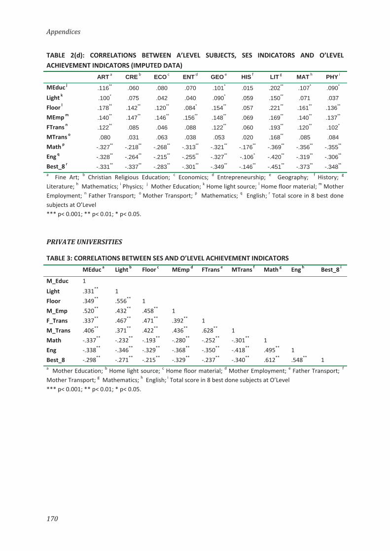
Appendices

170

TABLE 2(d): CORRELATIONS BETWEEN A’LEVEL SUBJECTS, SES INDICATORS AND O’LEVEL ACHIEVEMENT INDICATORS (IMPUTED DATA)


MEduc j .116** .060 .080 .070 .101* .015 .202** .107* .090* Light k .100* .075 .042 .040 .090* .059 .150** .071 .037 Floor l .178** .142** .120** .084* .154** .057 .221** .161** .136** MEmp m .140** .147** .146** .156** .148** .069 .169** .140** .137** FTrans n .122** .085 .046 .088 .122** .060 .193** .120** .102* MTrans o .080 .031 .063 .038 .053 .020 .168** .085 .084 Math p -.327** -.218** -.268** -.313** -.321** -.176** -.369** -.356** -.355** Eng q -.328** -.264** -.215** -.255** -.327** -.106* -.420** -.319** -.306** Best_8 r -.331** -.337** -.283** -.301** -.349** -.146** -.451** -.373** -.348** a Fine Art; b Christian Religious Education; c Economics; d Entrepreneurship; e Geography; f History; g Literature; h Mathematics; i Physics; j Mother Education; k Home light source; l Home floor material; m Mother Employment; n Father Transport; o Mother Transport; p Mathematics; q English; r Total score in 8 best done subjects at O’Level

*** p< 0.001; ** p< 0.01; * p< 0.05. PRIVATE UNIVERSITIES

TABLE 3: CORRELATIONS BETWEEN SES AND O’LEVEL ACHIEVEMENT INDICATORS MEduc a Light b Floor c MEmp d FTrans e MTrans f Math g Eng h Best_8 i

M_Educ 1 Light .331** 1 Floor .349** .556** 1 M_Emp .520** .432** .458** 1 F_Trans .337** .467** .471** .392** 1 M_Trans .406** .371** .422** .436** .628** 1 Math -.337** -.232** -.193** -.280** -.252** -.301** 1 Eng -.338** -.346** -.329** -.368** -.350** -.418** .495** 1 Best_8 -.298** -.271** -.215** -.329** -.237** -.340** .612** .548** 1 a Mother Education; b Home light source; c Home floor material; d Mother Employment; e Father Transport; f

Mother Transport; g Mathematics; h English; i Total score in 8 best done subjects at O’Level

*** p< 0.001; ** p< 0.01; * p< 0.05.

Appendices

171

TABLE 4(a): CORRELATIONS BETWEEN A’LEVEL SUBJECTS (QUESTIONNAIRE DATA)


ART 1

CRE .366** 1 ECO .105 .389** 1 ENT .292 .449** .448** 1 GEO .168 .422** .374** .275** 1 HIS .202* .412** .454** .168* .441** 1 LIT .676 .348* .473** .067 0.000 .550** 1

MAT -.134 - .277** .340* .068 - - 1 PHY -.153 - .254 .244 - - - .551** 1

CGPA .029 .063 .169** .234** .136* .131* .482** .154 .220

Fine Art; b Christian Religious Education; c Economics; d Entrepreneurship; e Geography; f History; g Literature; h Mathematics; i Physics

*** p< 0.001; ** p< 0.01; * p< 0.05. TABLE 4(b): CORRELATIONS BETWEEN A’LEVEL SUBJECTS (IMPUTED DATA)

ART CRE ECO ENT GEO HIS LIT MAT PHY

ART 1

CRE .485** 1 ECO .404** .568** 1 ENT .486** .662** .643** 1 GEO .461** .674** .589** .684** 1 HIS .384** .562** .533** .546** .595** 1 LIT .554** .762** .742** .768** .796** .710** 1

MAT .478** .701** .654** .714** .715** .629** .796** 1 PHY .519** .720** .685** .730** .751** .641** .823** .880** 1

CGPA .101* .094* .165** .167** .167** .138** .194** .171** .182**

Fine Art; b Christian Religious Education; c Economics; d Entrepreneurship; e Geography; f History; g Literature; h Mathematics; i Physics

*** p< 0.001; ** p< 0.01; * p< 0.05.

Appendices

172

TABLE 4(c): CORRELATIONS BETWEEN A’LEVEL SUBJECTS, SES INDICATORS AND O’LEVEL ACHIEVEMENT INDICATORS (QUESTIONNAIRE DATA)


MEduc j .172* .169** .149** .164* .239** .200** .398** .071 .175 Light k .133 .188** .020 .120 .199** .082 .111 .062 .261* Floor l .188* .148* .013 .046 .229** .131** .117 .021 .224 MEmp m .175* .159** .110* .171* .202** .116* .160 .117 .002 FTrans n .020 .162** .013 .126 .178** .127* .090 .116 .192 MTrans o .206* .223** .072 .147 .278** .230** .277 .082 .216 Math p -.062 -.341** -.321** -.430** -.364** -.244** -.378** -.393** -.413** Eng q -.151 -.296** -.245** -.333** -.335** -.248** -.436** -.280** -.442** Best_8 r -.107 -.467** -.410** -.512** -.353** -.284** -.380* -.464** -.486** a Fine Art; b Christian Religious Education; c Economics; d Entrepreneurship; e Geography; f History; g Literature; h Mathematics; i Physics; j Mother Education; k Home light source; l Home floor material; m Mother Employment; n Father Transport; o Mother Transport; p Mathematics; q English; r Total score in 8 best done subjects at O’Level

*** p< 0.001; ** p< 0.01; * p< 0.05.

TABLE 4(d): CORRELATIONS BETWEEN A’LEVEL SUBJECTS, SES INDICATORS AND O’LEVEL ACHIEVEMENT INDICATORS (IMPUTED DATA)


MEduc j .170** .183** .140** .192** .200** .182** .240** .197** .217** Light k .118** .138** .042 .144** .150** .095* .131** .107** .128** Floor l .141** .121** .053 .125** .172** .112** .141** .089* .129** MEmp m .173** .173** .120** .180** .170** .128** .188** .155** .155** FTrans n .074 .128** .023 .141** .152** .099* .124** .120** .129** MTrans o .179** .200** .080 .167** .226** .180** .218** .185** .207** Math p -.206** -.349** -.309** -.390** -.388** -.290** -.409** -.433** -.425** Eng q -.219** -.288** -.237** -.334** -.323** -.244** -.343** -.331** -.358** Best_8 r -.271** -.427** -.376** -.464** -.416** -.320** -.472** -.476** -.489** a Fine Art; b Christian Religious Education; c Economics; d Entrepreneurship; e Geography; f History; g Literature; h Mathematics; i Physics; j Mother Education; k Home light source; l Home floor material; m Mother Employment; n Father Transport; o Mother Transport; p Mathematics; q English; r Total score in 8 best done subjects at O’Level

*** p< 0.001; ** p< 0.01; * p< 0.05.

Appendices

173

APPENDIX C3: DESCRIPTIVE STATISTICS FOR SOME SES INDICATORS (PUBLIC AND PRIVATE UNIVERSITIES COMBINED)

TABLE 1: DESCRIPTIVE STATISTICS FOR SES INDICATORS

N Minimum Maximum Mean S.D

Father education level 1,257 0 7 4.10 1.711 Mother education level 1,195 0 7 3.65 1.737 Home light source 1,283 0 6 4.41 1.297 Home floor material 1,270 0 4 2.95 1.254 Home roof material 1,270 0 4 2.19 0.970 Number of books at home 1,249 0 5 2.32 1.617 Father employment 1,238 0 4 3.13 1.084 Mother employment 1,239 0 4 2.88 1.123 Father means of transport 1,101 0 4 2.94 1.226 Mother means of transport 960 0 4 2.60 1.270

Proportions per score category of SES indicators

TABLE 2 (a): PARENTAL EDUCATION

Proportion Educational Level [Likert scale value] Category Father Mother Not Sure [0] 1 6.8 0.079 No School [1] 2 2.3 0.053 Some or all of Primary School[ 2] 3 8.6 0.110 Some or all of Secondary School [3] 4 12.1 0.185 Vocational/Technical College Certificate or Diploma [4] 5 15.0 0.169 University Degree or Diploma [5] 6 33.0 0.281 Postgraduate Degree or Diploma [6] 7 19.5 0.122

TABLE 2 (b): LIGHT SOURCE

Description [Likert scale value] Category Proportion No lighting [0] 1 0.006 Firewood [1] 2 0.055 Tadoba ( a simple home-made paraffin lamp)[2] 3 0.040 Paraffin Lamp [3] 4 0.142 Gas Lamp [4] 5 0.010 Electricity [5] 6 0.678 Solar Lighting [6] 7 0.069

Appendices

174

TABLE 2 (c): FLOOR MATERIAL

Description [Likert scale value] Category Proportion Earth or Clay (With or without Covering) [0] 1 0.129 Canvas [1] 2 0.008 Wooden Planks [2] 3 0.014 Cement/Concrete [3] 4 0.483 Carpet/Tiles [4] 5 0.365

TABLE 2 (d): PARENTAL EMPLOYMENT

Proportion Employment [Likert scale value] Category Father Mother Professional (e.g. Accountant, Engineer, Diplomat, Banker, Government Worker, etc.) [4]

1 0. 468 0.012

Businessman [3] 2 0.286 0.195 Skilled Worker (e.g. Mechanic, Plumber, Construction Worker, Carpenter, Technician, etc.) [2]

3 0.065 0.038

Peasant Farmer [1] 4 0.131 0.409 Other [0] 5 0.009 0.345

TABLE 2 (e): PARENTAL TRANSPORTATION

Proportion Employment [Likert scale value] Category Father Mother Personal Car [4] 1 0.045 0.050 Official Car [3] 2 0.085 0.143 Public Transport [2] 3 0.260 0.357 On Foot [1] 4 0.107 0.057 Other [0] 5 0.503 0.393

TABLE 2 (f): BOOKS AT HOME WHEN GROWING UP

No Books 1-10 11-50 51 - 100 101 - 200 201 or more Missing Total N 187 309 254 246 118 205 43 1362 % 13.7% 22.7% 18.6% 18.1% 8.7% 15.1% 3.2% 100%

Appe

ndic

es

175

APPE

ND

IX C

4: S

EM O

UTP

UT

BASE

D O

N P

LAU

SIBL

E VA

LUES

GEN

ERAT

ED F

RO

M B

OTH

SEL

F-RE

POR

TED

AN

D

REG

ISTR

Y D

ATA

TABL

E 1(

a): M

EASU

RIN

G O

’LEV

EL P

ERFO

RMAN

CE U

SIN

G PL

AUSI

BLE

VALU

ES G

ENER

ATED

FRO

M S

ELF-

REPO

RTED

DAT

A O

NLY

PU

BLIC

UN

IVER

SITI

ES

PRIV

ATE

UN

IVER

SITI

ES

UN

IVER

SITI

ES C

OM

BIN

ED

Es

timat

e S.

E.

P-Va

lue

Estim

ate

S.E.

P-

Valu

e Es

timat

e S.

E.

P-Va

lue

SES

Mea

n be

st 8

subj

ects

0.

866

0.02

2 0.

000

0.78

7 0.

025

0.00

0 0.

837

0.01

5 0.

000

Mat

h sc

ore

0.72

7 0.

027

0.00

0 0.

719

0.02

7 0.

000

0.72

7 0.

018

0.00

0 En

glish

scor

e 0.

748

0.02

6 0.

000

0.71

2 0.

027

0.00

0 0.

776

0.01

6 0.

000

TABL

E 1(

b): M

EASU

RIN

G O

’LEV

EL P

ERFO

RMAN

CE U

SIN

G PL

AUSI

BLE

VALU

ES G

ENER

ATED

FRO

M R

EGIS

TRY

DATA

PU

BLIC

UN

IVER

SITI

ES

PRIV

ATE

UN

IVER

SITI

ES

UN

IVER

SITI

ES C

OM

BIN

ED

Es

timat

e S.

E.

P-Va

lue

Estim

ate

S.E.

P-

Valu

e Es

timat

e S.

E.

P-Va

lue

SES

Mea

n be

st 8

subj

ects

0.

868

0.02

1 0.

000

0.78

9 0.

025

0.00

0 0.

840

0.01

5 0.

000

Mat

h sc

ore

0.72

9 0.

027

0.00

0 0.

722

0.02

7 0.

000

0.73

1 0.

018

0.00

0 En

glish

scor

e 0.

745

0.02

6 0.

000

0.70

7 0.

027

0.00

0 0.

770

0.01

6 0.

000

Appe

ndic

es

176

TABL

E 2(

a): M

EASU

RIN

G A’

LEVE

L PE

RFO

RMAN

CE U

SIN

G PL

AUSI

BLE

VALU

ES G

ENER

ATED

FRO

M S

ELF-

REPO

RTED

DAT

A O

NLY

PU

BLIC

UN

IVER

SITI

ES

PRIV

ATE

UN

IVER

SITI

ES

UN

IVER

SITI

ES C

OM

BIN

ED

1D

IM

2DIM

1D

IM

2DIM

1D

IM

2DIM

Mea

sure

Es

t. S.

E.

Est.

S.E.

Es

t. S.

E.

Est.

S.E.

Es

t. S.

E.

Est.

S.E.

A’LE

VEL

PERF

ORM

ANCE

Non

- Sci

ence

Fi

ne A

rt

0.42

6 0.

038

0.43

0 0.

038

0.35

9 0.

035

0.33

9 0.

036

0.40

9 0.

025

0.39

0 0.

026

Chris

tian

Relig

ious

Ed

0.61

2 0.

030

0.61

5 0.

031

0.59

8 0.

027

0.57

3 0.

028

0.66

4 0.

018

0.65

4 0.

018

Econ

omic

s 0.

650

0.02

8 0.

585

0.03

2 0.

628

0.02

6 0.

627

0.02

6 0.

695

0.01

6 0.

662

0.01

8 En

trep

rene

ursh

ip

0.63

8 0.

029

0.57

7 0.

032

0.64

0 0.

025

0.70

3 0.

023

0.68

0 0.

017

0.69

0 0.

017

Geog

raph

y 0.

704

0.02

5 0.

709

0.02

6 0.

681

0.02

3 0.

619

0.02

7 0.

723

0.01

5 0.

697

0.01

7 Hi

stor

y 0.

447

0.03

7 0.

497

0.03

6 0.

532

0.03

0 0.

576

0.02

8 0.

540

0.02

2 0.

585

0.02

0 Li

tera

ture

0.

557

0.03

3 0.

590

0.03

2 0.

660

0.02

4 0.

648

0.02

5 0.

676

0.01

7 0.

672

0.01

8 Sc

ienc

e

M

athe

mat

ics

0.67

3 0.

027

0.63

4 0.

034

0.68

3 0.

023

0.65

7 0.

028

0.62

8 0.

031

0.66

1 0.

021

Phys

ics

0.75

1 0.

023

0.65

8 0.

034

0.66

0 0.

024

0.69

3 0.

027

0.63

5 0.

031

0.67

5 0.

021

NO

N-S

CIEN

CE D

IMEN

SIO

N

1.

091

0.04

9

1.

029

0.04

0

1.

064

0.02

5 SC

IEN

CE D

IMEN

SIO

N

0.

893

0.05

1

0.

919

0.04

6

0.

904

0.02

8

Appe

ndic

es

177

TABL

E 2(

b): M

EASU

RIN

G A’

LEVE

L PE

RFO

RMAN

CE U

SIN

G PL

AUSI

BLE

VALU

ES G

ENER

ATED

FRO

M R

EGIS

TRY

DATA

PU

BLIC

UN

IVER

SITI

ES

PRIV

ATE

UN

IVER

SITI

ES

UN

IVER

SITI

ES C

OM

BIN

ED

1D

IM

2DIM

1D

IM

2DIM

1D

IM

2DIM

Mea

sure

Es

t. S.

E.

Est.

S.E.

Es

t. S.

E.

Est.

S.E.

Es

t. S.

E.

Est.

S.E.

A’LE

VEL

PERF

ORM

ANCE

Non

- Sci

ence

Fi

ne A

rt

0.50

7 0.

036

0.43

0 0.

038

0.48

0 0.

032

0.42

9 0.

033

0.50

9 0.

023

0.47

0 0.

024

Chris

tian

Relig

ious

Ed

0.57

5 0.

033

0.63

2 0.

029

0.65

3 0.

025

0.60

1 0.

027

0.67

0 0.

018

0.66

3 0.

018

Econ

omic

s 0.

632

0.03

0 0.

664

0.02

8 0.

588

0.02

8 0.

630

0.02

6 0.

649

0.01

8 0.

690

0.01

7 En

trep

rene

ursh

ip

0.60

0 0.

031

0.61

7 0.

030

0.67

7 0.

024

0.65

6 0.

025

0.68

7 0.

017

0.68

0 0.

017

Geog

raph

y 0.

649

0.02

9 0.

616

0.03

0 0.

690

0.02

3 0.

650

0.02

5 0.

706

0.01

6 0.

678

0.01

7 Hi

stor

y 0.

496

0.03

6 0.

526

0.03

4 0.

553

0.02

9 0.

562

0.02

9 0.

564

0.02

1 0.

586

0.02

0 Li

tera

ture

0.

559

0.03

3 0.

595

0.03

1 0.

663

0.02

4 0.

614

0.02

7 0.

671

0.01

8 0.

658

0.01

8 Sc

ienc

e

M

athe

mat

ics

0.59

7 0.

032

0.76

2 0.

024

0.52

8 0.

030

0.65

7 0.

028

0.56

4 0.

021

0.73

1 0.

017

Phys

ics

0.72

0 0.

025

0.73

3 0.

025

0.57

5 0.

028

0.69

3 0.

027

0.67

0 0.

018

0.75

4 0.

016

NO

N-S

CIEN

CE D

IMEN

SIO

N

0.

995

0.03

7

0.

955

0.03

1

0.

977

0.01

8 SC

IEN

CE D

IMEN

SIO

N

0.

990

0.03

9

0.

996

0.03

8

0.

991

0.02

1

Appe

ndic

es

178

TABL

E 3(

a): M

EASU

RIN

G SE

S U

SIN

G PL

AUSI

BLE

VALU

ES G

ENER

ATED

FRO

M S

ELF-

REPO

RTED

DAT

A O

NLY

PU

BLIC

UN

IVER

SITI

ES

PRIV

ATE

UN

IVER

SITI

ES

UN

IVER

SITI

ES C

OM

BIN

ED

Es

timat

e S.

E.

P-Va

lue

Estim

ate

S.E.

P-

Valu

e Es

timat

e S.

E.

P-Va

lue

SES

Mot

her E

duca

tion

0.53

8 0.

038

0.00

0 0.

566

0.03

1 0.

000

0.57

4 0.

023

0.00

0 Ho

me

light

sour

ce

0.60

9 0.

034

0.00

0 0.

664

0.02

6 0.

000

0.66

2 0.

019

0.00

0 Ho

me

floor

mat

eria

l 0.

685

0.03

1 0.

000

0.69

2 0.

024

0.00

0 0.

696

0.01

8 0.

000

Mot

her e

mpl

oym

ent

0.60

7 0.

035

0.00

0 0.

673

0.02

6 0.

000

0.67

4 0.

019

0.00

0 Fa

ther

tran

spor

t 0.

627

0.03

7 0.

000

0.73

3 0.

025

0.00

0 0.

696

0.02

0 0.

000

Mot

her t

rans

port

0.

700

0.03

5 0.

000

0.73

4 0.

027

0.00

0 0.

725

0.02

1 0.

000

Appe

ndic

es

179

TABL

E 3(

b): M

EASU

RIN

G SE

S U

SIN

G PL

AUSI

BLE

VALU

ES G

ENER

ATED

FRO

M R

EGIS

TRY

DATA

PU

BLIC

UN

IVER

SITI

ES

PRIV

ATE

UN

IVER

SITI

ES

UN

IVER

SITI

ES C

OM

BIN

ED

Es

timat

e S.

E.

P-Va

lue

Estim

ate

S.E.

P-

Valu

e Es

timat

e S.

E.

P-Va

lue

SES

Mot

her E

duca

tion

0.53

9 0.

038

0.00

0 0.

567

0.03

1 0.

000

0.57

5 0.

023

0.00

0 Ho

me

light

sour

ce

0.60

9 0.

034

0.00

0 0.

664

0.02

6 0.

000

0.66

2 0.

019

0.00

0 Ho

me

floor

mat

eria

l 0.

685

0.03

1 0.

000

0.69

2 0.

024

0.00

0 0.

696

0.01

8 0.

000

Mot

her e

mpl

oym

ent

0.60

7 0.

035

0.00

0 0.

673

0.02

6 0.

000

0.67

5 0.

019

0.00

0 Fa

ther

tran

spor

t 0.

628

0.03

7 0.

000

0.73

3 0.

025

0.00

0 0.

695

0.02

0 0.

000

Mot

her t

rans

port

0.

700

0.03

5 0.

000

0.73

4 0.

027

0.00

0 0.

725

0.02

1 0.

000

Appe

ndic

es

180

TABL

E 4(

a): M

EASU

RIN

G A’

LEVE

L SU

CCES

S FA

CTO

RS A

ND

UN

IVER

SITY

PRE

PARE

DNES

S U

SIN

G PL

AUSI

BLE

VALU

ES G

ENER

ATED

FRO

M S

ELF-

REPO

RTED

DAT

A O

NLY

PU

BLIC

UN

IVER

SITI

ES

PRIV

ATE

UN

IVER

SITI

ES

UN

IVER

SITI

ES C

OM

BIN

ED

Es

timat

e S.

E.

P-Va

lue

Estim

ate

S.E.

P-

Valu

e Es

timat

e S.

E.

P-Va

lue

A’LE

VEL

SUCC

ESS

FACT

ORS

The

less

ons g

iven

in c

lass

0.

403

0.04

6 0.

000

0.47

9 0.

036

0.00

0 0.

414

0.02

9 0.

000

Libr

ary

book

s 0.

375

0.04

7 0.

000

0.42

5 0.

038

0.00

0 0.

408

0.02

9 0.

000

Grou

p di

scus

sions

0.

522

0.04

1 0.

000

0.52

0 0.

035

0.00

0 0.

527

0.02

7 0.

000

Mod

el a

nsw

ers -

reve

rsed

0.

415

0.04

5 0.

000

0.49

0 0.

036

0.00

0 0.

465

0.02

8 0.

000

Sum

mar

ies o

f cla

ss n

otes

0.

325

0.04

7 0.

000

0.37

2 0.

039

0.00

0 0.

359

0.03

0 0.

000

“Spo

ttin

g” th

e ex

am -

reve

rsed

0.

068

0.05

1 0.

188

0.25

0 0.

042

0.00

0 0.

191

0.03

3 0.

000

A st

rict s

choo

l env

ironm

ent

0.42

5 0.

046

0.00

0 0.

474

0.03

7 0.

000

0.45

1 0.

029

0.00

0 Ex

tra

tuiti

on o

r coa

chin

g

0.20

6 0.

050

0.00

0 0.

275

0.04

1 0.

000

0.27

4 0.

032

0.00

0 Ex

tra-

curr

icul

ar a

ctiv

ities

0.

312

0.04

8 0.

000

0.31

0 0.

041

0.00

0 0.

329

0.03

1 0.

000

Regu

lar t

ests

and

exa

min

atio

ns

0.53

5 0.

042

0.00

0 0.

554

0.03

4 0.

000

0.53

7 0.

027

0.00

0 N

otes

pro

vide

d by

teac

her

0.39

7 0.

046

0.00

0 0.

396

0.03

9 0.

000

0.37

6 0.

030

0.00

0 He

lp d

irect

ly fr

om te

ache

rs

0.50

0 0.

042

0.00

0 0.

441

0.03

7 0.

000

0.47

0 0.

027

0.00

0 U

NIV

ERSI

TY P

REPA

REDN

ESS

A

broa

d ge

nera

l kno

wle

dge

0.66

2 0.

030

0.00

0 0.

593

0.03

2 0.

000

0.62

6 0.

022

0.00

0 W

ritin

g cl

early

and

effe

ctiv

ely

0.64

8 0.

032

0.00

0 0.

507

0.03

5 0.

000

0.57

8 0.

024

0.00

0 Sp

eaki

ng c

lear

ly a

nd e

ffect

ivel

y 0.

665

0.03

1 0.

000

0.59

7 0.

032

0.00

0 0.

638

0.02

2 0.

000

Anal

ysin

g re

al li

fe p

robl

ems

0.58

6 0.

034

0.00

0 0.

483

0.03

6 0.

000

0.53

5 0.

025

0.00

0 W

orki

ng w

ith o

ther

s 0.

709

0.02

9 0.

000

0.64

4 0.

030

0.00

0 0.

681

0.02

1 0.

000

Lear

ning

on

one’

s ow

n 0.

345

0.04

3 0.

000

0.33

4 0.

041

0.00

0 0.

334

0.02

9 0.

000

Ove

rall

prep

arat

ion

for U

nive

rsity

0.

502

0.03

9 0.

000

0.51

4 0.

036

0.00

0 0.

504

0.02

7 0.

000

Appe

ndic

es

181

TABL

E 4(

b):

MEA

SURI

NG

A’LE

VEL

SUCC

ESS

FACT

ORS

AN

D U

NIV

ERSI

TY P

REPA

REDN

ESS

USI

NG

PLAU

SIBL

E VA

LUES

GEN

ERAT

ED F

ROM

RE

GIST

RY D

ATA

PU

BLIC

UN

IVER

SITI

ES

PRIV

ATE

UN

IVER

SITI

ES

UN

IVER

SITI

ES C

OM

BIN

ED

Es

timat

e S.

E.

P-Va

lue

Estim

ate

S.E.

P-

Valu

e Es

timat

e S.

E.

P-Va

lue

A’LE

VEL

SUCC

ESS

FACT

ORS

The

less

ons g

iven

in c

lass

0.

400

0.04

6 0.

000

0.47

7 0.

036

0.00

0 0.

411

0.03

0 0.

000

Libr

ary

book

s 0.

374

0.04

7 0.

000

0.42

5 0.

038

0.00

0 0.

408

0.02

9 0.

000

Grou

p di

scus

sions

0.

524

0.04

1 0.

000

0.52

1 0.

035

0.00

0 0.

529

0.02

6 0.

000

Mod

el a

nsw

ers -

reve

rsed

0.

417

0.04

5 0.

000

0.49

0 0.

036

0.00

0 0.

465

0.02

8 0.

000

Sum

mar

ies o

f cla

ss n

otes

0.

327

0.04

7 0.

000

0.37

2 0.

039

0.00

0 0.

360

0.03

0 0.

000

“Spo

ttin

g” th

e ex

am -

reve

rsed

0.

069

0.05

1 0.

180

0.25

2 0.

042

0.00

0 0.

193

0.03

3 0.

000

A st

rict s

choo

l env

ironm

ent

0.42

5 0.

046

0.00

0 0.

473

0.03

7 0.

000

0.45

0 0.

029

0.00

0 Ex

tra

tuiti

on o

r coa

chin

g

0.21

2 0.

050

0.00

0 0.

275

0.04

1 0.

000

0.27

6 0.

032

0.00

0 Ex

tra-

curr

icul

ar a

ctiv

ities

0.

312

0.04

8 0.

000

0.31

1 0.

041

0.00

0 0.

332

0.03

1 0.

000

Regu

lar t

ests

and

exa

min

atio

ns

0.53

5 0.

042

0.00

0 0.

554

0.03

4 0.

000

0.53

5 0.

027

0.00

0 N

otes

pro

vide

d by

teac

her

0.39

6 0.

046

0.00

0 0.

396

0.03

9 0.

000

0.37

4 0.

030

0.00

0 He

lp d

irect

ly fr

om te

ache

rs

0.50

1 0.

042

0.00

0 0.

440

0.03

7 0.

000

0.47

0 0.

027

0.00

0 U

NIV

ERSI

TY P

REPA

REDN

ESS

A

broa

d ge

nera

l kno

wle

dge

0.66

2 0.

030

0.00

0 0.

592

0.03

2 0.

000

0.62

5 0.

022

0.00

0 W

ritin

g cl

early

and

effe

ctiv

ely

0.64

8 0.

032

0.00

0 0.

507

0.03

5 0.

000

0.57

8 0.

024

0.00

0 Sp

eaki

ng c

lear

ly a

nd e

ffect

ivel

y 0.

665

0.03

1 0.

000

0.59

7 0.

032

0.00

0 0.

638

0.02

2 0.

000

Anal

ysin

g re

al li

fe p

robl

ems

0.58

5 0.

034

0.00

0 0.

484

0.03

6 0.

000

0.53

5 0.

025

0.00

0 W

orki

ng w

ith o

ther

s 0.

709

0.02

9 0.

000

0.64

5 0.

030

0.00

0 0.

681

0.02

1 0.

000

Lear

ning

on

one’

s ow

n 0.

345

0.04

3 0.

000

0.33

4 0.

041

0.00

0 0.

334

0.02

9 0.

000

Ove

rall

prep

arat

ion

for U

nive

rsity

0.

502

0.03

9 0.

000

0.51

3 0.

036

0.00

0 0.

504

0.02

7 0.

000

Appe

ndic

es

182

TABL

E 5(

a): R

EGRE

SSIO

NS

BETW

EEN

OBS

ERVE

D AN

D LA

TEN

T VA

RIAB

LES

USI

NG

PLAU

SIBL

E VA

LUES

GEN

ERAT

ED F

ROM

SEL

F-RE

PORT

ED D

ATA

ON

LY

PU

BLIC

UN

IVER

SITI

ES

PRIV

ATE

UN

IVER

SITI

ES

UN

IVER

SITI

ES C

OM

BIN

ED

1D

IM

2DIM

1D

IM

2DIM

1D

IM

2DIM

Mea

sure

Es

t. S.

E.

Est.

S.E.

Es

t. S.

E.

Est.

S.E.

Es

t. S.

E.

Est.

S.E.

A’Le

vel P

erfo

rman

ce a O

N

SE

S -0

.041

0.

071

-0.0

43

0.06

8 -0

.157

0.

062

-0.1

54

0.06

2 -0

.120

0.

046

-0.1

12

0.04

4 O

’Lev

el b

-0.4

44

0.07

3 -0

.418

0.

075

-0.5

27

0.05

7 -0

.514

0.

058

-0.6

04

0.04

2 -0

.566

0.

044

A’Le

vel S

ucce

ss F

acto

rs

0.08

0 0.

051

0.00

8 0.

048

0.16

3 0.

043

0.16

6 0.

043

0.07

1 0.

031

0.05

6 0.

030

A’

Leve

l Per

form

ance

ON

Priv

ate

A’Le

vel S

choo

l 0.

013

0.10

4 -0

.025

0.

098

-0.0

70

0.09

7 -0

.041

0.

097

-0.0

66

0.06

6 -0

.071

0.

063

Non

-Use

A’L

evel

Sch

ool

0.59

9 0.

268

0.82

0 0.

254

0.31

1 0.

137

0.45

1 0.

136

0.39

2 0.

112

0.53

3 0.

107

Boar

ding

A’L

evel

Sch

ool

0.07

1 0.

166

0.01

7 0.

156

0.05

7 0.

117

0.09

5 0.

116

0.12

3 0.

089

0.12

6 0.

085

Sing

le-S

ex A

’Lev

el S

choo

l 0.

002

0.11

7 0.

032

0.11

1 -0

.135

0.

120

-0.1

30

0.12

0 -0

.056

0.

078

-0.0

35

0.07

5 a O

’Lev

el a

chie

vem

ent i

s mea

sure

d by

indi

cato

rs fo

r whi

ch a

low

num

ber i

s a h

igh

scor

e, a

nd a

hig

h nu

mbe

r is a

low

scor

e. T

his s

houl

d be

take

n in

to c

onsid

erat

ion

whe

n in

terp

retin

g re

gres

sion

coef

ficie

nts.

b A’

Leve

l ach

ieve

men

t is m

easu

red

by in

dica

tors

for w

hich

a lo

w n

umbe

r is a

low

scor

e, a

nd a

hig

h nu

mbe

r is a

hig

h sc

ore;

as s

uch,

it is

mea

sure

d in

the

oppo

site

dire

ctio

n to

O ‘L

evel

.

Appe

ndic

es

183

TABL

E 5(

a):

REGR

ESSI

ON

S BE

TWEE

N O

BSER

VED

AND

LATE

NT

VARI

ABLE

S U

SIN

G PL

AUSI

BLE

VALU

ES G

ENER

ATED

FRO

M S

ELF-

REPO

RTED

DAT

A O

NLY

(C

ON

TIN

UED

)

PU

BLIC

UN

IVER

SITI

ES

PRIV

ATE

UN

IVER

SITI

ES

UN

IVER

SITI

ES C

OM

BIN

ED

1D

IM

2D

IM

1D

IM

2D

IM

1D

IM

2D

IM

Mea

sure

Es

t. S.

E.

Est.

S.E.

Es

t. S.

E.

Est.

S.E.

Es

t. S.

E.

Est.

S.E.

Cum

ulat

ive

Grad

e Po

int A

vera

ge (C

GPA)

ON

SES

-0.1

23

0.07

2 -0

.115

0.

072

-0.0

46

0.05

9 -0

.054

0.

059

-0.0

64

0.04

9 -0

.065

0.

049

A’Le

vel a S

ucce

ss F

acto

rs

0.10

9 0.

069

0.12

6 0.

068

0.02

6 0.

074

0.01

6 0.

074

0.13

7 0.

049

0.13

4 0.

049

Uni

vers

ity P

repa

redn

ess

0.09

5 0.

064

0.10

8 0.

064

0.15

9 0.

073

0.16

5 0.

073

0.12

9 0.

048

0.13

0 0.

048

O’L

evel

b Per

form

ance

0.

117

0.08

2 0.

118

0.08

3 -0

.179

0.

076

-0.1

73

0.07

5 0.

002

0.06

4 0.

017

0.06

2 A’

Leve

l Per

form

ance

0.

296

0.06

5 0.

301

0.06

7 0.

209

0.05

9 0.

229

0.06

0 0.

080

0.04

9 0.

112

0.04

7 O

’Lev

el P

erfo

rman

ce O

N

SES

-0.4

65

0.05

1 -0

.468

0.

051

-0.5

19

0.04

9 -0

.521

0.

049

-0.5

17

0.03

4 -0

.521

0.

034

O

’Lev

el P

erfo

rman

ce O

N

Priv

ate

O’L

evel

Sch

ool

0.36

0 0.

118

0.36

6 0.

117

0.16

5 0.

110

0.16

7 0.

110

0.33

6 0.

074

0.33

6 0.

074

Non

-Use

O’L

evel

Sch

ool

-0.7

80

0.19

4 -0

.773

0.

194

-0.0

82

0.13

1 -0

.086

0.

131

-0.3

52

0.09

7 -0

.343

0.

098

Boar

ding

O’L

evel

Sch

ool

-0.2

56

0.14

3 -0

.248

0.

143

-0.2

97

0.12

3 -0

.299

0.

123

-0.2

72

0.08

7 -0

.273

0.

087

Sing

le-S

ex O

’Lev

el S

choo

l -0

.320

0.

109

-0.3

33

0.10

9 -0

.278

0.

121

-0.2

53

0.12

2 -0

.268

0.

076

-0.2

64

0.07

6 a O

’Lev

el a

chie

vem

ent i

s mea

sure

d by

indi

cato

rs fo

r whi

ch a

low

num

ber i

s a h

igh

scor

e, a

nd a

hig

h nu

mbe

r is a

low

scor

e. T

his s

houl

d be

take

n in

to c

onsid

erat

ion

whe

n in

terp

retin

g re

gres

sion

coef

ficie

nts.

b A’

Leve

l ach

ieve

men

t is m

easu

red

by in

dica

tors

for w

hich

a lo

w n

umbe

r is a

low

scor

e, a

nd a

hig

h nu

mbe

r is a

hig

h sc

ore;

as s

uch,

it is

mea

sure

d in

the

oppo

site

dire

ctio

n to

O ‘L

evel

.

Appe

ndic

es

184

TABL

E 5(

b): R

EGRE

SSIO

NS

BETW

EEN

OBS

ERVE

D AN

D LA

TEN

T VA

RIAB

LES

USI

NG

PLAU

SIBL

E VA

LUES

GEN

ERAT

ED F

ROM

REG

ISTR

Y DA

TA

PU

BLIC

UN

IVER

SITI

ES

PRIV

ATE

UN

IVER

SITI

ES

UN

IVER

SITI

ES C

OM

BIN

ED

1D

IM

2DIM

1D

IM

2DIM

1D

IM

2DIM

Mea

sure

Es

t. S.

E.

Est.

S.E.

Es

t. S.

E.

Est.

S.E.

Es

t. S.

E.

Est.

S.E.

A’Le

vel a P

erfo

rman

ce O

N

SES

-0.0

39

0.07

1 -0

.011

0.

070

-0.1

46

0.06

3 -0

.150

0.

063

-0.1

12

0.04

6 -0

.102

0.

046

O’L

evel

b -0

.456

0.

073

-0.4

22

0.07

3 -0

.523

0.

057

-0.5

74

0.05

6 -0

.586

0.

043

-0.6

06

0.04

2 A’

Leve

l Suc

cess

Fac

tors

-0

.013

0.

052

0.00

8 0.

051

0.13

6 0.

043

0.17

4 0.

043

0.04

0 0.

031

0.05

7 0.

031

A’

Leve

l Per

form

ance

ON

Priv

ate

A’Le

vel S

choo

l 0.

040

0.10

5 0.

009

0.10

4 -0

.091

0.

099

-0.0

76

0.10

1 -0

.063

0.

067

-0.0

55

0.06

7 N

on-U

se A

’Lev

el S

choo

l 0.

547

0.27

4 0.

538

0.26

9 0.

444

0.13

8 0.

416

0.14

3 0.

488

0.11

3 0.

436

0.11

4 Bo

ardi

ng A

’Lev

el S

choo

l 0.

112

0.16

8 0.

145

0.16

7 0.

059

0.11

9 0.

063

0.12

1 0.

136

0.09

1 0.

147

0.09

1 Si

ngle

-Sex

A’L

evel

Sch

ool

-0.0

22

0.11

9 0.

037

0.11

8 -0

.087

0.

122

-0.1

21

0.12

3 -0

.044

0.

080

-0.0

28

0.08

0

a O’L

evel

ach

ieve

men

t is m

easu

red

by in

dica

tors

for w

hich

a lo

w n

umbe

r is a

hig

h sc

ore,

and

a h

igh

num

ber i

s a lo

w sc

ore.

Thi

s sho

uld

be ta

ken

into

con

sider

atio

n w

hen

inte

rpre

ting

regr

essio

n co

effic

ient

s. b

A’Le

vel a

chie

vem

ent i

s mea

sure

d by

indi

cato

rs fo

r whi

ch a

low

num

ber i

s a lo

w sc

ore,

and

a h

igh

num

ber i

s a h

igh

scor

e; a

s suc

h, it

is m

easu

red

in th

e op

posit

e di

rect

ion

to O

‘Lev

el.

Appe

ndic

es

185

TABL

E 5(

b): R

EGRE

SSIO

NS

BETW

EEN

OBS

ERVE

D AN

D LA

TEN

T VA

RIAB

LES

USI

NG

PLAU

SIBL

E VA

LUES

GEN

ERAT

ED F

ROM

REG

ISTR

Y DA

TA (C

ON

TIN

UED

)

PU

BLIC

UN

IVER

SITI

ES

PRIV

ATE

UN

IVER

SITI

ES

UN

IVER

SITI

ES C

OM

BIN

ED

1D

IM

2D

IM

1D

IM

2D

IM

1D

IM

2D

IM

M

easu

re

Est.

S.E.

Es

t. S.

E.

Est.

S.E.

Es

t. S.

E.

Est.

S.E.

Es

t. S.

E.

Cum

ulat

ive

Grad

e Po

int A

vera

ge (C

GPA)

ON

SES

-0.1

22

0.07

2 -0

.126

0.

071

-0.0

49

0.05

8 -0

.045

0.

059

-0.0

61

0.04

8 -0

.062

0.

048

A’Le

vel a S

ucce

ss F

acto

rs

0.13

9 0.

068

0.13

3 0.

068

0.02

4 0.

073

0.01

1 0.

075

0.13

8 0.

049

0.13

5 0.

049

Uni

vers

ity P

repa

redn

ess

0.09

7 0.

064

0.09

9 0.

065

0.15

9 0.

072

0.15

8 0.

073

0.12

4 0.

048

0.12

6 0.

048

O’L

evel

b Per

form

ance

0.

129

0.08

3 0.

108

0.08

2 -0

.141

0.

076

-0.1

29

0.08

0 0.

056

0.06

4 0.

039

0.06

5 A’

Leve

l Per

form

ance

0.

318

0.06

8 0.

280

0.06

7 0.

269

0.05

9 0.

269

0.06

5 0.

170

0.05

0 0.

134

0.05

1 O

’Lev

el P

erfo

rman

ce O

N

SES

-0.4

64

0.05

1 -0

.463

0.

051

-0.5

18

0.04

9 -0

.520

0.

049

-0.5

17

0.03

4 -0

.516

0.

034

O

’Lev

el P

erfo

rman

ce O

N

Priv

ate

O’L

evel

Sch

ool

0.36

2 0.

118

0.36

0 0.

118

0.15

4 0.

110

0.18

8 0.

109

0.32

6 0.

074

0.34

5 0.

074

Non

-Use

O’L

evel

Sch

ool

-0.7

81

0.19

4 -0

.776

0.

195

-0.0

91

0.13

0 -0

.091

0.

130

-0.3

55

0.09

8 -0

.354

0.

098

Boar

ding

O’L

evel

Sch

ool

-0.2

56

0.14

3 -0

.281

0.

143

-0.2

99

0.12

3 -0

.310

0.

123

-0.2

74

0.08

7 -0

.293

0.

087

Sing

le-S

ex O

’Lev

el S

choo

l -0

.310

0.

109

-0.3

14

0.10

9 -0

.272

0.

121

-0.2

56

0.12

1 -0

.261

0.

077

-0.2

55

0.07

6 a O

’Lev

el a

chie

vem

ent i

s mea

sure

d by

indi

cato

rs fo

r whi

ch a

low

num

ber i

s a h

igh

scor

e, a

nd a

hig

h nu

mbe

r is a

low

scor

e. T

his s

houl

d be

take

n in

to c

onsid

erat

ion

whe

n in

terp

retin

g re

gres

sion

coef

ficie

nts.

b A’

Leve

l ach

ieve

men

t is m

easu

red

by in

dica

tors

for w

hich

a lo

w n

umbe

r is a

low

scor

e, a

nd a

hig

h nu

mbe

r is a

hig

h sc

ore;

as s

uch,

it is

mea

sure

d in

the

oppo

site

dire

ctio

n to

O ‘L

evel

.

Appe

ndic

es

186

TABL

E 6(

a): C

OVA

RIAN

CES

BETW

EEN

OBS

ERVE

D AN

D LA

TEN

T VA

RIAB

LES

USI

NG

PLAU

SIBL

E VA

LUES

GEN

ERAT

ED F

ROM

SEL

F-RE

PORT

ED

DATA

ON

LY

PU

BLIC

UN

IVER

SITI

ES

PRIV

ATE

UN

IVER

SITI

ES

UN

IVER

SITI

ES C

OM

BIN

ED

Es

timat

e S.

E.

P-Va

lue

Estim

ate

S.E.

P-

Valu

e Es

timat

e S.

E.

P-Va

lue

A’Le

vel S

ucce

ss F

acto

rs W

ITH

SES

0.03

2 0.

058

0.57

6 0.

080

0.04

8 0.

100

0.02

5 0.

037

0.49

3 U

nive

rsity

Pre

pare

dnes

s W

ITH

SE

S -0

.006

0.

053

0.90

7 0.

001

0.04

9 0.

982

-0.0

16

0.03

6 0.

662

A’Le

vel S

ucce

ss F

acto

rs

0.45

4 0.

050

0.00

0 0.

648

0.03

8 0.

000

0.54

9 0.

031

0.00

0 Pr

ivat

e O

’Lev

el S

choo

l WIT

H

SES

-0.1

17

0.05

3 0.

028

0.13

1 0.

046

0.00

5 0.

005

0.03

4 0.

885

A’Le

vel S

ucce

ss F

acto

rs

0.04

0 0.

061

0.50

8 0.

000

0.05

7 1.

000

0.04

1 0.

041

0.32

2 U

nive

rsity

Pre

pare

dnes

s -0

.100

0.

056

0.07

5 0.

032

0.05

9 0.

594

-0.0

17

0.04

1 0.

675

Non

-USE

O’L

evel

Sch

ool W

ITH

SES

0.45

9 0.

050

0.00

0 0.

457

0.04

3 0.

000

0.49

7 0.

031

0.00

0 A’

Leve

l Suc

cess

Fac

tors

-0

.042

0.

061

0.49

1 0.

002

0.05

5 0.

969

-0.0

50

0.04

0 0.

210

Uni

vers

ity P

repa

redn

ess

-0.0

67

0.05

6 0.

231

-0.0

33

0.05

7 0.

559

-0.0

56

0.03

9 0.

156

Boar

ding

O’L

evel

Sch

ool W

ITH

SE

S 0.

099

0.05

3 0.

063

0.13

5 0.

046

0.00

3 0.

140

0.03

4 0.

000

A’Le

vel S

ucce

ss F

acto

rs

0.02

7 0.

062

0.67

0 0.

105

0.05

6 0.

061

0.05

7 0.

042

0.17

1 U

nive

rsity

Pre

pare

dnes

s -0

.053

0.

058

0.36

0 0.

081

0.05

9 0.

169

0.01

5 0.

041

0.71

6 Si

ngle

-Sex

O’L

evel

Sch

ool W

ITH

SE

S 0.

175

0.05

2 0.

001

0.20

7 0.

045

0.00

0 0.

215

0.03

3 0.

000

A’Le

vel S

ucce

ss F

acto

rs

-0.0

41

0.06

0 0.

501

0.05

8 0.

056

0.29

7 -0

.008

0.

041

0.83

7 U

nive

rsity

Pre

pare

dnes

s 0.

012

0.05

6 0.

824

0.04

3 0.

058

0.45

2 0.

014

0.04

0 0.

717

Appe

ndic

es

187

TABL

E 6(

a): C

OVA

RIAN

CES

BETW

EEN

OBS

ERVE

D AN

D LA

TEN

T VA

RIAB

LES

USI

NG

PLAU

SIBL

E VA

LUES

GEN

ERAT

ED F

ROM

SEL

F-RE

PORT

ED

DATA

ON

LY (C

ON

TIN

UED

)

PU

BLIC

UN

IVER

SITI

ES

PRIV

ATE

UN

IVER

SITI

ES

UN

IVER

SITI

ES C

OM

BIN

ED

Es

timat

e S.

E.

P-Va

lue

Estim

ate

S.E.

P-

Valu

e Es

timat

e S.

E.

P-Va

lue

Priv

ate

A’Le

vel S

choo

l WIT

H

SES

-0.0

13

0.04

9 0.

798

0.08

5 0.

043

0.04

5 0.

011

0.03

1 0.

715

A’Le

vel S

ucce

ss F

acto

rs

0.11

4 0.

057

0.04

6 0.

011

0.05

2 0.

835

0.07

2 0.

038

0.05

7 U

nive

rsity

Pre

pare

dnes

s -0

.186

0.

052

0.00

0 -0

.020

0.

052

0.69

4 -0

.097

0.

037

0.00

8 N

on-U

SE A

’Lev

el S

choo

l WIT

H

SE

S 0.

308

0.05

3 0.

000

0.40

3 0.

044

0.00

0 0.

417

0.03

2 0.

000

A’Le

vel S

ucce

ss F

acto

rs

-0.0

74

0.06

2 0.

232

0.02

3 0.

056

0.68

1 -0

.043

0.

041

0.29

7 U

nive

rsity

Pre

pare

dnes

s -0

.085

0.

055

0.12

2 -0

.059

0.

057

0.29

4 -0

.070

0.

039

0.07

3 Bo

ardi

ng A

’Lev

el S

choo

l WIT

H

SES

0.21

1 0.

052

0.00

0 -0

.011

0.

045

0.80

1 0.

092

0.03

3 0.

006

A’Le

vel S

ucce

ss F

acto

rs

-0.0

16

0.05

9 0.

779

0.07

7 0.

054

0.15

2 0.

026

0.04

0 0.

512

Uni

vers

ity P

repa

redn

ess

-0.0

59

0.05

5 0.

283

0.07

1 0.

054

0.18

8 0.

004

0.03

8 0.

917

Sing

le-S

ex S

choo

l WIT

H

SE

S 0.

128

0.05

1 0.

012

0.05

2 0.

045

0.24

3 0.

118

0.03

2 0.

000

A’Le

vel S

ucce

ss F

acto

rs

-0.0

72

0.05

8 0.

213

0.06

6 0.

054

0.21

6 -0

.020

0.

039

0.61

7 U

nive

rsity

Pre

pare

dnes

s 0.

081

0.05

4 0.

131

0.08

7 0.

054

0.10

5 0.

070

0.03

8 0.

065

Appe

ndic

es

188

TABL

E 6(

b): C

OVA

RIAN

CES

BETW

EEN

OBS

ERVE

D AN

D LA

TEN

T VA

RIAB

LES

USI

NG

PLAU

SIBL

E VA

LUES

GEN

ERAT

ED F

ROM

REG

ISTR

Y DA

TA

PU

BLIC

UN

IVER

SITI

ES

PRIV

ATE

UN

IVER

SITI

ES

UN

IVER

SITI

ES C

OM

BIN

ED

Es

timat

e S.

E.

P-Va

lue

Estim

ate

S.E.

P-

Valu

e Es

timat

e S.

E.

P-Va

lue

A’Le

vel S

ucce

ss F

acto

rs W

ITH

SES

0.03

3 0.

058

0.57

1 0.

080

0.04

8 0.

099

0.02

6 0.

037

0.48

6 U

nive

rsity

Pre

pare

dnes

s W

ITH

SES

-0.0

06

0.05

3 0.

904

0.00

1 0.

049

0.98

4 -0

.015

0.

036

0.66

8 A’

Leve

l Suc

cess

Fac

tors

0.

451

0.05

0 0.

000

0.64

8 0.

038

0.00

0 0.

549

0.03

1 0.

000

Priv

ate

O’L

evel

Sch

ool W

ITH

SES

-0.1

17

0.05

3 0.

027

0.13

1 0.

046

0.00

5 0.

001

0.03

4 0.

966

A’Le

vel S

ucce

ss F

acto

rs

0.04

0 0.

061

0.51

8 0.

001

0.05

7 0.

986

0.04

2 0.

041

0.31

4 U

nive

rsity

Pre

pare

dnes

s -0

.103

0.

056

0.06

7 0.

031

0.05

9 0.

607

-0.0

18

0.04

1 0.

663

Non

-USE

O’L

evel

Sch

ool W

ITH

SES

0.46

4 0.

050

0.00

0 0.

458

0.04

3 0.

000

0.49

8 0.

031

0.00

0 A’

Leve

l Suc

cess

Fac

tors

-0

.041

0.

061

0.50

5 0.

003

0.05

5 0.

952

-0.0

49

0.04

0 0.

218

Uni

vers

ity P

repa

redn

ess

-0.0

65

0.05

6 0.

251

-0.0

36

0.05

7 0.

523

-0.0

56

0.03

9 0.

157

Boar

ding

O’L

evel

Sch

ool W

ITH

SE

S 0.

106

0.05

3 0.

046

0.13

7 0.

046

0.00

3 0.

143

0.03

4 0.

000

A’Le

vel S

ucce

ss F

acto

rs

0.03

1 0.

062

0.62

0 0.

106

0.05

6 0.

058

0.05

8 0.

042

0.16

1 U

nive

rsity

Pre

pare

dnes

s -0

.053

0.

057

0.35

4 0.

081

0.05

9 0.

169

0.01

4 0.

041

0.72

7 Si

ngle

-Sex

O’L

evel

Sch

ool W

ITH

SES

0.17

8 0.

052

0.00

1 0.

205

0.04

5 0.

000

0.21

7 0.

033

0.00

0 A’

Leve

l Suc

cess

Fac

tors

-0

.036

0.

060

0.54

7 0.

058

0.05

6 0.

295

-0.0

07

0.04

1 0.

869

Uni

vers

ity P

repa

redn

ess

0.01

4 0.

056

0.80

0 0.

043

0.05

8 0.

459

0.01

4 0.

040

0.71

5

Appe

ndic

es

189

TABL

E 6(

b): C

OVA

RIAN

CES

BETW

EEN

OBS

ERVE

D AN

D LA

TEN

T VA

RIAB

LES

USI

NG

PLAU

SIBL

E VA

LUES

GEN

ERAT

ED F

ROM

REG

ISTR

Y DA

TA

(CO

NTI

NU

ED)

PU

BLIC

UN

IVER

SITI

ES

PRIV

ATE

UN

IVER

SITI

ES

UN

IVER

SITI

ES C

OM

BIN

ED

Es

timat

e S.

E.

P-Va

lue

Estim

ate

S.E.

P-

Valu

e Es

timat

e S.

E.

P-Va

lue

Priv

ate

A’Le

vel S

choo

l WIT

H

SE

S -0

.013

0.

049

0.79

8 0.

085

0.04

3 0.

045

0.01

1 0.

031

0.71

5 A’

Leve

l Suc

cess

Fac

tors

0.

114

0.05

7 0.

046

0.01

1 0.

052

0.83

5 0.

072

0.03

8 0.

057

Uni

vers

ity P

repa

redn

ess

-0.1

86

0.05

2 0.

000

-0.0

20

0.05

2 0.

694

-0.0

97

0.03

7 0.

008

Non

-USE

A’L

evel

Sch

ool W

ITH

SES

0.30

8 0.

053

0.00

0 0.

403

0.04

4 0.

000

0.41

7 0.

032

0.00

0 A’

Leve

l Suc

cess

Fac

tors

-0

.074

0.

062

0.23

2 0.

023

0.05

6 0.

681

-0.0

43

0.04

1 0.

297

Uni

vers

ity P

repa

redn

ess

-0.0

85

0.05

5 0.

122

-0.0

59

0.05

7 0.

294

-0.0

70

0.03

9 0.

073

Boar

ding

A’L

evel

Sch

ool W

ITH

SES

0.21

6 0.

051

0.00

0 -0

.011

0.

045

0.80

4 0.

093

0.03

3 0.

005

A’Le

vel S

ucce

ss F

acto

rs

-0.0

17

0.05

9 0.

771

0.07

7 0.

054

0.15

0 0.

025

0.04

0 0.

522

Uni

vers

ity P

repa

redn

ess

-0.0

58

0.05

5 0.

294

0.07

0 0.

054

0.19

1 0.

005

0.03

8 0.

907

Sing

le-S

ex S

choo

l WIT

H

SE

S 0.

130

0.05

0 0.

010

0.04

9 0.

045

0.27

6 0.

118

0.03

2 0.

000

A’Le

vel S

ucce

ss F

acto

rs

-0.0

70

0.05

8 0.

224

0.06

9 0.

054

0.19

9 -0

.019

0.

039

0.62

7 U

nive

rsity

Pre

pare

dnes

s 0.

081

0.05

4 0.

131

0.08

9 0.

054

0.09

8 0.

070

0.03

8 0.

064

Appe

ndic

es

190

TABL

E 7(

a):

EXPL

AIN

ED V

ARIA

NCE

OF

OBS

ERVE

D VA

RIAB

LES(

R-SQ

UAR

E) U

SIN

G PL

AUSI

BLE

VALU

ES G

ENER

ATED

FRO

M S

ELF-

REPO

RTED

DA

TA O

NLY

PU

BLIC

UN

IVER

SITI

ES

PRIV

ATE

UN

IVER

SITI

ES

UN

IVER

SITI

ES C

OM

BIN

ED

Es

timat

e S.

E.

P-Va

lue

Estim

ate

S.E.

P-

Valu

e Es

timat

e S.

E.

P-Va

lue

Mot

her E

duca

tion

0.28

9 0.

041

0.00

0 0.

321

0.03

5 0.

000

0.32

9 0.

026

0.00

0

Hom

e lig

ht so

urce

0.

371

0.04

2 0.

000

0.44

1 0.

034

0.00

0 0.

439

0.02

6 0.

000

Ho

me

floor

mat

eria

l 0.

469

0.04

2 0.

000

0.47

9 0.

034

0.00

0 0.

484

0.02

6 0.

000

M

othe

r em

ploy

men

t 0.

369

0.04

2 0.

000

0.45

2 0.

034

0.00

0 0.

455

0.02

6 0.

000

Fa

ther

tran

spor

t 0.

393

0.04

6 0.

000

0.53

7 0.

037

0.00

0 0.

484

0.02

8 0.

000

M

othe

r tra

nspo

rt

0.49

0 0.

050

0.00

0 0.

539

0.04

0 0.

000

0.52

6 0.

030

0.00

0

O’L

evel

Mat

hem

atic

s 0.

529

0.03

9 0.

000

0.51

7 0.

038

0.00

0 0.

529

0.02

6 0.

000

O

’Lev

el E

nglis

h 0.

560

0.03

9 0.

000

0.50

7 0.

039

0.00

0 0.

601

0.02

5 0.

000

Sc

ore

in b

est 8

O’L

evel

subj

ects

0.

750

0.03

7 0.

000

0.61

9 0.

040

0.00

0 0.

700

0.02

5 0.

000

Fi

ne A

rt

0.18

2 0.

033

0.00

0 0.

129

0.02

5 0.

000

0.16

7 0.

020

0.00

0

Chris

tian

Relig

ious

Ed

0.37

5 0.

037

0.00

0 0.

357

0.03

2 0.

000

0.44

2 0.

023

0.00

0

Econ

omic

s 0.

422

0.03

7 0.

000

0.39

4 0.

032

0.00

0 0.

483

0.02

3 0.

000

En

trep

rene

ursh

ip

0.40

7 0.

037

0.00

0 0.

409

0.03

2 0.

000

0.46

2 0.

023

0.00

0

Geog

raph

y 0.

496

0.03

6 0.

000

0.46

4 0.

032

0.00

0 0.

523

0.02

2 0.

000

Hi

stor

y 0.

200

0.03

3 0.

000

0.28

3 0.

032

0.00

0 0.

291

0.02

3 0.

000

Li

tera

ture

0.

311

0.03

7 0.

000

0.43

6 0.

032

0.00

0 0.

457

0.02

3 0.

000

M

athe

mat

ics

0.45

3 0.

036

0.00

0 0.

467

0.03

2 0.

000

0.53

6 0.

022

0.00

0

Phys

ics

0.56

3 0.

034

0.00

0 0.

435

0.03

2 0.

000

0.55

2 0.

022

0.00

0

The

less

ons g

iven

in c

lass

0.

163

0.03

7 0.

000

0.22

9 0.

035

0.00

0 0.

171

0.02

4 0.

000

Li

brar

y bo

oks

0.14

1 0.

035

0.00

0 0.

181

0.03

3 0.

000

0.16

6 0.

024

0.00

0

Appe

ndic

es

191

TABL

E 7(

a):

EXPL

AIN

ED V

ARIA

NCE

OF

OBS

ERVE

D VA

RIAB

LES(

R-SQ

UAR

E) U

SIN

G PL

AUSI

BLE

VALU

ES G

ENER

ATED

FRO

M S

ELF-

REPO

RTED

DA

TA O

NLY

(CO

NTI

NU

ED)

PU

BLIC

UN

IVER

SITI

ES

PRIV

ATE

UN

IVER

SITI

ES

UN

IVER

SITI

ES C

OM

BIN

ED

Es

timat

e S.

E.

P-Va

lue

Estim

ate

S.E.

P-

Valu

e Es

timat

e S.

E.

P-Va

lue

Grou

p di

scus

sions

0.

172

0.03

7 0.

000

0.24

0 0.

035

0.00

0 0.

216

0.02

6 0.

000

M

odel

ans

wer

s to

past

exa

min

atio

ns

- rev

erse

d 0.

106

0.03

0 0.

001

0.13

8 0.

029

0.00

0 0.

129

0.02

1 0.

000

Sum

mar

ies o

f cla

ss n

otes

0.

005

0.00

7 0.

511

0.06

3 0.

021

0.00

3 0.

036

0.01

2 0.

003

Pred

ictin

g th

e ex

am (“

Spot

ting”

) -

reve

rsed

0.

181

0.03

9 0.

000

0.22

4 0.

035

0.00

0 0.

203

0.02

6 0.

000

A st

rict s

choo

l env

ironm

ent

0.04

3 0.

021

0.03

8 0.

076

0.02

3 0.

001

0.07

5 0.

017

0.00

0 Ex

tra

tuiti

on o

r coa

chin

g

0.09

8 0.

030

0.00

1 0.

096

0.02

5 0.

000

0.10

8 0.

020

0.00

0 Ex

tra-

curr

icul

ar a

ctiv

ities

0.

286

0.04

5 0.

000

0.30

6 0.

037

0.00

0 0.

288

0.02

8 0.

000

Regu

lar t

ests

and

exa

min

atio

ns

0.15

8 0.

037

0.00

0 0.

157

0.03

1 0.

000

0.14

1 0.

023

0.00

0 N

otes

pro

vide

d by

teac

her

0.25

0 0.

042

0.00

0 0.

194

0.03

2 0.

000

0.22

1 0.

026

0.00

0 He

lp d

irect

ly fr

om te

ache

rs

0.43

9 0.

040

0.00

0 0.

351

0.03

8 0.

000

0.39

1 0.

028

0.00

0 A

broa

d ge

nera

l kno

wle

dge

0.41

9 0.

041

0.00

0 0.

257

0.03

6 0.

000

0.33

4 0.

028

0.00

0 W

ritin

g cl

early

and

effe

ctiv

ely

0.44

2 0.

041

0.00

0 0.

357

0.03

8 0.

000

0.40

8 0.

028

0.00

0 Sp

eaki

ng c

lear

ly a

nd e

ffect

ivel

y 0.

343

0.04

0 0.

000

0.23

3 0.

035

0.00

0 0.

286

0.02

7 0.

000

Anal

ysin

g re

al li

fe p

robl

ems

0.50

3 0.

041

0.00

0 0.

415

0.03

9 0.

000

0.46

4 0.

028

0.00

0 W

orki

ng w

ith o

ther

s 0.

119

0.03

0 0.

000

0.11

2 0.

027

0.00

0 0.

112

0.02

0 0.

000

Lear

ning

on

one’

s ow

n 0.

252

0.03

9 0.

000

0.26

4 0.

037

0.00

0 0.

254

0.02

7 0.

000

Ove

rall

prep

arat

ion

for U

nive

rsity

0.

117

0.03

4 0.

001

0.14

1 0.

029

0.00

0 0.

064

0.01

7 0.

000

Cum

ulat

ive

Grad

e Po

int

Aver

age

0.

172

0.03

7 0.

000

0.24

0 0.

035

0.00

0 0.

216

0.02

6 0.

000

Appe

ndic

es

192

TABL

E 7(

b): E

XPLA

INED

VAR

IAN

CE O

F O

BSER

VED

VARI

ABLE

S(R-

SQU

ARE)

USI

NG

PLAU

SIBL

E VA

LUES

GEN

ERAT

ED F

ROM

REG

ISTR

Y DA

TA

PU

BLIC

UN

IVER

SITI

ES

PRIV

ATE

UN

IVER

SITI

ES

UN

IVER

SITI

ES C

OM

BIN

ED

Es

timat

e S.

E.

P-Va

lue

Estim

ate

S.E.

P-

Valu

e Es

timat

e S.

E.

P-Va

lue

Mot

her E

duca

tion

0.29

0 0.

041

0.00

0 0.

322

0.03

5 0.

000

0.33

0 0.

026

0.00

0 Ho

me

floor

mat

eria

l 0.

469

0.04

2 0.

000

0.47

9 0.

034

0.00

0 0.

484

0.02

6 0.

000

Mot

her e

mpl

oym

ent

0.36

9 0.

042

0.00

0 0.

453

0.03

4 0.

000

0.45

5 0.

026

0.00

0 Fa

ther

tran

spor

t 0.

394

0.04

6 0.

000

0.53

7 0.

037

0.00

0 0.

483

0.02

8 0.

000

Mot

her t

rans

port

0.

491

0.05

0 0.

000

0.53

9 0.

040

0.00

0 0.

526

0.03

0 0.

000

O’L

evel

Mat

hem

atic

s 0.

531

0.03

9 0.

000

0.52

2 0.

038

0.00

0 0.

534

0.02

6 0.

000

O’L

evel

Eng

lish

0.55

5 0.

039

0.00

0 0.

500

0.03

9 0.

000

0.59

3 0.

025

0.00

0 Fi

ne A

rt

0.25

7 0.

036

0.00

0 0.

230

0.03

0 0.

000

0.25

9 0.

023

0.00

0 Ch

ristia

n Re

ligio

us E

d 0.

331

0.03

7 0.

000

0.42

6 0.

032

0.00

0 0.

449

0.02

4 0.

000

Econ

omic

s 0.

399

0.03

8 0.

000

0.34

5 0.

032

0.00

0 0.

421

0.02

4 0.

000

Entr

epre

neur

ship

0.

360

0.03

8 0.

000

0.45

8 0.

032

0.00

0 0.

472

0.02

3 0.

000

Geog

raph

y 0.

422

0.03

8 0.

000

0.47

6 0.

032

0.00

0 0.

499

0.02

3 0.

000

Hist

ory

0.24

6 0.

036

0.00

0 0.

305

0.03

2 0.

000

0.31

8 0.

024

0.00

0 Li

tera

ture

0.

312

0.03

7 0.

000

0.43

9 0.

032

0.00

0 0.

450

0.02

4 0.

000

Mat

hem

atic

s 0.

357

0.03

8 0.

000

0.27

9 0.

032

0.00

0 0.

318

0.02

4 0.

000

Phys

ics

0.51

9 0.

037

0.00

0 0.

331

0.03

2 0.

000

0.44

9 0.

024

0.00

0 Th

e le

sson

s giv

en in

cla

ss

0.16

0 0.

037

0.00

0 0.

228

0.03

5 0.

000

0.16

9 0.

024

0.00

0 Li

brar

y bo

oks

0.14

0 0.

035

0.00

0 0.

181

0.03

3 0.

000

0.16

7 0.

024

0.00

0 Gr

oup

disc

ussio

ns

0.27

4 0.

043

0.00

0 0.

272

0.03

6 0.

000

0.27

9 0.

028

0.00

0

Appe

ndic

es

193

TABL

E 7(

b):

EXPL

AIN

ED V

ARIA

NCE

OF

OBS

ERVE

D VA

RIAB

LES(

R-SQ

UAR

E) U

SIN

G PL

AUSI

BLE

VALU

ES G

ENER

ATED

FRO

M R

EGIS

TRY

DATA

(C

ON

TIN

UED

)

PU

BLIC

UN

IVER

SITI

ES

PRIV

ATE

UN

IVER

SITI

ES

UN

IVER

SITI

ES C

OM

BIN

ED

Es

timat

e S.

E.

P-Va

lue

Estim

ate

S.E.

P-

Valu

e Es

timat

e S.

E.

P-Va

lue

Mod

el a

nsw

ers t

o pa

st e

xam

inat

ions

- r

ever

sed

0.17

4 0.

037

0.00

0 0.

241

0.03

5 0.

000

0.21

6 0.

026

0.00

0

Sum

mar

ies o

f cla

ss n

otes

0.

107

0.03

1 0.

000

0.13

8 0.

029

0.00

0 0.

129

0.02

1 0.

000

Pred

ictin

g th

e ex

am (“

Spot

ting”

) -

reve

rsed

0.

005

0.00

7 0.

503

0.06

3 0.

021

0.00

3 0.

037

0.01

3 0.

003

A st

rict s

choo

l env

ironm

ent

0.18

1 0.

039

0.00

0 0.

224

0.03

5 0.

000

0.20

3 0.

026

0.00

0 Ex

tra

tuiti

on o

r coa

chin

g

0.04

5 0.

021

0.03

3 0.

076

0.02

3 0.

001

0.07

6 0.

017

0.00

0 Ex

tra-

curr

icul

ar a

ctiv

ities

0.

098

0.03

0 0.

001

0.09

7 0.

025

0.00

0 0.

110

0.02

0 0.

000

Regu

lar t

ests

and

exa

min

atio

ns

0.28

6 0.

045

0.00

0 0.

307

0.03

7 0.

000

0.28

7 0.

028

0.00

0 N

otes

pro

vide

d by

teac

her

0.15

7 0.

037

0.00

0 0.

157

0.03

1 0.

000

0.14

0 0.

023

0.00

0 He

lp d

irect

ly fr

om te

ache

rs

0.25

1 0.

042

0.00

0 0.

194

0.03

2 0.

000

0.22

1 0.

026

0.00

0 A

broa

d ge

nera

l kno

wle

dge

0.43

9 0.

040

0.00

0 0.

351

0.03

8 0.

000

0.39

1 0.

028

0.00

0 W

ritin

g cl

early

and

effe

ctiv

ely

0.41

9 0.

041

0.00

0 0.

257

0.03

6 0.

000

0.33

4 0.

028

0.00

0 Sp

eaki

ng c

lear

ly a

nd e

ffect

ivel

y 0.

443

0.04

1 0.

000

0.35

6 0.

038

0.00

0 0.

408

0.02

8 0.

000

Anal

ysin

g re

al li

fe p

robl

ems

0.34

3 0.

040

0.00

0 0.

234

0.03

5 0.

000

0.28

6 0.

027

0.00

0 W

orki

ng w

ith o

ther

s 0.

503

0.04

1 0.

000

0.41

6 0.

039

0.00

0 0.

464

0.02

8 0.

000

Lear

ning

on

one’

s ow

n 0.

119

0.03

0 0.

000

0.11

2 0.

027

0.00

0 0.

112

0.02

0 0.

000

Ove

rall

prep

arat

ion

for U

nive

rsity

0.

252

0.03

9 0.

000

0.26

4 0.

037

0.00

0 0.

254

0.02

7 0.

000

Cum

ulat

ive

Grad

e Po

int

Aver

age

0.

128

0.03

7 0.

001

0.15

8 0.

030

0.00

0 0.

077

0.01

8 0.

000

Mea

n of

8 b

est O

’Lev

el su

bjec

ts

0.75

4 0.

037

0.00

0 0.

623

0.04

0 0.

000

0.70

6 0.

025

0.00

0

Appe

ndic

es

194

TABL

E 8(

a): E

XPLA

INED

VAR

IAN

CE O

F LA

TEN

T VA

RIAB

LES(

R-SQ

UAR

E) U

SIN

G PL

AUSI

BLE

VALU

ES G

ENER

ATED

FRO

M S

ELF-

REPO

RTED

DAT

A O

NLY

PU

BLIC

UN

IVER

SITI

ES

PRIV

ATE

UN

IVER

SITI

ES

UN

IVER

SITI

ES C

OM

BIN

ED

Es

timat

e S.

E.

P-Va

lue

Estim

ate

S.E.

P-

Valu

e Es

timat

e S.

E.

P-Va

lue

O’L

evel

Per

form

ance

0.

519

0.04

5 0.

000

0.38

1 0.

045

0.00

0 0.

491

0.03

0 0.

000

A’Le

vel P

erfo

rman

ce

0.23

5 0.

041

0.00

0 0.

271

0.04

1 0.

000

0.35

5 0.

029

0.00

0 TA

BLE

8(b)

: EXP

LAIN

ED V

ARIA

NCE

OF

LATE

NT

VARI

ABLE

S(R-

SQU

ARE)

USI

NG

PLAU

SIBL

E VA

LUES

GEN

ERAT

ED F

ROM

REG

ISTR

Y DA

TA

PU

BLIC

UN

IVER

SITI

ES

PRIV

ATE

UN

IVER

SITI

ES

UN

IVER

SITI

ES C

OM

BIN

ED

Es

timat

e S.

E.

P-Va

lue

Estim

ate

S.E.

P-

Valu

e Es

timat

e S.

E.

P-Va

lue

O’L

evel

Per

form

ance

0.

518

0.04

4 0.

000

0.38

2 0.

045

0.00

0 0.

490

0.03

0 0.

000

A’Le

vel P

erfo

rman

ce

0.23

9 0.

041

0.00

0 0.

290

0.04

2 0.

000

0.35

9 0.

029

0.00

0

Appe

ndic

es

195

TABL

E 9(

a): I

NTE

RCEP

TS O

F O

BSER

VED

AND

DEFI

NED

VAR

IABL

ES U

SIN

G PL

AUSI

BLE

VALU

ES G

ENER

ATED

FRO

M S

ELF-

REPO

RTED

DAT

A O

NLY

(U

NST

ANDA

RDIS

ED)

PU

BLIC

UN

IVER

SITI

ES

PRIV

ATE

UN

IVER

SITI

ES

UN

IVER

SITI

ES C

OM

BIN

ED

Es

timat

e S.

E.

P-Va

lue

Estim

ate

S.E.

P-

Valu

e Es

timat

e S.

E.

P-Va

lue

Mot

her E

duca

tion

3.97

5 0.

072

0.00

0 3.

372

0.06

4 0.

000

3.63

3 0.

048

0.00

0 Ho

me

light

sour

ce

4.67

7 0.

043

0.00

0 4.

200

0.05

1 0.

000

4.40

4 0.

035

0.00

0 Ho

me

floor

mat

eria

l 3.

168

0.04

5 0.

000

2.77

3 0.

047

0.00

0 2.

942

0.03

3 0.

000

Mot

her e

mpl

oym

ent

3.15

2 0.

042

0.00

0 2.

655

0.04

2 0.

000

2.86

8 0.

030

0.00

0 Fa

ther

tran

spor

t 3.

055

0.05

0 0.

000

2.71

0 0.

049

0.00

0 2.

857

0.03

5 0.

000

Mot

her t

rans

port

2.

660

0.05

6 0.

000

2.24

6 0.

054

0.00

0 2.

423

0.03

9 0.

000

O’L

evel

mat

hem

atic

s 6.

540

0.52

5 0.

000

5.93

4 0.

351

0.00

0 5.

916

0.27

3 0.

000

O’L

evel

Eng

lish

4.56

4 0.

454

0.00

0 4.

524

0.30

3 0.

000

4.42

7 0.

260

0.00

0 Sc

ore

in b

est 8

O’L

evel

subj

ects

40

.823

3.

216

0.00

0 38

.278

2.

083

0.00

0 37

.955

1.

706

0.00

0 Fi

ne A

rt

2.60

2 0.

314

0.00

0 2.

952

0.16

8 0.

000

2.76

7 0.

154

0.00

0 Ch

ristia

n Re

ligio

us E

d 2.

542

0.55

7 0.

000

2.81

8 0.

303

0.00

0 2.

496

0.29

8 0.

000

Econ

omic

s 2.

303

0.57

6 0.

000

2.39

9 0.

356

0.00

0 2.

089

0.33

1 0.

000

Appe

ndic

es

196

TABL

E 9(

a): I

NTE

RCEP

TS O

F O

BSER

VED

AND

DEFI

NED

VAR

IABL

ES U

SIN

G PL

AUSI

BLE

VALU

ES G

ENER

ATED

FRO

M S

ELF-

REPO

RTED

DAT

A O

NLY

(U

NST

ANDA

RDIS

ED -

CON

TIN

UED

)

PU

BLIC

UN

IVER

SITI

ES

PRIV

ATE

UN

IVER

SITI

ES

UN

IVER

SITI

ES C

OM

BIN

ED

Es

timat

e S.

E.

P-Va

lue

Estim

ate

S.E.

P-

Valu

e Es

timat

e S.

E.

P-Va

lue

Entr

epre

neur

ship

2.

661

0.49

7 0.

000

2.80

9 0.

337

0.00

0 2.

539

0.28

8 0.

000

Geog

raph

y 2.

259

0.59

5 0.

000

2.70

5 0.

353

0.00

0 2.

357

0.31

5 0.

000

Hist

ory

3.80

0 0.

354

0.00

0 3.

693

0.27

3 0.

000

3.54

2 0.

222

0.00

0 Li

tera

ture

2.

728

0.45

1 0.

000

2.67

8 0.

299

0.00

0 2.

449

0.27

1 0.

000

Mat

hem

atic

s 1.

765

0.53

1 0.

001

1.83

8 0.

336

0.00

0 1.

555

0.30

7 0.

000

Phys

ics

0.88

0 0.

637

0.16

7 1.

483

0.32

3 0.

000

1.08

3 0.

318

0.00

1 Th

e le

sson

s giv

en in

cla

ss

4.53

5 0.

036

0.00

0 4.

336

0.03

5 0.

000

4.42

3 0.

025

0.00

0 Li

brar

y bo

oks

3.51

2 0.

055

0.00

0 3.

658

0.04

8 0.

000

3.59

3 0.

036

0.00

0 Gr

oup

disc

ussio

ns

3.82

0 0.

055

0.00

0 3.

989

0.04

6 0.

000

3.91

3 0.

036

0.00

0 M

odel

ans

wer

s to

past

exa

min

atio

ns

- rev

erse

d 3.

779

0.05

5 0.

000

3.88

2 0.

047

0.00

0 3.

835

0.03

6 0.

000

Sum

mar

ies o

f cla

ss n

otes

4.

123

0.05

1 0.

000

4.24

1 0.

041

0.00

0 4.

188

0.03

2 0.

000

Pred

ictin

g th

e ex

am (“

Spot

ting”

) -

reve

rsed

2.

771

0.05

8 0.

000

3.25

9 0.

051

0.00

0 3.

042

0.03

9 0.

000

A st

rict s

choo

l env

ironm

ent

3.37

4 0.

064

0.00

0 3.

561

0.05

3 0.

000

3.47

7 0.

041

0.00

0 Ex

tra

tuiti

on o

r coa

chin

g

1.65

7 0.

048

0.00

0 2.

401

0.05

8 0.

000

2.07

4 0.

040

0.00

0 Ex

tra-

curr

icul

ar a

ctiv

ities

2.

507

0.06

2 0.

000

3.00

0 0.

058

0.00

0 2.

783

0.04

3 0.

000

Regu

lar t

ests

and

exa

min

atio

ns

4.13

1 0.

048

0.00

0 4.

202

0.04

0 0.

000

4.16

9 0.

031

0.00

0

Appe

ndic

es

197

TABL

E 9(

a): I

NTE

RCEP

TS O

F O

BSER

VED

AND

DEFI

NED

VAR

IABL

ES U

SIN

G PL

AUSI

BLE

VALU

ES G

ENER

ATED

FRO

M S

ELF-

REPO

RTED

DAT

A O

NLY

(U

NST

ANDA

RDIS

ED -

CON

TIN

UED

)

PU

BLIC

UN

IVER

SITI

ES

PRIV

ATE

UN

IVER

SITI

ES

UN

IVER

SITI

ES C

OM

BIN

ED

Es

timat

e S.

E.

P-Va

lue

Estim

ate

S.E.

P-

Valu

e Es

timat

e S.

E.

P-Va

lue

Not

es p

rovi

ded

by te

ache

r 4.

596

0.03

4 0.

000

4.50

7 0.

030

0.00

0 4.

545

0.02

2 0.

000

Help

dire

ctly

from

teac

hers

3.

712

0.05

8 0.

000

3.80

6 0.

049

0.00

0 3.

763

0.03

7 0.

000

A br

oad

gene

ral k

now

ledg

e 3.

420

0.03

9 0.

000

3.46

7 0.

030

0.00

0 3.

446

0.02

4 0.

000

Writ

ing

clea

rly a

nd e

ffect

ivel

y 3.

124

0.04

3 0.

000

3.27

0 0.

035

0.00

0 3.

205

0.02

7 0.

000

Spea

king

cle

arly

and

effe

ctiv

ely

3.25

5 0.

042

0.00

0 3.

355

0.03

3 0.

000

3.31

0 0.

026

0.00

0 An

alys

ing

real

life

pro

blem

s 3.

338

0.03

7 0.

000

3.36

8 0.

033

0.00

0 3.

354

0.02

5 0.

000

Wor

king

with

oth

ers

3.38

5 0.

037

0.00

0 3.

443

0.03

1 0.

000

3.41

7 0.

024

0.00

0 Le

arni

ng o

n on

e’s o

wn

3.45

2 0.

035

0.00

0 3.

434

0.03

1 0.

000

3.44

2 0.

023

0.00

0 O

vera

ll pr

epar

atio

n fo

r Uni

vers

ity

3.36

8 0.

038

0.00

0 3.

417

0.03

3 0.

000

3.39

5 0.

025

0.00

0 Cu

mul

ativ

e Gr

ade

Poin

t Av

erag

e

3.07

7 0.

131

0.00

0 3.

514

0.06

8 0.

000

3.45

8 0.

041

0.00

0 M

ean

of 8

bes

t O’L

evel

subj

ects

4.

596

0.03

4 0.

000

4.50

7 0.

030

0.00

0 4.

545

0.02

2 0.

000

Appe

ndic

es

198

TABL

E 9(

b):

INTE

RCEP

TS O

F O

BSER

VED

AND

DEFI

NED

VAR

IABL

ES U

SIN

G PL

AUSI

BLE

VALU

ES G

ENER

ATED

FRO

M R

EGIS

TRY

DATA

(U

NST

ANDA

RDIS

ED)

PU

BLIC

UN

IVER

SITI

ES

PRIV

ATE

UN

IVER

SITI

ES

UN

IVER

SITI

ES C

OM

BIN

ED

Es

timat

e S.

E.

P-Va

lue

Estim

ate

S.E.

P-

Valu

e Es

timat

e S.

E.

P-Va

lue

Mot

her E

duca

tion

3.97

9 0.

072

0.00

0 3.

374

0.06

4 0.

000

3.63

4 0.

048

0.00

0 Ho

me

light

sour

ce

4.67

9 0.

043

0.00

0 4.

202

0.05

1 0.

000

4.40

6 0.

035

0.00

0 Ho

me

floor

mat

eria

l 3.

171

0.04

5 0.

000

2.77

5 0.

047

0.00

0 2.

943

0.03

3 0.

000

Mot

her e

mpl

oym

ent

3.15

4 0.

042

0.00

0 2.

657

0.04

2 0.

000

2.86

9 0.

030

0.00

0 Fa

ther

tran

spor

t 3.

057

0.05

0 0.

000

2.71

2 0.

049

0.00

0 2.

858

0.03

5 0.

000

Mot

her t

rans

port

2.

664

0.05

6 0.

000

2.24

9 0.

054

0.00

0 2.

424

0.03

9 0.

000

O’L

evel

mat

hem

atic

s 6.

524

0.52

5 0.

000

5.96

7 0.

352

0.00

0 5.

940

0.27

4 0.

000

O’L

evel

Eng

lish

4.53

6 0.

452

0.00

0 4.

544

0.30

2 0.

000

4.43

5 0.

259

0.00

0 Fi

ne A

rt

3.16

3 0.

372

0.00

0 3.

376

0.22

6 0.

000

3.18

8 0.

192

0.00

0 Ch

ristia

n Re

ligio

us E

d 3.

369

0.48

0 0.

000

3.13

1 0.

334

0.00

0 2.

937

0.28

6 0.

000

Econ

omic

s 2.

182

0.60

6 0.

000

2.33

1 0.

341

0.00

0 2.

022

0.31

6 0.

000

Appe

ndic

es

199

TABL

E 9(

b):

INTE

RCEP

TS O

F O

BSER

VED

AND

DEFI

NED

VAR

IABL

ES U

SIN

G PL

AUSI

BLE

VALU

ES G

ENER

ATED

FRO

M R

EGIS

TRY

DATA

(U

NST

ANDA

RDIS

ED -

CON

TIN

UED

)

PU

BLIC

UN

IVER

SITI

ES

PRIV

ATE

UN

IVER

SITI

ES

UN

IVER

SITI

ES C

OM

BIN

ED

Es

timat

e S.

E.

P-Va

lue

Estim

ate

S.E.

P-

Valu

e Es

timat

e S.

E.

P-Va

lue

Entr

epre

neur

ship

2.

573

0.49

1 0.

000

2.34

4 0.

354

0.00

0 2.

152

0.29

4 0.

000

Geog

raph

y 2.

458

0.55

5 0.

000

2.43

5 0.

371

0.00

0 2.

187

0.31

2 0.

000

Hist

ory

3.65

5 0.

388

0.00

0 3.

421

0.30

2 0.

000

3.29

5 0.

240

0.00

0 Li

tera

ture

3.

061

0.45

4 0.

000

2.80

3 0.

314

0.00

0 2.

620

0.27

2 0.

000

Mat

hem

atic

s 0.

943

0.46

8 0.

044

1.47

4 0.

247

0.00

0 1.

197

0.21

7 0.

000

Phys

ics

0.55

0 0.

555

0.32

2 1.

103

0.25

4 0.

000

0.75

3 0.

253

0.00

3 Th

e le

sson

s giv

en in

cla

ss

4.53

5 0.

036

0.00

0 4.

336

0.03

5 0.

000

4.42

3 0.

025

0.00

0 Li

brar

y bo

oks

3.51

2 0.

055

0.00

0 3.

658

0.04

8 0.

000

3.59

3 0.

036

0.00

0 Gr

oup

disc

ussio

ns

3.82

0 0.

055

0.00

0 3.

989

0.04

6 0.

000

3.91

3 0.

036

0.00

0 M

odel

ans

wer

s to

past

exa

min

atio

ns

- rev

erse

d 3.

779

0.05

5 0.

000

3.88

2 0.

047

0.00

0 3.

835

0.03

6 0.

000

Sum

mar

ies o

f cla

ss n

otes

4.

123

0.05

1 0.

000

4.24

1 0.

041

0.00

0 4.

188

0.03

2 0.

000

Pred

ictin

g th

e ex

am (“

Spot

ting”

) -

reve

rsed

2.

771

0.05

8 0.

000

3.25

9 0.

051

0.00

0 3.

042

0.03

9 0.

000

A st

rict s

choo

l env

ironm

ent

3.37

3 0.

064

0.00

0 3.

561

0.05

3 0.

000

3.47

7 0.

041

0.00

0 Ex

tra

tuiti

on o

r coa

chin

g

1.65

6 0.

048

0.00

0 2.

400

0.05

8 0.

000

2.07

4 0.

040

0.00

0 Ex

tra-

curr

icul

ar a

ctiv

ities

2.

507

0.06

2 0.

000

3.00

0 0.

058

0.00

0 2.

783

0.04

3 0.

000

Regu

lar t

ests

and

exa

min

atio

ns

4.13

1 0.

048

0.00

0 4.

202

0.04

0 0.

000

4.16

9 0.

031

0.00

0

Appe

ndic

es

200

TABL

E 9(

b):

INTE

RCEP

TS O

F O

BSER

VED

AND

DEFI

NED

VAR

IABL

ES U

SIN

G PL

AUSI

BLE

VALU

ES G

ENER

ATED

FRO

M R

EGIS

TRY

DATA

(U

NST

ANDA

RDIS

ED -

CON

TIN

UED

)

PU

BLIC

UN

IVER

SITI

ES

PRIV

ATE

UN

IVER

SITI

ES

UN

IVER

SITI

ES C

OM

BIN

ED

Es

timat

e S.

E.

P-Va

lue

Estim

ate

S.E.

P-

Valu

e Es

timat

e S.

E.

P-Va

lue

Not

es p

rovi

ded

by te

ache

r 4.

596

0.03

4 0.

000

4.50

7 0.

030

0.00

0 4.

545

0.02

2 0.

000

Help

dire

ctly

from

teac

hers

3.

712

0.05

8 0.

000

3.80

6 0.

049

0.00

0 3.

763

0.03

7 0.

000

A br

oad

gene

ral k

now

ledg

e 3.

420

0.03

9 0.

000

3.46

7 0.

030

0.00

0 3.

446

0.02

4 0.

000

Writ

ing

clea

rly a

nd e

ffect

ivel

y 3.

123

0.04

3 0.

000

3.27

0 0.

035

0.00

0 3.

204

0.02

7 0.

000

Spea

king

cle

arly

and

effe

ctiv

ely

3.25

4 0.

042

0.00

0 3.

355

0.03

3 0.

000

3.31

0 0.

026

0.00

0 An

alys

ing

real

life

pro

blem

s 3.

337

0.03

7 0.

000

3.36

8 0.

033

0.00

0 3.

354

0.02

5 0.

000

Wor

king

with

oth

ers

3.38

5 0.

037

0.00

0 3.

443

0.03

1 0.

000

3.41

7 0.

024

0.00

0 Le

arni

ng o

n on

e’s o

wn

3.45

2 0.

035

0.00

0 3.

434

0.03

1 0.

000

3.44

2 0.

023

0.00

0 O

vera

ll pr

epar

atio

n fo

r Uni

vers

ity

3.36

8 0.

038

0.00

0 3.

417

0.03

3 0.

000

3.39

5 0.

025

0.00

0 Cu

mul

ativ

e Gr

ade

Poin

t Av

erag

e

3.06

7 0.

137

0.00

0 3.

462

0.07

5 0.

000

3.40

2 0.

049

0.00

0 M

ean

of 8

bes

t O’L

evel

subj

ects

5.

092

0.40

3 0.

000

4.80

6 0.

261

0.00

0 4.

761

0.21

4 0.

000

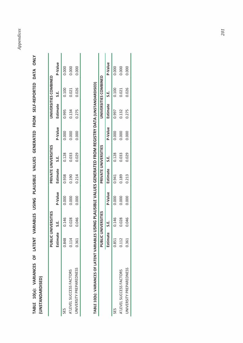
Appe

ndic

es

201

TABL

E 10

(a):

VARI

ANCE

S O

F LA

TEN

T VA

RIAB

LES

USI

NG

PLAU

SIBL

E VA

LUES

GE

NER

ATED

FR

OM

SE

LF-R

EPO

RTED

DA

TA

ON

LY

(UN

STAN

DARD

ISED

)

PU

BLIC

UN

IVER

SITI

ES

PRIV

ATE

UN

IVER

SITI

ES

UN

IVER

SITI

ES C

OM

BIN

ED

Es

timat

e S.

E.

P-Va

lue

Estim

ate

S.E.

P-

Valu

e Es

timat

e S.

E.

P-Va

lue

SES

0.84

8 0.

146

0.00

0 0.

938

0.12

8 0.

000

0.99

5 0.

100

0.00

0 A’

LEVE

L SU

CCES

S FA

CTO

RS

0.11

4 0.

028

0.00

0 0.

190

0.03

3 0.

000

0.13

4 0.

021

0.00

0 U

NIV

ERSI

TY P

REPA

REDN

ESS

0.36

1 0.

046

0.00

0 0.

214

0.02

9 0.

000

0.27

5 0.

026

0.00

0 TA

BLE

10(b

): VA

RIAN

CES

OF

LATE

NT

VARI

ABLE

S U

SIN

G P

LAU

SIBL

E VA

LUES

GEN

ERAT

ED F

ROM

REG

ISTR

Y DA

TA (U

NST

ANDA

RDIS

ED)

PU

BLIC

UN

IVER

SITI

ES

PRIV

ATE

UN

IVER

SITI

ES

UN

IVER

SITI

ES C

OM

BIN

ED

Es

timat

e S.

E.

P-Va

lue

Estim

ate

S.E.

P-

Valu

e Es

timat

e S.

E.

P-Va

lue

SES

0.85

1 0.

146

0.00

0 0.

941

0.12

8 0.

000

0.99

7 0.

100

0.00

0 A’

LEVE

L SU

CCES

S FA

CTO

RS

0.11

2 0.

028

0.00

0 0.

189

0.03

3 0.

000

0.13

2 0.

021

0.00

0 U

NIV

ERSI

TY P

REPA

REDN

ESS

0.36

1 0.

046

0.00

0 0.

213

0.02

9 0.

000

0.27

5 0.

026

0.00

0

Samenvatting

203

SAMENVATTING Het huidige strategisch onderwijsbeleid van Oeganda richt zich op de volgende belangrijke zorgen:

a) Basisonderwijs … te weinig kinderen verlaten het basisonderwijs met voldoende taal-,

reken- en algemene vaardigheden.

b) Voortgezet onderwijs … te weinig gediplomeerden hebben de kennis en de kunde die

benodigd is in de beroepsbevolking of het universitair onderwijs.

c) Universiteiten en technische instituten … slagen er niet in om studenten met een

achterstand in te laten stromen in een opleiding, noch adequaat in te spelen op een

groeiend aantal gekwalificeerde schoolverlaters met academische aspiraties.

(Ministerie van Onderwijs en Sport (Ministry of Education en Sports, MoES), 2008, pagina 3)

In dit proefschrift wordt het verband onderzocht tussen de omstandigheden in het voortgezet onderwijs en de prestaties van de studenten op de universiteit. De studenten die nu op de universiteit binnenkomen hebben hun vooropleiding gehad in een systeem dat veel veranderingen heeft ondergaan. In 1997 is het Algemene Basisonderwijs Programma (Universal Primary Education programme, UPE) gestart om alle kinderen met een schoolgaande leeftijd de mogelijkheid te bieden op onderwijs zonder schoolgeld. Helaas kon het systeem de toestroom die volgde niet aan, in het bijzonder die van de oudere kinderen. Dit resulteerde in een periode van aanpassingen, waarin klaslokalen overvol zaten en er een tekort aan gekwalificeerde leerkrachten was. Hoewel de introductie van UPE speciaal was gericht op meisjes en kinderen met lagere sociaaleconomische achtergronden, bleven er verscheidene sociale en economische factoren die zorgden voor een hoog uitval tijdens de basisschool en een slechte overgang naar het voortgezet onderwijs. De lage doorstroom werd gedeeltelijk veroorzaakt doordat families het schoolgeld voor het voortgezet onderwijs niet konden betalen, en gedeeltelijk door de te lage capaciteit van het voortgezet onderwijs voor deze nieuwe toestroom. Om te helpen dit probleem het hoofd te bieden startte de Oegandese overheid het Algemene Voortgezet Onderwijs Programma (Universal Secondary Education programme, USE) in 2007. Dit programma werd initieel geïmplementeerd op een klein aantal openbare scholen, maar is daarna ook overgenomen door enkele particuliere scholen. In de periode sinds de introductie van UPE en USE is het aantal universiteiten ook gegroeid van slechts 1 halverwege de jaren ’90 naar meer dan 30 nu. Hoewel deze snelle groei in het pre-universitair en universitair onderwijs de

Samenvatting

204

toegankelijkheid heeft bevorderd, zijn er zorgen dat er niet genoeg aandacht naar de kwaliteit is uitgegaan. Ook zijn er nog steeds zorgen over de toegankelijkheid voor studenten met een lagere sociaaleconomische achtergrond, in het bijzonder voor kwalitatief goed voortgezet en universitair onderwijs.

Vanuit de universiteiten is het wenselijk dat de studenten met de beste perspectieven worden geselecteerd voor de diverse academische opleidingen. Op dit moment is het belangrijkste selectiecriterium voor een student de score in het nationaal examen aan het einde van de tweede fase (advanced level of A’Level) van het voortgezet onderwijs. Maar, gezien de opvallende verschillen in slagingspercentages voor de verschillende A’Level vakken alsook in de gerapporteerde studieprogramma’s op veel scholen in het land, kan men zich afvragen of de A’Level scores een goed criterium zijn om studenten met de hoogste academische perspectieven te selecteren. Het hier beschreven onderzoek is gedaan om het verband tussen pre-universiteit scores en universiteit scores van studenten te onderzoeken. Dit is uitgevoerd in vier fasen:

a) Een verkennende studie om universiteitsstudenten onder te verdelen naar A’Level school, vakkenkeuze en scores

b) Een multilevel analyse om een aantal studenten school-gerelateerde factoren te bepalen, die mede verantwoordelijk zijn voor de variatie in A’Level scores

c) Een schatting van de relatieve A’Level moeilijkheidsgraad door gebruik te maken van de item response theorie (IRT)

d) Structural equation modellering (SEM) toepassen om te schatten in welke mate de A’Level scores de gemiddelde universitaire prestaties (cumulative grade point average, CGPA) voorspellen, gegeven de sociaaleconomische status (SES) van de student en de factoren van de vooropleiding

Een verkennende studie: Karakteriseren van Universiteitsstudenten

Om enige inzicht te verkrijgen in welke studenten succesvol op de universiteit in Oeganda instromen, werd een verkennende studie uitgevoerd. Op het moment van het verzamelen van de gegevens, waren er in Oeganda twaalf geaccrediteerde universiteiten en de gegevens komen van acht van deze. Omdat geesteswetenschappen door ongeveer 70% van de universiteitsstudenten gedaan worden, zijn op elke universiteit de volgende opleidingen geselecteerd: Bachelor of Development Studies, Bachelor of Business Administration en Bachelor of Information Technology. Gegevens waren beschikbaar voor drie tot vijf instroomgroepen op de verschillende universiteiten, van het academisch jaar 2005/2006 tot en met 2010/2011. De uiteindelijke selectie bestond uit ongeveer twaalfduizend studenten die hun A’Level gedaan hadden op ongeveer negenhonderd verschillende scholen, verspreid over de genoemde jaren (er zijn in Oeganda ongeveer 1200 scholen die A’Level examens afnemen). De verkennende studie laat het volgende zien:

1) De meerderheid van de studenten in de drie opleidingen kwam van slechts een klein deel van de scholen voor voortgezet onderwijs; In het bijzonder, meer dan

Samenvatting

205

50% van de studenten kwam van minder dan 10% van alle scholen voor voortgezet onderwijs.

2) Hoewel de universiteitsopleidingen in de gegevens varieerden van Development Studies tot Business Administration tot Information Technology, hadden de meeste studenten dezelfde vakken in hun A’Level, hoofdzakelijk kunst-gerelateerde vakken.

3) Het gemiddelde instroomcijfer voor studenten op openbare universiteiten was significant hoger dan die voor studenten op particuliere universiteiten.

Een Multilevel Analyse om Student- en School-gerelateerde Factoren te Bepalen,

die Mede Verantwoordelijk zijn voor de Variatie in A’Level Instroomcijfers op de

Universiteit

Voor dit deel van de studie zijn gegevens van de Nationale Examen Commissie van Oeganda (Uganda National Examination Board, UNEB) beschikbaar gesteld en deze bestonden uit de resultaten van alle studenten die het staatsexamen hadden afgelegd tussen 2005 en 2010. Gegroepeerd naar A’Level school, werd een multilevel analyse uitgevoerd op deze gegevens en op de gegevens van de instroom A’Level cijfers op de onderzochte universiteiten. De multilevel analyse laat het volgende zien:

1. Gecorrigeerd voor jaarlijkse fluctuaties, konden 30% van de variatie in studentprestaties aan het einde van de A’Level, en 24% van de variatie in universiteit instroomcijfers, worden toegeschreven aan de A’Level school waar de student op gezeten had.

2. Student-gerelateerde variabelen, zoals geslacht en leeftijd hebben weinig invloed, maar school-gerelateerde variabelen, zoals openbaar/particulier, wel of geen kostschool en wel of niet deelnemen aan het ondersteuningsbeleid van de overheid (USE programma) verklaren ongeveer 20% van het school-effect op A’Level en 13% op universiteit.

3. Toegelaten worden tot een bepaalde universiteit verklaart bijna 50% van het school-effect binnen instroomcijfers en meer dan 30% van de student-gerelateerde verschillen.

Schatting van A’Level Moeilijkheidsgraad per Vak

Sommige universiteiten beschouwen bepaalde A’Level vakken als essentieel voor sommige opleidingen en geven daarom de A’Level scores op die vakken de hoogste weegfactor. De meerderheid van de universiteitsopleidingen hebben niet zulke beperkingen op A’Level vakken en sommige passen zelfs de hoogste weegfactoren toe op de beste scores van de student. Om de vergelijkbaarheid van de scores in verschillende A’Level vakken te kunnen bestuderen, wordt een IRT analyse uitgevoerd. Een tweedimensionaal model blijkt het beste te passen op de gegevens, zodat de vakken worden verspreid over een exacte en een niet-exacte dimensie. Ook hadden exacte

Samenvatting

206

vakken, zoals scheikunde en natuurkunde niet alleen de hoogste geschatte moeilijkheidsgraad, maar hun A’Level scores gaven ook het hoogste onderscheidend vermogen in student prestatievermogen (Ability). Vakken, zoals geschiedenis en aardrijkskunde hadden een gemiddelde geschatte moeilijkheidsgraad en gaven een goed onderscheidend vermogen. Sommige andere vakken, zoals kunst en Kiswahilli hadden niet alleen een lage geschatte moeilijkheidsgraad, maar gaven ook weinig onderscheidend vermogen in het prestatievermogen. Een vergelijkbare procedure is gebruikt om de instroomcijfers in schalen voordat de geldigheid van hun voorspellend karakter voor de gemiddelde score op de universiteit (CGPA) bepaald wordt.

Bepalen van de Geldigheid van de het Voorspellend Karakter van het A’Level Staatsexamen

Dit proefschrift culmineert in een structural equation model (SEM) van student sociaaleconomische status, resultaten in de eerste fase (O’Level) en tweede fase (A’Level) van het voortgezet onderwijs en de gemiddelde score op de universiteit (CGPA). Vanwege verschillen in instroom karakteristieken en scoringsbeleid op universiteiten, worden studenten op openbare en particuliere universiteiten behandeld als afzonderlijke populaties. Uit de data bleek dat, na correctie voor de sociaaleconomische status en vooropleiding van de student, de instroomcijfers voor A’Level de CGPA voorspelden voor zowel openbare als particulieren universiteiten. Bovendien waren O’Level prestaties ook een goede indicatie voor A’Level prestaties voor universiteitsstudenten, en deze O’Level prestaties hingen nauw samen met de sociaaleconomische status. Echter, de effecten van de sociaaleconomische status waren nauwelijks significant bij de instroom op de universiteit, dit komt mogelijk doordat deze effecten sterker zijn bij eerdere selectiemomenten in het onderwijssysteem. Verrassend was dat studenten met een lage sociaaleconomische status iets beter presteerden op de universiteit dan studenten met een hoge sociaaleconomische status. Dit resultaat vraagt om meer onderzoek. Tot slot, O’Level prestaties hadden bijna geen effect op de gemiddelde score op de universiteit (CGPA), een bevinding die in tegenspraak is met observaties van vergelijkbare onderwijssystemen.

Al met al lijkt het dat, ondanks de opschudding ten gevolge van de vele veranderingen in het voortgezet en universitair onderwijs sinds eind jaren ‘90, de A’Level examen resultaten nog steeds een redelijk goede indicatie zijn voor instroomselectie voor de meeste universitaire opleidingen in Oeganda.

Ministerie van Onderwijs en Sport (Ministry of Education and Sports, MoES). (2008). Strategisch plan Herziening Onderwijssector 2007-2015. Kampala: Auteur. Gedownload van http://www.education.go.ug/files/downloads/Revised%20Education%20Sector%20strategic%20plan%202007-2015(1).pdf

thesis_C_Nshemereirwe.pdf - University of Twente Research ...

Documents

Transcript of thesis_C_Nshemereirwe.pdf - University of Twente Research ...