
From Classical to Tight Binding and First Principles Methods
195
POUR L'OBTENTION DU GRADE DE DOCTEUR ÈS SCIENCES acceptée sur proposition du jury: Prof. K. Johnsson, président du jury Prof. U. Röthlisberger, directrice de thèse Prof. M. Dal Peraro, rapporteur Prof. T. Frauenheim, rapporteur Dr A. P. Seitsonen, rapporteur Approaches to Increase the Accuracy of Molecular Dynamics Simulations: From Classical to Tight Binding and First Principles Methods THÈSE N O 5833 (2013) ÉCOLE POLYTECHNIQUE FÉDÉRALE DE LAUSANNE PRÉSENTÉE LE 30 JUILLET 2013 À LA FACULTÉ DES SCIENCES DE BASE LABORATOIRE DE CHIMIE ET BIOCHIMIE COMPUTATIONNELLES PROGRAMME DOCTORAL EN CHIMIE ET GÉNIE CHIMIQUE Suisse 2013 PAR Manuel DÖMER
-
Upload
khangminh22 -
Category
Documents
-
view
0 -
download
0
Transcript of From Classical to Tight Binding and First Principles Methods
POUR L'OBTENTION DU GRADE DE DOCTEUR ÈS SCIENCES
acceptée sur proposition du jury:
Prof. K. Johnsson, président du juryProf. U. Röthlisberger, directrice de thèse
Prof. M. Dal Peraro, rapporteur Prof. T. Frauenheim, rapporteur Dr A. P. Seitsonen, rapporteur
Approaches to Increase the Accuracy of Molecular Dynamics Simulations:
From Classical to Tight Binding and First Principles Methods
THÈSE NO 5833 (2013)
ÉCOLE POLYTECHNIQUE FÉDÉRALE DE LAUSANNE
PRÉSENTÉE LE 30 JUILLET 2013
À LA FACULTÉ DES SCIENCES DE BASELABORATOIRE DE CHIMIE ET BIOCHIMIE COMPUTATIONNELLES
PROGRAMME DOCTORAL EN CHIMIE ET GÉNIE CHIMIQUE
Suisse2013
PAR
Manuel DöMER


AcknowledgementsI would like to express my gratitude to all the people who have supported me along the way of
this thesis.
I thank my supervisor Ursula for accepting me as a PhD candidate in her group and giving me
the opportunity and freedom to delve into so many areas of computational chemistry. I also
thank Kai Johnson, Thomas Frauenheim, Ari Seitsonen and Matteo Dal Peraro for joining the
thesis jury.
From the LCBC I will remember Ivano as a great character with an admirable calmness who
opened the CPMD box for me. For the help on the initial tight binding project my thanks go to
Jan and the work on QM/MM force matching would not have been possible without Patrick.
Also with Elisa, Pablo and Matteo I have had a wonderful time working on projects that took
off based on friendship and the passion for solving problems. Indeed, the academic world
has connected me with so many great people - be it as office mates, at the coffee table or the
bar: Such as Basile, Tom, Stefano, Felipe, Bruno, Enrico and Julian. I also have to thank three
great friends for triggering my curiosity for computational sciences in the first place: Bettina,
Thomas and Daniele.
Besides working on the projects of my thesis I enjoyed my duties as a teaching assistant and to
support students with their semester projects. I probably learned more from Sebastian than
he did from me!
I would not even be here without the support of my parents, Michael and Angelika, my brother
Julian and Isabelle. I thank you for believing in me and just being in my life. This extends to
Cathrin and Pipe, thinking of all the wonderful moments we have shared.
Lausanne, 29 Mai 2013 M. D.
iii

AbstractThe predictive power of molecular dynamics simulations is determined by the accessible
system sizes, simulation times and, above all, the accuracy of the underlying potential energy
surface. Tremendous progress has been achieved in recent years to extend the system sizes via
multi-scale approaches and the accessible simulation times by enhanced sampling techniques.
Such improvements on the sampling issues shift the focus of development on the accuracy of
the potential energy surface.
A first goal of this thesis was to assess the accuracy limits of a variety of computational methods
ranging from classical force fields over the self-consistent-charge density functional tight-
binding method (SCC-DFTB), various density functional theory (DFT) methods, to wave
function based ab initio methods in identifying the correct lowest energy structures. As ex-
perimental benchmark data to assess the performance of different computational methods
we used high-resolution conformer-selective vibrational spectra, measured by cold-ion spec-
troscopy, of protonated tryptophan and gramicidin S in the group of T. Rizzo at EPFL. These
studies showed that most empirical force fields performed rather poorly in describing the
correct relative energetics of these molecules, possibly due to the limited transferability of
their underlying parameters.
With the goal to increase the accuracy of classical molecular mechanics force fields we imple-
mented a recently developed force-matching protocol for an automated parametrisation of
biomolecular force fields from mixed quantum mechanics/molecular mechanics (QM/MM)
reference calculations in the CPMD software package. Such a force field has an accuracy that
is comparable to the QM/MM reference, but at the greatly reduced computational cost of the
MM approach. We have applied this protocol to derive in situ FF parameters for the retinal
chromophore in rhodopsin embedded in a lipid bilayer.
In a similar effort, we employed iterative Boltzmann inversion to derive repulsive potentials for
SCC-DFTB. We used reference data at the DFT/PBE level to derive highly accurate parameters
for liquid water at ambient conditions, a particularly challenging case for conventional SCC-
DFTB. The newly determined parameters significantly improved the structural and dynamical
properties of liquid water at the SCC-DFTB level.
In a third project of the thesis we explored possible accuracy improvements in the context
of DFT methods. Dispersion Corrected Atom Centered Potentials (DACPs) are a recently
developed method to cure the failure of DFT methods within the generalised gradient approxi-
mation to describe dispersion interactions. Here, we complemented the existing library of
DCACP parameters by the halogens and compared the performance of various dispersion
v

Abstract
corrected DFT methods in reproducing high-level benchmark calculations on weakly bound
prototype complexes involving halogen atoms.
Keywords: Molecular Dynamics, Molecular Mechanics, Tight Binding, Density Functional
Theory, QM/MM, Force Matching, Iterative Boltzmann Inversion, Dispersion Interactions.
vi
KurzbeschreibungDie Voraussagekraft von Molekulardynamik-Simulationen wird durch die zugänglichen Sy-
stemgrössen, Simulationszeiten und vor allen Dingen durch die Genauigkeit der ihnen zu-
grunde liegenden Potentialoberflächen bestimmt. In den letzten Jahren konnten die System-
grössen mit Hilfe von Multi-Skalen-Methoden und die Simulationszeiten über verbesserte
Sampling-Verfahren erheblich erweitert werden. Diese Fortschritte lenken den Fokus weiterer
Entwicklungen immer mehr auf die Genauigkeit der Potentialoberflächen.
Ein erstes Ziel dieser Dissertation war, die Genauigkeit einer Auswahl von computergestützten
Methoden in der Vorhersage der stabilsten Struktur biologisch relevanter Moleküle beur-
teilen zu können. Die verwendeten Methoden reichten von klassischen Kraftfeldern über
die Self-Consistent-Charge Density Functional Tight-Binding (SCC-DFTB) Methode und ver-
schiedenen Dichtefunktionaltheorie (DFT) Methoden bis hin zu Wellenfunktions-basierten
ab initio-Methoden. Als experimentelle Referenz-Daten zur Beurteilung der verschiedenen
Methoden wurden hoch-aufgelöste konformations-spezifische Schwingungsspektren von
protoniertem Tryptophan und Gramicidin S bei Temperaturen um ≈10 K, welche in der
Gruppe von T. Rizzo an der EPFL aufgenommen worden waren, verwendet. Diese Untersu-
chungen haben gezeigt, dass die meisten empirischen Kraftfelder, möglicherweise aufgrund
der begrenzten Transferabilität der enthaltenen Parameter, unter Gasphasenbedingungen
die relativen Energien unterschiedlicher Konformationen dieser Moleküle relativ schlecht
beschreiben.
Mit dem Ziel, die Genauigkeit klassischer Kraftfelder zu verbessern, haben wir eine kürzlich
entwickelte Force-Matching-Methode zur automatischen Parameterisierung biomolekularer
Kraftfelder, basierend auf kombinierten Quantenmechanik/Molekülmechanischen (QM/MM)
Referenz-Rechnungen, im Software-Packet CPMD implementiert. Ein solches Kraftfeld hat
eine der QM/MM Referenz-Methode vergleichbare Genauigkeit, allerdings wird nur der deut-
lich kleinere Rechenaufwand der MM-Methode benötigt. Dieses Verfahren wurde nun zur
Bestimmung von in situ-Parametern für Retinal in Rhodopsin, eingebettet in einer Lipid-
Doppelmembran, verwendet.
In einer ähnlichen Studie wurde die Methode der iterativen Boltzmann-Inversion angewen-
det, um Repulsiv-Potentiale für die SCC-DFTB Methode zu parameterisieren. Dabei wurden
DFT/PBE Referenz-Rechnungen benutzt, um hochgenaue Parameter für flüssiges Wasser
bei Normalbedingunen zu bestimmen, welches ein besonders anspruchsvolles System für
konventionelles SCC-DFTB darstellt. Mit Hilfe der neuen Parameter konnten die strukturellen
und dynamischen Eigenschaften von flüssigem Wasser, wie sie vom SCC-DFTB beschrieben
vii

Abstract
werden, deutlich verbessert werden.
In einem dritten Projekt dieser Doktorarbeit wurden mögliche Verbesserungen in der Ge-
nauigkeit von DFT-Methoden erkundet. Mit Hilfe der kürzlich entwickelten Methode der
dispersionskorrigierten atomzentrierten Potentiale (DCACP) können Fehler von DFT Metho-
den, welche auf der verallgemeinerten Gradienten-Näherung basieren, bei der Beschreibung
von Dispersions-Wechselwirkungen behoben werden. In der vorliegenden Arbeit wurde die
bereits vorhandene Bibliothek von DCACP-Parametern um die Halogene ergänzt und die
Leistung unterschiedlicher dispersions-korrigierter DFT-Methoden gegenüber hochgenauen
Referenz-Rechnungen an prototypischen, schwach gebundenen Halogen-Komplexen vergli-
chen.
Stichwörter: Molekulardynamik, Molekülmechanik, Tight Binding, Dichtefunktionaltheorie,
QM/MM, Force Matching, Iterative Boltzmann-Inversion, Dispersions-Wechselwirkungen.
viii
ContentsAcknowledgements iii
Abstract (English/Deutsch) v
List of Figures xi
List of Tables xiv
Introduction 1
1 Theoretical Background 7
1.1 The Molecular Hamiltonian . . . . . . . . . . . . . . . . . . . . . . . . . . . . . . . 7
1.2 Density Functional Theory . . . . . . . . . . . . . . . . . . . . . . . . . . . . . . . 9
1.3 Self-Consistent Charge Density Functional Tight Binding (SCC-DFTB) . . . . . 13
1.4 Molecular Mechanics Force Fields . . . . . . . . . . . . . . . . . . . . . . . . . . . 17
1.5 Quantum Mechanical/Molecular Mechanics (QM/MM) . . . . . . . . . . . . . . 18
1.6 Molecular Dynamics . . . . . . . . . . . . . . . . . . . . . . . . . . . . . . . . . . . 21
2 Assessment of Computational Methods to Determine Low Energy Conformations of
Biomolecules 23
2.1 Cold-Ion Spectroscopy and Quantum Chemistry: A Successful Tandem to Deter-
mine Low Energy Structures of Bare and Microsolvated Protonated Tryptophan 23
2.1.1 Introduction . . . . . . . . . . . . . . . . . . . . . . . . . . . . . . . . . . . . 23
2.1.2 Methods . . . . . . . . . . . . . . . . . . . . . . . . . . . . . . . . . . . . . . 25
2.1.3 Results and Discussion . . . . . . . . . . . . . . . . . . . . . . . . . . . . . . 26
2.1.4 Determination of the Lowest Energy Conformers of [TrpH]+ . . . . . . . 27
2.1.5 Summary of the Performance of Different Computational Methods to
Reproduce CBS-C Energetics . . . . . . . . . . . . . . . . . . . . . . . . . . 40
2.1.6 Conclusions . . . . . . . . . . . . . . . . . . . . . . . . . . . . . . . . . . . . 41
2.2 Determination of the Intrinsic Structure of Gramicidin S . . . . . . . . . . . . . . 43
2.3 Assessing the Performance of Computational Methods for the Prediction of the
Ground State Structure of Gramicidin S . . . . . . . . . . . . . . . . . . . . . . . . 49
2.3.1 Introduction . . . . . . . . . . . . . . . . . . . . . . . . . . . . . . . . . . . . 49
2.3.2 Methods . . . . . . . . . . . . . . . . . . . . . . . . . . . . . . . . . . . . . . 51
2.3.3 Results . . . . . . . . . . . . . . . . . . . . . . . . . . . . . . . . . . . . . . . 51
ix
Contents
2.3.4 Discussion and Conclusions . . . . . . . . . . . . . . . . . . . . . . . . . . 57
3 Deriving Molecular Mechanics Force Field Parameters by Force Matching from DFT/MM
Calculations 61
3.1 Introduction . . . . . . . . . . . . . . . . . . . . . . . . . . . . . . . . . . . . . . . . 61
3.2 Methods . . . . . . . . . . . . . . . . . . . . . . . . . . . . . . . . . . . . . . . . . . 65
3.2.1 QM/MM Force Matching . . . . . . . . . . . . . . . . . . . . . . . . . . . . 65
3.2.2 Implementation in CPMD and Practical Remarks . . . . . . . . . . . . . . 67
3.2.3 Computational Details . . . . . . . . . . . . . . . . . . . . . . . . . . . . . . 70
3.3 Results and Discussion . . . . . . . . . . . . . . . . . . . . . . . . . . . . . . . . . . 71
3.3.1 Fit of Atomic Point Charges . . . . . . . . . . . . . . . . . . . . . . . . . . . 72
3.3.2 The Bonded Parameters . . . . . . . . . . . . . . . . . . . . . . . . . . . . . 73
3.3.3 Performance of the new force field . . . . . . . . . . . . . . . . . . . . . . . 77
3.4 Conclusions . . . . . . . . . . . . . . . . . . . . . . . . . . . . . . . . . . . . . . . . 79
4 Improving SCC-DFTB Parameters by Iterative Boltzmann Inversion 81
4.1 Introduction . . . . . . . . . . . . . . . . . . . . . . . . . . . . . . . . . . . . . . . . 81
4.2 Methods . . . . . . . . . . . . . . . . . . . . . . . . . . . . . . . . . . . . . . . . . . 83
4.2.1 The Repulsive Potentials . . . . . . . . . . . . . . . . . . . . . . . . . . . . . 83
4.2.2 The Iterative Boltzmann-Inversion Scheme Applied to Repulsive SCC-
DFTB Potentials . . . . . . . . . . . . . . . . . . . . . . . . . . . . . . . . . . 83
4.2.3 Computational Details . . . . . . . . . . . . . . . . . . . . . . . . . . . . . . 85
4.2.4 Analysis Methods . . . . . . . . . . . . . . . . . . . . . . . . . . . . . . . . . 86
4.3 Results and Discussion . . . . . . . . . . . . . . . . . . . . . . . . . . . . . . . . . . 87
4.3.1 Parameterisation of the Repulsive Potentials . . . . . . . . . . . . . . . . . 87
4.3.2 Structural Properties . . . . . . . . . . . . . . . . . . . . . . . . . . . . . . . 91
4.3.3 Dynamical Properties . . . . . . . . . . . . . . . . . . . . . . . . . . . . . . 92
4.3.4 Water Dimer . . . . . . . . . . . . . . . . . . . . . . . . . . . . . . . . . . . . 95
4.4 Conclusions . . . . . . . . . . . . . . . . . . . . . . . . . . . . . . . . . . . . . . . . 95
5 Intricacies of Describing Weak Interactions Involving Halogen Atoms Using Density
Functional Theory 97
5.1 Introduction . . . . . . . . . . . . . . . . . . . . . . . . . . . . . . . . . . . . . . . . 97
5.2 Methods . . . . . . . . . . . . . . . . . . . . . . . . . . . . . . . . . . . . . . . . . . 99
5.2.1 Dispersion Corrected Atom Centered Potentials (DCACPs) and Calibration 99
5.2.2 Computational Details . . . . . . . . . . . . . . . . . . . . . . . . . . . . . . 101
5.2.3 Statistical Quantities . . . . . . . . . . . . . . . . . . . . . . . . . . . . . . . 102
5.3 Results and Discussion . . . . . . . . . . . . . . . . . . . . . . . . . . . . . . . . . . 103
5.3.1 Performance for (X2)2 Complexes . . . . . . . . . . . . . . . . . . . . . . . 103
5.3.2 Performance for X2−Ar Complexes . . . . . . . . . . . . . . . . . . . . . . 105
5.3.3 Performance for the H3CX · · ·OCH2 Complexes . . . . . . . . . . . . . . . 105
5.3.4 Summary of the Performance of the Different Methods . . . . . . . . . . 107
5.4 Conclusion . . . . . . . . . . . . . . . . . . . . . . . . . . . . . . . . . . . . . . . . . 111
x

Contents
Summary and Outlook 113
A Supporting Information for Section 2.1 117
A.1 Experimental Approach for the Conformer-Selective Vibrational Spectra of Cold
Protonated Tryptophan . . . . . . . . . . . . . . . . . . . . . . . . . . . . . . . . . 117
A.2 The CBS-C Method . . . . . . . . . . . . . . . . . . . . . . . . . . . . . . . . . . . . 118
A.3 Basis Set Assessment on [Trp+H]+ . . . . . . . . . . . . . . . . . . . . . . . . . . . 119
A.4 Examples of different Low Energy Conformations and Water Binding Sites . . . 120
A.5 Assessment of different Methods to reproduce CBS-C energetics for [Trp+H]+ ·(H2O) . . . . . . . . . . . . . . . . . . . . . . . . . . . . . . . . . . . . . . . . . . . . 122
A.6 Assessment of different Methods to reproduce CBS-energetics for [Trp+H]+ ·(H2O)2 . . . . . . . . . . . . . . . . . . . . . . . . . . . . . . . . . . . . . . . . . . . 127
B QM/MM Force Matching in CPMD 133
B.1 Overview of the Force Matching Routines . . . . . . . . . . . . . . . . . . . . . . . 133
B.2 keywords . . . . . . . . . . . . . . . . . . . . . . . . . . . . . . . . . . . . . . . . . . 134
B.3 Files generated . . . . . . . . . . . . . . . . . . . . . . . . . . . . . . . . . . . . . . 138
B.4 CPMD routines . . . . . . . . . . . . . . . . . . . . . . . . . . . . . . . . . . . . . . 139
B.5 Forcematching Routines . . . . . . . . . . . . . . . . . . . . . . . . . . . . . . . . . 141
C A New Force Field for the Retinal Protonated Schiff Base in Rhodopsin 147
Bibliography 157
Curriculum Vitae 177
xi


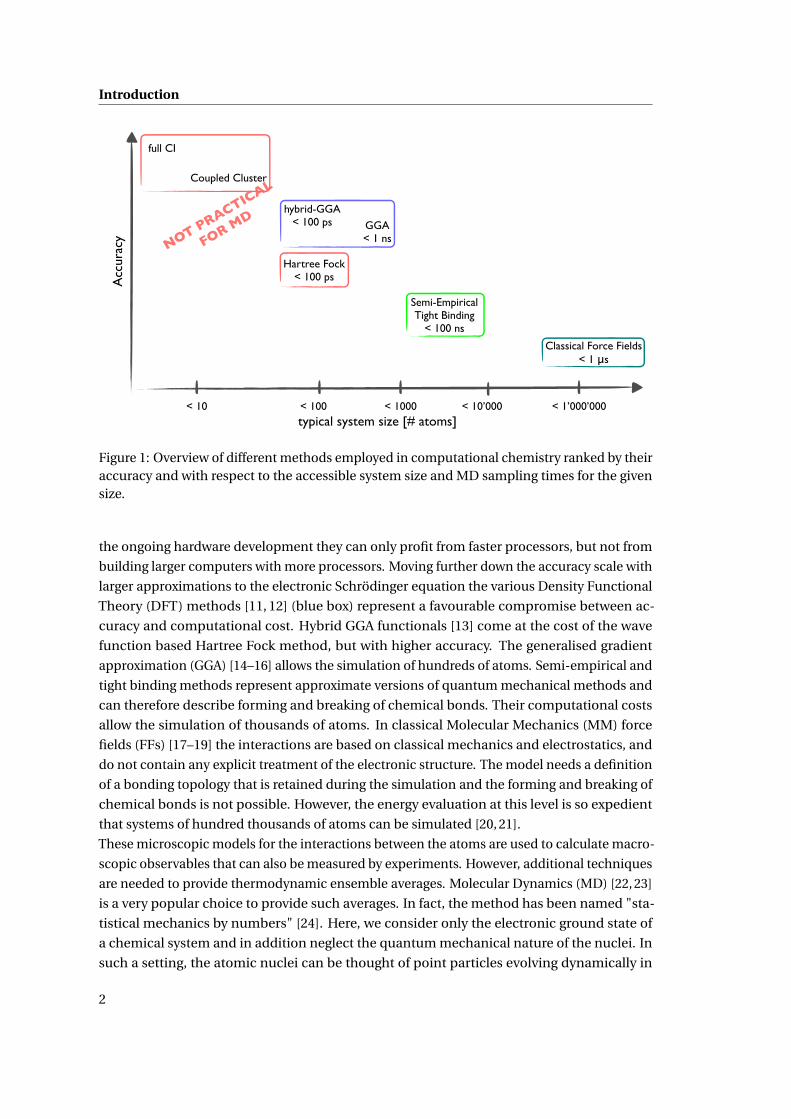
List of Figures1 Overview of different methods employed in computational chemistry . . . . . . 2
2 Illustration of the molecular dynamics method . . . . . . . . . . . . . . . . . . . 3
1.1 Illustration of the QM/MM boundary across a chemical bond . . . . . . . . . . . 19
1.2 Illustration of the electrostatic QM/MM coupling scheme . . . . . . . . . . . . . 20
2.1 Notation for bare and micro solvated tryptophan . . . . . . . . . . . . . . . . . . 27
2.2 Experimental and calculated IR spectra of the low energy structures of [TrpH]+ 28
2.3 Low energy conformations of [TrpH]+ . . . . . . . . . . . . . . . . . . . . . . . . . 28
2.4 Experimental and calculated IR spectra of the lowest energy conformation of
[TrpH · (H2O)]+ . . . . . . . . . . . . . . . . . . . . . . . . . . . . . . . . . . . . . . 34
2.5 Experimental and Calculated IR spectra for the lowest energy conformations of
[TrpH · (H2O)2]+ . . . . . . . . . . . . . . . . . . . . . . . . . . . . . . . . . . . . . . 39
2.6 Summary of the performance of various methods in reproducing the CBS-C
relative energetics for bare and micro solvated tryptophan . . . . . . . . . . . . 40
2.7 IR Spectra for the major conformation of Gramicidin S . . . . . . . . . . . . . . . 45
2.8 IR fingerprint region of the major conformation of Gramicidin S . . . . . . . . . 46
2.9 Gramicidin S lowest-energy conformer of the isolated species vs. crystal structure 47
2.10 Conformation R01 optimised at the M05-2X/6-31G(d,p) level of theory . . . . . 53
2.11 Experimental IR spectrum compared to calculated frequencies of R01 . . . . . . 54
2.12 R01 top and side view . . . . . . . . . . . . . . . . . . . . . . . . . . . . . . . . . . 58
2.13 R06 top and side view . . . . . . . . . . . . . . . . . . . . . . . . . . . . . . . . . . 59
2.14 R09 top and side view . . . . . . . . . . . . . . . . . . . . . . . . . . . . . . . . . . 60
3.1 Rhodopsin embedded in a lipid bilayer and water solvent . . . . . . . . . . . . . 64
3.2 11-cis retinal, Lys296 and Glu113 . . . . . . . . . . . . . . . . . . . . . . . . . . . . 64
3.3 Influence of the weighting factors on the electrostatic properties . . . . . . . . . 73
3.4 Atomic charges close to the QM/MM boundary . . . . . . . . . . . . . . . . . . . 74
3.5 Absorption spectra of bovine rhodopsin . . . . . . . . . . . . . . . . . . . . . . . 79
4.1 Definition of hydrogen bonding angles . . . . . . . . . . . . . . . . . . . . . . . . 86
4.2 Iterative Boltzmann inversion for the O-O repulsive potentials . . . . . . . . . . 88
4.3 Iterative Boltzmann inversion for the O-H repulsive potentials . . . . . . . . . . 89
4.4 Radial distribution functions for liquid water . . . . . . . . . . . . . . . . . . . . . 91
4.5 Probability distributions of the hydrogen bonding angles . . . . . . . . . . . . . 93
xiii

List of Figures
4.6 The orientational autocorrelation functions . . . . . . . . . . . . . . . . . . . . . 94
5.1 Interaction energies of the X2 · · ·X2 dimers (X=F, Cl, Br, I) . . . . . . . . . . . . . . 104
5.2 Interaction energies of the X2 · · ·Ar (X=F,Cl,Br,I) complexes . . . . . . . . . . . . 106
5.3 Interaction energies of the H3CX · · ·OCH2 complexes (X=Cl,Br,I) . . . . . . . . . 108
5.4 Comparison of the relative errors in the binding energy of different methods . . 109
5.5 Comparison of the MAX, RMS, MSE and MUE for different methods . . . . . . . 110
A.1 Working examples for the isomer notation . . . . . . . . . . . . . . . . . . . . . . 121
B.1 flow chart of the force matching protocol in cpmd . . . . . . . . . . . . . . . . . 133
B.2 example of the forcematching block within the “&QMMM” section of a cpmd
input file . . . . . . . . . . . . . . . . . . . . . . . . . . . . . . . . . . . . . . . . . . 134
xiv

List of Tables2.1 Relative energies of all low energy conformations of [TrpH]+ at various levels of
theory . . . . . . . . . . . . . . . . . . . . . . . . . . . . . . . . . . . . . . . . . . . . 30
2.2 Summary of the performance of different methods to reproduce the CBS-C
energetics of [TrpH]+ . . . . . . . . . . . . . . . . . . . . . . . . . . . . . . . . . . . 32
2.3 CBS-C relative energetics of the low energy conformations of [TrpH · (H2O)]+ . 33
2.4 Performance of various methods to reproduce the CBS-C relative energetics of
[TrpH · (H2O)]+ . . . . . . . . . . . . . . . . . . . . . . . . . . . . . . . . . . . . . . 35
2.5 CBS-C relative energetics of the low energy conformations of [TrpH · (H2O)2]+ . 38
2.6 Summary of the performance of different methods to reproduce the CBS-C
energetics of [TrpH · (H2O)2]+ . . . . . . . . . . . . . . . . . . . . . . . . . . . . . . 38
2.7 Structural parameters of [GS+2 H]2+ conformations R01-R09 . . . . . . . . . . . 52
2.8 M05-2X/6-31G(d,p) relative energetics of R01-R09 . . . . . . . . . . . . . . . . . 56
3.1 Derived atomic point charges for retinal in rhodopsin . . . . . . . . . . . . . . . 74
3.2 New parameters for the bonds in the RET and Lys296 moiety . . . . . . . . . . . 75
3.3 New parameters for the angles in the RET and Lys296 moiety . . . . . . . . . . . 76
3.4 Relevant properties obtained from the optimised classical force field for retinal 77
4.1 Diffusion Coefficients for liquid water . . . . . . . . . . . . . . . . . . . . . . . . . 92
4.2 Fitting parameters for the orientational auto-correlation functions . . . . . . . 93
4.3 Water dimer . . . . . . . . . . . . . . . . . . . . . . . . . . . . . . . . . . . . . . . . 95
5.1 DCACP parameters for the halogens . . . . . . . . . . . . . . . . . . . . . . . . . . 101
5.2 Equilibrium distances and interaction energies of the complexes X2 · · ·X2 . . . . 104
5.3 Unsigned error of the binding energies of the X2 · · ·X2 (X=F,Cl,Br,I) complexes . 105
5.4 Equilibrium distances and binding energies of the X2 · · ·Ar complexes . . . . . . 106
5.5 Unsigned error of the binding energies of the X2 · · ·Ar (X=F,Cl,Br,I) complexes . 107
5.6 Equilibrium properties of the H3CX · · ·OCH2 (X=Cl,Br,I) complexes . . . . . . . 107
5.7 Unsigned error of the binding energies of the H3CX · · ·OCH2 systems (X=Cl,Br,I) 108
5.8 Computational overhead of various dispersion corrected methods . . . . . . . . 111
A.1 Basis Set Assessment on two Conformations of [TrpH]+ . . . . . . . . . . . . . . 120
A.2 Basis Set Assessment on [TrpH]+ . . . . . . . . . . . . . . . . . . . . . . . . . . . . 120
A.3 Relative energetics for [TrpH ·H2O]+ at various levels of theory . . . . . . . . . . 122
xv

List of Tables
A.4 Relative energetics for [TrpH ·H2O]+ at various levels of theory . . . . . . . . . . 123
A.5 Relative energetics for [TrpH ·H2O]+ at various levels of theory . . . . . . . . . . 123
A.6 Relative energetics for [TrpH ·H2O]+ at various levels of theory . . . . . . . . . . 124
A.7 Relative energetics for [TrpH ·H2O]+ at various levels of theory . . . . . . . . . . 125
A.8 RMSD and MAX for [TrpH ·H2O]+ using different methods . . . . . . . . . . . . 126
A.9 Relative energetics for [TrpH · (H2O)2]+ at various levels of theory . . . . . . . . 128
A.10 Relative energetics for [TrpH · (H2O)2]+ at various levels of theory . . . . . . . . 129
A.11 Relative energetics for [TrpH · (H2O)2]+ at various levels of theory . . . . . . . . 130
A.12 Relative energetics for [TrpH · (H2O)2]+ at various levels of theory . . . . . . . . 131
A.13 RMSD and MAX for [TrpH · (H2O)2]+ using different methods . . . . . . . . . . . 132
xvi
Introduction
Along with the exponential increase in the performance of integrated electronic circuits [1]
computer simulations have earned an important role in chemistry [2]. They can be used
to compute properties of molecular systems and materials also under conditions that are
inaccessible to experiments or for which the synthesis is costly or time consuming. They
also allow to determine the three dimensional arrangements of atomic nuclei that are bound
together by their shared electrons, i.e. the chemical bonds. After all, chemistry is the study of
the rearrangements of atomic nuclei in molecules along with the electronic structure. How-
ever, most experiments do not give direct access to the three dimensional arrangements of
the nuclei, not to speak of the localisation of chemical bonds. On the other hand, structures
can be calculated via a computational model, which represents therefore an inherent part of
the protocol towards the interpretation of the experimental data. The calculated molecular
structure can serve as a basis for rationalisation, interpretation and prediction of chemical
properties.
The starting point for a computer simulation is the definition of a theoretical model for
the system under investigation. In this thesis, we restrict the models to atomistic resolution,
i.e. coarse grained methods [3, 4] are excluded from this discussion. Therefore, the size of
the model, its chemical composition and three dimensional structure need to be specified.
Furthermore, a choice has to be made for the level of theory at which the physical interactions
between the atoms are treated. Different levels of theory, each with particular advantages
and disadvantages, are available. Figure 1 ranks a selection of methods that are commonly
employed in computational chemistry according to their accuracy and gives their accessible
system size on today’s computer architectures. This overview is by far not exhaustive and
can only serve as a rough qualitative comparison. It illustrates, however, the unfortunate
restriction of the more accurate methods to smaller system sizes. The top of the accuracy scale
is occupied by methods based on quantum mechanics which allows an explicit description
of the electronic structure and the electronic rearrangements that occur during the forming
and breaking of chemical bonds. Among the wave function based methods (red boxes) com-
plete Configuration Interaction (CI) [5] (full CI in the complete basis set limit) represents the
exact numerical method for the solution of the time-independent non-relativistic electronic
Schrödinger equation [6]. The Coupled Cluster approach [7–10] predicts relative energies
within chemical accuracy. However, only systems with a few tens of atoms can be calculated.
Additionally, these methods are not ideal for parallelisation, which means that in terms of
1
Introduction
NOT PRACTICAL
FOR MD
Acc
urac
y
typical system size [# atoms]< 1’000’000< 10’000< 1000< 100< 10
Classical Force Fields< 1 μs
Semi-EmpiricalTight Binding
< 100 ns
GGA< 1 ns
hybrid-GGA< 100 ps
full CI
Coupled Cluster
Hartree Fock< 100 ps
Figure 1: Overview of different methods employed in computational chemistry ranked by theiraccuracy and with respect to the accessible system size and MD sampling times for the givensize.
the ongoing hardware development they can only profit from faster processors, but not from
building larger computers with more processors. Moving further down the accuracy scale with
larger approximations to the electronic Schrödinger equation the various Density Functional
Theory (DFT) methods [11, 12] (blue box) represent a favourable compromise between ac-
curacy and computational cost. Hybrid GGA functionals [13] come at the cost of the wave
function based Hartree Fock method, but with higher accuracy. The generalised gradient
approximation (GGA) [14–16] allows the simulation of hundreds of atoms. Semi-empirical and
tight binding methods represent approximate versions of quantum mechanical methods and
can therefore describe forming and breaking of chemical bonds. Their computational costs
allow the simulation of thousands of atoms. In classical Molecular Mechanics (MM) force
fields (FFs) [17–19] the interactions are based on classical mechanics and electrostatics, and
do not contain any explicit treatment of the electronic structure. The model needs a definition
of a bonding topology that is retained during the simulation and the forming and breaking of
chemical bonds is not possible. However, the energy evaluation at this level is so expedient
that systems of hundred thousands of atoms can be simulated [20, 21].
These microscopic models for the interactions between the atoms are used to calculate macro-
scopic observables that can also be measured by experiments. However, additional techniques
are needed to provide thermodynamic ensemble averages. Molecular Dynamics (MD) [22, 23]
is a very popular choice to provide such averages. In fact, the method has been named "sta-
tistical mechanics by numbers" [24]. Here, we consider only the electronic ground state of
a chemical system and in addition neglect the quantum mechanical nature of the nuclei. In
such a setting, the atomic nuclei can be thought of point particles evolving dynamically in
2
Introduction
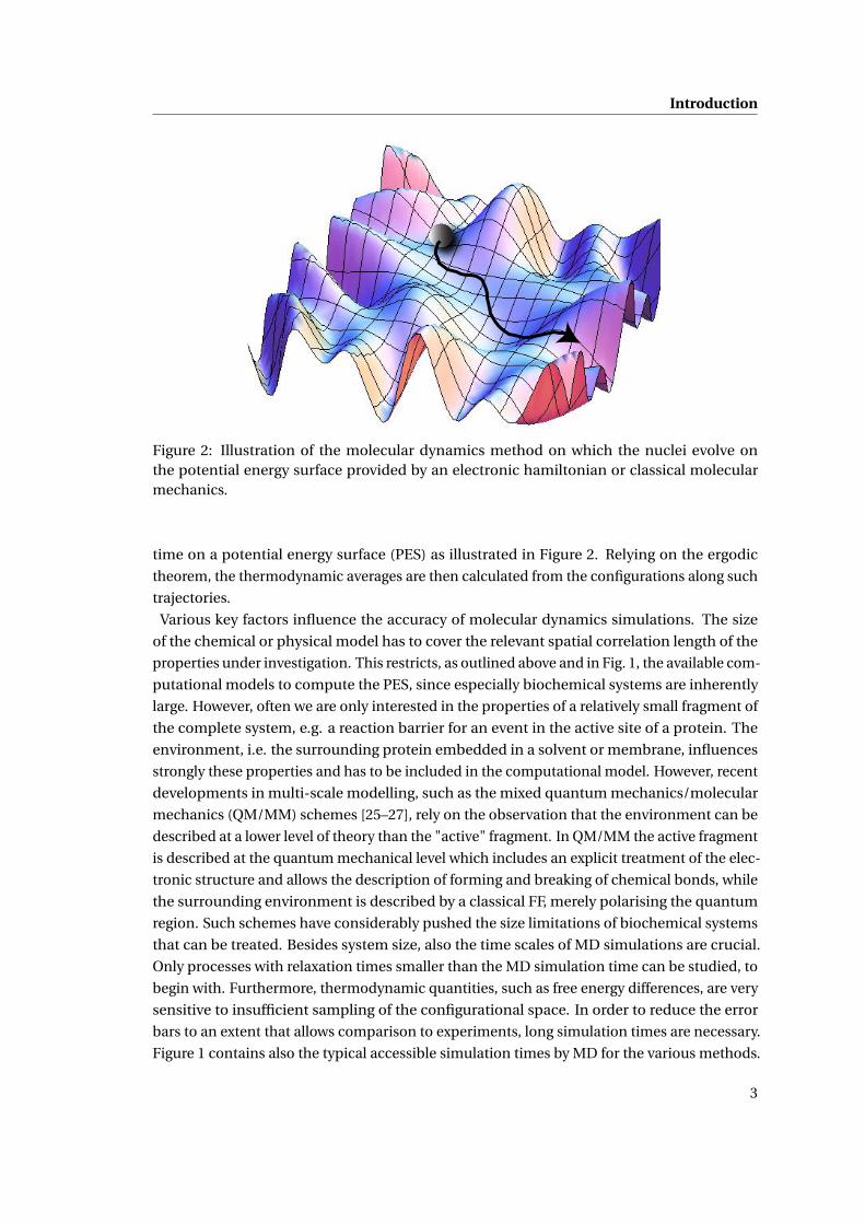
Figure 2: Illustration of the molecular dynamics method on which the nuclei evolve onthe potential energy surface provided by an electronic hamiltonian or classical molecularmechanics.
time on a potential energy surface (PES) as illustrated in Figure 2. Relying on the ergodic
theorem, the thermodynamic averages are then calculated from the configurations along such
trajectories.
Various key factors influence the accuracy of molecular dynamics simulations. The size
of the chemical or physical model has to cover the relevant spatial correlation length of the
properties under investigation. This restricts, as outlined above and in Fig. 1, the available com-
putational models to compute the PES, since especially biochemical systems are inherently
large. However, often we are only interested in the properties of a relatively small fragment of
the complete system, e.g. a reaction barrier for an event in the active site of a protein. The
environment, i.e. the surrounding protein embedded in a solvent or membrane, influences
strongly these properties and has to be included in the computational model. However, recent
developments in multi-scale modelling, such as the mixed quantum mechanics/molecular
mechanics (QM/MM) schemes [25–27], rely on the observation that the environment can be
described at a lower level of theory than the "active" fragment. In QM/MM the active fragment
is described at the quantum mechanical level which includes an explicit treatment of the elec-
tronic structure and allows the description of forming and breaking of chemical bonds, while
the surrounding environment is described by a classical FF, merely polarising the quantum
region. Such schemes have considerably pushed the size limitations of biochemical systems
that can be treated. Besides system size, also the time scales of MD simulations are crucial.
Only processes with relaxation times smaller than the MD simulation time can be studied, to
begin with. Furthermore, thermodynamic quantities, such as free energy differences, are very
sensitive to insufficient sampling of the configurational space. In order to reduce the error
bars to an extent that allows comparison to experiments, long simulation times are necessary.
Figure 1 contains also the typical accessible simulation times by MD for the various methods.
3

Introduction
Ab initio methods such as full CI or Coupled Cluster approaches, despite their accuracy, are
therefore not practical for molecular dynamics simulations due to their limitations not only in
system size, but also in sampling time. DFT methods reach sampling times in the range of
tens to hundreds of picoseconds, which offers, in combination with typical system sizes of a
few hundred atoms, adequate sampling for a range of structural and dynamical properties of
condensed phase systems [28–30]. Note however that the time scale of the reactions catalysed
by the fastest enzymes is in the order of microseconds, and protein folding occurs in the
microsecond to millisecond time frame [31, 32]. The latter can only, if at all, be reached by MD
based on classical force fields. Enhanced sampling techniques have improved this situation
considerably [33–38].
With the recent progress in extending the accessible system size and time scales in molecular
dynamics simulations, the remaining limiting factor is often the accuracy of the underlying
potential energy surface. To illustrate the typical accuracy that is needed for biological systems,
consider, for example, the temperature range of 100C for liquid water as the most important
solvent in biologically relevant applications. Such a temperature difference corresponds to
an energy difference of only 0.2 kcal/mol per degree of freedom, which poses very stringent
accuracy constraints on the potential energy landscape. This, however, can in practice only be
achieved by a trade-off, since the computation of a more accurate PES is also more demanding
in terms of computational resources and thereby restricts the accessible length and time scales
of the model system. Therefore a reasonable compromise between the level of accuracy and
the resulting computational cost has to be found.
The practical implications of the relation between accuracy and system size limitations are
explored in Chapter 2 of this thesis. With the aim of determining the lowest energy conforma-
tions of small protonated biomolecules, we explored the size limits for various levels of theory
and used high-resolution experimental data as a benchmark to test the accuracy of various
computational methods in identifying the correct lowest energy structures. In particular, we
assessed the composite ab initio method CBS-C [39, 40], MP2 [41], several DFT methods, a
Tight-Binding method [42], and several classical force fields [43–46]. These results demon-
strate how well high-level modern quantum chemistry methods and cold ion spectroscopy
work together in determining low energy structures of biomolecules in the gas phase, while
more approximate methods struggle to provide the necessary accuracy. However, the highly
accurate QM methods are only applicable to very small systems and do not allow for an ex-
haustive search of low energy conformers.
The remaining chapters of this thesis are therefore concerned with different strategies to
increase the accuracy of the underlying potential energy surface in empirical, tight binding
and DFT MD simulations. The common feature of these strategies is to parameterise lower
level methods by reference calculations from a higher level method. Simulations can then be
performed using the re-parameterised lower level method, which ideally can now reproduce
the higher level method’s accuracy, but at reduced computational cost. This in turn implies
that system sizes and sampling times are accessible that were prohibitive with the higher level
method.
Chapter 3 describes the implementation of a recently developed force-matching protocol [47]
4
Introduction
for an automated parametrisation of biomolecular FFs from QM/MM reference calcula-
tions [48] in the publicly available CPMD package [49]. In this scheme finite-temperature
QM/MM molecular dynamics simulations are performed with a QM fragment, for which MM
force field parameters are to be derived. Nuclear forces on the QM atoms and the electrostatic
potential and field are extracted from this trajectory to serve as target properties for the subse-
quent parameter fitting scheme. In this way, environment, finite temperature and pressure
effects are taken into account automatically. The force field determined in this manner has an
accuracy that is comparable to the one of the reference QM/MM calculation, but at the greatly
reduced computational cost of the MM approach. This allows calculating quantities that
would be prohibitive within a QM/MM approach, such as thermodynamic averages involving
slow motions of a protein. We have applied this protocol to derive in situ FF parameters for
the retinal chromophore in rhodopsin embedded in a lipid bilayer. Rhodopsin is a biological
pigment in the photoreceptor cells of the retina and constitutes the first member in a signalling
cascade responsible for the perception of light [50, 51]. The initial event upon light absorption
is the cis-trans isomerisation of the retinal chromophore within the binding pocket of the
protein [52–55]. The investigation of the structural variations after the absorption of light
has been an active field of research, both on the experimental [56–59] and computational
sides [60–63]. Biomolecular force fields have been employed to illuminate equilibrium prop-
erties of dark state rhodopsin and the large scale structural rearrangements of the protein
after light absorption [64, 65]. However, the parameter sets currently used for the retinal chro-
mophore [17, 61, 66] do not account for the variations of the carbon-carbon single and double
bonds along the conjugated π-system. This is a reasonable approximation if only large scale
conformational properties of the protein are concerned. However, recent investigations have
shown that the optical absorption spectrum calculated from configurations generated by such
an approximate bonding topology does not agree with experiments [67]. Currently, one has
to rely on QM/MM methods in order to generate realistic configurations for the calculations
of optical properties [68]. In order to overcome the time scale limitations associated with
this approach we apply the newly implemented QM/MM force matching protocol to derive a
consistent set of FF parameters that reproduce the structural and dynamical properties at the
QM/MM level. In contrast to the original FF, the new parameter set describes correctly the
variations of the carbon-carbon single and double bonds in the retinal. As a consequence, the
optical absorption spectrum calculated from configurations extracted from an MD trajectory
using the new FF, is in excellent agreement with the QM/MM and experimental references.
Moving up the hierarchy of computational methods, we next targeted a tight binding method.
The goal of Chapter 4 is the derivation of improved repulsive potentials for the self-consistent-
charge density functional tight-binding method (SCC-DFTB) [42] based on DFT reference
calculations. In the conventional parameterisation scheme for the SCC-DFTB repulsive poten-
tials the balanced description of different chemical environments involves significant human
effort and chemical intuition. Here, similar to the force matching protocol in Chapter 3, we
propose an in situ parameterisation method to derive parameters with reduced transferability
but maximal accuracy for the chemical and physical environment under investigation. In this
case we employ the iterative Boltzmann inversion method [69, 70] which uses radial distri-
5
Introduction
bution functions instead of atomic forces as a target quantity in the optimisation procedure.
Starting from an initial guess, we use iterative Boltzmann inversion to successively improve the
repulsive potentials. The corrections are extracted iteratively from the differences in the radial
distribution functions with respect to a reference calculated at the DFT/PBE level of theory. We
apply this new scheme to liquid water at ambient conditions, a particularly challenging case
for conventional SCC-DFTB [71, 72]. The newly determined parameters allow the calculations
of the structural and dynamical properties of liquid water with an accuracy similar to DFT/PBE
but at the cost of the normal SCC-DFTB method.
In Chapter 5, the accuracy of DFT is addressed and improved by a suitable parameterisation
protocol. In principle DFT is an exact theory [11, 12] but, the exact form of the exchange-
correlation functional is unknown. Today’s popular approximations, especially the functionals
based on the generalised gradient approximation (GGA) suffer from shortcomings in accu-
rately describing non-local long-range interactions (e.g. dispersion forces), which are of
pivotal importance in (bio-)chemical systems. In a recently introduced approach - based on
dispersion-corrected atom-centered potentials (DCACPs) [73] - the effect of dispersion forces
is taken into account via atomic orbital-dependent analytic potentials whose parameters are
determined from reference calculations at the coupled cluster level of theory. This scheme
was shown to be highly transferable [74–79]. It allows for an accuracy of essentially CCSD(T)
quality, while at the same time retaining the computational efficiency of the DFT/GGA method.
Especially, within the plane-wave/pseudopotential implementation of CPMD [49] the com-
putational overhead on the electronic structure calculation is only minor. In Chapter 5, the
existing element-specific DCACP library has been complemented with the parameters for
halogen atoms. Furthermore, we investigate the performance of various DFT methods, in-
cluding the newly derived DCACPs in conjunction with the BLYP functional, in reproducing
high-level wave function based benchmark calculations on the weakly bound halogen dimers,
as well as prototype halogen bonded complexes. Such an effort towards the identification of
computationally expedient and yet accurate methods to model halogen containing systems
is relevant for computational applications in a variety of fields, ranging from stratospheric
chemistry [80–84], materials science and engineering [85–92] to biological systems [93–96]
and medicinal chemistry [97–101].
In summary, we employed three different approaches to increase the accuracy of MD sim-
ulations. We used force matching to parameterise a classical force field for the retinal chro-
mophore in rhodopsin based on QM/MM reference calculations. Secondly, we employed
iterative Boltzmann inversion to derive improved repulsive potentials for the SCC-DFTB
method for liquid water. And, finally, we optimised element-specific DCACP parameters to
increase the accuracy of DFT methods for describing weak interactions involving halogen
atoms.
6
1 Theoretical Background
This chapter reviews, based on the indicated references, selected computational methods that
were used in the applications of Chapters 2 and 5 and that represent the underlying theoretical
framework for the developments in Chapters 3-5. For all of these methods a number of
excellent books and review articles is available and the interested reader is invited to consult
the suggested references for a discussion beyond this concise overview.
1.1 The Molecular Hamiltonian
The description of the breaking and forming of chemical bonds demands an explicit calcu-
lation of the electronic structure. Due to the wave like nature of the electrons, quantum
chemical methods have to be employed with the goal to find approximate solutions to the
time-independent, non-relativistic Schrödinger equation [6] for a molecular system consisting
of N electrons and M nuclei
H Ψ (ri , Rα) = E Ψ (ri , Rα) (1.1)
with the molecular Hamiltonian H [102, 103] in atomic units:
H =−1
2
M∑α=1
1
Mα∇2α−
1
2
N∑i=1
∇2i −
N∑i=1
M∑α=1
Zαriα
+N−1∑i=1
N∑j>i
1
ri j+
M−1∑α=1
M∑β>α
ZαZβRαβ
= Te + Tn + Ven + Vee + Vnn
(1.2)
α and β index the M nuclei, while i and j denote the N electrons in the system. The first two
terms represent the kinetic energy of the nuclei and electrons, respectively, with the nuclear
mass Mα. The third, fourth and fifth terms represent the nuclei-electrons and electrons-
electrons and nuclei-nuclei electrostatic interactions. ri j is the distance between electrons
i and j : ri j = |r j − ri |, analogously riα stands for the electron-nucleus distance and Rαβ for
the internuclear distance. The wave function Ψ (ri , Rα) is an eigenfunction of H with
eigenvalue E . It contains all information of the quantum mechanical system and depends on
7
Chapter 1. Theoretical Background
the collective spatial and spin coordinates of the N electrons ri and the spatial coordinates
of the nuclei, Rα. This Hamiltonian does not include relativistic corrections to the kinetic
energy, interactions of magnetic moments (orbit/orbit, spin/orbit, spin/spin), or interactions
with external electric and magnetic fields.
The Born-Oppenheimer (BO) approximation offers a simplification of the complex eigenvalue
problem in Eq. 1.1 by separating the nuclear from the electronic motion. This approach is
motivated by the significant difference in particle masses and assumes, that the electrons
adjust instantaneously to each new position of the nuclei. The approach is to calculate the
electronic wave functionΨelec for a situation of fixed nuclei, in which Tn = 0:
H elec (ri ; Rα) Ψelec (ri ; Rα) = E elec Ψelec (ri ; Rα) (1.3)
with
H elec = Te + Ven + Vee + Vnn (1.4)
Both, H elec (ri ; Rα) and Ψelec (ri ; Rα), depend explicitly on the electronic degrees of
freedom, but only parametrically on the nuclear coordinates Rα. Note, that Vnn is included
in the electronic Hamiltonian by convention, although it does not act on ri and results in a
trivial additive shift of the electronic energy. The resulting electronic energy (integrating over
the electronic degrees of freedom):
E elec (Rα) ≡ E elec[Ψelec (ri ; Rα)
]=
∫Ψelec* (ri ; Rα) H elec (ri ; Rα)Ψelec (ri ; Rα) dr
(1.5)
is a function of the nuclear coordinates.
The total electronic-nuclear wave function can be expanded in the complete orthonormal
set of eigenfunctions of H elec with the nuclear wave functions as the expansion coefficients.
Solving then the Schrödinger equation for the nuclear wave functions reveals coupling terms
in which Tn acts on the electronic states. Neglecting all such coupling terms leads to the
adiabatic BO approximation 1 and produces an effective Schrödinger equation for the nuclear
motion:
H nuc (Rα)χ (Rα) = Eχ (Rα) (1.6)
with
H nuc (Rα) = Tn (Rα)+E elec (Rα) (1.7)
1The Born-Oppenheimer approximation itself involves only the neglect of the terms in which Tn couplesdifferent electronic states. The term "adiabatic" is chosen in analogy to macroscopic processes which take placewithout heat transfer to the environment. See Refs. [28, 102] for more details and an explicit derivation.
8
1.2. Density Functional Theory
In this picture, E elec represents the effective potential energy surface on which the nuclear
wave functions χ (Rα) evolve.
We can, however, go one fundamental step further and neglect the quantum nature of the nu-
clei altogether. Contracting them to classical particles leaves us with a total energy expression
as a function of the nuclear coordinates and classical momenta Pα only:
E (Rα, Pα) = E elec (Rα)+Tn = E elec (Rα)+M∑α=1
P2α
2Mα(1.8)
Although at this point the initial problem of Eq. 1.1 has been simplified considerably, we are
still left with finding a solution to the electronic Schrödinger equation 1.3. The electronic
structure methods that were applied in this thesis seek for approximate solutions to E elec (Rα)
in the electronic ground stateΨelec0 . The corresponding E elec
0 can be obtained according to the
variational principle:
E elec0 = min
Ψ→Ψ0
E elec[Ψ] = minΨ→Ψ0
∫Ψelec* H elec Ψelec dr (1.9)
1.2 Density Functional Theory
This section is largely based on refs. [103, 104] and alternative presentations can be found in,
e.g., Refs. [105–107].
The Born-Oppenheimer approximation and the assumption of classical nuclei in the previous
section have simplified the full Schrödinger equation 1.1 to an electronic problem in which
the contribution from the nuclei is taken into account in the form of an "external potential"
Ven. At this point, various electronic structure methods are available to solve Eq. 1.3 in an
approximate way. Here, we focus on density functional theory (DFT) in which, contrary to
wave function based methods, the central quantity is the electron density
ρ(r) = N∫
d 3r2
∫d 3r3 ...
∫d 3rNΨ
∗(r,r2...,rN )Ψ(r,r2...,rN ) (1.10)
which is a function of three spatial coordinates r only (and, for spin polarized systems, the spin).
This is opposed to the 3N coordinates (or 4N variables if the spin is taken into account) of the
N particle wave-functionΨ(r1,r2...,rN ). According to the first Hohenberg-Kohn theorem [11]
the ground state density ρ0(r) is related to the external potential Ven by a one-to-one mapping
up to an additive constant. Consequently, the electronic Hamiltonian (see Eq. 1.4) H elec[ρ0(r)]
and the non degenerate ground state wave function Ψelec0 (ri ) = Ψ[ρ0(r)]elec are unique
functionals of ρ0(r). The ground-state energy E0[ρ(r)] = E elec[ρ0(r)] and all other ground-
state electronic properties are uniquely determined by the electron density. The variational
principle for the ground-state energy in the second Hohenberg-Kohn theorem [11] states that
the energy for a trial density ρ(r), satisfying ρ(r) ≥ 0 and∫ρ(r)dr = N , is always greater or
equal to the true ground-state energy: E elec[ρ(r)] ≥ E0[ρ(r)].
9
Chapter 1. Theoretical Background
The total energy functional reads:
E elec[ρ] = Te[ρ]+Vee[ρ]+Ven[ρ]+Vnn[ρ] (1.11)
with the universal system-independent functionals for the kinetic energy (T [ρ]) and the
electron-electron interaction (Vee[ρ]) and the unique, system dependent electron-nucleus
interaction Ven[ρ] = ∫vext(r)ρ(r) dr. Note, that Vnn[ρ] is again just an additive, system-
dependent term. Assuming, that suitable expressions or approximations for the individual
terms are available, DFT can, in principle, directly be employed to calculate the electronic
ground state energy by either self-consistently diagonalising Helec[ρ] in a given basis or by
minimising its expectation value:
E0[ρ(r)] = minΨ→Ψ0
∫Ψelec* H elec Ψelecdr
= minρ→ρ0
∫Ψelec*[ρ] H elec[ρ]Ψelec[ρ] dr = min
ρ→ρ0E elec[ρ]
(1.12)
With the resulting ρ0(r) all observables are available without having to solve the many-body
Schrödinger equation or without the need for a single-particle approximation.
However, since an analytic expression for the kinetic energy functional for the electron den-
sity is unknown, in the Kohn-Sham (KS) formalism the complicated many-body problem is
mapped onto an equivalent non-interacting (or single-particle) system [12]. The KS total
energy functional reads:
E elec[ρ] = Ts[ρ]+ J [ρ]+Exc[ρ]+Vnn (1.13)
with the kinetic energy
Ts[ρ] =−1
2
N∑i
∫dr ψ∗
i (r)∇2ψi (r) = Ts[ψi
[ρ(r)
]](1.14)
and the classical Coulomb interaction
J [ρ] = 1
2
N∑i
∫ψ∗
i (r)
[∫ρ(r′)|r− r′|dr′
]ψi (r) dr (1.15)
expressed in terms of the single-particle KS orbitals ψi (i = 1,2, ...N ) whose corresponding
density
ρ(r) =N∑i|ψi (r)|2 (1.16)
equals the density of the real interacting system. The exchange-correlation functional Exc
accounts for all the remaining, non-classical and many-body interactions. The KS orbitals are
determined by the KS equations (Eq. 1.17) which are derived by minimising the KS energy 1.13
10
1.2. Density Functional Theory
with respect to the density under the orthogonality constraint for the KS orbitals.(− 1
2∇2 + veff[ρ]
)ψi = εiψi (1.17)
with the effective KS potential
veff[ρ] = vext + 1
2
∫ρ(r′)|r− r′|dr′+ vxc[ρ] (1.18)
and the exchange-correlation potential
vxc[ρ] = δExc[ρ]
δρ(1.19)
Since veff depends via Eq. 1.16 on the KS orbitals themselves, the KS equations have to be
solved iteratively.
Up to this point, no approximations have been introduced, i.e. the solution of the KS equations
is formally equivalent to solving the electronic many-body Schrödinger equation 1.3. The
resulting total energy expression at self-consistency reads:
E KS[ρ(r)] =Nocc∑
ifi εi − 1
2
∫ρ(r)ρ(r′)|r− r′| dr dr′−
∫vXC (r)ρ(r) dr+EXC [ρ(r)] (1.20)
Unfortunately, the exact exchange-correlation functional is not known and in practice one
relies on approximate expressions. Consequently, the practical application of a DFT method
implies an approximate Hamiltonian, which is in contrast to the wave function based methods.
In the latter, the Hamiltonian is exact, but approximations to the form of the wave function
are being made. In analogy to the biblical Jacob’s Ladder to heaven, Perdew proposed a
classification of the different levels of approximations to the exchange-correlation functional
and suggested a systematic increase in accuracy by elaborating the underlying physical models
[108]. Note that, along with the sophistication in the functional forms the computational effort
increases as well.
The Local Density Approximation (LDA) relies on the assumption that the exchange-correlation
energy density at a given point in space, εxc(r), depends on the local density ρ(r) only, and
does not depend on the density in any other point.
E LDAxc =
∫εLDA
xc (ρ) ρ(r) dr (1.21)
Exc can therefore be written as a sum of the exchange and the correlation energies of the uni-
form electron gas. An analytic expression for the exchange part is given by the Dirac exchange
energy functional [109] and the correlation part can be determined by an interpolation [110]
of highly accurate Quantum Monte Carlo calculations [111] of the uniform electron gas.
11
Chapter 1. Theoretical Background
The Generalized Gradient Approximation (GGA) extends the description in so far that the
exchange correlation energy density is not only a function of the density ρ(r) at a particular
point in space r, but also of its gradient ∇ρ(r) in order to account, at least partially, for the
non-homogeneity of the real electron density in the molecular system. This is sometimes
referred to as semi-local approximation.
E GGAxc =
∫εGGA
xc (ρ,∇ρ)ρ(r) dr (1.22)
Popular representatives of this group of functionals are BLYP and PBE [14]. The latter was
developed in the spirit of a "controlled extrapolation away from the limit of slowly-varying den-
sity" [112]. BLYP combines the Becke exchange functional [15], which involves one parameter
determined to match the exact exchange energies of the rare gas atoms, and the expression
for the correlation energy by Lee, Yang and Parr [16] who determined the parameters in the
analytic expression for the correlation energy [113] by Colle and Salvetti from reference calcu-
lations on the helium atom.
Since GGA functionals do not include nonlocal quantities they fail to account for intrinsically
nonlocal correlation effects of the electron density, such as London dispersion interactions.
One recently proposed method to improve the description of dispersion interactions, while
at the same time retaining the computational efficiency of GGA calculations, are Dispersion
Corrected Atom Centered Potentials (DCACPs) [73, 75]. In Chapter 5 we derive atom-specific
DCACP parameters in conjunction with the BLYP functional for the halogens. DCACPs greatly
increase the accuracy of BLYP for the description of weak interactions.
Meta-GGA In the next step on the ladder the second derivative of the electron density,
∇2ρ(r), is included in the functional form of the exchange-correlation energy. For practical
reasons, the equivalent quantity for the KS orbitals, τ(r) =∑Ni
∣∣∇ψi (r)∣∣2, is used in more recent
functionals, such as TPSS [114] and M06-L [115]. The former function has been derived in the
spirit of constraint-satisfaction with respect to properties of the free electron gas and without
introducing empirical parameters, while the latter has been developed targeting property
satisfaction, i.e. besides satisfying some constraints of the free electron gas, it contains a
set of parameters that were determined by minimising the error with respect to higher level
reference calculations.
Hybrid-GGA (or hyper-GGA). In principle, the exact exchange energy is known from the
expectation value of the Coulomb operator for a single Slater determinant in Hartree-Fock
theory, E HFx . However, simply combining exact exchange energy, which is fully non-local in
nature, with a local or semi-local approximation to the correlation energy leads to an unbal-
anced description. One, in terms of practical performance, very successful route in alleviating
this problem is the mixing of exact exchange with approximate semi-local expressions, in
combination with suitable approximations to the correlation energy [13]. A very popular
example is the three-parameter functional B3LYP, where a fraction of exact exchange is mixed
12
1.3. Self-Consistent Charge Density Functional Tight Binding (SCC-DFTB)
with fractions of LDA and Becke exchange. The correlation part is constructed from LDA and
LYP.
Combinations of Meta-GGAs with exact exchange are hTPSS (one fitted parameter) and diverse
variants of the M05 and M06 functionals (22-38 fitted parameters).
1.3 Self-Consistent Charge Density Functional Tight Binding (SCC-
DFTB)
Tight binding (TB) methods were derived based on KS DFT with the goal to maintain the
electronic structure description, so that breaking and forming of chemical bonds can be de-
scribed. Approximations are put in place and explicit integrals are replaced by parameterised
functions in order to reduce the computational cost of the KS method, so that larger systems
and longer sampling times are accessible. Naturally, their accuracy depends on the quality and
transferability of the underlying parameter set, whose determination and validation requires
significant human effort.
One key idea in the derivation of tight binding methods is to describe the matrix elements of
an approximate electronic Hamiltonian by parameterised two-body functions, that depend
only on the internuclear distances [116, 117]. The parameters of the matrix elements are
determined by fitting to higher level reference calculations or experimental values. Further-
more, it is assumed that the total energy can be described as a sum of the band structure
term Eband, which is essentially the sum over the occupied orbital energies derived from the
diagonalization of the electronic Hamiltonian and a repulsive contribution Erep, which is
dominated by the nucleus-nucleus interaction and accounts for the approximations made in
the first term [118]:
E elec = Eband +Erep (1.23)
These ideas were also used in deriving the Density Functional Tight Binding (DFTB) method
and its Self-Consistent Charge extension (SCC-DFTB), as outlined below. Special care is taken
that all parameters can be determined based on DFT reference calculations and atomic forces
are readily available for geometry optimisations and molecular dynamics.
Second Order Expansion of the KS Total Energy Functional DFTB is derived from the KS
total energy functional (Eq. 1.20) by substituting the charge density by a superposition of a
reference density and a small fluctuation, ρ = ρr e f (r)+δρ(r) [119,120]. Appropriate rearrange-
13
Chapter 1. Theoretical Background
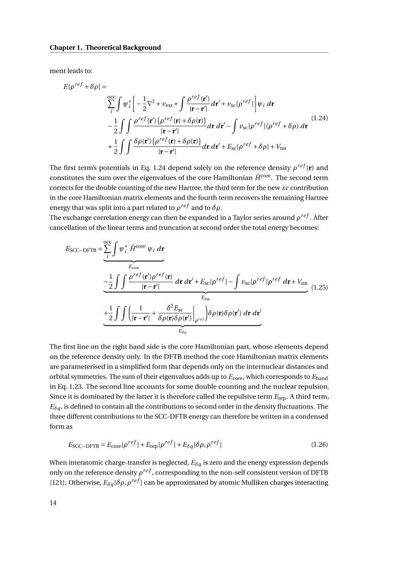
ment leads to:
E [ρr e f +δρ] =occ∑
i
∫ψ∗
i
[− 1
2∇2 + vext +
∫ρr e f (r′)|r− r′| dr′+ vxc[ρr e f ]
]ψi dr
− 1
2
∫ ∫ρr e f (r′)
(ρr e f (r)+δρ(r)
)|r− r′| dr dr′−
∫vxc[ρr e f ](ρr e f +δρ) dr
+ 1
2
∫ ∫δρ(r′)
(ρr e f (r)+δρ(r)
)|r− r′| dr dr′+Exc[ρr e f +δρ]+Vnn
(1.24)
The first term’s potentials in Eq. 1.24 depend solely on the reference density ρr e f (r) and
constitutes the sum over the eigenvalues of the core Hamiltonian H core. The second term
corrects for the double counting of the new Hartree, the third term for the new xc contribution
in the core Hamiltonian matrix elements and the fourth term recovers the remaining Hartree
energy that was split into a part related to ρr e f and to δρ.
The exchange correlation energy can then be expanded in a Taylor series around ρr e f . After
cancellation of the linear terms and truncation at second order the total energy becomes:
ESCC−DFTB =occ∑
i
∫ψ∗
i H core ψi dr︸ ︷︷ ︸Ecore
−1
2
∫ ∫ρr e f (r′)ρr e f (r)
|r− r′| dr dr′+Exc[ρr e f ]−∫
vxc[ρr e f ]ρr e f dr+Vnn︸ ︷︷ ︸Erep
+1
2
∫ ∫ (1
|r− r′| +δ2Exc
δρ(r)δρ(r′)
∣∣∣∣ρr e f
)δρ(r)δρ(r′) dr dr′︸ ︷︷ ︸
Eδq
(1.25)
The first line on the right hand side is the core Hamiltonian part, whose elements depend
on the reference density only. In the DFTB method the core Hamiltonian matrix elements
are parameterised in a simplified form that depends only on the internuclear distances and
orbital symmetries. The sum of their eigenvalues adds up to Ecore, which corresponds to Eband
in Eq. 1.23. The second line accounts for some double counting and the nuclear repulsion.
Since it is dominated by the latter it is therefore called the repulsive term Erep. A third term,
Eδq , is defined to contain all the contributions to second order in the density fluctuations. The
three different contributions to the SCC-DFTB energy can therefore be written in a condensed
form as
ESCC−DFTB = Ecore[ρr e f ]+Erep[ρr e f ]+Eδq [δρ,ρr e f ] (1.26)
When interatomic charge-transfer is neglected, Eδq is zero and the energy expression depends
only on the reference density ρr e f , corresponding to the non-self consistent version of DFTB
[121]. Otherwise, Eδq [δρ,ρr e f ] can be approximated by atomic Mulliken charges interacting
14
1.3. Self-Consistent Charge Density Functional Tight Binding (SCC-DFTB)
by a damped Coulomb potential. In this way the total energy can only be minimised self-
consistently and therefore this extension is referred to as Self-Consistent Charge Density
Functional Tight Binding (SCC-DFTB) [42].
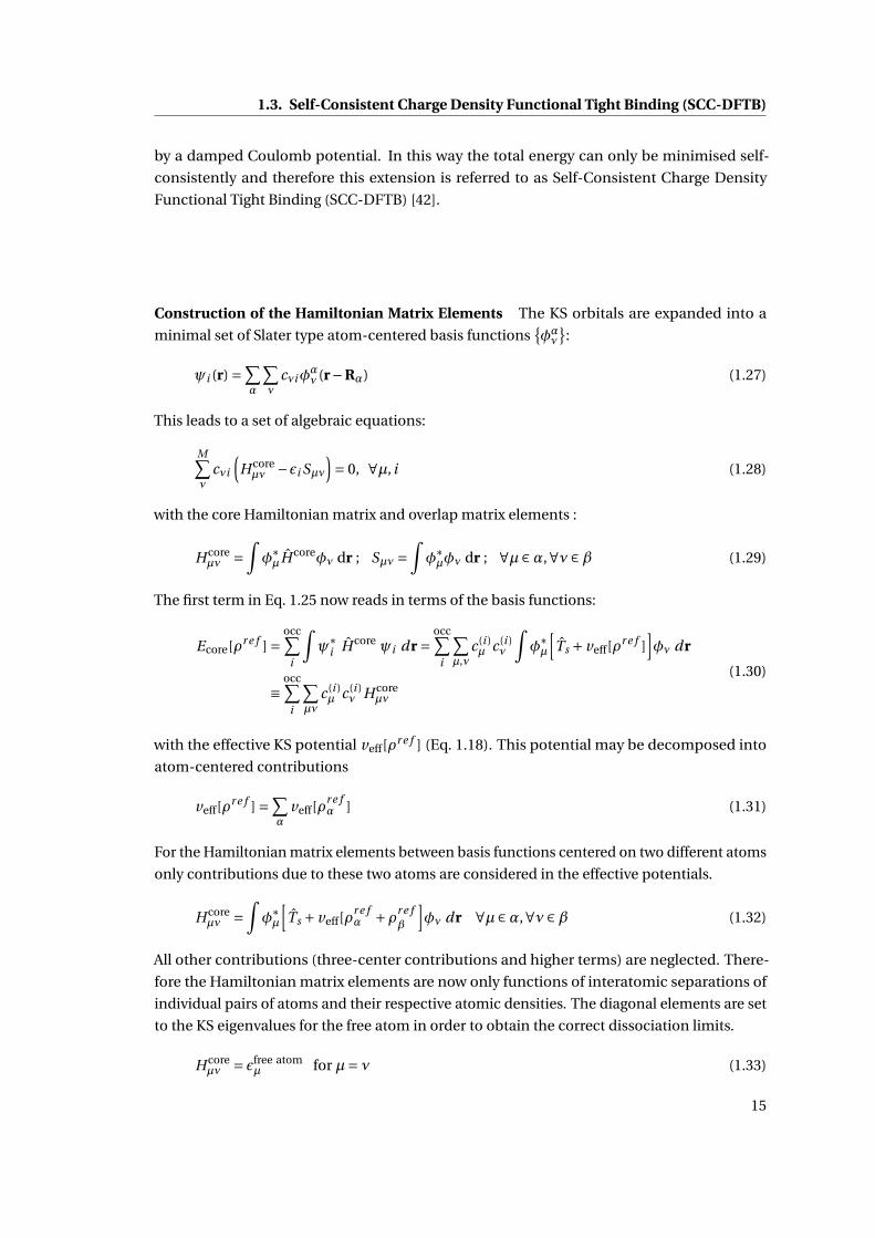
Construction of the Hamiltonian Matrix Elements The KS orbitals are expanded into a
minimal set of Slater type atom-centered basis functionsφαν
:
ψi (r) =∑α
∑ν
cνiφαν (r−Rα) (1.27)
This leads to a set of algebraic equations:
M∑ν
cνi
(H coreµν −εi Sµν
)= 0, ∀µ, i (1.28)
with the core Hamiltonian matrix and overlap matrix elements :
H coreµν =
∫φ∗µH coreφν dr ; Sµν =
∫φ∗µφν dr ; ∀µ ∈α,∀ν ∈β (1.29)
The first term in Eq. 1.25 now reads in terms of the basis functions:
Ecore[ρr e f ] =occ∑
i
∫ψ∗
i H core ψi dr =occ∑
i
∑µ,ν
c(i )µ c(i )
ν
∫φ∗µ
[Ts + veff[ρ
r e f ]]φν dr
≡occ∑
i
∑µν
c(i )µ c(i )
ν H coreµν
(1.30)
with the effective KS potential veff[ρr e f ] (Eq. 1.18). This potential may be decomposed into
atom-centered contributions
veff[ρr e f ] =∑
αveff[ρ
r e fα ] (1.31)
For the Hamiltonian matrix elements between basis functions centered on two different atoms
only contributions due to these two atoms are considered in the effective potentials.
H coreµν =
∫φ∗µ
[Ts + veff[ρ
r e fα +ρr e f
β
]φν dr ∀µ ∈α,∀ν ∈β (1.32)
All other contributions (three-center contributions and higher terms) are neglected. There-
fore the Hamiltonian matrix elements are now only functions of interatomic separations of
individual pairs of atoms and their respective atomic densities. The diagonal elements are set
to the KS eigenvalues for the free atom in order to obtain the correct dissociation limits.
H coreµν = εfree atom
µ for µ= ν (1.33)
15
Chapter 1. Theoretical Background
The basis functions φν and the input densities ρr e fα are determined from the SCF solution
of an atom in a confined KS potential within a DFT/GGA calculation. Once the φν and ρr e fα
are determined the Hamiltonian and overlap matrix elements can be calculated numerically
as a function of interatomic distances and tabulated. This means that for a DFTB electronic
structure calculation no integrals have to be calculated at run-time.
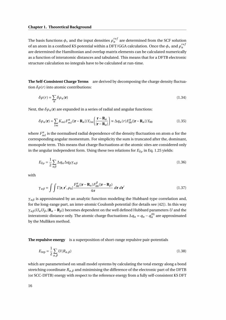
The Self-Consistent Charge Terms are derived by decomposing the charge density fluctua-
tion δρ(r ) into atomic contributions:
δρ(r ) =∑αδρα(r) (1.34)
Next, the δρα(r) are expanded in a series of radial and angular functions:
δρα(r) =∑l m
Kml Fαml (|r−Rα|)Ylm
(r−Rα
|r−Rα|)≈∆qα(r )Fα
00(|r−Rα|)Y00 (1.35)
where Fαml is the normalised radial dependence of the density fluctuation on atom α for the
corresponding angular momentum. For simplicity the sum is truncated after the, dominant,
monopole term. This means that charge fluctuations at the atomic sites are considered only
in the angular independent form. Using these two relations for Eδρ in Eq. 1.25 yields:
Eδρ =1
2
∑αβ
∆qα∆qβγαβ (1.36)
with
γαβ =∫ ∫
Γ[r,r′,ρ0]Fα
00(|r−Rα)Fβ00(|r−Rβ)
4πdr dr′ (1.37)
γαβ is approximated by an analytic function modeling the Hubbard-type correlation and,
for the long-range part, an inter-atomic Coulomb potential (for details see [42]). In this way
γαβ(UαUβ, |Rα−Rβ|) becomes dependent on the well defined Hubbard parameters U and the
interatomic distance only. The atomic charge fluctuations ∆qα = qα−q (0)α are approximated
by the Mulliken method.
The repulsive energy is a superposition of short-range repulsive pair-potentials
Erep = 1
2
∑α,β
U (Rα,β) (1.38)
which are parameterised on small model systems by calculating the total energy along a bond
stretching coordinate Rα,β and minimising the difference of the electronic part of the DFTB
(or SCC-DFTB) energy with respect to the reference energy from a fully self-consistent KS DFT
16
1.4. Molecular Mechanics Force Fields
calculation:
U (Rα,β) = E KS0 (Rαβ)−
(E core[ρr e f ](Rαβ)+Eδq [δρ,ρr e f ](Rαβ)
)(1.39)
If second order terms are neglected Eδq equals to zero. The functional form of U (Rα,β) consists
of a short-range exponential part, a mid-range cubic spline interpolation and, to assure the
correct behaviour at the cut-off distance, a long-range part with a fifth order spline.
Note that for K species K 2/2 potentials have to be parameterised. Furthermore, in the conven-
tional parameterisation scheme the balanced description of different chemical environments
involves significant human effort and chemical intuition. In Chapter 4 we have followed
a different route. We aimed at deriving in situ parameters with reduced transferability but
maximal accuracy for the chemical and physical environment under investigation. To this
end, we employed the iterative Boltzmann inversion method [69] to derive O-O and O-H
repulsive potentials for liquid water under ambient conditions, based on DFT/PBE reference
calculations.
1.4 Molecular Mechanics Force Fields
Molecular mechanics (MM) force fields (FFs) can be seen as the lowest level of theory among
the computational methods used in this thesis. They neglect the explicit effect of the elec-
trons altogether and consist of pairwise-additive, classical potentials for the nuclei. They
are therefore also referred to as classical FFs or simply FFs. FFs are "empirical", that is, their
functional form for the potential energy is not unique, but rather based on chemical concepts
and experience. As a representative example for currently widely used FFs in biomolecular
simulations Eq. 1.40 shows the basic functional form of the Amber FF family [17] as a function
of the nuclear positions Rα.
EMM (Rα) =N bonds∑
n=1Kbn
(bn −beq
n)2 +
N angles∑n=1
Kθn
(θn −θeq
n)2
+N dihedrals∑
n=1
Vn
2
[1+cos(mφn −ϕn)
]+ ∑α<β
[Aαβ
R12αβ
− Bαβ
R6αβ
+ qαqβεRαβ
] (1.40)
The first three terms cover the bonded interactions. Harmonic potentials are assigned to the
bond stretching coordinates bn ≡ Rαβ = |Rβ−Rα|. The associated parameters are the force
constants Kbn and equilibrium distances beqn , respectively. Terms for the angles θn , covering
three consecutively bonded atoms α−β−γ, are defined analogously. Contributions from
dihedral angles φn , between four consecutively bonded atoms α−β−γ−δ, are expressed as
a Fourier series with the corresponding parameter sets for the rotational barrier heights Vn ,
periodicity m and phase ϕn . Improper dihedral terms of the same form can be used to correct
for the out-of-plane motions in ring structures. The non-bonded interactions between atom
pairs α−β involve van der Waals interactions, modelled by a Lennard-Jones potential with
corresponding parameters Aαβ and Bαβ, and the Coulomb potential for atomic point charges
17

Chapter 1. Theoretical Background
qα in a medium with dielectric constant ε.
Various FFs that apply the basic functional form in Eq. 1.40 are available, but differ mainly in
their parameterisation protocol. In general, the Amber protocols rely as much as possible on
quantum mechanical calculations, which are only affordable for gas phase model compounds,
while, for example, the parameterisation protocols of the GROMOS FF family target primarily
experimental thermodynamic properties of condensed phase systems [18, 19]. Please consult
Refs. [122–124] for more detailed discussions of classical MM.
Since the potential energy of the form of Eq. 1.40 can be evaluated very efficiently, system
sizes (100’000 of atoms or more) and time scales (from nano to microseconds) relevant to
biological applications [20, 21] are accessible. However, such FFs can not describe the effects
of electronic rearrangements and therefore the bonding topology of a chemical system is
retained during the course of a simulation. Recent efforts in developing reactive FFs [125]
show promising results, but are still not routinely employed. Furthermore, the derivation
of accurate FF parameters requires substantial human effort and often the transferability to
physicochemical environments different from the parameterisation is limited. In some cases
polarisable FFs can be more accurate and transferable [126, 127], but they can not yet be
considered standard methods. In Chapter 3, we have used a different strategy to increase the
accuracy of (non-polarisable) biomolecular force fields. We implemented a recently developed
in situ parameterisation protocol based on the force matching method. Based on QM/MM
reference calculations [48], the method provides highly accurate FF parameters (ideally of
QM/MM quality) for a particular system at hand that are not optimised for transferability.
Such a parameter set can serve as an accuracy benchmark to assess the performance of more
sophisticated methods. The force-matching procedure can be used to identify situations
where a higher-level force field, e.g including polarisation, leads to an important improve-
ment, as opposed to situations where a minor improvement would not justify the additional
computational cost.
1.5 Quantum Mechanical/Molecular Mechanics (QM/MM)
For many applications in the fields of (bio-)chemistry and material science a description
within the framework of an electronic structure method is necessary. However, the typical
system sizes and relevant time scales are often beyond accessibility at this level of theory.
Mixed QM/MM schemes combine the advantages of electronic structure methods with the
classical force fields, while retaining an atomistic resolution. They involve a partitioning
of the system into a (small) reactive region, which is treated with an electronic structure
method, and the (larger) environment, which is represented by a classical FF (Fig. 1.1). In
this way, effects of the instantaneous rearrangement of the electronic structure are taken
into account where they are needed, e.g. the active site of a protein, while the non-reactive
environment can be faithfully described at the classical level. In principle, the QM part can
be calculated with different electronic structure methods, but throughout this thesis we will
use the term for the more specific case of DFT within the KS framework, as it is implemented
18
1.5. Quantum Mechanical/Molecular Mechanics (QM/MM)
MMQM
Q1
M1
cap
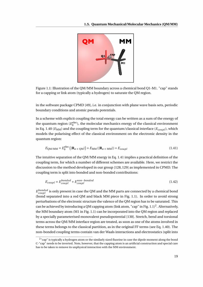
Figure 1.1: Illustration of the QM/MM boundary across a chemical bond Q1-M1. "cap" standsfor a capping or link atom (typically a hydrogen) to saturate the QM region.
in the software package CPMD [49], i.e. in conjunction with plane wave basis sets, periodic
boundary conditions and atomic pseudo potentials.
In a scheme with explicit coupling the total energy can be written as a sum of the energy of
the quantum region (E elec0 ), the molecular mechanics energy of the classical environment
in Eq. 1.40 (EMM) and the coupling term for the quantum/classical interface (Ecoupl ), which
models the polarising effect of the classical environment on the electronic density in the
quantum region:
EQM/MM = E elec0
(Rα ∈ QM
)+EMM (Rα ∈ MM)+Ecoupl (1.41)
The intuitive separation of the QM/MM energy in Eq. 1.41 implies a practical definition of the
coupling term, for which a number of different schemes are available. Here, we restrict the
discussion to the method developed in our group [128, 129] as implemented in CPMD. The
coupling term is split into bonded and non-bonded contributions:
Ecoupl = E bondedcoupl +E non−bonded
coupl (1.42)
E bondedcoupl is only present in case the QM and the MM parts are connected by a chemical bond
(bond separated into a red QM and black MM piece in Fig. 1.1). In order to avoid strong
perturbations of the electronic structure the valence of the QM region has to be saturated. This
can be achieved by introducing a QM capping atom (link atom, "cap" in Fig. 1.1)2. Alternatively,
the MM boundary atom (M1 in Fig. 1.1) can be incorporated into the QM region and replaced
by a specially parameterised monovalent pseudopotential [130]. Stretch, bend and torsional
terms across the QM/MM interface region are treated, as soon as one of the atoms involved in
these terms belongs to the classical partition, as in the original FF terms (see Eq. 1.40). The
non-bonded coupling terms contain van der Waals interactions and electrostatics (split into
2"cap" is typically a hydrogen atom or the similarly sized fluorine in case the dipole moment along the bondC-"cap" needs to be inverted. Note, however, that the capping atom is an artificial construction and special carehas to be taken to remove its unphysical interaction with the MM environment.
19

Chapter 1. Theoretical Background
QMNN
ESPME
RNN
RESP
Figure 1.2: Illustration of the electrostatic QM/MM coupling scheme by Laio et al. [129].
three regions):
E non−bondedcoupl = E vd w
coupl +ECoul omb−N Ncoupl +ECoul omb−ESP
coupl +ECoul omb−MEcoupl (1.43)
The van der Waals interactions are retained from the original force field.
E vd wcoupl =
∑α∈M M
∑β∈QM
[Aαβ
R12αβ
− Bαβ
R6αβ
](1.44)
The electrostatic coupling scheme is split into three regions, as illustrated in Fig. 1.2. In the
NN shell, nearest to the quantum region, the classical point charges are explicitly coupled
with the electronic density in the QM region. However, to prevent unphysical "spill-out" of the
electronic density, the Coulomb-potential is augmented by a damping function that ensures a
finite value of the potential at distances r shorter than the covalent radius:
ECoul omb−N Ncoupl = ∑
α∈ N Nqα
∫ρ(r)
r 4cα − r
r 5cα − r 5
dr (1.45)
where rcα is the atomic covalent radius of atom α and r = |r−Rα|. In order to estimate the
computational costs of the calculation of this interaction consider, that the grid based repre-
sentation of the electron density ρ involves in typical QM/MM applications ≈ 100′000 points.
If the NN shell would include all classical atoms α, which typically count ≈ 10′000−100′000,
the evaluation of the full sum becomes too costly. Therefore, the NN shell is kept as small as
possible.
For the classical atoms within RN N ≤ R < RESP the Coulomb interaction with the QM elec-
tronic density is approximated by the interaction with the atomic D-RESP charges of the QM
atoms QD−RESPj :
ECoul omb−ESPcoupl = ∑
α∈ ESP, β∈ QM
qαQD−RESPβ
|Rα−Rβ|(1.46)
The atomic point charges on the QM atoms are calculated at each time-step during an MD
20
1.6. Molecular Dynamics
simulation as Dynamically Restrained Electrostatic Potential derived charges (D-RESP) [129].
The D-RESP charges are fitted in order to reproduce the electrostatic potential due to the QM
electronic density at the positions of the MM atoms within the N N -shell.
Finally, in the long-range part the MM charges with R > RESP interact with with a multi-polar
expansion of the QM charge density:
ECoul omb−MEcoupl = ∑
i∈ MEqi
C1
|Ri −R| +∑α
Dα(Rα
i −Rα
)
|Ri −R|3 + 1
2
∑αβ
Qαβ(Rα
i −Rα
)(Rβ
i −Rβ
)
|Ri −R|5
(1.47)
where R is the geometrical center of the QM region and C , D and Q are the charge, dipole and
quadrupole moment of the quantum charge distribution, respectively.
1.6 Molecular Dynamics
Consider the expectation value of an arbitrary operator Ω with respect to the Boltzmann
distribution:
⟨Ω⟩NVT =∫
dRdPΩ(Rα, Pα) e−βE(Rα,Pα)∫dRdP e−βE(Rα,Pα)
, with β= 1
kB T(1.48)
This expression represents the link between microscopic models, such as the ones discussed
in the previous sections and observables represented byΩ [104]. However, the integrand in
Eq. 1.48 is too complex to allow for an analytical solution, but can be sampled by Monte Carlo
(MC) techniques in conjunction with importance sampling [131, 132].
The Molecular Dynamics (MD) method, on the other hand, relies on the ergodic hypothesis
[133], which allows to replace the ensemble average with the time average for ⟨Ω⟩:
⟨Ω⟩NVT = limTmax→∞
∑Tmaxt Ω (Rα(t ), Pα(t )) e−βE(Rα(t ),Pα(t ))∑Tmax
t e−βE(Rα(t ),Pα(t ))(1.49)
Assuming the Born-Oppenheimer approximation and classical nuclei (section 1.1), the total
energy is the sum of the kinetic energy of the classical nuclei and the potential energy E (Rα):
E(Rα, Pα) = E (Rα)+Tn(Pα) (1.50)
To sample ⟨Ω⟩ along t the classical many-body system can be propagated in time, employing
Newton’s equations of motion:
−∇RαE (Rα) = Mα
d 2Rα
d t 2 (1.51)
These equations are typically solved by numerical integration schemes, such as the popular
velocity-Verlet algorithm [122, 134].
21
Chapter 1. Theoretical Background
The potential energy surface E (Rα) can be obtained at various levels of theory. The first
molecular dynamics simulations were performed on hard spheres [22], later systems included
classical Lennard-Jones fluids [23] and liquid water [135]. In today’s classical MD simulations
on biological systems, force fields according to EM M in Eq. 1.40 are employed.
Ab initio molecular dynamics (AIMD) refers to a potential energy surface based on an elec-
tronic structure method: E elec in Eq. 1.3. DFT is a common choice (E0[ρ(r)] in Eqs. 1.12 and
1.20), or a mixed QM/MM energy (EQM/M M , Eq. 1.41) expression.
Two methods for AIMD are in common use. In Born-Oppenheimer molecular dynamics
(BOMD) the nuclei evolve on the effective potential in Eq. 1.9 exerted by the electrons within
the adiabatic BO approximation to the time-independent Schrödinger equation. This implies
that the electronic energy E elec is minimised at every MD step (for a different configuration
Rα). In a numerical integration scheme the time step for the equations of motions for the
nuclei can therefore be chosen relevant to nuclear motions. But the efficiency relies heavily
on the minimisation techniques [29] to quench the electronic degrees of freedom to the BO
surface.
Alternatively, in Car-Parrinello molecular dynamics (CPMD) [136] the classical nuclei and
electrons, represented by single-particle wave functions ψi , are propagated simultaneously
according to the extended Lagrangian
LCP =1
2
∑α
P2α
Mα+ 1
2µ
∑i
∫dr ψi
∗(r)ψi (r)−E elec[ψi ; Rα]
+∑i , jΛi j
(∫dr ψ∗
i (r)ψ j (r)−δi j
) (1.52)
where µ is a fictitious classical inertia attributed to the electronic degrees of freedom. ψi is
used as a short hand for the time derivatives of the electronic single particle orbitals. The
Lagrange multipliers Λi j enforce orthogonality for the orbitals (see Refs. [29, 30, 137] for a
more detailed discussion). Note that the electronic energy E elec and the ψi can, in principle,
originate from any kind of electronic structure method that employs single particle orbitals.
However, CPMD is typically performed within KS DFT, i.e. E K S[ψi ; Rα] in Eq. 1.20.
Provided that the lowest electronic frequency
√∆Egap
µ (∆Egap is the HOMO-LUMO gap) is much
higher than the nuclear vibrational frequency, the kinetic energy transfer between electrons
and nuclei is negligible [138] (adiabatic). If in a CPMD run the initial electronic structure has
been quenched to the BO surface the electrons follow the nuclear motion adiabatically while
remaining close to the electronic ground state. This necessitates a smaller integration time
step for the equations of motions than in BOMD. However, in CPMD the KS functional is only
evaluated once at each nuclear configuration and does not have to be minimised iteratively.
22
2 Assessment of Computational Meth-ods to Determine Low Energy Confor-mations of Biomolecules2.1 Cold-Ion Spectroscopy and Quantum Chemistry: A Successful
Tandem to Determine Low Energy Structures of Bare and Micro-
solvated Protonated Tryptophan
The computational results presented in this section have been obtained in collab-
oration with Dr. Matteo Guglielmi, while the experiments have been performed
by Dr. Natalia Nagornova and Dr. Oleg Boyarkin, Laboratoire de Chimie Physique
Moléculaire, group of Prof. Thomas R. Rizzo.
2.1.1 Introduction
Recent advances in cold-ion spectroscopy have made it possible to record conformer-selective
vibrational spectra of isolated charged molecules at low temperature [139]. The experimen-
tal setup used here combines electrospray ionisation for producing gas-phase protonated
biomolecular ions, collisional cooling in a cryogenic 22-pole ion trap and IR-UV double-
resonance techniques to record the spectra. The spectral resolution is, due to the low temper-
ature and the conformational separation, high enough to obtain vibrationally resolved spectra
even for molecules as large as a decapeptide [140–143]. In this highly controlled environment
the intrinsic properties of the molecules can be investigated without the complicating effects
of the environment. The high level of control allows the selective spectroscopic investigation
of complexes with given numbers of solvent molecules in the gas phase and thereby provides
insight into the role of the solvent [142].
Similar to many other experimental techniques that aim at the determination of the molecular
structure, cold-ion spectroscopy does not directly provide the 3-D arrangement of the nuclei.
Structures can only be calculated via a computational method, which represents therefore
an inherent part of the interpretation of the experimental data. One of the computational
challenges in identifying the structures of biomolecules is rooted in the high density of confor-
mational states that differ by only small amounts of energy. Even at cryogenic temperature
23
Chapter 2. Assessment of Computational Methods to Determine Low EnergyConformations of Biomolecules
(kBT ∼ 0.02 kcal/mol) many of these states might be accessible and, in order to distinguish the
relative energies accurately, high-level quantum chemical approaches have to be employed.
However, even comparably small-sized systems span a relatively large conformational space,
for which a comprehensive search is often only feasible with computationally more expedient
methods. These theoretical methods in turn have to be validated by comparing calculated
properties with experiment. In the case of IR spectroscopy, for instance, the compared quanti-
ties can be frequencies and intensities of vibrational transitions, which are a direct fingerprint
of the molecular structure.
Here we have chosen the single amino acid tryptophan to test the ability of different com-
putational methods to determine the lowest energy structures. Tryptophan represents a
prototypical compound for the study of the structure of isolated biomolecules in the gas
phase [144, 145] and is a frequently used optical probe for protein structure and dynam-
ics [146–149]. It has been studied intensively in the ground and excited state [150, 151], both
isolated and in the condensed phase [152, 153]. In this work our experimental collabora-
tors have determined the conformer-selective vibrational spectra of the conformations of
bare, mono- and doubly-solvated protonated tryptophan([Trp+H]+ · (H2O)n (n = 0,1,2)
)at a
temperature of approximately 10 K by cold-ion spectroscopy and we have tested a range of
computational methods to identify the 3D molecular structures of the lowest energy conforma-
tions. The high-resolution experimental data served as a benchmark to test the performance
of various computational methods in identifying the correct lowest energy structures. We
assessed the performance of a wide range of computational methods ranging from high level
ab initio to tight binding and classical force fields. In particular, we tested the composite
ab initio method CBS-C [39, 40], MP2 [41], several density functional theory (DFT) [11, 12]
methods, BLYP [15, 16, 154], B3LYP [15, 16, 110, 155], BLYP-D3 [15, 16, 154, 156, 157], M05 [158],
M05-2X [159], M06 [160], M06-2X [160] and M06-HF [161], the Self-Consistent Charge Density
Functional Tight-Binding (SCC-DFTB) method [42], including improved variants for hydrogen-
bonding [71] and dispersion interactions [162], and the Molecular Mechanics (MM) force
fields (FFs) FF96 [43], FF99SB [44], FF02polEP [45] and AMOEBA [46].
We used the highest computational level accessible to us for these systems, the CBS-C level
of theory, as a reference to assess the performance of the remaining methods in reproduc-
ing correct energetics. Anticipating our results, it turns out that the DFT methods M05-2X,
M06, M06-2X and M06-HF are able to reproduce CBS-C energetics very closely. In addition,
M05-2X also produces the experimental vibrational spectra. The overall excellent perfor-
mance of M05-2X, M06, M06-2X and M06-HF for these systems is essential to target larger
biomolecules [141, 142, 163], for which the costs of the CBS-C method become prohibitive.
Furthermore, for larger systems a systematic enumeration of the low energy structures, as
performed here for([Trp+H]+ · (H2O)n (n = 0,1,2)
), is not possible, but sampling techniques
based on Molecular Dynamics [22, 23] (MD) or Monte Carlo [131, 132] (MC) have to be used
in order to generate a representative ensemble of configurations. Due to the large number
of configurations the energy (and forces) evaluation has to be delegated to computationally
more expedient DFT, or even tight binding (e.g. SCC-DFTB) or MM methods, which we have
also included in our benchmarking suite for this purpose. If the lower level methods are able
24
2.1. Cold-Ion Spectroscopy and Quantum Chemistry: A Successful Tandem to DetermineLow Energy Structures of Bare and Microsolvated Protonated Tryptophan
to generate sufficiently accurate energetics, they could serve for an energetic pre-screening of
candidate structures prior to a refinement at the DFT level.
Comparison with the experimental data validate CBS-C as reference method for the relative
energetics and confirms the adequacy of DFT/M05-2X for the calculation of the vibrational
spectra. The computed results generated by these two methods are in excellent agreement
with the experimental data. The root mean square deviations (RMSDs) between experimen-
tally observed and calculated harmonic vibrational frequencies are as low as ∼ 5 cm−1. In this
way, we were able to identify the 3D molecular structures of the lowest energy conformations
of([Trp+H]+ · (H2O)n (n = 0,1,2)
)whose conformation-specific IR spectra were measured
experimentally at 10 K. In agreement with experiment, the theoretical predictions reveal that
bare protonated tryptophan is present in two distinct conformations differing in two dihedral
angles. In([Trp+H]+ · (H2O)
)only one conformation is appreciably populated with the water
molecule hydrogen-bonded to the ammonium group which enables an additional interaction
with the π-system of the indole ring. And, finally, in([Trp+H]+ · (H2O)2
)three conformations
could be identified, differing only in the water binding sites. The extensive benchmarking
of the more approximate computational methods (SCC-DFTB, FF96, FF99SB, FF02polEP
and AMOEBA) showed that for the systems investigated here the stringent demands on the
accuracy for reproducing the available experimental and high-level theoretical data cannot be
met by any of these methods.
These results demonstrate how well modern quantum chemistry methods and cold ion spec-
troscopy work together in determining low energy structures of biomolecules in the gas phase.
2.1.2 Methods
The experimental data were collected by our collaborators Dr. Natalia Nagornova and Dr. Oleg
Boyarkin in the Laboratoire de Chimie Physique Moléculaire, group of Prof. Thomas R. Rizzo.
The experimental protocol to obtain the conformer-selective vibrational spectra of bare and
micro solvated protonated tryptophan at approximately 10 K is described in Appendix A.1.
The ab initio method we used to compute the high level reference values for the relative
energies is based on the original CBS-Q method [39], but employing coupled cluster singles
and doubles with perturbative triples [CCSD(T)] [7, 8] in place of the quadratic configuration
interaction approach [QCISD(T)] [40]. In the rest of the text we refer to this method as CBS-C.
The individual contributions for this composite method are described in the Appendix A.2
and were calculated with the Gaussian G09 package [164].
All ground state DFT [11] calculations within the Kohn-Sham (KS) formulation [12] employing
the exchange correlation functionals BLYP [15, 16, 154], B3LYP [15, 16, 110], M05 [158], M05-
2X [159], M06 [160], M06-2X [160] and M06-HF [161] in conjunction with the 6-31+G(d,p)
[165, 166], aug-cc-pVDZ [167] and aug-cc-pVTZ [167] basis sets were carried out with the
Gaussian 09 code. An assessment of the influence of the basis set on the accuracy of interaction
energies and harmonic vibrational frequencies can be found in the Appendix A.3. We find that
for the relative energetics at the DFT level the 6-31+G(d,p), aug-cc-pVDZ and aug-cc-pVTZ
25
Chapter 2. Assessment of Computational Methods to Determine Low EnergyConformations of Biomolecules
basis sets are essentially equivalent, while for the vibrational frequencies the aug-cc-pVDZ
is mandatory. We therefore restrict our discussion to the aug-cc-pVDZ results and refer to
the Appendix A for the results from other basis sets. An ultra fine integration grid was used
for the DFT calculations in Gaussian G09. Geometry optimisations and the calculations
of the harmonic vibrational frequencies for the IR spectra and the zero-point energy (ZPE)
corrections have been performed using tight convergence criteria (RMS force set to 10−5 a.u.).
BLYP-D3 values employing Grimme’s DFT-D3 dispersion correction [156, 157] were obtained
with the Turbomole 6.4 software package [168] employing the aug-cc-pVDZ basis set, the m5
integration grid, convergence criteria of 10−5 a.u. for the Cartesian nuclear forces and 10−7
a.u. for the electronic degrees of freedom.
Geometry optimisations at the classical level using the FF96, FF99SB and FF02polEP force
fields were performed via simulated annealing as implemented in the AMBER9 software [169].
The time step was set to 1 fs, bonds involving hydrogen atoms were constrained using the
SHAKE algorithm [170]. The temperature was controlled by a Langevin thermostat with a
collision frequency of 3.0 ps−1. Heating for 3 ns, equilibration for 5 ns and linear cooling
for 20 ns. The geometry optimisations at the AMOEBA level [46] were performed within the
TINKER 5.0 software package [171]. The SCC-DFTB method [42] was used as implemented in
DFTB+, v.1.1 [172] in conjunction with the mio-0-1 parameter set [173]. Improvements for the
description of hydrogen bonding [71] and dispersion interactions [162] were considered as well
and will be denoted as SCC-DFTB(h) and SCC-DFTB(d), respectively. Geometry optimisations
were performed up to a convergence of 10−4 a.u. of the atomic forces.
2.1.3 Results and Discussion
Isomer Labeling Notation
We adopt the following notation for([Trp+H]+ · (H2O)n (n = 0,1,2)
):
W +φ1φ2φ3(s1,s2) (2.1)
where W is the single-letter amino acid code for tryptophan, φ1,φ2 and φ3 are three dihedrals
angles (φ1 = Cα−Cβ−Cγ−Cδ; φ2 = N −Cα−Cβ−Cγ; and φ3 = N −Cα−C −O as depicted
in Fig. 2.1(a)) and s1, s2 are the hydrogen-bonding sites of the solvating water molecules.
The possible hydrogen-bonding sites are out (water molecule "lateral" hydrogen-bonded
to the NH3 group, Fig. 2.1(b)), up (water molecule "vertical" hydrogen-bonded to the NH3
group, Fig. 2.1(c)), oh (water molecule hydrogen-bonded to the COOH group, Fig. 2.1(d))
and ind (water molecule hydrogen-bonded to the NH3 group and interacting with the π-
electron cloud of the indole ring, Fig. 2.1(d)). Thus, the dihedral angle subspace (φ1φ2φ3)
of notation 2.1 defines the geometrical conformation of the bare ion and the water position
subspace (s1, s2) defines the location of the solvating water molecules. It turns out that for
[Trp+H]+ ·(H2O)n (n = 0,1,2) the Potential Energy Surface (PES) of the ground state defined by
the subspace (φ1φ2φ3) is characterized by the presence of 8 local minima where each dihedral
26
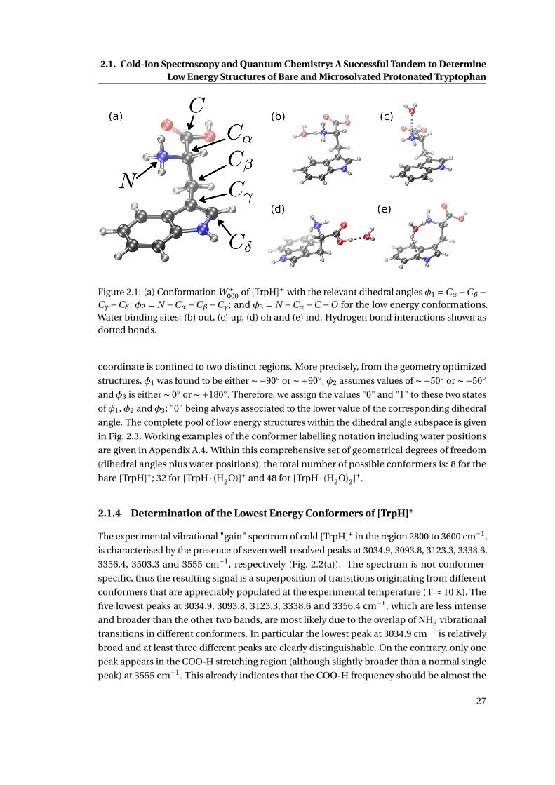
2.1. Cold-Ion Spectroscopy and Quantum Chemistry: A Successful Tandem to DetermineLow Energy Structures of Bare and Microsolvated Protonated Tryptophan
Figure 2.1: (a) Conformation W +000 of [TrpH]+ with the relevant dihedral angles φ1 =Cα−Cβ−
Cγ−Cδ; φ2 = N −Cα−Cβ−Cγ; and φ3 = N −Cα−C −O for the low energy conformations.Water binding sites: (b) out, (c) up, (d) oh and (e) ind. Hydrogen bond interactions shown asdotted bonds.
coordinate is confined to two distinct regions. More precisely, from the geometry optimized
structures, φ1 was found to be either ∼−90 or ∼+90, φ2 assumes values of ∼−50 or ∼+50
andφ3 is either ∼ 0 or ∼+180. Therefore, we assign the values "0" and "1" to these two states
of φ1, φ2 and φ3; "0" being always associated to the lower value of the corresponding dihedral
angle. The complete pool of low energy structures within the dihedral angle subspace is given
in Fig. 2.3. Working examples of the conformer labelling notation including water positions
are given in Appendix A.4. Within this comprehensive set of geometrical degrees of freedom
(dihedral angles plus water positions), the total number of possible conformers is: 8 for the
bare [TrpH]+; 32 for [TrpH · (H2O)]+ and 48 for [TrpH · (H2O)2]+.
2.1.4 Determination of the Lowest Energy Conformers of [TrpH]+
The experimental vibrational "gain" spectrum of cold [TrpH]+ in the region 2800 to 3600 cm−1,
is characterised by the presence of seven well-resolved peaks at 3034.9, 3093.8, 3123.3, 3338.6,
3356.4, 3503.3 and 3555 cm−1, respectively (Fig. 2.2(a)). The spectrum is not conformer-
specific, thus the resulting signal is a superposition of transitions originating from different
conformers that are appreciably populated at the experimental temperature (T ≈ 10 K). The
five lowest peaks at 3034.9, 3093.8, 3123.3, 3338.6 and 3356.4 cm−1, which are less intense
and broader than the other two bands, are most likely due to the overlap of NH3 vibrational
transitions in different conformers. In particular the lowest peak at 3034.9 cm−1 is relatively
broad and at least three different peaks are clearly distinguishable. On the contrary, only one
peak appears in the COO-H stretching region (although slightly broader than a normal single
peak) at 3555 cm−1. This already indicates that the COO-H frequency should be almost the
27

Chapter 2. Assessment of Computational Methods to Determine Low EnergyConformations of Biomolecules
Figure 2.2: (a) Experimental IR spectrum (measured by Dr. Natalia Nagornova and Dr. OlegBoyarkin) of [TrpH]+ (solid red line). Vibrational frequencies are observed at 3034.9, 3093.8,3123.3, 3338.6, 3356.4, 3503.3 and 3555.0 cm−1 (vertical dashed red lines). M05-2X IR spec-trum at the aug-cc-pVDZ basis set level of the two lowest conformers: W +
000 (RMS=2.9 cm−1,MAX=4.1 cm−1, SF=0.943) (blue bars), structure (b); W +
110 (RMS=3.1 cm−1, MAX=4.0 cm−1,SF=0.943) (green bars), structure (c).
same for all conformers present at the experimental conditions. The same observation holds
for the N-H stretching mode of the indole ring which corresponds to the narrower peak at
3503.3 cm−1.
Figure 2.3: Complete pool of [TrpH]+ conformers: (a) W +000, (b) W +
010, (c) W +100, (d) W +
110, (e)W +
001, (f ) W +011, (g) W +
101 and (h) W +111. Adapted from Ref. [174].
28

2.1. Cold-Ion Spectroscopy and Quantum Chemistry: A Successful Tandem to DetermineLow Energy Structures of Bare and Microsolvated Protonated Tryptophan
With these experimental information at hand the following paragraphs have the objective
to identify the 3D molecular structures of the lowest energy conformations that give rise to
vibrational spectra matching the experimental spectrum in Fig. 2.2(a). First, we perform a
systematic scan of the low-energy subspace defined by the dihedral angles φ1, φ2 and φ3 for
[TrpH]+ using the CBS-C method, the highest computational level accessible to us on this
system. We then assess the performance of several DFT functionals, different variants of a
tight binding method and MM force fields in reproducing the CBS-C reference energetics. We
also assess several DFT methods in reproducing the experimental vibrational spectra. The
composite nature of the CBS-C method is not suited to provide references for the vibrational
frequencies, since the only explicit calculation of the harmonic vibrational frequencies is
performed at the MP2 level, which is unsatisfactory, as shown later in this section.
Fig. 2.3 shows the eight possible conformations of [TrpH]+ within the low-energy subspace
defined by the dihedral angles φ1, φ2 and φ3. The first line of Tab. 2.1 shows the relative
energies for the 8 conformers of [TrpH]+ at the CBS-C level. Interestingly, the energy values
of conformers (e) to (h) in Fig. 2.3, in which the dihedral angle between the ammonium N
and the carbonyl O of the carboxyl group (φ3) assumes values ∼ 180 are all in the range
of 3-5 kcal/mol. Consequently, based on these CBS-C results, one can exclude W +001, W +
011,
W +101 and W +
111 from having a sizeable population at low temperature, and therefore to be
detected in the experimental IR spectrum. The candidates for the lowest-energy conformers
are thus restricted to the four conformers that have an intra-molecular hydrogen-bond be-
tween the unprotonated oxygen of the carboxylic group and one hydrogen of the NH3 moiety
(Fig. 2.3 (a) to (d)). CBS-C predicts W +110 as the most stable conformer (Fig. 2.3 (d)) and W +
000
only ∼ 0.5 kcal/mol higher in energy (Fig. 2.3 (a)). Note that the overall very small energy
differences and the fact that we are looking at a total energy range of only 5 kcal/mol sets
stringent constraints on the accuracy of the computational methods employed. As a general
trend the ZPE correction reduces the energy difference between the lowest conformer and
the other conformers by ∼ 0.1 kcal/mol (Tab. 2.1). The third conformer according to CBS-C
is W +100 (Fig. 2.1 (c)) but its energy of ∼ 0.9 kcal/mol makes it already too unfavourable at
low temperature. These results predict that a major (W +110) and a minor (W +
000) conformer
are likely to be observed in the experiment. Note that the Boltzmann weight associated to
the energy difference of the two lowest conformers is practically zero at 10 K, which would
make the second conformer completely unpopulated. On the other hand even CBS-C could
overestimate the energy separation by a few tens of a kcal/mol.
We assessed the performance of MP2 and the density functional methods M06-2X, M06-HF,
M06, M05-2X, M05, B3LYP, BLYP-D3 and BLYP in reproducing the relative energies at the
CBS-C level. As can be seen from Tab. 2.1, all these methods predict the conformations with
φ3 = 1 at 3 kcal/mol or higher, in line with the CBS-C results. Among the density functionals,
M05-2X, M06, M06-2X and M06-HF are all capable of reproducing the relative energies at
the CBS-C level. These four functionals are basically equivalent in terms of their accuracy
which is quantified by root mean square deviations (RMSD) of 0.1-0.3 kcal/mol and maximum
29
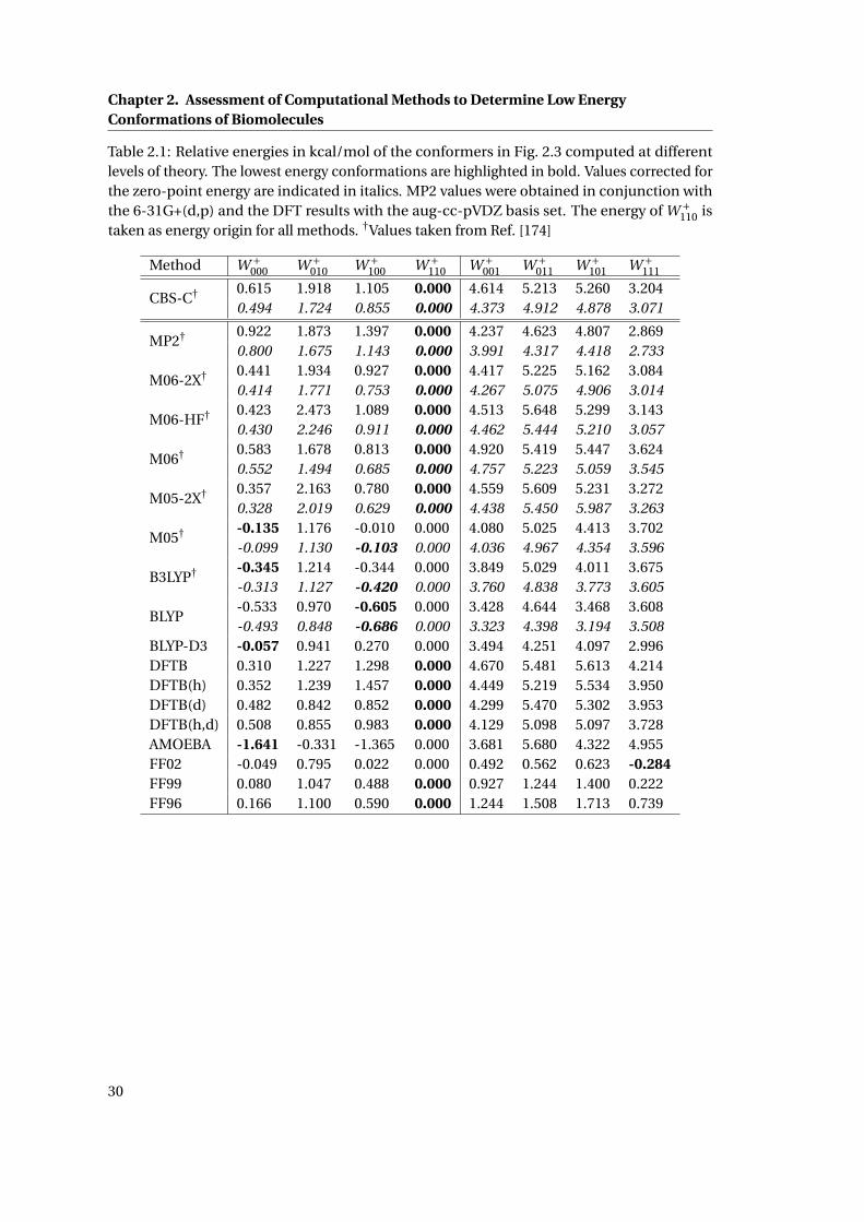
Chapter 2. Assessment of Computational Methods to Determine Low EnergyConformations of Biomolecules
Table 2.1: Relative energies in kcal/mol of the conformers in Fig. 2.3 computed at differentlevels of theory. The lowest energy conformations are highlighted in bold. Values corrected forthe zero-point energy are indicated in italics. MP2 values were obtained in conjunction withthe 6-31G+(d,p) and the DFT results with the aug-cc-pVDZ basis set. The energy of W +
110 istaken as energy origin for all methods. †Values taken from Ref. [174]
Method W +000 W +
010 W +100 W +
110 W +001 W +
011 W +101 W +
111
CBS-C† 0.615 1.918 1.105 0.000 4.614 5.213 5.260 3.2040.494 1.724 0.855 0.000 4.373 4.912 4.878 3.071
MP2† 0.922 1.873 1.397 0.000 4.237 4.623 4.807 2.8690.800 1.675 1.143 0.000 3.991 4.317 4.418 2.733
M06-2X† 0.441 1.934 0.927 0.000 4.417 5.225 5.162 3.0840.414 1.771 0.753 0.000 4.267 5.075 4.906 3.014
M06-HF† 0.423 2.473 1.089 0.000 4.513 5.648 5.299 3.1430.430 2.246 0.911 0.000 4.462 5.444 5.210 3.057
M06† 0.583 1.678 0.813 0.000 4.920 5.419 5.447 3.6240.552 1.494 0.685 0.000 4.757 5.223 5.059 3.545
M05-2X† 0.357 2.163 0.780 0.000 4.559 5.609 5.231 3.2720.328 2.019 0.629 0.000 4.438 5.450 5.987 3.263
M05† -0.135 1.176 -0.010 0.000 4.080 5.025 4.413 3.702-0.099 1.130 -0.103 0.000 4.036 4.967 4.354 3.596
B3LYP† -0.345 1.214 -0.344 0.000 3.849 5.029 4.011 3.675-0.313 1.127 -0.420 0.000 3.760 4.838 3.773 3.605
BLYP-0.533 0.970 -0.605 0.000 3.428 4.644 3.468 3.608-0.493 0.848 -0.686 0.000 3.323 4.398 3.194 3.508
BLYP-D3 -0.057 0.941 0.270 0.000 3.494 4.251 4.097 2.996DFTB 0.310 1.227 1.298 0.000 4.670 5.481 5.613 4.214DFTB(h) 0.352 1.239 1.457 0.000 4.449 5.219 5.534 3.950DFTB(d) 0.482 0.842 0.852 0.000 4.299 5.470 5.302 3.953DFTB(h,d) 0.508 0.855 0.983 0.000 4.129 5.098 5.097 3.728AMOEBA -1.641 -0.331 -1.365 0.000 3.681 5.680 4.322 4.955FF02 -0.049 0.795 0.022 0.000 0.492 0.562 0.623 -0.284FF99 0.080 1.047 0.488 0.000 0.927 1.244 1.400 0.222FF96 0.166 1.100 0.590 0.000 1.244 1.508 1.713 0.739
30
2.1. Cold-Ion Spectroscopy and Quantum Chemistry: A Successful Tandem to DetermineLow Energy Structures of Bare and Microsolvated Protonated Tryptophan
errors (MAX) of 0.2-0.5 kcal/mol, as reported in Tab. 2.2. ZPE corrections reduce the energy
difference between the lowest conformer found by each method and the other conformers
by ∼ 0.1 kcal/mol (Tab. 2.1). The methods BLYP, B3LYP, BLYP-D3 and M05 on the other hand,
show significant deviations from the reference values. In particular, none of them is able to
identify the most stable conformer and their RMSDs are of the order of 0.7 - 1.1 kcal/mol with
maximum errors of 1.1 - 1.8 kcal/mol (Tab. 2.2). Such an accuracy is clearly insufficient to
assign the experimentally observed conformers at very low temperatures.
The ability to predict the lowest energy conformers and their correct energetic ordering within
a given energy threshold is evaluated in Tab. 2.2. For each method the first two columns give
the energetic RMSD and MAX with respect to the CBS-C reference. The next two columns
indicate whether the method is able to predict the correct lowest and second lowest energy
conformation, respectively. The fifth column indicates whether for a given method, the two
lowest energy conformations predicted at the CBS-C level are lower than 1 kcal/mol. This infor-
mation is important, if the respective method should be used for pre-screening. All structures
within e.g. 1 kcal/mol at the pre screening level could then be considered for a refinement at a
higher level. If the two conformations do not fall into this (arbitrarily chosen) threshold, they
would be excluded from a consideration at the higher level. The last column gives the total
number of structures within the given threshold of 1 kcal/mol. All these structures would need
to be considered at the higher level after the pre-screening. A number significantly higher
than 2 means that extra computational work has to be done.
Among more approximate methods, we assessed the performance of several SCC-DFTB vari-
ants, as well as the Amber FF96, FF99SB and FF02polEP and the AMOEBA force fields in
their accuracy for predicting the relative conformational energies with respect to the CBS-C
references (Tables 2.1 and 2.2). All variants of SCC-DFTB are able to assign the correct lowest
and second lowest energy conformations. Furthermore the energetic separation between
the conformations featuring φ3 = 1 and the remaining ones, as predicted by CBS-C, is well
reproduced. The RMSDs and maximum errors amount to only ∼ 0.5 kcal/mol and 0.8-1.1
kcal/mol, respectively. Among the tested force fields only Amber FF96 and FF99 are able to
predict the correct lowest energy structure, but only FF99 predicts the correct minor con-
former. FF96, FF99 and FF02 produce RMSDs and maximum errors above 2 kcal/mol, with
the polarisable force field FF02 performing worst. They clearly underestimate the energy
separations, especially between the φ3 = 1 and φ3 = 0 structures. This results in a relatively
high number of geometries within a threshold of 1 kcal/mol (column 7 in Tab. 2.2). In the
worst case, for FF02 essentially all structures would need to be considered at a higher level of
theory. This is insufficient for an application for a reliable energetic pre-screening of candidate
structures. Also the AMOEBA force field is not able to reproduce the correct two lowest energy
conformations, predicting W +000 1.6 kcal/mol below W +
110. On the other hand it performs
slightly better than the other force fields in reproducing the energetic separation between the
φ3 = 1 and φ3 = 0 conformations and the RMSD is 1.6 kcal/mol with a maximum error 2.5
kcal/mol.
To validate the assignment of the most stable conformers predicted by CBS-C we have com-
31
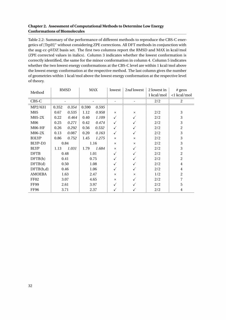
Chapter 2. Assessment of Computational Methods to Determine Low EnergyConformations of Biomolecules
Table 2.2: Summary of the performance of different methods to reproduce the CBS-C ener-getics of [TrpH]+ without considering ZPE corrections. All DFT methods in conjunction withthe aug-cc-pVDZ basis set. The first two columns report the RMSD and MAX in kcal/mol(ZPE corrected values in italics). Column 3 indicates whether the lowest conformation iscorrectly identified, the same for the minor conformation in column 4. Column 5 indicateswhether the two lowest energy conformations at the CBS-C level are within 1 kcal/mol abovethe lowest energy conformation at the respective method. The last column gives the numberof geometries within 1 kcal/mol above the lowest energy conformation at the respective levelof theory.
MethodRMSD MAX lowest 2nd lowest 2 lowest in # geos
1 kcal/mol <1 kcal/mol
CBS-C - - - - 2/2 2
MP2/631 0.352 0.354 0.590 0.595M05 0.67 0.535 1.12 0.958 × × 2/2 3M05-2X 0.22 0.464 0.40 1.109 X X 2/2 3M06 0.25 0.271 0.42 0.474 X X 2/2 3M06-HF 0.26 0.292 0.56 0.532 X X 2/2 2M06-2X 0.13 0.087 0.20 0.163 X X 2/2 3B3LYP 0.86 0.752 1.45 1.275 × × 2/2 3BLYP-D3 0.84 1.16 × × 2/2 3BLYP 1.13 1.031 1.79 1.684 × X 2/2 3DFTB 0.48 1.01 X X 2/2 2DFTB(h) 0.41 0.75 X X 2/2 2DFTB(d) 0.50 1.08 X X 2/2 4DFTB(h,d) 0.46 1.06 X X 2/2 4AMOEBA 1.63 2.47 × × 1/2 2FF02 3.07 4.65 × X 2/2 7FF99 2.61 3.97 X X 2/2 5FF96 3.71 2.37 X X 2/2 4
32
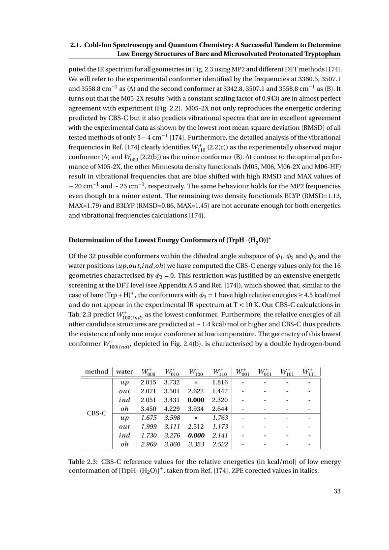
2.1. Cold-Ion Spectroscopy and Quantum Chemistry: A Successful Tandem to DetermineLow Energy Structures of Bare and Microsolvated Protonated Tryptophan
puted the IR spectrum for all geometries in Fig. 2.3 using MP2 and different DFT methods [174].
We will refer to the experimental conformer identified by the frequencies at 3360.5, 3507.1
and 3558.8 cm−1 as (A) and the second conformer at 3342.8, 3507.1 and 3558.8 cm−1 as (B). It
turns out that the M05-2X results (with a constant scaling factor of 0.943) are in almost perfect
agreement with experiment (Fig. 2.2). M05-2X not only reproduces the energetic ordering
predicted by CBS-C but it also predicts vibrational spectra that are in excellent agreement
with the experimental data as shown by the lowest root mean square deviation (RMSD) of all
tested methods of only 3−4 cm−1 [174]. Furthermore, the detailed analysis of the vibrational
frequencies in Ref. [174] clearly identifies W +110 (2.2(c)) as the experimentally observed major
conformer (A) and W +000 (2.2(b)) as the minor conformer (B). At contrast to the optimal perfor-
mance of M05-2X, the other Minnesota density functionals (M05, M06, M06-2X and M06-HF)
result in vibrational frequencies that are blue shifted with high RMSD and MAX values of
∼ 20 cm−1 and ∼ 25 cm−1, respectively. The same behaviour holds for the MP2 frequencies
even though to a minor extent. The remaining two density functionals BLYP (RMSD=1.13,
MAX=1.79) and B3LYP (RMSD=0.86, MAX=1.45) are not accurate enough for both energetics
and vibrational frequencies calculations [174].
Determination of the Lowest Energy Conformers of [TrpH · (H2O)]+
Of the 32 possible conformers within the dihedral angle subspace of φ1, φ2 and φ3 and the
water positions up,out ,i nd ,oh we have computed the CBS-C energy values only for the 16
geometries characterised by φ3 = 0. This restriction was justified by an extensive energetic
screening at the DFT level (see Appendix A.5 and Ref. [174]), which showed that, similar to the
case of bare [Trp+H]+, the conformers with φ3 = 1 have high relative energies ≥ 4.5 kcal/mol
and do not appear in the experimental IR spectrum at T < 10 K. Our CBS-C calculations in
Tab. 2.3 predict W +100(i nd) as the lowest conformer. Furthermore, the relative energies of all
other candidate structures are predicted at ∼ 1.4 kcal/mol or higher and CBS-C thus predicts
the existence of only one major conformer at low temperature. The geometry of this lowest
conformer W +100(i nd), depicted in Fig. 2.4(b), is characterised by a double hydrogen-bond
method water W +000 W +
010 W +100 W +
110 W +001 W +
011 W +101 W +
111
CBS-C
up 2.015 3.732 × 1.816 - - - -out 2.071 3.501 2.622 1.447 - - - -i nd 2.051 3.431 0.000 2.320 - - - -oh 3.450 4.229 3.934 2.644 - - - -up 1.675 3.598 × 1.763 - - - -out 1.999 3.111 2.512 1.173 - - - -i nd 1.730 3.276 0.000 2.141 - - - -oh 2.969 3.860 3.353 2.522 - - - -
Table 2.3: CBS-C reference values for the relative energetics (in kcal/mol) of low energyconformation of [TrpH · (H2O)]+, taken from Ref. [174]. ZPE corected values in italics.
33
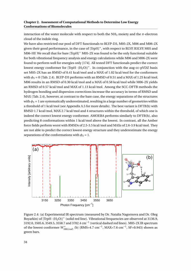
Chapter 2. Assessment of Computational Methods to Determine Low EnergyConformations of Biomolecules
interaction of the water molecule with respect to both the NH3 moiety and the π-electron
cloud of the indole ring.
We have also restricted our pool of DFT functionals to BLYP-D3, M05-2X, M06 and M06-2X
given their good performance, in the case of [TrpH]+, with respect to BLYP, B3LYP, M05 and
M06-HF. We recall that for bare [TrpH]+ M05-2X was found to be the only functional suitable
for both vibrational frequency analysis and energy calculations while M06 and M06-2X were
found to perform well for energies only [174]. All tested DFT functionals predict the correct
lowest energy conformer for [TrpH · (H2O)]+. In conjunction with the aug-cc-pVDZ basis
set M05-2X has an RMSD of 0.41 kcal/mol and a MAX of 1.02 kcal/mol for the conformers
with φ3 = 0 (Tab. 2.4). BLYP-D3 performs with an RMSD of 0.51 and a MAX of 1.25 kcal/mol.
M06 results in an RMSD of 0.30 kcal/mol and a MAX of 0.58 kcal/mol while M06-2X yields
an RMSD of 0.57 kcal/mol and MAX of 1.13 kcal/mol. Among the SCC-DFTB methods the
hydrogen bonding and dispersion corrections increase the accuracy in terms of RMSD and
MAX (Tab. 2.4), however, at contrast to the bare case, the energy separations of the structures
withφ3 = 1 are systematically underestimated, resulting in a large number of geometries within
a threshold of 1 kcal/mol (see Appendix A.5 for more details). The best variant is DFTB(h) with
RMSD 1.7 kcal/mol, MAX 2.7 kcal/mol and 4 structures within the threshold, of which one is
indeed the correct lowest energy conformer. AMOEBA performs similarly to DFTB(h), also
predicting 8 conformations within 1 kcal/mol above the lowest. In contrast, all the Amber
force fields perform worst with RMSDs of 2.5-3.5 kcal/mol and MAXs of 2.6-3.9 kcal/mol. They
are not able to predict the correct lowest energy structure and they underestimate the energy
separations of the conformations with φ3 = 1.
Figure 2.4: (a) Experimental IR spectrum (measured by Dr. Natalia Nagornova and Dr. OlegBoyarkin) of [TrpH · (H2O)]+ (solid red line). Vibrational frequencies are observed at 3136.9,3192.0, 3505.6, 3549.5, 3558.7 and 3702.4 cm−1 (vertical dashed red lines). M05-2X IR spectrumof the lowest conformer W +
100(i nd) (b) (RMS=4.7 cm−1, MAX=7.6 cm−1, SF=0.943) shown asgreen bars.
34
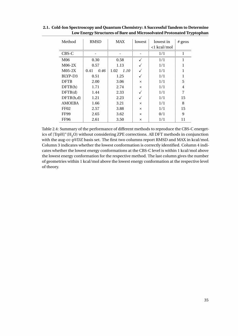
2.1. Cold-Ion Spectroscopy and Quantum Chemistry: A Successful Tandem to DetermineLow Energy Structures of Bare and Microsolvated Protonated Tryptophan
Method RMSD MAX lowest lowest in # geos<1 kcal/mol
CBS-C - - - 1/1 1
M06 0.30 0.58 X 1/1 1M06-2X 0.57 1.13 X 1/1 1M05-2X 0.41 0.46 1.02 1.10 X 1/1 1BLYP-D3 0.51 1.25 X 1/1 1DFTB 2.00 3.06 × 1/1 5DFTB(h) 1.71 2.74 × 1/1 4DFTB(d) 1.44 2.33 X 1/1 7DFTB(h,d) 1.21 2.23 X 1/1 15AMOEBA 1.66 3.21 × 1/1 8FF02 2.57 3.88 × 1/1 15FF99 2.65 3.62 × 0/1 9FF96 2.61 3.50 × 1/1 11
Table 2.4: Summary of the performance of different methods to reproduce the CBS-C energet-ics of [TrpH]+(H2O) without considering ZPE corrections. All DFT methods in conjunctionwith the aug-cc-pVDZ basis set. The first two columns report RMSD and MAX in kcal/mol.Column 3 indicates whether the lowest conformation is correctly identified. Column 4 indi-cates whether the lowest energy conformations at the CBS-C level is within 1 kcal/mol abovethe lowest energy conformation for the respective method. The last column gives the numberof geometries within 1 kcal/mol above the lowest energy conformation at the respective levelof theory.
35
Chapter 2. Assessment of Computational Methods to Determine Low EnergyConformations of Biomolecules
Fig. 2.4(a) shows the vibrational spectrum of the lowest conformer W +100(i nd) computed at the
M05-2X level, which has been validated in the previous section and Ref. [174]. The theoretical
predictions are in almost perfect agreement with the experimental spectrum within an RMSD
of 4.7 cm−1 and a MAX of 7.6 cm−1 when using a constant scaling factor of 0.943. These
are the lowest RMSDs and MAX on the set of vibrational frequencies with respect to the
full pool of 32 conformers. From the analysis of the vibrational normal modes we assign
the two experimental peaks at 3549.5 cm−1 and 3702.4 cm−1 to the SS and AS modes of
the water molecule hydrogen-bonded to both the NH3 group and the π-electron cloud of
the indole ring of the most abundant conformer W +100(i nd). This hydrogen-bond interaction
induces the red-shifts of the typical AS and SS frequencies of the free-water which are found at
3657 and 3756 cm−1, respectively. It is interesting to note how more environment sensitive
the SS mode is compared to the corresponding AS frequency. In our case, while the AS is
red-shifted by only 3756−3702.4 ' 50 cm−1, the SS frequency is red-shifted by as much as
3657−3549.5 ' 100 cm−1, which brings it in proximity to the COO-H stretching mode. The
two intense bands at 3505.6 and 3558.7 cm−1 are also confirmed to be originating from the
N-H stretching mode of the indole ring and the COO-H stretching mode of the carboxylic
group, respectively. It is interesting to note that the addition of a single water molecule to the
bare ion increases the COO-H stretching frequency by ∼ 4cm−1.
Determination of the Lowest-Energy Conformers of [TrpH · (H2O)2]+
For the 48 unique conformers identified by the dihedral angles φ1, φ2, φ3 and the water
positions up,out ,i nd ,oh we have computed the CBS-C energy values only for selected
geometries, since a screening at the DFT level indicated that all geometries with φ3 = 1 are
energetically unfavourable with energies ≥ 3 kcal/mol above the lowest energy conformer.
Tab. 2.5 shows the CBS-C energy reference values, for these 27 conformers. According to CBS-
C, the lowest-energy conformer is W +100(i nd ,oh) followed by two almost degenerate conformers
W +100(i nd ,up) and W +
100(i nd ,out ), at only ∼ 0.5 kcal/mol. These configurations are shown in
Fig. 2.5(b), (d) and (f). All three conformations share the same structure for tryptophan and
feature one water molecule interacting with the indole ring and the NH3-group. W +100(i nd ,up)
and W +100(i nd ,out ) both have the second water molecule attached to the NH3-group as well,
in contrast to the lowest energy conformation, W +100(i nd ,oh), which features the second water
molecule hydrogen bonded to the COOH group. Therefore, placing the second water molecule
at the NH3-group instead of the COOH group costs 0.5 kcal/mol, but the conformations, which
feature the hydrogen bonded water molecule in either vertical or lateral position, are almost
degenerate.
The relative energetics (including ZPE corrected values) of the different conformations em-
ploying the DFT methods B3LYP, BLYP-D3, M05-2X, M06, M06-2X and the pool of more
approximate methods are given in the Appendix A.6. Based on the DFT results, it turns out that
all geometries characterised by φ3 = 1 are energetically unfavourable with energies ≥ 3 kcal/-
mol. The performance of the DFT methods in reproducing the CBS-C relative energetics in
36
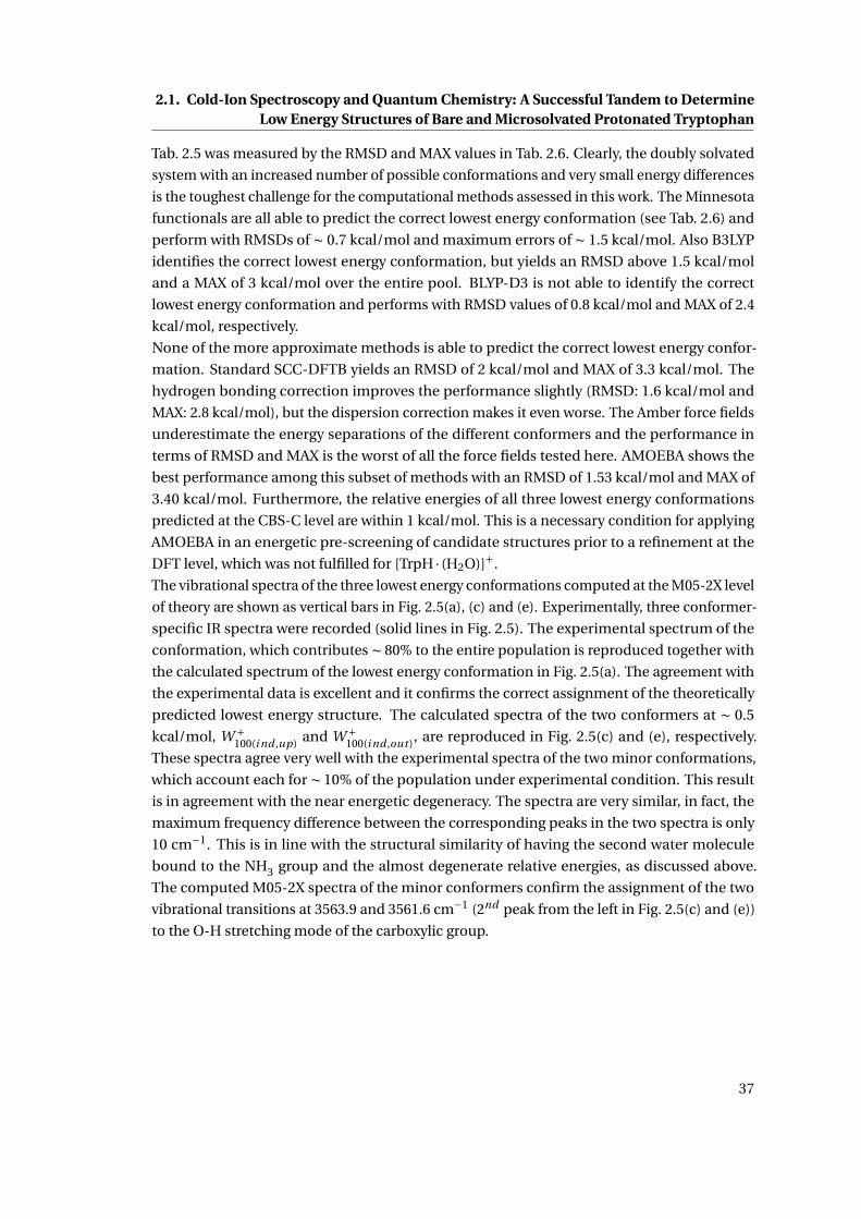
2.1. Cold-Ion Spectroscopy and Quantum Chemistry: A Successful Tandem to DetermineLow Energy Structures of Bare and Microsolvated Protonated Tryptophan
Tab. 2.5 was measured by the RMSD and MAX values in Tab. 2.6. Clearly, the doubly solvated
system with an increased number of possible conformations and very small energy differences
is the toughest challenge for the computational methods assessed in this work. The Minnesota
functionals are all able to predict the correct lowest energy conformation (see Tab. 2.6) and
perform with RMSDs of ∼ 0.7 kcal/mol and maximum errors of ∼ 1.5 kcal/mol. Also B3LYP
identifies the correct lowest energy conformation, but yields an RMSD above 1.5 kcal/mol
and a MAX of 3 kcal/mol over the entire pool. BLYP-D3 is not able to identify the correct
lowest energy conformation and performs with RMSD values of 0.8 kcal/mol and MAX of 2.4
kcal/mol, respectively.
None of the more approximate methods is able to predict the correct lowest energy confor-
mation. Standard SCC-DFTB yields an RMSD of 2 kcal/mol and MAX of 3.3 kcal/mol. The
hydrogen bonding correction improves the performance slightly (RMSD: 1.6 kcal/mol and
MAX: 2.8 kcal/mol), but the dispersion correction makes it even worse. The Amber force fields
underestimate the energy separations of the different conformers and the performance in
terms of RMSD and MAX is the worst of all the force fields tested here. AMOEBA shows the
best performance among this subset of methods with an RMSD of 1.53 kcal/mol and MAX of
3.40 kcal/mol. Furthermore, the relative energies of all three lowest energy conformations
predicted at the CBS-C level are within 1 kcal/mol. This is a necessary condition for applying
AMOEBA in an energetic pre-screening of candidate structures prior to a refinement at the
DFT level, which was not fulfilled for [TrpH · (H2O)]+.
The vibrational spectra of the three lowest energy conformations computed at the M05-2X level
of theory are shown as vertical bars in Fig. 2.5(a), (c) and (e). Experimentally, three conformer-
specific IR spectra were recorded (solid lines in Fig. 2.5). The experimental spectrum of the
conformation, which contributes ∼ 80% to the entire population is reproduced together with
the calculated spectrum of the lowest energy conformation in Fig. 2.5(a). The agreement with
the experimental data is excellent and it confirms the correct assignment of the theoretically
predicted lowest energy structure. The calculated spectra of the two conformers at ∼ 0.5
kcal/mol, W +100(i nd ,up) and W +
100(i nd ,out ), are reproduced in Fig. 2.5(c) and (e), respectively.
These spectra agree very well with the experimental spectra of the two minor conformations,
which account each for ∼ 10% of the population under experimental condition. This result
is in agreement with the near energetic degeneracy. The spectra are very similar, in fact, the
maximum frequency difference between the corresponding peaks in the two spectra is only
10 cm−1. This is in line with the structural similarity of having the second water molecule
bound to the NH3 group and the almost degenerate relative energies, as discussed above.
The computed M05-2X spectra of the minor conformers confirm the assignment of the two
vibrational transitions at 3563.9 and 3561.6 cm−1 (2nd peak from the left in Fig. 2.5(c) and (e))
to the O-H stretching mode of the carboxylic group.
37
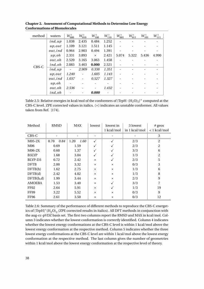
Chapter 2. Assessment of Computational Methods to Determine Low EnergyConformations of Biomolecules
method waters W +000 W +
010 W +100 W +
110 W +001 W +
011 W +101 W +
111
CBS-C
i nd ,up 1.038 2.435 0.484 1.252 - - - -up,out 1.109 3.121 1.511 1.145 - - - -
out , i nd 0.964 2.903 0.494 1.391 - - - -up,oh 2.331 3.893 × 2.421 5.074 5.322 5.436 4.990out ,oh 2.520 3.165 3.063 1.458 - - - -i nd ,oh 2.083 3.463 0.000 2.521 - - - -i nd ,up - 2.909 0.338 1.351 - - - -up,out 1.240 - 1.605 1.143 - - - -
out , i nd 1.037 - 0.527 1.327 - - - -up,oh - - - - - - - -out ,oh 2.536 - - 1.432 - - - -i nd ,oh - - 0.000 - - - - -
Table 2.5: Relative energies in kcal/mol of the conformers of [TrpH · (H2O)2]+ computed at theCBS-C level. ZPE corrected values in italics. (×) indicates an unstable conformer. All valuestaken from Ref. [174].
Method RMSD MAX lowest lowest in 3 lowest # geos1 kcal/mol in 1 kcal/mol < 1 kcal/mol
CBS-C - - - - - 3
M05-2X 0.70 0.84 1.20 1.60 X X 2/3 2M06 0.69 1.59 X X 2/3 2M06-2X 0.60 1.37 X X 3/3 6B3LYP 1.68 3.04 X X 1/3 2BLYP-D3 0.72 2.42 × X 2/3 5DFTB 2.00 3.32 × × 0/3 3DFTB(h) 1.62 2.75 × × 1/3 6DFTB(d) 2.42 4.02 × × 1/3 8DFTB(h,d) 1.99 3.44 × × 2/3 9AMOEBA 1.53 3.40 × X 3/3 7FF02 2.64 5.91 × X 1/3 19FF99 3.22 5.52 × × 0/3 9FF96 2.61 3.50 × × 0/3 12
Table 2.6: Summary of the performance of different methods to reproduce the CBS-C energet-ics of [TrpH]+(H2O)2 (ZPE corrected results in italics). All DFT methods in conjunction withthe aug-cc-pVDZ basis set. The first two columns report the RMSD and MAX in kcal/mol. Col-umn 3 indicates whether the lowest conformation is correctly identified. Column 4 indicateswhether the lowest energy conformations at the CBS-C level is within 1 kcal/mol above thelowest energy conformation at the respective method. Column 5 indicates whether the threelowest energy conformations at the CBS-C level are within 1 kcal/mol above the lowest energyconformation at the respective method. The last column gives the number of geometrieswithin 1 kcal/mol above the lowest energy conformation at the respective level of theory.
38
2.1. Cold-Ion Spectroscopy and Quantum Chemistry: A Successful Tandem to DetermineLow Energy Structures of Bare and Microsolvated Protonated Tryptophan
Figure 2.5: Experimental IR spectra (measured by Dr. Natalia Nagornova and Dr. Oleg Bo-yarkin) for [TrpH · (H2O)2]+ (solid lines). Observed vibrational frequencies (vertical dashedlines) for conformer A (a): 3507.0, 3551.0, 3646.9, 3703.9 and 3741.0 cm−1; conformer B (c):3508.4, 3563.9, 3576.2,3634.6, 3708.2 and 3728.6 cm−1; conformer C (e): 3508.5, 3561.6, 3574.9,3624.9, 3706.9 and 3719.6 cm−1. Calculated IR spectra (M05-2X) are shown as vertical bars in(a): RMS=4.7 cm−1, MAX=8.5 cm−1, SF=0.945; (c): RMS=3.3 cm−1, MAX=5.8 cm−1, SF=0.944;and (e): RMS=7.2 cm−1, MAX=13.5 cm−1, SF=0.944. The corresponding optimised structuresW +
100(oh,i nd) (b), W +100(up,i nd) (d) and W +
100(out ,i nd) (f).
39

Chapter 2. Assessment of Computational Methods to Determine Low EnergyConformations of Biomolecules
0.0
0.5
1.0
1.5
2.0
2.5
3.0
3.5
4.0
4.5
5.0
5.5
6.0
MP2
BLYP
B3LYP
M05
M05-2X
M06
M06-2X
M06-H
F
BLYP-D3
DFTB
DFTB(h)
DFTB(d)
DFTB(h,d)
AMOEBA
FF96
FF99
FF02
0.0
0.5
1.0
1.5
2.0
2.5
3.0
3.5
4.0
4.5
5.0
5.5
6.0
RM
SD
[kcal/m
ol]
MA
X [kcal/m
ol]
MAXRMSD
Figure 2.6: Comparison of the RMSDs (blue) and maximum errors (red) of various methods inreproducing the relative energetics at the CBS-C level of theory. DFT methods employing theaug-cc-pVDZ basis set. For each Method the bars are ordered from left to right correspondingto the systems [TrpH]+, [TrpH · (H2O)]+ and [TrpH · (H2O)2]+.
2.1.5 Summary of the Performance of Different Computational Methods to Re-produce CBS-C Energetics
The different conformations of [TrpH · (H2O)n]+ (n = 0,1,2) cover a narrow energy scale of
∼ 5 kcal/mol (Tabs. 2.1, 2.3 and 2.5). Furthermore, at these ultra cold temperatures the
experimentally observed conformers can only be separated by tenths of kcal/mol. This poses
stringent criteria on the accuracy of the computational methods for the energy evaluation.
Fig. 2.6 summarises the performance of MP2 and the DFT methods BLYP, B3LYP, M05, M05-
2X, M06, M06-2X, M06-HF and BLYP-D3, different variants of the SCC-DFTB method, the
polarisable force fields FF02 and AMOEBA and the non-polarisable force fields FF96 and
F99 in terms of their RMSD and MAX with respect to the CBS-C references. As a general
observation for all methods the performance decreases from the bare to the microsolvated
systems. Overall, the functionals M06 and M05-2X perform best with RMSDs below 1 kcal/mol
and MAXs below 1.5 kcal/mol, closely followed by BLYP-D3.
Among the more approximate methods the DFTB variants clearly perform the best for the bare
case, which is also in line with our recent results on the gas phase protonated decapeptide
gramicidin S [163]. SCC-DFTB is the only method that achieves here an RMSD of ∼ 1 kcal/mol.
On the other hand it performs significantly worse on the microsolvated systems showing that
SCC-DFTB has a problem with the description of intermolecular interactions involving water,
as already reported previously [71, 175]. AMOEBA performs worse than DFTB for the bare
case, but over all three systems it shows a more balanced performance with an RMSD of 1.5−2
kcal/mol. Furthermore, it predicts for all cases the correct lowest energy conformation within
40
2.1. Cold-Ion Spectroscopy and Quantum Chemistry: A Successful Tandem to DetermineLow Energy Structures of Bare and Microsolvated Protonated Tryptophan
a threshold of 1 kcal/mol. The force fields FF99, FF96 and FF02 generally underestimate the
energy separations of the individual conformations and perform with RMSDs above 2 kcal/mol
and MAXs higher than 3 kcal/mol. This accuracy is clearly insufficient to employ them for
an energetic pre-screening of candidate structures. FF96 and FF99 were parameterised for
condensed phase systems and a limited performance for gas phase systems can expected.
Surprisingly, the polarisation contribution to the FF02 potential energy function is not able to
increase the transferability to these systems.
2.1.6 Conclusions
We present highly resolved conformer specific IR spectra of gas phase bare and microsolvated
protonated tryptophan at cryogenic temperature. We employed high-level ab initio methods
to determine the molecular structures of the individual conformations present under experi-
mental conditions, which reproduce the measured IR spectra. These results demonstrate how
successful modern quantum chemistry methods and cold ion spectroscopy work together in
determining low energy structures of biomolecules in the gas phase.
Besides offering an understanding of the low energy structures of this prototype molecule, the
experimental data provides ideal benchmarks for computational methods. The small system
size and the lack of complicating effects due to a complex solution of protein environment
make it possible to employ high level ab initio methods and to perform a systematic enumera-
tion of the low energy conformational subspace at a high level of theory.
We identified three dihedral angles, each assuming values confined to two distinct regions,
and four different water binding sites governing the low energy conformational subspace.
We employed the CBS-C method for a systematic mapping of the low energy conformational
space defined by these dihedral angles and water binding sites. We assessed the performance
of several DFT methods (M06-2X, M06-HF, M06, M05- 2X, M05, B3LYP, BLYP-D3 and BLYP)
in reproducing the CBS-C reference energetics. Among this pool we find that the functionals
M06 and M05-2X perform best in reproducing the CBS-C energetics within RMSDs of 0.2-0.6
kcal/mol. We also benchmarked several variants of the SCC-DFTB method, the polarisable
force fields FF02polEP and AMOEBA and the non-polarisable force fields FF96 and FF99SB.
The most reliable method among this subset is AMOEBA, but in general they show RMSDs
significantly higher than 1 kcal/mol, especially for the microsolvated systems. This accuracy is
insufficient to employ them for an extensive unguided sampling of the conformational space
and an energetic pre-screening of candidate structures prior to refinement at the DFT level. In
practice, they can only be used in combination with constraints derived from experimental
information [141, 163].
In terms of reproducing the experimental IR spectra we find that, among the DFT functionals
tested in this work, M05-2X performs best with RMSDs of 3 to 7 cm−1. In agreement with
the experimental results we identified two distinct conformations of [Trp+H]+ present at the
experimental conditions differing in two dihedral angle conformations. In([Trp+H]+ · (H2O)
)only one conformation is appreciably populated with the water molecule hydrogen-bonded
to the ammonium group and interacting with the π-system of the indole ring. And, finally,
41

Chapter 2. Assessment of Computational Methods to Determine Low EnergyConformations of Biomolecules
in([Trp+H]+ · (H2O)2
)three low-energy conformations were identified. All of them preserve
the conformation of tryptophan and the first water molecule as in([Trp+H]+ · (H2O)
). They
differ only in the binding site of the second water molecule. This is in line with the recent
observation on gas phase double protonated gramicidin S, which undergoes large structural
changes induced by the first two bound water molecules, but remains essentially intact upon
further solvation [142].
42
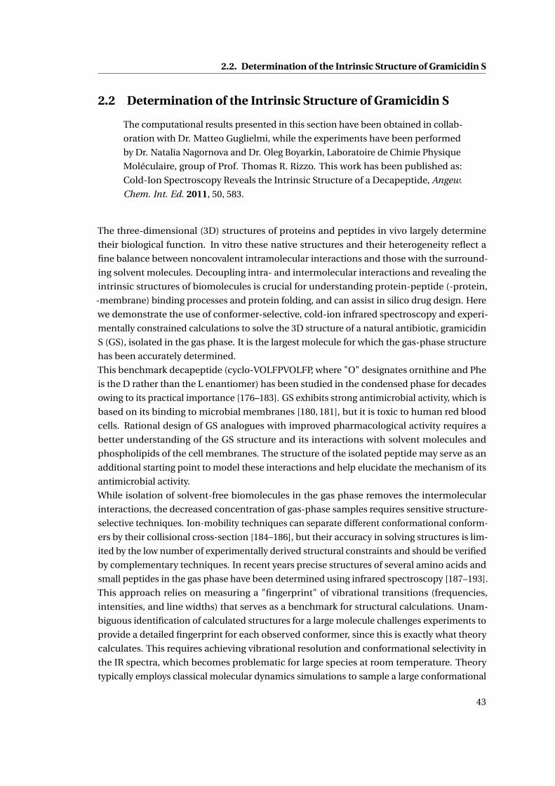
2.2. Determination of the Intrinsic Structure of Gramicidin S
2.2 Determination of the Intrinsic Structure of Gramicidin S
The computational results presented in this section have been obtained in collab-
oration with Dr. Matteo Guglielmi, while the experiments have been performed
by Dr. Natalia Nagornova and Dr. Oleg Boyarkin, Laboratoire de Chimie Physique
Moléculaire, group of Prof. Thomas R. Rizzo. This work has been published as:
Cold-Ion Spectroscopy Reveals the Intrinsic Structure of a Decapeptide, Angew.
Chem. Int. Ed. 2011, 50, 583.
The three-dimensional (3D) structures of proteins and peptides in vivo largely determine
their biological function. In vitro these native structures and their heterogeneity reflect a
fine balance between noncovalent intramolecular interactions and those with the surround-
ing solvent molecules. Decoupling intra- and intermolecular interactions and revealing the
intrinsic structures of biomolecules is crucial for understanding protein-peptide (-protein,
-membrane) binding processes and protein folding, and can assist in silico drug design. Here
we demonstrate the use of conformer-selective, cold-ion infrared spectroscopy and experi-
mentally constrained calculations to solve the 3D structure of a natural antibiotic, gramicidin
S (GS), isolated in the gas phase. It is the largest molecule for which the gas-phase structure
has been accurately determined.
This benchmark decapeptide (cyclo-VOLFPVOLFP, where "O" designates ornithine and Phe
is the D rather than the L enantiomer) has been studied in the condensed phase for decades
owing to its practical importance [176–183]. GS exhibits strong antimicrobial activity, which is
based on its binding to microbial membranes [180, 181], but it is toxic to human red blood
cells. Rational design of GS analogues with improved pharmacological activity requires a
better understanding of the GS structure and its interactions with solvent molecules and
phospholipids of the cell membranes. The structure of the isolated peptide may serve as an
additional starting point to model these interactions and help elucidate the mechanism of its
antimicrobial activity.
While isolation of solvent-free biomolecules in the gas phase removes the intermolecular
interactions, the decreased concentration of gas-phase samples requires sensitive structure-
selective techniques. Ion-mobility techniques can separate different conformational conform-
ers by their collisional cross-section [184–186], but their accuracy in solving structures is lim-
ited by the low number of experimentally derived structural constraints and should be verified
by complementary techniques. In recent years precise structures of several amino acids and
small peptides in the gas phase have been determined using infrared spectroscopy [187–193].
This approach relies on measuring a "fingerprint" of vibrational transitions (frequencies,
intensities, and line widths) that serves as a benchmark for structural calculations. Unam-
biguous identification of calculated structures for a large molecule challenges experiments to
provide a detailed fingerprint for each observed conformer, since this is exactly what theory
calculates. This requires achieving vibrational resolution and conformational selectivity in
the IR spectra, which becomes problematic for large species at room temperature. Theory
typically employs classical molecular dynamics simulations to sample a large conformational
43

Chapter 2. Assessment of Computational Methods to Determine Low EnergyConformations of Biomolecules
space to identify candidate structures. Subsequently, a few of the lowest energy structures are
optimised by ab initio theory to find the most stable conformer. The biggest challenge in these
calculations is in narrowing the conformational search among the thousands of structures
identified by molecular dynamics prior to optimising their structures at higher levels of theory
and calculating their spectra.
Our experiment combines electrospray ionization mass spectrometry, cryogenic cooling, and
laser spectroscopy (see the Supporting Information of ref. [141] for the details) [139]. Cooling
sample molecules to sufficiently low temperatures (≈ 10 K) allows vibrational resolution in the
UV and IR spectra of GS [140]. High resolution in the UV spectrum enables the use of IR/UV
double-resonance detection [187, 188, 194–196] for conformer-selective measurements of IR
spectra. We recently demonstrated application of this approach for spectroscopy of GS in
the 6 µm region [140]. Herein we extend it over a significant spectral range covering all the
light-atom stretching vibrations, and we use some special techniques, such as 15N isotopic
substitution and complexation of the peptide with a crown ether to help assign the vibrational
bands. Structural constraints derived from both our spectroscopic and mass spectrometric
data guide the conformational search to find the most stable calculated structures of isolated,
doubly protonated GS. By comparing the unique fingerprint provided by our highly resolved,
conformation-specific infrared spectrum with the theoretically derived vibrational spectrum
we can assign one of these candidate structures to the predominant conformer of GS that we
produce in the gas phase.
In the gas phase at low temperature [GS+2H]2+ adopts three different conformations, one of
which is significantly more abundant than the other two [140]. Fig. 2.7a) shows an infrared
spectrum of this main conformer cooled to approximately 12 K measured by photofragment-
detected IR/UV double resonance. The spectrum, which covers the NH, CH, and C−−O stretch-
ing and NH bending bands provide a set of nearly 30 spectroscopic reference frequencies for
selecting a 3D structure of doubly protonated GS from the calculated possibilities. In several
regions of the spectrum the resolved, closely spaced peaks impose stringent requirements
on the accuracy of calculated vibrational frequencies. Simply matching the calculated and
observed frequencies is necessary but not sufficient for identifying the proper structure, how-
ever. The assignment of the peaks to specific vibrational modes provides the true link between
experiment and theory.
We use several different methods to assign the vibrational bands in Fig. 2.7a). Isotopic labelling
of the two Val and two Leu residues by 15N should shift the amide NH stretching vibrations to
lower frequencies by approximately 8 cm−1 (in a harmonic oscillator approximation). In the
IR spectrum of Fig. 2.8b), we indeed observe a -8.5 cm−1 shift of two peaks in the isotopically
substituted molecule, allowing us to unambiguously assign these peaks to four NH stretching
vibrations of these residues. The fact that the isotopic substitution of four residues results in
the shift of only two peaks implies that the NH stretches in each pair of identical residues have
nearly degenerate frequencies, suggesting symmetrically equivalent positions of the identical
residues. This observation supports our earlier suggestion that the [GS+2H]2+ structure should
be highly symmetric (C2) [140]. Replacement of all amide hydrogens by deuterium atoms also
helps in the assignment of vibrational bands in that it shifts all ND stretching vibrations below
44
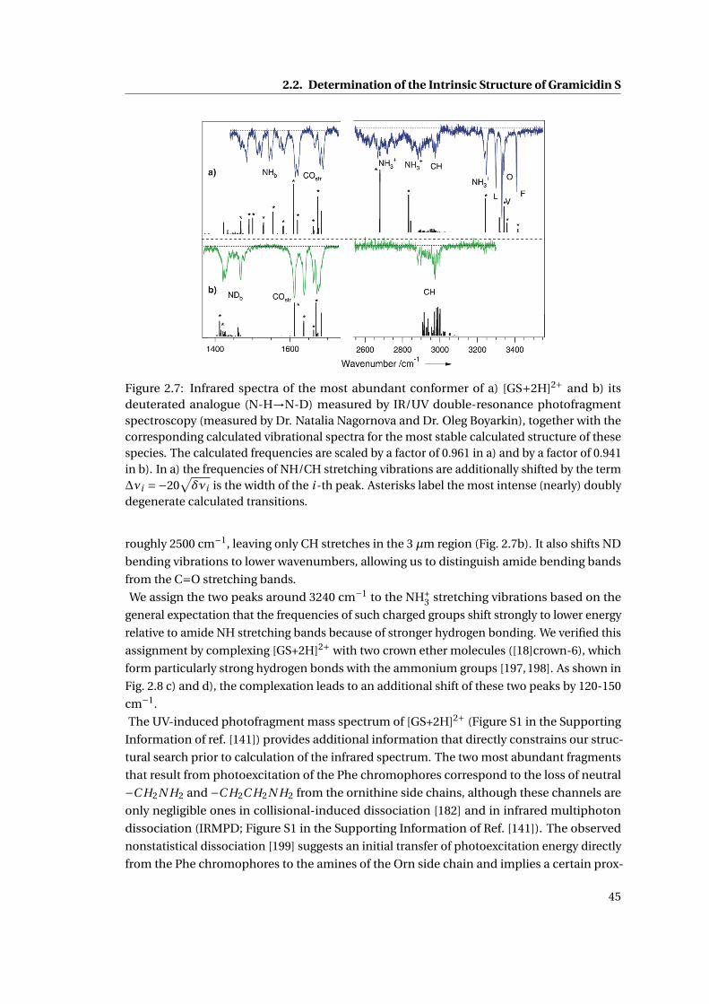
2.2. Determination of the Intrinsic Structure of Gramicidin S
Figure 2.7: Infrared spectra of the most abundant conformer of a) [GS+2H]2+ and b) itsdeuterated analogue (N-H→N-D) measured by IR/UV double-resonance photofragmentspectroscopy (measured by Dr. Natalia Nagornova and Dr. Oleg Boyarkin), together with thecorresponding calculated vibrational spectra for the most stable calculated structure of thesespecies. The calculated frequencies are scaled by a factor of 0.961 in a) and by a factor of 0.941in b). In a) the frequencies of NH/CH stretching vibrations are additionally shifted by the term∆νi =−20
√δνi is the width of the i -th peak. Asterisks label the most intense (nearly) doubly
degenerate calculated transitions.
roughly 2500 cm−1, leaving only CH stretches in the 3 µm region (Fig. 2.7b). It also shifts ND
bending vibrations to lower wavenumbers, allowing us to distinguish amide bending bands
from the C−−O stretching bands.
We assign the two peaks around 3240 cm−1 to the NH+3 stretching vibrations based on the
general expectation that the frequencies of such charged groups shift strongly to lower energy
relative to amide NH stretching bands because of stronger hydrogen bonding. We verified this
assignment by complexing [GS+2H]2+ with two crown ether molecules ([18]crown-6), which
form particularly strong hydrogen bonds with the ammonium groups [197, 198]. As shown in
Fig. 2.8 c) and d), the complexation leads to an additional shift of these two peaks by 120-150
cm−1.
The UV-induced photofragment mass spectrum of [GS+2H]2+ (Figure S1 in the Supporting
Information of ref. [141]) provides additional information that directly constrains our struc-
tural search prior to calculation of the infrared spectrum. The two most abundant fragments
that result from photoexcitation of the Phe chromophores correspond to the loss of neutral
−C H2N H2 and −C H2C H2N H2 from the ornithine side chains, although these channels are
only negligible ones in collisional-induced dissociation [182] and in infrared multiphoton
dissociation (IRMPD; Figure S1 in the Supporting Information of Ref. [141]). The observed
nonstatistical dissociation [199] suggests an initial transfer of photoexcitation energy directly
from the Phe chromophores to the amines of the Orn side chain and implies a certain prox-
45
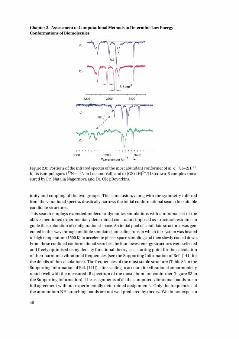
Chapter 2. Assessment of Computational Methods to Determine Low EnergyConformations of Biomolecules
Figure 2.8: Portions of the infrared spectra of the most abundant conformer of a), c) [GS+2H]2+,b) its isotopologues (15N←14N in Leu and Val), and d) [GS+2H]2+/[18]crown-6 complex (mea-sured by Dr. Natalia Nagornova and Dr. Oleg Boyarkin).
imity and coupling of the two groups. This conclusion, along with the symmetry inferred
from the vibrational spectra, drastically narrows the initial conformational search for suitable
candidate structures.
This search employs extended molecular dynamics simulations with a minimal set of the
above-mentioned experimentally determined constraints imposed as structural restraints to
guide the exploration of configurational space. An initial pool of candidate structures was gen-
erated in this way through multiple simulated annealing runs in which the system was heated
to high temperature (1500 K) to accelerate phase-space sampling and then slowly cooled down.
From these confined conformational searches the four lowest energy structures were selected
and freely optimised using density functional theory as a starting point for the calculation
of their harmonic vibrational frequencies (see the Supporting Information of Ref. [141] for
the details of the calculations). The frequencies of the most stable structure (Table S2 in the
Supporting Information of Ref. [141]), after scaling to account for vibrational anharmonicity,
match well with the measured IR spectrum of the most abundant conformer (Figure S2 in
the Supporting Information). The assignments of all the computed vibrational bands are in
full agreement with our experimentally determined assignments. Only the frequencies of
the ammonium NH stretching bands are not well predicted by theory. We do not expect a
46
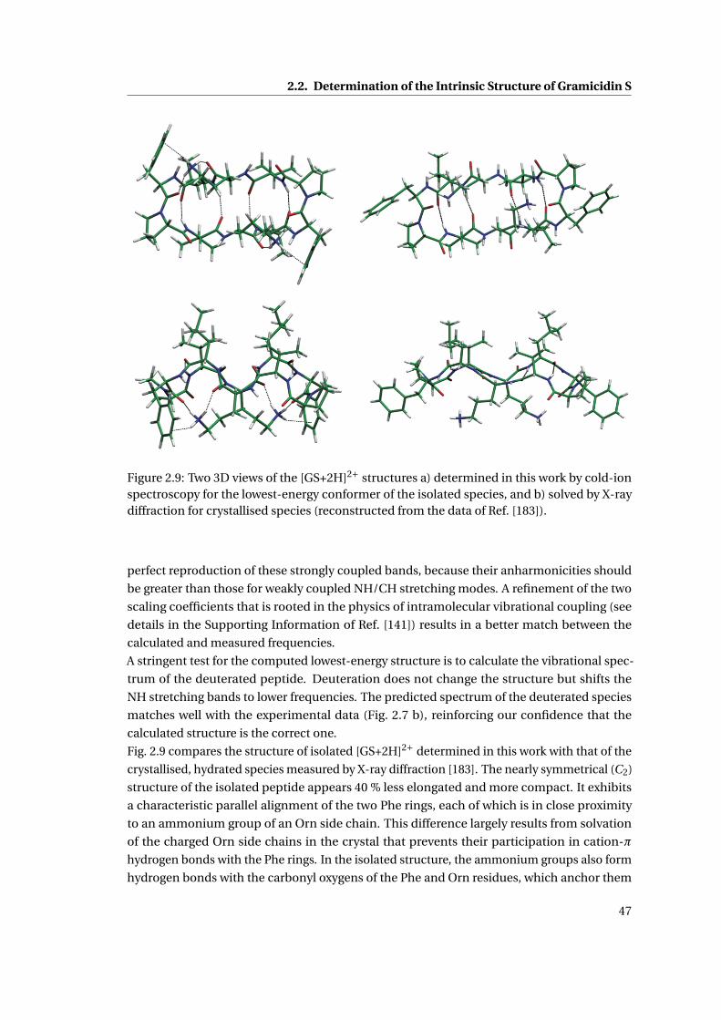
2.2. Determination of the Intrinsic Structure of Gramicidin S
Figure 2.9: Two 3D views of the [GS+2H]2+ structures a) determined in this work by cold-ionspectroscopy for the lowest-energy conformer of the isolated species, and b) solved by X-raydiffraction for crystallised species (reconstructed from the data of Ref. [183]).
perfect reproduction of these strongly coupled bands, because their anharmonicities should
be greater than those for weakly coupled NH/CH stretching modes. A refinement of the two
scaling coefficients that is rooted in the physics of intramolecular vibrational coupling (see
details in the Supporting Information of Ref. [141]) results in a better match between the
calculated and measured frequencies.
A stringent test for the computed lowest-energy structure is to calculate the vibrational spec-
trum of the deuterated peptide. Deuteration does not change the structure but shifts the
NH stretching bands to lower frequencies. The predicted spectrum of the deuterated species
matches well with the experimental data (Fig. 2.7 b), reinforcing our confidence that the
calculated structure is the correct one.
Fig. 2.9 compares the structure of isolated [GS+2H]2+ determined in this work with that of the
crystallised, hydrated species measured by X-ray diffraction [183]. The nearly symmetrical (C2)
structure of the isolated peptide appears 40 % less elongated and more compact. It exhibits
a characteristic parallel alignment of the two Phe rings, each of which is in close proximity
to an ammonium group of an Orn side chain. This difference largely results from solvation
of the charged Orn side chains in the crystal that prevents their participation in cation-π
hydrogen bonds with the Phe rings. In the isolated structure, the ammonium groups also form
hydrogen bonds with the carbonyl oxygens of the Phe and Orn residues, which anchor them
47

Chapter 2. Assessment of Computational Methods to Determine Low EnergyConformations of Biomolecules
to the peptide backbone. Table S3 in the Supporting Information of Ref. [141] provides atomic
coordinates of the calculated structure.
This work demonstrates that cold-ion spectroscopy, together with high-level theory, can be
used to solve conformer-selective structures of isolated midsize peptides. Although isolated
structures may not reflect the structures in vivo, in certain cases they should be helpful for
understanding in vivo interactions. For instance, the structure of gramicidin S interacting
with a membrane can differ from the structure determined in vitro by NMR or X-ray methods,
making the intrinsic structure determined here a valuable starting point for modelling the bio-
logical activity of this antibiotic in vivo. To our knowledge gramicidin S is the largest molecule
for which the accurate intrinsic structure has ever been determined.
48

2.3. Assessing the Performance of Computational Methods for the Prediction of theGround State Structure of Gramicidin S
2.3 Assessing the Performance of Computational Methods for the
Prediction of the Ground State Structure of Gramicidin S
This work has been published as: Assessing the Performance of Computational
Methods for the Prediction of the Ground State Structure of Gramicidin S, Int. J.
Quant. Chem. 2013, 113, 808-814.
2.3.1 Introduction
The structure and function of bio-molecular systems are closely linked, and the determination
of the native structure is often the basis for an understanding of the biological function and
mechanism of action.
Various methods, like X-ray or Neutron Diffraction, NMR, IR, Raman or microwave spec-
troscopy are available to obtain structural information. All of these techniques have inherent
advantages and disadvantages and differ in the type of information they provide as well as
in the applied measuring conditions, that might deviate to varying degrees from the in vivo
physiological conditions.
Except for diffraction methods, none of the aforementioned techniques is able to measure
directly the molecular structure. Structures can only be calculated by theoretical methods,
which in turn have to be validated by comparing predicted physical properties with experi-
ment. In the case of IR spectroscopy, for instance, the compared quantity can be frequencies
and intensities of vibrational transitions, which are directly linked to the molecular structure.
Theoretical methods are therefore, in conjunction with experiment, inherent parts of any
procedure that targets the determination of molecular structure. However, the small energy
separations between different conformational states pose stringent requirements on the accu-
racy of the computational method, which necessitates the use of high-level approaches. On
the other hand, even comparably small sized systems span a relatively large conformational
space for which a comprehensive conformational search is only possible with computationally
more expedient methods. Density functional methods usually represent a good trade-off be-
tween computational cost and accuracy. Especially modern exchange correlation functionals
with an improved functional form of the reduced density gradient and with a dependence on
the kinetic energy density [159, 160] show an impressive performance for weak interactions
that are crucial for the structure of biomolecules in both condensed phase and under isolated
vacuum conditions [200–203]. Even in conjunction with a well converged basis set, geometry
optimizations for systems up to few hundred atoms are feasible. Unfortunately, for such a
size a thorough screening of the complete conformational space is still not possible. More
approximate techniques, such as classical force fields or semi empirical quantum mechanical
(QM) methods have to be used for this purpose. Here, we test the performance of different
methods, including classical non-polarizable and polarizable force fields and a tight-binding
method, with respect to their ability of reproducing the relative energetics of a medium-sized
biomolecule. As reference data we use the results of a hybrid-meta GGA DFT method, which
we have previously validated against experimental data [141] and has been confirmed at a
49
Chapter 2. Assessment of Computational Methods to Determine Low EnergyConformations of Biomolecules
similar theoretical level by others [204, 205].
As a test set we use a pool of nine gas-phase conformations of protonated gramicidin S (GS), a
cyclic decapeptide with the highly symmetric sequence cyclo-ValOrnLeuPheProValOrnLeuPhePro,
where "Orn" designates ornithine and Phe is the D rather than the L enantiomer. GS is a nat-
ural antibiotic peptide against gram-positive and -negative bacteria and several pathogenic
fungi [206, 207]. The proposed mechanism of action is based upon distortions caused by its
binding to the microbial cell membranes. Unfortunately, it appears to be toxic to human blood
cells. GS has been studied extensively in the condensed phase [177, 178, 180–183, 208], but
no structure in its native membrane environment is available. A better understanding of its
structure and interactions with the solvent and cell membranes might help in the rational
design of GS analogs with reduced hemolytic activity and preserved antimicrobial features. In
this respect, it is important to know the intrinsic structure of gramicidin S in the absence of
any solvent and environment effects.
The experimental data (frequencies, intensities of vibrational transitions and their partial
assignment), which we use as a reference for validation of our calculations, were obtained by
measuring conformer-selective IR spectra of the protonated species ([GS+2H]2+) isolated in
the gas phase at T ∼12 K. The isolation of the target biomolecules removes their interaction
with the solvent, revealing weak intramolecular interactions that control structure and stability,
while the cryogenic cooling suppresses different types of inhomogeneous spectral broadening
and condenses most of the species at their vibrational ground levels. Conformational selec-
tivity of these measurements greatly simplifies the comparison with calculated vibrational
spectra, since the latter are obtained separately for each computed molecular structure. In
addition to the frequencies and intensities of vibrational transitions, the experiment provides
some structural information, such as the relative proximity of certain chemical groups or the
relative number of hydrogen bonds. However, it is still a very challenging task to deduce a 3D
molecular structure (Fig. 2.10) from the vibrational spectrum (Fig. 2.11) alone. Computational
techniques can be applied to determine the optimal arrangement of the nuclei and to calculate
the corresponding vibrational spectrum. Matching the calculated with the experimental IR
spectrum can then be used to identify the equilibrium geometry.
Besides its pivotal role in identifying the intrinsic structure of biomolecules, cold ion spec-
troscopy, as described in more detail in the Methodology section, also provides valuable
benchmark data for theoretical methods [140]. The gas-phase environment renders the
system feasible for first principles electronic structure methods and the highly resolved ex-
perimental IR spectra allow, in combination with isotope substitution experiments, direct
assignments with respect to the calculated vibrational bands. Before attempting to solve the
3D structure of cold protonated Gramicidin S, we have performed benchmarking studies on
bare and microsolvated protonated tryptophan in which we have assessed the performance
of various popular DFT methods to predict the lowest energy structure in comparison with
the high level wave function based CBS-C method [40] and experiments in Section 2.1. It
turned out, that in all cases CBS-C was able to predict the lowest energy conformers that
are in agreement with the experimentally observed vibrational spectra. M06 [160] and M05-
2X [159] provided energetics in close agreement with the CBS-C results, but only M05-2X and
50
2.3. Assessing the Performance of Computational Methods for the Prediction of theGround State Structure of Gramicidin S
B3LYP [16, 110, 155, 209] yielded highly-reliable predictions of the vibrational spectra.
In this work we extend our benchmarking effort to a larger size biomolecule, i. e. gas-phase
[GS+2H]2+. In particular, we tested the performance of the classical force fields AMBER
FF96 [43], FF99SB [44], FF02polEP [45] and AMOEBAbio09 [46] as well as the self-consistent
charge density functional tight-binding (SCC-DFTB) method [42] in predicting the relative
energetics of a pool of nine conformers with respect to the M05-2X/6-31G(d,p) level of theory.
The latter has been confirmed as a suitable reference method that predicts the correct ground
state structure also for [GS+2H]2+, as verified by comparison to experiment [141].
2.3.2 Methods
Geometry optimizations at the classical level using the FF96, FF99SB and FF02polEP force
fields were performed via simulated annealing as implemented in the AMBER9 software [169].
The time step was set to 1 fs, bonds involving Hydrogen atoms were constrained using the
SHAKE algorithm [170]. The temperature was controlled by a Langevin thermostat with a
collision frequency of 3.0 ps−1. Heating for 3 ns, equilibration for 5 ns and linear cooling for
20 ns. Calculations employing the AMOEBAbio09 [46] were performed within the TINKER
software package [171]. The SCC-DFTB method was used as implemented in DFTB+, v.1.1 [172]
in conjunction with the mio-0-1 parameter set citeElstner:1998wv [173]. Improvements for the
description of hydrogen bonding [71] and dispersion interactions [162] were considered as well
and will be denoted as SCC-DFTB(h) and SCC-DFTB(d), respectively. Geometry optimizations
were performed up to a convergence of 10−4 a.u. of the atomic forces.
DFT calculations with the M05-2X functional were performed using Gaussian G09 [164],
employing the 6-31G(d,p) basis set, tight convergence criteria and the UltraFine integration
grid option.
The experimental procedure to detect the conformer-selective vibrational spectra involved
a combination of electrospray ionization, mass spectrometry, cryogenic cooling and laser
spectroscopy. The protonated peptides in the gas phase were produced directly from an
aqueous solution using a nano spray ion source. In a quadrupole mass filter the parent ions
were pre-selected according to their mass-to-charge ratio and then transferred to a 22-pole
ion trap, where they were cooled to ∼ 6 K by collision with cold helium. At this temperature
vibrational resolution is possible even for a system as large as a decapeptide. Conformer-
selective vibrational spectra were measured by employing IR/UV double resonance detection,
where vibrational pre-excitation of the biomolecular ions by an IR pulse alters their subsequent
UV fragmentation yield [187, 188, 194, 195]. For more details see the Supporting Information
of Ref. [141].
2.3.3 Results
We have selected nine structures of [GS+2H]2+, chosen from simulated annealing runs at
the classical level or structural modifications from these, for our benchmarking study on the
energetics of a range of methods. Tab. 2.7 labels the different conformations according to their
51
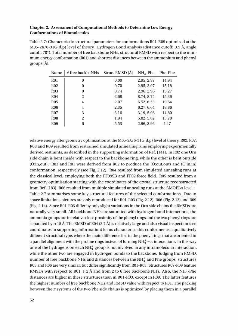
Chapter 2. Assessment of Computational Methods to Determine Low EnergyConformations of Biomolecules
Table 2.7: Characteristic structural parameters for conformations R01-R09 optimized at theM05-2X/6-31G(d,p) level of theory. Hydrogen Bond analysis (distance cutoff: 3.5 Å, anglecutoff: 70). Total number of free backbone NHs, structural RMSD with respect to the mini-mum energy conformation (R01) and shortest distances between the ammonium and phenylgroups [Å].
Name # free backb. NHs Struc. RMSD [Å] NH3-Phe Phe-Phe
R01 0 0.00 2.95, 2.97 14.94R02 0 0.70 2.95, 2.97 15.18R03 0 0.74 2.96, 2.96 15.27R04 2 2.68 8.74, 8.74 15.36R05 4 2.07 6.52, 6.53 19.64R06 4 2.35 6.27, 6.64 18.86R07 3 3.16 3.19, 5.96 14.80R08 2 1.94 5.02, 5.02 13.70R09 6 5.53 2.96, 2.96 4.47
relative energy after geometry optimization at the M05-2X/6-31G(d,p) level of theory. R02, R07,
R08 and R09 resulted from restrained simulated annealing runs employing experimentally
derived restraints, as described in the supporting information of Ref. [141]. In R02 one Orn
side chain is bent inside with respect to the backbone ring, while the other is bent outside
(O:in,out). R03 and R01 were derived from R02 to produce the (O:out,out) and (O:in,in)
conformation, respectively (see Fig. 2.12). R04 resulted from simulated annealing runs at
the classical level, employing both the FF99SB and FF02 force field. R05 resulted from a
geometry optimisation starting with the coordinates of the crystal structure reconstructed
from Ref. [183]. R06 resulted from multiple simulated annealing runs at the AMOEBA level.
Table 2.7 summarises some key structural features of the selected conformations. Due to
space limitations pictures are only reproduced for R01-R03 (Fig. 2.12), R06 (Fig. 2.13) and R09
(Fig. 2.14). Since R01-R03 differ by only slight variations in the Orn side chains the RMSDs are
naturally very small. All backbone NHs are saturated with hydrogen bond interactions, the
ammonia groups are in relative close proximity of the phenyl rings and the two phenyl rings are
separated by ≈ 15 Å. The RMSD of R04 (2.7 Å) is relatively large and also visual inspection (see
coordinates in supporting information) let us characterise this conformer as a qualitatively
different structural type, where the main difference lies in the phenyl rings that are oriented in
a parallel alignment with the proline rings instead of forming NH+3 −π interactions. In this way
one of the hydrogens on each NH+3 group is not involved in any intramolecular interaction,
while the other two are engaged in hydrogen bonds to the backbone. Judging from RMSD,
number of free backbone NHs and distances between the NH+3 and Phe groups, structures
R05 and R06 are very similar, but differ significantly from R01-R03. Structures R07-R09 feature
RMSDs with respect to R01 > 2 Å and from 2 to 6 free backbone NHs. Also, the NH3-Phe
distances are higher in these structures than in R01-R03, except in R09. The latter features
the highest number of free backbone NHs and RMSD value with respect to R01. The packing
between the π systems of the two Phe side chains is optimized by placing them in a parallel
52
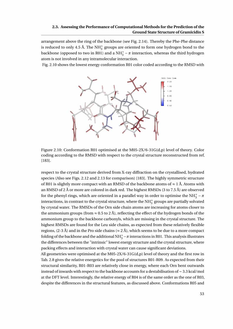
2.3. Assessing the Performance of Computational Methods for the Prediction of theGround State Structure of Gramicidin S
arrangement above the ring of the backbone (see Fig. 2.14). Thereby the Phe-Phe distance
is reduced to only 4.5 Å. The NH+3 groups are oriented to form one hydrogen bond to the
backbone (opposed to two in R01) and a NH+3 −π interaction, whereas the third hydrogen
atom is not involved in any intramolecular interaction.
Fig. 2.10 shows the lowest energy conformation R01 color coded according to the RMSD with
Figure 2.10: Conformation R01 optimised at the M05-2X/6-31G(d,p) level of theory. Colorcoding according to the RMSD with respect to the crystal structure reconstructed from ref.[183].
respect to the crystal structure derived from X-ray diffraction on the crystallised, hydrated
species (Also see Figs. 2.12 and 2.13 for comparison) [183]. The highly symmetric structure
of R01 is slightly more compact with an RMSD of the backbone atoms of ≈ 1 Å. Atoms with
an RMSD of 2 Å or more are colored in dark red. The highest RMSDs (3 to 7.5 Å) are observed
for the phenyl rings, which are oriented in a parallel way in order to optimise the NH+3 −π
interactions, in contrast to the crystal structure, where the NH+3 groups are partially solvated
by crystal water. The RMSDs of the Orn side chain atoms are increasing for atoms closer to
the ammonium groups (from ≈ 0.5 to 2 Å), reflecting the effect of the hydrogen bonds of the
ammonium group to the backbone carbonyls, which are missing in the crystal structure. The
highest RMSDs are found for the Leu side chains, as expected from these relatively flexible
regions, (2-3 Å) and in the Pro side chains (≈ 2 Å), which seems to be due to a more compact
folding of the backbone and the additional NH+3 −π interactions in R01. This analysis illustrates
the differences between the "intrinsic" lowest energy structure and the crystal structure, where
packing effects and interaction with crystal water can cause significant deviations.
All geometries were optimised at the M05-2X/6-31G(d,p) level of theory and the first row in
Tab. 2.8 gives the relative energetics for the pool of structures R01-R09. As expected from their
structural similarity, R01-R03 are relatively close in energy, where each Orn bent outwards
instead of inwards with respect to the backbone accounts for a destabilisation of ∼ 3.3 kcal/mol
at the DFT level. Interestingly, the relative energy of R04 is of the same order as the one of R03,
despite the differences in the structural features, as discussed above. Conformations R05 and
53
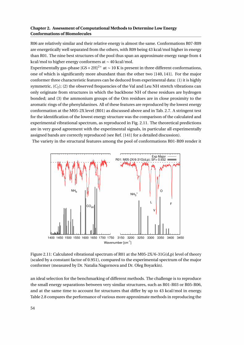
Chapter 2. Assessment of Computational Methods to Determine Low EnergyConformations of Biomolecules
R06 are relatively similar and their relative energy is almost the same. Conformations R07-R09
are energetically well separated from the others, with R09 being 43 kcal/mol higher in energy
than R01. The nine best structures of the pool thus span an approximate energy range from 4
kcal/mol to higher energy conformers at ∼ 40 kcal/mol.
Experimentally gas-phase [GS+2H]2+ at ∼ 10 K is present in three different conformations,
one of which is significantly more abundant than the other two [140, 141]. For the major
conformer three characteristic features can be deduced from experimental data: (1) it is highly
symmetric, (C2); (2) the observed frequencies of the Val and Leu NH stretch vibrations can
only originate from structures in which the backbone NH of these residues are hydrogen
bonded; and (3) the ammonium groups of the Orn residues are in close proximity to the
aromatic rings of the phenylalanines. All of these features are reproduced by the lowest energy
conformation at the M05-2X level (R01) as discussed above and in Tab. 2.7. A stringent test
for the identification of the lowest energy structure was the comparison of the calculated and
experimental vibrational spectrum, as reproduced in Fig. 2.11. The theoretical predictions
are in very good agreement with the experimental signals, in particular all experimentally
assigned bands are correctly reproduced (see Ref. [141] for a detailed discussion).
The variety in the structural features among the pool of conformations R01-R09 render it
1400 1450 1500 1550 1600 1650 1700 1750
Wavenumber [cm-1
]
NHb
COstr
3150 3200 3250 3300 3350 3400 3450
NH3+
L
V
O
F
Exp MajorR01: M05-2X/6-31G(d,p); SF= 0.932
Figure 2.11: Calculated vibrational spectrum of R01 at the M05-2X/6-31G(d,p) level of theory(scaled by a constant factor of 0.951), compared to the experimental spectrum of the majorconformer (measured by Dr. Natalia Nagornova and Dr. Oleg Boyarkin).
an ideal selection for the benchmarking of different methods. The challenge is to reproduce
the small energy separations between very similar structures, such as R01-R03 or R05-R06,
and at the same time to account for structures that differ by up to 43 kcal/mol in energy.
Table 2.8 compares the performance of various more approximate methods in reproducing the
54

2.3. Assessing the Performance of Computational Methods for the Prediction of theGround State Structure of Gramicidin S
energetics at the M05-2X/6-31G(d,p) level of theory. Standard SCC-DFTB is able to predict the
correct lowest energy conformer with respect to M05-2X. The largest errors occur in the high-
energy conformations R07-R09, with a maximum error of 16.72 kcal/mol and an RMSD of the
energies of all conformers of 8.1 kcal/mol. The hydrogen bonding corrected version DFTB(h)
improves the energetics, but not enough for the high energy conformations, resulting in a
maximum deviation of 27.2 kcal/mol for R09 and an RMSD of 10.4 kcal/mol. The dispersion
corrected DFTB is the only variant, that is not able to identify the correct lowest energy
conformation, but the three conformations R01, R05 and R06 appear as almost energetically
degenerate. The best variant, in terms of RMSD (7.6 kcal/mol) and maximum deviation
(13.4 kcal/mol) appears to be the combination DFTB(h,d). Note however, that the standard
parameter set (mio-0-1) for the N-H interactions produces rather large errors in the proton
affinities on sp3 hybridised nitrogen species [210]. This resulted in chemically unrealistic
protonation states in molecular dynamics simulation of [GS+2H]2+ at finite temperature. It
was therefore not possible to use the SCC-DFTB method for an extended sampling of the
conformational space of [GS+2H]2+ as in a simulated annealing protocol, for example. The
polarisable force field AMOEBA performs best, among the methods tested here, in terms of
RMSD (6.0 kcal/mol) and maximum deviation (12.4 kcal/mol), but it predicts R01, the lowest
energy structure at the DFT level, at 3.7 kcal/mol higher than R06. Compared to the other
tested methods the overall energetic ordering is reproduced best, although not in all cases
and for some the energy differences are overestimated. Both Amber force fields FF02polEP
and FF99SB predict R04 as the lowest energy conformation, where the average error is very
large ( 12 kcal/mol for both methods), compared to the overall energy range tested. FF99SB
performs slightly better in terms of RMSD and maximum deviation (12.4 and 20.7 kcal/mol)
than FF02polEP, which shows the largest errors in both RMSD (18.4 kcal/mol) and maximum
deviation (33.6 kcal/mol) among the selected methods. FF96 performs best among the Amber
force fields tested here, with an RMSD and maximum deviation (9.60 kcal/mol and 14.87
kcal/mol) in the range of the DFTB variants. On the other hand FF96 predicts, like AMOEBA
and DFTB(d), R06 as the lowest energy conformation (6.2 kcal/mol below R01).
55
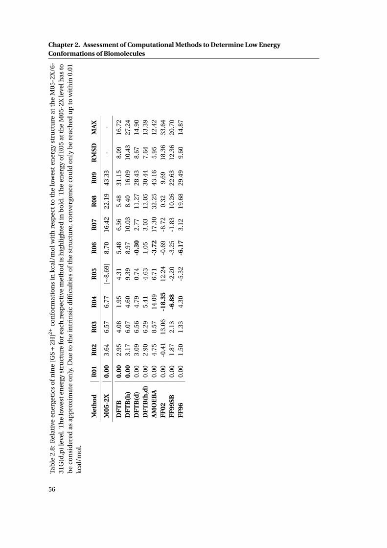
Chapter 2. Assessment of Computational Methods to Determine Low EnergyConformations of Biomolecules
Tab
le2.
8:R
elat
ive
ener
geti
cso
fn
ine
[GS+2
H]2+
con
form
atio
ns
inkc
al/m
olw
ith
resp
ect
toth
elo
wes
ten
ergy
stru
ctu
reat
the
M05
-2X
/6-
31G
(d,p
)le
vel.
Th
elo
wes
ten
ergy
stru
ctu
refo
rea
chre
spec
tive
met
ho
dis
hig
hli
ghte
din
bo
ld.T
he
ener
gyo
fR05
atth
eM
05-2
Xle
velh
asto
be
con
sid
ered
asap
pro
xim
ate
on
ly.
Du
eto
the
intr
insi
cd
iffi
cult
ies
oft
he
stru
ctu
re,c
on
verg
ence
cou
ldo
nly
be
reac
hed
up
tow
ith
in0.
01kc
al/m
ol.
Met
ho
dR
01R
02R
03R
04R
05R
06R
07R
08R
09R
MSD
MA
X
M05
-2X
0.00
3.64
6.57
6.77
[∼8.
69]
8.70
16.4
222
.19
43.3
3-
-
DF
TB
0.00
2.95
4.08
1.95
4.31
5.48
6.36
5.48
31.1
58.
0916
.72
DF
TB
(h)
0.00
3.17
6.07
4.60
9.39
8.97
10.0
38.
4016
.09
10.4
327
.24
DF
TB
(d)
0.00
3.09
6.56
4.79
0.74
-0.3
02.
7711
.27
28.4
38.
6714
.90
DF
TB
(h,d
)0.
002.
906.
295.
414.
631.
053.
0312
.05
30.4
47.
6413
.39
AM
OE
BA
0.00
4.75
8.57
14.0
96.
71-3
.72
17.3
032
.25
43.1
65.
9512
.42
FF
020.
00-0
.41
13.0
6-1
8.35
12.2
4-0
.69
-8.7
20.
329.
6918
.36
33.6
4F
F99
SB0.
001.
872.
13-6
.88
-2.2
0-3
.25
-1.8
310
.26
22.6
312
.36
20.7
0F
F96
0.00
1.50
1.33
4.30
-5.3
2-6
.17
3.12
19.6
829
.49
9.60
14.8
7
56
2.3. Assessing the Performance of Computational Methods for the Prediction of theGround State Structure of Gramicidin S
2.3.4 Discussion and Conclusions
We have presented a pool of conformations for gas-phase protonated gramicidin S that covers
a wide range of structural features and energy separations. This poses stringent constraints
on the accuracy of the employed computational methods. The lowest energy conformation
at the M05-2X level of theory has been validated with experimental data, measured by cold
ion spectroscopy. This experimental technique can produce highly resolved experimental
benchmark data on biologically and biochemically relevant systems to test the performance of
state of the art computational methods. From the work presented here and the benchmarking
efforts on protonated tryptophan in Section 2.1 we propose the family of Minnesota function-
als as reliable reference methods for the energetics and especially M05-2X for the calculation
of vibrational frequencies.
We have tested several more approximate methods including SCC-DFTB and its variants, as
well as AMOEBA and AMBER FF02polEP, FF99SB and FF96 for their performance in reproduc-
ing the energetics at the M05-2X level of theory of our pool of conformations. SCC-DFTB is
the only method among the ones tested in this work, that predicts the correct lowest energy
structure. Unfortunately, at the current state of the standard parameter set suggested for bio-
molecular systems, the N-H interactions are not represented in a balanced manner, biasing
sampling of unphysical protonation states. Without further methodological improvements
on this side, it is therefore to be excluded as an initial sampling tool. AMOEBA, on the other
hand, shows slightly better energetic ordering, better RMSD values and maximum deviations,
in particular for the high energy structures.
Unrestrained simulated annealing runs at the classical level did not lead to structures in
agreement with the experimental observations (1)-(3). The two AMBER force fields, FF99SB
and FF02polEP, and AMOEBA suggest conformations that are between 7 and 9 kcal/mol higher
in energy than the minimum at the M05-2X level and show significantly different structural
features. Surprisingly, simulated annealing employing the FF02polEP force field results in the
same conformation as FF99SB. Although both force fields were tailored to condensed phase
properties of biological molecules the polarisation could be expected to help transferability
to the gas-phase environment. Even more surprising is, that the energetic ranking on the
selected conformations is worse with the FF02polEP than with the FF99SB and FF96 force
fields. The latter is the best Amber force field tested in this work, but nevertheless it favours
conformations with significantly higher relative energies at the M05-2X level. We therefore
conclude that all three force fields can not be used reliably for the energetic prescreening of
candidate structures and sample mostly unrealistic regions of the potential energy surface.
Among the protocols tested in this work, only the incorporation of structural restraints derived
from experimental information in the conformational search at the FF99SB level lead to can-
didate structures with the desired structural features for the experimentally observed major
conformation. The approximate methods tested here, seem not to be suitable for a reliable
unbiased prescreening of candidate structures in the absence of experimental structural in-
formations. Although AMOEBA and SCC-DFTB perform significantly better than the AMBER
force fields, their RMSD and maximum deviations are still high compared to the overall energy
differences between the individual conformations calculated at the M05-2X level.
57
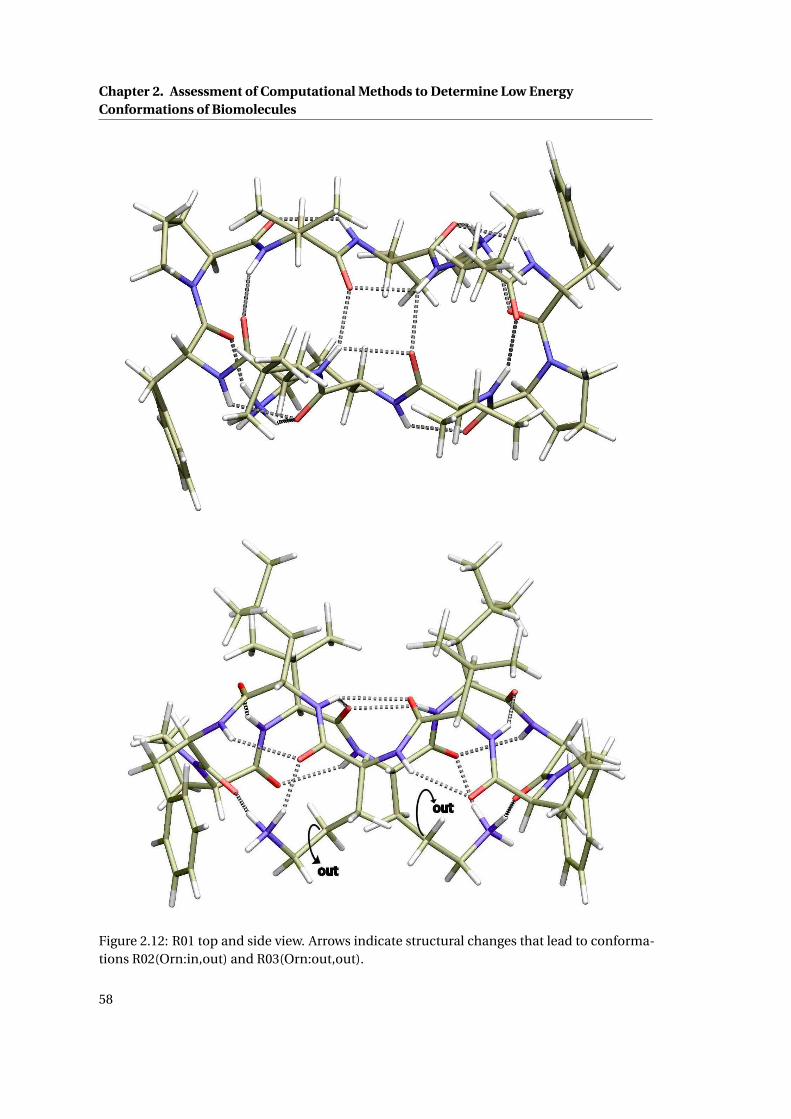
Chapter 2. Assessment of Computational Methods to Determine Low EnergyConformations of Biomolecules
Figure 2.12: R01 top and side view. Arrows indicate structural changes that lead to conforma-tions R02(Orn:in,out) and R03(Orn:out,out).
58
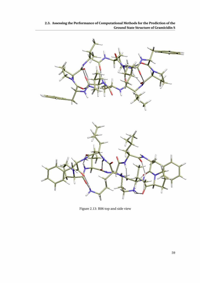
2.3. Assessing the Performance of Computational Methods for the Prediction of theGround State Structure of Gramicidin S
Figure 2.13: R06 top and side view
59
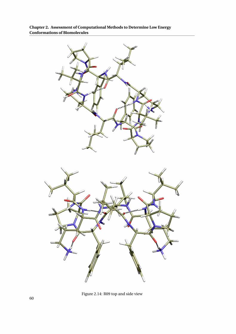
Chapter 2. Assessment of Computational Methods to Determine Low EnergyConformations of Biomolecules
Figure 2.14: R09 top and side view60

3 Deriving Molecular Mechanics ForceField Parameters by Force Matchingfrom DFT/MM Calculations3.1 Introduction
Classical Molecular Dynamics (MD) simulations based on Force Fields (FFs) represent an
important method in the investigation of large scale molecular systems of ∼ 100’000 atoms
and more in biology and materials science applications [211–213]. Typically, their functional
form does not allow the explicit description of a rearrangement of the electronic structure,
i.e. the bonding topology is retained over the course of a simulation. However, the energy
evaluation is computationally so expedient, that FFs can provide the underlying Potential
Energy Surface (PES) for MD simulations up to the microseconds time scale. This exceeds by
far the accessible time scales of first-principles MD based on electronic structure methods,
such as Density Functional Theory (DFT). FFs therefore represent an indispensable tool for
the computational modelling of e.g. large scale conformational motions of biomolecules at an
atomistic resolution.
However, the functional form of classical FFs and parameterisation is largely empirical and
the determination of accurate and transferable parameter sets involves significant human
effort. With a plethora of existing force fields and associated parameter sets a large variety
of biological systems can be studied. For systems that contain molecules for which no pa-
rameters are available it can be, however, a difficult and time consuming task to determine a
reliable force field. Typical approaches employ electronic structure calculations of a suitable
small model compound in the gas phase or in a continuum solvent to determine the missing
parameters [214]. Such procedures, however, come with the risk, that the newly determined
parameters are not necessarily transferable to the actual system under investigation in the con-
densed phase. Alternatively, in situ parameterisation methods, such as the "learn-on-the-fly"
approach [215] can be used to determine parameters from higher level reference calculations
on the system at hand in the condensed phase. The potential constructed in this way can be
used for the long-time propagation of a specific system, while its transferability is expected to
be limited. A similar approach is the force-matching technique [47] to parameterise classical
or semi-empirical potentials to reproduce the forces calculated by ab inito or DFT methods.
The method has been applied to optimise a glue potential for aluminium and, later on, an
61
Chapter 3. Deriving Molecular Mechanics Force Field Parameters by Force Matchingfrom DFT/MM Calculations
embedded atom method (EAM) potential for magnesium [216]. The clean-cut spirit of this
parameterisation method is very appealing and can be used with a manifold of different
classical and semi-empirical potential energy functions. For example, interaction potentials,
based on a (non-self-consistent) tight-binding model [217] and a modified embedded atom
method [218], were fitted for silicon from, among other properties in the target function, DFT
forces . In [219] a classical optimal potential (OP) was constructed to study the bulk properties
of iron at earth’s core conditions. Other applications can be found in Refs. [220–223]. In [224]
the force-matching methodology was modified to parameterise directly a spline interpolation
of interatomic forces. The method takes advantage of the fact that the subject of the fit was
linearly dependent on the fitting parameters and instead of directly minimising an objective
function the problem could be recast into solving an overdetermined system of linear equa-
tions. This modified parameterisation scheme can be seen as more reliable and tractable
for large numbers of parameters and was applied to studies on liquid water and hydrogen
fluoride [225]. The force matching protocol has also been applied to parameterise a reactive
FF [226].
Our group has recently developed a force matching protocol for biomolecular FFs based on
mixed Quantum Mechanics/Molecular Mechanics (QM/MM) reference calculations [48]. The
QM region is chosen in order to include all components of the system for which no parameters
are available. Finite-temperature QM/MM MD simulations are performed to generate a set
of reference configurations. Note however, that such reference configurations could also be
obtained from MD simulations at different levels of theory or by extrapolating along a given
collective coordinate, as long as they cover the relevant configurational space. Next, nuclear
forces on the QM atoms and electrostatic properties are extracted from this trajectory to serve
as target properties for the subsequent parameter fitting scheme. The force field parameters
are then optimised in order to reproduce the electrostatic properties and the nuclear forces of
the QM subsystem. Environment effects, finite temperature and pressure effects are taken into
account automatically. The optimised FF parameters can then be used to perform simulations
with the accuracy of a QM/MM treatment at the computational cost of classical MD. This
allows sampling times far beyond the limits of the QM/MM method and the calculation of
properties with long correlation times, such as thermodynamic averages involving slow mo-
tions of large biomolecules.This QM/MM force matching method has been applied to various
systems involving aqueous solutions of dihydrogenphosphate, a glycyl-alanine dipeptide, a
nitrosyl-dicarbonyl complex of technetium(I), an azole-bridged diplatinum anticancer drug
interacting with DNA [227] and organometallic ruthenium complexes [228]. Note however,
that these systems do not contain QM/MM boundaries across chemical bonds. The QM/MM
interactions therefore involve only non-bonded contributions. A similar scheme was proposed
in an adaptive formulation later on [229].
Here we describe the implementation of our QM/MM force matching protocol [48] within the
publicly available software package CPMD [49]. The goal was to provide a user friendly incor-
poration of the parameter fitting algorithms into the same code employed for the QM/MM
reference calculations. This is especially useful since in our scheme the charges are fitted
by relying on the D-RESP procedure implemented in the QM/MM interface of CPMD [129].
62
3.1. Introduction
The keywords controlling the parameter optimisation can be accessed within the same input
section as standard QM/MM calculations. A manual for the force matching keywords can be
found in the Appendix B. After the QM/MM force matching the optimised FF parameters can
be employed in conjunction with any software package for classical simulations. Furthermore,
we show how the QM/MM force matching protocol can be used for systems which involve
bonded QM-MM interactions within the pseudo link atom approach.
We have applied this protocol to derive in situ FF parameters for the retinal chromophore
in bovine rhodopsin embedded in a lipid bilayer, as shown in Figure 3.1. Rhodopsin is a
biological pigment in the photoreceptor cells of the retina and constitutes the first member
in a signalling cascade responsible for the perception of light [50, 51]. The initial event upon
light absorption is the cis-trans isomerisation of the retinal chromophore within the active
site of the protein [52–55] (red in Figure 3.1). A more detailed representation of the retinal
moiety is provided in Figure 3.2 (C1 −C15). It is covalently bound to the side chain of Lys296
(Cβ to NZ) via a protonated Schiff base. Another important residue is Glu113, which acts as a
counter ion for the positive charge of the protonated group. The light-induced isomerisation
occurs around the C11 =C12 double bound. The investigation of the structural variations after
the absorption of light has been an active field of research, both on the experimental [56–59]
and computational sides [60–63]. Biomolecular force fields have been employed to illuminate
equilibrium properties of dark state rhodopsin [230] and the large scale structural rearrange-
ments of the protein after light absorption [64,65]. However, the parameter sets currently used
for the retinal chromophore [17, 61, 66] do not account for the bond length alternation (BL A)
among carbon-carbon single and double bonds in the conjugated π-system. This is a reason-
able approximation if structural properties of the protein are concerned. However, recent
investigations have shown that optical properties calculated from configurations generated by
such an approximate bonding topology do not agree with experiments [67]. Currently, one has
to rely on QM/MM methods in order to generate realistic configurations for the calculations
of optical properties [68]. In order to overcome the time scale limitations associated with the
QM/MM approach we apply the newly implemented QM/MM force matching protocol to
derive a consistent set of FF parameters that reproduce the structural and dynamical prop-
erties at the QM/MM level. Especially, the new parameter set describes correctly the BL A in
the retinal. These subtle changes in the chromophore structure have a pronounced influence
on the optical properties. The optical absorption spectrum calculated from configurations
extracted from an MD trajectory using the new FF, is in excellent agreement with the QM/MM
and experimental references, while the original FF produces configurations that lead to a
substantial red-shift in the calculated absorption spectrum.
63
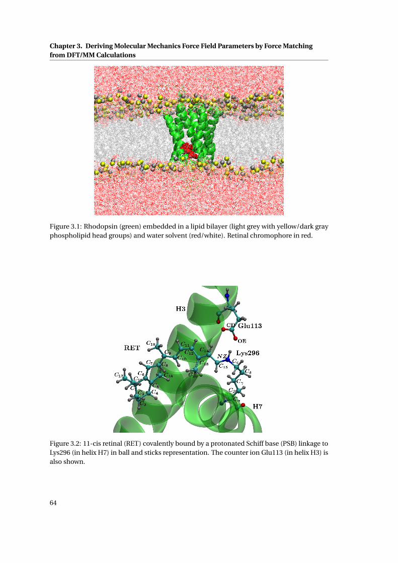
Chapter 3. Deriving Molecular Mechanics Force Field Parameters by Force Matchingfrom DFT/MM Calculations
Figure 3.1: Rhodopsin (green) embedded in a lipid bilayer (light grey with yellow/dark grayphospholipid head groups) and water solvent (red/white). Retinal chromophore in red.
Figure 3.2: 11-cis retinal (RET) covalently bound by a protonated Schiff base (PSB) linkage toLys296 (in helix H7) in ball and sticks representation. The counter ion Glu113 (in helix H3) isalso shown.
64

3.2. Methods
3.2 Methods
3.2.1 QM/MM Force Matching
The concept of the force-matching approach, as proposed in the seminal paper by Ercolessi et
al. [47], involves the minimisation of the force-dependend objective function defined as:
λ(τ) = 1
3 ·L ·N
L∑l=1
Nl∑α=1
|Flα(τ)−F0lα|2 (3.1)
where τ is the set of parameters in the interatomic classical or semi-empirical potentials that
are to be optimised by reproducing the reference forces calculated by ab inito or DFT methods.
L is the number of atomic configurations, N is the number of atoms, Flα(τ) is the force on
atom α in configuration l with the parameterisation τ and F0lα is the reference force. The
objective function can also be complemented by contributions from additional constraints,
e.g. experimental data.
In our force matching scheme a FF is parameterised for all the QM atoms of a complete
QM/MM system. In any QM/MM scheme, this relies on the assumption that the original
FF parameters provide a good representation for the rest of the system, i.e. the MM region.
The procedure involves four steps: First, a set of reference configurations l is generated.
Second, the nuclear forces on all the atoms of the QM subsystem as well as the electrostatic
potential and field in the surrounding of the electronic charge density are stored. Third, a
set of atomic point charges qα that reproduce the electrostatic potential and field in the
surrounding of the QM region is calculated. The fourth step involves the actual force matching.
The non-bonded contributions, computed with the charges obtained in the third step and
a given set of Lennard-Jones parameters from the MM force field, are subtracted from the
total reference forces on the QM atoms. The remaining forces are assumed to originate from
bonded interactions. The parameters for bonded interactions (torsions, bending, and bonds)
are thus optimised in order to reproduce the residual part of the reference forces. The entire
procedure and the implementation in the CPMD package is described in detail in the following
sections.
Reference Configurations
We extract the reference configurations from a finite temperature QM/MM CPMD run at the
same level of theory than the one that is used to compute the reference forces. In this way, the
coverage of the conformational space is consistent with the level of theory of the reference
forces, which is expected to lead to a better convergence for the equilibrium values in the
bonded interactions (Eq. 1.40). The disadvantage, however, is the limitation of the simulation
time at the QM/MM level. At such a time scale it is unlikely to observe dihedral transitions in
the QM subsystem. Therefore, the procedure described in this work provides a parameter set
that can be safely used only for a specific conformation of the system. It is possible to generate
a force field that also reproduces torsional barriers if the QM/MM dynamics are performed
65
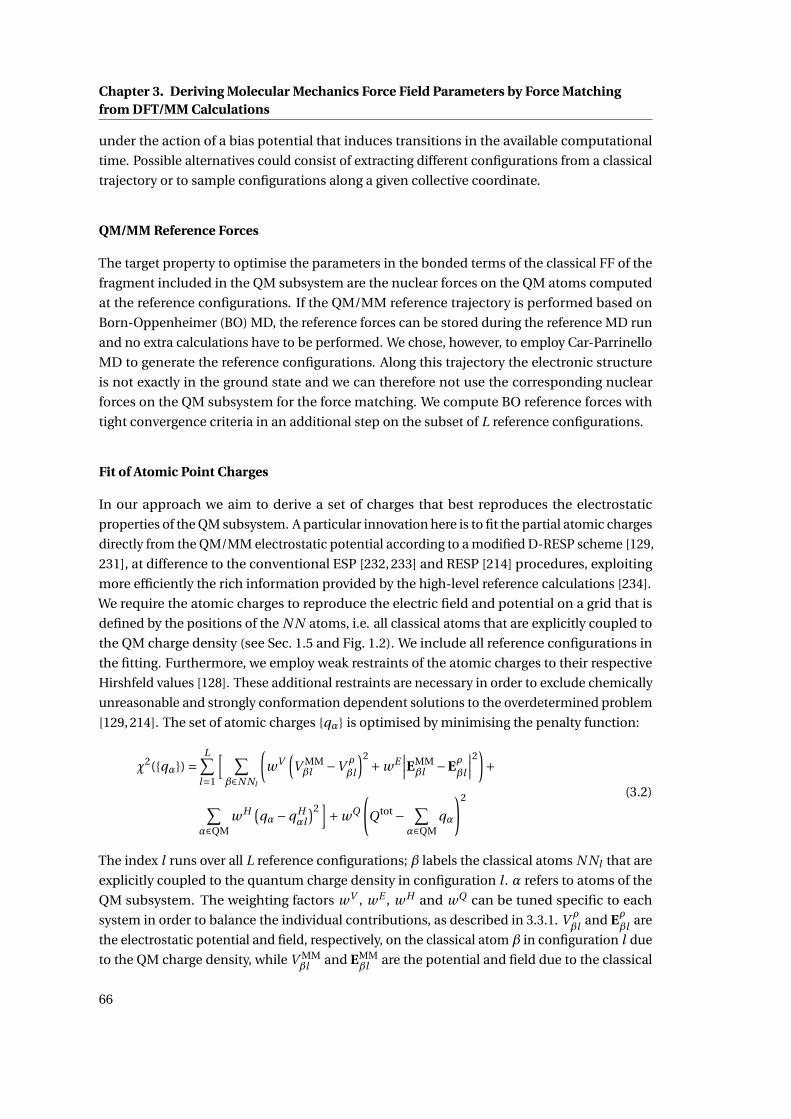
Chapter 3. Deriving Molecular Mechanics Force Field Parameters by Force Matchingfrom DFT/MM Calculations
under the action of a bias potential that induces transitions in the available computational
time. Possible alternatives could consist of extracting different configurations from a classical
trajectory or to sample configurations along a given collective coordinate.
QM/MM Reference Forces
The target property to optimise the parameters in the bonded terms of the classical FF of the
fragment included in the QM subsystem are the nuclear forces on the QM atoms computed
at the reference configurations. If the QM/MM reference trajectory is performed based on
Born-Oppenheimer (BO) MD, the reference forces can be stored during the reference MD run
and no extra calculations have to be performed. We chose, however, to employ Car-Parrinello
MD to generate the reference configurations. Along this trajectory the electronic structure
is not exactly in the ground state and we can therefore not use the corresponding nuclear
forces on the QM subsystem for the force matching. We compute BO reference forces with
tight convergence criteria in an additional step on the subset of L reference configurations.
Fit of Atomic Point Charges
In our approach we aim to derive a set of charges that best reproduces the electrostatic
properties of the QM subsystem. A particular innovation here is to fit the partial atomic charges
directly from the QM/MM electrostatic potential according to a modified D-RESP scheme [129,
231], at difference to the conventional ESP [232, 233] and RESP [214] procedures, exploiting
more efficiently the rich information provided by the high-level reference calculations [234].
We require the atomic charges to reproduce the electric field and potential on a grid that is
defined by the positions of the N N atoms, i.e. all classical atoms that are explicitly coupled to
the QM charge density (see Sec. 1.5 and Fig. 1.2). We include all reference configurations in
the fitting. Furthermore, we employ weak restraints of the atomic charges to their respective
Hirshfeld values [128]. These additional restraints are necessary in order to exclude chemically
unreasonable and strongly conformation dependent solutions to the overdetermined problem
[129, 214]. The set of atomic charges qα is optimised by minimising the penalty function:
χ2(qα) =L∑
l=1
[ ∑β∈N Nl
(wV
(V MMβl −V ρ
βl
)2 +wE∣∣∣EMMβl −Eρ
βl
∣∣∣2)+
∑α∈QM
w H (qα−q H
αl
)2]+wQ
(Qtot − ∑
α∈QMqα
)2 (3.2)
The index l runs over all L reference configurations; β labels the classical atoms N Nl that are
explicitly coupled to the quantum charge density in configuration l . α refers to atoms of the
QM subsystem. The weighting factors wV , wE , w H and wQ can be tuned specific to each
system in order to balance the individual contributions, as described in 3.3.1. V ρ
βl and Eρβl are
the electrostatic potential and field, respectively, on the classical atom β in configuration l due
to the QM charge density, while V MMβl and EMM
βl are the potential and field due to the classical
66
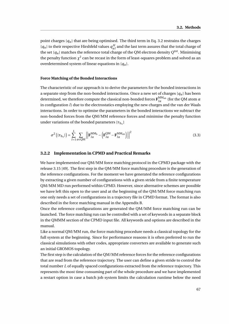
3.2. Methods
point charges qα that are being optimised. The third term in Eq. 3.2 restrains the charges
qα to their respective Hirshfeld values q Hαl and the last term assures that the total charge of
the set qα matches the reference total charge of the QM electron density Qtot. Minimising
the penalty function χ2 can be recast in the form of least-squares problem and solved as an
overdetermined system of linear equations in qα.
Force Matching of the Bonded Interactions
The characteristic of our approach is to derive the parameters for the bonded interactions in
a separate step from the non-bonded interactions. Once a new set of charges qα has been
determined, we therefore compute the classical non-bonded forces FMMnb
lα (for the QM atom α
in configuration l ) due to the electrostatics employing the new charges and the van der Waals
interactions. In order to optimise the parameters in the bonded interactions we subtract the
non-bonded forces from the QM/MM reference forces and minimise the penalty function
under variations of the bonded parameters τbn
σ2 (τbn
)= L∑l=1
∑α∈QM
∣∣∣∣∣∣FMMb
lα −(FQM
lα −FMMnb
lα
)∣∣∣∣∣∣2(3.3)
3.2.2 Implementation in CPMD and Practical Remarks
We have implemented our QM/MM force matching protocol in the CPMD package with the
release 3.15 [49]. The first step in the QM/MM force matching procedure is the generation of
the reference configurations. For the moment we have generated the reference configurations
by extracting a given number of configurations with a given stride from a finite temperature
QM/MM MD run performed within CPMD. However, since alternative schemes are possible
we have left this open to the user and at the beginning of the QM/MM force matching run
one only needs a set of configurations in a trajectory file in CPMD format. The format is also
described in the force matching manual in the Appendix B.
Once the reference configurations are generated the QM/MM force matching run can be
launched. The force matching run can be controlled with a set of keywords in a separate block
in the QMMM section of the CPMD input file. All keywords and options are described in the
manual.
Like a normal QM/MM run, the force matching procedure needs a classical topology for the
full system at the beginning. Since for performance reasons it is often preferred to run the
classical simulations with other codes, appropriate converters are available to generate such
an initial GROMOS topology.
The first step is the calculation of the QM/MM reference forces for the reference configurations
that are read from the reference trajectory. The user can define a given stride to control the
total number L of equally spaced configurations extracted from the reference trajectory. This
represents the most time consuming part of the whole procedure and we have implemented
a restart option in case a batch job system limits the calculation runtime below the need
67
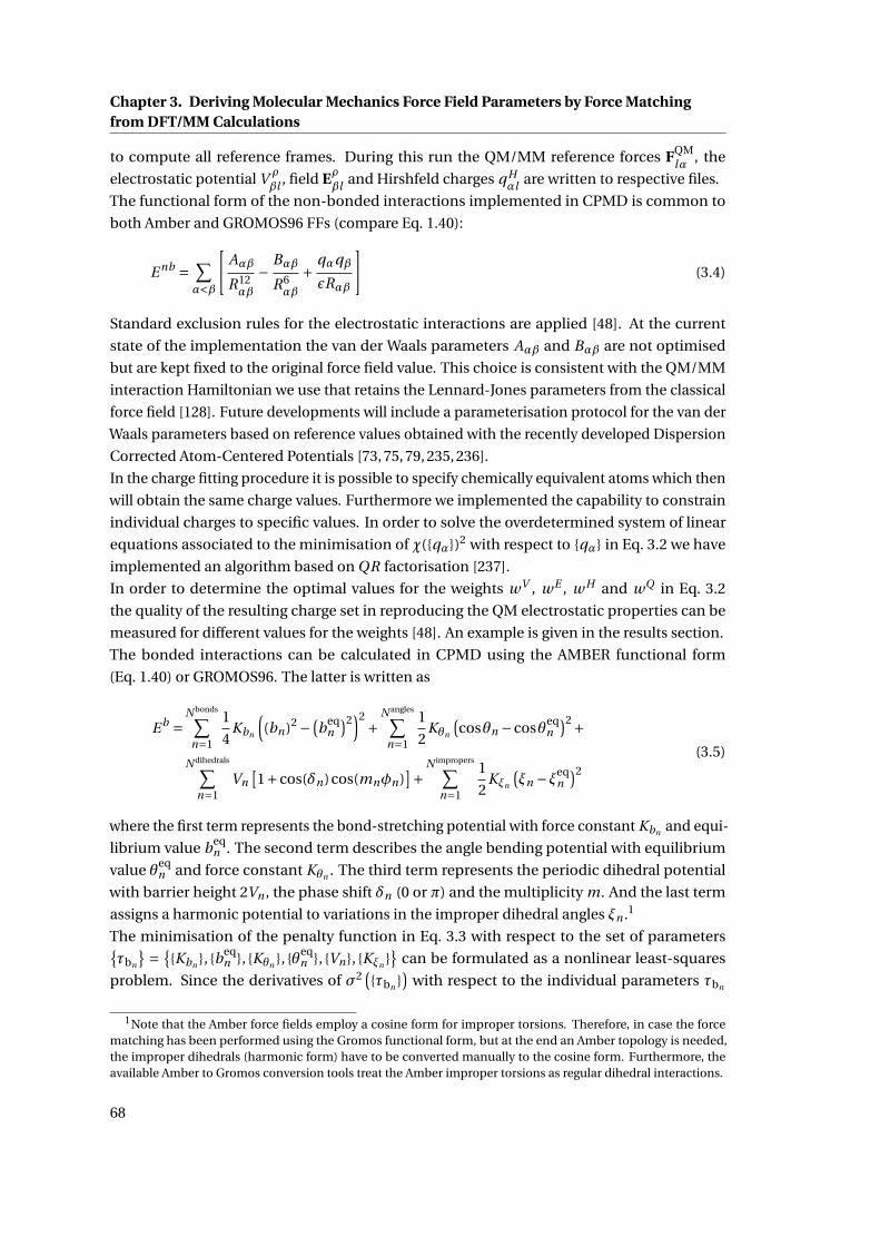
Chapter 3. Deriving Molecular Mechanics Force Field Parameters by Force Matchingfrom DFT/MM Calculations
to compute all reference frames. During this run the QM/MM reference forces FQMlα , the
electrostatic potential V ρ
βl , field Eρβl and Hirshfeld charges q H
αl are written to respective files.
The functional form of the non-bonded interactions implemented in CPMD is common to
both Amber and GROMOS96 FFs (compare Eq. 1.40):
E nb = ∑α<β
[Aαβ
R12αβ
− Bαβ
R6αβ
+ qαqβεRαβ
](3.4)
Standard exclusion rules for the electrostatic interactions are applied [48]. At the current
state of the implementation the van der Waals parameters Aαβ and Bαβ are not optimised
but are kept fixed to the original force field value. This choice is consistent with the QM/MM
interaction Hamiltonian we use that retains the Lennard-Jones parameters from the classical
force field [128]. Future developments will include a parameterisation protocol for the van der
Waals parameters based on reference values obtained with the recently developed Dispersion
Corrected Atom-Centered Potentials [73, 75, 79, 235, 236].
In the charge fitting procedure it is possible to specify chemically equivalent atoms which then
will obtain the same charge values. Furthermore we implemented the capability to constrain
individual charges to specific values. In order to solve the overdetermined system of linear
equations associated to the minimisation of χ(qα)2 with respect to qα in Eq. 3.2 we have
implemented an algorithm based on QR factorisation [237].
In order to determine the optimal values for the weights wV , wE , w H and wQ in Eq. 3.2
the quality of the resulting charge set in reproducing the QM electrostatic properties can be
measured for different values for the weights [48]. An example is given in the results section.
The bonded interactions can be calculated in CPMD using the AMBER functional form
(Eq. 1.40) or GROMOS96. The latter is written as
E b =N bonds∑
n=1
1
4Kbn
((bn)2 − (
beqn
)2)2 +
N angles∑n=1
1
2Kθn
(cosθn −cosθeq
n)2+
N dihedrals∑n=1
Vn[1+cos(δn)cos(mnφn)
]+N impropers∑n=1
1
2Kξn
(ξn −ξeq
n)2
(3.5)
where the first term represents the bond-stretching potential with force constant Kbn and equi-
librium value beqn . The second term describes the angle bending potential with equilibrium
value θeqn and force constant Kθn . The third term represents the periodic dihedral potential
with barrier height 2Vn , the phase shift δn (0 or π) and the multiplicity m. And the last term
assigns a harmonic potential to variations in the improper dihedral angles ξn .1
The minimisation of the penalty function in Eq. 3.3 with respect to the set of parametersτbn
= Kbn , beq
n , Kθn , θeqn , Vn, Kξn
can be formulated as a nonlinear least-squares
problem. Since the derivatives of σ2(τbn
)with respect to the individual parameters τbn
1Note that the Amber force fields employ a cosine form for improper torsions. Therefore, in case the forcematching has been performed using the Gromos functional form, but at the end an Amber topology is needed,the improper dihedrals (harmonic form) have to be converted manually to the cosine form. Furthermore, theavailable Amber to Gromos conversion tools treat the Amber improper torsions as regular dihedral interactions.
68
3.2. Methods
are readily available we employed the gradient-based Levenberg-Marquardt algorithm as
implemented in the MINPACK library [238, 239].
Special care has to be taken if the QM/MM boundary cuts a chemical bond. In order to
avoid strong perturbations of the electronic structure the valence of the QM region has to
be saturated. In CPMD this can be achieved by introducing a QM capping atom, typically a
hydrogen atom. The capping atom is an artificial construction and its unphysical interaction
with the MM environment is typically removed via exclusion rules. However, in the QM/MM
force matching scheme further complications arise from the unphysical nuclear forces on the
capping atom, since it is included in the QM region and therefore contributes to the QM/MM
reference forces. We therefore suggest to employ the alternative scheme implemented in
CPMD, in which the MM boundary atom is incorporated into the QM region and replaced by
a specially parameterised monovalent pseudopotential [130].2 This scheme has been applied
successfully in QM/MM simulations over the past ten years. Note however, that the electron
density in the surrounding of the monovalent pseudopotential is slightly perturbed and it
is therefore expected that in our QM/MM force matching scheme the fitting of the charges
leads to unreasonable solutions in this region. We found it best practice to fit, in a first step,
atomic point charges for all atoms included in the QM region as described in Sec. 3.2.1. The
charges on the monovalent pseudopotential and its nearest QM neighbours adopt chemically
unreasonable values but they account for the perturbations of the electronic structure at the
QM/MM boundary. The charges further away from the boundary are chemically sound and
represent well the electrostatic properties of the surrounding of the QM region. In a second
step, i.e. before fitting the bonded interactions, the charges on the monovalent pseudopoten-
tial and its nearest QM neighbours are replaced by their original FF values, while preserving
the total charge Qtot. The final atomic point charges in this region are therefore not optimised
but retained from the original FF, which should provide a more physically sound electrostatic
representation here. Furthermore, it might be necessary to constrain the bond between the
monovalent pseudopotential and the next QM atom during a QM/MM MD. A typical choice for
the bond length is the equilibrium value in the original FF. After fitting the bonded interactions
by force matching we recommend in such a case to retain all parameters involving one of
these atoms at the original FF values.
This procedure to handle the parameters involved in interactions close to the QM/MM bound-
ary works well if the QM region is chosen large enough and if the original classical point
charges and bonded parameters in the vicinity of the monovalent pseudopotential are rea-
sonably good. In the case of optimising parameters for the retinal moiety in rhodopsin, for
example, we deliberately extended the QM region up to Cβ of the LYS 296 side chain (see
Fig. 3.2). Naturally, in case the QM/MM boundary does not involve any bonded interactions,
e.g. a molecule in the QM region with the surrounding solvent treated at the classical level, no
such complications arise.
The QM/MM force matching run in CPMD generates a modified GROMOS topology file. In
2In case reference configurations were already generated using a capping atom, the monovalent pseudopotentialcan simply be introduced at the point when the reference forces are re-calculated, however the capping atomwould need to be removed at this point from the reference trajectory.
69
Chapter 3. Deriving Molecular Mechanics Force Field Parameters by Force Matchingfrom DFT/MM Calculations
case the classical simulations with the modified FF are to be run with a different code the
user has to extract the respective parameters from this modified topology file and update the
topology in the format of his choice by hand.
3.2.3 Computational Details
As a test application for the newly implemented force matching option in CPMD, we applied
this approach to develop an improved FF for the retinal moiety in rhodopsin.
Simulations were based on the crystal structure of dark-state rhodopsin (PDB code: 1U19)
[240]. All potentially charged amino acids were considered to be in their default protona-
tion states at physiological pH (i.e., charged), except Asp83 and Glu122 that were assumed
to be neutral in line with FTIR experiments [241]. Histidine residues were protonated ei-
ther at the Nδ position (His100, His211) or the Nε position (His65, His152, His195, His278).
The rhodopsin protein was embedded in an explicit membrane environment modeled by
1-palmitoyl-2-oleoyl-phosphatidylethanolamine (POPE) lipids, solvated with explicit water
molecules (covering both the cytoplasmic and extracellular sides), and neutralized with Na+
counterions. The final size of the simulation box was approximately 96x99x125 Å3, containing
about 25000 water molecules and 300 lipids, resulting in a total number of ∼118000 atoms.
The all-atom AMBER/parm99SB force field [17] was used to model standard protein residues
and counter ions, whereas the TIP3P model [242] was employed for water molecules. The force
field parameters for the palmitic acid residues bound to Cys322 and Cys323, for the retinal
chromophore, and for POPE lipids were taken from previous studies [60, 243]. Electrostatic
interactions were taken into account using the Particle Mesh Ewald algorithm [244] with a real
space cutoff of 10 Å. The same cutoff was employed for the treatment of the van der Waals inter-
actions. Bonds involving hydrogen atoms were constrained using the SHAKE algorithm [170].
An integration time step of 2 fs was used. Constant temperature (310 K) and pressure (1 atm)
were achieved by coupling the systems to a Langevin thermostat and a Nosé-Hoover Langevin
barostat, respectively [245,246]. After insertion of the protein in a pre-equilibrated lipid bilayer,
the system was minimised using the conjugate gradient algorithm and then heated up to 310
K in 500 ps while keeping positional restraints on the protein backbone atoms. A run of 3.2 ns
in the NPT ensemble, slowly removing the restraints, was initially carried out. A subsequent
simulation in the canonical ensemble was performed for another 120 ns. Data for analyses
were collected over the last 40 ns. All the classical MD simulations were carried out using the
NAMD package [247].
The QM/MM MD simulations and force matching were performed within the CPMD pack-
age release 3.15 [49] interfaced with GROMOS96 [248]. A 30 ps QM/MM Car-Parrinello MD
simulation was started using one of the equilibrated configurations from the aforementioned
classical run as initial structure. The electronic structure of the QM subsystem, formed by
the retinal PSB and the Lys296 side chain up to the Cγ atom, was described using the BLYP
exchange-correlation functional [15,16,113], while the remaining atoms, belonging to the MM
part, were considered at the classical level using the force field parameters mentioned above.
Valence electrons were described using a plane-wave expansion up to a kinetic energy cutoff
70
3.3. Results and Discussion
of 80 Ry, and soft norm-conserving Martins-Troullier pseudopotentials [249] were employed
to represent the interactions between the valence electrons and the ionic cores. A monovalent
pseudopotential was included at the position of the Cβ atom to saturate the electronic density
of the QM region at the Cγ atom. The Cβ−Cγ bond length was constrained to a value of 1.54 Å
to preserve the proper electronic structure at the centre of the QM subsystem. Long-range
electrostatic effects between MM atoms were described using the P3M method [250] with a
real space cutoff of 10 Å. Electrostatic interactions between QM and MM regions were taken
into account by means of a fully Hamiltonian hierarchical coupling scheme [128, 129, 231],
whereas bonded and van der Waals interactions between both subsystems were described at
the force field level. The inherent periodicity in the plane-wave calculations was circumvented
solving Poisson’s equation for non-periodic boundary conditions [251], while periodic bound-
ary conditions were retained for the classical simulation box. The propagation of the equations
of motion was performed within the Car-Parrinello scheme [136] using a fictitious electron
mass of 500 a.u. and a time step of 0.1 fs. Simulations were carried out in the canonical (NVT)
ensemble using a Nosé-Hoover chain of thermostats [252] to maintain the temperature at 310
K. 1000 equally spaced snapshots were taken from the last 15 ps of trajectory to re-parametrize
the force field used for the retinal chromophore via the force-matching protocol. On the ex-
tracted configurations, the electronic wave function was quenched to the Born-Oppenheimer
surface using a convergence threshold of 10−7 a.u., from which the nuclear reference forces
FQMlα in Eq. 3.3 and the electrostatic potential and field on the N N atoms were computed.
To test the quality of the structures generated by the newly developed FF, vertical excita-
tion energies were calculated for these configurations using the ZINDO/S semi-empirical
method [253] implemented in Gaussian09 [164]. This method has been calibrated on a large
set of compounds and its parameters have been optimised to give accurate excitation energies
for the calculation of absorption spectra in the visible range. In particular, previous studies
have shown that the application of the ZINDO/S methodology to the computation of vertical
excitation energies and oscillator strengths on retinal and related polyenals provides results in
very good agreement with experiments [68, 254].
All molecular images were generated with Visual Molecular Dynamics (VMD) [255].
3.3 Results and Discussion
We applied the QM/MM force matching to derive parameters for the retinal chromophore in
rhodopsin. This represents a particularly challenging system, since the QM/MM boundary
cuts a chemical bond.
We discuss first the fitting of the atomic charges and how the new bonded parameters compare
to the original force field. The complete list of the newly derived parameters can be found in the
Appendix C. We then assess the performance of the FF to reproduce structural properties of the
retinal binding pocket and the absorption spectrum from the QM/MM reference calculations
and experiment.
71
Chapter 3. Deriving Molecular Mechanics Force Field Parameters by Force Matchingfrom DFT/MM Calculations
3.3.1 Fit of Atomic Point Charges
We derived individual atomic charges for the atoms in the QM region that best reproduce the
electrostatic field and potential on the N N atoms (Eq. 3.2), with a sole constraint imposed on
chemically equivalent hydrogens of the methyl groups to adopt the same charges.
As a measure for the quality of the charge set qα we use the relative standard deviation (SD)
of the electrostatic potential (SDV ) and field (SDE ) with respect to the QM reference over all L
configurations on the N Nl probe sites:
SDV =
√√√√√∑Ll
∑α∈N Nl
(V MMαl −V ρ
αl
)2∑Ll
∑α∈N Nl
(V ρ
αl
)2 (3.6)
SDE =√√√√∑L
l
∑α∈N Nl
||EMMαl −Eρ
αl ||2∑Ll
∑α∈N Nl
||Eραl ||2
(3.7)
As described previously [48] we optimise the weighting parameters in Eq. 3.2 by deriving
charge sets for different values of wV , wE and w H . Fig. 3.3 shows SDV and SDE for all atoms
comprised in the QM subsystem as a function of wE with different values for w H . Fixed
values for wV =0.1 and wQ = 1000 were used. Naturally, increasing wE leads to a lower SDE ,
however also to a worse description of the electrostatic potential. Furthermore, it was observed
previously [48] that high values of wE in combination with small w H can lead to unphysical
atomic charges. For retinal in rhodopsin we find the best compromise at SDV ≈ 0.05 and
SDE ≈ 0.66 without allowing large deviations in the potential. The corresponding weights are
wV = 0.1, wQ = 1000, w H = 0.01 and wE = 0.1, which we use in order to derive the atomic
charges on the retinal chromophore.
A complication in deriving FF parameters for retinal in rhodopsin is the QM/MM boundary
which dissects a chemical bond, in our case Cβ−Cγ in Lys296. Note, that this is the first time
we apply the QM/MM force matching scheme to such a situation. In order to saturate the
QM valence we have placed a monovalent pseudopotential on Cβ (Fig. 3.2). Naturally, such a
perturbation of the electron density in the surrounding of Cβ affects the derivation of atomic
charges in the vicinity. We have explored various possibilities to restrain the charges of the
adjacent atoms to the values of the original force field during the charge fitting. However, this
leads simply to a shift of the problematic region further into the quantum region. In each case
the atomic charges closest to Cβ that were not restrained during the fitting procedure adopted
unphysical values in order to compensate for the boundary effects. The charges further inside
the QM region, i.e. starting from roughly three bonds away from Cβ, appear reasonable. Since
we were mainly interested in optimised parameters for the retinal moiety we found it best
practice to fit, in a first step, without any restraints atomic point charges for all atoms included
in the QM region as described in Sec. 3.2.1. The charges on Cβ and its nearest QM neighbours
adopted chemically unreasonable values due to the perturbations of the electronic structure
at the QM/MM boundary, as can be seen in Fig. 3.4. Clearly, the results from the unrestrained
72
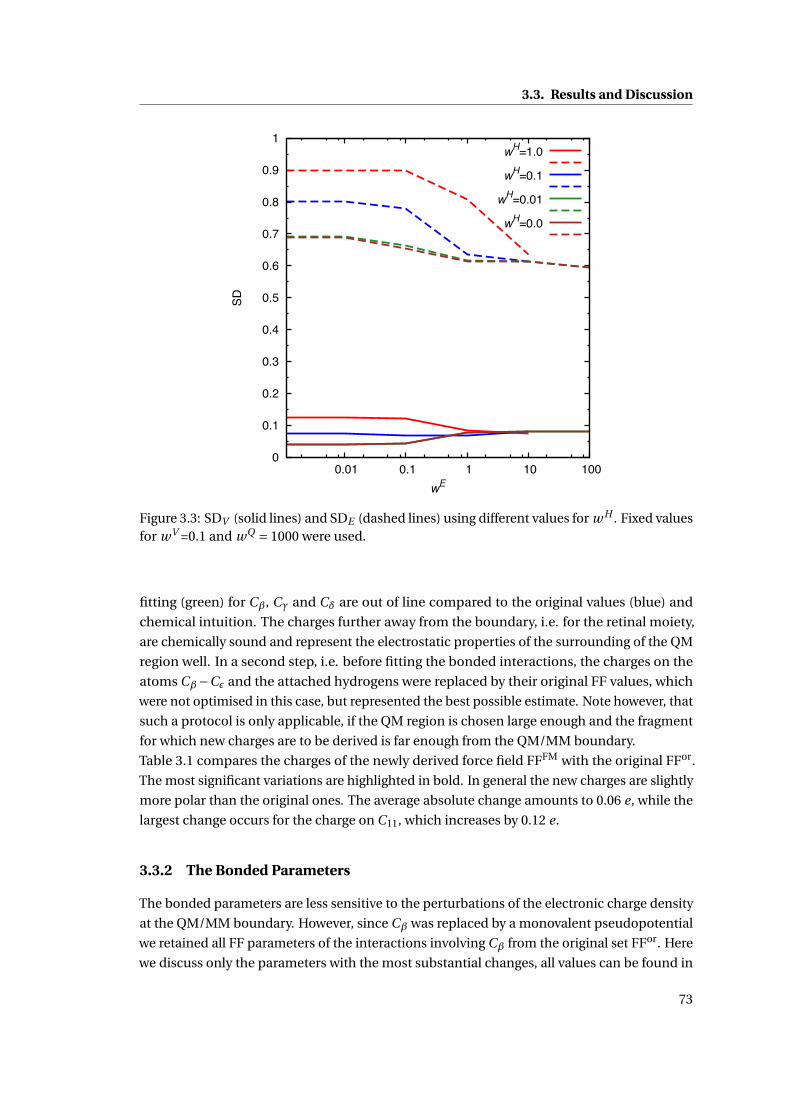
3.3. Results and Discussion
0
0.1
0.2
0.3
0.4
0.5
0.6
0.7
0.8
0.9
1
0.01 0.1 1 10 100
SD
wE
wH=1.0
wH=0.1
wH=0.01
wH=0.0
Figure 3.3: SDV (solid lines) and SDE (dashed lines) using different values for w H . Fixed valuesfor wV =0.1 and wQ = 1000 were used.
fitting (green) for Cβ, Cγ and Cδ are out of line compared to the original values (blue) and
chemical intuition. The charges further away from the boundary, i.e. for the retinal moiety,
are chemically sound and represent the electrostatic properties of the surrounding of the QM
region well. In a second step, i.e. before fitting the bonded interactions, the charges on the
atoms Cβ−Cε and the attached hydrogens were replaced by their original FF values, which
were not optimised in this case, but represented the best possible estimate. Note however, that
such a protocol is only applicable, if the QM region is chosen large enough and the fragment
for which new charges are to be derived is far enough from the QM/MM boundary.
Table 3.1 compares the charges of the newly derived force field FFFM with the original FFor.
The most significant variations are highlighted in bold. In general the new charges are slightly
more polar than the original ones. The average absolute change amounts to 0.06 e, while the
largest change occurs for the charge on C11, which increases by 0.12 e.
3.3.2 The Bonded Parameters
The bonded parameters are less sensitive to the perturbations of the electronic charge density
at the QM/MM boundary. However, since Cβ was replaced by a monovalent pseudopotential
we retained all FF parameters of the interactions involving Cβ from the original set FFor. Here
we discuss only the parameters with the most substantial changes, all values can be found in
73
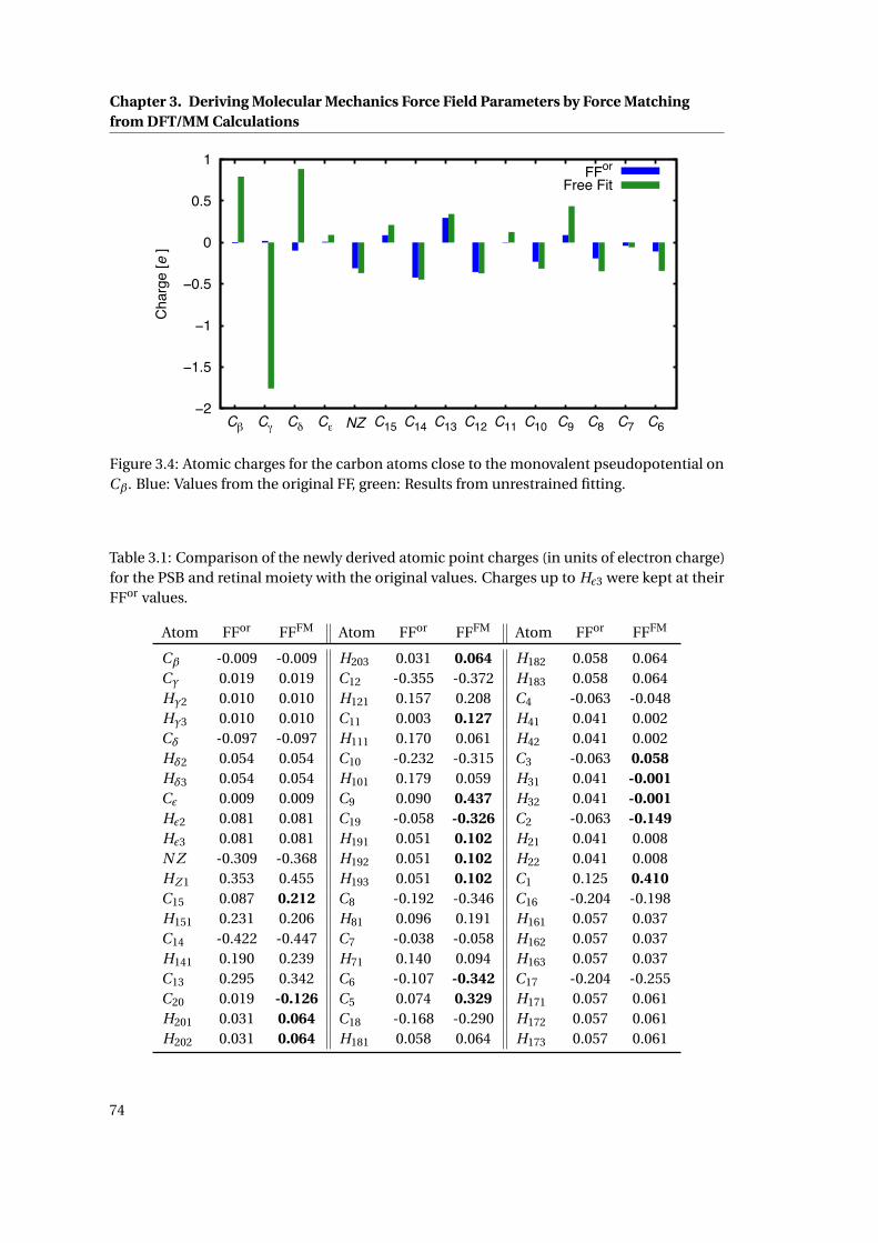
Chapter 3. Deriving Molecular Mechanics Force Field Parameters by Force Matchingfrom DFT/MM Calculations
−2
−1.5
−1
−0.5
0
0.5
1
Cβ Cγ Cδ Cε NZ C15 C14 C13 C12 C11 C10 C9 C8 C7 C6
Cha
rge
[e ]
FForFree Fit
Figure 3.4: Atomic charges for the carbon atoms close to the monovalent pseudopotential onCβ. Blue: Values from the original FF, green: Results from unrestrained fitting.
Table 3.1: Comparison of the newly derived atomic point charges (in units of electron charge)for the PSB and retinal moiety with the original values. Charges up to Hε3 were kept at theirFFor values.
Atom FFor FFFM Atom FFor FFFM Atom FFor FFFM
Cβ -0.009 -0.009 H203 0.031 0.064 H182 0.058 0.064Cγ 0.019 0.019 C12 -0.355 -0.372 H183 0.058 0.064Hγ2 0.010 0.010 H121 0.157 0.208 C4 -0.063 -0.048Hγ3 0.010 0.010 C11 0.003 0.127 H41 0.041 0.002Cδ -0.097 -0.097 H111 0.170 0.061 H42 0.041 0.002Hδ2 0.054 0.054 C10 -0.232 -0.315 C3 -0.063 0.058Hδ3 0.054 0.054 H101 0.179 0.059 H31 0.041 -0.001Cε 0.009 0.009 C9 0.090 0.437 H32 0.041 -0.001Hε2 0.081 0.081 C19 -0.058 -0.326 C2 -0.063 -0.149Hε3 0.081 0.081 H191 0.051 0.102 H21 0.041 0.008N Z -0.309 -0.368 H192 0.051 0.102 H22 0.041 0.008HZ 1 0.353 0.455 H193 0.051 0.102 C1 0.125 0.410C15 0.087 0.212 C8 -0.192 -0.346 C16 -0.204 -0.198H151 0.231 0.206 H81 0.096 0.191 H161 0.057 0.037C14 -0.422 -0.447 C7 -0.038 -0.058 H162 0.057 0.037H141 0.190 0.239 H71 0.140 0.094 H163 0.057 0.037C13 0.295 0.342 C6 -0.107 -0.342 C17 -0.204 -0.255C20 0.019 -0.126 C5 0.074 0.329 H171 0.057 0.061H201 0.031 0.064 C18 -0.168 -0.290 H172 0.057 0.061H202 0.031 0.064 H181 0.058 0.064 H173 0.057 0.061
74
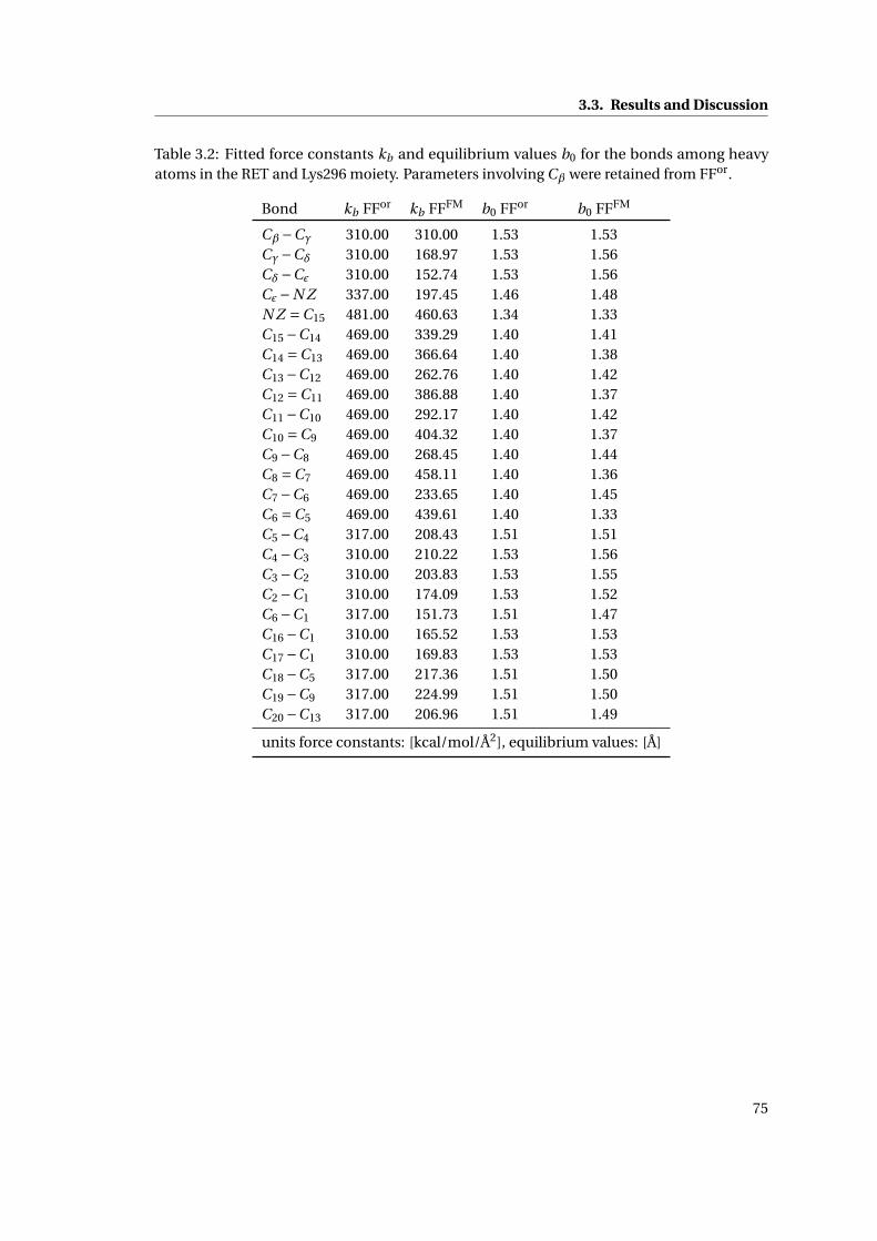
3.3. Results and Discussion
Table 3.2: Fitted force constants kb and equilibrium values b0 for the bonds among heavyatoms in the RET and Lys296 moiety. Parameters involving Cβ were retained from FFor.
Bond kb FFor kb FFFM b0 FFor b0 FFFM
Cβ−Cγ 310.00 310.00 1.53 1.53Cγ−Cδ 310.00 168.97 1.53 1.56Cδ−Cε 310.00 152.74 1.53 1.56Cε−N Z 337.00 197.45 1.46 1.48N Z =C15 481.00 460.63 1.34 1.33C15 −C14 469.00 339.29 1.40 1.41C14 =C13 469.00 366.64 1.40 1.38C13 −C12 469.00 262.76 1.40 1.42C12 =C11 469.00 386.88 1.40 1.37C11 −C10 469.00 292.17 1.40 1.42C10 =C9 469.00 404.32 1.40 1.37C9 −C8 469.00 268.45 1.40 1.44C8 =C7 469.00 458.11 1.40 1.36C7 −C6 469.00 233.65 1.40 1.45C6 =C5 469.00 439.61 1.40 1.33C5 −C4 317.00 208.43 1.51 1.51C4 −C3 310.00 210.22 1.53 1.56C3 −C2 310.00 203.83 1.53 1.55C2 −C1 310.00 174.09 1.53 1.52C6 −C1 317.00 151.73 1.51 1.47C16 −C1 310.00 165.52 1.53 1.53C17 −C1 310.00 169.83 1.53 1.53C18 −C5 317.00 217.36 1.51 1.50C19 −C9 317.00 224.99 1.51 1.50C20 −C13 317.00 206.96 1.51 1.49
units force constants: [kcal/mol/Å2], equilibrium values: [Å]
75

Chapter 3. Deriving Molecular Mechanics Force Field Parameters by Force Matchingfrom DFT/MM Calculations
Table 3.3: Original and new parameters for the angles in the RET and Lys296 moiety. Forceconstants kθ for changes by more than 50 % and equilibrium values θ0 for changes by morethan 10 %. Parameters involving Cβ were retained from FFor.
Angles kθ FFor kθ FFFM θ0 FFor θ0 FFFM
HZ 1 −N Z −Cε 52.80 24.62 118.40 99.93H42 −C4 −H41 36.50 34.57 109.50 98.32N Z −C15 −C14 73.57 74.04 120.00 134.68C3 −C2 −C1 41.61 70.40 109.50 108.74C4 −C3 −C2 41.61 83.52 109.50 111.71C5 −C6 −C1 73.57 37.58 120.00 122.49C6 −C1 −C2 66.38 65.45 120.00 94.80C8 −C7 −C6 66.38 50.45 120.00 133.54C10 −C9 −C8 66.38 65.43 120.00 133.16C16 −C1 −C2 41.61 65.80 109.50 100.02C16 −C1 −C6 66.38 60.01 120.00 97.75C17 −C1 −C2 41.61 79.17 109.50 103.00C17 −C1 −C6 66.38 63.34 120.00 98.94C17 −C1 −C16 41.61 70.04 109.50 100.56C19 −C9 −C10 73.57 48.03 120.00 133.79C19 −C9 −C8 73.57 51.49 120.00 132.10
units force constants: [kcal/mol/rad2], equilibrium values: []
the Appendix C.
Table 3.2 shows the newly derived parameters for the bonds among the heavy atoms, the
parameters involving hydrogens changed even less. The parameters for Cβ−Cγ were retained
from the original FF. In general, the new force constants are slightly smaller than the original
ones. FFor does not account for the BL A along the conjugated chain from C15 to C5. It rather
assigns the same equilibrium values and force constants to all these bonds. The latter are
relatively high, typical for double bonds. In contrast, the new b0’s describe the alternating
bond lengths of the single and double bonds. Moreover, the new force constants for the single
bonds are closer to typical values for single bonds.
Of the total of 108 new bending angle interactions only the ones with substantial changes are
shown in Table 3.3. The force constants kθ for angles involving a hydrogen atom changed on
average by 9 kcal/mol/rad2 to smaller values compared to θ0 FFor. The equilibrium values θ0
changed by 6 on average. A few stronger variations occurred mainly for the angles among the
heavy atoms for, which the average changes amount to 17 kcal/mol/rad2 for kθ and 9 for θ0.
The parameters for the dihedral angle interactions were not affected substantially, they can,
however, be found in the Appendix C.
76

3.3. Results and Discussion
Table 3.4: Comparison of local properties of the retinal binding pocket (Fig. 3.2) averaged overfinite temperature MD trajectories employing different levels of theory: QM/MM (15 ps), theoriginal force field FFor and the newly optimised force field FFFM (both 40 ns). Experimentalvalues for structural properties were extracted from the crystal structure PDB code 1U19 [240].Atomic RMSD values were calculated with respect to the crystal structure, considering theheavy atoms of the retinal only (RMSDRET) and including all heavy atoms within a radius of5 Å around the retinal (RMSDRET+5). The absorption maximum Emax was obtained from aGaussian fit to the ZINDO (S0 → S1) spectrum, averaged over 3000 configurations .
QM/MM FFor FFFM Exp.
RMSDRET [Å] 0.32 ± 0.07 0.36 ± 0.08 0.34 ± 0.06 -RMSDRET+5 [Å] 0.57 ± 0.04 0.57 ± 0.05 0.70 ± 0.07 -RNZ−C6 [Å] 11.12 ± 0.18 10.99 ± 0.17 11.09 ± 11.21φC5−C6−C7−C8 [] -44.8 ± 9.1 -50.9 ± 9.8 -50.1 ± 10.6 -30.3φC10−C11−C12−C13 [] -16.1 ± 8.4 -15.7 ± 8.4 -16.6 ± 8.8 -40.8BL A [Å] 0.31 ± 0.09 -0.02 ± 0.08 0.31 ± 0.10 0.45RNZ−CDGlu113 [Å] 3.68 ± 0.12 3.81 ± 0.15 3.75 ± 0.14 3.98RNZ−OEGlu113 [Å] 2.75 ± 0.08 2.85 ± 0.11 2.77 ± 0.09 3.45Emax [eV] 2.44 2.10 2.41 2.49 [256]
3.3.3 Performance of the new force field
In order to assess the quality of the newly derived parameters we calculated several properties
of the retinal chromophore and its nearby environment. We compared the results from the
simulations employing the original classical force field (FFor), QM/MM and the modified force
field with the parameters for the retinal chromophore optimised using the QM/MM force
matching protocol (FFFM) with experimental values.
The first two lines in Table 3.4 show the root mean square deviations (RMSD) of the atomic
positions with respect to the experimental crystal structure [240] for the heavy atoms of the
retinal only (RMSDRET) and including all atoms within a radius of 5 Å around the retinal
(RMSDRET+5). The values are all comparably small within 0.3 to 0.7 Å and do not differ much
between the two FFs and the QM/MM results. This confirms the initial statement that the orig-
inal FFor already gives a good representation of the retinal binding pocket if overall structural
properties are concerned. Furthermore the values for the overall length of the conjugated
chain RNZ−C6 , which accounts for the bent geometry of the chromophore in the binding pocket,
are in very good agreement. The dihedral angle φC10−C11=C12−C13 accounts for the interactions
with the residues in the protein pocket that significantly distort he conjugated chain of the
chromophore from planarity, which is well reproduced by all methods. φC5=C6−C7=C8 measures
the displacement of the ionone ring from the plane of the π-system.
The Bond Length Alternation (BL A) is defined as the difference between the sum of the bond
lengths of all the C−C single bonds and the sum of the lengths of all the C−−C double bonds
77
Chapter 3. Deriving Molecular Mechanics Force Field Parameters by Force Matchingfrom DFT/MM Calculations
between C5 and C15 of the retinal chromophore (Fig. 3.2):
BL A =[
RC6−C7 +RC8−C9 +RC10−C11 +RC12−C13 +RC14−C15
]−[
RC5=C6 +RC7=C8 +RC9=C10 +RC11=C12 +RC13=C14
] (3.8)
The BL A in the experimental crystal structure amounts to 0.45 Å (Table 3.4). In contrast, the
original FF does not account for the changes of the bond lengths between carbon-carbon
single and double bonds in the retinal chromophore and produces, as expected, a BL A close
to 0. Since in the derivation of the parameters for the FFFM all C−C bonds were treated
individually, a BL A in line with the QM/MM reference value of 0.31 Å was obtained. The
remaining discrepancy to the experimental represents the well known underestimation due
to the approximations in the exchange correlation functional employed for the QM part in
the reference calculations. Naturally, these deficiencies of the QM/MM reference calculations
can not be overcome by the FFFM. Furthermore the experimental values were obtained for a
crystal structure, while our calculations were performed at pseudo in vivo conditions in the
presence of the membrane and water.
As reported in previous studies [257], we observe considerable differences in the counter ion
distances. In the crystal structure the NZ-H moiety appears to be involved in two equivalent hy-
drogen bonds with the carboxylate oxygens OE of the Glu113 counter ion with a RNZ−OEGlu113
distance of 3.45 Å. In contrast, all simulations prefer a stronger hydrogen bond to only one of
the carboxylate oxygens. FFor predicts a distance between NZ and the closer OE of 2.85 Å. An
even shorter distance of 2.75 Å is observed during the QM/MM trajectory. As expected, the
optimised parameters in FFFM result in a distance closer to the QM/MM results around 2.77
Å. The FFor predicts a distance between N Z and the C D of Glu113 (RNZ−CDGlu113) of 3.81 Å ,
in good agreement with the crystal structure value of 3.98 Å. Again, the QM/MM reference
calculations and FFFM predict considerably shorter distances of 3.68 and 3.75 Å, respectively.
In order to validate further the optimised FF parameters for retinal we calculated absorption
spectra from the MD trajectories at 310 K. From each trajectory we extracted 3000 equally
spaced configurations over the respective total simulation times (15 ps for QM/MM, 40 ns for
FFor and FFFM). For the calculation of the excitation energies we reduced the total system of
each configuration to a cluster model including the retinal chromophore and a sufficiently
large surrounding of about 250 atoms in total, which covers all residues with contribution
of >0.01 eV to the excitation energies [68]. We calculated the ZINDO/S absorption spectra
on the cluster models by weighting the excitation energy of the four lowest states with the
corresponding oscillator strengths for the full set of frames. Figure 3.5 compares the resulting
S0 → S1 transition intensities, relative to the absorption maxima, calculated from the FFor,
QM/MM and FFFM trajectories. The maximum excitation energies are reported in Table 3.4.
The absorption maximum in the spectrum obtained from the QM/MM configurations is in
good agreement with the experimental result of 2.49 eV, while FFor produces configurations
that lead to a red-shift of 0.39 eV in the calculated absorption spectrum. As noted previ-
ously [68], the red-shifted absorption maximum is due to the deficiency of FFor to reproduce
the correct BL A. In contrast, the flexibility and quality of the new parameter set FFFM produces
78
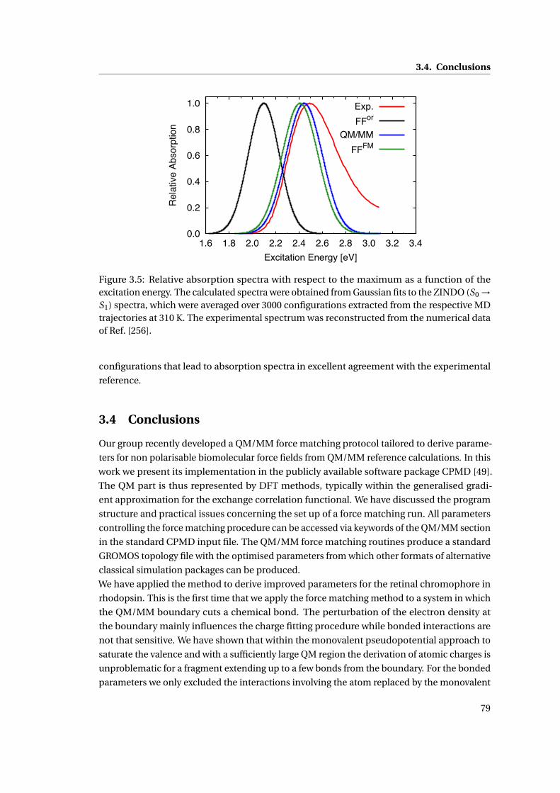
3.4. Conclusions
0.0
0.2
0.4
0.6
0.8
1.0
1.6 1.8 2.0 2.2 2.4 2.6 2.8 3.0 3.2 3.4
Rel
ativ
e Ab
sorp
tion
Excitation Energy [eV]
Exp.FFor
QM/MMFFFM
Figure 3.5: Relative absorption spectra with respect to the maximum as a function of theexcitation energy. The calculated spectra were obtained from Gaussian fits to the ZINDO (S0 →S1) spectra, which were averaged over 3000 configurations extracted from the respective MDtrajectories at 310 K. The experimental spectrum was reconstructed from the numerical dataof Ref. [256].
configurations that lead to absorption spectra in excellent agreement with the experimental
reference.
3.4 Conclusions
Our group recently developed a QM/MM force matching protocol tailored to derive parame-
ters for non polarisable biomolecular force fields from QM/MM reference calculations. In this
work we present its implementation in the publicly available software package CPMD [49].
The QM part is thus represented by DFT methods, typically within the generalised gradi-
ent approximation for the exchange correlation functional. We have discussed the program
structure and practical issues concerning the set up of a force matching run. All parameters
controlling the force matching procedure can be accessed via keywords of the QM/MM section
in the standard CPMD input file. The QM/MM force matching routines produce a standard
GROMOS topology file with the optimised parameters from which other formats of alternative
classical simulation packages can be produced.
We have applied the method to derive improved parameters for the retinal chromophore in
rhodopsin. This is the first time that we apply the force matching method to a system in which
the QM/MM boundary cuts a chemical bond. The perturbation of the electron density at
the boundary mainly influences the charge fitting procedure while bonded interactions are
not that sensitive. We have shown that within the monovalent pseudopotential approach to
saturate the valence and with a sufficiently large QM region the derivation of atomic charges is
unproblematic for a fragment extending up to a few bonds from the boundary. For the bonded
parameters we only excluded the interactions involving the atom replaced by the monovalent
79
Chapter 3. Deriving Molecular Mechanics Force Field Parameters by Force Matchingfrom DFT/MM Calculations
pseudopotential from the fitting.
The original force field for retinal [61] is not flexible enough to account for the bond length
alternation among the C−C single and double bonds of the retinal chromophore. While this
is a reasonable approximation to investigate large scale conformational properties of the
protein it does not produce configurations of the retinal moiety appropriate for the calculation
of absorption spectra. With our QM/MM force matching method we were able to derive a
parameter set that accounts for the correct bonding properties consistent with the QM/MM
reference calculations. The resulting absorption spectrum is in excellent agreement both with
the results based on the QM/MM configurations and experimental values.
Overall we have shown that the MD simulations with optimised parameters perform well
in reproducing properties from the QM/MM simulation. The agreement could further be
improved by employing a more sophisticated functional form for the classical force field, for
example by introducing a polarisable model. Our scheme can help at this point to determine
whether it is sufficient to optimise in situ the atomic point charges or whether polarisation
terms have to be added.
A limitation of our approach is the use of DFT to represent the electronic structure of the
QM subsystem in the QM/MM reference calculations. Naturally, the drawbacks of the DFT
method are inherited to the derived parameters, such as the failure in describing dispersion
interactions of standard GGA functionals. However, future extensions will include parameteri-
sation schemes for the Lennard-Jones potentials based on the recently developed dispersion-
corrected atom centered potentials [73, 75, 79, 235, 236]. A further concern is the limited
time scale accessible in the QM/MM reference calculations which is typically insufficient to
surpass torsional barriers. Enhanced sampling techniques or steered MD approaches could
be exploited to help in such situations [33–38].
80

4 Improving SCC-DFTB Parameters byIterative Boltzmann Inversion
4.1 Introduction
The choice of the underlying interaction model and its computational cost determines the
accessible system size, time scale, physical and chemical properties in molecular dynamics
(MD) simulations [22, 23]. Ultimately, it determines the properties that can be calculated at
a given accuracy from the trajectories [29]. Classical molecular mechanics force fields (FFs)
allow for sampling times up to microseconds even for large systems involved in biological and
materials science applications [32, 258]. On the other hand, their transferability is limited and
their functional form does usually not allow the description of chemical reactions. Electronic
structure methods, on the other hand, provide the functional flexibility to describe instanta-
neous electronic rearrangements and the transferability to different chemical environments
and points in the phase diagram. In particular, Kohn-Sham (KS) density functional theory
(DFT) [11, 12] has proven an efficient and flexible tool for electronic structure calculations in
a variety of fields [259–261]. Many modern DFT methods provide a reasonable compromise
between accuracy and accessible simulation time. Nevertheless, for larger system sizes sam-
pling times are limited to a few tens to a hundred picoseconds and, in practice, often not long
enough to extract structural, dynamical, thermodynamical or kinetic data at the necessary
accuracy from the trajectories.
Approximate electronic structure methods represent a bridge between DFT and FFs. They
are capable of describing rearrangements of the electronic structure, while being typically
2-3 orders of magnitude faster than DFT [213]. The latter’s limitations in sampling time and
system size can therefore be pushed further towards the regime currently dominated by the FF
methods. Two large families of such methods exist: The traditional semi-empirical (SE) wave
function based methods like the popular MNDO [262], AMx [263] and PMx [264] schemes,
which are derived from Hartree-Fock theory, and the Kohn-Sham DFT [12, 265] based tight-
binding (TB) methods [266].
A variant of the TB family is the self-consistent-charge density functional tight binding method
(SCC-DFTB) [42, 121]. It has been applied to many problems in biochemistry and material
science [267–269]. The method is entirely formulated in terms of parameterised two-body
81
Chapter 4. Improving SCC-DFTB Parameters by Iterative Boltzmann Inversion
interactions, which are naturally divided into a band structure term of a core Hamiltonian,
a charge fluctuation term and a sum of repulsive potentials. Obviously, the accuracy and
transferability of the method is determined to a large extent by the parameterisation.
In the traditional parameterisation scheme, the repulsive potentials in SCC-DFTB have to be
individually constructed for every possible diatomic combination of the elements by fitting
to selected reference data. In addition, they have to be tested case by case and therefore a
considerable amount of human effort and chemical intuition is needed to achieve accurate
and transferable results for a new system [269]. Furthermore, the quality of the fit not only
depends on the reference data, but also on the evaluation of the obtained parameters: The
same level and variety of experimental or computational reference data are not available for
all systems. Attempts towards automatized parameterisation schemes have been developed
based on the solution of a linear inverse problem [270, 271] and an approach similar to the
"Learn on the Fly" [215] method involving a genetic algorithm for the optimisation [272].
The present work focused on the development of an in situ parameterisation scheme with
respect to higher level computational reference data. We calculated highly accurate, system-
dependent parameters for repulsive potentials, while keeping the electronic parameters
unchanged. In this scheme, effects of the chemical environment, temperature and pressure
are automatically taken into account. From a practical point of view, the method is tailored
to provide a standard framework for the parameterisation procedure in condensed-phase
systems, i.e. a protocol with a minimal amount of manual interference. We employed the
so-called iterative Boltzmann inversion method, which has been developed previously in the
context of the parameterisation of empirical potentials from diffraction data [69] and extended
to deriving coarse-grained models based on atomistic simulations [70]. In both schemes the
interaction potentials for a given model were parameterised in order to reproduce reference
pairwise radial distribution functions (RDFs). We adopted a similar approach to parameterise
the SCC-DFTB repulsive potentials in order to reproduce the RDFs from DFT calculations. In
this way, we obtained parameters that allow for simulations with the accuracy comparable to
DFT at the computational cost of SCC-DFTB. As a challenging test case, we applied our new
scheme to liquid water at ambient conditions. Water is an ubiquitous solvent in biochemical
processes [273, 274] and the accurate description of its structural and dynamical properties
is essential for the modelling of chemical reactions in water [275, 276]. Unfortunately, water
has been notoriously difficult to model with approximate electronic structure methods. Only
very recently improvements could be achieved by extending NDDO type of methods by the
self-consistent polarisation approach [277, 278]. Also among the tight-binding methods the
unbalanced description of polarization has compromised the description of bulk water, but
recent work in this direction has shown great progress [279]. In SCC-DFTB the shortcomings
of the conventional method [71, 175] could be partially improved by a modified damping of
the charge fluctuation for hydrogen bonds [71] and a third-order extension [72] together with
an empirically modified O-H repulsive potential. In this work instead, we use the iterative
Boltzmann inversion method to parameterise in situ repulsive potentials without modifica-
tions in the electronic terms. This new parameter set yields significantly improved structural
and dynamical properties of liquid water.
82
4.2. Methods
4.2 Methods
4.2.1 The Repulsive Potentials
The Self-Consistent Charge Density Functional Tight-Binding (SCC-DFTB) method has been
reviewed in Section 1.3. We recall, that a set of additive pair-potentials is used to recover
some of the shortcomings in the approximate electronic terms. They are dominated by the
internuclear repulsion and are therefore called repulsive potentials. They are parameterised
specifically to pairs of chemical elements as functions of the internuclear distance:
Erep = 1
2
∑α,β
Uαβ(R) (4.1)
In the traditional approach to parameterise repulsive potentials Erep is defined with respect
to a DFT reference. A suitable reference system is chosen to parameterize a specific re-
pulsive potential, for example H2O to parameterise the O-H potential. The total energy
at the DFT level is then computed along one O-H bond stretching coordinate. The corre-
sponding repulsive potential is fitted to match the DFTB total energies to the DFT references:
Erep(ROH ) = EDFT(ROH )− [Ecore(ROH )+Eδq (ROH )]. In the case of the mio-0-1 parameter set
for biological systems [42, 173], which we used throughout this work for the electronic pa-
rameters and whose repulsive potentials served as an initial guess for our fitting scheme,
the B3LYP [13, 16] functional had been used to compute the DFT reference energies. In the
specific case of water: the O2 molecule served as a reference system to parameterise the O-O
potential and H2 to parameterise the H-H repulsive potential. This example illustrates the
human effort to produce accurate and at the same time transferable repulsive potentials for
each individual pair of chemical elements. Consider for example, that different hybridisation
states have to be accounted for, since the typical range of the repulsive potentials can extend
over various bond types. In the case of the C-C repulsive potential energy curves for triple,
double and single bond had to be considered and matched in a way to obtain a balanced de-
scription [269, 280]. A similar approach has been followed with the attempt to fit the repulsive
potentials to vibrational modes corresponding to specific bonds [281, 282]. Attempts towards
an automated parameterisation of the repulsive potentials have been undertaken following a
genetic algorithm-based approach [272] to fit total energies along a pre-defined reaction path
and based on the solution of a linear inverse problem [270]. In this work, we apply instead the
iterative Boltzmann inversion protocol based on DFT reference trajectories to obtain in situ
repulsive potentials, while retaining the original electronic parameters.
4.2.2 The Iterative Boltzmann-Inversion Scheme Applied to Repulsive SCC-DFTBPotentials
The central quantity for the following discussion is the radial distribution function (RDF)
gab(R), which measures in a system of N particles of different kinds a,b, ... in a VolumeΩ the
density of particles b at a distance R from a reference particle of type a relative to the bulk
83
Chapter 4. Improving SCC-DFTB Parameters by Iterative Boltzmann Inversion
density N /Ω [283]:
gab(R) = Ω
4πr 2 pab(R) (4.2)
with the probability density pab(R) of distances R between particle types b and a, which
can be readily extracted from the configurations of a MD trajectory. The pre-factor comes
from the spherical average. It has been demonstrated that in the case of particles interacting
by potentials of up to n-th order, the system is completely determined by all correlation
functions of n-th order [284]. Therefore, in order to derive effective pair-potentials, such as the
repulsive potentials Uab(R) considered here, we use the corresponding two-body correlation
functions gab(R) as target quantities. All remaining many-body effects are instead described
by the electronic terms, which we do not aim to re-parameterise in this work. The Boltzmann
inversion (BI) [285] relates the radial distribution function with the Helmholtz free energy:
Fab(R) =−kB T ln gab(R)+C (4.3)
It represents the effective potential of mean force (PMF) between two particles of types a
and b. T is the temperature of the system, kB is the Boltzmann constant and C is a constant
chosen to assure that the free energy of the most probable distribution is zero. In the limit of
an infinitely dilute system the PMF corresponds directly to a potential energy. Since in general
it is a free energy, only an approximate potential can be obtained from the BI, which can then
be refined iteratively.Within the restrictions of the functional form of the chosen potentials
and the simulation techniques, this procedure is likely to converge [69, 70].
In this work, the goal was to derive repulsive potentials Uab(R) that reproduce the reference
RDFs at the PBE level gab(R). We choose PBE for consistency, since the electronic terms had
already been parameterised against PBE references. The same approach can be applied to
target more accurate methods or even experimental data. Our practical implementation of
the iterative BI protocol looks as follows: From the reference trajectory we extract the RDFs
gab(R) between pairs of particle types. We use the mio-0-1 parameter set as initial guess for
the corresponding repulsive potentials U (0)ab (R) and extract the corresponding RDFs g (0)
ab (R)
from MD. We then correct the guess potentials by the difference in the PMFs with respect to
the reference :
∆F (0)ab (R) = kB T ln
[g (0)
ab (R)
gab(R)
](4.4)
This step is iterated:
U (i+1)ab (R) =U (i )
ab (R)+∆F (i )ab (R) (4.5)
with
∆F (i )ab (R) = kB T ln
[g (i )
ab(R)
gab(R)
](4.6)
84
4.2. Methods
until the gab(R) are reproduced.
The internal geometries of the individual water molecules in liquid bulk water are very well
reproduced by the standard mio-0-1 parameters. For the intermolecular interactions the domi-
nant contributions are the O-O and O-H potentials. In order to restrict our re-parameterisation
to a minimum, we modify only the O-O and O-H repulsive potentials, while keeping the H-H
repulsive potential fixed at the mio-0-1 parameter set.
4.2.3 Computational Details
For efficiency considerations the iterative Boltzmann-inversion protocol was performed for a
system of 32 water molecules in a periodic box of 9.853 Å3.
The Car-Parrinello molecular dynamics reference trajectory was generated with the CPMD
code [49] using the PBE [14] functional. Valence electrons were described using a plane-wave
expansion up to a kinetic energy cutoff of 80 Ry, and soft norm-conserving Martins-Troullier
pseudopotentials [249] were employed to represent the interactions between the valence
electrons and the ionic cores. The propagation of the equations of motion was performed
within the Car-Parrinello scheme [136] using a fictitious electron mass of 500 a.u. and a time
step of 0.1 fs. The system was initially thermalised for 3 ps using velocity rescaling to 300 K.
Subsequently, an NVE trajectory of 10 ps length was generated with configurations taken for
analysis every 500 steps.
All SCC-DFTB trajectories were performed with the DFTB+ code [172] v.1.1. The mio-0-1 set
of parameters [42, 173] was used throughout for the electronic terms and for the initial guess
of the repulsive potentials. In the iterative Boltzmann-inversion procedure for the repulsive
potentials we used the same periodic system as in the PBE reference. The Brillouin zone
was sampled at the Γ point only and for the electrostatic interaction Ewald summation was
employed. The SCF convergence criterion was set to 10−7 Hartree. The time step was 0.5 fs.
In each BI-iteration the system was equilibrated in the NVT ensemble at 300 K employing an
Andersen thermostat [286] with a selection probability of 0.01 for 100 ps. From this an NVE
trajectory of 100 ps length was restarted for the actual sampling. The configurations were
saved every 10 steps for analysis.
As a first transferability test to larger system sizes, the analysis of structural and dynamical
properties in Sections 4.3.2 and 4.3.3 were performed for periodic 64 water molecule systems.
Therefore, additional MD trajectories for 64 deuterated water molecule systems were generated
using the mio-0-1 and the improved parameter set obtained by iterative Boltzmann inversion
(mio-0-1+BI). In these sections for comparison, the Car-Parrinello trajectory, at the PBE [14]
level of theory, for 64 deuterated water molecules in a periodic box of 12.423 Å3 (corresponding
to a density of 1 g/cm3 of light water) was taken from a previous simulation [287], which had
been generated in the NVE ensemble with the CPMD code [49] with Goedecker-Teter-Hutter
pseudopotentials [288, 289], a plane-wave cutoff of 125 Ry, a fictitious electron mass of 600 au
and a time step of 0.1 fs. The average temperature is 314 K and the length of this trajectory is
117 ps with configurations taken for analysis every 10 steps.
For the geometry optimisations on the isolated water dimer we used PBE with the aug-cc-
85

Chapter 4. Improving SCC-DFTB Parameters by Iterative Boltzmann Inversion
OA
HAHA
HD
H
ODβ
α
θROO ROH
Figure 4.1: Definition of hydrogen bonding angles
pVQZ basis set, as implemented in Gaussian G09 [164] with tight convergence criteria. For
mio-0-1 and mio-0-1+BI the DFTB+ code [172] v.1.1 was used.
4.2.4 Analysis Methods
To evaluate the radial distribution functions gab(R) we computed the probability densities
of distances r in Eq. 4.2 within periodic boundary conditions from a finite number of M
configurations extracted from an MD trajectory by means of histogramming as described in
Refs. [123, 290]. In order to obtain the average coordination number of atoms of type b around
atoms of type a within a shell of radius R we integrate the corresponding radial distribution
function:
Nab(R) = 4πN
Ω
∫ R
0R2gab(R)dR (4.7)
The 3D-radial distribution functions are obtained in an analogous manner.
As a measure for the flexibility of the hydrogen bonds we analyzed the probability distribu-
tions for the hydrogen-bond angles α=∠OD−HD···OA , β=∠HD−OD···OA and θ =∠HD···OA−HA , as
depicted in Fig. 4.1. We considered angles within the first solvation shell with ROH ≤ 2.5 Å.
The self-diffusion coefficient D was evaluated using the Einstein relation from plotting the
mean-square displacement of the oxygen atoms (after removing the center of mass translation)
versus time:
⟨|R(t )−R(t0)|2⟩ = 6tD (4.8)
The MSD curve was averaged over several overlapping data blocks with the length of half of
the total simulation time. For each data block a different time origin t0 ranging from 0 to half
of the total simulation time was chosen. D was then determined from a least-square fit to the
MSD curve in the linear regime.
In order to analyse the time scale for molecular reorientations, we calculated the orientational
86
4.3. Results and Discussion
auto-correlation functions:
Cl=1,2 =1
N
∑i⟨Pl [cosθi (t )]⟩ (4.9)
in which the instantaneous molecular orientation was calculated as the axis connecting the
midpoint of the two hydrogen atoms with the oxygen atom. θi (t) is the angle between the
direction of the water molecule i at times t and t0. Pl is the Legendre polynomial of order l .
Again we averaged over an ensemble of data blocks of 20 ps length with different time origins
t0 = 0 to the total simulation length minus 20 ps. In order to extract time constants τα for this
relaxation process we fitted the functions Cl=1,2 to the functional form Al exp[−(t/τα,l )βl ]. To
account for the different time scales among the methods and relaxation processes we chose
the fit ranges for C1 0.1-20 ps for all methods. For C2, 0.5-20 ps for PBE and mio-0-1+BI and
0.1-20 ps for mio-0-1.
4.3 Results and Discussion
4.3.1 Parameterisation of the Repulsive Potentials
During the iterative Boltzmann inversion we improve the O-O and O-H repulsive potentials
simultaneously, while the H-H potential and all the electronic parameters are kept fixed at the
values of the mio-0-1 set. Figures 4.2 and 4.3 show the radial distribution functions (bottom),
the corresponding potentials of mean force (top) and the resulting repulsive potentials (mid-
dle) over the course of the iterative Boltzmann inversion for the O-O and O-H interactions. The
initial radial distribution functions, g (0)OO and g (0)
OH show the DFTB deficiencies in describing the
structure of liquid water. The peak corresponding to the first solvation shell in the initial g (0)OO is
positioned at ∼ 0.1 Å too long a distance with respect to the PBE reference gOO . Furthermore,
the structure of the second solvation shell is barely visible at this length scale. There is only a
shallow minimum at ∼ 3.8 Å. The structure of g (0)OH in Fig. 4.3 looks qualitatively better, with a
perfect agreement in the intramolecular peak at ∼ 0.9 Å. Also the hydrogen bonding peak at ∼1.8 Å is only slightly shifted towards longer distance, and the second intermolecular peak at ∼3.5 Å is well reproduced. This can be linked to the structure of the initial repulsive potential
U (0)OH , which goes to zero at 1.8 Å, in the middle of the hydrogen bonding peak in g (0)
OH . It also
features a minimum at 1.3 Å and a local maximum at 1.4 Å. The latter can directly be linked
with the shift of the hydrogen bond peak. This can be seen in the corresponding difference in
the potential of mean force with respect to the PBE reference ∆F (0)OH . The spike in the positive
range centered at 1.4 Å indicates that the potential should be more repulsive in this range,
while at 1.6 Å the potential is too repulsive. Furthermore, the maximum at 2.5 Å indicates that
a repulsive section is needed in order to enhance the structure between the first and second
intermolecular peak of the RDF. Compared to the mio-0-1 range, we elongated the repulsive
potential from 1.8 Å up to 2.9 Å, with an additional 0.5 Å to allow the first two derivatives to
go to zero smoothly. The boundaries, in which the repulsive potential was adjusted over the
course of the iterative Boltzmann inversion is indicated with black dotted vertical lines in
87
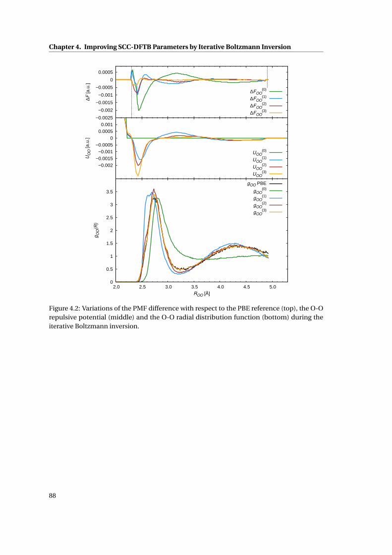
Chapter 4. Improving SCC-DFTB Parameters by Iterative Boltzmann Inversion
−0.0025
−0.002
−0.0015
−0.001
−0.0005
0
0.0005
∆F [a
.u.]
∆FOO(0)
∆FOO(1)
∆FOO(2)
∆FOO(3)
−0.002−0.0015
−0.001−0.0005
0 0.0005
0.001
UOO
[a.u
.]
UOO(0)
UOO(1)
UOO(2)
UOO(3)
0
0.5
1
1.5
2
2.5
3
3.5
2.0 2.5 3.0 3.5 4.0 4.5 5.0
gOO(R
)
ROO [Å]
gOO PBE
gOO(0)
gOO(1)
gOO(2)
gOO(3)
Figure 4.2: Variations of the PMF difference with respect to the PBE reference (top), the O-Orepulsive potential (middle) and the O-O radial distribution function (bottom) during theiterative Boltzmann inversion.
88

4.3. Results and Discussion
−0.002
−0.001
0
0.001
0.002
∆F [a
.u.]
∆FOH(0)
∆FOH(1)
∆FOH(2)
∆FOH(3)
−0.001 0
0.001 0.002 0.003 0.004 0.005 0.006 0.007
UOH
[a.u
.]
UOH(0)
UOH(1)
UOH(2)
UOH(3)
0
0.5
1
1.5
2
2.5
1.0 1.5 2.0 2.5 3.0 3.5 4.0 4.5
gOH(R
)
ROH [Å]
gOH PBE
gOH(0)
gOH(1)
gOH(2)
gOH(3)
Figure 4.3: Variations of the PMF difference with respect to the PBE reference (top), the O-Hrepulsive potential (middle) and the O-H radial distribution function (bottom) during theiterative Boltzmann inversion.
89
Chapter 4. Improving SCC-DFTB Parameters by Iterative Boltzmann Inversion
the top section. Over the iterations the UOH becomes more repulsive in the range below 1.4
Å, attractive in the range 1.4-1.9 Å and repulsive between 1.9 Å and 2.9 Å. Along this series
the features in the PMF differences decrease. Since the O-H and O-O potentials are adjusted
simultaneously, unphysical features appear at the early stages, like the double peak in the g (1)OH
at iteration 1. This is smoothed out quickly and already at the third iteration g (3)OH is in good
agreement with the PBE reference.
The tail of the mio-0-1 potential for the O-O interaction is plotted as U (0)OO in the middle part of
Fig. 4.2. It goes to zero at 2.2 Å. This is shorter than the first intermolecular peak in gOO and
any modification within a reasonable energy range would not influence the intermolecular
interactions. We therefore extended the range of the potential up to 5.0 Å. The initial PMF
difference with respect to the PBE reference,∆F (0)OO , shows a binding feature with a pronounced
tip at 2.5 Å in order to shift the first peak in the g (0)OO towards smaller distance, a repulsive
feature centered at 3.2 Å to account for first intermolecular minimum and, finally, an attractive
feature at 4.3 Å to shape the second solvation shell. This is directly reflected in the improved
UOO over the iterations, while, at the same time, the PMF differences decrease. Again, the RDF
shows a peculiar feature at 2.6 Åin the first iteration g (1)OO , which is caused by the simultaneous
correction scheme, but then improves quickly and already g (3)OO corresponds well to the PBE
reference gOO .
Two critical consequences for the structure of the repulsive potentials arise from the results of
this fitting scheme, which could both be seen as a breaking with the traditional definitions
and derivations of parameters in tight-binding methods in general and DFTB in particular.
First of all, the range of the potentials extends by far beyond the first neighbour shell. But the
restriction to the first neighbours in the parameterisation of the DFTB repulsive potentials is
mainly a consequence of the fact that only isolated molecules were used as reference systems
in the traditional parameterisation schemes, where only relatively short-range interactions
can be parameterised and a longer range of the repulsive potentials would therefore severely
compromise the transferability. In an in situ parameterisation scheme as applied in this work,
however, the effect of the surrounding species can directly be taken into account and the trans-
ferability is not a primary goal. We do not aim for a new set of universal SCC-DFTB parameters,
but rather a special set for water-water interactions at ambient conditions. Furthermore,
already U (0)OH reaches up to the first intermolecular peak in gOH and therefore extends over
the first neighbour interactions. Secondly, parts of the repulsive potentials become attractive,
since at longer ranges the core-core repulsion is not the dominant interaction missing in the
electronic terms anymore. Note as well, that also the U (0)OH is not monotonically decreasing,
but shows a local minimum at 1.3 Å. Moreover, the standard mio-0-1 H-H repulsive potential
has an attractive part as well.
In the following sections, we call the improved parameter set mio-0-1+BI, meaning that only
the UOO and UOH were improved by iterative Boltzmann inversion, while UH H and all elec-
tronic parameters were kept unchanged.
As a first transferability test to larger system sizes, the further analysis of structural and dy-
namical properties are performed on periodic systems of 64 deuterated water molecules.
90

4.3. Results and Discussion
0 0.5
1 1.5
2 2.5
3 3.5
4 4.5
2.5 3 3.5 4 4.5 5
gOO(R
) / N
OO(R
)
ROO [Å]
(a)
(b)
(c)
Exp.
PBE
mio−0−1
mio−0−1+BI
0 0.5
1 1.5
2 2.5
3 3.5
4 4.5
5
1.0 1.5 2.0 2.5 3.0 3.5 4.0 4.5
gOH(R
) / N
OH(R
)
ROH [Å]
(a)
(b)
(c)
Exp.
PBE
mio−0−1
mio−0−1+BI
0
0.5
1
1.5
2
2.5
3
3.5
1.0 1.5 2.0 2.5 3.0 3.5 4.0 4.5
gHH(R
)
RHH [Å]
(a)
(b)
(c)Exp.
PBE
mio−0−1
mio−0−1+BI
Figure 4.4: Comparison of computed RDFs (solid lines) using PBE, SCC-DFTB/mio-0-1 andSCC-DFTB/mio-0-1+BI with experimental data: O-O (a), O-H (b) and H-H (c). Integratedcoordination numbers are printed in dotted lines for the O-O and O-H interactions only.
4.3.2 Structural Properties
Fig. 4.4 compares the mio-0-1+BI RDFs for O-O, O-H and H-H with the PBE reference, standard
mio-0-1 and experiment. The PBE curves are over-structured compared to experiment and,
consequently, the mio-0-1+BI curves as well. Interestingly, although the UH H was not refitted,
the gH H of mio-0-1+BI matches closely the PBE curve, while the one of mio-0-1 is actually
closer to the experimental data. Note that the intramolecular peak in the gH H at 1.5 Å is
influenced by nuclear quantum effects, which are not taken into account neither by the PBE,
nor any SCC-DFTB MD simulation.
Integrating the RDFs according to Eq. 4.7 gives the average number of atoms of a given
species as a function of the distance from a reference species. From these plots average
coordination numbers can be determined by choosing the outer integration limit as the
91
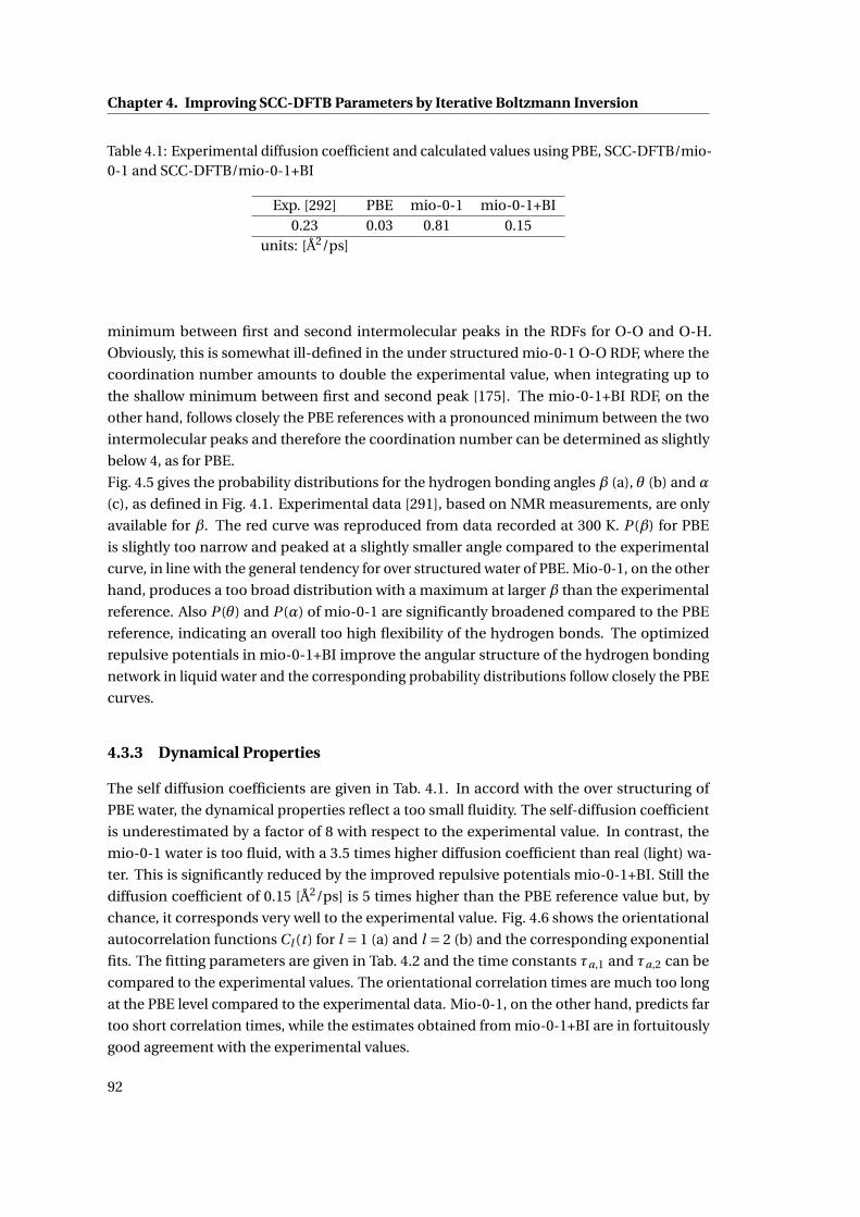
Chapter 4. Improving SCC-DFTB Parameters by Iterative Boltzmann Inversion
Table 4.1: Experimental diffusion coefficient and calculated values using PBE, SCC-DFTB/mio-0-1 and SCC-DFTB/mio-0-1+BI
Exp. [292] PBE mio-0-1 mio-0-1+BI0.23 0.03 0.81 0.15
units: [Å2/ps]
minimum between first and second intermolecular peaks in the RDFs for O-O and O-H.
Obviously, this is somewhat ill-defined in the under structured mio-0-1 O-O RDF, where the
coordination number amounts to double the experimental value, when integrating up to
the shallow minimum between first and second peak [175]. The mio-0-1+BI RDF, on the
other hand, follows closely the PBE references with a pronounced minimum between the two
intermolecular peaks and therefore the coordination number can be determined as slightly
below 4, as for PBE.
Fig. 4.5 gives the probability distributions for the hydrogen bonding angles β (a), θ (b) and α
(c), as defined in Fig. 4.1. Experimental data [291], based on NMR measurements, are only
available for β. The red curve was reproduced from data recorded at 300 K. P (β) for PBE
is slightly too narrow and peaked at a slightly smaller angle compared to the experimental
curve, in line with the general tendency for over structured water of PBE. Mio-0-1, on the other
hand, produces a too broad distribution with a maximum at larger β than the experimental
reference. Also P (θ) and P (α) of mio-0-1 are significantly broadened compared to the PBE
reference, indicating an overall too high flexibility of the hydrogen bonds. The optimized
repulsive potentials in mio-0-1+BI improve the angular structure of the hydrogen bonding
network in liquid water and the corresponding probability distributions follow closely the PBE
curves.
4.3.3 Dynamical Properties
The self diffusion coefficients are given in Tab. 4.1. In accord with the over structuring of
PBE water, the dynamical properties reflect a too small fluidity. The self-diffusion coefficient
is underestimated by a factor of 8 with respect to the experimental value. In contrast, the
mio-0-1 water is too fluid, with a 3.5 times higher diffusion coefficient than real (light) wa-
ter. This is significantly reduced by the improved repulsive potentials mio-0-1+BI. Still the
diffusion coefficient of 0.15 [Å2/ps] is 5 times higher than the PBE reference value but, by
chance, it corresponds very well to the experimental value. Fig. 4.6 shows the orientational
autocorrelation functions Cl (t ) for l = 1 (a) and l = 2 (b) and the corresponding exponential
fits. The fitting parameters are given in Tab. 4.2 and the time constants τa,1 and τa,2 can be
compared to the experimental values. The orientational correlation times are much too long
at the PBE level compared to the experimental data. Mio-0-1, on the other hand, predicts far
too short correlation times, while the estimates obtained from mio-0-1+BI are in fortuitously
good agreement with the experimental values.
92

4.3. Results and Discussion
0
0.02
0.04
0.06
0 10 20 30 40 50
P (
β)
β=∠HD−OD...OA
(a)
(b)
(c)
Exp.
PBE
mio−0−1
mio−0−1+BI
0
0.01
0.02
0.03
40 60 80 100 120 140 160 180
P (
θ)
θ=∠HD...OA−HA
(a)
(b)
(c)
PBE
mio−0−1
mio−0−1+BI
0
0.01
0.02
0.03
0.04
100 120 140 160 180
P (
α)
α=∠OD−HD...OA
(a)
(b)
(c)PBE
mio−0−1
mio−0−1+BI
Figure 4.5: Probability distributions of the hydrogen bonding angles β (a), θ (b) and α (c) asdefined in Fig. 4.1. Experimental values for β were determined from NMR data at 300K [291].
Table 4.2: Prefactors Al , time constants τα,l (in ps) and exponents βl of the orientationalauto-correlation functions Cl=1,2. Experimental values were measured at 300 K [293].
Method Al=1 τa,l=1 βl=1 Al=2 τα,l=2 βl=2
Exp. - 4.76 - - 1.92 -PBE 0.92 35.63 0.79 0.78 14.55 0.73
mio-0-1 0.83 0.48 0.96 0.64 0.19 0.87mio-0-1+BI 0.86 4.59 0.90 0.88 1.33 0.71
93
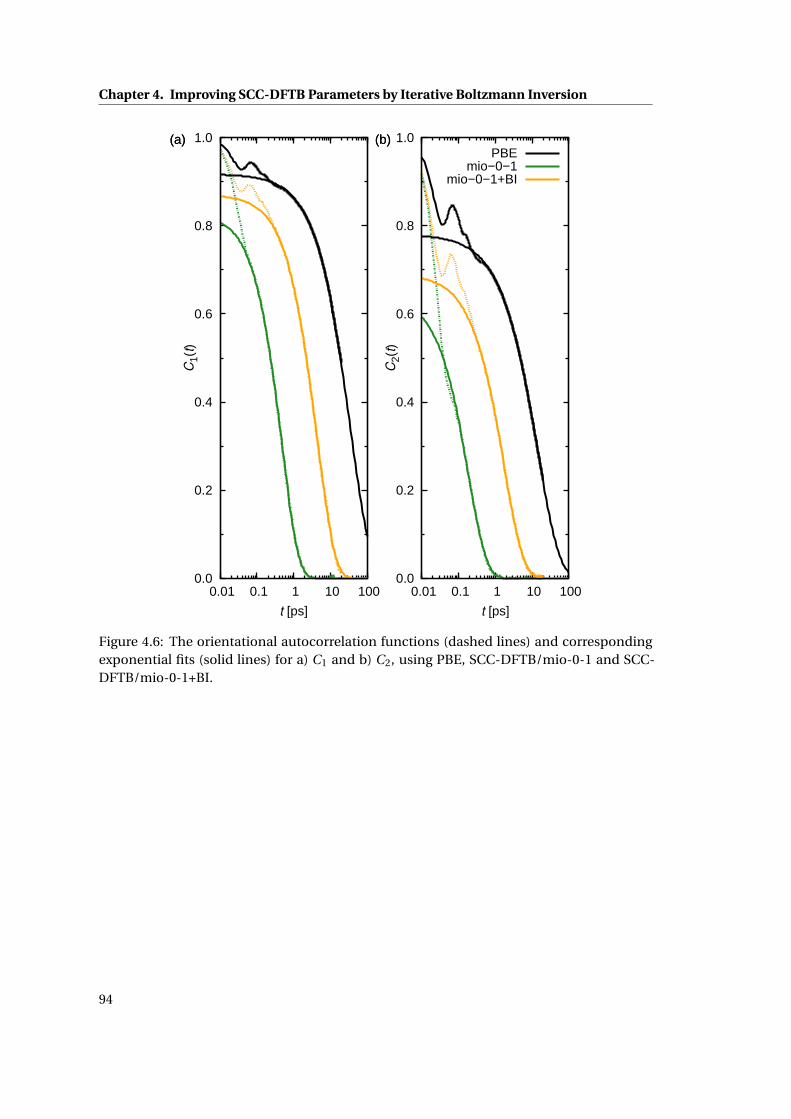
Chapter 4. Improving SCC-DFTB Parameters by Iterative Boltzmann Inversion
0.0
0.2
0.4
0.6
0.8
1.0
0.01 0.1 1 10 100
C1(t)
t [ps]
(a) (b)
0.0
0.2
0.4
0.6
0.8
1.0
0.01 0.1 1 10 100
C2(t)
t [ps]
(a) (b)PBE
mio−0−1mio−0−1+BI
Figure 4.6: The orientational autocorrelation functions (dashed lines) and correspondingexponential fits (solid lines) for a) C1 and b) C2, using PBE, SCC-DFTB/mio-0-1 and SCC-DFTB/mio-0-1+BI.
94
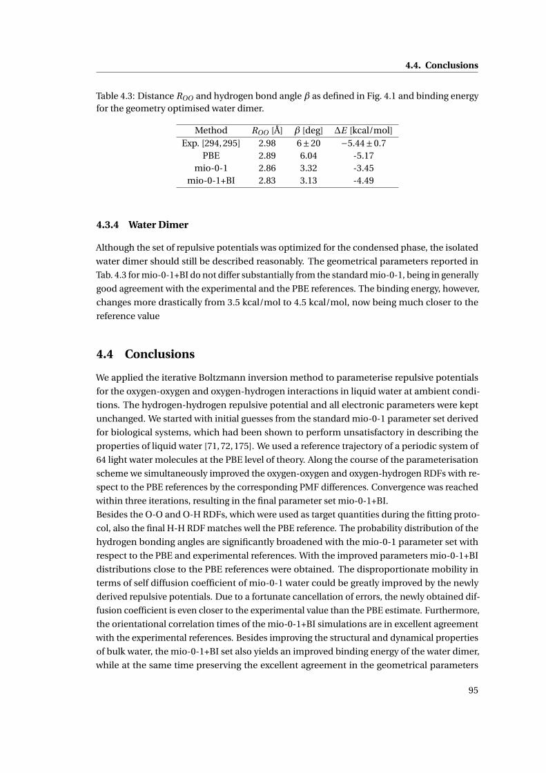
4.4. Conclusions
Table 4.3: Distance ROO and hydrogen bond angle β as defined in Fig. 4.1 and binding energyfor the geometry optimised water dimer.
Method ROO [Å] β [deg] ∆E [kcal/mol]Exp. [294, 295] 2.98 6±20 −5.44±0.7
PBE 2.89 6.04 -5.17mio-0-1 2.86 3.32 -3.45
mio-0-1+BI 2.83 3.13 -4.49
4.3.4 Water Dimer
Although the set of repulsive potentials was optimized for the condensed phase, the isolated
water dimer should still be described reasonably. The geometrical parameters reported in
Tab. 4.3 for mio-0-1+BI do not differ substantially from the standard mio-0-1, being in generally
good agreement with the experimental and the PBE references. The binding energy, however,
changes more drastically from 3.5 kcal/mol to 4.5 kcal/mol, now being much closer to the
reference value
4.4 Conclusions
We applied the iterative Boltzmann inversion method to parameterise repulsive potentials
for the oxygen-oxygen and oxygen-hydrogen interactions in liquid water at ambient condi-
tions. The hydrogen-hydrogen repulsive potential and all electronic parameters were kept
unchanged. We started with initial guesses from the standard mio-0-1 parameter set derived
for biological systems, which had been shown to perform unsatisfactory in describing the
properties of liquid water [71, 72, 175]. We used a reference trajectory of a periodic system of
64 light water molecules at the PBE level of theory. Along the course of the parameterisation
scheme we simultaneously improved the oxygen-oxygen and oxygen-hydrogen RDFs with re-
spect to the PBE references by the corresponding PMF differences. Convergence was reached
within three iterations, resulting in the final parameter set mio-0-1+BI.
Besides the O-O and O-H RDFs, which were used as target quantities during the fitting proto-
col, also the final H-H RDF matches well the PBE reference. The probability distribution of the
hydrogen bonding angles are significantly broadened with the mio-0-1 parameter set with
respect to the PBE and experimental references. With the improved parameters mio-0-1+BI
distributions close to the PBE references were obtained. The disproportionate mobility in
terms of self diffusion coefficient of mio-0-1 water could be greatly improved by the newly
derived repulsive potentials. Due to a fortunate cancellation of errors, the newly obtained dif-
fusion coefficient is even closer to the experimental value than the PBE estimate. Furthermore,
the orientational correlation times of the mio-0-1+BI simulations are in excellent agreement
with the experimental references. Besides improving the structural and dynamical properties
of bulk water, the mio-0-1+BI set also yields an improved binding energy of the water dimer,
while at the same time preserving the excellent agreement in the geometrical parameters
95

Chapter 4. Improving SCC-DFTB Parameters by Iterative Boltzmann Inversion
of the standard mio-0-1 parameter set with respect to the PBE reference. Future work will
address the transferability of the new water parameters to the solvation of charge defects and
organic molecules.
96

5 Intricacies of Describing Weak In-teractions Involving Halogen AtomsUsing Density Functional Theory
This work has been published as: Intricacies of Describing Weak Interactions
Involving Halogen Atoms Using Density Functional Theory, J. Chem. Theor. Comp.
2013, 9, 955.
5.1 Introduction
The understanding of non-covalent interactions involving halogen atoms is pivotal for a
variety of fields, ranging from stratospheric chemistry [80–84], materials science and engineer-
ing [85–92] to biological systems [93–96] and medicinal chemistry [97–101]. The importance
of halogens for pharmacology seems surprising at first, since only a few natural processes are
known in the human body that involve halogen atoms. Chloride ions appear in the stomach
acid, some membrane ion channels involved in signal transductions are selective to chloride
ions [296] and iodine is used by the thyroid gland to produce thyroxine [297]. On the other
hand, the scarcity of halogens in natural systems might to some extent explain the potency of
halogenated drug molecules since their particular chemical properties can be less interfered
with or screened by naturally occurring mechanisms. For example halogenation can render
molecules more lipophilic and therefore more transmissible through lipid membranes [100].
Furthermore replacing a C-H group by C-F inverts the dipole moment of the group and
therefore represents a powerful tool in fine tuning the electrostatic properties of a given lead
compound [298]. The greater strength of the C-F bond (∼ 110 kcal/mol) is an additional
important factor, since the group becomes less reactive [98].
In addition, a special non-covalent interaction involving halogens is observed between co-
valently bound halogen atoms (R-X) and Lewis bases (A): R−X · · ·A, which has been termed
halogen bond [85, 92, 299, 300], in analogy to the hydrogen bond [301–304]. Much scientific
interest has been devoted to the understanding of the underlying physical forces of halogen
bonding, both from the experimental and theoretical side. In the emerging picture the domi-
nating interactions are of electrostatic origin, where a region of positive electrostatic potential
97
Chapter 5. Intricacies of Describing Weak Interactions Involving Halogen Atoms UsingDensity Functional Theory
located at the end of the R-X bond, called "σ-hole", interacts with a region of negative electro-
static potential located on A. However, it has been shown recently that besides electrostatic
effects, dispersion seems to play an important role as well [305].
For a computational modeling of these types of weak, non-bonded interactions it is well estab-
lished that high level ab initio methods with a balanced description of electron correlation are
necessary [306], with the coupled cluster method involving single, doubles and a perturbative
treatment of the triple excitations [CCSD(T)] being the current gold standard. Unfortunately,
the high computational cost associated with these methods allow the treatment of only rela-
tively small-sized systems. Computationally more expedient methods would be highly desir-
able, since halogen bonding is important in biological systems, which are notoriously large.
Density Functional Theory (DFT) methods within the Kohn-Sham framework [11,12] represent
a good trade-off between computational cost and accuracy. Unfortunately, popular exchange-
correlation (xc) functionals in the local density approximation (LDA) and generalized gradient
approximation (GGA) show severe shortcomings in the description of non-bonded interac-
tions, such as London dispersion forces [200, 307, 308] since they depend on local quantities
(density and density gradient) only and therefore fail to account for intrinsically non-local
correlation effects of the electron density. A number of different strategies to overcome this
problem in DFT methods have been proposed in the recent literature. The incorporation of
dispersion interactions directly via nonlocal density functionals [309, 310] shows promising
results but is computationally not tractable for large-scale applications. Alternatively, classical
two-body potentials with C6/R6 dependence can be added to the DFT energy, where the C6
coefficient is determined either empirically [311–314], derived from atomic polarizabilities as
functional of the in-situ atomic electron density [315], or calculated from the instantaneous
dipole moment of the exchange hole [316–318]. Furthermore impressive results have been
obtained using highly parametrised meta-hybrid-GGA xc functionals [159, 319–321]. Alterna-
tively, in the DCACP approach dispersion interactions are captured by an empirical correction
term to the total Kohn-Sham potential which is decomposed into atom-centered non-local
contributions [73]. In a number of preceding communications it has been demonstrated that
DCACPs are highly transferable and show a great improvement in the description of weak in-
teractions over popular GGA xc functionals in systems as different as inert gases [75], aliphatic
and aromatic hydrocarbons [76], stacked base pairs [77], hydrogen-bonded complexes [77, 78]
and bulk water [322].
In view of the great importance of a reliable description of systems involving halogen atoms
we calculated interaction energy curves for the (X2)2 and X2-Ar (for X=F,Cl,Br,I) dimers, as
well as for the halogen bonded prototype complexes H3CX-OCH2 (X=Cl,Br,I) with a variety
of DFT approaches. We assessed the performance of the uncorrected Becke-Lee-Yang-Parr
(BLYP) [15,16] (BLYP) xc functional as well as the dispersion-corrected DFT approaches DCACP
augmented BLYP, BLYP-D3 [156], M06 [160] and M06-2X [160] in reproducing high-level wave
function based benchmark calculations. These performance tests show that uncorrected
BLYP is not able to describe these interactions and dispersion-corrected methods have to be
employed. The DCACP results are in excellent agreement with the CCSD(T) reference values
with a maximum error (MAX) of 0.13 kcal/mol and root mean square deviation (RMSD), mean
98
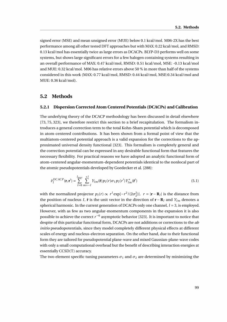
5.2. Methods
signed error (MSE) and mean unsigned error (MUE) below 0.1 kcal/mol. M06-2X has the best
performance among all other tested DFT approaches but with MAX: 0.22 kcal/mol, and RMSD:
0.13 kcal/mol has essentially twice as large errors as DCACPs. BLYP-D3 performs well on some
systems, but shows large significant errors for a few halogen containing systems resulting in
an overall performance of MAX: 0.47 kcal/mol, RMSD: 0.51 kcal/mol, MSE: -0.13 kcal/mol
and MUE: 0.32 kcal/mol. M06 has relative errors above 50 % in more than half of the systems
considered in this work (MAX: 0.77 kcal/mol, RMSD: 0.44 kcal/mol, MSE:0.34 kcal/mol and
MUE: 0.36 kcal/mol).
5.2 Methods
5.2.1 Dispersion Corrected Atom Centered Potentials (DCACPs) and Calibration
The underlying theory of the DCACP methodology has been discussed in detail elsewhere
[73, 75, 323], we therefore restrict this section to a brief recapitulation. The formalism in-
troduces a general correction term to the total Kohn-Sham potential which is decomposed
in atom-centered contributions. It has been shown from a formal point of view that the
multiatom-centered potential approach is a valid expansion for the corrections to the ap-
proximated universal density functional [323]. This formalism is completely general and
the correction potential can be expressed in any desirable functional form that features the
necessary flexibility. For practical reasons we have adopted an analytic functional form of
atom-centered angular-momentum-dependent potentials identical to the nonlocal part of
the atomic pseudopotentials developed by Goedecker et al. [288]:
vDC AC Pl (r,r′) =
lmax∑l=0
+l∑m=−l
Ylm(r)pl (r )σ1pl (r ′)Y ∗l m(r′) (5.1)
with the normalized projector pl (r ) ∝ r l exp[−r 2/(2σ22)]. r = |r−RI | is the distance from
the position of nucleus I , r is the unit vector in the direction of r−RI and Ylm denotes a
spherical harmonic. In the current generation of DCACPs only one channel, l = 3, is employed.
However, with as few as two angular-momentum components in the expansion it is also
possible to achieve the correct r−6 asymptotic behavior [323]. It is important to notice that
despite of this particular functional form, DCACPs are not additions or corrections to the ab
initio pseudopotentials, since they model completely different physical effects at different
scales of energy and nucleus-electron separation. On the other hand, due to their functional
form they are tailored for pseudopotential plane-wave and mixed Gaussian-plane-wave codes
with only a small computational overhead but the benefit of describing interaction energies at
essentially CCSD(T) accuracy.
The two element specific tuning parameters σ1 and σ2 are determined by minimizing the
99
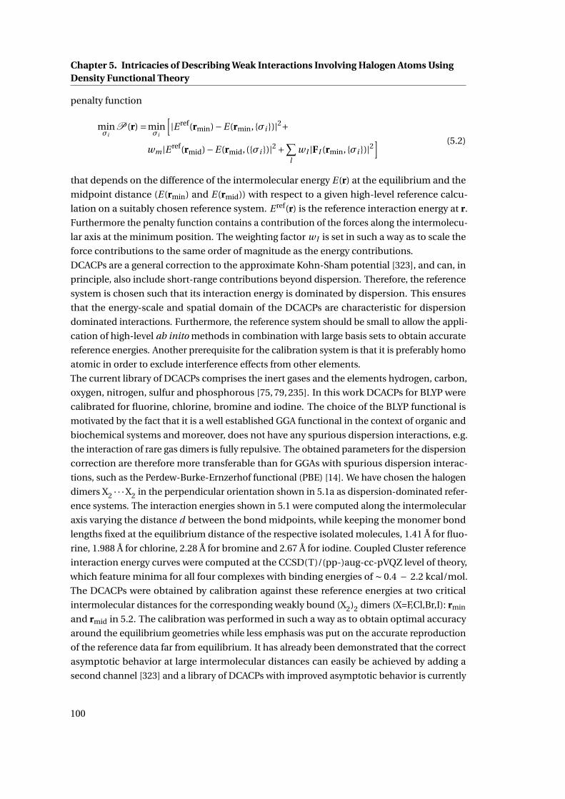
Chapter 5. Intricacies of Describing Weak Interactions Involving Halogen Atoms UsingDensity Functional Theory
penalty function
minσi
P(r) =minσi
[|E ref(rmin)−E(rmin, σi )|2+
wm |E ref(rmid)−E(rmid, (σi )|2 +∑l
w I |FI (rmin, σi )|2] (5.2)
that depends on the difference of the intermolecular energy E(r) at the equilibrium and the
midpoint distance (E(rmin) and E(rmid)) with respect to a given high-level reference calcu-
lation on a suitably chosen reference system. E ref(r) is the reference interaction energy at r.
Furthermore the penalty function contains a contribution of the forces along the intermolecu-
lar axis at the minimum position. The weighting factor w I is set in such a way as to scale the
force contributions to the same order of magnitude as the energy contributions.
DCACPs are a general correction to the approximate Kohn-Sham potential [323], and can, in
principle, also include short-range contributions beyond dispersion. Therefore, the reference
system is chosen such that its interaction energy is dominated by dispersion. This ensures
that the energy-scale and spatial domain of the DCACPs are characteristic for dispersion
dominated interactions. Furthermore, the reference system should be small to allow the appli-
cation of high-level ab inito methods in combination with large basis sets to obtain accurate
reference energies. Another prerequisite for the calibration system is that it is preferably homo
atomic in order to exclude interference effects from other elements.
The current library of DCACPs comprises the inert gases and the elements hydrogen, carbon,
oxygen, nitrogen, sulfur and phosphorous [75, 79, 235]. In this work DCACPs for BLYP were
calibrated for fluorine, chlorine, bromine and iodine. The choice of the BLYP functional is
motivated by the fact that it is a well established GGA functional in the context of organic and
biochemical systems and moreover, does not have any spurious dispersion interactions, e.g.
the interaction of rare gas dimers is fully repulsive. The obtained parameters for the dispersion
correction are therefore more transferable than for GGAs with spurious dispersion interac-
tions, such as the Perdew-Burke-Ernzerhof functional (PBE) [14]. We have chosen the halogen
dimers X2 · · ·X2 in the perpendicular orientation shown in 5.1a as dispersion-dominated refer-
ence systems. The interaction energies shown in 5.1 were computed along the intermolecular
axis varying the distance d between the bond midpoints, while keeping the monomer bond
lengths fixed at the equilibrium distance of the respective isolated molecules, 1.41 Å for fluo-
rine, 1.988 Å for chlorine, 2.28 Å for bromine and 2.67 Å for iodine. Coupled Cluster reference
interaction energy curves were computed at the CCSD(T)/(pp-)aug-cc-pVQZ level of theory,
which feature minima for all four complexes with binding energies of ∼ 0.4 − 2.2 kcal/mol.
The DCACPs were obtained by calibration against these reference energies at two critical
intermolecular distances for the corresponding weakly bound (X2)2 dimers (X=F,Cl,Br,I): rmin
and rmid in 5.2. The calibration was performed in such a way as to obtain optimal accuracy
around the equilibrium geometries while less emphasis was put on the accurate reproduction
of the reference data far from equilibrium. It has already been demonstrated that the correct
asymptotic behavior at large intermolecular distances can easily be achieved by adding a
second channel [323] and a library of DCACPs with improved asymptotic behavior is currently
100
5.2. Methods
Table 5.1: DCACP parameters for the l = 3 channel in Eq. 5.1 for the elements F, Cl, Br and I inconjunction with the BLYP xc functional in atomic units.
σ1 [10−4] σ2
F -7.03 2.4Cl -16.00 2.6709Br -14.08 2.9997I -22.22 3.0463
in preparation [324]. The weighting factors w I were therefore set to
w I =1.0 if F > 1.0 ·10−9
0.01 otherwise(5.3)
with F =∑I |FI (rmin, σi )|2. wm was set to
wm =1.0 if |E ref(rmin)−E(rmin, σi )|> 0.01 · |E ref(rmin)|
0.01 if |E ref(rmin)−E(rmin, σi )| < 0.01 · |E ref(rmin)|(5.4)
if F ≤ 1.0 ·10−9, and wm = 0.0 otherwise. The DCACP parameters determined in this work
are listed in Tab. 5.1 and the resulting DCACP-BLYP interaction energies closely match the
CCSD(T) references (see Tab. 5.2 and Fig. 5.1).
5.2.2 Computational Details
For the interaction energy between two monomers (K and L) in a dispersion bound dimer
(KL) we apply the definition Ei nt (K L) = EK L − (EK +EL). For the calculation of the interaction
energy no zero point energies or thermal corrections were included. In all calculations the
monomers were kept fixed at the respective equilibrium geometries, as described in the Re-
sults section. All plane wave (pw) DFT calculations were performed with the software package
CPMD [49] with the self-consistent field convergence criterion for the Kohn-Sham orbitals set
to 10−7 a.u. The scalar relativistic pseudopotentials of Goedecker et al. [288, 289, 325] were
employed using pw cutoffs of 600 (for fluorine), 150 (for chlorine) and 120 Ry (for bromine and
iodine containing systems), respectively. These calculations were carried out in isolated cubic
cells with edge lengths of 16 Å ((F2)2), 17 Å (F2Ar), 18 Å ((Cl2)2 and Cl2Ar), 20 Å ((X2)2 and X2Ar,
X=Br,I) and 28 Å (H3CX ·OCH2, X=Cl,Br,I), using the Hockney Poisson solver as implemented
in CPMD [251].
For the coupled cluster reference values, energies for the (X2)2 dimers were computed at the
CCSD(T) [7,8] level of theory with the aug-cc-pVQZ [167,326] (avqz) basis sets as implemented
in MOLPRO 2006.1 [327]. We also tested different extrapolation schemes to the CBS limit
(see supporting information of ref. [236]). To account for relativistic effects in iodine, pseu-
dopotentials, consistent with the respective correlation consistent basis sets, were applied
101
Chapter 5. Intricacies of Describing Weak Interactions Involving Halogen Atoms UsingDensity Functional Theory
(pp-aug-cc-pVQZ) [328].
The MO6/(pp)-aug-cc-pVQZ and M06-2X/(pp)-aug-cc-pVQZ calculations were performed
using the Gaussian G09 [164] software package employing tight convergence criteria and
an especially fine grid for integral evaluation ([350,770] for F and [350,590] for Cl, Br, I). See
the supporting information for a benchmark of different grid sizes and ref. [329] for a dis-
cussion of the effect of the grid spacing on the smoothness of the potential energy curves of
dispersion bound complexes in meta-GGA calculations. For the BLYP-D3 [156] calculations,
BLYP/(pp-)aug-cc-pVQZ energies from Gaussian G09 were augmented with the results from
Grimme’s DFT-D3 program [330] employing the Becke-Johnson damping [157]. All calcula-
tions of interaction energies involving atom-centered basis sets were corrected for the basis
set superposition error employing the counterpoise correction [331].
5.2.3 Statistical Quantities
In order to compare the performance of the various DFT methods on the test set for weak
interactions involving halogens we compute the maximum error (MAX, Eq. 5.5), root mean
square deviation (RMSD, Eq. 5.6), mean signed error (MSE, Eq. 5.7) and mean unsigned error
(MUE, Eq. 5.8) as follows:
MAX = max
E DF Ti nt (K L)−E r e f
i nt (K L)
N(5.5)
RMSD =√
1
N
∑N
(E DF T
i nt (K L)−E r e fi nt (K L)
)2(5.6)
MSE = 1
N
∑N
E DF Ti nt (K L)−E r e f
i nt (K L) (5.7)
MUE = 1
N
∑N
∣∣∣E DF Ti nt (K L)−E r e f
i nt (K L)∣∣∣ (5.8)
where E DF Ti nt (K L) represents the interaction energy in the dimer K L computed at the respective
DFT method and E r e fi nt (K L) is the reference CCSD(T) value. We evaluate the errors for all N = 11
dimers K L in X2 · · ·X2 (X=F,Cl,Br,I), X2 · · ·Ar (X=F,Cl,Br,I) and H3CX · · ·OCH2 (X=Cl,Br,I) in the
test set. These error quantities provide complementary information. RMSD is a measure
for the average performance over the test set with a comparably large weight on outliers.
MAX shows the variability of the error and possible unpredictable behaviour. MUE is a
similar measure like the RMSD, but does not stress strong outliers. MSE contains additional
information about possible systematic trends, e.g. negative values indicating a systematic
102
5.3. Results and Discussion
overestimation of the interaction energy.
5.3 Results and Discussion
5.3.1 Performance for (X2)2 Complexes
The interaction energy curves of the (X2)2 complexes at various levels of theory are shown
in Fig. 5.1. For all intermolecular separations the monomer bond lengths were kept fixed
at 1.41 Å for fluorine, 1.988 Å for chlorine, 2.28 Å for bromine and 2.67 Å for iodine. The
CCSD(T) reference curves feature a minimum for all four complexes, which extends to larger
intermolecular distance (3.05 - 4.05 Å) and larger binding energy (0.37 - 2.2 kcal/mol) when
moving down the group (Tab. 5.2). As expected, uncorrected BLYP fails in all four cases to
describe this interaction, predicting purely repulsive interaction energy curves. This is a
strong indication that the dominant interaction is indeed dispersion. For the calibration of
the DCACP parameters only the interaction energies at the reference equilibrium distance
and the midpoint were used. Therefore the interaction energies at the other distances are
already a first test for transferability. The DCACP-BLYP binding energy curves match well the
CCSD(T) references. The reference equilibrium distances are accurately reproduced, only
the Cl2 · · ·Cl2 distance is 0.05 Å too long. The largest relative error in the well depth amounts
to ∼ 1 % in (I2)2. For comparison, also Lennard-Jones 12-6 potentials with minima at the
respective DCACP-BLYP positions are shown. Furthermore, we tested the performance of
M06, M06-2X and BLYP-D3 for the closed-shell inter halogen interactions. Tabs. 5.2 and 5.3
summarize the numerical results and the relative percentage errors in the interaction energy
minimum are reproduced graphically in Fig. 5.4. M06 performs worst among these methods.
The overall trend of increasing well depth and longer equilibrium distance for the heavier
elements is correctly reproduced. However, the errors in the equilibrium distance range from
an overestimation by 0.5 Å in case of the fluorine complex to an underestimation by 0.1 Å in
case of the iodine complex. The well depth is generally underestimated by ∼ 30 - 60 %, with
the exception of an overestimation of 1 % in (I2)2 . M06-2X shows a more balanced and overall
better agreement with respect to the CCSD(T) references. The relative errors in the well depths
range from 24 % in case of fluorine to 1 % in case of chlorine. The equilibrium distance of (F2)2
is in almost perfect agreement with the CCSD(T) value, while for the remaining elements it is
slightly underestimated by ∼ 0.2 Å. For BLYP-D3 the interaction energy curve of the F2 · · ·F2
complex is purely repulsive, adding only a marginal dispersion contribution onto the BLYP
energies. The (X2)2 complexes for the heavier elements, on the other hand, are all bound,
but the interaction energies are overestimated by 10 to 66 %. The equilibrium distances are
predicted within 0.05 Å.
103
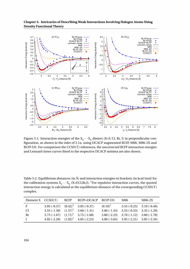
Chapter 5. Intricacies of Describing Weak Interactions Involving Halogen Atoms UsingDensity Functional Theory
XX
X Xd
!0.5!0.4!0.3!0.2!0.1
0 0.1 0.2 0.3 0.4 0.5 0.6 0.7
3 3.5 4 4.5 5 5.5 6
Inte
ract
ion
Ene
rgy
[kca
l/mol
]
F2···F2 Distance [Å]
(a) (F2)2 BLYP/avqzBLYP/pw
DCACP BLYPLennard!Jones
M06M06!2X
BLYP!D3CCSD(T)
−1.5
−1
−0.5
0
0.5
1
1.5
2
2.5
3 3.5 4 4.5 5 5.5 6
Inte
ract
ion
Ene
rgy
[kca
l/mol
]
Cl2···Cl2 Distance [Å]
(b) (Cl2)2 BLYP/avqzBLYP/pw
DCACP BLYPLennard−Jones
M06M06−2X
BLYP−D3CCSD(T)
−2.5
−2
−1.5
−1
−0.5
0
0.5
1
1.5
2
2.5
3
3.5 4 4.5 5 5.5 6 6.5
Inte
ract
ion
Ene
rgy
[kca
l/mol
]
Br2···Br2 Distance [Å]
(c) (Br2)2 BLYP/avqzBLYP/pw
DCACP BLYPLennard−Jones
M06M06−2X
BLYP−D3CCSD(T)
−4−3.5
−3−2.5
−2−1.5
−1−0.5
0 0.5
1 1.5
2 2.5
3 3.5
4
3.5 4 4.5 5 5.5 6 6.5 7 7.5 8
Inte
ract
ion
Ene
rgy
[kca
l/mol
]
I2···I2 Distance [Å]
(d) (I2)2 BLYP/avqzBLYP/pw
DCACP BLYPLennard−Jones
M06M06−2X
BLYP−D3CCSD(T)
Figure 5.1: Interaction energies of the X2 · · ·X2 dimers (X=F, Cl, Br, I) in perpendicular con-figuration, as shown in the inlet of 5.1a, using DCACP augmented BLYP, M06, M06-2X andBLYP-D3. For comparison the CCSD(T) references, the uncorrected BLYP interaction energiesand Lennard-Jones curves fitted to the respective DCACP minima are also shown.
Table 5.2: Equilibrium distances (in Å) and interaction energies in brackets (in kcal/mol) forthe calibration systems X2 · · ·X2 (X=F,Cl,Br,I). †For repulsive interaction curves, the quotedinteraction energy is calculated at the equilibrium distance of the corresponding CCSD(T)complex.
Element X CCSD(T) BLYP BLYP+DCACP BLYP-D3 M06 M06-2X
F 3.05 (-0.37) (0.42)† 3.05 (-0.37) (0.10)† 3.55 (-0.25) 3.10 (-0.46)Cl 3.55 (-1.30) (1.37)† 3.60 (-1.31) 3.60 (-1.43) 3.55 (-0.53) 3.35 (-1.29)Br 3.75 (-1.67) (1.71)† 3.75 (-1.68) 3.80 (-2.23) 3.70 (-1.12) 3.60 (-1.78)I 4.05 (-2.20) (1.02)† 4.05 (-2.23) 4.00 (-3.65) 3.95 (-2.21) 3.85 (-2.34)
104
5.3. Results and Discussion
Table 5.3: Unsigned error in percent with respect to the CCSD(T) references of the bindingenergy of the X2 · · ·X2 (X=F,Cl,Br,I) systems. †For repulsive interaction curves, the error iscalculated at the equilibrium distance of the corresponding CCSD(T) complex.
Element X BLYP BLYP+DCACP BLYP-D3 M06 M06-2X
F 213.5† 0.1 126.4† 32.0 24.3Cl 205.4† 0.6 10.0 59.4 0.8Br 202.4† 0.9 33.9 32.8 6.6I 146.4† 1.0 65.7 0.5 6.4
5.3.2 Performance for X2−Ar Complexes
In order to assess the performance of uncorrected BLYP, DCACP augmented BLYP, M06, M06-
2X and BLYP-D3 on a heteronuclear test system we computed the interaction energy curves of
X2 · · ·Ar complexes (in a T-shaped arrangement) along the distance between the center of mass
of X2 and Ar while keeping the monomer bond lengths fixed at the equilibrium distance of the
respective isolated molecule (1.41 Å F2, 1.988 Å Cl2, 2.28 Å Br2 and 2.67 Å I2). From figures 5.2b-
d it can be seen that as expected standard BLYP is not able to describe these interactions
predicting repulsive interaction energy curves for all four complexes. DCACP augmented
BLYP, on the other hand, reproduces very well the equilibrium distances and interaction
energies of the CCSD(T) reference data. The overall trend of larger binding energies and longer
equilibrium distances towards the heavier halogens is also correctly reproduced. The errors
in the well depths range from 2 % to 17 %. M06 predicts for all X2 · · ·Ar complexes a bonded
interaction energy curve, but underestimates the interaction energy by as much as 36 % to 64
% in parallel with an overestimation of the equilibrium distances by ∼ 0.4 Å. M06-2X performs
better than M06, both in terms of well depth and equilibrium distance. It underestimates the
interaction energy by 3 % (F2Ar) to 36 % (Cl2Ar). BLYP-D3 predicts correctly the overall trend
of stronger binding energies and longer equilibrium distances towards the heavier halogens,
however, it clearly underestimates the dispersion contribution of fluorine, producing a relative
error in the well depth of 79 % in the case of the F2 · · ·Ar complex. The errors in the remaining
systems are of the same order of magnitude as for BLYP-DCACP. The numerical results are
summarized in Tabs. 5.4 and 5.5 and the relative energetic errors are plotted in Fig. 5.4 for
comparison.
5.3.3 Performance for the H3CX · · ·OCH2 Complexes
As a second family of test systems for weak interactions involving halogens we selected the
halomethane-formaldehyde complexes H3CX · · ·OCH2 (X=Cl,Br,I), which are considered as
prototype systems for halogen bonding. This is expected to be a more serious test since
the binding is due to a delicate interplay between several types of weak interactions besides
dispersion [305]. The interaction energy curves along the C · · ·O axis (d in Fig. 5.3a) were
computed at the BLYP, DCACP, BLYP-D3, M06 an M06-2X level of theory (Fig. 5.3) keeping
105

Chapter 5. Intricacies of Describing Weak Interactions Involving Halogen Atoms UsingDensity Functional Theory
−0.4
−0.2
0
0.2
0.4
0.6
0.8
1
3 3.5 4 4.5 5 5.5 6
Inte
ract
ion
Ene
rgy
[kca
l/mol
]
F2···Ar Distance [Å]
(a) F2···ArBLYP/avqz
BLYP/pwDCACP BLYP
Lennard−JonesM06
M06−2XBLYP−D3CCSD(T)a
−0.8−0.6−0.4−0.2
0 0.2 0.4 0.6 0.8
1 1.2 1.4
3 3.5 4 4.5 5 5.5 6
Inte
ract
ion
Ene
rgy
[kca
l/mol
]
Cl2···Ar Distance [Å]
(b) Cl2···ArBLYP/avqz
BLYP/pwDCACP BLYP
Lennard−JonesM06
M06−2XBLYP−D3CCSD(T)b
−0.8−0.6−0.4−0.2
0 0.2 0.4 0.6 0.8
1 1.2 1.4
3 3.5 4 4.5 5 5.5 6
Inte
ract
ion
Ene
rgy
[kca
l/mol
]
Br2···Ar Distance [Å]
(c) Br2···ArBLYP/avqz
BLYP/pwDCACP BLYP
Lennard−JonesM06
M06−2XBLYP−D3CCSD(T)c
−1−0.8−0.6−0.4−0.2
0 0.2 0.4 0.6 0.8
1 1.2 1.4
3.5 4 4.5 5 5.5 6
Inte
ract
ion
Ene
rgy
[kca
l/mol
]
I2···Ar Distance [Å]
(d) I2···ArBLYP/avqz
BLYP/pwDCACP BLYP
Lennard−JonesM06
M06−2XBLYP−D3CCSD(T)d
Figure 5.2: Interaction energies in the weakly bound X2 · · ·Ar complexes. DCACP augmentedBLYP versus standard BLYP, M06, BLYP-D3 and CCSD(T) references. See caption of Tab. 5.4 fordetails and citations of the CCSD(T) references.
Table 5.4: Equilibrium distance in Å and binding energies in brackets in kcal/mol for theX2 · · ·Ar systems. †For repulsive interaction curves, the quoted interaction energy is calculatedat the equilibrium distance of the corresponding CCSD(T) complex. References for the X=F,Cl,Br,I systems at the CCSD(T) level of theory are available employing different types ofbasis sets: a aug-cc-pVQZ (this work); b aug-cc-pVQZ [332]; c SDD+G(3df) for Br and aug-cc-pVQZ+(3s3p2d2f1g) for Ar [333] ; d Stuttgart (SDD) / + (sp) + (3df) for I, aug-cc-pVQZ +(3s3p2d2f1g) for Ar [334].
Element X CCSD(T) BLYP BLYP+DCACP BLYP-D3 M06 M06-2X
F 3.45 (-0.29)a (0.36)† 3.45 (-0.27) 3.70 (-0.06) 4.05 (-0.19) 3.60 (-0.28)Cl 3.70 (-0.56)b (0.64)† 3.70 (-0.58) 3.75 (-0.51) 4.35 (-0.22) 3.70 (-0.36)Br 3.80 (-0.65)c (0.73)† 3.85 (-0.54) 3.85 (-0.64) 4.50 (-0.23) 3.70 (-0.43)I 3.96 (-0.67)d (0.82)† 4.00 (-0.68) 3.95 (-0.79) 4.30 (-0.29) 3.85 (-0.48)
106
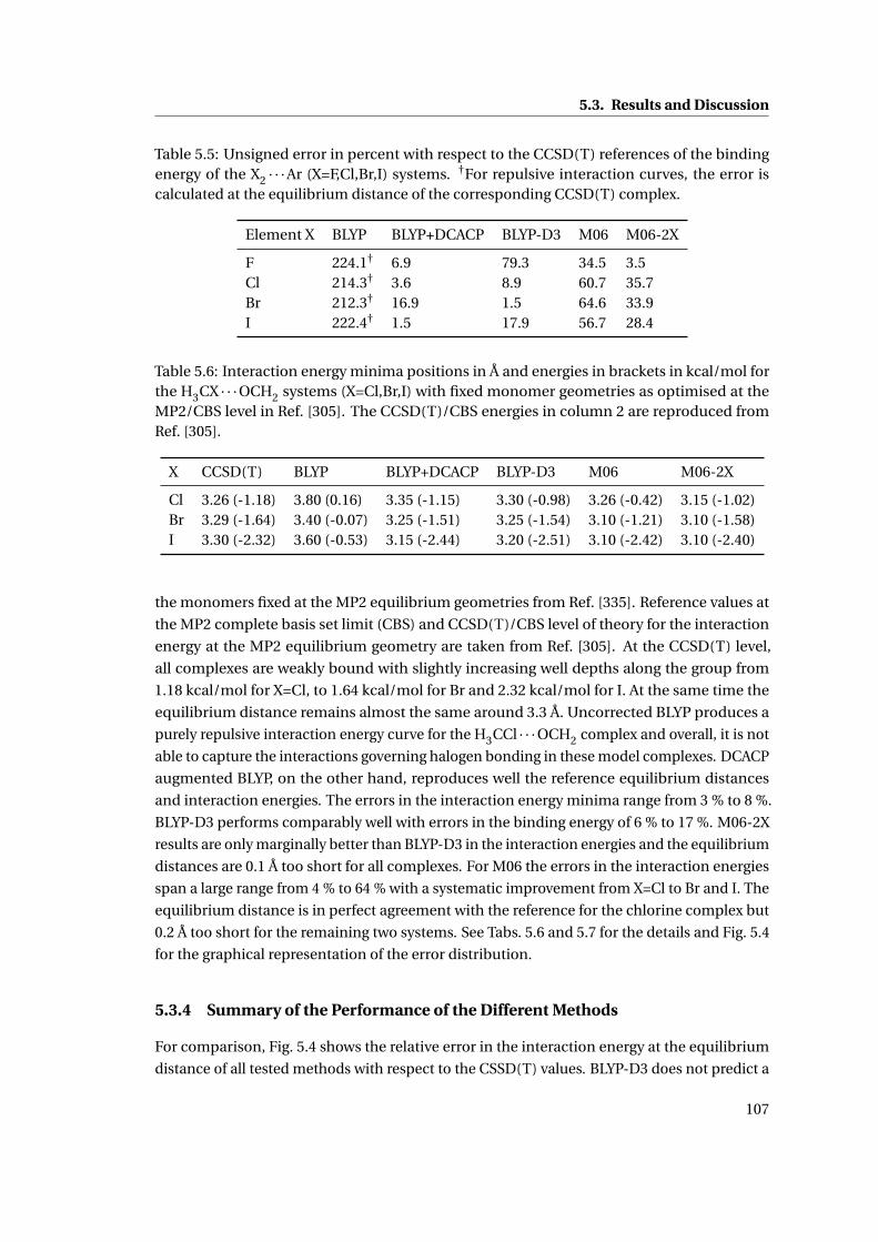
5.3. Results and Discussion
Table 5.5: Unsigned error in percent with respect to the CCSD(T) references of the bindingenergy of the X2 · · ·Ar (X=F,Cl,Br,I) systems. †For repulsive interaction curves, the error iscalculated at the equilibrium distance of the corresponding CCSD(T) complex.
Element X BLYP BLYP+DCACP BLYP-D3 M06 M06-2X
F 224.1† 6.9 79.3 34.5 3.5Cl 214.3† 3.6 8.9 60.7 35.7Br 212.3† 16.9 1.5 64.6 33.9I 222.4† 1.5 17.9 56.7 28.4
Table 5.6: Interaction energy minima positions in Å and energies in brackets in kcal/mol forthe H3CX · · ·OCH2 systems (X=Cl,Br,I) with fixed monomer geometries as optimised at theMP2/CBS level in Ref. [305]. The CCSD(T)/CBS energies in column 2 are reproduced fromRef. [305].
X CCSD(T) BLYP BLYP+DCACP BLYP-D3 M06 M06-2X
Cl 3.26 (-1.18) 3.80 (0.16) 3.35 (-1.15) 3.30 (-0.98) 3.26 (-0.42) 3.15 (-1.02)Br 3.29 (-1.64) 3.40 (-0.07) 3.25 (-1.51) 3.25 (-1.54) 3.10 (-1.21) 3.10 (-1.58)I 3.30 (-2.32) 3.60 (-0.53) 3.15 (-2.44) 3.20 (-2.51) 3.10 (-2.42) 3.10 (-2.40)
the monomers fixed at the MP2 equilibrium geometries from Ref. [335]. Reference values at
the MP2 complete basis set limit (CBS) and CCSD(T)/CBS level of theory for the interaction
energy at the MP2 equilibrium geometry are taken from Ref. [305]. At the CCSD(T) level,
all complexes are weakly bound with slightly increasing well depths along the group from
1.18 kcal/mol for X=Cl, to 1.64 kcal/mol for Br and 2.32 kcal/mol for I. At the same time the
equilibrium distance remains almost the same around 3.3 Å. Uncorrected BLYP produces a
purely repulsive interaction energy curve for the H3CCl · · ·OCH2 complex and overall, it is not
able to capture the interactions governing halogen bonding in these model complexes. DCACP
augmented BLYP, on the other hand, reproduces well the reference equilibrium distances
and interaction energies. The errors in the interaction energy minima range from 3 % to 8 %.
BLYP-D3 performs comparably well with errors in the binding energy of 6 % to 17 %. M06-2X
results are only marginally better than BLYP-D3 in the interaction energies and the equilibrium
distances are 0.1 Å too short for all complexes. For M06 the errors in the interaction energies
span a large range from 4 % to 64 % with a systematic improvement from X=Cl to Br and I. The
equilibrium distance is in perfect agreement with the reference for the chlorine complex but
0.2 Å too short for the remaining two systems. See Tabs. 5.6 and 5.7 for the details and Fig. 5.4
for the graphical representation of the error distribution.
5.3.4 Summary of the Performance of the Different Methods
For comparison, Fig. 5.4 shows the relative error in the interaction energy at the equilibrium
distance of all tested methods with respect to the CSSD(T) values. BLYP-D3 does not predict a
107
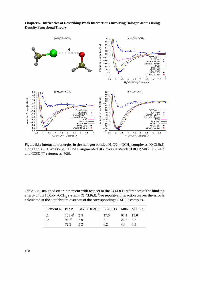
Chapter 5. Intricacies of Describing Weak Interactions Involving Halogen Atoms UsingDensity Functional Theory
(a) H3CX•••OCH2
d
−1.4−1.2−1.0−0.8−0.6−0.4−0.2
0.00.20.40.60.81.0
2.5 3 3.5 4 4.5 5 5.5 6 6.5 7
Inte
ract
ion
Ene
rgy
[kca
l/mol
]
H3CCl···OCH2 Distance [Å]
(b) H3CCl···OCH2
BLYP/avqzBLYP/pw
DCACP BLYPLennard−Jones
M06M06−2X
BLYP−D3MP2/CBS
CCSD(T)/CBS
−1.8−1.6−1.4−1.2−1.0−0.8−0.6−0.4−0.2
0.00.20.40.60.81.0
2.5 3 3.5 4 4.5 5 5.5 6 6.5 7
Inte
ract
ion
Ene
rgy
[kca
l/mol
]
H3CBr···OCH2 Distance [Å]
(c) H3CBr···OCH2
BLYP/avqzBLYP/pw
DCACP BLYPLennard−Jones
M06M06−2X
BLYP−D3MP2/CBS
CCSD(T)/CBS−2.6−2.4−2.2−2.0−1.8−1.6−1.4−1.2−1.0−0.8−0.6−0.4−0.2
0.00.20.40.60.8
2.5 3 3.5 4 4.5 5 5.5 6 6.5 7
Inte
ract
ion
Ene
rgy
[kca
l/mol
]
H3CI···OCH2 Distance [Å]
(d) H3CI···OCH2
BLYP/avqzBLYP/pw
DCACP BLYPLennard−Jones
M06M06−2X
BLYP−D3MP2/CBS
CCSD(T)/CBS
Figure 5.3: Interaction energies in the halogen bonded H3CX · · ·OCH2 complexes (X=Cl,Br,I)along the X · · ·O axis (5.3a). DCACP augmented BLYP versus standard BLYP, M06, BLYP-D3and CCSD(T) references [305].
Table 5.7: Unsigned error in percent with respect to the CCSD(T) references of the bindingenergy of the H3CX · · ·OCH2 systems (X=Cl,Br,I). †For repulsive interaction curves, the error iscalculated at the equilibrium distance of the corresponding CCSD(T) complex.
Element X BLYP BLYP+DCACP BLYP-D3 M06 M06-2X
Cl 136.4† 2.5 17.0 64.4 13.6Br 95.7† 7.9 6.1 26.2 3.7I 77.2† 5.2 8.2 4.3 3.5
108
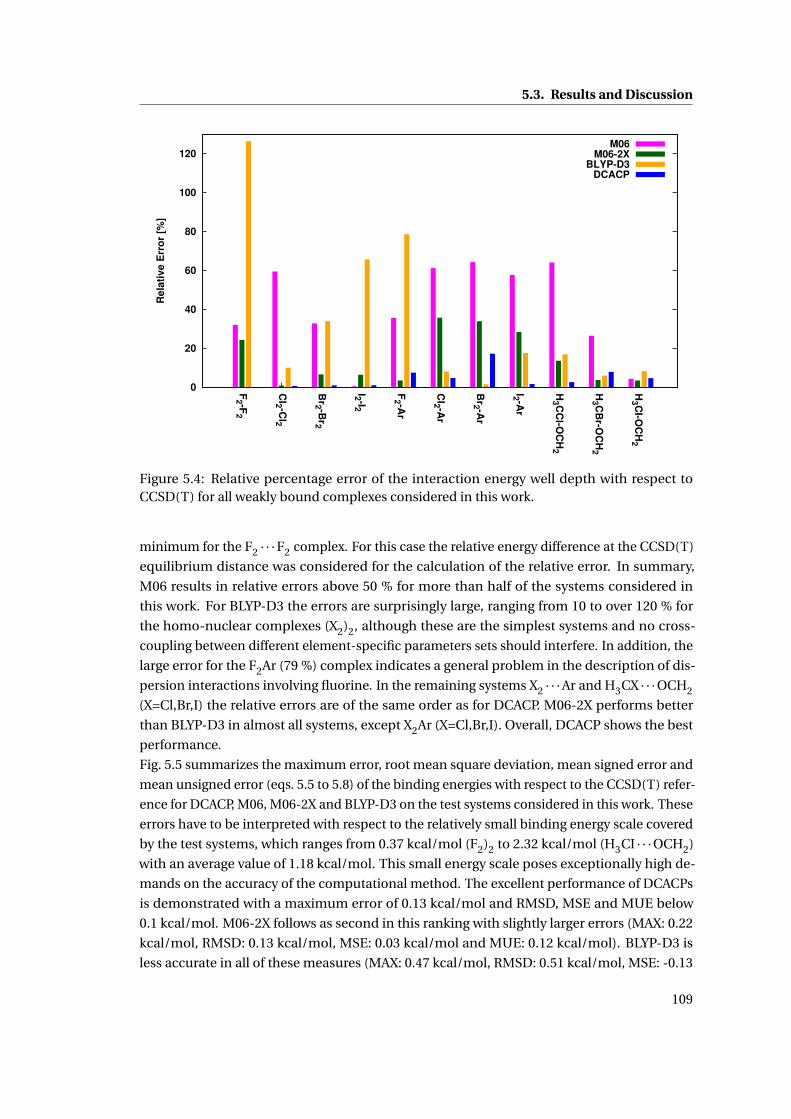
5.3. Results and Discussion
0
20
40
60
80
100
120
F2 -F
2
Cl2 -C
l2
Br2 -B
r2
I2 -I2
F2 -A
r
Cl2 -A
r
Br2 -A
r
I2 -Ar
H3 C
Cl-O
CH
2
H3 C
Br-O
CH
2
H3 C
I-OC
H2
Rela
tive E
rro
r [%
]
M06M06-2X
BLYP-D3DCACP
Figure 5.4: Relative percentage error of the interaction energy well depth with respect toCCSD(T) for all weakly bound complexes considered in this work.
minimum for the F2 · · ·F2 complex. For this case the relative energy difference at the CCSD(T)
equilibrium distance was considered for the calculation of the relative error. In summary,
M06 results in relative errors above 50 % for more than half of the systems considered in
this work. For BLYP-D3 the errors are surprisingly large, ranging from 10 to over 120 % for
the homo-nuclear complexes (X2)2, although these are the simplest systems and no cross-
coupling between different element-specific parameters sets should interfere. In addition, the
large error for the F2Ar (79 %) complex indicates a general problem in the description of dis-
persion interactions involving fluorine. In the remaining systems X2 · · ·Ar and H3CX · · ·OCH2
(X=Cl,Br,I) the relative errors are of the same order as for DCACP. M06-2X performs better
than BLYP-D3 in almost all systems, except X2Ar (X=Cl,Br,I). Overall, DCACP shows the best
performance.
Fig. 5.5 summarizes the maximum error, root mean square deviation, mean signed error and
mean unsigned error (eqs. 5.5 to 5.8) of the binding energies with respect to the CCSD(T) refer-
ence for DCACP, M06, M06-2X and BLYP-D3 on the test systems considered in this work. These
errors have to be interpreted with respect to the relatively small binding energy scale covered
by the test systems, which ranges from 0.37 kcal/mol (F2)2 to 2.32 kcal/mol (H3CI · · ·OCH2)
with an average value of 1.18 kcal/mol. This small energy scale poses exceptionally high de-
mands on the accuracy of the computational method. The excellent performance of DCACPs
is demonstrated with a maximum error of 0.13 kcal/mol and RMSD, MSE and MUE below
0.1 kcal/mol. M06-2X follows as second in this ranking with slightly larger errors (MAX: 0.22
kcal/mol, RMSD: 0.13 kcal/mol, MSE: 0.03 kcal/mol and MUE: 0.12 kcal/mol). BLYP-D3 is
less accurate in all of these measures (MAX: 0.47 kcal/mol, RMSD: 0.51 kcal/mol, MSE: -0.13
109
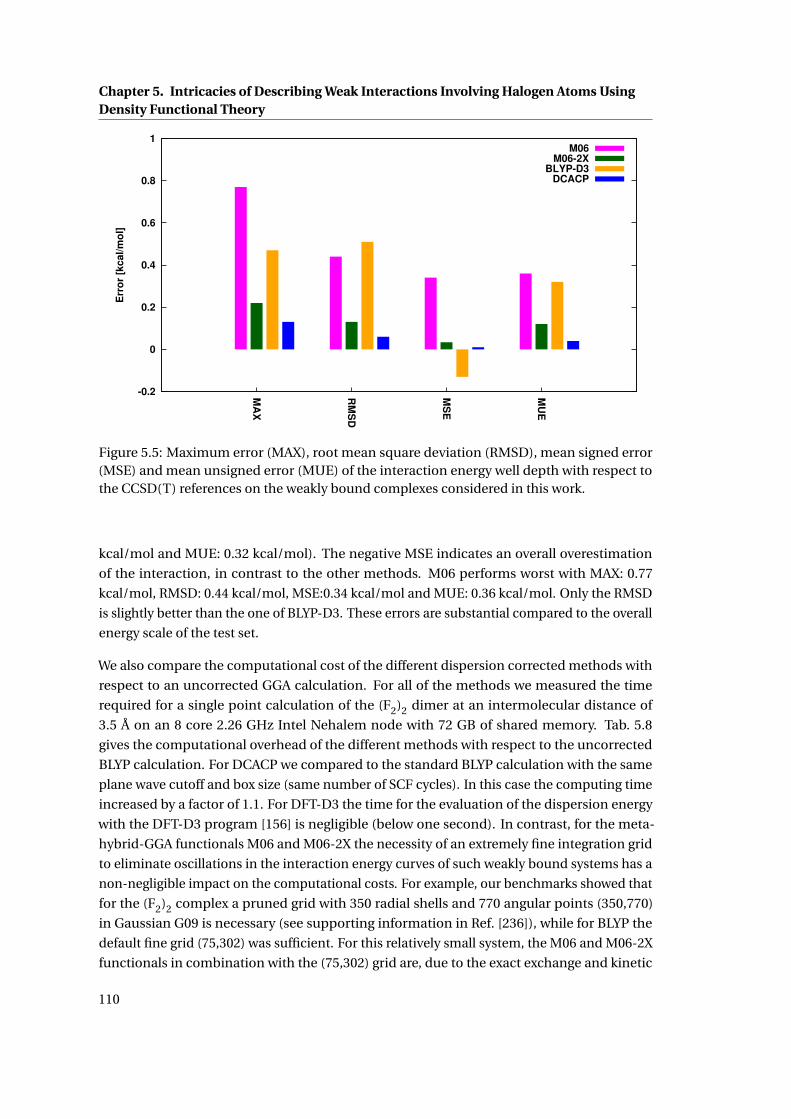
Chapter 5. Intricacies of Describing Weak Interactions Involving Halogen Atoms UsingDensity Functional Theory
-0.2
0
0.2
0.4
0.6
0.8
1
MA
X
RM
SD
MS
E
MU
E
Err
or
[kcal/m
ol]
M06M06-2X
BLYP-D3DCACP
Figure 5.5: Maximum error (MAX), root mean square deviation (RMSD), mean signed error(MSE) and mean unsigned error (MUE) of the interaction energy well depth with respect tothe CCSD(T) references on the weakly bound complexes considered in this work.
kcal/mol and MUE: 0.32 kcal/mol). The negative MSE indicates an overall overestimation
of the interaction, in contrast to the other methods. M06 performs worst with MAX: 0.77
kcal/mol, RMSD: 0.44 kcal/mol, MSE:0.34 kcal/mol and MUE: 0.36 kcal/mol. Only the RMSD
is slightly better than the one of BLYP-D3. These errors are substantial compared to the overall
energy scale of the test set.
We also compare the computational cost of the different dispersion corrected methods with
respect to an uncorrected GGA calculation. For all of the methods we measured the time
required for a single point calculation of the (F2)2 dimer at an intermolecular distance of
3.5 Å on an 8 core 2.26 GHz Intel Nehalem node with 72 GB of shared memory. Tab. 5.8
gives the computational overhead of the different methods with respect to the uncorrected
BLYP calculation. For DCACP we compared to the standard BLYP calculation with the same
plane wave cutoff and box size (same number of SCF cycles). In this case the computing time
increased by a factor of 1.1. For DFT-D3 the time for the evaluation of the dispersion energy
with the DFT-D3 program [156] is negligible (below one second). In contrast, for the meta-
hybrid-GGA functionals M06 and M06-2X the necessity of an extremely fine integration grid
to eliminate oscillations in the interaction energy curves of such weakly bound systems has a
non-negligible impact on the computational costs. For example, our benchmarks showed that
for the (F2)2 complex a pruned grid with 350 radial shells and 770 angular points (350,770)
in Gaussian G09 is necessary (see supporting information in Ref. [236]), while for BLYP the
default fine grid (75,302) was sufficient. For this relatively small system, the M06 and M06-2X
functionals in combination with the (75,302) grid are, due to the exact exchange and kinetic
110
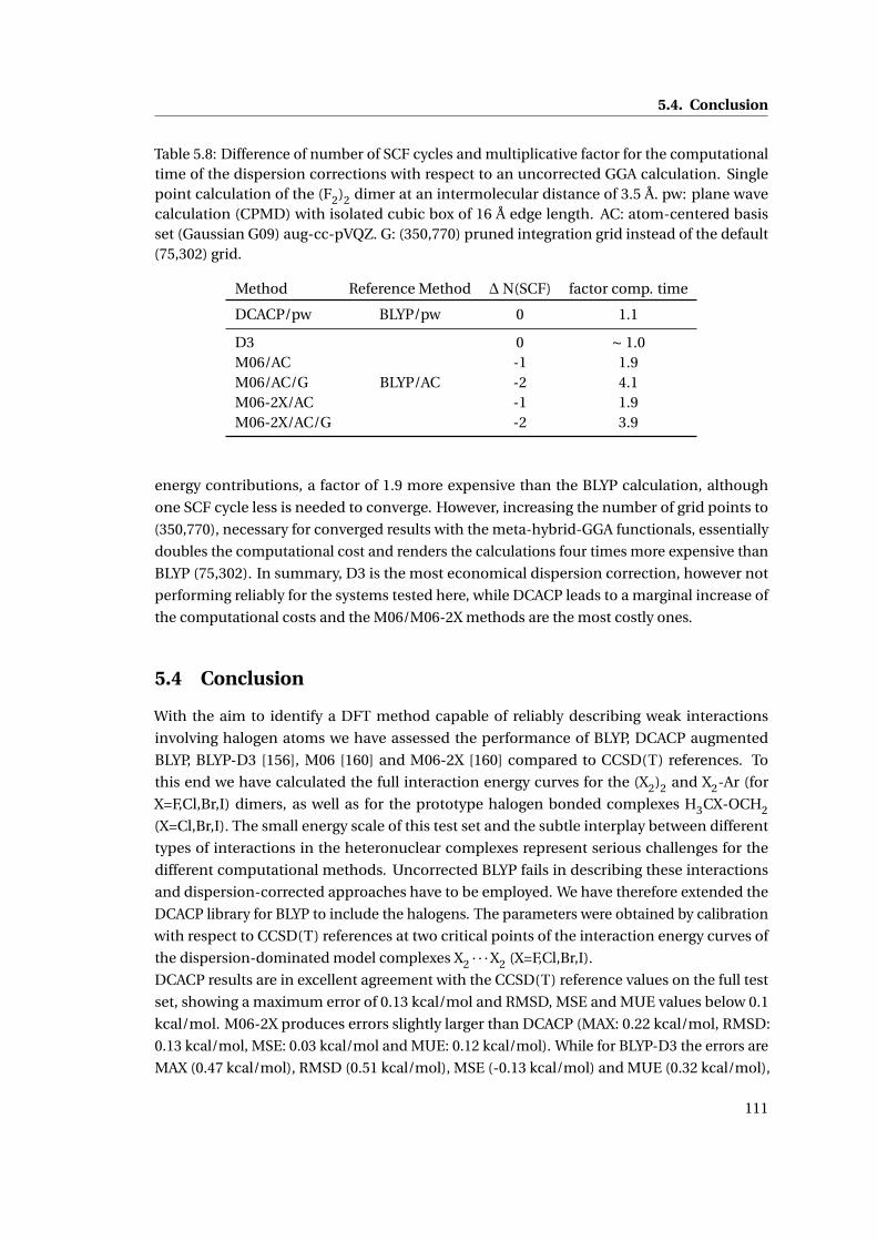
5.4. Conclusion
Table 5.8: Difference of number of SCF cycles and multiplicative factor for the computationaltime of the dispersion corrections with respect to an uncorrected GGA calculation. Singlepoint calculation of the (F2)2 dimer at an intermolecular distance of 3.5 Å. pw: plane wavecalculation (CPMD) with isolated cubic box of 16 Å edge length. AC: atom-centered basisset (Gaussian G09) aug-cc-pVQZ. G: (350,770) pruned integration grid instead of the default(75,302) grid.
Method Reference Method ∆N(SCF) factor comp. time
DCACP/pw BLYP/pw 0 1.1
D3
BLYP/AC
0 ∼ 1.0M06/AC -1 1.9M06/AC/G -2 4.1M06-2X/AC -1 1.9M06-2X/AC/G -2 3.9
energy contributions, a factor of 1.9 more expensive than the BLYP calculation, although
one SCF cycle less is needed to converge. However, increasing the number of grid points to
(350,770), necessary for converged results with the meta-hybrid-GGA functionals, essentially
doubles the computational cost and renders the calculations four times more expensive than
BLYP (75,302). In summary, D3 is the most economical dispersion correction, however not
performing reliably for the systems tested here, while DCACP leads to a marginal increase of
the computational costs and the M06/M06-2X methods are the most costly ones.
5.4 Conclusion
With the aim to identify a DFT method capable of reliably describing weak interactions
involving halogen atoms we have assessed the performance of BLYP, DCACP augmented
BLYP, BLYP-D3 [156], M06 [160] and M06-2X [160] compared to CCSD(T) references. To
this end we have calculated the full interaction energy curves for the (X2)2 and X2-Ar (for
X=F,Cl,Br,I) dimers, as well as for the prototype halogen bonded complexes H3CX-OCH2
(X=Cl,Br,I). The small energy scale of this test set and the subtle interplay between different
types of interactions in the heteronuclear complexes represent serious challenges for the
different computational methods. Uncorrected BLYP fails in describing these interactions
and dispersion-corrected approaches have to be employed. We have therefore extended the
DCACP library for BLYP to include the halogens. The parameters were obtained by calibration
with respect to CCSD(T) references at two critical points of the interaction energy curves of
the dispersion-dominated model complexes X2 · · ·X2 (X=F,Cl,Br,I).
DCACP results are in excellent agreement with the CCSD(T) reference values on the full test
set, showing a maximum error of 0.13 kcal/mol and RMSD, MSE and MUE values below 0.1
kcal/mol. M06-2X produces errors slightly larger than DCACP (MAX: 0.22 kcal/mol, RMSD:
0.13 kcal/mol, MSE: 0.03 kcal/mol and MUE: 0.12 kcal/mol). While for BLYP-D3 the errors are
MAX (0.47 kcal/mol), RMSD (0.51 kcal/mol), MSE (-0.13 kcal/mol) and MUE (0.32 kcal/mol),
111

Chapter 5. Intricacies of Describing Weak Interactions Involving Halogen Atoms UsingDensity Functional Theory
with main contributions from the fluorine containing complexes and the homo-nuclear (X2)2
(X=F,Cl,Br,I) systems. M06 performs with relative errors above 50 % in more than half of the
systems considered in this work (MAX: 0.77 kcal/mol, RMSD: 0.44 kcal/mol, MSE:0.34 kcal/mol
and MUE: 0.36 kcal/mol). These are relatively large errors compared to the overall very small
energy scale of the test set of halogen containing weakly bound complexes. Concerning the
computational cost, it is not surprising that D3 is the most economical dispersion correction,
while DCACP leads to a marginal increase in computational costs and M06/M06-2X are the
most costly ones, compared to uncorrected BLYP.
In conclusion, this study has revealed the challenges related to the accurate description of
weak interactions involving halogen atoms at the DFT level. These are reflected in the largely
varying performance among the different methods tested here (DCACP, BLYP-D3, M06 and
M06-2X). At the same time we have made a significant step towards the identifications of
computational expedient and yet accurate methods to model halogen containing systems
in material science, biology and medicinal chemistry. For the small test set considered here,
DCACPs feature the best ratio of accuracy versus computational costs.
112
Summary and Outlook
As a consequence of the progress in computational methods that have extended both the
accessible system sizes and simulation times, the quality of the underlying potential energy
surface has become a major issue in the accuracy of molecular dynamics simulations. With
this motivation, we have explored three different strategies to increase the accuracy of the
potential energy surface for molecular dynamics simulations at various levels of theory.
In our initial benchmarking study we assessed the accuracy limits of various computational
methods in comparison to experiments and high level theoretical reference values. We used
high-resolution conformer-selective vibrational spectra for small biomolecules isolated in the
gas phase at low temperatures as experimental reference data. We determined the lowest en-
ergy conformations with vibrational spectra that correspond to the experimental data. Based
on these results we assessed various methods in their ability to predict the correct relative
energetics among a pool of low energy conformations. These results demonstrate how well
modern quantum chemistry methods and cold ion spectroscopy work together in determining
low energy structures of biomolecules in the gas phase, while more approximate methods
struggle to provide the necessary accuracy. Especially empirical force fields performed rather
poorly in describing the correct relative energetics of these molecules, possibly due to the
limited transferability. Further improvements are clearly needed to employ them as reliable
tools for an energetic screening.
With the goal to increase the accuracy of classical molecular mechanics force fields we imple-
mented a recently developed force-matching protocol for an automated parametrisation of
biomolecular force fields from mixed QM/MM reference calculations in the CPMD software
package. Such a force field has an accuracy that is comparable to the QM/MM reference, but
at the greatly reduced computational cost of the MM approach. We have applied this protocol
to derive in situ FF parameters for the retinal chromophore in rhodopsin embedded in a lipid
bilayer. In contrast to the original parameter set, they describe correctly the bond length
alternation in the conjugated chain of the retinal, which results in an absorption spectrum in
excellent agreement with QM/MM and experimental references.
The findings on rhodopsin encourage future applications of the QM/MM force matching
method to other systems with sizes prohibitive for higher level methods. For example, work
113
Summary and Outlook
is underway to derive parameters for the deprotonated form of the retinal, which has, as of
today, not been studied at the classical level. This will open possibilities to investigate the so
far poorly understood activation mechanism of rhodopsin at the molecular level.
Classical force field methods are at the forefront of computational methods to reach the mil-
lisecond regime at atomic resolution. In combination with more accurate parameterisation
techniques, this will be of great advantage to answer pressing questions in biology. Future
developments on the methodology of the QM/MM force matching, for example, could involve
a parameterisation of the Van der Waals parameters consistent with the recently developed
dispersion-corrected DFT methods. Moreover, more sophisticated functional forms of the
classical force fields including polarisation effects could greatly increase the accuracy.
Since classical force fields can not describe the breaking and forming of chemical bonds, we
focused in a second part of part of this thesis on the SCC-DFTB method, which represents a
methodological bridge between force fields and DFT methods for MD simulations of molecu-
lar systems. It is ideally suited if the problem at hand demands for an explicit description of
the instantaneous rearrangement of the electronic structure, and a sampling that extends the
limitations of DFT methods. We built on the original spirit to determine the parameters based
on DFT reference calculations and explored an in situ parameterisation strategy. We employed
iterative Boltzmann inversion to derive repulsive potentials for SCC-DFTB based on DFT
references for liquid water at ambient conditions. The new repulsive potentials significantly
improve the structural and dynamical properties of liquid water with respect to the description
at the original SCC-DFTB level.
There is no doubt, that DFT represents the ideal reference method to parameterise SCC-DFTB,
since the functional form is essentially an approximation to the KS total energy functional. Dur-
ing the research on this project, it has, however, also became clear that a re-parameterisation
of repulsive potentials alone can not account for all the approximations and limitations of
the SCC-DFTB compared to DFT. In future efforts, the rich information contained in the DFT
reference calculations could, for example, be exploited more efficiently by a suitable in situ
parameterisation scheme for the electronic parameters.
In order to increase the accuracy to describe weak interactions involving halogen atoms by
DFT/GGA methods we determined halogen specific parameters for the recently developed
Dispersion Corrected Atom Centered Potentials (DCACPs) approach. We showed that in our
benchmarking study the newly derived DCACPs feature the best ratio of accuracy versus
computational costs compared to alternative dispersion corrected DFT methods. They repre-
sent therefore a promising method to model halogen containing systems in material science,
biology and medicinal chemistry.
DCACPs represent an efficient correction to the GGA exchange correlation functional. It is
in line with many recent attempts to increase the accuracy of DFT with (semi-)empirical
approaches to construct and correct exchange-correlation functionals. Such efforts are mo-
tivated especially by the demand for higher accuracy in the context of weak intermolecular
114

Summary and Outlook
interactions. At the same time, the computational costs should not exceed the GGA level,
since otherwise DFT would loose its advantageous balance between reasonable accuracy and
modest computational cost compared to wave function based ab initio methods. Empirical
approaches, however, always come with significant human effort in the derivation of accurate
and transferable parameters. Future developments could therefore involve less empirical
schemes in the development of exchange correlation functionals.
115

A Supporting Information for Section2.1
A.1 Experimental Approach for the Conformer-Selective Vibrational
Spectra of Cold Protonated Tryptophan
The experimental results presented in this section have been obtained by Dr. Na-
talia Nagornova and Dr. Oleg Boyarkin, Laboratoire de Chimie Physique Molécu-
laire, group of Prof. Thomas R. Rizzo.
Experimental approach and apparatus have been described in detail elsewhere [139, 192, 193].
Briefly, we generate protonated Trp and its water clusters in the gas phase from a 50/50
H2O/MeOH solution using a nanospray ion source. Protonated species are guided into the
vacuum chamber through a glass capillary and accumulated in a hexapole ion trap. After
approximately 85 ms, the ions are released from the hexapole and passed through the first
quadrupole mass filter, which selects parent ions of a particular mass-to-charge ratio (m/z).
An rf-only octopole guides them into a 22-pole ion trap, which is cooled to 6 K by a closed-cycle
refrigerator (Sumitomo, SRDK-408). Ions get collisionally cooled in collisions with a pulse of
helium, which is introduced into the trap before the arrival of the ion packet. After about 80
ms, when ions are cooled and He has been pumped out, we interrogate the ions in the trap
with a UV or IR and UV laser pulses. UV photofragmentation is performed using the 3-4 mJ
output of a frequency-doubled dye laser pumped by 7 ns pulses of a Nd:YAG laser. We select
the appearing charged fragments using second quadrupole mass filter and collect them on a
channeltron. UV photofragmentation spectrum is generated by monitoring the number of
photofragment ion counts as a function of wavenumber of the UV laser.
For IR spectroscopy we use 3-4 mJ output of an optical parametric oscillator (OPO, LaserVi-
sion), pumped by a Nd:YAG laser. To record IR spectra of [TrpH]+ and [TrpH · (H2O)2]+ we
employ IR-UV double resonance technique, [194] where an IR pulse precedes a UV pulse by
approximately 100 ns. In this scheme IR absorption spectra of parent ions are generated by
scanning the wavenumber of the IR laser while fixing the wavenumber of the UV laser on a
photofragmentation transition, and monitoring the change of the fragmentation yield. When
the infrared laser frequency is in resonance with a vibrational transition of the same conformer,
117
Appendix A. Supporting Information for Section 2.1
which is excited by the UV laser, these species become internally hot, altering the subsequent
UV photodissociation yield. If the UV spectrum of parent ions is vibrationally resolved, the
IR pre-heating results in a spectral broadening, which leads to a reduction of the otherwise
constant, UV-only photofragmentation yield [143]. Monitoring this reduction of UV fragmen-
tation in function of IR laser wavenumber yields an IR depletion spectrum, which truly reflects
frequencies of vibrational transitions and their width in a selected conformer. Here we apply
this approach only to [TrpH · (H2O)2]+, which UV spectrum is vibrationally resolved [151]. The
UV spectrum of even cold [TrpH]+ is already broad, which prohibits conformational selectivity
in IR-UV double resonance. However, the IR pre-heating of this species results in an additional
spectral broadening and to the red shift of the UV spectrum. This appears as an increase
in the photodissociation signal induced by the UV laser light only and IR spectrum appears
as a "gain" spectrum. We use this approach for conformer non-selective IR spectroscopy of
[TrpH]+. While IR spectra of a singly solvated tryptophan, which UV spectrum does not exhibit
vibrational resolution can also be measured this way, regarding a better quality of the spectra
we use IR photodissociation technique for conformer non-selective vibrational spectroscopy
of [TrpH · (H2O)]+. In this experiments the absorbed IR OPO photon reduces the cluster down
to [TrpH]+, which we detect in function of IR wavenumber.
A.2 The CBS-C Method
Description adapted from Ref. [174].The original CBS-Q method [39]requires the following
calculations:
1. UHF/6-31G† geometry optimization and frequencies,
2. MP2/6-31G† optimized geometry,
3. UMP2/6-311+G(3d2f,2df,2p) energy and CBS extrapolation,
4. MP4(SDQ)/6-31+G(d(f),p) energy,
5. QCISD(T)/6-31+G† energy.
Calculations (3)-(5) are performed at the geometry obtained in step (2). Note that the usual
basis set notation is generalized to accommodate the specification of different polarization
sets for different atoms. Thus, 6-311+G(3d2f,2df,2p) means 3d2f on the second row, 2df on
the first row, and 2p on hydrogen and 6-31+G(d(f),p) indicates a d function on both first and
second rows, an f on selected second row atoms, and a p function on hydrogen. The 6-31G†
basis is a modification of the 6-31G∗ basis obtained combining the 6-31G sp functions with
the 6-311G∗∗ polarization exponents. The total CBS-Q energy is calculated from:
E(C BS −Q) =E(U MP2)+∆E(C BS)+∆E(MP4)+∆E(QC I )
+∆E(Z PE)+∆E(emp)+∆E(spi n)(A.1)
118
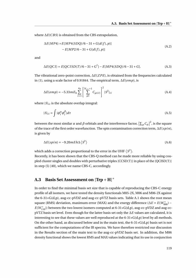
A.3. Basis Set Assessment on [Trp+H]+
where ∆E(C BS) is obtained from the CBS extrapolation,
∆E(MP4) =E [MP4(SDQ)/6−31+G(d( f ), p)]
−E [MP2/6−31+G(d( f ), p)](A.2)
and
∆E(QC I ) = E [QC I SD(T )/6−31+G†]−E [MP4(SDQ)/6−31+G]. (A.3)
The vibrational zero-point correction, ∆E(Z PE), is obtained from the frequencies calculated
in (1), using a scale factor of 0.91844. The empirical term, ∆E(emp), is
∆E(emp) =−5.33mEh
nβ∑i=1
[Nvi r +1∑µ1
Cµ(i i )
]2
|S2|i i (A.4)
where |S|i i is the absolute overlap integral:
|S|i i =∫
|φαi φβ
i |dτ (A.5)
between the most similar α and β orbitals and the interference factor,[∑
µCµ
]2, is the square
of the trace of the first order wavefunction. The spin contamination correction term,∆E (spi n),
is given by
∆E(spi n) =−9.20mEh∆⟨
S2⟩ (A.6)
which adds a correction proportional to the error in the UHF⟨
S2⟩
.
Recently, it has been shown that the CBS-Q method can be made more reliable by using cou-
pled cluster singles and doubles with perturbative triples [CCSD(T)] in place of the [QCISD(T)]
in step (5) [40], which we name CBS-C, accordingly.
A.3 Basis Set Assessment on [Trp+H]+
In order to find the minimal basis set size that is capable of reproducing the CBS-C energy
profile of all isomers, we have tested the density functionals M05-2X, M06 and M06-2X against
the 6-31+G(d,p), aug-cc-pVDZ and aug-cc-pVTZ basis sets. Table A.1 shows the root mean
square (RMS) deviation, maximum error (MAX) and the energy difference (∆E = E(W +000)−
E (W +110)) between the two lowest isomers computed at 6-31+G(d,p), aug-cc-pVDZ and aug-cc-
pVTZ basis set level. Even though for the latter basis set only the ∆E values are calculated, it is
interesting to see that these values are well reproduced at the 6-31+G(d,p) level by all methods.
On the other hand, as discussed below and in the main text, the 6-31+G(d,p) basis set is not
sufficient for the computations of the IR spectra. We have therefore restricted our discussion
in the Results section of the main text to the aug-cc-pVDZ basis set. In addition, the M06
density functional shows the lowest RMS and MAX values indicating that its use in conjunction
119
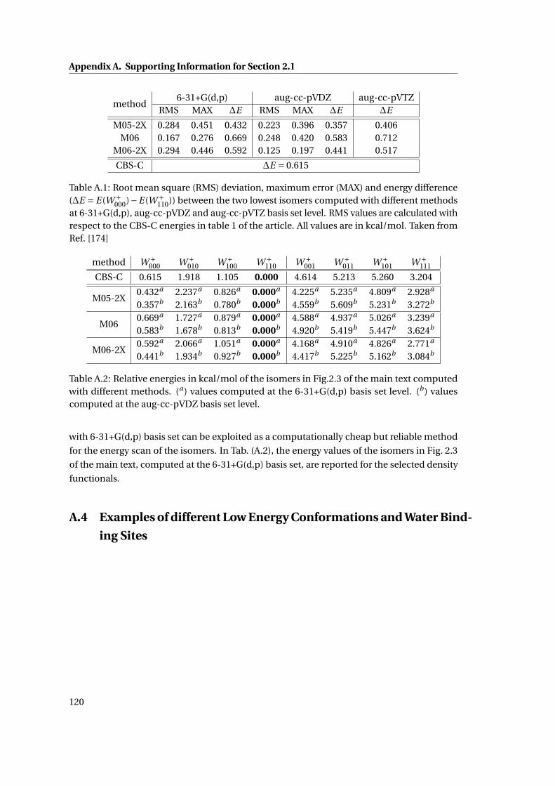
Appendix A. Supporting Information for Section 2.1
method6-31+G(d,p) aug-cc-pVDZ aug-cc-pVTZ
RMS MAX ∆E RMS MAX ∆E ∆E
M05-2X 0.284 0.451 0.432 0.223 0.396 0.357 0.406M06 0.167 0.276 0.669 0.248 0.420 0.583 0.712
M06-2X 0.294 0.446 0.592 0.125 0.197 0.441 0.517
CBS-C ∆E = 0.615
Table A.1: Root mean square (RMS) deviation, maximum error (MAX) and energy difference(∆E = E(W +
000)−E(W +110)) between the two lowest isomers computed with different methods
at 6-31+G(d,p), aug-cc-pVDZ and aug-cc-pVTZ basis set level. RMS values are calculated withrespect to the CBS-C energies in table 1 of the article. All values are in kcal/mol. Taken fromRef. [174]
method W +000 W +
010 W +100 W +
110 W +001 W +
011 W +101 W +
111
CBS-C 0.615 1.918 1.105 0.000 4.614 5.213 5.260 3.204
M05-2X0.432a 2.237a 0.826a 0.000a 4.225a 5.235a 4.809a 2.928a
0.357b 2.163b 0.780b 0.000b 4.559b 5.609b 5.231b 3.272b
M060.669a 1.727a 0.879a 0.000a 4.588a 4.937a 5.026a 3.239a
0.583b 1.678b 0.813b 0.000b 4.920b 5.419b 5.447b 3.624b
M06-2X0.592a 2.066a 1.051a 0.000a 4.168a 4.910a 4.826a 2.771a
0.441b 1.934b 0.927b 0.000b 4.417b 5.225b 5.162b 3.084b
Table A.2: Relative energies in kcal/mol of the isomers in Fig.2.3 of the main text computedwith different methods. (a) values computed at the 6-31+G(d,p) basis set level. (b) valuescomputed at the aug-cc-pVDZ basis set level.
with 6-31+G(d,p) basis set can be exploited as a computationally cheap but reliable method
for the energy scan of the isomers. In Tab. (A.2), the energy values of the isomers in Fig. 2.3
of the main text, computed at the 6-31+G(d,p) basis set, are reported for the selected density
functionals.
A.4 Examples of different Low Energy Conformations and Water Bind-
ing Sites
120
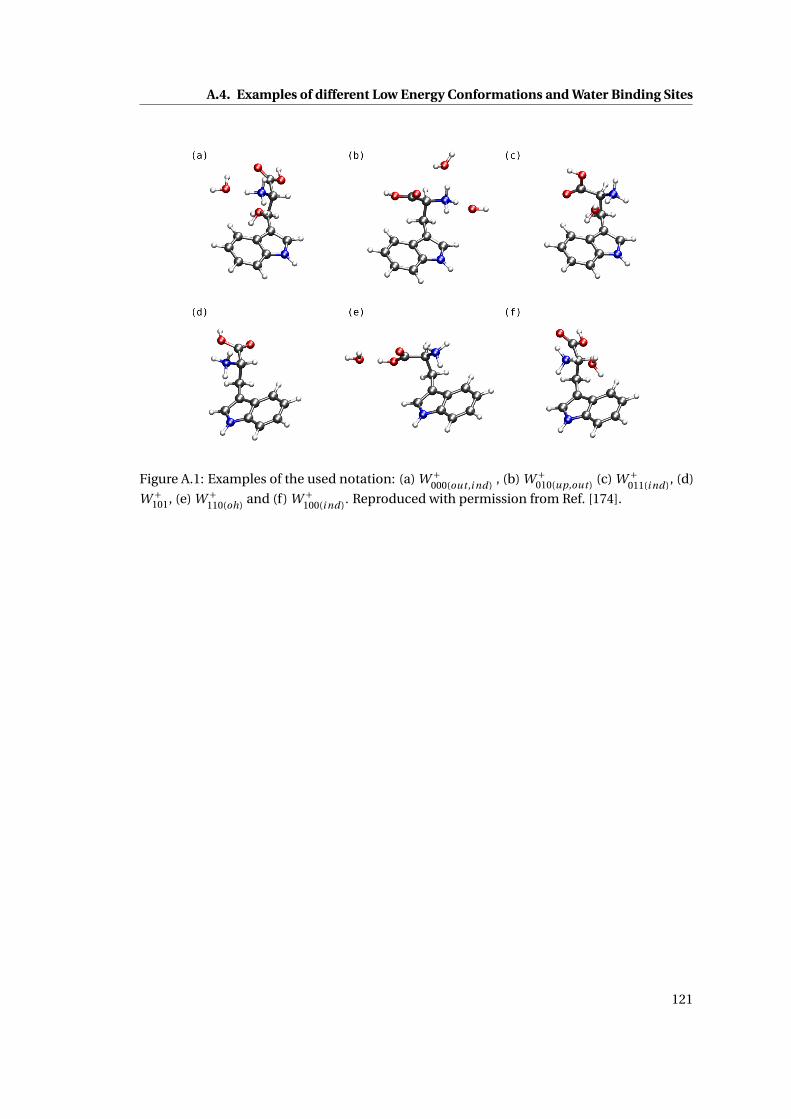
A.4. Examples of different Low Energy Conformations and Water Binding Sites
Figure A.1: Examples of the used notation: (a) W +000(out ,i nd) , (b) W +
010(up,out ) (c) W +011(i nd), (d)
W +101, (e) W +
110(oh) and (f) W +100(i nd). Reproduced with permission from Ref. [174].
121
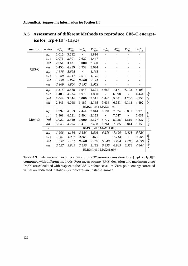
Appendix A. Supporting Information for Section 2.1
A.5 Assessment of different Methods to reproduce CBS-C energet-
ics for [Trp+H]+ · (H2O)
method water W +000 W +
010 W +100 W +
110 W +001 W +
011 W +101 W +
111
CBS-C
up 2.015 3.732 × 1.816 - - - -out 2.071 3.501 2.622 1.447 - - - -i nd 2.051 3.431 0.000 2.320 - - - -oh 3.450 4.229 3.934 2.644 - - - -up 1.675 3.598 × 1.763 - - - -out 1.999 3.111 2.512 1.173 - - - -i nd 1.730 3.276 0.000 2.141 - - - -oh 2.969 3.860 3.353 2.522 - - - -
M05-2X
up 1.578 3.888 1.943 1.621 5.658 7.171 6.105 5.403
6-31
+G(d
,p)
out 1.485 4.234 1.979 1.880 × 6.898 × 4.444i nd 2.049 3.344 0.000 2.311 5.445 5.881 4.206 4.554oh 2.841 4.068 3.185 2.135 5.638 6.751 6.143 4.497- RMS=0.444 MAX=0.749
up 1.992 4.353 2.444 2.014 6.194 7.824 6.831 5.970
aug-
cc-p
VD
Z
out 1.808 4.521 2.504 2.173 × 7.547 × 5.031i nd 2.022 3.410 0.000 2.377 5.777 5.955 4.519 4.827oh 3.043 4.294 3.410 2.458 6.261 7.385 6.844 5.150- RMS=0.413 MAX=1.020
up 1.908 4.186 2.384 1.803 6.278 7.400 6.421 5.724
aug-
cc-p
VD
Z
out 1.961 4.207 2.504 2.077 × 7.113 × 4.795i nd 1.837 3.181 0.000 2.137 5.249 5.794 4.280 4.696oh 2.527 3.849 2.895 2.182 5.835 6.943 6.323 4.964- RMS=0.460 MAX=1.096
Table A.3: Relative energies in kcal/mol of the 32 isomers considered for [TrpH · (H2O)]+
computed with different methods. Root mean square (RMS) deviation and maximum error(MAX) are calculated with respect to the CBS-C reference values. Zero-point energy correctedvalues are indicated in italics. (×) indicates an unstable isomer.
122

A.5. Assessment of different Methods to reproduce CBS-C energetics for [Trp+H]+ · (H2O)
method water W +000 W +
010 W +100 W +
110 W +001 W +
011 W +101 W +
111
CBS-C
up 2.015 3.732 × 1.816 - - - -out 2.071 3.501 2.622 1.447 - - - -i nd 2.051 3.431 0.000 2.320 - - - -oh 3.450 4.229 3.934 2.644 - - - -
M06
up 1.645 3.578 1.964 1.690 6.056 6.823 5.912 5.378
6-31
+G(d
,p)
out 1.461 3.537 1.769 1.546 × 6.188 × 4.396i nd 2.002 3.051 0.000 1.901 5.518 5.659 4.258 4.436oh 3.155 3.616 3.341 2.311 6.401 6.770 6.754 5.161- RMS=0.411 MAX=0.853
up 2.271 4.215 2.613 2.344 6.772 7.688 6.809 6.164
aug-
cc-p
VD
Z
out 2.078 3.981 2.534 2.028 × 7.137 × 5.076i nd 2.078 3.553 0.000 2.496 6.018 6.173 4.583 5.053oh 3.434 3.965 3.608 2.709 7.020 7.435 7.447 5.869- RMS=0.303 MAX=0.581
M06-2X
up 1.538 3.406 1.976 1.339 5.552 6.652 6.196 5.181
6-31
+G(d
,p)
out 1.238 4.297 1.910 2.068 × 6.791 × 4.474i nd 1.649 2.167 0.000 1.288 4.886 5.159 3.952 3.850oh 3.256 4.074 3.671 2.374 5.799 6.633 6.383 4.550- RMS=0.622 MAX=1.264
up 1.970 3.962 2.482 1.832 6.100 7.388 7.015 5.863
aug-
cc-p
VD
Z
out 1.605 4.633 2.449 2.452 × 7.474 × 5.132i nd 1.566 2.316 0.000 1.449 5.143 5.261 4.285 4.090oh 3.588 4.395 4.021 2.879 6.510 7.353 7.166 5.336- RMS=0.574 MAX=1.132
Table A.4: Relative energies in kcal/mol of the 32 isomers considered for [TrpH · (H2O)]+
computed with different methods. Root mean square (RMS) deviation and maximum error(MAX) are calculated with respect to the CBS-C reference values. Zero-point energy correctedvalues are indicated in italics. (×) indicates an unstable isomer.
method water W +000 W +
010 W +100 W +
110 W +001 W +
011 W +101 W +
111
CBS-C
up 2.015 3.732 × 1.816 - - - -out 2.071 3.501 2.622 1.447 - - - -i nd 2.051 3.431 0.000 2.320 - - - -oh 3.450 4.229 3.934 2.644 - - - -
BLYP-D3
up 2.289 4.057 × 2.555 - - - -
aug-
cc-p
VD
Z
out 1.822 4.101 2.710 2.697 - - - -i nd 1.539 2.758 0.000 2.244 - - - -oh 3.603 3.997 3.902 3.300 - - - -- RMS=0.513 MAX=1.250
Table A.5: Relative energies in kcal/mol of the 32 isomers considered for [TrpH · (H2O)]+
computed with different methods. Root mean square (RMS) deviation and maximum error(MAX) are calculated with respect to the CBS-C reference values. Zero-point energy correctedvalues are indicated in italics. (×) indicates an unstable isomer.
123
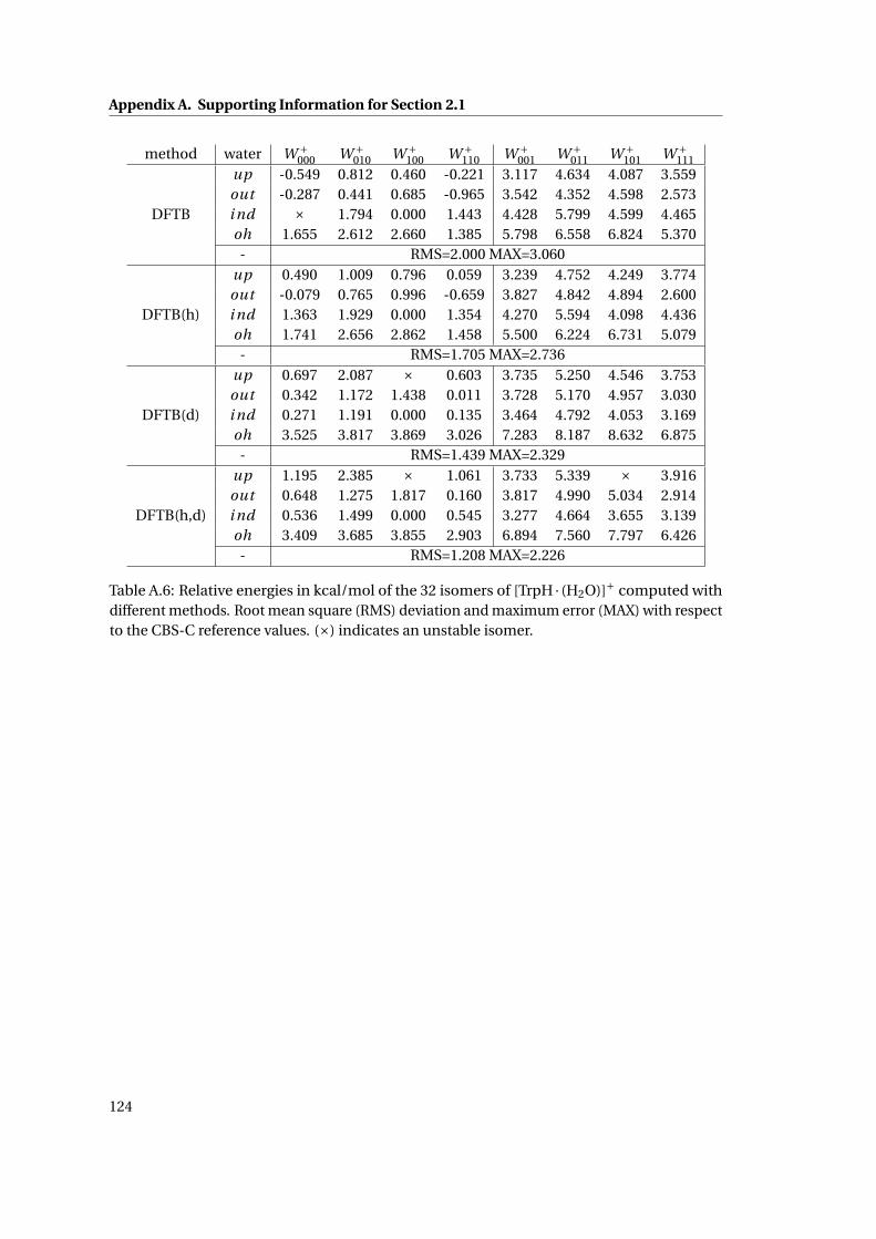
Appendix A. Supporting Information for Section 2.1
method water W +000 W +
010 W +100 W +
110 W +001 W +
011 W +101 W +
111
DFTB
up -0.549 0.812 0.460 -0.221 3.117 4.634 4.087 3.559out -0.287 0.441 0.685 -0.965 3.542 4.352 4.598 2.573i nd × 1.794 0.000 1.443 4.428 5.799 4.599 4.465oh 1.655 2.612 2.660 1.385 5.798 6.558 6.824 5.370- RMS=2.000 MAX=3.060
DFTB(h)
up 0.490 1.009 0.796 0.059 3.239 4.752 4.249 3.774out -0.079 0.765 0.996 -0.659 3.827 4.842 4.894 2.600i nd 1.363 1.929 0.000 1.354 4.270 5.594 4.098 4.436oh 1.741 2.656 2.862 1.458 5.500 6.224 6.731 5.079- RMS=1.705 MAX=2.736
DFTB(d)
up 0.697 2.087 × 0.603 3.735 5.250 4.546 3.753out 0.342 1.172 1.438 0.011 3.728 5.170 4.957 3.030i nd 0.271 1.191 0.000 0.135 3.464 4.792 4.053 3.169oh 3.525 3.817 3.869 3.026 7.283 8.187 8.632 6.875- RMS=1.439 MAX=2.329
DFTB(h,d)
up 1.195 2.385 × 1.061 3.733 5.339 × 3.916out 0.648 1.275 1.817 0.160 3.817 4.990 5.034 2.914i nd 0.536 1.499 0.000 0.545 3.277 4.664 3.655 3.139oh 3.409 3.685 3.855 2.903 6.894 7.560 7.797 6.426- RMS=1.208 MAX=2.226
Table A.6: Relative energies in kcal/mol of the 32 isomers of [TrpH · (H2O)]+ computed withdifferent methods. Root mean square (RMS) deviation and maximum error (MAX) with respectto the CBS-C reference values. (×) indicates an unstable isomer.
124
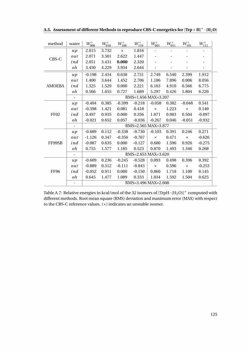
A.5. Assessment of different Methods to reproduce CBS-C energetics for [Trp+H]+ · (H2O)
method water W +000 W +
010 W +100 W +
110 W +001 W +
011 W +101 W +
111
CBS-C
up 2.015 3.732 × 1.816 - - - -out 2.071 3.501 2.622 1.447 - - - -i nd 2.051 3.431 0.000 2.320 - - - -oh 3.450 4.229 3.934 2.644 - - - -
AMOEBA
up -0.198 2.434 0.638 2.731 2.749 6.540 2.399 1.912out 1.400 3.644 1.452 2.706 1.186 7.896 0.006 8.056i nd 1.325 1.529 0.000 2.221 6.163 4.910 0.566 6.775oh 0.566 1.655 0.727 1.689 5.297 0.426 5.804 6.220- RMS=1.656 MAX=3.207
FF02
up -0.404 0.385 -0.399 -0.218 -0.058 0.382 -0.048 0.541out -0.398 1.421 0.081 0.418 × 1.223 × 0.140i nd 0.497 0.935 0.000 0.356 1.071 0.983 0.504 -0.097oh -0.021 0.652 0.057 -0.036 -0.267 0.046 -0.051 -0.932- RMS=2.565 MAX=3.877
FF99SB
up -0.689 0.112 -0.338 -0.730 -0.103 0.391 0.246 0.271out -1.126 0.347 -0.356 -0.767 × 0.471 × -0.626i nd -0.087 0.635 0.000 -0.127 0.680 1.596 0.926 -0.275oh 0.755 1.577 1.185 0.523 0.870 1.493 1.346 0.268- RMS=2.653 MAX=3.620
FF96
up -0.609 0.236 -0.245 -0.528 0.093 0.498 0.396 0.392out -0.889 0.312 -0.111 -0.843 × 0.596 × -0.253i nd -0.052 0.911 0.000 -0.150 0.860 1.718 1.100 0.145oh 0.645 1.477 1.089 0.333 1.034 1.592 1.504 0.625- RMS=3.496 MAX=2.608
Table A.7: Relative energies in kcal/mol of the 32 isomers of [TrpH · (H2O)]+ computed withdifferent methods. Root mean square (RMS) deviation and maximum error (MAX) with respectto the CBS-C reference values. (×) indicates an unstable isomer.
125
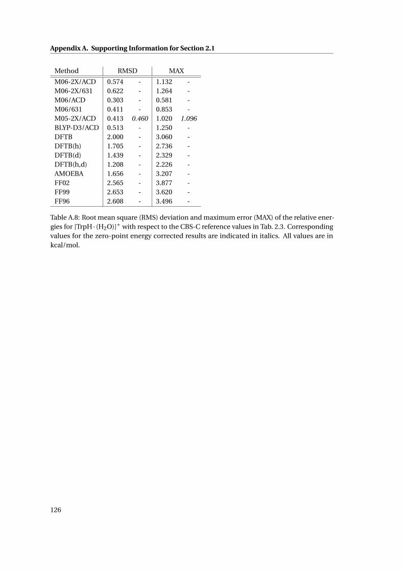
Appendix A. Supporting Information for Section 2.1
Method RMSD MAX
M06-2X/ACD 0.574 - 1.132 -M06-2X/631 0.622 - 1.264 -M06/ACD 0.303 - 0.581 -M06/631 0.411 - 0.853 -M05-2X/ACD 0.413 0.460 1.020 1.096BLYP-D3/ACD 0.513 - 1.250 -DFTB 2.000 - 3.060 -DFTB(h) 1.705 - 2.736 -DFTB(d) 1.439 - 2.329 -DFTB(h,d) 1.208 - 2.226 -AMOEBA 1.656 - 3.207 -FF02 2.565 - 3.877 -FF99 2.653 - 3.620 -FF96 2.608 - 3.496 -
Table A.8: Root mean square (RMS) deviation and maximum error (MAX) of the relative ener-gies for [TrpH · (H2O)]+ with respect to the CBS-C reference values in Tab. 2.3. Correspondingvalues for the zero-point energy corrected results are indicated in italics. All values are inkcal/mol.
126

A.6. Assessment of different Methods to reproduce CBS-energetics for [Trp+H]+ · (H2O)2
A.6 Assessment of different Methods to reproduce CBS-energetics
for [Trp+H]+ · (H2O)2
Tables A.9 to A.12 contain the relative energies for [Trp+H]+ · (H2O)2 at different levels of
theories. As in the case of the singly-solvated species, some configurations do not correspond
to stable minimum but relaxed to other minima (indicated by × in the tables). RMSD and
MAX values, summerized in table A.13, were computed with respect to the CBS-C references.
127
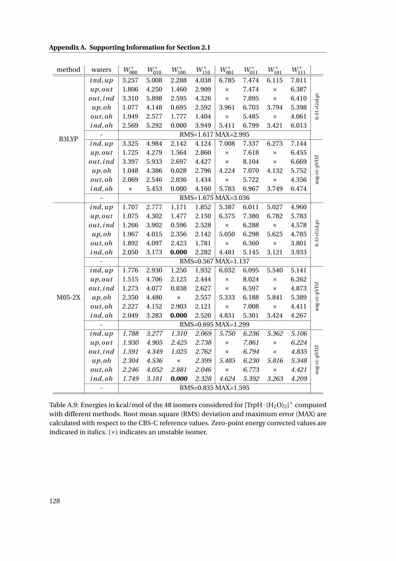
Appendix A. Supporting Information for Section 2.1
method waters W +000 W +
010 W +100 W +
110 W +001 W +
011 W +101 W +
111
B3LYP
i nd ,up 3.257 5.008 2.288 4.038 6.785 7.474 6.115 7.011
6-31
+G(d
,p)
up,out 1.806 4.250 1.460 2.909 × 7.474 × 6.387out , i nd 3.310 5.898 2.595 4.326 × 7.895 × 6.410
up,oh 1.077 4.148 0.695 2.592 3.961 6.703 3.794 5.398out ,oh 1.949 2.577 1.777 1.404 × 5.485 × 4.061i nd ,oh 2.569 5.292 0.000 3.949 5.411 6.799 3.421 6.013
- RMS=1.617 MAX=2.995i nd ,up 3.325 4.984 2.142 4.124 7.008 7.337 6.273 7.144
aug-
cc-p
VD
Z
up,out 1.725 4.279 1.564 2.860 × 7.618 × 6.455out , i nd 3.397 5.933 2.697 4.427 × 8.104 × 6.669
up,oh 1.048 4.386 0.028 2.796 4.224 7.070 4.132 5.752out ,oh 2.069 2.546 2.036 1.434 × 5.722 × 4.356i nd ,oh × 5.453 0.000 4.160 5.783 6.967 3.749 6.474
- RMS=1.675 MAX=3.036
M05-2X
i nd ,up 1.707 2.777 1.171 1.852 5.387 6.011 5.027 4.960
6-31
+G(d
,p)
up,out 1.075 4.302 1.477 2.150 6.375 7.380 6.782 5.783out , i nd 1.266 3.902 0.596 2.528 × 6.288 × 4.578
up,oh 1.967 4.015 2.356 2.142 5.050 6.298 5.625 4.785out ,oh 1.892 4.097 2.423 1.781 × 6.360 × 3.801i nd ,oh 2.050 3.173 0.000 2.282 4.481 5.145 3.121 3.933
- RMS=0.567 MAX=1.137i nd ,up 1.776 2.930 1.250 1.932 6.032 6.095 5.540 5.141
aug-
cc-p
VD
Z
up,out 1.515 4.706 2.125 2.444 × 8.024 × 6.262out , i nd 1.273 4.077 0.838 2.627 × 6.597 × 4.873
up,oh 2.350 4.480 × 2.557 5.333 6.188 5.841 5.389out ,oh 2.227 4.152 2.903 2.121 × 7.008 × 4.411i nd ,oh 2.049 3.283 0.000 2.520 4.831 5.301 3.424 4.267
- RMS=0.695 MAX=1.299i nd ,up 1.788 3.277 1.310 2.069 5.750 6.236 5.362 5.106
aug-
cc-p
VD
Z
up,out 1.930 4.905 2.425 2.738 × 7.861 × 6.224out , i nd 1.591 4.349 1.025 2.762 × 6.794 × 4.835
up,oh 2.304 4.536 × 2.399 5.485 6.230 5.816 5.348out ,oh 2.246 4.052 2.881 2.046 × 6.773 × 4.421i nd ,oh 1.749 3.181 0.000 2.328 4.624 5.392 3.263 4.209
- RMS=0.835 MAX=1.595
Table A.9: Energies in kcal/mol of the 48 isomers considered for [TrpH · (H2O)2]+ computedwith different methods. Root mean square (RMS) deviation and maximum error (MAX) arecalculated with respect to the CBS-C reference values. Zero-point energy corrected values areindicated in italics. (×) indicates an unstable isomer.
128

A.6. Assessment of different Methods to reproduce CBS-energetics for [Trp+H]+ · (H2O)2
method waters W +000 W +
010 W +100 W +
110 W +001 W +
011 W +101 W +
111
M06
i nd ,up 2.150 1.973 0.924 1.011 5.901 5.065 5.015 4.264
6-31
+G(d
,p)
up,out 0.770 3.483 0.928 1.847 × 6.542 6.487 5.374out , i nd 1.423 3.061 0.064 1.908 × 5.646 × 4.659
up,oh 2.170 3.492 2.475 2.321 4.992 6.063 5.202 4.960out ,oh 1.926 3.122 2.337 1.658 × 5.821 × 4.088i nd ,oh 2.031 2.804 0.000 2.169 4.819 4.827 3.438 4.118
- RMS=0.454 MAX=0.702i nd ,up 2.094 2.551 1.374 1.629 6.019 5.634 5.575 4.778
aug-
cc-p
VD
Z
up,out 1.477 4.192 1.846 2.275 × 7.545 × 6.131out , i nd 1.468 3.745 0.632 2.682 × 6.168 × 5.066
up,oh 2.677 4.240 2.976 3.020 5.689 6.912 6.055 5.823out ,oh 2.516 3.570 2.963 2.126 × 6.576 × 4.790i nd ,oh 2.073 3.475 0.000 2.795 5.219 5.427 3.684 4.732
- RMS=0.636 MAX=1.291
M06-2X
i nd ,up 1.106 1.344 0.714 0.723 4.578 5.248 4.506 4.120
6-31
+G(d
,p)
up,out 0.545 3.917 1.125 1.819 × 6.894 6.326 5.509out , i nd 0.444 2.662 0.119 1.768 × 5.650 × 3.943
up,oh 1.854 3.435 2.363 1.808 4.859 4.687 5.539 4.370out ,oh 1.652 3.801 2.322 1.903 × 6.188 × 3.760i nd ,oh 1.640 1.798 0.000 1.539 3.895 4.304 2.860 3.100
- RMS=0.574 MAX=1.091i nd ,up 1.034 1.557 0.776 0.717 4.663 5.299 4.761 4.224
aug-
cc-p
VD
Z
up,out 0.985 4.358 1.753 2.194 × 7.554 7.077 6.073out , i nd 0.325 2.911 0.271 1.813 × 5.880 × 4.141
up,oh 2.303 3.502 2.880 2.345 5.180 5.361 5.789 5.079out ,oh 2.017 4.111 2.845 2.362 × 6.796 × 4.447i nd ,oh 1.602 2.093 0.000 1.605 4.171 4.413 3.142 3.404
- RMS=0.579 MAX=1.049
BLYP-D3
i nd ,up 1.444 1.897 1.097 1.459 - - - -au
g-cc
-pV
DZ
up,out 1.324 4.220 2.151 -0.002 - - - -out , i nd 0.890 2.994 0.834 2.191 - - - -
up,oh 2.664 3.601 -0.002 -0.002 5.189 5.022 5.732 5.575out ,oh 2.296 3.736 3.176 2.610 - - - -i nd ,oh 2.005 2.541 0.000 2.321 - - - -
- RMS=0.716 MAX=2.423
Table A.10: Energies in kcal/mol of the 48 isomers considered for [TrpH · (H2O)2]+ computedwith different methods. Root mean square (RMS) deviation and maximum error (MAX) arecalculated with respect to the CBS-C reference values. Zero-point energy corrected values areindicated in italics. (×) indicates an unstable isomer.
129
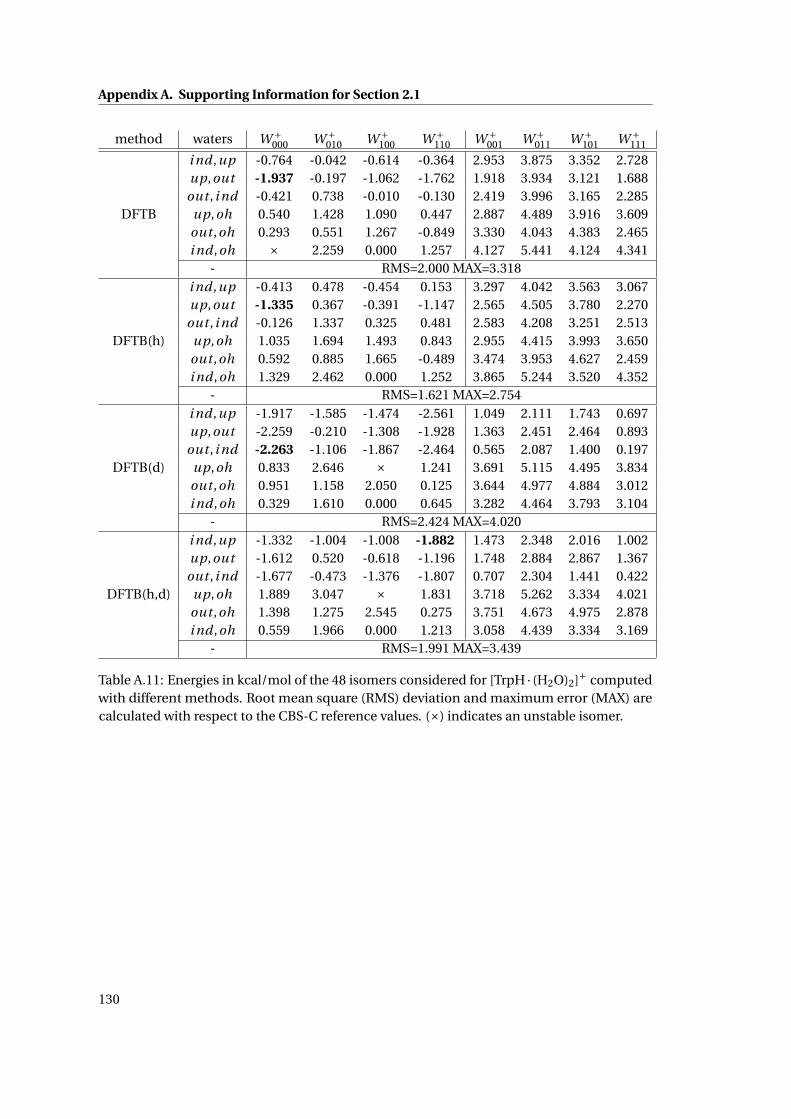
Appendix A. Supporting Information for Section 2.1
method waters W +000 W +
010 W +100 W +
110 W +001 W +
011 W +101 W +
111
DFTB
i nd ,up -0.764 -0.042 -0.614 -0.364 2.953 3.875 3.352 2.728up,out -1.937 -0.197 -1.062 -1.762 1.918 3.934 3.121 1.688
out , i nd -0.421 0.738 -0.010 -0.130 2.419 3.996 3.165 2.285up,oh 0.540 1.428 1.090 0.447 2.887 4.489 3.916 3.609out ,oh 0.293 0.551 1.267 -0.849 3.330 4.043 4.383 2.465i nd ,oh × 2.259 0.000 1.257 4.127 5.441 4.124 4.341
- RMS=2.000 MAX=3.318
DFTB(h)
i nd ,up -0.413 0.478 -0.454 0.153 3.297 4.042 3.563 3.067up,out -1.335 0.367 -0.391 -1.147 2.565 4.505 3.780 2.270
out , i nd -0.126 1.337 0.325 0.481 2.583 4.208 3.251 2.513up,oh 1.035 1.694 1.493 0.843 2.955 4.415 3.993 3.650out ,oh 0.592 0.885 1.665 -0.489 3.474 3.953 4.627 2.459i nd ,oh 1.329 2.462 0.000 1.252 3.865 5.244 3.520 4.352
- RMS=1.621 MAX=2.754
DFTB(d)
i nd ,up -1.917 -1.585 -1.474 -2.561 1.049 2.111 1.743 0.697up,out -2.259 -0.210 -1.308 -1.928 1.363 2.451 2.464 0.893
out , i nd -2.263 -1.106 -1.867 -2.464 0.565 2.087 1.400 0.197up,oh 0.833 2.646 × 1.241 3.691 5.115 4.495 3.834out ,oh 0.951 1.158 2.050 0.125 3.644 4.977 4.884 3.012i nd ,oh 0.329 1.610 0.000 0.645 3.282 4.464 3.793 3.104
- RMS=2.424 MAX=4.020
DFTB(h,d)
i nd ,up -1.332 -1.004 -1.008 -1.882 1.473 2.348 2.016 1.002up,out -1.612 0.520 -0.618 -1.196 1.748 2.884 2.867 1.367
out , i nd -1.677 -0.473 -1.376 -1.807 0.707 2.304 1.441 0.422up,oh 1.889 3.047 × 1.831 3.718 5.262 3.334 4.021out ,oh 1.398 1.275 2.545 0.275 3.751 4.673 4.975 2.878i nd ,oh 0.559 1.966 0.000 1.213 3.058 4.439 3.334 3.169
- RMS=1.991 MAX=3.439
Table A.11: Energies in kcal/mol of the 48 isomers considered for [TrpH · (H2O)2]+ computedwith different methods. Root mean square (RMS) deviation and maximum error (MAX) arecalculated with respect to the CBS-C reference values. (×) indicates an unstable isomer.
130
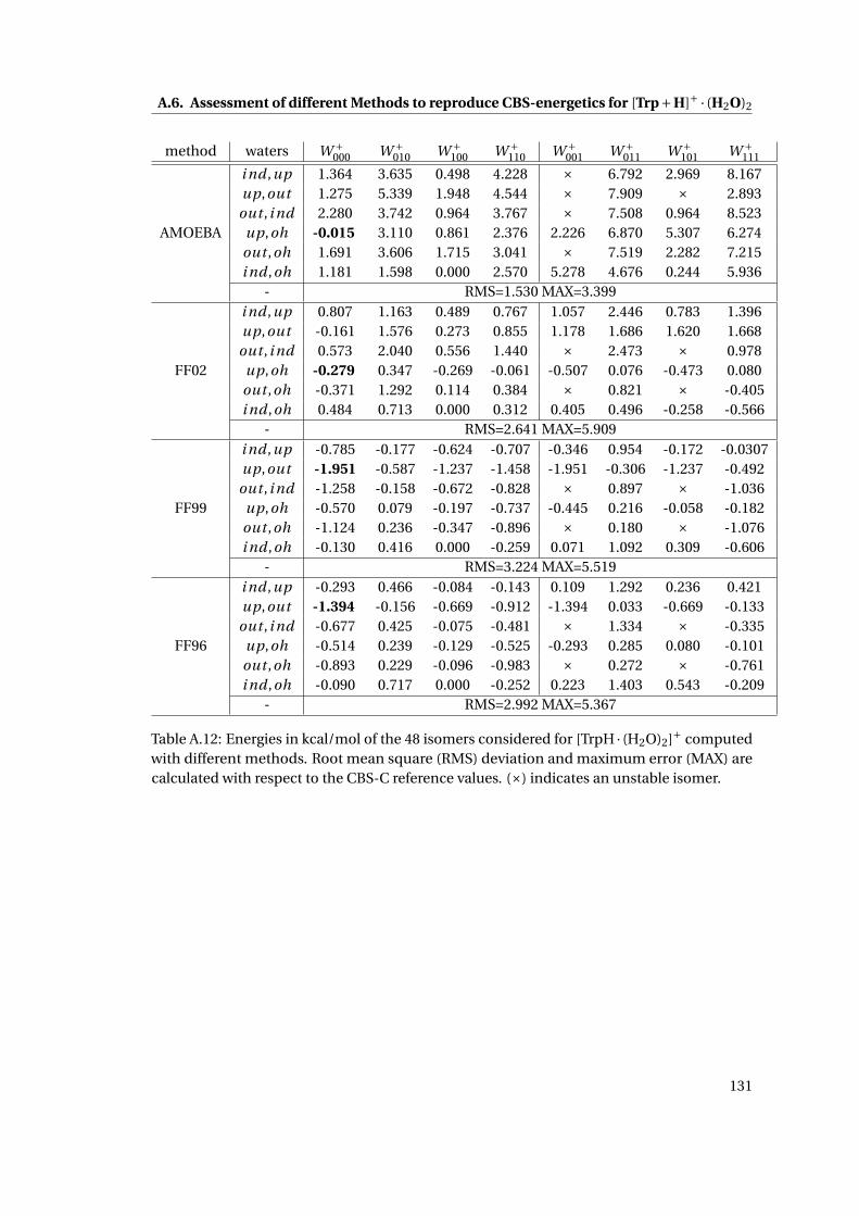
A.6. Assessment of different Methods to reproduce CBS-energetics for [Trp+H]+ · (H2O)2
method waters W +000 W +
010 W +100 W +
110 W +001 W +
011 W +101 W +
111
AMOEBA
i nd ,up 1.364 3.635 0.498 4.228 × 6.792 2.969 8.167up,out 1.275 5.339 1.948 4.544 × 7.909 × 2.893
out , i nd 2.280 3.742 0.964 3.767 × 7.508 0.964 8.523up,oh -0.015 3.110 0.861 2.376 2.226 6.870 5.307 6.274out ,oh 1.691 3.606 1.715 3.041 × 7.519 2.282 7.215i nd ,oh 1.181 1.598 0.000 2.570 5.278 4.676 0.244 5.936
- RMS=1.530 MAX=3.399
FF02
i nd ,up 0.807 1.163 0.489 0.767 1.057 2.446 0.783 1.396up,out -0.161 1.576 0.273 0.855 1.178 1.686 1.620 1.668
out , i nd 0.573 2.040 0.556 1.440 × 2.473 × 0.978up,oh -0.279 0.347 -0.269 -0.061 -0.507 0.076 -0.473 0.080out ,oh -0.371 1.292 0.114 0.384 × 0.821 × -0.405i nd ,oh 0.484 0.713 0.000 0.312 0.405 0.496 -0.258 -0.566
- RMS=2.641 MAX=5.909
FF99
i nd ,up -0.785 -0.177 -0.624 -0.707 -0.346 0.954 -0.172 -0.0307up,out -1.951 -0.587 -1.237 -1.458 -1.951 -0.306 -1.237 -0.492
out , i nd -1.258 -0.158 -0.672 -0.828 × 0.897 × -1.036up,oh -0.570 0.079 -0.197 -0.737 -0.445 0.216 -0.058 -0.182out ,oh -1.124 0.236 -0.347 -0.896 × 0.180 × -1.076i nd ,oh -0.130 0.416 0.000 -0.259 0.071 1.092 0.309 -0.606
- RMS=3.224 MAX=5.519
FF96
i nd ,up -0.293 0.466 -0.084 -0.143 0.109 1.292 0.236 0.421up,out -1.394 -0.156 -0.669 -0.912 -1.394 0.033 -0.669 -0.133
out , i nd -0.677 0.425 -0.075 -0.481 × 1.334 × -0.335up,oh -0.514 0.239 -0.129 -0.525 -0.293 0.285 0.080 -0.101out ,oh -0.893 0.229 -0.096 -0.983 × 0.272 × -0.761i nd ,oh -0.090 0.717 0.000 -0.252 0.223 1.403 0.543 -0.209
- RMS=2.992 MAX=5.367
Table A.12: Energies in kcal/mol of the 48 isomers considered for [TrpH · (H2O)2]+ computedwith different methods. Root mean square (RMS) deviation and maximum error (MAX) arecalculated with respect to the CBS-C reference values. (×) indicates an unstable isomer.
131

Appendix A. Supporting Information for Section 2.1
Table A.13: Root mean square (RMS) deviation and maximum error (MAX) of the relativeenergies for [TrpH · (H2O)2]+ with respect to the CBS-C reference values in Tab. 2.5 of the maintext. Corresponding values for the zero-point energy corrected results are indicated in italics.All values are in kcal/mol.
Method RMSD MAX
M06-2X/ACD 0.579 - 1.049 -M06-2X/631 0.574 - 1.091 -M06/ACD 0.636 - 1.291 -M06/631 0.454 - 0.702 -M05-2X/ACD 0.695 0.835 1.299 1.595M05-2X/631 0.567 - 1.137B3LYP/631 1.617 - 2.995B3LYP/ACD 1.675 - 3.036BLYP-D3/ACD 0.716 - 2.423 -DFTB 2.000 - 3.318 -DFTB(h) 1.621 - 2.754 -DFTB(d) 2.424 - 4.020 -DFTB(h,d) 1.991 - 3.439 -AMOEBA 1.530 - 3.399 -FF02 2.641 - 5.909 -FF99 3.224 - 5.519 -FF96 2.992 - 5.367 -
132
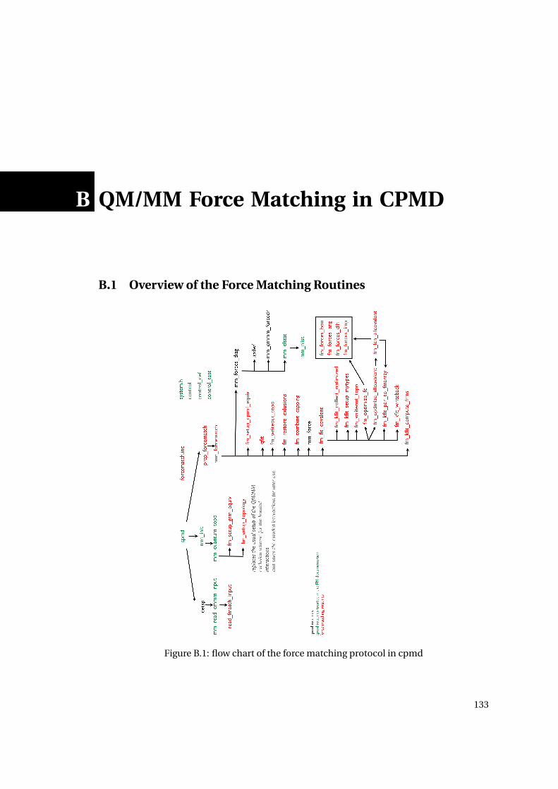
B QM/MM Force Matching in CPMD
B.1 Overview of the Force Matching Routines
Figure B.1: flow chart of the force matching protocol in cpmd
133

Appendix B. QM/MM Force Matching in CPMD
B.2 keywords
FORCEMATCH
The force matching keywords are read within the “&QMMM” section and have to be given
within a block “[FORCEMATCH ... END FORCEMATCH]”. Example:
Figure B.2: example of the forcematching block within the “&QMMM” section of a cpmd inputfile
READ REF FORCES [FILE],[COVALENT]
QM/MM reference forces are directly read from the file FM_REF_FORCES, i.e. no QM/MM
SPs are computed. In case of a different file name with the option FILE it can be specified on
the next line.
With the option COVALENT covalent forces are read from the file FM_REF_COVFORCES.
READ REF TRAJ [FILE]
Read reference trajectory from file TRAJECTORY_REF (or set the FILE option to read a non-
default file name from the next line) with a given stride and compute single points on the
respective frames.
RESTART SP
In cases that in a previous run not all of the SPs could be computed (e.g. limited wall time) this
flag indicates cpmd to restart the SP calculations. The FM_REF* files from the previous run
have to be present and they will be appended. Check that the frames contained in the already
existing FM_REF* files are consistent. There is a consistency-check, but you never know...
134
B.2. keywords
READ REF STRIDE
Stride to apply when reading the FM_REF_FORCES file is read from the next line. Default=1,
i.e. every frame is used for the SP calculations.
TOPOL OUT
Filename for the final topology file. Default=FMATCH.top.
INITWF [OFF]
Generate an initial guess for the wfkt for the SP calculations based on AOs (default). With the
OFF option the wfkt of the previous frame is used as an intial guess.
CHARGES [ONLY,NO],[FIX]
Charge fitting is on by default and can be switched off with the NO option. In this case the
charges from the initial topology will not be modified. ONLY will let the program stop after
the charge fitting and the other parameters are not updated.
With the FIX option target values for the restraints in the charge fitting on specific atoms can
be specified by the user. Usually the charges are restraint to the respective Hirschfeld values
(see equation xx). On the next line the number of charges to be fixed has to be given and then
the corresponding number of lines with: gromos index charge
OPT QFIT WEIGHT
[NOT IMPLEMENTED YET] optimize the weights (variables yy in equation xx) in the charge
fitting procedure by a build-in automatic procedure.
WV
Weight on the potential in the charge fitting (equation xx). Default=0.1.
WF
Weight on the field in the charge fitting (equation xx). Default=0.0.
WQ INDIVIDUAL
Weights on the charge restraints (variable in equation xx) can be given individually here. From
the next line the total number of individual weights is read. Then the lines with: gromos index
135

Appendix B. QM/MM Force Matching in CPMD
weight.
WQ GENERAL
The weight for all the charge restraints that were not specified by individual weights can be
given on the next line. Default=0.1
WTOT
Weight of the total charge contribution in the charge fitting (equation xx). Default=1.0E7
EQUIV
Specify equivalent atoms. Syntax:
EQUIVn_equivatom1 atom4atom1 atom3...atom5 atom7
There are n_equiv equivalencies specified (n_equiv lines are read from the input). For each
pair of equivalencies the gromos indexes have to be specified on one separate line. The lower
index has to be given first!
If an atom is equivalent to more then one other atom. E.g. atom1,atom3 and atom4 are
equivalent. Then this has to be encoded by:
atom1 atom3atom1 atom4
and not by:
atom1 atom4atom3 atom4
where atom1 has a lower gromos index then atom3 and atom3 has a lower one then atom4.
Per default no equivalencies are assumed.
136

B.2. keywords
OPT FC ONLY
Serves as a flag to remove the equilibrium values of the bonded interactions from the list of
fitted parameters. I. e. only force constants are fitted for the bonded interactions.
NO BONDS
Do not fit bonds. Default=.false.
NO ANGLES
Do not fit angles. Default=.false.
NO DIHEDRALS
Do not fit dihedrals. Default=.false.
NO IMPROPERS
Do not fit improper dihedrals. Default=.false.
FMCAP
Signal here whether hydrogen capping is used for the QM/MM coupling. Give the number
of capping hydrogens on the next line and then one line for each dummy hydrogen with its
gromos index and the index of the capped atom wo which the respective dummy H is linked
to Format:
FMCAPfm_n_capind_dummy_H1 ind_capped_C1...
MAXITER
Give on the next line the maximal number of iterations for the non-linear fitting procedure of
the bonded interactions. Default=500
137

Appendix B. QM/MM Force Matching in CPMD
COMPUTE RMS [NO]
Per default the RMS on the forces is computed after the fitting has been completed. Switch it
off with the NO option.
B.3 Files generated
Some of the following default filenames can be changed via the respective keywords in the
“FORCEMATCH” block.
TRAJECTORY_REF
Reference trajectory. Same format as the cpmd “TRAJECTORY” file. This file is read with a
given stride and QM/MM single points are computed for the selected frames. “NEW DATA”
marks can be handled by the program.
FM_REF_CHJ
Hirschfeld charges on the QM atoms for all the frames that were selected for the SP.Format:
Two lines per frame. First line contains frame index from the original “TRAJECTORY_REF” file.
Second line gives the Hirschfeld charges on the QM atoms in cpmd ordering.
FM_REF_PIP
For each frame extracted from the “TRAJECTORY_REF” file a line is printed with the number
of NN atoms in this very frame and the original frame index. Then, for all the QM and NN
atoms (in Gromos order) in this frame a line is printed with the columns:
1-3 position x,y ,z
4 label "QM" or "MM"
5 classical charge
6 electrostatic potential due to classical charges
7 Rsmear
8 electrostatic potential due to QM nuclei
9 electrostatic potential due to QM electronic density
10-12 electrostatic field x,y ,z
138

B.4. CPMD routines
FM_REF_FORCES
For each frame extracted from the reference trajectory and for which a QM/MM SP was
calculated, the QM/MM forces on the QM atoms are dumped into this file. One line per frame
with the original frame index and the number of QM atoms. Then for each QM atom in cpmd
ordering:
atom index,x,y,z,fx,fy,fz
FM_REF_COVFORCES
QM/MM reference forces on the QM atoms minus classical non-bonded forces. Forces to fit
the bonded interactions.
QFIT.top
Updated topology file after the charge fitting. The bonded parameters in here have no meaning,
since they reflect the modifications needed for the QM/MM coupling (exclusions!).
FMATCH.top
Updated topology file after the force matching.
B.4 CPMD routines
system.h
MLOGO increase and logical FMATCH as primary flag.
control
Search CPMD section for FORCEMATCH keyword.
control_test
Check for mutually excluding job keywords.
control_def
FMATCH=.false.
139

Appendix B. QM/MM Force Matching in CPMD
mm_init
If forcematching call mm_quantum_topo even for a classical run.
MM_Interface/mm_nlist
Some modification on the atoms to include in the NN list.
MM_Interface/mm_elstat
Write the FM_REF_PIP and FM_REF_CHJ files.
mm_read_qmmm_input
mm_read_qmmm_input.F
• default values for many of the forcematching parameters are set
• call read_fmatch_input
mm_quantum_topo
mm_quantum_topo.FClassical topology is modified to fit to the QM/MM coupling. For the force matching we need
something more sophisticated for the bonded exclusions and the initial purely MM exclusions
have to be saved before they are modified.
identify quantum atoms: mm_q
non-bonded interactions: mm_q_nb
if FMATCH then
call fm_setup_grm_equiv
call fm_setup_topology
else
set up the usual QM/MM exclusions for the bonded interactions
create a new bond type with force constant=0.0
go trough all the bonds in the topology
if they are QM-QM bonds, then change their type to the new bond type
the same with angles, dihedrals and improper dihedrals
end if
if FMATCH then
non-bonded exclusions are saved for later use
INE(I): last index in the exclusion list of atom I
140

B.5. Forcematching Routines
KNE(I): first index in the exclusion list of atom I
JSNE: non-bonded exclusions. Exclusions J of atom I are positioned at
JSNE(KNE(I)+1),...JSNE(KNE(I)+INE(I)). all J must be > I and in ascending order.
INE14
KNE14
JSNE14: 1-4 exclusions. Organization of the arrays analogous to JSNE.
end if
non-bonded exclusions are modified to fit the QM-MM coupling
B.5 Forcematching Routines
prep_forcematch
fm_setup_grm_equiv
forcematch_util.FSetup equivalencies in gromos ordering, i.e. fill the array grm_equiv.
From the input
EQUIV3 43 56 8
we have: fm_equiv(1,1)=3, fm_equiv(2,1)=4, fm_equiv(1,2)=3, fm_equiv(2,2)=5, fm_equiv(1,3)=6,
fm_equiv(2,3)=8
grm_equiv(i ) = i ∀ i = 1, ...,nr solute atoms Initially make any atom equivalent to itself
from the input we have fm_equiv()
update grm_equiv(:) according to the equivalencies in the input: atom i is equivalent to
atom grm_equiv(i)
and we get: grm_equiv = [1,2,3,3,3,6,7,6,9,10, ...,NRPT] (NRPT: total number of solute atoms)
fm_setup_topology
forcematch_kfit.F
1. Create new bonded interaction (bonds, angles, dihedrals, improper dihedrals) types if
necessary: increase NBTY, NTTY, NQTY, NPTY
2. Determine number of bonded interaction types to optimize: fm_nbonopt, fm_nangopt,
141

Appendix B. QM/MM Force Matching in CPMD
fm_nimpopt, fm_ndihopt
3. Create lists of the indexes for the bonded interaction types to optimize: fm_bonopt(1:fm_nbonopt),
fm_angopt(1:fm_nangopt), fm_impopt(1:fm_nimpopt), fm_dihopt(1:fm_ndihopt)
4. set to zero all the force constants of all the QM-only bonded interactions: CB, CT, CQ
and CP. Store the values for later: fm_kbon, fm_kang, fm_kimp, fm_kdih.
for all bonds i in the topo involving hydrogens do
if bond i is QM-QM then
for all other bonds j do
if type(bond j ) = type(bond i ) and bond j is QM-MM or MM-MM then
create a new type: NBTY ← NBTY+1
type(bond i ) ← NBTY
copy old parameters: CB(NBTY) ← CB(old_type), B0(NBTY) ← B0(old_type)
flag type(bond i ) to be optimized
end if
end for
if no new type was created and type(bond i ) was already flagged to be optimized then
there is already an earlier QM-QM bond of this type
for all bonds j < i do
if type(bond j ) = type(bond i ) and bonds i , j are not equivalent then
create a new type: NBTY ← NBTY+1
type(bond i ) ← NBTY
copy old parameters: CB(NBTY) ← CB(old_type), B0(NBTY) ← B0(old_type)
flag type(bond i ) to be optimized
end if[ if they are equivalent we don’t need a new type]
end for
end if
for all other bonds j > i do
if bond j is equivalent to bond i then
type(bond j ) ← type(bond i )
end if
end for
end if[ the QM-MM and MM-MM bonds we do not want to touch]
end for
the same is happening for all bonds without hydrogens
fm_nbonopt is calculated
fm_bonopt is filled with the indexes of the bonds to be optimized
the same with the angles involving hydrogens
the same is happening for all angles without hydrogens
fm_nangopt
fm_angopt
improper dihedrals involving hydrogens
142
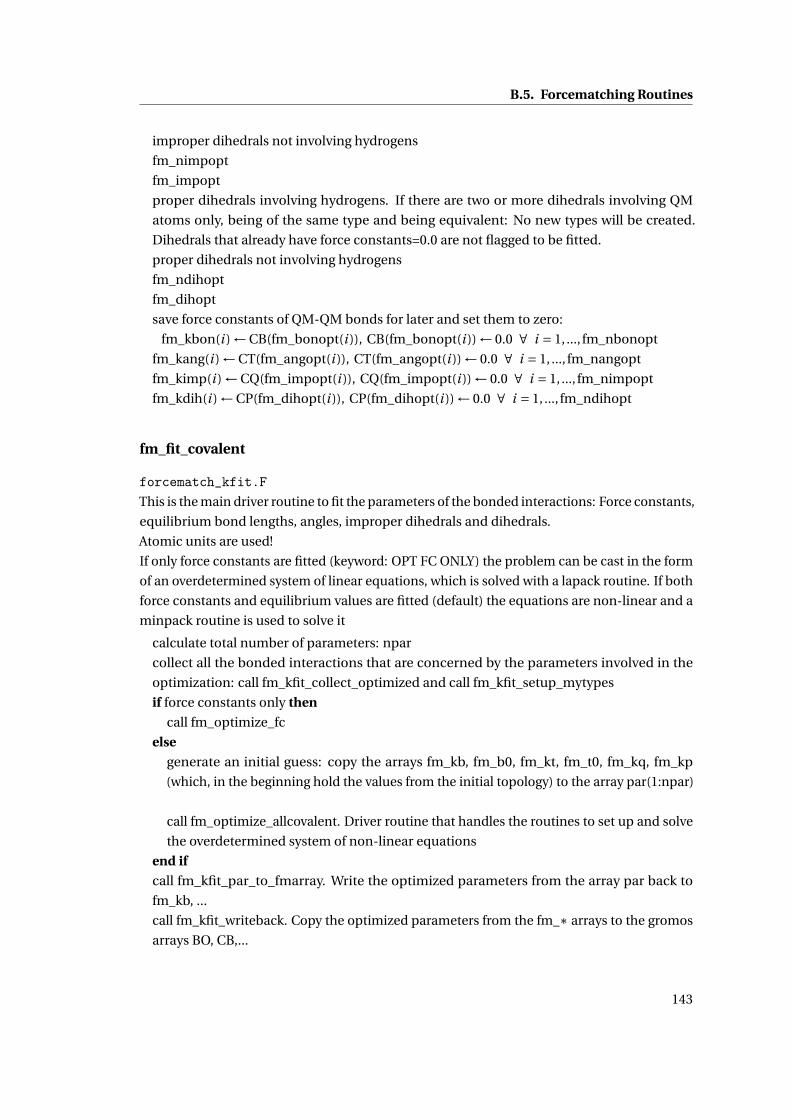
B.5. Forcematching Routines
improper dihedrals not involving hydrogens
fm_nimpopt
fm_impopt
proper dihedrals involving hydrogens. If there are two or more dihedrals involving QM
atoms only, being of the same type and being equivalent: No new types will be created.
Dihedrals that already have force constants=0.0 are not flagged to be fitted.
proper dihedrals not involving hydrogens
fm_ndihopt
fm_dihopt
save force constants of QM-QM bonds for later and set them to zero:
fm_kbon(i ) ← CB(fm_bonopt(i )), CB(fm_bonopt(i )) ← 0.0 ∀ i = 1, ..., fm_nbonopt
fm_kang(i ) ← CT(fm_angopt(i )), CT(fm_angopt(i )) ← 0.0 ∀ i = 1, ..., fm_nangopt
fm_kimp(i ) ← CQ(fm_impopt(i )), CQ(fm_impopt(i )) ← 0.0 ∀ i = 1, ..., fm_nimpopt
fm_kdih(i ) ← CP(fm_dihopt(i )), CP(fm_dihopt(i )) ← 0.0 ∀ i = 1, ..., fm_ndihopt
fm_fit_covalent
forcematch_kfit.FThis is the main driver routine to fit the parameters of the bonded interactions: Force constants,
equilibrium bond lengths, angles, improper dihedrals and dihedrals.
Atomic units are used!
If only force constants are fitted (keyword: OPT FC ONLY) the problem can be cast in the form
of an overdetermined system of linear equations, which is solved with a lapack routine. If both
force constants and equilibrium values are fitted (default) the equations are non-linear and a
minpack routine is used to solve it
calculate total number of parameters: npar
collect all the bonded interactions that are concerned by the parameters involved in the
optimization: call fm_kfit_collect_optimized and call fm_kfit_setup_mytypes
if force constants only then
call fm_optimize_fc
else
generate an initial guess: copy the arrays fm_kb, fm_b0, fm_kt, fm_t0, fm_kq, fm_kp
(which, in the beginning hold the values from the initial topology) to the array par(1:npar)
call fm_optimize_allcovalent. Driver routine that handles the routines to set up and solve
the overdetermined system of non-linear equations
end if
call fm_kfit_par_to_fmarray. Write the optimized parameters from the array par back to
fm_kb, ...
call fm_kfit_writeback. Copy the optimized parameters from the fm_∗ arrays to the gromos
arrays BO, CB,...
143
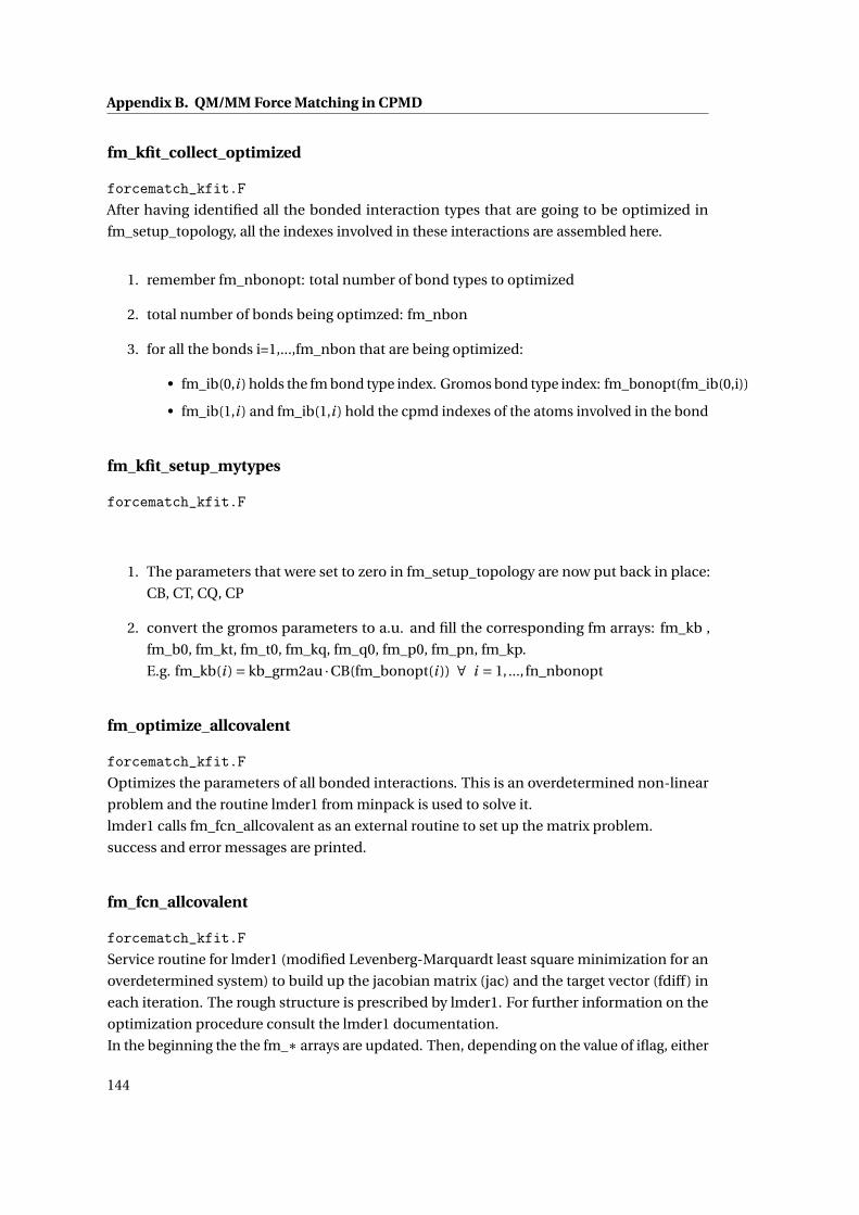
Appendix B. QM/MM Force Matching in CPMD
fm_kfit_collect_optimized
forcematch_kfit.FAfter having identified all the bonded interaction types that are going to be optimized in
fm_setup_topology, all the indexes involved in these interactions are assembled here.
1. remember fm_nbonopt: total number of bond types to optimized
2. total number of bonds being optimzed: fm_nbon
3. for all the bonds i=1,...,fm_nbon that are being optimized:
• fm_ib(0,i ) holds the fm bond type index. Gromos bond type index: fm_bonopt(fm_ib(0,i))
• fm_ib(1,i ) and fm_ib(1,i ) hold the cpmd indexes of the atoms involved in the bond
fm_kfit_setup_mytypes
forcematch_kfit.F
1. The parameters that were set to zero in fm_setup_topology are now put back in place:
CB, CT, CQ, CP
2. convert the gromos parameters to a.u. and fill the corresponding fm arrays: fm_kb ,
fm_b0, fm_kt, fm_t0, fm_kq, fm_q0, fm_p0, fm_pn, fm_kp.
E.g. fm_kb(i ) = kb_grm2au ·CB(fm_bonopt(i )) ∀ i = 1, ..., fn_nbonopt
fm_optimize_allcovalent
forcematch_kfit.FOptimizes the parameters of all bonded interactions. This is an overdetermined non-linear
problem and the routine lmder1 from minpack is used to solve it.
lmder1 calls fm_fcn_allcovalent as an external routine to set up the matrix problem.
success and error messages are printed.
fm_fcn_allcovalent
forcematch_kfit.FService routine for lmder1 (modified Levenberg-Marquardt least square minimization for an
overdetermined system) to build up the jacobian matrix (jac) and the target vector (fdiff) in
each iteration. The rough structure is prescribed by lmder1. For further information on the
optimization procedure consult the lmder1 documentation.
In the beginning the the fm_∗ arrays are updated. Then, depending on the value of iflag, either
144
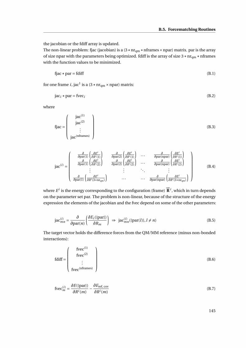
B.5. Forcematching Routines
the jacobian or the fdiff array is updated.
The non-linear problem: fjac (jacobian) is a (3∗nrqm∗nframes×npar) matrix. par is the array
of size npar with the parameters being optimized. fdiff is the array of size 3∗nrqm ∗nframes
with the function values to be minimized.
fjac∗par = fdiff (B.1)
for one frame i , jac1 is a (3∗nrqm ×npar) matrix:
jaci ∗par = fveci (B.2)
where
fjac =
jac(1)
jac(2)
...
jac(nframes)
(B.3)
jac(i ) =
∂∂par(1)
(∂E i
∂R i (1)
)∂
∂par(2)
(∂E i
∂R i (1)
). . . ∂
∂par(npar)
(∂E i
∂R i (1)
)∂
∂par(1)
(∂E i
∂R i (2)
)∂
∂par(2)
(∂E i
∂R i (2)
). . . ∂
∂par(npar)
(∂E i
∂R i (2)
)...
.... . .
...∂
∂par(1)
(∂E i
∂R i (3∗nrqm)
). . . . . . ∂
∂par(npar)
(∂E i
∂R i (3∗nrqm)
)
(B.4)
where E i is the energy corresponding to the configuration (frame)−→R i , which in turn depends
on the parameter set par. The problem is non-linear, because of the structure of the energy
expression the elements of the jacobian and the fvec depend on some of the other parameters:
jac(i )mn = ∂
∂par(n)
(∂Ei (par)
∂Rm
)⇒ jac(i )
mn(par(l ), l 6= n) (B.5)
The target vector holds the difference forces from the QM/MM reference (minus non-bonded
interactions):
fdiff =
fvec(1)
fvec(2)
...
fvec(nframes)
(B.6)
fvec(i )m = ∂E(par)
∂R i (m)− ∂Eref, cov
∂R i (m)(B.7)
145

Appendix B. QM/MM Force Matching in CPMD
The parameter array is organized as follows:
par = [fm_kb(1), fm_kb(2), . . . , fm_kb(nbonopt), fm_b0(1), . . . , fm_b0(nbonopt), fm_kt(1), . . . , fm_kt(nangopt),
fm_t0(1), . . . , fm_t0(nangopt), fm_kq(1), . . . , fm_kq(nimpopt), fm_kp(1), . . . , fm_kp(ndihopt)]
The routine can be called with two values for the flag iflag.
iflag=1: update the fdiff array without changing the jacobian. In this case all the fm_forces_∗routines are called with the flag ’ff’, i.e., the forces are computed.
iflag=2: update the jacobian. All the fm_forces_∗ routines are called with the flag ’dk’ and,
where applicable, ’d0’ in order to compute the derivative of the forces with respect to the
respective parameters.
fm_kfit_par_to_fmarray
forcematch_kfit.Ffm_optimize_allcovalent and fm_optimize_fc put the results into the array par(1:npar). Here
the arrays fm_kb, fm_b0, fm_kt, fm_t0, fm_kq, fm_kp are updated with the optimized parame-
ters.
In addition, fm_fcn_allcovalent needs this in each iteration to build up a new jacobian matrix.
fm_kfit_compute_frms
forcematch_kfit.FCompute RMS between the QM/MM and the new classical forces on the atoms involved in
the interactions that were fitted.
read_fmatch_input
mm_read_qmmm_input.FReads the FORCEMATCH block in the “&QMMM” section and sets the respective parameters.
forcematch.inc
forcematch.incInclude file for the forcematching subroutines.
146
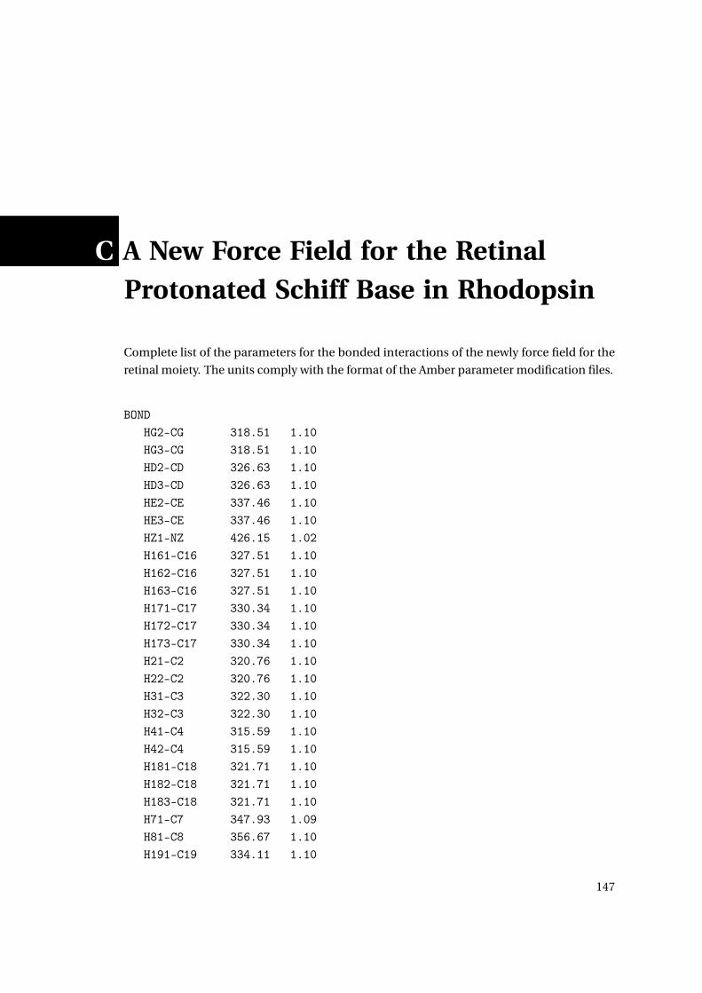
C A New Force Field for the RetinalProtonated Schiff Base in Rhodopsin
Complete list of the parameters for the bonded interactions of the newly force field for the
retinal moiety. The units comply with the format of the Amber parameter modification files.
BONDHG2-CG 318.51 1.10HG3-CG 318.51 1.10HD2-CD 326.63 1.10HD3-CD 326.63 1.10HE2-CE 337.46 1.10HE3-CE 337.46 1.10HZ1-NZ 426.15 1.02H161-C16 327.51 1.10H162-C16 327.51 1.10H163-C16 327.51 1.10H171-C17 330.34 1.10H172-C17 330.34 1.10H173-C17 330.34 1.10H21-C2 320.76 1.10H22-C2 320.76 1.10H31-C3 322.30 1.10H32-C3 322.30 1.10H41-C4 315.59 1.10H42-C4 315.59 1.10H181-C18 321.71 1.10H182-C18 321.71 1.10H183-C18 321.71 1.10H71-C7 347.93 1.09H81-C8 356.67 1.10H191-C19 334.11 1.10
147
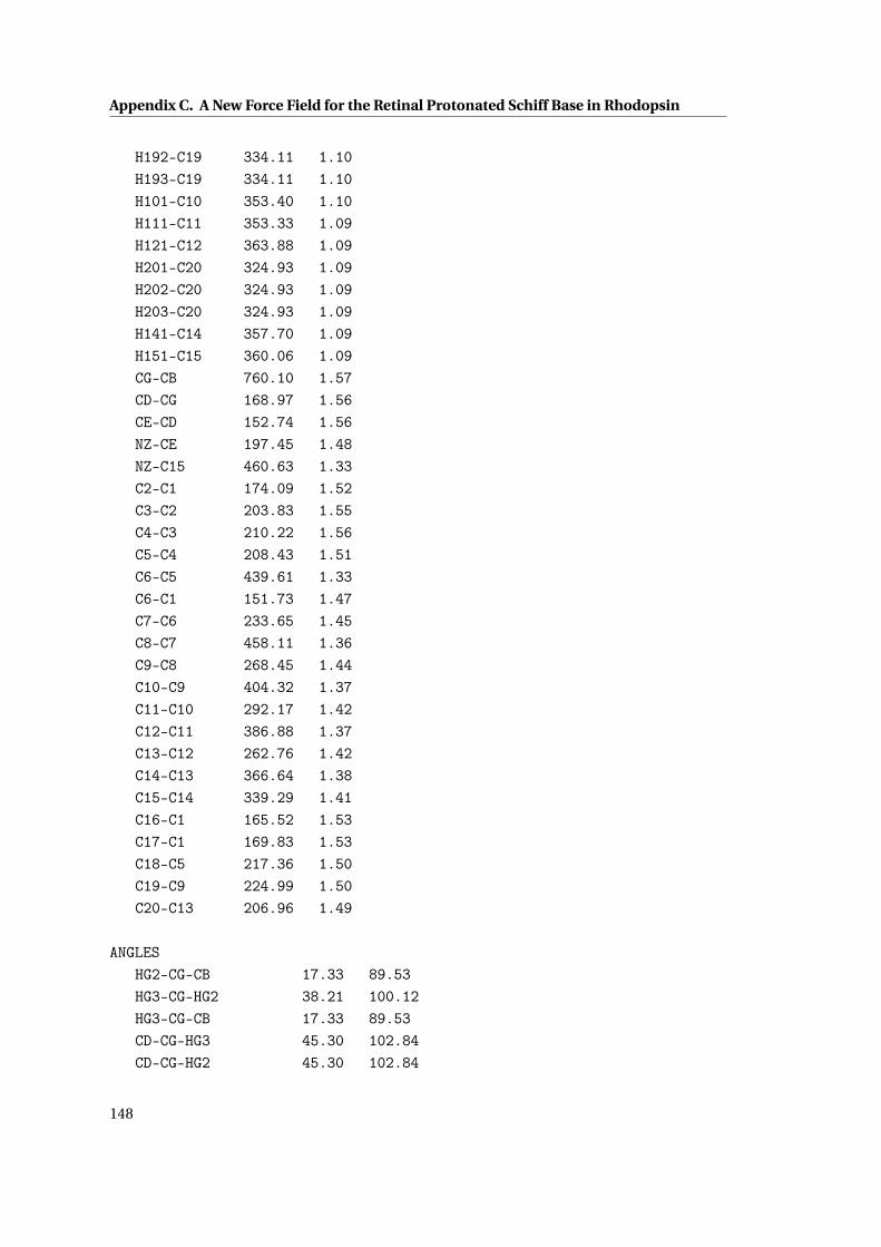
Appendix C. A New Force Field for the Retinal Protonated Schiff Base in Rhodopsin
H192-C19 334.11 1.10H193-C19 334.11 1.10H101-C10 353.40 1.10H111-C11 353.33 1.09H121-C12 363.88 1.09H201-C20 324.93 1.09H202-C20 324.93 1.09H203-C20 324.93 1.09H141-C14 357.70 1.09H151-C15 360.06 1.09CG-CB 760.10 1.57CD-CG 168.97 1.56CE-CD 152.74 1.56NZ-CE 197.45 1.48NZ-C15 460.63 1.33C2-C1 174.09 1.52C3-C2 203.83 1.55C4-C3 210.22 1.56C5-C4 208.43 1.51C6-C5 439.61 1.33C6-C1 151.73 1.47C7-C6 233.65 1.45C8-C7 458.11 1.36C9-C8 268.45 1.44C10-C9 404.32 1.37C11-C10 292.17 1.42C12-C11 386.88 1.37C13-C12 262.76 1.42C14-C13 366.64 1.38C15-C14 339.29 1.41C16-C1 165.52 1.53C17-C1 169.83 1.53C18-C5 217.36 1.50C19-C9 224.99 1.50C20-C13 206.96 1.49
ANGLESHG2-CG-CB 17.33 89.53HG3-CG-HG2 38.21 100.12HG3-CG-CB 17.33 89.53CD-CG-HG3 45.30 102.84CD-CG-HG2 45.30 102.84
148
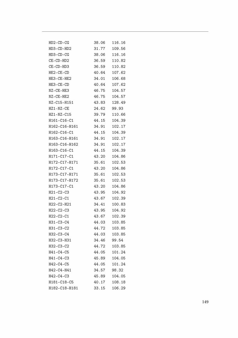
HD2-CD-CG 38.06 116.16HD3-CD-HD2 31.77 109.56HD3-CD-CG 38.06 116.16CE-CD-HD2 36.59 110.82CE-CD-HD3 36.59 110.82HE2-CE-CD 40.64 107.62HE3-CE-HE2 34.01 106.68HE3-CE-CD 40.64 107.62NZ-CE-HE3 46.75 104.57NZ-CE-HE2 46.75 104.57NZ-C15-H151 43.83 128.49HZ1-NZ-CE 24.62 99.93HZ1-NZ-C15 39.79 110.66H161-C16-C1 44.15 104.39H162-C16-H161 34.91 102.17H162-C16-C1 44.15 104.39H163-C16-H161 34.91 102.17H163-C16-H162 34.91 102.17H163-C16-C1 44.15 104.39H171-C17-C1 43.20 104.86H172-C17-H171 35.61 102.53H172-C17-C1 43.20 104.86H173-C17-H171 35.61 102.53H173-C17-H172 35.61 102.53H173-C17-C1 43.20 104.86H21-C2-C3 43.95 104.92H21-C2-C1 43.67 102.39H22-C2-H21 34.41 100.83H22-C2-C3 43.95 104.92H22-C2-C1 43.67 102.39H31-C3-C4 44.03 103.85H31-C3-C2 44.72 103.85H32-C3-C4 44.03 103.85H32-C3-H31 34.46 99.54H32-C3-C2 44.72 103.85H41-C4-C5 44.05 101.24H41-C4-C3 45.89 104.05H42-C4-C5 44.05 101.24H42-C4-H41 34.57 98.32H42-C4-C3 45.89 104.05H181-C18-C5 40.17 108.18H182-C18-H181 33.15 106.29
149
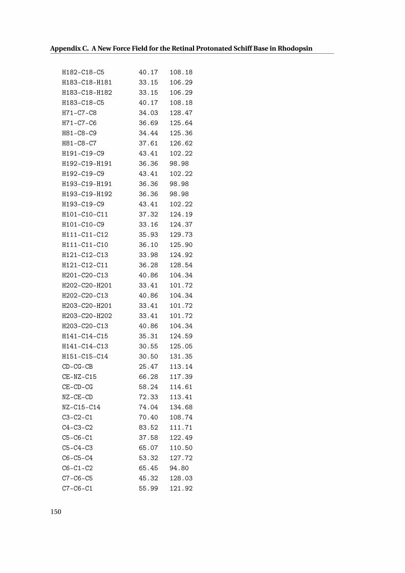
Appendix C. A New Force Field for the Retinal Protonated Schiff Base in Rhodopsin
H182-C18-C5 40.17 108.18H183-C18-H181 33.15 106.29H183-C18-H182 33.15 106.29H183-C18-C5 40.17 108.18H71-C7-C8 34.03 128.47H71-C7-C6 36.69 125.64H81-C8-C9 34.44 125.36H81-C8-C7 37.61 126.62H191-C19-C9 43.41 102.22H192-C19-H191 36.36 98.98H192-C19-C9 43.41 102.22H193-C19-H191 36.36 98.98H193-C19-H192 36.36 98.98H193-C19-C9 43.41 102.22H101-C10-C11 37.32 124.19H101-C10-C9 33.16 124.37H111-C11-C12 35.93 129.73H111-C11-C10 36.10 125.90H121-C12-C13 33.98 124.92H121-C12-C11 36.28 128.54H201-C20-C13 40.86 104.34H202-C20-H201 33.41 101.72H202-C20-C13 40.86 104.34H203-C20-H201 33.41 101.72H203-C20-H202 33.41 101.72H203-C20-C13 40.86 104.34H141-C14-C15 35.31 124.59H141-C14-C13 30.55 125.05H151-C15-C14 30.50 131.35CD-CG-CB 25.47 113.14CE-NZ-C15 66.28 117.39CE-CD-CG 58.24 114.61NZ-CE-CD 72.33 113.41NZ-C15-C14 74.04 134.68C3-C2-C1 70.40 108.74C4-C3-C2 83.52 111.71C5-C6-C1 37.58 122.49C5-C4-C3 65.07 110.50C6-C5-C4 53.32 127.72C6-C1-C2 65.45 94.80C7-C6-C5 45.32 128.03C7-C6-C1 55.99 121.92
150
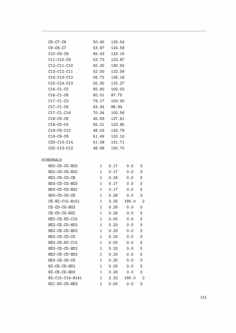
C8-C7-C6 50.45 133.54C9-C8-C7 53.97 124.59C10-C9-C8 65.43 133.16C11-C10-C9 53.73 123.87C12-C11-C10 55.30 130.92C13-C12-C11 52.50 122.58C14-C13-C12 58.72 136.18C15-C14-C13 55.30 115.27C16-C1-C2 65.80 100.02C16-C1-C6 60.01 97.75C17-C1-C2 79.17 103.00C17-C1-C6 63.34 98.94C17-C1-C16 70.04 100.56C18-C5-C6 45.69 127.61C18-C5-C4 65.21 123.85C19-C9-C10 48.03 133.79C19-C9-C8 51.49 132.10C20-C13-C14 51.08 131.71C20-C13-C12 48.88 130.70
DIHEDRALSHD2-CD-CG-HG3 1 0.17 0.0 3HD2-CD-CG-HG2 1 0.17 0.0 3HD2-CD-CG-CB 1 0.26 0.0 3HD3-CD-CG-HG3 1 0.17 0.0 3HD3-CD-CG-HG2 1 0.17 0.0 3HD3-CD-CG-CB 1 0.26 0.0 3CE-NZ-C15-H151 1 3.25 180.0 2CE-CD-CG-HG3 1 0.26 0.0 3CE-CD-CG-HG2 1 0.26 0.0 3HE2-CE-NZ-C15 1 0.00 0.0 3HE2-CE-CD-HD2 1 0.20 0.0 3HE2-CE-CD-HD3 1 0.20 0.0 3HE2-CE-CD-CG 1 0.20 0.0 3HE3-CE-NZ-C15 1 0.00 0.0 3HE3-CE-CD-HD2 1 0.20 0.0 3HE3-CE-CD-HD3 1 0.20 0.0 3HE3-CE-CD-CG 1 0.20 0.0 3NZ-CE-CD-HD2 1 0.20 0.0 3NZ-CE-CD-HD3 1 0.20 0.0 3NZ-C15-C14-H141 1 2.32 180.0 2HZ1-NZ-CE-HE3 1 0.00 0.0 3
151

Appendix C. A New Force Field for the Retinal Protonated Schiff Base in Rhodopsin
HZ1-NZ-CE-HE2 1 0.00 0.0 3HZ1-NZ-CE-CD 1 0.00 0.0 3HZ1-NZ-C15-H151 1 3.25 180.0 2HZ1-NZ-C15-C14 1 3.25 180.0 2H161-C16-C1-C2 1 0.26 0.0 3H161-C16-C1-C6 1 0.20 0.0 3H161-C16-C1-C17 1 0.26 0.0 3H162-C16-C1-C2 1 0.26 0.0 3H162-C16-C1-C6 1 0.20 0.0 3H162-C16-C1-C17 1 0.26 0.0 3H163-C16-C1-C2 1 0.26 0.0 3H163-C16-C1-C6 1 0.20 0.0 3H163-C16-C1-C17 1 0.26 0.0 3H171-C17-C1-C2 1 0.26 0.0 3H171-C17-C1-C6 1 0.20 0.0 3H171-C17-C1-C16 1 0.26 0.0 3H172-C17-C1-C2 1 0.26 0.0 3H172-C17-C1-C6 1 0.20 0.0 3H172-C17-C1-C16 1 0.26 0.0 3H173-C17-C1-C2 1 0.26 0.0 3H173-C17-C1-C6 1 0.20 0.0 3H173-C17-C1-C16 1 0.26 0.0 3H21-C2-C3-C4 1 0.26 0.0 3H21-C2-C1-C6 1 0.20 0.0 3H21-C2-C1-C16 1 0.26 0.0 3H21-C2-C1-C17 1 0.26 0.0 3H22-C2-C3-C4 1 0.26 0.0 3H22-C2-C1-C6 1 0.20 0.0 3H22-C2-C1-C16 1 0.26 0.0 3H22-C2-C1-C17 1 0.26 0.0 3H31-C3-C4-C5 1 0.20 0.0 3H31-C3-C2-H21 1 0.17 0.0 3H31-C3-C2-H22 1 0.17 0.0 3H31-C3-C2-C1 1 0.26 0.0 3H32-C3-C4-C5 1 0.20 0.0 3H32-C3-C2-H21 1 0.17 0.0 3H32-C3-C2-H22 1 0.17 0.0 3H32-C3-C2-C1 1 0.26 0.0 3H41-C4-C5-C6 1 0.00 0.0 2H41-C4-C5-C18 1 0.00 0.0 2H41-C4-C3-H31 1 0.17 0.0 3H41-C4-C3-H32 1 0.17 0.0 3
152
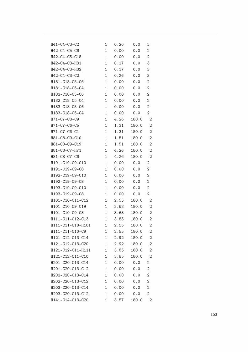
H41-C4-C3-C2 1 0.26 0.0 3H42-C4-C5-C6 1 0.00 0.0 2H42-C4-C5-C18 1 0.00 0.0 2H42-C4-C3-H31 1 0.17 0.0 3H42-C4-C3-H32 1 0.17 0.0 3H42-C4-C3-C2 1 0.26 0.0 3H181-C18-C5-C6 1 0.00 0.0 2H181-C18-C5-C4 1 0.00 0.0 2H182-C18-C5-C6 1 0.00 0.0 2H182-C18-C5-C4 1 0.00 0.0 2H183-C18-C5-C6 1 0.00 0.0 2H183-C18-C5-C4 1 0.00 0.0 2H71-C7-C8-C9 1 4.26 180.0 2H71-C7-C6-C5 1 1.31 180.0 2H71-C7-C6-C1 1 1.31 180.0 2H81-C8-C9-C10 1 1.51 180.0 2H81-C8-C9-C19 1 1.51 180.0 2H81-C8-C7-H71 1 4.26 180.0 2H81-C8-C7-C6 1 4.26 180.0 2H191-C19-C9-C10 1 0.00 0.0 2H191-C19-C9-C8 1 0.00 0.0 2H192-C19-C9-C10 1 0.00 0.0 2H192-C19-C9-C8 1 0.00 0.0 2H193-C19-C9-C10 1 0.00 0.0 2H193-C19-C9-C8 1 0.00 0.0 2H101-C10-C11-C12 1 2.55 180.0 2H101-C10-C9-C19 1 3.68 180.0 2H101-C10-C9-C8 1 3.68 180.0 2H111-C11-C12-C13 1 3.85 180.0 2H111-C11-C10-H101 1 2.55 180.0 2H111-C11-C10-C9 1 2.55 180.0 2H121-C12-C13-C14 1 2.92 180.0 2H121-C12-C13-C20 1 2.92 180.0 2H121-C12-C11-H111 1 3.85 180.0 2H121-C12-C11-C10 1 3.85 180.0 2H201-C20-C13-C14 1 0.00 0.0 2H201-C20-C13-C12 1 0.00 0.0 2H202-C20-C13-C14 1 0.00 0.0 2H202-C20-C13-C12 1 0.00 0.0 2H203-C20-C13-C14 1 0.00 0.0 2H203-C20-C13-C12 1 0.00 0.0 2H141-C14-C13-C20 1 3.57 180.0 2
153
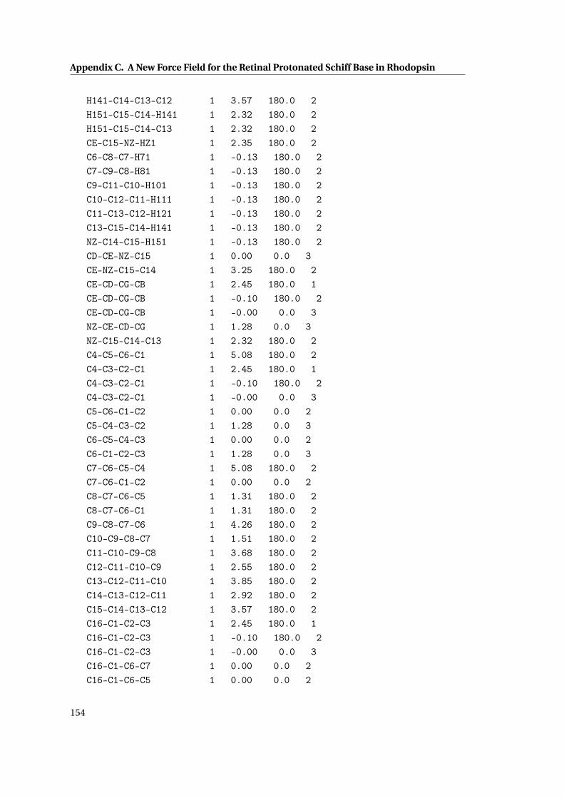
Appendix C. A New Force Field for the Retinal Protonated Schiff Base in Rhodopsin
H141-C14-C13-C12 1 3.57 180.0 2H151-C15-C14-H141 1 2.32 180.0 2H151-C15-C14-C13 1 2.32 180.0 2CE-C15-NZ-HZ1 1 2.35 180.0 2C6-C8-C7-H71 1 -0.13 180.0 2C7-C9-C8-H81 1 -0.13 180.0 2C9-C11-C10-H101 1 -0.13 180.0 2C10-C12-C11-H111 1 -0.13 180.0 2C11-C13-C12-H121 1 -0.13 180.0 2C13-C15-C14-H141 1 -0.13 180.0 2NZ-C14-C15-H151 1 -0.13 180.0 2CD-CE-NZ-C15 1 0.00 0.0 3CE-NZ-C15-C14 1 3.25 180.0 2CE-CD-CG-CB 1 2.45 180.0 1CE-CD-CG-CB 1 -0.10 180.0 2CE-CD-CG-CB 1 -0.00 0.0 3NZ-CE-CD-CG 1 1.28 0.0 3NZ-C15-C14-C13 1 2.32 180.0 2C4-C5-C6-C1 1 5.08 180.0 2C4-C3-C2-C1 1 2.45 180.0 1C4-C3-C2-C1 1 -0.10 180.0 2C4-C3-C2-C1 1 -0.00 0.0 3C5-C6-C1-C2 1 0.00 0.0 2C5-C4-C3-C2 1 1.28 0.0 3C6-C5-C4-C3 1 0.00 0.0 2C6-C1-C2-C3 1 1.28 0.0 3C7-C6-C5-C4 1 5.08 180.0 2C7-C6-C1-C2 1 0.00 0.0 2C8-C7-C6-C5 1 1.31 180.0 2C8-C7-C6-C1 1 1.31 180.0 2C9-C8-C7-C6 1 4.26 180.0 2C10-C9-C8-C7 1 1.51 180.0 2C11-C10-C9-C8 1 3.68 180.0 2C12-C11-C10-C9 1 2.55 180.0 2C13-C12-C11-C10 1 3.85 180.0 2C14-C13-C12-C11 1 2.92 180.0 2C15-C14-C13-C12 1 3.57 180.0 2C16-C1-C2-C3 1 2.45 180.0 1C16-C1-C2-C3 1 -0.10 180.0 2C16-C1-C2-C3 1 -0.00 0.0 3C16-C1-C6-C7 1 0.00 0.0 2C16-C1-C6-C5 1 0.00 0.0 2
154
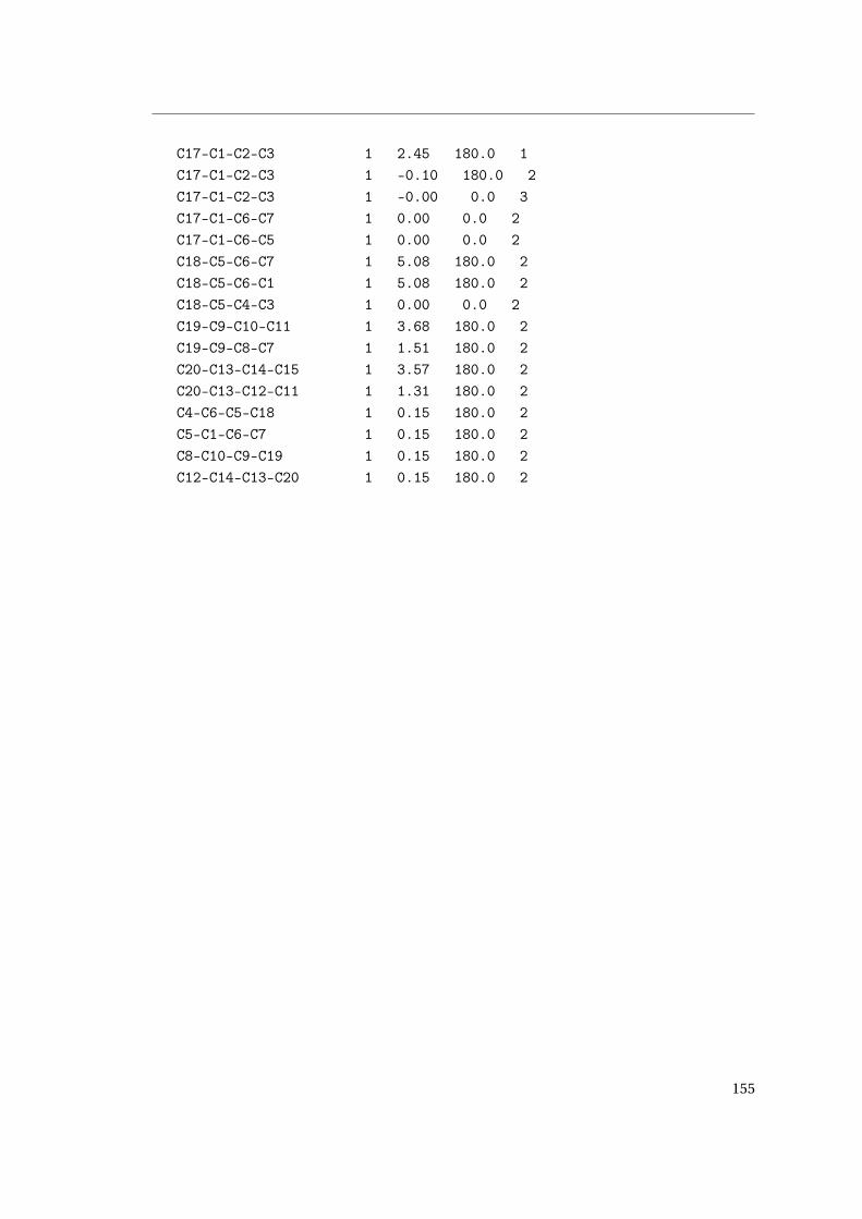
C17-C1-C2-C3 1 2.45 180.0 1C17-C1-C2-C3 1 -0.10 180.0 2C17-C1-C2-C3 1 -0.00 0.0 3C17-C1-C6-C7 1 0.00 0.0 2C17-C1-C6-C5 1 0.00 0.0 2C18-C5-C6-C7 1 5.08 180.0 2C18-C5-C6-C1 1 5.08 180.0 2C18-C5-C4-C3 1 0.00 0.0 2C19-C9-C10-C11 1 3.68 180.0 2C19-C9-C8-C7 1 1.51 180.0 2C20-C13-C14-C15 1 3.57 180.0 2C20-C13-C12-C11 1 1.31 180.0 2C4-C6-C5-C18 1 0.15 180.0 2C5-C1-C6-C7 1 0.15 180.0 2C8-C10-C9-C19 1 0.15 180.0 2C12-C14-C13-C20 1 0.15 180.0 2
155


Bibliography
[1] G. E. Moore, “Cramming more components
onto integrated circuits,” Electronics, vol. 38,
no. 8, pp. 2–4, 1965.
[2] M. Head Gordon and E. Artacho, “Chemistry
on the computer,” Physics Today, vol. 61,
pp. 58–63, 2008.
[3] S. O. Nielsen, C. F. Lopez, G. Srinivas, and
M. L. Klein, “Coarse grain models and the
computer simulation of soft materials,” J.
Phys.: Condens. Matter, vol. 16, no. 15,
pp. R481–R512, 2004.
[4] S. Riniker, J. R. Allison, and W. F. Van Gun-
steren, “On developing coarse-grained mod-
els for biomolecular simulation: a review,”
Phys. Chem. Chem. Phys., vol. 14, no. 36,
pp. 12423–12430, 2012.
[5] C. D. Sherrill and H. F. Schaefer, III, “The
Configuration Interaction Method: Ad-
vances in Highly Correlated Approaches,”
Adv. Quant. Chem., vol. 34, pp. 143–269,
1999.
[6] E. Schrödinger, “An undulatory theory of
the mechanics of atoms and molecules,”
Phys. Rev., vol. 28, no. 6, pp. 1049–1070,
1926.
[7] C. Hampel, K. A. Peterson, and H.-J. Werner,
“A comparison of the efficiency and accu-
racy of the quadratic configuration interac-
tion (QCISD), coupled cluster (CCSD), and
Brueckner coupled cluster (BCCD) meth-
ods,” Chem. Phys. Lett., vol. 190, no. 1, pp. 1–
12, 1992.
[8] J. D. Watts, J. Gauss, and R. J. Bartlett,
“Coupled Cluster Methods with Nonitera-
tive Triple Excitations for Restricted Open
Shell Hartree-Fock and other General Single
Determinant Reference Functions. Energies
and Analytical Gradients,” J. Chem. Phys.,
vol. 98, no. 11, pp. 8718–8733, 1993.
[9] R. Bartlett and M. Musiał, “Coupled-cluster
theory in quantum chemistry,” Rev. Mod.
Phys., vol. 79, no. 1, pp. 291–352, 2007.
[10] D. I. Lyakh, M. Musiał, V. F. Lotrich, and R. J.
Bartlett, “Multireference Nature of Chem-
istry: The Coupled-Cluster view,” Chem.
Rev., vol. 112, no. 1, pp. 182–243, 2012.
[11] P. Hohenberg and W. Kohn, “Inhomoge-
neous electron gas,” Phys. Rev., vol. 136,
no. 3 B, pp. B 864–B 870, 1964.
[12] W. Kohn and L. Sham, “Self-consistent equa-
tions including exchange and correlation
effects,” Phys. Rev., vol. 140, no. 4A, pp. A
1133–A 1138, 1965.
[13] A. D. Becke, “A new mixing of Hartree-Fock
and local density-functional theories,” J.
Chem. Phys., vol. 98, no. 2, pp. 1372–1377,
1993.
[14] J. Perdew, K. Burke, and M. Ernzerhof, “Gen-
eralized Gradient Approximation Made Sim-
ple,” Phys. Rev. Lett., vol. 77, no. 18, pp. 3865–
3868, 1996.
[15] A. D. Becke, “Density-functional exchange-
energy approximation with correct asymp-
totic behavior,” Phys. Rev. A, vol. 38, no. 6,
pp. 3098–3100, 1988.
157
Bibliography
[16] C. Lee, W. Yang, and R. Parr, “Development
of the Colle-Salvetti correlation-energy for-
mula into a functional of the electron den-
sity,” Phys. Rev. B, vol. 37, no. 2, pp. 785–789,
1988.
[17] W. D. Cornell, P. Cieplak, C. I. Bayly, I. R.
Gould, K. M. Merz, D. M. Ferguson, D. C.
Spellmeyer, T. Fox, J. W. Caldwell, and P. A.
Kollman, “A second generation force field
for the simulation of proteins, nucleic acids,
and organic molecules,” J. Am. Chem. Soc.,
vol. 117, no. 19, pp. 5179–5197, 1995.
[18] L. D. Schuler, X. Daura, and W. F. Van Gun-
steren, “An improved GROMOS96 force
field for aliphatic hydrocarbons in the con-
densed phase,” J. Comput. Chem., vol. 22,
no. 11, pp. 1205–1218, 2001.
[19] C. Oostenbrink, A. Villa, A. Mark, and
W. van Gunsteren, “A biomolecular force
field based on the free enthalpy of hydration
and solvation: The GROMOS force-field pa-
rameter sets 53A5 and 53A6,” J. Comput.
Chem., vol. 25, no. 13, pp. 1656–1676, 2004.
[20] Y. Liu, J. Strümpfer, P. L. Freddolino,
M. Gruebele, and K. Schulten, “Structural
characterization of l-repressor folding from
all-atom molecular dynamics simulations,”
J. Phys. Chem. Lett., vol. 3, no. 9, pp. 1117–
1123, 2012.
[21] D. E. Shaw, K. J. Bowers, E. Chow, M. P.
Eastwood, D. J. Ierardi, J. L. Klepeis, J. S.
Kuskin, R. H. Larson, K. Lindorff-Larsen,
P. Maragakis, M. A. Moraes, R. O. Dror, S. Pi-
ana, Y. Shan, B. Towles, J. K. Salmon, J. P.
Grossman, K. M. Mackenzie, J. A. Bank,
C. Young, M. M. Deneroff, and B. Bat-
son, “Millisecond-scale molecular dynam-
ics simulations on Anton,” SC ’09 Conf. Proc.,
vol. Article No. 39, pp. 1–11, 2009.
[22] B. Alder and T. Wainwright, “Studies in
molecular dynamics. I. General method,” J.
Chem. Phys., vol. 31, pp. 459–466, 1959.
[23] A. Rahman, “Correlations in the Motion of
Atoms in Liquid Argon,” Phys. Rev., vol. 136,
no. 2A, pp. 405–411, 1964.
[24] J. Maddox, “Statistical mechanics by num-
bers,” Nature, vol. 334, p. 561, 1988.
[25] A. Warshel and M. Levitt, “Theoretical stud-
ies of enzymic reactions: Dielectric, elec-
trostatic and steric stabilization of the car-
bonium ion in the reaction of lysozyme,”
Journal of Molecular Biology, vol. 103, no. 2,
pp. 227–249, 1976.
[26] U. C. Singh and P. A. Kollman, “A Com-
bined Ab Initio Quantum-Mechanical and
Molecular Mechanical Method for Carry-
ing Out Simulations on Complex Molecular-
Systems - Applications to the CH3Cl + Cl-
Exchange-Reaction and Gas-Phase Protona-
tion of Polyethers,” J. Comput. Chem., vol. 7,
no. 6, pp. 718–730, 1986.
[27] M. J. Field, P. A. Bash, and M. Karplus,
“A Combined Quantum-Mechanical
and Molecular Mechanical Potential for
Molecular-Dynamics Simulations,” J. Com-
put. Chem., vol. 11, no. 6, pp. 700–733,
1990.
[28] M. E. Tuckerman, “Ab initio molecular dy-
namics: Basic concepts, current trends and
novel applications,” J. Phys.: Condens. Mat-
ter, vol. 14, no. 50, pp. R1297–R1355, 2002.
[29] D. Marx and J. Hutter, Ab initio molecular
dynamics. basic theory and advanced meth-
ods, New York: Cambridge University Press,
2009.
[30] J. Hutter, “Car-Parrinello molecular dynam-
ics,” WIREs Comput Mol Sci, vol. 2, no. 4,
pp. 604–612, 2011.
[31] R. Zhou, “Trp-cage: Folding free energy
landscape in explicit water,” Proc. Natl.
Acad. Sci., vol. 100, no. 23, pp. 13280–13285,
2003.
[32] P. L. Freddolino, C. B. Harrison, Y. Liu, and
K. Schulten, “Challenges in protein-folding
simulations,” Nature Phys., vol. 6, no. 10,
pp. 751–758, 2010.
[33] P. G. Bolhuis, D. Chandler, C. Dellago,
and P. L. Geissler, “Transition path sam-
pling: Throwing ropes over rough mountain
158

Bibliography
passes, in the dark,” Annu. Rev. Phys. Chem.,
vol. 53, no. 1, pp. 291–318, 2002.
[34] K. Tai, “Conformational sampling for the
impatient,” Biophys. Chem., vol. 107, no. 3,
pp. 213–220, 2004.
[35] P. Minary, M. Tuckerman, and G. Mar-
tyna, “Long Time Molecular Dynamics
for Enhanced Conformational Sampling
in Biomolecular Systems,” Phys. Rev. Lett.,
vol. 93, no. 15, p. 150201, 2004.
[36] M. Christen and W. F. Van Gunsteren, “On
searching in, sampling of, and dynamically
moving through conformational space of
biomolecular systems: A review,” J. Comput.
Chem., vol. 29, no. 2, pp. 157–166, 2007.
[37] A. Laio and F. L. Gervasio, “Metadynamics:
a method to simulate rare events and recon-
struct the free energy in biophysics, chem-
istry and material science,” Rep. Prog. Phys.,
vol. 71, no. 12, p. 126601, 2008.
[38] A. Liwo, C. Czaplewski, S. Ołdziej, and H. A.
Scheraga, “Computational techniques for
efficient conformational sampling of pro-
teins,” Curr. Opin. Struc. Biol., vol. 18, no. 2,
pp. 134–139, 2008.
[39] J. W. Ochterski, G. Petersson, and J. Mont-
gomery Jr, “A complete basis set model
chemistry. V. Extensions to six or more
heavy atoms,” J. Chem. Phys., vol. 104, no. 7,
pp. 2598–2619, 1996.
[40] P. M. Mayer, C. J. Parkinson, D. M. Smith,
and L. Radom, “An assessment of theoret-
ical procedures for the calculation of reli-
able free radical thermochemistry: A rec-
ommended new procedure,” J. Chem. Phys.,
vol. 108, pp. 604–615, 1998.
[41] C. Møller and M. S. Plesset, “Note on an Ap-
proximation Treatment for Many-Electron
Systems,” Phys. Rev., vol. 46, no. 7, pp. 618–
622, 1934.
[42] M. Elstner, D. Porezag, G. Jungnickel, J. El-
sner, M. Haugk, T. Frauenheim, S. Suhai,
and G. Seifert, “Self-consistent-charge
density-functional tight-binding method
for simulations of complex materials prop-
erties,” Phys. Rev. B, vol. 58, no. 11, pp. 7260–
7268, 1998.
[43] P. A. Kollman, R. Dixon, W. Cornell, T. Fox,
C. Chipot, and A. Pohorille, “The develop-
ment/application of a ’minimalist’ organ-
ic/biochemical molecular mechanic force
field using a combination of ab initio cal-
culations and experimental data,” in Com-
puter Simulation of Biomolecular Systems
Volume 3: Theoretical and Experimental Ap-
plications (W. F. van Gunsteren, P. K. Weiner,
and A. J. Wilkinson, eds.), pp. 83–96, KLUW-
ER/ESCOM, 1997.
[44] V. Hornak, R. Abel, A. Okur, B. Strockbine,
A. Roitberg, and C. Simmerling, “Compari-
son of multiple Amber force fields and de-
velopment of improved protein backbone
parameters,” Proteins Struct. Funct. Bioinf.,
vol. 65, no. 3, pp. 712–725, 2006.
[45] Z.-X. Wang, W. Zhang, C. Wu, H. Lei,
P. Cieplak, and Y. Duan, “Strike a balance:
Optimization of backbone torsion param-
eters of AMBER polarizable force field for
simulations of proteins and peptides,” J.
Comput. Chem., vol. 27, no. 6, pp. 781–790,
2006.
[46] P. Ren, C. Wu, and J. W. Ponder, “Polarizable
Atomic Multipole-Based Molecular Mechan-
ics for Organic Molecules,” J. Chem. Theory
Comput., vol. 7, no. 10, pp. 3143–3161, 2011.
[47] F. Ercolessi and J. Adams, “Interatomic po-
tentials from first-principles calculations:
the force-matching method,” Europhys.
Lett., vol. 26, no. 8, pp. 583–588, 1994.
[48] P. Maurer, H. W. Hugosson, M. C. Colombo,
and U. Rothlisberger, “Automated
Parametrization of Biomolecular Force
Fields from Quantum Mechanics/Molec-
ular Mechanics (QM/MM) Simulations
Through Force Matching,” J. Chem. Theory
Comput., vol. 3, no. 2, pp. 628–639, 2007.
[49] J. Hutter et. al., Computer Code CPMD, ver-
sion 3.15, IBM Corp. and MPI-FKF Stuttgart,
1990-2008, http://www.cpmd.org.
159

Bibliography
[50] K. Palczewski, “G Protein–Coupled Receptor
Rhodopsin,” Annu. Rev. Biochem., vol. 75,
pp. 743–767, 2006.
[51] B. D. Gomperts, I. M. Kramer, and P. E. R.
Tatham, Signal Transduction. Amsterdam:
Elsevier/Academic Press, 2009.
[52] R. Hubbard and A. Kropf, “The Action of
Light on Rhodopsin,” Proc. Natl. Acad. Sci.,
vol. 44, no. 2, pp. 130–139, 1958.
[53] B. H. Green, T. G. Monger, R. R. Alfano,
B. Aton, and R. H. Callender, “Cis–trans iso-
merisation in rhodopsin occurs in picosec-
onds,” Nature, vol. 269, pp. 179–180, 1977.
[54] Q. Wang, R. W. Schoenlein, L. A. Peteanu,
R. A. Mathies, and C. V. Shank, “Vibra-
tionally coherent photochemistry in the
femtosecond primary event of vision,” Sci-
ence, vol. 266, pp. 422–424, 1994.
[55] P. Hamm, M. Zurek, T. Röschinger, and
H. Patzelt, “Femtosecond spectroscopy of
the photoisomerisation of the protonated
Schiff base of all-trans retinal,” Chem. Phys.
Lett., vol. 263, pp. 613–621, 1996.
[56] P. Kukura, D. W. McCamant, S. Yoon,
D. B. Wandschneider, and R. A. Mathies,
“Structural Observation of the Primary Iso-
merization in Vision with Femtosecond-
Stimulated Raman,” Science, vol. 310,
no. 5750, pp. 1006–1009, 2005.
[57] H. Nakamichi and T. Okada, “Crystallo-
graphic Analysis of Primary Visual Photo-
chemistry,” Angew. Chem., vol. 118, no. 26,
pp. 4376–4379, 2006.
[58] D. Salom, D. T. Lodowski, R. E. Stenkamp,
I. L. Trong, M. Golczak, B. Jastrzebska,
T. Harris, J. A. Ballesteros, and K. Palczewski,
“Crystal structure of a photoactivated depro-
tonated intermediate of rhodopsin,” Proc.
Natl. Acad. Sci., vol. 103, no. 44, pp. 16123–
16128, 2006.
[59] T. W. Schwartz, T. M. Frimurer, and B. Holst,
“Molecular mechanism of 7TM receptor
activation-a global toggle switch model,”
Annu. Rev. Pharmacol. Toxicol., vol. 46,
pp. 481–519, 2006.
[60] U. F. Röhrig, L. Guidoni, and U. Rothlis-
berger, “Early Steps of the Intramolecular
Signal Transduction in Rhodopsin Explored
by Molecular Dynamics Simulations,” Bio-
chemistry, vol. 41, no. 35, pp. 10799–10809,
2002.
[61] J. Saam, E. Tajkhorshid, S. Hayashi, and
K. Schulten, “Molecular Dynamics Investi-
gation of Primary Photoinduced Eventsin
the Activation of Rhodopsin,” Biophys. J.,
vol. 83, no. 6, pp. 3097–3112, 2002.
[62] U. F. Röhrig, L. Guidoni, A. Laio, I. Frank,
and U. Rothlisberger, “A Molecular Spring
for Vision,” J. Am. Chem. Soc., vol. 126,
no. 47, pp. 15328–15329, 2004.
[63] L. M. Frutos, T. Andruniow, F. Santoro,
N. Ferre, and M. Olivucci, “Tracking the
excited-state time evolution of the visual
pigment with multiconfigurational quan-
tum chemistry,” Proc. Natl. Acad. Sci.,
vol. 104, no. 19, pp. 7764–7769, 2007.
[64] P. S. Crozier, M. J. Stevens, L. R. Forrest, and
T. B. Woolf, “Molecular Dynamics Simula-
tion of Dark-adapted Rhodopsin in an Ex-
plicit Membrane Bilayer: Coupling between
Local Retinal and Larger Scale Conforma-
tional Change,” Journal of Molecular Biol-
ogy, vol. 333, no. 3, pp. 493–514, 2003.
[65] M. Neri, S. Vanni, I. Tavernelli, and U. Roth-
lisberger, “Role of aggregation in rhodopsin
signal transduction,” Biochemistry, vol. 49,
no. 23, pp. 4827–4832, 2010.
[66] T. Feldman, M. Ostrovsky, K. Kholmurodov,
and K. Yasuoka, “Model of Abnormal
Chromophore-Protein Interaction for
E181K Rhodopsin Mutation: Computer
Molecular Dynamics Study,” Open Biochem.
J., vol. 6, pp. 94–102, 2012.
[67] Campomanes P., Horta B., Neri M., Röhrig U.
F., Vanni S., Tavernelli I. and Rothlisberger
U., Origin of the Color Shift among the Early
Intermediates of the Rhodopsin Photocycle
(to be submitted).
160
Bibliography
[68] O. Valsson, P. Campomanes, I. Tavernelli,
U. Rothlisberger, and C. Filippi, “Rhodopsin
Absorption from First Principles: Bypassing
Common Pitfalls,” J. Chem. Theory Comput.,
vol. 9, no. 5, pp. 2441–2454, 2013.
[69] A. K. Soper, “Empirical potential Monte
Carlo simulation of fluid structure,” Chem.
Phys., vol. 202, pp. 295–306, 1996.
[70] D. Reith, M. Pütz, and F. Müller-Plathe, “De-
riving effective mesoscale potentials from
atomistic simulations,” J. Comput. Chem.,
vol. 24, no. 13, pp. 1624–1636, 2003.
[71] H. Hu, Z. Lu, M. Elstner, J. Hermans,
and W. Yang, “Simulating Water with the
Self-Consistent-Charge Density Functional
Tight Binding Method: From Molecular
Clusters to the Liquid State,” J. Phys. Chem.
A, vol. 111, no. 26, pp. 5685–5691, 2007.
[72] P. Goyal, M. Elstner, and Q. Cui, “Application
of the SCC-DFTB Method to Neutral and
Protonated Water Clusters and Bulk Water,”
J. Phys. Chem. B, vol. 115, no. 20, pp. 6790–
6805, 2011.
[73] O. A. v. Lilienfeld, I. Tavernelli, and U. Roth-
lisberger, “Optimization of Effective Atom
Centered Potentials for London Dispersion
Forces in Density Functional Theory,” Phys.
Rev. Lett., vol. 93, no. 15, p. 153004, 2004.
[74] O. von Lilienfeld, I. Tavernelli, U. Rothlis-
berger, and D. Sebastiani, “Performance
of optimized atom-centered potentials for
weakly bonded systems using density func-
tional theory,” Phys. Rev. B, vol. 71, no. 19,
p. 195119, 2005.
[75] I. Lin, M. Coutinho-Neto, C. Felsenheimer,
and O. A. v. Lilienfeld, “Library of dispersion-
corrected atom-centered potentials for gen-
eralized gradient approximation function-
als: Elements H, C, N, O, He, Ne, Ar, and
Kr,” Phys. Rev. B, vol. 75, no. 205131, pp. 1–5,
2007.
[76] E. Tapavicza, I. Lin, and O. von Lilienfeld,
“Weakly Bonded Complexes of Aliphatic and
Aromatic Carbon Compounds Described
with Dispersion Corrected Density Func-
tional Theory,” J. Chem. Theory Comput.,
vol. 3, pp. 1673–1679, 2007.
[77] I.-C. Lin and U. Rothlisberger, “Describ-
ing weak interactions of biomolecules with
dispersion-corrected density functional the-
ory,” Phys. Chem. Chem. Phys., vol. 10,
no. 19, pp. 2730–2734, 2008.
[78] J. S. Arey, P. C. Aeberhard, I.-C. Lin, and
U. Rothlisberger, “Hydrogen Bonding De-
scribed Using Dispersion-Corrected Den-
sity Functional Theory,” J. Phys. Chem. B,
vol. 113, no. 14, pp. 4726–4732, 2009.
[79] M. Cascella, I.-C. Lin, I. Tavernelli, and
U. Rothlisberger, “Dispersion Corrected
Atom-Centered Potentials for Phosphorus,”
J. Chem. Theory Comput., vol. 5, no. 11,
pp. 2930–2934, 2009.
[80] N. Kaltsoyannis and J. M. C. Plane, “Quan-
tum chemical calculations on a selection of
iodine-containing species (IO, OIO, INO3,
(IO)2, I2O3, I2O4 and I2O5) of importance
in the atmosphere,” Phys. Chem. Chem.
Phys., vol. 10, no. 13, pp. 1723–1733, 2008.
[81] J. Peiro-Garcia and I. Nebot-Gil, “An ab ini-
tio study on the mechanism of the F+O3
- FO+O2 reaction: comparative reactivity
study along the isoelectronic NH2, OH and
F radicals series,” Chem. Phys. Lett., vol. 391,
no. 1-3, pp. 195–199, 2004.
[82] A. M. Kosmas, “Theoretical Investigation
of Halogen-Oxygen Bonding and Its Impli-
cations in Halogen Chemistry and Reactiv-
ity,” Bioinorg. Chem. App., vol. 2007, pp. 1–9,
2007.
[83] B. G. de Oliveira, R. C. M. U. de Araújo, E. S.
Leite, and M. N. Ramos, “A theoretical anal-
ysis of topography and molecular parame-
ters of the CFCl3. . . O3 complex: Linear and
bifurcate halogen-oxygen bonding interac-
tions,” Int. J. Quantum Chem., vol. 111, no. 1,
pp. 111–116, 2011.
[84] M. J. Molina and F. S. Rowland, “Strato-
spheric Sink for Chlorofluoromethanes -
161

Bibliography
Chlorine Atomic-Catalysed Destruction of
Ozone,” Nature, vol. 249, no. 5460, pp. 810–
812, 1974.
[85] A. C. Legon, “The halogen bond: an interim
perspective,” Phys. Chem. Chem. Phys.,
vol. 12, no. 28, pp. 7736–7747, 2010.
[86] P. Metrangolo and G. Resnati, “Chemistry -
Halogen versus hydrogen,” Science, vol. 321,
no. 5891, pp. 918–919, 2008.
[87] P. Metrangolo, G. Resnati, T. Pilati, R. Lianto-
nio, and F. Meyer, “Engineering functional
materials by halogen bonding,” J. Polym. Sci.
Pol. Chem., vol. 45, no. 1, pp. 1–15, 2007.
[88] A. Crihfield, J. Hartwell, D. Phelps, R. B.
Walsh, J. Harris, J. Payne, W. Penning-
ton, and T. Hanks, “Crystal engineering
through halogen bonding. 2. Complexes
of diacetylene-linked heterocycles with or-
ganic iodides,” Crystal Growth Des., vol. 3,
no. 3, pp. 313–320, 2003.
[89] P. Metrangolo, T. Pilati, G. Resnati, and
A. Stevenazzi, “Halogen bonding driven self-
assembly of fluorocarbons and hydrocar-
bons,” Curr. Opin. Colloid Interface Sci.,
vol. 8, no. 3, pp. 215–222, 2003.
[90] R. B. Walsh, C. W. Padgett, P. Metrangolo,
G. Resnati, T. W. Hanks, and W. T. Penning-
ton, “Crystal Engineering through Halogen
Bonding: Complexes of Nitrogen Heterocy-
cles with Organic Iodides,” Crystal Growth
Des., vol. 1, no. 2, pp. 165–175, 2001.
[91] O. Hassel, “Structural Aspects of Inter-
atomic Charge-Transfer Bonding,” Science,
vol. 170, no. 3957, pp. 497–502, 1970.
[92] M. Fourmigué, “Halogen bonding: Recent
advances,” Curr. Opin. Solid State Mat. Sci.,
vol. 13, pp. 36–45, 2009.
[93] P. Zhou, J. Lv, J. Zoo, F. Tian, and Z. Shang,
“Halogen-water-hydrogen bridges in
biomolecules,” J. Struct. Biol., vol. 169, no. 2,
pp. 172–182, 2010.
[94] A. R. Voth, F. A. Hays, and P. S. Ho, “From the
Cover: Directing macromolecular confor-
mation through halogen bonds,” Proc. Natl.
Acad. Sci., vol. 104, no. 15, pp. 6188–6193,
2007.
[95] P. Auffinger, F. Hays, E. Westhof, and P. Ho,
“Halogen bonds in biological molecules,”
Proc. Natl. Acad. Sci., vol. 101, no. 48,
pp. 16789–16794, 2004.
[96] F. Hays, J. Vargason, and P. Ho, “Effect of
sequence on the conformation of DNA Holl-
iday junctions,” Biochemistry, vol. 42, no. 32,
pp. 9586–9597, 2003.
[97] H. Matter, M. Nazaré, S. Güssregen, D. W.
Will, H. Schreuder, A. Bauer, M. Urmann,
K. Ritter, M. Wagner, and V. Wehner, “Evi-
dence for C-Cl/C-Br. . . pi Interactions as an
Important Contribution to Protein-Ligand
Binding Affinity,” Angew. Chem. Int. Ed.,
vol. 48, no. 16, pp. 2911–2916, 2009.
[98] W. K. Hagmann, “The Many Roles for Fluo-
rine in Medicinal Chemistry,” J. Med. Chem.,
vol. 51, no. 15, pp. 4359–4369, 2008.
[99] H.-J. Böhm, D. Banner, S. Bendels, M. Kansy,
B. Kuhn, K. Müller, U. Obst-Sander, and
M. Stahl, “Fluorine in Medicinal Chemistry,”
ChemBioChem, vol. 5, no. 5, pp. 637–643,
2004.
[100] G. Gerebtzoff, X. Li-Blatter, H. Fischer,
A. Frentzel, and A. Seelig, “Halogenation
of drugs enhances membrane binding and
permeation,” ChemBioChem, vol. 5, no. 5,
pp. 676–684, 2004.
[101] B. Park, N. Kitteringham, and P. O’Neill,
“Metabolism of fluorine-containing drugs,”
Annu. Rev. Pharmacol. Toxicol., vol. 41,
pp. 443–470, 2001.
[102] P. W. Atkins and R. S. Friedman, Molecu-
lar quantum mechanics. Oxford University
Press, 4 ed., 1997.
[103] W. Koch and M. C. Holthausen, A Chemist’s
Guide to Density Functional Theory. Wiley-
VCH, 2001.
[104] T. D. Kühne, “Ab-Initio Molecular Dynam-
ics,” arXiv preprint arXiv:1201.5945, 2012.
162
Bibliography
[105] C. J. Cramer, Essentials of Computational
Chemistry: Theories and Models . Wiley-
VCH, 1 ed., 2004.
[106] K. Capelle, “A Bird’s-Eye View of Density-
Functional Theory,” Braz. J. Phys., vol. 36,
no. 4, p. 69, 2006.
[107] J. P. Perdew, A. Ruzsinszky, L. A. Constantin,
J. Sun, and G. I. Csonka, “Some Fundamen-
tal Issues in Ground-State Density Func-
tional Theory: A Guide for the Perplexed,” J.
Chem. Theory Comput., vol. 5, no. 4, pp. 902–
908, 2009.
[108] J. P. Perdew, “Jacob’s ladder of density func-
tional approximations for the exchange-
correlation energy,” AIP Conf. Proc., vol. 577,
no. 1, pp. 1–20, 2001.
[109] P. Dirac, “Note on exchange phenomena in
the Thomas atom,” Proc. Camb. Phil. Soc.,
vol. 26, pp. 376–385, 1930.
[110] S. Vosko, L. Wilk, and M. Nursair, “Accurate
spin-dependent electron liquid correlation
energies for local spin density calculations:
a critical analysis,” Can. J. Phys., vol. 58,
no. 8, pp. 1200–1211, 1980.
[111] D. Ceperley and B. Alder, “Ground state of
the electron gas by a stochastic method,”
Phys. Rev. Lett., vol. 45, no. 7, pp. 566–569,
1980.
[112] J. P. Perdew, M. Ernzerhof, A. Zupan, and
K. Burke, “Nonlocality of the density func-
tional for exchange and correlation: Physi-
cal origins and chemical consequences,” J.
Chem. Phys., vol. 108, pp. 1522–1531, 1998.
[113] R. Colle and O. Salvetti, “Approximate cal-
culation of the correlation energy for the
closed shells,” Theor. Chim. Acta, vol. 37,
pp. 329–334, 1975.
[114] J. Tao, J. Perdew, V. Staroverov, and G. Scuse-
ria, “Climbing the Density Functional Lad-
der: Nonempirical Meta–Generalized Gradi-
ent Approximation Designed for Molecules
and Solids,” Phys. Rev. Lett., vol. 91, no. 14,
p. 146401, 2003.
[115] Y. Zhao and D. G. Truhlar, “A new local
density functional for main-group ther-
mochemistry, transition metal bonding,
thermochemical kinetics, and noncova-
lent interactions,” J. Chem. Phys., vol. 125,
p. 194101, 2006.
[116] J. Slater and G. Koster, “Simplified LCAO
method for the periodic potential problem,”
Phys. Rev., vol. 94, no. 6, pp. 1498–1524,
1954.
[117] S. Froyen and W. A. Harrison, “Elementary
Prediction of Linear Combination of Atomic
Orbitals Matrix-Elements,” Phys. Rev. B,
vol. 20, no. 6, pp. 2420–2422, 1979.
[118] D. J. Chadi, “Atomic and Electronic-
Structures of Reconstructed Si(100) Sur-
faces,” Phys. Rev. Lett., vol. 43, no. 1, pp. 43–
47, 1979.
[119] J. Harris, “Simplified method for calculating
the energy of weakly interacting fragments,”
Phys. Rev. B, vol. 31, no. 4, pp. 1770–1779,
1985.
[120] W. M. C. Foulkes and R. Haydock, “Tight-
Binding Models and Density-Functional
Theory,” Phys. Rev. B, vol. 39, no. 17,
pp. 12520–12536, 1989.
[121] D. Porezag, T. Frauenheim, T. Köhler,
G. Seifert, and R. Kaschner, “Construction
of tight-binding-like potentials on the ba-
sis of density-functional theory: Applica-
tion to carbon,” Phys. Rev. B, vol. 51, no. 19,
pp. 12947–12957, 1995.
[122] A. R. Leach, Molecular Modelling: Principles
and Applications. Pearson Education, 2001.
[123] D. Frenkel and B. Smit, Understanding
Molecular Simulation. From Algorithms to
Applications, San Diego: Academic Press,
2002.
[124] M. P. Allen and D. J. Tildesley, Computer Sim-
ulation of Liquids. Oxford Science Publica-
tions, Clarendon Press, 1989.
163
Bibliography
[125] A. Van Duin, S. Dasgupta, and F. Lorant,
“ReaxFF: a reactive force field for hydrocar-
bons,” J. Phys. Chem. A, vol. 105, pp. 9396–
9409, 2001.
[126] P. Cieplak, F.-Y. Dupradeau, Y. Duan, and
J. Wang, “Polarization effects in molecular
mechanical force fields,” J. Phys.: Condens.
Matter, vol. 21, no. 33, p. 333102, 2009.
[127] A. Warshel, M. Kato, and A. V. Pisliakov, “Po-
larizable force fields: history, test cases, and
prospects,” J. Chem. Theory Comput., vol. 3,
no. 6, pp. 2034–2045, 2007.
[128] A. Laio, J. VandeVondele, and U. Rothlis-
berger, “A Hamiltonian electrostatic cou-
pling scheme for hybrid Car–Parrinello
molecular dynamics simulations,” J. Chem.
Phys., vol. 116, no. 16, pp. 6941–6947, 2002.
[129] A. Laio, J. VandeVondele, and U. Roth-
lisberger, “D-RESP: Dynamically Gener-
ated Electrostatic Potential Derived Charges
from Quantum Mechanics/Molecular Me-
chanics Simulations,” J. Phys. Chem. B,
vol. 106, pp. 7300–7307, 2002.
[130] M. Sulpizi, A. Laio, J. VandeVondele, A. Cat-
taneo, U. Rothlisberger, and P. Carloni, “Re-
action mechanism of caspases: insights
from QM/MM Car–Parrinello simulations,”
Proteins Struct. Funct. Bioinf., vol. 52, no. 2,
pp. 212–224, 2003.
[131] N. Metropolis and S. Ulam, “The Monte
Carlo Method,” J. Am. Stat. Ass., vol. 44,
no. 247, pp. 335–341, 1949.
[132] N. Metropolis, A. W. Rosenbluth, M. N.
Rosenbluth, A. H. Teller, and E. Teller, “Equa-
tion of State Calculations by Fast Comput-
ing Machines,” J. Chem. Phys., vol. 21, no. 6,
pp. 1087–1092, 1953.
[133] D. A. McQuarrie, Statistical mechanics. Uni-
versity Science Books, 2000.
[134] W. C. Swope, H. C. Andersen, P. H. Berens,
and K. R. Wilson, “A Computer-Simulation
Method for the Calculation of Equilibrium-
Constants for the Formation of Physical
Clusters of Molecules - Application to Small
Water Clusters,” J. Chem. Phys., vol. 76, no. 1,
pp. 637–649, 1982.
[135] A. Rahman and F. H. Stillinger, “Molecular
dynamics study of liquid water,” J. Chem.
Phys., vol. 55, no. 7, pp. 3336–3359, 1971.
[136] R. Car and M. Parrinello, “Unified Approach
for Molecular Dynamics and Density-
Functional Theory,” Phys. Rev. Lett., vol. 55,
no. 22, pp. 2471–2474, 1985.
[137] M. Parrinello, “From silicon to RNA: The
coming of age of ab initio molecular dynam-
ics,” Solid State Commun., vol. 102, no. 2-3,
pp. 107–120, 1997.
[138] G. Pastore, E. Smargiassi, and F. Buda, “The-
ory of ab initio molecular-dynamics calcula-
tions,” Phys. Rev. A, vol. 44, no. 10, pp. 6334–
6347, 1991.
[139] O. V. Boyarkin, S. R. Mercier, A. Kamario-
tis, and T. Rizzo, “Electronic spectroscopy of
cold, protonated tryptophan and tyrosine,”
J. Am. Chem. Soc., vol. 128, pp. 2816–2817,
2006.
[140] N. S. Nagornova, T. R. Rizzo, and O. V. Bo-
yarkin, “Highly Resolved Spectra of Gas-
Phase Gramicidin S: A Benchmark for Pep-
tide Structure Calculations,” J. Am. Chem.
Soc., vol. 132, no. 12, pp. 4040–4041, 2010.
[141] N. S. Nagornova, M. Guglielmi, M. Doemer,
I. Tavernelli, U. Rothlisberger, T. R. Rizzo,
and O. V. Boyarkin, “Cold-Ion Spectroscopy
Reveals the Intrinsic Structure of a Decapep-
tide,” Angew. Chem. Int. Ed., vol. 50, no. 23,
pp. 5383–5386, 2011.
[142] N. Nagornova and T. Rizzo, “Interplay of
Intra-and Intermolecular H-Bonding in a
Progressively Solvated Macrocyclic Peptide,”
Science, vol. 336, pp. 320–336, 2012.
[143] N. S. Nagornova, T. R. Rizzo, and O. V. Bo-
yarkin, “Exploring the Mechanism of IR-UV
Double-Resonance for Quantitative Spec-
troscopy of Protonated Polypeptides and
Proteins,” Angew. Chem. Int. Ed., vol. 52,
no. 23, pp. 6002–6005, 2013.
164
Bibliography
[144] T. R. Rizzo, Y. D. Park, and D. H. Levy,
“A molecular beam of tryptophan,” J. Am.
Chem. Soc., vol. 107, no. 1, pp. 277–278,
1985.
[145] Y. D. Park, T. R. Rizzo, L. A. Peteanu,
and D. H. Levy, “Electronic spectroscopy
of tryptophan analogs in supersonic jets:
3-Indole acetic acid, 3-indole propionic
acid, tryptamine, and N-acetyl tryptophan
ethyl ester,” J. Chem. Phys., vol. 84, no. 12,
pp. 6539–6549, 1986.
[146] A. G. Szabo and D. M. Rayner, “Fluorescence
decay of tryptophan conformers in aqueous
solution,” J. Am. Chem. Soc., vol. 102, no. 2,
pp. 554–563, 1980.
[147] J. W. Petrich, M. C. Chang, D. B. McDonald,
and G. R. Fleming, “On the origin of non-
exponential fluorescence decay in trypto-
phan and its derivatives,” J. Am. Chem. Soc.,
vol. 105, no. 12, pp. 3824–3832, 1983.
[148] V. Subramaniam, D. G. Steel, and A. Gafni,
“Room Temperature Tryptophan Phospho-
rescence as a Probe of Structural and Dy-
namic Properties of Proteins,” in Topics in
fluorescence spectroscopy (C. D. Geddes and
J. R. Lakowicz, eds.), pp. 43–65, Boston:
Kluwer Academic Publishers, 2002.
[149] T. Cellmer, M. Buscaglia, E. R. Henry,
J. Hofrichter, and W. A. Eaton, “Making con-
nections between ultrafast protein folding
kinetics and molecular dynamics simula-
tions,” Proc. Natl. Acad. Sci., vol. 108, no. 15,
pp. 6103–6108, 2011.
[150] D. Nolting, C. Marian, and R. Weinkauf,
“Protonation effect on the electronic spec-
trum of tryptophan in the gas phase,” Phys.
Chem. Chem. Phys., vol. 6, no. 10, pp. 2633–
2640, 2004.
[151] S. R. Mercier, O. V. Boyarkin, A. Kamario-
tis, M. Guglielmi, I. Tavernelli, M. Cascella,
U. Rothlisberger, and T. R. Rizzo, “Microsol-
vation effects on the excited-state dynamics
of protonated tryptophan.,” J. Am. Chem.
Soc., vol. 128, no. 51, pp. 16938–16943, 2006.
[152] Y. Iketaki, T. Watanabe, S. Ishiuchi, M. Sakai,
T. Omatsu, K. Yamamoto, M. Fujii, and
T. Watanabe, “Investigation of the fluores-
cence depletion process in the condensed
phase; application to a tryptophan aqueous
solution,” Chem. Phys. Lett., vol. 372, no. 5,
pp. 773–778, 2003.
[153] J. Léonard, D. Sharma, B. Szafarowicz,
K. Torgasin, and S. Haacke, “Formation
dynamics and nature of tryptophan’s pri-
mary photoproduct in aqueous solution,”
Phys. Chem. Chem. Phys., vol. 12, no. 48,
pp. 15744–15750, 2010.
[154] B. Miehlich, A. Savin, H. Stoll, and H. Preuss,
“Results obtained with the correlation en-
ergy density functionals of becke and Lee,
Yang and Parr,” Chem. Phys. Lett., vol. 157,
no. 3, pp. 200–206, 1989.
[155] A. D. Becke, “Density-functional thermo-
chemistry. III. The role of exact exchange,” J.
Chem. Phys., vol. 98, pp. 5648–5652, 1993.
[156] S. Grimme, J. Antony, S. Ehrlich, and
H. Krieg, “A consistent and accurate ab ini-
tio parametrization of density functional
dispersion correction (DFT-D) for the 94
elements H-Pu,” J. Chem. Phys., vol. 132,
p. 154104, 2010.
[157] S. Grimme, S. Ehrlich, and L. Goerigk, “Ef-
fect of the damping function in dispersion
corrected density functional theory,” J. Com-
put. Chem., vol. 32, pp. 1456–1465, 2011.
[158] Y. Zhao, N. E. Schultz, and D. G. Truh-
lar, “Exchange-correlation functional with
broad accuracy for metallic and nonmetal-
lic compounds, kinetics, and noncova-
lent interactions,” J. Chem. Phys., vol. 123,
p. 161103, 2005.
[159] Y. Zhao, N. E. Schultz, and D. G. Truhlar,
“Design of Density Functionals by Combin-
ing the Method of Constraint Satisfaction
with Parametrization for Thermochemistry,
Thermochemical Kinetics, and Noncova-
lent Interactions,” J. Chem. Theory Comput.,
vol. 2, no. 2, pp. 364–382, 2006.
165
Bibliography
[160] Y. Zhao and D. G. Truhlar, “The M06 suite of
density functionals for main group thermo-
chemistry, thermochemical kinetics, non-
covalent interactions, excited states, and
transition elements: two new functionals
and systematic testing of four M06-class
functionals and 12 other functionals,” Theor.
Chem. Acc., vol. 120, pp. 215–241, 2008.
[161] Y. Zhao and D. G. Truhlar, “Density func-
tional for spectroscopy: no long-range self-
interaction error, good performance for Ry-
dberg and charge-transfer states, and bet-
ter performance on average than B3LYP for
ground states,” J. Phys. Chem. A, vol. 110,
no. 49, pp. 13126–13130, 2006.
[162] L. Zhechkov, T. Heine, S. Patchkovskii,
G. Seifert, and H. A. Duarte, “An Efficient
a Posteriori Treatment for Dispersion Inter-
action in Density-Functional-Based Tight
Binding,” J. Chem. Theory Comput., vol. 1,
pp. 841–847, 2005.
[163] M. Doemer, M. Guglielmi, P. Athri, N. S.
Nagornova, T. R. Rizzo, O. V. Boyarkin, I. Tav-
ernelli, and U. Rothlisberger, “Assessing the
performance of computational methods for
the prediction of the ground state structure
of a cyclic decapeptide,” Int. J. Quantum
Chem., vol. 113, no. 6, pp. 808–814, 2012.
[164] Gaussian 09, Revision A.02, M. J. Frisch,
G. W. Trucks, H. B. Schlegel, G. E. Scuse-
ria, M. A. Robb, J. R. Cheeseman, G. Scal-
mani, V. Barone, B. Mennucci, G. A. Pe-
tersson, H. Nakatsuji, M. Caricato, X. Li, H.
P. Hratchian, A. F. Izmaylov, J. Bloino, G.
Zheng, J. L. Sonnenberg, M. Hada, M. Ehara,
K. Toyota, R. Fukuda, J. Hasegawa, M. Ishida,
T. Nakajima, Y. Honda, O. Kitao, H. Nakai,
T. Vreven, J. A. Montgomery, Jr., J. E. Per-
alta, F. Ogliaro, M. Bearpark, J. J. Heyd, E.
Brothers, K. N. Kudin, V. N. Staroverov, R.
Kobayashi, J. Normand, K. Raghavachari,
A. Rendell, J. C. Burant, S. S. Iyengar, J.
Tomasi, M. Cossi, N. Rega, J. M. Millam, M.
Klene, J. E. Knox, J. B. Cross, V. Bakken, C.
Adamo, J. Jaramillo, R. Gomperts, R. E. Strat-
mann, O. Yazyev, A. J. Austin, R. Cammi, C.
Pomelli, J. W. Ochterski, R. L. Martin, K. Mo-
rokuma, V. G. Zakrzewski, G. A. Voth, P. Sal-
vador, J. J. Dannenberg, S. Dapprich, A. D.
Daniels, Ö. Farkas, J. B. Foresman, J. V. Ortiz,
J. Cioslowski, and D. J. Fox, Gaussian, Inc.,
Wallingford CT, 2009.
[165] M. M. Francl, W. J. Pietro, W. J. Hehre, S. J.
Binkley, M. S. Gordon, D. J. DeFrees, and P. J.
A, “Self-consistent molecular orbital meth-
ods. XXIII. A polarization-type basis set
for second-row elements,” J. Chem. Phys.,
vol. 77, no. 7, pp. 3654–3665, 1982.
[166] M. J. Frisch, P. J. A, and S. J. Binkley, “Self-
consistent molecular orbital methods 25.
Supplementary functions for Gaussian basis
sets,” J. Chem. Phys., vol. 80, pp. 3265–3269,
1984.
[167] D. E. Woon and T. H. Dunning, Jr, “Gaus-
sian basis sets for use in correlated molec-
ular calculations. III. The atoms aluminum
through argon,” J. Chem. Phys., vol. 98, no. 2,
pp. 1358–1371, 1993.
[168] TURBOMOLE V6.4 2012, a development of
University of Karlsruhe and Forschungszen-
trum Karlsruhe GmbH, 1989-2007, TURBO-
MOLE GmbH, since 2007; available from
http://www.turbomole.com.
[169] D.A. Case, T.A. Darden, T.E. Cheatham, III,
C.L. Simmerling, J. Wang, R.E. Duke, R. Luo,
K.M. Merz, D.A. Pearlman, M. Crowley, R.C.
Walker, W. Zhang, B. Wang, S. Hayik, A. Roit-
berg, G. Seabra, K.F. Wong, F. Paesani, X. Wu,
S. Brozell, V. Tsui, H. Gohlke, L. Yang, C. Tan,
J. Mongan, V. Hornak, G. Cui, P. Beroza, D.H.
Mathews, C. Schafmeister, W.S. Ross, and
P.A. Kollman (2006), AMBER 9, University of
California, San Francisco.
[170] J.-P. Ryckaert, G. Ciccotti, and H. J. C.
Berendsen, “Numerical Integration of the
Cartesian Equations of Motion of a System
with Constraints: Molecular Dynamics of
n-Alkanes,” J. Comput. Phys., vol. 23, no. 3,
pp. 327–341, 1977.
[171] Jay W. Ponder TINKER: Software for Molec-
ular Design; Saint Louis, MO, 2004 avail-
166
Bibliography
able from http://dasher.wustl.edu/tinker/;
retrieved 08.09.2011.
[172] B. Aradi, B. Hourahine, and T. Frauenheim,
“DFTB+, a Sparse Matrix-Based Implemen-
tation of the DFTB Method,” J. Phys. Chem.
A, vol. 111, no. 26, pp. 5678–5684, 2007.
[173] General purpose parameter set for
bio-organic systems available from
http://www.dftb.org/parameters, retrieved
21 February 2011.
[174] M. Guglielmi, Photophysics and Photochem-
istry from First Principles: Applications to
Problems in Material Science and Biology.
PhD thesis, Ecole Polytechnique Federale
de Lausanne, 2010.
[175] C. M. Maupin, B. Aradi, and G. A. Voth,
“The Self-Consistent Charge Density Func-
tional Tight Binding Method Applied to Liq-
uid Water and the Hydrated Excess Proton:
Benchmark Simulations,” J. Phys. Chem. B,
vol. 114, pp. 6922–6931, 2010.
[176] G. F. Gause and M. G. Brazhnikova, “Gram-
icidin S and its use in the Treatment of In-
fected Wounds,” Nature, vol. 154, no. 3918,
pp. 703–703, 1944.
[177] D. T. Warner, “Proposed Molecular Models
of Gramicidin S and other Polypeptides,”
Nature, vol. 190, no. 4771, pp. 120–128, 1961.
[178] S. E. Hull, R. Karlsson, P. Main, M. M. Woolf-
son, and E. J. Dodson, “The crystal structure
of a hydrated gramicidin S–urea complex,”
Nature, vol. 275, no. 5677, pp. 206–207, 1978.
[179] Y. Xu, I. Sugár, and R. N. Krishna, “A vari-
able target intensity-restrained global op-
timization (VARTIGO) procedure for de-
termining three-dimensional structures of
polypeptides from NOESY data: applica-
tion to gramicidin-S,” J. Biomol. NMR, vol. 5,
pp. 37–48, 1995.
[180] G. Tishchenko, V. Andrianov, B. Vainstein,
M. Woolfson, and E. Dodson, “Channels in
the gramicidin S-with-urea structure and
their possible relation to transmembrane
ion transport,” Acta Crystallogr., Sect. D,
vol. 53, pp. 151–159, 1997.
[181] E. J. Prenner, R. N. A. H. Lewis, and R. N.
McElhaney, “The interaction of the antimi-
crobial peptide gramicidin S with lipid bi-
layer model and biological membranes,”
Biochim. Biophys. Acta Biomembr., vol. 1462,
no. 1-2, pp. 201–221, 1999.
[182] E. Pittenauer, M. Zehl, O. Belgacem, E. Rap-
takis, R. Mistrik, and G. Allmaier, “Com-
parison of CID spectra of singly charged
polypeptide antibiotic precursor ions ob-
tained by positive-ion vacuum MALDI
IT/RTOF and TOF/RTOF, AP-MALDI-IT and
ESI-IT mass spectrometry,” J. Mass Spec-
trom., vol. 41, no. 4, pp. 421–447, 2006.
[183] A. L. Llamas-Saiz, G. M. Grotenbreg,
M. Overhand, and M. J. van Raaij, “Double-
stranded helical twisted b-sheet channels
in crystals of gramicidin S grown in the
presence of trifluoroacetic and hydrochlo-
ric acids,” Acta Crystallogr., Sect. D, vol. 63,
no. 3, pp. 401–407, 2007.
[184] G. von Helden, T. Wyttenbach, and M. T.
Bowers, “Conformation of Macromolecules
in the Gas Phase: Use of Matrix-Assisted
Laser Desorption Methods in Ion Chro-
matography,” Science, vol. 267, no. 5203,
pp. 1483–1485, 1995.
[185] K. B. Shelimov, D. E. Clemmer, R. R. Hud-
gins, and M. F. Jarrold, “Protein Structure in
Vacuo: Gas-Phase Conformations of BPTI
and Cytochrome c,” J. Am. Chem. Soc.,
vol. 119, no. 9, pp. 2240–2248, 1997.
[186] R. R. Hudgins and M. F. Jarrold, “Helix
Formation in Unsolvated Alanine-Based
Peptides: Helical Monomers and Helical
Dimers,” J. Am. Chem. Soc., vol. 121, no. 14,
pp. 3494–3501, 1999.
[187] J. Carney and T. Zwier, “The infrared
and ultraviolet spectra of individual con-
formational isomers of biomolecules:
Tryptamine,” J. Phys. Chem. A, vol. 104,
no. 38, pp. 8677–8688, 2000.
167
Bibliography
[188] L. Snoek, E. Robertson, R. Kroemer, and
J. Simons, “Conformational landscapes in
amino acids: infrared and ultraviolet ion-
dip spectroscopy of phenylalanine in the
gas phase,” Chem. Phys. Lett., vol. 321,
pp. 49–56, 2000.
[189] C. Unterberg, A. Jansen, and M. Ger-
hards, “Ultraviolet/infrared-double reso-
nance spectroscopy and ab initio calcula-
tions on the indole+ and indole(H2O)1]+
cations,” J. Chem. Phys., vol. 113, no. 18,
pp. 7945–7954, 2000.
[190] W. Chin, F. Piuzzi, J.-P. Dognon, I. Dimicoli,
B. Tardivel, and M. Mons, “Gas Phase Forma-
tion of a 310-Helix in a Three-Residue Pep-
tide Chain: Role of Side Chain-Backbone
Interactions as Evidenced by IR-UV Double
Resonance Experiments,” J. Am. Chem. Soc.,
vol. 127, no. 34, pp. 11900–11901, 2005.
[191] M. S. de Vries and P. Hobza, “Gas-phase
spectroscopy of biomolecular building
blocks,” Annu. Rev. Phys. Chem., vol. 58,
pp. 585–612, 2007.
[192] J. A. Stearns, O. V. Boyarkin, and T. R. Rizzo,
“Spectroscopic signatures of gas-phase he-
lices: Ac-Phe-(Ala) 5-Lys-H+ and Ac-Phe-
(Ala) 10-Lys-H+,” J. Am. Chem. Soc., vol. 129,
no. 45, pp. 13820–13821, 2007.
[193] T. R. Rizzo, J. A. Stearns, and O. V. Boyarkin,
“Spectroscopic studies of cold, gas-phase
biomolecular ions,” Int. Rev. Phys. Chem.,
vol. 28, no. 3, pp. 481–515, 2009.
[194] R. H. Page, Y. R. Shen, and Y. T. Lee,
“Infrared–ultraviolet double resonance stud-
ies of benzene molecules in a supersonic
beam,” J. Chem. Phys., vol. 88, no. 9,
pp. 5362–5376, 1988.
[195] C. J. Gruenloh, J. R. Carney, F. C. Hagemeis-
ter, C. A. Arrington, T. S. Zwier, S. Y. Fred-
ericks, J. T. Wood, and K. D. Jordan, “Reso-
nant ion-dip infrared spectroscopy of the
S4 and D2d water octamers in benzene-
(water)8 and benzene2-(water)8,” J. Chem.
Phys., vol. 109, no. 16, pp. 6601–6614, 1998.
[196] C. Plützer, E. Nir, M. S. de Vries, and K. Klein-
ermanns, “IR–UV double-resonance spec-
troscopy of the nucleobase adenine,” Phys.
Chem. Chem. Phys., vol. 3, no. 24, pp. 5466–
5469, 2001.
[197] J. S. Brodbelt, “Probing molecular recog-
nition by mass spectrometry,” Int. J. Mass
Spectrom., vol. 200, no. 1-3, pp. 57–69, 2000.
[198] R. R. Julian and J. L. Beauchamp, “Site
specific sequestering and stabilization of
charge in peptides by supramolecular
adduct formation with 18-crown-6 ether by
way of electrospray ionization,” Int. J. Mass
Spectrom., vol. 210-211, pp. 613–623, 2001.
[199] M. Guidi, U. J. Lorenz, G. Papadopoulos,
O. V. Boyarkin, and T. R. Rizzo, “Spec-
troscopy of Protonated Peptides Assisted
by Infrared Multiple Photon Excitation,” J.
Phys. Chem. A, vol. 113, no. 5, pp. 797–799,
2009.
[200] E. G. Hohenstein, S. T. Chill, and C. D. Sher-
rill, “Assessment of the Performance of the
M05-2X and M06-2X Exchange-Correlation
Functionals for Noncovalent Interactions
in Biomolecules,” J. Chem. Theory Comput.,
vol. 4, no. 12, pp. 1996–2000, 2008.
[201] J. Jiang, Y. Wu, Z.-X. Wang, and C. Wu, “As-
sessing the Performance of Popular Quan-
tum Mechanics and Molecular Mechan-
ics Methods and Revealing the Sequence-
Dependent Energetic Features Using 100
Tetrapeptide Models,” J. Chem. Theory Com-
put., vol. 6, no. 4, pp. 1199–1209, 2010.
[202] Y. Zhao and D. G. Truhlar, “Applications and
validations of the Minnesota density func-
tionals,” Chem. Phys. Lett., vol. 502, pp. 1–13,
2011.
[203] J. Cao and T. van Mourik, “Performance
of the M06-L density functional for a
folded Tyr-Gly conformer,” Chem. Phys.
Lett., vol. 485, no. 1-3, pp. 40–44, 2010.
[204] P. Kupser, K. Pagel, J. Oomens, N. Polfer,
B. Koksch, G. Meijer, and G. von Helden,
“Amide-I and -II Vibrations of the Cyclic
168
Bibliography
beta-Sheet Model Peptide Gramicidin S in
the Gas Phase,” J. Am. Chem. Soc., vol. 132,
no. 6, pp. 2085–2093, 2010.
[205] K. Joshi, D. Semrouni, G. Ohanessian, and
C. Clavaguéra, “Structures and IR Spectra
of the Gramicidin S Peptide: Pushing the
Quest for Low Energy Conformations,” J.
Phys. Chem. B, vol. 116, no. 1, pp. 483–490,
2011.
[206] L. H. Kondejewski, S. W. Farmer, D. S.
Wishart, R. E. W. Hancock, and R. S. Hodges,
“Gramicidin S is active against both gram-
positive and gram-negative bacteria,” Int. J.
Pept. Prot. Res., vol. 47, no. 6, pp. 460–466,
1996.
[207] L. H. Kondejewski, S. W. Farmer, D. S.
Wishart, C. M. Kay, R. E. W. Hancock, and
R. S. Hodges, “Modulation of structure and
antibacterial and hemolytic activity by ring
size in cyclic gramicidin S analogs,” J. Biol.
Chem., vol. 271, no. 41, pp. 25261–25268,
1996.
[208] Y. Xu, I. P. Sugár, and N. R. Krishna, “A
variable target intensity-restrained global
optimization (VARTIGO) procedure for de-
termining three-dimensional structures of
polypeptides from NOESY data: applica-
tion to gramicidin-S,” J. Biomol. NMR, vol. 5,
no. 1, pp. 37–48, 1995.
[209] P. J. Stephens, F. J. Devlin, C. F. Cha-
balowski, and M. J. Frisch, “Ab-Initio Cal-
culation of Vibrational Absorption and
Circular-Dichroism Spectra Using Density-
Functional Force-Fields,” J. Phys. Chem.,
vol. 98, no. 45, pp. 11623–11627, 1994.
[210] Y. Yang, H. Yu, D. York, Q. Cui, and M. El-
stner, “Extension of the self-consistent-
charge density-functional tight-binding
method: Third-order expansion of the den-
sity functional theory total energy and intro-
duction of a modified effective coulomb in-
teraction,” J. Phys. Chem. A, vol. 111, no. 42,
pp. 10861–10873, 2007.
[211] T. Hansson, C. Oostenbrink, and W. van
Gunsteren, “Molecular dynamics simula-
tions,” Curr. Opin. Struc. Biol., vol. 12, no. 2,
pp. 190–196, 2002.
[212] M. Karplus and J. A. McCammon, “Molecu-
lar dynamics simulations of biomolecules,”
Nature Stru. Biol., vol. 9, no. 9, pp. 646–652,
2002.
[213] J. R. Reimers, Computational Methods for
Large Systems. Electronic Structure Ap-
proaches for Biotechnology and Nanotech-
nology, Weinheim: Wiley, 2011.
[214] C. I. Bayly, P. Cieplak, W. Cornell, and P. A.
Kollman, “A Well-Behaved Electrostatic Po-
tential Based Method Using Charge Re-
straints for Deriving Atomic Charges: The
RESP Model,” J. Phys. Chem., vol. 97, no. 40,
pp. 10269–10280, 1993.
[215] G. Csányi, T. Albaret, M. Payne, and
A. De Vita, “"Learn on the Fly": A Hybrid
Classical and Quantum-Mechanical Molec-
ular Dynamics Simulation,” Phys. Rev. Lett.,
vol. 93, no. 17, p. 175503, 2004.
[216] X. Liu, F. Ercolessi, and J. Moriarty, “EAM po-
tential for magnesium from quantum me-
chanical forces,” Modell. Simul. Mater. Sci.
Eng., vol. 4, pp. 293–303, 1996.
[217] T. Lenosky, J. Kress, I. Kwon, A. Voter, B. Ed-
wards, D. Richards, S. Yang, and J. Adams,
“Highly optimized tight-binding model of
silicon,” Phys. Rev. B, vol. 55, no. 3, pp. 1528–
1544, 1997.
[218] T. J. Lenosky, B. Sadigh, E. Alonso, V. V. Bu-
latov, T. D. de la Rubia, J. Kim, A. F. Voter,
and J. D. Kress, “Highly optimized empirical
potential model of silicon,” Modell. Simul.
Mater. Sci. Eng., vol. 8, no. 6, pp. 825–841,
2000.
[219] A. Laio, “Physics of iron at Earth’s core con-
ditions,” Science, vol. 287, pp. 1027–1030,
2000.
[220] Y. Umeno, T. Kitamura, K. Date, M. Hayashi,
and T. Iwasaki, “Optimization of inter-
atomic potential forSi/SiO2 system based
on force matching,” Comput. Mater. Sci.,
vol. 25, no. 3, pp. 447–456, 2002.
169
Bibliography
[221] Y. H. Li, D. J. Siegel, J. B. Adams, and
X. Y. Liu, “Embedded-atom-method tan-
talum potential developed by the force-
matching method,” Phys. Rev. B, vol. 67,
no. 12, p. 125101, 2003.
[222] A. Aguado, L. Bernasconi, and P. A. Madden,
“Interionic potentials from ab initio molec-
ular dynamics: The alkaline earth oxides
CaO, SrO, and BaO,” J. Chem. Phys., vol. 118,
no. 13, pp. 5704–5717, 2003.
[223] A. Aguado and P. A. Madden, “Fully transfer-
able interatomic potentials for large-scale
computer simulations of simple metal ox-
ides: Application to MgO,” Phys. Rev. B,
vol. 70, no. 24, p. 245103, 2004.
[224] S. Izvekov, M. Parrinello, C. J. Burnham, and
G. A. Voth, “Effective force fields for con-
densed phase systems from ab initio molec-
ular dynamics simulation: A new method
for force-matching,” J. Chem. Phys., vol. 120,
no. 23, pp. 10896–10913, 2004.
[225] S. Izvekov and G. A. Voth, “Effective Force
Field for Liquid Hydrogen Fluoride from Ab
Initio Molecular Dynamics Simulation Us-
ing the Force-Matching Method,” J. Phys.
Chem. B, vol. 109, pp. 6573–6586, 2005.
[226] C. Knight, C. M. Maupin, S. Izvekov, and
G. A. Voth, “Defining Condensed Phase Re-
active Force Fields from ab Initio Molecu-
lar Dynamics Simulations: The Case of the
Hydrated Excess Proton,” J. Chem. Theory
Comput., vol. 6, no. 10, pp. 3223–3232, 2010.
[227] K. Spiegel, A. Magistrato, P. Maurer, P. Rug-
gerone, U. Rothlisberger, J. Reedijk, and
M. L. Klein, “Parameterization of Azole-
Bridged Dinuclear Platinum Anticancer
Drugs via a QM/MM Force Matching Pro-
cedure,” J. Comput. Chem., vol. 29, no. 1,
pp. 39–49, 2008.
[228] C. Gossens, I. Tavernelli, and U. Roth-
lisberger, “DNA Structural Distortions In-
duced by Ruthenium-Arene Anticancer
Compounds,” J. Am. Chem. Soc., vol. 130,
pp. 10921–10928, 2008.
[229] O. Akin-Ojo, Y. Song, and F. Wang, “De-
veloping ab initio quality force fields
from condensed phase quantum-
mechanics/molecular-mechanics cal-
culations through the adaptive force
matching method,” J. Chem. Phys., vol. 129,
p. 064108, 2008.
[230] T. P. Sakmar, S. T. Menon, E. P. Marin, and
E. S. Awad, “R HODOPSIN: Insights from Re-
cent Structural Studies,” Annu. Rev. Biophys.
Biomol. Struct., vol. 31, no. 1, pp. 443–484,
2002.
[231] A. Laio, F. L. Gervasio, J. VandeVondele,
M. Sulpizi, and U. Rothlisberger, “A Varia-
tional Definition of Electrostatic Potential
Derived Charges,” J. Phys. Chem. B, vol. 108,
pp. 7963–7968, 2004.
[232] F. A. Momany, “Determination of partial
atomic charges from ab initio molecular
electrostatic potentials. Application to for-
mamide, methanol, and formic acid,” J.
Phys. Chem., vol. 82, no. 5, pp. 592–601,
1978.
[233] S. R. Cox and D. E. Williams, “Representa-
tion of the molecular electrostatic potential
by a net atomic charge model,” J. Comput.
Chem., vol. 2, no. 3, pp. 304–323, 1981.
[234] D. Bucher, L. Guidoni, P. Maurer, and
U. Rothlisberger, “Developing Improved
Charge Sets for the Modeling of the KcsA
K+ Channel Using QM/MM Electrostatic Po-
tentials,” J. Chem. Theory Comput., vol. 5,
pp. 2173–2179, 2009.
[235] P. Aeberhard, J. Arey, I. Lin, and U. Roth-
lisberger, “Accurate DFT Descriptions for
Weak Interactions of Molecules Containing
Sulfur,” J. Chem. Theory Comput., vol. 5,
pp. 23–28, 2009.
[236] M. Doemer, I. Tavernelli, and U. Rothlis-
berger, “Intricacies of Describing Weak In-
teractions Involving Halogen Atoms within
Density Functional Theory,” J. Chem. The-
ory Comput., vol. 9, no. 2, pp. 955–964, 2012.
170

Bibliography
[237] C. L. Lawson and R. J. Hanson, “Lawson:
Solving Least Squares Problems,” Engle-
wood Cliffs, 1974.
[238] B. S. Garbow, K. E. Hillstrom, and J. J. More,
“Implementation guide for MINPACK-1,”
Tech. Rep. ANL-80-68, Argonne National
Lab, 1980.
[239] J. J. Moré, “The Levenberg-Marquardt al-
gorithm: Implementation and theory,” in
Numerical analysis, pp. 105–116, Springer
Berlin Heidelberg, 1978.
[240] T. Okada, M. Sugihara, A.-N. Bondar, M. El-
stner, P. Entel, and V. Buss, “The Reti-
nal Conformation and its Environment in
Rhodopsin in Light of a New 2.2 A Crys-
tal Structure,” Journal of Molecular Biology,
vol. 342, no. 2, pp. 571–583, 2004.
[241] K. Fahmy, F. Jäger, M. Beck, T. A. Zvyaga, T. P.
Sakmar, and F. Siebert, “Protonation states
of membrane-embedded carboxylic acid
groups in rhodopsin and metarhodopsin II:
a Fourier-transform infrared spectroscopy
study of site-directed mutants,” Proc. Natl.
Acad. Sci., vol. 90, no. 21, pp. 10206–10210,
1993.
[242] W. L. Jorgensen, J. Chandrasekhar, J. D.
Madura, R. W. Imprey, and M. L. Klein,
“Comparison of simple potential functions
for simulating liquid water,” J. Chem. Phys.,
vol. 79, no. 2, pp. 926–935, 1983.
[243] C. J. Dickson, L. Rosso, R. M. Betz, R. C.
Walker, and I. R. Gould, “GAFFlipid: a Gen-
eral Amber Force Field for the accurate
molecular dynamics simulation of phospho-
lipid ,” Soft Matter, vol. 8, no. 37, pp. 9617–
9627, 2012.
[244] U. Essmann, L. Perera, M. L. Berkowitz,
T. Darden, H. Lee, and L. G. Pedersen, “A
smooth particle mesh Ewald method,” J.
Chem. Phys., vol. 103, no. 19, pp. 8577–8593,
1995.
[245] S. E. Feller, Y. Zhang, R. W. Pastor, and B. R.
Brooks, “Constant pressure molecular dy-
namics simulation: The Langevin piston
method,” J. Chem. Phys., vol. 103, no. 11,
pp. 4613–4621, 1995.
[246] G. J. Martyna, D. J. Tobias, and M. L. Klein,
“Constant pressure molecular dynamics al-
gorithms,” J. Chem. Phys., vol. 101, no. 5,
pp. 4177–4189, 1994.
[247] L. Kalé, R. Skeel, M. Bhandarkar, R. Brun-
ner, A. Gursoy, N. Krawetz, J. Phillips, A. Shi-
nozaki, K. Varadarajan, and K. Schulten,
“NAMD2: Greater Scalability for Parallel
Molecular Dynamics,” J. Comput. Phys.,
vol. 151, no. 1, pp. 283–312, 1999.
[248] W. R. P. Scott, P. H. Hünenberger, I. G. Tironi,
A. E. Mark, S. R. Billeter, J. Fennen, A. E.
Torda, T. Huber, P. Krüger, and W. F. Van Gun-
steren, “The GROMOS Biomolecular Simu-
lation Program Package,” J. Phys. Chem. A,
vol. 103, no. 19, pp. 3596–3607, 1999.
[249] N. Troullier and J. L. Martins, “Efficient pseu-
dopotentials for plane-wave calculations,”
Phys. Rev. B, vol. 43, no. 3, pp. 1993–2006,
1991.
[250] P. H. Hünenberger, “Optimal charge-
shaping functions for the particle-particle-
particle-mesh (P3M) method for computing
electrostatic interactions in molecular sim-
ulations,” J. Chem. Phys., vol. 113, no. 23,
pp. 10464–10476, 2000.
[251] R. Hockney, “Potential Calculation and
Some Applications,” Meth. Comput. Phys.,
vol. 9, pp. 135–211, 1970.
[252] S. Nosé, “A unified formulation of the
constant temperature molecular dynamics
methods,” J. Chem. Phys., vol. 81, no. 1,
pp. 511–519, 1984.
[253] J. Ridley and M. Zerner, “An intermediate
neglect of differential overlap technique
for spectroscopy: Pyrrole and the azines,”
Theor. Chim. Acta, vol. 32, no. 2, pp. 111–
134, 1973.
[254] C. S. López, O. N. Faza, S. L. Estévez, and
A. R. de Lera, “Computation of vertical exci-
tation energies of retinal and analogs: Scope
and limitations,” J. Comput. Chem., vol. 27,
no. 1, pp. 116–123, 2006.
171
Bibliography
[255] W. Humphrey, A. Dalke, and K. Schulten,
“VMD: Visual molecular dynamics,” J. Molec.
Graphics, vol. 14, no. 1, pp. 33–38, 1996.
[256] J. C. Partridge and W. J. De Grip, “A New
Template for Rhodopsin (vitamin A1 based)
Visual Pigments,” Vision research, vol. 31,
no. 4, pp. 619–630, 1991.
[257] O. Valsson and C. Filippi, “Photoisomeriza-
tion of model retinal chromophores: Insight
from quantum monte carlo and multicon-
figurational perturbation theory,” J. Chem.
Theory Comput., vol. 6, no. 4, pp. 1275–1292,
2010.
[258] R. R. Johnson, A. T. C. Johnson, and
M. L. Klein, “Probing the structure of DNA-
carbon nanotube hybrids with molecular
dynamics,” Nano letters, vol. 8, no. 1, pp. 69–
75, 2008.
[259] C. J. Cramer and D. G. Truhlar, “Density
functional theory for transition metals and
transition metal chemistry,” Phys. Chem.
Chem. Phys., vol. 11, no. 46, pp. 10757–
10816, 2009.
[260] J. K. Nørskov, F. Abild-Pedersen, F. Studt, and
T. Bligaard, “Density functional theory in
surface chemistry and catalysis,” Proc. Natl.
Acad. Sci., vol. 108, no. 3, pp. 937–943, 2011.
[261] B. Kirchner, P. di Dio, and J. Hutter, “Real-
World Predictions from Ab Initio Molecular
Dynamics Simulations,” Top. Curr. Chem.,
vol. 307, pp. 109–153, 2012.
[262] M. J. S. Dewar and W. Thiel, “Ground states
of molecules. 38. The MNDO Method. Ap-
proximations and Parameters,” J. Am. Chem.
Soc., vol. 99, no. 15, pp. 4899–4907, 1977.
[263] M. J. S. Dewar, E. G. Zoebisch, E. F. Healy,
and J. J. P. Stewart, “AM1: A New General
Purpose Quantum Mechanical Molecular
Model,” J. Am. Chem. Soc., vol. 107, pp. 3902–
3909, 1985.
[264] J. Stewart, “Optimization of parameters for
semiempirical methods I. Method,” J. Com-
put. Chem., vol. 10, no. 2, pp. 209–220, 1989.
[265] W. Kohn, “Nobel Lecture: Electronic struc-
ture of matter-wave functions and density
functionals,” Rev. Mod. Phys., vol. 71, no. 5,
pp. 1253–1266, 1999.
[266] C. Goringe, D. Bowler, and E. Hernandez,
“Tight-binding modelling of materials,” Rep.
Prog. Phys., vol. 60, no. 12, pp. 1447–1512,
1997.
[267] M. Elstner, T. Frauenheim, E. Kaxiras,
G. Seifert, and S. Suhai, “A Self-Consistent
Charge Density-Functional Based Tight-
Binding Scheme for Large Biomolecules,”
Phys. Status Solidi B, vol. 217, no. 1, pp. 357–
376, 2000.
[268] T. Frauenheim, G. Seifert, M. Elstner, Z. Ha-
jnal, G. Jungnickel, D. Porezag, S. Suhai,
and R. Scholz, “A Self-Consistent Charge
Density-Functional Based Tight-Binding
Method for Predictive Materials Simulations
in Physics, Chemistry and Biology,” Phys.
Status Solidi B, vol. 217, no. 1, pp. 41–62,
2000.
[269] M. Elstner, “The SCC-DFTB method and its
application to biological systems,” Theor.
Chim. Acta, vol. 116, no. 1, pp. 316–325,
2006.
[270] M. Gaus, C.-P. Chou, H. Witek, and M. Elst-
ner, “Automatized parametrization of SCC-
DFTB repulsive potentials: application to
hydrocarbons,” J. Phys. Chem. A, vol. 113,
no. 43, pp. 11866–11881, 2009.
[271] Z. Bodrog, B. Aradi, and T. Frauenheim, “Au-
tomated Repulsive Parametrization for the
DFTB Method,” J. Chem. Theory Comput.,
vol. 7, no. 8, pp. 2654–2664, 2011.
[272] J. Knaup, B. Hourahine, and T. Frauenheim,
“Initial Steps toward Automating the Fitting
of DFTB Erep(r),” J. Phys. Chem. A, vol. 111,
no. 26, pp. 5637–5641, 2007.
[273] S. K. Pal, J. Peon, and A. H. Zewail, “Biologi-
cal water at the protein surface: Dynamical
solvation probed directly with femtosecond
resolution,” Proc. Natl. Acad. Sci., vol. 99,
no. 4, pp. 1763–1768, 2002.
172

Bibliography
[274] P. Ball, “Water as a Biomolecule,”
ChemPhysChem, vol. 9, no. 18, pp. 2677–
2685, 2008.
[275] F. H. Stillinger, “Water revisited,” Science,
vol. 209, no. 4455, pp. 451–457, 1980.
[276] J. P. Bergsma, B. J. Gertner, K. R. Wilson,
and J. T. Hynes, “Molecular dynamics of
a model SN2 reaction in water,” J. Chem.
Phys., vol. 86, no. 3, pp. 1356–1376, 1987.
[277] D. T. Chang, G. K. Schenter, and B. C. Gar-
rett, “Self-consistent polarization neglect of
diatomic differential overlap: Application
to water clusters,” J. Chem. Phys., vol. 128,
no. 16, p. 164111, 2008.
[278] G. Murdachaew, C. J. Mundy, G. K. Schenter,
T. Laino, and J. Hutter, “Semiempirical Self-
Consistent Polarization Description of Bulk
Water, the Liquid-Vapor Interface, and Cu-
bic Ice,” J. Phys. Chem. A, vol. 115, pp. 6046–
6053, 2011.
[279] A. T. Paxton and J. J. Kohanoff, “A tight bind-
ing model for water,” J. Chem. Phys., vol. 134,
no. 4, p. 044130, 2011.
[280] M. Elstner, Weiterentwicklung quanten-
mechanischer Rechenverfahren für organ-
ische Moleküle und Polymere. PhD thesis,
Universität Paderborn, 1998.
[281] H. A. Witek, S. Irle, and K. Morokuma, “An-
alytical second-order geometrical deriva-
tives of energy for the self-consistent-charge
density-functional tight-binding method,” J.
Chem. Phys., vol. 121, no. 11, p. 5163, 2004.
[282] E. Małolepsza, H. A. Witek, and K. Mo-
rokuma, “Accurate vibrational frequencies
using the self-consistent-charge density-
functional tight-binding method,” Chem.
Phys. Lett., vol. 412, no. 4, pp. 237–243, 2005.
[283] R. van Zon and J. Schofield, “Constructing
smooth potentials of mean force, radial dis-
tribution functions, and probability den-
sities from sampled data,” J. Chem. Phys.,
vol. 132, no. 15, p. 154110, 2010.
[284] J. Zwicker and R. Lovett, “When does a pair
correlation function fix the state of an equi-
librium system?,” J. Chem. Phys., vol. 93,
no. 9, p. 6752, 1990.
[285] D. A. McQuarrie, Statistical Mechanics.
Sausalito CA: University Science Books,
2000.
[286] H. C. Andersen, “Molecular dynamics sim-
ulations at constant pressure and/or tem-
perature,” J. Chem. Phys., vol. 72, no. 4,
pp. 2384–2393, 1980.
[287] I.-C. Lin, A. P. Seitsonen, I. Tavernelli, and
U. Rothlisberger, “Structure and Dynamics
of Liquid Water from ab Initio Molecular
Dynamics-Comparison of BLYP, PBE, and
revPBE Density Functionals with and with-
out van der Waals Corrections,” J. Chem.
Theory Comput., vol. 8, no. 10, pp. 3902–
3910, 2012.
[288] S. Goedecker, M. Teter, and J. Hutter, “Sep-
arable dual-space Gaussian pseudopoten-
tials,” Phys. Rev. B, vol. 54, no. 3, pp. 1703–
1710, 1996.
[289] C. Hartwigsen, S. Goedecker, and J. Hutter,
“Relativistic separable dual-space Gaussian
pseudopotentials from H to Rn,” Phys. Rev.
B, vol. 58, no. 7, pp. 3641–3662, 1998.
[290] B. G. Levine, J. E. Stone, and A. Kohlmeyer,
“Fast analysis of molecular dynamics tra-
jectories with graphics processing units—
Radial distribution function histogram-
ming,” J. Comput. Phys., vol. 230, no. 9,
pp. 3556–3569, 2011.
[291] K. Modig, B. Pfrommer, and B. Halle,
“Temperature-Dependent Hydrogen-Bond
Geometry in Liquid Water,” Phys. Rev. Lett.,
vol. 90, no. 7, p. 075502, 2003.
[292] R. Mills, “Self-diffusion in normal and heavy
water in the range 1-45. deg.,” J. Phys. Chem.,
vol. 77, no. 5, pp. 685–688, 1973.
[293] M. S. Sansom, I. D. Kerr, J. Breed, and
R. Sankararamakrishnan, “Water in
channel-like cavities: structure and dynam-
ics,” Biophys. J., vol. 70, no. 2, pp. 693–702,
1996.
173
Bibliography
[294] K. Kuchitsu and Y. Morino, “Estimation of
Anharmonic Potential Constants. II. Bent
XY2 Molecules,” Bull. Chem. Soc. Jpn.,
vol. 38, no. 5, pp. 814–824, 1965.
[295] L. A. Curtiss, D. J. Frurip, and M. Blander,
“Studies of molecular association in H2O
and D2O vapors by measurement of ther-
mal conductivity,” J. Chem. Phys., vol. 71,
no. 6, pp. 2703–2711, 1979.
[296] A. S. Verkman and L. J. V. Galietta, “Chloride
channels as drug targets,” Nature Rev. Drug
Discov., vol. 8, no. 2, pp. 153–171, 2009.
[297] R. R. Cavalieri, “Iodine metabolism and thy-
roid physiology: Current concepts,” Thy-
roid, vol. 7, no. 2, pp. 177–181, 1997.
[298] P. Zhou, J. Zou, F. Tian, and Z. Shang, “Fluo-
rine Bonding - How Does It Work In Protein
- Ligand Interactions?,” J. Chem. Inf. Model.,
vol. 49, no. 10, pp. 2344–2355, 2009.
[299] P. Politzer, J. S. Murray, and T. Clark, “Halo-
gen bonding: an electrostatically-driven
highly directional noncovalent interaction,”
Phys. Chem. Chem. Phys., vol. 12, no. 28,
pp. 7748–7757, 2010.
[300] P. Metrangolo, F. Meyer, T. Pilati, G. Resnati,
and G. Terraneo, “Halogen Bonding in
Supramolecular Chemistry,” Angew. Chem.
Int. Ed., vol. 47, no. 33, pp. 6114–6127, 2008.
[301] H. D. Arman, R. L. Gieseking, T. W. Hanks,
and W. T. Pennington, “Complementary
halogen and hydrogen bonding: sulfur-
iodine interactions and thioamide ribbons,”
Chem. Commun., vol. 46, no. 11, pp. 1854–
1856, 2010.
[302] A. R. Voth, P. Khuu, K. Oishi, and P. Ho, “Halo-
gen bonds as orthogonal molecular inter-
actions to hydrogen bonds,” Nature Chem.,
vol. 1, pp. 74–79, 2009.
[303] C. B. Aakeroy, M. Fasulo, N. Schultheiss,
J. Desper, and C. Moore, “Structural com-
petition between hydrogen bonds and halo-
gen bonds,” J. Am. Chem. Soc., vol. 129,
no. 45, pp. 13772–13773, 2007.
[304] P. Metrangolo, H. Neukirch, T. Pilati, and
G. Resnati, “Halogen Bonding Based Recog-
nition Processes: A World Parallel to Hy-
drogen Bonding†,” Acc. Chem. Res., vol. 38,
pp. 386–395, 2005.
[305] K. E. Riley and P. Hobza, “Investigations
into the Nature of Halogen Bonding Includ-
ing Symmetry Adapted Perturbation Theory
Analyses,” J. Chem. Theory Comput., vol. 4,
no. 2, pp. 232–242, 2008.
[306] A. K. Rappe and E. R. Bernstein, “Ab initio
calculation of nonbonded interactions: Are
we there yet?,” J. Phys. Chem. A, vol. 104,
no. 26, pp. 6117–6128, 2000.
[307] Y. Zhao and D. Truhlar, “Benchmark
databases for nonbonded interactions and
their use to test density functional theory,” J.
Chem. Theory Comput., vol. 1, no. 3, pp. 415–
432, 2005.
[308] Y.-X. Lu, J.-W. Zou, J.-C. Fan, W.-N. Zhao, Y.-J.
Jiang, and Q.-S. Yu, “Ab Initio Calculations
on halogen-Bonded Complexes and Com-
parison with Density Functional Methods,”
J. Comput. Chem., vol. 30, no. 5, pp. 725–732,
2009.
[309] J. Tao and J. P. Perdew, “Test of a nonem-
pirical density functional: Short-range part
of the van der Waals interaction in rare-gas
dimers,” J. Chem. Phys., vol. 122, p. 114102,
2005.
[310] D. C. Langreth, M. Dion, H. Rydberg,
E. Schröder, P. Hyldgaard, and B. I.
Lundqvist, “Van der Waals density func-
tional theory with applications,” Int. J.
Quantum Chem., vol. 101, pp. 599–610,
2005.
[311] M. Bernasconi, G. L. Chiarotti, P. Focher,
M. Parrinello, and E. Tosatti, “Solid-state
polymerization of acetylene under pressure:
Ab initio simulation,” Phys. Rev. Lett., vol. 78,
no. 10, pp. 2008–2011, 1997.
[312] E. J. Meijer and M. Sprik, “A density func-
tional study of the intermolecular interac-
tions of benzene,” J. Chem. Phys., vol. 105,
no. 19, pp. 8684–8689, 1996.
174

Bibliography
[313] S. Grimme, “Accurate Description of van
der Waals Complexes by Density Functional
Theory Including Empirical Corrections,” J.
Comput. Chem., vol. 25, no. 12, pp. 1463–
1473, 2004.
[314] R. W. Williams and D. Malhotra, “van der
Waals corrections to density functional the-
ory calculations: Methane, ethane, ethylene,
benzene, formaldehyde, ammonia, water,
PBE, and CPMD,” Chem. Phys., vol. 327,
no. 1, pp. 54–62, 2006.
[315] A. Tkatchenko and M. Scheffler, “Accu-
rate Molecular Van Der Waals Interactions
from Ground-State Electron Density and
Free-Atom Reference Data,” Phys. Rev. Lett.,
vol. 102, no. 7, p. 073005, 2009.
[316] A. D. Becke and E. R. Johnson, “Exchange-
hole dipole moment and the dispersion
interaction,” J. Chem. Phys., vol. 122,
p. 154104, 2005.
[317] A. D. Becke and E. R. Johnson, “A density-
functional model of the dispersion interac-
tion,” J. Chem. Phys., vol. 123, p. 154101,
2005.
[318] E. R. Johnson and A. D. Becke, “A post-
Hartree-Fock model of intermolecular in-
teractions: Inclusion of higher-order correc-
tions,” J. Chem. Phys., vol. 124, p. 174104,
2006.
[319] Y. Zhao and D. G. Truhlar, “Hybrid Meta
Density Functional Theory Methods for
Thermochemistry, Thermochemical Kinet-
ics, and Noncovalent Interactions: The
MPW1B95 and MPWB1K Models and Com-
parative Assessments for Hydrogen Bond-
ing and van der Waals Interactions,” J. Phys.
Chem. A, vol. 108, pp. 6908–6918, 2004.
[320] Y. Zhao and D. G. Truhlar, “Exploring the
Limit of Accuracy of the Global Hybrid Meta
Density Functional for Main-Group Ther-
mochemistry, Kinetics, and Noncovalent In-
teractions,” J. Chem. Theory Comput., vol. 4,
no. 11, pp. 1849–1868, 2008.
[321] R. Peverati and D. G. Truhlar, “Improving
the Accuracy of Hybrid Meta-GGA Density
Functionals by Range Separation,” J. Phys.
Chem. Lett., vol. 2, pp. 2810–2817, 2011.
[322] I. Lin, A. Seitsonen, and M. Coutinho-Neto,
“Importance of van der Waals Interactions
in Liquid Water,” J. Phys. Chem. B, vol. 113,
pp. 1127–1131, 2009.
[323] I. Tavernelli, I. Lin, and U. Rothlisberger,
“Multicenter-type corrections to standard
DFT exchange and correlation functionals,”
Phys. Rev. B, vol. 79, p. 045106, 2009.
[324] http://lcbcpc21.epfl.ch/dcacp/dcacp.html.
[325] M. Krack, “Pseudopotentials for H to Kr
optimized for gradient-corrected exchange-
correlation functionals,” Theor. Chem. Acc.,
vol. 114, pp. 145–152, 2005.
[326] T. H. Dunning, Jr, “Gaussian basis sets for
use in correlated molecular calculations. I.
The atoms boron through neon and hydro-
gen,” J. Chem. Phys., vol. 90, no. 2, pp. 1007–
1023, 1989.
[327] MOLPRO, version 2006.1, a package of ab
initio programs, H.-J. Werner, P. J. Knowles,
R. Lindh, F. R. Manby, M. Schütz, P. Celani,
T. Korona, G. Rauhut, R. D. Amos, A. Bern-
hardsson, A. Berning, D. L. Cooper, M. J. O.
Deegan, A. J. Dobbyn, F. Eckert, C. Hampel
and G. Hetzer, A. W. Lloyd, S. J. McNicholas,
W. Meyer and M. E. Mura, A. Nicklass, P.
Palmieri, R. Pitzer, U. Schumann, H. Stoll,
A. J. Stone, R. Tarroni and T. Thorsteinsson,
see http://www.molpro.net.
[328] K. Peterson, D. Figgen, E. Goll, H. Stoll,
and M. Dolg, “Systematically convergent ba-
sis sets with relativistic pseudopotentials.
II. Small-core pseudopotentials and corre-
lation consistent basis sets for the post-
d group 16–18 elements,” J. Chem. Phys.,
vol. 119, no. 21, p. 11113, 2003.
[329] E. R. Johnson, A. D. Becke, C. D. Sher-
rill, and G. A. DiLabio, “Oscillations in
meta-generalized-gradient approximation
175

Bibliography
potential energy surfaces for dispersion-
bound complexes,” J. Chem. Phys., vol. 131,
p. 034111, 2009.
[330] DFT-D3 FORTRAN program and available
C6 coefficients from http://www.uni-
muenster.de/Chemie.oc/grimme/, re-
trieved 17 May 2011.
[331] S. F. Boys and F. Bernardi, “The calculation
of small molecular interactions by the dif-
ferences of separate total energies. Some
procedures with reduced errors,” Mol. Phys.,
vol. 19, no. 4, pp. 553–566, 1970.
[332] F. Y. Naumkin and F. R. McCourt, “A study of
the ArCl2 Van der Waals complex: Ab initio-
based potential energy surfaces, the rela-
tive stability of conformers, and the "hid-
den" microwave spectrum,” J. Chem. Phys.,
vol. 107, no. 15, pp. 5702–5713, 1997.
[333] Prosmiti, C. Cunha, P. Villarreal, and
G. Delgado-Barrio, “Ab initio ground state
potential energy surfaces for Rg–Br (Rg= He,
Ne, Ar) complexes,” J. Chem. Phys., vol. 116,
pp. 9249–9254, 2002.
[334] R. Prosmiti, P. Villarreal, and G. Delgado-
Barrio, “An ab initio CCSD (T) potential
energy surface for the Ar–I2 (X) complex,”
Chem. Phys. Lett., vol. 359, pp. 473–479,
2002.
[335] J. Rezác, P. Jurecka, K. E. Riley, J. Cerny,
H. Valdes, K. Pluhácková, K. Berka, T. Rezac,
M. Pitonák, J. Vondrasek, and P. Hobza,
“Quantum Chemical Benchmark Energy
and Geometry Database for Molecular
Clusters and Complex Molecular Systems
(www.begdb.com): A Users Manual and Ex-
amples,” Collect. Czech. Chem. Commun.,
vol. 73, no. 10, pp. 1261–1270, 2008.
176

M A N U E L D O M E R
personal information
Born in Frankfurt a. M. Germany, 11 May 1984
citizenship Swiss and German
email [email protected]
website http://lcbcpc21.epfl.ch/Group members/manuel/
phone (M) +41 (0) 79 551 64 17
goal
Observe, learn and communicate.
work experience
2008–Present Research Assistant, EPFL, Lausanne
Research Interest include:EPFL• Dispersion Corrections for Density Functional Theory Methods
• Parameterisation of Classical Force Fields and Tight Binding Methods
• Intrinsic Structures of Biomolecules
Teaching Duties include:
• Student supervisor for undergraduate research projects
• undergraduate course ”Introduction to Electronic Structure Methods”
• undergraduate course ”Atoms, ions, molecules and functions”
Reference: Prof. Ursula Rothlisberger · +41 (0)21 693 03 21 ·[email protected]
2004–2005 Information Services, Airport Grenchen
Part Time Employment in the Aeronautical Information Services.Airport GrenchenReference: Rene Meier · +41 (0) 79 333 63 93 · [email protected]
2002-2003 Internship, InfraLeuna — Leuna, Germany
Practical training in the laboratory for analytical chemistry. Special skills inInfraLeunamass spectrometry, high-performance liquid chromatography, optical emissionspectroscopy and water and soil sampling.Reference: Dr. Antje Mroczek · +49 (0)3461 43 64 67 · [email protected]
2003 Voluntary Work, Offa House — Offchurch, UK
Duties during my three months stay at the Retreat House and ConferenceOffa HouseCentre of the Dicocese of Coventry involved welcoming guest, house work andgardening.
177

education
2008-present Ecole Polytechnique Federale de Lausanne
School: Chemistry and Chemical EngineeringPh.D.Thesis: Approaches to Increase Accuracy in Molecular Dynamics SimulationsDescription: This thesis explores the accuracy limits of computational methodsfor molecular dynamics simulations. Various strategies are employed toincrease the accuracy of classical force fields, a tight-binding method anddensity functional theory methods.Advisor: Prof. Ursula Rothlisberger
2003-2008 The University of Zurich
Thesis: A Force Field Approach to Computational PhotochemistryMaster of Sciencein Chemistry Description: Degree with a broad fundament in Chemistry. Focus of the elective
subjects at the master level on Physical Chemistry and Computational Sciences.
publications
Faraday Discussion accepted, doi: 10.1039/C3FD00037K.
Photodynamics of Lys+-Trp Protein Motifs: Hydrogen Bonds EnsureApril 2013PhotostabilityAuthors: Matteo Guglielmi, Manuel Doemer, Ivano Tavernelli and UrsulaRothlisberger
Chemical Physics, vol. 410, p. 25.
Solvent rearrangements during the transition from hydrophilic to hydrophobicJanuary 2013solvationAuthors: Thomas J. Penfold, Ivano Tavernelli, Manuel Doemer, Rafael Abela,Ursula Rothlisberger and Majed Chergui
J. Chem. Theor. Comput., vol. 9, p. 955.
Intricacies of Describing Weak Interactions Involving Halogen Atoms withinDecember 2012Density Functional TheoryAuthors: Manuel Doemer, Ivano Tavernelli and Ursula Rothlisberger
Int. J. Quant. Chem., vol. 113, p. 808.
Assessing the Performance of Computational Methods for the Prediction of theApril 2012Ground State Structure of a Cyclic DecapeptideAuthors: Manuel Doemer, Matteo Guglielmi, Prashanth Athri, Natalia S.Nagornova, Thomas R. Rizzo, Oleg V. Boyarkin, Ivano Tavernelli, andUrsula Rothlisberger
Chimia, vol. 65, p. 667.
Pushing the Frontiers of First-Principles Based Computer Simulations ofSeptember 2011Chemical and Biological SystemsAuthors: Elisabeth Brunk and friends
Angew. Chem. Int. Ed., vol. 50, p. 5383.
Cold-Ion Spectroscopy Reveals the Intrinsic Structure of a DecapeptideMay 2011Authors: Natalia S. Nagornova, Matteo Guglielmi, Manuel Doemer, IvanoTavernelli, Ursula Rothlisberger, Thomas R. Rizzo, and Oleg V. Boyarkin
2
178

computer skills
Python, Fortran, Unix shell scriptsProgramming
CPMD, DFTB+, Gaussian, Turbomole, MolproComputationalChemistry Codes
Unix/Linux, Mac OS X, Microsoft WindowsOperating Systems
LATEX, OpenOffice, Microsoft Office, iWorksOffice
other information
2012 · Oral Presentation at the SCS meeting in Zurich.CommunicationSkills 2011 · Oral Presentation in ”Seminar ber Theorie der kondensierten Materie”,
University of Mainz Germany.
2011 · Oral Presentation at the DFT 2011 conference in Athens Greece.
German · MothertongueLanguages
English · Advanced
French · Intermediate (conversationally fluent)
Spanish · Basic
Climbing · Travelling · ReadingInterests
May 2, 2013
3
179