FREQUENCY RESPONSE FUNCTIONS OF RANDOM LINEAR MECHANICAL SYSTEMS AND PROPAGATION OF UNCERTAINTIES

FREQUENCY RESPONSE FUNCTIONS OF RANDOM LINEARMECHANICAL SYSTEMS AND PROPAGATION OF UNCERTAINTIES

Emmanuel Pagnaccoa, Rubens Sampaiob and Jose E. Souza de Cursia

aLMR, EA 3828, INSA Rouen BP 8, 76801 Saint-Etienne du Rouvray, France,

[email protected]

bPUC-Rio, Mechanical Eng. Dept. Rua Marquês de São Vicente, 225 22453-900 Rio de Janeiro RJ.

Brazil, [email protected]

Keywords: Dynamics of structures, Frequency Response Functions, Random vibration, Un-certainties, Propagation of uncertainties.

Abstract. In the modeling of dynamical systems, uncertainties are present and they must be taken intoaccount to improve the prediction of the models. It is very important to understand how they propagateand how random systems behave. The aim of this work is to discuss the probability distribution func-tion (PDF) of the amplitude and phase of the response of random linear mechanical systems when thestiffness are random. The novelty of the paper is that the computations are done analytically wheneverpossible. The propagation of uncertainties is then characterized. The PDF of the response of a systemwith random stiffness near the resonant frequency of the mean system has a complex structure and canpresents multimodality in certain conditions. In Statistics a mode is a maximum of the PDF, and themodes describe the most probable values of the random variable. This multimodality makes approxima-tions of the statistics, the mean for example, very difficult and sometimes meaningless since the behaviorof the mean system can be quite different of the mean of the realizations. More complex systems, discreteand continuous, are also discussed and they show similar behaviour.

Mecánica Computacional Vol XXX, págs. 3357-3380 (artículo completo)Oscar Möller, Javier W. Signorelli, Mario A. Storti (Eds.)

Rosario, Argentina, 1-4 Noviembre 2011

Copyright © 2011 Asociación Argentina de Mecánica Computacional http://www.amcaonline.org.ar

1 INTRODUCTION

In the modelling of dynamical systems, uncertainties are present and must be taken intoaccount to improve the prediction furnished by the models. Namely, it is essential to understandhow uncertainties propagate and how random systems behave.

The aim of this work is to discuss the Frequency Response Function (FRF) of random linearmechanical systems when uncertainty is considered in the stiffness to see for what conditionsone has multimodal behaviour. In order to make understanding easier, we consider in the sequelthe situation of a one degree of freedom system where damping is assumed deterministic andstiffness is random. This simplification allows analytical developments which widely simplifythe analysis and clarify the use of the concepts, but is not a limitation: the situation wheredamping is also random may be studied into an analogous way. Our main objective is to showthat a FRF (represented in amplitude and phase) of a random linear mass-spring-damper systemis frequently - in a sense that will be precisely defined in the sequel - multimodal for a fixedfrequency near a peak of the mean system. This work will explain and mathematically justifysuch a multimodal behaviour for dynamical systems and will characterise the conditions for itsappearance, explaining thus the meaning of frequently. In addition, it will be shown that themultimodal behaviour is also found for more complex linear systems, discrete or continuous.

This multimodal behaviour of the frequency response function, to the best of our knowl-edge, has been few discussed in the literature. In Udwadia (1987a) the case of a single degreeof freedom system with three random variables - the mass, the damping and the stiffness - isinvestigated regarding the probability distribution function of the natural frequency of this sys-tem. In Udwadia (1987b), the results of the response of a random system subjected to harmonicexcitations, deterministic transient excitations, and random stationary excitations are presentedfor the system considered in Udwadia (1987a), but only for parameters having uniform distri-butions. In this work, multimodality appears, but expressions of analytical probability densityfunctions are given only in an integral form (they are not explicit) due to the complexity in-volving with the three random parameters. In Heinkelé et al. (2006), the frequency responsefunction of a single degree of freedom having a single random variable - the damping - is inves-tigated using different tools and no statistical multimodality appears. In Pagnacco et al. (2009),a similar approach than that presented here is used, but for systems having both random stiffnessand random damping and for only one particular frequency: the resonant frequency of the meansystem; after the completion of this work it became clear that the multimodal behaviour comesonly from the randomness of the stiffness, and not from the damping. In facts, the dampingsmooths the possible discontinuities in the probability distribution function (PDF), in particularat the extrema, but, by itself, causes no multimodal behaviour. Hence this work studies only theinfluence of the stiffness.

The idea of this work appeared when we tried to approach the mean FRF of discrete systemswith chaos polynomial expansion and Monte Carlo simulations. The results were excellentexcept in small regions near the peaks of the mean system. The approximation did not improveincreasing the number of terms and order of randomness. This strange behaviour claimed forexplanation and this paper is our answer to that.

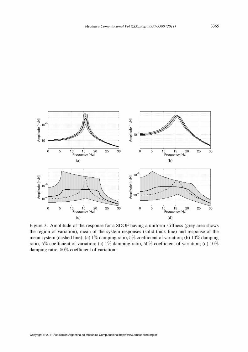
Indeed, to roughly understand what happens, let us consider an one DOF system with randomstiffness, say homogeneously distributed. For each realisation the stiffness changes and so doesthe peak of the FRF. Near the peak of the mean system the distribution of values of the FRF ofthe different realisations is rather complex and the FRF of the mean system and the mean FRFare quite different, as one sees in Figure 3. Near the peak of the mean system the mean value

E. PAGNACCO, R. SAMPAIO, J. SOUZA DE CURSI3358


is not representative of the behaviour, as is shown in this work, and tentatives to approach it byusing polynomials chaos approximations (PCA) are doomed to failure.

Given the PDF of the stiffness we compute analytically the PDF of the amplitude and phaseof the FRF - for the one DOF system and we give the envelopes of the FRF of the realisations.These envelopes will give the domain of definition of the PDF of the amplitude and phaseof the FRF for a fixed frequency. When it becomes impossible to obtain an analytical result,we may get an approximation instead, but the analytical results facilitate the construction of abenchmark, that will be useful to test the approximations obtained, for example, by PCA of thePDF.

We will now shortly describe the content of each section. Section 2 describes how the am-plitude and the phase of the FRF of the SDOF system relate with the stiffness for a fixed,deterministic frequency, that can be any non-negative real number. It also gives a general re-sult to show how the PDF of the stiffness relates to the PDF of the amplitude and the phase.A special case is computed analytically. Section 3 discusses the case where the stiffness hasuniform distribution. The envelopes of the FRF are defined and the mean and variance of theFRF for a fixed frequency are computed. The statistical modes of the amplitude and phase arecomputed analytically. Section 4 discuss the case where the stiffness has a Gamma distributionand presents the same results as in the last section. Section 5 discusses MDOFs and continu-ous systems and the results are computed with Monte Carlo simulations, in order to show thatmultimodality appears again for these cases. Section 6 presents some conclusions.

2 UNCERTAINTY IN THE SINGLE DEGREE OF FREEDOM SYSTEM

We consider the following Single Degree Of Freedom (SDOF) linear oscillator subject to anexternal harmonic forcing q in the frequency domain (Lin, 1967):

⇣k � !2

+ jc!⌘u (!) = q (!) (1)

! being the circular frequency. In this equation, the mass is normalised to unity and k and c arethe stiffness and damping system parameters. Since the response u (!) is a complex quantity,we need two real functions to characterise it. We choose the amplitude |u| and phase ✓ since itis the most used representation1. Thus, the system response amplitude and phase are given by:

|u| (!) =

q (!)

q(k � !2

)

2

+ 4⌘2k!2

and tan (✓ (!)) = �2⌘p

k!

k � !2

(2)

where we assume a damping ratio ⌘ =

c2

pk

such that 0 ⌘ < 1. But with respect to thedefinition of the FRF, a unit external forcing should be chosen for the sequel (i.e. q (!) = 1).This system is sketched on Figure 1. FRFs examples obtained for five stiffness values varying(±20

p3 %) around a 10, 000 N/m central stiffness and a 3 % damping ratio are presented on

Figure 2.This system becomes stochastic if the stiffness parameter or the external forcing (or both)

are random quantities.1However, it is not more difficult to study the real and imaginary parts. In such case it can be demonstrate

that statistical multimodality occur also frequently with generally four statistical modes for the real part and twostatistical modes for the imaginary part.

Mecánica Computacional Vol XXX, págs. 3357-3380 (2011) 3359


Figure 1: SDOF system

0 5 10 15 20 25 30

10−4

10−3

Frequency [Hz]

Ampl

itude

[m/N

]

(a)

0 5 10 15 20 25 30−π

−3π/4

−π/2

−π/4

0

Frequency [Hz]Ph

ase

[rd]

(b)

Figure 2: FRFs of a SDOF system; Five stiffness values are considered; (a) response amplitude;(b) response phase;

2.1 Amplitude of the response: a general result

Let us consider the situation when only the SDOF stiffness constant k is random. Randomvariables will be denoted capitalising the letter that represents the deterministic variable, henceK in this case. First, in this section, we will give a general result that is valid for a generalprobability distribution function (PDF), and then, in the following sections, we will establishmore detailed results for two particular PDF of the stiffness: the ones given by the MaximalEntropy Principle (Udwadia, 1989; Kapur and Kesavan, 1992) are: 1) the uniform distributionwhen the domain is fixed to be a bounded interval; and 2) the Gamma distribution if the domainis supposed to be the positive real.

Let pK the PDF of K having k as the mean and �k as the standard deviation. Without lossof generality, the domain of K is considered to be an interval having the boundaries k

inf

andk

sup

that may or may not belong to the interval. Then we will denote (kinf

, ksup

) the domain ofdefinition for pK . For this domain, the parenthesis imply that it is not known if the boundariesbelong or not to the interval of definition. For the left parenthesis, if the boundary belongs, theparenthesis is changed to a ], if not to [. For the right parenthesis it is similar. For example, foran uniform PDF k 2 [k

inf

, ksup

] with kinf

= k �p

3�k and ksup

= k +

p3�k, and the interval

is closed, that is, the boundaries belong to the interval. On the other hand, for a Gamma PDF,k 2 ]k

inf

, ksup

[ with kinf

= 0, ksup

= +1 , and the interval is open, the boundaries do notbelong to the interval.

Let us compute the PDF of the response of the system for a fixed ! 6= 0 (the special extremal-static- case ! = 0 is not considered in this work). Its random system response amplitude,denoted by U (!), without the bars to simplify the notation, and phase ⇥ (!), are given by:

U (!) = |U | (!) =

f (!)

q(K � !2

)

2

+ 4⌘2k!2

and tan (⇥ (!)) = � 2⌘p

k!

K � !2

(3)



where we assume a deterministic unit external forcing, f (!) = 1. In this expression, thedamping ratio does not need to have the same expression as for deterministic system and is nowchosen to be redefined as ⌘ =

c

2

pk. Since K is the single random variable of the problem, the

PDF pU is evaluated by the formula (Zwillinger and Kokoska, 2000):

pU (u) =

1��d|U |dK

��k1

pK (k1

) + · · · + 1��d|U |dK

��kn

pK (kn) (4)

where kj for j = 1, . . . , n denotes the roots of the algebraic equation u (k,!) = u , for ! fixed(notice that n = 1 for a bijective function). That is, one seeks all the stiffnesses, k, that give afixed amplitude u.

For ! fixed in the interval !2 < kinf

there is only one root, k1

=

1

u

q1� 4⌘2k!2u2

+!2. For

! fixed in the interval !2 > ksup

there is also only one root k1

= � 1

u

q1� 4⌘2k!2u2

+ !2. Ineither case one can write, from relation (4):

pU (u, !) =

1

u2

q1� 4⌘2k!2u2

⇥ pK (k1

(u, !)) (5)

If kinf

!2 ksup

, two roots could occur: k1,2 (u) = ⌥ 1

u

q1� 4⌘2k!2u2

+ !2, depending onsome conditions for u given by equation (6). We will have:

pU (u, !) =

8>>>>><

>>>>>:

pK(k1)

u2p

1�4⌘2k!2u2if k

1

(u) > kinf

and k2

(u) � ksup

pK(k1)+pK(k2)

u2p

1�4⌘2k!2u2if k

1

(u) > kinf

and k2

(u) < ksup

pK(k2)

u2p

1�4⌘2k!2u2if k

1

(u) kinf

and k2

(u) < ksup

. (6)

Thus, the PDF pU may have a discontinuity if the fixed frequency !2 2 (kinf

, ksup

) and ifthe stiffness distribution pK does not vanish at the boundaries of its domain. In fact, the sumof stiffness densities in the PDF pU comes from an aliasing of the distribution when taking thesquare of the apparent stiffness K � !2 since it is distributed -at least partially- around the zerovalue (k

inf

� !2 0 ksup

� !2).Moreover we will denote (u

inf

, usup

) the domain of definition for pU with the same conven-tion as above for the parenthesis. Hence, if the bounds belongs or not to the domain has to beevaluated separately for each given PDF. Moreover, since u

inf

(!) and usup

(!) are functions ofthe circular frequency !, they corresponds to the lower and upper envelopes of the amplituderesponses. The bounds of the domain of definition of the PDF are obtained from these envelopeswhen the frequency ! is fixed.

Statistical modes of the PDF pU are also of great interest. To assess if there is more than onemode in an open interval, one can search for roots of the first derivative of pU in its domain ofdefinition to see if there are interior points of minimum. If there is one, this indicate that thereare two maxima, either interior or in the boundaries. If the domain is closed, the extrema haveto be analysed independently. Thus, without the choice of a special form for the stiffness PDF,it is not possible to decide this question. We will see that in our case of interval, pU can bewritten as the product of two functions as

pU (u, !) = g (u, !)⇥ pK (u) (7)



and the analysis of the generic function g shows an answer. Indeed, since we have

@pU

@u=

@g

@upK + g

@pK

@u(8)

we could say that pU would be at its minimum close to the minimum of g if the term g @pK@u

could be neglected. Hence, finding @g@u (u, !) = 0 leads to a minimum for the function g at the

value u0

(!) =

�kp2k⌘!

. This leads also to a minimum of pU (u) if u0

belongs to the domain of

pU , i.e. if u0

(!) 2 [uinf

, usup

] and if g (u0

(!) , !)

@pK@u (u

0

(!)) can be neglected. Thus, we canconclude that the SDOF system PDF amplitude could have more than one statistical mode for avariety of stiffness distribution, depending on the domain of pU , or more precisely, on the fixedfrequency !, the damping ratio ⌘, the mean k and the coefficient of variation �k

k.

2.2 Phase of the response: a general result

Phase PDF p⇥

(✓) can be evaluated following the same strategy as given by formula (4). Wehave

dk

d✓(u, !) = �2

pk⌘!

sin (✓)2

(9)

which leads to

p⇥

(✓, !) =

2

pk⌘!

sin (✓)2

⇥ pK (✓) (10)

for2 ! 6= 0 and on the domain (✓inf

, ✓sup

) =

✓tan

�1

✓� 2⌘

pk!

kinf�!2

◆, tan

�1

✓� 2⌘

pk!

ksup�!2

◆◆with the

same convention as above for the parenthesis.To study the existence of more than one statistical mode, we follow the same reasoning as be-

fore. If we neglect the term @pK@✓ = 0, finding @p⇥

@✓ = 0 leads to seek for the root�2p⇥

cot (✓) = 0

which is ✓0

= �⇡2

. Thus, we can conclude that the SDOF system phase PDF could have morethan one statistical mode for a variety of stiffness distributions, depending on the frequencyexcitation !, and the stiffness distribution parameters.

3 SDOF SYSTEM WITH UNIFORM RANDOM STIFFNESS

Let us consider that K has an uniform distribution, say

pK (k) =

(1

2

p3�k

if k 2hk�

p3�

k

, k +

p3�

k

i

0 if not

(11)

For such a system, one can note that F , the natural frequency, is also a random variable. It isF =

1

2⇡

pK and has a distribution pF (f) = 8⇡2f ⇥pK (k(f))=

4⇡2fp3�k

, according to the relation

(4), which is defined over (finf

, fsup

) =

pk�

p3�k

2⇡ ,p

k+

p3�k

2⇡

�. Thus, the mean of this random

variableE [F ] =

4⇡2

3

p3�k

⇣f 3

sup

� f 3

inf

⌘(12)

2For ! = 0, the phase remains deterministic (✓ = 0) whatever the stiffness is random or not.



is not equal to the natural frequency of the mean system which is f0

=

1

2⇡

pk. At last, to

complete this statistic, note that

E

hF 2

i=

⇡2

p3�k

⇣f 4

sup

� f 4

inf

⌘(13)

while the statistical mode is located at fsup

.

3.1 Amplitude of the response

Relations (5), (6) and (11) give the PDF of the response amplitude.

3.1.1 Upper and lower envelopes for the amplitude

The upper envelope of the system response amplitude, denoted usup

(!), is the function

usup

(!) =

8>>>>>>><

>>>>>>>:

1q(

k�p

3�k�!2)

2+4⌘2k!2

for !2 2h0, k �

p3�k

i

1

2⌘!p

kfor !2 2

hk �

p3�k, k +

p3�k

i

1q(

k+

p3�k�!2

)

2+4⌘2k!2

for !2 2hk +

p3�k, +1

h(14)

Thus, the system response U (!) is unbounded if ⌘ ! 0 for all !2 2hk �

p3�k, k +

p3�k

i.

The lower envelope , denoted uinf

(!), is

uinf

(!) =

8>>><

>>>:

1q(

k+

p3�k�!2

)

2+4⌘2k!2

for !2 2h0, k

i

1q(

k�p

3�k�!2)

2+4⌘2k!2

for !2 2hk, +1

h (15)

Thus, bounds of the amplitude response PDF are given by the domain [uinf

(!) , usup

(!)] for afixed frequency !.

3.1.2 Statistic for fixed frequency of the PDF of the amplitude

We now compute analytically the first and second moments for the amplitude system re-sponse. These results are important for comparison with numerical simulations. They are givenby

E [U ] (!) =

usup(!)ˆ

uinf(!)

upU (u, !) du and E[U2

](!) =

usup(!)ˆ

uinf(!)

u2pU (u, !) du (16)

They could be evaluated analytically easily if we neglect the damping (this hypothesis isvalid for a small damping when !2 /2

hk �

p3�k, k +

p3�k

ior for medium damping at low

and high frequency):

E [U ] (!) ⇡usup(!)ˆ

uinf(!)

1p3�ku

du =

1p3�k

ln

u

sup

(!)

uinf

(!)

!



E

hU2

i(!) ⇡

usup(!)ˆ

uinf(!)

1p3�k

du =

1p3�k

(usup

(!)� uinf

(!))

But to obtain an exact estimation of these expectations over the full frequency range, it isnecessary to consider both the damping and the discontinuity which appears in the PDF (Eq.(6)) for !2 2

hk �

p3�k, k +

p3�k

i. Solving equations (6) for the variable u leads to lo-

cate the discontinuity for the PDF at the value u1

(!) =

1q(

k�p

3�k�!2)

2+4⌘2k!2

for the fre-

quency rangehk �

p3�k, k

iwhile it is located at u

1

(!) =

1q(

k+

p3�k�!2

)

2+4⌘2k!2

for the rangehk, k +

p3�k

i. Thus, we have

E [U ] (!) =

usup(!)ˆ

uinf(!)

1

2

p3�k

1

uq

1� 4⌘2k!2u2

du

=

1

2

p3�k

✓arccot

q4⌘2k!2u

sup

(!)� 1� arccot

q4⌘2k!2u

inf

(!)� 1

◆

for the range !2 2h0, k �

p3�k

i[hk +

p3�k, +1

h, while we have

E [U ] (!) =

u1(!)ˆ

uinf(!)

1

2

p3�k

1

uq

1� 4⌘2k!2u2

du +

usup(!)ˆ

u1(!)

1

2

p3�k

2

uq

1� 4⌘2k!2u2

du (17)

or

E [U ] (!) =

1p3�k

arccot

q4⌘2k!2u

sup

(!)� 1

1

2

p3�k

✓arccot

q4⌘2k!2u

1

(!)� 1 + arccot

q4⌘2k!2u

inf

(!)� 1

◆

for !2 2hk �

p3�k, k +

p3�k

i. Similarly, we have

E

hU2

i(!) =

1

4

p3⌘!

pk�k

✓arcsin

✓2⌘!

qku

sup

(!)

◆� arcsin

✓2⌘!

qku

inf

(!)

◆◆(18)

for the range !2 2h0, k �

p3�k

i[hk +

p3�k, +1

hand

E

hU2

i(!) =

1

2

p3⌘!

pk�k

arcsin

✓2⌘!

qku

sup

(!)

◆�

1

4

p3⌘!

pk�k

✓arcsin

✓2⌘!

qku

1

(!)

◆+ arcsin

✓2⌘!

qku

inf

(!)

◆◆

for !2 2hk �

p3�k, k +

p3�k

i. From these two results, it is possible to evaluate the standard

deviation of the response, �U , by �2

U = E [U2

]� E [U ]

2.The Figure 3 shows the system response amplitude, considering an uniform stiffness with

a 10, 000 N/m mean stiffness, for two stiffness coefficients of variation (�k

k) and two damping



0 5 10 15 20 25 30

10−4

10−3

Frequency [Hz]

Ampl

itude

[m/N

]

(a)

0 5 10 15 20 25 30

10−4

Frequency [Hz]

Ampl

itude

[m/N

]

(b)

0 5 10 15 20 25 30

10−4

10−3

Frequency [Hz]

Ampl

itude

[m/N

]

(c)

0 5 10 15 20 25 30

10−4

10−3

Frequency [Hz]

Ampl

itude

[m/N

]

(d)

Figure 3: Amplitude of the response for a SDOF having a uniform stiffness (grey area showsthe region of variation), mean of the system responses (solid thick line) and response of themean system (dashed line); (a) 1% damping ratio, 5% coefficient of variation; (b) 10% dampingratio, 5% coefficient of variation; (c) 1% damping ratio, 50% coefficient of variation; (d) 10%

damping ratio, 50% coefficient of variation;



Figure 4: PDF of the amplitude response at various frequencies for a SDOF system having anuniform stiffness (with a 3 % damping ratio and a 20 % coefficient of variation)

ratios. The region of variation is represented by the grey area. The mean of the system responsesand the response of the mean system are also represented.

Then, considering the case of a 20 % stiffness coefficient of variation and a 3 % dampingratio, the Figure 4 shows the PDF of the amplitude at several frequencies. It is seen on thisfigure that various PDF shapes are obtained.

3.1.3 Statistical modes of the amplitude response

At low (! ! 0) or at high (! ! 1) frequencies, the PDF pU (•, !) is monotonically de-creasing, thus the lower envelope u

inf

(!) is a statistical mode. But for intermediate frequency,the shape of this PDF could be more complex. It can have a minimum when its first derivativevanishes, at u

0

(!) =

1p6k⌘!

, if this value is in the domain definition of pU (•, !), i.e. if u0

(!) 2

[uinf

, usup

]. For example, if we consider the simplest situation when ! =

pk (which is the nat-

ural circular frequency of the mean system having a unit mass), if u0

⇣pk⌘ 1q

(

2⌘k)

2+3�2

k

, or

equivalently, if�k

ks

2

3

⌘ (19)

the amplitude system response U will have only one statistical mode, since u0

⇣pk⌘

/2hu

inf

⇣pk⌘, u

sup

⇣pk⌘i

. On the other hand, i.e. when u0

⇣pk⌘

> 1q(

2⌘k)

2+3�2

k

or �k

k>q

2

3

⌘



1 2 3 4 5 6x 10-3

500

1000

1500

2000

0.5 %

3 %

(a)

0 1 2 3 4 5x 10-3

500

1000

1500

2000

2500

3000

0.6 %

10 %

(b)

Figure 5: PDF of the amplitude response for a SDOF system having an uniform stiffness withvarious densities and damping ratio at frequency !2

= k; (a) amplitude PDF for �k

k= 5 %

and ⌘ = {0.5 %, 1 %, 1.5 %, 2 %, 2.5 %, 3 %}; (b) amplitude PDF for ⌘ = 1 % and �k

k=

{0.6 %, 1 %, 2.5 %, 10 %}

there are two statistical modes since u0

⇣pk⌘2hu

inf

⇣pk⌘, u

sup

⇣pk⌘i

. Multiple statisticalmode existence condition depends thus on the fixed frequency !, the damping ratio ⌘, the meank, and the coefficient of variation �k

k. Figure 5 shows examples of amplitude PDF for various

damping ratio and various stiffness coefficient of variation when the frequency is fixed at thenatural frequency of the mean system. All these examples have two statistical modes, except inthe case of a very low stiffness coefficient of variation, i.e. the 0.6 % curve on the right.

Considering now the frequency rangei0, k �

p3�k

h, the existence condition for multi-

modality, which occurs again when u0

(!) 2 [uinf

(!) , usup

(!)], is evaluated to be⇣k �

p3�k

⌘� !2

p2k!

< ⌘ <

⇣k +

p3�k

⌘� !2

p2k!

(20)

while, for the frequency !2 � k +

p3�k, we would have

!2 �⇣k +

p3�k

⌘

p2k!

< ⌘ <!2 �

⇣k �

p3�k

⌘

p2k!

(21)

These conditions are less restrictive for the frequency rangehk �

p3�k, k +

p3�k

i, since only

the lower bound has to be considered (indeed, u0

(!) is always less than usup

for this fre-quency range). Thus, the existence condition for u

0

(!) 2 [uinf

, usup

] in the frequency rangehk �

p3�k, k

iis given by

⌘ <

⇣k +

p3�k

⌘� !2

p2k!

(22)

while it is given by

⌘ <!2 �

⇣k �

p3�k

⌘

p2k!

(23)

for the frequency rangehk, k +

p3�k

i.



Having the existence condition of multiple statistical modes, one can see that they couldappear frequently in the vicinity of the resonant frequency of the mean system (! =

pk ) since

the damping ratio is generally small for real systems.From another point of view, an interesting question is “What range of frequency leads to

multimodality ?”. It is sufficient for this to solve conditions (20) and (21) for !2 to obtain:

k (1 + ⌘2

)�p

3�k�k⌘q

2� 2

p3

�k

k+ ⌘2 < !2 < k (1 + ⌘2

)+

p3�k+k⌘

q2 + 2

p3

�k

k+ ⌘2

To conclude about the number of statistical modes for the frequency rangehk �

p3�k, k

h[

ik, k +

p3�k

i, we have to consider also the discontinuity of the PDF. Then, it will exist only

one statistical mode if the previous conditions (22) or (23) are not fulfilled, whereas there aretwo or three statistical modes if they are fulfilled. Figure 4 shows examples of response am-plitude PDF at four frequencies taken in the range

hk �

p3�k, k

h[ik, k +

p3�k

i. They are

the third, fourth, sixth and seventh ones PDF (the fifth one being the PDF at !2

= k, the reso-nant frequency of the mean system). All of them exhibit a discontinuity. The fourth and sixthones have three statistical modes while the others have only two statistical modes. In fact, threestatistical modes arise when the discontinuity is located before the PDF minimum, i.e. whenu

1

(!) < u0

(!) or

1

r⇣k �

p3�k � !2

⌘2

+ 4⌘2k!2

<1p

6k⌘!(24)

for the frequency rangehk �

p3�k, k

hor

1

r⇣k +

p3�k � !2

⌘2

+ 4⌘2k!2

<1p

6k⌘!(25)

for the frequency rangeik, k +

p3�k

i.

Thus, statistical modes can be located on the envelopes uinf

(!) , usup

(!) and the discon-tinuity u

1

(!) (depending on the system properties, the random parameters, and the excitationfrequency !). Another comment concerns the upper envelope which could tend to infinite forthe (ideal) system having no damping. Thus, the rightmost mode of the PDF diminishes itsvalue when the damping decreases and the domain of definition increases. From this behaviour,we conclude that this mode will be difficult to detect if it has to be found by Monte Carlosimulations.

Finally, this multimodal behaviour of the response implies that the mean and the standarddeviation of the system response given in the previous section are insufficient to characterisethe response distribution, at least in the vicinity of the resonant frequency of the mean system.

3.2 Phase of the response

From the relations (10) and (11) we have

p⇥

(✓, !) =

pk⌘!p

3�k sin (✓)2

(26)

which is defined on the domaintan

�1

✓� 2⌘

pk!

k�p

3�k�!2

◆, tan

�1

✓� 2⌘

pk!

k+

p3�k�!2

◆�.



0 5 10 15 20 25 30−π

−3π/4

−π/2

−π/4

0

Frequency [Hz]

Phas

e [rd

]

(a)

0 5 10 15 20 25 30−π

−3π/4

−π/2

−π/4

0

Frequency [Hz]

Phas

e [rd

]

(b)

0 5 10 15 20 25 30−π

−3π/4

−π/2

−π/4

0

Frequency [Hz]

Phas

e [rd

]

(c)

0 5 10 15 20 25 30−π

−3π/4

−π/2

−π/4

0

Frequency [Hz]

Phas

e [rd

]

(d)

Figure 6: Phase of the response of a SDOF system having a uniform random stiffness; Meanphase of the system response (thick solid line) and phase response of the mean system (dashedline); grey area shows the region of variation; (a) 1% damping ratio, 5% coefficient of variation;(b) 10% damping ratio, 5% coefficient of variation; (c) 1% damping ratio, 50% coefficient ofvariation; (d) 10% damping ratio, 50% coefficient of variation;

The Figure 6 illustrate this phase response, considering an uniform stiffness with a 10, 000

N/m mean stiffness, two stiffness coefficients of variation (�k

k) and two damping ratios. The

region of variation is represented by the grey area. The mean of the system responses and theresponse of the mean system are also represented.

Then, considering the case of a 20 % stiffness coefficient of variation and a 3 % dampingratio, the Figure 7 shows the PDF response phase at several frequencies: the first one located ata very low frequency range, the second one a little before !2

= k , the third one at !2

= k, andthe last one a little after !2

= k. It is seen on this figure that various PDF shapes are obtained.For low frequencies (! ! 0) , the PDF p

⇥

(•, !) is monotonically increasing, thus the upperenvelope ✓

sup

(!) is a statistical mode, while at high frequencies p⇥

is monotonically decreasingleading to a statistical mode at the lower envelope.

For intermediate frequency, this PDF could have a minimum when its first derivative van-ishes, at ✓

0

(!) = �⇡2

, if this value is on the domain definition of p⇥

, i.e. if ✓inf

(!) < ✓0

(!) <✓sup

(!) or, by taking the cosines of this inequality, if

k �p

3�k < !2 < k +

p3�k (27)

Thus, there is one statistical mode at ✓sup

(!) if !2 k �p

3�k, one statistical mode at✓inf

(!) if !2 � k +

p3�k, and two statistical modes at ✓

sup

(!) and ✓inf

(!) otherwise.



Figure 7: PDF of the phase response at various frequencies for a SDOF system having anuniform stiffness (with a 3 % damping ratio and a 20 % coefficient of variation)

4 SDOF SYSTEM WITH GAMMA RANDOM STIFFNESS

Let us assume now a Gamma distribution for the stiffness, having the PDF

pK (k; a, b) =

8<

:

⇣kb

⌘a�1

exp

(

� kb )

b�(a)

if k > 0

0 if not

(28)

where a =

⇣k�k

⌘2

and b =

�2k

kare positive values.

For such a system, one can note that the natural frequency F has the bell shape distributiongiven by

pF (') =

2

'�(a)

4⇡2'2

b

!a

exp

�4⇡2'2

b

!

(29)

which is defined over ]0, +1[. We have

E [F ] =

pb�⇣a +

1

2

⌘

2⇡� (a)

and E

hF 2

i=

k

4⇡2

(30)

and a mode located at the value

qb(

a� 12)

2⇡ .

4.1 Amplitude of the response

From the domain definition of this random stiffness, we deduce that the system responsePDF given by the relation (5) and (6) can be simplified to

pU (u, !) =

pK (k1

; a, b) + pK (k2

; a, b)

u2

r1�

⇣2

pk⌘u!

⌘2

(31)

since pK (k1

; a, b) will vanish when the root k1

becomes negative.



To find the PDF support, we consider the relation (3). The idea is the following: since

K 2 ]0, +1[, K � !2 2i�k, +1

h, (K � !2

)

2 2 ]0, +1[,r

(K � !2

)

2

+

⇣2

pk⌘!

⌘2

2i2⌘p

k!, +1h, and U (!) 2

�0, 1

2⌘p

k!

. Then, we have

uinf

= 0 (32)

andu

sup

(!) =

1

2⌘p

k!(33)

The Figure 8 shows the system response amplitude, considering a Gamma stiffness with a10, 000 N/m mean stiffness, for two stiffness coefficients of variation and two damping ratios.The upper envelope is represented by a thin solid line and the response of the mean system isgiven by the dashed line. But to give more insights on this system, it is possible to represent themean of the system response and confidence intervals by using numerical tools to evaluate them.Then, confidence intervals are represented by two grey areas: the dark grey area corresponds tothe 95 % confidence interval, while the light grey corresponds to the 99 % confidence intervaland the mean of the system response is represented by a thick solid line.

However, it is possible to give some analytical results by considering a Normal approxima-tion of the Gamma distribution. It is the subject of the appendix, where expectations (equations(39) and (40)) and statistical modes are determined for the frequency !2

= k with the conditionon the system parameters to give multimodality.

Considering now the case of a 20 % stiffness coefficient of variation and a 3 % damping ratio,the Figure 9 shows the PDF of the amplitude at several frequencies. It is seen on this figure thatvarious PDF shapes are obtained: a bell shape at low frequencies and various bimodal shapesotherwise. From these graphs, it is clear that the mean value is not a representative value ofthe system responses when the frequency is not low. Thus, knowing the mean and standarddeviation of the system response is insufficient to characterise its response distribution.

The Figure 10 shows more examples of PDF when stiffness coefficient of variation anddamping ratios are varied. On this figure, two statistical modes are exhibiting only when therandom parameters satisfies the condition (38). Moreover, the Figure 11 shows a situationwhere the PDF exhibits three statistical modes for a 60% stiffness coefficient of variation witha 5% damping ratio. This behaviour is even found more pronounced for a higher coefficientof variation, but it is not expected by the normal approximation of the Gamma law since thisapproximation does not hold for such high values of the coefficient of variation.

4.2 Phase of the response

The phase PDF p⇥

(✓, !) for a Gamma distribution is obtained from the relations (10) and

(28) with k (✓) = !2 � 2

pk⌘!

tan(✓) . It is defined on the domain�tan

�1

✓�2⌘p

k�!

◆, 0.

The Figure 12 shows the system response phase for two damping ratios when consideringGamma random stiffnesses of 10, 000 N/m mean for two coefficients of variation. As for theamplitude, the region of variation are represented by grey areas, and the mean of the systemresponses and the response of the mean system are also represented.

The behaviour of the phase PDF when the stiffness follows a Gamma distribution is shownon Figure 13. Comparing these PDFs with the uniform ones given on Figure 6, we can see thatthey vanish smoothly at theirs bounds.



0 5 10 15 20 25 30

10−2

10−3

10−4

Frequency [Hz]

Ampl

itude

[m/N

]

(a)

0 5 10 15 20 25 30

10−4

10−3

Frequency [Hz]

Ampl

itude

[m/N

]

(b)

0 5 10 15 20 25 30

10−4

10−3

10−2

Frequency [Hz]

Ampl

itude

[m/N

]

(c)

0 5 10 15 20 25 30

10−4

10−3

Frequency [Hz]

Ampl

itude

[m/N

]

(d)

Figure 8: Amplitude response for a Gamma stiffness with the upper envelope (thin solid line),the mean of the system responses (thick solid line) and the response of the mean system (dashedline); dark grey and light grey areas show the 95 % and 99 % confidence region (respectively);(a) 1% damping ratio, 5% coefficient of variation; (b) 10% damping ratio, 5% coefficient ofvariation; (c) 1% damping ratio, 50% coefficient of variation; (d) 10% damping ratio, 50%

coefficient of variation;

Figure 9: PDF of the amplitude response at various frequencies for a SDOF system having aGamma stiffness (with a 3 % damping ratio and a 20 % coefficient of variation)



0 1 2 3 4 5x 10−3

0

200

400

600

800

1000

1200

2 %

1 %

3 %

(a)

0 1 2 3 4 5x 10−3

0

200

400

600

800

1000

1200

5 %

10 %

1 %

(b)

Figure 10: Amplitude response PDF for a Gamma stiffness at !2

= k; (a) �k

k= 5 % and

⌘ = {1 %, 2 %, 3 %} (b) �k

k= {1 %, 2.5 %, 5 %, 10 %} and ⌘ = 1 %

0 0.2 0.4 0.6 0.8 1x 10−3

0

500

1000

1500

2000

2500

3000

3500

4000

4500

(a)

0 1 2x 10−4

1350

1360

1370

1380

1390

1400

1410

1420

1430

1440

1450

(b)

Figure 11: Amplitude response PDF for a Gamma stiffness having a �k

k= 60 % coefficient of

variation; (a) complete domain; (b) zoom of the first mode



0 5 10 15 20 25 30−π

−3π/4

−π/2

−π/4

0

Frequency [Hz]

Phas

e [rd

]

(a)

0 5 10 15 20 25 30−π

−3π/4

−π/2

−π/4

0

Frequency [Hz]

Phas

e [rd

]

(b)

0 5 10 15 20 25 30−π

−3π/4

−π/2

−π/4

0

Frequency [Hz]

Phas

e [rd

]

(c)

0 5 10 15 20 25 30−π

−3π/4

−π/2

−π/4

0

Frequency [Hz]

Phas

e [rd

]

(d)

Figure 12: Phase response for a Gamma stiffness with the lower envelope (thin solid line), themean of the system responses (thick solid line) and the response of the mean system (dashedline); dark grey and light grey areas show the 95 % and 99 % confidence region (respectively);(a) 1% damping ratio, 5% coefficient of variation; (b) 10% damping ratio, 5% coefficient ofvariation; (c) 1% damping ratio, 50% coefficient of variation; (d) 10% damping ratio, 50%

coefficient of variation;

Figure 13: PDF of the phase response at various frequencies for a SDOF system having aGamma stiffness (with a 3 % damping ratio and a 20 % coefficient of variation)



Figure 14: Two degrees of freedom system

Table 1: Natural frequencies and damping ratio of the mean aluminium plate

Normal mode # 1 2 3 4Natural frequency [Hz] 4.40 10.7 11.3 17.6

Damping ratio [%] 1.81 0.74 0.70 0.45

5 MULTIPLE DOFS SYSTEMS AND CONTINUOUS STRUCTURES

Continuous linear systems or systems with MDOFs having uncertainties could exhibit sim-ilar behaviour, that is showing multiple statistical modes around resonant frequencies for theamplitude PDF. To illustrate these assertion, numerical experiments conducted by Monte-Carlosimulation (Rubinstein and Kroese (Rubinstein and Kroese, 2008)) are presented on two exam-ples: a two DOFs system and a plate.

5.1 Two DOFs system

A two DOFs system sketched in Figure 14 having 1.5 and 0.5 kg masses and a Gammadistribution with a 1, 000 and 150 N/m mean stiffness and a 5 % coefficient of variation isconsidered. Its damping ratios are 0.3 and 0.6 %. Consequently, the mean system has tworesonant frequencies located at 2.05 Hz and 4.50 Hz.

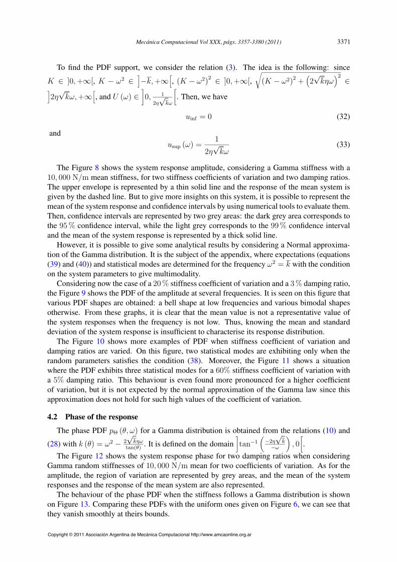
Its amplitude responses are presented on Figure 15 for each degree of freedom when a unitforce is applied on the first DOF. On this figure, the grey area depicts the 95 % confidenceinterval obtained by Monte Carlo simulations involving a 10

6 sample size.The Figure 15 shows also the histograms obtained for the two DOFs at various frequencies.

They exhibit again two statistical modes around the resonant frequencies. However, multi-modality is more pronounced for the second DOF (the unexcited one).

Moreover, the histogram close to the second resonant frequency for the driving point has ashape similar to the one obtained in this study for the SDOF system near its resonant frequency.On the contrary, the shape of the others histograms closed to the resonant frequencies lookslike the one obtained for the SDOF system of Pagnacco et al. (2009) when the stiffness and thedamping are random: they vanish smoothly at their maximal bound.

5.2 Continuous plate

We consider a continuous plate. This enable to investigate situations where normal modesare coupled by choosing a quasi-square geometry. In our example, we have chosen a 1 ⇥ 1.05

m

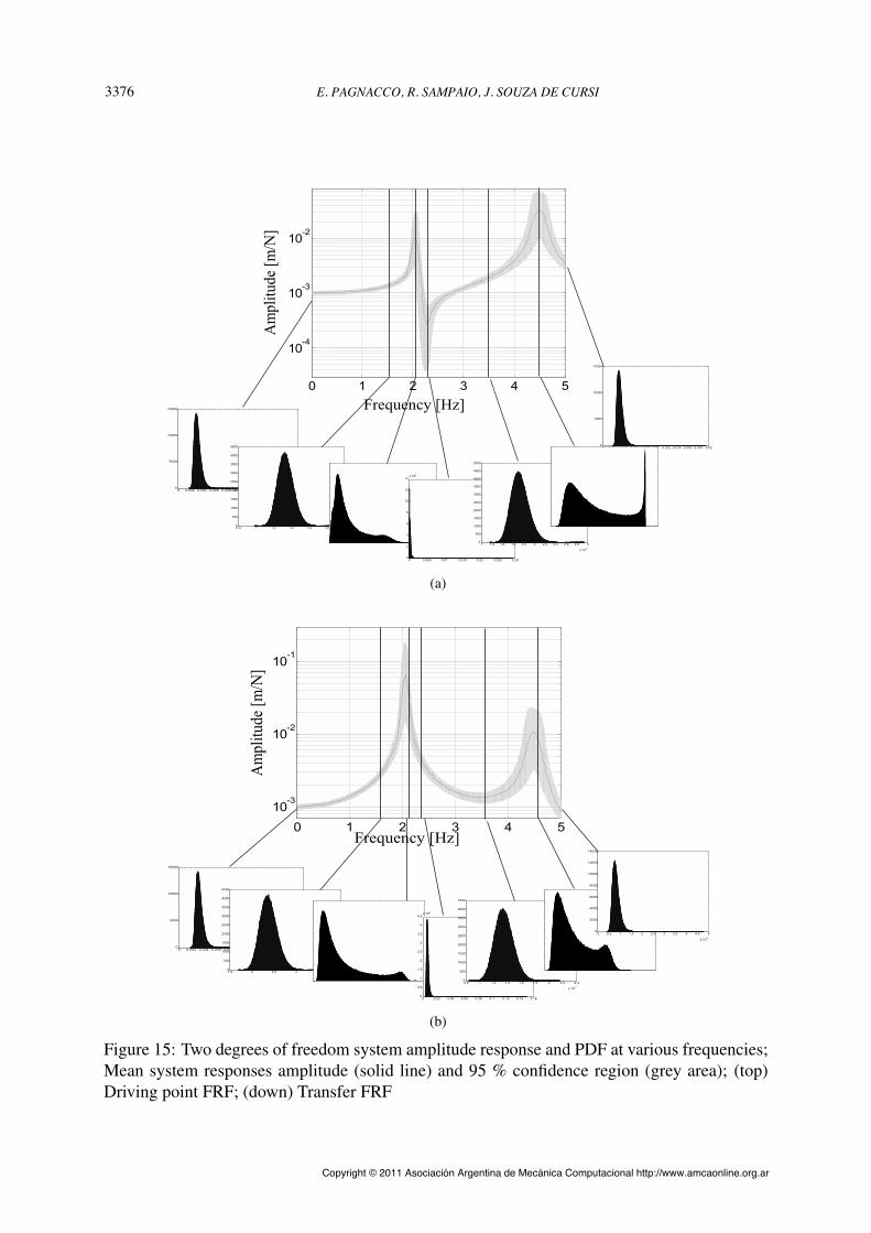
2 plate in order to couple the second and the third normal modes of the plate having the meanstiffness. It is made of aluminium alloy with a 1 mm thickness. Boundary conditions are simplesupports, leading to a simple analytical expression for the frequency response. The Table 1 givesnatural frequencies obtained for the mean stiffness and the damping ratio chosen. The Figure16 shows the location of the measurements points retained for the following illustrations. Thepoint 1 is chosen as the driving point.



(a)

(b)

Figure 15: Two degrees of freedom system amplitude response and PDF at various frequencies;Mean system responses amplitude (solid line) and 95 % confidence region (grey area); (top)Driving point FRF; (down) Transfer FRF



1

2 3

Figure 16: Location of measurements points for the plate

In this example, the Young modulus is considered uncertain and follows a Gamma distribu-tion with a 5% coefficient of variation. Figure 17 shows the amplitude response of the meanplate (solid line) with the 95 % confidence region (grey area) and the mean of amplitude re-sponses (dashed line) for the three measurements points (see the drawing located at the left upcorner of each FRF). Stochastic results for this plate are obtained through Monte Carlo numer-ical simulations.

Figure 17-up shows histograms of the plate driving point displacement response (i.e. at point1) at various frequencies. Many of them are chosen close to the normal modes frequencies ofthe mean plate. Analysis of these graphs indicates again a bi-modal statistical behaviour in caseof uncoupled normal modes, while multi-modal behaviour appeared in the coupled case. Theuncoupled behaviour exhibited here is thus very similar to the one found for the SDOF systemstudied in this work. But for the coupled case, many statistical modes appeared with raggedhistogram shapes around the frequencies of interest.

Figure 17-down shows the two cross-displacement responses between the point 1 and thetwo other chosen points. This indicates that a multi-modal statistical behaviour is also obtained,but with dissimilar histogram shapes.

6 CONCLUSIONS

The PDF of the amplitude and the phase of the response of a random linear single-degree-of-freedom mass-spring-damper system when the stiffness are random was discussed for a generalPDF of the stiffness. Then, to get more precise results, these PDF was discussed for the uniformand the Gamma distributions, that are the PDF that maximise the uncertainty (entropy) if thestiffness is bounded or unbounded, respectively.

These PDF were studied for a fixed, deterministic, frequency. They were completely charac-terised with their envelopes, and, when possible, statistics were derived analytically. Moreover,the conditions to have multimodes were described. From these conditions, it is concluded thatmultimodality occurs very frequently in the vicinity of the resonant frequency of the mean sys-tem since the damping ratio is generally small for real systems. Hence, in the vicinity of thesefrequencies, it is deduced that the mean and the standard deviation of the system response arenot representative of the random system response distribution. However, analytical statisticsremains useful to provided benchmark tests for numerical computations.

But concerning the rightmost mode of the PDF, the analytical result indicate that it dimin-ishes its value when the damping decreases, while the domain of definition increases. Knowingthis behaviour, we have concluded that this mode, found analytically, would be difficult to detectfor some random system parameters if it has to be found by Monte Carlo simulations.

Some complex systems, discrete and continuous, were also discussed and they show similarbehaviour. This multimodal behaviour of the PDF of the response of random linear systems, tothe best of our knowledge, has not been previously discussed in the literature.



(a)

(b)

Figure 17: Plate amplitude responses and PDF at various frequencies; FRFs of the mean plate(solid line), mean FRFs (dashed line) and the 95 % confidence region (grey area) ; measurementlocations are indicated on the grey rectangular area representing the plate (left up corner of theFRFs graphs)



Acknowledgements

The authors would like to thank the financial support of INSA-Rouen and of the Brazilianagencies CNPq, Capes, and FAPERJ.

APPENDIX A. APPROXIMATION OF THE AMPLITUDE PDF BY A NORMAL DIS-TRIBUTION

Analysis of the amplitude PDF for statistical modes analytically is rather difficult when thestiffness follows a Gamma distribution. An approximate way consists in considering a normalapproximation of the gamma distribution for the stiffness K ⇠ N

⇣k,�2

k

⌘, which is valid if �k

ktends towards zero:

pK

⇣k; k,�k

⌘=

1

�k

p2⇡

exp

0

B@�

⇣k � k

⌘2

2�2

k

1

CA (34)

In this case kinf

= �1 and ksup

= 1, but we have to notice that the probability of k becamenegative tends towards zero if �k

ktends towards zero. Then k

inf

< !2 < ksup

and there arealways two roots for the algebraic equation u (k,!) = u when ! is fixed and is strictly positive.In this case, the relation (6) leads to the system response PDF

pU (u, !) =

pK (k1

) + pK (k2

)

u2

q1� 4⌘2k!2u2

(35)

which is defined over�0, 1

2⌘p

k!

. Thus, for a fixed frequency ! =

pk, this last equation

simplifies to

pU (u, !) =

1

u2

q1� 4⌘2k

2

u2

⇥ 2

�k

p2⇡

exp

0

BBB@�

✓1

u

q1� 4⌘2k!2u2

◆2

2�2

k

1

CCCA (36)

Analysis of this result gives a first statistical mode at 1

2⌘k. Moreover, having define ⌘0 =

2⌘k�k

,roots of this PDF first derivative are

u1,2 =

1

�k

vuut1

6

+

1

3⌘02±p

4� 8⌘02 + ⌘04

6⌘02(37)

which lead to a maximum and a minimum for the first and the second value (respectively),when 4�8⌘02 +⌘04 � 0. This is an existence condition for another statistical mode. Thus, when

�k

k>

2

1 +

p3

⌘ (38)

there is two statistical modes for the response PDF, the first one being located at1

�k

r1

6

+

1

3⌘02 +

p4�8⌘02

+⌘04

6⌘02 and the second at 1

2⌘k, while only one mode exist at 1

2⌘k. Note

that in the no damping case, the first mode is at 1p2�k

, while the second tends to infinite.Having the response amplitude PDF given by equation (36), it is possible to evaluate some

expectations such as



E [U ]

✓qk◆

=

1

�k

p2⇡

exp

0

@⌘2k2

�2

k

1

AK0

0

@⌘2k2

�2

k

1

A (39)

and

E

hU2

i ✓qk◆

=

1

2⌘k�k

r⇡

2

exp

0

@2⌘2k2

�2

k

1

Aerfc

p2⌘k

�k

!

(40)

where K0

is the modified Bessel function of the second kind of order 0.

REFERENCES

Heinkelé C., Pernot S., Sgard F., and Lamarque C.H. Vibration of an oscillator with randomdamping: analytical expression for the probability density function. Journal of Sound and

Vibration, 296(1-2):383–400, 2006. ISSN 0022-460X.Kapur J. and Kesavan H.K. Entropy optimization principles with applications. Academic Press,

Inc., London, 1992.Lin Y.K. Probabilistic theory of structural dynamics. McGraw-Hill, Inc., New York, 1967.Pagnacco E., Sampaio R., and Souza de Cursi E. Multimodality of the Frequency Response

Functions of random linear mechanical systems. In XXX CILAMCE (Iberian-Latin-American

Congress on Computational Methods in Engineering). Rio de Janeiro, Brasil, 2009.Rubinstein R.Y. and Kroese D.P. Simulation and the Monte Carlo method. John Wiley & Sons,

Inc., New Jersey, USA, 2008.Udwadia F.E. Response of uncertain dynamic systems. i. Applied Mathematics and Computa-

tion, 22(2-3):115–150, 1987a.Udwadia F.E. Response of uncertain dynamic systems. ii. Applied Mathematics and Computa-

tion, 22(2-3):151–187, 1987b.Udwadia F.E. Some results on maximum entropy distributions for parameters known to lie in

finite intervals. SIAM Review, 31(1):103–109, 1989.Zwillinger D. and Kokoska S. Standard probability and statistics tables and formulae. Chapman

& Hall/CRC, New York, USA, 2000.



FREQUENCY RESPONSE FUNCTIONS OF RANDOM LINEAR MECHANICAL SYSTEMS AND PROPAGATION OF UNCERTAINTIES

Documents

Transcript of FREQUENCY RESPONSE FUNCTIONS OF RANDOM LINEAR MECHANICAL SYSTEMS AND PROPAGATION OF UNCERTAINTIES