arX

iv:n

lin/0

2110

12v1

[nl

in.C

D]

8 N

ov 2

002

Fractality of deterministic diffusion in the

nonhyperbolic climbing sine map

N. Korabel and R. Klages

Max-Planck-Institut fur Physik komplexer Systeme, Nothnitzer Straße 38, D-01187

Dresden, Germany

Abstract

The nonlinear climbing sine map is a nonhyperbolic dynamical system exhibitingboth normal and anomalous diffusion under variation of a control parameter. Weshow that on a suitable coarse scale this map generates an oscillating parameter-dependent diffusion coefficient, similarly to hyperbolic maps, whose asymptoticfunctional form can be understood in terms of simple random walk approximations.On finer scales we find fractal hierarchies of normal and anomalous diffusive regionsas functions of the control parameter. By using a Green-Kubo formula for diffusionthe origin of these different regions is systematically traced back to strong dynami-cal correlations. Starting from the equations of motion of the map these correlationsare formulated in terms of fractal generalized Takagi functions obeying generalizedde Rham-type functional recursion relations. We finally analyze the measure of thenormal and anomalous diffusive regions in the parameter space showing that inboth cases it is positive, and that for normal diffusion it increases by increasing theparameter value.

Key words: Deterministic diffusion, nonhyperbolic maps, fractal diffusioncoefficient, anomalous diffusion, periodic windowsPACS: 05.45.Df, 05.10.-a, 05.45.Ac, 05.60.-k

1 Introduction

Low-dimensional time-discrete maps are among the most important models forexploring different aspects of chaos. These systems display a very rich dynam-ical behavior but are still very amenable to straightforward computer simula-tions. Even more, in some cases rigorous analytical solutions are possible. Afterit was realized that diffusion processes can be generated by microscopic deter-ministic chaos in the equations of motion, time-discrete maps became useful

Preprint submitted to Elsevier Science 25 November 2013

tools in deterministic transport theory. The analysis of these simple models re-quired to suitably combine nonequilibrium statistical mechanics with dynam-ical systems theory leading to a more profound understanding of transport innonequilibrium situations [1,2,3,4]. However, time-discrete maps provide notonly a suitable starting point for studying normal diffusion but also for investi-gating the anomalous case [5,6,7,8,9,10,11,12,13,14,15,16,17,18,19,20,21,22,23,24,25,26].Moreover, there are certain classes of more realistic models which share spe-cific properties of maps such as being low-dimensional and exhibiting certainperiodicities. Indeed, theoretical investigations of chaotic billiards subject toexternal fields [27], of periodic Lorentz gases [28,29], and of pendulum-likedifferential equations [30,31,32,33,34,35,36] showed that many properties ofdeterministic transport in maps carry over to these more complex chaoticdynamical systems.

In this framework, recently a new feature of deterministic diffusion was discov-ered. For simple one-dimensional hyperbolic maps it was shown that the diffu-sion coefficient is typically a fractal function of control parameters [37,38,39,40].Subsequently an analogous behavior was detected for other transport coeffi-cients [41,42], and in more complicated models [27,28,29]. However, up to nowthe fractality of transport coefficients could be assessed for hyperbolic sys-tems only, whereas, to our knowledge, the fractal nature of classical transportcoefficients in the broad class of nonhyperbolic systems was not discussed.

On the other hand, studying nonhyperbolic dynamics appears to be more rel-evant in order to connect fractal transport coefficients to some known exper-iments. Here we think particularly of dissipative systems driven by periodicforces such as Josephson junctions in the presence of microwave radiation[43,44,45,46,47,48,49], superionic conductors [50,51], and systems exhibitingcharge-density waves [52] in which certain features of deterministic diffusionwere already observed experimentally. For these systems the equations of mo-tion are typically of the form of some nonlinear pendulum equation. In thelimiting case of strong dissipation they can be reduced to nonhyperbolic one-dimensional time-discrete maps sharing certain symmetries [53,54]. The so-called climbing sine map is a well-known example of this class of maps [5,6,9].

In this paper we pursue a detailed analysis of the diffusive and dynamicalproperties of the climbing sine map. Particularly, we show that the nonhyper-bolicity of this map does not destroy the fractal characteristics of deterministicdiffusive transport as they were found in hyperbolic systems. On the contrary,fractal structures appear for normal diffusive parameters as well as for anoma-lous diffusive regions. We argue that higher-order memory effects are crucial tounderstand the origin of these fractal hierarchies in this nonhyperbolic system.By using a Green-Kubo formula for diffusion, the dynamical correlations arerecovered in terms of fractal Takagi-like functions. These functions appear assolutions of a generalized integro-differential de Rham-type equation. We fur-

2

thermore show that the distribution of periodic windows exhibiting anomalousdiffusion forms Devil’s staircase like structures as a function of the parameterand that the complementary sets of chaotic dynamics have a positive measurein parameter space that increases by increasing the parameter value.

Our paper is organized as follows. In Sec. II we introduce the model. In Sec.III we explore the coarse functional form of the parameter-dependent diffusioncoefficient and discuss it in relation to previous results on hyperbolic maps.In Sec. IV our analysis is refined revealing complex scenarios of anomalousdiffusion, which are explained in terms of correlated random walk approxima-tions. In Sec. V generalized fractal Takagi functions are constructed for theclimbing sine map and the connection to the diffusion coefficient is workedout. Periodic windows exhibiting anomalous diffusion are studied in detail inSec. VI. We then draw conclusions and discuss our results in the final section.

2 The climbing sine map

The one-dimensional climbing sine map is defined as

-1 0 1 2X

-1

0

1

2

Ma

x0

...

...

Fig. 1. Illustration of the climbing sine map for the particular parameter value ofa = 1.189. The dashed line indicates the orbit of a moving particle starting fromthe initial position x0.

Xn+1 = Ma(Xn) , Ma(X) = X + a sin(2πX) , (1)

where a ∈ R is a control parameter and Xn is the position of a point parti-cle at discrete time n. Obviously, Ma(X) possesses translation and reflection

3

symmetry,

Ma(X + p) = Ma(X) + p , Ma(−X) = −Ma(X) . (2)

The periodicity of the map naturally splits the phase space into different boxes,(p, p + 1], p ∈ Z, as shown in Fig. 1. Eq. (1) as restricted to one box, i.e., ona circle, we call the reduced map,

ma(x) := Ma(X) mod 1 , x := X mod 1 . (3)

The probability ρn(x)dx to find a particle at a position between x and x + dxat time n then evolves according to the continuity equation for the probabilitydensity ρn(x), which is the Frobenius-Perron equation [55]

ρn+1(x) =∫

dy ρn(y)δ(x− ma(y)) . (4)

The stationary solution of this equation is called the invariant density, whichwe denote by ρ∗(x).

Due to its nonhyperbolicity, the climbing sine map possesses a rich dynamicsconsisting of chaotic diffusive motion, ballistic dynamics, and localized orbits.Under parameter variation these different types of dynamics are highly inter-twined resulting in complicated scenarios related to the appearance of periodicwindows [6,9]. In order to study diffusion we will be interested in parametersthat are greater than a > a0 = 0.732644... for which the extrema of the mapexceed the boundaries of each box for the first time indicating the onset ofdiffusive motion.

3 Coarse structure of the parameter-dependent diffusion coeffi-

cient

In this section we explore the relationship between nonlinear maps like theclimbing sine map and simple piecewise linear maps for which, in contrast tothe climbing sine map, the diffusion coefficient can be calculated exactly. Itis well-known that in special cases such different types of maps are linked toeach other via the concept of conjugacy. Indeed, we show that maps whichare approximately conjugate to each other exhibit a very similar oscillatorybehavior in the diffusion coefficient on coarse scales. Our argument refers tosome existing methods for calculating the diffusion coefficient of piecewiselinear maps, which we briefly review. We then describe how we numericallycalculated the complete parameter dependence of the diffusion coefficient forthe climbing sine map and discuss a first result.

4

3.1 Computing and comparing the diffusion coefficient for approximately con-

jugate maps

One speaks of normal deterministic diffusion if the mean square displacementof an ensemble of moving particles grows linearly in time. The diffusion coef-ficient is then given by the Einstein relation

D(a) = limn→∞

〈X2n〉/(2n), (5)

where the brackets denote an ensemble average over the moving particles.

There exist various efficient numerical as well as, for some system parame-ters, analytical methods to exactly compute diffusion coefficients for piecewiselinear hyperbolic maps, such as transition matrix methods based on Markovpartitions [37,38,39,40], cycle expansion methods[15,16,17,18], and more re-cently a very powerful method related to kneading sequences [42].

We first restrict our analysis of diffusion in the climbing sine map to parame-ters for which there are simple Markov partitions. For one-dimensional maps, apartition is a Markov partition if and only if parts of the partition get mappedagain onto parts of the partition, or onto unions of parts of the partition, seeRef. [38] and further references therein. An example of a Markov partitionconsisting of five parts is shown in the inset of Fig. 2. In case of the climbingsine map Markov partitions can be constructed simply by forward iterationof one of the critical points xc defined by the condition that m

′

a(xc) ≡ 0 inthe reduced map. If higher iterations of this point fall onto a periodic orbita Markov partition exits. Indeed, if a Markov partition is known, for piece-wise linear maps the diffusion coefficient can often be calculated analyticallyvia calculating the invariant measure of the map or via computing the sec-ond largest eigenvalue of the Frobenius-Perron operator written in form of atransition matrix.

One can now identify an infinite series of parameter values corresponding toa certain type of Markov partition [37,38,39,40]. For parameter values whichbelong to such a Markov partition series the corresponding invariant densitiesρ∗(x) have a very similar functional form. Note that, in case of nonlinear maps,singularities in the invariant density exactly correspond to the iteration of thecritical point xc [56]. An example of ρ∗(x) for one series of parameter values(marked as filled circles) is shown in the inset of Fig. 2.

By using respective series of Markov partitions piecewise linear maps can berelated to nonlinear maps. For this purpose let us consider, along with the

5

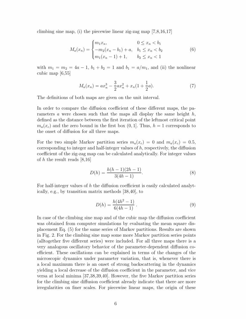
climbing sine map, (i) the piecewise linear zig-zag map [7,8,16,17]

Ma(xn) =

m1xn, 0 ≤ xn < b1

−m2(xn − b1) + a, b1 ≤ xn < b2

m1(xn − 1) + 1, b2 ≤ xn < 1

(6)

with m1 = m2 = 4a − 1, b1 + b2 = 1 and b1 = a/m1, and (ii) the nonlinearcubic map [6,55]

Ma(xn) = ax3n −

3

2ax2

n + xn(1 +1

2a). (7)

The definitions of both maps are given on the unit interval.

In order to compare the diffusion coefficient of these different maps, the pa-rameters a were chosen such that the maps all display the same height h,defined as the distance between the first iteration of the leftmost critical pointma(xc) and the zero bound in the first box (0, 1]. Thus, h = 1 corresponds tothe onset of diffusion for all three maps.

For the two simple Markov partition series ma(xc) = 0 and ma(xc) = 0.5,corresponding to integer and half-integer values of h, respectively, the diffusioncoefficient of the zig-zag map can be calculated analytically. For integer valuesof h the result reads [8,16]

D(h) =h(h − 1)(2h − 1)

3(4h − 1). (8)

For half-integer values of h the diffusion coefficient is easily calculated analyt-ically, e.g., by transition matrix methods [38,40], to

D(h) =h(4h2 − 1)

6(4h − 1). (9)

In case of the climbing sine map and of the cubic map the diffusion coefficientwas obtained from computer simulations by evaluating the mean square dis-placement Eq. (5) for the same series of Markov partitions. Results are shownin Fig. 2. For the climbing sine map some more Markov partition series points(alltogether five different series) were included. For all three maps there is avery analogous oscillatory behavior of the parameter-dependent diffusion co-efficient. These oscillations can be explained in terms of the changes of themicroscopic dynamics under parameter variation, that is, whenever there isa local maximum there is an onset of strong backscattering in the dynamicsyielding a local decrease of the diffusion coefficient in the parameter, and viceversa at local minima [37,38,39,40]. However, the five Markov partition seriesfor the climbing sine diffusion coefficient already indicate that there are moreirregularities on finer scales. For piecewise linear maps, the origin of these

6

irregularities was identified to be the topological instability of the dynamicsunder parameter variation [38,40]. That is, a small deviation of the parameterchanges the Markov partition and the corresponding invariant density which,in turn, is reflected in a change of the value of the diffusion coefficient. Notethat the dependence of the diffusion coefficient for a single Markov partitionseries appears to be a monotonously increasing function of the parameter [57].Nevertheless, computing D(a) for more and more Markov partitions series willreveal more and more irregularities in D(a) thus forming a fractal structure[37,38,39,40].

Since the climbing sine map shares the same topological features as piecewiselinear maps in terms of these series of Markov partitions, one may wonderwhether it is not possible to straightforwardly calculate the diffusion coefficientfor nonlinear maps from the one of piecewise linear maps by using the conceptof conjugacy [9,55,58], see also the definition in Appendix A. In fact, it wasstated by Grossmann and Thomae [9] that the diffusion coefficient is invariantunder conjugacy, however, without giving a proof. In Appendix A such aproof is provided. Unfortunately, conjugacies are explicitly known only in veryspecific cases and for maps acting on the unit interval [55,58]. As soon asthe map extrema exceed the unit interval, which is reminiscent of the onsetof diffusive behavior, only some approximate, piecewise conjugacies could beconstructed in a straightforward way, see Ref. [9] for an example.

We now apply this reasoning along the lines of conjugacy in order to under-stand the similarities between the diffusion coefficient of the three maps asdisplayed in Fig. 2. The functional form of the cubic map can be obtainedfrom a Taylor series expansion of sin(xn) by keeping terms up to third or-der thus representing a low-order approximation of the climbing sine map.This seems to be reflected in the fact that at any odd integer parametervalue of h the climbing sine map has an invariant density whose functionalform is very close to the one of the cubic map at parameter value h = 1,ρ∗(x) = π−1(x(1 − x))−1/2. Hence, one may expect that both diffusion coeffi-cients are possibly trivially related to each other, however, note the increasingdeviations between the respective results at larger h.

For h = 1, the cubic map and the piecewise linear zig-zag map are now in turnconjugate to each other [55,58]. However, for h > 1 we are not aware of theexistence of any exact conjugacy between zig-zag and cubic map. Still, alongthe lines of Ref. [9] one can at least approximately relate both maps to eachother via using piecewise conjugacies. This explains why the zig-zag map andthe climbing sine map display qualitatively the very same oscillatory behaviorin the diffusion coefficient, somewhat linked by diffusion in the cubic map.

In summary, by using Markov partitions and by arguing with the concept ofconjugacy we have shown that the structure of the diffusion coefficient for the

7

nonlinear climbing sine map has much in common with the one of respectivepiecewise linear maps, in the sense of displaying a non-trivial oscillatory pa-rameter dependence. However, to use conjugacies in order to exactly calculatethe diffusion coefficient for nonlinear maps does not appear to be straightfor-ward [56], hence in the following we restrict ourselves to alternative methodsas discussed in the next subsection.

1 2 3 4 5h

0

2

4

6

8

D(h)

0 0.5 1

0

0.5

1

Ma

0.5

x

2

4

ρ∗

Fig. 2. Diffusion coefficient at certain Markov partition parameter values for threedifferent maps, which are the zig-zag map Eq.(6) (squares), the climbing sine map(circles), and the cubic map Eq. (7) (triangles). The values for the zig-zag maprepresent analytical results, see Eqs.(8,9), the remaining values are from computersimulations. The lines are guides for the eyes. The inset shows an example of aMarkov partition for the climbing sine map on the unit interval and the corre-sponding invariant density.

3.2 Complete parameter dependence of the climbing sine diffusion coefficient

In order to obtain the full parameter dependence for the diffusion coefficientof the climbing sine map we numerically evaluated the Green-Kubo formulafor diffusion in maps [3,4,8,29,38,41] reading

Dn(a) = 〈ja(x)Jna (x)〉 −

1

2〈j2

a(x)〉 . (10)

Here the angular brackets denote an average over the invariant density of thereduced map, 〈. . .〉 =

∫

dxρ∗(x) . . .. The jump velocity ja(x) is defined by

ja(xn) := [Xn+1] − [Xn] ≡ [Ma(xn)] , (11)

where the square brackets denote the largest integer less than the argument.The sum

8

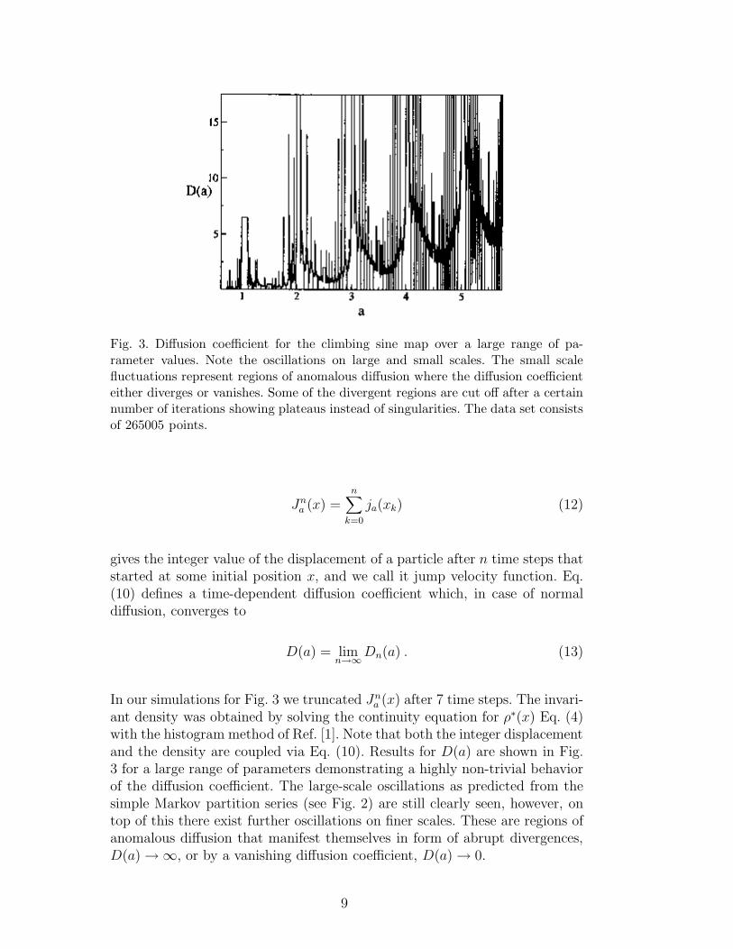
Fig. 3. Diffusion coefficient for the climbing sine map over a large range of pa-rameter values. Note the oscillations on large and small scales. The small scalefluctuations represent regions of anomalous diffusion where the diffusion coefficienteither diverges or vanishes. Some of the divergent regions are cut off after a certainnumber of iterations showing plateaus instead of singularities. The data set consistsof 265005 points.

Jna (x) =

n∑

k=0

ja(xk) (12)

gives the integer value of the displacement of a particle after n time steps thatstarted at some initial position x, and we call it jump velocity function. Eq.(10) defines a time-dependent diffusion coefficient which, in case of normaldiffusion, converges to

D(a) = limn→∞

Dn(a) . (13)

In our simulations for Fig. 3 we truncated Jna (x) after 7 time steps. The invari-

ant density was obtained by solving the continuity equation for ρ∗(x) Eq. (4)with the histogram method of Ref. [1]. Note that both the integer displacementand the density are coupled via Eq. (10). Results for D(a) are shown in Fig.3 for a large range of parameters demonstrating a highly non-trivial behaviorof the diffusion coefficient. The large-scale oscillations as predicted from thesimple Markov partition series (see Fig. 2) are still clearly seen, however, ontop of this there exist further oscillations on finer scales. These are regions ofanomalous diffusion that manifest themselves in form of abrupt divergences,D(a) → ∞, or by a vanishing diffusion coefficient, D(a) → 0.

9

4 Simple and correlated random walk approximations

In this section we study the parameter-dependent diffusion coefficient in moredetail. Based on the Green-Kubo formula we derive a systematic hierarchy ofapproximations for the diffusion coefficient and show how they can be used tounderstand the complex behavior of this curve in more detail.

4.1 Asymptotic functional form of the diffusion coefficient on large scales

We are first interested in understanding the coarse functional form of theparameter-dependent diffusion coefficient in the limit of very small and verylarge parameter values. For this purpose we use simple random walk approx-imations that are based on the assumption of a complete loss of memorybetween the single jumps. Such an analysis was already performed for hyper-bolic piecewise linear maps [38,39]. Here we apply the same reasoning to thenonlinear case of the climbing sine map.

We start in the limit of very small parameter values, i.e., near the onset ofdiffusion. Here we assume that particles make either a step of length one tothe left or to the right, or just remain in the box. The transition probabilityis then given by integrating over the respective invariant density in the escaperegion. Putting all this information into Eq. (5) yields [6]

D(a) ≃ ρ(xc)(2ǫ/a0π2)1/2, (14)

where ǫ = a− a0. Making the additional approximation that ρ(x) ≃ 1 we get

D(a) ≃ 0.525ǫ1/2, ǫ ≪ 1. (15)

The other limiting case concerns values of a ≫ 1. Here the precise value ofthe width of the escape region is much less important than the precise valueof the step length which is very large, hence by again assuming that ρ(x) ≃ 1Eq. (5) can be approximated to [38,39]

D(a) ≈1

2

∫ 1

0dx (Ma(x) − x)2 ≈

a2

4, a ≫ 1. (16)

These two asymptotic random walk approximations are shown in Fig. 4 asbold lines. One can clearly see that there is a dynamical crossover between thedifferent functional forms of these two asymptotic regimes. This crossover wasfirst observed in piecewise linear maps and appears to be typical for diffusivesystems exhibiting some spatial periodicity [38,39]. It was lateron also verifiedfor diffusion in the periodic Lorentz gas [28]. The coarse functional form of the

10

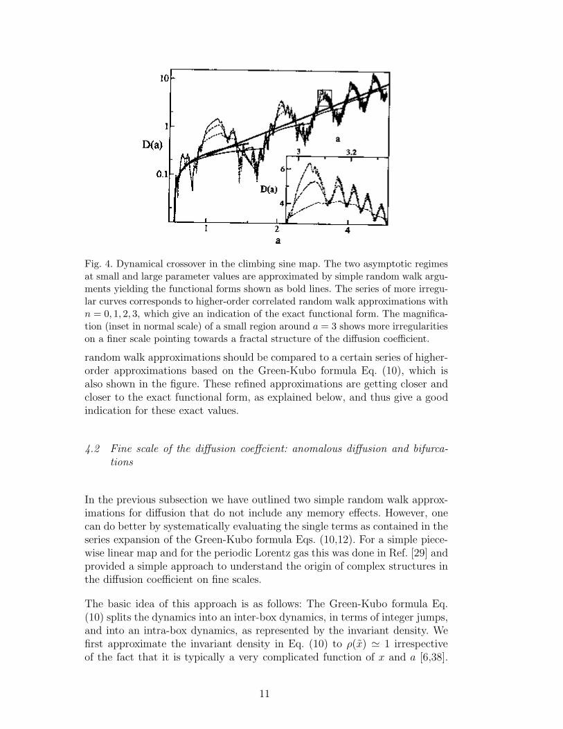
Fig. 4. Dynamical crossover in the climbing sine map. The two asymptotic regimesat small and large parameter values are approximated by simple random walk argu-ments yielding the functional forms shown as bold lines. The series of more irregu-lar curves corresponds to higher-order correlated random walk approximations withn = 0, 1, 2, 3, which give an indication of the exact functional form. The magnifica-tion (inset in normal scale) of a small region around a = 3 shows more irregularitieson a finer scale pointing towards a fractal structure of the diffusion coefficient.

random walk approximations should be compared to a certain series of higher-order approximations based on the Green-Kubo formula Eq. (10), which isalso shown in the figure. These refined approximations are getting closer andcloser to the exact functional form, as explained below, and thus give a goodindication for these exact values.

4.2 Fine scale of the diffusion coeffcient: anomalous diffusion and bifurca-

tions

In the previous subsection we have outlined two simple random walk approx-imations for diffusion that do not include any memory effects. However, onecan do better by systematically evaluating the single terms as contained in theseries expansion of the Green-Kubo formula Eqs. (10,12). For a simple piece-wise linear map and for the periodic Lorentz gas this was done in Ref. [29] andprovided a simple approach to understand the origin of complex structures inthe diffusion coefficient on fine scales.

The basic idea of this approach is as follows: The Green-Kubo formula Eq.(10) splits the dynamics into an inter-box dynamics, in terms of integer jumps,and into an intra-box dynamics, as represented by the invariant density. Wefirst approximate the invariant density in Eq. (10) to ρ(x) ≃ 1 irrespectiveof the fact that it is typically a very complicated function of x and a [6,38].

11

The resulting approximate diffusion coefficient we label with a superscriptin Eq. (10), D1

n(a). The term for n = 0 obviously excludes any higher-ordercorrelations and was already worked out in form of the simple random walkapproximation Eqs. (14)-(16).

The generalization D1n(a) , n > 0, which systematically includes more and

more dynamical correlations, may consequently be denoted as correlated ran-

dom walk approximation [29]. We now use this expansion to analyze the pa-rameter dependence of the diffusion coefficient of the climbing sine map interms of such higher-order correlations. Fig. 4 depicts results for Dn(a) at

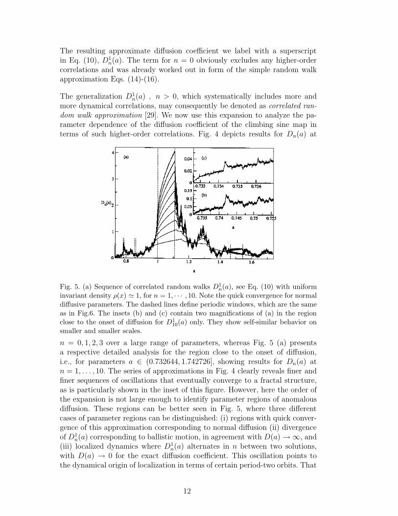
Fig. 5. (a) Sequence of correlated random walks D1n(a), see Eq. (10) with uniform

invariant density ρ(x) ≃ 1, for n = 1, · · · , 10. Note the quick convergence for normaldiffusive parameters. The dashed lines define periodic windows, which are the sameas in Fig.6. The insets (b) and (c) contain two magnifications of (a) in the regionclose to the onset of diffusion for D1

10(a) only. They show self-similar behavior onsmaller and smaller scales.

n = 0, 1, 2, 3 over a large range of parameters, whereas Fig. 5 (a) presentsa respective detailed analysis for the region close to the onset of diffusion,i.e., for parameters a ∈ (0.732644, 1.742726], showing results for Dn(a) atn = 1, . . . , 10. The series of approximations in Fig. 4 clearly reveals finer andfiner sequences of oscillations that eventually converge to a fractal structure,as is particularly shown in the inset of this figure. However, here the order ofthe expansion is not large enough to identify parameter regions of anomalousdiffusion. These regions can be better seen in Fig. 5, where three differentcases of parameter regions can be distinguished: (i) regions with quick conver-gence of this approximation corresponding to normal diffusion (ii) divergenceof D1

n(a) corresponding to ballistic motion, in agreement with D(a) → ∞, and(iii) localized dynamics where D1

n(a) alternates in n between two solutions,with D(a) → 0 for the exact diffusion coefficient. This oscillation points tothe dynamical origin of localization in terms of certain period-two orbits. That

12

these approximate solutions are non-zero is due to the fact that the invariantdensity was set equal to one. The dashed lines in Fig. 5 indicate the largestregions of anomalous diffusion. The approximate diffusion coefficient D1

10(a)of this figure is compared to the “numerically exact” one in Fig. 6. Here “nu-merically exact” we wish to be understood in the sense that no further adhoc-approximations are involved, i.e., we evaluated the Green-Kubo formulaaccording to the numerical method described in Sec. III. by truncating it after20 time steps. This comparison shows that in case of normal diffusion ourapproximation nicely reproduces the irregularities in the non-approximateddiffusion coefficient. Like the inset of Fig. 4, the magnifications in Fig.5 giveclear evidence for a self-similar structure of the diffusion coefficient. Theseresults thus show that dealing with correlated jumps only yields a qualitativeand to quite some extent even quantitative understanding of the regions ofnormal and anomalous diffusion in the climbing sine map.

The impact of specific features of the microscopic dynamics on the diffusioncoefficient is nicely elucidated by comparing the bifurcation diagram of thereduced climbing sine map Eq. (3) with the numerically exact diffusion coef-ficient, see Fig. 6. As one can see in the upper panel of Fig. 6, the bifurcationdiagram consists of (infinitely) many periodic windows. Whenever there is awindow the dynamics of Eq. (1) is either ballistic or localized [6,8]. Fig. 6demonstrates the strong impact of this bifurcation scenario on the diffusioncoefficient. For localized dynamics, orbits are confined within some finite in-terval in phase space implying subdiffusive behavior for which the diffusioncoefficient vanishes, whereas for ballistic motion particles propagate superdif-fusively with a diverging diffusion coefficient being proportional to n. Onlyfor normal diffusion D(a) is nonzero, finite and the limit in Eq. (13) exists.At the boundaries of each periodic window the diffusion coefficient is relatedto intermittent-like transient behavior eventually resulting in normal diffusionwith D(a) ∼ a(± 1

2) [5,6,9,10].

5 Diffusion coefficient in terms of fractal generalized Takagi func-

tions

In this section we further analyze the dynamical origin of the different struc-tures in the parameter-dependent diffusion coefficient by constructing objectscalled fractal generalized Takagi functions. These functions somewhat resem-ble usual Takagi functions but, as will be shown, they fulfill a more complicatedtype of functional recursion relations than standard de Rham-type equations.Interestingly, Takagi functions were known to mathematicians since about ahundred years [59,60,61], however, in the field of chaotic transport they wereappreciated by physicists only very recently [3,4,38,62,63].

13

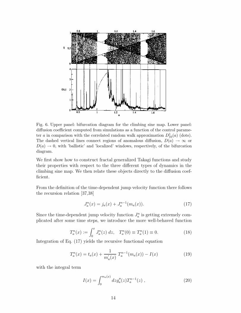
Fig. 6. Upper panel: bifurcation diagram for the climbing sine map. Lower panel:diffusion coefficient computed from simulations as a function of the control parame-ter a in comparison with the correlated random walk approximation D1

10(a) (dots).The dashed vertical lines connect regions of anomalous diffusion, D(a) → ∞ orD(a) → 0, with ’ballistic’ and ’localized’ windows, respectively, of the bifurcationdiagram.

We first show how to construct fractal generalized Takagi functions and studytheir properties with respect to the three different types of dynamics in theclimbing sine map. We then relate these objects directly to the diffusion coef-ficient.

From the definition of the time-dependent jump velocity function there followsthe recursion relation [37,38]

Jna (x) = ja(x) + Jn−1

a (ma(x)). (17)

Since the time-dependent jump velocity function Jna is getting extremely com-

plicated after some time steps, we introduce the more well-behaved function

T na (x) :=

∫ x

0Jn

a (z) dz, T na (0) ≡ T n

a (1) ≡ 0. (18)

Integration of Eq. (17) yields the recursive functional equation

T na (x) = ta(x) +

1

m′

a(x)T n−1

a (ma(x)) − I(x) (19)

with the integral term

I(x) =∫ ma(x)

0dzg′′

a(z)T n−1a (z) , (20)

14

where g′′

a(z) is the second derivative of the inverse function of ma(x). The

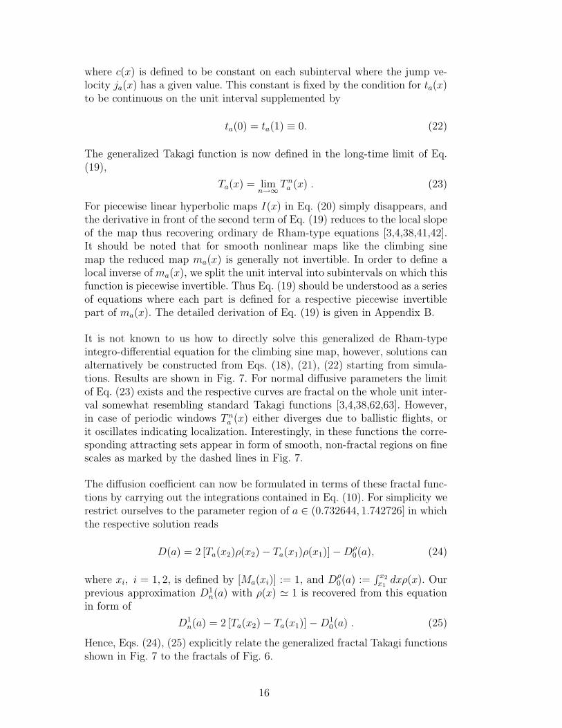
Fig. 7. (a): Generalized fractal Takagi functions for the diffusive climbing sine mapwith parameters a = 1.2397 (upper curve) and a = 1.7427 (lower curve). (b), (c): Anexample of nonconverging iterations of the generalized fractal Takagi functions forthe climbing sine map with parameters corresponding to (b) ballistic dynamics ata = 1.0 and to (c) localized dynamics at a = 1.5, both for the time steps n = 5, 6, 7.Note the divergence of the iterations in (b) and the alternation between two statesin (c).

function ta(x) is given by

ta(x) =∫

dzja(z) = xja(x) + c(x) , (21)

15

where c(x) is defined to be constant on each subinterval where the jump ve-locity ja(x) has a given value. This constant is fixed by the condition for ta(x)to be continuous on the unit interval supplemented by

ta(0) = ta(1) ≡ 0. (22)

The generalized Takagi function is now defined in the long-time limit of Eq.(19),

Ta(x) = limn→∞

T na (x) . (23)

For piecewise linear hyperbolic maps I(x) in Eq. (20) simply disappears, andthe derivative in front of the second term of Eq. (19) reduces to the local slopeof the map thus recovering ordinary de Rham-type equations [3,4,38,41,42].It should be noted that for smooth nonlinear maps like the climbing sinemap the reduced map ma(x) is generally not invertible. In order to define alocal inverse of ma(x), we split the unit interval into subintervals on which thisfunction is piecewise invertible. Thus Eq. (19) should be understood as a seriesof equations where each part is defined for a respective piecewise invertiblepart of ma(x). The detailed derivation of Eq. (19) is given in Appendix B.

It is not known to us how to directly solve this generalized de Rham-typeintegro-differential equation for the climbing sine map, however, solutions canalternatively be constructed from Eqs. (18), (21), (22) starting from simula-tions. Results are shown in Fig. 7. For normal diffusive parameters the limitof Eq. (23) exists and the respective curves are fractal on the whole unit inter-val somewhat resembling standard Takagi functions [3,4,38,62,63]. However,in case of periodic windows T n

a (x) either diverges due to ballistic flights, orit oscillates indicating localization. Interestingly, in these functions the corre-sponding attracting sets appear in form of smooth, non-fractal regions on finescales as marked by the dashed lines in Fig. 7.

The diffusion coefficient can now be formulated in terms of these fractal func-tions by carrying out the integrations contained in Eq. (10). For simplicity werestrict ourselves to the parameter region of a ∈ (0.732644, 1.742726] in whichthe respective solution reads

D(a) = 2 [Ta(x2)ρ(x2) − Ta(x1)ρ(x1)] − Dρ0(a), (24)

where xi, i = 1, 2, is defined by [Ma(xi)] := 1, and Dρ0(a) :=

∫ x2

x1dxρ(x). Our

previous approximation D1n(a) with ρ(x) ≃ 1 is recovered from this equation

in form of

D1n(a) = 2 [Ta(x2) − Ta(x1)] − D1

0(a) . (25)

Hence, Eqs. (24), (25) explicitly relate the generalized fractal Takagi functionsshown in Fig. 7 to the fractals of Fig. 6.

16

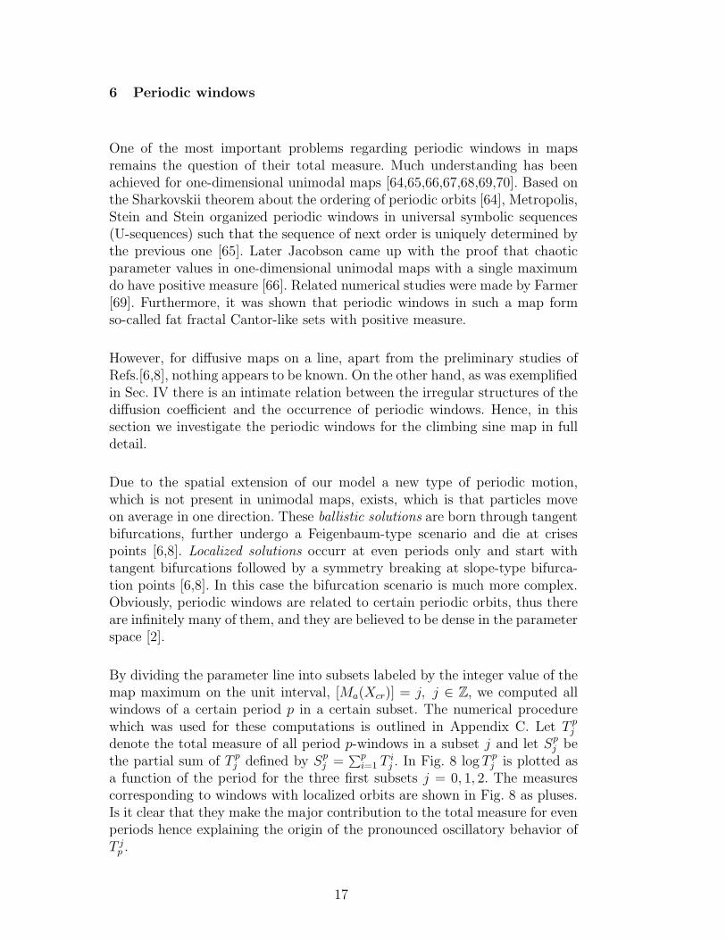
6 Periodic windows

One of the most important problems regarding periodic windows in mapsremains the question of their total measure. Much understanding has beenachieved for one-dimensional unimodal maps [64,65,66,67,68,69,70]. Based onthe Sharkovskii theorem about the ordering of periodic orbits [64], Metropolis,Stein and Stein organized periodic windows in universal symbolic sequences(U-sequences) such that the sequence of next order is uniquely determined bythe previous one [65]. Later Jacobson came up with the proof that chaoticparameter values in one-dimensional unimodal maps with a single maximumdo have positive measure [66]. Related numerical studies were made by Farmer[69]. Furthermore, it was shown that periodic windows in such a map formso-called fat fractal Cantor-like sets with positive measure.

However, for diffusive maps on a line, apart from the preliminary studies ofRefs.[6,8], nothing appears to be known. On the other hand, as was exemplifiedin Sec. IV there is an intimate relation between the irregular structures of thediffusion coefficient and the occurrence of periodic windows. Hence, in thissection we investigate the periodic windows for the climbing sine map in fulldetail.

Due to the spatial extension of our model a new type of periodic motion,which is not present in unimodal maps, exists, which is that particles moveon average in one direction. These ballistic solutions are born through tangentbifurcations, further undergo a Feigenbaum-type scenario and die at crisespoints [6,8]. Localized solutions occurr at even periods only and start withtangent bifurcations followed by a symmetry breaking at slope-type bifurca-tion points [6,8]. In this case the bifurcation scenario is much more complex.Obviously, periodic windows are related to certain periodic orbits, thus thereare infinitely many of them, and they are believed to be dense in the parameterspace [2].

By dividing the parameter line into subsets labeled by the integer value of themap maximum on the unit interval, [Ma(Xcr)] = j, j ∈ Z, we computed allwindows of a certain period p in a certain subset. The numerical procedurewhich was used for these computations is outlined in Appendix C. Let T p

j

denote the total measure of all period p-windows in a subset j and let Spj be

the partial sum of T pj defined by Sp

j =∑p

i=1 T ij . In Fig. 8 log T p

j is plotted asa function of the period for the three first subsets j = 0, 1, 2. The measurescorresponding to windows with localized orbits are shown in Fig. 8 as pluses.Is it clear that they make the major contribution to the total measure for evenperiods hence explaining the origin of the pronounced oscillatory behavior ofT j

p .

17

1 2 3 4 5 6p

0.0001

0.01

log

Tjp

1 2 3 4 5 6 7p

0.1

0.2

S jp

1

2

3

Fig. 8. Upper panel: The total measure Tpj of all period p-windows (lines with

symbols) for the first three parameter intervals (from top to bottom) as defined inthe text. The dotted lines represent exponential fits; for the parameters see Table 1.The measures corresponding to windows with localized orbits are shown as pluses.Lower panel: The partial sum S

pj for all periodic windows at a certain period p. The

dashed curves represent approximations as calculated from Eq. (27), the straightlines are their limiting values at p → ∞.

Table 1Fit parameters for the exponential decrease of the measure at even and odd periodsfor the first three subsets of the map control parameter labeled by j.

j aevenj beven

j aoddj bodd

j

0 0.284 0.61 ± 0.01 0.012 0.62

1 0.224 0.87 ± 0.01 0.007 0.89

2 0.242 1.01 ± 0.02 0.006 0.98

For odd periods all windows are due to ballistic orbits. Thus, we more carefullydistinguish between even and odd periods. The dotted lines in Fig. 8 representexponential fits to the functional dependence of the measure at even and oddperiods according to aeven

j exp(−bevenj p) and aodd

j exp(−boddj p), where j stands

18

1 5

log j

0.01

0.1

log

Tj1

1 3

log j

0.0001

0.01

log

Tjp

1

2

4

3

5

Fig. 9. Upper panel: Total measure T 1j for period one-windows as a function of the

control parameter interval labeled by j. The slope of the line appears to be −1 (seetext). Lower panel: the same as on the upper panel but here for different windowperiodicities p, and for smaller j. The labels at the single graphs give the value ofp.

for the box number j = 0, 1, 2, as defined above. The fit parameters aj , bj aregiven in Table 1. From Fig. 8 and Table 1 one can conclude that the totalmeasures at even and odd periods at a certain label j decrease approximatelywith the same rate, beven

j ∼ boddj ≃ bj . The exponential decrease of T p

j suggeststhat the measure of chaotic solutions in each box, which is complementary tothe measure of periodic windows, is indeed positive. Based on the informationof T p

j , it is straightforward to approximate the total measure of all the periodicwindows in the jth box by

Sj = T 1j +

∞∑

i=2

′

T ij +

∞∑

i=3

′′

T ij ≃ T 1

j +aeven

j + aoddj e−bj

e2bj − 1(26)

and to approximate the parameter dependence of the partial sum Spj to

Spj ≃ T 1

j e−bj(p−1

2) + Sj(1 − e−bj(p−

1

2)) . (27)

19

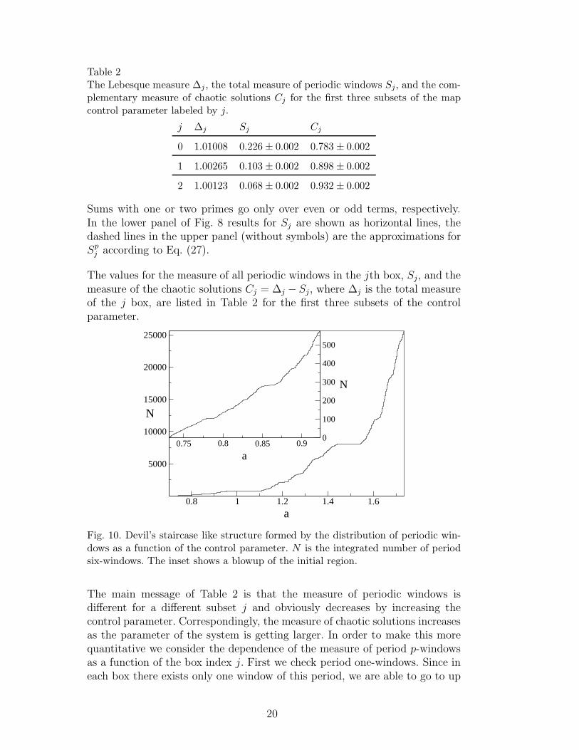
Table 2The Lebesque measure ∆j , the total measure of periodic windows Sj, and the com-plementary measure of chaotic solutions Cj for the first three subsets of the mapcontrol parameter labeled by j.

j ∆j Sj Cj

0 1.01008 0.226 ± 0.002 0.783 ± 0.002

1 1.00265 0.103 ± 0.002 0.898 ± 0.002

2 1.00123 0.068 ± 0.002 0.932 ± 0.002

Sums with one or two primes go only over even or odd terms, respectively.In the lower panel of Fig. 8 results for Sj are shown as horizontal lines, thedashed lines in the upper panel (without symbols) are the approximations forSp

j according to Eq. (27).

The values for the measure of all periodic windows in the jth box, Sj, and themeasure of the chaotic solutions Cj = ∆j − Sj, where ∆j is the total measureof the j box, are listed in Table 2 for the first three subsets of the controlparameter.

0.8 1 1.2 1.4 1.6

a

5000

10000

15000

20000

25000

N

0.75 0.8 0.85 0.9

a

0

100

200

300

400

500

N

Fig. 10. Devil’s staircase like structure formed by the distribution of periodic win-dows as a function of the control parameter. N is the integrated number of periodsix-windows. The inset shows a blowup of the initial region.

The main message of Table 2 is that the measure of periodic windows isdifferent for a different subset j and obviously decreases by increasing thecontrol parameter. Correspondingly, the measure of chaotic solutions increasesas the parameter of the system is getting larger. In order to make this morequantitative we consider the dependence of the measure of period p-windowsas a function of the box index j. First we check period one-windows. Since ineach box there exists only one window of this period, we are able to go to up

20

to j = 20. In the upper panel of Fig. 9 the logarithm of T 1j is plotted against

log j. We find that the slope of this function almost exactly equal to −1. Thebehavior of T p

j for different p is shown in the lower panel of Fig. 9. The slopeof the line for period two is also −1, for period three and four it is −2, andfor period five it is −3. Fig. 9 shows that even and odd periods decrease withrespectively different laws, where the decay rate appears to be precisely givenby the periodicity of the windows according to 1/jp/2 for even periods and1/j(p+1)/2 for odd periods.

In order to analyze the structure of the regions of anomalous diffusion in theparameter space, we sum up the number of period six-windows as a function ofthe parameter, that is, the total number is increased by one for any parametervalue at which a new period six-window appears. This sum forms a Devil’sstaircase like structure in parameter space indicating an underlying Cantorset like distribution for the corresponding anomalous diffusive region, see Fig.9. Since the Lebesque measure of periodic windows is positive, this set mustbe a fat fractal [68]. Its self-similar structure can quantitatively be assessedby computing the so-called fatness exponent. Following [69], let h(ε) be thetotal measure of all periodic windows whose width is greater than or equalto ε. Define the coarse-grained measure as µ(ε) = ∆ − h(ε), where ∆ isthe total measure of a box related to the control parameter. For quadraticmaps on the interval, it was conjectured and confirmed numerically that µ(ε)asymptotically scales as a power law in the limit of ε → 0,

µ(ε) ≈ µ(0) + Aεβ , (28)

where µ(0) is the measure of chaotic parameters. β was called the fatness expo-nent. For quadratic maps it was found to be β ≃ 0.45. Since our map belongs tothe same universality class as considered in Farmer’s case, namely the map hasa single quadratic maximum, one may expect that β will have the same value.For the climbing sine map a double-logarithmic plot of δµ(ε) = µ(ε)− µ(0) isshown in Fig. 11 for the first three boxes, j = 0, 1, 2. In all cases the bold lineshave the slope 0.45 with errors of 0.03, 0.04, 0.05, respectively, which seems tobe in agreement with Farmer’s conjecture about the universality of β. However,apart from this coarse linear behavior one can see an interesting oscillatorybehavior in δµ with respect to ε. This fine structure can be explained withrespect to the histogram distribution functions f of the window sizes d, whichare plotted in Fig. 11 in form of dashed lines. Somewhat surprisingly, the peri-odic windows are not distributed uniformly or smoothly with respect to theirsize but form certain peaks, in which preferably windows of certain periods aregrouped together. This non-uniformity is clearly reflected in the oscillations ofδµ(ε). Moreover, we find that the size distributions of periodic windows havea fine structure that appears to resemble a fractal function. Some evidencefor this property is given in the inset of Fig. 11 (c), which shows the size ofevery window of period five in the subset j = 2 as a function of its appearancewith respect to the map control parameter a, i.e., not the parameter itself

21

0.0001

0.0001

log ε

0.0004

0.02

log

δµ(ε

)0.0001

log d

109

f

(a)

10-8

10-8

10-6

10-6

10-4

10-4

10-2

10-2

100

100

log ε10

-6

10-4

10-2

100

log

δµ(ε

)

109

log d

f

(b)

10-8

10-8

10-4

10-4

log ε

10-4

10-3

log

δµ(ε

)

109

200 400 600

N

10-8.0

10-7.7

T5

2

log d

f

(c)

Fig. 11. Difference δµ = µ(ε)−µ(0), where µ(ε) is the total measure of windows thatare smaller than ε. Results are plotted for the first three subsets j = 0, 1, 2 of themap control parameter, from top to bottom. In all cases, the slope of the solid linesis approximately 0.45. The dashed lines in each graph represent the correspondingcoarse-grained window distribution functions. In the inset of Fig. (c) the measureof any single period five-window in the subset j = 2 is shown with respect to aninteger label that accounts for the ordering according to the map control parameter.

is plotted but just an integer running index N is given instead. Particularlythe height of the peaks is important, and one can clearly see a complicatedhierarchy of different peaks which are reminiscent of the fine structure in thecorresponding distribution function shown in Fig. 11 (c).

22

7 Conclusions

In this paper we have performed a detailed analysis of the parameter depen-dence of the diffusion coefficient in a nonhyperbolic dynamical system. Theclimbing sine map has been chosen as a paradigmatic example of such a sys-tem. We have shown that, on a coarse scale, there are certain analogies betweenthe parameter-dependent diffusion coefficient of this map and the ones in sim-ple hyperbolic piecewise linear maps, such as the existence of an oscillatorystructure, and the existence of asymptotic functional forms as derived fromsimple random walk models. However, in contrast to hyperbolic maps showingnormal diffusion only, in the nonhyperbolic climbing sine map fractal struc-tures appear for both normal and anomalous diffusive regions of the diffusioncoefficient. An understanding of the origin of these fractal structures was givenin terms of dynamical correlations starting from the Green-Kubo formula fordiffusion. We furthermore related these irregularities in the diffusion coeffi-cient more microscopically to different characteristics in corresponding fractalgeneralized Takagi functions. For this purpose we derived a new functionalrecursion relation that defines these fractal forms and generalizes ordinaryde Rham-type equations. Our analysis was completed by extensive numeri-cal studies of the periodic windows of the climbing sine map showing thatboth the periodic and the chaotic parameter regions have positive measuresin the parameter space. However, these measures are themselves parameter-dependent, and by increasing the parameter we found that the chaotic regionsoccupy larger and larger measures. We finally provided evidence that thesedifferent sets form fat fractals on the parameter axis.

In conclusion, we wish to remark that the climbing sine map is of the samefunctional form as the respective nonlinear equation in the two-dimensionalstandard map, which is considered to be a standard model for many physicalHamiltonian dynamical systems. Indeed, both models are motivated by thedriven nonlinear pendulum, both are strongly nonhyperbolic, and though thestandard map is area-preserving it too exhibits a highly irregular parameter-dependent diffusion coefficient. Understanding the origin of these irregularitieswas the subject of intensive research [2,19], however, so far the complexity ofthis system did not enable to reveal its possibly fractal nature. A suitablyadapted version of our approach to nonhyperbolic diffusive dynamics as pre-sented in this paper may enable to make some progress in this direction.

Another interesting problem is to possibly further exploit the concept of con-jugacy between nonlinear and piecewise linear maps, as explained in Sec. III,in order to exactly calculate diffusion coefficients for nonlinear maps. A verypromising approach in this direction was presented in Ref. [56]. Based on thesetechniques we are planning to perform a spectral analysis of the Frobenius-Perron operator governing the probability density of the diffusive climbing sine

23

map. Combining such an analysis with the Takagi function approach outlinedhere may lead to a general theory of nonhyperbolic transport.

It would furthermore be important to check out the applicability of periodicorbit theory for computing the parameter-dependent diffusion coefficient ofthe climbing sine map, which may provide an alternative method [15]. An-other promising direction of future research concerns establishing crosslinksbetween our work and the realm of strange kinetics and stochastic modelingas described in Refs. [24,25,26], e.g., by trying to apply continuous time ran-dom walk techniques to more complicated chaotic models exhibiting fractaldiffusion coefficients such as the climbing sine map.

We finally emphasize the importance to look for possibly fractal transportcoefficients in experiments. A very promising candidate appears to be thephase dynamics in SQUID’s, which was very recently analyzed theoretically[48] and studied experimentally [49].

A Diffusion coefficients of two conjugate maps

In this Appendix we give a proof of the statement of Grossmann and Thomae[9] that two diffusive maps which are conjugate to each other have the samediffusion coefficient.

Two diffusive maps F : I → I and G : J → J are called conjugate [58,9,55] ifthere exists a map H : I → J such that F (x) = H(G(H−1(x))). Let us assumein the following that the conjugation function H is sufficiently smooth. Letthe invariant densities of the corresponding reduced (mod 1) maps be ρ(x) forF (x) mod 1 and ρ(y) for G(y) mod 1; then it is, according to conservationof probability, ρ(x) = |(H−1(x))′| ρ(H−1(x)). The diffusion coefficients of themaps F (x) and G(y) we denote by DF and DG, respectively. Without loss ofgenerality let us furthermore assume that the maxima of both maps are in theinterval [1, 2].

We now start with the Green-Kubo formula written in correlated random walk

terms as

DF =1

2

1∫

0

[F (x)]2 ρ(x)dx +

1∫

0

[F (x)] · B(x) ρ(x)dx, (A.1)

where

B(x) = [F{F (x)}] + ... + [F ({F ({... ({F (x)}) ...})})] + ... , (A.2)

24

or shortly

DF = dF0+ dF1

+ dF2+ ... (A.3)

where

dF0=

1

2

1∫

0

[F (x)]2 ρ(x) dx, (A.4)

dF1=

1

2

1∫

0

[F (x)] [F{F (x)}] ρ(x) dx, (A.5)

and so on. Focusing on the first term, one can rewrite this expression usingthe symmetry of the map to

dF0=

1

2

1∫

0

[F (x)]2 ρ(x) dx =

x2∫

x1

ρ(x) dx, (A.6)

where x1, x2 defines an escape region. For the conjugate map G(y) the respec-tive term reads

dG0=

1

2

1∫

0

[G(y)]2 ρ(y) dy =

y2∫

y1

ρ(y) dy, (A.7)

where y1, y2 is the corresponding escape region for G. Note that the escaperegions (x1, x2) and (y1, y2) are not the same, however, it is straightforward toshow that H(xi) = yi , i = 1, 2, that is, the topology of both maps is conservedsuch that the two escape regions are mapped onto each other under conjugacy.

Taking into account the conservation of probability mentioned before one im-mediately gets

dF0= dG0

. (A.8)

All other terms dF1, dF2

, ... and dG1, dG2

, ... have the form

d(F,G)i= A

∫

δesc

ν(z) dz, i = 1, 2, ... (A.9)

where A is a constant, δesc is the respective escape region and ν(z) dz is thecorresponding invariant measure. Thus, the same argument can be applied toshow that dFi

= dGi, (i = 1, 2, ...). Combining all results we arrive at

DF = DG . (A.10)

25

B Recursion relation for generalized Takagi functions

We start with the recursion relation for the jump velocity function Eq. (17),

Jna (x) = ja(x) + Jn−1

a (ma(x)), (B.1)

by recalling the definition of the generalized Takagi function Eq. (18),

T na (x) :=

∫ x

0Jn

a (z) dz, T na (0) ≡ T n

a (1) ≡ 0, (B.2)

or differently

Jna (x) =

d

dxT n

a (x). (B.3)

0 0.5 1

x

0

0.3

0.6

0.9

ma

0 0.5 1y

0

0.3

0.6

0.9

ga

1

2 3

4

5 6

7

1

2

3

4

5

6

7

x1

x3

x2

... x7

Fig. B.1. Illustration of the construction of the inverse function of the climbing sinemap for the parameter value a = 1.189. Piecewise invertible branches are labeledby the integer numbers i = 1, · · · , 7.

We have to integrate Eq. (B.1),

x∫

0

dy Jna (y) =

x∫

0

dy ja(y) +

x∫

0

dy Jn−1a (ma(x)). (B.4)

By using of Eq. (B.2) we get

T na (x) = ta(x) + I(x), x ∈ (0, 1], (B.5)

where

I(x) =

x∫

0

dy Jn−1a (ma(y)), x ∈ (0, 1]. (B.6)

Without loss of generality let us assume that the maximum of the map is inthe interval [1, 2].

26

Depending on x the integral in Eq. (B.6) can be decomposed into

I1(x) =

x∫

0

dy Jn−1a (ma(y)), x ∈ (0, x1]; (B.7)

I2(x) =

x1∫

0

dy Jn−1a (ma(y)) +

x∫

x1

dy Jn−1a (ma(y)), x ∈ (x1, x2];

I3(x) = ..., x ∈ (x2, x3]; ... I6(x) = ..., x ∈ (x5, x6];

I7(x) =

x1∫

0

dy Jn−1a (ma(y)) + · · ·+

x∫

x6

dy Jn−1a (ma(y)), x ∈ (x6, x7].

Each integral in Eq. (B.7) now contains only one piecewise invertible branchof the reduced map mi

a(x) as shown in Fig. B.1. Here, the piecewise invertiblebranches of the reduced map are labeled by integers, and the correspondingbranches of the inverse function gi

a(y) have the same indices i = 1, · · · , 7. Sinceall integrals in Eq. (B.7) have the same form (only the inverse parts of thereduced map are different), we restrict ourselves to the integral

I(x) =

x∫

0

dy Jn−1a (mi

a(y)). (B.8)

Making the change of variables z = mia(y) and using the definition of the

generalized Takagi function Eq. (B.3) we get

I(x) =

mia(x)∫

0

dz (gia(z))

′ d

dzT n−1

a (z). (B.9)

Using integration by parts we arrive at

I(x) = (gia(z))

′

· T n−1a (z)|

mia(x)

0 −

mia(x)∫

0

dz (gia(z))

′′

· T n−1a (z). (B.10)

Now recall that according to Eq. (B.2) it is T n−1a (mi

a(xj)) ≡ 0, where the xj

define the boundaries of the piecewise invertible parts of ma(x), see Fig. B.1,and that (gi

a(z))′

|z=mia(x) ≡ 1/(mi

a(x))′

. Thus, by formally defining the inversefunction ga(x) as consisting of all branches i = 1, . . . , 7, we can finally writeEq. (B.5) in the form

T na (x) = ta(x) +

1

m′

a(x)T n−1

a (ma(x)) − I(x) (B.11)

27

with the integral term

I(x) =∫ ma(x)

0dzg′′

a(z)T n−1a (z). (B.12)

C Numerical procedure for calculating the measure of the periodic

windows

The parameter values atan which correspond to the tangent bifurcations ofthe p-periodic windows were found by solving the two coupled transcendentalequations

∂m(p)atan

(x)/∂x = 1, m(p)atan

(x) − x = 0, (C.1)

where m(p)a (x) denotes the p-times iterated reduced map. This corresponds to

the situation where m(p)a (x) touches the bisector. Somewhat after a tangent

bifurcation one will unavoidably find a situation where a critical point xc,which corresponds to an extremum of m(p)

a (x), crosses the bisector. When thiscritical point is exactly located on the diagonal, the reduced map or its higheriterations have a fixed point and there exists a specific Markov partition on theinterval [37,38]. The periodic orbit generated by the corresponding parametervalue ass is superstable,

m(p)ass

(xc) − xc = 0. (C.2)

By further increasing the parameter value up to acr a crisis takes place, andthis again corresponds to the existence of a certain Markov partition.

Based on this scenario, the full numerical procedure which was used for cal-culating the measure of periodic windows is as follows: The values of ass cor-responding to superstable solutions were first calculated by a combination ofbisection with the Newton method. The parameters for the tangent bifurca-tions could then usually be found by the modified two-dimensional Newtonmethod [69]. However, the highly discontinuous nature of m(p)

a (x) made itsimplementation very inefficient. Instead, starting in the vicinity of each ass

we again combined the one-dimensional Newton and bisection methods. Thisensured that no windows were missed. Finally, the parameter values corre-sponding to crisis points acr, which are also defined by Markov partitions, canbe found by solving respective equations that are formally analogous to Eq.(C.2).

References

[1] A. Lichtenberg and M. Lieberman, Regular and Stochastic Motion, Springer,New York, 1983.

28

[2] E. Ott, Chaos in dynamical systems, Cambridge University Press, Cambridge,England, 1997.

[3] P. Gaspard, Chaos, Schattering and Statistical Mechanics, CambridgeUniversity Press, Cambridge, England, 1998.

[4] J.R. Dorfman, An Introduction to Chaos in Non-Equilibrium StatisticalMechanics, Cambridge University Press, Cambridge, England, 1999.

[5] T. Geisel, J. Nierwetberg, Phys. Rev. Lett. 48, 7 (1982).

[6] M. Schell, S. Fraser, R. Kapral, Phys. Rev. A 26, 504 (1982).

[7] S. Grossmann and H. Fujisaka, Phys. Rev. A 26, 1779 (1982).

[8] H. Fujisaka and S. Grossmann, Z.Phys.B - Condensed Matter 48, 261 (1982).

[9] S. Grossmann and S. Thomae, Phys. Lett. 97A, 263 (1983).

[10] L.Sh. Tsimring, Physica D 63, 41 (1993).

[11] P. Reimann, Phys. Rev. E 50, 727 (1994).

[12] I. Dana and M. Amit, Phys. Rev. E 51, R2731 (1995).

[13] S. Prakash, C.-K. Peng and P. Alstøm, Phys. Lett. A 43, 6564 (1991).

[14] B.V. Chirikov and V.V. Vecheslavov, nlin.CD/0202017.

[15] P. Cvitanovic, R. Artuso, R. Mainieri, G. Tanner and G. Vattay, Classical and

Quantum Chaos, www.nbi.dk/ChaosBook/, Niels Bohr Institute (Copenhagen2001)

[16] R. Artuso, Phys. Lett. A 160, 528 (1991).

[17] H.-C. Tseng, H.-J. Chen, P.-C. Li, W.-Y. Lai, C.H. Chou, H.-W. Chen, Phys.Lett. A 21, (1994), 74.

[18] Ch.-Ch.. Chen, Phys. Rev. E 51, 2815-2822 (1995).

[19] A.B. Rechester, R.B. White, Phys. Rev. Lett. 44, 1586 (1980).

[20] A.B. Rechester, M.N. Rosenbluth, R.B. White, Phys. Rev. A 23, 2664 (1981).

[21] R. Ishizaki, et al. Prog. Theor. Phys. 85, 1013 (1991).

[22] G.M. Zaslavsky, M. Edelman, and B.A. Niyazov, Chaos 7(1), 159 (1997).

[23] P. Leboeuf, Physica 116D, 8 (1998).

[24] G. Zumofen, J. Klafter, Phys. Rev. E 47, 851 (1993).

[25] J. Klafter and G. Zumofen, Phys. Rev. E 49, 4873 (1994); ibid. 51, 1818 (1995).

[26] R. Metzler, J. Klafter, Phys. Rep. 339, 1 (2000).

[27] T. Harayama and P. Gaspard, Phys. Rev. E 64, 036215.

29

[28] R. Klages and C. Dellago, J. Stat. Phys. 101, 145 (2000).

[29] R. Klages, and N. Korabel J. Phys. A: Math. Gen. 35, 4823 (2002).

[30] B.V. Chirikov, Phys. Rep. 52, 263 (1979).

[31] B.A. Huberman, J.P. Crutchfield, and N.H. Packard, Appl. Phys. Lett. 37(8),750 (1980).

[32] N.F. Pedersen and A. Davidson, Appl. Phys. Lett. 39(10), 830 (1981).

[33] R.F. Miracky, M.H. Devoret, and J. Clarke, Phys. Rev. A 31, 2509 (1985).

[34] J.A. Blackburn, N. Grønbech-Jensen, Phys. Rev. E 53, 3068 (1996).

[35] R. Festa, A. Mazzino, and D. Vincenzi, nlin.CD/0204020.

[36] H. Sakaguchi, Phys. Rev. E 65, 067201.

[37] R. Klages, and J.R. Dorfman, Phys. Rev. Lett. 74, 387 (1995).

[38] R. Klages, Deterministic Diffusion in One-Dimensional Chaotic Dynamical

Systems (Wissenschaft & Technik Verlag, Berlin, 1996).

[39] R. Klages, and J.R. Dorfman, Phys. Rev. E 55, R1247 (1997).

[40] R. Klages, and J.R. Dorfman, Phys. Rev. E 59, 5361 (1999).

[41] P. Gaspard and R. Klages, Chaos 8, 409 (1998).

[42] J. Groeneveld and R. Klages, J. Stat. Phys. 109, 821 (2002).

[43] V.N. Belykh, N.F. Pedersen, and O.H. Soerensen, Phys. Rev. B 16, 4860 (1977).

[44] E. Ben-Jacob et al., Appl. Phys. Lett. 38(10), 822 (1981).

[45] M. Cirillo and N.F. Pedersen, Phys. Lett. 90A, 150 (1982).

[46] R.F. Miracky, J. Clarke, and R.H. Koch, Phys. Rev. Lett. 11, 856 (1983).

[47] J.M. Martinis and R.L. Kautz, Phys. Rev. Lett. 63, 1507 (1989).

[48] K.I. Tanimoto, T. Kato, and K. Nakamura, Phys. Rev. B 66, 012507 (2002).

[49] S. Weiss et al., Europhys. Lett. 51, 499 (2000).

[50] H.U. Beyeler, Phys. Rev. Lett. 37, 1557 (1976).

[51] S. Martin and W. Martienssen, Phys. Rev. Lett. 56, 1522 (1986).

[52] S.E. Brown, G. Mozurkewich, and G. Gruener, Phys. Rev. Lett. 52, 2277 (1984).

[53] H. Koga, H. Fujisaka, and M. Inoue, Phys. Rev. A 28, 2370 (1983).

[54] T. Bohr, P. Bak, M.H. Jensen, Phys. Rev. A 30, 1970 (1984).

[55] A. Lasota and M.C. MacKey, Chaos, Fractals, and Noise. Springer-Verlag, NewYork, 1994.

30

[56] D. Alonso, D. MacKernan, P. Gaspard, G. Nicolis, Phys. Rev. E 54, 2474(1996).

[57] S. Tasaki, private communications.

[58] S. Grossmann and H. Fujisaka, Z.Naturforsch. 32a, 1353 (1977).

[59] T. Takagi, The Collected papers of Teiji Takagi (Iwanami Shoten Pub., 1973,5-6).

[60] G. de Rham, Enseign. Math. 3, 71 (1957).

[61] M. Hata and M. Yamaguti, Japan J. Appl. Math. 1, 183 (1984).

[62] S. Tasaki, I. Antoniou and Z. Suchanecki, Phys. Lett. A 179, 97 (1993).

[63] P. Gaspard, Int. J. of Mod. Phys. B 15 (3), 209 (2001).

[64] A.N. Sharkovskii, Ukr. Mat. Z. 16, 61 (1964).

[65] N. Metropolis, M.L. Stein, and P.R. Stein, J. Combin. Theor. 15, 25 (1973);and references therein.

[66] M.V. Jacobson, Soviet. Math. Dokl. 19, 1452 (1978).

[67] M.J. Feigenbaum, J. Stat. Phys. 19, 25 (1979), and 21, 669 (1979); Physica7D, 16 (1983).

[68] J.A. Yorke et al., Phys. Rev. Lett. 54, 1095 (1985).

[69] J.D. Farmer, Phys. Rev. Lett. 55, 351 (1985).

[70] C. Grebogi and E. Ott, and J.A. Yorke, Physica 7D, 181 (1983).

31