1

High-Precision Measurement of Sine and PulseReference Signals using Software-Defined Radio

Carsten Andrich∗, Alexander Ihlow†, Julia Bauer∗, Niklas Beuster†, Giovanni Del Galdo∗†∗Fraunhofer Institute for Integrated Circuits IIS, 98693 Ilmenau, Germany

†Institute for Information Technology, Technische Universitat Ilmenau, 98693 Ilmenau, GermanyPhone: +49 3677 69-4281, Email: carsten dot andrich at iis dot fraunhofer dot de

Abstract—This paper addresses simultaneous, high-precisionmeasurement and analysis of generic reference signals by usinginexpensive commercial off-the-shelf Software Defined Radiohardware. Sine reference signals are digitally down-convertedto baseband for the analysis of phase deviations. Hereby, wecompare the precision of the fixed-point hardware Digital SignalProcessing chain with a custom Single Instruction Multiple Data(SIMD) x86 floating-point implementation. Pulse reference sig-nals are analyzed by a software trigger that precisely locates thetime where the slope passes a certain threshold. The measurementsystem is implemented and verified using the Universal SoftwareRadio Peripheral (USRP) N210 by Ettus Research LLC. Apply-ing standard 10 MHz and 1 PPS reference signals for testing,a measurement precision (standard deviation) of 0.36 ps and16.6 ps is obtained, respectively. In connection with standard PChardware, the system allows long-term acquisition and storageof measurement data over several weeks. A comparison is givento the Dual Mixer Time Difference (DMTD) and Time IntervalCounter (TIC), which are state-of-the-art measurement methodsfor sine and pulse signal analysis, respectively. Furthermore,we show that our proposed USRP-based approach outperformsmeasurements with a high-grade Digital Sampling Oscilloscope.

Index Terms—Phase Measurement, Time Measurement, Dig-ital Signal Processing, Measurement Techniques, Software De-fined Radio, Computerized Instrumentation, Reference Signal,10 MHz, 1 Pulse Per Second (1 PPS), Time Domain Analysis, TimeInterval Counter (TIC), Dual Mixer Time Difference (DMTD).

I. INTRODUCTION

REFERENCE signals are relied upon, when electronicmeasurements are required to meet demanding timing or

frequency precision constraints. Either a single device can becoupled with a more accurate external reference, or multipledevices can be synchronized using an appropriately distributedreference signal. A particularly challenging example is thesynchronization of a spatially distributed measurement setup,necessitating the use of multiple references, one for eachlocation of the measurement.

Exemplary frequency standards used to generate highlyprecise reference signals are atomic clocks or GPS DisciplinedOscillators (GPSDO). These standards usually output both asine wave and a pulse signal, while lab-grade measurementdevices have inputs for both signal types.

Published in IEEE Transactions on Instrumentation and Measurement,vol. 67, no. 5, pp. 1132 – 1141, May 2018. DOI: 10.1109/TIM.2018.2794940

A. Sine Wave Reference Signal

A simplified sine wave reference signal model is givenby Equation 1, consisting only of a perfect sine wave atthe reference frequency fr and a time-variant phase errorterm ϕe(t), neglecting signal levels and noise [1].

xsine(t) = sin(2πfrt+ ϕe(t)) (1)

Sine wave reference signals are used for relative timesynchronization, meaning that no drift between the time baseof the reference signal and the time base of the synchro-nized system will occur. This is usually achieved by usinga Phase Locked Loop (PLL) to lock the internal clock ofthe measurement system to the reference signal. In case ofRadio Frequency (RF) measurement devices, local oscillatorsmay also be locked to the reference signal to improve theirfrequency accuracy or to enable RF phase coherence.

The reference frequency fr may depend on the intendedapplication, but 10 MHz signals enjoy widespread devicesupport, with 5 MHz and 100 MHz being alternative choices.Although most applications rely on sine waves, some may userectangular signals instead. Fortunately, all considerations forsine waves apply to rectangular signals as well, since the lattercan be transformed into the former by means of a band-passfilter.

Due to their periodic nature, sine (and rectangular) referencesignals cannot provide an absolute time base. For this purpose,a trigger event is needed, i.e. a Pulse Reference Signal.

B. Pulse Reference Signal

A simplified pulse signal model is given by Equation 2,consisting of a pulse waveform pls(t) convolved with aninfinite series of Dirac pulses δ(t), which are equally spacedTperiod apart, except for a time error te[n].

xpulse(t) = pls(t) ∗∞∑

n=−∞δ(t− n · Tperiod − te[n]) (2)

The signal’s timing accuracy depends on its rise-time [2],which is inversely proportional to its bandwidth. As signalbandwidth is always finite and free of discontinuities (i.e. norectangular band-limitation), a simple pls(t) signal model isgiven by the 2nd order low-pass characteristic. This model maybe an oversimplification, but it shows two typical character-istics of pulse signals, namely a finite rise-time and transientovershoots.

Coypright c© 2018 IEEE. Personal use of this material is permitted. Permission from IEEE must be obtained for all other uses, in any current or future media, includingreprinting/republishing this material for advertising or promotional purposes, creating new collective works, for resale or redistribution to servers or lists, or reuse of any

copyrighted component of this work in other works.

arX

iv:1

803.

0143

8v2

[ee

ss.S

P] 1

0 A

pr 2

018

2

We will model a single edge of pls(t) using the 2nd or-der low-pass step response hLP2(t), with the angular cutofffrequency ω0 and the damping coefficient ζ:

hLP2(t) = 1− 1√1− ζ2

·e−ζω0t·sin(√

1− ζ2 ω0t+ acos(ζ))

Based on said step response, a single pulse with high-levelduration Thigh will be modeled as follows, again disregardingsignal amplitude (see Figure 1 for an example):

pls(t) =

0, if t < 0

hLP2(t), if 0 ≤ t < Thigh

hLP2(t)− hLP2(t− Thigh), if t ≥ Thigh

0 0.25 1 1.25 1.5

0

1

Thigh

Tperiod

te[1]

t/Tperiod

Nor

mal

ized

ampl

itude

Fig. 1. Exemplary pulse signal modeled according to Equation 2. Note thatevery pulse is offset by an individual time-error te[n].

Pulse signals complement sine wave reference signals byenabling absolute time synchronization. Typically, a so called1 Pulse Per Second (1 PPS) signal with a Tperiod of 1 second isused. For example, when using a GPSDO as a 1 PPS source,the rising edge of the signal coincides with the CoordinatedUniversal Time (UTC) second. When a measurement device isaccurately synchronized to full seconds using a 1 PPS signal,less precise mechanism, e.g. the Network Time Protocol (NTP)or a GPSDO’s serial output, can be used to achieve absolutesynchronization to UTC.

C. Reference Signal Measurement

Reference signal generators are purpose-built to providehighly stable signals and thus contain high-grade oscillators.These easily outperform those of laboratory measurementequipment and attempting to judge the stability of a referencesignal using a measurement device with an inferior clockwould defeat the purpose of the measurement. Therefore, thequality of reference signals is gauged by directly comparingtwo reference signals, eliminating the need for a highly-precisemeasurement clock.

To compare two sine signals of the same (or potentiallydifferent) frequency xsine,1(t) and xsine,2(t) (cf. Equation 1),the difference between their phase errors ∆ϕ(t) must bemeasured:

∆ϕ(t) = ϕe,1(t)− ϕe,2(t)

From this, the associated time error ∆tsine(t) can be computed:

∆tsine(t) =∆ϕ(t)

2πfr(3)

The comparison of two pulse signals xpulse,1(t) andxpulse,2(t) (cf. Equation 2) requires to determine the differencebetween their respective time errors ∆tpulse[n]:

∆tpulse[n] = te,1[n]− te,2[n]

As absolute time synchronization requires both signal types,a reference signal measurement system should compare bothsignal types of two reference sources simultaneously.

II. STATE-OF-THE-ART OF MEASUREMENT SYSTEMS

TWO reference signal measurement architectures currentlyenjoy widespread use. The Dual Mixer Time Difference

(DMTD) method is used for sinusoidal signals and the TimeInterval Counter (TIC) technique is employed for pulse sig-nals.

A. Time Interval Counter

A TIC is a digital circuit used to measure the time differ-ence ∆tpulse[n] between two (or more) pulse signals’ risingedges. A basic implementation relies on a high-frequencydigital clock, which is gated by digital circuitry responsiblefor pulse detection. The clock cycles between rising edges arecounted to determine ∆tpulse[n]. Therefore, a TIC’s resolutionand accuracy depends on its digital clock. [3]

GateFlip-Flop & Counter

Digital clock fTIC

xpulse,1(t)

xpulse,2(t)

xpulse,1(t)

xpulse,2(t)

Gate

Clock

Counts

Fig. 2. Non-interpolating Time Interval Counter block diagram and signaltiming graph. Note that the TIC’s precision depends on its digital clockfrequency fTIC.

Figure 2 illustrates the operation of a non-interpolating TIC.The time resolution can be significantly improved at the cost ofincreased system complexity by implementing an interpolatingTIC [4].

B. Dual Mixer Time Difference

The original DMTD method utilizes an analog, discretecircuit to measure the phase difference ∆ϕ(t) between twosine waves with (almost) identical frequency [5].

Fundamentally, the time difference between the sine waves’zero-crossings is measured using a TIC. However, instead ofusing the original reference signal at frequency fr, whichwould require a highly accurate TIC with a high-frequencydigital clock, the sine wave reference signal is down-convertedto ease the constraints on the TIC. Figure 3 shows a typicalDMTD block diagram illustrating this principle.

3

∼×

×

gLP(τ)

gLP(τ)

Zero-crossingdetection

Zero-crossingdetection

TICTransfer oscillatorft

xsine,1(t)

xsine,2(t)

Fig. 3. Dual Mixer Time Difference block diagram.

Real-valued down-conversion with an analog mixing cir-cuit and a transfer oscillator at frequency ft is employedto down-shift the reference signal from frequency fr to avery low intermediate frequency, the so-called beat frequencyfb = |fr − ft|. A low-pass filter gLP(τ) is applied to elimi-nate interfering signal components (image frequency and up-converted Direct Current (DC) bias) and to reduce the noisebandwidth, resulting in the beat signal:

xbeat(t) = {xsine(t) · sin(2πftt)} ∗ gLP(τ) (4)= {sin(2πfrt+ ϕe(t)) · sin(2πftt)} ∗ gLP(τ)

= sin(2πfbt+ ϕe(t))

Its phase error term ϕe(t) is identical to that of the originalsignal xsine(t) prior to down-conversion (cf. Equation 1).

0 0.5 1 1.5 2

−1

0

1

∆tTIC[0] ∆tTIC[2]∆tTIC[1] ∆tTIC[3]

t · fb

Nor

mal

ized

ampl

itude

Fig. 4. Exemplary Dual Mixer Time Difference beat signals after down-conversion and low-pass filtering (cf. Equation 4). Note the two zero-crossings per period and the time-difference between consecutive zero-crossings ∆tTIC[n], which is measured using a TIC.

Figure 4 illustrates the resulting beat signals, which will befed to a TIC to gauge the time difference between their zero-crossings ∆tTIC[n]. The time error of the original signal canbe computed as follows:

∆tsine[n] =frfb·∆tTIC[n]

As can be concluded from Figure 4, the beat frequency de-termines the amount of zero-crossings and thus measurementsper second (2fb). It also dictates the heterodyne factor fr

fbthat

quantifies the resolution gain over the TIC’s native resolution(see above Equation). [1]

III. DIGITAL SIGNAL PROCESSING APPROACH

THE presented TIC and DMTD measurement techniquesall rely on custom hardware setups and mixed-signal pro-

cessing, requiring comprehensive know-how and integrationeffort to build a precise measurement device.

Instead of building custom measurement hardware, commer-cial measurement gear equipped with Analog-to-Digital Con-verters (ADC) to sample the reference signals and subsequentDigital Signal Processing (DSP) to perform the time-differencemeasurement could be used. This novel idea was publishedonly recently1 by Sherman and Jordens [7] as well as us [8],with this paper being an extension of our initial contribution.

Both parties describe measurement systems that utilize in-expensive Software Defined Radios (SDR) as general-purposesampling platforms with built-in DSP capabilities and ex-tensive progammability. However, the described algorithmsare hardware-independent and can be implemented with anysampling platform that enables real-time or offline access tothe sampled data.

A. DSP for Sine Wave Reference Signals

The sine wave DSP algorithm and its analog DMTD coun-terpart share the same core principle, namely the use of fre-quency down-conversion and subsequent phase measurement.However, the DMTD relies upon real-valued down-conversion,requiring zero-crossing detection for phase-measurement.Thereby, both measurement rate and resolution are restrictedaccording to the chosen beat frequency fb (see Section II-B).

This significant limitation is overcome by the DSP algo-rithm’s use of complex down-conversion of the real-valuedinput signals (at sampling frequency fs). A Numerically Con-trolled Oscillator (NCO) at frequency ft is utilized as transferoscillator. A low-pass filter gLP[m] is required to suppresspotentially interfering signal components, i.e. image and up-converted DC bias.

We suggest choosing ft = fr, to result a beat frequencyfb = 0.2 The measured signal’s phase error ϕe[n] is thenequal to the phase angle of the complex signal. Otherwise, thephase angle contribution of fb must be subtracted, which maybe necessary, if the NCO is unable to exactly synthesize therequired ft. See Equations 5 and 6 for an analytic description.

zsine[n] ={xsine(fsn) · e−j2π

ftfsn}∗ gLP[m] (5)

=

{sin

(2πfrfsn+ ϕe[n]

)· e−j2π

ftfsn

}∗ gLP[m]

= ej2πfbfsn · ejϕe[n]

ϕe[n] = arg{zsine[n]} − arg{

ej2πfbfsn}

(6)

The algorithm yields a valid ϕe[n] measurement for everysample of the input data (band-limited by gLP[m]). Depend-ing on the intended application, all output samples can beused, e.g. to compute the phase noise power-spectral density.Alternatively, the sample rate can be decreased by meansof decimation (i.e. low-pass filtering and down-sampling) to

1 Mochizuki et al. published an ADC-based measurement system in 2007.However, their implementation is still a custom-hardware mixed-signal DMTDsystem that uses an ADC instead of a TIC. [6]

2Sherman and Jordens [7] suggest a non-zero beat frequency fb withoutgiving an explanation for this choice. We assume this to be adopted fromthe real-valued processing performed by analog DMTD systems. Although asmall, non-zero fb shouldn’t affect the measurement, fb = 0 is the logicalchoice if complex-valued down-conversion is used.

4

facilitate long-term measurements with enhanced precision dueto reduced noise bandwidth.

However, the computed phase error is only relative to theNCO that is implicitly driven by the sampling clock, whichis inadequate to gauge high-performance reference oscillators.To compare two reference sources against each other, theircomplex signals can be divided, yielding a complex residualsignal. See Figure 5 for an illustration of the algorithm.

∼×

×

gLP[m]

gLP[m]

÷ arg{·}NCOft

xsine,1[n]

xsine,2[n]

∆ϕ[n]

Fig. 5. Sine reference signal DSP algorithm block diagram. Note that singlelines denote real-valued signals and double lines indicate complex signals.

The relevance of phase measurement is not limited toreference signals for synchronization. The IEEE StandardC37.118.1-2011 [9] addresses synchronous phasor measure-ments for power grids. Its non-normative Annex C definesa measurement algorithm, which is also based on complexdown-conversion in the digital domain.

While synchronous phasor measurements must provide fastresponse times, our approach is tuned for high precision byapplying rigorous baseband filtering with very high stopbandattenuation. Furthermore, our approach employs dual-signalcomparison (cf. Figure 5), which can improve the measure-ment precision for 10 MHz signals by up to an order ofmagnitude, as explained in [7].

B. DSP for Pulse Reference Signals

As described in Section I-B, pulse reference signals arebest used as trigger events, wherefore the signal amplitudemust exceed a defined threshold. To check for this with anADC-based system, each sample’s value could be comparedagainst said threshold. However, this naıve approach wouldonly provide a time resolution limited to the inverse of thesample rate fs.

A simple TIC as described in Section II-A only possessesbinary high/low information of a pulse signal. In contrast, asampled version of the same pulse holds valuable amplitudeinformation that can be used to interpolate the exact locationof the signal edge exceeding the threshold level.

We suggest the following estimation algorithm to determinethe exact edge location (see Figure 6 for an illustration basedon a signal synthesized according to Section I-B):

1) Coarsely locate the rising/falling edge by applying aSchmitt-Trigger3 to the input signal at native samplerate. This provides an observation window with a con-figurable number of samples.

2) Increase the sample density within the observation win-dow in order to approximate the edge location by low-pass interpolation (e.g. zero-padding the spectrum).

3Due to hysteresis thresholding, the Schmitt-Trigger provides highly reli-able edge detection even in the presence of noise.

3) Ascertain the fractional sample index of the trigger eventby linear interpolation.

−3 −2 −1 0 1 2

0

0.5

1 linear interpolationof raw samples(for comparison only)

linear interpolationof low-pass interpolatedsamples (implemented)

Trigger high threshold

Trigger low threshold

Sample index relative to coarse edge estimation

Nor

mal

ized

ampl

itude

−3 −2 −1 0 1 2

0

0.5

1 linear interpolationof raw samples(for comparison only)

linear interpolationof low-pass interpolatedsamples (implemented)

Trigger high threshold

Trigger low threshold

Sample index relative to coarse edge estimation

Nor

mal

ized

ampl

itude

Fig. 6. Illustration of pulse signal edge estimation algorithm combininglow-pass interpolation and linear interpolation. Plot shows sampled edgesynthesized using Equation 2 (blue) and low-pass interpolated samples (black,hollow). Note how the low-pass interpolation improves the accuracy of thesubsequent linear interpolation.

IV. SOFTWARE DEFINED RADIO SOLUTION

SDRs are mixed-signal measurement platforms typicallyused for RF applications. They are highly configurable,

programmable and usually offer DSP capability on a FieldProgrammable Gate Array (FPGA) out of the box. Althoughmost SDRs rely on local oscillators and analog up/down-conversion to achieve a wide range of selectable RF bands,some offer direct baseband access to their ADCs and/orDigital-to-Analog Converters (DAC).

The baseband DSP of SDRs supports Digital Up/Down-Conversion (DUC/DDC) and decimators/interpolators to en-able configurable sample rates. Figure 7 illustrates a typicalbaseband DSP chain [10].

∼ADC

ADC

×

×

Decimator

Decimator

Clock NCO

DDC

DDC

xA(t)

xB(t)

zA[n]

zB[n]

Fig. 7. Real-mode baseband DSP chain of typical direct-conversion SDRreceiver. Note that when processing complex input data, no separate DDC isperformed. The decimator block uses low-pass filtering and downsampling toadjust the output sample rate, as the ADCs’ sample rate is fixed. Single linesdenote real-valued signals, whereas double lines indicate complex signals.

To simultaneously measure both reference signal types, anSDR with 4 synchronous ADC channels that can be directlyaccessed is required. Preferably, it also supports real-modebaseband DSP as depicted in Figure 7.

Regardless of our choice for a specific SDR platform, weexpect our suggested measurement technique to be applicableto a wide range of devices, not even limited to SDRs, sincethe algorithms described in Section III are hardware-agnostic.However, the widespread availability of SDRs and their built-in support for DSP primitives makes them a prime platformfor implementation, enabling a comparatively cheap and easyto handle hardware solution.

5

A. USRP Measurement Hardware

The Universal Software Radio Peripheral (USRP) developedby Ettus Research LLC constitutes a flexible SDR platform,which is actively used within the academic community for awide variety of communication or measurement scenarios. Theentry level USRP N210 costs less than $2,000 and featuresa dual-channel ADC and a dual-channel DAC interfaced byan FPGA. Although the N210 can be equipped with variousRF front-ends, called daughterboards, the $80 LFRX boardenables direct baseband access to the dual-channel 14-bitADC, also implementing the DSP chain illustrated in Figure 7.

The DDC is implemented using a Coordinate Rotation Dig-ital Computer (CORDIC) fixed-point algorithm [11] and thedecimator relies upon a Cascaded Integrator Comb (CIC) [12]filter with a final two-stage halfband Finite Impulse Response(FIR) filter [13] to steepen the overall frequency response. Thecombined filters enable integer decimation factors up to 500.

The N210 uses a Gigabit Ethernet connection to streamsampled data to a Personal Computer (PC) serving as a mea-surement host. The link’s maximum data rate is insufficient totransfer the ADC’s 100 Mega Samples (MS) per second datastream, necessitating a minimal decimation factor of 4 (for16-bit sample streaming) or 2 (for 8-bit sample streaming).

A single, unsynchronized USRP N210 is sufficient to mea-sure only one signal type. However, if both sine and pulsesignals are to be evaluated as depicted in Figure 8, a dualUSRP setup must be employed to reach the required count of4 coherently sampled channels.

We rely on a Multiple-Input Multiple-Output (MIMO) ca-ble to achieve inter-device clock synchronization, but strictsynchronicity is only required if signals are to be comparedacross the USRPs. Both signals of each type are sampled onthe same dual-channel ADC to improve sampling coherency.

DUT #1

Sine

Pulse

DUT #2

Sine

Pulse

USRPw/ LFRX

EthernetIN A

MIMOIN B

USRPw/ LFRX

EthernetIN A

MIMOIN B

Host PC

Ethernet

Host PC

Ethernet

Fig. 8. Schematic of the USRP hardware setup required to measure thesine and pulse signals of 2 Devices Under Test (DUT). To evaluate onlyone signal type, a single, unsynchronized USRP is sufficient. Actually, strictsynchronicity is only required if a cross-device signal comparison is desired.

B. Real-time Measurement Software

A real-time measurement software is implemented to sig-nificantly reduce the amount of data that need to be stored todisk compared to an off-line processing implementation. Thelatter would require a 200 MByte/s data stream to be stored,

which would imply a tremendous storage volume for long-term measurements.

Sine Signal Processing: A real-time implementation of thesine DSP algorithm described in Section III-A is supported bythe USRP’s DSP engine out of the box (compare Figures 5and 7). Minimal programming effort on the host PC is requiredto configure the down-conversion and decimation DSP blocksappropriately.

Although the down-conversion and decimation filter al-gorithms (CORDIC and CIC) are implemented in 24-bitfixed-point arithmetic [14], the CIC filter offers only aslittle as 53 dB of stopband attenuation [12]. Therefore, weimplemented single-precision floating-point down-conversionand FIR-based decimation on the host PC, so both DSPimplementations can be directly compared (see Section V-A).Additionally, the host decimator can be used in conjunctionwith the FPGA DSP, if a decimation factor higher than thelatter’s limit of 500 is desired.

The host DSP is implemented in the C programming lan-guage and optimized by using the Single Instruction MultipleData (SIMD) vector extensions of modern x86 processors.This enables real-time processing with 25 MS/s, providingbetter than 120 dB stop band attenuation of the FIR low-passfilter. Since 4 interleaved data streams must be processed inparallel (2 streams with an I/Q-pair each), vectorization can berealized efficiently. The host FIR decimator supports compile-time configuration of stage count, decimation factors, and FIRcoefficients, so the target sample rate can be chosen accordingto the use scenario.

For our measurements, a default of 3 stages with decimationfactor 10 was chosen as a trade-off between resulting band-width (20 kHz, 3 dB) and data rate (0.4 MByte/s), to enablelong-term measurements without losing high-frequency phasenoise information.

Pulse Signal Processing: The pulse DSP algorithm fromSection III-B cannot be implemented on board the USRP with-out significant modification of its FPGA code. To avoid time-consuming and intricate FPGA development, we implementedthe algorithm on the host PC using double-precision floating-point arithmetic and a low-pass interpolation factor of 20. NoSingle Instruction Multiple Data (SIMD) optimization effortwas undertaken, since the interpolation is only performed fora limited number of samples, depending on the pulse signal’sTperiod. Finally, only the interpolation result is stored to disk,resulting in a negligible data rate and minimal storage volume.

Software Implementation: The USRP device family is sup-ported by a wide variety of software development systems,including LabVIEW, MATLAB and GNU Radio. However, allof them lack an important feature vital to synchronized multi-USRP measurements. The User Datagram Protocol (UDP)used for sample transport between USRP and host PC is anunreliable transport layer protocol and is as such prone topacket loss. If packet loss occurs, the affected samples arelost and leave a zero-length gap in the sample stream, causingmultiple streams to be out-of-sync.

To mitigate packet loss, we use proprietary USRP software

6

based on the USRP Hardware Driver (UHD) C++ library. Ifpacket loss is detected, the stream is zero-padded appropriatelyto ensure a gap-free sample stream. Using a zero-copy ringbuffer, this sample stream is accessed from multiple threads,distributing the load of sample reception and processing (i.e.computationally demanding FIR decimation). This also relaxesthe real-time processing requirements, because the ring bufferallows for a considerable data processing delay.

To further reduce the likelihood of packet loss, we employa customized minimal Linux system with optimized networkinterface settings (large Direct Memory Access buffer andimproved interrupt coalescing) that successfully demonstratedzero packet loss within a week of continuous measurement ona 2011 laptop PC4.

C. Post-processing Software

As the real-time USRP software only performs limitedpre-processing and data reduction, the actual evaluation isperformed in a separate post-processing step. This approachwas chosen in order to evaluate recorded data in multiple ways.The implemented post-processing focuses on the examinedreferences’ relative long-term drift.

First, the downmixed sine signal data is passed through ad-ditional high-attenuation FIR decimators to reduce its samplerate to 1 sample per second. Subsequently, the phase differencebetween both sine signals is computed using complex division(cf. Figure 5), unwrapped, and translated into a time error (seeEquation 3).

The pulse signal pre-processing already produced interpo-lated edge times, so only the difference of both signals’ risingedges is computed.

The Allan Variance is the standard statistical analysismethod used in the field of frequency and time metrology[15]. Its aim is the description of random instabilities and thediscrimination of the various modulated noise types that occurin oscillators (e.g. flicker and white noise) [16]. Unfortunately,its design makes it immune to constant offset and linear drift,both of which are detrimental to the absolute and relativesynchronization of measurement devices. It is insufficient touse only the Allan Variance, if the synchronization-specificcharacteristics of an oscillator are to be considered.

Therefore, to determine the long-term drift of both signaltypes, a 1st order polynomial least-squares fit is applied.The resulting estimated linear drift can be used to adjustmost frequency standards that usually provide a mechanismto slightly tune the generated frequency.

Complementary to above linear drift estimation, weuse Savitzky-Golay filters [17]. These apply least-squares,moving-window, arbitrary-order polynomial fitting to the inputdata, smoothing it according to the chosen window lengthand polynomial order. Additionally, the same polynomial canbe used to differentiate the (smoothed) input data, whichwe rely upon to ascertain the short-term drift of the time

4 The laptop form factor was chosen to build a compact measurementsetup suitable for mobile use, e.g. outdoor GPSDO measurements. The PCis equipped with an i7-620M processor (2.66 GHz dual-core), 8 GiB randomaccess memory, and a Gigabit Ethernet network interface.

error within the configured observation window. We haveempirically chosen 2nd order polynomials to obtain a lineardifferentiation result.

V. MEASUREMENT PERFORMANCE EVALUATION

FOR the performance evaluation of our SDR measurementsetup, we chose the most widely used reference signal

types, i.e. 10 MHz sine and 1 PPS signals. To determinethe precision of such a system, generally the residual time-difference between two identical signals is measured, whichare generated by power-splitting a single signal [6], [7].

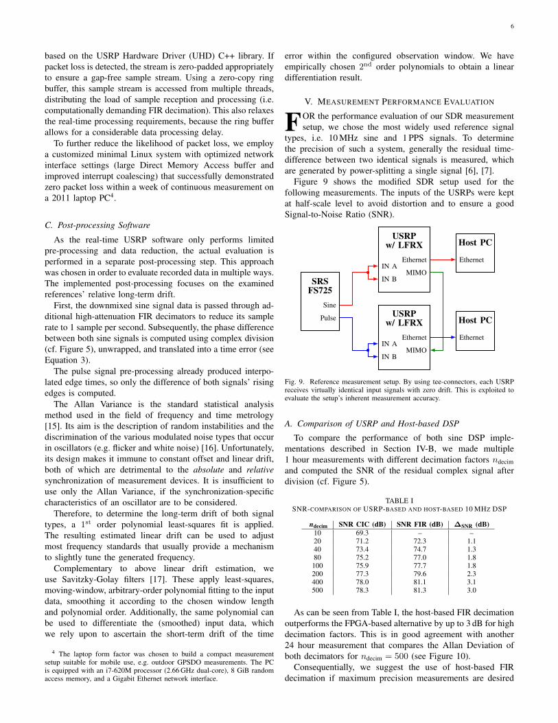
Figure 9 shows the modified SDR setup used for thefollowing measurements. The inputs of the USRPs were keptat half-scale level to avoid distortion and to ensure a goodSignal-to-Noise Ratio (SNR).

SRSFS725

Sine

Pulse

USRPw/ LFRX

EthernetIN A

MIMOIN B

USRPw/ LFRX

EthernetIN A

MIMOIN B

Host PC

Ethernet

Host PC

Ethernet

Fig. 9. Reference measurement setup. By using tee-connectors, each USRPreceives virtually identical input signals with zero drift. This is exploited toevaluate the setup’s inherent measurement accuracy.

A. Comparison of USRP and Host-based DSP

To compare the performance of both sine DSP imple-mentations described in Section IV-B, we made multiple1 hour measurements with different decimation factors ndecimand computed the SNR of the residual complex signal afterdivision (cf. Figure 5).

TABLE ISNR-COMPARISON OF USRP-BASED AND HOST-BASED 10 MHZ DSP

ndecim SNR CIC (dB) SNR FIR (dB) ∆SNR (dB)10 69.3 – –20 71.2 72.3 1.140 73.4 74.7 1.380 75.2 77.0 1.8

100 75.9 77.7 1.8200 77.3 79.6 2.3400 78.0 81.1 3.1500 78.3 81.3 3.0

As can be seen from Table I, the host-based FIR decimationoutperforms the FPGA-based alternative by up to 3 dB for highdecimation factors. This is in good agreement with another24 hour measurement that compares the Allan Deviation ofboth decimators for ndecim = 500 (see Figure 10).

Consequentially, we suggest the use of host-based FIRdecimation if maximum precision measurements are desired

7

10−4 10−3 10−2 10−1 100

10−7

10−8

10−9

10−10

10−11

10−12

Averaging time τ (s)

Alla

nD

evia

tionσy(τ

)

USRP CICHost FIR

Fig. 10. Allan Deviation of FPGA-based CIC and host-based FIR decimatorsfor ndecim = 500 during a 24 hour measurement. The Allan Deviation isdisplayed up to τ = 100 s for better readability, but both curves’ slope anddifference continue until at least τ = 104 s.

and its computational overhead is acceptable. We use the FIRdecimator for our subsequent measurements to benefit fromits superior precision.

B. Long-term Stability Measurement

To evaluate the SDR measurement system’s precision andlong-term stability, a continuous 95-hour measurement wastaken. The resulting measurement data was evaluated as de-scribed in Section IV-C with a 2 hour Savitzky-Golay windowlength.

−122.0

−121.5

−121.0

−120.5

−120.0

−119.5

−119.0

Tim

e er

ror

(ps)

0 12 24 36 48 60 72 84 96

Time (h)

−0.10

−0.05

0.00

0.05

0.10

Dri

ft (

ppq)

Fig. 11. 10 MHz signal reference measurement results. Figure shows raw timeerror (gray dots), linear drift fit (black dashed line), raw time error histogram(gray), normal distribution (black), Savitzky-Golay filtered time error (blue)and Savitzky-Golay differentiated short-time drift (red), the latter specifiedin parts-per-quadrillion (ppq, 10−15). See Section IV-C for time error anddrift definitions. Note the negligible linear drift (−2.67 ·10−19) and standarddeviation (σ = 359 fs).

Figure 11 illustrates the 10 MHz signal measurement results.Despite the raw data’s erratic appearance, its histogram revealsa normal distribution. The time error resolution is outstanding,with a 3σ accuracy of 1.08 ps, which corresponds to a phaseangle resolution of 14.0 seconds of arc. These results can mostlikely be explained by the tremendous level of decimation, i.e.averaging, applied to the analog input signals.

160

180

200

220

240

260

280

Tim

e er

ror

(ps)

0 12 24 36 48 60 72 84 96

Time (h)

−3

−2

−1

0

1

2

3

Dri

ft (

ppq)

Fig. 12. 1 PPS signal reference measurement results. Figure shows raw timeerror (gray dots), linear drift fit (black dashed line), raw time error histogram(gray), normal distribution (black), Savitzky-Golay filtered time error (blue)and Savitzky-Golay differentiated short-time drift (red), the latter specifiedin parts-per-quadrillion (ppq, 10−15). See Section IV-C for time error anddrift definitions. Note the minimal linear drift (−1.83 · 10−17) and standarddeviation (σ = 16.60 ps).

Figure 12 depicts the 1 PPS signal measurement results.Although significantly worse than the 10 MHz values, the 3σtime error resolution of 50 ps is still excellent, considering thehigh level of interpolation applied to the 25 MS/s input data(i.e. 40 ns of sample spacing).

TABLE II10 MHZ AND 1 PPS REFERENCE MEASUREMENT RESULTS

10 MHz 1 PPSσ 359 fs 16.6 psµ −121 ps 218 ps

Linear drift −2.67 · 10−19 −1.83 · 10−17

As can be concluded from Table II, both signal types’time errors show a comparatively high average value. Sincea constant difference is irrelevant for our intended drift mea-surements, we did not investigate possible sources. However,different propagation delays are a likely explanation, since120 ps correspond to only 2.4 cm of RG58 coax cabling.

If absolute measurement values are desired, further systemcalibration efforts beyond the scope of this paper becomenecessary.

C. Comparison with DMTD, TIC, and SDR Systems

A direct comparison from a synchronization-centric pointof view of DMTD and TIC systems with our SDR solutionwould be highly interesting. However, we do not have DMTDor TIC hardware at our disposal, necessitating us to limit ourcomparison to published standard performance data, i.e. AllanVariance (DMTD) or standard deviation (TIC), respectively.Regrettably, this rules out long-term stability considerations(cf. Figure 11, Figure 12, and Section IV-C).

8

10 MHz Signal: Figure 13 uses the Allan Variance to com-pare the 10 MHz signal measurement performance of multipleDMTD and both SDR systems. Although our SDR mea-surement performs slightly worse than most analog DMTDsystems for small τ , it outperforms all of them for τ � 103 s.

The results of Sherman and Jordens are not directly com-parable, because they employ a maximum likelihood time-domain optimization algorithm to determine the instantaneousfrequency ϕe(t) (cf. Equation 1), assuming a linear phase driftduring a variable observation window (see Appendix A of theirpaper [7]). This approach reduces the signal’s wideband noiseand therefore improves its signal-to-noise ratio, decreasing theAllan Variance.

However, Sherman’s algorithm will distort the spectralcharacteristics of the signal, if the instantaneous frequency isnot constant within the entire window. Particularly for longobservation durations (Sherman chose τ ≈ 103 s), a constantϕe(t) cannot be unconditionally assumed.

We avoid any such distortions, by using only spectrum-preserving post-processing prior to the computation of theAllan Variance, i.e. low-pass decimation with relatively highcut-off frequencies (fc,3 dB ≈ 0.8 fNyquist). Additionally, ourinvestigation of decimation on the host PC using floating-point arithmetic shows a 3 dB precision gain over Sherman’suse of the USRP’s built-in fixed-point DSP (see Section V-A).Therefore, we consider our algorithm a more general and moreaccurate approach.

100 101 102 103 104

10−12

10−13

10−14

10−15

10−16

10−17

Averaging time τ (s)

Alla

nD

evia

tionσy(τ

) A7 DMTD ShermanIREE SDR Sherman5110A SDR Andrich

Fig. 13. Allan Deviation of different 10 MHz measurement systems, namelythree DMTD systems (black lines, graphically extracted from [18]), anunknown DMTD system used for comparison by Sherman [7], and both SDR-based systems. Note that the SDR solutions perform comparably to DMTDhardware. Sherman’s SDR results were post-processed using an averaginginterval of τ ≈ 103 s. Therefore, their results are not comparable to ours (seeSection V-C for details).

1 PPS Signal: Table III lists the standard deviations σ ofmultiple TIC implementations capable of 1 PPS measurement,mostly taken from a comparison published by Szplet et al.[19]. The performance of our SDR system is comparableto that of FPGA-borne solutions (same order of magnitude).However, it is entirely software-based and therefore avoidsthe integration effort required to build a measurement systemusing only FPGA hardware. Since we are the first to publishsuch a solution [8], there are no references with other SDR-based 1 PPS measurements available for comparison.

TABLE IIIMEASUREMENT PERFORMANCE OF TIME INTERVAL COUNTERS

Ref., Year Platform Method σ (ps)[19] 2013 FPGA Equivalent coding line 6[20] 2014 FPGA Four-phase clock, 150

Time coding line[19] 2016 FPGA Multi-edge coding in 6

independent coding lines[19] 2016 FPGA Equivalent coding line 4.5This work SDR Low-pass and linear 16.6

interpolation

D. Comparison with Laboratory Measurement Equipment

Instead of specialized DMTD or TIC gear, general purposelaboratory measurement hardware can be relied upon forreference signal analysis. We have identified two devices tobe used in a long-term stability comparison, namely a Rohde& Schwarz FSUP Signal Source Analyzer and a TektronixDPO7254 Digital Sampling Oscilloscope. Similar devicesshould be available in any well-equipped RF laboratory, al-though results for other units will most likely vary.

Signal Analyzer: The Rohde & Schwarz FSUP combinesphase noise testing and spectrum analysis features in a single$100,000 class device. It supports various phase noise mea-surement scenarios, including the measurement of 2 DevicesUnder Test (DUT) against each other, which is requiredfor a comparison with our SDR solution. The double DUTmeasurement mandates control over at least one oscillator’sfrequency by supplying a tuning voltage, as is typical forVoltage Controlled Oscillators (VCO). However, referencesignal generators cannot be tuned like VCOs and the FSUPfails to lock its phase detector without tuning control.

Unfortunately, the FSUP does not enable the comparisonof 2 reference signal generators as is supported by our SDRsystem. Although the FSUP is solicited as phase noise tester,we assume that the use case was not envisioned or intended bythe designers, which is unfortunate, considering the device’scost. Consequently, the split-signal measurement to charac-terize the device’s precision (cf. Section V, Figure 9) is notpossible, either.

Digital Sampling Oscilloscope: The Tektronix DPO7254 isa 4 channel, 40 Giga Samples (GS) per second Digital Sam-pling Oscilloscope (DSO) with 2.5 GHz of analog bandwidth.It is a $30,000 class device with various built-in measure-ment features, including those required to measure the phasedifference of sinusoidal signals and the time difference (i.e.delay) between the edges of pulse signals. Thus, it supportsthe features required for a comparison with our SDR systemout of the box.

We realized the split-signal measurement from Figure 9,using a single DPO7254 instead of 2 synchronized USRPN210. The DPO’s channels used for 1 PPS measurementoperated at the full 2.5 GHz bandwidth for maximum timeresolution, while the 10 MHz measurement channels wereband-limited at 20 MHz to suppress wide-band noise. In orderto gain an insight into the DPO’s measurement abilities, wecompared 3 different configurations for 96 hours, each:

9

• Simultaneous measurement of 10 MHz and 1 PPS signalsas enabled by our SDR setup. Full quad-channel samplerate of 10 GS/s and 500 ns observation window with 40-fold interpolation, as trade-off between both signal types’precision.

• Only the 10 MHz signal, but at 20 GS/s dual-channelsample rate. Peak observation window length of 50 µswithout interpolation to minimize measurement dead-time.

• Only the 1 PPS signal, but at 20 GS/s dual-channelsample rate. Highest possible interpolation factor of 200with 50 ns observation window length to maximize timeresolution.

We employed the built-in phase and/or delay measurementfeatures of the DPO7254 and read out the values over Ethernetusing the VXI-11 protocol, yielding exactly one measurementper second by using the 1 PPS signal to trigger the DSO5.Table IV lists the standard deviation σ, mean µ, and lineardrift of the 3 measurements outlined above, as well as ourUSRP results from Table II for comparison.

Because different cables were used for both measurements(the DPO7254 has BNC inputs; the USRP N210 has SMAports) the different µ values are non-significant and subjectto calibration, anyway. All linear drifts are smaller than thecorresponding σ values and therefore negligible.

TABLE IVPERFORMANCE COMPARISON BETWEEN SDR AND DSO

10 MHz 1 PPSUSRP N210 σ 359 fs 16.6 ps4 channel µ −121 ps 218 ps25 MS/s Linear drift −2.67 · 10−19 −1.83 · 10−17

DPO7254 σ 128 ps 30.5 ps4 channel µ 120 ps −1.75 ps10 GS/s Linear drift −8.89 · 10−17 −3.70 · 10−19

DPO7254 σ 107 ps 32.1 ps2 channel µ 44.7 ps −8.60 ps20 GS/s Linear drift 4.93 · 10−17 −1.87 · 10−18

As an additional statistical comparison of the 10 MHzmeasurements, Figure 14 illustrates their Allan Variances.Similarly to the σ values, the USRP measurement setupoutperforms the DPO by more than 2 orders of magnitude.Although the DPO uses 400 (or even 800) times the samplerate of the USRP, this advantage is nullified by the DPO’ssubstantial measurement dead-time (zero vs. ≥ 99.995 %) andhigher noise bandwidth (0.8 Hz vs. 20 MHz), compared to theUSRP.

Although the Allan Variation is usually relied upon tocharacterize sinusoidal oscillators, we also use it to statisticallycompare the 1 PPS measurements (see Figure 15). Here, theUSRP and the DPO are much closer, but the USRP still leadsby a factor of 2. Curiously, the DPO’s precision deteriorateswhen switching from 10 GS/s to 20 GS/s. This could be caused

5Note that although the DPO7254 supports multiple measurements persecond, it only refreshes its value display twice in that interval. Curiously, thesame limitation applies to the VXI-11 value readout. Therefore, we did notattempt to increase the sample rate for the dual-channel 10 MHz measurementby using an external trigger signal faster than the 1 PPS. For both othermeasurements, the 1 PPS signal must be used as trigger, anyway.

100 101 102 103 104 105

10−10

10−11

10−12

10−13

10−14

10−15

10−16

10−17

Averaging time τ (s)

Alla

nD

evia

tionσy(τ

) USRP N210 25 MS/sDPO7254 4 ch. 10 GS/sDPO7254 2 ch. 20 GS/s

Fig. 14. Allan Deviation of 10 MHz signal long-term measurements. TheUSRP outperforms the DPO by more than 2 orders of magnitude. Note thatthe dual-channel DPO measurement enables a slight improvement over itsquad-channel counterpart.

by the DPO internally interleaving 2 ADCs to double thesample rate at the potential cost of increased noise and jitter.

It seems quite impressive that an inexpensive SDR out-performs a DSO, which provides more than 200 times theanalog bandwidth (i.e. time resolution) and 400 (or even 800)times the sample rate. This is facilitated by the versatility ofthe Software Defined Radio platform, allowing to implementcustomized algorithms that achieve vast precision gains. It alsoproves that our algorithm’s combination of low-pass and linearinterpolation (cf. Section III-B) is well suited for the preciseestimation of signal edges.

100 101 102 103 104 105

10−10

10−11

10−12

10−13

10−14

10−15

Averaging time τ (s)

Alla

nD

evia

tionσy(τ

) USRP N210 25 MS/sDPO7254 4 ch. 10 GS/sDPO7254 2 ch. 20 GS/s

Fig. 15. Allan Deviation of 1 PPS signal long-term measurements. Note thatthe USRP outperforms the DPO by 3 dB, despite its inferior analog bandwidth(i.e. time resolution) and sample rate, compared to the latter.

VI. CONCLUSIONS

WE presented a system for high-precision measurementand analysis of reference signals, based on commercial

off-the-shelf Software Defined Radio (SDR) hardware. AsSDR platforms are quite common in research laboratories, itseems likely to use them also for instrumentation in a cost-efficient way. In this paper, we described how to analyze thestability of sine and pulse reference signals on the basis of theUniversal Software Radio Peripheral (USRP) N210 by EttusResearch LLC.

Sine reference signals were digitally down-converted tobaseband for the analysis of phase deviations. For this purpose,out-of-the-box algorithms natively provided by common SDRscan be used as a basis. As an extension, we demonstrated thatthe precision of the Digital Signal Processing chain (whichis normally provided by SDRs using fixed-point arithmetic)

10

can be improved by custom software, running on the hostPC. Using floating-point arithmetic in connection with SingleInstruction Multiple Data (SIMD) vector extensions of modernprocessors, real-time performance can be provided even onmoderate hardware.

The analysis of pulse reference signals was realized by asoftware trigger running on the host PC that precisely locatesthe trigger event time, i.e. where the slope passes a certainthreshold. Clearly, due to limited sample rate an adequate post-processing was needed. Therefore, low-pass interpolation forincreasing the sample density was applied, followed by a linearinterpolation to ascertain the fractional sample index of thetrigger event.

Using the USRP N210 SDR-platform, a measurement pre-cision (standard deviation) of 0.36 ps and 16.6 ps was obtainedfor 10 MHz and 1 PPS reference signals, respectively, whichis in the same order of magnitude compared to state-of-the-artmethods such as the Dual Mixer Time Difference (DMTD)method and the Time Interval Counter (TIC).

Furthermore, joint and individual measurements of 10 MHzand 1 PPS signals with a Digital Sampling Oscilloscope (Tek-tronix DPO7254) showed that our proposed inexpensive SDR-based approach outperforms high-grade laboratory equipmentby more than 2 orders of magnitude for 10 MHz phaseestimation and by factor 2 for 1 PPS edge detection. The SDRis also less bulky, cheaper, and more power efficient.

The proposed SDR-setup can be used out of the box, e.g.to check the integrity or rather for calibration of referencesources against each other. It is suitable even for long-termmeasurements (days or weeks) and inherently provides aconsistent storage of data. A similar SDR-based approach wasrecently proposed by Sherman and Jordens [7] for the analysisof sine signals, only. However, such an SDR-based systembeing capable of joint sine and pulse reference signal analysisis not found in literature, so far.

ACKNOWLEDGEMENTS

This work was supported by the Free State of Thuringia andthe European Social Fund.

REFERENCES

[1] W. Riley and D. A. Howe, “Handbook of Frequency Stability Analysis,”NIST, 7 2008. [Online]. Available: https://www.nist.gov/publications/handbook-frequency-stability-analysis

[2] M. Siccardi, D. Rovera, and S. Romisch, “Delay measurements ofPPS signals in timing systems,” in 2016 IEEE International FrequencyControl Symposium (IFCS), 5 2016, pp. 1–6.

[3] J. Kalisz, “Review of methods for time interval measurements withpicosecond resolution,” Metrologia, vol. 41, no. 1, p. 17, 2004.[Online]. Available: http://stacks.iop.org/0026-1394/41/i=1/a=004

[4] R. Szplet, D. Sondej, and G. Grzeda, “Subpicosecond-resolution time-to-digital converter with multi-edge coding in independent coding lines,” in2014 IEEE International Instrumentation and Measurement TechnologyConference (I2MTC) Proceedings, 5 2014, pp. 747–751.

[5] D. W. Allan and H. Daams, “Picosecond Time Difference MeasurementSystem,” in 29th Annual Symposium on Frequency Control, 5 1975, pp.404–411.

[6] K. Mochizuki, M. Uchino, and T. Morikawa, “Frequency-StabilityMeasurement System Using High-Speed ADCs and Digital SignalProcessing,” IEEE Transactions on Instrumentation and Measurement,vol. 56, no. 5, pp. 1887–1893, 10 2007.

[7] J. A. Sherman and R. Jordens, “Oscillator metrology with softwaredefined radio,” Review of Scientific Instruments, vol. 87, no. 5, p. 054711,2016.

[8] C. Andrich, A. Ihlow, W. Kotterman, N. Beuster, and G. D. Galdo,“Using software defined radios for baseband phase measurement andfrequency standard calibration,” in 2017 IEEE International Instrumen-tation and Measurement Technology Conference (I2MTC), 5 2017, pp.1–5.

[9] “IEEE Standard for Synchrophasor Measurements for Power Systems,”IEEE Std C37.118.1-2011 (Revision of IEEE Std C37.118-2005), pp.1–61, 12 2011.

[10] P. Cruz, N. B. Carvalho, and K. A. Remley, “Designing and TestingSoftware-Defined Radios,” IEEE Microwave Magazine, vol. 11, no. 4,pp. 83–94, 6 2010.

[11] J. E. Volder, “The CORDIC Trigonometric Computing Technique,” IRETransactions on Electronic Computers, vol. EC-8, no. 3, pp. 330–334,9 1959.

[12] E. Hogenauer, “An economical class of digital filters for decimationand interpolation,” IEEE Transactions on Acoustics, Speech, and SignalProcessing, vol. 29, no. 2, pp. 155–162, 4 1981.

[13] L. Doolittle, “Filtering and Decimation by Eight in an FPGAfor SDR and Other Applications,” 2010. [Online]. Available: http://recycle.lbl.gov/∼ldoolitt/halfband/filter.pdf

[14] “USRP DDC Verilog source code,” Ettus Research LLC.[Online]. Available: https://github.com/EttusResearch/fpga/blob/UHD-3.10.1.1/usrp2/sdr lib/ddc chain.v#L108

[15] “IEEE Standard Definitions of Physical Quantities for FundamentalFrequency and Time Metrology – Random Instabilities,” IEEE Std 1139-2008 (Revision of IEEE Std 1139-1999), pp. 1–50, 2 2009.

[16] J. Rutman and F. L. Walls, “Characterization of frequency stability inprecision frequency sources,” Proceedings of the IEEE, vol. 79, no. 7,pp. 952–960, 7 1991.

[17] A. Savitzky and M. J. E. Golay, “Smoothing and Differentiation of Databy Simplified Least Squares Procedures,” Analytical Chemistry, vol. 36,no. 8, pp. 1627–1639, 1964.

[18] L. Sojdr, J. Cermak, and G. Brida, “Comparison of high-precisionfrequency-stability measurement systems,” in IEEE International Fre-quency Control Symposium and PDA Exhibition Jointly with the 17thEuropean Frequency and Time Forum, 2003. Proceedings of the 2003,5 2003, pp. 317–325.

[19] R. Szplet, P. Kwiatkowski, Z. Jachna, and K. Rozyc, “An eight-channel4.5-ps precision timestamps-based time interval counter in fpga chip,”IEEE Transactions on Instrumentation and Measurement, vol. 65, no. 9,pp. 2088–2100, 9 2016.

[20] R. Szplet, P. Kwiatkowski, K. Rozyc, M. Sawicki, and Z. Jachna,“Modular time interval counter,” in 2014 European Frequency and TimeForum (EFTF), 6 2014, pp. 494–497.