DEGREE PROJECT:FPGA IMPLEMENTATION OF THE ORB

ALGORITHM

BYZHANG XINYUAN

ANDEMIL STURK SELLSTEDT

Supervisor: Steffen MalkowskyCo-Supervisor: Lucas Ferreira

Examiner: Erik Larsson

Abstract

Image feature extraction has become a key technology in the field of autonom-ous Artificial Intelligence. The algorithm Oriented FAST and Rotated BRIEF(ORB), uses established technologies in image processing to allow a computerto ”see” and navigate its surroundings. This process however, is very per-formance intensive, but a field-programmable gate array (FPGA), a program-mable semiconductor device based on an integrated circuit, can be used toaccelerate this process with good power efficiency and make it feasible forsmall computationally challenged implementations, such as drones. In thisthesis an FPGA implementation of the ORB algorithm is taken as the re-search object, aiming at finding out an efficient way to implement ORB onan FPGA board. The main work of this thesis is as follows:

• Construct ORB in C++ without the OpenCV library to understand theprocess of ORB algorithm better.

• Based on the above step, present two methods to implement ORBcalculation on FPGA board.

• Discuss the results of the two methods and summarise their pros andcons.

I

Contents

Abstract I

1 Introduction 1

2 Theory 52.1 Visual SLAM . . . . . . . . . . . . . . . . . . . . . . . . . . . 62.2 ORB Algorithm . . . . . . . . . . . . . . . . . . . . . . . . . . 7

2.2.1 Gaussian image pyramid . . . . . . . . . . . . . . . . . 82.2.2 FAST . . . . . . . . . . . . . . . . . . . . . . . . . . . 112.2.3 Harris . . . . . . . . . . . . . . . . . . . . . . . . . . . 132.2.4 Intensity Centroid . . . . . . . . . . . . . . . . . . . . 162.2.5 BRIEF . . . . . . . . . . . . . . . . . . . . . . . . . . 18

3 Method 213.1 C++ deconstruction . . . . . . . . . . . . . . . . . . . . . . . . 223.2 Xilinx construction . . . . . . . . . . . . . . . . . . . . . . . . 23

3.2.1 Design flow of Vivado HLS . . . . . . . . . . . . . . . 233.2.2 Vivado Hardware construction . . . . . . . . . . . . . . 26

3.3 Python implementation . . . . . . . . . . . . . . . . . . . . . 27

4 Results and Discussion 284.1 Software Implementation . . . . . . . . . . . . . . . . . . . . . 28

4.1.1 C++ construction . . . . . . . . . . . . . . . . . . . . . 284.1.2 FPGA Python performance . . . . . . . . . . . . . . . 30

4.2 Hardware Implementation . . . . . . . . . . . . . . . . . . . . 324.2.1 Synthesis reports and result . . . . . . . . . . . . . . . 32

5 Conclusion 35

II

List of Figures

2.1 Simple diagram of the principle behind sparse visual SLAM . 72.2 Flowchart of ORB algorithm . . . . . . . . . . . . . . . . . . . 82.3 Basic image pyramid . . . . . . . . . . . . . . . . . . . . . . . 92.4 Processing time for 5x5 kernel [11] . . . . . . . . . . . . . . . 102.5 12 point segment test corner detection in an image patch. [4] . 122.6 Hardware implementation of FAST with a n = 9 pixels long

segment [12] . . . . . . . . . . . . . . . . . . . . . . . . . . . 132.7 Using OpenCV implementation: Left; 3158 Keypoints detec-

ted by FAST. Right; The 2000 Keypoints with the greatestHarris score . . . . . . . . . . . . . . . . . . . . . . . . . . . . 14

2.8 Left: Image gradient in horizontal dimension. Right: Imagegradient in vertical dimension . . . . . . . . . . . . . . . . . . 15

2.9 ORB Feature points with angles drawn as lines detected andcalculated using OpenCV implementations . . . . . . . . . . . 16

2.10 OpenCV ORB Feature matching of similar rBRIEF descriptors 18

3.1 The design flow inside Vivado HLS . . . . . . . . . . . . . . . 253.2 FAST detection after optimisation . . . . . . . . . . . . . . . 263.3 Block diagram . . . . . . . . . . . . . . . . . . . . . . . . . . . 26

4.1 OpenCV implementation of ORB (Left) compared to our (Right) 294.2 Software OpenCV ORB result (Left) compared to Vivado

ORB result (Right) . . . . . . . . . . . . . . . . . . . . . . . . 34

III

Chapter 1

Introduction

Two of the most well known technologies in recent years have been A.I. (Arti-

ficial Intelligence) and unmanned flying vehicles, often referred to as drones.

As the interest in these technologies continues to rise it seems inevitable that

the two technologies would be combined.

Autonomous drones can have a multitude of uses, such as search and

rescue, military operations, surveillance, deliveries [1][2] or simply allowing

drones to avoid obstacles. There has been a lot of development invested into

the field of self-navigating cars, and billions are being put into the field in

the hopes to be the first with a road safe and legal self-navigating vehicle.

Self-navigating drones have not received the same amount of industry fer-

vour as cars, and it is understandable why, as drones cater to a much more

niche market than the global transport sector. There are also several chal-

lenges that self-navigating drones face which are not of as large concern for

cars, and a few advantages they enjoy over their four wheeled counterparts.

One of the main advantages drones enjoy are that they are in general

slower than cars, meaning that the speed at which the drone’s A.I. has to

make decisions is slower than for the car’s. Drones are not subject to traffic

in the same way cars are, meaning that the drones do not need to be able

to process the same amount of information rapidly gathered from multiple

angles, but can instead focus on simply not hitting anything in its trajectory.

1

The main drawback drones face versus cars is their comparatively very

small size and power. While a car can carry with it fuel or batteries to drive

for hours, many drones have to make due with very limited size, weight, flight

time under an hour and limited access to power [1], as the limitation of bat-

teries has a big impact on the performance of drones.

As drones have not yet taken a large role in the transport section the

main functionality required of a self-navigating drone is to be able to stay

flying without hitting anything and to be able to orient itself within 3D space.

With the limitations mentioned earlier in mind the self navigation cannot re-

quire much space, or a large amount of power, as such the system must be

constructed using highly optimised tools and methods in order to maximise

flight capability. Some of the theorised methods include GPS based navig-

ation [1][2], as a GPS transmitter/receiver can be made very lightweight.

However, this does not grant a location with a degree of precision that one

can expect a self-navigating drone to need.

Another idea is to have the drones camera transmit its data to a remote

unit that performs the calculations required for self-navigating flight [1]. That

however faces the same drawbacks as a drone piloted by a human, and re-

quires the same line of sight between transmitter and receiver. The seemingly

most promising implementation is thus to use the pictures from the drone’s

front facing camera as input for the A.I. to navigate by, provided it can be

achieved within the set restrictions.

The core issue that must be solved is how to interpret the 2D pictures

captured by a camera into a 3D space that the drone can use to navigate,

and how to do it by using as little computational power as possible. The

currently most promising technology to achieve Simultaneous Localisation

and Mapping (SLAM) [3] is based on identifying and describing points of

interest, usually corners and edges, called feature points.

The process of generating feature points is called feature extraction, and

by repeated extractions on a series of images captured by a camera one can

2

track key locations. The tracking is performed by assigning each feature with

an identifying descriptor which should be retained over camera movement.

By knowing the drones movements, and observing the positional changes

of the tracked features one can then begin modelling the three dimensional

space around the camera [1].

The tasks needed for feature extraction can be performed by a number

of existing algorithms and methods: FAST (Features from Accelerated Seg-

ment Test) [4] is a well tested keypoint detector, and BRIEF (Binary Robust

Independent Elementary Features) [5] is a descriptor generator. They are

both fast compared to the main alternatives of using either the SIFT (scale-

invariant feature transform) [6] or SURF (scale-invariant feature transform)

[7] detectors/descriptors, with the additional advantage of not having the

licensing requirements of the proprietary SIFT and SURF technologies.

ORB [8] or Oriented FAST and Rotated BRIEF is based upon the FAST,

Harris and BRIEF algorithms and is a well tested and high performing

method to perform feature extraction and tracking, which requires a large

number of nonlinear function operations. An easy way to implement ORB in

software is to use OpenCV, an open-source library for image processing and

performing computer vision tasks. The calculation methods involve a large

number of floating point and division type operations which can be resource

intensive.

For Field-programmable gate array (FPGA) implementations, it is hard

to make OpenCV libraries run in the ARM processor. Meanwhile, the ORB al-

gorithm will consume a lot of computing resources and clocks in the hardware

implementation process, thus the system processing speed will be difficult to

meet the desired effect in practical use. To solve the problem mentioned and

compute ORB on the Zynq UltraScale+ MPSoC board, the topic of this pro-

ject is to discuss and compare two possible solutions, as followed, to find the

most efficient one for implementing ORB on the board.

• Using Vivado HLS video library for ORB algorithm and the OpenCV

3

library only for accessing the input and output images, providing the

design prototypes for video processing algorithm implementations. Then

design hardware hardware accelerators for crucial parts in order to meet

the needs of the drone system.

• Using OpenCV through python directly on the board’s processor.

4

Chapter 2

Theory

In order for an autonomous system to be able to navigate itself it needs to

be able to [9]:

• Observe its vicinity and measure the position of noticeable features

• Keep track of features detected in the surrounding area

• Determine its own location in reference to said features

These problems are covered under the umbrella of sparse Simultaneous

localisation and mapping, or sparse-SLAM. Once a system can achieve these

points it should be able to avoid collisions, perform navigational tasks (such

as moving from point A to B) and construct a three dimensional map of its

surroundings.

There are a multitude of ways for a unit to detect its surrounding such

as [9]: RADAR, LIDAR or SONAR. All of these methods do require both a

transmitter and a receiver, and they map everything within range and view of

their transmitters. This results in a lot of data to handle in real-time, which

is required for safe autonomous navigation.

An alternative would be to use a camera, which only needs a receiving

unit (the camera). Most cameras only collect data as a two dimensional grid

of pixels, without any measurements regarding distance to any particular

feature. However, there are systems that utilise RGB-D cameras [9], that

5

by emitting structured infrared light and observing its reflection can infer

depth. Regardless of if there is a depth component to the measurements:

further processing of the data is required in order to enable a camera-based

method of orientation.

Methods such as those mentioned above that measure the distance to

everything within view of the detector do not fall under sparse-SLAM but

are rather described as dense-SLAM. Sparse-SLAM works in the sub-set of

an image that is deemed most interesting. This drastically reduces the com-

putational requirements in comparison to the dense solutions. The simplicity

of sparse in relation to dense also makes sparse solutions easier to implement

in hardware.

2.1 Visual SLAM

Visual SLAM uses the data captured from a digital camera to construct

its environment and locate itself within it. However, as stated previously,

camera images do not contain any data regarding distance to an object. The

way visual SLAM resolves this issue is by detecting and extracting points

of interest, known as features and generating descriptors that identify these

features.

After the camera has moved, and the movement has been tracked by the

unit, if the same feature produces a descriptor which can be matched to

its previous extraction then, by knowing the different registered positions of

said features and the movement which produced the change, one can begin

to create a map of features in the surrounding area [9] [8]. A simple diagram

of this triangulation can be seen in Figure 2.1

6

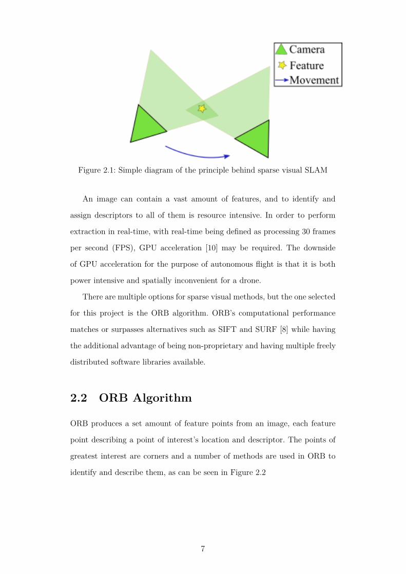
Figure 2.1: Simple diagram of the principle behind sparse visual SLAM

An image can contain a vast amount of features, and to identify and

assign descriptors to all of them is resource intensive. In order to perform

extraction in real-time, with real-time being defined as processing 30 frames

per second (FPS), GPU acceleration [10] may be required. The downside

of GPU acceleration for the purpose of autonomous flight is that it is both

power intensive and spatially inconvenient for a drone.

There are multiple options for sparse visual methods, but the one selected

for this project is the ORB algorithm. ORB’s computational performance

matches or surpasses alternatives such as SIFT and SURF [8] while having

the additional advantage of being non-proprietary and having multiple freely

distributed software libraries available.

2.2 ORB Algorithm

ORB produces a set amount of feature points from an image, each feature

point describing a point of interest’s location and descriptor. The points of

greatest interest are corners and a number of methods are used in ORB to

identify and describe them, as can be seen in Figure 2.2

7

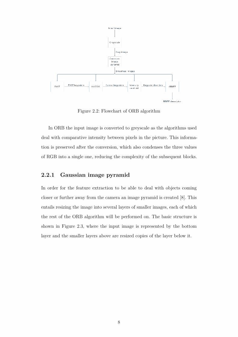
Figure 2.2: Flowchart of ORB algorithm

In ORB the input image is converted to greyscale as the algorithms used

deal with comparative intensity between pixels in the picture. This informa-

tion is preserved after the conversion, which also condenses the three values

of RGB into a single one, reducing the complexity of the subsequent blocks.

2.2.1 Gaussian image pyramid

In order for the feature extraction to be able to deal with objects coming

closer or further away from the camera an image pyramid is created [8]. This

entails resizing the image into several layers of smaller images, each of which

the rest of the ORB algorithm will be performed on. The basic structure is

shown in Figure 2.3, where the input image is represented by the bottom

layer and the smaller layers above are resized copies of the layer below it.

8

Figure 2.3: Basic image pyramid

Many of the methods used in ORB are based on comparing values of

singular pixels, and are therefore very noise-sensitive [5], this is why it is

important to smooth the image before processing. A Gaussian filtering is

generally performed via a pixel-wise convolution with a Gaussian kernel of

fixed size generated via [11]

G(x, y) =1

2πσyσx

exp((y − µy)2 − (x− µx)

2

2σyσx

),

where x and y are the spatial coordinates in the image plane. For a standard

Gaussian function the standard deviation σ = σx = σy and mean µ = µx =

µy. The standard deviation and the mean are the factors which determine

the width and amount of blurring performed by the filter [11].

In our implementation we use a commonly used pyramid with eight layers

and each layer’s image size being 0.833 of the previous layer’s. The perform-

ance of both FAST and smoothing scales with the inverse of the image’s

size, meaning that as the layer gets smaller their performance impact will

decrease. Still the requirement of a Gaussian pyramid introduces a need of

parallelism in hardware implementations of ORB, since each operations needs

to be performed in tandem for each layer for minimum wait times.

9

Hardware implications

The repeated convolution of the smoothing requires multiple ADD and MUL

operations to be performed, and there are several hardware designs available

to perform them. Gaussian 2D filtering possesses the property that it is

separable [11], which means that it can be performed as two passes of one

dimensional convolutions. A comparison between a separable filter and a

generalised filter with a kernel size of 5x5 proposed in [11] implemented on

a FPGA is shown in Figure 2.4.

Figure 2.4: Processing time for 5x5 kernel [11]

Both designs have a low impact in terms of resource utilisation, requiring

less than 1% of available register and LUTs slices of the FPGA [11]. For a 60

FPS camera, the maximum time a process can take in order to be finished

before the next frame is 16.67 ms. This means that even though the resource

requirements of the smoothing is low, for larger images it can have large

performance implications.

Since the smoothing has to be done on each layer of the pyramid, if each

image is not processed in parallel the performance impact will scale with

10

the amount of layers. However, as the images of the layers grow smaller the

processing time goes down. which means that if done in parallel the largest

image will be the performance bottleneck.

2.2.2 FAST

The FAST feature point detector is an effective and simple comparative de-

tector that has a low performance impact [4]. Due to its simple design it

does not produce any metric by which to compare and rank the quality of

different features, it is very much a binary pass-fail test. As such it is used

as a first pass to limit the work done by the more resource intensive Harris

corner detector, which does produce more nuanced results.

The FAST test is based om comparing the intensity of a pixel with the

intensity of surrounding pixels [4]. Specifically it works by checking if there

is a continuous segment of n pixels in a circle of radius r that all have

an intensity greater than that of the tested pixel by at least that of a pre-

determined threshold t. If the segment has a continuous segment of pixels

of length n with an intensity lower than that of the tested pixel minus the

threshold, then the central pixel would also be considered a feature point.

We shall focus on FAST using a radius of r = 3 pixels, and a segment

length of n = 12 out of the resulting 16 pixel circle. The method is visualised

in Figure 2.5 where the highlighted squares are the pixels used in the corner

detection. The pixel at p is the centre of a candidate corner. The arc indicated

by the dashed line passes through 12 contiguous pixels which are brighter

than p by more than the threshold

11

Figure 2.5: 12 point segment test corner detection in an image patch. [4].

This particular choice of radius and segment length has the property that

the segment length is 75% of the total length, which means that if one start

by testing the four pixels at the cardinal directions from the central pixel, i.e

pixels 1, 5, 9 and 13 in Figure 2.5 and less than three of them pass either of

the following two tests

Ix ≤ Ip − t,

Ix ≥ Ip + t,

where Ip is the intensity of the central pixel, Ix is the intensity of the pixel

on the circle being compared to p and t is the decided intensity threshold;

then that pixel can immediately be discarded. If the pixel is not discarded the

full segment test is performed, and if it passes by having at least a continuous

segment of n pixels that all pass the same of the two intensity test then it is

considered a feature point [4]. After the FAST detector has operated on each

level of the image pyramid, if there are fewer than desired detected features

the tests are done again but with a lowered t. The initial threshold is set in

inverse relation to the desired amount of features, but the default value for

an OpenCV FAST feature detector is 10.

12

Hardware implications

FAST is at its core a repeated comparison of two values, which is a standard

operation to implement in hardware. A solution used in [12] uses the design

showed in Figure 2.6 which ignores the fast selection criterion in favour of

dividing FAST into two tests, one for darker segments, one for brighter. Each

test then consists of an array of comparators that check if the circle pixels

are brighter/darker than the centre pixel by at least t. This produces two

binary vectors, and if either have a sub-vector of continuous ones of n then

it passes FAST.

Figure 2.6: Hardware implementation of FAST with a n = 9 pixels longsegment [12]

This implementation’s main hardware challenge is the loading of images

and the storing of the features once they are calculated. Depending on the

implementation of the detection of the sub-vector of ones, which for the

implementation of FAST-9 in [12] takes four cycles in worst case, pipelining

may be required.

2.2.3 Harris

In order to supplement the FAST feature detector ORB makes use of the

more computationally demanding Harris corner and edge detector. The Har-

ris method gives features a score based on its ”cornerness” and is useful to

determine edges from corners, and by using the score we can filter our FAST

13

points.

It is possible to skip FAST and just use a Harris detector initially, but as

we will show: the Harris method is far more complex and it being used in a

limited capacity is preferable from a performance viewpoint.

The features detected by FAST are first put through non-maximum sup-

pression (NMS) where out of features that are detected close together only

the feature with the greatest contrast between the centre pixel and and the

surrounding circle is kept. Harris is then used to give the remaining points a

score by to which they can be ranked, and the lowest scoring ones discarded.

As can be seen in Figure 2.7 this allows for a lot of superfluous features that

are not real corners to be ignored.

Figure 2.7: Using OpenCV implementation: Left; 3158 Keypoints detectedby FAST. Right; The 2000 Keypoints with the greatest Harris score

The Harris corner and edge detector scores a point within an image based

on shifting a local window a small amount in the image and determining the

average changes of image intensity [13]. If the intensity change is small for

shifts in all directions then the image patch is of a flat part of the image

with uniform pixels. If the intensity changes greatly along one axis but not

any other then the window likely straddles an edge. If shifts in all direction

cause large intensity shifts then the patch is either on a corner or a prominent

isolated point.

There are many possible windows that could be used in the Harris method.

However, to avoid potential noise induced by using a rectangular and binary

14

window a smooth circular window is preferred [13], with an example Gaussian

window:

W (x, y) = exp(−(x2 + y2)

2σxσy

),

In order to determine how the intensity shifts along different axis in an

image I the x and y image gradients are computed Ix, Iy. An example of

which using a 3x3 Sobel method is shown in Figure 2.8

Figure 2.8: Left: Image gradient in horizontal dimension. Right: Imagegradient in vertical dimension

Using these gradients and the chosen window function W the matrix M

can be constructed [13]:

M =∑

(x,y∈W )

I2x IxIy

IxIy I2y

,

The Harris corner response r is then calculated according to:

r = Det(M)− k trace2(M),

where k is an empirical constant between 0.04 and 0.06. If r is large then the

point is likely a corner, if r is large and negative it is deemed an edge, if r is

low the area is considered flat.

15

Hardware implications

The Harris algorithm heavily features matrix multiplication, both to determ-

ine the image gradients, and to then multiply said gradients together. These

are the sort of operations that GPUs can easily handle but for implementa-

tions in hardware require access to a lot of registers and logical units [14].

By using FAST first to select features to check, rather than performing

Harris over the whole image one reduces the amount of times one needs to

constructM and calculate r. However, the impact of calculating the gradients

of each frame is the same between implementations.

2.2.4 Intensity Centroid

To allow for greater matching between features that have rotated between

extractions the ORB method makes use of an intensity centroid measure to

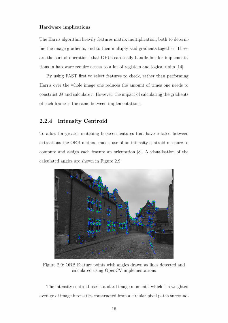
compute and assign each feature an orientation [8]. A visualisation of the

calculated angles are shown in Figure 2.9

Figure 2.9: ORB Feature points with angles drawn as lines detected andcalculated using OpenCV implementations

The intensity centroid uses standard image moments, which is a weighted

average of image intensities constructed from a circular pixel patch surround-

16

ing the feature point [15]. The patch moment is then calculated as follows:

mpq =∑(x,y)

xpyqI(x, y),

where x and y are the coordinates within the patch, I is the image intens-

ity and p and q are either 1 or 0 to define the different moments by which

the centroid C can be constructed.

c =

(m10

m00

,m01

m00

),

The orientation is thus defined as the vector −→oc with the origin o being

the centre of the corner. The orientation θ of the patch is [8]

θ = atan2(m01,m10),

where atan2 is the quadrant-aware version of arctan which returns the angle

θ (−π < θ ≤ π) for which the following holds:

m01 = rcos(θ),

m10 = rsin(θ),

Hardware implications

Depending on the desired precision with which one wants to describe θ the

hardware implementation chosen for the orientation calculation can differ.

However, since the BRIEF used in ORB discretises the angle in increments of

12 degrees (2π/30 radians) [8] a fixed point implementation with appropriate

error bars should be more than sufficient.

The proposed fixed-point implementation in [16] measures its FPGA im-

plementation in tens of nanoseconds and requires a small portion of available

resources. The moment calculations needed to be performed before atan2 are

simply repeated multiplications and additions on the stored image intensity

values, and should as such be able to be achieved by standard solutions.

17

2.2.5 BRIEF

In order to be able to match features across different images there needs to be

some measure to compare. This is the purpose of a feature point descriptor,

and the one used by the ORB algorithm is rotational BRIEF (rBRIEF) which

is a modified version of the BRIEF descriptor designed to increase matching

performance across rotations in the image plane.

BRIEF works by performing a series of binary tests, the results of which

produces a binary string, these strings can then be compared, and if the

Hamming distance between them is small enough, they can be considered a

match [5].

The two pictures in Figure 2.10 are from different perspectives along the

same street. The difference between them results in the descriptors of most

features not being similar enough to be matched, but a few key characteristics

that are not massively changed between photos can be matched along with

some mismatched features. Regardless of the mismatch ORB has shown to be

a robust method for extraction and matching, performing with comparative

or better result than other extractors [8] [17].

Figure 2.10: OpenCV ORB Feature matching of similar rBRIEF descriptors

BRIEF’s binary tests consists of comparing the intensity values of pixels

at predetermined locations in relations to the feature that is to be described.

Due to these comparisons being performed pixel by pixel basis BRIEF is very

sensitive to noise unless the image has been smoothed first, the greater the

difference between two images, the more important smoothing becomes [5].

18

A BRIEF binary test is defined as τ performed on an image patch p [5]:

τ(p; x, y) :=

1, if p(x) < p(y),

0, otherwise.,

where x and y are two different predetermined two dimensional locations

in relation to the origin which is the corner at the centre of the image patch.

So to produce a descriptor n bits long requires 2n test locations, which can

be defined as a 2 by n matrix S.

S =

x0, ..., xn

y0, ..., yn

,

From the locations in S and the test τ a BRIEF descriptor can be gener-

ated. However, while regular BRIEF performs well across shifts, it does not

perform well across rotations [8]. In order to compensate a steered version

of BRIEF is created using the orientation of the corner θ calculated from

the intensity centroid method. θ is discretised to increments of 12 degrees

and used to construct a rotation matrix Rθ [8], which for example can be

constructed as

Rθ =

cos(θ) sin(θ)

−sin(θ) cos(θ)

,

from which a steered version of S, Sθ is created.

Sθ = RθS, (2.1)

The coordinates chosen for the n test locations have large impacts on the

performance of the matching [8] [5]. In order to try and find a set of locations

which produces BRIEF tests with high variance, i.e tests which greatly react

to changes within the image patch, but still have good matching performance

the authors of [8] performed a greedy search to find a set of 256 binary tests

19

that produces descriptors with high variance that are uncorrelated (changes

at one test location does not affect the others) using a 31 by 31 pixel patch

with the test locations being pairs of 5 by 5 sub-windows in the patch.

By building S using the n = 256 tests that were found in [8] a rBRIEF

descriptor gn can be constructed as

gn(p, θ) :=∑

1≤i≤n

2i−1τ(p; xi, yi)|(xi, yi) ∈ Sθ,

which takes the form as a 256 bit long binary string that can be compared

with other stings by simple XOR operations. Due to the simplicity of this

operation and the short length of the descriptor [4] multiple features can be

compared quickly.

Hardware implications

The 2 x 2 and 2 x n matrix multiplication used to generate the test locations

in equation 2.1 is ideal for a GPU implementation as they are very good for

rapid matrix multiplications, but can be resource intensive if performed in

hardware.

Once the test locations are computed the binary nature of the test per-

formed to generate the descriptor makes for a simplistic hardware implement-

ation of n comparators. The challenge is instead to manage addresses and

memory access for an efficient processing of the image data [18].

20

Chapter 3

Method

The work as originally envisioned was split into two parts: to program a soft-

ware implementation in C++ that used as little code taken from the OpenCV

library as possible, and then to create a version of the ORB algorithm that

could run on the provided FPGA board. The C++ deconstruction was per-

formed because simply implementing a software library can be done with very

little understanding of the underlying methods, while to code it ourselves was

thought to provide greater insight into the workings of the algorithm.

If high level synthesis would be performed to create a hardware imple-

mentation, the thinking was also that not being dependant on the OpenCV

libraries would make it easier to perform HLS. But we were unable to find

a synthesisable Vitis vision/xvision library, which is similar to OpenCV lib-

rary, provided by Xilinx. So the process of ORB algorithm is changed a bit,

skipping some steps, for hardware implementation.

Ultimately the conclusion to the project was to use a SD card with a

Pynq image to boot a Linux environment on the board’s ARM processor

and run the ORB algorithm using provided Python OpenCV methods.

21

3.1 C++ deconstruction

The primary purpose of constructing the algorithm via original methods was

to gain an understanding for the ORB algorithm. As such it was made with

analysis of a singular image in mind and OpenCV methods were used for

the tasks of importing images and the OpenCV Mat structure was used to

store and manipulate them. The Mat structure is a matrix where each cell

of the matrix stores the pixel value of the corresponding pixel of an image.

These can then be read and manipulated in order to perform the steps of the

algorithm.

The first step to be implemented was a version of the FAST method to

generate the pixel location of points of interest. A series of comparative tests

were created as described in the theory section to generate over 2000 feature

point locations.

Before the Harris algorithm could be implemented the Gaussian blur func-

tion needed to be created, so methods were developed to create a Gaussian

Mat kernel and to perform repeated convolution on the image Mat object. In

addition the generation of the scale pyramid was implemented by construct-

ing a method for bilinear interpolation. The FAST method was altered to

generate over 2000 locations spread out over the 8 images in the pyramid.

Using our method for convolution with the vectors (−1, 0, 1)T and (−1, 0, 1)

[13] the image gradients were approximated as two new Mat objects for each

image. Then by using the methods in the theory section the Harris score was

calculated for each FAST location. The scores were then used to sort and

reduce the amount of feature points down to 2000.

The intensity centroid and rBRIEF were straightforwardly implemented

as described in the theory segment with the locations for the binary tests for

rBRIEF taken from bit_pattern_31 in OpenCV.

22

3.2 Xilinx construction

A large number of floating-point type operations and division-type opera-

tions are required by the ORB algorithm. The complexity of the calculations

makes it time consuming to implement ORB by programming in VHDL or

Verilog to create RTL design. The most time-efficient way for hardware con-

struction is to implement ORB by programming in C++ and synthesise it into

hardware code. Vivado HLS, the Vivado High-Level Synthesis compiler, im-

proves the abstraction level by allowing C, C++, and SystemC programming

to be directly targeted into Xilinx devices. It also facilitates the use of basic

hardware to build IP modules without developing RTL manually [19][20][21].

Vivado HLS can implement a variety of access protocols, from FIFO

interfaces to AXI4 Streams to make the data transfers between different

modules easier. Based on this, building the hardware construction contains

two key steps. The ORB algorithm IP is developed in Vivado HLS, then

exported to Vivado and built with other cores for hardware construction.

3.2.1 Design flow of Vivado HLS

OpenCV image processing is built based on the memory frame buffer. The

video frame data is always assumed to be stored in an external DDR memory.

Due to the limitation of the processor’s small-capacity cache performance,

OpenCV performs poorly in accessing partial images. Furthermore, the ar-

chitecture based on OpenCV is complicated and consumes a lot of power.

The OpenCV library seems to be sufficient to meet the requirements when

the resolution rate or frame rate is low. It, on the other hand, struggles to

meet the requirements of high performance and low power consumption for

high-resolution and high-frame-rate real-time processing. Furthermore, it is

not possible to directly synthesise the OpenCV library by Vivado HLS since

the functions in it generally involve dynamic memory allocation. As a result,

the OpenCV library can only be used for verifying the implementation of the

23

video processing algorithm.

The Xilinx Vivado HLS video library, hls_video.h, which can be synthes-

ised by Vivado HLS, can replace the OpenCV library. It implements several

basic functions contained in the OpenCV library and has similar interfaces.

The video library is mainly aimed at image processing functions implemented

in the FPGA architecture. It includes optimisations specifically for FPGAs,

such as on-chip line buffer, window buffer and fixed-point operations instead

of floating point arithmetic.

After synthesising, the processing program module can be integrated into

programmable logic. In this way, these program logic blocks can then process

the video stream produced by the processor as well as read data from files

and real-time video stream input from the outside.

The video processing module provided by Xilinx realises pixel data com-

munication that follows the AXI4 stream protocol. This ensures that each

frame has ROWS * COLS pixels, guaranteeing the integrity and resolution

of the video frames remain the same and the subsequent modules can process

the video frames properly. As shown in the Table 3.1, there are two video

data conversion functions that can be synthesised by Vivado HLS.

Table 3.1: The HLS Video Library synthesise functions [22]

Vivado Library Functions Descriptionhls::AXIvideo2Mat Converts data from an AXI4 video stream

representation to hls::Mat format.hls::Mat2AXIvideo Converts data stored as hls::Mat format to

an AXI4 video stream.

The design flow for the ORB image process within Vivado HLS is shown

in the Figure 3.1, taking all of the restrictions mentioned above into account.

In Vivado, it uses hls::Mat, which is essentially equivalent to the hls::steam

data type, to process video pixel stream rather than the matrix mat type

that is stored in external memory.

The synthesise blocks inside HLS are all processed based on video stream

data type, therefore the OpenCV library is used in the test bench to read the

24

image and convert it to the video stream format, and then convert processed

video stream format back to the image type after ORB processing. The syn-

thesiseable part is used to generate IP for the hardware construction inside

Vivado, including Gaussian filter, FAST detection, the principal direction of

each keypoint calculation and rBRIEF.

Figure 3.1: The design flow inside Vivado HLS

Several directives are added to the synthesizable block to optimize the

entire process. In a register transfer level (RTL) design, the same input and

output must be operated through the same port in the design interface and

typically using a specific input/output (I/O) protocol [22]. In this project,

input, output, rows, columns and threshold are all bound to specific ports to

ensure that they are not modified during function execution. In the meantime,

rows, columns and threshold are also assigned to the AXI4 interfaces.

The directive, HLS dataflow, is added to enable task-level pipelining, al-

25

lowing functions and loops to overlap in their operation to reduce latency

and improve concurrency and throughput [22]. After optimisation, the result

of fast detection is shown in Figure 3.2.

Figure 3.2: FAST detection after optimisation

3.2.2 Vivado Hardware construction

As it can be seen in Figure 3.3, there are other cores/blocks besides the IPs

generated from Vivado HLS required for building the hardware construction.

Figure 3.3: Block diagram

• AXI Video Direct Memory Access: It provides high-bandwidth direct

memory access between memory and AXI stream[23].A two-channel

VDMA is used in this project. It is in charge of sending the data fetched

from the input image to memory as well as storing the result data after

ORB processing.

26

• Zynq UltraScale+ MPSoC: This is the board core used in the pro-

ject. By setting parameters, including I/O, clock, DDR, PS-PL, PCle,

isolation configuration, and auto wire connection option, Vivado also

generates Processor System Reset and AXI Interconnect core to help

every block of this project connects to each other.

• Processor System Reset: It provides resets for an entire processor sys-

tem, including the processor, the interconnect and peripherals[24]. After

adding the two cores above, by choosing auto connection this core is

added and connected to others.

• AXI Interconnect core: It connects AXI memory-mapped master devices

to one or more memory-mapped slave devices[25]. It connects all the

cores used inside this project.

3.3 Python implementation

PYNQ is a open-source project provided by Xilinx. By using an SD card

with a bootable Linux image one can access a interactive Jupyter Notebook

environment via a USB connection in which one can program and run Python

code. It also has the capability to utilise specific libraries to use hardware

acceleration on the software.

Our implementation does not use any hardware libraries, and only runs

OpenCV software libraries on the ARM processor in conjunction with a USB

camera to do the real time feature detection and write the resulting features

and descriptors to the on board DRAM.

27

Chapter 4

Results and Discussion

In order to determine the quality of the work we have done, and to place it

in a larger context of SLAM functionality we need to measure and analyse

the performance of the different implementations.

4.1 Software Implementation

While our attempts to accelerate the ORB algorithm on the FPGA were

ultimately unsuccessful an analysis of the performance of the software im-

plementation can be of use to quantify how much the algorithm needs to be

accelerated to be viable, and what parts of the algorithm have the largest

impact on performance.

4.1.1 C++ construction

In order to be able to use the performance of our C++ implementation we first

need to establish that it works. A comparison between our implementation

and the established OpenCV one can be seen in Figure 4.1.

28

Figure 4.1: OpenCV implementation of ORB (Left) compared to our(Right)

As shown in the figure above our implementation does not produce the

exact same result as the OpenCV one. This can be due to a multitude of

reasons, however as the resulting image could be deemed similar enough. We

will use the performance of our algorithm in an attempt to analyse the per-

formance impact of the different blocks that make up ORB. These numbers

are to be taken very cautiously though as our implementation took over 6

times longer to complete than the OpenCV one. This performance differen-

tial is most likely due to the OpenCV library being worked on and optimised

by many talented individuals over multiple years, which does not hold true

for our implementation.

Table 4.1: Performance impact of different blocks in our ORB implementation

Block % of runtimeGaussian Pyramid 58.13FAST 13.31Harris 12.97Sorting 12.81Intensity Centroid 0.13rBRIEF 2.64

As shown in Table 4.1, for our algorithm the generation of the Gaussian

pyramid has the greatest impact by far. Supplementing our method with

the OpenCV methods for resizing and Gaussian blur the impact reduces to

25.44% indicating that generating an 8-layer Gaussian pyramid is a resource

intensive task, regardless of our inefficient implementations. This means that

29

in any hardware implementation pyramid generation will likely be a prime

candidate for acceleration.

According to the design that was examined in the theory section from

[11] Gaussian pyramid generation can be accelerated with low processing

time and little resource usage.

The sorting used is a simple naive sorting method, a carefully chosen

sorting algorithm would increase performance and should be used in any

serious implementation. The Harris block will always act on a limited number

of points while the load on FAST scales with the resolution of the image. So

depending on the resolution the impact, and therefore acceleration priority

shifts between the blocks.

The IC and rBRIEF take up comparatively little computational time, and

are thus of low priority to optimise and/or accelerate.

4.1.2 FPGA Python performance

When running the OpenCV Python implementation on the board with a

640x480 USB-camera feeding the processor could handle around 8-12 frames

per second, depending on the complexity and amount of details in the cam-

era’s view. That is too slow for reactive autonomous navigation, but since

it is running in software, if one had access to more processing resources the

performance would improve.

Compared to the performance of the A9 ARM processor implementation

shown in [3] where feature extraction takes 291 ms (3.47 FPS) the impact of

processor performance is clear when compared to the A53 processor used in

our testing. It is also clear that when one takes into account that complete

SLAM for autonomous flight needs to perform both extraction, storage and

matching at high a speeds a pure software implementation does not seem fit

for purpose.

In [10] by using a Nvidia Jetson Xavier GPU development kit as an

accelerator they were able accelerate the complete ORB-SLAM to reach 34

30

FPS, but at a great increase in power consumption which could be a problem

for a drone mounted solution. As an added note the Jetson Xavier kit used in

[10] weighs 648 grams, with most of the weight being due to cooling solutions.

For real-time applications 30 FPS is the minimum acceptable perform-

ance, which the Jetson Xavier solution is able to match. However, the added

weight may be of hindrance unless a lighter cooling method can be devised,

and the limited battery capability of a drone greatly limits how much GPU

acceleration can be utilised.

In [12] and [26] two FPGA hardware implementations of the ORB al-

gorithm are implemented with 81 FPS at 100 Mhz and 108 FPS at 200 Mhz

respectively, both at a resolution of 1920 x 1080. The implementations con-

sume 24.5 and 873 mW which needs to be taken into consideration in relation

to drone battery capacity [26]. Also clearly shows the massive performance

improvement between hardware and software implementations of ORB image

processing, with their results showing an over 20 times increase in FPS.

It seems clear that a pure software implementation is not currently ad-

equate for autonomous flight unless the circumstances for the drone are safe,

slow and predictable.

31

4.2 Hardware Implementation

The camera part is not included in the hardware construction, as stated

in the last chapter. The ORB algorithm block receives input directly from

the VDMA. To test the function of ORB hardware accelerator, the software

development environment for application projects, SDK, is used for sending

the input image data to VDMA. The verification steps are as followed:

• Converting the input image to arrays in C.

• Generating output products, exporting hardware and launching SDK

from Vivado.

• Copying the arrays into the source file and coding the main file for SDK

writing the arrays into one VDMA and displaying the result.

4.2.1 Synthesis reports and result

The interface RTL ports summary can be seen in the Table 4.2. Six ports are

generated as ap_ctrl_hs of block-level I/O interface protocol to control the

design process and indicate the state of the design. Three ports are generated

as ap_stable, which means they always remain stable after reset. There are 18

ports working through AXI4-Stream interface, including input data, output

data and control signals.

Table 4.2: Interface RTL ports summary

Protocol Amounts of ports directionap_ctrl_hs 3 inap_ctrl_hs 3 outap_stable 3 inaxis 9 inaxis 9 out

After adjusting synthesis time period to meet no negative slack, the tim-

ing report is shown in Table 4.3. The clock uncertainty, 1.50 ns, ensures there

is some timing margin available for the net delays due to place and routing

32

[27]. The estimated clock period, worst-case delay, is 8.25 ns. After applying

optimisation directives, the latency, the number of cycles it takes to produce

the output, is several cycles less than the interval, the number of clock cycles

before new inputs can be applied [22].

With the period time and the latency shown in Table 4.4, the estimated

execution time is around 17.4 ms for a image. So 57 FPS is the maximum

performance for this hardware accelerator.

Table 4.3: Timing summary

Clock(ns) Target Estimated Uncertaintyap_clk(ns) 10.00 8.25 1.50

Table 4.4: Latency summary

Latency(clock cycles) Interval(clock cycles)min max min max Type210 2111641 183 2111634 dataflow

FPGAs are made out of thousands of Configurable Logic Blocks (CLBs)

embedded in an ocean of programmable interconnects, which can implement

complex logic functions. Table 4.5 presents a summary of different FPGA

resources used in the design after synthesis. As seen under utilisation the

synthesised design uses a small amount of the available block ram, digital

signal processors, flip-flops and lookup tables. So the implementation is at

no risk of being bottlenecked due to lack of resources.

Table 4.5: Utilisation summary

Total Available Utilisation(%)BRAM 22 312 6.89DSP 3 1728 0.17FF 4344 460800 0.94LUT 5793 230400 2.51

As shown in the Figure 4.2, the ORB result from Xilinx Vivado simulation

does not exactly match to the result of software implemented OpenCV. This

is due to two key factors.

33

One is that the Gaussian filter function and the FAST detection function

are called directly by HLS video library. So the functions themselves do not

match perfectly with those in OpenCV library.

The other reason is that the Harris corner detector is not implemented in

the hardware design and the desired amount of keypoints is directly approx-

imated by adjusting the threshold in the FAST detection. This is unlike the

software implementation, where always exactly 2000 keypoints are selected

due to the Harris selection process.

Nonetheless, the result from the Vivado implementation is fairly similar

to that of software OpenCV. A non-fixed amount of keypoints could how-

ever produce issues in a full hardware implementation depending on how the

system stores and loads its features and descriptors.

Figure 4.2: Software OpenCV ORB result (Left) compared to Vivado ORBresult (Right)

34

Chapter 5

Conclusion

The topic of this thesis is to study ORB image feature extraction algorithms

and discuss two methods for implementing ORB computation on FPGA

boards.

For the hardware implementation method, there are two steps. First gen-

erate an ORB IP via Vivado HLS, then build a hardware construction for

FPGA board using this IP in Vivado. The advantages of this method are:

• Compared to programming in a hardware language such as VHDL dir-

ectly, Vivado HLS could improve the productivity by programming in

C++. Unlike VHDL, there is no need to consider about the parallelism

and sequence in C++. By synthesising the code through optimisation

directives, Vivado HLS could not only compile C++ to VHDL or verilog

level, but also schedule the whole process in a highly efficient way. This

makes the hardware design process more convenient and efficient.

• Compared to the method we used of running the OpenCV library in

software, a hardware implementation would be faster. Vivado HLS

helps compile C++ to the same level as VHDL. This allows for the

underlying logical circuit to perform the operations directly.

Compared to the easy to use Python implementation, a lower level

implementation is more abstract and usually involves a combination of

various hardware functionalities.

35

There are also some disadvantages:

• The utilisation of resources for a synthesised IP is often less efficient

than one programmed in VHDL directly by hand. In this project, this

disadvantage is particularly obvious, since the Gaussian filter function

and FAST detection function are called in the HLS video library dir-

ectly instead of coding them step by step.

• The design for a hardware implementation is much more complex than

that for using Python directly on board. Thus the amount of time and

work required is greater. Although the FAST detection and Gaussian

filter functions could be found in the HLS video library, the other parts

of ORB algorithm still need coding step by step. Therefore the Harris

corner detection is omitted in our hardware construction, making the

ORB accuracy not good as the Python one. Also, in Vivado it needs

to build every block and connect them for hardware construction. It

takes a lot of time to find which core is needed for the project and ad-

just the parameters setting again and again, especially the board Zynq

UltraScale+ MPSoC IP’s parameters. It is significantly more complex

and time-consuming for hardware construction .

Table 5.1: FPS comparison

Xilinx Python Python without Harris Python without pyramidFPS ~57 ~8 ~8 ~14

The speed comparison in Table 5.1 show the possible theoretical per-

formance of a successful Xilinx implementation in comparison to the meas-

ured performance of the OpenCV python method running in software on the

board.

With the above points and table in mind and taking into consideration

that a processor that is fast enough to run the entirety of the ORB algorithm

in software at a speed acceptable for drone mounted SLAM while being

light and power efficient enough to not impede the operation of said drone

36

has not turned up in this study; it seems that the most feasible way to

implement ORB for our stated purpose is by hardware acceleration of parts

of the algorithm. The easiest way to implement is via a PYNQ overlay.

A properly developed overlay allows one to implement HLS generated IP’s

on the FPGA and to read and write to them. For future work on running

ORB on an FPGA we would recommend to use the OpenCV Python libraries

in PYNQ and accelerate them by creating PYNQ overlays with IP’s for the

blocks that have the largest performance impact.

From our results and the measurements in Table 5.1 the areas to prioritise

would seem to be the Gaussian pyramid generation and FAST algorithm. We

cannot however, definitively state these as the greatest problem areas for the

on-board OpenCV implementation, as the performance impact of not using

an image pyramid may be more due to the reduced workload of not having

to perform ORB in every layer of the pyramid. It would also seem that the

limited use of Harris on around 2000 features has negligible impact, but that

could change if the implementation required a greater amount of features.

Regardless the complexities of hardware generation and the poor perform-

ance from software running on an adequately small processing units makes

an intelligently implemented hybrid the best alternative in our eyes.

37

Bibliography

[1] Erqian Tang, Sobhan Niknam and Todor Stefanov. ‘Enabling Cognitive

Autonomy on Small Drones by Efficient On-Board Embedded Comput-

ing: An ORB-SLAM2 Case Study’. In: 2019 22nd Euromicro Confer-

ence on Digital System Design (DSD). 2019, pp. 108–115.

[2] Karim Amer et al. ‘Deep convolutional neural network based autonom-

ous drone navigation’. In: International Conference on Machine Vision.

2021.

[3] Runze Liu et al. ‘eSLAM: An Energy-Efficient Accelerator for Real-

Time ORB-SLAM on FPGA Platform’. In: 2019 56th ACM/IEEE

Design Automation Conference (DAC) (2019), pp. 1–6.

[4] Edward Rosten and Tom Drummond. ‘Machine Learning for High-

Speed Corner Detection’. In: vol. 3951. July 2006. isbn: 978-3-540-

33832-1.

[5] Michael Calonder et al. ‘BRIEF: Binary Robust Independent Element-

ary Features’. In: 2010 European Conference on Computer Vision. Vol. 6314.

Sept. 2010, pp. 778–792. isbn: 978-3-642-15560-4.

[6] David G. Lowe. ‘Distinctive Image Features from Scale-Invariant Key-

points’. In: International Journal of Computer Vision 60 (Nov. 2004).

[7] Herbert Bay. Andreas Ess. Tinne Tuytelaars. Luc Van Gool. ‘Speeded-

Up Robust Features (SURF)’. In: Computer Vision and Image Under-

standing 110 (June 2008), pp. 346–359.

38

[8] Ethan Rublee et al. ‘ORB: An efficient alternative to SIFT or SURF’.

In: 2011 International Conference on Computer Vision. 2011, pp. 2564–

2571.

[9] Max Pfingsthorn and Andreas Birk. ‘Simultaneous localization and

mapping with multimodal probability distributions’. In: The Interna-

tional Journal of Robotics Research 32.2 (2013), pp. 143–171.

[10] Tao Peng et al. ‘An Evaluation of Embedded GPU Systems for Visual

SLAM Algorithms’. In: vol. 2020. Jan. 2020, pp. 325–1.

[11] Debasish Mukherjee and Susanta Mukhopadhyay. ‘Fast Hardware Ar-

chitecture for Fixed-point 2D Gaussian Filter’. In: AEU - International

Journal of Electronics and Communications 105 (Apr. 2019).

[12] Rongdi Sun et al. ‘A low latency feature extraction accelerator with

reduced internal memory’. In: 2017 IEEE International Symposium on

Circuits and Systems (ISCAS). 2017, pp. 1–4.

[13] Christopher G. Harris and M. J. Stephens. ‘A Combined Corner and

Edge Detector’. In: Alvey Vision Conference. 1988.

[14] Tak Lon Chao and Kin Hong Wong. ‘An efficient FPGA implement-

ation of the Harris corner feature detector’. In: 2015 14th IAPR In-

ternational Conference on Machine Vision Applications (MVA). 2015,

pp. 89–93.

[15] Paul Rosin. ‘Measuring Corner Properties’. In: Computer Vision and

Image Understanding 73 (Feb. 1999), pp. 291–307.

[16] Florent De Dinechin and Matei Istoan. ‘Hardware Implementations

of Fixed-Point Atan2’. In: 2015 IEEE 22nd Symposium on Computer

Arithmetic. 2015, pp. 34–41.

[17] A.V.Kulkarni. J.S.Jagtap. V.K.Harpale. ‘Object recognition with ORB

and its Implementation on FPGA’. In: ICETTR-2013, pp. 156–162.

39

[18] Roberto de Lima et al. ‘Accelerating the construction of BRIEF descriptors

using an FPGA-based architecture’. In: 2015 International Conference

on ReConFigurable Computing and FPGAs (ReConFig). Dec. 2015,

pp. 1–6.

[19] Xilinx. Xilinx Accelerates Productivity for Zynq-7000 All Programmable

SoCs with the Vivado Design Suite 2014.3, SDK, and New UltraFast

Embedded Design Methodology Guide.

[20] Xilinx. Vivado Design Suite 2014.1 Increases Productivity with Auto-

mation of UltraFast Design Methodology and OpenCL Hardware Accel-

eration.

[21] Clive Maxfield. Free High-Level Synthesis Guide for S/W Engineers.

Dec. 2021. url: https://www.xilinx.com/support/documentation/

sw_manuals/ug998-vivado-intro-fpga-design-hls.pdf.

[22] Xilinx. Vivado Design Suite User Guide, High-Level Synthesis, UG902.

May 2014.

[23] Xilinx. ‘AXI Video Direct Memory Access v6.3’. In: LogiCORE IP

Product Guide (Oct. 2017).

[24] Xilinx. ‘Processor System Reset Module v5.0’. In: LogiCORE IP Product

Guide (Nov. 2015).

[25] Xilinx. ‘AXI Interconnect v2.1’. In: LogiCORE IP Product Guide (Dec.

2017).

[26] Rongdi Sun et al. ‘A Flexible and Efficient Real-Time ORB-Based Full-

HD Image Feature Extraction Accelerator’. In: IEEE Transactions on

Very Large Scale Integration (VLSI) Systems 28.2 (2020), pp. 565–575.

[27] Xilinx. Vivado Design Suite User Guide, High-Level Synthesis, UG871.

May 2014.

40