An FPGA Implementation of the Mean-Shift Algorithm for ...
233
An FPGA Implementation of the Mean-Shift Algorithm for Object Tracking Stefan Wong Faculty Of Design And Creative Technologies AUT University A thesis submitted for the degree of Master of Engineering October 2014
-
Upload
khangminh22 -
Category
Documents
-
view
3 -
download
0
Transcript of An FPGA Implementation of the Mean-Shift Algorithm for ...

An FPGA Implementation of the
Mean-Shift Algorithm for Object
Tracking
Stefan Wong
Faculty Of Design And Creative Technologies
AUT University
A thesis submitted for the degree of
Master of Engineering
October 2014

Abstract
Object tracking remains an important field of study within the broader
discipline of Computer Vision. Over time, it has found application in a
wide variety of areas, including industrial automation [1] [2], user interfaces
[3] [4] [5], navigation [6] [7] [8], object retreival [9] [10] [11], surveillance [12]
[13], and many more besides [14] [15] [16] [17] [18] [19]. A subset of these
applications benefit from real-time or high-speed operation [20] [21] [22] [23].
This study attempts to implement the well known CAMSHIFT algorithm
from its original specification [24] in an FPGA. The inner loop operation
to compute the mean shift vector is unrolled and vectorised to achieve real
time operation. This allows the mean shift vector to be computed and the
target to be localised within the frame acquisition time without the need
for multiple clock domains.


Acknowledgements
Firstly, I must thank my supervisor Dr. John Collins for his honest feedback
and tireless patience during this study. I would also like to thank my family,
who’s support I could not have done without. As well as this, all the
previous researchers in the field, without whom I would have no foundation
to build on, and who are consistently more insightful and clever than myself.
Contents
List of Figures viii
List of Tables xv
1 Introduction 1
1.1 Motivation . . . . . . . . . . . . . . . . . . . . . . . . . . . . . . . . . . 1
1.2 Thesis Contributions . . . . . . . . . . . . . . . . . . . . . . . . . . . . . 2
1.3 Thesis Layout . . . . . . . . . . . . . . . . . . . . . . . . . . . . . . . . . 2
2 Literature Review 4
2.1 Visual Object Tracking . . . . . . . . . . . . . . . . . . . . . . . . . . . 4
2.1.1 Representation of Objects . . . . . . . . . . . . . . . . . . . . . . 6
2.2 Feature Selection and Extraction . . . . . . . . . . . . . . . . . . . . . . 6
2.3 Tracking Approaches in Literature . . . . . . . . . . . . . . . . . . . . . 8
2.4 Kernel-Based Trackers . . . . . . . . . . . . . . . . . . . . . . . . . . . . 9
2.5 Previous Tracking Implementations . . . . . . . . . . . . . . . . . . . . . 9
2.5.1 Software Implementations . . . . . . . . . . . . . . . . . . . . . . 9
2.5.2 Hardware Implementations . . . . . . . . . . . . . . . . . . . . . 20
2.5.3 Final Comment on Previous Implementations . . . . . . . . . . . 32
2.6 Review of Circuit Design and Verification . . . . . . . . . . . . . . . . . 34
2.6.1 Overview of Verification . . . . . . . . . . . . . . . . . . . . . . . 34
2.6.2 Review of Verification Literature . . . . . . . . . . . . . . . . . . 36
2.7 Thesis Contributions . . . . . . . . . . . . . . . . . . . . . . . . . . . . . 38
iii

CONTENTS
3 Theory Background 40
3.1 Colour Spaces . . . . . . . . . . . . . . . . . . . . . . . . . . . . . . . . . 40
3.2 Kernel Object Tracking . . . . . . . . . . . . . . . . . . . . . . . . . . . 44
3.2.1 Kernel Density Estimation . . . . . . . . . . . . . . . . . . . . . 45
3.3 Mean Shift Weight Images . . . . . . . . . . . . . . . . . . . . . . . . . . 46
3.3.1 Explicit Weight Image . . . . . . . . . . . . . . . . . . . . . . . . 46
3.3.2 Implicit Weight Image . . . . . . . . . . . . . . . . . . . . . . . . 47
3.4 A Closer Examination of Weight Images in Comaniciu, et.al . . . . . . . 49
3.5 Tracking Algorithm . . . . . . . . . . . . . . . . . . . . . . . . . . . . . . 51
3.5.1 Tracking in Bradski . . . . . . . . . . . . . . . . . . . . . . . . . 51
3.5.2 Tracking in Comainciu, Ramesh, and Meer . . . . . . . . . . . . 55
3.6 Mean Shift Vector . . . . . . . . . . . . . . . . . . . . . . . . . . . . . . 57
4 Hardware Implementation Considerations 59
4.1 Mean Shift Tracker Operation . . . . . . . . . . . . . . . . . . . . . . . . 59
4.1.1 Tracking and Frame Boundary . . . . . . . . . . . . . . . . . . . 61
4.2 Pipeline Orientation . . . . . . . . . . . . . . . . . . . . . . . . . . . . . 62
4.2.1 Segmentation Pipeline . . . . . . . . . . . . . . . . . . . . . . . . 63
4.3 Backprojection in Hardware . . . . . . . . . . . . . . . . . . . . . . . . . 65
4.3.1 Hardware implementations of histograms . . . . . . . . . . . . . 65
4.3.2 Indexing Histogram Bins . . . . . . . . . . . . . . . . . . . . . . 68
4.4 Maintaining Stream Architecture in Segmentation Pipeline . . . . . . . 69
4.4.1 Datapath Timing . . . . . . . . . . . . . . . . . . . . . . . . . . . 69
4.4.2 Memory Allocation for Streaming Operation . . . . . . . . . . . 71
4.4.3 Aligning Division with Blanking Interval . . . . . . . . . . . . . . 72
4.5 Weight Image Representation . . . . . . . . . . . . . . . . . . . . . . . . 73
4.6 Scaling Buffer . . . . . . . . . . . . . . . . . . . . . . . . . . . . . . . . . 76
4.6.1 Removing Background Pixels For Storage . . . . . . . . . . . . . 76
4.6.2 Predicting Memory Allocation . . . . . . . . . . . . . . . . . . . 77
4.6.3 Limitations of Scaling Buffer . . . . . . . . . . . . . . . . . . . . 82
4.7 Tracking Pipeline . . . . . . . . . . . . . . . . . . . . . . . . . . . . . . . 83
iv
CONTENTS
5 CSoC Module Architecture 85
5.1 Early Pipeline Stages . . . . . . . . . . . . . . . . . . . . . . . . . . . . . 86
5.1.1 CMOS Acquisition . . . . . . . . . . . . . . . . . . . . . . . . . . 86
5.1.2 Colour Space Transformation . . . . . . . . . . . . . . . . . . . . 88
5.2 Segmentation Pipeline . . . . . . . . . . . . . . . . . . . . . . . . . . . . 88
5.2.1 Histogram Bank . . . . . . . . . . . . . . . . . . . . . . . . . . . 88
5.2.2 Divider Bank . . . . . . . . . . . . . . . . . . . . . . . . . . . . . 90
5.2.3 Row-Oriented Backprojection . . . . . . . . . . . . . . . . . . . . 92
5.2.4 Row Backprojection Control Strategy . . . . . . . . . . . . . . . 94
5.2.5 Column-Oriented Backprojection . . . . . . . . . . . . . . . . . . 97
5.2.6 Column Buffer . . . . . . . . . . . . . . . . . . . . . . . . . . . . 98
5.2.7 Column Backprojection Control Strategy . . . . . . . . . . . . . 99
5.2.8 Ratio Histogram in Column Oriented Pipeline . . . . . . . . . . 100
5.2.9 Weight Image Resolution . . . . . . . . . . . . . . . . . . . . . . 100
5.3 Mean Shift Buffer . . . . . . . . . . . . . . . . . . . . . . . . . . . . . . . 102
5.3.1 Full Image Buffer . . . . . . . . . . . . . . . . . . . . . . . . . . . 103
5.3.2 Scaling Image Buffer . . . . . . . . . . . . . . . . . . . . . . . . . 103
5.4 Mean Shift Pipeline . . . . . . . . . . . . . . . . . . . . . . . . . . . . . 104
5.4.1 Mean Shift Controller Hierarchy . . . . . . . . . . . . . . . . . . 105
5.4.2 Top Level Controller . . . . . . . . . . . . . . . . . . . . . . . . . 105
5.4.3 Buffer Controller . . . . . . . . . . . . . . . . . . . . . . . . . . . 106
5.4.4 Mean Shift Controller . . . . . . . . . . . . . . . . . . . . . . . . 109
5.5 Mean Shift Accumulator . . . . . . . . . . . . . . . . . . . . . . . . . . . 112
5.5.1 Scalar and Vector Accumulation . . . . . . . . . . . . . . . . . . 112
5.5.2 Vector Mask . . . . . . . . . . . . . . . . . . . . . . . . . . . . . 114
5.5.3 Arithmetic Modules . . . . . . . . . . . . . . . . . . . . . . . . . 115
5.5.4 Accumulator Controller . . . . . . . . . . . . . . . . . . . . . . . 118
5.6 Window Parameter Computation . . . . . . . . . . . . . . . . . . . . . . 119
5.7 Parameter Buffer . . . . . . . . . . . . . . . . . . . . . . . . . . . . . . . 120
v

CONTENTS
6 CSoC Verification 121
6.1 csTool Overview . . . . . . . . . . . . . . . . . . . . . . . . . . . . . . . 121
6.2 Hierarchy of Verification . . . . . . . . . . . . . . . . . . . . . . . . . . . 122
6.3 csTool Architecture and Internals . . . . . . . . . . . . . . . . . . . . . . 124
6.4 Data Oriented Testing . . . . . . . . . . . . . . . . . . . . . . . . . . . . 127
6.4.1 Class Heirarchy . . . . . . . . . . . . . . . . . . . . . . . . . . . . 128
6.5 csTool Workflow . . . . . . . . . . . . . . . . . . . . . . . . . . . . . . . 129
6.5.1 Vector Data Format . . . . . . . . . . . . . . . . . . . . . . . . . 131
6.5.2 Generation Of Vector Data For Testing . . . . . . . . . . . . . . 131
6.6 Algorithm Exploration . . . . . . . . . . . . . . . . . . . . . . . . . . . . 134
6.6.1 Trajectory Analysis . . . . . . . . . . . . . . . . . . . . . . . . . 134
6.7 Verification And Analysis . . . . . . . . . . . . . . . . . . . . . . . . . . 136
6.7.1 Pattern Testing . . . . . . . . . . . . . . . . . . . . . . . . . . . . 137
7 Experimental Results 142
7.1 Comparison of Segmentation Methods . . . . . . . . . . . . . . . . . . . 142
7.1.1 Model Histogram Thresholding . . . . . . . . . . . . . . . . . . . 144
7.1.2 Spatially Weighted Colour Indexing . . . . . . . . . . . . . . . . 148
7.1.3 Row Segmentation . . . . . . . . . . . . . . . . . . . . . . . . . . 149
7.1.4 Block Segmentation . . . . . . . . . . . . . . . . . . . . . . . . . 155
7.1.5 Spatial Segmentation . . . . . . . . . . . . . . . . . . . . . . . . . 157
7.1.6 Relationship between segmentation and tracking performance . . 162
7.1.7 Bit-Depth in Weight Image . . . . . . . . . . . . . . . . . . . . . 165
7.2 Scaling Buffer Preliminary Tests . . . . . . . . . . . . . . . . . . . . . . 169
7.3 Synthesis and Simulation of Modules . . . . . . . . . . . . . . . . . . . . 171
7.3.1 Row-Oriented Backprojection Module . . . . . . . . . . . . . . . 173
7.3.2 Column-Oriented Backprojection Module . . . . . . . . . . . . . 174
7.3.3 Mean Shift Processing Module . . . . . . . . . . . . . . . . . . . 176
7.3.4 Vector Accumulator . . . . . . . . . . . . . . . . . . . . . . . . . 177
7.3.5 Inner Product MAC . . . . . . . . . . . . . . . . . . . . . . . . . 180
7.3.6 Mean Shift Buffer . . . . . . . . . . . . . . . . . . . . . . . . . . 180
7.4 Processing Time . . . . . . . . . . . . . . . . . . . . . . . . . . . . . . . 183
vi

CONTENTS
8 Discussion and Conclusions 186
8.1 Comparison of Row and Column Pipelines . . . . . . . . . . . . . . . . . 187
8.2 On chip tracking framework . . . . . . . . . . . . . . . . . . . . . . . . . 189
8.3 Extensions to Tracking Architecture . . . . . . . . . . . . . . . . . . . . 190
8.3.1 Multiple Viewpoints . . . . . . . . . . . . . . . . . . . . . . . . . 191
8.3.2 Selection of Vector Dimension Size . . . . . . . . . . . . . . . . . 193
8.4 Remarks on Segmentation Performance . . . . . . . . . . . . . . . . . . 194
8.5 Thesis Outcomes . . . . . . . . . . . . . . . . . . . . . . . . . . . . . . . 194
9 Future Work 196
References 198
Glossary 213
vii

List of Figures
2.1 Taxonomy of tracking methods. Reproduced from [25], pp-16 . . . . . . 8
2.2 A backprojection image from [24], p.5 . . . . . . . . . . . . . . . . . . . 11
2.3 Block diagram of object tracking in CAMSHIFT algorithm. Reproduced
from [24], p.2 . . . . . . . . . . . . . . . . . . . . . . . . . . . . . . . . . 12
2.4 Subway-1 sequence. Reproduced from [26] . . . . . . . . . . . . . . . . . 14
2.5 Tuning of class histograms for online discriminative tracking. Repro-
duced from [27], pp-9 . . . . . . . . . . . . . . . . . . . . . . . . . . . . . 16
2.6 Ranked weight images produced by segmentation stage in [27] (pp-13) . 17
2.7 Block diagram overview of tracking system in [27]. Reproduced from pp-14 18
2.8 Block diagram of joint motion-colour meanshift tracker, reproduced from
[28] . . . . . . . . . . . . . . . . . . . . . . . . . . . . . . . . . . . . . . . 20
2.9 Schematic view of colour histogram computation circuit. Reproduced
from [21] . . . . . . . . . . . . . . . . . . . . . . . . . . . . . . . . . . . . 22
2.10 Input images (a) and tracking windows (b) for a rotating object in [21],
p.5 . . . . . . . . . . . . . . . . . . . . . . . . . . . . . . . . . . . . . . . 23
2.11 Diagram of hardware structure in [29] . . . . . . . . . . . . . . . . . . . 24
2.12 Block diagram of object tracking system in [30], p2 . . . . . . . . . . . . 25
2.13 Data flow of mass center calculation module in [30] . . . . . . . . . . . . 26
2.14 Block diagram of system implemented in [31] . . . . . . . . . . . . . . . 28
2.15 Reproduction of block diagram of PCA object tracking system in [32] . 29
2.16 Diagram of board connections for MT9M413 sensor. The pixel outputs
have been highlighted in green. Reproduced from [33] . . . . . . . . . . 31
2.17 Block diagram of system implemented in [34] . . . . . . . . . . . . . . . 32
2.18 Outputs from results section of [34] . . . . . . . . . . . . . . . . . . . . . 33
viii

LIST OF FIGURES
2.19 Basic verification environment. Taken from [35], pp-74 . . . . . . . . . . 35
2.20 Diagrammatic representation of abstraction levels in verification. Taken
from [35], pp-114 . . . . . . . . . . . . . . . . . . . . . . . . . . . . . . . 35
2.21 Architecture of fault injection tool described in [36] . . . . . . . . . . . . 37
2.22 Architecture of functional fault injection system from [37] . . . . . . . . 38
3.1 CIE diagram of sRGB colour space [38] . . . . . . . . . . . . . . . . . . 41
3.2 RGB cube [39] . . . . . . . . . . . . . . . . . . . . . . . . . . . . . . . . 42
4.1 Dual clock histogram from [40] . . . . . . . . . . . . . . . . . . . . . . . 66
4.2 Timing diagram of histogram bank swap . . . . . . . . . . . . . . . . . . 70
4.3 Timing diagram of buffer operations in row oriented segmentation pipeline 70
4.4 Timing diagram of buffer operations in column oriented segmentation
pipeline. Note the addition of buffering stages to ensure that zero-cycle
switching is possible without loss of data . . . . . . . . . . . . . . . . . . 71
4.5 Timing diagram of processing aligned with FULL flag . . . . . . . . . . . 71
4.6 Illustration of vector format in scaling buffer. Address words are inserted
in the vector buffer to indicate where in the vector dimension to interpret
the bit patterns in the vector word entries. The address word loads the
vector LUT in the accumulator with the correct set of positions, while
the bits in the data word indicate the presence or absence of data points
on that vector . . . . . . . . . . . . . . . . . . . . . . . . . . . . . . . . . 78
4.7 Diagram of non-zero vector buffer . . . . . . . . . . . . . . . . . . . . . . 78
4.8 Illustration of 2× 2 majority vote window. The top buffer stores pixels
at the original scale. The buffer below divides the image space by 2,
effectively halving the number of pixels required. This stage can itself
be windowed to half the number of pixels again, and so on . . . . . . . . 79
4.9 Diagram of non-zero buffer with window scaling logic . . . . . . . . . . . 81
4.10 Memory usage for various weight image representations . . . . . . . . . 82
4.11 Memory usage for scaling buffer and standard one and two bit represen-
tations . . . . . . . . . . . . . . . . . . . . . . . . . . . . . . . . . . . . . 83
4.12 Accumulation pipeline showing vector buffer, expansion LUT, and vector
masking stages . . . . . . . . . . . . . . . . . . . . . . . . . . . . . . . . 84
ix

LIST OF FIGURES
5.1 Overview of the complete CSoC pipeline . . . . . . . . . . . . . . . . . . 87
5.2 Block diagram of histogram index vector generator. See section 4.4.1 for
full discussion . . . . . . . . . . . . . . . . . . . . . . . . . . . . . . . . . 89
5.3 Block diagram of histogram module logic. The one-hot index vector on
the input drives the enable lines for a bank of incrementers which drive
the histogram bin registers. At the end of the stream, the values in the
registers form the probability distribution of the image patch . . . . . . 90
5.4 Block diagram of vectored bin indexing operation . . . . . . . . . . . . . 91
5.5 Block diagram of vectored bin indexing operation . . . . . . . . . . . . . 91
5.6 Overview of row-oriented backprojection pipeline . . . . . . . . . . . . . 93
5.7 State diagram of buffer status controller for row-oriented backprojection 95
5.8 State diagram of input side controller for row-oriented backprojection . 96
5.9 State diagram of output side controller for row-oriented backprojection . 97
5.10 Overview of column-oriented backprojection . . . . . . . . . . . . . . . . 97
5.11 Block diagram of LUT adder for column backprojection . . . . . . . . . 98
5.12 Overview of buffer used to concatenate image pixels . . . . . . . . . . . 99
5.13 Indexing of ratio histogram in column oriented pipeline . . . . . . . . . 101
5.14 Schematic view of full mean shift buffer . . . . . . . . . . . . . . . . . . 103
5.15 Mean shift accumulation and windowing pipeline . . . . . . . . . . . . . 105
5.16 State Machine for determining which buffer contains the weight image . 107
5.17 State machine for FIFO controller . . . . . . . . . . . . . . . . . . . . . 108
5.18 State diagram for mean shift controller . . . . . . . . . . . . . . . . . . . 110
5.19 Mean shift accumulator . . . . . . . . . . . . . . . . . . . . . . . . . . . 113
5.20 Schematic overview of vector mask logic . . . . . . . . . . . . . . . . . . 114
5.21 Example of vector masking operation on 8-element vector word . . . . . 116
5.22 State diagram for accumulator controller . . . . . . . . . . . . . . . . . . 118
6.1 csTool main GUI. The left panel shows a frame on disk, the right panel
shows the segmented image and tracking parameters . . . . . . . . . . . 122
6.2 Correspondence between stages in csTool pipeline and data flow in
CSoC pipeline. csTool is capable of generating data from any of these
stages to simplify testing . . . . . . . . . . . . . . . . . . . . . . . . . . . 124
6.3 Internal architecture of csTool . . . . . . . . . . . . . . . . . . . . . . . 126
x
LIST OF FIGURES
6.4 Venn Diagram of verification concerns . . . . . . . . . . . . . . . . . . . 128
6.5 Diagrammatic Representation of Column Vector Data Format . . . . . . 132
6.6 Diagrammatic Representation of Row Vector Data Format . . . . . . . . 132
6.7 csTool vector generation GUI . . . . . . . . . . . . . . . . . . . . . . . . 133
6.8 Trajectory browser showing comparison of 2 tracking runs . . . . . . . . 135
6.9 Verification GUI with frame extracted from image sequence . . . . . . . 136
6.10 Verification GUI with offset frames . . . . . . . . . . . . . . . . . . . . . 137
6.11 Verification GUI in csTool showing the results from a synthetic tracking
run . . . . . . . . . . . . . . . . . . . . . . . . . . . . . . . . . . . . . . . 137
6.12 Example of pattern testing GUI . . . . . . . . . . . . . . . . . . . . . . . 139
6.13 Pattern test with output error . . . . . . . . . . . . . . . . . . . . . . . . 139
6.14 Rescaled view of error in pattern stream . . . . . . . . . . . . . . . . . . 140
6.15 Pattern test after controller operation is corrected . . . . . . . . . . . . 140
7.1 Original frame from End of Evangelion [41] scene . . . . . . . . . . . . . 144
7.2 Comparison of Pixel HBP (left) and Block HBP (right) in End of
Evangelion sequence . . . . . . . . . . . . . . . . . . . . . . . . . . . . . 145
7.3 Image histogram for End of Evangelion frame using Pixel HBP seg-
mentation (left), and model histogram (right) . . . . . . . . . . . . . . . 145
7.4 Ratio histogram generated from Pixel HBP method on frame shown in
figure 7.1, and resulting backprojection image . . . . . . . . . . . . . . . 146
7.5 Image histogram for End of Evangelion frame using the Block HBP
segmentation method in block (0, 0) (left), and model histogram (right) 146
7.6 Ratio histogram for block (0, 0) of End of Evangelion frame using Block
HBP segmentation method, and backprojection image after block (0, 0)
has been processed . . . . . . . . . . . . . . . . . . . . . . . . . . . . . . 147
7.7 Ratio histogram generated from Block HBP in block (19, 2), and cor-
responding backprojection image for blocks (0, 0)− (19, 2) . . . . . . . . 147
7.8 Percentage of error pixels across Psy sequence per frame using Row
HBP segmentation. Row HBP backprojection image shown on left . . 150
7.9 Percentage of error pixels across Running sequence per frame using Row
HBP segmentation. Row HBP backprojection image shown on left . . 150
xi

LIST OF FIGURES
7.10 Percentage of error pixels across Face sequence per frame using Row
HBP segmentation. Row HBP backprojection image shown on left . . 151
7.11 Percentage of error pixels across End of Evangelion sequence per frame
using Row HBP segmentation. Row HBP backprojection image shown
on left . . . . . . . . . . . . . . . . . . . . . . . . . . . . . . . . . . . . . 151
7.12 Tracking comparison of Pixel HBP and Row HBP (10% threshold)
for Psy sequence . . . . . . . . . . . . . . . . . . . . . . . . . . . . . . . 152
7.13 Tracking comparison of Pixel HBP and Row HBP for Running se-
quence at 0% threshold (top), 5% threshold (middle), and 10% threshold
(bottom) . . . . . . . . . . . . . . . . . . . . . . . . . . . . . . . . . . . . 153
7.14 Tracking comparison of Pixel HBP and Row HBP for End of Evan-
gelion sequence at 0% threshold (top), 5% threshold (middle), and 10%
threshold (bottom) . . . . . . . . . . . . . . . . . . . . . . . . . . . . . . 154
7.15 Percentage of error pixels across Psy sequence per frame using Block
HBP segmentation. Block HBP backprojection image shown on left . 155
7.16 Percentage of error pixels across Running sequence per frame using
Block HBP segmentation. Block HBP backprojection image shown
on left . . . . . . . . . . . . . . . . . . . . . . . . . . . . . . . . . . . . . 156
7.17 Percentage of error pixels across Face sequence per frame using Block
HBP segmentation. Block HBP backprojection image shown on left . 156
7.18 Percentage of error pixels across End of Evangelion sequence per frame
using Block HBP segmentation. Block HBP backprojection image
shown on left . . . . . . . . . . . . . . . . . . . . . . . . . . . . . . . . . 156
7.19 Tracking comparison of Pixel HBP and Block HBP (10% threshold)
for Psy sequence . . . . . . . . . . . . . . . . . . . . . . . . . . . . . . . 157
7.20 Tracking comparison of Pixel HBP and Block HBP for Running se-
quence at 0% threshold (top), 5% threshold (middle), and 10% threshold
(bottom) . . . . . . . . . . . . . . . . . . . . . . . . . . . . . . . . . . . . 158
7.21 Tracking comparison of Pixel HBP and Block HBP for End of Evan-
gelion sequence at 0% threshold (top), 5% threshold (middle), and 10%
threshold (bottom) . . . . . . . . . . . . . . . . . . . . . . . . . . . . . . 159
xii
LIST OF FIGURES
7.22 Percentage of error pixels across Psy sequence per frame using Block
HBP (Spatial) segmentation. Block HBP (Spatial) backprojection
image shown on left . . . . . . . . . . . . . . . . . . . . . . . . . . . . . 160
7.23 Percentage of error pixels across Running sequence per frame using
Block HBP (Spatial) segmentation. Block HBP (Spatial) back-
projection image shown on left . . . . . . . . . . . . . . . . . . . . . . . 160
7.24 Percentage of error pixels across Face sequence per frame using Block
HBP (Spatial) segmentation. Block HBP (Spatial) backprojection
image shown on left . . . . . . . . . . . . . . . . . . . . . . . . . . . . . 161
7.25 Percentage of error pixels across End of Evangelion sequence per frame
using Block HBP (Spatial) segmentation. Block HBP (Spatial)
backprojection image shown on left . . . . . . . . . . . . . . . . . . . . . 161
7.26 Tracking comparison of Pixel HBP and Block HBP (Spatial) (10%
threshold) for Psy sequence . . . . . . . . . . . . . . . . . . . . . . . . . 162
7.27 Tracking comparison of Pixel HBP with 1-bit backprojection image
and Block HBP (Spatial) (10% threshold) for Face sequence . . . . . 168
7.28 Tracking comparison of Pixel HBP with 2-bit backprojection image
and Block HBP (Spatial) (10% threshold) for Face sequence . . . . . 168
7.29 Trajectory comparison of windowed moment accumulation against
a scaling buffer with Sfac = 64 on Psy sequence . . . . . . . . . . . . . . 170
7.30 Trajectory comparison of windowed moment accumulation against
a scaling buffer with Sfac = 64 on Face sequence . . . . . . . . . . . . . 171
7.31 Trajectory comparison of windowed moment accumulation against
a scaling buffer with Sfac = 64 on End of Evangelion sequence . . . . . 172
7.32 RTL view of row-oriented backprojection pipeline with annotations . . . 173
7.33 RTL view of column-oriented backprojection pipeline with annotations . 175
7.34 RTL view of window computation module with annotations . . . . . . . 176
7.35 RTL view of mean shift accumulator with annotations . . . . . . . . . . 177
7.36 RTL view of masking logic in vector accumulator with annotations . . . 178
7.37 Vector expansion at start of frame. Note that the masked lut vec line
is all zeros at this point . . . . . . . . . . . . . . . . . . . . . . . . . . . 179
7.38 Vector expansion during processing. Weight image pixels enter (pictured
top), and are expanded and masked in the pipeline . . . . . . . . . . . . 179
xiii

LIST OF FIGURES
7.39 RTL view of inner product MAC with annotations . . . . . . . . . . . . 180
7.40 Waveform output showing vector masking and moment accumulation in
mean shift pipeline . . . . . . . . . . . . . . . . . . . . . . . . . . . . . . 181
7.41 RTL view of mean shift buffer with annotations . . . . . . . . . . . . . . 181
7.42 RTL schematic of mean shift buffer controller . . . . . . . . . . . . . . . 182
7.43 Waveform dump of first write sequence in mean shift buffer . . . . . . . 182
7.44 Waveform dump of first read sequence in mean shift buffer . . . . . . . . 183
8.1 Two fully independent tracking pipelines. Weight image A is generated
from Appearance Model A applied to Input Image A, as is B to its
respective input and model . . . . . . . . . . . . . . . . . . . . . . . . . 191
8.2 Multiple targets with independent appearance models tracked in the
same image . . . . . . . . . . . . . . . . . . . . . . . . . . . . . . . . . . 192
8.3 Multiple pipelines tracking in multiple images using the same appearance
module. The SAD module illustrates how such a configuration could be
used for stereoscopic object tracking . . . . . . . . . . . . . . . . . . . . 193
xiv

List of Tables
7.1 Overview of tracking error in terms of segmentation for Psy sequence.
Numbers in parenthesis refer to model histogram threshold. All mea-
surements are vs Pixel HBP . . . . . . . . . . . . . . . . . . . . . . . . 162
7.2 Overview of tracking error in terms of segmentation for Running se-
quence. Numbers in parenthesis refer to model histogram threshold. All
measurements are vs Pixel HBP . . . . . . . . . . . . . . . . . . . . . . 163
7.3 Overview of tracking error in terms of segmentation for Face sequence
with 1-bit backprojection image. All measurements are vs Pixel HBP . 164
7.4 Overview of tracking error in terms of segmentation for End of Evange-
lion sequence. Numbers in parenthesis refer to model histogram thresh-
old. All measurements are vs Pixel HBP . . . . . . . . . . . . . . . . . 164
7.5 Overview of tracking error for Running sequence using a fully weighted
backprojection image as the reference . . . . . . . . . . . . . . . . . . . 167
7.6 Revised of tracking error in terms of segmentation for Face sequence
with 2-bit backprojection image. All measurements are vs Pixel HBP . 167
7.7 Scaling buffer comparison for the Psy sequence . . . . . . . . . . . . . . 170
7.8 Scaling buffer comparison for the Face sequence . . . . . . . . . . . . . . 171
7.9 Scaling buffer comparison for the End of Evangelion sequence . . . . . . 172
7.10 Synthesis results for modules in the row backprojection pipeline . . . . . 174
7.11 Synthesis results for modules in the column backprojection pipeline . . . 175
7.12 Synthesis results for MS PROC TOP module . . . . . . . . . . . . . . . . . 176
7.13 Synthesis results for mean shift accumulator module . . . . . . . . . . . 179
7.14 Synthesis results for MS BUF TOP module . . . . . . . . . . . . . . . . . . 182
7.15 Number of cycles per module in mean shift pipeline . . . . . . . . . . . 184
xv

LIST OF TABLES
7.16 Processing time in mean shift loop in terms of iterations . . . . . . . . . 185
xvi

Declaration
I hereby declare that this submission is my own work and that, to the best
of my knowledge and belief, it contains no material previously published or
written by another person (except where explicitly defined in the acknowl-
edgements), nor material which to a substantial extent has been submitted
for the award of any other degree or diploma of a university or other insti-
tution of higher learning.

Chapter 1
Introduction
1.1 Motivation
Visual object tracking remains an important sub-discipline within the broader field of
computer vision, and finds application in a wide variety of fields. These range from
pedestrian detection in moving vehicles [42] to feature extraction in high speed video
[43] [44], to content analysis for video streams [15] [45] [16].
At the time of writing, there is relatively little in the way of hardware imple-
mentations for the mean shift algorithm in object tracking. While there are several
previous works that are obviously inspired by this technique, none of them represent
a comprehensive port of the algorithm into the hardware domain. Filling this gap in
the literature would allow for much higher throughput analysis of mean shift vectors
at much lower energy cost. This has application in areas such as mobile vision, and
low-power video content description encoders.
One explanation for the relative lack of mean shift publications in the hardware
domain may in part be the received wisdom that algorithms with a heavy focus on
iterative computation are ill-suited to hardware implementations. In general, simple,
repetitive functions, or systems with strongly geometric layouts are best suited to direct
hardware implementation1.
1The ultimate version of this is the systolic array, in which processing elements are connected in a
grid fashion, see [46].
1

1.2 Thesis Contributions
Rather than attempt to disprove this notion in the general sense, this thesis will
attempt to show that such a constraint need not prevent the mean shift algorithm being
implemented for use in the localisation stage of a visual object tracker.
1.2 Thesis Contributions
This thesis aims to develop a hardware architecture for implementing a mean shift
based object tracking system inspired by [24] and [26]. The thesis will attempt to
show such an architecture, implemented using a simple segmentation technique based
on colour features [47] and explain how it can be extended to work with more complex
segmentation techniques. The specific implementation pursued here is directly inspired
by the CAMSHIFT technique developed by Bradski in [24] and implemented in the
OpenCV library [48]. The term CSoC (CAMSHIFT on Chip) is used throughout this
document to refer to said architecture.
1.3 Thesis Layout
The thesis follows the structure given below
1. Introduction
The current chapter, which introduces the content of the study.
2. Literature Review
This chapter provides an overview of the field of object tracking, as well as review-
ing the history of the mean shift technique. A variety of previous implementations
are provided with comment. This comment is divided between software and hard-
ware implementations. As well as this, an overview of previous work in the field
of hardware verification is provided.
3. Theoretical Background
This chapter will cover the theory behind the mean shift tracking technique, and
explain the operation of the kernel density estimation technique.
2

1.3 Thesis Layout
4. Hardware Implementation Considerations
This chapter will discuss context-specific considerations which arise when porting
the context-free algorithm specification to the context-specific hardware domain.
In performing this mapping, there are certain domain-specific compromises that
must be met. These are examined in order to contextualise the implementation
presented in this study.
5. CSoC Module Architecture
This chapter will discuss the specific architecture put forward in this study. Based
on implementations considerations discussed in chapter 4, this chapter will show
the specific hardware implementation, and discuss the rationale behind particular
design choices.
6. Verification and Analysis
This chapter discusses the development of csTool, a data-driven verification tool
used in this study to evaluate and verify the correctness of modules in the CSoC
pipeline. This tool was developed to allow the verification of the design to be
carried out at a higher level of abstraction, avoiding the tedium of analysing
the data stream at the waveform level. The chapter explains the design and
philosophy of the tool, as well as examines the internals and data structures
used.
7. Simulation and Synthesis Results
This chapter will show and explain the simulation and synthesis results gathered
during the study.
8. Discussion and Conclusions
This chapter will outline the concluding remarks for the study. A discussion on
generalising the architecture presented in this study is given, that shows how each
component can be considered part of a framework. In this way, the techniques
developed here can be used to extend applicability of the CSoC pipeline.
9. Future Work
This chapter discusses possible future directions for the CSoC pipeline.
3
Chapter 2
Literature Review
2.1 Visual Object Tracking
Object tracking is a major discipline within computer vision, which has naturally accu-
mulated an extensive body of literature. The full extent of the study of object tracking
is outside the scope of this document, however various literatures surveys exist which
attempt to summarise the field to a greater or lesser extent. These include work by
Yilmaz [25], Cannons, [49], and Li [50]. Yilmaz in particular is written to enable a new
practitioner in the field to quickly find a suitable tracking algorithm, although due to
its age, it does not provide information on more recent developments. A summary of
the field is provided here to contextualise the research. The interested reader is directed
to the above referenced work for a more thorough treatment.
Visual object tracking is the ability to determine the location of an object in some
visual space through time. The visual space in question is normally taken to mean a
camera projection of some view in the real world, and the location of the object is the
position within this projection of the target. The location may be as simple as a point
in the frame where the target lies, or may include some summary statistics which can
vary in complexity from a blob that has some equivalence (e.g.: has the same area as
the target) to a complex statistical representation [49] [50].
A huge variety of techniques have been developed and proposed for object tracking.
Even so, most object tracking systems are composed of four basic stages, initialisation,
appearance modelling, motion estimation, and object localisation [50].
4
2.1 Visual Object Tracking
1. Initialisation
Before tracking can begin the parameters for the object model must be initialised.
This process can be either manual or automatic. Manual initialisation typically
involves a user delimiting the object location with some bounding region. Au-
tomatic initialisation is commonly performed with some kind of detection stage
which can identify the target, for example a face detector. Visual trackers which
require little user input have an obvious practical advantage over those that do,
however the problem of initialisation is often ignored in the literature, and simply
assumed to be performed in some earlier step outside the main body of work [49].
This is normally the result of studies placing focus on the tracking procedure
itself, relegating the initialisation procedure as being a relatively unimportant
background detail.
2. Appearance Modelling
This stage can be understood in two parts - visual representation and statistical
modelling. Visual Representation is concerned with the construction of robust
object descriptors using visual features. Statistical Modelling deals with building
effective models for object identification using statistical learning models.
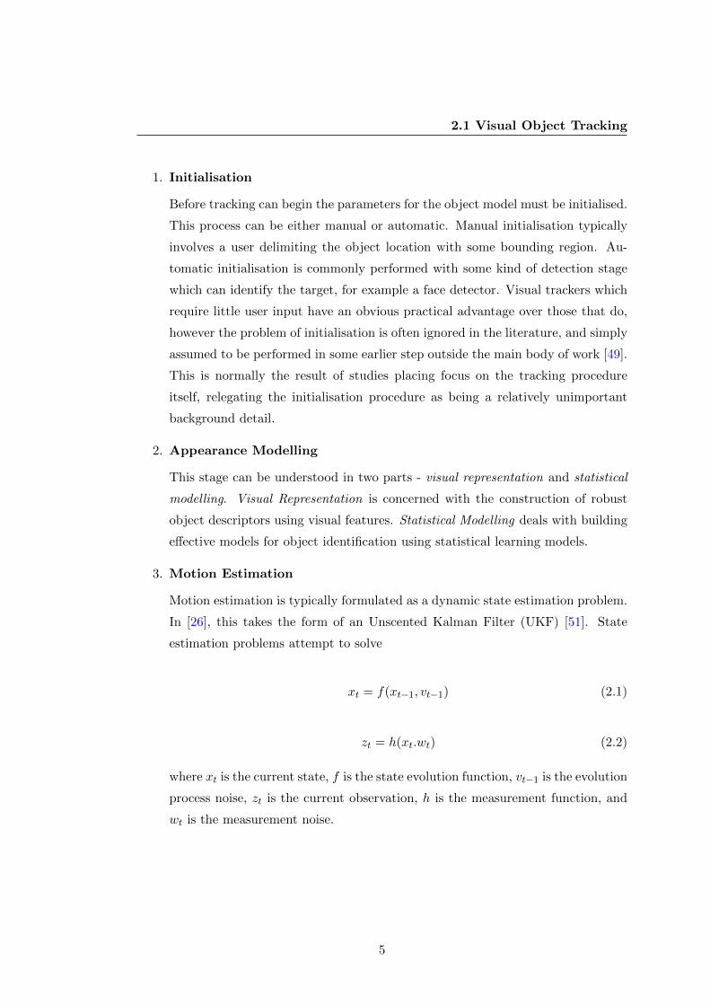
3. Motion Estimation
Motion estimation is typically formulated as a dynamic state estimation problem.
In [26], this takes the form of an Unscented Kalman Filter (UKF) [51]. State
estimation problems attempt to solve
xt = f(xt−1, vt−1) (2.1)
zt = h(xt.wt) (2.2)
where xt is the current state, f is the state evolution function, vt−1 is the evolution
process noise, zt is the current observation, h is the measurement function, and
wt is the measurement noise.
5

2.2 Feature Selection and Extraction
4. Object Localisation
A greedy search of maximum posterior estimation based on the motion estimation
in the previous step is performed to localise the object in the scene.
2.1.1 Representation of Objects
Objects can be thought of as a point of interest in a frame of video that is a candidate
for some further analysis. Objects can in principle be anything. Some common appli-
cations of object tracking include surveillance [52] [12] [13], industrial automation [1]
[2], human-computer interaction [24] [3] [4] [5], robot navigation [53] [8] [7] [6], video
compression and retrieval [15] [45] [9] [10] [11] [54], and many more areas besides [17]
[14] [18] [19].
Developing a model for robust object tracking poses many challenges. Changes
in lighting, changes in angle, low frame rate sensors, low bit-depth, colour distortion,
lens distortion, pose estimation, non-rigid objects, visual obstruction, and many other
factors all contribute to make specifying appearance models a challenging problem [50].
2.2 Feature Selection and Extraction
Feature extraction refers to the process of determining from an image a set of unique
and meaningful representations of a target or part of a target. For example, the pixel-
wise intensities of a target may be considered as a feature, and could therefore be used
to identify regions in an image where a target may lie. A feature set is one or more
features used to describe a target.
Common visual features include colour, edges, optical flow, and texture [25].
Selecting the appropriate features is essential for good tracking performance. While
the effectiveness of a particular feature is dependant on context and may be subjective,
it is generally the case that a good feature exhibits the property of uniqueness [25].
Some common features found in the tracking literature are
1. Colour
Arguably the most common feature used in the literature [49], colour features
gained attention in the mainstream tracking literature with implementations such
as [55] or the Pfinder system in [56]. These early attempts often dealt with mean
6
2.2 Feature Selection and Extraction
colour (particularly [55]), that is, a colour obtained by computing the mean values
of the R,G and B components of the target [49].
2. Edges
In computer vision, edges are strong changes in intensity formed around the
boundaries of objects in the scene. In general, edges are less sensitive to illu-
mination changes than colour features [25], and thus make a useful feature for
discriminating between objects, or between objects and backgrounds. By far the
most popular edge detection algorithm is the Canny edge detector [57], which is
both simple and accurate.
3. Optical Flow
Optical flow is a dense field of displacement vectors indicating the translation
of pixels in a region [25]. This essentially encodes the movement of every pixel
in a frame relative to its position in the previous frame, represented as a vector
showing the spatial displacement between these two points in time. This feature
is most commonly found in motion segmentation [58] and video tracking [15], and
some video encoding applications [59]. The most popular methods for computing
dense optical flow are those by Horn and Schunk [60] and Lucas and Kanade [61].
4. Texture
Texture refers to the variation of intensity of a surface which obeys some statistical
property and containing repeated similar structures [62]. Texture classification
can be divided into structural and statistical approaches, of which the statistical
approach is far more computationally efficient [63].
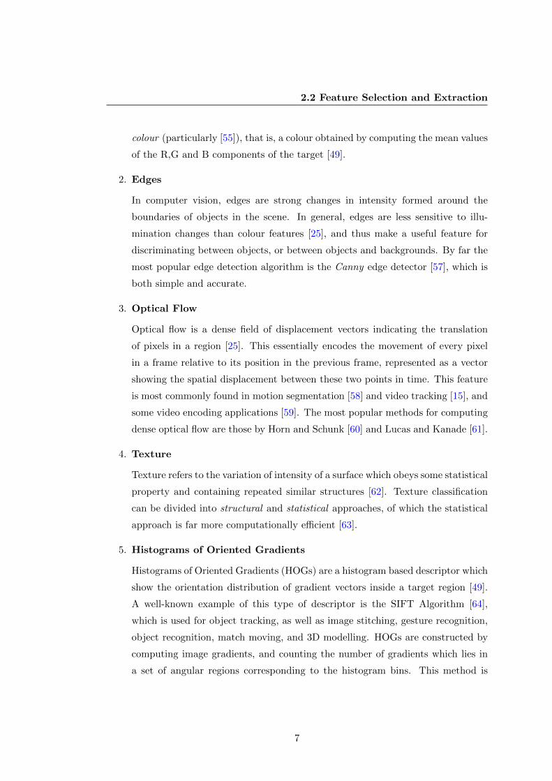
5. Histograms of Oriented Gradients
Histograms of Oriented Gradients (HOGs) are a histogram based descriptor which
show the orientation distribution of gradient vectors inside a target region [49].
A well-known example of this type of descriptor is the SIFT Algorithm [64],
which is used for object tracking, as well as image stitching, gesture recognition,
object recognition, match moving, and 3D modelling. HOGs are constructed by
computing image gradients, and counting the number of gradients which lies in
a set of angular regions corresponding to the histogram bins. This method is
7

2.3 Tracking Approaches in Literature
Figure 2.1: Taxonomy of tracking methods. Reproduced from [25], pp-16
more robust to illumination changes than colour histograms, however changed
in background clutter can adversely affect the algorithm if background gradients
provide undue influence on the target gradient model.
2.3 Tracking Approaches in Literature
Given the importance of visual object tracking within computer vision, it comes as lit-
tle surprise that several attempts have been made to implement hardware accelerations
of tracking procedures. Particularly in the embedded sphere, it is common to have a
real-time constraint that either demands more computational power, or a simplified
or otherwise computationally inexpensive approach. In these instances the benefits
of hardware acceleration are obvious - speed gains can be leveraged to meet a timing
constraint or to improve data throughput. The exact nature of the implementation de-
pends largely on the tracking technique used. An overview of some relevant approaches
is provided herein.
A taxonomy of tracking methods in the literature is shown in figure 2.1. This figure
is reproduced from Object Tracking: A Survey [25]. Although the figure is not strictly
current, reflecting the state of the art at the time of publication, it is sufficient to
illustrate the points made in this document.
8
2.4 Kernel-Based Trackers
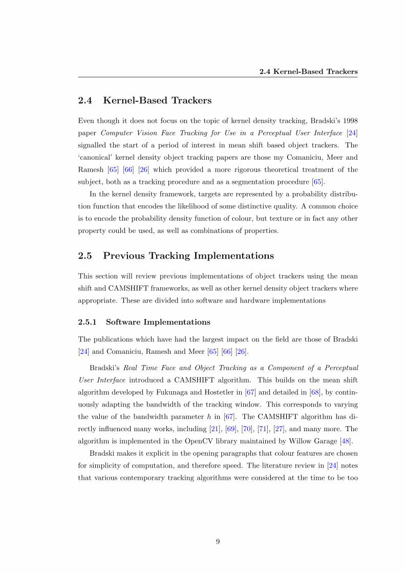
2.4 Kernel-Based Trackers
Even though it does not focus on the topic of kernel density tracking, Bradski’s 1998
paper Computer Vision Face Tracking for Use in a Perceptual User Interface [24]
signalled the start of a period of interest in mean shift based object trackers. The
‘canonical’ kernel density object tracking papers are those my Comaniciu, Meer and
Ramesh [65] [66] [26] which provided a more rigorous theoretical treatment of the
subject, both as a tracking procedure and as a segmentation procedure [65].
In the kernel density framework, targets are represented by a probability distribu-
tion function that encodes the likelihood of some distinctive quality. A common choice
is to encode the probability density function of colour, but texture or in fact any other
property could be used, as well as combinations of properties.
2.5 Previous Tracking Implementations
This section will review previous implementations of object trackers using the mean
shift and CAMSHIFT frameworks, as well as other kernel density object trackers where
appropriate. These are divided into software and hardware implementations
2.5.1 Software Implementations
The publications which have had the largest impact on the field are those of Bradski
[24] and Comaniciu, Ramesh and Meer [65] [66] [26].
Bradski’s Real Time Face and Object Tracking as a Component of a Perceptual
User Interface introduced a CAMSHIFT algorithm. This builds on the mean shift
algorithm developed by Fukunaga and Hostetler in [67] and detailed in [68], by contin-
uously adapting the bandwidth of the tracking window. This corresponds to varying
the value of the bandwidth parameter h in [67]. The CAMSHIFT algorithm has di-
rectly influenced many works, including [21], [69], [70], [71], [27], and many more. The
algorithm is implemented in the OpenCV library maintained by Willow Garage [48].
Bradski makes it explicit in the opening paragraphs that colour features are chosen
for simplicity of computation, and therefore speed. The literature review in [24] notes
that various contemporary tracking algorithms were considered at the time to be too
9

2.5 Previous Tracking Implementations
computationally expensive for use as part of a perceptual user interface. These included
[55], [72], and [73].
In [55], which tracks objects from frame to frame based on regions of similar nor-
malised colour. An example configuration of 6 regions is given on pp-21-22. Colours in
the image are tested against a colour vector Vt = (ri, gi, bi) which represents the colour
of the target. A set of 9-lattice points form a local region surrounding the hypothe-
sised location of the target. A new hypothesis is tested at each point in the lattice for
each frame in the sequence. Estimation of velocity is accomplished using a Kalman
filter [74]. The authors note that the Kalman filter is not strictly applicable to the
tracking operation as the noises in the target measurement do not exhibit a Gaussian
distribution.
In [72], segmentation of faces is performed using a region growing algorithm at
course resolutions, creating a set of connected components. Shape information is eval-
uated for each connected component, and the best fit ellipse is computed on the basis
of moments for each component. A contour is also generated by minimising the interior
energy of a snake.
In [73], a connectionist face tracker is proposed that attempts to maintain a face in
the field of view at all times. The system is capable of manipulating the orientation and
zoom of a camera to which it is connected. The system can be divided into two stages
- locating and tracking. In locating mode, the system searches for faces in the field of
view. Once located, the system enters the tracking mode, where the target is followed.
The system also tries to learn features of the observed face while tracking, and uses
these to compensated for lighting variations. This system performs segmentation using
a normalised histogram. Additionally, shape features are used to distinguish between
faces and other similarly coloured object such as hands. Tracking is performed using a
neural network which is trained on a database of face images.
CAMSHIFT represents targets in the image as a discretized probability distribu-
tion. Colour is chosen as the feature, and so targets are represented as histograms
in the feature space. The distribution of the background is subject to change over
time which requires the algorithm to continuously update the distribution of the back-
ground and compute new candidates for the target. Images are transformed into the
HSV colour space [75] and 1-dimensional histograms are formed from the Hue channel.
The initial window location is set manually by the user, triggering a sampling routine
10

2.5 Previous Tracking Implementations
Figure 2.2: A backprojection image from [24], p.5
that generates the initial model histogram. The weight image is constructed using his-
togram backprojection. A ratio histogram is formed that expresses the importance of
pixels in the image in terms of the target. Taking each pixel and backprojecting it into
image space generates a weight image with intensities corresponding to the likelihood
that a pixel is part of the target. This technique was first published in Swain & Bal-
lard [47], and developed further in other publications, including [76]. An example of a
backprojection image taken from [24] is reproduced in figure 2.2.
The mean search location is expressed as the centroid of the distribution within
a tracking window. This is expressed as the central moments weighted by the pixel
intensity in the weight image. These can be summarily expressed as
Mpq =∑x
∑y
xpyqI(x, y) (2.3)
where I(x, y) is the intensity of the pixel (x, y) in the weight image, and x and y
range over the search window. The zeroth moment conceptually represents the area1
of the target, while the first order moments in x and y represent the location of the
target in the image. The search window is computed based on the equivalent ellipse
[77], which is an ellipse that shares the same orientation, zero, first, and second order
moments as the target. The window in [24] is tuned for tracking faces, and thus the
shape is additionally scaled by
s = 2
√M00
Pmax(2.4)
1In this context, area is used to refer to the relative size of the target, as opposed to the actual
geometric area which is occupies. Some literature uses the term mass instead [48]
11

2.5 Previous Tracking Implementations
Figure 2.3: Block diagram of object tracking in CAMSHIFT algorithm. Reproduced
from [24], p.2
where M00 is the zero order moment (area) of the distribution, Pmax is the maximum
numerical value that a pixel can take, and s is the size of the window. The equation in
[24] substitutes the value 255, however this figure is meant to represent the maximum
value of any pixel in the distribution, rather than the maximum possible value. It is
noted that for tracking faces, the window width is typically set to s. and the height to
1.5 × s, to account for the somewhat elliptical shape of faces [24]. The block diagram
of the tracking procedure is reproduced in figure 2.3. An extended discussion on the
CAMSHIFT procedure can be found in section 3.3.1.
CAMSHIFT is an early example of a colour histogram object tracker. The weight
image technique used in CAMSHIFT explicitly generates a new image by backprojec-
tion pixels from the ratio histogram space to the image space. However despite its
early success, this system still suffers from the same problems that are common to all
colour feature trackers. Namely, sensitivity to illumination changes, and lack of dis-
criminatory power. Illumination changes are a particular problem for outdoor scenes,
as pixel intensity is dependant on many factors, including global illumination, sensor
quantisation effects, and so on. The ability to compute the position and orientation of
the target with no extra calibration at 30 frames per second circa 1998 still marks this
as an impressive and influential work.
12

2.5 Previous Tracking Implementations
The ideas developed in [24] have also been directly applied in many other papers,
including [69], [70], [27], [78], [79], [80], and many many more. An expanded theoretical
framework for this method of object tracking was developed in [66] and [26], with further
work by Collins in [71].
Comaniciu, Ramesh, and Meer’s Kernel-Based Object Tracking [26] gives the most
comprehensive explanation of this style of object tracker. This paper introduced the
concept of masking a target in a scene with an isotropic kernel function. This allows a
spatially-smooth similarity function to be defined, which in turn reduces the problem
of tracking the target to a search in the basin of attraction of this function. Targets
are modelled by a probability density function q in some feature space. In [26], the
colour probability density function is chosen as the feature for tracking. The target
is represented by an ellipsoid in the image, normalised to a unit circle to eliminate
possible distortions due to scale. Use of a differentiable kernel profile will yield a
differentiable similarity function. Various functions can be used [81]. A similarity
function is defined based on the Bhattcharyya coefficient [82] which allows comparison
between histograms. This function is used to maximise the similarity between the
histogram of the target PDF, and the histogram of the image PDF. This is equivalent
to minimising the distance between the target and the kernel window. The expression
of the target model is given in [26] as
qu = C
n∑i=1
k(‖x∗i ‖
2)δ [b(x∗i )− u] (2.5)
where the function b : R2 → 1, . . . ,m associates the pixel at location x∗i the index
b(x∗i ) of its bin in quantised feature space. Target candidates are similarly defined by
a spatially weighted histogram given by
pu(y) = Ch
nh∑i=1
k
(∥∥∥∥y − xi
h
∥∥∥∥2)δ[b(xi − u] (2.6)
Details of the implementation of the algorithm in [26] are discussed further in sec-
tion 3.4. The target is transformed into a weight image which encodes the probability of
each pixel matching the appearance model. The mean location of the target centroid is
iteratively moved to the location that maximises the similarity of the model and image
histograms along the mean shift vector. In the implementation section of the paper, it
13

2.5 Previous Tracking Implementations
Figure 2.4: Subway-1 sequence. Reproduced from [26]
is noted that the algorithm can be simplified by not evaluating the Bhattacharya coef-
ficient. This reduces the computational complexity without significantly affecting the
performance of the tracker. Figure 2.4 reproduces a tracking sequence from [26], which
demonstrates the use of the background-weighted histogram. The formulation devised
in [66] forms the basis for the majority of mean shift trackers in the literature [49],
including [27], [83], [28], [84], [71], [80], [85], and many others, and has been extended
in [26] and [86].
Collins, Liu, and Leordeanu propose a mean shift based object tracker with a on-
line adaptive feature extraction system [27]. In the introduction the authors note that
the majority of tracking publications up to that point have used a apriori set of fixed
features, ignoring the fact that for many tracking applications, changes in the back-
ground may not always be possible to specify in advance. Similarly, it is noted that in
general, good tracking performance is strongly correlated with how well the target can
be distinguished from the background. In addition, the foreground and background
appearance are subject to change during the course of the tracking, due to illumination
change, occlusion, and so on. To simplify the task of selecting features, the assumption
is made that features need only be locally discriminative. That is, the object only needs
to be distinct from its immediate surroundings, rather than globally distinct. In this
way, the tracker can swap features that are finely tuned for a specific local instance,
14

2.5 Previous Tracking Implementations
for example a moment in time or a particular location in the image. The candidate
features are formed as linear combinations of R, G, and B pixel values. The specific
feature set used is
F = {w1R+ w2G+ w3B|w∗ ∈ [−2,−1, 0, 2, 2]} (2.7)
which consists of linear combinations of R, G and B weighted with integer values
between -2 and 2. Redundant coefficients in the set are pruned, leaving a pool of 49
distinct features. All features are normalisd to the range 0 through 255 and discretised
into histograms of length 2b, where b is the number of bits of resolution. The features
in [27] are discretised to 5 or 6 bits, giving histograms with 32 or 64 bins respectively.
The feature extraction approach is based on a log-likelihood ratio between feature
value distributions in the object versus feature value distributions in the background.
A feature is created that maximises the discrimination between foreground and back-
ground pixels. Pixels are sampled from both the object and the background using a
center-surround approach. An inner rectangle of dimension h×w pixels is surrounded
by an outer margin of 0.75×max(h,w) pixels from which the target and background
are sampled respectively. This strategy attempts to discriminate features in the target
and background irrespective of the direction of motion of the target within the frame.
A figure illustrating this approach is reproduced in figure 2.5.
Class histograms for the foreground and background features are used to compute a
log-likelihood ratio function that maps object pixels to positive values, and background
pixels to negative values. This can be used to generate a weight image by backprojecting
image pixels in a fashion similar to [47] or [24]. The log-likelihood ratio of a feature is
given by
L(i) = logmax{p(i), δ}max{q(i), δ}
(2.8)
where p(i) is the probability distribution of the object, q(i) is the probability dis-
tribution of the background, and δ is a small value that prevents division by zero. In
[27] this is set to 0.001. Feature discriminability is based on the variance ratio which
15
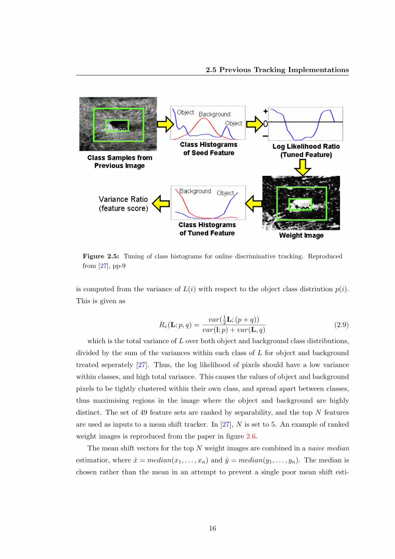
2.5 Previous Tracking Implementations
Figure 2.5: Tuning of class histograms for online discriminative tracking. Reproduced
from [27], pp-9
is computed from the variance of L(i) with respect to the object class distriution p(i).
This is given as
Rv(L; p, q) =var(12L; (p+ q))
var(l; p) + var(L, q)(2.9)
which is the total variance of L over both object and background class distributions,
divided by the sum of the variances within each class of L for object and background
treated seperately [27]. Thus, the log likelihood of pixels should have a low variance
within classes, and high total variance. This causes the values of object and background
pixels to be tightly clustered within their own class, and spread apart between classes,
thus maximising regions in the image where the object and background are highly
distinct. The set of 49 feature sets are ranked by separability, and the top N features
are used as inputs to a mean shift tracker. In [27], N is set to 5. An example of ranked
weight images is reproduced from the paper in figure 2.6.
The mean shift vectors for the top N weight images are combined in a naive median
estimatior, where x = median(x1, . . . , xn) and y = median(y1, . . . , yn). The median is
chosen rather than the mean in an attempt to prevent a single poor mean shift esti-
16

2.5 Previous Tracking Implementations
Figure 2.6: Ranked weight images produced by segmentation stage in [27] (pp-13)
mation from influencing the pooled median estimate. A block diagram of the tracking
system is reproduced in figure 2.7.
The novelty in this paper comes primarily from the ranked weight images and the
pooling mechanism. The actual mean shift loop does not differ significantly from that
in [66] and [26]. What this paper does demonstrate is that with little modification,
the basic mean shift object tracker can be greatly extended. The results section in
[27] is quite comprehensive, showing the results of many different tracking runs as
well as providing a thorough and robust discussion. The claim in [87] that the basic
requirement for a useful mean shift tracker is the production of weight images1 suggests
that any process capable of producing such an image can be used as the input stage
to the mean shift inner loop. This in turn implies that the development of a hardware
mean shift inner loop may also be similarly modular in its application.
Tomiyasu, Hirayama, and Mase apply the mean shift algorithm to point tracking
in [88]. An mean shift procedure is initialised from a wide area in the image by a point
search based on a Kalman filter [74]. The SURF detector is employed to detect feature
1See section 3.3 for an extended discussion on mean shift weight images
17

2.5 Previous Tracking Implementations
Figure 2.7: Block diagram overview of tracking system in [27]. Reproduced from pp-14
points in each frame. A Kalman filter predicts locations for feature points to remove
the need for brute-force search. Points that lie within a circle surrounding the target
are considered for a finer grain mean shift search in the neighbourhood of the feature
point. This search attempts to converge on the correct location of the feature point.
Finally, a mean shift search in both the image space and scale space is performed on
a set of neighbouring pixels. This process is iterated in each space alternately until
convergence is achieved in both the image space and scale space.
From the published results, the algorithm appears to exhibit good performance,
and is quite capable of tracking small, fine-grain features. However the full proce-
dure, described in pp.2-4 is quite complex, and would be poorly suited to hardware
implementation with contemporary technology at the time of writing.
Yilmaz extends the framework in [26] by allowing the use of asymmetric kernels
which can change in scale and orientation [83]. Kernel scale in [26] is decided by
computing various scales in the neighbourhood of the target and selecting the scale
that maximises the appearance similarity [49] [83]. The framework in [66] and [26]
also imposes a radially symmetric structure, which has obvious limitations for tracking
object in realistic scenarios. Yilmaz represents the scale of object pixels in a scale
dimension. A linear trasformation of image coordinates is computed from the ratio
between δ(xi) of point xi and the bandwidth observed at angle θi. This is given as
σi =δ(xi)
r(θi)=|xi − o|r(θi
(2.10)
18
2.5 Previous Tracking Implementations
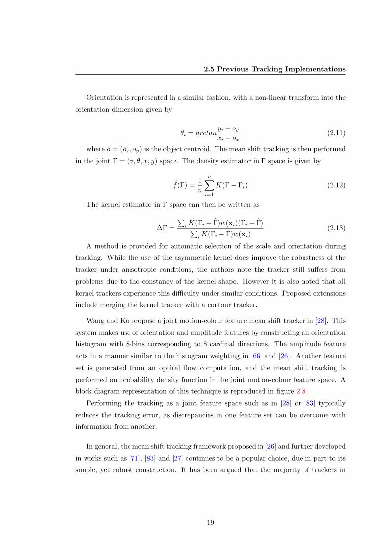
Orientation is represented in a similar fashion, with a non-linear transform into the
orientation dimension given by
θi = arctanyi − oyxi − ox
(2.11)
where o = (ox, oy) is the object centroid. The mean shift tracking is then performed
in the joint Γ = (σ, θ, x, y) space. The density estimator in Γ space is given by
f(Γ) =1
n
n∑i=1
K(Γ− Γi) (2.12)
The kernel estimator in Γ space can then be written as
∆Γ =
∑iK(Γi − Γ)w(xi)(Γi − Γ)∑
iK(Γi − Γ)w(xi)(2.13)
A method is provided for automatic selection of the scale and orientation during
tracking. While the use of the asymmetric kernel does improve the robustness of the
tracker under anisotropic conditions, the authors note the tracker still suffers from
problems due to the constancy of the kernel shape. However it is also noted that all
kernel trackers experience this difficulty under similar conditions. Proposed extensions
include merging the kernel tracker with a contour tracker.
Wang and Ko propose a joint motion-colour feature mean shift tracker in [28]. This
system makes use of orientation and amplitude features by constructing an orientation
histogram with 8-bins corresponding to 8 cardinal directions. The amplitude feature
acts in a manner similar to the histogram weighting in [66] and [26]. Another feature
set is generated from an optical flow computation, and the mean shift tracking is
performed on probability density function in the joint motion-colour feature space. A
block diagram representation of this technique is reproduced in figure 2.8.
Performing the tracking as a joint feature space such as in [28] or [83] typically
reduces the tracking error, as discrepancies in one feature set can be overcome with
information from another.
In general, the mean shift tracking framework proposed in [26] and further developed
in works such as [71], [83] and [27] continues to be a popular choice, due in part to its
simple, yet robust construction. It has been argued that the majority of trackers in
19

2.5 Previous Tracking Implementations
Figure 2.8: Block diagram of joint motion-colour meanshift tracker, reproduced from [28]
the literature are based on this principle [49], however whether this remains the case
is yet to be seen. The concept of maximising a density function in some feature space
allows flexibility. Many of the trackers presented here, such as [28], or [85] extend
the basic mean shift framework by applying the inner loop to joint feature spaces.
This typically allows some deficiency in one feature set to be overcome by information
in another. Extensions of this kind are relatively straightforward, and can provide
significant accuracy gains when done correctly.
2.5.2 Hardware Implementations
In [21] a high speed colour histogram tracking system is developed using a modified
CAMSHIFT algorithm. The system is capable of tracking a single target at 2000
frames per second within a 512 × 511 pixel image using a Photron FASTCAM MH4-
10K CMOS sensor [89]. The system extracts size, position, and orientation information
about the target completely in hardware using a moment feature extraction explicitly
derived from the CAMSHIFT algorithm [24]. The target is expressed as a colour feature
in the HSV colour space. Pixels are thresholded and binarised according to the function
Ci(x, t0) =
{1 (S(x, t0) > θS , V (x, t0) > θV , (i− 1)d ≤ H(x, t0) < id)
0 otherwise(2.14)
20
2.5 Previous Tracking Implementations
where Ci(x, t0) is the binary image for colour bin i at time t0, and i ranges over the
number of bins such that (i = 1, . . . , I). The weight image is generated by backpro-
jecting the pixels back to the image space according to
W (x, t) =
I∑i=1
QiCi(x, t) (2.15)
The authors provide a section titled Improved CamShift Algorithm (sic) which de-
tails the moment accumulation procedure used in the paper. The paragraph opens by
noting that the CAMSHIFT algorithm in [24] involves redundant multiplications dur-
ing the calculation of the backprojection image. The additive property of the moment
computation suggests that the moments for the backprojection image can be obtained
by a weighted sum of the moments of each bit-plane image.
The moments in [21] are re-written as
Mpq(W (x, t)) =∑
x∈R(t)
xpyq
(I∑
i=1
wiCi(x, t)
)(2.16)
=I∑
i=1
wi
∑x∈R(t)
xpyqCi(x, t) (2.17)
=I∑
i=1
wiMipq(t) (2.18)
Then the moments for each colour bin are computed as
M ipq(t) =
∑x∈R(t)
xpyqCi(x, t) (2.19)
where i = (1, . . . , I, p+q ≤ 2) and M ipq is the moment for colour bin i. The moment
features for the backprojection image are then computed as a linear weighted sum of
Mpq as
Mpq(t) =
I∑i=1
wiMipq(t) (2.20)
This allows the computation to be split efficiently across many processing units.
The tracking window is the calculated from the moment features of the weight image.
The zero, first and second order moments are computed from W (x, t). The window is
21

2.5 Previous Tracking Implementations
Figure 2.9: Schematic view of colour histogram computation circuit. Reproduced from
[21]
selected as the minimum rectangular region whose edges are parallel to the x and y axis
when the entire target is within the window. The schematic for the colour histogram
circuit in [21] is reproduced in figure 2.9. After colour conversion, 16 moment feature
computation circuits take 4 8-bit hue, saturation, and value pixels, and perform bina-
risation and parallel moment accumulation. The computation of the window boundary
is similar to that in [24] or [77]. The tracking window is computed as a separate sub-
process computed on a PC communicating with the PCI-Express bus. The authors
note that even though the tracking is not done in hardware, the system as a whole is
capable of tracking objects at 2000 frames per second [21], p.4.
The system is implemented on a Photron IDP Express board containing a Xilinx
XC3S500 FPGA for image processing functions, and Xilinx XCVFX60 for interfacing
to the MH4-10K CMOS sensor and the PCI-Express endpoint. This sensor and the
IDP Express board are also used in [20], [22], and [23]. A more detailed block diagram
showing the roles of each FPGA is given in [22], p.3.
Two sets of results are provided in the paper. The first it titled Colour Pattern
Extraction for a Rotating Object, and demonstrates the ability of the system to perform
colour object tracking. The test involves a rotating card with various graphics printed
on one side. The card rotates at a speed of 7 r/s, and is moved back and forth in
front of the camera at a distance ranging between 90cm and 130cm 3 times within 3s.
In the first test, the target object is a printed colour graphic of a carrot containing
an large orange region and a smaller green region. The thresholds for binarisation
22

2.5 Previous Tracking Implementations
Figure 2.10: Input images (a) and tracking windows (b) for a rotating object in [21], p.5
(equation 2.14) are set to θs = 5, θv = 35. The 6 figure tracking sequence presented
in the results is reproduced in figure 2.10. The input image of the rotating graphic is
shown in the top row, the bounding region extracted by the system is shown in the
bottom row.
The second test consists of tracking a hand with 2 degrees of freedom. A paragraph
in [21], p.7 notes that the hand was correctly tracked, even under rapid motion and in
front of a complex background. Frames from the tracking sequence are given, as well
as graphs showing the change in position for each axis with respect to time. It is noted
at the end of the paragraph that the system is responsive enough for use as a real-time
vision sensor for robotic feedback
While the performance for the system is impressive, it does depend on the availabil-
ity of specialised high speed sensors, in particular the Photron FASTCAM MH4-10K
[89]. The IDP-Express board (also manufactured by Photron Inc.) could in principle
be replaced with another system, leaving the sensors as the only non-replaceable part.
However a PC or other general purpose processor is still required for computation of
the window parameters.
A Multi-Object tracker for mobile navigation in outdoor environments in given by
Xu, Sun, Cao, Liang, and Li [29]. This system is based around a smart tracking device
consisting of a DSP, FPGA, a CMOS sensor and a fish eye lens, and uses a mean shift
embedded particle filter (MSEPF) to perform the tracking operation. This operation
consists of a particle filter [90] which generates points for the mean shift tracker, in
effect a kind of weight image generator (see section 3.3 for further discussion of weight
images in the mean shift tracking framework). The weight image is based on shape
23
2.5 Previous Tracking Implementations
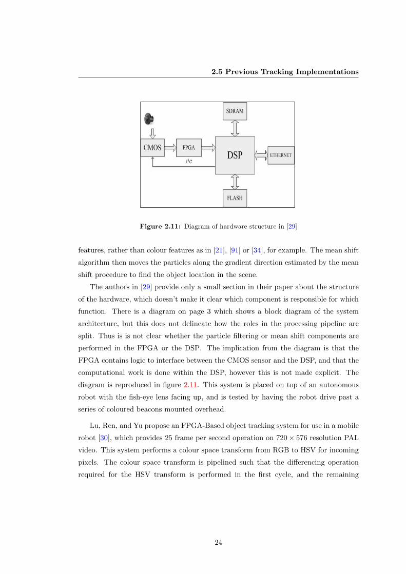
Figure 2.11: Diagram of hardware structure in [29]
features, rather than colour features as in [21], [91] or [34], for example. The mean shift
algorithm then moves the particles along the gradient direction estimated by the mean
shift procedure to find the object location in the scene.
The authors in [29] provide only a small section in their paper about the structure
of the hardware, which doesn’t make it clear which component is responsible for which
function. There is a diagram on page 3 which shows a block diagram of the system
architecture, but this does not delineate how the roles in the processing pipeline are
split. Thus is is not clear whether the particle filtering or mean shift components are
performed in the FPGA or the DSP. The implication from the diagram is that the
FPGA contains logic to interface between the CMOS sensor and the DSP, and that the
computational work is done within the DSP, however this is not made explicit. The
diagram is reproduced in figure 2.11. This system is placed on top of an autonomous
robot with the fish-eye lens facing up, and is tested by having the robot drive past a
series of coloured beacons mounted overhead.
Lu, Ren, and Yu propose an FPGA-Based object tracking system for use in a mobile
robot [30], which provides 25 frame per second operation on 720× 576 resolution PAL
video. This system performs a colour space transform from RGB to HSV for incoming
pixels. The colour space transform is pipelined such that the differencing operation
required for the HSV transform is performed in the first cycle, and the remaining
24

2.5 Previous Tracking Implementations
Figure 2.12: Block diagram of object tracking system in [30], p2
operations are performed in the following cycle1. Tracking is performed by the mean
shift algorithm. All components are implemented in an Altera Cyclone EP1C6 FPGA.
The object tracking process is implemented with a clock frequency of 100MHz. The
system block diagram is reproduced from [30], p2 in figure 2.12.
Mean shift tracking is accomplished by moment analysis of the weight image. There
is relatively little detail on how the weight image is generated, other than the hue
channel of the transformed image is used to generate a histogram of the target, which
is used to determine if a pixel belongs to the target. It can be inferred from this that
some kind of colour indexing [47] [76] or histogram backprojection [24] [87] is being
used, however the implementation of the technique is not mentioned.
In the tracking stage, a new kernel function is introduced that surrounds the target
with a search window, similar to the system in [27]. The initial window location is
selected manually, and the algorithm automatically extends the search window 100
1A more detailed treatment of the HSV colour space in given in section 3.1
25
2.5 Previous Tracking Implementations
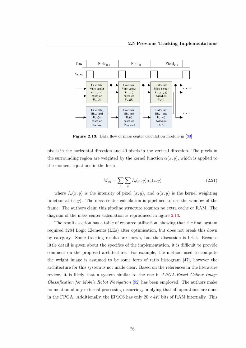
Figure 2.13: Data flow of mass center calculation module in [30]
pixels in the horizontal direction and 40 pixels in the vertical direction. The pixels in
the surrounding region are weighted by the kernel function α(x, y), which is applied to
the moment equations in the form
Mpq =∑p
∑q
In(x, y)αn(x.y) (2.21)
where In(x, y) is the intensity of pixel (x, y), and α(x, y) is the kernel weighting
function at (x, y). The mass center calculation is pipelined to use the window of the
frame. The authors claim this pipeline structure requires no extra cache or RAM. The
diagram of the mass center calculation is reproduced in figure 2.13.
The results section has a table of resource utilisation, showing that the final system
required 3284 Logic Elements (LEs) after optimisation, but does not break this down
by category. Some tracking results are shown, but the discussion is brief. Because
little detail is given about the specifics of the implementation, it is difficult to provide
comment on the proposed architecture. For example, the method used to compute
the weight image is assumed to be some form of ratio histogram [47], however the
architecture for this system is not made clear. Based on the references in the literature
review, it is likely that a system similar to the one in FPGA-Based Colour Image
Classification for Mobile Robot Navigation [92] has been employed. The authors make
no mention of any external processing occurring, implying that all operations are done
in the FPGA. Additionally, the EP1C6 has only 20× 4K bits of RAM internally. This
26

2.5 Previous Tracking Implementations
immediately rules out iterating over the weight image, which would require 414720 bits
of memory with a bit depth of 1-bit per pixel. This suggests that the system only
computes the center of mass of the weight image as it streams through the tracking
module, rather than computing the mean shift vector by iterating along the gradient
of a density function.
FPGA-based moment analysis has also been applied to the problem of feature ex-
traction. Gu, Takaki, and Ishii propose a 2000 frame per second feature extraction
system which operates on 512× 512 pixel images and is capable of extracting 25 high-
order autocorrelation features for 1024 objects simultaneously for recognition [43]. This
is achieved by dividing the image into 8×8 cells and computing the zero and first order
moments within these cells, and then performing connected-component labelling using
a technique developed by Gu in [44]. Moment calculation for connected components is
performed by exploiting the additive property of moments.
There are some FPGA-based object trackers in the literature which use the mean
shift algorithm, or a variant of it, to obtain the target in the scene, but do not perform
the mean shift iteration in hardware. One such design is given by Norouznezhad etal in
[93] and [31]. This system uses a bank of complex Gabor Filters to extract local oriented
energy features for each pixel in an image, and generates a feature histogram from this
for the target candidate and region. The best candidate for the target is then computed
by the mean shift algorithm. The motion pattern of the target region is estimated from
the local phase information. The feature histogram for the system has as many bins as
the filter bank has channels. The implementation in both [93] and [31] uses 12 channels
in the filtering stage, and therefore implements a 12 bin histogram. In this system
the Complex Gabor Filter bank, which includes a 7 × 7 convolution block, histogram
accumulation logic, and local oriented energy feature logic are implemented in a Xilinx
Virtex-5 XC5VSX50T FPGA. The mean shift computation is implemented on a Xilinx
Microblaze soft-core processor with a clock frequency of 125MHz. The authors note
that the Microblaze processor was chosen for ease of use rather than performance. A
block diagram showing the system architecture is reproduced from [31] in figure 2.14.
The authors also make some note about a prototype system developed in MATLAB,
however the details of this fall outside the scope of the publication and are not made
explicit.
27
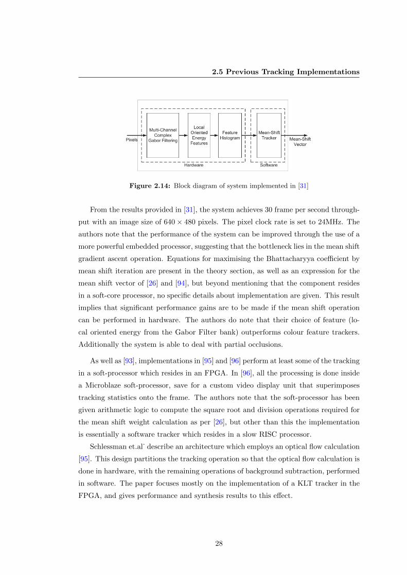
2.5 Previous Tracking Implementations
Figure 2.14: Block diagram of system implemented in [31]
From the results provided in [31], the system achieves 30 frame per second through-
put with an image size of 640× 480 pixels. The pixel clock rate is set to 24MHz. The
authors note that the performance of the system can be improved through the use of a
more powerful embedded processor, suggesting that the bottleneck lies in the mean shift
gradient ascent operation. Equations for maximising the Bhattacharyya coefficient by
mean shift iteration are present in the theory section, as well as an expression for the
mean shift vector of [26] and [94], but beyond mentioning that the component resides
in a soft-core processor, no specific details about implementation are given. This result
implies that significant performance gains are to be made if the mean shift operation
can be performed in hardware. The authors do note that their choice of feature (lo-
cal oriented energy from the Gabor Filter bank) outperforms colour feature trackers.
Additionally the system is able to deal with partial occlusions.
As well as [93], implementations in [95] and [96] perform at least some of the tracking
in a soft-processor which resides in an FPGA. In [96], all the processing is done inside
a Microblaze soft-processor, save for a custom video display unit that superimposes
tracking statistics onto the frame. The authors note that the soft-processor has been
given arithmetic logic to compute the square root and division operations required for
the mean shift weight calculation as per [26], but other than this the implementation
is essentially a software tracker which resides in a slow RISC processor.
Schlessman et.al˙ describe an architecture which employs an optical flow calculation
[95]. This design partitions the tracking operation so that the optical flow calculation is
done in hardware, with the remaining operations of background subtraction, performed
in software. The paper focuses mostly on the implementation of a KLT tracker in the
FPGA, and gives performance and synthesis results to this effect.
28

2.5 Previous Tracking Implementations
Figure 2.15: Reproduction of block diagram of PCA object tracking system in [32]
Techniques other than the mean shift algorithm have been implemented in hard-
ware. Bravo, Mazo, Lazaro, Gardel, Jimenez, and Pizarro developed an FPGA based
system to detect moving object using Principal Component Analysis [32]. This paper
spends a great deal of time presenting the matrix manipulation architecture used to
compute the different stages of the PCA. The authors note in their conclusions that
there had not previously been a completely integrated PCA solver implemented on an
FPGA, making the work all the more impressive.
The system in [32] makes use of the Micron MT9M413 CMOS sensor [33], a 1.3
megapixel (1280× 1024) unit capable of 500 frame per second operation with an input
clock of 66MHz. The sensor has integrated 10-bit ADC, and is capable of providing
10 10-bit digital outputs. This gives excellent performance, however this comes with
a high parts cost1 and provides some engineering challenges to utilise in a tracking
system. Specifically, the 10 10-bit outputs requires a total of 100 pins to be routed
into the FPGA or ASIC. A diagram showing the connections to the MT9M413 is
reproduced from [33] in figure 2.16. The pixel data output has been selected. The
1At the time of writing, Octopart quotes an average price of $1072.00 USD. There are no price
breaks. It should be noted that this part is no longer available, and Aptina’s current catalogue consists
mainly of sensors that provide 1 pixel per clock
29

2.5 Previous Tracking Implementations
system performance is high, both in terms of accuracy (97% [32]) and speed (250
frames per second [32]). However the high cost for the sensor may be a limiting factor
in choosing this architecture for an application.
Shah, Jain, Bhatt, Engineer, and Mehul present what may be the only completely
hardware mean shift tracker in the literature up to the time of writing1 [34]2. This
system implements the algorithm presented in [26], including the computation of the
Bhattacharyya coefficient, and an external memory interface for storing the input im-
age.
The algorithm presented operates in a 24-bit RGB colour space. Images are cap-
tured via a camera and buffered in an external memory bank. The total number of
frames buffered is not made explicit in the text, but is said to be based on both the
clock frequency of the device, and the pixel clock of the camera. A histogram is con-
structed for each frame and compared to a model histogram using the Bhattacharyya
coefficient as the distance metric. A bounding region is computed using weighted and
normalised row and column arrays.
The implementation seems to follow the description given in [26] exactly. Data is
buffered into an external memory via the Frame Capture and Memory Access Logic
(FCMA). Once a frame has been received, a refrence histogram of the frame is gen-
erated. A second frame is read into memory from some incoming sensor. Reference
histograms are generated for the second frame. The target centroid is computed for the
two frames by a mean shift inner loop that performs 20 iterations. The weight image
is computed naively using Comaniciu, Ramesh and Meers method, which involves a
square root and divide operation for each pixel in the weight image. Because device
utilisation data is not given, it is difficult to know the resource requirements for this
implementation. Several block diagrams of parts are given, but the timing of the data-
path is not always clear. Since the image is stored in external memory, and the weight
image is calculated for each pixel, it may be the case that the entire architecture is
serialised due to memory bandwidth limitations. Thus the throughput of the system
would be determined primarily by the memory clock rate. It should be noted that these
details are note clear from the text.
1circa. early 20142Republished in [97]
30
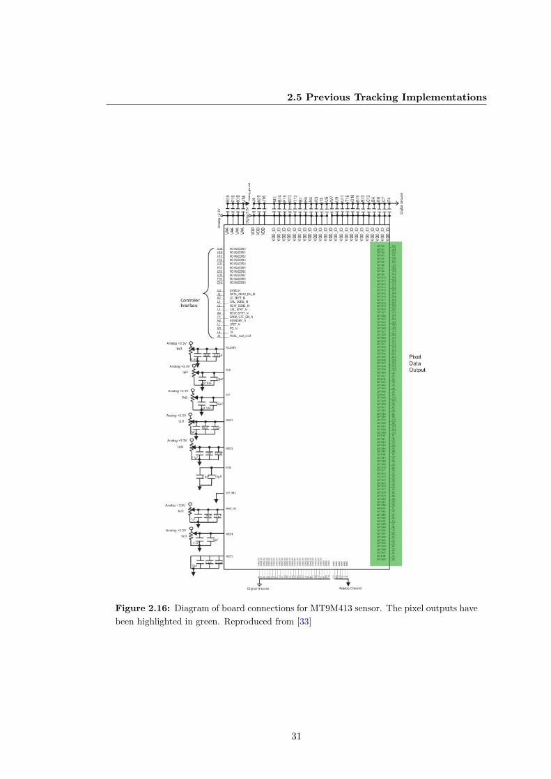
2.5 Previous Tracking Implementations
Figure 2.16: Diagram of board connections for MT9M413 sensor. The pixel outputs have
been highlighted in green. Reproduced from [33]
31

2.5 Previous Tracking Implementations
Figure 2.17: Block diagram of system implemented in [34]
Results in [34] are brief. A single paragraph and 4 images grouped as a lattice are
provided to demonstrate the operation of the system. The 4 images are reproduced here
in figure 2.18. The paper does not explain the diagrams other than to say that . . .the
difference was only that the MATLAB output was with using floating point and Verilog
output was using fixed point (sic)It can be assumed that figures on the left represent
results obtained in MATLAB, and figures on the right represent results obtained via
some Verilog simulation.
2.5.3 Final Comment on Previous Implementations
It has previously been argued that the majority of mean shift trackers in the literature
were focused primarily on single object tracking, with little scene clutter [49]1. pp 160-
163. Most of these systems perform segmentation in a binary sense, classifying pixels
into background and non-background.
Looking at the progression of ideas developed in section 2.5.1, there is a clear
development in the complexity of the segmentation algorithm, including the application
of joint feature spaces [27] [28] [88], scale adaptation [71] [83], and multiple feature
1In fact, in [49] it is argued that the majority of region-based trackers are focused on single object
tracking
32

2.5 Previous Tracking Implementations
Figure 2.18: Outputs from results section of [34]
extraction techniques [88]. However there remains the common theme of finding a
single target in a frame while ignoring outliers which arise due to noise corruption,
occlusion, or interference.
In the hardware review of section 2.5.2, virtually all the methods to date applying
some form of mean shift algorithm are tracking a single target [93], and often with
little to no background clutter [21]. Except for [34], none of the systems here per-
form the window calculation in hardware. In [31] and [93], the mean shift component
is realised as a software routine. In [21], the windowing component is realised as a
software process, but the remainder of the tracking is done in hardware. The actual
performance specification and capabilities of the system described in [34] are not given
in the text. The paper was reprinted in [97], although the text is very similar and no
additional detail is given. Of particular concern is the fact that the conclusion has not
been expanded, consisting of the same short paragraph and 4-image lattice of results
reproduced in figure 2.18.
Additionally, none of the papers presented in section 2.5.2 attempt to track multiple
targets. This stems mostly from the fact that mean shift trackers in general are focused
on tracking singular targets [49]. Nevertheless, it leaves a significant area in the design
space to explore.
33

2.6 Review of Circuit Design and Verification
In summary, the kernel object tracking framework remains a popular choice in the
literature [25] [49] [50]. A natural consideration for extracting additional performance
is to consider hardware accelerated implementations. To date there seems to be little
in the way of a definitive mean shift tracking framework that is well conditioned for
deployment on a chip, and poised to take advantage of the unique opportunities such
a domain offers.
2.6 Review of Circuit Design and Verification
During the course of this research, much effort was placed on validating the function
of the pipeline was correct. This involved the development of some custom verification
tools that facilitated both exploration of possible architectures and implementations,
as well as a framework to verify functional correctness. This system, called csTool, is
detailed in chapter 6. Because the development of csTool was a significant component
of the research, some background on the field of circuit verification is provided here for
context. The subject of hardware verification is, much like object tracking, enormous in
its scope, and cannot be covered comprehensively within this document. Nonetheless,
a summary of the field is provided below. The interested reader is directed to one of the
many literature surveys in the field, including [98], [99], as well as books by Bergeron
[100], [101], and Wile & Goss [35]. This field has significant crossover into the world
of software verification, formal methods, and the like, and so literature with a focus on
software such as [102] and [103] are still relevant in a discussion
2.6.1 Overview of Verification
Improvements in process technology and circuit integration techniques have made it
possible to produce increasingly complex circuits in short amounts of time. However
verifying that the function of these devices is correct requires more time and effort than
the design itself [100] [104]. The complexity of verification is thought to be growing
faster than the complexity of design [104] [105].
Functional verification describes any method used to test the functional correctness
of a circuit [35]. This is commonly achieved by writing testbenches which apply stim-
ulus to a device under test (DUT), and output monitors which review the responses
generated by the DUT when it is subject to those stimulus.
34
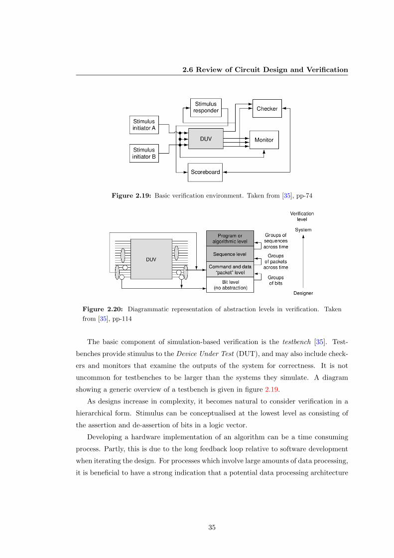
2.6 Review of Circuit Design and Verification
Figure 2.19: Basic verification environment. Taken from [35], pp-74
Figure 2.20: Diagrammatic representation of abstraction levels in verification. Taken
from [35], pp-114
The basic component of simulation-based verification is the testbench [35]. Test-
benches provide stimulus to the Device Under Test (DUT), and may also include check-
ers and monitors that examine the outputs of the system for correctness. It is not
uncommon for testbenches to be larger than the systems they simulate. A diagram
showing a generic overview of a testbench is given in figure 2.19.
As designs increase in complexity, it becomes natural to consider verification in a
hierarchical form. Stimulus can be conceptualised at the lowest level as consisting of
the assertion and de-assertion of bits in a logic vector.
Developing a hardware implementation of an algorithm can be a time consuming
process. Partly, this is due to the long feedback loop relative to software development
when iterating the design. For processes which involve large amounts of data processing,
it is beneficial to have a strong indication that a potential data processing architecture
35

2.6 Review of Circuit Design and Verification
will be functionally correct before the design is deployed to hardware. This concern
was the motivation behind csTool, which is described in chapter 6. Conceptually, this
tool shares many ideas with other published works such as [106], [107] and [108].
2.6.2 Review of Verification Literature
In [108], Brier and Mitra develop a C-language framework for investigating implemen-
tation of a signal processing operation. The specific operation used in the paper to
illustrate the technique is an image resizer. A C-language model is developed to verify
the low level RTL functions of the resizer module. The C Model forms a Golden Ref-
erence for the RTL implementation against which the correctness of the RTL can be
checked. Brier and Mitra take care to point out that elevating the status of the C model
to golden does bring problems with small differences in implementation. For example,
the golden model may make use of a data structure for convenience that is not a true
representation of the register transfers in the device. Care must be taken to ensure that
these structural differences, some of which are unavoidable, do not impact the ability
of the model to act as a reference during the testing phase. The authors note that
there were some problems with number representation in their work, specifically minor
numerical inconsistencies that arose comparing the C model of the resizer, implemented
with floating point arithmetic, and the RTL model, implemented with fixed-point arith-
metic. These issues are resolved in [108] using manual inspection by a domain expert.
While this technique is sufficient for the purposes in [108], the approach cannot scale
to designs beyond a certain size. A functional verification system somewhat similar to
this was developed as part of this study, and is detailed in chapter 6.
Reva developed a fault injection tool for testing FPGA designs in [36]. Fault types
are categorised into fault profiles, which aim to capture something about the nature of
a fault or failure. Various levels of automation are provided in the fault injection stage.
In the fully automatic mode, the user only chooses a source file into which the fault
is injected, and the type of fault to inject. The semi-automatic mode allows the user
to choose the source file, a code region to inject the fault into, and a fault from the
fault set. The fully manual mode also allows the user to generate a custom fault. The
architecture for the fault injection tool has been reproduced from [36] in figure 2.21.
36

2.6 Review of Circuit Design and Verification
Figure 2.21: Architecture of fault injection tool described in [36]
Unlike the work in [108], the fault tool in [36] is focused more on checking for
correctness with the language itself. In this sense, the tool has more in common with
formal verification and proof checking methods [99], [109]. The tool developed for this
study (csTool) is a more functionally oriented tool, which shares more similarities with
[108]. csTool only operates on data produced by an event-driven or cycle-driven RTL
simulator (for example, Veripool’s Verilator [110] or Mentor Graphics’ Modelsim), and
does not perform language checking, or any other RTL checks. Nevertheless, a fault
injection system can still find use at the functional level of the design, however such
a system, despite the structural similarities, would be quite separate to the system in
[36].
An example of a functional fault injection environment was given by Benso, Bosio,
Di Carlo, and Mariani in [37]. The fault injection framework consists of a fault free
golden reference and a faulty DUT simulated in parallel under the same workload.
Faults are injected into the test device (the faulty DUT) and monitors attached to
both the golden and faulty devices generate results for comparison.
Random constrained verification finds use throughout hardware verification, such as
[111], which applies random constrained test vectors to cache design. In [107], Silveria,
Da Silva, and Melcher present a random-constrained movie generator for testing an
MPEG-4 decoder. Here the process of generating video input for the core is both
simplified compared to generating actual encoded video frames, as well as made more
37
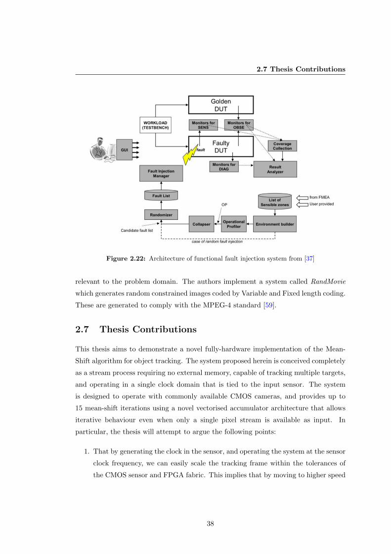
2.7 Thesis Contributions
Figure 2.22: Architecture of functional fault injection system from [37]
relevant to the problem domain. The authors implement a system called RandMovie
which generates random constrained images coded by Variable and Fixed length coding.
These are generated to comply with the MPEG-4 standard [59].
2.7 Thesis Contributions
This thesis aims to demonstrate a novel fully-hardware implementation of the Mean-
Shift algorithm for object tracking. The system proposed herein is conceived completely
as a stream process requiring no external memory, capable of tracking multiple targets,
and operating in a single clock domain that is tied to the input sensor. The system
is designed to operate with commonly available CMOS cameras, and provides up to
15 mean-shift iterations using a novel vectorised accumulator architecture that allows
iterative behaviour even when only a single pixel stream is available as input. In
particular, the thesis will attempt to argue the following points:
1. That by generating the clock in the sensor, and operating the system at the sensor
clock frequency, we can easily scale the tracking frame within the tolerances of
the CMOS sensor and FPGA fabric. This implies that by moving to higher speed
38

2.7 Thesis Contributions
grade FPGA or a higher speed sensor, we can increase the frame rate with little
to no modification of the pipeline itself.
2. That by vectorising the data processing pipeline, the data processing throughput
required to perform 15 iterations per frame can be comfortably achieved without
the need for a second clock domain.
3. A demonstration of an architecture which is capable of performing the operations
required of a basic CAMSHIFT style tracker that can be implemented completely
within a single low-cost FPGA, without the need for any external peripherals such
as external memory, save for the requirement for a CMOS sensor. Additionally,
a discussion is provided as to how memory requirements can be reduced, and
what architectural possibilities exist for expanding the system, for example, for
improved background subtraction, while keeping the system within a single chip.
4. Develop a system that does not depend on the presence of expensive high-performance
sensors such as [89] or [33].
39

Chapter 3
Theory Background
Computer vision is the field of study that concerns itself with the development of tech-
niques and frameworks that allow computers to mimic the visual processing capabilities
of humans (and to a lesser extent, animals). The faculties possessed by humans in this
domain include, but are not limited to, motion perception, object discrimination, scene
understanding, and so on. The discipline of computer vision has experienced consider-
able development over the previous 20 or so years which makes a general overview far
outside the scope of this document. Nevertheless, a more detailed discussion of relevant
theory from the field is provided here.
3.1 Colour Spaces
Vision is the perception of light. Certain wavelengths of light fall into a range known
as the visible spectrum of light. These are wavelengths which can be perceived by the
human eye, and lie between 390 and 700nm (around 430THz - 790THz) [112]. The ap-
parent colour of a light source is a function of frequency. Representing these frequencies
is fundamental to the field of computer vision, and indeed all image processing.
Consider an image as a two-dimensional lattice of pixels. The well-known RGB
colour space defines each of these pixels in terms relative intensity of 3 fixed wavelengths
of light. Figure 3.1 shows a chromaticity diagram of the sRGB colour space which is
commonly used in computer monitors and televisions. A full mathematical treatment
of the sRGB colour space is outside the scope of this document, however it is instructive
to note that the extremities of the sRGB ‘triangle’ correspond to the wavelengths of
40

3.1 Colour Spaces
Figure 3.1: CIE diagram of sRGB colour space [38]
the red, green and blue primary colours of the colour space. The area enclosed by these
points represents the gamut of colours in the colour space.
Since each pixel is composed of some mix of red green and blue colours, changes
in illumination can cause the pixel values for a particular image to change drastically,
even if the ‘true’ colour of an object in the scene does not change. The HSL/HSV
colour space, developed by Alvy Ray Smith [75] attempts to create a more intuitive
notion of colour by mapping the RGB cube of figure 3.2 onto a cylinder or cone. In
computer graphics, this provides a more straight-forward method to choose colours
based on a perceptually relevant arrangement of hues. In the context of computer
vision, this transformation is typically used to reduce the effect of illumination changes
41
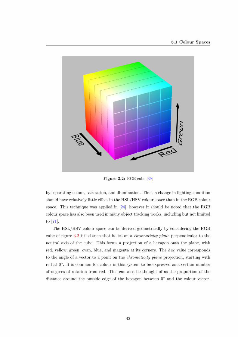
3.1 Colour Spaces
Figure 3.2: RGB cube [39]
by separating colour, saturation, and illumination. Thus, a change in lighting condition
should have relatively little effect in the HSL/HSV colour space than in the RGB colour
space. This technique was applied in [24], however it should be noted that the RGB
colour space has also been used in many object tracking works, including but not limited
to [71].
The HSL/HSV colour space can be derived geometrically by considering the RGB
cube of figure 3.2 titled such that it lies on a chromaticity plane perpendicular to the
neutral axis of the cube. This forms a projection of a hexagon onto the plane, with
red, yellow, green, cyan, blue, and magenta at its corners. The hue value corresponds
to the angle of a vector to a point on the chromaticity plane projection, starting with
red at 0◦. It is common for colour in this system to be expressed as a certain number
of degrees of rotation from red. This can also be thought of as the proportion of the
distance around the outside edge of the hexagon between 0◦ and the colour vector.
42

3.1 Colour Spaces
Points projecting into the origin are normally undefined, and are commonly rendered
as grays whose intensity corresponds to the lightness/value.
A pixel in the RGB colour space can be transformed into the HSL space as follows.
Let R, G, and B represent the values of the red, green, and blue channels respectively.
Let max and min represent the maximum and minimum value on any channel for a
given pixel. Then, the hue value for the pixel p = (R,G,B) is given by
H =
60◦ × G−B
max−min if max = R
60◦ × B−Rmax−min if max = G
60◦ × R−Gmax−min if max = B
(3.1)
In the HSL colour space, the saturation is simply the chroma scaled to fill the
interval [01] for each combination of hue and lightness or value.
SHSL =
0 ifmax=minmax−minmax+min if 0 ≤L≤ 1
2max−min
2−(max+min) if L≥ 12
(3.2)
The HSV representation is conical, and thus the saturation is also a function of
distance along the cone. Therefore the expression is simply the ratio of the chroma
value to the value component of the colour space.
SHSV =
{0 ifC = 0CV otherwise
(3.3)
In the HSL model, lightness is a function of the average of the largest and smallest
colour components. This forms a double conical shape which tapers to a point at the
top and bottom.
L =1
2(max+min) (3.4)
In the HSV model, the value is a function of the largest component of a colour.
This forms a hexagonal pyramid and gives the expression for the value as
V = max (3.5)
In the RGB colour space, a change in illumination will cause values in all 3 channels
to change. Because the chroma or hue component is separate from the brightness,
43

3.2 Kernel Object Tracking
images in the HSV colour space a relatively less susceptible to sudden value changes
due to illumination differences compared to the same images in RGB colour space. For
this reason, the HSV colour space has found wide application in computer vision, as a
single dimensional colour feature.
Object tracking is almost always a component of a larger system, typically as a
front end that discriminates some region of an image for further processing. In a
surveillance application, this may be the detection of suspicious behaviours or events,
and a tracker may be providing the locations of the points of interest in the frame.
In a video compression application, a tracker may provide information about parts of
the scene that undergo motion, and therefore need to be encoded with more detail (a
higher bit rate, for example).
Object tracking finds application in a wide variety of fields. The most obvious of
these is simply tracking the motion of a target, for example to perform surveillance or to
monitor traffic. Less obvious is for detecting and tracking objects for video compression
[59].
3.2 Kernel Object Tracking
As the material in this thesis is concerned with implementing the CAMSHIFT algorithm
in hardware, it is appropriate that some time be devoted to covering the theory behind
this technique, namely kernel object tracking.
Being a discipline of significance within the computer vision canon, visual object
tracking has attracted a number of literature surveys, including but not limited to [49],
[50], [25], [113], and many others. Within these surveys a taxonomy of visual tracking
methods begins to form. In particular, this section will make reference to the taxonomy
expressed in [50] on page 4. We see that within this framework, kernel density tracking
is classified as a generative statistical method which is grouped with mixture models
and subspace learning.
Kernel Object tracking represents targets in the frame with some combination of a
discrete probability distribution and a kernel weighting function. A probability density
function in some feature space F is generated that can be used to describe the target.
44

3.2 Kernel Object Tracking
3.2.1 Kernel Density Estimation
Kernel density estimation is a non-parametric approach to estimating the density of a
probability distribution function. Consider a set of data samples xi, for i = 1, . . . , n.
The underlying density function can be estimated by convolving the distribution with
some kernel function H to generate a smooth function in x, f(x). This convolution is
conceptually equivalent to superimposing a set of smaller kernels at each data point
and summing the result.
A smooth kernel function K(x) satisfies the condition
∫K(x)dx = 1 (3.6)
In practise, K(x) is typically a radially symmetric unimodal probability density
function. For example, a Gaussian kernel is given by
K(x) =1
(2π)d/2exp
(−1
2xTx
)(3.7)
If x1, . . . , xn ∈ Rd is a distribution of sample points from an unknown density f ,
then the kernel density estimate f is given by
f(x, h) =1
nhd
n∑i=1
K
(x− xih
)(3.8)
For radially symmetric kernels, height at a point is a function of only the distance
from the center. Therefore, the kernel density estimation can be written in terms of a
1-dimensional profile function in terms of radius. For example, consider the simplified
kernel density estimator H given by
f(x) =∑
H(xi − x) (3.9)
This expression is still concerned with some superposition of kernels H centered at
xi. Re-writing this in terms of its 1-dimensional profile function using squared radius
gives
H(xi − x) = h(‖xi − x‖2) (3.10)
H(xi − x) = h((xi − x)T (xi − x)
)(3.11)
45
3.3 Mean Shift Weight Images
H(xi − x) = h(r)r(x) = (xi − x)T (xi − x) (3.12)
The profile kernel must satisfy the condition
h′(r) = −Ck(r) (3.13)
3.3 Mean Shift Weight Images
Before performing the gradient ascent procedure, we require a segmented image which
indicates which pixels belong to the target and which belong to the background. Ideally,
we want an indicator function that returns true for all pixels in the target, and false for
all pixels in the background. Because the target is specified as a probability distribution
in the feature space F , we perform segmentation by computing a likelihood map and
assigning values to a pixel p based on the likelihood that p belongs to the target for all
pixels in the image. The output of this process is a weight image which forms the input
to the tracking procedure on which the gradient ascent process described in section 3.6
is performed. The weight image is effectively the view of the world from the perspective
of the mean shift algorithm.
Broadly speaking, there are two approaches to generating weight images for the
mean shift tracker. The explicit method involves computing a ratio histogram of the
image and target as a lookup table to assign pixel values. The implicit method is
based on taking derivatives of the Bhattacharyya coefficient with respect to the image
location of the window of samples. Each of these is discussed below.
3.3.1 Explicit Weight Image
In [24] the weight image (also known as the backprojection image) is formed using a
histogram estimate of the feature f . If we let p be a pixel in the image I, and let P (c)
and P (o) be the probability of a colour and object pixel respectively, then by Bayes
rule we have the following Bayesian classifier
P (o|c) =P (c|o)× P (o)
P (c)(3.14)
46

3.3 Mean Shift Weight Images
If we make the simplifying assumption that P (o) = P (c), and is therefore a constant
[94], then the classifier reduces to
P (o|c) = P (c|o) (3.15)
This concept was first developed in Swain and Ballard [47] for performing recogni-
tion with colour histograms. In [47] a ratio histogram R is computed as
Ri = min(Mi
Ii, 1) (3.16)
where M is the histogram of the object, I is the histogram of the image, and Mi
and Ii are the ith bins of the object and image histograms respectively. Here, R is
interpreted as the importance of object colour relative to the current image.
Swain and Ballard’s formulation convolves the backprojected image with a circular
disk. The effect of this is analogous with the tracking windows found in [24] and [26].
Peaks within the circular disk indicate pixels that belong to the target.
This is projected back to image (i.e.: image values are replaced by values of R they
index)
Tracking is achieved by finding the region in the image which has the highest density
of candidate pixels. The segmentation step is responsible for determining which of the
pixels in the image are likely to be part of the target according to some matching
metric.
3.3.2 Implicit Weight Image
In the implicit formulation, there is no weight image per se. Rather, the weight image
is embedded in the procedure. In Comaniciu, Ramesh and Meer [26] the ‘weight image’
is formed by taking derivatives of the Bhattacharyya coefficient with respect to the
location within the image of the window of samples.
In [26] the colour histogram of the target is represented by
q = {quu=1,...m}m∑
u=1
qu = 1 (3.17)
47

3.3 Mean Shift Weight Images
and the colour histogram of a target candidate is represented by
ˆp(y) = {puu=1,...m}m∑
u=1
pu = 1 (3.18)
The histograms are compared using a similarity function that defines the distance
between the histograms. A metric structure is imposed on this distance to allow com-
parisons between various targets. The distance is given as
d(y) =√
1− ρ[p(y), q] (3.19)
which is a function of window location y. In this formulation, ρ is the Bhattacharyya
coefficient, which is given as
ˆρ(y) ≡ ρ[p(y), q] =
m∑u=1
√pu(y)qu (3.20)
This formulation allows the distance between the histograms to be considered geo-
metrically as the cosine of the angle betweenm-dimensional unit vectors (√p1, . . .
√pm)T
and (√q1, . . .
√qm)T . It also uses discrete densities, and is therefore invariant to scale
up to quantisation effects [26].
The histograms are then computed by Parzen estimation [114]
qu = C
n∑i=1
k(‖x∗i ‖2)δ[b(x∗i )− u] (3.21)
where k is a kernel function. Substituting a radially symmetric smoothing kernel
into equation 3.21 gives
pu(y) = Ch
nh∑i=1
k
(∥∥∥∥y − xih
∥∥∥∥2)δ[b(xi)− u] (3.22)
Formulating the Parzen estimation in this fashion allows the histogram pu to be
differentiated with respect to y by interpolating histograms in off-lattice locations. At
this point, the Bhattacharyya coefficient can be maximised iteratively by the mean
shift procedure [67] [66]. This is achieved by taking the linear approximation of the
48

3.4 A Closer Examination of Weight Images in Comaniciu, et.al
Bhattacharyya coefficient (equation 3.20) and substituting the expression for the model
histogram (equation 3.18) to produce
ρ(p(y), q) ≈ 1
2
m∑u=1
√pu(y0)qu +
Ch
2
nh∑i=1
wik
(∥∥∥∥y − x∗ih
∥∥∥∥2)
(3.23)
In equation 3.23 the weighting term wi is given by
wi =
m∑u=1
√qu
pu(y0)δ[b(xi)− u] (3.24)
The histogram of the model must be used for this maximisation as it is the only
expression which is a function of distance y. It can be seen that the second term in
equation 3.23 is a kernel density estimation similar to equation 3.21 with the additional
weighting term wi. The local optimum of equation 3.21 can be found by the mean shift
vector given in equation 3.55. This vector is elaborated on in section 3.6.
In Comaniciu [26] the weight image changes between iterations. This is opposed
to the explicit style in section 3.3.1 where the mean shift procedure iterated towards
convergence on a single weight image that does not change between iterations.
3.4 A Closer Examination of Weight Images in Comani-
ciu, et.al
Section 3.3 discusses the difference between the explicit and implicit weight image
formulations. Understanding the weight images in the explicit method is straight-
forward - they simply consist of a weight image where pixel intensities represent the
likelihood of a pixel belonging to an object of interest. The implicit image is embed-
ded in the weight terms given in equation 3.24. For ease of reference, this equation is
reproduced here. For each pixel xi, one can consider there to be a corresponding weight
pixel given by
wi =m∑
u=1
√qu
pu(y0)δ[b(xi)− u] (3.25)
49

3.4 A Closer Examination of Weight Images in Comaniciu, et.al
Here, the expression δ[b(xi) − u] describes a histogram in the feature space. The
function b maps pixel xi to its bin in the histogram. Thus if pixel xi falls into bin u,
there should be a corresponding weight term
wi =
√qu
pu(y0)(3.26)
Consider the following example. Let qu be a model histogram such that qu =
[q1, q2, . . . , qm]. Let pu be the current image histogram such that pu = [p1, p2, . . . , pm].
Because the weight image is determined by the value of the weight pixels given in
equation 3.26, the weight image is subject to change each time pu is evaluated. We
form the weight terms
W = [q1p1,q2p2, . . . ,
qmpm
] (3.27)
First we consider the scenario where the model and image histograms are balanced.
Let the histogram of the model be given by q1 = 0.5 and q2 = 0.5 with all other pu = 0.
Also let the histogram of the image be given by p1 = 0.5, and p2 = 0, 5 with all other
pu = 0. The weight terms for a pixel x1 that falls into bin 1 is given by
w1 =
√0.5
0.5= 1.0 (3.28)
w2 =
√0.5
0.5= 1.0 (3.29)
In this example, the weighting term in equation 3.27 acts as an indicator function
which highlights pixels in the image that match the model histogram. Now consider
the case where the terms in the model and image histograms not balanced. Say that
the histogram of the model is given by q1 = 0.2 and q2 = 0.8 with qu = 0 for all other u.
Also say the histogram of the image is given by p1 = 0.5, p2 = 0.5, with pu = 0 for all
other u. If pixel x1 maps to bin 1, and pixel x2 maps to bin 2, then the corresponding
weight terms are
w1 =
√0.2
0.5= 0.63246 (3.30)
w2 =
√0.8
0.5= 1.2649 (3.31)
50
3.5 Tracking Algorithm
In this example, pixel x1 produces a weight less than 1, while pixel x2 produces
a weight greater than 1. Bin 2 of the model representation has a weight of 0.8, but
the corresponding bin in the image is only weighted 0.5. This causes pixels which
map to bin 2 to be weighted more strongly in the center of mass calculation (see
equation 3.54. If the value of bin 2 of the image histogram were to increase above that
of the corresponding bin in the model histogram, for example to 0.1, the weight for a
pixel xi is now given by
wi =
√0.8
0.9= 0.94281 (3.32)
which causes pixels which map to bin 2 to be weighted less in the center of mass
calculation.
3.5 Tracking Algorithm
Section 3.3 discussed the two major approaches to generating weight images. These
approaches roughly divide the procedure into two categories, the implicit and explicit
methods. In a similar way, these lend themselves to two tracking methods, roughly
corresponding to the method in Bradski [24], and the method in Comaniciu, Ramesh,
and Meer [66] [26]. This section discusses the procedures detailed in each of these
papers.
3.5.1 Tracking in Bradski
In Bradski [24] the weight image generation is explicit. That is, an actual lattice of
values is generated that encodes the weights of each pixel in the feature space - the
so-called explicit method [94].
The CAMSHIFT algorithm requires that the target is described by its probability
distribution in some feature space F . In [24], F is a colour feature. The input image is
transformed into the HSV colour space (see section 3.1 for further discussion of colour
spaces) and the Hue channel is used as the feature space. This is done in an attempt
to minimise interference due to illumination change, as the HSV colour space is more
resistant in this regard compared with the RGB or normalised RGB colour spaces. The
probability distribution of the target is discretized as a histogram which is stored as
a lookup table during the tracking operation. In [24], this histogram is referred to as
51

3.5 Tracking Algorithm
the model histogram. Each frame of data is transformed into a weight image in using
the colour indexing technique in [47]. In this technique, a ratio histogram is computed
which expresses the importance of pixels in the image in terms of the model histogram.
The ratio histogram is given in equation 3.16. Pixels are then backprojected into image
space by replacing each pixel in image space with a pixel whose value is equal to the
value in the ratio histogram which that pixel indexes. For example, if pixel p(x, y), falls
into bin n of the ratio histogram, the value of b(x, y), the pixel in the backprojection
image at the same location, will be b(x, y) = Rn, where Rn is the value of the ratio
histogram for bin n. Repeating this procedure over the entire image in image space
produces the explicit weight image b.
CAMSHIFT attempts to climb the gradient of b in accordance with [67]. Since b
can be thought of as a probability distribution of pixels that are ranked by how likely
they are to be part of the target, the maxima of the density function should correspond
to the location (x, y) in the image that is most likely to contain the target. Unlike
the procedure in [67], CAMSHIFT adjusts the window size for every frame. This is
analogous to adjusting the bandwidth parameter h in [67].
The procedure from [24] is given below
1. Initialise Tracker
The initial size and location of the search window is defined.
2. Compute Mean Position Within Window
The mean position in the search window is computed according to
pk(W ) =1
|W |∑j∈W
pj (3.33)
The mean shift procedure [67] climbs the gradient of f(p).
pk(W )− pk =f ′(pk)
f(pk)(3.34)
3. Center The Window
The tracking window is centered at pk(W ).
52
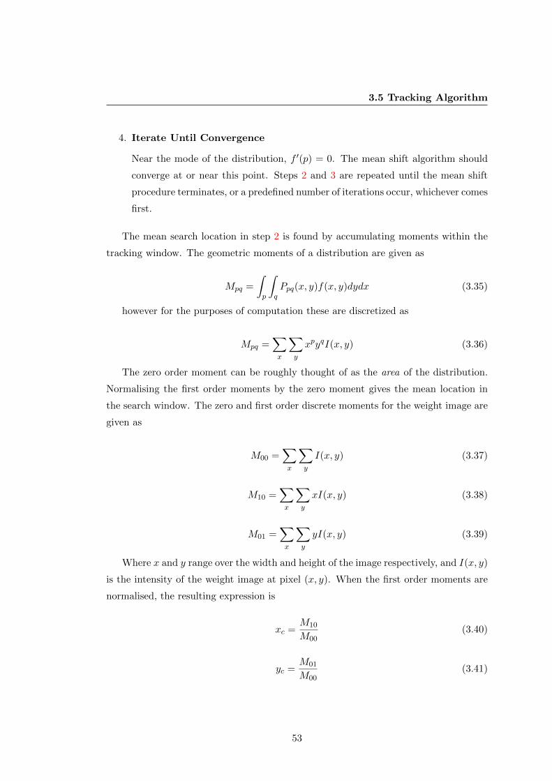
3.5 Tracking Algorithm
4. Iterate Until Convergence
Near the mode of the distribution, f ′(p) = 0. The mean shift algorithm should
converge at or near this point. Steps 2 and 3 are repeated until the mean shift
procedure terminates, or a predefined number of iterations occur, whichever comes
first.
The mean search location in step 2 is found by accumulating moments within the
tracking window. The geometric moments of a distribution are given as
Mpq =
∫p
∫qPpq(x, y)f(x, y)dydx (3.35)
however for the purposes of computation these are discretized as
Mpq =∑x
∑y
xpyqI(x, y) (3.36)
The zero order moment can be roughly thought of as the area of the distribution.
Normalising the first order moments by the zero moment gives the mean location in
the search window. The zero and first order discrete moments for the weight image are
given as
M00 =∑x
∑y
I(x, y) (3.37)
M10 =∑x
∑y
xI(x, y) (3.38)
M01 =∑x
∑y
yI(x, y) (3.39)
Where x and y range over the width and height of the image respectively, and I(x, y)
is the intensity of the weight image at pixel (x, y). When the first order moments are
normalised, the resulting expression is
xc =M10
M00(3.40)
yc =M01
M00(3.41)
53
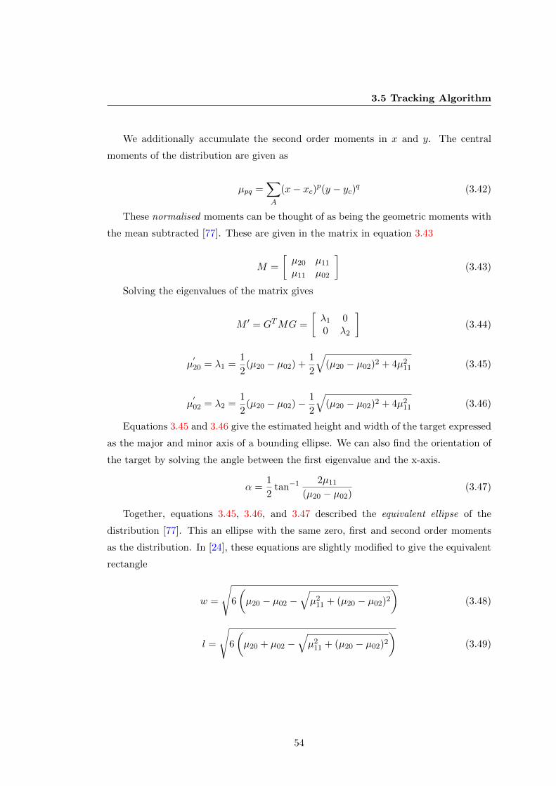
3.5 Tracking Algorithm
We additionally accumulate the second order moments in x and y. The central
moments of the distribution are given as
µpq =∑A
(x− xc)p(y − yc)q (3.42)
These normalised moments can be thought of as being the geometric moments with
the mean subtracted [77]. These are given in the matrix in equation 3.43
M =
[µ20 µ11µ11 µ02
](3.43)
Solving the eigenvalues of the matrix gives
M ′ = GTMG =
[λ1 00 λ2
](3.44)
µ′20 = λ1 =
1
2(µ20 − µ02) +
1
2
√(µ20 − µ02)2 + 4µ211 (3.45)
µ′02 = λ2 =
1
2(µ20 − µ02)−
1
2
√(µ20 − µ02)2 + 4µ211 (3.46)
Equations 3.45 and 3.46 give the estimated height and width of the target expressed
as the major and minor axis of a bounding ellipse. We can also find the orientation of
the target by solving the angle between the first eigenvalue and the x-axis.
α =1
2tan−1
2µ11(µ20 − µ02)
(3.47)
Together, equations 3.45, 3.46, and 3.47 described the equivalent ellipse of the
distribution [77]. This an ellipse with the same zero, first and second order moments
as the distribution. In [24], these equations are slightly modified to give the equivalent
rectangle
w =
√6
(µ20 − µ02 −
√µ211 + (µ20 − µ02)2
)(3.48)
l =
√6
(µ20 + µ02 −
√µ211 + (µ20 − µ02)2
)(3.49)
54

3.5 Tracking Algorithm
This is projected on the weight image in the screen captures given in [24]. The
method used to set the tracking window in [24] is tailored specifically to the application
(face tracking), and generalises poorly. The window size s is given as
s = 2
√M00
Vmax(3.50)
where Vmax is the maximum value a weight image pixel has for the current iteration.
It is important to stress that Vmax is the maximum value in the distribution, and not
the maximum value possible. The square root term converts the 2-dimensional region
under the image into a 1-dimensional ‘length’. Vmax acts as a scaling term. The ‘length’
of the window is set to 1.2× s. The size of the search window in [24] is also controlled
indirectly by scaling the model histogram by a constant. Doing this affects the pixel
values in the weight image, in turn affecting the value of M00 and therefore the value
of s.
3.5.2 Tracking in Comainciu, Ramesh, and Meer
In Comaniciu, Ramesh and Meer [26] the weight image generation is embedded in
the procedure - the so-called implicit method [94]. Minimising the distance given
by equation 3.19 as function of y finds the location of the target in the frame. The
procedure to find the target in the current frame starts from the target location in the
previous frame and searches the surrounding neighbourhood. The similarity function
in equation 3.23 inherits the properties of the kernel profile k(x). Therefore, choosing
k(x) such that its profile is differentiable yields a differentiable similarity function. This
allows the tracking procedure to use gradient information provided by the mean shift
vector (equation 3.55).
Colour features are chosen in [26], although in principle any feature can be used [94].
Minimisation of equation 3.19 is equivalent to maximising equation 3.20. This requires
that the second term in equation 3.23 is maximised, as it depends on y, the target
location in the frame computed with kernel k(x), weighted by wi given in equation 3.24.
The mode of the density in the neighbourhood around y is found using the mean shift
55

3.5 Tracking Algorithm
procedure. This causes the kernel to be recursively moved from the current location y0
to some new location yi according to
yi =
∑Nhi=1 xiwig
(∣∣∣ y0−xi
h
∣∣∣2)∑Nh
i=1wig
(∣∣∣ y0−xi
h
∣∣∣2) (3.51)
where g(x) = −k′(x). This assumes the derivative of k(x) exists for all x ∈ [0, inf).
The complete target tracking procedure in [26] is given below
1. Initialise Target Location
The initial location of the target y0 is set. The histogram of the target model
qu(u = 1, . . . ,m) is provided as an initial parameter. The target candidate his-
togram pu(y0) is computed, and the distance function in equation 3.19 is com-
puted.
2. Derive Bhattacharyya Coefficient Weights
The weights wi, (i = 1, . . . ,m) are computed according to equation 3.24.
3. Compute New Target Location
The next candidate location is found by equation 3.51.
4. Compute New Histogram Distance
The new target candidate histogram pu(y1) is computed, and the histogram dis-
tance in equation 3.19 for location yi such that
p(y1, q) =
m∑u=1
√pu(y1)qu (3.52)
5. Minimise Histogram Distance
Iteratively converge on minimum histogram distance. While p(y1) is less than
p(y0), set y1 as 12(y0 + y1). If the distance falls below some minimum threshold
ε, stop the loop and update. Otherwise go to step 2.
56

3.6 Mean Shift Vector
In practise, not all the above steps are implemented. In particular, step 5 of the
algorithm is omitted from the implementation in [26] as it is found to have little effect
in practise1. Thus, only the computation of the mean shift vector in equation 3.51 is
required for tracking.
The computation is further simplified by the choice of kernel. Recall the expression
in equation 3.51 uses the kernel profile g(x), where g(x) = −k′(x). Substituting the
Epanechnikov kernel, given by
kE(x) =
{12c−1d (d+ 2)(1− x) if x ≤ q
0 otherwise(3.53)
into the mean shift vector expression gives
m(x) =
∑nhi=1 xiwi∑nhi=1wi
(3.54)
This is due to the fact that the derivative of kE(x) is a constant, which in turn
reduces the mean shift vector in equation 3.51 to a simple weighted average. In this
form, the inner loop of the tracking procedure is much closer to that in [24], the main
difference being that the weight image is embedded in the procedure.
3.6 Mean Shift Vector
The mean shift formulation was first described by Fukunaga in [67]. In this work, the
gradient of a density function is estimated iteratively by computing the mean of a set
of points
The mean shift vector is the vector along which the target window W is translated
from its position in p(xn, yn) in frame n to a new position p(xn+1, yn+1) in frame n+ 1.
This vector is given as the spatially weighted average of the kernel density estimation
of the weight image
m(x) =
[∑nhi=1 x
∗iwig(‖y0−x
∗i
h ‖2)∑nhi=1wig(‖y0−x
∗i
h ‖2)
](3.55)
1The purpose of step 5 is to avoid possible numerical problems in the linear approximation of the
Bhattacharyya coefficient [26]. Since step 5 is omitted, there is also no need to compute the weight
terms (equation 3.24) in steps 1 and 4
57

3.6 Mean Shift Vector
Where g(x) is the profile of the kernel function, and is given as
g(x) = k′(x) (3.56)
The most common choice of kernel in the literature is the Epanechnikov kernel,
which is normally given as per equation 3.53. This kernel is normally chosen because
its derivative is flat [94] [26]. When the kernel is substituted into equation 3.56, the
mean shift vector equation in 3.55 reduces to equation 3.54, which is the arithmetic
average of the position of points in the weight image.
The mean shift vector in equation 3.55 is used to perform the Bhattacharyya coeffi-
cient maximisation of equation 3.23 as per the technique described in [67] and [26]. This
tracking window is then translated along the mean shift vector given in equation 3.55
until convergence. This is then repeated in the subsequent frame, and so on over all
the frames in the series.
58

Chapter 4
Hardware Implementation
Considerations
4.1 Mean Shift Tracker Operation
The operation of the mean shift algorithm for tracking is described in detail in sec-
tion 3.5.1. This section will consider the operation of the CAMSHIFT pipeline in
terms of the physical and temporal computational requirements.
To briefly review, a feature description of a target is used to generate a weight
image, where the intensity of each pixel corresponds to the likelihood that the pixel
is part of the target. This mean shift algorithm [67] is applied to locally maximise a
density function on the weight image. This maximisation procedure is iterative, and
involves translating a window to the basin of attraction in the density function [68].
These concepts are explained in detail in sections 3.3, and 3.5. This section will consider
these operations in terms of hardware requirements. This includes temporal concerns
such as datapath timing, memory access patterns, as well as more general concerns
about area and logic complexity.
This chapter will cover the following design considerations in terms of hardware
implementation.
1. Weight Image Generation
In software implementations such as [24], [27], [83], and so on, it can normally be
assumed that retrieving pixel values from memory is a trivial task. The implicit
weight image formulation (section 3.3) forms the weight image by a weighting
59

4.1 Mean Shift Tracker Operation
function that contains the term xi, representing the ith pixel in the dataset. This
requires access to the original image which in turn requires a significant block of
memory to exist in the system. This consideration is discussed in more detail in
section 4.5.
2. Weight Image Storage
Because the algorithm iterates over the weight image to localise the target, the
weight image must be stored somewhere in the system. It is therefore natural to
consider the most efficient representation for the weight image. This is discussed
in more detail in section 4.4.2.
3. Mean Shift Vector Calculation
Vectors of weight image pixels are supplied to the accumulator for moment ac-
cumulation. The centroid of the windowed distribution is computed from the
moments until successive reads produce centroids within 1 pixel of each other.
The primary concern with implementing this component in hardware is main-
taining the vectorised data stream. The accumulator must be able to process V
pixels simultaneously, which requires that scalar terms in the moment accumu-
lation are expanded. This in turn directly affects the area consumption of the
accumulation stage.
4. Window Parameter Calculation
This stage of the calculation is the most straightforward to implement. Arithmetic
modules capable of performing the required calculations are chained together in a
pipeline, along with a controller which asserts control signals at the correct time.
Thus, the datapath realises the calculation of the equivalent ellipse.
Design decisions in the hardware pipeline are strongly influenced by the need to
move away from the more software focused approach of read, compute, and write-back.
Iterating over an array of pixels by reading each pixel from memory, performing some
processing operation, and writing the result back to memory is not a feasible paradigm.
In the remainder of the chapter, the choice of implementation for each major component
is explained.
60

4.1 Mean Shift Tracker Operation
4.1.1 Tracking and Frame Boundary
Iterating over the weight image in the mean shift inner loop requires multiple data
reads. If these data reads are to occur before the next frame arrives there are two
possible implementations
1. Multiple clock domains
The data is acquired from the sensor in one clock domain, and is processed in
another, faster clock domain. This implementation has the drawback of limiting
the rate at which data can be acquired to half the maximum feasible clock rate.
2. Vectorise data pipeline
The data is accumulated into vectors and multiple pixels are processed simulta-
neously. In this implementation the data acquisition and processing can occur in
the same clock domain, at the cost of increased area and complexity.
Since most sensors only provide one pixel per cycle, vectoring the calculation does
offer the possibility to perform multiple iterations of the mean shift inner loop while
waiting for new data to enter the pipeline. The maximum number of iterations that
can be performed per image is a function of the ratio between the number of pixels
which can enter the pipeline to the number of pixels that can be processed on each
cycle, which can be given as
Imax =Wproc
Wacq− 1 (4.1)
where Wacq is the width of the acquisition input in pixels, Wproc is the width of
the processing pipeline in pixels, and Imax is the maximum number of iterations. This
implies that a certain value of Imax can be maintained even for sensors which provide
multiple pixels per cycle, so long as the resource and timing for the target device is
sufficient to provide
Wproc =Imax
Wacq+ 1 (4.2)
pixel processing pipelines.
61

4.2 Pipeline Orientation
4.2 Pipeline Orientation
Although the order in which pixels are processed has no bearing on the algorithm itself,
it does have some important consequences on the design of the tracking hardware. To
the greatest extent possible, it is neccessary to avoid caching or buffering the image
in whole or in part as memory in the FPGA is limited, and iterating over it to per-
form operations is both slow and, depending on the nature of the addressing pattern,
potentially complex.
Assume the data stream entering the pipeline is scalar. That is, on each cycle only
one data point enters the pipeline. Vectorising this data stream requires that data
points are accumulated in a buffer and concatenated into vectors before processing.
Because an image is being processed, it is natural to consider the data structure as a
two-dimensional lattice of values which represent the light intensity at each quantised
position in space. Most commercially available CMOS sensors provide the pixel data
stream as a raster which scans over each row of the image in turn, typically from
top-to-bottom, left-to-right [115].
This leaves the question of how best to concatenate the data for use in a vector
processing architecture. Immediately two possibilities arise
1. Along the dimension of the raster
This scheme involves buffering together V pixels to use as a processing unit, where
V is the dimension of the vector. In this scheme pixels directly enter a buffer of
depth V which lies in the same dimension as the input stream.
2. Orthogonal to the dimension of the raster
This scheme involves buffering V rows of the image data and joining together the
kth element of every V rows to form a data vector. In this scheme pixels enter a
larger buffer and are concatenated along the dimension orthogonal to the input
stream.
For the remainder of this document, the spatial relationship between the input data
stream and the pipeline data stream will be termed the orientation of the pipeline. For
a two dimensional lattice such as an image, there are two possible orientations, which
are termed here as the row-orientation and column-orientation. In the context
62
4.2 Pipeline Orientation
of this pipeline, the row-orientation concatenates vectors along the same dimension
as the input raster. The column-orientation concatenates vectors orthogonal to the
input raster.
4.2.1 Segmentation Pipeline
The segmentation pipeline is concerned with extracting pixels belonging to the target
from the input image. To minimise hardware cost, this pipeline performs a colour space
transform from the RGB space to the HSV space. This transform means the colour
information is represented in a single channel, and therefore the colour feature space
has only a single dimension. The approach outlined here, while one-dimensional, can
be applied to multiple dimensions by simply instantiating multiple pipelines. This can
dramatically improve the segmentation performance of the system, with the obvious
cost of additional area, routing, and timing constraints. This study will focus on a
one-dimensional segmentation pipeline, and this fact should be assumed throughout
the remainder of the document.
The segmentation is performed using the method in [47]. This requires that the
histogram of the input image is found. Pixels from the original image are replaced by
the values they index in the histogram. Therefore, pixels in the input image cannot
be discarded until the image histogram is found and the ratio histogram is computed.
This presents a problem, as the entire image is too large to store entirely in memory.
To alleviate this bottleneck, the image is processed in segments. The shape of
the segment depends on the orientation of the pipeline (see section 4.2). In the row-
oriented pipeline, the histogram is accumulated on a 1-dimensional row of pixels which
lie along the dimension of the raster. In the column-oriented pipeline, the data is
buffered over several rows of the image, and the histogram is accumulated in blocks
of V × V pixels, where V is the vector dimension. The stages in the pipeline are as
follows.
1. Bin Indexing
As each pixel enters the pipeline, the histogram bin into which it falls is deter-
mined by an indexing module (section 4.3.2).
2. Image Pixel Buffer
63
4.2 Pipeline Orientation
Each pixel which enters the indexing module is also stored in a buffer. The data
is read out at the end of the operation when the ratio histogram is computed.
3. Histogram Increment
For every pixel entering the pipeline, a new index vector is generated. The accu-
mulation of these index vectors over the length of the buffer forms the histogram
of the image.
4. Ratio Histogram
At the end of the block, the image histogram for the current patch of data has been
accumulated, and this forms the denominator of the ratio histogram. The model
histogram, which is stored in a separate memory, is provided as the numerator to
a divider bank.
5. Ratio Histogram Indexing
Once the ratio histogram is found, the pixels in the pixel buffer are passed through
another histogram indexing module. The indexing vector generated here is used
to look up values from the ratio histogram. The output value for each pixel in
the buffer is assigned the value in the ratio histogram which that pixel indexes.
The orientation of the pipeline has a more significant effect on the segmentation
architecture than the tracking architecture. The Colour Indexing Technique uses the
ratio of two histograms to separate the target from the background, requiring a bin-
wise division operation to occur [47] [24] [94]. Additionally, the need for a histogram
in general implies that the operation must be performed on groups of pixels. In order
to perform the indexing operation which discriminates the target, we replace the pixels
with the value in the bin they index, thereby requiring us to remember the pixel values
until the end of the operation. This requires some staging memory to hold currently
unprocessed pixels while the ratio histogram is being computed.
Because the orientation affects the way data is stored and accessed, it has a direct
impact on the way memory is allocated in the pipeline. For both orientations, pixels
must be held in memory until the ratio histogram has been computed. The time
required to compute the ratio histogram is equal to
Rt = P × tdiv (4.3)
64

4.3 Backprojection in Hardware
where P is the size of the image patch the histogram is accumulated over, and tdiv
is the number of cycles required to perform the division. This calculation assumes that
pixels enter the pipeline at a rate of one per cycle. Thus, computing the image histogram
over a larger patch of the image places more pressure on the available memory.
4.3 Backprojection in Hardware
Section 3.3 discusses the two categories of weight image generation that are commonly
accepted in the literature, the implicit and explicit methods. The implicit method
embeds the weight image in the tracking procedure by taking derivatives of the Bhat-
tacharyya coefficient with respect to the image position. However computing the
weights requires a square root operation, which is relatively costly in hardware and
time.
The explicit method generates a Lookup Table of values from the ratio histogram,
which encodes the importance of colour features in the target to colours in the back-
ground. Generating and indexing a Lookup Table of values is a simple operation to
implement in hardware, eliminates the requirement to compute a square root for each
pixel, allows for relatively simple choices of number representation, and does not require
multiple cycles to access.
4.3.1 Hardware implementations of histograms
A typical hardware implementation of a histogram consists of a memory bank whose
entries represent the bins of the histogram [116]. Each memory location holds a count
representing the number of times the value has been accessed, and is addressed by the
value of the incoming data. Thus, over the course of a data stream the memory will
come to hold values indicating the number of times a particular value was seen [117]
[40].
The data increment for the system is usually achieved by reading the count data
at the bin address Abin, adding 1, and writing the count back to the same location in
memory [117]. This requires two cycles for each increment - one cycle for accessing
the memory, and one cycle for writing the incremented value back to Abin. Storing a
histogram in this format requires a memory with a depth equal to the number of bins
in the histogram Nbins, and a width equal to dlog2(Nbins)e.
65

4.3 Backprojection in Hardware
Figure 4.1: Dual clock histogram from [40]
This presents problems if it is required to compute the new values for several bins
simultaneously. Additionally, employing on-chip memory within the FPGA incurs a
time penalty to write zeros to the histogram between image blocks.
In the column oriented backprojection pipeline V new bin values must be found
simultaneously, where V is the vector dimension of the pipeline. Implementing his-
togram increment logic in parallel is difficult as it brings associated costs in time or
complexity to decode the histogram values. Various schemes have been proposed to
parallelise the histogram increment process.
A technique to execute to perform the increment and write back in a single cycle is
described in [40]. This technique uses a dual-ported dual-clocked RAM with input data
stream on one side and the increment on the other as shown in figure 4.1. The tech-
nique requires that the increment is performed in another clock domain with twice the
frequency of the input clock. This automatically means that the data clock frequency
can not exceed 50% of the maximum frequency of the device. For low-cost devices with
maximum clock frequencies that will not practically exceed 100MHz, this means the
data pipeline is limited to 50MHz or less. For stream processing as in section 4.4 this
technique fails to deliver any significant speed benefit, partly because the data pipeline
can only run at half the speed of the histogram memory, and partly because there is
still no method that can quickly clear the histogram between pixel blocks.
Several approaches are discussed in [118] for solving the parallel implementation
problem. However none of these approaches are suitable for a heavily-pipelined stream
66

4.3 Backprojection in Hardware
implementation such as that presented in this work. Additionally, the techniques in
[118] suffer from area and timing trade-offs which becomes unacceptable for a parallel
reading factor greater than 8.
It should also be noted that the implementations presented in [40], [118], [116],
[119] are designed for use in applications where the number of bins is close to or equal
to the number of possible values in the data stream. The results in [47] suggest that
the number of bins in the ratio histogram is relatively unimportant, and that a small
number of bins may have a desirable filtering effect. This makes some of the assumptions
used in the above implementations invalid.
For the CSoC pipeline, all histograms are implemented as arrays of registers. There
are two motivations for this. Firstly, the fact that a small number of bins is sufficient
[47]. The OpenCV implementation of CAMSHIFT defaults to 16 bins [48]. Comaniciu
also uses 16 bins in [26], however it should be noted that the implementation in [26]
tracks features in an RGB colour space, with 16 bins provided per channel1. Conversely,
[24] and [48] are implemented in a single dimensional hue feature space, and as such
only provide 16 bins total. In CSoC, 16 bins are provided, primarily to limit the register
use in the device.
Secondly, the weight image is generated patch-wise from the incoming pixel stream
to save memory. Therefore the effective image size in the pipeline is only a fraction
of the total, causing the histograms to contain only a relatively small number of data
points. In the case of the column oriented backprojection, the image patch is V × Vpixels in size. In the row oriented backprojection, the image patch is half a row of
the image. As well as being relatively small, the histogram needs to be cleared to zero
at the end of a patch. If implemented as a RAM block, this would require writing
a zero to each location in RAM. In the row oriented pipeline, this does not place
any additional time pressure on the pipeline, since the size of the image patch is large
compared with the number of bins. However in the column oriented backprojection,
it becomes difficult to write zeros into a memory bank which has to be ready V cycles
later, and contains V entries.
1To clarify, the feature space in [26] is quantised into 16 × 16 × 16 bins
67
4.3 Backprojection in Hardware
4.3.2 Indexing Histogram Bins
To prevent data stalls and maintain a stream architecture (section 4.4) there must be
a fast way to index the bins of the various histograms in the segmentation pipeline.
Again, the orientation of the pipeline effects the method used to index the histogram.
1. Row Orientated Bin Index
A bank of parallel comparators is used to generate an index vector. Within the
comparator bank, comparator k takes as one input the upper limit of the bin in
position k, and the pixel word as the other. This generates a compare pattern that
shows whether the value of the incoming pixel is less than the upper limit of the
bin associated with its comparator. The pixel falls into the first bin that fails the
compare. Implementing the indexing like this removes the need to compare both
the upper and lower limit of the bin, thus saving a compare. The output of the
comparator bank is fed through a LUT that generates a one-hot vector indicating
which bin the pixel falls into. This one-hot vector is used in the remainder of
the pipeline for histogram indexing, and can directly drive the incrementer in the
histogram bank logic (section 4.4.1). This can be interpreted as a vector which
indicates the bin to be incremented.
2. Column Oriented Bin Index
Because the column orientation is orthogonal to the input raster, the histogram
indexing operation is vectored. Thus, V comparator banks as described above
must be available in parallel to find the V one-hot index vectors for all V pixels,
where V is the vector dimension. The output of this bank cannot directly drive
the histogram increment, as there may be several pixels that fall into the same
bin1. Therefore, an adder tree array must be placed on the output of the V -
dimensional comparator bank to sum the bin-wise increments. This produces
an intermediate vector of bin increments that can be used to drive a modified
histogram module. In the column oriented pipeline, the histogram module
takes as its input a data word that indicates how many counts to add to each
bin.
1In principle, all the pixels in the vector may fall into the same bin
68

4.4 Maintaining Stream Architecture in Segmentation Pipeline
4.4 Maintaining Stream Architecture in Segmentation Pipeline
The CMOS sensor on the input captures the amount of photons that were present in
each pixel at the moment of quantisation. Without the aid of an external memory, it
is not possible to recover these values once they have been read from the sensor. Since
limiting memory consumption is an implicit design goal throughout the system, the
ideal segmentation is one which takes a stream of image pixels as input and immediately
produces a weight image. While this outcome is not strictly possible due to the nature
of the backprojection technique [47], it must be the case that the design does not
require any interruption of the incoming pixel stream. Because the pixel data must be
be backprojected into image space once the ratio histogram has been computed, this
requires some redundant components to continuously handle the input stream while
back-end processing operations are occurring.
4.4.1 Datapath Timing
Central to the problem of streaming all pixels into the pipeline is the division operation
used to form the ratio histogram Lookup Table. This requires Wbin cycles to complete
using a restoring divider, where Wbin is the word width of a bin in the histogram.
Additionally, the histogram values must be cleared before the next image patch arrives.
However, unless the operation is occurring near the blanking interval of the sensor, the
next pixel in the stream will arrive on the following cycle. This implies the histogram
must be reset in zero time.
Pixels from the data stream must be buffered for at least Pimg + Wbin + 1 cycles
in parallel with the histogram increment stage for backprojection by ratio histogram
lookup. In this expression, Pimg represents the size of the image patch. As with the
histogram increment, unless the data always occurs on the blanking interval, the next
data point arrives on the following cycle. This means that there is zero time to re-
purpose the buffer from one patch to the next.
To overcome this difficulty, both the histogram increment logic and pixel buffers are
duplicated and swapped alternately between image patches. Each histogram module
contains a bank of incrementers which are driven by the bin select vector from the
histogram comparator, and a register array to hold the bin counts. At the end of an
image patch, the accumulating bank is switched. This gives time for the divider inputs
69

4.4 Maintaining Stream Architecture in Segmentation Pipeline
Figure 4.2: Timing diagram of histogram bank swap
Figure 4.3: Timing diagram of buffer operations in row oriented segmentation pipeline
to be registered from the outputs of the previous histogram bank, while also preventing
pixels from being dropped out of the stream. The previous histogram bank is cleared
just before it is required for the upcoming image patch. Figure 4.2 illustrates the timing
for this operation.
A similar requirement is imposed on the pixel buffer, although the specific details
of this depend on the orientation of the pipeline. In the row oriented pipeline, two
buffers are provided both of which are dual ported. The division operation interrupts
the flow of the pipeline, and therefore each buffer will be both reading and writing
during the division stage to prevent data loss from the previous image patch. Once
the division is complete, the previous buffer is read into the ratio histogram lookup
table. This allows the read pointer to stay ahead of the write pointer at all times, thus
preventing data loss. Figure 4.3 illustrates this.
In the row oriented pipeline the time required to perform the division is small
relative to the depth of the buffer. In the column oriented pipeline this is no longer
the case. This demands more holding registers on the inputs and outputs of modules
to allow for zero-cycle switching. For example, the read cycle pre-empts the division
by Datree cycles, where Datree is the depth of the vector comparator bank adder tree.
Another consideration that arises when timing the datapath operations is when
to begin reading data from the waiting buffer. Consider the general operation of the
backprojection pipeline in terms of buffer reads and writes. Incoming data is written
70

4.4 Maintaining Stream Architecture in Segmentation Pipeline
Figure 4.4: Timing diagram of buffer operations in column oriented segmentation
pipeline. Note the addition of buffering stages to ensure that zero-cycle switching is possible
without loss of data
Figure 4.5: Timing diagram of processing aligned with FULL flag
to the first buffer, and once full, data is written to the second buffer. During the write
to the second buffer, a processing step (the division operation) is performed, and the
data is read from the first buffer. This cycle repeats over the entire image stream,
interrupted only by the blanking interval of the input sensors. The question arises as
to where in time to place the read operation. Consider the diagram of figure 4.5.
4.4.2 Memory Allocation for Streaming Operation
A large image patch will directly impact memory use. However increasing the time
required for the division also adds pressure to memory resource. This is more true in
the column oriented pipeline, where the number of cycles required for the division
is close to the length of the image patch in pixels. Since the vectors are oriented
vertically, and one vector is processed in each cycle, the time taken for the division
71

4.4 Maintaining Stream Architecture in Segmentation Pipeline
effectively determines the number of buffering registers required to ensure no data is
lost.
As well as this, the vector size in the column oriented pipeline is equal to V ×Wpixel, where Wpixel is the width of the pixel word in bits. This means that a 16
element vector of 8-bit hue pixels requires 128-bits of memory. This affects the entire
data path of the column backprojection module. Both pixel buffers must have a total
input width of 128 bits1.
4.4.3 Aligning Division with Blanking Interval
One could observe that by designing the pipeline so the division always occurred in the
blanking interval, the control strategy could be greatly simplified. This however does
not take into account all the factors that generate memory pressure in the pipeline.
For example, in the column oriented pipeline, making the pixel buffer depth equal
to the width of the image simply duplicates the column buffer on the input. Even
if the pixel buffer is removed and the column buffer acts as the pixel buffer in the
backprojection step, the size of the histogram word must increase to account for the
fact that there are now V × wimg pixels to be backprojected, where wimg is the width
of the image. This is turn requires more registers for each bin of the histogram, and a
longer division time (or alternately, a more complex divider scheme). In saying that,
the need for a second histogram bank is now gone, which saves the equivalent counting
and multiplexing logic.
For a 640 × 480 image and a vector dimension of 16, the column buffer will hold
10240 pixels. This requires 14 bits per bin for all histograms in the pipeline, plus an
overflow bit2.
In the row oriented pipeline, the effect is far less pronounced. Taking the image
patch to be half a complete row long, the same 640×480 image in the previous paragraph
1The term total width is used, rather than just width, as the pixel buffer could equally be imple-
mented by having V buffers in parallel, each with a width of Wpixel, if such an outcome was desired.2The overflow bit is to account for the possibility that every pixel that comes into the buffer could
fall into the same bin. This scenario is more likely for small image patches, so one could conceivably
argue that with an image patch the size of the column buffer (16 rows by 640 columns in this example)
the chance of all these pixels falling into the same bin is extremely slight, and therefore the overflow
bit is not required, however the histogram will catastrophically fail if the assumption is violated, since
overflow will zero out the histogram for a large region of the image
72
4.5 Weight Image Representation
would require two buffers, each with a depth of 320 pixels. If the division operation is to
be aligned with the blanking interval, the two buffers (which are already dual-ported)
could be merged into single dual-port buffer with a depth equal to the entire width of
the image. This can work if the blanking interval is sufficiently long that the division
can be completed and at least one data point read out before the data for the next
row appears at the input. Doing so would prevent data from the previous row being
overwritten by data in the current row. This requires that the read point is kept ahead
at all times by at least one address.
Designing the pipeline like this does little to save resource. Firstly, the same amount
of memory is required in both cases. Either two buffers are required so that data isn’t
lost during the divide, or one buffer is required that is the size of the two small buffers
combined. Secondly, because the image patch has increased in size from half a row
to an entire row, the number of pixels to be accumulated has also increased, in turn
requiring a larger register size in the histogram bins. This directly affects the time
required for the division, and the resource consumption of the divider hardware.
4.5 Weight Image Representation
Mean shift trackers like CAMSHIFT attempt to estimate the gradient of the density
function by iteratively computing the mean shift vector in equation 3.55. This necessar-
ily requires that the weight image pixels over which the iteration takes place are stored
and accessed over the entire tracking run. Ideally the tracker would be implemented en-
tirely as a stream processor, taking weight image pixels as input and producing lists of
co-ordinates for each target. However in practise this is impossible due to the multiple
access requirement. Therefore a buffering system must be provided in the pipeline to
store at least some relevant part of the image for further processing. Moving to off-chip
memory allows for much more storage to be used at the cost of heavily constrained
memory bandwidth.
This constraint dramatically changes the parameters for what makes an optimal
pipeline. In particular, it makes locking the processing speed to the camera frame
rate more difficult as it implies the need for multiple clock domains. As the memory
requirement is not particularly onerous by the standards of contemporary memory
73

4.5 Weight Image Representation
capacity1, it also adds little utility. This study focuses on implementing the tracker
using only internal memory of the device, and therefore the techniques considered in this
section should be considered with this in mind. Several approaches can be considered
for implementing a weight image buffer on chip, these are explored below.
1. Buffer Complete Image
The entire image is buffered into memory and read out pixel by pixel on request.
In practise this consists of placing a block of RAM large enough to store the
entire image into the system with an address generator to provide the pixels
in the correct order. This system is simple and effective, but requires enough
memory to store the entire image. In a large number of cases, the target can
reasonably be anticipated to occupy less than the entire viewing area. Under
these conditions this system is quite wasteful of on-chip memory.
2. Buffer Compressed Representation
Since the weight image has much less information density than the original image,
it may be possible to compress this representation and store only the compressed
format. A possible compression scheme was developed as part of this study and is
detailed in sections 4.6 and 5.3.2. This representation is a buffer which stores the
scalar and vector dimensions of the vectorised weight image in separate memories,
and attempts to scale the resolution of the whole image by a power of 2 (up to
the vector dimension V ) in order to compress the image into a smaller fixed
memory size. Unlike spatial compression systems such as the discrete cosine
transform, this geometric compression requires almost no arithmetic. This results
in a relatively small compression ratio, but has the benefit of requiring almost
no arithmetic logic. This reduces area requirements and processing time, while
maintaining a smaller memory footprint.
3. Buffer Selected Regions of Image
If the target occupies only a small region of the image, then beyond a certain
boundary pixels can be discarded from the image without affecting the quality
of the tracker. This is possible because the tracking is windowed, and so beyond
1circa 2013 components
74

4.5 Weight Image Representation
the window border pixels have no effect on the target location. However because
the tracking window is translated until convergence, some pixels that are outside
the tracking window must be included in the procedure in order for the result to
be correct. Therefore, the technique implies the need for some motion prediction
capability to determine likely future positions for the tracking window to take on
next. This could be based on extrapolation from, say, the previous k tracking
windows. Since the goal of such a buffering system is to conserve memory, we
would ideally included the minimum number of additional pixels required to en-
sure that the tracking window would never be translated to some point on the
image where data was not available.
This presents another problem - how much fixed memory to allocate to the buffer?
Over allocating memory reduces the chance that an insufficient number of border-
ing pixels will be included for the window translation step, however the purpose
of the exercise is to reduce memory requirements, and allocating more memory
runs counter to this. Under allocating memory allows the total required physical
memory to be reduced, at the possible cost of being unable to buffer enough bor-
der pixels to correctly identify the target in the frame. This problem is referred
to in this document as the initial allocation problem (see section 4.6.2). More
complicated prediction may yield better results, however this could come at a
significant logic and timing cost.
4. Hybrid Approach
Some combination of the above methods could be used to reduce the total memory
requirement for the weight image. This might involve buffering a selected region
of the image which has a size that is a power of 2, and supplying pixels in this
region to a compression routine such as the scaling buffer. This design could
bring substantial memory savings in cases where there is significant clutter that
isn’t removed by thresholding alone, however the extent to which this system
represents an overall gain depends on the complexity cost, particularly of the
prediction step.
Recall section 3.3.2 which discusses how pixels are weighted in [26]. Because the
weights are derived by taking derivatives of the Bhattacharyya coefficient with respect
75
4.6 Scaling Buffer
to image location, the implicit technique requires access to the original image pixels.
This occurs in equation 3.21 as the weighted histogram term δ[b(xi) − u], where xi is
the ith pixel in the image.
Techniques using an implicit weight image present some problems for hardware im-
plementation. Consider a CAMSHIFT pipeline which uses a 1-dimensional hue feature
to describe the target. At 8-bit per pixel resolution storing only the hue channel, a
640× 480 image requires 24.576 megabits of memory. This makes implementation us-
ing only on-chip memory difficult. While data can be moved to an external memory
(DRAM, for instance), this reduces the memory bandwidth between the image buffer
and mean shift inner loop. By using the explicit formulation, the hue image can be
transformed into a weight image which can be more effectively compressed. For ex-
ample, the ratio histogram can be thresholded during the indexing stage to produce
a binarised weight image. This would reduce the memory requirement to 1-bit per
pixel. Weighting can be performed by allowing multiple bits per pixel, and providing
a comparator bank for each bin of the ratio histogram to quantise the weight image.
4.6 Scaling Buffer
One possible buffer scheme was developed in this study. This scheme attempts to save
only non-zero (foreground) pixels in the weight image, while also preserving the vector
dimension for the mean shift accumulator (section 5.5.1).
4.6.1 Removing Background Pixels For Storage
While removing background pixels seems like an obvious step to reduce the memory
required to store the weight image, this must be done in a manner consistent with
the data format of the vector accumulator. This requires that vectors have their value
tested against zero, rather than individual pixels. This also precludes any data format
that incorporates tagged pixel entries of the form p = (x, y, w), where x and y are
positions in the weight image, and w is a weight. Even if the image is binarised, which
would render the w term redundant, this still requires enough memory to store the
position data for every pixel in the weight image, which can be expressed as
M = R× log2(Wimg)× log2(Himg) (4.4)
76

4.6 Scaling Buffer
Where R is the size of the target region in pixels, and Wimg and Himg are the
width and height of the image respectively. Beyond a certain value, this requires more
memory than storing a 1-bit per pixel representation of the weight image itself. As well
as this, the scheme suffers from the initial allocation problem (section 4.5).
Firstly, consider the case where only non-zero (foreground) pixels are kept in the
weight image. The vector accumulator must be supplied with a new vector on each
cycle, therefore the data representation must be in terms of either row or column
vectors. Each vector supplied by the segmentation pipeline is tested and zero values
are discarded. The accumulator architecture is based on the expansion of vector data
points into pixel positions via a Lookup Table (section 4.7). Scalar data points are dealt
with using a row and column pointer to indicate image position. Because the non-zero
vectors may occur in any order, recovering the scalar pointer using an incrementer is
no longer possible. Thus, every non-zero vector must also be associated with a position
value that indicates where on the scalar axis of the image the vector lies.
With this in mind, the weight image is split into two buffers, a vector buffer,
which stores a bit pattern corresponding to the incidences of pixels in that vector, and
a scalar buffer which stores the position of the vector on the scalar axis of the image.
As well as this, an address is stored between each set of vectors, which indicates the
position on the vector dimension where the data occurs. This address entry is used to
index the LUT in the accumulator which restores the pixel positions for data in the
vector. As well as this, the position in the scalar dimension where each vector falls is
stored in a separate scalar buffer. When data is read out of the vector buffer, the
high order bit indicates whether or not the data is a vector pattern or an address in the
vector dimension. Each non-address read in the vector buffer causes a data point to be
read from the scalar buffer. The format of the data vectors is illustrated in figure 4.6.
Figure 4.7 shows a schematic view of how such a non-zero buffer is implemented.
When a new entry in the vector dimension is reached, the buffer controller multiplexes
the address information into the vector buffer with the address bit set.
4.6.2 Predicting Memory Allocation
The scheme in section 4.6.1 goes some way to reducing the overall memory requirement.
In particular, up to V pixels can be encoded with V + log2(Dscalar) bits, where Dscalar
is the size of the image along the scalar dimension. However there is still no way to
77

4.6 Scaling Buffer
Figure 4.6: Illustration of vector format in scaling buffer. Address words are inserted in
the vector buffer to indicate where in the vector dimension to interpret the bit patterns in
the vector word entries. The address word loads the vector LUT in the accumulator with
the correct set of positions, while the bits in the data word indicate the presence or
absence of data points on that vector
Figure 4.7: Diagram of non-zero vector buffer
78

4.6 Scaling Buffer
Figure 4.8: Illustration of 2 × 2 majority vote window. The top buffer stores pixels at
the original scale. The buffer below divides the image space by 2, effectively halving the
number of pixels required. This stage can itself be windowed to half the number of pixels
again, and so on
79
4.6 Scaling Buffer
predict in advance how many pixels will be in the target, and V + log2(Dscalar) bits
are required even if only 1 pixel is in the vector, before taking into account memory
overheads from the addressing scheme. This creates a situation where the designer
may have to over-allocate memory to avoid loss of information in some cases, defeating
the purpose of a more complex representation, or save memory at the expense of some
larger targets being difficult or impossible to track, in other words, the system is still
faced with the initial allocation problem. Both of these scenarios can be overcome by
allocating a fixed amount of memory, and then scaling the image dimensions such that
the weight image is always smaller than some fixed amount. This idea is the motivation
behind the scaling buffer.
Firstly, note that the dimension and position of the target is determined by the
moments of the distribution that lies within the window. We note that several dis-
tributions can feasibly have the same moments. If pixels were to be removed from
the weight image at regular intervals, then the normalised moments of the distribution
should remain relatively unchanged [77]. This is analogous to removing a percentage
of mass, evenly distributed, from some physical object. If the distribution maintains
the same ratio, the object will balance about the same point before and after the mass
is removed.
Consider now the initial allocation problem, in which the amount of physical memory
must be adequate to hold weight image pixels for the largest possible target. As the
target begins to occupy more pixels in the frame, the relative contribution of each pixel
to the centroid reduces. Therefore we posit that as the target grows larger1 the image
can be rescaled to a new, smaller resolution, and for a given target size, the ability of
the system to determine the target position will remain relatively unaffected.
Scaling is performed by placing sets of 2 × 2 windowing functions over the vector
data. Each window function performs a majority vote on the weight image pixels,
transforming each window into a new weight image with half the number of pixels.
This process is chained to achieve different scaling factors. Each set of 2× 2 windows
feeds another set which looks at pixels in the previous scale space. The transform from
one domain to next is illustrated diagrammatically in figure 4.8
Each 2× scaled vector is held in staging buffer which shifts 2 vectors together. At
the end of all scaling operations, the staging buffer will have shifted n vectors together,
1Represented by an increase in the term M00
80
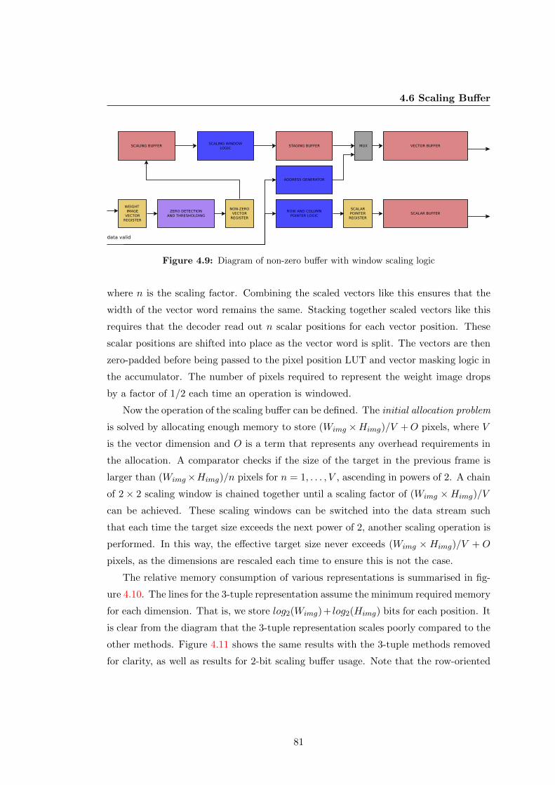
4.6 Scaling Buffer
Figure 4.9: Diagram of non-zero buffer with window scaling logic
where n is the scaling factor. Combining the scaled vectors like this ensures that the
width of the vector word remains the same. Stacking together scaled vectors like this
requires that the decoder read out n scalar positions for each vector position. These
scalar positions are shifted into place as the vector word is split. The vectors are then
zero-padded before being passed to the pixel position LUT and vector masking logic in
the accumulator. The number of pixels required to represent the weight image drops
by a factor of 1/2 each time an operation is windowed.
Now the operation of the scaling buffer can be defined. The initial allocation problem
is solved by allocating enough memory to store (Wimg ×Himg)/V +O pixels, where V
is the vector dimension and O is a term that represents any overhead requirements in
the allocation. A comparator checks if the size of the target in the previous frame is
larger than (Wimg×Himg)/n pixels for n = 1, . . . , V , ascending in powers of 2. A chain
of 2× 2 scaling window is chained together until a scaling factor of (Wimg ×Himg)/V
can be achieved. These scaling windows can be switched into the data stream such
that each time the target size exceeds the next power of 2, another scaling operation is
performed. In this way, the effective target size never exceeds (Wimg ×Himg)/V + O
pixels, as the dimensions are rescaled each time to ensure this is not the case.
The relative memory consumption of various representations is summarised in fig-
ure 4.10. The lines for the 3-tuple representation assume the minimum required memory
for each dimension. That is, we store log2(Wimg)+ log2(Himg) bits for each position. It
is clear from the diagram that the 3-tuple representation scales poorly compared to the
other methods. Figure 4.11 shows the same results with the 3-tuple methods removed
for clarity, as well as results for 2-bit scaling buffer usage. Note that the row-oriented
81

4.6 Scaling Buffer
Figure 4.10: Memory usage for various weight image representations
scaling buffer uses more memory than the column-oriented scaling buffer due to the
requirement to buffer pixels along the row dimension.
4.6.3 Limitations of Scaling Buffer
Implicit in the discussion in section 4.6.2 is the idea that the weight image will contain
only pixels relating to the target, and little to background clutter. In practise, this
may not be the case. Depending on the type and number of features used to generate
the weight image, there could be objects outside the tracking window that are present
in the weight image, which in turn will cause the value of M00 to increase. This affects
the assumption built into the scaling system that larger targets require less spatial
resolution, as a small target with large amount of clutter will be compressed1.
Overcoming this problem requires that the tracking module predict the location of
the target in the next frame2 and supply this information to the scaling buffer so that
pixels outside this area are not buffered.
1In the extreme case, a target that is 16 × 16 pixels in size, in a weight image with enough clutter
such that there is at least N = (Wimg ×Himg)/2 + 1) non-zero pixels, will be completely compressed
out in this scheme, although this could be overcome by enforcing a minimum number of target pixels
when (Wimg ×Himg)/2) or more weight image pixels are in the scene2This does not require a high level of accuracy. In fact, a larger prediction window is preferable
to a smaller one (although at the logical extreme, this is just another example of the initial allocation
82

4.7 Tracking Pipeline
Figure 4.11: Memory usage for scaling buffer and standard one and two bit representa-
tions
4.7 Tracking Pipeline
The role of the tracking pipeline is to take the weight image generated in the seg-
mentation step and iterate over the foreground pixels to generate the moments of the
distribution. Considerations for storing the weight image are described in detail in sec-
tion 4.5. Once the weight image is in the buffer, the remainder of the tracking pipeline
is conceptually straightforward.
The mean shift accumulator can be considered a SIMD processor which accumulates
the moments of the weight image. Since the moments of a probability distribution are
additive, we can process an arbitrary number of weight image pixels in each cycle, as
long as the required amount of arithmetic hardware is present. Thus the limitation on
our acceleration due to vectorisation is limited only by the ratio of pipelines to input
pixels (section 4.1.1). The accumulator consists of a bank of wide MAC units and
associated control logic. Pixel values are masked into the MACs based on the values in
the weight image vector. Designing the architecture this way reduces the need to store
individual pixel locations in memory.
problem). However it must be accurate enough to remove the need to buffer large amounts of redundant
data.
83
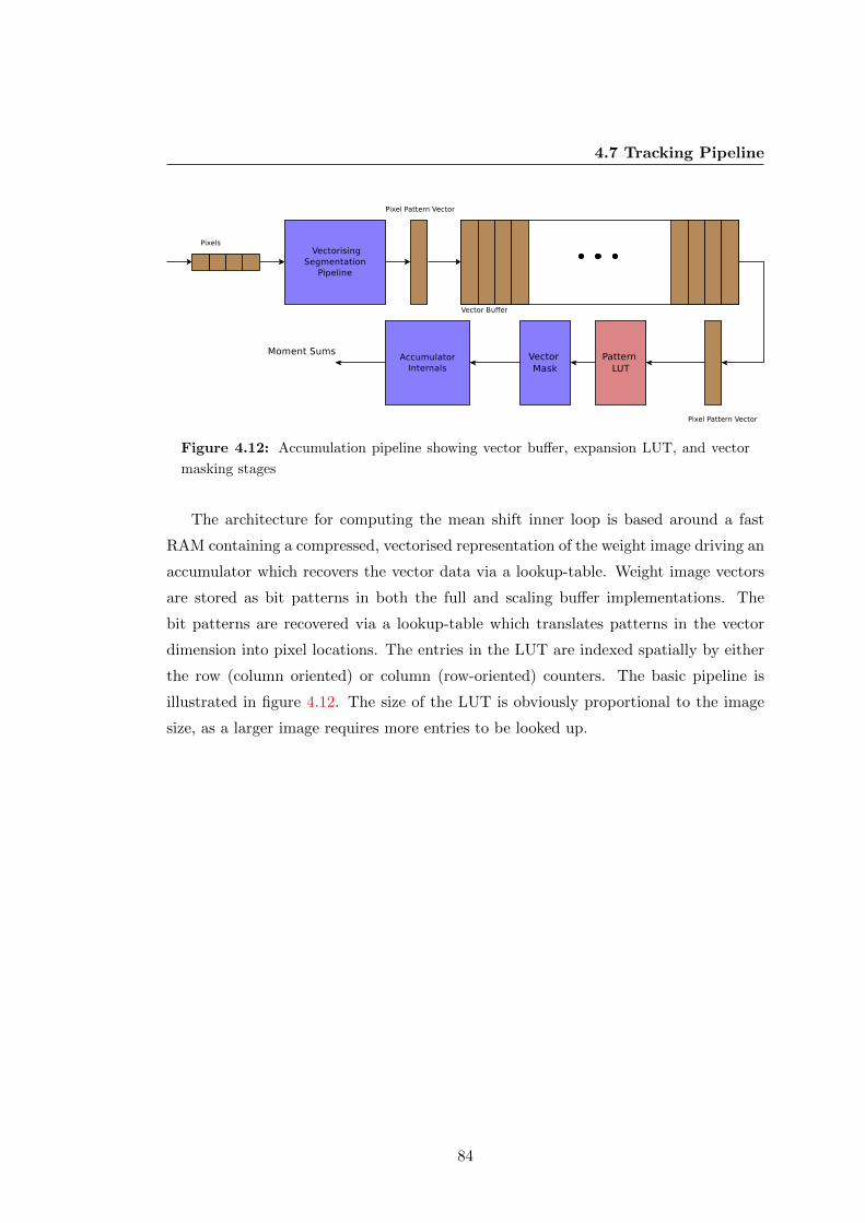
4.7 Tracking Pipeline
Figure 4.12: Accumulation pipeline showing vector buffer, expansion LUT, and vector
masking stages
The architecture for computing the mean shift inner loop is based around a fast
RAM containing a compressed, vectorised representation of the weight image driving an
accumulator which recovers the vector data via a lookup-table. Weight image vectors
are stored as bit patterns in both the full and scaling buffer implementations. The
bit patterns are recovered via a lookup-table which translates patterns in the vector
dimension into pixel locations. The entries in the LUT are indexed spatially by either
the row (column oriented) or column (row-oriented) counters. The basic pipeline is
illustrated in figure 4.12. The size of the LUT is obviously proportional to the image
size, as a larger image requires more entries to be looked up.
84

Chapter 5
CSoC Module Architecture
This chapter presents a detailed overview of the major components in the CSoC pipeline
from segmentation through to generating the tracking vector. Each section outlines
the design trade-offs made during development and explains the reasons behind these
decisions.
Figure 5.1 shows a simplified schematic representation of the entire tracking pipeline
from data acquisition to tracking output. The segmentation and tracking sections
comprise the majority of the CSoC functions, and are therefore illustrated in more
detail in figure 5.1. The segmentation and tracking pipelines are discussed in more
detail in sections 5.2 and 5.4 respectively.
The remainder of the chapter is organised as follows
1. Pre-Segmentation
Modules that occur ahead of the segmentation pipeline are described briefly here.
As these modules are somewhat outside the scope of the document, relatively less
detail is given, and all components are grouped into a single section
2. Segmentation Pipeline
The row and column segmentation pipeline is described in detail. The operation
and purpose of each module is explained along with diagrams.
3. Tracking Pipeline
Similarly, the internals of the tracking pipeline are examined. This module is
decomposed hierarchically over several sections.
85

5.1 Early Pipeline Stages
4. Controller Hierarchy
The interaction of state machines in the tracking pipeline is examined. Most
control operations are abstracted by a state machine to provide simpler interfaces
between modules. This approach is favoured over a single large state machine to
reduce state explosion.
5. Mean Shift Accumulator
This section breaks down the internals of the mean shift accumulator, which
performs the high speed arithmetic used to translate the window and compute
the size and orientation of the target.
6. Window Parameter Computation
The internals used to generate the window parameters are examined, including
the control strategy for enabling the modules in the correct sequence.
5.1 Early Pipeline Stages
This section details modules that appear ahead of the segmentation step in the pipeline.
This includes the acquisition logic, and colour space transformation logic. Only a brief
overview is provided, as these modules perform standard operations found in all systems
of this type.
5.1.1 CMOS Acquisition
Some front-end logic is required to interface to the input sensor. The specific details
of this logic depend largely on the manufacturers data sheet, and would typically be
implemented in accordance with the chosen sensor. Most sensors provide output in
the Bayer Pattern to compensate for the lack of a prism to split light. While this
dramatically decreases the amount of light information the sensor can provide, it does
help to reduce the size of the module. In systems that have multiple CCDs and a prism,
the acquisition logic would be different again.
In this pipeline, a reference design provided by Terasic corporation is used for the
acquisition stage. This design interfaces to the TRDB-D5M camera [115] and provides
a 1280-pixel line buffer used for De-Bayering the output. This in turn results in a 30-bit
86
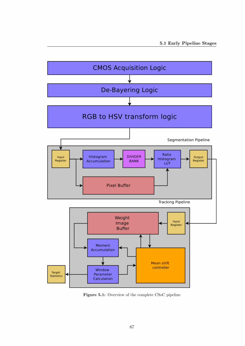
5.1 Early Pipeline Stages
Figure 5.1: Overview of the complete CSoC pipeline
87
5.2 Segmentation Pipeline
RGB stream being produced, with 10-bits of resolution per channel. This is truncated
to 8-bits per channel before entering the colour space transform module.
5.1.2 Colour Space Transformation
The 24-bit RGB stream is then transformed into a 24-bit HSV stream in a colour
transformation module. This operation can be implemented as a set of arithmetic
processors which compute the expression for each channel, or as a lookup table which
maps each RGB value on the input side to an HSV value on the output side. Lookup
table implementations are preferable if the bit resolution is sufficiently low. For this
pipeline, the 30-bit RGB input is sampled down to 24-bits (from 10-bit per channel to
8-bit per channel), meaning that the LUT for each of the Hue, Saturation, and Value
outputs only requires 256 entries. The saturation value is used as a kind of high-pass
filter to remove pixels with indeterminate colours, but otherwise the only value that is
kept for the remainder of the pipeline is the hue value.
5.2 Segmentation Pipeline
The Segmentation Pipeline is responsible for taking the hue pixels described in sec-
tion 5.1.2 and performing the histogram backprojection operation described in sec-
tion 3.5.1. As previously mentioned, the pipeline uses the explicit method of [24] and
[47] to generate the weight image that is fed into the pipeline in section 5.4. The weight
image is stored in a buffer in the mean shift processing module described in section 5.3.
In the row oriented configuration, the segmentation pipeline produces a new weight
image vector approximately every V cycles, where V is the vector dimension after the
initial processing delay. In the column oriented configuration, the pipeline produces
Iwidth weight image vectors every V × Iwidth cycles, where Iwidth is the width of the
image in pixels.
5.2.1 Histogram Bank
Section 4.4.1 discusses the requirement to have multiple histogram banks to accumulate
the image histogram. This requirement arises due to the need to perform zero-cycle
switching between image patches.
88
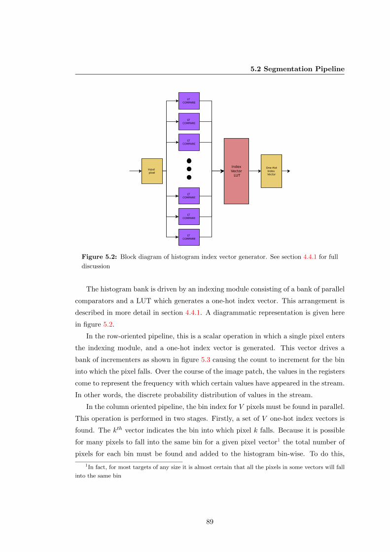
5.2 Segmentation Pipeline
Figure 5.2: Block diagram of histogram index vector generator. See section 4.4.1 for full
discussion
The histogram bank is driven by an indexing module consisting of a bank of parallel
comparators and a LUT which generates a one-hot index vector. This arrangement is
described in more detail in section 4.4.1. A diagrammatic representation is given here
in figure 5.2.
In the row-oriented pipeline, this is a scalar operation in which a single pixel enters
the indexing module, and a one-hot index vector is generated. This vector drives a
bank of incrementers as shown in figure 5.3 causing the count to increment for the bin
into which the pixel falls. Over the course of the image patch, the values in the registers
come to represent the frequency with which certain values have appeared in the stream.
In other words, the discrete probability distribution of values in the stream.
In the column oriented pipeline, the bin index for V pixels must be found in parallel.
This operation is performed in two stages. Firstly, a set of V one-hot index vectors is
found. The kth vector indicates the bin into which pixel k falls. Because it is possible
for many pixels to fall into the same bin for a given pixel vector1 the total number of
pixels for each bin must be found and added to the histogram bin-wise. To do this,
1In fact, for most targets of any size it is almost certain that all the pixels in some vectors will fall
into the same bin
89
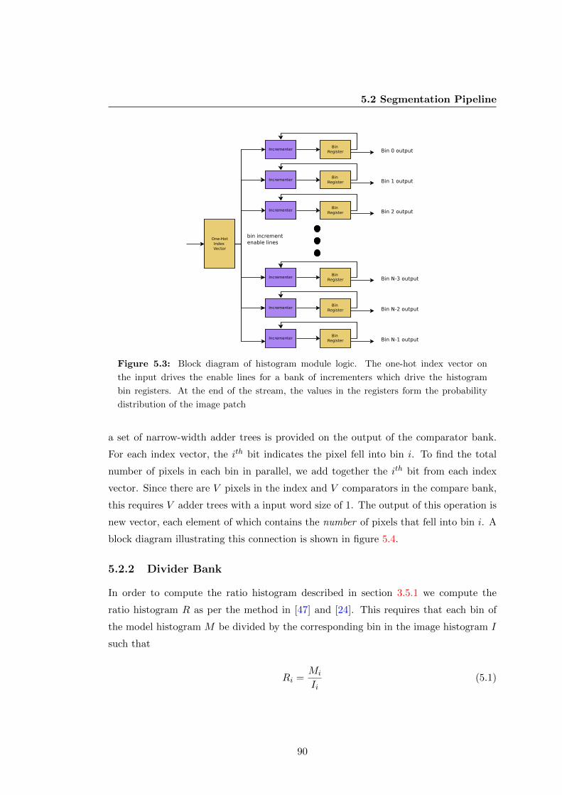
5.2 Segmentation Pipeline
Figure 5.3: Block diagram of histogram module logic. The one-hot index vector on
the input drives the enable lines for a bank of incrementers which drive the histogram
bin registers. At the end of the stream, the values in the registers form the probability
distribution of the image patch
a set of narrow-width adder trees is provided on the output of the comparator bank.
For each index vector, the ith bit indicates the pixel fell into bin i. To find the total
number of pixels in each bin in parallel, we add together the ith bit from each index
vector. Since there are V pixels in the index and V comparators in the compare bank,
this requires V adder trees with a input word size of 1. The output of this operation is
new vector, each element of which contains the number of pixels that fell into bin i. A
block diagram illustrating this connection is shown in figure 5.4.
5.2.2 Divider Bank
In order to compute the ratio histogram described in section 3.5.1 we compute the
ratio histogram R as per the method in [47] and [24]. This requires that each bin of
the model histogram M be divided by the corresponding bin in the image histogram I
such that
Ri =Mi
Ii(5.1)
90
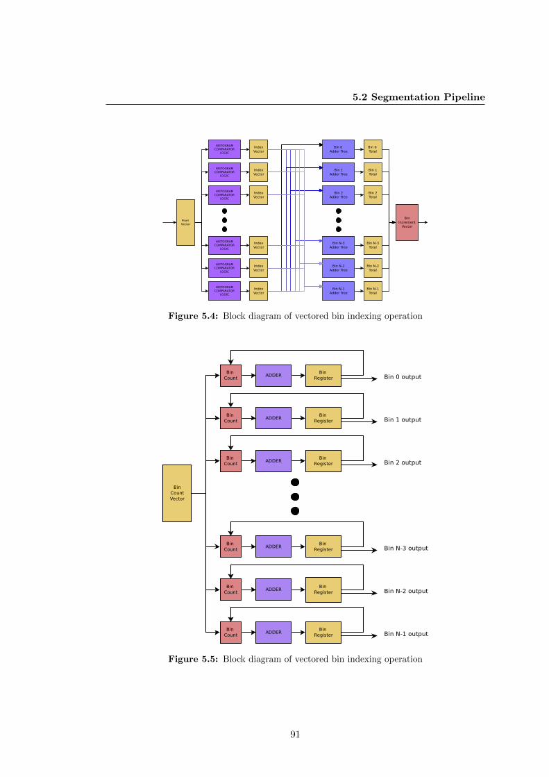
5.2 Segmentation Pipeline
Figure 5.4: Block diagram of vectored bin indexing operation
Figure 5.5: Block diagram of vectored bin indexing operation
91

5.2 Segmentation Pipeline
This requires that a divider module be present for each bin in the histogram, with the
ith divider having Mi as its numerator, and Ii as its numerator. The input words Mi
and Ii are shifted left by Wbin bits, where Wbin is the width of the word used to represent
a single bin in the histogram. This is done so that the output of the division operation
always falls in the range [0,Wbin − 1].The size of the division word and the type of
division scheme used have implications for the control strategy, as they determine the
minimum processing time for a block of data. This is discussed further in section 5.2.7
and section 5.2.4.
Restoring dividers are used in the pipeline, however in principle other division
schemes could be used (non-restoring, for instance). The size of the image patch has a
direct impact on the complexity of the division, as a large image patch requires more
pixels, and therefore increases the maximum value of the accumulation. This in turn
means that pixels must be buffered for more cycles before being backprojected into
image space.
The Column-Oriented backprojection pipeline is significantly more complicated
than the Row-Oriented backprojection, for the simple reason that the Row-Oriented
pipeline is aligned with the raster of the CMOS sensor. Thus the Row-Oriented pipeline
appears as a scalar pipeline with a shift register at the end for concatenation, whereas
the Column-Oriented Pipeline is vectored in the dimension of the sensor. This auto-
matically means that the column orientation has a greater area requirement than the
row orientation, and this area requirement is geometric in V , the vector dimension.
5.2.3 Row-Oriented Backprojection
The row oriented segmentation pipeline performs scalar pixel transformations on a
stream of input pixels in a 1-dimensional hue space. An diagrammatic overview of the
pipeline is given in figure 5.6. On each cycle, a single pixel enters on the left of the
diagram, a bin index is computed by an indexing comparator (shown in figure 5.2)
which drives a histogram bank like that shown in figure 5.3. Two histogram modules
are provided for zero-cycle switching (see section 4.4.1), the output is multiplexed into
the divider bank by the controller.
While the image histogram is accumulated, pixels are buffered into one of the pixel
FIFOs shown in red at the bottom of the diagram. Two buffers are provided for reasons
outlined in section 4.4.1. The timing diagram for the buffers is given in figure 4.3. The
92

5.2 Segmentation Pipeline
16 waycompare
HistogramBin Index
Histogram Accumulation
Divider Bank
Model Histogram Controller
Pixel Staging Buffer
Ratio Histogram
Lookup
16 waycompare
Pix
el V
ect
or
Row Vector Concatenation
HistogramBin Index
Figure 5.6: Overview of row-oriented backprojection pipeline
93
5.2 Segmentation Pipeline
size of the image patch in the row-oriented pipeline is half the width of the image.
Thus, each buffer holds 320 words. Each hue pixel is down-sampled to 8-bits before
segmentation, giving a memory size of 320×8 = 2560 bits bits per buffer, for 2560×2 =
5120 bits of memory in total.
Once the ratio histogram has been computed, pixels are read from the buffer into a
second indexing stage. The index vector generated here is used to select a value from
the ratio histogram for the current pixel. V pixels are placed in a shift register which
concatenates the row vector. For the purposes of zero-cycle switching, two physical
shift registers are provided with a controller that selects the correct input and output.
Once the shift register is full, a ready signal is generated to indicate to the next module
that a new vector is available.
5.2.4 Row Backprojection Control Strategy
The row backprojection controller is responsible for managing the interaction of ele-
ments in the backprojection datapath. The segmentation process must be managed
around this pixel stream in such a fashion that no data is lost or corrupted. This re-
quirement in turn influences the design of the datapath, and consequently the control
strategy.
Note that in the colour indexing formulation, pixels are backprojected into image
space via the ratio histogram, which assigns weights to each pixel. These weights are
generated by indexing the pixels into the ratio histogram. This requires that pixel
data is held in a buffer while the ratio histogram is computed. This in turn implies a
relationship between the pixel data rate, the size of the image patch upon which the
histogram is computed, and the rate at which processing can occur.
This relationship can be described as
Ncycles =W
D× (Tproc + Tctrl) (5.2)
where Tctrl represents the total number of cycles required for control operations for
an image patch, Tproc represents the number of cycles required for processing operations
in an image patch, W is the width of the image1 and D is the depth of the buffer for
the image patch.
1In this case, the image raster is assumed to go along the width dimension of the image. In the
case of a vertical raster, the term W would be replaced by H, the height of the image
94

5.2 Segmentation Pipeline
Figure 5.7: State diagram of buffer status controller for row-oriented backprojection
To prevent glitches, all state transitions, inputs and outputs in the controller module
are registered. While this gives superior high speed operation, it also introduces some
latency into the control loop. This means that if a buffer signals to the controller that
its state has changed, there is a lower limit on how quickly the controller can react that
is imposed by the number of registers the signal must pass through. To compensate for
this, all pixel buffers include pre-emptive status lines. As well as the normal full and
empty flags that signal the buffer status, a near full and near empty flag is provided.
These are asserted Tctrl cycles earlier than the normal flags, where Tctrl is the controller
latency in cycles. This allows the controller to prepare a state change in time such that
no data is lost on the incoming stream. In this implementation, the controller latency
is 4 cycles.
To simplify the implementation, the controller is split internally across several state
machines. Each state machine deals with a certain aspect of the processing pipeline,
as well as a global state machine to keep track of which buffer is currently holding
95
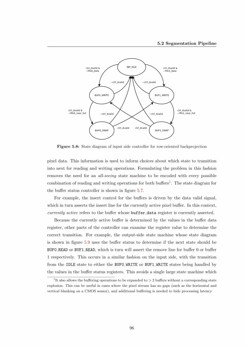
5.2 Segmentation Pipeline
Figure 5.8: State diagram of input side controller for row-oriented backprojection
pixel data. This information is used to inform choices about which state to transition
into next for reading and writing operations. Formulating the problem in this fashion
removes the need for an all-seeing state machine to be encoded with every possible
combination of reading and writing operations for both buffers1. The state diagram for
the buffer status controller is shown in figure 5.7.
For example, the insert control for the buffers is driven by the data valid signal,
which in turn asserts the insert line for the currently active pixel buffer. In this context,
currently active refers to the buffer whose buffer data register is currently asserted.
Because the currently active buffer is determined by the values in the buffer data
register, other parts of the controller can examine the register value to determine the
correct transition. For example, the output-side state machine whose state diagram
is shown in figure 5.9 uses the buffer status to determine if the next state should be
BUF0 READ or BUF1 READ, which is turn will assert the remove line for buffer 0 or buffer
1 respectively. This occurs in a similar fashion on the input side, with the transition
from the IDLE state to either the BUF0 WRITE or BUF1 WRITE states being handled by
the values in the buffer status registers. This avoids a single large state machine which
1It also allows the buffering operations to be expanded to > 2 buffers without a corresponding state
explosion. This can be useful in cases where the pixel stream has no gaps (such as the horizontal and
vertical blanking on a CMOS sensor), and additional buffering is needed to hide processing latency
96
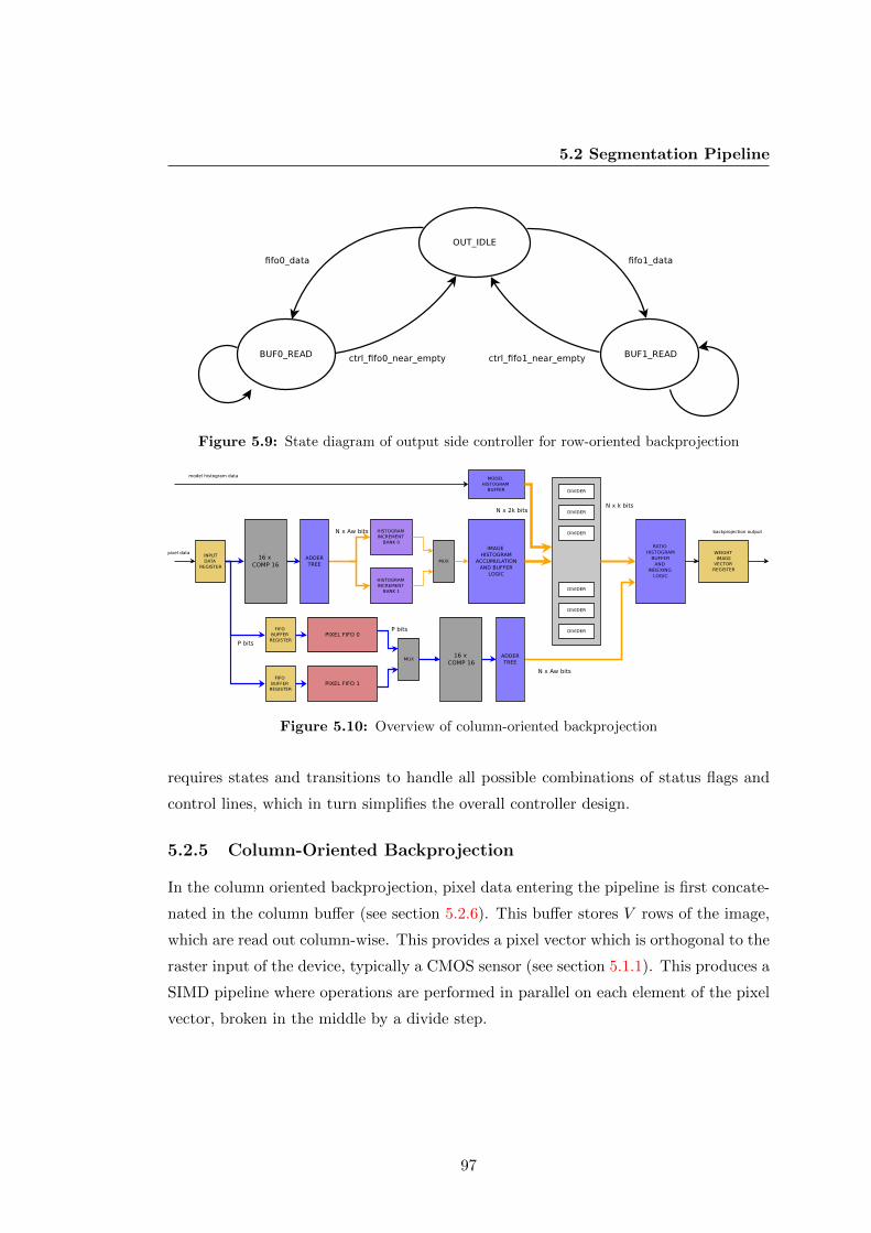
5.2 Segmentation Pipeline
Figure 5.9: State diagram of output side controller for row-oriented backprojection
Figure 5.10: Overview of column-oriented backprojection
requires states and transitions to handle all possible combinations of status flags and
control lines, which in turn simplifies the overall controller design.
5.2.5 Column-Oriented Backprojection
In the column oriented backprojection, pixel data entering the pipeline is first concate-
nated in the column buffer (see section 5.2.6). This buffer stores V rows of the image,
which are read out column-wise. This provides a pixel vector which is orthogonal to the
raster input of the device, typically a CMOS sensor (see section 5.1.1). This produces a
SIMD pipeline where operations are performed in parallel on each element of the pixel
vector, broken in the middle by a divide step.
97

5.2 Segmentation Pipeline
Figure 5.11: Block diagram of LUT adder for column backprojection
The column oriented backprojection is capable of processing V pixels at a time. In
order to perform the histogram binning computation in parallel, there must be V bin
conversion modules, each accepting one element of the pixel vector. The bin conversion
module produces a one-hot bin index vector which indicates the bin into which the kth
element of the pixel vector V falls. Accumulating the image histogram requires that all
V bin index vectors are summed element-wise, as it may be that many separate pixels
fall into the same bin and thus produce the same bin index vector. This operation
requires a set of V adder trees with V bits of input each for a total of V V − 1 bits of
summation.
To minimise the routing pressure imposed by such a set of adder trees, the addition
is implemented in two stages. Since V is chosen to be 16 in this study, the incoming 16
bit codeword is decomposed into 4 4-bit words which are summed by table lookup to
produce 4 3-bit sums. These are then combined in a two stage adder tree to produce a
5-bit sum for each bin. This scheme is shown in figure 5.11. The summation must be
performed in a bin-wise fashion. This is achieved by writing adder tree k with the kth
bit of each comparator codeword. Thus tree 0 adds the 0th bit of all codewords, tree 1
adds the 1st bit, and so on.
5.2.6 Column Buffer
Because the column-oriented pipeline is orthogonal to the raster direction, is it neces-
sary to concatenate together V rows of the image before processing can begin. The
column buffer acts as a staging area for this concatenation. Effectively, the buffer con-
sists of a set of V buffers with individual write controls and a linked read control. This
98

5.2 Segmentation Pipeline
Figure 5.12: Overview of buffer used to concatenate image pixels
allows each row to be written to as the data arrives, while each column can be read
simultaneously, thus providing a column pixel vector for the backprojection module.
This is shown in figure 5.12.
The column buffer contains a controller module which drives both the internal read
and write lines for each buffer, as well as the data valid line which drives the remainder
of the pipeline. Because the CMOS sensor has a blanking interval at the end of each
row, the controller can ‘pre-empt’ the next row and begin reading before new data
arrives. If the buffers are dual-ported, this means we only need 1 cycle of blanking to
avoid the write operation in the top row catching up with the read operation across all
the buffers.
5.2.7 Column Backprojection Control Strategy
Because of the division stage, there is a delay between when data has been read from a
buffer and when the buffer is available to receive new data. This delay is equal to the
number of cycles required to perform the division step. In the current implementation,
restoring dividers are used. While requiring less area than more complex division
schemes, they trade this off against time, requiring Sw cycles where Sw is the size of
the data word in bits.
99

5.2 Segmentation Pipeline
5.2.8 Ratio Histogram in Column Oriented Pipeline
Indexing the ratio histogram in the column oriented pipeline requires a large number
of decoders. As with the input side, a bank of comparators provide V index vectors for
each pixel vector. Each pixel in the weight image vector must then be replaced with
the value of the ratio histogram (quantised to the correct resolution, see section 5.2.9)
that lies in the bin indicated by the index vector. For a 16 element vector with a 16 bin
histogram, this requires routing a 128-bit bus into the ratio histogram module. This can
be minimised by transforming the one-hot representation to a binary representation,
thus reducing the width of the bus to V × log2(Nbins). This can be easily done using a
small Lookup Table. The output is a selection vector whose elements indicate the bin
u that each pixel p in the pixel vector falls into.
On the ratio histogram side, a V dimensional vector must be generated, which has
as each of its elements the value of the ratio histogram in bin u. The value of u is
encoded in element k of the selection vector encoded in the previous step. As with the
input side, it is possible1 that several pixels in the pixel vector fall into the same bin,
and therefore must be assigned the same value. To ensure that all bin values correctly
fall through to all pixels, a bank of decoders is provided. The layout of these encoders
is the reverse of the adder tree layout shown in figure 5.4. Each pixel is connected to
every bin output through a selector. The value in the selection vector selects which bin
arrives in the kth position in the weight image vector. This arrangement is illustrated
in figure 5.13.
5.2.9 Weight Image Resolution
By default, the modules are instantiated such that the weight image on the output is
binarised. Within the ratio histogram logic, a set of comparators are provided which
can perform a thresholding operation on the ratio histogram. Thus, only bin values that
have counts above some threshold produce a 1 in the weight image output. Attaching
this to a settable register allows the thresholding to be tuned during operation.
It may be desired to provide more weighting values than simply target and not
target. This can be achieved by increasing the bit depth of pixels in the weight image.
Allowing 2-bits per pixel provides 3 levels of weighting. This allows pixels that are
1In fact, likely
100

5.2 Segmentation Pipeline
Figure 5.13: Indexing of ratio histogram in column oriented pipeline
101
5.3 Mean Shift Buffer
somewhat similar to the target to provide some weighting, but not as much as pixels
which are a close match.
Clearly, implementing this scheme requires twice the memory of a binarised weight
image for buffering. In the segmentation pipeline, only the ratio histogram logic is
affected. In order to produce values that are correctly weighted, the indexing logic
must perform 2wp compares, where wp is the width of the weight pixel.
5.3 Mean Shift Buffer
The mean shift computation at the heart of the tracker is iterative. Therefore the
weight image must be stored in a buffer for future access. Ideally, we wish to guarantee
convergence in frame n before we have received all of frame n+ 1. To do this the mean
shift gradient ascent procedure (section 3.6) is performed on data from the previous
frame while the current frame is being accumulated. This requires that two completely
separated buffers are provided - one to accumulate the current image into, and one to
read the previous image out of for performing the mean shift inner loop.
The buffer controller acts as an abstraction layer between the buffering module
and the rest of the device. Externally, the buffering module should appear as a single
contiguous dual-port memory block, which can read and write to the same address
simultaneously. Internally, the controller contains two memory blocks which can be
assigned the role of reading or writing. At the end of the frame, the buffers swap roles.
To keep track of which buffer is assigned which role, a second state machine is
embedded within the controller (see section 5.3.1). Implementing the control strategy
this way simplifies the state transition matrix for the main controller, as it removes the
need to check many combinations of status registers.
External modules issue commands to read data from or write data to the buffer.
The controller takes the command and asserts the control signals for the buffer which
currently has the required role.
Because the buffer is used to store data that arrives in a raster format, the address
generation can be done with a counter. This is combined with the full and empty flag
generation in the FIFO logic.
102

5.3 Mean Shift Buffer
Figure 5.14: Schematic view of full mean shift buffer
5.3.1 Full Image Buffer
The simplest solution to buffering the weight image pixels is to simply write each pixel
into a RAM block. This requires enough memory to store all the pixels in the image.
For binarised images where the weighting simply indicates the presence or absence of
a target pixel, this issue may seem less worthwhile of attention, however as the bit
resolution of the weight image increases there is a linear increase in the amount of
memory required. As mentioned in section 5.3, two physical memories are required
so that accumulation of the current frame does not interfere with processing of the
previous frame.
5.3.2 Scaling Image Buffer
Clearly the buffering system in 5.3.1 does not make the most efficient use of memory.
One obvious improvement would be to discard the ‘dark’ pixels in the weight image,
leaving only the candidate pixels. However this strategy brings with it some compli-
103

5.4 Mean Shift Pipeline
cations. The weight image must still be processed as a vector otherwise the ability to
converge the mean shift iteration before the next frame is lost.
Naively, we might posit a solution as follows. Each candidate pixel is tagged spatial
information in the form of an (x, y) pair, as well as a weight value, forming a 3-tuple
of (x, y, w) where w is the weight. In this way the data is formed as a kind of linked
list. The problem with this approach lies in efficiently allocating memory to the linked
list. It is possible (and in fact likely) that the target will change scale during tracking.
The degree to which this might happen is difficult to predict in advance. Failure to
allocated sufficient memory for tracking will result in errors in the tracking vector. Over
allocation of memory will result in wasted Block-RAM on the device. We can safely
assume that in the majority of cases a relatively small region of the possible image area
will be occupied by a target, certainly under 50%.
As well as this is the problem of the size of a naive sparse representation. In the
3-tuple (x, y, w), the word size required to store x and y is dependant on the size of the
image. In the case of a 640 x 480 image, we require 10-bits and 9-bits for the x and y
components respectively. This can quickly add up to a significant memory requirement.
In fact for large number of pixels, this representation is less efficient than simply storing
the pixel data into an array and recovering the co-ordinate data from the array index.
Because this transform is to be done completely in hardware, we wish to have an
approach that allows us to allocate a fixed amount of memory at design time, which
can be used flexibly at run time with minimal overhead. As this memory will store
the weight image during all the mean shift iterations, we also want this to be as small
as possible. In addition to this, we prefer to minimise the amount of arithmetic to
be performed, as this will impact not only the timing and area, but also the depth of
the pipeline. A more detailed discussion of the scaling buffer is given in section 4.6.2,
including the motivation and implementation concerns.
5.4 Mean Shift Pipeline
Once the pixels have been processed by the segmentation pipeline in section 5.2, and
the resulting weight image is buffered into the mean shift buffer of section 5.3 the
pixels are read out by the top-level controller in the mean shift processing pipeline.
104

5.4 Mean Shift Pipeline
Figure 5.15: Mean shift accumulation and windowing pipeline
This controller ensures that the mean shift accumulator is constantly provided with
vector data for processing.
5.4.1 Mean Shift Controller Hierarchy
Within the mean shift processing module there are 3 levels of control. At the top level,
the MS CTRL module is responsible for the overall management of data and processing in
the pipeline. The buffering module contains a controller which separates the low-level
memory management operations from the processing components. Finally, a controller
within the mean shift computation pipeline itself schedules the order in which arith-
metical operations are performed once the moment accumulation is complete. Each of
these controllers is examined in greater detail below.
5.4.2 Top Level Controller
This controller is ultimately responsible for scheduling and ordering the various ele-
ments of the mean shift pipeline. When data enters the pipeline from the backprojec-
tion module, the controller instructs the buffering module to begin accumulating data.
The details of the buffer internals are hidden from operations at the level this controller
occupies.
Every major processing step in the pipeline requires at least one end of its interaction
to be processed by this controller. For example, the mean shift processing module
(section 5.4) issues data requests to the main controller. Because it cannot directly
105
5.4 Mean Shift Pipeline
issue requests to the buffer, it must wait for the controller to complete the transaction
on its behalf.
The behaviour of the top-level controller is governed primarily by 4 control lines,
the ctrl dvalid line, the ctrl data req line, the ctrl frame new line, and the ctrl -
frame end line. The overall pipeline operation is sequenced in terms of these signals.
5.4.3 Buffer Controller
This controller deals with low-level memory management. This includes deciding which
buffer is reading the current frame or accumulating the next frame, and managing the
insert and remove behaviour for each Block-RAM. Since the buffer is designed to be
read many times for each write, it is not feasible to use the full and empty flags of the
buffer modules directly. Thus, the control structure of this module is designed so that
this detail is hidden from the top level. As well as this, the fact that two independent
buffers are present is not visible at the interface level. The buffer controller provides an
interface that presents the buffer a single continuous memory which can be written to
and read from like a dual-port RAM block, but where read and write pointers can be
the same without data being overwritten. This allows the old image to be read many
times as the new image is being written.
The overall buffer control strategy is divided amongst 3 state machines. The first
state machine is responsible for co-ordinating the insert and remove lines for each of the
physical buffers. A separate and smaller state machine records which buffer currently
holds data that is to be read by the mean shift processing module. Finally, each FIFO
has its own controller which atomises the operation of clearing the read pointer for
multiple reads.
The state of each buffer is managed by a separate state machine to minimise state
explosion in the main state machine. Each time the full signal for a buffer is asserted,
the state machine transitions into the BUF NEW state for that buffer. Once the remove
line is asserted, the state machine transitions into the BUF DATA state for that buffer.
The ctrl buf1 data and ctrl buf2 data registers keep track of which buffer contains
the current weight image. The transitions in the main state machine are informed by
the values of these registers. The state diagram for this controller is shown in figure 5.16.
Because the weight image data is read many times for each write, it is necessary
to reset the read pointer without resetting the write pointer. This is achieved by the
106

5.4 Mean Shift Pipeline
Figure 5.16: State Machine for determining which buffer contains the weight image
addition of the ctrl data req signal which is used to reset the read pointer in the
FIFO logic module. The controller cycles through the BUF DATA REQ before the data is
read so that the ctrl data req signal can be asserted ahead of the read operation.
The states in the FIFO controller are described below
1. IDLE
Initially the buffer waits in this state for a read or write request. Asserting the
ctrl rem req line causes a transition to the BUF DATA REQ state, asserting the
ctrl ins req line causes a transition to the BUF WRITE state.
2. BUF DATA REQ
This state acts as a one cycle delay to assert the ctrl data req which resets the
read pointer for the FIFO. This behaviour is required to enable multiple reads
for each write.
3. BUF READ
In this state the ctrl buf rem signal is asserted which causes data to be read
from the FIFO. Since the address generation is linear it can be performed in the
FIFO control logic with a counter that wraps to the buffer size. When all the
data has been read from the buffer, the FIFO logic will assert the ctrl buf empty
signal
107
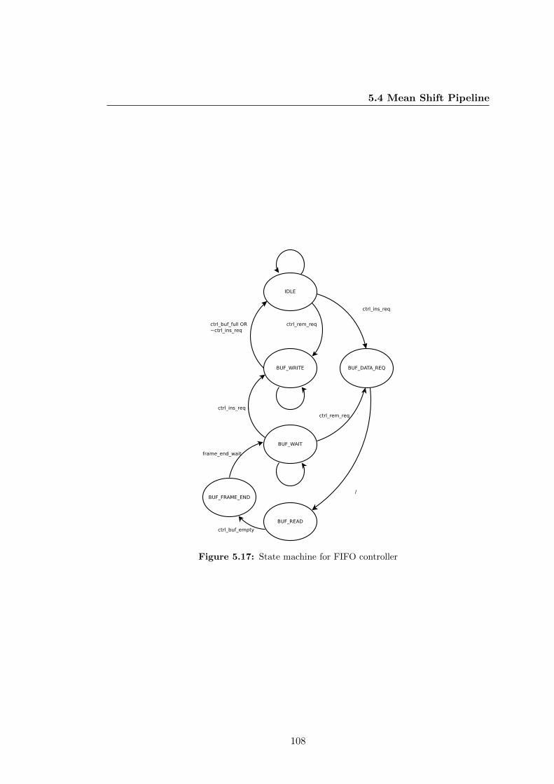
5.4 Mean Shift Pipeline
Figure 5.17: State machine for FIFO controller
108

5.4 Mean Shift Pipeline
4. BUF FRAME END
This state is a one cycle delay in which the ctrl frame end signal is asserted to
the top level controller. After this the controller automatically transitions to the
BUF WAIT state.
5. BUF WAIT
In this state the controller waits for either the ctrl ins req or ctrl rem req to
be asserted, and then transitions into the relevant state. This is to allow time
for the mean shift processing pipeline to perform the division and convergence
operations. At the end of the processing the mean shift pipeline may issue another
data request. The controller does not transition back to the IDLE state except at
the end of a write.
Each time a buffer is filled, the ctrl frame new signal is asserted, which signals to
the top level controller that a new frame is available.
This pattern of operation is dependant on certain assumptions about the pipeline
being true. Namely that the rate at which vectors are written is in fact some factor
slower than the rate at which they are read. This assumption is not encoded directly
into the controller.
5.4.4 Mean Shift Controller
This controller is responsible for managing the timing for arithmetical operations re-
lating the window parameter calculation. Of the 3 controllers, this one has the most
limited scope, as its role is essentially to ensure the correct modules are turned on at
the correct time. Processing starts once the top level controller in section 5.4.2 asserts
the MS PROC EN signal. At the same time, the iREM signal on the buffer is asserted,
at which point the buffer produces data for the mean shift accumulator. Once the
accumulation is complete, the controller enables the divider bank. Upon division a
convergence test is carried out. If the window has not met the convergence criteria, the
controller issues a data request to the top-level controller and waits for the MS PROC EN
signal. If the convergence test passes, a new window is calculated and the results in
the window parameter buffer are updated. At the end of the calculation, the controller
109

5.4 Mean Shift Pipeline
Figure 5.18: State diagram for mean shift controller
110

5.4 Mean Shift Pipeline
issues a PROC DN signal to the top-level controller to indicated that no more data fetches
are required.
Compared to the buffer module, there are relatively few combinations of events
that can occur during processing. The only major decision that must be made in this
control strategy is whether or not to request additional data from the buffer, which is
contingent on the convergence criteria being met.
A description of each state and transition is provided below
1. IDLE
The controller sits in the IDLE state until the ctrl dvalid signal is asserted
by the MS CTRL module at the top level. Asserting the ctrl dvalid causes the
controller to transition into the ACCUM state.
2. ACCUM
In this state the enable signal for the mean shift accumulator is asserted. Since
the weight image data is written to the weight image buffer (see section 5.3) before
accumulation, the data can be provided in an unbroken stream. The accumulator
generates a ready signal (ctrl accum rd) once the end of the image is reached,
which causes a transition to the DIV state.
3. DIV
The start signal is asserted for all 5 divider modules in the mean shift pipeline.
A counter is started which generates a tick after Wdiv cycles, where Wdiv is the
size of the division word in bits.
4. CONV CHECK
The ctrl conv en is asserted and the convergence check module determines the
difference between the current and previous centroids. The convergence check
module asserts two signals - ctrl conv and ctrl conv dn which indicates the
convergence operation has completed. On assertion of ctrl conv dn, the con-
troller transitions to the DATA REQ.
5. DATA REQ
111

5.5 Mean Shift Accumulator
If the convergence signal is asserted, or the maximum number of iterations is
exceeded, the controller moves to the MEAN SUB state and begins the window
parameter calculation with the current data. If convergence has not been achieved
then the ctrl data req signal is asserted to request new data and the controller
transitions to the IDLE state to wait for a new ctrl dvalid signal, where the
accumulation and convergence loop begins again.
6. MEAN SUB
In this state, the normalised image moments are computed and the mean is sub-
tracted. The output terms from the mean sub computation module are organised
to simplify processing in later modules.
7. THETA SQRT
The ctrl cordic en and ctrl sqrt1 dn signals are asserted, which trigger the
CORDIC and first square root modules to begin computing the angle and the
inner square root term of the equivalent rectangle window.
5.5 Mean Shift Accumulator
This module is responsible for accumulating the moment sums for the backprojection
image. In order to perform this processing before the next frame is available, the
computation is vectored such that V pixels are computed in parallel, where V is the
vector dimension.
Conceptually, the mean shift accumulator consists of a set of wide Multiply-Add
units driving a set of accumulating registers. As each weight image pixel enters the
pipeline its position is weighted by the value of that pixel and added to the moment
registers. At the end of the frame the accumulator should produce the values for the
first and second order geometric moments in x and y.
5.5.1 Scalar and Vector Accumulation
It is instructive to consider the operation of the scalar accumulation pipeline. Consider a
1-bit per pixel weight image that enters an accumulator with no windowing, Computing
the target location requires thatM00, M10, andM01 are computed. This in turn requires
2 multiply-accumulate (MAC) operations and an accumulating sum corresponding to
112
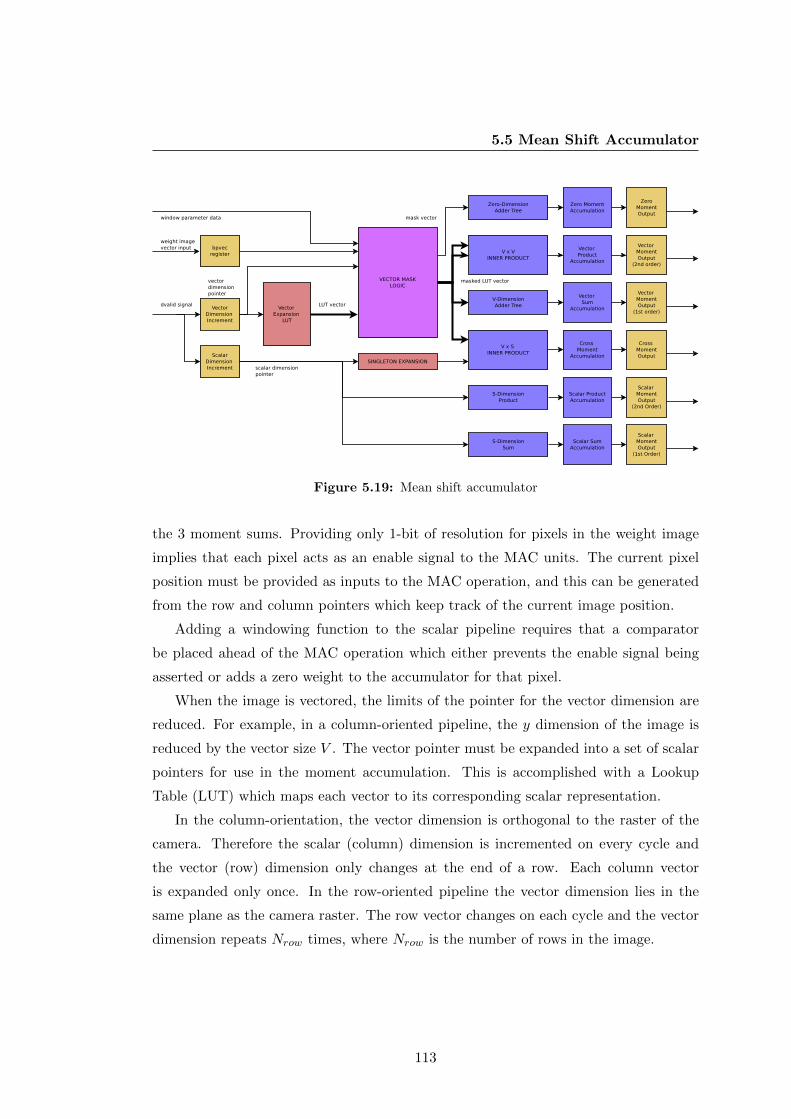
5.5 Mean Shift Accumulator
Figure 5.19: Mean shift accumulator
the 3 moment sums. Providing only 1-bit of resolution for pixels in the weight image
implies that each pixel acts as an enable signal to the MAC units. The current pixel
position must be provided as inputs to the MAC operation, and this can be generated
from the row and column pointers which keep track of the current image position.
Adding a windowing function to the scalar pipeline requires that a comparator
be placed ahead of the MAC operation which either prevents the enable signal being
asserted or adds a zero weight to the accumulator for that pixel.
When the image is vectored, the limits of the pointer for the vector dimension are
reduced. For example, in a column-oriented pipeline, the y dimension of the image is
reduced by the vector size V . The vector pointer must be expanded into a set of scalar
pointers for use in the moment accumulation. This is accomplished with a Lookup
Table (LUT) which maps each vector to its corresponding scalar representation.
In the column-orientation, the vector dimension is orthogonal to the raster of the
camera. Therefore the scalar (column) dimension is incremented on every cycle and
the vector (row) dimension only changes at the end of a row. Each column vector
is expanded only once. In the row-oriented pipeline the vector dimension lies in the
same plane as the camera raster. The row vector changes on each cycle and the vector
dimension repeats Nrow times, where Nrow is the number of rows in the image.
113

5.5 Mean Shift Accumulator
Figure 5.20: Schematic overview of vector mask logic
5.5.2 Vector Mask
In the scalar pipeline each pixel enters serially and is added to the moment sums based
on the weight image value. In the vector pipeline, V pixels enter simultaneously which
may or may not need to be added to the moment sums. A method is required that can
extract all the correct pixel values on each cycle.
The expanded vector described in section 5.5.1 contains all pixel positions that
occur in the current vector dimension. However it may be the case that not all of the
pixels in any particular weight image vector will be required. The role of the vector
masking module is to generate an output vector which has only the pixels required.
The scalar pipeline described in section 5.5.1 can be windowed by inserting a limit
compare module in series with the MAC enable signal that checks the row and column
pointers against the window boundary. In the vector pipeline this operation must be
performed for each element in the expanded vector pointer, requiring V window limit
comparisons.
Figure 5.21 illustrates the operation of the vector masking module. The figure uses
a vector size of 8 to minimise space. In practice a value of 16 is used. The expanded
LUT vector is shown in the top left of the diagram, and is connected directly to a
114

5.5 Mean Shift Accumulator
window limit bank on its right. Each module in the window limit bank compares the
pixel position value shown next to each box in the LUT vector to the limits of the
window. For the sake of clarity, the window is assumed to have a border on pixel 3.
The region which falls into the window is illustrated in the diagram as a green highlight
over the LUT vector and window limit bank. Pixels which fall outside this highlight
are zeroed out irrespective of value.
In the lower portion of the diagram is the weight image bank. To simplify the illus-
tration each pixel in the weight image vector has been reduced to a 1-bit representation.
This vector acts as the select line to a bank of multiplexers, effectively switching out
pixels which were not segmented in the weight image. The output is a masked vector
word which contains only the pixel values that both fall in the tracking window and
are part of the weight image. The values that appear in the output of this example are
showed on the far right of the diagram. In practise the window limits are stored in a
separate buffer and provided combinationally to each of the window limit comparators.
The values in the masked vector word can then be used in the moment accumulation.
5.5.3 Arithmetic Modules
The masked output contains the position values of pixels which appear in the weight
image. These values must be accumulated into the moment sum registers on each cycle
that data is available.
For the sake of illustration, assume there is a column-oriented accumulator which is
accumulating the values of the first and second order moments in x and y. This means
that all pixels in the y dimension enter the pipeline as vectors. When computing the
first order moments in x, the expression,
M10 =∑
xI(x, y) (5.3)
where I(x, y) is the intensity of the weight image at pixel (x, y), simply requires a
multiply for the x term and an add to accumulate the sum. The second order moment
in x only requires a second multiply.
115

5.5 Mean Shift Accumulator
Figure 5.21: Example of vector masking operation on 8-element vector word
116

5.5 Mean Shift Accumulator
In the y dimension, the y term is in fact a vector. Therefore the first and second
order moments are given by
M01 =∑
yI(x, y) (5.4)
M02 =∑
y2I(x, y) (5.5)
The cross moment becomes
M11 =∑
xyI(x, y) (5.6)
Thus to compute the first order moment in y, all the elements in the masked vector
word (see section 5.5.2) must be summed. For the second order moments, the value
which must be added to the moment accumulation registers is equal to the inner product
of the vector itself for M02, and the vector and the x term for M11. Thus on each cycle
we compute
M02 = M02 + yT y (5.7)
for the second order moment in y, and
M11 = M11 + yTx (5.8)
for the cross moment.
This requires that two Multiply-Accumulate (MAC) modules be provided to com-
pute new terms for M02 and M01. These are implemented as a bank of multipliers
connected to an adder tree. Values which are masked out by the vector masking mod-
ule in section 5.5.2 are multiplied by zero in the MAC front end. For the M02 term,
each element of the mask vector is applied to both inputs of each multiplier. For the
M11 term, the scalar pointer must first be expanded to a vector of size V , such that
each multiplier has one element of the mask vector and the scalar pointer value as its
inputs.
For the first order term in y, an adder tree that takes as its input the positions
of pixels in the weight image vector is sufficient to find the next term to accumulate
into the M01 register. As with all modules in the accumulator arithmetic pipeline, the
117
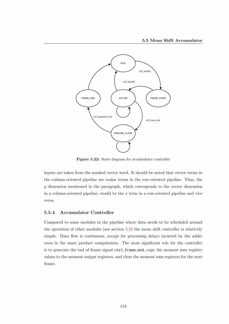
5.5 Mean Shift Accumulator
Figure 5.22: State diagram for accumulator controller
inputs are taken from the masked vector word. It should be noted that vector terms in
the column-oriented pipeline are scalar terms in the row-oriented pipeline. Thus, the
y dimension mentioned in the paragraph, which corresponds to the vector dimension
in a column-oriented pipeline, would be the x term in a row-oriented pipeline and vice
versa.
5.5.4 Accumulator Controller
Compared to some modules in the pipeline where data needs to be scheduled around
the operation of other modules (see section 5.2) the mean shift controller is relatively
simple. Data flow is continuous, except for processing delays incurred by the adder
trees in the inner product computation. The most significant role for the controller
is to generate the end of frame signal ctrl frame end, copy the moment sum register
values to the moment output registers, and clear the moment sum registers for the next
frame.
118
5.6 Window Parameter Computation
5.6 Window Parameter Computation
The mean shift accumulator (section 5.5) computes the windowed moments of the
weight image. The moment sums are then used to derive the window parameters in the
remainder of the pipeline. The moment sums are first normalised in a divider bank.
Parameters from the previous iteration of the mean shift inner loop are buffered and
used to determine convergence. Convergence is said to be achieved once successive
iterations exhibit a difference less than some value ε, typically one pixel. Setting this
value to be greater than one pixel provides faster convergence at the expense of poorer
accuracy, which may lead to tracking drift.
Once the mean shift loop converges, the mean is subtracted from the normalised
moments to form the so called µ terms [77]. These are
µ10 =M10
M00= x (5.9)
µ01 =M01
M00= y (5.10)
µ11 =M11
M00− xy (5.11)
µ20 =M20
M00− x2 (5.12)
µ02 =M02
M00− y2 (5.13)
These terms are further manipulated for convenience. For example, the expression
for the orientation of the target is simply the angle between the first eigenvalue of the
normalised moment matrix and the x-axis. The expression for this is given as
α =1
2tan−1
(2µ11
µ20 − µ02
)(5.14)
This expression is computed with a CORDIC solver [120] which has X and Y inputs
corresponding to those in the function atan2(Y,X)1. Thus, it is more convenient in
1The CORDIC algorithm naively implements the atan() function, however the implementation in
this work performs quadrant mapping to expand the convergence range of the module [121].
119

5.7 Parameter Buffer
the hardware to provide the input as X = (µ20 − µ02) and Y = 2µ11. This is done
within the mean subtraction module to allow for better optimisation during synthesis,
although conceptually the operation is not related to mean subtraction.
In [24], the target is represented by its equivalent rectangle. The expression for the
height and width of the target are given by equations 3.45 and 3.46. Each of these
expressions requires the solution to two square roots, one common to both expressions,
and one unique to each expression. To solve this, two square root modules are provided
so that the width and height can be computed in parallel. The first solver is used
initially to solve the common term√µ211 + (µ20 − µ02)2. The input is then multiplexed
with the width term, while the other module is loaded with the height term.
5.7 Parameter Buffer
The mean shift tracking framework requires parameters of the tracking window to be
stored between frames, and between iterations. In the CSoC pipeline, this is performed
with a parameter buffer module that holds the current window parameters, loads new
parameters from the mean shift computation pipeline, and can receive parameters from
an external module. This is primarily used to set the initial window parameters in the
simulation, and can easily be extended to receive parameters from an external device
such as a remote host via a soft-core processor or similar.
To minimise the number of pins required, the parameter buffer is loaded serially via
a single Wp bit input, where Wp is the width of the parameter word. An internal state
machine assigns incoming values to the correct set of registers in the pipeline. The
parameter buffer directly feeds the window parameters to the Accumulator module,
which are used to calculate the window limits used in the moment accumulation.
120

Chapter 6
CSoC Verification
In the course of this study, the need arose for more specific and powerful verification
tools. This chapter presents csTool, a data-driven verification and architecture explo-
ration framework developed to meet these needs.
6.1 csTool Overview
It is generally the case that the largest portion of development effort for any large
technology project is consumed by verification and testing [104], and the CSoC pipeline
is no different in this regard. During the early development of the CSoC pipeline,
various data vector generation scripts were written to provide stimulus to testbenches.
As the complexity of the modules under test grew, so to did the complexity of the data
generation scripts. In turn this increased the complexity of the checkers used to verify
that the simulation results were correct. Because the scripts were mostly independent,
being written in most cases for a specific module, there was little coherency in the test
environment between distinct, but connected components. This meant that gaining an
insight into the correctness of the entire data processing operation was cumbersome
and error prone. It was therefore decided to unify this collection of scripts into a single
verification tool which could generate and analyse all the relevant data vectors for all
modules in the CSoC datapath.
The result of this development is csTool, which combines a model of the CSoC
pipeline with direct test vector generation and verification capability. As well as this,
csTool is able to verify peripheral issues with the pipeline such as datapath timing.
121
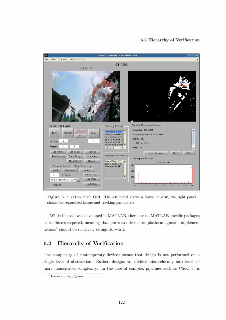
6.2 Hierarchy of Verification
Figure 6.1: csTool main GUI. The left panel shows a frame on disk, the right panel
shows the segmented image and tracking parameters
While the tool was developed in MATLAB, there are no MATLAB specific packages
or toolboxes required, meaning that ports to other more platform-agnostic implemen-
tations1 should be relatively straightforward.
6.2 Hierarchy of Verification
The complexity of contemporary devices means that design is not performed on a
single level of abstraction. Rather, designs are divided hierarchically into levels of
more manageable complexity. In the case of complex pipelines such as CSoC, it is
1For example, Python
122

6.2 Hierarchy of Verification
natural to consider the verification hierarchically. At the lowest level of the hierarchy,
the correctness of individual units is verified against the intended behaviour. For the
purposes of this discussion, a unit can be thought of as an atomic element in the
verification hierarchy. That is, for the purposes of verification, this is the smallest
complete operation that can be performed. It should be noted that the definition of
atomic in this context depends largely on the verification context. In an FPGA, where
device fabric may contain hardware multipliers that are synthesised by inference, a
multiply operation may not be considered atomic, as the correctness of the module
can be assumed. In an ASIC, the multiplier may no longer be a discrete block, and
therefore would not be considered atomic.
Each major module is in turn comprised of many smaller modules, which may in
turn be comprised of smaller modules and so on. At some point, these modules can be
considered atomic - that is, they perform some singular and complete operation. An
example of an atomic operation will vary depending on context, as it may be unhelpful
to classify very complicated systems in terms of very simple atomic operations such as
AND or NOT. For the purposes of this study, we consider an atomic operation to be
in the order of complexity of an add or multiply.
Similarly, it a natural to consider the verification of a system hierarchically. In this
case, the method used to verify a component of the design changes depending on the
level of abstraction required. The exact nature of a verification hierarchy will depend
on the specifics of the device under test (DUT). An example of a verification hierarchy
for a microprocessor is proposed in [122] (pp 37). From the lowest to highest levels of
abstraction, these are given as
1. Designer Level
2. Unit Level
3. Chip Level
4. Board Level
5. System Level
Not all of these levels are applicable to every design. For example, the Board
Level is outside the scope of this document as this study is not concerned with PCB
layouts. However the overall concept remains instructive.
123
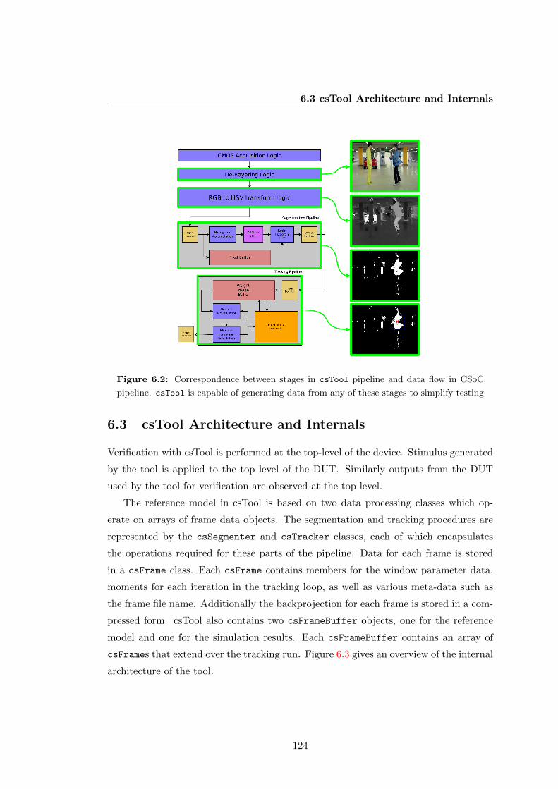
6.3 csTool Architecture and Internals
Figure 6.2: Correspondence between stages in csTool pipeline and data flow in CSoC
pipeline. csTool is capable of generating data from any of these stages to simplify testing
6.3 csTool Architecture and Internals
Verification with csTool is performed at the top-level of the device. Stimulus generated
by the tool is applied to the top level of the DUT. Similarly outputs from the DUT
used by the tool for verification are observed at the top level.
The reference model in csTool is based on two data processing classes which op-
erate on arrays of frame data objects. The segmentation and tracking procedures are
represented by the csSegmenter and csTracker classes, each of which encapsulates
the operations required for these parts of the pipeline. Data for each frame is stored
in a csFrame class. Each csFrame contains members for the window parameter data,
moments for each iteration in the tracking loop, as well as various meta-data such as
the frame file name. Additionally the backprojection for each frame is stored in a com-
pressed form. csTool also contains two csFrameBuffer objects, one for the reference
model and one for the simulation results. Each csFrameBuffer contains an array of
csFrames that extend over the tracking run. Figure 6.3 gives an overview of the internal
architecture of the tool.
124

6.3 csTool Architecture and Internals
Both the csSegmenter and csTracker classes are designed to facilitate exploration
of the design space. Each contains a list of fully parameterised algorithms which can
be selected at runtime. This allows different algorithms to be rapidly developed and
compared.
Because the reference model is integrated into csTool, test vectors can be generated
directly from the model. This allows the development to be iterated at the data level.
For example, the computation of the window parameters in 3.5 can be modified quickly
in the reference model so that the output of a new RTL specification can be immediately
verified.
1. A Reference Model.
An offline model of the pipeline is integrated into csTool. This model follows the
equations given in chapter 3. This model serves dual purposes. Firstly, it allows
exploration of design space as various techniques for performing the CAMSHIFT
operation can be tested quickly in a software environment before any RTL has
been written. Secondly, it provides a reference against which the device under
test can be verified.
2. Test Vector Generation Module.
The verification utility of the tool comes from the ability to quickly generate test
vectors from the reference model. In this way the parameters of the model can
be iterated and tested.
3. Test Vector Analyser.
During each simulation tracking and frame data is written to disk for later verifi-
cation. This data is read into csTool at the end of the simulation and compared
to the data in the reference model. Included in this step is any pre-processing
required to transform the output from the RTL simulation and the internal model
data into a common format for verification.
4. Report Generation
Once the verification is complete, a set of reports are generated which show the
errors found in that verification.
125
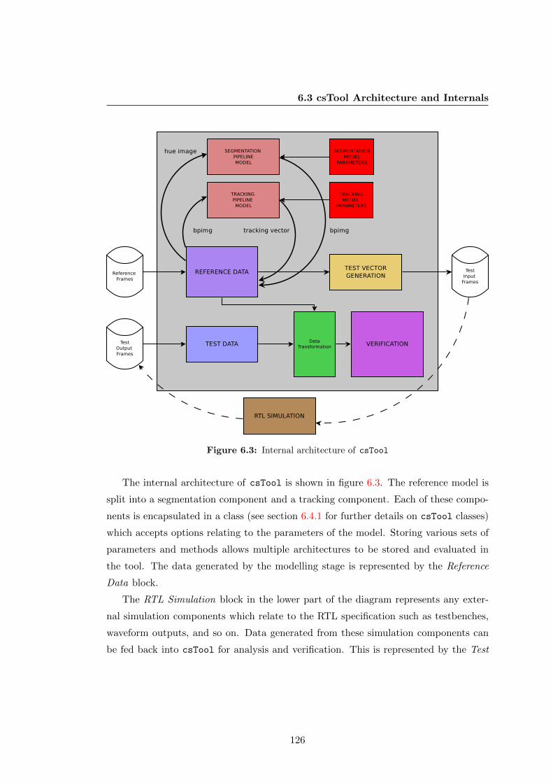
6.3 csTool Architecture and Internals
Figure 6.3: Internal architecture of csTool
The internal architecture of csTool is shown in figure 6.3. The reference model is
split into a segmentation component and a tracking component. Each of these compo-
nents is encapsulated in a class (see section 6.4.1 for further details on csTool classes)
which accepts options relating to the parameters of the model. Storing various sets of
parameters and methods allows multiple architectures to be stored and evaluated in
the tool. The data generated by the modelling stage is represented by the Reference
Data block.
The RTL Simulation block in the lower part of the diagram represents any exter-
nal simulation components which relate to the RTL specification such as testbenches,
waveform outputs, and so on. Data generated from these simulation components can
be fed back into csTool for analysis and verification. This is represented by the Test
126

6.4 Data Oriented Testing
Data, Data Transformation, and Verification blocks, which summarise the verification
pipeline within the tool.
6.4 Data Oriented Testing
In this study, we can interpret the verification of the CSoC datapath as the intersection
of the context-free algorithm, and the context-sensitive domain considerations. Consider
these terms in turn, the context-free algorithm refers to the algorithm specification [24]
[26], which expresses the sequence of operations required to perform mean shift tracking.
In this instance, context-free refers to the fact algorithmic specification is not concerned
with any implementation details, instead leaving these in the hands of the designer.
By contrast, the context-sensitive domain considerations are concerned with the
correctness of domain specific implementation constraints. In the case of a software
implementation, these may include a real-time constraint, available memory size and
speed, data-structure implementation, language constraints and expressive power, and
so on. In the hardware domain, these may including datapath timing, placement and
routing, fitting, structural requirements, memory bandwidth and size, control sequence
generation, and so on. Failure to meet these context-sensitive requirements directly
affects the ability to meet context-free requirements by violating constraints imposed
by the implementation domain. These constraints may not be linked to the algorithm
procedure in any way, but will necessarily cause the implementation to be incorrect if
violated. A Venn diagram of this intersection is presented in figure 6.4.
The correct implementation can therefore be considered the implementation which
produces an output consistent with the algorithmic specification, while violating none
of the domain constraints. In this view, csTool can be understood as a kind of transla-
tion layer that interfaces between the context-free algorithm, and the context-sensitive
domain requirements.
In the case of csTool, the algorithm in embedded in the model from which the data
is generated. The context-sensitive elements of the design are simulated in parallel to
the more functional simulation of the model1. This is done for two reasons. Firstly, it is
often simpler in practise to isolate these components of the design for testing. Secondly,
creating models for functional verification which encapsulate all the implementation
1See the Pattern Testing Tool in section 6.7.1
127
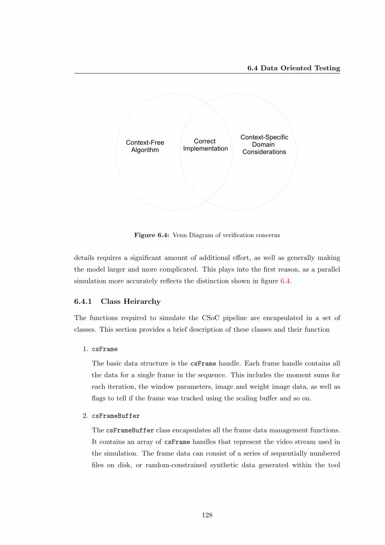
6.4 Data Oriented Testing
Figure 6.4: Venn Diagram of verification concerns
details requires a significant amount of additional effort, as well as generally making
the model larger and more complicated. This plays into the first reason, as a parallel
simulation more accurately reflects the distinction shown in figure 6.4.
6.4.1 Class Heirarchy
The functions required to simulate the CSoC pipeline are encapsulated in a set of
classes. This section provides a brief description of these classes and their function
1. csFrame
The basic data structure is the csFrame handle. Each frame handle contains all
the data for a single frame in the sequence. This includes the moment sums for
each iteration, the window parameters, image and weight image data, as well as
flags to tell if the frame was tracked using the scaling buffer and so on.
2. csFrameBuffer
The csFrameBuffer class encapsulates all the frame data management functions.
It contains an array of csFrame handles that represent the video stream used in
the simulation. The frame data can consist of a series of sequentially numbered
files on disk, or random-constrained synthetic data generated within the tool
128

6.5 csTool Workflow
itself. All functions to query and manipulate csFrame data are contained in the
csFrameBuffer.
3. csSegmenter
The csSegmenter class is responsible for taking the image stored in the csFrame
handle and performing a user-specified segmentation operation, returning the
weight image and optionally the ratio histogram for that frame, and parameters
such as the number of bits per output word and number of histogram bins,
4. csTracker
The csTracker class encapsulates the behaviour of the mean shift inner loop
computation. This includes a processing loop which executes the selected moment
accumulation and window parameter calculation routines.
5. vecManager
Functions to manipulate and query the tracking, image, and simulation vectors
are encapsulated in the vecManager class. This class contains methods to take
an image and transform it into a set of vector files according to the procedure de-
scribed in section 6.5.1, as well as read the resulting files from disk and convert to
a format suitable for storing in a csFrameBuffer object. This class also contains
routines to convert the vector data stored in the csFrame handles and vector
data read from disk into an intermediate format for verification. Additionally,
the trajectory buffer described in section 6.6.1 is encapsulated in this class.
6.5 csTool Workflow
csTool is designed to complement an existing verification workflow. The tool is not
capable of performing assertion checking or formal proofs on a system. Rather it is
designed to perform analysis and checking on data going into and coming out of the
DUT.
A typical simulation run with csTool will involve 4 major steps
1. Execute Model
129

6.5 csTool Workflow
Some test vectors must be generated that will stimulate the DUT. These can
either be taken from a series of files captured from a video, or a synthetic psuedo-
random backprojection image generator. Test data can be generated at any major
intersection point in the design as shown in figure 6.2. For example a series
of frames can be read from disk, and a set of RGB vectors, HSV vectors, and
backprojection vectors can be generated.
2. Generate Test Vectors
Test vectors are generated directly from the model. This is both faster and
allows direct comparison against the model in the verification step. Options are
provided to generate vectors that are suited to the DUT. For example, as per
the requirements outlined in 6.5.1, the vector size V can be varied, as well as
the orientation (see section 4.2 for further discussion about pipeline orientation)
and vector type. Available types are RGB, HSV, Hue, and Backprojection, each
corresponding to the output of a different stage in the process (see figure 6.2 for
an illustration of the output data at each stage).
3. Run Simulation
Once the data is generated, the actual RTL simulation is executed. The test-
benches for each module are designed to capture relevant information during the
simulation run so that data verification can be performed by csTool. This varies
depending on the specific module under test, but will typically be output frame
data along with some relevant parameters. For example, the testbench for the
mean shift processing module also generates window parameter data and (op-
tionally) moment sum data. During verification csTool will automatically look
for these extra files and if they are present, read the data into the GUI for visual
analysis. An example of this can be seen in figure 6.9.
4. Verify Testbench Output
The data written to disk in the testbench is read into csTool for verification.
Because the data is formatted into files as per section 6.5.1 the data is transformed
into a common representation before comparison is performed.
130

6.5 csTool Workflow
6.5.1 Vector Data Format
For the input to the column oriented backprojection pipeline, and for the concatenated
backprojection output, there are possible issues with number representation. At 8 bits
per pixel and with a vector dimension of 16, the image vector input to the column
oriented backprojection pipeline is 128 bits wide. Both the row and column oriented
pipeline will produce vectors with a width Wbp, which will be V in the case of a binary
image, 2V for a 3 weight image, and so on. This means in practise the output will be
either 16 or 32 bits wide. To provide flexibility when generating and verifying vectors
from various stages of the pipeline, each input or output image is stored as a set of V
files, where each file is a stream representing the kth element of the input or output
vector V . Thus, each file is N = Dv/V elements long, where Dv is the length of the
image dimension which is vectored. Thus for the column oriented backprojection, rows
1, (V + 1), (2V + 1), and so on are combined together to form a stream of all 1st
elements. This process repeats for row 2, (V + 2), (2V + 2) and so on. In general, row
k will be written to the Kth file containing rows k, (V + k), (2V + k) and so on. This
process is the same in the row oriented backprojection, except that columns are written
to the file rather than rows. This approach allows more flexibility for generating test
vectors, at the cost of some additional complexity in the tool.
This data format is represented in figures 6.5 and 6.6 for the column and row cases
respectively. To simplify the diagrams, the vector size V is chosen to be 4, with colours
representing the elements of the vectors. The column diagram in figure 6.5 shows a
summarised diagram of the weight image on the left-hand side, ranging from vector row
1 through N , and a representation of the concatenated vector stream for each element
on the right hand side. Colour coded arrows diagrammatically indicate how vectors in
the weight image are split into segments in the vector stream.
The same colour convention is applied to the row data format diagram in figure 6.6.
As in figure 6.6, a summary diagram of the weight image is shown on the left, with
vector streams on the right. The colour coding in figure 6.5 and figure 6.6 is the same.
6.5.2 Generation Of Vector Data For Testing
The vector generation panel of csTool is shown in figure 6.7. This window provides op-
tions to generate vectors in the form specified above. The RGB, HSV, Hue, and Back-
131

6.5 csTool Workflow
Figure 6.5: Diagrammatic Representation of Column Vector Data Format
Figure 6.6: Diagrammatic Representation of Row Vector Data Format
132

6.5 csTool Workflow
projection options represent vectors from different stages in the processing pipeline.
The vector generation routine automatically splits and names the files according to the
procedure in section 6.5.1. For example, an image that represents the output of a col-
umn backprojection pipeline with a vector dimension V equal to 16 will produce a set of
numbered files in the form filename-frame001-vec001 - filename-frame001-vec016
for frame 1, and so on through to frame n. Additionally the window parameters and
moments sums are written to disk both for use in the testbench and verification. These
files are written in the form filename-framen-wparam.dat for frames 1 through n.
Figure 6.7: csTool vector generation GUI
The generation GUI has options to choose the orientation of size of the vector
output. The low and high range options select how many frames in the buffer to
generate vector files from. A transport panel is provided at the bottom of the panel
133
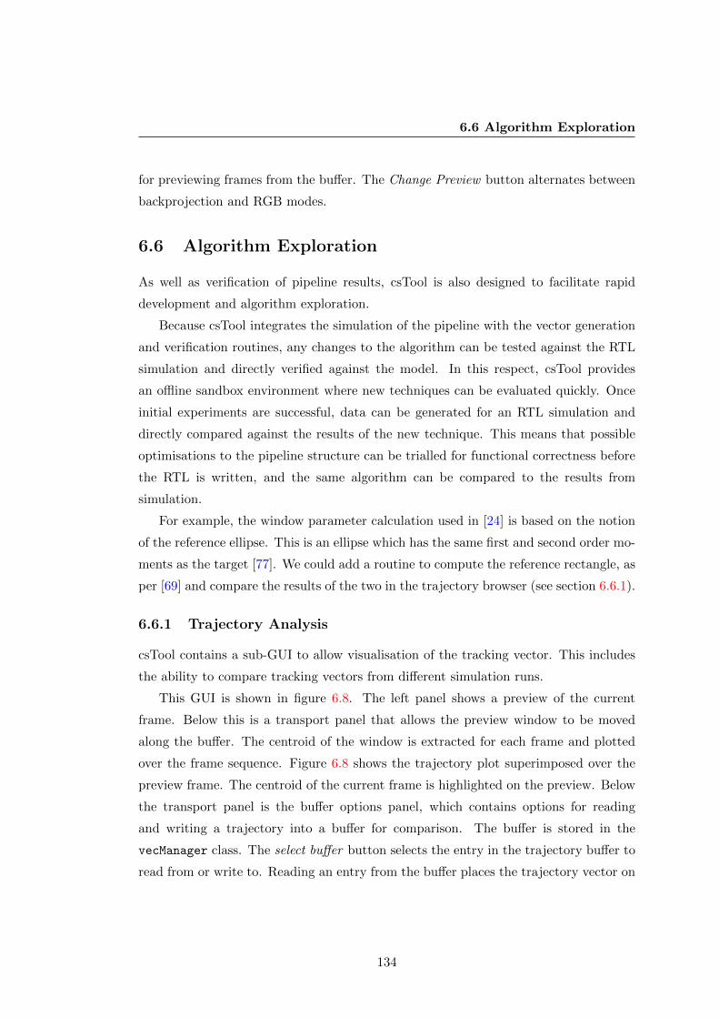
6.6 Algorithm Exploration
for previewing frames from the buffer. The Change Preview button alternates between
backprojection and RGB modes.
6.6 Algorithm Exploration
As well as verification of pipeline results, csTool is also designed to facilitate rapid
development and algorithm exploration.
Because csTool integrates the simulation of the pipeline with the vector generation
and verification routines, any changes to the algorithm can be tested against the RTL
simulation and directly verified against the model. In this respect, csTool provides
an offline sandbox environment where new techniques can be evaluated quickly. Once
initial experiments are successful, data can be generated for an RTL simulation and
directly compared against the results of the new technique. This means that possible
optimisations to the pipeline structure can be trialled for functional correctness before
the RTL is written, and the same algorithm can be compared to the results from
simulation.
For example, the window parameter calculation used in [24] is based on the notion
of the reference ellipse. This is an ellipse which has the same first and second order mo-
ments as the target [77]. We could add a routine to compute the reference rectangle, as
per [69] and compare the results of the two in the trajectory browser (see section 6.6.1).
6.6.1 Trajectory Analysis
csTool contains a sub-GUI to allow visualisation of the tracking vector. This includes
the ability to compare tracking vectors from different simulation runs.
This GUI is shown in figure 6.8. The left panel shows a preview of the current
frame. Below this is a transport panel that allows the preview window to be moved
along the buffer. The centroid of the window is extracted for each frame and plotted
over the frame sequence. Figure 6.8 shows the trajectory plot superimposed over the
preview frame. The centroid of the current frame is highlighted on the preview. Below
the transport panel is the buffer options panel, which contains options for reading
and writing a trajectory into a buffer for comparison. The buffer is stored in the
vecManager class. The select buffer button selects the entry in the trajectory buffer to
read from or write to. Reading an entry from the buffer places the trajectory vector on
134
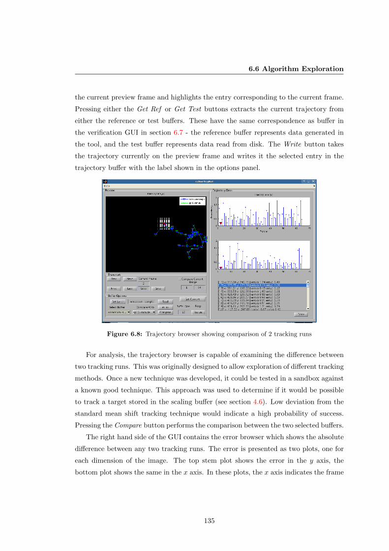
6.6 Algorithm Exploration
the current preview frame and highlights the entry corresponding to the current frame.
Pressing either the Get Ref or Get Test buttons extracts the current trajectory from
either the reference or test buffers. These have the same correspondence as buffer in
the verification GUI in section 6.7 - the reference buffer represents data generated in
the tool, and the test buffer represents data read from disk. The Write button takes
the trajectory currently on the preview frame and writes it the selected entry in the
trajectory buffer with the label shown in the options panel.
Figure 6.8: Trajectory browser showing comparison of 2 tracking runs
For analysis, the trajectory browser is capable of examining the difference between
two tracking runs. This was originally designed to allow exploration of different tracking
methods. Once a new technique was developed, it could be tested in a sandbox against
a known good technique. This approach was used to determine if it would be possible
to track a target stored in the scaling buffer (see section 4.6). Low deviation from the
standard mean shift tracking technique would indicate a high probability of success.
Pressing the Compare button performs the comparison between the two selected buffers.
The right hand side of the GUI contains the error browser which shows the absolute
difference between any two tracking runs. The error is presented as two plots, one for
each dimension of the image. The top stem plot shows the error in the y axis, the
bottom plot shows the same in the x axis. In these plots, the x axis indicates the frame
135

6.7 Verification And Analysis
Figure 6.9: Verification GUI with frame extracted from image sequence
number, and the y axis indicates the error in pixels on the specified dimension. The
average and standard deviation of the error over the tracking run is shown next to the
list of summary statistics.
6.7 Verification And Analysis
A verification GUI is provided for analysis of output frame data and tracking vectors.
This includes the ability to graphically compare images produced by the backprojection
pipeline and their associated tracking vectors against a known reference.
The verification routines are built into the GUI shown in figure 6.9. This GUI
contains routines to perform the vector assembly as per the method described in sec-
tion 6.5.1.
The panel on the left of the GUI shows the backprojection image from the ref-
erence frame buffer. This image was generated in the tool using the csSegmenter
and csTracker routines, and is used as the verification reference for data from the
testbench.
The middle panel shows the backprojection image in the test buffer. This image is
read from disk, normally from a set of split files as described in section 6.5.1. These
files are assembled into a complete image to allow rapid visual inspection of errors
in the result. Window parameters are written to disk during testing, and the tool
looks for files with names in the form filename-frame001-wparam.dat to read into
the verification GUI. The rightmost panel of the GUI shows the error image. This is
simply the absolute difference of pixels in the reference and test images. This allows
errors to be quickly discovered. A tracking run of the same sequence offset by a few
136

6.7 Verification And Analysis
frames is shown in figure 6.10. In this figure, the error image is visible showing what
appears to be a hybrid of the two input images.
Figure 6.10: Verification GUI with offset frames
The top-right part of the GUI contains two panels which show the moment sums
and window parameter data for each frame. The left panel is parameter data for the
reference frame, the right is data for the test frame read from disk. In figure 6.9 the
test data has been generated directly from the reference data, and so the error image
appears blank.
Figure 6.11: Verification GUI in csTool showing the results from a synthetic tracking run
6.7.1 Pattern Testing
Several stages in the pipeline require a double buffering system to allow processing
to occur while the data stream is active. The double buffering typically exists to
hide some processing latency in the system. For example, in both the row and column
backprojection pipelines, the division operation interrupts the flow of pixels through the
137
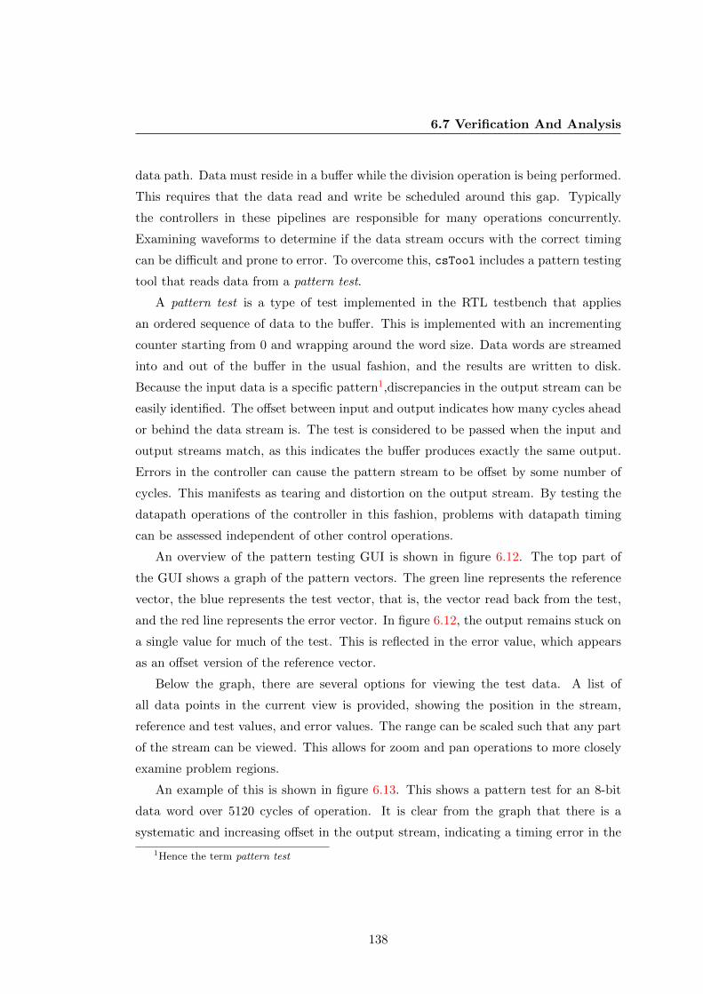
6.7 Verification And Analysis
data path. Data must reside in a buffer while the division operation is being performed.
This requires that the data read and write be scheduled around this gap. Typically
the controllers in these pipelines are responsible for many operations concurrently.
Examining waveforms to determine if the data stream occurs with the correct timing
can be difficult and prone to error. To overcome this, csTool includes a pattern testing
tool that reads data from a pattern test.
A pattern test is a type of test implemented in the RTL testbench that applies
an ordered sequence of data to the buffer. This is implemented with an incrementing
counter starting from 0 and wrapping around the word size. Data words are streamed
into and out of the buffer in the usual fashion, and the results are written to disk.
Because the input data is a specific pattern1,discrepancies in the output stream can be
easily identified. The offset between input and output indicates how many cycles ahead
or behind the data stream is. The test is considered to be passed when the input and
output streams match, as this indicates the buffer produces exactly the same output.
Errors in the controller can cause the pattern stream to be offset by some number of
cycles. This manifests as tearing and distortion on the output stream. By testing the
datapath operations of the controller in this fashion, problems with datapath timing
can be assessed independent of other control operations.
An overview of the pattern testing GUI is shown in figure 6.12. The top part of
the GUI shows a graph of the pattern vectors. The green line represents the reference
vector, the blue represents the test vector, that is, the vector read back from the test,
and the red line represents the error vector. In figure 6.12, the output remains stuck on
a single value for much of the test. This is reflected in the error value, which appears
as an offset version of the reference vector.
Below the graph, there are several options for viewing the test data. A list of
all data points in the current view is provided, showing the position in the stream,
reference and test values, and error values. The range can be scaled such that any part
of the stream can be viewed. This allows for zoom and pan operations to more closely
examine problem regions.
An example of this is shown in figure 6.13. This shows a pattern test for an 8-bit
data word over 5120 cycles of operation. It is clear from the graph that there is a
systematic and increasing offset in the output stream, indicating a timing error in the
1Hence the term pattern test
138
6.7 Verification And Analysis
Figure 6.12: Example of pattern testing GUI
Figure 6.13: Pattern test with output error
139

6.7 Verification And Analysis
Figure 6.14: Rescaled view of error in pattern stream
Figure 6.15: Pattern test after controller operation is corrected
controller. In particular, at around 300 cycles there is a large spike in the error vector.
In the view shown in figure 6.13 it is difficult to see the error in detail. Rescaling the
range to show only the first 512 cycles results in the graph shown in figure 6.14. In
this example, the test is being performed on the row-oriented backprojection pipeline,
which has a buffer depth of 320 pixels. The view in figure 6.14 shows that the slowly
increasing output error begins at the end of the first buffer transition on cycle 320.
The output of the corrected controller is shown in figure 6.15. Here the test vector lies
exactly on top of the reference vector, indicating no errors in the data stream.
This shows how the pattern test can highlight so-called off-by-one errors in the data
stream that arise when the output is not correctly timed. Even when a pause in the
data flow occurs due to a processing delay, this cannot be allowed to affect the order of
the output stream, or else errors will occur. Pattern testing falls under the category of
context-sensitive testing as outlined in section 6.4, and illustrated in the Venn diagram
140

6.7 Verification And Analysis
in figure 6.4. This element of the implementation is not encapsulated in the model
itself, but rather tested for in parallel with the functional aspects of the model.
141

Chapter 7
Experimental Results
This chapter will detail the experimental results gathered in this study, and explain their
significance to the broader work. The opening part of this chapter compares the var-
ious segmentation methods proposed within the Histogram Backprojection framework
derived from [47] and [24]1. Following that, preliminary tests outlining the feasibility
of the scaling buffer are given, followed by results gathered from the CSoC RTL speci-
fication itself, including event-driven simulation results, synthesis outputs, and timing
and routing results.
7.1 Comparison of Segmentation Methods
Several segmentation methods are available in csTool. Each method is designed to
simulate a different kind of pipeline configuration. The methods are
1. Pixel HBP
This method performs Histogram Backprojection pixel-wise. This serves as a
reference method that is functionally identical to a software implementation. The
image histogram is accumulated over the entire image in the first pass, followed
by the ratio histogram, and finally the backprojection image, which is generated
by using the ratio histogram as a lookup table as per [24] or [48], [69], [70].
1Also implemented in [48]
142

7.1 Comparison of Segmentation Methods
2. Row HBP
This method performs Histogram Backprojection by backprojecting each row sep-
arately. Histograms are accumulated for each row, and the results are combined
to form the final backprojection image. This method is intended to simulate the
row-oriented pipeline.
3. Block HBP
This method performs Histogram Backprojection by backprojecting square re-
gions of the image V pixels on each side, where V is the vector dimension. His-
tograms are accumulated for each block, and the blocks are combined to form
the final backprojection image. This method is intended to simulate the column-
oriented pipeline.
4. Block HBP (Spatial Weight)
This method performs Histogram Backprojection on blocks as per the previous
method, but ignores blocks that are more than a specified distance away from
the tracking window. The distance is settable in both the x and y dimensions.
This method is intended to simulate the column-oriented pipeline with window
position feedback.
5. Row HBP (Spatial Weight)
This method performs Histogram Backprojection on rows as per the Row HBP
method, but again weights pixels beyond a specified region outside the tracking
window towards zero. This method is intended to simulate the row-oriented
pipeline with window position feedback.
The method of computing the backprojection image in small parts is a compromise
designed to save the limited memory available on the device. However performing any
histogram based operation on anything less than the whole image can only provide at
best an approximation of the distribution of pixels. In many cases, the results may be
wildly incorrect. This is due to the fact that it cannot be known how many fall into a
feature of the image without checking every pixel in the image.
143
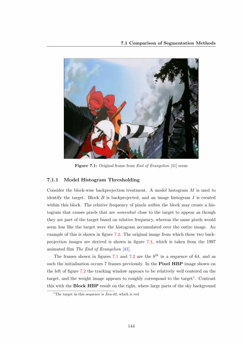
7.1 Comparison of Segmentation Methods
Figure 7.1: Original frame from End of Evangelion [41] scene
7.1.1 Model Histogram Thresholding
Consider the block-wise backprojection treatment. A model histogram M is used to
identify the target. Block B is backprojected, and an image histogram I is created
within this block. The relative frequency of pixels within the block may create a his-
togram that causes pixels that are somewhat close to the target to appear as though
they are part of the target based on relative frequency, whereas the same pixels would
seem less like the target were the histogram accumulated over the entire image. An
example of this is shown in figure 7.2. The original image from which these two back-
projection images are derived is shown in figure 7.1, which is taken from the 1997
animated film The End of Evangelion [41].
The frames shown in figures 7.1 and 7.2 are the 8th in a sequence of 64, and as
such the initialisation occurs 7 frames previously. In the Pixel HBP image shown on
the left of figure 7.2 the tracking window appears to be relatively well centered on the
target, and the weight image appears to roughly correspond to the target1. Contrast
this with the Block HBP result on the right, where large parts of the sky background
1The target in this sequence is Eva-02, which is red
144

7.1 Comparison of Segmentation Methods
Figure 7.2: Comparison of Pixel HBP (left) and Block HBP (right) in End of Evan-
gelion sequence
.
0 2 4 6 8 10 12 14 160
2
4
6
8
10
12x 10
4
Bin #
# o
f p
ixe
ls
Image Histogram (Pixel HBP method)
0 2 4 6 8 10 12 14 160
0.5
1
1.5
2
2.5
3
3.5x 10
5
Bin #
# o
f p
ixe
ls
Model Histogram
Figure 7.3: Image histogram for End of Evangelion frame using Pixel HBP segmentation
(left), and model histogram (right)
have been incorporated into the weight image. The window is centered roughly in the
middle of the frame, and while the target is still visible (and does match the target
outline in the Pixel HBP image), the huge amount of background clutter obscures
this, giving dramatically different tracking results.
To understand why this is the case, consider the image histograms below. The
diagram on the left of figure 7.3 shows the image histogram for the frame in figure 7.1,
taken across the entire image. The right of figure 7.3 shows the model histogram used
to generate the backprojection image. The ratio histogram is shown in figure 7.4.
145
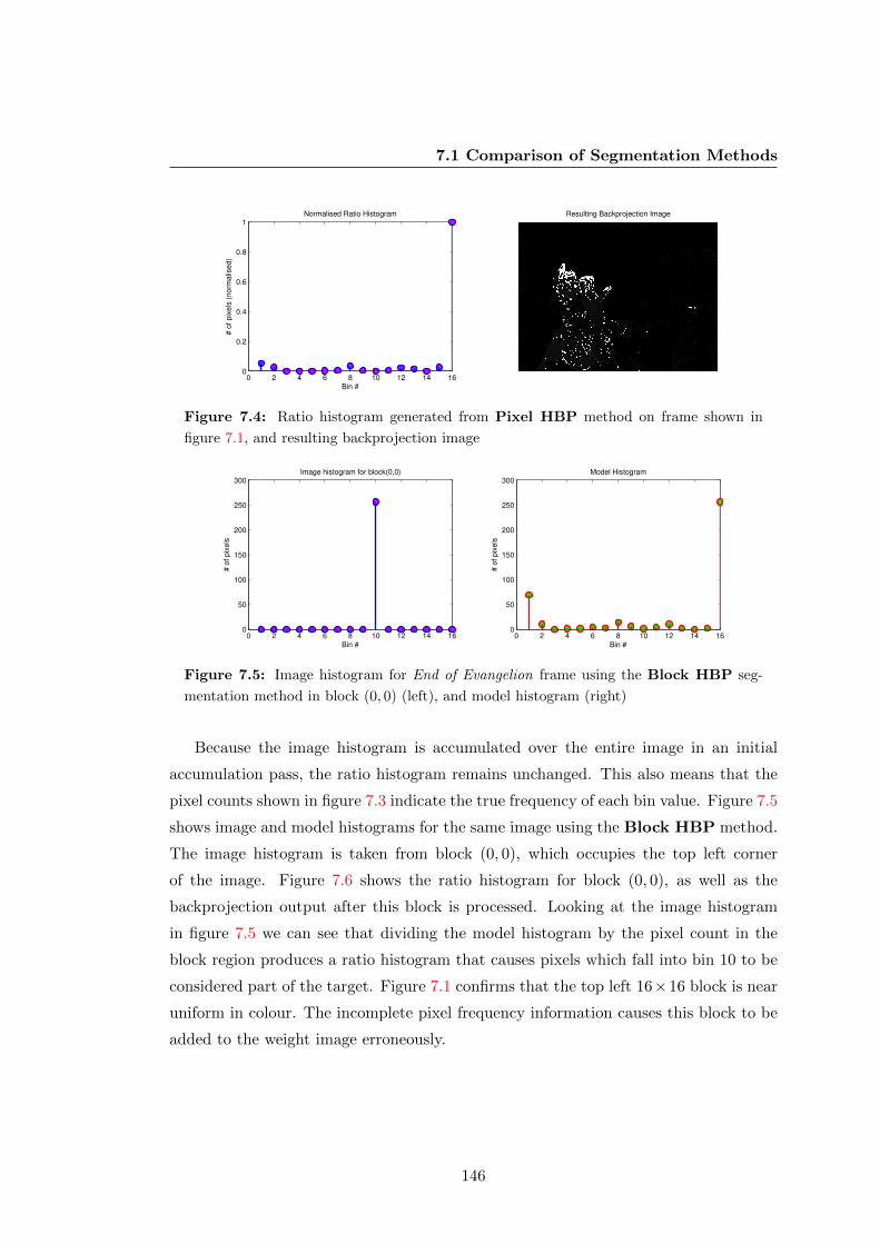
7.1 Comparison of Segmentation Methods
0 2 4 6 8 10 12 14 160
0.2
0.4
0.6
0.8
1
Bin #
# o
f p
ixe
ls (
no
rma
lise
d)
Normalised Ratio Histogram Resulting Backprojection Image
Figure 7.4: Ratio histogram generated from Pixel HBP method on frame shown in
figure 7.1, and resulting backprojection image
0 2 4 6 8 10 12 14 160
50
100
150
200
250
300
Bin #
# o
f p
ixe
ls
Image histogram for block(0,0)
0 2 4 6 8 10 12 14 160
50
100
150
200
250
300
Bin #
# o
f p
ixe
ls
Model Histogram
Figure 7.5: Image histogram for End of Evangelion frame using the Block HBP seg-
mentation method in block (0, 0) (left), and model histogram (right)
Because the image histogram is accumulated over the entire image in an initial
accumulation pass, the ratio histogram remains unchanged. This also means that the
pixel counts shown in figure 7.3 indicate the true frequency of each bin value. Figure 7.5
shows image and model histograms for the same image using the Block HBP method.
The image histogram is taken from block (0, 0), which occupies the top left corner
of the image. Figure 7.6 shows the ratio histogram for block (0, 0), as well as the
backprojection output after this block is processed. Looking at the image histogram
in figure 7.5 we can see that dividing the model histogram by the pixel count in the
block region produces a ratio histogram that causes pixels which fall into bin 10 to be
considered part of the target. Figure 7.1 confirms that the top left 16×16 block is near
uniform in colour. The incomplete pixel frequency information causes this block to be
added to the weight image erroneously.
146

7.1 Comparison of Segmentation Methods
0 2 4 6 8 10 12 14 160
0.2
0.4
0.6
0.8
1
Bin #
# o
f p
ixe
ls (
no
rma
lise
d)
Ratio Histogram for block(0,0) Backprojection Image
Figure 7.6: Ratio histogram for block (0, 0) of End of Evangelion frame using Block
HBP segmentation method, and backprojection image after block (0, 0) has been processed
0 2 4 6 8 10 12 14 160
0.2
0.4
0.6
0.8
1
Bin #
# o
f p
ixe
ls (
no
rma
lise
d)
Ratio Histogram for block(19,2) Backprojection Image [up to block(19,2)]
Figure 7.7: Ratio histogram generated from Block HBP in block (19, 2), and corre-
sponding backprojection image for blocks (0, 0)− (19, 2)
Note here how the model histogram in figure 7.5 suggests that the target should
contain mostly pixels which fall into bin 16, with a small number falling into bin 1,
whereas the ratio histogram in figure 7.6 will produce larger weight values for pixels
which fall into bin 10. The effect is caused by the presence of small non-zero values
in the model histogram in bin 10, which in turn generate ratio histograms as seen in
figure 7.6. This is because the tracking is initialised from the head of Eva-02 1 which
has many small non-red details that are captured in the model histogram. Whenever a
model histogram is captured from an actual scene, there is always the possibility that
some noise is captured, which can in turn cause unrelated elements in the scene to
be considered as part of the weight image. If we allow the backprojection to continue
block-wise until block (19, 2), we obtain an output like that shown on the right of
figure 7.7. The left portion of figure 7.7 shows the ratio histogram for block (19, 2).
1The red object being tracked in the left of the frame
147
7.1 Comparison of Segmentation Methods
This effect more or less vanishes if the model histogram is thresholded such that
small values are rounded towards zero. The definition of a small value may vary with
context. In this example, small values are defined as less than 10% of the maximum
number of pixels that could be assigned to a block. In the case of a 16× 16 block, this
value is rounded to 25. In terms of hardware, this requires that the model histogram
buffer contains a comparator stage that rounds to zero, non-zero bins which have a
smaller magnitude than the rejection threshold. Since the model histogram controller
implemented in this study is loaded serially, this can be accomplished with a single
comparator block at load time, making the change relatively cost-free.
7.1.2 Spatially Weighted Colour Indexing
The Spatial-Weighting methods are an attempt to prevent some background pixels, that
are incorrectly identified due to relative frequency error, from adversely affecting the
tracking performance. In this technique, only pixels which fall within some pre-defined
distance of the tracking window are backprojected. Pixels outside this range are all
rounded to zero. This can be understood as a simplified implementation of the circular
disk convolution used in [47] which is adapted to make the hardware easier to design
and manage, since it only requires a parameter buffer (such as the one in the mean shift
pipeline), and a window limit test (such as the one in the vector accumulator) against
the expanded tracking window.
In practice, the effectiveness of this technique is heavily dependent on lighting condi-
tions and background clutter. While this problem does affect the original CAMSHIFT
formulation in [24], the lack of a coherent histogram in the block and row processing
methods exacerbates this aspect. Knowing that this technique suffers from this draw-
back, it is important to quantify how much of an approximation this represents. A set
of tracking sequences has been generated, each consisting of 64 frames. The backpro-
jection methods in csTool are applied to the sequences in turn, using the same initial
conditions. The initial target position is selected manually, and is kept through each
of the tests. After segmentation, tracking is performed using the windowed moment
accumulation method in csTool.
The Pixel HBP method is used as a reference for comparison. All results are in
terms of the data generated using the Pixel HBP segmentation method, and win-
dowed moment accumulation tracking method. All segmentation images are quan-
148

7.1 Comparison of Segmentation Methods
tised to a single bit of precision, and use csTool ’s FPGA mode. All images are scaled
from the source material to have a dimension of 640× 480 pixels to match the pipeline
specification.
Frame sequences have been extracted from various sources for use in this study. In
particular, tests are performed on the following sequences.
1. Psy sequence
This sequence is taken from a well-known music video by a famous South-Korean
entertainer [123].
2. Running sequence
This sequence is taken from the TV series Black Mirror by Charlie Brooker [124],
and consists of a woman dressed in grey running through a wooded area.
3. Face sequence
This sequence is taken from the 2009 motion picture In The Loop[125], adapted
from the television series The Thick Of It by Armando Iannucci. The scene
consists of a single figure which exhibits relatively small motion, making this
scene well suited to comparative analysis.
4. End of Evangelion sequence
This sequence is taken from the Animated Motion Picture End of Evangelion
[41], and consists of two animated characters engaged in a physical struggle. The
red coloured object (behind) is the target for tracking.
7.1.3 Row Segmentation
Figure 7.8 shows the percentage of error pixels over the tracking run. This figure is
taken with model histogram thresholding set to 0%. The figure shows that less than
1% of the pixels differed between sequences. It should be noted that this graph does
not indicate where in the image these error pixels lie.
The percentage of error pixels in the Psy sequence are shown in figure 7.8. This
method gives much noisier results with around twice as much error compared to the
Block HBP method (figure 7.15) or the Block HBP (Spatial) method (figure 7.22),
although the total error is still very small.
149

7.1 Comparison of Segmentation Methods
Backprojection Image (Frame 1)
0 10 20 30 40 50 600
0.05
0.1
0.15
0.2
0.25
Frame Number
% e
rror
pix
els
Percentage of pixels different between sequences
Figure 7.8: Percentage of error pixels across Psy sequence per frame using Row HBP
segmentation. Row HBP backprojection image shown on left
Backprojection Image (Frame 1)
0 10 20 30 40 50 600
1
2
3
4
5
Frame Number
% e
rror
pix
els
Percentage of pixels different between sequences
Figure 7.9: Percentage of error pixels across Running sequence per frame using Row
HBP segmentation. Row HBP backprojection image shown on left
Figure 7.9 shows the same data for the Running sequence, again comparing between
the Pixel HBP and Row HBP methods. Results in figure 7.9 are generated with the
model histogram rejection threshold set at 5%.
Figure 7.10 shows the error pixel results for the Face sequence. The backprojection
image is generated using a rejection threshold of 10%, and gives results that are broadly
in line with other sequences. By inspection, the average percentage difference between
sequences is less than 1%.
Figure 7.11 shows the error pixel rate for the End of Evangelion sequence. Results
in this figure are shown with the model histogram rejection threshold at 10%.
Comparing the error pixel results for the Running and End of Evangelion sequences,
the former averages around twice that of the latter Although it can be difficult to visu-
alise the entire sequence of backprojection images from a single frame, visual inspection
of the sample frames in figures 7.9 and 7.11 show that the Row HBP delivers visually
150
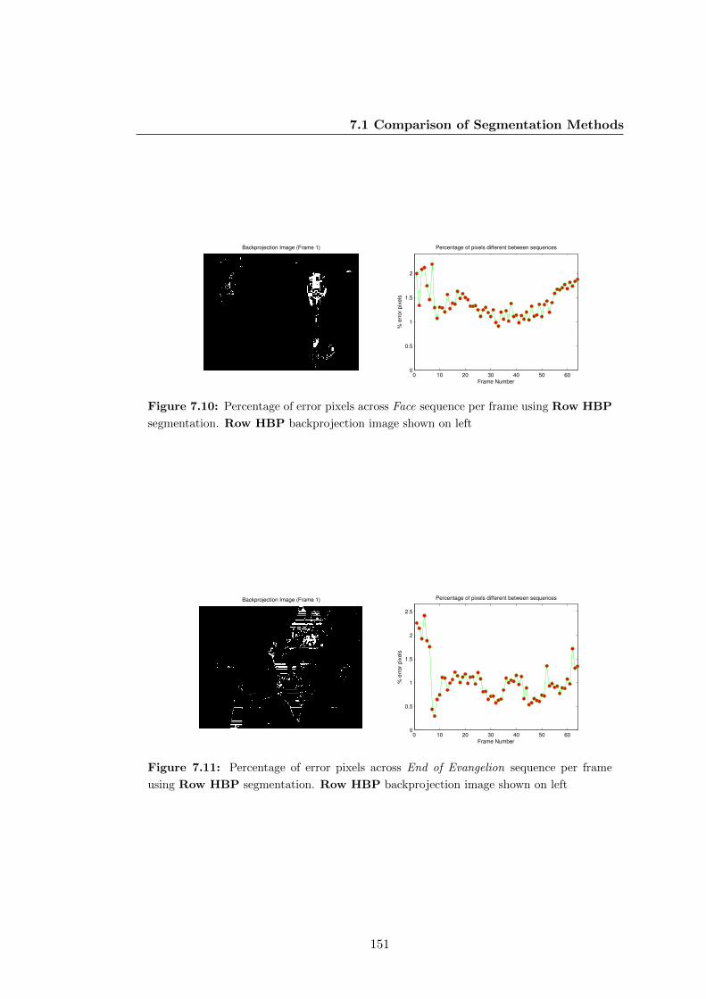
7.1 Comparison of Segmentation Methods
Backprojection Image (Frame 1)
0 10 20 30 40 50 600
0.5
1
1.5
2
Frame Number
% e
rro
r p
ixe
ls
Percentage of pixels different between sequences
Figure 7.10: Percentage of error pixels across Face sequence per frame using Row HBP
segmentation. Row HBP backprojection image shown on left
Backprojection Image (Frame 1)
0 10 20 30 40 50 600
0.5
1
1.5
2
2.5
Frame Number
% e
rro
r p
ixe
ls
Percentage of pixels different between sequences
Figure 7.11: Percentage of error pixels across End of Evangelion sequence per frame
using Row HBP segmentation. Row HBP backprojection image shown on left
151
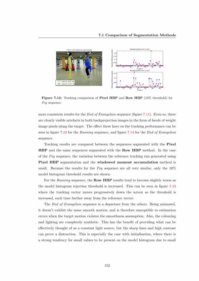
7.1 Comparison of Segmentation Methods
Frame 1 with trajectories superimposed
10 20 30 40 50 600
0.05
0.1
0.15
0.2
Frame #
Absolu
te D
iffe
rence (
pix
els
) Absolute position error (x axis)
10 20 30 40 50 600
0.05
0.1
0.15
Frame #
Absolu
te D
iffe
rence (
pix
els
) Absolute position error (y axis)
waccum−pixel−seg
waccum−row10−seg
Figure 7.12: Tracking comparison of Pixel HBP and Row HBP (10% threshold) for
Psy sequence
more consistent results for the End of Evangelion sequence (figure 7.11). Even so, there
are clearly visible artefacts in both backprojection images in the form of bands of weight
image pixels along the target. The effect these have on the tracking performance can be
seen in figure 7.13 for the Running sequence, and figure 7.14 for the End of Evangelion
sequence.
Tracking results are compared between the sequences segmented with the Pixel
HBP and the same sequences segmented with the Row HBP method. In the case
of the Psy sequence, the variation between the reference tracking run generated using
Pixel HBP segmentation and the windowed moment accumulation method is
small. Because the results for the Psy sequence are all very similar, only the 10%
model histogram threshold results are shown.
For the Running sequence, the Row HBP results tend to become slightly worse as
the model histogram rejection threshold is increased. This can be seen in figure 7.13
where the tracking vector moves progressively down the screen as the threshold is
increased, each time further away from the reference vector.
The End of Evangelion sequence is a departure from the others. Being animated,
it doesn’t exhibit the same smooth motion, and is therefore susceptible to estimation
errors when the target motion violates the smoothness assumption. Also, the colouring
and lighting are completely synthetic. This has the benefit of providing what can be
effectively thought of as a constant light source, but the sharp lines and high contrast
can prove a distraction. This is especially the case with initialisation, where there is
a strong tendency for small values to be present on the model histogram due to small
152

7.1 Comparison of Segmentation Methods
Figure 7.13: Tracking comparison of Pixel HBP and Row HBP for Running sequence
at 0% threshold (top), 5% threshold (middle), and 10% threshold (bottom)
153

7.1 Comparison of Segmentation Methods
Figure 7.14: Tracking comparison of Pixel HBP and Row HBP for End of Evangelion
sequence at 0% threshold (top), 5% threshold (middle), and 10% threshold (bottom)
colouring details in the animation cel. The specific model histogram used with this
sequence is shown in figure 7.3.
Figure 7.14 shows the same 2 row error plots as for the other sequences. It can be
seen that as the model histogram rejection threshold is increased, the error relative to
the Pixel HBP reference drops. This is also evident in the collated results presented
in table 7.4.
154

7.1 Comparison of Segmentation Methods
Backprojection Image (Frame 3)
0 10 20 30 40 50 600
0.05
0.1
0.15
0.2
0.25
0.3
0.35
0.4
Frame Number
% e
rror
pix
els
Percentage of pixels different between sequences
Figure 7.15: Percentage of error pixels across Psy sequence per frame using Block HBP
segmentation. Block HBP backprojection image shown on left
7.1.4 Block Segmentation
Figure 7.15 shows the percentage of error pixels in the Psy sequence between Pixel
HBP and Row HBP segmentation methods. Much like the Row HBP results in
figure 7.8, the total amount of variation in this sequence is small.
Figure 7.16 shows the percentage of error pixels in the Running sequence. These
results are comparable to the results generated for the same sequence using the Row
HBP technique at around 5%. Near the end there is a slight increase, which can
likely be attributed to a lighting change in the original material. Figure 7.10 shows the
error result for the Face sequence with model histogram rejection threshold of 10%.
Figure 7.18 shows error pixels for the End of Evangelion sequence. This particular
figure is taken with the ratio histogram rejection threshold set at 10%. The number of
error pixels here is partly a function of how much of a smoothing effect results from
the rejection threshold. In this case, the model histogram is simple, having only 2
significant bins.
In the Psy sequence, the motion is quite smooth and occurs over a relatively small
part of the frame. There is little background clutter near the target, and so the tracking
window is usually centered well enough to avoid large distractions. Consequently, all
the block methods provide more or less equal results, with all errors being less than 1
pixel in all cases. Only the results for block segmentation with a 10% model histogram
threshold are shown in figure 7.19 to save space.
Block results for the Running sequence are given in figure 7.20. Block results in the
0% case are very rough for this sequence. The test (blue) trajectory vector in the top-
155
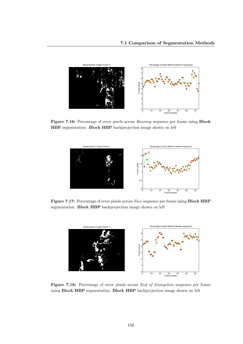
7.1 Comparison of Segmentation Methods
Backprojection Image (Frame 1)
0 10 20 30 40 50 600
1
2
3
4
5
6
7
8
Frame Number
% e
rror
pix
els
Percentage of pixels different between sequences
Figure 7.16: Percentage of error pixels across Running sequence per frame using Block
HBP segmentation. Block HBP backprojection image shown on left
Backprojection Image (Frame 1)
0 10 20 30 40 50 600
0.5
1
1.5
2
Frame Number
% e
rro
r p
ixe
ls
Percentage of pixels different between sequences
Figure 7.17: Percentage of error pixels across Face sequence per frame using Block HBP
segmentation. Block HBP backprojection image shown on left
Backprojection Image (Frame 1)
0 10 20 30 40 50 600
1
2
3
4
5
6
Frame Number
% e
rro
r p
ixe
ls
Percentage of pixels different between sequences
Figure 7.18: Percentage of error pixels across End of Evangelion sequence per frame
using Block HBP segmentation. Block HBP backprojection image shown on left
156

7.1 Comparison of Segmentation Methods
Frame 1 with trajectories superimposed
10 20 30 40 50 600
0.05
0.1
Frame #
Absolu
te D
iffe
rence (
pix
els
) Absolute position error (x axis)
10 20 30 40 50 600
0.1
0.2
0.3
Frame #
Absolu
te D
iffe
rence (
pix
els
) Absolute position error (y axis)
waccum−pixel−seg
waccum−block10−seg
Figure 7.19: Tracking comparison of Pixel HBP and Block HBP (10% threshold) for
Psy sequence
left-most sub figure is quite obviously different to the reference (green) trajectory figure.
As the model histogram rejection threshold is increased to 5%, the result noticeably
improves, with the vectors appearing to lie on the same y plane. When the threshold is
increased again to 10%, the test trajectory falls below the reference trajectory in the y
plane, and the total error appears to increase. An extended discussion of the accuracy
of the reference vector can be found in section 7.1.6.
Figure 7.21 shows the effect of increasing the model histogram rejection threshold
on the End of Evangelion sequence. As mentioned in section 7.1.3, the fact that the
End of Evangelion sequence is animated provides a unique challenge. Like the row
segmentation results, increasing the model histogram rejection threshold reduces the
tracking error relative to the Pixel HBP method (see also table 7.4).
7.1.5 Spatial Segmentation
All sequences using spatial tracking are performed with a window expansion region
of 32 pixels in each dimension. The same single bit precision mode is used, initial
conditions, and model histogram are used as per the other segmentation tests.
The percentage of error pixels in the Psy sequence is shown in figure 7.26. Overall
the error performance is similar to the Block HBP method, although with larger
errors near the start of the sequence owing to the difference between regions initially
cropped out of the spatially segmented image.
Figure 7.23 shows the error pixel results for the Running sequence. These results are
taken with a 5% model histogram rejection threshold. Overall the percentage difference
157
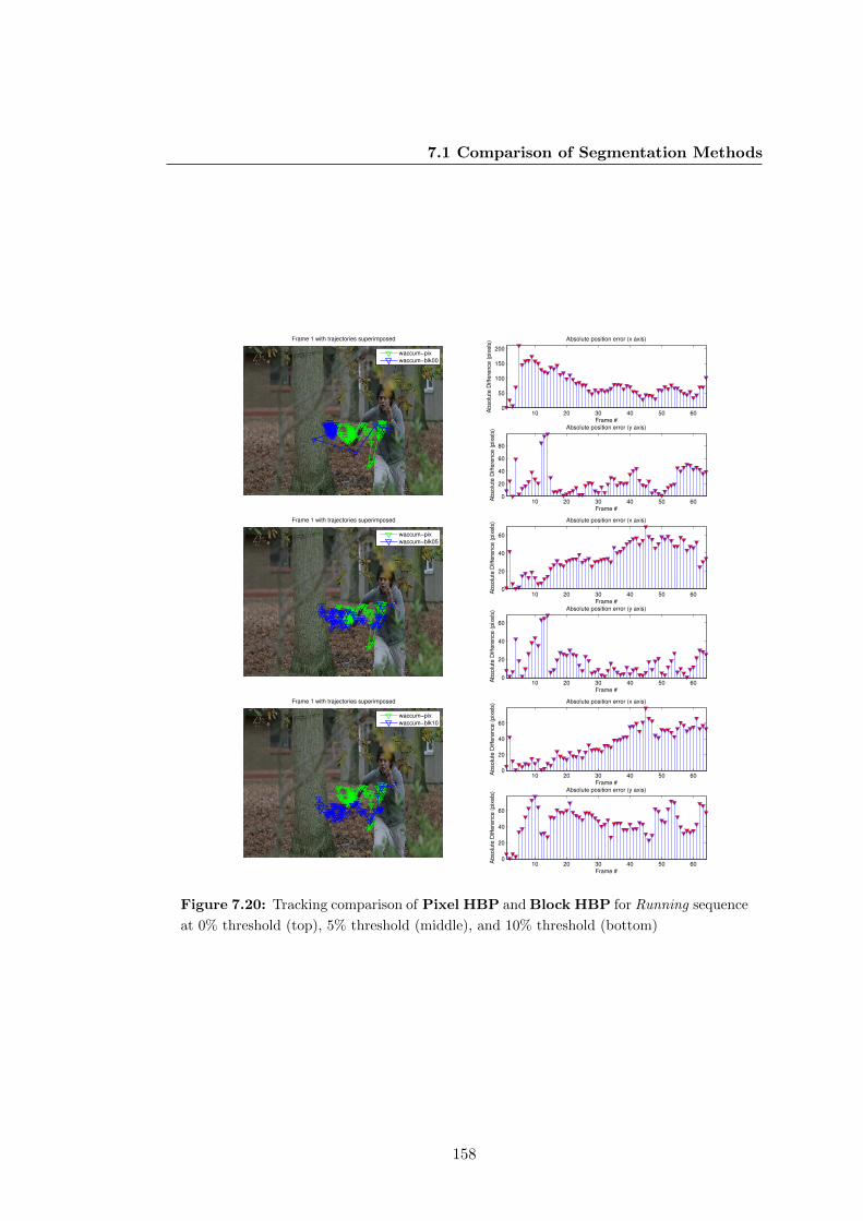
7.1 Comparison of Segmentation Methods
Figure 7.20: Tracking comparison of Pixel HBP and Block HBP for Running sequence
at 0% threshold (top), 5% threshold (middle), and 10% threshold (bottom)
158

7.1 Comparison of Segmentation Methods
Figure 7.21: Tracking comparison of Pixel HBP and Block HBP for End of Evangelion
sequence at 0% threshold (top), 5% threshold (middle), and 10% threshold (bottom)
159

7.1 Comparison of Segmentation Methods
Backprojection Image (Frame 3)
0 10 20 30 40 50 600
0.5
1
1.5
2
2.5
Frame Number
% e
rror
pix
els
Percentage of pixels different between sequences
Figure 7.22: Percentage of error pixels across Psy sequence per frame using Block HBP
(Spatial) segmentation. Block HBP (Spatial) backprojection image shown on left
Backprojection Image (Frame 4)
0 10 20 30 40 50 600
1
2
3
4
5
6
7
Frame Number
% e
rror
pix
els
Percentage of pixels different between sequences
Figure 7.23: Percentage of error pixels across Running sequence per frame using Block
HBP (Spatial) segmentation. Block HBP (Spatial) backprojection image shown on
left
between the backprojection images in the Block HBP and Row HBP sequences are
similar, hovering around 6%.
Figure 7.24 shows the error pixel results for the Face sequence, taken with a ratio
histogram rejection threshold of 5%. The sequence shows a low overall error of around
2% across all frames, with a slight increase to 2.5% towards the end.
Figure 7.25 show the error pixel results for the End of Evangelion sequence. Error
results using this method are comparable to other methods, with an average error in
the order of 5%. Unlike the Face sequence, the histogram rejection threshold is set to
10% in figure 7.25.
The tracking results for the Psy sequence using the Block HBP (Spatial) are
comparable to those derived using the other methods. Again, the variation in result
160
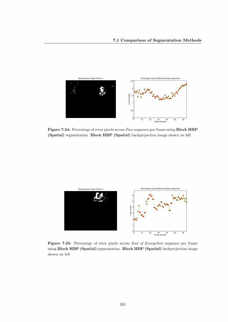
7.1 Comparison of Segmentation Methods
Backprojection Image (Frame 1)
0 10 20 30 40 50 600
0.5
1
1.5
2
2.5
Frame Number
% e
rro
r p
ixe
ls
Percentage of pixels different between sequences
Figure 7.24: Percentage of error pixels across Face sequence per frame using Block HBP
(Spatial) segmentation. Block HBP (Spatial) backprojection image shown on left
Backprojection Image (Frame 1)
0 10 20 30 40 50 600
1
2
3
4
5
6
Frame Number
% e
rro
r p
ixe
ls
Percentage of pixels different between sequences
Figure 7.25: Percentage of error pixels across End of Evangelion sequence per frame
using Block HBP (Spatial) segmentation. Block HBP (Spatial) backprojection image
shown on left
161

7.1 Comparison of Segmentation Methods
Frame 1 with trajectories superimposed
10 20 30 40 50 600
0.2
0.4
0.6
Frame #
Absolu
te D
iffe
rence (
pix
els
) Absolute position error (x axis)
10 20 30 40 50 600
0.2
0.4
0.6
0.8
Frame #
Absolu
te D
iffe
rence (
pix
els
) Absolute position error (y axis)
waccum−pixel−seg
waccum−blocksp10−seg
Figure 7.26: Tracking comparison of Pixel HBP and Block HBP (Spatial) (10%
threshold) for Psy sequence
with respect to model histogram rejection threshold is low, and so only the 10% case
is shown in figure 7.26.
7.1.6 Relationship between segmentation and tracking performance
The performance of the tracker is strongly dependant on the quality of the weight
images, which are in turn strongly dependant on illumination, background, appearance
modelling, and so on. The following tables provide summary statistics for each of the
tracking sequences in sections 7.1.3, 7.1.4, and 7.1.5.
In all the following tables, the units for error are pixels.
Table 7.1: Overview of tracking error in terms of segmentation for Psy sequence. Numbers
in parenthesis refer to model histogram threshold. All measurements are vs Pixel HBP
Method Avg Error (x) Avg Error (y) Std. Dev x Std. Dev y
vs Block HBP (%0) 0.02 0.02 0.03 0.05
vs Block HBP (%5) 0.02 0.03 0.03 0.05
vs Block HBP (%10) 0.02 0.03 0.03 0.05
vs Row HBP (%0) 0.02 0.02 0.04 0.04
vs Row HBP (%5) 0.02 0.02 0.04 0.04
vs Row HBP (%10) 0.02 0.02 0.04 0.04
vs BlkSp HBP (%0) 0.12 0.25 0.15 0.23
vs BlkSp HBP (%5) 0.12 0.25 0.15 0.23
vs BlkSp HBP (%10) 0.12 0.25 0.15 0.23
162

7.1 Comparison of Segmentation Methods
Table 7.2: Overview of tracking error in terms of segmentation for Running sequence.
Numbers in parenthesis refer to model histogram threshold. All measurements are vs Pixel
HBP
Method Avg Error (x) Avg Error (y) Std Dev (x) Std Dev (y)
vs Block HBP (0%) 80.29 24.71 42.39 21.23
vs Block HBP (5%) 35.52 16.85 16.98 15.31
vs Block HBP (10%) 33.7 45.73 20.36 16.81
vs Row HBP (0%) 10.65 17.73 5.14 17.24
vs Row HBP (5%) 11.41 17.97 5.29 16.73
vs Row HBP (10%) 13.52 25.94 6.15 13.10
vs BlkSp HBP (0%) 66.91 21.86 38.72 19.52
vs BlkSp HBP (5%) 32.94 21.62 14.32 15.97
vs BlkSp HBP (10%) 34.10 47.63 20.87 16.32
For the Face sequence, using the same backprojection technique used in other se-
quences as a reference1 tends to create a trajectory vector that follows the target poorly.
This is because the backprojection image generated by pixel-wise processing generates
some noise behind the target, which in turn enlarges the tracking window just enough
that the tie falls within the window boundary. Since the tie falls into the same hue
bin as the face, the window is enlarged further and the centre of the target is now
considered to lie somewhere between the face and the tie. This is possible because the
reference technique binarises the weight image, therefore any pixel which falls into a
non-zero bin will have the same weight after backprojection.
Table 7.3 shows the tracking comparison using the standard reference technique.
It can be seen in the results that the error tends to increase as the model histogram
rejection threshold is increased. However visual inspection of the trajectory vector will
show that the trajectories with the highest error appear to follow the motion of the
actual target more closely. Using a weighted backprojection image tends to reduce
this error in the Face sequence. Therefore, the results are repeated with a reference
trajectory generated from a 2-bit backprojection image, allowing 3 weights + the zero
weight. The effect of weighting the backprojection image is explored in more detail in
section 7.1.7. The revised results for the Face sequence are shown in table 7.6.
1To review, the reference sequence is generated using the Pixel HBP technique, with FPGA
mode set.
163

7.1 Comparison of Segmentation Methods
Table 7.3: Overview of tracking error in terms of segmentation for Face sequence with
1-bit backprojection image. All measurements are vs Pixel HBP
Method Avg Error (x) Avg Error (y) Std Dev (x) Std Dev (y)
vs Block HBP (0%) 5.11 39.29 5.09 38.08
vs Block HBP (5%) 8.63 72.46 5.22 48.97
vs Block HBP (10%) 17.17 34.75 11.90 11.44
vs Row HBP (0%) 8.75 12.30 8.17 10.02
vs Row HBP (5%) 2.57 17.64 3.28 21.78
vs Row HBP (10%) 3.09 19.69 4.35 24.74
vs BlkSp HBP (0%) 5.23 40.23 5.38 38.02
vs BlkSp HBP (5%) 8.60 72.35 5.22 48.98
vs BlkSp HBP (10%) 8.60 72.35 5.22 48.98
The revised results give much better error performance in the y dimension, except
when the Row HBP methods are used, in which the error increases.
Table 7.4: Overview of tracking error in terms of segmentation for End of Evangelion
sequence. Numbers in parenthesis refer to model histogram threshold. All measurements
are vs Pixel HBP
Method Avg Error (x) Avg Error (y) Std. Dev x Std. Dev y
vs Block HBP (0%) 44.20 34.88 37.88 30.53
vs Block HBP (5%) 44.20 34.88 37.88 30.53
vs Block HBP (10%) 26.26 73.56 20.44 28.81
vs Row HBP (0%) 30.86 31.15 23.33 21.74
vs Row HBP (5%) 22.94 39.55 17.25 27.05
vs Row HBP (10%) 19.76 43.96 19.75 28.52
vs BlkSp HBP (0%) 41.47 32.61 29.73 28.51
vs BlkSp HBP (5%) 48.00 81.26 29.15 32.36
vs BlkSp HBP (10%) 25.83 72.44 19.96 28.66
The Psy sequence (table 7.1) shows consistently low errors for all tracking methods.
As well as this, the number of error pixels for each sequence is relatively low, in the
order of 15% or less. Many of these error pixels are outside the tracking region, and
therefore have no effect on the tracking results.
164
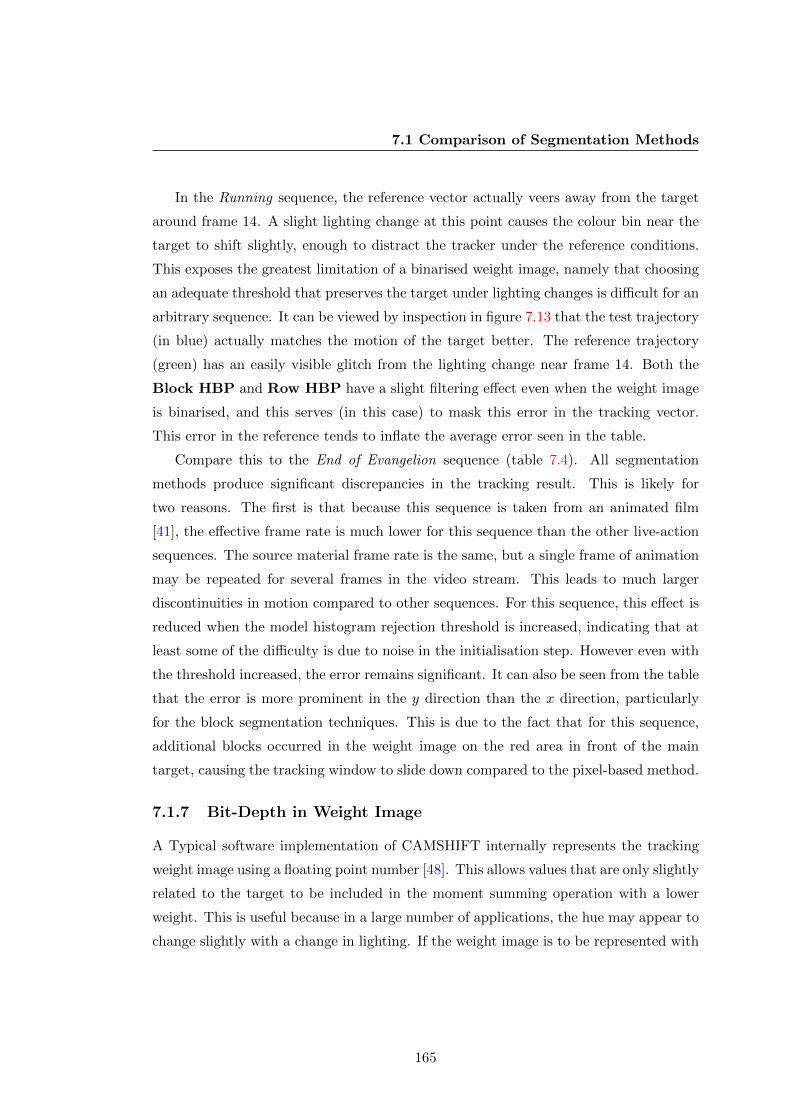
7.1 Comparison of Segmentation Methods
In the Running sequence, the reference vector actually veers away from the target
around frame 14. A slight lighting change at this point causes the colour bin near the
target to shift slightly, enough to distract the tracker under the reference conditions.
This exposes the greatest limitation of a binarised weight image, namely that choosing
an adequate threshold that preserves the target under lighting changes is difficult for an
arbitrary sequence. It can be viewed by inspection in figure 7.13 that the test trajectory
(in blue) actually matches the motion of the target better. The reference trajectory
(green) has an easily visible glitch from the lighting change near frame 14. Both the
Block HBP and Row HBP have a slight filtering effect even when the weight image
is binarised, and this serves (in this case) to mask this error in the tracking vector.
This error in the reference tends to inflate the average error seen in the table.
Compare this to the End of Evangelion sequence (table 7.4). All segmentation
methods produce significant discrepancies in the tracking result. This is likely for
two reasons. The first is that because this sequence is taken from an animated film
[41], the effective frame rate is much lower for this sequence than the other live-action
sequences. The source material frame rate is the same, but a single frame of animation
may be repeated for several frames in the video stream. This leads to much larger
discontinuities in motion compared to other sequences. For this sequence, this effect is
reduced when the model histogram rejection threshold is increased, indicating that at
least some of the difficulty is due to noise in the initialisation step. However even with
the threshold increased, the error remains significant. It can also be seen from the table
that the error is more prominent in the y direction than the x direction, particularly
for the block segmentation techniques. This is due to the fact that for this sequence,
additional blocks occurred in the weight image on the red area in front of the main
target, causing the tracking window to slide down compared to the pixel-based method.
7.1.7 Bit-Depth in Weight Image
A Typical software implementation of CAMSHIFT internally represents the tracking
weight image using a floating point number [48]. This allows values that are only slightly
related to the target to be included in the moment summing operation with a lower
weight. This is useful because in a large number of applications, the hue may appear to
change slightly with a change in lighting. If the weight image is to be represented with
165

7.1 Comparison of Segmentation Methods
a single bit of precision1 then values that fall outside the thresholding region will be
ignored completely, which may in turn cause the tracking results to veer significantly
away from the target. Floating point representation allows the weight image to more
accurately represent the Bayesian classifier from which it is derived (see section 3.3.1
for further discussion).
Due to the relatively high hardware cost of this implementation, it would be prefer-
able from the perspective of pipeline complexity to represent the weight image pixels
in the simplest and smallest possible form. Clearly the smallest form possible is a
binarised weight image where a single bit is used to represent each pixel. Additional
bits of precision could be added with some hardware cost. This section will attempt to
quantify the effect of various bit precisions on the tracking performance.
In section 7.1.6, the quality of the Pixel HBP reference for the Running sequence
was questioned. In particular, frame 14 of this sequence appears to deviate sharply
toward the bottom of the frame, as is visible in figures 7.13 and 7.20. Despite this, the
segmentation method was not changed in order to make the results for this sequence
comparable with others. A revised set of error figures for this sequence is shown in
table 7.5. These figures are obtained by comparing the same tracking vectors as in
table 7.2 against a reference trajectory generated from a set of fully weighted backpro-
jection images. That is, a set of backprojection images where each pixel is represented
as a floating point number with a range 0 - 1.
As can be seen, the results in table 7.5 show a marked decrease in the overall
tracking error.
This is also the case in the Face sequence. Using a binary weight image with no
thresholding results in some background pixels distracting the window away from the
true target. This happens in part because the effect of any pixel in the binary weight
image is the same. Weighting allows these pixels to contribute less to the window
position, thus resulting in a visually more accurate tracking vector. The effect of this
is noted in tables 7.3 and 7.6 which show trajectory error results in the Face sequence
for binarised and 2-bit weight images respectively. Except in the row case (noted in
section 7.1.6) the trajectory appears to track the target more closely when a 2-bit
image is used. The reference trajectory vector generated from the 1-bit weight image
1In other words, if we use a binary weight image
166

7.1 Comparison of Segmentation Methods
Table 7.5: Overview of tracking error for Running sequence using a fully weighted back-
projection image as the reference
Method Avg Error (x) Avg Error (y) Std Dev (x) Std Dev (y)
vs Pix (FPGA) 18.24 15.52 8.75 14.05
vs Block HBP (0%) 65.08 27.91 49.78 14.24
vs Block HBP (5%) 18.34 9.09 9.10 6.35
vs Block HBP (10%) 17.17 34.75 11.9 11.44
vs Row HBP (0%) 8.75 12.30 8.17 10.02
vs Row HBP (5%) 8.07 11.15 8.18 8.52
vs Row HBP (10%) 6.44 13.44 6.98 9.55
vs BlkSp HBP (0%) 52.71 22.46 44.17 13.84
vs BlkSp HBP (5%) 15.51 10.98 7.53 7.51
vs BlkSp HBP (10%) 19.01 36.54 12.18 11.91
is shown in green on the left side of figure 7.27. The vector generated from the 2-bit
weight image is shown in green on the left of figure 7.28.
Table 7.6: Revised of tracking error in terms of segmentation for Face sequence with 2-bit
backprojection image. All measurements are vs Pixel HBP
Method Avg Error (x) Avg Error (y) Std Dev (x) Std Dev (y)
vs Block HBP (0%) 8.59 36.15 7.71 38.65
vs Block HBP (5%) 2.05 3.37 1.52 3.22
vs Block HBP (10%) 2.05 3.37 1.52 3.22
vs Row HBP (0%) 9.87 55.01 7.84 42.03
vs Row HBP (5%) 9.07 56.61 7.29 43.22
vs Row HBP (10%) 8.93 53.06 7.23 42.32
vs BlkSp HBP (0%) 8.44 35.27 7.73 37.90
vs BlkSp HBP (5%) 2.09 3.38 1.55 3.16
vs BlkSp HBP (10%) 2.09 3.38 1.55 3.16
167
7.1 Comparison of Segmentation Methods
Frame 1 with trajectories superimposed
10 20 30 40 50 600
5
10
15
Frame #
Absolu
te D
iffe
rence (
pix
els
)
Absolute position error (x axis)
10 20 30 40 50 600
50
100
Frame #
Absolu
te D
iffe
rence (
pix
els
)
Absolute position error (y axis)
waccum−pixbp1
waccum−blk10
Figure 7.27: Tracking comparison of Pixel HBP with 1-bit backprojection image and
Block HBP (Spatial) (10% threshold) for Face sequence
Frame 1 with trajectories superimposed
10 20 30 40 50 600
2
4
Frame #
Ab
so
lute
Diffe
ren
ce
(p
ixe
ls)
Absolute position error (x axis)
10 20 30 40 50 600
5
10
15
20
Frame #
Ab
so
lute
Diffe
ren
ce
(p
ixe
ls)
Absolute position error (y axis)
waccum−pixbp4
waccum−blk10
Figure 7.28: Tracking comparison of Pixel HBP with 2-bit backprojection image and
Block HBP (Spatial) (10% threshold) for Face sequence
168
7.2 Scaling Buffer Preliminary Tests
7.2 Scaling Buffer Preliminary Tests
A working implementation of the scaling buffer was not developed in this study due
to time constraints. However simulations which demonstrate the principle of operation
are available in csTool, the output of which is provided here.
csTool allows the scaling buffer to be selected as the tracking mechanism for gen-
erating reference data. Options are provided to select the scaling factor. The window
parameter browser in the csTool main panel shows the scaling factor of a frame when
the scaling operation has been applied, as well as the number of backprojection pixels.
This implementation does not use any form of predictive windowing, which could fur-
ther reduce the number of backprojection pixels that need to be stored in the actual
hardware buffer.
For each scaling buffer test, a set of reference backprojection frames is generated.
The reference tracking vector uses the windowed moment accumulation technique.
Each subsequent tracking vector in the test set is generated using the scaling buffer
technique, with the scaling factor increased by a power of two. The results are given
as error tables, with the error number representing the average difference in pixels
compared to the reference implementation.
Table 7.7 shows the test results for the Psy sequence. For scaling factor values
below 16, there is almost no effect on the tracking accuracy. This is because the scaling
buffer operation should be identical to the standard windowed moment accumulation
technique when the number of backprojection pixels is less than (imgw × imgh)/Sfac,
where Sfac is the scaling factor. In this sequence, the number of backprojection pixels
is less than 192001 for more than 2/3 of the sequence, and so the average error is almost
completely derived from a few frames near the end. Figure 7.29 shows the trajectory
comparison and error plot when the scaling factor is 64.
Table 7.8 shows the results for the Face sequence. This sequence demonstrates the
effect of increasing the scaling factor when the number of pixels in the weight image
are relatively small. For scaling factors of 32 or less, the overall error in the tracking
vector remains small. However once the scaling factor reaches 64, the y dimension error
suddenly increases. This is because the face region under the tracking window becomes
much smaller in the y dimension near the top at the same time that pixels in the tie
1The image dimensions are 640 × 480, therefore 19200 = (640 × 480)/16
169

7.2 Scaling Buffer Preliminary Tests
Table 7.7: Scaling buffer comparison for the Psy sequence
Scaling Factor Avg Error (x) Avg Error (y) Std Dev (x) Std Dev (y)
x4 0.09 0.09 0.20 0.28
x8 0.09 0.09 0.20 0.28
x16 0.28 0.26 0.3 0.33
x32 2.50 1.57 2.62 2.04
x64 8.13 4.21 4.60 3.67
Frame 1 with trajectories superimposed
10 20 30 40 50 600
5
10
15
20
25
Frame #
Ab
so
lute
Diffe
ren
ce
(p
ixe
ls)
Absolute position error (x axis)
10 20 30 40 50 600
5
10
Frame #
Ab
so
lute
Diffe
ren
ce
(p
ixe
ls)
Absolute position error (y axis)
psy−waccum
psy−sp64
Figure 7.29: Trajectory comparison of windowed moment accumulation against a
scaling buffer with Sfac = 64 on Psy sequence
170

7.3 Synthesis and Simulation of Modules
Frame 1 with trajectories superimposed
10 20 30 40 50 600
5
10
15
20
Frame #
Absolu
te D
iffe
rence (
pix
els
) Absolute position error (x axis)
10 20 30 40 50 600
20
40
60
80
Frame #
Absolu
te D
iffe
rence (
pix
els
) Absolute position error (y axis)
itl−waccum
itl−sp64
Figure 7.30: Trajectory comparison of windowed moment accumulation against a
scaling buffer with Sfac = 64 on Face sequence
the character is wearing, some of which fall into the same model histogram bin, become
relatively closer to the target area due to the scaling effect. This causes the tracking
window to tend down towards the tie. The effect can be seen in the trajectory vector
on the left of figure 7.30.
Table 7.8: Scaling buffer comparison for the Face sequence
Scaling Factor Avg Error (x) Avg Error (y) Std Dev (x) Std Dev (y)
x4 0 0 0 0
x8 1.25 1.20 0.65 0.95
x16 1.25 1.20 0.65 0.95
x32 1.56 1.69 0.66 1.03
x64 8.41 34.06 7.99 42.67
Table 7.9 shows the test results for the End of Evangelion sequence. Again, the
results show almost no variation until Sfac is 64 due to the relatively small number of
pixels in the weight image. The trajectory error when Sfac = 64 is shown in figure 7.31
7.3 Synthesis and Simulation of Modules
In order to simplify the task of constraining the design for synthesis, output registers
are added to all modules. All state machines have registered outputs and in many case
registered inputs [126]. All logic clouds have been timed for operation with a 10ns clock
171

7.3 Synthesis and Simulation of Modules
Table 7.9: Scaling buffer comparison for the End of Evangelion sequence
Scaling Factor Avg Error (x) Avg Error (y) Std Dev (x) Std Dev (y)
x4 0.15 0.08 0.94 0.28
x8 0.15 0.08 0.94 0.28
x16 0.15 0.08 0.94 0.28
x32 0.15 0.10 0.94 0.32
x64 1.00 1.32 2.00 4.50
Frame 1 with trajectories superimposed
10 20 30 40 50 600
5
10
Frame #
Ab
so
lute
Diffe
ren
ce
(p
ixe
ls)
Absolute position error (x axis)
10 20 30 40 50 600
5
10
15
20
25
Frame #
Ab
so
lute
Diffe
ren
ce
(p
ixe
ls)
Absolute position error (y axis)
eoe−waccum
eoe−waccum−sp64
Figure 7.31: Trajectory comparison of windowed moment accumulation against a
scaling buffer with Sfac = 64 on End of Evangelion sequence
172

7.3 Synthesis and Simulation of Modules
Figure 7.32: RTL view of row-oriented backprojection pipeline with annotations
period. Tables of results are generated with all pins of the synthesised module set to
VIRTUAL during synthesis.
7.3.1 Row-Oriented Backprojection Module
An annotated screen capture of the RTL schematic for the row-oriented backprojection
pipeline is shown in figure 7.32. From left to right, the model histogram buffer, FIFO
bank, and input side histogram indexing module process incoming pixel data. Behind
the FIFO bank lies the module controller, followed by the image histogram bank. As
per the requirements of the timing diagram in figure 4.3, both the FIFO and Image
Histogram banks are double buffered, and the output multiplexer for each bank is
visible in the figure.
173

7.3 Synthesis and Simulation of Modules
Synthesis results for the row-oriented pipeline are given in table 7.10. Divider results
in the table are given for all dividers in the bank. The vector dimension for this pipeline
is 16.
Table 7.10: Synthesis results for modules in the row backprojection pipeline
Module Comb. Reg. Mem. DSP
Controller 59 49 0 0
FIFO0 40 25 516 0
FIFO1 40 25 516 0
RHIST 78 145 0 0
IMHIST0 148 128 0 0
IMHIST1 144 128 0 0
RHIST0 0 128 0 0
RHIST1 0 128 0 0
MHIST 5 260 0 0
RHIST COMP 24 0 0 0
DIVIDER (Total) 1904 1088 0 0
Top Level 2632 2164 1032 0
7.3.2 Column-Oriented Backprojection Module
An annotated screen capture of the RTL schematic for the column-oriented backpro-
jection pipeline is shown in figure 7.33. The differences between the row and column
pipelines are apparent from the corresponding RTL diagrams. In the column oriented
pipeline, the histogram indexing must be done in parallel for each element in the pixel
vector. This is reflected in the larger resource utilisation of the Input Compare and
Output Compare in the column orientated pipeline. This is seen in the synthesis results
in table 7.11.
Synthesis results for the column backprojection module and submodules in shown
in table 7.11. As per the row oriented pipeline in section 7.3.1, the synthesis results
are generated with a vector dimension of 16, and the divider bank figure is given for
all dividers in the bank.
174

7.3 Synthesis and Simulation of Modules
Figure 7.33: RTL view of column-oriented backprojection pipeline with annotations
Table 7.11: Synthesis results for modules in the column backprojection pipeline
Module Comb. Reg. Mem. DSP
Controller 56 66 0 0
Input Compare 656 336 0 0
Output Compare 384 0 0 0
RHIST 430 384 0 0
FIFO0 37 15 1088 0
FIFO1 37 15 1088 0
IMHIST0 160 128 0 0
IMHIST1 144 128 0 0
RHIST0 0 112 0 0
RHIST1 0 112 0 0
MHIST 5 260 0 0
DIVIDER (Total) 1824 1136 0 0
Top Level 3888 2781 2176 0
175

7.3 Synthesis and Simulation of Modules
Figure 7.34: RTL view of window computation module with annotations
7.3.3 Mean Shift Processing Module
The mean shift processing module implements the moment accumulation and window
computation stages of the mean shift pipeline. An annotated screen capture of the
RTL schematic for this stage is shown in figure 7.34.
Two square root solvers are provided so that each side of the reference rectangle
can be computed simultaneously. In the first pass, one of these is used to compute
the inner square root term in the expression. On the second pass, both are used to
compute the two outer square root terms in parallel.
Table 7.12: Synthesis results for MS PROC TOP module
Resource Type Amount
Combinational 4529
Register 3831
Memory (bits) 614620
DSP 89
DSP 9x9 17
DSP 18x18 36
Figure 7.34 shows a highlighted view of the synthesised RTL for the accumulator
and window computation engine of the mean shift processing module. Two square root
solvers are provided for computing the reference rectangle.
176

7.3 Synthesis and Simulation of Modules
Figure 7.35: RTL view of mean shift accumulator with annotations
7.3.4 Vector Accumulator
Figure 7.35 shows the RTL view of the accumulator internals. The module is designed
to meet timing with a clock period of 10ns. Each major group of components within
the module is annotated on the diagram. In the top left is the row and column pointer
logic. This is simply a set of incrementers driven from the data valid signal. Since the
raster direction is the same regardless of orientation, this logic does not differ between
the row and column accumulators.
When coupled with the scaling buffer, the row and column pointer logic is replaced
with a vector expansion decoder. The scaling buffer only stores data points for pixels in
the image, therefore the row and column pointers cannot be incremented simply from
the data valid signal.
Once the scaled vector data is recovered, the data point in the vector dimension must
be expanded into position values in image space. To the right of the row and column
logic is the vector expansion LUT and vector masking module (see section 4.6.1). An
annotated RTL view of the vector masking module is shown in figure 7.36.
The vector masking module drives the arithmetic modules immediately to the right.
These perform the inner product and summing operations required to find the scalar
moment quantities for each dimension. To the right of this is the pipelined accumulation
block. The large number of multiplexers in this section are required in order to write
zeros to the accumulation registers at the end of the frame. Finally a set of registers sit
on the output which hold the previous moment values. This allows moment data to be
read during the accumulation, as well as simplifying the task of constraining the design
for synthesis [126]. Since the expanded LUT vector is V ×Wbp bits wide, pipelining
this module can become relatively expensive. The RTL in figure 7.36 are taken from
177
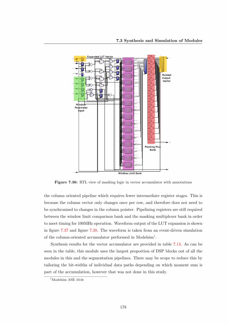
7.3 Synthesis and Simulation of Modules
Figure 7.36: RTL view of masking logic in vector accumulator with annotations
the column oriented pipeline which requires fewer intermediate register stages. This is
because the column vector only changes once per row, and therefore does not need to
be synchronised to changes in the column pointer. Pipelining registers are still required
between the window limit comparison bank and the masking multiplexer bank in order
to meet timing for 100MHz operation. Waveform output of the LUT expansion is shown
in figure 7.37 and figure 7.38. The waveform is taken from an event-driven simulation
of the column-oriented accumulator performed in Modelsim1.
Synthesis results for the vector accumulator are provided in table 7.13. As can be
seen in the table, this module uses the largest proportion of DSP blocks out of all the
modules in this and the segmentation pipelines. There may be scope to reduce this by
tailoring the bit-widths of individual data paths depending on which moment sum is
part of the accumulation, however that was not done in this study.
1Modelsim ASE 10.0c
178

7.3 Synthesis and Simulation of Modules
Figure 7.37: Vector expansion at start of frame. Note that the masked lut vec line is
all zeros at this point
Figure 7.38: Vector expansion during processing. Weight image pixels enter (pictured
top), and are expanded and masked in the pipeline
Table 7.13: Synthesis results for mean shift accumulator module
Resource Type Amount
Combinational 1455
Register 2133
Memory (bits) 188
DSP 55
DSP 9x9 17
DSP 18x18 19
179
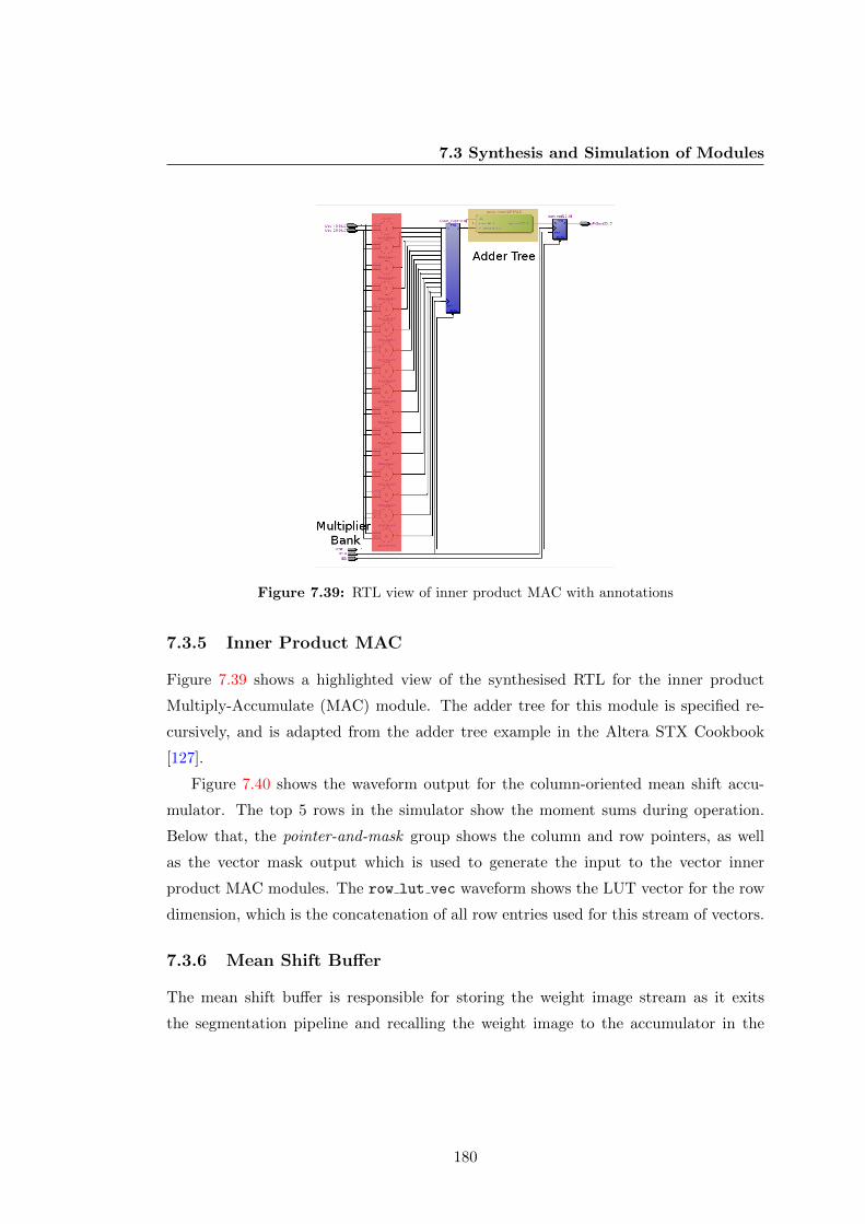
7.3 Synthesis and Simulation of Modules
Figure 7.39: RTL view of inner product MAC with annotations
7.3.5 Inner Product MAC
Figure 7.39 shows a highlighted view of the synthesised RTL for the inner product
Multiply-Accumulate (MAC) module. The adder tree for this module is specified re-
cursively, and is adapted from the adder tree example in the Altera STX Cookbook
[127].
Figure 7.40 shows the waveform output for the column-oriented mean shift accu-
mulator. The top 5 rows in the simulator show the moment sums during operation.
Below that, the pointer-and-mask group shows the column and row pointers, as well
as the vector mask output which is used to generate the input to the vector inner
product MAC modules. The row lut vec waveform shows the LUT vector for the row
dimension, which is the concatenation of all row entries used for this stream of vectors.
7.3.6 Mean Shift Buffer
The mean shift buffer is responsible for storing the weight image stream as it exits
the segmentation pipeline and recalling the weight image to the accumulator in the
180

7.3 Synthesis and Simulation of Modules
Figure 7.40: Waveform output showing vector masking and moment accumulation in
mean shift pipeline
Figure 7.41: RTL view of mean shift buffer with annotations
mean shift pipeline. An annotated RTL diagram of the mean shift buffer is shown in
figure 7.41.
Synthesis results for the mean shift buffer are shown in table 7.14. Each of the two
buffers holds a 307200 bit weight image, meaning that 614400 of the 614432 bits shown
in the table are utilised by the image buffers. Because no arithmetic is performed in
this module, the number of required DSP blocks is 0.
The RTL schematic for the buffer controller is shown in figure 7.42 with annotations.
Figure 7.42 shows the RTL schematic of the mean shift buffer controller. This
controller is responsible for co-ordinating reads and writes between the two RAM blocks
in such a fashion that the buffer appears as a single dual-port buffer with simultaneous
read and write. A waveform dump of the initial write sequence is shown in figure 7.43.
Figure 7.44 shows the waveform dump for the initial read sequence of the mean
shift buffer. The ctrl buf1 ins line has been de-asserted, and after a 4-cycle delay
181

7.3 Synthesis and Simulation of Modules
Table 7.14: Synthesis results for MS BUF TOP module
Resource Type Amount
Combinational 260 (18)
Register 151 (33)
Memory (bits) 614432
DSP 0
DSP 9x9 0
DSP 18x18 0
Figure 7.42: RTL schematic of mean shift buffer controller
Figure 7.43: Waveform dump of first write sequence in mean shift buffer
182

7.4 Processing Time
Figure 7.44: Waveform dump of first read sequence in mean shift buffer
through the status flag pipeline, the ctrl buf1 data line is asserted, indicating that
the first buffer now contains weight image data.
7.4 Processing Time
The time required to process a frame and produce a converged mean shift vector is in
practise a function of how well the target is defined in the scene, how much distance the
target has moved since the previous frame, and so on. It can be shown how many cycles
are required to compute the new target location for a given number of iterations, and
this is compiled into table 7.16. These figures are computed from the number of cycles
required for each module in the mean shift pipeline, which is shown in table 7.15. The
number for controller overhead is given as an average for an entire frame. In practise,
there will be 1 cycle of overhead for each convergence test. For the CORDIC module,
the number of cycles is given as between 6 and 32. This is to reflect the fact that early
convergence of the CORDIC and square root operations that happen in that stage of
the pipeline will cause the pipeline to move forward early. If an answer cannot be found
in 32 cycles, the stage is skipped and a previous result is used. This means that for
some angles, and some values in the mean-subtracted mu matrix the actual processing
time could be much lower. The minimum number of cycles to converge is typically 4,
however the average is closer to 5 or 6.
183

7.4 Processing Time
Table 7.15: Number of cycles per module in mean shift pipeline
Module Cycles
Divider 32
Convergence Test 2
Mean Subtraction 4
CORDIC + SQRT 6 - 32
Rectangle Length 10
Eigen Pair 2
Control Overhead 4
Table 7.16 shows the total number of cycles and the total processing time in terms
of the number of iterations of the inner loop. The first column shows the number of
iterations performed. The second column shows the total number of cycles required
to process the data for the corresponding number of iterations. The third column
shows the total number of cycles required to read the data required to perform the
corresponding number of iterations. The final column shows the time that this required
in milliseconds, assuming a 100MHz clock. The cycle number can be multiplied by any
given clock period to produce figures for faster or slower devices. Since 4 is the average
number of iterations before convergence [26], iteration 4 is highlighted in bold in the
table.
184

7.4 Processing Time
Table 7.16: Processing time in mean shift loop in terms of iterations
No. Iterations Mean shift cycles Buffer read cycles Total Time (ms)
1 86 19200 19287 385.72
2 120 38400 38520 770.4
3 154 57600 57754 1155.08
4 188 76800 76988 1539.76
5 222 96000 96222 1924.44
6 256 115200 115456 2309.12
7 290 134400 134690 2693.8
8 324 153600 153924 3078.48
9 358 172800 173158 463.16
10 392 192000 192039 3847.84
11 426 211200 211626 4232.52
12 460 230400 230860 4617.2
13 494 249600 250094 5001.88
14 528 268800 269328 5386.56
15 562 288000 288562 5771.24
185

Chapter 8
Discussion and Conclusions
The previous chapters have detailed the framework for a visual object tracking system
based on the mean shift algorithm [67] using a simple segmentation technique based
on a single colour feature [47] [24]. Chapter 2 gave a basic overview of the state of
computer vision and visual object tracking, as well as examining previous work done
using kernel histogram methods such as the mean shift tracker. The progression of
the idea from Fukunaga and Hostetler’s original paper [67], through Bradski [24] and
Comaniciu, Ramesh, and Meer’s [26] visual object tracking systems, and onto more
modern and increasingly complex ideas [27] [83] [28] [88] [128] [129] [130] [80].
Chapter 3 discussed the use of colour features for tracking, and how this relates to
Fukunaga and Hostetler’s mean shift algorithm [67]. The link between the theory in
[67] and the implementation in Comaniciu, Ramesh, and Meer [66] [26] is given. As
well as this, comment is made about the observation of Collins, that the mean shift
tracking framework only requires a weight image to perform the tracking operation,
[94] and that any segmentation method that can generate such an image can be used
for tracking [27]. The notion of the implicit and explicit weight image was introduced,
and this distinction is used to frame some of the work in the field.
Chapter 4 discussed the implementation considerations that arise when trying to
map the colour indexing technique of Swain and Ballard from a context-free algorithm
to a context sensitive implementation. The chapter considered the domain-specific
challenges that arise during this mapping process and suggests solutions which are
used in this work.
186

8.1 Comparison of Row and Column Pipelines
Chapter 5 discussed the specific implementation used in this study, examining the
datapath structure and control hierarchy which implements the mean shift process.
Each module in the datapath is examined in detail, along with schematic diagrams
illustrating the datapath layout.
Chapter 6 discussed an application called csTool, which was developed as part
of this study for architecture exploration, and verification and analysis of the CSoC
implementation. The chapter discussed how the tool is intended to act as a translation
layer between the context free mean shift algorithm, and the context specific FPGA
implementation. The chapter looks at the architecture and internal data structures
of the tool, and discusses the various test vector generation and verification routines
available within it. The design and philosophy behind the tool’s development is also
considered.
Chapter 7 discussed the performance of various segmentation methods, and com-
pared the tracking vectors of each to determine the effectiveness of each method. As
well as this, the synthesis and simulation results for each of the major modules in the
CSoC pipeline is presented. An analysis of possible implementations is given, showing
the relative change in area and resource usage for various architectures when scaled.
8.1 Comparison of Row and Column Pipelines
In chapter 4, the idea of orientation was developed (see section 4.2 for details). In
summary, this idea was intended to capture the architectural implications of vectoring
the pixel pipeline. While the differences are intended to be comparative, considering
one or another orientation to be superior is not the point of the exercise. Rather, the
differences should be considered as trade-offs that arise from different design choices.
The following section will give a brief overview of these differences, and consider how
they affect different parts of the CSoC pipeline.
It should be clear from inspection that the column orientation, with its requirement
for many operations in parallel, is a more expensive choice from the perspective of
resource utilisation. However the column orientation offers two distinct benefits over
the row orientation. The first is that it required less memory to use the column oriented
backprojection pipeline in conjunction with the scaling buffer. This is because less
data is required to form the 2-dimensional lattice required for the scaling operation.
187

8.1 Comparison of Row and Column Pipelines
In the row orientation, V rows need to be buffered before this can occur. While it
may seem that this would be no different to the column buffer required at the input
stage of the column oriented backprojection, it should be noted that once the pixels
have been backprojected they are unique to a particular appearance model. Therefore,
multiple appearance models such as those illustrated in figures 8.2 or 8.3 cannot share
any memory for stages after the weight image has been computed. If the histogram
backprojection method is used, the control scheme for the column backprojection is
also more complex because of the need to complete the division step before the next
image patch is accumulated. Larger image patches relax this timing requirement at the
expense of more image patch memory. Higher radix division also reduces the processing
time, but at the cost of more division logic1.
As well as this, the column oriented mean shift accumulation stage requires less
energy than the row oriented one, as the pointer in the vector dimension changes less
frequently, therefore requiring fewer look-ups. The drawback is that the resource us-
age is higher with the column orientation. For cases where either the scaling buffer
is not required, or the available device resource is limited2 the row oriented pipeline
may be better suited. The controller for the row orientation is also much simpler,
since the accumulation time is very long relative to the processing time. It should be
made clear that these control limitations are a property of the histogram backprojection
method, and that other segmentation methods will likely have different timing penal-
ties and constraints. See chapter 9 for a brief discussion on alternative segmentation
frameworks, and section 8.4 for remarks on segmentation performance in the histogram
backprojection framework.
The terms row and column could equally be replaced with the terms scalar and
vector respectively, as this conveys the intended meaning. Because it is common for
rasters to operation from left to right, top to bottom, the terms row and column should
be sufficient. However in unusual cases, they can be generalised as scalar and vector.
Sensors that provide pixel lattice outputs are considered to be outside the scope of this
study.
1Although the cost of more division logic is arguably less than the cost of more memory, depending
on the resource availability in the FPGA. Because a divider is needed for each bin in the histogram,
the total resource cost for higher radix division is mostly a function of the number of histogram bins2Use of the term device here implies an FPGA, however the same idea applies in principal to an
ASIC or similar
188

8.2 On chip tracking framework
8.2 On chip tracking framework
The implementation in this thesis consists of a simple colour segmentation front end
which generates a weight image using the colour indexing technique [47], and performs
the mean shift tracking operation using a windowed moment accumulation technique
[24] [48] [70] [69]. However the framework shown here can be extended into a more
general architecture for on-chip object tracking using the mean shift technique.
Firstly, we note again the observation by Collins that the mean shift tracker sees
the weight image. This immediately implies two things:
1. Any feature space can be used, so long as the segmentation pipeline can generate
as its output a weight image.
2. Joint feature spaces can be considered as an extension of regular feature spaces,
and as such can use the same accumulation and windowing stage1.
It should therefore be possible to consider the segmentation step as completely in-
dependent of the tracking step, subject to the constraint that it deliver a weight image
using a specified data representation. The scaling buffer implementation discussed in
section 4.6 is an example of a data representation2 that reduces the pipelines depen-
dency on row and column counters by encoding the positions of pixels directly into the
representation. The effect is akin to a list data structure, in the sense that it contains
only the elements of the weight image that we are interested in. This is discussed in
more detail in section 8.4
Performance results in chapter 7 would suggest that the memory saving techniques
applied to the segmentation stage can in many cases produce noticeably offset tracking
vectors compared to a pixel-by-pixel reference implementation (see section 7.1). This
is compounded by the simplicity of the appearance model, which consists of a single
colour feature with no edge detection, as well as the various numerical approximations
used to simplify the device implementation. While sensitivity to initial conditions is
a problem in the original formulation [24] [26], as well as in current implementations3
1See section 5.42The term data structure doesn’t seem accurate in this context, but can be considered as a direct
analogy3Assuming of course, that the same (or substantially similar) appearance model is used. Tracking
performance can obviously be improved through the application of more robust appearance models,
including appearance models that combine features from multiple feature spaces, for example in [27].
189

8.3 Extensions to Tracking Architecture
[48], the localised nature of the Row HBP and Block HBP segmentation methods
requires that small values be pruned from the model histogram before segmentation.
8.3 Extensions to Tracking Architecture
Performing the tracking operation using moment accumulation means that there is no
spatial dependency in the computation. All the information about the distribution is
reduced to a set of summary statistics represented by the normalised moment matrix
µ. Because we only need the weight image to perform tracking, and because we can
traverse the weight image in any order, we can split the weight image across many
buffers1 and compute the moment sums across those patches in parallel. This incurs
some hardware overhead, but can dramatically improve the speed at which tracking
can occur. The basic framework can be generalised to that shown in figure 4.12.
The method used to represent the weight has a significant effect on the flexibility
of the pipeline. The scaling buffer implementation discussed in section 4.6 considers
a buffer which stores only non-zero vectors in the weight image. This means that the
computation time is directly proportional to the number of pixels in the weight image.
The location of each vector is encoded in the buffer. The role of the vector accumulator
in this implementation is to decode the buffer data in the order that it is read. There is
no requirement for the read order to be the same as the write order, and the fact that
this happens in practise is a consequence of the buffer being directly attached to the
pixel stream. Unlike a raster implementation, the pixel location is not recovered by a
set of linked counters which maintain the row and column pointers2. Therefore, these
vectors can easily be split across multiple buffers in order to gain higher performance.
This study is concerned with an implementation in which pixel data arrives from a
CMOS sensor, which has a blanking time around the data stream. In this particular
context, additional speed-ups in tracking time are not required, since wait time is built
in to the sensor operation. However were the architecture to be extended to a more
general implementation designed to handle arbitrary data streams, the capability to
1Effectively, splitting the image into patches2Rather, the row and column information is directly encoded in the vector
190

8.3 Extensions to Tracking Architecture
Figure 8.1: Two fully independent tracking pipelines. Weight image A is generated from
Appearance Model A applied to Input Image A, as is B to its respective input and model
increase the processing speed almost arbitrarily1 by spreading the computation across
several patches2 in parallel can help to meet any real-time requirements imposed by
the processing domain.
8.3.1 Multiple Viewpoints
If we can instantiate multiple tracking pipelines in order to gain a higher parallel
processing advantage, then it also stands to reason we can instantiate more pipelines
to increase data processing capability in other ways.
Consider the diagram shown in figure 8.1. This diagram shows a set of parallel,
independent segmentation and tracking pipelines. Each pipeline receives an image,
generates a weight image based on its respective appearance model, and produces a
tracking vector corresponding to the position of the respective target.
This implies a device3 which contains several totally independent pipelines, possibly
connected to several cameras. Another possibility is to use multiple pipelines to extract
a plurality of targets from the same image. This arrangement is shown in figure 8.2.
1The word almost is used in this context to imply the fact that increased processing capability in
turn requires more hardware. It goes without saying that this places a upper bound on the maximum
speed gain that can be achieved2In the case of the scaling buffer, the definition of a patch of the image is somewhat arbitrary once
the image has been encoded, as regions of the image can be quite disjointed once all zero vectors have
been discarded3For the purposes of this discussion, device refers to an FPGA.
191
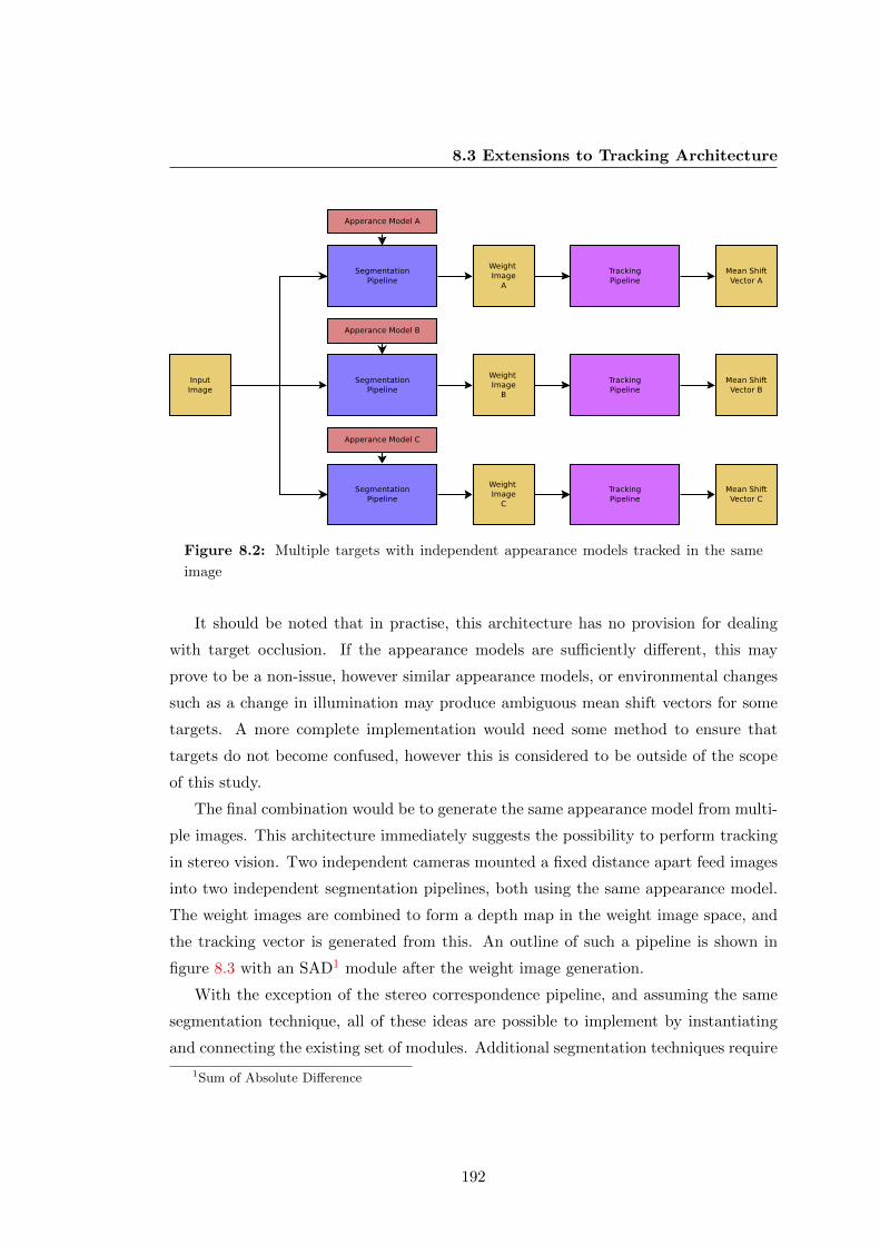
8.3 Extensions to Tracking Architecture
Figure 8.2: Multiple targets with independent appearance models tracked in the same
image
It should be noted that in practise, this architecture has no provision for dealing
with target occlusion. If the appearance models are sufficiently different, this may
prove to be a non-issue, however similar appearance models, or environmental changes
such as a change in illumination may produce ambiguous mean shift vectors for some
targets. A more complete implementation would need some method to ensure that
targets do not become confused, however this is considered to be outside of the scope
of this study.
The final combination would be to generate the same appearance model from multi-
ple images. This architecture immediately suggests the possibility to perform tracking
in stereo vision. Two independent cameras mounted a fixed distance apart feed images
into two independent segmentation pipelines, both using the same appearance model.
The weight images are combined to form a depth map in the weight image space, and
the tracking vector is generated from this. An outline of such a pipeline is shown in
figure 8.3 with an SAD1 module after the weight image generation.
With the exception of the stereo correspondence pipeline, and assuming the same
segmentation technique, all of these ideas are possible to implement by instantiating
and connecting the existing set of modules. Additional segmentation techniques require
1Sum of Absolute Difference
192
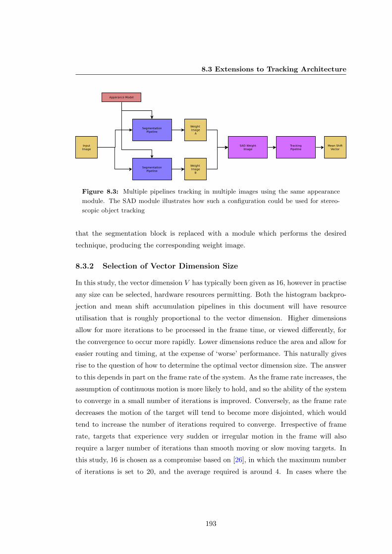
8.3 Extensions to Tracking Architecture
Figure 8.3: Multiple pipelines tracking in multiple images using the same appearance
module. The SAD module illustrates how such a configuration could be used for stereo-
scopic object tracking
that the segmentation block is replaced with a module which performs the desired
technique, producing the corresponding weight image.
8.3.2 Selection of Vector Dimension Size
In this study, the vector dimension V has typically been given as 16, however in practise
any size can be selected, hardware resources permitting. Both the histogram backpro-
jection and mean shift accumulation pipelines in this document will have resource
utilisation that is roughly proportional to the vector dimension. Higher dimensions
allow for more iterations to be processed in the frame time, or viewed differently, for
the convergence to occur more rapidly. Lower dimensions reduce the area and allow for
easier routing and timing, at the expense of ‘worse’ performance. This naturally gives
rise to the question of how to determine the optimal vector dimension size. The answer
to this depends in part on the frame rate of the system. As the frame rate increases, the
assumption of continuous motion is more likely to hold, and so the ability of the system
to converge in a small number of iterations is improved. Conversely, as the frame rate
decreases the motion of the target will tend to become more disjointed, which would
tend to increase the number of iterations required to converge. Irrespective of frame
rate, targets that experience very sudden or irregular motion in the frame will also
require a larger number of iterations than smooth moving or slow moving targets. In
this study, 16 is chosen as a compromise based on [26], in which the maximum number
of iterations is set to 20, and the average required is around 4. In cases where the
193
8.4 Remarks on Segmentation Performance
motion of the target is expected to be smooth, the vector dimension could be reduced
to around 8, but this would leave the pipeline with little ability to deal with an unex-
pected change in motion. In short, the decision is likely to be based on the designers
intuition about the implementation domain, rather than a mathematical formula.
8.4 Remarks on Segmentation Performance
As can be seen in tables 7.2, 7.3, and 7.4 the actual tracking performance is wholly
dependant on the weight image forming a ‘good’ representation.
Architecturally, it is argued that the vectored inner loop and LUT vector recovery
represent sound design choices that can deliver tangible speed gain to mean shift object
tracking in an FPGA or ASIC based context. Direct improvements to tracking perfor-
mance can be achieved through the use of more sophisticated segmentation techniques.
Because of the claim in [27], any technique which is capable of producing a weight image
at its output is suitable as a candidate in a mean shift based object tracker. Obviously,
there are implementation limitations where an on-chip system is desired. For example,
making extensive use of databases to perform pattern recognition is prohibitive due
to memory limitations. On-chip implementations of more sophisticated segmentation
systems will lead to improved tracking performance in this framework. Examples of
such system in the existing literature include [27], [42], [129], [128], [131], [28], and
many more besides.
8.5 Thesis Outcomes
The major contributions of the thesis can be summarised in the following four points.
1. Weight Image Generation Stage
A method to generate a weight-image from an appearance model, which is output
as a vector of points.
2. A Weight Image Compression Scheme
This can range from a simple 1-bit per pixel representation (section 4.5), to the
scaling buffer (section 4.6), a proposed method to reduce the size of the weight
image for use in the tracking pipeline.
194
8.5 Thesis Outcomes
3. Vector Recovery
A method to recover the pixel position information from the weight image data
buffered in the compression scheme. In this study, a LUT-based architecture is
developed so that pixel location does not need to be explicitly stored in the buffer.
4. Vectorised Inner Loop Operation
A vectorised inner loop computation which allows the image moments to be com-
puted at high speed without the need for a second clock domain. This allows the
tracking loop to be performed while a subsequent image in the sequence is being
accumulated into the mean shift buffer.
Point 4 must be understood in context, The double buffering system employed in
the segmentation pipeline is sufficient for use in systems where some kind of blanking
interval is provided which will allow the buffer to ‘catch-up’ after the processing latency.
In systems where the stream is continuous, it may be required to implement a third
buffer to hide the processing latency in the segmentation stage.
As well as this, the results given in section 7.1.6 show that the tracking performance
is strongly dependent on the quality of the weight image. In this study, quality has been
sacrificed in favour of implementation simplicity throughout the segmentation pipeline.
This can be seen in tables 7.2, 7.3, and 7.4 where the parameters and approximations
used can have a dramatic effect on the tracking performance1.
Points 2 and 1 are illustrated in figure 4.12. The weight image is streamed into
a buffer in some compressed representation. In the simplest implementation, this is
simply giving each pixel a single bit of precision. More complex implementations may
include the Scaling Buffer, which is discussed in section 4.6.
Point 1 can be argued to be a minor contribution, as the segmentation pipeline in
this study (see sections 5.2.3 and 5.2.5) lacks generality (see section 8.4). More sophis-
ticated segmentation systems are an obvious area for future research (see chapter 9)
1As well as this, the initial conditions and the quality of the appearance model have a significant
effect on the tracking performance, and both of these factors are affected by approximation errors that
can arise from pipeline simplifications
195

Chapter 9
Future Work
At the end of this study, there are three major areas of focus for extension and future
work.
1. Improved Segmentation
Many of the issues with tracking can be remedied through improved segmenta-
tion techniques. For example, in [42] a mean shift tracker based on Edge Oriented
Histogram for Pedestrian Tracking is discussed. This technique incorporates edge
features in a way that the standard CAMSHIFT algorithm does not. It should
be noted that while incorporating more features can generally be thought of as
being correlated with increased tracking performance, there are also constraints
that arise from the implementation domain. As an example, in [27], a plurality
of feature spaces are generated, and ranked according to their ability to discrim-
inate target and background. Mean shift vectors of the top 5 feature spaces are
aggregated to find the best tracking vector. While this technique does demon-
strate success at following objects, even through significant visual distraction, it
has the drawback of requiring memory to store images generated in every fea-
ture space. Clearly, in a device like an FPGA where memory is limited, storing
large numbers of images, even with some kind of compression mechanism, can
easily consume expensive resources. Because the main limitation of the track-
ing performance is the simplicity of the appearance model (consisting of a single
feature subject to many approximation errors), a separate study concerned with
implementing a more sophisticated segmentation scheme in hardware will almost
certainly improve the results in this study.
196

2. Implementation of Scaling Buffer
The scaling buffer (see section 4.6) can provide additional memory savings that
allow the system to be implemented in a smaller area. This can help to offset
any memory complexity that results from an improved segmentation technique,
thus increasing the feasibility of such techniques from a memory consumption
perspective.
3. On-chip Implementation
In this study, a working physical implementation of the CSoC architecture was not
completed. While the design is routed to achieve 100MHz operation, achieving
this speed in practise depends on various external electrical factors, such as short
length electrical contacts between the FPGA and CMOS device.
197
References
[1] Youngrock Yoon, G.N. DeSouza, and A.C. Kak. Real-time tracking
and pose estimation for industrial objects using geometric features.
In Robotics and Automation, 2003. Proceedings. ICRA ’03. IEEE International
Conference on, 3, pages 3473–3478 vol.3, Sept 2003. ii, 6
[2] L. Armesto and J. Tornero. Automation of industrial vehicles: A
vision-based line tracking application. In Emerging Technologies Factory
Automation, 2009. ETFA 2009. IEEE Conference on, pages 1–7, Sept 2009. ii, 6
[3] James Patten, Hiroshi Ishii, Jim Hines, and Gian Pangaro. Sensetable:
A Wireless Object Tracking Platform for Tangible User Interfaces. In
Proceedings of the SIGCHI Conference on Human Factors in Computing Systems,
CHI ’01, pages 253–260, New York, NY, USA, 2001. ACM. ii, 6
[4] Alex Olwal and Andrew D. Wilson. SurfaceFusion: Unobtrusive
Tracking of Everyday Objects in Tangible User Interfaces. pages 235–
242, May 2008. ii, 6
[5] Markus Vincze, Michael Zillich, Wolfgang Ponweiser, Vaclav
Hlavac, Jiri Matas, Stepan Obdrzalek, Hilary Buxton, Jonathan
Howell, Kingsley Sage, Antonis Argyros, et al. Integrated vision
system for the semantic interpretation of activities where a person
handles objects. Computer Vision and Image Understanding, 113(6):682–692,
2009. ii, 6
[6] Donghwa Lee, Gonyop Kim, Donghoon Kim, Hyun Myung, and Hyun-
Taek Choi. Vision-based object detection and tracking for autonomous
198

REFERENCES
navigation of underwater robots. Ocean Engineering, 48(0):59 – 68, 2012.
ii, 6
[7] Andreas Ess, Konrad Schindler, Bastian Leibe, and Luc Van Gool.
Object Detection and Tracking for Autonomous Navigation in Dy-
namic Environments. Int. J. Rob. Res., 29(14):1707–1725, December 2010. ii,
6
[8] J. Almeida, A. Almeida, and R. Araujo. Tracking multiple moving ob-
jects for mobile robotics navigation. In Emerging Technologies and Factory
Automation, 2005. ETFA 2005. 10th IEEE Conference on, 1, pages 8 pp.–210,
Sept 2005. ii, 6
[9] Dan Schonfeld, Caifeng Shan, Dacheng Tao, and Liang Wang, editors.
Video Search and Mining, 287 of Studies in Computational Intelligence. Springer,
2010. ii, 6
[10] Xiang Ma, Xu Chen, Ashfaq A. Khokhar, and Dan Schonfeld. Motion
Trajectory-Based Video Retrieval, Classification, and Summarization.
In Video Search and Mining, Studies in Computational Intelligence, pages 53–82.
2010. ii, 6
[11] Lan Dong, Imad Zoghlami, and Stuart Schwartz. Object Tracking in
Compressed Video with Confidence Measures. 2012 IEEE International
Conference on Multimedia and Expo, 0:753–756, 2006. ii, 6
[12] K. Mehmood, M. Mrak, J. Calic, and A. Kondoz. Object tracking
in surveillance videos using compressed domain features from scalable
bit-streams. Signal Processing: Image Communication, 24(10):814 – 824, 2009.
ii, 6
[13] K. Susheel Kumar, S. Prasad, P.K. Saroj, and R.C. Tripathi. Multiple
Cameras Using Real Time Object Tracking for Surveillance and Secu-
rity System. In Emerging Trends in Engineering and Technology (ICETET),
2010 3rd International Conference on, pages 213–218, Nov 2010. ii, 6
199

REFERENCES
[14] Bilge Gunsel, A. Mufit Ferman, and A. Murat Tekalp. Temporal
video segmentation using unsupervised clustering and semantic object
tracking. Journal of Electronic Imaging, 7(3):592–604, 1998. ii, 6
[15] Wen-Nung Lie and Wei-Chuan Hsiao. Content-based video retrieval
based on object motion trajectory. In Multimedia Signal Processing, 2002
IEEE Workshop on, pages 237–240, Dec 2002. ii, 1, 6, 7
[16] Xin Sun, Hongxun Yao, Zhongqian Sun, and Bineng Zhong. A De-
termined Binary Level Set Method Based on Mean Shift for Contour
Tracking. In Proceedings of the 11th Pacific Rim Conference on Advances in
Multimedia Information Processing: Part I, PCM’10, pages 425–436, Berlin, Hei-
delberg, 2010. Springer-Verlag. ii, 1
[17] Chuang Gu and Ming-Chieh Lee. Semantic video object tracking using
region-based classification. In Image Processing, 1998. ICIP 98. Proceedings.
1998 International Conference on, pages 643–647 vol.3, Oct 1998. ii, 6
[18] Danny Roobaert, Michael Zillich, and J-O Eklundh. A pure learning
approach to background-invariant object recognition using pedagogical
support vector learning. In Computer Vision and Pattern Recognition, 2001.
CVPR 2001. Proceedings of the 2001 IEEE Computer Society Conference on, 2,
pages II–351. IEEE, 2001. ii, 6
[19] Michael Stark, Philipp Lies, Michael Zillich, Jeremy Wyatt, and
Bernt Schiele. Functional object class detection based on learned
affordance cues. In Computer Vision Systems, pages 435–444. Springer Berlin
Heidelberg, 2008. ii, 6
[20] Y. Watanabe, T. Komuro, and M. Ishikawa. 955fps Real-Time Shape
Measurement of a Moving/Deforming Object Using High Speed Vision
for Numerous-Point Analysis. In Proc. of IEEE International Conference on
Robotics and Automation, Roma, Italy, 2007. ii, 22
[21] I. Ishii, T. Tatebe, Q. Gu, and T. Takaki. 2000fps Real-Time Target
Tracking Vision System Based on Color Histogram. pages 787103–787103–
8, 2011. ii, viii, 9, 20, 21, 22, 23, 24, 33
200
REFERENCES
[22] I. Ishii, T. Tatebe, Qingyi Gu, Y. Moriue, T. Takaki, and K. Tajima.
2000 fps real-time vision system with high-frame-rate video recording.
In Robotics and Automation (ICRA), 2010 IEEE International Conference on,
pages 1536–1541, May 2010. ii, 22
[23] Qingyi Gu, A. Al Noman, T. Aoyama, T. Takaki, and I. Ishii. A fast
color tracking system with automatic exposure control. In Information
and Automation (ICIA), 2013 IEEE International Conference on, pages 1302–
1307, Aug 2013. ii, 22
[24] Gary R. Bradski. Real Time Face and Object Tracking as a Component
of a Perceptual User Interface. In Fourth IEEE Workshop on Applications
of Computer Vision WACV’98, Princeton, NJ, 1998. ii, viii, 2, 6, 9, 11, 12, 13,
15, 20, 21, 22, 25, 42, 46, 47, 51, 52, 54, 55, 57, 59, 64, 67, 88, 90, 120, 127, 134,
142, 148, 186, 189, 213
[25] A. Yilmaz, O. Javed, and M. Shah. Object Tracking: A survey. ACM
Computing Surveys, 38, 2006. viii, 4, 6, 7, 8, 34, 44
[26] D. Comaniciu, V. Ramesh, and P. Meer. Kenel-Based Object Tracking.
In IEEE Transactions on Pattern Analysis and Machine Intelligence, 25, May
2003. viii, 2, 5, 9, 13, 14, 17, 18, 19, 28, 30, 47, 48, 49, 51, 55, 56, 57, 58, 67, 75,
127, 184, 186, 189, 193
[27] R.T. Collins, Yanxi Liu, and M. Leordeanu. Online selection of dis-
criminative tracking features. Pattern Analysis and Machine Intelligence,
IEEE Transactions on, 27(10):1631–1643, Oct 2005. viii, 9, 13, 14, 15, 16, 17,
18, 19, 25, 32, 59, 186, 189, 194, 196
[28] Han Wang and Hanseok Ko. Real-time multi-cue mean-shift hand
tracking algorithm in cluttered background. In Image and Signal Pro-
cessing (CISP), 2011 4th International Congress on, 3, pages 1310–1314, Oct
2011. viii, 14, 19, 20, 32, 186, 194
[29] Yan Xu, Meilian Sun, Zuoliang Cao, Jianpeng Liang, and Tao Li.
Multi-object tracking for mobile navigation in outdoor with embedded
201

REFERENCES
tracker. In Natural Computation (ICNC), 2011 Seventh International Confer-
ence on, 3, pages 1739–1743, July 2011. viii, 23, 24
[30] Xiaofeng Lu, Diqi Ren, and Songyu Yu. FPGA-based real-time ob-
ject tracking for mobile robot. In Audio Language and Image Processing
(ICALIP), 2010 International Conference on, pages 1657–1662, Nov 2010. viii,
24, 25, 26
[31] E. Norouznezhad, A. Bigdeli, A. Postula, and B. C. Lovell. Ro-
bust Object Tracking Using Local Oriented Energy Features and its
Hardware/Software Implementation. In Control Automation Robotics Vi-
sion (ICARCV), 2010, 11th International Conference on, pages 2060–2066, Dec
2010. viii, 27, 28, 33
[32] I. Bravo, M. Mazo, J. L. Lazaro, A. Gardel, P. Jimenez, and
D. Pizarro. An Intelligent Architecture Based on Field-Programmable
Gate Arrays Designed to Detect Moving Objects by Using Principal
Component Analysis. Sensors, 10:1424–8220, Oct 2010. viii, 29, 30
[33] Micron Technology Ltd. Micron Technology 1.3 Megapixel CMOS Active-Pixel
Digital Image Sensor MT9M413, 2004. viii, 29, 31, 39
[34] Rahul V. Shah, Amit Jain, Rutul B. Bhatt, Pinal Engineer, and
Ekata Mehul. Mean-Shift Algorithm: Verilog HDL Approach. In-
ternational Journal of Advanced Research In Computer and Communication En-
gineering, 1, April 2012. viii, 24, 30, 32, 33
[35] Bruce Wile, John C. Goss, and Wolfgang Roesner. Comprehensive
Functional Verification. The Complete Industry Cycle. Morgan Kaufmann, 500
Sansome Street, Suite 400, San Francisco, CA 94111, 2005. ix, 34, 35, 213
[36] L. Reva, V. Kulanov, and V. Kharchenko. Design Fault Injection
Based Tool for FPGA Projects Verification. In Design Test Symposium
(EWDTS), 2011 9th East-West, pages 191–195, September 2011. ix, 36, 37, 213
[37] A. Benso, A. Bosio, S. Di Carlo, and R. Mariani. A Functional Veri-
fication based Fault Injection Environment. In Defect and Fault-Tolerance
202

REFERENCES
in VLSI Systems, 2007. DFT ’07. 22nd IEEE International Symposium on, pages
114–122, Sept 2007. ix, 37, 38
[38] Spigget. CIE chart with sRGB gamut. http://en.wikipedia.org/wiki/
File:Cie_Chart_with_sRGB_gamut_by_spigget.png, 2007. Accessed: 2013-11-
06. ix, 41
[39] Micheal Horvath. RGB Cube. http://en.wikipedia.org/wiki/File:
RGB_Cube_Show_lowgamma_cutout_a.png, 2010. Accessed: 2013-11-08. ix, 42
[40] A. Shahbahrami, J. Y. Hur, B. Juurlink, and S. Wong. FPGA Imple-
mentation of Parallel Histogram Computation. In 2nd HiPEAC Workshop
on Reconfigurable Computing, pages 63–72, Gothenburg, Sweeden, 2008. ix, 65,
66, 67
[41] Hideaki Anno. The End of Evangelion, July 1997. xi, 144, 149, 165
[42] Daniel Schugk, Anto Kummert, and Christian Nunn. Adaption of the
Mean Shift Tracking Algorithm to Monochrome Vision Systems for
Pedestrian Tracking Based on HoG Features. SAE Technical Paper, 2014.
1, 194, 196
[43] Qingyi Gu, T. Takaki, and I. Ishii. Fast FPGA-Based Multiobject
Feature Extraction. Circuits and Systems for Video Technology, IEEE Trans-
actions on, 23(1):30–45, Jan 2013. 1, 27
[44] Qingyi Gu, Takeshi Takaki, and Idaku Ishii. A Fast Multi-Object Ex-
traction Algorithm Based on Cell-Based Connected Components La-
beling. IEICE Transactions, 95-D(2):636–645, 2012. 1, 27
[45] Thi-Lan Le, Monique Thonnat, Alain Boucher, and Francois
Bremond. Appearance Based Retrieval for Tracked Objects in Surveil-
lance Videos. In Proceedings of the ACM International Conference on Image
and Video Retrieval, CIVR ’09, pages 40:1–40:8, New York, NY, USA, 2009.
ACM. 1, 6
203
REFERENCES
[46] John Morris. Computer Architecture: The Anatomy of Modern Pro-
cessors. https://www.cs.auckland.ac.nz/ jmor159/363/html/systolic.html, 1998.
1
[47] M. J. Swain and D. H. Ballard. Color Indexing. International Journal of
Computer Vision, 1991. 2, 11, 15, 25, 26, 47, 52, 63, 64, 67, 69, 88, 90, 142, 148,
186, 189
[48] Dr. Gary Rost Bradski and Adrian Kaehler. Learning Opencv, 1st Edi-
tion. O’Reilly Media, Inc., first edition, 2008. 2, 9, 11, 67, 142, 165, 189, 190
[49] Kevin Cannons. A review of visual tracking. Technical report, Techni-
cal Report CSE-2008-07, York University, Department of Computer Science and
Engineering, 2008. 4, 5, 6, 7, 14, 18, 20, 32, 33, 34, 44
[50] Xi Li, Weiming Hu, Chunhua Shen, Zhongfei Zhang, Anthony Dick,
and Anton van den Hengel. A Survey of Appearance Models in Visual
Object Tracking. ACM Transactions on Intelligent Systems and Technology,
2013. 4, 6, 34, 44
[51] S. J. Julier and J. K. Uhlmann. New extension of the Kalman filter
to nonlinear systems. In I. Kadar, editor, Signal Processing, Sensor Fusion,
and Target Recognition VI, 3068 of Society of Photo-Optical Instrumentation
Engineers (SPIE) Conference Series, pages 182–193, July 1997. 5
[52] I. Cohen and G. Medioni. Detecting and tracking moving objects for
video surveillance. In Computer Vision and Pattern Recognition, 1999. IEEE
Computer Society Conference on., 2, pages –325 Vol. 2, 1999. 6
[53] Michael Zillich, Dietmar Legenstein, Minu Ayromlou, and Markus
Vincze. Robust object tracking for robot manipulation and naviga-
tion. INTERNATIONAL ARCHIVES OF PHOTOGRAMMETRY AND RE-
MOTE SENSING, 33(B5/2; PART 5):951–958, 2000. 6
[54] Christopher Bulla, Christian Feldman, Magnus Schafer, Florian
Heese, Thomas Schlien, and Martin Schink. High Quality Video Con-
ferencing: Region of Interest Encoding and Joint Video/Audio Anal-
ysis. 6, pages 153–163, 2013. 6
204

REFERENCES
[55] P. Fieguth and D. Terzopoulos. Color-based tracking of heads and
other mobile objects at video frame rates. In Computer Vision and Pattern
Recognition, 1997. Proceedings., 1997 IEEE Computer Society Conference on,
pages 21–27, Jun 1997. 6, 7, 10
[56] Christopher Wren, Ali Azarbayejani, Trevor Darrell, and Alex
Pentland. Pfinder: Real-Time Tracking of the Human Body. IEEE
Transactions on Pattern Analysis and Machine Intelligence, 19:780–785, 1997. 6
[57] J. Canny. A computational approach to edge detection. In IEEE Trans-
actions in Pattern Analysis and Machine Intelligence, 6, pages 679–698, 1986.
7
[58] Hui Zhang, Jason E. Fritts, and Sally A. Goldman. Image Segmen-
tation: A Survey of Unsupervised Methods. Computer Vision and Image
Understanding, 110(2):260–280, 2008. 7
[59] T. Sikora. The MPEG-4 Video Standard Verification Model. 1997. 7,
38, 44
[60] Berthold K.P. Horn and Brian G. Schunck. Determining Optical
Flow. Technical report, Cambridge, MA, USA, 1980. 7
[61] Bruce D. Lucas and Takeo Kanade. An Iterative Image Registration
Technique with an Application to Stereo Vision. In Proceedings of the 7th
International Joint Conference on Artificial Intelligence - Volume 2, IJCAI’81,
pages 674–679, San Francisco, CA, USA, 1981. Morgan Kaufmann Publishers
Inc. 7
[62] Ali Farhadi. https://courses.cs.washington.edu/courses/cse455/09wi/Lects/lect12.pdf,
2013. Lecture Slides. [link]. 7
[63] Manik Varma and Andrew Zisserman. A Statistical Approach to Tex-
ture Classification from Single Images. Int. J. Comput. Vision, 62(1-2):61–
81, April 2005. 7
205

REFERENCES
[64] D.G. Lowe. Object recognition from local scale-invariant features. In
Computer Vision, 1999. The Proceedings of the Seventh IEEE International Con-
ference on, 2, pages 1150–1157 vol.2, 1999. 7
[65] D. Comaniciu, V. Ramesh, and P. Meer. Mean Shift Analysis and
Applications. In The Proceedings of the Seventh IEEE Conference on Computer
Vision, pages 1197–1230, Kerkyra, Greece, June 1999. 9
[66] D. Comaniciu, V. Ramesh, and P. Meer. Real Time Tracking of Non-
Rigid Objects Using Mean Shift. In Proc. of IEEE Conference on Computer
Vision and Pattern Recognition, Hilton Head Island, SC, 2000. 9, 13, 14, 17, 18,
19, 48, 51, 186
[67] K. Fukunaga and L. Hostetler. The estimation of the gradient of a
density function, with applications in pattern recognition. Information
Theory, IEEE Transactions on, 21(1):32–40, 1975. 9, 48, 52, 57, 58, 59, 186
[68] K. Fukunaga. Introduction To Statistical Pattern Recognition. Academic Press,
1990. 9, 59
[69] L. Rocha, L. Velho, and P. Carvalho. Image Moments-Based Struc-
turing and Tracking of Objects. In Proceedings of the 15th Brazilian Sympo-
sium on Computer Graphics and Image Processing, Brazil, 2002. 9, 13, 134, 142,
189
[70] John G. Allen, Richard Y. D. Xu, and Jesse S. Jin. Object Tracking
Using Camshift Algorithm and Multiple Quantized Feature Spaces. In
Pan-Sydney Area Workshop on Visual Information Processing VIP2003. Aus-
tralian Computer Society, 2004. 9, 13, 142, 189
[71] R. T. Collins. Mean Shift Blob Tracking Through Scale Space. In IEEE
Computer Society Conference on Computer Vision and Pattern Recognition, 1,
pages 234–240, June 2003. 9, 13, 14, 19, 32, 42
[72] K. Sobottka and I. Pitas. Segmentation and tracking of faces in color
images. In Automatic Face and Gesture Recognition, 1996., Proceedings of the
Second International Conference on, pages 236–241, Oct 1996. 10
206

REFERENCES
[73] Martin Hunke and Alex Waibel. Face Locating and Tracking for
Human-Computer Interaction. In Proc. Twenty-Eight Asilomar Conference
on Signals, Systems & Computers, pages 1277–1281, 1994. 10
[74] R. E. Kalman. A New Approach to Linear Filtering and Prediction
Problems. Transactions of the ASME Journal of Basic Engineering, (82):35–
45, 1960. 10, 17
[75] A. R. Smith. Color Gamut Transform Pairs. SIGGRAPH Conference Pro-
ceedings, pages 12–19, 1978. 10, 41
[76] B. V. Funt and G. D. Finlayson. Color Constant Color Indexing. IEEE
Transactions on Pattern Analysis and Machine Intelligence, 17:522–529, 1995.
11, 25
[77] J. Flusser, T. Suk, and B. Zitova. Moments and Moment Invariants in
Pattern Recognition. John Wiley & Sons, October 2009. 11, 22, 54, 80, 119, 134
[78] G. Bieszczad and T. Sosnowski. Real-Time Mean-Shift Based Tracker
for Thermal Vision Systems. Proceedings of 9th International Conference on
Quantitative InfraRed Thermography, 2008. 13
[79] Benjamin Gorry, Zezhi Chen, Kevin Hammond, Andy Wallace, and
Greg Michaelson. Using Mean-Shift Tracking Algorithms for Real-
Time Tracking of Moving Images on an Autonomous Vehicle Testbed
Platform. 1(10):182 – 187, 2007. 13
[80] Yongwei Zheng, Huiyuan Wang, and Qianxi Guo. A novel Mean Shift
algorithm combined with Least Square approach and its application in
target tracking. In Signal Processing (ICSP), 2012 IEEE 11th International
Conference on, 2, pages 1102–1105, Oct 2012. 13, 14, 186
[81] J. Puzicha, J.M. Buhmann, Y. Rubner, and C. Tomasi. Empirical eval-
uation of dissimilarity measures for color and texture. In Computer
Vision, 1999. The Proceedings of the Seventh IEEE International Conference on,
2, pages 1165–1172 vol.2, 1999. 13
[82] Konstantinos G. Derpanis. The Bhattacharyya Measure, 2008. 13
207
REFERENCES
[83] A. Yilmaz. Object Tracking by Asymmetric Kernel Mean Shift with
Automatic Scale and Orientation Selection. In Computer Vision and Pat-
tern Recognition, 2007. CVPR ’07. IEEE Conference on, pages 1–6, June 2007.
14, 18, 19, 32, 59, 186
[84] Xiang Zhang, Yuan-Ming Dai, Zhang-Wei Chen, and Huai-Xiang
Zhang. An improved Mean Shift tracking algorithm based on color
and texture feature. In Wavelet Analysis and Pattern Recognition (ICWAPR),
2010 International Conference on, pages 38–43, July 2010. 14
[85] Wang Changjun and Zhang Li. Mean shift based orientation and loca-
tion tracking of targets. In Natural Computation (ICNC), 2010 Sixth Inter-
national Conference on, 7, pages 3593–3596, Aug 2010. 14, 20
[86] Bohyung Han, Dorin Comaniciu, Ying Zhu, and Larry S. Davis. Se-
quential Kernel Density Approximation and Its Application to Real-
Time Visual Tracking. In IEEE Transactions on Pattern Analysis and Ma-
chine Intelligence, 30, July 2008. 14
[87] Robert Collins. Video Tracking: Mean Shift. 2006. 17, 25
[88] F. Tomiyasu, T. Hirayama, and K. Mase. Wide-Range Feature Point
Tracking with Corresponding Point Search and Accurate Feature Point
Tracking with Mean-Shift. In Pattern Recognition (ACPR), 2013 2nd IAPR
Asian Conference on, pages 907–911, Nov 2013. 17, 32, 33, 186
[89] Photron Limited. FASTCAM MH4-10K, November 2006. 20, 23, 39
[90] Arnaud Doucet, Nando De Freitas, and Neil Gordon, editors. Sequential
Monte Carlo methods in practice. Springer Verlag, 2001. 23
[91] K. Yamaoka, T. Morimoto, H. Adachi, T. Koide, and H.-J. Mattausch.
Image segmentation and pattern matching based FPGA/ASIC imple-
mentation architecture of real-time object tracking. In Design Automa-
tion, 2006. Asia and South Pacific Conference on, pages 6 pp.–, Jan 2006. 24
208

REFERENCES
[92] Qingrui Zhou, Kui Yuan, Hui Wang, and Huosheng Hu. FPGA-based
colour image classification for mobile robot navigation. In Industrial
Technology, 2005. ICIT 2005. IEEE International Conference on, pages 921–925,
Dec 2005. 26
[93] Ehsan Nourouznezhad, Abbas Bigdeli, Adam Postula, and Brian C.
Lovell. Object Tracking on FPGA-based Smart Cameras Using Local
Oriented Energy and Phase Features. International Conference on Dis-
tributed Smart Cameras, 2010. 27, 28, 33
[94] Robert Collins. More on Mean-Shift. CSE598G Spring 2006, 2006. 28, 47,
51, 55, 58, 64, 186
[95] J. Schlessman, Cheng-Yao Chen, W. Wolf, B. Ozer, K. Fujino, and
K. Itoh. Hardware/Software Co-Design of an FPGA-based Embedded
Tracking System. In Computer Vision and Pattern Recognition Workshop,
2006. CVPRW ’06. Conference on, pages 123–123, June 2006. 28
[96] U. Ali, M.B. Malik, and K. Munawar. FPGA/soft-processor based
real-time object tracking system. In Programmable Logic, 2009. SPL. 5th
Southern Conference on, pages 33–37, April 2009. 28
[97] RahulV. Shah, Amit Jain, RutulB. Bhatt, Pinal Engineer, and Ekata
Mehul. Mean-Shift Algorithm: Verilog HDL Approach. In Vinu V.
Das, editor, Proceedings of the Third International Conference on Trends in In-
formation, Telecommunication and Computing, 150 of Lecture Notes in Electrical
Engineering, pages 181–194. Springer New York, 2013. 30, 33
[98] Guo Liping. A Survey of Hardware Design Verification. San Jose State Univer-
sity, 2003. 34
[99] Christoph Kern and Mark R. Greenstreet. Formal Verification in
Hardware Design: A Survey. ACM Trans. Des. Autom. Electron. Syst.,
4(2):123 – 193, April 1999. 34, 37
[100] J. Bergeron. Writing Testbenches: Functional Verification of HDL models.
Kluwer Academic Publishers, 2003. 34
209

REFERENCES
[101] Janick Bergeron. Writing Testbenches Using SystemVerilog. Springer Science
and Business Media, 2006. 34
[102] G. Weissenbacher V. D’Silva, D. Kroening. A Survey of Automated
Techniques for Formal Software Verification. Computer-Aided Design of
Integrated Circuits and Systems, IEEE Transactions on, 27(7):1165–1178, July
2008. 34
[103] Ian Sommerville. Software Engineering. Addison-Wesley, Harlow, England, 9
edition, 2010. 34
[104] Mike Bartley. Lies, Damned Lies and Hardware Verification. SNUG
Europe 2008, 2008. 34, 121
[105] Laung-Tern Wang, Charles E. Stroud, and Nur A. Touba. System on
Chip Test Architectures. Morgan Kaufmann Publishers, 2008. 34
[106] G. Van der Wal, F. Brehm, M. Piacentino, J. Marakowitz, E. Gudis,
A. Sufi, and J. Montante. An FPGA-Based Verification Framework
for Real-Time Vision Systems. In Computer Vision and Pattern Recognition
Workshop, 2006. CVPRW ’06. Conference on, pages 124–124, 2006. 36
[107] George Sobral Silveria, Karina R.G. Da Silva, and Elmar U. K.
Melcher. Functional Verification of an MPEG-4 Decoder Design us-
ing a Random Constrained Movie Generator. In Proceedings of the 20th
Annual Conference on Integrated Circuits and Systems Design, pages 360–364,
New York, NY, USA, 2007. ACM. 36, 37
[108] David Brier and Raj S. Mitra. Use of C/C++ models for architecture
exploration and verification of DSPs. In Proceedings of the 43rd annual
Design Automation Conference, DAC ’06, pages 79–84, New York, NY, USA,
2006. ACM. 36, 37
[109] Alok Sanghavi. What is formal verification? EE Times-Asia, pages 1–2,
2010. 37
[110] Wilson Snyder. Verilator 3.862. Veripool, June 2014. 37
210

REFERENCES
[111] Li Tiejun, Zhnag Jianmin, and Li Sikun. An FPGA-based Random
Functional Verification Method for Cache. In Networking, Architecture,
and Storage (NAS), 2013 IEEE Eighth International Conference on, pages 277–
281, July 2013. 37
[112] C. Starr, C.A. Evers, and L. Starr. Biology: Concepts and Applications.
Brooks/Cole biology series. Thomson, Brooks/Cole, 2006. 40
[113] B. Zhan, N. D. Monekosso, P. Remagnino, S. A. Velastin, and L. Q.
Xu. Crowd Analysis : A survey. Mach. Vision Appl., 19(5-6):345–357,
September 2008. 44
[114] Emanuel Parzen. On Estimation of a Probability Density Function and
Mode. The Annals of Mathematical Statistics, 33(3):1065–1076, 09 1962. 48
[115] Terasic Corporation. Terasic TRDB-D5M Hardware Specification, June 2009. 62,
86
[116] S. A. Fahmy. Histogram-Based Probability Density Function Estima-
tion on FPGAs. In 2010 International Conference on Field-Programmable
Technology, pages 449–453, Beijing, China, December 2010. 65, 67
[117] Edgard Garcia. Implementing a Histogram for Image Processing Ap-
plications. 38:40–46, 2000. 65
[118] E. Jamro, M. Wielgosz, and K. Wiatr. FPGA Implementation of
Strongly Parallel Histogram Equalisation. In Design and Diagnostics of
Electronic Circuits and Systems, pages 1–6, Krakow, September 2007. 66, 67
[119] Jung Uk Cho, Seung Hun Jin, Xuan Dai Pham, and Dongkyun Kim
Jae Wook Jeon. FPGA-Based real-time visual tracking system using
adaptive colour histograms. pages 172–177, Dec 2007. 67
[120] Jack E. Volder. The Birth of Cordic. J. VLSI Signal Process. Syst.,
25(2):101–105, June 2000. 119
[121] X. Hu, R.G. Harber, and S.C. Bass. Expanding the range of con-
vergence of the CORDIC algorithm. Computers, IEEE Transactions on,
40(1):13–21, Jan 1991. 119
211
REFERENCES
[122] Bruce Wile, John C. Goss, and Wolfgang Roesner. Comprehensive
Functional Verification. Morgan Kaufmann Publishers, 2005. 123
[123] Cho Soo-hyun. Gangnam Style, July 2012. 149
[124] Charlie Brooker. White Bear (Black Mirror), February 2013. 149
[125] Armando Iannucci. In The Loop, January 2009. 149
[126] Clifford E. Cummings. Coding and Scripting Techniques for FSM De-
signs with Synthesis-Optimized, Glitch-Free Outputs. Technical report,
Sunburst Design Inc., 2000. 171, 177
[127] Altera Corporation. Advanced Synthesis Cookbook, July 2011. 180, 213
[128] Lei Qin, Hichem Snoussi, and Fahed Abdallah. Object Tracking Using
Adaptive Covariance Descriptor Clustering-Based Model Updating for
Visual Surveillance. Sensors, pages 9380–9407, May 2014. 186, 194
[129] Xuyang Wang and Yan Zhang. A Hybrid Tracking Algorithm Based
on Adaptive Fusion of Multiple Cues. Journal of Information and Compu-
tational Science, 10:2445–2452, 2013. 186, 194
[130] Yaming Wang, Jianxin Zhang, Lang Wu, and Zhiyu Zhou. Mean Shift
Tracking Algorithm Based on Multi-Feature Space and Grey Model.
Journal of Computational Information Systems, 6:3731–3739, 2010. 186
[131] Irene Y. H. Gu, Vasile Gui, and Zhifei Xu. Video Segmentation Using
Joint Space-Time-Range Adaptive Mean Shift. Springer-Verlag, 2006. 194
212
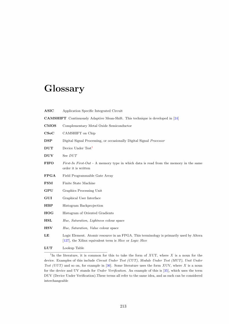
Glossary
ASIC Application Specific Integrated Circuit
CAMSHIFT Continuously Adaptive Mean-Shift. This technique is developed in [24]
CMOS Complementary Metal Oxide Semiconductor
CSoC CAMSHIFT on Chip
DSP Digital Signal Processing, or occasionally Digital Signal Processor
DUT Device Under Test1
DUV See DUT
FIFO First-In First-Out - A memory type in which data is read from the memory in the same
order it is written
FPGA Field Programmable Gate Array
FSM Finite State Machine
GPU Graphics Processing Unit
GUI Graphical User Interface
HBP Histogram Backprojection
HOG Histogram of Oriented Gradients
HSL Hue, Saturation, Lightness colour space
HSV Hue, Saturation, Value colour space
LE Logic Element. Atomic resource in an FPGA. This terminology is primarily used by Altera
[127], the Xilinx equivalent term is Slice or Logic Slice
LUT Lookup Table
1In the literature, it is common for this to take the form of X UT, where X is a noun for the
device. Examples of this include Circuit Under Test (CUT), Module Under Test (MUT), Unit Under
Test (UUT) and so on, for example in [36]. Some literature uses the form X UV, where X is a noun
for the device and UV stands for Under Verification. An example of this is [35], which uses the term
DUV (Device Under Verification).These terms all refer to the same idea, and as such can be considered
interchangeable
213

GLOSSARY
MAC Multiply-Accumulate
RAM Random-Access Memory
RTL Register Transfer Level
SAD Sum of Absolute Differences
214