Fourth International Workshop on Data Management on New Hardware

(DaMoN 2008)

June 13, 2008

Vancouver, Canada

In conjunction with ACM SIGMOD/PODS Conference

Qiong Luo and Kenneth A. Ross (Editors)

Industrial Sponsors

FOREWARD

Objective The aim of this one-day workshop is to bring together researchers who are interested in optimizing database performance on modern computing infrastructure by designing new data management techniques and tools.

Topics of Interest The continued evolution of computing hardware and infrastructure imposes new challenges and bottlenecks to program performance. As a result, traditional database architectures that focus solely on I/O optimization increasingly fail to utilize hardware resources efficiently. CPUs with superscalar out-of-order execution, simultaneous multi-threading, multi-level memory hierarchies, and future storage hardware (such as flash drives) impose a great challenge to optimizing database performance. Consequently, exploiting the characteristics of modern hardware has become an important topic of database systems research.

The goal is to make database systems adapt automatically to the sophisticated hardware characteristics, thus maximizing performance transparently to applications. To achieve this goal, the data management community needs interdisciplinary collaboration with computer architecture, compiler and operating systems researchers. This involves rethinking traditional data structures, query processing algorithms, and database software architectures to adapt to the advances in the underlying hardware infrastructure.

Workshop Co-Chairs Qiong Luo (Hong Kong University of Science and Technology, luo@cse.ust.hk) Kenneth A. Ross (Columbia University, kar@cs.columbia.edu)

Program Committee Anastasia Ailamaki (Carnegie Mellon University) Bishwaranjan Bhattacharjee (IBM Research) Peter Boncz (CWI Amsterdam) Shimin Chen (Intel Research) Goetz Graefe (HP Labs) Stavros Harizopoulos (HP Labs) Martin Kersten (CWI Amsterdam) Bongki Moon (University of Arizona) Jun Rao (IBM Research) Jingren Zhou (Microsoft Research)

i

TABLE OF CONTENTS

Session 1: Query Processing on Novel Storage CAM Conscious Integrated Answering of Frequent Elements and Top-k Queries over Data Streams ................................................................................................................................................... 1 Sudipto Das (University of California, Santa Barbara) Divyakant Agrawal (University of California, Santa Barbara) Amr El Abbadi (University of California, Santa Barbara) Modeling the Performance of Algorithms on Flash Memory Devices ......................................11 Kenneth A. Ross (IBM T. J. Watson Research Center and Columbia University) Fast Scans and Joins using Flash Drives .............................................................................................17 Mehul A. Shah (HP Labs) Stavros Harizopoulos (HP Labs) Janet L. Wiener (HP Labs) Goetz Graefe (HP Labs) Session 2: Parallelism and Contention Data Partitioning on Chip Multiprocessors ........................................................................................25 John Cieslewicz (Columbia University) Kenneth A. Ross (Columbia University) Critical Sections: Re-emerging Scalability Concerns for Database Storage Engines ...........35 Ryan Johnson (Carnegie Mellon University) Ippokratis Pandis (Carnegie Mellon University) Anastasia Ailamaki (Ecole Polytechnique Federale de Lausanne) Session 3: Page Layout Avoiding Version Redundancy for High Performance Reads in Temporal DataBases ......41 Khaled Jouini (Universite Paris Dauphine) Geneviève Jomier (Universite Paris Dauphine) DSM vs. NSM: CPU Performance Tradeoffs in Block-Oriented Query Processing ............47 Marcin Zukowski (CWI Amsterdam) Niels Nes (CWI Amsterdam) Peter Boncz (CWI Amsterdam)

ii

CAM Conscious Integrated Answering of FrequentElements and Top-k Queries over Data Streams∗

Sudipto Das Divyakant Agrawal Amr El AbbadiDepartment of Computer Science

University of California, Santa BarbaraSanta Barbara, CA 93106, USA

{sudipto, agrawal, amr}@cs.ucsb.edu

ABSTRACTFrequent elements and top-k queries constitute an im-portant class of queries for data stream analysis appli-cations. Certain applications require answers for bothfrequent elements and top-k queries on the same stream.In addition, the ever increasing data rates call for pro-viding fast answers to the queries, and researchers havebeen looking towards exploiting specialized hardware forthis purpose. Content Addressable Memory(CAM) pro-vides an efficient way of looking up elements and henceare well suited for the class of algorithms that involvelookups. In this paper, we present a fast and efficientCAM conscious integrated solution for answering bothfrequent elements and top-k queries on the same stream.We call our scheme CAM conscious Space Saving withStream Summary (CSSwSS), and it can efficiently an-swer continuous queries. We provide an implementa-tion of the proposed scheme using commodity CAMchips, and the experimental evaluation demonstratesthat not only does the proposed scheme outperformsexisting CAM conscious techniques by an order of mag-nitude at query loads of about 10%, but the proposedscheme can also efficiently answer continuous queries.

Categories and Subject DescriptorsH.4 [Information Systems Applications]: Miscella-neous.

General TermsStream Algorithms, Design, Performance.

KeywordsData Streams, Frequent elements queries, Top-k queries,

∗This work is partly supported by NSF Grants IIS-0744539 and CNS-0423336

Permission to make digital or hard copies of all or part of this work forpersonal or classroom use is granted without fee provided that copies arenot made or distributed for profit or commercial advantage and that copiesbear this notice and the full citation on the first page. To copy otherwise, torepublish, to post on servers or to redistribute to lists, requires prior specificpermission and/or a fee.Proceedings of the Fourth International Workshop on Data Management onNew Hardware (DaMoN 2008), June 13, 2008, Vancouver CanadaCopyright 2008 ACM 978-1-60558-184-2 ...$5.00.

Content Addressable Memory, Network Processor.

1. INTRODUCTIONData stream applications, such as click stream anal-

ysis for fraud detection and network traffic monitoring,have gained in popularity over the last few years. Com-mon queries posed by the users include frequent ele-ments [16, 4, 7, 19, 17], top-k queries [6, 18, 17], quantilesummarization [11], heavy distinct hitters [22] and manymore. The frequent elements query looks for elementswhose frequency is above a certain threshold. For ex-ample, a network administrator interested in finding theIP addresses that are contributing to more than 0.1% ofthe network traffic will issue a frequent elements query.On the other hand, the 100 most popular search termsin a stream of queries constitute a top-k query. Quan-tile queries are used for stream summarization such aspercentiles and medians, whereas a heavy distinct hitterquery is used for detecting malicious activities such asspreading of worms in the network.

The frequent elements and top-k queries are used bydifferent analysis applications such as network and webtraffic monitoring, click stream analysis, financial mon-itoring and so on. Besides applications where the usersare either interested in frequent elements or top-k el-ements, there are certain applications where the useris interested in both frequent elements and top-k ele-ments on the same stream of tuples. As an example, ifwe consider the case of a search engine, in order to opti-mize the performance of the engine, the designer mightdecide to cache the answers to the 1000 most popularqueries. This requires a top-k query on the stream ofquery terms. On the other hand, for auctioning thesearch keywords, the designer will be interested in thequeries which are above a certain threshold, and accord-ingly assign bidding price to these keywords. In thiscase a frequent elements query is used for some supportthreshold of 0.5%.

Even though frequent elements and top-k queries seemto be very similar, there is a fundamental difference. Infrequent elements computation, there is a notion of theminimum possible frequency of an element but no order-ing information is necessary, whereas in answering top-kqueries, the exact frequencies of the elements might notbe of interest as long as an ordering of the elements isknown. As a result, answering frequent elements cannotbe used as a pre-processing step for top-k queries, and

1

vice versa. A specialized solution is therefore sought forthe applications that need frequent elements and top-k queries on the same stream of elements. Metwallyet. al. [17] suggest an efficient integrated solution, knownas Space Saving, for answering both frequent elementsand top-k queries. The authors propose a counter basedtechnique for frequency counting, and a data structureto order the elements by their frequencies so that top-kqueries can be easily answered.

Besides the need for having an integrated solution forfrequent elements and top-k queries, the ever increasingdata stream rates call for fast and efficient processing.In addition, new hardware paradigms have opened upnew frontiers for efficient data management solutionsleveraging specialized hardware features [5, 10, 8, 12,3, 25, 23, 2]. A Content Addressable Memory (CAM)can also be exploited for accelerating stream processing.An interesting property of CAM is that in addition tonormal read and write operations, it supports constanttime lookup operation in hardware. A CAM obviatesthe need for complex data structures, such as Hashta-bles or search trees, to process efficient lookups. Hence,a CAM can be efficiently used by algorithms that per-form frequent lookups or searches. Bandi et al. [1] pro-pose a CAM conscious adaptation for the Space Savingalgorithm and demonstrate acceleration compared to asoftware implementation. A disadvantage of the pro-posed adaptation is that the elements are not sortedby their frequencies. As a result, the algorithm cannotanswer top-k queries efficiently. Additionally, since theelements are not sorted, adapting the approach in [1]for continuous queries, or even moderately high queryloads, is not straightforward. In this paper, we pro-pose a CAM conscious version of the Space Saving algo-rithm that also maintains the ordering of the elementsand hence can answer both frequent elements and top-kqueries on the same stream. Our scheme, CAM con-scious Space Saving with Stream Summary (CSSwSS),can efficiently answer continuous queries. The majorcontributions of this paper are summarized as follows:

• This is the first approach of using CAM for provid-ing an “integrated” solution to frequent elementsand top-k queries.

• We propose a CAM based data structure to countoccurrences of the elements and efficiently main-tain the sorted order of the elements in terms oftheir frequency. We explore the possible designalternatives and analyze their advantages and dis-advantages.

• We provide an implementation of the proposed al-gorithm using a commodity CAM chip, and reportthe performance of this algorithm on an experi-mental prototype using synthetic data sets.

The rest of the paper is organized as follows: Sec-tion 2 summarizes the work that has been carried infrequent elements and top-k computation, and in us-ing specialized hardware for data management opera-tions, Section 3 explains the hardware prototype usedfor our implementation, Section 4 explains in detail our

proposed algorithm, Section 5 provides a thorough ex-perimental evaluation and analysis of the results andSection 6 concludes the paper.

2. RELATED WORKFrequent elements and top-k queries are among the

most common queries in data stream processing appli-cations, and a large number of approaches have beensuggested to answer these queries. The algorithms foranswering frequent elements queries are broadly dividedinto two categories: sketch based and counter based. Thesketch based techniques such as the one proposed byCharikar et al. [4] try to represent the entire stream’sinformation as a “sketch” which is updated as the ele-ments are processed. Since the “sketch” does not storeper element information, the error bounds of these tech-niques are not very stringent. In addition, these tech-niques generally process each stream element using aseries of hash functions, and hence the processing costper element is also high. These approaches are thereforenot suitable for providing fast answers to queries.

On the other hand, the counter based techniques suchas [17] monitor a subset of the stream elements andmaintain an approximate frequency count of the ele-ments. Different approaches use different heuristics todetermine the set of elements to be monitored. Forexample, Manku et al. [16] propose a technique calledLossy Counting in which the stream is divided into rounds,and at the end of every round, potentially non-frequentelements are deleted. This ε-approximate algorithm hasa space bound of O( 1

εlog(εN)), where N is the length

of the stream. Panigrahy et al. [19] suggest a samplingbased counting technique which monitors a subset of el-ements and manipulates the counters based on whethera sampled element is already being monitored or not.For a bursty stream this approach has a space bound ofO(F2

t), where F2 is the 2nd frequency moment and t is

the minimum frequency to be reported. Most of thesecounter based algorithms [16, 17, 19] are a generaliza-tion of the classic Majority algorithm [9], and the goalis to minimize the space as well as reduce the error inapproximation.

Different solutions have also been suggested for an-swering top-k queries. Mouratidis et al. [18] suggestthe use of geometrical properties to determine the k-skyband and use this abstraction to answer top-k queries,whereas Das et al. [6] propose a technique which is ca-pable of answering ad-hoc top-k queries, i.e., the algo-rithm does not need apriori knowledge of the attributeon which the top-k queries have to be answered.

With the growing data rates and faster processingspeed requirements, researchers are also striving for ac-celerating these queries. Bandi et al. [1] suggested theuse of Content Addressable Memories (CAM) for ac-celerating the frequent elements queries. The authorsleverage the constant time lookups of CAM to acceler-ate a couple of counter based techniques. As pointed outearlier, this approach cannot efficiently answer continu-ous top-k and frequent elements queries. Bandi et al. [2]also proposed the use of CAM for Database operations.Other approaches for data management on new hard-

2

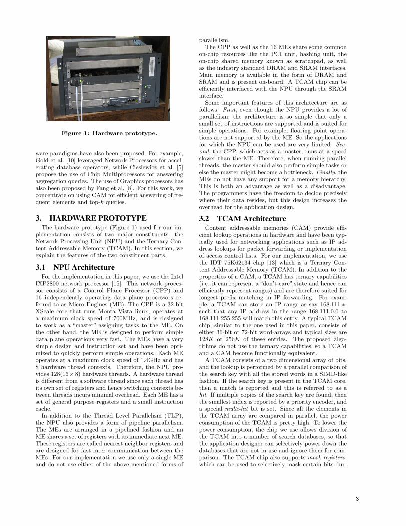
Figure 1: Hardware prototype.

ware paradigms have also been proposed. For example,Gold et al. [10] leveraged Network Processors for accel-erating database operators, while Cieslewicz et al. [5]propose the use of Chip Multiprocessors for answeringaggregation queries. The use of Graphics processors hasalso been proposed by Fang et al. [8]. For this work, weconcentrate on using CAM for efficient answering of fre-quent elements and top-k queries.

3. HARDWARE PROTOTYPEThe hardware prototype (Figure 1) used for our im-

plementation consists of two major constituents: theNetwork Processing Unit (NPU) and the Ternary Con-tent Addressable Memory (TCAM). In this section, weexplain the features of the two constituent parts.

3.1 NPU ArchitectureFor the implementation in this paper, we use the Intel

IXP2800 network processor [15]. This network proces-sor consists of a Control Plane Processor (CPP) and16 independently operating data plane processors re-ferred to as Micro Engines (ME). The CPP is a 32-bitXScale core that runs Monta Vista linux, operates ata maximum clock speed of 700MHz, and is designedto work as a “master” assigning tasks to the ME. Onthe other hand, the ME is designed to perform simpledata plane operations very fast. The MEs have a verysimple design and instruction set and have been opti-mized to quickly perform simple operations. Each MEoperates at a maximum clock speed of 1.4GHz and has8 hardware thread contexts. Therefore, the NPU pro-vides 128(16×8) hardware threads. A hardware threadis different from a software thread since each thread hasits own set of registers and hence switching contexts be-tween threads incurs minimal overhead. Each ME has aset of general purpose registers and a small instructioncache.

In addition to the Thread Level Parallelism (TLP),the NPU also provides a form of pipeline parallelism.The MEs are arranged in a pipelined fashion and anME shares a set of registers with its immediate next ME.These registers are called nearest neighbor registers andare designed for fast inter-communication between theMEs. For our implementation we use only a single MEand do not use either of the above mentioned forms of

parallelism.The CPP as well as the 16 MEs share some common

on-chip resources like the PCI unit, hashing unit, theon-chip shared memory known as scratchpad, as wellas the industry standard DRAM and SRAM interfaces.Main memory is available in the form of DRAM andSRAM and is present on-board. A TCAM chip can beefficiently interfaced with the NPU through the SRAMinterface.

Some important features of this architecture are asfollows: First, even though the NPU provides a lot ofparallelism, the architecture is so simple that only asmall set of instructions are supported and is suited forsimple operations. For example, floating point opera-tions are not supported by the ME. So the applicationsfor which the NPU can be used are very limited. Sec-ond, the CPP, which acts as a master, runs at a speedslower than the ME. Therefore, when running parallelthreads, the master should also perform simple tasks orelse the master might become a bottleneck. Finally, theMEs do not have any support for a memory hierarchy.This is both an advantage as well as a disadvantage.The programmers have the freedom to decide preciselywhere their data resides, but this design increases theoverhead for the application design.

3.2 TCAM ArchitectureContent addressable memories (CAM) provide effi-

cient lookup operations in hardware and have been typ-ically used for networking applications such as IP ad-dress lookups for packet forwarding or implementationof access control lists. For our implementation, we usethe IDT 75K62134 chip [13] which is a Ternary Con-tent Addressable Memory (TCAM). In addition to theproperties of a CAM, a TCAM has ternary capabilities(i.e. it can represent a “don’t-care” state and hence canefficiently represent ranges) and are therefore suited forlongest prefix matching in IP forwarding. For exam-ple, a TCAM can store an IP range as say 168.111.∗,such that any IP address in the range 168.111.0.0 to168.111.255.255 will match this entry. A typical TCAMchip, similar to the one used in this paper, consists ofeither 36-bit or 72-bit word-arrays and typical sizes are128K or 256K of these entries. The proposed algo-rithms do not use the ternary capabilities, so a TCAMand a CAM become functionally equivalent.

A TCAM consists of a two dimensional array of bits,and the lookup is performed by a parallel comparison ofthe search key with all the stored words in a SIMD-likefashion. If the search key is present in the TCAM core,then a match is reported and this is referred to as ahit. If multiple copies of the search key are found, thenthe smallest index is reported by a priority encoder, anda special multi-hit bit is set. Since all the elements inthe TCAM array are compared in parallel, the powerconsumption of the TCAM is pretty high. To lower thepower consumption, the chip we use allows division ofthe TCAM into a number of search databases, so thatthe application designer can selectively power down thedatabases that are not in use and ignore them for com-parison. The TCAM chip also supports mask registers,which can be used to selectively mask certain bits dur-

3

e1, ǫ1

f1 = 1

e3, ǫ3

(a) After the ele-ments 〈e1, e3〉.

e1, ǫ1 e3, ǫ3

f2 = 2f1 = 1

(b) Element 〈e3〉.

e1, ǫ1 e2, ǫ2 e3, ǫ3

f2 = 2f1 = 1

(c) Element 〈e2〉.

f1 = 1 f2 = 2

e1, ǫ1 e2, ǫ2 e3, ǫ3

(d) End of the stream.

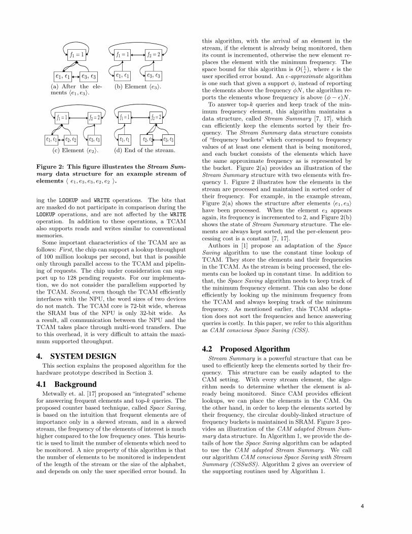
Figure 2: This figure illustrates the Stream Sum-mary data structure for an example stream ofelements 〈 e1, e3, e3, e2, e2 〉.

ing the LOOKUP and WRITE operations. The bits thatare masked do not participate in comparison during theLOOKUP operations, and are not affected by the WRITE

operation. In addition to these operations, a TCAMalso supports reads and writes similar to conventionalmemories.

Some important characteristics of the TCAM are asfollows: First, the chip can support a lookup throughputof 100 million lookups per second, but that is possibleonly through parallel access to the TCAM and pipelin-ing of requests. The chip under consideration can sup-port up to 128 pending requests. For our implementa-tion, we do not consider the parallelism supported bythe TCAM. Second, even though the TCAM efficientlyinterfaces with the NPU, the word sizes of two devicesdo not match. The TCAM core is 72-bit wide, whereasthe SRAM bus of the NPU is only 32-bit wide. Asa result, all communication between the NPU and theTCAM takes place through multi-word transfers. Dueto this overhead, it is very difficult to attain the maxi-mum supported throughput.

4. SYSTEM DESIGNThis section explains the proposed algorithm for the

hardware prototype described in Section 3.

4.1 BackgroundMetwally et. al. [17] proposed an “integrated” scheme

for answering frequent elements and top-k queries. Theproposed counter based technique, called Space Saving,is based on the intuition that frequent elements are ofimportance only in a skewed stream, and in a skewedstream, the frequency of the elements of interest is muchhigher compared to the low frequency ones. This heuris-tic is used to limit the number of elements which need tobe monitored. A nice property of this algorithm is thatthe number of elements to be monitored is independentof the length of the stream or the size of the alphabet,and depends on only the user specified error bound. In

this algorithm, with the arrival of an element in thestream, if the element is already being monitored, thenits count is incremented, otherwise the new element re-places the element with the minimum frequency. Thespace bound for this algorithm is O( 1

ε), where ε is the

user specified error bound. An ε-approximate algorithmis one such that given a support φ, instead of reportingthe elements above the frequency φN , the algorithm re-ports the elements whose frequency is above (φ− ε)N .

To answer top-k queries and keep track of the min-imum frequency element, this algorithm maintains adata structure, called Stream Summary [7, 17], whichcan efficiently keep the elements sorted by their fre-quency. The Stream Summary data structure consistsof “frequency buckets” which correspond to frequencyvalues of at least one element that is being monitored,and each bucket consists of the elements which havethe same approximate frequency as is represented bythe bucket. Figure 2(a) provides an illustration of theStream Summary structure with two elements with fre-quency 1. Figure 2 illustrates how the elements in thestream are processed and maintained in sorted order oftheir frequency. For example, in the example stream,Figure 2(a) shows the structure after elements 〈e1, e3〉have been processed. When the element e3 appearsagain, its frequency is incremented to 2, and Figure 2(b)shows the state of Stream Summary structure. The ele-ments are always kept sorted, and the per-element pro-cessing cost is a constant [7, 17].

Authors in [1] propose an adaptation of the SpaceSaving algorithm to use the constant time lookup ofTCAM. They store the elements and their frequenciesin the TCAM. As the stream is being processed, the ele-ments can be looked up in constant time. In addition tothat, the Space Saving algorithm needs to keep track ofthe minimum frequency element. This can also be doneefficiently by looking up the minimum frequency fromthe TCAM and always keeping track of the minimumfrequency. As mentioned earlier, this TCAM adapta-tion does not sort the frequencies and hence answeringqueries is costly. In this paper, we refer to this algorithmas CAM conscious Space Saving (CSS).

4.2 Proposed AlgorithmStream Summary is a powerful structure that can be

used to efficiently keep the elements sorted by their fre-quency. This structure can be easily adapted to theCAM setting. With every stream element, the algo-rithm needs to determine whether the element is al-ready being monitored. Since CAM provides efficientlookups, we can place the elements in the CAM. Onthe other hand, in order to keep the elements sorted bytheir frequency, the circular doubly-linked structure offrequency buckets is maintained in SRAM. Figure 3 pro-vides an illustration of the CAM adapted Stream Sum-mary data structure. In Algorithm 1, we provide the de-tails of how the Space Saving algorithm can be adaptedto use the CAM adapted Stream Summary. We callour algorithm CAM conscious Space Saving with StreamSummary (CSSwSS). Algorithm 2 gives an overview ofthe supporting routines used by Algorithm 1.

4

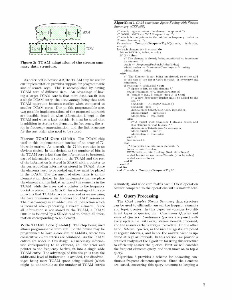
e1, ǫ1 e2, ǫ2 e3, ǫ3

f2 = 2f1 = 1 SRAM

TCAM

Figure 3: TCAM adaptation of the stream sum-mary data structure.

As described in Section 3.2, the TCAM chip we use forour implementation provides support for programmablesize of search keys. This is accomplished by havingTCAM core of different sizes. An advantage of hav-ing a larger TCAM core is that more data can fit intoa single TCAM entry; the disadvantage being that eachTCAM operation becomes costlier when compared tosmaller TCAM cores. Due to this programmable size,two possible implementations of the proposed approachare possible, based on what information is kept in theTCAM and what is kept outside. It must be noted thatin addition to storing the elements, its frequency, the er-ror in frequency approximation, and the link structurefor the sort order also need to be stored.

Narrow TCAM Core (72-bit): The TCAM chipused in this implementation consists of an array of 72-bit wide entries. As a result, the 72-bit core size is anobvious choice. In this design, as the number of bits inthe TCAM core is less than the information to be stored,part of information is stored in the TCAM and the restof the information is stored in SRAM with a pointer tothe corresponding information stored in TCAM. Sincethe elements need to be looked up, they must be placedin the TCAM. The placement of other items is an im-plementation choice. In this implementation, we placethe element and the link structure of the elements in theTCAM, while the error and a pointer to the frequencybucket is placed in the SRAM. An advantage of this ap-proach is that TCAM space is preserved as we are usingthe bare minimum when it comes to TCAM resources.The disadvantage is an added level of indirection whichis incurred when processing a stream element. Sinceall information is not stored in the TCAM, a TCAMLOOKUP is followed by a SRAM read to obtain all infor-mation corresponding to an element.

Wide TCAM Core (144-bit): The chip being usedallows programmable word size. So the device may beprogrammed to have a core size of 144-bits, where twoconsecutive 72-bit entries are combined. As the TCAMentries are wider in this design, all necessary informa-tion corresponding to an element, i.e. the error andpointer to the frequency bucket, fit into a single wideTCAM entry. The advantage of this design is that theadditional level of indirection is avoided, the disadvan-tages being more TCAM space being utilized (whichmight be undesirable as the number of TCAM entries

Algorithm 1 CAM conscious Space Saving with StreamSummary (CSSwSS)

/* mask1 register masks the element component *//* LOOKUP, WRITE are TCAM operations. *//* min fr is the pointer to the minimum frequency bucket inStream Summary. */Procedure ComputeFrequentTopK(stream, table size,min fr)for each element 〈e〉 in stream do

hit ← LOOKUP(e, index, mask1)if (hit) then

/* The element is already being monitored, so incrementits counter. */cur fr ← FrequencyBucketAtIndex(index)added bucket ← IncrementCounter(cur fr, index)added elem ← index

else/* The Element is not being monitored, so either addto the end of the list if there is space, or overwrite theminimum. */if (cur size < table size) then

/* Space is left, so add element */WRITE(free index, e, 0, 〈link structure〉)if (min fr = NULL || min fr→freq > 1) then

/* A new Frequency Bucket must be added to thelist. */new node ← AllocateNewNode()new node→freq ← 1AddElementToList(new node, free index)added bucket ← new nodeadded elem ← free index

else/* A bucket with frequency 1 already exists, addthis element to that bucket. */AddElementToList(min fr, free index)added bucket ← min fradded elem ← free index

end iffree index++

else/* Overwrite the minimum element. */index ← min fr→elemWRITE(index, e, min fr→freq, 〈link structure〉)added bucket ← IncrementCounter(min fr, index)added elem ← index

end ifend if

end forend Procedure ComputeFrequentTopK

is limited), and wide core makes each TCAM operationcostlier compared to the operations with a narrow core.

4.3 Query ProcessingThe CAM adapted Stream Summary data structure

can be used to efficiently answer the frequent elementsand top-k queries. In this paper we consider two dif-ferent types of queries, viz. Continuous Queries andInterval Queries. Continuous Queries are posed withevery update, i.e. with every stream element processed,and the answer cache is always up-to-date. On the otherhand, Interval Queries, as the name suggests, are posedat regular intervals, and hence the answer cache is up-dated at regular intervals. In this section, we provide adetailed analysis of the algorithm for using this structureto efficiently answer the queries. First we will considerthe frequent elements query, and then move on to top-kquery.

Algorithm 3 provides a scheme for answering con-tinuous frequent elements queries. Since the elementsare sorted, answering this query amounts to keeping a

5

Algorithm 2 Supporting method for CSSwSS

/* READ is a TCAM operation. */

Procedure IncrementCounter(freq node, element index)/* Increments the count of the specific element. */new fr ← freq node→freq + 1next node ← freq node→nextif (freq node→count = 1 & next node→freq 6= new fr) then

/* This bucket can be promoted to become the new bucket.*/freq node→freq ← new frreturn freq node

end ifRemoveElementFromList(freq node, index)if (next node→freq = new fr) then

/* The element moves to the next node. */AddElementToList(next node, index)return next node

else/* A New Frequency Bucket need to be inserted next to thecurrent node. */new node ← AllocateNewNode()AddToNext(new node, freq node)AddElementToList(new node, index)return new node

end ifend Procedure IncrementCounter

pointer to the bucket that has the minimum frequencyabove the support φ. We can use the CAM adaptedStream Summary structure to efficiently maintain thispointer (ptrφ). The intuition behind this algorithm isthat after processing an element, a bunch of elementsmight become infrequent, while only one element canbecome frequent. These elements can be determinedfrom Theorems 4.1 and 4.3 and Corollary 4.2.

Theorem 4.1. When processing continuous frequentelements queries, if element ei ∈ bucketi becomes infre-quent then all elements ej ∈ bucketi and only elementsej become infrequent.

Proof. The proof is of the theorem consists of twoparts.

• All elements ej ∈ bucketi becomes infrequent ifei ∈ bucketi becomes infrequent. This is intuitivefrom the structure of the CAM adapted StreamSummary structure as all elements in the samefrequency bucket have the same frequency.

• Only elements ej become infrequent. Since we areanswering continuous queries, the length of thestream increases by 1 at each step. Now, sinceφ = λN , where 0 < λ < 1 and N is the length ofthe stream, and if fi is the frequency of ei, as eiwas reported as frequent in the previous step, andconsidering the fact that N increased by 1 afterthe previous step, all fk > fi must be reportedas frequent. The CAM adapted Stream Summarystructure ensures that all buckets to the right ofbucketi (refer to Figure 2 for illustration) will havefk > fi. Therefore, only the elements ej becomeinfrequent if ei become infrequent.

Algorithm 3 Answering continuous frequent elementsqueries

/* added bucket and added elem are the bucket added andelements added.*/Procedure ContinuousQueryFrequent(φ)/*ptrφ is the pointer to the bucket with minimum frequencyabove support φ*//* φ is the minimum frequency to be reported. */if (ptrφ 6= NULL) then

next node ← ptrφ→nextmin freq ← ptrφ→freqif (min freq < φ) then

/* At least one element has become infrequent. */if (next node→freq > min freq) thenptrφ ← next node

elseptrφ ← NULL

end ifend ifif (added bucket→freq ≥ φ & added bucket→freq <min freq) then

/* An infrequent element has become frequent. */ptrφ ← added bucket

end ifelse

/* No frequent element yet. */if (added bucket→freq ≥ φ) thenptrφ ← added bucket

end ifend ifend Procedure ContinuousQueryFrequent

Corollary 4.2. Only the elements with the mini-mum frequency amongst the set of reported frequent el-ements can become infrequent.

Proof. The proof follows from Theorem 4.1, sincefor each new element, only the elements from a singlefrequency bucket can become infrequent, and since thebuckets in CAM adapted Stream Summary are in sortedorder.

Theorem 4.3. When processing continuous frequentelements queries, only the element seen last can becomefrequent.

Proof. An element ei with frequency fi will be re-ported as frequent ⇐⇒ fi > φ where φ = λN and0 < λ < 1. Since the number of elements N is mono-tonically increasing, therefore φ is also monotonicallyincreasing. If el is the last element processed, then flis the only frequency that increases over the previousstep. Hence el can be the only element that might be-come frequent.

From the theorems, it is evident that updating ptrφinduces a constant cost per element being processed: re-porting an element becoming frequent is constant andreporting p elements as infrequent is O(p). This is in-dependent of the number of elements in the stream orthe number of elements monitored in the CAM adaptedStream Summary structure. This is a drastic improve-ment from the CAM conscious Space Saving (CSS) in [1],where the cost of query answering is O(n), n being thenumber of elements currently being monitored, and ev-idently, p� n in most iterations.

Since answering continuous queries is not efficient forCSS, in our experiments we compare CSS with CSSwSSusing varying query load, i.e., instead of the queries be-ing continuous, now the queries are issued at regular

6

Algorithm 4 Answering frequent elements queries atregular intervals

/* added bucket and added elem are the bucket added andelements added.*/Procedure IntervalQueryFrequent(φ)/*ptrφ is the pointer to the bucket with minimum frequencyabove support φ*//* φ is the minimum frequency to be reported. */if (ptrφ 6= NULL) then

cur fr ← ptrφelse

cur fr ← added bucketend ifnext node ← cur fr→nextprev node ← cur fr→prevfreq ← cur fr→freqif (freq ≥ φ) then

/*Check if any infrequent element has become frequent.*/while (prev node→freq < cur fr→freq & prev node→freq≥ φ) do

cur fr ← prev nodeprev node ← cur fr→prev

end whileptrφ ← cur fr

else/* Some frequent elements have become infrequent, so up-date the cache. */while (next node→freq > cur fr→freq) do

cur fr ← next nodenext node ← cur fr→next

end whileif (next node→freq < cur fr→freq) thenptrφ ← NULL

elseptrφ ← cur fr

end ifend ifend Procedure IntervalQueryFrequent

interval. Algorithm 4 gives an overview of the schemeused for answering queries at regular intervals. Sincethe queries are not issued after processing every sin-gle element, Theorems 4.1 and 4.3 do not hold. HenceAlgorithm 3 cannot be used for this purpose. It canbe seen that Algorithm 4 uses an idea similar to thatof Algorithm 3, except that Algorithm 4 scans throughthe structure, because the number of elements that havebeen processed since the last invocation is not known.But it can be easily proved that the time taken by Al-gorithm 4 is O(m), where m is the number of elementsprocessed since the last invocation. So, in the worst caseit might reduce to a continuous query, but as demon-strated in the experiments in a later section, the perfor-mance is much better for most practical cases.

The CAM adapted Stream Summary structure can beused to efficiently answer continuous top-k as well. Theidea is the same as with continuous frequent elementsqueries and the top-k set is selected using the layoutof the CAM adapted Stream Summary structure. Thealgorithm is very similar to the corresponding algorithmin [17] and has been adapted to efficiently leverage theCAM adapted Stream Summary. An overview of thealgorithm for continuous top-k monitoring is providedin Algorithm 5.

Again, it is straightforward to see that the per-elementcost of continuous maintenance of set of top-k elementsis pretty small and the CAM adapted Stream Summarystructure can be used to efficiently maintain the top-kset. It is therefore evident that CSSwSS can be used to

Algorithm 5 Answering continuous top-k queries

/* added bucket and added elem are the bucket added andelements added.*/Procedure ContinuousQueryTopK(k)/* Setk is the set of elements in top-k cache with minimumfrequency. *//* ptrk is the pointer to the bucket containing elements inSetk*/if (num elems topk < k) then

/* There are not enough elements in the top-k set. */if (added elem /∈ top-k set) then

Report added elem ∈ top-knum elems topk++

end ifif (num elems topk = k) then

/* k elements have now been reported, enter maintenancemode. */ptrk ← min freqSetk ← ElementsInBucket(ptrk)

end ifelse

/* Check for updates, if any. */

ptr+k ← ptrk→next

if (added bucket = ptr+k & ptr+k→freq − ptrk→freq = 1)then

if (added elem ∈ Setk) thenSetk ← Setk − added elem

elseSelect elem ∈ SetkSetk ← Setk − elemReport elem /∈ top-kReport added elem ∈ top-k

end ifif (Setk is empty) then

ptrk ← ptr+kSetk ← ElementsInBucket(ptrk)

end ifend if

end ifend Procedure ContinuousQueryTopK

efficiently answer frequent elements and top-k queries.

5. EXPERIMENTAL EVALUATIONWe implement the CAM conscious Space Saving with

Stream Summary (CSSwSS) algorithm on a commod-ity TCAM chip IDT75K62134 [13] which interfaces ef-ficiently with the IXP2800 NPU [15]. The TCAM chiphas 128K 72-bit wide entries, supports programmableword size, and up to 128 parallel request contexts. De-velopment is done using the Teja NP ADE [21] and IntelDevelopment Workbench [14]. Implementation of thealgorithms involve coding in TejaCTM andMicroCTM .Times reported are actual execution times of the algo-rithms on the MEs (Micro Engine), and are obtainedfrom the Timestamp register common to all the ME’s.The experiments have been repeated multiple times andthe values have been averaged over multiple runs.

The experiments have been performed with syntheticZipfian data which has been shown to closely resemblerealistic data sets [24]. The data set used for experi-ments consists of 1 million hits, taken from an alphabetof size 10, 000. The alphabet is the number of distinctelements in the stream. Since the performance of theSpace Saving algorithm is not dependent on the size ofthe alphabet, we expect similar results for smaller orlarger alphabet sizes. The zipfian factor is varied from0 to 3 in steps of 0.5, where zipfian factor 0 representsuniform distribution while 3 is a highly skewed distribu-

7

TCAM Operation 72-bit 144-bit

READ 0.32 0.64LOOKUP 0.2971 0.3673WRITE 0.32 0.3314

Table 1: Time (in secs) for a million TCAM op-erations for different sizes of TCAM core.

tion. The error bound ε is set to 0.001. We compare theperformance of the proposed algorithms with the CAMconscious Space Saving adaptation in [1], which we referto as CAM conscious Space Saving (CSS).

5.1 Cost of Frequency CountingIn this section, we experimentally evaluate the two

possible design alternatives. First we need to determinethe cost of the primitive operations in narrow and wideTCAM cores. The operations of interest are LOOKUP,

READ and WRITE. We evaluate this using an experimentwhere we time only the operations of interest, and Ta-ble 1 summarizes the results.

There are a few interesting observations about thestatistics in Table 1. LOOKUP is one of the most impor-tant operations, and this operation is done at least oncefor each stream element. As we increase the width ofthe TCAM core, the cost of LOOKUP increases, but theincrease in the cost of WRITE does not increase signifi-cantly. The highest increase is for the READ operationswhere the time almost doubles, as the chip used onlysupports up to 72-bit wide READ operations. As a result,a 144-bit READ comprises of two 72-bit READ operations.But this is not very alarming as the layout of elementscan be designed in a manner that would never require a144-bit READ, i.e. the algorithm will need either the firstor the second 72-bit entry but not both, so that onlythe cost of 72-bit wide READ operations is incurred.

Another interesting observation about the times inTable 1 is that the LOOKUP throughput is nowhere nearthe peak throughput of about 100 million LOOKUPs persecond as stated in Section 3.2. This is primarily be-cause we use only a single ME for implementing our al-gorithm and accessing the TCAM, and the high through-put can be obtained by parallel accesses to the TCAM.We will exploit this parallelism in future work. In ad-dition, it must be noted that we are using a single MEthat runs at a speed of only 1.4GHz.

Before evaluating the performance of the algorithmsfor answering queries, we evaluate the cost of count-ing the frequencies and keeping them sorted. Since theauthors in [1] provide an efficient frequency countingalgorithm (CSS), we compare the performance of theproposed schemes with CSS. Figure 4 provides a com-parison of time taken for frequency counting. From thefigure it can be seen that for uniform data, keeping theelements sorted is almost twice as costly as simple fre-quency counting. But as the data becomes skewed, theelements can be kept sorted almost for free. This differ-ence in performance is due to the fact that the proposedscheme involves managing the structure of frequencybuckets, which becomes costly when the sort order ofelements is changing rapidly, which is the case for the

0.5

1

1.5

2

2.5

3

3.5

4

0 0.5 1 1.5 2 2.5 3

Tim

e (i

n se

cs)

Zipfian factor

CSSwSS (72-bit)CSSwSS (144-bit)

CSS

Figure 4: Comparing the performance of CSSwith CSSwSS for 72 & 144 bit TCAM core sizes.This figure reports only the time for frequencycounting.

uniform distribution (zipfian factor close to 0). On theother hand, when the data is skewed, the sort orderdoes not change much, and the proposed scheme per-forms better as the cost of maintaining the minimum fre-quency element in CSS now becomes significant, whichis not present in CSSwSS.

Now analyzing the performance of the two alternativedesigns, it can be seen from Figure 4 that the approachusing 72-bit TCAM core performs better for moderateand heavily skewed distributions, whereas the 144-bitdesign performs better for uniform distribution. Thisis because for uniform data, the CAM adapted StreamSummary structure undergoes a lot of changes, and theoverhead due to the added level of indirection for the72-bit implementation dominates. However, for skeweddata, the increased cost of the 144-bit TCAM operationsmakes the 72-bit implementation cheaper.

Since the zipfian factor ranging between 1 and 2 repre-sents most realistic data sets, from Figure 4 we can con-clude that the implementation using 72-bit wide coreswould perform better for real data. In addition to thesavings in time, another advantage of the 72-bit imple-mentation is that it saves TCAM space which can be ascarce resource.

5.2 Cost of Answering QueriesIn this section, we analyze the cost of answering fre-

quent elements and top-k queries using the proposedalgorithm. Since the proposed algorithm keeps the ele-ments sorted, it can therefore be easily adapted to an-swer queries efficiently and incrementally. As CSS doesnot maintain the elements in sorted order, there is nostraightforward technique for the incremental reportingof frequent elements. Every time a query arrives, thebest-effort adaptation of CSS would scan through all thecounters to report the frequent elements. On the otherhand, the CAM adapted Stream Summary structure inCSSwSS can be leveraged to incrementally report thefrequent elements. Section 4.3 provides efficient algo-rithms to answer queries and also provides a thoroughanalysis of the cost incurred by these algorithms. In thissection, we evaluate these algorithms experimentally.

8

1

1.5

2

2.5

3

3.5

4

4.5

0 0.5 1 1.5 2 2.5 3

Tim

e (i

n se

cs)

Zipfian factor

CSSwSS (72-bit)CSSwSS (144-bit)

(a) Frequent elements

1

1.5

2

2.5

3

3.5

4

4.5

0 0.5 1 1.5 2 2.5 3

Tim

e (i

n se

cs)

Zipfian factor

CSSwSS (72-bit)CSSwSS (144-bit)

(b) Top-k

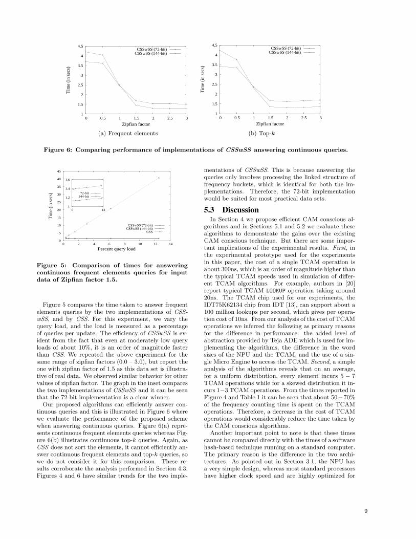
Figure 6: Comparing performance of implementations of CSSwSS answering continuous queries.

1

1.2

1.4

1.6

0 13

72-bit144-bit

0

5

10

15

20

25

30

35

40

45

0 2 4 6 8 10 12 14

Tim

e (i

n se

cs)

Percent query load

CSSwSS (72-bit)CSSwSS (144-bit)

CSS

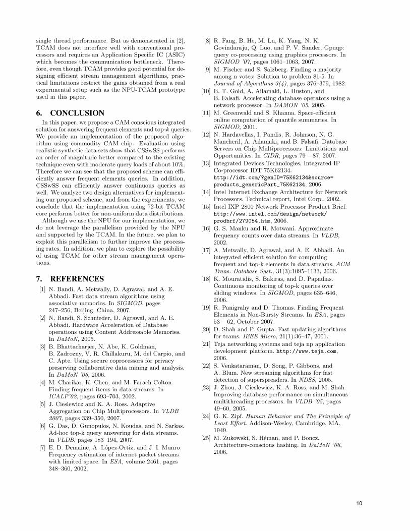
Figure 5: Comparison of times for answeringcontinuous frequent elements queries for inputdata of Zipfian factor 1.5.

Figure 5 compares the time taken to answer frequentelements queries by the two implementations of CSS-wSS, and by CSS. For this experiment, we vary thequery load, and the load is measured as a percentageof queries per update. The efficiency of CSSwSS is ev-ident from the fact that even at moderately low queryloads of about 10%, it is an order of magnitude fasterthan CSS. We repeated the above experiment for thesame range of zipfian factors (0.0 – 3.0), but report theone with zipfian factor of 1.5 as this data set is illustra-tive of real data. We observed similar behavior for othervalues of zipfian factor. The graph in the inset comparesthe two implementations of CSSwSS and it can be seenthat the 72-bit implementation is a clear winner.

Our proposed algorithms can efficiently answer con-tinuous queries and this is illustrated in Figure 6 wherewe evaluate the performance of the proposed schemewhen answering continuous queries. Figure 6(a) repre-sents continuous frequent elements queries whereas Fig-ure 6(b) illustrates continuous top-k queries. Again, asCSS does not sort the elements, it cannot efficiently an-swer continuous frequent elements and top-k queries, sowe do not consider it for this comparison. These re-sults corroborate the analysis performed in Section 4.3.Figures 4 and 6 have similar trends for the two imple-

mentations of CSSwSS. This is because answering thequeries only involves processing the linked structure offrequency buckets, which is identical for both the im-plementations. Therefore, the 72-bit implementationwould be suited for most practical data sets.

5.3 DiscussionIn Section 4 we propose efficient CAM conscious al-

gorithms and in Sections 5.1 and 5.2 we evaluate thesealgorithms to demonstrate the gains over the existingCAM conscious technique. But there are some impor-tant implications of the experimental results. First, inthe experimental prototype used for the experimentsin this paper, the cost of a single TCAM operation isabout 300ns, which is an order of magnitude higher thanthe typical TCAM speeds used in simulation of differ-ent TCAM algorithms. For example, authors in [20]report typical TCAM LOOKUP operation taking around20ns. The TCAM chip used for our experiments, theIDT75K62134 chip from IDT [13], can support about a100 million lookups per second, which gives per opera-tion cost of 10ns. From our analysis of the cost of TCAMoperations we inferred the following as primary reasonsfor the difference in performance: the added level ofabstraction provided by Teja ADE which is used for im-plementing the algorithms, the difference in the wordsizes of the NPU and the TCAM, and the use of a sin-gle Micro Engine to access the TCAM. Second, a simpleanalysis of the algorithms reveals that on an average,for a uniform distribution, every element incurs 5 − 7TCAM operations while for a skewed distribution it in-curs 1−3 TCAM operations. From the times reported inFigure 4 and Table 1 it can be seen that about 50−70%of the frequency counting time is spent on the TCAMoperations. Therefore, a decrease in the cost of TCAMoperations would considerably reduce the time taken bythe CAM conscious algorithms.

Another important point to note is that these timescannot be compared directly with the times of a softwarehash-based technique running on a standard computer.The primary reason is the difference in the two archi-tectures. As pointed out in Section 3.1, the NPU hasa very simple design, whereas most standard processorshave higher clock speed and are highly optimized for

9

single thread performance. But as demonstrated in [2],TCAM does not interface well with conventional pro-cessors and requires an Application Specific IC (ASIC)which becomes the communication bottleneck. There-fore, even though TCAM provides good potential for de-signing efficient stream management algorithms, prac-tical limitations restrict the gains obtained from a realexperimental setup such as the NPU-TCAM prototypeused in this paper.

6. CONCLUSIONIn this paper, we propose a CAM conscious integrated

solution for answering frequent elements and top-k queries.We provide an implementation of the proposed algo-rithm using commodity CAM chip. Evaluation usingrealistic synthetic data sets show that CSSwSS performsan order of magnitude better compared to the existingtechnique even with moderate query loads of about 10%.Therefore we can see that the proposed scheme can effi-ciently answer frequent elements queries. In addition,CSSwSS can efficiently answer continuous queries aswell. We analyze two design alternatives for implement-ing our proposed scheme, and from the experiments, weconclude that the implementation using 72-bit TCAMcore performs better for non-uniform data distributions.

Although we use the NPU for our implementation, wedo not leverage the parallelism provided by the NPUand supported by the TCAM. In the future, we plan toexploit this parallelism to further improve the process-ing rates. In addition, we plan to explore the possibilityof using TCAM for other stream management opera-tions.

7. REFERENCES[1] N. Bandi, A. Metwally, D. Agrawal, and A. E.

Abbadi. Fast data stream algorithms usingassociative memories. In SIGMOD, pages247–256, Beijing, China, 2007.

[2] N. Bandi, S. Schnieder, D. Agrawal, and A. E.Abbadi. Hardware Acceleration of Databaseoperations using Content Addressable Memories.In DaMoN, 2005.

[3] B. Bhattacharjee, N. Abe, K. Goldman,B. Zadrozny, V. R. Chillakuru, M. del Carpio, andC. Apte. Using secure coprocessors for privacypreserving collaborative data mining and analysis.In DaMoN ’06, 2006.

[4] M. Charikar, K. Chen, and M. Farach-Colton.Finding frequent items in data streams. InICALP’02, pages 693–703, 2002.

[5] J. Cieslewicz and K. A. Ross. AdaptiveAggregation on Chip Multiprocessors. In VLDB2007, pages 339–350, 2007.

[6] G. Das, D. Gunopulos, N. Koudas, and N. Sarkas.Ad-hoc top-k query answering for data streams.In VLDB, pages 183–194, 2007.

[7] E. D. Demaine, A. Lopez-Ortiz, and J. I. Munro.Frequency estimation of internet packet streamswith limited space. In ESA, volume 2461, pages348–360, 2002.

[8] R. Fang, B. He, M. Lu, K. Yang, N. K.Govindaraju, Q. Luo, and P. V. Sander. Gpuqp:query co-processing using graphics processors. InSIGMOD ’07, pages 1061–1063, 2007.

[9] M. Fischer and S. Salzberg. Finding a majorityamong n votes: Solution to problem 81-5. InJournal of Algorithms 3(4), pages 376–379, 1982.

[10] B. T. Gold, A. Ailamaki, L. Huston, andB. Falsafi. Accelerating database operators using anetwork processor. In DAMON ’05, 2005.

[11] M. Greenwald and S. Khanna. Space-efficientonline computation of quantile summaries. InSIGMOD, 2001.

[12] N. Hardavellas, I. Pandis, R. Johnson, N. G.Mancheril, A. Ailamaki, and B. Falsafi. DatabaseServers on Chip Multiprocessors: Limitations andOpportunities. In CIDR, pages 79 – 87, 2007.

[13] Integrated Devices Technologies, Integrated IPCo-processor IDT 75K62134.http://idt.com/?genID=75K62134&source=

products_genericPart_75K62134, 2006.

[14] Intel Internet Exchange Architecture for NetworkProcessors. Technical report, Intel Corp., 2002.

[15] Intel IXP 2800 Network Processor Product Brief.http://www.intel.com/design/network/

prodbrf/279054.htm, 2006.

[16] G. S. Manku and R. Motwani. Approximatefrequency counts over data streams. In VLDB,2002.

[17] A. Metwally, D. Agrawal, and A. E. Abbadi. Anintegrated efficient solution for computingfrequent and top-k elements in data streams. ACMTrans. Database Syst., 31(3):1095–1133, 2006.

[18] K. Mouratidis, S. Bakiras, and D. Papadias.Continuous monitoring of top-k queries oversliding windows. In SIGMOD, pages 635–646,2006.

[19] R. Panigrahy and D. Thomas. Finding FrequentElements in Non-Bursty Streams. In ESA, pages53 – 62, October 2007.

[20] D. Shah and P. Gupta. Fast updating algorithmsfor tcams. IEEE Micro, 21(1):36–47, 2001.

[21] Teja networking systems and teja np applicationdevelopment platform. http://www.teja.com,2006.

[22] S. Venkataraman, D. Song, P. Gibbons, andA. Blum. New streaming algorithms for fastdetection of superspreaders. In NDSS, 2005.

[23] J. Zhou, J. Cieslewicz, K. A. Ross, and M. Shah.Improving database performance on simultaneousmultithreading processors. In VLDB ’05, pages49–60, 2005.

[24] G. K. Zipf. Human Behavior and The Principle ofLeast Effort. Addison-Wesley, Cambridge, MA,1949.

[25] M. Zukowski, S. Heman, and P. Boncz.Architecture-conscious hashing. In DaMoN ’06,2006.

10

Modeling the Performance of Algorithms on FlashMemory Devices

Kenneth A. RossIBM T. J. Watson Research Center and Columbia University

rossak@us.ibm.com, kar@cs.columbia.edu

ABSTRACTNAND flash memory is fast becoming popular as a com-ponent of large scale storage devices. For workloads re-quiring many random I/Os, flash devices can providetwo orders of magnitude increased performance relativeto magnetic disks. Flash memory has some unusualcharacteristics. In particular, general updates requirea page write, while updates of 1 bits to 0 bits can bedone in-place. In order to measure how well algorithmsperform on such a device, we propose the “EWOM”model for analyzing algorithms on flash memory devices.We introduce flash-aware algorithms for counting, list-management, and B-trees, and analyze them using theEWOM model. This analysis shows that one can usethe incremental 1-to-0 update properties of flash mem-ory in interesting ways to reduce the required numberof page-write operations.

1. INTRODUCTIONSolid state disks and other devices based on NAND

flash memory allow many more random I/Os per second(up to two orders of magnitude more) than conventionalmagnetic disks. Thus they can, in principle, supportworkloads involving random I/Os much more effectively.

However, flash memory cannot support general in-place updates. Instead, a whole data page must be writ-ten to a new area of the device, and the old page mustbe invalidated. Groups of contiguous pages form eraseunits, and an invalidated page becomes writable againonly after the whole erase unit has been cleared. Erasetimes are relatively high (several milliseconds). Flash-based memory does, however, allow in-place changes of1-bits to 0-bits without an erase cycle [5]. Thus it is pos-sible to reserve a region of flash memory initialized toall 1s, and incrementally use it in a write-once fashion.

Traditional measures of algorithm complexity do not

Permission to make digital or hard copies of all or part of this work forpersonal or classroom use is granted without fee provided that copies arenot made or distributed for profit or commercial advantage and that copiesbear this notice and the full citation on the first page. To copy otherwise, torepublish, to post on servers or to redistribute to lists, requires prior specificpermission and/or a fee.Proceedings of the Fourth International Workshop on Data Management onNew Hardware (DaMoN 2008), June 13, 2008, Vancouver, Canada.Copyright 2008 ACM 978-1-60558-184-2 ...$5.00.

model flash I/O behavior well, because the high costof a general update (relative to a 1-to-0 update) is notaccounted for. Previous models for write-once memory(“WOM”) have been proposed to model devices like pa-per tape and optical disks in which the write process isdestructive, so that once a bit is set it cannot be un-set [10]. Maier proposes using write-once storage for a“Read-Mostly Store” (RMS) where the memory is grad-ually consumed as updates occur [8]. However, thesemodels are too restrictive for devices like flash memorywhere a bulk erase allows memory to be reused.

1.1 The EWOM ModelWe propose a new model for evaluating an algorithm

on a flash-like device. We call it the “Erasable WriteOnce Memory” model, or the “EWOM” model. In addi-tion to counting traditional algorithmic steps, we counta page-write step whenever a write causes a 0 bit tochange to a 1 bit. If an algorithm performs a group oflocal writes to a single page as one transactional step,we count the group as a single page-write step. Evenif only a few bytes are updated, a whole page must bewritten.

The true cost of a page-write step has several compo-nents. There is an immediate cost incurred because afull page must be copied to a new location, with the bitsin question updated. If there are multiple updates to asingle page from different transactional operations, theycan be combined in RAM and applied to the flash mem-ory once, although one must be careful in such a schemeto guarantee data persistence if that is an applicationrequirement.

There is also a deferred cost incurred because the flashdevice must eventually erase the erase unit containingthe old page. It is a deferred cost because the write itselfdoes not have to wait for the erase to finish; the erasecan be performed asynchronously. Nevertheless, erasetimes are high, and a device burdened by many eraseoperations may not be able to sustain good read/writeperformance. Further, in an I/O intensive workload asteady state can be reached in which erasure cannotkeep up, and writes end up waiting for erased pages tobecome available.

There is an additional longer-term cost of page erasesin terms of device longevity. On current flash devicesan erase unit has a lifetime of about 105 erases. Thus, ifspecial-purpose algorithms reduce the number of erases

11

needed by a factor of f , the expected lifetime of thedevice can in principle be multiplied by f .

Our model can distinguish between situations wherethe I/O device is saturated, and where the device islightly loaded. Algorithms might include a low-prioritybackground process that asynchronously traverses datastructure elements and reorganizes them to improve per-formance. The extra I/O workload will not be notice-able in a lightly-loaded setting, and most data structureelements will end up in the optimized state. In a sat-urated or near-saturated scenario, however, the back-ground process will rarely run, and the data structureelements will remain in the unoptimized state.

We choose not to model “seek” time for flash memory.While there is a small overhead involved in moving fromone memory location to another, this overhead is smallrelative to the erase costs. Further, this cost is orders ofmagnitude smaller than seek times for magnetic disks,whose performance models often distinguish between se-quential and random I/O.

Traditional I/O devices have a fixed block transfersize, and it is customary to count the number of blockstransferred when measuring I/O complexity. RAM al-lows fine-grained data access, and so it is customaryto simply count the number of computational steps toperform a given operation as the complexity measure.Flash memory occupies a middle-ground between tradi-tional I/O devices and RAM. Some flash devices requiretransfers to happen in block-sized units, where a singledevice may support multiple block sizes, while others al-low fine-grained access. For the purposes of the presentwork, we will adopt the convention that the flash mem-ory is a fine-grained access device for reads and 1-to-0writes, and we measure complexity by counting the to-tal number of computational steps. For general updates,we also count a page write.1

1.2 Pages and Erase UnitsErase units are typically large, around 128KB. Copy-

ing a full erase unit on every update would not be effi-cient. It is therefore common for data copying to happenin page-sized units, where the page size P depends onhow the device is configured. A typical value of P mightbe 2KB, meaning 64 pages in a 128KB erase unit.

We assume that there is a memory mapping layer thatmaps logical page addresses to physical page addresses.Such mapping is commonly implemented in hardwarewithin page-granularity devices: when an update hap-pens, the physical address changes, but the logical ad-dress remains the same so that updates do not needto be propagated to data structures that refer to thedata page. When the device itself does not providesuch a layer, it is common to implement such a layerin software. The mapping layer also ensures that wearon the device is shared among physical pages, becauseflash pages have a limited lifetime of approximately 105

erase cycles. The mapping layer can also hide faulty orworn-out pages from the operating system. The EWOMmodel assumes that a logical-to-physcial mapping layer

1If we fill a page using simple 1-to-0 writes, there areno page write operations counted.

is present.If updates are performed on pages, then at any point

in time, an erase unit may contain some valid pages andsome invalid pages that need to be erased. If an eraseunit contains valid pages, then those valid pages mustbe written to alternate locations before the erase unitcan be erased. We assume that the same hardware orsoftware that monitors the logical-to-physical mappingof pages also monitors the validity of pages for the pur-poses of managing erase units for garbage collection.

In a lightly loaded device, such extra copying mightnot be noticeable. However, in a heavily loaded system,with high demand for new erase units, this overhead willbe noticeable.

A “best-case” workload for erase-unit recycling wouldoccur when all pages in an erase unit are invalid at erasetime. This kind of workload might happen if the dataaccess pattern is highly clustered, such as when a file issequentially updated, page by page. In that case, eachpage write contributes to approximately P/E erases,where E is the size of an erase unit.

A “worst-case” workload would occur when all eraseunits available for recycling hold just one invalid page.This kind of workload might happen on a device thatis almost full, and for which the data access pattern isscattered over the various erase units. In this case, eachpage write causes an erase.

There are obviously many intermediates between thebest and worst cases, and the range is wide. Thus it isnot always possible to predict the erase frequency givenjust the page update frequency. More information aboutworkload characteristics is usually needed.

2. COUNTINGWe begin our analysis with a simple task: maintain

a counter in EWOM storage. The counter is initializedto zero, and may be incremented. A naive, in-place so-lution would rewrite the counter, stored in conventionalbinary form, on every update. Since an increment al-ways changes some 0 to a 1, every update requires apage write. Reads have cost proportional to the wordsize W of the counter in binary.2

An alternative solution represents the counter in unaryform, with the number of zero bits indicating the count.An increment operation can be handled by changing abit from 1 to 0 without a page-write operation. Unarycounters are severely limited in their counting capacitysince they have space complexity linear in the currentvalue of the counter. Reads and writes can be handledin logarithmic time using an exponential expansion fol-lowed by a binary search to find the first 0 in the bitarray.

A hybrid scheme stores a binary base counter, to-gether with a unary increment counter of fixed lengthL, where L ≤ P−W so that the counter fits in a page [2].The counter is computed by adding the base counter tothe offset of the first zero in the unary array, which canbe found using binary search. A page-write is needed

2Depending on one’s memory model, W is either con-stant or O(log n), where n is the value of the counter.

12

Method Space (bits) Read time Write time Page-WritesNaive W W 2W 1Unary n Θ(log n) Θ(log n) 1

PHybrid (lightly loaded) W + L W + 1 2 0Hybrid (saturated) W + L W +O(log L) O(log L) + 2W

L1L

Figure 1: Amortized complexity for counting

every L steps, at which time the base counter is recom-puted, and the unary counter is reset.

A low-priority asynchronous operation may look throughpages containing counters, and also perform this recom-pute/reset operation. We assume that in the lightlyloaded case, the asynchronous background updates hap-pen at least as often as writes, and promptly after thosewrites. This assumption means that the state of thecounter on the flash device will usually have a zero unaryincrement value, with the binary part of the countercontaining the current count. Reads become simpler(because they don’t have to traverse the unary incre-ment value), and writes become simpler (because thereis always space for unary increments — no page-writesare necessary).

The complexity of these alternatives is summarized inFigure 1, where n is the number of increment operations,and P is the size of a page in bits. Read time is mea-sured in terms of the number of bit operations needed.For the write step, we assume that the writer does notknow the previous value of the counter, only that thecounter needs to be incremented. As Figure 1 shows,the hybrid counting method amortizes page-writes al-most as well as the unary method, while keeping readand write performance close to the naive method.

2.1 Arbitrary IncrementsOne can generalize the hybrid method if increments

(or decrements) by arbitrary amounts are possible. Asingle base counter is maintained in binary form. Aunary counter is kept for recording increments by multi-ples of 20, 21, 22, etc. An increment is broken down intoits binary form, and the corresponding unary countersare updated. A separate set of counters is maintainedfor decrements. Read operations need to scan throughthe various counters to compute the net change to thebinary stored value.

In the event that one of the unary counters is full,it may still be possible to process an addition withouta page write by decomposing the addition into a largernumber of smaller increments. For example, if the unarycounter corresponding to 25 is full, we could add thevalue 25 by appending two bits to the unary countercorresponding to 24.

Other configurations are also possible. For example,instead of recording increments using a unary counterfor each power of 2, one could use unary counters forpowers of an arbitrary value k. The number of bits toset for each counter would be determined by the corre-sponding digit of the value to be added when written inbase-k notation.

3. LINKED LISTSA linked list is a commonly used data structure. In an

EWOM context, standard list operations would requirea page write. A page write would be needed to keeptrack of the tail of the list, to implement list elementdeletion, to insert an element into the list, and to updatenodes within the linked list.

Suppose that we interpret the all-1 bit pattern as aNULL pointer. Then one can append to the list usingonly 1-to-0 updates by updating the NULL pointer inthe last element of the list to point to a new element.The new element itself would be written in an area ofthe page initialized to all-1s. Unlike traditional appendoperations to a list, this variant would need to first tra-verse the entire list. On the other hand, a page-write isavoided.

Deletions would need to be handled in an indirectway, such as by using a “deleted” flag within the nodestructure. This would complicate list traversal slightly,because deleted nodes would remain in the list and needto have their flags checked.

Like for counting, we could implement a low-prioritybackground process that “cleans up” lists on a page andwrites a new page. In this new page, the deleted ele-ments would be omitted. One could also store a short-cut to the current tail, so that future append operationsdo not have to start from the head of the list.

4. BLOOM FILTERSSome data structures are inherently monotonic in their

update behavior, and map well to the EWOM modelwithout modification. An example is the Bloom filter[1]. If we interpret a vector of 1 bits to mean the emptyBloom filter, then every insertion can be achieved bysetting some 1 bits to 0 bits. In the EWOM model, in-sert operations do not need to perform any page-writes.

5. B-TREESWithin a database system, one of the places where

random I/O occurs frequently is in accessing B-tree in-dexes in response to OLTP workloads. Indexes are searched(to find the record to update), new records are inserted,and old records are deleted. One way to deal with B-treeupdate-heavy workloads is to batch the updates. Thatway, the costs associated with restructuring a page canbe amortized over many updates. Batching happensimplicitly when a page resides in the database system’sbuffer pool.3 Batching can also happen close to the

3Note that the database system is ensuring persistencein this case by maintaining a recovery log.

13

physical device in a RAM-based cache. However, if thelocality of reference of the database access is poor, suchas when the table and/or index is much bigger than thebuffer pool and records are being accessed randomly,there will be little effective batching in practice.

We therefore propose a new way to organize leaf nodesin a B-tree to avoid the page-write cost most of the time,while still processing updates one at a time. We focuson leaf nodes because that is where the large majorityof changes happen.

Suppose that an entry in a leaf node consists of an8-byte key, and an 8-byte RID referencing the indexedrecord. We assume a leaf node can hold L entries, taking16L bytes. We shall assume that a leaf node has sizethat exactly matches the page size of the device.

With the requirement that leaf nodes be at least halffull, a conventional B-tree leaf node will contain betweenL/2 and L entries stored in sorted key order. The or-dering property allows for keys to be searched in loga-rithmic time using binary search.

A first attempt at a page-write-friendly leaf node wouldbe to store all entries in an append-only array in the or-der of insertion [8]. A bitmap would be kept to markdeleted entries. When the node becomes full, it is split,and (nondeleted) entries are divided among the two re-sulting pages. The obvious drawback of this approachis that search time within the node will be linear ratherthan logarithmic, dramatically slowing down both searchesand updates.

5.1 The Proposed ApproachApart from the initial root node, all leaf nodes are

created as a result of a split. When a split happens,we sort the (nondeleted) records into key order, andstore them in that order in the append-only array. Wekeep track of the endpoint of this array by storing itexplicitly in the leaf node. Subsequent insertions arethen appended to the array as before.

So far, we have improved performance slightly be-cause one can do a binary search over at least half of theentries, followed by a linear search of the remaining en-tries to find a key. However, the asymptotic complexityis still linear in the size of the array.

To speed up the search of the newly-inserted elementswe store some additional information. Choose positiveinteger constants c and k. For every c entries in the newinsertions, we store a c-element index array. Each entryin this index array stores an offset into the segment ofnew insertions, and the index array is stored in key or-der. (It is not maintained incrementally; it is generatedonly when there have been c new insertions.)

To search an array of m new elements (m ≤ L), weneed at most (m/c) log2 c+ (c− 1) comparisons. Whilewe have reduced the asymptotic search time by a factorof c/ log2 c, it remains linear in m. The trick is to applythis idea recursively.

Suppose that after kc elements, instead of a c-elementoffset array, we store a kc-element offset array coveringthe previous kc newly inserted records. Now we needat most one linear search of at most c − 1 elements,at most k − 1 binary searches of c elements, and bm

kcc

binary searches of kc elements. If we keep scaling the

offset array each time m crosses c, kc, k2c, k3c etc., thenthe total cost is O(log2 m). (There are O(logm) binarysearches, each taking O(logm) time.)

A complete search therefore takesO(log(n/L)+log2 L) =O(log n+log2 L) time, where n is the number of elementsin the tree.

The space overhead of this approach is the total sizeof the index arrays. This size is equal to

bmccc+ bm

ckc(ck − c) + b m

ck2 c(ck2 − ck) + . . .

≈ m logk(m/c) = O(m logm).

The overhead for one node is thus O(L logL), and theoverhead for the entire tree is O(n logL). This is a clas-sical computer-science trade-off in which we use morespace to reduce the time overhead. Different choices forc and k represent alternative points in the space-timetrade-off.

In practice, the space overhead is unlikely to be oner-ous. For example, suppose that the page size is 16KB.8KB can be devoted to new entries and the offset ar-rays. This places an upper bound of 512 new entries. Ifc = 32 and k = 3, the largest index array we will buildwill have 288 entries. The total space in bytes to storem new entries is then

16m+32(bm/32c)+(96−32)(bm/96c)+2(288−96)(bm/288c).(Here, we’re assuming one byte offsets for up to 255elements, and two-byte offsets for 256 or more elements.)Based on these numbers, we could store 446 new entriesin the leaf node before we ran out of space. 1056 bytesout of 16K bytes (6.4%) is the space overhead, ignoringthe pointer to the start of the new elements and the bitsto record deletions.

Under lightly loaded conditions, where one has sparecycles to do background leaf optimization, one couldconvert a leaf node to sorted format and reset the point-ers to new entries, writing the resulting node to a newmemory location. For such “fresh” leaf nodes, searchtime goes down from O(log2 m) time to O(logm) time.Note that because of the logical-to-physical page map-ping, parent nodes are unchanged by leaf freshening.

5.2 AnalysisEvery c entries, an updating transaction needs to sort

c elements costing O(c log c) time. When the systemgets to a kic-byte boundary, it only needs to sort thelast c elements, then merge k ordered lists of size ki−1c,which can be done in O(c log c+ kic log k) time. Amor-tizing over all insertions, the cost per insertion has order

Pblogk(m/c)ci=1 (kic log k)(b m

ckic)/m

≈ log kblogk(m/c)c ≈ log(m/c)

Similarly, split processing can merge the array segmentsrather than fully sorting the array.

One needs to know where the array of new valuesends, in order to decide when to terminate the search,and where to append new values. The simplest way todo this is to assume that a pattern of all 1-bits is nota valid (key,RID) pair. One can then binary search tofind the last valid pair. One could try to explicitly store

14

Method Space (bits) Read time Write time Page WritesStandard O(n) O(log n) O(log n) 1Append-Only O(n) O(log n + L) O(log n) 1

LHybrid (lightly loaded) O(n logL) O(log n) O(log n) 0

Hybrid (saturated) O(n logL) O(log n + log2 L) O(log n + logL) O( logLL

)

Figure 2: Amortized B-tree complexity for a tree of size n, treating c and k as constants.

Pointer to the endpoint of initial sorted prefix.Prefix P containing sorted (key,RID) pairs. Calculated during most recent page-write.Sequence S of (key,RID) pairs in insertion order.Indexes of first group of c elements of S, in sorted order.Indexes of second group of c elements of S, in sorted order.. . .

Indexes of k − 1st group of c elements of S, in sorted order.Indexes of first group of kc elements of S, in sorted order.

Indexes of k + 1st group of c elements of S, in sorted order.. . .Deletion bitsLog Sequence Number (using generalized counter)

Figure 3: The final structure of a B-tree node of (key,RID) pairs.

the offset using the counters of Section 2, but such amethod would consume more space than necessary.

Figure 2 shows the amortized asymptotic complex-ity for the proposed B-tree structure. We assume thatwrites do not need to check whether the key alreadyexists in a node before insertion. If such a check is nec-essary, the entry for the append-only method would be-come O(log n+L) and the entry for the hybrid methodwith saturated writes would become O(log n + log2 L).Note that even in the saturated setting, the hybrid methodonly needs a page-write every O((log L)/L) insertions,while having better asymptotic read complexity thanthe append-only method.

5.3 RefinementsWe have assumed that leaf nodes contain (key,RID)

pairs. Sometimes, to save space, B-tree leaf nodes aredesigned to associate a key with a list of RIDs. Theproposed structure can be modified so that at the timeof reorganization (i.e., when a page-write occurs), theinitial segment of data is in (key,RID-list) form. Analternative would be to keep a linked list of RIDs foreach key, using the linked-list techniques described inSection 3.

In real B-tree implementations, a leaf node contains alog sequence number (LSN) recording information rele-vant for node recovery in case of failure. On an EWOMdevice, the LSN could be implemented using a gener-alized counter as described in Section 2.1. Note thatLSNs are monotonically increasing, meaning that onlyincrements, not decrements, need to be considered.

The final structure of a B-tree node is summarized inFigure 3. This figure shows a node containing (key,RID)pairs. If RID-lists were used, a region within the pagewould be used as a heap for allocating new RID nodes

to add to RID-lists.

6. RELATED WORKAn interesting technique related to counting was pro-

posed by Rivest and Shamir for the WOM model [10].They show, for example, that it is possible to overwritean arbitrary number from {0, 1, 2, 3} with another ar-bitrary number from that set (a) using only monotonicbit changes, and (b) with only 3 bits of storage. Eachpossible number has two valid 3-bit encodings, such as

0 : 000, 111; 1 : 001, 110; 2 : 010, 101; 3 : 100, 011

The first code for a number is used for the initial write.The second code is used for the subsequent write, unlessthe second write has the same value, in which case thereis no change. One could extend techniques like this tothe EWOM model by erasing when necessary, which inthis example would be after two or more updates.

Others have studied B-tree implementations for flashdevices. Wu et al. [11] describe a B-tree method thatuses a combination of RAM-resident buffers and “indexunits”representing flash-resident incremental changes toa B-tree node. The logical view of a B-tree node is re-constructed using the node together with these indexunits. The work of Wu et al. assumes a page-level in-terface to the flash device, without fine-grained access.

Nath et al., also study B-tree indexes on flash devices,with the aim of minimizing power and maximizing per-formance on a low-power mobile device [9]. Their sys-tem optimizes B-tree parameters in a self-tuning fash-ion, based on the workload and device characteristics.They also employ a page-level interface to the flashmemory.

OLTP workloads frequently need to perform small up-dates in place. Lee and Moon show how to restructure

15

database pages and modify the logging protocol to min-imize the required number of page erases [7]. Multipleversions of a data element are kept on a page in a write-once log-like structure within the page, and reads mustconsult the log to look for changes. Data is written tothe flash storage in sector-sized units (512 bytes in [7]).

7. CURRENT DEVICESThe two basic types of flash memory available to-

day are NOR-flash and NAND-flash. These technolo-gies have contrasting behaviors that make them suit-able for different classes of application [4]. For example,NAND-flash tends to have larger capacity, faster writesand erases, and page-level data access. NOR-flash tendsto have faster reads, and fine-grained random access todata. Hybrid NAND/NOR devices exist (e.g., [6]).

The types of flash memory interaction allowed by adevice vary. Some devices implement only a page-levelAPI such as FTL [5], and updates to pages always causea new page to be written. Such a choice allows an SSDdevice to resemble a magnetic disk device, and be usedin existing systems that employ disk devices. Other de-vices (together with a software layer) expose flash as a“Memory Technology Device” (MTD) via UBI [3], whichallows partial updates to pages. Low level flash inter-faces have been defined by the ONFI working group4.In this paper, we assume an interface in which partialwrites to a page are allowed, as long as they only involvetrasitions from a 1 bit to a 0 bit.

Not every flash device may provide an interface thatallows fine-granularity in-place 1-to-0 updates. As men-tioned above, flash-based solid-state disks currently pro-vide disk-like APIs, with pages or sectors as the unit ofdata transfer. Nevertheless, future devices may providefiner-grained APIs if there is a potential performanceimprovement. The results of this paper are a step inthis direction, showing what is possible with such anAPI.

Some flash devices store error-correcting codes in re-served portions of the flash memory. Incremental changesto pages would also require incremental changes to theerror-correcting codes. Even if the data changes aremonotonic 1-to-0 writes, the resulting error-correctingcode changes are unlikely to be monotonic. It maythus be necessary to reserve space for an array of error-correcting code values, and to write a new element intothe array after each write.

While our EWOM model is motivated by flash mem-ory, it is also possible that other technologies such asPRAM memory may, in the future, have similar blockerase characteristics.

8. CONCLUSIONSWe have described a new model for measuring the

performance of algorithms on write-once devices withan erase capability. We have adapted several standardalgorithms to take account of the high page-write cost ofarbitrary updates, and have analyzed their performance.

4www.onfi.org

The results of this paper are unlikely to represent thefinal word on how to implement even the few techniqueswe have addressed. For example, it may be possibleto trade space for time (or write performance for readperformance) in different ways to get new algorithmicvariants.

AcknowledgementsThanks to Bishwaranjan Bhattacharjee, Christian Lang,Bruce Lindsay, Tim Malkemus, George Mihaila, HaixunWang, and Mark Wegman for helpful discussions andsuggestions.

9. REFERENCES[1] Burton H. Bloom. Space/time trade-offs in hash

coding with allowable errors. Commun. ACM,13(7):422–426, 1970.

[2] Paul England and Marcus Peinado. System andmethod for implementing a counter, 2006. USPatent Number 7,065,607.

[3] T. Gleixner, F. Haverkamp, and A. Bityutskiy.UBI - Unsorted Block Images, 2006.

[4] Toshiba Inc. NAND vs. NOR flash memory, 2006.Downloaded May 2008 fromhttp://www.toshiba.com/taec/components/Generic/Memory Resources/NANDvsNOR.pdf.

[5] Intel Corp. Understanding the Flash TranslationLayer (FTL) Specification, 1998.

[6] T. H. Kuo et al. Design of 90nm 1Gb ORNANDflash memory with MirrorBit technology. InSymposium on VLSI Circuits, Digest of TechnicalPapers, pages 114–115, 2006.

[7] Sang-Won Lee and Bongki Moon. Design offlash-based DBMS: an in-page logging approach.In SIGMOD ’07: Proceedings of the 2007 ACMSIGMOD international conference onManagement of data, pages 55–66, New York, NY,USA, 2007. ACM.

[8] David Maier. Using write-once memory fordatabase storage. In PODS ’82: Proceedings of the1st ACM SIGACT-SIGMOD symposium onPrinciples of database systems, pages 239–246,New York, NY, USA, 1982. ACM.

[9] Suman Nath and Aman Kansal. Flashdb: dynamicself-tuning database for nand flash. In IPSN ’07:Proceedings of the 6th international conference onInformation processing in sensor networks, pages410–419, New York, NY, USA, 2007. ACM.

[10] Ronald L. Rivest and Adi Shamir. How to reuse awrite-once memory (preliminary version). InSTOC ’82: Proceedings of the fourteenth annualACM symposium on Theory of computing, pages105–113, New York, NY, USA, 1982. ACM.

[11] Chin-Hsien Wu, Tei-Wei Kuo, and Li Ping Chang.An efficient B-tree layer implementation forflash-memory storage systems. Trans. onEmbedded Computing Sys., 6(3):19, 2007.

16

Fast Scans and Joins using Flash Drives

Mehul A. Shah Stavros Harizopoulos Janet L. Wiener Goetz Graefe

HP Labs{firstname.lastname}@hp.com

ABSTRACTAs access times to main memory and disks continue to di-verge, faster non-volatile storage technologies become moreattractive for speeding up data analysis applications. NANDflash is one such promising substitute for disks. Flash offersfaster random reads than disk, consumes less power thandisk, and is cheaper than DRAM. In this paper, we investi-gate alternative data layouts and join algorithms suited forsystems that use flash drives as the non-volatile store.

All of our techniques take advantage of the fast randomreads of flash. We convert traditional sequential I/O algo-rithms to ones that use a mixture of sequential and randomI/O to process less data in less time. Our measurements oncommodity flash drives show that a column-major layout ofdata pages is faster than a traditional row-based layout forsimple scans. We present a new join algorithm, RARE-join,designed for a column-based page layout on flash and com-pare it to a traditional hash join algorithm. Our analysisshows that RARE-join is superior in many practical cases:when join selectivities are small and only a few columns areprojected in the join result.

1. INTRODUCTIONWith the ever increasing disparity between main memory

and disk access times, enterprise applications are hungeringfor a faster non-volatile store. In this paper, we explore howto leverage one such promising technology, flash drives, fordata analysis applications.

Driven by the consumer electronics industry, flash is be-coming a practical non-volatile storage technology. Flashdrives are ubiquitous in cameras, cell-phones, and PDAs.Major PC vendors are shipping laptops with flash drives.Moreover, flash is starting to make its way into the enterprisemarket. For example, vendors such as SimpleTech, Mtron,and FusionIO are selling flash-based solid-state drives aimedat replacing SCSI drives and entire disk arrays. But, areflash drives an effective replacement for traditional disks?

Flash drives have several traits that make them attrac-

Permission to make digital or hard copies of all or part of this work forpersonal or classroom use is granted without fee provided that copies arenot made or distributed for profit or commercial advantage and that copiesbear this notice and the full citation on the first page. To copy otherwise, torepublish, to post on servers or to redistribute to lists, requires prior specificpermission and/or a fee.Proceedings of the Fourth International Workshop on Data Management onNew Hardware (DaMoN 2008), June 13, 2008, Vancouver, Canada.Copyright 2008 ACM 978-1-60558-184-2 ...$5.00.

tive for read-mostly enterprise applications such as web-pageserving and search. Table 1 compares flash drives to disks.Flash drives offer more random read I/Os per second (1500to 100,000 IO/s), offer comparable sequential bandwidth(20-80 MB/s), and use a tenth of the power (0.5 W). Flash ischeaper than DRAM (∼$18/GB) and is non-volatile. More-over, flash continues to get faster, cheaper, and denser at arapid pace. In particular, NAND flash density has doubledevery year since 1999 [13].

Unfortunately, flash offers little or no benefit when used asa simple drop-in replacement for disk for data analysis work-loads in databases. Traditional query processing algorithmsfor data analysis are tuned for disks; they stress sequen-tial I/O and avoid random I/O whenever possible. Thus,they fail to take advantage of the fast random reads of flashdrives.

In this paper, we investigate query processing methodsthat are better suited for the characteristics of flash drives.In particular, we focus on speeding up scan (projection) andjoin operations over tables stored on flash. Our algorithmsuse a mixture of random reads and sequential I/O. Whenonly a fraction of the input (rows and columns) are needed,these algorithms leverage the fast random reads of flash toretrieve and process less data and thereby improve perfor-mance.

To make scans and projections faster, we examine a PAX-based page layout [2], which arranges rows within a pagein column-major order. When only a few columns are pro-jected, this layout avoids transferring most of the data whileincurring the cost of “random” I/Os to seek between differ-ent columns. We explore the tradeoff between row-basedand PAX-based layouts on flash experimentally. Our resultsshow that a PAX-based layout is as good or better even ata relatively small page size of 64KB, a size that works wellwith traditional buffer management.

We then present a new join algorithm, called RARE-join(RAndom Read Efficient Join), that leverages the PAX-based layout. RARE-join first constructs a join index andthen retrieves only the pages and columns needed for com-puting the join result. We show both analytically and usingtimes from our scan experiments that this join outperformstraditional hash-based joins in many practical cases: whenjoin selectivities are small and only a few columns are pro-jected in the join result [6]. Although the specific methodswe leverage in our algorithms have been previously studied,motivating their use and applying them in the context offlash storage is our main contribution.

In the next section, we give an overview of flash tech-

17

NATA USB IDE FCDisk Flash Flash Flash

GB 500 4 32 146$/GB $0.20 $5.00 $15.62Watts (W) 13 0.5 0.5 8.4seq. read (MB/s) 60 26 28 92seq. write (MB/s) 55 20 24 108ran. read (IO/s) 120 1,500 2,500 54,000ran. write (IO/s) 120 40 20 15,000IO/s/$ 1.2 75 5IO/s/W 9.2 3,000 5,000 6,430

Table 1: Disk and Flash characteristics from manu-facturer specs or as measured where possible. Pricesfrom online retailers as of May 16, 2008. SATA-disk:Seagate Barracuda; USB-Flash: Buffalo; IDE-Flash:Samsung 2.5”IDE; FC-Flash: STech’s ZeusIOps 3.5”FibreChannel.

nology. Section 3 describes our experiments with scans andprojections. Section 4 describes our join algorithm and com-pares it to traditional join methods. In section 5, we presentthe related work and then we conclude in Section 6.

2. FLASH CHARACTERISTICSThere are two types of flash available: NAND and NOR.

NAND flash is typically used for data storage, and NOR istypically used in embedded devices as a substitute for pro-grammable ROM. Since current solid state drives are typi-cally composed of NAND flash, we focus on NAND.

Table 1 summarizes the relevant characteristics of currentflash drives compared to disks.1 Along with the conventionalmetrics, the table also lists the random I/O rate per dol-lar (IO/s/$), which measures the drive’s price-performance,and the random I/O rate per Watt consumed (IO/s/W),which measures the drive’s energy-efficiency. Although flashdrives are more costly per gigabyte, they well outperformdisk drives on metrics such as IO/s, IO/s/$ and IO/s/Watt.

NAND flash is typically organized into blocks of 128KB,which are the minimum erase units, and these blocks aresubdivided into pages of 2KB. Once erased, all bits in theblock are set to “1”. Subsequently, selected bits can be pro-grammed or set to “0” at a finer granularity. There is nogeneric rewrite option. Thus, unoptimized random writesare slow because they typically involve a read, erase (whichis slow), and program.

Currently, most NAND flash is limited to about 100,000erase-write cycles per block. To avoid premature failure,most flash drives include wear leveling logic that remapswrites to evenly update all blocks. With wear leveling, writ-ing continuously to a 32GB drive at 40 MB/s would causethe drive to wear-out after 2.5 years. Since most drives arenot fully utilized, this typically implies a lifespan of 5-10years, which is acceptable.

3. SCANS AND PROJECTIONSRelational scans and projections return some of the columns

for some of the rows in a table. Since “seeks” are relatively

1Although we do not quote a price for the ZeusIOps drive,enterprise flash drives like this one are significantly moreexpensive in terms of $/GB.

4 8 32 4Row 0

Row 1

…

Row layout

10.8 KB mini-pagefor 8-byte column

ABC

PAX layout

43.7 KB mini-pagefor 32-byte column

Mini-page for 4-byte column

Mini-page for 4-byte column

…XYZABC XYZ

Figure 1: Row and PAX page layout

cheap on flash, it can be cost-effective to introduce addi-tional seeks instead of reading data not needed in the query.In this section, we consider the PAX page layout, which isefficient for reading one column at a time but requires a seekto skip over columns.

In Section 3.1, we describe the PAX page layout, discussthe drawbacks for using PAX to reduce disk I/O, and showwhy it is suitable for flash. In Section 3.2 we present our im-plementation and experimental results that verify the bene-fits of our approach.

3.1 PAX on FlashMost commercial relational DBMS use a row-based page

format where entire rows are stored contiguously, as shownon the left side of Figure 1. A slot array of 2-byte slots atthe end of the page contains pointers to the start of eachrow. In this example, the table has four columns of sizes 4,8, 32, and 4 bytes; the row size is 48 bytes. The page size is64 KB. A full page contains 64 KB / (48+2) bytes = 1310rows. We ignore page headers here for simplicity.

In contrast, the PAX (partition attributes across) lay-out [2] creates mini-pages within each page. The rows ofthe page are vertically partitioned among the mini-pages.Each mini-page stores data for a single column. Each mini-page for a fixed-length column is an array of column valueswith an entry for every row on that page; the ith entry oneach mini-page is the column value for row i. Mini-pages forvariable-length columns use slot arrays. The right side ofFigure 1 shows this layout for the same example table. The4-byte columns get 64 KB * (4/48) = 5460 byte mini-pages;the 32-byte column’s mini-page is 43,680 bytes. Since noslot arrays are needed for these fixed length columns, thepage with PAX layout holds data for 1365 rows.

In the original PAX proposal, Ailamaki et al. argued for aPAX layout to improve CPU cache utilization when scanninga subset of the columns [2]. They did not, however, considera change to disk I/O access patterns. Here, we consider howa PAX layout can be used with flash to reduce total datatransferred and thereby improve performance for scans.

With the row-based layout, a scan query that needs only asubset of the table columns must retrieve all of the columnsof the table. With the PAX layout, however, a scan querycan read only the required columns by “seeking” to the nextcolumn’s mini-page (when the columns are not adjacent).

18

When the time spent seeking from one mini-page to thenext is less than the time to read the unneeded mini-pagesbetween them, performing the random read (seek) is better.

Enterprise disk drives can read sequential pages at around100 MB/s and a short seek takes about 3-4 ms. Therefore,a seek to skip mini-pages on disk must skip at least 300-400KB (100 MB/s × 3-4 ms) to be worthwhile. If mini-pagesare 300 KB, then full pages must be multiple MB. However,the “right” page size in a relational DBMS reflects manyother factors, such as buffer pool size, buffer-cache hit ra-tios, update frequency, and per-page algorithmic overheads.Unfortunately, these and other economic considerations [4]lead most commercial RDBMSs to use much smaller pagesizes, typically between 8 KB and 64 KB.

Although the PAX layout does not improve read perfor-mance for disks, it is worthwhile on flash. The seek over-head on flash is much smaller. For the IDE flash drive inTable 1 with 28 MB/s sequential read bandwidth and 0.25ms seek time, it makes sense to skip mini-pages of only 7KB (28 MB/s × 0.25 ms). Full pages can therefore be only32-128 KB. With a 32 KB (or larger) page, a scan querythat projects less than three-quarters of a table will com-plete faster using a PAX layout. Since mini-pages are notalways aligned at page-size boundaries of flash pages; someextra data will be read when bringing a single column intomemory. In the next section, we verify these numbers ex-perimentally.

Column stores also partition the table data by columns toallow fast access to a subset of the columns [14]. Our queryprocessing methods apply to such column layouts as wellas to PAX layouts on flash. However, a column layout hastwo important limitations when compared to PAX layout.First, many parts of a traditional database engine, such asthe storage layer, I/O subsystem, buffer pool, recovery sys-tem, indexes, some operators, and so on, expect and operateon fixed size pages. Thus, a column layout requires touchingall these components and effectively redesigning the engine.A PAX layout, on the other hand, only requires reimple-menting the storage layer methods that retrieve data froma page, since only the page organization has changed froma traditional row layout, not the page contents. Second,column stores may require multiple I/Os to update multiplecolumns of a single row. With a PAX layout, only one I/O isneeded, since all columns are stored on the same page. Wetherefore investigate performance with PAX layouts sincethey involve a less disruptive change.

3.2 ExperimentsIn our implementation, we use tightly packed mini-pages.

We read data in multiples of 4 KB, even if the needed mini-page is less than 4KB. For our experiments, we modified thecode released in [6], which is a bare-bones high-performancestorage manager. This code implements relational scannerson a single-threaded C++ code base, using Linux’s Asyn-chronous I/O capabilities to issue multiple outstanding I/Orequests and overlap computation with disk transfer time.

We evaluate a single scan query of the form “select O1,O2, .. from ORDERS where predicate(O1)” in which thepredicate yielded 10% selectivity. The ORDERS table isloosely modeled after TPC-H data. We simplify the schema:the table contains eight 4-byte integers for a row length of32 bytes; we create 60 million rows, for a total table sizeof about 2 GB. We ran the experiments on the Samsung

Single IDE flash drive - 2GB scan

0102030405060708090

100

0 4 8 12 16 20 24 28 32

bytes projected per tuple

quer

y co

mpl

etio

n tim

e (s

ec)

Row32K pax page64K pax page128K pax pageideal pax

Figure 2: Comparing row vs. PAX layouts for scansand projections.

32 GB IDE flash drive (from Table 1) formatted with theLinux ext3 file-system. The baseline case is a scan of theentire table, which corresponds to the performance of a rowstore.

Figure 2 compares the performance of scans as we varythe number of columns projected for three different pagesizes: 32 KB, 64 KB, and 128 KB. For all page sizes, thefewer columns the query projects, the better it performs.The “ideal” curve assumes the true read bandwidth of theIDE drive and no “seek” delays. As we increase the pagesize (and thus each mini-page read is larger), the overheadof seeking is amortized. PAX pages of 32 KB are as good asthe baseline (row layout) case no matter how many columnsare read, and better when up to 88% of the data are read.PAX pages of 64 KB always outperform the baseline caseand come close to ideal performance.

4. JOINSIn this section, we show how to leverage the PAX layout

to compute joins. We analytically compare a traditionalGrace-hash join to a new join algorithm, RARE-join, thatincurs additional random I/Os to save total data accessed.

4.1 RARE-joinOur new join algorithm, called the RARE-join (RAndom

Read Efficient join), has two main conceptual steps.

• It computes a join index by accessing only the joincolumns of the input tables.

• It adapts Li and Ross’ jive-join [10] for PAX layoutson flash. Jive-join uses a join index to compute thejoin result in a single read pass through the input.

The main idea is to save I/Os by accessing only the joincolumns and mini-pages holding the values needed in theresult rather than the entire input. The savings comes atthe cost of increased “seeks” and computing the join index,which we show can be worthwhile when using flash.

To describe RARE-join and illustrate its benefits, we com-pare it with a well-known hash-based join: Grace-hash [8].Traditional Grace-hash operates over a row layout. We alsoinclude a simple variant, Grace-PAX, which operates overa PAX layout; the underlying scans access only the mini-pages for columns projected in the result. We analyze twobasic modes for these joins: when there is enough memory

19

to compute the join in one pass through the input, and whenmore passes are needed. We also analyze an important, in-between mode for RARE-join: when it makes one pass overthe input but must materialize the join index.

For each algorithm, we assume that I/O cost dominatesruntime and give its costs in terms of the number of I/Osrequired. We assume that the costs of a sequential read,a sequential write, and a random read are the same. Tocorrect for this simplifying assumption, we adjust the I/Ocosts in our examples using measurements from Section 3where possible and appropriate. Table 2 shows the notationthat we use for the pseudocode and cost equations.

Symbol MeaningT1 Table 1R Join resultJ1 Join column of T1

V1 Remaining columns of T1 projected in resultid2 Row-id of join result from Table 2I2 Temp file filled with id2

JI Temp file holding join indexM Memory available for joinh Hash-table overheadσp1 Fraction of T1 pages needed

for computing the join

Table 2: Notation used for cost equations. T2 isalways the smaller table and its symbols are analo-gous to those for T1. The |X| notation specifies thenumber of page I/Os for X.

4.2 One-pass joinsGrace hash can compute the result in one simple pass over

the input if a hash-table on T2, the smaller table, can fit inmemory, i.e. h|T2| < |M |, It first reads and builds a hash-table on T2. Then it reads T1, probes the hash-table, andspools the results to R. All accesses are sequential and thetotal I/O cost is simply:

|T1|+ |T2|+ |R| (1)

Grace-PAX is better for two reasons. First, it needs lessmemory to operate in one pass because only the join andprojection columns of T2 must fit in memory, h(|J2|+|V2|) <|M |. Second, since it skips the unneeded columns, the totalI/O cost is less:

|J1 + V1|+ |J2 + V2|+ |R| (2)

In roughly the same memory as a 1-pass Grace-PAX, a1-pass RARE-join, shown in Figure 3, reduces the I/O costfurther. RARE-join reads and builds a hash-table on thejoin column, J2, and row-id, id2. Then, it probes the hash-table with J1. Unlike Grace, it fetches only those mini-pages necessary to produce the join result. For all matches,RARE-join fetches and pins the mini-pages containing rowid2 from V2 and fetches the mini-pages containing row id1

from V1. Since it scans in T1 order, the new V1 mini-pagescan immediately replace old ones while the V2 pages arebuffered. RARE-join spools the result to R. More precisely,the memory requirement is: h(|J2|+ |id2|) + σp2|V2| < |M |,and the total I/O cost is:

1. Read J2 and build hash-table2. Read J1 and probe hash-tableforeach join result <id1, id2> do

Read projected values of row id1 from V1

Read projected values of row id2 from pinned V2

mini-pages else from flashWrite result into R

Figure 3: 1-pass RARE-join: when the hash-tableon J2 and needed mini-pages of V2 fit in memory.

1. Read J2 and build hash-table2. Read J1 and probe hash-tableforeach join result <id1, id2> do

Read projected values of row id1 from V1

/* R and I2 are both partitioned by id2 */

Write projected values into partition of RWrite id2 into partition of I2

3. Read I2 and process it.foreach partition of I2 do

foreach id2 in partition doRead projected values of row id2 from V2

Write values into partition of R

Figure 4: (1+ ε) pass RARE-join: when the hash-table on J2 and output buffers fit in memory.

|J1|+ σp1|V1|+ |J2|+ σp2|V2|+ |R| (3)

Thus, given sufficient memory for the 1-pass case, RARE-join outperforms Grace-PAX which outperforms Grace inour cost model. In reality, however, the advantages de-pend upon the overheads for each I/O of mini-pages and the“page” selectivity. Depending on these parameters, we canadapt RARE-join to make it behave more like Grace-PAX:fetch V2 with J2 or V1 with J1 or both.

4.3 More than 1 passIf there is not enough memory to hold the hash-table on T2

for Grace or on J2 and V2 for Grace-PAX, both degrade intoa two pass algorithm. The first pass partitions both tableson the join column such that the runs of the smaller tablefit into memory. This pass involves a read and write. Thesecond pass reads each partition into memory and computesthe join. Thus, the total I/O cost for Grace is:

3(|T1|+ |T2|) + |R| (4)

and likewise for Grace-PAX:

3(|J1 + V1|+ |J2 + T2|) + |R| (5)

Most joins will need at most two passes with flash, sincethe outgoing buffer size can be small, e.g., 64 KB. With 2 GBof main memory, there is room to create 32,000 partitions.Therefore, a two-pass Grace join suffices for T2 up to 65TB,which is much larger than the size of current flash drives.

4.3.1 (1 + ε) pass RARE-joinRARE-join has more flexibility than Grace and thereby

provides improved performance. If J2 fits in memory, but

20

Name Address Age TeamBen 18 Main St 7 OrangeJulie 21 Iris Ln 8 RedSam 110 Hays Dr 7 GreenSarah 2 Main St 7 BlueAlex 90 Primrose 8 RedLena 44 Madison 7 Orange

Figure 5: Player Table.

Team Field Time Row IdRed Terman 1 1Orange Ohlone 9 2Orange Carmelo 3 3Blue Briones 2 3

Figure 6: Game Table.

V2 does not, RARE-join can still compute the result withone pass through the input, but must materialize the joinindex. This (1 + ε) pass RARE-join is shown in Figure 4.To illustrate the algorithm, we step through it for the ex-ample join query: “select name, team, time from player,game where player.team = game.team;” using the Playerand Game tables shown in Figures 5 and 6.

As in the 1-pass case, RARE-join first builds a hash-tableon J2 and probes it with J1. Figure 7 shows the hash-tablefor our example.

The result of probing the table in step 2 is the join index,which has one entry for each row in the join result R. Sincethe probes occur in J1 order, the necessary V1 mini-pagescan be read sequentially and written directly to the result R.Since we use a PAX layout, we write only the V1 columns toR and leave the portion of each page for V2 columns “blank”until step 3. Note, this write pattern for R is efficient onflash since we pay the cost of the erase in this phase and“program” the V2 values in step 3.

Unlike in the 1-pass case, we cannot fit V2 in memory.A simple approach is to read the needed V2 mini-pages ondemand. This approach, however, might retrieve the samemini-pages more than once since we generate results in J1

order. Instead, like jive-join, we partition the join index intoruns in step 2, so that the V2 mini-pages referenced in eachrun can fit in memory. Actually, jive join [10] creates sortedruns of the join index, which it then merges so that it canlater fetch the rows of T2 sequentially. We borrow from thisidea, but observe that, with flash, we need not access V2

in sequential order. We only need to ensure that all valuesneeded from a single page are obtained with one page read.

Therefore, in step 2, we simply partition the join index bythe T2 page number (encoded in id2), so all row ids for thesame T2 pages go in the same partition. We need not materi-alize the id1 column of the join index since V1 is streamlinedto the result in step 2. Thus, the I2 partitions only containid2 values and are implicitly in T1 order.

For step 3, the entire set of V2 pages in a partition mustfit in memory at once. The number of partitions neededis therefore |V2|/|M | and the partitioning function can beeither a hash or range partitioning scheme. We partition Rthe same way so that in step 3, we can fill in the blank partsof R with corresponding V2 values, one partition at a time.After step 3, we combine the pages from all partitions of R

Blue, 3Red, 1Orange, 2 → Orange, 3

Figure 7: (1 + ε) RARE: hash-table on Game.Team

141

2323

Figure 8: (1 + ε) pass RARE, step 2: I2 partitions.

into a single file simply by linking them together. Figures 8and 9 show the contents of the partitions in our exampleand Figure 10 shows the final result table.

Since we need one buffer page for each partition of R andI2 in step 2 and there are at most |V2|/|M | partitions, thememory requirement is h(|J2|+ |id2|) + 2(|V2|/|M |) < |M |.The total I/O cost of all three steps is:

|J1|+ σp1|V1|+ |J2|+ σp2|V2|+ |R|+ 2|I2| (6)

Combining the previous two equations, RARE outperformsGrace-PAX when:

2|J1|+ (3− σp1)|V1|+ 2|J2|+ (3− σp2)|V2| > 2|I2| (7)

The left hand side is savings from reading the join columnsand only the needed mini-pages of V1 and V2 once insteadof three times. This savings must outweigh the additionalcost of materializing and reading the row-ids id2 from thejoin index.

We illustrate the potential benefits of RARE-join with thefollowing example. Suppose T1 and T2 each have 8 columnsof 4 bytes and the join result contains only 3 columns fromeach, i.e. 5 total with the common join column. Let T1

and T2 contain 256 million rows (8 GB) apiece. Furthersuppose half the rows in T1 each match one row in T2 andthe page selectivities are 1. Also, assume a system with 2GB of memory. We can then estimate the savings using theperformance numbers from Section 3 as follows.

Both V1 and V2, which hold two columns, are 2 GB, andJ1 and J2 are 1 GB each. This setup puts Grace-PAX inthe two-pass mode and RARE-join in the (1+ ε) pass mode.Assuming row-ids are 4 bytes, R and I2 each will have 128Mrows and be 2.6 GB and 512 MB, respectively. Assumingwe use 64 KB pages, reading J1 (one column) takes 55.1 s,reading V1 (two columns) takes 86.5 s, and reading J1 + V1

(three columns) takes 117.8 sec; the transfer times are thesame for J2 and V2. Note, these account for the mini-page“seek”overheads as measured in Section 3. We estimate thatwriting R takes 91.4 s and one pass through I2 takes 18.3 s.Therefore, Grace-PAX will take 3(117.8× 2) + 91.4 = 798.2s while RARE-join will take 2(55.1+86.5)+91.4+2∗18.3 =411.2 s, a savings of 387 s or speedup of 1.94x. The savingsfrom making only a single pass through the input is 423 s,and the penalty for reading and writing the join index isonly 36.6 s.

4.3.2 Two-pass RARE-joinFigure 11 shows the pseudocode for RARE-join when J2

and the outgoing buffers do not fit in memory. In this case,

21

Julie RedSarah BlueAlex Red

Ben OrangeBen OrangeLena OrangeLena Orange

Figure 9: (1 + ε) pass RARE, step 2: partitioned R

Julie Red 1Sarah Blue 2Alex Red 1Ben Orange 9Ben Orange 3Lena Orange 9Lena Orange 3

Figure 10: (1 + ε) pass RARE, end: Result, R

steps 1 and 2 are similar to those in Grace-hash join. RARE-join hash partitions the join column of both tables so thateach J2 partition can fit in memory. In step 3, it computesand materializes the join index < id1, id2 > for each par-tition. Note that within each partition, the join index isordered by id1.

In step 4, RARE-join merges the partitions of JI intoT1 order and fetches the needed projection columns V1. Itspools the result and id2 values to partitions of R and I2, asin the (1 + ε) pass algorithm. Then, step 5 is the same asstep 3 of the (1 + ε) RARE algorithm. Note, the join indexis exactly twice the size of I2, since it contains id1 and id2.Again, RARE-join fetches only the needed mini-pages of V1

and V2, but makes multiple passes over the join columns.The total cost is therefore

3|J1|+ σp1|V1|+ 3|J2|+ σp2|V2|+ |R|+ 6|I2|. (8)

Two-pass RARE-join therefore beats two-pass Grace-PAXwhen

(3− σp1)|V1|+ (3− σp2)|V2| > 6|I2| (9)

The left hand side is the savings from only accessing theneeded pages of V1 and V2 once instead of thrice. The righthand side is the penalty for materializing and passing overthe join index multiple times.

We again illustrate the savings from RARE-join with anexample. Suppose T1 and T2 have the same schema as inthe previous example but are four times larger, 32 GB each.Also, consider the same join query as above with the samerow and page selectivities. In this case, J1 and J2 are 4 GBeach, and V1 and V2 are 8 GB each. These input sizes placeboth RARE-join and Grace-PAX in the two-pass mode. Theresult has 512M rows, with 5 attributes of 4 bytes each.Thus, R is 10.2 GB and I2 is 2 GB. Assuming the sameperformance as above, reading J1 (one column) takes 220 s,reading V1 (two columns) takes 346 s, and reading J1 + V1

(three columns) takes 471.2 s. We estimate writing R takes366 s, and one pass through I2 takes 73.1 s. Therefore,Grace-PAX will take 3(471.2 × 2) + 366 = 3193 s whileRARE-join will take 3(220×2)+(346×2)+366+(6×73.1) =2817 s, a savings of 376 s or speedup of 1.12x. The penaltyfor I/O on the join index was 439 s, but the savings frommaking only one pass through the projected columns was 815s. A more selective query would only improve the RARE-

1. Read J2 and partition it (hash on join value)2. Read J1 and partition it (same hash function)3. Compute JIforeach partition of J2 do

Read J2 and build hash-tableRead partition of J1 and probe hash-tableforeach row in join result do

Write id1, id2 in JI partition

4. Merge partitions of JI on id1

foreach join result <id1, id2> doRead projected values of row id1 from V1

/* R and I2 are partitioned by id2 */

Write projected values into partition of RWrite id2 into partition of I2

5. Read I2 and process it.foreach partition of I2 do

foreach id2 in partition doRead projected values of row id2 from V2

Write values into partition of R

Figure 11: Two-pass RARE-join: when the hash-table on J2 and output buffers do not fit in mem-ory.

join performance relative to Grace-PAX.Extending RARE-join for more passes is analogous to ex-

tending Grace-hash, so we omit the description here.

4.4 DiscussionAlthough we believe our cost model is sufficient to high-

light the potential benefits of RARE-join, we still need toimplement and measure its benefits. We need to measureits true performance and map out the tradeoffs in compari-son to Grace, Grace-PAX, and more sophisticated variantsof hash-based joins. There are a number of complicatingfactors that might affect performance. For example, ouranalysis ignores CPU costs, underestimates I/O overheads,and ignores the fact that sequential writes on flash are slowerthan sequential reads.

A disadvantage of RARE-join, similar to jive-join, is thatthe join results must be materialized. For some data analysisfunctions, such as computing materialized views, this is notan issue. However, when used in a pipelined query plan, theabove comparison is unfair. In that case, we need to penalizeRARE-join with the cost for reading and writing R. Evenso, RARE-join can be more efficient if the join result size orselectivity is sufficiently small.

Nonetheless, there are still opportunities to improve RARE-join. The hash-table on the join column could use compres-sion for duplicate values. We could modify the algorithm topipeline results better at the cost of additional I/Os. As Hy-brid hash join does, we could potentially use available mem-ory more effectively on the first pass through the data. Wewould also like to consider adapting other join algorithms,such as index-nested loops join and sort-merge join, for PAXlayouts on flash.

5. RELATED WORKWe briefly review recent work on using flash in databases.

Graefe [4] revisits the five-minute rule in the context of flashand suggests that flash serve as the middle level of a 3-level

22

memory hierarchy. Given current technology, this analysisshows that 32KB is too small for pages stored on a SATAdisk and fairly large for pages stored on NAND flash. Helists several potential uses for flash, some which treat flashas an extension of memory and others that treat it as a fasterdisk. Graefe [5] also considers sorting over flash, althoughthat paper is primarily concerned with improving memoryutilization and robustness rather than with improving sortperformance. In contrast, we focus solely on query process-ing over flash. For the future, we should consider adaptingour methods to a 3-level hierarchy.

Lee and Moon [9] also present new variants of standarddatabase algorithms that are adapted for the characteris-tics of flash. They consider techniques for updating rows inpages on flash. To avoid random writes, their approach logsupdates to database pages in a clean“log” section at the endof each flash erase block rather than applying the updates inplace. Once the log section is exhausted, they relocate theentire erase block and apply the updates. This approachamortizes the cost of the erase over multiple updates.

Next, we outline previous ideas that we adapted for queryprocessing on flash drives. Ailamaki et al. [2] proposed thePAX database page design to improve the cache performanceof TPC-H queries rather than to save on disk I/O. Read-ing only the relevant columns for each query is the centraltheme of column-oriented DBMSs such as C-Store and Mon-etDB [3, 14]. These systems reportedly perform well oncertain types of queries [1, 6], using traditional disk drives.For example, Harizopoulos et al. [6] show that a carefullydesigned column store can out-perform a row-store for read-mostly workloads. Further, Abadi et al. [1] look at join pro-cessing over column layouts. As mentioned earlier, we caneasily apply our algorithms to column stores on flash andprovide similar benefits as with PAX. We, however, focuson a PAX layout since it imposes less disruptive changes totraditional database architectures. Moving to a flash stor-age and using the PAX page layout blurs the line betweencolumn-stores and row-stores. Like us, Zhou and Ross [15]use a scheme similar to PAX, called MBSM, that co-locatescolumn values in blocks within larger “super-blocks” to re-duce I/O. They optimize their methods, however, for tradi-tional disks rather than flash.

Li and Ross [10] present efficient join algorithms, jive-joinand slam-join, that leverage a join index and stores the re-sults in a column-oriented format. We modify the jive-joinby streamlining it with join index creation and by avoid-ing the unnecessary steps used to optimize disk accesses.To make disk I/Os sequential, jive-join sorts the join in-dex before fetching the matching pages from the inner tableand re-orders the returned tuples to match the order of theouter. Although this difference does not affect total datatransferred, it introduces additional CPU overheads whichcan be important.

Some have also explored the energy-efficiency benefits offlash. Rivoire et al. [11, 12] show that using flash can im-prove the energy-efficiency of database operations like sort.Kgil and Mudge [7] employ flash for a buffer cache for web-servers to reduce their energy use.

6. CONCLUSIONIn this paper, we present techniques for making core query

processing operations, i.e. scans and joins, faster when usingflash. Our techniques rely on using a PAX-based page lay-

out, which allows scans to avoid reading columns not neededfor the query. A PAX layout works well for flash drives sincethey offer much shorter seek times than traditional disks.We then present a join algorithm, RARE-join, that lever-ages the PAX structure to read only the columns neededto compute the join result. Roughly speaking, RARE-joinfirst computes a join index by retrieving the join-columnsand then fetches the remaining columns for the result. Weshow that RARE-join using a PAX layout beats traditionalhash-based joins when few columns are returned and theselectivity is low.

Several directions suggest themselves for future work. Ob-viously, additional measurements on new hardware is an on-going task. We also plan on studying scan and join per-formance on flash for generalized vertical partitioning, e.g.,storing first name and last name together rather than sep-arately. In addition, we plan on investigating merits andissues of RARE-join in complex query execution plans, e.g.,pipelining and scheduling in bushy plans, memory manage-ment, and materialization of intermediate results. Finally, inaddition to strict performance metrics, we plan on reviewingthe new techniques with respect to energy efficiency as wellas robustness of performance under adverse run-time condi-tions, e.g., errors in cardinality estimation, distribution andduplicate skew, and memory contention. We expect thatsteps in these directions will speed the eventual adoption offlash in enterprise systems.

7. ACKNOWLEDGMENTSWe thank Jennifer Burge for her initial experiments that

illuminated the benefits of flash for database workloads.

8. REFERENCES[1] D. J. Abadi, S. R. Madden, and N. Hachem.

Column-stores vs. row-stores: How different are theyreally? SIGMOD, 2008.

[2] A. Ailamaki, D. J. DeWitt, M. D. Hill, andM. Skounakis. Weaving relations for cacheperformance. VLDB, pages 169–180, 2001.

[3] P. Boncz, M. Zukowski, and N. Nes. Monetdb/x100:Hyper-pipelining query execution. CIDR, 2005.

[4] G. Graefe. The five-minute rule twenty years later, andhow flash memory changes the rules. DaMoN, 2007.

[5] G. Graefe. Sorting with flash memory. Unpublishedmanuscript., 2008.

[6] S. Harizopoulos, V. Liang, D. J. Abadi, andS. Madden. Performance tradeoffs in read-optimizeddatabases. VLDB, pages 487–498, 2006.

[7] T. Kgil and T. N. Mudge. Flashcache: a nand flashmemory file cache for low power web servers. CASES,pages 103–112, 2006.

[8] M. Kitsuregawa, H. Tanaka, and T. Moto-Oka.Application of hash to data base machine and itsarchitecture. New Generation Comput., 1(1):63–74,1983.

[9] S.-W. Lee and B. Moon. Design of flash-based dbms:an in-page logging approach. SIGMOD, pages 55–66,2007.

[10] Z. Li and K. A. Ross. Fast joins using join indices.VLDB J., pages 1–24, 1999.

[11] S. Rivoire, M. A. Shah, P. Ranganathan, and

23

C. Kozyrakis. Joulesort: a balanced energy-efficiencybenchmark. SIGMOD, pages 365–376, 2007.

[12] S. Rivoire, M. A. Shah, P. Ranganathan,C. Kozyrakis, and J. Meza. Models and metrics toenable energy-efficiency optimizations. IEEEComputer, 40:39–48, Dec. 2007.

[13] Samsung. Samsung Semiconductor Products. Online.http://www.samsung.com/global/business/ semicon-ductor/products/flash/Products NANDFlash.html.

[14] M. Stonebraker et al. C-store: A column-orienteddbms. VLDB, pages 553–564, 2005.

[15] J. Zhou and K. A. Ross. A multi-resolution blockstorage model for database design. IDEAS, July 2003.

24

Data Partitioning on Chip Multiprocessors

John Cieslewicz∗ †

Columbia UniversityNew York, NY

johnc@cs.columbia.edu

Kenneth A. Ross†

Columbia UniversityNew York, NY

kar@cs.columbia.edu

ABSTRACTPartitioning is a key database task. In this paper we explorepartitioning performance on a chip multiprocessor (CMP)that provides a relatively high degree of on-chip thread-levelparallelism. It is therefore important to implement the par-titioning algorithm to take advantage of the CMP’s parallelexecution resources. We identify the coordination of writingpartition output as the main challenge in a parallel par-titioning implementation and evaluate four techniques forenabling parallel partitioning. We confirm previous work insingle threaded partitioning that finds L2 cache misses andtranslation lookaside buffer misses to be important perfor-mance issues, but we now add the management of concurrentthreads to this analysis.

1. INTRODUCTIONPartitioning is a core database task used for many pur-

poses. Partitioning can divide a larger task into constituentsmaller subtasks that can be processed more quickly thanthe overall task taken as a whole. An example of this iswhen a complete task, done all at once, would not be en-tirely cache resident and could therefore suffer from a highnumber of cache misses. Smaller subtasks may fit within acache, thereby experiencing good cache performance. Parti-tioning is also important because of its ability to group likevalues. In the case of a hash join, both relations are parti-tioned using the same hash function and only tuples fromequivalent partitions can join to form part of the result. Sim-ilarly, range partitioning based on a sort key can improve theperformance of sorting, which itself is a core database oper-ation. In the context of parallelism, partitioning assists loadbalancing by producing similarly sized subtasks.

A chip multiprocessor (CMP) is a single chip that sup-ports multiple concurrent threads of execution with multiple

∗Supported by a U.S. Department of Homeland SecurityGraduate Research Fellowship†Supported by NSF grant IIS-0534389

Permission to make digital or hard copies of all or part of this work forpersonal or classroom use is granted without fee provided that copies arenot made or distributed for profit or commercial advantage and that copiesbear this notice and the full citation on the first page. To copy otherwise, torepublish, to post on servers or to redistribute to lists, requires prior specificpermission and/or a fee.Proceedings of the Fourth International Workshop on Data Management onNew Hardware (DaMoN 2008) June 13, 2008, Vancouver, Canada.Copyright 2008 ACM 978-1-60558-184-2 ...$5.00.

processor cores per chip, multiple threads per core, or both.This paper uses a specific CMP, the Sun UltraSPARC T1,which has eight cores and four threads per core for a totalof 32 threads on a single chip [11].

In this paper we examine in-memory hash-based parti-tioning performance on a chip multiprocessor. Though othertypes of partitioning (such as range partitioning) are com-mon, we identify the process of writing partitioning output,rather than the method of computing a tuple’s partition as-signment, to be key to partitioning performance. Therefore,we focus on hash-based partitioning and explore differentmeans of coordinating the writing of output.

High performance partitioning on a CMP requires balanc-ing parallelism with interthread coordination and on-chipresource sharing. Because partitioning requires writing out-put to many different locations, shared cache and translationlookaside buffer (TLB) resources can become a source of con-tention between threads, causing lower performance. Cacheand TLB pressure is a problem for single-threaded parti-tioning implementations [8]. The problem is compoundedby the presence of multiple concurrent threads for two rea-sons. First, each additional thread may increase the numberof output locations that are active at any one time. Andsecond, the interthread coordination required to effectivelymanage the shared on-chip resources can become a bottle-neck itself. In this paper we will describe the impact of theseissues and present techniques that overcome them to achievehigh performance partitioning on CMPs.

The rest of the paper is organized as follows. In Sec-tion 2 we will present work related to both partitioning anddatabase operations on chip multiprocessors. Section 3 de-scribes partitioning techniques and implementation options.Our experimental platform and setup is described in Sec-tion 4 and experiments are presented in Section 5. Wepresent future work in Section 6 and conclude in Section 7.

2. RELATED WORKPartitioning has been studied in a number of contexts,

both parallel and not. It is central to many database op-erations, including joins and aggregates, and it is also im-portant for load balancing [4, 3, 8, 10]. Many variants ofparallel sorting include an initial partitioning step [5, 6]. Asparallelism is now available on-chip, we revisit partitioningto investigate techniques that provide the best parallel par-titioning performance on new CMPs.

Manegold et al. introduce a clustering (partitioning) algo-rithm that performs well on modern architectures by opti-mizing cache and TLB usage [8]. Though their analysis fo-

25

Technique Contiguous Output Contention

Independent No NoConcurrent Yes, per partition Yes

Count-then-move Yes NoParallel Buffers Mostly per partition No

Table 1: CMP Partitioning Techniques

cused on single threaded execution, it provides an excellentstarting point for exploring the issues associated with in-memory parallel partitioning on chip multiprocessors. Ourwork differs in two main ways. First, our goal is high perfor-mance parallel partitioning on a CMP rather than a unipro-cessor. And second, our target platform uses very simplecores optimized for thread-level parallelism rather than sin-gle threaded performance.

A motivation for examining parallel partitioning arose fromobservations made during an analysis of aggregation on CMPswhere it was found that contention between threads forshared resources as well as interthread communication werekey factors affecting performance [2]. Because locality of ref-erence is important to hash aggregation performance, paral-lel partitioning may be able to improve aggregation through-put by clustering the input. This paper explores the charac-teristics of such a parallel partitioning. As mentioned in Sec-tion 1, coordinating the writing of output between threadsis an important aspect of a parallel partitioning implemen-tation. The parallel buffer data structure proposed in [1]provides a framework for parallel, contention free access toa mostly contiguous shared buffer. Using the parallel bufferstructure is one of the options for implementing parallel par-titioning described next in Section 3.

3. PARTITIONING TECHNIQUESPartitioning data is a two step process. In the first step,

the output partition to which a tuple belongs is identified.In the second step, the tuple is copied to its output loca-tion. The choice of the partitioning function in the first stepdepends on the properties desired from the partitioning. Inthis paper we focus on hash partitioning. Identifying a tu-ple’s partition using hashing is an O(1) operation. We willuse multiplicative hashing and describe the number of out-put partitions in terms of b, the number of hash bits used topartition the input. The use of b hash bits results in 2b out-put partitions. Because the input is read only, it can easilybe divided among t threads for parallelism. Writing the in-put to different partitions, however, involves trade-offs inthread coordination and resource sharing. We examine fourmethods of enabling parallelism in the writing of tuples tooutput partitions. The methods are summarized in Table 1and described below.

3.1 Independent OutputIn the independent output technique, each thread has its

own output buffers for each output partition, i.e. t ∗ 2b out-put buffers. There is no sharing of output space betweenthreads and therefore no thread coordination required asidefrom assigning input tuples to each thread. Each buffer re-quires the storage of metadata, such as the current writingindex and the size of the buffer. As the number of threadsor hash bits increases, the number of buffers required alsoincreases. At the same time, the expected size of each buffer,

Nt∗2b , decreases1, which means that the storage overhead as-sociated with metadata increases.

The complete independence of each thread helps enableparallelism by avoiding any contention between threads. Un-intentional false sharing in the cache can be avoided by en-suring that each thread’s buffer metadata does not share acache line with the metadata from another thread.

There are two main disadvantages of this approach. First,the metadata overhead increases as additional threads orpartitions are used. And second, each partition is frag-mented into t separate buffers. The operator that next pro-cesses the partition must either accept fragmented input ora further consolidation step is needed.

3.2 Concurrent OutputThe concurrent output technique uses a single buffer for

each output partition. The one buffer is shared among allthreads, which coordinate writing through the use of atomicinstructions or locks. Specifically, the current writing indexmust be atomically incremented before each write. In con-trast to the independent technique, the number of outputbuffers no longer depends on the number of threads, t. Interms of storage overhead, therefore, the concurrent outputmethod scales better as more threads are used. Also, usingthis method, each partition’s output is stored contiguously,which may make further processing of a partition easier.

The atomic instructions or locks required for the correct-ness of this technique are expensive and susceptible to con-tention. In the independent approach, incrementing a writeindex takes one cycle, whereas performing the atomic in-crement required for the concurrent technique takes 22 cy-cles2on the Sun T1 [12]. Not only do atomic instructionshave longer latency, but they can also cause contention.When many threads attempt to atomically increment thesame variable, only one can proceed, forcing all other threadsto wait. In the worst case, all threads serialize due to atomicincrements to the same variable(s), which severely degradesperformance because no parallel computation occurs.

3.3 Count-Then-MoveThe count-then-move technique uses two passes over the

input to partition the data into a single contiguous bufferin which consecutive partitions reside within consecutiveranges in the buffer. In the first pass, each thread processesan assigned range of input tuples, counting the number oftuples it would have placed in each partition. This steprequires 2b counters per thread. Each thread works inde-pendently, so a high degree of parallelism is possible. Aswith the independent technique above, care should be takento avoid false sharing in the cache by ensuring that no twothreads’ counters share a cache line.

Following the first pass, all of the threads must synchro-nize to signal that counting is complete. Using the countssupplied by all threads, each thread can then compute theexact offset at which it will start writing output for each par-tition. Each thread must therefore store 2b writing offsets.

1Assuming that the partitioning keys are unique and uni-formly distributed.2The Sun UltraSPARC T1 may not be used in an SMP con-figuration as it does not support off-chip cache coherencyand atomic operations. This atomic latency would be higherin a comparable processor that supported off-chip cache co-herency and was used in an SMP configuration.

26

Once these offsets are computed, the second pass begins.Each thread processes the same assigned range of tuplesfrom the first pass, but this time, once a tuple’s assignedpartition is determined, it is written using the thread’s off-set for that partition. The offset is then incremented. Thesecond pass also requires no interthread coordination.

A drawback of this approach is that it requires two passesover the input to accomplish what other techniques accom-plish in one pass. On the other hand, the entire result iscontiguous, which may be more useful than the fragmentedresults produced by the other methods. The other methodsrequire further processing to produce contiguous output.

3.4 Parallel BuffersThe partitioning technique using parallel buffers [1] is very

similar to the concurrent output approach except that in-stead of coordinating between threads on every write, coor-dination occurs at the coarser granularity of a “chunk”of tu-ples. Each thread atomically obtains a contiguous chunk ofone or more tuples from the buffer. It then has exclusive ac-cess to those tuples and only needs to engage in interthreadcoordination when it acquires a new chunk. The cost ofatomic operations is amortized over many writes and thechance of contention for shared data structures is reduced.An appropriately sized chunk can eliminate all coordinationcontention, as shown in [1]. The parallel buffer is designedso that all but the first t chunks are either completely full orcompletely empty and that there are no holes, i.e., all datanot in the first t chunks is contiguous.

Using parallel buffers has the advantage of avoiding in-terthread contention while using a mostly contiguous sharedbuffer. Output written into a parallel buffer is also ready tobe read in parallel by subsequent tasks. A disadvantageis that each parallel buffer requires more metadata thanthe other techniques in order to support the managementof chunks and parallel access by multiple threads. Addi-tionally, each buffer must have at least one chunk for eachthread. Even when the chunk size is set to just one tuple,the parallel buffer must be at least t tuples in size.

4. EXPERIMENTAL SETUPAll experiments were conducted on real hardware, a Sun

UltraSPARC T1, the details of which may be found in inTable 2. We chose this platform because the T1 and itsrecently introduced successor, the T2, are the commodityCMPs with the most on-chip thread level parallelism.

Input CharacteristicsThe input to all experiments consists of 16 byte tuples withan 8 byte partitioning key and an 8 byte payload. The par-titioning keys are unique and uniformly distributed. Thisinput is similar to the input used in [8], but updated for a64-bit processor. Due to space limitations we do not explorethe implications of non-uniform and non-unique input here,but we do discuss some of these issues in Section 6.

3The miss latency varies with the workload and with theload on the various processors [7].4The TLB is shared among the 4 threads on the core, buteach thread’s entries are kept mutually exclusive [11].

Clock rate 1 GHzCores (Threads/core) 8 (4)RAM 8GBShared L2 Cache 3MB, 12-way associative

64B Cache LineHit latency: 21 cycles

Miss latency: 90–155 cycles3

L1 Data Cache 8KB per core16B Cache Line

Shared by 4 threadsL1 Instruction Cache 16KB per core

Shared by 4 threads

TLB 64 Entries per core4

Supported Page Sizes 8KB, 64KB, 4MB, 256MBOn-chip bandwidth 132GB/sOff-chip bandwidth 25GB/s over 4 DDR2Operating System Solaris 10Compiler Sun C 5.9Flags -fast -xtarget=native64 -mt

Table 2: Specifications of the Sun UltraSPARC T1.

Implementation DetailsWe used the pthreads library for all multithreading. Wherepossible we implement atomic operations with atomic intrin-sics provided by the compiler rather than by using a mutexavailable in the threading library. This is advantageous be-cause atomic instructions have lower latency than acquiringand releasing a lock.

Physical memory frame allocation by the operating sys-tem must be done atomically. Frame allocation may sig-nificantly reduce parallelism because threads must serializewhen handling page faults that cause frame allocation fromthe operating system. To avoid this overhead, our codetouches all of the pages to be used for writing output beforecollecting profiling or timing information. This is a reason-able modification because a long running database processcould avoid this frame allocation bottleneck by reusing allo-cated buffers for partitioning and other operations.

To avoid the issue of growing an output buffer, the inde-pendent, concurrent, and parallel buffers use buffers that areallocated to be more than 50% larger than their expectedsize. This leads to some space overhead but simplifies theimplementation and analysis. Issues such as needing to growan output buffer in a thread safe manner are discussed inSection 6.

For all techniques, variables used for counting purposesare 32 bit integers, which helps lower the metadata overheadof each technique compared with using a 64 bit integer. Forour experimental input, 32 bits is sufficient for this purpose,but in the future significantly larger partitions may requirethe use of 64 bit integers. The parallel buffers used in theseexperiments are a slightly improved version of the buffersused in [1]. The amount of metadata required per buffer hasbeen reduced and code for writing and reading tuples hasbeen made more modular, but the overall operation of theparallel buffer remains the same.

In the count-then-move technique, during the first passone could record each tuple’s assigned partition in a paral-lel array. During the second pass, this parallel array couldbe read instead of recomputing each tuple’s partition. Wetried both options and found that for hash partitioning the

27

0

20

40

60

80

100

120

140

160

0 2 4 6 8 10 12 14 16 18

Mill

ions

of T

uple

s pe

r S

econ

d

Hash Bits

IndependentCount-then-move

ConcurrentParallel Buffers

(a) Page Size = 8KB

0

20

40

60

80

100

120

140

160

0 2 4 6 8 10 12 14 16 18

Mill

ions

of T

uple

s pe

r S

econ

d

Hash Bits

IndependentCount-then-move

ConcurrentParallel Buffers

(b) Page Size = 64KB

0

20

40

60

80

100

120

140

160

0 2 4 6 8 10 12 14 16 18

Mill

ions

of T

uple

s pe

r S

econ

d

Hash Bits

IndependentCount-then-move

ConcurrentParallel Buffers

(c) Page Size = 4MB

0

20

40

60

80

100

120

140

160

0 2 4 6 8 10 12 14 16 18

Mill

ions

of T

uple

s pe

r S

econ

d

Hash Bits

IndependentCount-then-move

ConcurrentParallel Buffers

(d) Page Size = 256MB

Figure 1: Comparing the throughput of four partitioning techniques using 32 threads and all available page

sizes. The input cardinality was 224 tuples.

performance was comparable so for the experiments in thispaper we recompute the hash function.

5. EXPERIMENTSIn this section we present an experimental evaluation of

the four partitioning techniques described in Section 3. Wealso present data collected using the T1’s hardware perfor-mance counters. All throughput values reported are aver-aged over eight trials of the same experiment.

5.1 Performance and ContentionThe performance of the four partitioning techniques is

shown in Figure 1. At best, partitioning can only equalthe performance of copying the same quantity of data, i.e, amemcpy. As a comparison point, we present the performanceof a multithreaded memcpy operation in Figure 2.

The performance of memcpy represents an extreme up-per bound on partitioning performance because the C stan-dard library memcpy uses a number of optimizations that ourgeneric partitioning code cannot leverage. If a store instruc-tion writes to a cache line that is not in the cache, normallya cache miss is first triggered to load the cache line and thenthe store proceeds. This is important because the store mayonly modify part of the cache line. However, it also meansthat writes can cause cache misses. Because memcpy knowsthat it is writing many full cache lines of data, it is able touse a block initializing store instruction that does not read

the cache line from memory, but rather allocates a new ze-roed cache line directly in the cache. Thus memcpy is able toavoid a large number of cache misses and reduce the amountof memory bandwidth that it requires. A generic partition-ing algorithm has difficulty using such a store instructionbecause writes to the same output partition may be sepa-rated in time and across threads, therefore having an entirecache line to write at once may not be practical, but we ex-amine using such an instruction in Section 5.6. Figure 2 alsoshows a naıve, user implemented multithreaded memcpy togive a sense of the best performance we might expect fromany of our partitioning techniques. The independent andparallel buffer techniques actually slightly exceed the per-formance of this memcpy implementation for small numbersof partitions.

The only technique to suffer from contention is the con-current output technique (Section 3.2). Figure 1 shows thatwhen fewer than six hash bits are used, performance of theconcurrent buffer technique suffers due to contention. Thismakes sense given that there were 32 threads used and five orfewer hash bits means that there were 32 or fewer output lo-cations. Because the input data is uniform and unique, oncethe number of partitions exceeds the number of threads eachthread will likely be writing to a different partition. Eventhough the parallel buffer technique shares a buffer, its useof chunks of tuples successfully avoids contention. In theseexperiments the maximum chunk size was 128 tuples, but

28

0

20

40

60

80

100

120

140

160

180

200

0 2 4 6 8 10 12 14 16 18 20 22 24 26 28 30 32

Mill

ions

of T

uple

s pe

r S

econ

d

Number of Threads

memcpySimple

Figure 2: Throughput for copying 40,000 tuples us-

ing C Standard Library memcpy and using a simple

user implemented copying loop.

that was scaled down to a size of 1 as the number of parti-tions increased and the expected partition size decreased.

The following sections explore in detail the factors influ-encing the performance reported in Figure 1, including TLBmisses, cache misses, and scaling.

5.2 TLB MissesTLB misses are known to be a significant performance is-

sue during partitioning [8] and our experiments on a CMPconfirm this observation. The TLB is a special cache thatthe processor uses to quickly translate virtual addresses tophysical addresses. Because partitioning requires writingoutput to different partitions, TLB misses may become fre-quent if the TLB is not large enough to hold all of the pagesto which output needs to be written. The size of a pageof memory, therefore, influences the TLB’s ability to con-tain all output pages. The Sun T1 has one 64-entry TLBper core that supports four different page sizes. Partition-ing performance using those page sizes is shown in Figure 1.The difference in performance between different page sizesis due in large part to the impact of TLB misses.

TLB miss data is presented in Figure 3 and for each tech-nique, two graphs are shown: those on the left plot only userlevel TLB misses, and those on the right plot both user andsystem level TLB misses.

Figure 3(a) shows the user level TLB misses incurred pertuple partitioned by the independent technique. A page sizeof 256MB results in zero TLB misses because the 64 entryTLB has a reach of 16GB, which is double the size of themachine’s RAM! Each TLB is shared by four threads onone core. Because each thread has its own output locationfor each partition, the number of output locations the TLBmust cover is 2b ∗ 4 = 2b+2. For small pages, the 64 TLBentry limit is reached when b = 4 as shown in Figure 3(a).Because the parallel buffers share a contiguous buffer, theyshare some output pages causing TLB misses to begin in-creasing at b = 5 instead (Figure 3(e)). The concurrentbuffer has only one output location per partition regardlessof the number of threads. It therefore sees no increase untilb = 6 when the number of partitions equals the number ofTLB entries (Figure 3(c)).

The plateau around one TLB miss per tuple seen for mosttechniques when using 8KB or 64KB pages is explained byrequiring a TLB miss for the output location alone. This

happens as soon as there are more than 64 output locationsactive per core. The number of misses then grows to two pertuple for both the independent and concurrent techniques,Figures 3(a) and 3(c), respectively. The second miss is ex-plained by needing another miss to access the metadata as-sociated with the output buffer. As the number of partitionsincreases, the storage overhead and, therefore, the numberof pages required by the metadata also increases.

Figures 4(a) and 4(b) show the number of pages of meta-data required for the independent and concurrent techniques,respectively. Each output buffer requires 16 bytes of stateand there is one buffer per partition in the case of concur-rent output or one buffer per thread per partition in thecase of independent output. As Figure 4 demonstrates, theTLB cannot hold entries for all of the metadata pages whensmaller page sizes are used. Because metadata pages alsocompete with input and output pages in the TLB, two ormore TLB misses per tuple partitioned becomes increas-ingly likely for larger numbers of hash bits when smallerpages are used. Comparing Figures 4(a) and 4(b) with Fig-ures 3(a) and 3(c) one can see the rise in TLB misses fromone to two per tuple processed roughly coincides with thepoint at which the number of metadata pages exceeds theTLB capacity. This makes sense, because given our uni-form input distribution, metadata pages, which contain themetadata for many output locations, are more frequentlyaccessed than output pages. Therefore, metadata pages aremore likely to be in the cache even when the number of out-put pages greatly exceeds the TLB capacity. It is only whenthe metadata pages also exceed the TLB capacity that webegin to see TLB misses for metadata as well. The impactof metadata on cache misses is discussed in Section 5.3.

In general, when using smaller page sizes, increasing thenumber of output partitions beyond the reach of the TLBincreases the number of TLB misses, which decreases per-formance. Large page sizes, such as those available on theT1, can mitigate this TLB reach issue.

The count-then-move technique’s TLB misses (Figure 3(g))also plateau around one miss per tuple, but then increase toat least three misses per tuple when more hash bits are used.This is because each pass incurs a TLB miss while readingthe meta data, plus one miss when writing the output. Onthe first pass, the metadata miss occurs when the counteris incremented and on the second pass it happens when thewrite offset is read and incremented.

Similarly, parallel buffers (Figure 3(e)) incur more thantwo misses per tuple. This is because pieces of its meta-data are stored separately to avoid false sharing betweenthreads. More sophisticated metadata allocation could elim-inate some of these TLB misses by placing all metadata fora buffer on the same page, albeit on separate cache lines toavoid false sharing.

The recorded user level misses make sense given the pat-tern of memory accesses caused by the different partitioningtechniques. What is less obvious is the total misses – userand system level (the right column of Figure 3). In all casesexcept the count-then-move technique, the total TLB missesexceed the user level misses at high partitioning cardinali-ties.

We suspect that the system is incurring additional systemTLB misses while servicing user TLB misses. When a largenumber of partitions are used, the amount of metadata re-quired is quite large and requires many pages when small

29

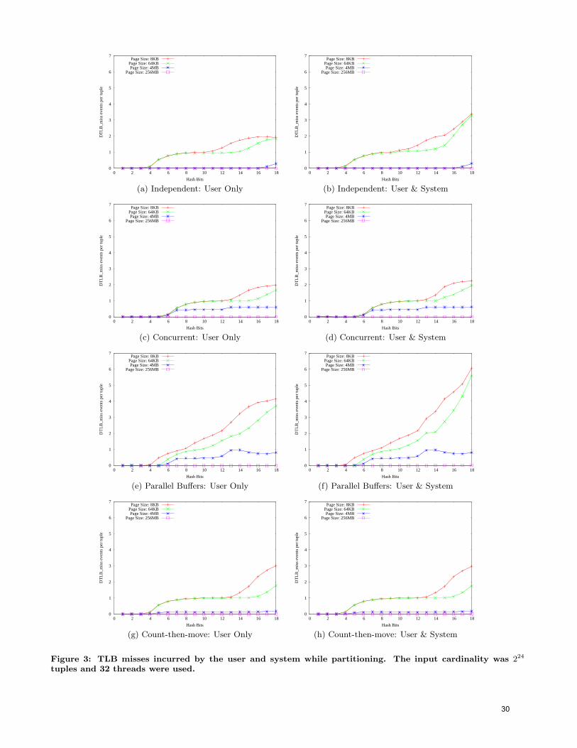
0

1

2

3

4

5

6

7

0 2 4 6 8 10 12 14 16 18

DT

LB_m

iss

even

ts p

er tu

ple

Hash Bits

Page Size: 8KBPage Size: 64KBPage Size: 4MB

Page Size: 256MB

(a) Independent: User Only

0

1

2

3

4

5

6

7

0 2 4 6 8 10 12 14 16 18

DT

LB_m

iss

even

ts p

er tu

ple

Hash Bits

Page Size: 8KBPage Size: 64KBPage Size: 4MB

Page Size: 256MB

(b) Independent: User & System

0

1

2

3

4

5

6

7

0 2 4 6 8 10 12 14 16 18

DT

LB_m

iss

even

ts p

er tu

ple

Hash Bits

Page Size: 8KBPage Size: 64KBPage Size: 4MB

Page Size: 256MB

(c) Concurrent: User Only

0

1

2

3

4

5

6

7

0 2 4 6 8 10 12 14 16 18

DT

LB_m

iss

even

ts p

er tu

ple

Hash Bits

Page Size: 8KBPage Size: 64KBPage Size: 4MB

Page Size: 256MB

(d) Concurrent: User & System

0

1

2

3

4

5

6

7

0 2 4 6 8 10 12 14 16 18

DT

LB_m

iss

even

ts p

er tu

ple

Hash Bits

Page Size: 8KBPage Size: 64KBPage Size: 4MB

Page Size: 256MB

(e) Parallel Buffers: User Only

0

1

2

3

4

5

6

7

0 2 4 6 8 10 12 14 16 18

DT

LB_m

iss

even

ts p

er tu

ple

Hash Bits

Page Size: 8KBPage Size: 64KBPage Size: 4MB

Page Size: 256MB

(f) Parallel Buffers: User & System

0

1

2

3

4

5

6

7

0 2 4 6 8 10 12 14 16 18

DT

LB_m

iss

even

ts p

er tu

ple

Hash Bits

Page Size: 8KBPage Size: 64KBPage Size: 4MB

Page Size: 256MB

(g) Count-then-move: User Only

0

1

2

3

4

5

6

7

0 2 4 6 8 10 12 14 16 18

DT

LB_m

iss

even

ts p

er tu

ple

Hash Bits

Page Size: 8KBPage Size: 64KBPage Size: 4MB

Page Size: 256MB

(h) Count-then-move: User & System

Figure 3: TLB misses incurred by the user and system while partitioning. The input cardinality was 224

tuples and 32 threads were used.

30

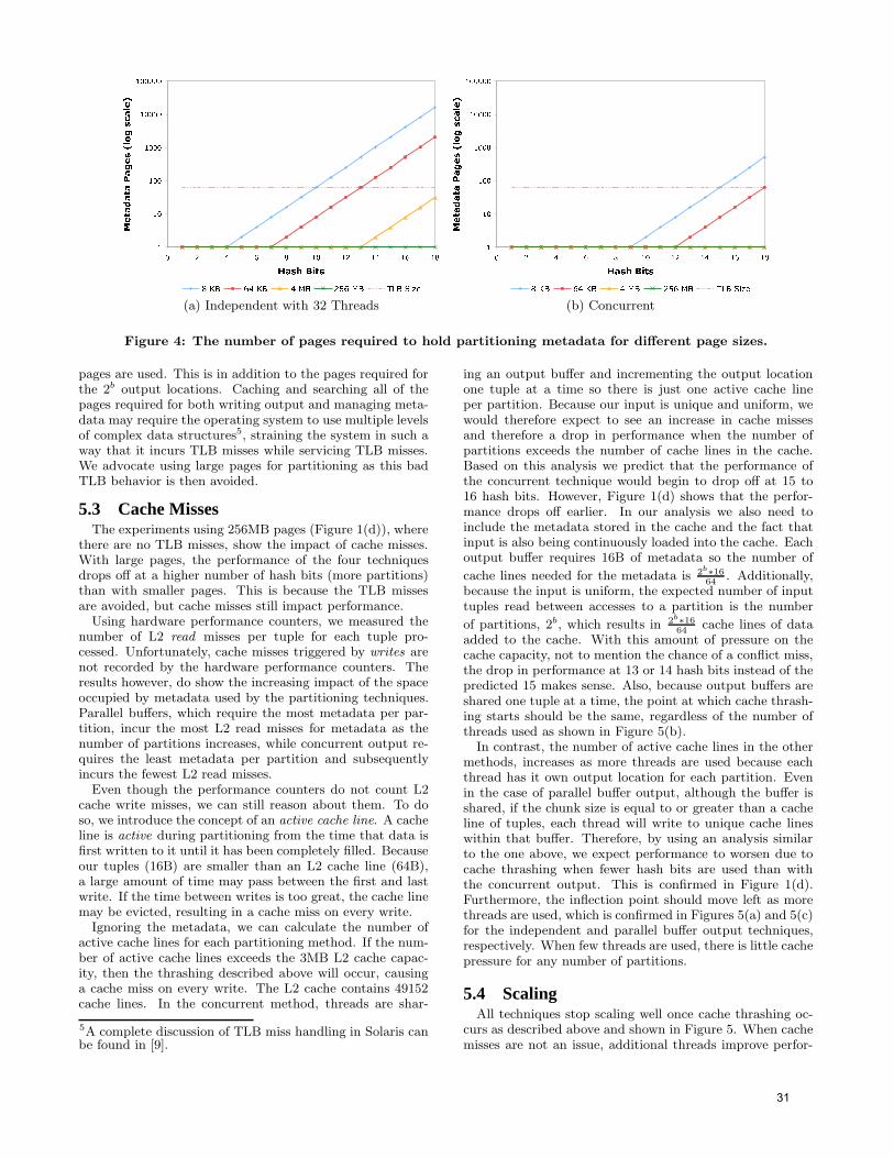
(a) Independent with 32 Threads (b) Concurrent

Figure 4: The number of pages required to hold partitioning metadata for different page sizes.

pages are used. This is in addition to the pages required forthe 2b output locations. Caching and searching all of thepages required for both writing output and managing meta-data may require the operating system to use multiple levelsof complex data structures5, straining the system in such away that it incurs TLB misses while servicing TLB misses.We advocate using large pages for partitioning as this badTLB behavior is then avoided.

5.3 Cache MissesThe experiments using 256MB pages (Figure 1(d)), where

there are no TLB misses, show the impact of cache misses.With large pages, the performance of the four techniquesdrops off at a higher number of hash bits (more partitions)than with smaller pages. This is because the TLB missesare avoided, but cache misses still impact performance.

Using hardware performance counters, we measured thenumber of L2 read misses per tuple for each tuple pro-cessed. Unfortunately, cache misses triggered by writes arenot recorded by the hardware performance counters. Theresults however, do show the increasing impact of the spaceoccupied by metadata used by the partitioning techniques.Parallel buffers, which require the most metadata per par-tition, incur the most L2 read misses for metadata as thenumber of partitions increases, while concurrent output re-quires the least metadata per partition and subsequentlyincurs the fewest L2 read misses.

Even though the performance counters do not count L2cache write misses, we can still reason about them. To doso, we introduce the concept of an active cache line. A cacheline is active during partitioning from the time that data isfirst written to it until it has been completely filled. Becauseour tuples (16B) are smaller than an L2 cache line (64B),a large amount of time may pass between the first and lastwrite. If the time between writes is too great, the cache linemay be evicted, resulting in a cache miss on every write.

Ignoring the metadata, we can calculate the number ofactive cache lines for each partitioning method. If the num-ber of active cache lines exceeds the 3MB L2 cache capac-ity, then the thrashing described above will occur, causinga cache miss on every write. The L2 cache contains 49152cache lines. In the concurrent method, threads are shar-

5A complete discussion of TLB miss handling in Solaris canbe found in [9].

ing an output buffer and incrementing the output locationone tuple at a time so there is just one active cache lineper partition. Because our input is unique and uniform, wewould therefore expect to see an increase in cache missesand therefore a drop in performance when the number ofpartitions exceeds the number of cache lines in the cache.Based on this analysis we predict that the performance ofthe concurrent technique would begin to drop off at 15 to16 hash bits. However, Figure 1(d) shows that the perfor-mance drops off earlier. In our analysis we also need toinclude the metadata stored in the cache and the fact thatinput is also being continuously loaded into the cache. Eachoutput buffer requires 16B of metadata so the number of

cache lines needed for the metadata is 2b∗1664

. Additionally,because the input is uniform, the expected number of inputtuples read between accesses to a partition is the number

of partitions, 2b, which results in 2b∗1664

cache lines of dataadded to the cache. With this amount of pressure on thecache capacity, not to mention the chance of a conflict miss,the drop in performance at 13 or 14 hash bits instead of thepredicted 15 makes sense. Also, because output buffers areshared one tuple at a time, the point at which cache thrash-ing starts should be the same, regardless of the number ofthreads used as shown in Figure 5(b).

In contrast, the number of active cache lines in the othermethods, increases as more threads are used because eachthread has it own output location for each partition. Evenin the case of parallel buffer output, although the buffer isshared, if the chunk size is equal to or greater than a cacheline of tuples, each thread will write to unique cache lineswithin that buffer. Therefore, by using an analysis similarto the one above, we expect performance to worsen due tocache thrashing when fewer hash bits are used than withthe concurrent output. This is confirmed in Figure 1(d).Furthermore, the inflection point should move left as morethreads are used, which is confirmed in Figures 5(a) and 5(c)for the independent and parallel buffer output techniques,respectively. When few threads are used, there is little cachepressure for any number of partitions.

5.4 ScalingAll techniques stop scaling well once cache thrashing oc-

curs as described above and shown in Figure 5. When cachemisses are not an issue, additional threads improve perfor-

31

0

20

40

60

80

100

120

140

160

0 2 4 6 8 10 12 14 16 18

Mill

ions

of T

uple

s pe

r S

econ

d

Hash Bits

Threads: 1Threads: 2Threads: 4Threads: 8

Threads: 16Threads: 32

(a) Independent

0

20

40

60

80

100

120

140

160

0 2 4 6 8 10 12 14 16 18

Mill

ions

of T

uple

s pe

r S

econ

d

Hash Bits

Threads: 1Threads: 2Threads: 4Threads: 8

Threads: 16Threads: 32

(b) Concurrent

0

20

40

60

80

100

120

140

160

0 2 4 6 8 10 12 14 16 18

Mill

ions

of T

uple

s pe

r S

econ

d

Hash Bits

Threads: 1Threads: 2Threads: 4Threads: 8

Threads: 16Threads: 32

(c) Parallel Buffers

0

20

40

60

80

100

120

140

160

0 2 4 6 8 10 12 14 16 18

Mill

ions

of T

uple

s pe

r S

econ

d

Hash Bits

Threads: 1Threads: 2Threads: 4Threads: 8

Threads: 16Threads: 32

(d) Count-then-move

Figure 5: Comparing the scaling of partitioning techniques as the number of threads is varied. The input

cardinality was 224 tuples and the page size was 256MB.

mance, but the scaling is not perfect, i.e., a doubling ofthreads does not double the partitioning throughput. Also,as noted above, for all techniques other than the concur-rent buffer, increasing the number of threads increases thecache pressure. This means that cache thrashing will occurat fewer and fewer output partitions as more threads areused. That cache thrashing is such an impediment to goodscaling confirms the observation by [8] that suggests multi-pass partitioning, where each pass fits within the cache andthe TLB, will give better performance than a single passusing a larger number of output partitions. For CMPs, thisanalysis is complicated slightly by the fact that output datastructures that help to avoid thread contention also scale interms of the number of active cache lines as the number ofthreads used increases. Future CMPs with more threads,all other characteristics being equal, will be limited to fewerand fewer cache resident output partitions per pass assumingthat all threads are applied to the partitioning.

5.5 Multiple PassesFigure 6 shows the performance of the parallel and con-

current buffer techniques using one and two passes. In thetwo pass versions, the first and second passes partition using⌈ b

2⌉ and ⌊ b

2⌋ hash bits, respectively. As in [8], for very large

numbers of partitions, making two passes using fewer hashbits performs better than one pass using all hash bits. A new

0

20

40

60

80

100

120

140

160

0 2 4 6 8 10 12 14 16 18

Mill

ions

of T

uple

s pe

r S

econ

d

Hash Bits

Parallel Buffers - One PassParallel Buffers - Two Pass

Concurrent - One PassConcurrent - Two Pass

Figure 6: One vs. two pass partitioning using 32

threads and 256MB pages to partition 224 tuples.

result, however, is the balancing of parallelism and the sizeof data structures that enable parallelism. Although paral-lel buffers avoid contention and have high performance whenless than nine hash bits are used, two pass parallel buffer par-titioning performance is worse than single pass concurrentbuffer performance when nine or more hash bits are used.This is because the concurrent technique requires less meta-data and fewer active cache lines per thread, therefore stay-

32

0

20

40

60

80

100

120

140

160

180

0 2 4 6 8 10 12 14 16 18

Mill

ions

of T

uple

s pe

r S

econ

d

Hash Bits

No bufferBuffer

Buffer + Block Init. Store

(a) Page Size = 8KB

0

20

40

60

80

100

120

140

160

180

0 2 4 6 8 10 12 14 16 18

Mill

ions

of T

uple

s pe

r S

econ

d

Hash Bits

No bufferBuffer

Buffer + Block Init. Store

(b) Page Size = 64 KB

0

20

40

60

80

100

120

140

160

180

0 2 4 6 8 10 12 14 16 18

Mill

ions

of T

uple

s pe

r S

econ

d

Hash Bits

No bufferBuffer

Buffer + Block Init. Store

(c) Page Size = 4MB

0

20

40

60

80

100

120

140

160

180

0 2 4 6 8 10 12 14 16 18

Mill

ions

of T

uple

s pe

r S

econ

d

Hash Bits

No bufferBuffer

Buffer + Block Init. Store

(d) Page Size = 256MB

Figure 7: A throughput comparison of the independent output technique with different page sizes when using

buffering with and without block initializing stores.

ing cache resident to larger numbers of partitions. Even onceone-pass concurrent partitioning performance drops off, twopass concurrent partitioning still performs better than twopass parallel buffer partitioning. Note also, though, that us-ing two-pass concurrent partitioning results in a larger rangeof hash bits in which it experiences contention.

5.6 Buffering and Block Initializing StoresBuffering tuples for writing to each output location may

improve partitioning performance in some circumstances.One performance problem identified in Section 5.2 is thatfor high numbers of output partitions, each write results ina TLB miss. By collocating output buffers for all partitions,the buffers take up fewer pages than the corresponding activeoutput partitions. Therefore, placing a tuple into a bufferis more likely to be a TLB hit. Further, when a buffer isflushed to the actual output location, only one TLB missis required for the entire buffer, thus amortizing the cost ofthe TLB miss over many tuples. A comparison of the in-dependent technique with and without a buffer is shown inFigure 7. Figure 8 demonstrates that buffering significantlylowers the number of TLB misses per tuple. Buffering alone,however, introduces additional overheads, both in terms ofstorage and computation, that make it perform worse thanno buffering in some cases. This performance can be im-proved by using a block initializing store instruction when

flushing a full buffer to its corresponding output partition.When a valid block initializing store instruction is exe-

cuted, rather than taking a cache miss to load the requestedline from memory, a zeroed cache line is allocated directly inthe L2 cache [12]. Using such an instruction when writing abuffer of tuples to an output partition, we avoid the latencyof a cache miss and save some memory bandwidth. Blockinitializing stores on the UltraSPARC T1 must start at anoffset aligned to the start of a cache line and should writea full cache line to memory. Therefore, buffering of tuplessmaller than a cache line in size is required to use block ini-tializing stores. Combining buffering with block initializingstores results in better performance as shown in Figure 7.

Because block initializing stores require the writing of en-tire cache lines, tuples that do not fit evenly withing a cacheline or span multiple cache lines may be more challengingto properly buffer and write to a destination. In our experi-ment, not only are the tuples smaller than a cache line, butthey also fit evenly within a cache line. Buffering is usefulfor our data, but may not be appropriate in all situations. Abuffered partitioning implementation for tuples of arbitrarysize would need to balance total buffer size with the benefitof amortizing TLB misses. If block initializing stores are tobe used, one must also ensure correct writing of whole cachelines, which may be non-trivial if tuples span cache lines andthe output buffer is shared among threads.

33

0

1

2

3

4

5

6

7

0 2 4 6 8 10 12 14 16 18

DT

LB_m

iss

even

ts p

er tu

ple

Hash Bits

No BufferBuffer

Figure 8: TLB user level misses for the independent

output technique using 8KB pages with and without

buffering.

6. FUTURE WORKWe realize that not all input is uniform and that uni-

form input, as used in these experiments, may not representa worst case scenario for CMP partitioning. Future workincludes examining CMP partitioning performance on non-unique, non-uniform input. Non-uniform distributions willhave some “heavy hitter” values that may cause some par-titions to grow much larger than the expected size given anassumption of uniform input.

In such a case, partition cardinality estimation may berequired and output buffers must be able to grow efficientlyand concurrently. Concurrent growth, in particular, may bea challenge for the techniques described in this paper thatuse shared buffers. The two-pass algorithm would remainunchanged for non-uniform input because the initial count-ing phase handles any amount of skew in actual partitionsize. The presence of heavy hitters in the input may actuallyimprove performance by improving the locality of referenceto some partitions, thereby reducing TLB and cache misses.On the other hand, frequently accessed partitions could be-come a source of contention if shared between threads.

Other future work includes using CMP partitioning to aidin the parallelizing or improving the performance of otherCMP database operations. For instance, it was observedin [2] that an efficient means of clustering group by keys inthe input to multithreaded hash aggregation could improvethe overall performance of the aggregation operation. Un-fortunately, the performance of CMP partitioning on thisparticular machine does not seem high enough to be able toimprove the aggregation performance reported in [2].

CMP partitioning should also be investigated on CMPswith “fatter” cores than the UltraSPARC T1. These coresmay have different performance characteristics due to moresophisticated support for prefetching and out-of-order execu-tion and different capabilities in terms of atomic operations.As of publication, however, no commodity “fat” core CMPchips have on-chip thread-level parallelism to match the T1.

7. CONCLUSIONIn this paper we have identified output coordination to be

a key component of CMP partitioning performance and havepresented four techniques for enabling parallel partitioning.

As described in Section 3, all of the techniques have differentcharacteristics in terms of the format of their output and themeans with which they enable concurrent partitioning on aCMP. Our results confirm the work of Manegold et al. [8] inthat reducing TLB and cache misses is paramount to achiev-ing good partitioning performance. In our study, large pagesand sharing output pages among threads eliminate or reduceTLB misses. We also find that cache misses are influencedby the number of partitions, whether the number of activecache lines scales with the number of threads used, and howmuch per thread metadata is required to manage the out-put buffers. Finally, an analysis of two pass partitioningshows the importance of balancing space efficiency with en-abling contention free parallelism. For smaller numbers ofpartitions, it is important to use data structures that enablecontention-free partitioning. As the number of partitionsincreases, one must switch to more compact, shared bufferstrategies and employ more than one pass for maximum per-formance. In conclusion, high performance CMP partition-ing requires a careful balancing of parallelism, contention,active cache lines, and metadata size.

8. ACKNOWLEDGMENTSThanks to Peter Boncz and Marcin Zukowski for the sug-

gestion of exploring partitioning as a means to improve theperformance of our adaptive aggregation technique presentedat VLDB 2007. We also thank the anonymous reviewers fortheir helpful suggestions.

9. REFERENCES[1] J. Cieslewicz et al. Parallel buffers for chip

multiprocessors. In DaMoN, June 2007.

[2] J. Cieslewicz and K. A. Ross. Adaptive aggregation onchip multiprocessors. In VLDB, pages 339–350, 2007.

[3] D. J. DeWitt et al. Implementation techniques formain memory database systems. In SIGMOD, pages1–8, 1984.

[4] D. J. Dewitt et al. The gamma database machineproject. IEEE Trans. on Knowl. and Data Eng.,2(1):44–62, 1990.

[5] D. J. DeWitt et al. Parallel sorting on ashared-nothing architecture using probabilisticsplitting. In Parallel and Distributed Information

Systems, pages 280–291, 1991.

[6] G. Graefe. Parallel external sorting in volcano.Technical Report CU-CS-459-90, University ofColorado, 1990.

[7] J. L. Hennessy and D. A. Patterson. Computer

Architecture. Morgan Kaufman, 4th edition, 2007.

[8] S. Manegold et al. Optimizing main-memory join onmodern hardware. IEEE Trans. Knowl. Data Eng.,14(4):709–730, 2002.

[9] R. McDougall and J. Mauro. Solaris Internals, chapter8-13. Prentice Hall, 2nd edition, 2007.

[10] A. Shatdal et al. Cache conscious algorithms forrelational query processing. In VLDB, pages 510–521,1994.

[11] Sun Microsystems, Inc. OpenSPARC T1microarchitecture specification, August 2006.

[12] Sun Microsystems, Inc. UltraSPARC T1 supplementto the UltraSPARC architecture 2005, March 2006.

34

Critical Sections: Re-emerging Scalability Concerns for Database Storage Engines

Ryan Johnson*, Ippokratis Pandis* Anastasia Ailamaki*††École Polytechnique Fédérale de Lausanne*Carnegie Mellon University

ABSTRACTCritical sections in database storage engines impact performanceand scalability more as the number of hardware contexts per chipcontinues to grow exponentially. With enough threads in the sys-tem, some critical section will eventually become a bottleneck.While algorithmic changes are the only long-term solution, theytend to be complex and costly to develop. Meanwhile, changes inenforcement of critical sections require much less effort. Weobserve that, in practice, many critical sections are so short thatenforcing them contributes a significant or even dominating frac-tion of their total cost and tuning them directly improves databasesystem performance. The contribution of this paper is two-fold:we (a) make a thorough performance comparison of the varioussynchronization primitives in the database system developer’stoolbox and highlight the best ones for practical use, and (b) showthat properly enforcing critical sections can delay the need tomake algorithmic changes for a target number of processors.

1. INTRODUCTIONIdeally, a database engine would scale perfectly, with throughputremaining (nearly) proportional to the number of clients even fora large number of clients. In practice several factors limit data-base engine scalability. Disk and compute capacities often limitthe amount of work that can be done in a given system, andbadly-behaved applications (like TPC-C) generate high levels oflock contention and limit concurrency. However, these bottle-necks are all largely external to the database engine; within thestorage manager itself, threads share many internal data struc-tures. Whenever a thread accesses a shared data structure, it mustprevent other threads from making concurrent modifications ordata races and corruption will result. These protected accesses areknown as critical sections, and can reduce scalability, especiallyin the absence of other, external bottlenecks.

For the forseeable future, computer architects will double thenumber of processor cores available each generation rather thanincreasing single-thread performance. Database engines arealready designed to handle hundreds or even thousands of concur-rent transactions, but with most of them blocked on I/O or data-base locks at any given moment. Even in the absence of lock or I/O bottlenecks, a limited number of hardware contexts used tobound contention for the engine’s internal shared data structures.Historically, the database community has largely overlooked criti-cal sections, either ignoring them completely or considering thema solved problem [1]. We find that as the number of active

threads grows the engine’s internal critical sections become a newand significant obstacle to scalability. Analysis of several opensource storage managers [11] shows critical sections become bot-tlenecks with a relatively small number of active threads, withBerkeleyDB scaling to 4 threads, MySQL to 8, and PostgreSQLto 16. These findings indicate that many database engines areunprepared for this explosion of hardware parallelism.

As the database developer optimizes the system for scalability,algorithmic changes are required to reduce the number of threadscontending for particular critical section. Additionally, we findthat the method by which existing critical sections are enforced isa crucial factor in overall performance and, to some extent, scal-ability. Database code exhibits extremely short critical sections,such that the overhead of enforcing those critical sections is a sig-nificant or even dominating fraction of their total cost. Reducingthe overhead of enforcing critical sections directly impacts perfor-mance and can even take critical sections off the critical pathwithout the need for costly changes to algorithms.

The literature abounds with synchronization approaches andprimitives which could be used to enforce critical sections, eachwith its own strengths and weaknesses. The database systemdeveloper must then choose the most appropriate approach foreach type of critical section encountered in during the tuning pro-cess or risk lowering performance significantly.

To our knowledge there is only limited prior work thataddresses the performance impact and tuning of critical sections,leaving developers to learn by trial and error which primitives aremost useful. This paper illustrates the performance improve-ments that come from enforcing critical sections properly, usingour experience developing Shore-MT [11], a scalable enginebased on the Shore storage manager [4]. We also evaluate themost common types of synchronization approaches, then identifythe most useful ones for enforcing the types of critical sectionsfound in database code. Database system developers can then uti-lize this knowledge to select the proper synchronization tool foreach critical section and maximize performance.

The rest of the paper is organized as follows. Sections 2 and 3give an overview of critical sections in database engines and thescalability challenges they raise. Sections 4 and 5 present an over-view of common synchronization approaches and evaluate theirperformance. Finally, Sections 6 and 7 discuss high-level obser-vations and conclude.

2. CRITICAL SECTIONS INSIDE DBMSDatabase engines purposefully serialize transaction threads inthree ways. Database locks enforce consistency and isolationbetween transactions by preventing other transactions fromaccessing the lock holder’s data. Locks are a form of logical pro-tection and can be held for long durations (potentially severaldisk I/O times). Latches protect the physical integrity of databasepages in the buffer pool, allowing multiple threads to read themsimultaneously, or a single thread to update them. Transactionsacquire latches just long enough to perform physical operations

Permission to make digital or hard copies of all or part of this work for per-sonal or classroom use is granted without fee provided that copies are notmade or distributed for profit or commercial advantage and that copies bearthis notice and the full citation on the first page. To copy otherwise, torepublish, to post on servers or to redistribute to lists, requires prior spe-cific permission and/or a fee.Proceedings of the Fourth International Workshop on Data Management onNew Hardware (DaMoN 2008), June 13, 2008, Vancouver, Canada.Copyright 2008 ACM 978-1-60558-184-2 ...$5.00.

35

(at most one disk I/O), depending on locks to protect that datauntil transaction commit time. Locks and latches have been stud-ied extensively [1][7]. Database locks are especially expensive tomanage, prompting proposals for hardware acceleration [21].

Critical sections form the third source of serialization. Data-base engines employ many complex, shared data structures; criti-cal sections (usually enforced with semaphores or mutex locks)protect the physical integrity of these data structures in the sameway that latches protect page integrity. Unlike latches and locks,critical sections have short and predictable durations because theyseldom span I/O requests or complex algorithms; often the threadonly needs to read or update a handful of memory locations. Forexample, a critical section might protect traversal of a linked list.Critical sections abound throughout the storage engine’s code. InShore-MT, for example, we estimate that a TPC-C Payment trans-action — which only touches 4-6 database records — entersroughly one hundred critical sections before committing. Underthese circumstances, even uncontended critical sections areimportant because the accumulated overhead can contribute a sig-nificant fraction of overall cost. The rest of this section presentsan overview of major storage manager components and lists thekinds of critical sections they make use of.

Buffer Pool Manager. The buffer pool manager maintains a poolfor in-memory copies of in-use and recently-used database pagesand ensures that the pages on disk and in memory are consistentwith each other. The buffer pool consists of a fixed number offrames which hold copies of disk pages and provide latches to pro-tect page data. The buffer pool uses a hash table that maps pageIDs to frames for fast access, and a critical section protects the listof pages at each hash bucket. Whenever a transaction accesses apersistent value (data or metadata) it must locate the frame for thatpage, pin it, then latch it. Pinning prevents the pool manager fromevicting the page while a thread acquires the latch. Once the pageaccess is complete, the thread unlatches and unpins the page,allowing the buffer pool to recycle its frame for other pages if nec-essary. Page misses require a search of the buffer pool for a suit-able page to evict, adding yet another critical section. Overall,acquiring and releasing a single page latch requires at least 3-4critical sections, and more if the page gets read from disk.

Lock Manager. Database locks preserve isolation and consistencyproperties between transactions. Database locks are hierarchical,meaning that a transaction wishing to lock one row of a table mustfirst lock the database and the table in an appropriate intent mode.Hierarchical locks allow transactions to balance granularity withoverhead: fine-grained locks allow high concurrency but areexpensive to acquire in large numbers. A transaction which plansto read many records of a table can avoid the cost of acquiring rowlocks by escalating to a single table lock instead. However, othertransactions which attempt to modify unrelated rows in the sametable would then be forced to wait. The number of possible locksscales with the size of the database, so the storage engine main-tains a lock pool very similar to the buffer pool.

The lock pool features critical sections that protect the lockobject freelist and the linked list at each hash bucket. Each lockobject also has a critical section to “pin” it and prevent recyclingwhile it is in use, and another to protect its internal state. Thismeans that, to acquire a row lock, a thread enters at least threecritical sections for each of the database, table, and row locks.

Log Manager. The log manager ensures that modified pages inmemory are not lost in the event of a failure: all changes to pages

are logged before the actual change is made, allowing the page’slatest state to be reconstructed during recovery. Every log insertrequires a critical section to serialize log entries and another tocoordinate with log flushes. An update to a given database recordoften involves several log entries due to index and metadataupdates that go with it.

Free Space Management. The storage manager maintains meta-data which tracks disk page allocation and utilization. This infor-mation allows the storage manager to allocate unused pages totables efficiently. Each record insert (or update that increasesrecord size) requires entering several critical sections to determinewhether the current page has space and to allocate new pages asnecessary. Note that the transaction must also latch the free spacemanager’s metadata pages and log any updates.

Transaction Management: The system maintains a total order oftransactions in order to resolve lock conflicts and maintain propertransaction isolation. Whenever a transaction begins or ends thisglobal state must be updated. In addition, no transaction may com-mit during a log checkpoint operation, in order to ensure that theresulting checkpoint is consistent. Finally, multi-threaded transac-tions must serialize the threads within a transaction in order toupdate per-transaction state such as lock caches.

3. THE DREADED CRITICAL SECTIONBy definition, critical sections limit scalability by serializing thethreads which compete for them. Each critical section is simplyone more limited resource in the system that supports some maxi-mum throughput. As Moore's Law increases the number ofthreads which can execute concurrently, the demand on criticalsections increases and they invariably enter the critical path tobecome the bottleneck in the system. Database engine designerscan potentially improve critical section capacity (i.e. peakthroughput) by changing how they are enforced or by alteringalgorithms and data structures.

3.1 Algorithmic ChangesAlgorithmic changes address bottleneck critical sections by eitherreducing how often threads enter them (ideally never), or bybreaking them into several “smaller” ones in a way that distrib-utes contending threads as well (ideally, each thread can expectan uncontended critical section). For example, buffer pool manag-ers typically distribute critical sections by hash bucket so thatonly probes for pages in the same bucket must be serialized.

In theory, algorithmic changes are the superior approach foraddressing critical sections because they can remove or distributecritical sections to ease contention. Unfortunately, developing andimplementing new algorithms is challenging and time consuming,with no guarantee of a breakthrough for a given amount of effort.In addition, even the best-designed algorithms will eventuallybecome bottlenecks again if the number of threads increasesenough, or if non-uniform access patterns cause hotspots.

3.2 Changing Synchronization PrimitivesThe other approach for improving critical section throughput isby altering how they are enforced. Because the critical sectionswe are interested in are so short, the cost of enforcing them is asignificant — or even dominating — fraction of their overall cost.Reducing the cost of enforcing a bottleneck critical section canimprove performance a surprising amount. Also, critical sections

36

tend to be encapsulated by their surrounding data structures, sothe developer can change how they are enforced simply byreplacing the existing synchronization primitive with a differentone. These characteristics make critical section tuning attractive ifit can avoid or delay the need for costly algorithmic changes.

3.3 Both are NeededFigure 1 illustrates how algorithmic changes and synchronizationtuning combined give the best performance. It presents the per-formance of Shore-MT at several stages of tuning, with through-put given on the log-scale y-axis as the number of threads in thesystem varies along the x-axis. These numbers came from theexperience of converting Shore to Shore-MT [11]. The processinvolved beginning with a thread-safe but very slow version ofShore and repeatedly addressing critical sections until internalscalability bottlenecks had all been removed. The changesinvolved algorithmic and synchronization changes in all the majorcomponents of the storage manager, including logging, locking,and buffer pool management. The figure shows the performanceand scalability of Shore-MT at various stages of tuning. Eachthread repeatedly runs transactions which insert records into a pri-vate table. These transactions exhibit no logical contention witheach other but tend to expose many internal bottlenecks. Notethat, in order to show the wide range of performance the y-axis ofthe figure is log-scale; the final version of Shore-MT scalesnearly as well as running each thread in an independent copy ofShore-MT.

The “B1” line at the bottom represents the thread-safe butunoptimized Shore; the first optimization (A1) replaced the cen-tral buffer pool mutex with one mutex per hash bucket. As aresult, scalability improved from one thread to nearly four, butsingle-thread performance did not change. The second optimiza-tion (T1) replaced the expensive pthread mutex protecting bufferpool buckets with a fast test and set mutex (see Section 4 fordetails about synchronization primitives), doubling throughput fora single thread. The third optimization (T2) replaced the test-and-set mutex with a more scalable MCS mutex, allowing the doubledthroughput to persist until other bottlenecks asserted themselvesat four threads.

B2 represents the performance of Shore-MT after many subse-quent optimizations, when the buffer pool again became a bottle-neck. Because the critical sections were already as efficient aspossible, another algorithmic change was required (A2). Thistime the open-chained hash table was replaced with a cuckoo

hash table to further reduce contention for hash buckets, improv-ing scalability from 8 to 16 threads and beyond (details in [11]).

This example illustrates how both proper algorithms and propersynchronization are required to achieve the highest performance.In general, tuning primitives improves performance significantly,and sometimes scalability as well; algorithmic changes improvescalability and might help or hurt performance (more scalablealgorithms tend to be more expensive). Finally, we note that thetwo tuning optimizations each required only a few minutes toapply, while each of the algorithmic changes required severaldays to implement and debug. The performance impact and easeof reducing critical section overhead makes tuning an importantpart of the optimization process.

4. SYNCHRONIZATION APPROACHESThe literature abounds with different synchronization primitivesand approaches, each with different overhead (cost to enter anuncontended critical section) and scalability (whether, and byhow much, overhead increases under contention). Unfortunately,efficiency and scalability tend to be inversely related: the cheap-est primitives are unscalable, and the most scalable ones imposehigh overhead; as the previous section illustrated, both metricsimpact the performance of a database engine. Next we present abrief overview of the types of primitives available to the designer.

4.1 Synchronization PrimitivesThe most common approach to synchronization is to use a syn-chronization primitive to enforce the critical section. There are awide variety of primitives to choose from, all more or less inter-changeable with respect to correctness.

Blocking Mutex. All operating systems provide heavyweightblocking mutex implementations. Under contention these primi-tives deschedule waiting threads until the holding thread releasesthe mutex. These primitives are fairly easy to use and understand,in addition to being portable. Unfortunately, due to the cost of con-text switching and their close association with the kernel sched-uler, they are not particularly cheap or scalable for the short criticalsections we are interested in.

Test-and-set Spinlocks. Test-and-set (TAS) spinlocks are the sim-plest mutex implementation. Acquiring threads use an atomicoperation such as a SWAP to simultaneously lock the primitive anddetermine if it was already locked by another thread, repeatinguntil they lock the mutex. A thread releases a TAS spinlock using asingle store. Because of their simplicity TAS spinlocks areextremely efficient. Unfortunately, they are also among the least-scalable synchronization approaches because they impose a heavyburden on the memory subsystem. Variants such as test-and-test-and-set [22] (TATAS), exponential back-off [2], and ticket-based[20] approaches reduce the problem somewhat, but do not solve itcompletely. Backoff schemes, in particular, are very difficult (andhardware-dependent) to tune.

Queue-based Spinlocks. Queue-based spinlocks organize con-tending threads into a linked list queue where each thread spins ona different memory location. The thread at the head of the queueholds the lock, handing off to a successor when it completes.Threads compete only long enough to append themselves to thetail of the queue. The two best-known queuing spinlocks are MCS[16] and CLH [5][15], which differ mainly in how they managetheir queues. MCS queue links point toward the tail, while CLH

Figure 1.Algorithmic changes and tuning combine to give best per-formance.A<n> is an algorithm change; B<n> is a baseline;T<n> is synchronization tuning.

Tuning Examples from Shore-MT

1

10

100

0 4 8 12 16Threads

Thro

ughp

ut

A2B2T2T1A1B1

37

links point toward the head. Queuing improves on test-and-set byeliminating the burden on the memory system and also by decou-pling lock contention from lock hand-off. Unfortunately, eachthread is responsible to allocate and maintain a queue node foreach lock it acquires. In our experience, memory management canquickly become cumbersome in complex code, especially for CLHlocks, which require heap-allocated state.

Reader-Writer Locks. In certain situations, threads enter a criticalsection only to prevent other threads from changing the data to beread. Reader-writer locks allow either multiple readers or onewriter to enter the critical section simultaneously, but not both.While operating systems typically provide a reader-writer lock, wefind that the pthreads implementation suffers from extremely highoverhead and poor scalability, making it useless in practice. Themost straightforward reader-writer locks use a normal mutex toprotect their internal state; more sophisticated approaches extendqueuing locks to support reader-writer semantics [17][13].

A Note About Convoys. Some synchronization primitives, suchas blocking mutex and queue-based spinlocks, are vulnerable toforming stable quasi-deadlocks known as convoys [3]. Convoysoccur when the lock passes to a thread that has been descheduledwhile waiting its turn. Other threads must then wait for the threadto be rescheduled, increasing the chances of further preemptions.The result is that the lock sits nearly idle even under heavy conten-tion. Recent work [8] has provided a preemption-resistant form ofqueuing lock, at the cost of additional overhead which can putmedium-contention critical sections squarely on the critical path.

4.2 Alternatives to LockingUnder certain circumstances critical sections can be enforcedwithout resorting to locks. For example, independent reads andwrites to a single machine word are already atomic and need nofurther protection. Other, more sophisticated approaches such asoptimistic concurrency control and lock-free data structures allowlarger critical sections as well.

Optimistic Concurrency Control. Many data structures featureread-mostly critical sections, where updates occur rarely, and oftencome from a single writer. The reader's critical sections are oftenextremely short and overhead dominates the overall cost. Underthese circumstances, optimistic concurrency control schemes canimprove performance dramatically by assuming no writer willinterfere during the operation. The reader performs the operationwithout enforcing any critical section, then afterward verifies that

no writer interfered (e.g. by checking a version stamp). In the rareevent that the assumption did not hold, the reader blocks or retries.The main drawbacks to OCC are that it cannot be applied to allcritical sections (since side effects are unsafe until the read is veri-fied), and unexpectedly high writer activity can lead to livelock asreaders endlessly block or abort and retry.

Lock-free Data Structures. Much current research focuses onlock-free data structures [9] as a way to avoid the problems thatcome with mutual exclusion (e.g. [14][6]). These schemes usuallycombine optimistic concurrency control and atomic operations toproduce data structures that can be accessed concurrently withoutenforcing critical sections. Unfortunately there is no known gen-eral approach to designing lock free data structures; each must beconceived and developed separately, so database engine designersare have a limited library to choose from. In addition, lock-freeapproaches can suffer from livelock unless they are also wait-free,and may or may not be faster than the lock-based approaches underlow and medium contention (many papers provide only asymptoticperformance analyses rather than benchmark results).

Transactional Memory. Transactional memory approachesenforce critical sections using database-style “transactions” whichcomplete atomically or not at all. This approach eases many of thedifficulties of lock-based programming and has been widelyresearched. Unfortunately, software-based approaches [23] imposetoo much overhead for the tiny critical sections we are interestedin, while hardware approaches [10][19] generally suffer from com-plexity, lack of generality, or both, and have not been adopted.Finally, we note that transactions do not inherently remove conten-tion; at best transactional memory can serialize critical sectionswith very little overhead.

5. CHOOSING THE RIGHT APPROACHThis section evaluates the different synchronization approachesusing a series of microbenchmarks that replicate the kinds of crit-ical sections found in database code. We present the performanceof the various approaches as we vary three parameters: Con-tended vs. uncontended accesses, short vs. long duration, andread-mostly vs. mutex critical sections. We then use the results toidentify the primitives which work best in each situation.

Each microbenchmark creates N threads which compete for alock in a tight loop over a one second measurement interval (typi-cally 1-10M iterations). The metric of interest is cost per iterationper thread, measured in nanoseconds of wall-clock time. Eachiteration begins with a delay of To ns to represent time spent out-

Figure 2.Performance of mutex locks as the contention (left) and the duration of the CS (right) vary.

Scalability vs. Duration

0

200

400

600

800

0 100 200 300Duration (nsec)

Cos

t/Ite

ratio

n (n

sec)

Scalability vs. Contention

0

200

400

600

800

0 8 16 24 32Threads

Cos

t/Ite

ratio

n (n

sec) ideal

tatas

mcsppmcs

pthread

38

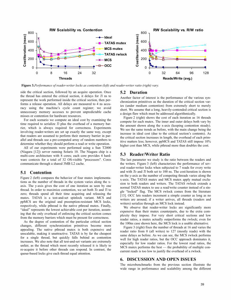
side the critical section, followed by an acquire operation. Oncethe thread has entered the critical section, it delays for Ti ns torepresent the work performed inside the critical section, then per-forms a release operation. All delays are measured to 4 ns accu-racy using the machine’s cycle count register; we avoidunnecessary memory accesses to prevent unpredictable cachemisses or contention for hardware resources.

For each scenario we compute an ideal cost by examining thetime required to serialize Ti plus the overhead of a memory bar-rier, which is always required for correctness. Experimentsinvolving reader-writers are set up exactly the same way, exceptthat readers are assumed to perform their memory barrier in par-allel and threads use a pre-computed array of random numbers todetermine whether they should perform a read or write operation.

All of our experiments were performed using a Sun T2000(Niagara [12]) server running Solaris 10. The Niagara chip is amulti-core architecture with 8 cores; each core provides 4 hard-ware contexts for a total of 32 OS-visible "processors". Corescommunicate through a shared 3MB L2 cache.

5.1 ContentionFigure 2 (left) compares the behavior of four mutex implementa-tions as the number of threads in the system varies along the x-axis. The y-axis gives the cost of one iteration as seen by onethread. In order to maximize contention, we set both To and Ti tozero; threads spend all their time acquiring and releasing themutex. TATAS is a test-and-set spinlock variant. MCS andppMCS are the original and preemption-resistant MCS locks,respectively, while pthread is the native pthread mutex. Finally,“ideal” represents the lowest achievable cost per iteration, assum-ing that the only overhead of enforcing the critical section comesfrom the memory barriers which must be present for correctness.

As the degree of contention of the particular critical sectionchanges, different synchronization primitives become moreappealing. The native pthread mutex is both expensive andunscalable, making it unattractive. TATAS is by far the cheapestfor a single thread, but quickly falls behind as contentionincreases. We also note that all test-and-set variants are extremelyunfair, as the thread which most recently released it is likely tore-acquire it before other threads can respond. In contrast, thequeue-based locks give each thread equal attention.

5.2 DurationAnother factor of interest is the performance of the various syn-chronization primitives as the duration of the critical section var-ies (under medium contention) from extremely short to merelyshort. We assume that a long, heavily-contended critical section isa design flaw which must be addressed algorithmically.

Figure 2 (right) shows the cost of each iteration as 16 threadscompete for each mutex. The inner and outer delays both vary bythe amount shown along the x-axis (keeping contention steady).We see the same trends as before, with the main change being theincrease in ideal cost (due to the critical section’s contents). Asthe critical section increases in length, the overhead of each prim-itive matters less; however, ppMCS and TATAS still impose 10%higher cost than MCS, while pthread more than doubles the cost.

5.3 Reader/Writer RatioThe last parameter we study is the ratio between the readers andthe writers. Figure 3 (left) characterizes the performance of sev-eral reader-writer locks when subjected to 7 reads for every writeand with To and Ti both set to 100 ns. The cost/iteration is shownon the y-axis as the number of competing threads varies along thex-axis. The TATAS mutex and MCS mutex apply mutual exclu-sion to both readers and writers. The TATAS rwlock extends anormal TATAS mutex to use a read/write counter instead of a sin-gle “locked” flag. The MCS rwlock comes from the literature[13]. OCC lets readers increment a simple counter as long as nowriters are around; if a writer arrives, all threads (readers andwriters) serialize through an MCS lock instead.

We observe that reader-writer locks are significantly moreexpensive than their mutex counterparts, due to the extra com-plexity they impose. For very short critical sections and lowreader ratios, a mutex actually outperforms the rwlock; even forthe 100ns case shown here, the MCS lock is a usable alternative.

Figure 3 (right) fixes the number of threads at 16 and varies thereader ratio from 0 (all writes) to 127 (mostly reads) with thesame delays as before. As we can see, the MCS rwlock performswell for high reader ratios, but the OCC approach dominates it,especially for low reader ratios. For the lowest read ratios, theMCS mutex performs the best — the probability of multiple con-current reads is too low to justify the overhead of a rwlock.

6. DISCUSSION AND OPEN ISSUESThe microbenchmarks from the previous section illustrate thewide range in performance and scalability among the different

Figure 3.Performance of reader-writer locks as contention (left) and reader-writer ratio (right) vary.

RW Scalability vs. Contention

0

200

400

600

800

0 8 16 24 32Threads

Cos

t/ite

ratio

n (n

sec) Ideal

TATAS mutexMCS mutexTATAS rwlockMCSOCC

RW Scalability vs. R/W ratio

0

200

400

600

800

0 32 64 96 128Reads/Write (avg.)

Cos

t/ite

ratio

n (n

sec)

39

primitives. From the contention experiment we see that theTATAS lock performs best under low contention due to havingthe lowest overhead; for high contention, the MCS lock is supe-rior thanks to its scalability. The experiment also highlights howexpensive it is to enforce critical sections. The ideal case (mem-ory barrier alone) costs 50 ns, and even TATAS costs twice that.The other alternatives cost 250 ns or more. By comparison a storecosts roughly 10 ns, meaning critical sections which update onlya handful of values suffer more than 80% overhead. As the dura-tion experiment shows, pthread and TATAS are undesirable evenfor longer critical sections that amortize the cost somewhat.Finally, the reader-writer experiment demonstrates the extremelyhigh cost of reader-writer synchronization; a mutex outperformsrwlocks at low read ratios by virtue of its simplicity, while opti-mistic concurrency control wins at high ratios. Figure 4 summa-rizes the results of the experiments, showing which of the threesynchronization primitives to use under what circumstances. Wenote that, given a suitable algorithm, the lock free approach mightbe best.

The results also suggest that there is much room for improve-ment in the synchronization primitives that protect small criticalsections. Hardware-assisted approaches (e.g. [18]) and imple-mentable transactional memory might be worth exploring furtherin order to reduce overhead and improve scalability. Reader-writer primitives, especially, do not perform well as threads muststill serialize long enough to identify each other as readers andcheck for writers.

7. CONCLUSIONCritical sections are emerging as a major obstacle to scalability asthe number of hardware contexts in modern systems continues togrow and a large part of the execution is computation-bound. Weobserve that algorithmic changes and proper use of synchroniza-tion primitives are both vital to maximize performance and keepcritical sections off the critical path in database engines and thateven uncontended critical sections sap performance because ofthe overhead they impose. We identify a small set of especiallyuseful synchronization primitives which a developer can use forenforcing critical sections. Finally, we identify several areaswhere currently available primitives fall short, indicating poten-tial avenues for future research.

8. ACKNOWLEDGEMENTSWe thank Brian Gold and Brett Meyer for their insights and sug-gestions, and the reviewers for their helpful comments. This work

was partially supported by grants and equipment from Intel; aSloan research fellowship; an IBM faculty partnership award; andNSF grants CCR-0205544, CCR-0509356, and IIS-0133686.

9. REFERENCES[1] R. Agrawal, M. Carey, and M. Livny. “Concurrency control

performance modeling: alternatives and implications.” ACMTODS, 12(4), 1987.

[2] T. Anderson. “The performance of spin lock alternatives forshared-memory multiprocessors.” IEEE TPDS, 1(1), 1990.

[3] M. Blasgen, J. Gray, M. Mitona, and T. Price. “The ConvoyPhenomenon.” ACM SIGOPS, 13(2), 1979.

[4] M. Carey, et al. “Shoring up persistent applications.” In Proc.SIGMOD, 1994.

[5] T. Craig. “Building FIFO and priority-queueing spin locksfrom atomic swap.” Technical Report TR 93-02-02, Univer-sity of Washington, Dept. of Computer Science, 1993.

[6] M. Fomitchev, and E. Rupert. “Lock-free linked lists and skiplists.” In Proc. PODC, 2004.

[7] V. Gottemukkala, and T. J. Lehman. “Locking and latching ina memory-resident database system.” In Proc. VLDB, 1992.

[8] B. He, W. N. Scherer III, and M. L. Scott. “Preemption adap-tivity in time-published queue-based spin locks.” In Proc.HiPC, 2005.

[9] M. Herlihy. “Wait-free synchronization.” ACM TOPLAS,13(1), 1991.

[10] M. Herlihy and J. Moss. “Transactional memory: architecturalsupport for lock-free data structures.” In Proc. ISCA, 1993.

[11] R. Johnson, I. Pandis, N. Hardavellas, and A. Ailamaki.“Shore-MT: A Quest for Scalability in the Many-Core Era.”CMU-CS-08-114.

[12] P. Kongetira, K. Aingaran, and K. Olukotun. “Niagara: A 32-Way Multithreaded SPARC Processor.” IEEE MICRO, 2005.

[13] O. Krieger, M. Stumm, and R. Unrau. “A Fair Fast ScalableReader-Writer Lock.” In Proc. ICPP, 1993

[14] M. Maged. “High performance dynamic lock-free hash tablesand list-based sets.” In Proc. SPAA, 2002.

[15] P. Magnussen, A. Landin, and E. Hagersten. “Queue locks oncache coherent multiprocessors.” In Proc. IPPS, 1994.

[16] J. Mellor-Crummey, and M. Scot. “Algorithms for scalablesynchronization on shared-memory multiprocessors.” ACMTOCS, 9(1), 1991.

[17] J. Mellor-Crummey, and M. L. Scott. “Scalable Reader-Writer Synchronization for Shared-Memory Multiproces-sors.” In Proc. PPoPP, 1991.

[18] R. Rajwar, and J. Goodman. “Speculative lock elision:enabling highly concurrent multithreaded execution.” IEEEMICRO, 2001.

[19] R. Rajwar and J. Goodman. “Transactional lock-free executionof lock-based programs.” SIGPLAN Notices, 37(10), 2002.

[20] D. P. Reed, and R. K. Kanodia. “Synchronization with event-counts and sequencers.” Commun. ACM 22(2), 1979.

[21] J. T. Robinson. “A fast, general-purpose hardware synchroni-zation mechanism.” In Proc. SIGMOD, 1985.

[22] L. Rudolph and Z. Segall. “Dynamic decentralized cacheschemes for MIMD parallel processors.” In Proc ISCA, 1984.

[23] N. Shavit and D. Touitou. “Software Transactional Memory.”In Proc. PODC, 1995.

Figure 4.The space of critical section types. Each corner of thecube is marked with the appropriate synchronization primitive touse for that type of critical section.

OCC Read-mostly

Long

Contended

Uncontended

Mutex

ShortOCC

OCCMCS

TAS

Lock-free

40

Avoiding Version Redundancy for High PerformanceReads in Temporal DataBases

Khaled Jouinikhaled.jouini@dauphine.fr

Geneviève Jomiergenevieve.jomier@dauphine.fr

Université Paris DauphinePlace du Maréchal de Lattre de Tassigny

Paris, France

ABSTRACTA major performance bottleneck for database systems is thememory hierarchy. The performance of the memory hier-archy is directly related to how the content of disk pagesmaps to the L2 cache lines, i.e. to the organization of datawithin a disk page, called the page layout. The prevalentpage layout in database systems is the N-ary Storage Model(NSM). As demonstrated in this paper, using NSM for tem-poral data deteriorates memory hierarchy performance forquery-intensive workloads. This paper proposes two cache-conscious, read-optimized, page layouts for temporal data.Experiments show that the proposed page layouts are sub-stantially faster than NSM.

1. INTRODUCTIONDatabase systems (DBMS) fetch data from non-volatile

storage (e.g. disk) to processor in order to execute queries.Data goes through the memory hierarchy which consists ofdisk, main memory, L2 cache, L1 cache [4]. The communi-cation between the main memory and the disk has been tra-ditionally recognized as the dominant database performancebottleneck. However, architectural research on modern plat-forms has pointed out that the L2 cache miss penalty has anincreasing impact on response times [3]. As a result, DBMSshould be designed to be sensitive, not only to disk and mainmemory performance, but also to L2 cache performance [2].The mapping of disk page content to L2 cache lines is

determined by the organization of data within the page,called the page layout [2]. Thus, the page layout highlyimpacts the memory hierarchy utilization of DBMS [15].The prevalent page layout in commercial DBMS is the N-ary Storage Model (NSM), also called row-store architec-ture [16]. NSM stores all the attributes of a tuple contigu-ously within a disk page. While NSM provides a genericplatform for a wide range of data storage needs, recentstudies demonstrate that it exhibits poor memory hierar-chy performance for query-intensive applications [17]. Incontrast with OLTP-style applications, query-intensive ap-

Permission to make digital or hard copies of all or part of this work forpersonal or classroom use is granted without fee provided that copies arenot made or distributed for profit or commercial advantage and that copiesbear this notice and the full citation on the first page. To copy otherwise, torepublish, to post on servers or to redistribute to lists, requires prior specificpermission and/or a fee.Proceedings of the Fourth International Workshop on Data Management onNew Hardware (DaMoN 2008), June 13, 2008, Vancouver, Canada.Copyright 2008 ACM 978-1-60558-184-2 ...$5.00.

plications require faster reads, while tolerating slower writes.Hence, they should be read-optimized [16]. Typical examplesare data warehouses and customer relationship managementsystems, where relatively long periods of ad-hoc queries areinterspersed with periodic bulk-loading of new data [16].Recently, page layouts alternative to NSM have been imple-mented in academic and commercial read-optimized systems[20, 19, 5, 21].This paper focuses on read-optimized, cache-conscious page

layouts for temporal data. Various characteristics of tempo-ral data make this problem novel. In temporal databases,in order to keep past, whenever a modeled entity e is mod-ified, its old version is retained and a new version of e iscreated. Thus, an entity e may be represented in a singletemporal relation by a set of tuples. Each tuple containsa timestamp t and records the state (or the version) of eat t. Figure 1.a depicts a sample temporal relation product(entity surrogate, timestamp, name, price, CO2 consump-tion) in NSM-style representation. In this example, as inthe remainder of this paper, time is assumed to be linearand totally ordered: ti < ti+1. Let ti and tj be two times-tamps such that: (i) ti < tj ; and (ii) the state of an entity eis modified at ti and at tj , but is unchanged between them.As the state of e remains unchanged between ti and tj , itis recorded only once by the tuple identified by (e, ti). Thetuple (e, ti) is said to be alive or valid for each t ∈ [ti, tj);[ti, tj) expresses the lifespan or the time validity of (e, ti).In most cases: (i) only a small fraction of the attributes of

an entity are time-varying; and (ii) time-varying attributesvary independently over time. With NSM, even if only oneattribute is updated, all the other attributes are duplicated.For example, in figure 1.a the update of the price of prod-

e t name price CO2 e1 t1 A 50 0.5 e1 t3 A 52 0.5 e1 t5 A 52 0.3 e2 t2 B 100 0.7 e2 t4 B 105 0.7

(a)

e t name price CO2 e1 t1 A 50 0.5 e1 t3 A 52 0.5 e1 t5 A 52 0.3 e2 t2 B 100 0.7 e2 t4 B 105 0.7 (d) (c)

e t price e1 t1 50 e1 t3 52 e2 t2 100 e2 t4 105

e t CO2 e1 t1 0.5 e1 t5 0.3 e2 t2 0.7

e t name e1 t1 A e2 t2 B

(b)

ts e 1 e1 2 e1 3 e1 4 e2 5 e2

ts t 1 t1 2 t3 3 t5 4 t2 5 t4

ts name 1 A 2 A 3 A 4 B 5 B

ts price 1 50 2 52 3 52 4 100 5 105

ts CO2 1 0.5 2 0.5 3 0.3 4 0.7 5 0.7

Figure 1: (a) A sample temporal relation prod-uct (entity surrogate, timestamp, name, price, CO2

consumption) in NSM-style representation. (b)Straight-forward DSM; ts: tuple surrogate. (c)Temporal DSM. (d) PSP only stores values writtenin black. Other values are implicit.

41

PH1 TH1 e1 t1 A 50 0.5 TH2 e1 t3 A 52 0.5 TH3 e1 t3 A 52 0.3 ...

NSM Page

(a) (b)

line size Offset vector

L2 Cache

Offset vector Cache line 1

Cache line 4 Cache line 3 Cache line 2

Cache line 5

PH1 TH1 e1 t1

A 50 0.5 TH2 e1 t3 A 52 0.5 TH3 e1 t3

Cache line 6 A 52 0.3

Figure 2: (a) NSM page layout. (b) Cache behaviorfor "find the CO2 consumption history of A".

uct A at t3 leads to the replication of his name and CO2

consumption. We call this type of replication version re-dundancy. The important issue here is not the disk spaceconsumed by version redundancy, as disk space costs virtu-ally nothing nowadays. The issue is that loading the mem-ory hierarchy several times with the same data: (i) wastesdisk and main memory bandwidths; (ii) pollutes the mainmemory and the L2 cache; and (iii) increases the amount ofCPU cycles wasted in waiting for data loading.This paper introduces the Temporal Decomposition Stor-

age Model (TDSM) and the Per Surrogate Partitioning stor-age model (PSP), two page layouts specifically tailored fortemporal data. TDSM and PSP aim at avoiding version re-dundancy to achieve: (i) reasonable performance for writes;and (ii) high-performance reads. The remainder of this pa-per is organized as follows. Section 2 illustrates the useof conventional page layouts for temporal data. Section 3introduces TDSM and PSP. Section 4 compares the perfor-mance of PSP, NSM and TDSM. Section 5 reviews relatedwork. Section 6 concludes the paper.

2. CONVENTIONAL PAGE LAYOUTS

2.1 N-ary Storage ModelEach NSM page has a Page Header (PH) containing infor-

mation such as the page identifier and the total remainingfree space [13]. Each tuple in an NSM page is precededby a Tuple Header (TH) providing metadata about the tu-ple, such as the length of the tuple and offsets of variable-length attributes [13]. To locate tuples within a page, thestarting offsets of tuples are kept in an offset vector [13].Typically, the tuple space grows downwards while the offsetvector grows upwards (figure 2.a).Consider the query: "find the CO2 consumption history

of product A" and assume that the NSM page of figure 2.ais already in main memory and that the cache line size issmaller than the tuple size. As shown in figure 2.b, to ex-ecute the query, the page header and the offset vector arefirst loaded in the cache in order to locate product A tuples(cache lines 1 and 2). Next, each A tuple is loaded in thecache (cache lines 3 to 6). Product A name and price, whichare useless for the query, are brought more than once in thecache, leading to the waste of main memory bandwidth, L2cache space and CPU cycles.

2.2 Decomposition Storage ModelAn alternative storage model to NSM is the Decomposi-

tion Storage Model (DSM) [6], also called column-store ar-chitecture [16]. As illustrated in figure 1.b, DSM partitionsvertically a relation R with arity n, into n sub-relations.Each sub-relation holds: (i) the values of an attribute ofR; and (ii) the tuple surrogates identifying the original tu-ples that the values came from. The trade-offs between DSMand NSM are still being explored [10, 1]. The two most cited

(a) (b)

TH1 e1 t1 50 TH2 e1 t3 52 TH3 e2 t2 100 Offset vector

D1

[e1,+∞),[t1,t4),D1 [e1,+∞),[t4,+∞),D2

I1

TH1 e1 t1 50 TH2 e1 t3 52 TH3 e2 t2 100 Offset vector

D1 TH2 e1 t3 52 TH4 e2 t5 105

Offset vector

D2

Figure 3: (a) The TSB-tree starts with one datapage. (b) Time split of D1 at t4

strengths of DSM are: (i) improved memory hierarchy uti-lization: with DSM, a DBMS needs only read the values ofattributes required for processing a given query [2]; (ii) im-proved data compression [16]: as the values of an attributeare stored contiguously, DSM enables further compressionopportunities.The most cited drawbacks of DSM are: (i) increased seek

time: "disk seeks between each read might be needed asmultiple attributes are read in parallel" [1]; (ii) increasedcost of insertions: DSM performs poorly for insertions be-cause multiple distinct pages have to be updated for eachinserted tuple [1]; and (iii) increased tuple reconstructioncost : for queries involving several attributes, DSM needs tojoin the participating sub-relations together [2]. In additionto the drawbacks aforementioned, using DSM for temporaldata does not avoid version redundancy.

3. READ-OPTIMIZED PAGE LAYOUTS

3.1 Temporal Decomposition Storage Model

3.1.1 PrincipleTDSM is a temporal extension of DSM. As illustrated in

figure 1.c, TDSM does not store the timestamp attributein a separate sub-relation as in the straight-forward DSM.Rather, the timestamp attribute is stored with each of theother attributes. With this approach, TDSM has the follow-ing advantages when compared to DSM: (i) TDSM avoidsversion redundancy and hence improves memory hierarchyutilization; and (ii) TDSM reduces the insertion cost whenthe attributes of an entity are updated, because only thepages storing the updated values are modified.For queries involving several attributes, TDSM needs to

join the participating sub-relations as in DSM. However, un-like DSM, where equi-joins on tuple surrogate are performed,TDSM joins two tuples only if their entity surrogates areequal and their lifespans intersect (i.e. Temporal Equi-join[7, 8]). Such a temporal equi-join is known to be more ex-pensive to process than a conventional equi-join [7].At the current state of TDSM implementation, we use

an indexed join scheme to reduce tuple reconstruction cost.With this approach, each sub-relation is implemented as aclustering Time-Split B-tree (TSB-tree) [12] and a slightlymodified merge join is used to connect sub-relations tuplesselected by the TSB-trees. Obviously, more elaborate jointechniques could be used [7, 8]. However, as demonstrated in[7], the adopted approach provides a reasonable simplicity-efficiency tradeoff. The following subsection reviews theTSB-tree and details tuple reconstruction in TDSM.

3.1.2 TSB-Tree and Tuple ReconstructionThe TSB-tree is a variant of the B+tree. Leaf nodes con-

tain data and are called data pages. Non-leaf nodes, calledindex pages, direct search from the root and contain only

42

Input: L1, L2 {Two sorted list of resp. n1 and n2 tuples; eachtuple T1 (resp. T2) of L1 (resp. L2) has an entity surrogate e, atimestamp t and an attribute a1 (resp. a2).}

Output: Lr {List of tuples resulting from the merge join of L1 andL2. Each tuple Tr of Lr has an entity surrogate, a timestamp andtwo attributes a1 and a2.}i ← 0; j ← 0;while i < n1 or j < n2 do

if i < n1 and j < n2 thenT1 ← L1[i]; T2 ← L2[j];if T1.e = T2.e then

Tr.e ← T1.e;if T1.t = T2.t then

Tr.t ← T1.t; Tr.a1 ← T1.a1; Tr.a2 ← T2.a2;i + +; j + +;

else if T1.t < T2.t thenTr.t ← T1.t; Tr.a1 ← T1.a1; i + +;{Tr.a2 keeps its old value}

elseTr.t ← T2.t; Tr.a2 ← T2.a2; j + +;{Tr.a1 keeps its old value}

end ifelse if T1.e < T2.e then

Tr.e ← T1.e; Tr.t ← T1.t; Tr.a1 ← T1.a1; i + +;else

Tr.e ← T2.e; Tr.t ← T2.t; Tr.a2 ← T2.a2; j + +;end if

else if i < n1 thenT1 ← L1[i]; Tr.t ← T1.t; Tr.a1 ← T1.a1; i + +;

elseT2 ← L2[j]; Tr.t ← T2.t; Tr.a2 ← T2.a2; j + +;

end ifLr.push_back(Tr);

end whilereturn Lr;

Figure 4: Merge Join in TDSM

Lp Lc Output Step 1)

2)

3)

4) e1, t1, 50 e1, t3, 52 e1, t1, 50, 0.5 e1, t3, 52, 0.5 e1, t5, 52, 0.3 e1, t1, 0.5 e1, t5, 0.3

e1, t1, 50 e1, t3, 52 e1, t1, 50, 0.5 e1, t3, 52, 0.5 e1, t5, 52, 0.3 e1, t1, 0.5 e1, t5, 0.3

e1, t1, 50 e1, t3, 52 e1, t1, 0.5 e1, t5, 0.3

e1, t1, 50, 0.5

e1, t1, 50, 0.5 e1, t3, 52, 0.5 i j

e1, t1, 50 e1, t3, 52 e1, t1, 0.5 e1, t5, 0.3

i j

i j

i j

Figure 5: Merging of two sorted temporal lists

search information. TSB-tree pages at a given level parti-tion the surrogate-time space. An entry of an index page isa triple ([emin, emax), [tstart, tend), I), where [emin, emax) isa surrogate interval, [tstart, tend) is a time interval and I theidentifier of a child page. Such entry indicates that the datapages of the subtree rooted at I contain tuples (e,t), suchthat e ∈[emin,emax) and t ∈[tstart, tend).Tuples within a data page are ordered by entity surrogate

and then by timestamp. If the insertion of a tuple causesa data page overflow, the TSB-tree uses either, time split,surrogate split or a combination of both. A surrogate splitoccurs when the overflowing data page only contains currenttuples (i.e. tuples alive at the current time). It is similar toa split in a B+tree: tuples with surrogate greater than orequal to the split surrogate are moved to the newly allocateddata page. A time split occurs when the overflowing datapage, D, contains both current and historical tuples. Thetime split of D separates its tuples according to the currenttime t: (1) a new data page D′ with time interval [t, +∞) isallocated; (2) tuples of D valid at t are copied in D′ (figure3.b). After a time split, if the number of tuples copied in D′

exceeds a threshold θ, a surrogate split of D′ is performed.An index page split is similar to a data page split.Consider the query "find the price and the CO2 consump-

tion history of product A" and assume that sub-relations

t1 (1, ) (2, ) (2, ) A t3 50 52 t5 0.5 0.3 Price zone CO2 zone

Sub-Page Header(SPH) Name zoneCreation time Zone offsets

Figure 6: Sub-page layout

price and CO2 are, respectively indexed, by TSBp and TSBc.The query is processed as follows. First, TSBp and TSBc

are searched in order to locate product A prices and CO2

consumptions. Two list of tuples, Lp and Lc, sorted on en-tity surrogate and on timestamp, are created to hold tuplesrespectively selected by TSBp and TSBc. Finally, Lp andLc are merged. The algorithm of merge join used in TDSMis shown in figure 4. Figure 5 illustrates the merge process.

3.2 Per Surrogate Partitioning ModelAs illustrated in figure 1.d, the goal of PSP is: (i) to store

each information only once; and (ii) to allow easy tuple re-constructions. In order to allow easy tuple reconstructions,PSP keeps all the attribute values of a tuple in the samepage, as in NSM. Unlike NSM, PSP organizes attribute val-ues within a page, so that, version redundancy is avoided.Within a page, PSP packs tuples into sub-pages, so that

tuples of distinct sub-pages have distinct entity surrogatesand tuples of any sub-page have the same entity surrogate.Thus, a sub-page records the history of an entity. Within asub-page, to be able to avoid version redundancy, PSP packsthe values of each attribute contiguously in an attribute zone.The remainder of this section details the design of PSP.

3.2.1 Attribute ZoneLet s be a sub-page recording the history of an entity e.

An attribute zone is an area within s, storing the history ofan attribute a of e: the values taken by a over time. Forinstance, in figure 6, the price zone of product A, storestogether its successive amounts. Each zone of an attributea is prefaced by a timestamp vector holding the timestampsof updates on a. The values of a are put at the end of thetimestamp vector in the same order as timestamps. When avariable-length attribute is also time-varying, its values arepreceded by an offset vector.Let tc be the lowest timestamp identifying a tuple record-

ing a state of an entity e; tc is called the creation time ofe: e.g. in figure 1.a the creation time of entity e1 is t1. Toavoid redundancy, tc is not stored in the timestamp vectorof each attribute zone; rather, tc is stored only once at thesub-page level. Thus, if an attribute is time-invariant, thetimestamp vector of its attribute zone is empty. For exam-ple, in figure 6, the timestamp vector of the name zone ofproduct A is empty.

3.2.2 Sub-Page and Page LayoutsAs shown in figure 6, each sub-page corresponding to an

entity e is preceded by a Sub-Page Header (SPH) containing:the creation time of e and a vector of pairs (v,z ), where z isthe starting offset of the zone of an attribute a of e and v isthe number of a distinct values.As an entity may have tens or even hundreds of versions,

a vector of sub-page offsets in PSP is expected to be muchsmaller than a vector of tuple offsets in NSM. In addition,the page header size is typically smaller than an L2 cache linesize. Thus, for PSP it makes sense to store the page headerand the offset vector contiguously, so that, loading the page

43

PH1 e1 e2

e2 Sub-page

SPH1 A t3 50 52 t5 0.5 0.3

PSP Page

(a) (b)

line size

L2 Cache

SPH1 A t3 50

Cache line 1

Cache line 3 Cache line 2

Sub-page offsets

PH1 e1 e2

52 t5 0.5 0.3

Figure 7: (a) PSP page layout. (b) Cache behaviorfor "find the CO2 consumption history of A".

header also loads the offset vector or a large part of it. Asillustrated in figure 7.a, in a PSP page, the sub-page spacegrows upwards while the offset vector grows downwards.Situations occur where the whole history of an entity does

not fit in a single page, i.e. a sub-page is too large to fit ina single page. PSP copes with this large sub-page problem,as follows. Let s be a large sub-page storing the historyof an entity e and t be the time of the last update of e.The solution consists in creating a new sub-page s′ and ini-tializing it with the version of e valid at t. This solutionintroduces some (limited) redundancy but has an importantadvantage: the search for e tuples alive at a timestamp ti,such that ti ≥ t, is only performed within s′ and the searchfor e tuples alive at a timestamp tj , such that tj < t, is onlyperformed within s.

3.3 DiscussionConsider the query "find the CO2 consumption history

of product A". As shown in figure 7.b, PSP improves thecache space and the main memory bandwidth consumed bythis query, because it avoids fetching the same value sev-eral times (as opposed to NSM and DSM). In addition, PSPimproves the data spatial locality, because the requested val-ues are stored contiguously. PSP also requires less storagespace than NSM, because: (i) it stores unchanged valuesonly once; and (ii) it factorizes common entity metadata,whereas NSM stores a header for each tuple. Thus, PSPalso improves disk bandwidth and main memory space uti-lization, as a PSP page is expected to contain more infor-mations than the corresponding NSM page.In case of time-invariant data, each attribute zone within a

PSP page stores a single value and has an empty timestampvector. Thus, in such case a PSP sub-page has a layoutsimilar to a typical tuple format in NSM. As a result, a PSPpage and an NSM page have similar layouts and behaviorswhen used for non temporal data.For queries involving several attributes, PSP only needs

to perform joins among attribute zones stored contiguouslywithin a single sub-page (as opposed to DSM and TDSM).

4. PERFORMANCE EVALUATIONThis section compares the performance of the different

storage models. For vertical decomposition, as TDSM isexpected to outperform the straight-forward DSM and dueto the lack of space, only TDSM is considered.NSM and DSM systems often use their own sets of query

techniques that can provide additional performance improve-ments [10]. As this paper only focuses on the differencesbetween NSM, TDSM and PSP related to the way data arestored in pages, we have implemented a TDSM, an NSM anda PSP storage managers, in C++ from scratch (our codeis compiled using GCC). The performance of these storagemanagers are measured with identical datasets and query

workloads, generated following the specifications of the costmodels presented in [18, 11]. To provide a fair comparison,the implmented storage managers use clustering TSB-trees.

4.1 Workload and AssumptionsThe cost models proposed in [11, 18] model a temporal

relation R by a set of E entities and T timestamps. Eachentity e is subject to updates; each update occurring attimestamp t, generates a new entity version (e,t), whosevalue is recorded in a tuple of R. The proportion δ of enti-ties updated at each timestamp, called data agility [18], isassumed to be constant. Thus, the total number of tuplesin R is: E + δE(T − 1). R is assumed to be indexed byTSB-trees, using NSM, TDSM (one TSB-tree per attribute)or PSP. The goal is to evaluate the storage, insertion andquery costs. The storage cost is measured by the numberof occupied data pages. The insertion cost is measured bythe average time elapsed during the insertion of a tuple.The cost of a query q is measured by the following param-eters: (i) the average number of data pages loaded in mainmemory; (ii) the execution time when data are fetched fromdisk; (iii) the average number of L2 cache misses when therequested pages are main-memory resident; and (iv) the ex-ecution time when the requested pages are main-memoryresident. To be as general as possible, we follow [18] andassume that a temporal query q has the following form:select qa attributes from R where e ∈ [ei, ej) and t ∈ [tk, tl)

where qa is the number of involved time-varying attributes,[ei, ej) an interval of entity surrogates containing qs surro-gates and [tk, tl) a time interval containing qt timestamps.

4.2 Settings and Measurement ToolsA large number of simulations have been performed to

compare NSM, TDSM and PSP. However, due to the lackof space, only few results are presented herein. For the pre-sented simulations, data are generated as follows. A tem-poral relation R is assumed to have ten 4-byte numeric at-tributes, in addition to an entity surrogate and a timestamp.Four attributes of R are time-varying. Time-varying at-tributes are assumed to vary independently over time, withthe same agility. E and T are respectively set to 200K en-tities and 200 timestamps. At the first timestamp, 200Ktuples are inserted in R (one tuple per entity). Then, ateach of the following 199 timestamps, δE entities, randomlyselected, are updated. The data agility δ is varied in or-der to obtain different temporal relations. For example, ifδ = 15%, R contains 6.17 millions tuples (200K + 200K ×15%× (200− 1)=6.17 millions).Simulations are performed on a dual core 2.80 GHz Pen-

tium D system, running Windows 2003 Server. This com-puter features 1GB main memory (DDR2-667MHz), 800MHz Front Side Bus, and 2×2 MB L2 cache. The cache linesize is 64B. The storage managers were configured to use a8KB page size. The execution time is measured by functionQueryPerformanceCounter provided by the API Win32. L2cache events are collected using Intel VTune.

4.3 ResultsStorage Cost. Figure 8 depicts the storage costs as func-

tion of data agility. PSP requires up to ≈ 7.4 times lessstorage space than NSM and on average ≈ 2 times less stor-age space than TDSM. The superiority of PSP and TDSMagainst NSM increases as the agility increases, because, the

44

0

20000

40000

60000

80000

1% 5% 10% 15%

Occu

piedd

ata pa

ges

Data agility

PSP TDSM NSM

Figure 8: Storage cost as function of data agility

0

1

2

3

1% 5% 10% 15%

Elaps

edTim

e per

tuple

(ms)

Data agility

PSP TDSM NSM

Figure 9: Insertions: average elapsed time per tupleas function of data agility

qs=2000, qt=10 qs=20, qt=100

δ=5%

δ=15

%

0

20

40

60

1 2 3 4

Load

edda

ta pa

ges

Number of requested attributes

PSP TDSM NSM

0

50

100

150

1 2 3 4

Load

ed da

ta pa

ges

Number of requested attributes

PSP TDSM NSM

0

5

10

15

1 2 3 4

Load

ed da

ta pa

ges

Number of requested attributes

PSP TDSM NSM

0

15

30

45

1 2 3 4

Load

ed da

ta pa

ges

Number of requested attributes

PSP TDSM NSM

Figure 10: Queries: average loaded disk pages

qs=2000, qt=10 qs=20, qt=100

δ=5%

δ=15

%

0

8

16

24

1 2 3 4

Exec

tuion

time (

ms)

Number of requested attributes

PSP TDSM NSM

01,53

4,5

1 2 3 4

Exec

tuion

time (

ms)

Number of requested attributes

PSP TDSM NSM

0

15

30

45

1 2 3 4

Exec

tuion

time (

ms)

Number of requested attributes

PSP TDSM NSM

0

5

10

15

1 2 3 4

Exec

tuion

time (

ms)

Number of requested attributes

PSP TDSM NSM

Figure 11: Queries: average execution time whendata are fetched from disk

qs=2000, qt=10 qs=20, qt=100

δ=5%

δ=15

%

0

2000

4000

6000

1 2 3 4

L2 ca

che m

isses

Number of requested attributes

PSP TDSM NSM

0

2000

4000

6000

1 2 3 4

L2 ca

che m

isses

Number of requested attributes

PSP TDSM NSM

0

4000

8000

12000

1 2 3 4

L2 ca

che m

isses

Number of requested attributes

PSP TDSM NSM

0

3000

6000

9000

1 2 3 4

L2 ca

che m

isses

Number of requested attributes

PSP TDSM NSM

Figure 12: Queries: average L2 cache misses whendata are fetched from main memory

larger is the agility and the larger is the number of tuplesper entity, hence, the larger is the disk space saved by PSPand TDSM.Insertion Cost. To provide fair comparison of insertion

costs, we assume that all data requests are served fromdisk. Figure 9 depicts the insertion costs as function of dataagility. Insertions in NSM are on average ≈ 2 times fasterthan in PSP. The main reason is that with NSM a singlewrite suffices to push all the attributes of a tuple, whilewith PSP, an additional effort is needed for sub-page reor-ganizations. Although TDSM performance are penalized bythe fact that the operating system scheduler handles writerequests for multiple relations, TDSM exhibits good perfor-mance. Note that TDSM performance should be worst ifmore than one attribute is updated at a time.Query Cost. To evaluate the query cost, we consider a

moderately agile temporal relation, δ = 5%, and a highlyagile temporal relation, δ = 15%. For each temporal rela-tion, eight query workloads are considered; each one consist-ing of 100 queries. Queries in a workload involve the same ofnumber of consecutive entity surrogates, qs, the same num-ber of consecutive timestamps, qt, and the same number oftemporal attributes, qa. The surrogate intervals and thetime intervals of queries of a given workload are uniformallydistributed in the surrogate-timestamp space. The reportedresults for a given workload are the average of performanceachieved by the 100 queries composing it. The first fourquery workloads involve a relatively large surrogate inter-val, qs = 2000, a small time interval, qt = 10, and differentnumbers of time-varying attributes: qa varies from 1 to 4.The latter ones involve a small qs = 20, a relatively largeqt = 100, and different qa: qa varies from 1 to 4.Figure 10 depicts the average numbers of data pages loaded

in main memory to answer the query workloads describedabove. As expected, TDSM outperforms PSP and NSMwhen a single attributes is involved (qa = 1). In all cases,TDSM and PSP outperform NSM. Figure 11 depicts theaverage query execution time when the requested pages arefetched from disk. As expected TDSM and PSP outperformNSM in all casses: TDSM is on average ≈ 2.74 times fasterthan NSM; PSP is on average ≈ 3.6 times faster than NSM.Figure 12 depicts the average numbers of L2 cache misses,when the requested pages are main-memory resident. Asshown in figure 12, in all cases, PSP and TDSM generateless L2 cache misses than NSM. In particular, PSP gener-ates up to 9 times less L2 cache misses than NSM. Figure13 depicts the average execution time, when the requested

qs=2000, qt=10 qs=20, qt=100

δ=5%

δ=15

%

0

0,2

0,4

0,6

1 2 3 4

Exec

tuion

time (

ms)

Number of requested attributes

PSP TDSM NSM

0

0,02

0,04

0,06

1 2 3 4

Exec

tuion

time (

ms)

Number of requested attributes

PSP TDSM NSM

0

0,4

0,8

1,2

1 2 3 4

Exec

tuion

time (

ms)

Number of requested attributes

PSP TDSM NSM

0

0,06

0,12

0,18

1 2 3 4

Exec

tuion

time (

ms)

Number of requested attributes

PSP TDSM NSM

Figure 13: Queries: average execution time whendata are fetched from main memory

45

pages are main-memory resident. TDSM has a better be-havior than PSP when a single attribute is involved. How-ever, TDSM performance deteriorates very quickly as qa, thenumber of involved attributes in a query, increases. This isdue to temporal joins. As shown in figure 13, PSP is in gen-eral faster than either NSM and TDSM: on average ≈ 6.54times faster than NSM and ≈ 3.66 faster than TDSM, whendata are already in main memory.

5. RELATED WORKSeveral approaches have been proposed in order to achieve

high performance for read operations. In [9], [2] and [15]cache-conscious page layouts have been proposed, namelyData Morphing, Partition Attributes Across (PAX) and Clo-tho. Among these, PAX is closest to PSP in design philos-ophy. Given a relation R with arity n, PAX partitions eachpage into n minipages. The ith minipage stores all the valuesof the ith attribute of R. PAX provides a high degree of spa-tial locality for sequential access to values of one attribute.Nevertheless, PAX stores data in entry sequence (probablyto achieve good performance for updates). Thus, using PAXfor temporal data does not avoid version redundancy.A number of academic and commercial read-optimized

systems implement DSM: Sybase IQ [20], Fractured Mirrors[14], Monet [5], C-Store [16, 21], etc.. These systems re-duce the tuple reconstruction cost of DSM using techniquessuch as join indexes and chunk-based reconstructions [14,16]. However, except C-Store and Fractured Mirrors, asthey store data in entry sequence order, their performancesuffer from the same problems as NSM.Fractured Mirrors [14] stores two copies of a relation, one

using DSM and the other using NSM. The read requestsgenerated during query execution are appropriately sched-uled between mirrors. With this approach, Fractured Mir-rors provides better query performance than either storagemodel can provide separately. However, as Fractured Mir-rors have not been designed to handle temporal data theproblem of version redundancy has not been considered.C-Store [16] implements a relation as a collection of ma-

terialized overlapping projections. To achieve high perfor-mance reads, C-Store: (i) sorts projections from the samerelation on different attributes; (ii) allows a projection froma given relation to contain any number of other attributesfrom other relations (i.e. pre-joins); (iii) stores projectionsusing DSM; and (iv) uses join indexes to reconstruct tuples.The implementation of C-Store implicitly assumes that pro-jections from the same relation have the same number oftuples. Thus, C-Store is unable to avoid version redundancy.

6. CONCLUSIONThis paper compares the conventional page layout, NSM,

to TDSM and PSP, two read-optimized, cache-conscious,page layouts specifically tailored for temporal data. TDSMexhibits interesting features that need to be further explored.In particular, TDSM performance can be substantially im-proved if join techniques, more adapted to vertical decompo-sition than those commonly used for temporal data, are de-signed. PSP optimizes performance at all levels of the mem-ory hierarchy: (i) it avoids version redundancy (as opposedto NSM and DSM); and (ii) it allows easy tuple reconstruc-tions, (as opposed to vertical decomposition). In additionto the advantages aforementioned, PSP can be used for non

temporal data with the same performance as NSM.

7. ACKNOWLEDGMENTSWe would like to thank Claudia Bauzer Medeiros for many

helpful discussions and reviews that improved this paper.

8. REFERENCES[1] D. Abadi. Column Stores for Wide and Sparse Data.

In CIDR, pages 292–297, 2007.[2] A. Ailamaki, D. DeWitt, M. Hill, and M. Skounakis.

Weaving Relations for Cache Performance. In VLDB,pages 169–180, 2001.

[3] A. Ailamaki, D. DeWitt, M. Hill, and D. Wood.DBMSs on a Modern Processor: Where Does TimeGo? In VLDB, pages 266–277, 1999.

[4] E. Baykan. Recent Research on Database SystemPerformance. Technical report, LBD-EcolePolytechnique Fédérale de Lausanne, 2005.

[5] P. A. Boncz, M. Zukowski, and N. Nes.MonetDB/X100: Hyper-Pipelining Query Execution.In CIDR, pages 225–237, 2005.

[6] G. P. Copeland and S. Khoshafian. A DecompositionStorage Model. In S. B. Navathe, editor, SIGMOD,pages 268–279. ACM, 1985.

[7] Z. Donghui, V. Tsotras, and B. Seeger. EfficientTemporal Join Processing Using Indices. In ICDE,page 103. IEEE Computer Society, 2002.

[8] D. Gao, S. Jensen, T. Snodgrass, and D. Soo. JoinOperations in Temporal Databases. The VLDBJournal, 14(1):2–29, 2005.

[9] R. A. Hankins and J. M. Patel. Data Morphing: AnAdaptive, Cache-Conscious Storage Technique. InVLDB, pages 417–428, 2003.

[10] S. Harizopoulos, V. Liang, D. Abadi, and S. Madden.Performance Tradeoffs in Read-Optimized DataBases.In VLDB, pages 487–498, 2006.

[11] K. Jouini and G. Jomier. Indexing MultiversionDataBases. In CIKM, pages 915–918. ACM, 2007.

[12] D. B. Lomet and B. Salzberg. The Performance of aMultiversion Access Method. In SIGMOD, pages353–363. ACM, May 1990.

[13] R. Ramakrishnan and J. Gehrke. DatabaseManagement Systems, chapter 3 Data Storage andIndexing. McGraw-Hill, 2000.

[14] R. Ramamurthy, D. J. DeWitt, and Q. Su. A Case forFractured Mirrors. The VLDB J., 12(2):89–101, 2003.

[15] M. Shao, J. Schindler, S. W. Schlosser, and Al.Clotho: Decoupling Memory Page Layout fromStorage Organization. In VLDB, pages 696–707, 2004.

[16] M. Stonebraker, D. J. Abadi, A. Batkin, and Al.C-store: A Column-Oriented DBMS. In VLDB, pages553–564, 2005.

[17] M. Stonebraker, S. Madden, D. Abadi, and Al. TheEnd of an Architectural Era: (it’s Time for aComplete Rewrite). In VLDB, pages 1150–1160, 2007.

[18] Y. Tao, D. Papadias, and J. Zhang. Cost Models forOverlapping and Multiversion structures. TODS,27(3):299–342, 2002.

[19] www.sensage.com/.[20] www.sybase.com/products/datawarehousing/sybaseiq.[21] www.vertica.com/v zone/product_documentation.

46

DSM vs. NSM: CPU Performance Tradeoffs inBlock-Oriented Query Processing

Marcin Zukowski Niels Nes Peter Boncz

CWI, Amsterdam, The Netherlands{Firstname.Lastname}@cwi.nl

ABSTRACTComparisons between the merits of row-wise storage (NSM)and columnar storage (DSM) are typically made with re-spect to the persistent storage layer of database systems. Inthis paper, however, we focus on the CPU efficiency trade-offs of tuple representations inside the query execution en-gine, while tuples flow through a processing pipeline. Weanalyze the performance in the context of query engines us-ing so-called ”block-oriented” processing – a recently popu-larized technique that can strongly improve the CPU effi-ciency. With this high efficiency, the performance trade-offsbetween NSM and DSM can have a decisive impact on thequery execution performance, as we demonstrate using bothmicrobenchmarks and TPC-H query 1. This means thatNSM-based database systems can sometimes benefit fromconverting tuples into DSM on-the-fly, and vice versa.

1. INTRODUCTIONAs computer architecture evolves, and the“make the com-

mon case fast” rule is applied to more and more CPU fea-tures, the efficiency of an application program can no longerbe measured by the number of instructions it executes, asinstruction throughput can vary enormously due to manyfactors, among which: (i) CPU cache and TLB miss ratio,resulting from the data access patterns; (ii) the possibility ofusing SIMD operations (e.g. SSE) to process multiple dataitems with one instruction; (iii) the average amount of in-flight instructions unbound by code- or data-dependencies,thus available to keep the instruction pipelines filled.

While such factors and their (significant) impact on per-formance may be well-understood, even in the specific con-text of data management tasks, and a range of so-calledarchitecture-conscious query processing algorithms has beenproposed, our goal is to investigate how such ideas can beintegrated in real database systems. Therefore, we studyhow architectural-conscious insights can be integrated intothe (typical) architecture of query engines.

The central question addressed in this research is how tu-

Permission to make digital or hard copies of all or part of this work forpersonal or classroom use is granted without fee provided that copies arenot made or distributed for profit or commercial advantage and that copiesbear this notice and the full citation on the first page. To copy otherwise, torepublish, to post on servers or to redistribute to lists, requires prior specificpermission and/or a fee.Proceedings of the Fourth International Workshop on Data Management onNew Hardware (DaMoN 2008), June 13, 2008, Vancouver, Canada.Copyright 2008 ACM 978-1-60558-184-2 ...$5.00.

ple layout in a block-oriented query processor impacts perfor-mance. This work is presented from the context of the Mon-etDB/X100 prototype [5], developed at CWI. MonetDB/X100uses the standard open-next-close iterator execution model,but its most notable characteristic is the pervasive use ofblock-oriented processing [15, 5], under the moniker “vector-ized execution”. In block-oriented processing, rather thanprocessing a single tuple per next() call, in each iterationthe operator returns a block of tuples. This block can con-tain from a few tens to hundreds of tuples, thereby strikingmiddle ground between tuple-at-a-time processing and fulltable materialization. Typically, performance increases withincreasing block size, as long as the the cumulative size oftuple-blocks flowing between the operators in a query planfits in the CPU cache. The main advantage of block-orientedprocessing is a reduction in the amount of method calls (i.e.,query interpretation overhead). Additional benefit comesfrom the fact that the lowest level primitive functions in thequery engine now expose independent work on multiple tu-ples (arrays of tuples). This can help compiler and CPU –and sometimes the algorithm designer – to achieve higherefficiency at run-time.

While MonetDB/X100 is known as a column-store1, ourfocus here is not persistent storage, rather the representa-tion of tuples as they flow through a block-oriented queryprocessing engine, which can be different from the storageformat. In particular, we experiment with both horizontaltuple layout (NSM) and vertical layout (DSM) and also dis-cuss indirect value addressing (to avoid tuple copying).

Our main research questions are: (i) what are the advan-tages and disadvantages of DSM and NSM for tuple repre-sentations during query execution? (ii) what specific oppor-tunities and challenges arise when considering tuple layout inthe context of block-oriented processing (SIMD, prefetching,block size)? (iii) can query executors be made to work onboth representations, and allowed to (dynamically) switchbetween them, given that depending on the situation, andeven depending on the query sub-expression, either DSM orNSM can be better?

1.1 Outline and Findings.In Section 2 we first describe the NSM and DSM lay-

outs considered. Section 3 starts with a number of micro-benchmarks contrasting the behavior of DSM and NSM insequential and random-access algorithms. DSM is signifi-cantly faster in sequential scenarios thanks to simpler ad-

1In fact, it also supports the hybrid PAX layout [4].

47

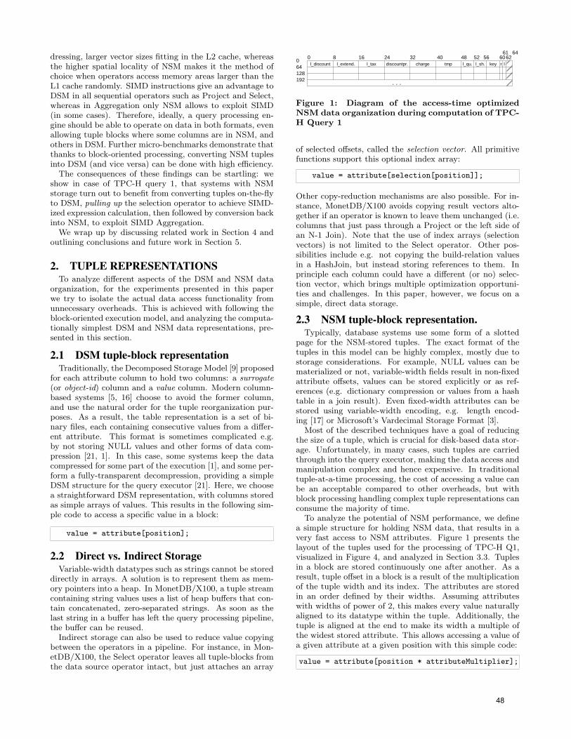
dressing, larger vector sizes fitting in the L2 cache, whereasthe higher spatial locality of NSM makes it the method ofchoice when operators access memory areas larger than theL1 cache randomly. SIMD instructions give an advantage toDSM in all sequential operators such as Project and Select,whereas in Aggregation only NSM allows to exploit SIMD(in some cases). Therefore, ideally, a query processing en-gine should be able to operate on data in both formats, evenallowing tuple blocks where some columns are in NSM, andothers in DSM. Further micro-benchmarks demonstrate thatthanks to block-oriented processing, converting NSM tuplesinto DSM (and vice versa) can be done with high efficiency.

The consequences of these findings can be startling: weshow in case of TPC-H query 1, that systems with NSMstorage turn out to benefit from converting tuples on-the-flyto DSM, pulling up the selection operator to achieve SIMD-ized expression calculation, then followed by conversion backinto NSM, to exploit SIMD Aggregation.

We wrap up by discussing related work in Section 4 andoutlining conclusions and future work in Section 5.

2. TUPLE REPRESENTATIONSTo analyze different aspects of the DSM and NSM data

organization, for the experiments presented in this paperwe try to isolate the actual data access functionality fromunnecessary overheads. This is achieved with following theblock-oriented execution model, and analyzing the computa-tionally simplest DSM and NSM data representations, pre-sented in this section.

2.1 DSM tuple-block representationTraditionally, the Decomposed Storage Model [9] proposed

for each attribute column to hold two columns: a surrogate(or object-id) column and a value column. Modern column-based systems [5, 16] choose to avoid the former column,and use the natural order for the tuple reorganization pur-poses. As a result, the table representation is a set of bi-nary files, each containing consecutive values from a differ-ent attribute. This format is sometimes complicated e.g.by not storing NULL values and other forms of data com-pression [21, 1]. In this case, some systems keep the datacompressed for some part of the execution [1], and some per-form a fully-transparent decompression, providing a simpleDSM structure for the query executor [21]. Here, we choosea straightforward DSM representation, with columns storedas simple arrays of values. This results in the following sim-ple code to access a specific value in a block:

value = attribute[position];

2.2 Direct vs. Indirect StorageVariable-width datatypes such as strings cannot be stored

directly in arrays. A solution is to represent them as mem-ory pointers into a heap. In MonetDB/X100, a tuple streamcontaining string values uses a list of heap buffers that con-tain concatenated, zero-separated strings. As soon as thelast string in a buffer has left the query processing pipeline,the buffer can be reused.

Indirect storage can also be used to reduce value copyingbetween the operators in a pipeline. For instance, in Mon-etDB/X100, the Select operator leaves all tuple-blocks fromthe data source operator intact, but just attaches an array

. . .

00 8 16 24 32 40 48 52 56 60

6162

64

64128192

l_discount l_tax charge tmp key r ll_extend. discountpr. l_qu. l_sh.

Figure 1: Diagram of the access-time optimizedNSM data organization during computation of TPC-H Query 1

of selected offsets, called the selection vector. All primitivefunctions support this optional index array:

value = attribute[selection[position]];

Other copy-reduction mechanisms are also possible. For in-stance, MonetDB/X100 avoids copying result vectors alto-gether if an operator is known to leave them unchanged (i.e.columns that just pass through a Project or the left side ofan N-1 Join). Note that the use of index arrays (selectionvectors) is not limited to the Select operator. Other pos-sibilities include e.g. not copying the build-relation valuesin a HashJoin, but instead storing references to them. Inprinciple each column could have a different (or no) selec-tion vector, which brings multiple optimization opportuni-ties and challenges. In this paper, however, we focus on asimple, direct data storage.

2.3 NSM tuple-block representation.Typically, database systems use some form of a slotted

page for the NSM-stored tuples. The exact format of thetuples in this model can be highly complex, mostly due tostorage considerations. For example, NULL values can bematerialized or not, variable-width fields result in non-fixedattribute offsets, values can be stored explicitly or as ref-erences (e.g. dictionary compression or values from a hashtable in a join result). Even fixed-width attributes can bestored using variable-width encoding, e.g. length encod-ing [17] or Microsoft’s Vardecimal Storage Format [3].

Most of the described techniques have a goal of reducingthe size of a tuple, which is crucial for disk-based data stor-age. Unfortunately, in many cases, such tuples are carriedthrough into the query executor, making the data access andmanipulation complex and hence expensive. In traditionaltuple-at-a-time processing, the cost of accessing a value canbe an acceptable compared to other overheads, but withblock processing handling complex tuple representations canconsume the majority of time.

To analyze the potential of NSM performance, we definea simple structure for holding NSM data, that results in avery fast access to NSM attributes. Figure 1 presents thelayout of the tuples used for the processing of TPC-H Q1,visualized in Figure 4, and analyzed in Section 3.3. Tuplesin a block are stored continuously one after another. As aresult, tuple offset in a block is a result of the multiplicationof the tuple width and its index. The attributes are storedin an order defined by their widths. Assuming attributeswith widths of power of 2, this makes every value naturallyaligned to its datatype within the tuple. Additionally, thetuple is aligned at the end to make its width a multiple ofthe widest stored attribute. This allows accessing a value ofa given attribute at a given position with this simple code:

value = attribute[position * attributeMultiplier];

48

0.1

1

10

100

1 32 1K 32K 1M

Nan

osec

onds

per

ope

ratio

n (lo

g sc

ale)

Vector size (tuples, log scale)

Global SUM primitive

DSM-SIMD DSM NSM-1 NSM-2

1 32 1K 32K 1M

Vector size (tuples, log scale)

Streaming ADD primitive

NSM-4 NSM-8 NSM-16 NSM-32

Figure 2: Sequential access: performance of the SUM and ADD routines with DSM and NSM and varyingtuple widths.

3. EXPERIMENTSIn this section we analyze the performance of NSM and

DSM data organization schemas on database performance.We start with a series of micro-benchmarks, presenting thebaseline performance on some basic data access and ma-nipulation activities. Then we demonstrate how these mi-crobenchmark results are confirmed during the processing ofthe TPC-H Query 1. There, we also discuss some optimiza-tion techniques, that depend heavily on data organization,as well as on-the-fly data conversion.

3.1 Experimental setupThe experimental platform used is a Core2 Quad Q6600

2.4GHz with 8GB RAM running Linux with kernel 2.6.23-15. The per-core cache sizes are: 16KB L1 I-cache, 16KB L1D-cache, 4MB L2 cache (shared among 2 cores). All experi-ments are single-core and in-memory. We used 2 compilers,GCC 4.1.22 and ICC 10.03.

We have performed similar experiments on a set of otherCPUs: Athlon 64 X2 3800+ (2GHz), Itanium 2 and SunNiagara. For Athlon and Itanium the results were mostlyin line with the Core2 results. On Niagara the performancebenefit of DSM was typically higher, and the impact of thedata location was lower. This is caused by lower perfor-mance of Niagara in terms of sequential execution: it has alower clock speed and in-order execution pipeline. Since Ni-agara was designed with multi-threaded processing in mind,it would be interesting to see how the presented, currentlysingle-threaded, benchmarks perform when running in par-allel. This might be a topic for future research.

3.2 MicrobenchmarksIn this section we analyze the baseline performance of

the DSM and NSM models in typical data-processing op-erations: sequential computations, random-access, and datacopying.

2compilation: gcc -O6 -Wall -g -mtune=core23compilation: icc -O3 -Wall -axT

3.2.1 Sequential data accessThe left part of Figure 2 present the results of the experi-

ment in which a SUM aggregate of a 4-byte integer column iscomputed repeatedly in a loop over a fixed dataset. The sizeof the data differs, to simulate different block sizes, which al-lows identifying the impact of the interpretation overhead,as well as the location (cache, memory) in block-orientedprocessing. We used GCC, using standard processing, andadditionally ICC to generate SIMD-ized DSM code (NSMdid not benefit from SIMD-ization). In the NSM imple-mentation, we use tuples consisting of a varying number ofintegers, represented with NSM-x.

To analyze the impact of the data organization on CPUefficiency, we look at the performance of NSM-1, which hasexactly the same memory access pattern and requirementsas the DSM implementation. The GCC results show thatfor a single-integer table the performance of the DSM andNSM-1 is very close. The small benefit of DSM, ca. 15%in the optimal case, comes from the fact that thanks to asimpler data access the compiler is able to generate slightlymore efficient code. However, with ICC-generated SIMDinstructions, DSM is a clear winner, being almost 5 timesfaster in the optimal case. Note that SIMD can only be ap-plied if the same operation is executed on adjacent memorylocations, therefore it can only be used in DSM.

The other aspect of this benchmark is the impact of theinterpretation overhead and data location. While for smallblock sizes the performance is dominated by the functioncalls4, for larger sizes, when the data does not fit in theL1 cache anymore, the data location aspect becomes cru-cial. Performance of NSM-1 and DSM without SIMD isrelatively flat, since even for main-memory sized data (1M+tuples), the sequential bandwidth is close enough to balancethe CPU activity. However, with the highly efficient (sub-cycle cost) SIMD DSM implementation, it operates fastestwhile the block still fits in the L1 CPU cache, then goes toan intermediate plateau when its fits L2, to become mem-

4In a real DBMS, function call overhead is significantlylarger [5] – this was a hard-coded micro-benchmark.

49

1

10

100

1 32 1K 32K 1MNan

osec

onds

per

ope

ratio

n (lo

g sc

ale)

Hash-table size (tuples, log scale)

1 column

DSMDSM prefetchedNSMNSM prefetched

1 32 1K 32K 1M

Hash-table size (tuples, log scale)

4 columns

DSMDSM prefetchedNSMNSM prefetched

1 32 1K 32K 1M

Hash-table size (tuples, log scale)

16 columns

DSMDSM prefetchedNSMNSM prefetched

Figure 3: Random access: running a grouped SUM aggregate on DSM input data, using a DSM or NSMhash table, with or without prefetching, and a varying number of GROUP BY keys (X-axis)

ory bandwidth limited for larger sizes (i.e. L1 bandwidthexceeds L2 bandwidth which exceeds RAM bandwidth).

Looking at the performance of wider NSM tuples, wesee that the performance degrades with the increasing tu-ple width. As long as the tuples are in L1, all widths areroughly equal. However, for NSM-16 and higher (64 bytetuples or longer) once the data shifts to L2, the impact isimmediately visible. This is caused by the fact, that only asingle integer from the entire cache-line is used. For NSM-2 to NSM-8, the results show that the execution is limitedby the L2 bandwidth: when a small fraction of a cache-lineis used (e.g. NSM-8) the performance is worse than whenmore integers are touched (e.g. NSM-2). Similar behaviorcan be observed for the main-memory datasets.

The SUM primitive has a relatively low memory demandcompared to the CPU activity, as it only consumes a sin-gle attribute. The right part of Figure 2 presents a similarexperiment, that uses an ADD routine which consumes twoattributes and produces a new result attribute. Results fol-low the trends of the SUM operation, but there are someimportant differences. First, the higher number of parame-ters passed to the NSM routine (pointers + tuple widths VSonly pointers) results in a higher interpretation overhead.Secondly, comparing DSM and NSM-1 for L1-resident data,shows that multiple more complex value-access computa-tions in NSM have a higher impact on the CPU performance.Finally, with a higher memory demand, the impact of datalocality on performance is significantly bigger, making eventhe DSM implementation fully memory-bound and in parwith the NSM-1 version.

Concluding, we see that if access is purely sequential,DSM outperforms NSM for multiple reasons. First, thearray-based structure allows simple value-access code. Sec-ond, individual primitive functions (e.g. SUM,ADD) usecache lines fully in DSM, and L2 bandwidth is enough tokeep up. As mentioned before, during query processing, alltuple blocks in use in a query plan should fit the CPU cache.If the target for this is L2, this means significantly largerblock sizes than if it were L1, resulting in reduced functioncall overhead. Finally, the difference in sequential process-ing between DSM and NSM can be huge if the operation isexpressible in SIMD, especially when the blocks fit in L1,and is still significant when in L2.

3.2.2 Random data accessFor this experiment, we use a table that consists of a single

key column and multiple data columns. The table contains4M tuples, is stored in DSM for efficient sequential access,number of data columns varies, and the range of the keycolumn differs from 1 to 4M. We perform an experimentequivalent to this SQL query:

SELECT SUM(data1), ..., SUM(dataN)FROM TABLE GROUP BY key;

To store the aggregate results, we use an equivalent of ahash-table in the hash-aggregation, but instead of the hash-value processing, we use the key column as a direct index.In DSM, the result table it is just a collection of arrays, onefor each data attribute. In NSM, it is a single array of asize equal to the number of tuples multiplied by the num-ber of data attributes. We apply block-oriented processing,using a block size of 256 tuples. In each iteration, all valuesfrom different data attributes are added to the respectiveaggregates, stored at the same vertical position in the table.

Figure 3 presents the results of this experiment for 1, 4and 16 data columns. For a single column, the faster accesscode of the DSM version makes it slightly (up to 10%) fasterthan NSM as long as the aggregate table fits in the L1 cache.Once it enters L2 or main memory, the results of DSM andNSM are equal as they are memory-latency limited.

For wider tuples, DSM maintains its advantage for L1-based key ranges. However, once the data expands into L2or main-memory, the performance of DSM becomes signifi-cantly worse than that of NSM. This is caused by the fact,that in DSM every memory access is expected to cause acache-miss. In contrast, in NSM, it can be expected thata cache-line accessed during processing of one data column,will be accessed again with the next data column in thesame block, as all the columns use the same key position.With the increasing number of computed aggregates, thesame cache-line is accessed more often, benefiting NSM overDSM.

Figure 3 also shows experiments that use software prefetch-ing, that is, we interspersed SUM computations with explicitprefetch instructions on the next tuple block. On Core2 weused the prefetcht0 instruction. We also made sure the ag-

50

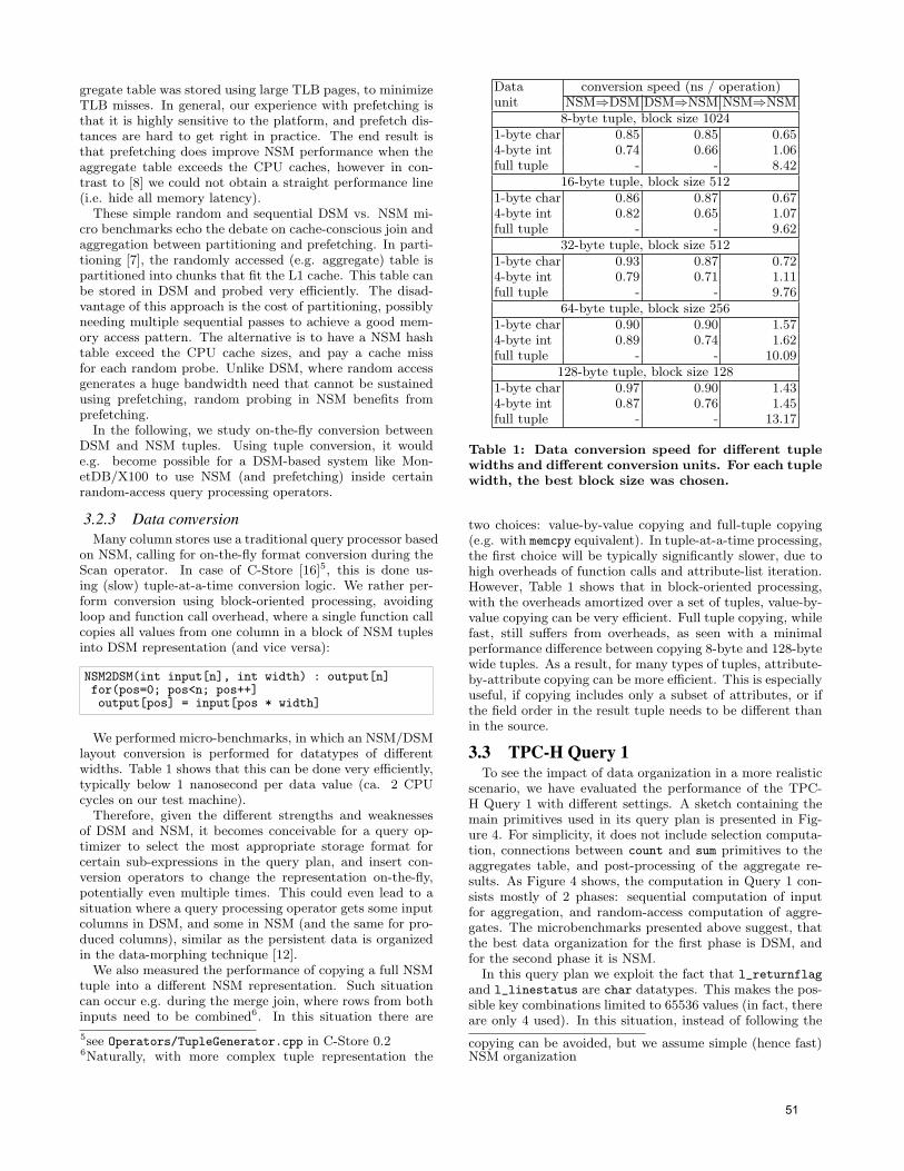
gregate table was stored using large TLB pages, to minimizeTLB misses. In general, our experience with prefetching isthat it is highly sensitive to the platform, and prefetch dis-tances are hard to get right in practice. The end result isthat prefetching does improve NSM performance when theaggregate table exceeds the CPU caches, however in con-trast to [8] we could not obtain a straight performance line(i.e. hide all memory latency).

These simple random and sequential DSM vs. NSM mi-cro benchmarks echo the debate on cache-conscious join andaggregation between partitioning and prefetching. In parti-tioning [7], the randomly accessed (e.g. aggregate) table ispartitioned into chunks that fit the L1 cache. This table canbe stored in DSM and probed very efficiently. The disad-vantage of this approach is the cost of partitioning, possiblyneeding multiple sequential passes to achieve a good mem-ory access pattern. The alternative is to have a NSM hashtable exceed the CPU cache sizes, and pay a cache missfor each random probe. Unlike DSM, where random accessgenerates a huge bandwidth need that cannot be sustainedusing prefetching, random probing in NSM benefits fromprefetching.

In the following, we study on-the-fly conversion betweenDSM and NSM tuples. Using tuple conversion, it woulde.g. become possible for a DSM-based system like Mon-etDB/X100 to use NSM (and prefetching) inside certainrandom-access query processing operators.

3.2.3 Data conversionMany column stores use a traditional query processor based

on NSM, calling for on-the-fly format conversion during theScan operator. In case of C-Store [16]5, this is done us-ing (slow) tuple-at-a-time conversion logic. We rather per-form conversion using block-oriented processing, avoidingloop and function call overhead, where a single function callcopies all values from one column in a block of NSM tuplesinto DSM representation (and vice versa):

NSM2DSM(int input[n], int width) : output[n]for(pos=0; pos<n; pos++]output[pos] = input[pos * width]

We performed micro-benchmarks, in which an NSM/DSMlayout conversion is performed for datatypes of differentwidths. Table 1 shows that this can be done very efficiently,typically below 1 nanosecond per data value (ca. 2 CPUcycles on our test machine).

Therefore, given the different strengths and weaknessesof DSM and NSM, it becomes conceivable for a query op-timizer to select the most appropriate storage format forcertain sub-expressions in the query plan, and insert con-version operators to change the representation on-the-fly,potentially even multiple times. This could even lead to asituation where a query processing operator gets some inputcolumns in DSM, and some in NSM (and the same for pro-duced columns), similar as the persistent data is organizedin the data-morphing technique [12].

We also measured the performance of copying a full NSMtuple into a different NSM representation. Such situationcan occur e.g. during the merge join, where rows from bothinputs need to be combined6. In this situation there are

5see Operators/TupleGenerator.cpp in C-Store 0.26Naturally, with more complex tuple representation the

Data conversion speed (ns / operation)unit NSM⇒DSM DSM⇒NSM NSM⇒NSM

8-byte tuple, block size 10241-byte char 0.85 0.85 0.654-byte int 0.74 0.66 1.06full tuple - - 8.42

16-byte tuple, block size 5121-byte char 0.86 0.87 0.674-byte int 0.82 0.65 1.07full tuple - - 9.62

32-byte tuple, block size 5121-byte char 0.93 0.87 0.724-byte int 0.79 0.71 1.11full tuple - - 9.76

64-byte tuple, block size 2561-byte char 0.90 0.90 1.574-byte int 0.89 0.74 1.62full tuple - - 10.09

128-byte tuple, block size 1281-byte char 0.97 0.90 1.434-byte int 0.87 0.76 1.45full tuple - - 13.17

Table 1: Data conversion speed for different tuplewidths and different conversion units. For each tuplewidth, the best block size was chosen.

two choices: value-by-value copying and full-tuple copying(e.g. with memcpy equivalent). In tuple-at-a-time processing,the first choice will be typically significantly slower, due tohigh overheads of function calls and attribute-list iteration.However, Table 1 shows that in block-oriented processing,with the overheads amortized over a set of tuples, value-by-value copying can be very efficient. Full tuple copying, whilefast, still suffers from overheads, as seen with a minimalperformance difference between copying 8-byte and 128-bytewide tuples. As a result, for many types of tuples, attribute-by-attribute copying can be more efficient. This is especiallyuseful, if copying includes only a subset of attributes, or ifthe field order in the result tuple needs to be different thanin the source.

3.3 TPC-H Query 1To see the impact of data organization in a more realistic

scenario, we have evaluated the performance of the TPC-H Query 1 with different settings. A sketch containing themain primitives used in its query plan is presented in Fig-ure 4. For simplicity, it does not include selection computa-tion, connections between count and sum primitives to theaggregates table, and post-processing of the aggregate re-sults. As Figure 4 shows, the computation in Query 1 con-sists mostly of 2 phases: sequential computation of inputfor aggregation, and random-access computation of aggre-gates. The microbenchmarks presented above suggest, thatthe best data organization for the first phase is DSM, andfor the second phase it is NSM.

In this query plan we exploit the fact that l_returnflag

and l_linestatus are char datatypes. This makes the pos-sible key combinations limited to 65536 values (in fact, thereare only 4 used). In this situation, instead of following the

copying can be avoided, but we assume simple (hence fast)NSM organization

51

sub

100 l_discount

tmp l_extendedprice 100 l_tax l_returnflag

mul

256

addmul

discountprice tmp key l_linestatus

addmul

charge l_quantity key

countsumsumsumsumsum

Random−access aggregate processing

Sequential computations

Figure 4: Simplified plan of TPC-H Query 1 (omit-ted date selection, links to the aggregates table, andpost-aggregation computations)

traditional hash-table based processing, we use direct aggre-gation [5], in which the position in the aggregates table iscomputed directly from the key attributes. Since the origi-nal Query 1 only uses 4 GROUP BY key combinations, we alsotested a slightly modified version of it that adds a 3rd ex-

trakey column, and artificially fills all three key columns tosimulate different numbers of GROUP BY combinations.

3.3.1 Pull Selections UpIn DSM, calculations on simple directly addressed arrays

(i.e. without selection vector) are amendable for SIMD-ization, hence execute significantly faster. Therefore, if aSelect does not eliminate many tuples and is followed bycomputation (e.g. a Project), it becomes beneficial to firstdo the calculations with SIMD, and the selection only after-wards. This counter-intuitive “pull selections up” strategy isin fact applicable to TPC-H Q1. Note that for this optimiza-tion, it is not strictly necessary to put the Select on top ofthe Project. In MonetDB/X100, the Select is still executedfirst, but for each tuple-block by looking at the selectivity(the length of the selection vector m) Project primitives maychoose to ignore the selection vector sel and compute resultsfor all n tuples, benefiting from SIMD:

ADD(long a1[n],a2[n]; int sel[m]): int output[n]if (m > n/2) // if many selected, compute on allfor(pos=0; pos<n; pos++)output[pos] = ADD(a1[pos],a2[pos]) // SIMD

elsefor(idx=0; idx<n; idx++)pos = sel[idx]output[pos] = ADD(a1[pos],a2[pos])

In fact, this performance boost makes it beneficial for a planthat starts with NSM tuples to switch to DSM.

3.3.2 SIMD AggregationAnother SIMD optimization concerns grouped aggrega-

tion in NSM. If multiple identical aggregate functions mustbe computed (e.g. TPC-H Q1 has 5 grouped SUMs), we canSIMD-ize the aggregate update operation. This means thatwe have a primitive SUM2 function, that sums two adjacentNSM columns of 64-bit longs (its start pointer is denoted

col2 here) with two adjacent 64-bits aggregate totals (tot2):

SUM2(long tot2[m],col2[n]; int grp[n],w1,w2)for(pos=0;pos<n;pos++)simd_t* dst = (simd_t*) (tot2 + w2*group[pos])simd_t* src = (simd_t*) (col2 + w1*pos)*dst = SIMD_ADD2_LONG(*dst, *src)

As grouped aggregation takes more than half of the execu-tion time in TPC-H Q1, applying SIMD here significantlyaffects performance. In fact, SIMD Aggregation makes itbeneficial to switch back from DSM to NSM after the cal-culations to profit from SIMD.

3.3.3 On-the-Fly NSM/DSM ConversionsWe run TPC-H on data that is in both NSM and DSM

storage layouts, but consider switching layout before andafter doing the calculations (i.e. Select and Project). Also,the format of the aggregate table can be DSM or NSM.

The results of the experiment, presented in Figure 5, con-firm the trends from the micro-benchmarks. The DSM-formatted input (A,B,C) achieves significantly better per-formance. However, the DSM-formatted hash table suffersfrom random memory accesses (A,D,E). Using an NSM hashtable removes this problem (B,G), and converting the DSMdata on the fly into NSM allows to perform SIMD-basedaggregation, further improving the performance (C,H). ForNSM input we see that converting it into DSM allows fastersequential computation (E,G). For additional analysis of theperformance, Table 2 presents the profiling of different sce-narios for a case with 32K unique GROUP BY keys. It shows,that the extra data conversion before doing the projectionand the aggregation phase can be in some cases more thanbalanced by the performance improvement gained in the fol-lowing computation.

The performance benefits presented in this section are lim-ited due to a fact that most of the computation is based on8-byte integers. The currently available SSE3 SIMD instruc-tion set provides only 128-bit SIMD operations, allowing just2 operations to be executed at once. Since SIMD function-ality is continuously improving, we expect these gains tobecome more significant in the future.

4. RELATED WORKBlock-oriented processing [15, 5] recently gained popu-

larity as a technique to improve query processor efficiency.Traditionally, its main goal was to reduce the number offunction calls [15]. Further research demonstrated that italso can result in a much higher CPU instruction cachehit-ratio [19]. Block-oriented processing is also an enablingtechnique for different performance optimizations that re-quire multiple tuples to work on: exploiting SIMD instruc-tions [18], memory-prefetching [8], and performing efficientdata (de)compression [20].

The trade-offs between NSM and DSM as disk storage for-mats were analyzed in [13], where it is demonstrated thatDSM performs better when only a fraction of the attributesis accessed. In contrast to what our paper proposes, thesystem described in [13] forces a conversion of DSM dataon disk into NSM before entering the block-oriented itera-tor pipeline, allowing DSM layout only in the early scan-select stages. Avoiding early materialization of NSM tuplesin column stores also was the topic of [2], but this workstill requires forming NSM tuples at some moment in the

52

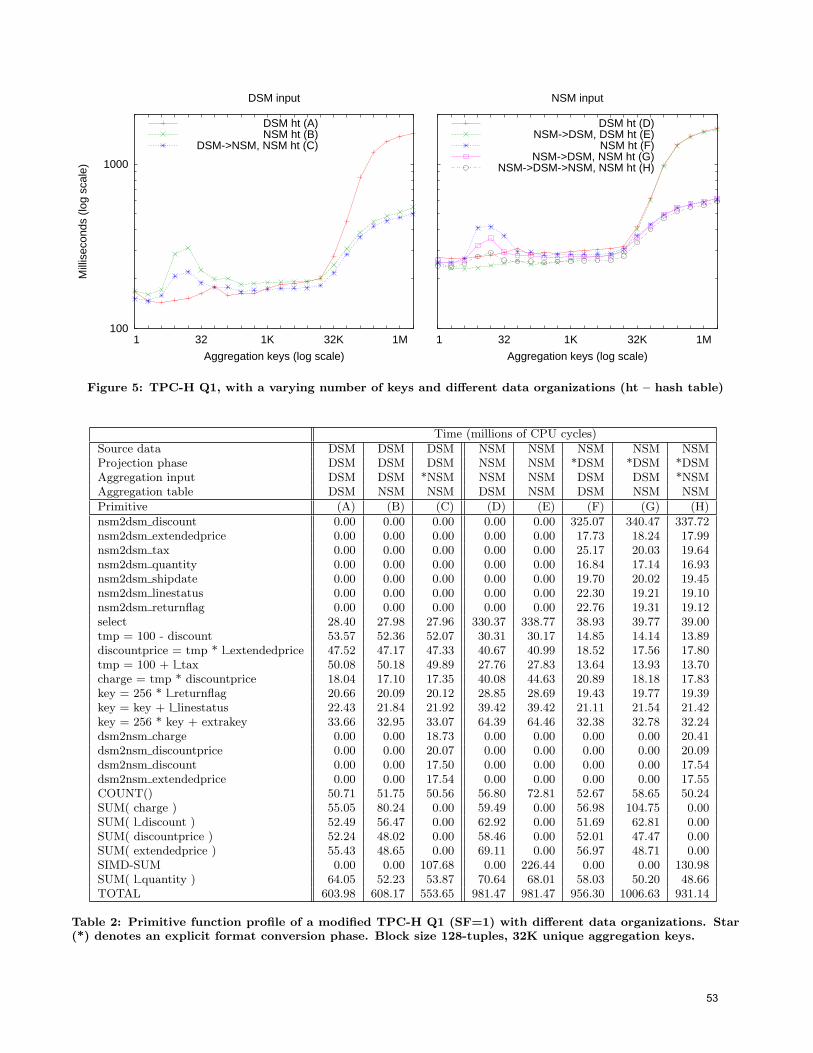
100

1000

1 32 1K 32K 1M

Mill

isec

onds

(lo

g sc

ale)

Aggregation keys (log scale)

DSM input

DSM ht (A)NSM ht (B)

DSM->NSM, NSM ht (C)

1 32 1K 32K 1M

Aggregation keys (log scale)

NSM input

DSM ht (D)NSM->DSM, DSM ht (E)

NSM ht (F)NSM->DSM, NSM ht (G)

NSM->DSM->NSM, NSM ht (H)

Figure 5: TPC-H Q1, with a varying number of keys and different data organizations (ht – hash table)

Time (millions of CPU cycles)

Source data DSM DSM DSM NSM NSM NSM NSM NSMProjection phase DSM DSM DSM NSM NSM *DSM *DSM *DSMAggregation input DSM DSM *NSM NSM NSM DSM DSM *NSMAggregation table DSM NSM NSM DSM NSM DSM NSM NSM

Primitive (A) (B) (C) (D) (E) (F) (G) (H)

nsm2dsm discount 0.00 0.00 0.00 0.00 0.00 325.07 340.47 337.72nsm2dsm extendedprice 0.00 0.00 0.00 0.00 0.00 17.73 18.24 17.99nsm2dsm tax 0.00 0.00 0.00 0.00 0.00 25.17 20.03 19.64nsm2dsm quantity 0.00 0.00 0.00 0.00 0.00 16.84 17.14 16.93nsm2dsm shipdate 0.00 0.00 0.00 0.00 0.00 19.70 20.02 19.45nsm2dsm linestatus 0.00 0.00 0.00 0.00 0.00 22.30 19.21 19.10nsm2dsm returnflag 0.00 0.00 0.00 0.00 0.00 22.76 19.31 19.12select 28.40 27.98 27.96 330.37 338.77 38.93 39.77 39.00tmp = 100 - discount 53.57 52.36 52.07 30.31 30.17 14.85 14.14 13.89discountprice = tmp * l extendedprice 47.52 47.17 47.33 40.67 40.99 18.52 17.56 17.80tmp = 100 + l tax 50.08 50.18 49.89 27.76 27.83 13.64 13.93 13.70charge = tmp * discountprice 18.04 17.10 17.35 40.08 44.63 20.89 18.18 17.83key = 256 * l returnflag 20.66 20.09 20.12 28.85 28.69 19.43 19.77 19.39key = key + l linestatus 22.43 21.84 21.92 39.42 39.42 21.11 21.54 21.42key = 256 * key + extrakey 33.66 32.95 33.07 64.39 64.46 32.38 32.78 32.24dsm2nsm charge 0.00 0.00 18.73 0.00 0.00 0.00 0.00 20.41dsm2nsm discountprice 0.00 0.00 20.07 0.00 0.00 0.00 0.00 20.09dsm2nsm discount 0.00 0.00 17.50 0.00 0.00 0.00 0.00 17.54dsm2nsm extendedprice 0.00 0.00 17.54 0.00 0.00 0.00 0.00 17.55COUNT() 50.71 51.75 50.56 56.80 72.81 52.67 58.65 50.24SUM( charge ) 55.05 80.24 0.00 59.49 0.00 56.98 104.75 0.00SUM( l discount ) 52.49 56.47 0.00 62.92 0.00 51.69 62.81 0.00SUM( discountprice ) 52.24 48.02 0.00 58.46 0.00 52.01 47.47 0.00SUM( extendedprice ) 55.43 48.65 0.00 69.11 0.00 56.97 48.71 0.00SIMD-SUM 0.00 0.00 107.68 0.00 226.44 0.00 0.00 130.98SUM( l quantity ) 64.05 52.23 53.87 70.64 68.01 58.03 50.20 48.66TOTAL 603.98 608.17 553.65 981.47 981.47 956.30 1006.63 931.14

Table 2: Primitive function profile of a modified TPC-H Q1 (SF=1) with different data organizations. Star(*) denotes an explicit format conversion phase. Block size 128-tuples, 32K unique aggregation keys.

53

query plan. Comparing DSM and NSM execution is alsothe focus of a recent paper [10], though the methodology isa high-level systems comparison without investigating theinteraction with computer architecture.

Some performance analysis of DSM and NSM data struc-tures has been presented in [11] where the authors propose“super-tuples” for both rows and columns. Related researchis PAX [4], a storage format that combines low NSM costsfor getting a single tuple from disk with good cache behaviorof ”thinner” DSM storage. In memory PAX is almost equiv-alent to DSM (the only difference is a possible impact on thepossible block sizes), it has the same properties during theprocessing. The PAX idea has been generalized in [12] in thedata-morphing technique, that allows part of the attributesin a given disk page to be stored in DSM and part in NSM,depending on the query load. This research, focused onlyon persistent data reorganization based on the query load.Our technique goes further, by proposing dynamic reorga-nization of transient, in-flight data.

On many architectures, SIMD instructions expect the in-put data to be stored in simple arrays, as in DSM. Sincemost database systems work on NSM, the potential of SIMDcan often not be used. Notable exceptions include [18], aswell as the family of MonetDB processing kernels [6, 5].SIMD instructions are also becoming more relevant due toappearance of architectures such as Cell that provide SIMDonly [14]. Interestingly, in this context it was already shownthat grouped aggregates can only be SIMD-ized when usinga NSM-like data organization (array of structures).

5. CONCLUSIONS AND FUTURE WORKWe have shown how different tuple layouts in the pipeline

of a block-oriented query processor can strongly influenceperformance. For sequential access, DSM is the best repre-sentation, usually as long as the tuple blocks fit L2; DSMalso wins for random access inside L1. If a sequential op-erator is amendable for SIMD-ization, this causes DSM tostrongly outperform NSM; the difference sometimes evenmaking it profitable to pull selections upwards to keep datadensely organized for SIMD. NSM, on the other hand, ismore efficient for random access operations (hash join, ag-gregation) into memory regions that do not fit L1. UnlikeDSM, random access memory latency to NSM can be hiddenusing software prefetching. Finally, grouped Aggregation al-lows SIMD calculations only in case of NSM.

This means that it depends on the query which data lay-out is the most efficient in a given part of the plan. With theconversion between NSM and DSM being relatively cheap,we show that query plans such as TPC-H Q1 can be ac-celerated by using both formats with on-the-fly conversions.Therefore, we think that this work opens the door for futureresearch into making tuple layout planning a query opti-mizer task. Additionally, more complex data representationsshould be investigated, including mixing NSM and DSM inone data block, as well as using indirect data storage.

6. REFERENCES[1] D. Abadi, S. Madden, and M. Ferreira. Integrating

Compression and Execution in Column-OrientedDatabase Systems. In SIGMOD, 2006.

[2] D. J. Abadi, D. S. Myers, D. J. DeWitt, and S. R.Madden. Materialization Strategies in aColumn-Oriented DBMS. In ICDE, 2007.

[3] S. Agarwal and H. Daeubler. Reducing Database Sizeby Using Vardecimal Storage Format. Microsoft, 2007.

[4] A. Ailamaki, D. J. DeWitt, M. D. Hill, andM. Skounakis. Weaving Relations for CachePerformance. In VLDB, Rome, Italy, 2001.

[5] P. Boncz, M. Zukowski, and N. Nes. MonetDB/X100:Hyper-Pipelining Query Execution. In CIDR, 2005.

[6] P. A. Boncz. Monet: A Next-Generation DBMSKernel For Query-Intensive Applications. Ph.d. thesis,Universiteit van Amsterdam, May 2002.

[7] P. A. Boncz, S. Manegold, and M. L. Kersten.Database Architecture Optimized for the NewBottleneck: Memory Access. In VLDB, pages 54–65,Edinburgh, 1999.

[8] S. Chen, A. Ailamaki, P. B. Gibbons, and T. C.Mowry. Improving hash join performance throughprefetching. ACM Trans. Database Syst., 32(3):17,2007.

[9] A. Copeland and S. Khoshafian. A DecompositionStorage Model. In SIGMOD, Austin, TX, USA, 1985.

[10] N. H. Daniel J. Abadi, Samuel R. Madden.Column-Stores vs. Row-Stores: How Different AreThey Really? In SIGMOD, Vancouver, Canada, 2008.

[11] A. Halverson, J. L. Beckmann, J. F. Naughton, andD. J. DeWitt. A Comparison of C-Store andRow-Store in a Common Framework. Technical ReportTR1570, University of Wisconsin-Madison, 2006.

[12] R. A. Hankins and J. M. Patel. Data Morphing: AnAdaptive, Cache-Conscious Storage Technique. InVLDB, pages 417–428, Berlin, Germany, 2003.

[13] S. Harizopoulos, V. Liang, D. Abadi, and S. Madden.Performance Tradeoffs in Read-Optimized Databases.In VLDB, 2006.

[14] S. Heman, N. Nes, M. Zukowski, and P. Boncz.Vectorized Data Processing on the Cell BroadbandEngine. In DAMON, 2007.

[15] S. Padmanabhan, T. Malkemus, R. Agarwal, andA. Jhingran. Block Oriented Processing of RelationalDatabase Operations in Modern ComputerArchitectures. In ICDE, Heidelberg, Germany, 2001.

[16] M. Stonebraker, D. J. Abadi, A. Batkin, X. Chen,M. Cherniack, M. Ferreira, E. Lau, A. Lin, S. Madden,E. J. O’Neil, P. E. O’Neil, A. Rasin, N. Tran, andS. B. Zdonik. C-Store: A Column-oriented DBMS. InVLDB, Trondheim, Norway, 2005.

[17] T. Westmann, D. Kossmann, S. Helmer, andG. Moerkotte. The implementation and performanceof compressed databases. SIGMOD Record,29(3):55–67, September 2000.

[18] J. Zhou and K. A. Ross. Implementing databaseoperations using SIMD instructions. In SIGMOD,Madison, USA, 2002.

[19] J. Zhou and K. A. Ross. Buffering Accesses toMemory-Resident Index Structures. In VLDB, Berlin,Germany, 2003.

[20] M. Zukowski, S. Heman, and P. Boncz.Architecture-Conscious Hashing. In DAMON,Chicago, IL, USA, 2006.

[21] M. Zukowski, S. Heman, N. Nes, and P. Boncz.Super-Scalar RAM-CPU Cache Compression. InICDE, Atlanta, GA, USA, 2006.

54