Forward modeling and retrieval of water vapor from the Global Ozone Monitoring Experiment: Treatment...

Forward modeling and retrieval of water vapor from the Global

Ozone Monitoring Experiment:

Treatment of narrowband absorption spectra

Rudiger Lang,1,2 Ahilleas N. Maurellis,3 and Wim J. van der ZandeFOM Institute for Atomic and Molecular Physics, Amsterdam, Netherlands

Ilse Aben and Jochen LandgrafSRON National Institute for Space Research, Utrecht, Netherlands

Wim UbachsDepartment of Physics and Astronomy, Vrije Universiteit, Amsterdam, Netherlands

Received 1 November 2001; revised 10 December 2001; accepted 10 December 2001; published 27 August 2002.

[1] We present the algorithm and results for a new fast forward modeling techniqueapplied to the retrieval of atmospheric water vapor from satellite measurements using aweak ro-vibrational overtone band in the visible. The algorithm uses an OpticalAbsorption Coefficient Spectroscopy (OACS) method which is well suited to situationswhere line widths in the absorption spectrum are much narrower than the instrumentalresolution and where efficient numerical solutions of the equation of radiative transfer areneeded. We present examples of OACS forward modeled reflectivity which include thedifferential contribution of singly scattered photons and compare them with spectralmeasurements of the Global Ozone Monitoring Experiment (GOME). In particular, weapply OACS to the retrieval of water vapor column (WVC) densities from GOME spectraldata between 585 and 600 nm. Method precisions are better than 0.7% for high and betterthan 3.4% for low WVC. The total accuracy of the retrieval method appears to be betterthan 0.8 and 4% for high and low WVC, respectively. The retrieval results are compared toWVC values given by European Centre for Medium-Range Weather Forecasts and SpecialSensor Microwave Imager and allow us to conclude that the OACS retrieval method isreliable except in cloud-rich situations. In cloud-free cases, an upper limit of 18% error onthe retrieved WVC due to the impact of multiple and aerosol scattering as well as aerosolextinction is estimated. In addition, the accuracy of the retrieval is sufficient to permit thedetection of systematic differential fit mismatches between modeled and real GOMEspectra. The magnitude of such mismatches places an upper limit on the accuracy ofHITRAN’96 water vapor line strength values of about 10–20%. INDEX TERMS: 0933

Exploration Geophysics: Remote sensing; 0360 Atmospheric Composition and Structure: Transmission and

scattering of radiation; 0365 Atmospheric Composition and Structure: Troposphere—composition and

chemistry; 3210 Mathematical Geophysics: Modeling; 3260 Mathematical Geophysics: Inverse theory;

KEYWORDS: water vapor, retrieval, GOME, sampling technique, spectroscopy

1. Introduction

[2] Spectroscopic measurements from satellite-basedinstruments covering relatively broad wavelength regionsmay be used to affect column and vertical profile retrieval

for many different atmospheric constituents. The GlobalOzone Monitoring Experiment (GOME) spectrometer onthe European Space Agency’s ERS-2 satellite [EuropeanSpace Agency (ESA), 1995; Burrows et al., 1999] covers awavelength region between 240 and 790 nm. In this wave-length region absorption bands of many constituents suchas, for example, O2, NO2, H2O, O3, (O2)2, and OClO aremeasurable. Column concentration retrieval is routinelycarried out for O3 and NO2 (level 2 products). Importantinformation about OClO, volcanic SO2, H2CO from bio-mass burning and tropospheric BrO, has also been delivered[Thomas et al., 1998].[3] The Scanning Imaging Absorption Spectrometer for

Atmospheric Cartography (SCIAMACHY) [Bovensmann

JOURNAL OF GEOPHYSICAL RESEARCH, VOL. 107, NO. D16, 10.1029/2001JD001453, 2002

1Also at Space Research Organization Netherland, Utrecht, Nether-lands.

2Also at Department of Physics and Astronomy, Vrije Universiteit,Amsterdam, Netherlands.

3Now at SRON National Institute for Space Research, Utrecht,Netherlands.

Copyright 2002 by the American Geophysical Union.0148-0227/02/2001JD001453$09.00

ACH 11 - 1

et al., 1999] will be launched on ENVISAT in 2001 and willextend wavelength coverage into the near infrared up to1750 nm while adding two additional channels in regionsbetween 1.9 and 2.4 microns. Thus GOME’s list of targetedspecies will be extended to include CO, CO2, N2O and CH4.The absorption features of some of these gases are oftencontaminated by strong water vapor absorption bands[Schrijver, 1999; Buchwitz et al., 2000]. Retrieval of suchspecies would thus require fast forward modeling of thewater vapor using the results of a sensitive retrieval methodretrieving water vapor column (WVC) concentrations, forexample in the visible region of the instrument.[4] This paper focuses on the retrieval of WVC from

GOME measurements in the visible between 585 and600 nm. This relatively weak absorption window was firstdescribed by Maurellis et al. [2000a]. It contains additionalabsorption features due to sodium, the ozone Chappuisband, the (O2)2 collision complex, which we account forin this work as well as a weak contribution of NO2. Incontrast, the most prominent water vapor absorption bandcovered by the GOME detectors is at 720 nm. This bandcontains, on average, features which are up to an order ofmagnitude more optically dense than the strongest featuresin the weak 590 nm band. Nevertheless, we expect that thereflectivity measured in the 720 nm region is less sensitiveto changes in pressure and temperature over altitude. Due tothe strong absorption in the line center and the strongoverlap of the line wings in the lower troposphere, at highpressures and high water vapor content, the 720 nm regionis less sensitive to changes in WVC. In this paper wepresent a new method called Optical Absorption CoefficientSpectroscopy (OACS) which allows both for fast andaccurate forward modeling of GOME reflectivity measure-ments affected by water vapor absorption as well asrelatively fast retrievals of WVC.[5] Until recently the retrieval of WVC from GOME

measurements was not successful without the introductionof substantial modification [Noel et al., 1999; Casadio etal., 2000] to differential methods such as the DifferentialOptical Absorption Spectroscopy method (DOAS) [Platt,1994, 1999] used for the retrieval of GOME level 2products [Burrows et al., 1999]. In principle DOAS oper-ates by separating out the broadband absorption structuredue to elastic scattering or broadband absorption from thedifferential structure of the trace gas under study in order tofit Beer’s Law to a measured reflectivity spectrum. DOASoffers a good compromise between speed, numerical accu-racy and instrument performance and has repeatedly provenits usefulness for many molecular species. However it isfrequently combined with a simple arithmetic wavelength-averaging of optical densities for broadband absorbers inorder to establish a linear dependence between the loga-rithm of the measured reflectivity and the fit parameters[Marquard et al., 2000; Burrows et al., 1999]. In this case,the retrieval of the atmospheric water vapor concentrationswould result in a systematic underestimation of the expectedWVC due to an inadequate sampling of highly varyingoptical densities by a single detector pixel [Maurellis et al.,2000a, 2000b]. In addition, discrepancies may also arise outof inadequate treatment of air mass factors used to accountfor the contribution of atmospheric scattering [Noel et al.,1999; Casadio et al., 2000].

[6] It is important to make the distinction between narrow-band and broadband absorbers in the context of a spectralfitting window in order to separate the reflectivity contribu-tion of absorbers with strong differential structure from therelatively smooth background. In addition to coping withintrinsic spectral complexity the retrieval of atmospherictrace gas columns also requires accurate spectral informationas well as spectrometers which operate at sufficient spectralresolution. However, spectral coverage (i.e., the potential toretrieve a wide variety of atmospheric constituents using asingle instrument) usually has to be compromised by areduction in spectral resolution. For example, two lineararray detectors with 1024 detector pixels each are neededin order to cover thewavelength range of theOzone Chappuisband between 400 and 800 nm using the GOME instrument(channel three and four), where each detector pixel covers awavelength range of about 0.2 nm. The spectral sampling issufficient to resolve spectral absorption features of manyspecies especially in the near ultraviolet where line-broad-ening by predissociation of excited molecular states causesthe optical density to vary little within the span of a singledetector pixel (for example in the case of ozone). In contrast,many species with absorption bands in the visible and near-infrared (for example, water vapor, NO2, methane, or atomicspecies like sodium) lack smoothing from line-broadeningand may contain a number of distinct absorption lines withinthe wavelength region covered by one detector pixel. Thisalso holds for wide parts of the solar irradiance spectrum overthe entire ultraviolet and visible regions which containsnarrowband Fraunhofer absorption lines.[7] The fast forward modeling and retrieval method

presented here focuses on the problem of spectral samplingin cases of such narrowband absorption spectra. This meansthat the spectral width of the instrumental function and thesampling width of the detector is much broader than thewidth of a single absorption line. In such cases a convolutionand sampling integral over the modeled highly structuredreflectivity spectra has to be introduced when modeling thespectra measured by an instrument with insufficient sam-pling capacity. The proposed Optical Absorption CoefficientMethod (OACS) shows that this problem can be solvedaccurately and with sufficient efficiency that, using opera-tional data from GOME in the visible, the water vaporcolumn (WVC) retrieved is comparable to other fundamentaldifferent satellite measurement techniques and data assim-ilation models [Vesperini, 1998; Chaboureau et al., 1998].[8] The problem of the treatment has also been dealt with

by a new Spectral Structure Parameterization (SSP) method[Maurellis et al., 2000b]. In the latter work it was shownthat the complexity of spectra ranging from single lineabsorption to broadband absorption may be characterized,to second order in accuracy, by a simple parameterizationscheme. In what follows we show that the OACS retrievalmethod permits both fast and accurate forward modeling ofreflectivities as well as relatively fast retrievals of trace gasconcentrations.[9] In principle, an OACS retrieval method could take

advantage of the DOAS method in the sense that it couldutilize a first-order polynomial in order to account for theunknown surface albedo as well as the non-structuredbackground contribution of atmospheric scattering. How-ever, in order to account for the contribution of single-

ACH 11 - 2 LANG ET AL.: RETRIEVAL OF WATER VAPOR FROM GOME

scattered photons, we show that a more accurate represen-tation can be obtained in the form of an additional OACSterm derived from the solution of the equation of radiativetransfer. However, the contribution of multiple scattering canbe significant in the visible region covered by this instrument.Therefore a polynomial similar to the one used in standardDOAS methods is introduced to account for the broadbandcontribution of multiple-scattered photons. The influence ofthe neglected differential contribution of the latter on themodeled reflectivities as well as fit residuals and retrievedWVCs has to be estimated and discussed in some detail.However, apart from these assumptions, OACS already dis-plays the ability to retrieve WVCs for low cloud coversituations with an accuracy of state-of-the-art products likethe ones from the European Center of Medium RangeWeather Forecast (ECMWF) and the Special Sounder Micro-wave Imager (SSM/I). In addition, this first extensive studyretrieving water vapor from GOME operational data in thevisible shows the potential of OACS to be applied to WVCretrieval from the forthcoming SCIAMACHY instrumentespecially in the infrared.[10] In section 2 we introduce the radiation transport

scheme on which OACS is based together with the mathe-matical formulation of the method. Section 4 Measurementsbriefly describes the GOME instrument performance andhow GOME-measured earth radiances and solar irradiancesare handled for the purposes of WVC retrieval. The issue ofundersampling and the specific definition of reflectivityused for retrievals from GOME data are also presented. Insection 5 the HITRAN’96 water vapor line-strength valuesused in the OACS method are described in some detail sincethe method’s sensitivity to changes in the reflectivity withrespect to the cross-section of the trace gas under studyrequires an accurate knowledge of the line parameters andtheir dependence on the pressure and temperature for aspecific geolocation. A retrieval of WVCs from an entirewater vapor absorption band requires accurate modeling ofall additional absorbers within this band in order to preventthe fit from confusing part of the instrumentally smoothedwater vapor absorption spectrum with the background. Anintroduction in the modeling of this background togetherwith a description of the required input data is also given insection 5. Section 6 estimates the intrinsic OACS method-related error due to the specific sampling of the intensities.Section 7 describes the forward modeling of GOME spectralmeasurements using the OACS method. The results arecompared to an independent solution of the equation ofradiative transfer using a doubling-adding model (DAM)[de Haan et al., 1987]. In section 8 the effect on the retrievedWVC due to the differential contribution of photons scat-tered more than once in the atmosphere (multiple scattering)as well as aerosol scattering and absorption are discussedand quantified using results of the DAM model. In section 9we estimate the precision and the accuracy of the method byretrieving WVCs from artificial absorption spectra which areforward modeled using a lbl calculation. Here we alsopresent a study of the influence of multiple scattering andaerosol loading on the retrieved WVC. The results of WVC-retrieval from three different GOME tracks are presented insection 10. In this section we also discuss the impact ofdifferential fit mismatches on the residuals and the retrievedWVCs which we relate predominantly to instrumental errors

and to errors in the water vapor line-strength values takenfrom the HITRAN’96 database. A preliminary validation ofthe OACS retrieval results using ECMWF and SSM/I data isset out in section 11. The latter is discussed in conjunctionwith the effect of clouds. Finally, in section 12, we focus onpotential implementation of the OACS method in routineretrieval and its use for forward modeling of water vaporabsorption bands in spectral regions containing narrowbandabsorption features other than water vapor.

2. Radiative Transfer

[11] The transport equation of scalar radiative transfer inits plane parallel approximation is given by

mdIl

dzðz;�Þ ¼ �bextðzÞfIlðz;�Þ � Jlðz;�Þg ð1Þ

where Il is the specific intensity field for a given wavelengthl, Jl is the corresponding source function and bext is theextinction coefficient (see Table 1). Further, z represents thealtitude and � is the direction of the intensity field with � =(u, j), where m = |u| is the cosine of the zenith angle. Il issubject to boundary conditions at the top and bottom of theatmosphere (z = 0 and ztop), respectively, of the form

Ilðztop;��Þ ¼ 0 ð2Þ

Ilð0;�þÞ ¼lpF# ð3Þ

for which we have assumed isotropic ground reflection by aLambertian surface with an albedo �. Here, �+ and ��indicate upward and downward directions, respectively, andF# is the downward flux at the lower boundary of theatmosphere,

F# ¼Z��

Ið0;�Þ m d�: ð4Þ

Table 1. Summary of Some of the Most Important Notations Used

in This Paper

Sign Description

k A. c.a with broadband X-s.b

f A. c. with narrowband X-s.

‘ Atmospheric layer

mo, m Incoming and outgoing angle cosinej Detector pixel numberi Cross-section bin

�að‘Þij

Alpha value interpolated in p, T

xi X-s. bin center value� Instrument slit-width�l Detector pixel widthg WV-line HWHMdl Grid size reference spectraI, I0 Specific intensitiesR Reflectivity (=(p/mo)I/I0)� Surface albedo

Sn Line-strength

�f Differential fit mismatch correctionaAtmospheric constituent.bCross-section.

LANG ET AL.: RETRIEVAL OF WATER VAPOR FROM GOME ACH 11 - 3

Neglecting multiple scattering in the visible part of the solarspectrum, the source function is given by

Jlðz;�Þ ¼ Fo

bscaðzÞbextðzÞ

Pðz;�o;�Þ e�tðzÞ=mo ð5Þ

where bsca is the scattering coefficient, Fo is the incomingsolar flux, P is the scattering phase function and �o, modescribes the solar geometry. The optical depth t is definedby

tðzÞ ¼Zz0

bextðz0Þ dz0: ð6Þ

[12] Thus, in the single scattering approximation, theradiative transfer equation (1) can be integrated easily,which provides the reflected intensity field at the top ofthe atmosphere as a function of the boundary condition (3),

Ilðztop;�Þ ¼ Ilð0;�Þ e�tð0Þ=m

þFo

m

Zztopo

bscaðzÞ e�tðzÞmoþm

mom Pðz;�;�oÞdzð7Þ

If we further assume that the downward flux F$ in (3) isdominated by its direct beam contribution

F# � mo Fo e�tð0Þ=mo ; ð8Þ

we can approximate the specific intensity in the viewingdirection of the satellite with

Ilðztop;�Þ ¼lpmoFo e

�tð0Þmoþmmom

þFo

m

Zztopo

bscaðzÞ e�tðzÞmoþm

mom Pðz;�;�oÞdzð9Þ

[13] Let us now assume that Rayleigh scattering is thedominant form of single-scattering. In this case we maywrite the scattering coefficient bsca(z, l) as,

bscaðz;lÞ ¼ sRðlÞXKk¼1

nkðzÞ: ð10Þ

[14] Here nk denotes the density of the kth species andsR(l) is the Rayleigh scattering cross-section with a corre-sponding phase function of

Pð�o ! �Þ ¼ pðqÞ ¼ 3

4ð1þ cos2 qÞ; ð11Þ

satisfying

1

4p

Zp0ð� ! �0Þd� ¼ 1: ð12Þ

[15] We now consider a satellite instrument which spec-trally redistributes incoming intensities because of the slit inthe path of the optics. The result is, that the detectors sample

a smoothed intensity. We assume that this may be accountedfor by convolving the measured intensity using an instru-mental response function H(l, l0;�) with a spectral s-width�. After the convolution is performed the intensity issampled by simply averaging over the wavelength region�l covered by one detector pixel. In addition we assumethat the differential contribution of Fraunhofer line absorp-tion in the measured solar irradiance is negligible. Bydividing I � Il(ztop, �) from equation (9) with moFo wewrite the unitless normalized reflectivity R measured by asingle detector pixel j as

Rj ¼Z�lj

Z þ1

�1

pImoFo

Hðl;l0; �Þdl0 dl�lj

: ð13Þ

[16] Here, the outermost wavelength integral takes placeover detector pixel wavelength range �lj. For convenienceit is possible to separate equation (13) into a pure surfacereflectance and an atmospheric single-scattering part, Rj =Rsurf,j + Rss,j, using equation (9) with ~m � ð 1mo þ 1Þ in thecase of a nadir viewing instrument (m = 1), such that

Rsurf ;j ¼ �

Z�lj

Z þ1

�1e�tðz0;l0Þ~mHðl;l0; �Þdl0 dl

�lj

ð14Þ

accounts for the reduced intensity of the measured lightreflected at the ground level by absorption and scatteringout of the light path and

Rss;j ¼pðqÞ4mo

Z�lj

Z þ1

�1

Z 1

0

bscaðz;l0Þe�tðz;l0Þ~mdz

� �

�Hðl;l0;�Þdl0 dl�lj

ð15Þ

accounts for light undergoing single-scattering at eachaltitude z. We now separate the various absorbers intoconstituents k, for which the change in cross-section withinthe wavelength region �l is very small (for example theRayleigh scattering cross section sR) and constituents f withnarrowband cross-sections within�l. In the case of�l��we may exchange the position of the sampling and theconvolution integral and write equations (14) and (15) as

Rsurf ;j ¼ �

Z þ1

�1

�e�PK

k¼1

R1

z0�sk ðz0Þnk ðz0 Þ~mdz0

�Z�lj

e�PF

f¼1

R1

z0sf ðz0;lÞnf ðz0Þ~mdz0 dl

�lj

g

�Hðl; l0; �Þdl0; ð16Þ

and

Rss;j ¼pðqÞ4mo

Z þ1

�1

(Z 1

0

bscaðz;l0Þ½

�e�PK

k¼1

R 1

z�sk ðz0Þnk ðz0Þ~mdz0

�Z�lj

e�PF

f¼1

R1

zsf ðz0;lÞnf ðz0Þ~mdz0 dl

�lj

#dz

)

�Hðl;l0; �Þdl0: ð17Þ


Here �sk is the arithmetic mean cross-section of the kthabsorber with a low-frequency spectral-structure within �l.The problem remains to formulate the innermost integral, i.e.the sampling term over the high frequency components, in away that is still suitable for a relatively fast forward modelingand fitting.

3. Optical Absorption Coefficient Spectroscopy

[17] Recently a new opacity-sampling technique wasproposed [Maurellis, 1998] which rapidly evaluates thewavelength-averaged Lambert-Beer’s Law transmittancedue to any general line or continuum absorption spectrumin a non-grey atmosphere. It utilizes numerical realizationsof pressure- and temperature-dependent absorption crosssections in order to compute the non-normalized discretizedprobability density function (pdf ), denoted aij, of the cross-section at a value of xi, over a wavelength range �l. Thepdf thus carries the information of the detailed spectralstructure as a function of absorption cross-section xi withinthe wavelength range of a detector pixel j and satisfiesZ

�ljsðlÞdl �

Xi2R

aijxidl:

R denotes an ordered, non-overlapping set of bin indicescovering the full range of possible values of the absorptioncross-section and with bin centers given by the values of xi.[18] It has been shown [Maurellis, 1998] that the Beer’s

law component of a one-species form of equation (14) maybe expressed without the convolution in the integral asZ�lj

exp �Z z

1sðl; z0Þnðz0Þdz0

� �dl�lj

�Xi2R

hij exp �xi

Z z

1nðz0Þ dz0

� �dl�lj

;

where

hij ¼R z1 aijðz0Þ nðz0Þ dz0R z

1 nðz0Þ dz0

The wavelength grid size, dl, is the crucial parameter in thetrade-off between computational speed and the accuracy ofthe representation in equation (18). We choose dl = 2 �10�3�l in this work. Next, the integral over path S may bealtitude-discretized by writing it as a summation over aseries of atmospheric layers ‘ with column densities N‘ (seeFigure 1), viz.Z�lj

exp �Z1sðl; z0Þnðz0Þdz0

� �dl�lj

�Xi

�h‘ij exp �xiXL‘¼1

N‘

!dl�lj

;

where

�h‘ij ¼

PL‘¼1

�að‘Þij N‘

PL‘¼1

N‘

;

and �að‘Þij ¼ aijðT‘ðz‘Þ; p‘ðz‘ÞÞ. In this formulation N‘ contains an

implicit multiplicative factor which accounts for the greater

air mass traversed by non-zero solar zenith angle photons. Inall calculations we assume that this air mass correction factoris determined simply by spherical geometry.[19] The use of equation (19) to replace the spectral

sampling integral we call an Opacity Coefficient Method(OCM). The coefficients �að‘Þ

ij represent the probabilitydensity function for cross-section averaged out over eachatmospheric level ‘. In practice they are determined fromspectral realizations (see section 5) for each detector pixel jwhich have been pre-calculated for a range of temperaturesand pressures. These pre-calculations are used to compile anaij(p, T ) table for every combination of i and j. Independ-ently acquired temperature and pressure profiles (in terms ofan altitude grid fz0; z‘g, see Figure 1) corresponding to aspecific reflectivity measurement are then used to interpo-late between entries in the aij(p, T ) tables in order to obtain�a‘ij appropriate to each atmospheric altitude level.[20] Substituting equation (19) back into equation (16)

and (17) yields

Rsurf ;j ¼ �

Z þ1

�1

�e�PK

k¼1

R1

z0�sk ðz0Þnk ðz0Þ~mdz0

:

�Xi

P‘ �a

ð‘Þij N‘~mP

‘ N‘~me

�xiP

‘N‘~mð Þ dl

�lj

)

�Hðl;l0;�Þdl0 ð20Þ

Rss; j ¼pðqÞ4mo

Z þ1

�1

Z 1

0

"bscaðz;l0Þ

(

�e�PK

k¼1

R1

z�sk ðz0Þnk ðz0Þ~mdz0

�Xi

P‘ �a

ð‘Þij N‘~mP

‘ N‘~me

�xiP

‘N‘~mð Þ dl

�lj

#dz

)

�Hðl;l0; �Þdl0 ð21Þ

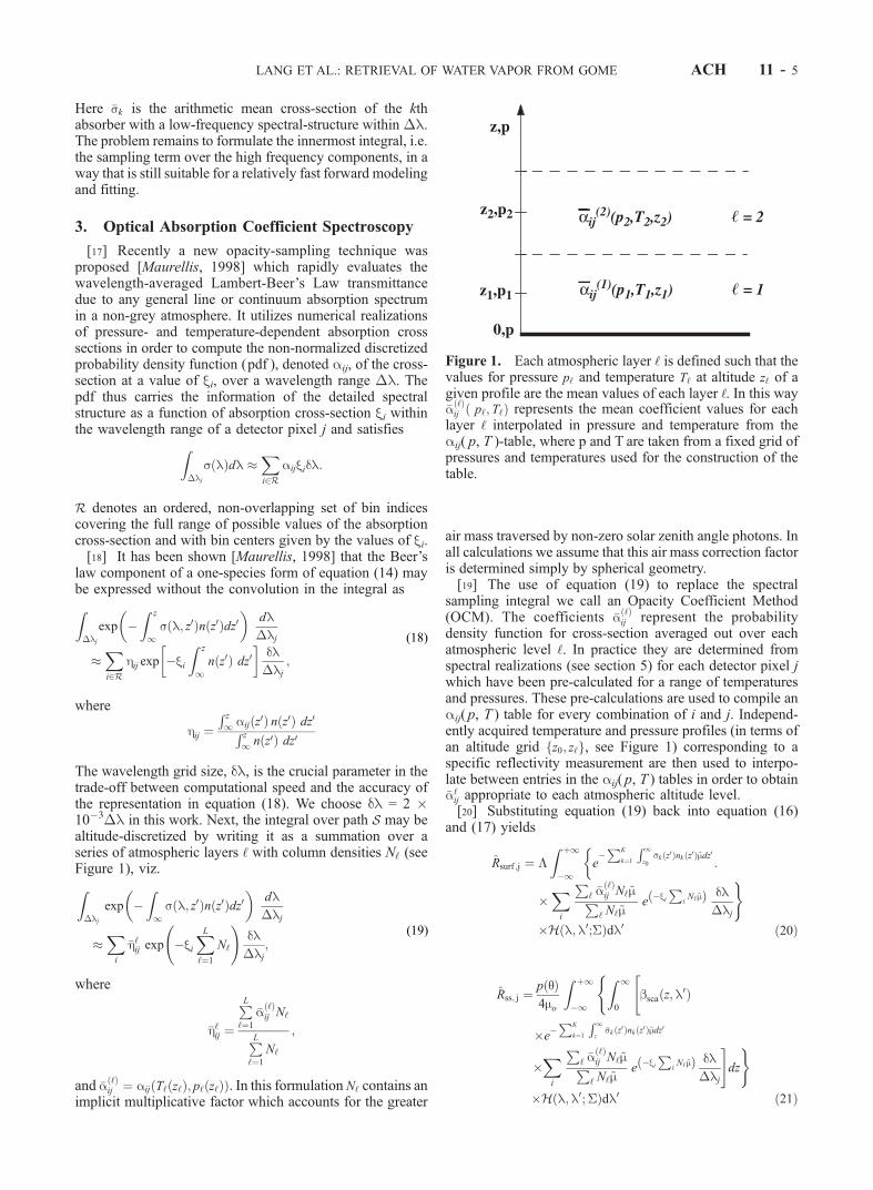
Figure 1. Each atmospheric layer ‘ is defined such that thevalues for pressure p‘ and temperature T‘ at altitude z‘ of agiven profile are the mean values of each layer ‘. In this way�að‘Þij ð p‘; T‘Þ represents the mean coefficient values for each

layer ‘ interpolated in pressure and temperature from theaij( p, T )-table, where p and T are taken from a fixed grid ofpressures and temperatures used for the construction of thetable.

(19)

(18)


which is the basic form used in this work for verificationagainst forward modeling of the equations (14) and (15).We further include an additional first order polynomial termto account for the broadband contribution of aerosolscattering and multiply scattered photons, both for forwardmodel verification against results from other radiativetransfer models as well as in the retrieval algorithm (seesection 7). The impact of the differential spectral contribu-tion of this additional term is discussed in section 8.

4. GOME Measurements

4.1. Operation

[21] The GOME instrument is a four-channel gratingspectrometer covering a wavelength range between 240 to790 nm. The spectra are recorded simultaneously for eachwavelength. The instantaneous nadir field of view (IFOV) is2.9� � 0.14� (along � across the track) and earth radiancesare integrated for 1.5 seconds by scanning from east to westwhich corresponds to an earth footprint of about 40 � 320km2 (Figure 2). In the current study only nadir radiances areused so that the mean angle between the satellite IFOV andzenith is zero. However, we could easily account for otherangles between the satellites line-of-sight and the zenith.GOME solar irradiance measurements are performed once aday. The detector pixel-to-pixel variability is smaller than2% and is monitored by LED’s illuminating the detectorarrays. The correction for the pixel-to-pixel variability, thestraylight and leakage fraction, and the noise produced bythe cross-talk from the Peltier coolers is part of the level 0to 1 data processing [Deutsches Zentrum fur Luft- undRaumfahrt (DLR), 1996, 1999]. The solar irradiance andthe earth radiance measurements are also corrected for thepolarization sensitivity of the instrument. After applyingthese corrections the GOME level 1 data product provides acalibrated earth radiance spectrum I in photons (cm2 � nm �sec � sr) and a calibrated sun irradiance spectrum pF inphotons/(cm2 � nm � sec). Table 2 summarizes some of the

most important instrument characteristics of the GOMEinstrument.

4.2. Spectral Resolution and Undersampling

[22] In a retrieval or in a study of forward modeledreflectivity using high resolution reference cross sections,a instrumental response function with a s-width � has to beapplied to the modeled reflectivity (equation (13)). Thisfunction takes into account the photon energy redistributiondue to the slit. In the case of the GOME instrument it maybe represented by convolving the radiatively transportedabsorption spectra with a Gaussian function which has afull-width-half-maximum (FWHM) of 0.27 nm. The detec-tor pixel coverage is about 0.2 nm within channel 3, i.e. theconvolved absorption spectrum is wavelength averagedover a wavelength region of 0.2 nm covered by eachdetector pixel. This means that in the case of GOME thespectral resolution (�) is close to the spectral sampling bythe detector pixels (�l) and so the requirement that �l bemuch less than �, as was assumed for equations (16) and(17), is not satisfied, i.e the instrument undersamples allabsorption features with effective widths close to or smallerthan the FWHM of the slit function.

4.3. Spectral Calibration and Rebinning

[23] The in-flight spectral wavelength calibration of theradiance and the irradiance is done using an on-board Pt /Cr/Ne hollow cathode gas-discharge lamp. Temperaturechanges over the orbit are taken into account in thespectral calibration. The error on the calibration is knownto be on the order of 0.004 nm [Caspar and Chance,1997]. We note that the interpolation of radiances meas-ured by an instrument with a low sampling rate onto adifferent grid may introduce significant errors [Roscoeet al., 1996]. Moreover different wavelength calibrationsare used for the sun irradiance measurement and the earthradiance. Thus, in this study, both spectra are rebinnedinstead of interpolated on a standard wavelength griddefined for an OACS retrieval. The rebinning procedureis carried out as follows. For each measurement, theGOME-reported radiance and irradiance wavelengths areassumed to define the central wavelengths of two differentsets of bins. After adjustment for Doppler shift (seefollowing paragraph), a fraction of the intensity withineach bin is redistributed to the nearest bin of the prede-fined standard grid according to their fractional overlap inwavelength. In this way, the intensity of a high resolutionreference absorption spectra integrated over one bin ofthe standard grid with dl � �l can be correlated with therebinned GOME detector pixel averaged intensity on the

Table 2. GOME Instrument Performance (585–600 nm)

Value

Number of used detector pixels 69FWHM slit function (ch3)a 0.27 nmDetector pixel width �l (ch3) 0.2 nmInstantaneous Field Of View 2.9� � 0.14�Ground pixel size (Figure 2) 40 � 320 km2

Pixel-to-pixel variability <2%Random noise value 0.1%Accuracy of absolute radiances 1%

aChannel 3.

Figure 2. GOME ground surface pixel coverage (solidboxes) of about 0.4� � 4� shown along with the 1�-grid sizeof the ECMWF assimilation model (dotted grid).


same grid without introducing errors in the integratedreflectivity per detector pixel bin. Thus, rather then adjust-ing the alpha coefficients for a shift of the wavelength griddue to different calibrations we adjust the measuredGOME spectra to the standard grid used by OACS. Thealpha coefficients can therefore be taken from a look-uptable interpolated only over pressure and temperature (andnot over wavelength).[24] We correct the Doppler-shifted irradiance calibration

with a knowledge of the relative velocity of the spacecraft tothe sun provided for each sun irradiance measurement. Therelative velocity is about 6 km/sec which results in awavelength shift of about 0.01 nm (about 5% with respectto a pixel). Hereafter, reflectivity always refers to a Dopplershift-corrected measurement.

5. Molecular Absorption Spectra andAtmospheric Profiles

5.1. Water Vapor Absorption Spectra

[25] We use the HITRAN’96 database to calculate anumber of realizations of a water vapor absorption spectrumcovering the entire altitude range for which we havepressure and temperature profiles available, for each givengeolocation. The main spectral parameters provided by theHITRAN’96 database are the integrated cross-section val-ues (line strength) Sn in cm�1/(molec � cm�2) and thepressure-dependent air-broadened line half-width gair incm�1/atm. For a detailed description of the calculation ofthe temperature correction of the integrated line intensity thereader is referred to Rothman et al. [1998].[26] The pressure-broadened line half-width-half-maxi-

mum HWHM g(p, T ) for a gas at pressure pair [atm] andtemperature T [K] is calculated by

gð p; TÞ ¼ T

Tref

� �n

gairð pref ; Tref Þpair� �

; ð22Þ

where gair is the line-broadening contribution due tocollisions with all other molecules, mainly nitrogen andoxygen, and n is the coefficient for the temperaturedependence of the total line half-width [Rothman et al., 1998].[27] The largest expected volume mixing ratio of water

vapor is of the order of 10�2. Therefore the self-broadeningcontribution is neglected in the calculation of the full-linehalf-width [cf. Liou, 1980]. Using a Doppler half-width, incm�1, given by �vD ¼ �n=cð

ffiffiffiffiffiffiffiffiffiffiffiffiffiffiffi2kT=M

pÞ, we calculate the

wavenumber dependent cross-section in cm2/molec usinga Voigt line shape via

sð�n; �n0; p; TÞ ¼ S�nðTÞ �n; �n0; p; Tð Þ; ð23Þ

where is the normalized Voigt function in units ofcentimeters. The Voigt profile is numerically calculatedusing the algorithm by Armstrong [1967].[28] Figure 3 shows an example of the change of the

cross section due to the change in pressure and temperatureover the dominant water vapor absorption altitude regionfrom 0 to 16 km for one selected water vapor absorptionline at 16804.04 cm�1.[29] The 590 nm water band is a ro-vibrational overtone

band which is part of the 5n-polyad (see Table 3). Theband spans weak absorptions from about 565–605 nm.Due to an intensity mismatch of the GOME instrumentresulting from spectral aliasing (P. Stammes, technicalmemo, 2000) between channel 3 and 4 we do not makeany use of absorption lines above 600 nm. The lines below585 nm are considered to be too weak and modeling of thebackground is complicated by a strong (O2)2 absorptionfeature (see section 5.2 and Figure 5). The average lifetimeof the exited ro-vibrational states is long enough for acollisional redistribution of the absorbed energy in thetroposphere. Therefore the water vapor line shape isdominated by pressure broadening (Lorentz line shape)which introduces a significant change in the total trans-mitted light especially due to changes in the wings of thelines, where the cross-section may change over an order ofmagnitude over the first 16 km. Decreasing pressure andtemperature gives rise to a significant decrease in theabsorption. This effect may be different for two lines withoverlapping wings, as is often the case for a typical watervapor spectrum.[30] Following recent measurements of the cross-section

of water vapor in the visible and near infrared evidence isgrowing for systematic deviations in the line-strengthvalues from those given by the HITRAN’96 database[Carleer et al., 1999; Belmiloud et al., 2000; Learner etal., 2000; Giver et al., 1999]. We will discuss systematic

Figure 3. The effect on the shape of a water vaporabsorption line at 16804.42 cm�1 in the earth’s atmospheredue to the vertical change in temperature and pressure. Thefive line profiles in panel (a) correspond to five differentaltitudes taken from typical equatorial profiles of tempera-ture (panel b) and pressure (panel c).

Table 3. Spectroscopic Values Relevant to the Water Vapor Band

Under Study

Value

WV-band (5n-polyad) wavelength range 585 – 600 nmOther atmospheric constituents within above range (O2)2, O3, NaNumber of WV-lines (HITRAN’96) 638HWHM WV-line g 0.09 [cm�1]a

Grid size of reference spectra dl 0.0117 [cm�1]aAverage value within the WV-band at 1 atm.


patterns in the residuals between the results of our fits andthe measured GOME spectra which we relate predomi-nantly to errors in the values of the line parameters. A senseof the magnitude of the differences between such line-strength values coming from the database and the ones‘‘measured’’ by the satellite instrument may be estimatedfor a specific radiative transport scenario. This estimate isbased on residuals between forward models utilizing theHITRAN’96 line parameters and GOME measurements.The results are used to correct for differential fit mis-matches (see section 10).

5.2. Other Sources of Extinction

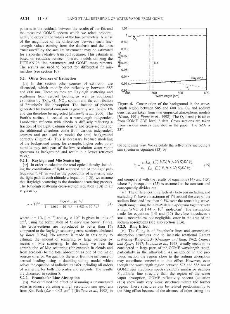
[31] In this section other sources of extinction arediscussed, which modify the reflectivity between 585and 600 nm. These sources are Rayleigh scattering andscattering from aerosol loading as well as additionalextinction by (O2)2, O3, NO2, sodium and the contributionof Fraunhofer line absorption. The fraction of photonsgenerated by thermal emission is generally well below 1%and can therefore be neglected [Buchwitz et al., 2000]. TheEarth’s surface is treated as a wavelength-independentLambertian reflector with albedo � diffusely reflecting afraction of the light. Column density and cross-sections forthe additional absorbers come from various independentsources and are used to model the total backgroundcorrectly (Figure 4). This is necessary because modelingof the background using, for example, higher order poly-nomials may treat part of the low resolution water vaporspectrum as background and result in a lower retrievedWVC.5.2.1. Rayleigh and Mie Scattering[32] In order to calculate the total optical density, includ-

ing the contribution of light scattered out of the light path(equation (14)) as well as the probability of scattering intothe light path at each altitude z (equation (15)), we assumethat Rayleigh scattering is the dominant scattering process.The Rayleigh scattering cross-section (equation (10)) in airis given by

sR � 1024 ¼ 3:9993� 10�4n4

1� 1:069� 10�2n2 � 6:681� 10�5n4; ð24Þ

where n = 1/l [mm�1] and sR � 1024 is given in units ofcm2, using the formulation of Chance and Spurr [1997].The cross-sections are reproduced to better than 1%compared to the Rayleigh scattering cross sections tabulatedby Bates [1984]. No attempt is made in this study toestimate the amount of scattering by large particles bymeans of Mie scattering. In this study we treat thecontribution of Mie scattering (for example in clouds andfrom aerosols) to the total absorption as one of the majorsources of error. We quantify the error from the influence ofaerosol loading using a doubling-adding model whichsolves the equation of radiative transfer including all ordersof scattering for both molecules and aerosols. The resultsare discussed in section 8.5.2.2. Fraunhofer Line Absorption[33] We estimated the effect of assuming a unstructured

solar irradiance F0 using a high resolution sun spectrumfrom Kitt Peak (�n = 0.02 cm�1) [Wallace et al., 1998] in

the following way. We calculate the reflectivity including asun spectra in equation (13) by

Rj ¼pmo

R�lj

Rþ1�1 IðF0ÞHðl;l0; �Þdl0 dl

�ljR�lj

Rþ1�1 F0Hðl;l0; �Þdl0 dl

�lj

; ð25Þ

and compare it with the results of equations (14) and (15),where F0 in equation (25) is assumed to be constant andconsequently divides out.[34] The differences in reflectivity between including and

excluding F0 have a maximum of 1% around the area of thesodium lines and less than 0.3% over the remaining wave-length range using the Kitt-Peak sun-spectrum together witha high WVC of 1.44 � 1023 molec/cm2. The assumptionmade for equations (14) and (15) therefore introduces asmall, nevertheless not negligible, error in the area of thesodium absorptions (see also section 11.4).5.2.3. Ring Effect[35] The filling-in of Fraunhofer lines and atmospheric

absorption structures due to inelastic rotational Ramanscattering (Ring-effect) [Grainger and Ring, 1962; Chanceand Spurr, 1997; Vountas et al., 1998] usually needs to beconsidered in large parts of the GOME wavelength range,particularly in the ultraviolet. As mentioned in the pre-vious section the region close to the sodium absorptionmay contribute somewhat to this effect. However, eventhough the wavelength region between 575 and 585 nm ofGOME sun irradiance spectra exhibits similar or strongerFraunhofer line structure than the region of the watervapor absorption, GOME reflectivity spectra (equation(13)) show only very weak structures within the formerregion. These structures can be related predominantly tothe Ring effect because of the absence of other strong line

Figure 4. Construction of the background in the wave-length region between 585 and 600 nm. O2 and sodiumdensities are taken from two empirical atmospheric models[Hedin, 1991; Plane et al., 1998]. The O3-density is takenfrom GOME GDP level 2 data. Cross sections are takenfrom various sources described in the paper. The SZA is23�.


absorbers between 575 and 585 nm. It is thereforeexpected that also the Ring structures in the water absorp-tion wavelength region is relatively small. In addition,accurate modeling of the Ring effect including polariza-tion, which is needed for a polarization sensitive instru-ment such as GOME [Aben et al., 2001], is verycomplicated and far beyond the scope of this paper. Wetherefore neglect he Ring effect for this study and discussit as a possible source of error.5.2.4. Sodium[36] In this work we model the contribution of the sodium

background in the earth atmosphere at 588.9 and 589.5 nmto the total background absorption by calculating columnconcentrations for the non-sporadic atmospheric sodiumlayer at 90 km from a model by Plane et al. [1998]. Itscontribution to the total sodium absorption with respect tothe sodium Fraunhofer lines is very weak. A typical meansodium column in the earth atmosphere is about 6.9 � 109

molec/cm2. Nevertheless, it was found that modeling thesodium earth background absorption reduces the fit residualand improves convergence time. Thus, it is used in bothforward modeling and the retrieval.5.2.5. (O2)2 Collision Complex[37] The atmospheric absorption feature of the (O2)2-

collision complex within the region of 560 and 600 nmwas investigated by Perner and Platt [1980]. Subsequently,Pfeilsticker et al. [1997] presented atmospheric measure-ments of (O2)2 in the wavelength range from about 450 to650 nm and Solomon et al. [1998] modeled and calculatedthe contribution of (O2)2 to the total absorption in thisregion. Cross-sections of (O2)2 have been measured by, forexample, Greenblatt et al. [1990] and Newnham andBallard [1998]. The cross-sections we use in this workare measured by means of Cavity Ring Down Spectroscopyby Naus and Ubachs [1999] for pressures between 0 and 1atmospheres at room temperature. The results of bothGreenblatt et al. and Naus and Ubachs indicate that wemay safely assume negligible temperature dependence forthe cross-section. The optical density is calculated for eachground pixel using an O2-density column from the NeutralAtmosphere Empirical Model MSISE90 [Hedin, 1991] for agiven date, time, altitude-range and geolocation. Due tosmall variations in the O2-density the difference in densitiesin the slant path of the light with respect to the used verticalcolumn densities from the Hedin model is small and mayaffect the results only for very high SZA. There is asignificant absorption due to (O2)2 visible in the GOMEspectra on the blue side of our wavelength window for highSZA. Figure 5 shows such an absorption peak in the GOMEspectra for the region between 560 and 600 nm at 62�latitude and for a SZA of 73�. For comparison we show a lblforward calculation based on equations (14) and (15)including absorptions from (O2)2, O3, sodium and watervapor. The modeled spectrum is adjusted to the GOMEmeasurement by fitting a first order polynomial to accountfor the unknown surface albedo � together with a first-order polynomial to account for the broadband contributionof aerosol loading and multiple scattering (equations (30)and (28)). Apart from the water window described in thisstudy another water absorption at the blue side of thespectrum between 565 and 580 nm superimposed on the(O2)2 absorption peak is clearly visible. The latter is

reproduced well in the region between 565 and 575 nm,whereas the absorption features superimposed on the peakbetween 575 and 580 nm are poorly reproduced. This couldbe related to problems in the water vapor cross-sectiondatabase.5.2.6. NO2

[38] Within our wavelength region of interest, NO2 hasan optical density of a maximum of 1 � 10�3 [Richter andBurrows, 2000] which is two to three orders of magnitudesmaller than water vapor and about two orders smaller thanthe optical density of ozone. For the purpose of this paperand within the wavelength region used we neglect thecontribution of NO2 which is below the sensitivity limitof our method. Nevertheless small contributions of NO2

absorption for high NO2 content, for example in case ofbiomass burning, may contribute additional structure to ourresiduals.5.2.7. Ozone[39] For the cross-section of the ozone Chappuis absorp-

tion band we use high-resolution reference spectraat atmospheric temperatures of 202, 221, 241, 273 and293 K and pressures at 100 and 1000 mbar recorded usingFourier-Transform spectroscopy in the UV-visible-NIRspectral regions (240–850 nm) by Voigt et al. [2001].The ozone slant column density (SCD) for a specificgeolocation and SZA is taken from the GOME DataProcessor (GDP) [Balzer and Loyola, 1996; DLR, 1999]level 2 data product [Burrows et al., 1999]. Its accuracy isknown to be on the order of 5% for SZA less than 70�. Theoptical density is calculated by integrating over the alti-tudes corresponding to the five cross section temperatures

Figure 5. Comparison of a forward modeled lbl calcula-tion (dashed curve) of the reflectivity using equations (14),(15) and (28) with a GOME measurement (solid curve)taken at 62�N (SZA = 73�). The background consists of(O2)2, O3 and sodium. The stronger of the two (O2)2absorption peaks is clearly visible around 577 nm withanother water vapor absorption band between 565 and 580nm superimposed on it. In the case of the latter there aresome discrepancies between model and measurement in theregion between 575 and 580 nm which could be related toproblems in the water vapor cross-section database.


listed above assuming the local pressure and temperatureprofile.

5.3. Pressure and Temperature Profiles

[40] The pressure and temperature profiles used in theretrieval are taken from ECMWF (compare section 5.1).The ECMWF data assimilation model [Vesperini, 1998]provides us with 31, 50 or 60 altitude levels in pressureand temperature, according as the date is before March1999, after March 1999 and after October 1999 respectively.Data is provided for the entire globe at 0h, 6h, 12h, and 18hUTC with a ground pixel resolution of 1� in latitude andlongitude. The data is interpolated onto a 0.5� grid thatmatches the resolution of SSM/I data and improves theoverlap between ECMWF ground pixels and GOMEground pixel. GOME level 1 geolocation data consists of5 data-tuples in latitude and longitude: 4 components for theedges and one for the center of a ground pixel. They span anarea of roughly 0.4� � 2.5� in latitude and longitude(depending on the geolocation, see Figure 2). For eachdata-tuple the nearest ECMWF value is sorted out and amean pressure and temperature is calculated for eachaltitude layer ‘. In this study we use up to 31 pressure andtemperature levels which cover an altitude range between 0and 23 km. The atmospheric layers ‘ are defined asdescribed in section 2. For each ground pixel a set of �a ‘ð Þ

j

per detector pixel j for a given altitude layer ‘ is calculatedby interpolating alpha tables to the mean pressure andtemperature (compare equation (30) and Figure 1) to beused in an OACS fast forward model or in an OACS fit tobe described next.

6. Intrinsic OACS Accuracy

[41] The intrinsic accuracy of the OACS method islimited by two method-related sources of error: (1) thediscretization error due to the Opacity Coefficient Method(OCM) caused by replacing the integrals in equations(16) and (17) (equations (20) and (21)); (2) exchange ofthe convolution with the sampling integral. This error isrelated to the fact that GOME detectors undersample theinstrumental function of the instrument by �l 6� � (sec-tion 4.2). As mentioned in section 2 the first error maybe reduced arbitrarily by decreasing dl and thus increas-ing the number of realization points per absorption lineof the high resolution reference spectrum. The seconderror, related to the basic transport equations (equations(14) and (15)), is introduced by performing the samplingof the high resolution reflectivity spectrum before theconvolution (convolution problem), as is done for bothequations (16), (17) and for the basic OACS equation(equations (20) and (21)). However, performing thesampling before the convolution makes the fitting muchmore efficient, because the convolution has to be per-formed only over 69 measurement points during eachiteration step and not over the high-resolution absorptionspectrum.[42] In order to quantify the intrinsic method-related

error we will compare the reflectivity calculated using theOACS method (equations (20) and (21)) with a lbl calcu-lation based on equations (14) and (15). The densitysubcolumn profiles of water vapor per atmospheric level

for two specific geolocations are taken from the ECMWFdata assimilation model. Figure 6 shows the comparisonbetween both calculations for a typical equatorial scenarioover the ocean with a high WVC of 1.34 � 1023 molec/cm2

and a low WVC of 8.19 � 1021 molec/cm2 over land atSZAs of 23.5� and 73�, respectively. Both ground pixelsare cloud-free. The two figures also show the relativeresiduals between the lbl and the OACS forward model,which is defined as (lbl-OACS)/lbl, hereafter. From theresiduals we conclude that, for dl = 2 � 10�3�l, therelative spectral accuracy of the method in reflectivity isbetter than 2% for high WVC and better than 0.2% for lowWVC. For a comparison of reflectivities between theresults of the lbl and the OACS forward model withoutperforming the convolution the accuracy of the method

Figure 6. Comparison of modeled spectra for specificmeasurement scenes. The reflectivity plot shows a forwardmodeled lbl calculation using equations (14) and (15) (solidline) and a forward modeled reflectivity using the OACSmethod (equations (20) and (21); dashed line). The residualplot shows the relative method-related intrinsic error inreflectivity ([lbl-OACS]/lbl; used throughout the paper).Upper two panels: A high WVC of 1.34 � 1023 molec/cm2

measurement over the Pacific at 23� latitude and 250�longitude for a SZA of 23.5�. Lower two panels: A lowWVC of 8.19 � 1021 molec/cm2 for a measurement overland at 62� latitude and 262.5� longitude for a SZA of 73�.


appears to be better than 0.4% for high and better than0.2% for low WVC. We conclude that the residual isdominated by error source number (2) above, namely theconvolution problem.

7. Forward Model

[43] We use equations (20) and (21) to construct a basicfast forward model reflectivity spectrum which includessingle-scattering via

Rj ¼ RðN‘;�j; ~m‘Þsurf ; j þ RðN‘; ~m‘Þss;j; ð26Þ

where j is the jth detector pixel within the window ofinterest. The altitude-dependent path length factor ~m‘ iscalculated using a Chapman function [Banks and Kockarts,1973] which takes the curvature of the atmosphere intoaccount. We adjust the forward modeled spectrum to theGOME measurement in the region between 585 and 600 nmby fitting a first-order polynomial for the unknown surfacealbedo �j, assuming

�j ¼ Alj þ B; ð27Þ

where A and B are free fit parameters. Since the differentialcontribution of multiple scattering and aerosol extinctionappears to be lower than 2% in cases of cloud-free groundpixels (see section 8) within our spectral region of interestwe include an additional first-order polynomial,

Rms; j ¼ Clj þ D; ð28Þ

where C and D are additional free fit parameters in order toaccount for the broadband contribution of higher orders ofscattering.[44] Thus, in its entirety, the forward model consists of

three terms, viz.

Rj ¼ RðN‘;�j; ~m‘Þsurf ; j þ RðN‘; ~m‘Þss; j þ Rms; j: ð29Þ

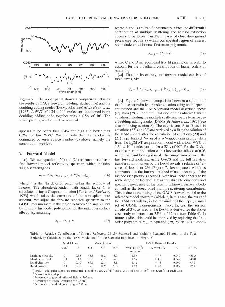
[45] Figure 7 shows a comparison between a solution ofthe full scalar radiative transfer equation using an independ-ent method and the OACS forward model described above(equation (29)). For the full solution of the radiative transferequation including the multiple scattering source term we usea doubling-adding model (DAM) [de Haan et al., 1987] (seealso following section 8). The coefficients A to D used inequations (27) and (28) are retrieved by a fit to the solution ofthe DAM-model after the calculation of equations (20) and(21) is performed. We used a WV-subcolumn profile takenfrom the ECMWF assimilation model with a total WVC of1.34 � 1023 molec/cm2 under a SZA of 40�. For the DAM-model a maritime situation with a low surface albedo of 0.03without aerosol loading is used. The comparison between thefast forward modeling using OACS and the full radiativetransfer solution given by the DAM reveals a relative differ-ence of less than 2% (Figure 7, lower panel) which iscomparable to the intrinsic method-related accuracy of themethod (see previous section). Note how there appears to besome degree of freedom left in the absolute quantities andspectral dependence of the usually unknown surface albedoas well as the broad-band multiple-scattering contribution.This is due to the fitting of the OACS forward model to thereference model spectrum (which is, in this case, the result ofthe DAM but will be, in the remainder of the paper, a smallset of GOME measurements). Nevertheless, the surfacealbedo of 3%, as used in the DAM, is derived for the abovecase study to better than 35% at 592 nm (see Table 4). Infuture studies, this could be improved by replacing the first-order polynomial Rms in equation (29) by an OACS-modi-

Figure 7. The upper panel shows a comparison betweenthe results of OACS forward modeling (dashed line) and thedoubling adding model (DAM, solid line) of de Haan et al.[1987]. AWVC of 1.34 � 1023 molec/cm2 is assumed in thedoubling adding code together with a SZA of 40�. Thelower panel gives the relative residual.

Table 4. Relative Contribution of Ground-Reflected, Singly Scattered and Multiply Scattered Photons to the Total

Reflectivity Calculated by the DAM Model and for the Scenario Introduced in Figure 7a

Model Input Model Output OACS Retrieval Results

AODb � GRc SSd MSe WVC (�1023),molec/cm2

� WVC, % � ��, %

Maritime clear sky 0 0.03 43.8 48.2 8.0 1.33 �7.7 0.040 +33.3Maritime aerosol 0.21 0.03 20.0 53.2 26.8 1.65 +14.8 0.042 +40.0Rural clear sky 0 0.10 69.1 22.8 8.1 1.42 �1.6 0.105 +5.0Rural Aerosol 0.51 0.10 17.9 30.9 51.2 1.69 +17.6 0.109 +9.0

aDAM model calculations are performed assuming a SZA of 40� and a WVC of 1.44 � 1023 [molec/cm2] for each case.bAerosol optical depth.cPercentage of ground reflected light at 592 nm.dPercentage of single scattering at 592 nm.ePercentage of multiple scattering at 592 nm.


fied term which accounts for the differential contribution ofhigher-order scattering. In addition the surface albedo couldalso be retrieved from a fit to the spectrum in a spectralregion beyond the water vapor absorption which mayimprove the robustness of the fit (see also section 11.5).[46] A detailed description of the influence of different

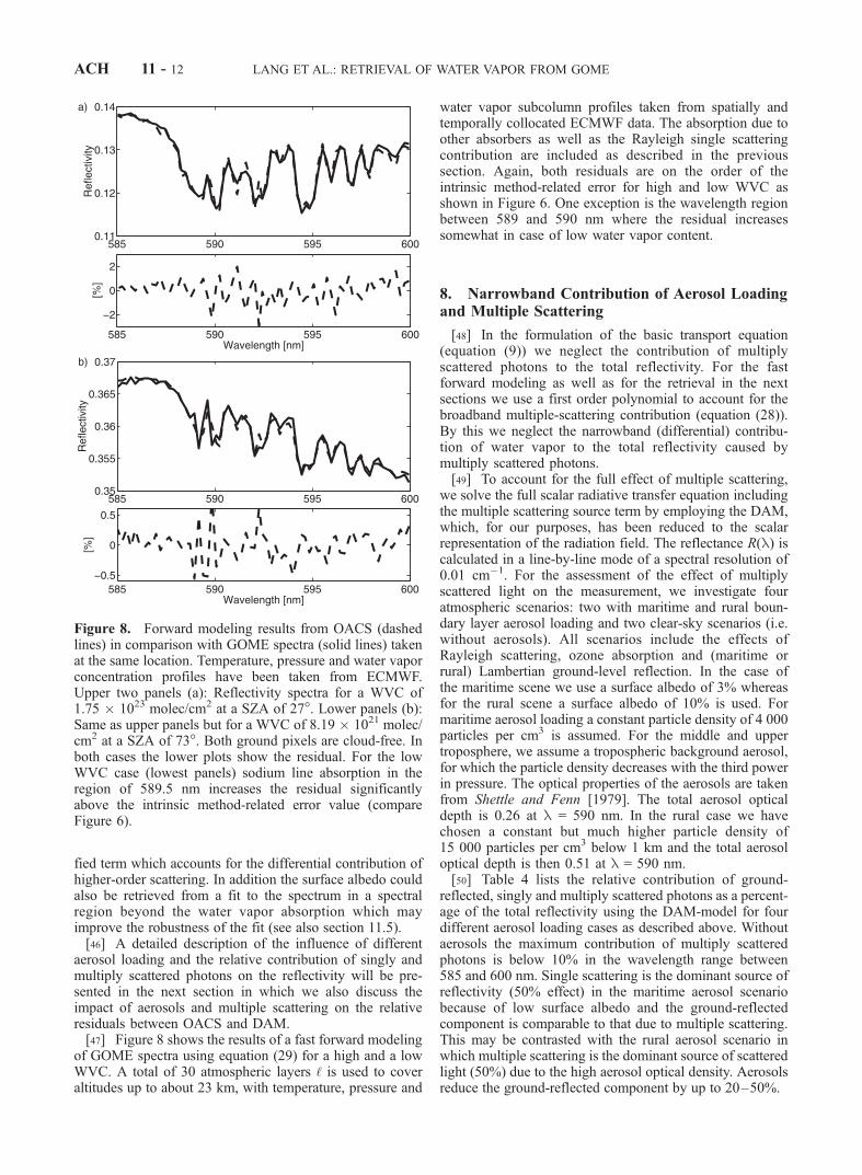
aerosol loading and the relative contribution of singly andmultiply scattered photons on the reflectivity will be pre-sented in the next section in which we also discuss theimpact of aerosols and multiple scattering on the relativeresiduals between OACS and DAM.[47] Figure 8 shows the results of a fast forward modeling

of GOME spectra using equation (29) for a high and a lowWVC. A total of 30 atmospheric layers ‘ is used to coveraltitudes up to about 23 km, with temperature, pressure and

water vapor subcolumn profiles taken from spatially andtemporally collocated ECMWF data. The absorption due toother absorbers as well as the Rayleigh single scatteringcontribution are included as described in the previoussection. Again, both residuals are on the order of theintrinsic method-related error for high and low WVC asshown in Figure 6. One exception is the wavelength regionbetween 589 and 590 nm where the residual increasessomewhat in case of low water vapor content.

8. Narrowband Contribution of Aerosol Loadingand Multiple Scattering

[48] In the formulation of the basic transport equation(equation (9)) we neglect the contribution of multiplyscattered photons to the total reflectivity. For the fastforward modeling as well as for the retrieval in the nextsections we use a first order polynomial to account for thebroadband multiple-scattering contribution (equation (28)).By this we neglect the narrowband (differential) contribu-tion of water vapor to the total reflectivity caused bymultiply scattered photons.[49] To account for the full effect of multiple scattering,

we solve the full scalar radiative transfer equation includingthe multiple scattering source term by employing the DAM,which, for our purposes, has been reduced to the scalarrepresentation of the radiation field. The reflectance R(l) iscalculated in a line-by-line mode of a spectral resolution of0.01 cm�1. For the assessment of the effect of multiplyscattered light on the measurement, we investigate fouratmospheric scenarios: two with maritime and rural boun-dary layer aerosol loading and two clear-sky scenarios (i.e.without aerosols). All scenarios include the effects ofRayleigh scattering, ozone absorption and (maritime orrural) Lambertian ground-level reflection. In the case ofthe maritime scene we use a surface albedo of 3% whereasfor the rural scene a surface albedo of 10% is used. Formaritime aerosol loading a constant particle density of 4 000particles per cm3 is assumed. For the middle and uppertroposphere, we assume a tropospheric background aerosol,for which the particle density decreases with the third powerin pressure. The optical properties of the aerosols are takenfrom Shettle and Fenn [1979]. The total aerosol opticaldepth is 0.26 at l = 590 nm. In the rural case we havechosen a constant but much higher particle density of15 000 particles per cm3 below 1 km and the total aerosoloptical depth is then 0.51 at l = 590 nm.[50] Table 4 lists the relative contribution of ground-

reflected, singly and multiply scattered photons as a percent-age of the total reflectivity using the DAM-model for fourdifferent aerosol loading cases as described above. Withoutaerosols the maximum contribution of multiply scatteredphotons is below 10% in the wavelength range between585 and 600 nm. Single scattering is the dominant source ofreflectivity (50% effect) in the maritime aerosol scenariobecause of low surface albedo and the ground-reflectedcomponent is comparable to that due to multiple scattering.This may be contrasted with the rural aerosol scenario inwhich multiple scattering is the dominant source of scatteredlight (50%) due to the high aerosol optical density. Aerosolsreduce the ground-reflected component by up to 20–50%.

Figure 8. Forward modeling results from OACS (dashedlines) in comparison with GOME spectra (solid lines) takenat the same location. Temperature, pressure and water vaporconcentration profiles have been taken from ECMWF.Upper two panels (a): Reflectivity spectra for a WVC of1.75 � 1023 molec/cm2 at a SZA of 27�. Lower panels (b):Same as upper panels but for a WVC of 8.19 � 1021 molec/cm2 at a SZA of 73�. Both ground pixels are cloud-free. Inboth cases the lower plots show the residual. For the lowWVC case (lowest panels) sodium line absorption in theregion of 589.5 nm increases the residual significantlyabove the intrinsic method-related error value (compareFigure 6).


[51] In addition to the evidently broadband aerosol effectsjust discussed it is also reasonable to expect that a significantdifferential contribution due to multiply scattered photonsmay affect the retrieved WVC. Since the radiation transportmodel presented in this paper does not explicitly account forthe latter we present a comparison in Figure 9 between a lblcalculation based on equations (14), (15) and (28) and theresults of the DAM forward model for the four scenariosdiscussed above. The parameters C and D needed for the lblcalculation are obtained by a fit to the DAM result. Thedifferences in the residuals between Figures 9a and 9c andFigures 9b and 9d indicate that aerosol-loaded scenarios maygive rise to significant differential structure. The latter is a2% effect compared with a 20–25% broadband aerosolcontribution. Even though this is comparable to or justbelow the 2% precision of the OACS method for highWVC it is a systematic effect. In section 9.4 we thereforeperform OACS retrieval on all four spectra modeled by theDAM in order to estimate the effect of multiple scatteringdue to Rayleigh and aerosol scattering on the retrieved WVCtogether with the effect of aerosol extinction.

9. Sensitivity Analysis of the Retrieval Method

9.1. Retrieval Method

[52] We fit equation (29) to GOME reflectivity spectraalong with optical densities of O3, (O2)2 and sodium as wellas the Rayleigh scattering contribution as described insection 5. The numerical method used is a robust, non-linear, large-scale trust-region method [Byrd et al., 1988]which solves the optimization problem

minN‘;�j;Rms;j

Xj

hRj � RðN‘;�j; ~m‘Þsurf ; j

�þ RðN‘; ~m‘Þss; j þ Rms; j

�i2:

ð30Þ

[53] The fit parameters are the vertical water vaporcolumn densities N‘ of ‘ atmospheric layers and the surfacealbedo and multiple scattering parameters (see section 7).All 69 measurement points j within our region of interestare fitted simultaneously together with the four parametersA to D.[54] For each OACS fit we start with a flat water vapor

sub-column profile N‘;0 ¼ 1016, where the N‘ are given inunits of the water vapor vertical column density per atmos-pheric layer (compare equation (19)). Each fit is constrainedby an upper limit N‘;max in the form of a step function withhigh values over the first atmospheric layers and lowervalues for the higher levels. The lower profile constraint isset to N‘;lower ¼ 0. The constraints prevent the fit from givingtoo much weight to the higher altitude levels which other-wise would increase the relative contribution of the singlescattered photons and, in so doing, decrease the total meanfree path length. The latter would lead to a reduced totalWVC. The effect of introducing this constraint is to repro-duce the relative single-scattering contribution to the totalreflectivity to better than 1% when compared to the resultsgiven by the lbl forward model.

9.2. Precision and Accuracy of the Fitting Method

[55] We henceforth adopt the term precision to describemeasurement-related random errors and the term accuracyto describe the absolute difference between the true and theretrieved value due to systematic errors. These differencesare caused by the response of the result due to the intrinsicmethod-related error as well as the robustness of the resultto errors in the main input quantities: the accuracy of themeasurement and the altitudes profiles of atmospherictemperature and pressure. The random noise of a typicalsatellite measurement is dependent on photon shot noise,detector shot noise and digitization effects and is quantifiedto be about 0.1% of the absolute radiance in the case ofGOME [DLR, 1999]. The GOME instrument is also sensi-tive to the polarization of the light which is measured foreach channel. In what follows we adopt a total system errorfor GOME measurements of about 1%. This is derived froma full error calculation including random noise errors, theerror of the fractional polarization values, the polarizationcorrection factor and the error on the instrument responsefunction known from pre-flight calibration studies. Asmentioned in section 4.3 the error on the spectral calibrationis known to be on the order of 0.001 nm within ourwavelength region [Caspar and Chance, 1997]. For thetemperature and pressure profiles taken from the ECMWFdata assimilation model an uncertainty of 0.3% [Filiberti etal., 1998] in pressure and 0.1% in temperature [Francis andSchweiger, 2000] is assumed.[56] We estimate precisions and accuracies for the retrieval

of WVCs using OACS (equation (30)) from the lbl forwardmodeled spectrum used before to estimate the intrinsicmethod-related error (section 6, Figure 6) as follows. Onehundred simulated reflectivity spectra are produced by add-ing random noise errors normally distributed around onethird of the reflectivity values, randomly chosen, where the2s range is given by their random noise values provided withthe measurement. The noise values are taken from level 1data for both solar irradiance and earth radiance. At the sametime and for each modified spectrum the wavelength grid is

Figure 9. Relative differences between the lbl modelpresented in this paper based on equations (14), (15) and(28) and the result of the DAM for the specific scenariopresented in Figure 7. The upper two panels show theresults for a maritime case with a surface albedo of 3%under (a) clear sky conditions and (b) with maritime aerosolloading. The lower two panels show the results for a ruralcase with surface albedo of 10% for (c) clear sky conditionsand (d) with rural aerosol loading.


shifted randomly within the calibration error range in order tosimulate calibration errors. In a separate calculation we shiftthe temperature and pressure profiles used in the fit to theirexpected maximum and minimum values due to potentialsystematic errors in the ECMWF database. In the samesimulations we similarly increase and decrease the reflectiv-ity by 1% in order to explore the effects of the systematicuncertainties in the measured intensities. This permits acheck of the precision (standard deviation for the meanretrieved WVC from artificial spectra with random noiseadded), the accuracy (mean retrieved WVC for the randomnoise modified spectra) and the robustness or total accuracy(response to shifted input profiles and known systematicerrors in the measurements) of the method.

9.3. Sensitivity Study Results

[57] Figure 10 shows two representative examples ofOACS WVC fit results for two artificial modified spectrautilizing different altitude ranges for a fixed density sub-column profile with a relatively high WVC of 1.34 � 1023

molec/cm2. Each fit covers a range of atmospheric levelsbetween 0 and the value denoted on the x-axis. Eachatmospheric level is defined as described in section 3 andshown in Figure 1. In general, best results are obtained withan altitude range covering 18 atmospheric levels (corre-sponding to a range of about 10 km above the earth surface)with the full range of WVCs agreeing to better than 2%.This altitude range is sufficient to cover the bulk of thewater vapor at any geolocation while still keeping thenumber of fit parameters as small as possible (the waterdensity drops by more than two orders of magnitude overthe first 10 km, see WV-subcolumn profile in Figure 11).

For higher altitude ranges there is not sufficient informationto restrict the fit. These findings are supported by thecalculation of mean weighting functions

@Rð‘Þ=@nð‘ÞVC

ij

per atmospheric layer and per detector pixel j (Figure 11),where R is the OACS formulation of the reflectivity basedon equation (29). Up to the 18th altitude level the weightingfunctions show similar changes in the reflectivity peraltitude level with respect to changes in the water vapordensity n (Figure 1). Above about the 20th level smallchanges in the water vapor density induce large unsyste-matic changes in the reflectivity for different wavelengths.This results in additional local fit minima which makes thefit unstable and increases the uncertainties in the fit results(see retrieved WVC results in Figure 10 using more than 20atmospheric layers). For the retrieval of WVCs presented inthis paper we therefore utilize 18 atmospheric levels toachieve best results for the full range of very high and verylow WVCs.[58] Figure 12 shows retrieved WVCs from 100 forward

modeled, random noise-modified spectra. Two extremecases are considered: a high WVC (1.34 � 1023 molec/cm2) and a low WVC (8.19 � 1021 molec/cm2). First, weperformed 100 OACS fits to the modified spectra usingexactly the same pressure and temperature profiles as usedin the forward model. The precision of the method is given

Figure 10. Relative residuals of the retrieved WVC (dots)from lbl forward modeled spectra using the OACS method.Typical examples are given for a high WVC (upper panel) of1.34 � 1023 molec/cm2 and a low WVC (lower panel) of8.19 � 1021 molec/cm2 covering different altitude ranges asfollows. Each value x on the abscissa represents theutilization of ‘ ¼ 1 to x atmospheric layers in the retrieval.Best results were achieved when using about 18 altitudelevels (covering the range of 0 to 10 km). For the low WVCthe fit fails to converge within the given limits when utilizingmore than 24 levels.

Figure 11. Change in reflectivity due to change in watervapor density over altitude (weighting functions @R /@n) forthe forward modeled reflectivity over altitude using OACS.The left panel shows the result for the high WVC and themiddle panel for the low WVC used in Figure 10. Each plotconsists of 69 weighting functions, one for each GOMEdetector pixel in the wavelength range between 585 and600 nm. The dotted line denotes the maximum (18th)atmospheric level (right axes) used in the retrieval. Forcomparison the panel on the right shows the correspondingwater vapor subcolumn profile for the low (dashed line) andthe high WVC (solid line). Above the 18th level smallchanges in the water vapor density introduce large changesin the reflectivity value.


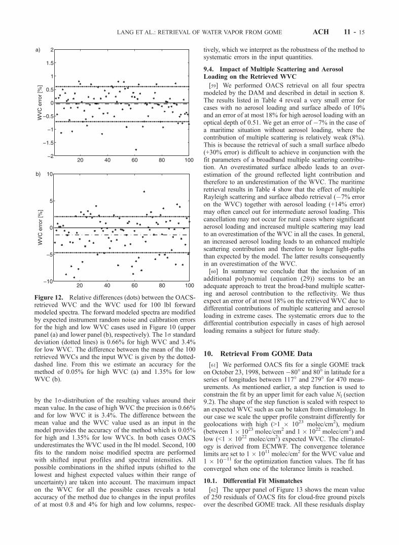
by the 1s-distribution of the resulting values around theirmean value. In the case of high WVC the precision is 0.66%and for low WVC it is 3.4%. The difference between themean value and the WVC value used as an input in themodel provides the accuracy of the method which is 0.05%for high and 1.35% for low WVCs. In both cases OACSunderestimates the WVC used in the lbl model. Second, 100fits to the random noise modified spectra are performedwith shifted input profiles and spectral intensities. Allpossible combinations in the shifted inputs (shifted to thelowest and highest expected values within their range ofuncertainty) are taken into account. The maximum impacton the WVC for all the possible cases reveals a totalaccuracy of the method due to changes in the input profilesof at most 0.8 and 4% for high and low columns, respec-

tively, which we interpret as the robustness of the method tosystematic errors in the input quantities.

9.4. Impact of Multiple Scattering and AerosolLoading on the Retrieved WVC

[59] We performed OACS retrieval on all four spectramodeled by the DAM and described in detail in section 8.The results listed in Table 4 reveal a very small error forcases with no aerosol loading and surface albedo of 10%and an error of at most 18% for high aerosol loading with anoptical depth of 0.51. We get an error of �7% in the case ofa maritime situation without aerosol loading, where thecontribution of multiple scattering is relatively weak (8%).This is because the retrieval of such a small surface albedo(+30% error) is difficult to achieve in conjunction with thefit parameters of a broadband multiple scattering contribu-tion. An overestimated surface albedo leads to an over-estimation of the ground reflected light contribution andtherefore to an underestimation of the WVC. The maritimeretrieval results in Table 4 show that the effect of multipleRayleigh scattering and surface albedo retrieval (�7% erroron the WVC) together with aerosol loading (+14% error)may often cancel out for intermediate aerosol loading. Thiscancellation may not occur for rural cases where significantaerosol loading and increased multiple scattering may leadto an overestimation of the WVC in all the cases. In general,an increased aerosol loading leads to an enhanced multiplescattering contribution and therefore to longer light-pathsthan expected by the model. The latter results consequentlyin an overestimation of the WVC.[60] In summary we conclude that the inclusion of an

additional polynomial (equation (29)) seems to be anadequate approach to treat the broad-band multiple scatter-ing and aerosol contribution to the reflectivity. We thusexpect an error of at most 18% on the retrieved WVC due todifferential contributions of multiple scattering and aerosolloading in extreme cases. The systematic errors due to thedifferential contribution especially in cases of high aerosolloading remains a subject for future study.

10. Retrieval From GOME Data

[61] We performed OACS fits for a single GOME trackon October 23, 1998, between �80� and 80� in latitude for aseries of longitudes between 117� and 279� for 470 meas-urements. As mentioned earlier, a step function is used toconstrain the fit by an upper limit for each value Nl (section9.2). The shape of the step function is scaled with respect toan expected WVC such as can be taken from climatology. Inour case we scale the upper profile constraint differently forgeolocations with high (>1 � 1023 molec/cm2), medium(between 1 � 1023 molec/cm2 and 1 � 1022 molec/cm2) andlow (<1 � 1022 molec/cm2) expected WVC. The climatol-ogy is derived from ECMWF. The convergence tolerancelimits are set to 1 � 1011 molec/cm2 for the WVC value and1 � 10�11 for the optimization function values. The fit hasconverged when one of the tolerance limits is reached.

10.1. Differential Fit Mismatches

[62] The upper panel of Figure 13 shows the mean valueof 250 residuals of OACS fits for cloud-free ground pixelsover the described GOME track. All these residuals display

Figure 12. Relative differences (dots) between the OACS-retrieved WVC and the WVC used for 100 lbl forwardmodeled spectra. The forward modeled spectra are modifiedby expected instrument random noise and calibration errorsfor the high and low WVC cases used in Figure 10 (upperpanel (a) and lower panel (b), respectively). The 1s standarddeviation (dotted lines) is 0.66% for high WVC and 3.4%for low WVC. The difference between the mean of the 100retrieved WVCs and the input WVC is given by the dotted-dashed line. From this we estimate an accuracy for themethod of 0.05% for high WVC (a) and 1.35% for lowWVC (b).


similar spectral patterns which are related to the spectralpattern of the intrinsic method error residual shown inFigure 6. This high frequency pattern has a rate of 0.8nm�1 which corresponds to a half-cycle of 4 detector pixelseach of which covers a region of 0.2 nm. The second panelshows a moving average of the mean residual values over 8detector pixels, i.e over two cycles of the intrinsic errorresidual. The result is a clear averaging out of the highfrequency structure. However in the region between 591and 597 nm a lower frequency structure contained withinthe residuals does not vanish. We relate this low frequencydifferential fit mismatch predominantly to instrumentalerrors as well as systematic deviations in the line strengthvalues given by the HITRAN’96 database used in thisstudy. However, other systematic errors introduced by themeasurement or the modeling of the background may alsocontribute to this effect (see end of next section anddiscussion in section 11.4).[63] In November 1999 new measurements of the water

vapor absorption lines lying both within the 590 nm band aswell as in other bands were published [Giver et al., 1999]which showed relative differences in the integrated lineintensities with respect to the values given by HITRAN’96of up to 17%. However measurements of water vaporabsorption bands other than the one used in this study[Learner et al., 2000] recently showed discrepancies rangingfrom about 100% for small lines to about 20% for stronglines for the main water vapor absorption bands in the regionbetween 1110 and 685 nm. They also found systematicdifferences in various bands ranging from 6% to 33%. Eventhough measurements by Learner et al. in the wavelength

range between 585 and 600 nm have not intensively beenstudied yet large differences in some of the water absorptionbands between 1110 and 685 nm suggest the presence ofpotentially large uncertainties in the reference cross sectionsof the HITRAN’96 database used in this study. In addition,the measurements by Giver et al. correct the line intensitiesin many cases to lower values whereas in the measurementsof Learner et al. predominantly higher values where found[Belmiloud et al., 2000]. Measurements of the water vaporabsorption bands by Carleer et al. [1999] and results ofCavity Ring Down measurements performed by Naus et al.[2001] also show significant differences from HITRAN’96in the absorption line strengths within the 590 nm band. Thissuggests that systematic database errors may contributesignificantly to the observed differential fit mismatch.

10.2. Adjustment for Errors in Input Quantities

[64] In order to describe a mismatch in the jth pixelbetween the model and the measurement we define aparameter f as follows. Assume that Rmod (f0)]j is the top-of-the-atmosphere reflectivity calculated by a lbl forwardmodel using the values from a specific spectral database, i.e.Rmod (f0)]j is the modeled reflectivity before applying anyspectral database correction. The modeled reflectivity shouldproperly include all physical effects such as backgroundscattering or other absorptions as well as a convolutionintegral and pixel-binning to simulate the instrument sam-pling. It is further assumed that there exists some �f, i.e. asmall correction to the parameter f, which may be applied tothe modeled reflectivity Rmod (f0)]j in order to reproduce themeasured satellite reflectivity Rsat]j,

f0 ! f0 þ�f ¼ f ð31Þ

Rmodðf0Þ�j ! RmodðfÞ�j ¼ Rsat�j: ð32Þ

Without loss of generality it is possible to represent thegeneral model reflectivity Rmod(f)]j as an exponent of afunction f containing f, so that

RsatðfÞ�j ¼ e f ðfÞ � Rmodðf0Þ�j exp@f

@f

�f¼f0

�f

!; ð33Þ

Here f has been expanded in a Taylor series to first orderassuming a linear response to errors in f. Thus equation(33) allows direct estimation of �f directly from measure-ments and models of those measurements, assuming that themodels are correct. equation (33) is also used in the retrievalpresented in this paper to correct for the systematicdifferential fit mismatches showed in Figure 13.[65] It is possible to show empirically that �f is a robust

quantity with respect to the geometry of themeasurement (i.e.it is independent of the geolocation) when @ f/@f]f= f0 isidentified with effective optical density of a pixel t. In orderto do so, we calculate �f using equation (33) for threedifferent GOMEmeasurements Rsat in the equatorial, the subtropics and polar region, i.e. for a high, mean and low watercolumn (Figure 14). In each case a lbl forward model RMwasused based on equations (14) and (15) including a fit to thesurface albedo � and the broadband multiple scatteringcontribution using equations (27) and (28) respectively. Forthe forward modeling we use water vapor subcolumn profiles

Figure 13. A cumulative plot of 250 OACS fit residuals ofcloud-free ground pixels for a GOME track on October 23,2000 between �80�0 and +80� in latitude. The upper panelshows the mean value and outer limits of all residuals forOACS fits without any correction applied. The second panelshows the mean value of a moving average applied over 8detector pixels. Note the different scale with respect to thefirst panel. The third panel shows the residuals in thecorrected cases applying equation (33). We use only onecalculation of�f, i.e. from one geolocation, for all fits. Thelowest panel shows the moving average over 8 pixelsapplied to the residuals after corrected fitting.


from the ECMWF database where the total column densitiesdiffer less than 5% from the SSM/I value. Two important errorsources have to be taken into account: (1), the assumption onthe water subcolumn profile made by using the ECMWFwater vapor values and (2), the contribution of differentialresidual pattern due to narrowband multiple scattering effectswhich may both affect the spectral shape of the curves.However, the effect of both of these errors should be seenin the spectral dependence of the derived �f (Figure 14) asthey both would display the characteristic absorption patternof the water vapor lines. In contrast to this the derived�f inFigure 14 does not show this characteristic pattern for all threescenarios. The figure also shows that the spectral dependenceof �f exhibits a similar shape in all cases in the region ofstrong water absorption between 587 and 598 nm which isindependent of the geometry of the light path.[66] Uncertainty in spectral database information might be

summed up as arising either out of missing line data or errorsin existing line parameters. Belmiloud et al. [2000] showedthat for water vapor the effect of erroneous line intensitieswas probably greater than the effect of missing lines, at leastin the case of HITRAN’96 which is the database used for ourretrieval. Thus in what follows we assume that the relativeerror in the cross-section of a pixel is dominated by therelative error in the pixel-averaged line intensity,

�ss

¼ �S�n

S�n; ð34Þ

where S�n represents a pixel-averaged line intensity (compareequation (23)). It is also assumed that the effect on the line

intensity of different temperatures for different light paths issmall.[67] In order to link the�f correction, which we relate to

the differential fit mismatch, to uncertainties in line inten-sities of the gas in question we consider the following.[68] Assume that effective cross-sections ssat; jðsÞ and

smod; jðsÞ exist which satisfy

Rsat �j ¼ exp �Zs

ssat; jðsÞnðsÞds� �

; ð35Þ

Rmod �j ¼ exp �Zs

smod; jðsÞnðsÞds� �

: ð36Þ

[69] Then setting ssat; jðsÞ � smod; jðsÞ ¼ �s and smod; j ¼ sin equation (34) we obtain

Rsat �j ¼ Rmod �j � exp �Zs

ssat; jðsÞ � smod; jðsÞ� �

nðsÞds� �

;

¼ Rmod �j � exp ��S�n; j

S�n; j

Zs

smod; jðsÞnðsÞds !

:

ð37Þ

[70] If @f/@f]f= f0 from equation (33) is identified withthe optical density in equation (37) then �fj ¼ ��S�n; j=S�n; jis a quantity which depends purely on errors in pixel-averaged line strength. It represents the correction requiredto bring the cross-section using the line strength values ofthe spectral database into agreement with what the real crosssection should be, given the correct atmospheric profile andthe assumptions listed above.[71] The third panel in Figure 13 shows the same mean

residual as in the upper most panel but now for fits wherethe correction (equation (33)) is applied using only onecalculation of the differential fit mismatch �f for a singlegeolocation. For these fits the low frequency pattern in theregion between 591 and 597 nm vanishes when applyingthe moving average over eight detector pixels (lowestpanel). The derived WVCs are changing by applying thecorrection to values which are on average 17% higher thanthe values received from the uncorrected fits. Based on theassumption of a non-scattering atmosphere and relating thedifferential fit mismatch �fj solely to systematic errors inthe cross-section, we estimate the error in the pixel-averaged line strength �S�n=S�n (equation (37)) to be onthe order of 10 to 20%. Apart from these errors in the linestrength values of the spectral database, additional system-atic contributions to the differential fit mismatch can beinstrumental errors or the structures in the sun irradiancespectrum due to Fraunhofer line absorption. The latter isestimated to contribute less than 15% to the value of thedifferential fit mismatch in the region of the sodium linesand less than 5% to the remaining wavelength regionbased on the calculations explained under 5.2 usingequation (25) with and without a constant F0 together withequation (33).

10.3. Corrected Retrieval Results

[72] Figure 15 shows OACS WVC fit results whichinclude the line-strength correction for the same track as

Figure 14. Pixel-to-pixel variation of �f calculated forthree different GOME measurements. In each case theGOME measurement is used together with the correspond-ing lbl forward model result to calculate �f from equation(33). Values of�f for a high (solid), medium (dashed) and alow WVC (dotted line) are shown. The measurements weretaken at significantly different geolocations with SZAs of37�, 23�, 73�, respectively. The three curves show simi-lar spectral patterns which are quite different from theabsorption signature of water vapor (compare Figure 13).Below 588 and above 598 nm the differences between themodeled and measured spectra are small and the results aredominated by the noise of the measurement.


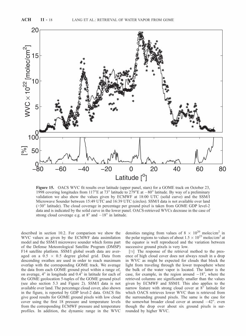
described in section 10.2. For comparison we show theWVC values as given by the ECMWF data assimilationmodel and the SSM/I microwave sounder which forms partof the Defense Meteorological Satellite Program (DMSP)F14 satellite platform. SSM/I global swath data are aver-aged on a 0.5 � 0.5 degree global grid. Data fromdescending swathes are used in order to reach maximumoverlap with the corresponding GOME track. We averagethe data from each GOME ground pixel within a range of,on average, 4� in longitude and 0.4� in latitude for each ofthe GOME geolocation 5-tuples of the GOME ground pixel(see also section 5.3 and Figure 2). SSM/I data is notavailable over land. The percentage cloud cover, also shownin the figure, is reported by GDP level-2 data. OACS fitsgive good results for GOME ground pixels with low cloudcover using the first 18 pressure and temperature levelsfrom the corresponding ECMWF pressure and temperatureprofiles. In addition, the dynamic range in the WVC

densities ranging from values of 8 � 1020 molec/cm2 inthe polar regions to values of about 1.5 � 1023 molec/cm2 atthe equator is well reproduced and the variation betweensuccessive ground pixels is very low.[73] The response of the retrieval method to the pres-

ence of high cloud cover does not always result in a dropin WVC as might be expected for clouds that block thelight from traveling through the lower troposphere wherethe bulk of the water vapor is located. The latter is thecase, for example, in the region around �18�, where theretrieved columns are significantly smaller than the valuesgiven by ECMWF and SSM/I. This also applies to thenarrow feature with strong cloud cover at 8� latitude forwhich OACS retrieves lower WVC than is retrieved fromthe surrounding ground pixels. The same is the case forthe somewhat broader cloud cover at around �42�. eventhough the drop over about six ground pixels is sur-rounded by higher WVC.

Figure 15. OACS WVC fit results over latitude (upper panel, stars) for a GOME track on October 23,1998 covering longitudes from 117�E at 73� latitude to 279�E at �80� latitude. By way of a preliminaryvalidation we also show the values given by ECMWF at 18:00 UTC (solid curve) and the SSM/IMicrowave Sounder between 15:49 UTC and 16:39 UTC (circles). SSM/I data is not available over land(>30� latitude). The cloud coverage in percentage per ground pixel is taken from GOME GDP level-2data and is indicated by the solid curve in the lower panel. OACS-retrieved WVCs decrease in the case ofstrong cloud coverage e.g. at 8� and �18� in latitude.


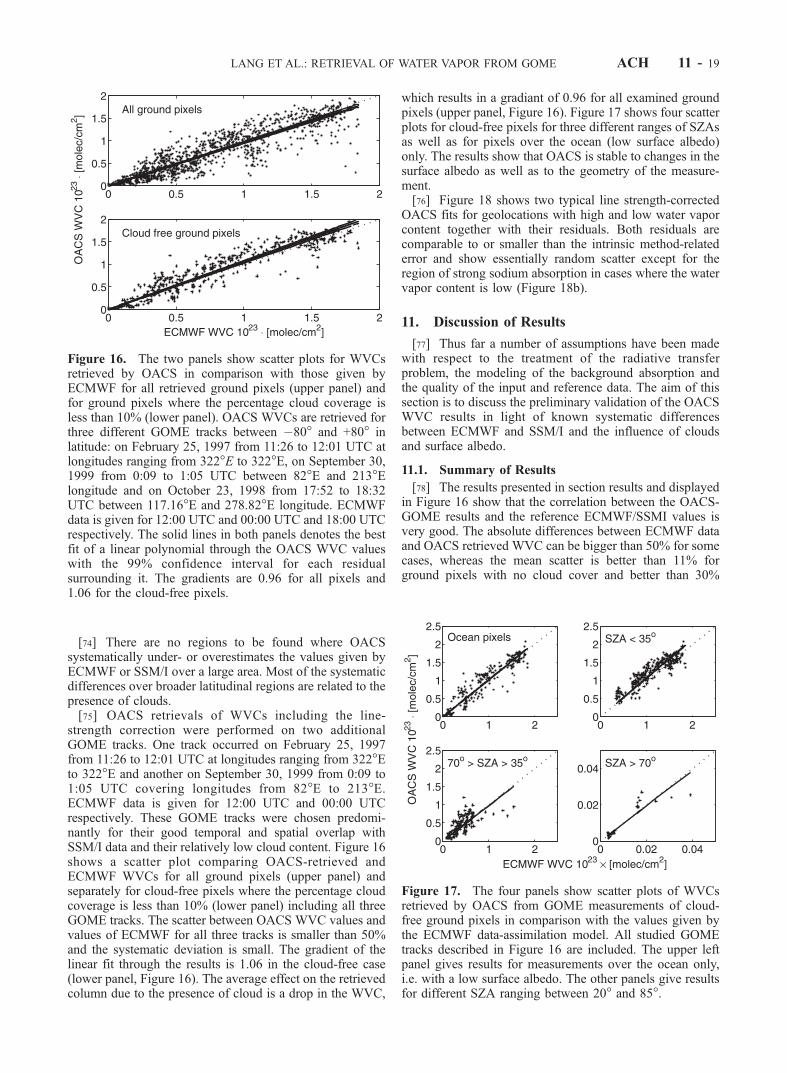
[74] There are no regions to be found where OACSsystematically under- or overestimates the values given byECMWF or SSM/I over a large area. Most of the systematicdifferences over broader latitudinal regions are related to thepresence of clouds.[75] OACS retrievals of WVCs including the line-

strength correction were performed on two additionalGOME tracks. One track occurred on February 25, 1997from 11:26 to 12:01 UTC at longitudes ranging from 322�Eto 322�E and another on September 30, 1999 from 0:09 to1:05 UTC covering longitudes from 82�E to 213�E.ECMWF data is given for 12:00 UTC and 00:00 UTCrespectively. These GOME tracks were chosen predomi-nantly for their good temporal and spatial overlap withSSM/I data and their relatively low cloud content. Figure 16shows a scatter plot comparing OACS-retrieved andECMWF WVCs for all ground pixels (upper panel) andseparately for cloud-free pixels where the percentage cloudcoverage is less than 10% (lower panel) including all threeGOME tracks. The scatter between OACS WVC values andvalues of ECMWF for all three tracks is smaller than 50%and the systematic deviation is small. The gradient of thelinear fit through the results is 1.06 in the cloud-free case(lower panel, Figure 16). The average effect on the retrievedcolumn due to the presence of cloud is a drop in the WVC,

which results in a gradiant of 0.96 for all examined groundpixels (upper panel, Figure 16). Figure 17 shows four scatterplots for cloud-free pixels for three different ranges of SZAsas well as for pixels over the ocean (low surface albedo)only. The results show that OACS is stable to changes in thesurface albedo as well as to the geometry of the measure-ment.[76] Figure 18 shows two typical line strength-corrected

OACS fits for geolocations with high and low water vaporcontent together with their residuals. Both residuals arecomparable to or smaller than the intrinsic method-relatederror and show essentially random scatter except for theregion of strong sodium absorption in cases where the watervapor content is low (Figure 18b).

11. Discussion of Results

[77] Thus far a number of assumptions have been madewith respect to the treatment of the radiative transferproblem, the modeling of the background absorption andthe quality of the input and reference data. The aim of thissection is to discuss the preliminary validation of the OACSWVC results in light of known systematic differencesbetween ECMWF and SSM/I and the influence of cloudsand surface albedo.

11.1. Summary of Results

[78] The results presented in section results and displayedin Figure 16 show that the correlation between the OACS-GOME results and the reference ECMWF/SSMI values isvery good. The absolute differences between ECMWF dataand OACS retrieved WVC can be bigger than 50% for somecases, whereas the mean scatter is better than 11% forground pixels with no cloud cover and better than 30%

Figure 17. The four panels show scatter plots of WVCsretrieved by OACS from GOME measurements of cloud-free ground pixels in comparison with the values given bythe ECMWF data-assimilation model. All studied GOMEtracks described in Figure 16 are included. The upper leftpanel gives results for measurements over the ocean only,i.e. with a low surface albedo. The other panels give resultsfor different SZA ranging between 20� and 85�.

Figure 16. The two panels show scatter plots for WVCsretrieved by OACS in comparison with those given byECMWF for all retrieved ground pixels (upper panel) andfor ground pixels where the percentage cloud coverage isless than 10% (lower panel). OACS WVCs are retrieved forthree different GOME tracks between �80� and +80� inlatitude: on February 25, 1997 from 11:26 to 12:01 UTC atlongitudes ranging from 322�E to 322�E, on September 30,1999 from 0:09 to 1:05 UTC between 82�E and 213�Elongitude and on October 23, 1998 from 17:52 to 18:32UTC between 117.16�E and 278.82�E longitude. ECMWFdata is given for 12:00 UTC and 00:00 UTC and 18:00 UTCrespectively. The solid lines in both panels denotes the bestfit of a linear polynomial through the OACS WVC valueswith the 99% confidence interval for each residualsurrounding it. The gradients are 0.96 for all pixels and1.06 for the cloud-free pixels.


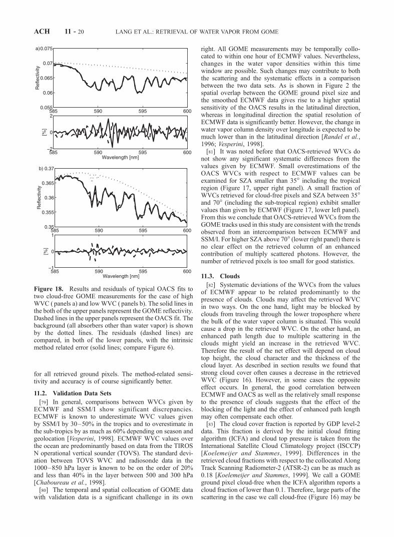
for all retrieved ground pixels. The method-related sensi-tivity and accuracy is of course significantly better.

11.2. Validation Data Sets

[79] In general, comparisons between WVCs given byECMWF and SSM/I show significant discrepancies.ECMWF is known to underestimate WVC values givenby SSM/I by 30–50% in the tropics and to overestimate inthe sub-tropics by as much as 60% depending on season andgeolocation [Vesperini, 1998]. ECMWF WVC values overthe ocean are predominantly based on data from the TIROSN operational vertical sounder (TOVS). The standard devi-ation between TOVS WVC and radiosonde data in the1000–850 hPa layer is known to be on the order of 20%and less than 40% in the layer between 500 and 300 hPa[Chaboureau et al., 1998].[80] The temporal and spatial collocation of GOME data

with validation data is a significant challenge in its own

right. All GOME measurements may be temporally collo-cated to within one hour of ECMWF values. Nevertheless,changes in the water vapor densities within this timewindow are possible. Such changes may contribute to boththe scattering and the systematic effects in a comparisonbetween the two data sets. As is shown in Figure 2 thespatial overlap between the GOME ground pixel size andthe smoothed ECMWF data gives rise to a higher spatialsensitivity of the OACS results in the latitudinal direction,whereas in longitudinal direction the spatial resolution ofECMWF data is significantly better. However, the change inwater vapor column density over longitude is expected to bemuch lower than in the latitudinal direction [Randel et al.,1996; Vesperini, 1998].[81] It was noted before that OACS-retrieved WVCs do

not show any significant systematic differences from thevalues given by ECMWF. Small overestimations of theOACS WVCs with respect to ECMWF values can beexamined for SZA smaller than 35� including the tropicalregion (Figure 17, upper right panel). A small fraction ofWVCs retrieved for cloud-free pixels and SZA between 35�and 70� (including the sub-tropical region) exhibit smallervalues than given by ECMWF (Figure 17, lower left panel).From this we conclude that OACS-retrieved WVCs from theGOME tracks used in this study are consistent with the trendsobserved from an intercomparison between ECMWF andSSM/I. For higher SZA above 70� (lower right panel) there isno clear effect on the retrieved column of an enhancedcontribution of multiply scattered photons. However, thenumber of retrieved pixels is too small for good statistics.

11.3. Clouds

[82] Systematic deviations of the WVCs from the valuesof ECMWF appear to be related predominantly to thepresence of clouds. Clouds may affect the retrieved WVCin two ways. On the one hand, light may be blocked byclouds from traveling through the lower troposphere wherethe bulk of the water vapor column is situated. This wouldcause a drop in the retrieved WVC. On the other hand, anenhanced path length due to multiple scattering in theclouds might yield an increase in the retrieved WVC.Therefore the result of the net effect will depend on cloudtop height, the cloud character and the thickness of thecloud layer. As described in section results we found thatstrong cloud cover often causes a decrease in the retrievedWVC (Figure 16). However, in some cases the oppositeeffect occurs. In general, the good correlation betweenECMWF and OACS as well as the relatively small responseto the presence of clouds suggests that the effect of theblocking of the light and the effect of enhanced path lengthmay often compensate each other.[83] The cloud cover fraction is reported by GDP level-2

data. This fraction is derived by the initial cloud fittingalgorithm (ICFA) and cloud top pressure is taken from theInternational Satellite Cloud Climatology project (ISCCP)[Koelemeijer and Stammes, 1999]. Differences in theretrieved cloud fractions with respect to the collocated AlongTrack Scanning Radiometer-2 (ATSR-2) can be as much as0.18 [Koelemeijer and Stammes, 1999]. We call a GOMEground pixel cloud-free when the ICFA algorithm reports acloud fraction of lower than 0.1. Therefore, large parts of thescattering in the case we call cloud-free (Figure 16) may be

Figure 18. Results and residuals of typical OACS fits totwo cloud-free GOME measurements for the case of highWVC ( panels a) and lowWVC ( panels b). The solid lines inthe both of the upper panels represent the GOME reflectivity.Dashed lines in the upper panels represent the OACS fit. Thebackground (all absorbers other than water vapor) is shownby the dotted lines. The residuals (dashed lines) arecompared, in both of the lower panels, with the intrinsicmethod related error (solid lines; compare Figure 6).


attributed to ground pixels partially covered by clouds orerrors in the cloud fraction values given by GDP level-2 data.

11.4. Differential Fit Mismatch

[84] For the calculation of the error �f of the modelinput parameter f we assumed that the water vapor sub-column profile concentrations used in the calculation of RM

given by ECMWF are close to reality. We further assumedthat the differential contribution of multiple scattered pho-tons are weak. The signatures of both of these errors, not tomention some contribution of the Ring effect and theFraunhofer line effect discussed in sections 5.2 and 10.2especially in the two pixels covering the sodium lines,should also contribute to the differential spectral structureof the calculated cross-section correction �f. We quantifiedthe contribution of the Fraunhofer line effect to be less than15% of�f in the area around the sodium lines and less than5% in the remaining wavelength region. The signature ofneglecting the differential impact of multiple scattering inthe calculation of �f should be visible as an systematiceffect (compare section 8 and Figure 9) displaying thedifferential structure of the water vapor absorption. Thiseffect is extremely small. Consequently, we relate thedifferential fit mismatch predominantly to instrumentalpixel-to-pixel variations which are not corrected for by thelevel 1 data processing together with errors in the linestrength databases. This places an upper limit of accuracyon the latter of about 10 to 20%.

11.5. Surface Albedo

[85] For each OACS fit we retrieve a surface albedo �(equation (27)) assuming that the surface may be modeled

as a Lambertian reflector. Figure 19 shows the retrievedalbedo at 590 nm together with the cloud cover for thesame GOME track shown and described in Figure 15. Thecloud-free results are comparable with those of Koele-meijer et al. [1997] using GOME measurements with anatmospheric correction scheme. However, the wavelengthdependence of the albedo (equation (27)) within ourspectral window might be influenced by the simultane-ously fitted multiple scattering term (equation (28)). A fitto the solution of the DAM revealed an albedo accuracy ofabout 30% at 592 nm for a ocean type surface albedo of0.03 (Table 4). For higher albedo over land (around 0.1)the accuracy is better than 10% due to the model calcu-lations and retrievals. The impact of multiple scatteringand aerosol extinction can introduce errors in the retrievedalbedo value of up to 40% for maritime cases. Theresponse to clouds is also clearly visible in Figure 19. Inthe case of strong cloud cover the retrieved albedo caneasily reach 0.5.

12. Overview and Outlook

12.1. Summary

[86] We have shown that OACS is able to forward modelupwelling reflectivity with accuracies better than 2%, whencompared to results from a lbl calculation. In columnretrieval terms, the precision of OACS (which depends oninstrumental characteristics) is 0.66% for high WVC and3.4% for low WVC. The accuracy of the method is betterthan 0.05% and 1.4% for high and low WVC, respectively.Besides calibrated radiances, the only necessary inputs froman operational perspective are specific temperature andpressure profiles for a given geolocation and SCDs ofozone. Method inputs which are pre-calculated and storedin lookup tables include pdfs of water vapor cross-sectionrealizations taken from the HITRAN’96 database and cross-sections of (O2)2 and O3. The robustness or total accuracy ofthe method due to errors in the input pressure and temper-ature profile was found to between 0.8% and 4% for highand low WVC, respectively. The obtained WVCs for cloud-free ground pixel situations correlate very well to WVCsgiven by ECMWF and SSM/I. The ground pixel-to-pixelvariation of the retrieved column densities are low and themethod is robust to changes in surface albedo as well aschanges in the SZA.

12.2. Implementation and Routine Retrieval

[87] We have introduced, tested and presented a prelimi-nary validation of a novel, fast forward modeling andretrieval method. The intention was to develop a relativelyfast method for modeling spectral measurements for whichthe instrumental resolution is much broader than the absorp-tion features of the trace gas under study. OACS uses a pdfcoefficient method for the calculation of reflectivities con-taining the full altitude-dependent structure of the spectrumwhich can be stored in a look-up table. OACS forwardmodeling is very fast with respect to line-by-line methodsand a retrieval of trace gas column from constituents withnarrowband absorption spectra can be done on reasonabletime scales. A retrieval of WVCs as described in this paperutilizing 18 altitude levels takes about 20 minutes permeasurement on a Pentium II, 450 MHz, using an uncom-

Figure 19. Surface albedo � at 590 nm retrieved with theOACS method for the GOME track described in Figures 15(upper panel). The first part of the track (which covers 40�to 60� latitude at about 260� in longitude) starts over theCanadian Shield which is dominated by water in the form oflakes and by vegetation. OACS retrieved albedos between0.03 and 0.1 for cloud free pixels (the percentage cloudcover is shown in the lower panel). The other part, from theRocky Mountains over the Gulf of California and thePacific (40� to 20� latitude at about 255� in longitude),frequently yielded albedos below 0.05.


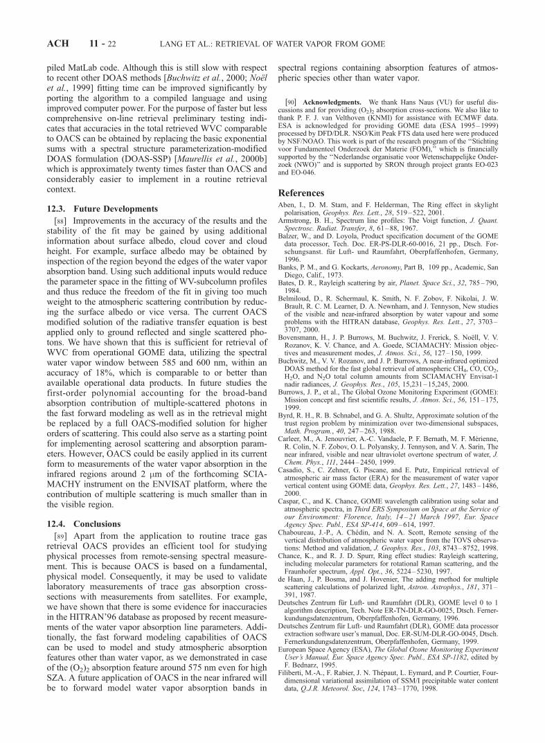
piled MatLab code. Although this is still slow with respectto recent other DOAS methods [Buchwitz et al., 2000; Noelet al., 1999] fitting time can be improved significantly byporting the algorithm to a compiled language and usingimproved computer power. For the purpose of faster but lesscomprehensive on-line retrieval preliminary testing indi-cates that accuracies in the total retrieved WVC comparableto OACS can be obtained by replacing the basic exponentialsums with a spectral structure parameterization-modifiedDOAS formulation (DOAS-SSP) [Maurellis et al., 2000b]which is approximately twenty times faster than OACS andconsiderably easier to implement in a routine retrievalcontext.

12.3. Future Developments

[88] Improvements in the accuracy of the results and thestability of the fit may be gained by using additionalinformation about surface albedo, cloud cover and cloudheight. For example, surface albedo may be obtained byinspection of the region beyond the edges of the water vaporabsorption band. Using such additional inputs would reducethe parameter space in the fitting of WV-subcolumn profilesand thus reduce the freedom of the fit in giving too muchweight to the atmospheric scattering contribution by reduc-ing the surface albedo or vice versa. The current OACSmodified solution of the radiative transfer equation is bestapplied only to ground reflected and single scattered pho-tons. We have shown that this is sufficient for retrieval ofWVC from operational GOME data, utilizing the spectralwater vapor window between 585 and 600 nm, within anaccuracy of 18%, which is comparable to or better thanavailable operational data products. In future studies thefirst-order polynomial accounting for the broad-bandabsorption contribution of multiple-scattered photons inthe fast forward modeling as well as in the retrieval mightbe replaced by a full OACS-modified solution for higherorders of scattering. This could also serve as a starting pointfor implementing aerosol scattering and absorption param-eters. However, OACS could be easily applied in its currentform to measurements of the water vapor absorption in theinfrared regions around 2 mm of the forthcoming SCIA-MACHY instrument on the ENVISAT platform, where thecontribution of multiple scattering is much smaller than inthe visible region.

12.4. Conclusions

[89] Apart from the application to routine trace gasretrieval OACS provides an efficient tool for studyingphysical processes from remote-sensing spectral measure-ment. This is because OACS is based on a fundamental,physical model. Consequently, it may be used to validatelaboratory measurements of trace gas absorption cross-sections with measurements from satellites. For example,we have shown that there is some evidence for inaccuraciesin the HITRAN’96 database as proposed by recent measure-ments of the water vapor absorption line parameters. Addi-tionally, the fast forward modeling capabilities of OACScan be used to model and study atmospheric absorptionfeatures other than water vapor, as we demonstrated in caseof the (O2)2 absorption feature around 575 nm even for highSZA. A future application of OACS in the near infrared willbe to forward model water vapor absorption bands in

spectral regions containing absorption features of atmos-pheric species other than water vapor.

[90] Acknowledgments. We thank Hans Naus (VU) for useful dis-cussions and for providing (O2)2 absorption cross-sections. We also like tothank P. F. J. van Velthoven (KNMI) for assistance with ECMWF data.ESA is acknowledged for providing GOME data (ESA 1995–1999)processed by DFD/DLR. NSO/Kitt Peak FTS data used here were producedby NSF/NOAO. This work is part of the research program of the ‘‘Stichtingvoor Fundamenteel Onderzoek der Materie (FOM),’’ which is financiallysupported by the ‘‘Nederlandse organisatie voor Wetenschappelijke Onder-zoek (NWO)’’ and is supported by SRON through project grants EO-023and EO-046.

ReferencesAben, I., D. M. Stam, and F. Helderman, The Ring effect in skylightpolarisation, Geophys. Res. Lett., 28, 519–522, 2001.

Armstrong, B. H., Spectrum line profiles: The Voigt function, J. Quant.Spectrosc. Radiat. Transfer, 8, 61–88, 1967.

Balzer, W., and D. Loyola, Product specification document of the GOMEdata processor, Tech. Doc. ER-PS-DLR-60-0016, 21 pp., Dtsch. For-schungsanst. fur Luft- und Raumfahrt, Oberpfaffenhofen, Germany,1996.

Banks, P. M., and G. Kockarts, Aeronomy, Part B, 109 pp., Academic, SanDiego, Calif., 1973.

Bates, D. R., Rayleigh scattering by air, Planet. Space Sci., 32, 785–790,1984.

Belmiloud, D., R. Schermaul, K. Smith, N. F. Zobov, F. Nikolai, J. W.Brault, R. C. M. Learner, D. A. Newnham, and J. Tennyson, New studiesof the visible and near-infrared absorption by water vapour and someproblems with the HITRAN database, Geophys. Res. Lett., 27, 3703–3707, 2000.

Bovensmann, H., J. P. Burrows, M. Buchwitz, J. Frerick, S. Noell, V. V.Rozanov, K. V. Chance, and A. Goede, SCIAMACHY: Mission objec-tives and measurement modes, J. Atmos. Sci., 56, 127–150, 1999.

Buchwitz, M., V. V. Rozanov, and J. P. Burrows, A near-infrared optimizedDOAS method for the fast global retrieval of atmospheric CH4, CO, CO2,H2O, and N2O total column amounts from SCIAMACHY Envisat-1nadir radiances, J. Geophys. Res., 105, 15,231–15,245, 2000.

Burrows, J. P., et al., The Global Ozone Monitoring Experiment (GOME):Mission concept and first scientific results, J. Atmos. Sci., 56, 151–175,1999.

Byrd, R. H., R. B. Schnabel, and G. A. Shultz, Approximate solution of thetrust region problem by minimization over two-dimensional subspaces,Math. Program., 40, 247–263, 1988.

Carleer, M., A. Jenouvrier, A.-C. Vandaele, P. F. Bernath, M. F. Merienne,R. Colin, N. F. Zobov, O. L. Polyansky, J. Tennyson, and V. A. Sarin, Thenear infrared, visible and near ultraviolet overtone spectrum of water, J.Chem. Phys., 111, 2444–2450, 1999.

Casadio, S., C. Zehner, G. Piscane, and E. Putz, Empirical retrieval ofatmospheric air mass factor (ERA) for the measurement of water vaporvertical content using GOME data, Geophys. Res. Lett., 27, 1483–1486,2000.

Caspar, C., and K. Chance, GOME wavelength calibration using solar andatmospheric spectra, in Third ERS Symposium on Space at the Service ofour Environment: Florence, Italy, 14 – 21 March 1997, Eur. SpaceAgency Spec. Publ., ESA SP-414, 609–614, 1997.

Chaboureau, J.-P., A. Chedin, and N. A. Scott, Remote sensing of thevertical distribution of atmospheric water vapor from the TOVS observa-tions: Method and validation, J. Geophys. Res., 103, 8743–8752, 1998.

Chance, K., and R. J. D. Spurr, Ring effect studies: Rayleigh scattering,including molecular parameters for rotational Raman scattering, and theFraunhofer spectrum, Appl. Opt., 36, 5224–5230, 1997.

de Haan, J., P. Bosma, and J. Hovenier, The adding method for multiplescattering calculations of polarized light, Astron. Astrophys., 181, 371–391, 1987.

Deutsches Zentrum fur Luft- und Raumfahrt (DLR), GOME level 0 to 1algorithm description, Tech. Note ER-TN-DLR-GO-0025, Dtsch. Ferner-kundungsdatenzentrum, Oberpfaffenhofen, Germany, 1996.

Deutsches Zentrum fur Luft- und Raumfahrt (DLR), GOME data processorextraction software user’s manual, Doc. ER-SUM-DLR-GO-0045, Dtsch.Fernerkundungsdatenzentrum, Oberpfaffenhofen, Germany, 1999.

European Space Agency (ESA), The Global Ozone Monitoring ExperimentUser’s Manual, Eur. Space Agency Spec. Publ., ESA SP-1182, edited byF. Bednarz, 1995.

Filiberti, M.-A., F. Rabier, J. N. Thepaut, L. Eymard, and P. Courtier, Four-dimensional variational assimilation of SSM/I precipitable water contentdata, Q.J.R. Meteorol. Soc, 124, 1743–1770, 1998.


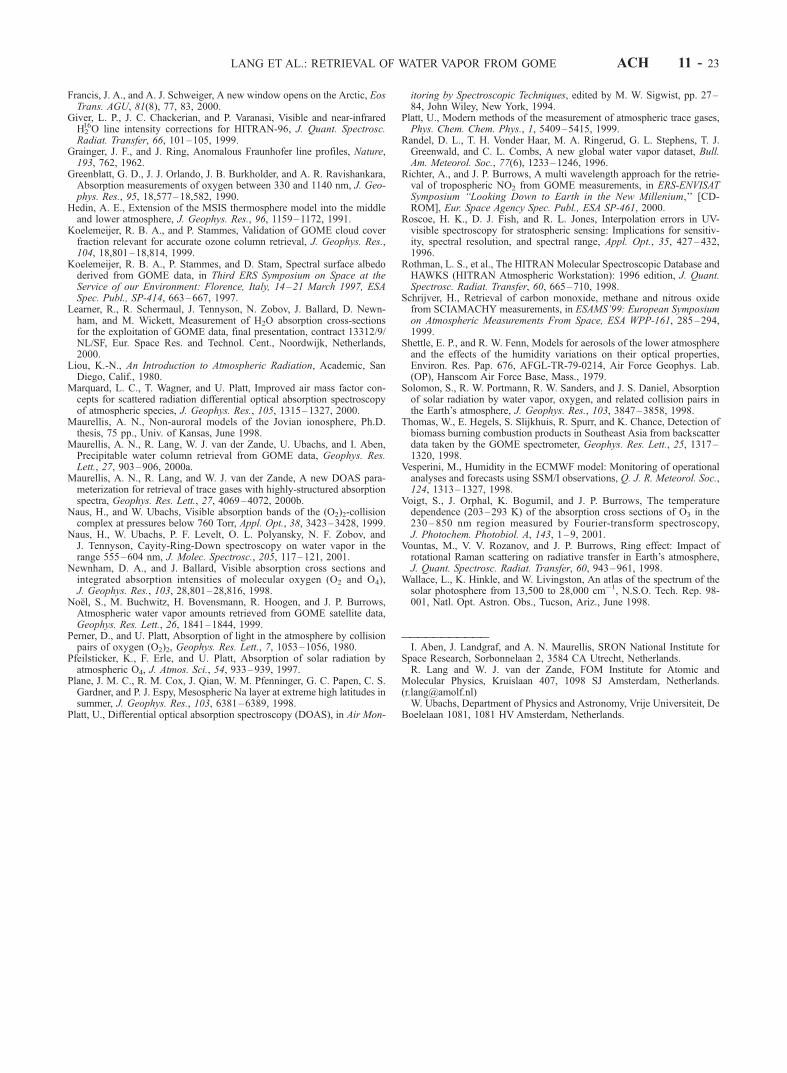
Francis, J. A., and A. J. Schweiger, A new window opens on the Arctic, EosTrans. AGU, 81(8), 77, 83, 2000.

Giver, L. P., J. C. Chackerian, and P. Varanasi, Visible and near-infraredH216O line intensity corrections for HITRAN-96, J. Quant. Spectrosc.

Radiat. Transfer, 66, 101–105, 1999.Grainger, J. F., and J. Ring, Anomalous Fraunhofer line profiles, Nature,193, 762, 1962.

Greenblatt, G. D., J. J. Orlando, J. B. Burkholder, and A. R. Ravishankara,Absorption measurements of oxygen between 330 and 1140 nm, J. Geo-phys. Res., 95, 18,577–18,582, 1990.

Hedin, A. E., Extension of the MSIS thermosphere model into the middleand lower atmosphere, J. Geophys. Res., 96, 1159–1172, 1991.

Koelemeijer, R. B. A., and P. Stammes, Validation of GOME cloud coverfraction relevant for accurate ozone column retrieval, J. Geophys. Res.,104, 18,801–18,814, 1999.

Koelemeijer, R. B. A., P. Stammes, and D. Stam, Spectral surface albedoderived from GOME data, in Third ERS Symposium on Space at theService of our Environment: Florence, Italy, 14–21 March 1997, ESASpec. Publ., SP-414, 663–667, 1997.

Learner, R., R. Schermaul, J. Tennyson, N. Zobov, J. Ballard, D. Newn-ham, and M. Wickett, Measurement of H2O absorption cross-sectionsfor the exploitation of GOME data, final presentation, contract 13312/9/NL/SF, Eur. Space Res. and Technol. Cent., Noordwijk, Netherlands,2000.

Liou, K.-N., An Introduction to Atmospheric Radiation, Academic, SanDiego, Calif., 1980.

Marquard, L. C., T. Wagner, and U. Platt, Improved air mass factor con-cepts for scattered radiation differential optical absorption spectroscopyof atmospheric species, J. Geophys. Res., 105, 1315–1327, 2000.

Maurellis, A. N., Non-auroral models of the Jovian ionosphere, Ph.D.thesis, 75 pp., Univ. of Kansas, June 1998.

Maurellis, A. N., R. Lang, W. J. van der Zande, U. Ubachs, and I. Aben,Precipitable water column retrieval from GOME data, Geophys. Res.Lett., 27, 903–906, 2000a.

Maurellis, A. N., R. Lang, and W. J. van der Zande, A new DOAS para-meterization for retrieval of trace gases with highly-structured absorptionspectra, Geophys. Res. Lett., 27, 4069–4072, 2000b.

Naus, H., and W. Ubachs, Visible absorption bands of the (O2)2-collisioncomplex at pressures below 760 Torr, Appl. Opt., 38, 3423–3428, 1999.

Naus, H., W. Ubachs, P. F. Levelt, O. L. Polyansky, N. F. Zobov, andJ. Tennyson, Cayity-Ring-Down spectroscopy on water vapor in therange 555–604 nm, J. Molec. Spectrosc., 205, 117–121, 2001.

Newnham, D. A., and J. Ballard, Visible absorption cross sections andintegrated absorption intensities of molecular oxygen (O2 and O4),J. Geophys. Res., 103, 28,801–28,816, 1998.

Noel, S., M. Buchwitz, H. Bovensmann, R. Hoogen, and J. P. Burrows,Atmospheric water vapor amounts retrieved from GOME satellite data,Geophys. Res. Lett., 26, 1841–1844, 1999.

Perner, D., and U. Platt, Absorption of light in the atmosphere by collisionpairs of oxygen (O2)2, Geophys. Res. Lett., 7, 1053–1056, 1980.

Pfeilsticker, K., F. Erle, and U. Platt, Absorption of solar radiation byatmospheric O4, J. Atmos. Sci., 54, 933–939, 1997.

Plane, J. M. C., R. M. Cox, J. Qian, W. M. Pfenninger, G. C. Papen, C. S.Gardner, and P. J. Espy, Mesospheric Na layer at extreme high latitudes insummer, J. Geophys. Res., 103, 6381–6389, 1998.

Platt, U., Differential optical absorption spectroscopy (DOAS), in Air Mon-

itoring by Spectroscopic Techniques, edited by M. W. Sigwist, pp. 27–84, John Wiley, New York, 1994.

Platt, U., Modern methods of the measurement of atmospheric trace gases,Phys. Chem. Chem. Phys., 1, 5409–5415, 1999.

Randel, D. L., T. H. Vonder Haar, M. A. Ringerud, G. L. Stephens, T. J.Greenwald, and C. L. Combs, A new global water vapor dataset, Bull.Am. Meteorol. Soc., 77(6), 1233–1246, 1996.

Richter, A., and J. P. Burrows, A multi wavelength approach for the retrie-val of tropospheric NO2 from GOME measurements, in ERS-ENVISATSymposium ‘‘Looking Down to Earth in the New Millenium,’’ [CD-ROM], Eur. Space Agency Spec. Publ., ESA SP-461, 2000.

Roscoe, H. K., D. J. Fish, and R. L. Jones, Interpolation errors in UV-visible spectroscopy for stratospheric sensing: Implications for sensitiv-ity, spectral resolution, and spectral range, Appl. Opt., 35, 427–432,1996.

Rothman, L. S., et al., The HITRAN Molecular Spectroscopic Database andHAWKS (HITRAN Atmospheric Workstation): 1996 edition, J. Quant.Spectrosc. Radiat. Transfer, 60, 665–710, 1998.

Schrijver, H., Retrieval of carbon monoxide, methane and nitrous oxidefrom SCIAMACHY measurements, in ESAMS’99: European Symposiumon Atmospheric Measurements From Space, ESA WPP-161, 285–294,1999.

Shettle, E. P., and R. W. Fenn, Models for aerosols of the lower atmosphereand the effects of the humidity variations on their optical properties,Environ. Res. Pap. 676, AFGL-TR-79-0214, Air Force Geophys. Lab.(OP), Hanscom Air Force Base, Mass., 1979.

Solomon, S., R. W. Portmann, R. W. Sanders, and J. S. Daniel, Absorptionof solar radiation by water vapor, oxygen, and related collision pairs inthe Earth’s atmosphere, J. Geophys. Res., 103, 3847–3858, 1998.

Thomas, W., E. Hegels, S. Slijkhuis, R. Spurr, and K. Chance, Detection ofbiomass burning combustion products in Southeast Asia from backscatterdata taken by the GOME spectrometer, Geophys. Res. Lett., 25, 1317–1320, 1998.

Vesperini, M., Humidity in the ECMWF model: Monitoring of operationalanalyses and forecasts using SSM/I observations, Q. J. R. Meteorol. Soc.,124, 1313–1327, 1998.

Voigt, S., J. Orphal, K. Bogumil, and J. P. Burrows, The temperaturedependence (203–293 K) of the absorption cross sections of O3 in the230 – 850 nm region measured by Fourier-transform spectroscopy,J. Photochem. Photobiol. A, 143, 1–9, 2001.

Vountas, M., V. V. Rozanov, and J. P. Burrows, Ring effect: Impact ofrotational Raman scattering on radiative transfer in Earth’s atmosphere,J. Quant. Spectrosc. Radiat. Transfer, 60, 943–961, 1998.

Wallace, L., K. Hinkle, and W. Livingston, An atlas of the spectrum of thesolar photosphere from 13,500 to 28,000 cm�1, N.S.O. Tech. Rep. 98-001, Natl. Opt. Astron. Obs., Tucson, Ariz., June 1998.

��I. Aben, J. Landgraf, and A. N. Maurellis, SRON National Institute for

Space Research, Sorbonnelaan 2, 3584 CA Utrecht, Netherlands.R. Lang and W. J. van der Zande, FOM Institute for Atomic and

Molecular Physics, Kruislaan 407, 1098 SJ Amsterdam, Netherlands.([email protected])W. Ubachs, Department of Physics and Astronomy, Vrije Universiteit, De

Boelelaan 1081, 1081 HV Amsterdam, Netherlands.


Forward modeling and retrieval of water vapor from the Global Ozone Monitoring Experiment: Treatment...

Documents

Transcript of Forward modeling and retrieval of water vapor from the Global Ozone Monitoring Experiment: Treatment...