Formation of ultrashort triangularpulses in optical fibers

S. O. Iakushev,1 O. V. Shulika,2,∗ I. A. Sukhoivanov,2V. I. Fesenko,1,3 M. V. Andres,4 and H. Sayinc5

1R&D Lab. ”Photonics”, Kharkiv National University of Radio Electronics, Ukraine2Department of Electronic Engineering, DICIS, University of Guanajuato, Mexico

3Department of Microwave Electronics, Institute of Radio Astronomy of NASU, Ukraine4Department of Applied Physics, University of Valencia, Spain

5Laser Development Department, Laser Zentrum Hannover, Hannover, Germany∗oshulika@ugto.mx

Abstract: Specialty shape ultrashort optical pulses, and triangular pulsesin particular, are of great interest in optical signal processing. Compactfiber-based techniques for producing the special pulse waveforms fromGaussian or secant pulses delivered by modern ultrafast lasers are in demandin telecommunications. Using the nonlinear Schrodinger equation in anextended form the transformation of ultrashort pulses in a fiber towardstriangular shape is characterized by the misfit parameter under variety ofincident pulse shapes, energies, and chirps. It is shown that short (1-2 m)conventional single mode fiber can be used for triangular pulse formation inthe steady-state regime without any pre-chirping if femtosecond pulses areused for pumping. The pulses obtained are stable and demonstrate linearchirp. The ranges and combinations of the pulse parameters found herewill serve as a guide for scheduling the experiments and implementation ofvarious all-fiber schemes for optical signal processing.

© 2014 Optical Society of AmericaOCIS codes: (190.4370) Nonlinear optics, fibers; (320.7110) Ultrafast nonlinear optics;(320.5540) Pulse shaping.

References and links1. S. Boscolo and C. Finot, “Nonlinear pulse shaping in fibers for pulse generation and optical processing,” Int. J.

Optics 2012, 1–14 (2012).2. F. Parmigiani, P. Petropoulos, M. Ibsen, P. J. Almeida, T. T. Ng, and D. J. Richardson, “Time domain add-drop

multiplexing scheme snhanced using a saw-tooth pulse shaper,” Opt. Express 17, 8362–8369 (2009).3. F. Parmigiani, M. Ibsen, P. Petropoulos, and D. J. Richardson, “Efficient all-optical wavelength conversion

scheme based on a saw-tooth pulse shaper,” IEEE Photon. Technol. Lett. 21, 1837–1839 (2009).4. A. I. Latkin, S. Boscolo, R. S. Bhamber, and S. K. Turitsyn, “Doubling of optical signals using triangular pulses,”

J. Opt. Soc. Am. B 26, 1492–1496 (2009).5. R. S. Bhamber, S. Boscolo, A. I. Latkin, and S. K. Turitsyn, “All-optical TDM to WDM signal conversion and

partial regeneration using XPM with triangular pulses,” in “Optical Communication, 2008. ECOC 2008. 34thEuropean Conference on,” (Brussels, Begium, 2008).

6. A. M. Weiner, “Femtosecond pulse shaping using spatial light modulators,” Rev. Scien. Instrum. 71, 1939–1960(2000).

7. A. M. Clarke, D. G. Williams, M. A. F. Roelens, and B. J. Eggleton, “Reconfigurable optical pulse generatoremploying a Fourier-domain programmable optical processor,” J. Lightwave Technol. 28, 97–103 (2010).

8. D. Nguyen, M. U. Piracha, D. Mandridis, and P. J. Delfyett, “Dynamic parabolic pulse generation using temporalshaping of wavelength to time mapped pulses,” Opt. Express 19, 12305–12311 (2011).

9. J. Ye, L. Yan, W. Pan, B. Luo, X. Zou, A. Yi, and S. Yao, “Photonic generation of triangular-shaped pulses basedon frequency-to-time conversion,” Opt. Lett. 36, 1458–1460 (2011).

10. P. Petropoulos, M. Ibsen, A. D. Ellis, and D. J. Richardson, “Rectangular pulse generations based on pulsereshaping using a superstructured fiber bragg grating,” J. Lightwave Technol. 19, 746–752 (2001).

11. T. Hirooka, M. Nakazawa, and K. Okamoto, “Bright and dark 40 GHz parabolic pulse generation using a pi-cosecond optical pulse train and an arrayed waveguide grating,” Opt. Lett. 33, 1102–1104 (2008).

12. C. Finot, L. Provost, P. Petropoulos, and D. J. Richardson, “Parabolic pulse generation through passive nonlinearpulse reshaping in a normally dispersive two segment fiber device,” Opt. Express 15, 852–864 (2007).

13. S. Boscolo, A. I. Latkin, and S. K. Turitsyn, “Passive nonlinear pulse shaping in normally dispersive fiber sys-tems,” IEEE J. Quantum Electron. 44, 1196–1203 (2008).

14. S. O. Iakushev, O. V. Shulika, and I. A. Sukhoivanov, “Passive nonlinear reshaping towards parabolic pulses inthe steady-state regime in optical fibers,” Opt. Commun. 285, 4493–4499 (2012).

15. I. A. Sukhoivanov, S. O. Iakushev, O. V. Shulika, A. Dıez, and M. Andres, “Femtosecond parabolic pulse shapingin normally dispersive optical fibers,” Opt. Express 21, 17769–17785 (2013).

16. H. Wang, A. I. Latkin, S. Boscolo, P. Harper, and S. K. Turitsyn, “Generation of triangular-shaped optical pulsesin normally dispersive fibre,” J. Opt. 12, 035205–1–5 (2010).

17. N. Verscheure and C. Finot, “Pulse doubling and wavelength conversion through triangular nonlinear pulse re-shaping,” Electron. Lett. 47, 1194–1196 (2011).

18. G. P. Agrawal, Nonlinear Fiber Optics (Academic, 2007), 4th ed.19. A. Zeytunyan, G. Yesayan, L. Mouradian, P. Kockaert, P. Emplit, F. Louradour, and A. Barthelemy, “Nonlinear-

dispersive similariton of passive fiber,” J. Euro. Opt. Soc. - Rapid Pub. 4, 09009–1–7 (2009).20. A. Tomlinson, R. H. Stolen, and C. V. Shank, “Compression of optical pulses chirped by self-phase modulation

in fibers,” J. Opt. Soc. Am. B 1, 139–149 (1984).21. M. Karlsson, “Optical fiber-grating compressors utilizing long fibers,” Opt. Commun. 112, 48–54 (1994).22. S. Boscolo and S. K. Turitsyn, “Intermediate asymptotics in nonlinear optical systems,” Phys. Rev. A 85, 043811

(2012).23. S. Ramachandran, Fiber Based Dispersion Compensation (Springer, 2007).24. Thorlabs, “Specification sheet: 780 HP – Single Mode Optical Fiber, 780 – 970 nm, � 125 µm cladding (Rev.

D, 2013-April-1, 6829-s01),” http://www.thorlabs.com/thorcat/6800/780HP-SpecSheet.pdf (2013). Accessed:2014-June-27.

25. OFS, “TrueWave Ocean Fibers SRS,” http://ofsoptics. thomasnet-navigator.com/Asset/TrueWaveSRSFiber-121-web.pdf (2013). Accessed: 2014-June-27.

26. B. B. Bale, S. Boscolo, K. Hammani, and C. Finot, “Effects of fourth-order fiber dispersion on ultrashortparabolic optical pulses in the normal dispersion regime,” J. Opt. Soc. Am. B 28, 2059–2065 (2011).

1. Introduction

Ultrashort optical pulses of special waveforms are very important in a number of scientific ap-plications, including ones in all-optical signal processing and manipulation, ultra-high-speedoptical systems, nonlinear and quantum optics [1]. The state of the art ultrafast lasers deliverusually Gaussian or secant pulse waveforms. However, many practical applications require em-ployment of larger variety of pulse waveforms such as flat-top (rectangular-like), parabolic, andtriangular pulses. Particularly, triangular pulses have found numerous applications in time do-main add-drop multiplexing [2], wavelength conversion [3], optical signal doubling [4], time-to-frequency mapping of multiplexed signals [5]. Therefore the development of simple andefficient optical approaches for picosecond and sub-picosecond pulse reshaping is an actualtask. Conventional optical pulse shaping in picosecond and femtosecond time scales impliesdirect filtering of pulse amplitude and phase in spectral domain or in temporal one [6–11]. Thistechnique requires application of special devices such as acousto-optic spatial light modulatorsor those one based on liquid crystals, fiber Bragg gratings, arrayed waveguide gratings [6–11].

In order to fulfill requirements of telecommunications, the compact fiber-based techniquesfor producing the special pulse waveforms from Gaussian or secant pulses delivered by mod-ern ultrafast lasers are required. Another approach based on the nonlinear pulse reshaping innormally dispersive optical fibers has been also proposed. And it was shown that this approachallows obtaining ultrashort parabolic waveform [12–15] via combined action of self-phase mod-ulation (SPM) and normal dispersion (ND) on the pulse shape and spectrum during pulse propa-gation in single mode normal dispersion fibers. As it was demonstrated this approach could alsoprovide triangular pulse formation [13,16]. Particularly it was shown that triangular pulses can

be obtained from Gaussian pulses having specific chirp and energy, within the narrow range ofthe fiber lengths up to one dispersion length. Also the picosecond triangular pulse formation wasexperimentally demonstrated applying long 2-4 km normal dispersion fiber for pulse reshapingand 400-700 m fiber with anomalous dispersion for pre-chirping [16]. The same scheme hasbeen applied in [17] with secant hyperbolic incident pulses.

However, the conditions of triangular pulse formation in normal dispersive fibers are still notfully understood. Here we investigate via numerical modeling formation of triangular pulsesin normally dispersive fibers under variety of conditions: different initial pulse shapes, largevariation of the fiber length, initial chirp and soliton order. Special attention is focused on theformation of stable triangular pulses which can preserve the triangular shape and triangularspectrum during propagation in the fiber over the long distance. We expand here our approachproposed previously for formation of stable parabolic pulses via passive nonlinear reshapingin normal dispersion optical fibers [14, 15] to the triangular waveforms formation. We showthat this approach allow implementation of the compact fiber-based schemes (1-2 m of con-ventional normal dispersion fiber) of triangular pulse formation in the steady-state propagationregime without any pre-chirping stage from Gaussian or secant femtosecond pulses deliveredby conventional ultrafast lasers. This approach is much simpler for implementation and devicedevelopment.

2. Theoretical description of pulse transformation under propagation in a fiber

The formation of the nearly triangular pulses in the normal dispersion optical fibers is gov-erned by the interplay of normal group velocity dispersion and nonlinearity. This fundamentalmechanism is the same as for passive nonlinear reshaping to parabolic pulses [12–15] andwell described by the nonlinear Schrodinger equation (NLSE) [18]. However, here we extendstandard NLSE by including the fiber loss and the third-order dispersion in order to take intoaccount parameters of real fibers. Thus, the nonlinear Schrodinger equation (NLSE) of the fol-lowing form is used to describe the evolution of an ultrashort pulse during its propagation in anormal-dispersion optical fiber with Kerr nonlinearity:

∂A∂ z

=−α

2A− i

β2

2∂ 2A∂T 2 +

β3

6∂ 3A∂T 3 + iγ|A|2A, (1)

where A is the slowly varying complex envelope of the pulse; α is the losses; β2 is the secondorder dispersion; β3 is the third order dispersion; γ is the nonlinear coefficient; T is the time in aco-propagating time-frame; z is the propagation distance. In Eq. (1), the dispersion coefficientsβn are accounted for by expanding the mode-propagation constant β (ω) in a Taylor seriesaround the frequency ω0 at which the pulse spectrum is centered:

β (ω) = ne f fω

c= ∑

n>0

1n!

∂ nβ (ω0)

∂ωn (ω−ω0) (2)

The Eq. (1) is solved numerically using the split-step Fourier method [18]. For the subsequentdiscussion it is convenient to use following notations for the dispersion length LD , nonlinearlength LNL, soliton order N, and normalized distance ξ :

LD =T 2

0|β2|

, LNL =1

γP0, N =

√LD

LNL, ξ =

zLD

. (3)

In these expressions, P0 is the initial pulse peak power, T0 is the initial pulse duration (half-width at 1/e intensity level).

0 3 6 9 1 2 1 50 , 0 00 , 0 50 , 1 00 , 1 50 , 2 00 , 2 50 , 3 00 , 3 5

Misfit

param

eter M

N o r m a l i z e d d i s t a n c e ξ

0 , 3 0 , 4 0 , 5 0 , 6 0 , 70 , 0 20 , 0 30 , 0 40 , 0 5 ξ= 0 . 4 2

ξ= 0 . 3 3

(a)

2 4 6 8 1 0 1 2 1 40 , 0 00 , 0 50 , 1 00 , 1 50 , 2 00 , 2 50 , 3 00 , 3 5

Misfit

param

eter M

N o r m a l i z e d d i s t a n c e ξ

0 , 3 0 , 4 0 , 50 , 0 40 , 0 80 , 1 2

ξ= 0 . 3 3ξ= 0 . 4 2

(b)

Fig. 1. Evolution of the misfit parameter M versus normalized distance ξ for the temporal(a) and spectral (b) pulse shapes at N = 10 and C = −4, which corresponds to the caseexample of [16] shown there on Fig. 1. Black dashed lines correspond to the level M = 0.04. The insets in the figures show the enlarged areas of the minima where M < 0.04.

The quality of the triangular pulse is estimated through the deviation of its temporal intensityprofile |A(T )|2 and a triangular fit |A∆(T )|2 of the same energy; it characterizes quantitativelyvia the misfit parameter M [16]:

M =

∫ (|A|2−|A∆|2

)2∂T∫

|A|4∂T. (4)

We use the following expression for the triangular fit of the pulse envelope A∆(T ) of theenergy E∆ = P∆T∆

√2.5

A∆(T ) =

√

P∆

√1−∣∣∣ T

T∆

√2.5

∣∣∣, |T |6 T∆

√2.5

0, otherwise(5)

where P∆ is the peak power of the triangular pulse, T∆ is the duration of the triangular pulse(the half-width at 1/e intensity point). The misfit parameter M allows estimating the pulse shapeimperfection quntitavtively as compared to the triangular shape; a smaller value of M showsbetter fit to the triangular waveform. Usually we can consider a pulse shape to be close enoughto the triangular one when M < 4%.

Results presented in this paper are obtained for both an unchirped and chirped pulses. Weinclude the chirp into the initial pulse in the following way:

Achirp = A0 exp(

iCT 2

2T 20

), (6)

where A0 and Achirp are the waveform of an unchirped and chirped initial pulse, respectively;C is the chirp parameter. Adding the chirp in this way leads to the linear dependence of instan-taneous frequency defined as:

ω = ω0 +CTT 2

0. (7)

The instantaneous frequency in this case increases linearly from the leading to the trailingedge of the pulse for C > 0 (positive chirp) while the opposite process occurs for C < 0 (negativechirp).

3. Triangular pulse formation in the transient-state and steady-state propagationregimes

The passive nonlinear pulse reshaping in normally dispersive fibers is governed by the interplaybetween SPM and group velocity dispersion (GVD). Here one can mark out two propagationregimes previously studied for parabolic pulse formation [12–15]. The first one implies for-mation of the pulses of particular shape at the short propagation distance in the fiber usuallyshorter than the dispersion length (ξ < 1) [12, 13]. In this case pulse reshaping appears understrong action of SPM, which at first leads to fast changes of the pulse shape and its spectrum,and usually results in rather nonlinear pulse chirp. The desired pulse shape can be achievedhere within the narrow range of the fiber lengths; however, further pulse propagation in thefiber leads, in general case, to the change of the pulse shape. Therefore, we term this regime ofpulse formation as a transient-state propagation (TSP) regime throughout the paper. Formation

- 8 - 4 0 4 80 , 0

0 , 5

1 , 0 T r i a n g u l a r f i t M = 0 . 0 2 4

Inten

sity, a

.u.

T i m e , ( T / T 0 )(a)

- 8 - 4 0 4 80 , 0

0 , 5

1 , 0 T r i a n g u l a r f i t M = 0 . 0 3Int

ensity

, a.u.

T i m e , ( T / T 0 )(b)

- 3 0 - 2 0 - 1 0 0 1 0 2 0 3 00 , 0

0 , 5

1 , 0 T r i a n g u l a r f i t M = 0 . 1 4

Spec

trum,

a.u.

F r e q u e n c y , ( νT 0 )(c)

- 3 0 - 2 0 - 1 0 0 1 0 2 0 3 00 , 0

0 , 5

1 , 0 T r i a n g u l a r f i t M = 0 . 0 3 3

Spec

trum,

a.u.

F r e q u e n c y , ( νT 0 )(d)

Fig. 2. Normalized pulse temporal intensity (a), (b) and spectrum (c), (d) in the transient-state propagation (TSP) regime produced from chirped Gaussian pulse (N = 10, C = −4)at the distances ξ = 0.33 (the left column) and ξ = 0.42 (the right column), respectively.The right column corresponds to the case example of [16] shown there on Fig. 1. The insetslocated in the upper right corner show the value of misfit parameter M. Red curves showcorresponding triangular fits.

of triangular pulses reported in [16] is achieved exactly in the TSP-regime.Another mode of pulse formation in normally dispersive fiber is the steady-state propagation

(SSP) regime [14, 15]. It implies formation of pulses of a particular shape at a longer propaga-tion distance which usually exceeds a few dispersion lengths, and can be expressed roughly byξ > 1. The pulse reshaping in this case occurs under much weaker action of SPM and dom-ination of GVD. In this regime pulse gains spectronic properties [19]. Particularly the pulseshape repeats its spectrum profile and the chirp of the pulse becomes perfectly linear. In thisregime the spectral width of the pulse approaches its maximum asymptotic value leading to thesaturation of the pulse compression factor [20] and achievement of maximal compression [21].We term this regime as the steady-state one, because of both the pulse temporal profile andthe spectral profile are changing very slowly and are actually approaching some limit. Triangu-lar shape pulses, like those one formed passive fibers in SSP-regime, can also be generated inactive systems like mode-locked fiber lasers, as has been discussed in [22].

As we just pointed out, duration of SSP-produced pulses will be larger as compared to TSP-produced ones, due to the large temporal broadening undergone in the first case; it could be anissue for high repetition rate signal. However, this possible issue can be overcame within theall-fiber (or in-fiber) implementation using variety of accessible concepts [23].

The ultimate goal of this paper is to find detailed conditions of the triangular pulse formationboth in the transient-state propagation regime and in the steady-state propagation regime.

We start from the combination of parameters for triangular pulse formation in the TSP-regime presented in [16]. It will serve as a benchmark for our simulations and also will allowus highlighting the problem in hands. The M-plots shown in Fig. 1 demonstrate the dependenceof the misfit parameter M versus the normalized length ξ for both the temporal Fig. 1(a) andspectral Fig. 1(b) pulse shapes for fixed values of the soliton order N = 10 and chirp parame-ter C = −4. Note, that another definitions of the normalized chirp parameter was used in [16](scaling factor is -2). In case of spectral profile the Eqs. (4) and (5) are applied to the spectralpulse amplitude instead of temporal waveforms. Pulse shape and spectrum for these parametersat the fiber length ξ = 0.33 as well as triangular fits are shown in Fig. 2(a) and Fig. 2(c). Theseresults are in good agreement with [16]. We can see that at ξ = 0.33 the pulse shape indeed isvery close to the ideal triangular waveform (M = 0.024), but spectral profile here considerablydiffers from triangular one (M = 0.14). However, from Fig. 1 we can see that at fiber lengthξ = 0.42 there is a minimum for spectral profile deviation where M < 0.04 . From Fig. 2(b) andFig. 2(d) we can see that indeed pulse shape and spectrum are both close to the ideal triangularprofile at the distance ξ = 0.42.

Thus, in the TSP-regime one can find the region of the fiber lengths where both temporal andspectral profiles are close to the triangular shape. However, these regions of the fiber lengths(where M < 0.04) are very narrow. For the temporal profile we have 0.29 < ξ < 0.76, whereasfor spectral profile it is 0.396< ξ < 0.432 . Further pulse propagation in the fiber leads to strongand rapid deviation from the triangular profile as Fig. 1 clearly shows. Thus, in the SSP-regimewe cannot obtain a triangular pulse for given parameters. Therefore, detailed analysis of theconditions of triangular pulse formation both in TSP- and in SSP-regimes is required.

4. The impact of the soliton order

Soliton order (or soliton number, energy parameter) N appears originally in the soliton theoryin the anomalous dispersion region of the fibers. However, in the normal dispersion region it isstill useful, because it shows the relative strength of SPM and GVD action on the pulse in thefiber [18]. We consider in this paper the case when N > 1, such that the impact of SPM is largeras compared to GVD over at least a few stages of pulse evolution in the fiber. This providesnonlinear reshaping of the pulse shape in the fiber. Larger number on N provides stronger

N = 2 N = 5 N = 7 N = 1 0 N = 2 0

0 3 6 9 1 2 1 5

0 , 0 4

0 , 0 8

0 , 1 2

Misfit

param

eter M

N o r m a l i z e d d i s t a n c e ξ0 , 0 2

(a)

0 3 6 9 1 2 1 50 , 0 2

0 , 0 4

0 , 0 6

0 , 0 8

Misfit

param

eter M

N o r m a l i z e d d i s t a n c e ξ

N = 2 N = 5 N = 7 N = 1 0 N = 2 0

(b)

Fig. 3. Evolution of the misfit parameter M versus normalized distance ξ for the temporal(a) and spectral (b) pulse shapes in case of the initial unchirped Gaussian pulse.

impact of SPM. Whereas in the case N 6 1 dispersion dominates (linear case) and nonlinearpulse reshaping is not sufficient. We calculated the M-plots, which represent the dependenceof the misfit parameter M on the normalized distance ξ for various values of the soliton orderN . Results presented here were obtained for the case of initially unchirped (C = 0) pulseswith different initial shapes: the Gaussian, the hyperbolic-secant, and the super-Gaussian. TheGaussian and the secant pulses are typically emitted by modern ultrafast lasers, whereas thesuper-Gaussian waveform allows usually modeling of pulses with steeper edges as comparedto the conventional Gaussian pulse.

Let us first consider the pulse reshaping in case of the initial Gaussian pulse shape, shownin Fig. 3. We show here only dependencies of M(ξ ) for temporal waveforms, because the tri-angular temporal shape is more important from the practical point of view. One has to notethat in the steady-state regime temporal and spectral shapes always repeat each other, whereasin the transient-state regime they coincide rarely. From Fig. 3 we can see that there is not anyminimum in the range ξ < 1, i.e. we cannot achieve triangular waveform for these conditions inTSP-regime. Whereas in SSP-regime (ξ > 1) the pulse shape can be quite diverse, dependingon the N . Notably, the misfit parameter M decreases considerably with increasing of the solitonorder N that leads to decreasing of deviation from the triangular shape. Fig. 3 shows that misfit

0 3 6 9 1 2 1 50 , 0 00 , 0 40 , 0 80 , 1 20 , 1 6

Misfit

param

eter M

N o r m a l i z e d d i s t a n c e ξ

N = 2 N = 3 N = 5 N = 1 0 N = 2 0

(a)

0 3 6 9 1 2 1 50 , 0 00 , 0 40 , 0 80 , 1 20 , 1 6

Misfit

param

eter M

N o r m a l i z e d d i s t a n c e ξ

N = 2 N = 3 N = 5 N = 1 0 N = 2 0

(b)

Fig. 4. Evolution of the misfit parameter M versus normalized distance ξ for the temporal(a) and spectral (b) pulse shapes in case of the initial unchirped secant hyperbolic pulse.

parameter achieves a magnitude less than 4% at N > 7. Besides, as follows from these plots,the required distance to achieve a fully triangular pulse shape (M < 0.04) is decreasing withincreasing of N. For example, these distances are ξ = 2.14 at N = 10 and ξ = 1.14 at N = 20.Next, we consider pulse reshaping in case of initial hyperbolic secant pulse shape, which isshown in Fig. 4. In transient-state propagation regime we also cannot achieve triangular wave-form. However, in steady-state propagation regime pulse reshaping process provides formationof triangular pulse (M < 0.04) for smaller values of soliton order as compared to the initialGaussian pulse, starting already from N > 3 . Moreover, the value of misfit parameter M in thesteady-state regime is smaller as compared to the initial Gaussian pulse. Thus, application ofsecant pulses is preferable for obtaining triangular pulses in the steady-state. However, one hasto note that the minimal distance required for triangular pulses to be formed in the steady-stateregime is slightly larger for a given value of soliton order as compared to the initial Gaussianpulse. For example, these distances are ξ = 3.75 at N = 10 and ξ = 2.07 at N = 20.

Now we address pulse reshaping when the initial pulse possesses third-order super-Gaussianshape. The corresponding M-plots are shown in Fig. 5. We can see that in the steady-stateregime we cannot achieve triangular waveform from super-Gaussian pulse by changing thesoliton order. However, in the transient-state regime (see Fig. 5(c)) one can see the appearanceof minima (M 6 0.04) for 7 6 N 6 15. Thus, in this case we can obtain triangular pulses in

2 4 6 8 1 0 1 2 1 40 , 0 4

0 , 0 8

0 , 1 2

0 , 1 6

0

N = 2 N = 5 N = 7 N = 1 0 N = 1 5 N = 2 0

Misfit

param

eter M

N o r m a l i z e d d i s t a n c e ξ0 , 0 2

(a)

0 3 6 9 1 2 1 5

0 , 1

0 , 2

0 , 3 N = 2 N = 5 N = 7 N = 1 0 N = 1 5 N = 2 0

Misfit

param

eter M

N o r m a l i z e d d i s t a n c e ξ0 , 0 4

(b)

0 , 0 0 , 2 0 , 4 0 , 60 , 0 4

0 , 0 8

0 , 1 2

0 , 1 6

N = 2 N = 5 N = 7 N = 1 0 N = 1 5 N = 2 0Misfit

param

eter M

N o r m a l i z e d d i s t a n c e ξ(c)

0 , 0 0 , 2 0 , 4 0 , 60 , 0 4

0 , 0 8

0 , 1 2

0 , 1 6

N = 2 N = 5 N = 7 N = 1 0 N = 1 5 N = 2 0Mi

sfit pa

ramete

r M

N o r m a l i z e d d i s t a n c e ξ(d)

Fig. 5. Evolution of the misfit parameter M versus ξ for temporal (a) and spectral (b) pulseshapes in case of the initial unchirped 3-rd order super-Gaussian pulse. Figures (c) and(d) shows the enlarged areas of the minima of M in the transient-state propagation (TSP)regime extracted from Fig. 5(a) and Fig. 5(b), respectively.

temporal domain, but corresponding spectral profiles are noticeably diverging from triangularwaveform (see Fig. 5(d)).

Thus, the soliton order has significant influence on the pulse reshaping process, and, thus, canbe used to control this transformation. In the transient-state regime variation of the soliton orderin the case of unchirped pulses provides formation of triangular pulses only from initial super-Gaussian (3-rd order) pulse when 7 6 N 6 15. Whereas initial unchirped Gaussian or secantpulses do not transform to the triangular waveform in the transient-state regime. The oppositeappears in the steady-state regime. Here the variation of soliton order allows producing oftriangular pulses from initial unchirped Gaussian pulse (N > 7) and from secant pulse (N > 3).Whereas initial unchirped super-Gaussian (3-rd order) pulse does not transform to the triangularwaveform in the steady-state regime.

5. The impact of the initial pulse chirp

Results presented above, in Sec. 4, were obtained under in-coupling of unchirped pulses, i.e.when C = 0; now we examine an influence of both positive (C > 0) and negative (C < 0)initial pulse chirps on the pulse reshaping towards triangular waveform. As before, we considervarious initial pulse shapes (Gaussian, secant hyperbolic, and super-Gaussian) and a wide rangeof initial chirp values up to |C|= 12. Larger values of the chirp parameter C are related alreadyto significant dispersion broadening. The soliton order was chosen to be N = 10 in this section,in order to meet all the conditions of Sec. 4.

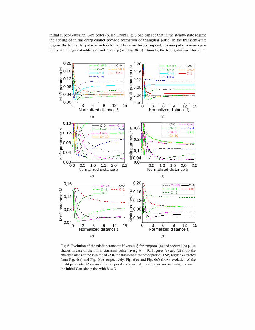
At first the pulse evolution for the initial Gaussian pulse is considered. The M-plots presentedin Fig. 6 demonstrate the dependence of the misfit parameter M on the normalized distance ξ

for various values of chirp parameter C for the temporal Figs. (6(a), 6(c), 6(e)) and spectralFigs. (6(b), 6(d), 6(f)) pulse profiles. From these figures we can see that the initial chirp is ableto change significantly pulse evolution as compared to the unchirped initial pulse (C = 0). Atfirst, in the transient-state propagation regime one can see the appearance of minima (M 6 0.04)for negative values of chirp. Fig. 6(c) clearly shows that triangular pulses can be achieved inthe transient-state regime (ξ < 1) when −8 6 C 6 −2 . The best choice is C = −2 at ξ = 1:here the misfit parameter is the smallest one (M = 0.015) and spectral profile is also close to theideal triangular waveform. Increasing the amount of negative chirp leads to the shifting of theminima to the smaller values of ξ and larger values of M. One has to note that for N = 3 evenadding initial negative chirp dos not lead to the triangular pulse formation as Fig. 6(e) shows.Therefore, the necessary condition for triangular pulse formation from Gaussian pulses withnegative chirp in the transient-state propagation regime is N > 3.

In the steady-state propagation regime (see Fig. 6(a) and Fig. 6(c)) we can see that, in gen-eral, the adding of the initial positive or negative chirp increases the deviation form triangularwaveform as compared to unchirped initial pulse. However, there is the range of initial chirp−0.5 6 C 6 0.4 where the pulse in the steady-state propagation regime preserves triangularprofile both in temporal and spectral domains. Adding a small negative chirp (C ∼ −0.5) iseven preferable allowing to slightly reduce the distance of triangular pulse formation in thesteady-state regime (ξ ∼ 1.5).

Now we consider the impact of initial chirp on reshaping of secant hyperbolic pulse towardstriangular waveform, shown in Fig. 7. Here one can see that the adding of initial chirp doesnot lead to the formation of triangular pulses in the transient-state regime. In the steady-stateregime the adding of the initial chirp also increases the deviation form triangular waveform ascompared to unchirped initial pulse similarly to the Fig. 6. Within the following range of initialchirp −0.8 6 C 6 0.5 pulse preserves triangular profile both in temporal and spectral domainin the stead-state regime.

Finally we investigate the impact of initial chirp on the triangular pulse formation from the

initial super-Gaussian (3-rd order) pulse. From Fig. 8 one can see that in the steady-state regimethe adding of initial chirp cannot provide formation of triangular pulse. In the transient-stateregime the triangular pulse which is formed from unchirped super-Gaussian pulse remains per-fectly stable against adding of initial chirp (see Fig. 8(c)). Namely, the triangular waveform can

0 3 6 9 1 2 1 50 , 0 00 , 0 40 , 0 80 , 1 20 , 1 60 , 2 0

Misfit

param

eter M

N o r m a l i z e d d i s t a n c e ξ

C = - 0 . 5 C = 0 C = - 2 C = 0 . 4 C = - 3 C = 1 C = - 4

(a)

0 3 6 9 1 2 1 50 , 0 00 , 0 40 , 0 80 , 1 20 , 1 60 , 2 0

Misfit

paraa

meter

M

N o r m a l i z e d d i s t a n c e ξ

C = - 0 . 5 C = 0 C = - 2 C = 0 . 4 C = - 3 C = 1 C = - 4

(b)

0 , 0 0 , 5 1 , 0 1 , 5 2 , 0 2 , 50 , 0 00 , 0 40 , 0 80 , 1 20 , 1 6

Misfit

param

eter M

N o r m a l i z e d d i s t a n c e ξ

C = 0 C = - 1 C = - 2 C = - 4 C = - 6 C = - 8 C = - 1 0

(c)

0 , 5 1 , 0 1 , 5 2 , 0 2 , 50 , 0

0 , 1

0 , 2

0 , 3Mi

sfit pa

ramete

r M

N o r m a l i z e d d i s t a n c e ξ

C = 0 C = - 1 C = - 2 C = - 4 C = - 6 C = - 8 C = - 1 0

0 , 0 4

(d)

0 3 6 9 1 2 1 50 , 0 4

0 , 0 8

0 , 1 2

0 , 1 6

Misfit

param

eter M

N o r m a l i z e d d i s t a n c e ξ

C = - 0 . 5 C = 0 C = - 1 C = 1 C = - 2

(e)

0 3 6 9 1 2 1 50 , 0 40 , 0 80 , 1 20 , 1 60 , 2 0

Misfit

param

eter M

N o r m a l i z e d d i s t a n c e ξ

C = - 0 . 5 C = 0 C = - 1 C = 1 C = - 2

(f)

Fig. 6. Evolution of the misfit parameter M versus ξ for temporal (a) and spectral (b) pulseshapes in case of the initial Gaussian pulse having N = 10. Figures (c) and (d) show theenlarged areas of the minima of M in the transient-state propagation (TSP) regime extractedfrom Fig. 6(a) and Fig. 6(b), respectively. Fig. 6(e) and Fig. 6(f) shows evolution of themisfit parameter M versus ξ for temporal and spectral pulse shapes, respectively, in case ofthe initial Gaussian pulse with N = 3.

0 3 6 9 1 2 1 50 , 0

0 , 1

0 , 2

0 , 3

Misfit

param

eter M

N o r m a l i z e d d i s t a n c e ξ

C = - 0 . 8 C = 0 C = - 2 C = 0 . 5 C = - 3 C = 1 C = - 4

(a)

0 3 6 9 1 2 1 50 , 00 , 10 , 20 , 30 , 40 , 5

Misfit

param

eter M

N o r m a l i z e d d i s t a n c e ξ

C = - 0 . 8 C = 0 C = - 2 C = 0 . 5 C = - 3 C = 1 C = - 4

(b)

Fig. 7. Evolution of the misfit parameter M versus normalized distance ξ for the temporal(a) and spectral (b) pulse shapes in case of the initial secant hyperbolic pulse with N = 10and various values of chirp.

be achieved for a large range of negative chirp (at least up to C = −12) , in case of positivechirp triangular waveform can be achieved for the maximal amount C = 4.

We can conclude that the impact of initial chirp on the pulse reshaping is also significant.In the transient-state regime the addition of an initial chirp allows the generation of triangularpulses from initial Gaussian pulses, particularly for N = 10 one has to apply chirp in the follow-ing range−8 6C 6−2. However, the necessary condition in this case is N > 3, a smaller valueof the soliton order does not provide triangular pulse formation even after the adding of negativeinitial chirp. Secant initial pulses do not transform to the triangular waveform in the transient-state propagation regime at all regardless of the initial chirp. As regards the super-Gaussianpulse, the triangular waveform is achieved here already from unchirped pulse. Triangular pulseformation in this case is preserved after the adding of initial chirp in the wide range, for N = 10it is −12 6C 6 4.

In the steady-state propagation regime in general, the adding of initial chirp increases thedeviation form triangular waveform as compared to unchirped initial pulses. However, thereis also the range of initial chirp −0.5 6 C 6 0.4 for initial Gaussian pulse and −8 6 C 6 0.5for initial secant pulse where pulse in the stead-state regime preserves triangular profile bothin temporal and spectral domains. Whereas for super-Gaussian pulse the adding of initial chirpdoes not lead to the triangular pulse formation in the stead-state propagation regime.

6. Practical recommendations for triangular pulse formation in optical fibers

Finally we are discussing some practical conditions required for triangular pulse formationin optical fibers. From the presented above results one can see that triangular pulses in thetransient-state propagation regime can be obtained only from Gaussian or super-Gaussianpulses (3-rd order). As modern ultrafast lasers generate mostly Gaussian or secant pulses, theapplication of initial Gaussian pulse in this case is the most preferable. The necessary conditionfor triangular pulse formation is large enough amount of pulse energy, i.e. the soliton order Nshall be sufficiently large: It is N > 3 in transient-state propagation regime for the incident pulseof the Gaussian shape. Another necessary condition is negative chirp of a particular value: forexample for N = 10 one needs −8 6 C 6 −2 . Therefore, one has to provide a pre-chirpingstage by using anomalous dispersion fiber [16] or other dispersion elements before the nonlin-ear reshaping of the pulse in normally dispersive fiber.

In steady-state propagation regime triangular pulses can be obtained from both the Gaussian

0 3 6 9 1 2 1 50 , 0 40 , 0 80 , 1 20 , 1 60 , 2 0

Misfit

param

eter M

N o r m a l i z e d d i s t a n c e ξ

C = 0 C = 2 C = 4 C = 6 C = - 6 C = - 1 2

(a)

0 3 6 9 1 2 1 50 , 0 40 , 0 80 , 1 20 , 1 60 , 2 0

Misfit

param

eter M

N o r m a l i z e d d i s t a n c e ξ

C = 0 C = 2 C = 4 C = 6 C = - 6 C = - 1 2

(b)

0 , 0 0 , 1 0 , 2 0 , 30 , 0 40 , 0 80 , 1 20 , 1 6

Misfit

psram

eter M

N o r m a l i z e d d i s t a n c e ξ

C = 0 C = 4 C = - 6 C = 6 C = - 1 2

(c)

0 , 0 0 , 1 0 , 2 0 , 3

0 , 1

0 , 2

0 , 3

0 , 0 4Misfit

param

eter M

N o r m a l i z e d d i s t a n c e ξ

C = 0 C = 4 C = - 6 C = 6 C = - 1 2

(d)

Fig. 8. Evolution of the misfit parameter M versus normalized distance ξ for the temporal(a) and spectral (b) pulse shapes in case of the initial super-Gaussian pulse with N = 10and various values of chirp C. Fig. 8(c) and Fig. 8(d) show the enlarged areas of the min-ima in the transient-state propagation regime extracted from figures Fig. 8(a) Fig. 8(b),respectively.

and the secant hyperbolic initial pulses. The necessary conditions for triangular pulse formationin the steady-state propagation regime are: N > 7 for Gaussian pulse and N > 3 for secanthyperbolic pulse. Because of unchirped pulses can be used for triangular pulse formation in thesteady-state regime, there is no need to provide a pre-chirping stage here. Initial chirp in thiscase is rather negative factor because it increases the deviation form the triangular waveform ascompared to unchirped initial pulses. However, there is the range of initial chirp where pulseshape remains triangular in the steady-state propagation regime. For N = 10 these regions are−0.5 6 C 6 0.4 for initial Gaussian pulse, and −0.8 6 C 6 0.5 for initial secant hyperbolicpulse. We have combined the conditions for triangular pulse formation all together in Table 1.

Important issue is the duration of the initial pulses. If picosecond Gaussian pulses (e.g. ∼ 5ps) are used in a typical single mode fiber, such as Thorlabs 780HP [24], then, for example,at λ = 1064 nm (β2 = 25 ps2/km) the dispersion length is LD = 360 m. It means that requiredfiber length for triangular pulse formation in the transient-state regime (0.1LD < z < LD) is inthe range 36 < z < 360 m, whereas in the steady-state propagation regime (z > LD) the requiredfiber length has to be larger of 360 m. At λ = 1550 nm the normal dispersion in a single modefiber is smaller. For example, the TrueWave fiber [25] has β2 = 4 ps2/km, and this providesdispersion length LD = 2.2 km. Thus, one can see that application of picosecond initial pulsesrequires long fibers for pulse reshaping from a few hundred meters up to a few kilometers. If pi-

Table 1. Summary of the conditions for the formation of triangular pulses in a fiber.

Incident pulse shape Transient-state propagation (TSP) regime Steady-state propagation (SSP) regime

Gaussian N > 3, with negative initial chirp in quitewide range corresponding to particularvalue of N.

N > 7, unchirped or slightly chirped inthe narrow range corresponding to partic-ular value of N.

E. g. N = 10, −8 6C 6−2. Example forparticular value C =−4 shown in Fig. 2

E. g. N = 10, −0.5 6 C 6 0.4. Examplefor particular values N = 7, C = 0 shownin Fig. 9(a), 9(c))

Secant hyperbolic – N > 3, unchirped or slightly chirped inthe narrow range corresponding to partic-ular value of N.

E. g. N = 10, −0.8 6 C 6 0.5. Examplefor particular values N = 6, C = 0 shownin Fig. 9(b), 9(d))

Super-Gaussian (3-d order) 7 6 N 6 15 , unchirped or chirped inthe wide range corresponding to particu-lar value of N.

–

E. g. N = 10,−126C 6 4. Examples canbe found in Fig. 5, 8

cosecond Gaussian pulses are used (e.g. ∼ 5 ps) the necessary conditions N > 3 in TSP-regimeand N > 7 in SSP-regime for triangular pulse formation lead to the following minimal pulseenergies required in the TrueWave fiber at λ = 1550 nm: ET SP

0 > 8 pJ, ESSP0 > 45 pJ, respec-

tively (γ1550 = 2.5 (W·km)−1). Whereas at λ = 1064 nm, due to the larger normal dispersion insingle mode fibers (e.g. in Thorlabs 780HP) minimal pulse energies have to be larger to meetthose conditions: ET SP

0 > 36 pJ, ESSP0 > 0.2 nJ, respectively (γ1064 = 3.6 (W·km)−1 ). However,

modern commercially available picosecond fiber lasers are able to reach these pulse energieseasily.

Application of femtosecond pulses for nonlinear reshaping looks much more attractive. Iffemtosecond Gaussian pulses are used (e.g. 200 fs) then the dispersion length in TrueWavefiber at λ = 1550 nm is LD = 3.6 m. Thus, the required fiber length for pulse reshaping issufficiently smaller in this case: a few meters for triangular pulse formation in the steady-statepropagation regime and even less than 1 meter for transient-state propagation regime. At 800nm in single mode fibers such as Thorlabs 780HP the dispersion length is even smaller LD = 37cm due to the larger normal dispersion (β2 = 39 ps2/km). Therefore, pulse reshaping at 800nm with femtosecond pulses requires applications of very short single mode fibers: a few tensof centimeters in the transient-state propagation regime and about one meter in the steady-statepropagation regime. In this case one can realize really compact scheme of pulse reshaping basedon application of normal dispersive optical fibers. If femtosecond Gaussian pulses are used (200fs) then the necessary conditions N > 3 TSP-regime and N > 7 SSP-regime for triangular pulseformation lead to the following minimal pulse energies required in the TrueWave fiber @1550nm: ET SP

0 > 0.2 nJ, ESSP0 > 1.1 nJ, respectively. Whereas at 800 nm minimal pulse energies

have to be larger to meet those conditions: ET SP0 > 0.4 nJ and ESSP

0 > 2.3 nJ, respectively, forthe fiber Thorlabs 780HP (γ800 = 12 (W·km)−1 ). Modern commercially available femtosecondTi:Sapphire and fiber lasers are able to reach these pulse energies.

Finally we present an estimation of triangular pulse formation in real fiber such as conven-tional single mode fiber Thorlabs 780HP, intended for application at near infrared wavelengths.It is considered triangular pulse formation in the steady-state regime from initial unchirped

- 8 - 4 0 4 801 0 02 0 03 0 04 0 0 T r i a n g u l a r f i t M = 0 . 0 3 9

Inten

sity, W

T i m e , p s- 4 0- 2 002 04 0

Chirp, THz

(a)

- 1 0 - 5 0 5 1 00

1 0 0

2 0 0

3 0 0 T r i a n g u l a r f i t M = 0 . 0 3 9

Inten

sity, W

T i m e , p s- 4 0- 2 002 04 0

Chirp, THz

(b)

- 2 0 - 1 0 0 1 0 2 00 , 0

0 , 5

1 , 0 T r i a n g u l a r f i t M = 0 . 0 3 4

Spec

trum,

a.u.

F r e q u e n c y , T H z(c)

- 2 0 - 1 0 0 1 0 2 00 , 0

0 , 5

1 , 0 T r i a n g u l a r f i t M = 0 . 0 3 8

Spec

trum,

a.u.

F r e q u e n c y , T H z(d)

Fig. 9. Triangular pulses produced in the Thorlabs 780HP fiber. The left column showsresults ((a) - temporal intensity and chirp (green curve), (c) - spectrum) for triangularpulse generated in the steady-state regime at the fiber length 1.4527 m (ξ = 4) from initialunchirped Gaussian pulse (N = 7, E0 = 2.39 nJ, FWHM=200 fs). Right column ((b), (d))shows triangular pulse generated in the steady-state regime at the fiber length 1.9435 m(ξ = 6) from initial unchirped secant pulse (N = 6, E0 = 2.101 nJ, FWHM=200 fs). Theinsets located in the upper right corner show the amount of misfit parameter M. Red curvesshow corresponding triangular fits.

Gaussian and the hyperbolic secant pulses with central wavelength λ0 = 800 nm. The parame-ters of the pump pulses are chosen to be similar to those one produced by typical Ti:Sapphirelasers or Er3+-doped fiber lasers with second harmonic generation. Particularly pulse durationis 200 fs and pulse energy equal to a few nanojoules.

The fiber parameters at 800 nm used in NLSE, Eq. (1), are: β2 = 39.73 ps2/km, β3 = 2.62×10−2 ps3/km, γ = 12 (W·km)−1, and α = 8.0589× 10−4 m−1 . Dispersion coefficients βn arecalculated from D(λ ), [ps/(nm·km)], whereas nonlinear coefficient γ is calculated from themode field diameter of the fiber using nonlinear refractive index of the silica nSiO2 = 3×10−20

m2/W.Fig. 9 shows characteristics of triangular pulses obtained in the steady-state regime from

initial unchirped secant and Gaussian pulses. Fig. 9 clearly shows that applying initial Gaussianor secant pulses we can obtain indeed pulses close to the ideal triangular profile both in spectraland temporal domains. One can see that the main deviations form ideal triangular waveformappear preliminary in the top of the pulse profile. In all cases the top is not perfectly sharp ascompared to the ideal triangular profile. However, the most part of pulse edges is nearly linear.One has to note also that the chirp of obtained triangular pulses is also perfectly linear here.

Results shown in Fig. 9 are obtained neglecting the fourth order dispersion (FOD) and in-

Table 2. Comparisons of contributions of the fourth order dispersion and Raman intrapulsescattering into distortion of triangular pulses in the Thorlabs 780HP fiber

Incident Pulse Shape Original misfit parameter Misfit including FODMisfit including FODand Raman scattering

Mτ Mω Mτ Mω Mτ Mω

Gaussian 0.039 0.034 0.039 0.033 0.043 0.032

Secant hyperbolic 0.039 0.038 0.033 0.033 0.032 0.032

trapulse Raman scattering. The role of the FOD in transformation of parabolic optical pulsesto triangular wave forms in the normal dispersion regime has been addressed in [26]. It hasbeen shown that FOD may be one ingredient leading to the emergence of triangular pulse ina nonlinear system. However, it should be observed that analysis made in [26] embraces onlytransient-state propagation regime (particularly ξ � 1), and thus conclusions made are validstrictly for these conditions. Nevertheless one can expect that accounting for the FOD could beimportant in cases considered here as well. Given also the spectral extend of the resulting pulsesthat are shown in Fig.9 one can expect an influence of intrapulse Raman scattering. Thus, bothfactors can potentially destroy conditions for triangular pulse formation. In order to clarify thecontribution of these phenomena in our case we made simulation of triangular pulse formationfor the case shown in Fig.9, taking into account FOD only, and both factors as well, the FODand the Raman intrapulse scattering. We found no noticeable contributions. The shapes of thespectra and wave forms do not changed; the only minor variations appear, which are not observ-able in the linear scale but led to minor change (tenth part of percent) of the misfit parameters;they are shown in Table 2. It can be noted a tendency to decreasing of misfit parameter whenincluding higher-order nonlinear and dispersion effects into account. Thus simulations withoutFOD and Raman intrapulse scattering allow us talk about an utmost estimation of the condi-tions for triangular pulse formation; knowing these estimation we can be sure that pulses willbe obtained in real fibers.

7. Conclusion

We have investigated numerically formation of ultrashort triangular pulses by means of passivenonlinear reshaping in normal dispersive optical fibers. The conditions for triangular pulsesformation both in the transient-state regime and in the steady-state regime were found depend-ing on the initial pulse shape, chirp and soliton order. It was shown that in the transient-stateregime triangular pulses can be obtained only from Gaussian pulses when N > 3 with negativechirp (e.g. −8 6C 6−2, N = 10) and from unchirped or chirped super-Gaussian pulses when7 6 N 6 15 (e.g. −12 6 C 6 4, N = 10). Whereas nor soliton order variation nor chirp varia-tion does not provide formation of triangular pulses form secant waveform in the transient-stateregime.

In the steady-state regime triangular pulses can be obtained from both unchirped Gaussian(N > 7) and secant (N > 3) initial pulses for sufficiently large value of soliton order. In generalapplication of secant pulses is more preferable for obtaining of triangular pulses. For secant ini-tial pulses smaller soliton order is required for triangular pulse formation and misfit parameteris slightly lower. In the steady-state regime in general the adding of initial chirp increases thedeviation form triangular waveform as compared to unchirped initial pulses. However, there isthe range of initial chirp−0.56C 6 0.4 (N = 10) for initial Gaussian pulse and−0.86C 6 0.5(N = 10) for initial secant pulse where pulse in the stead-state regime preserves triangular pro-

file both in temporal and spectral domain. Whereas nor soliton order variation nor chirp varia-tion does not provide formation of triangular pulses from super-Gaussian (3-rd order) pulses inthe steady-state regime.

Finally, we have shown the possibility of generating triangular pulses in the steady-stateregime from unchirped femtosecond Gaussian and hyperbolic secant pulses applying 1-2 mof the conventional single mode fiber Thorlabs 780HP. Both pulse temporal shape and spec-trum are close to the triangular waveform and remain triangular shape during subsequent pulsepropagation in the fiber, whereas pulse chirp is linear.

Acknowledgments

This work is supported by University of Guanajuato (projects DAIP-334/13 and DAIP-192/13),by Secretarıa de Educacion Publica via program PROMEP (project UGTO-PTC-371).