Footpoint versus loop-top hard X–ray emission sources in ...
12
Astronomy & Astrophysics manuscript no. aa6115-06 c ESO 2006 September 22, 2006 Footpoint versus loop-top hard X–ray emission sources in solar flares M. Tomczak and T. Ciborski Astronomical Institute, University of Wroclaw, ul. Kopernika 11, PL-51–622 Wroclaw, Poland, e-mail: [email protected] Received 26 June 2006 / Accepted 5 September 2006 ABSTRACT Aims. The hard X-ray flux ratio of the footpoint sources to the loop-top source has been used to investigate non-thermal electron trapping and precipitation in solar flares. Methods. Considering the mission-long Yohkoh Hard X–ray Telescope database, from which we selected 117 flares, we investigated a dependence of the ratio on flare loop parameters like height h and column depth N. We used non-thermal electron beams as a diagnostic tool for magnetic convergence. Results. The ratio decreases with h which we interpret as an effect of converging field geometry. Two branches seen in the − h diagram suggest that in the solar corona two kinds of magnetic loops can exist: a more-converged ones that are more frequent (above 80%) and less-converged loops that are less frequent (below 20%). A lack of correlation between the ratio and N can be due to a more complex configuration of investigated events than seen in soft X–rays. Conclusions. Obtained values of the magnetic mirror ratio are consistent with previous works and suggest a strongly nonpotential configuration. Further investigation including RHESSI data is needed to verify our results. Key words. Sun: corona – flares – X–rays, gamma rays 1. Introduction Images taken by the Hard X–ray Telescope (HXT) onboard Yohkoh show different spatial distributions of hard X–ray emis- sion in solar flares. Classifications of hard X–ray emission sources observed in solar flares have been reported (e.g. Kosugi 1994, Masuda 2002, Aschwanden 2004). However, an unifica- tion is possible in which hard X–ray emission sources are di- vided into two classes: coronal and chromospheric. Members of the first class usually occur within or above the top of the mag- netic coronal loop clearly seen in soft X–rays, thus we call them loop-top or above-the-loop-top sources. Members of the second class occur at the entrance of the same magnetic coronal loops into the chromosphere, thus we call them footpoint sources. For the more complicated morphologies, interacting loops or an ar- cade of loops, such a division still works, however, more hard X–ray sources can be seen at times. The majority of flares show the presence of hard X–ray emission sources of both classes: loop-top source and footpoint ones. However, their basic properties are different. The footpoint sources are stronger than the loop-top ones during the hard X– ray bursts of the impulsive phase. Footpoint sources grow with higher-energy photons. At the end of the impulsive phase the footpoint sources fade and the loop-top source becomes brighter but its radiation only rarely exceeds 30 keV. Energy spectra of hard X–ray photons emitted during the im- pulsive phase of flares have a non-thermal shape. They can be de- scribed by a single or a double power-law function. Usually the energy spectra of footpoint sources are flatter than the spectra of the loop-top sources i.e. the index γ of the function I (E) = AE −γ is smaller for the footpoint sources than for the loop-top ones. Send offprint requests to: M. Tomczak Spectra of loop-top sources adopt a quasi-thermal shape with time i.e. an increase of the index γ with the energy of photons is seen. Both classes of hard X–ray emission sources have different mechanism of radiation. The loop-top sources are connected di- rectly to the process of energy release in flares. Due to magnetic reconnection some electrons are accelerated up to high energies and they immediately radiate their energy excess in the loop-top region via thin-target or thermal bremsstrahlung. In some mod- els the area occupied by the loop-top source defines the recon- nection site (Jakimiec et al. 1998, Petrosian & Donaghy 1999). In other models, the reconnection X–point occurs higher in the corona and the loop-top source is a consequence of interaction between a downward reconnection outflow and plasma filling a soft X–ray flare loop (Tsuneta 1997, Shibata 1999). The motion of the magnetic field lines in the cusp structure below the recon- nection site and above the underlying flare loops, which we call the collapsing magnetic trap, also can be an efficient accelerator of electrons (Somov & Kosugi 1997, Jakimiec 2002, Karlick´ y & Kosugi 2004, Karlick´ y & B´ arta 2006). The footpoint sources are regions in which accelerated electrons are precipitated into the chromosphere and radiate via thick-target bremsstrahlung (Brown 1971). A simultaneous investigation of the loop-top and footpoint hard X–ray emission sources offers a chance to better under- stand the main physical processes occurring during the impul- sive phase in solar flares. The first attempt of such a kind of anal- ysis was made by Masuda (1994) who compared some character- istics of loop-top and footpoint sources for 10 single-loop flares observed by Yohkoh between 1991 and 1993. He reported the presence of hard X–ray emission sources of both classes in the majority of investigated flares. He found that during the impul- Article published by EDP Sciences and available at http://www.edpsciences.org/aa To be cited as: A&A preprint doi http://dx.doi.org/10.1051/0004-6361:20066115
-
Upload
khangminh22 -
Category
Documents
-
view
3 -
download
0
Transcript of Footpoint versus loop-top hard X–ray emission sources in ...
Astronomy & Astrophysics manuscript no. aa6115-06 c© ESO 2006September 22, 2006
Footpoint versus loop-top hard X–ray emission sourcesin solar flares
M. Tomczak and T. Ciborski
Astronomical Institute, University of Wrocław, ul. Kopernika 11, PL-51–622 Wrocław, Poland, e-mail:[email protected]
Received 26 June 2006 / Accepted 5 September 2006
ABSTRACT
Aims. The hard X-ray flux ratio� of the footpoint sources to the loop-top source has been used to investigate non-thermal electrontrapping and precipitation in solar flares.Methods. Considering the mission-long Yohkoh Hard X–ray Telescope database, from which we selected 117 flares, we investigateda dependence of the ratio � on flare loop parameters like height h and column depth N. We used non-thermal electron beams as adiagnostic tool for magnetic convergence.Results. The ratio� decreases with h which we interpret as an effect of converging field geometry. Two branches seen in the�− hdiagram suggest that in the solar corona two kinds of magnetic loops can exist: a more-converged ones that are more frequent (above80%) and less-converged loops that are less frequent (below 20%). A lack of correlation between the ratio� and N can be due to amore complex configuration of investigated events than seen in soft X–rays.Conclusions. Obtained values of the magnetic mirror ratio are consistent with previous works and suggest a strongly nonpotentialconfiguration. Further investigation including RHESSI data is needed to verify our results.
Key words. Sun: corona – flares – X–rays, gamma rays
1. Introduction
Images taken by the Hard X–ray Telescope (HXT) onboardYohkoh show different spatial distributions of hard X–ray emis-sion in solar flares. Classifications of hard X–ray emissionsources observed in solar flares have been reported (e.g. Kosugi1994, Masuda 2002, Aschwanden 2004). However, an unifica-tion is possible in which hard X–ray emission sources are di-vided into two classes: coronal and chromospheric. Members ofthe first class usually occur within or above the top of the mag-netic coronal loop clearly seen in soft X–rays, thus we call themloop-top or above-the-loop-top sources. Members of the secondclass occur at the entrance of the same magnetic coronal loopsinto the chromosphere, thus we call them footpoint sources. Forthe more complicated morphologies, interacting loops or an ar-cade of loops, such a division still works, however, more hardX–ray sources can be seen at times.
The majority of flares show the presence of hard X–rayemission sources of both classes: loop-top source and footpointones. However, their basic properties are different. The footpointsources are stronger than the loop-top ones during the hard X–ray bursts of the impulsive phase. Footpoint sources grow withhigher-energy photons. At the end of the impulsive phase thefootpoint sources fade and the loop-top source becomes brighterbut its radiation only rarely exceeds 30 keV.
Energy spectra of hard X–ray photons emitted during the im-pulsive phase of flares have a non-thermal shape. They can be de-scribed by a single or a double power-law function. Usually theenergy spectra of footpoint sources are flatter than the spectra ofthe loop-top sources i.e. the index γ of the function I(E) = AE−γis smaller for the footpoint sources than for the loop-top ones.
Send offprint requests to: M. Tomczak
Spectra of loop-top sources adopt a quasi-thermal shape withtime i.e. an increase of the index γ with the energy of photons isseen.
Both classes of hard X–ray emission sources have differentmechanism of radiation. The loop-top sources are connected di-rectly to the process of energy release in flares. Due to magneticreconnection some electrons are accelerated up to high energiesand they immediately radiate their energy excess in the loop-topregion via thin-target or thermal bremsstrahlung. In some mod-els the area occupied by the loop-top source defines the recon-nection site (Jakimiec et al. 1998, Petrosian & Donaghy 1999).In other models, the reconnection X–point occurs higher in thecorona and the loop-top source is a consequence of interactionbetween a downward reconnection outflow and plasma filling asoft X–ray flare loop (Tsuneta 1997, Shibata 1999). The motionof the magnetic field lines in the cusp structure below the recon-nection site and above the underlying flare loops, which we callthe collapsing magnetic trap, also can be an efficient acceleratorof electrons (Somov & Kosugi 1997, Jakimiec 2002, Karlicky& Kosugi 2004, Karlicky & Barta 2006). The footpoint sourcesare regions in which accelerated electrons are precipitated intothe chromosphere and radiate via thick-target bremsstrahlung(Brown 1971).
A simultaneous investigation of the loop-top and footpointhard X–ray emission sources offers a chance to better under-stand the main physical processes occurring during the impul-sive phase in solar flares. The first attempt of such a kind of anal-ysis was made by Masuda (1994) who compared some character-istics of loop-top and footpoint sources for 10 single-loop flaresobserved by Yohkoh between 1991 and 1993. He reported thepresence of hard X–ray emission sources of both classes in themajority of investigated flares. He found that during the impul-
Article published by EDP Sciences and available at http://www.edpsciences.org/aaTo be cited as: A&A preprint doi http://dx.doi.org/10.1051/0004-6361:20066115
2 M. Tomczak and T. Ciborski: Footpoint versus loop-top hard X–ray emission sources in solar flares
sive phase the loop-top source mimics a variability of footpointsources. He also pointed out that the coronal sources shiftedabove the loop-top are systematically more energetic (with alower index γ) than the sources that are co-spatial with the loop-top.
More comprehensive analysis was performed by Petrosian etal. (2002). They selected and analyzed HXT images of 18 flaresfrom 1991–1998 and included multiple-loop events. The authorsconclude that the loop-top and footpoint hard X–ray emissionsources are a common characteristic of the impulsive phase ofsolar flares. They found an obvious correlation between loop-topand footpoint hard X–ray fluxes over more than two decades offlux, and obtained that the footpoint sources are systematicallystronger and more energetic (with a lower index γ) than loop-topones.
In this paper we extend the previous studies. We discuss therelation between the loop-top and footpoint hard X–ray emissionsources in solar flares for a larger number of events. Our databaseincludes flares observed over the entire Yohkoh mission (1991–2001) and we modified the selection criteria.
The paper is organized as follows. In Section 2 a short de-scription of scientific instruments is given as are the selectioncriteria. In Section 3 we define the flux ratio� of the footpointand loop-top hard X–ray emission sources in investigated flaresand present its dependence on other parameters such heightof the flare loop and column density along the flare loop. InSection 4 we discuss the implications of our results for the mag-netic field configuration in solar flares. In Section 5 we present asummary and our conclusions.
2. Scientific instruments and data selection
We used data from two imaging instruments onboard Yohkoh:the HXT and the Soft X–ray Telescope (SXT). The HXT(Kosugi et al. 1991) is a Fourier synthesis imager observing thewhole Sun. It consisted of 64 independent subcollimators whichmeasured spatially modulated intensities in four energy bands(L: 14–23 keV, M1: 23–33 keV, M2: 33–53 keV, and H:53–93 keV). During the flare the intensities were integrated, in eachenergy band, over 0.5 s. Some reconstruction routines are avail-able that allow us to obtain hard X–ray images with an angularresolution of up to 5 arcsec. We used the Maximum EntropyMethod developed for HXT data by Sakao (1994). This methodworks very efficiently since the in-orbit calibration of the HXTresponse function was performed (Sato et al. 1999).
The SXT (Tsuneta et al. 1991) is a grazing-incidence tele-scope sensitive to 0.4–4.2 keV soft X–rays, with a CCD detec-tor and filters to provide wavelength discrimination. During flaremode the SXT usually recorded frames of 64 × 64 pixels. Imageswere taken sequentially with different filters every 2 seconds andtheir spatial resolution was 2.45 arcsec2. In our analysis we usedtwo filters: a 119 µm beryllium filter (Be119) and a 11.6 µm alu-minium filter (Al12). The signal ratio of these filters allows us toestimate the temperature and emission measure of the soft X–rayflare plasma (Hara et al. 1992).
Masuda (1994) used two criteria for flare selection: a helio-centric longitude greater than 80◦, and peak count rate in theM2 band greater than 10 counts per second per subcollimator.The first criterion ensures maximum angular separation betweenloop-top and footpoint sources. The second criterion ensures thatat least one image can be obtained at energies where the thermalcontribution should be negligible. The same criteria was used byPetrosian et al. (2002).
In our analysis we slightly modified these criteria becausewe found out them too strict. We qualified flares that occurredat heliocentric longitudes greater than 65◦, instead of 80◦, andhad a peak count rate in the M1 band greater than 10 countsper second per subcollimator, instead of the M2 band. For flaresbetween 65◦ and 80◦ a separation between loop-top and foot-point sources is still possible. We limited our analysis presentedin Section 3 to the moment of peak count rate in the band M1,instead of the time interval over the entire impulsive duration offlares which has been used in previous works. At that moment,emission of non-thermal electrons strongly dominates the ther-mal contribution, which is proved by almost the same momentof peak count rate in the bands M1, M2, and H for the majorityof flares.
In the catalog including flares observed over the entireYohkoh mission (1991–2001)1 we found that our criteria werefulfilled by 198 out of 3071 events. Among these 198 flares weexcluded some events due to: a lack of SXT images, poor qual-ity of HXT images, and location behind the solar limb wherewe can observe loop-top sources only. We then considered 117flares presented in Table 3. Such a large number of analyzedevents offers the chance to statistically model the relation be-tween loop-top and footpoint hard X–ray emission sources insolar flares. Our list contains almost all the flares analyzed pre-viously by Masuda (1994) and Petrosian et al. (2002). Excludedare the flare of April 23, 1998 which occurred 13◦ behind thesolar limb (Sato 2001) and the flares of May 8 and 9, 1998 forwhich there were no SXT images for the investigated time pe-riod.
3. The flux ratio� of hard X–ray sources
For each flare from the list we computed one image at the peakcount rate in the M1 band. To obtain an image of good qualitywe need about 200 counts per subcollimator, therefore we accu-mulated signal within a time interval of between 0.5 and 11 s(see column (7) in Table 3), depending on the total number ofcounts in the band M1. Next, we carefully defined the shape ofthe individual emission sources and combined the signal from allpixels inside each source separately. Due to the limited dynamicrange of the HXT and the image reconstruction process, esti-mated to be about one decade (Sakao 1994), we considered asbackground the pixels having a signal below 10% of the bright-est one. Sometimes emission sources in the M1 band were notwell resolved, thus we calculated images in higher energy bands,if available, to define the border between the sources more pre-cisely.
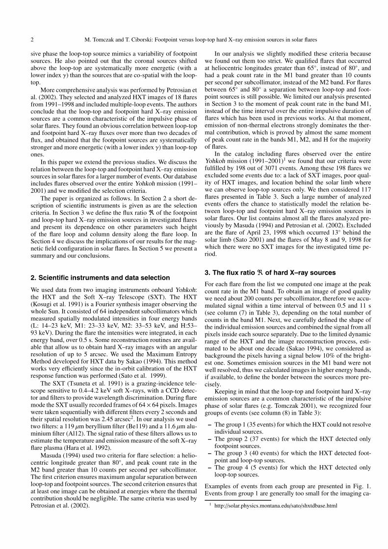
Keeping in mind that the loop-top and footpoint hard X–rayemission sources are a common characteristic of the impulsivephase of solar flares (e.g. Tomczak 2001), we recognized fourgroups of events (see column (8) in Table 3):
– The group 1 (35 events) for which the HXT could not resolveindividual sources.
– The group 2 (37 events) for which the HXT detected onlyfootpoint sources.
– The group 3 (40 events) for which the HXT detected foot-point and loop-top sources.
– The group 4 (5 events) for which the HXT detected onlyloop-top sources.
Examples of events from each group are presented in Fig. 1.Events from group 1 are generally too small for the imaging ca-
1 http://solar.physics.montana.edu/sato/shxtdbase.html
M. Tomczak and T. Ciborski: Footpoint versus loop-top hard X–ray emission sources in solar flares 3
Fig. 1. Examples of groups introduced in the text. The contours and the half-tones show the HXT/M1 and SXT/Be119 images, respectively. Thepixel size is 2.45 arcsec2. North is at the top, west – to the right.
pability of the HXT, thus we excluded them from further analy-sis. The presence of groups 2 and 4 is likely caused by the limiteddynamic range of the HXT. For events from group 2, footpointsources are brighter than the loop-top source by more than 10times, opposite to events from group 4 for which the loop-topsource is brighter than footpoint sources by more than 10 times.In both cases the fainter sources cannot be resolved from thebackground but we expect that they exist.
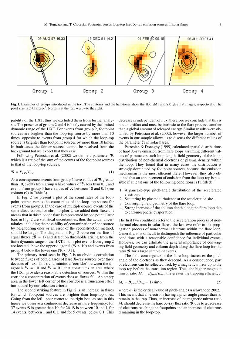
Following Petrosian et al. (2002) we define a parameter �which is a ratio of the sum of the counts of the footpoint sourcesto that of the loop-top sources.
� = FFP/FLT (1)
As a consequence, events from group 2 have values of� greaterthan 10, events from group 4 have values of� less than 0.1, andevents from group 3 have values of � between 10 and 0.1 (seecolumn (9) in Table 3).
In Fig. 2 we present a plot of the count rates of the foot-point source versus the count rates of the loop-top source forevents from group 3. In the case of multiple-source events of thesame class, coronal or chromospheric, we added their fluxes. Itmeans that in this plot one flare is represented by one point. Errorbars in Fig. 2 are statistical uncertainties, thus the actual uncer-tainties, including the possibility of contamination of one sourceby neighboring ones or an error of the reconstruction method,should be larger. The diagonals in Fig. 2 represent the line ofequal fluxes (� = 1) and detection thresholds arising from thefinite dynamic range of the HXT. In this plot events from group 2are located above the upper diagonal (� > 10) and events fromgroup 4 below the lower one (� < 0.1).
The primary trend seen in Fig. 2 is an obvious correlationbetween fluxes of both classes of hard X–ray sources over threedecades of flux. This trend mimics a ‘corridor’ between the di-agonals � = 10 and � = 0.1 that constitutes an area wherethe HXT provides a reasonable detection of sources. Within thecorridor a concentration of events rises as fluxes fall. An emptyarea in the lower left corner of the corridor is a truncation effectintroduced by our selection criteria.
The second striking feature in Fig. 2 is an increase in flaresfor which footpoint sources are brighter than loop-top ones.Going from the left upper corner to the right bottom one in thisfigure we observe a continuous decrease in flare frequency: for37 events� is greater than 10, for 26,� is between 10 and 1, for14 events, between 1 and 0.1, and for 5 events, below 0.1. This
decrease is independent of flux, therefore we conclude that this isnot an artifact and must be intrinsic to the flare process, anotherthan a global amount of released energy. Similar results were ob-tained by Petrosian et al. (2002), however the larger number ofevents in our sample allows us to discuss the different values ofthe parameter� in solar flares.
Petrosian & Donaghy (1999) calculated spatial distributionsof hard X–ray emission from flare loops assuming different val-ues of parameters such loop length, field geometry of the loop,distribution of non-thermal electrons or plasma density withinthe loop. They found that in many cases the distribution isstrongly dominated by footpoint sources because the emissionmechanism is the most efficient there. However, they also ob-tained that an enhancement of emission from the loop-top is pos-sible if at least one of the following conditions is fulfilled:
1. A pancake-type pitch-angle distribution of the acceleratedelectrons.
2. Scattering by plasma turbulence at the acceleration site.3. Converging field geometry of the flare loop.4. Strong increase of the column depth along the flare loop due
to chromospheric evaporation.
The first two conditions refer to the acceleration process of non-thermal electrons in solar flares, the last two refer to the prop-agation process of non-thermal electrons within the flare loop.Generally, it is difficult to distinguish the influence of particularconditions with a reasonable confidence for individual events.However, we can estimate the general importance of converg-ing field geometry and column depth along the flare loop for theratio� for a large sample of events.
The field convergence in the flare loop increases the pitchangle of the electrons as they descend. As a consequence, partof electrons can be reflected back by a magnetic mirror up to theloop-top before the transition region. Thus, the higher magneticmirror ratio Mr = B f oot/Btop, the greater the trapping efficiency:
Mr = B f oot/Btop = 1/sin2αc (2)
where αc is the critical value of pitch-angle (Aschwanden 2002).This means that all electrons having a pitch angle greater than αcremain in the trap. Thus, an increase of the magnetic mirror ratioMr should decrease the hard X–ray flux ratio� due to a decreaseof electrons reaching the footpoints and an increase of electronsremaining in the loop-top.
4 M. Tomczak and T. Ciborski: Footpoint versus loop-top hard X–ray emission sources in solar flares
Fig. 2. Counts from the footpoints versus loop-top counts in the HXT/M1 energy band for 40 flares of group 3. The diagonals represent lines ofconstant ratio�. The lines� = 10 and� = 0.1 establish detection thresholds of the instrument. Above the line� = 10 we find the group 2 (37events), below the line � = 0.1, the group 4 (5 events). The dotted curves show lines of the constant total flux; the lowest one marks the eventselection threshold.
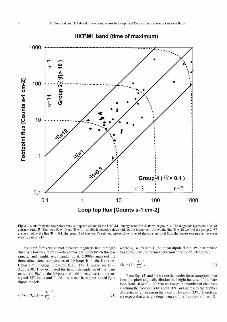
For limb flares we cannot measure magnetic field strengthdirectly. However, there is well-known relation between this pa-rameter and height. Aschwanden et al. (1999a) analyzed thethree-dimensional coordinates of 30 loops from the Extreme-Ultraviolet Imaging Telescope (EIT) 171 Å image on 1996August 30. They estimated the height dependence of the mag-netic field B(h) of the 30 potential field lines closest to the an-alyzed EIT loops and found that it can be approximated by adipole model:
B(h) = B f oot(1 +h
hD)−3
, (3)
where hD = 75 Mm is the mean dipole depth. We can rewritethis formula using the magnetic mirror ratio, Mr , definition:
Mr = (1 +h
hD)3
. (4)
From Eqs. (2) and (4) we see that under the assumption of anisotropic pitch-angle distribution the height increase of the flareloop from 10 Mm to 20 Mm decreases the number of electronsreaching the footpoints by about 20% and increases the numberof electrons remaining in the loop-top by about 33%. Therefore,we expect that a height dependence of the flux ratio of hard X–
M. Tomczak and T. Ciborski: Footpoint versus loop-top hard X–ray emission sources in solar flares 5
ray sources �(h) should exist where � drops as h increases.This relation is independent of the energy of electrons.
The mean free-path of electrons l f in a volume having elec-tron density ne can be estimated according to (Tsuneta et al.1997):
l f = 8.3 × 10¹⁷E2/ne, (5)
where E is the electron energy in keV and ne is counted per cm−3.Thus, in conditions typical of the pre-flare phase (ne ∼ 109÷1010
cm−3), l f is greater than the loop semi-length. This means thatalmost all electrons accelerated at the top of the flare loop eas-ily reach the transition region producing hard X–ray footpointsources. An increase of electron density within the flare loop dueto chromospheric evaporation limits the number of electrons thatdeposit their energy in the footpoints. As a consequence, the fluxratio of hard X–ray sources�(h) should decrease as the columndepth, N = neL, measured along the loop of the semi-length L,increases.
Such relatively simply relationships�(h) and�(N) can be-come more complex if anomalous electron scattering occurs(Melrose 1980). This is caused by MHD turbulence which can beexcited in the coronal segment of the flare loop by anisotropiesoccurring in the distribution of accelerated particles. Electronswith such a distribution can excite whistler waves. The MHDpitch-angle scattering is more effective than the Coulomb scat-tering and it pushes electrons with large pitch angles into thesmall pitch-angle regime. Thus, the anomalous scattering con-tributes to the footpoint yield electrons which would otherwisebe mirrored high in the corona. The importance of this effecthas been proved for energetic ions (Hua et al. 1989) and for rel-ativistic electrons (Miller & Ramaty 1989). Recently, Karlicky(2005) has shown that anomalous scattering can be importantalso for superthermal electrons.
To determine the relationships�(h) and�(N) we estimatedvalues of h, L, and ne for flares from Table 3 using SXT images.The height, h, was directly measured in the Be119 images with aconstant error of half of the SXT pixel i.e. about 0.9 Mm. Then, itwas corrected for the projection effect by using flare heliocentriccoordinates (column (4) in Table 3). We assumed a perpendicularorientation of loops relative to the solar surface. To verify ourvalues we also measured the separation between footpoints andassuming circular loops we obtained an independent estimationof the height. Differences in obtained values of h are consideredas a measure of their uncertainty. Having h we calculated thesemi-length L of the loop, L = 0.5πh, assuming circular loops.
To estimate the electron density within the flare loop wechose a pair of SXT images taken with the filters Be119 andAl12 closest in time to the moment of peak maximum in the M1band. We calculated values of temperature and emission measureaveraged over the whole flare loop. To estimate the emitting vol-ume we assumed the thickness of flare loop to be equal to itsdiameter ±0.5 SXT pixel. Having the emission measure and vol-ume we calculated the value of ne, thus the column depth N.Obtained values of h and N are given in Table 3 in column (10)and (11).
For 21 events we could not calculate electron density dueto a lack of useable SXT images for the maximum in the M1band. As a substitute we adapted records from the GeostationaryEnvironmental Operational Satellites (GOES). We used normal-ization coefficients for different satellites as well as recent coef-ficients for a polynomial approximation to the GOES tempera-ture and emission measure response (White et al. 2005). The ob-tained values of the column depth (see column (12) in Table 3)
are systematically higher than those obtained by the SXT (by afactor 4, on average).
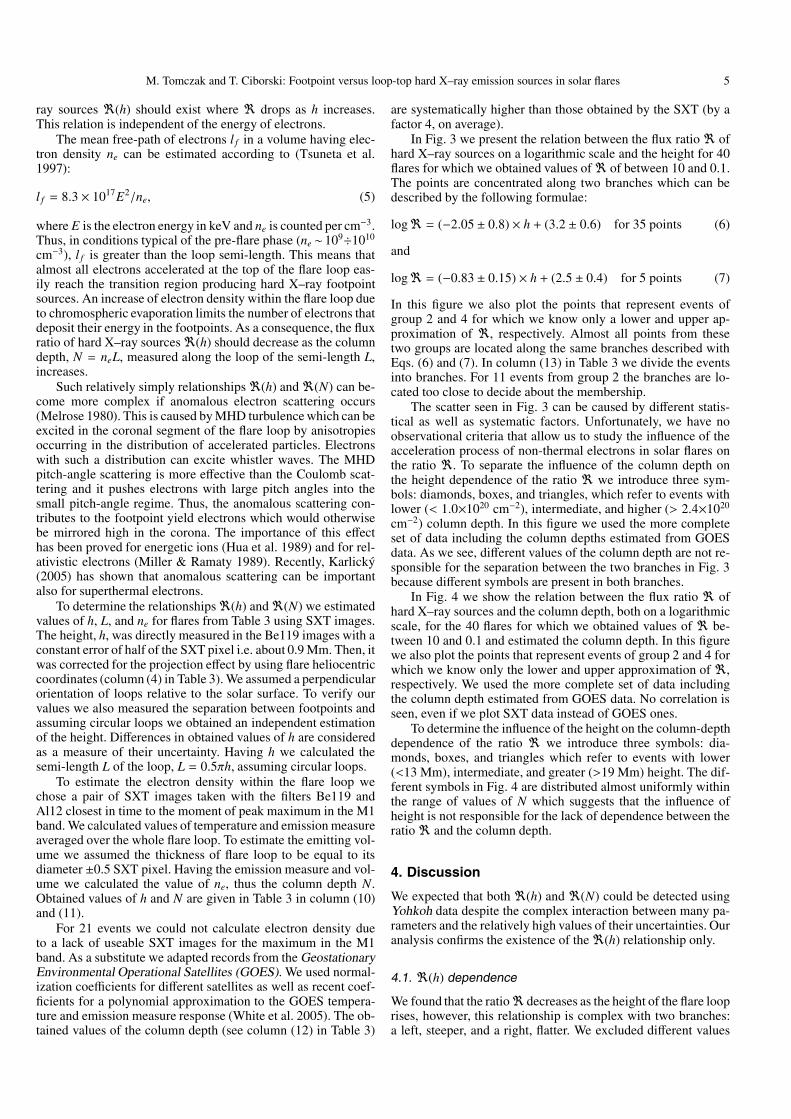
In Fig. 3 we present the relation between the flux ratio� ofhard X–ray sources on a logarithmic scale and the height for 40flares for which we obtained values of� of between 10 and 0.1.The points are concentrated along two branches which can bedescribed by the following formulae:
log� = (−2.05 ± 0.8) × h + (3.2 ± 0.6) for 35 points (6)
and
log� = (−0.83 ± 0.15) × h + (2.5 ± 0.4) for 5 points (7)
In this figure we also plot the points that represent events ofgroup 2 and 4 for which we know only a lower and upper ap-proximation of �, respectively. Almost all points from thesetwo groups are located along the same branches described withEqs. (6) and (7). In column (13) in Table 3 we divide the eventsinto branches. For 11 events from group 2 the branches are lo-cated too close to decide about the membership.
The scatter seen in Fig. 3 can be caused by different statis-tical as well as systematic factors. Unfortunately, we have noobservational criteria that allow us to study the influence of theacceleration process of non-thermal electrons in solar flares onthe ratio �. To separate the influence of the column depth onthe height dependence of the ratio � we introduce three sym-bols: diamonds, boxes, and triangles, which refer to events withlower (< 1.0×1020 cm−2), intermediate, and higher (> 2.4×10²⁰
cm−2) column depth. In this figure we used the more completeset of data including the column depths estimated from GOESdata. As we see, different values of the column depth are not re-sponsible for the separation between the two branches in Fig. 3because different symbols are present in both branches.
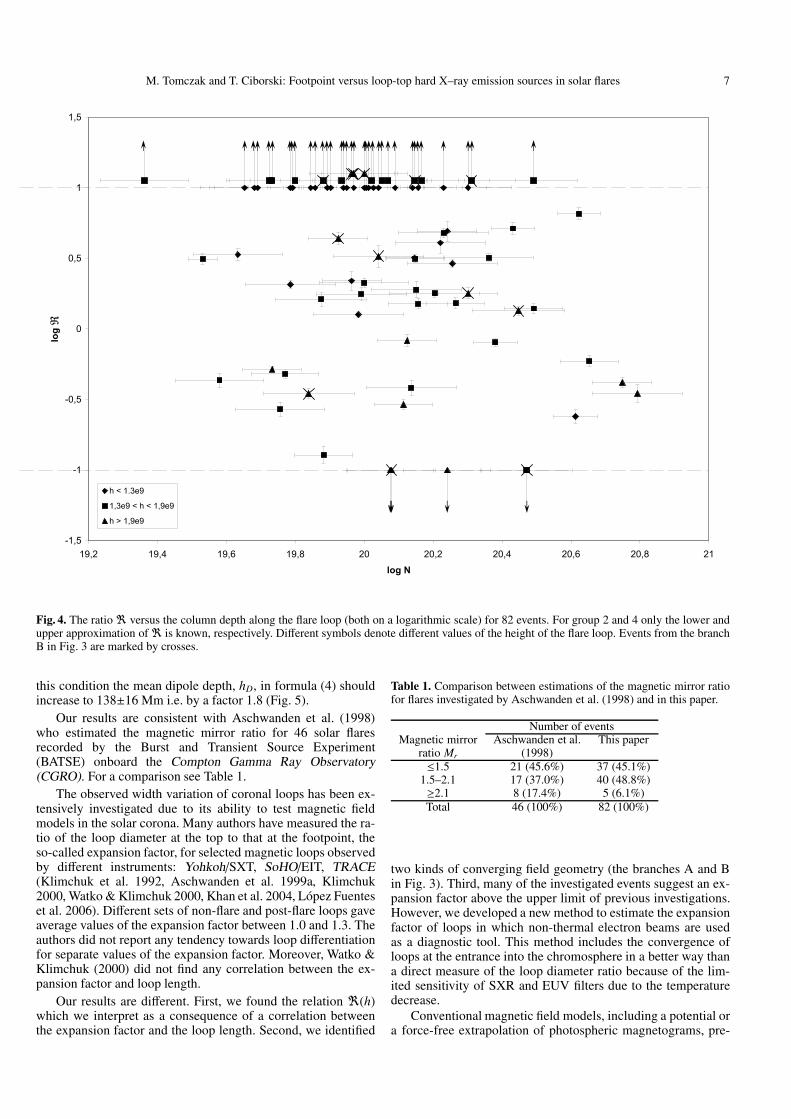
In Fig. 4 we show the relation between the flux ratio � ofhard X–ray sources and the column depth, both on a logarithmicscale, for the 40 flares for which we obtained values of � be-tween 10 and 0.1 and estimated the column depth. In this figurewe also plot the points that represent events of group 2 and 4 forwhich we know only the lower and upper approximation of �,respectively. We used the more complete set of data includingthe column depth estimated from GOES data. No correlation isseen, even if we plot SXT data instead of GOES ones.
To determine the influence of the height on the column-depthdependence of the ratio � we introduce three symbols: dia-monds, boxes, and triangles which refer to events with lower(<13 Mm), intermediate, and greater (>19 Mm) height. The dif-ferent symbols in Fig. 4 are distributed almost uniformly withinthe range of values of N which suggests that the influence ofheight is not responsible for the lack of dependence between theratio� and the column depth.
4. Discussion
We expected that both �(h) and �(N) could be detected usingYohkoh data despite the complex interaction between many pa-rameters and the relatively high values of their uncertainties. Ouranalysis confirms the existence of the�(h) relationship only.
4.1. �(h) dependence
We found that the ratio� decreases as the height of the flare looprises, however, this relationship is complex with two branches:a left, steeper, and a right, flatter. We excluded different values

6 M. Tomczak and T. Ciborski: Footpoint versus loop-top hard X–ray emission sources in solar flares
-1,5
-1
-0,5
0
0,5
1
1,5
0,5 1 1,5 2 2,5 3 3,5 4 4,5 5
h [10e9]
log
log N < 2020 < log N < 20,4log N > 20,4
A B
Fig. 3. The ratio � (on a logarithmic scale) versus the height of the flare loop for 82 events. For group 2 and 4 only the lower and upperapproximation of� is known, respectively. Different symbols denote different values of the column depth along the flare loop. A linear fit to thepoints from two branches is described by Eqs. (6) and (7).
of the column depth as the cause of the membership of a par-ticular branch. We do not think that the acceleration process ofnon-thermal electrons decides into which branch the event falls.If so, then all points from the branch B in Fig. 3 should havea particular distribution of electrons which makes propagationinto the footpoints more efficient than for other events. Thus,the points from the branch B in Fig. 3 should also show highervalues of the ratio � for similar values of the column depth inFig. 4. These points are marked by crosses and as we see, this isnot the case.
We suggest that events from different branches in Fig. 3 oc-curred in magnetic loops having different converging field ge-ometries. Thus, events from branch A occurred in more con-verged loops than the events from branch B. This is confirmedby the different inclination of the branches. For the branch A anincrease of the height of about 9.5 Mm, on average, transformsthe flux ratio� from the value of 10 into the value of 0.1, i.e. itmakes the event of group 4 instead of the event of group 2. To dothe same for the branch B an increase of height of about 24 Mmis needed.
We used our data to estimate the frequency of occurrence ofmore-converged and less-converged loops in the solar corona.We have classified 58 events into branch A and 13 events intobranch B (see column (13) in Table 3). This gives an 82% con-
tribution of the more-converged loops and an 18% contributionof the less-converged ones. For group 2 the branches are situatedvery close each to other, therefore a safer method is to take intoaccount only events of group 3 and 4. In this case the contribu-tion of the more-converged loops is even higher (38 events of 45i.e. 84%) and the contribution of the less-converged ones is 16%(7 events of 45).
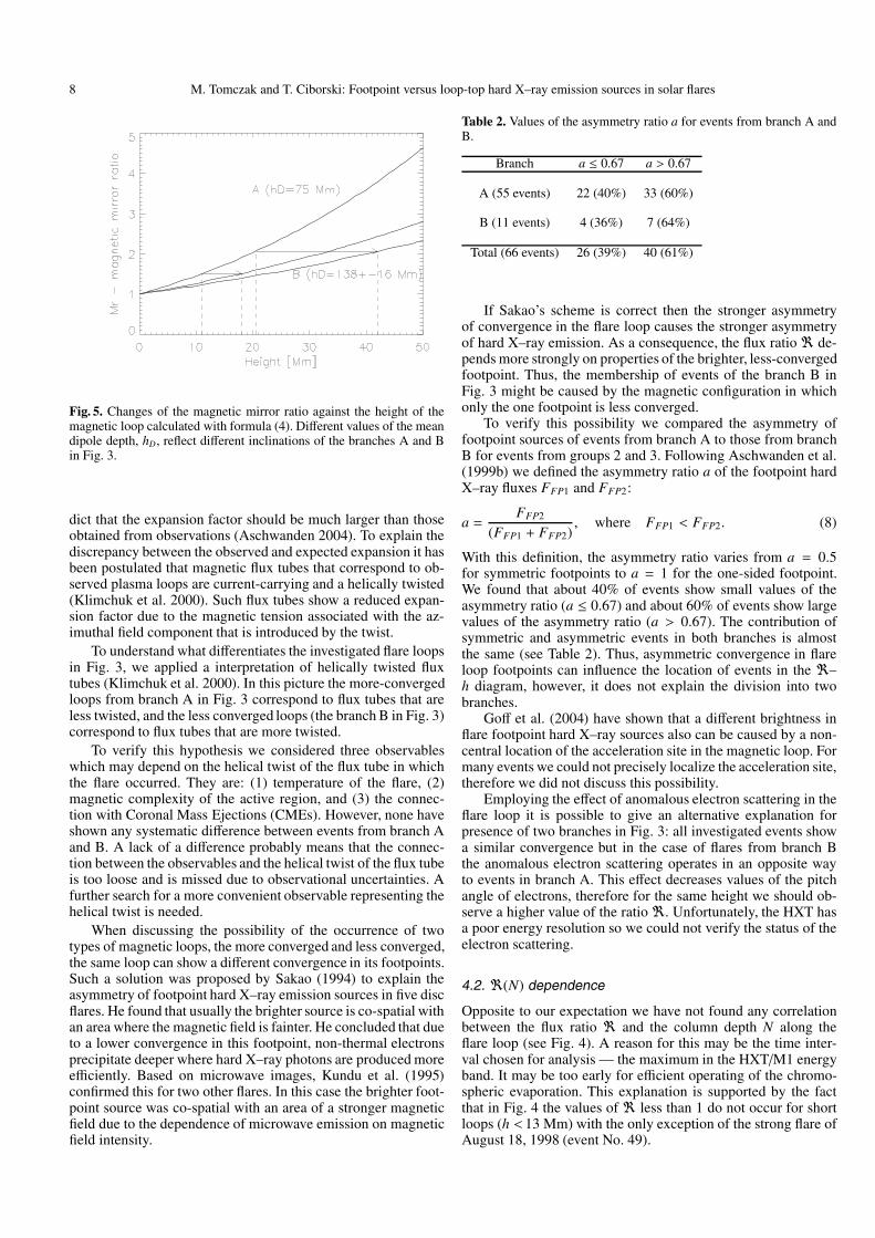
To describe the convergence of the investigated magneticloops more quantitatively we used formula (4) and assumed apriori that it works for more frequent events from branch A(Fig. 5). We calculated the magnetic mirror ratio, Mr, for termi-nal heights, 11 and 20.5 Mm, establishing the group 3 for branchA. The obtained values of Mr are 1.51 and 2.06, respectively.This means that an increase of the magnetic mirror ratio by afactor 1.36 completely changes the spatial distribution of hardX–ray emission in solar flares. For Mr ≤ 1.51 the population ofelectrons reaching the footpoints is so large that the HXT candetect only footpoint sources. For Mr ≥ 2.06 the population ofelectrons trapped around the loop-top is so large that the HXTcan detect only loop-top sources.
If our explanation is consistent, the magnetic loops frombranch B should reach the same values of Mr, 1.51 and 2.06, forgreater terminal heights, 18 and 42 Mm, respectively. To fulfil
M. Tomczak and T. Ciborski: Footpoint versus loop-top hard X–ray emission sources in solar flares 7
-1,5
-1
-0,5
0
0,5
1
1,5
19,2 19,4 19,6 19,8 20 20,2 20,4 20,6 20,8 21
log N
log
h < 1.3e9
1,3e9 < h < 1,9e9
h > 1,9e9
Fig. 4. The ratio� versus the column depth along the flare loop (both on a logarithmic scale) for 82 events. For group 2 and 4 only the lower andupper approximation of� is known, respectively. Different symbols denote different values of the height of the flare loop. Events from the branchB in Fig. 3 are marked by crosses.
this condition the mean dipole depth, hD, in formula (4) shouldincrease to 138±16 Mm i.e. by a factor 1.8 (Fig. 5).
Our results are consistent with Aschwanden et al. (1998)who estimated the magnetic mirror ratio for 46 solar flaresrecorded by the Burst and Transient Source Experiment(BATSE) onboard the Compton Gamma Ray Observatory(CGRO). For a comparison see Table 1.
The observed width variation of coronal loops has been ex-tensively investigated due to its ability to test magnetic fieldmodels in the solar corona. Many authors have measured the ra-tio of the loop diameter at the top to that at the footpoint, theso-called expansion factor, for selected magnetic loops observedby different instruments: Yohkoh/SXT, SoHO/EIT, TRACE(Klimchuk et al. 1992, Aschwanden et al. 1999a, Klimchuk2000, Watko & Klimchuk 2000, Khan et al. 2004, Lopez Fuenteset al. 2006). Different sets of non-flare and post-flare loops gaveaverage values of the expansion factor between 1.0 and 1.3. Theauthors did not report any tendency towards loop differentiationfor separate values of the expansion factor. Moreover, Watko &Klimchuk (2000) did not find any correlation between the ex-pansion factor and loop length.
Our results are different. First, we found the relation �(h)which we interpret as a consequence of a correlation betweenthe expansion factor and the loop length. Second, we identified
Table 1. Comparison between estimations of the magnetic mirror ratiofor flares investigated by Aschwanden et al. (1998) and in this paper.
Number of eventsMagnetic mirror Aschwanden et al. This paper
ratio Mr (1998)≤1.5 21 (45.6%) 37 (45.1%)
1.5–2.1 17 (37.0%) 40 (48.8%)≥2.1 8 (17.4%) 5 (6.1%)Total 46 (100%) 82 (100%)
two kinds of converging field geometry (the branches A and Bin Fig. 3). Third, many of the investigated events suggest an ex-pansion factor above the upper limit of previous investigations.However, we developed a new method to estimate the expansionfactor of loops in which non-thermal electron beams are usedas a diagnostic tool. This method includes the convergence ofloops at the entrance into the chromosphere in a better way thana direct measure of the loop diameter ratio because of the lim-ited sensitivity of SXR and EUV filters due to the temperaturedecrease.
Conventional magnetic field models, including a potential ora force-free extrapolation of photospheric magnetograms, pre-
8 M. Tomczak and T. Ciborski: Footpoint versus loop-top hard X–ray emission sources in solar flares
Fig. 5. Changes of the magnetic mirror ratio against the height of themagnetic loop calculated with formula (4). Different values of the meandipole depth, hD, reflect different inclinations of the branches A and Bin Fig. 3.
dict that the expansion factor should be much larger than thoseobtained from observations (Aschwanden 2004). To explain thediscrepancy between the observed and expected expansion it hasbeen postulated that magnetic flux tubes that correspond to ob-served plasma loops are current-carrying and a helically twisted(Klimchuk et al. 2000). Such flux tubes show a reduced expan-sion factor due to the magnetic tension associated with the az-imuthal field component that is introduced by the twist.
To understand what differentiates the investigated flare loopsin Fig. 3, we applied a interpretation of helically twisted fluxtubes (Klimchuk et al. 2000). In this picture the more-convergedloops from branch A in Fig. 3 correspond to flux tubes that areless twisted, and the less converged loops (the branch B in Fig. 3)correspond to flux tubes that are more twisted.
To verify this hypothesis we considered three observableswhich may depend on the helical twist of the flux tube in whichthe flare occurred. They are: (1) temperature of the flare, (2)magnetic complexity of the active region, and (3) the connec-tion with Coronal Mass Ejections (CMEs). However, none haveshown any systematic difference between events from branch Aand B. A lack of a difference probably means that the connec-tion between the observables and the helical twist of the flux tubeis too loose and is missed due to observational uncertainties. Afurther search for a more convenient observable representing thehelical twist is needed.
When discussing the possibility of the occurrence of twotypes of magnetic loops, the more converged and less converged,the same loop can show a different convergence in its footpoints.Such a solution was proposed by Sakao (1994) to explain theasymmetry of footpoint hard X–ray emission sources in five discflares. He found that usually the brighter source is co-spatial withan area where the magnetic field is fainter. He concluded that dueto a lower convergence in this footpoint, non-thermal electronsprecipitate deeper where hard X–ray photons are produced moreefficiently. Based on microwave images, Kundu et al. (1995)confirmed this for two other flares. In this case the brighter foot-point source was co-spatial with an area of a stronger magneticfield due to the dependence of microwave emission on magneticfield intensity.
Table 2. Values of the asymmetry ratio a for events from branch A andB.
Branch a ≤ 0.67 a > 0.67
A (55 events) 22 (40%) 33 (60%)
B (11 events) 4 (36%) 7 (64%)
Total (66 events) 26 (39%) 40 (61%)
If Sakao’s scheme is correct then the stronger asymmetryof convergence in the flare loop causes the stronger asymmetryof hard X–ray emission. As a consequence, the flux ratio� de-pends more strongly on properties of the brighter, less-convergedfootpoint. Thus, the membership of events of the branch B inFig. 3 might be caused by the magnetic configuration in whichonly the one footpoint is less converged.
To verify this possibility we compared the asymmetry offootpoint sources of events from branch A to those from branchB for events from groups 2 and 3. Following Aschwanden et al.(1999b) we defined the asymmetry ratio a of the footpoint hardX–ray fluxes FFP1 and FFP2:
a =FFP2
(FFP1 + FFP2), where FFP1 < FFP2. (8)
With this definition, the asymmetry ratio varies from a = 0.5for symmetric footpoints to a = 1 for the one-sided footpoint.We found that about 40% of events show small values of theasymmetry ratio (a ≤ 0.67) and about 60% of events show largevalues of the asymmetry ratio (a > 0.67). The contribution ofsymmetric and asymmetric events in both branches is almostthe same (see Table 2). Thus, asymmetric convergence in flareloop footpoints can influence the location of events in the �–h diagram, however, it does not explain the division into twobranches.
Goff et al. (2004) have shown that a different brightness inflare footpoint hard X–ray sources also can be caused by a non-central location of the acceleration site in the magnetic loop. Formany events we could not precisely localize the acceleration site,therefore we did not discuss this possibility.
Employing the effect of anomalous electron scattering in theflare loop it is possible to give an alternative explanation forpresence of two branches in Fig. 3: all investigated events showa similar convergence but in the case of flares from branch Bthe anomalous electron scattering operates in an opposite wayto events in branch A. This effect decreases values of the pitchangle of electrons, therefore for the same height we should ob-serve a higher value of the ratio�. Unfortunately, the HXT hasa poor energy resolution so we could not verify the status of theelectron scattering.
4.2. �(N) dependence
Opposite to our expectation we have not found any correlationbetween the flux ratio � and the column depth N along theflare loop (see Fig. 4). A reason for this may be the time inter-val chosen for analysis — the maximum in the HXT/M1 energyband. It may be too early for efficient operating of the chromo-spheric evaporation. This explanation is supported by the factthat in Fig. 4 the values of � less than 1 do not occur for shortloops (h < 13 Mm) with the only exception of the strong flare ofAugust 18, 1998 (event No. 49).

M. Tomczak and T. Ciborski: Footpoint versus loop-top hard X–ray emission sources in solar flares 9
Fig. 6. Reproduced from Hori et al. (1997). Field lines connecting a heatsource and footpoints extend outside the bright loop seen in soft X-rayswhich is an apparent product of successive energy release and inertia ofthe chromospheric evaporation.
The lack of correlation in Fig. 4 can be explained also by thescheme presented in Fig. 6. This figure is reproduced from Horiet al. (1997). As we see, field lines connecting a heat sourceand footpoints extend beyond the bright loop seen in soft X-rays. The impression that we observe a single bright loop wascaused by successive energy release from the innermost loopto the outermost and the inertia of chromospheric evaporation.If this scheme is correct we should rather measure the columndepth outside the bright legs seen in SXT images which appar-ently connect the loop-top and footpoint hard X–ray sources.The scheme from Fig. 6 does not need to work for each of the in-vestigated events to argue against a correlation between the fluxratio and the column depth. Anomalous electron scattering canbe an additional cause that makes the correlation between� andN unclear.
5. Conclusions
We investigated the spatial distribution of hard X–ray emissionin solar flares. We concentrated on the relationship between theloop-top and footpoint emission sources. In comparison to pre-vious studies (Masuda 1994, Petrosian et al. 2002) the list ofinvestigated flares is more complete (117 events instead of 10 or18, respectively) due to the mission-long Yohkoh/HXT databasethat was included and the more liberal selection criteria that wereused.
We investigated the dependence of the flux ratio � of thefootpoint and loop-top sources on other observational parame-ters like the flare loop height h and the column depth N alongthe flare loop. We found a clear correlation between � and h(Fig. 3) which we interpret as an effect of converging field ge-ometry. Since this correlation is stronger than other parametersand observational uncertainties we conclude that the influence ofmagnetic convergence on the spatial distribution of hard X–rayemission in solar flares is the strongest, at least under conditionsdefined in this investigation i.e during the early phase of the flareevolution. This is confirmed, to some extent, by the lack of anycorrelation between the flux ratio � and the column depth N(Fig. 4). However, this can be also caused by a more complexconfiguration of investigated events than is seen in soft X–rays(see Fig. 6).
Using the formula from Aschwanden et al. (1999a) we de-veloped a new method of calculating the magnetic mirror ratioin solar flare loops using non-thermal electron beams as a diag-nostic tool for magnetic convergence. The obtained values of themagnetic mirror ratio are consistent with previous results and
suggest a nonpotential configuration strongly distorted by thepresence of longitudinal currents.
The two branches seen in the �− h diagram suggest that inthe solar corona two kinds of magnetic loops can exist: a moreconverged kind that is more frequent (above 80%) and a lessconverged kind that is less frequent (below 20%). In a dipoleapproximation the mean dipole depth hD differs between thebranches by a factor of 1.8, on average. Despite the observeddichotomy in solar flare loops into more converged and less con-verged cases, we have no independent proof confirming such adivision. Therefore, we cannot conclude, whether the division isreal or random. Finally, what is a role of the anomalous electronscattering? Further studies are needed including more and betterobserved flares to answer these questions. For this, the ReuvenRamaty High-Energy Solar Spectroscopic Imager (RHESSI) isideal due to its dynamic range and energy resolution better thanthe HXT. This work is in progress.
We hope that further study will allow us to understand alsothe concentration in the rarely-occupied branch B in Fig. 3 ofmany known and extensively investigated flares e.g. of January13, 1992 (Masuda et al. 1994), of February 17, 1992 (Doscheket al. 1995), of June 28, 1992 (Tomczak 1997), and of October4, 1992 (Masuda et al. 1995).
Acknowledgements. The Yohkoh satellite is a project of the Institute of Spaceand Astronautical Science of Japan. The authors are grateful to the referee, Dr.Marian Karlicky, for his valuable remarks which helped to improve the paper.This work was supported by a Polish Ministry of Science and High Educationgrant.
References
Aschwanden, M. J. 2002, Space Sci. Rev., 101, 1Aschwanden, M. J. 2004, Physics of the Solar Corona. An Introduction,
Springer: PraxisAschwanden, M. J., Fletcher, L., Sakao, T., Kosugi, T., & Hudson, H. 1999b,
ApJ, 517, 977Aschwanden, M. J., Newmark, J. S., Delaboudiniere, J.-P., et al. 1999a, ApJ, 515,
842Aschwanden, M. J., Schwartz, R. A., & Dennis, B. R. 1998, ApJ, 502, 468Brown, J. C. 1971, Solar Phys., 18, 489Doschek, G. A., Strong, K. T., & Tsuneta, S. 1995, ApJ, 440, 370Hara, H., Tsuneta, T., Lemen, J. R., Acton, L. W., & McTiernan, J. M. 1992,
PASJ, 44, L135Hori, K., Yokoyama, T., Kosugi, T., & Shibata, K. 1997, ApJ, 489, 426Hua, X.-M., Ramaty, R., & Lingenfelter, R. E. 1989, ApJ, 341, 516Goff, C. P., Matthews, S. A., van Driel-Gesztelyi, L., & Harra, L. K. 2004, A&A,
423, 363Jakimiec, J. 2002, in Proc. 10th European Solar Physics Meeting, Solar
Variability: From Core to Outer Frontiers, ed. E. Wilson (ESA SP–506),645
Jakimiec, J., Tomczak, M., Falewicz, R., Phillips, J. H. K., & Fludra, A. 1998,A&A, 334, 1112
Karlicky, M. 2005, Hvar Obs. Bull., 29, 137Karlicky, M., & Barta, M. 2006, ApJ, 647, 1472Karlicky, M., & Kosugi, T. 2004, A&A, 419, 1159Khan, J. I., Hudson, H. S., & Mouradian, Z. 2004, A&A, 416, 323Klimchuk, J. A. 2000, Solar Phys., 193, 53Klimchuk, J. A., Antiochos, S. K., & Norton, D. 2000, ApJ, 542, 504Klimchuk, J. A., Lemen, J. R., Feldman, U., Tsuneta, S., & Uchida, Y. 1991,
PASJ, 44, L181Kosugi, T. 1994, in Proc. of Kofu Symposium, ed. S. Enome, & T. Hirayama
(Nobeyama Radio Observatory Report No. 360), 11Kosugi, T., Makishima, K., Murakami, T., at al. 1991, Solar Phys., 136, 17Kundu, M. R., Nitta, N., White, S. M., et al. 1995, ApJ, 454, 522Lopez Fuentes, M. C., Klimchuk, J. A., & Demoulin, P. 2006, ApJ, 639, 459Masuda, S. 1994, Ph. D. thesis, University of TokyoMasuda, S. 2002, in Proc. of Yohkoh 10th Anniversary Meeting, ed. P.C.H.
Martens, & D. Cauffman (COSPAR Colloquia Series Vol. 13), 351Masuda, S., Kosugi, T., Hara, H., et al. 1995, PASJ, 47, 677Masuda, S., Kosugi, T., Hara, H., Tsuneta, S, & Ogawara, Y. 1994, Nature, 371,
495

10 M. Tomczak and T. Ciborski: Footpoint versus loop-top hard X–ray emission sources in solar flares
Melrose, D. B. 1980, Plasma Astrophysics (New York: Gordon and Breach)Miller, J. A., & Ramaty, R. 1989, ApJ, 344, 973Petrosian, V., & Donaghy, T. Q. 1999, ApJ, 527, 945Petrosian, V., Donaghy, T. Q., & McTiernan, J. M. 2002, ApJ, 569, 459Sakao, T. 1994, Ph. D. thesis, University of TokyoSato, J. 2001, ApJ, 558, L137Sato, J., Kosugi, T., & Makishima, K. 1999, PASJ, 51, 127Shibata, K. 1999, Ap&SS, 264, 129Somov, B. V., & Kosugi, T. 1997, ApJ, 485, 859Tomczak, M. 1997, A&A, 317, 223Tomczak, M. 2001, A&A, 366, 294Tsuneta, S. 1997, ApJ, 483, 507Tsuneta, S., Acton, L., Bruner, M., et al. 1991, Solar Phys., 136, 37Tsuneta, S., Masuda, S., Kosugi, T., & Sato, J. 1997, ApJ, 478, 787Watko, J. A., & Klimchuk, J. A. 2000, Solar Phys., 193, 77White, S. M., Thomas, R. J., & Schwartz, R. A. 2005, Solar Phys., 227, 231
M. Tomczak and T. Ciborski: Footpoint versus loop-top hard X–ray emission sources in solar flares 11
Table 3: List of selected flares (a Values in parenthesis are estimated from SXTimages; b M – Masuda 1994, P – Petrosian et al. 2002).
No. Date GOES Disk NOAA M1 Time Group � h N [1020 cm−2] Branch Rem.b
class positiona AR cts. interval [Mm] SXT GOES [Fig. 3](1) (2) (3) (4) (5) (6) (7) (8) (9) (10) (11) (12) (13) (14)
1 91/11/09 M1.4 S14W69 6906 105 20:52:09+2 2 15 0.34 1.4 ?2 91/11/17 M1.9 S12E78 6929 49 18:33:17+2 2 10 0.20 1.7 A3 91/12/02 M3.6 N16E87 6955 24 04:53:44+4.5 3 0.48 14 0.21 0.59 A M, P4 91/12/03 X2.2 N17E72 6955 1297 16:36:30+0.5 1 12 0.79 2.25 91/12/07 C6.4 N09E72 6961 17 21:52:46+7.5 1 12 0.52 0.276 91/12/08 M2.6 N08E65 6961 12 07:35:00+9 1 15 0.61 0.927 91/12/09 M1.1 S06E88 6966 13 18:53:46+9.5 3 6.6 17 0.31 4.1 A8 91/12/15 C6.0 S12E76 6972 14 14:21:42+5 2 12 0.20 0.62 A M, P9 91/12/16 C7.8 S10E69 6972 43 03:13:06+2.5 2 10 0.27 0.80 A
10 91/12/16 M1.6 S12E67 6972 50 06:38:15+2.5 2 9 1.4 1.4 A11 91/12/18 M3.5 S10E88 6980 106 10:27:30+1.5 3 1.4 15 0.31 3.1 A M, P12 92/01/13 M2.0 S16W86 6994 29 17:28:11+3.5 2 24 0.11 0.93 B M, P13 92/02/06 M7.6 N05W82 7030 144 03:23:50+1 4 22 0.38 1.7 A M, P14 92/02/17 M1.9 S16W81 7050 21 15:40:54+5 2 17 0.16 0.63 B M, P15 92/02/19 M3.7 N04E85 7067 17 03:48:23+6.5 3 4.4 22 0.23 0.84 B16 92/02/26 M1.3 S16W90 7073 15 01:37:58+6.5 2 12 0.33 2.0 A17 92/04/01 M2.3 S04E86 7123 38 10:13:04+3 2 9 0.64 1.0 A M, P18 92/04/19 C3.9 N04E85 7138 16 02:11:11+6.5 2 22 0.11 0.92 B19 92/06/26 C2.9 N08W82 7205 11 12:52:15+9.5 1 9 0.26 0.9720 92/06/28 M1.6 N10W89 7216 17 13:56:43+5.5 4 45 1.1 B21 92/08/11 M1.4 (S15E81) 7260 77 22:25:20+1.5 1 14 0.19 0.4222 92/09/09 M3.1 S09W71 7270 32 02:10:29+3.5 1 16 0.27 1.723 92/09/09 M1.9 S11W78 7270 15 17:58:33+6 1 14 0.17 1.524 92/10/04 M2.4 S05W90 7293 30 22:19:07+3 2 19 0.91 1.4 B M, P25 92/10/11 C8.3 S16W68 7301 14 02:03:36+10.5 2 15 0.14 0.54 ?26 92/11/05 M2.0 S17W84 7323 36 06:19:22+3 1 10 0.40 1.0 M, P27 92/11/22 M1.6 N11E76 7348 31 23:07:49+4 2 9 0.73 0.61 A28 92/12/04 M1.4 N19W71 7352 47 11:38:32+2 2 15 0.31 0.86 ?29 93/02/05 C7.7 S07E78 7420 29 07:53:38+3.5 1 15 0.5530 93/02/06 C5.6 S08E66 7420 23 05:25:56+4.5 1 8 0.9031 93/02/14 M2.0 S22E78 7427 53 12:53:04+3 1 14 0.50 2.332 93/02/17 M5.8 S07W87 7420 94 10:36:21+1 3 2.2 12 0.22 0.92 A M, P33 93/02/21 M1.4 N13E75 7433 14 00:39:35+8.5 3 2.9 11 0.60 1.8 A34 93/03/15 C3.0 N06W88 7411 15 09:59:44+9 2 12 0.11 0.92 A35 93/06/11 C5.7 S13W80 7518 12 10:14:59+9.5 3 0.35 34 0.69 B36 93/06/25 M5.1 (S09E90) 7530 17 03:18:23+6 3 1.5 13 0.22 1.4 A37 93/09/27 M1.8 (N09E89) 7590 41 12:08:14+4.5 2 9 0.62 1.1 A P38 93/10/09 M1.1 N11W78 7590 11 08:08:18+10 3 3.4 10 0.25 0.43 A39 93/11/30 C9.2 (N19E84) 7618 70 06:03:31+4 2 14 0.21 1.0 ? P40 94/01/16 M6.1 N09E70 7654 57 23:17:27+2 3 0.83 20 0.51 1.3 A41 94/01/17 C9.3 N06E65 7654 12 09:14:49+10.5 2 15 0.16 1.2 ?42 97/08/09 C8.5 N19W85 8069 12 16:33:35+10 1 9 1.443 97/09/14 C2.8 S23W79 8083 17 02:53:26+6 2 15 0.23 ?44 97/11/15 M1.0 N20E65 8108 15 22:42:04+5.5 4 49 3.2 B45 98/05/08 M3.1 (S16W90) 8210 48 01:57:35+2 3 1.8 14 0.19 1.6 A P46 98/05/28 C8.7 (N16W89) 8226 12 19:02:55+10 3 2.1 12 0.15 0.61 A47 98/08/14 M3.1 S23W74 8293 65 08:25:57+2 1 10 1.4 2.248 98/08/18 X2.8 (N34E85) 8307 599 08:20:29+0.5 4 14 1.1 3.1 A P49 98/08/18 X4.9 N33E87 8307 2819 22:16:40+0.5 3 0.24 11 1.2 4.1 A P50 98/09/02 M2.2 (N18W82) 8319 20 17:03:50+5 2 13 0.35 0.48 ?51 98/09/28 C9.5 (S14W90) 8342 26 12:00:22+4.5 2 9 0.20 1.4 A52 98/09/28 C6.8 (S14W90) 8342 21 16:08:14+5.5 2 9 0.17 0.45 A53 98/11/09 C4.9 N22W70 8375 21 21:12:21+5.5 3 4.8 16 0.20 1.7 A54 98/11/10 C7.9 N20W76 8375 51 00:12:25+2 1 11 0.64 1.355 98/11/10 C3.3 N21W76 8375 18 06:52:25+6 1 12 0.77 4.056 98/11/10 M1.8 N21W78 8375 56 15:42:44+2 1 15 0.23 2.057 98/11/11 M1.0 N22W86 8375 18 04:05:54+6 3 3.2 15 0.62 2.3 A58 98/11/11 C3.5 N22W90 8375 13 07:36:32+10 1 14 0.28 0.8559 98/11/22 X3.7 S29W80 8384 1200 06:39:38+0.5 3 0.42 20 0.86 5.6 A60 98/11/22 X2.5 S29W86 8384 830 16:20:42+0.5 3 0.59 17 1.6 4.5 A61 98/11/23 C4.9 (S30W89) 8386 14 05:58:55+9.5 3 0.51 20 0.11 0.54 A62 98/11/24 C8.4 N19E77 8395 18 22:12:33+6.5 2 12 0.12 1.0 A63 98/11/25 C6.4 (N19E69) 8395 14 14:01:01+9.5 2 8 0.30 0.87 A64 99/01/14 M3.0 (N20E65) 8460 12 10:14:42+9.5 1 21 2.0
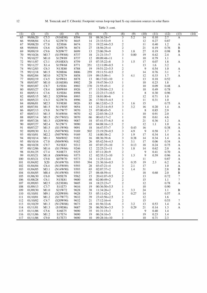
12 M. Tomczak and T. Ciborski: Footpoint versus loop-top hard X–ray emission sources in solar flares
Table 3: cont.
(1) (2) (3) (4) (5) (6) (7) (8) (9) (10) (11) (12) (13) (14)65 99/06/20 C5.5 (N16E90) 8594 18 08:36:24+7 3 5.2 14 0.10 2.7 A66 99/08/04 C5.4 S22W70 8645 14 23:33:52+9 1 12 0.27 0.8767 99/08/20 C7.8 S23E66 8674 21 19:22:44+5.5 2 11 0.40 1.2 A68 99/09/01 C6.6 S28W76 8674 27 18:56:25+4 2 21 0.19 0.76 B69 99/09/19 C9.6 N20W77 8699 13 23:06:39+9 3 1.8 27 0.19 0.98 B70 99/10/26 M3.7 (S15W88) 8737 18 21:21:33+7 3 0.80 19 0.42 2.4 A71 99/10/27 M1.0 S12W89 8737 12 09:09:48+11 1 10 0.79 1.172 99/11/07 C3.1 (N10E83) 8759 15 07:35:22+8 3 1.5 17 0.07 1.8 A73 99/11/27 X1.4 S15W68 8771 351 12:11:09+0.5 1 13 1.6 3.274 99/12/03 C6.3 N13E80 8788 19 19:51:22+5.5 2 9 0.54 1.0 A75 99/12/18 M1.5 N20E66 8806 259 19:11:51+0.5 2 14 0.76 3.1 ?76 00/02/04 M3.0 N27E79 8858 119 09:15:09+1 3 4.1 12 0.33 1.7 A77 00/02/19 C4.5 S19W81 8878 13 06:17:02+10 1 13 0.18 0.5278 00/03/07 M1.0 (S16E88) 8902 28 19:47:56+3.5 1 10 0.23 1.879 00/03/07 C8.7 S15E84 8902 170 21:55:45+1 2 10 0.09 0.48 A80 00/03/27 C8.4 S09W69 8926 37 13:59:04+2.5 1 10 0.49 0.7881 00/05/11 C3.6 S15E84 8998 11 22:23:17+10.5 1 8 0.30 0.9682 00/05/15 M1.2 S20W66 8993 22 18:01:00+6 1 12 0.71 1.083 00/05/23 C4.3 S22W76 8996 26 17:50:15+4.5 1 11 0.31 1.084 00/06/01 M2.5 N19E80 9026 83 06:12:02+1.5 3 1.6 15 0.75 A85 00/07/01 M1.5 N11W85 9054 14 23:23:14+9.5 3 3.2 16 0.20 1.4 A86 00/07/13 C9.8 N17W77 9070 23 07:00:45+5 1 8 0.85 2.987 00/07/13 M1.5 N16W84 9070 42 22:03:38+2.5 1 10 0.91 2.088 00/07/14 M1.5 (N17W83) 9070 66 00:43:17+2 1 18 0.61 4.689 00/07/26 M1.3 (S20W90) 9087 18 07:41:57+6.5 4 21 0.36 1.2 A90 00/07/27 M2.4 N12W71 9090 65 04:08:16+1.5 2 12 1.1 1.0 A91 00/07/27 M1.5 (S11W90) 9091 18 16:47:57+7 3 0.43 16 0.38 A92 00/09/30 X1.2 (N07W90) 9169 502 23:19:29+0.5 3 4.9 9 0.58 1.7 A93 00/10/01 M2.2 (N07W90) 9169 52 14:00:38+2 3 1.9 17 0.34 1.4 A94 00/10/14 M1.1 N04W82 9182 16 08:36:39+6 3 0.38 14 0.34 1.4 A95 00/10/16 C7.0 (N04W90) 9182 26 05:42:54+4.5 3 3.1 17 0.06 0.34 A96 00/10/28 C9.7 N15E83 9212 10 07:07:25+10 3 0.13 18 0.24 0.75 A97 00/12/06 M1.6 (S11W66) 9246 12 22:25:21+11 3 1.8 14 0.62 2.0 A98 01/01/25 C7.4 N10E73 9325 12 07:11:20+9 2 9 0.41 0.70 A99 01/03/21 M1.8 (S06W66) 9373 12 02:35:12+10 3 1.3 9 0.59 0.96 A
100 01/03/21 C9.8 S07W70 9373 34 11:25:12+4 2 11 0.87 A101 01/04/02 X20 (N16W70) 9393 394 21:36:16+0.5 3 0.35 19 2.3 6.2 A102 01/04/04 C6.4 (N15W89) 9393 28 03:47:21+4 3 2.1 17 1.0 A103 01/04/05 M3.1 (N14W90) 9393 65 02:07:37+2 3 1.4 31 2.8 B104 01/04/05 M8.4 (N14W90) 9393 27 08:48:59+4 2 18 0.68 2.0 B105 01/06/30 C6.0 N05E78 9562 15 20:41:07+9.5 2 13 0.72 ?106 01/08/28 C6.1 N15E81 9600 48 02:00:49+2 2 15 1.1 ?107 01/09/03 M2.5 (S23E88) 9605 18 18:23:23+7 2 12 0.78 A108 01/09/13 C3.7 S11E73 9616 19 00:36:50+5.5 1 10 0.90109 01/09/30 M1.0 S21W72 9628 38 11:34:26+2 3 3.3 24 1.1 B110 01/10/01 M9.1 (S20W89) 9628 53 05:11:42+2 3 0.27 14 0.57 A111 01/10/01 M1.2 (S17W77) 9632 39 23:43:56+2.5 1 12 1.6112 01/10/02 C4.7 (S20W90) 9632 21 17:12:16+4 2 15 0.53 ?113 01/10/29 M1.3 (N12W88) 9673 18 01:56:32+6 3 3.2 13 0.53 1.4 A114 01/11/01 M1.3 (S19E86) 9687 28 06:50:36+3.5 3 0.29 21 0.14 1.3 A115 01/11/06 C5.6 S16E75 9690 35 01:31:15+3 1 9 0.40 1.4116 01/11/06 M1.2 S17E74 9690 19 06:24:16+5 1 19 0.23 1.4117 01/11/06 C9.0 S17E73 9690 10 09:28:16+10 1 10 0.71 2.3