Folding of a model three-helix bundle protein: a thermodynamic and kinetic analysis1

Article No. jmbi.1999.2936 available online at http://www.idealibrary.com on J. Mol. Biol. (1999) 293, 917±951

Folding of a Model Three-helix Bundle Protein: AThermodynamic and Kinetic Analysis

Yaoqi Zhou1 and Martin Karplus1,2*

1Department of Chemistry &Chemical Biology, HarvardUniversity, Cambridge, MA02138, USA2Laboratoire de ChimieBiophysique, ISIS, UniversiteÂLouis Pasteur67000, Strasbourg, France

E-mail address of the [email protected]

0022-2836/99/440917±35 $30.00/0

The kinetics and thermodynamics of an off-lattice model for a three-helixbundle protein are investigated as a function of a bias gap parameterthat determines the energy difference between native and non-native con-tacts. A simple dihedral potential is used to introduce the tendency toform right-handed helices. For each value of the bias parameter, 100trajectories of up to one microsecond are performed. Such statisticallyvalid sampling of the kinetics is made possible by the use of the discretemolecular dynamics method with square-well interactions. This permitsmuch faster simulations for off-lattice models than do continuous poten-tials. It is found that major folding pathways can be de®ned, althoughensembles with considerable structural variation are involved. The largegap models generally fold faster than those with a smaller gap. For thelarge gap models, the kinetic intermediates are non-obligatory, whileboth obligatory and non-obligatory intermediates are present for smallgap models. Certain large gap intermediates have a two-helix micro-domain with one helix extended outward (as in domain-swappeddimers); the small gap intermediates have more diverse structures. Theimportance of studying the kinetic, as well as the thermodynamics, offolding for an understanding of the mechanism is discussed and therelation between kinetic and equilibrium intermediates is examined. It isfound that the behavior of this model system has aspects that encompassboth the ``new'' view and the ``old'' view of protein folding.

# 1999 Academic Press

Keywords: protein folding; kinetic intermediates; equilibriumintermediates; two-state cooperativity; three-helix bundle
*Corresponding author
Introduction

How a protein folds from a random coil into aunique native state in a relatively short time(microseconds to seconds) is a fundamental ques-tion in structural biology. The current ``new'' view(SÏali et al., 1994; Baldwin, 1995; Wolynes et al.,1996; Dill & Chan, 1997; Karplus, 1997; Dobsonet al., 1998), due largely to simulation-based simplemodels (Karplus & SÏali, 1995; Dill et al., 1995;Shakhnovich, 1996; Thirumalai et al., 1997) andtheoretical studies (Bryngelson & Wolynes, 1989;Shakhnovich & Gutin, 1989; Plotkin et al., 1997), isthat proteins are able to ®nd their native states inthe observed time because a bias in their energysurface reduces the number of con®gurations thatare sampled in the folding process, relative to theastronomic number envisaged in the Levinthalparadox (Levinthal, 1969). Equally important, the

ing author:

transition region, from which folding to the nativestate is fast, includes a large number of con®gur-ations (SÏali et al., 1994a; Dinner & Karplus, 1999).A focus on the overall energy or free energy sur-face (the ``energy landscape'') replaces the speci®cfolding pathways suggested by Levinthal (1968)with a distribution of the folding trajectories overmultiple pathways. Although experimental datahave provided speci®c information on no morethan a few competing pathways (Kiefhaber, 1995;Nath et al., 1996; Matagne et al., 1997; Wildegger &Kiefhaber, 1997), each of these may well involvebroad ensembles of structures except in the neigh-bourhood of the native state. For example, theextensive protein engineering data for thetransition state of chymotrypsin inhibitor 2(Jackson & Fersht, 1991; Itzhaki et al., 1995) areconsistent with ensemble distributions involvingrms differences of the order of 15 AÊ found in aseries of 24 unfolding simulations with anall-atom model (Lazaridis & Karplus, 1997).

# 1999 Academic Press

Figure 1. Left: The three-helix bundle protein (resi-dues 10-55 of the B domain of Staphylococcus aureus pro-tein A (Protein Data Bank accession no. 1bdd). Right:The global energy-minimum structure for the model.The Figures were drawn with the MOLSCRIPT program(Kraulis, 1991).

918 Folding of a Model Three-helix Bundle Protein

For a deeper understanding of protein folding, itis necessary to have a detailed knowledge of thethermodynamics and kinetics involved in goingfrom the denatured to the native state. At the pre-sent time, the necessary information can beobtained only by the use of simpli®ed models. Inprevious work (Zhou & Karplus, 1997), we studiedthe complete thermodynamics of a square-well,off-lattice, free-jointed-bead model, which has alowest energy (native) structure corresponding tothe three-helix bundle fragment of Staphylococcusaureus protein A (Gouda et al., 1992). It was shownthat the model exhibits the experimentallyobserved protein transitions: a collapse transition,a disordered globule to ordered (molten) globuletransition, a globule to native-state (folding) tran-sition and a transition to a surface frozen inactivestate (Zhou & Karplus, 1997). The Lindemanncriterion (Lindemann, 1910) was used to link theprotein phase diagram with the thermodynamicsand dynamics of other ®nite systems including vander Waals clusters (Berry, 1997) and homo-polymers (Zhou et al., 1997). The magnitude of thecooperativity and other aspects of the various tran-sitions in the model were shown to be controlledby a single parameter that determines the relativestrength of the native and the non-native contacts.The conclusion that a native state is a surface-molten solid is in accord with simulations ofcrambin using an all-atom representation and ananalysis of temperature-dependent X-ray diffrac-tion data for ribonuclease A (Zhou et al., 1999).

Since the model reproduces the thermodynamicsof real proteins, it is of interest to investigate thedetails of its folding kinetics. The present analysisrelates the thermodynamic phase diagram and thekinetic data from folding trajectories. Further, theoff-lattice model studies complement the equili-brium analysis of the free energy surface for an all-atom representation of the same three-helix bundle(Boczko & Brooks, 1995; Guo et al., 1997), as wellas kinetic studies based on lattice simulations(Kolinski et al., 1998) and thermodynamic studiesof a different off-lattice model (Pande & Rokhsar,1998).

The kinetics of a freely jointed-bead model forthe three-helix bundle proteins used here can becomplicated by intermediates that have structuralelements consisting of left-handed and right-handed helices; this was observed in earlier latticemodel studies of lysozyme (Ueda et al., 1978). Left-handed helical elements are rare in real proteins,because they are sterically unfavorable as a resultof the chirality of the amino acid residues otherthan glycine (Branden & Tooze, 1991). In the pre-sent study, a bias toward right-handed helices isincorporated by introducing a pseudo-dihedral(Ca-Ca-Ca-Ca) potential consistent with the square-well potential model that discriminates against anegative (left-handed) pseudo-dihedral angle; priorexamples of the use of dihedral or other biasingpotentials in simple models can be found (Guo &Thirumalai, 1996; Rev & Skolnick, 1993). Compari-

son with the earlier work on the three-helix bundleprotein (Zhou & Karplus, 1997) shows that theeffect of dihedral potential on the thermodynamicsis small and easy to understand. It should be notedthat left-handed pseudo-dihedral angles still occurin the model, particularly in turn regions. This isconsistent with the results for protein, in general(Nagarajara et al., 1993) and for the three-helix-bundle native structure, in particular (see alsobelow).

The folding thermodynamics and kinetics of there®ned three-helix bundle model are studied byuse of the constant-temperature discontinuousmolecular dynamic simulation method (Zhou et al.,1996, 1997). The thermodynamics is investigatedby equilibrium simulations at a series of tempera-tures covering the range of interest. The foldingkinetics are investigated via temperature quenchingfrom the denatured state equilibrated at a hightemperature. Each kinetic study involves at least100 independent simulations that start from differ-ent equilibrium con®gurations and velocities. Thefolding and unfolding trajectories are sampledfor up to 105 to 106 reduced time units, which isequivalent to approximately 0.1 to 1 ms. The dataobtained from the simulations provide the basis foran in-depth analyses of this model system, whichshows parallel pathways of fast folding and fold-ing via intermediates, as do real proteins(Kiefhaber, 1995; Nath et al., 1996; Matagne et al.,1997; Wildegger & Kiefhaber, 1997).

Model

The three-helix bundle model (Zhou & Karplus,1997) consists of 46 beads, each of which representsan amino acid residue; the beads can be regardedas localized at the Ca atoms. The global minimum

Figure 2. The simple dihedral potential (continuousline) is compared with a typical continuous dihedralpotential used in protein modeling (Guo & Thirumulai,1996) (broken line). Three possible types of collisions areillustrated. For our model, only the relative energyvalue, the barrier height, is important.

Folding of a Model Three-helix Bundle Protein 919

structure of the model (Figure 1) mimics the three-helix-bundle fragment (residues 10-55) of S. aureusprotein A (Gouda et al., 1992). The interactionpotential, uij(r), between two non-bonded beads iand j is given by a square-well or square-shoulderpotential:

uij�r� �1 r < sc

Bije sc < r < sd

0; r > sd

8<:9=; �1�

where Bije is the interaction strength between resi-due pair i and j with the energy scale e. The hard-core diameter sc is taken to be 4.27 AÊ , which is theminimum distance between two ``non-bonded''Ca atoms found in the original three-helix bundlestructure (Gouda et al., 1992). The square-well(shoulder) diameter sd is 1.5sc � 6.4 AÊ . The inter-action cutoff distance is close to 6.5 AÊ , the distanceused by Miyazawa & Jernigan (1985) to deriveempirical pair contact energy parameters.

To obtain a model with the minimum number ofparameters that has the designed structure as theglobal energy minimum, only two types of residueinteractions were used. The square-well depth (orshoulder height) for a pair of residues Bije is BNe ifthe pair is in contact within the square-well diam-eter in the global minimum structure and it is BOe(BO > BN), otherwise. This Go-type potential(Taketomi et al., 1975; Ueda et al., 1978) makes itpossible to relate the thermodynamics and kineticsof the model protein into a single parameter, the``bias gap'' g (g � 1 ÿ BO/BN). The gap is ameasure of the difference in stability between theglobal minimum contacts and other contacts; it hasbeen used as an optimization parameter in thedesign of lattice models with stable structures(Abkevich et al., 1996). A large value of g corre-sponds to a large stabilization energy of the globalminimum structure, relative to other collapsedstructures. In the limit of g � 0, the model reducesto a homopolymer.

Bonded beads i and i � 1 interact via an in®nitelydeep square-well potential:

ui;i�1bond �r� �1 r < �1ÿ d�sb

0; �1ÿd�sb < r< �1�d�sb

1 r > �1� d�sb

8<:9=; �2�

where the bond length, sb is chosen to be 3.8 AÊ ,the average Ca-Ca distance. The bond lengthbetween two neighboring beads is allowed to varyfreely between (1 ÿ d)sb and (1 � d)sb withd(d � 0.1), the bond-length-¯exibility parameter.This ¯exible square-well bond, sometimes called aBellemans bond (Bellemans et al., 1980), is intro-duced to decouple multibody collisions into binarycollisions between monomer beads in a polymerchain in the discontinuous molecular dynamicssimulation (see below) (Rapaport, 1978, 1979;Bellemans et al., 1980).

All amino acid residues (except glycine) of natu-ral proteins are chiral. This causes a bias toward f

values between ÿ40 � and ÿ180 � on a Ramachan-dran plot (Ramachandran & Sasisekharan, 1968),which in turn leads to the preponderance of right-handed helices (Branden & Tooze, 1991). To intro-duce a chirality bias in the spirit of the square-wellmodel, we use a dihedral angle potential for thepseudo-dihedral angle ai between the correspond-ing Ca atoms i, i � 1, i � 2, and i � 3. It has anenergy eb (>0) for ÿ180 < ai < 0 and 0 for0 < ai < 180 (Figure 2). It should be noted that thebias of the dihedral angle f in real proteins men-tioned above is different, because the dihedralangle involves four atoms in the same residue anda neighboring residue rather than four Ca atoms indifferent residues. Thus, it is the bias of severaldihedral angles f that act collectively to yield abias on the pseudo-dihedral angle a of the back-bone. Since the number of global minimum con-tacts (254; see below) is much greater than thenumber of dihedral angles (43), the magnitude ofeb has to be much larger than the magnitude of thenative interaction. Otherwise, systems in which aleft-handed helix is stabilized by native contactscould still occur to a signi®cant extend during thefolding kinetic simulations. The value of eb is cho-sen to be 4jBNje (Figure 2). A large barrier wasused in the four-helix-bundle model for the samereason (Guo & Thirumalai, 1996).

The global minimum structure of the modelobtained earlier (Zhou & Karplus, 1997) is used inthis work. The structure was obtained by annealingthe NMR structure of the three-helix bundle frag-ment (residues 10-55) of S. aureus protein A(Gouda et al., 1992) without the use of dihedralpotentials described above. The annealing was


necessary for the simple ``backbone-only'' model(sometimes this type of model has been called a``sidechain-only'' model, for reasons that escape us(Honig & Cohen, 1997)) to obtain a compact struc-ture analogous to those of real proteins. The 46beads (residues) were initially placed at the Ca pos-itions of the protein. To ensure the original 97native contacts remain intact, the native Bij termswere assigned an ``in®nite'' value (ÿ1011e), whileall others were set to ÿ1e during the annealingfrom the reduced temperature T* � kBT/e � 1 toT* � 0.001 for 200 million collisions. The ®nalbead-model structure (Figure 1) has reasonablepacking with 254 contacts and a radius of gyrationof 6.8 AÊ , which is smaller than the original one(9.3 AÊ ). Helix I of the global minimum structure ofthe model includes beads 1 to 13, helix II includes15 to 30, and helix III includes 32 to 46. The num-bers of intrahelical native contacts for helices I, IIand III are 36, 53, and 46, respectively, makinghelix II and III more stable than helix I, in agree-ment with experiment (Bottomley et al., 1994).There is slightly more helical structure than in thethree-helix bundle protein; it has three helicesinvolving residues 1-10, 16-28 and 33-46, respect-ively. (Note that residue 1 here is residue 10 in thesequence for the B domain of protein A (Goudaet al., 1992).) The increase in the helical contentsduring compactization suggests that constrainingparts of the model to be helical causes the helicalstructure to propagate to improve the packing.This is a case where compaction leads to increasedhelix formation (Chan & Dill, 1990), although, ingeneral, more speci®c forces, such as hydrogenbonding, appear to be involved (Hunt et al., 1994;Socci et al., 1994; Yee et al., 1994).

The dihedral potential described above isapplied only to the dihedral angles that are posi-tive (right-handed) in the global minimum struc-ture. Negative dihedral angles are unconstrainedto mimic the existence of residues such as glycinethat are ¯exible in dihedral space. There are intotal eight negative dihedral angles in the designedglobal minimum structure. Five of the angles (a11,a12, a14, a28 and a31) are in the turn regions, sincethey involve one or more of the turn ``residues'';e.g. the dihedral angle a11 involves residues 11, 12,13, and 14, the last of which is part of the ®rstturn. The three-helix bundle fragment of S. aureusprotein A (Gouda et al., 1992) contains four nega-tive pseudo dihedral angles in the turn regions;they are a10, a13, a14, and a28. They involve prolineresidues, whose energy difference between right-handed and left-handed conformations is small(Creighton, 1983). In the model protein, threeadditional negative dihedrals (a23, a25, and a40) arelocated in the middle of helices. To test the effectof the number of negative dihedrals on the thermo-dynamic and kinetic behavior, we have designedthe native state without negative dihedrals in themiddle of the helices. The overall kinetic character-istics such as number of pathways and intermedi-

ates, are the same (Zhou & Karplus, unpublishedresults).

Algorithms

Molecular dynamics simulation algorithms forchains interacting with discontinuous potentialssuch as square-well potentials are different fromthose for chains interacting with soft potentialssuch as Lennard-Jones interactions. Unlike softpotentials, discontinuous potentials exert forcesonly when particles collide. The binary collisiondynamics for discontinuous potentials can besolved exactly. Thus, the discontinuous moleculardynamics (DMD) algorithm (Alder & Wainwright,1959; Wood, 1975; Rapaport, 1980; Liu et al., 1994;Smith et al., 1996) involves searching for the nextcollision time and collision pair, moving all beadsfor the duration of the collision time, and then cal-culating the velocity changes of the colliding pair.The implemented simulation methods (Zhou &Karplus, 1997) can treat both square-well andsquare-shoulder potentials (Heyes & Aston, 1992).Since the method, other than for the dihedral term,is the same as that used previously (Zhou &Karplus, 1997), we describe only the dihedral termhere.

Incorporating the dihedral potential into the dis-crete molecular dynamics algorithm involves calcu-lations of dihedral collision times and collisiondynamics. The dihedral collision time (ti

dih) for thedihedral angle i is the time at which the dihedralpotential changes. For the present model (Figure 2),the dihedral potential changes only at ai � 0 � and�180 �. Thus, ti

dih involving beads i, j, k, l can bedetermined from the equations in sin(ai) � 0 orrkl

new �rijnew � rjk

new � 0 by solving for the smallestpositive root. Here, rij

new � rinew ÿ rj

new andrm

new � rm � Vmtidih with the current position rm and

velocity Vm for the bead m. Note that between col-lisions, particles move with constant velocities.

The equation sin(ai) � 0 can be rewritten in termof a cubic equation for ti

dih as follows:

�Vij�Vjk �Vkl��tdihi �3 � �rij �Vjk �Vkl �Vij

� rjk �Vkl � Vij �Vjk � rkl��tdihi �2

� �rij � rjk �Vkl � rij �Vjk � rkl

�Vij � rjk � rkl�tdihi � rij � rjk � rkl � 0

�3�

The cubic equation is solved using a combinationof bisection and Newton-Raphson methods (Presset al., 1989). A dihedral collision is said to occur ifthe dihedral collision time, ti

dih, for the dihedralangle i is the next collision when compared withall other collision times (square-well, bond, core,and ghost collision times) (Zhou et al., 1997) aswell as dihedral collision times for other dihedralangles. Then, the whole system is moved for theduration of the dihedral collision time and a dihe-dral collision dynamics is performed.


There are three possible types of dihedral col-lisions (Figure 2). A ``capture'' by the dihedralpotential well occurs when the dihedral anglechanges from an unfavorable negative to a favor-able positive angle and the system gains the energyeb. For the opposite process from a favorable to anunfavorable angle, the collision type can be eithera bounce or barrier crossing, depending onwhether the magnitudes of the velocities are largeenough to overcome the energy barrier eb. Since atai � 0 � or 180 �, the four beads i, j, k, and l are inthe same plane, only velocities that are perpendicu-lar to the dihedral plane contribute to overcomethe energy barrier. In other words, only velocitiesthat are perpendicular to the dihedral plane arechanged during a dihedral collision. Thus:

�Vm � CVm � a=jaj2 �4�where �Vm is the velocity change for bead m, C isa constant pre-factor, Vm is the velocity prior thecollision and a � rij � rjk is the vector that is per-pendicular to the dihedral plane consisting ofbeads i, j, k, and l. During the collision process, thetotal energy is conserved; that is, the change of kin-etic energy [1/2 M�m(Vm � �Vm)2 ÿ 1/2 M�mVm

2 ]is equal to the negative change of dihedral poten-tial energy (0, or, �eb depending on collisiontypes). The same mass M is used for all beads. Therequirement for conservation of energy leads to asimple quadratic equation for the prefactor C. Forcapture, it is found that:

C � ÿ1��

1� 2ebjaj2=X

m

�Vm � a�2" #vuut �5�

where the summation is over all four beads. Forbarrier crossing:

C � ÿ1��

1ÿ 2ebjaj2=X

m

�Vm � a�2" #vuut �6�

When [1 ÿ 2ebjaj2/�m (Vm �a)2] < 0, the collision isa bounce and C � ÿ 2.

Introducing the dihedral collisions leads to abouta factor of 2 increase in overall computational time.However, since the model is more optimized interm of the reduced dihedral angle space, the fold-ing speed is found to be increased by a factor of 10or more depending on the bias energy gap.

A bond angle potential could be implementedby constraining the distance between beads i andi � 2. However, it was found earlier (Guo &Thirumalai, 1996; Nymeyer et al., 1998) and ourown studies (unpublished) that bond-angle inter-actions do not change the overall folding behavior.Thus, a bond-angle constraint was not employedin this work.

The DMD simulation is conducted in the canoni-cal ensemble with the system temperature ®xed byAndersen's method (Andersen, 1980). The basic

idea of the method is that polymer beads experi-ence random collisions with imaginary heat-bathghost particles. If a collision occurs between a beadand a ghost particle (ghost collision), the velocityof the bead is reset from the Maxwell-Boltzmanndistribution at the simulated temperature (Zhouet al., 1996, 1997; Andersen, 1980).

Both equilibrium and kinetic simulations areconducted in this study. For equilibrium simu-lations, we followed the approach described pre-viously (Zhou & Karplus, 1997). The initialcon®gurations were obtained by self-avoidingrandom walks and the initial velocities were fromrandom numbers generated from the Maxwell-Boltzmann distribution at the simulation tempera-ture. The equilibrium results were averaged over®ve independent simulations (different initialcon®guration and velocities) at each temperature;they lasted from 10 million to 1 billion collisions,depending on temperature; the ®rst half of the col-lisions (equilibration) were discarded. For low-tem-perature simulations, the random initialcon®guration was annealed from high temperature(for example, T* � 1) or heated from the globalminimum structures before performing an equili-brium simulation to avoid the possibility that thesystem was kinetically trapped in a localfree-energy minimum. Equilibrium simulationswere done at T* � 0.10, 0.15, 0.20, 0.25, 0.30, 0.35,0.40, 0.50, 0.60, 0.70, 0.80, 0.90, 1.0, 1.2, 1.5, 2.0, and2.5.

The protein folding kinetics is investigated viatemperature quenching from the ``denatured'' stateequilibrated at high temperature. Each kineticstudy involves 100 independent simulations thatstart from different equilibrium con®gurations andvelocities. Although the number of collisions aretime steps in a discontinuous molecular dynamicssimulation, all parameters are followed in terms ofreal time in reduced units (t� � t

��e=Ms2

c

pas

explained below). Since folding speeds vary overseveral orders of magnitude, con®gurations weresaved on a logarithmic time-scale so that bothshort time (t* � 102) and long time (t* � 105) beha-vior could be examined. We used an interval of�logt* � 0.01 for t* > 10; for t* < 10, an equal spa-cing of 0.1 was used to make clear the initial timedependence. During the simulations of the kinetics,the ®rst-passage time for each increment in thenumber of global minimum contacts was recorded.

Unlike the equilibrium results, the kinetics canbe affected by the frequency of ghost collisionsused for temperature control. The latter dependson the temperature and the number density ofghost particles, ng, assigned at the beginning ofsimulation (Zhou et al., 1997). The ghost particledensity is a parameter for controlling the tempera-ture ¯uctuations that has a role similar to the ther-mal inertia parameter in the NoseÂ-Hoover constanttemperature method (NoseÂ, 1984; Hoover, 1985)and the friction coef®cient in Langevin dynamics(Ermak & Yeh, 1974; Schneider & Stroll, 1978). Thehigher the number density of ghost particles, the


faster the system achieves thermal equilibriumwith the thermal bath. In this work, we use areduced number density, ngsc

3, equal to 0.1 forboth equilibrium and kinetic simulations. This den-sity yields 1 %-6 % ghost collisions out of all thecollisions at reduced temperatures in the range of0.1 to 2.5. A low ghost-collision rate minimizes theimpact of ghost collisions on the folding kineticsbut at the same time, leads to a slower rate ofreaching thermal equilibrium. We found that withngsc

3 � 0.1 it took about 50 reduced time units toreach the equilibrium temperature T* � 0.24 fromT* � 2.5, regardless of the bias gap used in themodel. Similar cooling rates occur in the differentmodels, due to the fact that there is only a �5 %difference in the total energy released in coolingfrom T* � 2.5 to T* � 0.24 for the models withdifferent gaps. The rate for reaching thermal equili-brium can be increased by increasing ng; forexample, it takes only about ®ve reduced timeunits to reach thermal equilibrium with ngsc

3 � 1.We found that the signi®cant kinetic behavior,such as number of pathways and characteristics ofkinetic intermediates, is insensitive to the ghost-collision frequency. It should be emphasized thatthe occurrence of the ghost collisions is determinedby the ghost collision frequency (Zhou et al., 1997),so that it is not necessary to specify number ofghost particles in the system. In a recent paper thatmakes use of the discrete dynamics method forexamining certain question in protein folding,Dokholyan et al. (1998) treat the ``ghost'' particles asreal particles; the original method (Zhou et al., 1997)is considerably more ef®cient computationally.

Thermodynamic Quantities andProgress Variables

The thermodynamic quantities such as free-energy, energy, and heat-capacity are calculatedwith the weighted-histogram method as before(Ferrenberg & Swendsen, 1989; Zhou et al., 1997).The weighted-histogram method is applied to equi-librium simulation results at different tempera-tures. We also determine the mean-squared radiusof gyration Rg

2, which is de®ned by the equation:

Table 1. The average native values (at T* � 0.models (g � 0.3 and g � 1.3)

g�0.3

Native GMa

Rg2/sc

2 2.69 2.57

Qb 0.908 1

Nintrac 129.9 135

Ninterd 85.81 100

a Global minimum values.b The average number of global minimum contacc The average number of intrahelical contacts.d The average number of interhelical contacts.

R2g �

1

N

XN

i�1

��xi ÿ xc�2 � �yi ÿ yc�2 � �zi ÿ zc�2� �7�

when N is the chain length (� 46), xi, yi, and zi arethe coordinates for bead i, and xc, yc, and zc are thecenter of mass coordinates for the chain. Theradius of gyration is a commonly used orderparameter for characterizing the polymer collapsetransition (Flory, 1953).

A single ideal reaction coordinate that describesthe protein folding reaction is unlikely to exist (Duet al., 1998; Chan & Dill, 1998; Dobson et al., 1998;Karplus, 1999), particularly if alternative pathwaysare important. Nevertheless, it is important for auseful description to ®nd a reduced set of vari-ables, referred to as progress variables, with whichthe essential features of the reaction can beexpressed. Finding such variables, which arerelated to the structural properties of the proteinsthat vary with time, is an important part of theanalysis of the protein folding reaction (Dinner &M.K., unpublished results). One widely used pro-gress variable is the fraction of global minimumcontacts (SÏali et al., 1994b; Karplus & SÏali, 1995;Lazaridis & Karplus, 1997), Q, de®ned by theequation:

Q � Ngmc

Ntotgmc

�8�

where Ngmc is the number of contacts that are thesame as the contacts in the global minimum struc-ture (Ngmc

tot � 254). Since the present reaction iscomplex (i.e. several signi®cantly different major``pathways'' occur), additional progress variablesare needed. As in experiments (Plaxco & Dobson,1996; Dobson et al., 1998), another parameter tocharacterize the folding kinetics is the moleculardimension (radius of gyration). Also, the secondaryand tertiary structural contents, which here arede®ned in terms of the appropriate contacts, are ofinterest.

Two types of ratios are used in the analysis. Oneis based on the global minimum structure and theother is based on the ``native'' structure, de®ned asthe equilibrium structure at T* � 0.24, the tempera-ture used in the folding simulation. The results ofnative values and global minimum values for

24) versus global minimum values for two

g�1.3

Native GMa

2.70 2.57

0.912 1

130.1 135

86.32 100

t at T* � 0.24 is equal to 254Q.


squared radius of gyration, fraction of nativecontacts, and number of helical and inter-helicalcontacts are shown in Table 1. Note that even atT* � 0.24, where the native state is stable thermo-dynamically, only �86 % inter-helical global mini-mum contacts are formed on average.

Units

All quantities are reported in terms of reducedunits unless speci®ed otherwise. The equations forreduced energy, heat-capacity, temperature, radiusof gyration, and time, are E* � E/e, CV* � CV/kB,T* � kBT/e, (Rg*)2 � Rg

2/sc2, and t� � t

��e=Ms2

c

p,

respectively. These reduced formula are the sameas those used for Lennard-Jones systems (Allen &Tildesley, 1987), where all units can be determinedin terms of basic units of mass, energy and length.An estimate of the physical time-scale can beobtained from the equation t� � t

��e=Ms2

c

p. The

average molecular mass M of a protein residue is110Da and the hard-core diameter, sc, of themodel is 4.27 AÊ . The energy parameter e equals2.3 kcal/mol by scaling the thermal-denaturationtemperature (T* � 0.3) of the model protein to350 K (Zhou & Karplus, 1997), a typical transitiontemperature for protein heat denaturation. Theenergy parameter is close to the average residue-residue contact energy in the widely usedMiyazawa & Jernigan (1985) contact potential;their value is in the range ÿ1.6 to ÿ2.38 kcal/mol,depending on the value assumed for the foldingtemperature (SÏali et al., 1994b). Given these valuesfor the parameters, each reduced time unit t* corre-sponds approximately to 1 ps, so that a foldingsimulation that lasts t* � 106 is formally equivalentto a simulation of 1 ms in ``physical'' time. How-ever, since the collapse process is signi®cantly fas-ter (by a factor of 102 to 103), than that observedexperimentally (Hagen et al., 1996) due to the sim-plicity of the model, a more meaningful conversionfactor is t* close to 1 ns; in this case, t* � 106,would correspond to 1 ms, a very reasonable scalefor the folding time. Experimentally, the folding ofthe three-helix-bundle protein is essentially com-plete within 6 ms dead-time of the quench-¯owapparatus (Bai et al., 1997).

Results

Thermodynamics

The equilibrium transitions of the model systemcan be characterized by the heat-capacity andradius of gyration data. Five models with the gapg ranging from 0.3 to 1.3 are studied. The resultsfor the largest and the smallest gaps are shown inFigure 3. The overall transition behavior of themodel with the dihedral potential is qualitativelythe same as that of the freely jointed-bead model(Zhou & Karplus, 1997), although there are quanti-tative differences (see below). Moreover, detailedstructural and dynamic (Lindemann parameter;

Lindemann, 1910; Zhou & Karplus, 1997) analysesindicate that the physical origins are the same forvarious transitions with or without the dihedralpotential. The ®rst heat-capacity peak (startingfrom high temperatures) represents a transitioninto a liquid-like ordered globule state, while thesecond peak is caused by a transition from anordered globule to a surface-molten solid state. Theordered globule state has a well-de®ned but ¯ex-ible three-helix bundle structure that permits rela-tively large-scale liquid-like motions. The surface-molten solid state, by contrast, has a compact rigidcore with only the surface residues being liquid-like in their motions. The properties of orderedglobule and surface-molten solid states (Zhou &Karplus, 1997) are similar to those of moltenglobules (Ptitsyn, 1995) and native states(Frauenfelder & McMahon, 1998; Zhou et al., 1999),respectively. The third heat-capacity peak, which isdue to the solidi®cation of the entire model protein(Zhou & Karplus, 1997), is related to the so-called``glass'' transition found in proteins (Zhou et al.,1999; Tilton et al., 1992; Ferrand et al., 1993). Thefourth heat-capacity peak is due to a subtle orienta-tional rearrangement to the ®nal global minimum.The temperature at which it occurs is too low for itto be of interest, except for very low temperaturephysical studies, such as dynamics of ligand bind-ing of myoglobin (Austin et al., 1975; Ober et al.,1997) and low-temperature spectral diffusionmeasurements (Fritsch et al., 1996).

The relation between the collapse transition andthe transitions indicated by heat capacity peaks isthe same for the models with or without thedihedral potential. The transition into the orderedglobule state (signi®ed by the ®rst heat-capacitypeak) coincides with a collapse transition for themodel with the large bias gap g � 1.3 (Figure 3).For the g � 0.3 model, a collapse transition to a dis-ordered globule occurs at a higher temperature(Zhou & Karplus, 1997). Thus, the small-gapmodels with or without the dihedral potential havea disordered compact globule state (Zhou &Karplus, 1997); the transition to this state is notassociated with a heat-capacity peak.

There are some quantitative difference betweenthe restricted dihedral and freely jointed beadmodels. They concern the locations and strength ofcertain types of transition. For both g � 1.3 andg � 0.3 models, the introduction of the dihedralpotential leads to a stronger transition into theordered-globule state (the ®rst Cv peak) and a shiftof the transition to a higher temperature but nosigni®cant change for the transition to the nativestate (the second peak). This is understandable,since the ordered globule state has a well-de®nedthree-helix bundle structure (Zhou & Karplus,1997) with the dihedral angles generally havingfavorable (positive) values. As a result, there is nosigni®cant change for the transition between theordered globule state and the native state with orwithout the dihedral potential. On the other hand,the dihedral potential does lead to a lower energy

Figure 3. The reduced heat-capacities per bead (top) and reduced radius of gyration square per bead (bottom) as afunction of temperature for the model with g � 0.3 (left) and 1.3 (right), respectively. The results for the model with arestrictive dihedral potential (continuous line) are compared with those for the freely jointed model (broken line)(Zhou & Karplus, 1997). The crosses indicate the locations at which T* � 2.5 and 0.24, respectively (see the text).Lines for CV are obtained from the weighted histogram method. The lines for Rg

2 are obtained by a spline ®t of indi-vidual simulation data points (open and ®lled symbols).


for the ordered globule state relative to the coiland disordered globule, since the latter has a great-er number of negative dihedral angles and thushas an overall higher energy. As shown in Figure 4,at T* � 2, the average potential energy per bead forthe g � 1.3 model with and without dihedralpotentials are ÿ0.01 and ÿ0.99, respectively, whilethe ordered globule energies at T* � 0.5 are ÿ4.23and ÿ4.18, respectively. The increased energydifference between the ordered globules and coil(or disordered-globule) states produces a strongertransition that is at a higher temperature for thenew model.

The cooperativity of the thermodynamic tran-sitions can be determined by the energy distri-bution in the transition region. It should be notedthat the logarithm of the distribution is directlyproportional to free energy. A two-state-like tran-sition has a bimodal distribution indicating coexis-tence of two states at the transition temperature aswell as the existence of a free-energy barrierbetween the two states. Figure 5 shows the distri-butions for two transitions of the weak and strongenergy bias case. Corresponding to the freelyjointed model (Zhou & Karplus, 1997), the tran-

sition into the molten globule state is two-state-likeonly for the large gap model (here, g � 0.7, 1.0,and 1.3) while the folding transition is two-state-like only for the small gap model (g � 0.3).Between two extremes (g � 0.5), both transitionsare not cooperative. In the highly optimized (largegap) models, the molten globule and native statesare so similar to each other that they are not separ-ated by a free-energy barrier and there is a con-tinuous transition between the two. At g � 0.7, thestronger transition into the ordered globule statecorresponds to a cooperative transition for themodel with the dihedral potential but not for thefreely jointed model.

The phase diagram for the dihedral restrainedsystem is shown in Figure 6. It is essentially identi-cal in form with that obtained previously for thefreely jointed model (compare with Figure 3 ofZhou & Karplus, 1997). This makes it clear that thephase diagram is not sensitive to the presence ofthe dihedral restraints for the three-helix bundleprotein model and interaction parameters con-sidered here. Quantitatively (Zhou & Karplus,1997), the transition into the ordered globule andthe native states for both models occur around the

Figure 4. The reduced potential energy per bead as afunction of temperature for the models with (a) g � 1.3and (b) g � 0.3. The results for the model with a restric-tive dihedral potential (continuous line) are comparedwith those for the freely jointed model (broken line).(Zhou & Karplus, 1997).

Figure 5. The energy distribution for the models withg � 1.0 and g � 0.3 at the transitions into (a) the orderedglobule state and (b) the native state. For the g � 1.0model, results are for T* equals 1.03 and 0.30, respect-ively. For the g � 0.3 model, results are for T* equals0.79 and 0.27, respectively. Because the g � 1.0 model(BO � 0) has fewer energy levels than the g � 0.3 model,a higher maximum for the population distribution isobserved. The strongly oscillating distribution at lowtemperature for the g � 0.3 model is due to the existenceof states with non-native contacts.


average fraction of global minimum contacts, hQi,equal to 0.5 and 0.87, respectively. One can furtherdivide hQi in terms of the contribution from intra-helical and interhelical contacts. At hQi � 0.5,hQiintra � 0.6 and hQiinter � 0.3 while at hQi � 0.87,hQiintra � 0.94 and hQiinter � 0.80. The collapse tran-sition, on the other hand, can occur at hQi valuesranging from �0.2 at g � 0.3 to �0.4 at g � 1.3. Inother words, unlike the ordered globule and nativestate, a disordered globule does not have a well-de®ned hQi range, a fact that is consistent with thedisordered nature of the state. The results for the

Table 2. The transition temperatures for two sets of model

g�0.3 g�0.5

Freea Dihedralb Free Dihedral Free

Collapsec 1.62 1.60 1.34 1.30 0.96Globuled 0.55 0.79 0.73 0.94 0.85Foldinge 0.26 0.26 0.28 0.28 0.29

a Freely jointed model.b Restrictive dihedral model.c Collapse transition.d The disorder-to-order globule transition.e Folding transition (liquid-to-sold transition of core).

transition temperatures for the two types of models(freely jointed versus dihedral restrictive) areshown in Table 2.

Folding kinetics

We investigate the kinetics of folding from thecoil state at T* � 2.5 to a native state at T* � 0.24. It

g�0.7 g�1.0 g�1.3

Dihedral Free Dihedral Free Dihedral

1.10 0.92 1.10 0.92 1.051.01 0.90 1.03 0.91 1.030.30 0.30 0.30 0.30 0.31

Figure 6. Phase diagram for the three-helix bundleprotein with dihedral angle potential (see the text). Thetransition temperatures for the ®rst three heat-capacitypeaks are obtained from the locations of the heat-capacity maxima (open circles connected by continuouslines). The collapse transition temperature is determinedfrom the temperature at which dRg

2/dT is a maximum(based on the spline ®t). Two-state transitions aredenoted by a ®lled diamond. The temperatures corre-sponding to the fraction of global minimum contactsequal to 50 % and 87 % are also shown (open trianglesconnected by dot-dashed line). All lines are drawn as aguide.


can be seen from Figure 6 that at T* � 2.5, the sys-tem is completely denatured (the average fractionof global minimum contacts is 0.17-0.18), while the®nal temperature (T* � 0.24) is in the middle of thesurface-molten-solid native state stability region(see also Figure 3). As already stated above, wede®ne the native state as con®gurations populatedat equilibrium at T* � 0.24; the average values forthe squared radius of gyration, fraction of globalminimum contacts, and the number of helical andinter-helical contacts are shown in Table 1. Thechoice of the native state is somewhat differentfrom that usually used in lattice simulations,where the global minimum state is taken to be asthe native state (Dill et al., 1995; Karplus & SÏali,1995; Shakhnovich, 1996; but see Kolinski et al.,1998). For off-lattice models (Honeycutt &Thirumalai, 1992; Zhou & Karplus, 1997) and realproteins (Elber & Karplus, 1987), the native state isnot the global minimum structure but an ensembleof structurally similar states that are populated atthe temperatures where the native state is stableand functional (Elber & Karplus, 1987; Kitao et al.,1998).

The kinetics of folding is studied by quenchingthe system from T* � 2.5 to T* � 0.24 at t* � 0.

Initial con®gurations and velocities for the foldingsimulations are obtained every 100,000 collisionsfrom the equilibrium simulations of the coil state atT* � 2.5, which consist of 20 million collisions foreach bias gap model. The large time-intervalbetween the coil states used as starting con®gur-ations ensures that the sampled con®gurations areindependent. Since models with different gapshave slightly different initial and ®nal states interms of native contacts, the kinetic studies for the®ve different bias gap models (g � 0.3, 0.5, 0.7, 1.0and 1.3) are done independently and 100 indepen-dent folding simulations for each model are calcu-lated to obtain statistics for the various aspects ofthe folding kinetics. As mentioned already, for theghost-particle condition used here, the temperatureequilibration requires 50 reduced time units(�50,000 collisions) and the initial collapse occursduring this short (50 ps) time period. The model isconsidered to have reached the folded state whenthe properties of the system begin to oscillatearound the native average values (see Table 1).Since the protein is stable at T* � 0.24, it remainsfolded after it has reached the native state for the®rst time in all the simulations; thus, the foldingtime and the mean-®rst-passage time are identical.The average number of global minimum contactscorresponds to 230.6-231.6 for the various modelswith different bias gaps. For convenience, a singlenumber, Ngmc � 232, that is slightly greater thanthe average value, is used to compute the foldingtime for all the models investigated. Regardless ofwhether the model is folded, the simulations arestopped at t* � 105, which corresponds to approxi-mately 100 million collisions and 0.1 ms of realtimes. Due to low folding yields for the g � 0.3model, a longer cutoff time (t* � 106) is used. Anadditional set of 100 independent kinetic foldingsimulations for the g � 1.3 model demonstratedthat 100 simulations are enough to capture thequalitative and quantitative characteristics of thekinetics.

Global analysis

Figure 7 shows a log-log plot of the fraction ofthe chains that have not reached the native state asa function of time for the various models. The com-parison of the fractions unfolded between 100 and200 trajectories for the g � 1.3 model indicates thatthe result based on 100 simulations is quantitat-ively accurate up to t* � 1000, while the longertime behavior is less certain because only a fewsimulations folded in that time range. For the otherg values, where folding is slower, the longer timeresults are meaningful up to the last few points. Ingeneral, models with a larger bias gap fold faster,in agreement with earlier lattice simulation results(SÏali et al., 1994a,b). The folding speed variesapproximately linearly with the bias gap betweeng � 0.3 and g � 0.7, but the increment in foldingspeed decreases for g > 0.7 (Figure 8). Similar beha-

Figure 7. Log-log plot of the fraction of not foldedchains as a function of reduced time for models withvarious bias gaps (as indicted). For the g � 1.3 model,the results based on 200 independent simulations arealso shown; all other results are based on 100 indepen-dent simulations.

Figure 9. Time-dependence of parameters for variousmodels. (a) Inverse native fraction for the square of theradius of gyration. (b) Fractions of native intrahelicaland interhelical contacts.


vior has been found in lattice simulations (A. R.Dinner and M.K., unpublished results).

To ®nd out why the increase in folding speed issmaller for the large-gap models, we examinedifferent measures of the folding behavior; they arethe native fractions of the inverse radius of gyra-tion squared, fr, the number of intrahelical contactsand the number of inter-helical contacts. The

Figure 8. The fraction of folded chains as a functionof the bias gap (open squares correspond to t* � 104 and®lled triangles to t* � 105).

results obtained by averaging over all 100 (includ-ing both folded and not folded) trajectories as afunction of time are shown in Figure 9. We focus®rst on fr in Figure 9(a). For t* < 50, the model witha smaller gap has a larger fr value and thuscollapses faster. This is true even when the initialvalue for the fraction is renormalized so that allcurves start at the same point. A faster initialcollapse is expected for the smaller gap model,since it has a stronger overall attraction amongbeads. This is in accord with the thermodynamicsresult that the collapsed species appear at highertemperature for a smaller gap model. For t* > 3000,the fr values are all near unity regardless of thevalue of the bias gap. For example, the times forreaching 95 % of the native value vary by less thanone order of magnitude (between 103.2 and 103.7)for different gaps. Thus, the times for essentiallycomplete collapse of the various models are simi-lar. Although the small-gap model has overallstronger attractions between its monomers, thedominant contribution is due to native contactsthat have the same strength for different gaps. Infact, the energy difference between T* � 0.24 and


T* � 2.5 changes by only 5 % in going from g � 0.3to g � 1.3.

Unlike the collapse process, the times for the for-mations of the native intrahelical and interhelicalcontacts differ by several orders of magnitude forthe different models (Figure 9(b)). For example, theaverage fraction of native intrahelical contactsreaches 90 % at t* � 26 for the g � 1.3 model, but itdoes not reach 90 % within the simulation time oft* � 105 for the g � 0.3 model. The formation of ter-tiary structure, represented by fractions of nativeinterhelical contacts, is always slower, on average,than the formation of secondary structure (intrahe-lical contacts), since the latter is made mainly oflocal contacts. Smaller gap models are consistentlyslower in the formation of both interhelical andintrahelical native contacts. The g � 1.0 and 1.3models behave very similarly, in accord with theupper limit for the speed of folding shown inFigure 8.

The origin of the limit of the overall foldingspeed at large gaps can be seen by comparing frwith the fractions of native intrahelical and interhe-lical contacts for the same model (Figure 10). Forg � 0.3, the formation of intra-helix contacts isinitially faster than the collapse and there is somepartial helix formation during collapse. However,for longer times (i.e. the time required forfr � 0.95), both the helical and tertiary contact for-mations are slower than the collapse. As the gapincreases, the speed of the helix formation (intrahe-lical contacts) changes from being the same as thatfor the collapse (g � 0.5) to faster than the collapse(g � 0.7 and 1.3). The speed for the formation of

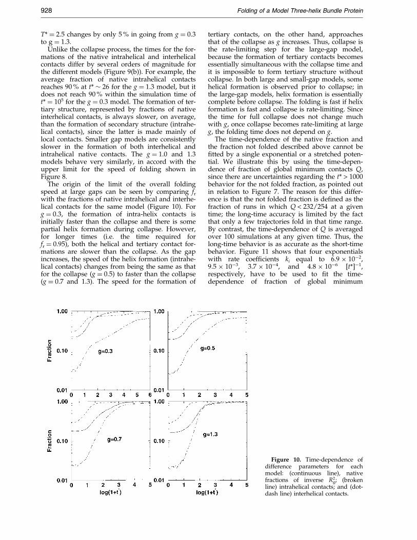
tertiary contacts, on the other hand, approachesthat of the collapse as g increases. Thus, collapse isthe rate-limiting step for the large-gap model,because the formation of tertiary contacts becomesessentially simultaneous with the collapse time andit is impossible to form tertiary structure withoutcollapse. In both large and small-gap models, somehelical formation is observed prior to collapse; inthe large-gap models, helix formation is essentiallycomplete before collapse. The folding is fast if helixformation is fast and collapse is rate-limiting. Sincethe time for full collapse does not change muchwith g, once collapse becomes rate-limiting at largeg, the folding time does not depend on g.

The time-dependence of the native fraction andthe fraction not folded described above cannot be®tted by a single exponential or a stretched poten-tial. We illustrate this by using the time-depen-dence of fraction of global minimum contacts Q,since there are uncertainties regarding the t* > 1000behavior for the not folded fraction, as pointed outin relation to Figure 7. The reason for this differ-ence is that the not folded fraction is de®ned as thefraction of runs in which Q < 232/254 at a giventime; the long-time accuracy is limited by the factthat only a few trajectories fold in that time range.By contrast, the time-dependence of Q is averagedover 100 simulations at any given time. Thus, thelong-time behavior is as accurate as the short-timebehavior. Figure 11 shows that four exponentialswith rate coef®cients ki equal to 6.9 � 10ÿ2,9.5 � 10ÿ3, 3.7 � 10ÿ4, and 4.8 � 10ÿ6 [t*]ÿ1,respectively, have to be used to ®t the time-dependence of fraction of global minimum

Figure 10. Time-dependence ofdifference parameters for eachmodel: (continuous line), nativefractions of inverse Rg

2; (brokenline) intrahelical contacts; and (dot-dash line) interhelical contacts.

Figure 11. Average fraction of global minimum con-tacts as a function of time for the g � 1.3 model. Resultsobtained from ®ts with one to four exponentials are alsoshown.


contacts; the amplitudes Ai of the various contri-butions are ÿ0.358, ÿ0.343, ÿ0.042, and ÿ0.022,respectively, with Q(t* �1) � 0.918. Here,Q(t*) � Q(t* �1) � �iAi exp(ÿkit*). The complex-ity of folding mechanism of the model three-helixbundle indicated by Figure 11 arises from kineticintermediates that cause deviation from simpleexponential folding behavior (see below).

Structural analysis and intermediates for theg�1.3 model

The distribution of the fraction of global mini-mum contacts, Q, as a function of reduced time isshown in Figure 12(a). The native state for theg � 1.3 model at T* � 0.24 is clearly indicated bythe population of Q values that oscillate aroundthe native value of 0.91 (Table 1) for times greaterthan log(1 � t*) � 2.3. In addition to the nativestate, there are two well-separated long-lastingpopulations with Q � 0.7 (the intermediate I1) and0.85 (the intermediate I2), respectively. Both inter-mediates have Q values within the range for theequilibrium molten globule state (Figure 6).

To further analyze the two intermediates, we cal-culate the normalized population distribution of frversus Q from all 100 trajectories by summing overall times 0 < t* < 105. This population is useful forpinpointing the locations of intermediates based ontwo progress variables, since any reasonably long-lasting kinetic intermediates will show signi®cantpopulations.

Figure 12(b) shows the population distributionin the Q versus fr plane. The highly populated

states are indicated by darker colors and enclosedby contour lines. The population at fr � 0.2 and0 < Q < 0.5 represents the coil state (the initialstate), while the native state (the ®nal state) islocated at Q � 0.91 and fr � 1. Intermediate I2 atQ � 0.85 has a narrow range of fr values near 0.95.Intermediate I1 at Q � 0.7, on the other hand, has awide range of fr values from 0.5 to 0.8. Thus I1 isan ensemble of relatively open structures that havea large variation in chain dimension, while inter-mediate I2 is almost as compact as the native state.In addition to the highly populated I1 and I2 states,there is a population at fr � 0.25 and 0.5 < Q < 0.6.This indicates a short-lived intermediate, which isevident also in Figure 12(a).

Figure 12(c) shows the cumulative time distri-bution function of the fraction of native intrahelicaland interhelical contacts. In addition to the initialcoil and ®nal native state, the two large populatedareas correspond to I1 and I2. Both have a highhelical content (>90 %) but they have a very differ-ent level for the fractions of native interhelical con-tacts (0.2-0.5 for I1 versus 0.8-0.9 for I2). Thus, bothI1 and I2 are molten globule-like, but I1 is relativelymore open and has fewer interhelical contacts.

The simple structure of the folded protein makespossible a more detailed description of the inter-mediates. Intermediate I1 is found to involve theincorrect position of one helix relative to the micro-domain formed by the other two helices, whichhave the approximately native relative orientationand interhelical contacts. Docking the third helixon to different sides of a two-helix domain yieldstwo topologically different species, as has been dis-cussed for synthetic three-helix bundles (Brysonet al., 1998). The native structure has a counter-clockwise arrangement of three helices whenviewed from the N-terminal end. Figure 13 showsthe accessible surface of the native helix II-III sub-domain. Only the native side provides a site fordocking the third helix. However, the third helixcan either point away from the other two, stick out(see Figures 14 and 15) or, to a lesser extent,loosely dock on the wrong side (as indicated bytwo peaks in the Q versus fr distribution of I1,Figure 12(b); see also Figure 16) due to incorrectdihedral angles in the turn region. Both the I-II andII-III microdomains are observed, with I-II slightlymore common, although the difference is not stat-istically signi®cant. This is consistent with the factthat the number of interhelical contacts betweenhelices II and III (35) is only slightly more thanthat between helices I and II (31). Since only twohelices are in a good contact, the fraction of nativeinterhelical contacts for I1 is about one-third(Figure 12(c)).

An example of I1 is shown in Figure 14(a). Thepseudo-dihedral angle a11 is in the trans (ÿ130 �)rather than the native cis (ÿ12 �) conformation. Thedihedral angle of a12 also is changed from thenative value of ÿ170 � to 150 �. The dihedral anglechanges lead to helix I pointing away from thehelix II-III microdomain. The contact map of this

Figure 12. (Legend opposite)


Figure 12. Folding kinetics of the large gap (g � 1.3) model. (a) Distribution of the fraction of global minimum con-acts, Q, as a function of log(1 � t*). (b) Contour plot of the cumulative time distribution of global minimum contactsQ) as a function of the inverse native Rg

2 fraction (fr). The native state is indicated by the dark area at Q � 0.9 and

r � 1. Intermediate I2 is located at Q � 0.85 and fr � 0.95, while intermediate I1 is at Q � 0.7 and 0.5 < fr < 0.8. Thenitial unfolding state is between 0.1 < Q < 0.4 at fr � 0.15. (c) Contour plot of the cumulative time distribution func-ion for the fraction of native intrahelical contacts versus the fraction of interhelical contacts. Four states (unfoldednitial state, I1, I2, and the native state) are evident as four highly populated (dark) regions (see the text).


t(fiti

Figure 13. The accessible surfacefor the native helix II-III subdo-main. The surface is constructedwith a radius of sc/2 for the probeand the native docking site is theconcave top region.

Figure 14. (a) A typical structureof the intermediate I1 for theg � 1.3 model (dark) as comparedwith the global-minimum structure(light). Helix I (the top isolatedhelix) is pointing away from themicrodomain formed by helices IIand III. (Drawn in cross-eyedstereo.) (b) Contact map for theintermediate in (a). All 254 possibleglobal minimum contacts areshown as open diamonds. Thosepresent in the intermediate areindicated by ®lled diamonds. Thenon-native contact in the intermedi-ate between residues 10 and 46 isindicated by the open triangle.Note the native contacts betweenthe C terminus and the turn regionthat stabilize the incorrect dihedralin the turn region and tilt helix Itoward the incorrect side (here theright side of the Figure) of the helixII-III subdomain.


structure is compared with that of global minimumstructure in Figure 14(b). Almost all of helices I, II,and III intrahelical contacts, as well as the helixII-III interhelical contacts, are well established.There are also four native interhelical contactsbetween residues 9 and 13 of helix I and residues45 and 46 of helix III. Two additional contacts existbetween turn residue 14 and residues 45 and 46 ofhelix III. The contacts between helix I and III stabil-ize the incorrect dihedral angle, while the contactsbetween residue 9 of helix I and the residues 45and 46 of helix III tilt the helix I toward the incor-

rect side (the right side in the Figure) of the two-helix sub-domain.

Figure 15 shows a different I1 type intermediate,where helix III points away from the helix I-IIdomain due to a positive a31 (72 �); the turn dihe-dral angle a31 is negative (ÿ160 �) in the nativestructure. As the contact map (Figure 15(b)) shows,all three helices and the contact between helix Iand II are well established. The tip of helix I (resi-dues 1 and 2) has four native contacts with helixIII (residues 33, 34, and 38). These four contactsstabilize the incorrect dihedral a31 that involves

Figure 15. (a) As in Figure 14(a)but for a structure with helix IIIpointing away from the helices I-IIdomain. (b) As in Figure 14(b) forthe intermediate shown in (a).


beads 31, 32, 33, and 34. The native contactsbetween bead 38 and beads 1 and 2 tilt the helix IIIin the wrong direction.

Intermediates that do not have one helix separ-ated from the other two also occur. For example,helix I can be loosely packed on the wrong side ofthe helix II, helix III microdomain (Figure 16), or,helix I can stack on the top of helix III (see the dis-cussion of Figure 20).

From this analysis, it is clear that the ``I1 inter-mediate'', with certain ranges of Q values and ofintra/interhelical contacts, as shown in Figure 12,actually involves signi®cantly different structures

of similar topology. Furthermore, the wide rangeof values for the radius of gyration of I1 (Figure 12)indicate that the third helix can be trapped indifferent orientations. It is clear that unless speci®ccontacts are monitored (helix II and helix III versushelix I and helix II, for example), the two types ofintermediates cannot be distinguished.

The intermediate I2, on the other hand, is native-like (Q � 0.85 versus Q � 0.9 for the native state,the fractions of native interhelical and intrahelicalcontacts are around 90 %). It differs from the nativestate in having one or two incorrect dihedralangles. An example is shown in Figure 17, where

Figure 16. As in Figure 13 butfor an example of intermediate I1 inwhich the helix I is loosely packedin the wrong side of the helice II-IIImicrodomain.


a16 < 0 instead of >0. The misfolded dihedrals canoccur anywhere. In fact, nearly all dihedrals wereobserved as ``misfolded'' during a certain fractionof the time in one or another of the kinetic simu-lations except for the two end dihedrals (a1 anda43). The latter are unlikely to be trapped in awrong con®guration, because the end beads areless restricted in their moves. Since only the eightdihedral angles with a < 0 in the native structurehave no dihedral potential, unfavorable dihedralangles arise when they are stabilized by nativecontacts. This is because of the g � 1.3 model, thenon-native contacts are destabilizing. Many I2

intermediates (about 50 %), have a structure withtwo neighbouring dihedral angles near �180 �.This corresponds to a ®ve-residue b-strand-likeextended stretch of the polypeptide chain. Such astructure could be a local minimum in a real pro-tein; in the present model, it is stabilized dynami-cally. Two neighbouring dihedrals share threebeads, so that when both angles are near 180 �, thevelocity changes due to ``bounce'' collisions in twodihedrals are opposite for the three commonbeads. This leads to a kinetic trap. It is not clear ifthis type of trap would also appear when a con-tinuous dihedral potential with a minimum at180 � is used (Figure 2). The intermediate I2 is thusa collection of states that have locally misfoldedregions at various locations. Due to the dynamictrapping, their relative lifetimes probably are long-er than they would be in real proteins.

It is of interest to know how the protein modelis trapped in and escapes from the intermediate

states. Since each individual trajectory is different,we analyze the example shown in Figure 14.Figure 18 plots the number of global minimumcontacts as a function of the reduced time alongwith the location of the ®rst passage time for theNgmc values. This is a relatively fast folding trajec-tory (i.e. folding is complete in 650 time units andwe show the range 0 to 800). An I1 type intermedi-ate is indicated by an average Ngmc value of about180 (Q � 0.7) that lasts about 500 reduced timeunits (from 70 to 600). The intermediate state has alarge ¯uctuation in Ngmc and a signi®cant numberof native contacts have to be broken for the inter-mediate to become more native-like. For example,more than ten native contacts have to be broken inorder to increase Ngmc by 1 from time points a to c,c to e and e to g in Figure 18. From f to g, thereappears to be a near down-hill motion to reach thenative state (Figure 18). The structure at time-pointa is shown in Figure 14. it is consistent with theresults for the native fractions of interhelical andintrahelical contacts (Figure 19) that indicate thatthree helices are well established. The helix II-IIImicrodomain is essentially formed in a near-nativestructure (though there are signi®cant deviations,see below), while there are only minimal contactsbetween helix I and helix II or III.

The structures of the protein at the times corre-sponding to a (blue), d (red), e (yellow), and g (vio-let) in Figure 18 are shown in Figure 20. Atposition a, helix I is nearly parallel with the subdo-main of helices II-III. The helix I tends to move tothe incorrect side of helix II-III subdomain due to

Figure 17. As in Figure 13(a) butfor intermediate I2. The misfoldedregion, which is in the lower leftcorner, is in an ``imaged'' con®gur-ation relative to the native struc-ture.

Figure 18. The number of globalminimum contacts, Ngmc, as a func-tion of time from the run corre-sponding to the intermediateshown in Figure 14. The open circleindicates the location of the ®rst-passage time for every value ofNgmc and the open diamond showsthe location of the minimum value,Ngmc, sampled between two pas-sage times. The continuous linethat connects the circles and dia-monds indicates the path alongwhich the number of global mini-mum contacts is increased. Theinset shows ®ner details for theintermediate. Five time-points (a tog) are labeled. After f, the systemfollows a primarily downhillmotion to the native state.


favorable contacts between helix III and the turnregion between helices I and II (Figure 14(b)).However, such an incorrectly folded structure isnot possible, as is evident from Figure 13. Further-

more, with helix I pointing away from the II-IIImicrodomain, the latter already has the tightlypacked, essentially native structure and theC-terminal end is displaced slightly upward (com-

Figure 19. The native fraction ofintrahelical and interhelical contactsas a function of reduced timeduring the existence of intermedi-ate I1, shown in Figure 18; the sym-bols a to g correspond to those inthat Figure (inset). Note that thesame scale for the y axis is used forthe top and middle panel, but thescale for the bottom panel is differ-ent. In the top panel, the results forhelices I, II, and III are shown bycontinuous, dotted, and brokenlines, respectively.

Figure 20. Five structures thatshow the escape from an I1-typekinetic trap. The blue structure(position a in Figures 18 and 19)occurs at t* � 131.18, the red (d) att* � 314.77, the yellow (e) att* � 488.96, the violet (g) att* � 595.33.)


pare the red structure with the violet one inFigure 20). This structural shift prevents normalfolding and traps the intermediate. As a result,in the period encompassed by time-points ato c, the structure ¯uctuates around the positionshown in (a). The downward movement of the C-terminal beads (see Figure 20) leads to a moreopen helix II-III microdomain (with a smallernative fraction) near point d (see Figure 19). Thisallows helix I to tilt (see the red structure d inFigure 20) and a further downward movement ofthe C terminus leads to an even looser helix II-IIImicrodomain at t* � 400 and the formation of anear-¯at surface consisting of beads 42-46. The lat-ter permits a reorientation of helix I (the yellowstructure e in Figure 20). The helix II-III micro-domain then opens to its native form at point f(Figure 19), which leads to a rapid docking of helixI on the helix II-III microdomain. In short, the pro-tein was trapped due to the incorrect position ofthe C-terminal beads of helix III and the overlytight packing of the helix II-III microdomain. Theprotein escapes from the intermediate when themicrodomain opens up, presumably, as a result ofa thermal ¯uctuation.

To verify that the intermediate I1 is trapped onthe potential surface, rather than being a kinetic``accident'' (e.g. helix I is moving in the wrongdirection), 400 additional simulations were madestarting with structure a (Figures 20 and 14) butwith different initial velocities generated from theMaxwell-Boltzmann distribution at T* � 0.24. All400 simulations (run for only 200 reduced timeunits) remains trapped in I1, although some areshorter-lived than the others. The shortest trappingtime is around 70 reduced time units. Furthermore,a direct quench simulation, where only down hillmotions are allowed, indicates that the structure ofthe I1 intermediate is stable for a duration of 106

time units. Thus, I1 is indeed in an energy mini-mum. However, such energy minima are notobserved if the average energy is shown either inthe Q versus fr plane (Figure 21) or in the plane ofinterhelical versus intrahelical contacts (not shown).This suggests that care is required in interpretingexperimental studies of intermediates. Clearly,measurements of progress variables that give infor-mation on the intermediates and their structuresare required. It may be necessary to focus on vari-ables such as the speci®c contacts that exist only inkinetic intermediates. Real-time nuclear resonanceappears to be a possible approach (van Nulandet al., 1998).

Not all 100 trajectories for the g � 1.3 model foldvia kinetic intermediates. In fact, only 69 out of the100 simulations are trapped in one or two kineticintermediates, in that the progress variable Q oscil-lates around a nn-native value for a signi®cantperiod of time. (An operational de®nition of�logt* > 0.15 is used, since the con®gurations weresaved on a logarithmic scale; see Algorithms.) Sev-eral runs are shown in Figure 22. Run 38 inFigure 22(a) has an I2-type intermediate, since Qoscillates around 0.85. (Note that the initial plateauat Q � 0.2 is not an intermediate but correspondsto the initial coil state before the cooling takeseffect). The I1-type intermediate appears in runs 9and 100 (Figure 22(b)). Two intermediates of theI1 type appear in run 9 with somewhat different Qvalues; both can be classi®ed as I1 type, based onQ. This corresponds to the fact that I1 is a collectionof states, as illustrated in the several adjacentpeaks (caused by different orientations of the mis-placed helix) in the cumulative time distributionfunction for intermediate I1 shown in Figure 12.The longest life-times for intermediates I1 and I2

are found to exceed the total simulation time of 106

reduced time units for a few runs.

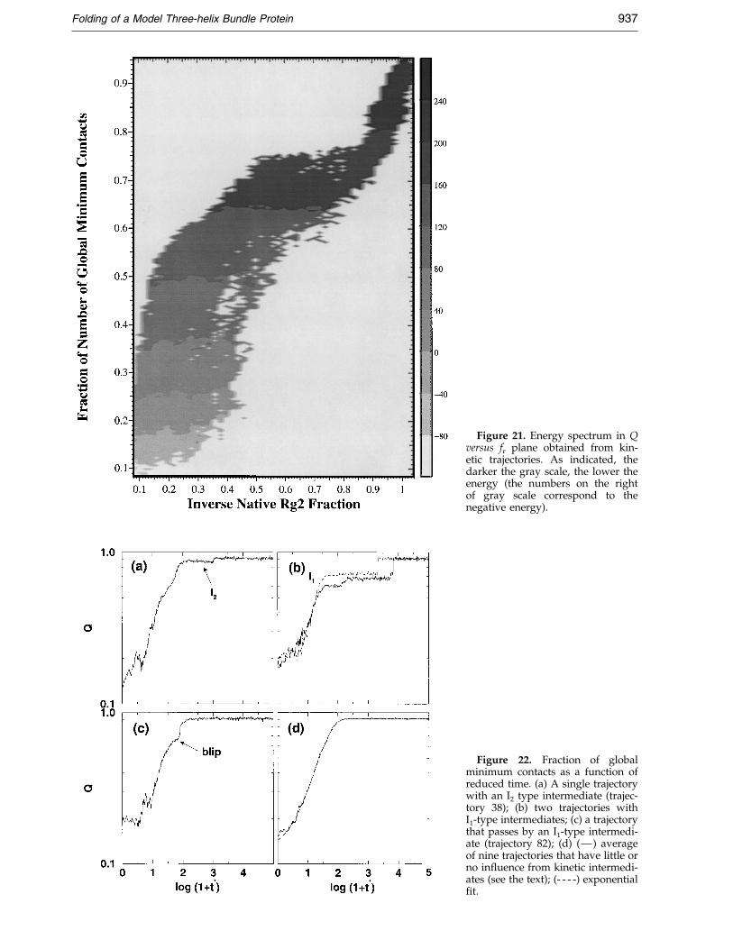
Figure 21. Energy spectrum in Qversus fr plane obtained from kin-etic trajectories. As indicated, thedarker the gray scale, the lower theenergy (the numbers on the rightof gray scale correspond to thenegative energy).

Figure 22. Fraction of globalminimum contacts as a function ofreduced time. (a) A single trajectorywith an I2 type intermediate (trajec-tory 38); (b) two trajectories withI1-type intermediates; (c) a trajectorythat passes by an I1-type intermedi-ate (trajectory 82); (d) (Ð) averageof nine trajectories that have little orno in¯uence from kinetic intermedi-ates (see the text); (- - - -) exponential®t.


Figure 23. Folding kinetics scheme for the large-gap(g � 1.3) model (see the text).


Many of the 31 `ìntermediate-free'' folding tra-jectories show a sudden change in slope of the Qversus log(1 � t*) plot. Figure 22(c) shows one suchexample, in which the trajectory visited intermedi-ates but manages to escape very quickly. Ninetrajectories show no in¯uence from kinetic inter-mediates. Their average Q value can be ®tted verywell by a single exponential (Figure 22(d)) andthey fold very fast; the average folding time is onlyabout 170 reduced time units. Thus, nearly 10 %trajectories for the g � 1.3 model can be character-ized as folded via a two-state ``fast-track'' pathway.

The stepwise increments in Q due to intermedi-ates observed in individual simulations (Figure 22)are replaced by a smooth curve on averaging overall trajectories, as shown in Figure 12. Thus, theexistence of kinetic intermediates is manifested inthe non-exponential behavior of the fraction of glo-bal minimum contacts Q (see Figure 11); i.e. thenon-exponential behavior is a direct, though notobvious, consequence of the presence of intermedi-ates. The same number of exponentials arerequired to ®t the time-dependence of Rg

2, theenergy, the helical and the non-local contacts.Some of the trajectories are still not folded evenafter longer simulations that extend for 106 timeunites. These slowly folding trajectories (with inter-mediates) are at least four orders of magnitudelonger than the fast-track two-state pathway.

The folding kinetics of the g � 1.3 model aresummarized in Figure 23. Out of the 100 trajec-tories, 87 fold during the simulations of 105 timeunits. The system can fold directly to native statevia a fast-track two-state pathway (nine out of 87).It may also be trapped in I1 (52 out of 87) or I2

(nine out of 87) or both (17 out of 87) before reach-ing the native state. Thus, most chains fold via I1.Since a ``direct'' fast-track pathway is available,both I1 and I2 correspond to ``non-obligatory''intermediates. However, six out of the ninefast-track trajectories involve docking of eitherhelix I or helix III onto the microdomain formed bythe two other helices. Thus, they pass throughstructures corresponding to I1, although I1 is veryshort-lived because the third helix is not trapped ina local minimum. There is also a fast pathway (twoout of nine) that corresponds to the three helicescoming together at the same time. In all of the fast-folding trajectories, most of the secondary structureis formed ®rst and the ¯uctuating helices diffuse to®nd the native structure, in accord with the diffu-sion-collision model (Karplus & Weaver, 1994).One out of the nine involves the concurrentformation of secondary and tertiary structure.

Structural analysis (g � 0.3)

For the less optimized model with g � 0.3, thefolding kinetics are very different. The time-depen-dent distribution of the fraction of global minimumcontacts is shown in Figure 24(a). Only 29 out of100 simulations reach the native state during thesimulations of 106 reduced units. Almost all trajec-

tories are trapped at Q � 0.5 (corresponding tointermediate I01, as described below) for at least1000 reduced time units and the shortest foldingtime is 1928 reduced time units. After that, themajority are trapped at Q � 0.65 and Q � 0.8 untilthe end of the trajectory. For g � 0.3 the equili-brium disorder-to-order transition occurs atQ � 0.5 (Figure 6) and initial trapping at Q � 0.5arises from the existence of a kinetic, barrierbetween the ``disordered'' and `òrdered'' globules;that is, the transition involving a search for theordered, partly helical state is a slow step. The bar-rier is kinetic because there is no thermodynamicfree-energy barrier between the two states(Figure 5). Such a kinetic barrier does not exist atlarge g because there is no ``disordered'' collapsestate. Instead, both free-energy and kinetic barriersare present in the collapse to the ordered globule.

In the distribution of Q versus native Rg2 fraction

fr (Figure 24(b)), there are two well-de®ned peaks,other than the native peak. The largest peak,I10, corresponds to Q � 0.4-0.5 and fr�1. It is an

`òbligatory'' intermediate for the g � 0.3 modelsince it appears in all 100 kinetic simulations. I1

0has a wide distribution in Q but a narrow distri-bution for Rg

2 that is near 1n native like. This is

exactly the inverse of the properties of I1 found inthe g � 1.3 model (Figure 12).

The diversity in Q for I10 suggests that a wide

range of structures is involved. This is supportedby the cumulative time distribution function forthe fraction of native intrahelical versus interhelicalcontacts (Figure 24(c)). I1

0 can have a fraction ofintrahelical contacts ranging from as low as 0.6 to0.95, while interhelical contacts are in the range of0.15 to 0.4. The wide range of values for the intra-helical fractions suggest that the new intermediateinvolves both disordered and ordered collapsedstates. In fact, there is a separate population peakwithin I1

0 with high helical contents. This is inaccord with the fact that both disordered andordered globules exist and there is a free-energybarrier separating the native state from the orderedglobule state for the small gap model, as discussedabove.

Figure 24. Folding kinetics of the small-gap (g � 0.3) model. For an explanation, see Figure 12.



To illustrate the nature of I10, two folding trajec-

tories are shown in Figures 25 and 26. Run 15 hasseveral stepwise increments in Q during the fold-ing trajectory (Figure 25(a)). This suggests thatthere are several traps although all of them corre-spond to I1

0 as de®ned here, based on the range ofQ values (see Figure 24). The results for intrahelicaland interhelical contacts, as well as several struc-tural snapshots (Figure 25(b)), show that there isearly helix formation without any interactionsbetween the helices. This is followed by formationof the helix II, III microdomain and ®nally, byhelix I docking on that microdomain. As can beseen by comparing Figures 25(a) and (b), the inter-mediate at Q � 0.5 has nearly all the intrahelicalcontacts but no interhelical contacts. Thus, the fold-ing mechanism is similar to that for the large gapmodel in Figure 20. In both the small (Figure 25)and large (Figure 20) gap models, the two runshave short-lived intermediates corresponding tothe ordered globule phase.

Run 67, which represents the dominant behaviorof the small gap model, is very different, as is evi-dent from Figure 26. It involves a gradual incre-ment of Q values before there occurs a suddentransition to the native state (Figure 26(a)). Thefolding proceeds with a nearly concurrent for-mation of secondary and tertiary structures(Figure 26(b)) and I1

0 is a disordered globule-likeintermediate. Figure 27 shows the native intraheli-cal and interhelical contacts as function of time.The intrahelical contacts contain regions where thenative contacts tend to remain ®xed after for-mation; examples are the contacts among residues15 through 20 (shown as 1-6, 8, 9, 12 in Figure 27for helix II; see caption). They also involve nativecontacts that form and are broken before ®nalreformation; examples are contacts between resi-dues 18 and 21 and between 26 and 29 (shown as13 and 49 in Figure 27 for helix II). Correspondingbehavior is found for the interhelical contacts; forexample, the contact between residues 5 and 42(shown as 20 in Figure 27 for interhelical contactsbetween I and III) is ®xed after formation while thecontact between 4 and 39 (shown as 12 in Figure 27for interhelical contacts between I and III) isformed, broken and reformed. Thus, Run 67 corre-sponds to a collapse followed by a restricted searchwithin the compact set of states. It can be referredto as ``on-site'' correction of misfolded regions(Kolinski et al., 1998) since mainly local motionsoccur for such a compact system (Figure 26).

It is likely that entropy plays a more importantrole in the folding of a small-gap model than alarge-gap model. Because the non-native contactsare only slightly less favorable than the native con-tacts in the small-gap model, there exist manystructurally different compact states that are localminima with similar energies. These include boththe disorganized and organized globules, whichlead to the great diversity in the structures of theI01 type intermediates. For example, increasing Q by

one from time points a to b, b to c, and c to d

(Figure 26(a)), requires breaking more than 13native contacts between each step. That the varioustrajectories are very different (i.e. they involvedifferent orders of forming native contacts) leadsto a broad ensemble of states and a large effectiveentropy of the folding reaction for the small-gapmodel.

A I21n type intermediate (0.75 < Q < 0.85) also

exists as shown in Figure 24. It occupies a similarlocation in the plane of the fraction of native intra-helical contacts versus that of the native interhelicalcontacts as the I2 intermediate in the g � 1.3 model(Figure 12). The I2 intermediates for both theg � 0.3 and g � 1.3 models are due to locally mis-folded regions.

The folding kinetic scheme of the small gap(g � 0.3) models is shown in Figure 28. From therandom coil state, the system passes through oneof the many obligatory intermediate I1

0 structures.The latter can then fold directly to the native stateor do so via the non-obligatory intermediate I2.Although each intermediate state includes a broadrange of structures, it appears as a single kinetic``state'' when it is described by an (overly) reducedset of progress variables, such as the various nativefractions and radius of gyration. This makes clearthe necessity of using many different probes tocharacterize experimental kinetic and/or equili-brium intermediates (Dobson et al., 1998).

Analysis of the transition from the model withg � 1.3 to the model with g � 0.3

Between two extremes (g � 1.3 and g � 0.3),there is a smooth transition from one type ofkinetic behavior to the other. The essential differ-ence is that at high g all trajectories pass throughorganized globules, while at low g there are twotypes of populations: One set folds in a mannercorresponding to the large gap case and the othermakes a search through the disorganized globulestate. A comparison of the cumulative time distri-bution function of Q versus fr for the differentmodels is made in Figure 29. Intermediate I2 ispresent in all models. As to I1, there exists twopopulations in the g � 1.3 model, re¯ecting thedifferent orientations of the misplaced third helix(Figure 12(a)); for example, one is in a looselypacked form but with one helix loosely docked onthe incorrect side (Figure 16), while the other has amore open structure as shown in Figures 14(a) and15(a). The two adjacent peaks at Q � 0.7 moveapart for the g � 1.0 and g � 0.7 models. The areaof the peak with a low fr (high Rg

2) value shrinksfrom g � 1.3 to g � 0.7 and vanishes in the range ofg � 0.3 to g � 0.5. In contrast, the peak with a highfr value moves to even larger fr and wider Q valuesas the gap decreases. It becomes I1

0 for the g � 0.3and 0.5 models.

Figure 25. Folding kinetics for a small-gap (g � 0.3) trajectory with early helix formation (trajectory 15). (a) Fractionof native contacts and native fractions of intrahelical and interhelical contacts as a function of reduced time.(b) Sample structures at t* � 0, 102, 103, 104, and 105.


Figure 26. Folding kinetics for a small-gap (g � 0.3) trajectory with simultaneous collapse and partial helix for-mation (trajectory 67). (a) Same as in Figure 25; (b) sample structures at t* � 0, 102, 103.5, and 105.


Discussion

A detailed study of the folding thermodynamicsand kinetics of an off-lattice model for a 46 residuethree-helix bundle protein is reported. The modelis the same as that used earlier for investigation ofthe folding thermodynamics, except that a Ca dihe-dral-angle potential is introduced to penalize left-handed helices, in accord with the observed struc-tures of proteins. Simulations have been made fora range of values of the energy bias parameter, g,

which determine the difference between native andnon-native contacts. The use of discontinuous mol-ecular dynamics permits us to do multiple simu-lations (600 folding trajectories) of up to 106

reduced time units (�1 ms). Each one takes about17 hours on a Linux Alpha workstation. For com-parison, it would take approximately 32.5 years(3 � 105 hours) on the same machine to do a single1 ms all-atom simulation for a 36 residue protein inexplicit solvent with the approach of Duan &Kollman (1998).

Figure 27. Individual intrahelicaland interhelical native contacts as afunction of log(1 � t*) for trajectory67. The native contact pairs arearranged in a numerical sequentialorder based on their indices. Forexample, there are 31 contactsbetween helices I and II. They arebetween pairs (1,27), (1,30), (2,27). . . which appear as 1, 2, 3, . . . inthe Figure.


Folding thermodynamics

The present results on the thermodynamics offolding are very similar to those obtained in theearlier work (Zhou & Karplus, 1997), although thetransition to the ordered globule state becomesstronger in the re®ned model. There is a collapsetransition, a disordered to a ordered globule tran-sition, a globule to native state transition and thetransition from the active native state to a frozeninactive state. As has been noted (Zhou & Karplus,1997), if one scales the thermal-denaturation tem-perature (T* � 0.3) of the large-gap model proteinto 350 K, the transition to solid state (Figure 6) is atabout 230 K, in satisfactory agreement with theexperiment ``glass'' transition temperature (Zhouet al., 1999; Tilton et al., 1992; Ferrand et al., 1993).The collapse transition, however, would occur atabove 1000 K. This is likely due to the absence oftemperature-dependent protein-solvent interactionsin the model but is not inconsistent with the factthat protein thermal denaturation in the accessibletemperature range (up to 373 K) produces onlycollapsed conformations that can be furtherdenatured by strong denaturants (Ptitsyn, 1995).

Use of the Lindemann criterion (Lindemann,1910) makes it possible to distinguish the foldingtransition from the transition into the ordered

Figure 28. Folding kinetic scheme for the small-gap(g � 0.3) model (see the text).

(molten) globule state, although both transitionsyield the three-helix bundle-like motifs and bothcan be ®rst-order-like two-state transitions. Thefolding transition occurs at a fraction of globalminimum contacts, Q, of about 0.87, while thetransition into an ordered (molten) globule occursat Q � 0.5. Both the Q � 0.5 and Q � 0.87transitions have been observed in lattice (SÏali et al.,1994a,b; Socci & Onuchic, 1995; Onuchic et al.,1995; Abkevich et al., 1996; Dinner et al., 1996;Kolinski et al., 1996; Plotkin et al., 1997; Pande &Rokhsar, 1998; Hao & Scheraga, 1998) and off-lattice models (Guo & Thirumalai, 1996; Guo &Brooks, 1997; Nelson et al., 1997; Berriz et al., 1997;Nymeyer et al., 1998; Pande & Rokhsar, 1998).However, most previous analyses of the origin ofthe cooperativity of the folding transition (Chanet al., 1995; Kolinski et al., 1996; Berriz et al., 1997;Hao & Scheragi, 1998) appear to be more appropri-ate for the transition to the ordered (molten)globule state. Pande & Rokhsar (1998) used asomewhat different model to represent the samethree-helix bundle protein as that studied by Zhou& Karplus (1997) and reached similar conclusionsconcerning the thermodynamic phase diagram.However, it should be noted that the foldingtransition of their model is a weak continuous tran-sition, in contrast to the present study, in whichboth the folding transition and the transition to themolten globule state can be ®rst-order two-statetransition.

Folding kinetics

Time-scale and folding rate

The collapse process takes 103 reduced timeunits to complete (on average), regardless of thebias gap; the collapse is said to be complete when

Figure 29. Contour plot of the cumulative distribution function of global minimum contacts (Q) versus the inverseradius of gyration fraction for models with g � 1.0, g � 0.7, 0.5 and 0.3 from left to right. The population density forgiven values of the two variables increases with the darkness of the gray-scale.



the inverse of the radius of gyration is more than90 % of the native value. For individual trajectories,the collapse time varies between 102 and 3 � 103

time units for the g � 0.3 model. For the g � 1.3model, full collapse for a few trajectories is notachieved after 106 time units, due to the existenceof uncollapsed intermediates. Since the threehelices are well established before collapse formost trajectories in the large-gap model, the col-lapse process is in fact a reorganization (diffusion-collision-like) of the three helices to form the nativeconformation for the fast track (that without inter-mediates), as well as for some slow tracks with theuncollapsed intermediates I1.

That collapse can be slow and appear as a rate-limiting process has been suggested for the foldingof cytochrome c (Sosnick et al., 1996), where thecollapse apparently can take as long as severalmilliseconds. This was explained in term of theexistence of uncollapsed intermediates, in agree-ment with our results. However, it should benoted that the exact nature of the various processesthat contribute to cytochrome c folding is not fullyresolved (Shastry et al., 1998).

To translate the simulation time-scale into aphysical time-scale, it is useful to compare the pre-sent simulations with the experimental studies ofthe collapse transition. The time-scale for thecollapse of cold-denatured apomyoglobin has beenfound to be about 5 ms (Ballew et al., 1996). Themicrosecond collapse time-scale is consistent withother estimates (Hagen et al., 1996; MunÄoz et al.,1997); it is somewhat slower than the extrapolatedfolding time (10ÿ8 seconds) for the Arc repressordimer (Robinson & Sauer, 1996). The time-scale ismuch longer than the present sub-nanosecondtime-scale, presumably as a result of the simpli®edbead model for the chain and the absence of expli-cit solvent. This suggests that a physically mean-ingful conversion factor for the present simulationsis that a reduced simulation time unit t* is about 1ns; corresponding time-scales have been used forthe elementary step in lattice Monte Carlo simu-lation (Dobson et al., 1998). Given this time-scale,the overall folding rate for the large-gap model isof the order of milliseconds and that for the small-gap model is in the range of milliseconds toseconds. If the results obtained here, that the rateof collapse is essentially independent of ``optimiz-ation'', are general, it would be possible to extractinformation regarding the energy bias gap by com-paring the rate of folding with the rate of collapsefor a set of mutants of the same protein or for aseries of proteins that have essentially the samestructures but different sequences.

The rate of folding for the present modelincreases with the size of the bias gap for0.3 < g < 0.7 but is only weakly correlated for largergaps. The weak dependence on the bias gap forhighly optimized models indicates that otherfactors become more important. In the presentcase, the collapse transition, which is insensitive to

the bias gap, becomes dominant in determining thefolding rate for large bias gaps.

Pathways in folding

Based on reasonable progress variables, such asthe chain dimension, the amount of secondarystructure and the amount of tertiary structure, thefolding reaction of large or small-gap models canbe characterized as involving a small number ofpathways (Figures 23 and 28). When analyzed indetail, however, each pathway corresponds to abroad statistical ensemble of trajectories that can bevery different from each other. Even the nine tra-jectories that constitute the fast two-state pathwayfor the large-gap model fold differently; six out ofthe nine fast-track trajectories involve docking ofeither helix I or helix III onto the microdomainformed by the two other helices, two out of thenine correspond to the three helices comingtogether at the same time and one involves theconcurrent formation of secondary and tertiarystructure. Moreover, kinetic intermediates that arecharacterized as a ``single'' state based on a certainprogress variables can have very different struc-tures; for example, I2 consists of locally misfoldedregions that occur at different locations. Thus, thenumber of observed ``pathways'' and the nature ofthe intermediates depends on the progress vari-ables used to de®ne them. Each ensemble of path-ways can appear to be narrowly or widelydistributed depending on the choice of order par-ameters. As the spatial and time-resolution ofexperiments improves and they are better able todistinguish the members of an ensemble, the greatheterogeneity of the folding process will becomemore evident (Dobson et al., 1998). An ability tomeasure the distribution of conformations ratherthan only their average would signi®cantlyimprove our understanding of the folding ensem-bles. The dif®culties and complexities of a detaileddescription of folding based on experiments isillustrated by the present interpretations of theresults from widely different techniques used tostudy cytochrome c (Shastry et al., 1998; Yeh et al.,1998; Englander et al., 1998). Thus, care in theinterpretation of experiments is required to over-come what is a version of the ``blindmen andelephant'' problem.

Folding mechanisms

Several mechanisms have been proposed for thekinetics of protein folding. The ``diffusion-collision'' model (Karplus & Weaver, 1979, 1994)or the ``framework'' mechanism (Kim & Baldwin,1990) assumes that local secondary structureelements, which are partly formed at an earlystage, diffuse until they collide and form thecorrect tertiary structure. The classical ``nucleation''theory (Wetlaufer, 1990) and its recent elaborationas the nucleation-condensation model (Fersht,1997), assume that the native structure grows from


a nucleus that involves interactions among a smallset of residues. The ``hydrophobic-collapse'' theory(Dill et al., 1995) postulates that folding starts withrapid collapse and is followed by slow rearrange-ment to the native structure in the collapsed state.

The results of the kinetic analysis of the three-helix bundle and their variation with the bias gapparameter suggest that a range of phenomenologi-cal models and/or a combination of them may berequired to describe protein folding (see alsoDobson et al., 1998). For the large-gap (g � 1.3)model, the folding time is close to the collapsetime, and the secondary structure is well estab-lished before the collapse occurs. Thus, the foldingis well described as the assembly of the parts(microdomains) made up of secondary structuralelements. This is in accord with the diffusion-collision model (Karplus & Weaver, 1979, 1994)and with the analysis of experiments on apomyo-globin (Pappu & Weaver, 1998) and the l repressor(Burton et al., 1998). Diffusion-collision type foldinghas been found (Kolinski et al., 1998) for the three-helix bundle protein with a Monte Carlo latticemodel that has a potential energy function basedon protein statistics and includes side-chain inter-actions and hydrogen bonding. In the small-gapregion (g � 0.3), a small number of trajectories foldby the large-gap diffusion-collision mechanism.However, most of them involve the simultaneouscollapse and partial secondary structure formation,followed by reorganization to the native structurefrom the collapsed state. Thus, the small-gap sys-tem may be characterized as a combination of thehydrophobic-collapse and diffusion collisionmodels.

The calculated folding process for the three-helixbundle does not correspond to a nucleation mech-anism for any of the gap parameters. There existsno well-de®ned nucleus and each trajectory followsa somewhat different pathway and goes throughtraps involving different intermediates. Even forfast-track two-state folding without intermediates,there is no well-de®ned nucleation core (seeabove). In fact, early formation of certain nativecontacts can lead to the formation of trapped(off-pathway) intermediates that slow the folding.

The range of folding behavior found in the pre-sent simulations may represent that for helical pro-teins such as cytochrome c (Shastry et al., 1998; Yehet al., 1998; Englander et al., 1998), apomyoglobin(Gruebele et al., 1998; Dyer et al., 1998; Pappu &Weaver, 1998), and the l repressor (Burton et al.,1998). Different folding mechanisms may wellapply to proteins with other types of structures.Changes in topology from all a, a/b, to all b inhigh-coordination lattice models led to a changefrom diffusion-collision to ``on-site zipping'' mech-anisms (Kolinski et al., 1998). Using average contactenergy as a parameter, the folding mechanism oflattice proteins has been changed from speci®c col-lapse to non-speci®c collapse (Gutin et al., 1995;Socci et al., 1998). Experimentally, both collapseprior to helix formation (barstar folding) (Agashe

et al., 1995) and signi®cant helix formation prior tocompaction (RNase A folding) (NoÈppert et al.,1998) have been suggested. In the latter protein, akinetic intermediate with high secondary contentsis found to be relatively open (NoÈppert et al., 1998),similar to the I1 intermediate for the large-gapmodel. Nucleation condensation is found in a,bproteins such as CI2 (Fersht, 1997) and has beensuggested for other small fast-folding proteins.This mechanism has been found in lattice simu-lations as the folding mechanism for medium-sized(36 to 48 residues) and larger (125 residue) models(Abkevich et al., 1994; Dinner et al., 1996) as well asin off-lattice simulations (Guo & Thirumalai, 1995,1997).

Characteristics of intermediates

In the present model, the off-pathway intermedi-ate is structurally relatively well de®ned while theon-pathway intermediate is more diverse. The on-pathway intermediate exists only in weakly opti-mized models. How general these results are andwhether they apply to proteins remains to be seen.

The kinetic intermediates are related to the equi-librium intermediates. For example, only modelsthat have the disordered globule state can havekinetic intermediates with a ``disordered'' compactstructure. (It is not completely disordered but hassome secondary structural contents.) For the highlyoptimized g � 1.3 model, there exist only kineticintermediates with well-de®ned helical structures,which correspond well with the equilibriumordered globule state. This suggests that kineticintermediates are related to the equilibrium inter-mediate state but have more non-native inter-actions. Thus, the analysis of equilibriumintermediates, a common practice in experimentalfolding studies (e.g. see Kuciel et al., 1997; Blumet al., 1998; Fink et al., 1998) clearly can provideinformation on kinetic intermediates, but import-ant differences between kinetic and equilibriumintermediates do exist.

The misfolded dihedrals as shown in intermedi-ates I1 and I2 highlight the importance of chiralityin protein folding. One of the key features in thestructures of both intermediates can be describedas containing misfolded segments that are imagedconformations of their corresponding native struc-tures such as cis versus trans and left-handed versusright-handed. Experimentally, many slow path-ways are caused by the cis-trans isomerization ofproline residues, which can be described as changeof backbone chiral symmetry (Nall, 1994). It is alsoproposed that the slow pathway for lysozyme isdue to the switch between left-handed and right-handed conformers of disul®de bonds (Chaffotteet al., 1992; Roder & EloÈve, 1994). Kinetic inter-mediates of cytochrome c, on the other hand, origi-nated from non-native histidine ligands to heme(Sosnick et al., 1994; EloÈve et al., 1994). In addition,common occurrence of the termination of right-handed helices with residues in left-handed helical


conformations (Nagarajara et al., 1993) alsosuggests possible intermediates involving mis-folded turns and loop regions. Thus, what hasbeen observed in our model may re¯ect a generalcharacteristics of kinetic intermediates. It is inter-esting that a recent microsecond folding simulationof an all-atom model of villin in explicit solvents(Duan & Kollman, 1998) reveals an intermediatewith many misfolded pseudo-dihedral angles inboth the helical and non-helical regions (notshown).

Earlier theoretical studies of the three-helix bun-dle protein, a high coordination lattice model(Kolinski et al., 1998), an off-lattice model withspeci®c hydrogen bonds (Pande & Rokhsar, 1998)and all-atom model (Boczko & Brooks, 1995) of thethree-helix bundle protein all suggested a twohelix subdomain as a possible intermediate. In par-ticular, Kolinski et al. (1998) found helix formationprior to collapse, which is similar to our large-gapmodel. In addition, both helices I-II and helices II-III microdomains were observed during folding.Experimental evidence suggested a helical hairpinkinetic intermediate (two helix microdomain, par-ticularly helices II-III) (Bottomley et al., 1994),although the intermediates was not found in amore recent experiment beyond 6 ms of apparatusdead-time (Bai et al., 1997).

Kinetic intermediates are thought to play a rolein the formation of amyloid and other proteinaggregates (Fink, 1995). In particular, it has beensuggested by Eisenberg and co-workers(Schlunegger et al., 1997) that domain swappingmay be involved in aggregate formation. The kin-etic intermediate I1 (g � 1.3) with one helix separ-ated from the subdomain of the other two helices,appears to be a good candidate for the formationof a domain-swapped dimer (Schlunegger et al.,1997; Liu et al., 1998). Experiments showing thatthe three-helix bundle fragment forms such adimer would provide indirect evidence for theexistence of the domain swapped kinetic inter-mediate I1.

Folding without dihedral potentials

We have obtained folding kinetics for proteinswithout dihedral potentials (unpublished results).The overall folding characteristics, such as numberof pathways, are the same. The key difference isthat both I1 and I2 may now contain two or morehelix segments (even an entire helix) in a left-handed symmetry. Such a model folds more thanan order of magnitude slower. This might be ofinterest for the folding of sequences with mixedL and D amino acids produced by proteinengineering.

Concluding remarks

There is considerable discussion in the literatureregarding the ``old'' and ``new'' views of proteinfolding (Baldwin, 1995; Wolynes et al., 1996; Dill &Chan, 1997; Karplus, 1997; Pande et al., 1998). Theold view assumes that a small number of well-de®ned folding pathways exist and that folding isa hierarchical assembly process; e.g. the randomcoil ®rst forms secondary structure, which is thenorganized into the native tertiary structure. In thenew view, structurally less well de®ned ensemblesprogress to the native state along multiple path-ways. The present results suggest that the speci®cbehavior for small a-helical proteins depends onthe optimization of the system. For a highlyoptimized model (g � 1.3), the old view provides asatisfactory description. Folding proceeds througha small number of structurally well-de®nedpathways that begin with helix formation; this isfollowed by the formation of two-helix microdo-mains and docking of the third helix on two-helixmicrodomains to form the native structure. Struc-tural optimization apparently leads to the intro-duction of non-obligatory intermediates due tomisfolded dihedrals that can result in signi®cantslowing of the folding process. Less optimizedmodels (g � 0.3) have a collapse to a disordered-globule-like intermediate and do not have a well-de®ned folding pattern. There are many differentways for the collapsed globule to reach the nativestate, in accord with the new view of protein fold-ing. It thus appears that even for small a-helicalproteins a wide range of mechanisms that encom-pass both the old and new views is possible.Experiments are crucial for determining the bestdescription of the folding mechanism for speci®chelical proteins.

Acknowledgements

We are indebted to Professor K.-H. MuÈ ller for sendingus a copy of his program MEXFIT, which is speciallydesigned for multiple exponential ®t (Eur. J. Biophys. 19,231 (1991)) and to Dr Y. Duan and Professor P. A. Koll-man for sending us the PDB ®les for the intermediatesobserved in their simulations (Duan & Kollman, 1998).This work was supported, in part, by a grant fromthe NSF and a grant from Pittsburgh SupercomputingCenter and from UC Berkeley Network of Workstations(NOW) through NAPCI (National Partnership forAdvanced Computational Infrastructure). Y.Z. is aNational Institutes of Health postdoctoral fellow. Thecalculations at Harvard were conducted on HP 9000/735, DEC Alpha, and SUN UltraSparc workstations.

References

Abkevich, V. I., Gutin, A. M. & Shakhnovich, E. I.(1994). Speci®c nucleus as the transition state forprotein folding. Evidence from the lattice model.Biochemistry, 33, 10026-10036.


Abkevich, V. I., Gutin, A. M. & Shakhnovich, E. I.(1996). Improved design of stable and fast-foldingmodel proteins. Fold. Des. 1, 221-230.

Agashe, V. R., Shastry, M. C. R. & Udgaonkar, J. B.(1995). Initial hydrophobic collapse in the folding ofbarstar. Nature, 377, 754-757.

Alder, B. J. & Wainwright, T. E. (1959). Studies in mol-ecular dynamics I. General method. J. Chem. Phys.31, 459-466.

Allen, M. P. & Tildesley, D. J. (1987). Computer Simu-lation of Liquids, Oxford University Press, Oxford.

Andersen, H. C. (1980). Molecular dynamics simulationsat constant pressure and/or constant temperature.J. Chem. Phys. 72, 2384-2393.

Austin, R. H., Beeson, K. W., Eisenstein, L.,Frauenfelder, H. & Gunsalus, I. C. (1975). Dynamicsof ligand binding to myoglobin. Biochemistry, 14,5355-5373.

Bai, Y. W., Karimi, A., Dyson, H. J. & Wright, P. E.(1997). Absence of a stable intermediate on the fold-ing pathway of protein A. Protein Sci. 6, 1449-1457.

Baldwin, R. L. (1995). The nature of protein foldingpathways - the classical versus the new view.J. Biomol. NMR, 5, 103-109.

Ballew, R. M., Sabelko, J. & Gruebele, M. (1996). Directobservation of fast protein folding: the initialcollapse of apomyoglobin. Proc. Natl Acad. Sci. USA,93, 5759-5764.

Bellemans, A., Orban, J. & Belle, D. V. (1980). Moleculardynamics of rigid and non-rigid necklaces of harddiscs. Mol. Phys. 39, 781-782.

Berriz, G. F., Gutin, A. M. & Shakhnovich, E. I. (1997).Langevin model of protein folding: cooperativityand stability. J. Chem. Phys. 106, 9276-9285.

Berry, R. S. (1997). Melting and freezing phenomena.Microscale Thermophys. Eng. 1, 1-18.

Blum, O., Haick, A., Cwikel, D., Dori, Z., Meade, T. J. &Gray, H. B. R. S. (1998). Isolation of a myoglobinmolten globule by selective cobalt (III) - inducedunfolding. Proc. Natl Acad. Sci. USA, 95, 6659-6662.

Boczko, E. M. & Brooks, C. L., III (1995). First principlescalculation of the folding free energy of a three-helix bundle protein. Science, 269, 393-396.

Bottomley, S. P., Popplewell, A. G., Scawan, M., Wan,T., Sutton, B. J. & Gore, M. G. (1994). The stabilityand unfolding of an IgG binding protein basedupon the B domain of protein A from Staphylococcusaureus probed by tryptophan substitution and ¯uor-escence spectroscopy. Protein Eng. 7, 1463-1470.

Branden, C. & Tooze, J. (1991). Introduction to ProteinStructure, Garland Publishing, Inc., New York andLondon.

Bryngelson, J. D. & Wolynes, P. G. (1989). Intermediatesand barrier crossing in a random energy model(with applications to protein folding). J. Phys. Chem.93, 6902-6915.

Bryson, J. W., Desjarlais, J. R., Handel, T. M. &Degrado, W. F. (1998). From coiled coils to smallglobular proteins - design of a native-like three-helix bundle. Protein Sci. 7, 1404-1414.

Burton, R. E., Myers, J. K. & Oas, T. G. (1998). Proteinfolding dynamics. Quantitative comparison betweentheory and experiment. Biochemistry, 37, 5337-5343.

Chaffotte, A. F., Guillou, Y. & Goldberg, M. E. (1992).Kinetic resolution of peptide bond and side-chainfar-UV circular dichroism during the folding of henegg-white lysozyme. Biochemistry, 31, 9694-9702.

Chan, H. S. & Dill, K. A. (1990). The origins of structurein globular proteins. Proc. Natl Acad. Sci. USA, 83,6388-6392.

Chan, H. S., Bromberg, S. & Dill, K. A. (1995). Modelsof cooperativity in protein folding. Phil. Trans. Roy.Soc. ser. B, 348, 61-70.

Chan, Y. & Dill, K. A. (1998). Protein folding in thelandscape perspective - chevron plots and non-Arrhenius kinetics. Proteins: Struct. Funct. Genet. 30,1-33.

Creighton, T. E. (1983). Proteins: Structures and MolecularPrinciples, W. H. Freeman and Company, NewYork.

Dill, K. A. & Chan, H. S. (1997). From Levinthal to path-ways to funnels. Nature Struct. Biol. 4, 10-19.

Dill, K. A., Bromberg, S., Yue, K., Fiebig, K. M., Yee,D. P., Thomas, P. D. & Chan, H. S. (1995). Prin-ciples of protein folding - a perspective from simpleexact models. Protein Sci. 4, 561-602.

Dinner, A. R. & Karplus, M. (1999). The thermodyn-amics and kinetics of protein folding. A latticemodel analysis of multiple pathways with inter-mediates. J. Mol. Biol.

Dinner, A. R., SÏali, A. & Karplus, M. (1996). The foldingmechanism of larger model proteins: role of nativestructure. Proc. Natl Acad. Sci. USA, 93, 8356-8361.

Dinner, A. R., Abkevich, V., Shakhnovich, E. & Karplus,M. (1999). Factors that affect the folding ability ofproteins. Proteins: Struct. Funct. Genet. 35, 34-40.

Dobson, C. M., SÏali, A. & Karplus, M. (1998). Proteinfolding: a perspective from theory and experiment.Angew Chem. Int. Ed. 37, 868-893.

Dokholyan, N. V., Buldyrev, S. V., Stanley, H. E. &Shakhnovich, E. I. (1998). Discrete moleculardynamics studies of the folding of a protein-likemodel. Fold. Des. 3, 577-587.

Du, R., Pande, V. S., Grosberg, A. Y., Tanaka, T. &Shakhnovich, E. S. (1998). On the transition coordi-nate for the protein folding. J. Chem. Phys. 108, 334-350.

Duan, Y. & Kollman, P. A. (1998). Pathways to a proteinfolding intermediate observed in a 1-microsecondsimulation in aqueous solution. Science, 282, 740-744.

Dyer, R. B., Gai, F., Woodruff, W. H., Gilmanshin, R. &Cakllender, R. H. (1998). Infrared studies of fastevents in protein folding. Acc. Chem. Res. 31, 709-716.

Elber, R. & Karplus, M. (1987). Multiple conformationalstates of proteins: a molecular dynamics analysis ofmyoglobin. Science, 235, 318-321.

EloÈve, G. A., Bhuyan, A. K. & Roder, H. (1994). Kineticmechanism of cytochrome c folding: involvement ofthe heme and its ligands. Biochemistry, 33, 5925-6935.

Englander, S. W., Sosnick, T. R., Mayne, L. C.,Shtilerman, M., Qi, P. X. & Bai, Y. (1998). Fast andslow folding in cytochrome c. Acc. Chem. Res. 31,737-744.

Ermak, D. L. & Yeh, Y. (1974). Equilibrium electrostaticeffects on behavior of polyions in solution: polyion-mobile ion interaction. Chem. Phys. Letters, 24, 243-248.

Ferrand, M., Dianoux, A. J., Petry, W. & Zaccai, G.(1993). Thermal motions and functions of bacterior-hodopsin in purple membranes: effects of tempera-ture and hydration studied by neutron scattering.Proc. Natl Acad. Sci. USA, 90, 9668-9672.


Ferrenberg, A. M. & Swendsen, R. H. (1989). OptimizedMonte Carlo data analysis. Phys. Rev. Letters, 63,1195-1197.

Fersht, A. R. (1997). Nucleation mechanisms in proteinfolding. Curr. Opin. Struct. Biol. 7, 3-9.

Fink, A. L. (1995). Compact intermediate states in pro-tein folding. Annu. Rev. Biophys. Biomol. Struct. 24,495-522.

Fink, A. L., Oberg, K. A. & Seshadri, S. (1998). Discreteintermediate versus molten globule models for pro-tein folding - `characterization' of partially foldedintermediates of apomyoglobin. Fold. Des. 3, 19-25.

Flory, P. J. (1953). Principles of Polymer Chemistry, CornellUniversity Press, Ithaca and London.

Frauenfelder, H. & McMahon, B. (1998). Dynamics andfunction of proteins: the search for general concepts.Proc. Natl Acad. Sci. USA, 95, 4795-4797.

Fritsch, K., Friedrich, J., Parak, F. & Skinner, J. L. (1996).Spectral diffusion and the energy landscape of aprotein. Proc. Natl Acad. Sci. USA, 93, 15141-15145.

Gouda, H., Torigoe, H., Saito, A., Sato, M., Arata, Y. &Shimada, I. (1992). Three-dimensional solutionstructure of the B domain of staphylococcal proteinA: comparisons of the solution and crystal struc-tures. Biochemistry, 31, 9665.

Gruebele, M., Sabelko, J., Ballew, R. & Ervin, J. (1998).Laser temperature jump induced protein refolding.Acc. Chem. Res. 31, 699-707.

Guo, Z. Y. & Brooks, C. L., III (1997). Thermodynamicsof protein folding - a statistical mechanical study ofa small all-beta protein. Biopolymers, 42, 745-757.

Guo, Z. & Thirumalai, D. (1995). Kinetics of proteinfolding: nucleation mechanism, time scales, andpathways. Biopolymers, 36, 83-102.

Guo, Z. & Thirumalai, D. (1996). Kinetics and thermo-dynamics of folding of a de novo designed four-helix bundle protein. J. Mol. Biol. 263, 323-343.

Guo, Z. & Thirmulai, D. (1997). The nucleation-collapsemechanism in protein folding: evidence for the non-uniqueness of the folding nucleus. J. Mol. Biol. 2,377-391.

Guo, Z. Y., Brooks, C. L., III & Boczko, E. M. (1997).Exploring the folding free energy surface of a three-helix bundle protein. Proc. Natl Acad. Sci. USA, 94,10161-10166.

Gutin, A. M., Abkevich, V. I. & Shakhnovich, E. I.(1995). Is burst hydrophobic collapse necessary forprotein folding. Biochemistry, 34, 3066-2076.

Hagen, S. J., Hofrichter, J., Szabo, A. & Eaton, W. A.(1996). Diffusion-limited contact formation inunfolded cytochrome c: estimating the maximumrate of protein folding. Proc. Natl Acad. Sci. USA, 93,11615-11617.

Hao, M. H. & Scheraga, H. A. (1998). Molecular mech-anisms for cooperative folding of proteins. J. Mol.Biol. 277, 973-983.

Heyes, D. M. & Aston, P. J. (1992). Square-well andsquare-shoulder ¯uids: simulation and equations ofstate. J. Chem. Phys. 97, 5738-5748.

Honeycutt, J. D. & Thirumalai, D. (1992). The nature offolded states of globular proteins. Biopolymers, 32,695-709.

Honig, B. & Cohen, F. E. (1997). Adding backbone toprotein folding why proteins are polypeptides. Fold.Des. 1, R17-R20.

Hoover, W. G. (1985). Nonequilibrium moleculardynamics. Phys. Rev. ser. A, 31, 1695.

Hunt, N. G., Gregoret, L. M. & Cohen, F. E. (1994). Theorigins of protein secondary structure. Effects of

packing density and hydrogen bonding studied bya fast conformational search. J. Mol. Biol. 241, 214-225.

Itzhaki, L. S., Otzen, D. E. & Fersht, A. R. (1995). Thestructure of the transition state for folding ofchymotrypsin inhibitor 2 analysed by proteinengineering methods. Evidence for a nucleation-condensation mechanism for protein folding. J. Mol.Biol. 254, 260-288.

Jackson, S. E. & Fersht, A. R. (1991). Folding of chymo-trypsin inhibitor 2. I. Evidence for a two-state tran-sition. Biochemistry, 30, 10428-10435.

Karplus, M. (1997). The Levinthal paradox: yesterdayand today. Fold. Des. 2, S68-S75.

Karplus, M. (1999). In Simplicity and Complexity in Pro-tein and Nucleic Acids (Fraurenfelder, H., et al., ed.),Dahlem University Press, Berlin.

Karplus, M. & SÏali, A. (1995). Theoretical studies of pro-tein folding and unfolding. Curr. Opin. Struct. Biol.5, 58-73.

Karplus, M. & Weaver, D. L. (1979). Diffusion-collisionmodel for protein folding. Biopolymers, 18, 1421-1437.

Karplus, M. & Weaver, D. L. (1994). Protein foldingdynamics - the diffusion-collision model and exper-imental data. Protein Sci. 3, 650-668.

Kiefhaber, T. (1995). Kinetic traps in lysozyme folding.Proc. Natl Acad. Sci. USA, 92, 9029-9033.

Kim, P. S. & Baldwin, R. L. (1990). Intermediates in thefolding reactions of small proteins. Annu. Rev. Bio-chem. 59, 631-660.

Kitao, A., Hayward, S. & Go, N. (1998). Energy land-scape of a native protein. Jumping-among-minimamodel. Proteins: Struct. Funct. Genet. 33, 496-577.

Kolinski, A., Galazka, W. & Skolnick, J. (1996). On theorigin of the cooperativity of protein folding: Impli-cation from model simulations. Proteins: Struct.Funct. Genet. 26, 271-287.

Kolinski, A., Galazka, W. & Skolnick, J. (1998). MonteCarlo studies of the thermodynamics and kineticsof reduced protein models application to small heli-cal, beta, and alpha/beta proteins. J. Chem. Phys.108, 2608-2617.

Kraulis, P. (1991). MOLSCRIPT: a program to produceboth detailed and schematic plots of protein struc-tures. J. Applied Crystallog. 24, 946-950.

Kuciel, R. & Mazurkiewicz, A. (1997). Molten globule asan intermediate on the human prostatic phos-phatase folding pathway. Acta Biochim. Polonica, 44,645-657.

Lazaridis, T. & Karplus, M. (1997). Multiple unfoldingsimulations reconcile the ``new view'' of proteinfolding with the old. Science, 278, 1928-1931.

Levinthal, C. (1968). Are three pathways for proteinfolding? J. Chim. Phys. 65, 44-45.

Levinthal, C. (1969). How to fold graciously. In Moss-bauer Spectroscopy in Biological Systems, Proceedings ofa Meeting held at Allerton House, Monticello, Illinois(Debrunner, P., Tsibris, J. C. M. & MuÈ nck, E., eds),vol. 22, University of Illinois Press, Urbana.

Lindemann, F. A. (1910). The calculation of molecularvibration frequencies. Physik, Z. 11, 609-612.

Liu, J., Bowman, T. L., II & Elliott, J. R., Jr (1994). Dis-continuous molecular dynamics simulation ofhydrogen-bonding systems. Ind. Eng. Chem. Res. 33,957-964.

Liu, Y., Hart, P. J., Schlunegger, M. P. & Eisenberg, D.(1998). The crystal structure of a 3D domain-


swapped dimer of RNase A at a 2.1-AÊ resolution.Proc. Natl Acad. Sci. USA, 95, 3437-3442.

Matagne, A., Radford, S. E. & Dobson, C. M. (1997).Fast and slow tracks in lysozyme folding: insightinto the role of domains in the folding process.J. Mol. Biol. 267, 1068-1074.

Miyazawa, S. & Jernigan, R. L. (1985). Estimation ofeffective interresidue contact energies from proteincrystal structures: quasi-chemical approximation.Macromolecules, 18, 534-552.

MunÄ noz, V., Thompson, P. A., Hofrichter, J. & Eaton,W. A. (1997). Folding dynamics and mechanism ofbeta-hairpin formation. Nature, 390, 196-199.

Nagarajara, H. A., Sowdhamini, R., Ramakrishnan, C. &Balaram, P. (1993). Termination of right-handedhelices in proteins by residues in left-handed helicalconformations. FEBS Letters, 321, 79-83.

Nall, B. T. (1994). Proline isomerization as a rate-limitingstep. In Mechanisms of Protein Folding (Pain, R. H.,ed.), IRL Press at Oxford University Press, Oxford,New York, Tokyo.

Nath, U., Agashe, V. R. & Udganokar, J. B. (1996). Initialloss of secondary structure in the unfolding of bar-star. Nature Struct. Biol. 3, 920-923.

Nelson, E. D., Teneyck, F. & Onuchic, J. N. (1997). Sym-metry and kinetic optimization of protein likeheteropolymers. Phys. Rev. Letters, 79, 3534-3537.

NoÈppert, A., Gast, K., Zirwer, D. & Damaschun, G.(1998). Initial hydrophobic collapse is not necessaryfor folding RNAse A. Fold. Des. 3, 213-221.

NoseÂ, S. (1984). A molecular dynamics method for simu-lations in the canonical ensemble. Mol. Phys. 52,255-268.

Nymeyer, H., GarcõÂa, A. E. & Onuchic, J. N. (1998).Folding funnels and frustration in off-lattice minim-alist protein landscapes. Proc. Natl Acad. Sci. USA,95, 5921-5928.

Ober, C., Burkardt, M., Winkler, H., Trautwein, A. X.,Zharikov, A. A., Fischer, S. F. & Paarak, F. (1997).Low temperature study of myoglobin ligandrebinding kinetics with MoÈssbauer spectroscopy.Eur. Biophys. J. 26, 227-237.

Onuchic, J. N., Wolynes, P. G., Luthey-Schulten, Z. &Socci, N. D. (1995). Toward an outline of the topo-graphy of a realistic protein-folding funnel. Proc.Natl Acad. Sci. USA, 92, 3626-3630.

Pande, V. S. & Rokhsar, D. S. (1998). Is the molten glo-bule a third phase of proteins? Proc. Natl Acad. Sci.USA, 95, 1490-1494.

Pande, V. S., Grosberg, A. Y., Tanaka, T. & Rokhsar,D. S. (1998). Pathways for protein folding - is a newview needed. Curr. Opin. Struct. Biol. 8, 68-79.

Pappu, R. V. & Weaver, D. (1998). The early foldingkinetics of apomyoglobin. Protein Sci. 7, 480-490.

Plaxco, K. W. & Dobson, C. M. (1996). Time-resolvedbiophysical methods in the study of protein folding.Curr. Opin. Struct. Biol. 6, 630-636.

Plotkin, S. S., Wang, J. & Wolynes, P. G. (1997). Statisti-cal mechanics of a correlated energy landscapemodel for protein folding funnels. J. Chem. Phys.106, 2932-2948.

Press, W. H., Teukolsky, S. A., Vetterling, W. T. &Flanner, B. P. (1989). Numerical Recipes: The Art ofScienti®c Computing, Cambridge University Press,Cambridge.

Ptitsyn, O. B. (1995). Molten globule and protein folding.Advan. Protein Chem. 47, 83-230.

Ramachandran, G. N. & Sasisekharan, V. (1968). Confor-mation of polypeptides and proteins. Advan. ProteinChem. 23, 283-437.

Rapaport, D. C. (1978). Molecular dynamics simulationof polymer chains with excluded volume. J. Phys.A: Math. Gen. 11, L213-L216.

Rapaport, D. C. (1979). Molecular dynamics study of apolymer chain in solution. J. Chem. Phys. 71, 3299-3303.

Rapaport, D. C. (1980). The event scheduling problem inmolecular dynamics simulation. J. Comput. Phys. 34,184-201.

Rey, A. & Skolnick, J. (1993). Computer modeling andfolding of four helix bundles. Proteins: Struct. Funct.Genet. 16, 199-219.

Robinson, C. R. & Sauer, R. T. (1996). Equilibriumstability and sub-millisecond refolding of adesigned single-chain arc repressor. Biochemistry, 35,13878-13884.

Roder, H. & EloÈve, g. A. (1994). Early stage of proteinfolding. In Mechanisms of Protein Folding (Pain, R. H.,ed.), pp. 26-54, IRL Press at Oxford UniversityPress, Oxford, New York, Tokyo.

SÏali, A., Shakhnovich, E. I. & Karplus, M. (1994a). Howdoes a protein fold? Nature, 369, 248-251.

SÏali, A., Shakhnovich, E. I. & Karplus, M. (1994b).Kinetics of protein folding: a lattice model study ofthe requirements for folding to the native state.J. Mol. Biol. 235, 1614-1636.

Schlunegger, M., Bennett, M. & Eisenberg, D. (1997).Oligomer formation by 3D domain swapping: amodel for protein assembly and misassembly.Advan. Protein Chem. 50, 61-122.

Schneider, T. & Stroll, E. (1978). Molecular dynamicsstudy of a three-dimensional one-component modelfor distortive phase transition. Phys. Rev. ser. B, 17,1302-1322.

Shakhnovich, E. I. (1996). Modeling protein folding: thebeauty and power of simplicity. Fold. Des. 1, R50-R54.

Shaknovich, E. I. & Gutin, A. M. (1989). Formation ofunique structure in polypeptide chains. Theoreticalinvestigation with the aid of a replica approach.Biophys. Chem. 34, 187-199.

Shastry, M. C. R., Sauder, J. M. & Roder, H. (1998). Kin-etic and structural analysis of submillisecond fold-ing events in cytochrome c. Acc. Chem. Res. 31, 717-725.

Smith, S. W., Hall, C. K. & Freeman, B. D. (1996). Mol-ecular dynamic study of entangled hard-chain¯uids. J. Chem. Phys. 104, 5616-5637.

Socci, N. D. & Onuchic, J. N. (1995). Kinetic and thermo-dynamic analysis of protein like heteropolymers:Monte Carlo histogram technique. J. Chem. Phys.103, 4732-4744.

Socci, N. D., Bialek, W. S. & Onuchic, J. N. (1994). Prop-erties and origins of protein secondary structure.Phys. Rev. ser. A, 49, 3440-3443.

Socci, N. D., Onuchic, J. N. & Wolynes, P. G. (1998).Protein folding mechanisms and the multidimen-sional folding funnel. Proteins: Struct. Funct. Genet.32, 136-158.

Sosnick, T. R., Mayne, L., Hiller, R. & Englander, W.(1994). The barriers in protein folding. Nature Struct.Biol. 1, 149-156.

Sosnick, T. R., Mayne, L. & Englander, S. W. (1996).Molecular collapse: the rate-limiting step in two-state cytochrome c folding. Proteins: Struct. Funct.Genet. 24, 413-426.


Taketomi, H., Ueda, Y. & Go, N. (1975). Studies on pro-tein folding, unfolding and ¯uctuations by compu-ter simulations. Int. J. Pept. Protein Res. 7, 445-459.

Thirumalai, D., Klimov, D. K. & Woodson, S. A. (1997).Kinetic partitioning mechanism as a unifying themein the folding of biomolecules. Theoret. Chem. Acc.96, 14-22.

Tilton, R. F., Jr, Dewan, J. C. & Petsko, G. A. (1992).Effects of temperature on protein structure anddynamics: X-ray crystallographic studies of the pro-tein ribonuclease-A at nine different temperaturesfrom 98 to 320 K. Biochemistry, 31, 2469-2481.

Ueda, Y., Taketomi, H. & Go, N. (1978). Studies on pro-tein folding, unfolding and ¯uctuations by compu-ter simulations. II. A three-dimensional latticemodel of lysozyme. Biopolymers, 17, 1531-1548.

van Nuland, N. A. J., Forge, V., Balbach, J. & Dobson,C. M. (1998). Real-time NMR studies of proteinfolding. Acc. Chem. Res. 31, 773-780.

Wetlaufer, D. B. (1990). Nucleation in protein folding -confusion of structure and process. Trends Biochem.Sic. 15, 414-415.

Wildegger, G. & Kiefhaber, T. (1997). Three-state modelfor lysozyme folding: triangular folding mechanismwith an energetically trapped intermediate. J. Mol.Biol. 270, 294-304.

Wolynes, P. G., Luthey-Schulten, Z. & Onuchic, J. N.(1996). From Levinythal to pathways to funnels.Chem. Biol. 3, 425-432.

Wood, W. W. (1975). Computer studies on ¯uid systemsof hard-core particles. In Fundamental Problems inStatistical Mechanics III, pp. 331, North-Holland/American Elsevier, Amsterdam, New York.

Yee, D. P., Chan, H. S., Havel, T. F. & Dill, K. A. (1994).Does compactness induce secondary structure inproteins. A study of polyalanine chains computedby distance geometry. J. Mol. Biol. 241, 557-573.

Yeh, S., Hun, S. & Rousseau, D. (1998). Cytochrome cfolding and unfolding: a biphasic mechanism. Acc.Chem. Res. 31, 727-736.

Zhou, Y. & Karplus, M. (1997). Folding thermodynamicsof a model three-helix bundle protein. Proc. NatlAcad. Sci. USA, 94, 14429-14432.

Zhou, Y., Hall, C. K. & Karplus, M. (1996). A ®rst-orderdisorder-to-order transition in an isolated homopo-lymer model. Phys. Rev. Letters, 77, 2822-2825.

Zhou, Y., Karplus, M., Wichert, J. M. & Hall, C. K.(1997). Equilibrium thermodynamics of homopoly-mers and clusters: molecular dynamics and MonteCarlo simulations of systems with square-well inter-actions. J. Chem. Phys. 107, 10691-10708.

Zhou, Y., Vitkup, D. & Karplus, M. (1999). Native pro-teins are surface-molten solids: application of theLindemann criterion for the solid versus liquid state.J. Mol. Biol. 285, 1371-1377.

Edited by A. R. Fersht

(Received 19 February 1999; received in revised form 4 June 1999; accepted 11 June 1999)

Folding of a model three-helix bundle protein: a thermodynamic and kinetic analysis1

Documents

Transcript of Folding of a model three-helix bundle protein: a thermodynamic and kinetic analysis1