Flux schemes based finite volume method for internal transonic flow with condensation

INTERNATIONAL JOURNAL FOR NUMERICAL METHODS IN FLUIDSInt. J. Numer. Meth. Fluids 2011; 65:953–968Published online 12 March 2010 in Wiley Online Library (wileyonlinelibrary.com). DOI: 10.1002/fld.2223

Flux schemes based finite volume method for internal transonicflow with condensation

J. Halama1,2,∗,†, F. Benkhaldoun3,4 and J. Fort1

1Department of Technical Mathematics, Faculty of Mechanical Engineering, CTU Prague, Karlovo namestı 13,CZ-121 35, Prague 2, Czech Republic

2Institute of Thermomechanics, Academy of Sciences, Dolejskova 5, CZ-182 00, Prague 8, Czech Republic3CMLA ENS Cachan, 61 Av. du President Wilson, F-94235 Cachan, France

4Institut Gallilee, Universite Paris 13, 99 Av. J.B. Clement, F-93430 Villetaneuse, France

SUMMARY

This paper describes the development of numerical method for the solution of condensing steam flow ininternal aerodynamics problems. The numerical method is based on the fractional step method, where theresulting set of ODEs is solved by the two-stage Runge–Kutta method and the homogeneous set of PDEsby a finite volume method. The flow does not contain both phases (gas and liquid) in the whole domain,therefore we discuss properties of used finite volume methods in several cases of single-phase transonicflow in a channel and a turbine cascade. We present numerical results of two-phase flow of condensingsteam in 2D nozzle achieved by several numerical methods and show the differences in results caused bynumerical diffusion. Copyright q 2010 John Wiley & Sons, Ltd.

Received 3 October 2008; Revised 22 September 2009; Accepted 27 September 2009

KEY WORDS: VFFC flux; SRNH flux; two-phase homogeneous flow; fractional step method; conden-sation

1. INTRODUCTION

Transonic flow of vapor and water droplets mixture with phase change is typical for many practicalapplications, such as flow in steam turbines or high-speed flow of humid air. We consider aninviscid flow model, homogeneous nucleation, convection of droplets by vapor, and small valuesof liquid mass fraction (wetness). Under these assumptions Stastny and Sejna created a flow model[1], which consists of equations describing conservation of mass momentum and energy for themixture, and further transport equations for wetness and Hills moments. The modification of thismodel is employed here. Numerical results of two-phase flow have been already achieved by thefractional step method with the Lax–Wendroff finite volume method for convection and the two-stage Runge–Kutta method for condensation part, for details see [2–4]. Examples of numericalsolution for different configurations (2D nozzle, 2D and 3D cascade and turbine stage) can befound, e.g. in [5]. The aim of current work is to implement modern and less dissipative schemes,such as characteristic flux finite volume scheme [6] (further denoted as VFFC from the FrenchVolumes Finis a Flux Caracteristiques) or Riemann solver for non-homogeneous problems [7]

∗Correspondence to: J. Halama, Department of Technical Mathematics, Faculty of Mechanical Engineering, CTUPrague, Karlovo namestı 13, CZ-121 35, Prague 2, Czech Republic.

†E-mail: [email protected]

Contract/grant sponsor: Research plan MSM CR; contract/grant number: 6840770003Contract/grant sponsor: GACR; contract/grant number: 201/08/0012

Copyright q 2010 John Wiley & Sons, Ltd.

954 J. HALAMA, F. BENKHALDOUN AND J. FORT

(further denoted as SRNH from the French Solveur de Riemann Non Homogene) for convectionpart, to get more precise prediction of temperature field, which is essential for nucleation anddroplet growth modeling. We are interested in the solution of transonic flow in nozzles or turbinecascades, where the flow field often contains one-phase flow regions filled only by vapor. Therefore,the behavior of finite volume method for one-phase transonic flow cases is also important for us.Finally, numerical results of two-phase flow in convergent–divergent nozzle are presented.

2. GOVERNING EQUATIONS

We assume a 2D compressible inviscid flow of mixture of steam and water droplets. This mixturein considered applications can be modeled as a continuum and its flow can be described by the2D Euler equations with appropriate additional equations: transport equation for mass fraction ofliquid phase � (wetness) and transport equation for integral parameters (moments) of droplet sizespectra. Therefore, we actually use three Hill’s moments Q0, Q1, and Q2

Q0=N , Q1=N∑i=1

ri , Q2=N∑i=1

r2i , (1)

where N is the total number of droplets per unit mass and ri is the radius of i-th droplet. Thesystem of equations reads

�tW+�xF+�yG=Q, (2)

��t

⎡⎢⎢⎢⎢⎢⎢⎢⎢⎢⎢⎢⎢⎢⎢⎢⎢⎣

�

�u

�v

e

��

�Q2

�Q1

�Q0

⎤⎥⎥⎥⎥⎥⎥⎥⎥⎥⎥⎥⎥⎥⎥⎥⎥⎦+ �

�x

⎡⎢⎢⎢⎢⎢⎢⎢⎢⎢⎢⎢⎢⎢⎢⎢⎢⎣

�u

�u2+ p

�uv

(e+ p)u

��u

�Q2u

�Q1u

�Q0u

⎤⎥⎥⎥⎥⎥⎥⎥⎥⎥⎥⎥⎥⎥⎥⎥⎥⎦+ �

�y

⎡⎢⎢⎢⎢⎢⎢⎢⎢⎢⎢⎢⎢⎢⎢⎢⎢⎣

�v

�vu

�v2+ p

(e+ p)v

��v

�Q2v

�Q1v

�Q0v

⎤⎥⎥⎥⎥⎥⎥⎥⎥⎥⎥⎥⎥⎥⎥⎥⎥⎦=

⎡⎢⎢⎢⎢⎢⎢⎢⎢⎢⎢⎢⎢⎢⎢⎢⎢⎢⎢⎣

0

0

0

0

4

3�r3c �l J+4��Q2r�l

r2c J+2�Q1r

rc J+�Q0r

J

⎤⎥⎥⎥⎥⎥⎥⎥⎥⎥⎥⎥⎥⎥⎥⎥⎥⎥⎥⎦

. (3)

This system is closed by the equation for pressure p (the common pressure and the commonvelocity is considered for both phases), for details see Appendix A.1.

p= (�−1)(1−�)

1+�(�−1)

[e− 1

2�(u2+v2)+��L

]. (4)

The symbol � denotes mixture density, u and v are mixture velocity components, e is total mixtureenergy, the specific heat ratio �=�(T ) is a function of temperature T , and L= L(T ) is the latentheat of condensation–evaporation. If no liquid phase is present, then �=Q0=Q1=Q2=0, andthe system of PDEs turns into the Euler equations for vapor. The nucleation rate J, according toBecker and Doring [8], gives number of new droplets per second and per unit volume

J =√

2�

�m3v

· �2v

�l·exp

(−�· 4�r

2c �

3kBTv

), (5)

where the surface tension �=�(T ) is corrected by the coefficient � of Petr and Kolovratnık [9].The vapor temperature is Tv= p/(�vRv) and vapor density �v=(1−�)�. The symbol �l denotesthe density of liquid, kB=1.3804×10−23 JK−1 is the Boltzmann constant, mv =2.99046×10−26 kg

Copyright q 2010 John Wiley & Sons, Ltd. Int. J. Numer. Meth. Fluids 2011; 65:953–968DOI: 10.1002/fld

FINITE VOLUME METHOD FOR CONDENSING STEAM FLOW 955

is the mass of one water molecule, and Rv=461.52Jkg−1K−1 is the vapor gas constant. Theradius of new droplet is equal to critical radius rc and the droplet growth is given by r

rc= 2�

L�lln(Ts/T ), r = �v(Ts−T )

L�l(1+3.18 ·Kn)· r−rc

r2, (6)

where the saturation temperature Ts is computed by the library function of industrial tables for steamproperties International Association for the Properties of Water and Steam (IAPWS), �v=�v(T )

is the thermal conductivity, Kn=v ·√2�RvTv/(4rp) is the Knudsen number, and v is the vapordynamic viscosity. Average droplet radius r is taken as r =√

Q2/Q0. If �<10−6, we set r =0 tostabilize numerical method. For further details see, e.g. [1, 5].

3. NUMERICAL METHOD

Let us start with temporal discretization. Now, if we forget boundary conditions (which will bediscussed later), we see that the initial value problem for the original Equation (2) has stiff characterdue to the source term (the time scale of condensation can be much smaller than the time scale ofconvection), therefore we use symmetrical splitting method according to Strang [10]

�tW∗ =Q(W∗), (7)

�tW∗∗ =−�xF(W∗∗)−�yG(W∗∗), (8)

�tW∗∗∗ =Q(W∗∗∗), (9)

i.e. we solve successively three initial value problems (7)–(9) with following initial conditions:W∗(t)=W(t), W∗∗(t)=W∗(t+�t/2), W∗∗∗(t)=W∗∗(t+�t) and the solution W∗∗∗(t+�t/2)corresponds to the solution W(t+�t) of the original unsplit system (2) plus some splitting error.A finite volume cell-vertex method, described later, is used to solve the convection-diffusion part (8)and the explicit two-stage Runge–Kutta method

W(t+�t) = W(t)+�tK2,

K1 = Q(W(t)),

K2 = Q(W(t)+ �t

2K1

),

(10)

is applied in each grid point to compute condensation parts (7) and (9). Let us denote one stepof finite volume method by FV(Wn

K ,�t) with initial data WnK and time step �t (subscript ·K

denotes the K -th cell and superscript ·n means n-th time level). Similarly, RK(WnK ,�t) denotes

one step of the Runge–Kutta method. Presented numerical method can be written by the followingequations

W( j+1)K = RK

(W( j)

K ,�t

2m

), j =0, . . . ,m−1,

W(m+1)K = FV(W(m)

K ,�t),

W( j+1)K = RK

(W( j)

K ,�t

2m

), j =m+1, . . . ,2m,

(11)

where W(0)K =Wn

K and Wn+1K =W(2m+1)

K . The local number of sub-steps is m=�t/, where isthe time scale of condensation and �t is the time step of finite volume method for the Equation (8).



3.1. Finite volume solver for convection part

The integral form of the Equations (2) over a fixed volume V is given by

�t∫VWdV +

∫V(�xF(W)+�yG(W))dV =

∫VQ(W)dV . (12)

The finite volume treatment of source term Q is described here only for completeness, becausedue to splitting method it is not currently used. Divergence theorem for the second integral on theleft-hand side leads to

�t∫VWdV +

∫�V

F(W;n)d�=∫VQ(W)dV, (13)

where F(W;n)=F(W)nx +G(W)ny , the symbol �V is the surface surrounding the volume Vand n=(nx ,ny)T denotes the unit outward normal to the surface �V .

We further formulate two flux schemes for general 2D grid composed of triangles or quadrilat-erals, structured or unstructured. The first one is the SRNH method, which is based on predictor–corrector stepping in time integration. In the predictor step, a non-conservative approach is usedto determine the intermediate state, whereas in the corrector step, a fully conservative solution isachieved by solving a series of local Riemann problems based on data from the predictor step.Consider the spatial domain � discretized by elements Ti (e.g. triangles) as �=⋃Ne

i=1Ti , withthe total number of elements Ne. Each element represents a control volume with all variableslocated in the geometric centers, i.e. cell-centered approach with piecewise constant representationof all unknowns

Wi = 1

|Ti |∫Ti

WdV, (14)

where |Ti | denotes the area of the element Ti . Let us divide the time domain into sub-intervals[tn, tn+1] with time step size �t . If we consider the grid in the Figure 1, then the Equation (2) isdiscretized as

Wn+1i =Wn

i − �t

|Ti |∑

j∈C(i)

∫�ij

F(Wn;n)d�+ �t

|Ti |∫Ti

Q(Wn)dV, (15)

where C(i) is the set of neighboring cells of the cellTi andWni is the average value ofW in the cell

Ti at time tn , and �ij is the j-th part of boundary of cell Ti . Note that the spatial discretization of(13) is complete when numerical reconstruction of convection fluxes

∫�ij

F(Wn;n)d� is selected.Applied to the convection part in (15), the SRNH reconstruction yields [11]∫

�ij

F(Wn;n)d�≈�SRNH(Wni ,W

nj , Sij,nij)|�ij| :=F(Wn

ij;nij), (16)

where |�ij| is the length of the interface �ij between cells Ti and T j , nij is the outward normalto �ij, Wi and W j are the values of W at cells Ti and T j , respectively. The numerical flux in

Figure 1. Generic triangular elements and notations.



the SRNH scheme �SRNH, which is defined in the Equation (16), is not approximated directly(like e.g. for the Roe scheme), but it is equal to physical flux evaluated from a reconstructed stateWn

ij at the interface. Remark that the numerical flux �SRNH also depends on the Rusanov speedSij, which has to be approximated. The SRNH scheme results in

Wnij =

1

2(Wn

i +Wnj )−

�nij2Snij

(F(Wnj ;nij)−F(Wn

i ;nij))+�nij2Snij

Qnij,

Wn+1i = Wn

i − �t

|Ti |∑

j∈C(i)�SRNH(Wi ,W j , Sij,nij)|�ij|+�tQn

i ,

(17)

where �nij is a positive control parameter chosen according to certain stability conditions analyzedin [7, 12–14] and the symbol Snij is the Rusanov speed defined as

Snij =maxp

(|�np,i |, |�np, j |), (18)

where �np,i denotes the pth eigenvalue of the Jacobian matrix ∇F of the system evaluated at thestate Wn

i . The analysis reported in [12–15] reveals that the parameter �nij in (17) can be interpretedas a diffusion coefficient in the SRNH scheme such that more numerical dissipation is added forlarger values of �nij. In the present work, the diffusion coefficient is approximated in a matrix formsuch that a local maximum principle for the intermediate state Wn

ij is ensured, see [7, 12] for moredetails. Hence

�nij= Snij |∇F(Wnij;nij)−1|, (19)

where ∇F(Wnij;nij) is the Jacobian matrix with respect to W, and W

nij is the Roe’s average of

two states Wni and Wn

j . Using (19) in (17) and taking into account the fundamental properties of

the Roe matrix ∇F[W(WL ,WR)]F(WR;n)−F(WL ;n)=∇F[W(WL ,WR)](WR−WL) (20)

and that |X−1|X=sign(X)‡, the intermediate state can be reformulated as

Wnij=

Wni +Wn

j

2−sign(∇F(W

nij;nij))

Wnj −Wn

i

2+ 1

2|∇F(W

nij;nij)−1|Qn

ij. (21)

Note that in practical numerical computation, it is sufficient to take

Wnij= 1

2 (Wni +Wn

j ). (22)

The SRNH scheme with scalar �nij has been used by Benkhaldoun and Quivy [14] for hyperbolicsystems with source terms. Note also that for homogeneous systems (Q=0) like here due to theused splitting, the scheme (17) using (22) reduces to the Volumes Finis Roe (VFRoe) scheme earlystudied by Masella et al. [16].

It should be pointed out that the selection (19) leads to a first-order SRNH scheme. In order todevelop a second-order SRNH scheme, we use a Monotone Upstream Centered Schemes Conser-vation Laws (MUSCL) method incorporating slope limiters in the spatial approximation and atwo-step Runge–Kutta method for time integration. The MUSCL projection uses an approximationof the state W by linear interpolation at each cell interface �ij

Wij = Wi + 12∇Wi ·−−−→XiX j ,

Wji = W j − 12∇W j ·−−−→XiX j ,

(23)

‡For a given matrix A, which can be written in a diagonalized form: A= R�R−1, with �=Diag(�k) is a diagonalmatrix whose diagonal elements are the eigenvalues �k , one writes | A |= R |� | R−1, | A−1 |= R |�−1 | R−1 andsign(A)= R sign(�) R−1, with respectively: |� |=Diag(|�k |), |�−1 |=Diag(|�−1

k |), and sign(�)=Diag(sign(�k)).

From this, one has | A−1 | A= RDiag(|�−1k |)Diag(�k)R−1= RDiag(�k/|�k |)R−1=sign(A).



where Xi =(xi , yi )T and X j =(x j , y j )T , where (xi , yi ) and (x j , y j ) are the barycenter coordinatesof cells Ti and T j , respectively, see Figure 1. Thus, the cell gradient ∇Wi =(X,Y ) is evaluatedby minimizing the quadratic function

�i (X,Y )= ∑j∈M(i)

|Wi +(x j −xi )X+(y j − yi )Y −W j |2, (24)

where M(i) is the set of indices of neighborhood cells that have a common edge or vertex withthe control volume Ti . To preserve the Total Variation Diminishing (TVD) property of the SRNHscheme, we use techniques based on slope limiters. It is preferable to apply simple slope limitersin which the degrees of freedom Wi for a given cell Ti are compared to the average of theapproximate solution overTi and the average of the neighboring cells of the given edge. The well-established MinMod limiter can be an example of these limiter functions. The MinMod limiter isvery easy to implement, but it can cause numerical smoothing of the solution. More sophisticatedlimiters, which are less dissipative, are also applicable. For instance, in the computational resultspresented in Section 4, we have also applied the VanAlbada limiter [17].

The second numerical method uses the same finite volume framework with different numericalflux known as VFFC flux. Let us consider the cell interface �ij parallel with y-axis, then the VFFCflux reads

UVFFC(Wi ,W j ,�ij) =8∑

k=1

[lk(�ij)

(F(Wi )+F(W j )

2

−sign(�k(�ij))F(W j )−F(Wi )

2

)]rk(�ij), (25)

where �k(�ij), lk(�ij), and rk(�ij) are the k-th eigenvalue, the k-th left, and the k-th right eigenvectorsof Jacobian matrix (30) evaluated for the cell area weighted average of Wi and W j

�ij=|Ti |Wi +|T j |W j

|Ti |+|T j | . (26)

Let us now consider a general position of cell interface �ij and a rotation which aligns this interfaceparallel to y axis. The vector of unknowns after rotation W is given by matrix product W=TWwith

T=

⎡⎢⎢⎢⎢⎢⎢⎢⎢⎢⎢⎢⎢⎢⎢⎢⎢⎣

1 0 0 0 0 0 0 0

0 nx ny 0 0 0 0 0

0 −ny nx 0 0 0 0 0

0 0 0 1 0 0 0 0

0 0 0 0 1 0 0 0

0 0 0 0 0 1 0 0

0 0 0 0 0 0 1 0

0 0 0 0 0 0 0 1

⎤⎥⎥⎥⎥⎥⎥⎥⎥⎥⎥⎥⎥⎥⎥⎥⎥⎦, T−1=

⎡⎢⎢⎢⎢⎢⎢⎢⎢⎢⎢⎢⎢⎢⎢⎢⎢⎣

1 0 0 0 0 0 0 0

0 nx −ny 0 0 0 0 0

0 ny nx 0 0 0 0 0

0 0 0 1 0 0 0 0

0 0 0 0 1 0 0 0

0 0 0 0 0 1 0 0

0 0 0 0 0 0 1 0

0 0 0 0 0 0 0 1

⎤⎥⎥⎥⎥⎥⎥⎥⎥⎥⎥⎥⎥⎥⎥⎥⎥⎦, (27)

where (nx ,ny)=nij. The VFFC flux across this interface can be expressed as

UVFFC(Wi ,W j ,�ij)=T−1ij UVFFC(Wi ,W j , �ij), (28)

and the VFFC method is then given as

Wn+1i =Wn

i − �t

|Ti |∑

j∈C(i)T−1ij UVFFC(Wi ,W j , �ij)|�ij|+�tQn

i . (29)



3.2. Eigenstructure of flow model

If we apply the transformation for flux evaluation, we need to find only the eigenstructure of theJacobian matrix

�F�W

=

⎡⎢⎢⎢⎢⎢⎢⎢⎢⎢⎢⎢⎢⎣

0 1 0 0 0 0 0 0a21 u(2−�) −�v � a25 0 0 0−uv v u 0 0 0 0 0

u(a21+u2−H) H−�u2 −�uv u(1+�) ua25 0 0 0−�u � 0 0 u 0 0 0

−Q2u Q2 0 0 0 u 0 0−Q1u Q1 0 0 0 0 u 0−Q0u Q0 0 0 0 0 0 u

⎤⎥⎥⎥⎥⎥⎥⎥⎥⎥⎥⎥⎥⎦, (30)

where

a21=� c2−u2+�u2+v2

2, a25=�L− c2, H = e+ p

�, c2= �p

�,

�=(�−1)1−�

1+�(�−1), = 1

1+�(�−1)

1

1−�.

This matrix has eigenvalues

�1=u− c, �2=u+ c, �3,4,5,6,7,8=u, (31)

with speed of sound c=√�(H+�L−(u2+v2)/2), which depends also on the mass fraction of

liquid phase. The corresponding right eigenvectors rk are columns of matrix R

R=

⎡⎢⎢⎢⎢⎢⎢⎢⎢⎢⎢⎢⎢⎢⎣

1 1 1 0 0 0 0 0u− c u+ c u 0 0 0 0 0

v v v 1 0 0 0 0

H−uc H+ucu2+v2

2+L� v r45 0 0 0

� � � 0 1 0 0 0Q2 Q2 0 0 0 1 0 0Q1 Q1 0 0 0 0 1 0Q0 Q0 0 0 0 0 0 1

⎤⎥⎥⎥⎥⎥⎥⎥⎥⎥⎥⎥⎥⎥⎦, (32)

where r45=c2/(�−1)(1−�)2−L and left eigenvectors lk are lines of matrix L=R−1.

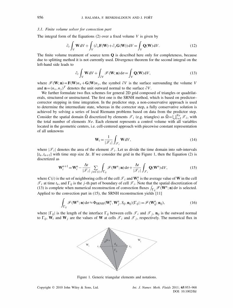
3.3. Computational domain and boundary conditions

Internal flow problems lead typically to initial-boundary value problems on finite computationaldomain. The boundary of domain is divided into inlet �i, outlet �o, and non-permeable wall �wparts. The solution of flow in turbine can be considered periodic in y direction, see the periodicpart of boundary �p in the Figure 2. The x-component of velocity along inlet boundary is subsonicfor all here mentioned applications, so according to 1D linear theory of characteristics, we specifythe Dirichlet condition for total temperature T0, total pressure p0, flow angle �, and �=Q0=Q1=Q2=0 along the inlet boundary. Along the non-permeable wall we prescribe the zero normalvelocity. The x-component of velocity along outlet boundary is depending on application subsonicor supersonic. We prescribe the value of pressure for subsonic and no condition for the supersoniccase. Along periodical boundary, we consider direct grid connectivity, i.e. we prescribe point topoint periodicity.



x

y

Γi

w

w

p

p

p

p

o

Γ

Γ

Γ

Γ

Γ

Γ

Γ

Figure 2. Computational domain for 2D axial turbine cascade.

3.4. Implementation of some boundary conditions

With respect to 1D linear theory of characteristics, one parameter at the inlet boundary should beextrapolated from computational domain. We extrapolate the value of Mach number M , and thenusing the inlet boundary conditions and isentropic flow assumption, we can compute the state inthe ghost cell outside the domain:

�=(1+ �−1

2M2

) 11−�

�0, (33)

�u=(1+ �−1

2M2

) 11−� − 1

2

M�0c0 cos(�), (34)

�v=(1+ �−1

2M2

) 11−� − 1

2

M�0c0 sin(�), (35)

e=(1+ �−1

2M2

) �1−�

(1

�(�−1)+ M2

2

)�0c

20, (36)

where �0= p0/RvT0 is inlet total density, c0=√�RvT0 is inlet total speed of sound, and Rv is

the gas constant of vapor (we expect only one-phase flow of vapor at the inlet). Let us considerthe outlet boundary condition for subsonic x-component of velocity along the outlet boundary.Internal flows have often a pressure gradient along the outlet boundary, therefore unphysicaloscillations of solution might appear if one imposes a constant value of pressure along the outletboundary. To avoid oscillations, we extrapolate the shape of pressure distribution pout(y) fromthe computational domain and manipulate the magnitude to get prescribed mean value of pressurepgiven. The corrected outlet pressure distribution is given by the function pout(y)

pout= 1

Y

∫ Y

0pout(y)dy, pout(y)= pout(y)

pgivenpout

, (37)

where y∈〈0,Y〉 is the variable along �o. Finally, we extrapolate components of W into ghost celloutside the computational domain and correct e in the ghost cell using extrapolated componentsof W and pressure pout(y).



4. NUMERICAL RESULTS: ONE-PHASE FLOW TEST CASES

We have tested the behavior of the VFFC scheme for typical transonic one-phase flow problems onboth structured and unstructured grids, because hybrid grids combining structured and unstructuredblocks seem to be a good choice for complex geometries. The VFFC scheme yields very goodresults on both structured quadrilateral and unstructured triangular grids in the case of transonicinviscid flow of air in Geselschaft fur Angewandte Mathematik und Mechanik (GAMM) channelthat was already presented in [18].

It also delivers numerical results qualitatively comparable to other commonly used modernschemes [19] in the case of transonic inviscid flow of air (�=1.4) in 2D turbine cascade SE1050,for cascade data see [20]. The examples of numerical results and comparison with experimentaldata for the flow case with the inlet total pressure 105 Pa, the inlet total temperature 273.15K, theinlet flow angle 19.3◦, and the outlet mean pressure 42322Pa are given in Figure 3 (the second-order method was used with MinMod limiter). Note also that the second-order SRNH scheme onthe same grid structured quadrilateral grid yielded same numerical results (coinciding shape ofMach number isolines and coinciding pressure distribution) as second-order VFFC scheme withsign function as well as with the smooth approximation of sign function, which is discussed later,therefore the results of the SRNH scheme are not plotted.

Problems with the VFFC scheme were observed in the case of symmetrical geometry of 2Dnozzle with structured quadrilateral grid, because the sonic line (the line where the eigenvalue

0

s/ b

0.2

0.4

0.6

0.8

1

p/p0

VFFC, 1st orderVFFC, 2nd orderexperiment

0.2 0.4 0.6 0.8 1

(a) (b)

(c) (d)

Figure 3. Cascade SE1050, structured quadrilateral grid. Mach number isolines are plotted with�M=0.05 and bold line is M=1. Experimental data have been gathered at ARTI [20]. (a) Isolinesof M , first-order VFFC; (b) isolines of M , second-order VFFC; (c) experimental data—interferogram;

and (d) pressure distribution along profile.



-1-1

-0.75

-0.5

-0.25

0

0.25

0.5

0.75

1

P3(x)

-0.5 0 0.5 1

Figure 4. Polynomial P3(x).

x

y

0.010.0050-500.0

0.035

0.0375

0.04

0.0425

x

0.010.0050-500.0

y

0.035

0.0375

0.04

0.0425

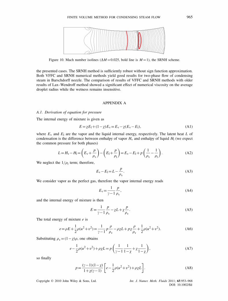
Figure 5. Mach number isolines (�M=0.025, bold line is M=1) and detail of grid around sonic line forsmooth grid (upper figures) and perturbed grid (lower figures).

�1 changes the sign) is almost aligned with grid lines. Most probably due to the switchingof sign(�1) between −1 and 1 oscillations of numerical solution leading to divergent behaviorappeared. Note that the SRNH scheme did not exhibit such behavior and the VFFC scheme wassuccessfully used without this problem in the case of GAMM channel and SE1050 turbine cascade.The oscillations of VFFC solution for nozzle can be avoided, e.g. using a perturbed grid, seeFigure 5.

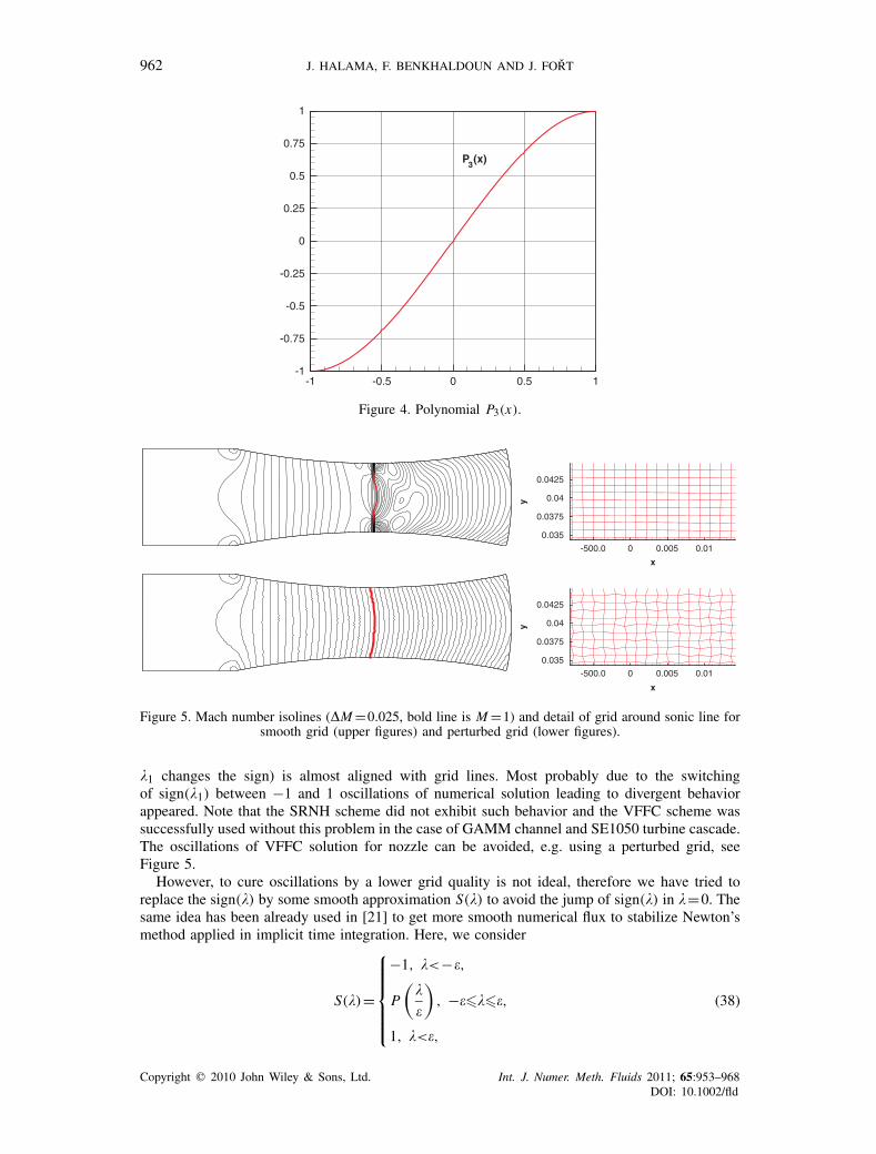
However, to cure oscillations by a lower grid quality is not ideal, therefore we have tried toreplace the sign(�) by some smooth approximation S(�) to avoid the jump of sign(�) in �=0. Thesame idea has been already used in [21] to get more smooth numerical flux to stabilize Newton’smethod applied in implicit time integration. Here, we consider

S(�)=

⎧⎪⎪⎪⎪⎨⎪⎪⎪⎪⎩−1, �<−�,

P

(�

�

), −��,

1, �<�,

(38)



0x

0

0.5

1

dens

ity

exact solutionVFFC, sign functionVFFC, epsilon=0.1VFFC, epsilon=1.0

x

0

0.5

1

pres

sure

exact solutionVFFC, sign functionVFFC, epsilon=0.1VFFC, epsilon=1.0

0.2 0.4 0.6 0.8 1 0 0.2 0.4 0.6 0.8 1(a) (b)

Figure 6. Density (a) and pressure (b) at t=0.2, the sign function approximated by P3.

where �>0 and P(x) is polynomial, which satisfies P(−1)=−1, P(1)=1, and P ′(−1)= P ′(1)=0.We propose the cubic polynomial P3(x)=− 1

2 (x−1)3− 32 (x−1)2+1, see Figure 4.

First, we have tested this polynomial approximation of the sign function for the shock tube testwith �=1.4 and domain [x, t]∈(0;1)×(0;T ) with initial data in t=0

�(x,0)={1.00,0�x<0.5,

0.06,0.5<x�1,p(x,0)=

{1.00,0�x<0.5,

0.05,0.5<x�1,(39)

and u(x,0)=0. Figure 6 shows the comparison of numerical results with exact solution§ at timet=0.2. The computational grid is uniform with 100 cells and the second-order VFFC methodincludes linear reconstruction with MinMod limiter and 3-stage Runge–Kutta method for timeintegration. We see that numerical results for parameter �=0.1 are almost identical to resultsachieved with sign function, for more details see Appendix A.2.

5. NUMERICAL RESULTS: TWO-PHASE FLOW IN BARSCHDORFF NOZZLE

Figures 7–10 show numerical results of two-phase flow with condensation in Barschdorff nozzle[22] for the flow case with the inlet total pressure 78 390 Pa, the inlet total temperature 373K,axial inlet flow direction and supersonic outlet velocity. The wetness � and the Hills momentsQ0, Q1, and Q2 are equal to zero at the inlet. The surface tension correction coefficient fromthe Equation (5) is �=1.194, according to given inlet total temperature and pressure. Results ofpresented method match well the experimental data of [22] and agree with results of the Lax–Wendroff method [5]. The shape of isolines in the Figures 8–10 corresponds also to numericalresults published in [23]. Both the VFFC and the SRNH first-order methods deliver sharpercondensation shock compared with the Lax–Wendroff method (which has artificial dissipation termsand also a bigger stencil). Note that the VFFC method was used with sign function approximationwith P3 and �=0.1c. Interesting is effect of numerical dissipation on the average droplet radius.Lower dissipation leads to sharper condensation shock, which signalizes stronger nucleation, i.e.we get more droplets of smaller size, see Figure 7(c),(d). The total amount of condensed water(wetness) seems to be insensitive to numerical dissipation, see Figure 7(c). This phenomenon hasbeen justified also by adjusting the different levels of artificial dissipation in the Lax–Wendroffmethod.

§Exact solution was computed by the code provided at http://www.grc.nasa.gov/WWW/wind/valid/stube/stube.html.



0.10-1.0-2.0

0.10-1.0-2.00.10-1.0-2.0

x [m]

0.3

0.4

0.5

0.6

0.7

0.8

pres

sure

/ to

tal p

ress

ure

L-WVFFC with P_3(x)experimentSRNH

-0.02 0.06

x [m]

0.4

0.45

0.5

0.55

0.6

pres

sure

/ to

tal p

ress

ure

L-WVFFC with P_3(x)experimentSRNH

x [m]

0

0.01

0.02

0.03

0.04

0.05

0.06

wet

ness

L-WVFFC with P_3(x)SRNH

x [m]

0

1e-08

2e-08

3e-08

4e-08

radi

us

L-WVFFC with P_3(x)SRNH

0 0.02 0.04

(a) (b)

(c) (d)

Figure 7. Barschdorff nozzle, distributions along nozzle axis: (a) pressure; (b) detail of pressure;(c) wetness; and (d) average droplet radius.

Figure 8. Mach number isolines (�M=0.025, bold line is M=1), L–W scheme.

Figure 9. Mach number isolines (�M=0.025, bold line is M=1), the VFFC scheme with sign functionapproximation by polynomial P3 and �=0.1c.

6. CONCLUSIONS

Proposed approximation of sign function increases the robustness of the VFFC method in specificcases with sonic line aligned to grid lines (this may happen in numerous configurations withstructured or hybrid grid). Numerical computations showed that the loss of scheme dissipation dueto smooth approximation of sign function need not to be compensated by additional terms in all



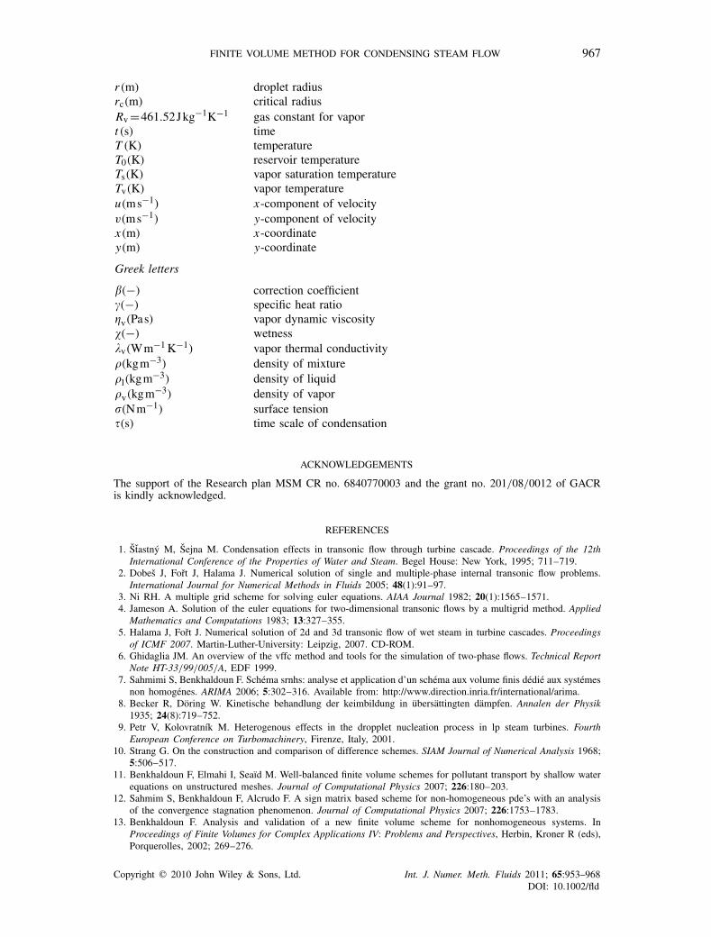
Figure 10. Mach number isolines (�M=0.025, bold line is M=1), the SRNH scheme.

the presented cases. The SRNH method is sufficiently robust without sign function approximation.Both VFFC and SRNH numerical methods yield good results for two-phase flow of condensingsteam in Barschdorff nozzle. The comparison of results of VFFC and SRNH methods with olderresults of Lax–Wendroff method showed a significant effect of numerical viscosity on the averagedroplet radius while the wetness remains insensitive.

APPENDIX A

A.1. Derivation of equation for pressure

The internal energy of mixture is given as

E=�El+(1−�)Ev=Ev−�(Ev−El), (A1)

where Ev and El are the vapor and the liquid internal energy, respectively. The latent heat L ofcondensation is the difference between enthalpy of vapor Hv and enthalpy of liquid Hl (we expectthe common pressure for both phases)

L=Hv−Hl=(Ev+ p

�v

)−

(El+ p

�l

)=Ev−El+ p

(1

�v− 1

�l

). (A2)

We neglect the 1/�l term; therefore,

Ev−El= L− p

�v. (A3)

We consider vapor as the perfect gas, therefore the vapor internal energy reads

Ev= 1

�−1

p

�v, (A4)

and the internal energy of mixture is then

E= 1

�−1

p

�v−�L+�

p

�v. (A5)

The total energy of mixture e is

e=�E+ 1

2�(u2+v2)= 1

�−1p

�

�v−��L+ p�

�

�v+ 1

2�(u2+v2). (A6)

Substituting �v=(1−�)�, one obtains

e− 1

2�(u2+v2)+��L= p

(1

�−1

1

1−�+�

1

1−�

), (A7)

so finally

p= (�−1)(1−�)

1+�(�−1)

[e− 1

2�(u2+v2)+��L

]. (A8)



A.2. Some analysis of sign function approximation

Let us consider simple scalar 1D linear advection equation

�t u+a�xu=0, (A9)

for which the VFFC scheme can be written as

un+1i =uni − �t

�x(�n

i+1/2−�ni−1/2), (A10)

with flux

�ni+1/2=a

(uni +uni+1

2−S(a)

uni+1−uni2

), (A11)

where S(a) is defined by the Equation (38). Substituting �ni−1/2 and �n

i+1/2 into (A10), we get

un+1i −uni

�t+a

uni+1−uni−1

2�x= aS(a)�x

2

uni−1−2uni +uni−1

�x2, (A12)

which corresponds to equation

�t u+a�xu= aS(a)�x

2�xxu+O(�x2+�t). (A13)

The product aS(a) is positive, i.e. the right hand side represents the dissipation term. The amountof dissipation is locally reduced for a∈(−�,�) compared with the scheme with the sign function.This loss of dissipation can be compensated by additional term, for details see [21]. The resultswithin this paper have been achieved without such term.

NOMENCLATURE

c(ms−1) speed of sounde(Jm−3) total energy of mixture per unit volumeE(Jkg−1) internal energyH(Jkg−1) enthalpyJ (m−3 s−1) nucleation ratekB=1.3804×10−23 JK−1 Boltzmann constantKn(−) Knudsen numberL(Jkg−1) latent heatmv =2.99046×10−26 kg water molecule massM(−) Mach numberN (kg−1) total number of droplets per unit massp(Pa) pressure of mixturep0(Pa) reservoir pressureps(Pa) saturation pressureQ0(kg−1) zeroth Hill’s momentQ1(mkg−1) first Hill’s momentQ2(m2kg−1) second Hill’s moment



r(m) droplet radiusrc(m) critical radiusRv=461.52Jkg−1K−1 gas constant for vaport (s) timeT (K) temperatureT0(K) reservoir temperatureTs(K) vapor saturation temperatureTv(K) vapor temperatureu(ms−1) x-component of velocityv(ms−1) y-component of velocityx(m) x-coordinatey(m) y-coordinate

Greek letters

�(−) correction coefficient�(−) specific heat ratiov(Pas) vapor dynamic viscosity�(−) wetness�v(Wm−1K−1) vapor thermal conductivity�(kgm−3) density of mixture�l(kgm

−3) density of liquid�v(kgm

−3) density of vapor�(Nm−1) surface tension(s) time scale of condensation

ACKNOWLEDGEMENTS

The support of the Research plan MSM CR no. 6840770003 and the grant no. 201/08/0012 of GACRis kindly acknowledged.

REFERENCES

1. Stastny M, Sejna M. Condensation effects in transonic flow through turbine cascade. Proceedings of the 12thInternational Conference of the Properties of Water and Steam. Begel House: New York, 1995; 711–719.

2. Dobes J, Fort J, Halama J. Numerical solution of single and multiple-phase internal transonic flow problems.International Journal for Numerical Methods in Fluids 2005; 48(1):91–97.

3. Ni RH. A multiple grid scheme for solving euler equations. AIAA Journal 1982; 20(1):1565–1571.4. Jameson A. Solution of the euler equations for two-dimensional transonic flows by a multigrid method. Applied

Mathematics and Computations 1983; 13:327–355.5. Halama J, Fort J. Numerical solution of 2d and 3d transonic flow of wet steam in turbine cascades. Proceedings

of ICMF 2007. Martin-Luther-University: Leipzig, 2007. CD-ROM.6. Ghidaglia JM. An overview of the vffc method and tools for the simulation of two-phase flows. Technical Report

Note HT-33/99/005/A, EDF 1999.7. Sahmimi S, Benkhaldoun F. Schema srnhs: analyse et application d’un schema aux volume finis dedie aux systemes

non homogenes. ARIMA 2006; 5:302–316. Available from: http://www.direction.inria.fr/international/arima.8. Becker R, Doring W. Kinetische behandlung der keimbildung in ubersattingten dampfen. Annalen der Physik

1935; 24(8):719–752.9. Petr V, Kolovratnık M. Heterogenous effects in the dropplet nucleation process in lp steam turbines. Fourth

European Conference on Turbomachinery, Firenze, Italy, 2001.10. Strang G. On the construction and comparison of difference schemes. SIAM Journal of Numerical Analysis 1968;

5:506–517.11. Benkhaldoun F, Elmahi I, Seaıd M. Well-balanced finite volume schemes for pollutant transport by shallow water

equations on unstructured meshes. Journal of Computational Physics 2007; 226:180–203.12. Sahmim S, Benkhaldoun F, Alcrudo F. A sign matrix based scheme for non-homogeneous pde’s with an analysis

of the convergence stagnation phenomenon. Journal of Computational Physics 2007; 226:1753–1783.13. Benkhaldoun F. Analysis and validation of a new finite volume scheme for nonhomogeneous systems. In

Proceedings of Finite Volumes for Complex Applications IV: Problems and Perspectives, Herbin, Kroner R (eds),Porquerolles, 2002; 269–276.



14. Benkhaldoun F, Quivy L. A non homogeous riemann solver for shallow water and two phase flows. FlowTurbulence Combustion 2006; 76:391–402.

15. Alcrudo F, Benkhaldoun F. Exact solutions to the riemann problem of the shallow water equations with a bottomstep. Computers and Fluids 2001; 30:643–671.

16. Masella JM, Faille I, Gallouet T. On an approximate godunov scheme. International Journal of ComputationalFluid Dynamics 1999; 13:133–149.

17. VanAlbada GD, Leer BV, Roberts WW. A comparative study of computational methods in cosmic gas dynamics.Astronomy and Astrophysics 1982; 76:76–93.

18. Halama J, Benkhaldoun F. Finite volume characteristic flux scheme for transonic flow problems. Proceedings ofConference Colloquium Fluid Dynamics. IT CAS CZ: Praha, 2006; 39–42. ISBN: 80-87012-01-1.

19. Furst J. A finite volume scheme with weighted least square reconstruction. Finite Volumes for ComplexApplications IV. Hermes Science Publishing: London, U.K., 2005; 345–354. ISBN: 1 905209 48 7.

20. Stastny M, Safarık P. Boundary layer effects on the transonic flow in a straight turbine cascade. Technical Report,1992; Paper 92-GT-155.

21. DeVuyst F, Ghidaglia JM, LeCoq G. On the numerical simulation of multiphase water flows with changes ofphase and strong gradients using the homogenous equilibrium model. International Journal on Finite Volumes2005; 2(1):1–36.

22. Barschdorff D. Verlauf der zustandgroesen und gasdynamische zuammenhaenge der spontanen kondensationreinen wasserdampfes in lavaldusen. Forschung auf dem Gebiete des Ingenieur Wesens 1971; 37(5).

23. Dykas S, Goodheart K, Schnerr GH. Numerical study of accurate and efficient modelling for simulation ofcondensing flow in transonic steam turbines. Fifth European Conference on Turbomachinery, Praha, 2003;751–760.


Flux schemes based finite volume method for internal transonic flow with condensation

Documents

Transcript of Flux schemes based finite volume method for internal transonic flow with condensation