Flutter of an elastic plate in a channel flow:

confinement and finite-size effects

Olivier Doarea, Martin Sauzadea, Christophe Eloyb

aENSTA Paristech, Unite de Mecanique, Chemin de la Huniere, 91761 Palaiseau, FrancebIRPHE, CNRS & Aix-Marseille Universite, 49 rue Joliot-Curie, 13013 Marseille, France

Abstract

When a cantilevered plate lies in an axial flow, it is known to exhibit self-sustained oscillations once a critical flow velocity is reached. This flutter in-stability has been investigated theoretically, numerically and experimentally bydifferent authors, showing that the critical velocity is always underestimated bytwo-dimensional models. However, it is generally admitted that if the plate isconfined in the spanwise direction by walls, three-dimensionality of the flow isreduced and the two-dimensional models can apply. The aim of this article is toquantify this phenomenon by analyzing the effect of the clearance between theplate and the side walls on the flutter instability. To do so, the pressure distri-bution around an infinite-length plate is first solved in the Fourier space, whichallows to develop an empirical model for the pressure jump. This empiricalmodel is then used in real space to compute instability thresholds as a functionof the channel clearance, the plate aspect ratio and mass ratio. Our main resultshows that, as the value of the clearance is reduced, the convergence towards thetwo-dimensional limit is so slow that this limit is unattainable experimentally.

Keywords: Flow-induced vibration, Cantilevered plate, Flutter instability,Channel flow.

1. Introduction

Cantilevered plates in axial flow are known to exhibit self-sustained oscilla-tions once a critical flow velocity is reached. This phenomenon has been themain focus of a large amount of studies, motivated by applications in biome-chanics (Auregan and Depollier, 1995; Huang, 1995), paper industry (Watanabeet al., 2002b), aerospace and nuclear engineering (Guo and Paidoussis, 2000) oraeronautics (Kornecki et al., 1976). Plates are usually differentiated from flagsthrough the restoring force that maintains the structure in the flat equilibriumposition. The restoring force is due to elastic bending rigidity for plates, whileit is a tensile force induced by fluid friction and flag weight in the flag case.

Email address: olivier.doare@ensta.fr (Olivier Doare)

Preprint submitted to Journal of Fluids and Structures April 19, 2010

A plate of infinite span and infinite length in a potential flow has been provento be unstable at any non-zero flow velocity (Rayleigh, 1879). It was found sincethen that taking into account the finite size of the plate (its span and/or chord)tends to stabilize it, so that the critical velocity for flutter instability is no longerzero but has a finite value.

Many studies have considered finite-length and infinite-span plates, which in-volved a two-dimensional homogeneous flow around the structure, modeled as anEuler-Bernoulli beam. Here, since the flow is considered to be two-dimensional,independent of the spanwise coordinate, this approach is referred to as two-dimensional. In the literature, one can distinguish two methods when solvingthis problem. The first one, used by Kornecki et al. (1976), introduces circula-tion around the plate and wake vortices so that the Kutta condition is satisfiedat the trailing edge, as done by Theodorsen (1935) in the context of airfoil flut-ter. Huang (1995) and Watanabe et al. (2002a) used the same modeling andprovided complementary results on the linear stability of the plate. The secondapproach was introduced by Guo and Paidoussis (2000) and consists in impos-ing continuity of the pressure everywhere except across the plate. The pressuredistribution is then solved in the Fourier space, assuming that no singularityexists at both leading and trailing edges of the plate. However, this model im-plies an incoming “wake” regularizing the flow at the leading edge, which doesnot happen in real situations. Yet, the two models give very similar resultsprovided the plate is long and flexible enough (Eloy et al., 2008; Michelin andLlewellyn Smith, 2009).

Another asymptotic case can be considered when the plate span is small com-pared to its chord. This so-called slender-body approach was first introduced byLighthill (1960) in his seminal paper on fish locomotion and recently applied byLemaitre et al. (2005) to address the flow-induced instability of slender platestensioned by gravity.

The flutter of cantilevered plates has been investigated experimentally byTaneda (1968), Datta and Gottenberg (1975), Kornecki et al. (1976), Yam-aguchi et al. (2000), Watanabe et al. (2002b) and Eloy et al. (2008). Theyshowed that the deflection of the plate during the self-sustained oscillations isindependent of the spanwise coordinate, validating the use of an Euler-Bernoullibeam model for the plate deflection. However, the experimental values of crit-ical velocity was always found to be higher than predicted by the theoreticaltwo-dimensional models. In the case of plates of small aspect ratio, the experi-ments and slender-body theory have been compared by (Lemaitre et al., 2005).The experimental critical velocity has also been found to be higher than thetheoretical one. In other words, plates in the experiments appear invariablymore stable than predicted.

Numerical simulations have been carried out to adress the instability thresh-old in the two-dimensional case. In these simulations the plate is modeled withan Euler-Bernoulli beam equation and the fluid is described either by the Navier-Stokes equations (Watanabe et al., 2002a; Balint and Lucey, 2005; Howell et al.,2009) or using vortex methods (Tang and Paıdoussis, 2007; Michelin et al., 2008;Alben and Shelley, 2008). All these simulations recovered the instability thresh-

2

old of the two-dimensional theoretical models. Additionally, these numericalstudies provided a better insight into the instability mechanism and the energyexchange between the fluid and the flexible structure.

The discrepancy between theoretical and experimental values for the criticalvelocity motivated the development of a three-dimensional model for the fluidflow around the plate (Eloy et al., 2007, 2008). Here, the plate remained modeledby an Euler-Bernoulli beam equation while the three-dimensional flow aroundthe plate was modeled using the same assumptions as in Guo and Paidoussis(2000). This model was found to improve the prediction of critical velocities aswell as to provide a unified theory that fills the gap between two-dimensionalmodels and slender-body models.

Most of the works cited above have considered the flutter of a flexible plate inan unbounded flow. Motivated by the study of snoring, some authors howeverexamined the effect of confinement. The two-dimensional problem of a plateof infinite span in a channel flow has been modeled by Auregan and Depollier(1995) and Guo and Paidoussis (2000) and the channel flow confinement wasfound to have a destabilizing effect. The limit of extremely low values of thechannel width leads to the so called leakage flow instability problem (Wu andKaneko, 2005). Comparatively, the channel flow confinement in the spanwise di-rection was overlooked. In his experiments, Huang (1995) mentions a plate thatspans over the entire 6cm width of the channel with a small clearance of 2mmon each side, in order to reduce the three-dimensionality of the flow. Aureganand Depollier (1995) noticed a discrepancy between their two-dimensional the-ory and experiments, that they attributed to the clearance on the transversesides of the plate. To overcome this difference, they introduced in their modelan effective span 90% smaller than the real span. It is commonly admittedthat confining the flow in the spanwise direction limits the three-dimensionaleffects. However, to the author’s knowledge, except the empirical correctionproposed by Auregan and Depollier (1995), this effect has never been addressedquantitatively.

The main objective of this paper is hence to quantify the effect of the clear-ance between plate and channel walls on the instability thresholds. In section 2,the problem of a finite span, finite chord plate in a finite height, infinite widthchannel flow will be presented. Equations and boundary conditions satisfied bythe potential flow will be developed to obtain an Helmholtz problem for thepressure jump in the Fourier space. This problem will be solved numericallyand theoretically in the third section and the data obtained will be used toformulate an empirical model. In section 4, the instability thresholds will becomputed as function of the plate aspect ratio and the channel clearance usingthis empirical model. Finally, the effect of the gap on the critical velocity willbe discussed in relation to experiments.

3

C

C

H

L

X

YZ

W

U

Figure 1: Schematic view of a cantilevered plate in an axial potential flow bounded by tworigid walls.

2. Formulation of the problem

2.1. Equation of motion

As sketched in Fig. 1, a cantilevered plate of length (or chord) L and height(or span) H is considered. The plate is surrounded by an airflow of constantvelocity U in the X direction and bounded above and below by rigid walls ata distance H + 2C, so that the gap between the plate and the walls is C (alsocalled the clearance in the text). The lateral plate deflection is noted W , and isconsidered to be independent of the vertical coordinate Y , so that it is governedby the linearized Euler-Bernoulli beam equation with an additional forcing termdue to the fluid pressure,

MWTT +DWXXXX = 〈[P ]〉, (1)

where D is the flexural rigidity of the plate, M its surface density and 〈[P ]〉the mean value along the span H of the pressure jump across the plate (thenotation [P ] stands for P (Z = 0+) − P (Z = 0−)). Considering a finite lengthL, boundary conditions will be those of a clamped-free beam, W = WX = 0 inX = 0, and WXX = WXXX = 0 in X = L.

The following dimensionless quantities are introduced

x =x

L, y =

Y

L, z =

Z

L, w =

W

L, t =

UT

L, p =

P

ρU2, (2)

4

where ρ is the fluid density, so that the dimensionless equation of motion (1) is

wtt +1

U∗2wxxxx = M∗〈[p]〉, (3)

where U∗ and M∗ are the reduced velocity and mass ratio, defined as

U∗ =

√

M

DLU, M∗ =

ρL

M. (4)

With this choice of dimensionless parameters, the plate span is h = H/L, andthe gap is c = C/L.

2.2. Potential flow

Assuming a large Reynolds number, the flow around the plate is consideredto be potential. For the present linear model, this means that the vorticity isentirely concentrated in the surface z = 0, both in the plate itself to modelthe viscous boundary layers and in its wake where the vorticity is shed withvelocity U . Under these hypothesis, the perturbation pressure p(x, y, z, t) andthe perturbation potential φ(x, y, z, t) are related by the unsteady linearizedBernoulli equation

p = −(∂t + ∂x)φ. (5)

Boundary conditions are given by the impermeability condition on the walls andon the plate and yields a Neumann problem for the Laplace equation satisfied bythe potential φ. Applying the operator (∂t + ∂x) on these boundary conditionsgives another Neumann problem for the pertubation pressure

∆p = 0, (6)

[py]|y|=h/2+c = 0, (7)

[pz]z=0= −(∂t + ∂x)2w for (x, y) ∈ D, (8)

where D is the plate area.

2.3. Problem in the Fourier space

To solve the set of equations (6–8), the pressure field is expressed in theFourier space such that

p =

∫ ∞

−∞

ψ(k, y, z)eikx dk, (9)

where ψ satisfy the following equations

(∂2y + ∂2

z )ψ = k2ψ, (10)

[ψy]|y|=h/2+c = 0, (11)

[ψz ]z=0= v(k) for |y| < h/2, (12)

5

and v(k) is the Fourier transform of −(∂t + ∂x)2w∫ ∞

−∞

v(k) eikx dk = −(∂t + ∂x)2w. (13)

The set of equation (10–12) defines the problem in the Fourier space. It is a twodimensional problem where the field ψ is solution of the Helmoltz equation (10)with Neumann boundary conditions (11–12). The problem being linear, for agiven wavenumber k, ψ is proportional to v(k) such that the average along thespan of the potential jump can always be written in the form

〈[ψ]〉 = −2

kg(k, h, c) v(k). (14)

The linear problem given by equations (10–12) will be solved in the next sectionnumerically and theoretically with the aim of evaluating the function g(k, h, c).

Taking the x-derivative of equation (9) and executing an inverse Fouriertransform yields

ψ =1

2πik

∫ 1

0

∂xp e−ikx dx. (15)

Taking the jump across the surface z = 0 of the above equation and averagingalong the span gives

〈[ψ]〉 =1

2πik

∫ 1

0

p′(ξ) e−ikξ dξ, (16)

where p′(x) = 〈[∂xp]〉 is the x-derivative of averaged pressure jump. Inserting(14) and (16) into (13) and inverting the integral signs yields the followingintegral equation for p′

1

2π−

∫ 1

0

p′(ξ)G(x − ξ, h, c) dξ = (∂t + ∂x)2w, (17)

where

G(x, h, c) =

∫ ∞

0

sin(kx)

g(k, h, c)dk, (18)

and the bar on the integral sign denotes that the Cauchy principal value shouldbe taken (see Mangler, 1951) as the kernel G has an inverse-power singularityin x = 0. Solving the inverse problem (17) and integrating allows to find theaveraged pressure distribution for a given motion of the plate w(x, t).

It should be noted that the boundary condition in the Fourier space givenby equation (12) is only an approximation. Indeed, the Neumann boundarycondition given by equation (8) applies only on the plate area D and not in thewake. Therefore, when expressed in the Fourier space, v(k) can slightly dependon y in general. The approximation will be accurate however when the wakebehind the fluttering plate has the same properties as the flow over the plate.This will be realized when the dimensionless frequency ω = ΩL/U is of orderunity (where Ω is the angular frequency) or in the asymptotic cases of large andsmall aspect ratios.

6

−1 1

z

d

y

Figure 2: Schematic representation of the problem in the Fourier space.

3. Pressure jump in the Fourier space

In the Fourier space, rescaling all lengths by h/2, the rescaled perturbationpotential satisfies the following system

∆ϕ = κ2ϕ, (19)

[ϕy]|y|=1+d = 0, (20)

[ϕz ]z=0= 1, for |y| < 1, (21)

where κ = kh/2, d = 2c/h and ϕ = 2ψ/hv(k). The first equation is the Helmoltzequation (the ∆ is the Laplace operator in two-dimensions here), and the twoothers are the boundary conditions on the plate and on the walls. This problemis sketched in Fig. 2.

The goal of this section is to determine the function g now defined as

g(κ, d) = −κ

2〈[ϕ]〉 = −κ〈ϕ+〉. (22)

where ϕ+ is a shortcut for ϕ(z = 0+).Before solving these equations in the general case, let us recall the results in

the two-dimensional and slender-body limit cases when the clearance is infinite.The slender-body limit corresponds to κ ≪ 1 and can be deduced from theresults of Lighthill (1960)

ϕ+ ≃ −√

1 − y2, for |y| < 1 and κ≪ 1. (23)

The two-dimensional limit corresponds to κ ≫ 1. In this situation, the pres-sure potential is independent of the spanwise coordinate and the resolution ofequations (19-21) yields

ϕ+ ≃ −1

κ, for |y| < 1 and κ≫ 1. (24)

3.1. Numerical calculation

Numerical resolution of the Helmoltz problem defined by equations (19–21) is now presented. First of all, the problem has to be of finite size to allow

7

e

d1

z

y∆ϕ = κϕ

ϕz = 1 ϕ = 0

ϕz = 0

ϕy = 0ϕy = 0

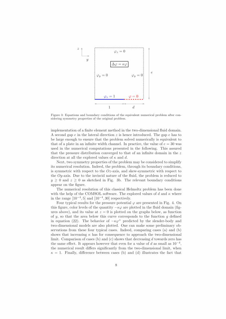
Figure 3: Equations and boundary conditions of the equivalent numerical problem after con-sidering symmetry properties of the original problem.

implementation of a finite element method in the two-dimensional fluid domain.A second gap e in the lateral direction z is hence introduced. The gap e has tobe large enough to ensure that the problem solved numerically is equivalent tothat of a plate in an infinite width channel. In practice, the value of e = 30 wasused in the numerical computations presented in the following. This assuredthat the pressure distribution converged to that of an infinite domain in the zdirection at all the explored values of κ and d.

Next, two symmetry properties of the problem may be considered to simplifyits numerical resolution. Indeed, the problem, through its boundary conditions,is symmetric with respect to the Oz-axis, and skew-symmetric with respect tothe Oy-axis. Due to the inviscid nature of the fluid, the problem is reduced toy ≥ 0 and z ≥ 0 as sketched in Fig. 3b. The relevant boundary conditionsappear on the figure.

The numerical resolution of this classical Helmoltz problem has been donewith the help of the COMSOL software. The explored values of d and κ wherein the range [10−4, 5] and [10−4, 30] respectively.

Four typical results for the pressure potential ϕ are presented in Fig. 4. Onthis figure, color levels of the quantity −κϕ are plotted in the fluid domain (fig-ures above), and its value at z = 0 is plotted on the graphs below, as functionof y, so that the area below this curve corresponds to the function g definedin equation (22). The behavior of −κϕ+ predicted by the slender-body andtwo-dimensional models are also plotted. One can make some preliminary ob-servations from these four typical cases. Indeed, comparing cases (a) and (b)shows that increasing κ has for consequence to approach the two-dimensionallimit. Comparison of cases (b) and (c) shows that decreasing d towards zero hasthe same effect. It appears however that even for a value of d as small as 10−4,the numerical result differs significantly from the two-dimensional limit, whenκ = 1. Finally, difference between cases (b) and (d) illustrates the fact that

8

0

1

2

3

4

0 1 0

1

2

0

1

2

3

4

0 1 0

1

2

0

1

2

3

4

0 1 0

1

2

0

1

2

3

4

0 1 0

0.5

1

0

0.2

0.4

0.6

0.8

1

(a) (b) (c) (d)

y

−κϕ+

z

Figure 4: Filled contours representing levels of −κϕ in the (y, z) space (above) and corre-sponding values at z = 0+ plotted as function of y (below, bold lines), for four typical setsof parameters κ and d; (a), κ = 5 and d = 0.3; (b), κ = 1 and d = 0.3; (c), κ = 1 andd = 10−4; (d), κ = 0.1 and d = 0.3. Dashed lines and dashed-dotted lines indicates value of−κϕ+ predicted by the slender-body and two-dimensional theories respectively [see equations(23) and (24)]. The values have been multiplied by 8 in the color plot of case (d) in order toimprove the visibility.

9

10−4

10−3

10−2

10−1

100

101

10−4

10−3

10−2

10−1

100

0.00010.0003 0.001 0.003 0.01 0.03 0.1 0.3 1

g

d

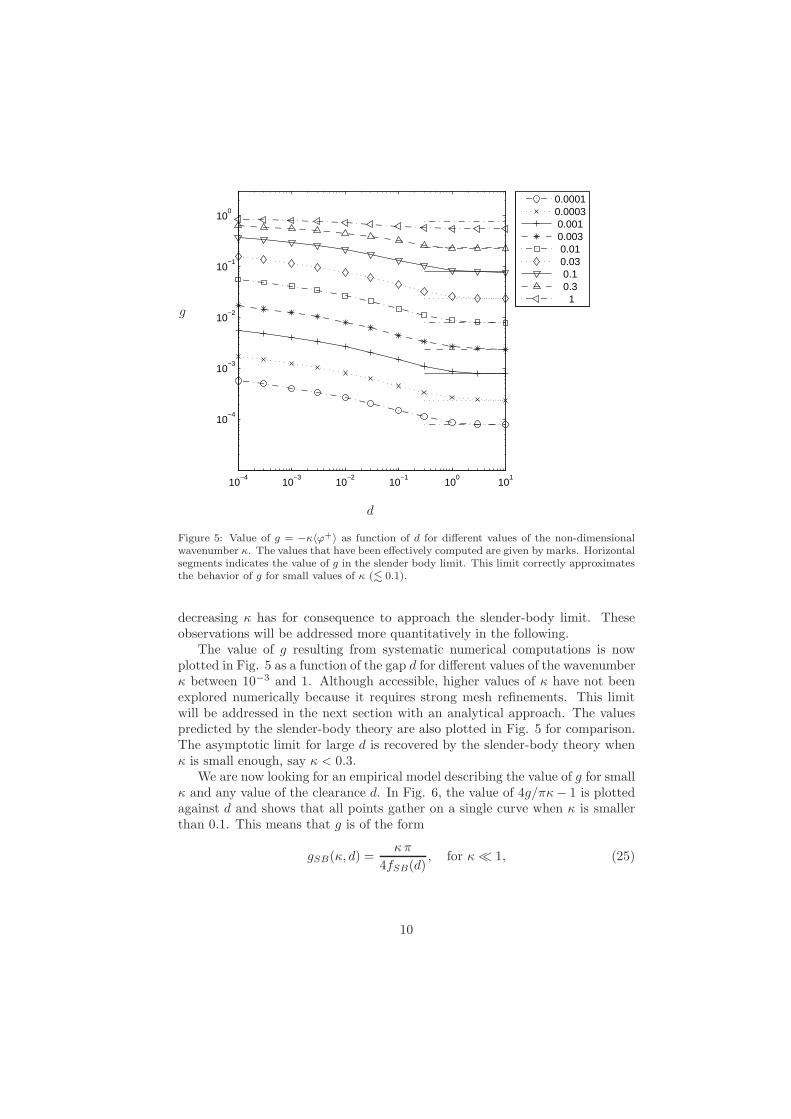
Figure 5: Value of g = −κ〈ϕ+〉 as function of d for different values of the non-dimensionalwavenumber κ. The values that have been effectively computed are given by marks. Horizontalsegments indicates the value of g in the slender body limit. This limit correctly approximatesthe behavior of g for small values of κ (. 0.1).

decreasing κ has for consequence to approach the slender-body limit. Theseobservations will be addressed more quantitatively in the following.

The value of g resulting from systematic numerical computations is nowplotted in Fig. 5 as a function of the gap d for different values of the wavenumberκ between 10−3 and 1. Although accessible, higher values of κ have not beenexplored numerically because it requires strong mesh refinements. This limitwill be addressed in the next section with an analytical approach. The valuespredicted by the slender-body theory are also plotted in Fig. 5 for comparison.The asymptotic limit for large d is recovered by the slender-body theory whenκ is small enough, say κ < 0.3.

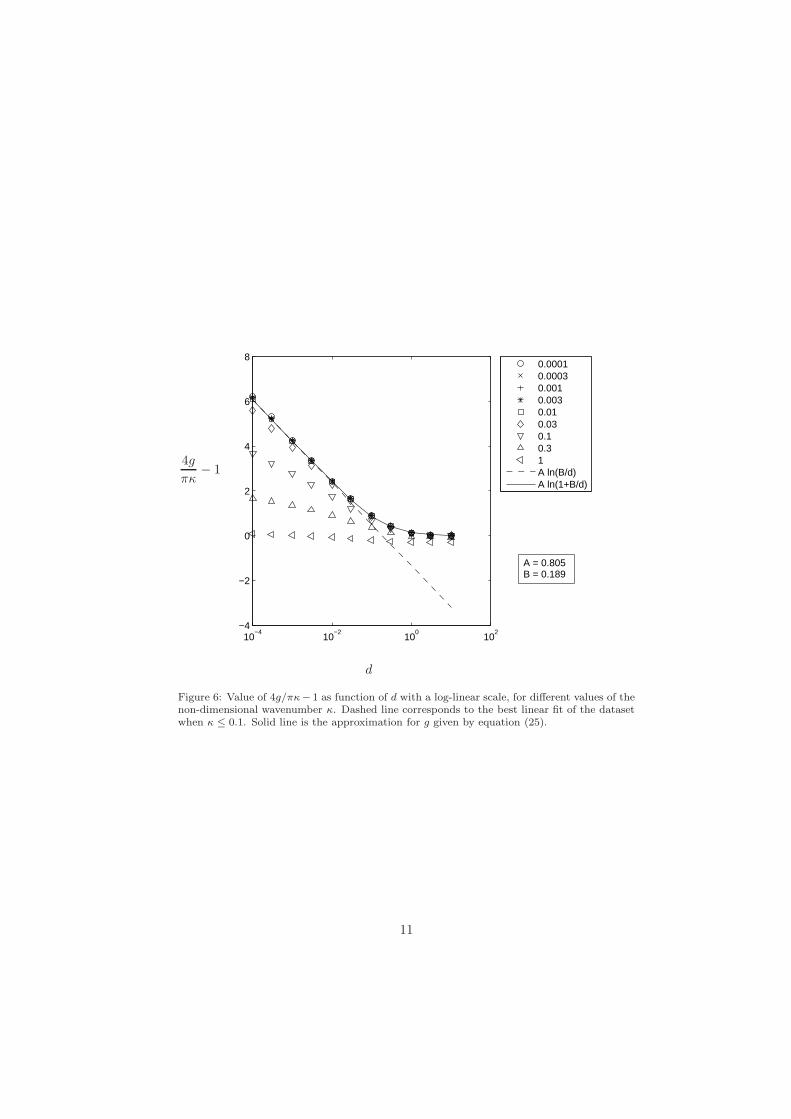
We are now looking for an empirical model describing the value of g for smallκ and any value of the clearance d. In Fig. 6, the value of 4g/πκ− 1 is plottedagainst d and shows that all points gather on a single curve when κ is smallerthan 0.1. This means that g is of the form

gSB(κ, d) =κπ

4fSB(d), for κ≪ 1, (25)

10

10−4

10−2

100

102

−4

−2

0

2

4

6

8

0.00010.00030.0010.0030.010.030.10.31A ln(B/d)A ln(1+B/d)

A = 0.805B = 0.189

4g

πκ− 1

d

Figure 6: Value of 4g/πκ− 1 as function of d with a log-linear scale, for different values of thenon-dimensional wavenumber κ. Dashed line corresponds to the best linear fit of the datasetwhen κ ≤ 0.1. Solid line is the approximation for g given by equation (25).

11

z

2dy

v

Figure 7: Schematic representation of the equivalent problem in the Fourier space using themirror symmetry.

where fSB can be determined by fitting the numerical results

fSB(d) ≈

[

1 + 0.805 ln

(

d+ 0.189

d

)]−1

. (26)

Equation (25) describes the extension of the slender-body theory to account forthe presence of the walls. It is valid for any value of the clearance d as long as κis small enough (κ < 0.1), that is when the wavelength of the deflection is largecompared to the plate span.

3.2. Theoretical calculation

As illustrated in Fig. 7, the Helmotlz problem of a plate moving at constantvelocity between two boundaries given by equations (19-21) can be transformedby replacing the walls by mirror symmetry planes. The equivalent problem isthus an infinite number of similar plates separated by a distance 2d all movingat the same constant velocity v.

Using the Green’s representation theorem, the perturbation potential satis-fies

ϕ(y, z) =

∫

Sp

[ϕ](η) [∂ζH(y, z, η, ζ)]ζ=0dη, (27)

where Sp is the plate surfaces, [ϕ] is the potential jump across the plate (i.e.[ϕ](y) = ϕ(y, 0+)−ϕ(y, 0−) and H is the Green function of the Helmoltz equa-tion in two dimensions

H(y, z, η, ζ) =1

2πK0

(

κ√

(y − η)2 + (z − ζ)2)

, (28)

with Kν the modified Bessel function of the second kind.Differentiating equation (27) with respect to z and taking the limit z = 0

yields

[ϕz ]z=0= ×

∫

Sp

[ϕ](η)F (|y − η|)dη = 1, for |y| < 1, (29)

where the cross on the integral sign stands for the integration in the finite partsense (Hadamard, 1932; Mangler, 1951) and the kernel is

F (y) =κK1(κy)

2πy. (30)

12

Here the integration is not defined in the usual sense because the kernel F (y)behaves like 1/(2πy2) in the limit of small y.

The inverse problem (29) can be solved numerically for a given value ofthe wavenumber κ. To do that, the potential jump [ϕ] is expanded on evenChebyshev polynomials of the second kind such that

[ϕ](y) =√

1 − y2

∞∑

i=1

AiU2i−2(y), (31)

where the prefactor√

1 − y2 ensures the correct behavior as |y| → 1. Insertingthe expansion (31) into equation (29) and evaluating the discrete scalar productwith the Chebyshev polynomials of the first kind Tj(y) leads to a linear systemfor the vector (Ai) which can be solved numerically. The averaged potentialjump along the plate span is then given by 〈[ϕ]〉y = −πA1/2 and therefore thefunction g is

g(κ, d) =πκ

4A1(κ, d). (32)

The theoretical method described here to calculate the averaged potentialjump 〈[ϕ]〉 is complementary to the numerical method described above. It allowsto carry out the calculation in the limit of large wavenumber κ and small gap dwith the product κd asymptotically small. When κ is small however, the numberof plate replicas needed to obtain an accurate calculation of the potential variesas 1/κ. The present theoretical method is therefore not pertinent in this limit.

Examples of such calculations are given in Fig. 8 where the averaged poten-tial jump is given as a function of the gap d for different wavenumbers κ. Forlarge clearance d, the large span approximation obtained by Eloy et al. (2007)is recovered

g(κ, d) ≃ 1 −1

2κ, for d≫ 1, κ≫ 1. (33)

Let us now estimate the function of g in the limit large κ for any value of d.In Fig. 9, (1− g/2κ) is plotted as a function of κd with a logarithmic scale. Allthe points gather on a single curve showing that, in the large-span limit, g is ofthe form

gLS(κ, d) ≃ 1 −f(κd)

2κ, for κ≫ 1. (34)

where f(κd) behaves as a power law for small values of κd. An empirical eval-uation of this function can be found by fitting the results and yields

f(x) ≈

(

1 +0.18

x2

)−0.075

. (35)

The equation (34), where f is given by (35), will be referred to as the largespan approximation for g(κ, d), valid for any value of the clearance d and largevalue of the wavenumber κ, that is when the deflection wavelength is smallcompared to the plate span.

13

10−3

10−2

10−1

100

0.5

0.6

0.7

0.8

0.9

1

1.1

k = 100k = 30k = 10k = 3k = 1

g

d

Figure 8: Function g as a function of the gap d for different values of the wavenumber κ. Thehorizontal lines correspond to the limit d ≫ 1 and the segments between symbols are justguides for the eye.

14

10−4

10−2

100

102

10−1

100

k = 100k = 30k = 10k = 3k = 1CD(κ d)−2D

(1+C/(κ d)2)D

C = 0.18D = −0.075

1 − g

2κ

κd

Figure 9: Function 1− g/2κ as a function of κd for different values of the wavenumber κ. Thedashed line shows the power law 1.14(κd)0.15 and the solid line represents the approximationof g given by equation (34) where f is given by (35).

15

0 0.1 0.2 0.3 0.4 0.5 0.6 0.7 0.8 0.9 10

0.1

0.2

0.3

0.4

0.5

0.6

0.7

0.8

0.9

1

g from empirical model

g fr

om n

umer

ical

or

theo

retic

al d

ata

Figure 10: Complete dataset of the numerical and theoretical values of the averaged pressurejump g, plotted as function of the empirical model ge given by equation (36); (*), numericaldata; (o), theoretical data.

3.3. Empirical model for the pressure jump

In sections 3.1 and 3.2 we have derived empirical models for the functiong(κ, d), valid for small and large values of κ respectively. A good approximationfor all values of κ can be obtained from a composite extension of these twoempirical models,

ge(κ, d) = 1 −

[

1

1 − gLS+ exp

(

gSB −1

1 − gLS

)]−1

, (36)

where the functions gSB and gLS are given by the equations (25) and (34)respectively.

To assess the validity of the above approximation for g, the entire dataset ofnumerical and theoretical values of the pressure jump g is plotted as a functionof ge in Fig. 10. All symbols lie on the line g = ge, indicating that the empir-ical model given by equation (36) correctly predicts the pressure jump with amaximum error of 8% at any value of κ and d.

To solve the problem in the real space, the Fourier transform of 1/ge is nowevaluated to obtain the kernel G given by equation (18). It yields

G(x, h, c) ≈1

x+ sgn(x)

[

π

2

fLS (|x|/c)

h+ 2|x|+

(

4

h−

4

h+ 2|x|

)

fSB(2c/h)

]

, (37)

16

where the function fSB is given by equation (26) and

fLS(x) ≈ (1 + 0.5x)−0.16 . (38)

The functions fSB and fLS describe in the slender-body and large-span limit theeffect of channel confinement. For an asymptotically large channel (i.e. c≫ 1),these functions are equal to one and the kernel G(x, h, c) found in Eloy et al.(2007, 2008) is recovered. On the other hand, when the clearance c goes to zero,these two functions decrease and therefore the kernel G tends to 1/x which isthe two-dimensional limit.

4. Stability analysis

4.1. Galerkin decomposition

Similarly to what was done by Eloy et al. (2007, 2008), the stability analysisis performed by assuming a complex frequency ω, and decomposing the platedeformation on Galerkin modes

w(x, t) = eiωt∑

i

aiwi(x), (39)

where the spatial Galerkin modes wi(x) are the eigenmodes of a clamped-freebeam in vacuo in order to satisfy the boundary conditions in x = 0 and x = 1.

Inserting the decomposition (39) into equation of motion (3) and executingscalar products with the modes wj(x) yields a linear problem for the unknownamplitude vector ai. This eigenvalue problem admits a non trivial solutiononly if the determinant of the linear operator is zero which is achieved for discretevalues of the complex frequency ωi. The real part of these frequency givesthe angular frequency of the oscillations and its imaginary part gives the modegrowth rate σ = −ℑ(ω). For a given eigenmode, the growth rate is a function ofthe dimensionless parameters of the problem: the reduced velocity U∗, the massration M∗, the aspect ratio h and the dimensionless clearance c. The aim of thestability analysis is to find, for a given set of parameters (M∗, h, c), the criticalvalue of the reduced velocity U∗

c(M∗, h, c) above which at least one mode is

unstable (i.e. has a positive growth rate σ).

4.2. Solution for the pressure

The solution for the inverse problem (17) is sought for a given Galerkin modewi

1

2π−

∫ 1

0

p′i(ξ)G(x − ξ, h, c) dξ = (iω + dx)2wi, (40)

where G is given by (37), by expanding p′i on Chebyshev polynomials such that

p′i(x) =

∞∑

j=1

AijTj(2x− 1)√

x(1 − x), (41)

17

10−1

100

101

0

5

10

15

20

25

U∗c

h

Figure 11: Critical velocity as a function of the aspect ratio h for a mass ratio M∗ = 0.5. Thedifferent symbols correspond to different gaps: c = ∞ (circle), c = 1 (star), c = 10−2 (crosse),c = 10−4 (plus); and the dashed line corresponds to the two-dimensional limit h = ∞.

thus assuming an inverse square-root singularity at the leading and trailing edgefor p′i. In this expansion, Tj are the Chebyshev polynomials of the first kind.

Inserting (41) into equation (40) and applying a scalar product with theChebyshev polynomials of the second kind Uk(2x− 1) leads to a linear problemforAij which is solved numerically for given values of the geometrical parametersh and c. The averaged pressure jump 〈[pi]〉 is then found by integrating p′i givenby equation (41). This leads to no singularity on the leading and trailing edges(as the averaged pressure jump goes as x1/2). As it has been discussed in Eloyet al. (2008), it is not physically correct as one expects the pressure jump tohave an inverse square-root singularity at the leading edge. However, it has beenshown in the same paper that taking into account this leaging-edge singularitydo not modify greatly the stability characteristics as the leading edge is clampedand the pressure forces do not work at this position.

In practice, 15 Galerkin modes and 20 Chebyshev polynomials have beenused in the following computations.

4.3. Results

Now that the average pressure jump 〈[pi]〉 for a given Galerkin mode wi canbe found by inverting the problem (40), we are able to compute the eigenmodes

18

10−1

100

101

0

5

10

15

U∗c

M∗

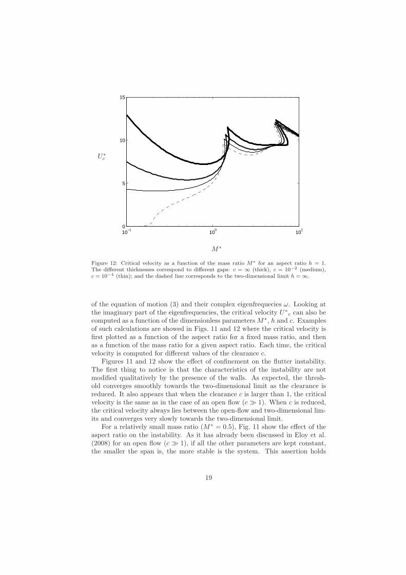
Figure 12: Critical velocity as a function of the mass ratio M∗ for an aspect ratio h = 1.The different thicknesses correspond to different gaps: c = ∞ (thick), c = 10−2 (medium),c = 10−4 (thin); and the dashed line corresponds to the two-dimensional limit h = ∞.

of the equation of motion (3) and their complex eigenfrequecies ω. Looking atthe imaginary part of the eigenfrequencies, the critical velocity U∗

c can also becomputed as a function of the dimensionless parametersM∗, h and c. Examplesof such calculations are showed in Figs. 11 and 12 where the critical velocity isfirst plotted as a function of the aspect ratio for a fixed mass ratio, and thenas a function of the mass ratio for a given aspect ratio. Each time, the criticalvelocity is computed for different values of the clearance c.

Figures 11 and 12 show the effect of confinement on the flutter instability.The first thing to notice is that the characteristics of the instability are notmodified qualitatively by the presence of the walls. As expected, the thresh-old converges smoothly towards the two-dimensional limit as the clearance isreduced. It also appears that when the clearance c is larger than 1, the criticalvelocity is the same as in the case of an open flow (c≫ 1). When c is reduced,the critical velocity always lies between the open-flow and two-dimensional lim-its and converges very slowly towards the two-dimensional limit.

For a relatively small mass ratio (M∗ = 0.5), Fig. 11 show the effect of theaspect ratio on the instability. As it has already been discussed in Eloy et al.(2008) for an open flow (c ≫ 1), if all the other parameters are kept constant,the smaller the span is, the more stable is the system. This assertion holds

19

also when the plate is confined between two walls and the clearance c is keptconstant.

For a square plate (h = 1), Fig. 12 show the influence of the mass ratio onthe instability threshold. This stability diagram exhibits several lobes corre-sponding to different eigenmodes. For M∗ . 1.5, the second mode is the mostunstable (assuming that the modes are ordered with increasing frequency). Notethat, classically, the first mode is always stable for these clamped-free boundaryconditions (see Paıdoussis, 2004, for instance). For 1.5 . M∗ . 6, the thirdeigenmode is the most unstable, and so on. The effect of confinement does notmodify this picture significantly. Figure 12 also show that for large mass ratios,all the curves converge towards U∗

c ≈ 10, for all values of the clearance. This isdue to the fact that the number of mode wavelengths along the plate chord in-creases as M∗ increases. The dimensionless wavenumber κ introduced in section3 thus increases and the pressure jump converges towards its two-dimensionallimit.

5. Discussion

In this article, the effect of channel clearance on the flow-induced instabilityof a cantilevered flat plate has been addressed. Numerical and theoretical cal-culations were performed to obtain the pressure distribution around the platein the Fourier space as function of the various parameters. Using these numer-ical and theoretical data, an empirical model for the pressure jump has beenderived. This model allowed to compute the eigenfrequencies of the coupledflow-structure problem. Critical velocities for the flutter instability as a func-tion of the different parameters of the problem have then been computed. Asexpected, when the clearance is reduced to zero, the critical velocity was foundto approach the limit predicted by a two-dimensional model. However, this limitwas found to be reached only for very small values of the clearance. Indeed fora value as small as c = 10−4, a large discrepancy between the two-dimensionalmodel and our empirical model persists. The mass ratio effect has also beeninvestigated, and it has been observed that the influence of the rigid walls ismore pronounced for relatively heavy and rigid plates (i.e. M∗ < 1).

These results raise the following question: for heavy and rigid plates, is thecomparison between two-dimensional models and experiments relevant ? In-deed, the value of the clearance would have to be far smaller than 10−4, whichis unattainable experimentally. Among the works that investigated experimen-tally the flutter of plates in channel flow, the values of the clearance can beestimated to be O(1) (Yamaguchi et al., 2000) or O(10−2) (Huang, 1995). Ourresults indicate that the flow in these experimental studies cannot be consid-ered two-dimensional to correctly predict critical velocities for such values ofthe clearance. In the work of Auregan and Depollier (1995), the clearance hasa value of approximately 10−2 (Auregan, 2010), and the same recommenda-tion should apply. But here, the channel confinement in the Y -direction is alsoimportant, which effect can be roughly estimated as an increase of the massratio M∗. The present article shows that this has for consequence to reduce the

20

influence of the channel clearance. A two-dimensional model has hence morechances to give satisfying results in this case. Regarding the experimental workof Watanabe et al. (2002b), our model is probably not applicable in this casebecause the authors observed three-dimensional deformations of the paper sheetwhen small clearance values of order 10−2 were attained. This is not compatiblewith our one-dimensional deformation hypothesis. In conclusion, the only caseswhere a two-dimensional approximation is pertinent are the very long and/orvery flexible plates (i.e. M∗ ≫ 1) or the soap film experiments such as theexperimental work of Zhang et al. (2000).

These observations indicates that an experimental work focusing on the ef-fect of channel clearance would be necessary to complement the theoreticalresults of the present article. Also, extending our model to take into accountthe confinement in the transverse direction would bring some insight into theinstability phenomenon, and would fill the gap between the flag-type problemand the snoring or leakage flow problems.

References

Alben, S., Shelley, M.J., 2008. Flapping states of a flag in an inviscid fluid:Bistability and the transition to chaos. Physical Review Letters 100, 074301.

Auregan, Y., 2010. Private Communication.

Auregan, Y., Depollier, C., 1995. Snoring: Linear stability and in-vitro experi-ments. Journal of Sound and Vibration 188, 39–53.

Balint, T.S., Lucey, A.D., 2005. Instability of a cantilevered flexible plate inviscous channel flow. Journal of Fluids and Structures 20, 893–912.

Datta, S., Gottenberg, W., 1975. Instability of an elastic strip hanging in anairstream. Journal of Applied Mechanics 42, 195–198.

Eloy, C., Lagrange, R., Souilliez, C., Schouveiler, L., 2008. Aeroelastic instabil-ity of cantilevered flexible plates in uniform flow. Journal of Fluid Mechanics611, 97–106.

Eloy, C., Souilliez, C., Schouveiler, L., 2007. Flutter of a rectangular plate.Journal of Fluids and Structures 23, 904–919.

Guo, C.Q., Paidoussis, M.P., 2000. Stability of Rectangular Plates With FreeSide-Edges in Two-Dimensional Inviscid Channel Flow. Journal of AppliedMechanics 67, 171–176.

Hadamard, J., 1932. Lectures on Cauchy’s problem in linear differential equa-tion. Dover, New York.

Howell, R.M., Lucey, A.D., Carpenter, P.W., Pitman, M.W., 2009. Interactionbetween a cantilevered-free flexible plate and ideal flow. Journal of Fluidsand Structures 25, 544–566.

21

Huang, L., 1995. Flutter of cantilevered plates in axial flow. Journal of Fluidsand Structures 9, 127–147.

Kornecki, A., Dowell, E.H., O’Brien, J., 1976. On the aeroelastic instability oftwo-dimensional panels in uniform incompressible flow. Journal of Sound andVibration 47, 163–178.

Lemaitre, C., Hemon, P., de Langre, E., 2005. Instability of a long ribbonhanging in axial air flow. Journal of Fluids and Structures 20, 913–925.

Lighthill, M., 1960. Note on the swimming of slender fish. Journal of FLuidMechanics 9, 305–317.

Mangler, K.W., 1951. Improper integrals in theoretical aerodynamics. Tech.Rep. Aero 2424. British Aeronautical Research Council.

Michelin, S., Llewellyn Smith, S.G., 2009. Linear stability analysis of coupledparallel flexible plates in an axial flow. Journal of Fluids and Structures 25,1136–1157.

Michelin, S., Llewellyn Smith, S.G., Glover, B.J., 2008. Vortex shedding modelof a flapping flag. Journal of Fluid Mechanics 607, 109–118.

Paıdoussis, M.P., 2004. Fluid-structure Interactions. Slender Structures andAxial Flow. volume 2. Academic Press.

Rayleigh, L., 1879. On the instability of jets. Proc. London Mat. Soc. X, 4–13.

Taneda, S., 1968. Waving motions of flags. Journal of the Physical Society ofJapan 24, 392–401.

Tang, L., Paıdoussis, M.P., 2007. On the instability and the post-critical be-haviour of two-dimensional cantilevered flexible plates in axial flow. Journalof Sound and Vibration 305, 97–115.

Theodorsen, T., 1935. General theory of aerodynamic instability and the mech-anism of flutter. NACA Report 496.

Watanabe, Y., Isogai, K., Suzuki, S., Sugihara, M., 2002a. A theoretical studyof paper flutter. Journal of Fluids and Structures 16, 543–560.

Watanabe, Y., Suzuki, S., Sugihara, M., Sueoka, Y., 2002b. An experimentalstudy of paper flutter. Journal of Fluids and Structures 16, 529–542.

Wu, X., Kaneko, S., 2005. Linear and nonlinear analyses of sheet flutter inducedby leakage flow. Journal of Fluids and Structures 20, 927–948.

Yamaguchi, N., Sekiguchi, T., Yokota, K., Tsujimoto, Y., 2000. Flutter Limitsand Behavior of a Flexible Thin Sheet in High-Speed Flow– II: ExperimentalResults and Predicted Behaviors for Low Mass Ratios. Journal of FluidsEngineering 122, 74–83.

22

Zhang, J., Childress, S., Libchaber, A., Shelley, M., 2000. Flexible filaments ina flowing soap film as a model for one-dimensional flags in a two-dimensionalwind. Nature 408, 835–839.

23