Fluid-Dynamic Force Measurement of Ahmed Model in Steady ...

energies

Article

Fluid-Dynamic Force Measurement of Ahmed Modelin Steady-State Cornering

Takuji Nakashima 1,*, Hidemi Mutsuda 1 , Taiga Kanehira 1 and Makoto Tsubokura 2,3

1 Graduate School of Advanced Science and Engineering, Hiroshima University, 1-4-1 Kagamiyama,Higashi-Hiroshima, Hiroshima 739-8527, Japan; [email protected] (H.M.);[email protected] (T.K.)

2 RIKEN Center for Computational Science (R-CCS), 7-1-26 Minatojima-minami-machi, Chuo-ku, Kobe,Hyogo 650-0047, Japan; [email protected] or [email protected]

3 Graduate School of System Informatics, Kobe University, 1-1, Rokkodai-cho, Nada-ku, Kobe-shi,Hyogo 657-8501, Japan

* Correspondence: [email protected]

Received: 20 November 2020; Accepted: 11 December 2020; Published: 14 December 2020 ��

Abstract: The effects of on-road disturbances on the aerodynamic drag are attracting attentionin order to accurately evaluate the fuel efficiency of an automobile on a road. The present studyinvestigated the effects of cornering motion on automobile aerodynamics, especially focusing on theaerodynamic drag. Using a towing tank facility, measurements of the fluid-dynamic force acting onAhmed models during steady-state cornering were conducted in water. The investigation includedAhmed models with slant angles θ = 25◦ and 35◦, reproducing the wake structures of two differenttypes of automobiles. The drag increase due to steady-state cornering motion was experimentallymeasured, and showed good agreement with previous numerical research, with the measurementsconducted at a Reynolds number of 6 × 105, based on the model length. The Ahmed model withθ = 35◦ showed a greater drag increase due to the steady-state cornering motion than that withθ = 25◦, and it reached 15% of the total drag at a corner with a radius that was 10 times the vehiclelength. The results indicated that the effect of the cornering motion on the automobile aerodynamicswould be more important, depending on the type of automobile and its wake characteristics.

Keywords: aerodynamics; automobile; cornering; Ahmed model; drag increase; on-road condition;towing tank test

1. Introduction

In recent years, the aerodynamic drag performance of an automobile has become more importantfor its fuel efficiency because the efficiency of the powertrain has rapidly been improved throughhybridization, electrification, and the improvement of combustion technology. In the conventionaldevelopment process of vehicle aerodynamics, a vehicle subjected to a steady and uniform airflow in awind tunnel or numerical simulation has been considered. This condition assumes a relative airflowacting on a vehicle running at a constant speed and a steady posture in stationary air. Additionally,the changes in the relative wind direction caused by on-road disturbance and their effects havebeen investigated using the so-called yaw condition or steady crosswind method [1], in which a realautomobile [2] or an experimental vehicle model [3–5] is placed at a steady yaw angle with respect to auniform flow. However, the impact of more realistic on-road disturbances on automobile aerodynamicshas attracted attention to further increase the accuracy when evaluating the aerodynamic performanceof an automobile on a road. For example, the on-road turbulence properties [6,7] and the effects of theirfluctuation on the aerodynamic drag [8–10] have been investigated. The changes in the aerodynamic

Energies 2020, 13, 6592; doi:10.3390/en13246592 www.mdpi.com/journal/energies

http://www.mdpi.com/journal/energies

http://www.mdpi.com

https://orcid.org/0000-0003-4403-5590

http://dx.doi.org/10.3390/en13246592

http://www.mdpi.com/journal/energies

https://www.mdpi.com/1996-1073/13/24/6592?type=check_update&version=2

Energies 2020, 13, 6592 2 of 20

drag due to more specific disturbances from a passing vehicle [11] have also been reported. Moreover,vehicle motion, which is another type of on-road disturbance, also affects the aerodynamics. As atypical vehicle motion on a road, the effects of a cornering motion on the aerodynamics have beeninvestigated [12–16].

Although vehicle cornering is accompanied by a complicated posture change, the main componentother than the forward motion is the yaw rotation. Because of the yaw rotation, the yaw angle of thefree-stream flow acting on the vehicle is distributed in the longitudinal direction of the vehicle [13].This spatial distribution of the relative flow direction causes the aerodynamics to be different fromthose under the general yaw condition in a wind tunnel. This effect should be clarified to understandthe vehicle aerodynamics during cornering. Keogh et al. [13] conducted a large-eddy simulation of asimplified vehicle body during cornering. They reported the cornering effects on the aerodynamicsand clarified the related aerodynamic phenomena. The cornering effects increased the drag force andgenerated a side force toward the center of the corner, as well as a yaw moment that dampened the yawrotation. Josefsson et al. [14] conducted a steady Reynolds-averaged Navier–Stokes (RANS) simulationof a sedan-type vehicle during steady-state cornering and indicated that the asymmetric geometryof the underbody affected the drag increase due to the cornering motion. Tsubokura et al. [15] andOkada et al. [16] numerically investigated the unsteady aerodynamic characteristics of a sedan-typevehicle during meandering motion, focusing on the responses of the side force and yaw moment inrelation to the drivability of the automobile. These researchers adopted special numerical techniquesusing non-inertial reference frame and modified boundary condition [17] for vehicle aerodynamics toreproduce the cornering motion. However, they investigated the cornering effects on the aerodynamicsfor a specific vehicle geometry, with the shape variation in the research limited to details of the bodyshape [14] or aerodynamic parts [15,16]. To understand the effects more universally, it would be effectiveto investigate the effects on vehicles with different fundamental aerodynamic characteristics underthe same cornering condition. A typical difference in the fundamental aerodynamic characteristicsis a difference in the wake flow structure, which is generally classified as a notch-back, fast-back,or square-back type of flow in association with the classical rear end shapes [18].

Furthermore, it is difficult to conduct wind tunnel experiments that reproduce the effects ofcornering motion because the streamlines of the relative airflow observed from the cornering vehicle arenot straight but curved. When a curved test section is used to generate the curved free-stream, the flowvelocity is distributed in the radial direction, and a pressure gradient balanced by the centrifugalforce is also generated. Even when other special techniques are used, such as a bent model [19],which reproduces the effects of curved flow in a straight flow field, or a special wind tunnel witha rotating test section [20] designed to cancel out the radial pressure distribution, it is difficult toprecisely and flexibly reproduce the relative flow acting on a cornering vehicle. On the other hand,a ship model basin for a towing test, which is generally used to measure the hydrodynamic forceacting on a ship model, can measure the fluid-dynamic forces under steady-state cornering conditions,which is the so-called circular motion test (CMT) [21]. Such towing tank facilities can directly applythe cornering motion to a vehicle model, without requiring the Galilean transformation assumed inwind tunnel measurements. Moreover, because a towing tank uses water as the fluid, it has otheradvantages over a wind tunnel that uses air. Due to the lower dynamic viscosity, the similar flow at thesame Reynolds number can be observed as a relatively slower phenomenon in the water tank. Due tothe higher density of water, relatively larger fluid-dynamic force acts on the same length-scale modelin the similar flow field, allowing for more accurate measurements. Therefore, some towing tanktests on automobile aerodynamics [22–25] have already been reported. When moving ground systemswere not standard in automobile aerodynamics measurement, some studies on the ground effect ofautomobile aerodynamics have been conducted in a towing tank, taking the advantage of not requiringthe Galilean transformation. Vorwaller and Germane [22] towed two race-car models with a lengthof 0.25 m to measure the drag force under the ground effect with rolling wheels. Larsson et al. [23]towed a real production automobile in a water basin to investigate the ground effect. They measured

Energies 2020, 13, 6592 3 of 20

fluid-dynamic drag and lift forces and compared them with the wind tunnel measurement. From thecomparisons, they reported a considerable over estimation of lift force in a wind tunnel with a groundsimulation using upstream boundary layer suction, while the drag force in both facilities showedgood agreement. Aoki et al. [24] conducted towing tests of a one-fifth-scale sedan-type automobilemodel in a ship model basin to measure the fluid-dynamic force and surface pressure acting on theautomobile model under the ground effect, and to visualize the flow around the vehicle. Towing tanktests have also been used to measure the fluid-dynamic responses of automobile models with pitchingmotion [25]. Because the density of the experimental model can easily be close to the density of water,the inertial force due to the model acceleration becomes relatively smaller than that during wind tunnelmeasurements. This characteristic is also suitable for the fluid dynamics measurement of a vehicleduring cornering motion because the cornering motion is an accelerating motion in the lateral directionof the vehicle. In our previous research [26,27], the fluid-dynamic force acting on a one-fifth-scalemodel of a sedan-type automobile during steady-state cornering was measured in a towing tank facility.These measurements clarified the characteristics of the side force and yaw moment, which were similarto those with a simplified model [13], focusing on the aerodynamic effects on the drivability. However,the effects of the cornering motion on the drag force were not experimentally measured and clarified.Moreover, the measurement was conducted on one vehicle model without geometric variation.

In research on automobile aerodynamics, the shapes of actual automobiles are too complicatedto draw a universal conclusion. Therefore, fundamental research on automobile aerodynamics oftenuses a very simplified vehicle model that reproduces the essential characteristics of the flow aroundan automobile. The simplified model proposed by Ahmed et al. [28], the so-called Ahmed modelor Ahmed body, is one of the most famous models in the automobile aerodynamics research field.As shown in Figure 1, this model has a smooth round head and a box-shaped body with a slantsurface from the rear end of the roof to the top of the base. Only slant angle θ is a shape parameterthat affects the aerodynamic characteristics of the model. In particular, at the critical slant angleof 30◦, the drag and lift change drastically with the wake structure. The differences in the wakestructure and the detailed characteristics of the flow field before and after the critical slant anglehave been investigated using experimental measurements [28–31] and numerical analyses [32,33].Slant angles θ = 25◦ and θ = 35◦ have often been adopted as the subcritical and postcritical conditions.The subcritical model with θ = 25◦ shows a highly three-dimensional flow (called a “three-dimensionalseparated (TDS) flow” [31] or “strongly three-dimensional wake” [32]), in which the flow separated atthe leading edge of the slant surface reattaches to the surface. The post-critical flow field representedby θ = 35◦ has a pseudo two-dimensional flow structure (called a “quasi-axisymmetric- separated(QAS) flow” [31] or “quasi-two-dimensional wake” [32]), with uniformity in the lateral direction ofthe model without any reattachment of the flow onto the slanted surface. These wake structurescan be regarded as fast-back and square-back flows in the classification of the wake structures ofautomobiles [18], respectively. Furthermore, Ahmed models with different wake structures haveshown significantly different response characteristics to disturbances [1,4,34]. Regarding the responseto a steady crosswind condition, only the postcritical model showed aerodynamic bi-stability undera certain yaw angle condition [4]. The responses of the wake velocity distribution and turbulencecharacteristics to a steady crosswind were also different between the sub- and post-critical models [1].The aerodynamic responses to changes in the relative wind speed [34] also showed some differenttrends for the drag and lift behaviors between the sub- and post-critical models. These results impliedthe importance of considering the difference in the wake structure in research on the aerodynamicresponse of a vehicle to an on-road disturbance.

The purpose of this study was to experimentally measure the effects of a cornering motion onvehicles’ aerodynamics, especially the aerodynamic drag, and to further understand their characteristics.For this purpose, fluid-dynamic force measurements were conducted on vehicle models duringcornering using a towing tank facility to experimentally clarify the cornering effects. To clarifythe universal characteristics of the cornering effects, simplified vehicle models with different wake

Energies 2020, 13, 6592 4 of 20

characteristics were investigated. Ahmed models with different slant angles, for which the wakestructures could be categorized as those of square-back and fast-back type automobiles, were chosen asthe investigated vehicle models. To validate the measurement results, the influences of the submersiondepth and towing speed were investigated, and the fluid-dynamic force was compared with thatin previous numerical research [13]. Then, the cornering effects on the fluid-dynamic force werequantitatively clarified. This investigation focused on the differences in the effects between thetwo models, which should have depended on their different wake characteristics. Furthermore,the characteristics of the change in the fluid-dynamic force due to the cornering motion were alsoexamined in comparison with a uniform crosswind condition. This investigation clarified the similaritiesand differences in the aerodynamic characteristics of a cornering vehicle compared to the steadycrosswind aerodynamics that can be measured in general wind-tunnel tests.

Energies 2020, 13, x FOR PEER REVIEW 4 of 20

the influences of the submersion depth and towing speed were investigated, and the fluid-dynamic force was compared with that in previous numerical research [13]. Then, the cornering effects on the fluid-dynamic force were quantitatively clarified. This investigation focused on the differences in the effects between the two models, which should have depended on their different wake characteristics. Furthermore, the characteristics of the change in the fluid-dynamic force due to the cornering motion were also examined in comparison with a uniform crosswind condition. This investigation clarified the similarities and differences in the aerodynamic characteristics of a cornering vehicle compared to the steady crosswind aerodynamics that can be measured in general wind-tunnel tests.

(a)

(b)

(c)

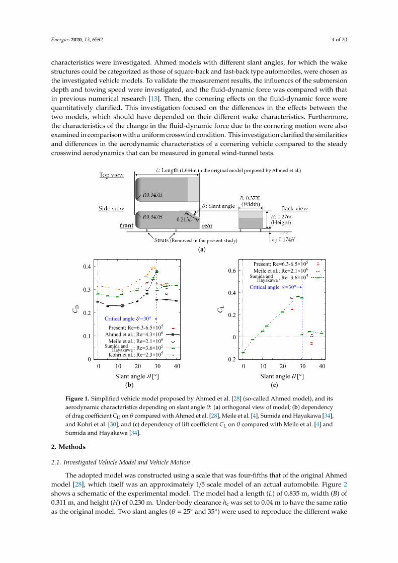
Figure 1. Simplified vehicle model proposed by Ahmed et al. [28] (so-called Ahmed model), and its aerodynamic characteristics depending on slant angle θ: (a) orthogonal view of model; (b) dependency of drag coefficient CD on θ compared with Ahmed et al. [28], Meile et al. [4], Sumida and Hayakawa [34], and Kohri et al. [30]; and (c) dependency of lift coefficient CL on θ compared with Meile et al. [4] and Sumida and Hayakawa [34].

2. Methods

2.1. Investigated Vehicle Model and Vehicle Motion

The adopted model was constructed using a scale that was four-fifths that of the original Ahmed model [28], which itself was an approximately 1/5 scale model of an actual automobile. Figure 2 shows a schematic of the experimental model. The model had a length (L) of 0.835 m, width (B) of 0.311 m, and height (H) of 0.230 m. Under-body clearance hc was set to 0.04 m to have the same ratio as the original model. Two slant angles (θ = 25° and 35°) were used to reproduce the different wake structures for fast-back and square-back type automobiles [18], respectively. They were realized using exchangeable rear parts for the model. The four struts under the body in the original geometry were removed, and a circular rod covered by a part of the wing section was introduced to suspend the model from above.

0

0.1

0.2

0.3

0.4

0 10 20 30 40

Critical angle =30°

Sumida andHayakawa

CD

Slant angle [°]

Present; Re=6.3-6.5×105

Ahmed et al.; Re=4.3×106

Meile et al.; Re=2.1×106

; Re=3.6×105

Kohri et al.; Re=2.3×105-0.2

0

0.2

0.4

0.6

0 10 20 30 40

Critical angle =30°

Sumida andHayakawa

CL

Slant angle [°]

Present; Re=6.3-6.5×105

Meile et al.; Re=2.1×106

; Re=3.6×105

Figure 1. Simplified vehicle model proposed by Ahmed et al. [28] (so-called Ahmed model), and itsaerodynamic characteristics depending on slant angle θ: (a) orthogonal view of model; (b) dependencyof drag coefficient CD on θ compared with Ahmed et al. [28], Meile et al. [4], Sumida and Hayakawa [34],and Kohri et al. [30]; and (c) dependency of lift coefficient CL on θ compared with Meile et al. [4] andSumida and Hayakawa [34].

2. Methods

2.1. Investigated Vehicle Model and Vehicle Motion

The adopted model was constructed using a scale that was four-fifths that of the original Ahmedmodel [28], which itself was an approximately 1/5 scale model of an actual automobile. Figure 2shows a schematic of the experimental model. The model had a length (L) of 0.835 m, width (B) of0.311 m, and height (H) of 0.230 m. Under-body clearance hc was set to 0.04 m to have the same ratioas the original model. Two slant angles (θ = 25◦ and 35◦) were used to reproduce the different wake

Energies 2020, 13, 6592 5 of 20

structures for fast-back and square-back type automobiles [18], respectively. They were realized usingexchangeable rear parts for the model. The four struts under the body in the original geometry wereremoved, and a circular rod covered by a part of the wing section was introduced to suspend themodel from above.Energies 2020, 13, x FOR PEER REVIEW 5 of 20

Figure 2. Schematic image of experimental model. The figure shows the dimensions, configuration, and inner structure of the model, with the side and top of the left half of the body translucent. The sub-figure on the upper right shows the cross-sectional geometry of the strut.

Figure 3 shows the definitions of the investigated vehicle motions and coordinate system fixed on the vehicle. One is the steady-state cornering motion, and the other is a side-slip motion simulating the steady crosswind condition. The steady-state cornering motion consisted of constant yaw rate ω at the center of the model and constant forwarding speed Ut, which was given as the towing speed in the measurement, as shown in Figure 3a. The relationship between normalized yaw rate ω’ = ω/(Ut/L) and cornering radius R = Ut/ω during the steady-state cornering motion can be derived as follows. Thus, normalized cornering radius R’ = R/L becomes a reciprocal of ω’. For a discussion of a local fluid-dynamic response at the rear part of the model, the local yaw angle at the trailing edges of the model is defined as βTE.

ω’ = ω/(Ut/L) = (Ut/R)/(Ut/L) = (R/L)−1. (1)

Based on yaw rate ω and distance L/2 from the rotational center to the edges, βTE during steady state cornering can be determined as follows:

βTE = tan−1{−(L/2) ω/Ut} ≈ −Lω/2Ut = −ω’/2 [rad], (2)

assuming ω’ << 1. Another investigated vehicle motion is a straight towing motion with constant speed Ut and yaw

angle β, as shown in Figure 3b. It reproduces the steady crosswind condition where the uniform relative flow acts on the model at yaw angle β. The βTE value was the same as yaw angle β at the model center because of the uniform relative flow.

(a)

(b)

Figure 3. Definitions of vehicle motions and their components: (a) steady-state cornering motion parameterized by forwarding speed Ut and yaw rate ω at longitudinal center of model; and (b) steady crosswind condition parameterized by Ut and yaw angle β. In addition, definitions of a coordinate system x-y-z fixed on the vehicle and the local yaw angle βLE at the trailing edge are also drawn.

Figure 2. Schematic image of experimental model. The figure shows the dimensions, configuration,and inner structure of the model, with the side and top of the left half of the body translucent.The sub-figure on the upper right shows the cross-sectional geometry of the strut.

Figure 3 shows the definitions of the investigated vehicle motions and coordinate system fixed onthe vehicle. One is the steady-state cornering motion, and the other is a side-slip motion simulating thesteady crosswind condition. The steady-state cornering motion consisted of constant yaw rate ω at thecenter of the model and constant forwarding speed Ut, which was given as the towing speed in themeasurement, as shown in Figure 3a. The relationship between normalized yaw rate ω’ = ω/(Ut/L)and cornering radius R = Ut/ω during the steady-state cornering motion can be derived as follows.Thus, normalized cornering radius R’ = R/L becomes a reciprocal of ω’. For a discussion of a localfluid-dynamic response at the rear part of the model, the local yaw angle at the trailing edges of themodel is defined as βTE.

ω′ = ω/(Ut/L) = (Ut/R)/(Ut/L) = (R/L)−1. (1)

Based on yaw rate ω and distance L/2 from the rotational center to the edges, βTE during steadystate cornering can be determined as follows:


assuming ω’ << 1.Another investigated vehicle motion is a straight towing motion with constant speed Ut and

yaw angle β, as shown in Figure 3b. It reproduces the steady crosswind condition where the uniformrelative flow acts on the model at yaw angle β. The βTE value was the same as yaw angle β at the modelcenter because of the uniform relative flow.


Figure 2. Schematic image of experimental model. The figure shows the dimensions, configuration, and inner structure of the model, with the side and top of the left half of the body translucent. The sub-figure on the upper right shows the cross-sectional geometry of the strut.

Figure 3 shows the definitions of the investigated vehicle motions and coordinate system fixed on the vehicle. One is the steady-state cornering motion, and the other is a side-slip motion simulating the steady crosswind condition. The steady-state cornering motion consisted of constant yaw rate ω at the center of the model and constant forwarding speed Ut, which was given as the towing speed in the measurement, as shown in Figure 3a. The relationship between normalized yaw rate ω’ = ω/(Ut/L) and cornering radius R = Ut/ω during the steady-state cornering motion can be derived as follows. Thus, normalized cornering radius R’ = R/L becomes a reciprocal of ω’. For a discussion of a local fluid-dynamic response at the rear part of the model, the local yaw angle at the trailing edges of the model is defined as βTE.

ω’ = ω/(Ut/L) = (Ut/R)/(Ut/L) = (R/L)−1. (1)

Based on yaw rate ω and distance L/2 from the rotational center to the edges, βTE during steady state cornering can be determined as follows:


assuming ω’ << 1. Another investigated vehicle motion is a straight towing motion with constant speed Ut and yaw

angle β, as shown in Figure 3b. It reproduces the steady crosswind condition where the uniform relative flow acts on the model at yaw angle β. The βTE value was the same as yaw angle β at the model center because of the uniform relative flow.

(a)

(b)

Figure 3. Definitions of vehicle motions and their components: (a) steady-state cornering motion parameterized by forwarding speed Ut and yaw rate ω at longitudinal center of model; and (b) steady crosswind condition parameterized by Ut and yaw angle β. In addition, definitions of a coordinate system x-y-z fixed on the vehicle and the local yaw angle βLE at the trailing edge are also drawn.

Figure 3. Definitions of vehicle motions and their components: (a) steady-state cornering motionparameterized by forwarding speed Ut and yaw rate ω at longitudinal center of model; and (b) steadycrosswind condition parameterized by Ut and yaw angle β. In addition, definitions of a coordinatesystem x-y-z fixed on the vehicle and the local yaw angle βLE at the trailing edge are also drawn.

Energies 2020, 13, 6592 6 of 20

Here and after, the measurements for the steady-state cornering motion are called the resultsof the “circular motion test” (CMT) [21]. Moreover, the measurements under the steady crosswindcondition and the straight towing measurements with a zero yaw angle are called the results of the“steady cross-wind test” (SCW) and “straight motion test” (SMT), respectively.

2.2. Experimental Setup

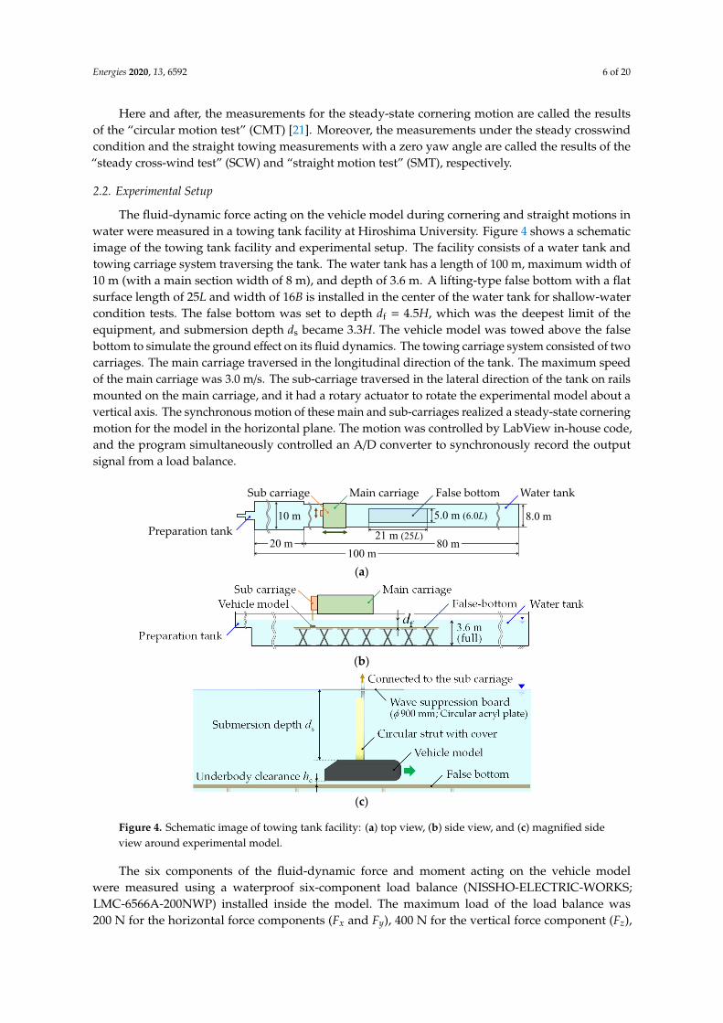
The fluid-dynamic force acting on the vehicle model during cornering and straight motions inwater were measured in a towing tank facility at Hiroshima University. Figure 4 shows a schematicimage of the towing tank facility and experimental setup. The facility consists of a water tank andtowing carriage system traversing the tank. The water tank has a length of 100 m, maximum width of10 m (with a main section width of 8 m), and depth of 3.6 m. A lifting-type false bottom with a flatsurface length of 25L and width of 16B is installed in the center of the water tank for shallow-watercondition tests. The false bottom was set to depth df = 4.5H, which was the deepest limit of theequipment, and submersion depth ds became 3.3H. The vehicle model was towed above the falsebottom to simulate the ground effect on its fluid dynamics. The towing carriage system consisted of twocarriages. The main carriage traversed in the longitudinal direction of the tank. The maximum speedof the main carriage was 3.0 m/s. The sub-carriage traversed in the lateral direction of the tank on railsmounted on the main carriage, and it had a rotary actuator to rotate the experimental model about avertical axis. The synchronous motion of these main and sub-carriages realized a steady-state corneringmotion for the model in the horizontal plane. The motion was controlled by LabView in-house code,and the program simultaneously controlled an A/D converter to synchronously record the outputsignal from a load balance.


Here and after, the measurements for the steady-state cornering motion are called the results of the “circular motion test” (CMT) [21]. Moreover, the measurements under the steady crosswind condition and the straight towing measurements with a zero yaw angle are called the results of the “steady cross-wind test” (SCW) and “straight motion test” (SMT), respectively.

2.2. Experimental Setup

The fluid-dynamic force acting on the vehicle model during cornering and straight motions in water were measured in a towing tank facility at Hiroshima University. Figure 4 shows a schematic image of the towing tank facility and experimental setup. The facility consists of a water tank and towing carriage system traversing the tank. The water tank has a length of 100 m, maximum width of 10 m (with a main section width of 8 m), and depth of 3.6 m. A lifting-type false bottom with a flat surface length of 25L and width of 16B is installed in the center of the water tank for shallow-water condition tests. The false bottom was set to depth df = 4.5H, which was the deepest limit of the equipment, and submersion depth ds became 3.3H. The vehicle model was towed above the false bottom to simulate the ground effect on its fluid dynamics. The towing carriage system consisted of two carriages. The main carriage traversed in the longitudinal direction of the tank. The maximum speed of the main carriage was 3.0 m/s. The sub-carriage traversed in the lateral direction of the tank on rails mounted on the main carriage, and it had a rotary actuator to rotate the experimental model about a vertical axis. The synchronous motion of these main and sub-carriages realized a steady-state cornering motion for the model in the horizontal plane. The motion was controlled by LabView in-house code, and the program simultaneously controlled an A/D converter to synchronously record the output signal from a load balance.

(a)

(b)

(c)

Figure 4. Schematic image of towing tank facility: (a) top view, (b) side view, and (c) magnified side view around experimental model.

The six components of the fluid-dynamic force and moment acting on the vehicle model were measured using a waterproof six-component load balance (NISSHO-ELECTRIC-WORKS; LMC-6566A-200NWP) installed inside the model. The maximum load of the load balance was 200 N for the horizontal force components (Fx and Fy), 400 N for the vertical force component (Fz), and 20 Nm for all three moments (Mx, My, and Mz). Based on the results of the calibration test at the full scale of the load, the maximum hysteresis and non-linearity of each force component were less than 0.10 N

Main carriageSub carriage False bottom

100 m

8.0 m21 m (25L)

5.0 m (6.0L)Preparation tank

80 m20 m

10 m

Water tank

Figure 4. Schematic image of towing tank facility: (a) top view, (b) side view, and (c) magnified sideview around experimental model.

The six components of the fluid-dynamic force and moment acting on the vehicle modelwere measured using a waterproof six-component load balance (NISSHO-ELECTRIC-WORKS;LMC-6566A-200NWP) installed inside the model. The maximum load of the load balance was200 N for the horizontal force components (Fx and Fy), 400 N for the vertical force component (Fz),

Energies 2020, 13, 6592 7 of 20

and 20 Nm for all three moments (Mx, My, and Mz). Based on the results of the calibration test atthe full scale of the load, the maximum hysteresis and non-linearity of each force component wereless than 0.10 N and 0.046 N, respectively. These errors corresponded to force coefficients of 0.0045and 0.0020, respectively, at a towing speed of 0.80 m/s. In the same evaluation for the moment errors,the summation of the maximum hysteresis and non-linearity was 7 × 10−4 in terms of the momentcoefficients. The interference between the six components was linearly corrected using a correctionmatrix. As shown in Figure 2, the balance was supported by a stainless circular rod that penetrated theroof of the model with 2 mm of clearance to measure the fluid-dynamic force acting on the model,except for the strut. The circular rod was connected to the sub-carriage of the towing tank facility,and electric cables from the load balance were connected to an amplifier through the inside of a rodcover, which had the cross-sectional shape of the trailing part of the NACA0040 wing section. The strainoutput from the load balance was amplified by a dynamic strain amplifier (IZUMISOKKI; DA-18K)and recorded by a 16-bit A/D converter (NI; PCIe-6321). In the CMT, the sampling rate was set to20 Hz, similar to the control rate of the towing carriage, and the data were recorded with the carriagemotion simultaneously. The output signal was filtered by a 10 Hz low pass filter at the amplifier priorto the A/D conversion. Under the other measurement conditions, the output signal was filtered by30 Hz low pass filter and sampled at 100 Hz.

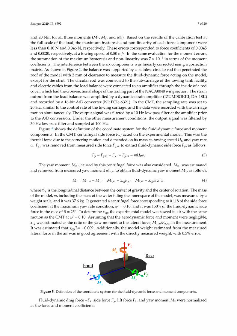
Figure 5 shows the definition of the coordinate system for the fluid-dynamic force and momentcomponents. In the CMT, centrifugal side force Fy,i acted on the experimental model. This was theinertial force due to the cornering motion and depended on its mass m, towing speed Ut, and yaw rateω. Fy,i was removed from measured side force Fy,m to extract fluid-dynamic side force Fy, as follows:

Fy = Fy,m − Fy,i = Fy,m − mUtω. (3)

The yaw moment, Mz,i, caused by this centrifugal force was also considered. Mz,i was estimatedand removed from measured yaw moment Mz,m to obtain fluid-dynamic yaw moment Mz, as follows:

Mz = Mz,m −Mz,i = Mz,m − xcgFy,I = Mz,m − xcgmUtω, (4)

where xcg is the longitudinal distance between the center of gravity and the center of rotation. The massof the model, m, including the mass of the water filling the inner space of the model, was measured by aweight scale, and it was 37.6 kg. It generated a centrifugal force corresponding to 0.118 of the side forcecoefficient at the maximum yaw rate condition, ω’ = 0.10, and it was 150% of the fluid-dynamic sideforce in the case of θ = 25◦. To determine xcg, the experimental model was towed in air with the samemotion as the CMT at ω’ = 0.10. Assuming that the aerodynamic force and moment were negligible,xcg was estimated as the ratio of the yaw moment to the lateral force, Mz,m/Fy,m, in the measurement.It was estimated that xcg/L= +0.009. Additionally, the model weight estimated from the measuredlateral force in the air was in good agreement with the directly measured weight, with 0.5% error.


and 0.046 N, respectively. These errors corresponded to force coefficients of 0.0045 and 0.0020, respectively, at a towing speed of 0.80 m/s. In the same evaluation for the moment errors, the summation of the maximum hysteresis and non-linearity was 7 × 10−4 in terms of the moment coefficients. The interference between the six components was linearly corrected using a correction matrix. As shown in Figure 2, the balance was supported by a stainless circular rod that penetrated the roof of the model with 2 mm of clearance to measure the fluid-dynamic force acting on the model, except for the strut. The circular rod was connected to the sub-carriage of the towing tank facility, and electric cables from the load balance were connected to an amplifier through the inside of a rod cover, which had the cross-sectional shape of the trailing part of the NACA0040 wing section. The strain output from the load balance was amplified by a dynamic strain amplifier (IZUMISOKKI; DA-18K) and recorded by a 16-bit A/D converter (NI; PCIe-6321). In the CMT, the sampling rate was set to 20 Hz, similar to the control rate of the towing carriage, and the data were recorded with the carriage motion simultaneously. The output signal was filtered by a 10 Hz low pass filter at the amplifier prior to the A/D conversion. Under the other measurement conditions, the output signal was filtered by 30 Hz low pass filter and sampled at 100 Hz.

Figure 5 shows the definition of the coordinate system for the fluid-dynamic force and moment components. In the CMT, centrifugal side force Fy,i acted on the experimental model. This was the inertial force due to the cornering motion and depended on its mass m, towing speed Ut, and yaw rate ω. Fy,i was removed from measured side force Fy,m to extract fluid-dynamic side force Fy, as follows:

Fy = Fy,m − Fy,i = Fy,m − mUtω. (3)

The yaw moment, Mz,i, caused by this centrifugal force was also considered. Mz,i was estimated and removed from measured yaw moment Mz,m to obtain fluid-dynamic yaw moment Mz, as follows:

Mz = Mz,m − Mz,i = Mz,m − xcgFy,I = Mz,m − xcgmUtω, (4)

where xcg is the longitudinal distance between the center of gravity and the center of rotation. The mass of the model, m, including the mass of the water filling the inner space of the model, was measured by a weight scale, and it was 37.6 kg. It generated a centrifugal force corresponding to 0.118 of the side force coefficient at the maximum yaw rate condition, ω’ = 0.10, and it was 150% of the fluid-dynamic side force in the case of θ = 25°. To determine xcg, the experimental model was towed in air with the same motion as the CMT at ω’ = 0.10. Assuming that the aerodynamic force and moment were negligible, xcg was estimated as the ratio of the yaw moment to the lateral force, Mz,m/Fy,m, in the measurement. It was estimated that xcg/L= +0.009. Additionally, the model weight estimated from the measured lateral force in the air was in good agreement with the directly measured weight, with 0.5% error.

Figure 5. Definition of the coordinate system for the fluid-dynamic force and moment components.

Fluid-dynamic drag force −Fx, side force Fy, lift force Fz, and yaw moment Mz were normalized as the force and moment coefficients: = , = , = , and = , (5)

Figure 5. Definition of the coordinate system for the fluid-dynamic force and moment components.

Fluid-dynamic drag force −Fx, side force Fy, lift force Fz, and yaw moment Mz were normalizedas the force and moment coefficients:

Energies 2020, 13, 6592 8 of 20

CD =−2Fx

ρU2t Af

, CS =2Fy

ρU2t Af

, CL =2Fz

ρU2t Af

, and CYM =2Mz

ρU2t AfL

, (5)

respectively. Here, ρ, Ut, and Af are the density of the water, towing speed, and frontal area of themodel, respectively.

2.3. Measurement Conditions

The conditions of normalized yaw rate ω’ in the CMT and yaw angle β in the SCW are listedin Table 1. The lateral acceleration of a passenger car under normal driving conditions is up to4.0 m/s2 [35]. Assuming 13.9 m/s (50 kph) for the running speed and 4.8 m for the vehicle length,the centrifugal force due to steady-state cornering motion reached 4.0 m/s2 at cornering radius R = 48 m,which corresponded to normalized yaw rate ω’ = 0.10. When ω’ was 0.10, the local yaw angle at therear end of the model, βTE, became 2.9◦ (=0.05 rad). Therefore, the maximum ω’ and β values were setat 0.10 and 3.0◦, respectively.

Table 1. Measurement conditions of yaw rate ω’ for circular motion test (CMT) and yaw angle β forsteady cross-wind test (SCW).

Test Series Parameter Value

CMT ω’ (=1/R’) [–] 0, ±0.0067, ±0.013, ±0.020 *, ±0.033 *, ±0.048, ±0.067, ±0.1SCW β [◦] 0, ±0.25, ±0.50 #, ±0.75, ±1.0, ±1.5 #, ±2.0 ##, ±2.5 ##, ±3.0

* ω’ = +0.020, ±0.033 for the model with θ = 25◦ were measured once more than the standard. # β = −0.5, −1.5,for the model with θ = 35◦ were measured once more than the standard. ## β = ±2.0◦ for both models, and at β = 2.5◦

for the model with θ = 35◦ were measured three times more than the standard.

Regarding the number of measurements, 47 and 41 SMT measurements were conducted for themodels with θ = 25◦ and θ = 35◦, respectively. For the CMT, the standard numbers of measurementswere set at six and three for each positive and negative ω’, respectively. For the SCW, the standardnumber of measurements at each yaw angle on both sides was set at three. Under some of themeasurement conditions, additional measurements were conducted once or three times. They aredescribed by the superscript marks and footnote in Table 1. Additional measurements for the validationin Section 3.1, the measurements in each condition were conducted at least three times.

The measurement results were summarized by assuming symmetricity in the width directionof the model because the all fluid-dynamic coefficients showed approximately symmetric behaviorsin that direction. The drag and lift forces were summarized using the absolute values of ω’ and β.Concerning the side force and yaw moment, not the absolute values of CS and CYM, but their changesfrom the straight motion condition (∆CS and ∆CYM) were inverted and added. The variability ofthe measurement results under each condition was statistically determined, and the 95% confidenceinterval was estimated using Student’s t-distribution. The confidence intervals are displayed as errorbars for all the data plots. Then, the dependencies of the results on ω’ and β in the CMT and SCW werefitted to polynomials of ω’ and β, respectively. Second-order polynomials were adopted to fit drag andlift coefficients CD and CL. Changes in the side-force and yaw-moment coefficients ∆CS and ∆CYM

were fitted to linear functions. The fitting was performed using Gnuplot 5.2 software.In each measurement, after recording the zero point of the balance for 15 s, the model was

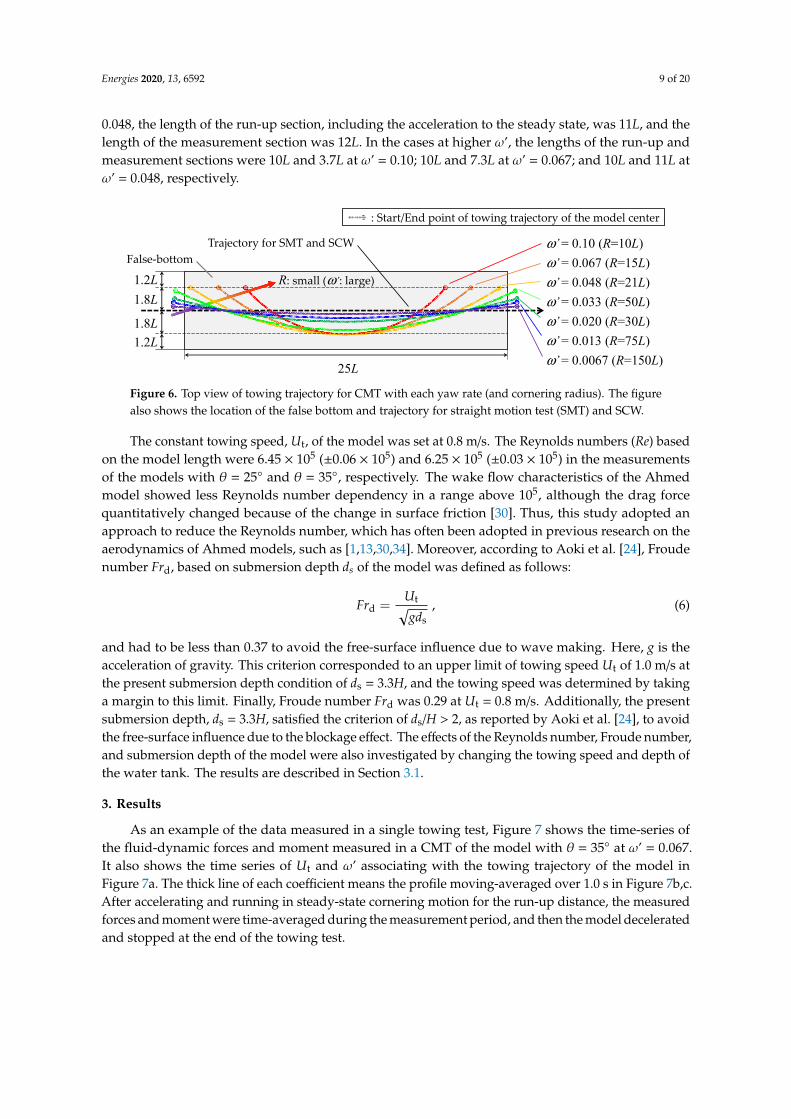
towed and accelerated to the steady state under each measurement condition. In the SMT and SCW,towing started before the front of the false bottom. A run-up section with a length of 10L was takenafter the model entered above the false bottom. Then, the fluid-dynamic forces and moments weremeasured and averaged in the 12L long measurement section. In the CMT, the towing started aboveor near the front of the false bottom after recording the zero point of the balance. Figure 6 showsthe towing trajectory of the CMT. As shown in the figure, the towing area was limited to a widthof 3.6L to avoid the effects of the false bottom edges. Because of the limitation of the arc height ofthe trajectory, the towing distance was shortened at higher values for ω’. When ω’ was less than

Energies 2020, 13, 6592 9 of 20

0.048, the length of the run-up section, including the acceleration to the steady state, was 11L, and thelength of the measurement section was 12L. In the cases at higher ω’, the lengths of the run-up andmeasurement sections were 10L and 3.7L at ω’ = 0.10; 10L and 7.3L at ω’ = 0.067; and 10L and 11L atω’ = 0.048, respectively.Energies 2020, 13, x FOR PEER REVIEW 9 of 20

Figure 6. Top view of towing trajectory for CMT with each yaw rate (and cornering radius). The figure also shows the location of the false bottom and trajectory for straight motion test (SMT) and SCW.

The constant towing speed, Ut, of the model was set at 0.8 m/s. The Reynolds numbers (Re) based on the model length were 6.45 × 105 (±0.06 × 105) and 6.25 × 105 (±0.03 × 105) in the measurements of the models with θ = 25° and θ = 35°, respectively. The wake flow characteristics of the Ahmed model showed less Reynolds number dependency in a range above 105, although the drag force quantitatively changed because of the change in surface friction [30]. Thus, this study adopted an approach to reduce the Reynolds number, which has often been adopted in previous research on the aerodynamics of Ahmed models, such as [1,13,30,34]. Moreover, according to Aoki et al. [24], Froude number Frd, based on submersion depth ds of the model was defined as follows: = , (6)

and had to be less than 0.37 to avoid the free-surface influence due to wave making. Here, g is the acceleration of gravity. This criterion corresponded to an upper limit of towing speed Ut of 1.0 m/s at the present submersion depth condition of ds = 3.3H, and the towing speed was determined by taking a margin to this limit. Finally, Froude number Frd was 0.29 at Ut = 0.8 m/s. Additionally, the present submersion depth, ds = 3.3H, satisfied the criterion of ds/H > 2, as reported by Aoki et al. [24], to avoid the free-surface influence due to the blockage effect. The effects of the Reynolds number, Froude number, and submersion depth of the model were also investigated by changing the towing speed and depth of the water tank. The results are described in Section 3.1.

3. Results

As an example of the data measured in a single towing test, Figure 7 shows the time-series of the fluid-dynamic forces and moment measured in a CMT of the model with θ = 35° at ω’ = 0.067. It also shows the time series of Ut and ω’ associating with the towing trajectory of the model in Figure 7a. The thick line of each coefficient means the profile moving-averaged over 1.0 s in Figure 7b,c. After accelerating and running in steady-state cornering motion for the run-up distance, the measured forces and moment were time-averaged during the measurement period, and then the model decelerated and stopped at the end of the towing test.

ω’ = 0.10 (R=10L)

ω’ = 0.0067 (R=150L)ω’ = 0.013 (R=75L)

ω’ = 0.033 (R=50L)ω’ = 0.020 (R=30L)

ω’ = 0.048 (R=21L)ω’ = 0.067 (R=15L)

Trajectory for SMT and SCWFalse-bottom

: Start/End point of towing trajectory of the model center

25L

1.2L1.8L

1.8L1.2L

R: small (ω’: large)

Figure 6. Top view of towing trajectory for CMT with each yaw rate (and cornering radius). The figurealso shows the location of the false bottom and trajectory for straight motion test (SMT) and SCW.

The constant towing speed, Ut, of the model was set at 0.8 m/s. The Reynolds numbers (Re) basedon the model length were 6.45 × 105 (±0.06 × 105) and 6.25 × 105 (±0.03 × 105) in the measurementsof the models with θ = 25◦ and θ = 35◦, respectively. The wake flow characteristics of the Ahmedmodel showed less Reynolds number dependency in a range above 105, although the drag forcequantitatively changed because of the change in surface friction [30]. Thus, this study adopted anapproach to reduce the Reynolds number, which has often been adopted in previous research on theaerodynamics of Ahmed models, such as [1,13,30,34]. Moreover, according to Aoki et al. [24], Froudenumber Frd, based on submersion depth ds of the model was defined as follows:

Frd =Ut√gds

, (6)

and had to be less than 0.37 to avoid the free-surface influence due to wave making. Here, g is theacceleration of gravity. This criterion corresponded to an upper limit of towing speed Ut of 1.0 m/s atthe present submersion depth condition of ds = 3.3H, and the towing speed was determined by takinga margin to this limit. Finally, Froude number Frd was 0.29 at Ut = 0.8 m/s. Additionally, the presentsubmersion depth, ds = 3.3H, satisfied the criterion of ds/H > 2, as reported by Aoki et al. [24], to avoidthe free-surface influence due to the blockage effect. The effects of the Reynolds number, Froude number,and submersion depth of the model were also investigated by changing the towing speed and depth ofthe water tank. The results are described in Section 3.1.

3. Results

As an example of the data measured in a single towing test, Figure 7 shows the time-series ofthe fluid-dynamic forces and moment measured in a CMT of the model with θ = 35◦ at ω’ = 0.067.It also shows the time series of Ut and ω’ associating with the towing trajectory of the model inFigure 7a. The thick line of each coefficient means the profile moving-averaged over 1.0 s in Figure 7b,c.After accelerating and running in steady-state cornering motion for the run-up distance, the measuredforces and moment were time-averaged during the measurement period, and then the model deceleratedand stopped at the end of the towing test.

Energies 2020, 13, 6592 10 of 20


(a)

(b)

(c)

Figure 7. Time-series of vehicle motion and fluid-dynamic force measured in CMT with θ = 35° at ω’ = 0.067: (a) towing speed Ut and normalized yaw rate ω’ (bottom) with a top view of the towing trajectory (top); (b) drag, and lift coefficients, CD and CL; (c) side force and yaw moment coefficients, CS and CYM. The coefficients were calculated using a constant towing speed of 0.8 m/s rather than the instantaneous Ut. The thick line of each coefficient means the profile moving-averaged over 1.0 s.

3.1. Validation of Measurement Results

Before the main measurements of the CMT and SCW, the measurement results were validated. First, the drag and lift force differences between the two Ahmed models with θ = 25° and θ = 35° were compared with the results of previous studies to confirm the reproduction of the fluid-dynamic characteristics. Then, to evaluate the influence of the test conditions on the measurement results, the dependency of the fluid-dynamic force on the submersion depth and towing speed was clarified. Finally, to quantitatively validate the results of the CMT, the changes in the fluid-dynamic coefficients of the Ahmed model with θ = 25° due to the steady state cornering motion were compared with the numerical results by Keogh et al. [13].

3.1.1. Slant Angle Dependency

The slant angle dependency of the fluid-dynamic drag and lift in the SMT was compared with that in previous studies [4,28,30,34], and the reproduction of the essential fluid dynamics of the Ahmed models with θ = 25° and θ = 35° was confirmed, as displayed in Figure 1b,c. Table 2 also shows comparisons of the CD and CL values of the models with θ = 25° and θ = 35°. The variations in CD and CL between the models with θ = 25° and θ = 35° show good agreement with the previous studies, while the absolute values of each CD and CL were quantitatively different as a result of the differences in the measurement conditions, especially in the Reynolds number shown in the second column of Table 2. According to Kohri et al. [30], the wake flow characteristics and base pressure have less Reynolds number dependency even at a lower Reynolds number of 2.3 × 105. Thus, the difference in CD depending on the Reynolds number was mainly caused by the change in the friction drag. Moreover, the drag coefficient of the model with θ = 25° in the present study showed reasonable agreement with an estimated drag coefficient at the same Reynolds number by the approximate function derived by Meile et al. [4]. Although the present CD value was still 0.014 smaller than the estimated one, the removal of four struts may have caused the difference. Concerning the lift force, lift coefficients that were approximately 0.1 smaller than those in previous studies [4,34] were also reasonable because of the different conditions under the body. The ground surface was not static but

Figure 7. Time-series of vehicle motion and fluid-dynamic force measured in CMT with θ = 35◦ atω’ = 0.067: (a) towing speed Ut and normalized yaw rate ω’ (bottom) with a top view of the towingtrajectory (top); (b) drag, and lift coefficients, CD and CL; (c) side force and yaw moment coefficients,CS and CYM. The coefficients were calculated using a constant towing speed of 0.8 m/s rather than theinstantaneous Ut. The thick line of each coefficient means the profile moving-averaged over 1.0 s.

3.1. Validation of Measurement Results

Before the main measurements of the CMT and SCW, the measurement results were validated.First, the drag and lift force differences between the two Ahmed models with θ = 25◦ and θ = 35◦

were compared with the results of previous studies to confirm the reproduction of the fluid-dynamiccharacteristics. Then, to evaluate the influence of the test conditions on the measurement results,the dependency of the fluid-dynamic force on the submersion depth and towing speed was clarified.Finally, to quantitatively validate the results of the CMT, the changes in the fluid-dynamic coefficientsof the Ahmed model with θ = 25◦ due to the steady state cornering motion were compared with thenumerical results by Keogh et al. [13].

3.1.1. Slant Angle Dependency

The slant angle dependency of the fluid-dynamic drag and lift in the SMT was compared withthat in previous studies [4,28,30,34], and the reproduction of the essential fluid dynamics of the Ahmedmodels with θ = 25◦ and θ = 35◦ was confirmed, as displayed in Figure 1b,c. Table 2 also showscomparisons of the CD and CL values of the models with θ = 25◦ and θ = 35◦. The variations in CD andCL between the models with θ = 25◦ and θ = 35◦ show good agreement with the previous studies,while the absolute values of each CD and CL were quantitatively different as a result of the differencesin the measurement conditions, especially in the Reynolds number shown in the second column ofTable 2. According to Kohri et al. [30], the wake flow characteristics and base pressure have lessReynolds number dependency even at a lower Reynolds number of 2.3 × 105. Thus, the difference in CD

depending on the Reynolds number was mainly caused by the change in the friction drag. Moreover,the drag coefficient of the model with θ = 25◦ in the present study showed reasonable agreementwith an estimated drag coefficient at the same Reynolds number by the approximate function derivedby Meile et al. [4]. Although the present CD value was still 0.014 smaller than the estimated one,the removal of four struts may have caused the difference. Concerning the lift force, lift coefficients

Energies 2020, 13, 6592 11 of 20

that were approximately 0.1 smaller than those in previous studies [4,34] were also reasonable becauseof the different conditions under the body. The ground surface was not static but moving relatively inthe present study, which could have decreased the pressure on the bottom of the body as a result of thehigher flow rate under the body. This tendency corresponds to the conclusion of Larsson et al. [23],in which the higher lift force under a fixed ground condition in a wind tunnel than a moving groundcondition in a towing tank. Therefore, the slant angle dependencies of the drag and lift coefficientswere verified, and the reproduction of the essential fluid dynamics of the Ahmed models with θ = 25◦

and θ = 35◦ was validated.

Table 2. Comparison of slant angle dependencies of CD and CL [4,28,30,34].

Reynolds No.Re × 10−6

Drag Coefficient CD Lift Coefficient CL

θ = 25◦ θ = 35◦ Diff. θ = 25◦ θ = 35◦ Diff.

Present study 0.63–0.65 0.333 0.310 0.023 0.255 −0.057 −0.312

Ahmed et al. [28] 4.29 0.29 0.26 0.03 N.A. N.A. N.A.

Meile et al. [4]2.05 0.30 0.28 0.02 0.36 0.01 −0.350.69 0.34 N.A. N.A. 0.34 N.A. N.A.0.65 0.347 † N.A. N.A. N.A. N.A. N.A.

Sumida andHayakawa [34] 0.36 0.33 * 0.32 ** 0.01 0.32 * 0.05 ** −0.27

Kohri et al. [30] 0.23 0.36 0.33 0.03 N.A. N.A. N.A.† Estimated value from an approximate function of Reynolds number dependency of CD [4]. * Estimated value fromlinear interpolation between the values of θ = 20◦ and θ = 28◦. ** Estimated value from linear interpolation betweenthe values of θ = 34◦ and θ = 40◦.

3.1.2. Submersion Depth Dependency

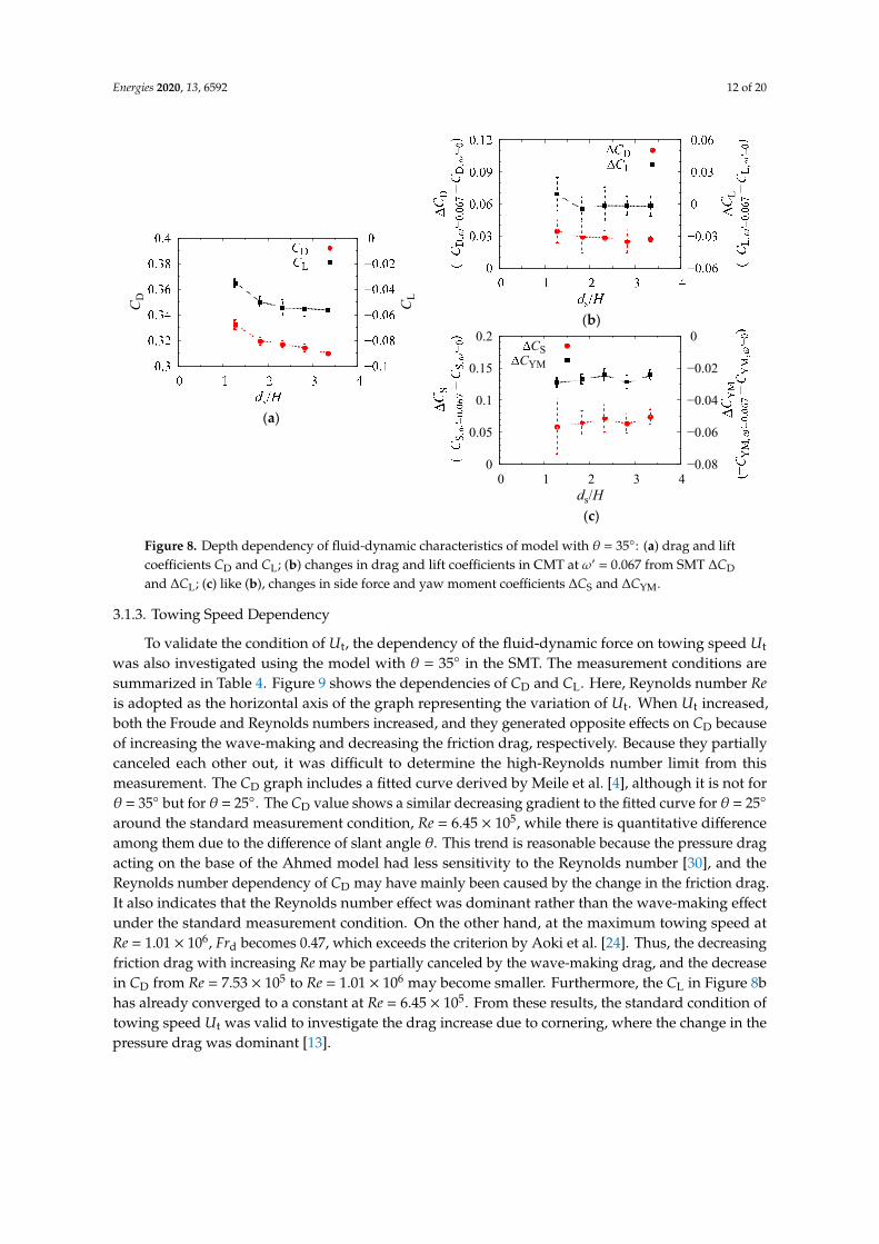
Regarding the effects of a blockage in the test section and wave-making of the model on themeasurement results, their dependency on submersion depth ds of the model and the validity of thecondition of ds were investigated. The fluid-dynamic forces acting on the model with θ = 35◦ in theSMT and CMT at ω’ = 0.067 were measured under some submersion depth conditions, as shown inTable 3. Figure 8 shows the dependencies of CD and CL on normalized submersion depth ds/H. The liftconverged to a constant in ds/H > 2.0, as reported by Aoki et al. [24]. Though the drag was still slightlydecreasing at standard depth ds/H = 3.3, the variation was within a range of 0.01. In addition, the similarconvergence of CD and CL in the SMT has also been confirmed in the model with θ = 25◦, though it wasmeasured under different conditions due to a different water temperature. Moreover, the dependenciesof the changes in the coefficients of drag ∆CD, lift ∆CL, side-force ∆CS, and yaw-moment ∆CYM dueto the cornering motion at ω’ = 0.067 in Figure 8b,c showed less sensitivity to the submersion depth.The variation in the change in each coefficient was smaller than its confidence interval. Therefore,the submersion depth did not to affect the conclusions about the effects of the cornering motion, and thecondition was validated.

Table 3. Measurement conditions to investigate effect of submersion depth.

Test Series Model Submersion Depth ds Froude No. Frd Reynolds No. Re

Straight motion,CMT (ω’ = ±0.067) θ = 35◦

0.29 m (1.3H) 0.47

6.25 × 105

(±0.02 × 105)

0.42 m (1.8H) 0.390.54 m (2.3H) 0.350.65 m (2.8H) 0.31

0.77 m (3.3H) * 0.29

* The standard conditions of the present study.

Energies 2020, 13, 6592 12 of 20


(a)

(b)

(c)

Figure 8. Depth dependency of fluid-dynamic characteristics of model with θ = 35°: (a) drag and lift coefficients CD and CL; (b) changes in drag and lift coefficients in CMT at ω’ = 0.067 from SMT ΔCD and ΔCL; (c) like (b), changes in side force and yaw moment coefficients ΔCS and ΔCYM.

3.1.3. Towing Speed Dependency

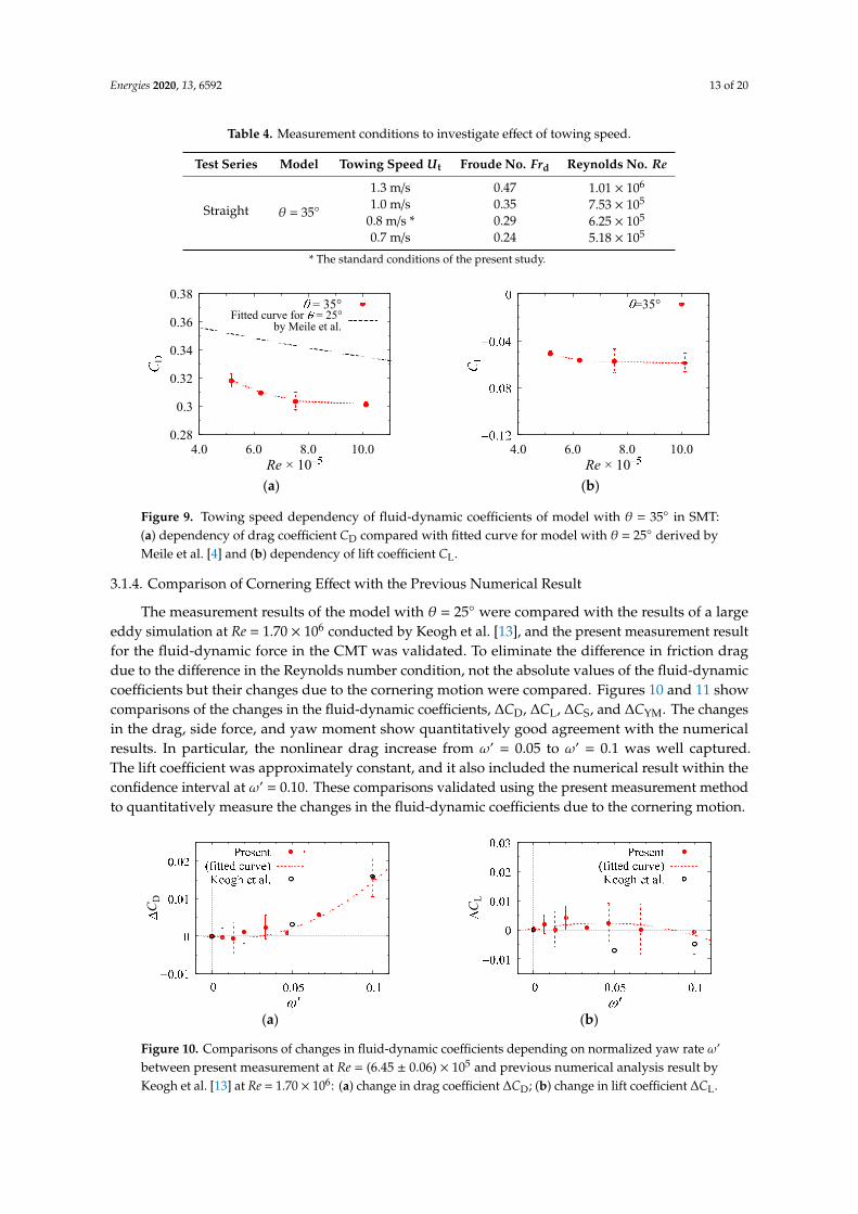
To validate the condition of Ut, the dependency of the fluid-dynamic force on towing speed Ut was also investigated using the model with θ = 35° in the SMT. The measurement conditions are summarized in Table 4. Figure 9 shows the dependencies of CD and CL. Here, Reynolds number Re is adopted as the horizontal axis of the graph representing the variation of Ut. When Ut increased, both the Froude and Reynolds numbers increased, and they generated opposite effects on CD because of increasing the wave-making and decreasing the friction drag, respectively. Because they partially canceled each other out, it was difficult to determine the high-Reynolds number limit from this measurement. The CD graph includes a fitted curve derived by Meile et al. [4], although it is not for θ = 35° but for θ = 25°. The CD value shows a similar decreasing gradient to the fitted curve for θ = 25° around the standard measurement condition, Re = 6.45 × 105, while there is quantitative difference among them due to the difference of slant angle θ. This trend is reasonable because the pressure drag acting on the base of the Ahmed model had less sensitivity to the Reynolds number [30], and the Reynolds number dependency of CD may have mainly been caused by the change in the friction drag. It also indicates that the Reynolds number effect was dominant rather than the wave-making effect under the standard measurement condition. On the other hand, at the maximum towing speed at Re = 1.01 × 106, Frd becomes 0.47, which exceeds the criterion by Aoki et al. [24]. Thus, the decreasing friction drag with increasing Re may be partially canceled by the wave-making drag, and the decrease in CD from Re = 7.53 × 105 to Re = 1.01 × 106 may become smaller. Furthermore, the CL in Figure 8b has already converged to a constant at Re = 6.45 × 105. From these results, the standard condition of towing speed Ut was valid to investigate the drag increase due to cornering, where the change in the pressure drag was dominant [13].

CD CL

0

0.05

0.1

0.15

0.2

0 1 2 3 4−0.08

−0.06

−0.04

−0.02

0

ds/H

CSCYM

Figure 8. Depth dependency of fluid-dynamic characteristics of model with θ = 35◦: (a) drag and liftcoefficients CD and CL; (b) changes in drag and lift coefficients in CMT at ω’ = 0.067 from SMT ∆CD

and ∆CL; (c) like (b), changes in side force and yaw moment coefficients ∆CS and ∆CYM.

3.1.3. Towing Speed Dependency

To validate the condition of Ut, the dependency of the fluid-dynamic force on towing speed Ut

was also investigated using the model with θ = 35◦ in the SMT. The measurement conditions aresummarized in Table 4. Figure 9 shows the dependencies of CD and CL. Here, Reynolds number Reis adopted as the horizontal axis of the graph representing the variation of Ut. When Ut increased,both the Froude and Reynolds numbers increased, and they generated opposite effects on CD becauseof increasing the wave-making and decreasing the friction drag, respectively. Because they partiallycanceled each other out, it was difficult to determine the high-Reynolds number limit from thismeasurement. The CD graph includes a fitted curve derived by Meile et al. [4], although it is not forθ = 35◦ but for θ = 25◦. The CD value shows a similar decreasing gradient to the fitted curve for θ = 25◦

around the standard measurement condition, Re = 6.45 × 105, while there is quantitative differenceamong them due to the difference of slant angle θ. This trend is reasonable because the pressure dragacting on the base of the Ahmed model had less sensitivity to the Reynolds number [30], and theReynolds number dependency of CD may have mainly been caused by the change in the friction drag.It also indicates that the Reynolds number effect was dominant rather than the wave-making effectunder the standard measurement condition. On the other hand, at the maximum towing speed atRe = 1.01 × 106, Frd becomes 0.47, which exceeds the criterion by Aoki et al. [24]. Thus, the decreasingfriction drag with increasing Re may be partially canceled by the wave-making drag, and the decreasein CD from Re = 7.53 × 105 to Re = 1.01 × 106 may become smaller. Furthermore, the CL in Figure 8bhas already converged to a constant at Re = 6.45 × 105. From these results, the standard condition oftowing speed Ut was valid to investigate the drag increase due to cornering, where the change in thepressure drag was dominant [13].

Energies 2020, 13, 6592 13 of 20

Table 4. Measurement conditions to investigate effect of towing speed.

Test Series Model Towing Speed Ut Froude No. Frd Reynolds No. Re

Straight θ = 35◦

1.3 m/s 0.47 1.01 × 106

1.0 m/s 0.35 7.53 × 105

0.8 m/s * 0.29 6.25 × 105

0.7 m/s 0.24 5.18 × 105





Straight θ = 35°

1.3 m/s 0.47 1.01 × 106 1.0 m/s 0.35 7.53 × 105

0.8 m/s * 0.29 6.25 × 105 0.7 m/s 0.24 5.18 × 105


(a)

(b)

Figure 9. Towing speed dependency of fluid-dynamic coefficients of model with θ = 35° in SMT: (a) dependency of drag coefficient CD compared with fitted curve for model with θ = 25° derived by Meile et al. [4] and (b) dependency of lift coefficient CL.

3.1.4. Comparison of Cornering Effect with the Previous Numerical Result

The measurement results of the model with θ = 25° were compared with the results of a large eddy simulation at Re = 1.70 × 106 conducted by Keogh et al. [13], and the present measurement result for the fluid-dynamic force in the CMT was validated. To eliminate the difference in friction drag due to the difference in the Reynolds number condition, not the absolute values of the fluid-dynamic coefficients but their changes due to the cornering motion were compared. Figures 10 and 11 show comparisons of the changes in the fluid-dynamic coefficients, ΔCD, ΔCL, ΔCS, and ΔCYM. The changes in the drag, side force, and yaw moment show quantitatively good agreement with the numerical results. In particular, the nonlinear drag increase from ω’ = 0.05 to ω’ = 0.1 was well captured. The lift coefficient was approximately constant, and it also included the numerical result within the confidence interval at ω’ = 0.10. These comparisons validated using the present measurement method to quantitatively measure the changes in the fluid-dynamic coefficients due to the cornering motion.

(a)

(b)

Figure 10. Comparisons of changes in fluid-dynamic coefficients depending on normalized yaw rate ω’ between present measurement at Re = (6.45 ± 0.06) × 105 and previous numerical analysis result by Keogh et al. [13] at Re = 1.70 × 106: (a) change in drag coefficient ΔCD; (b) change in lift coefficient ΔCL.

0.28

0.3

0.32

0.34

0.36

0.38

4.0 6.0 8.0 10.0

Fitted curve for = 25°by Meile et al.

Re × 10

= 35°

4.0 6.0 8.0 10.0Re × 10

=35°

CD CL

Figure 9. Towing speed dependency of fluid-dynamic coefficients of model with θ = 35◦ in SMT:(a) dependency of drag coefficient CD compared with fitted curve for model with θ = 25◦ derived byMeile et al. [4] and (b) dependency of lift coefficient CL.


The measurement results of the model with θ = 25◦ were compared with the results of a largeeddy simulation at Re = 1.70 × 106 conducted by Keogh et al. [13], and the present measurement resultfor the fluid-dynamic force in the CMT was validated. To eliminate the difference in friction dragdue to the difference in the Reynolds number condition, not the absolute values of the fluid-dynamiccoefficients but their changes due to the cornering motion were compared. Figures 10 and 11 showcomparisons of the changes in the fluid-dynamic coefficients, ∆CD, ∆CL, ∆CS, and ∆CYM. The changesin the drag, side force, and yaw moment show quantitatively good agreement with the numericalresults. In particular, the nonlinear drag increase from ω’ = 0.05 to ω’ = 0.1 was well captured.The lift coefficient was approximately constant, and it also included the numerical result within theconfidence interval at ω’ = 0.10. These comparisons validated using the present measurement methodto quantitatively measure the changes in the fluid-dynamic coefficients due to the cornering motion.




Straight θ = 35°

1.3 m/s 0.47 1.01 × 106 1.0 m/s 0.35 7.53 × 105

0.8 m/s * 0.29 6.25 × 105 0.7 m/s 0.24 5.18 × 105


(a)

(b)

Figure 9. Towing speed dependency of fluid-dynamic coefficients of model with θ = 35° in SMT: (a) dependency of drag coefficient CD compared with fitted curve for model with θ = 25° derived by Meile et al. [4] and (b) dependency of lift coefficient CL.


The measurement results of the model with θ = 25° were compared with the results of a large eddy simulation at Re = 1.70 × 106 conducted by Keogh et al. [13], and the present measurement result for the fluid-dynamic force in the CMT was validated. To eliminate the difference in friction drag due to the difference in the Reynolds number condition, not the absolute values of the fluid-dynamic coefficients but their changes due to the cornering motion were compared. Figures 10 and 11 show comparisons of the changes in the fluid-dynamic coefficients, ΔCD, ΔCL, ΔCS, and ΔCYM. The changes in the drag, side force, and yaw moment show quantitatively good agreement with the numerical results. In particular, the nonlinear drag increase from ω’ = 0.05 to ω’ = 0.1 was well captured. The lift coefficient was approximately constant, and it also included the numerical result within the confidence interval at ω’ = 0.10. These comparisons validated using the present measurement method to quantitatively measure the changes in the fluid-dynamic coefficients due to the cornering motion.

(a)

(b)

Figure 10. Comparisons of changes in fluid-dynamic coefficients depending on normalized yaw rate ω’ between present measurement at Re = (6.45 ± 0.06) × 105 and previous numerical analysis result by Keogh et al. [13] at Re = 1.70 × 106: (a) change in drag coefficient ΔCD; (b) change in lift coefficient ΔCL.

0.28

0.3

0.32

0.34

0.36

0.38

4.0 6.0 8.0 10.0

Fitted curve for = 25°by Meile et al.

Re × 10

= 35°

4.0 6.0 8.0 10.0Re × 10

=35°

CD CL

Figure 10. Comparisons of changes in fluid-dynamic coefficients depending on normalized yaw rate ω’between present measurement at Re = (6.45 ± 0.06) × 105 and previous numerical analysis result byKeogh et al. [13] at Re = 1.70 × 106: (a) change in drag coefficient ∆CD; (b) change in lift coefficient ∆CL.

Energies 2020, 13, 6592 14 of 20Energies 2020, 13, x FOR PEER REVIEW 14 of 20

(a)

(b)

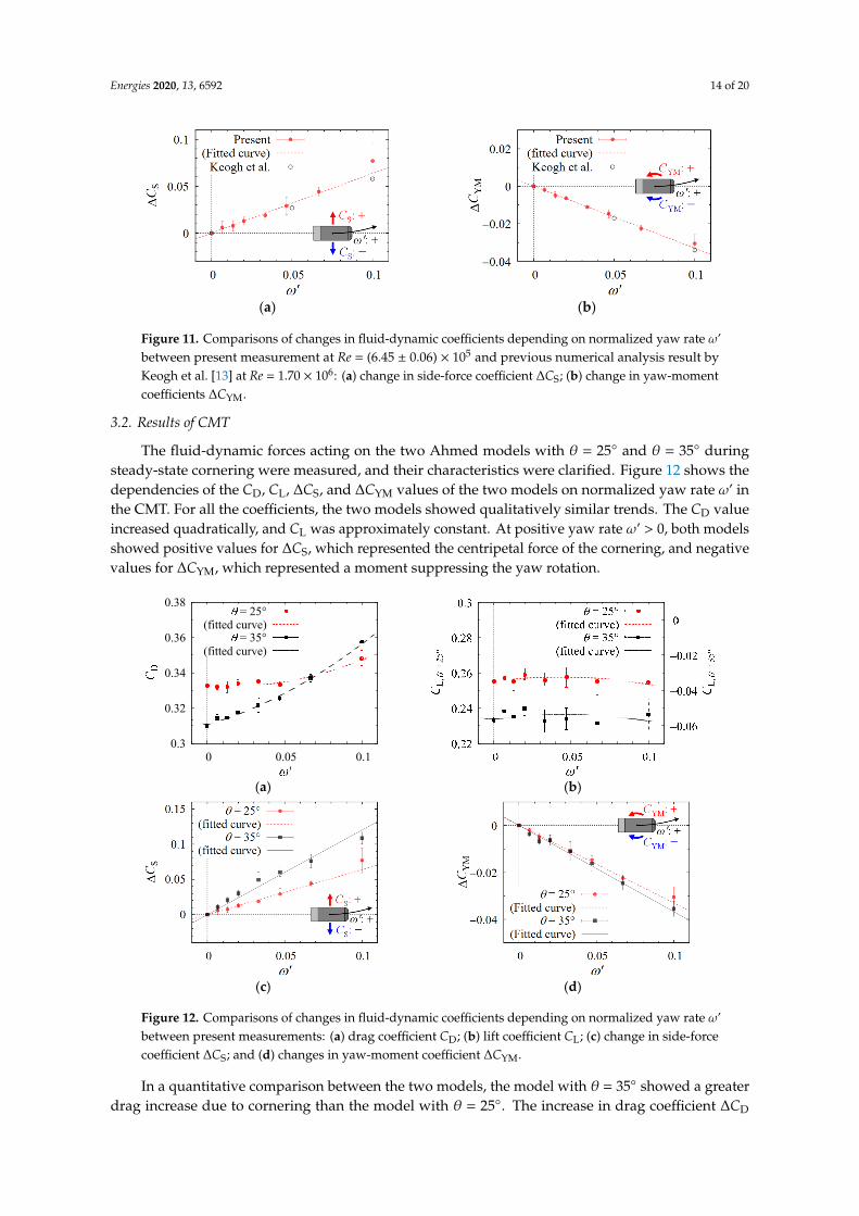
Figure 11. Comparisons of changes in fluid-dynamic coefficients depending on normalized yaw rate ω’ between present measurement at Re = (6.45 ± 0.06) × 105 and previous numerical analysis result by Keogh et al. [13] at Re = 1.70 × 106: (a) change in side-force coefficient ΔCS; (b) change in yaw-moment coefficients ΔCYM.

3.2. Results of CMT

The fluid-dynamic forces acting on the two Ahmed models with θ = 25° and θ = 35° during steady-state cornering were measured, and their characteristics were clarified. Figure 12 shows the dependencies of the CD, CL, ΔCS, and ΔCYM values of the two models on normalized yaw rate ω’ in the CMT. For all the coefficients, the two models showed qualitatively similar trends. The CD value increased quadratically, and CL was approximately constant. At positive yaw rate ω’ > 0, both models showed positive values for ΔCS, which represented the centripetal force of the cornering, and negative values for ΔCYM, which represented a moment suppressing the yaw rotation.

(a)

(b)

(c)

(d)

Figure 12. Comparisons of changes in fluid-dynamic coefficients depending on normalized yaw rate ω’ between present measurements: (a) drag coefficient CD; (b) lift coefficient CL; (c) change in side-force coefficient ΔCS; and (d) changes in yaw-moment coefficient ΔCYM.

0.3

0.32

0.34

0.36

0.38

0 0.05 0.1'

= 25°(fitted curve)


Figure 11. Comparisons of changes in fluid-dynamic coefficients depending on normalized yaw rate ω’between present measurement at Re = (6.45 ± 0.06) × 105 and previous numerical analysis result byKeogh et al. [13] at Re = 1.70 × 106: (a) change in side-force coefficient ∆CS; (b) change in yaw-momentcoefficients ∆CYM.

3.2. Results of CMT

The fluid-dynamic forces acting on the two Ahmed models with θ = 25◦ and θ = 35◦ duringsteady-state cornering were measured, and their characteristics were clarified. Figure 12 shows thedependencies of the CD, CL, ∆CS, and ∆CYM values of the two models on normalized yaw rate ω’ inthe CMT. For all the coefficients, the two models showed qualitatively similar trends. The CD valueincreased quadratically, and CL was approximately constant. At positive yaw rate ω’ > 0, both modelsshowed positive values for ∆CS, which represented the centripetal force of the cornering, and negativevalues for ∆CYM, which represented a moment suppressing the yaw rotation.


(a)

(b)

Figure 11. Comparisons of changes in fluid-dynamic coefficients depending on normalized yaw rate ω’ between present measurement at Re = (6.45 ± 0.06) × 105 and previous numerical analysis result by Keogh et al. [13] at Re = 1.70 × 106: (a) change in side-force coefficient ΔCS; (b) change in yaw-moment coefficients ΔCYM.

3.2. Results of CMT

The fluid-dynamic forces acting on the two Ahmed models with θ = 25° and θ = 35° during steady-state cornering were measured, and their characteristics were clarified. Figure 12 shows the dependencies of the CD, CL, ΔCS, and ΔCYM values of the two models on normalized yaw rate ω’ in the CMT. For all the coefficients, the two models showed qualitatively similar trends. The CD value increased quadratically, and CL was approximately constant. At positive yaw rate ω’ > 0, both models showed positive values for ΔCS, which represented the centripetal force of the cornering, and negative values for ΔCYM, which represented a moment suppressing the yaw rotation.

(a)

(b)

(c)

(d)

Figure 12. Comparisons of changes in fluid-dynamic coefficients depending on normalized yaw rate ω’ between present measurements: (a) drag coefficient CD; (b) lift coefficient CL; (c) change in side-force coefficient ΔCS; and (d) changes in yaw-moment coefficient ΔCYM.

0.3

0.32

0.34

0.36

0.38

0 0.05 0.1'



Figure 12. Comparisons of changes in fluid-dynamic coefficients depending on normalized yaw rate ω’between present measurements: (a) drag coefficient CD; (b) lift coefficient CL; (c) change in side-forcecoefficient ∆CS; and (d) changes in yaw-moment coefficient ∆CYM.

In a quantitative comparison between the two models, the model with θ = 35◦ showed a greaterdrag increase due to cornering than the model with θ = 25◦. The increase in drag coefficient ∆CD

Energies 2020, 13, 6592 15 of 20

with θ = 35◦ reached 0.048 at ω’ = 0.10, while ∆CD = 0.016 in the model with θ = 25◦ under thesame conditions. They correspond to 15% and 4.7% of the total drag in the SMT, respectively. The liftforces of the two models showed similar profiles for the fitted curves, while the absolute values wereapproximately 0.3 different. The model with θ = 35◦ also showed a greater centripetal side force andyaw moment opposing the yaw rotation than the model with θ = 25◦. In the model with θ = 35◦,the absolute values of the gradients for ∆CS and ∆CYM were 63% and 11% greater than those of themodel with θ = 25◦.

3.3. Results of SCW

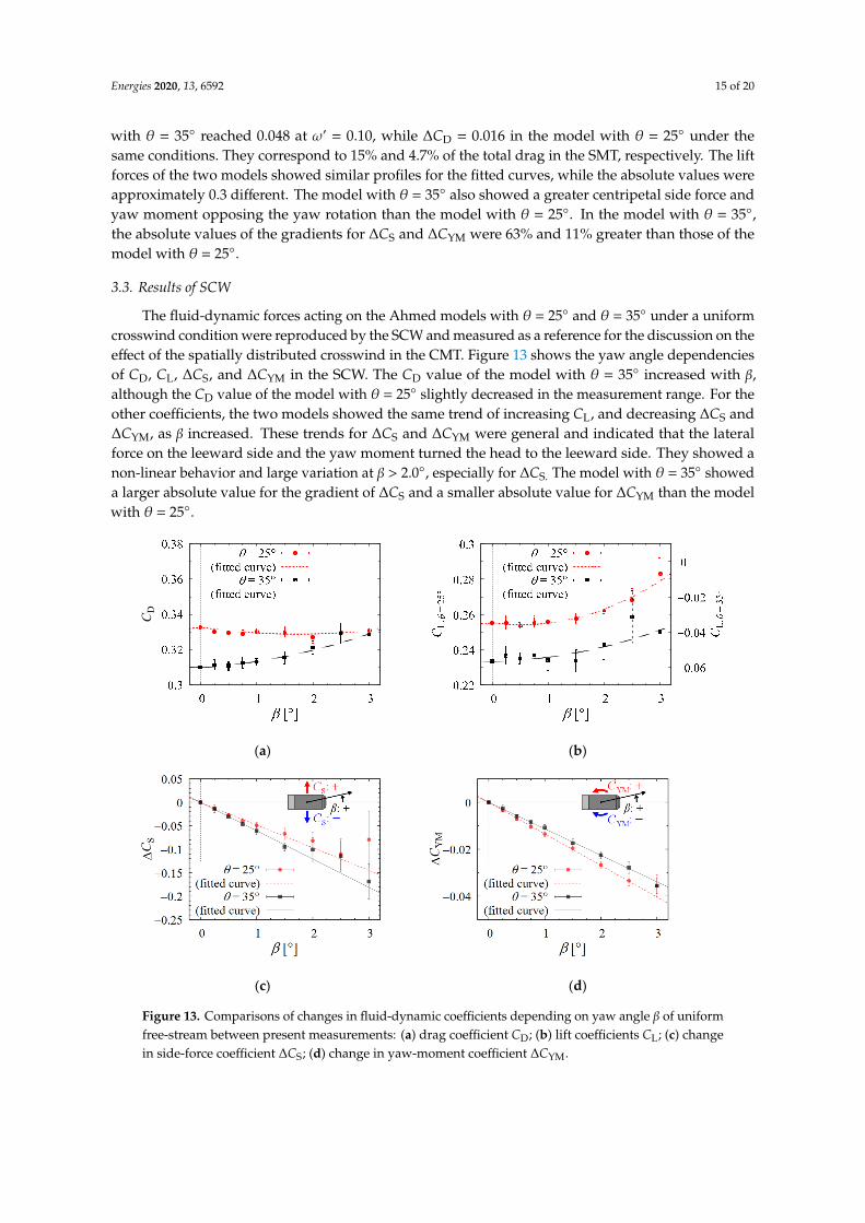
The fluid-dynamic forces acting on the Ahmed models with θ = 25◦ and θ = 35◦ under a uniformcrosswind condition were reproduced by the SCW and measured as a reference for the discussion on theeffect of the spatially distributed crosswind in the CMT. Figure 13 shows the yaw angle dependenciesof CD, CL, ∆CS, and ∆CYM in the SCW. The CD value of the model with θ = 35◦ increased with β,although the CD value of the model with θ = 25◦ slightly decreased in the measurement range. For theother coefficients, the two models showed the same trend of increasing CL, and decreasing ∆CS and∆CYM, as β increased. These trends for ∆CS and ∆CYM were general and indicated that the lateralforce on the leeward side and the yaw moment turned the head to the leeward side. They showed anon-linear behavior and large variation at β > 2.0◦, especially for ∆CS. The model with θ = 35◦ showeda larger absolute value for the gradient of ∆CS and a smaller absolute value for ∆CYM than the modelwith θ = 25◦.


In a quantitative comparison between the two models, the model with θ = 35° showed a greater drag increase due to cornering than the model with θ = 25°. The increase in drag coefficient ΔCD with θ = 35° reached 0.048 at ω’ = 0.10, while ΔCD = 0.016 in the model with θ = 25° under the same conditions. They correspond to 15% and 4.7% of the total drag in the SMT, respectively. The lift forces of the two models showed similar profiles for the fitted curves, while the absolute values were approximately 0.3 different. The model with θ = 35° also showed a greater centripetal side force and yaw moment opposing the yaw rotation than the model with θ = 25°. In the model with θ = 35°, the absolute values of the gradients for ΔCS and ΔCYM were 63% and 11% greater than those of the model with θ = 25°.

3.3. Results of SCW

The fluid-dynamic forces acting on the Ahmed models with θ = 25° and θ = 35° under a uniform crosswind condition were reproduced by the SCW and measured as a reference for the discussion on the effect of the spatially distributed crosswind in the CMT. Figure 13 shows the yaw angle dependencies of CD, CL, ΔCS, and ΔCYM in the SCW. The CD value of the model with θ = 35° increased with β, although the CD value of the model with θ = 25° slightly decreased in the measurement range. For the other coefficients, the two models showed the same trend of increasing CL, and decreasing ΔCS and ΔCYM, as β increased. These trends for ΔCS and ΔCYM were general and indicated that the lateral force on the leeward side and the yaw moment turned the head to the leeward side. They showed a non-linear behavior and large variation at β > 2.0°, especially for ΔCS. The model with θ = 35° showed a larger absolute value for the gradient of ΔCS and a smaller absolute value for ΔCYM than the model with θ = 25°.

(a)

(b)

(c)

(d)

Figure 13. Comparisons of changes in fluid-dynamic coefficients depending on yaw angle β of uniform free-stream between present measurements: (a) drag coefficient CD; (b) lift coefficients CL; (c) change in side-force coefficient ΔCS; (d) change in yaw-moment coefficient ΔCYM.

CD

Figure 13. Comparisons of changes in fluid-dynamic coefficients depending on yaw angle β of uniformfree-stream between present measurements: (a) drag coefficient CD; (b) lift coefficients CL; (c) changein side-force coefficient ∆CS; (d) change in yaw-moment coefficient ∆CYM.

Energies 2020, 13, 6592 16 of 20

4. Discussion

Based on the CMT results shown in Section 3.2, the model with θ = 35◦, simulating the wake ofa square-back type automobile, caused a larger drag increase due to cornering than the model withθ = 25◦, simulating the wake of a fastback-type automobile. The model with θ = 35◦ showed a dragincrease of 15% at ω’ = 0.10, which represented a corner with a constant radius of 10 times the vehiclelength. This drag increase corresponded to approximately 80% of the drag increase in the model withθ = 25◦ at a corner with a radius of five times the vehicle length, as predicted by Keogh et al. [13].Because a corner with a larger radius has a higher encounter probability on the road and can betraversed at higher speeds, the drag increase at a corner with a larger radius has a greater impact onthe average drag on the road. Therefore, the drag increase of the model with θ = 35◦ in the presentresults indicated that the drag increase due to cornering motion becomes more important dependingon the type of automobile and wake structure.

The changes in the side force and yaw moment due to cornering motion were also greater withθ = 35◦ than with θ = 25◦. Here, the side force acted toward the center of the corner, and the yawmoment acted in the opposite direction to the yaw motion. Thus, the aerodynamic center of thepressure was behind the center of the vehicle. When an external centripetal force acts on a corneringvehicle at a point behind the “center of gravity” (CoG) of the vehicle, the force enhances the understeercharacteristics of the vehicle and the stability of its cornering motion. This aerodynamic stabilizingeffect depends on both the strength of the centripetal force and the backward distance from the CoG tothe force application point. Based on the differences in the side force and yaw moment characteristicsbetween the models with θ = 25◦ and θ = 35◦, the centripetal side force of the model with θ = 35◦

was greater than that of the model with θ = 25◦, while the force application point of the model withθ = 35◦ was further forward than that of the model with θ = 25◦. Therefore, the relationship betweenthe stabilizing effects of the models with θ = 25◦ and θ = 35◦ on the cornering motion depended on thelocation of the CoG.

Based on the SCW results shown in Section 3.3, the models with θ = 25◦ and θ = 35◦ qualitativelyreproduced the relationship of changes in drag, side force and yaw moment between the fast-backtype and square-back type automobiles, respectively. The model with θ = 35◦ showed greater increaseof drag and side force magnitude, and smaller increase of yaw moment magnitude than the modelwith θ = 25◦. This tendency corresponded to the general one that the yaw angle dependency of thesquare-back type automobile has larger changes in drag and side force and smaller change in yawmoment than the yaw angle dependency of the fast-back type automobile [18].

From another point of view, the effects of the crosswind components distributed in the space due toa cornering motion were investigated. The two models had different wake structures and aerodynamiccharacteristics depending on the slant angle at the rear end of the body. Therefore, the relative flowdirection acting on the rear end of the vehicle was considered. The dependency of the fluid-dynamicforce on local yaw angle βTE is used for the discussion. Figure 14 shows the change in the aerodynamicforce measured by the CMT and SCW with respect to βTE. For simplicity, only the fitted curves for eachaerodynamic force in Figures 12 and 13 are shown in the graphs. Here, the approximate curve of theCMT result was converted using the relationship between βTE and ω’ in Equation (3). The comparisonbased on the βTE values also shows that the drag increase due to a cornering motion is greater thanthe drag increase in a uniform crosswind, while the qualitative differences in the drag increase valuesbetween the models with θ = 25◦ and θ = 35◦ are consistent in the CMT and SCW. Our previousstudy [26] discussed the physical mechanisms generating the fluid-dynamic centripetal force due tothe cornering motion and indicated that the circulation directly applied to the vehicle body by theyaw rotation generates the centripetal force due to the Magnus effect. This phenomenon would alsocontribute to the drag increase as its induced drag, which could be one of the reasons that the dragincrease in the CMT was greater than that in the SCW.

The lift force shown in Figure 14b only increased under a uniform crosswind condition. However,this difference was caused by a different phenomenon above the top surface of the model. Under uniform

Energies 2020, 13, 6592 17 of 20

crosswind conditions, a longitudinal vortex above the top surface is formed starting at the front ofthe windward edge of the surface [36]. This vertical vortex created negative pressure on the roof,which may have contributed to the increased lift. On the other hand, the cornering motion, where thewind direction is distributed, does not generate such a vortex [13] because the local yaw angle at thecenter of the model is always approximately zero, and the lift did not increase.


on the roof, which may have contributed to the increased lift. On the other hand, the cornering motion, where the wind direction is distributed, does not generate such a vortex [13] because the local yaw angle at the center of the model is always approximately zero, and the lift did not increase.

(a)

(b)

(c)

(d)

Figure 14. Comparisons of changes in fluid-dynamic coefficients depending on local yaw angle βTE at the rear end of the model between the CMT and SCW: (a) drag coefficient CD; (b) lift coefficient CL; (c) change in side-force coefficient ΔCS; (d) change in yaw-moment coefficient ΔCYM.

Regarding the side force and yaw moment shown in Figure 14c,d, consider the local fluid-dynamic response at the rear part of the model to local yaw angle βTE. Figure 15 shows a schematic diagram that can be referenced for the following discussion. Because βTE becomes negative during steady-state cornering with a positive yaw rate, and the inside of the corner becomes the leeward side, it can be assumed that the local side force acting on the rear part of the model acts toward the inside of the corner. From the relationship between the changes in the fluid-dynamic forces due to cornering of the models with θ = 25° and θ = 35°, the model with θ = 35° shows a greater side force toward the center of the corner than the model with θ = 25°. The model with θ = 35° also shows a greater yaw moment in the opposite direction of the yaw rotation than the model with θ = 25°. Therefore, the local fluid-dynamic side force acting on the model with θ = 35° toward the inside of the corner can be estimated to be greater than that for the model with θ = 25°. Under a uniform crosswind condition, it can also be assumed that the side force at the rear part acts toward the leeward side and generates a yaw moment that rotates the head toward the windward direction. This increases the absolute value of ΔCS and decreases the absolute value of ΔCYM in the SCW results. Because the model with θ = 35° shows a larger |ΔCS| value and smaller |ΔCYM| value than the model with θ = 25°, the local fluid-dynamic side force acting on the rear part of the model with θ = 35° can be estimated to be greater than that for the model with θ = 25°. These estimations in CMT and SCW

0.3

0.32

0.34

0.36

0.38

0 1 2 3TE [°]

CMT = 25°= 35°

SCW = 25°= 35°

CL,

= 2

5°

CL,

= 3

5°

Figure 14. Comparisons of changes in fluid-dynamic coefficients depending on local yaw angle βTE atthe rear end of the model between the CMT and SCW: (a) drag coefficient CD; (b) lift coefficient CL;(c) change in side-force coefficient ∆CS; (d) change in yaw-moment coefficient ∆CYM.

Regarding the side force and yaw moment shown in Figure 14c,d, consider the local fluid-dynamicresponse at the rear part of the model to local yaw angle βTE. Figure 15 shows a schematic diagramthat can be referenced for the following discussion. Because βTE becomes negative during steady-statecornering with a positive yaw rate, and the inside of the corner becomes the leeward side, it can beassumed that the local side force acting on the rear part of the model acts toward the inside of the corner.From the relationship between the changes in the fluid-dynamic forces due to cornering of the modelswith θ = 25◦ and θ = 35◦, the model with θ = 35◦ shows a greater side force toward the center of thecorner than the model with θ = 25◦. The model with θ = 35◦ also shows a greater yaw moment in theopposite direction of the yaw rotation than the model with θ = 25◦. Therefore, the local fluid-dynamicside force acting on the model with θ = 35◦ toward the inside of the corner can be estimated to begreater than that for the model with θ = 25◦. Under a uniform crosswind condition, it can also beassumed that the side force at the rear part acts toward the leeward side and generates a yaw momentthat rotates the head toward the windward direction. This increases the absolute value of ∆CS and

Energies 2020, 13, 6592 18 of 20

decreases the absolute value of ∆CYM in the SCW results. Because the model with θ = 35◦ showsa larger |∆CS| value and smaller |∆CYM| value than the model with θ = 25◦, the local fluid-dynamicside force acting on the rear part of the model with θ = 35◦ can be estimated to be greater than thatfor the model with θ = 25◦. These estimations in CMT and SCW results were consistent with eachother. Furthermore, considering that the drag increase of the model with θ = 35◦ is also greater thanthat of the model with θ = 25◦, the model with θ = 35◦ can be considered to generate a fluid-dynamicforce with a greater magnitude at the rear part in response to the local yaw angle than the model withθ = 25◦.


results were consistent with each other. Furthermore, considering that the drag increase of the model with θ = 35° is also greater than that of the model with θ = 25°, the model with θ = 35° can be considered to generate a fluid-dynamic force with a greater magnitude at the rear part in response to the local yaw angle than the model with θ = 25°.

Figure 15. Schematic image for discussion of side force and yaw moment. The dependency of the side force component of the local fluid-dynamic force acting on the rear part of the model on slant angle θ is assumed to be consistent in both the CMT and SCW results and the estimation.

5. Conclusions

Experimental measurements of the fluid-dynamic forces acting on cornering Ahmed models with different wake characteristics were conducted in a towing tank facility. The increase in drag due to the cornering motion, which was indicated by a previous numerical analysis by Keogh et al. [13], was experimentally captured. Furthermore, the Ahmed model with a slant angle of θ = 35°, which had a quasi-two-dimensional separated wake, showed a greater drag increase due to the steady-state cornering motion than the model with θ = 25°, which had a highly three-dimensional wake structure. The drag increase of the model with θ = 35° reached 15% when the cornering radius was 10 times the vehicle length, while the model with θ = 25° showed a 5% drag increase under the same cornering condition. Therefore, it will be more important to consider the cornering effects on the automobile aerodynamics during the development process depending on the type of automobile and its wake characteristics.

When a consistent response is assumed for the local fluid-dynamic characteristics in the local flow direction at the rear end of the body, it is possible to qualitatively explain the relationship between the differences in the drag, side force, and yaw moment from the differences in the geometry and motion of the model. However, the amount of drag increase under the steady-state cornering condition was greater than that under the steady crosswind condition in a comparison based on the local yaw angle defined at the rear end of the model. Therefore, in the quantitative estimation of automobile aerodynamics under realistic on-road conditions, the cornering effects must be precisely reproduced and considered.

Author Contributions: Conceptualization, T.N. and M.T.; methodology, T.N.; software, T.N.; validation, T.N.; formal analysis, T.N.; investigation, T.N.; resources, T.N., H.M., and T.K.; data curation, T.N.; writing—original draft preparation, T.N.; writing—review and editing, T.N., H.M., and T.K.; visualization, T.N.; supervision, H.M. and M.T.; project administration, T.N.; funding acquisition, T.N. All authors have read and agreed to the published version of the manuscript.

Funding: This research was funded by JSPS-KAKENHI (grant numbers 26420115, 17K06159, and 20K04286).

Conflicts of Interest: The authors declare no conflicts of interest.

Figure 15. Schematic image for discussion of side force and yaw moment. The dependency of the sideforce component of the local fluid-dynamic force acting on the rear part of the model on slant angle θ isassumed to be consistent in both the CMT and SCW results and the estimation.

5. Conclusions

Experimental measurements of the fluid-dynamic forces acting on cornering Ahmed modelswith different wake characteristics were conducted in a towing tank facility. The increase in drag dueto the cornering motion, which was indicated by a previous numerical analysis by Keogh et al. [13],was experimentally captured. Furthermore, the Ahmed model with a slant angle of θ = 35◦, which hada quasi-two-dimensional separated wake, showed a greater drag increase due to the steady-statecornering motion than the model with θ = 25◦, which had a highly three-dimensional wake structure.The drag increase of the model with θ = 35◦ reached 15% when the cornering radius was 10 timesthe vehicle length, while the model with θ = 25◦ showed a 5% drag increase under the samecornering condition. Therefore, it will be more important to consider the cornering effects on theautomobile aerodynamics during the development process depending on the type of automobile andits wake characteristics.

When a consistent response is assumed for the local fluid-dynamic characteristics in the local flowdirection at the rear end of the body, it is possible to qualitatively explain the relationship betweenthe differences in the drag, side force, and yaw moment from the differences in the geometry andmotion of the model. However, the amount of drag increase under the steady-state cornering conditionwas greater than that under the steady crosswind condition in a comparison based on the local yawangle defined at the rear end of the model. Therefore, in the quantitative estimation of automobileaerodynamics under realistic on-road conditions, the cornering effects must be precisely reproducedand considered.

Author Contributions: Conceptualization, T.N. and M.T.; methodology, T.N.; software, T.N.; validation, T.N.;formal analysis, T.N.; investigation, T.N.; resources, T.N., H.M., and T.K.; data curation, T.N.; writing—originaldraft preparation, T.N.; writing—review and editing, T.N., H.M., and T.K.; visualization, T.N.; supervision, H.M.and M.T.; project administration, T.N.; funding acquisition, T.N. All authors have read and agreed to the publishedversion of the manuscript.

Funding: This research was funded by JSPS-KAKENHI (grant numbers 26420115, 17K06159, and 20K04286).

Conflicts of Interest: The authors declare no conflict of interest.

Energies 2020, 13, 6592 19 of 20

References

1. Tunay, T.; Firat, E.; Sahin, B. Experimental investigation of the flow around a simplified ground vehicle undereffects of the steady crosswind. Int. J. Heat Fluid Flow 2018, 71, 137–152. [CrossRef]

2. Bonitz, S.; Larsson, L.; Sebben, S. Unsteady pressure analysis of the near wall flow downstream of the frontwheel of a passenger car under yaw conditions. Int. J. Heat Fluid Flow 2018, 73, 188–198. [CrossRef]

3. Guilmineau, E.; Chikhaoui, O.; Deng, G.; Visonneau, M. Cross wind effects on a simplified car model by aDES approach. Comput. Fluids 2013, 78, 29–40. [CrossRef]

4. Meile, W.; Ladinek, T.; Brenn, G.; Reppenhagen, A.; Fuchs, A. Non-symmetric bi-stable flow around theAhmed body. Int. J. Heat Fluid Flow 2016, 57, 34–47. [CrossRef]

5. Wieser, D.; Vayeri, C.N.; Paschereit, C.O. Wake structures and surface patterns of the DrivAer Notchback carmodel under side wind conditions. Energies 2020, 13, 320. [CrossRef]

6. Wordley, S.; Saunders, J. On-road turbulence. SAE Int. J. Passeng. Cars Mech. Syst. 2009, 1, 341–360.[CrossRef]

7. Wordley, S.; Saunders, J. On-road turbulence: Part 2. SAE Int. J. Passeng. Cars Mech. Syst. 2009, 2, 111–137.[CrossRef]

8. Carlino, G.; Cogotti, A. Simulation of Transient Phenomena with the Turbulence Generation System in the PininfarinaWind Tunnel; SAE Technical Paper; SAE International: Warrendale, PA, USA, 2006. [CrossRef]

9. Carlino, G.; Cardano, D.; Cogotti, A. A New Technique to Measure the Aerodynamic Response of Passenger Cars bya Continuous Flow Yawing; SAE Technical Paper; SAE International: Warrendale, PA, USA, 2007. [CrossRef]

10. Stoll, D.; Schoenleber, C.; Wittmeier, F.; Kuthada, T.; Wiediemann, J. Investigation of Aerodynamic Drag inTurbulent Flow Conditions. SAE Int. J. Passeng. Cars Mech. Syst. 2016, 9, 733–742. [CrossRef]

11. Shimizu, K.; Nakashima, T.; Hiraoka, T.; Nakamura, Y.; Nouzawa, T.; Doi, Y. Aerodynamic drag change ofsimplified automobile models influenced by a passing vehicle. Mech. Eng. J. 2020, 7, 19–00366. [CrossRef]

12. Keogh, J.; Doig, G.; Diasinos, S.; Barber, T. The influence of cornering on the vortical wake structures of aninverted wing. Proc. Inst. Mech. Eng. D J. Automob. Eng. 2015, 229, 1817–1829. [CrossRef]

13. Keogh, J.; Barber, T.; Diasinos, S.; Doig, G. The aerodynamic effects on a cornering Ahmed body. J. Wind Eng.Ind. Aerodyn. 2016, 154, 34–46. [CrossRef]

14. Josefsson, E.; Hagvall, R.; Urquhart, M.; Sebben, S. Numerical Analysis of Aerodynamic Impact on PassengerVehicles during Cornering; SAE Technical Paper; SAE International: Warrendale, PA, USA, 2018. [CrossRef]

15. Tsubokura, M.; Ikawa, Y.; Nakashima, T.; Okada, Y.; Kamioka, T.; Nouzawa, T. Unsteady vehicle aerodynamicsduring a dynamic steering action: 2nd report, numerical analysis. SAE Int. J. Passeng. Cars Mech. Syst. 2012,5, 340–357. [CrossRef]

16. Okada, Y.; Nakashima, T.; Tsubokura, M.; Morikawa, Y.; Kouno, R.; Okamoto, S.; Nouzawa, T. AerodynamicsEvaluation of Road Vehicles in Dynamic Maneuvering; SAE Technical Paper; SAE International: Warrendale, PA,USA, 2016. [CrossRef]

17. Keogh, J.; Barber, T.; Diasinos, S.; Doig, G. Techniques for Aerodynamic Analysis of Cornering Vehicles; SAETechnical Paper; SAE International: Warrendale, PA, USA, 2015. [CrossRef]

18. Schuetz, T. Aerodynamics of Road Vehicles, 5th ed.; SAE International: Warrendale, PA, USA, 2015; pp. 282–290.19. Gordes, A. Process for Simulating Curved Airflows on Wheeled Vehicles in Fluid Flow Channels with a

Straight Measuring Section. Patent No. EP1610111A2, 28 December 2005.20. Keogh, J.; Barber, T.; Diasinos, S.; Doig, G. A New Type of Wind Tunnel for the Evaluation of Curved Motion.

In Proceedings of the 54th AIAA Aerospace Sciences Meeting, San Diego, CA, USA, 4–8 January 2016;No. AIAA 2016-1774. [CrossRef]

21. Ueno, M.; Yoshimura, Y.; Tsukada, Y.; Miyazaki, H. Circular motion tests and uncertainty analysis for shipmaneuverability. J. Mar. Sci. Technol. 2009, 14, 469. [CrossRef]

22. Vorwaller, M.L.; Germane, G.J. Aerodynamic Drag Studies on Rolling Vehicles by Underwater Tow Testing;SAE Technical Paper; SAE International: Warrendale, PA, USA, 1986. [CrossRef]

23. Larsson, L.; Hammar, L.; Nilsson, L.U.; Berndtsson, A.; Knutson, K.; Danielson, H. A Study of GroundSimulation Correlation between Wind Tunnel and Water-Basin Tests of a Full-Scale Car; SAE Technical Paper;SAE International: Warrendale, PA, USA, 1989. [CrossRef]

24. Aoki, K.; Miyata, H.; Kanai, M.; Hanaoka, Y.; Zhu, M. A Water-Basin Test Technique for the Aerodynamic Designof Road Vehicles; SAE Technical Paper; SAE International: Warrendale, PA, USA, 1992. [CrossRef]

http://dx.doi.org/10.1016/j.ijheatfluidflow.2018.03.020


http://dx.doi.org/10.1016/j.compfluid.2011.08.020


http://dx.doi.org/10.3390/en13020320

http://dx.doi.org/10.4271/2008-01-0475

http://dx.doi.org/10.4271/2009-01-0002

http://dx.doi.org/10.4271/2006-01-1031

http://dx.doi.org/10.4271/2007-01-0902

http://dx.doi.org/10.4271/2016-01-1605

http://dx.doi.org/10.1299/mej.19-00366

http://dx.doi.org/10.1177/0954407015571673

http://dx.doi.org/10.1016/j.jweia.2016.04.002

http://dx.doi.org/10.4271/2018-37-0014

http://dx.doi.org/10.4271/2012-01-0448

http://dx.doi.org/10.4271/2016-01-1618

http://dx.doi.org/10.4271/2015-01-0022

http://dx.doi.org/10.2514/6.2016-1774

http://dx.doi.org/10.1007/s00773-009-0065-2

http://dx.doi.org/10.4271/860091

http://dx.doi.org/10.4271/890368

http://dx.doi.org/10.4271/920348

Energies 2020, 13, 6592 20 of 20

25. Ogawa, A.; Mashio, S.; Yano, S.; Kawamura, T. Quantitative representations of aerodynamic effects onhandling response and flat ride of vehicles. SAE Int. J. Passeng. Cars Mech. Syst. 2012, 5, 304–323. [CrossRef]

26. Nakashima, T.; Tsubokura, M.; Okada, Y.; Nouzawa, T.; Mizokane, M.; Doi, Y. Aerodynamic force acting on aroad vehicle in steady-state cornering. Trans. JSME (in Japanese) 2014, 80, FE0301. [CrossRef]

27. Nakashima, T.; Tsubokura, M.; Okada, Y.; Nouzawa, T.; Kono, R.; Doi, Y. Aerodynamic Characteristicsof a Road Vehicle in Steady-State Cornering. In Proceedings of the ASME/JSME/KSME 2015 Joint FluidsEngineering Conference, Seoul, Korea, 26–31 July 2015; V01AT17A002. [CrossRef]

28. Ahmed, S.; Ramm, G.; Faltin, G. Some Salient Features of the Time-Averaged Ground Vehicle Wake; SAE TechnicalPaper; SAE International: Warrendale, PA, USA, 1984. [CrossRef]

29. Lienhart, H.; Stoots, C.; Becker, S. Flow and Turbulence Structures in the Wake of a Simplified Car Model(Ahmed Modell). In New Results in Numerical and Experimental Fluid Mechanics III. Notes on Numerical FluidMechanics (NNFM); Wagner, S., Rist, U., Heinemann, H.J., Hilbig, R., Eds.; Springer: Berlin/Heidelberg,Germany, 2002; Volume 77. [CrossRef]

30. Kohri, I.; Yamanashi, T.; Nasu, T.; Hashizume, Y.; Katoh, D. Study on the transient behaviour of the vortexstructure behind Ahmed body. SAE Int. J. Passeng. Cars Mech. Syst. 2014, 7, 586–602. [CrossRef]

31. Kasai, A.; Shiratori, S.; Kohri, I.; Kobayashi, Y.; Katoh, D.; Nagano, H.; Shimano, K. Large-scale separatedvortex generated in a wake flow of Ahmed’s body. Flow Turbul. Combust. 2019, 102, 373–388. [CrossRef]

32. Guilmineau, E. Computational study of flow around a simplified car body. J. Wind Eng. Ind. Aerodyn. 2008,96, 1207–1217. [CrossRef]

33. Guilmineau, E.; Deng, G.B.; Leroyer, A.; Queutey, P.; Visonneau, M.; Wackers, J. Assessment of hybridRANS-LES formulations for flow simulation around the Ahmed body. Comput. Fluids 2018, 176, 302–319.[CrossRef]

34. Sumida, M.; Hayakawa, K. Aerodynamic forces acting on Ahmed-type vehicles under fluctuating headwindconditions. J. Appl. Fluid Mech. 2019, 12, 1563–1574. [CrossRef]

35. Bae, I.; Moon, J.; Seo, J. Toward a comfortable driving experience for a self-driving shuttle bus. Electronics2019, 8, 943. [CrossRef]

36. Rao, A.; Minelli, G.; Basara, B.; Krajnovic, S. On the two flow states in the wake of a hatchback Ahmed body.J. Wind Eng. Indust. Aerodyn. 2018, 173, 262–278. [CrossRef]

Publisher’s Note: MDPI stays neutral with regard to jurisdictional claims in published maps and institutionalaffiliations.

© 2020 by the authors. Licensee MDPI, Basel, Switzerland. This article is an open accessarticle distributed under the terms and conditions of the Creative Commons Attribution(CC BY) license (http://creativecommons.org/licenses/by/4.0/).

http://dx.doi.org/10.4271/2012-01-0445

http://dx.doi.org/10.1299/transjsme.2014fe0301

http://dx.doi.org/10.1115/AJKFluids2015-17553

http://dx.doi.org/10.4271/840300

http://dx.doi.org/10.1007/978-3-540-45466-3_39

http://dx.doi.org/10.4271/2014-01-0597

http://dx.doi.org/10.1007/s10494-018-9950-2


http://dx.doi.org/10.1016/j.compfluid.2017.01.005

http://dx.doi.org/10.29252/jafm.12.05.29774

http://dx.doi.org/10.3390/electronics8090943


http://creativecommons.org/

http://creativecommons.org/licenses/by/4.0/.

Fluid-Dynamic Force Measurement of Ahmed Model in Steady ...

Documents

Transcript of Fluid-Dynamic Force Measurement of Ahmed Model in Steady ...