This article was downloaded by: [Catherine J. Noakes]On: 08 January 2015, At: 11:22Publisher: Taylor & FrancisInforma Ltd Registered in England and Wales Registered Number: 1072954 Registered office: Mortimer House,37-41 Mortimer Street, London W1T 3JH, UK

Click for updates

Science and Technology for the Built EnvironmentPublication details, including instructions for authors and subscription information:http://www.tandfonline.com/loi/uhvc21

Computational fluid dynamics analysis to assessperformance variability of in-duct UV-C systemsAzael Capetilloa, Catherine J. Noakesa & P. Andrew Sleigha

a Pathogen Control Engineering Institute (PaCE), School of Civil Engineering, University ofLeeds, Woodouse Lane, LS2 9JT, Leeds, United KingdomPublished online: 06 Jan 2015.

To cite this article: Azael Capetillo, Catherine J. Noakes & P. Andrew Sleigh (2015) Computational fluid dynamics analysis toassess performance variability of in-duct UV-C systems, Science and Technology for the Built Environment, 21:1, 45-53

To link to this article: http://dx.doi.org/10.1080/10789669.2014.968512

PLEASE SCROLL DOWN FOR ARTICLE

Taylor & Francis makes every effort to ensure the accuracy of all the information (the “Content”) containedin the publications on our platform. However, Taylor & Francis, our agents, and our licensors make norepresentations or warranties whatsoever as to the accuracy, completeness, or suitability for any purpose of theContent. Any opinions and views expressed in this publication are the opinions and views of the authors, andare not the views of or endorsed by Taylor & Francis. The accuracy of the Content should not be relied upon andshould be independently verified with primary sources of information. Taylor and Francis shall not be liable forany losses, actions, claims, proceedings, demands, costs, expenses, damages, and other liabilities whatsoeveror howsoever caused arising directly or indirectly in connection with, in relation to or arising out of the use ofthe Content.

This article may be used for research, teaching, and private study purposes. Any substantial or systematicreproduction, redistribution, reselling, loan, sub-licensing, systematic supply, or distribution in anyform to anyone is expressly forbidden. Terms & Conditions of access and use can be found at http://www.tandfonline.com/page/terms-and-conditions

Science and Technology for the Built Environment (2015) 21, 45–53Copyright C© 2015 ASHRAE.ISSN: 2374-4731 print / 2374-474X onlineDOI: 10.1080/10789669.2014.968512

Computational fluid dynamics analysis to assessperformance variability of in-duct UV-C systems

AZAEL CAPETILLO, CATHERINE J. NOAKES∗, and P. ANDREW SLEIGH

Pathogen Control Engineering Institute (PaCE), School of Civil Engineering, University of Leeds, Woodouse Lane, Leeds LS2 9JT,United Kingdom

UV-C is becoming a mainstream air sterilization technology and is marketed in the form of energy-saving and infection-reductiondevices. An accurate rating of device performance is essential to ensure appropriate microbial reduction yet avoid wastage of energy dueto over performance. This article demonstrates the potential benefits from using computational fluid dynamics to assess performance.A computational fluid dynamics model was developed using discrete ordinate irradiation modeling and Lagrangian particle trackingto model airborne microorganisms. The study calculates the UV dose received by airborne particles in an in-duct UV system basedon published EPA experimental tests for single-, four-, and eight-lamp devices. Whereas the EPA tests back calculated UV dose frommeasured microorganism inactivation data, the computational fluid dynamics model directly computes UV dose, then determinesinactivation of microorganisms. Microorganism inactivation values compared well between the computational fluid dynamics modeland the EPA tests, but differences between UV dosages were found due to uncertainty in microorganism UV susceptibility data. Thestudy highlighted the need for careful consideration of test microorganisms and a reliable dataset of UV susceptibility values in air toassess performance. Evaluation of the dose distribution demonstrated the importance of creating an even UV field to minimize therisk of ineffective sterilization of some particles while not delivering excessive energy to others.

Introduction

Air-cleaning technologies are used to control the indoor airquality by removing or inactivating contaminants in the en-vironment. Such technologies may also have a role in energyefficiency by enabling recirculation of air and keeping HVACequipment free of deposited particles and microbial growththat diminish airflow rates and affect heat transfer (Fisk et al.2002). Fibrous mechanical filtration, which employs trappingand adsorption mechanisms (Sutherland 2007), can be con-sidered the most popular air-cleaning technology. Howeverfilters that are capable of removing very small particles, suchas airborne microorganisms, induce a large pressure drop inan HVAC system, increasing energy consumption (Fisk et al.2002). In recent years, interest has grown in the potential forphotochemical air filters, such as UV-C irradiation, to supple-ment or replace fine particle filtration for microbial control.These devices have the capacity of destroying or decomposingmicroorganisms and potentially volatile organic compounds(VOCs), and they may have energy performance benefits overconventional filters (Blatt 2006; Kowalski 2009; Lee et al.2009).

Received April 27, 2014; accepted September 10, 2014Azael Capetillo is a PhD Student. Catherine J. Noakes, PhD,CEng, is a Professor. P. Andrew Sleigh, PhD, is a SeniorLecturer.∗Corresponding author e-mail: C.J.Noakes@leeds.ac.ukColor versions of one or more of the figures in the article can befound online at www.tandfonline.com/uhvc.

In-duct devices typically comprise one or more UV-C lampsmounted within the HVAC system to create a UV irradiationfield inside an airflow duct. Microorganisms contained in theair passing through the UV field incur DNA damage propor-tional to the UV irradiance, time of exposure, and species ofmicroorganism; with sufficient exposure, the damage may belethal, rendering microorganisms inactive. The technology hasalso shown reduction of bacteria concentration on surfaces af-ter UV-C has been installed within a ventilation system (Tayloret al. 1995), leading to applications for reducing bio foulingof cooling coils and the potential for improving system energyefficiency (Blatt 2006; Kowalski 2009; Lee et al. 2009). Withincreasing application of in-duct UV-C systems, it is impor-tant to accurately quantify the technology’s performance, andappropriate analysis and test mechanisms must be set in place.For an in-duct air system, the efficiency of UV-C sterilizationdepends on many factors, including UV irradiation intensity,dwell time of the microorganisms in the UV field within a ductor device, microorganism susceptibility to UV irradiation, airvelocity, air temperature, humidity, reflectivity of duct or de-vice internal surfaces, velocity profile, air mixing, and lampposition.

A number of studies have explored the influence of some ofthese parameters through mathematical modeling. Kowalski(2009) predicted UV device performance with average irradia-tion fields determined using a view factor approximation, andLau (2009) explored the effects of airflow velocity and tem-perature on lamp output. However, these models assumed afully mixed airflow and did not consider the 3D flow–UV fieldinteraction that happens in a real case. Computational fluid

Dow

nloa

ded

by [

Cat

heri

ne J

. Noa

kes]

at 1

1:22

08

Janu

ary

2015

46 Science and Technology for the Built Environment

dynamics (CFD) modeling can take this into account and hasbeen successfully applied to UV water systems (Wright andHargreaves 2001) and upper-room UV (Gilkeson and Noakes2013). This same issue is also apparent in experimental assess-ment of UV device efficacy. The EPA tests series “BiologicalInactivation Efficiency by HVAC In-Duct Ultraviolet LightSystems” (EPA 2006a, 2006b, 2006c) presents experimentaldata on UV inactivation and is a popular reference for theperformance of UV in-duct sterilization systems. However,such tests only show mean performances and give little insightinto the mechanisms for airflow and microorganism interac-tion with the UV field.

With the help of CFD analysis, hidden details of the per-formance of in-duct devices, which cannot be shown on abiodosimetry test, can be revealed. Through simulation ofthree EPA tests, this article demonstrates the capabilities ofCFD analysis for assessing in-duct UV air sterilization de-vices, highlighting the variability in performance due to flowpatterns and the importance of UV susceptibility and decaymodel assumptions on biodosimetry test results.

EPA experimental tests

The study compared CFD simulations to three EPA tests:EPA 600/R-06/050, which used a device containing a sin-gle 53-cm mercury lamp located perpendicular to the airflow,EPA 600/R-06/051, which compromises a device using four53-cm-long UV lamps located perpendicular to the airflowand evenly distributed over the height of the duct, and EPA600/R-06/055, which uses a system of eight UV lamps each41.4 cm in length installed perpendicular to the airflow in twoarrays of four lamps over the height of the duct. These testsare conducted on real devices and show increasingly complexlamp geometry for comparison between experimental resultsand CFD. The lamp and UV systems specifications for eachtest are listed in Table 1. The EPA experimental tests were con-ducted using two bacteria (Bacillus atrophaeus and Serratiamarcescens) and one virus (MS2 bacteriophage) aerosolizedinto an enclosed ducting ventilation test unit. The studies usedbioaerosol samples taken before and after the UV device toquantify the efficacy of the UV sterilization system in terms ofthe fraction of microorganisms surviving. Full details of theexperimental methods adopted by the EPA are given in thereports (EPA 2006a, 2006b, 2006c).

In each case, the average UV dose delivered by the UVdevice was calculated assuming a single-stage decay model.As shown in Equation 1, the microorganism survival fractionS can be given by

S = e−K.D. (1)

Here, k is the microorganism UV susceptibility expressed inm2.J−1, and D is the UV dose received by the microorgan-isms expressed in J.m−2. From Equation 1, UV dose can be

Table 1. EPA 600/R-06/050 test specifications.

600/R- 600/R- 600/R-Parameter 06/050 06/051 06/055

Number of lamps 1 4 8Lamp power (W) 58 25 60Lamp UV-C power (W) 19 8.5 18Total system power (W) 58 100 480Total system UV power (W) 19 34 144Lamp length (cm) 53.3 53.82 41Lamp diameter (cm T6) 1.9 1.9 1.9Duct (cm) 61 × 61 61 × 61 61 × 61

calculated by rearranging to yield Equation 2:

D = − ln (S)k

. (2)

Experimental results in the test reports were expressed interms of microbiological inactivation, or “kill” (1-survival),and a calculated mean UV dose was obtained with Equa-tion 2 using a microorganism susceptibility constant for B. at-rophaeus. The reported inactivation and calculated UV doseare shown in Table 2. Kowalski (2009) later used the sameinactivation rates to calculate a dose of 10 J.m−2 for EPA600/R-06/050, 18 J.m−2 for EPA 600/R-06/051, and 73 J.m−2

for EPA 600/R-06/055; the reasons for the difference are dis-cussed in the Results section below along with the newly cal-culated UV doses determined from the CFD analysis.

CFD modeling

CFD models of the EPA tests described above were developedusing Fluent (ANSYS v14.0). The geometry of the UV cham-ber was based on details reported by the EPA and consisted ofa duct with a cross-sectional area of 0.61 × 0.61 m and a lengthof 1.83 m (Kowalski 2009), as shown in Figure 1. A structuredmesh containing 280,000 cells refined close to the lamps wasdefined using the ANSYS meshing module; the quality of thismesh is discussed in the Results section below.

Mathematical modeling of the UV irradiation field in anair sterilization reactor is essential for calculation of perfor-mance and further optimization. Irradiation models have beenwidely debated in literature, and yet a definitive model doesnot exist. A common drawback of analytical models is their

Table 2. EPA tests reported microbial inactivation.

600/R- 600/R- 600/R-Microorganism 06/050 06/051 06/055

S. marcesens (%) 99 99.8 99.9MS2 bacteriophage (%) 39 46 82B. atrophaeus (%) 4 0 40EPA reported average

UV dose (J.m−2)2.47 2.95 31.80

Dow

nloa

ded

by [

Cat

heri

ne J

. Noa

kes]

at 1

1:22

08

Janu

ary

2015

Volume 21, Number 1, January 2015 47

Fig. 1. CFD model geometry for single-lamp case. a. Showingexample mesh around the lamp. b. Showing modeled particletrajectories passing the lamp in the duct.

inability to account for physical phenomena, such as lightabsorption, emission, or scattering, as in the case of the in-verse square model (Beggs 2002), point source models (Bolton2000; Irazoqui et al. 1976), and line source models (Irazoquiet al. 1976). Physical models, such as the radiative transferequation (RTE; Cassano et al. 1995), represent propagationof radiation through a media, stating that as a beam of ra-diation travels, it loses energy to absorption, gains energy byemission, and redistributes energy by scattering.. As expected,the more sophisticated the model is, the more difficult it is tosolve. However, with the use of CFD, complex models, such asthe RTE, can be solved by the discrete ordinates (DO) method(Ho 2009).

In this case, the ANSYS Fluent DO non-gray radiationmodel is applied to solve the RTE (Equation 3) for a finitenumber of discrete solid angles at a single wavelength λ, inthis case 254 nm:

∇. (Iλ (�r , �s) �s) + (aλ + σs) Iλ (�r , �s) (3)

= aλn2 Ibλ + σs

4π∫4π

0 Iλ(�r , �s ′) �(�s.�s ′)d�′. (4)

Here:

�r = position vector;�s = direction vector;�s ′ = scattering direction vector;s = path length;aλ = absorption coefficient;n = refractive index;σs = scattering coefficient;Ibλ = black body intensity;Iλ = radiation intensity, which depends on position (�r ) and

direction (�s);λ = wavelength;� = phase function; and�′ = solid angle.

By solving the RTE in a discretized manner, it is possi-ble to calculate the 3D irradiation profile around a UV lamp(W.m−2). A comprehensive explanation of the DO model canbe found in the work of Cassano et al. (1995). Within theFluent DO model, the material properties, the lamp output,and angular discretization parameters are defined by the user(ANSYS 2009). The angular discretization is a key parame-ter, as it defines the distribution of the irradiation within thenumerical model (Pareek 2004). Although the average irradia-tion in the domain area will remain the same, the distributionof the irradiation will vary depending on the mesh and twoparameters, θ and φ, that define the discrete solid angles; themore angular divisions there are, the more even the resultingirradiation field is. In this case, ten divisions for both θ and φ

were used, as this gave a field distribution of acceptable qualityfor the mesh without excessive computational time.

The materials used for the simulation were air as fluid andaluminum as solid walls. All properties remained as standard,except for the absorption coefficient and refractive index ofaluminum, which were adjusted to fit the wavelength of steril-ization UV light (253.7 nm) with values of 1,474,900 m−1 and0.19097, respectively (Polyanskiy 2011). Reflection is an inte-gral part of the RTE model and is accounted by the internalemissivity of the material; basically, a surface producing reflec-tions acts as a source of radiation emitting power in relationwith the material light absorption and the energy it receives.This extra irradiation is then added to the irradiation fieldwithin the system. Lamp output was based on the power andgeometry stated in the EPA reports (Table 1). Flow was as-sumed to be steady and isothermal in all cases, with turbulenceapproximated through the k-epsilon model with standardwall functions. Boundary conditions were set as indicated inTable 3.

Second-order discretization was applied, and calculationswere run for approximately 3000 iterations. Once a convergedflow field had been obtained, a Lagrangian particle model withdiscrete random walk was used to simulate airborne microor-ganisms carried by the flow (King et al. 2013). Particles withphysical characteristics of water liquid droplets and a diam-eter distribution ranging from 1 × 10−6 to 1 × 10−4 m wereinjected by surface at the inlet of the CFD models.

A user-defined function adapted from Ho (2009) was usedto determine the cumulative UV dose (J.m−2) received by each

Dow

nloa

ded

by [

Cat

heri

ne J

. Noa

kes]

at 1

1:22

08

Janu

ary

2015

48 Science and Technology for the Built Environment

Table 3. CFD model boundary conditions.

600/R- 600/R- 600/R-Zone Property 06/050 06/051 06/055

Inlet Velocitymagnitude(m.s−1)

2.5 2.5 2.5

Turbulentintensity (%)

10 10 10

Hydraulicdiameter (m)

0.61 0.61 0.61

Walls No slip — — —

UV lamps Directirradiation(W.m−2)

0 0 0

Diffuseirradiation(W.m−2), perlamp

597.2 294.17 494.36

particle as it passed through the UV field by a trapezoidal ruleto approximate the integral (Equation 4):

UVdose = dT ∗i=n∑

i=1

UVi + UVi+1

2. (5)

Here dT is a time interval, and UVi and UVi + 1 are the UVirradiances in the computational cell at the beginning and endof the time step. Microorganism inactivation was calculatedfrom the received dose at the end of the computational do-main using Equation 1 with an appropriate microorganismsusceptibility constant.

Results and discussion

Mesh independency tests were carried out for the single-lamp(EPA 600/R-06/050) CFD model. The simulation was ini-tially run for three different mesh sizes containing 100,000,160,000, and 280,000 elements, respectively. In each case, theaverage UV dose at the end of the domain was calculated usingthe arithmetic mean of all the particle tracks. All three meshesyielded similar results, with values of average UV dose in therange 9.73 to 10.09 J.m−2 (Table 4). These results are consis-tent with each other and are also in good agreement with thedose of 10 J.m−2 calculated by Kowalski (2009) for these sameEPA experimental tests using an analytical approach that didnot take into consideration airflow patterns or particle tra-jectories. Although the behavior of the three mesh sizes aresimilar, the 280,000 mesh is able to better capture the sub-tleties of the dose distribution due to the greater number ofparticles tracked; for this reason, it is used in further simu-lations. The other two models, EPA 600/R-06/051 and EPA600/R-06/055, were simulated using the same element size asthe 280,000 mesh for the EPA 600/R-06/050 CFD model.

Table 4. Calculated UV dose for three mesh sizes for EPA 600/R-06/050 CFD models.

Model

Averagedose

(J/m2)

Averagevelocity(m/s)

Averagepressure

(Pa)

Numberof

particles

100,000 mesh 10.09 2.499 0.19 6510160,000 mesh 10.08 2.500 0.20 9841280,000 mesh 9.73 2.499 0.21 14,390Kowalski (2009) 10 2.500 — —

Influence of UV susceptibility for the single-lamp model

All three EPA test reports measured microbiological kill rateof B. atrophaeus, S. marcescens, and MS2 bacteriophage, thendetermined UV dose via back-calculation based on the suscep-tibility of B. atrophaeus. However, the CFD model directly cal-culates UV dose from the trajectory of the simulated microor-ganism through the UV field, then determines inactivation.Both approaches depend on appropriate data for microorgan-ism susceptibility. To compare the CFD results directly to theEPA tests, each microorganism was independently consideredin the single-lamp model with published UV susceptibilitydata.

The UV susceptibility of S. marcescens in air has been ex-tensively tested. Fletcher et al. (2003) showed comprehensivesurvival data for S. marcescens under various UV doses at twodifferent humidity levels, which suggests the microorganismcan be represented using a single-stage decay model. Theircalculated susceptibility constant of 0.939 m2.J−1 compareswell to the value of 0.92 m2.J−1 given by Lai et al. (2004), al-though both are higher than the value of 0.445 m2.J−1 reportedin Sharp (1940). As shown in Table 5, calculated inactivationfor S. marcescens from the EPA 600/R-06/050 CFD model atthe average dose of 9.73 J.m−2 are in good agreement to theEPA measured values for these three published k factors forrelative humidities of up to 70%.

For the case of MS2 bacteriophage, Walker and Ko (2007)reported susceptibility values of k = 0.038 m2.J−1 for 32–50%relative humidity and k = 0.048 m2.J−1 for 74–82% relativehumidity. Using these values, and again assuming the single-stage decay model (Equation 1), the inactivation calculatedfrom the CFD model again compares well to the results of theEPA 600/R-06/050 experimental test, as shown in Table 5.

Bacillus atrophaeus is a reclassification of certain strains ofBacillus subtilis (Fritze and Pukall 2001; Nakamura 1989).The susceptibility value used by the EPA (2006a) is k =0.016 m2.J−1 and assumed a single-stage decay. The RTI studyby VanOsdell and Foarde (2002) reported the susceptibilityof B. subtilis spores to be 0.02 m2.J−1. However studies haveshown that B. subtilis spores do not follow a first-order decaymodel and are better represented with a shoulder (n) in thedecay model (Kowalski 2009; Nicholson and Galeano 2003).Ke et al. (2009) reported the susceptibility value of B. subtilisspores to be 0.017 m2.J−1 with a shoulder of n = 3 for relativehumidity levels of 50–60% and 0.014 m2.J−1 with a shoulderof n = 2 for relative humidity levels of 70–83%.

Dow

nloa

ded

by [

Cat

heri

ne J

. Noa

kes]

at 1

1:22

08

Janu

ary

2015

Volume 21, Number 1, January 2015 49

Table 5. EPA 600/R-06/050 CFD calculated performance against test results.

Reference values Microorganism

Relativehumidity

(%)CFD dose

(J.m−2)Shouldern value km2.J−1

EPA testinactivation

(%)CFD calculatedinactivation (%)

Fletcher et al. (2003) S. marcescens 48 9.73 — 0.939 99 99.98Sharp (1940) Low — 0.445 98.65Lai et al. (2004) 68 — 0.92 99.98Average — — 0.662 99.46Walker and Ko

(2007)MS2 bacteriophage 32–50 9.73 — 0.038 39 30.78

Walker and Ko(2007)

74–85 — 0.048 37.16

Average — — 0.043 34.05EPA (2006a) B. subtilis — 9.73 — 0.016 4 15.20VanOsdell and

Foarde (2002)(B. atrophaeus) — 0.02 17.34

Ke et al. (2009) 50–60 3 0.017 0.62Ke et al. (2009) 70–83 2 0.014 1.71Average — — — 8.72

It can be seen from Table 5 that there is considerablevariation in the calculated inactivation of B. atrophaeus fromthe CFD model UV dose depending on the susceptibilityconstant and whether single-stage or shoulder decay assump-tions are used. This is of paramount importance if measuredinactivation rates are used to calculate by regression the UVdose, and it explains why the reported UV dose calculatedfrom the EPA tests (Table 2) is lower than that determinedhere or by Kowalski (2009). EPA test 600/R-06/050 rated theperformance of the single-lamp UV system to be 2.47 J.m−2

(247 μW.S.cm−2), obtained by regression of the kill rate of B.atrophaeus in single-stage decay at the susceptibility value of0.016 m2.J−1 (EPA 2006a). If such a UV dose value is used tocalculate the inactivation of the other tested microorganisms,S. marcescens and MS2 bacteriophage, using the averagesusceptibility constants as given in Table 5, the results wouldbe obtained as shown in Table 6.

The UV dose stated in the EPA report is more than threetimes lower than that calculated from the CFD model and, asillustrated by the calculation in Table 6, is clearly an underes-timation. The UV dose delivered by an enclosed UV systemworking under normal constant operation should remain con-stant, as it is a function of the physical and irradiation param-eters of the system only. Therefore, when calculating the UV

Table 6. Average calculated kill rate at 2.47 J.m−2 dose.

MicroorganismDose

(J.m−2) Reference

Calculatedinactivation

(%)

EPAmeasured

inactivation(%)

B. atrophaeus 2.47 Average 2.20 4S. marcescens Average 90.16 99MS2 bacterio-

phageAverage 10.07 39

dose of a system by regression of biodosimetry test results, thecalculated dose of the system should remain constant, inde-pendent of the microorganism used; if it is different, then itis an indication that the microorganism decay model used forthe calculation is wrong.

UV dose distribution within a duct

CFD analysis can help to visualize important data that wouldotherwise be impossible to capture on a biodosimetry test.While the average UV dose for the single-lamp model is cal-culated at 9.73 J.m−2, the CFD model is able to show thevariation of the dose within the system. Figure 2 shows thedose distribution received by particles at the end of the duct.From this distribution, it can be seen that the mode UV doseis 6.5 J.m−2, considerably lower than the average. The averagedose appears to be increased by a small number of particlesgaining a very high dose, while a large population (53% ofparticles) receives less than the average dose.

In reference to Figure 2, the ideal design would deliver asingle sharp peak with all particles receiving the required UV

Fig. 2. Dose distributions by particle track at the end of the ductfor single-lamp case.

Dow

nloa

ded

by [

Cat

heri

ne J

. Noa

kes]

at 1

1:22

08

Janu

ary

2015

50 Science and Technology for the Built Environment

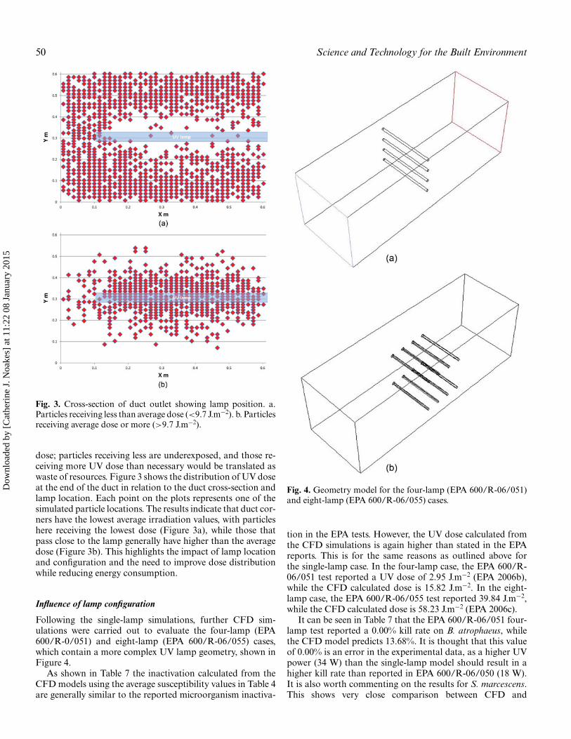
Fig. 3. Cross-section of duct outlet showing lamp position. a.Particles receiving less than average dose (<9.7 J.m−2). b. Particlesreceiving average dose or more (>9.7 J.m−2).

dose; particles receiving less are underexposed, and those re-ceiving more UV dose than necessary would be translated aswaste of resources. Figure 3 shows the distribution of UV doseat the end of the duct in relation to the duct cross-section andlamp location. Each point on the plots represents one of thesimulated particle locations. The results indicate that duct cor-ners have the lowest average irradiation values, with particleshere receiving the lowest dose (Figure 3a), while those thatpass close to the lamp generally have higher than the averagedose (Figure 3b). This highlights the impact of lamp locationand configuration and the need to improve dose distributionwhile reducing energy consumption.

Influence of lamp configuration

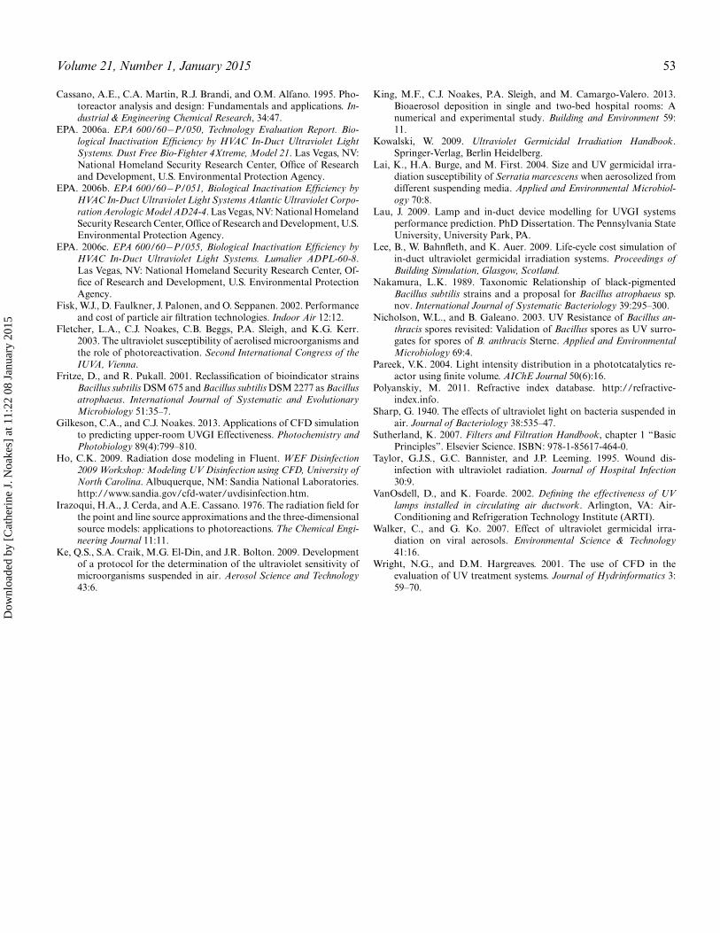
Following the single-lamp simulations, further CFD sim-ulations were carried out to evaluate the four-lamp (EPA600/R-0/051) and eight-lamp (EPA 600/R-06/055) cases,which contain a more complex UV lamp geometry, shown inFigure 4.

As shown in Table 7 the inactivation calculated from theCFD models using the average susceptibility values in Table 4are generally similar to the reported microorganism inactiva-

Fig. 4. Geometry model for the four-lamp (EPA 600/R-06/051)and eight-lamp (EPA 600/R-06/055) cases.

tion in the EPA tests. However, the UV dose calculated fromthe CFD simulations is again higher than stated in the EPAreports. This is for the same reasons as outlined above forthe single-lamp case. In the four-lamp case, the EPA 600/R-06/051 test reported a UV dose of 2.95 J.m−2 (EPA 2006b),while the CFD calculated dose is 15.82 J.m−2. In the eight-lamp case, the EPA 600/R-06/055 test reported 39.84 J.m−2,while the CFD calculated dose is 58.23 J.m−2 (EPA 2006c).

It can be seen in Table 7 that the EPA 600/R-06/051 four-lamp test reported a 0.00% kill rate on B. atrophaeus, whilethe CFD model predicts 13.68%. It is thought that this valueof 0.00% is an error in the experimental data, as a higher UVpower (34 W) than the single-lamp model should result in ahigher kill rate than reported in EPA 600/R-06/050 (18 W).It is also worth commenting on the results for S. marcescens.This shows very close comparison between CFD and

Dow

nloa

ded

by [

Cat

heri

ne J

. Noa

kes]

at 1

1:22

08

Janu

ary

2015

Volume 21, Number 1, January 2015 51

Table 7. CFD calculated performance against test results.

600/R-06/051 600/R06/055

Reference values Microorganism

CFDcalculated

kill rate (%)

EPAreported

kill rate (%)

CFDcalculated

kill rate (%)

EPAreported

kill rate (%)

Average S. marcescens 99.99 99.99 100.00 99.9Average MS2 bacteriophage 49.35 46.00 91.82 82.00Average B. subtilis (B. atrophaeus) 13.68 0.00 46.32 40.00

experiments for all three lamp configurations. However, sus-ceptibility constant k is so high that any UV dose over 10J.m−2 would show a 99.99% kill rate. It is therefore not a goodreference microorganism to conduct UV dose calculations orexperimental assessments for duct-mounted installations.

As with the single-lamp case, the CFD analysis of thesemulti-lamp devices also shows how dose distribution changesaccording to lamp geometry and UV power. The case with fourlamps evenly distributed over the height of the duct (Figure5a) shows a double peaked distribution, with the mode closerto the average UV dose of the system than in the single-lampcase. The eight-lamp model shows a wider dose distribution,yet the peak is again closer to the system average UV dose.

Fig. 5. Dose distributions. a. For EPA 600/R-06/051. b. For EPA600/R-06/055.

Figure 6 shows the location of particles that received theaverage UV dose of the system or more for the four-lamp(Figure 6a) and eight-lamp (Figure 6b) models. It can be seenagain that there are few particles at the corners receiving asufficient UV dose; however, in both cases, there is greatercoverage than the single-lamp case, indicating a more evendistribution.

Comparing all three cases indicates that the more even theUV dose distribution is, the more efficient the system is. Re-sults for the single-lamp system show that 3.15% of particles

Fig. 6. Cross-section of duct outlet showing lamp position andparticles receiving the average dose or more. a. Four-lamp case(EPA 600/R-06/051). b. Eight-lamp case (EPA 600/R-06/055).

Dow

nloa

ded

by [

Cat

heri

ne J

. Noa

kes]

at 1

1:22

08

Janu

ary

2015

52 Science and Technology for the Built Environment

received half the average dose of the system or less, while 6.2%of particles received double the average dose of the system.These values change when the dose is more closely distributedtoward the average. In the four-lamp design, 1.73% of parti-cles received less than half the average dose, and only 0.4% ofparticles received double than the average dose; for the eight-lamp system, there were no particles receiving less than halfthe average dose, and only 0.9% received double the averagedose. This indicates that the energy input into the device isbeing better used, with the more even distribution resulting insubstantially less under- and over-performance.

Model limitations

While the CFD simulation results are in good agreement withthe experimental results, it is important to consider the lim-itations of the model. The model assumes isothermal flow;however, in reality, the lamp will act as a heat source, and theincoming air into the system may range from 0◦C or less to over35◦C depending on the local climate, whether it is outdoor orindoor air, and whether it has had any pre-conditioning priorto UV irradiation. It is likely that the flow pattern in a ventila-tion duct will be largely straight and dominated by the velocityprovided by the fan. The presence of the lamp heat source mayincrease the mixing in the duct slightly, which may be benefi-cial from a UV disinfection perspective. Where there is a largetemperature gradient between the air and the lamp and at lowflow rates, buoyancy effects may influence the flow field andmay need to be included in models. Similarly, the influence oflamp-mounting arrangements has not been considered, whichmay also promote mixing of the airflow in the system.

Conclusions and future work

This study compares CFD modeling of three in-duct UV sys-tems with published experimental data and demonstrates thatCFD models are a viable method of predicting performanceand supporting system design. DO UV irradiance models ap-plied in a CFD model appear to be a reliable technique for thecalculation of the UV field, UV dose, and microorganism inac-tivation within in-duct UV sterilization systems. Good com-parison is seen between CFD calculated inactivation, EPA(2006a, 2006b, 2006c) test results, and previously publishedaverage UV dose calculations (Kowalski 2009).

The results highlight important considerations in selectingappropriate test microorganisms for performance assessments.B. subtilis and B. atrophaeus present a shoulder on their decaycurve. The results show that not accounting for such a shoulderwhen calculating UV dose by regression from microbiologicaltests may result in an under calculation of the UV systemdose. The results also indicate that S. marcescens is not a goodreference microorganism for the calculation of a system UVdose as it has a high susceptibility to UV and any dose over10 J.m−2 will result in kill rates of 99.99% regardless of systemdesign.

The results also show the limitations of current UV suscep-tibility data in the literature. While there are a good number

of studies that report susceptibility data, there is a consider-able amount of variability between studies, which depends ontest conditions and the particular strain of a microorganismspecies. A more comprehensive database of UV susceptibilityof microorganisms that includes the full spectrum of the mi-croorganism decay is required for accurate calculation of theUV power demands for the sterilization of air. This is the casefor performance assessment through modeling or experimen-tal approaches.

System design and the method of evaluation are shown tohave a significant effect on the energy efficiency and steriliza-tion efficacy of a UV installation. Calculating UV dose byregression from biodosimetry tests using the wrong microor-ganism decay model or incorrect UV susceptibility values willresult in miscalculation of UV dose. This, in turn, can leadto underpowered systems in which the sterilization efficiencywould be compromised or overpowered UV systems resultingin a waste of energy and excessive capital and maintenancecosts. Furthermore, the average dose delivered by a systemmay be a poor representation of its performance. In the single-lamp case average data compare well between experiments andCFD models, yet the CFD analysis showed that more than halfof the particles received less than the average calculated doseand 6.2% received over double the average dose. This indi-cates a poor design with both under-performance and excessenergy use apparent within the same device. CFD analysis iscapable of identifying this variability in dose distribution thatwould otherwise be impossible to identify by a biodosimetrytest. Initial simulations with four- and eight-lamp configura-tions show the benefit of positioning lamps to create a moreeven UV irradiance field and, hence, UV dose in the system.However, it is likely that neither of these are optimal solutions.Ongoing studies are focusing on lamp position optimizationto enable the most effective UV sterilization and the best useof the energy input into the system. This includes comparisonof lamps positioned parallel or perpendicular to the airflowand assessment of lamps located in staggered as well as in-linearrangements within the duct.

Funding

This work was carried out as part of a PhD studentship fundedby Conacyt (Mexico).

References

ANSYS. 2009. Discrete ordinates (DO) radiation model theory. https://www.sharcnet.ca/Software/Fluent12/html/th/node115.htm.

Beggs, C.B. 2002. A quantitative method for evaluating the photoreacti-vation of ultraviolet damaged microorganisms. Photochemistry andPhotobiological Science, 1:8.

Blatt, M.H. 2006. Advanced HVAC systems for improving indoor en-vironmental quality and energy performance of California K–12schools; applications guide for off-the-shelf equipment for UVCuse. Report CEC-500-03-003. California Energy Commission.http://www.archenergy.com/ieq-k12/.

Bolton, J.R. 2000. Calculation of ultraviolet fluence rate distribution inan annular reactor: Significance of refraction and reflection. WaterResearch 34:10.

Dow

nloa

ded

by [

Cat

heri

ne J

. Noa

kes]

at 1

1:22

08

Janu

ary

2015

Volume 21, Number 1, January 2015 53

Cassano, A.E., C.A. Martin, R.J. Brandi, and O.M. Alfano. 1995. Pho-toreactor analysis and design: Fundamentals and applications. In-dustrial & Engineering Chemical Research, 34:47.

EPA. 2006a. EPA 600/60−P/050, Technology Evaluation Report. Bio-logical Inactivation Efficiency by HVAC In-Duct Ultraviolet LightSystems. Dust Free Bio-Fighter 4Xtreme, Model 21. Las Vegas, NV:National Homeland Security Research Center, Office of Researchand Development, U.S. Environmental Protection Agency.

EPA. 2006b. EPA 600/60−P/051, Biological Inactivation Efficiency byHVAC In-Duct Ultraviolet Light Systems Atlantic Ultraviolet Corpo-ration Aerologic Model AD24-4. Las Vegas, NV: National HomelandSecurity Research Center, Office of Research and Development, U.S.Environmental Protection Agency.

EPA. 2006c. EPA 600/60−P/055, Biological Inactivation Efficiency byHVAC In-Duct Ultraviolet Light Systems. Lumalier ADPL-60-8.Las Vegas, NV: National Homeland Security Research Center, Of-fice of Research and Development, U.S. Environmental ProtectionAgency.

Fisk, W.J., D. Faulkner, J. Palonen, and O. Seppanen. 2002. Performanceand cost of particle air filtration technologies. Indoor Air 12:12.

Fletcher, L.A., C.J. Noakes, C.B. Beggs, P.A. Sleigh, and K.G. Kerr.2003. The ultraviolet susceptibility of aerolised microorganisms andthe role of photoreactivation. Second International Congress of theIUVA, Vienna.

Fritze, D., and R. Pukall. 2001. Reclassification of bioindicator strainsBacillus subtilis DSM 675 and Bacillus subtilis DSM 2277 as Bacillusatrophaeus. International Journal of Systematic and EvolutionaryMicrobiology 51:35–7.

Gilkeson, C.A., and C.J. Noakes. 2013. Applications of CFD simulationto predicting upper-room UVGI Effectiveness. Photochemistry andPhotobiology 89(4):799–810.

Ho, C.K. 2009. Radiation dose modeling in Fluent. WEF Disinfection2009 Workshop: Modeling UV Disinfection using CFD, University ofNorth Carolina. Albuquerque, NM: Sandia National Laboratories.http://www.sandia.gov/cfd-water/uvdisinfection.htm.

Irazoqui, H.A., J. Cerda, and A.E. Cassano. 1976. The radiation field forthe point and line source approximations and the three-dimensionalsource models: applications to photoreactions. The Chemical Engi-neering Journal 11:11.

Ke, Q.S., S.A. Craik, M.G. El-Din, and J.R. Bolton. 2009. Developmentof a protocol for the determination of the ultraviolet sensitivity ofmicroorganisms suspended in air. Aerosol Science and Technology43:6.

King, M.F., C.J. Noakes, P.A. Sleigh, and M. Camargo-Valero. 2013.Bioaerosol deposition in single and two-bed hospital rooms: Anumerical and experimental study. Building and Environment 59:11.

Kowalski, W. 2009. Ultraviolet Germicidal Irradiation Handbook.Springer-Verlag, Berlin Heidelberg.

Lai, K., H.A. Burge, and M. First. 2004. Size and UV germicidal irra-diation susceptibility of Serratia marcescens when aerosolized fromdifferent suspending media. Applied and Environmental Microbiol-ogy 70:8.

Lau, J. 2009. Lamp and in-duct device modelling for UVGI systemsperformance prediction. PhD Dissertation. The Pennsylvania StateUniversity, University Park, PA.

Lee, B., W. Bahnfleth, and K. Auer. 2009. Life-cycle cost simulation ofin-duct ultraviolet germicidal irradiation systems. Proceedings ofBuilding Simulation, Glasgow, Scotland.

Nakamura, L.K. 1989. Taxonomic Relationship of black-pigmentedBacillus subtilis strains and a proposal for Bacillus atrophaeus sp.nov. International Journal of Systematic Bacteriology 39:295–300.

Nicholson, W.L., and B. Galeano. 2003. UV Resistance of Bacillus an-thracis spores revisited: Validation of Bacillus spores as UV surro-gates for spores of B. anthracis Sterne. Applied and EnvironmentalMicrobiology 69:4.

Pareek, V.K. 2004. Light intensity distribution in a phototcatalytics re-actor using finite volume. AIChE Journal 50(6):16.

Polyanskiy, M. 2011. Refractive index database. http://refractive-index.info.

Sharp, G. 1940. The effects of ultraviolet light on bacteria suspended inair. Journal of Bacteriology 38:535–47.

Sutherland, K. 2007. Filters and Filtration Handbook, chapter 1 “BasicPrinciples”. Elsevier Science. ISBN: 978-1-85617-464-0.

Taylor, G.J.S., G.C. Bannister, and J.P. Leeming. 1995. Wound dis-infection with ultraviolet radiation. Journal of Hospital Infection30:9.

VanOsdell, D., and K. Foarde. 2002. Defining the effectiveness of UVlamps installed in circulating air ductwork. Arlington, VA: Air-Conditioning and Refrigeration Technology Institute (ARTI).

Walker, C., and G. Ko. 2007. Effect of ultraviolet germicidal irra-diation on viral aerosols. Environmental Science & Technology41:16.

Wright, N.G., and D.M. Hargreaves. 2001. The use of CFD in theevaluation of UV treatment systems. Journal of Hydrinformatics 3:59–70.

Dow

nloa

ded

by [

Cat

heri

ne J

. Noa

kes]

at 1

1:22

08

Janu

ary

2015