FLOW CHARTS AND INDICES FOR EVALUATING TRUE EFFICIENCY AND EFFECTIVENESS OF HARMONIC FILTERS IN POWER SYSTEMS by HILDE AMUSHEMBE Thesis submitted in fulfilment of the requirements for the degree Master of Technology: Electrical Engineering in the Faculty of Engineering at the Cape Peninsula University of Technology Supervisor: Professor Gary Atkinson-Hope Cape Town November 2014

CPUT copyright information

The dissertation/thesis may not be published either in part (in scholarly, scientific or technical

journals), or as a whole (as a monograph), unless permission has been obtained from the

University

ii

DECLARATION

I, Hilde Amushembe, declare that the contents of this dissertation/thesis represent my own

unaided work, and that the dissertation/thesis has not previously been submitted for

academic examination towards any qualification. Furthermore, it represents my own opinions

and not necessarily those of the Cape Peninsula University of Technology.

Signed Date

iii

ABSTRACT

Traditionally, efficiency is defined for sinusoidal networks and not for non-sinusoidal

networks. For this reason, the efficiency formula and indices for efficiency calculations are

reviewed. The concepts for determining powers, efficiency and power direction of flow in a

non-sinusoidal network are explained. A new index „True Efficiency‟ is introduced to

represent efficiency in non-sinusoidal circuits. Harmonic filters are installed in networks with

harmonic distortion levels above the set standards for harmonic mitigation. However, there

are no specific indices for evaluating the effectiveness of filter(s), hence the introduction of

the index „Filter Effectiveness‟.

Two software tools are utilised to develop flow charts and indices for evaluating true

efficiency and effectiveness of harmonic filters in a power system under distorted waveform

conditions. In this way, the effect that distortions have on efficiency can be determined and

the effectiveness of the mitigation measure in place can be evaluated. The methodologies

are developed using a step-by-step approach for two software packages.

Three case studies were conducted on a large network. This network has multiple harmonic

sources and capacitor banks. The first case study considered a network with two harmonic

sources and three capacitor banks of which two are at the point of common coupling (PCC)

and one is at a load bus; the second case study considered Case 1 with two capacitor banks

at the PCC used as components for the 2nd - order filter and the third case considered Case

2 with a Notch filter added at one of the load buses. The network was simulated using

DIgSILENT and SuperHarm software packages. DIgSILENT can calculate powers while

SuperHarm gives current and voltages and power is hand calculated. The two packages

were used together to test their compatibility and verify the network modelling.

For the different investigations conducted, the software-based methodologies developed to

calculate true efficiency in a network with multiple harmonic sources and capacitor banks

have been shown to be effective. The indices developed for evaluating the effectiveness of

harmonic filters proved to be effective too. The two software packages used proved to be

compatible as the results obtained are similar. The methodologies can easily be adapted for

investigations of other large networks as demonstrated in this study. The true efficiency

methodologies are thus recommended for application in this field as it will help determine

efficiency for networks with non-linear loads and help mitigate the distortions.

iv

ACKNOWLEDGEMENTS

The author would like to give thanks to everybody who was directly or indirectly involved with

this research. The research would not have been successful without your help and support.

Special gratitude is extended to:

God, my Lord for his many blessings, protection and guidance. He once again proved

that He is indeed The Most High God.

My supervisor, Prof G. Atkinson-Hope, for his great supervision, expert advice,

encouragement, commitment and dedication throughout this project.

The CPUT, especially the Centre of Power System Research (CPSR): I will always be

grateful to you for availing simulation software packages to assist me in completing

my investigations leading to my contribution to the field of electrical power

engineering.

My parents, my mother Lydia and father Barnabas, to my siblings and the entire

family, my heartfelt appreciation goes out to you for your patience and support during

my research.

Friends and fellow students, thanks for always asking me if I am a quitter whenever I

felt like quitting, well here it is so I guess I am not a quitter after all.

My employer, the Ministry of Works and Transport – Republic of Namibia for granting

me study leave and for recommending me for a scholarship.

The Ministry of Education – Republic of Namibia for granting me a Scholarship.

Cape Peninsula University of Technology, specifically the Faculty of Engineering

Postgraduate department for granting me a bursary.

Praise the Lord, O my soul, and forget not all His benefits. Psalm 103:2

v

DEDICATION

For Rauna „ka_aunty’ Hamutenya, you know what you mean to me.

vi

TABLE OF CONTENTS

Declaration ii

Abstract iii

Acknowledgements iv

Dedication

Table of Contents

List of Figures

List of Tables

v

vi

ix

xii

Glossary xiv

CHAPTER 1: INTRODUCTION

1.1 Background 1

1.2 Shortcoming and need for research 3

1.3 Objective of research 3

1.4 Thesis outline 5

1.5 List of publications 5

CHAPTER 2: THEORY AND CONCEPTS

2.1 Sinusoidal circuits 6

2.1.1 Power in sinusoidal circuits 6

2.1.1.1

2.1.1.2

2.1.1.3

2.1.2

Instantaneous and average or active power in sinusoidal circuits

Reactive power in sinusoidal circuits

Apparent power in sinusoidal circuits

RMS values in sinusoidal waveforms

6

8

8

8

2.1.3

2.1.4

2.2

2.2.1

2.2.1.1

2.2.1.2

2.2.1.3

2.2.2

2.2.3

Power factor (PF) in sinusoidal circuits

Efficiency in sinusoidal circuits

Non-sinusoidal circuits

Power in non-sinusoidal circuits

Active power in non-sinusoidal circuits

Reactive Power in non-sinusoidal circuits

Apparent power in non-sinusoidal circuits

Total harmonic distortion (THD)

RMS values in non-sinusoidal (distorted) waveforms

10

10

11

12

12

12

13

13

14

vii

2.2.4

2.2.5

2.3

PF in non-sinusoidal circuits

Efficiency in non-sinusoidal circuits

Summary

15

15

16

CHAPTER 3: THEORETICAL BACKGROUND OF POWER SYSTEMS ELEMENTS

UNDER HARMONIC CONDITIONS

3.1

3.1.1

3.2

3.2.1

3.2.2

3.2.3

3.2.3.1

3.2.3.2

3.2.4

3.2.4.1

3.2.4.2

3.3

Power system analysis

Theoretical basis for computer modelling of elements in power

systems with harmonics

Harmonics in power systems

Harmonic sources

Effects of harmonic distortion in power systems

Harmonic resonances

Series resonance

Parallel resonance

Harmonic mitigation measures

Notch filter

2nd – order filter

Summary

17

17

19

20

21

22

23

24

25

27

29

30

CHAPTER 4: COMPUTER TOOLS USED FOR HARMONIC ANALYSIS (DIGSILENT &

SUPERHARM)

4.1

4.1.1

4.1.1.1

4.1.1.2

4.1.1.3

4.1.1.4

4.1.1.5

4.1.1.6

4.1.1.7

4.1.2

4.1.2.1

4.1.2.2

4.1.2.3

DIgSILENT PowerFactory Software

Creating power system elements

Busbars

AC voltage source

Transformers

Line or branch

Linear and non-linear loads

Capacitor banks

Shunt filters

DIgSILENT calculation process

Load flow calculations at f1

Harmonic injection analysis

Impedance scan

31

31

33

33

34

34

34

36

36

37

37

38

39

viii

4.2

4.2.1

4.2.1.1

4.2.1.2

4.2.1.3

4.2.1.4

4.2.1.5

4.2.1.6

4.2.1.7

4.2.2

4.3

SuperHarm Software

Creating the text file in Notepad

Voltage source

Transformers

Capacitor banks

Line or branch impedance

Shunt filter

Linear load

Non-linear load

SuperHarm calculation process

Summary

40

40

41

41

42

42

43

44

44

45

47

CHAPTER 5: CONTRIBUTIONS

5.1

5.2

5.3

5.4

5.4.1

5.4.2

5.4.3

5.4.4

5.5

The need for this study

Main contributions

Delineations

Development of methodologies:

DIgSILENT steps for case studies simulations, THDv, resonance

points, efficiency and filter effectiveness calculations

SuperHarm steps for case studies simulations, THDv, resonance

points, efficiency and filter effectiveness calculations

Filter effectiveness

Application of the developed methodologies using Figure 5.4

Summary

48

49

50

51

54

55

57

57

58

CHAPTER 6: NETWORK CASE STUDIES & RESULTS

6.1

6.2

6.3

Application of Flow Chart A to DIgSILENT case studies

Application of Flow Chart A to SuperHarm case studies

Summary

59

72

81

CHAPTER 7: ANALYSIS AND FINDINGS

7.1 True Efficiency calculations and application of Flow Chart B to 82

ix

7.2

7.3

7.4

case studies (DIgSILENT)

True Efficiency calculations and application of Flow Chart B to

case studies (SuperHarm)

Findings

Summary

89

97

98

CHAPTER 8: CONCLUSIONS

8.1

8.2

Conclusions

Future work

99

101

REFERENCES 102

LIST OF FIGURES

Figure 2.1:

Figure 2.2:

Figure 2.3:

Figure 2.4:

Figure 3.1:

Figure 3.2:

Figure 3.3:

Figure 3.4:

Figure 4.1:

Figure 4.2:

Figure 4.3:

Figure 4.4:

Figure 4.5:

Figure 4.6:

Figure 4.7:

Figure 4.8:

Figure 5.1:

Figure 5.2:

Figure 5.3:

Power Triangle

Voltage sinusoidal waveforms

Typical Six-Pulse Front End Converter for AC Drive

Non-sinusoidal waveforms

Difference between linear and non-linear loads

System frequency responses to capacitor size variation

Series circuit and its resonance curve

Effects of resistance loads on parallel resonance

One line diagram

Grid dialog box

The Load flow

Harmonic load flow calculation button

Impedance scan button

Impedance scan graph

Solve ‘GO’ button

TOP 2000 icon

Current flow direction of linear and non-linear load

Flow Chart A: True efficiency with & without filter(s)

(DIgSILENT & SuperHarm)

Flow chart B: Filter effectiveness (DIgSILENT &

8

9

12

14

20

23

24

24

32

32

37

38

39

39

45

45

49

52

53

x

Figure 5.4:

Figure 6.1:

Figure 6.2:

Figure 6.3:

Figure 6.4:

Figure 6.5:

Figure 6.6:

Figure 6.7:

Figure 6.8:

Figure 6.9:

Figure 6.10:

Figure 6.11:

Figure 6.12:

Figure 6.13:

Figure 6.14:

Figure 6.15:

Figure 6.16:

Figure 6.17:

Figure 6.18:

Figure 6.19:

Figure 6.20:

Figure 6.21:

Figure 6.22:

Figure 6.23:

Figure 6.24:

Figure 7.1:

Figure 7.2:

Figure 7.3:

Figure 7.4:

Figure 7.5:

Figure 7.6:

Figure 7.7:

Figure 7.8:

Figure 7.9:

Figure 7.10:

Figure 7.11:

SuperHarm)

One-line diagram for application of methodologies

developed

One-line diagram of the network

Case 1 ZScan (DIgSILENT)

Case1 Voltage waveform at Bus3 (DIgSILENT)

Case 1 TS1 current waveform (DIgSILENT)

Network with 2nd – order filter

2nd – order filter model in DIgSILENT

Case 2 ZScan (DIgSILENT)

Case 2 Voltage waveform at Bus3 (DIgSILENT)

Case 2 TS1 current waveform (DIgSILENT)

Notch filter model in DIgSILENT

Case 3 ZScan (DIgSILENT)

Case 3 Voltage waveform at Bus3 (DIgSILENT)

Case 3 TS1 current waveform (DIgSILENT)

Case 1 ZScan (SuperHarm)

Case1 Voltage waveform at Bus3 (SuperHarm)

Case 1 TS1 current waveform (SuperHarm)

2nd – order filter and computer model in SuperHarm

Case 2 ZScan (SuperHarm)

Case 2 Voltage waveform at Bus3 (SuperHarm)

Case 2 TS1 current waveform (SuperHarm)

Notch filter and computer model in SuperHarm

Case 3 ZScan (SuperHarm)

Case 3 Voltage waveform at Bus3 (SuperHarm)

Case 3 TS1 current waveform (SuperHarm)

DIgSILENT resonance point magnitude

DIgSILENT resonance severity at hch

THDv for DIgSILENT

True Efficiency for DIgSILENT software

Filter effectiveness (TPh(in)) for DIgSILENT

Filter effectiveness (%η(TRUE)) for DIgSILENT

Filter effectiveness (%THDv) for DIgSILENT

SuperHarm resonance point magnitude

SuperHarm resonance severity at hch

THDv for SuperHarm

True Efficiency for SuperHarm

54

59

62

64

64

65

66

67

67

68

69

70

71

71

73

74

74

76

76

77

77

78

79

79

80

82

83

84

87

88

88

89

90

91

91

94

xi

Figure 7.12:

Figure 7.13:

Figure 7.14:

Figure 7.15:

Figure 7.16:

Figure A1.1:

Figure A1.2:

Figure A1.3:

Figure A1.4:

Figure A1.5:

Figure A1.6:

Figure A1.7:

Figure A1.8:

Figure A1.9:

Figure A1.10:

Figure A1.11:

Figure A1.12:

Figure A1.13:

Figure A1.14:

Figure A1.15:

Figure A1.16:

Figure A1.17:

Figure A1.18:

Figure A1.19:

Figure A1.20:

Figure A1.21:

Figure A2.1:

Figure A2.2:

Figure A2.3:

Figure A2.4:

Figure A2.5:

Figure A2.6:

Figure A2.7:

Figure A3.1:

Figure A3.2:

Figure A3.3:

Figure A3.4:

Filter effectiveness (TPh(in)) for SuperHarm

Filter effectiveness (%η(TRUE)) for SuperHarm

Filter effectiveness (%THDv) for SuperHarm

Resonance frequency points (DIgSILENT & SuperHarm)

TS1 power direction

Busbar model (e.g. Bus1)

Voltage source model (e.g. VSRC)

Transformer model A (e.g. TS1)

Transformer model B

Line model information (e.g. Line1)

Line1 load flow data

General Load modelling

Linear and non-linear load model

Linear and non-linear load data model

Linear and non-linear load voltage dependency index

Linear and non-linear load type model

Harmonic current model

Harmonic source spectrum

Capacitor model (e.g. Cap1)

Shunt Filter model

Load flow command dialog

List of load flow available variables

Results of the load flow calculation

Frequency Set dialog box

HLDF results

List of Impedance scan variables

Status window

Solution Complete status window

SuperHarm Data dialog box

Table Quantity Select dialog box

Harmonic Summary Data dialog box

ZScan Data

Summed ZScans

Drive1 spectrum

Drive2 spectrum

2nd – order filter model

Notch filter model

95

95

96

97

98

105

105

106

106

106

107

107

108

108

108

109

109

109

110

110

111

111

112

112

113

113

116

116

116

117

117

118

118

119

119

121

123

xii

LIST OF TABLES

Table 2.1:

Table 4.1:

Table 5.1:

Table 6.1:

Table 6.2:

Table 6.3:

Table 6.4:

Table 6.5:

Table 6.6:

Table 6.7:

Table 6.8:

Table 6.9:

Table 6.10:

Table 6.11:

Table 6.12:

Table 6.13:

Table 6.14:

Table 6.15:

Table 6.16:

Table 6.17:

Table 6.18:

Table A2.1:

Table A2.2:

Table A4.1:

Table A4.2:

Table A4.3:

Table A4.4:

IEEE Standard 519-1992

Comparison between DIgSILENT and SuperHarm

Fundamental Power variables for overall efficiency

Line parameters

Transformers parameters

Loads parameters

DIgSILENT harmonic current spectrum (Drive1 & Drive2)

Case 1 TS1 fundamental power (DIgSILENT)

Case 1 TS1 harmonic powers (DIgSILENT)

Case 2 TS1 fundamental power (DIgSILENT)

Case 2 TS1 harmonic powers (DIgSILENT)

Case 3 TS1 fundamental power (DIgSILENT)

Case 3 TS1 harmonic powers (DIgSILENT)

Resonance points (DIgSILENT)

Resonance magnitude for hch at PCC (DIgSILENT)

DIgSILENT THDv (%)

SuperHarm harmonic current spectrum (Drive1 & Drive2)

Resonance points (SuperHarm)

Resonance magnitude for hch at PCC (SuperHarm)

SuperHarm THDv (%)

SuperHarm Powers for all case studies

Frequency Data Points results

Harmonic Summary Data Results

Case 1 TS1 Currents (SuperHarm)

Case 1 TS1 voltages (SuperHarm)

Case 2 TS1 currents and voltages (SuperHarm)

Case 3 TS1 currents and voltages (SuperHarm)

13

47

58

60

60

61

61

62

63

66

68

69

70

72

72

72

72

80

80

81

81

117

118

133

133

142

152

xiii

APPENDICES 105

Appendix 1: Elements modelling in DIgSILENT 105

Appendix 2: Elements modelling in SuperHarm 114

Appendix 3: Case studies simulation in DIgSILENT

119

Appendix 4: Case studies simulation in SuperHarm 124

xiv

GLOSSARY

Abbreviations

AC

f

f1

fh

h

Vh

Ih

1ɸ

3ɸ

Φh

θh

ω1

THDv

THDi

TP

θspectrum

P1

Ph

θ1

I1

Hz

HVDC

fr

Zh

hr

Xr

Qc

Q

hch

PF

Xc

htuned

Z

TS1

TPh

Definitions

Alternating Current

Frequency

Fundamental frequency

Harmonic frequency

Harmonic number

Harmonic voltage

Harmonic current

Single phase

Three phase

Current phase angle

Voltage phase angle

Fundamental angular

Total voltage harmonic distortion

Total current harmonic distortion

Total power

Current spectrum angle

Fundamental power

Harmonic power

Fundamental current phase angle

Fundamental current

Unit of frequency

High Voltage Direct Current

Resonant frequency

Resonance impedance

Harmonic resonance

Resonance reactance

Capacitor reactive power

Quality factor

Characteristic harmonics

Power factor

Capacitor reactance

Harmonic tuned frequency

Impedance

Supply transformer 1

Total harmonic power

xv

TPh(out)

TPh(in)

TPF

Ω

Total harmonic output power

Total harmonic input power

True power factor

Resistance unit, ohms

A Current unit, Amperes

VA Apparent power unit, Volt-Ampere

W Active power unit, Watts

var

η

η(TRUE)

LDF

HLDF

LV

HV

Reactive power unit, Vars

Efficiency

True efficiency

Load flow

Harmonic load flow

Low voltage

High voltage

1

CHAPTER 1: INTRODUCTION

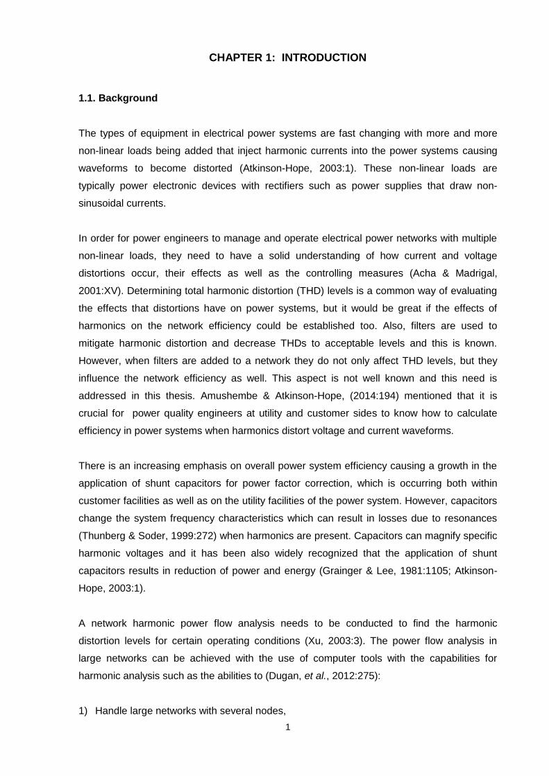
1.1. Background

The types of equipment in electrical power systems are fast changing with more and more

non-linear loads being added that inject harmonic currents into the power systems causing

waveforms to become distorted (Atkinson-Hope, 2003:1). These non-linear loads are

typically power electronic devices with rectifiers such as power supplies that draw non-

sinusoidal currents.

In order for power engineers to manage and operate electrical power networks with multiple

non-linear loads, they need to have a solid understanding of how current and voltage

distortions occur, their effects as well as the controlling measures (Acha & Madrigal,

2001:XV). Determining total harmonic distortion (THD) levels is a common way of evaluating

the effects that distortions have on power systems, but it would be great if the effects of

harmonics on the network efficiency could be established too. Also, filters are used to

mitigate harmonic distortion and decrease THDs to acceptable levels and this is known.

However, when filters are added to a network they do not only affect THD levels, but they

influence the network efficiency as well. This aspect is not well known and this need is

addressed in this thesis. Amushembe & Atkinson-Hope, (2014:194) mentioned that it is

crucial for power quality engineers at utility and customer sides to know how to calculate

efficiency in power systems when harmonics distort voltage and current waveforms.

There is an increasing emphasis on overall power system efficiency causing a growth in the

application of shunt capacitors for power factor correction, which is occurring both within

customer facilities as well as on the utility facilities of the power system. However, capacitors

change the system frequency characteristics which can result in losses due to resonances

(Thunberg & Soder, 1999:272) when harmonics are present. Capacitors can magnify specific

harmonic voltages and it has been also widely recognized that the application of shunt

capacitors results in reduction of power and energy (Grainger & Lee, 1981:1105; Atkinson-

Hope, 2003:1).

A network harmonic power flow analysis needs to be conducted to find the harmonic

distortion levels for certain operating conditions (Xu, 2003:3). The power flow analysis in

large networks can be achieved with the use of computer tools with the capabilities for

harmonic analysis such as the abilities to (Dugan, et al., 2012:275):

1) Handle large networks with several nodes,

2

2) Perform simultaneous solution of numerous harmonic sources to estimate the actual

current and voltage distortions,

3) Perform a frequency scan,

4) Have built in models of common harmonic sources (voltage and current sources), and

5) Display results in a meaningful and user friendly manner (e.g. graphs and tables), etc.

Electrical efficiency is traditionally expressed as a percentage (%η) in a network when

waveforms at the inputs and outputs of elements are sinusoidal and is given by equation

(1.1) (Shepherd, 1970:275).

Efficiency is the ratio of the total electrical power output to the total electrical power input and

the powers are at fundamental frequency (f1), but the total electrical power output and total

electrical power input powers are not defined for harmonic frequencies (e.g. f5, f7, f11, etc.) in

literature.

If equation (1.1) is used to calculate efficiency at fundamental frequency, then it can be

rewritten as:

And since f1 is an individual frequency, equation (1.2) can be rewritten for any individual

harmonic frequencies (fh) as:

where Ph is harmonic power at individual frequency, and

h is the harmonic number.

To calculate efficiency in a network with multiple harmonic frequencies, total power must first

be determined, making the equation for efficiency at multiple harmonic frequencies different

from equations (1.2) & (1.3). To distinguish between efficiency at f1 or fh and efficiency at

multiple harmonic frequencies the term “True Efficiency” is introduced. Calculating true

efficiency to determine the effects of distortions on power systems with multiple harmonic

3

sources is sound power quality control practice. Such a decision is quite complex for larger

networks and does not have an obvious solution.

How to formulate and analyse this problem is the requisite basis for this research.

1.2 Short coming and need for research

The traditional formula for efficiency calculation (e.g. equation (1.2)) only takes into account

the power at fundamental frequency (Amushembe & Atkinson-Hope, 2014:194). There is

thus a need to develop a formula for electrical efficiency that considers total powers at

harmonic frequencies.

It is easy to calculate what happens in the system (inductors & capacitors) of a radial line

with a single sending end and single receiving end, but when the system is big, hand

calculations becomes unreliable. The use of software packages therefore minimises the

errors encountered during hand calculations and reduces time spent on hand calculations,

hence the need for a study that utilises power system software package(s).

Literature mentions that harmonics reduce efficiency, but do not quantify it nor does it show

how efficiency can be calculated when harmonics are present. There is also nothing much

published in literature on efficiency calculations for power networks operating under distorted

conditions. Thus, there is a need to develop flow charts methodologies for a network that

shows how power and efficiency is calculated using software results. Also, there is a need to

evaluate the effect of harmonic filters that are used for mitigating harmonics discussing their

role on how they impact on efficiency in a power system.

1.3 Objective of research

The objective of this thesis is to use power system software packages (i) to investigate a

large distribution network with multiple capacitors and harmonic sources and (ii) develop

methodologies for network simulations and formulae for efficiency calculations and filter

effectiveness in power networks with harmonic distortions. The developed formulae can be

used as guidance by network operators to enable them to determine efficiency at

fundamental as well as at harmonic frequencies as well as when filters are applied. A further

objective is to conduct case studies. All case studies are conducted using industrial grade

power system software packages.

4

i) Importance of this research

Under harmonic conditions, there is a need to take into account the power flow directions at

harmonic frequencies as well as determining the total powers for efficiency calculations.

There is also a need to determine how filter effectiveness can be evaluated in power

systems.

ii) Contributions

The contributions of this work to harmonic powers and efficiency calculations are:

a) Identification and selection of efficiency calculations

Literature based on efficiency calculations in power system networks is reviewed. From the

reviewed literatures, a formula used for efficiency calculation in sinusoidal networks is

identified. The effectiveness of this formula was evaluated and a basis for the development

of efficiency formula for networks with distortions was formed.

b) Methodologies

The methodologies, in a form of flow charts, which are unique, are developed using a step-

by-step approach for conducting the investigations.

c) Case studies

A large distribution network is identified for investigations and two software packages and

their models are used to conduct fundamental frequency and harmonic frequencies load flow

case studies to compare results, confirm their modelling and compatibilities. Three case

studies are conducted. One case study is a network that includes multiple capacitors and

harmonic sources. The other two case studies investigate the impact of harmonic mitigation

on efficiency and resonance severity.

d) Analysis of results

Results for harmonic penetration and mitigation measures applied are analysed in terms of

established network standard limits and constraints to ensure acceptable state of operation

and to demonstrate the application and effectiveness of the developed methodologies.

5

1.4 Thesis outline

This thesis is divided into eight chapters:

Chapter 2 introduces the theoretical background and definitions of terms and concepts as

well as derivations of equations to give support to the work established in this thesis.

A brief theoretical background of power system elements under harmonic conditions is given

in Chapter 3.

Chapter 4 gives detailed descriptions on how the software tools are used to develop the

methodology as well as the modelling of elements using those software tools. Here two

packages (DIgSILENT and SuperHarm) are compared.

In Chapter 5, the contributions of the thesis and the step-by-step approach for the

development of methodologies and formulae to calculate true efficiency as well as indices for

evaluating the effectiveness of harmonic filters in networks with harmonics are outlined.

Chapter 6 provides the application of the flow charts in the step-by-step approach to case

studies in DIgSILENT and SuperHarm.

The results obtained from the case studies are analysed and their findings are highlighted in

Chapter 7.

Chapter 8 finally presents the overall conclusions and recommendations on the main

contributions and points out ideas for future studies.

1.5 List of publications

1. Amushembe, H. & Atkinson-Hope, G. 2014. The use of DIgSILENT PowerFactory software for power system efficiency calculations under distorted conditions. Proceedings of the 22nd South African Universities Power Engineering Conference. 30 – 31 January 2014. ISBN: 978-1-86840-619-7. pp194 - 199.

2. Atkinson-Hope, G., Amushembe, H. & Stemmet, W. 2014. Effectiveness of Filter Types

on Efficiency in Networks Containing Multiple Capacitors and Harmonic Sources. Australasian Universities Power Engineering Conference, AUPEC 2014, Curtin University, Perth, Australia, 28th September – 1st October 2014. ISBN: 978-0-646-92375-8, pp1 - 6. http://ieeexplore.ieee.org/xpls/abs_all.jsp?arnumber=6966492

6

CHAPTER 2 : THEORY AND CONCEPTS

This chapter gives theoretical background of the electrical terms/concepts relevant to this

thesis. The two sections in this chapter give definitions of instantaneous power, active power,

root mean square (RMS) values, apparent power and power factor for both sinusoidal and

non-sinusoidal circuits. The derivations of equations for all quantities for circuits under the

two conditions are also illustrated.

2.1 Sinusoidal circuits

Acha & Madrigal, (2001:38) states that instantaneous power, active power, RMS values,

apparent power and power factor are valid for any shape of the voltage and current

waveforms as long as these waveforms are periodic.

2.1.1 Power in sinusoidal circuits

The three universally accepted power definitions for networks with sinusoidal voltage and

current waveforms are (Stemmet, 2004:1, Atkinson-Hope, 2003:16): active power P

measured in watts (W), reactive power Q measured in Vars (Var) and apparent power S

measured in volt-ampere (VA).

In sinusoidal steady-state:

where is the maximum current, is the maximum voltage.

2.1.1.1 Instantaneous and average or active power in sinusoidal circuits

Power system engineers define „power‟ as the rate of change of energy with respect to time

in terms of voltage and current. Instantaneous power delivered by a source to the load at any

instant is the product of instantaneous voltage drop given by equation (2.1) across the load

and the instantaneous current given by equation (2.2) into the load (Stevenson, 1982:12;

Acha & Madrigal, 2001:36; Atkinson-Hope, 2003:16).

7

The active power is defined in Acha & Madrigal, (2001:37) as the instantaneous power

consumed in a period T. Active power is calculated by integrating equation (2.3) as shown in

equation (2.5). This is also the power that is read on the wattmeter as watts when active

power is measured.

where T is a period of the voltage and is the frequency.

∫

For a purely resistive load is zero and by substituting equations (2.1), (2.2) and (2.4) into

equation (2.5), the active power equation becomes:

∫

Applying the trigonometric identity, to equation (2.6) becomes:

*

,

-+

The cosine term is one at both limits, thus equation (2.7) reduces to:

where is the angle between current and voltage, is the voltage angle, is the current

angle.

8

2.1.1.2 Reactive power in sinusoidal circuits

For sinusoidal quantities, the reactive power in a single phase AC network is defined as the

product of the voltage, the current, and the sine of the phase angle between them (Von

Meier, 2006:70).

θ0

j Im S

S

P

jQ

Re S

Figure 2.1: Power Triangle

Reactive power is calculated in Vars. From the power triangle shown in Figure 2.1, the

reactive power can be calculated in equation (2.11) as:

√| |

2.1.1.3 Apparent power in sinusoidal circuits

Apparent power is the power value obtained in an AC circuit by multiplying the effective value

of voltage and current ( ) and they are the effective voltage and current delivered

to the load. Therefore, apparent power for single phase (1ϕ) is given by:

| | | | | |

√

2.1.2 RMS values in sinusoidal waveforms

The RMS value of a quantity is the square root of the mean value of the squared values of

the quantity taken over an interval. One of the principal applications of RMS values is with

9

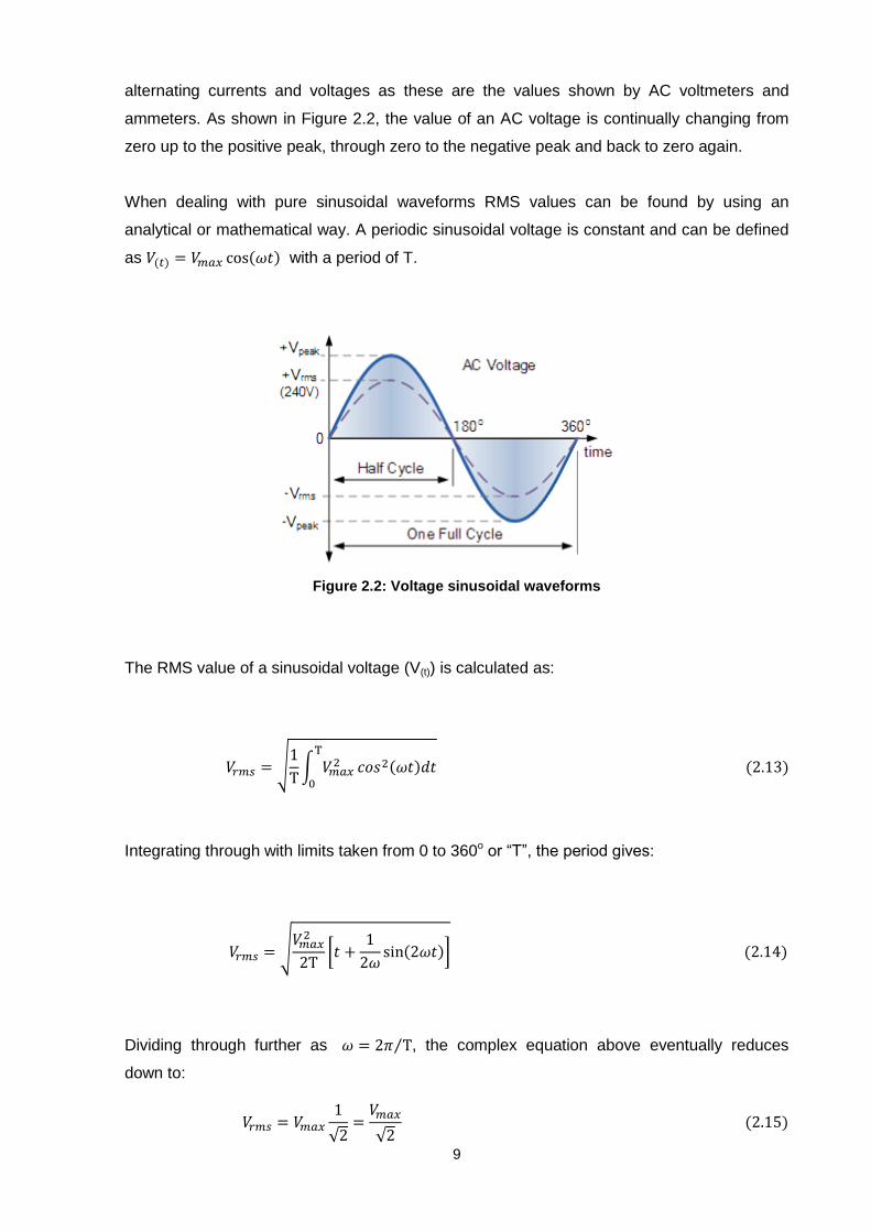
alternating currents and voltages as these are the values shown by AC voltmeters and

ammeters. As shown in Figure 2.2, the value of an AC voltage is continually changing from

zero up to the positive peak, through zero to the negative peak and back to zero again.

When dealing with pure sinusoidal waveforms RMS values can be found by using an

analytical or mathematical way. A periodic sinusoidal voltage is constant and can be defined

as with a period of T.

Figure 2.2: Voltage sinusoidal waveforms

The RMS value of a sinusoidal voltage (V(t)) is calculated as:

√

∫

Integrating through with limits taken from 0 to 360o or “T”, the period gives:

√

[

]

Dividing through further as ⁄ , the complex equation above eventually reduces

down to:

√

√

10

Similarly for current,

√

√

The RMS voltage or current, which can also be referred to as the effective value, depends on

the magnitude of the waveform and is not a function of either the waveforms frequency or its

phase angle.

2.1.3 Power factor (PF) in sinusoidal circuits

There are a couple of definitions for power factor in literature. For instance, Izhar, et al.,

(2003:227) defined power factor as a quantity used to measure how effectively a load uses

the current it draws from the source or supply. While, Acha & Madrigal, (2001:38) defines

power factor as the ratio by which the apparent power is multiplied to obtain the active power

in an AC circuit. The cosine of phase angle between voltage and current from equation (2.9)

is also called power factor (Stevenson, 1982:16; Negumbo, 2009:6). For sinusoidal

waveform, power factor is calculated using fundamental power quantities as derived in

equation (2.17).

where V1 and I1 are the fundamental voltage and current respectively.

When the system is symmetrical and all loads are linear, the power factor is called

displacement power factor (DPF) (Amushembe & Atkinson-Hope, 2014:195) and is

determined by equation (2.18) as:

2.1.4 Efficiency in sinusoidal circuits

Efficiency of an entity (a device, component, or system) in electrical engineering is defined as

electrical power output divided by the total electrical power input (a fractional expression). It

is typically denoted by “Eta” ( ) and is determined by equation (1.1). The total power input

and total power output for a sinusoidal circuit are calculated by equation (2.8).

11

2.2 Non-sinusoidal circuits

The traditional power system quantities are defined for fundamental frequency context

assuming pure sinusoidal conditions. However, in the presence of harmonic distortions,

these power quantities and analysis for sinusoidal conditions do not apply for non-sinusoidal

conditions (Dugan, et al., 2012:203). Different power, RMS and PF terms and definitions

have appeared in the literature over the years, and to date, it is still debatable as to what set

of power terms, definitions or standards should be used in cases of non-sinusoidal

operations. This is because some of these terms yield insight while others do not.

A distorted periodic current or voltage waveform expanded into a Fourier series is expressed

as follows:

∑

∑

where is the harmonic peak current, is the harmonic peak voltage, is the

harmonic current phase angle, is the harmonic voltage phase angle, is the

fundamental angular frequency, , is the fundamental frequency.

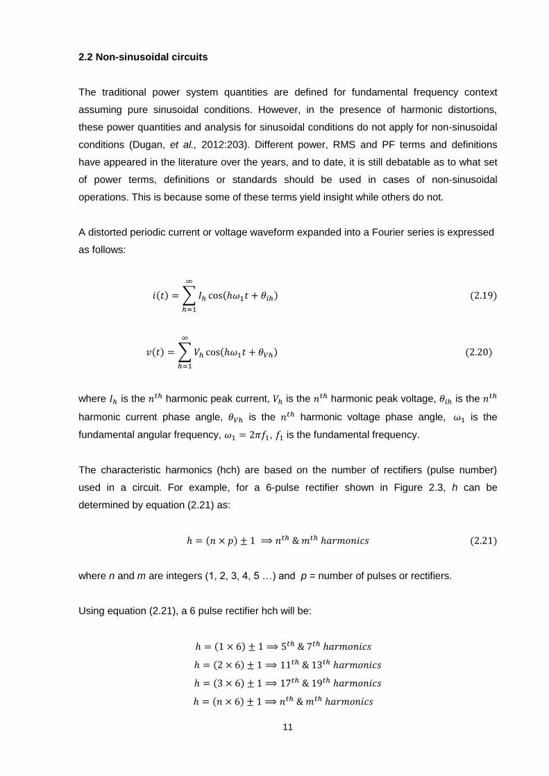
The characteristic harmonics (hch) are based on the number of rectifiers (pulse number)

used in a circuit. For example, for a 6-pulse rectifier shown in Figure 2.3, h can be

determined by equation (2.21) as:

where n and m are integers (1, 2, 3, 4, 5 …) and p = number of pulses or rectifiers.

Using equation (2.21), a 6 pulse rectifier hch will be:

12

Load

Ac line

A

B

C

DC Bus

+

-

Figure 2.3: Typical Six-Pulse Front End Converter for AC Drive

(Adapted from Square D, 1994:2)

2.2.1 Power in non-sinusoidal circuits

2.2.1.1 Active power in non-sinusoidal circuits

a) Active power in a non-sinusoidal circuit is

b) Substituting equations (2.19) and (2.20) into equation (2.22) becomes:

∑

where is the individual harmonic active power.

c) According to Perera, et al., (2002:1), one of the methods of determining who is

responsible for injecting harmonics into the system is by checking the sign of Ph:

1) If , in other words if is positive, the utility side is responsible for harmonic

distortions, and

2) If , or in other words if negative, then the customer side is the cause of

harmonic distortions.

2.2.1.2 Reactive power in non-sinusoidal circuits

Reactive power is defined as,

13

∑

2.2.1.3 Apparent power in non-sinusoidal circuits

The apparent power when waveforms are non-sinusoidal is:

√∑

√ for non-sinusoidal circuits. Therefore the equation (2.12) is not

valid for non-sinusoidal waveforms.

2.2.2 Total Harmonic Distortion

The harmonic currents produced by nonlinear loads can interact adversely with the utility

supply system. This interaction gives rise to voltage and current harmonic distortion (Dugan,

et al., (2012:255). When these harmonics are summed, they are termed total harmonic

distortion (THD), which defines and quantifies the thermal effect of all harmonics (Uzunoglu,

et al., 2004:43). The term THD is used to express how badly a waveform is distorted as a

percentage of the fundamental voltage and current waveforms (Singh & Singh, 2010:1; Izhar,

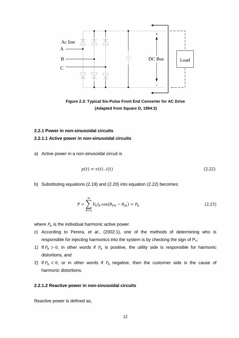
et al., 2003:227). THD applies to both current and voltage and is determined by the RMS

value of harmonics divided by the RMS value of the fundamental, and then multiplied by 100

%, as shown in equations (2.28 & 2.30). THD of the current (THDi) can actually vary up to

more than 100 %, but THD of the voltage (THDV) is only acceptable when below 5 % as

stipulated in the IEEE 519 standards shown in Table 2.1 (Dugan, et al., 2012: 258; Wakileh,

2001:137; Lee & Lee, 1999:194).

Table 2.1: IEEE Standard 519-1992

Bus voltage at PCC, Vn (kV) Individual harmonic voltage

distortion (%)

Total voltage distortion,

THDVn (%)

Vn ≤ 69 3.0 5.0

69, Vn ≤ 161 1.5 2.5

Vn > 161 1.0 1.5

14

√

√∑

Similarly for current,

√

√∑

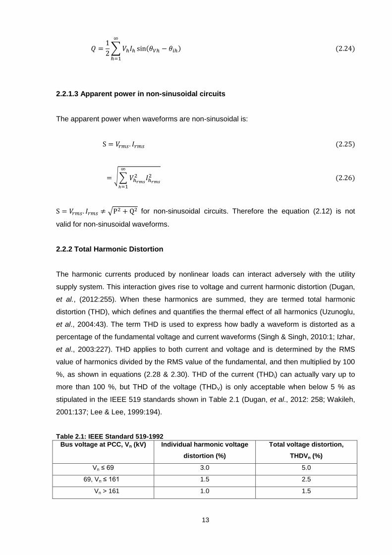
2.2.3 RMS value in non-sinusoidal (distorted) waveforms

In power systems, distortions in the waveform are caused by harmonics. Harmonics always

increase RMS values which lead to increased losses and reduced average power.

Multiplying the peak or maximum value by the constant 0.7071 or √ only applies to

sinusoidal waveforms (see Figure 2.2). In a distorted waveform shown in Figure 2.4, only

one period “T” needs to be defined and can be broken up to a fundamental component

(corresponding to the period T) and its harmonics.

Figure 2.4: Non-sinusoidal waveforms

15

A uni-directional term (direct component) may also be present. This series of terms is known

as Fourier Series (equations 2.19 & 2.20). One can provide expressions for the RMS voltage

and current from equations (2.19) and (2.20) as:

√∑

√∑

2.2.4 PF in non-sinusoidal circuits

PF is the ratio of real power to apparent power and has traditionally been determined by

examining the phase angle between voltage and current for sinusoidal circuits. For non-

sinusoidal waveforms, this technique always presents a power factor reading which is

erroneously high. The accurate technique, however, shown in equation (2.33) is attained by

averaging the instantaneous power in equation (2.23) divided by the product of the true RMS

voltage in equation (2.31) and the true RMS current equation (2.32) (PG&E, 2004:3;

Atkinson-Hope, 2003:18).

∑

When the system has non-linear loads, the PF is called true power factor (TPF) and is

determined by:

∑

∑

2.2.5 Efficiency in non-sinusoidal circuits

The algebraic sum of is the total active harmonic power (TPh) at a node. The

determined in equation (2.23) can have different signs thus TPh is determined using different

equations at different points in the network with harmonics (see sub-section 2.2.1.1(c)).

Efficiency is one of the evaluation factors that need to be determined. When waveforms are

distorted the term “True Efficiency” (η(TRUE)) should be used, linked to “True Power Factor”.

16

According to Amushembe & Atkinson-Hope, (2014:195,198), equations at nodes in a

network for TPh in a non-sinusoidal circuit with a 6-pulse drive injections can be of the forms:

∑

∑

∑

And depending on which of the above powers calculated in equations (2.35), (2.36) and

(2.37) is output power and which is input power, the formula for calculating true efficiency

can be written as:

|

|

This depends upon the network configuration and needs to be empirically determined. The

total input and output power used to calculate efficiency in a non-sinusoidal circuit would

have different expressions depending on the direction of harmonic current at the point of

measurement. This statement forms the basis of the need for this research to develop

formulae or methodologies for power and efficiency calculations under distorted conditions.

2.3 Summary

The theory and concepts of power, RMS, PF and efficiency in a sinusoidal circuit and in a

non-sinusoidal circuit are reviewed. Formulae to determine the above-mentioned are also

reviewed. The formula for calculating true efficiency is introduced to indicate it as an index

when waveforms are distorted in a power system thus, moving the knowledge from

traditional efficiency calculations (no waveform distortion) to systems with distortions.

17

CHAPTER 3 : THEORETICAL BACKGROUND OF POWER SYSTEM ELEMENTS

UNDER HARMONIC CONDITIONS

Very often computer software tools are used in power system analysis. This is because real

life measurements are expensive, tedious and could cause disruptions to plant operations.

This chapter gives a brief theoretical background on power systems elements that form the

basis of power system modelling and simulation under harmonic conditions. It further

explains the concept of harmonics, gives examples of harmonic sources, mentions the

different effects harmonics have on power system equipment and finally presents mitigation

measures applicable for harmonics reduction or elimination.

3.1 Power system analysis

Ideal power systems are theoretically supplied with a single and constant frequency at a

specified voltage level of constant magnitude, but practically, none of these conditions are

met. Power engineers are thus faced with the problem of voltage and frequency deviations

and they have to develop methodologies to control and predict harmonic voltages and

currents effects (Acha & Madrigal, 2001:XV, 4; Arrilaga & Watson, 2003:1). One of the

approaches to understand the impact harmonics have on a power system is to do a power

system harmonic analysis. Harmonic analysis serves as reference for system planning,

system operation, troubleshooting and maintenance of equipment, and verification of

standard compliance (Xu, 2003:1; Uzunoglu, et al., 2004:41). According to Dugan,

(1996:171), when carrying out any power system harmonics study, it is crucial to keep in

mind that the objective of the study is well determined and followed. It is also important to

make sure the characteristics of harmonic sources are known and understood and that the

software tool to use is compatible with the type of data at hand.

3.1.1 Theoretical basis for computer modelling of elements in power systems with

harmonics

With the widespread use of digital computers, the use of software packages has become a

modern norm for harmonic analysis. The modelling of elements in power systems operating

under harmonic conditions involves (Barret, et al., 1997:178):

Determining the impedance of the system to harmonic frequencies, and

Representing the harmonic sources.

18

The modelling of main power system elements under harmonic conditions is given by Acha &

Madrigal, (2001:56 - 57) as:

1. Lines: are modelled as passive elements and all passive elements such as resistors,

inductors and capacitors are considered to behave linearly with frequency. They have the

following characteristics,

where and are the rated inductive and capacitive reactances, respectively.

2. Transformers: are linear elements whose harmonic impedance is derived as:

√

where R is derived from the transformer power losses and is the transformers short -

circuit reactance.

3. Capacitor banks: are considered to be passive elements. The salient features of the

method used to model the power factor correction capacitor are:

where is the rms line voltage in kV and is the three - phase reactive power in MVA.

4. Non-linear loads are mostly represented as harmonic current sources, and the magnitude

and phase angle of the current source representing the non-linearity can be obtained

from manufacturers as published spectrum, measured or calculated using equations (3.6)

19

and (3.7). The harmonic content for ideal current sources is assumed to be inversely

proportional to the harmonic number. Thus, the magnitude for the fifth harmonic number

is one-fifth times fundamental current, seventh is one-seventh times fundamental current,

etc. The harmonic frequency is the harmonic number multiplied with the fundamental

frequency (e.g. for a 5th harmonic number, harmonic frequency is ) (Xu, 2003:2;

Atkinson-Hope, 2003:18; Dugan, et al., 1996:174).

| | | |

3.2 Harmonics in power systems

Harmonics are defined as frequencies that are multiple integers of the fundamental

frequency (Wakileh, et al., 2001:41; Arrilaga & Watson, 2003:2). Harmonics are again

defined by Dugan, et al., (1996:125) as the sinusoidal voltages or currents having

frequencies that are integer multiples of the frequency at which the supply is designed to

operate, usually 50 or 60 Hz. A rise in harmonic problems in power systems is caused by an

increase in harmonic current sources, by high harmonic impedance at the harmonic source

locations resulting from resonance phenomena, phase imbalances, and high input voltage or

current (Cui & Xu, 2007:1; Ko, et al., 2011:66.1).

Harmonic distortions on power systems phenomenon appeared in technical literature from as

early as 1930s, but then transformers were considered the source (Dugan, et al., 1996:124).

Harmonic distortion is defined by Ko, et al, (2011:66.1) as a form of pollution in the electric

plant that cause disturbances every time the harmonic currents rises above the limits.

Dugan, et al., (1996:1) and Ko, et al., (2011:66.2-66.3) states that the greatest problem

caused by harmonics is voltage and current waveform distortion. The additional current

resulting from these distortions does not yield any net energy, but rather constitute additional

losses in the power system elements or impedance they pass through (Dugan, et al.,

1996:133; Amushembe & Atkinson-Hope, 2014:194). An increasing emphasis on power

system efficiency has prompted an increase in the use of electronic converters in the 1970s,

but these devices resulted in increasing harmonic levels in power systems (Dugan, et al.,

1996:1; 123).

20

3.2.1 Harmonic Sources

Harmonic distortion is caused by non-linear devices with current which is non-proportional to

the supply voltage. These devices distort the sinusoidal waveform of current and voltage

causing circulation of harmonic components in power systems by drawing current in high

amplitude short pulses (Dugan, et al., 1996: 124-125; Wakileh, 2001:81; Uzunoglu, et al.,

2004:42; Singh & Singh, 2010:1). Barret, et al., (1997:183) states that harmonic sources can

either be intrinsic to the system or can be due to the nature of loads connected depending on

the origins.

The traditional harmonic sources are transformers, rotating machines and arc furnaces

(Wakileh, 2001:45-47; Dugan, et al., 1996:124). However, in the modern era, as mentioned

by De la Rosa, (2006:1), Wakileh, (2001:47), Ko, et al., (2011:66.3), harmonics are mainly

caused by non-linear loads such as fluorescent lamps, electronic controls, thyristor-controlled

devices such as rectifiers, inverters static VAR compensator, Adjustable Speed Drives

(ASDs) and HVDC transmission. Manufactures of ASDs only market the benefits such as

high efficiency, noise reduction, enhanced product quality and improved equipment reliability

but leave out the effects such as harmonic effects (Domijan & Embriz-Santander, 1990:98-

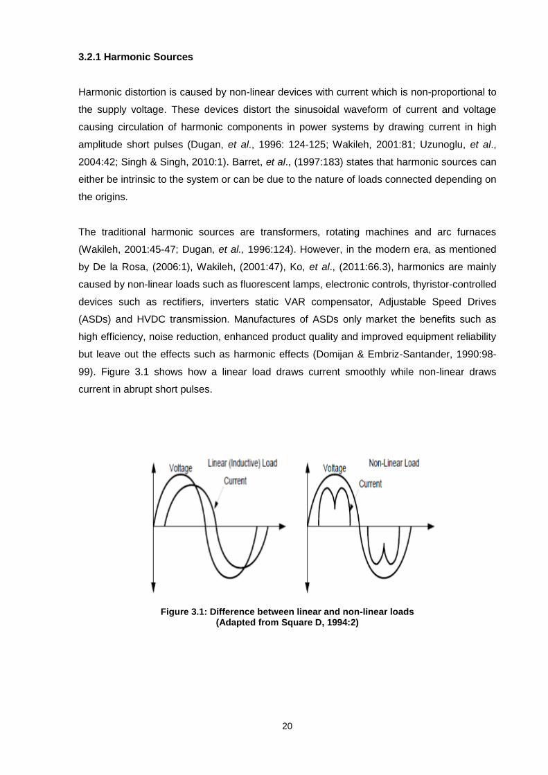
99). Figure 3.1 shows how a linear load draws current smoothly while non-linear draws

current in abrupt short pulses.

Figure 3.1: Difference between linear and non-linear loads (Adapted from Square D, 1994:2)

21

3.2.2 Effects of harmonic distortion in power systems

Many studies have been done about harmonic effects on power system elements, with some

authors even comparing it to the effects that stress and high blood pressure has on a human

body (Domijan & Embriz-Saintander, 1990:99; Square D, 1994:4). Harmonics greatest effect

on power system is increased equipment losses due to overheating and loss-of-life caused

by premature insulation breakdown. Harmonics causes mal-operation and component failure

in sensitive equipment such as communication equipment, protection relays, etc. (Wakileh,

2001:81, 84; Acha & Madrigal, 2001:5). Czarnecki (1996:1244) states that current harmonics

produced by loads cause an increase in active power loss mainly in the distribution system.

Harmonic distortions have different effect on different power system equipment. Arrilaga, et

al., (1985:113 - 117) states that in transformers, harmonic voltages increase the hysteresis

and eddy current losses and stresses the insulation whereas harmonic current increases the

copper losses. Harmonic voltages and currents also give rise to additional loss in the stator

windings, rotor circuits, and stator and rotor laminations on rotating machines. An increase in

induction motor losses depicts a decrease in its efficiency. In the presence of harmonics, if

rated output power of equipment is kept constant, then the input power has to be increased.

This means the utility has to supply extra power for the same amount of work (Lee & Lee,

1999:198). Effects on capacitor banks are series and parallel resonances, which can cause

overvoltage and high currents increasing the losses and overheating of capacitors.

Harmonic currents affect metering and instrumentations of the electrical meters particularly if

the circuit is under resonant conditions. The induction disc devices such as watt-hour meters

and overcurrent relays are designed to monitor only fundamental current, thus harmonic

currents caused by harmonic distortion can cause erroneous operation of these devices

(Ortmeyer, et al., 1985:2559). Voltage distortion on cables increases the dielectric stress in

proportion to their crest voltages. This effect shortens the useful life of the cable. It also

increases the number of faults and therefore the cost of repairs. Harmonic currents increase

losses in the cables resulting in temperature increase. An increase in current rms for an

equal active power consumed and an increase in the apparent resistance of the core with

frequency due to skin effect all cause additional losses in cables and equipment.

A poor power factor has disadvantages of increased line losses, increased generator and

transformer ratings and extra regulation equipment for the case of a low lagging power

factor. It is thus essential to install capacitor banks to reduce the system‟s reactive and

apparent power, hence increasing the system‟s power factor (Wakileh, 2001:35). However, in

cases with harmonics present in the system, resonance might occur. All circuits containing

22

capacitances and inductances have one or more natural frequencies. A resonance may be

developed when one of those natural frequencies lines up with a frequency that is being

produced on the power system. The current and voltage at that frequency continue to persist

at very high values.

According to Domijan & Embriz-Santander, (1990:100); Square D, (1994:4); Wakileh,

(2001:85); Arrilaga & Watson, (2003:110); Hossam-Eldin & Hasan, (2006:547), the main

effects of voltage and current harmonics within the power system can be summarised as

follows:

1. Harmonic magnification resulting from series and parallel resonances, which can cause

dielectric failure or ruptures of capacitors.

2. Harmonics cause a reduction in the efficiency of the generation, transmission and

utilisation of electrical energy as well as in inductive devices.

3. Harmonic distortions cause errors in utility meter readings, leading to higher customer

billings.

4. Harmonics increases the rate of ageing of the insulation of electrical plant components

with consequent shortening of their useful life.

5. Harmonics causes malfunction of system or plant components.

3.2.3 Harmonic resonances

The existence of resonance in the power system can be identified by carrying out a

frequency scan (Cui & Xu, 2007:1; Xu, 2003:5). The two common types of resonances that

occur in a power system are series resonance and parallel resonance (Negumbo 2009:34,

Zobaa, 2004:256). The basic resonant frequency (fr) for both simple series and parallel

circuits is given by the same equation (3.8), provided the resistance (R) is small in

comparison with the reactance (X) (Dugan, 1996:160; Hoag, 2007:1).

√

The effect the varying of capacitor size has on the system impedance and system frequency

is shown in Figure 3.2. The Figure shows that when there is no capacitor in the system, there

is no resonance and the response is linear. When there is a 10 % capacitor size installed,

there is higher resonance impedance (Zh) occurring at a higher frequency or harmonic

number (between 13th and 17th harmonic frequency). When the capacitor size is increased to

30 % and 50 %, Zh is decreased and the system frequency is also reduced further to a lower

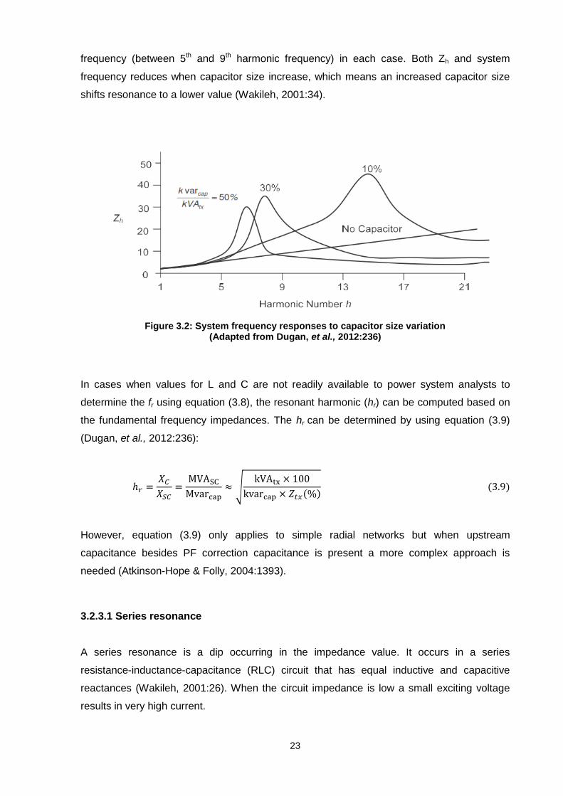
23

frequency (between 5th and 9th harmonic frequency) in each case. Both Zh and system

frequency reduces when capacitor size increase, which means an increased capacitor size

shifts resonance to a lower value (Wakileh, 2001:34).

Figure 3.2: System frequency responses to capacitor size variation (Adapted from Dugan, et al., 2012:236)

In cases when values for L and C are not readily available to power system analysts to

determine the fr using equation (3.8), the resonant harmonic (hr) can be computed based on

the fundamental frequency impedances. The hr can be determined by using equation (3.9)

(Dugan, et al., 2012:236):

√

However, equation (3.9) only applies to simple radial networks but when upstream

capacitance besides PF correction capacitance is present a more complex approach is

needed (Atkinson-Hope & Folly, 2004:1393).

3.2.3.1 Series resonance

A series resonance is a dip occurring in the impedance value. It occurs in a series

resistance-inductance-capacitance (RLC) circuit that has equal inductive and capacitive

reactances (Wakileh, 2001:26). When the circuit impedance is low a small exciting voltage

results in very high current.

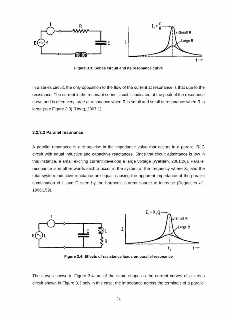
24

Figure 3.3: Series circuit and its resonance curve

In a series circuit, the only opposition to the flow of the current at resonance is that due to the

resistance. The current in the resonant series circuit is indicated at the peak of the resonance

curve and is often very large at resonance when R is small and small at resonance when R is

large (see Figure 3.3) (Hoag, 2007:1).

3.2.3.2 Parallel resonance

A parallel resonance is a sharp rise in the impedance value that occurs in a parallel RLC

circuit with equal inductive and capacitive reactances. Since the circuit admittance is low in

this instance, a small exciting current develops a large voltage (Wakileh, 2001:26). Parallel

resonance is in other words said to occur in the system at the frequency where XC and the

total system inductive reactance are equal, causing the apparent impedance of the parallel

combination of L and C seen by the harmonic current source to increase (Dugan, et al.,

1996:159).

Figure 3.4: Effects of resistance loads on parallel resonance

The curves shown in Figure 3.4 are of the same shape as the current curves of a series

circuit shown in Figure 3.3 only in this case, the impedance across the terminals of a parallel

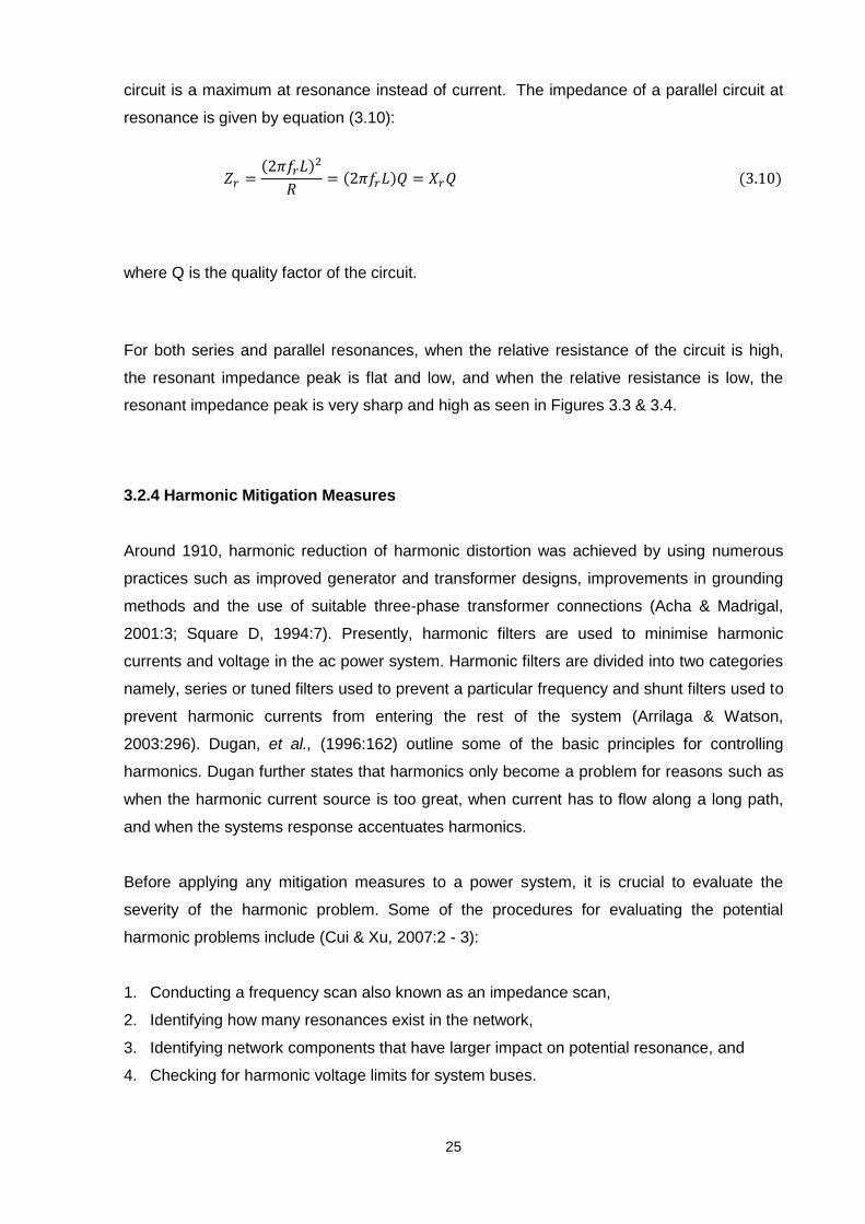
25

circuit is a maximum at resonance instead of current. The impedance of a parallel circuit at

resonance is given by equation (3.10):

where Q is the quality factor of the circuit.

For both series and parallel resonances, when the relative resistance of the circuit is high,

the resonant impedance peak is flat and low, and when the relative resistance is low, the

resonant impedance peak is very sharp and high as seen in Figures 3.3 & 3.4.

3.2.4 Harmonic Mitigation Measures

Around 1910, harmonic reduction of harmonic distortion was achieved by using numerous

practices such as improved generator and transformer designs, improvements in grounding

methods and the use of suitable three-phase transformer connections (Acha & Madrigal,

2001:3; Square D, 1994:7). Presently, harmonic filters are used to minimise harmonic

currents and voltage in the ac power system. Harmonic filters are divided into two categories

namely, series or tuned filters used to prevent a particular frequency and shunt filters used to

prevent harmonic currents from entering the rest of the system (Arrilaga & Watson,

2003:296). Dugan, et al., (1996:162) outline some of the basic principles for controlling

harmonics. Dugan further states that harmonics only become a problem for reasons such as

when the harmonic current source is too great, when current has to flow along a long path,

and when the systems response accentuates harmonics.

Before applying any mitigation measures to a power system, it is crucial to evaluate the

severity of the harmonic problem. Some of the procedures for evaluating the potential

harmonic problems include (Cui & Xu, 2007:2 - 3):

1. Conducting a frequency scan also known as an impedance scan,

2. Identifying how many resonances exist in the network,

3. Identifying network components that have larger impact on potential resonance, and

4. Checking for harmonic voltage limits for system buses.

26

Harmonics can be controlled by modifying the system frequency response in the following

manners (Dugan, et al., 2012:263 - 265; Wakileh, 2001:29 - 34):

1. Changing capacitor size (Dugan, et al., 2012:265). This is a method of decreasing the

resonance magnitude as a means of mitigation. It is achieved by increasing the capacitor

size which moves the resonance to a low value (Wakileh, 2001:34).

2. Damping. This is a method of reducing the resonance impedance by keeping the

resistance (R) minimal. The circuit impedance at resonance is purely resistive and is

equal to R:

The quality factor Q is:

As shown on Figure 3.3 and Figure 3.4, the system resistance has to be kept high to keep

the resonance point low. This is mostly influenced by the quality factor and looking at

equation (3.12) means Q has to be as high as possible.

3. Transformer connection. Distribution transformers are usually delta connected on the

high voltage and star connected on the low voltage side for harmonic mitigation

purposes. A delta-connected winding will act as an open circuit while a star connected

winding will act as a short circuit, thus blocking the flow of zero-sequence harmonics

(Arrilaga and Watson, 2003:270). Zigzag and grounding transformers can shunt the

triplen harmonics off the line (Dugan, et al., 2012:264).

4. Adding shunt filters. Filters are the commonly used form of harmonic mitigation.

Harmonic filters are used to decrease system losses, improve power factor and reduce

total harmonic distortion (THD). The commonly used types of filters are passive filter.

This is because they are known to be relatively inexpensive compared to other means of

harmonic mitigation (Memon, et al., et al., 2012:355). Passive filters are made up of

inductance, capacitance, and resistance elements configured and tuned to control

harmonics (Ko, et al., 2011:66.5). Passive filters can be designed as either single tuned

27

filters that provide a low impedance path to harmonic currents or as band-pass devices

that can filter over a certain frequency bandwidth.

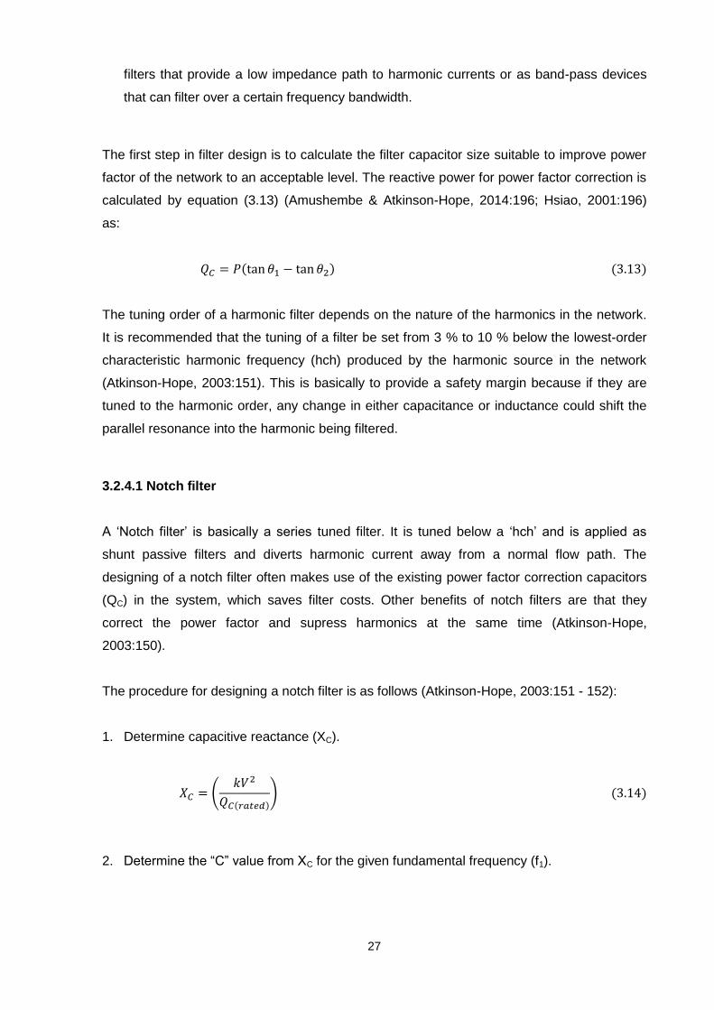
The first step in filter design is to calculate the filter capacitor size suitable to improve power

factor of the network to an acceptable level. The reactive power for power factor correction is

calculated by equation (3.13) (Amushembe & Atkinson-Hope, 2014:196; Hsiao, 2001:196)

as:

The tuning order of a harmonic filter depends on the nature of the harmonics in the network.

It is recommended that the tuning of a filter be set from 3 % to 10 % below the lowest-order

characteristic harmonic frequency (hch) produced by the harmonic source in the network

(Atkinson-Hope, 2003:151). This is basically to provide a safety margin because if they are

tuned to the harmonic order, any change in either capacitance or inductance could shift the

parallel resonance into the harmonic being filtered.

3.2.4.1 Notch filter

A „Notch filter‟ is basically a series tuned filter. It is tuned below a „hch‟ and is applied as

shunt passive filters and diverts harmonic current away from a normal flow path. The

designing of a notch filter often makes use of the existing power factor correction capacitors

(QC) in the system, which saves filter costs. Other benefits of notch filters are that they

correct the power factor and supress harmonics at the same time (Atkinson-Hope,

2003:150).

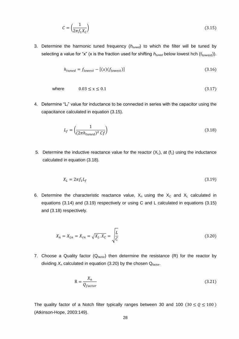
The procedure for designing a notch filter is as follows (Atkinson-Hope, 2003:151 - 152):

1. Determine capacitive reactance (XC).

(

)

2. Determine the “C” value from XC for the given fundamental frequency (f1).

28

(

)

3. Determine the harmonic tuned frequency (htuned) to which the filter will be tuned by

selecting a value for “x” (x is the fraction used for shifting htuned below lowest hch ( )).

where

4. Determine “Lf” value for inductance to be connected in series with the capacitor using the

capacitance calculated in equation (3.15).

(

)

5. Determine the inductive reactance value for the reactor (XL), at (f1) using the inductance

calculated in equation (3.18).

6. Determine the characteristic reactance value, Xn using the XC and XL calculated in

equations (3.14) and (3.19) respectively or using C and L calculated in equations (3.15)

and (3.18) respectively.

√ √

7. Choose a Quality factor (Qfactor) then determine the resistance (R) for the reactor by

dividing Xn calculated in equation (3.20) by the chosen Qfactor.

The quality factor of a Notch filter typically ranges between 30 and 100

(Atkinson-Hope, 2003:149).

29

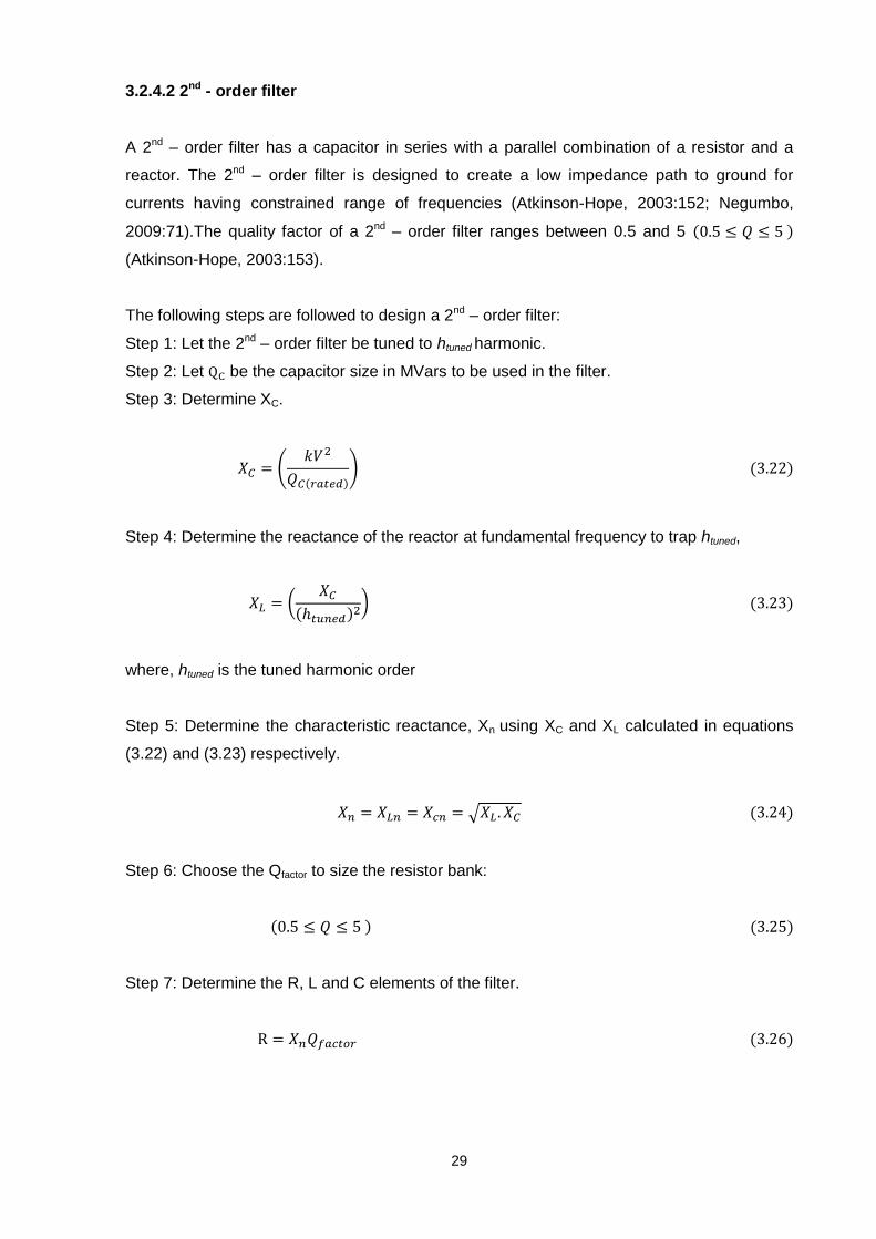
3.2.4.2 2nd - order filter

A 2nd – order filter has a capacitor in series with a parallel combination of a resistor and a

reactor. The 2nd – order filter is designed to create a low impedance path to ground for

currents having constrained range of frequencies (Atkinson-Hope, 2003:152; Negumbo,

2009:71).The quality factor of a 2nd – order filter ranges between 0.5 and 5

(Atkinson-Hope, 2003:153).

The following steps are followed to design a 2nd – order filter:

Step 1: Let the 2nd – order filter be tuned to htuned harmonic.

Step 2: Let be the capacitor size in MVars to be used in the filter.

Step 3: Determine XC.

(

)

Step 4: Determine the reactance of the reactor at fundamental frequency to trap htuned,

(

)

where, htuned is the tuned harmonic order

Step 5: Determine the characteristic reactance, Xn using XC and XL calculated in equations

(3.22) and (3.23) respectively.

√

Step 6: Choose the Qfactor to size the resistor bank:

Step 7: Determine the R, L and C elements of the filter.

30

3.3 Summary

The theoretical background of power systems elements under harmonic conditions is given.

This theory forms the basis for computer modelling of elements such as transformers,

capacitor banks, transmission lines, etc. The main concepts of harmonics are defined.

Resonances both series and parallel are reviewed and the procedures for designing a notch

filter and a 2nd – order filter are given. The effects of harmonics on power system elements as

well as the mitigation measures available for reducing these effects are presented.

31

CHAPTER 4 : COMPUTER TOOLS USED FOR HARMONIC ANALYSIS (DIGSILENT & SUPERHARM)

This chapter gives an insight into functions and capabilities of the two software packages

(DIgSILENT & SuperHarm) used for conducting case investigations in this study. It

introduces network elements and how they are modelled and elucidates on their load flow

and harmonic analyses capabilities. Pointing out their strengths and differences and the

reasons why they were chosen for this research project.

4.1 DIgSILENT PowerFactory Software

As defined by DIgSILENT 14.1, Technical Reference, (2004:2), the name DIgSILENT stands

for “Digital SImuLation and Electrical NeTwork calculation program”. The DIgSILENT

package makes use of an integrated graphic one-line interface. The interactive one-line

diagram includes drawing functions, elements editing capabilities, and features for static and

dynamic calculations. Many organisations for power system planning and operations have

confirmed the accuracy and validity of the load flow (LDF), harmonic load flow (HLDF) and

impedance scan (ZScan) analysis results of the DIgSILENT package (DIgSILENT 13.1,

Basic User‟s Manual, 2004:B-1, Atkinson-Hope & Stemmet, 2008:20).

DIgSILENT PowerFactory provides a wide variety of calculation commands, among which

the two below were chosen for this study (Atkinson-Hope & Stemmet, 2008:38):

a) Load flow,

b) Harmonic load flow or harmonic penetration, and

c) Impedances scan studies.

DIgSILENT is able to calculate the input and output powers at fundamental and harmonic

frequencies for network elements, it can calculate the total power which is supply power less

power losses, and it can also calculate the power losses. The starting point in using this

software is the development of an interpreted interface one-line graphic (diagram) that

comprise of power system elements such as transformers, branches, etc.

4.1.1 Creating power system elements

As an example the one-line diagram in Figure 4.1 is chosen to demonstrate how network

elements are created in DIgSILENT. For the scope of this thesis, eight types of elements are

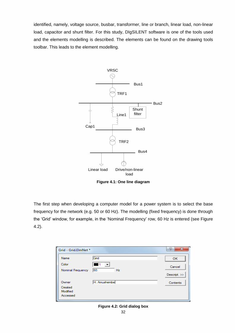
32

identified, namely, voltage source, busbar, transformer, line or branch, linear load, non-linear

load, capacitor and shunt filter. For this study, DIgSILENT software is one of the tools used

and the elements modelling is described. The elements can be found on the drawing tools

toolbar. This leads to the element modelling.

Shunt

filter

VRSC

TRF1

Line1

Bus1

Bus2

Cap1

TRF2

Drive/non-linear

load

Linear load

Bus3

Bus4

Figure 4.1: One line diagram

The first step when developing a computer model for a power system is to select the base

frequency for the network (e.g. 50 or 60 Hz). The modelling (fixed frequency) is done through

the „Grid‟ window, for example, in the „Nominal Frequency‟ row, 60 Hz is entered (see Figure

4.2).

Figure 4.2: Grid dialog box

33

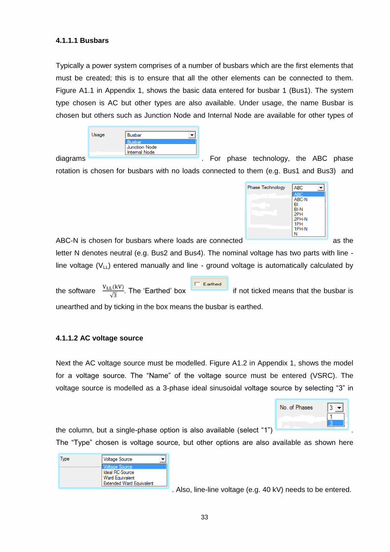
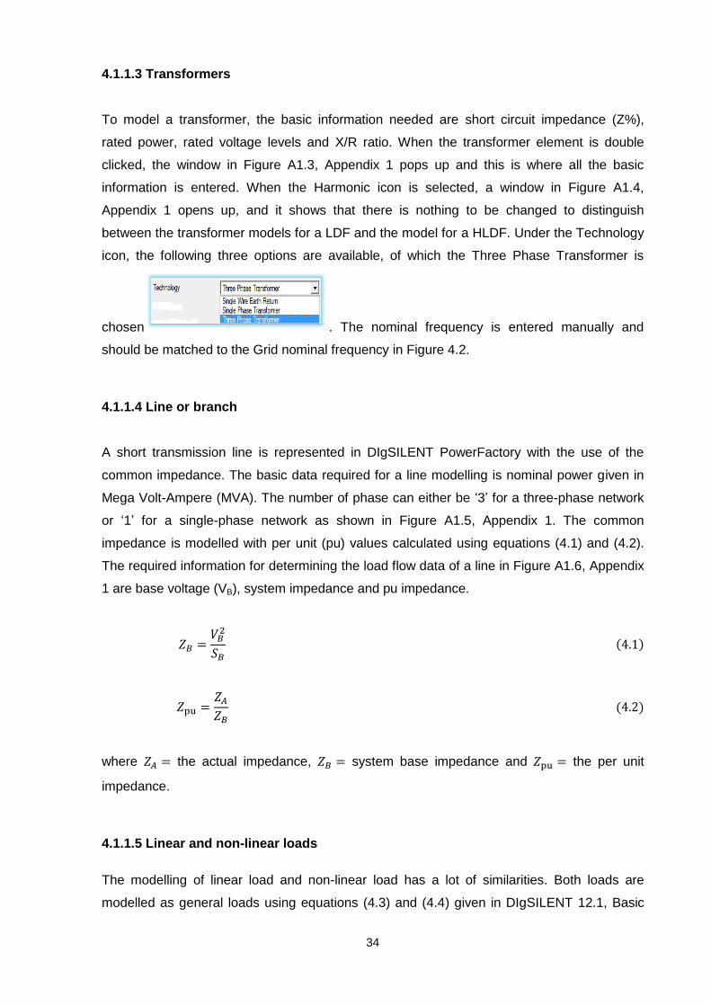
4.1.1.1 Busbars

Typically a power system comprises of a number of busbars which are the first elements that

must be created; this is to ensure that all the other elements can be connected to them.

Figure A1.1 in Appendix 1, shows the basic data entered for busbar 1 (Bus1). The system

type chosen is AC but other types are also available. Under usage, the name Busbar is

chosen but others such as Junction Node and Internal Node are available for other types of

diagrams . For phase technology, the ABC phase

rotation is chosen for busbars with no loads connected to them (e.g. Bus1 and Bus3) and

ABC-N is chosen for busbars where loads are connected as the

letter N denotes neutral (e.g. Bus2 and Bus4). The nominal voltage has two parts with line -

line voltage (VLL) entered manually and line - ground voltage is automatically calculated by

the software

√ . The „Earthed‟ box if not ticked means that the busbar is

unearthed and by ticking in the box means the busbar is earthed.

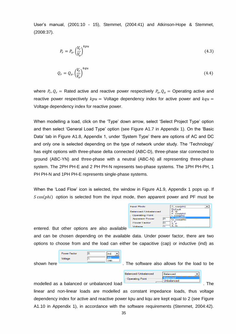
4.1.1.2 AC voltage source

Next the AC voltage source must be modelled. Figure A1.2 in Appendix 1, shows the model

for a voltage source. The “Name” of the voltage source must be entered (VSRC). The

voltage source is modelled as a 3-phase ideal sinusoidal voltage source by selecting “3” in

the column, but a single-phase option is also available (select “1”) .

The “Type” chosen is voltage source, but other options are also available as shown here

. Also, line-line voltage (e.g. 40 kV) needs to be entered.

34

4.1.1.3 Transformers

To model a transformer, the basic information needed are short circuit impedance (Z%),

rated power, rated voltage levels and X/R ratio. When the transformer element is double

clicked, the window in Figure A1.3, Appendix 1 pops up and this is where all the basic

information is entered. When the Harmonic icon is selected, a window in Figure A1.4,

Appendix 1 opens up, and it shows that there is nothing to be changed to distinguish

between the transformer models for a LDF and the model for a HLDF. Under the Technology

icon, the following three options are available, of which the Three Phase Transformer is

chosen . The nominal frequency is entered manually and

should be matched to the Grid nominal frequency in Figure 4.2.

4.1.1.4 Line or branch

A short transmission line is represented in DIgSILENT PowerFactory with the use of the

common impedance. The basic data required for a line modelling is nominal power given in

Mega Volt-Ampere (MVA). The number of phase can either be „3‟ for a three-phase network

or „1‟ for a single-phase network as shown in Figure A1.5, Appendix 1. The common

impedance is modelled with per unit (pu) values calculated using equations (4.1) and (4.2).

The required information for determining the load flow data of a line in Figure A1.6, Appendix

1 are base voltage (VB), system impedance and pu impedance.

where the actual impedance, system base impedance and the per unit

impedance.

4.1.1.5 Linear and non-linear loads

The modelling of linear load and non-linear load has a lot of similarities. Both loads are

modelled as general loads using equations (4.3) and (4.4) given in DIgSILENT 12.1, Basic

35

User‟s manual, (2001:10 - 15), Stemmet, (2004:41) and Atkinson-Hope & Stemmet,

(2008:37).

(

)

(

)

where Rated active and reactive power respectively Operating active and

reactive power respectively Voltage dependency index for active power and

Voltage dependency index for reactive power.

When modelling a load, click on the „Type‟ down arrow, select „Select Project Type‟ option

and then select „General Load Type‟ option (see Figure A1.7 in Appendix 1). On the „Basic

Data‟ tab in Figure A1.8, Appendix 1, under „System Type‟ there are options of AC and DC

and only one is selected depending on the type of network under study. The „Technology‟

has eight options with three-phase delta connected (ABC-D), three-phase star connected to

ground (ABC-YN) and three-phase with a neutral (ABC-N) all representing three-phase

system. The 2PH PH-E and 2 PH PH-N represents two-phase systems. The 1PH PH-PH, 1

PH PH-N and 1PH PH-E represents single-phase systems.

When the „Load Flow‟ icon is selected, the window in Figure A1.9, Appendix 1 pops up. If

option is selected from the input mode, then apparent power and PF must be

entered. But other options are also available

and can be chosen depending on the available data. Under power factor, there are two

options to choose from and the load can either be capacitive (cap) or inductive (ind) as

shown here . The software also allows for the load to be

modelled as a balanced or unbalanced load . The

linear and non-linear loads are modelled as constant impedance loads, thus voltage

dependency index for active and reactive power kpu and kqu are kept equal to 2 (see Figure

A1.10 in Appendix 1), in accordance with the software requirements (Stemmet, 2004:42).

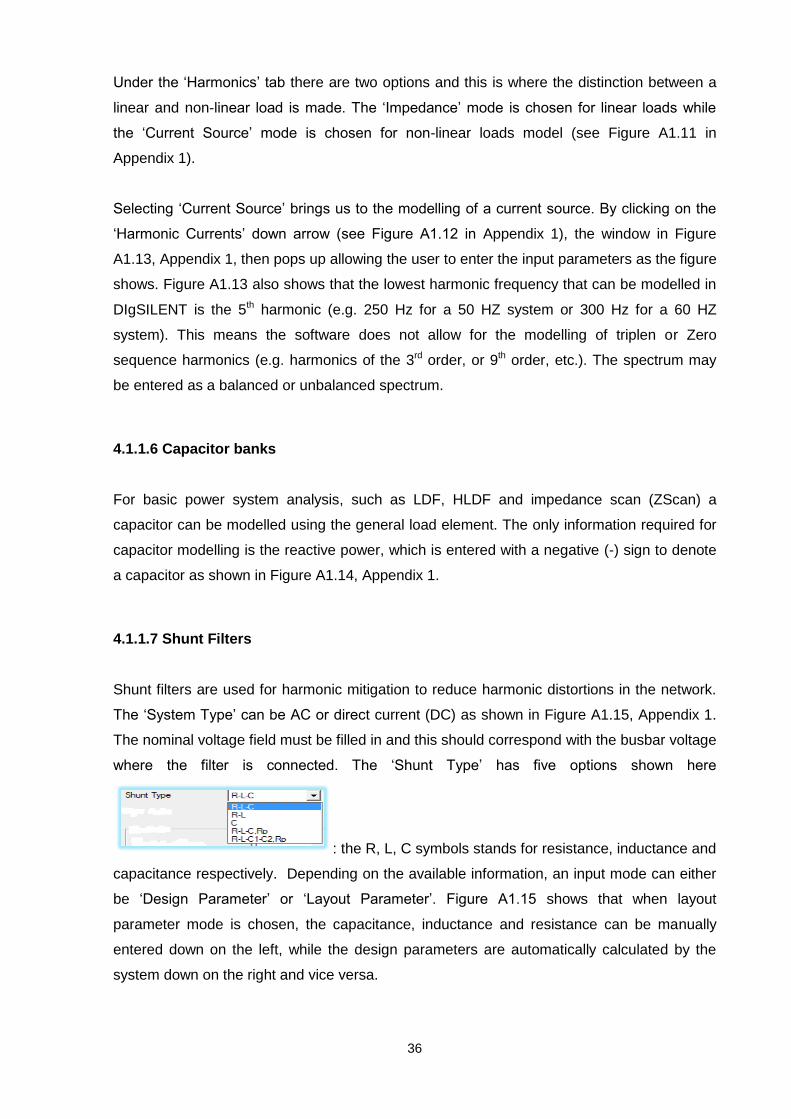
36

Under the „Harmonics‟ tab there are two options and this is where the distinction between a

linear and non-linear load is made. The „Impedance‟ mode is chosen for linear loads while

the „Current Source‟ mode is chosen for non-linear loads model (see Figure A1.11 in

Appendix 1).

Selecting „Current Source‟ brings us to the modelling of a current source. By clicking on the

„Harmonic Currents‟ down arrow (see Figure A1.12 in Appendix 1), the window in Figure

A1.13, Appendix 1, then pops up allowing the user to enter the input parameters as the figure

shows. Figure A1.13 also shows that the lowest harmonic frequency that can be modelled in

DIgSILENT is the 5th harmonic (e.g. 250 Hz for a 50 HZ system or 300 Hz for a 60 HZ

system). This means the software does not allow for the modelling of triplen or Zero

sequence harmonics (e.g. harmonics of the 3rd order, or 9th order, etc.). The spectrum may

be entered as a balanced or unbalanced spectrum.

4.1.1.6 Capacitor banks

For basic power system analysis, such as LDF, HLDF and impedance scan (ZScan) a

capacitor can be modelled using the general load element. The only information required for

capacitor modelling is the reactive power, which is entered with a negative (-) sign to denote

a capacitor as shown in Figure A1.14, Appendix 1.

4.1.1.7 Shunt Filters

Shunt filters are used for harmonic mitigation to reduce harmonic distortions in the network.

The „System Type‟ can be AC or direct current (DC) as shown in Figure A1.15, Appendix 1.

The nominal voltage field must be filled in and this should correspond with the busbar voltage

where the filter is connected. The „Shunt Type‟ has five options shown here

: the R, L, C symbols stands for resistance, inductance and

capacitance respectively. Depending on the available information, an input mode can either

be „Design Parameter‟ or „Layout Parameter‟. Figure A1.15 shows that when layout

parameter mode is chosen, the capacitance, inductance and resistance can be manually

entered down on the left, while the design parameters are automatically calculated by the

system down on the right and vice versa.

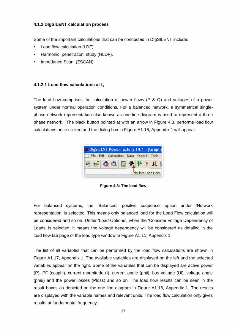
37

4.1.2 DIgSILENT calculation process

Some of the important calculations that can be conducted in DIgSILENT include:

• Load flow calculation (LDF).

• Harmonic penetration study (HLDF).

• Impedance Scan, (ZSCAN).

4.1.2.1 Load flow calculations at f1

The load flow comprises the calculation of power flows (P & Q) and voltages of a power

system under normal operation conditions. For a balanced network, a symmetrical single-

phase network representation also known as one-line diagram is used to represent a three

phase network. The black button pointed at with an arrow in Figure 4.3, performs load flow

calculations once clicked and the dialog box in Figure A1.16, Appendix 1 will appear.

Figure 4.3: The load flow

For balanced systems, the „Balanced, positive sequence‟ option under „Network

representation‟ is selected. This means only balanced load for the Load Flow calculation will

be considered and so on. Under „Load Options‟, when the „Consider voltage Dependency of

Loads‟ is selected, it means the voltage dependency will be considered as detailed in the

load flow tab page of the load type window in Figure A1.11, Appendix 1.

The list of all variables that can be performed by the load flow calculations are shown in

Figure A1.17, Appendix 1. The available variables are displayed on the left and the selected

variables appear on the right. Some of the variables that can be displayed are active power

(P), PF (cosphi), current magnitude (I), current angle (phii), bus voltage (Ul), voltage angle

(phiu) and the power losses (Ploss) and so on. The load flow results can be seen in the

result boxes as depicted on the one-line diagram in Figure A1.18, Appendix 1. The results

are displayed with the variable names and relevant units. The load flow calculation only gives

results at fundamental frequency.

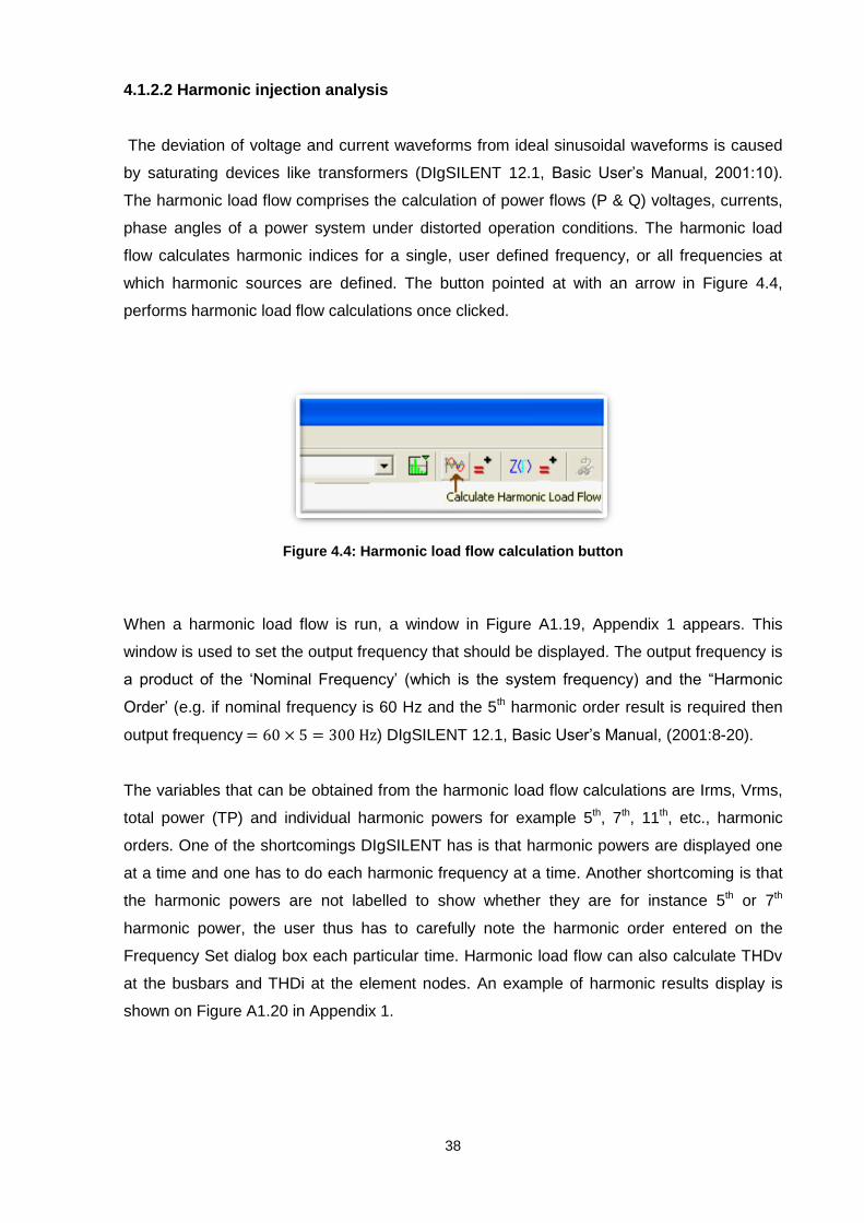
38

4.1.2.2 Harmonic injection analysis

The deviation of voltage and current waveforms from ideal sinusoidal waveforms is caused

by saturating devices like transformers (DIgSILENT 12.1, Basic User‟s Manual, 2001:10).

The harmonic load flow comprises the calculation of power flows (P & Q) voltages, currents,

phase angles of a power system under distorted operation conditions. The harmonic load

flow calculates harmonic indices for a single, user defined frequency, or all frequencies at

which harmonic sources are defined. The button pointed at with an arrow in Figure 4.4,

performs harmonic load flow calculations once clicked.

Figure 4.4: Harmonic load flow calculation button

When a harmonic load flow is run, a window in Figure A1.19, Appendix 1 appears. This

window is used to set the output frequency that should be displayed. The output frequency is

a product of the „Nominal Frequency‟ (which is the system frequency) and the “Harmonic

Order‟ (e.g. if nominal frequency is 60 Hz and the 5th harmonic order result is required then

output frequency ) DIgSILENT 12.1, Basic User‟s Manual, (2001:8-20).

The variables that can be obtained from the harmonic load flow calculations are Irms, Vrms,

total power (TP) and individual harmonic powers for example 5th, 7th, 11th, etc., harmonic

orders. One of the shortcomings DIgSILENT has is that harmonic powers are displayed one

at a time and one has to do each harmonic frequency at a time. Another shortcoming is that

the harmonic powers are not labelled to show whether they are for instance 5th or 7th

harmonic power, the user thus has to carefully note the harmonic order entered on the

Frequency Set dialog box each particular time. Harmonic load flow can also calculate THDv

at the busbars and THDi at the element nodes. An example of harmonic results display is

shown on Figure A1.20 in Appendix 1.

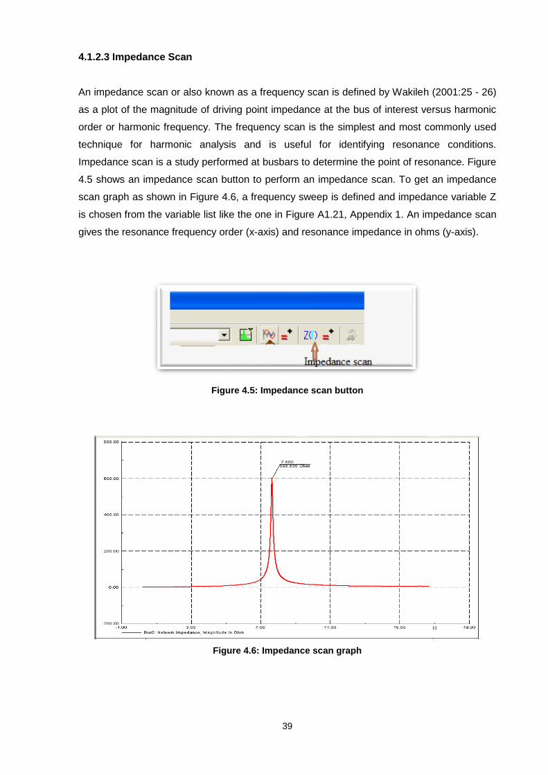
39

4.1.2.3 Impedance Scan

An impedance scan or also known as a frequency scan is defined by Wakileh (2001:25 - 26)

as a plot of the magnitude of driving point impedance at the bus of interest versus harmonic

order or harmonic frequency. The frequency scan is the simplest and most commonly used

technique for harmonic analysis and is useful for identifying resonance conditions.

Impedance scan is a study performed at busbars to determine the point of resonance. Figure

4.5 shows an impedance scan button to perform an impedance scan. To get an impedance

scan graph as shown in Figure 4.6, a frequency sweep is defined and impedance variable Z

is chosen from the variable list like the one in Figure A1.21, Appendix 1. An impedance scan

gives the resonance frequency order (x-axis) and resonance impedance in ohms (y-axis).

Figure 4.5: Impedance scan button

Figure 4.6: Impedance scan graph

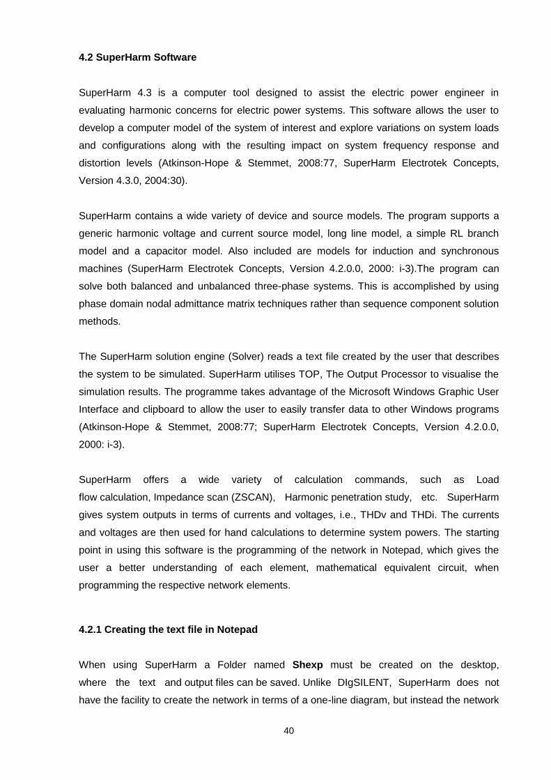
40

4.2 SuperHarm Software

SuperHarm 4.3 is a computer tool designed to assist the electric power engineer in

evaluating harmonic concerns for electric power systems. This software allows the user to

develop a computer model of the system of interest and explore variations on system loads

and configurations along with the resulting impact on system frequency response and

distortion levels (Atkinson-Hope & Stemmet, 2008:77, SuperHarm Electrotek Concepts,

Version 4.3.0, 2004:30).

SuperHarm contains a wide variety of device and source models. The program supports a

generic harmonic voltage and current source model, long line model, a simple RL branch

model and a capacitor model. Also included are models for induction and synchronous

machines (SuperHarm Electrotek Concepts, Version 4.2.0.0, 2000: i-3).The program can

solve both balanced and unbalanced three-phase systems. This is accomplished by using

phase domain nodal admittance matrix techniques rather than sequence component solution

methods.

The SuperHarm solution engine (Solver) reads a text file created by the user that describes

the system to be simulated. SuperHarm utilises TOP, The Output Processor to visualise the

simulation results. The programme takes advantage of the Microsoft Windows Graphic User

Interface and clipboard to allow the user to easily transfer data to other Windows programs

(Atkinson-Hope & Stemmet, 2008:77; SuperHarm Electrotek Concepts, Version 4.2.0.0,

2000: i-3).

SuperHarm offers a wide variety of calculation commands, such as Load

flow calculation, Impedance scan (ZSCAN), Harmonic penetration study, etc. SuperHarm

gives system outputs in terms of currents and voltages, i.e., THDv and THDi. The currents

and voltages are then used for hand calculations to determine system powers. The starting

point in using this software is the programming of the network in Notepad, which gives the

user a better understanding of each element, mathematical equivalent circuit, when

programming the respective network elements.

4.2.1 Creating the text file in Notepad

When using SuperHarm a Folder named Shexp must be created on the desktop,

where the text and output files can be saved. Unlike DIgSILENT, SuperHarm does not

have the facility to create the network in terms of a one-line diagram, but instead the network

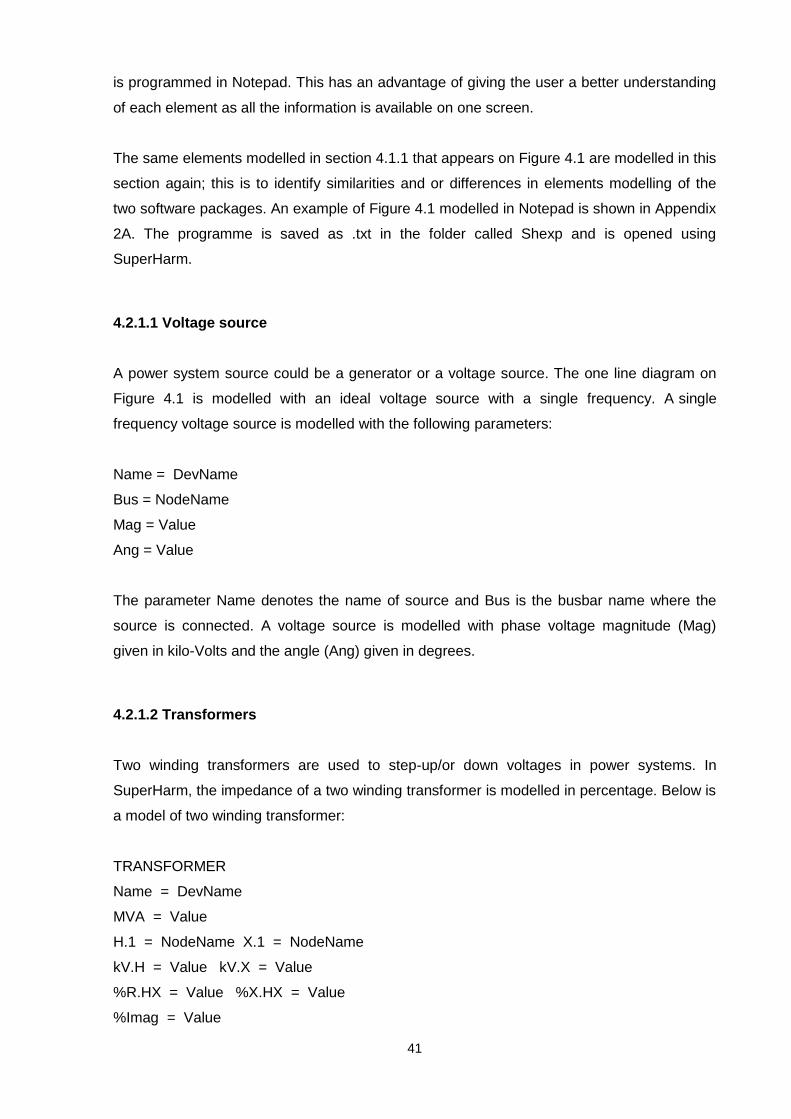
41

is programmed in Notepad. This has an advantage of giving the user a better understanding

of each element as all the information is available on one screen.

The same elements modelled in section 4.1.1 that appears on Figure 4.1 are modelled in this

section again; this is to identify similarities and or differences in elements modelling of the

two software packages. An example of Figure 4.1 modelled in Notepad is shown in Appendix

2A. The programme is saved as .txt in the folder called Shexp and is opened using

SuperHarm.

4.2.1.1 Voltage source

A power system source could be a generator or a voltage source. The one line diagram on

Figure 4.1 is modelled with an ideal voltage source with a single frequency. A single

frequency voltage source is modelled with the following parameters:

Name = DevName

Bus = NodeName

Mag = Value

Ang = Value

The parameter Name denotes the name of source and Bus is the busbar name where the

source is connected. A voltage source is modelled with phase voltage magnitude (Mag)

given in kilo-Volts and the angle (Ang) given in degrees.

4.2.1.2 Transformers

Two winding transformers are used to step-up/or down voltages in power systems. In

SuperHarm, the impedance of a two winding transformer is modelled in percentage. Below is

a model of two winding transformer:

TRANSFORMER

Name = DevName

MVA = Value

H.1 = NodeName X.1 = NodeName

kV.H = Value kV.X = Value

%R.HX = Value %X.HX = Value

%Imag = Value

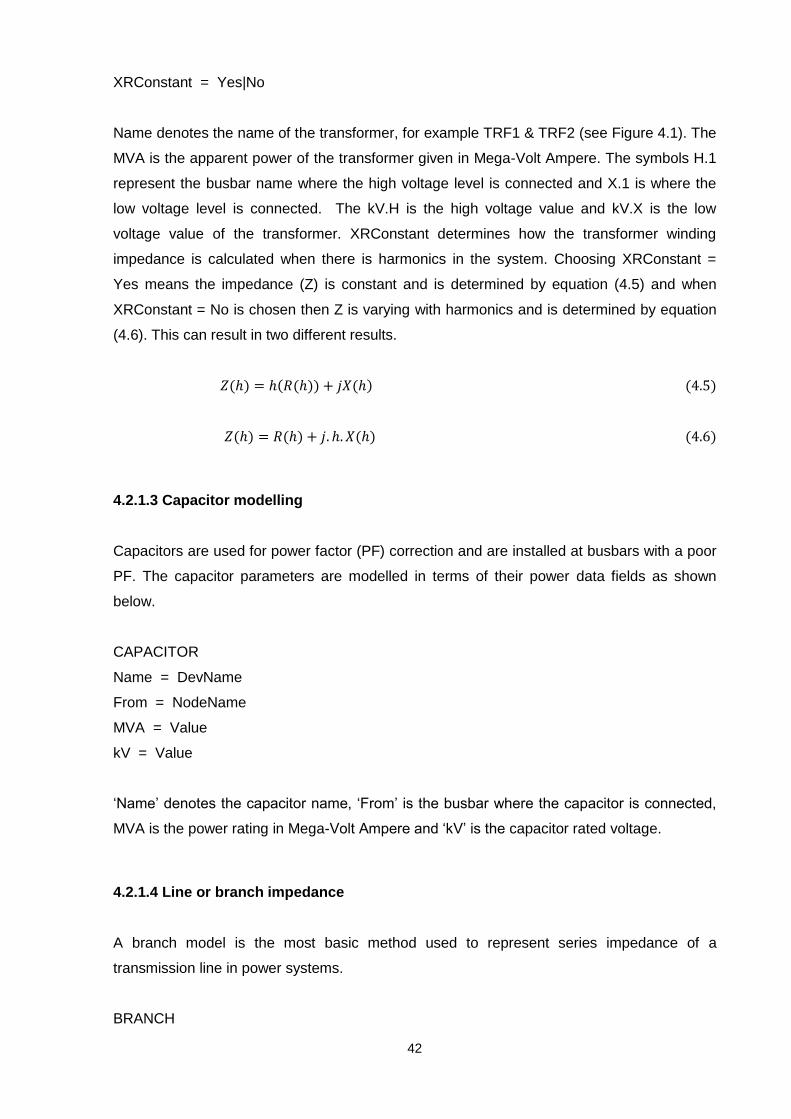
42

XRConstant = Yes|No

Name denotes the name of the transformer, for example TRF1 & TRF2 (see Figure 4.1). The

MVA is the apparent power of the transformer given in Mega-Volt Ampere. The symbols H.1

represent the busbar name where the high voltage level is connected and X.1 is where the

low voltage level is connected. The kV.H is the high voltage value and kV.X is the low

voltage value of the transformer. XRConstant determines how the transformer winding

impedance is calculated when there is harmonics in the system. Choosing XRConstant =

Yes means the impedance (Z) is constant and is determined by equation (4.5) and when

XRConstant = No is chosen then Z is varying with harmonics and is determined by equation

(4.6). This can result in two different results.

4.2.1.3 Capacitor modelling

Capacitors are used for power factor (PF) correction and are installed at busbars with a poor

PF. The capacitor parameters are modelled in terms of their power data fields as shown

below.

CAPACITOR

Name = DevName

From = NodeName

MVA = Value

kV = Value

„Name‟ denotes the capacitor name, „From‟ is the busbar where the capacitor is connected,

MVA is the power rating in Mega-Volt Ampere and „kV‟ is the capacitor rated voltage.

4.2.1.4 Line or branch impedance

A branch model is the most basic method used to represent series impedance of a

transmission line in power systems.

BRANCH

43

Name = DevName

From = NodeName

To = NodeName

R = Value

X = Value

„Name‟ is line or branch name. The line is connected between two busbars, thus „From‟ is

where the line is connected from and „To‟ is where the line is connected to. R is the line

resistance and X is the line reactance which will be (+) for inductance and (-) for capacitance.

4.2.1.5 Shunt Filter

Filters are used for harmonic mitigation in power systems. Since the filter is made up of a

resistor, inductor and capacitor as their components, the modelling is similar to that of a

branch and capacitor models combined. For example a 1st order filter is modelled using the

following parameters:

Capacitor Name = DevName

From = NodeName

To = NodeName

MVA = Value

kV =Value

Branch Name = DevName

From = NodeName

To = NodeName

R = value

X = value

Branch Name = DevName

From = NodeName

To = NodeName

R = value

X = value

One branch will be a resistor and another branch an inductor. X=0 for the resistor branch,

and R=0 for the inductor branch.

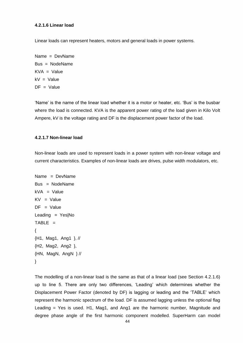
44

4.2.1.6 Linear load

Linear loads can represent heaters, motors and general loads in power systems.

Name = DevName

Bus = NodeName

KVA = Value

kV = Value

DF = Value

„Name‟ is the name of the linear load whether it is a motor or heater, etc. „Bus‟ is the busbar

where the load is connected. KVA is the apparent power rating of the load given in Kilo Volt

Ampere, kV is the voltage rating and DF is the displacement power factor of the load.

4.2.1.7 Non-linear load

Non-linear loads are used to represent loads in a power system with non-linear voltage and

current characteristics. Examples of non-linear loads are drives, pulse width modulators, etc.

Name = DevName

Bus = NodeName

kVA = Value

KV = Value

DF = Value

Leading = Yes|No

TABLE =

H1, Mag1, Ang1 , //

H2, Mag2, Ang2 ,

HN, MagN, AngN //

The modelling of a non-linear load is the same as that of a linear load (see Section 4.2.1.6)

up to line 5. There are only two differences, „Leading‟ which determines whether the

Displacement Power Factor (denoted by DF) is lagging or leading and the „TABLE‟ which

represent the harmonic spectrum of the load. DF is assumed lagging unless the optional flag

Leading = Yes is used. H1, Mag1, and Ang1 are the harmonic number, Magnitude and

degree phase angle of the first harmonic component modelled. SuperHarm can model

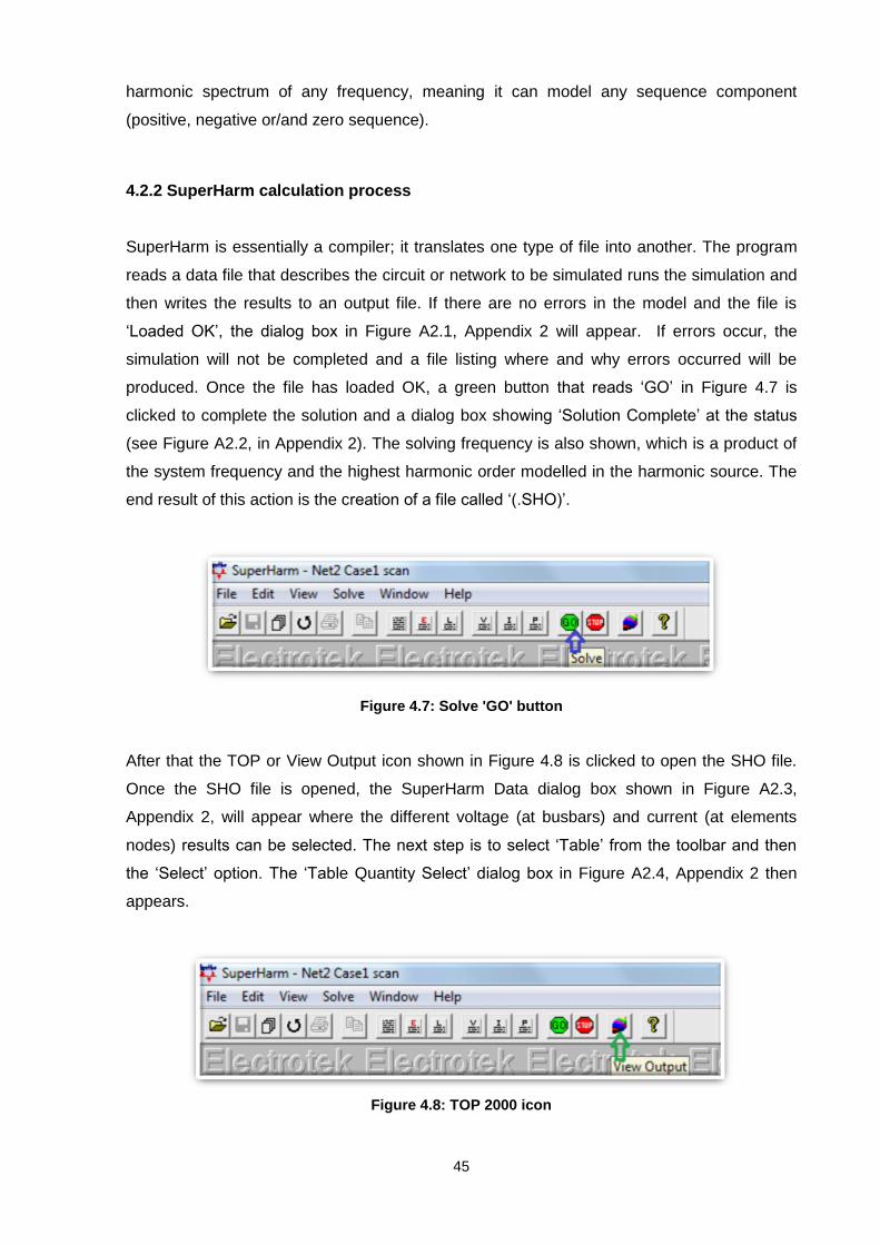
45

harmonic spectrum of any frequency, meaning it can model any sequence component

(positive, negative or/and zero sequence).

4.2.2 SuperHarm calculation process

SuperHarm is essentially a compiler; it translates one type of file into another. The program

reads a data file that describes the circuit or network to be simulated runs the simulation and

then writes the results to an output file. If there are no errors in the model and the file is

„Loaded OK‟, the dialog box in Figure A2.1, Appendix 2 will appear. If errors occur, the

simulation will not be completed and a file listing where and why errors occurred will be

produced. Once the file has loaded OK, a green button that reads „GO‟ in Figure 4.7 is

clicked to complete the solution and a dialog box showing „Solution Complete‟ at the status

(see Figure A2.2, in Appendix 2). The solving frequency is also shown, which is a product of

the system frequency and the highest harmonic order modelled in the harmonic source. The

end result of this action is the creation of a file called „(.SHO)‟.

Figure 4.7: Solve 'GO' button

After that the TOP or View Output icon shown in Figure 4.8 is clicked to open the SHO file.

Once the SHO file is opened, the SuperHarm Data dialog box shown in Figure A2.3,

Appendix 2, will appear where the different voltage (at busbars) and current (at elements

nodes) results can be selected. The next step is to select „Table‟ from the toolbar and then

the „Select‟ option. The „Table Quantity Select‟ dialog box in Figure A2.4, Appendix 2 then

appears.

Figure 4.8: TOP 2000 icon

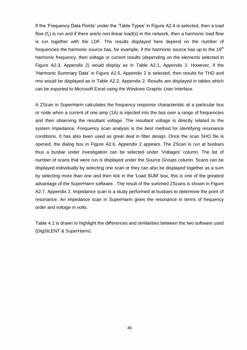
46

If the „Frequency Data Points‟ under the „Table Types‟ in Figure A2.4 is selected, then a load

flow (f1) is run and if there are/is non-linear load(s) in the network, then a harmonic load flow

is run together with the LDF. The results displayed here depend on the number of

frequencies the harmonic source has, for example, if the harmonic source has up to the 19th

harmonic frequency, then voltage or current results (depending on the elements selected in

Figure A2.3, Appendix 2) would display as in Table A2.1, Appendix 2. However, if the

„Harmonic Summary Data‟ in Figure A2.5, Appendix 2 is selected, then results for THD and

rms would be displayed as in Table A2.2, Appendix 2. Results are displayed in tables which

can be exported to Microsoft Excel using the Windows Graphic User Interface.

A ZScan in SuperHarm calculates the frequency response characteristic at a particular bus

or node when a current of one amp (1A) is injected into the bus over a range of frequencies

and then observing the resultant voltage. The resultant voltage is directly related to the

system impedance. Frequency scan analysis is the best method for identifying resonance

conditions. It has also been used as great deal in filter design. Once the scan SHO file is

opened, the dialog box in Figure A2.6, Appendix 2 appears. The ZScan is run at busbars

thus a busbar under investigation can be selected under „Voltages‟ column. The list of

number of scans that were run is displayed under the Source Groups column. Scans can be

displayed individually by selecting one scan or they can also be displayed together as a sum

by selecting more than one and then tick in the „Load SUM‟ box, this is one of the greatest

advantage of the SuperHarm software. The result of the summed ZScans is shown in Figure

A2.7, Appendix 2. Impedance scan is a study performed at busbars to determine the point of

resonance. An impedance scan in SuperHarm gives the resonance in terms of frequency

order and voltage in volts.

Table 4.1 is drawn to highlight the differences and similarities between the two software used

(DIgSILENT & SuperHarm).

47

Table 4.1: Comparison between DIgSILENT and SuperHarm

DIgSILENT SuperHarm

- Make use of one-line interface to model

the network.

- Network model is programmed in

Notepad.

- Calculates powers (Ph, TPh) - Does not calculate power.

- Can only display one frequency results at

a time.

- Displays all frequency results under

consideration altogether.

- Can calculate THDv & THDi - Can calculate THDv & THDi

- The voltage source and non-linear loads

are modelled with line voltage.

- The voltage source and non-linear loads

are modelled with phase voltage.

- Can only display summed ZScans. - Can display ZScans individually or

summed together.

- Can only model harmonic frequency

spectrum from the 5th harmonic order.

- Can model harmonic spectrum of any

harmonic order.

- Can only model harmonic frequency of

positive and negative sequence.

- Can model harmonic spectrum of

positive, negative and zero sequence.

4.3 Summary

The capabilities of the two software packages (DIgSILENT & SuperHarm), which are chosen

to support this research are individually presented. The steps on how each software package

models the different power system elements are demonstrated. The different power analysis

that can be performed by both DIgSILENT & SuperHarm are illustrated and steps on how

each software package conduct these studies are also given. Also, the possible results that

can be obtained from the various studies are given. Finally, the two tools are compared.

48

CHAPTER 5 : CONTRIBUTIONS

This chapter describes the need for this study and the contributions it makes to research in

the power system field. This chapter describes the new step-by-step approaches

(methodologies) developed for determining true efficiency calculations for networks under

distorted waveform conditions. Traditionally, efficiency calculations are limited to systems

where waveforms are assumed to be sinusoidal. However, modern systems have non-

sinusoidal waveforms and the contribution of this work is to determine how to detail true

efficiency that takes into account harmonic powers beside fundamental power. Indices for

evaluating the effectiveness of harmonic filter(s) are also introduced.

5.1 The need for this study

Any investigation on a power system that contains a significant number of non-linear loads

requires new technology engineers to be equipped with top of the range software tools to

plan, operate, maintain and manage (Acha & Madridal, 2001:6) efficiencies. When a simple

radial system with a single sending-end and a single receiving-end is analysed, it is easy to

calculate the losses through the impedance (resistor and inductor) and determine efficiency.

However, as the system reaches many buses, power flow hand calculations that include

waveform distortions become tedious and unreliable. The use of capable software is thus

necessary to minimise errors encountered through hand calculations process such as

rounding off values, etc. It is also difficult to draw accurate waveforms by hand especially

when adding or subtracting waveforms of different magnitude (like adding scans for different

buses to get their total effect).

There is a need to demonstrate the power direction of flow in non-sinusoidal networks with

multiple harmonic sources. Different network branches (shunt and series) could have

different power directions. The harmonic current directions of flow for linear and non-linear

loads is defined by Negumbo, (2009:39) and Dugan, et al., (2012:249) in Figure 5.1, which

subsequently means the power flows in the same directions. For the non-linear load, P1 is

positive meaning flowing into the load from the grid while harmonic powers (Ph) are negative

meaning flowing away from the load into the network. This satisfies condition 2 under Sub-

section 2.2.1.1(c), meaning that the customer side is responsible for harmonic currents

injection. For the linear load, both P1 and Ph are flowing into the load. This means that all

powers in the shunt branches are positive and/or flows downstream. However, the power

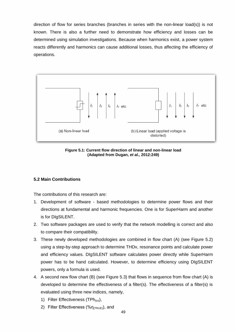
49

direction of flow for series branches (branches in series with the non-linear load(s)) is not

known. There is also a further need to demonstrate how efficiency and losses can be

determined using simulation investigations. Because when harmonics exist, a power system

reacts differently and harmonics can cause additional losses, thus affecting the efficiency of

operations.

Figure 5.1: Current flow direction of linear and non-linear load (Adapted from Dugan, et al., 2012:249)

5.2 Main Contributions

The contributions of this research are:

1. Development of software - based methodologies to determine power flows and their

directions at fundamental and harmonic frequencies. One is for SuperHarm and another

is for DIgSILENT.

2. Two software packages are used to verify that the network modelling is correct and also

to compare their compatibility.

3. These newly developed methodologies are combined in flow chart (A) (see Figure 5.2)

using a step-by-step approach to determine THDv, resonance points and calculate power

and efficiency values. DIgSILENT software calculates power directly while SuperHarm

power has to be hand calculated. However, to determine efficiency using DIgSILENT

powers, only a formula is used.

4. A second new flow chart (B) (see Figure 5.3) that flows in sequence from flow chart (A) is

developed to determine the effectiveness of a filter(s). The effectiveness of a filter(s) is

evaluated using three new indices, namely,

1) Filter Effectiveness (TPh(in)),

2) Filter Effectiveness (%η(TRUE)), and

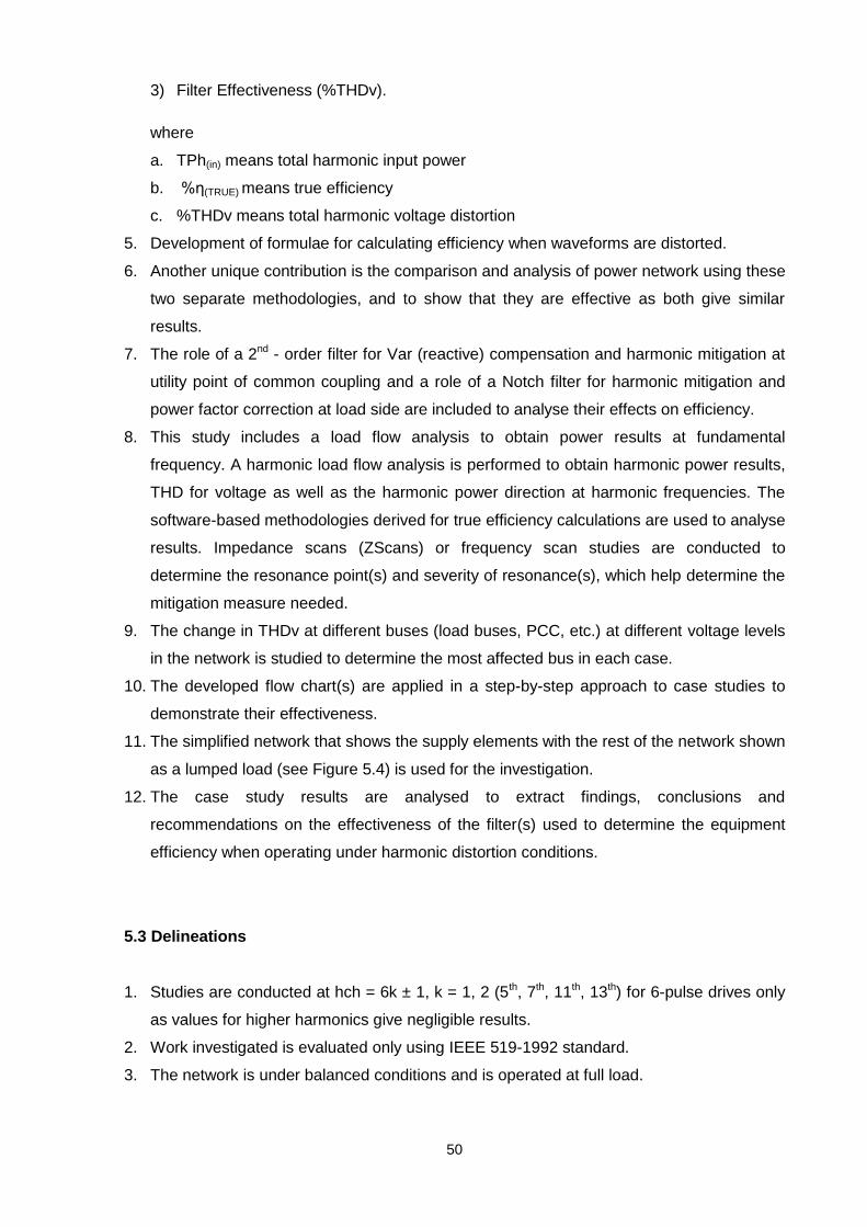
50

3) Filter Effectiveness (%THDv).

where

a. TPh(in) means total harmonic input power

b. %η(TRUE) means true efficiency

c. %THDv means total harmonic voltage distortion

5. Development of formulae for calculating efficiency when waveforms are distorted.

6. Another unique contribution is the comparison and analysis of power network using these

two separate methodologies, and to show that they are effective as both give similar

results.

7. The role of a 2nd - order filter for Var (reactive) compensation and harmonic mitigation at

utility point of common coupling and a role of a Notch filter for harmonic mitigation and

power factor correction at load side are included to analyse their effects on efficiency.

8. This study includes a load flow analysis to obtain power results at fundamental

frequency. A harmonic load flow analysis is performed to obtain harmonic power results,

THD for voltage as well as the harmonic power direction at harmonic frequencies. The

software-based methodologies derived for true efficiency calculations are used to analyse

results. Impedance scans (ZScans) or frequency scan studies are conducted to

determine the resonance point(s) and severity of resonance(s), which help determine the

mitigation measure needed.

9. The change in THDv at different buses (load buses, PCC, etc.) at different voltage levels

in the network is studied to determine the most affected bus in each case.

10. The developed flow chart(s) are applied in a step-by-step approach to case studies to

demonstrate their effectiveness.

11. The simplified network that shows the supply elements with the rest of the network shown

as a lumped load (see Figure 5.4) is used for the investigation.

12. The case study results are analysed to extract findings, conclusions and

recommendations on the effectiveness of the filter(s) used to determine the equipment

efficiency when operating under harmonic distortion conditions.

5.3 Delineations

1. Studies are conducted at hch = 6k ± 1, k = 1, 2 (5th, 7th, 11th, 13th) for 6-pulse drives only

as values for higher harmonics give negligible results.

2. Work investigated is evaluated only using IEEE 519-1992 standard.

3. The network is under balanced conditions and is operated at full load.

51

5.4 Development of methodologies:

How to apply software tools to calculate efficiencies is not well known at all and it is the

purpose of this work to provide designers and efficiency evaluators with the methodologies to

do so. Figure 5.2 shows the comparison of the new developed flow chart for true efficiency

calculations in a network with harmonic sources and with and/or without filter(s). The flow

chart depicts the steps in conducting harmonic analysis in terms of LDF, impedance scans

and harmonic penetration studies. Figure 5.3 shows a developed flow chart for calculating

the effectiveness of a filter(s). The flow charts are evaluated using a typical simplified

network given in Figure 5.4. The network is analysed using SuperHarm and DIgSILENT to

obtain load flow (LDF), harmonic load flow and impedance scans (ZSCAN) results. The two

software packages have different methods of carrying out the mentioned power system

analyses. The steps how each software calculates true efficiency are given in sections 5.4.1

and 5.4.2 and the steps in determining the effectiveness of filter(s) are given in section 5.4.3.

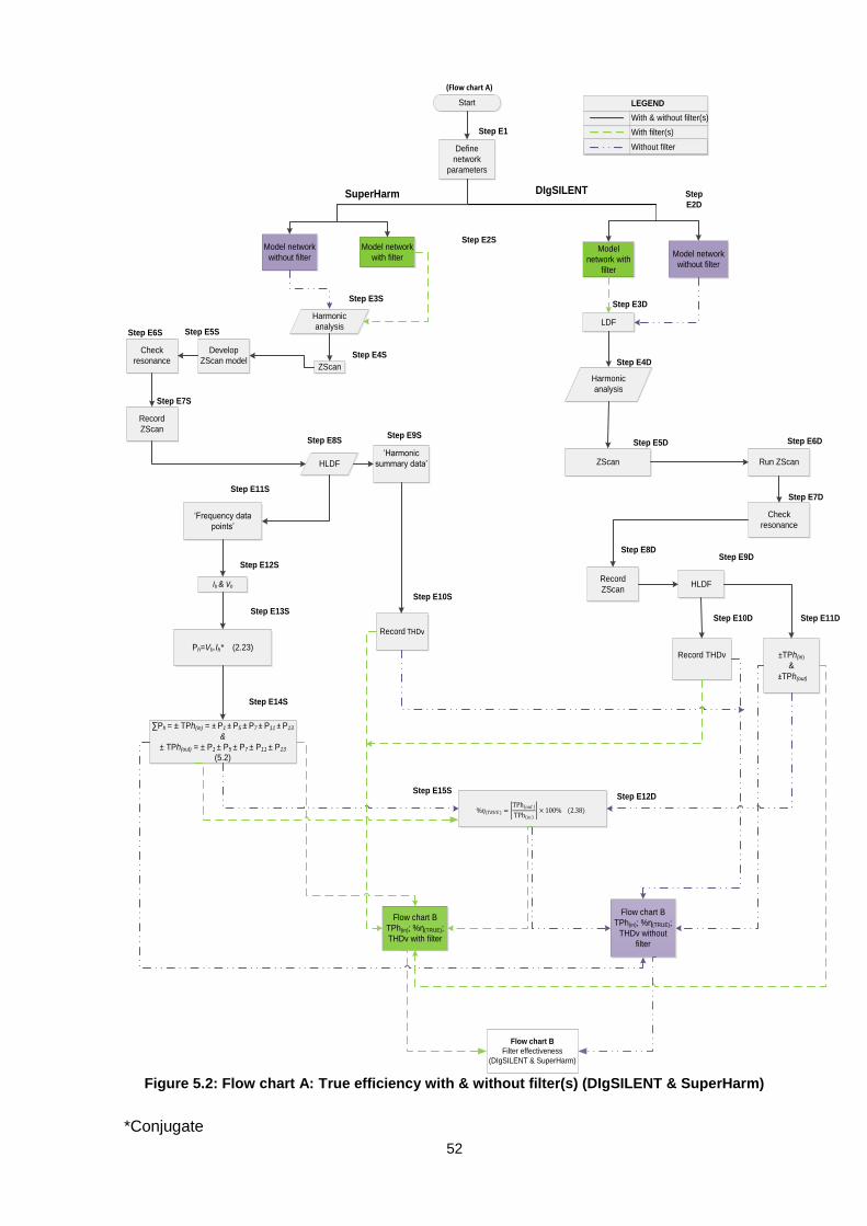
52

Start

Define

network

parameters

Model network

with filterModel

network with

filter

Harmonic

analysis

HLDF

„Frequency data

points‟

LDF

Harmonic

analysis

SuperHarm DIgSILENT

Step E1

Step E2S

Step E3S

Step E7S

Step E4S

Step E8SStep E9S

Step E12S

Step E11S

Step E10D

Step

E2D

Step E3D

Step E4D

Step E5D

Step E8D

Step E7D

±TPh(in)

&

±TPh(out)

Ih & Vh

Step E11D

„Harmonic

summary data‟

Step E12D

HLDF

ZScan

ZScan

Step E6S

Step E13S

(Flow chart A)

Develop

ZScan model

Step E5S

Run ZScan

Step E6D

Step E9D

Step E10S

Check

resonance

Record

ZScan

Check

resonance

Record

ZScan

Ph=Vh.Ih* (2.23)

∑Ph = ± TPh(in) = ± P1 ± P5 ± P7 ± P11 ± P13

&

± TPh(out) = ± P1 ± P5 ± P7 ± P11 ± P13

(5.2)

Step E14S

Step E15S

Model network

without filter Model network

without filter

Record THDv

Record THDv

Flow chart B

TPh(in); %η(TRUE);

THDv with filter

Flow chart B

TPh(in); %η(TRUE);

THDv without

filter

Flow chart B

Filter effectiveness

(DIgSILENT & SuperHarm)

LEGEND

With & without filter(s)

With filter(s)

Without filter

% ( 𝑈𝐸) = |TPh

TPh | × 100% (2.38)

Figure 5.2: Flow chart A: True efficiency with & without filter(s) (DIgSILENT & SuperHarm)

*Conjugate

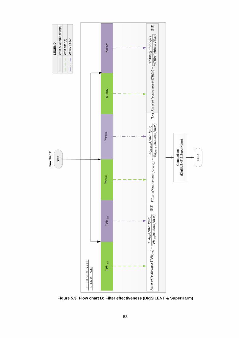
53

%η

(TR

UE)

𝐹 𝑙 𝑒

𝑒

𝑒

𝑒

𝑒

(

) =

(

)( 𝑙 𝑒

𝑦

𝑒

)

(

)(𝑤

𝑙 𝑒

)

(5

.3)

EF

FE

CT

IVE

NE

SS

O

F

FIL

TE

R A

T P

CC

.

EN

D

Co

mp

ariso

n

(DIg

SIL

EN

T &

Su

pe

rHa

rm)

Sta

rt

%η

(TR

UE)

%T

HD

v

(

) %

TH

Dv

Flo

w c

ha

rt B

𝐹 𝑙 𝑒

𝑒

𝑒

𝑒

𝑒

𝑈𝐸

=

%

𝑈𝐸

( 𝑙 𝑒

𝑦

𝑒)

%

𝑈𝐸

(𝑤

𝑙 𝑒

)

(5

.4)

𝐹 𝑙 𝑒

𝑒

𝑒

𝑒

𝑒 %

𝐻

𝐷

=%

TH

Dv(

𝑙 𝑒

𝑦

𝑒

)

%T

HD

v(𝑤

𝑙 𝑒

)

(5.5

)

(

)

LE

GE

ND

With

& w

ith

ou

t filte

r(s)

With

filt

er(

s)

With

ou

t filte

r

Figure 5.3: Flow chart B: Filter effectiveness (DIgSILENT & SuperHarm)

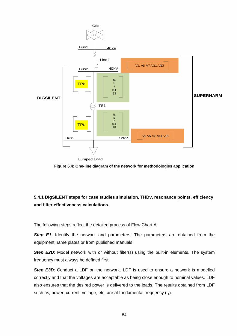
54

Grid

40kVBus1

Bus2

Line1

40kV

12kVBus3

TS1

I1

I5I7I11

I13

I1I5

I7I11

I13

V1, V5, V7, V11, V13

V1, V5, V7, V11, V13

Lumped Load

TPh

TPh

SUPERHARMDIGSILENT

Figure 5.4: One-line diagram of the network for methodologies application

5.4.1 DIgSILENT steps for case studies simulation, THDv, resonance points, efficiency

and filter effectiveness calculations.

The following steps reflect the detailed process of Flow Chart A

Step E1: Identify the network and parameters. The parameters are obtained from the

equipment name plates or from published manuals.

Step E2D: Model network with or without filter(s) using the built-in elements. The system

frequency must always be defined first.

Step E3D: Conduct a LDF on the network. LDF is used to ensure a network is modelled

correctly and that the voltages are acceptable as being close enough to nominal values. LDF

also ensures that the desired power is delivered to the loads. The results obtained from LDF

such as, power, current, voltage, etc. are at fundamental frequency (f1).

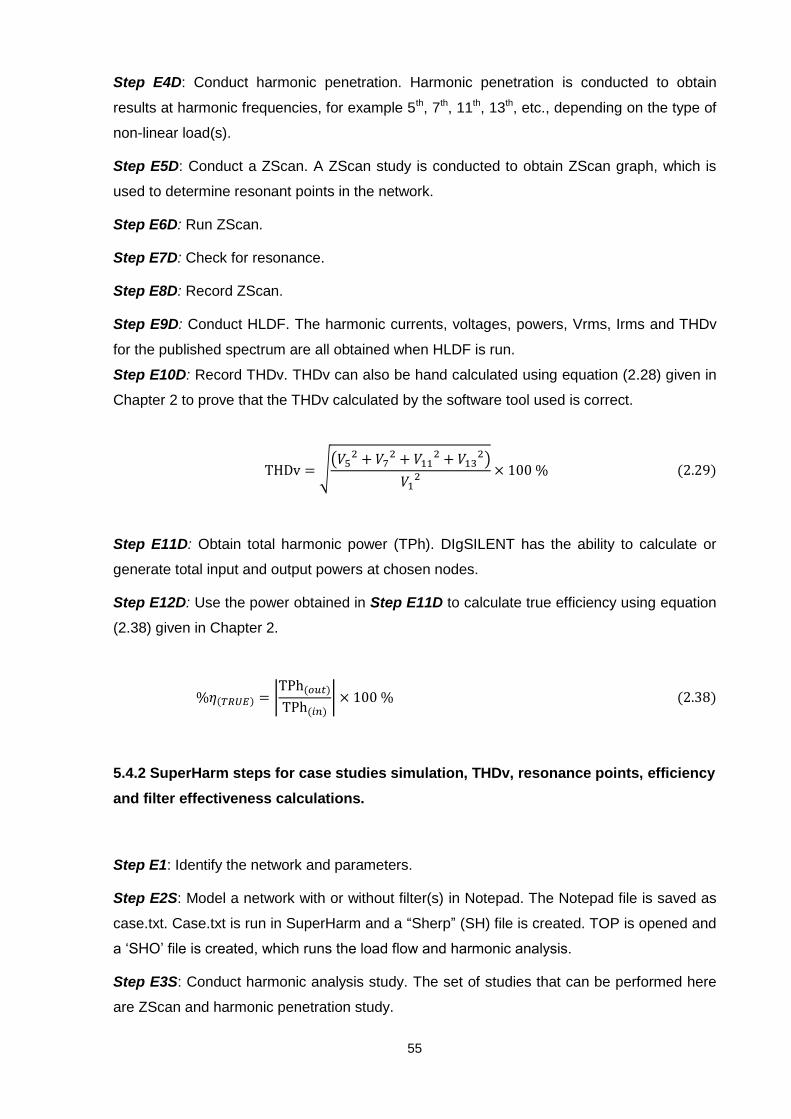
55

Step E4D: Conduct harmonic penetration. Harmonic penetration is conducted to obtain

results at harmonic frequencies, for example 5th, 7th, 11th, 13th, etc., depending on the type of

non-linear load(s).

Step E5D: Conduct a ZScan. A ZScan study is conducted to obtain ZScan graph, which is

used to determine resonant points in the network.

Step E6D: Run ZScan.

Step E7D: Check for resonance.

Step E8D: Record ZScan.

Step E9D: Conduct HLDF. The harmonic currents, voltages, powers, Vrms, Irms and THDv

for the published spectrum are all obtained when HLDF is run.

Step E10D: Record THDv. THDv can also be hand calculated using equation (2.28) given in

Chapter 2 to prove that the THDv calculated by the software tool used is correct.

√

Step E11D: Obtain total harmonic power (TPh). DIgSILENT has the ability to calculate or

generate total input and output powers at chosen nodes.

Step E12D: Use the power obtained in Step E11D to calculate true efficiency using equation

(2.38) given in Chapter 2.

|

|

5.4.2 SuperHarm steps for case studies simulation, THDv, resonance points, efficiency

and filter effectiveness calculations.

Step E1: Identify the network and parameters.

Step E2S: Model a network with or without filter(s) in Notepad. The Notepad file is saved as

case.txt. Case.txt is run in SuperHarm and a “Sherp” (SH) file is created. TOP is opened and

a „SHO‟ file is created, which runs the load flow and harmonic analysis.

Step E3S: Conduct harmonic analysis study. The set of studies that can be performed here

are ZScan and harmonic penetration study.

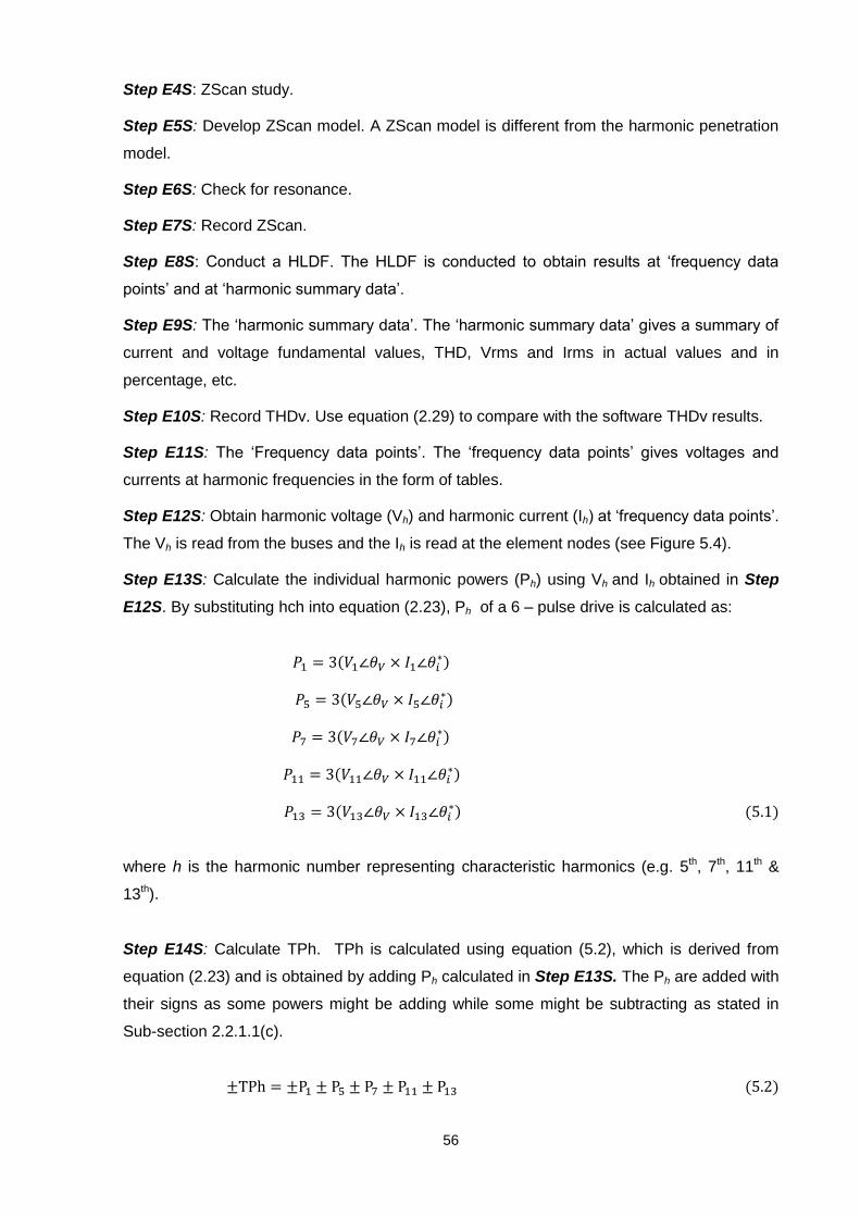
56

Step E4S: ZScan study.

Step E5S: Develop ZScan model. A ZScan model is different from the harmonic penetration

model.

Step E6S: Check for resonance.

Step E7S: Record ZScan.

Step E8S: Conduct a HLDF. The HLDF is conducted to obtain results at „frequency data

points‟ and at „harmonic summary data‟.

Step E9S: The „harmonic summary data‟. The „harmonic summary data‟ gives a summary of

current and voltage fundamental values, THD, Vrms and Irms in actual values and in

percentage, etc.

Step E10S: Record THDv. Use equation (2.29) to compare with the software THDv results.

Step E11S: The „Frequency data points‟. The „frequency data points‟ gives voltages and

currents at harmonic frequencies in the form of tables.

Step E12S: Obtain harmonic voltage (Vh) and harmonic current (Ih) at „frequency data points‟.

The Vh is read from the buses and the Ih is read at the element nodes (see Figure 5.4).

Step E13S: Calculate the individual harmonic powers (Ph) using Vh and Ih obtained in Step

E12S. By substituting hch into equation (2.23), Ph of a 6 – pulse drive is calculated as:

where h is the harmonic number representing characteristic harmonics (e.g. 5th, 7th, 11th &

13th).

Step E14S: Calculate TPh. TPh is calculated using equation (5.2), which is derived from

equation (2.23) and is obtained by adding Ph calculated in Step E13S. The Ph are added with

their signs as some powers might be adding while some might be subtracting as stated in

Sub-section 2.2.1.1(c).

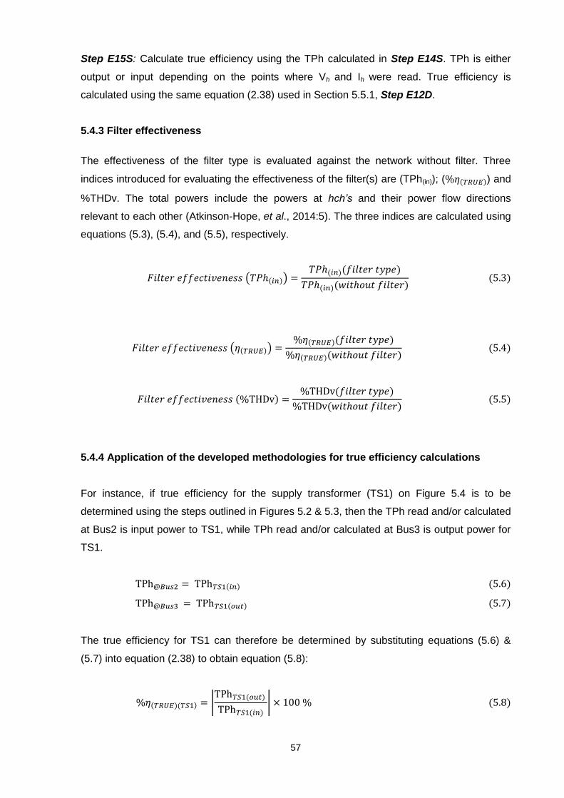
57

Step E15S: Calculate true efficiency using the TPh calculated in Step E14S. TPh is either

output or input depending on the points where Vh and Ih were read. True efficiency is

calculated using the same equation (2.38) used in Section 5.5.1, Step E12D.

5.4.3 Filter effectiveness

The effectiveness of the filter type is evaluated against the network without filter. Three

indices introduced for evaluating the effectiveness of the filter(s) are (TPh(in)); ( ) and

%THDv. The total powers include the powers at hch’s and their power flow directions

relevant to each other (Atkinson-Hope, et al., 2014:5). The three indices are calculated using

equations (5.3), (5.4), and (5.5), respectively.

𝐹 𝑙 𝑒 𝑒 𝑒 𝑒 𝑒 𝑙 𝑒 𝑦 𝑒

𝑤 𝑙 𝑒

𝐹 𝑙 𝑒 𝑒 𝑒 𝑒 𝑒 𝑙 𝑒 𝑦 𝑒

𝑤 𝑙 𝑒

𝐹 𝑙 𝑒 𝑒 𝑒 𝑒 𝑒 𝑙 𝑒 𝑦 𝑒

𝑤 𝑙 𝑒

5.4.4 Application of the developed methodologies for true efficiency calculations

For instance, if true efficiency for the supply transformer (TS1) on Figure 5.4 is to be

determined using the steps outlined in Figures 5.2 & 5.3, then the TPh read and/or calculated

at Bus2 is input power to TS1, while TPh read and/or calculated at Bus3 is output power for

TS1.

The true efficiency for TS1 can therefore be determined by substituting equations (5.6) &

(5.7) into equation (2.38) to obtain equation (5.8):

|

|

58

Efficiency of TS1 at fundamental frequency (f1)

A single frequency power can be used to calculate efficiency at a single frequency. For

example, for TS1, efficiency at f1 can be calculated by using the same equation as would be

used for efficiency calculations in power systems that are harmonic free or purely sinusoidal.

When the fundamental power (P1) at Bus2 and Bus3 are inserted into equation (1.2) it

becomes:

Table 5.1: Power variables for efficiency calculation

= fundamental power at Bus2 = fundamental power at Bus3

= TS1 fundamental output power = TS1 fundamental input power

= total harmonic power at Bus2 = total harmonic power at Bus3

= TS1 total output harmonic power = TS1 total input harmonic power

= TS1 true efficiency = TS1 fundamental efficiency

5.5 Summary

The need for this research is given. The main contributions of this study are new flow charts

and indices for evaluating true efficiency and effectiveness filters. It includes THDv,

resonance severity and a new index „filter effectiveness‟, which are outlined in the developed

flow charts. The steps for the development of the true efficiency calculation methodologies in

network under distorted condition using SuperHarm and DIgSILENT are developed.

SuperHarm uses separate models for harmonic analysis, one for harmonic penetration and

one for a scan study. The developed formulae are applied to case studies in the next chapter

to prove their effectiveness.

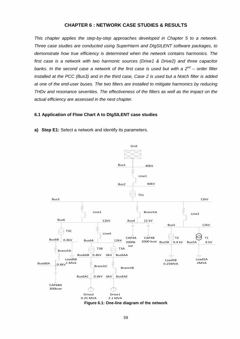
59

CHAPTER 6 : NETWORK CASE STUDIES & RESULTS

This chapter applies the step-by-step approaches developed in Chapter 5 to a network.

Three case studies are conducted using SuperHarm and DIgSILENT software packages, to

demonstrate how true efficiency is determined when the network contains harmonics. The

first case is a network with two harmonic sources (Drive1 & Drive2) and three capacitor

banks. In the second case a network of the first case is used but with a 2nd – order filter

installed at the PCC (Bus3) and in the third case, Case 2 is used but a Notch filter is added

at one of the end-user buses. The two filters are installed to mitigate harmonics by reducing

THDv and resonance severities. The effectiveness of the filters as well as the impact on the

actual efficiency are assessed in the next chapter.

6.1 Application of Flow Chart A to DIgSILENT case studies

a) Step E1: Select a network and identify its parameters.

Grid

40kVBus1

Bus2

Line1

40kV

12kVBus3

Line3

12kVBus6

0.4kV

T3C

Bus6B

Line4

T3AT3B

0.4kV

12kVBus6A

Bus6AB

TS1

Line2

T1T2

Load5B0.25MVA

Load5A2MVA

Drive20.25 MVA

Drive12.1 MVA

CAP6BA300kvar

BranchD

Load6B1 MVA

0.4kV 6kV

6kV0.4kV

BranchCBranchB

Bus5B Bus5A

Bus5 12kV

BranchA

Bus4 12 kV

CAP4A CAP4B2000 kvar2000k

var

Bus6AC

Bus6AA

Bus6AE

6 kV0.4 kV

Bus6BA

Figure 6.1: One-line diagram of the network

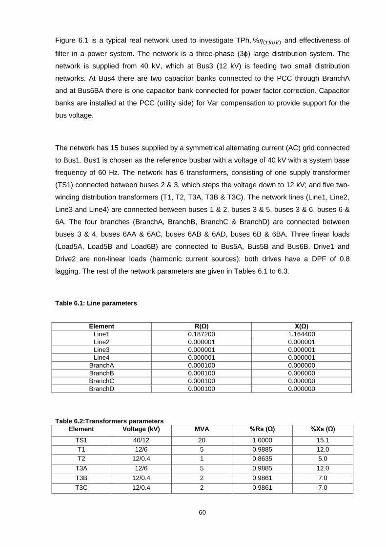
60

Figure 6.1 is a typical real network used to investigate TPh, and effectiveness of

filter in a power system. The network is a three-phase (3ϕ) large distribution system. The

network is supplied from 40 kV, which at Bus3 (12 kV) is feeding two small distribution

networks. At Bus4 there are two capacitor banks connected to the PCC through BranchA

and at Bus6BA there is one capacitor bank connected for power factor correction. Capacitor

banks are installed at the PCC (utility side) for Var compensation to provide support for the

bus voltage.

The network has 15 buses supplied by a symmetrical alternating current (AC) grid connected

to Bus1. Bus1 is chosen as the reference busbar with a voltage of 40 kV with a system base

frequency of 60 Hz. The network has 6 transformers, consisting of one supply transformer

(TS1) connected between buses 2 & 3, which steps the voltage down to 12 kV; and five two-

winding distribution transformers (T1, T2, T3A, T3B & T3C). The network lines (Line1, Line2,

Line3 and Line4) are connected between buses 1 & 2, buses 3 & 5, buses 3 & 6, buses 6 &

6A. The four branches (BranchA, BranchB, BranchC & BranchD) are connected between

buses 3 & 4, buses 6AA & 6AC, buses 6AB & 6AD, buses 6B & 6BA. Three linear loads

(Load5A, Load5B and Load6B) are connected to Bus5A, Bus5B and Bus6B. Drive1 and

Drive2 are non-linear loads (harmonic current sources); both drives have a DPF of 0.8

lagging. The rest of the network parameters are given in Tables 6.1 to 6.3.

Table 6.1: Line parameters

Element R(Ω) X(Ω)

Line1 0.187200 1.164400

Line2 0.000001 0.000001

Line3 0.000001 0.000001

Line4 0.000001 0.000001

BranchA 0.000100 0.000000

BranchB 0.000100 0.000000

BranchC 0.000100 0.000000

BranchD 0.000100 0.000000

Table 6.2:Transformers parameters

Element Voltage (kV) MVA %Rs (Ω) %Xs (Ω)

TS1 40/12 20 1.0000 15.1

T1 12/6 5 0.9885 12.0

T2 12/0.4 1 0.8635 5.0

T3A 12/6 5 0.9885 12.0

T3B 12/0.4 2 0.9861 7.0

T3C 12/0.4 2 0.9861 7.0

61

Table 6.3: Load parameters

Element Voltage (kV) kVA Power factor

Load5A 6.0 2000 0.5

Load5B 0.4 250 0.9

Load6AB 0.4 1000 0.8

Drive1 6.0 2100 0.8

Drive2 0.4 250 0.8

b) Step E2D: Figure 6.1 is selected for the three case studies. How to model the elements

is illustrated in Chapter 4 under Section 4.1.1 with the details for each model

(parameters) given in Appendix 1.

- Case 1: Network without filter (DIgSILENT)

In Case 1, the two drives, Drive1 & Drive2 at buses 6AC and 6AD are modelled as 6 - pulse

drives. Each of the drives is assumed to inject only hch = 6k±1, k = 1, 2 and 3 characteristic

harmonics into the system. The 6 pulse drives are chosen for this study because they are a

common type of drives found in the industry. The 6 - pulse drive generates low order

harmonics (5th, 7th), which are usually high in magnitude, thus offering sufficient harmonic

quantities (current and voltage) for harmonic analysis studies. Table 6.4 shows the

parameters for the harmonic current magnitudes and angles of the drives for DIgSILENT

models. The models (spectrums) are shown in Figures A3.1 and A3.2 in Appendix 3.

Each harmonic source is operating at a different voltage level, Drive1 at 6 kV and Drive2 at

0.4 kV.

Table 6.4: DIgSILENT harmonic current spectrum (Drive1 & Drive2)

Harmonic order

Drive1 Drive2

Magnitude (%) Angle ( ) Magnitude (%) Angle ( ) 5 17.9999 0 17.9999 0

7 11.9999 0 11.9999 0

11 5.9999 0 5.9999 0

13 3.9999 0 3.9999 0

c) Step E3D: Conduct a load flow study on the network to obtain TS1 power at fundamental

frequency. TS1 fundamental frequency power is obtained at Bus2 & Bus3 from the load

flow study conducted, results are shown in Table 6.5.

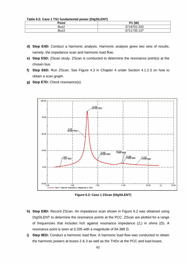
62

Table 6.5: Case 1 TS1 fundamental power (DIgSILENT)

Point P1 (W)

Bus2 3718702.333

Bus3 -3711735.137

d) Step E4D: Conduct a harmonic analysis. Harmonic analysis gives two sets of results,

namely, the impedance scan and harmonic load flow.

e) Step E5D: ZScan study. ZScan is conducted to determine the resonance point(s) at the

chosen bus.

f) Step E6D: Run ZScan. See Figure 4.3 in Chapter 4 under Section 4.1.2.3 on how to

obtain a scan graph.

g) Step E7D: Check resonance(s).

Figure 6.2: Case 1 ZScan (DIgSILENT)

h) Step E8D: Record ZScan. An impedance scan shown in Figure 6.2 was obtained using

DIgSILENT to determine the resonance points at the PCC. ZScan are plotted for a range

of frequencies that includes hch against resonance impedance (Zr) in ohms (Ω). A

resonance point is seen at 5.335 with a magnitude of 84.388 Ω.

i) Step 9ED: Conduct a harmonic load flow. A harmonic load flow was conducted to obtain

the harmonic powers at buses 2 & 3 as well as the THDv at the PCC and load buses.

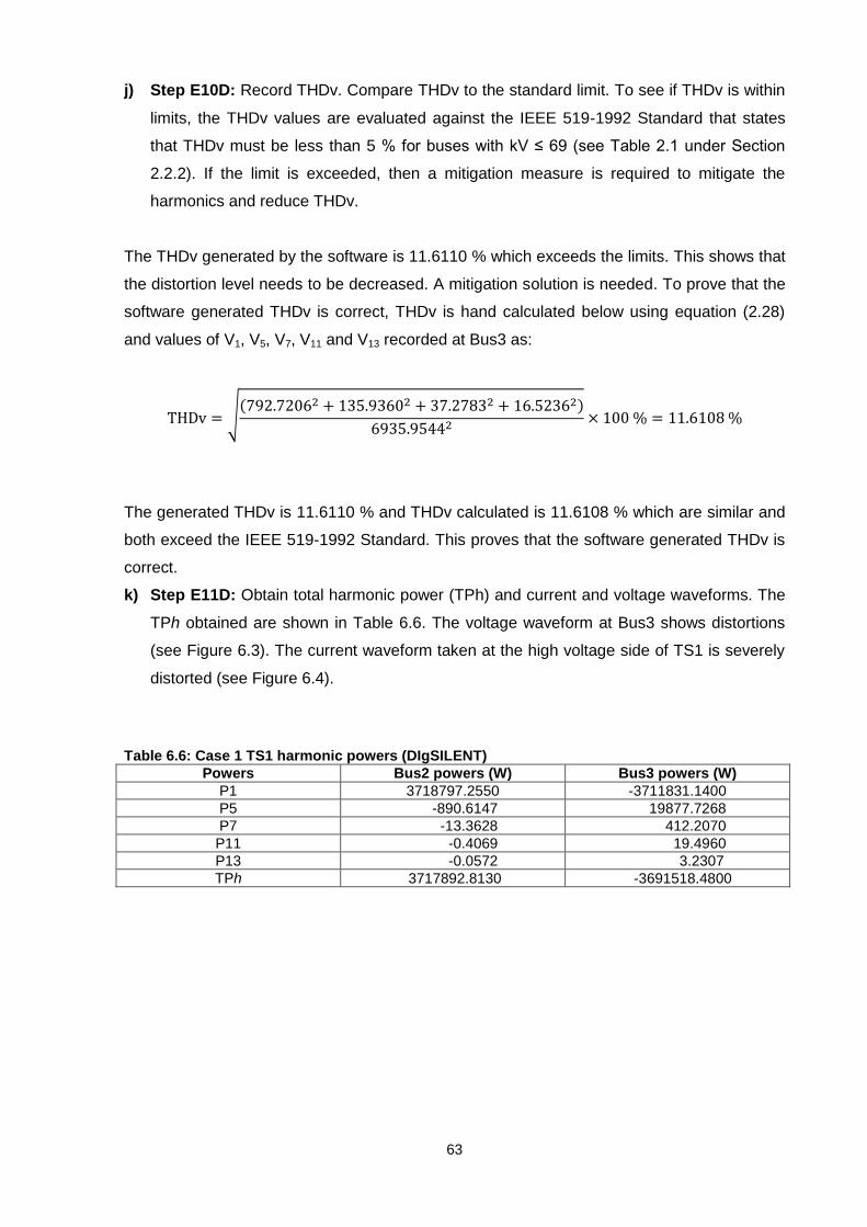
63

j) Step E10D: Record THDv. Compare THDv to the standard limit. To see if THDv is within

limits, the THDv values are evaluated against the IEEE 519-1992 Standard that states

that THDv must be less than 5 % for buses with kV ≤ 69 (see Table 2.1 under Section

2.2.2). If the limit is exceeded, then a mitigation measure is required to mitigate the

harmonics and reduce THDv.

The THDv generated by the software is 11.6110 % which exceeds the limits. This shows that

the distortion level needs to be decreased. A mitigation solution is needed. To prove that the

software generated THDv is correct, THDv is hand calculated below using equation (2.28)

and values of V1, V5, V7, V11 and V13 recorded at Bus3 as:

√

The generated THDv is 11.6110 % and THDv calculated is 11.6108 % which are similar and

both exceed the IEEE 519-1992 Standard. This proves that the software generated THDv is

correct.

k) Step E11D: Obtain total harmonic power (TPh) and current and voltage waveforms. The

TPh obtained are shown in Table 6.6. The voltage waveform at Bus3 shows distortions

(see Figure 6.3). The current waveform taken at the high voltage side of TS1 is severely

distorted (see Figure 6.4).

Table 6.6: Case 1 TS1 harmonic powers (DIgSILENT)

Powers Bus2 powers (W) Bus3 powers (W)

P1 3718797.2550 -3711831.1400

P5 -890.6147 19877.7268

P7 -13.3628 412.2070

P11 -0.4069 19.4960

P13 -0.0572 3.2307

TPh 3717892.8130 -3691518.4800

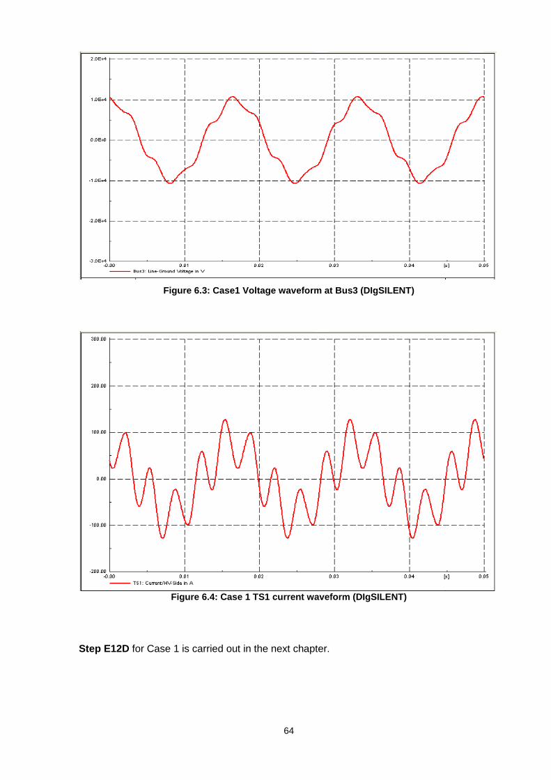
64

Figure 6.3: Case1 Voltage waveform at Bus3 (DIgSILENT)

Figure 6.4: Case 1 TS1 current waveform (DIgSILENT)

Step E12D for Case 1 is carried out in the next chapter.

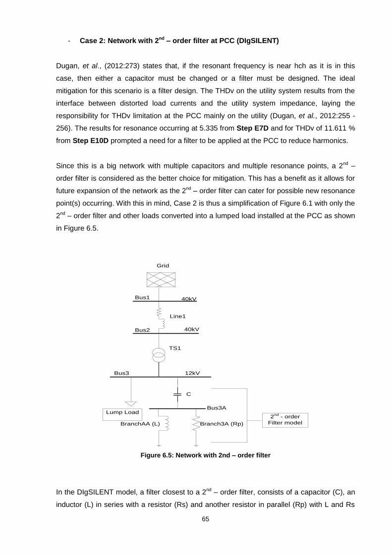
65

- Case 2: Network with 2nd – order filter at PCC (DIgSILENT)

Dugan, et al., (2012:273) states that, if the resonant frequency is near hch as it is in this

case, then either a capacitor must be changed or a filter must be designed. The ideal

mitigation for this scenario is a filter design. The THDv on the utility system results from the

interface between distorted load currents and the utility system impedance, laying the

responsibility for THDv limitation at the PCC mainly on the utility (Dugan, et al., 2012:255 -

256). The results for resonance occurring at 5.335 from Step E7D and for THDv of 11.611 %

from Step E10D prompted a need for a filter to be applied at the PCC to reduce harmonics.

Since this is a big network with multiple capacitors and multiple resonance points, a 2nd –

order filter is considered as the better choice for mitigation. This has a benefit as it allows for

future expansion of the network as the 2nd – order filter can cater for possible new resonance

point(s) occurring. With this in mind, Case 2 is thus a simplification of Figure 6.1 with only the

2nd – order filter and other loads converted into a lumped load installed at the PCC as shown

in Figure 6.5.

Grid

40kVBus1

Bus2

Line1

40kV

12kVBus3

TS1

Lump Load2

nd - order

Filter modelBranch3A (Rp)

C

BranchAA (L)

Bus3A

Figure 6.5: Network with 2nd – order filter

In the DIgSILENT model, a filter closest to a 2nd – order filter, consists of a capacitor (C), an

inductor (L) in series with a resistor (Rs) and another resistor in parallel (Rp) with L and Rs

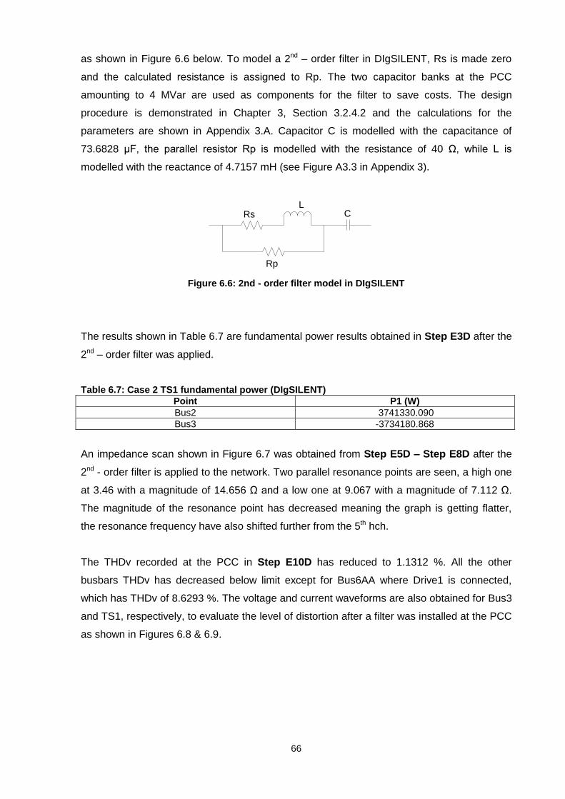
66

as shown in Figure 6.6 below. To model a 2nd – order filter in DIgSILENT, Rs is made zero

and the calculated resistance is assigned to Rp. The two capacitor banks at the PCC

amounting to 4 MVar are used as components for the filter to save costs. The design

procedure is demonstrated in Chapter 3, Section 3.2.4.2 and the calculations for the

parameters are shown in Appendix 3.A. Capacitor C is modelled with the capacitance of

73.6828 μF, the parallel resistor Rp is modelled with the resistance of 40 Ω, while L is

modelled with the reactance of 4.7157 mH (see Figure A3.3 in Appendix 3).

RsL

C

Rp

Figure 6.6: 2nd - order filter model in DIgSILENT

The results shown in Table 6.7 are fundamental power results obtained in Step E3D after the

2nd – order filter was applied.

Table 6.7: Case 2 TS1 fundamental power (DIgSILENT)

Point P1 (W)

Bus2 3741330.090

Bus3 -3734180.868

An impedance scan shown in Figure 6.7 was obtained from Step E5D – Step E8D after the

2nd - order filter is applied to the network. Two parallel resonance points are seen, a high one

at 3.46 with a magnitude of 14.656 Ω and a low one at 9.067 with a magnitude of 7.112 Ω.

The magnitude of the resonance point has decreased meaning the graph is getting flatter,

the resonance frequency have also shifted further from the 5th hch.

The THDv recorded at the PCC in Step E10D has reduced to 1.1312 %. All the other

busbars THDv has decreased below limit except for Bus6AA where Drive1 is connected,

which has THDv of 8.6293 %. The voltage and current waveforms are also obtained for Bus3

and TS1, respectively, to evaluate the level of distortion after a filter was installed at the PCC

as shown in Figures 6.8 & 6.9.

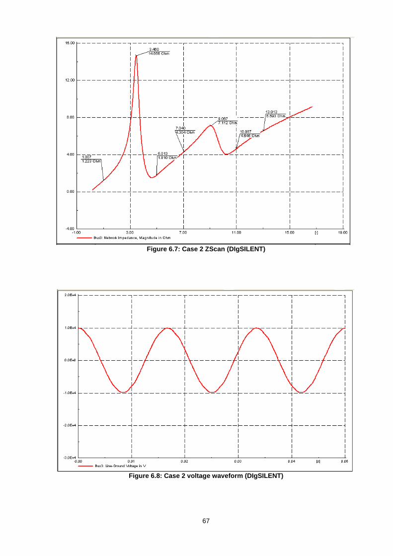
67

Figure 6.7: Case 2 ZScan (DIgSILENT)

Figure 6.8: Case 2 voltage waveform (DIgSILENT)

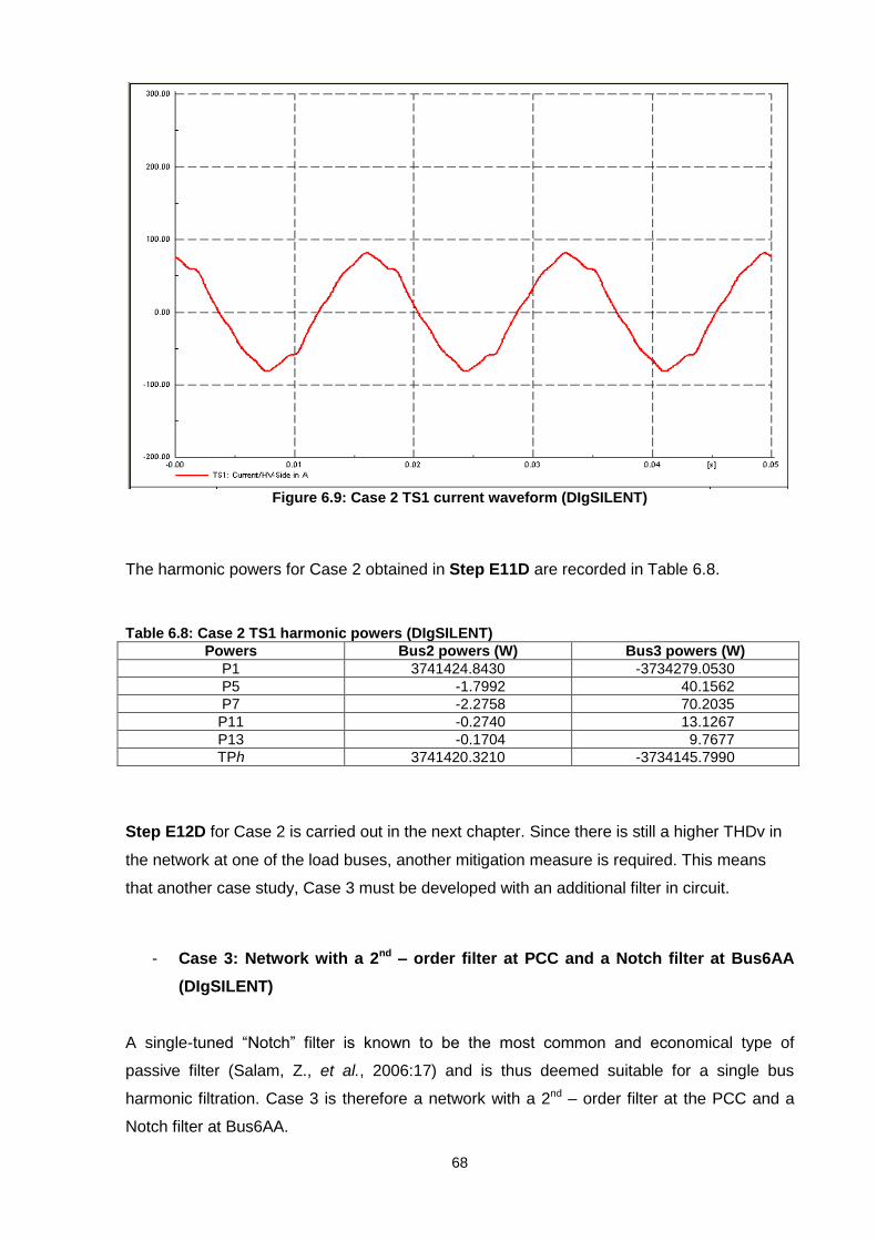
68

Figure 6.9: Case 2 TS1 current waveform (DIgSILENT)

The harmonic powers for Case 2 obtained in Step E11D are recorded in Table 6.8.

Table 6.8: Case 2 TS1 harmonic powers (DIgSILENT)

Powers Bus2 powers (W) Bus3 powers (W)

P1 3741424.8430 -3734279.0530

P5 -1.7992 40.1562

P7 -2.2758 70.2035

P11 -0.2740 13.1267

P13 -0.1704 9.7677

TPh 3741420.3210 -3734145.7990

Step E12D for Case 2 is carried out in the next chapter. Since there is still a higher THDv in

the network at one of the load buses, another mitigation measure is required. This means

that another case study, Case 3 must be developed with an additional filter in circuit.

- Case 3: Network with a 2nd – order filter at PCC and a Notch filter at Bus6AA

(DIgSILENT)

A single-tuned “Notch” filter is known to be the most common and economical type of

passive filter (Salam, Z., et al., 2006:17) and is thus deemed suitable for a single bus

harmonic filtration. Case 3 is therefore a network with a 2nd – order filter at the PCC and a

Notch filter at Bus6AA.

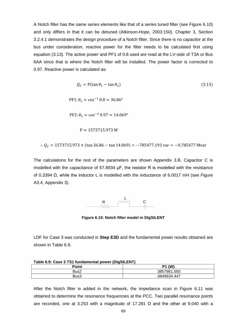
69

A Notch filter has the same series elements like that of a series tuned filter (see Figure 6.10)

and only differs in that it can be detuned (Atkinson-Hope, 2003:150). Chapter 3, Section

3.2.4.1 demonstrates the design procedure of a Notch filter. Since there is no capacitor at the

bus under consideration, reactive power for the filter needs to be calculated first using

equation (3.13). The active power and PF1 of 0.8 used are read at the LV-side of T3A or Bus

6AA since that is where the Notch filter will be installed. The power factor is corrected to

0.97. Reactive power is calculated as:

The calculations for the rest of the parameters are shown Appendix 3.B. Capacitor C is

modelled with the capacitance of 57.8934 μF, the resistor R is modelled with the resistance

of 0.3394 Ω, while the inductor L is modelled with the inductance of 6.0017 mH (see Figure

A3.4, Appendix 3).

RL

C

Figure 6.10: Notch filter model in DIgSILENT

LDF for Case 3 was conducted in Step E3D and the fundamental power results obtained are

shown in Table 6.9.

Table 6.9: Case 3 TS1 fundamental power (DIgSILENT)

Point P1 (W)

Bus2 3857981.550

Bus3 -3849634.447

After the Notch filter is added in the network, the impedance scan in Figure 6.11 was

obtained to determine the resonance frequencies at the PCC. Two parallel resonance points

are recorded, one at 3.253 with a magnitude of 17.281 Ω and the other at 9.040 with a

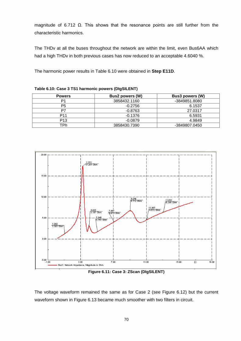
70

magnitude of 6.712 Ω. This shows that the resonance points are still further from the

characteristic harmonics.

The THDv at all the buses throughout the network are within the limit, even Bus6AA which

had a high THDv in both previous cases has now reduced to an acceptable 4.6040 %.

The harmonic power results in Table 6.10 were obtained in Step E11D.

Table 6.10: Case 3 TS1 harmonic powers (DIgSILENT)

Powers Bus2 powers (W) Bus3 powers (W)

P1 3858432.1160 -3849851.8080

P5 -0.2756 6.1537

P7 -0.8763 27.0317

P11 -0.1376 6.5931

P13 -0.0879 4.9849

TPh 3858430.7390 -3849807.0450

Figure 6.11: Case 3: ZScan (DIgSILENT)

The voltage waveform remained the same as for Case 2 (see Figure 6.12) but the current

waveform shown in Figure 6.13 became much smoother with two filters in circuit.

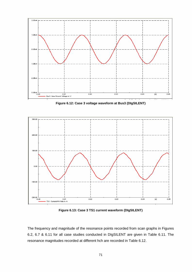
71

Figure 6.12: Case 3 voltage waveform at Bus3 (DIgSILENT)

Figure 6.13: Case 3 TS1 current waveform (DIgSILENT)

The frequency and magnitude of the resonance points recorded from scan graphs in Figures

6.2, 6.7 & 6.11 for all case studies conducted in DIgSILENT are given in Table 6.11. The

resonance magnitudes recorded at different hch are recorded in Table 6.12.

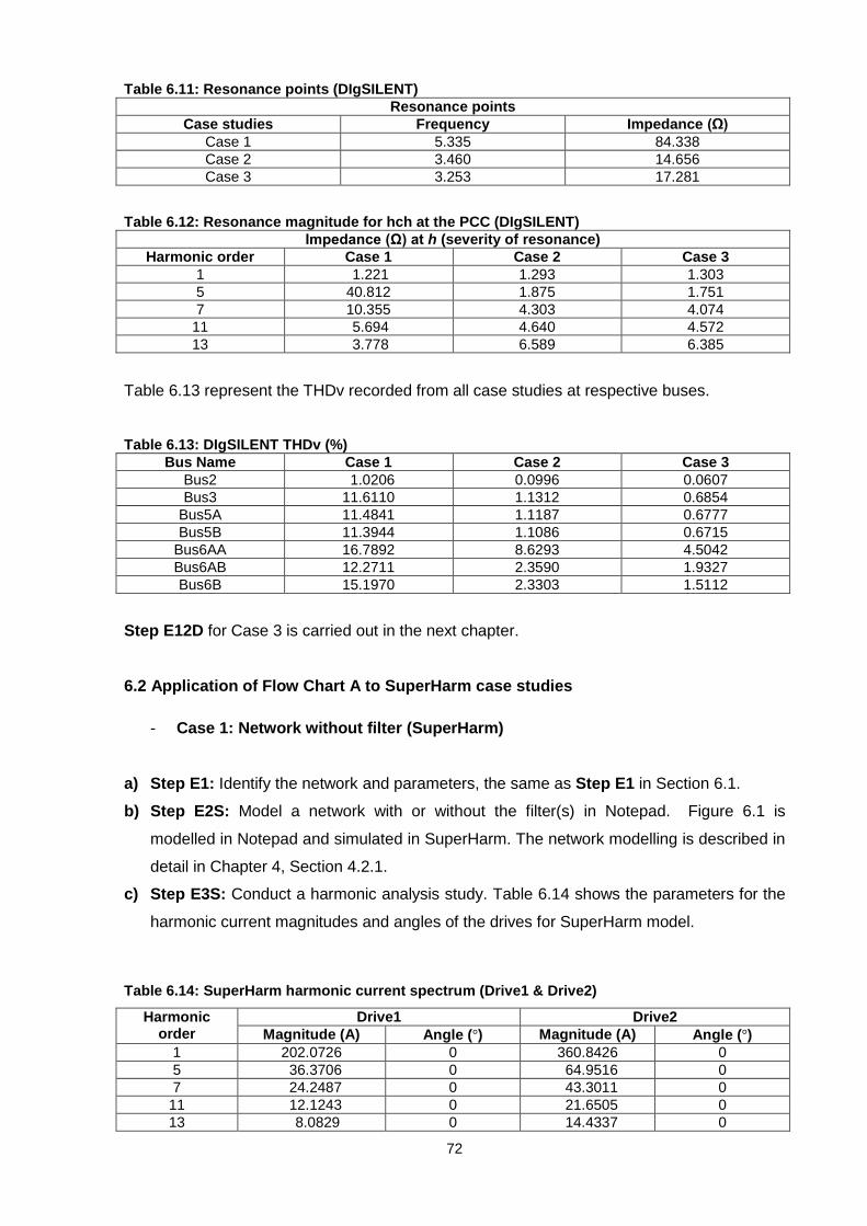
72

Table 6.11: Resonance points (DIgSILENT)

Resonance points

Case studies Frequency Impedance (Ω)

Case 1 5.335 84.338

Case 2 3.460 14.656

Case 3 3.253 17.281

Table 6.12: Resonance magnitude for hch at the PCC (DIgSILENT)

Impedance (Ω) at h (severity of resonance)

Harmonic order Case 1 Case 2 Case 3

1 1.221 1.293 1.303

5 40.812 1.875 1.751

7 10.355 4.303 4.074

11 5.694 4.640 4.572

13 3.778 6.589 6.385

Table 6.13 represent the THDv recorded from all case studies at respective buses.

Table 6.13: DIgSILENT THDv (%)

Bus Name Case 1 Case 2 Case 3

Bus2 1.0206 0.0996 0.0607

Bus3 11.6110 1.1312 0.6854

Bus5A 11.4841 1.1187 0.6777

Bus5B 11.3944 1.1086 0.6715

Bus6AA 16.7892 8.6293 4.5042

Bus6AB 12.2711 2.3590 1.9327

Bus6B 15.1970 2.3303 1.5112

Step E12D for Case 3 is carried out in the next chapter.

6.2 Application of Flow Chart A to SuperHarm case studies

- Case 1: Network without filter (SuperHarm)

a) Step E1: Identify the network and parameters, the same as Step E1 in Section 6.1.

b) Step E2S: Model a network with or without the filter(s) in Notepad. Figure 6.1 is

modelled in Notepad and simulated in SuperHarm. The network modelling is described in

detail in Chapter 4, Section 4.2.1.

c) Step E3S: Conduct a harmonic analysis study. Table 6.14 shows the parameters for the

harmonic current magnitudes and angles of the drives for SuperHarm model.

Table 6.14: SuperHarm harmonic current spectrum (Drive1 & Drive2)

Harmonic order

Drive1 Drive2

Magnitude (A) Angle ( ) Magnitude (A) Angle ( ) 1 202.0726 0 360.8426 0

5 36.3706 0 64.9516 0

7 24.2487 0 43.3011 0

11 12.1243 0 21.6505 0

13 8.0829 0 14.4337 0

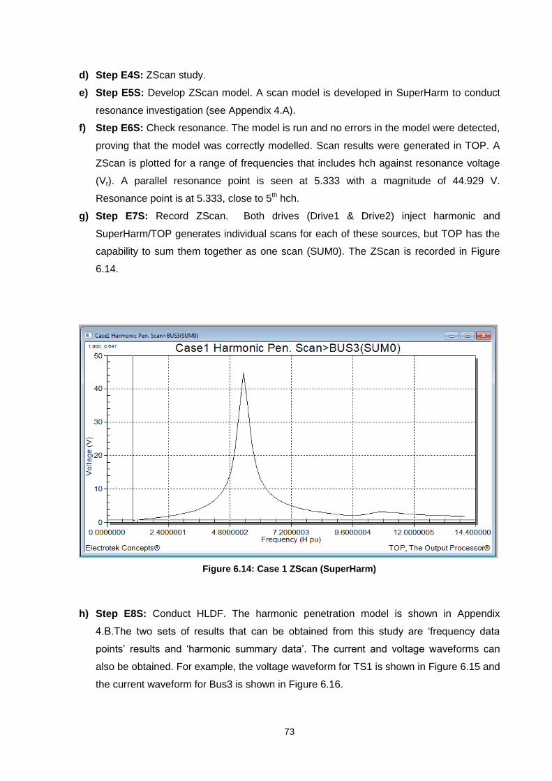
73

d) Step E4S: ZScan study.

e) Step E5S: Develop ZScan model. A scan model is developed in SuperHarm to conduct

resonance investigation (see Appendix 4.A).

f) Step E6S: Check resonance. The model is run and no errors in the model were detected,

proving that the model was correctly modelled. Scan results were generated in TOP. A

ZScan is plotted for a range of frequencies that includes hch against resonance voltage

(Vr). A parallel resonance point is seen at 5.333 with a magnitude of 44.929 V.

Resonance point is at 5.333, close to 5th hch.

g) Step E7S: Record ZScan. Both drives (Drive1 & Drive2) inject harmonic and

SuperHarm/TOP generates individual scans for each of these sources, but TOP has the

capability to sum them together as one scan (SUM0). The ZScan is recorded in Figure

6.14.

Figure 6.14: Case 1 ZScan (SuperHarm)

h) Step E8S: Conduct HLDF. The harmonic penetration model is shown in Appendix

4.B.The two sets of results that can be obtained from this study are „frequency data

points‟ results and „harmonic summary data‟. The current and voltage waveforms can

also be obtained. For example, the voltage waveform for TS1 is shown in Figure 6.15 and

the current waveform for Bus3 is shown in Figure 6.16.

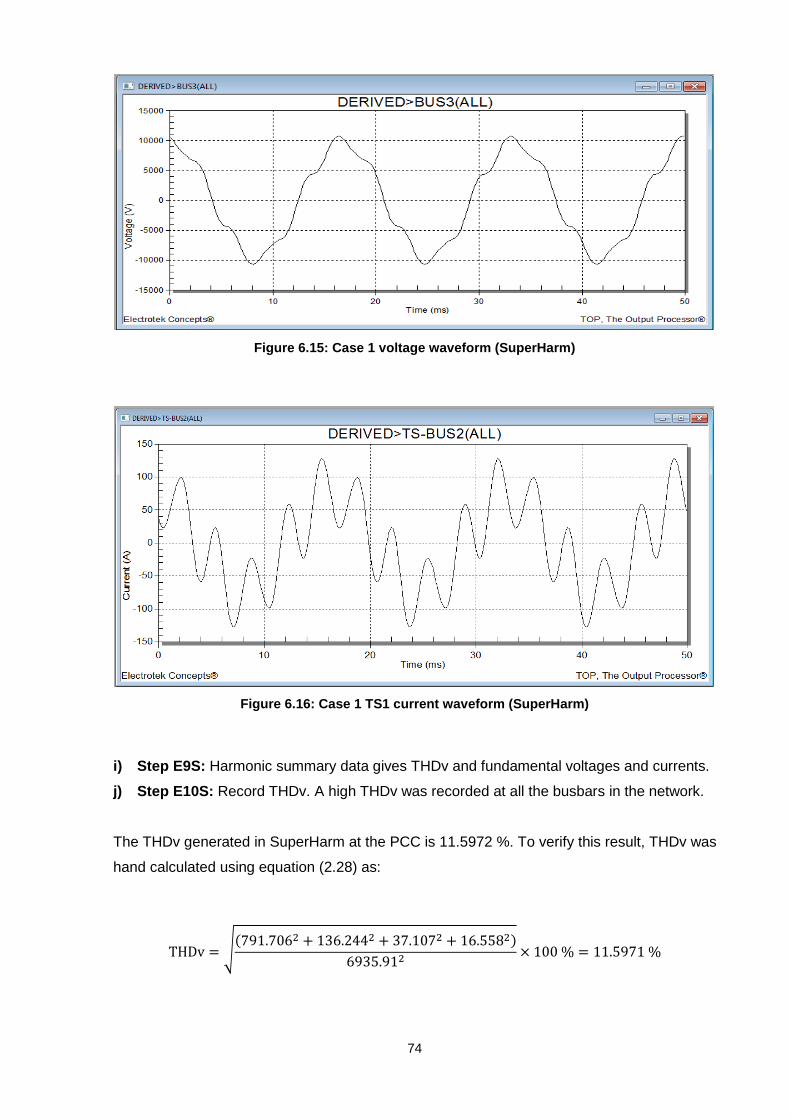
74

Figure 6.15: Case 1 voltage waveform (SuperHarm)

Figure 6.16: Case 1 TS1 current waveform (SuperHarm)

i) Step E9S: Harmonic summary data gives THDv and fundamental voltages and currents.

j) Step E10S: Record THDv. A high THDv was recorded at all the busbars in the network.

The THDv generated in SuperHarm at the PCC is 11.5972 %. To verify this result, THDv was

hand calculated using equation (2.28) as:

√

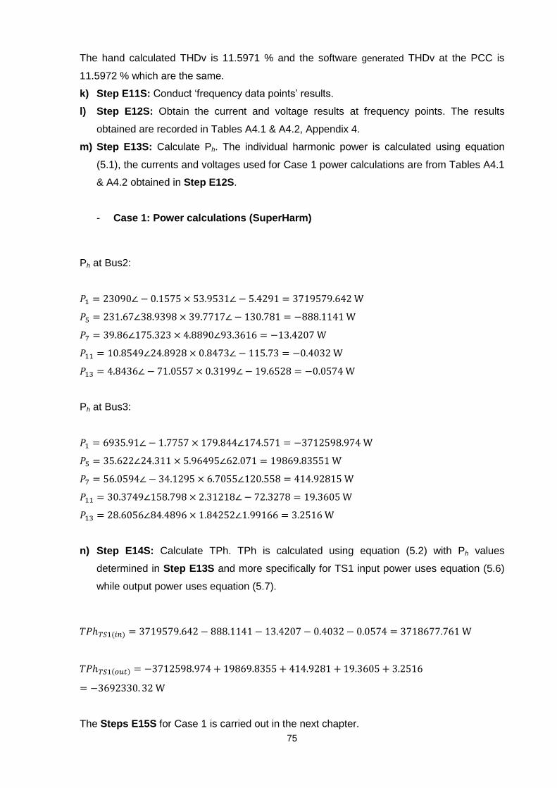
75

The hand calculated THDv is 11.5971 % and the software generated THDv at the PCC is

11.5972 % which are the same.

k) Step E11S: Conduct „frequency data points‟ results.

l) Step E12S: Obtain the current and voltage results at frequency points. The results

obtained are recorded in Tables A4.1 & A4.2, Appendix 4.

m) Step E13S: Calculate Ph. The individual harmonic power is calculated using equation

(5.1), the currents and voltages used for Case 1 power calculations are from Tables A4.1

& A4.2 obtained in Step E12S.

- Case 1: Power calculations (SuperHarm)

Ph at Bus2:

Ph at Bus3:

n) Step E14S: Calculate TPh. TPh is calculated using equation (5.2) with Ph values

determined in Step E13S and more specifically for TS1 input power uses equation (5.6)

while output power uses equation (5.7).

The Steps E15S for Case 1 is carried out in the next chapter.

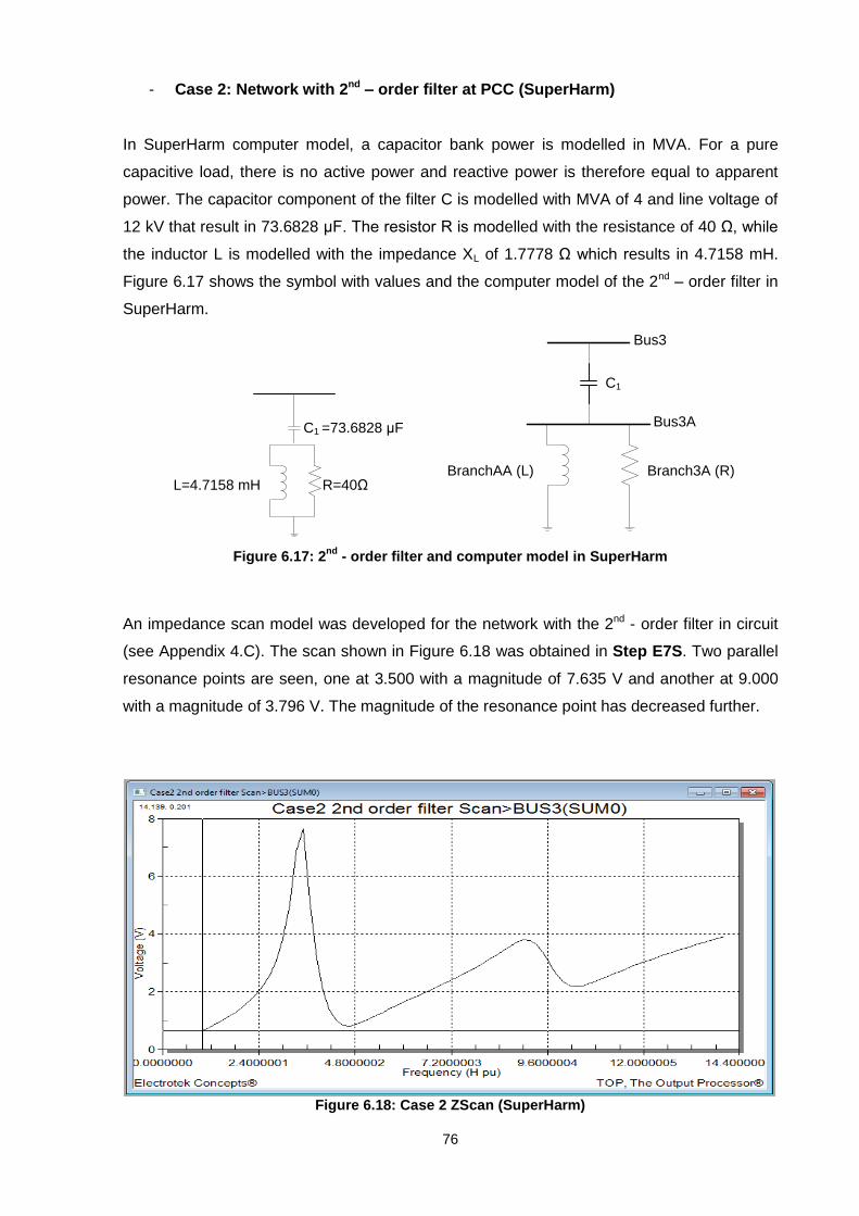
76

- Case 2: Network with 2nd – order filter at PCC (SuperHarm)

In SuperHarm computer model, a capacitor bank power is modelled in MVA. For a pure

capacitive load, there is no active power and reactive power is therefore equal to apparent

power. The capacitor component of the filter C is modelled with MVA of 4 and line voltage of

12 kV that result in 73.6828 μF. The resistor R is modelled with the resistance of 40 Ω, while

the inductor L is modelled with the impedance XL of 1.7778 Ω which results in 4.7158 mH.

Figure 6.17 shows the symbol with values and the computer model of the 2nd – order filter in

SuperHarm.

Branch3A (R)

C1

BranchAA (L)

Bus3

Bus3A

L=4.7158 mH R=40Ω

C1 =73.6828 μF

Figure 6.17: 2nd

- order filter and computer model in SuperHarm

An impedance scan model was developed for the network with the 2nd - order filter in circuit

(see Appendix 4.C). The scan shown in Figure 6.18 was obtained in Step E7S. Two parallel

resonance points are seen, one at 3.500 with a magnitude of 7.635 V and another at 9.000

with a magnitude of 3.796 V. The magnitude of the resonance point has decreased further.

Figure 6.18: Case 2 ZScan (SuperHarm)

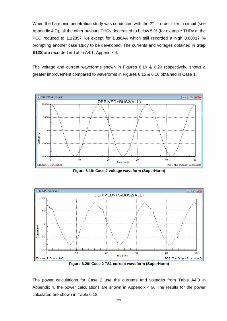
77

When the harmonic penetration study was conducted with the 2nd – order filter in circuit (see

Appendix 4.D), all the other busbars THDv decreased to below 5 % (for example THDv at the

PCC reduced to 1.12897 %) except for Bus6AA which still recorded a high 8.60017 %

prompting another case study to be developed. The currents and voltages obtained in Step

E12S are recorded in Table A4.1, Appendix 4.

The voltage and current waveforms shown in Figures 6.19 & 6.20 respectively, shows a

greater improvement compared to waveforms in Figures 6.15 & 6.16 obtained in Case 1.

Figure 6.19: Case 2 voltage waveform (SuperHarm)

Figure 6.20: Case 2 TS1 current waveform (SuperHarm)

The power calculations for Case 2 use the currents and voltages from Table A4.3 in

Appendix 4, the power calculations are shown in Appendix 4.G. The results for the power

calculated are shown in Table 6.18.

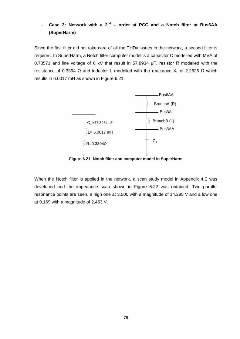
78

- Case 3: Network with a 2nd – order at PCC and a Notch filter at Bus6AA

(SuperHarm)

Since the first filter did not take care of all the THDv issues in the network, a second filter is

required. In SuperHarm, a Notch filter computer model is a capacitor C modelled with MVA of

0.78571 and line voltage of 6 kV that result in 57.8934 μF, resistor R modelled with the

resistance of 0.3394 Ω and inductor L modelled with the reactance XL of 2.2626 Ω which

results in 6.0017 mH as shown in Figure 6.21.

C1 =57.8934 μF

R=0.3394Ω

L= 6.0017 mH

C1

BranchA (R)

BranchB (L)

Bus3AA

Bus6AA

Bus3A

Figure 6.21: Notch filter and computer model in SuperHarm

When the Notch filter is applied in the network, a scan study model in Appendix 4.E was

developed and the impedance scan shown in Figure 6.22 was obtained. Two parallel

resonance points are seen, a high one at 3.500 with a magnitude of 14.295 V and a low one

at 9.169 with a magnitude of 2.453 V.

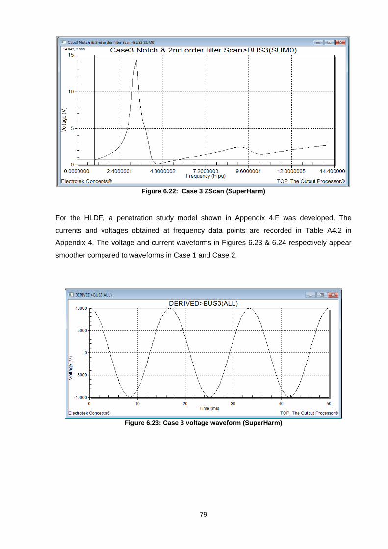
79

Figure 6.22: Case 3 ZScan (SuperHarm)

For the HLDF, a penetration study model shown in Appendix 4.F was developed. The

currents and voltages obtained at frequency data points are recorded in Table A4.2 in

Appendix 4. The voltage and current waveforms in Figures 6.23 & 6.24 respectively appear

smoother compared to waveforms in Case 1 and Case 2.

Figure 6.23: Case 3 voltage waveform (SuperHarm)

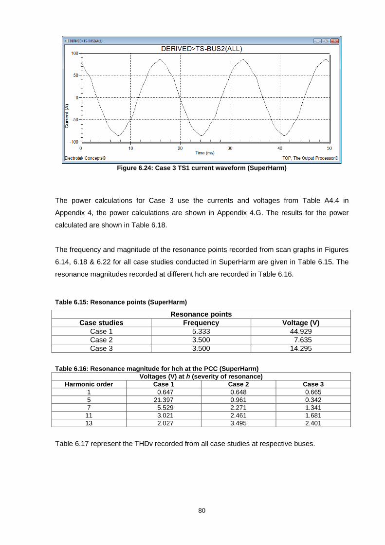
80

Figure 6.24: Case 3 TS1 current waveform (SuperHarm)

The power calculations for Case 3 use the currents and voltages from Table A4.4 in

Appendix 4, the power calculations are shown in Appendix 4.G. The results for the power

calculated are shown in Table 6.18.

The frequency and magnitude of the resonance points recorded from scan graphs in Figures

6.14, 6.18 & 6.22 for all case studies conducted in SuperHarm are given in Table 6.15. The

resonance magnitudes recorded at different hch are recorded in Table 6.16.

Table 6.15: Resonance points (SuperHarm)

Resonance points

Case studies Frequency Voltage (V)

Case 1 5.333 44.929

Case 2 3.500 7.635

Case 3 3.500 14.295

Table 6.16: Resonance magnitude for hch at the PCC (SuperHarm)

Voltages (V) at h (severity of resonance)

Harmonic order Case 1 Case 2 Case 3

1 0.647 0.648 0.665

5 21.397 0.961 0.342

7 5.529 2.271 1.341

11 3.021 2.461 1.681

13 2.027 3.495 2.401

Table 6.17 represent the THDv recorded from all case studies at respective buses.

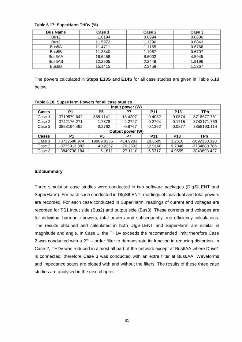
81

Table 6.17: SuperHarm THDv (%)

Bus Name Case 1 Case 2 Case 3

Bus2 1.0194 0.0994 0.0606

Bus3 11.5972 1.1290 0.6843

Bus5A 11.4711 1.1165 0.6766

Bus5B 11.3840 1.1067 0.6707

Bus6AA 16.6458 8.6002 4.5945

Bus6AB 12.2505 2.3449 1.9196

Bus6B 15.1415 2.3458 1.5267

The powers calculated in Steps E13S and E14S for all case studies are given in Table 6.18

below.

Table 6.18: SuperHarm Powers for all case studies

Input power (W)

Cases P1 P5 P7 P11 P13 TPh

Case 1 3719579.642 -888.1141 -13.4207 -0.4032 -0.0574 3718677.761

Case 2 3742176.271 -1.7878 -2.2727 -0.2704 -0.1715 3742171.769

Case 3 3858194.492 -0.2762 -0.8767 -0.1362 -0.0877 3858193.114

Output power (W)

Cases P1 P5 P7 P11 P13 TPh

Case 1 -3712598.974 19869.8355 414.9281 19.3605 3.2516 -3692330.320

Case 2 -3735013.882 40.2257 70.2502 12.9160 9.7046 -3734880.786

Case 3 -3849738.184 6.1811 27.1110 6.5317 4.9555 -3849693.427

6.3 Summary

Three simulation case studies were conducted in two software packages (DIgSILENT and

SuperHarm). For each case conducted in DIgSILENT, readings of individual and total powers

are recorded. For each case conducted in SuperHarm, readings of current and voltages are

recorded for TS1 input side (Bus2) and output side (Bus3). These currents and voltages are

for individual harmonic powers, total powers and subsequently true efficiency calculations.

The results obtained and calculated in both DIgSILENT and SuperHarm are similar in

magnitude and angle. In Case 1, the THDv exceeds the recommended limit; therefore Case

2 was conducted with a 2nd – order filter to demonstrate its function in reducing distortion. In

Case 2, THDv was reduced in almost all part of the network except at Bus6AA where Drive1

is connected; therefore Case 3 was conducted with an extra filter at Bus6AA. Waveforms

and impedance scans are plotted with and without the filters. The results of these three case

studies are analysed in the next chapter.

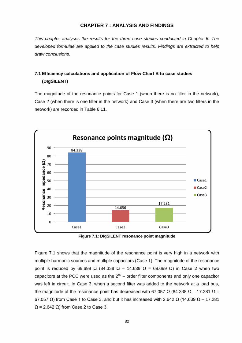
82

CHAPTER 7 : ANALYSIS AND FINDINGS

This chapter analyses the results for the three case studies conducted in Chapter 6. The

developed formulae are applied to the case studies results. Findings are extracted to help

draw conclusions.

7.1 Efficiency calculations and application of Flow Chart B to case studies

(DIgSILENT)

The magnitude of the resonance points for Case 1 (when there is no filter in the network),

Case 2 (when there is one filter in the network) and Case 3 (when there are two filters in the

network) are recorded in Table 6.11.

Figure 7.1: DIgSILENT resonance point magnitude

Figure 7.1 shows that the magnitude of the resonance point is very high in a network with

multiple harmonic sources and multiple capacitors (Case 1). The magnitude of the resonance

point is reduced by 69.699 Ω (84.338 Ω – 14.639 Ω = 69.699 Ω) in Case 2 when two

capacitors at the PCC were used as the 2nd – order filter components and only one capacitor

was left in circuit. In Case 3, when a second filter was added to the network at a load bus,

the magnitude of the resonance point has decreased with 67.057 Ω (84.338 Ω – 17.281 Ω =

67.057 Ω) from Case 1 to Case 3, and but it has increased with 2.642 Ω (14.639 Ω – 17.281

Ω = 2.642 Ω) from Case 2 to Case 3.

0

10

20

30

40

50

60

70

80

90

Case1 Case2 Case3

84.338

14.656 17.281

Reso

nan

ce I

mp

ed

an

ce (

Ω)

Resonance points magnitude (Ω)

Case1

Case2

Case3

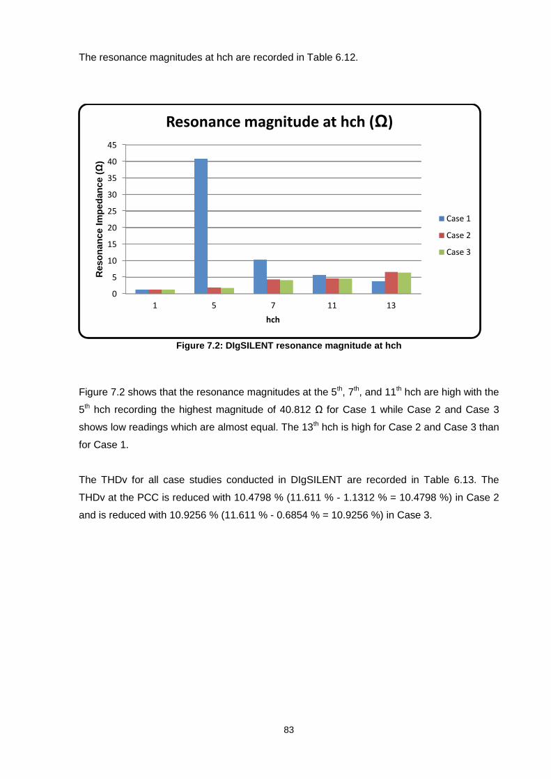
83

The resonance magnitudes at hch are recorded in Table 6.12.

Figure 7.2: DIgSILENT resonance magnitude at hch

Figure 7.2 shows that the resonance magnitudes at the 5th, 7th, and 11th hch are high with the

5th hch recording the highest magnitude of 40.812 Ω for Case 1 while Case 2 and Case 3

shows low readings which are almost equal. The 13th hch is high for Case 2 and Case 3 than

for Case 1.

The THDv for all case studies conducted in DIgSILENT are recorded in Table 6.13. The

THDv at the PCC is reduced with 10.4798 % (11.611 % - 1.1312 % = 10.4798 %) in Case 2

and is reduced with 10.9256 % (11.611 % - 0.6854 % = 10.9256 %) in Case 3.

0

5

10

15

20

25

30

35

40

45

1 5 7 11 13

Reso

nan

ce I

mp

ed

an

ce (

Ω)

hch

Resonance magnitude at hch (Ω)

Case 1

Case 2

Case 3

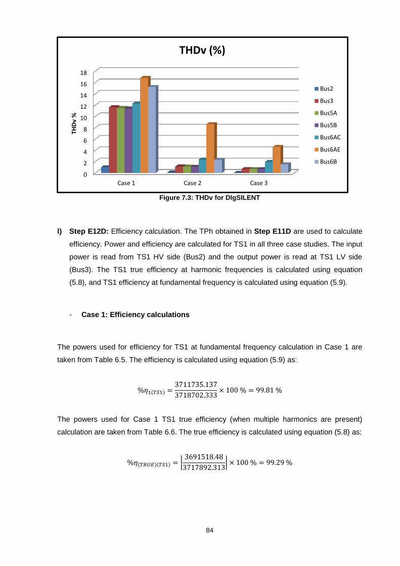
84

Figure 7.3: THDv for DIgSILENT

l) Step E12D: Efficiency calculation. The TPh obtained in Step E11D are used to calculate

efficiency. Power and efficiency are calculated for TS1 in all three case studies. The input

power is read from TS1 HV side (Bus2) and the output power is read at TS1 LV side

(Bus3). The TS1 true efficiency at harmonic frequencies is calculated using equation

(5.8), and TS1 efficiency at fundamental frequency is calculated using equation (5.9).

- Case 1: Efficiency calculations

The powers used for efficiency for TS1 at fundamental frequency calculation in Case 1 are

taken from Table 6.5. The efficiency is calculated using equation (5.9) as:

The powers used for Case 1 TS1 true efficiency (when multiple harmonics are present)

calculation are taken from Table 6.6. The true efficiency is calculated using equation (5.8) as:

|

|

0

2

4

6

8

10

12

14

16

18

Case 1 Case 2 Case 3

THD

v %

THDv (%)

Bus2

Bus3

Bus5A

Bus5B

Bus6AC

Bus6AE

Bus6B

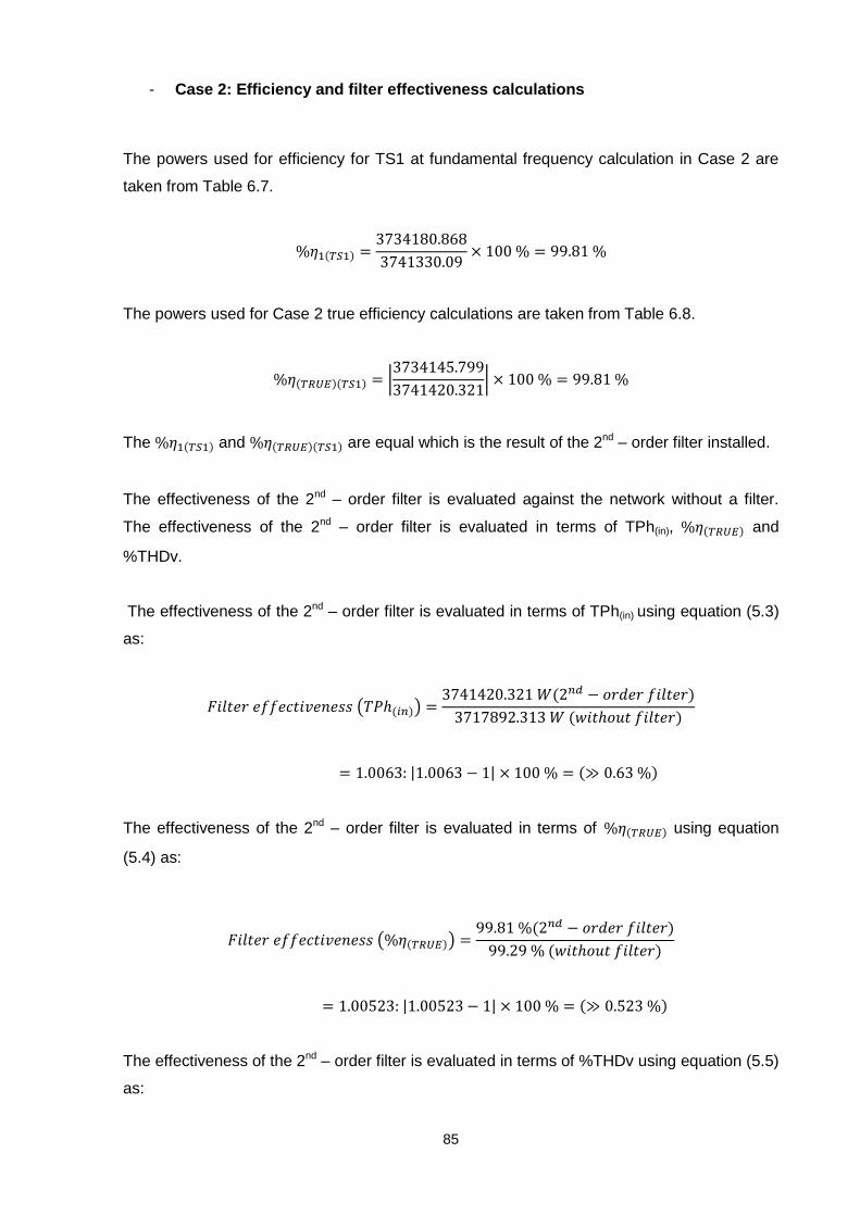
85

- Case 2: Efficiency and filter effectiveness calculations

The powers used for efficiency for TS1 at fundamental frequency calculation in Case 2 are

taken from Table 6.7.

The powers used for Case 2 true efficiency calculations are taken from Table 6.8.

|

|

The and are equal which is the result of the 2nd – order filter installed.

The effectiveness of the 2nd – order filter is evaluated against the network without a filter.

The effectiveness of the 2nd – order filter is evaluated in terms of TPh(in), and

%THDv.

The effectiveness of the 2nd – order filter is evaluated in terms of TPh(in) using equation (5.3)

as:

𝐹 𝑙 𝑒 𝑒 𝑒 𝑒 𝑒 𝑒 𝑙 𝑒

𝑤 𝑙 𝑒

| |

The effectiveness of the 2nd – order filter is evaluated in terms of using equation

(5.4) as:

𝐹 𝑙 𝑒 𝑒 𝑒 𝑒 𝑒 𝑒 𝑙 𝑒

𝑤 𝑙 𝑒

| |

The effectiveness of the 2nd – order filter is evaluated in terms of %THDv using equation (5.5)

as:

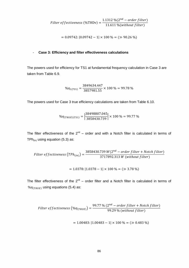
86

𝐹 𝑙 𝑒 𝑒 𝑒 𝑒 𝑒 𝑒 𝑙 𝑒

𝑤 𝑙 𝑒

| |

- Case 3: Efficiency and filter effectiveness calculations

The powers used for efficiency for TS1 at fundamental frequency calculation in Case 3 are

taken from Table 6.9.

The powers used for Case 3 true efficiency calculations are taken from Table 6.10.

|

|

n)

The filter effectiveness of the 2nd – order and with a Notch filter is calculated in terms of

TPh(in) using equation (5.3) as:

𝐹 𝑙 𝑒 𝑒 𝑒 𝑒 𝑒 𝑒 𝑙 𝑒 𝑙 𝑒

𝑤 𝑙 𝑒

| |

The filter effectiveness of the 2nd – order filter and a Notch filter is calculated in terms of

using equations (5.4) as:

𝐹 𝑙 𝑒 𝑒 𝑒 𝑒 𝑒 𝑒 𝑙 𝑒 𝑙 𝑒

𝑤 𝑙 𝑒

| |

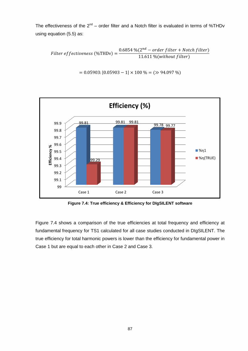
87

The effectiveness of the 2nd – order filter and a Notch filter is evaluated in terms of %THDv

using equation (5.5) as:

𝐹 𝑙 𝑒 𝑒 𝑒 𝑒 𝑒 𝑒 𝑙 𝑒 𝑙 𝑒

𝑤 𝑙 𝑒

| |

Figure 7.4: True efficiency & Efficiency for DIgSILENT software

Figure 7.4 shows a comparison of the true efficiencies at total frequency and efficiency at

fundamental frequency for TS1 calculated for all case studies conducted in DIgSILENT. The

true efficiency for total harmonic powers is lower than the efficiency for fundamental power in

Case 1 but are equal to each other in Case 2 and Case 3.

99

99.1

99.2

99.3

99.4

99.5

99.6

99.7

99.8

99.9

Case 1 Case 2 Case 3

99.81 99.81 99.78

99.29

99.81 99.77

Effi

cie

ncy

%

Efficiency (%)

%η1

%η(TRUE)

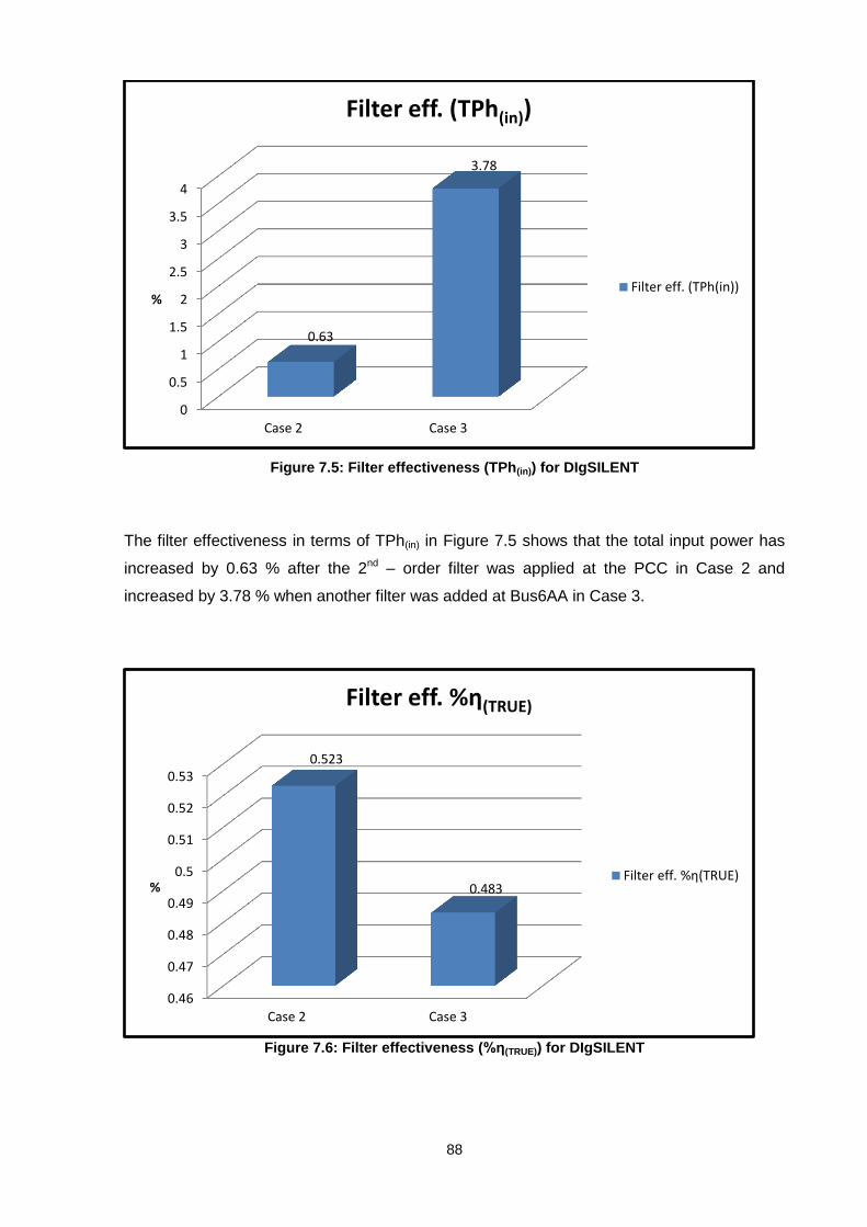
88

Figure 7.5: Filter effectiveness (TPh(in)) for DIgSILENT

The filter effectiveness in terms of TPh(in) in Figure 7.5 shows that the total input power has

increased by 0.63 % after the 2nd – order filter was applied at the PCC in Case 2 and

increased by 3.78 % when another filter was added at Bus6AA in Case 3.

Figure 7.6: Filter effectiveness (%η(TRUE)) for DIgSILENT

0

0.5

1

1.5

2

2.5

3

3.5

4

Case 2 Case 3

0.63

3.78

%

Filter eff. (TPh(in))

Filter eff. (TPh(in))

0.46

0.47

0.48

0.49

0.5

0.51

0.52

0.53

Case 2 Case 3

0.523

0.483 %

Filter eff. %η(TRUE)

Filter eff. %η(TRUE)

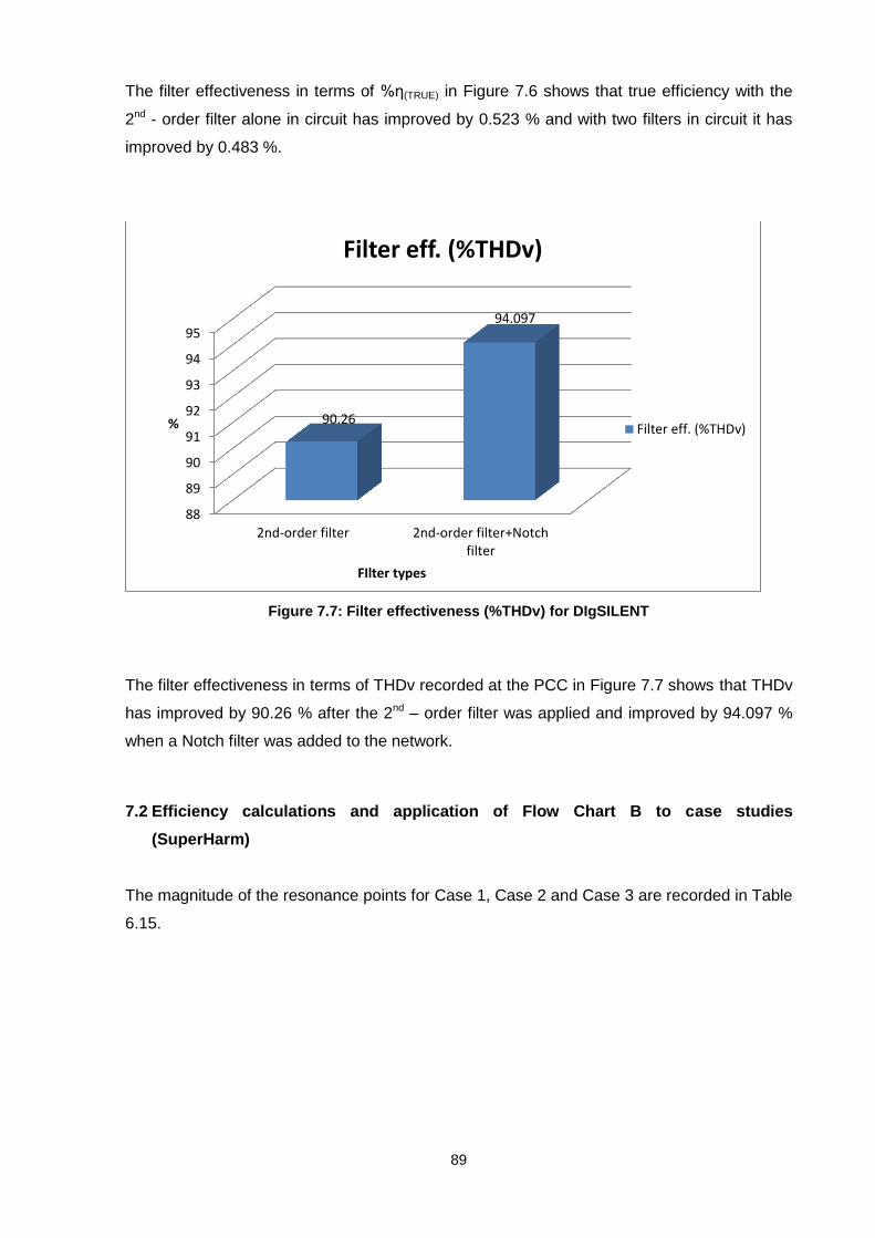
89

The filter effectiveness in terms of %η(TRUE) in Figure 7.6 shows that true efficiency with the

2nd - order filter alone in circuit has improved by 0.523 % and with two filters in circuit it has

improved by 0.483 %.

Figure 7.7: Filter effectiveness (%THDv) for DIgSILENT

The filter effectiveness in terms of THDv recorded at the PCC in Figure 7.7 shows that THDv

has improved by 90.26 % after the 2nd – order filter was applied and improved by 94.097 %

when a Notch filter was added to the network.

7.2 Efficiency calculations and application of Flow Chart B to case studies

(SuperHarm)

The magnitude of the resonance points for Case 1, Case 2 and Case 3 are recorded in Table

6.15.

88

89

90

91

92

93

94

95

2nd-order filter 2nd-order filter+Notchfilter

90.26

94.097

%

FIlter types

Filter eff. (%THDv)

Filter eff. (%THDv)

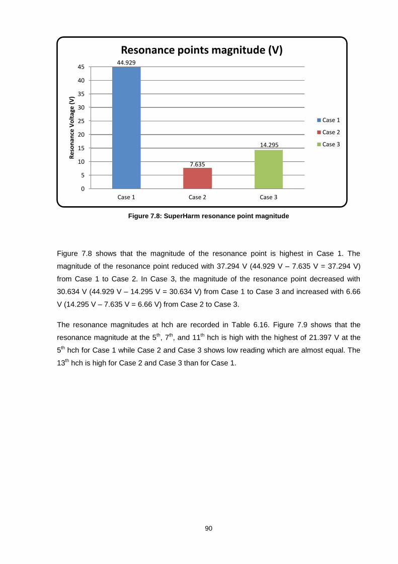
90

Figure 7.8: SuperHarm resonance point magnitude

Figure 7.8 shows that the magnitude of the resonance point is highest in Case 1. The

magnitude of the resonance point reduced with 37.294 V (44.929 V – 7.635 V = 37.294 V)

from Case 1 to Case 2. In Case 3, the magnitude of the resonance point decreased with

30.634 V (44.929 V – 14.295 V = 30.634 V) from Case 1 to Case 3 and increased with 6.66

V (14.295 V – 7.635 V = 6.66 V) from Case 2 to Case 3.

The resonance magnitudes at hch are recorded in Table 6.16. Figure 7.9 shows that the

resonance magnitude at the 5th, 7th, and 11th hch is high with the highest of 21.397 V at the

5th hch for Case 1 while Case 2 and Case 3 shows low reading which are almost equal. The

13th hch is high for Case 2 and Case 3 than for Case 1.

0

5

10

15

20

25

30

35

40

45

Case 1 Case 2 Case 3

44.929

7.635

14.295

Re

son

ance

Vo

ltag

e (

V)

Resonance points magnitude (V)

Case 1

Case 2

Case 3

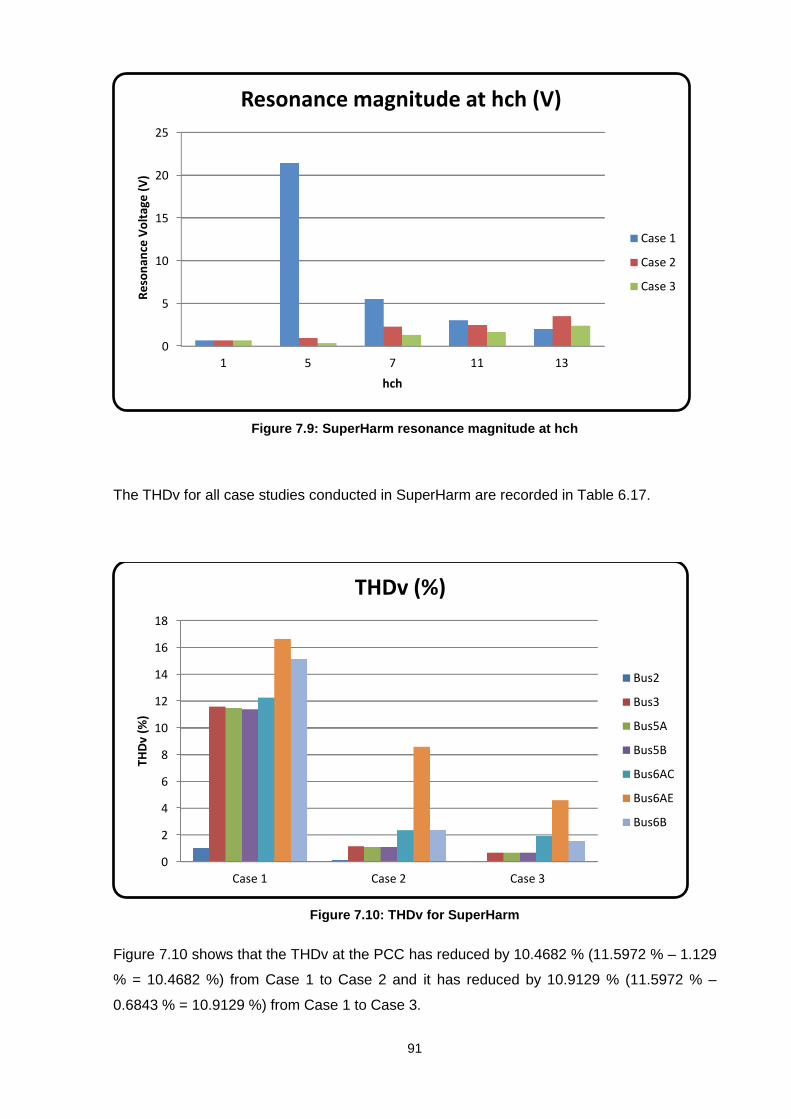
91

Figure 7.9: SuperHarm resonance magnitude at hch

The THDv for all case studies conducted in SuperHarm are recorded in Table 6.17.

Figure 7.10: THDv for SuperHarm

Figure 7.10 shows that the THDv at the PCC has reduced by 10.4682 % (11.5972 % – 1.129

% = 10.4682 %) from Case 1 to Case 2 and it has reduced by 10.9129 % (11.5972 % –

0.6843 % = 10.9129 %) from Case 1 to Case 3.

0

5

10

15

20

25

1 5 7 11 13

Re

son

ance

Vo

ltag

e (

V)

hch

Resonance magnitude at hch (V)

Case 1

Case 2

Case 3

0

2

4

6

8

10

12

14

16

18

Case 1 Case 2 Case 3

THD

v (%

)

THDv (%)

Bus2

Bus3

Bus5A

Bus5B

Bus6AC

Bus6AE

Bus6B

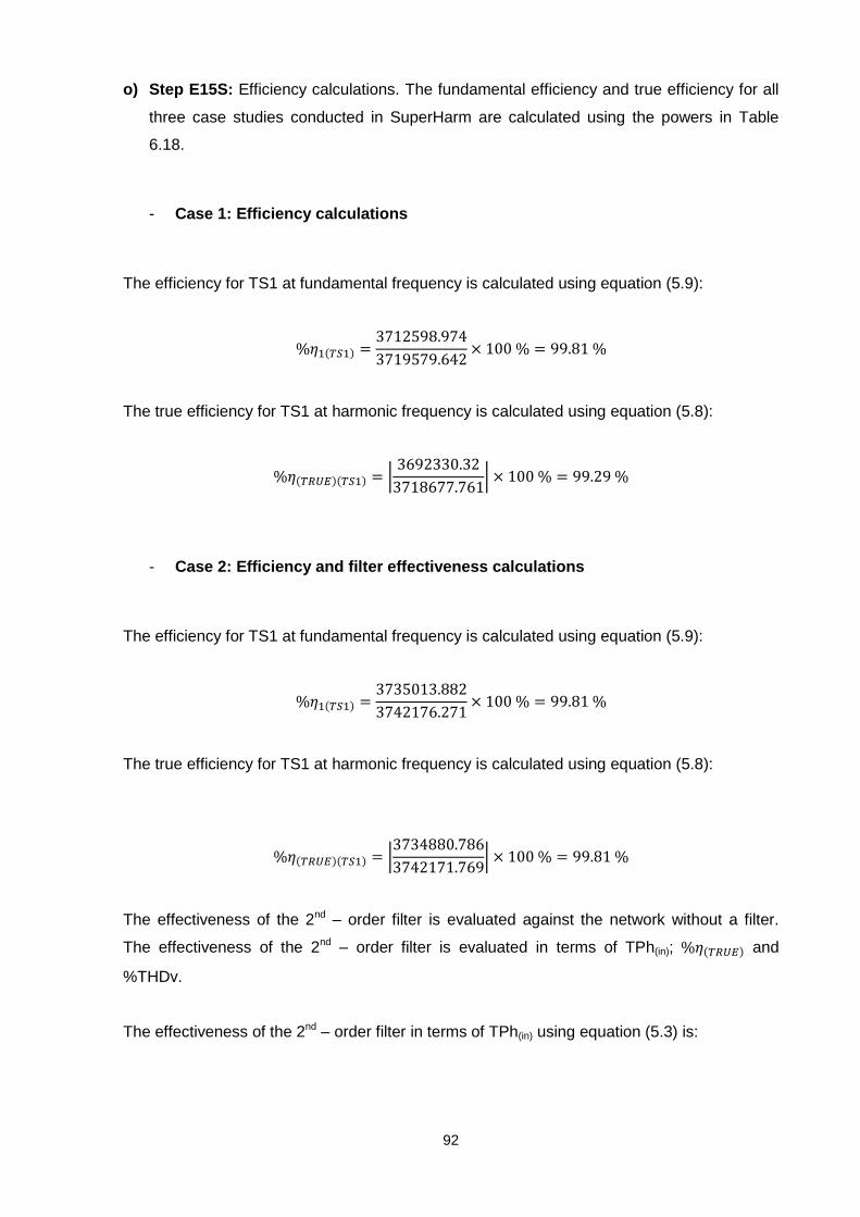
92

o) Step E15S: Efficiency calculations. The fundamental efficiency and true efficiency for all

three case studies conducted in SuperHarm are calculated using the powers in Table

6.18.

- Case 1: Efficiency calculations

The efficiency for TS1 at fundamental frequency is calculated using equation (5.9):

The true efficiency for TS1 at harmonic frequency is calculated using equation (5.8):

|

|

- Case 2: Efficiency and filter effectiveness calculations

The efficiency for TS1 at fundamental frequency is calculated using equation (5.9):

The true efficiency for TS1 at harmonic frequency is calculated using equation (5.8):

|

|

p) F

The effectiveness of the 2nd – order filter is evaluated against the network without a filter.

The effectiveness of the 2nd – order filter is evaluated in terms of TPh(in); and

%THDv.

The effectiveness of the 2nd – order filter in terms of TPh(in) using equation (5.3) is:

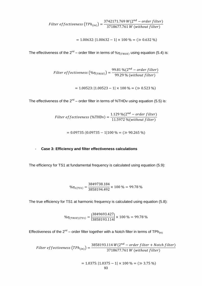
93

𝐹 𝑙 𝑒 𝑒 𝑒 𝑒 𝑒 𝑒 𝑙 𝑒

𝑤 𝑙 𝑒

| |

The effectiveness of the 2nd – order filter in terms of using equation (5.4) is:

𝐹 𝑙 𝑒 𝑒 𝑒 𝑒 𝑒 𝑒 𝑙 𝑒

𝑤 𝑙 𝑒

| |

The effectiveness of the 2nd – order filter in terms of %THDv using equation (5.5) is:

𝐹 𝑙 𝑒 𝑒 𝑒 𝑒 𝑒 𝑒 𝑙 𝑒

𝑤 𝑙 𝑒

| |

- Case 3: Efficiency and filter effectiveness calculations

The efficiency for TS1 at fundamental frequency is calculated using equation (5.9):

The true efficiency for TS1 at harmonic frequency is calculated using equation (5.8):

|

|

Effectiveness of the 2nd – order filter together with a Notch filter in terms of TPh(in):

𝐹 𝑙 𝑒 𝑒 𝑒 𝑒 𝑒 𝑒 𝑙 𝑒 𝑙 𝑒

𝑤 𝑙 𝑒

| |

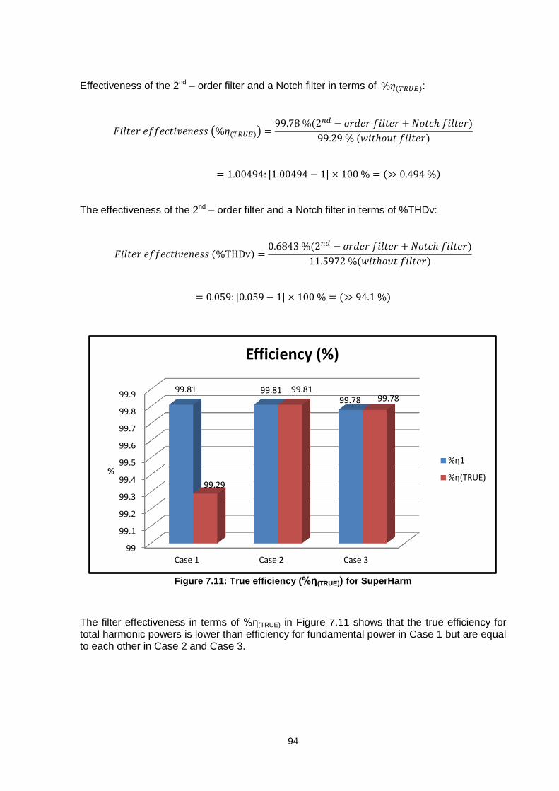
94

Effectiveness of the 2nd – order filter and a Notch filter in terms of :

𝐹 𝑙 𝑒 𝑒 𝑒 𝑒 𝑒 𝑒 𝑙 𝑒 𝑙 𝑒

𝑤 𝑙 𝑒

| |

The effectiveness of the 2nd – order filter and a Notch filter in terms of %THDv:

𝐹 𝑙 𝑒 𝑒 𝑒 𝑒 𝑒 𝑒 𝑙 𝑒 𝑙 𝑒

𝑤 𝑙 𝑒

| |

Figure 7.11: True efficiency (%η(TRUE)) for SuperHarm

The filter effectiveness in terms of %η(TRUE) in Figure 7.11 shows that the true efficiency for total harmonic powers is lower than efficiency for fundamental power in Case 1 but are equal to each other in Case 2 and Case 3.

99

99.1

99.2

99.3

99.4

99.5

99.6

99.7

99.8

99.9

Case 1 Case 2 Case 3

99.81 99.81 99.78

99.29

99.81 99.78

%

Efficiency (%)

%η1

%η(TRUE)

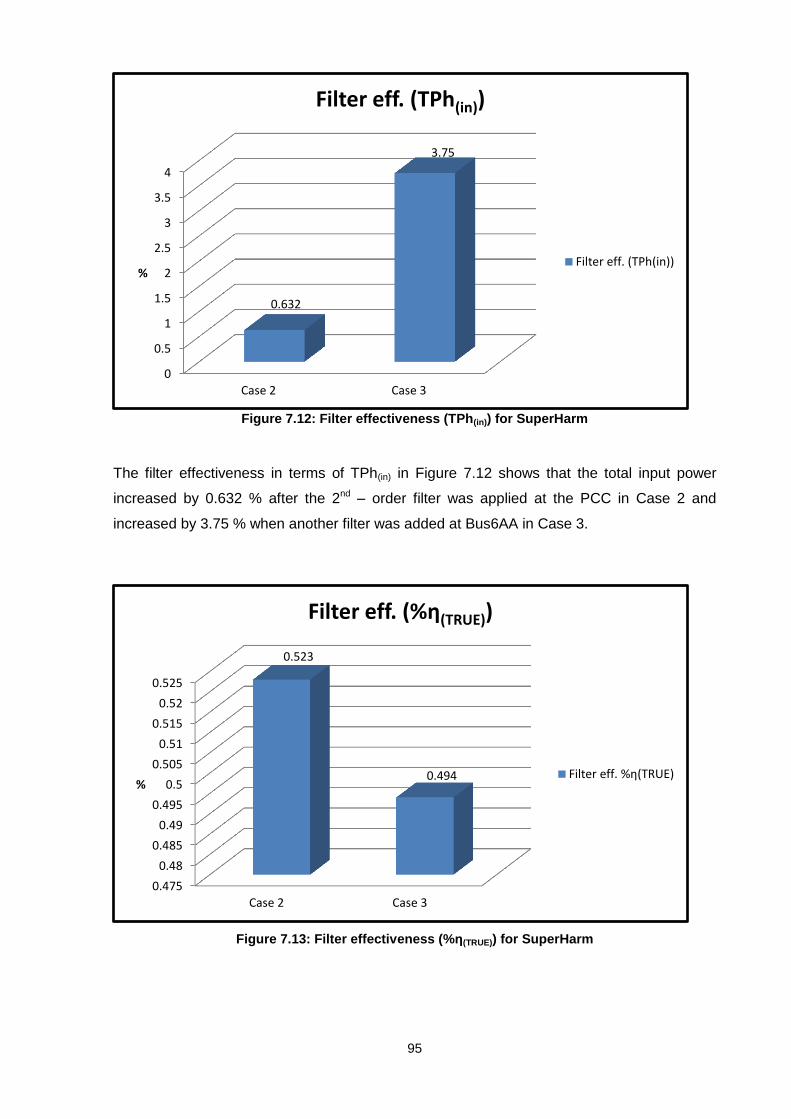
95

Figure 7.12: Filter effectiveness (TPh(in)) for SuperHarm

The filter effectiveness in terms of TPh(in) in Figure 7.12 shows that the total input power

increased by 0.632 % after the 2nd – order filter was applied at the PCC in Case 2 and

increased by 3.75 % when another filter was added at Bus6AA in Case 3.

Figure 7.13: Filter effectiveness (%η(TRUE)) for SuperHarm

0

0.5

1

1.5

2

2.5

3

3.5

4

Case 2 Case 3

0.632

3.75

%

Filter eff. (TPh(in))

Filter eff. (TPh(in))

0.475

0.48

0.485

0.49

0.495

0.5

0.505

0.51

0.515

0.52

0.525

Case 2 Case 3

0.523

0.494 %

Filter eff. (%η(TRUE))

Filter eff. %η(TRUE)

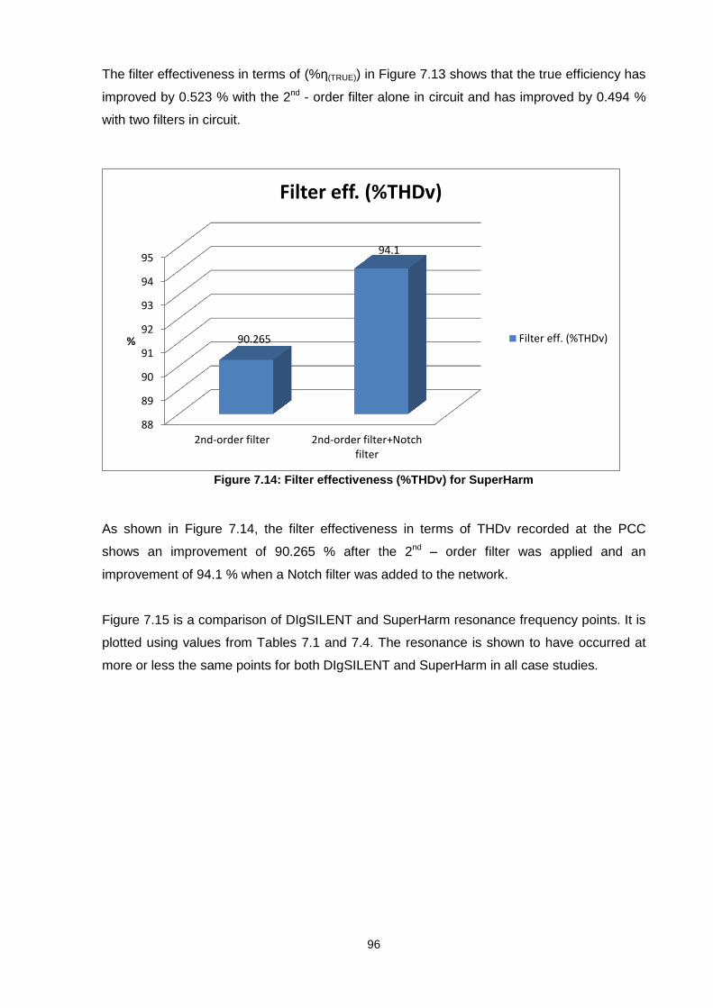
96

The filter effectiveness in terms of (%η(TRUE)) in Figure 7.13 shows that the true efficiency has

improved by 0.523 % with the 2nd - order filter alone in circuit and has improved by 0.494 %

with two filters in circuit.

Figure 7.14: Filter effectiveness (%THDv) for SuperHarm

As shown in Figure 7.14, the filter effectiveness in terms of THDv recorded at the PCC

shows an improvement of 90.265 % after the 2nd – order filter was applied and an

improvement of 94.1 % when a Notch filter was added to the network.

Figure 7.15 is a comparison of DIgSILENT and SuperHarm resonance frequency points. It is

plotted using values from Tables 7.1 and 7.4. The resonance is shown to have occurred at

more or less the same points for both DIgSILENT and SuperHarm in all case studies.

88

89

90

91

92

93

94

95

2nd-order filter 2nd-order filter+Notchfilter

90.265

94.1

%

Filter eff. (%THDv)

Filter eff. (%THDv)

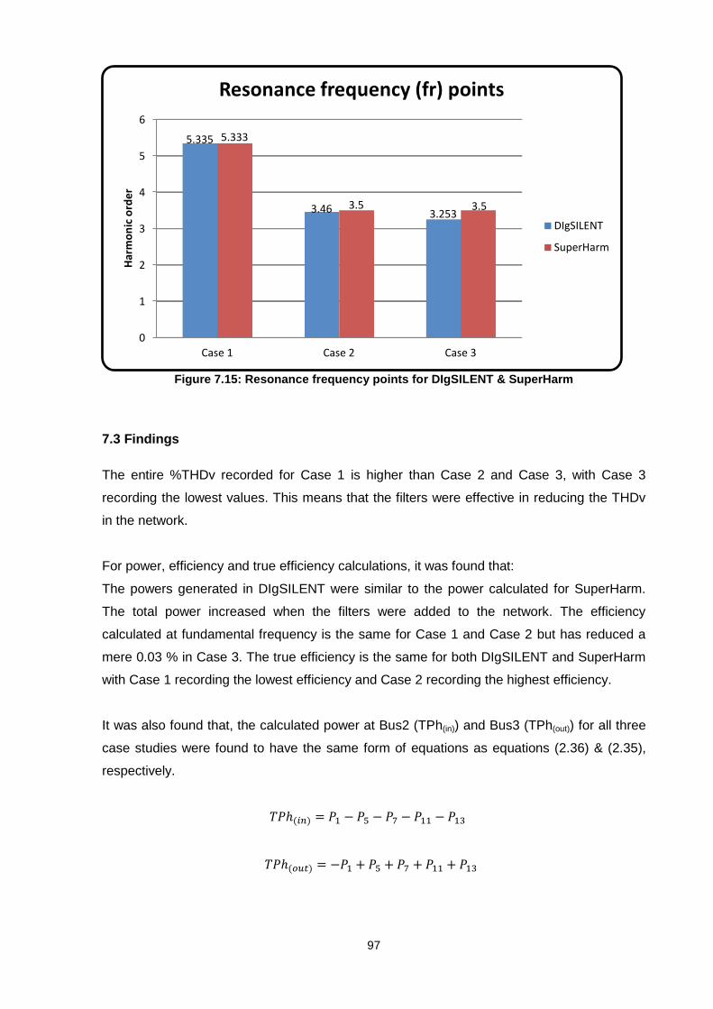
97

Figure 7.15: Resonance frequency points for DIgSILENT & SuperHarm

7.3 Findings

The entire %THDv recorded for Case 1 is higher than Case 2 and Case 3, with Case 3

recording the lowest values. This means that the filters were effective in reducing the THDv

in the network.

For power, efficiency and true efficiency calculations, it was found that:

The powers generated in DIgSILENT were similar to the power calculated for SuperHarm.

The total power increased when the filters were added to the network. The efficiency

calculated at fundamental frequency is the same for Case 1 and Case 2 but has reduced a

mere 0.03 % in Case 3. The true efficiency is the same for both DIgSILENT and SuperHarm

with Case 1 recording the lowest efficiency and Case 2 recording the highest efficiency.

It was also found that, the calculated power at Bus2 (TPh(in)) and Bus3 (TPh(out)) for all three

case studies were found to have the same form of equations as equations (2.36) & (2.35),

respectively.

0

1

2

3

4

5

6

Case 1 Case 2 Case 3

5.335

3.46 3.253

5.333

3.5 3.5

Har

mo

nic

ord

er

Resonance frequency (fr) points

DIgSILENT

SuperHarm

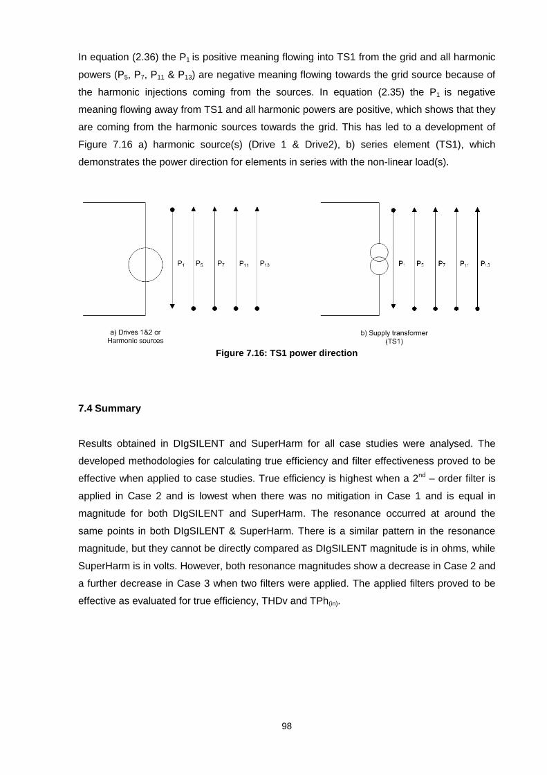
98

In equation (2.36) the P1 is positive meaning flowing into TS1 from the grid and all harmonic

powers (P5, P7, P11 & P13) are negative meaning flowing towards the grid source because of

the harmonic injections coming from the sources. In equation (2.35) the P1 is negative

meaning flowing away from TS1 and all harmonic powers are positive, which shows that they

are coming from the harmonic sources towards the grid. This has led to a development of

Figure 7.16 a) harmonic source(s) (Drive 1 & Drive2), b) series element (TS1), which

demonstrates the power direction for elements in series with the non-linear load(s).

Figure 7.16: TS1 power direction

7.4 Summary

Results obtained in DIgSILENT and SuperHarm for all case studies were analysed. The

developed methodologies for calculating true efficiency and filter effectiveness proved to be

effective when applied to case studies. True efficiency is highest when a 2nd – order filter is

applied in Case 2 and is lowest when there was no mitigation in Case 1 and is equal in

magnitude for both DIgSILENT and SuperHarm. The resonance occurred at around the

same points in both DIgSILENT & SuperHarm. There is a similar pattern in the resonance

magnitude, but they cannot be directly compared as DIgSILENT magnitude is in ohms, while

SuperHarm is in volts. However, both resonance magnitudes show a decrease in Case 2 and

a further decrease in Case 3 when two filters were applied. The applied filters proved to be

effective as evaluated for true efficiency, THDv and TPh(in).

99

CHAPTER 8 : CONCLUSIONS AND FUTURE WORK

8.1 Conclusions

Traditional efficiency formula applies to sinusoidal networks and not to non-sinusoidal

networks. But sinusoidal networks are almost impossible to find in this era with a large

number of power electronic devices connected onto power systems. There is thus a need to

develop formulae for calculating efficiency, powers and power directions in non-sinusoidal

networks.

A step-by-step approach was used to develop flow chart methodologies that can be used by

utility operators and planners as well as customers to calculate true efficiency using software

tools. It was found that by using DIgSILENT and SuperHarm, true efficiency as well as

power flow directions can be determined under distorted conditions.

The developed methodologies, in the form of flow charts, which are the unique contributions

to the studying of power and efficiency calculations under distorted conditions have been

shown to be effective and are/is recommended for use in the industry and academia. The

methodologies can be easily adapted so that they can be applied to any network with any

number of harmonic sources. The two new indices, „True Efficiency‟ and „Filter Effectiveness‟

are introduced and shown to be helpful in determining efficiency in networks with harmonic

distortions and evaluating the effectiveness of filters.

Three case studies were conducted to apply and evaluate the effectiveness of the

methodologies: Case 1 considered a network with two harmonic sources, Case 2 considered

Case 1 with a 2nd –order filter installed at Bus3; and the third case considered Case 2 with a

Notch filter added at Bus6AA. The developed steps for each software tool were applied to all

the case studies. All case studies were modelled and simulated in DIgSILENT and

SuperHarm, the harmonic analyses were conducted to obtain powers, currents and voltages

used to determine efficiency and indices for effectiveness of filter(s).

For Case 1, it was found that, the resonances are severe at the PCC and all the load buses.

The resonance also occurred at the same points (close to the 5th hch) for both DIgSILENT

and SuperHarm. Both DIgSILENT and SuperHarm recorded the same THDv.

For Case 2, it was found that, the resonance magnitude reduced and the resonance points

also shifted away from the 5th harmonic when the 2nd – order filter was applied at the PCC.

100

THDv reduced at the PCC and most load buses except for Bus6AA where Drive1 is

connected.

For Case 3, it was found that, the entire network is clear of harmonic risks. This is because

all the buses THDv is within the limit and the resonance are not near any hch.

It was found that the DIgSILENT approach is shorter than the SuperHarm approach to

determine true efficiency. The true efficiencies calculated for each case study are the same

for both DIgSILENT and SuperHarm. The 2nd – order filter offered mitigation for THDv at

almost all buses in the network except for Bus6AA where Drive1 is connected. After an

additional filter was added at Bus6AA, the THDv at all the buses in the network reduced to

within acceptable limits. The resonance point frequency has shifted away from the

characteristic harmonics, particularly 5th where it was closer to in Case 1. The ZScan graph

has flattened further with every filter installed. The methodologies shown are effective for

investigating networks containing multiple capacitors and multiple harmonic sources.

Several specific conclusions can be drawn from the studies as follows:

a) When a filter is installed at the PCC, THDv decreased to below the set limit. This means

that the mitigation measure applied is effective. A filter is a solution for when the

resonance is severe (close to or at hch) and when THDv is above the specified limit.

b) DIgSILENT can directly calculate powers but SuperHarm cannot. The powers obtained in

DIgSILENT can be used directly to calculate true efficiency. For SuperHarm, however,

the individual powers (Ph) need to be calculated first using the generated voltages and

currents, then the total powers (TPh) must be calculated using the calculated Ph and only

then can the true efficiency be calculated using TPh. Figures 5.2 & 5.3 are flow diagrams

that illustrate the developed steps of how power and true efficiency as well as the

effectiveness of filter(s) can be determined from SuperHarm and DIgSILENT results. So

in summary, DIgSILENT calculates true efficiency in 12 steps while SuperHarm

calculates true efficiency in 15 steps.

c) All waveforms obtained in SuperHarm and DIgSILENT are the same. The voltage

waveforms at Bus3 in Figures 6.3 & 6.1 recorded for Case 1 became smoother

waveforms after the 2nd – order filter was applied as shown in Figures 6.8 & 6.19

recorded for Case 2. Similarly for the current waveforms in Figures 6.9 & 6.20 for Case 2

shows fewer distortions compared to Figures 6.4 & 6.16 for Case 1.

d) SuperHarm plots ZScan in terms of resonance frequency (fr) against resonance voltage

(Vr) whereas DIgSILENT plots ZScan in terms of resonance frequency (fr) against

resonance impedance (Zr).

101

e) The hand calculated THDv and the THDv generated by both DIgSILENT and SuperHarm

are the same, meaning that both DIgSILENT & SuperHarm approve of equation (2.28).

f) The resonance magnitude shows a decrease at hch in both DIgSILENT & SuperHarm.

g) The total input power for TS1 increased after filters were applied in Case 2 and Case 3.

THDv decreased and true efficiency increased when the filter(s) were applied to the

network proving the filter(s) to be effective.

h) Harmonic powers are positive and moves upstream from the harmonic source toward the

system source for elements in series with the harmonic source(s), and are negative and

moves downstream from the harmonic source for elements in shunt with the harmonic

source(s).

8.2 Future work

a. A network working at different loading percentages (e.g. 25 %, 50 %, 75 %, etc.) needs to

be studied as most networks do not normally operate at full load.

b. The effectiveness of additional types of filters needs to be investigated in terms of their

impact on efficiency.

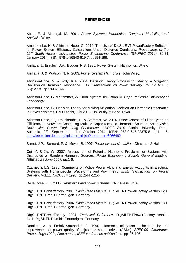
102

REFERENCES

Acha, E. & Madrigal, M. 2001. Power Systems Harmonics: Computer Modelling and Analysis. Wiley. Amushembe, H. & Atkinson-Hope, G. 2014. The Use of DIgSILENT PowerFactory Software for Power System Efficiency Calculations Under Distorted Conditions. Proceedings of the 22nd South African Universities Power Engineering Conference (SAUPEC 2014), 30-31 January 2014, ISBN: 978-1-86840-619-7. pp194-199. Arrilaga, J., Bradley, D.A., Bodger, P.S. 1985. Power System Harmonics. Wiley. Arrillaga, J. & Watson, N. R. 2003. Power System Harmonics. John Wiley. Atkinson-Hope, G. & Folly, K.A. 2004. Decision Theory Process for Making a Mitigation Decision on Harmonic Resonance. IEEE Transactions on Power Delivery, Vol. 19, NO. 3, July 2004. pp 1393-1399. Atkinson-Hope, G. & Stemmet, W. 2008. System simulation IV. Cape Peninsula University of Technology.

Atkinson-Hope, G. Decision Theory for Making Mitigation Decision on Harmonic Resonance in Power Systems, PhD Thesis, July 2003. University of Cape Town. Atkinson-Hope, G., Amushembe, H. & Stemmet, W. 2014. Effectiveness of Filter Types on Efficiency in Networks Containing Multiple Capacitors and Harmonic Sources. Australasian Universities Power Engineering Conference, AUPEC 2014, Curtin University, Perth, Australia, 28th September – 1st October 2014. ISBN: 978-0-646-92375-8, pp1 - 6. http://ieeexplore.ieee.org/xpls/abs_all.jsp?arnumber=6966492 Barret, J.P., Bornard, P. & Meyer, B. 1997. Power system simulation. Chapman & Hall. Cui, Y. & Xu, W. 2007. Assessment of Potential Harmonic Problems for Systems with Distributed or Random Harmonic Sources. Power Engineering Society General Meeting. IEEE 24-28 June 2007. pp.1-6. Czarnecki, L.S. 1996. Comments on Active Power Flow and Energy Accounts in Electrical Systems with Nonsinusoidal Waveforms and Asymmetry. IEEE Transactions on Power Delivery. Vol.11. No.3. July 1996. pp1244 -1250. De la Rosa, F.C. 2006. Harmonics and power systems. CRC Press. USA. DIgSILENTPowerfactory. 2001. Basic User’s Manual. DIgSILENTPowerFactory version 12.1. DIgSILENT GmbH Gormarigen. Germany. DIgSILENTPowerfactory. 2004. Basic User’s Manual. DIgSILENTPowerFactory version 13.1. DIgSILENT GmbH Gormarigen. Germany. DIgSILENTPowerFactory. 2004. Technical Reference. DIgSILENTPowerFactory version 14.1. DIgSILENT GmbH Gormarigen. Germany.

Domijan, A. & Embriz-Santander, E. 1990. Harmonic mitigation techniques for the improvement of power quality of adjustable speed drives (ASDs). APEC’90, Conference Proceedings 1990., Fifth annual, IEEE conference publications. pp. 96-105.

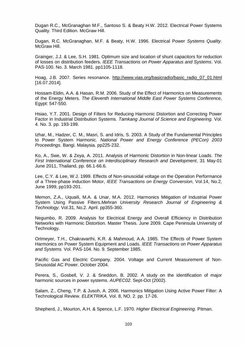
103

Dugan R.C., McGranaghan M.F., Santoso S. & Beaty H.W. 2012. Electrical Power Systems Quality. Third Edition. McGraw Hill. Dugan, R.C. McGranaghan, M.F. & Beaty, H.W. 1996. Electrical Power Systems Quality. McGraw Hill. Grainger, J.J. & Lee, S.H. 1981. Optimum size and location of shunt capacitors for reduction of losses on distribution feeders. IEEE Transactions on Power Apparatus and Systems. Vol. PAS-100. No. 3. March 1981. pp1105-1118. Hoag, J.B. 2007. Series resonance. http://www.vias.org/basicradio/basic_radio_07_01.html [16.07.2014]. Hossam-Eldin, A.A. & Hasan, R.M. 2006. Study of the Effect of Harmonics on Measurements of the Energy Meters. The Eleventh International Middle East Power Systems Conference, Egypt: 547-550. Hsiao, Y.T. 2001. Design of Filters for Reducing Harmonic Distortion and Correcting Power Factor in Industrial Distribution Systems. Tamkang Journal of Science and Engineering. Vol. 4. No. 3. pp. 193-199. Izhar, M., Hadzer, C. M., Masri, S. and Idris, S. 2003. A Study of the Fundamental Principles to Power System Harmonic. National Power and Energy Conference (PECon) 2003 Proceedings. Bangi. Malaysia. pp225-232. Ko, A., Swe, W. & Zeya, A. 2011. Analysis of Harmonic Distortion in Non-linear Loads. The First International Conference on Interdisciplinary Research and Development, 31 May-01 June 2011, Thailand, pp. 66.1-66.6. Lee, C.Y. & Lee, W.J. 1999. Effects of Non-sinusoidal voltage on the Operation Performance of a Three-phase induction Motor, IEEE Transactions on Energy Conversion, Vol.14, No.2, June 1999, pp193-201. Memon, Z.A., Uquaili, M.A. & Unar, M.A. 2012. Harmonics Mitigation of Industrial Power System Using Passive Filters.Mehran University Research Journal of Engineering & Technology. Vol.31, No.2. April. pp355-360. Negumbo, R. 2009. Analysis for Electrical Energy and Overall Efficiency in Distribution Networks with Harmonic Distortion. Master Thesis. June 2009. Cape Peninsula University of Technology. Ortmeyer, T.H., Chakravarthi, K.R. & Mahmoud, A.A. 1985. The Effects of Power System Harmonics on Power System Equipment and Loads. IEEE Transactions on Power Apparatus and Systems. Vol. PAS-104. No. 9. September 1985. Pacific Gas and Electric Company. 2004. Voltage and Current Measurement of Non-Sinusoidal AC Power. October 2004. Perera, S., Gosbell, V. J. & Sneddon, B. 2002. A study on the identification of major harmonic sources in power systems. AUPEC02. Sept-Oct (2002). Salam, Z., Cheng, T.P. & Jusoh, A. 2006. Harmonics Mitigation Using Active Power Filter: A

Technological Review. ELEKTRIKA. Vol. 8, NO. 2. pp. 17‐26.

Shepherd, J., Mourton, A.H. & Spence, L.F. 1970. Higher Electrical Engineering. Pitman.

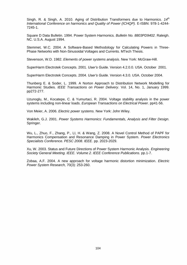
104

Singh, R. & Singh, A. 2010. Aging of Distribution Transformers due to Harmonics. 14th International Conference on harmonics and Quality of Power (ICHQP). E-ISBN: 978-1-4244-7245-1. Square D Data Bulletin. 1994. Power System Harmonics. Bulletin No. 8803PD9402. Raleigh. NC. U.S.A. August 1994. Stemmet, W.C. 2004. A Software-Based Methodology for Calculating Powers in Three-Phase Networks with Non-Sinusoidal Voltages and Currents. MTech Thesis. Stevenson, W.D. 1982. Elements of power systems analysis. New York: McGraw-Hill. SuperHarm Electrotek Concepts. 2001. User’s Guide. Version 4.2.0.0. USA. October 2001. SuperHarm Electrotek Concepts. 2004. User’s Guide. Version 4.3.0. USA. October 2004. Thunberg E. & Soder, L. 1999. A Norton Approach to Distribution Network Modelling for Harmonic Studies. IEEE Transactions on Power Delivery. Vol. 14, No. 1, January 1999. pp272-277. Uzunoglu, M., Kocatepe, C. & Yumurtaci, R. 2004. Voltage stability analysis in the power systems including non-linear loads. European Transactions on Electrical Power. pp41-56. Von Meier, A. 2006. Electric power systems. New York: John Wiley. Wakileh, G.J. 2001. Power Systems Harmonics: Fundamentals, Analysis and Filter Design. Springer.

Wu, L., Zhuo, F., Zhang, P., LI, H. & Wang, Z. 2008. A Novel Control Method of PAPF for Harmonics Compensation and Resonance Damping in Power System. Power Electronics Specialists Conference. PESC 2008. IEEE. pp. 2023-2029. Xu, W. 2003. Status and Future Directions of Power System Harmonic Analysis. Engineering Society General Meeting. IEEE. Volume 2. IEEE Conference Publications. pp.1-7. Zobaa, A.F. 2004. A new approach for voltage harmonic distortion minimization. Electric Power System Research, 70(3): 253-260.

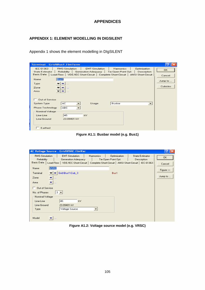
105

APPENDICES

APPENDIX 1: ELEMENT MODELLING IN DIGSILENT

Appendix 1 shows the element modelling in DIgSILENT

Figure A1.1: Busbar model (e.g. Bus1)

Figure A1.2: Voltage source model (e.g. VRSC)

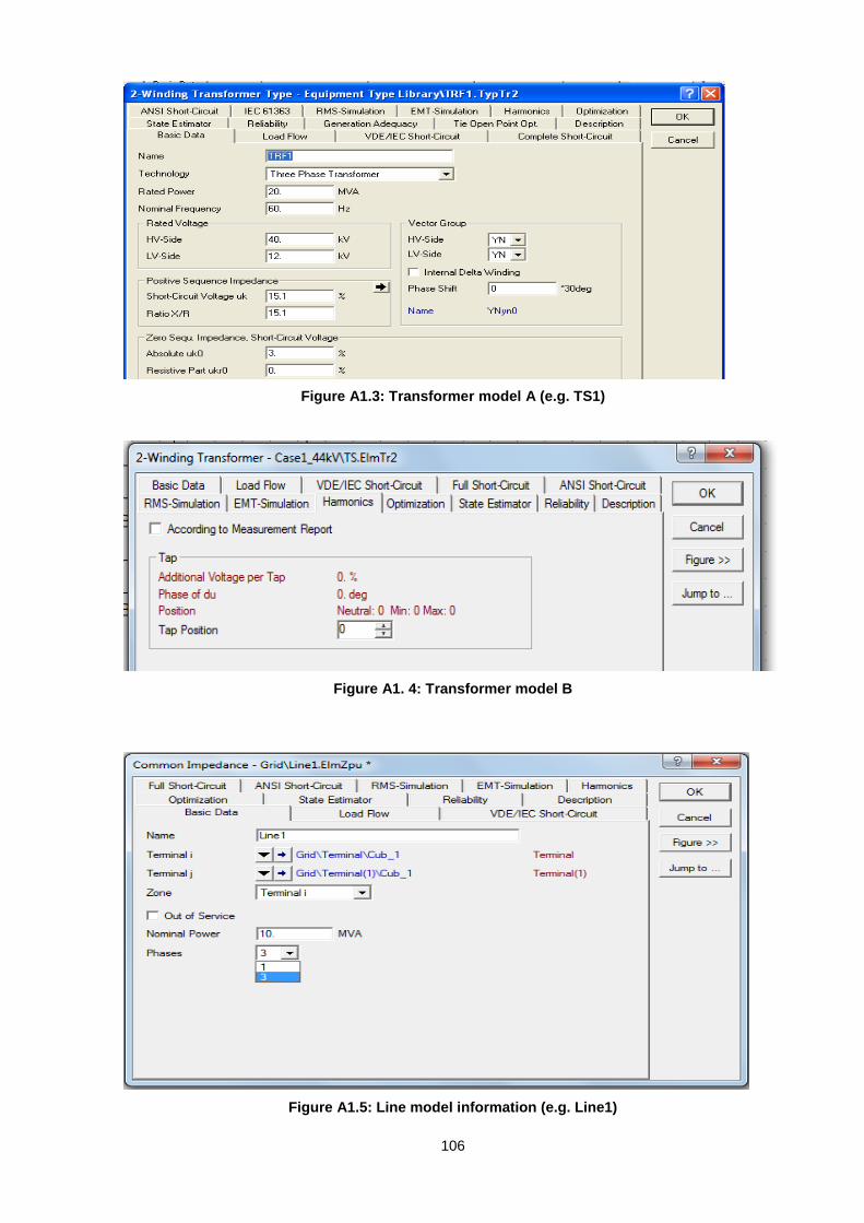
106

Figure A1.3: Transformer model A (e.g. TS1)

Figure A1. 4: Transformer model B

Figure A1.5: Line model information (e.g. Line1)

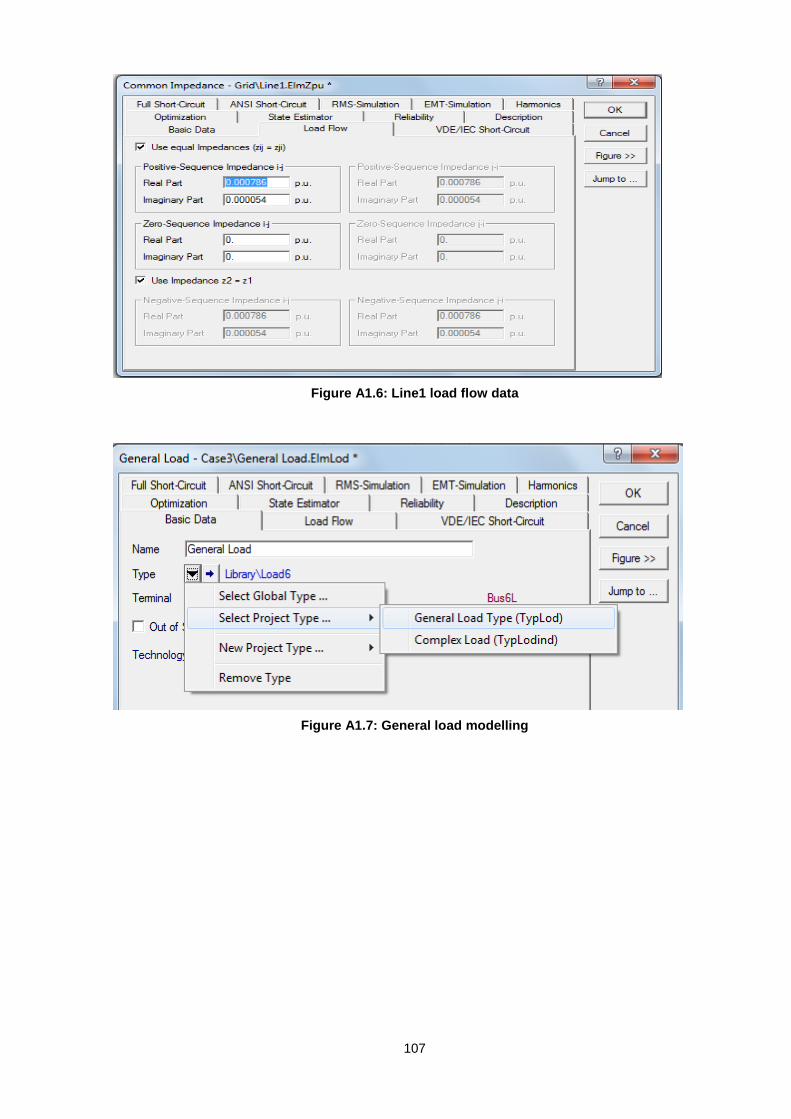
107

Figure A1.6: Line1 load flow data

Figure A1.7: General load modelling

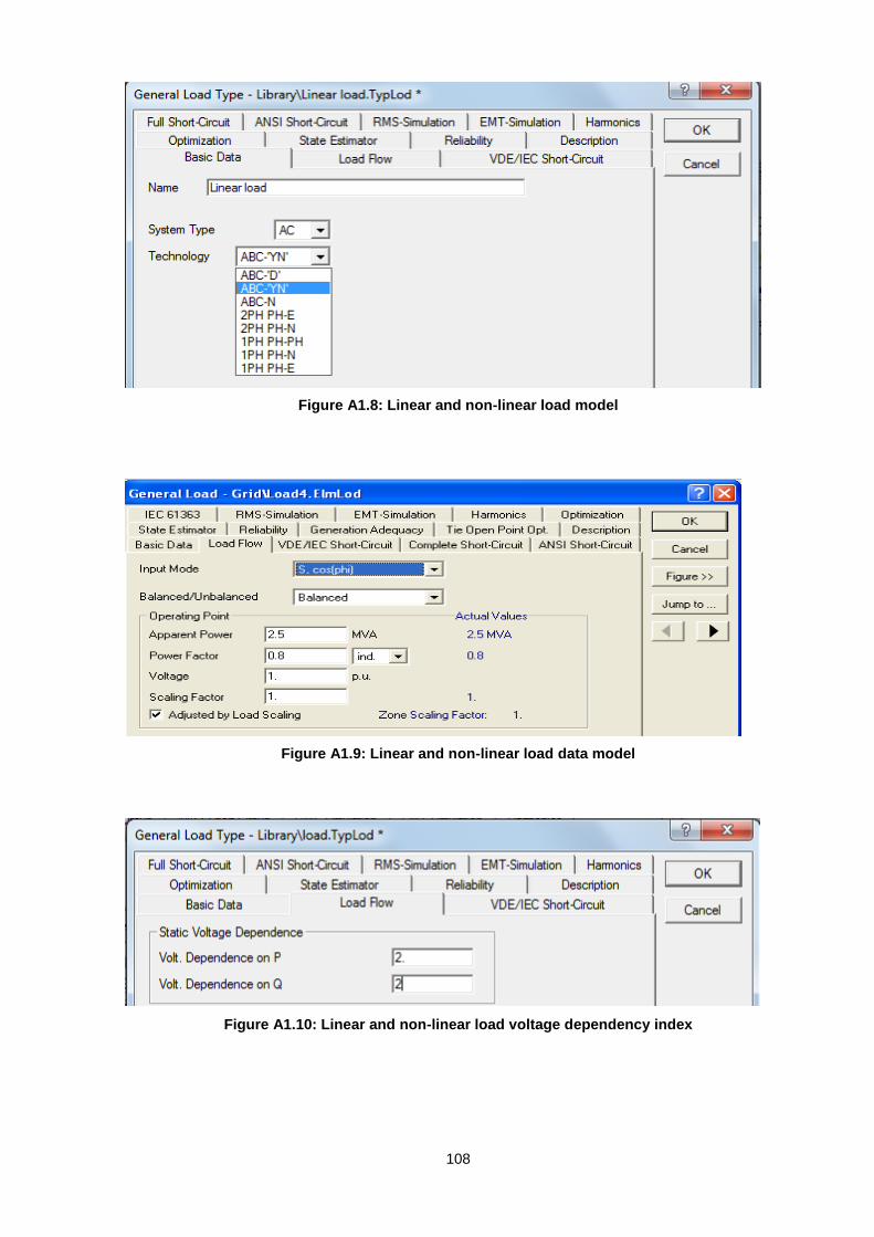
108

Figure A1.8: Linear and non-linear load model

Figure A1.9: Linear and non-linear load data model

Figure A1.10: Linear and non-linear load voltage dependency index

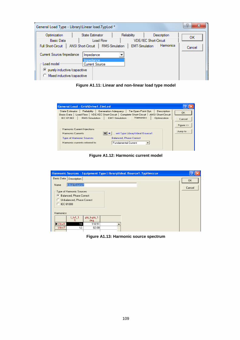
109

Figure A1.11: Linear and non-linear load type model

Figure A1.12: Harmonic current model

Figure A1.13: Harmonic source spectrum

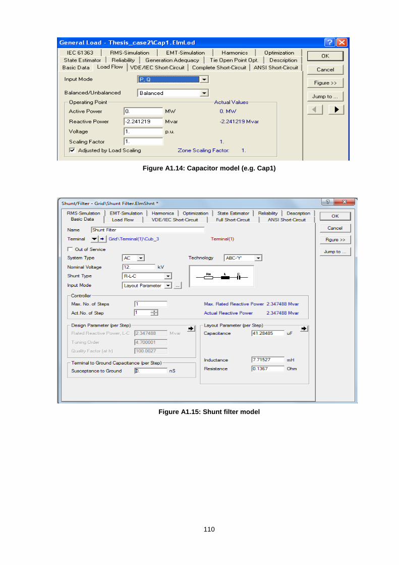
110

Figure A1.14: Capacitor model (e.g. Cap1)

Figure A1.15: Shunt filter model

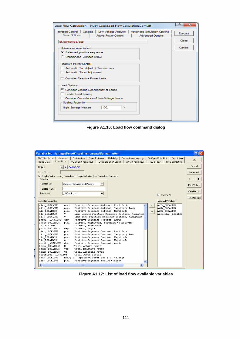
111

Figure A1.16: Load flow command dialog

Figure A1.17: List of load flow available variables

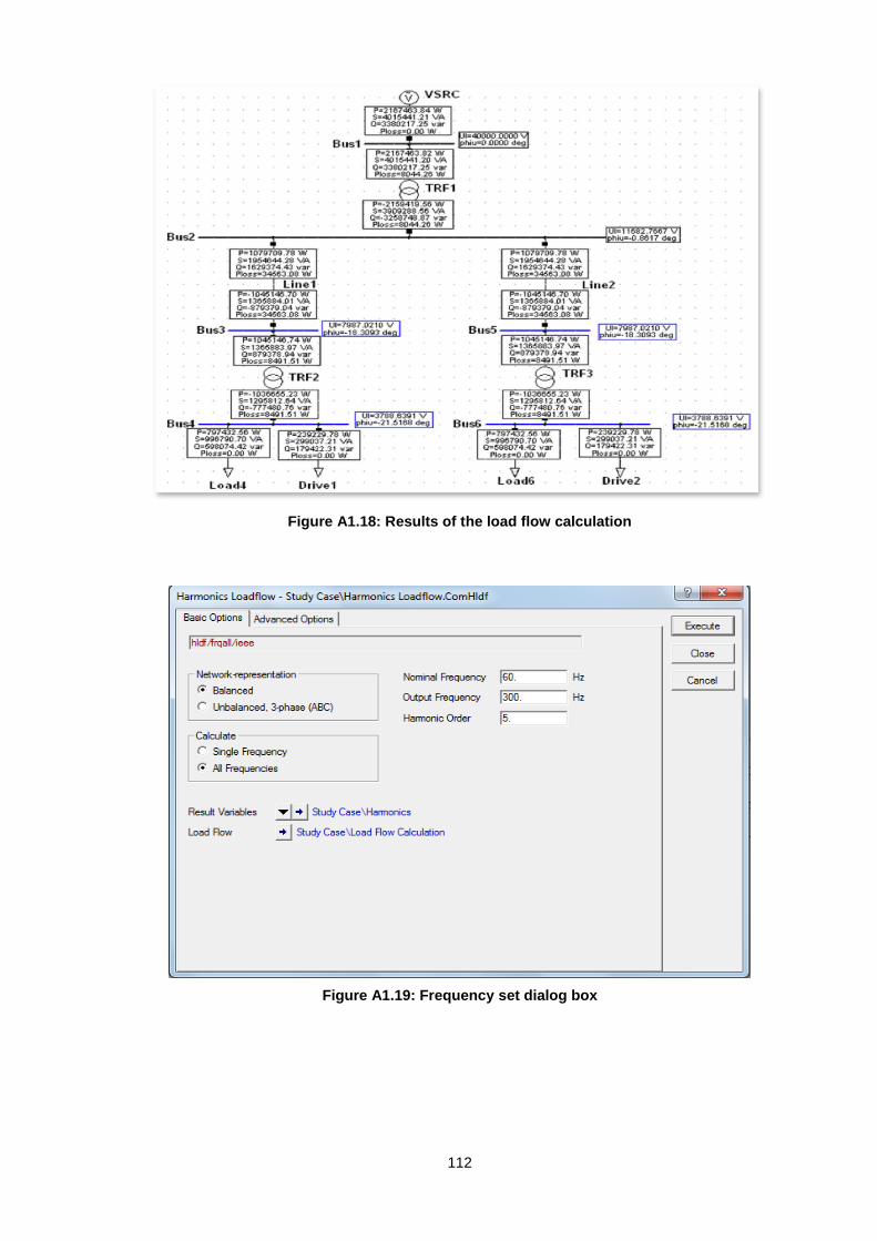
112

Figure A1.18: Results of the load flow calculation

Figure A1.19: Frequency set dialog box

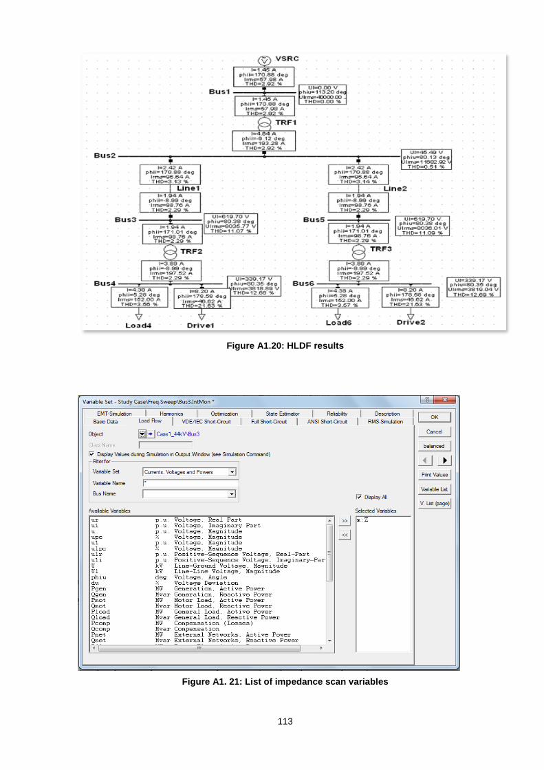
113

Figure A1.20: HLDF results

Figure A1. 21: List of impedance scan variables

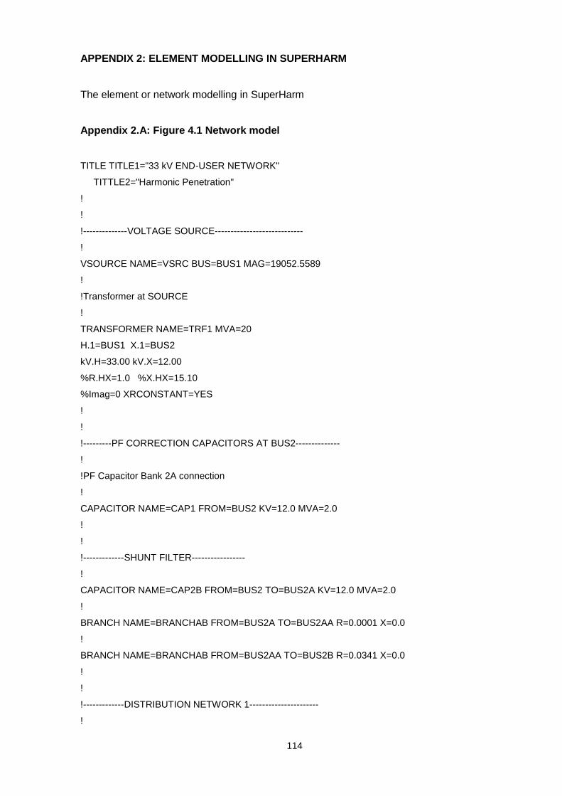
114

APPENDIX 2: ELEMENT MODELLING IN SUPERHARM

The element or network modelling in SuperHarm

Appendix 2.A: Figure 4.1 Network model

TITLE TITLE1="33 kV END-USER NETWORK"

TITTLE2="Harmonic Penetration"

!

!

!--------------VOLTAGE SOURCE----------------------------

!

VSOURCE NAME=VSRC BUS=BUS1 MAG=19052.5589

!

!Transformer at SOURCE

!

TRANSFORMER NAME=TRF1 MVA=20

H.1=BUS1 X.1=BUS2

kV.H=33.00 kV.X=12.00

%R.HX=1.0 %X.HX=15.10

%Imag=0 XRCONSTANT=YES

!

!

!---------PF CORRECTION CAPACITORS AT BUS2--------------

!

!PF Capacitor Bank 2A connection

!

CAPACITOR NAME=CAP1 FROM=BUS2 KV=12.0 MVA=2.0

!

!

!-------------SHUNT FILTER-----------------

!

CAPACITOR NAME=CAP2B FROM=BUS2 TO=BUS2A KV=12.0 MVA=2.0

!

BRANCH NAME=BRANCHAB FROM=BUS2A TO=BUS2AA R=0.0001 X=0.0

!

BRANCH NAME=BRANCHAB FROM=BUS2AA TO=BUS2B R=0.0341 X=0.0

!

!

!-------------DISTRIBUTION NETWORK 1----------------------

!

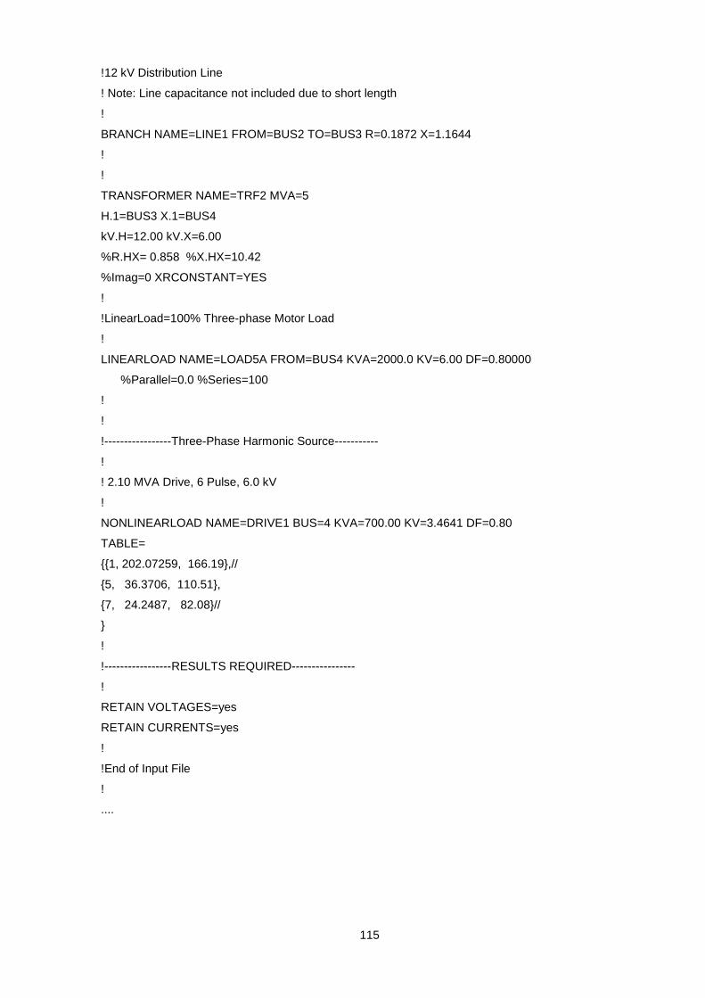
115

!12 kV Distribution Line

! Note: Line capacitance not included due to short length

!

BRANCH NAME=LINE1 FROM=BUS2 TO=BUS3 R=0.1872 X=1.1644

!

!

TRANSFORMER NAME=TRF2 MVA=5

H.1=BUS3 X.1=BUS4

kV.H=12.00 kV.X=6.00

%R.HX= 0.858 %X.HX=10.42

%Imag=0 XRCONSTANT=YES

!

!LinearLoad=100% Three-phase Motor Load

!

LINEARLOAD NAME=LOAD5A FROM=BUS4 KVA=2000.0 KV=6.00 DF=0.80000

%Parallel=0.0 %Series=100

!

!

!-----------------Three-Phase Harmonic Source-----------

!

! 2.10 MVA Drive, 6 Pulse, 6.0 kV

!

NONLINEARLOAD NAME=DRIVE1 BUS=4 KVA=700.00 KV=3.4641 DF=0.80

TABLE=

1, 202.07259, 166.19,//

5, 36.3706, 110.51,

7, 24.2487, 82.08//

!

!-----------------RESULTS REQUIRED----------------

!

RETAIN VOLTAGES=yes

RETAIN CURRENTS=yes

!

!End of Input File

!

....

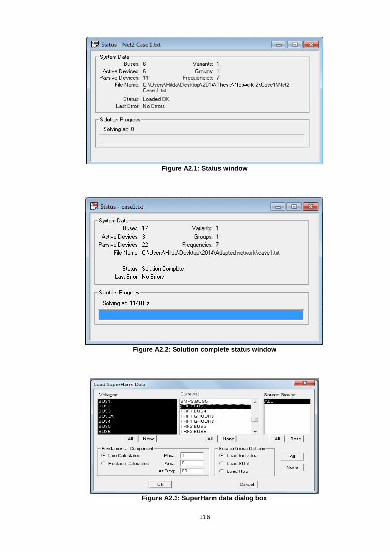
116

Figure A2.1: Status window

Figure A2.2: Solution complete status window

Figure A2.3: SuperHarm data dialog box

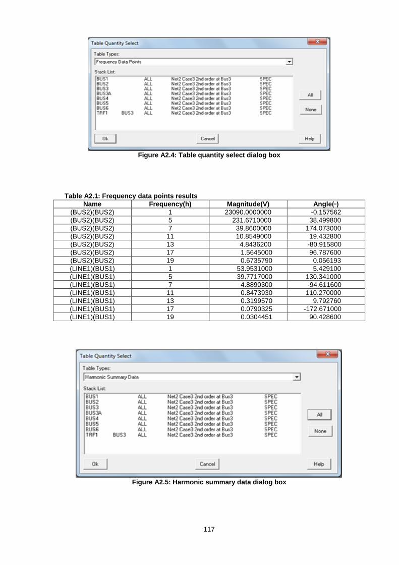
117

Figure A2.4: Table quantity select dialog box

Table A2.1: Frequency data points results

Name Frequency(h) Magnitude(V) Angle()

(BUS2)(BUS2) 1 23090.0000000 -0.157562

(BUS2)(BUS2) 5 231.6710000 38.499800

(BUS2)(BUS2) 7 39.8600000 174.073000

(BUS2)(BUS2) 11 10.8549000 19.432800

(BUS2)(BUS2) 13 4.8436200 -80.915800

(BUS2)(BUS2) 17 1.5645000 96.787600

(BUS2)(BUS2) 19 0.6735790 0.056193

(LINE1)(BUS1) 1 53.9531000 5.429100

(LINE1)(BUS1) 5 39.7717000 130.341000

(LINE1)(BUS1) 7 4.8890300 -94.611600

(LINE1)(BUS1) 11 0.8473930 110.270000

(LINE1)(BUS1) 13 0.3199570 9.792760

(LINE1)(BUS1) 17 0.0790325 -172.671000

(LINE1)(BUS1) 19 0.0304451 90.428600

Figure A2.5: Harmonic summary data dialog box

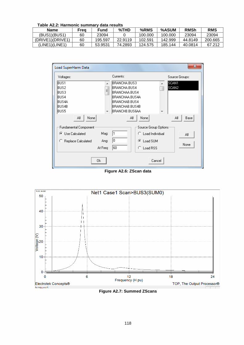
118

Table A2.2: Harmonic summary data results

Name Freq Fund %THD %RMS %ASUM RMSh RMS

(BUS1)(BUS1) 60 23094 0 100.000 100.000 23094 23094

(DRIVE1)(DRIVE1) 60 195.597 22.9119 102.591 142.999 44.8149 200.665

(LINE1)(LINE1) 60 53.9531 74.2893 124.575 185.144 40.0814 67.212

Figure A2.6: ZScan data

Figure A2.7: Summed ZScans

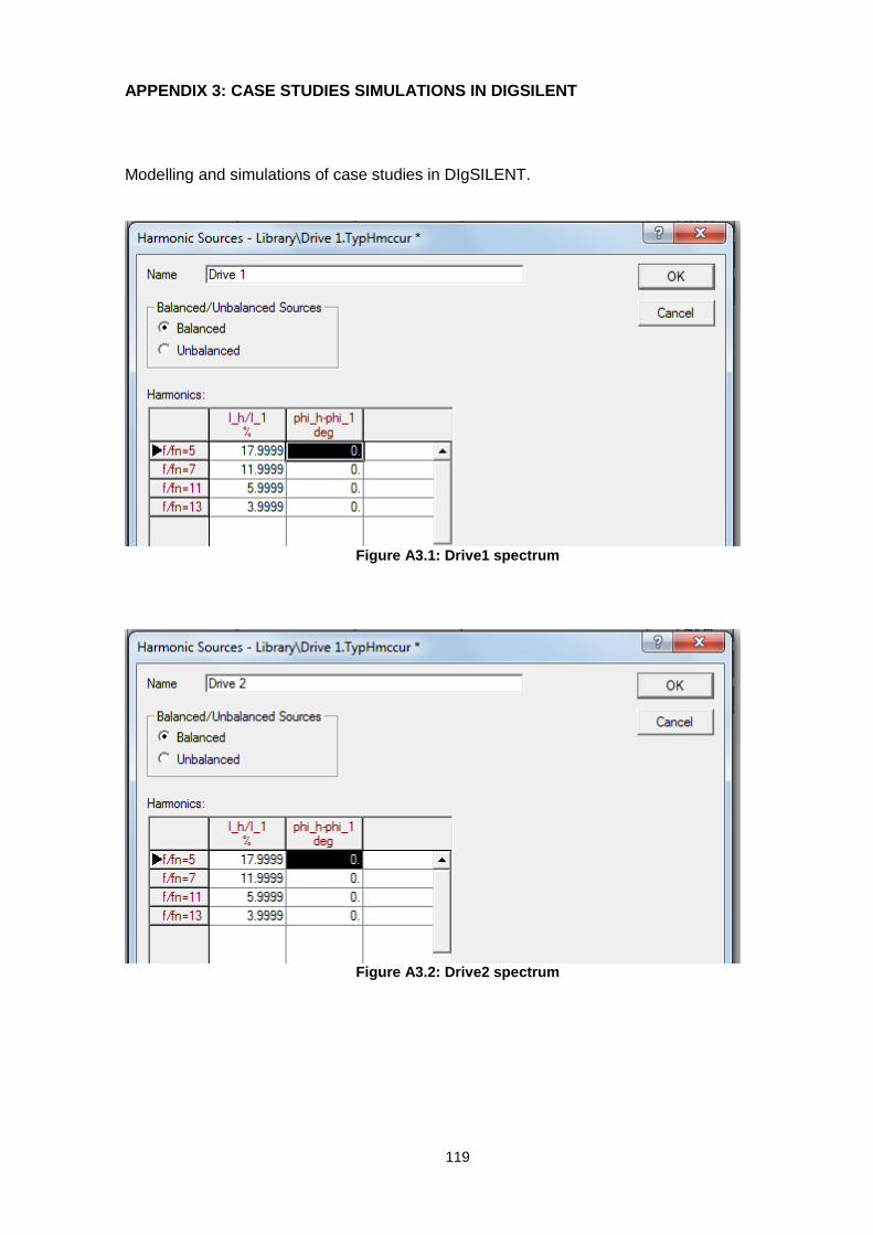
119

APPENDIX 3: CASE STUDIES SIMULATIONS IN DIGSILENT

Modelling and simulations of case studies in DIgSILENT.

Figure A3.1: Drive1 spectrum

Figure A3.2: Drive2 spectrum

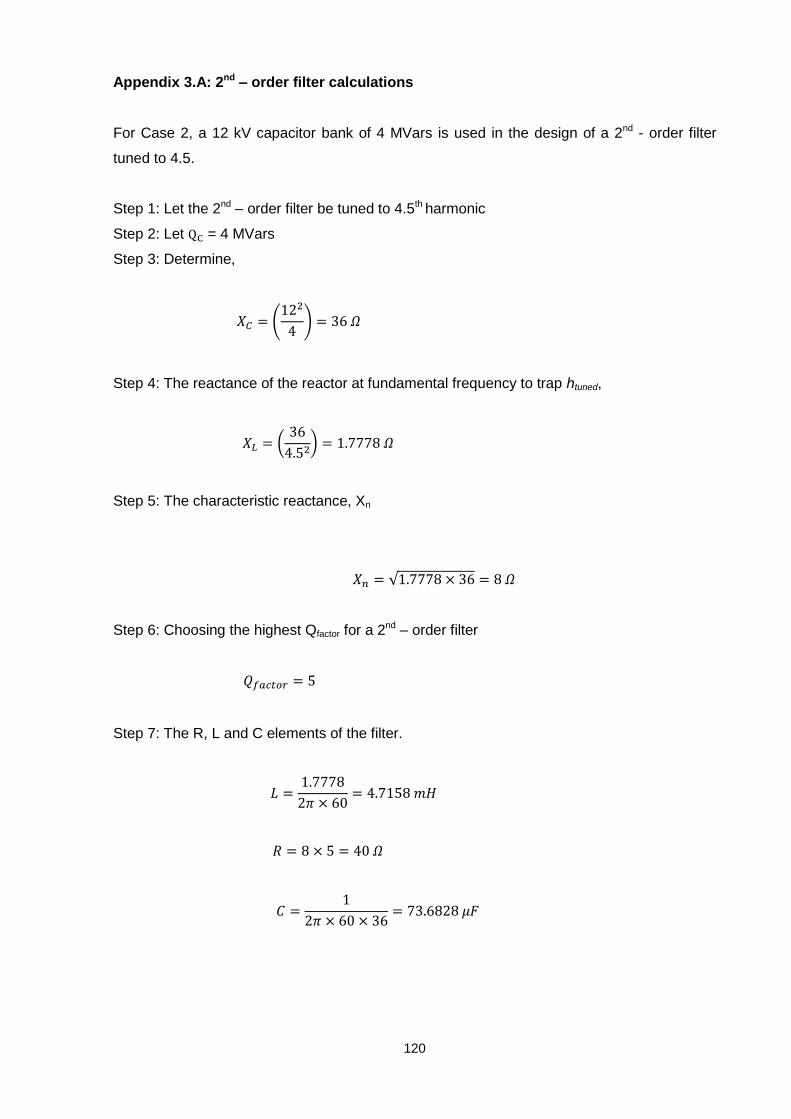
120

Appendix 3.A: 2nd – order filter calculations

For Case 2, a 12 kV capacitor bank of 4 MVars is used in the design of a 2nd - order filter

tuned to 4.5.

Step 1: Let the 2nd – order filter be tuned to 4.5th harmonic

Step 2: Let = 4 MVars

Step 3: Determine,

(

)

Step 4: The reactance of the reactor at fundamental frequency to trap htuned,

(

)

Step 5: The characteristic reactance, Xn

√

Step 6: Choosing the highest Qfactor for a 2nd – order filter

Step 7: The R, L and C elements of the filter.

𝐻

𝐹

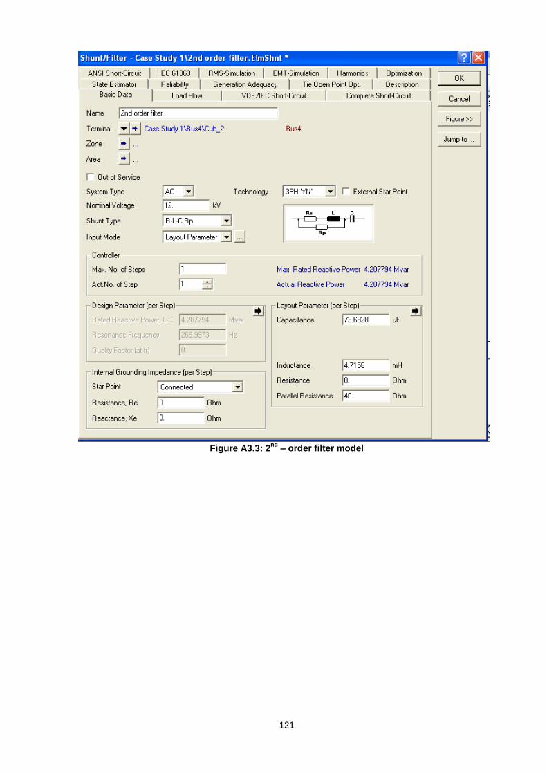
121

Figure A3.3: 2

nd – order filter model

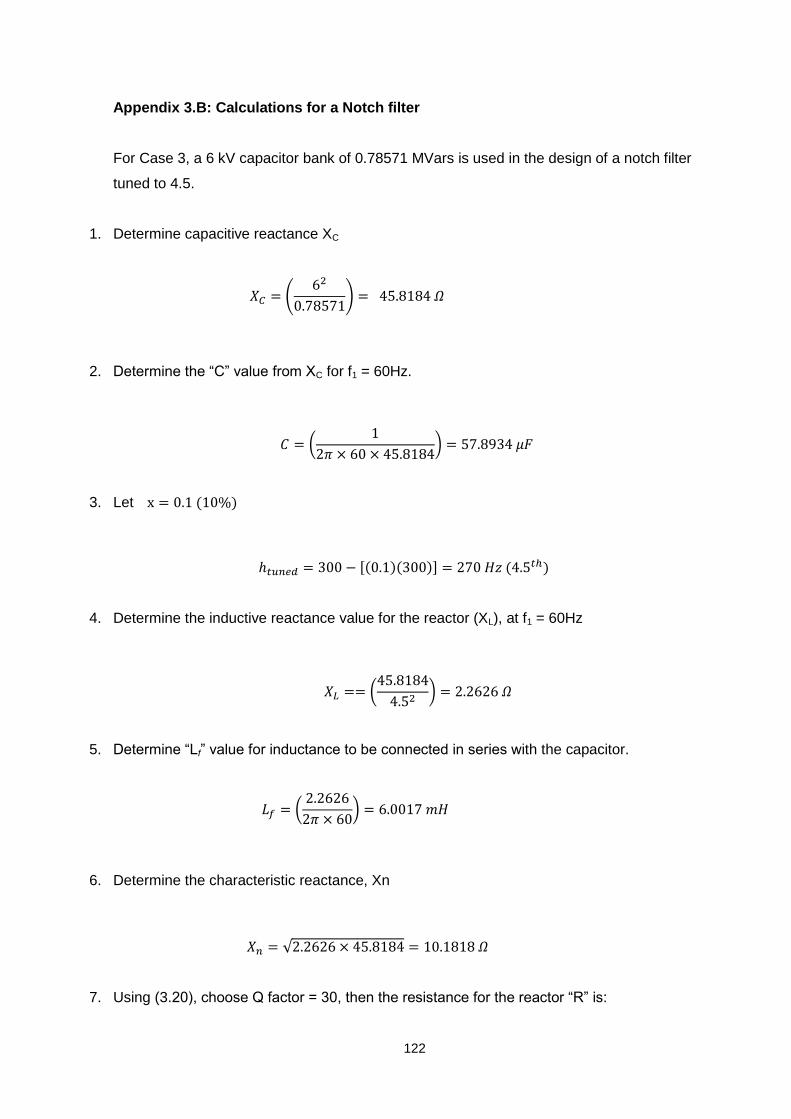
122

Appendix 3.B: Calculations for a Notch filter

For Case 3, a 6 kV capacitor bank of 0.78571 MVars is used in the design of a notch filter

tuned to 4.5.

1. Determine capacitive reactance XC

(

)

2. Determine the “C” value from XC for f1 = 60Hz.

(

) 𝐹

3. Let

𝐻

4. Determine the inductive reactance value for the reactor (XL), at f1 = 60Hz

(

)

5. Determine “Lf” value for inductance to be connected in series with the capacitor.

(

) 𝐻

6. Determine the characteristic reactance, Xn

√

7. Using (3.20), choose Q factor = 30, then the resistance for the reactor “R” is:

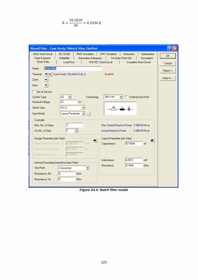
123

Figure A3.4: Notch filter model

124

APPENDIX 4: CASE STUDIES SIMULATIONS IN SUPERHARM

Case studies network modelling and simulations in SuperHarm.

Appendix 4.A: Case 1 scan study model

TITLE TITLE1="40 kV End-User Network-Consumers 1, 2 and 3"

TITLE2="PF Capacitor Banks at Buses 4A, 4B and 6BA"

TITLE3="Case1 Scan study"

!

!

!Case: Harmonic Resonance case, Single-phase representation

! of a three-phase network

!

! Scan case

!

! Solution will be for 1 Amp Injection

! over a range of frequencies (60 Hz to 840 Hz)

!

!

!-------------SCAN SOURCE GROUP------------------------

!

SCAN NAME=SCAN1 BUS=BUS6AE FMIN=60 FMAX=840 FINC=10 ANG=0.0

SCAN NAME=SCAN2 BUS=BUS6AC FMIN=60 FMAX=840 FINC=10 ANG=0.0

!

!

!--------------VOLTAGE SOURCE----------------------------

!

!Utility source, Positive Sequence Source

!

VSOURCE NAME=VSRC BUS=BUS1 MAG=23094

!

!

!Positive Sequence Source Equivalent at 40 KVBUS

! Note: Impedance Value Given in Ohms at 60 Hz

!

BRANCH NAME=LINE1 FROM=BUS1 TO=BUS2 R=0.1872 X=1.1644

!

!Transformer at SOURCE

!

TRANSFORMER NAME=TS MVA=20

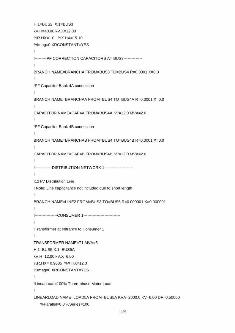
125

H.1=BUS2 X.1=BUS3

kV.H=40.00 kV.X=12.00

%R.HX=1.0 %X.HX=15.10

%Imag=0 XRCONSTANT=YES

!

!---------PF CORRECTION CAPACITORS AT BUS3--------------

!

BRANCH NAME=BRANCHA FROM=BUS3 TO=BUS4 R=0.0001 X=0.0

!

!PF Capacitor Bank 4A connection

!

BRANCH NAME=BRANCHAA FROM=BUS4 TO=BUS4A R=0.0001 X=0.0

!

CAPACITOR NAME=CAP4A FROM=BUS4A KV=12.0 MVA=2.0

!

!PF Capacitor Bank 4B connection

!

BRANCH NAME=BRANCHAB FROM=BUS4 TO=BUS4B R=0.0001 X=0.0

!

CAPACITOR NAME=CAP4B FROM=BUS4B KV=12.0 MVA=2.0

!

!-------------DISTRIBUTION NETWORK 1----------------------

!

!12 kV Distribution Line

! Note: Line capacitance not included due to short length

!

BRANCH NAME=LINE2 FROM=BUS3 TO=BUS5 R=0.000001 X=0.000001

!

!-----------------CONSUMER 1----------------------------

!

!Transformer at entrance to Consumer 1

!

TRANSFORMER NAME=T1 MVA=5

H.1=BUS5 X.1=BUS5A

kV.H=12.00 kV.X=6.00

%R.HX= 0.9885 %X.HX=12.0

%Imag=0 XRCONSTANT=YES

!

!LinearLoad=100% Three-phase Motor Load

!

LINEARLOAD NAME=LOAD5A FROM=BUS5A KVA=2000.0 KV=6.00 DF=0.50000

%Parallel=0.0 %Series=100

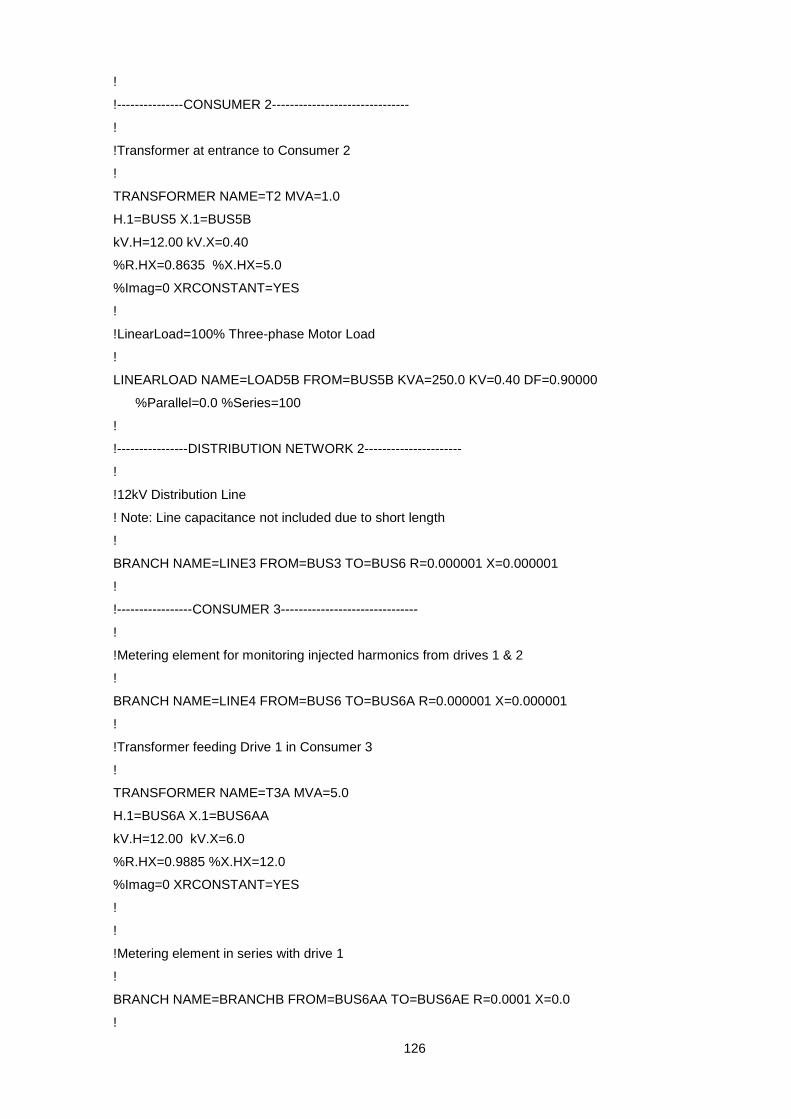
126

!

!---------------CONSUMER 2-------------------------------

!

!Transformer at entrance to Consumer 2

!

TRANSFORMER NAME=T2 MVA=1.0

H.1=BUS5 X.1=BUS5B

kV.H=12.00 kV.X=0.40

%R.HX=0.8635 %X.HX=5.0

%Imag=0 XRCONSTANT=YES

!

!LinearLoad=100% Three-phase Motor Load

!

LINEARLOAD NAME=LOAD5B FROM=BUS5B KVA=250.0 KV=0.40 DF=0.90000

%Parallel=0.0 %Series=100

!

!----------------DISTRIBUTION NETWORK 2----------------------

!

!12kV Distribution Line

! Note: Line capacitance not included due to short length

!

BRANCH NAME=LINE3 FROM=BUS3 TO=BUS6 R=0.000001 X=0.000001

!

!-----------------CONSUMER 3-------------------------------

!

!Metering element for monitoring injected harmonics from drives 1 & 2

!

BRANCH NAME=LINE4 FROM=BUS6 TO=BUS6A R=0.000001 X=0.000001

!

!Transformer feeding Drive 1 in Consumer 3

!

TRANSFORMER NAME=T3A MVA=5.0

H.1=BUS6A X.1=BUS6AA

kV.H=12.00 kV.X=6.0

%R.HX=0.9885 %X.HX=12.0

%Imag=0 XRCONSTANT=YES

!

!

!Metering element in series with drive 1

!

BRANCH NAME=BRANCHB FROM=BUS6AA TO=BUS6AE R=0.0001 X=0.0

!

127

!Three-Phase Harmonic Source 1

!

! 2.10 MVA Drive, 6 Pulse, 6.0 kV

!

NONLINEARLOAD NAME=DRIVE1 BUS=BUS6AE KVA=700.00 KV=3.4641 DF=0.80

TABLE=

1, 202.07259, 0,//

5, 36.3706, 0,

7, 24.2487, 0,

11, 12.1243, 0,

13, 8.0829, 0,

17, 4.0414, 0,

19, 2.0207, 0 //

!

!Transformer feeding Drive2 in Consumer 3

!

TRANSFORMER NAME=T3B MVA=2.0

H.1=BUS6A X.1=BUS6AB

kV.H=12.0 kV.X=0.40

%R.HX=0.9861 %X.HX=7.0

%Imag=0 XRCONSTANT=YES

!

!Metering element in series with drive2

!

BRANCH NAME=BRANCHC FROM=BUS6AB TO=BUS6AC R=0.0001 X=0.0

!

!

!Three-Phase Harmonic Source 2

!

! 0.25 MVA Drive, 6 Pulse, 0.4 kV

!

NONLINEARLOAD NAME=DRIVE2 BUS=BUS6AC KVA=83.333 KV=0.2309401 DF=0.80

TABLE=

1, 360.8426, 0,//

5, 64.9516, 0,

7, 43.3011, 0,

11, 21.6505, 0,

13, 14.4337, 0,

17, 7.2168, 0,

128

19, 3.6084, 0 //

!

!

!Transformer feeding pf corrected load in consumer 3

!

TRANSFORMER NAME=T3C MVA=2.0

H.1=BUS6 X.1=BUS6B

kV.H=12.00 kV.X=0.40

%R.HX=0.9861 %X.HX=7.0

%Imag=0 XRCONSTANT=YES

!

!LineraLoad=100% Three-phase Motor Load in Consumer 3

!

LINEARLOAD NAME=LOAD6A FROM=BUS6B KVA=1000.0 KV=0.40 DF=0.80000

%Parallel=0.0 %Series=100

!

!PF Capacitor in Consumer 3

!

!Metering element in series with capacitor

!

BRANCH NAME=BRANCHD FROM=BUS6B TO=BUS6BA R=0.0001 X=0.0

!

CAPACITOR NAME=CAP6BA FROM=BUS6BA KV=0.40 MVA=0.30

!

!-----------------RESULTS REQUIRED----------------

!

RETAIN VOLTAGES=yes

RETAIN CURRENTS=yes

!

!

!End of Input File

!

....

129

Appendix 4.B: Case 1 Penetration study

TITLE TITLE1="40 kV End-User Network-Consumers 1, 2 and 3"

TITLE2="PF Capacitor Banks at Buses 4A, 4B and 6BA"

TITLE3="Case1 Harmonic Penetration"

!

!

!Case: Case1 Network with harmonic source, Single-phase

! representation of a three-phase network

!

!

!--------------VOLTAGE SOURCE----------------------------

!

!Utility source, Positive Sequence Source

!

VSOURCE NAME=VSRC BUS=BUS1 MAG=23094.01077

!

!

!Positive Sequence Source Equivalent at 40 KVBUS

! Note: Impedance Value Given in Ohms at 60 Hz

!

BRANCH NAME=LINE1 FROM=BUS1 TO=BUS2 R=0.1872 X=1.1644

!

!Transformer at SOURCE

!

TRANSFORMER NAME=TS MVA=20

H.1=BUS2 X.1=BUS3

kV.H=40.00 kV.X=12.00

%R.HX=1.0 %X.HX=15.10

%Imag=0 XRCONSTANT=YES

!

!---------PF CORRECTION CAPACITORS AT BUS3--------------

!

BRANCH NAME=BRANCHA FROM=BUS3 TO=BUS4 R=0.0001 X=0.0

!

!PF Capacitor Bank 4A connection

!

BRANCH NAME=BRANCHAA FROM=BUS4 TO=BUS4A R=0.0001 X=0.0

!

CAPACITOR NAME=CAP4A FROM=BUS4A KV=12.0 MVA=2.0

!

!PF Capacitor Bank 4B connection

130

!

BRANCH NAME=BRANCHAB FROM=BUS4 TO=BUS4B R=0.0001 X=0.0

!

CAPACITOR NAME=CAP4B FROM=BUS4B KV=12.0 MVA=2.0

!

!-------------DISTRIBUTION NETWORK 1----------------------

!

!12 kV Distribution Line

! Note: Line capacitance not included due to short length

!

BRANCH NAME=LINE2 FROM=BUS3 TO=BUS5 R=0.000001 X=0.000001

!

!-----------------CONSUMER 1----------------------------

!

!Transformer at entrance to Consumer 1

!

TRANSFORMER NAME=T1 MVA=5

H.1=BUS5 X.1=BUS5A

kV.H=12.00 kV.X=6.00

%R.HX= 0.9885 %X.HX=12.0

%Imag=0 XRCONSTANT=YES

!

!LinearLoad=100% Three-phase Motor Load

!

LINEARLOAD NAME=LOAD5A FROM=BUS5A KVA=2000.0 KV=6.00 DF=0.50000

%Parallel=0.0 %Series=100

!

!---------------CONSUMER 2-------------------------------

!

!Transformer at entrance to Consumer 2

!

TRANSFORMER NAME=T2 MVA=1.0

H.1=BUS5 X.1=BUS5B

kV.H=12.00 kV.X=0.40

%R.HX=0.8635 %X.HX=5.0

%Imag=0 XRCONSTANT=YES

!

!LinearLoad=100% Three-phase Motor Load

!

LINEARLOAD NAME=LOAD5B FROM=BUS5B KVA=250.0 KV=0.40 DF=0.90000

%Parallel=0.0 %Series=100

!

131

!----------------DISTRIBUTION NETWORK 2----------------------

!

!12kV Distribution Line

! Note: Line capacitance not included due to short length

!

BRANCH NAME=LINE3 FROM=BUS3 TO=BUS6 R=0.000001 X=0.000001

!

!-----------------CONSUMER 3-------------------------------

!

!Metering element for monitoring injected harmonics from drives 1 & 2

!

BRANCH NAME=LINE4 FROM=BUS6 TO=BUS6A R=0.000001 X=0.000001

!

!Transformer feeding Drive 1 in Consumer 3

!

TRANSFORMER NAME=T3A MVA=5.0

H.1=BUS6A X.1=BUS6AA

kV.H=12.00 kV.X=6.0

%R.HX=0.9885 %X.HX=12.0

%Imag=0 XRCONSTANT=YES

!

!

!Metering element in series with drive 1

!

BRANCH NAME=BRANCHB FROM=BUS6AA TO=BUS6AE R=0.0001 X=0.0

!

!Three-Phase Harmonic Source 1

!

! 2.10 MVA Drive, 6 Pulse, 6.0 kV

!

NONLINEARLOAD NAME=DRIVE1 BUS=BUS6AE KVA=700.00 KV=3.464102 DF=0.80

TABLE=

1, 202.07259, 0,//

5, 36.3706, 0,

7, 24.2487, 0,

11, 12.1243, 0,

13, 8.0829, 0 //

!

!Transformer feeding Drive2 in Consumer 3

!

132

TRANSFORMER NAME=T3B MVA=2.0

H.1=BUS6A X.1=BUS6AB

kV.H=12.0 kV.X=0.40

%R.HX=0.9861 %X.HX=7.0

%Imag=0 XRCONSTANT=YES

!

!Metering element in series with drive2

!

BRANCH NAME=BRANCHC FROM=BUS6AB TO=BUS6AC R=0.0001 X=0.0

!

!

!Three-Phase Harmonic Source 2

!

! 0.25 MVA Drive, 6 Pulse, 0.4 kV

!

NONLINEARLOAD NAME=DRIVE2 BUS=BUS6AC KVA=83.333 KV=0.2309401 DF=0.80

TABLE=

1, 360.8426, 0,//

5, 64.9516, 0,

7, 43.3011, 0,

11, 21.6505, 0,

13, 14.4337, 0 //

!

!

!Transformer feeding pf corrected load in consumer 3

!

TRANSFORMER NAME=T3C MVA=2.0

H.1=BUS6 X.1=BUS6B

kV.H=12.00 kV.X=0.40

%R.HX=0.9861 %X.HX=7.0

%Imag=0 XRCONSTANT=YES

!

!LineraLoad=100% Three-phase Motor Load in Consumer 3

!

LINEARLOAD NAME=LOAD6A FROM=BUS6B KVA=1000.0 KV=0.40 DF=0.80000

%Parallel=0.0 %Series=100

!

!PF Capacitor in Consumer 3

!

!Metering element in series with capacitor

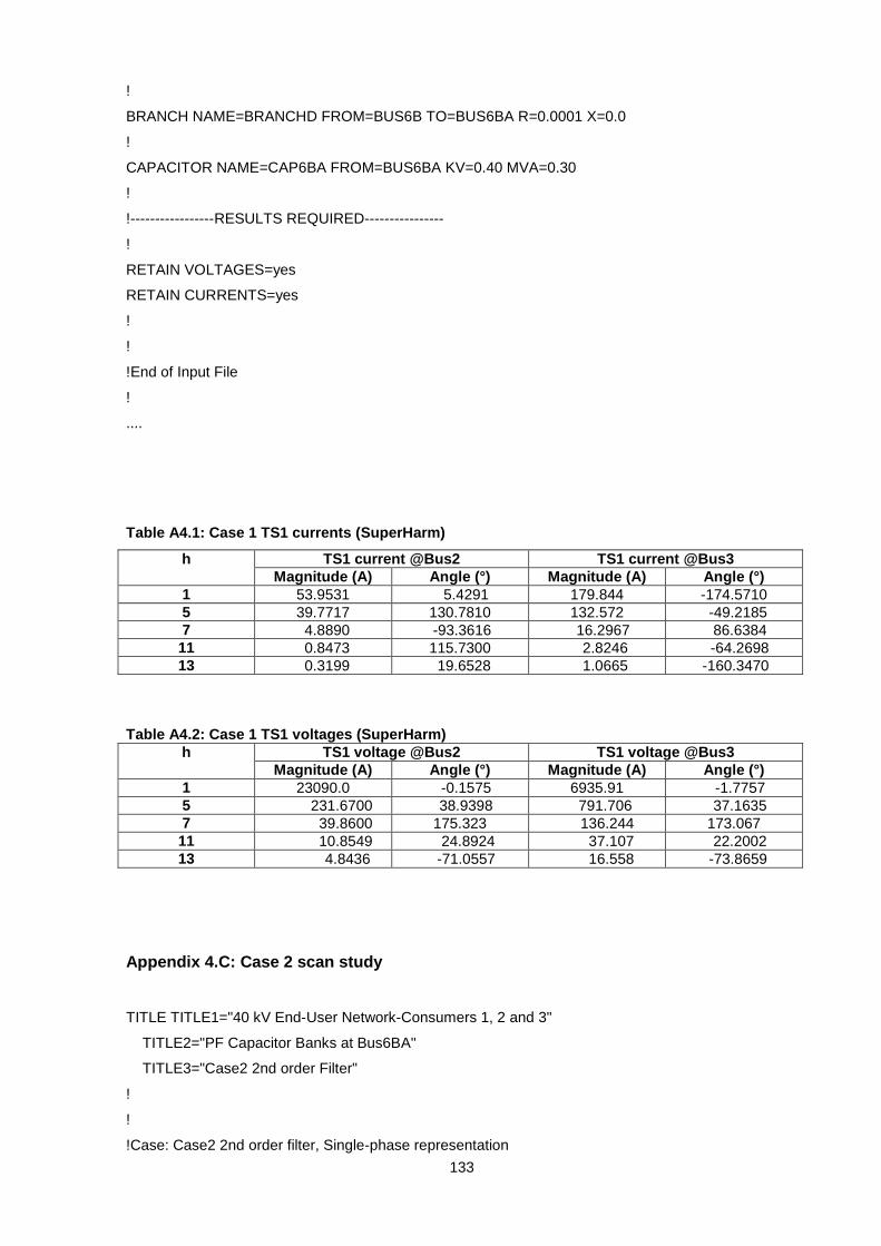
133

!

BRANCH NAME=BRANCHD FROM=BUS6B TO=BUS6BA R=0.0001 X=0.0

!

CAPACITOR NAME=CAP6BA FROM=BUS6BA KV=0.40 MVA=0.30

!

!-----------------RESULTS REQUIRED----------------

!

RETAIN VOLTAGES=yes

RETAIN CURRENTS=yes

!

!

!End of Input File

!

....

Table A4.1: Case 1 TS1 currents (SuperHarm)

h TS1 current @Bus2 TS1 current @Bus3

Magnitude (A) Angle (°) Magnitude (A) Angle (°)

1 53.9531 5.4291 179.844 -174.5710

5 39.7717 130.7810 132.572 -49.2185

7 4.8890 -93.3616 16.2967 86.6384

11 0.8473 115.7300 2.8246 -64.2698

13 0.3199 19.6528 1.0665 -160.3470

Table A4.2: Case 1 TS1 voltages (SuperHarm)

h TS1 voltage @Bus2 TS1 voltage @Bus3

Magnitude (A) Angle (°) Magnitude (A) Angle (°)

1 23090.0 -0.1575 6935.91 -1.7757

5 231.6700 38.9398 791.706 37.1635

7 39.8600 175.323 136.244 173.067

11 10.8549 24.8924 37.107 22.2002

13 4.8436 -71.0557 16.558 -73.8659

Appendix 4.C: Case 2 scan study

TITLE TITLE1="40 kV End-User Network-Consumers 1, 2 and 3"

TITLE2="PF Capacitor Banks at Bus6BA"

TITLE3="Case2 2nd order Filter"

!

!

!Case: Case2 2nd order filter, Single-phase representation

134

! of a three-phase network

!

! Scan case

!

! Solution will be for 1 Amp Injection

! over a range of frequencies (60 Hz to 840 Hz)

!

!

!-------------SCAN SOURCE GROUP------------------------

!

SCAN NAME=SCAN1 BUS=BUS6AE FMIN=60 FMAX=840 FINC=10 ANG=0.0

SCAN NAME=SCAN2 BUS=BUS6AC FMIN=60 FMAX=840 FINC=10 ANG=0.0

!

!

!--------------VOLTAGE SOURCE----------------------------

!

!Utility source, Positive Sequence Source

!

VSOURCE NAME=VSRC BUS=BUS1 MAG=23094

!

!

!Positive Sequence Source Equivalent at 40 KVBUS

! Note: Impedance Value Given in Ohms at 60 Hz

!

BRANCH NAME=LINE1 FROM=BUS1 TO=BUS2 R=0.1872 X=1.1644

!

!Transformer at SOURCE

!

TRANSFORMER NAME=TS MVA=20

H.1=BUS2 X.1=BUS3

kV.H=40.00 kV.X=12.00

%R.HX=1.0 %X.HX=15.10

%Imag=0 XRCONSTANT=YES

!

! ------------2nd-ORDER FILTER AT BUS3(PCC)--------------

!

! Metering element in series with filter

!

!

CAPACITOR NAME=CAP4A FROM=BUS3 TO=BUS3A KV=12.0 MVA=4.0

!

BRANCH NAME=BRANCH3A FROM=BUS3A R=40.00 X=0.0

135

!

BRANCH NAME=BRANCHAA FROM=BUS3A R=0.0 X=1.7778

!

!-------------DISTRIBUTION NETWORK 1----------------------

!

!12 kV Distribution Line

! Note: Line capacitance not included due to short length

!

BRANCH NAME=LINE2 FROM=BUS3 TO=BUS5 R=0.000001 X=0.000001

!

!-----------------CONSUMER 1----------------------------

!

!Transformer at entrance to Consumer 1

!

TRANSFORMER NAME=T1 MVA=5

H.1=BUS5 X.1=BUS5A

kV.H=12.00 kV.X=6.00

%R.HX= 0.9885 %X.HX=12.0

%Imag=0 XRCONSTANT=YES

!

!LinearLoad=100% Three-phase Motor Load

!

LINEARLOAD NAME=LOAD5A FROM=BUS5A KVA=2000.0 KV=6.00 DF=0.50000

%Parallel=0.0 %Series=100

!

!---------------CONSUMER 2-------------------------------

!

!Transformer at entrance to Consumer 2

!

TRANSFORMER NAME=T2 MVA=1.0

H.1=BUS5 X.1=BUS5B

kV.H=12.00 kV.X=0.40

%R.HX=0.8635 %X.HX=5.0

%Imag=0 XRCONSTANT=YES

!

!LinearLoad=100% Three-phase Motor Load

!

LINEARLOAD NAME=LOAD5B FROM=BUS5B KVA=250.0 KV=0.40 DF=0.90000

%Parallel=0.0 %Series=100

!

!----------------DISTRIBUTION NETWORK 2----------------------

!

136

!12kV Distribution Line

! Note: Line capacitance not included due to short length

!

BRANCH NAME=LINE3 FROM=BUS3 TO=BUS6 R=0.000001 X=0.000001

!

!-----------------CONSUMER 3-------------------------------

!

!Metering element for monitoring injected harmonics from drives 1 & 2

!

BRANCH NAME=LINE4 FROM=BUS6 TO=BUS6A R=0.000001 X=0.000001

!

!Transformer feeding Drive 1 in Consumer 3

!

TRANSFORMER NAME=T3A MVA=5.0

H.1=BUS6A X.1=BUS6AA

kV.H=12.00 kV.X=6.0

%R.HX=0.9885 %X.HX=12.0

%Imag=0 XRCONSTANT=YES

!

!

!Metering element in series with drive 1

!

BRANCH NAME=BRANCHB FROM=BUS6AA TO=BUS6AE R=0.0001 X=0.0

!

!Three-Phase Harmonic Source 1

!

! 2.10 MVA Drive, 6 Pulse, 6.0 kV

!

NONLINEARLOAD NAME=DRIVE1 BUS=BUS6AE KVA=700.00 KV=3.4641 DF=0.80

TABLE=

1, 202.07259, 0,//

5, 36.3706, 0,

7, 24.2487, 0,

11, 12.1243, 0,

13, 8.0829, 0 //

!

!Transformer feeding Drive2 in Consumer 3

!

TRANSFORMER NAME=T3B MVA=2.0

H.1=BUS6A X.1=BUS6AB

137

kV.H=12.0 kV.X=0.40

%R.HX=0.9861 %X.HX=7.0

%Imag=0 XRCONSTANT=YES

!

!Metering element in series with drive2

!

BRANCH NAME=BRANCHC FROM=BUS6AB TO=BUS6AC R=0.0001 X=0.0

!

!

!Three-Phase Harmonic Source 2

!

! 0.25 MVA Drive, 6 Pulse, 0.4 kV

!

NONLINEARLOAD NAME=DRIVE2 BUS=BUS6AC KVA=83.333 KV=0.2309401 DF=0.80

TABLE=

1, 360.8426, 0,//

5, 64.9516, 0,

7, 43.3011, 0,

11, 21.6505, 0,

13, 14.4337, 0 //

!

!

!Transformer feeding pf corrected load in consumer 3

!

TRANSFORMER NAME=T3C MVA=2.0

H.1=BUS6 X.1=BUS6B

kV.H=12.00 kV.X=0.40

%R.HX=0.9861 %X.HX=7.0

%Imag=0 XRCONSTANT=YES

!

!LineraLoad=100% Three-phase Motor Load in Consumer 3

!

LINEARLOAD NAME=LOAD6A FROM=BUS6B KVA=1000.0 KV=0.40 DF=0.80000

%Parallel=0.0 %Series=100

!

!PF Capacitor in Consumer 3

!

!Metering element in series with capacitor

!

BRANCH NAME=BRANCHD FROM=BUS6B TO=BUS6BA R=0.0001 X=0.0

138

!

CAPACITOR NAME=CAP6BA FROM=BUS6BA KV=0.40 MVA=0.30

!

!-----------------RESULTS REQUIRED----------------

!

RETAIN VOLTAGES=yes

RETAIN CURRENTS=yes

!

!

!End of Input File

!

....

Appendix 4.D: Case 2 Penetration study

TITLE TITLE1="40 kV End-User Network-Consumers 1, 2 and 3"

TITLE2="PF Capacitor Banks at Bus6BA"

TITLE3="Case2 2nd order Filter"

!

!

!Case: Case2 2nd order filter, Single-phase representation

! of a three-phase network

!

!

!--------------VOLTAGE SOURCE----------------------------

!

!Utility source, Positive Sequence Source

!

VSOURCE NAME=VSRC BUS=BUS1 MAG=23094

!

!

!Positive Sequence Source Equivalent at 40 KVBUS

! Note: Impedance Value Given in Ohms at 60 Hz

!

BRANCH NAME=LINE1 FROM=BUS1 TO=BUS2 R=0.1872 X=1.1644

!

!Transformer at SOURCE

!

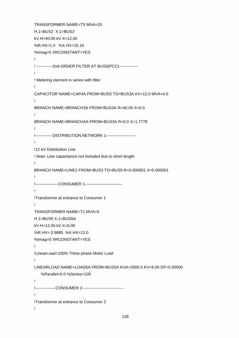
139

TRANSFORMER NAME=TS MVA=20

H.1=BUS2 X.1=BUS3

kV.H=40.00 kV.X=12.00

%R.HX=1.0 %X.HX=15.10

%Imag=0 XRCONSTANT=YES

!

! ------------2nd-ORDER FILTER AT BUS3(PCC)--------------

!

! Metering element in series with filter

!

CAPACITOR NAME=CAP4A FROM=BUS3 TO=BUS3A KV=12.0 MVA=4.0

!

BRANCH NAME=BRANCH3A FROM=BUS3A R=40.00 X=0.0

!

BRANCH NAME=BRANCHAA FROM=BUS3A R=0.0 X=1.7778

!

!-------------DISTRIBUTION NETWORK 1----------------------

!

!12 kV Distribution Line

! Note: Line capacitance not included due to short length

!

BRANCH NAME=LINE2 FROM=BUS3 TO=BUS5 R=0.000001 X=0.000001

!

!-----------------CONSUMER 1----------------------------

!

!Transformer at entrance to Consumer 1

!

TRANSFORMER NAME=T1 MVA=5

H.1=BUS5 X.1=BUS5A

kV.H=12.00 kV.X=6.00

%R.HX= 0.9885 %X.HX=12.0

%Imag=0 XRCONSTANT=YES

!

!LinearLoad=100% Three-phase Motor Load

!

LINEARLOAD NAME=LOAD5A FROM=BUS5A KVA=2000.0 KV=6.00 DF=0.50000

%Parallel=0.0 %Series=100

!

!---------------CONSUMER 2-------------------------------

!

!Transformer at entrance to Consumer 2

!

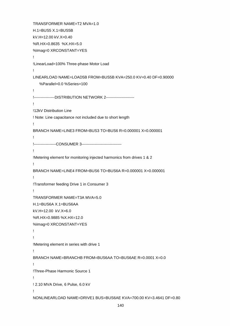
140

TRANSFORMER NAME=T2 MVA=1.0

H.1=BUS5 X.1=BUS5B

kV.H=12.00 kV.X=0.40

%R.HX=0.8635 %X.HX=5.0

%Imag=0 XRCONSTANT=YES

!

!LinearLoad=100% Three-phase Motor Load

!

LINEARLOAD NAME=LOAD5B FROM=BUS5B KVA=250.0 KV=0.40 DF=0.90000

%Parallel=0.0 %Series=100

!

!----------------DISTRIBUTION NETWORK 2----------------------

!

!12kV Distribution Line

! Note: Line capacitance not included due to short length

!

BRANCH NAME=LINE3 FROM=BUS3 TO=BUS6 R=0.000001 X=0.000001

!

!-----------------CONSUMER 3-------------------------------

!

!Metering element for monitoring injected harmonics from drives 1 & 2

!

BRANCH NAME=LINE4 FROM=BUS6 TO=BUS6A R=0.000001 X=0.000001

!

!Transformer feeding Drive 1 in Consumer 3

!

TRANSFORMER NAME=T3A MVA=5.0

H.1=BUS6A X.1=BUS6AA

kV.H=12.00 kV.X=6.0

%R.HX=0.9885 %X.HX=12.0

%Imag=0 XRCONSTANT=YES

!

!

!Metering element in series with drive 1

!

BRANCH NAME=BRANCHB FROM=BUS6AA TO=BUS6AE R=0.0001 X=0.0

!

!Three-Phase Harmonic Source 1

!

! 2.10 MVA Drive, 6 Pulse, 6.0 kV

!

NONLINEARLOAD NAME=DRIVE1 BUS=BUS6AE KVA=700.00 KV=3.4641 DF=0.80

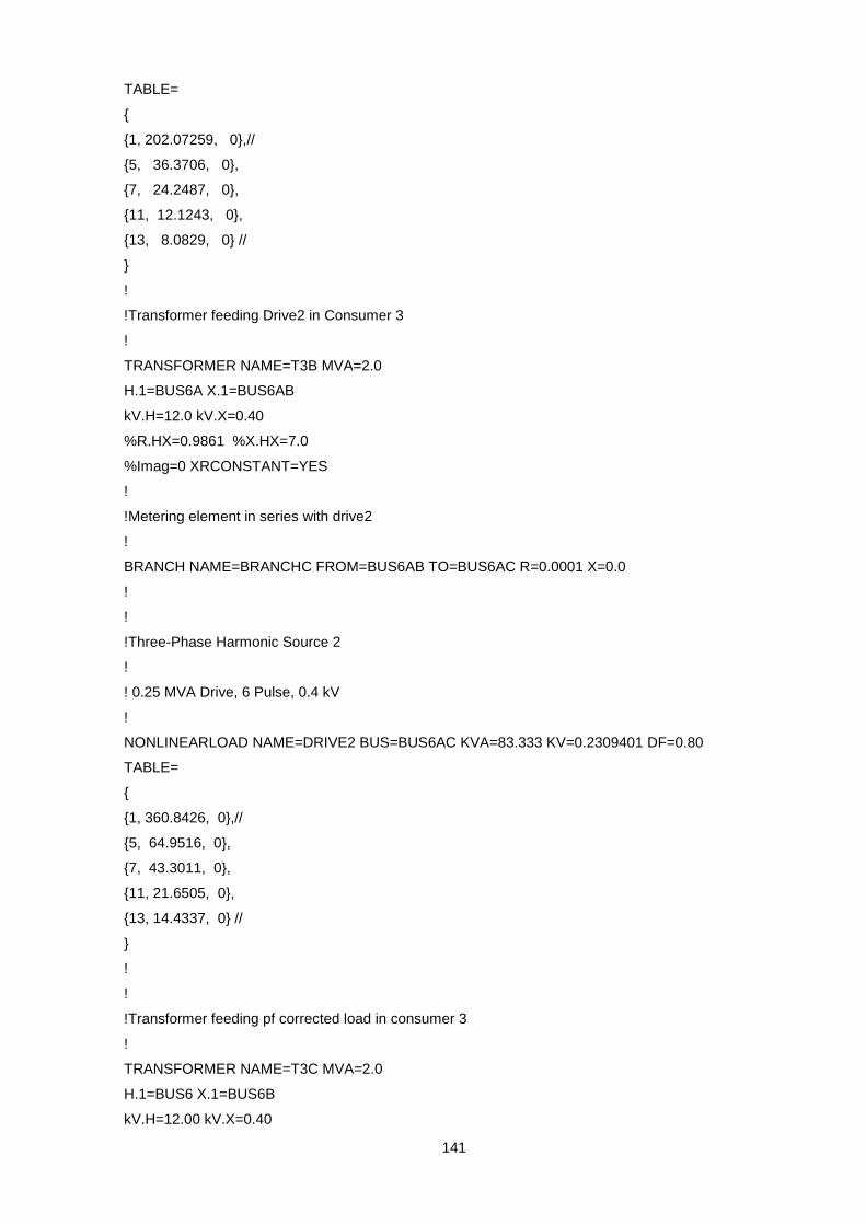
141

TABLE=

1, 202.07259, 0,//

5, 36.3706, 0,

7, 24.2487, 0,

11, 12.1243, 0,

13, 8.0829, 0 //

!

!Transformer feeding Drive2 in Consumer 3

!

TRANSFORMER NAME=T3B MVA=2.0

H.1=BUS6A X.1=BUS6AB

kV.H=12.0 kV.X=0.40

%R.HX=0.9861 %X.HX=7.0

%Imag=0 XRCONSTANT=YES

!

!Metering element in series with drive2

!

BRANCH NAME=BRANCHC FROM=BUS6AB TO=BUS6AC R=0.0001 X=0.0

!

!

!Three-Phase Harmonic Source 2

!

! 0.25 MVA Drive, 6 Pulse, 0.4 kV

!

NONLINEARLOAD NAME=DRIVE2 BUS=BUS6AC KVA=83.333 KV=0.2309401 DF=0.80

TABLE=

1, 360.8426, 0,//

5, 64.9516, 0,

7, 43.3011, 0,

11, 21.6505, 0,

13, 14.4337, 0 //

!

!

!Transformer feeding pf corrected load in consumer 3

!

TRANSFORMER NAME=T3C MVA=2.0

H.1=BUS6 X.1=BUS6B

kV.H=12.00 kV.X=0.40

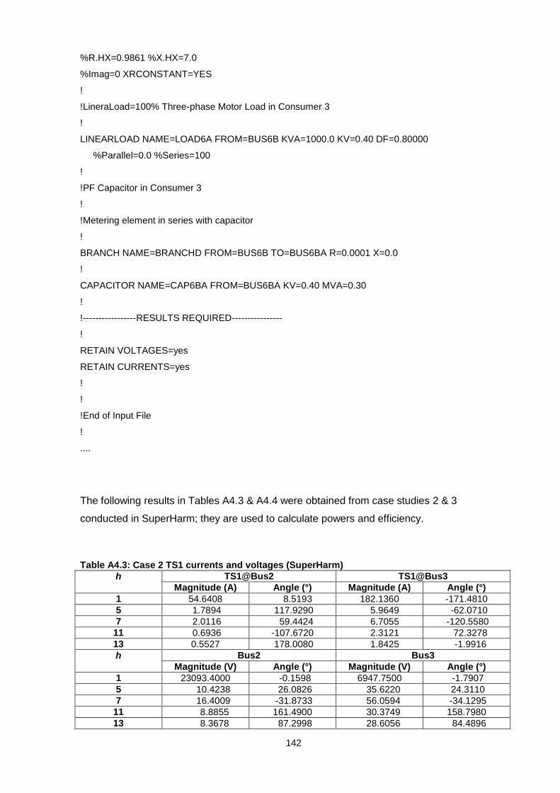
142

%R.HX=0.9861 %X.HX=7.0

%Imag=0 XRCONSTANT=YES

!

!LineraLoad=100% Three-phase Motor Load in Consumer 3

!

LINEARLOAD NAME=LOAD6A FROM=BUS6B KVA=1000.0 KV=0.40 DF=0.80000

%Parallel=0.0 %Series=100

!

!PF Capacitor in Consumer 3

!

!Metering element in series with capacitor

!

BRANCH NAME=BRANCHD FROM=BUS6B TO=BUS6BA R=0.0001 X=0.0

!

CAPACITOR NAME=CAP6BA FROM=BUS6BA KV=0.40 MVA=0.30

!

!-----------------RESULTS REQUIRED----------------

!

RETAIN VOLTAGES=yes

RETAIN CURRENTS=yes

!

!

!End of Input File

!

....

The following results in Tables A4.3 & A4.4 were obtained from case studies 2 & 3

conducted in SuperHarm; they are used to calculate powers and efficiency.

Table A4.3: Case 2 TS1 currents and voltages (SuperHarm)

h TS1@Bus2 TS1@Bus3

Magnitude (A) Angle (°) Magnitude (A) Angle (°)

1 54.6408 8.5193 182.1360 -171.4810

5 1.7894 117.9290 5.9649 -62.0710

7 2.0116 59.4424 6.7055 -120.5580

11 0.6936 -107.6720 2.3121 72.3278

13 0.5527 178.0080 1.8425 -1.9916

h Bus2 Bus3

Magnitude (V) Angle (°) Magnitude (V) Angle (°)

1 23093.4000 -0.1598 6947.7500 -1.7907

5 10.4238 26.0826 35.6220 24.3110

7 16.4009 -31.8733 56.0594 -34.1295

11 8.8855 161.4900 30.3749 158.7980

13 8.3678 87.2998 28.6056 84.4896

143

Appendix 4.E: Case 3 Scan study

TITLE TITLE1="40 kV End-User Network-Consumers 1, 2 and 3"

TITLE2="PF Capacitor Banks at Bus6BA"

TITLE3="Case3 2nd order Filter at Bus3 and Notch filter at Bus6AE"

!

!

!Case: Case3 2nd order filter and Notch filter, Single-phase

! representation of a three-phase network

!

! Scan case

!

! Solution will be for 1 Amp Injection

! over a range of frequencies (60 Hz to 840 Hz)

!

!

!-------------SCAN SOURCE GROUP------------------------

!

SCAN NAME=SCAN1 BUS=BUS6AE FMIN=60 FMAX=840 FINC=10 ANG=0.0

SCAN NAME=SCAN2 BUS=BUS6AC FMIN=60 FMAX=840 FINC=10 ANG=0.0

!

!

!

!--------------VOLTAGE SOURCE----------------------------

!

!Utility source, Positive Sequence Source

!

VSOURCE NAME=VSRC BUS=BUS1 MAG=23094

!

!

!Positive Sequence Source Equivalent at 40 KVBUS

! Note: Impedance Value Given in Ohms at 60 Hz

!

BRANCH NAME=LINE1 FROM=BUS1 TO=BUS2 R=0.1872 X=1.1644

!

!Transformer at SOURCE

!

TRANSFORMER NAME=TS MVA=20

H.1=BUS2 X.1=BUS3

kV.H=40.00 kV.X=12.00

%R.HX=1.0 %X.HX=15.10

144

%Imag=0 XRCONSTANT=YES

!

! ------------2nd-ORDER FILTER AT BUS3(PCC)--------------

!

! Metering element in series with filter

!

CAPACITOR NAME=CAP4A FROM=BUS3 TO=BUS3A KV=12.0 MVA=4.0

!

BRANCH NAME=BRANCH3A FROM=BUS3A R=40.00 X=0.0

!

BRANCH NAME=BRANCHAA FROM=BUS3A R=0.0 X=1.7778

!

!-------------DISTRIBUTION NETWORK 1----------------------

!

!12 kV Distribution Line

! Note: Line capacitance not included due to short length

!

BRANCH NAME=LINE2 FROM=BUS3 TO=BUS5 R=0.000001 X=0.000001

!

!-----------------CONSUMER 1----------------------------

!

!Transformer at entrance to Consumer 1

!

TRANSFORMER NAME=T1 MVA=5

H.1=BUS5 X.1=BUS5A

kV.H=12.00 kV.X=6.00

%R.HX= 0.9885 %X.HX=12.0

%Imag=0 XRCONSTANT=YES

!

!LinearLoad=100% Three-phase Motor Load

!

LINEARLOAD NAME=LOAD5A FROM=BUS5A KVA=2000.0 KV=6.00 DF=0.50000

%Parallel=0.0 %Series=100

!

!---------------CONSUMER 2-------------------------------

!

!Transformer at entrance to Consumer 2

!

TRANSFORMER NAME=T2 MVA=1.0

H.1=BUS5 X.1=BUS5B

kV.H=12.00 kV.X=0.40

%R.HX=0.8635 %X.HX=5.0

145

%Imag=0 XRCONSTANT=YES

!

!LinearLoad=100% Three-phase Motor Load

!

LINEARLOAD NAME=LOAD5B FROM=BUS5B KVA=250.0 KV=0.40 DF=0.90000

%Parallel=0.0 %Series=100

!

!----------------DISTRIBUTION NETWORK 2----------------------

!

!12kV Distribution Line

! Note: Line capacitance not included due to short length

!

BRANCH NAME=LINE3 FROM=BUS3 TO=BUS6 R=0.000001 X=0.000001

!

!-----------------CONSUMER 3-------------------------------

!

!Metering element for monitoring injected harmonics from drives 1 & 2

!

BRANCH NAME=LINE4 FROM=BUS6 TO=BUS6A R=0.000001 X=0.000001

!

!Transformer feeding Drive 1 in Consumer 3

!

TRANSFORMER NAME=T3A MVA=5.0

H.1=BUS6A X.1=BUS6AA

kV.H=12.00 kV.X=6.0

%R.HX=0.9885 %X.HX=12.0

%Imag=0 XRCONSTANT=YES

!

!

!Metering element in series with drive 1

!

BRANCH NAME=BRANCHB FROM=BUS6AA TO=BUS6AE R=0.0001 X=0.0

!

!Three-Phase Harmonic Source 1

!

! 2.10 MVA Drive, 6 Pulse, 6.0 kV

!

NONLINEARLOAD NAME=DRIVE1 BUS=BUS6AE KVA=700.00 KV=3.4641 DF=0.80

TABLE=

1, 202.07259, 0,//

5, 36.3706, 0,

146

7, 24.2487, 0,

11, 12.1243, 0,

13, 8.0829, 0 //

!

! ------------NOTCH FILTER AT BUS6AE--------------

!

! Metering element in series with filter

!

CAPACITOR NAME=CAP6A FROM=BUS6AE TO=BUS6AAE KV=6.0 MVA=0.78571

!

BRANCH NAME=BRANCH6AAE FROM=BUS6AAE TO=BUS6BAE R=0.3394 X=0.0

!

BRANCH NAME=BRANCHBAE FROM=BUS6BAE R=0.0 X=2.2626

!

!Transformer feeding Drive2 in Consumer 3

!

TRANSFORMER NAME=T3B MVA=2.0

H.1=BUS6A X.1=BUS6AB

kV.H=12.0 kV.X=0.40

%R.HX=0.9861 %X.HX=7.0

%Imag=0 XRCONSTANT=YES

!

!Metering element in series with drive2

!

BRANCH NAME=BRANCHC FROM=BUS6AB TO=BUS6AC R=0.0001 X=0.0

!

!

!Three-Phase Harmonic Source 2

!

! 0.25 MVA Drive, 6 Pulse, 0.4 kV

!

NONLINEARLOAD NAME=DRIVE2 BUS=BUS6AC KVA=83.333 KV=0.2309401 DF=0.80

TABLE=

1, 360.8426, 0,//

5, 64.9516, 0,

7, 43.3011, 0,

11, 21.6505, 0,

13, 14.4337, 0 //

!

147

!

!Transformer feeding pf corrected load in consumer 3

!

TRANSFORMER NAME=T3C MVA=2.0

H.1=BUS6 X.1=BUS6B

kV.H=12.00 kV.X=0.40

%R.HX=0.9861 %X.HX=7.0

%Imag=0 XRCONSTANT=YES

!

!LineraLoad=100% Three-phase Motor Load in Consumer 3

!

LINEARLOAD NAME=LOAD6A FROM=BUS6B KVA=1000.0 KV=0.40 DF=0.80000

%Parallel=0.0 %Series=100

!

!PF Capacitor in Consumer 3

!

!Metering element in series with capacitor

!

BRANCH NAME=BRANCHD FROM=BUS6B TO=BUS6BA R=0.0001 X=0.0

!

CAPACITOR NAME=CAP6BA FROM=BUS6BA KV=0.40 MVA=0.30

!

!-----------------RESULTS REQUIRED----------------

!

RETAIN VOLTAGES=yes

RETAIN CURRENTS=yes

!

!

!End of Input File

!

....

148

Appendix 4.F: Case 3 Penetration study

TITLE TITLE1="40 kV End-User Network-Consumers 1, 2 and 3"

TITLE2="PF Capacitor Banks at Bus6BA"

TITLE3="Case3 2nd order Filter at Bus3 and Notch filter at Bus6AE"

!

!

!Case: Case3 2nd order filter and Notch filter at Bus6AE,

! Single-phase representation of a three-phase network

!

!

!--------------VOLTAGE SOURCE----------------------------

!

!Utility source, Positive Sequence Source

!

VSOURCE NAME=VSRC BUS=BUS1 MAG=23094

!

!

!Positive Sequence Source Equivalent at 40 KVBUS

! Note: Impedance Value Given in Ohms at 60 Hz

!

BRANCH NAME=LINE1 FROM=BUS1 TO=BUS2 R=0.1872 X=1.1644

!

!Transformer at SOURCE

!

TRANSFORMER NAME=TS MVA=20

H.1=BUS2 X.1=BUS3

kV.H=40.00 kV.X=12.00

%R.HX=1.0 %X.HX=15.10

%Imag=0 XRCONSTANT=YES

!

! ------------2nd-ORDER FILTER AT BUS3(PCC)--------------

!

! Metering element in series with filter

!

CAPACITOR NAME=CAP4A FROM=BUS3 TO=BUS3A KV=12.0 MVA=4.0

!

BRANCH NAME=BRANCH3A FROM=BUS3A R=40.00 X=0.0

!

BRANCH NAME=BRANCHAA FROM=BUS3A R=0.0 X=1.7778

!

!-------------DISTRIBUTION NETWORK 1----------------------

149

!

!12 kV Distribution Line

! Note: Line capacitance not included due to short length

!

BRANCH NAME=LINE2 FROM=BUS3 TO=BUS5 R=0.000001 X=0.000001

!

!-----------------CONSUMER 1----------------------------

!

!Transformer at entrance to Consumer 1

!

TRANSFORMER NAME=T1 MVA=5

H.1=BUS5 X.1=BUS5A

kV.H=12.00 kV.X=6.00

%R.HX= 0.9885 %X.HX=12.0

%Imag=0 XRCONSTANT=YES

!

!LinearLoad=100% Three-phase Motor Load

!

LINEARLOAD NAME=LOAD5A FROM=BUS5A KVA=2000.0 KV=6.00 DF=0.50000

%Parallel=0.0 %Series=100

!

!---------------CONSUMER 2-------------------------------

!

!Transformer at entrance to Consumer 2

!

TRANSFORMER NAME=T2 MVA=1.0

H.1=BUS5 X.1=BUS5B

kV.H=12.00 kV.X=0.40

%R.HX=0.8635 %X.HX=5.0

%Imag=0 XRCONSTANT=YES

!

!LinearLoad=100% Three-phase Motor Load

!

LINEARLOAD NAME=LOAD5B FROM=BUS5B KVA=250.0 KV=0.40 DF=0.90000

%Parallel=0.0 %Series=100

!

!----------------DISTRIBUTION NETWORK 2----------------------

!

!12kV Distribution Line

! Note: Line capacitance not included due to short length

!

BRANCH NAME=LINE3 FROM=BUS3 TO=BUS6 R=0.000001 X=0.000001

150

!

!-----------------CONSUMER 3-------------------------------

!

!Metering element for monitoring injected harmonics from drives 1 & 2

!

BRANCH NAME=LINE4 FROM=BUS6 TO=BUS6A R=0.000001 X=0.000001

!

!Transformer feeding Drive 1 in Consumer 3

!

TRANSFORMER NAME=T3A MVA=5.0

H.1=BUS6A X.1=BUS6AA

kV.H=12.00 kV.X=6.0

%R.HX=0.9885 %X.HX=12.0

%Imag=0 XRCONSTANT=YES

!

!

!Metering element in series with drive 1

!

BRANCH NAME=BRANCHB FROM=BUS6AA TO=BUS6AE R=0.0001 X=0.0

!

!Three-Phase Harmonic Source 1

!

! 2.10 MVA Drive, 6 Pulse, 6.0 kV

!

NONLINEARLOAD NAME=DRIVE1 BUS=BUS6AE KVA=700.00 KV=3.4641 DF=0.80

TABLE=

1, 202.07259, 0,//

5, 36.3706, 0,

7, 24.2487, 0,

11, 12.1243, 0,

13, 8.0829, 0 //

!

! ------------NOTCH FILTER AT BUS6AE--------------

!

! Metering element in series with filter

!

CAPACITOR NAME=CAP6A FROM=BUS6AE TO=BUS6AAE KV=6.0 MVA=0.78571

!

BRANCH NAME=BRANCH6AAE FROM=BUS6AAE TO=BUS6BAE R=0.3394 X=0.0

!

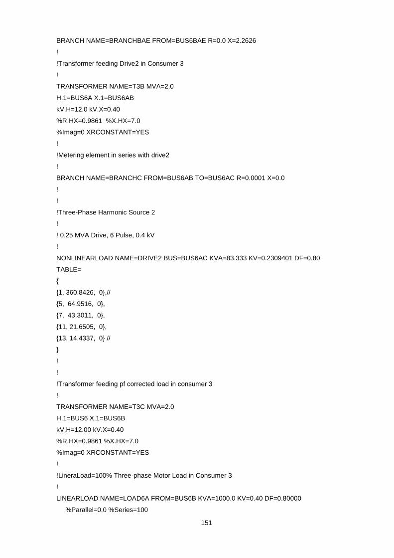
151

BRANCH NAME=BRANCHBAE FROM=BUS6BAE R=0.0 X=2.2626

!

!Transformer feeding Drive2 in Consumer 3

!

TRANSFORMER NAME=T3B MVA=2.0

H.1=BUS6A X.1=BUS6AB

kV.H=12.0 kV.X=0.40

%R.HX=0.9861 %X.HX=7.0

%Imag=0 XRCONSTANT=YES

!

!Metering element in series with drive2

!

BRANCH NAME=BRANCHC FROM=BUS6AB TO=BUS6AC R=0.0001 X=0.0

!

!

!Three-Phase Harmonic Source 2

!

! 0.25 MVA Drive, 6 Pulse, 0.4 kV

!

NONLINEARLOAD NAME=DRIVE2 BUS=BUS6AC KVA=83.333 KV=0.2309401 DF=0.80

TABLE=

1, 360.8426, 0,//

5, 64.9516, 0,

7, 43.3011, 0,

11, 21.6505, 0,

13, 14.4337, 0 //

!

!

!Transformer feeding pf corrected load in consumer 3

!

TRANSFORMER NAME=T3C MVA=2.0

H.1=BUS6 X.1=BUS6B

kV.H=12.00 kV.X=0.40

%R.HX=0.9861 %X.HX=7.0

%Imag=0 XRCONSTANT=YES

!

!LineraLoad=100% Three-phase Motor Load in Consumer 3

!

LINEARLOAD NAME=LOAD6A FROM=BUS6B KVA=1000.0 KV=0.40 DF=0.80000

%Parallel=0.0 %Series=100

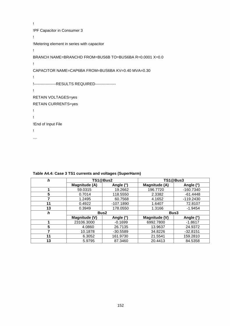
152

!

!PF Capacitor in Consumer 3

!

!Metering element in series with capacitor

!

BRANCH NAME=BRANCHD FROM=BUS6B TO=BUS6BA R=0.0001 X=0.0

!

CAPACITOR NAME=CAP6BA FROM=BUS6BA KV=0.40 MVA=0.30

!

!-----------------RESULTS REQUIRED----------------

!

RETAIN VOLTAGES=yes

RETAIN CURRENTS=yes

!

!

!End of Input File

!

....

Table A4.4: Case 3 TS1 currents and voltages (SuperHarm)

h TS1@Bus2 TS1@Bus3

Magnitude (A) Angle (°) Magnitude (A) Angle (°)

1 59.0315 19.2662 196.7720 -160.7340

5 0.7014 118.5550 2.3382 -61.4448

7 1.2495 60.7568 4.1652 -119.2430

11 0.4922 -107.1890 1.6407 72.8107

13 0.3949 178.0550 1.3166 -1.9454

h Bus2 Bus3

Magnitude (V) Angle (°) Magnitude (V) Angle (°)

1 23106.3000 -0.1699 6992.7800 -1.8617

5 4.0860 26.7135 13.9637 24.9372

7 10.1878 -30.5589 34.8226 -32.8151

11 6.3052 161.9730 21.5541 159.2810

13 5.9795 87.3460 20.4413 84.5358

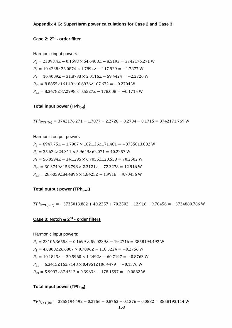
153

Appendix 4.G: SuperHarm power calculations for Case 2 and Case 3

Case 2: 2nd - order filter

Harmonic input powers:

Total input power (TPh(in))

Harmonic output powers

Total output power (TPh(out))

Case 3: Notch & 2nd - order filters

Harmonic input powers:

Total input power (TPh(in))

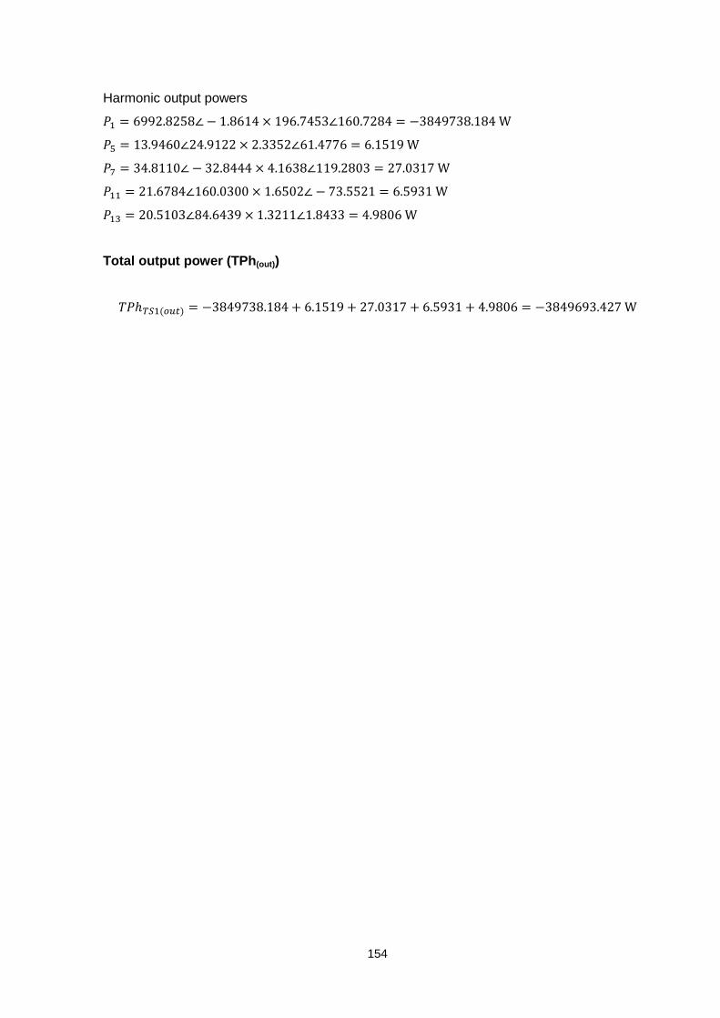
154

Harmonic output powers

Total output power (TPh(out))