Floods in a Changing Climate

Pradeep MujumdarIISc Bangalore

ICFM Webinar No.5

Rescue Operations in ChamoliSource: business-standard.com

Glacier break off in UttarakhandSource: newindianexpress.com

Hydropower plant in Uttarakhand damaged bythe flash floods

Source: indiatoday.in

Himalayan Floods (Uttarakhand) Feb 2021

Overview:• Date of occurrence: 7th February 2021

• Location: Garhwal Himalayas in Uttarakhand state, India -Tapovan area of Joshimath in Chamoli district

• 70 deaths

• Area affected: 60 square kms

• Flood occurred in the RishigangaRiver, tributary of Dhauliganga River,originating from Raikhana glacier

• Disruption of 4 hydropower projects:Rishiganga HP, Tapovan VishnugadHP, Vishnuprayag HP, VishnugadPipalkoti HP

• Deluge wiped out 5 bridges, some ofwhich ran 40 feet above typical riverlevels

Sources: www.icimod.org, www.sciencenews.org,

Source: reliefweb.int

2

(Possible) Causes of the Flood:• It is believed to have been caused by a landslide, an avalanche or a glacial lake outburst flood

• Initial reports suggested that the flood was caused due to the Glacier Lake Outburst (GLOF) howeverthere were no lakes visible in the satellite images upstream of the area flooded;

• Rockslide that occurred 22kms upstream of the river lead to a cascading impact, carrying debris, ice,snowmelt and running river water, causing sedimentation all along the way and damaging fourhydropower projects in the flood path.

• Rockslide is possibly caused by the avalanche, occurred somewhere between 19 September to 9October 2016, that displaced huge mass of ice, debuttressing a huge surface area of the rock, exposing itto frequent freeze-thaw cycles (however, this cannot explain the 150m depth of the rock displaced, asfreezing and thawing would only affect first 10 m of the rock), possibly combined with a seismic activity.

• It is also suggested that a hanging glacier "15 football fields long and five across" had separated from amountain and plummeted into the Ronti Gad, a tributary of the Rishiganga (Source : Wikipedia;Scientific American, Feb 2021)

Sources: www.icimod.org, www.sciencenews.org, www.business-standard.com

Sl. No. Description Amount in INR

(Crores)Amount in USD

(Millions)

1 Four Hydropower projects 1500 206.85

2 53 Road Projects 12072 1664.71

Economic Losses (Damaged Infrastructure)

Source: www.business-standard.com 3

Kerala Flood 2018

An aerial view of partially submerged houses inKeralaSource : www.bbc.com

Cyclonic storm near the coastal areadue to depression in Arabian seaSource: www.scroll.in

Transportation of residents to emergencyrelief campsSource : www.theguardian.com

Cumulative rainfall recorded from10th to 16th August 2018Source : www.bbc.com

Kerala before and after the floods, released by NASA.The images are false-colour, which makes flood waterappear dark blue and vegetation bright green.Source : www.wikipedia.org

Flood affected and landslideaffected villagesSource : www.sdma.kerala.gov.in

Overview:• Period: July - August 2018

• 11 of Kerala’s 14 districts were severelyaffected

• 433 deaths; over 5.4 million people affected,displaced 1.4 million people

• Kerala received 2346.6 mm rainfall betweenJune 1 and August 19, 2018, which is about42% higher than the normal rainfall of 1649.5mm during the same period

• 1260 out of 1664 villages were affected, 687km2 land flooded, 14315 houses fullydamaged, 270000 houses partially affected,0.15 Million Ha of standing crops damaged,751000 poultry, and 7953 domestic animalslost, 3 million electric connections damaged,510 bridges and culverts damaged, 9538 kmof major roads and 77328 km of rural roadsdestroyed

• Total economic loss approximately Rs.31000Crore

Sources: www.business-standard.com, reliefweb.int,india.mongabay.com,

Causes:• Rainfall during June, July, and August 1-19, 2018 was 15%, 18% and 164% respectively

above normal rainfall

• Flood was due to the combined effects of perigean spring tide and strong onshore winds

• Alteration in land use during the past decades with increase in built up area and reduction in

water bodies and vegetation also majorly contributed to the floods

Sources: thewire.in, reliefweb.int, india.mongabay.com, Hunt, et. Al. 2020

Economic lossesSl. No.

Description Amount in INR (Crores)

Amount in USD(Millions)

1 Tea industry 35-40 4.82-5.522 Rubber sector 420 57.923 Airport 40 5.524 Roads 12000 1654.76

Source : www.business-standard.com

Photos from the devastating Chennai floods of 2015

Source: indiatimes.com, skymetweather.com

Chennai Floods 2015

Accumulated rainfall between November 29 and December 2 over Chennai and

neighbourhood measured by NASA's GPM satellites

Source: Frontline, 2015b

Chennai city's land-cover Source: Sundaram, map

India, 2009

Flood inundation map of Chennai Floods 2015

Source: Citizen’s report on the 2015 floods in Chennai

Overview:• Duration: November 2015 to

December 2015• Over 400 deaths ; 2.3 million houses

inundated• Caused disruption of power and

telecommunication services, haltedair, rail and road transport, andextensive public and private propertydamage

• Rainfall received in November 2015was 121.86, which was thrice theusual rainfall, 40.74 cm

• The rainfall received on December 1st

, 2015 was 19.1 cm, a 100 year recordbreaking rainfall event

• Extremely high releases from twoupstream reservoirs aggravated thefloods

Sources: www.cag.org.in, Audit report on Chennai Floods 2015, B. Narasimham et. al., 2016

Economic Losses – Chennai Floods, 2015

Sl. No. Description Amount in INR

(Crores)Amount in USD

(Millions)

1 Chennai Real Estate 30000 4136.94

2 Small & Medium Industrial Units(Entire Tamil Nadu) 14000 1930.57

3 Insurance Companies 4800 661.91

4 Street vendors 225 31.03

B. Narasimham et. al., 2016

Kashmir Floods 2014

Tens of thousands of homes have beendestroyed by flash floods andlandslides on the border of India andPakistanSource : www.dailymail.co.uk

Transportation of residents toemergency relief campsSource: www.oneindia.com

Cumulative flood inundationspatial extent (light bluecolour) observed in KashmirValley between 8 and 25September 2014.Source : Bhatt et al., (2017)

Precipitation analysis (mm) formed from themerger of IMD rain-gauge data with the TRMMTMPA satellite-derived rainfall estimates from 3to 6 September 2014Source: Ray et al.,(2015)

Overview:• Duration: 2nd to 26th September 2014

• Heavy monsoon rainfall commenced on 2nd

September 2014 and continued for 5 daysand led to unprecedented widespreadflooding and landslide

• 277 people in India died due to the floodswith economic losses of 1 trillion INR

• Banks of the river Jhelum, Chenab, Tawi andmany other streams were burst

• About 557 km2 of the Kashmir Valley'sgeographical area was inundated

• 5642 villages were affected across the statewith 2489 in Kashmir valley, 3153 in Jammudivision and 800 villages remained sub-merged for over two weeks

• Damaged 2,61,361 structures, 3,27,000hectares of agricultural land and 3,96,000hectares of horticultural land

Sources: scroll.in, reliefweb.int, hwnews.in

Causes:• As per IMD, Jammu and Kashmir received 1645 mm rainfall in South Kashmir area which was way

above the normal rainfall (124.9 mm) from 28th August to 10th September 2014

• Manmade rampant alteration on the natural landscape, increasing global temperature, an increase in

habitation in high slope zones and deforestation were the main causes

• Rapid urbanisation, degradation and depletion of wetlands and unrestrained land-use changes with a

huge increase in built up area from 18.10 sq. km to 84.50 sq. km (29.20%) between the year 1972-

2004 also favoured the flood conditions

• Flat topography of the basin and blockage of natural drainage channel with dense settlement caused

water logging in the areaSources: Ray, Kamaljit, et. Al., 2015, http://www.iwrs.org.in, www.ncbi.nlm.nih.gov, http://www.mcrhrdi.gov.in

Economic lossesSl. No. Description Amount in INR

(Crores)Amount in USD

(Millions)

1 Housing sector 30,000 4137.69

2 Business sector 70,000 9654.62

3 Horticulture sector 5,611 773.886

4 Tourism infrastructure and government residentialcolonies 5,000 689.615 Source : Tabish et al.,(2015)

“Value of Water” : Issues of of Interest

• We must account for the mammoth losses due to floods within the framework of “Value of Water”, in a Changing Climate.

Research Questions:

• Are the high intensity precipitation events increasing – globally, regionally, locally? If yes, is such an increase due to climate change?

• How do we estimate the changing frequencies of high intensity precipitation/streamflow; changing flood risk and vulnerability?

• Has the hydrologic response of the catchments deteriorated over the years because of landuse change?

• Can we use hydrologic models with high resolution NWP models to reconstruct past floods and forecast the future ones?

10

11

IPCC (2012)

103.68

88.46

66.48 63.41

56.18

47.0424.24

19.93

22.6313.25

7.42

Increase in Urban Precipitation Intensities: Bangalore city

10 year Return Period

12

13

Urban Flooding

Bangalore Floods

Likely changes in IDF (Intensity-Duration-Frequency) relationships due to climate change

How do the short term intensities of rainfall respond to the climate change?

14

Downscaling

15

The developing culture of prophesising the future, guided by deterministic climate modelling approaches, has seriously affected hydrology. Therefore, aspired advances are related to abandoning the certainties of deterministic approaches and returning to stochastic descriptions, seeking in the latter theoretical consistency and optimal use of available data.

Demetris Koutsoyiannis (2021)

Advances in stochastics of hydroclimatic extremes, L’ ACQUA 1/2021

GCM model with future climate scenarios and latitude-longitudeModel Name Latitude Longitude Abbreviation Climate Scenarios

ACCESS1_0 12.5 N 76.875 E A1 RCP 4.5, RCP 8.5

BCC-CSM1-1 12.55 N 78.75 E BC1 RCP 2.6, RCP 4.5, RCP 6.0, RCP 8.5

BCC-CSM1-1-M 12.89 N 77.6 E BC1M RCP 2.6, RCP 4.5, RCP 6.0, RCP 8.5

BNU-ESM 12.55 N 78.75 E BNU RCP 2.6, RCP 4.5, RCP 8.5

CanESM2 12.55 N 78.7 E CAN RCP 2.6, RCP 4.5, RCP 8.5

CCSM4 12.7225 N 77.5 E C4 RCP 2.6, RCP 4.5, RCP 6.0, RCP 8.5

CMCC-CMS 12.1 N 76.8 E CMS RCP 4.5, RCP 8.5

CNRM-CM5 11.9 N 77.34 E CN5 RCP 4.5, RCP 8.5

CSIRO-MK3-6-0 12.12 N 76.875 E CM60 RCP 2.6, RCP 4.5, RCP 6.0, RCP 8.5

FGOALS-G2 12.55 N 78.75 E FG2 RCP 2.6, RCP 4.5, RCP 8.5

FGOALS-S2 12.4 N 75.9 E FS2 RCP 2.6, RCP 4.5, RCP 6.0, RCP 8.5

GFDL-CM3 13 N 78.75 E GF3 RCP 2.6, RCP 6.0

GFDL-ESM2G 13.14 N 76.25 E GF2G RCP 2.6, RCP 4.5, RCP 6.0, RCP 8.5

GFDL-ESM2M 13.14 N 76.25 E GF2M RCP 2.6, RCP 4.5, RCP 6.0, RCP 8.5

GISS-E2-R 13 N 76.25 E GISS RCP 4.5

HadGEM2-CC 12.5 N 76.87 E HADC RCP 4.5, RCP 8.5

HadGEM2-ES 12.5 N 76.875 E HADE RCP 2.6, RCP 4.5, RCP 6.0, RCP 8.5

INMCM4 12.75 N 78 E IN4 RCP 4.5, RCP 8.5

IPSL-CM5A-LR 12.31 N 78.75 E IPCL RCP 2.6, RCP 4.5, RCP 6.0, RCP 8.5

IPSL-CM5A-MR 12.6 N 77.5 E IPCM RCP 2.6, RCP 4.5, RCP 6.0, RCP 8.5

MIROC5 11.9 N 78.75 E MI5 RCP 2.6, RCP 4.5, RCP 6.0, RCP 8.5

MIROC-ESM-CHEM 12.55 N 78.75 E MIEC RCP 2.6, RCP 4.5, RCP 6.0, RCP 8.5

MIROC-ESM 12.55 N 78.75 E MIE RCP 2.6, RCP 4.5, RCP 6.0, RCP 8.5

MPI-ESM-LR 12.12 N 78.75 E MPI RCP 2.6, RCP 4.5, RCP 6.0, RCP 8.5

MRI-CGCM3 12.89 N. 77.62 E MRI RCP 2.6, RCP 4.5, RCP 6.0, RCP 8.5

NorESM1-M 12.31 N 77.5 E NEM RCP 2.6., RCP 4.5, RCP 6.0, RCP 8.5

16

Model Uncertainty

Bangalore City : Projected change in the IDF Relationship :- CMIP5 models with AR5 scenarios (85 simulations; uncertainty with REA)

CMIP 5 Ensemble

Downscaling (Daily Scale) Rainfall

Stochastic Disaggregation

Hourly and Sub-hourly Scale Rainfall Intensity

Ensemble Averaged Projections

CLIMATE CHANGE IMPACTS

d d dt tE Z E Zbl lé ù é ù=ë û ë û

The quantiles and raw moments of any order are scale invariant; d is the order of the moment.

Scale invariance

Hydromet Model Simulation Workflow forSep 8-9, 2020 Extreme Event over Bangalore

Forecast data generated at Sep 7, 2020, 6 pm for the next 72 hours is given as boundary conditions to run the WRF model.

One dimensional model using SWMM which are calibrated and validated

using various rainfall eventsHECRAS 2D Model is developed for flood

inundation

9 km

3 km

25 km 05

1015202530

9/8/

2020

0:0

09/

8/20

20 2

:45

9/8/

2020

5:3

09/

8/20

20 8

:15

9/8/

2020

11:

009/

8/20

20 1

3:45

9/8/

2020

16:

309/

8/20

20 1

9:15

9/8/

2020

22:

009/

9/20

20 0

:45

9/9/

2020

3:3

09/

9/20

20 6

:15

9/9/

2020

9:0

09/

9/20

20 1

1:45

9/9/

2020

14:

309/

9/20

20 1

7:15

9/9/

2020

20:

009/

9/20

20 2

2:45R

ainf

all (

mm

)

The rainfall corresponding to each station is extracted from the WRF 3 km gridded output.

18

September 16, 2019 June 25, 2020

VrishabhavathinagarWLS

Magadi Road M S WLS

Flood Modelling using PCSWMM

The model is capable to capture peak flows in comparison with the observed water levels as shown.

Water Levels in SWD

RMSE = 0.833 R square = 0.518

RMSE = 0.693 R square = 0.367

Water Levels in SWD

RMSE = 0.718 R square = 0.705

Water Levels in SWD

RMSE = 0.536 R square = 0.729

Water Levels in SWD

20

• Traditional frequency analysis cannot reveal anything about the interacting processes.• Therefore, statistical approaches which can enhance process based understanding are requiredin hydrology to improve the prediction of floods and droughts.

• River flooding is not merely the result of highrainfall.

• Other mechanisms such as antecedent soilmoisture conditions and snowmelt contributesto excess runoff in most of the catchments.

1) Which flood generating mechanism isdominant in the river basin?

2) Are the interactions of multiple processescausing floods?

3) Out of multiple interacting physicalmechanisms, which interaction is dominant?

21

¢ Recent high impact extremesprovide evidences forinterconnections of extremes.

How often an extreme event can be equalled

or exceeded?

Accurate estimation of probabilities of extremes is essential for planningrisk management strategies and taking preventive actions.

Univariate vs multivariate return periods. From: AghaKouchak et al. (2014)

Global warming and the associated increase in extreme temperatures substantially increase the chance of concurrent droughts and heatwaves.

Blue : univariateRed : Multi-variate

Slide credit : Shailza Sharma

22Source: Unnikrishnan and Shankar (2007)

Rise in Sea Levels

Sea

Leve

l (m

m)

Sea level rise in India

Black : Univariate, present climateRed : Bivariate, Present ClimateOther colors (except blue) : future climate

Storm Surge : a rising of the sea as a result of wind and atmospheric pressure changes associated with a storm.

Heavy rainfall for 4 consecutive days(June 14 to June 17)

(Uttarakhand 2013 Floods)

23

Incessant heavy rainfall (Sept 2 to Sept 6)

(Kashmir 2014 Floods)

Prolonged high intensity rainfall (July-August)

(Kerala 2018 Floods)

• Extreme rainfall for a few consecutive days leads to saturation of soil, whichreduces infiltration and increases surface runoff.

• This excess runoff results in stagnation of water in urban areas and increase inwater levels of rivers.

• Such flooding situations are arising more frequently; therefore it is important toinclude such changes in frequency analysis

A continuous spell of extreme rainfall has devastating consequences compared to asingle day extreme rainfall event.

24

log$%

(201

0/19

80)

An increase is observed in the probabilities ofextreme rainfall spells for both the sites.

Heavy rainfall for 4 consecutive days(June 14 to June 17)

(Uttarakhand 2013 Floods)

What happens to the concept of ‘return period’ under non-stationarity?

25

Columbia River: Projections

26

� The macroscale VIC model is run at a spatial resolution of 1/16th degree latitude and longitude (Hamlet and Lettenmaier (2005))

� Bias corrected and spatially downscaled (BCSD) meteorological forcings used in the VIC for the IPCC A1B and B1 scenarios for 1950-2097

Slide credit : Arpita Mondal

Time of detection – floods in the Columbia River

27

Model Reconstruction of Uttarakhand Floods 2013

28

Upper Ganga Basin (UGB)

Figure 1: Topography of the study region (shown with black outline) as represented in the WRF model for (i) Domain 1 – 27 km grid spacing; (ii) Domain 2a – 9 km grid spacing (downscaling ratio – 1:3); and (iii) Domain 2b –3 km grid spacing (downscaling ratio – 1:9). Locations of the rain gauge stations within the UGB are presented as

black dots in Figure 1 (iii).29

Simulation of Flood Events

Figure. Flood discharge simulations obtained from (a) the WRF-VIC coupled model, and the stand-aloneVIC model driven using (b) the TMPA data, and (c) the reanalysis datasets for the three events underconsideration. The coupled WRF-VIC system is seen to give least bias in the simulated flood discharges.30

WRF Model for Rainfall Simulation

VIC Hydrologic Model for Flow Simulation

¢The concept of “Value of Water” must account forthe mammoth losses due to floods. This necessitatesan improved assessment of evolving flood risk andvulnerability at a range of space-time scales.

¢Intensities of rainfall are known to be increasingacross different space-time scales.

¢Scale issues and uncertainties need to be addressedin quantification of the likely changes in the floodrisk and vulnerability under climate change.

¢Coupled weather forecasting and hydrologic modelsare needed for developing reliable flood forecasts.

31

SUMMARY

Thank You

32

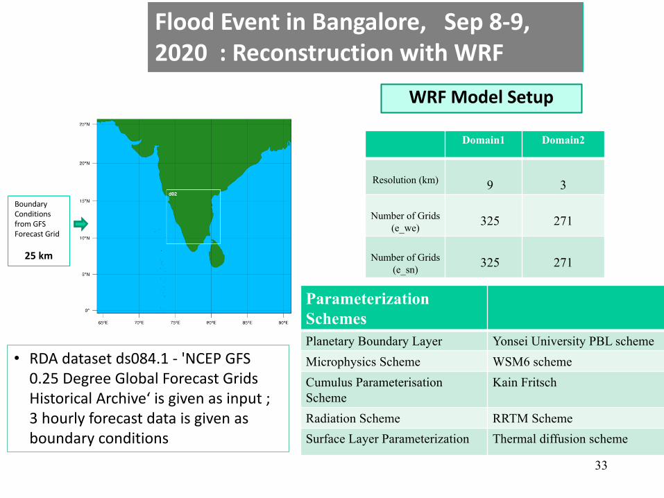
Flood Event in Bangalore, Sep 8-9, 2020 : Reconstruction with WRF

Domain1 Domain2

Resolution (km) 9 3

Number of Grids (e_we) 325 271

Number of Grids (e_sn) 325 271

Boundary Conditions from GFS Forecast Grid

25 km

9 km

3 km

WRF Model Setup

ParameterizationSchemesPlanetary Boundary Layer Yonsei University PBL scheme

Microphysics Scheme WSM6 scheme

Cumulus ParameterisationScheme

Kain Fritsch

Radiation Scheme RRTM Scheme

Surface Layer Parameterization Thermal diffusion scheme

• RDA dataset ds084.1 - 'NCEP GFS 0.25 Degree Global Forecast Grids Historical Archive‘ is given as input ; 3 hourly forecast data is given as boundary conditions

33

Spatial Distribution of Rainfall on September 8, 2020

WRF ModelObserved TRG data (KSNDMC)

0

10

20

30

40

50

60

1 2 3 4 5 6 7 8 9 10 11 12 13 14 15 16 17 18 19 20 21 22 23 24 25 26 27 28 29 30 31 32 33 34 35 36 37 38 39 40 41

Rai

nfal

l Acm

ulat

ed fo

r Se

p 8

TRG Stations

Station Data vs WRF Grid values WRF OBS

RMSE (%) MAE (%)

17.82 12.81

34

Rainfall Data – June 2013

Figure 2: Observed daily and cumulative rainfall along with historic monthly mean (2004–2010) values at the 18 rain gauges in the upstream region of the UGB.

35

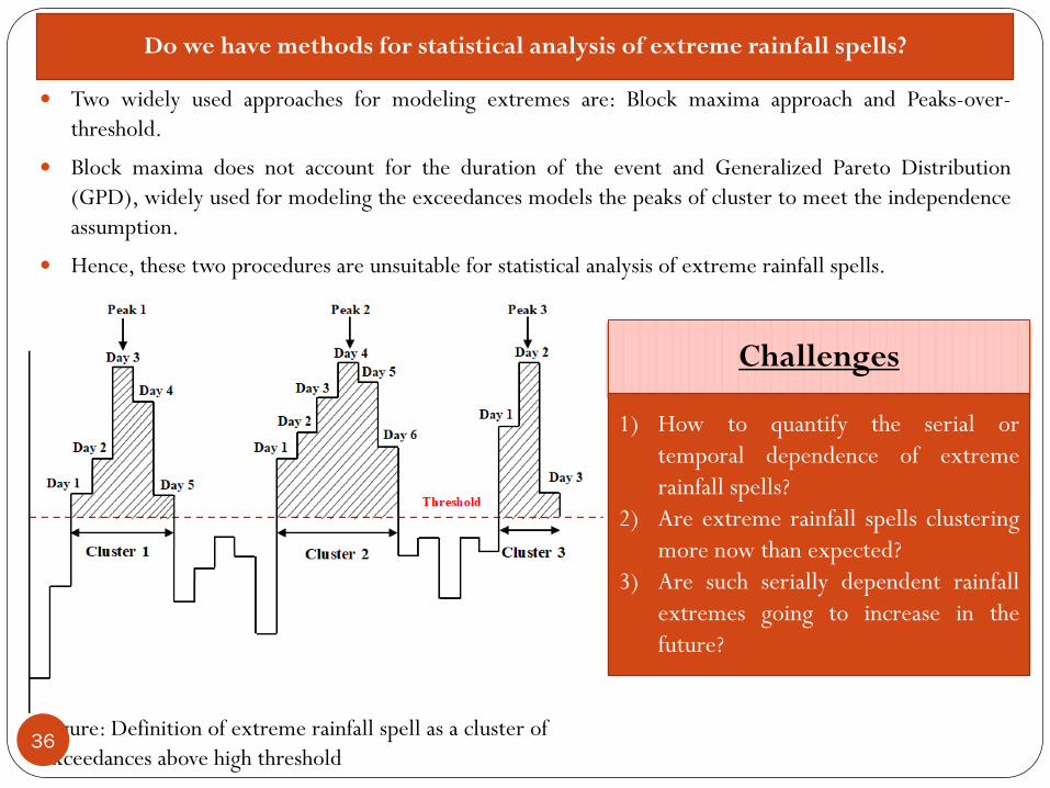
� Two widely used approaches for modeling extremes are: Block maxima approach and Peaks-over-threshold.

� Block maxima does not account for the duration of the event and Generalized Pareto Distribution(GPD), widely used for modeling the exceedances models the peaks of cluster to meet the independenceassumption.

� Hence, these two procedures are unsuitable for statistical analysis of extreme rainfall spells.

Do we have methods for statistical analysis of extreme rainfall spells?

Figure: Definition of extreme rainfall spell as a cluster of exceedances above high threshold

Challenges

1) How to quantify the serial ortemporal dependence of extremerainfall spells?

2) Are extreme rainfall spells clusteringmore now than expected?

3) Are such serially dependent rainfallextremes going to increase in thefuture?

36

37

compound events can be (1) two or more extremeevents occurring simultaneously or successively, (2) combinations ofextreme events with underlying conditions that amplify the impact ofthe events, or (3) combinations of events that are not themselvesextremes but lead to an extreme event or impact when combined.

A changing climate can be expected to lead to changes in climate and weather extremes. But it is challenging to associate a singleextreme event with a specific cause such as increasing greenhouse gases because a wide range of extreme events could occur even inan unchanging climate, and because extreme events are usually caused by a combination of factors. Despite this, it may be possible tomake an attribution statement about a specific weather event by attributing the changed probability of its occurrence to a particularcause. For example, it has been estimated that human influences have more than doubled the probability of a very hot European summerlike that of 2003.

38

PMP – It is the greatest or the extreme rainfall for a given duration that is physically possible over a raingauge station or a basin. It is that rainfall over a basin which would produce a flood with no risk of being exceeded.

Probable Maximum Flood (PMF). The largest flood that could conceivably be expected to occur at a particular location, usually estimated from probable maximum precipitation. The PMF defines the maximum extent of flood prone land, that is, the floodplain. It is difficult to define a meaningful Annual Exceedance Probability for the PMF, but it is commonly assumed to be of the order of 104 to 107(once in 10,000 to 10,000,000 years) (10).

For multivariate analysis, copulas (which are non-parametric models) are used to address the dependence among different variables. Shailzas work deals with developing parametric models.