
Flight Delay-Cost Simulation Analysis and Airline Schedule ...
194
Flight Delay-Cost Simulation Analysis and Airline Schedule Optimization A thesis submitted in fulfillment of requirement for the degree of Doctor of Philosophy Duojia Yuan B. Eng. School of Aerospace, Mechanical and Manufacturing Engineering Faculty of Science, Engineering and Technology RMIT University, Victoria, Australia February 2007
-
Upload
khangminh22 -
Category
Documents
-
view
2 -
download
0
Transcript of Flight Delay-Cost Simulation Analysis and Airline Schedule ...
Flight Delay-Cost Simulation Analysis and
Airline Schedule Optimization
A thesis submitted in fulfillment of requirement for the
degree of Doctor of Philosophy
Duojia Yuan
B. Eng.
School of Aerospace, Mechanical and Manufacturing Engineering
Faculty of Science, Engineering and Technology
RMIT University, Victoria, Australia
February 2007

Declaration
I certify that except where due acknowledgement has been made, the work is that of
the author alone; the work has not been submitted previously, in whole or in part, to
qualify for any other academic award; the content of the thesis is the result of work
which has been carried out since the official commencement date of the approved
research program; and any editorial work, paid or unpaid, carried out by a third party
is acknowledged.
Duojia Yuan
February 2007

To My Son Runxing Yuan

Abstract
I
Abstract
Flight Delay-Cost Simulation Analysis and Airline Schedule Optimization
By
Duojia YUAN
In order to meet the fast-growing demand, airlines have applied much more
compact air-fleet operation schedules which directly lead to airport congestion. One
result is the flight delay, which appears more frequently and seriously; the flight delay
can also significantly damage airline’s profitability and reputation
The aim of this project is to enhance the dispatch reliability of Australian X
Airline’s fleet through a newly developed approach to reliability modeling, which
employs computer-aided numerical simulation of the departure delay distribution and
related cost to achieve the flight schedule optimization.
The reliability modeling approach developed in this project is based on the
probability distributions and Monte Carlo Simulation (MCS) techniques. Initial (type
I) delay and propagated (type II) delay are adopted as the criterion for data
classification and analysis. The randomicity of type I delay occurrence and the
internal relationship between type II delay and changed flight schedule are considered
as the core factors in this new approach of reliability modeling, which compared to
the conventional assessment methodologies, is proved to be more accurate on the

Abstract
II
departure delay and cost evaluation modeling.
The Flight Delay and Cost Simulation Program (FDCSP) has been developed
(using Visual Basic 6.0) to perform the complicated numerical calculations through
significant amount of pseudo-samples. FDCSP is also designed to provide
convenience for varied applications in dispatch reliability modeling. The end-users
can be airlines, airports and aviation authorities, etc.
As a result, through this project, a 16.87% reduction in departure delay is
estimated to be achieved by Australian X Airline. The air-fleet dispatch reliability has
been enhanced to a higher level – 78.94% compared to initial 65.25%. Thus, 13.35%
of system cost can be saved.
At last, this project also achieves to set a more practical guideline for air-fleet
database and management upon overall dispatch reliability optimization.

Acknowledgement
III
Acknowledgement
As for anyone else, a dissertation is a milestone as well as a journey in my life
full of challenges. Without the help and support from many people, the completion of
this work would have been impossible. Although a few words do not justice to their
contribution I would like to thank the following people for making this dissertation
possible.
I would like to express my gratitude to my supervisor, Dr. He Ren. I thank him
for leading me into the research field. His generous encouragement, continuing
support and guidance throughout the course of the research work have made this
dissertation possible.
I would also like to thank Mrs. Xiaoyang Sun, Jo Connolly, Mr. Tianlun Yuan,
Erjiang Fu, Richard Zhou, and Miss Xiaojie Bai for their data providing, comments
and suggestions during the process of this thesis.
My thanks also go to other friends who work or study in RMIT, Thanks for the
various help I got from them and the precious time we spent together.
Finally, and most importantly, I wish to thank my family members, especially my
parents, Ding Yuan and Dafeng Zhang, for their endless patience and support. Thank
you for sharing both my enjoyment and endurance.

Table of Contents
IV
Table of Contents
ABSTRACT............................................................................................................................................. I
ACKNOWLEDGEMENT................................................................................................................... III
TABLE OF CONTENTS..................................................................................................................... IV
LIST OF FIGURES ............................................................................................................................VII
LIST OF TABLES.............................................................................................................................VIII
CHAPTER 1 INTRODUCTION .................................................................................................... 1
1.1 COMMERCIAL AVIATION INDUSTRY BACKGROUND FACT ......................................................... 1
1.2 BASIC PRINCIPLES.................................................................................................................... 3
1.2.1 Flight Delay & Delay Propagation..................................................................................... 3
1.2.2 Simulation Methodology ..................................................................................................... 5
1.2.3 Cost Model Analysis............................................................................................................ 7
1.3 PROJECT SCOPE & OBJECTIVES................................................................................................ 7
1.4 THESIS STRUCTURE.................................................................................................................. 9
CHAPTER 2 LITERATURE REVIEW........................................................................................11
2.1 RELIABILITY ENGINEERING EVOLUTION .................................................................................11
2.1.1 Basic Concepts.................................................................................................................. 12
2.1.2 The Development History of Reliability ............................................................................ 14
2.2 THE CONVENTIONAL RELIABILITY METHODOLOGIES DEVELOPMENT ................................... 17
2.3 DEVELOPMENT OF FUZZY RELIABILITY ................................................................................. 24
2.4 MONTE CARLO SIMULATION METHODOLOGY........................................................................ 28
2.5 DISPATCH RELIABILITY & DELAY COST ................................................................................. 32
2.6 SCHEDULING ISSUES IN AIRLINES OPERATION MANAGEMENT ............................................... 38
2.7 AIRPORT OPERATION MANAGEMENT, RELATED RUNWAY CONGESTION AND FLIGHT DELAY. 41
2.8 USA HISTORICAL DATA COLLECTION & ANALYSIS................................................................ 48
CHAPTER 3 BASIC CONCEPTIONS & RELEVANT DEFINITIONS.................................. 52
3.1 DEFINITION OF RELEVANT CONCEPTIONS .............................................................................. 52
3.2 DEPARTURE PROCESS ANALYSIS ............................................................................................ 59
3.3 DELAY CLASSIFICATION & CRITERIA ..................................................................................... 62
3.4 CREW/AIRCRAFT TURNAROUND PROCESS AND RELEVANT REGULATIONS............................. 65
3.4.1 Crewmember Turnaround Process & Availability Regulation .......................................... 65
3.4.2 Regulation Related to Aircraft Availability ....................................................................... 69
CHAPTER 4 TYPE I DELAY ANALYSIS AND MODELING ................................................. 72
4.1 INTRODUCTION ...................................................................................................................... 72
4.2 TYPE I DELAY CAUSES........................................................................................................... 73
4.3 DATA COLLECTION................................................................................................................. 74
4.4 AUSTRALIAN DATA ANALYSIS................................................................................................ 75
Table of Contents
V
4.5 DISPATCH RELIABILITY MODELING........................................................................................ 79
4.5.1 Assumptions ...................................................................................................................... 79
4.5.2 Dispatch Reliability Model ............................................................................................... 80
4.6 TYPE I DELAY MODELING SUMMARY .................................................................................... 83
CHAPTER 5 DELAY COST MODELING ................................................................................. 85
5.1 INTRODUCTION ...................................................................................................................... 85
5.2 ANALYSIS OF THE PROBLEM................................................................................................... 86
5.3 AIRPORTS FEE STRUCTURE .................................................................................................... 88
5.3.1 Landing Fee ...................................................................................................................... 89
5.3.2 Aircraft Parking and Hanger Fee ..................................................................................... 89
5.3.3 The Passengers Fee .......................................................................................................... 90
5.3.4 Other Aeronautical Fee..................................................................................................... 91
5.3.5 Airport Price Regulation in Australia ............................................................................... 91
5.4 PASSENGER DELAY COST ....................................................................................................... 94
5.5 AIRCRAFT SCHEDULED TIME COST........................................................................................ 95
5.6 OTHER RELEVANT DELAY COST............................................................................................. 97
5.7 THE FACTORS OF DELAY COST............................................................................................... 98
5.8 DATA COLLECTION & ANALYSIS .......................................................................................... 102
5.8.1 Data Collection............................................................................................................... 102
5.8.2 Analysis ........................................................................................................................... 102
5.9 ASSUMPTIONS ...................................................................................................................... 104
5.10 DEPARTURE DELAY COST MODELING .................................................................................. 104
5.10.1 Parking Cost ............................................................................................................... 104
5.10.2 Airline Crewmember/Staff Cost................................................................................... 105
5.10.3 Passenger Cost ........................................................................................................... 105
5.10.4 Other Aeronautical cost .............................................................................................. 106
5.10.5 The Sum of Delay Cost................................................................................................ 106
5.11 SAMPLE CALCULATION ........................................................................................................ 107
5.12 SUMMARY .............................................................................................................................111
CHAPTER 6 TYPE II DELAY MODELING AND MONTE CARLO SIMULATION .........113
6.1 INTRODUCTION .....................................................................................................................113
6.2 TYPE II DELAY MODELING METHODOLOGY .........................................................................115
6.3 MODELING WITH MONTE CARLO SIMULATION .....................................................................118
6.3.1 Radom Number Definition ...............................................................................................118
6.3.2 Arithmetic Model and Simulation Logic ..........................................................................119
6.3.3 The Model of Cost Computing ........................................................................................ 121
6.4 SOFTWARE DEVELOPMENT................................................................................................... 123
6.4.1 Software Flow Chart ....................................................................................................... 123
6.4.2 Software Language and Interface ................................................................................... 124
6.4.3 Process of Simulation...................................................................................................... 126
6.4.4 Software Function ........................................................................................................... 127
6.5 AUSTRALIAN X AIRLINE DELAY PROPAGATION SIMULATION............................................... 129
6.5.1 Assumptions and Data Processing.................................................................................. 129

Table of Contents
VI
6.5.2 Program Running Environment ...................................................................................... 130
6.5.3 Simulation ....................................................................................................................... 130
6.5.4 Error Analysis ................................................................................................................. 131
6.6 SUMMARY ............................................................................................................................ 132
CHAPTER 7 AUSTRALIAN X AIRLINE FLIGHT SCHEDULE OPTIMIZATION.......... 133
7.1 INTRODUCTION .................................................................................................................... 133
7.2 CURRENT AIR-FLEET OPERATION ANALYSIS ........................................................................ 134
7.3 OVERALL SYSTEM COST MODELING.................................................................................... 136
7.4 FLIGHT SCHEDULE OPTIMIZATION ....................................................................................... 138
7.4.1 Data Collection............................................................................................................... 138
7.4.2 Current Airlines Delay Situation Analysis ...................................................................... 138
7.4.3 Flight Schedule Optimization.......................................................................................... 142
7.4.4 Sensitivity Test and Analysis............................................................................................ 145
7.5 SUMMARY ............................................................................................................................ 154
CHAPTER 8 CONCLUSION ..................................................................................................... 156
REFERENCE..................................................................................................................................... 161
APPENDIX A LIST OF U.S. AIRPORTS USED IN THE RESEARCH ...................................... 170
APPENDIX B AIRPORT SLOT DEMAND MANAGEMENT TECHNIQUES.......................... 174
APPENDIX C SAMPLE OF X AIRLINE DEPARTURE DELAY DATA .................................... 178
APPENDIX D RANDOM NUMBER DEFINITION SHEET........................................................ 182
APPENDIX E OUTPUT FORM OF FDCSP .................................................................................. 183

List of Figures
VII
List of Figures
FIGURE 1.1-1 WORLD-WIDE GROWTH BY DOMICILED AIRLINES......................................................... 1
FIGURE 2.8-1 DEPARTURE AND DELAY INCREASE RATE...................................................................... 50
FIGURE 2.8-2 RATIO OF DELAY IN TOTAL DEPARTURE & THE INCREASED RATE OF DEPARTURE .... 51
FIGURE 4.4-1 PROPORTION OF DELAY ................................................................................................. 75
FIGURE 4.4-2 DELAY NUMBERS BY CAUSES ......................................................................................... 76
FIGURE 4.4-3 DEPARTURE DELAY TIME BY CAUSES............................................................................ 77
FIGURE 4.4-4 RATIO OF DELAY NUMBERS DISTRIBUTION................................................................... 77
FIGURE 4.4-5 RATIO OF DEPARTURE DELAY DISTRIBUTION ............................................................... 78
FIGURE 4.4-6 FLIGHT DAILY PEAKS..................................................................................................... 78
FIGURE 4.5-1 DELAY DENSITY FUNCTION............................................................................................ 82
FIGURE 5.11-1 DELAY COST PROPORTION BY FACTORS.................................................................... 109
FIGURE 5.11-2 COST DISTRIBUTION BY DELAY TIME ........................................................................ 109
FIGURE 5.11-3 TOTAL DELAY COST DISTRIBUTION............................................................................110
FIGURE 5.11-4 TOTAL DELAY COST PROPORTION BY DELAY TIME SEGMENT ..................................111
FIGURE 6.4-1 SOFTWARE FLOW CHART............................................................................................. 123
FIGURE 6.4-2 AIRPORT INFORMATION INPUT INTERFACE................................................................. 124
FIGURE 6.4-3 SCHEDULE INFORMATION INPUT INTERFACE.............................................................. 125
FIGURE 6.4-4 ITERATION TIMES SET INTERFACE .............................................................................. 126
FIGURE 7.4-1 PROPORTION OF DELAYED FLIGHTS BY DIFFERENT DELAY LENGTH........................ 140
FIGURE 7.4-2 PROPORTION OF TOTAL DELAY TIME BY DIFFERENT DELAY LENGTH ...................... 140
FIGURE 7.4-3 PROPORTION OF DELAY COST BY DIFFERENT DELAY LENGTH.................................. 141
FIGURE 7.4-4 STRUCTURE OF DELAY COST BY DIFFERENT DELAY LENGTH .................................... 142
FIGURE 7.4-5 OPTIMIZATION CURVE ................................................................................................. 144
FIGURE 7.4-6 OPTIMIZATION CURVE WITH -2% DEPARTURE DELAY .............................................. 146
FIGURE 7.4-7 OPTIMIZATION CURVE WITH -5% DEPARTURE DELAY .............................................. 147
FIGURE 7.4-8 OPTIMIZATION CURVE WITH -10% DEPARTURE DELAY ............................................ 148
FIGURE 7.4-9 OPTIMIZATION CURVE WITH -20% DEPARTURE DELAY ............................................ 149
FIGURE 7.4-10 OPTIMIZATION CURVE WITH +2% DEPARTURE DELAY ........................................... 150
FIGURE 7.4-11 OPTIMIZATION CURVE WITH +5% DEPARTURE DELAY............................................ 151
FIGURE 7.4-12 OPTIMIZATION CURVE WITH +10% DEPARTURE DELAY ......................................... 152
FIGURE 7.4-13 OPTIMIZATION CURVE WITH +20% DEPARTURE DELAY ......................................... 153

List of Tables
VIII
List of Tables
TABLE 2.8-1 STATISTICS OF DEPARTURE DELAY IN USA..................................................................... 49
TABLE 4.4-1 CAUSE OF DELAY.............................................................................................................. 76
TABLE 5.2-1 AIRLINES INFRASTRUCTURE AND COST RATE ................................................................ 87
TABLE 5.3-1 PARKING & LANDING FEE RATES.................................................................................... 90
TABLE 5.3-2 AIRPORT CHARGES RATES IN AUSTRALIA ...................................................................... 92
TABLE 5.7-1 DELAY COST FACTORS ..................................................................................................... 98
TABLE 5.11-1 RELATIVE PARAMETERS IN MODELING....................................................................... 107
TABLE 5.11-2 CALCULATION RESULTS ............................................................................................... 108
TABLE 6.5-1 RESULTS OF 100 ITERATION TIMES SIMULATION ......................................................... 130
TABLE 6.5-2 RESULTS OF 500 ITERATION TIMES SIMULATION ......................................................... 131
TABLE 6.5-3 RESULTS OF 1000 ITERATION TIMES SIMULATION ....................................................... 131
TABLE 6.5-4 ERROR ANALYSIS DATA ................................................................................................. 132
TABLE 7.4-1 COMPUTING RESULT OF CURRENT SCHEDULE ............................................................. 139
TABLE 7.4-2 ADDITIONAL GROUND BUFFER TIME OF DIFFERENT SCHEME .................................... 143
TABLE 7.4-3 OPTIMIZATION CALCULATION RESULT......................................................................... 144
TABLE 7.4-4 SCHEME COMPARISON ................................................................................................... 145
TABLE 7.4-5 OPTIMIZATION WITH -2% DELAY ................................................................................. 146
TABLE 7.4-6 OPTIMIZATION RESULT WITH -5% DELAY.................................................................... 147
TABLE 7.4-7 OPTIMIZATION RESULT WITH -10% DELAY.................................................................. 148
TABLE 7.4-8 OPTIMIZATION RESULT WITH -20% DELAY.................................................................. 149
TABLE 7.4-9 OPTIMIZATION RESULT WITH +2% DELAY................................................................... 150
TABLE 7.4-10 OPTIMIZATION RESULT WITH +5% DELAY................................................................. 151
TABLE 7.4-11 OPTIMIZATION RESULT WITH +10% DELAY ............................................................... 152
TABLE 7.4-12 OPTIMIZATION RESULT WITH +20% DELAY............................................................... 153

Introduction
1
Chapter 1 Introduction
1.1 Commercial Aviation Industry Background Fact
Based on the models of major traffic flow around the world, Airbus has done an
all-sided research (www.Airbus.com, 2004) on econometric modelling techniques,
integrate various analysis of the regional and structural changes that are expected to
influence the dynamics and development of the current and future air transport system,
in addition, the growing importance of the LCCs (Low Cost Carriers) around the
world, as well as the Asia-Pacific region.
Figure 1.1-1 World-wide Growth by Domiciled Airlines
The results of careful analysis in these areas show that the average annual world
traffic growth to 2023 is 5.3% per year.
As a matter of fact, since 11/9 disaster, the aviation industry and even the world
economic have once touched down to the bottom. Recently, the economic recovery,
the return of business confidence and corporate investment, the sustained trade in
commodities and a pent-up demand in world-wide air travel, have all resulted in a

Introduction
2
much stronger rebound in air traffic than previous anticipated.
One solution to this changing air-traffic environment is to employ more aircrafts.
For example, very large aircrafts (e.g. Airbus A380, Boeing 747) will need to be
acquired to enhance those hub-to-hub services; meanwhile more compact aircrafts
(e.g. Airbus A350, Boeing 787) will replace a significant amount of existing aircraft
models in those point-to-point services.
On the other hand, the problems are raised at the same time. Because of the
limitation of the operation resources, the load factors have been in excess of 75% on
the current aviation market; the increasing amount of air vehicles and their flight
frequency has also forced the airlines apply even more demanding operation
schedules, which directly results in serious airport congestion and more frequent flight
delays. As one vital factor in air-fleet management, the dispatch reliability and
schedule punctuality can not only significantly damage airlines’ profitability and their
reputation, and also becomes hindrance which would slow down the overall industry
growing.
In this chapter, some basic principles related to this project will be introduced.
Some analysis will be carried out on flight delay and its propagation. Furthermore, the
methodology, project scope and objective will also be specified in the following
sections.

Introduction
3
1.2 Basic Principles
High demand of air transport demands and the limitation of the resources (such as
available aircrafts, pilots, on-board attendants, airport gate space, ground service and
staff, etc.) becomes a contradiction to be faced by the operators. In this bottle-neck
like situation, airlines have to make the flight schedules even more compact and
demanding, which leads to a higher probability of the occurrence of flight delays. It
also brings huge impact on airline economy. For instance, research has indicated that
there were 22.5 million minutes airlines scheduled delays in 1999, which cost over 3.2
billion dollars in U.S. This represents a 27% drain on financial resources, comparing
to roughly 7.85 billion dollars in net profit for all airlines (Mueller & Chatterji, cited
in Office of Inspector General, 2000). Delay due to air traffic alone cost the nation $5
billion annually (Air Transport Assn., 2000). “The FAA estimates that airlines lose as
much as $1,600 for every hour an airliner sits delayed on a runway” (David Field of
Insight on the News explains, 1995, p. 39).
1.2.1 Flight Delay & Delay Propagation
A complex chain of events occurs before aircraft departure and any of them may
cause unexpected delay. Delay factors or causes are varied as aircraft mechanical
failure, unscheduled maintenance, passenger or crewmember absence, weather,
terrorism, airport capacity, Air Traffic Control (ATC), embarkation, administration,
human factors and delay propagation, etc. Sometimes a delay results from a single
reason, but the most come with multiple causes. It is vital to model all those dynamic

Introduction
4
factors in a practical queue-resource simulation framework, which has been done at
later stages in this project.
Upon airport operation and management, the operators are always trying to
spread the flights uniformly over the entire day to minimize the congestion. However,
differing from other transportation enterprises, airports are usually subject to peak
demands. For example, the air-service provided by airlines is mostly concentrated in
some specific time period simply because consumers wouldn’t like to travel too early
in the morning or very late in the night. Especially exacerbating in those hub airports,
the uneven distribution of aircraft movement brings on the concentration of departures
and arrivals in narrow time-band through daily operation, which induces more serious
congestion, lower airport circulation efficiency, higher cost penalties and higher
probability in flight delays.
When airlines establish the turnaround schedules for aircrafts and crewmembers,
in order to absorb statistically foreseeable delays, a buffer is assigned to scheduled
ground and airborne segment of a flight. However, the scheduled operation would not
be as smooth as expected if there occurs a serious delay which exceeds the buffer. In
addition, the accumulation of a series flight delays could also generate the same
problem which would disrupt the initial schedule. In both cases, one important
characteristic of flight delay has been explicated, that is delay propagation.
Numerous literatures have been found describing the methodologies of analysing
and evaluating dispatch reliability, delay, delay propagation and delay cost. However,

Introduction
5
few of them has distinguished the difference of mathematic characteristics between
the original/initial delay (Type I) and the propagated delay (Type II), which have
always been studied together by employing statistics method only. Meanwhile the
characteristics of delay propagation and its effects on operation schedules have been
ignored during the research process.
Generally, it is capable to enable the delay reduction by identifying the factors of
Type I delay, which therefore can be studied by statistics method. At the same time,
Type II delay can only decrease by cutting down the effect of previous delay or being
managed by embedding enough buffer time into schedule; it is not suitable to be
analysed by approach of statistics alone, since it is related to various and complicated
factors such as human factor and time factor, etc.
1.2.2 Simulation Methodology
In this project, Monte Carlo Simulation (MCS) has been employed to model the
airline schedule system with a high level complexity and randomicity. MCS model is
developed by producing a series of pseudo-samples to simulate the integrated delay
scenarios according to airline’s historical data and schedule. This newly proposed
approach takes on solid ability of managing with complicated system as well as
recognizing the randomicity embedded. Meanwhile, the MCS model also enables the
observation of the system behaviour with the interactions between fix flight schedules
and stochastic disrupting events occurring in operation (Wu, 2005).
In order to study the trend of air transport demand/development and its

Introduction
6
relationship with departure delay. The data collected in this project is based on U.S.
historical departure data, which has been chosen as a representative research object.
The data is abstracted from 9 million departures which occurred at 88 principal U.S.
airports from 1995 to 2002 via the official record of Bureau of Transportation
Statistics (BTS). The yearly increasing rates of departure and departure delay have
been computed and compared respectively. In order to enable the universality of this
project for Australian X Airline, the USA data has been chosen as a comparable
sample as it is representative for the most airlines in the world.
Airlines historical departure delay data and correlative information was collected
from websites of some major airports and airlines or by direct interview. 2002 yearly
departure data (as a specific representative) has been collected from one of main
airlines in Australia. Delay has been sorted into type I and type II respectively.
Statistics method was employed to study type I delay; the distribution of the record
has been determined into several different candidate families; the goodness-of-fit
parameters have also been found. Moreover, MCS technique has been applied to build
up a model to simulation type II delay and work over departure delay as a whole.
The Flight Delay & Cost Simulation Program (FDCSP) has been developed using
Visual Basic 6.0 to perform the complicated numerical evaluation. As an important
factor to the accuracy of the result, the iteration times input of simulation has been set
to a relatively high level of 2,000.

Introduction
7
1.2.3 Cost Model Analysis
It is true that airlines dispatch reliability can be improved simply by introducing
longer buffer. However, it will whilst cause the increase of cost to airlines and airports.
The trade-off between the desirable dispatch reliability and relatively low cost
becomes fairly necessary and important. This trade-off has been done through the
overall cost evaluation in this project. The cost has been considered as one major
factor in the final optimization of ground buffer time and airline flight schedule.
A simulation model for computing delay cost is built up through FDCSP. Airport
service charge rates were collected from Melbourne International Airport and Sydney
International Airport. In order to make research result more universal and
representative, the information related to airlines operation cost has been collected
from Singapore Airlines, China Airlines, and Vietnam Airlines. A specific case study
was carried out to demonstrate validity of the simulation using true data of cost rates,
airline flight schedule, aircraft and crew turnaround schedule which operated between
Sydney and Melbourne.
1.3 Project Scope & Objectives
The boundary of this project is limited in Civil Aviation operation. The main
focus will be departure delay (especially gate delay and relevant propagation) and its
impact on aviation economy. The simulation modeling is based on the data source of
Australian and U.S.A airlines. The analysis is aided by computer programming
simulation, known as FDCSP. The final result can be used in airport and airlines’

Introduction
8
dispatch reliability assessment, air-fleet operation management and flight schedule
optimization. Accordingly, the cost induced from delay can also be estimated as well.
The main purposes to conduct this project are to investigate the departure delay,
delay propagation and its effect on overall schedule operation; establish a mathematic
simulation model for further study and analysis; develop an integrated method to
accurately assess flight delays and relevant cost; providing operators or decision
makers a practical tool in optimization of operation schedules; improve the utilization
of aviation resources and enhance the overall dispatch reliability and schedule
punctuality.
In order to achieve the goals as mentioned above, this project is to accomplish the
following objectives:
1. Collect relevant data and information to identify some major problems in air-fleet
management;
2. Review existing literature to classify the delay and define the reasons;
3. Establish delay model and exam the delay time distribution;
4. Collaborate with airlines to construct delay and cost model (Australia based);
5. Use computer programming to accurately simulate dispatch reliability and
relevant cost;
6. Investigate the impact of delay propagation on overall cost and optimize the
airline operation schedule.

Introduction
9
The dynamic approach used in this project is found to be more precise in
analysing the internal relationships among initial delay, propagated delay, air-fleet
operation schedules and other related aspects, which is the area that still remains
ambiguous in today’s commercial aviation management field.
1.4 Thesis Structure
This thesis is to be written in 8 Chapters:
Chapter 1 is a comprehensive introduction of the project, including the research
background, current commercial aviation industry status, the basic principles of the
research process, the scope and the main objectives.
Chapter 2 has discussed some major related aspects such as reliability
development history, simulation methodologies, departure delay and delay
propagation, system cost of airline operation, airline and airport management, and
schedule optimization techniques. The author will summarize and synthesize those
conventional methodologies from different researcher and approach.
Chapter 3 has introduced all the relevant conceptions and terminologies in this
paper. The criterion of delay classification has also been discussed. Some relevant
hypotheses, airline aircraft and crewmember turnaround principle, airport
management rule, and information of delay cost factors and rates are given in this
chapter as well.
Chapter 4 will analyse and model the Type I delay in detail. A comprehensive

Introduction
10
study will be conducted. A real case study will also be included.
Chapter 5 will discuss all the issues of delay cost and airline operation cost. The
various cost factors are described and analysed. The advantages and disadvantages of
different models are listed and compared. Model of delay cost calculation will be
revealed in this chapter. The calculation is presented based on Australian X Airline
historical data.
Chapter 6 is one vital part of the core in this project. The focus has been put on
delay propagation. A software has been developed based on Monte Carlo Simulation
Methodology, which is proved to be a practical tool in future flight dispatch reliability
management.
Chapter 7 is done especially for Australian X Airline flight schedule optimization.
This can be regarded as a successful example in using the outcome of this project in
airline fleet management.
Chapter 8 concludes the whole research project, some recommendations are also
included. Additionally, some important results from this project are presented.

Literature Review
11
Chapter 2 Literature Review
This literature review is based on the theory and background of the concept –
reliability. The author has paid special attention to some major related aspects such as
reliability development history, simulation methodologies, departure delay and delay
propagation, system cost of airline operation, airline and airport management, and
schedule optimization techniques.
There are a few conventional research studies being achieved in this area. The
author will summarize and synthesize the methodologies from different researcher
and approach. The purpose of this literature review is to get an overview of current
academic/professional environment and provide a background for the further
investigation. In addition, this piece of work also helps the author to further define the
project research and objectives.
2.1 Reliability Engineering Evolution
The real world is not perfect and not always runs as people expected. Human
beings have experienced various kinds of failures and accidents all along, some of
which could be disasters, such as space shuttle explosion (Challenger space shuttle,
1986), nuclear reaction accident (Chernobyl, 1986), airplane crash, chemical plant
leak, bridge break, electrical network collapse. The causes of failures could be various
under diverse circumstances, the research on various failures become essential and
vital when the failure effects tend to be critical (Patrick & O’Connor, 1988).

Literature Review
12
2.1.1 Basic Concepts
Through the investigation upon failure characteristics of products and systems,
the discipline of reliability has been paid specific attention and finally been
established and well-developed. Igor Bazovsky (1961) had expressed the concept of
reliability in his book as: “reliability is the probability of a device performing its
purpose adequately for the period of time intended under the operating conditions
encountered”. Meanwhile, the failure could be defined as: the inability of a system,
subsystem, or component to perform its required function (Dhillon, 2005). The
reason of a product failure could be the insufficiency of system concept, design, or
operation standard, and also is the deviation between the design and actual operating
environment (Frankel, 1988). The failure factors of the system are also varied a lot;
they could be design deficiencies, poor system compatible, improper manufacture
and materials selection, incorrect operation and maintenance, human factor and
communication and coordination problem, and such on (Aggarwal, 1993).
Another concept needs to be discussed here is the ‘quality’. John P. Bentley
(1993) had discussed the relationship between quality and reliability; the definition
of quality was given in his book: “the totality of features and characteristics of a
product, process or service that bear on its ability to satisfy stated or implied needs”.
Quality and reliability are two different concepts which also interrelate. Generally,
the quality is static without the considering of time variable, it can be measured
quantitatively according to performance characteristics. Meanwhile the reliability of
a product is dynamic, should be considered and measured over a period of time
Literature Review
13
(Bentley 1993). Igor Bazovsky (1961) also described the reliability as: a yardstick of
the capability of equipment to operate without failures when put into service.
Reliability predicts the behaviors of equipment mathematically under expected
operating conditions. Comparing with quality, reliability is strictly defined with the
time factor and operation environment. Reliability expresses in numbers the chance
of equipment to operate without failure for a given length of time in an environment
for which it was designed (Bazovsky 1961).
As one important concept in reliability discipline, availability can be defined as:
the probability or degree to which an equipment will be ready to start a mission
when needed (Frankel, 1988). Reliability can measure the likelihood of a product or
system operating without failure during a specific period, whilst availability can
measure the likelihood of a product or system can operate or not at all points of time
into future (Billinton & Allan, 1992). Availability is usually divided into three types;
they are up-time availability, steady state availability, and instant availability
(Frankel, 1988).
Additionally, ‘safety’ has also been concerned a lot; it can be considered as a
freedom degree from hazardous condition of specific product or system. It is a relative
term that implies a level of risk that is measurable and acceptable. The objective of
system safety is mishap risk management through hazard identification and control
techniques (Ericson II, 2005). Safety margins should be based on risk factors, the
reliability is a major factor in the establishment of safety margins (Frankel, 1988). The
concept of reliability and availability illustrate that no one measure is universally

Literature Review
14
applicable, and other measures are also important, including reparability and
maintainability (Billinton & Allan, 1992).
2.1.2 The Development History of Reliability
The development of reliability theory has suffered several stages. At the early of
industrial age, reliability issue had be considered and confined to mechanical
equipment. The various failures related aspects were almost studied and practiced
respectively. With the great advances in technology and growing in complexity of
system, various failures related aspects have been becoming more and more
important and closely connected. The occurrence of the terminology “system failure
engineering” is accompanying this trend (Cai, 1996). Till 20th century, reliability
entered a new era with the advent of the electronic age. As the rapidly growing of
electronic technology, the occurring of complex equipment and system with
mass-produced component parts led to the need of higher degree of variability in the
parameters and dimensions. Shooman (1968) had pointed that the fields of
communication and transportation had gained rapidly in complexity when reliability
engineering became identified as a separate discipline in the late 1940’s and early
1950’s.
The concept of reliability was only intuitive, subjective, and qualitative before
Second World War, probability opens the door to the investigation of complex
product and system (Page, 1989). The concept of quantitative reliability appears
during the Second World War, and continues today, required by the size and
complexity of modern system (Dhillon & Singh 1981). In December 1950, the Air

Literature Review
15
Force formed an ad hoc Group on Reliability of Electronic Equipment to study the
whole reliability situation and recommend measures that world increase the
reliability of equipment and reduce maintenance. By the 1952 the Department of
Defense had established the Advisory Group on Reliability of Electronic Equipment
(AGREE). AGREE published its first report on reliability in June of 1957 (AGREE
1957). This report included minimum acceptability limits, requirement for reliability
tests, effect of storage on reliability etc. (Barlow & Proschan, 1969).
In 1951 Epstein and Sobel began work in the field of life-testing which was to
result in a long stream of important and extremely influential paper. This work
marked the beginning of the widespread assumption of the exponential distribution
in life-testing research (Barlow & Proschan 1969). This development may be viewed
as an outgrowth from the field of quality control since certain aspects such as “life
testing” may be shown to be special applications of quality control procedures
according to Duncan (1974).
Had recognized the significance of failure history data on failure characters
studying, failure rate data banks were created in the mid-1960s as a result of work at
such organizations as UKAEA (UK Atomic Energy Authority) and RRE (Royal
Radar Establishment, UK) and RADC (Rome Air Development Corporation US).
During the Second World War, US Air Force lost 21000 set aircraft due to various
sort of failures, it is 1.5 times as more as the amount of aircraft which was shot
down. It made US army study more formal methods of reliability engineering
(Smith 2001).
The abstract conception of reliability might mean different thing to different

Literature Review
16
people. Borrowed the concept from the original hardware and mechanical reliability,
the new concepts had been developed in the new disciplines, such as software
reliability and human reliability. The areas of application such as computer system,
power system, and transit systems have also developed their own definitions,
concepts, and techniques of reliability (Dhillon & Singh 1981).
In engineering and in mathematical statistics, reliability not only can be exactly
defined and also difficult to be calculated, objectively evaluated, measured, tested,
and even designed into a piece of engineering equipment (Bazovsky 1961). The
modern reliability discipline is distinguished from the old one by quantitative
evaluation versus the old qualitative evaluation. When reliability is defined
quantitatively, it is specified, analyzed, and measured quantitatively, and becomes a
parameter of design that can be traded off against other parameters such as cost and
performance (Singh & Kankam 1979). Reliability could affect system specification,
design, operation, maintenance, spare part stocking, and, in fact, all aspects of a
system. The consequences of unreliability in engineering could be extremely costly
and often tragic (Frankel 1988). Billinton (1992) had pointed that analyzing
reliability quantitatively has two practical purposes: the first is assessment of past
performance and the second is for prediction of future performance.
The conventional reliability theory is based on statistics and probability.
Generally it is assumed that component and system have only two abrupt states:
good or bad. Even in research of multi-state system, the failure or success criterion
is also assumed to be binary. It is obvious that this assumption is valid in extensive
Literature Review
17
cases (Cai 1996). However, it may be natural that the system is a multiple states and
that the transition from one state to the other is not abrupt. The system state is
divided into several states not clearly but fuzzily, thus the fuzzy set is introduced
into modern reliability concept. This unique approach will be further discussed in
later section.
Reliability engineering today can be identified into four main branches, which is
system reliability, structure reliability, human reliability, and software reliability
(Volta, 1986). It is believed that all of these four subdivisions are contained in the
complicated aviation reliability discipline.
2.2 The Conventional Reliability Methodologies Development
The reliability theory and relevant methodologies have been developed via
several phases. There were three main technical areas evolved during the growth
process: (1) reliability engineering, which includes system reliability analysis,
design review, and related task; (2) operation analysis, includes failure investigation
and corrective action; (3) reliability mathematics, which includes statistics and
related mathematical knowledge (Amstadter, 1971).
Since no equipment is failure free, the risk against the benefit of activities and
the cost of further risk reduction need to be considered with tradeoff. Reliability
engineering is a discipline which seeks a better way to balance the cost of failure
reduction against the value of the enhancement. To achieve this, accurately assessing
failure rate of a system is necessary. The quantified reliability-assessment is one

Literature Review
18
basic technique (Smith, 2001).
In the earlier times, the reliability was focused on mechanical equipment and
hardware area. A technology with reliability is a result of lessons learnt from failure.
“Test and correct” principle was used before the formal data collection and analysis
procedure development. During the design phase, to maximize the rate of reliability,
the feedback principle was required through the formal data collection technique.
And this is very useful to improve the inherent reliability. The failure data is the base
of reliability research. Failure data was manipulated and calculated to get the failure
rate.
Applications of renewal theory to replacement problems were discussed in 1939
by A.J.Lotks. N.R. Campbell in 1941 also approached replacement problems using
renewal theory techniques. W. Feller is generally credited with developing renewal
theory as a mathematical discipline (Feller, 1941, 1949). K.K.Aggarwal (1993) had
described the methods to approach the reliability problem in the early days by using:
(1) Very high safety factors which tremendously added to the cost and weight
off the equipment;
(2) By extensive use of redundancy which again added to the overall cost and
weight.
(3) By learning from the failures and breakdowns of previous designs when
designing new equipment and system of a similar configuration.
During 1940’s the major statistical effect on reliability problem was in the area

Literature Review
19
of quality control. As the equipments and systems becoming bigger, more complex
and expensive, the traditional approaches became impractical in front of new
complex objects. Very little experience could be gained from previous failure in
most case since the extremely growth of complexity and cost of whole system of
product, such as jet aircraft or nuclear power plant system. (Frankel, 1988).
Estimates of the reliability of equipment or complex system depend heavily on
the field of mathematics known as statistics and probability (Page, 1989). Even at a
fairly elementary level, probability opens the door to the investigation of complex
systems and situations. The language of probability is adapted to answer such
questions as “What is the chance of that happening?” or “How much do we expect
to gain if we make the decision?” (Page, 1989). However, it was not till the Korean
War that quantitative reliability became widely used and statistics method were
applied to its measurement (Amstadter, 1971).
In the early 1950’s, some research result had been done on area of life testing,
electronic and missile reliability problems. Some earliest procedures in life testing,
and the use of the exponential distribution were developed by Epstein and Sobel
(1953). Weibull (1951) first proposed an important distribution, which was named
Weibull distribution late. Facing up seriously to the problem of tube reliability, the
airlines set up an organization called Aeronautical Radio, Inc. (ARINC) which
collected and analyzed defective tubes and returned then to the tube manufacturer.
ARINC achieved significant success in improving the reliability of a number off
tube types. The ARINC program has been focused on military reliability problems

Literature Review
20
since 1950 (Leitch, 1995).
Igor Bazovsky (1961) addressed three characteristic sorts of failures, which are
called as “early failure”, “wear out failure”, and “chance failure”. The different of
these types of failure follows a specific statistic distribution and requires different
mathematical method to treat, and different methods must be used for their estimate.
For example, wear out failures usually cluster around the mean wear out life of
components, so the probability of component wear out failure occurrence at any
operation period can be mathematically calculated according to their failure
distribution. Meanwhile, the early and chance failure usually occur at random
intervals, they obey different characteristic distribution from wear out failure, and
the probability of their occurrence in a given operation period can also be
mathematically calculated (Igor, 1961).
Since the statistics approach were engaged in the safety and reliability field
during the period of World War II, the reliability theories and methodologies have
been developed deeply (Cox & Tait 1991). As the coming of mass production age,
cost of reliability is too expensive to afford for industry. The balance had to been
sought between the reliability and benefit. It led to the higher demand of quantified
reliability-assessment techniques. Reliability prediction modeling techniques is
produced by using valid repeatable failure rate of standard component to calculate
and estimate the reliability of equipment or system. The development of computer
technology makes it is easier to sort the data and analyze the failure into failure
mode.

Literature Review
21
In electric engineering area, redundancy system design and environmental
screening/stress test techniques, Fault Tree Analysis (FTA), and Failure Mode Effect
and Catastrophic Analysis (FMECA) techniques were applied widely. In structure
engineering, the first order reliability methods (FORM) and second order reliability
methods (SORM) were approaching mature. However, the common weakness of
conventional methods is failure to describe the nature of malfunction in
micro-process.
In addition, the Failure Mode and Effect Analysis (FMEA) is an intelligent
response surface method based on simplified model; it is a successful tool for
system reliability analysis (Ditlevsen & Johannesen, 1999). Monte Carlo Simulation
(MCS) is versatile tool to analyze and estimate the reliability and maintainability for
complex system. Fault Tree Analysis (FTA) is another widely used tool for system
risk assessment. The Fault Tree Analysis by the fuzzy failure probability has the
advantages as follow: it is not necessary to know crisp values of the failure and error
probabilities of basic events in a fault tree (Kerre et al, 1998). People will find Fuzzy
theory can be a useful tool to complement probability theory (Sundararajan, 1995).
The faulty tree and three-state devices are the widely used tools of reliability
engineers to study complex system (Dhillon & Singh, 1981). Patrick D. T. and
O’Connor (1988) had discussed the quality control technique of the manufacturing
process and quality costs.
The classic index used to assess reliability is “probability” as its definition.

Literature Review
22
However many other indices are also frequently used. Typical additional indices
include (Billinton & Allan, 1992):
- the expected number of failures that will occur in a specified period of time (λ);
- the average time between failures (MTBF);
- the average duration or down time of a system or a device(MDT);
- the expected loss in revenue due to failure;
- the expected loss of output due to failure;
The reliability is statistically computed from the mean time between failures
(MTBF) frequently, which obtained from normal failure of operating period
(Frankel, 1988). MTBF (Mean Time Between Faults) or MTTF (Mean Time To
Failure). The average time between successive failures, estimated by the total
measured operating time of a population of items divided by the total number of
failures within the population during the measured time period. Alternatively, MTBF
of a repairable item is estimated as the ratio of the total operating time to the total
number of failures.
MTBF=λ1 2.1
λ =))((
)()(
1
1
iiis
isis
tttN
tNtN
−
−=
+
+ 2.2
λ is Failure Rate, which is the rate at which failures occur in a specified time
interval. So MTBF is the mean time of satisfactory performance of a system or
Literature Review
23
product between failures for a given period. It is also a main parameter to indicate
the reliability for given productions or systems.
The conventional reliability theories have two basic assumptions: One is
“binary assumption”, which assume the system only has two states: success and
failure (good and bad), and the two states are exclusive each other. Another is
“probability assumption”. We know probability has four presuppositions. First: the
samples must be independence and defined clearly. Second: there are enough
quantity samples. Third: samples have repeat regular. Fourth: samples should not be
affected by human factors. Unfortunately, in many cases, the situation doesn’t
satisfy all those assumptions. For example, Classical reliability models must deal
with extremely small probabilities, e.g., 10-7 or 10-8. It is to be desired that these
probabilities should be estimated from a large amount of data. In practice, it is quite
obvious that it is almost impossible to determine these probabilities adequately for
each component of complex system (such as aircraft) due to financial and time
restrictions (Kerre et al, 1998).
Nowadays, the subject of reliability prediction, based on the concept of validly
repeatable component failure rates, has become controversial. The failure rates of
complex products or system do not always simply follow from component failure
rates which are generally identified under some supposed identical environmental and
operating conditions. The factors influenced the reliability of complex system are
widely various, it could including software elements, human factors or operating
documentation, and even continuously changed environmental factors. The system

Literature Review
24
reliability model and the relationship among contribution factors are also becoming
more complicated. The hypotheses of conventional reliability theory are also the
limitation of their application. So the theory and methodologies with the fuzzy set and
Monte Carlo Simulation have been developed to supplement the conventional
reliability theory.
2.3 Development of Fuzzy Reliability
As already being discussed, the conventional reliability is built on two
fundamental hypotheses:
- the probability assumption (PRO); and
- The binary-state assumption (BIST).
The assumptions imply that the system failure behavior is fully measured by
probability indices, since the system can be demonstrated only two absolute states:
completely functional or completely failed. So the conventional reliability theory is
also categorized as PROBIST reliability theory. Although the two hypotheses of
conventional reliability theory can satisfy most PROBIST system reliability analysis,
fuzzy concept can be also used to PROBIST system. For example, the probability of
occurrence of a precisely defined system failure may be fuzzy.
It may be natural that the system is a multiple states and that the transition from
one state to the other is not abrupt. The system state is divided into several states not
clearly but fuzzily (Kerre et al 1998). It is seem that the fuzzy information should be

Literature Review
25
treated as fuzzy sets. An extension of the number of states by fuzzy sets is addressed
with PROFUST reliability, which is based on the following two hypotheses:
- The probability assumption (PRO); and
- The fuzzy-state assumption (FUST).
The fuzzy-state assumption implies that there is not a clear circumscription
between the system functional and failure. In other words, the state of system should
be characterized by fizzy states. For example, at any given time a system can be
viewed as being in one of the two fuzzy states: fuzzy functioning or fuzzy failed.
Each state is defined in a vague manner.
Although probability theory is very effective and well established, it is not
almighty. Probability can be abused, just as can most tools. The best mathematical
model can’t produce true answers if incorrect or naïve assumptions are fed into it
(Page 1989). Probability can not deal with all the possible events in extremely
complex situation. It is this disadvantage that prompted the introduction of
possibility theory. Possibility and reliability concepts are combined by Cai in 1990,
and extended to formulate a theory named POSBIST reliability. POSBIST reliability
is based on the following assumptions:
- The possibility assumption (POS); and
- The binary-state assumption (BIST).
These assumptions imply that the system failure behavior is fully characterized

Literature Review
26
by possibility indices, while the system is in either of the binary states at any given
time. Till to Utkin and Gurov (1996), a real fuzzy reliability concept - POSFUST is
delivered. POSFUST reliability theory is based on the following two assumptions:
- The possibility assumption (POS); and
- The fuzzy-state assumption (FUST).
These assumptions imply that the system failure behavior is fully characterized
by possibility indices, and the system demonstrates success and failure as
characterized by fuzzy states.
Most times, aviation system is complicated. It contains huge amounts of
uncertain information, vague processes, and almost all kinds of reliability problems.
How to estimate and improve the safety and reliability of aviation systems is one of
the major tasks of whole industry. Although conventional reliability based on
probability and binary hypotheses have been used in aircraft structural risk
assessment, system reliability analysis and design, and fault diagnosis frequently,
there is some limitations on the projects or events with some uncertain information
and fuzzy processes, especially within the aspect of dispatch reliability and cost
trade off analysis, and aviation risk management (Page, 1989). The classic
deterministic and probability theories is suitable for the analysis of large samples
and clear stat, however, fuzzy set theories in conjunction with possibility concept are
likely the best way to deal with the integrative trade off analysis. That undoubtedly
is the developing direction of reliability engineering.

Literature Review
27
In order to consummate the conventional reliability theories, fuzzy reliability
theories gave other two assumptions, which are: Fuzzy-state assumption and
Possibility assumption (Page, 1989). In fact, the theory of fuzzy sets has been widely
developed especially in recently, nevertheless, at present the number of practical
applications based on fuzzy model is rather scarce (Epstein & Sobel, 1953).
With fuzzy reliability theories, it will be possible to analyse and estimate the
detailed process exist between the success and failure states. Also fuzzy reliability
can be used for making quantitative judgments in a highly complex case. Although
the conventional deterministic and probability theories are suited for the analysis of
quantitative information, fuzzy set theory is best suited for the analysis of qualitative
information (Cai, 1996).
Currently, the fuzzy reliability theories and methodology have not been developed
maturely enough to be applied widely in air safety (Ren, 1997). Because the
membership functions are hardly to be found for some particularly cases. The
possibility conception should be introduced to some factors that affect air safety and
reliability instead of probability one. Fuzzy reliability theories for air safety and
reliability should be further developed.

Literature Review
28
2.4 Monte Carlo Simulation Methodology
Generally, there are two kinds of solution can be derived from mathematical
model of a problem. First one is an analytic solution which is usually obtained
directly from its mathematical representation in form of equations. The other
solution is numerical, which is generally an approximate solution obtained as a
substitution of numerical value for the variables and parameters of the model
(Rubinstein, 1981). Monte Carlo Simulation is a type of numerical solution methods.
Naylor et al (1966) gave a definition of simulation as follows: Simulation is a
numerical technique for conducting experiments on a digital computer, which
involves certain types of mathematical and logical models that describe the behavior
of business or economic system (or some component thereof) over extended periods
of real time. But it is obviously that simulation method can also be used to solve
many complex problems which is not related to business and economic system, such
as aircraft tunnel test or other engineering problems.
Naylor et al (1966) had described the situations where simulation can be
successful used:
1. Firstly, it may be either impossible or extremely expensive to obtain data from
certain processes in the real world. Such as the performance of large-scale rocket
engines. In this case, the simulation data are necessary to formulate hypotheses
about the system.
2. Secondly, the observed system may be so complex that it cannot be described in

Literature Review
29
terms of a set of mathematical equations for which analytic solutions are
obtainable. For example, most economic system and large-scale queuing are
belonged to this category.
3. Thirdly, even through a mathematical model can be formulated to describe some
system of interest, it may not be possible to obtain a solution to the model by
straightforward analytic techniques.
4. Fourthly, it may be either impossible or very costly to perform validating
experiments on the mathematical models describing the system
Reuven Y. Rubinstein (1981) had discussed in his book: the simulation is not a
precise technique, it provides only statistical estimates rather than exact results, and
compare alternatives rather than generating the optimal one. The general definition
is often called simulation in a wide sense, whereas simulation in a narrow sense, or
stochastic simulation, is defined as experimenting with the model over time; it
includes sampling stochastic variates from probability distribution (Kleinen, 1974).
Therefore stochastic simulation is actually a statistical sampling experiment with the
model. This model involves all the problem of statistical design analysis. The
stochastic simulation is sometimes called Monte Carlo simulation, since random
numbers are used to sampling from a particular distribution. Historically, the Monte
Carlo simulation was considered to be a technique, sampling from a particular
distribution involves the use of random numbers, for solution of a model.
Monte Carlo Simulation techniques have been developed for a long time. In the

Literature Review
30
19th century, “statistical sampling” method was applied in physics area frequently
until it was coined as “Monte Carlo” by Nicolas Metropolis in 1949 (Newman,
1999). In the beginning of the 20th century, the Monte Carlo method was used to
examine the Boltzmann equation. In 1908 the famous statistician Student used this
method to estimate the correlation coefficient in his t-distribution. The term “Monte
Carlo” was introduced by von Neumann and Ulam during World War II, as a code
word for the secret work at Los Angeles, it was suggested by the gambling casinos at
the city of Monte Carlo in Monaco (Rubinstein, 1981). The development is
attributed to work of Von Neumann and Ulam is considered to be historically
significant. The Monte Carlo method was applied to solve some problems related to
the atomic bomb.
Reuven Y. Rubinstein (1981) had mentioned some differences between the
Monte Carlo method and simulation:
1. In the Monte Carlo method time does not play as substantial a role as it does in
stochastic simulation.
2. The observations in the Monte Carlo method, as a result, are independent. In
simulation, however, we experiment with the model over time so, as a rule, the
observations are serially correlated.
3. In the Monte Carlo method it is possible to express the response as a rather
simple function of the stochastic input variates. In simulation the response is usually
a very complicated one and can be expressed explicitly only by the computer

Literature Review
31
program itself.
There are two problems to be faced when using Monte Carlo technique, the first
one is how to generate random number. After the random numbers have been
generated, the other problem is how to transform it to a variate based on the history
data and the distribution. There are three main methods have been found to generate
random number. Initially, manual methods were used, such as coin flipping, dice
rolling, card shuffling, and roulette wheels. It is believed that only mechanical or
electronic devices can generate “truly” random number. The disadvantage of these
methods is too slow for general use, and sequence can not be reproduced. After the
advent of computer, one method with computer’s aid is preparing a table and storing
the table in computer’s memory. In 1955, the RAND Corporation published a well
known table of a million random digits that can be used to form such a table (Page,
1959). Although the random generated by this method is reproducibility, it has the
risk of exhausting the table, and is lack of speed. Then John von Neumann proposed
a new method named mid-square method (Neumann, 1951). The idea is to take the
square of the preceding random number and extract the middle digits. In fact the
number is produced by this method are not real random, but they can be referred to
as pseudorandom or quasi-random. Currently, the most common method used to
yield pseudorandom number is one that produces a nonrandom sequence of numbers
according to some recursive formula. Generally a method is considered as a good
one if they are uniformly distributed, statistically independent, and reproducible
(Rubinstein, 1981).

Literature Review
32
Monte Carlo method can be used not only for solution of stochastic problem and
also for the solution of deterministic problem. Monte Carlo Simulation (MCS) has
also become more accurate as a result of the invention of new algorithms (Newman,
1999). Although it is versatile, the cost of the analysis is prohibitively high, especially
if very low probabilities are involved. In the early stage, numerical calculations were
performed by hand using pencil and paper and perhaps slide-rule. The development of
computer techniques has also brought down the cost of computing (Cai, 1996). Monte
Carlo Simulation (MCS) is a very powerful tool to analyse and estimate the reliability
and risk for complex system. Particularly in the last twenty years, many new ideas
have been put forward. This methodology has been enhanced significantly and
applied to solve a wide range complex problem. The model developed in this project
is based on this method.
2.5 Dispatch Reliability & Delay Cost
Departure delay is main contributing factor which affect dispatch reliability.
Departure delay has increased significant in past decade since the increasing demand
of air transport. It had become a main obstacle of airline to achieve high profitability.
Many papers and reports have presented these effects, and some conventional
models and methodologies have also been developed to analyze and estimate the
delay and delay cost. However, they are not precise and practical enough to solve
the problem.
The aims to study on the delay are varied, and the different criteria also had

Literature Review
33
been employed on the delay definition and statistic. In U.S, there are two main
agencies belong to government, The Bureau of Transportation Statistics (BTS) and
Federal Aviation Administration (FAA), record the statistic of the air traffic delay
data of whole nation. The BTS defined the departure delay as an aircraft fails to
release its parking brake less than 15 minutes after the schedule departure time;
when FAA defined it as when a flight requires 15 minutes or longer time over the
standard taxi-in or taxi-out time. The BTS consider more about the passengers’
benefits comparing to FAA seems more interested in aircraft inefficient movement
(Mueller & Chatterji 2002). FAA also classifies the delay into several aspects such
as gate delay, taxi-out delay, en route delay, terminal delay and taxi-in delay. The
different air carriers also use different criteria to record flight delay. For business
reason, some airlines report the gate arrive when parking brake is applied, and others
report when the passengers door is opening.
The increase of flight schedule delay leads to more demand of flight punctuality
predictions. Many methods and tools have been employed by related organizations
to study and predict flight punctuality. Such as the Collaborative Routing
Coordination Tools (CRCT) program was developed and used by FAA and CAASD;
the Future ATM Concepts Evaluation Tool (FACET) by NASA; and the Center
TRACON Automation System (CTAS) based on Traffic Flow Automation System
(TFAS) by NASA and FAA (Clayton & Murphy 2001; Bilimoria et al 2001; Wanke
2000).
Eric R. Mueller and Gano B. Chatterji (2002) used 12 variables to describe the

Literature Review
34
distribution of delay. These variables are showed as table 2.1.
Table 2.1 Variables of Delay Distribution
Variable Definition
f1 Avg. number of aircraft that departed/arrived in a single day
f2 Avg. minutes of delay for a single aircraft
f3 Pcnt. of aircraft departing/arriving after the schedule time
f4 Avg. minutes of delay for aircraft defined by f3
f5 Avg. minutes of delay for aircraft not defined by f3
f6 Avg. minutes of delay for aircraft that are later than 15 minutes
f7 Avg. minute early of the earliest aircraft on a given day
f8 Avg. minutes late of the latest aircraft on a given day
f9 Pcnt. of aircraft departing/arriving later than 15 minute
f10 Pcnt. of aircraft departing/arriving later than 45 minutes
f11 Mean of the delay distribution
f12 Standard deviation of the delay distribution
The Normal and Poisson distribution had been used to compare with raw data,
and the Least Squares method has also been employed to good-fit the parameters. But
this kind of method is not able to consider the delay propagation in micro-process; it
can not be used to analyze the interrelation between the delay propagation and flight
schedule.
For most air carriers, the delay would propagate through airline schedule
because of the limitation of the operation resources such as aircraft, crews and
passengers. Along with the development of air transportation, it is becoming more
difficult to improve the accuracy of flight schedule punctuality prediction, especially

Literature Review
35
without a good understanding of the relationship between delay propagation and
flight schedule. In order to study the delay propagation and the effects on airline
flight schedule, Roger Beatty (1998) proposed a concept of Delay Multiplier (DM),
DM was defined as:
DM = (I+D)/D 2.3
Where the time of ‘I’ is initial delay and ‘D’ is the initial delay time, ‘I’ is sum of all
downline delay time; all values of delay are in minutes. The initial delay with larger
DM value shows the significance of the effect on delay propagation. Generally, the
delay, which occurs earlier and last longer time, would have a larger value since it is
easier to cause delay propagation. The research also demonstrated that even small
amounts of decrease in initial delay would significantly reduce the effect upon
overall schedule (Beatty et al 1998). Even so, the DM just gives a qualitative
analysis and evaluation of initial delay effect on delay propagation. It could not be
used to calculate the delay, delay propagation and delay cost base on different airline
flight schedule.
Cheng-Lung Wu and Robert E. Caves (2000) developed a mathematical model
to quantitatively study the relationship between the flight schedule punctuality and
aircraft turnaround efficiency. This model was used to help airline optimizing the
ground buffer time of aircraft turnaround via simulating the aircraft turnaround
operation with different schedule and minimum of total cost (Wu 2005; Wu & Caves
2002; Wu & Caves 2000; Beatty et al 1998). In the model which was presented by

Literature Review
36
Wu, he connected the delay and aircraft turnaround schedule successfully by
simulation method. But it was failed to find the dynamic interaction between
propagation delay and airline schedule changing, which can’t be traced and
quantitatively assessed.
Khaled F. Abdelghany and Sharmila S. Shah (2004) had also tried to use the
classic shortest path algorithm to model and predict the flight schedule delay for
United Airlines of U.S. The model used a directed acyclic graph containing a series
of nodes, which were sorted topologically in a liner time, to represent and simulate
the process of scheduled flights operation and delay propagation. In his method, the
node was used to represent the four main scheduled events of each flight: departure,
wheels-off, wheels-on, and arrival; the arcs represent taxing-out, fly, and taxing-in
respectively. Each resource was represented using a set of nodes and arcs standing
for different events and activities scheduled for this resource (Abdelghany et al
2004). The model had been used at United Airlines’ Operation Control Center (OCC)
to monitor the daily schedule operation. After input the information of resources
(including aircraft and crewmembers etc.), flight schedule and Ground Delay
Program (GDP) which is issued by FAA, the model is able to monitor and predict
the schedule flight delay based on future 12 hours horizon. And the controller could
take some recovery actions such as replacing aircraft or trip-pairs (pilot and flight
attendant) to avoid or reduce the schedule disruptions based on the delay prediction
mentioned above. This model hasn’t got the function of optimizing the slack time
between flights and the flights schedule in advance, even it can computer how much

Literature Review
37
slack time have between two connective flights.
Civil aviation operation is becoming more complex since it has to be operated
safely and economized. Besides the estimation of dispatch reliability and departure
delay, how to evaluate the airlines operation cost and delay cost accurately is one
important problem which the airlines have to face. Till now, the method of using
average delay cost and total delay time has been applied most frequently to analyze
and calculate the delay cost by relevant agencies, such as International Civil Aviation
Organization (ICAO). Although the methods which use the simulation method to
analyse quantitatively the relationship between flight delay and airlines operation
schedule have been developed successfully (Wu & Caves 2000), there are still some
debates on the method of cost evaluation including the operation cost and delay cost.
Most existing methods and models use average cost rate or simplified method of cost
computing. Although these methods can significantly reduce the computing process
and satisfy some special purposes, such as roughly estimate the sum of delay cost.
The calculation results provided by these simplified methods are not accurate enough
to optimize the flight schedule because of the following reasons:
- The cost factors and cost rates are extremely various according to different
airlines and different airports.
- The average schedule opportunity cost of aircraft or crewmember is much
different between international flight and domestic flight, since the domestic
flights generally have much down time during night time.

Literature Review
38
How to identify cost factors and rates? How to build up a model which can
calculate the delay cost more accurately? These are the problems to be solved in this
research. The issue of airlines operation cost and flights delay cost are discussed in
detail in chapter 5.
Mathematical model can be classified in many ways: static and dynamic model,
or deterministic and stochastic model. Static models are those that do not explicitly
take time-variation into account, where dynamic models deal explicitly with
time-variation interaction. In a deterministic model all mathematical and logical
relationship between the elements are fixed. As a consequence, these relationships
completely determine the solutions. In a stochastic model at least one variable is
random (Rubinstein 1981). The models which only explore the delay distribution are
belonged to static model; when others are dynamic which use simulation method to
study schedule issue. The model developed in this research is dynamic and stochastic
model, which is based on Monte Carlo Simulation method.
2.6 Scheduling Issues in Airlines Operation Management
The deregulation, happened at the end of the 20th Century, has created new
opportunities and brought challenges for commercial aviation industry. The amount
of people traveling on scheduled airlines jumped from 9 million in 1945 to about
1.25 billion of mid-1990. Air-cargo market has also robustly grown from 1.3 million
tone miles in 1970 to 7.8 million in 1994 (Dempsey & Gesell, 1997). Struggling to
achieve profitability, more than 100 airlines have fallen into the abyss of bankruptcy

Literature Review
39
since 1978. Till early 21st century, more than 1,000 scheduled airlines operate more
than 15,000 aircraft. The strategy of prudent management is a main contribution
factor making airline survival in the fiercely competitive environment.
In order to develop strategic vision for an airline, management must evaluate the
internal and external factors affecting revenue achievement. Route structure and
flight operation schedule are internal factors which influence whether airlines are
able to accomplish desired objectives.
Schedule planning is a complex issue since the demand of the market is highly
cyclical which could depend on varied (time) factors. For example, business traffic
peaks usually appear from 7:00 a.m. to 9:00 a.m. and 4:00 p.m. to 6:00 p.m. during
weekdays. Whilst leisure traffic peaks arises during holidays and weekends.
Additionally, according to the “S-Curve” phenomenon identified by economist
William Fruhan in 1972 which illustrated the effect of flight frequency on demand
and revenue, the connecting points added to hub networks can be able to bring a
geometric increase in product lines, which stimulates passenger and revenue growth
(Dempsey & Gesell, 1997). Tretheway & Oum (1992) indicated a carrier with 60%
of the flights may receive 80% of the passengers, and even more of the revenue.
Passenger flow is the major consideration of airline scheduling.
Generally, development of a schedule, especially at a major hub with capacity
problem, is an extreme complicated problem. Airline should also consider a series of
important factors as following:
(1) Aircraft utilization and load factors;

Literature Review
40
(2) Reliability and schedule punctuality;
(3) Runway slot, airport pricing policies, and terminal constraints;
(4) Crewmember availability;
(5) Aircraft availability; For example, a B747 might be limited to 120 hours of
continuous operation. After this, 8 hours of maintenance is required,
including terminal and towing times, which could mean 12 hours downtime.
A further 24-hour maintenance break is required every three weeks, and at
three-month intervals a major maintenance check is necessary. This might
be 2.5 days, 5 days, or even a month depending on the aircraft’s position in
its 20,000-hour maintenance cycle.
(6) Long-haul scheduling windows and short-haul convenience
(7) Marketability; and
(8) Season variations.
The survey also indicated that the schedule is a secondary issue for
discretionary travelers and the primary reason for high-yield business passenger on
choosing airlines (Aviation Daily, Oct. 1991). The S-Curve phenomenon carries out
a practical simulation for carriers to possibly offer more capacity in important
markets. Airlines have relatively low variable cost, accounting for less than 25% of
full allocated cost, Once aircraft is purchased, crew is trained, and flights are
scheduled, almost all cost are fixed. High cost of airline capacity results in the
trade-off between excessive capacity/schedule frequency and operation cost.
However excessive capacity and schedule frequency can also incur geometric

Literature Review
41
increase in passengers and revenue. As a result, airline schedule optimization should
be not only based on the cost and also on the revenue.
Unlike the fixed cost, airlines variable costs are extremely difficult to estimate
and manage. The borderline between fixed and variable cost is not always clear.
Load rate also have a significant impact on airline profitability (Dempsey & Gesell,
1997).
In this project, a model of variable operation cost assessment is established to
accurately evaluate the direct or hidden factors in cost analysis.
2.7 Airport Operation Management, Related Runway Congestion and
Flight Delay
Airport insufficient capacity is another main factor affected flight delay. The
rapidly growing of passenger and cargo demand for air transportation has made
airports become serious congested worldwide. There is complex interrelationship
among the passenger, airport, and airlines. The strategies of the airlines and airports
to deal with the ‘peaks’ are not coincide. Airlines always try to maximize fleet
utilization and improve load factors by offering services in the most attractive time
slot. On the other hand, the airport operators would like to decrease the need for
services during the peak segment. Additionally, passengers only concern if they can
safely arrive the destination on time. Several indices can be used to measure airport
peaking: United Kingdom and elsewhere in Europe use SBR (Standard Busy Rate);
BHR (Busy Hour Rate); FAA uses TPHP (Typical Peak Hour Passengers); and BTH

Literature Review
42
(Busiest Timetable Hour).
Another problem is runway congestion, which can be defined as: congestion
arising when the demand for access to a runway, in order to execute an aircraft
landing or take-off, exceeds the capacity of a runway. According to the definition of
runway capacity, a slot is to schedule either a landing or take-off within a particular
period, and has specific time dimensions which define the exact duration within a
day, within a week, and with in a year. It is ruled by government policy that the
capacity at Sydney’s Kingsford Smith airport is capped at 80 aircraft movements per
hour, and this cap will be achieved by implementing a system of slot rights for
airport access (Elderton, S., 1996).
There are essentially two approaches to eliminate or reduce runway congestion.
The first is by expanding existing runway capacity or by building new airports. In
order to add new runways and build related facilities (e.g. paving more aircraft
apron parking area, expanding the terminal, concourses, or number of gates),
enormous economic resources are needed. According to the data of airline industry’s
International Air Transport Association (IATA) and the U.N. International Civil
Aviation Organization (ICAO), US$250 billion will be spent for airports project in
the worldwide by the year 2010. Even if the financial resources are available, the
airport development projects are often constrained by land, environment and politic
considerations.
The second approach is using administration, which classified into demand
management method and traffic management method.

Literature Review
43
The demand management technique is a long-term strategy which can control
runway congestion by better allocating existing runway capacity. This technique is
divided into two terms: administrative techniques; and price techniques.
Administrative techniques involve an executive body making decisions on the order
of aircraft to get access to the runway, it includes: restrictions on aircraft operations
(quotas and bans); use of schedule committees; and allocation of slots by lottery.
The most famous administrative techniques application worldwide is the “schedule
coordination approach” of IATA. Schedule coordination is carried out at Schedule
Coordination Conference (SCCs) organized by the IATA every November and June
and attended by numerous representatives of airports, airlines and civil aviation
organizations around the world (Neufville & Odoni, 2003).
Pricing techniques rely on whether or not aircraft operators shall pay the access
fee to use a runway during a specific period in a day; it includes peak period pricing
and auctioning of airport slots. The relevant definitions and detailed information
about demand management techniques are attached in appendix B.
For example, slot allocation is an issue at Vancouver and Toronto in Canada, as
the other Canadian airports operate well blew capacity. In Vancouver, under the
chairmanship of Airport Authority, a scheduling committee consisting of airlines
allocates slot times on a quarterly basis. The “grandfather” is the only rule used by
them. Slots are allocated by day of week and time of day. If a carrier drops a flight,
it loses its original slot. The number of hourly slots is capped at Toronto airport.
Slots are also allocated by a scheduling committee, which works much like

Literature Review
44
Vancouver’s. At congested Heathrow and Gatwick airports of the United Kingdom,
scheduling committees comprising resident airlines are responsible for allocating
slots. The process was implemented by a coordinator supported by specialists. In the
United States of America, slot quotas were introduced in some main airports in 1968,
and were allocated on a six-month basis by scheduling committees. User classes for
quota purposes are certified air carriers, scheduled air taxi/ commuter services, and
other. Trading of slots as well as other forms of explicit bargaining are prohibited.
Unlike other countries, the scheduling committees did not operate using IATA
principle, on the other hand, slot allocation was discussed within the scheduling
committee and has to be agreed upon unanimously. If there were disagreements and
a deadlock could not be resolved, the FAA has to choose a method for slot allocation
according to its priority rules. The FAA performs an important role as a threat for the
committee to reach agreement. Some methods used by the FAA were:
first-come-first-served; arbitrary administrative allocation; lotteries; auctions and
grandfathering of slot rights.
In Australia, the capacity cap of Sydney Kingsford Smith Airport is designated
as a maximum of 80 aircraft movements per hour (Sydney Airport Demand
Management Act 1997). Details of system for allocating slot are set out in the Slot
Management Scheme 1998 (made under the Airport Act), including “grandfather”
rights to slot, the “use it or lose it” principle. Swapping slot among airlines is
permitted. Another feature of this scheme is the “regional ring fence” which
produces a separate slot pool for regional service operator. The slots are allocated

Literature Review
45
and administered by the Slot Manager, Airport Coordination Australia (Banks,
Snape & Byron, 2002). The advantages and disadvantages of pricing slot is
discussed ardently since airport deregulation and privatization of 2002. The pricing
rule is believed to be able to generate more efficient outcomes of airport operation
and become a trend in the future.
The traffic management technique is short-term which generally executed by
ATC or relevant government agencies to compulsively decrease the requirement of
airport service during peak segment. For example, FAA has several tools to handle
this problem. Ground Delay Programs (GDPs) and Ground Stops (GSes) are traffic
management initiatives used to strategically manage arrivals at an airport by
controlling the departure times of flights going to that airport
(www.fly.faa.gov/Products/ July 2006). The programs delay departures in a manner so
that the arrivals can be handled by the destination airport and airspace. A GDP is run
in two cases: when the capacity of an airport is reduced, e.g., due to weather, and
cannot handle the normal demand; or when the demand at an airport becomes
unusually high, (e.g., due to a local convention), and exceeds the normal capacity.
Airspace Flow Programs (AFPs) are similar to GDPs in that they attempt to
meet a desired arrival rate by controlling departure times. However, AFPs control
flights arriving at a Flow Constrained Area (FCA) rather than an airport. An AFP
might be used, for example, to reduce the flow rate of flights through a center when
that center has reduced en route capacity due to severe weather.
There are two primary tools used to issue and manage GDPs, GSes, and AFPs:

Literature Review
46
- Flight Schedule Monitor (FSM) – FSM is the used to monitor airport or airspace
demand, model GDPs, GSes, and AFPs in certain functions, and initiate the
sending of the program.
- Enhanced Traffic Management System (ETMS) – ETMS is the underlying
database and communications system for traffic management. ETMS produces
demand data, applies control times to the data, processes user substitutions, and
generates user reports.
Generally, the dynamic characteristics of airfield delay are difficult to be accurately
predicted. Airport delay generally has features below (Neufville & Odoni, 2003):
- May occur during period when the demand rate is lower than capacity.
- Depend in a nonlinear way on changes in demand and capacity, become very
sensitive to even small changes when demand is close to or greater than capacity.
- Present a complex dynamic behavior over any time span when the runway
system is utilized heavily.
Galliher and Wheeler (1958) contributed the earliest attempts at using numerical
solution to help describe the transient of airport landing queue. They provided
assumes that the entry into the queuing system is a Poisson process. Rue and
Rosenshine (1979) used a Semi-Markov decision process to show the advantages of
using the social optimum to control aircraft arrival access to an airport. Gross and
Miller (1984) presented a method to achieve a transient solution to discrete state
space, continuous time Markov processes. Odoni et al (1987) offered a general

Literature Review
47
discussion of airport capacity estimation and aircraft delay optimization. One
primary conclusion from him is that “optimization tends to favor large aircraft
(biases) and long flights”. Shumsky (1993) delivered a research for FAA to help
agency to predict flights take-off time. He tried to identify the causes for delay in
take-off time, which includes delay propagation and airports capacity limitation.
Gilbo (1993) also provided an approach of estimating an airport’s operation capacity.
His method involves analyzing the observed number of departures and arrivals over
a fixed time period. Gilbo explained that peak operating capacity might periodically
surge beyond rates which are sustainable so that his estimates were determined after
rejecting extreme outlier observations.
In addition, aircraft ramp service is one main portion contributing to round time.
Inefficient ramp service can also incur gate delay. These ramp services may include:
fault service; fueling; wheels and tires visual check; ground power supply; deicing
and washing, cooling/heating; cleaning; catering and so forth. Unless the ramp
service procedure can be performed efficiently with many services being carried out
synchronously, the aircraft will have to experience long turnaround times so that no
productive revenue is earned. Inefficient ramp servicing can lead to low level of
aircraft and staff utilization and airline productivity. Aircraft delay generates
significant negative financial effects upon the airlines management. The impact of
delay in terms of extra cost and lost revenue can be very serious. To control ground
handling efficiency, monthly complaint report and monthly punctuality report are
required by most airlines.

Literature Review
48
Simulation technique is also used to study the Taxi and ramp delay. Ottman,
Ford and Reinhardt (1999) used simulation technique to deliver The Taxi Simulation
Model (TSM) for The Louisville International Airport and United Parcel Service
(UPS). The information of flight schedule, Parking positions, direction of takeoff
and other variables based on aircraft type and airport regulations can be take into
account. The result of simulation can assist airport management staff make decision
on parking planning and departure schedule for flights.
It is necessary to discuss the effect of airports operation capacity on departure
delay. Furthermore, it is necessary to develop an integrated method connecting delay
problem with flight schedule as a whole, which has been done through this project.
2.8 USA Historical Data Collection & Analysis
In order to investigate civil aviation departure delay development trend, a large
numbers of data in a long-term time framework need to be collected. United States of
America has the most mature aviation market. In U.S. the annual schedule delay
reached 22.5 million minutes in 1999, the cost of delay was over 3.2 billion dollars,
while the net profit of all airlines is roughly 7.85 billion U.S. dollars. Therefore the
U.S. civil aviation historical data is chosen and collected to study, as the most
representative and typical sample.
Since 1995, historical departure delay data of U.S airports had been published by
Bureau of Transportation Statistics (BTS). From 1995 to 2002, eight years historical
delay summary drawing from a total of about 9 million departures at 88 main U.S

Literature Review
49
airports has been collected via the BTS website. These 88 candidates are chosen from
278 U.S. airports. The airports’ names and codes have been collected and listed in
appendix A.
The data collected from BTS include: the total numbers of departure, departure
delay, cancelled and diverted flights which occurred at the 88 main U.S. airports
(names are showed in Appendix A) during 1995-2002. These detailed data is showed
in table 2.8-1. The yearly increasing rates of departure and departure delay are
computed and compared respectively.
Departure Delay Proportion Cancelled Proportion Diverted Proportion
1995 4,734,850 946,904 20.00% 80,456 1.70% 9,137 0.19%
1996 4,765,073 1,106,941 23.23% 113,926 2.39% 12,488 0.26%
1997 4,837,304 979,444 20.25% 85,706 1.77% 10,643 0.22%
1998 4,817,574 976,125 20.26% 128,191 2.66% 11,658 0.24%
1999 4,967,058 1,058,175 21.30% 139,488 2.81% 12,103 0.24%
2000 5,129,655 1,247,895 24.33% 171,635 3.35% 12,870 0.25%
2001 5,302,441 1,001,461 18.89% 205,490 3.88% 11,384 0.21%
2002 4,706,521 779,617 16.56% 53,876 1.14% 7,193 0.15%
Total 39,260,476 8,096,562 20.62% 898,312 2.29% 87,476 0.22%
Table 2.8-1 Statistics of Departure Delay in USA

Literature Review
50
The summary table illustrates that departure delay occupied 20.62%, the
cancelled flight carried 2.29%, and the diverted flight taken 0.22% in the totally
39,260,476 departures at 88 main US airports from 1995 to 2002. That apparently
indicates flight departure failure is a significant problem to aviation industries. Here
the departure delay was defined as a flight that fails to release its parking brake within
15 minutes after the scheduled departure time.
The annual increase rates of departure and its delay numbers from 1995 to 2002
are shown in figure 2.8-1. The comparison between the ratio of departure delay and
the annual departure increased rate is shown as in figure 2.8-2. Generally, the total
departure number has stably increased by a ratio of 12% from 1995 to 2001, while the
increase ratio of annual delay is greatly varied during same period. However, the
proportion of departure delay in total departure numbers keep relative stable except
1995. In some way, the increase of departure delay is relational to the increasing of
the total departure numbers. It also demonstrates the increasing of air transport
demand will cause the increasing of departure delay.
-20
-10
0
10
20
30
40
1994 1995 1996 1997 1998 1999 2000 2001 2002 2003
Year
Increased Rate
departure
Delay
Figure 2.8-1 Departure and Delay Increase Rate

Literature Review
51
-5
0
5
10
15
20
25
30
1994 1996 1998 2000 2002 2004
Year
Percentage
Departure Increased Rate
Proportion of Delay
Figure 2.8-2 Ratio of Delay in Total Departure & the Increased Rate of Departure
The departure delay had a significant decline starting from 2001, there was 24.4%
departure delay occurred in 2000, but only 18.9% in 2001 and 16.6% in 2002. Till
2001, both of cancelled and diverted flights had a steady rise. But in 2002, all number
showed in table had a significant decrease. It illustrates U.S. aviation transportation
demand is seriously affected by the 11/9 attack, which demonstrates that the airport
capacity and air service demand are not the only factors which can affect departure
delay. Although infrastructure expansion and new airports building are the efficient
solutions for airports congestion and departure delay in the long term, it is very costly
and causing many environmental problems. Therefore it is proved to be a better way
to reduce the departure delay by using technical and managerial methods till the
service demand is highly excess the airport capacity.
The purpose to collect and analyze the historical data from USA is to show the
importance of this project as the delay becomes a serious problem in the current
commercial airline industry. Furthermore, the data trends in the last decade also
indicated that the situation will become even worse.
Basic Conceptions & Relevant Definitions
52
Chapter 3 Basic Conceptions & Relevant Definitions
In this chapter, firstly, some basic concepts, terminologies and criteria will be
defined, including dispatch reliability, departure failure, and delay classification, etc.
Secondly, some details in aircraft/crew turnaround process and relevant airworthiness
regulations will be described.
3.1 Definition of Relevant Conceptions
Some terminologies that referred in this thesis are defined in details as below:
Reliability
It can be simply defined as the probability that a system or product would perform in
a satisfactory manner for a given period of time when used under specified operating
condition. Reliability can be measured in term of mean time between failure
(MTBF), mean time to failure (MTTF), or mean time between maintenance
(MTBM). Thus, the aspect of time is the critical in reliability measurement (Smith,
2001).
Dispatch Reliability
Dispatch reliability is normally defined as the probability that an aircraft can
departure in a satisfactory manner during a given period of time at the specified
airport or area. Satisfactory departure means a successful takeoff without failure.

Basic Conceptions & Relevant Definitions
53
Failure
It is the termination of the ability of an item to perform its specified function. Or,
Non-conformance to some defined performance criteria (Smith, 2001).
Failure Rate
A value expressing the frequency of failure occurrence over any specified time
interval or cycles of operation.
Failure Mode
It means the various manner or ways in which failures occur and the resulting
operating condition of item at the time of failure.
Departure failure
It can be defined as an aircraft fails to take off successfully or departure delay more
than 15 minutes comparing to scheduled departure time due to any accidents and
incidents happen in departure period, but except the unexpected factors and
scheduled human actions, such as strikes and wars. Departure failure can be
expressed as a distribution function [F (t)], which is related to various risk factors.
For the civil aviation, the departure failure includes: flights cancellation, flight divert
and flight departure delay.
Pushback
The point in time when an aircraft is pushed away from the departure gates so that it
may commence taxi-out. This is also known as the gate departure time.

Basic Conceptions & Relevant Definitions
54
R (t) – It is reliability function, over the time.
F (t) – It is failure distribution function, or the unreliability function. If the random
variable t has a density function of f(t), then
∫∞
=−=t
dttftFtR )()(1)( (3-1)
Assuming that the time to failure is described by an exponential density function,
then
θ
θ/1
)( tetf −= (3-2)
where θ is the mean life, it is the arithmetic average of the lifetimes of all items
considered, the mean life θ for the exponential function is equivalent to mean time
between failures (MTBF). t is the time period of interest, e is the natural
logarithm base (2.7183). The reliability at time t is
tMttt
teeedtetR λθθ
θ−−−−∞
==== ∫ ///1)( (3-3)
Whereθ
λ1
= , λ is instantaneous failure rate, M is the MTBF, which is Mean
Lifetime (ET).
)()()()(00
tRdttRdtttfetf t λλ λ ==== ∫∫∞∞− (3-4)
Out Time
It refers to the time of pushback, especially when the parking brake is released and
may commence to taxi-out. It is also known as the gate departure time.

Basic Conceptions & Relevant Definitions
55
Off Time
It refers to the takeoff time at which the aircraft weight is no longer borne on the
landing gear.
On time
It is associated with the touchdown time, it is the time that aircraft’s weight is borne
on the landing gear again.
In time
It is related to the moment the parking brake is applied at the gate. These times are
recorded and reported by the respective airlines.
Departure Queue
It refers to the line consisting of aircraft waiting for their turn to take off.
Demand for service
It is the time when an aircraft is ready to be granted access to the runway. This does
not imply that the runway is available for this aircraft to use. If other aircraft are
already waiting for the service, then the occurrence of a demand for service means
that an aircraft has entered the end of the departure queue to wait its turn for take
off.

Basic Conceptions & Relevant Definitions
56
Roll-out
It is the time interval between pushback and the start of the aircraft take-off. This
time includes taxi-out time and time spent waiting in the queue.
Taxi-out
It is the time interval between pushback and demand for service.
Taxi-in
It is the time interval between touchdown and the aircraft parking brake is applied at
the gate.
Down time
Also called outage, it is the period during which equipment is in the failed state.
Availability (A)
It is the probability that an item, when used under stated conditions in an ideal
support environment (i.e., ideal spare parts, personnel, diagnosis equipment,
procedures, etc.), will be operational at a given time (Modarres, 1993). or degree to
which an equipment will be ready to start a mission when needed. Availability is
divided into up-time availability, steady state availability, and instant availability.
When u is uptime during total time T, and d is downtime during total time T, the
availability A can be expressed by:
du
u
TotalTime
UpTimeA
+== (3-5)

Basic Conceptions & Relevant Definitions
57
Maintainability
A characteristic of design and installation which is expressed as the probability that
a failed item will be restored to operational effectiveness within a given period of
time when the repair action is performed in accordance with prescribed procedures
and resources. This, in turn, can be paraphrased as “the probability of repair in a
given time”.
Dependability
It is the probability or degree to which an equipment will continue to work until a
mission is completed.
Mean time between failures (MTBF)
For a stated period in the life of an item the mean value of the length of time
between consecutive failures, computer as the ratio of the total cumulative observed
time to the total number of failures.
Mean time to failure (MTTF)
For a stated period in the life of an item, it is the ratio of cumulative time to the total
number of failures.
Mean life
It is the mean of the times to failure where each item is allowed to failure.

Basic Conceptions & Relevant Definitions
58
Fault tree
It is a graphical method of describing the combinations of events leading to a
defined system failure. In fault tree terminology the system failure mode is known as
the top event. The fault tree involves essentially three logical possibilities and hence
two main symbols. The three types are: The OR gate whereby any input causes the
output to occur; The AND gate whereby all inputs need to occur for the output to
occur; The Voted gate, similar to the AND gate, whereby two or more inputs are
needed for the output to occur. Two symbols are for the AND and OR gates.
RAMS
It is the abbreviation of Reliability, Availability, Maintainability and Safety-integrity.
Type I delay
Also named original delay, it can be defined as the flight delay occur due to the
factors of a specific flight itself – not related to any previous flight delay. The delay
factors can be mechanism, weather, airport operation, passenger, crew human factor,
maintenance.
Type II delay
Also named propagated delay, it can be defined as the flight delay occurs due to the
delay of its previous flight. the delay propagated through airlines schedule, since the
operation resources, such as aircraft, crew operation schedule, and passengers or
luggage are limited. In the other word, this sort of delay happens due to delay

Basic Conceptions & Relevant Definitions
59
multiplication.
Runway capacity
It can be defined as the number of ‘slots’ available at an airport in a given period
(often one hour). A slot is the right to schedule either a landing or take-off within a
particular period, and has specific time dimensions which define where occurs
within a day, within a week, and with in a year.
Turnaround time
For a short-haul flight, it is defined as the time for an aircraft to complete full
off-loading, loading and where required, catering and cabin cleaning procedures; For
long-haul flights, the time including comprehensive technical and cabin services
should be considered instead (international Air Transport Association, 1997). The
scheduled ground time of a turnaround aircraft is defined as consisting of two portions,
namely the standard ground service time and schedule buffer time (if applicable)
3.2 Departure Process Analysis
In order to accurately determine departure delay, it is important to understand the
departure processes. Generally, flight pilot is allowed to release parking brakes and
leave the gate for taxi-out when receives the departure permit from ATC of the
airport. The time prior to the aircraft’s parking brake released is called out time, and
is also reported as flight gate departure time. After arrived at the end of runway, the
flight pilot needs to send ATC the request of service so as to get the permit to use the

Basic Conceptions & Relevant Definitions
60
runway before access and start to take off. The time interval between sending
request of service and receiving take-off clearance is called queue time. After got the
take-off clearance from airport ATC, the aircraft is granted to access the runway and
start to take-off. The time for aircraft take-off is recorded as off time.
The out time, off time, on time, and in time are usually recorded as OOOI (out,
off, on, in time) data, which indicates four important time check points of whole flight
phase. The whole phase of departure runs through from out time to off time. The
departure process can be divided into 2 stages: gating, and roll-out. Gating includes
the aircraft sending and receiving the departure permit from airport ATC, then
releasing the parking brake and leaving the gate. The roll-out also can be broken into
two stages: the first stage is pushback from gate to runway or departure queue, second
stage is runway or from departure queue to take-off. It is showed as in Figure 3.1.
Figure 3-1 Departure Process Illustration
According to the period of departure during which delay happened, the departure
From Gate to Runway or
Departure Queue
Departur
e
Gating
Taxi-out
Departure Queue
Access runway to
take off

Basic Conceptions & Relevant Definitions
61
delay includes gate delay and taxi-out delay. The gating delay occupies significant
proportion of departure delay since there are many factors can cause flight departure
delay before it leaves the gate. This issue will be discussed in detail in later sections.
But there should be paid specific attention that some departure queues happen at
gate because of the airport ATC instruction.
Currently, as the application of those compact schedules, airline flight schedule
are especially sensitive to individual flight delays as a result of the manner in which
operating resources are linked together. Basically, there is a buffer involved in the
planned flight time on published airline schedules in order to absorb statistically
foreseeable delays. The buffer can be assigned to scheduled ground and airborne
segment of a flight. Arrival delays would occur once accumulated delays exceed the
buffer. When the duration of arrival delay exceeds followed flight ground buffer,
departure delay of later flight occurs, then delay is propagated.
It needs to be noticed that many taxi-delays and en route delays are hidden in
departure delay. It is because the ability of absorbing delay of airborne buffer is
limited and costly. Different from automobile, rail and ship traffic, airplane can not
stop and wait unlimited amount of time in the middle of its journey. So the delay
necessary for buffering can be spread out over a large scope, or taken on the ground
before departure. Modeling these dynamics in a standard queue-resource simulation
framework becomes difficult due to airplanes limited capacity of delay absorption
(Boesel, 2003).

Basic Conceptions & Relevant Definitions
62
3.3 Delay Classification & Criteria
There is not any standard definition or measurement for delay used industry-wide.
According to the flight process discussed in section 3.2, there are standard and
precisely defined events that can be used: Out-time, Off-time, On-time, and In-time
(OOOI). Therefore the Federal Aviation Administration (FAA) categorizes delay into
gate delay, taxi-out delay, en route (in flight) delay, and taxi-in delay (or terminal
delay). Gate delay is judged by comparing out-time and airlines published schedule
departure time. Taxi-out delay is estimated by comparing the standard taxi-out time
and actual flight taxi-out time. Through the analysis of the data which come from
Department of transportation (DOT), the contribution of the delay occurrence
according to flight phases can be computed, and is shown as blow.
8%
16%
26%
50%
1
2
3
4
Figure 3-2 Contribution of delay Occurrence
It is obvious that the Off-time can directly affect the flight arrive time (On-time
or In-time) rather than Out-time, without considering en route delay. From academic
view, we trend to consider that the take off time should be used as the measure
Gate
Airborne
Taxi-out
Taxi-in

Basic Conceptions & Relevant Definitions
63
criterion of departure delay. Generally, the passengers’ real concern is if they can
arrive at their destination on time. The en route buffer can absorb very limited
departure delay, so it is the Off-time that affects arrival time in most situations,
despite the departure delay happened at gate or during roll out.
From figure 3.2, we can find 76% delay occurred during departure phase, while
gate delay and taxi-out delay contributed 50% and 26% respectively. And many
occurrences of arrival delay are directly caused by departure delay.
For airlines practical operation, gate delay seems more significant than others.
Because there are total 50% delay happened at gate and taxi-out delay, en route
delay, and taxi-in delay are out of airlines operation control in most circumstance
(controlled by ATC). Therefore the term – ‘departure delay’, mentioned in later part
of this dissertation, is mostly related to ‘gate delay’ except those with specific
illustration.
Generally, serious delay propagation would incur huge impact on flight
schedule. Airlines published schedules incorporate buffer time which is added to the
planned flight time and ground time to absorb foreseeable delays. So the time of
arriving delay ArrD can be calculated by blow equation:
BufTIEnrTODepArr TDDDDD −+++= (3-6)
Where the DepD is departure delay time, TOD is Taxi-out delay time, EnrD is en
route delay time, TID is Taxi-in delay time, and BufT is buffer time which include
en route buffer time and ground buffer time.

Basic Conceptions & Relevant Definitions
64
According to the delay propagation phenomena, the departure delay could also
be classified into ‘Type I delay’ (original delay) and ‘Type II delay’ (propagated
delay). Type II delay occurs due to the delay of previous flight, despite the delay
happened at gate, taxi-out, en route, or Taxi-in period. The delay propagated through
aircraft, crewmember, passengers, luggage, and even airport ground services. Unlike
the Type I delay, Type II delay can not be eliminated or reduced directly by
improving the operation and delay factors of a specific flight. To reduce and
eliminate delay, we should focus on study of type I delay factors and optimize
airlines operation schedules.
The conventional methods have limitation on studying of delay propagation issue.
Because of the type II delay is not independent event. Propagated delay comes from
previous delay and also relates to airlines schedules. According to the research report
of Beatty et al (1998), large type I delay which occurred in the early time of operating
day has more serious effect on delay propagation, while the short delays which
occurred at later time in operating day have little or no propagation through the
schedule. Delay propagation is not a stochastic problem. All of these features
contravene the hypotheses of statistics. An alternative method is need at this stage,
which has been studied and developed in this project.

Basic Conceptions & Relevant Definitions
65
3.4 Crew/Aircraft Turnaround Process and Relevant Regulations
3.4.1 Crewmember Turnaround Process & Availability Regulation
To optimize the aircraft and crewmember turnaround schedule, the process of
turnaround, the relevant regulations about aircraft and crew down time are the issues
to be understood. Generally, crewmember’s down time and their work schedules are
the result of negotiation which held between the company and union, since the civil
aviation industry is heavily unionized.
The trip-pair is known as the type of crewmember schedule design, which
means a pilot and flight attendants would form a work group and is assigned a
specific flight duty. The duration of a trip-pair is usually in the range of 1-5 days.
Each day is generally a duty period for domestic assignment. A trip-pair should start
from one base station and finish at the same base station. A rest period as known as
layover is given to trip-pair member between the periods of their two successive
duties. Similarly, between two successive flight duties, the crewmember is given a
reasonable connection time that is enough to let them connect from the previous
arrival gate to next departure gate.
A typical operation process of two-way trip-pair is showed as figure 3.3
(Abdelghany et al, 2004). ‘A’ is crewmember’s domicile, there are three flights in
duty # 1, the first one is from ‘A’ to ‘B’, then from ‘B’ to ‘S’, after that is ‘S’ to ‘H’,
the time between two flights is connection time, and they have away-from-home
layover at station ‘H’. After layover, trip-pair perform other three flights for duty #2,

Basic Conceptions & Relevant Definitions
66
which is ‘H’ to “L’, ‘L’ to ‘H’, and from ‘H’ back to ‘A’ finally.
Time away from base
Duty # 1 Duty # 2
LayoverConnection time
A B SB S H LH L H H A
Sign In Sign OutSign InSign Out
Figure 3-3 The Process of Crewmember Turnaround
According to airworthiness and other relevant government regulations,
crewmembers are required to have enough rest between two duty periods. The
length of duty period, and the rest time between layovers, are determined based on a
series of rules specified by the related air traffic administration agency (which
usually belongs to the national government) regulations and labor agreements.
Government regulations are generally designed to ensure airlines operate safely.
Similarly, aircrafts need maintenance after a running period and airlines companies
usually suffer severe fines if they fail to adhere to these regulations. These
regulations usually make delay propagation become more serious, and airlines
managements to feel more difficulty in rearranging available resources, especially
for those airlines that are operated with more compact schedules.
According to a set of rules that are specified in the relevant government

Basic Conceptions & Relevant Definitions
67
regulations and labor agreements, the length of duty periods and layovers are
determined. For example, in the United States, the FAA mandates a list of
regulations, which are designed mainly to ensure safe operations. Airlines
companies who disobey these regulations are subjected to severe fines. In addition,
airlines companies and labor unions set agreements to regulate the relation between
the two sides, since the airlines industry is heavily unionized. Form the labor
prospective, these contracts are set to ensure that crews are receiving the right
compensation, training, and good quality life. From the companies’ aspect, these
contracts obligate each employee to fulfill the assigned work load based on the rules
in the negotiated agreements.
There are two main rules affect the day-to-day operations, which are:
(1) Legal rest: Each crewmember must be given the adequate rest between any two
successive duties. The length of the rest depends on a combination of several
factors, which may include:
- Flying time in the last 24 hours or length of the previous duty.
- Rest location (crewmembers are at their base or not).
- Crewmember work status (reserve or line-holder).
- Market of the trip (domestic/international).
Rest periods increase as flying time in last 24h increases or the length of previous
duty increases. Layovers at the crew base station are usually longer than whose

Basic Conceptions & Relevant Definitions
68
which is away from base. Also, reserve crewmembers have longer layovers than
line-holder crewmembers. In addition, crewmembers who execute duty of
international trips usually have longer rest period than whose execute duty of
domestic trips.
(2) Legal duty: Each crewmember can not exceed a certain number of working
hours in one duty. Factors affecting the length of the duty are:
- The scheduled departure time for the first flight in the duty.
- The last time when the crewmember received a rest.
- Existence of augmented crew on the flight.
Crewmember duty period started early in the morning (around 2 or 3 A.M.) is
usually shorter than those started later (such as 7 or 8 A.M.). The last time of
crewmember having a rest also affects the length of their next duty period. For
example, the FAA mandates a rule that any crewmember has to receive unbroken
rest of eight hours in any consecutive 24 hours period for any domestic trop-pair
(http://www.alpa.org). As a result, any domestic duty period cannot exceed more
than 16 hours. However, if a flight is scheduled to have augmented crew, on board
crewmembers are expected to have longer duty periods.
Various operation breaks could happen under irregular operations conditions.
These breaks are defined as follows (Abdelghany et al, 2004):
(1) Misconnect break: It occurs when a connecting crewmember is projected to

Basic Conceptions & Relevant Definitions
69
arrive late such that she/he is unable to timely connect to the next flight.
(2) Rest break: This break is similar to the misconnect break. It occurs when a
crewmember gets a rest period (layover) that is less than the minimum
required (legal) rest period because of late arrival at the end of the previous
duty period. In this case, the crewmember would be unable to fly the first
flight segment in the next duty period on time.
(3) Duty break: is occurs when the actual duty period exceeds the duty period limit
due to delaying one or more flights in the duty period cannot be flown by
their original crewmember. Under this situation, a substitute crewmember
is needed at this departure station to fulfill the flight duty as its originally
assigned crewmember cannot beyond her or his duty period limit.
Aircraft down time and schedule should abide relevant regulations of
airworthiness. Aircraft maintenances is usually required based on cyclic basis, which
could be scheduled based on time, number of flown hours, number of
landing/take-offs, etc. Aircraft route are designed to ensure that all maintenance
activities are conducted at the base airport which has the maintenance stations in the
required dates.
3.4.2 Regulation Related to Aircraft Availability
Each aircraft must undergo a comprehensive check at a maintenance and
engineering base. According to FAA regulation, the designated number of flight
hours and pressurization cycles is various by aircraft type. Maintenance checks are

Basic Conceptions & Relevant Definitions
70
of four types:
- A-Check: required about 125-150 flight hours. It consists of a visual examination
of airframe, power plant, avionics, and accessories to ascertain the general
condition of aircraft. The A-Check requires about 8 hours of ground hours, and
about 60 hours of labor.
- B-Check: required about every 700 hours flight hours. It includes an A-check,
plus selected operational checks, fluid servicing, and lubrication, as well as an
open inspection of the panels and cowling during which preventive maintenance
is performed. The B-check requires about 8 hours of ground time and 200 hours
labour.
- C-Check: required about 3000 flight hours. It includes an A-Check and a B-Check,
and consists of a detailed inspection of the airframe, engines and accessories,
heavy controls are calibrated, major internal mechanisms are tested, and FAA
service Bulletin requirements are fulfilled. The C-Check requires about 72 hours
of ground time and 3000 hours of labor.
- D-Check: required about every 20, 000 flight hours. It includes removal of cabin
interiors to allow careful structure inspection, in effect, stripping the aircraft to its
shell and rebuilding the interior.
A and B Checks are considered “line maintenance”, C and D Checks are considered
“heavy maintenance”.
Similar to crew, aircraft routes are designed to cover a list of consecutive flights.

Basic Conceptions & Relevant Definitions
71
Ground time, which is the time interval between two successive flights in the same
route, is scheduled to finish the aircraft service or maintenance activities. Ground
slack/buffer time is always added into ground time to absorb foreseeable flight delay.
Aircraft service includes fueling, cleaning, baggage handling, and catering. A similar
set of breaks for the aircraft could also occur just like what happened on crewmember
during a state of irregular operation. For example, a misconnect break (short turn) can
occur when an aircraft arrives late and its projected ready time is beyond the
scheduled departure time of the next flight after adding service or maintenance time.
Furthermore, similar to crew duty break, a substitute aircraft is needed to perform the
next flight duty when the original aircraft is going to violate its due maintenance.

Type I Delay Analysis and Modeling
72
Chapter 4 Type I Delay Analysis and Modeling
4.1 Introduction
The availability of the aircraft comprises of many factors, such as scheduled and
unscheduled maintenance, logistic and administration, security and departure delay,
etc. Any down time, will be translated into a significant cost for the operators (Yuan &
Ren, 2004).
The growth rate in commercial aviation had been forecasted at 37% by FAA from
1999 to 2007. As the rapid growth of air transport demand and vigorous market
competition, airlines and airports are becoming more concerned with schedule
punctuality as which heavily influences flight safety, the airlines’ profitability and the
enterprise reputation.
As described in previous chapters, departure delay can be classified into two
types – Type I & Type II.
Type I delay occurs due to the outside factors such as administration, unscheduled
maintenance, weather, airport operation, human factors, etc. The occurrence of this
sort of delay has no relationship to its previous flight and aircraft/crew operation
schedule. Type I delay is independent and random. Therefore, the probability
functions can be applied to analyze and estimate this type of delay.
In this chapter, a statistic model will be established to analyse the Type I delay.
The type I delay causes, related historical data and historical performance of

Type I Delay Analysis and Modeling
73
Australian X Airline will also be discussed. The statistic model conducted in this
chapter can also be used to estimate relevant delay cost. Additionally, the probability
distribution of the historical delay for Australian X Airline will be found.
4.2 Type I Delay Causes
As mentioned before, the occurrence of Type I delay is independent and random.
The causes can be greatly varied as listed below:
� Weather
� Aircraft mechanical failure
� Maintenance issue
� Absence of passengers/crewmembers
� Airport capacity and ATC management
� The change of operation procedure
� Terrorism
� Administration
� Human factors
� Delay propagation

Type I Delay Analysis and Modeling
74
4.3 Data Collection
For analysis of distribution of the delay, random flight samples were abstracted
from the Australian X airlines’ database in the period of 2003-2004. (For the
commercial confidential reason, the name of the airline is ignored here.)
The original delay and propagated delay data are classified and studied
respectively. Additionally the original delay factors are also analyzed and identified
according to the original delay data.
As required, the probability distribution of Type I departure delay can be gained
based on the historical data. To fulfill above objects, the blow information is
necessary to be collected from airlines:
(a) The number of flights for each day;
(b) Flight date;
(c) The type of aircraft;
(d) The scheduled departure time of flight;
(e) The actual departure time of flight;
(f) The reasons of flight departure delay/delay code;
(g) Airlines flight schedule
(h) Other relative background information if applied.

Type I Delay Analysis and Modeling
75
4.4 Australian Data Analysis
A certain number of flights have been randomly taken from the data record of
Australian X airlines in the period of 2003~2004, (sample data has been listed in
Appendix) the analysis results show that there were 7 % of flights took off right on
scheduled time; 58% flights delay 1~14 minutes; and 35% of flights delayed more
than 15 minutes. The proportion of delay according to time is showed as figure
4.4.2-1. The longest delay was 548 minutes. As a matter of fact, there are hundred
reasons can cause departure delay in practice.
7%
35%
58%
1
2
3
Figure 4.4-1 Proportion of Delay
For further study on the causes of delays, all information was collected into
categories such as: aircraft, maintenance, operation management, etc. The detailed
definitions are listed in table 4.4-1.
On-time
0-14 minutes
More than 15 minutes

Type I Delay Analysis and Modeling
76
Category Aircraft Technical Problem &
Maintenance
Operational
Procedures
Others
Contents
Any technique problem due to
aircraft design and manufacture
including delay due to scheduled
and unscheduled maintenance
Any delay due
to operational
or
management
procedures
Such as accidents
and weather factors
etc.
Table 4.4-1 Cause of Delay
Normally the departure delay is generally defined and recorded as the aircraft
fails to release its parking brake less than 15 minutes after the scheduled departure
time. However the additional delay cost could be brought by any excess minutes to
scheduled departure time. All departure delay including those less than 15 minutes
should be also taken into account when studying delay cost.
202
14 9 120
50
100
150
200
250
A ircraft M aitenance operation others
Delay Factors
Delay numbers
Figure 4.4-2 Delay Numbers by Causes
The causes of departure delay are categorized and statistically plotted in figure

Type I Delay Analysis and Modeling
77
4.4-2, and the cumulative delay time (minutes) of each reason is illustrated in figure
4.4-3 accordingly. Additionally, the proportions are also indicated.
7526
1098
303 291
0
1000
2000
3000
4000
5000
6000
7000
8000
Aircraft Maitenance operations others
Delay causes
Delay time
Figure 4.4-3 Departure Delay Time by Causes
The ratio of departure delay numbers distribution is shown as in figure 4.4-4.
85%
6%4% 5%
1
2
3
4
Technique
Maintenance
Operation
Others
Figure 4.4-4 Ratio of Delay Numbers Distribution

Type I Delay Analysis and Modeling
78
The percentage of departure delay by causes is shown below.
82%
12%
3% 3%
1
2
3
4
Technique
Maintenance
Operation
Others
Figure 4.4-5 Ratio of Departure Delay Distribution
According to the illustrations above, the delay due to technical problems and
maintenance factor occupies 94% of total departure delay time whilst it occupies 91%
in total delay number. Obviously, in order to decrease airlines’ delay time/cost,
technical aspect is the key point and solution.
In addition, research shows that there are two daily delay peaks as shown in the
diagram below, which is corresponding to the peak time of business travelling.
0
100
200
300
400
500
600
700
Figure 4.4-6 Flight Daily Peaks
Delay Occurrence
Business Time of the Day (6 a.m. – 10 a.m.)

Type I Delay Analysis and Modeling
79
4.5 Dispatch Reliability Modeling
4.5.1 Assumptions
(1) Only gate delay is considered as departure delay, taxi-out delay is ignored in this
model.
(2) All factors of type ‘I’ delay is independent, and the occurrence of delay is random.
Base on above assumptions, the dispatch reliability (DR) can be defined as equations:
∫−=−=t
dttftFDR15
)(1)(1 (4-1)
∫=t
dttftF15
)()( (4-2)
)(tF is departure failure distribution function, while )(tf is density function, t is
delay time. The probability of a flight will departure at t minute later than scheduled
departure time )(tPt is:
∫∆+
=tt
tt dttftP )()( )10,( ≤∆<+∞≤<−∞ tt (4-3)
Then the probability of a flight will departure at t minute later than schedule time due
to ith contribution factor )(tPti can be calculated by equation 4-4:
∫∆+
=tt
titi dttftP )()( )10,0( ≤∆<+∞≤< tt (4-4)
)(tf i is the distribution which is related with ith contribution factor. These factors
could be technique, maintenance, weather and so on.

Type I Delay Analysis and Modeling
80
4.5.2 Dispatch Reliability Model
In order to build up the reliability model of the flight dispatching, the estimation
method applied is to identify the distribution and parameters. Here, Exponential,
normal, lognormal and Weibull distribution have been chosen respectively to find
out the characteristics of the flight delays for Australian X Airline.
1730 departure delay data of 2002 have been abstracted from Australian X
airlines historical departure database. The mean value of data equals to 38.97, while
variance is 17431.2. The process and results of calculation are presented as blow.
Case A: When exponential distribution is considered, mean life equals to
38.97, standard deviation is 38.97, failure rate 1p is .2566E-01, and initial time 2p
is 0. Using chi-square test, degree of freedom equals to 11, then rejected region
⟩2x 19.68 when level of significance is 5%, and ⟩2x 17.28 when level of
significance is 10%. 2x equals to 21.56 ⟩ 19.68 (the value of 2x when significance
is 5%). the level of significance for accepting is 2.80%, so this distribution is
rejected.
Case B: When delay is assumed to follow normal distribution, mean life
equals to 38.97, standard deviation is 41.75. Using chi-square test, degree of
freedom is 10, the rejected region ⟩2x 18.31 when level of significance is 5%, and
⟩2x 15.99 when level of significance is 10%. 2x equals to 120.3 ⟩ 18.31(the value
of 2x when significance is 5%). So normal distribution is rejected.

Type I Delay Analysis and Modeling
81
Case C: When lognormal distribution is considered, mean life equals to
39.54, standard deviation is 44.27, log average equals to 3.271, and log standard
deviation is 0.9254. Using chi-square test, degree of freedom equals to 10, then
rejected region ⟩2x 18.31 when level of significance is 5%, and ⟩2x 15.99 when
level of significance is 10%. 2x equals to 5.215 ⟨ 15.99 (the value of 2x when
significance is 10%). the level of significance for accepting is 95%, so this
distribution is accepted.
Case D: When Weibull distribution is considered, mean life equals to 39.22,
standard deviation is 34.59, scale parameter equals to 41.07, and shape parameter is
1.136. Using chi-square test, degree of freedom equals to 10, then rejected region
⟩2x 18.31 when level of significance is 5%, and ⟩2x 15.99 when level of
significance is 10%. 2x equals to 15.82 ⟨ 15.99 (the value of 2x when significance
is 10%). the level of significance for accepting is 10.48%, so this distribution can be
also accepted but with lower significance level comparing with lognormal
distribution.
As a result, It was found that X airline departure delay time variation most likely
follows the lognormal distribution, (Case C) which formula is:
]2
)(ln[
2
2
2
1)( σ
µ
πσ
−−
=t
etf t>0 (4-5)
Where µ and 2σ are the mean and variance respectively. The parameters result
as µ =3.271, σ =0.9254, 2σ =0.8564, with significance level 95%. Thus the

Type I Delay Analysis and Modeling
82
density function of departure delay can be expressed as:
2)271.3(ln5838.03196.2)( −−= tetf t>0 (4-6)
And the curve of the density function has been plotted as in figure 4.5.2-1,
0
0.5
1
1.5
2
2.5
1 47 93 139 185 231 277 323 369 415 461 507 553 599 645 691
Departure delay time t(minute)
f(t)
Figure 4.5-1 Delay Density Function
Then the dispatch reliability (DR) of this airline’s fleet would be:
)9254.0
271.3ln(2709.1
3196.21)(15
)271.3(ln5838.0 2
−Φ−=
−= ∫ −−
t
dtetDRt
t
t>15 minutes (4-8)
However, for most airports in Australia, any delay after the scheduled departure
time will be charged by airport, which means any excess time need to be accounted
for the cost estimation. Thus, it is necessary to consider the probability of any delay
excess the scheduled departure time, rather than only determine the time after 15
minutes behind the schedule. In that case, the departure failure probability function
)(tPt is shown as equation 4-9, )(0 tP t− represents the probability of a flight which
delays 0-t minutes:

Type I Delay Analysis and Modeling
83
)9254.0
271.3ln(
3196.2)(0
)271.3(ln5838.0
0
2
−Φ=
= ∫ −−−
t
dtetPt
t
t
t>0 (4-9)
4.6 Type I Delay Modeling Summary
In this chapter, a statistic model has been applied for Type I delay and related
cost analysis. This model has also been used to describe and analyse the dispatch
reliability for the whole airline fleet based on the historical data.
The result has indicated that the delay of Australian X Airline obeys the
lognormal distribution; meanwhile the good-fitness parameters have been identified.
Thus, the probability of future flight delay can be predicted through the model
developed in this chapter which has provided a practical tool to estimate the impact
of specific factor on delay and related cost.
As being illustrated, there were about 93% flights leaving gate later than
scheduled time; 35% of them left later than 15 minutes, which is normally the
critical time to record a delayed flight. However, the airports will charge the
operators/airlines for every minute after the scheduled departure time. Therefore, all
those 93% flights delay need to be taken into consideration for the economy
estimation purpose. (The detailed discussion and analysis of cost related issues will
be in the following chapter.)
Additionally, the main reason of those departure delays is subject to aircraft
technical and maintenance problems, which lead to even more cost.
On the other hand, there are still limitations at this stage.

Type I Delay Analysis and Modeling
84
With this modeling method, all relevant factors (such as the distribution of type
I delay occurrence and operation schedules) are not variable. Thus, this method can
not be employed to analyse delay propagation and optimize the schedule.
Furthermore, when the operation conditions have been changed, this model can
not be used to predict flight delay any more.
But this modeling method can always be effective to calculate the dispatch
reliability not only for Australian X Airline and also for most airlines in the world.
In order to reduce and eliminate departure delay, rather than a comprehensive
investigation on the Type I, even more attention should be paid on the research in
Type II delay, which is often ignored by some conventional studies. The method of
type II delay estimation will be presented in chapter 6.

Delay Cost Modeling
85
Chapter 5 Delay Cost Modeling
5.1 Introduction
The cost induced by departure delay is tremendous. As mentioned in Section 1.2,
in 1999, there are more than 3.2 billion dollars drained out due to flight delay in U.S.
This compares to roughly 7.85 billion dollars in net profit for all airlines, representing
a 27% drain on financial resources (Mueller & Chatterji, cited in Office of Inspector
General 2000). “FAA estimates that airlines lose as much as $1,600 for every hour
an airliner sits delayed on a runway” (David Field of Insight on the News explains,
1995, p. 39).
As one main objective of this project, optimizing the flight schedule may
significantly affect the profitability of airlines, especially those principle ones, who
use more compact schedules. Basically, the process of the schedule optimization is a
trade-off among profit, cost and reliability.
Departure delay incurs four main group substantial costs: aircraft operators,
airline passengers, airports and local communities. Despite people have already
realized the negative impacts due to departure delays, there is still not an effective
way to solve the problem, which even became worse.
- In Western Europe, the proportion of flights delayed doubled to 24 percent between
1986 and 1989, resulting in an estimated congestion cost of US$1.5 billion per year

Delay Cost Modeling
86
(SRI international 1990) ;
- In the United States, during 1986, the direct cost of congestion to aircraft operators
was estimated at US$2 billion (Hong and Harker 1992) ; and
- In Australia, the Price Surveillance Authority, in 1993, estimated that congestion at
Kingsford Smith airport was costing airlines and passengers at least Aus$40 million
per year.
In this chapter, it will start from the analysis of the current problems in the areas
related to cost. The airport fee structure will be introduced as a supplementary
background analysis. All the delay cost will also be identified and sorted as to raise
the accuracy of the result. The focus will be put on Australia X Airline. A practical
departure delay cost model will be established, which can also be used for any
potential end-users.
5.2 Analysis of the Problem
Currently, one of most common methods of computing delay cost is using
average delay cost of unit time (hourly or minutely) multiply by the total delay time
of the whole fleet. It is almost the easiest way of computing delay cost, however it is
found that this ‘easy approach’ wouldn’t be accurate or practical enough in real
scenarios. Thus, the main problem in delay cost modeling is to find an effective
method.
As been investigated, it is really difficult to set up a standard average value in

Delay Cost Modeling
87
terms of hourly or minutely delay cost. In fact, it is hardly possible to get such a
standard value for different airlines in different countries; because the factors and
their rates contributing to the delay cost are great varied even the airlines are belonged
or operating in the same country.
Heavy Jet Large Jet Medium Jet Operation Cost
Lufthansa 8% 16% 76% $3407/h
United Airlines 9% 15% 76% $2736/h
British Airways 32% 42% 26% $4498/h
British Midland 0 0 100% $2822/h
KLM 10% 33% 57% $4757/h
American Airlines 0 19% 81% $2207/h
Table 5.2-1 Airlines Infrastructure and Cost Rate
One reason could be the different infrastructure of their fleet. And the other
reason could be the airlines purchase products or services from the suppliers with
different price. So most of airlines have the different hourly operation cost. The
statistic data from IACO showed as table 5.2-1 could demonstrate the difference (Wu
& Caves 2000).
Some literatures have revealed the aircraft delay cost on ground. The cost rates
for European airlines are $1330, $2007 and $3022 per hour for medium, large and
heavy jets respectively (Janic, 1997), meanwhile the values are $430, $1300, and
$2225 with respect to small, medium and large aircraft in the US (Richetta and Odoni,

Delay Cost Modeling
88
1993). But,even for those airlines, which have similar fleet structure, could also have
different operation cost. For instance, Lufthansa and United Airlines have very similar
fleet structure but the average operation costs are still various as $3407 and $2736 per
hour respectively (Wu & Caves 2000).
Even for the same airlines, the result of fleet total delay cost which is calculated
through the average delay cost of unit time may be also not accurate. As discussed
before, the airlines’ total delay cost usually is not a simple linear function of the total
delay time of the whole fleet. For example, the cost of total 1000 minutes delay would
be greatly different if the corresponding flight number is different. According to the
analysis on several main delay cost factors, the payment for the crew is more likely to
be linear with the delay time; airport charge could be also considered to be linear with
delay time based on some assumptions. However, the compensation of passengers
when flight delay happens is definitely not ratable to delay time. Till now, there is not
any published standard delay cost of unit time is accurate and credible enough to be
applied by all airlines.
Different calculation models can be chosen according to the result accuracy
requirement. In order to have a better understanding of the delay cost estimation basis
in this project, it is necessary to have an overview on the airport fee structures.
5.3 Airports Fee Structure
Airlines are facing a number of airport charges for commercial aircrafts. Some of
charges are the causation which incur additional cost for the flight delays. And these

Delay Cost Modeling
89
charges are the main contribution to the total airline delay cost. It is necessary to well
understand the structure of airports charges before identifying some critical delay cost
factors.
5.3.1 Landing Fee
In the majority of airports all over the world, the landing fee is paid on arrival per
landing and has covered the departure fee of the aircraft itself. Generally, the landing
fee is based on the weight of aircraft, which normally defined by the Maximum
Take-Off Weight (MTOW) or the Maximum Authorized Weight (MAW). Landing fee
may also cover 2-6 hours free-parking which according to how busy the airport is.
Usually, the busier airport would provide shorter free-parking period.
5.3.2 Aircraft Parking and Hanger Fee
Beyond the free-parking period, aircraft must be charged if it parked on the gate,
airport apron, taxiways ramps or hangars. The parking fee may vary between different
areas of the airports. For example, a position closer to the terminals would surely be
more expensive. The parking charge is calculated usually on the basis of the aircraft’s
weight or the time staying on its area. Another way is to charge the parking fee as a
percentage of the landing fee that is weight based.
Parking fee rates are various as the different areas, countries or airports.
Generally, more parking fee would be charged in busier airports.
Another important parameter is time. For most airports, the aircrafts parking time
would be calculated start from the In-time (the moment the parking brake turns into

Delay Cost Modeling
90
operation at the gate) or the schedule arriving time, and end at Out-time. The payable
time equal to the margin between the parking time and the free parking time
The following example is to indicate how the departure delay would increase the
airlines’ expenditure. The main charges level of Melbourne international airport and
Sydney airport of Australia is shown as in table 5.3.2-1.
Airports Passenger Fee Parking Fee Landing Fee
Melbourne $11.00/person $27.50/per 15 Minutes $3.81/per 1000 kg MTOW
Sydney $22.63/person $38.50/per 15 Minutes $6.60/per 1000 kg MTOW
Table 5.3-1 Parking & Landing Fee Rates
For both airports above, the landing Fee is applied for freight aircraft only, free
parking hours is 6 hour at Melbourne airport, and generally parking fee is not charged
when airport is not busy, free parking hours is 2 hours at Sydney airport. If an aircraft
delay 4 hours, the airline would lose AUS$440 at Melbourne airport, or AUS$616 at
Sydney airport for additional parking time.
5.3.3 The Passengers Fee
The passenger fee is normally charged by the number of departing passenger only.
The arrivals are not taken into account. Many countries levy a lower or even exempt
the charges on domestic passengers, because international passengers are more costly
to handle in terms of facilities and staff. The rates shown in the table 5.3.5-1 are only
applied for the passengers taking international flights.

Delay Cost Modeling
91
5.3.4 Other Aeronautical Fee
The other aeronautical fee includes: terminal navaid charge; fuel throughput
charge; fee for airbridges, buses, mobile lounges, or terminal facilities include counter
fee; fee for handling passengers, baggage, or freight; security fees and other ground
handling fee.
5.3.5 Airport Price Regulation in Australia
In late 1990’s, most Australian airports started to be privatized as a reformation of
the industry structure. In 1997, the Commonwealth Government granted the
long-term leases of 50 years to private sector operators at Brisbane, Melbourne and
Perth airport (phase 1). And further sell the leases of even more airports in 1998
(Adelaide, Alice Springs, Canberra, Coolangatta, Darwin, Hobart, Launceston,
Townsville, Mount Isa, Tennant Creek, Archerfield, Jandakot, Moorabbin and
Parafield airport).
Core-regulated airports: leased airports designated as such under the airport Act
1996. 12 of 22 leased airports were designated as ‘core-regulated’ airports which
comprised Adelaide, Alice Spring, Brisbane, Canberra, Coolangatta, Darwin, Hobart,
Launceston, Melbourne, Perth, Sydney and Townsville airports. These 12 airports
include Sydney airport and 11 privatized airports were subject to price regulation
under the prices Surveillance Act 1983 (PS Act)..
Price regulation of core-regulated airport included prices notification, price
monitoring, price-cap arrangements and special provisions for necessary new

Delay Cost Modeling
92
investment at airports. A range of service provided by core-regulated airports was
subject to price notification or monitoring under the PS Act for the period following
the granting of leases until October 2001. The ASA (Airservices Australia) charges
and charges subject to the price cap at core-regulated airports are shown as table 5-3
(Price Regulation of Airport Services, 2002). ASA charges here include terminal
navigation, aviation rescue, and firefighting charges. All charges included GST.
Airport in
Australia
Runway Fee
(A$/t MTOW)
International
Terminal Fee
(A$/t MTOW)
Aircraft
Parking Fee
(A$/aircraft)
ASA
(A$/t MTOW)
Adelaide 4.72 1.05 11/day 10.39
Alice Spring 5.55 N/A 0 12.14
Brisbane 5.30 2.43 11/day 5.67
Canberra (2.27)
a
N/A 0 10.83
Coolangatta 5.32 N/A 0 11.99
Darwin 5.55 1.02 0 8.89
Hobart 5.55 1.05 11/day 13.79
Launceston 5.61 N/A 0 14.53
Melbourne 5.34 3.80 50/day 4.06
Perth 5.06 2.48 10/day 8.19
Sydney (2000) 2.92 7.92 11/day 4.65
Sydney (2001) (6.88)
b (35.10)
c
35/per 15 Min 4.65
Townsville 5.75 1.05 0 4.33
Table 5.3-2 Airport Charges Rates in Australia

Delay Cost Modeling
93
a - Per passenger charge.
b - Based on a runway charge of $3.44/t MTOW, which is levied at landing and
take-off. Other core-regulated airports charge for landing only.
c - Based on a per passenger charge of $17.55, which is levied on each arriving and
departing passenger, and cover runway, passenger, and security screening
services.
From October 2001, the changes were made by Commonwealth Government as
following:
- Melbourne, Brisbane and Perth airports were allowed a once-only price increase,
as a pass-through in the price cap, of up to 6.2, 6.7 and 7.2 per cent of starting point
price at privatization respectively. In all other respects, price regulation at these
airports remained unchanged.
- Price caps on aeronautical services at Adelaide, Canberra and Darwin airports were
replaced by price monitoring under the PS Act.
- Coolangatta, Alic Springs, Hobart, Launceston and Townsville airports are no long
subject to any price regulation. Both of the price caps and price monitoring have
been removed.
- Sydney Airport remained unchanged on price regulation, which included price
notification of aeronautical service and price monitoring of aeronautical-related
services.
In order to effectively improve the airport operation quality, nowadays, the

Delay Cost Modeling
94
deregulation and privatization of airport have been a trend in the worldwide (Ashford,
1997).
5.4 Passenger Delay Cost
The compensation for passengers is another main factor of airlines’ flight delay
cost. As the civil aviation industry’s convention, when the delay happened to
passenger, the airlines should provide passenger with certain compensation according
to the delay duration. For example, when delay time is less than 2 hours, the airline
don’t need provide compensation; if delay lasts between 2-6 hours, airline need to
provide least additional refreshment; if delay time last more than 6 hours, the meal
and accommodation (if it is needed) should be provided.
To use passenger’s average salary as the standard (conventional approach) to
calculate passenger delay cost has several disadvantages. First of all, the airlines
rarely compensate passengers according to their salary standard when flight delay
occurs. This method will enlarge the passenger delay cost comparing to airlines’
actual passenger delay compensation. Additionally, how to calculate the passenger
average salary accurately is another problem since the passengers’ salary is great
varied according to their occupations.
Furthermore, to analyse passenger delay cost from the point of view of society is
also not accurate enough to calculate passenger time value. Because in real cases, this
value would not be as same as the exact amount of passengers’ salary. A coefficient
may be necessary to be applied on passengers’ time value calculation according to

Delay Cost Modeling
95
relevant economic increase rate. However it would be another problem to specify the
coefficient value and it would not be discussed in detailed in this dissertation. To
optimizing aircraft and crewmember turnaround schedule, and flight schedule,
providing the support to airlines operation planning, airlines actual payment to delay
passengers is proposed to be used on passenger delay cost computing.
5.5 Aircraft Scheduled Time Cost
Aircraft scheduled time cost can be another component of delay cost. The fee of
aircraft purchase or renting and its maintenance determine the using aircraft will incur
cost.
The aircraft ground time comprises of three sections: the scheduled ground
service time, schedule buffer time and unscheduled delay time (if applicable).
Meanwhile the airborne block time could also contain three sections: standard flight
time, airborne buffer time, and airborne delay time (if applicable). It should not be
simply deemed that ground time would incur the schedule time-opportunity cost.
Since the scheduled ground service time is necessary part of airlines normal flights
operation and revenue generation. So the aircraft scheduled ground service time and
standard flight time should be both considered as aircraft available operation time,
and aircraft available operation time can also be optimized to improve the aircraft
utilization efficiency during its life period. Meanwhile the buffer time and the delay
time could be considered as aircraft unavailable operation time. The airlines ideal
aircraft turnaround and flights operation schedule can be defined as ‘the operation

Delay Cost Modeling
96
schedule without considering any aircraft unavailable operation time impact’.
Furthermore, the aircraft schedule time cost should not be simply counted in for
all flight delays. A hypothesis has been applied that the total cost of a single aircraft
during its life cycle is invariable or not related to the flight delay; the delay can only
reduce the profit of the aircraft employment by cutting the scheduled flight amount
that the aircraft can perform. It is obvious that not all delay will affect an aircraft to
perform its scheduled flight, especially for those aircraft which fly domestic route.
Based on analysis above, it is assumed that the standard ground service time of a
specific aircraft at the same airport is fixed. It is proposed that the policy of whether
aircraft schedule time cost should be applied is: during an aircraft specific operation
schedule period between maintenance intervals (day, week or others), an aircraft
schedule time cost should be applied when this aircraft unavailable operation time
increase significant enough to reduce the aircraft available operation time; otherwise
aircraft schedule time-opportunity cost should not be counted in. In other words, to
decide whether the schedule time cost should be applied, the criterion is to check-up
if the aircraft actual available operation time (in a specific time framework) has been
cut or not.
For example, most domestic flights don’t operate 24 hours circularly. If the
occurrence of delay and the increase of buffer time are not really serious, the
operation time (number of flights) of the aircraft wouldn’t be reduced, it would only
shorten the night halt intervals. Other operation cost would happen in this case, but

Delay Cost Modeling
97
there is no schedule time cost. On the other hand, if the aircraft could not fulfil the
planned amount of daily flight tasks due to some serious delay or disruption, which
could affect the aircraft operation service for the next day, then both of the cost should
be taken into account, which includes the schedule time cost.
5.6 Other Relevant Delay Cost
Other operation cost may include: crew cost; ground staff cost; petrol and oil cost;
ATC service cost etc.
The crew cost feature is similar with aircraft schedule cost one. And they also
operate according to the schedules. But the difference is, even the crew schedule time
cost is not applicable, airlines still need to pay more allowance to crew when delay
happened because they need work longer than usual. For example, about additional
$15/hr averagely need to pay to each crew personnel due to delay in some airline.
Some departure delay won’t incur ground staff cost, such as the delay due to
airport ATC; meanwhile some will, such as the delay due to the passenger late
arriving or unscheduled maintenance. In some situation, when the delay occurred, the
check-in counter using also needs to be extended. It would be charged more of the
counter and staffs. The level of charges is also varied by different airlines or service
companies.

Delay Cost Modeling
98
5.7 The Factors of Delay Cost
In order to accurately assess the delay cost, a cost computing model has been
developed based on cost factor analysis. The factors contributed to delay cost are
identified as below based on social aspect and airlines finance respectively.
(a)Social Aspects (b)Airlines Finance
Engine-off Engine-on Engine-off Engine-on
1Passenger (Time) Cost ✈ ✈ ✈ ✈
2Airport Ground Staff Cost ✈ ✈
3A/C Utilization Time-Opp. Cost ✈ ✈ ✈ ✈
4Airline Abroad Staff Cost ✈ ✈ ✈ ✈
5Airport Facility Utilization Cost ✈ ✈ ✈
6Airport Energy/Resources Cost ✈
7ATC Operation Cost ✈ ✈ ✈ ✈
8Petrol & Oil Utilization Cost ✈ ✈
9Exhaust & Noise Pollution Cost ✈ ✈
10Reputation & Passenger Loss ✈ ✈
Table 5.7-1 Delay Cost Factors
(a) From the point of view of whole society, delay cost is very difficult to be
estimated quantitatively. But we still can identify some factors and evaluate them
qualitatively in a way. Here when delay occurs on the gate or ground, it has been
taken as ‘Engine-off’, while it has been taken as ‘Engine-on’ when the delayed

Delay Cost Modeling
99
aircraft was taxi-in or taxi-out.
(b) Comparing to delay social cost, it becomes easier to estimate delay cost
quantitatively when we consider it from airline finance aspect, which will be
analyzed in later sections.
1. For Social Aspect: Passenger time cost equal to the total social value could be
created by each specific passenger during the flight delay time;
For Airline Finance: Passenger cost is equal to actual additional cost the airline
spent on each specific passenger due to the flight delay;
2. For Social Aspect: Airport ground staff time cost is equal to the total social
value could be created by each specific staff during the flight delay time;
For Airline Finance: Airport ground staff cost is equal to actual additional
payment the airline spent on each specific staff due to the flight delay;
3. Aircraft Utilization Time-Opportunity Cost
For Social Aspect: it is equal to the social value which this specific aircraft can
create during the delay time;
For Airline Finance: if applicable, it is equal to the airlines business value which
this specific aircraft can create during the delay time;
4. For Social Aspect: Airline aboard staff (pilots and crew) cost is equal to the
social value could be created by each specific aboard staff during the flight delay
time;
For Airline Finance: Airline aboard staff (pilots and crew) cost is equal to actual

Delay Cost Modeling
100
additional payment the airline spent on each specific aboard staff;
5. For Social Aspect: Airport facility utilization (time-opportunity) cost is equal
to the social value could be created by these specific facility during the flight
delay time;
For Airline Finance: Airport facility utilization (time-opportunity) cost is equal
to airlines actual additional payment spent on these specific facility due to the
flight delay;
6. For Social Aspect: Airport energy and other resources cost is equal to the
social value could be created by these specific amount energy or other resources
that have been used on this flight due to its delay;
7. For Social Aspect: ATC operation cost is equal to the social value could be
created by the specific ATC service resource that had been wasted due to the
flight delay;
For Airline Finance: ATC operation cost, if applicable, it is equal to actual
additional payment the airline spent on ATC service due to the flight delay;
8. For Social Aspect: Petrol & oil utilization cost is equal to the social value
could be created by these specific amount petrol and oil that had been used on
this flight due to its delay;
For Airline Finance: Petrol & oil utilization cost is equal to additional cost the
airline spent on these specific amount petrol and oil due to the flight delay;
9. For Social Aspect: Exhaust gas and noise pollution cost is equal to the social

Delay Cost Modeling
101
value that is lost due to these additional exhaust gas and noise pollution;
For Airline Finance: Exhaust gas and noise pollution cost, if applicable, is equal
to the actual additional payment e the airline spent on these additional exhaust
gas and noise pollution due to the flight delay;
10. Airlines negative impact on reputation and potential passenger loss.
Most social costs of flight delay, the airlines’ reputation and potential passenger
loss are very hard to accurately estimate, and these parts are also not belonged to the
core of this project. To provide a trade-off tools for airlines operation schedule
optimization, this research will focus on the analysis and estimation delay cost based
on airline finance. So airlines delay cost can be mainly classified into: aircraft using
cost; crew cost; passenger cost; airport using cost and other operation cost etc. The
model of cost calculation is presented in detailed in section 5.8.

Delay Cost Modeling
102
5.8 Data Collection & Analysis
5.8.1 Data Collection
Besides of the collected data of airlines delay history which mentioned in chapter
4, to quantitatively evaluate delay cost, relevant airport service charge items and rates
are collected from Melbourne International Airport and Sydney International Airport.
To deliver a more universal and representative delay cost estimation method, even
more airports are involved; Singapore Airline; Air China; Southern Airline of China;
Qantas Airline; Vietnam Airline have also been interviewed for the data collection
related to delay cost. Historical data from Australian previous second biggest airline -
Ansett has also been collected. The cost factors and cost rates which can be used for
this research have been analyzed and identified. The collected information is
including the data as listed below:
(1) The structure of airport charge
(2) The rate of airport charges
(4) The passenger’s compensation
(5) The allowance rate of crewmembers
(6) Other relative background information if applied.
5.8.2 Analysis
As mentioned before, the main factor which affects dispatch reliability is
departure delay. According to the analysis of data collected, it can be known that the

Delay Cost Modeling
103
departure delay occur 20.6%, the cancelled flight occur 2.5%, 0.22% diverted in the
totally 39,259,682 departures happened at 88 main US airports from 1995 to 2002.
The actual number of delay flights and minutes has been shown in table 4-1.
It has been indicated that the departure delay will surely increase the airlines cost.
The main charges level of Melbourne international airport and Sydney airport of
Australia is showed as table 5.3-1.
As previously discussed, enormous economic resources are needed to expand the
current airport capacities to meet the fast growing demands. International Air
Transport Association (IATA) and the U.N. International Civil Aviation Organization
(ICAO) indicated that US$250 billion will be spent for airports project by the year
2010 worldwide. Even so, the airport development projects are often constrained by
land, environmental and political problems. This project is to provide a solution that is
both affordable and practical in today’s commercial aviation industry. In the following
sections, a delay cost modeling methodology will be established as an important
criterion of the overall airline flight schedule optimization. This methodology can be
applied to most of the current airlines as a tool which can be able to assist in air-fleet
management and decision making process.

Delay Cost Modeling
104
5.9 Assumptions
� The delay referred in the following modeling represents the gate delay only.
Taxi-way and en route delay is excluded from data.
� Actual delay time has been taken to estimate the cost of delay instead of the delay
report criteria of D+15.
� The following model has been developed only counting the cost factors based on
airline. As some of the other factors are difficult to estimate, such as the social
cost.
� The maximum delay time is set to a reasonable value. Since a delayed flight
could be cancelled or standby when disruption is serious enough.
� Petrol fee is not counted when delay occurred at gate.
5.10 Departure Delay Cost Modeling
5.10.1 Parking Cost
The excess airport parking fee rate ap can be defined as equation 5-1:
p
p
aT
Ap = (5-1)
pA is the charge of an excess parking, pT is the time of excess parking. For
example, at Melbourne International Airport, the excess parking fee is $27.5 per 15
minutes, so pA is $27.5, pT equals 15min, then aP =1.83. The increase airport
parking cost due to departure delay aC can be defined as equation 5-2:

Delay Cost Modeling
105
∑∑==
==N
t
taat
N
t
aaa ttPpntPtpnC11
)()( (5-2)
an is the total amount of flights. Any departure delay may incur the excess cost, even
it only delays 1 minute. So the t should start from 1, but not 15 or any others. )(tPt
is the probability of flight delay t minutes which can be computed by equation 4-3.
5.10.2 Airline Crewmember/Staff Cost
The increased airline crew cost due to delay cC can be defined as equation 5-3:
∑∑==
==N
t
tcct
N
t
ccc ttPpntPtpnC11
)()( (5-3)
cn is the total number of airline crew on duty, cp is the crew payment rate. The
model is also applicable to ground staff worked overtime due to delay.
5.10.3 Passenger Cost
Then the increased passenger cost pC is defined as equation 3.4:
∑∑==
∆ ==N
t
tptpt
N
t
tppp tPpntPpnC11
)()( (5-4)
pn is the total number of passenger, tpp ∆ is the passengers cost rate when delay
time is during t∆ period. Since the cost spent on the delayed passenger by airline is
not simply direct ratio relation to flight delay time, it keeps constantly during a delay
interval. For example, when t∆ =1 means the flight will delay 0-2 hours, and airlines
might cost almost nothing for delay passengers; if a flight delayed 2-6 hours, t∆ =2,
the airlines need provided passengers refreshment or meal, the cost rate is $15/person;
Delay Cost Modeling
106
when flight delay more than 6 hours, t∆ =3, the airline need provide accommodation
and more meal, so the cost rate might be $60/person. )(tPt is the probability of flight
will delay during t∆ period.
5.10.4 Other Aeronautical cost
oC is other increased aeronautical fee due to departure delay if applicable. It can be
calculated by equation 5-5:
∑∑==
==N
t
toa
N
t
toao ttPpnttPpnC11
)()( (5-5)
Where op is the charge rate for other aeronautical service due to delay. op would
be variable when multi-service is applicable.
5.10.5 The Sum of Delay Cost
So the total delay cost DC due to departure delay is defined as:
opcaD CCCCC +++= (5-6)
If we study the delay cost by some specified ( ith ) factor, the equations is defined as:
)(1
tPtpnC ti
N
t
aaiai ∑=
= (5-7)
)(1
ttPpnCN
t
ticcici ∑=
= (5-8)
∑=
∆=N
t
titppipi tPpnC1
)( (5-9)
∑=
=N
t
tioaoi tPpnC1
)( (5-10)

Delay Cost Modeling
107
oipiciaiDi CCCCC +++= (5-11)
)(tPti is the probability of flight t minutes caused by thi factor.
5.11 Sample Calculation
In this sample calculation, the Australian X airlines’ delay historical data and
some results calculated in chapter 4 are used to calculate overall airline delay cost.
According to the computing result of last chapter, departure delay follows lognormal
distribution, and the parameters are: µ =3.271, σ =0.9254, 2σ =0.8564. It is
assumed that the airline has 1000 flights will departure late than schedule time from
Melbourne airport during a specific period. the aircrafts type is Boeing 737 series
which contain 130 seats, the load factor is 70%, there are 6 crew staff for each flight
averagely, the average crew payment rate is $15/hr, the airport excess parking fee is
$27.5 per 15 minutes, the passengers payment rate is $15/person if flight delay 2-6
hours or $70/person if flight delay more than 6hours, and there are not any other
aeronautical fee will be charged due to departure delay. The relative parameters are
showed in table 5.11-1:
Items an ap cn cp pn 1pp 2pp op
Data 1000 $1.83/min 6000p $0.25/min 91000p $14/p $70/p 0
Table 5.11-1 Relative Parameters in Modeling
Therefore the increased delay cost of example airlines due to technique factor can
be calculated by bellowed equations:

Delay Cost Modeling
108
)9254.0
271.3ln(
1
−Φ= ∑
=
ttpnC
N
t
aaat (5-12)
)9254.0
271.3ln(
1
−Φ= ∑
=
ttpnC
N
t
cctct (5-13)
)9254.0
271.3ln(
1
−Φ= ∑
=∆
tpnC
j
t
ptppt (514)
∑=
−Φ=
N
t
oatot
ttpnC
1
)9254.0
271.3ln( (5-15)
otptctatt CCCCC +++= (5-16)
And the calculation result is showed in table 5.11-2:
Items atC ctC ptC otC tC
Data $80390.4 $60292.8 $140683.2 0 $281366.4
Table 5.11-2 Calculation results
The delay cost proportion by factors is showed in figure 5.11-1. It indicates
passenger delay cost occupies 50%, parking cost is following by 29% contribution,
and crewmember cost is 21% of total delay cost.

Delay Cost Modeling
109
29%
21%
50%1
2
3 Passenger Cost
Parking Cost
Crew Cost
Figure 5.11-1 Delay Cost Proportion by Factors
Cost distribution by delay time is showed by figure 5.11-2, the sudden increasing
of cost value occur at 120th minutes and 360th minutes, because of payment rate to
delayed passengers start to change from these two time points.
0
1000
2000
3000
4000
5000
6000
7000
8000
9000
0 100 200 300 400 500
Time (Minutes)
Cost (Au$)
Figure 5.11-2 Cost Distribution by Delay Time
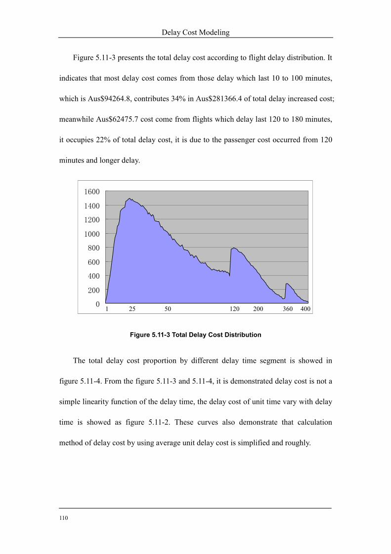
Delay Cost Modeling
110
Figure 5.11-3 presents the total delay cost according to flight delay distribution. It
indicates that most delay cost comes from those delay which last 10 to 100 minutes,
which is Aus$94264.8, contributes 34% in Aus$281366.4 of total delay increased cost;
meanwhile Aus$62475.7 cost come from flights which delay last 120 to 180 minutes,
it occupies 22% of total delay cost, it is due to the passenger cost occurred from 120
minutes and longer delay.
0
200
400
600
800
1000
1200
1400
1600
Figure 5.11-3 Total Delay Cost Distribution
The total delay cost proportion by different delay time segment is showed in
figure 5.11-4. From the figure 5.11-3 and 5.11-4, it is demonstrated delay cost is not a
simple linearity function of the delay time, the delay cost of unit time vary with delay
time is showed as figure 5.11-2. These curves also demonstrate that calculation
method of delay cost by using average unit delay cost is simplified and roughly.
1 25 120 360 400 50 200

Delay Cost Modeling
111
34%
22%
44% 1
2
3
10-100minute
120-180minute
Other Minutes
Figure 5.11-4 Total Delay Cost Proportion by Delay Time Segment
5.12 Summary
As one main factor affecting departure reliability, departure delay significantly
cuts down the profitability of the growing commercial air transport industry. The
flight delay causes cost increase in four main aspects: aircraft operators, airline
passengers, airports and communities. Furthermore, from the point view of society
aspect, delay results in even more social cost which is hardly to be estimated.
The parking cost, crew cost and passenger cost are three main contributions to the
overall delay cost and the passenger cost occupies 50% of them, which is the largest
portion among those three aspects.
According to the sample delay cost model of Australian X Airlines, the company
will have to pay an additional cost of AUD$281,366 for the occurrence of 1000
delayed flights at Melbourne airport. The passenger cost occupies 50% of total
increased cost. In order to cut down this unexpected expenditure dramatically, the

Delay Cost Modeling
112
airline should manage to reduce the delay in the majority proportion within all delay
time segments as shown in figure 5.11-4. Approximately 56% of the total delay cost
would be saved if those delays during 10-180minutes are eliminated.
Being different from the conventional approaches which using average cost in
delay cost estimation, the modeling method demonstrated in this project can compute
and model the delay cost more accurately, since the analysis is subject to all the
factors which result in flight delays.
Through this newly developed modeling, firstly, the delay distribution can be
found and the factors of delay cost can also be clearly identified. Some mathematical
equations are used to calculate the cost corresponding to the factors respectively.
On the other hand, the delay distribution used in this model is only based on Type
I Delay data which comes from the result in Chapter 4. Therefore, the outcome can
only represent the Type I Delay cost. However, the modeling methodology developed
in this chapter is also effective for the cost estimation of whole delay when all delay
data in included.

Type II Delay Modeling and Monte Carlo Simulation
113
Chapter 6 Type II Delay Modeling and Monte Carlo
Simulation
6.1 Introduction
Flight delay can be categorised into Type I and Type II. Distinguished from Type I
delay (original delay/initial delay), Type II delay is not independent and stochastic.. It
is related to the factors such as the length of the original delays, standard operation
time, the specific time of the delay occurrence, the scheduled buffer time and the
compactibility of the airline schedules, etc. Due to the high complexity of the Type II
delay, it is even more difficult to be eliminated compared to Type I. Under the same
operation condition, in order to reduce the propagation of the delay, Type I delay has
to be decreased or shortened and airlines’ operation schedule has to be changed by
providing more slack time.
In early years, Type I and Type II delay were not studied separately. The result
was still acceptable since the delay propagation was not really serious and did not
start to significantly influence airlines’ operation and revenue. With the fast growing
of air transportation in the last decade, more compact flight schedules are applied by
many carriers and airports, especially those airlines that have more market share.
Departure delay and its propagation is becoming into one major problem. Because the
delay cost significantly impacts the airlines’ finance meanwhile affects airlines’
reputation as well. Commercial aviation industry has now fully realized the negative
effect of delay propagation and the importance to optimize the operation schedules.

Type II Delay Modeling and Monte Carlo Simulation
114
As discussed in previous chapters, for the mathematical modeling, the
conventional statistics method is not valid for the analysis of Type II delay at this
stage. An alternative way has been developed in this dissertation; it is a dynamic
method which uses numerical simulation to analysis. Usually, dynamic methods can
be much more concentrated on time-related variables. Therefore, it is used to study
the dynamic relationship among the flight delays, airlines operation schedules, airlines
schedule punctuality prediction and schedule optimization, which are the core factors
of the delay propagation analysis.
Airlines flight schedule punctuality is particularly sensitive to individual
flight delays and their propagation. Initial delay can be propagated by various
turnaround schedules and airports service queue. The effect brought from original
delays on delay propagations is definitely different according to its duration and the
occurrence time of the day. That explains why evaluating result of statistics approach
is quite inaccurate with using only total delay time for the analysis. Combined with
statistics methodology and Monte Carlo Simulation (MCS), an integrated method has
been established in this project. This newly developed approach is proved to be able
to quantitatively evaluate the delay (including original delay and propagated delay
synthetically) and relevant cost as a whole.

Type II Delay Modeling and Monte Carlo Simulation
115
6.2 Type II Delay Modeling Methodology
Beatty (1998) proposed a numerical definition of ‘delay multiplier’ (DM) in
developing a ‘generic’ total value of both the original delay and its continuing
consequences on the airlines schedule. DM is calculated based on the length of the
initial delay and the time of day it occurred. DM is not used to predict the actual
downline flight delay, but it can estimate a specific initial delay’s influence on
downline flights through a specific schedule.
The research indicated that under a same schedule operation condition, reducing a
60 minutes delay to 30 minutes or reducing a serious disruption in the early time of
day is much more valuable than reducing a 30 minutes delay to zero or reducing a
serious delay in late time of day. It is obvious that airlines’ delay propagation is more
serious with a high frequency, short turn time operation schedule.
Type I delay occurred due to its own factors of a specific flight. The factors of
type I delay are random and independent; therefore type I delay can be studied by
using statistic methodology. Besides the randomicity, Type II delay is tightly related
to the time of day when Type I delay occurs, the length of Type I delay last, and the
airlines’ aircraft and crew operation schedule. In fact, Type II delay can be controlled
by human action in some way. Hence type II delay is not independent event. In order
to accurately analyze issues mixed by Type I delay and II delay together, Monte Carlo
numerical simulation has been chosen by its advantage, together with the aid of
computer technique.

Type II Delay Modeling and Monte Carlo Simulation
116
Generally, most statistic models have to make many assumptions that would limit
the method application and reduce errors of estimating results. On the other hand,
Monte Carlo Simulation has proved its advantage on solving complicated problems.
In this chapter, some models and tools with MCS is constructed to analyze the
tradeoff between the delay propagation and the airline schedule optimization.
Monte Carlo Simulation offers an alternative to analytical mathematics for
understanding a statistic’s sampling distribution and evaluating its behavior in random
samples. Monte Carlo simulation does this empirically by using random samples from
known populations of simulated data to track a statistic’s behavior (Mooney, 1997).
Monte Carlo simulation is very simple in concept. Simulation is using random
number technique to conduct stochastic experiment, which involves certain types of
mathematical and logical models that describe the behavior of aimed system. Monte
Carlo is one of these techniques of providing such random numbers.
The general procedure of Monte Carlo Simulation method is as follow (Mooney,
1997):
(1) Specify the pseudo-population in symbolic terms in such a way that it can be used
to generate samples. This usually means developing a computer algorithm to data
in a specified manner.
(2) Sample from the pseudo-population (a pseudo-sample) in ways reflective of the
statistical situation of interest, for example, with the same sampling strategy,
sample size, and so forth.

Type II Delay Modeling and Monte Carlo Simulation
117
(3) Calculate aimed variable in the pseudo-sample and store it in a vector,
(4) Repeat step 2 and 3 t times, where t is the number of trials.
(5) Construct a relative frequency distribution of the t times trials result, which is the
Monte Carlo estimate of the sampling distribution of aimed variable under the
conditions specified b the pseudo-population and the sampling procedures.
The modeling procedure which is applied in this chapter is showed as follow:
(a) According to history data, give definition to random;
(b) Build up arithmetic model;
(c) Set up computer algorithm and Program Flow Diagram;
(d) Develop software of trial;
(e) Running software with case data to text built model;
(f) Analyse results.

Type II Delay Modeling and Monte Carlo Simulation
118
6.3 Modeling with Monte Carlo Simulation
6.3.1 Radom Number Definition
The delay time of each flight needs to be calculated first so as to determine the
relevant delay cost. Here, it is assumed that Type I can be able to estimated according
to historical data. Delay propagation is determined by when and where Type I delay
occurs, as well as the time duration it lasts.
As calculated through airlines’ historical data, Type I delay distribution function
(i.e. the percentage of delay flights number by delay length) is applied to define the
random numbers. The level of accuracy is set by the digit of random number, which
has been fixed at the very beginning. 4 digits number has been applied in this
simulation process, which means that the applicable random numbers are from 0 to
9999. (10,000 numbers in all)
Each random number represents one time occurrence of delay. The duration of
each delay is defined from 0 to n minutes, where 0 means the flight departs on time
(no delay), and n is the maximum value of the delay time. The distribution of the
value (duration of the delay) for each random number (each delay) has been defined
as same as the probability distribution of Type I delay occurrence according to the
historical data. For example, assume there are 5.3% of Type I delays whose duration
are 10 minutes; in other words, the occurrence probability of 10 minutes Type I delay
is 5.3%. Thus, for 10,000 times of delay (random numbers), 530 of them would have
a 10-minute duration of delay, which is the value for each one of those 530 random
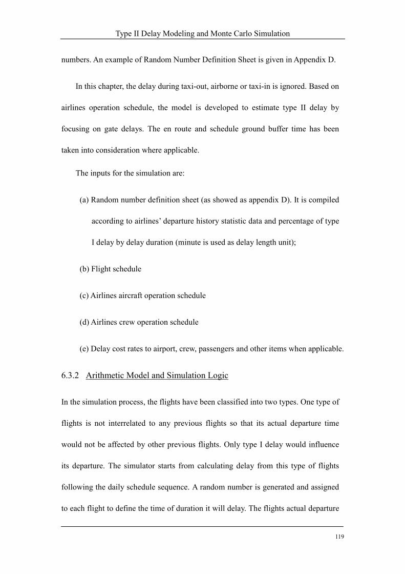
Type II Delay Modeling and Monte Carlo Simulation
119
numbers. An example of Random Number Definition Sheet is given in Appendix D.
In this chapter, the delay during taxi-out, airborne or taxi-in is ignored. Based on
airlines operation schedule, the model is developed to estimate type II delay by
focusing on gate delays. The en route and schedule ground buffer time has been
taken into consideration where applicable.
The inputs for the simulation are:
(a) Random number definition sheet (as showed as appendix D). It is compiled
according to airlines’ departure history statistic data and percentage of type
I delay by delay duration (minute is used as delay length unit);
(b) Flight schedule
(c) Airlines aircraft operation schedule
(d) Airlines crew operation schedule
(e) Delay cost rates to airport, crew, passengers and other items when applicable.
6.3.2 Arithmetic Model and Simulation Logic
In the simulation process, the flights have been classified into two types. One type of
flights is not interrelated to any previous flights so that its actual departure time
would not be affected by other previous flights. Only type I delay would influence
its departure. The simulator starts from calculating delay from this type of flights
following the daily schedule sequence. A random number is generated and assigned
to each flight to define the time of duration it will delay. The flights actual departure

Type II Delay Modeling and Monte Carlo Simulation
120
time ADT and actual arrival time AAT can be calculated by formulas below:
RID TT = (6-1)
IDSDAD TTT += (6-2)
ABADAA TTT += (6-3)
IDT is the duration of flight type I delay, RT is delay duration defined according to
the random number given by the simulator, SDT is scheduled departure time, ABT
is flight en route time.
To the opposite, the other type of flights is interrelated to the previous flights.
Besides type I delay, the actual departure time ADT for this type of flights could be
also affected by the actual arrival time of previous flights. From then on, the
simulator starts to compute flight delays following the sequence of their previous
flights actual arrive time AAAT . In other words, the simulator has taken the propagated
delay time into consideration. In this case, the actual departure time of a flight is
calculated by formulas below:
DSDAD TTT += (6-4)
{ }IIDIDD TTT ,max= (6-5)
{ }SDCPACAApAAAIID TTTTTT −++= ,max (6-6)
DT is the duration of departure delay, IIDT is flight II delay duration, which is
determined by previous flight delay and operation schedule; AAAT is aircraft actual
arrive time of previous flight, APT is turnaround aircraft ground preparing time at a
specific airport for next flight; ACAT is the turnaround crewmember actual arrive

Type II Delay Modeling and Monte Carlo Simulation
121
time of previous flight, CPT is turnaround crewmember ground preparing time at a
specific airport for next flight.
The integrated result of delay can be produced by above model. The actual
delay duration DT includes Type I delay and Type II delay. Together with the cost
model presented in chapter 5, the gross of delay cost can be computed as shown in
the next section. And dispatch reliability DR can be computed as below:
T
O
N
NDR = (6-7)
TN is the total amount of departure flights as schedule, ON is the total amount of
flights which depart not late 15 minutes comparing to schedule departure time.
6.3.3 The Model of Cost Computing
Different from the cost model presented in chapter 5, here, the value of delay
duration of each specific flight can be calculated via simulation modeling. Therefore
the delay cost model can be modified as blow. The flight i delay cost iC is defined
as equation 6-8:
oipiciaii CCCCC +++= (6-8)
The increase of airport parking cost of flight i aC can be defined as equation 6-9:
a
a
DiaDiaiT
ATpTC ==
(6-9)
ap is the excess parking fee rate of airport a, pA is the charge for an excess airport
parking per calculation unit, pT is minutes of per charge calculation unit. The

Type II Delay Modeling and Monte Carlo Simulation
122
increased airline crew cost due to delay cC can be computed as equation 6-10:
ciDici pTC = (6-10)
cip is the crew payment rate of flight i. Then the increased passenger cost piC can
be calculated according to equation 6-11:
pnipi pNC = n=1, 2, 3… (6-11)
iN is the passenger number of flight i, pnp is the payment rate to the passengers
when DiT is in different period, because the increased passenger cost is same during
a period. oC is other increased aeronautical fee due to departure delay. It can be
calculated by equation 6-12:
oiDioi pTC = (6-12)
oip is the aeronautical charge rate on flight i. So the total delay related cost of
airlines fleet is computed as:
∑=
=n
i
iD CC1 (6-13)

Type II Delay Modeling and Monte Carlo Simulation
123
6.4 Software Development
6.4.1 Software Flow Chart
Based on previous analysis, computer programming is illustrated in Fig 6.4-1.
Figure 6.4-1 Software Flow Chart
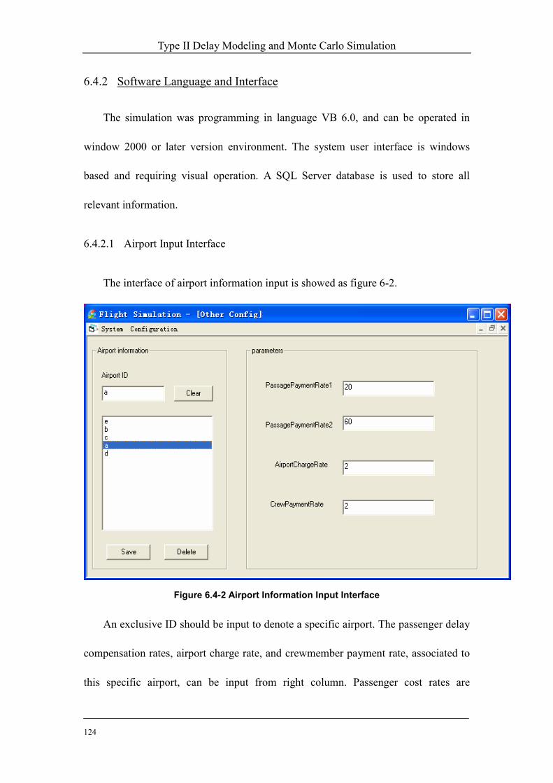
Type II Delay Modeling and Monte Carlo Simulation
124
6.4.2 Software Language and Interface
The simulation was programming in language VB 6.0, and can be operated in
window 2000 or later version environment. The system user interface is windows
based and requiring visual operation. A SQL Server database is used to store all
relevant information.
6.4.2.1 Airport Input Interface
The interface of airport information input is showed as figure 6-2.
Figure 6.4-2 Airport Information Input Interface
An exclusive ID should be input to denote a specific airport. The passenger delay
compensation rates, airport charge rate, and crewmember payment rate, associated to
this specific airport, can be input from right column. Passenger cost rates are

Type II Delay Modeling and Monte Carlo Simulation
125
Australian dollar, and the unit of airport charge rate and crew payment rate are
AU$/per minute.
6.4.2.2 Schedules Parameters Input Interface
Schedule information input interface is showed as figure 6.4-3.
Figure 6.4-3 Schedule Information Input Interface
After a schema is selected, its flight information can be input or amended. The
parameters of a flight includes: flight number, departure Airport, arrival airport,
scheduled departure time, previous flight number of aircraft, previous flight number
of crewmember, standard en route time, standard crew ground preparing time,
standard aircraft ground preparing time, number of aircraft seats, and load rate. The
unit of en route time, aircraft and crew ground time are minute. Iteration times set
interface is showed as figure 6.4-4.

Type II Delay Modeling and Monte Carlo Simulation
126
Figure 6.4-4 Iteration Times Set Interface
6.4.2.3 Output Interface
The results of program running are output to database of Access application
firstly. The data can be further exported from database to the sheets of excel
application as required. An example of Output Form of FDCSP is given in Appendix
E.
6.4.3 Process of Simulation
To calculate the flight actual delay time, the simulation starts from the flight
departed earliest on schedule. A random number is generated by computer to
determine this flight type I delay duration IDT according to the value of random
number, random number definition sheet, and formula 6-1. Because the actual
departure time of this flight would not be affected by any other flight, so the actual
depart time ADT and actual arrival time AAT can be computed by equations 6-2, 6-3
respectively. IDT will be recorded as actual delay time DT of this flight, and type I
will be recorded as delay classification as well. Furthermore, the delay cost can be
computed according to the formulas 6-8.
The following flights will be simulated one by one for calculating their delay

Type II Delay Modeling and Monte Carlo Simulation
127
duration according to the sequence of scheduled departure time till the occurrence of
the first flight which will used aircraft or/and crewmembers of previous flight. After
then, the same computing process as above is used to calculate the flight type I delay
duration. The type II delay duration is computed by equation 6-6,. So the actual delay
duration DT of this sort of flights is calculated by equation 6-5. The actual depart
time and arrival time can be gained by equations 6-4, and 6-3 respectively. When DT
> 0 and IDT ≥ IIDT , the delay is recorded as type I delay; when IDT < IIDT , it will be
recorded as type II delay. And the sequence of following flights simulation is
according to the actual arrival time of their previous flight.
It is recorded as iteration once when all flights on schedule have been calculated
once. The simulation computing will keep iterating till the setting numbers of iteration
have been fulfilled and enough pseudo-population has been gained.
6.4.4 Software Function
In the simulation, each scheduled flight is corresponding to a random number
which is generated by computer. According to the flight schedule, aircraft and
crewmember turnaround schedule, standard ground time, scheduled buffer time,
actual delay time, and standard en route time, the flight actual arriving time can be
calculated. Then the computer will determine whether the delay is propagated to the
next flight. A new random number is produced and given to the following flight to
determine its type I delay length. Actual departure time of this following flight can
be obtained by combining its type I delay length and the delay propagated

Type II Delay Modeling and Monte Carlo Simulation
128
previously. In the end, the flight actual arriving time, final delay time, and delay cost
can be computed. After all scheduled flights have been simulated and computed, the
computer will record it as one time of iteration. The software will keep running till
the required iteration times have been performed.
The input of the parameter and information includes: airport name and code,
airport charge rate, flight number, scheduled departure and arriving airports,
scheduled departure time, standard airborne route time, the former flight number of
aircraft and crew, aircraft and crew ground preparing time, aircraft capability and
load rate. Ground slack time is contained in flight schedule information.
The output data includes: flights number, scheduled departure and arriving time,
actual departure and arriving time, aircraft and crewmember turnaround time,
departure delay time, airport delay charge, crew and passengers delay cost, and total
delay cost. Delay classification is given by comparing which delay (type I or type II)
determined the final actual departure time. Data can be output to excel and access
sheet. The sample excel sheet of output is presented in Appendix E.

Type II Delay Modeling and Monte Carlo Simulation
129
6.5 Australian X Airline Delay Propagation Simulation
6.5.1 Assumptions and Data Processing
To test the program and analyze computing result, Australian X Airline’s 2002
departure delay data is applied as sample. The airline’s actual dispatch reliability can
be calculated from Airline’s 2002 departure data. The dispatch reliability estimated
by the program is used to test the validity and efficiency of the software by
comparing with the actual value. Data is analyzed first and type I delay data are
abstracted to build Radom Definition Sheet. The following assumptions are made
for this simulation program testing:
- The flight standard aircraft and crew ground time in same airport is same
- Only gate delay is considered for this simulation implement, taxi-out, en route,
taxi-in delay is ignored.
- Maximum delay duration is bounded
To process, firstly, open the Airport Information window, showed as figure 6.4-2,
from configuration menu. Input the airport ID, then passenger, crewmember, and
airport cost rates based on various airports respectively. Click “Save” button to save
this data into program database. Secondly, open Flight Information window
presented in figure 6.4-3 from configuration menu also. Choose a schema first, input
flight number. Infill flight departure and arrival airport ID; last flight number of
aircraft and crewmember if applicable; schedule departing time; schedule en route

Type II Delay Modeling and Monte Carlo Simulation
130
time; aircraft and crewmember schedule ground preparing time; the number of
aircraft seats and load rates. These information is also saved into database.
Set iteration times as 100; 500; and 1000 and compute airline fleet dispatch
reliability three times respectively. Compare computing result with history data and
analyze the error.
6.5.2 Program Running Environment
The computer hardware environment is Pentium(R) 4 CUP with 3.00 GHz
frequency, and 512 MB memory. Computer operation system is Microsoft Windows
XP Professional 2002, and Visual Basic 6.0 compiler is also needed to run this
program.
6.5.3 Simulation
The computing result of 100, 500, 1000 iteration times are presented in table
6.5-1, 6.5-2, 6.5-3 respectively.
Total flights
0-15mins
Delay
15mins more
delay
Dispatch
Reliability
1th run 6200 4145 2055 0.6685
2th run 6200 4170 2030 0.6726
3th run 6200 3990 2210 0.6435
Table 6.5-1 Results of 100 Iteration Times Simulation
Total flights
0-15mins
Delay
15mins more
delay
Dispatch
Reliability
1th run 31000 20801 10199 0.6710
2th run 31000 20750 10250 0.6694
3th run 31000 19980 11020 0.6445

Type II Delay Modeling and Monte Carlo Simulation
131
Table 6.5-2 Results of 500 Iteration Times Simulation
Total flights
0-15mins
Delay
15mins more
delay
Dispatch
Reliability
1th run 31000 20801 10199 0.6710
2th run 31000 20750 10250 0.6694
3th run 31000 19980 11020 0.6445
Table 6.5-3 Results of 1000 Iteration Times Simulation
6.5.4 Error Analysis
It is assumed that the deviation between the simulation result and true value
obey normal distribution. When iteration times equal to 100, based on the data of
table 6-1, average value of predicted DR (dispatch reliability) is 66.16%, σ =
0.012, and n = 3. The significance level of simulation result can be estimated based
on blow equations:
kx =− 0µ (6-12)
n
kz
/2/
σσ = (6-13)
According to Australian X airline 2002 departure data, the actual value of
dispatch reliability can be calculated as 65.1%, so 0µ =65.1%. Then 2/αz =1.53,
2
α=0.063, and significance level is 87%.
Similarly, when iteration times is 500, x = 66.16%, σ = 0.011, n = 3, we can
get 2/αz = 1.67, 2
α = 0.0475, and significance level is 90%; when iteration times
equal to 1000, x = 64.97%, σ = 0.001, so 2/αz is 1.88, 2
α = 0.03 and
significance level is 94%. The data of error analysis with different iteration times is

Type II Delay Modeling and Monte Carlo Simulation
132
presented in table 6.5-4.
Iteration
Times x 0µ
n σ 2/αz 2
α
Significance
Level
100 66.16% 65.1% 3 0.012 1.53 0.063 87%
500 66.16% 65.1% 3 0.011 1.67 0.048 90%
1000 64.97% 65.1% 3 0.001 1.88 0.030 94%
Table 6.5-4 Error Analysis Data
6.6 Summary
The estimation model and computer program are based on MCS technique.
They have been developed in this project to accurately assess the Type II delay,
when the operation condition and flight schedules are dynamic.
Australian X Airline 2002 departure data and the value of dispatch reliability are
applied to test the efficiency of the program. With the computer (introduced in 6.5.2),
190 minutes are needed for per 1000 times simulation iteration. The estimated
significance level of simulation result is 87%, 90%, and 94% when iteration times are
100, 500, and 1000 respectively. To save computing time and get higher significance
level result, 2000 iteration is proposed for practical application of this program.

Australian X Airline Flight Schedule Optimization
133
Chapter 7 Australian X Airline Flight Schedule
Optimization
7.1 Introduction
Australian X airline has been experiencing unsatisfactory flight punctuality
performance in the past several years. The dispatch reliability has been remaining at a
relatively low level due to the increase of air transportation market.
The negative impacts include serious airline profitability damaging and reputation
loss. Compared to the acquisition of more new aircrafts, schedule optimizing is
believed to be a more economical approach in enhancing airline punctuality
performance and profitability in a way.
The accuracy of the assessment for the flight delay distribution and relevant cost
is vital in the flight schedule optimization. Unusually, the influence of the delay
propagation has been solved using the MCS techniques developed in previous
chapters.
In this chapter, the schedule optimization scheme of Australian X Airline will be
conducted. The target will be on the flight schedule optimization by minimizing the
system cost for Australian X Airline.

Australian X Airline Flight Schedule Optimization
134
7.2 Current Air-fleet Operation Analysis
Good schedule punctuality performance can maintain or improve customers’
satisfaction and loyalty, meanwhile enhance airlines’ profitability. These business
require airline to have an efficient management of their aircrafts, pilots, and flight
attendants turnaround schedule. The objectives are aimed:
(1) Minimizing operating cost;
(2) Maximizing profits;
(3) Maintain a satisfactory level of safety.
Aircraft using cost usually points at the fee of aircraft purchase or hiring and the
related maintenance. Wu (2000) named this sort of cost as aircraft schedule
time-opportunity cost or schedule time cost to calculate the airline delay cost and
optimize the aircraft and crew operation schedule. It is assumed that the aircraft
scheduled ground time can be alternatively used as revenue-generation airborne
block hours. Generally aircraft ground time contains three sections:
(1) Scheduled ground service time, which is necessary aircraft preparing time for
next flight duty. Generally, this segment time can’t be shorten or eliminated
unless the standard or process of ground service is changed.
(2) Schedule buffer time, which is set to absorb unscheduled delay. The length of
this segment time can be adjusted according to schedule delay situation or

Australian X Airline Flight Schedule Optimization
135
financial condition by airlines’ management staff.
(3) Unscheduled delay time (if applicable). It occurs when the delay, is longer than
ground buffer time.
Similarly, airborne block time could also contain three sections: standard en
route time, airborne buffer time, and airborne delay time (if applicable). As same as
standard en route time, the scheduled ground service time is also part of the process
for flights operation. Hence both of the aircraft scheduled ground service time and
standard en route time should be considered as aircraft available operation time and
also can be optimized to improve the aircraft utilization efficiency during its life
cycle. It is obvious that aircraft ground time can not be simply used for schedule
time-opportunity cost calculation. To the opposite, even the aircraft available time
has been accounted in; airborne buffer time should still be considered as unavailable
time of aircraft since it may also decrease airline revenue.
As a result, both of the buffer time and the delay time should be considered as
aircraft unavailable operation time. Furthermore, if it is assumed that there is not any
delay occurrence and buffer time applicable, then the ideal aircraft turnaround and
flights operation schedule can be defined as: the operation schedule without any
impact from aircraft unavailable operation time. For example, assume that aircraft A
should fulfill 6 flight-duties as scheduled, when some delay occurred, if it still can
accomplish these 6 scheduled flights without influencing the scheduled tasks for the
next day, there only occurs operation cost instead of aircraft schedule using cost. If

Australian X Airline Flight Schedule Optimization
136
this aircraft can’t complete this 6 flight duties or delay is propagated to next day’s
scheduled flight mission, the aircraft schedule using cost should be taken into
account. In fact, most domestic flights schedules don’t employ aircrafts continually
operating 24 hours per day. There are stand-by intervals between their daily
operations. In many cases, the increased buffer time or delay time only reduce
aircraft night leisure interval instead of reducing aircraft available operation time.
Based on the above, the criteria to decide whether the additional aircraft using
cost should be applied is proposed as: during an aircraft specific operation schedule
period (day, week or others), an aircraft schedule time cost should be applied when its
unavailable operation time increases enough to reduce the aircraft available operation
time comparing with its ideal operation schedule of the same period; or it won’t incur
the schedule time-opportunity cost.
7.3 Overall System Cost Modeling
Airlines’ flight overall system cost SC is used to trade off dispatch reliability
and airlines’ operation cost. System Cost consists of flight delay cost DC and
additional flight operation cost OPC which is caused by the change of initial
operation schedule. SC can be calculated by the following formulas:
OPDS CCC += (7-1)
DC is flight delay cost, which can be calculated by formula 5-6, DC consists of
additional parking cost against delay aC , additional crew cost cC , delayed
passenger cost pC and other delay aeronautic cost oC . These delay cost can be also

Australian X Airline Flight Schedule Optimization
137
computed respectively by formulas 5-2, 5-3, 5-4 and 5-5. Additional flight operation
cost OPC can be computed by equation 7-2.
OAACCWPKOP CCCCC +++= (7-2)
Where PKC is the additional parking cost due to schedule change, CWC is
additional crewmember cost, ACC is aircraft schedule time cost if applicable, and
OAC is other applicable aeronautic cost due to schedule change. They can be
calculated by following equations:
PKaPK TpC = (7-3)
CWccCW TpnC = (7-4)
ACACAC TpC = (7-5)
OAOAOA TpC = (7-6)
ap is airport parking charge rate, it can be computed by formula 5-1, PKT is
aircraft additional parking time (computing unit is minute) of new operation schedule;
cn is total number of on board crew, cp is the crew payment rate, CWT is
additional crew labor time (computing unit is minute) of new schedule; ACp is
aircraft schedule time cost rate, ACp = the cost of aircraft whole life cycle/ aircraft
total schedule available time, this parameter is generally provided by airlines, ACT is
aircraft available operation reduced by new schedule; OAp is other applicable
aeronautic charge rate, and OAT is additional applicable charged time.

Australian X Airline Flight Schedule Optimization
138
7.4 Flight Schedule Optimization
7.4.1 Data Collection
Flight schedule and aircraft turnaround schedule are provided by this Australian
X Airline. Because of commercial confidential agreement, flights number and
airports names are replaced by assigned codes.
Several assumptions are made as following:
� A single type of aircraft is used for shuttle flight;
� Average loading rate is assumed at 75%;
� The value of PKT , CWT , ACT , OAT are set as constant variable under same
operation environment.
� The other aeronautic cost is ignored here.
7.4.2 Current Airlines Delay Situation Analysis
Currently, the schedule employed by X Airline is very compact. As a result, the
delay and delay propagation occur more frequently in recent year.
Relevant delay parameters with current operation schedule are calculated by
using simulation software which is described in earlier chapters.
In order to get a higher level of accuracy in this real-world case, computing
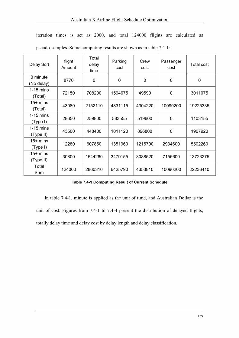
Australian X Airline Flight Schedule Optimization
139
iteration times is set as 2000, and total 124000 flights are calculated as
pseudo-samples. Some computing results are shown as in table 7.4-1:
Delay Sort flight
Amount
Total
delay
time
Parking
cost
Crew
cost
Passenger
cost Total cost
0 minute
(No delay) 8770 0 0 0 0 0
1-15 mins
(Total) 72150 708200 1594675 49590 0 3011075
15+ mins
(Total) 43080 2152110 4831115 4304220 10090200 19225335
1-15 mins
(Type I) 28650 259800 583555 519600 0 1103155
1-15 mins
(Type II) 43500 448400 1011120 896800 0 1907920
15+ mins
(Type I) 12280 607850 1351960 1215700 2934600 5502260
15+ mins
(Type II) 30800 1544260 3479155 3088520 7155600 13723275
Total
Sum 124000 2860310 6425790 4353810 10090200 22236410
Table 7.4-1 Computing Result of Current Schedule
In table 7.4-1, minute is applied as the unit of time, and Australian Dollar is the
unit of cost. Figures from 7.4-1 to 7.4-4 present the distribution of delayed flights,
totally delay time and delay cost by delay length and delay classification.

Australian X Airline Flight Schedule Optimization
140
7%
23%
35%
10%
25%
0 Mins delay 1-15 mins I delay
1-15 mins II delay 15+ mins I Delay
15+ mins II Delay
Figure 7.4-1 Proportion of Delayed Flights by Different Delay Length
9%
16%
21%
54%
1-15 mins I delay 1-15 mins II delay
15+ mins I Delay 15+ mins II Delay
Figure 7.4-2 Proportion of Total Delay Time by Different Delay Length

Australian X Airline Flight Schedule Optimization
141
5%9%
25%
61%
1-15 mins I delay 1-15 mins II delay
15+ mins I Delay 15+ mins II Delay
Figure 7.4-3 Proportion of Delay Cost by Different Delay Length
There are only 8770 flights depart on time in total 124000 pseudo samples. 72150
flights delay 1-15 minutes, occupies 58.19% of total flights, while contributes 24.76%
of total delay time, and about 13.54% delay cost. Its average delay cost is Au$4.25/
min. Meanwhile there are 34.74% delay lasted longer than 15 minutes, which
contributes 75.24% of total delay time and 86.46% of total delay cost. Type II delay
contributes more delay time and cost than type I delay. Its average delay cost is
Au$8.93/min. The difference of average delay cost between varied delay length
demonstrates that the method of delay cost calculation with average cost rate is
difficult to provide accurate result. And the passenger cost is the main reason incurred
this difference.

Australian X Airline Flight Schedule Optimization
142
0.00
500.00
1000.00
1500.00
TousandDollar
Parking Cost 58.36 101.11 135.20 347.92
Crew Cost 51.96 89.68 121.57 308.85
Passenger Cost 0.00 0.00 293.46 715.56
1-15mins I
1-15mins
15+mins I
15+mins
Figure 7.4-4 Structure of Delay cost by Different Delay Length
7.4.3 Flight Schedule Optimization
Buffer time is generally embedded into flight schedule to absorb probably
occurred flight delays. The basic principle of the airline flight schedule optimizing is
to determine an appropriate buffer segment to minimize the system cost of the
schedule execution.
The system cost SC can be calculated according to equation 7-1. To gain the
value of delay cost DC and operation cost OPC , FDCSP runs with the different
flight schedules. Original actual schedule is set as scheme 1, and an additional 5
minutes segment of buffer time is added to next scheme till to scheme 9 which
would have 40 minutes more buffer time than the original scheme. According to
formula 7-2, 40 minutes buffer time will incur more than 21 million dollars
additional operation cost, which has approached to the total delay cost when actual
schedule is applied. This indicates that the longer buffer time would not give a lower

Australian X Airline Flight Schedule Optimization
143
system cost.
With the using of a series of gradually increasing buffer time, a group of SC can
be generated after running FDCSP and calculation. The optimizing curve can be
drawn according to values of SC . The scheme with the minimal system cost is
identified as optimal schedule. The different buffer time values of each scheme are
presented in table 7.4-2. Iteration parameter is set as 2000 times, that means there are
124000 flights is simulated as pseudo-samples. Optimization calculation result and
optimization curve are showed as table 7.4-3 and figure 7.4-5.
Scheme
No.
Scheme
1
scheme
2
Scheme
3
Scheme
4
Scheme
5
Scheme
6
Scheme
7
Scheme
8
Scheme
9
Ground
Buffer time
Current
applied
5 Mins
more
10 mins
more
15 mins
more
20 mins
more
25 mins
more
30 mins
more
35 mins
more
40 mins
more
Table 7.4-2 Additional Ground Buffer Time of Different Scheme

Australian X Airline Flight Schedule Optimization
144
Additional
Buffer Time
Totally Delay
Time
Totally Delay
Cost
Additional
Operation Cost
System Cost
Sum
Scheme 1 2,860,310 22,236,410 0 22,236,410
Scheme 2 5 2,116,190 17,433,000 2,635,000 20,068,000
Scheme 3 10 2,036,250 13,997,370 5,270,000 19,267,370
Scheme 4 15 1,892,480 13,173,430 7,905,000 21,078,430
Scheme 5 20 1,763,880 12,902,120 10,540,000 23,442,120
Scheme 6 25 1,601,960 12,368,320 13,175,000 25,543,320
Scheme 7 30 1,598,160 11,720,180 15,810,000 27,530,180
Scheme 8 35 1,474,760 10,867,850 18,445,000 29,312,850
Scheme 9 45 1,409,180 10,054,240 21,080,000 31,134,240
Table 7.4-3 Optimization Calculation Result
0
5,000,000
10,000,000
15,000,000
20,000,000
25,000,000
30,000,000
35,000,000
1 2 3 4 5 6 7 8 9
Schemes
Cost (D
ollar)
Delay Cost Operation Cost System Cost
Figure 7.4-5 Optimization Curve

Australian X Airline Flight Schedule Optimization
145
According to computing result, scheme 3, which embedded additional 10 minutes
buffer time into schedule, is the optimal scheme with lowest system cost. The related
parameters of scheme 1 and scheme 3 are listed in table 7.4-4.
Amount of
0 Mins
Delay
Amount of
1-15 mins
delay
Amount of
15 +Mins
Delay
Dispatch
Reliability
Delay Cost System
Cost
Scheme 1 8,770 72,150 43,089 65.25% 22,236,410 22,236,410
Scheme 3 28,200 69,690 26,110 78.94% 13,997,370 19,267,370
Table 7.4-4 Scheme Comparison
Comparing with original schedule, optimal schedule will reduce 16.87%
departure delay, dispatch reliability can be increased by 20.98%, and reduce delay
cost 37.05%, save 13.35% system cost.
7.4.4 Sensitivity Test and Analysis
A test is done to analyze and assess the sensitivity of the models and FDCSP to
the changing of departure delay. The test assumes additional 8 group data of departure
delay, which has -20%, -10%, -5%, -2%, +2%, +5%, +10%, and +20% delays
respectively comparing with original history delay data. The calculation results are
listed in table 7.4-5, 7.4-6, 7.4-7, 7.4-8, 7.4-9, 7.4-10, 7.4-11, and 7.4-12, the schedule
optimizing curves are presented as figure 7.4-6, 7.4-7, 7.4-8, 7.4-9, 7.4-10, 7.4-11,
7.4-12, and 7.4-13. Simulation iteration is also set as 2000 times.

Australian X Airline Flight Schedule Optimization
146
Additional
Buffer Time
Totally Delay
Time
Totally Delay
Cost
Additional
Operation Cost
System Cost
Sum
Scheme 1 0 2,783,620 21,543,620 0 21,543,620
Scheme 2 5 2,121,740 17,326,670 2,635,000 19,961,670
Scheme 3 10 1,800,900 13,442,860 5,270,000 18,712,860
Scheme 4 15 1,661,340 12,950,500 7,905,000 20,855,500
Scheme 5 20 1,507,960 11,885,420 10,540,000 22,425,420
Scheme 6 25 1,498,240 10,170,410 13,175,000 23,345,410
Scheme 7 30 1,398,320 9,689,520 15,810,000 25,499,520
Scheme 8 35 1,226,520 9,309,700 18,445,000 27,754,700
Scheme 9 45 1,182,280 8,760,770 21,080,000 29,840,770
Table 7.4-5 Optimization with -2% Delay
0
5,000,000
10,000,000
15,000,000
20,000,000
25,000,000
30,000,000
35,000,000
1 2 3 4 5 6 7 8 9
Schemes
Cost (D
ollar)
Delay Cost Operation Cost System Cost
Figure 7.4-6 Optimization Curve with -2% Departure Delay

Australian X Airline Flight Schedule Optimization
147
Additional
Buffer Time
Totally Delay
Time
Totally Delay
Cost
Additional
Operation Cost
System Cost
Sum
Scheme 1 0 2,578,320 20,430,680 0 20,430,680
Scheme 2 5 2,089,880 16,885,730 2,635,000 19,520,730
Scheme 3 10 1,852,820 15,534,820 5,270,000 20,804,820
Scheme 4 15 1,680,980 14,040,120 7,905,000 21,945,120
Scheme 5 20 1,588,480 12,077,480 10,540,000 22,617,480
Scheme 6 25 1,575,160 11,755,100 13,175,000 24,930,100
Scheme 7 30 1,478,620 10,615,860 15,810,000 26,425,860
Scheme 8 35 1,420,300 9,222,200 18,445,000 27,667,200
Scheme 9 45 1,328,760 8,681,320 21,080,000 29,761,320
Table 7.4-6 Optimization Result with -5% Delay
0
5,000,000
10,000,000
15,000,000
20,000,000
25,000,000
30,000,000
35,000,000
1 2 3 4 5 6 7 8 9
Schemes
Cost (Dollar)
Delay Cost Operation Cost System Cost
Figure 7.4-7 Optimization Curve with -5% Departure Delay

Australian X Airline Flight Schedule Optimization
148
Additional
Buffer Time
Totally Delay
Time
Totally Delay
Cost
Additional
Operation Cost
System Cost
Sum
Scheme 1 0 2,487,260 17,703,320 0 17,703,320
Scheme 2 5 1,963,700 13,604,880 2,635,000 16,239,880
Scheme 3 10 1,652,500 12,919,500 5,270,000 18,189,500
Scheme 4 15 1,500,200 11,619,100 7,905,000 19,524,100
Scheme 5 20 1,470,200 10,698,280 10,540,000 21,238,280
Scheme 6 25 1,405,500 10,073,050 13,175,000 23,248,050
Scheme 7 30 1,350,800 9,842,780 15,810,000 25,652,780
Scheme 8 35 1,311,000 8,887,700 18,445,000 27,332,700
Scheme 9 45 1,284,300 8,065,900 21,080,000 29,145,900
Table 7.4-7 Optimization Result with -10% Delay
0
5,000,000
10,000,000
15,000,000
20,000,000
25,000,000
30,000,000
35,000,000
1 2 3 4 5 6 7 8 9
Schemes
Cost (Dollar)
Delay Cost Operation Cost System Cost
Figure 7.4-8 Optimization Curve with -10% Departure Delay

Australian X Airline Flight Schedule Optimization
149
Additional
Buffer Time
Totally Delay
Time
Totally Delay
Cost
Additional
Operation Cost
System Cost
Sum
Scheme 1 0 2,302,060 15,724,390 0 15,724,390
Scheme 2 5 1,871,450 14,031,390 2,635,000 16,666,390
Scheme 3 10 1,764,300 13,411,000 5,270,000 18,681,000
Scheme 4 15 1,622,500 12,062,100 7,905,000 19,967,100
Scheme 5 20 1,467,000 11,888,000 10,540,000 22,428,000
Scheme 6 25 1,345,700 10,240,450 13,175,000 23,415,450
Scheme 7 30 1,205,500 9,832,100 15,810,000 25,642,100
Scheme 8 35 1,093,500 8,100,950 18,445,000 26,545,950
Scheme 9 45 925,200 7,857,000 21,080,000 28,937,000
Table 7.4-8 Optimization Result with -20% Delay
0
5,000,000
10,000,000
15,000,000
20,000,000
25,000,000
30,000,000
35,000,000
1 2 3 4 5 6 7 8 9
Schemes
Cost (Dollar)
Delay Cost Operation Cost System Cost
Figure 7.4-9 Optimization Curve with -20% Departure Delay

Australian X Airline Flight Schedule Optimization
150
Additional
Buffer Time
Totally Delay
Time
Totally Delay
Cost
Additional
Operation Cost
System Cost
Sum
Scheme 1 0 2,852,600 22,272,350 0 22,272,350
Scheme 2 5 2,273,300 19,435,800 2,635,000 22,070,800
Scheme 3 10 1,907,300 16,021,100 5,270,000 21,291,100
Scheme 4 15 1,758,200 14,364,100 7,905,000 22,269,100
Scheme 5 20 1,659,700 13,738,300 10,540,000 24,278,300
Scheme 6 25 1,559,000 12,796,600 13,175,000 25,971,600
Scheme 7 30 1,335,500 11,945,850 15,810,000 27,755,850
Scheme 8 35 1,221,000 11,030,900 18,445,000 29,475,900
Scheme 9 45 1,126,200 10,190,700 21,080,000 31,270,700
Table 7.4-9 Optimization Result with +2% Delay
0
5,000,000
10,000,000
15,000,000
20,000,000
25,000,000
30,000,000
35,000,000
1 2 3 4 5 6 7 8 9
Schemes
Cost (Dollar)
Delay Cost Operation Cost System Cost
Figure 7.4-10 Optimization Curve with +2% Departure Delay

Australian X Airline Flight Schedule Optimization
151
Additional
Buffer Time
Totally Delay
Time
Totally Delay
Cost
Additional
Operation Cost
System Cost
Sum
Scheme 1 0 2,895,710 24,614,240 0 24,614,240
Scheme 2 5 2,577,600 21,425,000 2,635,000 24,060,000
Scheme 3 10 2,199,100 18,225,390 5,270,000 23,495,390
Scheme 4 15 1,952,300 15,774,500 7,905,000 23,679,500
Scheme 5 20 1,804,000 14,630,900 10,540,000 25,170,900
Scheme 6 25 1,702,100 13,588,120 13,175,000 26,763,120
Scheme 7 30 1,624,700 12,442,600 15,810,000 28,252,600
Scheme 8 35 1,490,200 11,365,700 18,445,000 29,810,700
Scheme 9 45 1,270,850 10,261,660 21,080,000 31,341,660
Table 7.4-10 Optimization Result with +5% Delay
0
5,000,000
10,000,000
15,000,000
20,000,000
25,000,000
30,000,000
35,000,000
1 2 3 4 5 6 7 8 9
Schemes
Cost (Dollar)
Delay Cost Operation Cost System Cost
Figure 7.4-11 Optimization Curve with +5% Departure Delay

Australian X Airline Flight Schedule Optimization
152
Additional
Buffer Time
Totally Delay
Time
Totally Delay
Cost
Additional
Operation Cost
System Cost
Sum
Scheme 1 0 2,960,200 25,889,700 0 25,889,700
Scheme 2 5 2,600,100 22,002,500 2,635,000 24,637,500
Scheme 3 10 2,294,400 18,616,290 5,270,000 23,886,290
Scheme 4 15 2,118,000 15,052,200 7,905,000 22,957,200
Scheme 5 20 1,904,600 14,505,100 10,540,000 25,045,100
Scheme 6 25 1,7553,510 14,019,100 13,175,000 27,194,100
Scheme 7 30 1,7085,000 13,543,900 15,810,000 29,353,900
Scheme 8 35 1,628,640 12,792,400 18,445,000 31,237,400
Scheme 9 45 1,553,200 11,895,790 21,080,000 32,975,790
Table 7.4-11 Optimization Result with +10% Delay
0
5,000,000
10,000,000
15,000,000
20,000,000
25,000,000
30,000,000
35,000,000
1 2 3 4 5 6 7 8 9
Schemes
Cost (Dollar)
Delay Cost Operation Cost System Cost
Figure 7.4-12 Optimization Curve with +10% Departure Delay

Australian X Airline Flight Schedule Optimization
153
Additional
Buffer Time
Totally Delay
Time
Totally Delay
Cost
Additional
Operation Cost
System Cost
Sum
Scheme 1 0 3,243,970 27,895,500 0 27,895,500
Scheme 2 5 2,909,400 25,012,800 2,635,000 27,647,800
Scheme 3 10 2,705,850 21,712,600 5,270,000 26,982,600
Scheme 4 15 2,254,900 18,106,700 7,905,000 26,011,700
Scheme 5 20 2,054,100 15,118,000 10,540,000 25,658,000
Scheme 6 25 1,887,550 14,321,300 13,175,000 27,496,300
Scheme 7 30 1,774,600 13,789,710 15,810,000 29,599,710
Scheme 8 35 1,709,360 13,002,200 18,445,000 31,447,200
Scheme 9 45 1,618,840 12,370,140 21,080,000 33,450,140
Table 7.4-12 Optimization Result with +20% Delay
0
5,000,000
10,000,000
15,000,000
20,000,000
25,000,000
30,000,000
35,000,000
40,000,000
1 2 3 4 5 6 7 8 9
Schemes
Cost (Dol
lar)
Delay Cost Operation Cost System Cost
Figure 7.4-13 Optimization Curve with +20% Departure Delay

Australian X Airline Flight Schedule Optimization
154
It is shown that the buffer time required by optimal schedule is declined
accompanying with the reducing of departure delay. When departure delay is reduced
by 5% to 10%, Scheme 2 becomes optimal schedule which embedded additional 5
minutes buffer only. The current actual schedule become optimal one when delay is
declined 20%. By contraries, the buffer time of optimal schedule is required to extend
as departure delay increasing. 15 minutes buffer is needed when delay increased 10%,
and 20 minutes is required as 20% increasing of delay. The result of schedule
optimization is stable when departure delay changes between -2% to +5%. It
demonstrates the model and software developed in this project is a stable approach to
optimize flight schedule by embedding various buffer time.
7.5 Summary
In this chapter, it has been introduced and proved that the enhancement of the
airline dispatch reliability can be achieved through flight schedule optimization. The
MCS technique is employed to simulate the air-fleet operation of Australian X
Airline. Compared to the conventional literatures or studies, the accuracy has been
raised to a higher level, which can enable the modeling results to be more reliable.
The key innovation at this stage is to classify the type of the delay into a logical and
rational way. Type I is the initial/original delay, while Type II is the propagated
delay.
As analysed before, the impact brought by the delay propagation is much more
serious than Type I delay. Thus, the assessment of Type II delay has performed as

Australian X Airline Flight Schedule Optimization
155
the core of the flight delay simulation. The usual statistics method has been shown
as invalid in such cases. Therefore FDCSP software has been developed to
accurately estimate the departure delay and related cost for Australian X Airline.
As a result, the schedule with additional 10 minutes buffer is verified to be
optimal. The application of new optimal schedule can be able to improve the
dispatch reliability of X Airline from current 65.25% to 78.94%, meanwhile reduce
16.8% of departure delay and 13.35% system cost.
Sensitivity test has also been done to analyze the impact of the probability of type
I delay occurrence on schedule optimization. The results have been demonstrated as
being stable when departure delay changes from -2% to +5%. Along with the
operation in the future, it will be necessary to revise the schedule optimization process
periodically, especially when the probability of type I delay occurrence has obviously
changed. Continuing the approach of this project, Australian X Airline need to adjust
the parameters to ensure the whole air-fleet has been managed in the most
cost-effective way.

Conclusion
156
Chapter 8 Conclusion
The significance of this project is to enhance the dispatch reliability of Australian
X Airline’s fleet through a newly developed approach to reliability modeling, which
employs computer-aided numerical simulation of the delay distribution and related
cost to achieve the flight schedule optimization. Additionally, airlines, airports,
aviation authorities and other related organizations can also adopt the methodology
and the outcome of this project in varied applications.
Flight delays have both randomicity and inevitability. It is hardly possible to
predict exactly when or where a delay would occur. Meanwhile, it is practical for the
operators to minimize the impact from unexpected flight delays through management
techniques. The main achievement of this project is to develop a unique modeling
system that can assist in estimating the delay and relevant cost with high accuracy.
In this project, the different mathematical characteristics of type I and type II
have been distinguished and analysed in depth, more advanced and suitable
approaches have been used respectively to build the models to gain the more accurate
estimating results. Based on previous research works, delay cost factors have been
examined and identified again, and new delay cost assessment model has been
developed by factors analysis. These various models and approaches are integrated by
a computer-aid program developed in this project to evaluate departure delay and
related cost as a whole.
However, to optimize the air-fleet operation schedule can only solve the partial
Conclusion
157
problem in the current air-transportation market environment. On the other hand, the
excess of the capacity is the substaintial cause of the increase of flight delays and
delay propagation. In some cases, this problem can only be solved through a costly
way, which is to purchase or hire more aircrafts and employ aircrafts with larger
capacity (e.g. Airbus A380). At this stage, an integrated model needs to be developed
to take both of aspects into consideration. Because the air-fleet management technique
and the airline financial strategy usually supplement each other. In other words, it is
always indispensable to conduct the tradeoff among the cost, revenue, reliability,
safety, spend and profit during the airline business management.
Through this project, Australian X Airline’s fleet dispatch reliability has been
estimated. The main delay factors have been identified. The flight schedule has been
optimized which improves airline’s dispatch reliability and significantly reduces the
operational cost.
The distribution of Australian X Airline’s flight delay occurrence has been found
as lognormal. A series of model have been built up including the FDCSP, which is a
software programming through Monte Carlo Simulation methodology.
In this project, Monte Carlo Simulation methodology has been proved to be a
useful tool and a practical modeling method in flight dispatching optimization. In fact,
the approach of MCS in this project can be a successful example for the application of
this methodology in even more scenarios and areas in aviation industry. Because the
MCS method can be established to consider factors such as reliability and
maintainability (R&M) characteristics of the aircraft, weather conditions,

Conclusion
158
management, number of aircraft, route structure, maintenance level, personnel skills,
spare parts supply, and so forth. The analysis results through MCS can provide the
decision-making basis to improve an aircraft's R&M and to adjust flight, dispatch
procedure, logistic supports, etc., rationally for airlines
The accuracy of the results has been raised to a high level as the unique delay
classification employed in this project. Distinguished from those conventional studies,
the delay has been classified into Type I (Initial/Original Delay) and Type II
(Propagated Delay). The MCS simulation technique has also provided an effective
assessment model which can catch the randomicity of type I delay and the internal
relationship between type II delay and operation schedule.
In this project, the taxi-out and en route delay has not been taken into
consideration due to the absence of data. The current database established by the
operators and relevant agencies hasn’t included such catalogue which is an essential
contribution to the accuracy of the assessment.
The lack of available data is always a major obstacle of air safety and reliability
research. Motivation of staff to provide field reports with sufficient relevant detail is a
current management problem. Besides non-punishment policies, the incentive could
be provided by airline to encourage more completed and accurate information
collection. Official departure and arrival punctuality data, aircraft delay factors and
other published finding should be organized and published by government agencies
on a regular basis with more detailed catalogue classification. Through the research of
this project, it is also found that the current category of delay from those operators and

Conclusion
159
authorities are not practical enough. As previously discussed, delay should be
classified into Type I and Type II, which can be set as a standard classification criteria.
Thus, the current procedure and format of data collection need to be modified in a
proper way to provide convenience for any future study.
In recent years, Australian X Airline has been suffering from frequent
occurrence of delay. Delay propagation has been shown as the core factor resulting
in this low reliability performance. Additionally, based on the calculation in the
previous chapter, Type II delay has also occupied the larger portion of the overall
delay cost at around 70%, which is significant to the business management of this
Australian carrier. With the further increase of the market demand in the future, the
situation would come to even worse.
As a result, through this project, the additional 10 minutes buffer has been
verified to be optimal. The application of new optimal schedule can be able to
improve the dispatch reliability of X Airline from current 65.25% to 78.94%,
meanwhile reduce 16.8% of departure delay and 13.35% system cost.
At last but not least, this project also has achieved to set a more practical
standard and guideline for air-fleet delay management upon overall dispatch
reliability optimization. The modeling system and the FDCSP developed in this
project can be applied for varied applications in dispatch reliability investigations.
The end-users can be airlines, airports and aviation authorities, etc. The software
program established in this project can be further developed to be accessed through

Conclusion
160
internet as a real-time remote application. Using VB.NET, the FDCSP can be used
remotely with the installation of .NET run time on the Windows based web server.
User interface will be web based. This application can enable the FDSCP as a
practical and universal tool in the air-fleet (dispatch reliability) management which
could benefit most of the airlines in the world.

Reference
161
Reference
Abdelghany, K. F., Shah, S. S., Raina, S., & Abdelghany, A. F. 2004, A Model for
Projecting Flight Delay During Irregular Operation Conditions, Journal of Air
Transport Management 10 (2004) 385-394.
Advisory Group on Reliability of Electronic Equipment [AGREE], 1957, Reliability of
Military Electronic Equipment, Washington, D.C. U.S.
Aggarwal, K.K. 1993, Reliability Engineering, Kluwer Academic Publishers.
Amstadter, B. L. 1971, Reliability Mathematics, McGraw-Hill, Inc.
Ascher, H. & Feingold, H. 1984, Repairable System Reliabiilty, Marcel Dekker, Inc. New
York.
Ashford, N. J. 1997, Airport Operations, McGraw Hill, New York.
Aven, T. 1992, Reliability, and Risk analysis, Elsevier applied science.
Bachner, R. Burke, J. Manczak, M. Runde, C. 2001, Modeling Airline economics: Airline
Decision Making in A Hub and Spoke Environment, 2001 System Engineering
Capstone Conference • University of Virginia.
Beatty, R., Hsu, R., Lee, B., & Rome, J. 1th - 4th December 1998, Preliminary Evaluation
of Flight Delay Propagation through an Airline Schedule, 2nd USA/EUROPE
AIR TRAFFIC MANAGEMENT R&D SEMINAR, Orlando,.
Beyer, M. 2003, Sky Marshals, Rosen Book Works, Inc.
Bilimoria K. D., Sridhar B., Chatterji G. B., Sheth K. S., & Grabbe S. R. 2001, FACET:
Future AT Concepts Evaluation Tool, Air Traffic Control Quarterly, Vol. 9,

Reference
162
No.1,.
Bachner, R., Burke, J., Manczak, M. & Runde, C. 2001, Modeling Airline economics:
Airline Decision Making in A Hub and Spoke Environment, 2001 System
Engineering Capstone Conference • University of Virginia.
Banks, G. Snape, R. Byron, N. 2002, Price Regulation of Airport Services, Productivity
Commission, report no. 19, AusInfo, Canberra.
Barlow, R. E. & Proschan, F. 1969, Mathematical Theory of Reliability, John Wiley &
Sons, Inc.
Barlow, R. E. & Proschan, F. 1975, Statistical Theory of Reliability and Life Testing, Holt,
Rinehart and Winston, Inc.
Bazovsky, I. 1961, Reliability Theory and Practice, Prentice-Hall, Inc. Englewood Cliffs,
New Jersey.
Beatty, R., Hsu, R., Lee, B. & Rome, J. 1st-4th December 1998, Preliminary Evaluation of
Flight Delay Propagation Through An Airline Schedule; 2nd USA/Europe Air
Traffic Management R&D Seminar, Orlando.
Bentley, J. P. 1993, Reliability & Quality Engineering, Longman Scientific & Technical,
Longman Group UK Limited.
Billinton, R. & Allan, R. N. 1992, Reliability Evaluation of Engineering Systems, 2nd Ed,
Plenum Press and Pitman Publishing Limited, New York.
Blanchard, B. S. 1998, Logistics Engineering and management, Upper Saddle River, N.J.
Prentice Hall.
Boesel, J. 2003, Simulation Aircraft Delay Absorption, Proceedings of the 2003 Winter

Reference
163
Simulation Conference.
Cai, K. Y. 1990, Study on Fuzzy Reliability, Ph.D dissertation of Beijing University of
Aeronautics and Astronautics.
Cai, K.Y., 1996, Introduction to Fuzzy Reliability, Kluwer Academic Publishers.
Chambers, R.P., Feb.1961, Random Number Generation on Digital Computers”, IEEE
Spectrum, 4, pp48-56.
Clayton J. & Murphy J. 2001, Preliminary Analysis of TFAS Prediction Performance,
Metron Inc., 11911 Freedom Drive, Suite 800, Reston, VA 20190, Sep.
Clinton, V., Oster, JR., Strong, J. S. & Zorn, C. K. 2000, Improving Air Safety:
Long-Term Challenges, Issues in Science and Technology, v17, i2, p77.
Cox, S. J. & Tait, N. R. S. 1991, Reliability, Safety, and Risk Management, an integrated
approach, Butterworth-Heinemann Ltd.
Croxton, F. E., Cowden, D. J. & Klein, S. 1967, Applied General Statistics, Sir Isaac
Pitman Sons Ltd. London.
Decker, B. D. 2001, Measuring Reliability and Availability, Conklin & de Decker
Associates, Inc.
Dempsey, P. S, 2000, Airport Planning and Development Handbook: A Global Survey,
McGraw-Hill Companies, Inc.
Dempsey, P. S. & Gesell, L. 1997, Airline Management: Strategies for 21st Century,
Coast Aire Publication.
Dhillon, B. S. 2005, Reliability, Quality and Safety for Engineers, CRC Press.
Dhillon, B. S. & Singh, C. 1981, Engineering Reliability, John Wiley & Sons, Inc.

Reference
164
Ditlevsen, O. & Johannes, M. 1999, System reliability analysis by model correction
factor method, ICASP 8, Application of statistics and probability, Volume 2,
pp623-628.
Doganis, R. 1992, The Airport business, Routledge, Chapman and Hall, Inc.
Duncan, & Acheson, J. 1974, Quality Control and Industrial Statistics, 4th ed. Richard D.
Irwin, Inc.,.
Elderton, S., 1996, Techniques For Managing Airport Runway Congestion, Bureau of
Transport and Communication Economics working paper.
Epstein, B. & Sobel, M. 1953, life Testing, JASA, 48, pp486-502.
Ericson, II. C. A. 2005, Hazard Analysis Techniques for System Safety, A John Wiley &
Sons, Inc..
Fabian, V. & Hannan, J. 1985, Introduction to Probability and Mathematical Statistics,
John Wiley & Sons.
Frankel, E. G.. 1988, System Reliability and Risk Analysis, Kluwer Academic Publishers
Group.
Galliher, H. P. & Wheeler R. C. January 1958, Nonstationary Queuing Probabilities for
Landing Congestion of Aircraft, Operation Research Vol. 6, No. 3: 264-275.
Gertman, D. I. 1994, Human Reliability & Safety Analysis Data Handbook, New York:
Wiley.
Gilbo, E. P. September 1993, Airport Capacity: Representation, Estimation, Optimization,
IEEE Transactions on Control System Technology, Vol. 1, No. 3: 144-154.
Gross, D. & Miller D. R. 1984, The Randomization Technique as a Modeling Tool and

Reference
165
Solution Procedure for Transient Markov Processes, Operations Research, Vol.
32, No. 2: 343-361.
Haugen, E. B. 1968, Probabilistic Approaches to Design, John Wiley & Sons, Inc., New
York.
Henley, E. J. & Kumamoto, H. 1992, Probabilistic Risk Assessment, IEEE Press.
Hignett, K. C. 1996, Practical Safety and Reliability Assessment, E & FN Spon.
Jendo, S. & Niczyj, J. 1999, Reliability-based polyoptimization of structural system using
fuzzy logic, ICASP 8, Application of statistics and probability, Volume 2,
pp629-636.
Juan, A. & Vila, A. March 2002, SREMS: System Reliability Using Monte Carlo
Simulation With VBA and Excel; Quality Engineering, Vol.15, No. 2, pp.
333-340,
Kerre, E., Onisawa, T., Cappelle, B. & Gazdik, I. 1998, Fuzzy sets in decision analysis,
operation research and statistics, Chapter 12, Kluwer Academic Publishers, pp
391-420,
Kleinen, J. P. C. 1974, Statistical Techniques in Simulation, Part 1, Marcel Decker, New
York.
Kumamoto, H. & Henley, E. J. 1996, Probability Risk Assessment and Management for
Engineers and Scientists, the Institute of Electrical and Electronic Engineering
(IEEE) PRESS, New York.
Leitch Bsc, R.D. 1988, Basic Reliability Engineering Analysis, Butterworth & Co. Ltd.
Mengali, G.. September 2001, Fuzzy modelling for aircraft dynamics identification, The

Reference
166
Aeronautical Journal, , pp 551-555.
Modarres, M, 1993, What Every Engineer Should Know About-Reliability abd Risk
Analysis, Marcel Dekker, Inc. New York.
Mooney, C.Z. 1997, Monte Carlo Simulation, Sage Publications, Inc. California, U.S.
Moubray, J. 1997, Reliability-Centred Maintenance, 2nd Ed, Butterworth-Heinemann,
Linacre House, Jordan Hill, Oxford OX2 8DP,
Mueller, E. R. & Chatterji, G. B. 2002, Analysis of Aircraft Arrival and Departure Delay
Characteristics, AIAA 2002-5866, NASA Ames Research Center, Moffett Field,
CA 94035-1000
Naylor, T.J., Balintfy, J.L., Burdick, D.S. & Chu, K. 1966, Computer Simulation
Techniques, Wiley, New York.
Neufville, R. D. & Odoni, A. R. 2003, Airport System: Planning, Design, and
Management, McGraw-Hill.
Noland, R.B., Small, K.A., Koskenojia, P.M., & Chu, X. 1998, Simulating Travel
reliability; Elsevier Regional Science and Urban Economics. 28. 1998.
535-564.
Odoni, A. R. et al, 1987, Flow Control of Congested Networks, Heidelberg, Germany:
Springer-Verlag.
Office of Inspector General, July 2000, Air Carrier Flight Delays and Cancellations,
Audit Report: CR-2000-112, U.S. Department of Transportation, Washington,
DC.
Office of Inspector General, Sep. 2000, Flight Delay and Cancellations, Report:

Reference
167
CR-2000-112, U.S. Department of Transportation, Washington, DC.
Ostle, B. &. Malone, L. C. 1988, Statistics in Research, fourth edition, Iowa State
University Press/Ames.
Page, L. B. 1989, Probability for Engineering with Applications to reliability, Computer
Science Press, Inc..
Patrick, D. T. & O’Connor, 1988, Practical Reliability Engineering, John Wiley & Sons
Ltd.
Ren, H. 1997, Study on Fuzzy- Random Reliability of Aircraft Mechanism Wear and
Structure Corrosion, Northwest Polytechnic University (China).
Ren, H. 2002, Aircraft Maintainability Design and Maintenance Management,
AV732/AE831 Course Note, RMIT.
Rubinstein, R. Y. 1981, Simulation and the Monte Carlo Method, John Wiley & Sons, Inc.
New York.
Rue, R. C. & Rosenshine, M. May 1985, The Application of Semi-Markov Decision
Processes to Queueing of Aircraft for Landing at an Airport, Transportation
Science, 19:154-172.
Schaefer, L. & Miller, D. 2001, Flight Delay Propagation Analysis with The Detailed
Policy Assessment Tool, Proceedings of the 2001 IEEE System, Man, and
Cybernetics Conference.
Shooman, M. 1968, Probability Reliability: An Engineering Approach, McGraw-Hill.
Shumsky, R. 1993, Dynamic Models for the prediction of Take-Off Times: An
Exploratory Data Analysis, Cambridge MA: Massachusetts Institute of

Reference
168
Technology Operations Research Center.
Singh, C. & Kankam, M.D. 1979, Failure Data Analysis for Transit Vehicles, Proceedings
of the 1979 Annual Reliability and Maintainability Symposium, IEEE, New
York.
Smith, D. J. 2001, Reliability Maintainability and Risk, Butterworth-Heinemann, A
division of Reed Educational and Professional Publishing Ltd.
Sundararajan, C. 1995, Probabilistic Structural Mechanics Handbook,
Taylor, L. 1997, Air travel: how safe is it? Blackwell science.
Utkin, L.V. & Gurov, S. V. Oct. 1996, A General Formal Approach for Fuzzy Reliability
Analysis in the Possible Context, Fuzzy Set and System, Volume 83, Issue 2,
Pages 203-213.
Vose, D. 1996, Quantitative Risk Analysis: A Guide to Monte Carlo Simulation Modelling,
John Wiley & Sons.
Volta, G. 1986, Reliability Engineering in Europe, Proceedings of the 5th Euredata
Conference, Heidelberg, Germany, April 9-11, 1986.
Wanke C. November 2000, Collaborative Routing Coordination Tools (CRCT):
Developing Traffic Flow Management Decision Support Concepts, Proc. Of
2000 Air Traffic Control Association Conference.
Weibull, W. 1951, A Statistical Distribution Function of Wide Application, J. Appl. Mech.,
18, pp293-297.
Wells, Alexander, 2004, Airport Planning & management, New York: McGraw-Hill.
Wu, C. & Caves, R. E. 2000, Aircraft Operational Costs and Turnaround Efficiency at

Reference
169
Airports, Journal of Air Transport Management 6 (2000) 201-208.
Wu, C. & Caves, R. E. 2002, Towards the Optimisation of the Schedule Reliability of
Aircraft Rotations, Journal of Air Transport Management 8 (2002) 419-426.
Wu, C. 2005, Inherent Delays and Operational Reliability of Airline Schedules, Journal
of Air Transport Management 11 (2005) 273-282.
Yen, J. W. & Birge, J. R., A Stochastic Programming Approach to the Airline Crew
Scheduling Problem, Industrial Engineering University of Washington Seattle,
Washington, USA.
www.airbus.com/store/mm_repository/pdf/att00003033/media_object_file_GMF2004_fu
ll_issue.pdf
www.airdisaster.com
www.alpa.org
www.boeing.com/commercial/777family/777technical.html
www.bts.gov/ontime/statistics/
http://www.faa.gov/aboutfaa/working_delays.cfm
www.fly.faa.gov/Products/NASDOCS/ICD_%20for_Substitutions_during_GDPs_and_A
FPs_v3.0.doc
http://www.melair.com.au/index.asp
http://www.melbourneairport.com
http://www.sydneyairport.com.au
www.Safe-skies.com

Appendix A List of U.S. Airports Used in the Research
170
Appendix A
List of U.S. Airports Used in the Research
No. Name Code
1 Albany, NY – Albany County ALB
2 Albuquerque, NM – Albuquerque International ABQ
3 Atlanta, GA – Hartsfield International ATL
4 Austin, TX – Austin – Bergstrom International AUS
5 Baltimore, MD – Baltimore/Washington International BWI
6 Birmingham, AL – Birmingham International BHM
7 Boston, MA – Logan International BOS
8 Buffalo, NY – Buffalo Niagra International BUF
9 Burbank, CA – Burbank – Glendale - Pasadena BUR
10 Charlotte, NC – Charlotte Douglas International CLT
11 Chicago, IL – Chicago O’Hare International ORD
12 Cleveland, OH – Cleveland – Hopkins International CLE
13 Colorado Springs, CO – Colorado Springs COS
14 Columbus, OH – Port Columbus International CMH
15 Dayton, OH – James M Cox/Dayton International DAY
16 Dallas/Ft. Worth, TX – Dallas/Ft. Worth International DFW
17 Des Moines, IA – Des Moines International DSM
18 Denver, CO – Denver International DEN
19 Detroit, MI – Detroit Metropolitan Wayne County DTW
20 Eagle, CO – Eagle County Regional EGE
21 EI Paso, TX – EI Paso International ELP
22 Fresno, CA – Fresno Air Terminal FAT
23 Ft. Lauderdale, FL – Ft Lauderdale – Hollywood International FLL
24 Ft. Myers, FL – Southwest Florida International RSW

Appendix A List of U.S. Airports Used in the Research
171
25 Greensboro/High Point, NC – Piedmont Triad International GSO
26 Gunnison, CO – Gunnison County GUC
27 Harrisburg, PA – Harrisburg International MDT
28 Hartford, CT – Bradley International BDL
29 Honolulu, Oahu, HI – Honolulu International HNL
30 Houston, TX – George Bush International IAH
31 Huntsville/Decatur, AL – Huntsville International HSV
32 Indianapolis, IN – Indianapolis International IND
33 Indio/Palm Springs, CA – Palm Springs International PSP
34 Islip/Long Island, NY – Long Island - MacArthur ISP
35 Jackson, WY – Jackson Hole JAC
36 Jacksonville, FL – Jacksonville International JAX
37 Kahului, HI - Kahului OGG
38 Kansas City, MO – Kansas City International MCI
39 Las Vegas, NV – McCarran International LAS
40 Little Rock, AR – Adams Field LIT
41 Los Angeles, CA – Los Angeles International LAX
42 Louisville, KY – Standiford Field SDF
43 Memphis, TN – Memphis International MEM
44 Miami, FL – Miami International MIA
45 Minneapls/St Paul, MN – Minneapolis – St Paul International MSP
46 Mission/McAllen, TX – McAllen Miller International MFE
47 Nashville, TN – Nashville International BNA
48 New York, NY – John F Kennedy International JFK
49 New York, NY - LaGuardia LGA
50 Newark, NJ – Newark International EWR
51 Newburgh, NY – Stewart International SWF
52 Norfolk/Virginia Beach, VA – Norfolk International ORF
53 Oakland, CA – Oakland International OAK

Appendix A List of U.S. Airports Used in the Research
172
54 Oklahoma City, OK – Will Rogers World OKC
55 Omaha, NE – Eppley Airfield OMA
56 Ontario, CA – Ontario International ONT
57 Orange County, CA – John Wayne/Orange County SNA
58 Orlando, FL – Orlando International MCO
59 Philadelphia, PA – Philadelphia International PHL
60 Phoenix, AZ – Phoenix Sky Harbor International PHX
61 Pittsburgh, PA – Pittsburgh International PIT
62 Portland, OR – Portland International PDX
63 Providence, RI – T.F. Green International PDV
64 Raleigh/Durham, NC – Raleigh – Durham International RDU
65 Reno, NV – Reno Cannon International RNO
66 Richmond, VA – Richmond International RIC
67 Rochester, MN – Rochester International RST
68 Rochester, NY – Rochester International ROC
69 Sacramento, CA – Sacramento Executive SMF
70 Salt Lake City, UT – Salt Lake City International SLC
71 San Antonio, TX – San Antonio International SAT
72 San Diego, CA – San Diego International SAN
73 San Francisco, CA – San Francisco International SFO
74 San Jose, CA – San Jose International SJC
75 San Juan, PR _ Luis Munoz Marin International SJU
76 Seattle, WA – Seattle Tacoma International SEA
77 St. Croix, VI – Henry E. Rholsen STX
78 St. Louis, MO – Lambert – St Louis International STL
79 St. Thomas, VI – Cyril E. King STT
80 Steamboat Springs, CO – Yampa Valley HDN
81 Syracuse, NY – Syracuse Hancock International SYR
82 Tampa, FL – Tampa International TPA

Appendix A List of U.S. Airports Used in the Research
173
83 Tucson, AZ – Tucson International TUS
84 Tulsa, OK – Tulsa International TUL
85 Washington, DC – Ronald Reagan Washington National DCA
86 Washington, DC – Washington Dulles International IAD
87 West Palm Beach, FL – Palm Beach International PBI
88 White Plains, NY – Westchester County HPN
Appendix B Airport Slot Demand Management Techniques
174
Appendix B
Airport Slot Demand Management Techniques
1. Administrative Techniques
Quotas are usually applied to the number of movements allowed per hour by an aircraft
category, such as international scheduled regular public transport (RPT). For example, if
the hourly capacity of a runway system is 80 movements, 30 of these movement slots
might be reserved for international RPT flights. Quotas system is a simple way to treat
congestion problem and are attractive to airport authorities because they can strictly relate
the volume of access rights to the technical capacity of the airport. It is important as
movement delays begin to increase exponentially when demand approaches airport – a
small reduction in the volume of traffic at an airport approaching congestion can result in
a relatively large decrease in overall traffic delay.
Bans can be used to exclude particular types of aircraft movements during congested
periods. These would most commonly be movements which airport authorities feel are of
less value than other types of movement, or perhaps are of less cost to the community if
they are excluded, For example, an airport might ban freight aircraft from congested peak
hours, allowing only passenger aircraft movements.
A disadvantage of both quotas and bans is that, in individual instances of aircraft
movements, they may result in an economically inefficient allocation of access rights.
Schedule committees are usually made up of airline representatives, and in some cases
airport operators, and meet at regular intervals for the purpose of allocating scarce airport
access rights among competing demands. These access rights are in the form of airport
slots. They operate at two levels. At the first level, biannual meetings of the International
Air Transport Association (IATA) coordinate worldwide international airline schedules.
At the second level, local scheduling committees provide schedule and access

Appendix B Airport Slot Demand Management Techniques
175
coordination at their own airports. The main principles can be summarized as follows:
- Airline are entitled to keep slots granted to them previously (grandfather rights)
- Services (flights) which operate for a long duration have preference (for example, a
year round service has priority over a summer peak service); and
- Services which are operated on more days of the week have priority (a daily service
has priority over a service operated five days a week)
The advantage and disadvantage of schedule committee:
- Scheduling committees, in allocating slots according to the principle of grandfather
rights, appear to encourage certainty in airline route planning, and encourage
continuity in services by rewarding the investments made by airlines in developing
new routes;
- However, scheduling committees are also viewed as having anti-competitive effects,
and by biasing slot allocation towards incumbent airlines are suspected of reducing
the contestability of the aviation industry.
- In not using price signals to determine who obtains slot rights, the potential exists for
scheduling committees to make inefficient slot allocations; and
- While scheduling committees have been used extensively around the world to
allocate scarce access rights, airport congestion is generally on the rise, and
scheduling committees tend to become less and less workable as the gap between
airport access demand and supply widens.
Allocating airport slots by lottery. Lotteries may only form a small part of a slot
allocation system. Its feature is showed as blow:
- Lotteries can be used as part of an overall system of slot allocation to circumvent the
bias that scheduling committees tend to give towards incumbent airlines, and can thus
be used as a means to foster the entry of new airlines and in crease the contestability
of airline markets,
- Lotteries can result in inefficient allocations of slots and may require secondary
market trading in slots so airlines can untangle unusable allocations- a corollary of

Appendix B Airport Slot Demand Management Techniques
176
this is that lotteries can generate windfall gains to airlines, in particular if the buying
and selling of slots in secondary market trading is allowed;
- Lotteries can result in slot allocation that do not fit in with airline schedules and can
thus be a cause of uncertainty in airline scheduling and planning- but this might be
remedied by establishing a secondary market for trading in slot rights;
- The many disadvantage of lotteries mean that they are not a suitable means of
allocating all airport slots, but could have a minor role in increasing competitiveness
as a subsidiary part of a more efficient and workable slot allocation system.
2. Pricing Techniques
There are 2 main demand management methods which rely on prices. One, which is
used in practice at airports around the world, is peak period pricing. The other, which
doesn’t seem to have been used in practice, is airport slot auctions.
Peak period pricing typically takes the form of a surcharge levied on the use of an
airport during busy hours with the aim of encouraging some aircraft operators to shift
flights out of the most congested periods to other less busy times.
- The method is easy to implement and does not inherently discriminate against any
user group; that is, if charges are “set correctly” the method can help alleviate
congestion problems, and the revenue raised can be used for airport expansion;
- Even if the intention of peak period charge is to remove certain type of movements
from the peak, it is still difficult to determine the appropriate charge to do this, other
than through a process of trial and error;
- Further, once determined, the peak period charge is not likely to be static for very
long as underlying demand for peak period access will continue to change – regular
adjustments to the charge may be needed;
- It may be difficult to use peak period pricing as a peak demand spreading technique
due to the low cross elasticity of demand between peak and off-peak periods for some
categories of users, such as domestic RPT airlines who have flight schedules tightly
tied to daily business cycles and network requirements;
- Some critics of peak period pricing argue that it is inequitable, favouring large RPT
airlines who can spread the access charge across a large passenger revenue base.

Appendix B Airport Slot Demand Management Techniques
177
Auctioning airport slots
- There is no practical illustration yet that slot auctions can be successfully
implemented, in theory such a system of demand management would allow airlines to
freely bid for one or more of a predetermined number of access rights within a given
time period, with the rights going to the bidder prepared to pay the highest;
- This approach should ensure slots are obtained by the users who value them the most,
and the auction would help establish the ‘true’ market price of a slot and thus provide
a guide for future airport investment.
- It is also suggested that allocating slots by this method would increase cthe
contestability of the aviation industry.
- However, there are also some concerns expressed about a system which auctions
airport slots. The main one concerns the difficulty of successfully implementing
auctions, given that there is no tried and tested system. The secondary concerns are
equity or social issue, such as: the potential for large airlines to exclude entry by
weaker rivals and those that ar3e capital poor; and the inherent inequity of a method
that favours large RPT airlines who can spread the slot price across a large revenue
base.
Europe: 1993 the European Council Regulation on common rules for the allocation of
slots at community airports took effect. The main provisions were:
- Confirmation of the principle of grandfather rights;
- Creation of slot pools comprising newly created, unused and returned slots, of which
50 percent would be made available to “new entrants” – a new entrant was defined by
the number, and proportion o slots held by the airline at the airport or airport system;
- Slots would be lost if they were not used for at least 80% of the time for which they
were allocated;
- Slots may be freely exchanged between airlines or transferred between routes and
types of service;
Slots for domestic services may be protected by government action in certain
circumstances.

Appendix C Sample of X Airline Departure Delay Data
178
Appendix C
Sample of X Airline Departure Delay Data
Date SVR VH Service Dep Arr Cod Hrs Mi
30/11/2002 105 TJD XXXX SYD MEL 521 0 17
30/11/2002 110 TJD XXXX SYD ADL 510 0 14
30/11/2002 128 THE XXXX SYD ADL 020 0 50
30/11/2002 131 ZXD XXXX SYD MEL 430 0 40
30/11/2002 134 EAN XXXX SYD MEL 461 0 35
30/11/2002 135 EAN XXXX SYD MEL 4X2 0 0
30/11/2002 173 EAO XXXX MEL SYD 020 0 42
30/11/2002 186 TJG XXXX MEL ADL 4X2 0 0
30/11/2002 206 EAN XXXX MEL SYD 4X2 0 0
05/10/2002 1 OJH XXXX MEL SYD 431 0 4
05/10/2002 181 OGB XXXX MEL SYD 0 0 0
05/10/2002 224 NOA XXXX MEL SYD 0 0 0
15/09/2002 5 OJK XXXX SYD MEL 010 0 15
15/09/2002 7 OJM XXXX SYD MEL 020 1 0
15/09/2002 19 OGH XXXX SYD MEL 440 1 8
15/09/2002 66 TJX XXXX SYD MEL 400 0 8
15/09/2002 83 OGS XXXX SYD MEL 410 0 4
15/09/2002 113 NOA XXXX SYD MEL 410 0 8
15/09/2002 114 OGS XXXX MEL SYD 460 0 8
15/09/2002 119 ZXE XXXX MEL SYD 410 0 6
15/09/2002 121 TJE XXXX MEL ADL 410 0 31

Appendix C Sample of X Airline Departure Delay Data
179
Date SVR VH Service Dep Arr Cod Hrs Mi
15/09/2002 123 OGS XXXX MEL SYD 410 0 42
15/09/2002 125 VXM XXXX MEL BNE 460 0 4
15/09/2002 126 TJX XXXX MEL SYD 020 0 28
15/09/2002 129 ZXD XXXX MEL SYD 410 0 5
15/09/2002 132 ZXG XXXX MEL ADL 020 0 7
15/09/2002 148 TJS XXXX MEL CBR 460 0 23
15/09/2002 178 TAB XXXX ADL SYD 401 0 10
15/09/2002 200 OGP XXXX PER MEL 431 0 3
21/08/2002 1 OJK XXXX MEL SYD 410 0 20
21/08/2002 64 NOA XXXX SYD CNS 410 0 10
21/08/2002 71 ZXG XXXX SYD MEL 460 0 21
21/08/2002 94 ZXA XXXX MEL SYD 020 0 19
21/08/2002 97 ZXG XXXX MEL SYD 0 0 0
21/08/2002 123 OGL XXXX MEL SYD 410 0 38
21/07/2002 22 OGT XXXX SYD MEL 410 0 5
21/07/2002 111 ZXG XXXX SYD MEL 410 0 6
21/07/2002 120 TJT XXXX SYD MEL 0 0 0
21/07/2002 122 VXK XXXX SYD ADL 430 0 11
21/07/2002 152 EAJ XXXX MEL SYD 410 0 5
21/07/2002 170 TJT XXXX MEL SYD 0 0 0
21/07/2002 172 OGH XXXX MEL PER 410 0 5
09/06/2002 19 OJO XXXX SYD MEL 460 2 37
09/06/2002 62 TJD XXXX SYD MEL 400 0 5
09/06/2002 69 TJR XXXX SYD MEL 510 0 7
09/06/2002 80 ZXE XXXX SYD PER 420 0 16

Appendix C Sample of X Airline Departure Delay Data
180
Date SVR VH Service Dep Arr Cod Hrs Mi
10/05/2002 67 ZXB XXXX SYD MEL 0 0 0
10/05/2002 80 EAM XXXX SYD MEL 440 0 3
10/05/2002 87 OGL XXXX SYD MEL 410 0 23
10/05/2002 93 TJG XXXX SYD PER 461 0 24
10/05/2002 129 ZXA XXXX MEL SYD 430 0 7
10/05/2002 138 ZXB XXXX MEL SYD 0 0 0
10/05/2002 210 TAJ XXXX ADL MEL 410 0 30
09/06/2002 87 OGV XXXX SYD MEL 410 0 33
09/06/2002 90 TAK XXXX SYD MEL 460 0 27
11/04/2002 147 VXA XXXX MEL ADL 410 0 8
11/04/2002 150 OGM XXXX MEL SYD 431 0 41
11/04/2002 160 OGG XXXX MEL SYD 410 0 6
11/04/2002 166 VXD XXXX MEL BNE 410 0 6
26/03/2002 104 ZXC XXXX SYD MEL 461 0 36
26/03/2002 107 ZXB XXXX SYD MEL 461 0 48
26/03/2002 109 ZXC XXXX SYD MEL 461 0 48
26/03/2002 111 ZXC XXXX SYD MEL 461 0 11
26/03/2002 113 ZXB XXXX SYD MEL 461 1 21
26/03/2002 115 ZXC XXXX SYD BNE 461 2 11
26/03/2002 118 ZXB XXXX SYD MEL 461 1 12
26/03/2002 119 ZXB XXXX SYD MEL 410 0 59
26/03/2002 123 ZXB XXXX SYD MEL 461 1 2
26/03/2002 131 EAO XXXX SYD MEL 461 1 37
26/03/2002 133 EAO XXXX SYD MEL 461 1 14

Appendix C Sample of X Airline Departure Delay Data
181
Date SVR VH Service Dep Arr Cod Hrs Mi
26/03/2002 148 TAZ XXXX MEL ADL 420 0 41
26/03/2002 171 TJF XXXX MEL ADL 410 0 24
26/03/2002 180 ZXC XXXX MEL SYD 411 0 10
06/02/2002 72 ZXF XXXX SYD MEL 410 0 4
06/02/2002 95 EAQ XXXX SYD MEL 461 0 32
06/02/2002 97 EAQ XXXX SYD MEL 410 0 8
06/02/2002 100 TJV XXXX SYD ADL 461 2 2
06/02/2002 153 EAQ XXXX MEL ADL 460 1 28
06/02/2002 157 EAL XXXX MEL SYD 410 0 7
16/01/2002 67 TJG XXXX SYD MEL 410 0 48
16/01/2002 77 EAM XXXX SYD MEL 020 0 56
16/01/2002 103 TAJ XXXX SYD ADL 420 1 58
16/01/2002 142 TJQ XXXX MEL ADL 480 0 5
16/01/2002 143 TJP XXXX MEL SYD 430 0 9
16/01/2002 144 EAL XXXX MEL SYD 430 0 15
16/01/2002 161 OGK XXXX MEL SYD 410 0 5
16/01/2002 173 TJM XXXX MEL SYD 520 0 15
16/01/2002 180 ZXB XXXX MEL SYD 650 0 6

Appendix D Random Number Definition Sheet
182
Appendix D
Random Number Definition Sheet
Delay Time (Minutes) Random number
0 0-3391
1 3392-3460
2 3461-3631
3 3632-3927
4 3928-4329
5 4330-4867
... …
71 9846-9848
72 9849-9851
73 9852-9854
74 9855-9857
75 9858-9860
… …
101 9906-9907
102 9908-9909
104 9910-9911
105 9912-9913
106 9914-9915
… …
320 9991-9992
340 9993-9994
360 9995-9996
380 9997-9998
400 9999-9999

Appendix E Output Form of FDCSP
183
Appendix E
Output Form of FDCSP