Transportation 18: 151--173, 1991 © 1991 KluwerAcademic Publishers. Printed in the Netherlands.

Flexible long range planning using low cost information

J U A N D E D1OS O R T I 3 Z A R 1 & LUIS G. W I L L U M S E N 2.

1 Department of Transport Engineering, Pontificia Universidad Cat6lica de Chile, Casilla 6177, C6digo 105, Santiago 22, Chile; 2 Steer Davies Gleave, 23 Sheen Road, Richmond, Surrey TW91BN, UK. (* requests for offprints)

Accepted 2 January 1991

Key words: disaggregate models, matrix estimation, model updating, low-cost data, moni- toring function, logit model forms

Abstract. Contemporary transport planning requires a flexible modelling approach which can be used to monitor the implementation of a long term plan checking regularly its short term performance with easily available data; the original model is periodically updated using low cost information and this allows the evaluation of the changes to the plan which may be required. Such an approach requires models suited to regular updating and to the use of data from different sources. Models to update trip matrices from traffic counts have been available for some time; however, the estimation and/or updating of other model stages with low cost data has escaped analytical treatment. The paper discusses this idea and formulates the updating problem for an example involving a joint destination/mode choice model under various assumptions about the nature of the available data. Analytical solutions are proposed as well as some general conclusions.

Introduction

During the last twenty years impor tan t changes to t ranspor t demand modell ing and forecast ing have occur red in the developed world. These started with a growing disenchantment with the classical long range (one- off) modell ing app roach which was soon coupled with a strong p romot ion of individual choice models , part icularly well suited for the relatively short t e rm analysis of marginal improvement s to existing t ranspor t systems. It seems however , that the emphasis is changing again as infrastructure construct ion projects (road, rail) and long te rm planning issues (telematics, pollution, car use and road pricing) have b e c o m e key political issues once m o r e in industrialised countries.

In the developing world the first trend, away f rom long range planning, was ra ther unhelpful as the need for evaluating large infrastructure pro- jects did not abate in all these years. The new emerging view, support ing a

152

longer term consideration of problems and a revival of larger scale studies (hopefuUy avoiding their original pitfalls) is thus very welcome. It has been shown that many traditional models suffered from poor model specifica- tion and required expensive data collection exercises which would be difficult to justify today. The evidence available on the forecasting ability of these models acknowledges these problems; moreover, the work of Mackinder & Evans (1981) has shown that inaccuracies in forecasting basic planning variables like population, employment and income explained most of the errors in demand estimation using traditional models.

Now, it may be argued that it does not matter: transport demand models produce conditional forecasts which only have to be accurate enough to discriminate between two alternative schemes or strategies; uncertainties about future values for planning variables can be handled using sensitivity analysis. Of course, the models must be theoretically sound and based on reliable data. This approach merits two type of comments: first, sensitivity analysis seldom covers uncertainties about planning variables as it would involve a considerable additional workload; second, the approach assumes that either all likely changes in planning variables can be studied beforehand or that the models will be re-run whenever major changes in them are detected.

Trying to plan and manage a transport system with the help of models based on obsolescent data is a risky and frustrating enterprise. It is clear that any valid modelling approach for the nineties must be flexible enough to include the possibility of changing plans if new data on current circum- stances show the weaknesses of previous forecasts. The models should be adapted, therefore, to regular updating and this poses two interesting questions:

• What has been learnt in the last decades which will help modellers produce long term plans while avoiding the pitfalls of earlier studies?

• What type of modelling tools are required to support a more flexible approach to long range transport planning and forecasting?

The above questions are particularly relevant in less developed coun- tries for three main reasons. First, because of their greater need for infrastructure development; second, because they share higher rates of change than industrialised nations thus making forecasting much harder; and finally, they share a general scarcity of resources, both financial and of skilled professionals, which makes the cost of making wrong or ill- informed decision much more damaging to the economy.

This paper is organised as follows. The next section discusses how to incorporate a time dimension into the planning process in order to

153

support continuous improvement of modelling and forecasts. The follow- ing section undertakes a brief technical review of three of the most sig- nificant enhancements to modelling in the eighties: Stated Preferences measurement, trip matrix estimation from aggregate data and model transfer techniques. These improvements provide the background for an approach which attempts to make use of regularly collected data to update and enhance transport modelling; the rest of the paper discusses one possible exploration of the technical developments needed to combine matrix estimation and mode choice modelling using low cost data. Such an improvement to transport modelling will go a long way to support a continuous planning and modelling approach based on a sound moni- toring system. The paper ends with some conclusions and recommenda- tions for further research.

The Monitoring function

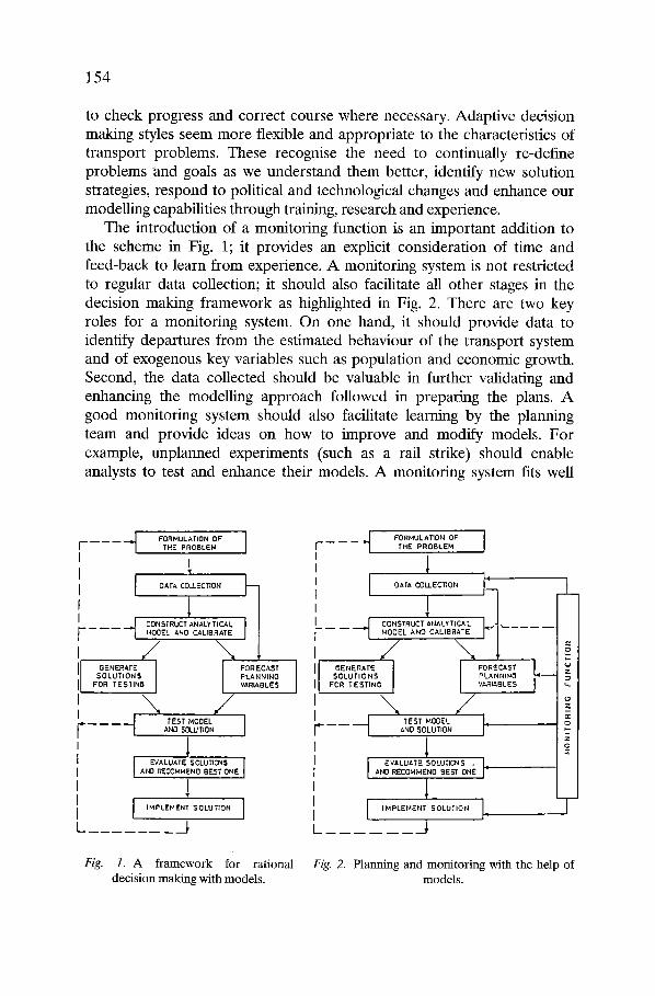
Transport planning models on their own do not solve transport problems. To be useful they must be utilised as part of an effective decision making framework. The classic four-stage transport model seems to have been developed for an idealised normative decision making approach (see Fig. 1). Within this framework transport models may be used to formulate one-off Master Plans, but these are not very flexible constructs.

This decision making style implicitly assumes that the problem can be fully specified, its constraints and decision space can be defined, and the objective function identified (e.g. maximise Net Present Value) and ideally quantified. Emphasis in infrastructure planning and formal cost-benefit analysis reflect this approach. However, real transport systems seldom obey the restrictions above; objective functions and constraints are often difficult to define. By narrowing a transport problem we may gain the illusion of being able to solve it; unfortunately, transport problems have the habit of reappearing in different places and under different guises; new features and perspectives are added as our understanding of the system progresses; changes in the external factors and planning variables throw our detailed transport plans off-course. A strong but inflexible normative decision making framework may be suitable for simpler, well defined and constrained problems but it hardly helps to deal with richer, more complex, many-featured and multi-dimensional transport issues.

In order to improve this general approach to cope with an evolving world, it seems essential to recognise that the future is more tenuous than our forecasting models would lead us to believe. Therefore, Master Plans need revising at regular intervals on the basis of fresh information collected

154

to check progress and correct course where necessary. Adaptive decision making styles seem more flexible and appropriate to the characteristics of transport problems. These recognise the need to continually re-define problems and goals as we understand them better, identify new solution strategies, respond to political and technological changes and enhance our modelling capabilities through training, research and experience.

The introduction of a monitoring function is an important addition to the scheme in Fig. 1; it provides an explicit consideration of time and feed-back to learn from experience. A monitoring system is not restricted to regular data collection; it should also facilitate all other stages in the decision making framework as highlighted in Fig. 2. There are two key roles for a monitoring system. On one hand, it should provide data to identify departures from the estimated behaviour of the transport system and of exogenous key variables such as population and economic growth. Second, the data collected should be valuable in further validating and enhancing the modelling approach followed in preparing the plans. A good monitoring system should also facilitate learning by the planning team and provide ideas on how to improve and modify models. For example, unplanned experiments (such as a rail strike) should enable analysts to test and enhance their models. A monitoring system fits well

FORMULATION O ' I [ ..... THE PROBLEM r--- - -

f ~ ' I i I I OATAC~B=ON ~ l

f I iT I

I I F . . . . ...~ CON STRUCT AN ALy TICA L 14OOEL AND CALIBRATE I

GENERATE I FORECAST I SOLUTION $ I PLANNING

FOR TESTING VARIABLES

\ / . ~ _ _ _ _ _ _ . ~ TEST MOOEL I

AND SOLUTION

I I EVALUATE SOLUTIONS AN) RECOMMEND BF-.ST ONE [

I 'M'LEMENT SOLU'ON I }

_ ~ PORMULArl0N OF [ THE PROBLEM

0ATA COLLECTION~ !!~B~_.~ i 1 I .~ CONSTRUCT ANALYTICAL -- -- -- MODEL AND CALIBRATE

GENERATE I F U ~OLUT,ONB ~>; ~

FOR T ESTING u.

\ / o -I T.T.GOEL I' o= • e- ---- AND SOLUTION ~"

o I EVALUATE SOLUTIC]~S . I

ANO RECBMMENO BEST ONE i

l i 'MRLE'ENT'OLU"ON I,

Fig. 1. A framework for rational Fig. 2. Planning and monitoring with the help of decision making with models, models.

155

with the idea of a regular or continuous planning approach in transport. If such a system is not in place, it should be established as part of any transportation study.

Monitoring the performance of a transport system and plans is such an important function that deserves influencing the choice of transport models used to support planning and policy making. The use of models which can be re-run and updated using low cost and easy to collect data, seem particularly appropriate to this task. However, these simpler models cannot provide all the behavioural richness of other more detailed approaches; nevertheless, there is scope for combining the two techniques applying the tool with the highest resolution to the critical parts of the problem and using coarser but easier to update tools to monitor progress and identify where and when a new detailed modelling effort is needed (see for example de Cea et al. 1986).

The adoption of a monitoring function enables the implementation of a continuous planning process. This is in contrast to the conventional approach of spending considerable resources over a period of one or two years to undertake a large-scale transport study. This burst of activity may be followed by a much longer period of limited effort in planning and updating of plans, and soon the reports and Master Plans become obsolete or simply forgotten.

Some years later a new major planning and modelling effort is em- barked upon and the cycle is repeated. This style of planning with the help of models in fits and starts is wasteful of resources, does not encourage learning and adaptation as a planning skill, and alienates analysts from finding solutions to real problems. This approach is particularly painful in developing countries: they do not have resources to waste and the rapid change experienced there speeds up plan and data obsolescence.

Furthermore, models are estimated to replicate a transport system provided most external conditions remain more or less stable. However, if new issues arise that need analysis or economic policies change radically over time, even well calibrated models will begin to lose their relevance. An expensive conventional model becomes a surrogate in this new context and its use to manage a transport system will result in weak planning and ineffectual decision making.

What is needed, we argue, is twofold:

• Techniques to monitor the evolution of the transport/land use system and the economy, checking the validity of both planning variables and transport model forecasts, and

• Methods for updating and transferring models from one context (place and/or time) to another, using low cost or easily available data, and

156

which ensure that the models are adequate for the new conditions and political environment.

A monitoring system should not only provide data to identify depar- tures from the estimated behaviour of the transport system and of the exogenous planning variables, such as population and car ownership growth, but also the data collected should be valuable in further validating and enhancing the modelling approach followed in the preparation of plans. The interested reader is advised to read the discussion about the role of models, planning and monitoring, given by Orttizar & Willumsen (1990, Chapter 1).

We are especially interested in a mixture of three improvements to modelling which appear particularly valuable in this context. The first one is the development of advanced discrete choice models which has been augmented in recent years by the use of Stated Preferences techniques, in particular to assist the modelling of completely new alternatives (see for example Steer & Willumsen 1983; Fowkes & Wardman 1988). This approach has reduced the costs of data collection and considerably enriched the demand models we can use and estimate. The second one is the development of techniques to estimate and update trip matrices and distribution models from traffic counts (see for example Cascetta & Nguyen 1988; Tamin & Willumsen 1989). Models of this type seem ideal for updating demand estimates using regularly collected data and there- fore may play a key role in any demand monitoring process. The third improvement in modelling techniques is a result of major advances in the theory and practice of model transfer over space and time. These theo- retical developments provide the ideal framework for discussing the enhanced approach proposed in this paper.

Brief technical review

(a) Stated preferences measurement and modelling

Transport models have been traditionally estimated using observations about the actual travel choices of individuals or groups of them. These observations reveal the preferences of travellers for particular attributes of services or destinations; the model estimation task is essentially to identify and quantify these preferences within a functional form. Traditional models, therefore, are based on Revealed Preferences (RP) data. There are known problems with this data source: very often it does not provide enough variation as the services offered in practice are too homogeneous

157

in their attributes (similar speed, price, etc); there is no 'revealed prefer- ences data' on options that do not yet exist but we would like to estimate demand for their introduction; data collection costs may be high.

For these and other reasons, modellers have been trying for many years to elicit these preferences by directly asking individuals about them. Stated Preferences (SP) data is obtained by asking individuals about what they would do in a hypothetical situation. Therefore, a basic problem of the approach is how much faith can we put on individuals actually doing what they stated they would do when the case arises.

In fact, experience in the 1970s was not very good in this sense, with up to 100% differences between predicted and actual choice found in many studies (see Ortfizar 1980). The situation improved considerably in the 1980s and recently very good agreement with reality has been reported from models estimated using SP data (Louviere 1988). However, this has occurred because SP data collection methods have improved enormously and are now very demanding, not only in terms of survey design expertise, but also in terms of their requirements for operational resources. For example, ad-hoc software and computerised data collection equipment are strongly recommended (see Bradley 1988).

A modelling exercise based on SP data has the following key stages: identification of attributes and data collection methods, experimental design, stimulus presentation issues, design of sampling strategy, data collection, and finally analysis and modelling. The main questions involved in these stages are outlined below:

Attributes and data collection methods A stated preferences experiment has as one of its main elements the construction of a set of hypothetical (although realistic) options, which we will refer to as technologically feasible alternatives; these are defined on the basis of the factors assumed to influence most strongly the choice problem under consideration. Practical experience recommends contem- plating at least the following stagaes in this task:

-- Identify the attributes to be considered (through experience and group discussions) and their likely levels of variation.

-- Design an initial version of the experiment and of the survey instru- ment: using simulated data check that the design allows to recover all model parameters.

- - Pre-test the survey instrument using a small stratified sample in order to consider the opinion of the largest possible number of interesting sectors of the population.

-- Evaluate the pre-test results both in terms of the quality of the survey

158

instrument and of the intuitive quality of the responses obtained by population strata; correct the instrument before its distribution.

1. Experimental design The number of attributes (a) and the number of levels each one can take (n), determine a factorial design (na). Tables exist (see for example Kocur et al. 1982) which give the number of hypothetical options needed to test most designs of interest and guarantee independence among options (orthogonality).

The designs distinguish cases considering principal effects only and cases allowing the treatment of interactions (ie when the effects of two variables are not additive they may enter as the product of the two variables, see Fig. 3). A problem with the latter is that they require the construction of many more options: for this reason fractional factorial designs, which assume that some or all variable products are negligible, are often used.

In fact, a key design issue is complexity. Experience has shown that people give the most reliable responses when asked to consider simul- taneous changes in up to four factors only. The complexity of the response task can thus be expected to influence the amount of error in the data; pre-tests, survey monitoring and subsequent debriefing, can uncover general problems and checks can be incorporated in the instrument to identify individuals with poor understanding. In this sense interactive survey procedures appear to be particularly appropriate because they

,u vl w

FREOUENCY ( B u I ~ / H c ]

I I I I J I [ I I r t I I ,

20 ~;0 Fare

I I

I I I t t I I i I , ,

30 SO F a r e

A| WITHOUT INTEi"tACTION B) WITH INTERACTION

Fig. 3. Presence and absence of attribute interaction.

159

allow to detect such problems and immediately probe further or provide additional instructions (see Pearmain and Kroes 1990).

Once the factorial design has been decided, the technologically feasible alternatives are constructed (which may, of course, be just hypothetical) and eventually the experiment conducted and the data collected. Fowkes and Wardman (1988) make a series of practical recommendations for the desirable variation of the attribute levels; their experience indicates that often it may be beneficial to sacrifice some purity in the experimental design (e.g. lose complete orthogonality) if one gains in realism.

2. Stimulus presentation In order to guarantee realistic responses by the interviewee, it is very important that the attributes of the options are presented in terms similar to those perceived by the traveller, see for example Steer and Willumsen (1983). Interactive procedures are once more invaluable to adapt the experiment to each individual, given some basic characteristics (ie age, sex, location, purpose of trip).

3. Sampfing strategy As in any other data collection exercise, issues such as sample composi- tion and size are very important in the design of an appropriate SP experi- ment. Also, in common with revealed preferences (RP) studies, a basic requirement is to obtain a sufficiently large and representative sample; however, because SP experiments are statistically efficient, samples are typically smaller than for comparable RP studies.

4. Stated preferences modelling An important feature of the SP approach is that each respondent may contribute with more than one observation. There are three main types of responses: ratings, rankings and choices. In the first case, the subject is asked to assign a rating, usually a number between 1 and 5 or 10, to each option. The result of this rating exercise is often interpreted as the strength of the individual preference for each alternative. Therefore, normal alge- braic operations can be carried out on them, for example extracting a ratio or subtracting one from another.

In the second case individuals are asked to rank N hypothetical options in order of desirability. In this case, if ri denotes the alternative ranked in the ith position, the response may be interpreted as implying that:

U(r ) >1 U(r ) >1 . . . >i U(r )

where U(ri) is the utility of ith ranked option.

160

In the case of choices the individual is only asked to choose his preferred option from the alternatives in the choice set; therefore in this case the response corresponds with the usual discrete choice RP approach, although both alternatives and choices are hypothetical.

The preferred modelling technique is currently the latter which has been greatly enhanced by the use of "adaptive" questionnaire design and interview programs such as Game Generator (SDG 1990); choice data allows more flexibility in model specification than rank data (the latter is constrained to multinominal logit only, see Chapman and Staelin 1982) and is a more natural task than rating for most individuals.

It is interesting to mention that SP data lacks, by design, some sources of error. In particular, there is no measurement error since all attribute values are presented to respondents (although there may be some percep- tion problems). Also, since the options are in principle fully represented by their attributes, there is no cause for unobservable factors; an exception to this occurs when respondents are asked to express a preference between alternatives with easily identifiable properties (say bus and rail), because choice may depend on variables not included in the design but implicit in the individual's perception of the options.

Apart from specification error, which clearly does still apply, there is another potentially serious source of error related to the response itself. Although practical results are generally encouraging, in terms of suggest- ing that most respondents do understand what is expected of them, there is no guarantee that they are able to complete an SP experiment with total accuracy.

In fact, a good review by Bates (1988) discusses the following types of potential error applying to all types of SP data:

-- respondent fatigue, which obviously increases with the complexity of the experimental design (see the discussion above)

-- policy response bias, which might occur if the respondent is interested in affecting the outcome of the analysis

- - self selectivity bias, when respondents either inadvertently or on purpose, cast their existing behaviour in a better light.

The outcome of all this is that we may have measurement error in the dependent variable, ie instead of getting a true estimate of the utility U, we are obtaining some pseudo utility /.). The problem comes in forecasting, because in that case we are interested in making estimates of U, and what we would get from applying this model are estimates of U provided the same distribution of errors applying in the design year. For this reason some kind of scaling of the coefficients of the estimated utilities is required

161

(similar to the model updating approach we discuss in the next section) and this is typically done using additional RP data (see Kocur et al. 1982).

The latest advance in this area entails the possibility of combining SP and RP data in model estimation. This is not an easy task, given the different sorts of errors each type of information has, but has potentially great advantages as discussed by Ben Akiva & Morikawa (1990) and Bradley & Kroes (1990).

Co) Trip matrix estimation

An origin-destination (O-D) matrix is a useful construct condensing a good deal of the information about travel patterns in a transport system. In order to avoid the need to collect expensive survey data, several methods to estimate these matrices from cheaper or more reliable data have been devised in recent years. It is clear that the most popular items of information in alternative methods is a set of volume counts. Willumsen (1981) has discussed the basis for this approach at some length, we will only offer here some of the basic principles as required for this paper. The general estimation problem in this case may be posed as follows: the flow F a on link a is the result of combining a trip matrix Tij with a route choice pattern. This can be written as:

Fo = 0 4 1 (1) /]"

where the variables p~, denoting the proportion of trips between zones i and j using link a, are estimated with a suitable assignment model. If we let F* denote the vector of L observed traffic counts, we can now write:

F ~ = F a --~ 1~ a E ( E a ) ~ 0 (2)

The assumption of zero mean residual error, which has been supported empirically, allows estimates of the residual variances to be obtained from traffic counts and the adopted assignment model. The problem is to find estimates of all the Tgj (i.e. N 2 quantities for a system with N zones) with just L simultaneous equations of the form (1), As typically L is smaller than N:, it is clear that the solution space needs to be restricted somehow in order to obtain a unique answer. One, now standard method, is to use additional information on t, a prior or outdated matrix, and choose the most likely trip matrix consistent with all the information available. Another method to restrict the solution space consists in assuming that the estimates of T may be represented by a trip distribution model. Tamin &

162

WiUumsen (1989) review the subject comparing several models and estimation approaches.

(c) Mode choice update or transference

During the past decade a substantial body of literature has emerged with empirical evidence about the stability of disaggregate travel demand models across space, cultures and time (see for example Gunn et al. 1985; Koppelrnan, Kuah & Wilmot 1985; Orttizar 1986). The model transfer approach is based on the idea that model parameters from a previous study may provide useful information for estimating the same model in a new area, even when the true parameter values are not expected to be the same. Updating methods are needed to modify these parameters so that they represent behaviour in the application context more accurately. The use of disaggregate data in model updating is now well understood (Ben Akiva & Bolduc 1987); we will briefly discuss below the more interesting (for our purposes) case of model updating using aggregate data on modal shares and aggregate demographic and level of service variables.

Consider a model of choice ej.q{ gjq(O, X)} which gives the probability that and individual q, belonging to a population or group Q, selects an option Aj belonging to his choice set A(q). The probabilities are calcu- lated on the basis of the values of utility function Vjq which are a function of a set of estimated parameters 0 -- { 0 1 , 0 2 , . . . , Op} and the explanatory variables X. The latter may be both level of service attributes of the options and socioeconomic characteristics of the individuals (see Orttizar 1982). A general presentation of the simplest choice model, the linear multinomial logit model, considers the explicit inclusion of a set of location parameters m and a scale parameter/~, as in:

exp[ H (rnj + Xp(CpXjqp) l PJq = Y'Ak A(q) exp[bt(m + Xp(CvXkqp)]

(3)

where the location parameters represent the models and the scale parame- ter is proportional to the inverse of the common standard deviation of the distributions of errors of the utilities of each alternative; the parameters C are the attribute weightings employed by the individuals in evaluating options. As not all the above parameters are uniquely identifiable, they cannot all be estimated. Firstly, it is not possible to estimate H but only the products /zm and PC; defining these products as M and 0 respectively, we obtain the more familiar version of the model as:

exp[Mj + Np(O~qp)] PJq = YA~A(q) exp[Mk + Np(O~qp)]"

(4)

163

Secondly, one of the "alternative specific constants" M is arbitrarily set to zero without loss of generality. Aggregation of the individual probabilities over the population yields aggregate modelled shares PjQ which may be compared with observed market shares PfQ. If the disaggregate model has a full set of constants, observed and modelled shares coincide for linear logit specifications (see Orttizar 1982).

Consider a naive aggregation where the representative utility of option Aj for a certain group z (say residents of a given zone) is simply estimated a s :

= Mj + (5) p

m

where Xjz is the vector of average variable values for option Aj in group z and Mj is its alternative specific constant. Updating of both alternative specific constants and scale using aggregate data may be accomplished by a simple procedure described by Koppelman, Kuah & Rose (1985). First, compute non-constant utility for the application (A) context:

then postulate an expression for the representative utility of group z in the application context allowing for updating of both constants and scale, as:

~A _-- M A + r A ~ (6)

where M A and rA are chosen such as to maximise the logarithm of the likelihood function:

L(M A, vA) = y~ Wz ~ p~ log pj~(ZA, MA, ~.A) z ]

(7)

with w z a weight, usually the number of observations, which indicates the relative importance of the group in the data set. A more refined method to update scale and constants using the ALOGIT package is described by Gunn & Pol (1985).

The aggregation issue in the above discussion is not trivial as it is well known that the naive method may introduce a bias. In this sense it is interesting to mention that the methodology discussed above is wholly consistent with the aggregation approach implicit in most British transport studies, where disaggregate model parameters were used as input to generalised cost funtions, and later "scale" and "bias" parameters were

164

fitted using aggregate data (see the discussion in Williams & Orttizar 1982). A more elaborate version of this approach was recently used for the Santiago Strategic Transport Study (ESTRAUS 1989); disaggregate mode choice parameters were firstly estimated using data for 1983, 1985 and 1986 (see Ortfzar & Ivelic 1988) and later used for building gener- alised cost functions from network data for 1977. Aggregate trip distribu- tion/model split models were then estimated for that year (as a large O-D survey was available) and validated using volume counts and other aggre- gate data for 1986.

We have argued that a key element in an enhanced planning approach is the availability and use of models which are easy to transfer and update using low cost data. Important theoretical and practical advances have been made in the area of matrix estimation but similar improvements have, so far, eluded areas like mode and destination choice modelling. This is a very significant difficulty and the main objective of the research discussed in this paper was to explore the scope for developing destination and mode choice models which could be estimated or updated using different sources of low cost data. When considering each model we had to address the following issues:

- - what type of information could be used to estimate and update the model?

- - is it possible to cast the estimation problem in a sound statistical and mathematical programming framework?

1 can we show that there is a unique solution to this problem? - - can we develop a suitable and efficient solution algorithm? - - what are the properties of this solution?

During the course of this research we discovered that the problem presented several difficulties, some of which we were able to tackle whereas others remain as topics for further research efforts. The rest of the paper summarises our findings in this area; these should be interpreted as an example of the type of technical progress that is needed in order to provide a frilly supported continuous planning approach.

A l o g i t d e s t i n a t i o n / m o d e c h o i c e m o d e l

We consider a singly constrained aggregate destination/mode choice model of the following logit form:

O~Sj Zk exp(ZpOpXP.k) T0 = ZaSd Y.k exp(Zp OpXfak) (8)

165

where Oi are the total number of trips generated at zone i and Sj is a measure of the attractiveness of zone j (i.e. its total number of jobs); the mode choice component of the model is given by:

exp(Zv OpX .O Pijk = Y'm exp(ZpOvXL) (9)

Although the derivations we will present below are for the simpler multi- nomial logit case, they can be extended easily to consider the simultaneous estimation of more general (nested logit) forms as discussed by Orttizar (1989). Let us consider first a unimodal case with a single scale parameter x, multiplying a "generalised cost" variable Cij, to be estimated. In this simple example (8) reduces to:

O~,S) exp(rCo- ) (10) Tq -- ZdSd exp(rCia)"

Now, assume we possess observations on a set of link flows F*, and also that we know, from an assignment model, the proportion p ~. for all links with an observed flow. In this case we can postulate that equation (1) holds and to estimate the value of r we can, for example, seek to minimise the following normalised non-linear least squares function:

S o = ~ [(F* - - Fa)/F*a] 2. (11) g

In order to use a method such as Newton-Raphson to find the minimum, we need first and second derivatives of S O with respect to r; the first order condition is:

(0S0/0r) = )~ [2 (F*- Fa)/F 2] (OFa/i)r) = O. a

(12)

The expression for the first and second derivatives when (10) is replaced in (12) and in the corresponding expression for the second order condi- tions are presented in Orttizar (1989). Unfortunately, even in this simple case the functions appear rather intractable so a unique solution to the problem may be difficult to establish.

Updating with aggregate shares only

Consider the transference of model (8)--(9) with parameters 0 estimated

166

in another context; we ignore the original constants as they ensure repro- duction of the aggregate market shares in that context. Define a transfer utility function as:

= + E o xfj ) P (13)

with X~j k being zonal values for the level of service and socioeconomic variables in the new context; r and M are, as before, a scale parameter and a set of (K - 1) mode specific constants to be estimated; K is the total number of modes.

(a) Information at the origin zone level

Assume that we have information about aggregate mode shares P*k at every origin zone (where we require Z~P*k ---- 1); we would like to compare these with modelled shares defined as:

Pi~ -~ ZJT0k ---- ZjS/exp(V,j~) (14) Zj T~j Z~m Sj exp(V0m)

In this case we can find estimates of r and M by maximising the following log-likelihood function:

$1 -- Y~ O, ~ P*~ log Pik (15) i k

and the first order conditions can be shown to be given by:

(OSl/~l:)=~i Oi I~Pi* {~] SijkZijk/~ Z~jk}-~jmSijmZtym//Oil =0 ( 1 6 )

(OS1/OMk) = }~ Oi(P*k -- 5,0---- 0, k = 1 , . . . K -- 1 (17) i In this case a unique optimum solution is guaranteed for the case of estimating the constants only (i.e. for fixed r) as shown in Orttizar (1989).

(b) Information at the aggregate level

Consider now the more realistic case where we only have available

167

information about the aggregate market shares P~ for the whole area; therefore, we require that XkP ~ = 1. We want to compare these shares with the corresponding modelled shares which can be defined this time as follows:

Y-,ijZjk _ Y~ijO, Sj exp(Gjk) (18) Pk ---- y~jTo Y.~j OiSj. Zm exp(V~jm)'

In this case to find estimates of r and M we need to maximise the follow- ing log-likelihood function:

S 2 = ~ P~ log Pk(V/jk). (19) k

The first order conditions can be shown to reduce to:

(OS2/OMk) = ( P ~ - Pk) = 0, k - - 1 , . . . , K - 1 (21)

and again an optimum can be find uniquely for fixed r. This approach can be generalised for the case when modal shares by person type are available (Ortfizar 1989).

Updating with passenger counts only

The main problems arise when we are interested in mixed-mode combina- tions but only possess counts on the pure modes. Consider the case of having mode choice among car, bus, Metro and combinations (typically of the first two with the latter); although we may have separate passenger counts for car, bus and Metro, it is obvious that these include mixed-mode counts.

The situation can be stated as follows:

1. Let the models be Car (1), Bus (2), Metro (3), P&R (4) and Feeder Bus (5). We have (linearly dependent) passenger counts for Car (and P&R) and Bus (which include Feeder Bus counts), and independent passenger counts for Metro (which include passengers with all three "access" modes to the system, i.e. on foot, by car and by bus). Assum-

168

ing we do not know the proportions of each pure mode count corre- sponding to each mode of interest, we would have:

Car counts: V*I = Fa*l + Fa*4 l surface network Bus counts: V* 2 ---- F * 2 + F* 5 ] Metro counts: V~3 = F~3 + F~4 + F~5 underground network

2. We have private and public transport assignment models yielding proportions P~k of trips between zones i and J" by mode k using arc a. The modelled counts are thus given by:

V~I F~ + F a 4 ~. (T/] 1 .{._ 1 a = = T i j4 )P i j l i]

Va2 Fa2 .at-Fa5 ~ (T/j 2 Ji- 1 a = = r i j s ) P i j 2 q

Vb3 = Fb3"31-Fb4"Ji-Fb5 = E (Z~j3 + To.4 + T ~ j s ) P ~ j 3 2 a ij

w h e r e Tlijk stands for the l th leg of a mixed-mode trip.

. Clearly it is not possible to estimate the mode specific constants M for all modes in thise case; however, we can certainly try to estimate the scale parameter r and constants for the three pure modes (although understanding that they are now "composite" modes). To do this we may wish to minimise:

& = ~ [f l ( Va*l - - Val) 2 "q- f2( Va*2 - - Va2)2l "3V ~ f3( V~b3 - - Vb3) 2 ( 2 2 ) a b

where:

= (o~ + o~)/o' v~, ~ - - ( a ~ + 2 2 2 a3)/o V~2

= ( ~ + ~ ) / ~ ' v ~

o 2 = ax 2 + a~ + o 2

and a 2 are the variances of the various counts; here, then, we are not only normalising as before (i.e. by dividing by the observed count values) but incorporating the possibility that the various counts may

169

have different levels of accuracy. We will postulate similar techniques when combining data of different nature as in the next section.

Updating with combined information

Assume we want to update ~" and M of (13) and we have available aggregate shares P~ and sets of observed passenger counts F*I and F*2, f o r a ~ L.

(a) Maximum likelihood approach

In this case we will get different functions to maximise and hence different first order conditions (and optima) depending on the assumptions made about the distribution of the errors e a in equation (2). The favourite assumptions have been Multinomial, independent Poisson and indepen- dent Normal (see for example Cascetta & Nguyen 1988; Tamin Willum- sen 1989). As it can be assumed that data on counts is independent of data on aggregate shares, the combined log-likelihood function for the independent Normal case is the sum of an expression such as (19) and the following:

--0.5 Zak(Fa* k - - Y~ii TqkP; 'k) 2 L = 2 (23)

I~ a k

where a2ak is the variance of the observed counts, ff it is assumed that the counts are free of error, a final case of interest results which just requires maximising (19) subject to (1). Expressions for the Multinomial and independent Poisson cases, plus first order conditions for each of these problems are given by Ortdzar (1989). There is no guarantee, however, that either of these conduces to a unique optimum.

Co) Generalised least squares approach

This approach has two advantages: the first is that no distributional assumptions are needed on the data set, and the second is the possibility of incorporating explicitly differences in the accuracy of each data item prior to estimation. The need for normalising is also very evident here given the different order of magnitude of the differences between observed and modelled variables for both types of data. For example, the maximum difference in the case of aggregate shares is 1, while differences in count data may run easily into figures in the thousands. Given all this, it is

170

possible to postulate that the function to minimise in this case takes the form:

S 4 = ~ ~ (~ak[ (Fa~k - - F.~)/F.*k] 2 + (1 - fl) ~. d~k[(P' ~ --Pk)/P~] 2 ka k

with:

~ 2 2 a,/(ac +

where a~ are the variances of the count and share data respectively, and dak takes the value of 1 if mode k uses link a and 0 otherwise. To estimate the a values we need extra information from the data or we can guess them from previous experience knowing sample size. First order condi- tions for the above expression can be found in Ortfizar (1989).

Conclusions

• We have argued that current transport planning issues require an adaptive modelling approach which can use readily available data to update models, forecasts and plans. The introduction of a formal monitoring function supported by suitable models is seen as an essen- tial element of this new approach.

• This enhanced transport planning approach requires models which are easy to estimate and update using low cost and regularly collected data. Only limited progress has been achieved in this area so far.

• Three areas of research seem to bear promise for the development of this enhanced modelling approach: the use of stated preferences modelling techniques, methods for estimating matrices and distribution models from count data and new advances in destination and mode choice model transfer.

• Models based on SP data, because of their low cost and flexibility, may provide an initial basis for update and transfer to specific geographic or temporal frames. Recent advances in the techniques have resulted in more robust and reliable models.

• Techniques for estimating trip matrices and distribution models from traffic and person counts have been developed over the last 10 years; the estimation of mode choice models from similar data has remained an elusive problem. We have proposed an approach which takes advantage of recent progress in logit model transferability methods and combines the advantages of model estimation from count data.

171

• The proposed strategy combines destination and mode choice estima- tion in a single problem and different analytical solution have been proposed depending on the availability of data. This approach uses recent advances in model transfer theory as its basic framework. The practicalities of each case are as follows.

• If information is available on aggregate model shares only, it appears that maximum likelihood is the most appropriate estimation method. If only the mode specific constants need updating, a unique solution to the optimisation problem is guaranteed which can be reached easily by adapting fairly standard software. However, this is not so if the scale parameter also requires updating, as in general no unique solution can be guaranteed in this case.

• When only data on passenger counts is available, the updating problem is conceptually straightforward but difficult to solve in practice due to the relative intractability of the optimisation problem. In many practical cases, such as areas with non-negligible mixed-mode movements, data considerations alone will normally prevent updating of a full set of constants.

• If data on shares and counts is forthcoming, a range of methodologies is available in principle but their relative practical merits cannot be ascer- tained without recourse to experimentation; the methods include maxi- mum likelihood (four versions) and generalised least squares.

• The proposed approach offers considerable promise in terms of com- bining the behavioural richness of disaggregate models with properties which make them easier to update and transfer. This is an essential requirement for a consistent and robust long term planning approach which relies on regular updating of demand forecasts and plans.

• Additional research is needed to refine these models, explore these properties further, to develop better solution algorithms and to extend the approach to other areas. Experience on the use of these models over an extended period is needed before they can fully replace existing approaches.

Acknowledgements

The work reported in this paper was carried out with additional support from the British Science and Engineering Research Council through a SERC Visiting Fellowship. Financial support was also obtained from the Royal Society, The British Council, Fundaci6n Andes and The Chartered Institute of Transport.

172

References

Bates JJ (1988) Econometric issues in stated preference analysis. Journal of Transport Economics and Policy XXII(1): 59--69.

Ben Akiva ME & Bolduc D (1987) Approaches to model transferability and updating: the combined transfer estimator. Transportation Research Record 1139: 1--7.

Ben Akiva ME & Morikawa T (1990) Estimation of travel demand models from multiple sources. Proceedings, 11th International Symposium on Transportation and Traffic Theory, Yokohama, Japan.

Bradley M (1988) Realism and adaptation in designing hypothetical travel choice concepts. Journal of Transport Economics and Policy XXII(1): 121--137.

Bradley M & Kroes E (1990) Simultaneous analysis of stated preference and revealed preference information. Proceedings 18th PTRC Summer Annual Meeting, University of Sussex, England.

Cascetta E & Nguyen S (1988) A unified framework for estimating or updating origin/ destination matrices from traffic counts. Transportation Research 22B(6): 437--455.

Chapman RG & Staelin R (1982) Exploiting rank ordered choice set data within the stochastic utility model. Journal of Marketing Research XIX(3): 288--301.

De Cea J, Orttizar J de Dios & Willumsen LG (1986) Evaluating marginal improvements to a transport network: An application to the Santiago underground. Transportation 13(3): 211--233.

ESTRAUS (1989) Estudio estrattgico de transporte del Gran Santiago. Informe Final a la Secretarfa Ejecutiva de la Comisi6n de Transporte Urbano, Consorcio SIGDOKOP- PERS-CIS, Santiago.

Fowkes AS & Wardman M (1988) The design of stated preference travel choice experi- ments, with special reference to interpersonal taste variations. Journal of Transport Economics and Policy XXII(1): 27--44.

Gunn I-IF, Ben Akiva ME & Bradley MA (1985) Tests of the scaling approach to transferring disaggregate travel demand models. Transportation Research Record 1037: 21--30.

Gunn HF & Pol H (1985) Model transferability: the potential for increasing cost-effective- ness. International Conference on Travel Behaviour, Noordwijk, April 1985, The Netherlands.

Kocur GT, Adler T, Hyman W & Aunet B (1982) Guide to forecasting travel demand with direct utility assessment. Report Ae UMTA-NH-11-O001-82, Urban Mass Transportation Administration, U.S. Department of Transportation, Washington, D.C.

Koppelman FS, Kuah G-K & Rose G (1985) Transfer model updating with aggregate data. 64th Annual TRB Meeting, Transportation Research Board, Washington, D.C, January 1985, U.S.A.

Koppelman FS, Kuah G-K & Wilmot CG (1985) Transfer model updating using dis- aggregate data. Transportation Research Record 1037: 102--107.

Louviere JJ (1988) Conjoint analysis modelling of stated preferences: A review of theory, methods, recent developments and external validity. Journal of Transport Economics and Policy XXII(1): 93--119.

Mackinder IH & Evans SE (1981) The predictive accuracy of British transport studies in urban areas. Supplementary Report SR 699, Transport and Road Research Laboratory, Crowthorne.

Orttzar J de Dios (1980) Mixed-mode demand forecasting techniques. Transportation Planning and Technology 6(2): 81--95.

173

- - (1982) Fundamentals of discrete multimodal choice modelling. Transport Reviews 2(1): 47--48.

- - (1986) The cultural and temporal transferability of discrete choice disaggregate model split models. Proceedings IV Worm Conference on Transport Research, University of British Columbia, May 1986, Canada.

- - (1989) Estimation of trip matrices and mode choice models integrating flow informa- tion and other data types. Technical Note, Transport Studies Group, University College London.

Orttizar J de Dios & Ivelic AM (1988) Influencia de nivel de agregacidn de los datos en la estimacidn de modelos logit de elecci6n discreta. Actas del V Congresco Panamericano de lngenieria de Trdnsito y Transporte, Universidad de Puerto Rico en Mayagiiez, July 1988, Puerto Rico.

Orttizar J de Dios & Willumsen LG (1990) Modelling Transport. London: John Wiley & Sons.

Pearmain D & Kroes E (1990) Stated Preference Techniques: A Guide to Practice. Steer Davies Gleave and Hague Consulting Group, London, England.

SDG (1990) Game-Generator, User Manual. Steer Davies Gleave, London, England. Steer J & Willumsen LG (1983) An investigation of passenger preference structures. In:

Carpenter & Jones (eds) Recent Advances in Travel Demand Analysis (pp 423--433). Gower Press.

Tamin OZ & Willumsen LG (1989) Transport demand model estimation from traffic counts. Transportation 16(1): 3--26.

Williams HCWL & Orttizar J de Dios (1982) Travel demand and response analysis: some integrating themes. Transportation Research 16A(5/6): 345--362.

Willumsen LG (1981) Simplified transport demand models based on traffic counts. Transportation 10(3): 257--278.