
Flexible Demand in Smart Grids, Modeling and Coordination
202
Flexible Demand in Smart Grids Modeling and Coordination Zur Erlangung des akademischen Grades eines Doktors der Wirtschaftswissenschaften (Dr. rer. pol.) von der Fakultät für Wirtschaftswissenschaften des Karlsruher Instituts für Technologie (KIT) genehmigte DISSERTATION von Dipl.-Wi.-Ing. Christoph Michael Flath Tag der mündlichen Prüfung: 28. Mai 2013 Referent: Prof. Dr. Christof Weinhardt Korreferent: Prof. Dr. Wolf Fichtner Karlsruhe, 2013
-
Upload
khangminh22 -
Category
Documents
-
view
3 -
download
0
Transcript of Flexible Demand in Smart Grids, Modeling and Coordination

Flexible Demand in Smart GridsModeling and Coordination
Zur Erlangung des akademischen Grades einesDoktors der Wirtschaftswissenschaften
(Dr. rer. pol.)
von der Fakultät fürWirtschaftswissenschaften
des Karlsruher Instituts für Technologie (KIT)
genehmigte
DISSERTATION
von
Dipl.-Wi.-Ing. Christoph Michael Flath
Tag der mündlichen Prüfung: 28. Mai 2013
Referent: Prof. Dr. Christof Weinhardt
Korreferent: Prof. Dr. Wolf Fichtner
Karlsruhe, 2013


Abstract
T he transition towards very high shares of fluctuating energy generation sourcesrequires significant changes to the power system and electricity markets. Smart
grids will play a key role in addressing this challenge. Through improved monitor-ing, forecasting and control capabilities they will be able to empower the so far pas-sive demand side of the power system. Yet, the successful establishment of smartgrids will require both sound technical and economic concepts. The economic anal-ysis of smart grid capabilities needs to incorporate physical boundaries as hard con-straints which need to be facilitated by means of flexibility potentials and intelligentdispatching. Due to the distributed nature of demand, economic coordination alsoneeds to be able to facilitate a multitude of individual agents. Consequently, thedesign of future power systems and electricity markets needs to embrace the im-portance of distributed agents and facilitate their integration. The thesis followsthis decentral and demand-centric vision of the smart grid. Questions concerningthe modeling and coordination of an active demand side are addressed using toolsand techniques from information systems and economics. Building on a frameworkfor the design of smart grid customer models relevant coordination approaches arediscussed. This framework is applied within two distinct application scenarios —household customer models and electric vehicle models.
Household customer models are derived by applying a cluster analysis to iden-tify customer segments within smart metering data from a regional utilities com-pany. This data mining approach reveals distinct customer segments which differfrom standard load profiles. The customer heterogeneity motivates the design ofcustomer-specific electricity rates. To this end, a mixed-integer optimization modelto determine efficient time-of-use electricity rates for individual customer segmentsis proposed and evaluated. It obtains that rate update frequency is of greater impor-tance than rate granularity.
Charging needs of electric vehicles are modeled using current technical speci-fications and empirical mobility data. Based on these model primitives, a varietyof decision models encapsulating different price and trip information regimes arediscussed and implemented. This allows assessing likely charging behavior of indi-vidual electric vehicles in the presence of different incentive schemes, battery wearor load-based demand charges. These individual models are then aggregated toanalyze the load impact of population-wide charging behavior. Based on these pop-ulation models, two charging load coordination mechanisms are discussed — lo-cational pricing and capacity management. Using surcharges reflecting local trans-former utilization, area pricing successfully mitigates violations of stability limits

vi
while retaining the economic incentives of load shifting. The capacity managementscheme can achieve similar coordination results using a non-price-based approach.
Describing novel modeling techniques and coordination approaches, this thesiscontributes to the energy informatics literature and aims at establishing a notion ofsmart grid market design.

Acknowledgements
This work would not have been possible without the support of several people whocontributed with ideas, conversations, guidance, and care. To begin, I am verythankful that my supervisor Prof. Dr. Christof Weinhardt gave me the opportu-nity to pursue my dissertation providing the necessary guidance while at the sametime allowing me to freely develop my ideas. I would also like to thank co-advisorProf. Dr. Wolf Fichtner, Prof. Dr. Thomas Setzer, and Prof. Dr. Orestis Terzidis,who have served on my thesis committee, for providing valuable comments andsuggestions.
Furthermore, I would like to express my gratitude to my fellow colleagues at thechair of Information and Market Engineering as well as to my former colleagues atthe FZI Research Center for Information Technology. It was a special and gratifyingexperience to work on projects and pursue research with such a fun and inspiringgroup of people.
Among the set of colleagues, it is my pleasure to express special thanks to a se-lected group of people who for various reasons have played a very important roleon my path to finishing my dissertation: Florian Teschner for making me believe insalad and my research. Benoît Chevalier-Roignant for being an amazing Frenchman.Jens for being the most supportive co-worker one can wish for. Sebastian Gottwaltfor inspiring discussions on ants, football and electric vehicles. Philipp Ströhle forhaving taught me to trust in obscure tools. John Khawam for being one of the nicestand most helpful persons in the world. Rico Knapper for being a great Berlin guideand “co-sufferer”. Alex Schuller for his patient and calm nature. David Dauer forhis never-ending programming resources. Timm Teubner for board games and foot-ball. Philipp Astor for the Cannoli.
I am also very happy and thankful that over the years I was supported by manyfriends who helped me making difficult decisions, stick through times of frustra-tions and allowed me to enjoy great moments of community and camaraderie. Forthese reasons I want to especially thank Christoph, Daniel, David, Katharina, Kon-sti, Michi, Milena, Patrick, Robert and Timo.
Finally, I am deeply indebted to my family, especially my parents Thomas andUlrike. You have always supported and encouraged me throughout school, univer-sity studies as well as the dissertation time and I am very grateful for this.

Contents
1 Introduction 1
1.1 Smart grids as Techno-Economic Systems . . . . . . . . . . . . . . . . 21.2 Smart Grid Economics . . . . . . . . . . . . . . . . . . . . . . . . . . . 31.3 Research Questions & Problem Description . . . . . . . . . . . . . . . 4
1.3.1 Modeling Smart Grid Customers . . . . . . . . . . . . . . . . . 51.3.2 Smart Grid Coordination . . . . . . . . . . . . . . . . . . . . . . 6
1.4 Structure . . . . . . . . . . . . . . . . . . . . . . . . . . . . . . . . . . . 71.5 Research Path . . . . . . . . . . . . . . . . . . . . . . . . . . . . . . . . 7
I Smart Grid Economics 9
2 Smart Grid and Energy Markets 11
2.1 Electricity Value Chain . . . . . . . . . . . . . . . . . . . . . . . . . . . 112.1.1 Generation . . . . . . . . . . . . . . . . . . . . . . . . . . . . . . 122.1.2 Transmission and Distribution . . . . . . . . . . . . . . . . . . 142.1.3 Consumption . . . . . . . . . . . . . . . . . . . . . . . . . . . . 142.1.4 Power Grid Structure . . . . . . . . . . . . . . . . . . . . . . . . 15
2.2 The Energy Trilemma . . . . . . . . . . . . . . . . . . . . . . . . . . . . 162.2.1 Cost . . . . . . . . . . . . . . . . . . . . . . . . . . . . . . . . . . 172.2.2 Reliability . . . . . . . . . . . . . . . . . . . . . . . . . . . . . . 172.2.3 Sustainability . . . . . . . . . . . . . . . . . . . . . . . . . . . . 18
2.3 Smart Grids . . . . . . . . . . . . . . . . . . . . . . . . . . . . . . . . . 192.3.1 Demand Side Management . . . . . . . . . . . . . . . . . . . . 192.3.2 Electricity Pricing . . . . . . . . . . . . . . . . . . . . . . . . . . 21
2.4 Discussion . . . . . . . . . . . . . . . . . . . . . . . . . . . . . . . . . . 22
3 Customer Model Framework 23
3.1 Static Customer Characteristics . . . . . . . . . . . . . . . . . . . . . . 243.2 Model Size and Scope . . . . . . . . . . . . . . . . . . . . . . . . . . . . 24
3.2.1 Top-Down Models . . . . . . . . . . . . . . . . . . . . . . . . . 243.2.2 Bottom-up Models . . . . . . . . . . . . . . . . . . . . . . . . . 25
3.3 Load Response . . . . . . . . . . . . . . . . . . . . . . . . . . . . . . . . 253.3.1 Demand Response . . . . . . . . . . . . . . . . . . . . . . . . . 263.3.2 Interruptible Capacity . . . . . . . . . . . . . . . . . . . . . . . 27
3.4 Model Adaptivity over Time . . . . . . . . . . . . . . . . . . . . . . . . 28

x CONTENTS
3.4.1 Rate Utility and Selection . . . . . . . . . . . . . . . . . . . . . 283.4.2 Dynamic Investment Behavior . . . . . . . . . . . . . . . . . . 31
3.5 Discussion . . . . . . . . . . . . . . . . . . . . . . . . . . . . . . . . . . 33
II Modeling and Coordinating Residential Loads 35
4 Customer Modeling Using Smart Meter Data 37
4.1 Problem Relevance and Related Work . . . . . . . . . . . . . . . . . . 384.1.1 Business Intelligence and Knowledge Discovery . . . . . . . . 384.1.2 Data Mining in the Electricity Sector . . . . . . . . . . . . . . . 39
4.2 Cluster Analysis of Load Data . . . . . . . . . . . . . . . . . . . . . . . 394.2.1 System Environment and Analysis Process Design . . . . . . . 404.2.2 Data Preparation . . . . . . . . . . . . . . . . . . . . . . . . . . 40
4.3 Cluster Analysis Implementation . . . . . . . . . . . . . . . . . . . . . 424.3.1 k-Means Clustering . . . . . . . . . . . . . . . . . . . . . . . . . 424.3.2 Clustering Evaluation . . . . . . . . . . . . . . . . . . . . . . . 43
4.4 Evaluation of Clustering Results . . . . . . . . . . . . . . . . . . . . . 444.4.1 Day Profiles . . . . . . . . . . . . . . . . . . . . . . . . . . . . . 444.4.2 Customer Type Identification . . . . . . . . . . . . . . . . . . . 474.4.3 Week Profiles . . . . . . . . . . . . . . . . . . . . . . . . . . . . 47
4.5 Customer Modeling using Cluster Results . . . . . . . . . . . . . . . . 474.5.1 Behavioral Load Curve Interpretation . . . . . . . . . . . . . . 504.5.2 Characterizing Demand Response . . . . . . . . . . . . . . . . 52
4.6 Discussion . . . . . . . . . . . . . . . . . . . . . . . . . . . . . . . . . . 524.6.1 Limitations . . . . . . . . . . . . . . . . . . . . . . . . . . . . . . 534.6.2 Future opportunities . . . . . . . . . . . . . . . . . . . . . . . . 53
5 Customized Time of Use Rate Design 55
5.1 Time of Use Design Requirements . . . . . . . . . . . . . . . . . . . . . 565.2 Formal Representation of Time of Use Rates . . . . . . . . . . . . . . . 565.3 MIP Optimization Model for Time of Use Rates . . . . . . . . . . . . . 58
5.3.1 Decision Variables . . . . . . . . . . . . . . . . . . . . . . . . . . 595.3.2 Constraints . . . . . . . . . . . . . . . . . . . . . . . . . . . . . . 605.3.3 Objective Functions . . . . . . . . . . . . . . . . . . . . . . . . . 615.3.4 Procurement Cost Matching . . . . . . . . . . . . . . . . . . . . 625.3.5 Profit Maximization . . . . . . . . . . . . . . . . . . . . . . . . . 63
5.4 Evaluation . . . . . . . . . . . . . . . . . . . . . . . . . . . . . . . . . . 655.4.1 Scenario . . . . . . . . . . . . . . . . . . . . . . . . . . . . . . . 665.4.2 Workflow and System Design . . . . . . . . . . . . . . . . . . . 67
5.5 Rate Structures . . . . . . . . . . . . . . . . . . . . . . . . . . . . . . . . 675.5.1 Rate Granularity . . . . . . . . . . . . . . . . . . . . . . . . . . 675.5.2 Rate Updating Frequency . . . . . . . . . . . . . . . . . . . . . 69
5.6 Rate Efficiency . . . . . . . . . . . . . . . . . . . . . . . . . . . . . . . . 70

CONTENTS xi
5.6.1 Descriptive Analysis . . . . . . . . . . . . . . . . . . . . . . . . 705.6.2 Regression Analysis . . . . . . . . . . . . . . . . . . . . . . . . 73
5.7 Discussion . . . . . . . . . . . . . . . . . . . . . . . . . . . . . . . . . . 755.7.1 Limitations . . . . . . . . . . . . . . . . . . . . . . . . . . . . . . 765.7.2 Future Opportunities . . . . . . . . . . . . . . . . . . . . . . . . 76
III Modeling and Coordinating Electric Vehicle Loads 77
6 Electric Vehicle Models 79
6.1 Static Characterization of Electric Vehicle Models . . . . . . . . . . . . 806.1.1 Driving Profiles . . . . . . . . . . . . . . . . . . . . . . . . . . . 806.1.2 Driving Distance Distributions and Synthetic Profiles . . . . . 816.1.3 Locational Clustering . . . . . . . . . . . . . . . . . . . . . . . . 836.1.4 Vehicle Technical Data . . . . . . . . . . . . . . . . . . . . . . . 846.1.5 Charging System Specification . . . . . . . . . . . . . . . . . . 856.1.6 Wholesale prices . . . . . . . . . . . . . . . . . . . . . . . . . . 86
6.2 A Formalized Electric Vehicle Charging Model . . . . . . . . . . . . . 866.3 Simple Charging Protocol . . . . . . . . . . . . . . . . . . . . . . . . . 876.4 Optimal Smart Charging . . . . . . . . . . . . . . . . . . . . . . . . . . 89
6.4.1 Smart Charging Modifications . . . . . . . . . . . . . . . . . . . 906.4.2 Alternative Objectives and Charging Losses . . . . . . . . . . . 95
6.5 Heuristic Smart Charging . . . . . . . . . . . . . . . . . . . . . . . . . 986.5.1 As Late as Possible Charging . . . . . . . . . . . . . . . . . . . 986.5.2 Extensions of as Late as Possible Charging . . . . . . . . . . . 100
6.6 Categorization of Economic Charging Strategies . . . . . . . . . . . . 1056.7 Comparisons and Evaluation Results . . . . . . . . . . . . . . . . . . . 106
6.7.1 Vehicle Availability Levels . . . . . . . . . . . . . . . . . . . . . 1066.7.2 Charging Costs . . . . . . . . . . . . . . . . . . . . . . . . . . . 1066.7.3 Cost of Availability . . . . . . . . . . . . . . . . . . . . . . . . . 1086.7.4 Price vs. Trip Information . . . . . . . . . . . . . . . . . . . . . 108
6.8 Discussion . . . . . . . . . . . . . . . . . . . . . . . . . . . . . . . . . . 1106.8.1 Limitations . . . . . . . . . . . . . . . . . . . . . . . . . . . . . . 1106.8.2 Beyond Charging Strategies . . . . . . . . . . . . . . . . . . . . 110
7 EV Charging Coordination 113
7.1 Bottom-up Population Model . . . . . . . . . . . . . . . . . . . . . . . 1137.1.1 Aggregate Load Without Charging Coordination . . . . . . . . 1147.1.2 Aggregate Load with Exogenous Charging Coordination . . . 1177.1.3 Aggregate Load with Endogenous Charging Coordination . . 1197.1.4 Summary and Future Research . . . . . . . . . . . . . . . . . . 126
7.2 Top-down Population Model and Coordination . . . . . . . . . . . . . 1277.2.1 Revenue Management . . . . . . . . . . . . . . . . . . . . . . . 1277.2.2 Charging Coordination as a PARM Model . . . . . . . . . . . . 128

xii CONTENTS
7.2.3 Capacity Allocation Approaches . . . . . . . . . . . . . . . . . 1337.2.4 Numerical Analysis . . . . . . . . . . . . . . . . . . . . . . . . . 1377.2.5 Summary and Future Research . . . . . . . . . . . . . . . . . . 140
7.3 Discussion . . . . . . . . . . . . . . . . . . . . . . . . . . . . . . . . . . 143
IV Finale 145
8 Summary and Future Research 147
8.1 Smart Grid Economics . . . . . . . . . . . . . . . . . . . . . . . . . . . 1478.2 Residential Load Modeling and Coordination . . . . . . . . . . . . . . 1488.3 Electric Vehicle Load Modeling and Coordination . . . . . . . . . . . 150
9 Conclusion and Outlook 153
References 169
A List of Abbreviations 173
B Benefits of Demand Side Management 175
C Cluster Analysis 177
D Rate Design 179
E EV Modeling 183
F Charging Coordination 187

List of Figures
1.1 ICT connects physical and market layer in the smart grid . . . . . . . 31.2 Research Model . . . . . . . . . . . . . . . . . . . . . . . . . . . . . . . 51.3 Structure of the Thesis . . . . . . . . . . . . . . . . . . . . . . . . . . . 8
2.1 Functions and Sub-Functions in the Electricity Value Chain . . . . . . 122.2 Capacity and output share of different energy sources . . . . . . . . . 122.3 Merit Order Curve of Electricity Generation . . . . . . . . . . . . . . . 132.4 Basic structure and components of the electricity system . . . . . . . . 162.5 Layered model of the (future) energy system . . . . . . . . . . . . . . 20
3.1 Four levels of customer modeling . . . . . . . . . . . . . . . . . . . . . 243.2 Characterization of demand response types . . . . . . . . . . . . . . . 26
4.1 Phases of the CRISP-DM reference model . . . . . . . . . . . . . . . . 394.2 Phases of Cluster Analysis Implementation . . . . . . . . . . . . . . . 404.3 Cluster analysis scenarios . . . . . . . . . . . . . . . . . . . . . . . . . 414.4 Clustering results – Day profiles (Workdays, Winter) . . . . . . . . . . 454.5 Clustering results – Day profiles (Weekend, Winter) . . . . . . . . . . 464.6 BDEW Standard Load Profiles . . . . . . . . . . . . . . . . . . . . . . . 484.7 Clustering results – Week profiles (Winter) . . . . . . . . . . . . . . . . 494.8 Exemplary load quantile levels . . . . . . . . . . . . . . . . . . . . . . 51
5.1 Equivalent representations of a time-of-use rate . . . . . . . . . . . . . 575.2 Number of TOU rate structures for different values of K (|T | = 24) . 585.3 Daily EPEX price curves in 2012 . . . . . . . . . . . . . . . . . . . . . . 665.4 Integrated System for Custom Rate Design . . . . . . . . . . . . . . . 675.5 Evolution of optimal rate structure . . . . . . . . . . . . . . . . . . . . 685.6 Comparison of annual rates with symmetric and asymmetric zoning 695.7 Visualization of Optimal Rate Structures (Absolute Error) . . . . . . . 715.8 Efficiency of different rate granularity levels . . . . . . . . . . . . . . . 725.9 Comparison of annual rates with symmetric and asymmetric zoning
for weekend days . . . . . . . . . . . . . . . . . . . . . . . . . . . . . . 73
6.1 Distribution of trip lengths, begin and work day within driving pro-file data of 1,000 employees. (data source: Zumkeller et al., 2010) . . . 81
6.2 Histogram of unique commute distances and fitted Gamma distribu-tion (data source: Zumkeller et al., 2010) . . . . . . . . . . . . . . . . . 82
6.3 Relative share of vehicle presence at different locations (data source:Zumkeller et al., 2010) . . . . . . . . . . . . . . . . . . . . . . . . . . . 83

xiv LIST OF FIGURES
6.4 Relationship between EV range and consumption (data source: Salahet al., 2011) . . . . . . . . . . . . . . . . . . . . . . . . . . . . . . . . . . 85
6.5 Upscaled and interpolated EPEX Spot prices 2010 . . . . . . . . . . . 866.6 SOC level evolution of electric vehicle population under AFAP charging 886.7 Comparison of average AFAP charging costs . . . . . . . . . . . . . . 896.8 Comparison of average optimal smart charging costs . . . . . . . . . 916.9 Cost-optimal SOC trajectories for different minimum thresholds . . . 936.10 Impact of price information on charging costs . . . . . . . . . . . . . . 946.11 Required Charging Power . . . . . . . . . . . . . . . . . . . . . . . . . 976.12 Determination of critical battery level . . . . . . . . . . . . . . . . . . 996.13 Battery level evolution of individual EVs under ALAP charging . . . 1006.14 Comparison of average heuristic charging costs . . . . . . . . . . . . . 1026.15 SOC level evolution of individual EVs under uniform ALAP charging 1046.16 Taxonomy of Economic Charging Strategies . . . . . . . . . . . . . . . 1056.17 Charging cost under different minimum SOC levels . . . . . . . . . . 1096.18 State Space for Electric Vehicle Learning . . . . . . . . . . . . . . . . . 111
7.1 Model work flow for bottom-up population model without coordina-tion . . . . . . . . . . . . . . . . . . . . . . . . . . . . . . . . . . . . . . 114
7.2 Aggregate load under AFAP charging . . . . . . . . . . . . . . . . . . 1167.3 Aggregate load under minimal maximum load charging . . . . . . . 1167.4 Aggregate Load under heuristic smart charging . . . . . . . . . . . . 1187.5 Aggregate Load under optimal smart charging . . . . . . . . . . . . . 1187.6 Model work flow for vehicle-based aggregation . . . . . . . . . . . . . 1217.7 Model work flow for time-based aggregation with charging granularity1227.8 Charging behavior for different charging granularity levels . . . . . . 1237.9 Aggregate load under optimal smart charging with area pricing . . . 1257.10 Aggregate load under heuristic smart charging with area pricing . . . 1257.11 Average Charging Costs per EV for 10 Example Weeks . . . . . . . . 1267.12 Distribution of Payments . . . . . . . . . . . . . . . . . . . . . . . . . . 1277.13 Stylized capacity model . . . . . . . . . . . . . . . . . . . . . . . . . . 1297.14 Representation of continuous and general charging programs . . . . 1307.15 Probability density functions of spot and regular demand . . . . . . . 1327.16 Cumulative probability density functions of spot and regular demand 1327.17 First-come, first-served scheme . . . . . . . . . . . . . . . . . . . . . . 1337.18 Capacity protection mechanism . . . . . . . . . . . . . . . . . . . . . . 1347.19 Two-class reservation scheme . . . . . . . . . . . . . . . . . . . . . . . 1347.20 Inverse cummulative probability function of spot demand . . . . . . 1367.21 Optimal protection level – restricted value domain . . . . . . . . . . . 1387.22 Optimal protection level – exhaustive value domain . . . . . . . . . . 1397.23 Welfare of capacity protection . . . . . . . . . . . . . . . . . . . . . . . 1407.24 Unused capacity – unlimited capacity . . . . . . . . . . . . . . . . . . 1417.25 Unused capacity – limited capacity . . . . . . . . . . . . . . . . . . . . 141

List of Tables
2.1 Net load of different industry sectors in Germany, 2011 (BDEW, 2012) 152.2 Average cost of a one hour interruption for different industries . . . . 15
5.1 Overview of decision variables . . . . . . . . . . . . . . . . . . . . . . 595.2 OLS regression for matching errors . . . . . . . . . . . . . . . . . . . . 745.3 OLS regression for matching errors (model with interaction terms) . 75
6.1 Shape parameters of empirical commuter trip data and Gamma fit . . 836.2 Technical data of current electric vehicles (Salah et al., 2011) . . . . . . 846.3 Charging modes as specified by IEC standard 61851-1 . . . . . . . . . 856.4 Average (maximum) lookahead times in hours . . . . . . . . . . . . . 1006.5 Cost and driving flexibility evaluation of different charging strategies 107
7.1 Aggregate impact of AFAP charging under different maximum charg-ing speeds φ . . . . . . . . . . . . . . . . . . . . . . . . . . . . . . . . . 115
7.2 Aggregate impact of Min MaxLoad charging . . . . . . . . . . . . . . 1157.3 Impact of maximum charging speed φ and charging strategies on av-
erage costs . . . . . . . . . . . . . . . . . . . . . . . . . . . . . . . . . . 1197.4 Impact of maximum charging speed φ and charging strategies on av-
erage costs . . . . . . . . . . . . . . . . . . . . . . . . . . . . . . . . . . 1247.5 Summary of input parameters . . . . . . . . . . . . . . . . . . . . . . . 1387.6 Limit values of protection level . . . . . . . . . . . . . . . . . . . . . . 1397.7 PARM classification of basic EV capacity management model . . . . . 142


Chapter 1
Introduction
R eduction of carbon emissions and increased independence from resource im-ports are central goals of the European Union. In 2010, the member states
committed to a significant reduction of greenhouse gas emissions (20% over the1990 levels by 2020). Furthermore, at least one fifth of energy consumption is to becovered from renewable sources. The Energy Roadmap 20501 significantly extendsthese goals and envisions a virtually carbon-free European power system by 2050:
“The EU goal to cut greenhouse gas emissions by 80–95% by 2050 has seri-ous implications for our energy system. [...] Electricity production needs to bealmost emission-free, despite higher demand.”
The necessary large-scale integration of renewable energy sources required toachieve these ambitious goals necessitates a transition from a traditional centralizedpower system based on conventional and controllable generators towards a systemincorporating a multitude of distributed and intermittent generators (e.g., solar pan-els, micro-Combined Heat and Power (CHP) plants or wind turbines). The EnergyRoadmap 2050 confirms this observation and notes, that
“our energy system has not [...] been designed to deal with such challenges.By 2050, it must be transformed. Only a new energy model will make oursystem secure, competitive and sustainable in the long-run.”
To achieve these goals, the “new energy model” needs new forms of electricity gen-eration as well as a new control approach to ensure stable system operations: His-torically, the balance of system load and generation — crucial for grid stability —was maintained through central control of storage systems and conventional powerplants (Stoft, 2002). However, intermittent generators cannot offer this degree ofsupply flexibility and centralized electricity storage is very costly (Ahlert and Block,2010). Therefore, new ways of grid balancing will be needed.
1Details concerning the 2020 goals and the Energy Roadmap can be found at ec.europa.eu/europe2020/targets/eu-targets and ec.europa.eu/energy/energy2020/roadmap/index_en.htm.

2 CHAPTER 1. INTRODUCTION
A promising approach is fostering Demand Response (DR), that is engaging thedemand side to adapt its energy consumption through monetary incentives or di-rect load control (Albadi and El-Saadany, 2008). These approaches are likely toincrease load flexibility which helps to compensate the inflexibility of intermittentgenerators. Implementing DR approaches requires upgrading electric distributiongrids with Information and Communication Technology (ICT) equipment (Aminand Wollenberg, 2005; Block et al., 2008; Appelrath et al., 2012) to create a smartgrid. Smart grids connect and control generators, storage devices and intelligentappliances by means of ICT (DKE, 2010). Establishing the smart grid will requiresignificant infrastructure investments. Furthermore, it poses challenges to the elec-tricity system along various dimensions: interoperability and technological stan-dards, coordination and control structures, system security, as well as privacy anddata protection.
1.1 Smart grids as Techno-Economic Systems
Research on smart grids so far focused on technological demonstration projects.2
This research has provided valuable insights concerning technological feasibility(von Dollen, 2009) as well as possible adoption and implementation paths (Ipakchiand Albuyeh, 2009; Faruqui et al., 2009; Farhangi, 2010). However, the infrastruc-ture is only one part of the smart grid system, the other being business models es-tablished on top of this technical system (Block et al., 2008). An important precursorfor such smart grid market research was the Self Organization & Spontaneity in Lib-eralized and Harmonized Markets (SESAM) project, see e.g., Rolli et al. (2004) orEsser et al. (2007). SESAM for the first time identified economic design challenges innew energy markets and outlined novel solution approaches. Figure 1.1 illustrates aconceptual framework of the electricity system as a combination of technical equip-ment, ICT systems and business models. While the technological foundations arenecessary for creating an intelligent energy system, it is the economic incentivesthat may ultimately decide whether and how potential stakeholders will participatein such a system.
The focus on aligned system coordination marks a shift in the smart grid re-search agenda — away from implementation tasks towards “engineering” a techno-economic system as a whole (Roth, 2002). The market engineering framework asproposed by Weinhardt et al. (2003) establishes a coherent system for designing elec-tronic market platforms which help guiding design decision for ICT-based markets.Consequently, Weinhardt (2012) adopts this framework for smart grid markets.
2Some more recent exemplary projects include the the e-Energy model regions in Germany (www.e-energy.de), the Pacific Northwest Smart Grid Demonstration Project (www.pnwsmartgrid.org) or the Smart Energy Collective (www.smartenergycollective.nl).

1.2. SMART GRID ECONOMICS 3
The physical layer remains the backbone of the system but control and usage may become more efficient
Network technology communication greatly simplifies information exchange between dispersed and organizationally separated parties (grid operator, generators, consumers)
New technological possibilities facilitate innovative business ideas that may unleash synergies and hidden potentials
Figure 1.1: ICT connects physical and market layer in the smart grid (Block et al., 2008)
1.2 Smart Grid Economics
Given the efficiency potentials of novel incentive systems in the retail electricitymarket (e.g., Borenstein et al., 2002; Chassin and Kiesling, 2008), the economic anal-ysis of smart grids is of great importance. Yet relevant insights on the economics ofsmart grid systems remain limited. Consequently, establishing the concept of SmartGrid Economics (SGE) as coined by Chapel (2008) will require a holistic system de-sign taking into account both technical and economic constraints. It is illustrativeto look at two characteristic problems in smart grid systems that may arise from anincomplete economic analysis:
Avalanche Effects Exogenously set price patterns — e.g., pre-specified Time-Of-Use (TOU) electricity rates — are likely to induce situations of over-coordination where a large number of customers jointly respond to a discretelower price level (Ramchurn et al., 2012). This herding may yield significantload spikes defeating the original goal of price-based coordination, i.e. shap-ing the load profile to match current system conditions. Gottwalt et al. (2011)refer to this problem as the “avalanche-effect” of TOU electricity pricing. In-terestingly, many current projects still envision such exogenous time-varyingrates as the preferred coordination instrument.
Strategic Behavior Another pitfall of technically oriented research projects isignoring the strategic nature of economic interactions: Engineers often designand evaluate complex systems implicitly assuming that system participantswill truthfully disclose individual costs, availability or service level require-ments. These reports are then used to determine efficient payments and re-source allocations accordingly.3 However, in many cases non-truthful reportsmay improve a participant’s individual welfare. The literature on economicmechanism design (see Dasgupta et al., 1979; Nisan and Ronen, 2001; Dash
3Another point in case is retail supply chain management where the impact from strategic behav-ior of buyers has also been ignored for a long time (Su and Zhang, 2008).

4 CHAPTER 1. INTRODUCTION
et al., 2003) indicates that this is a problem of incentive-compatibility. Hence,efficiency potentials reported from non-strategic evaluation of smart grid sys-tems may potentially be too optimistic.
Recognizing these obstacles, I am interested in economic mechanisms that canachieve the desired coordination of system participants while taking into accountthe emergent behavior within larger populations of self-interested actors. Only re-cently, research on the underlying economic interactions and incentives in smartgrids have emerged: For example, Block et al. (2010) and Vytelingum et al. (2010)discuss trading agent approaches for smart grids, Ahlert and Block (2010), Ram-churn et al. (2011) and Gottwalt et al. (2011) discuss economic control of storagesystems and smart homes, while Gerding et al. (2011) analyze online mechanismdesign for electric vehicle charging.
1.3 Research Questions & Problem Description
This thesis aims to model and evaluate future smart grids as economic systems.This follows the smart grid market engineering proposal due to Weinhardt (2012).Acknowledging the ideas put forward by Ostrom (2010), I do not exclusively focuson “markets” in the literal sense but instead consider decentral (polycentric) sys-tems in general. Therefore, in the remainder the term market will, if not indicatedotherwise, describe a microeconomic system as defined by Smith (1982) — an eco-nomic environment (population) and an economic institution (mechanism).4 Thismotivates the overarching research question of this thesis:
Research Question 1 – SMART GRID MARKETS. What characterizes afeasible modeling and evaluation approach for representing the market layerof the smart grid as a microeconomic system?
Building on Smith (1982), Ostrom (2010) and Weinhardt (2012) I structure theresearch along the population (customers) and economic institutions (coordinationmechanisms) as shown in Figure 1.2. I focus on these two core elements to betteranalyze the economic problems arising in polycentric smart grid markets. This re-quires developing appropriate modeling techniques to capture diverse smart gridpopulations which may feature, e.g., smart homes, Electric Vehicles (EVs), storagesystems or heat pumps. As noted before, the demand side is of special interest inthe future energy system. Therefore, I want to focus on developing and evaluatingtechniques for creating customer models. These need to represent the technologi-cal properties, information availability and customer usage behavior. Similarly, it isimportant to identify and evaluate appropriate coordination mechanisms to achievefair, reliable and (economically and ecologically) efficient allocation of limited gridresources taking into account the regulatory regime. These two elements — cus-
4With respect to the market engineering framework, these elements correspond to the marketparticipants and the market microstructure.

1.3. RESEARCH QUESTIONS & PROBLEM DESCRIPTION 5
tomer models and coordination mechanisms — allow us to represent and corre-spondingly account for economic objectives when designing smart grid systems.
Technology
InformationCustomerModels
RQ2,RQ3,RQ4
Behavior
CoordinationMechanisms
RQ5,RQ6
Resources
Regulation
EconomicSystem Design
Figure 1.2: Research Model
1.3.1 Modeling Smart Grid Customers
Keshav and Rosenberg (2011), as well as Ramchurn et al. (2012) illustrate how smartgrid design can leverage on concepts from the domains of internet communicationand artificial intelligence. A key aspect in their observations is the decentral natureof the smart grid which is constituted by a multitude of individuals which each aresmall compared to the aggregate system. Thus, coordination of dispersed entities isa major task in smart grid systems. Following the notion of experimental and com-putational economics these individuals are interpreted as economic agents (Hollandand Miller, 1991). Given appropriate agent models the emergent aggregate behav-ior of an agent population can be used to characterize likely system behavior. Thesetasks motivate the second research question:
Research Question 2 – GENERAL CUSTOMER MODELING. Whatcharacterizes smart grid customer models?
A key distinction for customer models is model scope — that is the modelinggranularity chosen to represent the real-world entity. Top-down models provide astylized means from a macro-perspective to model a larger group of similar cus-tomers. These models are especially relevant for representing aggregated popula-tions. On the other hand, bottom-up modeling aims to establish micro-foundation ofagent actions on an elementary level by representing individual customer propertiesin high detail. Given the generic customer model specification it is of special interestto apply it to concrete use cases. Modeling household customers serves as a naturalstarting point. To complement current bottom-up models (e.g., Gottwalt et al., 2011)a top-down modeling approaches with similar expressiveness is proposed. This ap-proach leverages the availability of smart metering data which should be availablefrom an increasing number of households in the future. In a similar fashion, EVfleets are also modeled in a top-down manner.

6 CHAPTER 1. INTRODUCTION
Research Question 3 – SMART GRID MODEL SCOPE. Can top-downcustomer models be derived to represent household or EV population demandin a compact top-down manner?
A novel electrical load of increasing importance are EVs which can be connecteddirectly to the electrical grid for charging their batteries (Clement-Nyns et al., 2011;Galus et al., 2009). With increasing prevalence and shifting flexibility EVs may verywell attain a central role in smart grid coordination constituting a significant loadshare in distribution grids. Consequently, EV charging activity needs to be carefullyanalyzed in order to build meaningful and robust smart grid models. I want toenhance current EV modeling approaches (Dietz et al., 2011; Lopes et al., 2009) byexplicitly accounting for uncertainty with respect to electricity prices and mobilitybehavior.
Research Question 4 – ELECTRIC VEHICLE CUSTOMER MODELS.
What is the impact of price and trip uncertainty on electric vehicle charg-ing behavior?
Addressing these questions, allows modeling smart grid customers in a coherentand multi-faceted way. This facilitates proper design and evaluation of economic co-ordination mechanisms for the smart grid which ultimately will allow establishinga better smart grid.
1.3.2 Smart Grid Coordination
Having established appropriate smart grid modeling principles, coordination mech-anism for allocating grid resources in an efficient manner can be designed and eval-uated. Resources in the electricity system encompass generation, line and trans-former capacities across space and time (cf. Bohn et al., 1984). To characterize thecoordination goals the resources most relevant in the smart grid scenario need to beidentified:
Research Question 5 – SMART GRID RESOURCES. What are relevantresource bottlenecks and coordination goals in smart grid scenarios?
Economic coordination mechanisms can be price-, capacity- or market-based andneed to allocate the available resources while achieving good overall system effi-ciency (with respect to, e.g., profits, social welfare, costs or emissions). As noted be-fore avalanche effects have been identified as a major drawback of exogenous pricesignals. Therefore, smart grid coordination needs to pay special attention to suchover-coordination effects. This mandates both careful design and an appropriateevaluation, e.g., using simulation tools, to ensure the robustness of a coordination

1.4. STRUCTURE 7
mechanism. Furthermore, I am interested in coordination approaches of limited tocomplexity to maintain both comprehensibility as well as transparency which arecrucial success factors in real word application scenarios.
By explicitly accounting for the economic behavior of smart grid agents I wantto identify appropriate economic coordination mechanisms:
Research Question 6 – COORDINATION MECHANISMS. Which coor-dination mechanisms are appropriate for different resources in the smartgrid?
1.4 Structure
This section provides a short outline of the thesis structure (see Figure 1.3). Chapter2 introduces the fundamentals of power systems and smart grids. The followingChapter 3 lays out the Customer Modeling framework used in the remainder of thethesis. In addition to modeling, this thesis also focuses Smart Grid Coordination as de-scribed in Section 1.3. These two main branches are addressed for different customertypes in two main parts: Within Part II household customer models are created us-ing smart meter data (Chapter 4). In Chapter 5 a Mixed-Integer-Program (MIP) ap-proach for customized rate design is developed and evaluated. Part III focuses onelectric vehicle customers. In Chapter 6 different models for representing individ-ual EVs are described and evaluated. Chapter 7 looks at vehicle population modelsand appropriate coordination approaches. Chapter 8 summarizes and evaluates theresearch contribution. Chapter 9 concludes and provides an outlook on subsequentresearch opportunities.
1.5 Research Path
As this thesis spans research activity over a time span of several years some of theresearch contributions were previously published in conference proceedings andjournals. This section provides an overview and relates the contents of the thesis tothese research activities.
• The customer modeling framework proposed in Chapter 3 is part of the PowerTAC game specification (Ketter et al., 2011).
• The rate selection process as described in Chapter 3 was adopted for a confer-ence paper on IT service portfolio design at the IEEE International Conference onService Oriented Computing & Applications 2011 (Knapper et al., 2011). A relatedmodel was used in an article on cloud service brokering which was publishedin the International Journal of Computational Science and Engineering (Jrad et al.,2013).
• The material on dynamic investment in Chapter 3 is a smart grid adopted ver-sion of a full paper on optimal investment decisions in the presence of strategic

8 CHAPTER 1. INTRODUCTION
1 Introduction
2 Smart Grid and Energy Markets
3 Customer Modeling
4 Household Modeling
5 Customized Rate Design
6 EV Modeling
7 EV Coordination
8 Summary and Future Research
9 Conclusion and Outlook
PAR
TI
PAR
TII
P AR
TII
I
PAR
TIV
Figure 1.3: Structure of the Thesis
interactions and uncertainty published in the European Journal of OperationalResearch (Chevalier-Roignant et al., 2011).
• The material on the cluster analysis in Chapter 4 was previously published inthe Wirtschaftsinformatik Special Issue on the “Internet of Energy” (Flath et al.,2012).
• A very preliminary model for segment-specific rate design problem discussedin Chapter 5 was presented at the Multikonferenz Wirtschaftsinformatik 2012(Ighli et al., 2012).
• The formal EV charging model and the material on EV charging strategiesin Chapter 6 are extensions of papers presented at the Americas Conference onInformation Systems 2012 (Flath et al., 2012) and accepted for publication inTransportation Science (Flath et al., 2013). The latter also describes the locationalpricing used in Chapter 7. An additional paper on a corresponding case studywith a Swiss grid operator is currently under review with Energy Policy (Salahet al., 2011) (revise and resubmit).
• The capacity management approach described in Chapter 7 was previouslypublished as a conference paper at the Hawaii International Conference on SystemSciences 2012 (Flath et al., 2012).
These sources are mentioned explicitly in the corresponding parts of this thesis.

Part I
Smart Grid Economics


Chapter 2
Smart Grid and Energy Markets
T he electrical power system is crucial to the functioning of today’s societiesand economies. Established in the beginning of the last century this com-
plex system has demonstrated great efficiency, scalability and reliability. This wasachieved by means of a hierarchical approach using central and dispatchable large-scale power plants for generation and high voltage transmission lines for transportto serve low voltage distribution. The shift towards a major share of decentral andintermittent generation units poses a fundamental challenge to retain these historicstability and efficiency levels. The development of the smart grid is a crucial pre-requisite to realize potential advantages through integration of flexible loads in thefuture power system.
This chapter provides a brief overview of traditional power system design as-pects and identifies relevant coordination criteria within this setting. Subsequently,the characteristics and potentials of smart grids are discussed.
2.1 Electricity Value Chain
The value chain of today’s power system is spanned by the fundamental functionsgeneration, transmission, distribution and consumption. Figure 2.1 shows this valuechain and emphasizes the fact that these generic functions encompass very heteroge-neous sub-functions. Given the non-storability of electricity and the instantaneousnature of electrical currents, this value chain is highly integrated with individualfunctions being highly dependent on each other. The synergies from joint cental op-erations are one of the reasons why the supply functions (generation, transmissionand distribution) were historically performed by large integrated utilities compa-nies. However, following the regulatory unbundling requirements enacted withinthe liberalization of electricity markets generation activities were separated fromgrid operations (Joskow, 2008a). Generation companies are active in a competitive(wholesale) market, while grid operators are regulated monopolies. In the follow-ing, these different functions are discussed in detail.

12 CHAPTER 2. SMART GRID AND ENERGY MARKETS
Generation Consumption Distribution Transmission
� Dispatchable, central conventional power plants (coal, gas, nuclear)
� Dispatchable, decentral generators (small gas turbines, diesel generators)
� Intermittent, renewable generators, both central and decentral (solar, wind)
� Very high voltage transmission grid lines (both AC and DC)
� Transformer substations
� Cross-border system interconnectors
� Frequency regulation through ancillary service procurement (electricity storage, fly wheels)
� Local distribution grids (medium and low voltage)
� Transformer substations
� Power quality control and voltage regulation
� Large Industrial electricity demand � High-voltage hook-up � Load-measured and DR-
enabled
� Household and small business electricity demand � Low-voltage hook-up � Very limited metering and
DR-capabilities
Figure 2.1: Functions and Sub-Functions in the Electricity Value Chain
2.1.1 Generation
As noted before, electricity generation options are fairly heterogeneous with signifi-cant differences with respect to inputs, operation and capacity costs, scale, location,reliability or flexibility. Figure 2.2 illustrates this diversity for the German market.All generation technologies feature relevant shares of installed capacity. In recentyears, the installed capacity of renewable energy generation has grown significantlyin recent years. At the same time, the effective net output illustrates the distinctlydifferent plant utilization patterns. Lignite coal, nuclear power and to a lesser extentAnthracite coal plants are classic examples for base load plants that are operated ina continuous fashion with minimal ramping. On the other hand oil, natural gas andpumped hydro plants are used on a less constant base but rather are ramped fre-quently in response to current system and market conditions. Finally, intermittent,renewable energy sources (Photovoltaic (PV), wind) are operated in an always-onfashion but exhibit low availability levels due to their stochastic generation profile.
Share of total installed capacity (total 167,820 MW)
Share of net output (total 579.3 TWh)
0.00
0.25
0.50
0.75
1.00
valu
e
Source
Wind
Water and other Renewables
Photovoltaic
Oil, Pumped Hydro and Others
Nuclear
Natural Gas
Lignite
Anthracite
Figure 2.2: Capacity and output share of different energy sources in Germany 2011 (BDEW, 2012)

2.1. ELECTRICITY VALUE CHAIN 13
These utilization patterns are driven by the plants’ fundamental operationalproperties — marginal cost of generation on the one hand, ramping costs, oper-ational constraints and availability on the other. Given a portfolio of generators,generation units are typically dispatched in order of increasing marginal generationcost taking into account availability and ramping constraints (Stoft, 2002; Schweppeet al., 1988). This yields the so-called merit order dispatch as shown in Figure 2.3.1
Besides the dispatch schedule, the merit order curve also indicates the market priceat the intersection of the demand and supply curve. The supply from additional lowmarginal cost generators from renewable generation shifts the merit order curve tothe right and thus reduces the market price. This is referred to as the merit order ef-fect of renewable energies (Sensfuss et al., 2008). This effect becomes evident whencomparing the left and right panel of Figure 2.3.
The stochastic nature of electricity demand requires a technological mix of base-and peak-load power plants. While operational costs and constraints are the centralfactor behind dispatch decisions, investment decision are additionally governed bycapacity costs. Plant investors thus need to balance capacity investments and oper-ational costs against market revenues from the wholesale electricity market to for-mulate investment decisions. Recently, however, this energy-focused remunerationhas been challenged by falling wholesale prices due to generation from renewableenergy sources which may no longer cover operational and capacity costs. This“missing money” problem2 for conventional generation is amplified by the fact thatrenewable generators are typically subsidized in the form of feed-in tariffs or in-vestment rebates to ensure investment viability (Haas et al., 2004). This has spurreddiscussions aiming for a more integrated market design honoring both capacity pro-vision and energy supply through the creation of capacity markets (Cramton andStoft, 2005; Creti and Fabra, 2007).
No Renewables Renewables present
Nuc
lear
Lign
ite
Ant
hrac
ite
Nat
ural
Gas
DemandDemandDemandDemandDemand
SupplySupplySupplySupplySupply
Ren
ewab
les
Nuc
lear
Lign
ite
Ant
hrac
ite
Nat
ural
Gas
DemandDemandDemandDemandDemandDemand
SupplySupplySupplySupplySupplySupply
0
25
50
75
100
0 50 100 150 0 50 100 150Cumulative Capacity [MW]
Mar
gina
l Cos
ts [€
/MW
h]
Figure 2.3: Merit order curve of electricity generation and the impact of renewable energy sources(Sensfuss et al., 2008)
1For an in-depth treatise of economic dispatch decision, see Schweppe et al. (1988, Appendix B).2See Cramton and Stoft (2006), Joskow (2008b) or Mount et al. (2010) for a detailed treatise of the
missing money discussion.

14 CHAPTER 2. SMART GRID AND ENERGY MARKETS
2.1.2 Transmission and Distribution
Power plant economies of scale, heterogeneous availability of natural resources andother locational factors as well as risk management aspects have been the major rea-sons behind the emergence of centralized electricity generation. This has spurredthe development of high-voltage transmission grids for inter-regional electricitytransport and medium-to-low-voltage distribution grids for customer supply. Ger-many has approximately 35,000 km of high voltage transmission lines operated at220 and 380 kV (BDEW, 2012). Similar to other network industries, electricity gridsare characterized by high investment costs and very low operational costs (mainte-nance, management and losses3). Therefore, they are considered as natural monop-olies (Train, 2003) and subject to regulatory supervision as well as price regulation(Jamasb and Pollitt, 2000).
Transmission and distribution costs are typically allocated according to indi-vidual energy consumption for residential and small business customers whereasindustrial customers often are power-metered and billed accordingly, e.g., usingpower-based load measurement (RLM). Demand charges are a variant to energy-only pricing observed in some markets. Here, customer grid costs are based on theirmaximum load level (Neufeld, 1987; Taylor and Schwarz, 1990) while consumptionis billed based on energy consumption. This can facilitate a more transparent andfairer cost allocation but also requires more sophisticated metering equipment. Fur-thermore, Bohn (1982) notes that this billing approach will not necessarily maximizesystem efficiency.
2.1.3 Consumption
Naturally, the demand side of the power system is even more heterogeneous thanthe supply side. Table 2.1 provides an overview of the load shares of the differentsectors of the German economy. These different sectors exhibit a wide range of totalscale, temporal patterns as well as flexibility potentials with respect to their electric-ity demand. The latter is a central point. Demand in the current electricity systemexhibits very limited responsiveness. This is both due to a lack of incentives (linearelectricity rates) and technical limitations (simple metering equipment). Complexrates as well as sophisticated metering are costly and consequently it is mostly largeindustrial customers who are currently equipped with the relevant systems. Thetransition towards a smarter grid and decreasing system costs create the base fora more responsive demand. In combination with new incentive schemes, this willin the future facilitate participation of a larger share of customers through DemandSide Management (DSM). Then, both generation and demand can jointly and moreefficiently contribute to system stability (Gonatas, 2012). It seems plausible that theheterogeneity of customer load profiles will facilitate the creation of custom DSMpools which will benefit from complementary demand properties. This is becausecustomer heterogeneity allows to achieve more efficient allocations through appro-priate trade-offs.
3In Germany, transmission and distribution losses account for 4-5% of total electricity output(data.worldbank.org/indicator/EG.ELC.LOSS.ZS).

2.1. ELECTRICITY VALUE CHAIN 15
Table 2.1: Net load of different industry sectors in Germany, 2011 (BDEW, 2012)
Sector Net load
Industry 249.6 TWh (46.6%)Households 136.6 TWh (25.5%)Trade and Service 76.5 TWh (14.3%)Public Service 46.9 TWh (8.8%)Transportation 16.6 TWh (3.1%)Agriculture 9.0 TWh (1.7%)
Total 535.2 TWh
Yet, the economic viability of DSM for household customers may currently belimited in the absence of automatic appliances Gottwalt et al. (2011) and electric ve-hicles (Flath et al., 2012). On the other hand, industrial customers already exhibitsignificant load flexibility potentials as demonstrated by the increasing presence ofDSM aggregators such as EnerNOC in the USA or Entelios in Germany (Schisleret al., 2008). These services leverage untapped load flexibility embedded in cus-tomers’ processes and systems. Going beyond committed flexibility resources, fu-ture emergency procedures should also account for the value of operations of certaincustomers. Table 2.2 illustrates the great differences in outage costs for different in-dustries. Again heterogeneity would facilitate the identification and realization ofmore efficient allocation of available electricity resources, e.g., by inducing selectiveblack-outs on customers in a lower service tier to shield higher service classes. Suchreliability (service quality) tiering is considered a major opportunity in future smartgrids (Varaiya et al., 2011; Stroehle et al., 2012).
Table 2.2: Average cost of a one hour interruption for different industries (Galvin Electricity Initia-tive, 2011)
Industry Average cost of1-Hour Interruption
Cellular communications $41,000Telephone ticket sales $72,000
Airline reservation system $90,000Semiconductor manufacturer $2,000,000
Credit card operation $2,580,000Brokerage operation $6,480,000
2.1.4 Power Grid Structure
Besides the functional structure of the value chain, the modern power grid can alsobe structured along the voltage hierarchies. Transmission is more efficient at highervoltages while consumption occurs at medium to low voltage due to scale and safetyreasons. This has spurred the development of the hierarchical structure of today’spower grid as illustrated in Figure 2.4.

16 CHAPTER 2. SMART GRID AND ENERGY MARKETS
Local distribution
G
C C
C G
G
G
C
Generator
Consumer
Transmission
Generation
Substation with transformer
High voltage
Low voltage
Figure 2.4: Basic structure and components of the electricity system
Generation typically takes place in a centralized fashion connected to the high-voltage grid while consumption typically occurs in the low voltage distributiongrid. Exceptions are decentral generation occurring at lower voltage levels and in-dustrial consumption occurring at higher voltage levels. Given the correspondencebetween the voltage level and the electricity functions, the power system is generallydesigned for uni-directional power flows from high to low voltage levels. However,growing amounts of renewable generation increase feed-in at lower voltages whichmay lead to more frequent power flow reversals (Turitsyn et al., 2010).
2.2 The Energy Trilemma
Efficiency of energy systems is typically assessed along the dimensions of costs (e.g.,investment outlay, fuel usage, maintenance expenses), reliability (e.g., system avail-ability, power quality) as well as ecological objectives (e.g., emissions, waste). Thesegeneric objectives are co-dependent and often inhibit one another: Lignite is a lowcost and reliable energy source but creates very high emissions. Hence, economictrade-offs need to be made. Sautter et al. (2008) coined the term “energy trilemma”to refer to the trade-off between these conflicting objectives in the energy sector.4
To establish effective coordination in the power system, concrete coordinationgoals need to be identified in these categories to characterize appropriate trade-offs.Currently, reliability is typically treated as a hard constraint with system operatorsaiming for very high reliability levels at all times.5 On the other hand, sustainabilityand costs are treated as competing objectives with support schemes fostering invest-ments in (expensive) sustainable generation technology while market competitionestablishes incentives to reduce overall cost inefficiencies.
4In Germany, this trilemma is referred to as “Energewirtschaftliches Dreieck”.5Poudineh and Jamasb (2012) quote a target system reliability level of 99.97 percent.

2.2. THE ENERGY TRILEMMA 17
2.2.1 Cost
As noted before, electricity system costs are two-part reflecting both marginal costsof electricity generation (e.g., fuel costs) as well as capacity costs of generators andthe grid infrastructure. In the liberalized electricity market, generation costs resultfrom wholesale market interaction while grid costs are regulated. Focusing on astable set of generation and grid assets as well as assuming a competitive whole-sale market, the minimization of procurement costs is the central objective for load-serving entities. By furthermore assuming a corresponding incentive structure andload flexibility individual customers’ electricity demand would be aligned with thiscentral price vector as well. The remainder of this thesis uses these assumptionsas a base for evaluating economic coordination potentials. This is equivalent to ashort-term operational perspective as opposed to long-term portfolio planning.
2.2.2 Reliability
Besides illustrating the structure of the power system, Figure 2.4 also facilitates theidentification of three central operational capacity constraints:
1. Generation adequacy (Sufficient generation to serve load)
2. Transmission capacity (Intra-regional electricity transfer)
3. Capacity of local physical equipment (e.g., transformer capacity)
Depending on the scenario at hand, each of these bottlenecks may constitute a rele-vant coordination goal. However, this thesis focuses on the smart distribution gridsand therefore the third constraint is of special interest. This is discussed for eachcapacity constraint in the following.
Generation adequacy
To guarantee stability and thus high system reliability in electrical grids, generationhas to match consumption to ensure Alternating Current (AC) frequency stability.6
If this crucial balance is not achieved, system stability is at risk and power quality isreduced, physical destruction of equipment or outages can occur. Currently, balanc-ing is realized by a mixture of storage facilities, sophisticated forecasting tools anddispatching of large, centralized power plants increasing or decreasing their output.Ancillary service providers absorb deviations by providing short-term balancing forfrequency stability (Stoft, 2002). The interaction of these components allows electric-ity generation to follow demand and balance the system.
Most theoretic models of power system coordination focus on addressing thegeneration adequacy constraint.7 Instead of explicitly modeling system-wide sup-
6 The rate of change of AC frequency is proportional to the mismatch between total generation Gand total system load D, that is f ∼ G − D. Hence, frequency rises if generation is greater than theload and vice versa.
7Varaiya et al. (2011) also remark that “the simplest model of the power system is to ignore trans-mission constraints and focus only on adequacy of generation to meet load demand”.

18 CHAPTER 2. SMART GRID AND ENERGY MARKETS
ply and demand balance it can typically be approximated through the procurementcost objective because of the direct correspondence between market price and thesupply-demand-balance. Within this thesis, the latter approach is applied.
Transmission Capacity
Given the interconnectedness of the power system and the spatial separation of loadand generation centers, the observation of transmission line capacities is a centralin ensuring reliable system operations. Naturally, the direction and magnitude ofpower flows in the grid are governed by physical laws and the current load situa-tions at the individual nodes. Thus, grid operators can only ensure stable systemstates by influencing generation and load levels. This crucial task is supported bycomprehensive surveillance and monitoring systems as well as redundant systemlayout. In the remainder of this thesis the focus lies on distribution level coordina-tion challenges. Hence, transmission capacity is typically not considered.
Capacity of Local Physical Equipment
While transmission constraints arise from power flow limitations between nodes inthe transmission grids, local constraints manifest themselves within a local node inthe grid. The underlying reasons can be local line limits, transformer substationcapacity limitations or unwanted power flow reversals. Violations of these limitshave a limited, mostly local impact (e.g., voltage band deviations, premature agingof equipment, local black-outs). Therefore, distribution grids exhibit lower redun-dancy levels and limited monitoring capabilities compared to transmission grids.
Historically, distribution grids have exhibited very high reliability despite thislimited surveillance. This is because of a combination of both capacity over-investment (worst case design) and stable operational conditions. Increasing levelsof intermittent generation (especially PV) in distribution grids have lead to higherlocal in-feed as well as increasing volatility in low-voltage grids. Increasing electri-fication will at the same time introduce new and large loads (e.g., electric vehiclesor heat pumps) which will put further stress on the distribution system. Going for-ward, new coordination and control approaches will be needed to avoid even higherover-investment levels. This way, system operators can jointly pursue both cost andreliability goals.
2.2.3 Sustainability
The third dimension of the energy trilemma is sustainability. The power system con-flicts with sustainability goals with respect to CO2 emissions as well as land usage ofgeneration sites and transmission lines.8 When considering the strategic long-termperspective, power system sustainability is a question of a “green” power systemfootprint. This includes low-emission portfolios and reducing the impact of grid
8It should be noted that there are other sustainability conflicts, e.g., radiation, when assessingnuclear power.

2.3. SMART GRIDS 19
infrastructure on the ecosystem. These goals can be pursued through investmentsupport schemes for renewable energy generators and regulatory requirements fortransmission grid planning.
On the other hand, ensuring sustainability in a short-term perspective is mostlyabout ensuring a sustainable generation mix. Emission-free generators, i.e. windand solar power, are intermittent and hence cannot be dispatched. Therefore, CO2emissions can be minimized by scheduling flexible loads to times of high availabilityof renewable generation. Interestingly, the goal of increased utilization of renewablegeneration is also aligned with cost goals as renewable generators have no marginalcost of generation. Vytelingum et al. (2010) note that average carbon content is typ-ically increasing in system load and hence peak load reduction would support bothsustainability and generation adequacy goals. However, it may be conflicting withtransmission and distribution constraints due to spatial dispersion of generation(e.g., wind turbines in northern Germany, high local feed-in) and load (e.g., factoriesin southern Germany, high local load). Within this thesis, I am primarily consideredwith optimal short-term operational decisions. Hence, long-term portfolio planning(capacity) decisions are not accounted for.
2.3 Smart Grids
The smart grid provides possibilities to monitor and control the system status ona granular local level in real time. This extends grid operators’ monitoring andcontrol capabilities already present in today’s high and extra-high voltage grids, tothe distribution grid where supervision was so far impossible (Varaiya et al., 2011).Hence, distribution grid control can evolve from a “blind” manual operation modeinto a more sophisticated dynamic task in a complex granular system (Ipakchi andAlbuyeh, 2009) which enables operators to improve overall efficiency. This is key toachieving a better balance of supply and demand over space and time.
In addition to better data quality and higher accuracy in control and monitor-ing tasks, the possibility to exchange data and share information enables the de-velopment of new control and influence models — for example new decentralizedalgorithms or variable rates. In particular the historic rule that supply follows de-mand gradually changes into a more system with both sides playing an active role.Therefore, smart grid capabilities can foster the establishment of new business mod-els and market systems in the distribution grid where economic coordination washardly present so far (Figure 2.5).
The remainder of this chapter serves to provide an overview over different keyaspects in smart grids. Demand side management and dynamic pricing are dis-cussed as major efficiency levers.
2.3.1 Demand Side Management
A flexible demand is controlled or influenced by DSM system which potentiallyleads to benefits in power system. Such demand side management helps to addressthe central challenge of integrating fluctuating renewable energy sources into the

20 CHAPTER 2. SMART GRID AND ENERGY MARKETS
Figure 2.5: Layered model of the (future) energy system (BDI, 2011)
power system. DSM aims to adapt current consumption to current generation inorder to maintain the balance between supply and demand.9
The visionary article by Schweppe et al. (1980) on homeostatic control proposed aconsistent incentive system to reward system-compliant behavior of all power sys-tem participants. This work has subsequently been extended in (Schweppe et al.,1988). These abstract concepts were complemented with specific residential ap-proaches in Schweppe et al. (1989). The authors provide a taxonomy of flexibledevices distinguishing between thermal storage, periodic use devices, reschedula-ble and non-reschedulable appliances. Furthermore, the authors note, “[that] anend use device uses electric energy to provide a service to the customer." This dif-ferentiated view on electricity consumption paves the way for DSM approachesthat adapt energy consumption to external signals such as availability of renewablegeneration, prices, system frequency or even temperature (Albadi and El-Saadany,2008). Today, the most common DSM systems include night-time heating, direct-load control, time-of-use pricing, demand bidding and smart, i.e. price-responsiveappliances. Going forward smart homes (Gottwalt et al., 2011) and electric vehi-cle charging (Flath et al., 2012) may emerge as a very flexible load types. Fur-thermore, researchers have proposed intelligent scheduling of CHP fleets (Bosmanet al., 2012), prices-to-devices approaches (Sioshansi, 2011) or decentral optimiza-tion of integrated building energy systems (Hu et al., 2012). The challenges thatDSM schemes have to overcome include, among others, inappropriate market struc-tures and a lack of incentives (Strbac, 2008). Still, fostering DSM and demand sideflexibility is an important element of cost-efficient smart grids as this may greatlydecrease the costly storage investments.
Along with balancing generation and consumption, DSM can reduce invest-ments in the grid and the cost of generation (Strbac, 2008) while customers can ex-pect savings in their electricity bill (Albadi and El-Saadany, 2008). Two polar DSM
9Consumption flexibility is not only relevant in the context of smart grids and has also been in-vestigated in more traditional areas, such as commuting (Small, 1982).

2.3. SMART GRIDS 21
approaches are typically assumed: centralized direct load control and decentralizedincentives to influence consumption. A mix of both approaches is decentralizedload control based on local parameters and predefined contracts for specific loads. Iwill mainly focus on dynamic prices. Price-based coordination approaches are keyconcepts of DSM (Strbac, 2008).
2.3.2 Electricity Pricing
In their seminal work, Schweppe et al. (1988) provide an overview of the theory andimplementation of time- and space-varying electricity prices. In addition to aggre-gate energy usage, individual user cost can dynamically depend on other attributeslike usage, current load or aggregate consumption. However, in most countries res-idential electricity customers are still offered simple linear rates on total energy con-sumption. While utilities enter bilateral agreements with large industrial customersconcerning sheddable load and peak prices, such contracts create inefficiently hightransaction costs to be viable for residential and small business customers. In thelatter case, dynamic pricing typically occurs in the form of simple TOU rates withtwo price levels — high prices in hours with high consumption and low prices typi-cally during the night. Since these prices are not flexible in the short run, TOU ratesare not flexible enough to influence consumer demand dynamically to achieve allbenefits of DSM (Borenstein, 2005a).
Bohn et al. (1984) show that optimal spot pricing dynamically reflecting both sys-tem costs and constraints will lead to efficient allocations. However, this reasoningis based on a central planner perspective and is not necessarily robust to strategicconsiderations. Therefore, it is helpful to look at distinct value components for dy-namic electricity pricing — time, location and load level:
Temporal Pricing The temporal component of electricity pricing should reflect themarginal cost of generation. In wholesale electricity markets, generators offer theirelectricity output to retailers. Marginal costs for the different power plants dependon fuel prices, operational costs and efficiency. Power plants are scheduled by usingfirst generation units available with the lowest short-run marginal costs of produc-tion. Last in this order are typically peaking plants, e.g., gas turbines (Holmbergand Newbery, 2010). The last plant scheduled to cover electricity demand — theone with the highest marginal costs of all generators online — determines the powerprice for all generators in operation. Thus in times of high demand, generation costsare also high. Electricity prices in the wholesale market also reflect the generationof renewable sources. As wind turbines and solar power have almost zero marginalcost of generation and they displace peaking plants with high marginal costs. There-fore, in times of production from renewable sources the wholesale price is reduced(Sensfuss et al., 2008).
Spatial Pricing Cost of transmission and utilization of low-voltage grids are thefundamental drivers behind spatial price differences. Considering all operationalconstraints leads to individual nodal prices at each point where electricity is gener-

22 CHAPTER 2. SMART GRID AND ENERGY MARKETS
ated or consumed. However, such a system may be too complex for application onthe end-customer level.
Zonal pricing reduces this complexity: Here, instead of pricing at each nodegroups of nodes are aggregated to larger zones. Within these zones prices are de-termined according to the system state. These zones can be pre-defined or dynami-cally established depending on grid conditions. Aggregating several nodes to largerzones reduces the pricing complexity and thus simplifies the application in practice.However, it also results in a loss of control granularity. Still, zonal pricing allows areasonable trade-off between pricing complexity and the coordination ability of thepricing scheme (Leuthold et al., 2008).
Demand Charges Demand charges are a variant to energy-only pricing observedin some markets. Here, customer grid costs are based on their maximum load level(Neufeld, 1987; Taylor and Schwarz, 1990) while consumption is billed based onenergy consumption. This can facilitate a more transparent and fairer cost allocationbut also requires more sophisticated metering equipment. Furthermore, Bohn (1982)notes that this billing approach will not necessarily maximize system efficiency.
2.4 Discussion
The transition towards largely intermittent generation portfolios presents a disrup-tive change of today’s power system. This change is guided by conflicting designobjectives concerning system costs, reliability and sustainability. The smarteningof the grid through Advanced Metering Infrastructure (AMI) and distributed con-trol technology will play a crucial role in ensuring a viable power system. Thesechanges create new challenges and opportunities for generators, grid operators andconsumers. New incentive structures capable of conveying this market uncertaintywill emerge. This development will help establish new business models. Informa-tion systems and economic coordination of the demand side will play a central rolein this change.
In their recent review, Ramchurn et al. (2012) stressed the importance of dis-tributed coordination and artificial intelligence approaches in the smart grid. Theyraised challenges to be tackled in the areas of DSM, EV charging control, virtualpower plants, prosumers and self-healing networks. The design of the future powersystem and electricity market needs to embrace the importance of distributed agentsand facilitate their integration. In the same vein, this thesis follows a demand-centricvision of a decentral smart grid.

Chapter 3
Customer Model Framework
D esigners of future electricity markets are confronted with a large varietyof actors and technologies. Thus, the analysis of these markets may eas-
ily become too complex for traditional planning and optimization approaches.Simulation-based approaches are a promising alternative; agent-based simulationmodels are particularly attractive since they facilitate a coherent and principledmicro-foundation for the simulation environment (Bonabeau, 2002). The precon-dition of meaningful smart grid market simulation models is the implementa-tion of robust and realistic customer models. For example, a standard householdmodel should exhibit load behavior reflecting typical human activities (e.g., sleep-ing, working, getting sick, enjoying leisure activities, leaving on vacation) as well asa the technical equipment properties. Smart grid customer models also need to in-teract logically with diverse elements of a smart grid simulation environment suchas time or weather conditions. Furthermore, in order to analyze economic coordina-tion, customer models need to internalize incentives and respond accordingly withtheir decisions. Given the central theme of economic coordination these decision-theoretic modeling aspects are the the focus of this chapter.1
To structure the modeling process I use four levels (see Figure 3.1): The first levelcaptures the static properties of a customer model and thus essentially describes itstypical load patterns. To achieve a scalable smart grid model appropriate modelsize and scope to be determined. The choices here will crucially influence the thirdlevel — demand response characteristics. Here, the dynamic load behavior of a cus-tomer is characterized with respect to outside incentives. The relevance of the fourthmodeling aspect, dynamic adaptivity, depends on the analysis goal. For analyzingshort-term system behavior this level of detail is not required. However, when inter-ested in dynamic evolution, e.g., migration paths and adoption behavior, one needsto model whether or not and how customers change tariffs and adopt new technicalequipment. While I address all modeling levels in this chapter the main focus in theremainder of this thesis will lie on the second and third level.
1The customer modeling framework proposed in this chapter is part of the Power TAC gamespecification (Ketter et al., 2011).

24 CHAPTER 3. CUSTOMER MODEL FRAMEWORK
Static Customer Characteristics
ModelAdaptivityover Time
DemandResponse
Characteristics
Model Size and Scope
Figure 3.1: Four levels of customer modeling
3.1 Static Customer Characteristics
The most fundamental property of customer models are static customer characteris-tics which remain invariant over time. In the context of smart grid customer models,i.e. consumer of electricity, one is primarily interested in characteristics determin-ing customer load behavior. These include technical specifications (e.g., maximumpower level) as well as static usage patterns arising from inflexible consumption(milking machines on a farm). Reflecting these basic load patterns is a necessary firststep for obtaining meaningful customer models. Yet, subsequent modeling steps areof similar importance.
3.2 Model Size and Scope
Creating customer models as true to life as possible improves the dynamics of theenvironment and may increase the plausibility of testbed scenarios (Hirsch et al.,2010). Only then can the resulting consumption and production patterns be con-sidered valid. As crucial as this aspect is, it certainly has drawbacks. Smart gridmarket environments are characterized by a multitude of small actors. Establishingan increased degree of detail and decision-making freedom at the micro-level nat-urally gives rise to significant computational complexity which must be addressed.To guarantee scalable performance as well as a diverse simulation environment, ef-ficient aggregation schemes are required. To this end, I want to look at the suitabilityof traditional Top-down and Bottom-Up models (Swan and Ugursal, 2009).
3.2.1 Top-Down Models
Top-down customer models typically represent entire system loads or customer seg-ments (e.g., the German H0 load profile for households). These large groups aremodeled in a synthetic manner based on historical load data records. For planningand load forecasting purposes these models are augmented with current weatherconditions, calendar date information or economic indicators. Traditionally, this de-mand modeling approach has successfully allowed to maintain short-term systemstability and has provided guidance for long-term planning of grid resources. Giventheir proven robustness, scalability and their simple input information (cf. Swanand Ugursal, 2009) top-down models will certainly play an important role for smartgrid system analysis. Going forward, it is of special interest to obtain models for

3.3. LOAD RESPONSE 25
very specific customer types and reflecting some demand response capabilities (seeSection 3.3). This is in line with Varaiya et al. (2011) who put forward the need foran approach that aggregates DSM capabilities of individual customers in a similarway as an availability curve of a renewable generator.
However, the aggregated nature of top-down models does not allow a detailedanalysis of individual customer behavior. Therefore, they are less applicable fordescribing smaller scenarios where individual actions have a larger impact, e.g., mi-crogrids (Block et al., 2008) or local energy cooperatives (Chalkiadakis et al., 2011).Furthermore, their reliance on historical data complicates their usage for modelingnovel load types in future electricity systems. These limitations may necessitate thedevelopment of more expressive bottom-up models.
3.2.2 Bottom-up Models
Whereas top-down customer models generate load profiles from historic aggregateload data; bottom-up models determine the load from individual devices and con-sumption activities. These atomic usage decisions need to be explicitly scheduledgiven corresponding customer decisions. This approach facilitates the creation ofrich customer models reflecting new load types and being able to engage in fairlycomplex demand response schemes. Yet with this level of detail come two distinctdisadvantages over top-down models (Swan and Ugursal, 2009): The computationalcomplexity of individual bottom-up models is exponential in the number of loadtypes considered (Paatero and Lund, 2006). Thus, for real-time evaluation of largerpopulations this modeling technique may become infeasible. Furthermore, highlevels of model detail will require significant amounts of input data to avoid ar-bitrary modeling assumptions. However, with comprehensive load measurementsfrom future metering systems such data should be more readily available (Dalenand Weinhardt, 2012).
Summarizing, the bottom-up technique seems to be especially relevant for mod-eling customer models that exhibit high levels of flexibility (e.g., EVs or smarthomes). In these cases the action space as well as the relevant incentive schemes maybe fairly complex and thus warrant a detailed analysis. Isolating specific load typesmay facilitate hybrid approaches where highly flexible loads are modeled bottom-up and other load types are modeled top-down.
3.3 Load Response
While static load characteristics and model scope are key decisions when creatingarbitrary customer models, it is the representation of load response capabilities thatessentially creates “smart” customer behavior. Electricity consumption and produc-tion by retail customers depends on different factors, which can be grouped intothree basic categories — static, demand-response and environment-dependent factors.Static factors are model primitives like household size, work shift hours or tech-nical equipment, characterizing a customer’s fundamental load profile. Demandresponse factors influencing the realization of customer load profiles describe the

26 CHAPTER 3. CUSTOMER MODEL FRAMEWORK
effect of different rate specifications, e.g., TOU, Real-Time Pricing (RTP) or inter-ruptible load agreements. Lastly, environment-dependent factors represent loadadjustments triggered by effects such as weather conditions.
Careful representation of static and weather-dependent factors is very importantfor building good models. However, this task essentially boils down to extensiveanalysis of empirical data to achieve the relevant statistical representation. On theother hand incorporating demand-response behavior requires appropriate decision-theoretic modeling to reflect the underlying economic behavior. Therefore, I providean overview how to address this modeling challenge.
3.3.1 Demand Response
To properly capture the demand response paradigm, modeling the effect of elec-tricity rates on customers’ realized load patterns is of central interest for the eco-nomic analysis of smart grid systems. Customers’ demand response potential (con-sumption and production flexibility) can be categorized along the dimensions ofconsumption amount and timing (see Figure 3.2). This way fully static models (I),models with static amounts and flexible timing (II), models with flexible amountsand static timing (III) as well as fully flexible models (IV) can be identified.
Static Flexible
I II
III IV
TIMING
Stat
icFl
exib
leA
MO
UN
T
Figure 3.2: Characterization of demand response types
• Fully static consumption These are customer models that do not adjust theirconsumption to the rates of their current rate. This could be due to lack ofshifting capabilities or relative insignificance of electricity costs or completeabsence of flexibility incentives. This is also the appropriate model for non-controllable generation facilities (e.g., solar or wind).
• Static amount, flexible timing of consumption These customer models canchange the timing of their loads (e.g., modify appliance scheduling) but can-not adjust the consumption amount. Under a given rate such models can min-imize the cost of electricity by appropriately scheduling activities taking intoaccount the relevant flexibility constraints.
• Flexible amount, static timing This type of customer model implements a sim-ple demand behavior: at any point in time the optimal consumption amount

3.3. LOAD RESPONSE 27
is decreasing in the current electricity price. The typical case in point for thisbehavior is substitution: e.g., at low electricity prices a Plug-in Hybrid Electricvehicle (PHEV) could be run on electricity while at higher prices it may payoff to switch to gasoline (Gerding et al., 2011). Controllable generation unitswith well-defined cost functions (e.g., CHP units) are also captured by thismodeling approach.
• Fully dynamic consumption Models with fully dynamic consumption featureboth flexible consumption amounts as well as flexible consumption timing.Thus, fully dynamic models can endogenize price for activity occurrence andscheduling.
Clearly, type I is of limited interest when trying to model smart grid customerswhere the analysis of demand responsiveness is of central interest. At the sametime static models are a natural starting point when considering the current stateof customer flexibility. Moving to model types with demand response capabilitiesthen requires integrating appropriate shifting and/ or adjustment capabilities in thestatic customer model.
3.3.2 Interruptible Capacity
Besides load shifting (also referred to as peak shaving or valley filling) another de-mand response paradigm is of special interest, interruptible capacity agreementsand consumption-interruption programs. Such programs are described by Tuanand Bhattacharya (2003) and may offer significant additional benefits to improvegrid stability. Under these schemes, customers transfer partial control of specificloads (e.g., EV charging, heat pump operations) to system operators, typically inexchange for some monetary compensation. Operators can use these control capa-bilities for load balancing by aggregating a large number of such customers.
Assessing the potential benefit of such interruption programs requires carefulmodeling of their effect on customer behavior: A simple approach is capturing thesecapabilities leveraging load-response capabilities as noted in 3.3. Then, charging adynamic price p → ∞ corresponds to requesting consumption interruption. How-ever, this naïve will only work if customers’ consumption flexibility is always suffi-cient to be able to avoid the usage charge of ∞ — that is, they need to either be able toshift consumption to a time with finite usage charge (type-II model) or reduce con-sumption to 0 (type-III). Otherwise, they would incur an ill-defined infinite chargewhich would render entering this load interruption agreement not acceptable for acustomer in the first place.
A more coherent view on controllable loads is achieved when considering fullavailability vs. interruptible electricity service as quality-of-service classification forelectricity provision. For a theoretical assessment of two-class electricity service Irefer to Strauss and Oren (1993) as well as Chao et al. (1986).2 Adopting this ser-vice quality view on interruptible electricity supply, appropriate customer models
2A somewhat related service discrimination concept are costly priority lanes in road transporta-tion (Brownstone and Small, 2005). Customers also pay to obtain better service quality — similarly,interruptible load agreements specify savings in exchange for lower reliability.

28 CHAPTER 3. CUSTOMER MODEL FRAMEWORK
need to implement distinct (but likely correlated) consumption behavior for thesedifferent service classes (e.g., electric heating would be interruptible, whereas stoveusage would not). Within this framing the adoption of load interruption programsis consistent with customer utility maximization as they would cease consumptionunder interruption conditions. A key question is then the assessment of possibleadoption patterns.
3.4 Model Adaptivity over Time
The previous modeling aspects addressed the representation of customers withstatic properties. Besides this static representation, endogenous changes to cus-tomers’ load response behavior over time in response to market conditions are ofspecial interest. From an economic point of view, dynamic acquisition of capabilitiesshould fundamentally be driven by agents’ individual benefits from these adoptionchoices. Heffner (2010) suggests different types of benefits from demand responseand provides appropriate measures for estimation as well as corresponding analyticmethods (see Table B.1). From this set I focus on the monetary evaluation criterion.3
As described in Section 3.3 rate properties influence consumption behavior. Simi-larly, investment in new technical capabilities — e.g., storage or smart appliances— will also modify customer load behavior. Besides learning effects (Ramchurnet al., 2012; Dauer et al., 2013), committing to a new electricity rate or the acquisi-tion of certain technical equipment are the main factors that dynamically influencechanges in demand response behavior. To analyze a smart grid system’s evolution itis necessary to capture these adoption dynamics. This allows identification of likelymigration paths and estimation of equilibrium penetration levels. Such an assess-ment can help regulators guide market developments in the desired direction. In thefollowing economic modeling of both capability adoption aspects are addressed.
3.4.1 Rate Utility and Selection
Smart grids may greatly reduce transaction costs in the retail energy market. Thismay establish new market roles and business models. Therefore, it is argued thatcompetition may intensify (Vytelingum et al., 2010). There will be novel contractoptions and rate specifications from different suppliers from which customers willchoose in a competitive market environment according to their needs and prefer-ences. Consequently, the complexity of provider-customer relationships will in-crease. Regulatory guidance may be needed to achieve a fair and efficient rate mar-ket: For example, Borenstein et al. (2002) note the implicit adverse selection andfairness problems that may arise from voluntary RTP programs. Similarly, to pro-tect customers from the in-transparency arising from a multitude of electricity ratesthe German Energy Industry Act (EnWG) emphasizes customer rights: The timefor completing an electricity supplier change is limited and suppliers are required
3As always, alternative optimization goals (emissions, reliability) can be applied as well.

3.4. MODEL ADAPTIVITY OVER TIME 29
to provide their customers with concise billing documentation.4 To address theseproblems arising from complex rate markets customer modeling needs to reflect thedynamics of rate switching processes.
A key element of modeling customer rate choice is determining an appropriateevaluation of rate attractiveness. Goett et al. (2000) and Gerpott and Paukert (2013)perform conjoint analyses to determine empirical distributions of customer prefer-ences over different rate characteristics. Based on these results one can determineutility values for different rate specifications and subsequently characterize likelycustomer choice behavior. Roop and Fathelrahman (2003) wrap this approach inan agent-based simulation to determine customer choice between static, TOU andRTP rates. In the following a simple rate evaluation framework is sketched. Thisapproach accounts for additional choice aspects compared to the one described byRoop and Fathelrahman.
In general, rate evaluation needs to account for expected cost as a major buildingblock. This quantity obtains as the expected variable payments for electricity con-sumption.5 The derivation of expected costs needs to properly reflect a customer’sendogenous consumption choice under the rate to be evaluated. Therefore, ratechoice needs to be anticipate and account for the potentially modified consumptionplan under the new rate as described in Section 3.3. The monetary evaluation is com-plemented by an additional assessment of other rate aspects, e.g., energy sourcesor interruptibility properties. The rate utility function and the corresponding ratechoice logic are the factors determining customer actions in a tariff market.
To illustrate a simple customer rate utility function I consider generalized addi-tive independence between the attributes. Rate utility of a given rate i can then berepresented as
(3.1) ui = −ciαcost − riαrisk − Iiαinertia,
where the alphas are customer-specific weighting parameters for the different rate-specific realizations of the sub-disutility types. The sub-disutility values for ex-pected costs ci, rate risk ri, and customer inertia Ii can then be specified individually:
Expected Costs ci Future consumption payments need to be estimated factoringin the endogenous consumption plan choice corresponding to the new rate. Oneapproach is to sample k random days, deriving each day’s consumption under therate to be evaluated and finally averaging the realized costs c∗v(k):
cv =∑k c∗v(k)
k
For representative sampling over potential consumption and rate states this ap-proach asymptotically yields an unbiased estimate of the expected rate costs.
4In particular, suppliers are required to explain the relevant calculation factors as well as thevarious price components and provide customers with a graphical depiction of their consumptionprofile.
5I abstract from fixed payments which are easily reflected by a corresponding offset value.

30 CHAPTER 3. CUSTOMER MODEL FRAMEWORK
Rate Risk ri Under a fully dynamic RTP rate customers face the risk of unfavorablerate developments. Following Borenstein et al. (2002) retail electricity customersshould be assumed risk-averse and will thus have a preference for “bill stability”.This indicates a negative utility from cost fluctuations. This is very similar to theexpected return expected from risky financial investments: In the seminal portfolioselection model due to Markowitz (1952), the volatility of a risky asset must be com-pensated for by a higher expected return. Analogously, a dynamic rate’s rate riskshould be compensated by a lower expected total payment. Therefore, rate risk canbe expressed as a function of the variance of expected payments. This variance canbe approximated in the the same fashion as expected rate costs.
Customer Inertia Ii Faruqui et al. (2010) remark that customers may have behav-ioral costs of changing to a new rate. Such switching costs can be easily reflected bymeans of an inertia model as discussed by Train (2000). In its simplest formulationinertia Ii of a given rate i and the customer’s current rate j is given by
(3.2) Ii =
{1 if i �= j0 if i = j.
Using varying levels of inertia costs αinertia such models help explain why marketsmay only slowly converge to efficient adoption levels of variable tariffs.
Rate Choice A rate utility function specification like the one above allows assess-ing the utility of any rate offered. Based on a set of evaluated tariffs a customermodel can choose the appropriate rate. An overall rate choice does not necessarilyneed to follow a deterministic choice of the highest utility value. A smoother de-cision rule which allocates the selection choice proportionally over multiple similartariffs may be more appropriate. A logit choice model facilitates this type of ratechoice randomization (Train, 2000). Instead of providing a discrete rate decision, achoice probability Pi is obtained for each rate i from the set of rate considered T:
(3.3) Pi =eλui
∑t∈T eλut
Here, the parameter λ ≥ 0 is a measure for how rationally a customer chooses tar-iffs: λ = 0 represents random, irrational choice, while for λ → ∞ the choice logicconverges towards perfectly rational customers always choosing the highest utilityvalue. Depending on the customer model type this choice probability can be usedin two ways — either to represent somewhat randomized, not perfectly rational ratechoice in case of single customer models or to assign population shares to differenttariffs in case of a population customer model.
As mentioned before, variable rates between retail customers and distributioncompanies are central for establishing economic incentives in the smart grid. Inorder to achieve efficient matching of electricity consumer needs and generator ca-pabilities contract relationships will become more heterogeneous. However, goingforward customer-specific rate specifications tailored towards individual load prop-erties can be imagined. These can further improve the matching of supply and de-

3.4. MODEL ADAPTIVITY OVER TIME 31
mand. For example, such agreements may be necessary to facilitate complex cus-tomer relationships within virtual power plants (Ramchurn et al., 2012). Realizingsuch individual rate specifications will require some form of bilateral negotiationsbetween providers and customers. Consequently, complex rate negotiations mayconstitute another step in improving coordination capabilities of Smart Grids.
3.4.2 Dynamic Investment Behavior
In a recent study6 Steria Mummert, a consultancy, polled German local utility com-panies concerning their business plans to 2014. They found that less than half ofthe companies wanted to pursue smart grid investments. From a financial decision-making point of view this stance makes intuitive sense: The central obstacle in thiscontext are the high investment outlays required in the presence of a highly stochas-tic market due to variable electricity prices as well as regulatory and technologicalchanges. Several research contributions provide valuation models for smart grid in-vestments (e.g., Sezgen et al., 2007; Ahlert and van Dinther, 2009; Dietz et al., 2011)yet these are typically formulated in a static setting and taking an individual cus-tomer’s perspective. As such, these investment valuation models do not provideinsights on possible migration paths. This gap is addressed by Vytelingum et al.(2010) who use agent-based modeling and evolutionary game theory to analyzepopulation-wide storage adoption: They first determine the population-wide opti-mal aggregate storage level and then demonstrate that the equilibrium dynamicallyconverges towards this level.
A similar adoption analysis can also be achieved with a more generic ap-proach inspired by the literature on investment under uncertainty and competition(Chevalier-Roignant, Flath, Huchzermeier, and Trigeorgis, 2011). The remainderof this section serves to map smart grid adoption decisions to the framework pro-posed by Chevalier-Roignant et al.. For this I first reiterate the value of flexibilityand optimal timing and then address the strategic interaction arising in competitiveinvestment situations.
Value of Flexibility Investments in smart grid components extract a major partof their value from dynamic adjustments to current market situations.7 The cor-responding investment problem is thus not appropriately captured by a cash flowcalculation based on static behavior but rather needs to take into account the optimalutilization of this flexibility.8
In the presence of a real-time price for electricity the market price can be appliedas a natural underlying for the value of load adjustment capabilities. Sezgen et al.(2007) develop option valuation for determining the value of different demand re-sponse approaches focusing on load curtailment and load shifting. Assuming elec-
6www.steria.com/de/presse/publikationen/studien/studien-details/?s_uid=168&cque=20
7Clearly, the availability of variable rates is a prerequisite for the economic viability of costlydemand response adoption (Ahlert and van Dinther, 2009).
8This is the analogue to the discussion on rate choice which also needs to factor in subsequentchanges in load behavior.

32 CHAPTER 3. CUSTOMER MODEL FRAMEWORK
tricity prices follow a geometric Brownian motion the value of these option valuescan be expressed using the Black-Scholes-Merton (Black and Scholes, 1973) optionpricing approach. These stylized assumptions yield closed-form expressions for theinvestment values. Moving to numerical valuation methods (see Möst and Keles,2010; Keles et al., 2012, for EEX price models) these methods can be adapted toricher and more realistic settings.
Optimal Investment Timing Valuation of a given investment opportunity is animportant task. However, to assess the dynamic adoption behavior one needs notonly to consider a momentary value but also needs to additionally identify the op-timal timing of investment decisions. Using the analogy with an American call op-tions McDonald and Siegel (1986) established the value of waiting in investmenttiming.9 Then, investments under volatile market conditions (e.g., fluctuating elec-tricity prices) can be characterized as an optimal stopping problem. Firms will thenadopt a threshold policy where investment occurs when distinct price levels arereached. Such an investment behavior can be used to describe customer modelevolution over time. Concerning energy efficiency investments, Hassett and Met-calf (1993) argue that this option value of flexibility may be a reason for under-investment in energy efficiency.
Strategic Investment Besides being exposed to market uncertainty, smart grid in-vestments are typically competitive in the sense that their viability may depend onthe actions of other market participants. For example, an increasing number of de-centralized storage systems may dampen the price spreads eroding the economicprofitability of all storage systems (cf. Ahlert and Block, 2010). Therefore, smartgrid investment policies should dynamically depend on the system state. This com-petitive interaction may lead to strategic preemption among competing entrants.Therefore, adoption may occur faster in a competitive situation. On the other hand,second-mover advantages (e.g., technological spillover) may reduce the adoptionspeed in dynamic markets (Mason and Weeds, 2010).
Chevalier-Roignant et al. (2011) identify a set of industry and investment prop-erties that managers need to factor in when devising strategic investment strategies.Out of this set I want to highlight factors that may be of special importance for smartgrid investments:
• Lumpiness of investments Larger capacity increments will slow down invest-ment activity. In the smart grid this could mean that offering a greater varietyof smart grid solutions (e.g., smaller storage systems, different CHP sizes) toretail customers may increase adoption of such technologies. This can also beseen as an argument for group formation to reduce individual contribution re-quirements. Such smart grid investment cooperatives would be analogue tothe generation and consumption cooperatives described by Chalkiadakis et al.(2011).
9Dixit and Pindyck (1994) provide a comprehensive treatise of the theory of investment underuncertainty.

3.5. DISCUSSION 33
• Load Flexibility Smart grid investments aim to be facilitate demand and sup-ply side flexibility. This flexibility helps mitigate the externalities imposed byvolatile market prices. Given the interaction between multiple self-interestedagents aggregate demand and supply are more volatile in more competitivemarkets. Therefore, smart grid investments enhancing load flexibility will thusbe more valuable in such markets. Hence, market liberalization and fosteringof smart grid investments go hand in hand.
• Hybrid investments Platform investments give rise to two stages of competi-tion — initial platform (standard) adoption and subsequent market compe-tition. Large uncertainty in the first stage (missing standards, quick techno-logical change) may slow down first stage investments and thus hinders re-duce second-stage innovations. Smart meters are central to enabling smartgrid functionality. However, standardization and financing issues currentlystand in the way of their roll-out. This significantly dampens innovation andinvestment in subsequent technologies.
• First-mover advantages Direct advantages for initial investors will unambigu-ously increase adoption speed. However, under competitive subsidy schemes(e.g., establishing global cap levels) investment may occur too early from awelfare perspective, that is before technology matures sufficiently or marketprices reach a sufficiently high levels. Feed-in subsidies have a long tradi-tion for investments in PV installations and purchase incentives have beendiscussed for EVs as well. The market has seen subsidies being reduced overtime and a corresponding building boom prior to reduction dates (Hübneret al., 2012). Careful analysis of such effects induced by granting first-moveradvantages should guide future subsidy policies.
Smart grids will profoundly alter the economics of power systems by increasingcompetition through integration of a greater variety of economic agents (prosumers,micro-generation, storage operators) as well as by establishing greater flexibility lev-els. These changes challenge traditional investment evaluation techniques. This isan important insight for both investors as well as regulators.
3.5 Discussion
The increasing intermittency of generation increases the importance of demand sideparticipation in the future power system. To assess aggregate potentials of flexibledemand as well as technology describes diffusion dynamics appropriate customermodels are required. This chapter proposed a principled approach for modelingcustomers in the smart grid. The remainder of this thesis focuses on the first threelevels discussed in this framework and aims at achieving a better understanding offlexible demand as demanded by Varaiya et al. (2011).
Still, questions concerning the dynamics of adoption and diffusion of smart gridcapabilities are of great importance as well. Therefore, future research is required toevaluate the proposed techniques and derive corresponding regulatory recommen-dations.


Part II
Modeling and CoordinatingResidential Loads


Chapter 4
Customer Modeling Using SmartMeter Data
W ithin distribution grids, residential and small business customers (annualconsumption below 100,000 kWh) constitute a significant load share. Con-
cerning total load, these customers account for approximately 40% of the total load(see Table 2.1). This customer segment has so far hardly been integrated in DSM ac-tivities. However, it is a central goal to increase their role in the future power system(Faruqui et al., 2010). Given the absence of real-world DSM implementations, recentsmart grid research has aimed at assessing the flexibility potentials of householdsusing bottom-up models (Paatero and Lund, 2006; Gottwalt et al., 2011). These mod-els confirm the DSM potentials but critically hinge on several assumptions (deviceusage patterns, household equipment) and are limited to households. Furthermore,the overhead of bottom-up modeling for a large number of relatively small loadsseems unwarranted. Therefore, a granular representation of small customers usinga top-down approach based on real-world load data is desired.1
The key to this approach is smart metering data which facilitates customer seg-mentation based on dynamic load patterns instead of mere load totals. Using DataMining (DM) clustering techniques, distinct customer groups can be identified. Aload profile clustering analysis was developed, implemented and evaluated in co-operation with ENERGY4U GmbH2 and Allgäuer Überlandwerk (AÜW)3. Whilethis cluster analysis approach facilitates top-down customer modeling, the mainuse cases for the industry partners are the design of segment-specific rates (Ramosand Vale, 2008; Ighli et al., 2012) and improved forecasting capabilities (Räsänen andKolehmainen, 2009).
In the following I describe the implementation and evaluation of the smart meterdata cluster analysis. A software artifact was created following the design scienceapproach as outlined by Hevner et al. (2004): First the problem relevance and therelated literature are addressed. Subsequently, I describe the technical and method-ological realization as well as the evaluation using real data. Finally, the integrationof load response capabilities is discussed.
1This chapter was previously published as a research paper (Flath et al., 2012).2Energy4U is an IT consulting firm for SAP solutions in the utilities sector (www.energy4u.org).3Allgäuer Überlandwerk is a regional utility based in Kempten. (www.auew.de).

38 CHAPTER 4. CUSTOMER MODELING USING SMART METER DATA
4.1 Problem Relevance and Related Work
New regulatory requirements, a changing public opinion towards the energy sys-tem, technological change and increasing resource scarcity are the main drivers ofchange for the energy sector. Responsibilities and tasks that were traditionally per-formed by a single integrated company are getting split up and distributed. Thisunbundling and the development of new market roles changes the electricity valuechain and creates opportunities for new entrants. The introduction of smart metersmay result in another paradigm change — especially in the areas of customer andportfolio management.
Since power-based (in contrast to energy-based) load measurement is alreadycommon practice for large industrial customers, a particular challenge of a large-scale smart meter roll-out involves the design of business processes for many smallcustomers and the handling of the associated large sets of micro-data. Performing acustomer segmentation based on consumption data potentially reveals characteris-tic customer load profiles within the heterogeneous population. This provides elec-tricity suppliers with an in-depth overview of their customer portfolio and at thesame time allows easy data interchange with other corporate Information Technol-ogy (IT) systems like Enterprise Resource Planning (ERP) or Customer RelationshipManagement (CRM) solutions.
4.1.1 Business Intelligence and Knowledge Discovery
Business Intelligence (BI) has emerged as the standard way to process large datasets into information and business-relevant knowledge in corporations (Cody et al.,2010). Through IT-based data access, analysis and processing BI supports decisionmakers handling data-intensive problems (Strauch and Winter, 2002). BI itself isnot bound to a specific system, in fact a diversity of information retrieval and anal-ysis systems can be applied. Kemper et al. (2004) suggest a classification of thesesystems into ad hoc and model-driven systems. In this work, the focus lies on themodel-driven analysis in line with Knowledge Discovery in Databases (KDD) asestablished by Fayyad et al. (1996). KDD refers to the overall analysis process con-sisting of data preparation, data mining and reporting. Within this process, datamining is the actual tool identifying and extracting previously unknown and poten-tially useful patterns from the data (Han and Kamber, 2006; Bissantz and Hagedorn,2009). The knowledge generated in this process can be used, for instance, in decisionsupport systems (Kemper and Baars, 2006) or reporting tools. In recent years, theCross Industry Standard Process for Data Mining (CRISP-DM) reference model hasemerged as a quasi-standard for KDD tasks (Kurgan and Musilek, 2006; Shearer,2000). Herein, the starting point for the data analysis is determined by businessproblems and tasks which are systematically addressed in six process phases (Busi-ness Understanding, Data Understanding, Data Preparation, Modeling, Evaluation,Deployment).

4.2. CLUSTER ANALYSIS OF LOAD DATA 39
Data
Deployment
Evaluation
DataPreparation
Modeling
BusinessUnderstanding
DataUnderstanding
Figure 4.1: Phases of the CRISP-DM reference model (Shearer, 2000)
4.1.2 Data Mining in the Electricity Sector
The advancing liberalization of energy markets and the rising availability of con-sumption data have recently spotlighted data mining approaches to analyze loadprofile data. Pitt and Kitschen (1999) and Ramos and Vale (2008) study the appli-cability of different clustering techniques for the classification of large industrialclients’ daily power consumption. Espinoza et al. (2005) consult the cluster analysisto scrutinize the daily and weekly load data delivered from transformer substations.Figueiredo et al. (2005) develop a procedural model to cluster and classify powercustomers which is then used for the analysis of customer data on the distributionnetwork. Gerbec et al. (2002) consider consumption profiles of business customersand extract different types of typical load profiles. They propose and test differentmethods of clustering, where average consumption values are used.
Varaiya et al. (2011) note that sensors and smart meters will provide system oper-ators with more detailed information on the power system state. With respect to theconsumption data, electricity providers can use the revealed information patterns toimprove their business processes. For instance, Chicco et al. (2003) study the mar-gin opportunity in the design of optimized tariffs for identified customer clusters.Espinoza et al. (2005) develop forecast models based on customer clusters on thedistribution network. Given the increasing adaption of smart grid technologies it ishardly surprising that Keshav and Rosenberg (2011) as well as Ramos and Liu (2011)underline the central importance of data mining techniques for the transformationof the electricity system.
4.2 Cluster Analysis of Load Data
As mentioned above, DM techniques offer a methodically sound approach to an-alyze load profiles. Furthermore, they offer a variety of potentials for applicationin the energy industry. However, its actual implementation within corporations re-quires a suitable technical realization. In doing so, processes and systems in the

40 CHAPTER 4. CUSTOMER MODELING USING SMART METER DATA
energy industry as well as the peculiarities of the smart metering landscape haveto be taken into account. In the following, I will briefly describe the technical andmethodical design decisions that underlie the cluster analysis implementation.
4.2.1 System Environment and Analysis Process Design
The cluster analysis was realized within the data warehouse software SAPNetWeaver Business Intelligence (SAP BI) as this system was already used by theproject partner. However, this decision actually increases the practical relevance ofthe work since SAP BI is applied in various mid- and large-sized corporations in theelectricity sector. Still, the concrete analysis methods are independent of the chosenplatform and can be implemented in any other KDD-package.
In the pilot implementation a three-phase analysis process roughly followingphases three to five of the CRISP-DM reference model (see Figure 4.2) was chosen:First the raw load data is prepared by performing error correction and transformingit into the appropriate format. Next DM tools are applied to achieve the desiredclustering results which are then deployed and evaluated (for an extensive processoverview see Figure C.1 in the Appendix).
1. Data Preparation
2. Cluster Analysis
3. Deployment and Evaluation
Figure 4.2: Phases of Cluster Analysis Implementation
4.2.2 Data Preparation
Data preparation for the cluster analysis is a crucial step of the KDD process. At first,the integrity of the raw data has to be assured through filtering and construction ofrepair values. Thereafter, the data is converted to the format required by the clusteranalysis.
Data Cleaning Data transmission in smart metering systems usually spans a mul-titude of technical components (e.g. smart meter, data concentrators, gateways, etc.).If one of these components fails, corrupted values or recording gaps are likely to oc-cur. Clearly, such data faults need to be avoided to guarantee integrity of the anal-ysis. In order to interpolate time series of consumption data, literature proposesdifferent approaches. For instance, Ramos and Vale (2008) apply artificial neuralnetworks while Figueiredo et al. (2005) rely on a regression approach. Both ap-proaches rely on comprehensive preliminary operations on a given load data set andare thus not applicable to handle general load data sets as required for a generic on-line implementation. For the most part, the analyzed data set exhibits only singularcorrupted values (the smallest time segment equals 15 minutes). Therefore, a sim-ple linear interpolation approach for data cleansing was chosen. This lightweight

4.2. CLUSTER ANALYSIS OF LOAD DATA 41
Customer profiles
Day profiles
Summer
Week days
Weekend
Winter
Week days
Weekend
Transition
Week days
Weekend
Week profiles
Summer
Winter
Transition
Figure 4.3: Cluster analysis scenarios
approach achieves robust results for minor data gaps. However, it cannot reliablyestimate major data gaps. Therefore, daily records with recording gaps exceedingone hour were discarded.
Clustering Scenarios In case of volatile consumption patterns, the arithmeticmean does not entirely capture the customers’ behavior. Academia proposes twoapproaches to cope with this issue. On the one hand, Räsänen and Kolehmainen(2009) extend the clustering objects by additional data points (e.g., standard devia-tion or skewness of the 15-minutes consumption). Ramos and Vale (2008) introducea segmentation of the analysis days (weekday, season) which separates the raw datasets into more homogeneous subsets. As the load profiles with 15-minutes segmentsalready give rise to very large data objects, a segmentation approach suggested byRamos and Vale (2008) was chosen in order to sustain scalability. For the data prepa-ration, the characteristic load profiles for nine “cluster scenarios” can be assembledfrom cluster type (week, weekday, weekend) and season (summer, winter, transi-tional). The described segmentation is illustrated in Figure 4.3. This approach al-lows for a simple benchmarking with the standard load profiles utilized by the Ger-man energy industry which distinguish between similar day types (BDEW, 2010;Gottwalt et al., 2011).
Load Profile Normalization Using the arithmetic mean over all observations, the(scenario-specific) average load profile vector for each smart meter data set is de-rived. However, these average load profiles cannot readily be compared against oneanother due to varying absolute load levels. To achieve comparability independentof the load level the data needs to be normalized(Han and Kamber, 2006). This isachieved by means of a normalization function σ(X) which transforms an absoluteload profile vector X to a relative normalized one X′, that is
(4.1) X′ = σ(X)

42 CHAPTER 4. CUSTOMER MODELING USING SMART METER DATA
As load data profiles represent a collection of the same measurement variable overtime, the different dimensions of the load vector should be equally weighted. Thenthe normalization function trivially obtains by scaling with the load profile’s maxi-mum value, that is
(4.2) σ(xi) =xi
maxj=1..|X|
{xj} .
Based upon this normalized load curve σ(X), a characteristic load profile per timeperiod (one day or one week) can be determined for each smart meter data set.
To complete the data preparation phase, the clustering data can be enriched withfurther information that is available in other IT systems (e.g. ERP or CRM data).Such a linkage of data can guide and support the subsequent analysis. However, inthe present work such cross-validation was not possible due to data usage restric-tions.
4.3 Cluster Analysis Implementation
A cluster analysis aims at discovering structures in large data sets. According to Ro-drigues et al. (2003), the k-means algorithm and a combination of k-means and artifi-cial neural networks are suitable approaches for the clustering of load profiles. Bothapproaches achieve a similar clustering performance in the handling of customerload profile. The k-means algorithm is considered to be the best known and mostfrequently applied partitioning clustering technique (Vercellis, 2009). Therefore, itis implemented as a standard algorithm in most of the established data mining soft-ware (also in SAP BI).
4.3.1 k-Means Clustering
Given its robustness and wide availability in DM packages, only the k-means algo-rithm was used for the following analysis. The k-means algorithm (see Algorithm4.1) works iteratively: It divides the data set into k clusters by minimizing the sumof all distances to the respective cluster centers. The algorithm does not guaranteea global optimum (Beringer, 2008). He notes that it is hence important to random-ize initialization values in order to achieve better results by covering a larger searchspace.
Furthermore, the choice of the number of clusters k is a crucial algorithm inputinfluencing the clustering quality. The proper number of clusters is not known exante, therefore, the cluster analysis is initially conducted with all cluster numbersthat are to be considered. Subsequently, the results of the various starting valuesand the number of clusters are rated with respect to their performance in order toidentify the best clustering.

4.3. CLUSTER ANALYSIS IMPLEMENTATION 43
Algorithm 4.1 k-Means Clustering with n data objectsset kfor i = 1 → k do
DetermineInitialClusterCenter(k)loop
noChange = Truefor i = 1 → n do
r = CurrentAssignment(i)s = BestAssignment(i)if s �= r then
CurrentAssignment(i) = snoChange = False
if numberOfIterations > maxIterations ∨ noChange thenTerminate
for i = 1 → k doDetermineClusterCenter(k)
numberOfIterations++
4.3.2 Clustering Evaluation
In order to numerically evaluate the cluster quality, literature proposes, for in-stance, the Clustering Dispersion Indicator and the Mean Index Adequacy Indicator(Ramos and Vale, 2008; Rodrigues et al., 2003). Both indicators have in common thatthey are monotonically increasing with the number of clusters. Thus, they are notsuitable for a simultaneous determination of the optimal number of clusters. Daviesand Bouldin (1979) propose a cluster evaluation index which does not exhibit thisproperty. The Davies-Bouldin Index (DBI) is given by
(4.3) DBI =1k
k
∑i=1
maxj �=i
S(Ci) + S(Cj)
d(Ci,Cj),
where S(Ci) denotes the average distance between data objects and the cluster cen-ter in cluster Ci and d(Ci,Cj) denotes the distance between the centers of clusters Ciand Cj.
The DBI evaluates the clustering quality based on the sum of the fractions ofthe variance within two clusters and their centers’ distances and weighs this valueagainst the total number of clusters.4 The identification of local index minimumsthus allows for the determination of a suitable number of clusters. For the search,only the basic domain needs to be indicated. This is typically given by the applica-tion context. It is not unlikely that different cluster numbers are chosen for differentapplication contexts (e.g., customer modeling, tariff design, load forecast). In thiswork’s technical realization, the DBI has been modeled and integrated in the Analy-sis Process Designer (APD). Moreover, the Silhouette Index (Rousseeuw, 1987) andthe index proposed by Dunn (1974) were included as additional measures for eval-uating the quality of different clustering results.
4As such, it follows the spirit of information criteria aiming for model parsimony.

44 CHAPTER 4. CUSTOMER MODELING USING SMART METER DATA
4.4 Evaluation of Clustering Results
After selecting the final cluster specification, the results need to be processed forbusiness applications. This is realized through appropriate reporting as well as au-tomatic exchange with other applications, e.g., decision support or CRM systems.In the presented pilot implementation, the results were visualized using the SAPanalysis- and reporting tool BEx Analyzer which is embedded in Microsoft Excel.The BEx analyzer provides capabilities for both graphical and tabular reporting.Figures 4.4, 4.5 and 4.7 show that the clustering approach facilitates a homogenouscustomer segmentation based on daily and weekly load profiles: One can identifycustomer groups with distinct load profiles.
4.4.1 Day Profiles
In the analysis scenario weekdays (winter), load data from 215 customers was an-alyzed. This analysis yielded a configuration with 14 clusters (Figure 4.4).5 In con-trast the scenario weekend days (winter) yielded only 10 clusters (Figure 4.5). Thediffering number of clusters indicate a lower diversity of weekend load profiles.Some of the profiles (e.g., cluster 11) only exist during the week which is typicalfor enterprises. Moreover, one can see a convergence of household consumptionbehavior on weekend days. This confirms the scenario-based clustering approach.Another characteristic difference between weekday and weekend clusters is the con-sumption distribution over the day. Weekdays exhibit a large share of consumptionon mornings and evenings, while weekends exhibit a more homogenous consump-tion distribution.
5Additional information on the weekday clusters is provided in Table C.1.

4.4. EVALUATION OF CLUSTERING RESULTS 45
0
20
40
60
80
100
00:0
001
:45
03:3
005
:15
07:0
008
:45
10:3
012
:15
14:0
015
:45
17:3
019
:15
21:0
022
:45
0
20
40
60
80
100
00:0
001
:45
03:3
005
:15
07:0
008
:45
10:3
012
:15
14:0
015
:45
17:3
019
:15
21:0
022
:45
0
20
40
60
80
100
00:0
001
:45
03:3
005
:15
07:0
008
:45
10:3
012
:15
14:0
015
:45
17:3
019
:15
21:0
022
:45
0
20
40
60
80
10000
:00
01:4
503
:30
05:1
507
:00
08:4
510
:30
12:1
514
:00
15:4
517
:30
19:1
521
:00
22:4
5
0
20
40
60
80
100
00:0
001
:45
03:3
005
:15
07:0
008
:45
10:3
012
:15
14:0
015
:45
17:3
019
:15
21:0
022
:45
0
20
40
60
80
100
00:0
001
:45
03:3
005
:15
07:0
008
:45
10:3
012
:15
14:0
015
:45
17:3
019
:15
21:0
022
:45
0
20
40
60
80
100
00:0
001
:45
03:3
005
:15
07:0
008
:45
10:3
012
:15
14:0
015
:45
17:3
019
:15
21:0
022
:45
0
20
40
60
80
100
00:0
001
:45
03:3
005
:15
07:0
008
:45
10:3
012
:15
14:0
015
:45
17:3
019
:15
21:0
022
:45
0
20
40
60
80
100
00:0
001
:45
03:3
005
:15
07:0
008
:45
10:3
012
:15
14:0
015
:45
17:3
019
:15
21:0
022
:45
0
20
40
60
80
100
00:0
001
:45
03:3
005
:15
07:0
008
:45
10:3
012
:15
14:0
015
:45
17:3
019
:15
21:0
022
:45
0
20
40
60
80
100
00:0
001
:45
03:3
005
:15
07:0
008
:45
10:3
012
:15
14:0
015
:45
17:3
019
:15
21:0
022
:45
0
20
40
60
80
100
00:0
001
:45
03:3
005
:15
07:0
008
:45
10:3
012
:15
14:0
015
:45
17:3
019
:15
21:0
022
:45
0
20
40
60
80
100
00:0
001
:45
03:3
005
:15
07:0
008
:45
10:3
012
:15
14:0
015
:45
17:3
019
:15
21:0
022
:45
0
20
40
60
80
100
00:0
001
:45
03:3
005
:15
07:0
008
:45
10:3
012
:15
14:0
015
:45
17:3
019
:15
21:0
022
:45
1 2 3
4 5 6
10
8 97
11 12
13 14
Figure 4.4: Clustering results – Day profiles (Workdays, Winter)

46 CHAPTER 4. CUSTOMER MODELING USING SMART METER DATA
0
20
40
60
80
100
00:0
001
:45
03:3
005
:15
07:0
008
:45
10:3
012
:15
14:0
015
:45
17:3
019
:15
21:0
022
:45
0
20
40
60
80
100
00:0
001
:45
03:3
005
:15
07:0
008
:45
10:3
012
:15
14:0
015
:45
17:3
019
:15
21:0
022
:45
0
20
40
60
80
100
00:0
001
:45
03:3
005
:15
07:0
008
:45
10:3
012
:15
14:0
015
:45
17:3
019
:15
21:0
022
:45
0
20
40
60
80
100
00:0
001
:45
03:3
005
:15
07:0
008
:45
10:3
012
:15
14:0
015
:45
17:3
019
:15
21:0
022
:45
0
20
40
60
80
100
00:0
001
:45
03:3
005
:15
07:0
008
:45
10:3
012
:15
14:0
015
:45
17:3
019
:15
21:0
022
:45
0
20
40
60
80
100
00:0
001
:45
03:3
005
:15
07:0
008
:45
10:3
012
:15
14:0
015
:45
17:3
019
:15
21:0
022
:45
0
20
40
60
80
100
00:0
001
:45
03:3
005
:15
07:0
008
:45
10:3
012
:15
14:0
015
:45
17:3
019
:15
21:0
022
:45
0
20
40
60
80
100
00:0
001
:45
03:3
005
:15
07:0
008
:45
10:3
012
:15
14:0
015
:45
17:3
019
:15
21:0
022
:45
0
20
40
60
80
100
00:0
001
:45
03:3
005
:15
07:0
008
:45
10:3
012
:15
14:0
015
:45
17:3
019
:15
21:0
022
:45
0
20
40
60
80
100
00:0
001
:45
03:3
005
:15
07:0
008
:45
10:3
012
:15
14:0
015
:45
17:3
019
:15
21:0
022
:45
1 2 3
4 5 6
10
8 97
Figure 4.5: Clustering results – Day profiles (Weekend, Winter)

4.5. CUSTOMER MODELING USING CLUSTER RESULTS 47
4.4.2 Customer Type Identification
As the clustering is solely based on consumption data, the adequacy of the clus-tering results can be evaluated by trying to determine each clusters’ predominantcustomer type. The German standard load profiles provide a natural benchmark forthis type of evaluation on daily load profiles (Figure 4.6).
The clusters 11, 12 and 13 show distinct similarity with the standard load profilesfor businesses (11), heat pumps (12) and farms (13). These assumptions are also sup-ported by the absolute consumption levels. On the other hand the clusters 1-6, 10and 14 with average annual consumption of about 3,600 kWh are most likely exclu-sively composed of private household customers. The diversity of these householdclusters and their large difference to the German standard household load profileH0 show that cluster analysis of smart metering data can facilitate a more granu-lar customer characterization. For instance cluster 5 exhibits a comparatively highconsumption share during evening and early night hours. Given the similarity withcluster 9, the challenge of determining a clear distinction of such micro-segmentsbecomes evident. For clusters 7, 8 and 9 the type assessment is less clear suggest-ing that they are most likely composed of different customer types. Extending theconsumption data with additional information may facilitate better differentiationof these clusters and thus improve the clustering results.
4.4.3 Week Profiles
The week (winter) load profile scenario yields a grouping with 16 clusters. Dueto their repetitive structure a graphical distinction between the different clusters ismore difficult than in the case of single day load profiles. However, we can againspot distinct patterns (especially clusters 10, 13 and 15). At first glance the consump-tion ratios between different days as well as the periodicity of the load developmentseem fairly homogenous. The main exceptions are clusters 8 and 9 which exhibitdistinctly lower consumption on weekends with Sunday consumption levels beingeven lower than on Saturday.
4.5 Customer Modeling using Cluster Results
While labeling of the diverse clusters may be difficult, they can still be used as thebase for modeling a heterogeneous customer population with a large number ofmicro-segments. Then, each cluster represents a micro-segment and one can thendirectly apply the clusters’ representative load curves to obtain simple static cus-tomer models with constant demand levels as indicated by the clusters’ character-istic load curves. To appropriately reflect the customer population, the size of thesemodels should be chosen according to the number of profiles represented by thecluster. Furthermore, to account for individual size differences (e.g., large family vs.small family) within customer segments, one needs to consider that the clusteringoccurs on the basis of relative load profiles.

48 CHAPTER 4. CUSTOMER MODELING USING SMART METER DATA
H0
L0G
0
G1
G2
G3
G4
G5
G6
0.00
0.25
0.50
0.75
1.00
0.00
0.25
0.50
0.75
1.00
0.00
0.25
0.50
0.75
1.00
00:0004:00
08:0012:00
16:0020:00
00:0000:0004:00
08:0012:00
16:0020:00
00:0000:0004:00
08:0012:00
16:0020:00
00:00Tim
e of Day
Normalized Load Level
Daytype
weekday
weekend
Seasonsumm
er
transition
winter
Fig
ure
4.6
:BDEW
StandardLoad
Profiles(BD
EW,2010)

4.5. CUSTOMER MODELING USING CLUSTER RESULTS 49
020406080100
00:00
08:00
16:00
00:00
08:00
16:00
00:00
08:00
16:00
00:00
08:00
16:00
00:00
08:00
16:00
00:00
08:00
16:00
00:00
08:00
16:00
Mon
tag
Dien
stag
Mitt
woc
hDo
nner
stag
Frei
tag
Sam
stag
Sonn
tag
020406080100
00:00
08:00
16:00
00:00
08:00
16:00
00:00
08:00
16:00
00:00
08:00
16:00
00:00
08:00
16:00
00:00
08:00
16:00
00:00
08:00
16:00
Mon
tag
Dien
stag
Mitt
woc
hDo
nner
stag
Frei
tag
Sam
stag
Sonn
tag
020406080100
00:00
08:00
16:00
00:00
08:00
16:00
00:00
08:00
16:00
00:00
08:00
16:00
00:00
08:00
16:00
00:00
08:00
16:00
00:00
08:00
16:00
Mon
tag
Dien
stag
Mitt
woc
hDo
nner
stag
Frei
tag
Sam
stag
Sonn
tag
020406080100
00:00
08:00
16:00
00:00
08:00
16:00
00:00
08:00
16:00
00:00
08:00
16:00
00:00
08:00
16:00
00:00
08:00
16:00
00:00
08:00
16:00
Mon
tag
Dien
stag
Mitt
woc
hDo
nner
stag
Frei
tag
Sam
stag
Sonn
tag
020406080100
00:00
08:00
16:00
00:00
08:00
16:00
00:00
08:00
16:00
00:00
08:00
16:00
00:00
08:00
16:00
00:00
08:00
16:00
00:00
08:00
16:00
Mon
tag
Dien
stag
Mitt
woc
hDo
nner
stag
Frei
tag
Sam
stag
Sonn
tag
020406080100
00:00
08:00
16:00
00:00
08:00
16:00
00:00
08:00
16:00
00:00
08:00
16:00
00:00
08:00
16:00
00:00
08:00
16:00
00:00
08:00
16:00
Mon
tag
Dien
stag
Mitt
woc
hDo
nner
stag
Frei
tag
Sam
stag
Sonn
tag
020406080100
00:00
08:00
16:00
00:00
08:00
16:00
00:00
08:00
16:00
00:00
08:00
16:00
00:00
08:00
16:00
00:00
08:00
16:00
00:00
08:00
16:00
Mon
tag
Dien
stag
Mitt
woc
hDo
nner
stag
Frei
tag
Sam
stag
Sonn
tag
020406080100
00:00
08:00
16:00
00:00
08:00
16:00
00:00
08:00
16:00
00:00
08:00
16:00
00:00
08:00
16:00
00:00
08:00
16:00
00:00
08:00
16:00
Mon
tag
Dien
stag
Mitt
woc
hDo
nner
stag
Frei
tag
Sam
stag
Sonn
tag
020406080100
00:00
08:00
16:00
00:00
08:00
16:00
00:00
08:00
16:00
00:00
08:00
16:00
00:00
08:00
16:00
00:00
08:00
16:00
00:00
08:00
16:00
Mon
tag
Dien
stag
Mitt
woc
hDo
nner
stag
Frei
tag
Sam
stag
Sonn
tag
020406080100
00:00
08:00
16:00
00:00
08:00
16:00
00:00
08:00
16:00
00:00
08:00
16:00
00:00
08:00
16:00
00:00
08:00
16:00
00:00
08:00
16:00
Mon
tag
Dien
stag
Mitt
woc
hDo
nner
stag
Frei
tag
Sam
stag
Sonn
tag
020406080100
00:00
08:00
16:00
00:00
08:00
16:00
00:00
08:00
16:00
00:00
08:00
16:00
00:00
08:00
16:00
00:00
08:00
16:00
00:00
08:00
16:00
Mon
tag
Dien
stag
Mitt
woc
hDo
nner
stag
Frei
tag
Sam
stag
Sonn
tag
020406080100
00:00
08:00
16:00
00:00
08:00
16:00
00:00
08:00
16:00
00:00
08:00
16:00
00:00
08:00
16:00
00:00
08:00
16:00
00:00
08:00
16:00
Mon
tag
Dien
stag
Mitt
woc
hDo
nner
stag
Frei
tag
Sam
stag
Sonn
tag
020406080100
00:00
08:00
16:00
00:00
08:00
16:00
00:00
08:00
16:00
00:00
08:00
16:00
00:00
08:00
16:00
00:00
08:00
16:00
00:00
08:00
16:00
Mon
tag
Dien
stag
Mitt
woc
hDo
nner
stag
Frei
tag
Sam
stag
Sonn
tag
020406080100
00:00
08:00
16:00
00:00
08:00
16:00
00:00
08:00
16:00
00:00
08:00
16:00
00:00
08:00
16:00
00:00
08:00
16:00
00:00
08:00
16:00
Mon
tag
Dien
stag
Mitt
woc
hDo
nner
stag
Frei
tag
Sam
stag
Sonn
tag
020406080100
00:00
08:00
16:00
00:00
08:00
16:00
00:00
08:00
16:00
00:00
08:00
16:00
00:00
08:00
16:00
00:00
08:00
16:00
00:00
08:00
16:00
Mon
tag
Dien
stag
Mitt
woc
hDo
nner
stag
Frei
tag
Sam
stag
Sonn
tag
020406080100
00:00
08:00
16:00
00:00
08:00
16:00
00:00
08:00
16:00
00:00
08:00
16:00
00:00
08:00
16:00
00:00
08:00
16:00
00:00
08:00
16:00
Mon
tag
Dien
stag
Mitt
woc
hDo
nner
stag
Frei
tag
Sam
stag
Sonn
tag
12
34
56
78
910
1112
1314
1516
Mon
day
Tues
day
Wed
nesd
ayTh
ursd
ayFr
iday
Satu
rday
Sund
ayM
onda
yTu
esda
yW
edne
sday
Thur
sday
Frid
aySa
turd
aySu
nday
Mon
day
Tues
day
Wed
nesd
ayTh
ursd
ayFr
iday
Satu
rday
Sund
ayM
onda
yTu
esda
yW
edne
sday
Thur
sday
Frid
aySa
turd
aySu
nday
Mon
day
Tues
day
Wed
nesd
ayTh
ursd
ayFr
iday
Satu
rday
Sund
ayM
onda
yTu
esda
yW
edne
sday
Thur
sday
Frid
aySa
turd
aySu
nday
Mon
day
Tues
day
Wed
nesd
ayTh
ursd
ayFr
iday
Satu
rday
Sund
ayM
onda
yTu
esda
yW
edne
sday
Thur
sday
Frid
aySa
turd
aySu
nday
Mon
day
Tues
day
Wed
nesd
ayTh
ursd
ayFr
iday
Satu
rday
Sund
ayM
onda
yTu
esda
yW
edne
sday
Thur
sday
Frid
aySa
turd
aySu
nday
Mon
day
Tues
day
Wed
nesd
ayTh
ursd
ayFr
iday
Satu
rday
Sund
ayM
onda
yTu
esda
yW
edne
sday
Thur
sday
Frid
aySa
turd
aySu
nday
Mon
day
Tues
day
Wed
nesd
ayTh
ursd
ayFr
iday
Satu
rday
Sund
ayM
onda
yTu
esda
yW
edne
sday
Thur
sday
Frid
aySa
turd
aySu
nday
Mon
day
Tues
day
Wed
nesd
ayTh
ursd
ayFr
iday
Satu
rday
Sund
ayM
onda
yTu
esda
yW
edne
sday
Thur
sday
Frid
aySa
turd
aySu
nday
Fig
ure
4.7
:C
lust
erin
gre
sult
s–
Wee
kpr
ofile
s(W
inte
r)

50 CHAPTER 4. CUSTOMER MODELING USING SMART METER DATA
Cluster analysis of load data provides us with a representation of static customercharacteristics as required in the first level of customer modeling (Chapter 3). How-ever, as noted before, such static load behavior is not sufficient for pursuing mean-ingful smart grid analysis. For customer models to interact meaningfully, the staticcharacterization needs to extended in order to reflect their dynamic load behavior.
4.5.1 Behavioral Load Curve Interpretation
A cluster’s representative daily load curve describes a customer group’s electricalenergy consumption over the course of a day. Trivially, peaks represent times of theday where on average this customer group consumes electricity more often than atnon-peak times. Note, that if device-level load curves were available these could bedirectly interpreted as frequency diagrams for device usage at a given time. Con-sequently, load curves are greatly shaped by a customer segment’s typical activitytimes as well as appliance usage patterns. Given this observation, a customer seg-ment’s average load curve under a traditional linear electricity rate can be inter-preted as a revealed preference (cf. Esser et al., 2007) for device usage timing. There-fore, a change in the load curve represents a move away from the most preferredconsumption timing and as such must be induced through appropriate (monetary)incentives. Similarity of load curves is then an initial measure for the likeliness of analternative consumption plan. However, the aggregate load level may be too coarseto identify the underlying usage diversity: An average value of 1kW at noon couldindicate a total load of 1kW always active or a load of 10kW active 10% of all times.
Load Quantile Characterization Realizing that a customer’s load profile is notcaptured by a single time series (e.g., the average value) but rather by a collectionof such observations over the course of a longer interval (e.g., one year), a moredifferentiated analysis is required. One can recover some of the underlying usagediversity information by looking at load quantile levels instead of the absolute loadcurve level: The 0%-quantile represents the amount of energy that is at least con-sumed in any case, that is, in 100 percent of all days, or the minimum consumptionfor a given hour. Following this scheme, the x percent quantile represents the x per-cent lowest consumption observations, that is, the amount of energy which is at leastconsumed in 100 − x percent of all days. Finally, the 100 percent quantile denotesthe maximum consumption for a given time interval.6 Figure 4.8 illustrates this ap-proach and shows that there are obvious differences in the occurence regularity ofcertain load levels. This load level variance can be interpreted as load flexibility asthe customer segment does intrinsically vary its consumption level at the given timeof the day. Similarly, one can also identify loads that are highly intrinsic to the givencustomer, namely the ones that exhibit 0.25 quantile levels close to the average loadlevel as can be seen during nighttime. These “sticky” loads can be interpreted ashighly inflexible. However, one problem with this approach obtains from automaticloads present in the historic load pattern — e.g., the night-time heating loads in clus-ter 12 in Figure 4.4. These would incorrectly be classified as fixed loads while they
6Note that each load quantile requires a separate data set. To maintain scalability (cf. Section4.2.2) and also to guarantee distinctiveness I want to limit the number of quantile levels used.

4.5. CUSTOMER MODELING USING CLUSTER RESULTS 51
are actually highly flexible because they occur in an arbitrarily scheduled fashionso far. Therefore, the presence of automatic loads needs to be accounted for whenassessing load flexibility from quantile load levels.
�
����
���
����
���
����
� � � � � � � � �� �� �� �� �� �� � � �� �� �� �� �� ��
Load
leve
l in
kWh
Hour of the day
���� ������������ �����
��� ������������ �����
��� ������������ ������������ ����
Figure 4.8: Exemplary load quantile levels
Load Type Differentiation The more intrinsic (“sticky”) a pattern in the demandcurve is to the load behavior of a customer segment, the more likely it is expectedto occur at lower quantile-levels — that is, more often over the course of the ob-servation period. This empirical pattern can be interpreted as different load flexi-bility types when applying appropriate quantile levels. Limiting the observation tothree quantile levels (which also preserves scalability) the approach aligns well withWang et al. (2010) who categorize energy consumption into three distinct flexibilitytypes7, fixed, shiftable and avoidable consumption:
• Fixed loads — certain electricity consumption decisions in a customer are fixed,i.e. not movable to a different time slot or avoidable at all. Hence, this typeof consumption will not adjust to power prices. Typical examples for this loadclass are lighting, cooking and electronic entertainment devices.
• Shiftable loads — certain electricity consumption decisions in a customer haveto occur at some point in time over the course of the day but the exact timingmay be chosen freely to some extend. As stated in the introduction, consump-tion choice under a flat tariff is a revelation of customer preferences and henceany change from this preferred consumption timing will come at a utility costfor the household. Typical examples for this consumption type are washingmachines, dryers as well as charging of major appliances, e.g., electric vehi-cles.
• Avoidable loads — for certain consumption types consumers can choose differ-ent operating levels, e.g. AC or heating. This allows the customer to respondto a price vector by curtailing or expanding consumption.
Using the load quantile approach I attach different quantile levels to determinethe corresponding share of these different load types over time. Exemplary, one
7This approach is common to a variety of papers, e.g., Chang (1988), Schweppe et al. (1989) orGottwalt et al. (2011).

52 CHAPTER 4. CUSTOMER MODELING USING SMART METER DATA
could define the 0.25 load quantile as the threshold for fixed loads and the 0.75 loadquantile as threshold for shiftable loads. These exemplary threshold levels are assuch arbitrary.8 Clearly, their careful choice is key to a meaningful characterizationof demand response behavior. While a proper evaluation would be desirable it ishard to realize with aggregate data set. However, using a variety of threshold levelsan appropriate sensitivity analysis of the results can be obtained.
Having determined the threshold levels, the average load at a given time canbe allocated accordingly to the flexibility levels. Following Carpaneto and Chicco(2008) one can then further generalize the approach by using parameterized statis-tical distributions instead of historic averages.
4.5.2 Characterizing Demand Response
Having established the relative higher importance of low-quantile-levels, it isstraightforward to concede a higher relative value to this consumption. It can beassumed that the degree of difference between a given, genuine consumption pro-file and an adjusted one (e.g., for time dependent prices) is correlated with the disu-tility induced by this adjustment. Understanding the “cost” of changing from aconsumption plan to another is the key component for building a demand modelthat captures intra-day load shifting and shedding. It can be intuited that this disu-tility is composed of avoidance and shifting disutility. While the former essentiallycaptures well-known price elasticity effects, the latter is a unique part of the electric-ity consumption problem. Following Wang et al. (2010)’s notion of fixed, shiftableand avoidable loads the parameters for the two disutility components are readilydetermined: Fixed loads have infinite shifting and shedding disutility, flexible loadshave finite shifting and infinite shedding disutility while for sheddable loads bothcomponents are finite. Besides, maximum shifting distances and other operationalconstraints need to be accounted for (Mohsenian-Rad and Leon-Garcia, 2010).9
Customer consumption choice then needs to balance cost as described by thevector of hourly prices against the disutility from changing the revealed preferredconsumption plan under a flat tariff. Given the discrete time structure derived fromthe price vector, the corresponding household optimization model is readily con-structed in a similar fashion as the linear optimization problem used by Esser et al.(2007) or the mixed integer program used by Sou et al. (2011).
4.6 Discussion
The broad roll-out of smart meters poses significant challenges to electricity utilities.On the one hand large investments in the metering infrastructure are required andon the other hand traditional business processes need to be redesigned. Throughprocessing and utilization of customer consumption data from smart meters electric-ity companies may be able to achieve big efficiency gains. This chapter presented an
8As is the number of flexibility classes proposed by Wang et al. (2010).9Given the lack of tariff data, these costs cannot be properly characterized. To avoid arbitrary
assumptions I only sketch the general approach.

4.6. DISCUSSION 53
implementation and evaluation of a cluster analysis approach for smart meter datawithin a business intelligence environment. Using DM techniques one can extractdistinct customer segments from smart meter load data. By creating a pilot imple-mentation within a business intelligence environment of a regional utility we wereable to demonstrate the applicability in practice. Given a direct integration withexisting IT systems (e.g., ERP or CRM) this clustering approach is relevant for me-tering service companies as well as utilities. Based on the cluster analysis meteringservice companies can offer innovative service products like energy managementplanning or regional load profiles. Suppliers can profit from the possibility of de-signing segment-specific rates (see Chapter 5). The combination of data-driven cus-tomer clustering and the quantile-based provide an initial solution to the challengeof “how to aggregate demand response of individual consumers into a probabilisticdemand curve” (Varaiya et al., 2011).
4.6.1 Limitations
The presented analysis used the workhorse k-means algorithm to demonstrate thepossibility of extracting information from smart meter consumption records. Uti-lization of more sophisticated clustering techniques (e.g., neural networks or self-organizing maps) may further increase clustering quality. Additional limitationsarise from restrictions of the employed data set and the absence of dynamic rates.Therefore, it was impossible to extract or evaluate price elasticity values of the iden-tified clusters. This would be a central asset for rate design tasks based on theclustering results. Similarly, while the introduction of different analysis scenariosincreased cluster homogeneity, it also gives rise to a multitude of potential clus-ter combinations that may serve as a basis for subsequent decision support tasks. Acentral challenge in this process is the selection of an appropriate base scenario to de-termine the most relevant clustering. However, the cluster analysis results indicatethat different individual customer mixes constitute the different cluster populationsacross the different analysis scenarios.
4.6.2 Future opportunities
The cluster analysis gives rise to subsequent research questions. To validate the ro-bustness of the identified clusters regionally and temporally additional data sets arerequired. Moreover, the integration of additional data sources such as current elec-tricity rate information, or household properties such as demographic data can beleveraged for better segmentation. Following Newsham and Bowker (2010), thereis an insufficient understanding to what extent households adapt their load behav-ior given their socio-economic properties. As this is a central question for futuredemand-centered control paradigms, future research needs to focus on assessingload shifting potentials and demand elasticity values. Based on such richer datasets, static household models can be enhanced using the quantile-based analysis ofthe load curves. Moving away from average values and acknowledging load vari-ance patterns, additional flexibility information can then be extracted from the rawdata. This can be used to implement demand response capabilities in top-down

54 CHAPTER 4. CUSTOMER MODELING USING SMART METER DATA
models using the approaches described by Esser et al. (2007) and Wang et al. (2010).Furthermore, alternative clustering techniques and selection procedures could betested to ensure the robustness of the results.

Chapter 5
Customized Time of Use Rate Design
T he availability of detailed customer models (Chapter 3) not only improves theforecasting ability for loads in the power system, it also enables the design
of appropriate coordination mechanisms. For retail electricity customers equippedwith smart metering infrastructure, the development of optimized dynamic retailelectricity (Chapter 2) rates is a promising avenue offering great business opportu-nities for utilities as they allow improved price discrimination and facilitate the re-duction of peak loads. Their importance in the electricity sector is described, amongothers, by Parmesano (2007).1 By influencing the demand side, dynamic electricityrates can improve system efficiency. Furthermore, time-differentiated billing allowsgreater transparency with respect to the impact of generation costs for the formationof retail electricity prices. Therefore, they achieve an increased coupling betweencosts and prices which improves the fairness of retail electricity pricing (Faruquiet al., 2010).
Given the identification of distinct customer segments (see Section 4), segment-specific rate design with individual time-variable rates for each customer segmentare of special interest. This allows better consideration of heterogeneity in consump-tion behavior while avoiding the complexity of rate design on the individual cus-tomer level. Furthermore, it provides a natural workaround for the avalanche ef-fect put forward by Gottwalt et al. (2011) — if customer rates are heterogeneous,over-coordination may be less problematic than in a scenario with population-widerates. In the context of customer-specific rates, I want to focus on TOU rates. Whileit is known that TOU rates are less efficient than RTP pricing approaches (see, e.g.,Bohn, 1982), Borenstein (2005b) stresses the fact that TOU pricing is structurally eas-ier to understand and has thus attained wider acceptance. This view comports withCelebi and Fuller (2007) who note that “TOU pricing can reduce the inefficiency ofsingle pricing while being more practical [...] than real-time pricing”. Woo et al.(2008) argue that attaining customer acceptance is key to realizing a successful DSMimplementation. Similarly, Dütschke and Paetz (2013) show that customers are hes-
1One can also find application scenarios in other domains. Fore example, Saure et al. (2010) applyTOU rates to improve the utilization of cloud computing services.

56 CHAPTER 5. CUSTOMIZED TIME OF USE RATE DESIGN
itant to adopt too complex rates. Therefore, I want to develop a structured way toderive segment-specific TOU rates.2
5.1 Time of Use Design Requirements
The design of segment-specific TOU rates requires determining the relevant endoge-nous parameters for each customer segment depending on its load curve. I leveragethe load profiles described in Chapter 4 to develop the rate specifications. Whilesuch load profile-based rate design has been applied before (e.g., Chicco et al., 2003;Panapakidis et al., 2012), the literature so far does not provide a coherent and prin-cipled approach for determining TOU rates.
Unlike under a RTP regime, where the rate specification can follow fairly arbi-trary patterns and price levels are determined individually, a valid TOU rate struc-ture, characterized by a set of rate zones, needs to additionally reflect underlyingrate requirements, the most important ones being:
• the number of rate zones,
• the start as well as end times of the rate zones, and
• the price level of the rate zones.
Besides the rate specification itself, the TOU rate design needs to account for opti-mization objectives and constraints related to the electricity provider, his customersand the regulatory environment. TOU pricing is used to induce load shifting byelectricity consumers. The underlying rationales vary and include procurement costminimization (focus on load balancing), profit maximization (strategic pricing) orminimizing load peaks (grid stability focus). These objectives facilitate the qualityassessment of rates and provide a base for optimal design approaches of customrates. Thus another set of requirements are characterized by,
• modeling and maximization of provider objective,
• customer response and acceptance, as well as
• regulatory restrictions (price limits and rate zone limitations).
5.2 Formal Representation of Time of Use Rates
The first step to building a TOU model is the conceptualization of an abstract repre-sentation of such rates. A helpful building block can be identified by realizing thatthe TOU structure can not only be characterized by rate zones with distinct levelsand start times, but also as a collection of price jump decisions over the rate horizon.Then, the presence of a rate jump (non-zero jump magnitude) marks the beginningof a new rate zone. This is illustrated in Figure 5.1.
2A very preliminary version of this chapter using an approximate optimization model was pre-sented at the Multikonferenz Informatik 2012 (Ighli et al., 2012).

5.2. FORMAL REPRESENTATION OF TIME OF USE RATES 57
t
zone 1
zone 2
zone 3
(a) Rate zone structure
t
jump 1 jump 2 jump 3 jump 4
inital price
(b) Rate jump structure
Figure 5.1: Equivalent representations of a time-of-use rate
To describe this TOU rate with three rate zones (Z = 3), one can either specify thethree price levels and three zone start times — the start point of the initial zone indi-cating the end of the terminal zone assuming a daily looped structure for the TOUrate. Alternatively, one can specify the initial level and a jump amount (positive ornegative) for each time slot change. The example shows how the latter approachincludes redundant information (the zero-magnitude jump at t = 2). As we will see,this “over-specification” provides a reliable structure for formulating an optimiza-tion model. However, it should be noted that this structure is not directly capable ofcapturing more subtle semantics of TOU rates, such as price zones defined by a setof prices (e.g., a shoulder-peak-shoulder rate structure).
Within a fully specified rate jump structure, the number of time zones Z is givenby
max{J,1},
where J is the number of jumps with absolute magnitude exceeding zero. Further-more, for looped TOU rates it holds that J �= 1. This is because there needs to beat least one additional jump to return to the original level after a first rate jump oc-curred. This representation provides another helpful insight as it helps to formalizethe complexity of deriving a TOU with a specified number of rate zones. Acknowl-edging the equivalence between rate jumps and rate zone starts, the total number Nof possible TOU rate structures with Z rate zones is readily expressed as choosing Zrate beginnings from the set of time slots, that is
(5.1) N =
(|T |Z
).
For very small Z values as well as values close to |T | the number of possible ratestructures is fairly limited (1 for Z = 0 and Z = |T |), whereas for Z values around|T |2 the number of combinations becomes very large (see Figure 5.2 for an illustra-
tion for |T | = 24). Given the exponential growth of the factorial, the problem com-plexity increases drastically when a longer time horizons or more granular timediscretizations are considered. While such a more granular temporal resolutionmay not be relevant for private household customers (complexity, acceptance), itwould resonate well with the quarter-hour contracts traded at European Power Ex-

58 CHAPTER 5. CUSTOMIZED TIME OF USE RATE DESIGN
change (EPEX) and may thus be an interesting option for industrial customers.3 Onthe other hand, one can also imagine rate designs spanning more than 24 hours,e.g., a weekly rate. Such rates may attract acceptance by retail customers but a naïvedesign approach would also suffer from the exponential growth of the underlyingsolution space.
This poses an interesting challenge to rate design: For efficiency reasons, onewants to avoid rate structures with a small number of rate zones, while for customeracceptance reasons one wants to avoid exceedingly complex rate specifications. Atthe same time rate specifications with an intermediate number of zones pose a com-plex design problem. This signifies the importance of an appropriate decision toolto support efficient derivation of custom TOU rates with an intermediate number ofrate zones.
5 10 15 20Z
500000
1.0 μ 106
1.5 μ 106
2.0 μ 106
2.5 μ 106
number of rate structures
Figure 5.2: Number of TOU rate structures for different values of K (|T | = 24)
5.3 MIP Optimization Model for Time of Use Rates
Previous work on TOU rate design (see, e.g., Oren et al., 1987; Celebi and Fuller,2007, 2012; Saure et al., 2010) uses exogenous assumptions on the rate structure (i.e.number of rate zones and switching times). Given this rate framework a customizedTOU specification obtains as a set of price levels for the exogenous structure. Withmild restrictions on the demand functions this optimal price level determination isa convex problem that can be efficiently solved. Such models allow analyzing theefficiency potentials of TOU pricing in certain scenarios but provide no guidanceor decision support for suppliers seeking to develop custom rates (e.g., for market-ing or hedging purposes). For example, Reiss and White (2005) empirically derivea demand function for electricity and subsequently test the effect of introducing aspecific TOU rate with five zones. However, they do not consider alternative specifi-cations of this rate. Ahlert and van Dinther (2009) propose another simple approach
3www.epexspot.com/en/press-media/press/details/press/Fifteen-Minute_Contracts_Successfully_Launched_on_German_Intraday_Market

5.3. MIP OPTIMIZATION MODEL FOR TIME OF USE RATES 59
for determining TOU rates based on symmetric zoning where all rate zones are ofequal length. Given this exogenous rate structure (i.e. symmetric zoning), the opti-mal rate are then obtained by optimizing each zone independently. Given an hourlyjump structure, this allows deriving rates with 2, 3, 4, 6, 8 or 12 zones.4
I follow an alternative approach and present a unified optimization model thatallows for joint, endogenous derivation of rate structure and price levels buildingusing a MIP. The described artifact is generic in that it can readily be used to re-flect alternative optimization objectives as well as incorporate additional or modi-fied constraints. Using an industry-grade optimization suite5 facilitates integrationinto data management systems which allows embedding the optimized decisionsinto near-real-time decision-making. This allows increasing the update frequency ofTOU rates which addresses the major drawback of these rates pointed out by Bohn(1982). My MIP approach determines an optimal (with respect to a given objective)and valid (exhibiting a given number of rate zones) TOU rate structure. I developthe problem by first establishing the relevant decision variables as well as a set ofconstraints to encapsulate the rate structure and ensure rate validity. Subsequently,I turn to the optimization objectives and formulate instances of the optimizationproblem that can be solved efficiently.
5.3.1 Decision Variables
As noted before, one can structure TOU rates as a collection of rate jump decisionsover the time horizon T = {1, ...t, ...T}. For each time slot t ∈ T there is a positivereal decision variable pt ∈ R+
0 , indicating the corresponding price level in t.6 To ac-knowledge the presence of rate jumps, I define two binary decision variable vectorsj+t ∈ {0,1} and j−t ∈ {0,1} indicating whether or not there is a positive (negative)rate jump in t as well as two positive real decision variables Δ+
t ∈ R+0 and Δ−
t ∈ R+0
which determine the magnitude of the positive (negative) rate jump in t. Table 5.1provides an overview of the decision variables.
Table 5.1: Overview of decision variables
Variable Domain Description
pt R+0 Price level at time t
j+t {0,1} Occurrence of positive rate jump at time tj−t {0,1} Occurrence of negative rate jump at time tΔ+
t R+0 Positive rate jump magnitude at time t
Δ−t R+
0 Negative rate jump magnitude at time t
Clearly, this is not a minimal (mutually exclusive) set of decision variables asmost variables are inter-related. Yet, this expressiveness allows an easier formula-tion of constraints ensuring internal validity.
4Zones with non-integer length seem implausible and would yield limited customer acceptance.5IBM ILOG OPL Studio with the CPLEX solver.6Without loss of generality I restrict this discussion to non-negative price levels.

60 CHAPTER 5. CUSTOMIZED TIME OF USE RATE DESIGN
5.3.2 Constraints
To ensure a valid rate specification, the above set of decision variables requires acorresponding set of constraints:
• Price level constraint — The price level specified through pt must be consistentwith the price level pt−1 plus the rate jump in t:
(5.2) pt = pt−1 + Δ+t − Δ−
t ∀t ∈ {2, ...T}
• Looping condition — The price level p1 must be consistent with the price levelpT plus the rate jump in t = 1:7
(5.3) p1 = pT + Δ+1 − Δ−
1
• Jump consistency constraint — Price jump magnitude in t is zero if there is norate jump in t:
Δ+t ≤ j+t · ξ ∀t ∈ {1, ...T}(5.4a)
Δ−t ≤ j−t · ξ ∀t ∈ {1, ...T} ,(5.4b)
where ξ is a sufficiently large positive number.
• Unique Jumps — In any given time slot t, there cannot be both a positive and anegative rate jump:8
(5.5) j+t + j−t ≤ 1 ∀t ∈ {1, ...T}
Besides these constraints governing internal validity of the rate structure, one alsoneeds to account for external rate restrictions. As mentioned before, the limitationon price zones, that is Z < |T |, renders segment-specific TOU rate design a complextask compared to a RTP regime where Z = |T |. One thus needs to incorporate a ratezone limit constraint, that is the total number of rate jumps cannot exceed rate zonelimit Z:
(5.6)T
∑t=1
(j+t + j−t ) ≤ Z
One could also imagine a setting where Z is not provided as an exogenous con-straints, but rather endogenized in the form of goodwill/ administrative costs ofincreasing rate complexity. Z would the be an additional decision variable with anappropriate “cost” term in the objective function.9 In the following, I focus on thecase of an exogenously specified Z value.
7Note that I label the price jump occurring after T with 1.8Given the typically binding nature of constraint (5.6), this constraint is not necessary for problem
validity but provides the solver with additional cutting planes.9For a discussion of a related problem with complexity costs of product diversification, see Knap-
per et al. (2011).

5.3. MIP OPTIMIZATION MODEL FOR TIME OF USE RATES 61
Additional Constraints
Moreover, depending on the regulatory regime, operators may be faced with priceceilings requiring period price levels to remain below certain levels, average costlimitations restricting total costs borne by customers, minimum zone length require-ments or limitations on the magnitude of rate jumps. Further constraints need to beintroduced to properly account for such additional design limitations on rate design.The rate model as formalized above facilitates the easy creation of these additionalconstraints. For example, a minimum zone length requirement of two time slots canbe enforced by modifying Equation (5.5) in the following manner:10
(5.7) j+t + j−t + j+t+1 + j−t+1 ≤ 1 ∀t ∈ {1, ...T − 1}
Again modeling rate zones as a series of jumps provides an expressive way to de-scribe fairly complex rate rules: One can limit the number of rate jumps in twosubsequent time slots to one. This translates to a rate zone length of at least twotime slots.
Similarly, one can implement rates with symmetric zoning by requiring jumps tooccur at boundaries of the symmetric zones (the set of boundaries is denoted by B):
(5.8) j+b + j−b ≥ 1 ∀b ∈ B
These additional constraints illustrate the design power embedded in the MIPframework for TOU rate design.
5.3.3 Objective Functions
The answer to the question “what is a good rate” ultimately boils down to the ob-jective function applied for the rate determination. Candidate functions need toretain the problem’s feasibility (linear or semi-definite quadratic program) and atthe same time need to account for possible reactions to rate specification. In certaincases, the latter may require the introduction of further constraints to ensure prob-lem and rate validity. Focusing on the establishment of a functional framework forthe design of customized TOU rates, I illustrate only exemplary objective functionsin the following — procurement cost matching and supplier profit maximization.Alternative coordination goals, e.g., peak load reduction or demand smoothing canbe achieved by using appropriately adjusted optimization problems. Furthermore,I restrict my attention to stylized demand functions and do not address alternativedemand modeling approaches.11 Furthermore, one needs to account for the chal-lenges arising when considering own-price and cross-price elasticity of demand.
10An additional constraint is required to ensure the rate zone length from t = T to t = 1.11This is in line with the goal of obtaining a top-down characterization of responsive household
load in Chapter 4.

62 CHAPTER 5. CUSTOMIZED TIME OF USE RATE DESIGN
5.3.4 Procurement Cost Matching
A straight-forward objective for TOU rate design is optimizing the match betweenprocurement cost and retail price of electricity — i.e. minimizing the deviation be-tween the two. This objective corresponds to the task of an electricity broker aimingto minimize risk when buying and selling electricity. In this setting, the energyprovider tries to couple retail customers to the wholesale electricity in the spirit ofFaruqui et al. (2010). Thus the energy provider is not acting strategically in the senseof setting profit-maximizing prices but rather acts as a market maker minimally in-terfering with customer-market interaction.12
The main building block for this objective function is the collection of hourlyspreads between retail price pt and procurement costs ct, pt − ct. Depending on theconcrete scenario (hedging cost structure, supplier risk evaluation), one can eitherminimize the sum of absolute spreads13,
(5.9) minpt,j+t ,j−t ,Δ+
t ,Δ−t
T
∑t=1
|pt − ct| ,
or the sum of quadratic spreads,
(5.10) minpt,j+t ,j−t ,Δ+
t ,Δ−t
T
∑t=1
(pt − ct)2 .
Note that while the objective function only features the set of price level decisionvariables pt, the full program also needs to determine j+t , j−t ,Δ+
t and Δ−t which en-
sures rate structure validity in correspondence with the optimization constraintsdiscussed above. The absolute spread formulation implicitly introduces additionalinteger constraints reflecting the embedded logical structure. The quadratic spread,on the other hand, model yields a quadratic program posing additional constraintson the optimization problem to ensure semi-definiteness. Other functional formsare not readily applicable within the MIP framework.
Besides these alternative weighting approaches for the spread magnitude, elec-tricity brokers may also want to account for the demand level xt when designinga rate. This is because a rate mismatch is more costly in the case of high trade vol-umes (i.e. during times of the day with a high demand level). The adjusted objectivefunctions then read as
(5.11) minpt,j+t ,j−t ,Δ+
t ,Δ−t
T
∑t=1
xt |pt − ct| ,
12Concerning the vertical relationship between generator, supplier and customer this scenario willnot induce double marginalization (Spengler, 1950; Economides and Woroch, 1992) as the supplierwill effectively act in a translucent manner.
13See Code D.1 in the Appendix for the complete ILOG OPL specification of the optimizationproblem.

5.3. MIP OPTIMIZATION MODEL FOR TIME OF USE RATES 63
and respectively,
(5.12) minpt,j+t ,j−t ,Δ+,Δ−
t
T
∑t=1
xt (pt − ct)2 .
With the availability of customer-specific load profiles (Chapter 4), demand-weighted rate design provides a straight-forward and easily implemented meansto determine individualized rates for different customer segments.
An obvious limitation of the latter formulations is the exogenous nature of thedemand term xt. Clearly, customer demand will typically respond to price varia-tions (this is the underlying rationale for monetary DSM approaches, Strbac, 2008).Thus an appropriate formulation will have to endogenize demand effects of pricechanges using a functional relationship between the demand vector x and the TOUprice vector p, that is x(p). I look at this problem in more detail in the subsequentsection on profit maximization.
5.3.5 Profit Maximization
Fundamentally, time-of-use pricing provides a means for price discrimination assuppliers can extract rents from inflexible consumption (Oren et al., 1987). Abstract-ing from retail competition14, this is a case of the multi-product monopolist pricingproblem (Tirole, 1990, pp. 69–72) where the “products” are the different consump-tion periods specified through the TOU rate. When following a profit maximiza-tion goal in rate design, one must account for the impact on the demand level toformulate a bounded optimization problem. Otherwise, an energy supplier wouldoptimally drive prices up to infinity. Therefore, one needs to model price elasticityof demand. For a comprehensive overview of applied demand modeling I refer toTalluri and van Ryzin (2004, pp. 311–327). Kirschen (2003) discusses general issuesin electricity demand modeling and Espey and Espey (2004) provide a meta-studyon the price elasticity measures of electricity demand.
For brevity and exposition, I focus on linear demand functions which is a stan-dard approach in electricity market modeling as reported by Ventosa et al. (2005).Such linear demand models are also an attractive choice given their robust estima-tion properties (Talluri and van Ryzin, 2004, p. 323). Here, the demand for electricityin period t, xt is given by
(5.13) xt(pt) = (at − bt pt),
where the intercept at indicates the gross demand potential of the period and theslope bt encapsulates the price sensitivity of demand. To ensure non-negative de-mand levels, one needs to include an additional constraint,
(5.14) pt ≤at
bt∀t ∈ T .
14While this is a strong assumption, the results obtained are indicative for a competitive setting.

64 CHAPTER 5. CUSTOMIZED TIME OF USE RATE DESIGN
Besides the own-price elasticity, one may also consider cross-price elasticity in aTOU context: the price in period i can influence the demand level in another periodj (Venkatesan et al., 2012). Talluri and van Ryzin (2004) specify the generalized lineardemand function with cross-price elasticity as
(5.15) x(p) = a + Bp,
where x is the demand vector over the different periods, p is the price vector, ais the gross demand vector and B the elasticity matrix. The determination of theelasticity matrix B is a central obstacle to applying multi-product demand functionsin TOU settings as there is so far only very limited data available. However, withincreasing penetration of advanced metering infrastructure as well as innovativepricing regimes, more data for elasticity estimation should become available.15
Theoretical Benchmark Problem
For a general demand function and a fixed rate structure (a given set of products),the optimal prices are characterized by the following condition (Tirole, 1990, p. 70):
(5.16)pi − ci
pi≡ 1
εii− ∑
j∈T \i
(pj − cj)xjεij
Riεii∀i ∈ T ,
whereεii = −∂xi
∂pi
pi
xi
is the own-price elasticity of electricity demand in time slot i, and
εij = −∂xj
∂pi
pi
xj
is the cross-price elasticity of demand for electricity consumption in time slot j withrespect to the price of electricity in time slot i. For the case of substitute products– a typical assumption when considering electrical load shifting – the monopolistoptimally adjusts period prices upwards to account for the implicit “competition”between time slots.
While this is an elegant and generic approach to determine the profit-maximizing RTP levels or fixed TOU rate structures, it cannot be applied when ratestructure and price levels are being derived simultaneously.
Profit Maximization within the MIP Implementation
The linear optimization program specified above becomes quadratic when opti-mizing firm profit under the simple (no cross-substitution) linear demand function
15See Taylor et al. (2005) for an extensive analysis of industrial cross-elasticities.

5.4. EVALUATION 65
(5.13). The objective function of the rate design problem is then given by
(5.17) maxpt,j+t ,j−t ,Δ+
t ,Δ−t
T
∑t=1
xt(pt)(pt − ct).
Running the above problem specification yields a profit-maximizing TOU rate spec-ification. This demand specification can also be applied to the cost-price spreadminimization objective discussed before.
One can identify two limitations of the optimization program which are thereliance on the linear demand model and the absence of cross-product substitu-tion effects. The former limitation arises from restrictions on the functional formwithin MIP optimization which can only handle linear or quadratic objective func-tions. However, linear approximations provide a work-around for this problem (seeAhlert, 2010). The application of the full demand functions with cross-product ef-fects (5.15) is problematic for another reason: Let the price pj in period j (a de-cision variable of the TOU design problem) influence demand xi in period i, thatis xi(pj, ...). Then, the profit objective will contain the term pixi(pj) and thus fea-ture a multiplicative relationship between two decision variables, pi and pj. Suchproblems cannot be solved in the chosen MIP framework as products of decisionvariables violate the underlying linear programming requirement. In the following,I sketch an iterative approximation to include cross-product substitution.
Iterative Approximation of Substitution Effects
Recognizing that one cannot account for cross-product substitution during the op-timization, one can tackle the rate design problem iteratively: One first initializesthe problem as described above and obtain a myopically optimal rate design onlyaccounting for own-price elasticity. Then, the cross-substitution effects which areinduced by this rate and increase the gross demand (single product demand with-out other products) for all time slots by these substitution amounts are determined.The optimization problem is run again with the modified demand intercepts.16 Onerepeats this procedure iteratively until the profit expression converges. While thisprocedure does not warrant optimality of the rate obtained, my results indicate thatit can substantially increase the efficiency of the rate design.
5.4 Evaluation
This section serves to illustrate the results from customized TOU rate design. I wantto primarily analyze the rates obtained under different number of rate zones andcompare these with rates obtained with symmetric zoning. I describe the energybroker scenario considered as well as the system setup used to run this analysis.Finally, I perform both visual and statistical analysis on the results.
16To improve continuity of the approximation scheme I use a linear combination of the substitutiondemand from the current and previous price vectors.

66 CHAPTER 5. CUSTOMIZED TIME OF USE RATE DESIGN
January 2012 February 2012 March 2012 April 2012
May 2012 June 2012 July 2012 August 2012
September 2012 October 2012 November 2012 December 2012
−25
0
25
50
75
100
−25
0
25
50
75
100
−25
0
25
50
75
100
0 5 10 15 20 0 5 10 15 20 0 5 10 15 20 0 5 10 15 20Hour
Pric
e[E
UR
/MW
h]
Figure 5.3: Daily EPEX price curves in 2012 (incomplete curves are due to values above 100 EU-R/MWh or below -20 EUR/MWh
5.4.1 Scenario
For sake of exposition, I focus on a scenario with hourly price adjustments and a ratetime horizon of one day, i.e. a maximum of 24 possible rate zones.17 Abstractingfrom demand side response, the procurement cost matching objective is especiallyhelpful for illustrating the efficiency potentials of customized TOU rate design asit requires a very limited set of assumptions on costs (price scenarios) and the spe-cific objective function (absolute versus quadratic deviation). On the other hand,a setting incorporating demand reactions will require a large number of assump-tion concerning the functional specification of demand. To avoid the additional biasarising from these assumptions, I restrict my analysis to the cost-matching objec-tive. Specifically, I consider the case of an electricity broker with procurement costsbased on German EPEX spot prices from 2012. As shown in Figure 5.3, these pricesexhibit significant volatility. I look at the structure of the rates obtained for differentvalues of Z over different optimization horizons and considering alternative objec-tive functions. Furthermore, I quantify the efficiency gains that can be achieved byincreasing the number of rate zones. To account for the effect of aggregation biasesand to quantify the potential of updated TOU rates, I look at different price scenarioswith different rate design horizons.
17It should be noted that the MIP scales fairly efficiently in the number of time zones for problemswith linear objective functions. Experiments indicate that even for Z = 336 a solution is found withinapproximately 10 seconds for linear objective functions. However, for quadratic objective functionsthe solution speed is significantly worse.

5.5. RATE STRUCTURES 67
5.4.2 Workflow and System Design
To be able to efficiently derive and evaluate custom TOU rates in a variety of scenar-ios I use an integrated approach using JAVA for data handling (import and export)and problem modeling, IBM ILOG for optimization tasks and GNU R for visualiza-tion and statistical analyses. This setup can be considered a pilot setup for a ratedesign Decision Support System (DSS). In a professional setting these tools wouldadditionally have to be linked with other corporate systems such as ERP or CRM.
1 – JAVAdata import, OPL
initialization
2 – IBMILOG OPLoptimization
3 – JAVAdata export
4 – GNU Rvisualization, statistics
Figure 5.4: Integrated System for Custom Rate Design
5.5 Rate Structures
The goal is to optimally determine both the rate structure and the price level ofcustom TOU rates. The most basic evaluation is thus a visual analysis of the ratestructures obtained in different scenarios. On the one hand, this allows a simpleverification of the optimization program functionality, on the other hand it facilitatesa high-level identification of typical structural patterns within customized rates.
5.5.1 Rate Granularity
I have argued, that the central design feature of a TOU rate is the number ofrate zones Z. Figure 5.5 illustrates for a single day the optimal rate structure forZ ∈ {1, ..24}. One can directly see the importance of endogenously determining thelength and position of the rate zone. For Z = 2, the lower price night rate is dis-tinctly shorter than the day rate zone. Similarly, additional time zones are oftenused to shape a specific rate feature. This indicates, a symmetric zoning approachfor determining TOU rates as used by Ahlert and van Dinther (2009) is not optimaland will yield a less efficient TOU rate structure for a given number of rate zones.Figure 5.6 illustrates the comparison of optimal rate designs with symmetric zonesand asymmetric zones for Z ∈ {2,3,4,6,8,12}. Especially for Z = 2 and Z = 3, thezone symmetry requirement yields very different rate designs than the optimal un-constrained rate: For Z = 2 one effectively ends up with a single zone and for Z = 3there are only two zones. In both cases, zone symmetry effectively defeats the po-tential of an additional rate zone. Therefore, symmetric rate zones not only limit theset of possible zone numbers, it also yields suboptimal usage of a given number ofzones.
Interestingly, the rate structures obtained for Z = 4,5,6 exhibit distinct shoulder-peak-shoulder characteristics with the price level before and after the 15.00-19.00peak being almost identical. Considering the discussion on rate zones versus price

68 CHAPTER 5. CUSTOMIZED TIME OF USE RATE DESIGN
Z=1Z=2
Z=3Z=4
Z=5Z=6
Z=7Z=8
Z=9Z=10
Z=11Z=12
Z=13Z=14
Z=15Z=16
Z=17Z=18
Z=19Z=20
Z=21Z=22
Z=23Z=24
−10 0 10 20 30 40 50 60 70
−10 0 10 20 30 40 50 60 70
−10 0 10 20 30 40 50 60 70
−10 0 10 20 30 40 50 60 70
04
812
1620
240
48
1216
2024
04
812
1620
240
48
1216
2024
04
812
1620
240
48
1216
2024
Hour of D
ay
Price Level (EUR)
Fig
ure
5.5
:Evolutionofoptim
alratestructures
forprocurem
entcostmatching
forincreasing
Z(A
nnualrateupdating,absolute
errorw
eighting)

5.5. RATE STRUCTURES 69
Z=2 Z=3 Z=4
Z=6 Z=8 Z=12
−10
0
10
20
30
40
50
60
70
−10
0
10
20
30
40
50
60
70
0 4 8 12 16 20 24 0 4 8 12 16 20 24 0 4 8 12 16 20 24Hour of Day
Pric
e Le
vel (
EU
R)
symmetric
asymmetric
symmetric
Figure 5.6: Comparison of annual rates with symmetric and asymmetric zoning
zones in Section 5.2, this observation confirms the slight discrepancy between priceand rate zone-based formalization of TOU rates.
5.5.2 Rate Updating Frequency
The TOU critique by Bohn (1982) centers mainly around the static nature of theserates. However, with the availability of smart grid ICT infrastructure, more frequentrate updates can be imagined. For an initial assessment of the potential of suchdynamic TOU rates, it is illustrative to consider the varying rate structures obtainedunder different updating schemes.
For the rate structures depicted in Figure 5.7 I consider annual, quarterly,monthly, weekly and daily rate updates for a selected number of rate granularitylevels with Z ∈ {1,2,3,6,12}. Here, the annual column shows the single optimalrate design that minimizes cost deviation based on the average hourly EPEX pricesin 2012. Similarly, the second column shows the four optimal rate designs for eachquarter and the third column the twelve rates for each month. To avoid visual over-load, the last two columns only feature a selection of the possible 52 respectively366 optimized rate structures obtained under weekly and daily updating. The ratestructures obtained for alternative objective functions (minimization of quadraticand demand-weighted deviation) can be found in the Appendix (Figures D.1 andD.2). As the differences are not too pronounced, I focus on minimizing the absolutedeviation in the remainder.

70 CHAPTER 5. CUSTOMIZED TIME OF USE RATE DESIGN
The heterogeneity of rate structures in scenarios with more frequent updating in-dicates the potential efficiency gains offered by dynamic TOU rates. Besides this ob-vious relationship, a more subtle observation can be made when considering com-binations of rate granularity level and updating frequency: For low updating fre-quencies (annual to monthly), one can see only limited differences between the ratestructures for Z values greater one, whereas for weekly and daily updates there ismuch greater variety in rate structure shapes, especially for Z = 6 and Z = 12. Thishints towards the possibility, that theoretic efficiency gains of more granular ratesmay note be achieved with infrequent rate updates.
5.6 Rate Efficiency
Having established the functionality of the customized TOU rate design approach,I am interested in evaluating the efficiency level achieved with respect to rate gran-ularity and update frequency. Owing to my broker scenario (and the optimizationobjective), my rate efficiency measure is the average hourly matching error betweenspot and retail price in a given scenario. Besides rate granularity and update fre-quency, I additionally look at separating weekdays and weekend days to reduceprice variance. This is analogue to the clustering scenarios used in Chapter 4. Formy analysis, the rates are optimized based on the average hourly spot price over allcorresponding scenario hours. Clearly, one cannot evaluate the efficiency using theaverage prices but rather needs to consider concrete realizations. Efficiency is thusdetermined by summing the absolute deviation between all scenario hours and thecorresponding rate levels.
5.6.1 Descriptive Analysis
The results of the efficiency analysis are summarized in Figure 5.8. The top panelillustrates the differences between symmetric and asymmetric TOU rate designs forZ ∈ {1,2,3,6,12}. One can see a fairly large efficiency improvement when goingfrom one to two price levels. As expected, symmetric zoning mostly performsworse than asymmetric zone structures. These differences are less pronouncedfor more granular rates. Interestingly, symmetric rate designs exhibit distinct non-monotonicities of efficiency in the number of rate zones. This is an important resultwhich requires us to choose the number of rate zones for TOU rates with symmetriczones more carefully.
To be able to visually interpret further efficiency potentials, I remove Z = 1 fromthe lower panel and extend the range of rate zones Z = 24. The analysis shows thatproviding distinct weekend and workday rates improves the cost matching abilityof optimally chosen TOU rates.18 Similarly, rate efficiency is increasing for higherupdate frequencies. The efficiency gain from increasing the updating frequency isfairly gradual when moving from annual to weekly updating. Roughly speaking, anincrease in update frequency by one level improves efficiency by a similar amount
18Clearly, for daily updating this argument is not applicable as each day is already provided witha distinct rate design.

5.6. RATE EFFICIENCY 71
1 −
Ann
ual R
ate
Upd
ates
2 −
Qua
rterly
Rat
e U
pdat
es3
− M
onth
ly R
ate
Upd
ates
4 −
Wee
kly
Rat
e U
pdat
es5
− D
aily
Rat
e U
pdat
es
−10010203040506070 −10010203040506070 −10010203040506070 −10010203040506070 −10010203040506070
Z=1 Z=2 Z=3 Z=6 Z=12
04
812
1620
240
48
1216
2024
04
812
1620
240
48
1216
2024
04
812
1620
24H
our o
f Day
Price Level (EUR)
Fig
ure
5.7
:O
ptim
alra
test
ruct
ures
for
proc
urem
ent
cost
mat
chin
gun
der
diff
eren
tup
dati
ngfr
eque
ncie
sfo
rse
lect
edZ
valu
es(a
bsol
ute
erro
rw
eigh
ting
,onl
yse
lect
edra
tes
are
depi
cted
for
wee
kly
and
daily
upda
tes)

72 CHAPTER 5. CUSTOMIZED TIME OF USE RATE DESIGN
as increasing rate granularity from Z = 2 to Z = 24 does. Additionally, one can seethat without daily updating efficiency gains from higher rate granularity very muchstagnate around Z = 8.
1 − Annual Rate Updates 3 − Monthly Rate Updates 4 − Weekly Rate Updates 5 − Daily Rate Updates
0
5
10
15
2 4 6 8 10 12 2 4 6 8 10 12 2 4 6 8 10 12 2 4 6 8 10 12Number of rate zones
Aver
age
Hou
rly M
atch
ing
Err
or (E
UR
/MW
h)
Shape
asymmetric
symmetric
Day Groups
All Days
Weekdays
Weekend Days
1 − Annual Rate Updates 3 − Monthly Rate Updates 4 − Weekly Rate Updates 5 − Daily Rate Updates
0
5
10
15
4 8 12 16 20 24 4 8 12 16 20 24 4 8 12 16 20 24 4 8 12 16 20 24Number of rate zones
Aver
age
Hou
rly M
atch
ing
Err
or (E
UR
/MW
h)
Day Groups
All Days
Weekdays
Weekend Days
Figure 5.8: Efficiency of different rate granularity levels and rate zone symmetry constraints (abso-lute weighting of errors, upper panel: Z ∈ {1,2,3,6,12}, lower panel: Z ∈ {2..24})
As the rates are derived from the average price curve over the updating intervalit should be noted that there is no strict efficiency gain from a greater number ofrate zones except for daily updating where this forecast error vanishes. Under thisregime the average matching error is strictly declining in the number of rate zoneswith the average matching error reaching zero for Z = 24. However, already for Z =12 one obtains hourly matching errors below 1 e/MWh. These results are obtainedunder perfect foresight and thus need to be interpreted accordingly.
Another particularly striking observation is the behavior of the efficiency curvefor symmetric rates on the weekend. Here, efficiency drops significantly from threeto fours rate zones. This is because the even spacing of three rate zones is betteraligned with the optimal asymmetric rate zone than the even spacing of four ratezones. This is illustrated in Figure 5.9.
In summary, these observations suggest that efficient usage of TOU rates needsto jointly account for rate granularity and update frequency — for infrequent rateupdates a two zone rate is sufficient while for daily rate updates twelve or morezones should be considered. Furthermore, the results suggest that symmetric timezone requirements have a detrimental effect on rate efficiency.

5.6. RATE EFFICIENCY 73
Z=2 Z=3 Z=4
Z=6 Z=8 Z=12
−10
0
10
20
30
40
50
60
70
−10
0
10
20
30
40
50
60
70
0 4 8 12 16 20 24 0 4 8 12 16 20 24 0 4 8 12 16 20 24Hour of Day
Pric
e Le
vel (
EU
R)
symmetric
asymmetric
symmetric
Figure 5.9: Comparison of annual rates with symmetric and asymmetric zoning for weekend days
5.6.2 Regression Analysis
I want to complement the qualitative results by estimating the parameters of a linearregression model in order to explain the matching errors. Considering the insightsobtained from Figure 5.8, I restrict the analysis to the data set without single zonerates. Similarly, I condense the day groups into a single dummy variable represent-ing either pooled or differentiated day types (i.e. workdays and weekend days sep-arated). This yields the following set of independent variables: Number of rate zonesand dummy variables indicating the presence of Quarterly Rate Updates, MonthlyRate Updates, Weekly Rate Updates, Daily Rate Updates, Symmetric Zoning Requirementand Differentiated Day Types.
All independent variables obtain as significant in reducing the matching error(Table 5.2) and one achieves a high level of explained variance with an adjusted R2
of 0.489. Each additional time zones reduces the hourly matching error by 0.2 whichindicates the value of more granular electricity pricing. Introducing more frequentupdating also greatly reduces the hourly matching error — by 1.277 Euro for quar-terly, 1.646 Euro for monthly, 2.473 Euro for weekly and 7.347 Euro for daily rateupdates. Similarly, the introduction of differentiated day types reduces the match-ing error by 0.460 Euro. Requiring symmetric zone lengths increases the hourlymatching error by 1.406 Euro.
The first regression model specification does not allow an interpretation concern-ing the interplay between rate updating and rate granularity. However, the analysisof Figure 5.8 suggests this interconnection. To quantitatively address this question,

74 CHAPTER 5. CUSTOMIZED TIME OF USE RATE DESIGN
Table 5.2: OLS regression for matching errors
Dependent variable:hourly matching error
OLS
Number of rate zones −0.200∗∗∗
(0.003)Quarterly Rate Updates −1.277∗∗∗
(0.326)Monthly Rate Updates −1.646∗∗∗
(0.303)Weekly Rate Updates −2.473∗∗∗
(0.295)Daily Rate Updates −7.347∗∗∗
(0.292)Differentiated Day Types −0.460∗∗∗
(0.033)Symmetric Zoning Requirement 1.406∗∗∗
(0.045)Constant 11.329∗∗∗
(0.294)
Observations 28,158Adjusted R2 0.489Residual Std. Error 2.768(d f = 28150)F statistic 3,853.183∗∗∗(d f = 7;28150)Note: ∗p < 0.1;∗∗ p < 0.05;∗∗∗ p < 0.01
I specify a second regression model featuring additional interaction terms betweenthe number of time zones and the various updating frequencies.19
While this richer model only has a slightly higher adjusted R2 of 0.506, it shedslight onto the mechanics of the matching error with the results confirming my initialhypotheses concerning the interplay between updating frequency and rate granu-larity: The number of rate zones is no longer a significant variable. The explanationfor this changed result lies in the interaction term between daily updating and thenumber of rate zones which obtains highly significant with a coefficient value of-0.222. Therefore, the rate at which rate granularity can contribute to reducing thematching error critically hinges on the updating scheme. In the same vein, the effi-ciency impact of daily updates is less pronounced in the second regression (-5.090vs. -7.347) — moving to daily updating of rates is thus most effective when com-bined with a more granular rate structure. The other observations concerning otherupdating frequency levels, the differentiation of day types and symmetric the zon-ing requirement remain valid in the richer model.
19Note that the number of rate zones are encoded as 0-23. This choice avoids a distorted parameterestimate for the updating variables arising from the presence interaction effects.

5.7. DISCUSSION 75
Table 5.3: OLS regression for matching errors (model with interaction terms)
Dependent variable:matching error
OLS
Number of rate zones −0.018(0.042)
Quarterly Rate Updates −1.114∗
(0.570)Monthly Rate Updates −1.160∗∗
(0.531)Weekly Rate Updates −1.991∗∗∗
(0.515)Daily Rate Updates −5.090∗∗∗
(0.511)Differentiated Day Types −0.460∗∗∗
(0.033)Symmetric Zoning Requirement 1.408∗∗∗
(0.044)Number of rate zones:Quarterly Updates −0.016
(0.046)Number of rate zones:Monthly Updates −0.047
(0.043)Number of rate zones:Weekly Updates −0.047
(0.042)Number of rate zones:Daily Updates −0.222∗∗∗
(0.042)Constant 9.469∗∗∗
(0.511)
Observations 28,158Adjusted R2 0.506Residual Std. Error 2.721(d f = 28146)F statistic 2,627.036∗∗∗(d f = 11;28146)Note: ∗p < 0.1;∗∗ p < 0.05;∗∗∗ p < 0.01
5.7 Discussion
As intuited, well-specified rates can achieve very high efficiency levels. Therefore,customized TOU rates can help mitigate the misalignment between customer ac-ceptance and load coordination goals as one can determine rates with limited com-plexity (i.e. rates with an intermediate number of time zones) and still ensure highefficiency. Energy suppliers have three main levers to improve rate efficiency withrespect to representing procurement costs — rate granularity, rate update frequencyand differentiation of day types.
The analysis shows that the most effective first step for achieving better cost rep-resentation through retail electricity prices is establishing well-designed (i.e. non-symmetric) TOU rates with two zones. Subsequently, an increase of the update fre-quency of the rate allows to further improve rate efficiency. Similarly, differentiatingrate designs on a day type base allows to reduce the cost matching error. Additionalrate zones beyond two yield only limited efficiency increases if rates are not up-

76 CHAPTER 5. CUSTOMIZED TIME OF USE RATE DESIGN
dated on a daily basis. However, in a daily updating regime higher rate granularitylevels help achieve much higher efficiency. I also show that it is detrimental to theefficiency of TOU rates to require symmetric rate zone lengths.
5.7.1 Limitations
Within the evaluation, rate design was based on hourly means obtained under per-fect foresight. While the subsequent efficiency assessment uses individual scenariosand is thus able to analyze the effect of the different rate design aspects, the effectof uncertainty with respect to the hourly means remains unclear as illustrated bythe zero forecast error for the daily updating regime with 24 zone rates. Potentially,the presence of uncertainty improves the relative efficiency of less granular rate de-signs due to higher robustness. Price backcasting as discussed in Chapter 6, randomdistortion (Ahlert, 2010) or price processes (Möst and Keles, 2010) can be applied toincorporate price uncertainty in rate design.
I have focused on the cost-matching objective to avoid arbitrary demand spec-ifications. However, my evaluation is based on the implicit assumption that theenergy supplier procures all energy on the spot market. This ignores the availabil-ity of futures and forwards markets which are typically leveraged for sake of riskmanagement. Concerning the practical relevance, the current regulatory regime inGermany does not yet facilitate a roll-out of time-variable nor dynamic electricitypricing. Consequently, the results are not directly applicable in a business contextand depending on new market rules may likely need to be adapted appropriately.
5.7.2 Future Opportunities
My analysis currently only considers rate updates specifying a complete rate struc-ture. However, one alternative could be to issue partial rate updates that transformthe previous rate in a simple manner, e.g., by shifting all price levels up with otherrate elements remaining unchanged. Such limited price updates could potentiallyreduce rate (and communication) complexity and thus assist in increasing customeracceptance. It would be interesting to see, how much welfare is lost through con-strained updating and how it interacts with other rate design elements. Similarly,it may be worthwhile to investigate the efficiency impact of other rate design con-straints such as minimum zone length, price jump limits or limiting the number ofdistinct price levels. The effect of uncertainty is especially interesting in the contextof rates with longer horizon, spanning, e.g., a whole week instead of a single day.
As noted above, the interconnection between demand modeling — determiningprice elasticity as well as demand functions — and rate design is of special inter-est, especially when determining rates with a profit maximization objective. Conse-quently, the rate design approach can be applied in conjunction with richer demandmodels. Similarly, future research can also investigate the customer side with re-spect to behavioral dimensions such as the acceptance and response to alternativeTOU specifications. The analyses by Goett et al. (2000) and Gerpott and Paukert(2013) offer first insights into customer acceptance and choice of rates.

Part III
Modeling and Coordinating ElectricVehicle Loads


Chapter 6
Electric Vehicle Models
L arge-scale charging of EVs will constitute both a large (the energy requiredfor an annual driving distance of 18,000 km roughly equals average annual
household electric energy consumption in Germany) and flexible load (ICT-enabledsystems can realize charging at any time of the day). Furthermore, EVs have lim-ited range which requires frequent recharging as well as adapting new mobilityexpectations and requirements. Consequently, the analysis of the effects of a large-scale EV roll-out has attracted researchers from diverse disciplines — e.g., electricalengineering, economics as well as information systems. These research contribu-tions (e.g., Lopes et al., 2009; Sioshansi, 2012; Goebel, 2013) aim to characterize themobility potentials of EVs and estimate the resulting charging loads as well as toidentify options for efficient charging coordination aligning mobility requirementsand charging activity. Appropriate EV customer models constitute the base for suchanalysis. Given their central importance I want to revisit EV customer modeling inlight of the framework from Chapter 3.1
I first derive the EV model primitives — technical vehicle specifications as wellas general driving behavior — from empirical data. The required charging energy ofa given EV model can be described through these basic properties. This establishesEVs as part of an electrical grid and corresponds to the first level of customer mod-eling. Then, I characterize demand response characteristics using charging strategieswhich map mobility requirements and other decision-relevant information (e.g.,prices) to temporally differentiated charging decisions (third level of customer mod-eling). Note that model scope is discussed in detail in Chapter 7. As mentionedabove, EVs have limited range which is often seen as one major obstacle of elec-tric mobility. Any charging strategy thus needs to moderate between a customer’smobility requirements and other objectives. Besides this tradeoff another questionfor understanding EV charging behavior is the availability of relevant informationon future mobility requirements and prices. Prior work has typically assumed ei-ther fully informed or uniformed decision-making. Both are somewhat implausible— full foresight of all necessary parameters will be most likely impossible whilecompletely agnostic decision-making ignores the fundamental economic rationale
1The material presented in this chapter adapts and extends ideas previously developed and dis-cussed in a series of individual research papers (Flath et al., 2013; Salah et al., 2011; Flath et al., 2012).

80 CHAPTER 6. ELECTRIC VEHICLE MODELS
of customers. Using heuristic charging strategies I investigate the effect of differentinformation regimes.
6.1 Static Characterization of Electric Vehicle Models
Currently, EV market penetration is low mainly due to the small choice of modelsand high purchase cost. Especially battery costs have to drop significantly in orderfor EVs to be able to compete with internal combustion engine vehicles without re-quiring special subsidies (Hidrue et al., 2011). Apart from high costs, another impor-tant reason limiting higher market shares is the range limitation of EVs. Eberle andvon Helmolt (2010) coined the term range anxiety to describe customers’ fears fromEV range limitations — including both vehicle break-downs while driving as wellas insufficient range for spontaneous trips (e.g., for going to the hospital). However,this fear may be over-rated as several recent studies from the USA indicate that EVscan guarantee a sufficient mobility level: Khan and Kockelman (2012) note that anEV with 160 km range could meet the driving needs of 50 % of single-vehicle house-holds and 80 % of multiple-vehicle households. Similarly, Gonder and Markel (2007)state that only 5 % of the vehicles are driven more than 100 miles per day. Hence,range anxiety may be strongly to in adequate information of user (Flath et al., 2012).The everyday suitability of EVs in combination with future cost reductions shouldlead to growing vehicle penetration rates in industrialized countries over the nextyears.2
Given the limited availability of electric vehicles, one cannot readily obtain ap-propriate data sets to validate synthetic demand models against. To circumvent thisproblem, I follow the literature (e.g., Dietz et al., 2011; Sioshansi, 2012) by evaluatingempirical driving profiles from conventional vehicles using technical EV specifica-tions (battery size, charging power, consumption). For the driving data, I use weeklymobility data from a panel of German employees (Zumkeller et al., 2010). Appropri-ate vehicle specs are obtained from an overview of currently marketed EVs (Salahet al., 2011).
6.1.1 Driving Profiles
For short trips (e.g., commuting) it seems reasonable that car owners will maintainsimilar mobility behavior with EV as with internal combustion vehicles.3 Hence,mobility panel data is a reasonable source for inferring EV charging requirementsand this is the approach followed by the majority of research on EV charging mod-eling.
I extract driving profiles of 1,000 employees from the German Mobility Panel(Zumkeller et al., 2010). For each driving profile this data source provides the de-parture time, origin, arrival time and destination as well as the distance traveled
2Different studies estimate in the most optimistic scenarios penetration rates of 24 % (Becker et al.,2009) or 19 % (National Research Council, 2010) of the US light vehicle rate in 2030. In Europe, Nemryand Brons (2010) calculate a share between 7 % and 27 % of electric cars in the fleet by 2030.
3Clearly, modeling long distance trips exceeding the EV range does not yield additional insights.

6.1. STATIC CHARACTERIZATION OF ELECTRIC VEHICLE MODELS 81
����������������� �����������
Trip length in km
Den
sity
0 50 100 150 200
0.00
0.01
0.02
0.03
0.04
0.05
��������������� ������� �������������
Hour of day
Den
sity
0 5 10 15 20
0.0
0.2
0.4
0.6
Figure 6.1: Distribution of trip lengths, begin and work day within driving profile data of 1,000employees. (data source: Zumkeller et al., 2010)
over one week. This mobility data is available with a granularity of 15 minute inter-vals.
While the original driving profiles were recorded using conventional vehicles,one can use them to create fictive EV driving profiles. To do so, the driving profilesfrom the mobility panel are replicated assuming they were completed by (homoge-neous) EVs. Such trip-level modeling clearly represents a bottom-up approach byrepresenting individual trips as atomic model elements whereas a top-down modelwould assess aggregate charging loads. Presuming a certain initialization batterylevel one can track the EV battery State-Of-Charge (SOC) — the amount of electri-cal energy currently stored in the battery — over the course of time and identifycharging requirements which can be mapped against the charging availability asprovided by the scenario. This approach is warranted as the typical trip distancesin the data set are well achievable with typical EVs (6.1).
Still, because of excessive trip distances or insufficient charging time betweensubsequent trips a driving profile may not be feasible with a typical EV. Underthe technical specifications outlined in Sections 6.1.4 and 6.1.5, 93 infeasible drivingprofiles have to be removed. This leaves 907 feasible driving profiles on which theremaining analyses are based on.
6.1.2 Driving Distance Distributions and Synthetic Profiles
While empirical data records are helpful for the static evaluation of a given scenariothis approach is somewhat limited for building simulation models as the set of validdriving profiles is limited in size. Therefore, I am interested in extracting the rele-vant statistical information from the empirical driving profiles to feed back into ageneric driving model. Greene (1985) proposes to model the daily travel length oflimited-range vehicles as being Gamma-distributed:

82 CHAPTER 6. ELECTRIC VEHICLE MODELS
I want to apply the Gamma-fit to commuter data from the German mobilitypanel (Zumkeller et al., 2010). Using GNU-R4 with the MASS package5 a maxi-mum likelihood estimation on trip distance distributions is perfomed. Total tripdata (Figure 6.1) is fairly heterogeneous with different trip purposes such as leisure,commuting or shopping pooled. Therefore, fitting a generic distribution is not eas-ily achieved for the whole trip set. However, the subset of unique work trip lengthsindicates a good fit (see Figure 6.2). These trips are identified as direct connectionsfrom the home to the work location and vice versa. The difference to the total num-ber of driving profiles indicates that some employees did not commute directly tothe work location during the time the mobility data set was recorded.
Commuter trip distance distribution
Trip length in km
Den
sity
0 5 10 15 20
0.00
0.02
0.04
0.06
0.08
0.10
0.12
0.14
Figure 6.2: Histogram of unique commute distances and fitted Gamma distribution (data source:Zumkeller et al., 2010)
The following values for the Gamma distribution parameters shape α and scaleθ are obtained as best fit:6
α = 2.064 θ = 3.034(6.1)
I want to further assess the adequacy of this estimated fit by looking at the firstfour normalized moments (see Table 6.1). All moments have the same sign and forthe first three moments one obtains a very good result for the Gamma fit. Further-more, the Kolmogorov-Smirnov statistic for the goodness of fit between the fittedGamma distribution and the empirical data obtains as D = 0.046 which translatesto a p-value of 0.095 exceeding the required threshold of 0.05. Hence, the Gammadistribution offers a reasonable representation of the empirical distribution of worktrip lengths.
4www.r-project.org5cran.r-project.org/web/packages/MASS/index.html6The scale is often also reported as rate β = 1
θ .

6.1. STATIC CHARACTERIZATION OF ELECTRIC VEHICLE MODELS 83
Table 6.1: Shape parameters of empirical commuter trip data and Gamma fit
Empirical Data Gamma Fit
Mean 6.260 6.260Variance 17.664 18.994Skewness 0.923 1.392Kurtosis 0.431 2.908
0.0
0.2
0.4
0.6
0.8
1.0
0 − Home 1 − Work 2 − Other 3 − Driving
●
●
●●
Pro
babi
lity
Location
Figure 6.3: Relative share of vehicle presence at different locations (data source: Zumkeller et al.,2010)
Using synthetic distributions to model EV driving behavior facilitates the cre-ation of scalable and yet well-calibrated models. Additionally, an analysis can read-ily be adapted to a different scenario by applying the corresponding distributionalinformation. This increases model flexibility and reusability.
6.1.3 Locational Clustering
While the data set provides a multitude of vehicle locations, one can reasonablycluster these into four groups when accounting for relative probability: Home (0),Work (1), Other (2) and Driving (3). I use this numeric coding when referring to spe-cific locations within equations. Figure 6.3 shows driving profile presence in thesedifferent states. One can directly use this locational information to infer the avail-ability of charging services for each time slot. In line with typical EV scenarios, Ionly consider charging at home and at the workplace. Positing a spatial clusteringamong individual Home and Work locations (e.g., assuming a residential and indus-trial zone), one can additionally use the locational information as a proxy for track-ing spatial clustering of charging activity in the distribution grid of these genericzones. This approach is similar to the analysis of residential area load as describedby Rahman and Shrestha (1993) or the four-hub mobility network used by Waraichet al. (2013).

84 CHAPTER 6. ELECTRIC VEHICLE MODELS
6.1.4 Vehicle Technical Data
The Mitsubishi i-MiEV was one of the first mass-produced battery electric vehicles.This sub-compact car has been produced in Japan since 2009 and sold all over theworld. In the field of compact cars the Nissan Leaf has been produced since 2010.Recently, an increasing number of electric vehicles from major OEMs have becomeavailable either to customer or within field trials. The relevant characteristics formodeling EV grid loads are electricity consumption, battery capacity and vehiclemaximum range. Table 6.2 lists this data for a selection of current electric vehicles.For my model I deviate from original EV specifications and rather use a fictitiousvehicle. The rationale here is to better reflect the potential capabilities of futurestandard EVs.
Table 6.2: Technical data of current electric vehicles (Salah et al., 2011)
Make and Model Curb Battery Range ConsumptionWeight Capacity
(kg) (kWh) (km) (kWh/km)
Citroën C-Zero 1,110 16 150 0.107Ford Transit Electric 2,340 28 130 0.215Karabag Fiat 500 E 1,120 20 140 0.148Mercedes A-Class E-Cell 1,591 36 255 0.141Mitsubishi i-MiEV 1,110 16 150 0.107Nissan Leaf 1,520 24 160 0.150Peugeot iOn 1,110 16 150 0.107Renault Fluence Z.E. 1,610 22 185 0.119Renault Kangoo Z.E. 1,410 22 170 0.129Renault Twizzy 75 450 7 100 0.070Renault Zoe 1,392 22 210 0.105Smart Fortwo Electric Drive 975 17.6 140 0.126Tesla Roadster 1,220 53 393 0.135Think Global Th!nk City 1,038 23 160 0.144
Average 1,285 23 178 0.129
While one would expect a direct relation between weight and consumption (cf.Knitte, 2011), this relationship is only confirmed by the data if both the RenaultTwizzy and Ford Transit Electric (the lightest and the heaviest vehicle) are consid-ered (see Figure 6.4). Therefore, I do not consider a weight-consumption relation-ship when creating the generic EV model and rather assume a consumption valueof 0.129 kWh
km in the model (reflecting the average value). This simplification estab-lishes a direct correspondence between range and given battery size, i.e. vehiclerange will increase for larger battery size while in reality the extra weight from thebattery would increase consumption and thus dampen the range increase. Notethat I further simplify by using a singular consumption value per kilometer whilein reality this consumption value will heavily depend on external factors such astemperature, vehicle speed or the height profile of the route. Abstracting from thesecomplexities, I focus on a single EV specification with 30kWh battery capacity and astatic consumption value of 0.129 kWh
km .

6.1. STATIC CHARACTERIZATION OF ELECTRIC VEHICLE MODELS 85
0 500 1000 1500 2000 2500
0.00
0.05
0.10
0.15
0.20
0.25
All Vehicles
Curb Weight [kg]
Con
sum
ptio
n [k
Wh
/ km
]
0 500 1000 1500 2000 2500
0.00
0.05
0.10
0.15
0.20
0.25
w/o Transit and Twizzy
Curb Weight [kg]
Con
sum
ptio
n [k
Wh
/ km
]
Figure 6.4: Relationship between EV range and consumption (data source: Salah et al., 2011)
6.1.5 Charging System Specification
The IEC standard 61851-1 specifies a set of modes for EV charging.7 These encom-pass AC 16 Ampere 1-phase charging (3.7 kW), 16 Ampere 3-phase charging (11 kW)as well as 32 Ampere 1-phase charging (7.4 kW) and 32 Ampere 3-phase charging(22 kW). I mostly focus on the 11 kW mode which results in a charging time of about165 minutes for a complete charge of a 30 kWh-battery. Furthermore the standarddescribes fast Direct Current (DC) charging with currents up to 450 Ampere. Tomatch the temporal resolution of driving profiles I discretize the charging processusing 15 minutes segments and assume a linear charging process. This translates toa maximum charge amount of φ = 2.75 kWh per time slot for the 11 kW case. Table6.3 summarizes the different modes and provides the corresponding φ values. Forillustration purposes, I also include DC charging but will not consider this mode inthe remainder.
Table 6.3: Charging modes as specified by IEC standard 61851-1
Mode AC/DC CPS8 Current Phases Power φ
1 AC no ≤ 16A 1 3.7kW 0.9251 AC no ≤ 16A 3 11kW 2.75
2,3 AC yes ≤ 32A 1 7.4kW 1.852,3 AC yes ≤ 32A 3 22kW 5.5
4 DC yes ≤ 450A n/a ≤ 90kW ≤ 22.5
Another technical aspect are losses in the charging process. These losses scalequadratically in charging current (Ploss = I2R). Consequently, there is a trade-off be-tween charging speed and charging efficiency. However, internal resistance of mod-ern batteries is very low. Krieger and Arnold (2012) as well as Amoroso and Cap-puccino (2012) report a limited decline in charging efficiency for C-rates (capacity-
7Figure E.1 in the Appendix summarizes the specified modes8Control Pilot Signal

86 CHAPTER 6. ELECTRIC VEHICLE MODELS
normalized charging speed battery capacity1h ) below 1.0 with efficiency ranging from
0.99 at 0.1 C to 0.91 at 1.0 C. Compared to the large fluctuations in wholesale elec-tricity prices, this efficiency drop has a limited effect on optimal charging policies forthe different IEC charging modes (C-rates between 0.12 and 0.73). Therefore, I ab-stract from charging losses and assume a loss-free charging process with efficiencyη = 1. When analyzing even higher charging speeds exceeding 1.0 C (i.e., greaterthan 30 kW), these power-dependent losses should no longer be neglected.
6.1.6 Wholesale prices
To incentivize the shifting of EV charging loads time-based electricity prices are as-sumed. For the model I use hourly electricity prices from the EPEX spot market.9
These include neither taxes nor license or transmission fees. For sake of exposition,the average hourly prices of 2010 are normalized to the average retail electricityprice in Germany in the same year (0.237 e/kWh). To better map hourly prices tothe 15-minute resolution of the driving profiles, the hourly wholesale prices are lin-early interpolated on the same interval. Figure 6.5 depicts the upscaled and interpo-lated electricity prices for one week. This approach follows prior research on smartgrid and EV applications (Hartmann and Özdemir, 2011; Gottwalt et al., 2011). Dueto the merit-order effect, the wholesale price can also be considered as a proxy forthe availability of low-cost renewable generation within the power system (Sensfusset al., 2008). Consequently, EV charging should ideally occur in low-price periods,both from an economic and ecologic perspective.
0.05
0.10
0.15
0.20
0.25
0.30
Pric
e [E
uro/
kWh]
Mo 0:00 Tu 0:00 We 0:00 Th 0:00 Fr 0:00 Sa 0:00 Su 0:00 Mo 0:00
Figure 6.5: Upscaled and interpolated EPEX Spot prices 2010
6.2 A Formalized Electric Vehicle Charging Model
An empirical or synthetic driving profile yields a consumption vector γi =⟨γi
1, ...,γiT⟩
as well as a location vector li =⟨li1, ..., li
T⟩
which form the static basisof modeling an electric vehicle. The consumption vector specifies the required elec-trical energy for driving for each time slot while the location vector indicates a ve-
9www.epexspot.com/en/market-data/

6.3. SIMPLE CHARGING PROTOCOL 87
hicle’s current location lit over the collection of time slots t ∈ [1..T]. This decision
vector constitutes the dynamic load behavior. The time horizon also spans a (poten-tially dynamic) price vector c = 〈c1, ..., cT〉 indicating the price of electricity at eachpoint in time. Given this discrete time structure, the EVs’ charging decisions can berepresented as charging vectors φi =
⟨φi
1, ...φiT⟩.10 The total load at location x at time
t then obtains as
Φt,x =n
∑i=1
[(litφ
it
)1(x = li
t)]
where 1(·) is the indicator function of event (·). Following the time resolution of theEV profiles, all consumption (driving) and charging actions are discretized on a 15-minute interval. Hence, I model the time horizon as a collection of 15-minute timeslots. Table E.1 in the Appendix provides a summary of the model nomenclature.
I represent individual charging behavior in the form of charging strategies. In theliterature on economic EV grid integration, charging strategies are a central conceptfor characterizing EV charging schedules. A charging strategy determines whenand how much to charge based on currently available information. The fundamen-tal trade-off in this decision is between flexibility of mobility and availability of thevehicle on the one hand and cost savings, system compliance, sustainability goalsor other objectives on the other hand. Following the DSM notion of price signalsI focus on economic EV charging strategies that optimize charging costs while en-forcing vehicle availability for planned trips as a constraint. However, the modelingapproach can equivalently be applied when considering alternative objective func-tions. This is discussed in Section 6.4.2.
Definition 6.1 [ECONOMIC CHARGING STRATEGY]. An economic charging strategydetermines individual charging amounts given the driving profile and electricity costs, thatis a mapping (γi, li,c) �→ φi.
Within the research on EV integration and coordination two polar chargingstrategies are typically identified: simple charging (Lopes et al., 2009) and optimalsmart charging (Sioshansi et al., 2010; Dietz et al., 2011). In the first regime EVs arealways charged when they are connected to the grid, while in the second regime caroperators derive a cost-minimal charging program fulfilling the mobility require-ments. This optimal solution is typically obtained under the assumption of perfectforesight with respect to electricity prices and future mobility requirements. Clearly,for realistic modeling the perfect knowledge assumption is not directly applicable.To moderate these limitations, I develop heuristic charging strategies requiring lim-ited information inputs.
6.3 Simple Charging Protocol
The simplest strategy for electric vehicles is to charge the battery whenever possible,i.e., independent of any other decision factors like battery SOC or charging costs.
10When referring to individual vehicle decisions I will sometimes drop the i index from γi and φi
for ease of exposition.

88 CHAPTER 6. ELECTRIC VEHICLE MODELS
Day of the week
Bat
tery
SO
C le
vel i
n kW
h
0 1 2 3 4 5 6 7
05
1015
2025
30
Figure 6.6: Battery level evolution of electric vehicle population under as fast as possible charging(charging at home, one week)
This As Fast As Possible Charging Strategy (AFAP) approach is often referred toas “dumb” or “naïve” charging. Under this charging protocol drivers initialize theEV charge process at maximum power directly after arriving at a location wherecharging is possible. A key property of AFAP charging is the fact that it maximizesEV range:
Proposition 6.1. As Fast as Possible charging maximizes an electric vehicle’s range at anygiven time.
Proof. AFAP charging will always choose the largest charging amount possible.Consequently, no other charging protocol can achieve a higher battery level andthus vehicle range is maximized.
Moreover, AFAP charging requires no information on future trips of the EV user.Therefore, one can reinterpret Proposition 6.1 and use the AFAP protocol to analyzethe feasibility of any given driving profile under EV battery restrictions. At thesame time simple charging is completely static and cannot be influenced by externalsignals (e.g., price, congestion or renewable generation signal). Intelligent chargingstrategies need to improve on this minimal strategy with respect to these objectiveswhile maintaining the same vehicle availability. Figure 6.6 illustrates the SOC acrossdriving profiles under simple charging behavior. The distinct clustering in the upperthird of the diagram illustrates the regularity of mobility patterns across a largenumber of driving profiles. The very light coloring of the lower diagram sectionillustrates that only a very small fraction of a 30kWh EV battery is actually usedacross the population.
Figure 6.7 illustrates the resulting average charging costs for the EV popula-tion in selected weeks using the EPEX-based pricing as described above. The costs

6.4. OPTIMAL SMART CHARGING 89
graphs are distinctly skewed and resemble the graphs put forward by Faruqui(2010). This analysis confirms that there are instant winners and losers when in-troducing RTP electricity rates under AFAP charging. Furthermore, these resultsare robust to the selected price week.
Week 5 Week 15 Week 20 Week 25
Week 30 Week 35 Week 40 Week 45
0.0
0.1
0.2
0.3
0.4
0.5
0.0
0.1
0.2
0.3
0.4
0.5
0 250 500 750 0 250 500 750 0 250 500 750 0 250 500 750Vehicle Index
Aver
age
Cha
rgin
g C
osts
Figure 6.7: Comparison of average AFAP charging costs
In the literature AFAP charging is often used as the reference case for uncoor-dinated charging behavior. It is also most applicable if drivers are not offered eco-nomic incentives for charging flexibility, i.e. in the absence of time-variable electric-ity prices. Some extensions to the simple charging protocol have been proposed:Lopes et al. (2009) allow charging only when the standing time exceeds four hourswhile Qian et al. (2011) allow charging only during nighttime.
6.4 Optimal Smart Charging
Previous work on economic EV charging optimization typically formulates the op-timal charging problem as a linear program (Dietz et al., 2011; Sioshansi, 2012). Theobjective is to minimize total charging costs subject to meeting mobility require-ments as specified by a statistical driving profile as well as charging and batterycapacity constraints. These models yield the cost-minimal charging pattern for real-izing the mobility needs of any feasible driving profile. Denoting the initial batterylevel by SOC0, battery capacity by SOC and the maximum charging amount in one

90 CHAPTER 6. ELECTRIC VEHICLE MODELS
time slot by φ, the following linear program obtains:
(6.2) minφ
T
∑t=1
(ct · φt)
subject to:
(6.3) 0 ≤ SOCt ≤ SOC ∀t ∈ [1..T]
(6.4) 0 ≤ φt ≤ κ(lt) ∀t ∈ [1..T]
(6.5) where κ(lt) =
{φ if charging is possible at location lt,0 otherwise.
(6.6) SOCt = SOCt−1 + φt − γt ∀t ∈ [2..T]
(6.7) SOCT = SOC0
Equation (6.2) is the objective function which in this case corresponds to mini-mizing total charging costs. The objective function is easily adapted to alternativeoptimization goals, e.g., minimizing emissions or maximizing battery life. Equation(6.3) ensures the battery level remains within the proper range, Equations (6.4) and(6.5) reflect the charging capability at the current location (charging availability andcharging speed) and Equation (6.6) is the storage carry-over condition capturing thetemporal interdependence between time slots. Furthermore, one needs to specifya terminal SOC level to avoid complete discharging at the end of the optimizationhorizon (6.7). The OPL optimization code is provided in the Appendix (AlgorithmE.1). Figure 6.8 illustrates the individual average charging costs in the EV for se-lected price weeks. Compared to 6.7, the curves are much lower illustrating thesubstantial economic potential of smart charging. Furthermore, the curves are flat-ter. Therefore, the RTP fairness issues raised by Faruqui (2010) are less pronouncedin the presence of highly flexible demand. This is an important finding concerningpossible acceptance issues of RTP pricing schemes.
6.4.1 Smart Charging Modifications
The optimization program clearly requires perfect knowledge of both future powerprices as well as the vehicle’s future trips. Additionally, greedy optimization behav-ior will exploit the minimum allowed battery level in Equation (6.3) to react to laterlow price realizations. While this behavior does not violate the optimization con-straints it will significantly reduce the vehicle’s availability level for spontaneoustrips. Both the perfect information requirement and the reduction of spontaneousEV range limit the practical relevance of optimal smart charging. Relying on theseoptimal results one may, therefore, overestimate the impact from economic charging

6.4. OPTIMAL SMART CHARGING 91
Week 5 Week 15 Week 20 Week 25
Week 30 Week 35 Week 40 Week 45
0.0
0.1
0.2
0.3
0.4
0.5
0.0
0.1
0.2
0.3
0.4
0.5
0 250 500 750 0 250 500 750 0 250 500 750 0 250 500 750Vehicle Index
Aver
age
Cha
rgin
g C
osts
Figure 6.8: Comparison of average optimal smart charging costs
coordination. Still, the results from optimal smart charging provide a robust upperbound to benchmark alternative strategies against. In the following subsections,I suggest two modifications of the optimization program which ensure (i) a min-imum vehicle availability level (countering range anxiety) and (ii) reflect limitedknowledge of future prices to increase the practical applicability of optimal smartcharging. Flath et al. (2012) argue that such modifications or appropriate heuristicsare crucial elements for developing robust EV DSS.
Minimum Battery Level
As noted before, range anxiety is commonly considered a major adoption obstaclefor range-limited vehicles. The linear optimization program as specified above doesnot reflect this critical issue. More drastically, the optimal charging policy typicallyexhibits regular discharging down to SOC levels of 0 to fully leverage later lowprice occurrences. Such SOC trajectories may be highly discomforting from a user’sperspective.
Ideally, one wants to counter such undesired behavior by requiring the chargingpolicy to recharge the vehicle when the battery SOC drops below a certain level,SOC. Clearly, one cannot simply enforce SOC > SOC for all t ∈ [0..T] as this wouldbe equivalent to never using the battery capacity between 0 and SOC — i.e. reducingthe usable battery capacity from SOC to SOC − SOC. Furthermore, I want to retainthe linear properties of the optimization problem and thus want to avoid the use

92 CHAPTER 6. ELECTRIC VEHICLE MODELS
of logical “if/ else” constraints.11 One can achieve the desired result of triggeringcharging activity below SOC when possible by adding an additional constraint tothe linear program.
(6.8) φt ≥κt · (SOC − SOCt−1)
SOC∀t ∈ [0..T]
The above formulation retains the linear program properties which facilitates ef-ficient computation. The charging amount enforced from securing the minimumcharge levels varies with the difference between SOCt and SOC — the farther be-low the threshold the current battery level is, the higher is the enforced chargingamount.
This also reflects behavioral aspects as the urgency of recharging will typicallybe greater at low SOC levels. Figure 6.9 illustrates the effect on exemplary SOCtrajectories from 30 kWh battery packs. In the SOC = 0.1 and SOC = 0.2 cases theresulting trajectory charts are almost identical to the case of optimal charging witha 22.5 kWh battery — the optimal minimum battery level aware charging policyavoids reaching levels below this threshold level by securing an sufficiently highlevel before a driving discharge. That is, the policy will tend to over-provision priorto trips compared to optimal charging without minimum battery level. Clearly, thisis exactly what we were looking for in the first place — a limited amount of addi-tional charging guaranteeing a certain level of EV availability at most times. Forincreasing minimum battery levels, one can observe a larger number of trajectorieswhere the SOC undershoots the minimum level over the course of the week.12 How-ever, the number still remains fairly limited even at a very high threshold level of50% with the majority of driving profiles not dropping below the minimum batterylevel.
These results suggest that most drivers can achieve their typical driving behaviorwith much lower total vehicle range than typically expected.13 More importantly,it also implies that smart charging with minimum SOC level can greatly increaseEV standby range without sacrificing the potentials of cost-oriented smart charging.Furthermore, minimum range requirements help to apply optimal smart chargingin situations with prevalent trip uncertainty: Then, the amount of minimum spon-taneous range required corresponds with an expectation over “surprise trip require-ments”. This observation offers new perspectives and extension possibilities as onecould dynamically adjust the minimum range requirement, e.g., to account for tem-poral fluctuations of driving uncertainty.
11Such logical constructs are easily introduced in optimization languages such as ILOG OPL, butwill inevitably turn the optimization problem into a computationally more demanding mixed-integerprogram.
12Note how each occurrence of “forced charging” fully exploits the smooth approach from belowas permitted by Equation (6.8).
13This result is in line with the observations by Gonder and Markel (2007) or Pearre et al. (2011).

6.4. OPTIMAL SMART CHARGING 93
min SOC = 0
Day of the week
Bat
tery
SO
C le
vel i
n kW
h
0 1 2 3 4 5 6 7
05
1015
2025
30
min SOC = 0.1
Day of the weekB
atte
ry S
OC
leve
l in
kWh
0 1 2 3 4 5 6 7
05
1015
2025
30min SOC = 0.2
Day of the week
Bat
tery
SO
C le
vel i
n kW
h
0 1 2 3 4 5 6 7
05
1015
2025
30
min SOC = 0.3
Day of the week
Bat
tery
SO
C le
vel i
n kW
h
0 1 2 3 4 5 6 7
05
1015
2025
30
min SOC = 0.4
Day of the week
Bat
tery
SO
C le
vel i
n kW
h
0 1 2 3 4 5 6 7
05
1015
2025
30
min SOC = 0.5
Day of the week
Bat
tery
SO
C le
vel i
n kW
h
0 1 2 3 4 5 6 7
05
1015
2025
30
Figure 6.9: Cost-optimal SOC trajectories for different minimum thresholds

94 CHAPTER 6. ELECTRIC VEHICLE MODELS
Individual agent average costs
EV Index
Aver
age
cost
per
kW
h
200 400 600 8000.00
0.05
0.10
0.15
0.20
0.25
0.30
0.35
100% error75% error50% error25% error0% errorAFAP
0% 25% 50% 75% 100% AFAP
Population average costs
Magnitude of forecast error
Aver
age
cost
per
kW
h
0.00
0.05
0.10
0.15
0.20
0.25
0.30
0.35
Figure 6.10: Impact of price information on charging costs
Price Backcasting
Given the highly stochastic behavior of electricity prices, the perfect information as-sumption underlying optimal smart charging is difficult to justify. Sioshansi et al.(2009) address a similar forecasting problem for the operation of centralized electric-ity storage systems. They use “stale” prices from the prior week to derive the opti-mal policy and evaluate its effectiveness using the prices of the current week. Dueto regular weekly price patterns and stable operation patterns, large storage systemsachieve approximately 80% of optimal profits under price backcasting. Optimal EVcharging occurs in a more “spikey” fashion than pumped-hydro plan operations— i.e., the charger is mostly idle except for a few very low cost time slots whencharging occurs. This may limit the potential of backcasting for EV charging opti-mization. To moderate this problem, I modify the Sioshansi et al. (2009) approachby using fictive price vectors obtained as weighted linear combinations of the pastand the future price vector.14 In a practical implementation such updates could benear-time weather or demand forecasts indicating when lower electricity prices willbe more likely to occur. The linear mix of backcast and forward-looking prices aimsto mimic this relation.
Using a one year run with the 2010 EPEX prices and looping the weekly driv-ing profiles I evaluate the cost impact of impairing price information: Figure 6.10shows that the charging cost are greatly improved by introducing these fictive pricevectors derived from linear combinations of past and future prices. Compared tothe charging costs under AFAP charging the results remain very good even for purebackcasting without the “forecast element”. Therefore, baseline weekly price pat-
14Alternative approaches to modeling this price uncertainty would be direct modeling of forecasterrors (Ahlert and Block, 2010; Ahlert, 2010) or using stochastic price processes (Möst and Keles,2010; Keles et al., 2012).

6.4. OPTIMAL SMART CHARGING 95
terns seem to be sufficiently stable with limited information being able to capturethe concrete differences between the current and the prior week. The inter-agentcost analysis (right panel) indicates that reduced forecast quality will especially im-pact those agents that incur the lowest charging costs. This makes sense as lowaverage costs obtain from precise targeting of very select time slots of very lowprice events. Given the large improvement over naïve charging, I argue that onecan achieve smart charging decisions with limited price information.
6.4.2 Alternative Objectives and Charging Losses
Optimal smart charging as specified above is clearly not restricted to cost optimiza-tion but can also serve to achieve other charging goals such as optimizing batteryhealth or maximizing usage of available renewable generation. In this section I ad-dress optimization goals that are influenced by a temporally varying external signalas well as full endogenous objectives that are exclusively influenced by the selectedcharging policy. Similarly, as indicated in Section 6.1.5 charging losses may be of rel-evance for higher charging speed levels. Consequently, these need to be accountedfor in the smart charging protocol.
Alternative Temporal Optimization Goals
The charging cost vector c used above was motivated by temporal electricity pric-ing (i.e. TOU or RTP). However, for the optimization this vector only serves asa ranking over time slots. If an alternative optimization goal can be characterizedin a similar fashion in the sense of differentiated charging suitability across time,these alternative goals can be tackled with the identical optimization program byadopting c accordingly. Schuller et al. (2012) use different charging cost vectors toestablish “green” charging strategies which achieve a high utilization of availablerenewable generation. One can similarly represent “system-conformity”, i.e. gridusage levels. Clearly, purely cost-based optimization will also capture these effectsto a certain extent as wholesale prices are influenced by both system-wide demandand supply matching as well as the availability of renewable generation (Sensfusset al., 2008).
Incorporating Battery Health
Given its greedy nature optimal smart charging gives rise to a distinct “bang-bang”policy with respect to charging amounts — either charging at the maximum pos-sible charging or not charging at all. Bashash et al. (2011) note that high chargingcurrents (and consequently high charging power levels) can substantially harm bat-tery health.15 This will reduce battery life which has significant impact on EV totallife-cycle costs. Following Ahlert (2010) battery usage costs should be evaluated inmonetary terms and appropriately accounted for in an integrated objective function(Equation 6.2) acknowledging both types of costs — battery usage and charging
15The authors also note that deep discharges and full charges are harmful for battery managementbut to a lesser extent than the charging current.

96 CHAPTER 6. ELECTRIC VEHICLE MODELS
costs. Bashash et al. (2011) note that there is a quadratic impact of charging poweron battery health. Reflecting this effect using a “damage term”, dt = χφ2
t , yields aquadratic optimization problem which is computationally more involved than thelinear program above:
(6.9) minφ
T
∑t=1
[(ct + χφt)φt]
Intuitively, extreme charging levels are typically avoided under this battery-healthoptimized charging regime and charging occurs at more moderated levels. Still,large price variations in the electricity market will still induce noticeable “swings” incharging behavior. When concerned with a single optimization problem, i.e. an in-dividual vehicle optimization, battery health aspects should be accounted for whendetermining optimal charging policies. When modeling a large population the addi-tional computational burden of solving quadratic programs may exceed the addedinsights. Furthermore, the relevant battery damage and cost parameters will typi-cally be vehicle-specific and a generic parametrization will yield somewhat arbitraryresults. Therefore, the following analyses will abstract from battery health implica-tions.
Minimizing Charging Power
An alternative approach to optimizing battery health is minimizing the maximumcharging power level. It is fairly straight-forward to adopt the linear program fromSection 6.4 to reflect this alternative optimization goal while still retaining the pro-gram’s linearity. I replace the objective function (6.2) and aim to minimize the valueof maxLoad(T) which indicates highest charging power value occurred over the op-timization horizon:
(6.10) minφ
maxLoad(T)
In addition one needs to ensure that maxLoad(T) does indeed attain the highest loadvalue that occured over the course of the optimization horizon, that is
(6.11) maxLoad(t) ≥ maxLoad(t − 1) ∀t ∈ [2..T] .
Similarly, at any point in time the current maxLoad value must be greater than thecurrent charging load:
(6.12) maxLoad(t) ≥ φt ∀t ∈ [1..T]
The OPL optimization code is provided in the Appendix (Algorithm E.2).
Besides establishing a battery-conscious charging profile this optimization resultalso indicates the minimum charging power level at which a driving profile remainsfeasible. With a mean of 0.287 kW16 one observes fairly low values compared to theIEC specifications (Section 6.1.5). As one would expect, this value depends to a great
16Quantile values are as follows: 1st Qu. 0.081 kW, Median 0.184 kW, 3rd Qu. 0.352 kW

6.4. OPTIMAL SMART CHARGING 97
amount on the driving profiles’ weekly driving amount as depicted in Figure 6.11.Said low charging power requirements indicate that one can tap on a considerableflexibility pool through EV charging coordination. However, one needs to bear inmind that these results obtain under full foresight and are based on driving profileswith a weekly horizon.
0 200 400 600 800
01
23
45
67
EV Index
Req
uire
d C
harg
ing
Pow
er [k
W]
Minimal Charging PowerDriving Distance
EV Index
020
040
060
080
0
Driv
ing
Dis
tanc
e [k
m]
r=0.6917 (***)
Figure 6.11: Charging power required for EV profile feasibility and driving distance
Recognizing that the minimal maximum charging load also indicates the grid ca-pacity required by a given EV profile, this analysis can also be applied to assess gridimpacts. When incorporating demand charges for capacity usage one can character-ize the optimal trade-off between charging costs stemming from variable electricitypricing (ct) and demand charges DC,
(6.13) minφ
T
∑t=1
(ctφt) + DC · maxLoad(T).
While rate specifications implementing both dynamic pricing as well as demandcharges are not yet being offered, they seem to be a viable option. Already today,some grid operators offer differentiated pricing of charging services dependent onthe charging power (and location).17
Loss-Aware Charging
To capture power-dependent charging losses in the model, an effective chargingamount φt needs to be introduced for usage in the storage constraint (6.6). The valueof φt is constrained by efficiency as a function of charging speed, η(φt): φt ≤ φtη(φt).Under a linear relationship between efficiency and charging speed the program willbecome quadratic. Given the limited scale of these losses (see Section 6.1.5) and the
17www.enbw.com/content/de/privatkunden/innovative_tech/e_mobility/elektronauten-ladekarte/120425_Fly_Ladekarte_Onl_mSt_31-8__2_.pdf

98 CHAPTER 6. ELECTRIC VEHICLE MODELS
reduced optimization performance of the quadratic program I restrict the analysisto a loss-free model (φt ≡ φt).
6.5 Heuristic Smart Charging
While optimal smart charging fully endogenizes incentives as well as vehicle sta-tus, it is difficult to implement in practice as it relies on full foresight of future tripinformation. I want to complement prior work on EV charging strategies with anotion of smart charging based on a heuristic strategy. Unlike optimal smart charg-ing the heuristic smart charging decisions should not depend on perfect knowledgeof future prices and trip plans but should rather condition decisions on currentlyavailable information (e.g., charging price, battery state-of-charge). However, bywaiving charging opportunities and thus departing from the naïve as fast as possi-ble strategy one runs the risk of the EV not being available at the beginning of a trip.This observation is summarized in Proposition 6.2.
Proposition 6.2. Without advance information on an upcoming trip any non-AFAP charg-ing strategy cannot guarantee the same driving profile feasibility as simple AFAP charging.
Proof. AFAP charging maintains the maximum spontaneous range at any point intime (Proposition 6.1). When departing from AFAP behavior one consequently losesspontaneous range. Thus, one can trivially construct a driving profile with a sur-prise long-distance trip which is feasible under AFAP charging but not under unin-formed non-AFAP charging which proves the claim.
Given this proposition, one needs to provide some form of advance informationto guarantee the same profile feasibility as achieved by simple AFAP for non-AFAPcharging protocols. More specifically, one needs to know the required battery leveland the departure time of an upcoming trip. Given this information, an alternativecharging protocol will ensure this goal battery level before the time of departure andthus guarantee vehicle availability.
6.5.1 As Late as Possible Charging
Following Proposition 6.2, one need to provide at least some limited foresight intothe upcoming trip to ensure profile feasibility with non-AFAP charging. One canachieve this by specifying a critical SOC level SOC∗
t for each time slot using Algo-rithm 6.1. Whenever SOCt is below SOC∗
t the EV will require a charging amountφt = SOC∗
t − SOCt to be able to complete its next trip. I refer to this charging ap-proach as the As Late As Possible Charging Strategy (ALAP). This is because itensures driving availability “as late as possible”. Due to the SOC∗
t determinationtaking into account charging availability, the resulting charging amounts are solelyderived by comparing the current SOC level to the current critical SOC level:
(6.14) φALAPt = max{0,SOC∗
t − SOCt}

6.5. HEURISTIC SMART CHARGING 99
Algorithm 6.1 Critical SOC determination for ALAP chargingSOC∗
T = SOC0for t = T to 1 do
if γt > 0 thenSOC∗
t−1 = SOC∗t + γt
else if κt = 0 thenSOC∗
t−1 = SOC∗t
else if SOC∗t > κt then
SOC∗t−1 = SOC∗
t − κtelse
SOC∗t−1 = 0
The left panel of Figure 6.12 illustrates the determination of SOC∗t prior to a trip.
However, for some driving profiles knowledge of multiple future trips may be re-quired as charging during the parking period between two trips may not always bepossible or parking times may not be sufficient to reach SOC∗
t , especially for lowφ values. The right panel of Figure 6.12 depicts this situation: Here, knowledge ofthree trips is required. Prior to trip 3 the vehicle cannot be charged and before trip 2parking time is too short, resulting in an increase of SOC∗
t prior to trip 1.
Clearly, real-world applicability of ALAP charging hinges on how far ahead oneneeds to plan to determine SOC∗
t . This “lookahead time” is driven by the chargingspeed as well as the availability of charging spots. Table 6.4 provides an overviewof the average lookahead times in different charging scenarios required for the em-ployee driving profiles from the German mobility panel. Even in the most conser-vative scenario (charging at home with 3.7 kW), average lookahead times stay wellbelow one day confirming the applicability of the ALAP approach. Furthermore,the analysis reveals that EV driving flexibility is to a great extent governed by thespatial availability of charging services and to a lesser extent by the charging speed.This is a valuable insight for more efficient planning of charging infrastructure in-vestments.
Figure 6.13 illustrates the development of battery SOC over time for a group ofEVs using ALAP charging. One can see that this charging approach tends to main-tain fairly low battery levels with charging occurring shortly before a trip. The spike
Consumption
Home Driving Work Home Driving Other Driving Work Driving Home
Figure 6.12: Determination of critical battery level SOC∗t (For illustration purposes I simplify con-
sumption per time slot to match φ.)

100 CHAPTER 6. ELECTRIC VEHICLE MODELS
Table 6.4: Average (maximum) lookahead times in hours
φ [kW]
Charging locations 3.7 7.4 11 22
Home 6.8 (12.3) 6.1 (11.0) 5.9 (10.6) 5.7 (10.2)Home and work 2.3 (6.8) 1.8 (5.7) 1.7 (5.4) 1.5 (5.0)Home, work and other 1.1 (2.7) 0.7 (1.7) 0.6 (1.4) 0.5 (1.1)
on the right end of the interval is induced by an arbitrary full battery requirementat the end of the week.
Day of the week
Bat
tery
SO
C le
vel i
n kW
h
0 1 2 3 4 5 6 7
05
1015
2025
30
Figure 6.13: Battery level evolution of individual EVs under ALAP charging
Regular morning commutes lead to SOC∗t typically inducing charging activity in
the early morning/ late night (see Figure 6.1). Together with prevailing low night-time prices in electricity markets, this may result in an average charging cost de-crease when moving from AFAP to ALAP charging regime. I want to emphasizethat ALAP charging does not internalize any economic incentives and as such it isnot any smarter than AFAP charging.
6.5.2 Extensions of as Late as Possible Charging
Given its simple structure with sequential and independent decisions, the ALAP-heuristic can be invoked on a per time step base to sequentially obtain the individ-ual charging decisions depending on currently available information. This structurefacilitates extending the ALAP strategy by using appropriate thresholds which canincorporate the available information. For example, by using price information tomodify the ALAP policy one can introduce an economic charging rationale. There-fore, the ALAP strategy provides a flexible basis for additional charging strategies.The remainder of this section illustrates a variety of such ALAP extensions that re-flect price-conscious charging, minimum range concerns or battery health.

6.5. HEURISTIC SMART CHARGING 101
As Late as Possible Charging with Price Thresholds
While the ALAP strategy does not respond to economic incentives it can easily beadapted to do so. Charging as late as possible offers the opportunity to observecurrent prices and use these observations to improve its charging costs. One canformulate a As Late As Possible Charging Strategy with price threshold (ALAP+)that induces charging when electricity prices are below a certain price threshold c orif the battery level is below SOC∗
t :
(6.15) φALAP+t =
{min
{κt,SOC − SOCt
}if ct < c,
max{0,SOC∗t − SOCt} otherwise.
The threshold c can be adapted to a driver’s driving behavior in order to fur-ther improve the effectiveness of the strategy. To determine a meaningful thresholdlevel some basic statistical information (e.g., distributional properties such as meanor median of the electricity prices) is helpful. While this price threshold is ideallyderived for each EV individually, I assume for ease of exposition a population-wideprice threshold specified as a quantile of a given week’s price distribution.
As Late as Possible Charging with Battery Threshold
ALAP charging clearly yields minimum EV availability and spontaneous range. Byintroducing a minimum battery level SOC that will trigger charging activity onecan, as under optimal smart charging with thresholds, avoid this problem. Chargingamounts of such ALAP-min charging then obtain as
(6.16) φALAP−mint =
{min
{κt,SOC − SOCt
}if SOCt < SOC,
max{0,SOC∗t − SOCt} otherwise.
The introduction of minimum battery levels within the ALAP regime yields charg-ing behavior resembling either AFAP charging, whenever SOC is binding (SOC∗
t <SOCt < SOC), or ALAP charging if SOC < SOCt < SOC∗
t .
Combined Heuristic Charging
By including both the price threshold p as well as the minimum battery level SOCinto the basic ALAP strategy one obtains a heuristic smart charging strategy whichresponds to monetary incentives while at the same time incorporating minimumrange levels. This represents EV charging behavior that reflects both economic andbehavioral motives and still requires only very limited information on future tripsand charging costs. Charging amounts of the heuristic are obtained as
(6.17) φHEURt =
{min
{κt,SOC − SOCt
}if SOCt < SOC ∨ ct < c,
max{0,SOC∗t − SOCt} otherwise.

102 CHAPTER 6. ELECTRIC VEHICLE MODELS
This heuristic charging strategy can serve as a representation of EV charging loadsfor simulation models investigating charging loads. It can also provide a robustand simple planning logic for decision support systems aiming to improve chargingcosts based on limited user inputs.
Figure 6.14 provides individual charging cost comparisons for different weeks.As would be expected the results are somewhat in between optimal smart and AFAPcharging: Both general cost levels and skewness are lower than under AFAP charg-ing (Figure 6.7) and higher than under optimal smart charging (Figure 6.8).
Week 5 Week 15 Week 20 Week 25
Week 30 Week 35 Week 40 Week 45
0.0
0.1
0.2
0.3
0.4
0.5
0.0
0.1
0.2
0.3
0.4
0.5
0 250 500 750 0 250 500 750 0 250 500 750 0 250 500 750Vehicle Index
Aver
age
Cha
rgin
g C
osts
Figure 6.14: Comparison of average heuristic charging costs (p = 0.3,SOC = 0.3
As Late as Possible Charging with Full Price Knowledge
An interesting variant of the ALAP strategy is obtained under the knowledge offuture prices. With knowledge of the next departure and the price path over theimmediate future, one can derive an optimal short-term charging schedule for agiven EV. Note that this approach is a combination of optimal smart charging andALAP charging. Hence one can either formulate this strategy as a collection offull-information optimization problems with each having a limited horizon or asa threshold strategy.
The optimization problem is obtained by adopting Equations (6.2 – 6.7) to theshorter time frame and the threshold strategy readily obtains given the ALAP pre-processing (Figure 6.12): Let ttrip be the time of the next departure and SOC∗
ttripthe
corresponding critical battery level to be able to start this trip as provided by Algo-rithm 6.1. Then,
TALAP =[t..ttrip − 1
]

6.5. HEURISTIC SMART CHARGING 103
is the set of time slots available for charging until departure and
SOCmissing = max{
0,SOC∗ttrip
− SOCt
}the charging amount to be obtained over this period. It is easily verified that abang-bang strategy, where charging occurs at the maximum admissible speed inthe lowest cost time slots, is optimal in this setting. Sorting TALAP by increasingcharging costs pt one obtains Tsorted
ALAP. Let �x� be the floor operator which returns thelargest integer less or equal than x. Then the number of full charge time slots τ isgiven by
(6.18) τ =
⌊SOCmissing
φ
⌋.
The optimal18 charging policy is then characterized as follows: Charge at φ in thefirst τ time slots in Tsorted
ALAP, charge at SOCmissing − τφ in the τ + 1-th time slot. Con-sidering the charging price in τ + 1 as a threshold c′ = cτ+1 yields a more compactrepresentation,
(6.19) φALAP−OPTt =
⎧⎪⎨⎪⎩
φ if ct < c′,SOCmissing − τφ if ct = c′,0 otherwise.
Note that Equation 6.19 structurally differs from Equation 6.15 as it incorporatesthe additional information encapsulated in SOCmissing and τ. Furthermore, it shouldbe emphasized that the extent of “perfect price knowledge” required for OptimalAs Late As Possible Charging Strategy (ALAP-OPT) is governed by the look-aheadtime as reported in Table 6.4. Consequently, it is still fairly limited price knowledgecompared to the extent of information available in optimal smart charging scenar-ios.19
Uniform ALAP Charging
In its standard form as defined in Algorithm 6.1 population-wide ALAP chargingyields load clustering prior to typical departure times (i.e. in the morning). Theseare the converse of evening load clusters exhibited in population-wide AFAP charg-ing. From Equation (6.14) it is furthermore clear that EV agents will adapt a “bang-bang” charging scheme with either full or zero charging intensity. Consideringbattery and other component health such extreme charging patterns are especiallyproblematic (Bashash et al., 2011). A smoother charging pattern with lower maxi-mum power levels is thus to be preferred. One can modify the ALAP charging ap-proach to minimize this effect by establishing a “uniform ALAP” procedure. Underthis strategy the charge amount required at departure is uniformly allocated acrossall preceding time slots with charging possibility. Algorithm 6.2 allows determina-
18Optimality with respect to the limited planning horizon setting.19In analogy to Section 6.4.1 one could also consider ALAP-OPT charging with backcast/ imperfect
price forecasts but the additional insights would be limited.

104 CHAPTER 6. ELECTRIC VEHICLE MODELS
Day of the week
Bat
tery
SO
C le
vel i
n kW
h
0 1 2 3 4 5 6 7
05
1015
2025
30
Figure 6.15: SOC level evolution of individual EVs under uniform ALAP charging
tion of the critical SOC for uniform ALAP charging. The charging decision is thenanalogue to Equation (6.14) using the updated critical SOC levels.
Algorithm 6.2 Critical SOC determination for uniform ALAP chargingSOC∗
T = 0for t = T to 1 do
if γt > 0 thenSOC∗
t−1 = SOC∗t + γt
else if κt = 0 thenSOC∗
t−1 = SOC∗t
elseSOCreq = SOC∗
tξ = twhile κξ > 0 do
ξ = t − 1for ψ = t to ξ do
SOC∗ψ−1 = SOC∗
ψ − SOCreq
ξ−t
t = ξ − 1
Figure 6.15 illustrates the evolution of individual battery levels of selected driv-ing profiles under uniform ALAP charging. In comparison with Figure 6.13, one canclearly see that charging occurs in a much more homogenous way (gentle slope ofSOC curve as compared to near-vertical segments). This indicates that the availabil-ity of high charging speeds is not necessarily fully exploited and primarily serves asa “flexibility reserve” (cf. Table 6.4).

6.6. CATEGORIZATION OF ECONOMIC CHARGING STRATEGIES 105
6.6 Categorization of Economic Charging Strategies
I have conceptualized the notion of economic charging strategies to characterize in-dividual charging decisions which internalize monetary incentives as well as behav-ioral constraints. Besides these output-oriented criteria (characterizing the proper-ties of the charging policy obtained), I also addressed different information regimesconcerning required input information to formulate strategies. Using these informa-tion requirements one can identify different regimes that span distinct smart charg-ing paradigms which EV decision support can address. Figure 6.16 summarizesthese findings by creating a taxonomy of the aforementioned charging strategiesspanned by informational requirements concerning future prices20 and upcomingtrips. In addition to the well-established corner cases optimal smart and simpleAFAP charging, it also bridges the intermediate in-between areas. This is due to thenovel heuristic charging strategies and modified optimization approaches which areable to internalize limited information regimes while still internalizing economic in-centives.
A special remark concerns the upper right cases where no trip information isavailable: Following Proposition 6.2, in situations without any information on fu-ture trips the only applicable charging strategy is the AFAP strategy as otherwisevehicle availability is no longer guaranteed. In the absence of price information(bottom row) one cannot formulate a meaningful objective and are hence restrictedto non-economic charging strategies. Depending on the available trip informationthese are the AFAP, (uniform) ALAP and the minimization of maximum chargingpower.
Full Limited None
Full Optimal ALAP-OPT n/a
Lim
ited Backcast
Optimal ChargingALAP+,HEUR
n/a
Non
e Minimal MaximumCharge Power
ALAP,Uniform ALAP,
ALAP-minAFAP
TRIP INFORMATION
PR
ICE
INF
OR
MA
TIO
N
Figure 6.16: Taxonomy of Economic Charging Strategies (Flath et al., 2012)
20As mentioned in Section 6.4.2, price information can be substituted for other temporal optimiza-tion criteria.

106 CHAPTER 6. ELECTRIC VEHICLE MODELS
6.7 Comparisons and Evaluation Results
To illustrate and compare the different charging strategies discussed above, I ana-lyze selected evaluation criteria concerning charging costs and driving flexibility fordifferent charging scenarios (charging speed and charging location). As describedin Section 6.1.6, the following results obtain from an annual analysis using 2010EPEX spot prices and looping the weekly driving profiles. Evaluation results arepresented in Table 6.5 and discussed in the remainder of this Section.
6.7.1 Vehicle Availability Levels
With range anxiety being a central obstacle to widespread adoption of electric ve-hicles I want to specifically look into the vehicle availability levels achieved underthe different charging regimes. The average SOC level over all vehicles and all timeslots provides a good indication as it effectively measures available spontaneousrange.
AFAP charging ensures average SOC levels well above 95% which once more in-dicates that the EV specification chosen in Section 6.1.5 provides ample range to ful-fill employee driving profiles. Here, average battery levels are increasing in charg-ing speed as vehicle range is more quickly restored upon connection of the charger.On the other hand, ALAP establishes the minimum average battery level and ex-hibits average battery levels decreasing in charging power as charging will starteven later. The gap of around 90% between AFAP and ALAP battery levels indicatesthat there is significant load flexibility in pursuing these very different charging pro-grams. Battery-conscious uniform ALAP charging somewhat increases average bat-tery levels. However, both ALAP regimes will skip initial charging opportunitiesand subsequently remain at very low SOC levels. This becomes evident given thecomparison with minimum MaxLoad charging which optimally distributes charg-ing activity and is thus similar in spirit to uniform ALAP charging. This approachyields average battery levels of 55%. Introducing price and battery thresholds toALAP charging greatly increases the average SOC. One can make an analogue ob-servation for optimal smart charging which exhibits average battery levels around54% to 62% in the standard form without minimum battery level. These levels cor-respondingly increase to 62% to 68% (72% to 76%) when introducing a minimumSOC level of 25% (50%) as described in Section 6.4.1.
6.7.2 Charging Costs
Achieving an improved demand-supply-matching is the key motivation behindprice-based charging coordination and lower average charging costs are thus an in-dication of charging strategies internalizing load shifting incentives and the adapt-ability to a given price regime. Average charging costs under AFAP charging ex-ceed the average electricity price of 0.237 e/kWh (as obtained from the scaled andinterpolated EPEX spot price as mentioned in Section 6.2). Therefore, AFAP charg-ing mostly occurs during times of increased system load. ALAP charging achievesminimally lower charging costs than AFAP but still exceeds the average price. The

6.7. COMPARISONS AND EVALUATION RESULTS 107T
ab
le6
.5:
Cos
tand
driv
ing
flexi
bilit
yev
alua
tion
ofdi
ffer
entc
harg
ing
stra
tegi
es(S
OC
0=
SOC
T=
0.5;
for
AFA
PSO
CT
will
typi
cally
behi
gher
)
Hom
e&
Wor
kO
nly
atH
ome
3.7
kW7.
4kW
11kW
22kW
7.4
kW11
kW
AF
AP
Avg
.cos
ts[e
kWh]
0.26
60.
270
0.27
10.
272
0.26
20.
264
Avg
.SO
C[p
ct.]
98.4
%98
.8%
98.9
%99
.0%
96.7
%96
.8%
AL
AP
Avg
.cos
ts[e
kWh]
0.26
20.
267
0.26
40.
270
0.25
80.
264
Avg
.SO
C[p
ct.]
4.4%
4.1%
6.1%
3.9%
6.3%
6.1%
Un
ifo
rmA
LA
PA
vg.c
osts
[e
kWh]
0.23
00.
231
0.23
10.
231
0.21
60.
216
Avg
.SO
C[p
ct.]
26.6
%26
.3%
26.2
%26
.2%
27.9
%27
.8%
Min
MaxL
oad
Avg
.cos
ts[e
kWh]
0.23
30.
233
0.23
30.
233
0.21
60.
216
Avg
.SO
C[p
ct.]
56.9
%56
.9%
56.9
%56
.9%
55.3
%55
.3%
AL
AP
-HE
UR
Avg
.cos
ts[e
kWh]
0.17
80.
185
0.18
90.
193
0.18
50.
189
SOC=
0.3,
c=
0.3
Avg
.SO
C[p
ct.]
91.3
%92
.6%
92.9
%93
.1%
92.5
%92
.7%
AL
AP
-HE
UR
Avg
.cos
ts[e
kWh]
0.15
90.
156
0.15
80.
160.
155
0.16
0SO
C=
0.25
,c=
0.1
Avg
.SO
C[p
ct.]
74.6
%78
.9%
80.2
%81
.3%
78.8
%81
.3%
AL
AP
-HE
UR
Avg
.cos
ts[e
kWh]
0.16
90.
157
0.15
50.
155
0.15
40.
154
SOC=
0.15
,c=
0.05
Avg
.SO
C[p
ct.]
59.8
%66
.7%
68.7
%70
.8%
66.8
%68
.8%
AL
AP
-OP
TA
vg.c
osts
[e
kWh]
0.18
00.
176
0.17
50.
176
0.15
20.
151
Avg
.SO
C[p
ct.]
24.9
%24
.8%
24.8
%24
.9%
26.3
%26
.3%
OP
T-b
ack
cast
Avg
.cos
ts[e
kWh]
0.14
50.
140
0.13
90.
137
0.14
00.
138
Avg
.SO
C[p
ct.]
53.9
%56
.5%
59.0
%62
.0%
56.3
%58
.8%
OP
T-m
inS
OC
50%
Avg
.cos
ts[e
kWh]
0.14
10.
133
0.13
10.
129
0.13
40.
132
Avg
.SO
C[p
ct.]
72.4
%73
.5%
74.4
%76
.0%
73.4
%74
.3%
OP
T-m
inS
OC
25%
Avg
.cos
ts[e
kWh]
0.12
60.
115
0.11
10.
108
0.11
60.
101
Avg
.SO
C[p
ct.]
62.2
%65
.5%
66.1
%67
.7%
65.4
%59
.1%
OP
TA
vg.c
osts
[e
kWh]
0.11
70.
106
0.10
10.
096
0.10
60.
101
Avg
.SO
C[p
ct.]
54.3
%57
.0%
59.2
%62
.0%
56.9
%59
.1%

108 CHAPTER 6. ELECTRIC VEHICLE MODELS
results are not too surprising as both strategies do not internalize economic incen-tives. Uniform ALAP spreads charging activity across available time windows andthis way secures cost improvements at night over the other two charging strategies.Minimum MaxLoad charging yields almost identical charging costs which further-more confirms that the two strategies yield very similar charging patterns.
On the other hand, cost-aware charging protocols achieve significant cost sav-ings. This is true for both optimal and heuristic smart charging. For optimal smartcharging average charging costs are decreasing in charging speeds as low price pe-riods (e.g., availability of electricity from renewable sources) can be used more ef-fectively. Interestingly, the same is not necessarily true under heuristic charging —without perfect price knowledge the reactivity to an à priori unknown price signalscannot always be fully eploited.
This observation is confirmed by the cost results achieved by ALAP chargingwith full price knowledge which are decreasing in charging power. ALAP-OPTcharging achieves lower costs when charging is restricted to homes. This is becausethe critical SOC level is determined on a per-trip basis factoring in the next chargingpossibility (see Figure 6.12). If charging is possible at work the energy requiredfor the trip home will be charged during work hours which coincide with higherEPEX prices. Still, heuristic smart charging achieves greatly reduced charging costsover AFAP charging as well as the average EPEX spot price. By adjusting the twothresholds one can moderate between cost optimization (charging costs) and rangeanxiety (average SOC).
6.7.3 Cost of Availability
By comparing the optimal smart charging results with the optimal results in thepresence of minimum SOC levels one obtains an indication of the cost of ensuringthese vehicle service levels. Considering the small cost gap per kWh (about one centfor 25%, about three cents for 50%) compared with non-constrained optimal smartcharging one can infer that smart charging is still very effective even in the pres-ence of minimum SOC constraints. This confirms the initial observation of similarcharging patterns from Figure 6.9.
For a closer analysis, I look at Figure 6.17. Note that a minimum SOC level of100% would intuitively reduce smart charging to AFAP charging. However, giventhe relaxed formulation of the minimum SOC charging condition in Equation (6.8)the optimization can still improve on plain AFAP charging.21 Clearly, this is goodnews as it means that addressing the omni-present range anxiety impairs economiccharging coordination only too a limited extent.
6.7.4 Price vs. Trip Information
Considering the overview of strategies from Figure 6.16, it is of special interest tocompare the relative importance of the different information regimes — trip and
21The average SOC level of 97.9% is consequently also lower than the value of 98.9% obtainedunder AFAP charging.

6.7. COMPARISONS AND EVALUATION RESULTS 109
0.0 0.2 0.4 0.6 0.8 1.0
0.00
0.05
0.10
0.15
0.20
0.25
0.30
Minimum SOC level
Aver
age
char
ging
cos
ts
AFAP costs
Optimal Costs
Figure 6.17: Average charging costs for different minimum SOC levels (11kW, SOC0 = SOCT = 0.5)
price information. The low cost of availability as discussed provides a first indi-cation as this range buffer is applied for unplanned trips, i.e. situations of limitedinformation on future trips. To further analyze this question I benchmark the charg-ing costs achieved under ALAP-OPT charging (with full price information) againstthe costs obtained under optimal smart charging with backcast prices. While onedoes know that
T
∑t=1
(ct · φOPT
t
)≤
T
∑t=1
(ct · φOPT−BACK
t
),
andT
∑t=1
(ct · φOPT
t
)≤
T
∑t=1
(ct · φALAP−OPT
t
),
the ranking of ALAP-OPT against smart charging with backcast prices is ambigu-ous. I focus on the charging at home cases as otherwise ALAP-OPT would performsignificantly worse due to charging at the workplace at typically elevated prices.The results suggest that trip information is more valuable than price information.This makes intuitive sense since certain price patterns are not too surprising (e.g.,low weekend prices) and backcast optimal charging can leverage these by post-poning charging activity. On the other hand, ALAP-OPT can only optimize charg-ing activity for each upcoming trip segment which prevents “saving” up. This iseven more evident when comparing the minimal charging cost differential betweenALAP-OPT and heuristic smart charging with aggressive price thresholds: The lat-ter has very limited information and still achieves reasonably low charging costs.Therefore, I argue that trip information is of greater relative importance compared toprice information. This is especially true when taking into account forecast prices asdiscussed in Section 6.4.1. These results indicate that preference elicitation, decisionsupport and incentive design for EV charging services should especially emphasizethe value of trip information.

110 CHAPTER 6. ELECTRIC VEHICLE MODELS
6.8 Discussion
Growing numbers of electric vehicles present both a challenge (large loads) and anopportunity (charging flexibility can be used for DSM) to the electricity grid. There-fore, charging loads and flexibility need to be assessed to evaluate the EV grid im-pact and to subsequently develop robust coordination procedures. Due to a verylimited number of currently active EV, appropriate models are essential in address-ing this task. This chapter applied the customer modeling framework to developEV models reflecting technical characteristics, driving behavior and charging strate-gies. Fundamentally, smart EV charging is about handling the trade-off betweenrange management and optimized charging schedules with respect to cost, emis-sions or battery health. Depending on the quality of price and trip information,different charging strategies can be determined. The evaluation results suggest thattrip information may be more important than price information.
6.8.1 Limitations
Sparse data on EV technical specifications and the lack of comprehensive mobilitydata based on actual EV present challenges to appropriate calibration of EV models.While the presented workarounds using synthetic EV driving profiles and genericEV technology parameters are sound and well-established in research, they may stillsomewhat limit the generalizations of the obtained results. Similarly, the assumedlinear charging model simplifies real-world battery management procedures. More-over, the presented analysis does not consider Vehicle-to-Grid (V2G) scenarios asproposed by Kempton and Letendre (1997). However, both optimal and heuristicsmart charging are readily adapted to include feeding back electricity to the grid.
6.8.2 Beyond Charging Strategies
The key motivation behind extending the charging strategy space towards lessinformation-reliant heuristic strategies is the uncertainty inherent to the electricityprices and mobility behavior. I especially argued that one cannot formulate sophis-ticated — i.e. improving on plain AFAP — charging strategies without trip informa-tion (Proposition 6.2). Static charging strategies provide a proper means to describeeconomic charging behavior in sufficiently stable settings with respect to prices andmobility behavior. To be precise, this setting corresponds to traditional scenarioswhere the mode of transportation is fixed and pricing is handled through a, poten-tially variable, posted price per kWh of electricity. On the other hand, future scenar-ios of integrated mobility services, more volatile electricity prices and complex rategreements may not comport with these requirements: Drivers may become moreflexible concerning their mode of transportation, switching regularly between EVand other mobility options. Similarly, electricity rates are envisioned to evolve intoa more market-style system where prices obtain from dynamic local matching ofgeneration and demand.

6.8. DISCUSSION 111
Trip-level Valuation
To ensure comparability across the different charging strategies, completion of alltrips specified in the driving profile was a central requirement in the sections be-fore. However, in an integrated system of mobility services, customers may poten-tially be willing to forfeit a car trip and take an alternative means of transportation(e.g., car- and ride-sharing or public transportation). Capturing this type of flex-ibility requires an appropriate representation of the costs and benefits of differentmobility modes. These costs can be direct, e.g., fuel costs (Gerding et al., 2011), orindirect, e.g., disutility from waiting or transportation mode changes (Domencichand McFadden, 1975). Furthermore, dynamic aspects such as risks of delay (Tseng,2008), trip scheduling (Small, 1982; Hendrickson and Plank, 1984) and the value ofindividual flexibility (Bertolini and Le Clercq, 2003) need to be represented.
Within such a more comprehensive model, one can analyze EV charging behav-ior in the context of multi-modal mobility chains. Consequently, the extent of EVusage will be endogenous in contrast to rigid driving profile models: High chargingcosts result in EV usage being reduced while low charging costs may increase thenumber of EV trips. Clearly, static optimization approaches are likely to fail in suchricher settings. Therefore, alternative approaches for smart charging like heuristicsor learning models are required.
Learning-based Electric Vehicle Charging Behavior
Dauer et al. (2013) propose a learning approach that endogenizes the fundamentalcharging trade-off between range and flexibility on the one hand, versus chargingcosts on the other. They formulate an appropriate learning approach which is capa-ble to determine the value of charging for different range-availability states. Denot-ing the trip time by T, these states are bounded from below by SOC∗
t for all t < T,and from above by SOC∗
T. Figure 6.18 illustrates this state representation. Clearly,these states implicitly wrap different levels of charging urgency which the EV charg-ing behavior needs to internalize.
SOC∗t
s0
s1
s2
s3
s4 s5
T
SOC∗T
t
SOC
t
Figure 6.18: State Space for Electric Vehicle Learning (Dauer et al., 2013)

112 CHAPTER 6. ELECTRIC VEHICLE MODELS
Charging Markets
A very direct implementation of the cost-availability trade-off is the establishment ofcharging markets where EV agents post bids for limited charging capacity. Clearly,engaging in such a charging market requires EV agents to formulate an appropriatebidding strategy (Ramchurn et al., 2012). Considering the fundamental trade-off ineconomic charging behavior between range and flexibility on the one hand versuscharging costs on the other, an appropriate learning approach will have to endoge-nously determine the value of given SOC levels. Requiring a high flexibility level(equivalent to AFAP charging) means submitting relatively high bids to be allocatedsufficient charging capacity. Conversely, cost-sensitive bidding behavior could yieldlower vehicle service levels with insufficient SOC levels for certain trips. Providedwith an appropriate valuation for vehicle availability a sophisticated learning envi-ronment can translate this trade-off into appropriate bidding behavior taking intoaccount market behavior, personal driving habits and current vehicle status.
Battery Change
While most car manufacturers focus on EV-internal charging solutions, the BetterPlace project22 pursues a combined approach of EV charging and battery switching.This battery swap offers drivers the possibility to automatically exchange the batteryin battery switch stations. The battery swap service allows customers to instanta-neously restore their vehicle range (Agassi, 2009) and solves some major problemsof EVs: For one, batteries can be charged in a more controlled manner within thecharging station due to a smoother charging schedule (Wang et al., 2011). Secondly,drivers’ range anxiety is greatly reduced. Furthermore, exchangeable batteries in-crease the reliability of EVs and avoid the risk of decreasing battery performance oreven defects. Given the high cost of batteries the number of replacement batteriesare a critical cost factor for the realization of this business models. One can adoptthe model framework used to describe EV charging behavior to include this batteryswap activity. Such an analysis offers insights on vehicle availability levels, sparebattery requirements as well as charging flexibility within battery change systems.
22www.betterplace.com

Chapter 7
EV Charging Coordination
I ndividual charging behavior of EV agents ultimately governs both vehicle-levelavailability and cost levels as well as the emergent population behavior (Ram-
churn et al., 2012). In the scope of this work, this essentially means determiningaggregate behavior of a given set of loads, in this case the total load resulting fromthe charging activity of a population of EVs i ∈ [1..n]. Focusing on load match-ing objectives (i.e. ignoring transmission or power flow constraints), charging loadaggregation only requires summing individual charging decisions (or respectivelydischarging decisions with negative sign, in the case of V2G scenarios) across the ve-hicle population, Φt = ∑n
i=0 φit. Depending on the analysis scenario, the concrete im-
plementation setting choice will differ with respect to the available information set,decision model and potential agent interactions due to coordination mechanisms.
Leveraging the two population modeling paradigms discussed in Chapter 3, thischapter presents both bottom-up and top-down approaches to analyze EV chargingload coordination. The first section uses a bottom-up model approach based onthe EV charging model introduced in previous chapter. Using appropriate aggre-gation schemes, the emergent population charging load is analyzed for alternativeincentive scenarios. Subsequently, a top-down approach for EV population charg-ing behavior is developed. This is used to develop and evaluate a capacity-basedcharging coordination approach based on the Perishable Asset Revenue Manage-ment (PARM) literature.1
7.1 Bottom-up Population Model
Individual EV models as described in the previous chapter can easily be appliedto describe an EV population using a proper aggregation scheme. By postulat-ing a certain locational clustering (see Section 6.1.3), charging loads can be alignedspatially. The identical time base of the driving profiles, furthermore, facilitatestemporal alignment. However, one needs to characterize sequential versus paralleldecision-making when analyzing coordination approaches. In the following I first
1The material in this chapter was in parts previously presented within Flath et al. (2012) and Flathet al. (2013).

114 CHAPTER 7. EV CHARGING COORDINATION
look at the aggregate loads obtained under uncoordinated charging. Subsequently,I look at aggregate load under exogenous (no feedback-loop) and endogenous (withfeedback-loop) coordination mechanisms and discuss the required changes to theaggregation scheme.
Building on the results from the previous chapter, all analyses and results re-ported in this chapter utilize the same base population of 907 driving profiles.Clearly, this is an illustrative choice and the approaches are easily adapted to moreexplicitly specified contexts, e.g., a concrete distribution grid scenario.
7.1.1 Aggregate Load Without Charging Coordination
In the absence of charging coordination mechanisms (e.g., linear pricing), EV driverswill either adopt AFAP charging behavior to maximize vehicle availability or theywill opt for maximizing battery health by minimizing the maximum chargingpower. In both cases individual EV agents formulate their policies independentof price information, the system state or the actions of other EVs. Under thesepremises, emergent population behavior can be replicated by aggregating chargingdecisions of individual EVs as shown in Figure 7.1.
t++
StartInitialize
Parameters;t := 0, i := 0
DetermineEV i’s charge
at time tt == T?
End Save results i == n? i++
no
yesno, t = 0
yes
PROGRAM CONTROL EV AGENTS
Figure 7.1: Model work flow for bottom-up population model without coordination
AFAP Charging Population
Figure 7.2 depicts the aggregate load pattern obtained under population-wide AFAPcharging. This aggregate load pattern tracks the commuter mobility behavior withload clustering occurring at the Work location in the morning and at Home in theevening. Due to the temporal heterogeneity in the driving profiles these cluster-ings are somewhat spread out. However, given the AFAP charging behavior with φcharging, one can still observe distinct peaks.
Table 7.1 reports the average charging costs, the average SOC level, the share ofoverload situations assuming a 2,000 kW transformer and the maximum load levelfor different charging modes over 51 weeks. Concerning the coordination goalsdiscussed in Section 2.2, the average charging costs are a proxy for load-generation

7.1. BOTTOM-UP POPULATION MODEL 115
matching while the maximum load as well as the overload share are measures forthe grid impact.
Table 7.1: Aggregate impact of AFAP charging under different maximum charging speeds φ on av-erage costs, average SOC levels and load spikes. SOCinit = 100%. Profiles infeasible at low chargingpower levels have been removed in the corresponding columns.
φ [kW]
3.7 7.4 11 22
AFAP Avg. costs [ ekWh ] 0.266 0.270 0.271 0.271SOC = 1.0 Avg. SOC [pct.] 98.4% 98.8% 98.9% 99.0%
Overloads [pct.] 0.0% 0.0% 0.0% 0.0%Max. Load [kW] 589 709 740 838
Confirming prior research (e.g., Sioshansi, 2012), AFAP charging exhibits verylimited load clustering with maximum load levels remaining well below 1,000 kWacross all charging speed levels. This indicates that driving patterns are sufficientlyheterogeneous to facilitate distributed charging behavior. Yet, average chargingcosts exceed the average electricity price of 0.237e/kWh. Therefore, AFAP chargingmostly occurs during times of higher than average system load.
Minimum MaxLoad Charging Population
One could already see in Figure 6.9 that EV mobility requirements can be met withfairly low maximum charging load levels. Consequently, population-wide adoptionof such charging behavior yields even lower aggregate load levels than under AFAPcharging (Figure 7.3). One can see that the charging pattern is spread out as much aspossible, both at the Home and the Work location. Considering the results over time,Table 7.2 does not account for different φ values as this quantity does not affect theoptimal policy under minimum MaxLoad Charging.
Table 7.2: Aggregate impact of Min MaxLoad charging under different maximum charging speeds φon average costs, average SOC levels and load spikes. SOCinit = 100%, SOCterminal = 50%.
Min MaxLoad Avg. costs [ ekWh ] 0.233SOC = 1.0 Avg. SOC [pct.] 56.9%
Overloads [pct.] 0.0%Max. Load [kW] 227
The results over 51 weeks confirm the impression from Figure 7.3 with a totalmaximum load of 227 kW. Average charging costs are 0.233 e. This corresponds tothe average EPEX spot price. This is hardly surprising as charging activity occursvery much distributed over all time intervals. As for AFAP charging, this especiallymeans that aggregate charging is not necessarily aligned with system-wide avail-ability of generation output.
In summary, while a “laissez-faire” approach to EV charging coordination shel-ters the grid from local overloads and load spikes, it is sub-optimal with respect toload-generation matching.

116 CHAPTER 7. EV CHARGING COORDINATION
Cha
rgin
g lo
ad [k
W]
020
040
060
080
010
00Charging load per location
Home
Work
Mo 0:00 Tu 0:00 We 0:00 Th 0:00 Fr 0:00 Sa 0:00 Su 0:00 Mo 0:00
Pric
e [E
uro/
kWh]
0.0
0.1
0.2
0.3
0.4
Price
EPEX Spot
Mo 0:00 Tu 0:00 We 0:00 Th 0:00 Fr 0:00 Sa 0:00 Su 0:00 Mo 0:00
Figure 7.2: Aggregate load under AFAP charging (φ = 11kW, SOC0 = 100%)
Cha
rgin
g lo
ad [k
W]
020
040
060
080
010
00
Charging load per location
Home
Work
Mo 0:00 Tu 0:00 We 0:00 Th 0:00 Fr 0:00 Sa 0:00 Su 0:00 Mo 0:00
Pric
e [E
uro/
kWh]
0.0
0.1
0.2
0.3
0.4
Price
EPEX Spot
Mo 0:00 Tu 0:00 We 0:00 Th 0:00 Fr 0:00 Sa 0:00 Su 0:00 Mo 0:00
Figure 7.3: Aggregate load under minimal maximum load charging (φ = 11kW, SOC0 = 100%,SOCT = 50%)

7.1. BOTTOM-UP POPULATION MODEL 117
7.1.2 Aggregate Load with Exogenous Charging Coordination
Given the importance of load-generation matching, an intuitive solution to achievebetter charging coordination lies in using the exogenous wholesale electricity mar-ket price as a coordination objective for individual vehicles. This can be achievedby means of RTP or appropriate granular TOU rates. I want to analyze aggregateload under both optimal full-information and heuristic limited-information charg-ing. For the latter, I fix p at the 0.3 quantile of the respective week and SOC to 30%of total battery capacity.
Under wholesale electricity price coordination one can find that aggregate loadexhibits extreme spikes greatly exceeding 2,000 kW independent of the chargingstrategy (Figures 7.4 and 7.5). Such herding effects are in line with results from priorresearch on the effects of price-based coordination in retail electricity markets andEV charging scenarios (Rahman and Shrestha, 1993; Gottwalt et al., 2011; Sioshansi,2012). Another striking observation is that, although charging is possible at both theHome and the Work location, hardly any charging activity occurs away from Home.
The reason for this load concentration is that low electricity prices typically coin-cide with night hours when private cars are parked at home. Consequently, pricingof EV charging services based on wholesale electricity prices will lead to both tem-poral and spatial clustering of charging activity. With increasing EV penetration, thestability of residential distribution grids may be significantly endangered.
Load Sensitivity to Charging Power
A key question arising from the significant load spikes observed on the aggregatepopulation level is their sensitivity to different maximum charging power levels.Intuitively, curtailing maximum charge power limits the magnitude of load spikesfor a given number of concurrent charge processes. Notably, by ensuring
nφ < Φlim ⇔ φ <Φlim
n
transformer overloads can be completely ruled out. While the magnitude of spikesis reduced, one can also intuit that longer charging times give rise to more temporaloverlap in EVs’ charging activity. Furthermore, low charging speeds also increasethe planning horizon (see Table 6.4) and, moreover, 12 additional driving profiles be-come infeasible at the lowest charging power level. Thus, curtailing charging loadsfurther limits EV flexibility and hence customer acceptance. Additionally, EVs can-not fully utilize low wholesale electricity prices under a low charging speed regime.This may prevent an efficient allocation of available renewable generation. Table7.3 reports the population average charging costs, average battery SOC levels, thepercentage of overloaded time slots and the maximum load level for different max-imum charging power levels and charging strategies.
The results for optimal smart charging confirm the basic intuitions concern-ing charging speed variations: Average charging costs are decreasing with highcharging speeds as low price periods (e.g., availability of electricity from renew-able sources) can be used more effectively. By the same token, maximum load levels

118 CHAPTER 7. EV CHARGING COORDINATION
Cha
rgin
g lo
ad [k
W]
020
0040
0060
0080
0010
000
Charging load per location
HomeWork
Mo 0:00 Tu 0:00 We 0:00 Th 0:00 Fr 0:00 Sa 0:00 Su 0:00 Mo 0:00
Pric
e [E
uro/
kWh]
0.0
0.1
0.2
0.3
0.4
Price
EPEX Spot
Mo 0:00 Tu 0:00 We 0:00 Th 0:00 Fr 0:00 Sa 0:00 Su 0:00 Mo 0:00
Figure 7.4: Aggregate Load under heuristic smart charging (φ = 11kW, SOC0 = 100%, SOCT = 90%,p = 0.3)
Cha
rgin
g lo
ad [k
W]
020
0040
0060
0080
0010
000
Charging load per location
HomeWork
Mo 0:00 Tu 0:00 We 0:00 Th 0:00 Fr 0:00 Sa 0:00 Su 0:00 Mo 0:00
Pric
e [E
uro/
kWh]
0.0
0.1
0.2
0.3
0.4
Price
EPEX Spot
Mo 0:00 Tu 0:00 We 0:00 Th 0:00 Fr 0:00 Sa 0:00 Su 0:00 Mo 0:00
Figure 7.5: Aggregate Load under optimal smart charging (φ = 11kW, SOC0 = 100%, SOCT = 90%)

7.1. BOTTOM-UP POPULATION MODEL 119
Table 7.3: Impact of maximum charging speed φ and charging strategies on average costs, averageSOC levels and load spikes. SOCinit = 100%, SOCterminal = 90%. Profiles infeasible at low chargingpower levels have been removed in the corresponding columns.
φ [kW]
3.7 7.4 11 22
OPT Avg. costs [ ekWh ] 0.119 0.107 0.102 0.097Avg. SOC [pct.] 68.3% 68.1% 68.2% 68.8%Overloads [pct.] 3.1% 3.2% 2.7% 2.0%Max. Load [kW] 3,297 6,671 9,900 19,623
HEUR Avg. costs [ ekWh ] 0.178 0.185 0.189 0.193SOC = 0.3 Avg. SOC [pct.] 91.3% 92.6% 92.9% 93.1%p = 0.3 Overloads [pct.] 2.3% 3.2% 2.9% 2.1%
Max. Load [kW] 2,977 5,802 8,388 15,357
(overload magnitude) greatly increase during these low price times while the ab-solute number of overloads decreases as charging occurs in fewer time slots. Asbefore, it is tempting to assume that these extreme load levels are driven by theclairvoyant nature of optimal smart charging strategy. However, the heuristic smartcharging results exhibit similar effects: Again, significant load spikes occur for alllevels of φ and the magnitude of these peaks is increasing in charging speed. Inter-estingly, while optimal charging costs are strictly lower for higher charging speed,the same is not necessarily true under heuristic charging — without perfect priceknowledge the reactivity to a priori unknown price signals is less effective.2 Still,heuristic smart charging achieves greatly reduced charging costs over AFAP charg-ing as well as the average EPEX spot price. By adjusting the two thresholds one canmoderate between cost optimization (charging costs) and range anxiety (averageSOC).
Under both optimal and heuristic smart charging transformer overloads occurindependent of the maximum charging power level. This indicates that coordina-tion through exogenous price signals (e.g., a national wholesale price) is prone toover-coordination. Lower charging power levels help reduce the magnitude of loadspikes but do not directly address the underlying problem of spatio-temporal clus-tering and limit EV availability. Ideally, one wants to mitigate spatial load cluster-ing while retaining price responsiveness and EV flexibility. Exogenous coordinationapproaches without feedback-loop cannot avoid avalanche effects while uncoordi-nated charging does not achieve a sufficient load-generation matching. Therefore, Inext consider an endogenous coordination approach with feedback-loop.
7.1.3 Aggregate Load with Endogenous Charging Coordination
To implement a feedback-loop within an EV population model, one can no longerformulate individual agent decisions on a myopic base but needs to account for
2Sioshansi and Short (2009) note that imperfect price forecasts can ensure improved coordinationresults.

120 CHAPTER 7. EV CHARGING COORDINATION
actions taken by other agents. Clearly, endogenous charging coordination is onlyrelevant in the context of smart charging behavior. Therefore, this section only ad-dresses optimal and heuristic smart charging.
Flath et al. (2013) extend the prior work on EV charging coordination by explic-itly accounting for both the temporal and the spatial dimension. Their area-pricingapproach facilitates price-based EV charging coordination while at the same timeaccounting for local distribution constraints. This mechanism is used in the follow-ing to illustrate both the potentials and the challenges for modeling coordinationmechanisms with feedback loop. A key concern is the temporal structure of agentdecision-making. For optimal smart charging, it is necessary to adopt a sequentialagent decision model while for heuristic smart charging a quasi-parallel one can beapplied.
Area Pricing Mechanism
Under the area pricing mechanism EV charging costs are split into two components,the exogenous wholesale electricity price and a locational price dependent on thetransformer load level at a given area (Flath et al., 2013). The latter is calculatedusing an appropriate convex function increasing in the load level.3 In the followingI rely on the specification provided by Flath et al.: Denoting substation maximumload at location x by Φlim
x and utilization by z = Φt,xΦlim
x, one obtains
(7.1) ploct,x =
{e3z−1e3−1 ploc
lim if z < 1p if z ≥ 1.
Note that I choose the median of the wholesale price vector p as the maximum lo-cational price obtained at the maximum utilization level. Furthermore, an arbitraryvalue of 3 is selected for the functional form of locational pricing function. For a sen-sitivity analysis with respect to this parameter the reader is referred to the originalpaper Flath et al. (2013).
To apply the area pricing mechanism the locational price needs to be continu-ously updated whenever a load change occurs. This updating requires a properintegration into the bottom-up population model depicted in Figure 7.1. The fol-lowing sections illustrate how this is achieved for the cases of optimal and heuristicsmart charging.
Sequential Decision Agent Decision Model
Optimal charging policies need to be formulated over the complete time horizon,whereas heuristic charging decisions are formulated on a single time slot base.Therefore, when determining the charging behavior of an individual vehicle imple-menting optimal smart charging one needs to specify a stable optimization environ-ment. In the case of cost optimization, this means providing a charging cost vector
3Without loss of generality, I abstract from other load types and exclusively focus on EV chargingloads.

7.1. BOTTOM-UP POPULATION MODEL 121
spanning the entire time horizon. The coordination mechanism providing this pricevector can thus only be updated by internalizing an EV’s complete charging policy.I refer to this as “vehicle-based aggregation” as complete charging policies of indi-vidual vehicles are aggregated. Figure 7.6 illustrates the corresponding work flowwith two loops — an outer one for vehicle indices, an inner one for time steps. Themechanism update is called from the outer loop.
t++
StartInitialize
Parameters;t := 0, i := 0
DetermineEV i’s charge
at time tt == T?
End Save results i == n?i++; Update
CoordinationMechanism
no
yesno, t = 0
yes
PROGRAM CONTROL EV AGENTS
Figure 7.6: Model work flow for vehicle-based aggregation
This mechanism update restriction limits EV agent interactions to be uni-directional, i.e. an earlier vehicle influences the decision problem of a latter vehi-cle but not vice versa. Clearly, this is a crude approximation as charging decisionswill typically be made simultaneously. By sequentially running individual vehiclesone can still approximate emergent behavior. However, one needs to bear in mindthat inaccuracies may arise from this posited sequential decision-making structure.This especially limits the capability of assessing welfare-effects of coordination ap-proaches.
Quasi-Parallel Decision Agent Decision Model
Given the limitations of vehicle-based aggregation, it would be preferred to updatethe coordination mechanism more frequently. Given its simple structure with inde-pendent charging decisions, the heuristic smart charging policy can be invoked on aper time step basis to obtain aggregate population charging decisions. This allows toexchange the loops compared to vehicle-based aggregation scheme and iterate overtime and in each time slot over the EV population aggregating individual decisions(and updating the coordination mechanism) after each time slot.
While time-based aggregation per se allows updating the mechanism more fre-quently, individual charging decisions per time slot are still only influenced by de-cision made by preceding EV agents. However, one can further leverage the inde-pendent charging decision property and achieve more granular charging decisionsby breaking every time slot t into m sub-intervals and apply time-based aggregation

122 CHAPTER 7. EV CHARGING COORDINATION
after each increment. This yields independent charge fractions
ψit,j ∈
[0,
φ
m
],
such that
φit =
m
∑j=0
ψit,j.
The corresponding heuristic charging amounts are then obtained using Equation(6.17) with charging capacity adapted to φ
m . Figure 7.7 shows the program flow fortime-based aggregation with charging granularity. Note that for m = 1 the j-decisionin the lower right will always follow the “yes” path reducing the program to twoloops. These loops are interchanged compared with Figure 7.6.
UpdateCoordinationMechanism
i++
Start
InitializeParameters;
t := 0,i := 0, j := 0
DetermineEV i’s charge
at time tj
i == n? j++
End Save results t == T? t++ j == m?
noyes
no, i = 0
yes
no, i = 0
yes, j = 0
PROGRAM CONTROL EV AGENTS
Figure 7.7: Model work flow for time-based aggregation with charging granularity
Within this aggregation scheme, any single fractional charge decision is still for-mulated in a myopic manner concerning the other agents. However, on a time-stepbase, charging decisions are taken in a quasi-parallel fashion. To illustrate the dif-ference between the results from simultaneous and sequential decision-making inthe presence of a coordination mechanism, one can consider the following: Underarea pricing for EV charging, increased charging activity at a given point in time ata certain location will result in an increased grid surcharge. This induces inter-agentinteractions as agents may price one another out of the system. The aggregation ap-proach used when creating the population model is crucial to appropriately reflectthis effect.
In a non-granular model (m = 1), Equation (6.17) will yield either no chargingor charging at full power. However, by introducing charging granularity, the charg-ing decisions do no longer exhibit this bang-bang structure but feature intermediatecharge levels (which are multiples of φ/m) arising from agent interactions throughthe area pricing mechanism. This is illustrated in Figure 7.8: For m = 1 one cansee bang-bang charging behavior with agents coming first securing themselves lowprices and charging at full power (if their battery level permits) and subsequently

7.1. BOTTOM-UP POPULATION MODEL 123
driving up the area price, thus pushing out later EVs. With charging granular-ity exceeding unity, each decision governs only a fractional charge allocation andone obtains a more equitable distribution of the available capacity as illustrated bysmoother distribution in the histogram.4
m=1
Charge Amount [kWh]
Den
sity
0.0 1.0 2.0 3.0
05
1015
20 n= 479,747
m=11
Charge Amount [kWh]
Den
sity
0.0 1.0 2.0 3.0
05
1015
20 n= 4,875,895
m=22
Charge Amount [kWh]
Den
sity
0.0 1.0 2.0 3.0
05
1015
20 n= 6,558,742
m=44
Charge Amount [kWh]
Den
sity
0.0 1.0 2.0 3.0
05
1015
20 n= 7,358,021
Figure 7.8: Charging behavior for different charging granularity levels (Zero charging amounts arenot displayed)
Area Pricing Results
Having established proper models for implementing the area pricing mechanism forEV populations (using optimal or heuristic smart charging), I want to evaluate theaggregate load behavior using the locational price as given by Equation 7.1. Figures7.10 and 7.9 show the resulting aggregate loads at the Home and Work location aswell as the locational prices at the Home location using heuristic and optimal smartcharging.5
As charging is triggered by low electricity prices, the area price component in-creases greatly in time slots with low EPEX spot prices. Notably, the locational pricenever reaches the limit price ploc
lim. This also indicates that the local load limit Φlim isnever violated. Compared to Figures 7.4 and 7.5, one can see distinctly more charg-ing activity at the Work location. Therefore, area pricing induces both temporal andspatial shifts in individual charging decisions and reduces load peaks significantly.At the same time, load-generation matching is maintained with charging occurringprimarily in time slots with low wholesale electricity prices. Comparing heuristicand optimal smart charging, one can see that the heuristic is more often forced intoemergency ALAP charging than without area pricing (the jagged load peaks at bothHome and Work prior to typical commuter departures). This is not too surprising, asthe area pricing increases the overall price level while the price threshold is still for-mulated only with respect to the wholesale prices. Therefore, area pricing reducesthe amount of price-based charging and the agents are often exhibiting low batterylevels with respect to the ALAP threshold or the minimum SOC. Therefore, theoverall price increase due to area pricing needs to be properly accounted for by ad-justing the heuristic’s parameters. Figures F.1, F.2 and F.3 in the Appendix show the
4Note that I select the m-values from multiples of 11 to better match the maximum charging powerof 11kW.
5The depicted locational prices represent the level reached after the final EV’s charging decision.

124 CHAPTER 7. EV CHARGING COORDINATION
results for alternative parameter choices leading to more coordinated load behaviorin the case of heuristic smart charging with area pricing.
The detailed analysis with different charging speeds in Table 7.4 illustrates thattotal average charging costs are distinctly lower than the benchmark naïve chargingwithout area pricing (Table 7.1). Overall, area pricing succeeds in keeping the localloads within the designated limits at all locations while still enabling EV owners totake advantage of low-cost generation. These results show that area pricing schemescan prevent aggregate load spikes exceeding stability limits by incentivizing loadshifting to times and locations with lower level of local demand.
Table 7.4: Impact of maximum charging speed φ and charging strategies on average costs, averageSOC levels and load spikes. SOCinit = 100%, SOCterminal = 90%. Profiles infeasible at low chargingpower levels have been removed in the corresponding columns.
φ [kW]
3.7 7.4 11 22
OPT Avg. wholesale costs [ ekWh ] 0.141 0.141 0.141 0.140Avg. locational costs [ ekWh ] 0.022 0.022 0.022 0.022Avg. SOC [pct.] 71.6% 72.5% 72.4% 72.4%Overloads [pct.] 0.0% 0.0% 0.0% 0.0%Max. Load [kW] 1,650 1,654 1,652 1,661
HEUR Avg. wholesale costs [ ekWh ] 0.174 0.175 0.175 0.175Avg. locational costs [ ekWh ] 0.017 0.018 0.018 0.018
SOC = 0.3 Avg. SOC [pct.] 75.6% 76.0% 76.2% 76.5%p = 0.3 Overloads [pct.] 0.0% 0.0% 0.0% 0.0%
Max. Load [kW] 1,598 1,643 1,642 1,643
Individual Effect of Area Pricing Mechanism Besides its coordination efficiency,the individual effects of the area pricing mechanism are also of interest. Figure 7.11depicts the average locational prices (as determined via Equation 7.1), wholesaleprices (for 10 weeks from 2010) and total costs per kWh paid by the individual EVagents under heuristic charging with three different levels of charging granularity(m = 1,m = 11,m = 44). One can clearly see that total costs per kWh are primarily de-termined by the average wholesale price with the locational price playing a smallerrole. Moreover, locational costs are smaller for agents that pay higher total costsas they need to charge during times of high wholesale prices (due to low chargingflexibility) when locational prices are typically low. The total cost distributions arevery similar to the ones identified in Sections 6.4 and 6.5. Thus, area pricing doesnot fundamentally alter agent payments.
However, the individual impact of different charging granularity levels is verypronounced. For m = 1, one obtains very heterogeneous locational and whole-sale price averages. This is because “early” agents can secure themselves both lowwholesale prices and low locational prices (because load levels are low) while lateragents have to either accept high locational prices (load levels have grown) or needto move to higher wholesale prices. For high granularity values (i.e. quasi-parallel

7.1. BOTTOM-UP POPULATION MODEL 125
Cha
rgin
g lo
ad [k
W]
050
010
0015
0020
00Charging load per location
HomeWork
Mo 0:00 Tu 0:00 We 0:00 Th 0:00 Fr 0:00 Sa 0:00 Su 0:00 Mo 0:00
Pric
e [E
uro/
kWh]
0.0
0.1
0.2
0.3
0.4
0.5
Price
EPEX SpotLocational Price Home
Mo 0:00 Tu 0:00 We 0:00 Th 0:00 Fr 0:00 Sa 0:00 Su 0:00 Mo 0:00
Figure 7.9: Aggregate load under optimal smart charging with area pricing (φ = 11kW, SOC0 = 100%,SOCT = 90%)
Cha
rgin
g lo
ad [k
W]
050
010
0015
0020
00
Charging load per location
HomeWork
Mo 0:00 Tu 0:00 We 0:00 Th 0:00 Fr 0:00 Sa 0:00 Su 0:00 Mo 0:00
Pric
e [E
uro/
kWh]
0.0
0.1
0.2
0.3
0.4
0.5
Price
EPEX SpotLocational Price Home
Mo 0:00 Tu 0:00 We 0:00 Th 0:00 Fr 0:00 Sa 0:00 Su 0:00 Mo 0:00
Figure 7.10: Aggregate load under heuristic smart charging with area pricing (φ = 11kW, SOC0 =100%, SOCT = 90%, p = 0.3)

126 CHAPTER 7. EV CHARGING COORDINATION
AvgLocational AvgWholesale AvgTotal
0.0
0.1
0.2
0.3
0.4
0.0
0.1
0.2
0.3
0.4
0.0
0.1
0.2
0.3
0.4
m=1
m=11
m=44
0 250 500 750 0 250 500 750 0 250 500 750EV Index
€/kW
h
Week
1
6
11
16
21
26
31
36
41
46
Figure 7.11: Average Charging Costs per EV for 10 Example Weeks
decision-making), the area pricing mechanism induces only minimal distortions ofthe agents’ optimal decisions (average wholesale costs are very similar to averagetotal costs). This is an important insight as it ensures effective load coordinationby mitigating overloads. This observation is confirmed by the histograms shownin Figure 7.12. At low granularity levels one can find a distinct mass at very lowaverage wholesale prices. This mass progressively vanishes for increasing granu-larity while the mass at high wholesale levels moves to the left. The population-wide range of realized charging costs thus becomes less spread out. This reflectsa more equitable distribution as there are fewer occurrences of very low and veryhigh charging costs and more occurrences of intermediate cost levels.
7.1.4 Summary and Future Research
This section showed that uncoordinated charging of EV populations tends to cre-ate load peaks during system peak times. On the other hand, charging coordi-nation based on exogenous wholesale prices induces significant load spikes dur-ing low-price times (avalanche effects). This motivates the introduction of endoge-nous coordination mechanisms which include a feedback loop. The area pricing ap-proach (Flath et al., 2013) achieves charging coordination with respect to both load-generation matching on the system-wide level and preventing local transformeroverloads. The pricing mechanism lends itself to adjustments as well: Currently, theprice for charging in an area reflects utilization of the grid capacity. It may be ben-

7.2. TOP-DOWN POPULATION MODEL AND COORDINATION 127
AvgLocational AvgWholesale AvgTotal
0
20
40
60
0.0 0.1 0.2 0.0 0.1 0.2 0.0 0.1 0.2€/kWh
Pro
babi
lity
Den
sity Granularity
m=1
m=11
m=44
Figure 7.12: Distribution of Payments
eficial to segment customers according to their charging needs and offer segment-specific rates.
7.2 Top-down Population Model and Coordination
As outlined in Chapter 3, for certain applications the usage of micro-foundedbottom-up population models may not be warranted given limited data availabil-ity or computational constraints. Still, questions of aggregate/ emergent effects ofa given EV population on grid loads need to be evaluated in these settings. Thismotivates the development of adequate top-down approaches.
As noted before, the EV charging capacity of a transformer substation may con-stitute a bottleneck when charging occurs in a highly clustered manner. When aim-ing to protect system stability by avoiding transformer overloads, one can optimizethe utilization of the capacity trying to maximize the number of customers servedwhile respecting capacity limits. However, coordination approaches that just maxi-mize penetration of EVs are too shortsighted since they ignore the presence of differ-ent customer valuations for charging capacity. By adapting capacity control mech-anisms from Revenue Management (RM), more efficient allocation schemes can beidentified. First, charging coordination is formalized as a minimal revenue manage-ment problem. Then an appropriate advance sale mechanism is characterized. Byaccounting for heterogeneous customer segments, this approach can achieve a so-cially efficient allocation of available charging capacity. Using a local neighborhoodscenario, I evaluate the potentials of such an approach.
7.2.1 Revenue Management
The central operational challenge when managing limited capacity circles aroundthe trade-off between idle capacity and availability. Firms are hesitant to over-provision costly physical capacity and thus adapt management strategies to opti-

128 CHAPTER 7. EV CHARGING COORDINATION
mally utilize available resources. Firms will typically optimize capacity usage withthe objective of enhancing revenue or profits. Hence, the RM is the common termfor management strategies aiming at better capacity utilization.
RM provides firms with decision tools and processes to better leverage demandpotentials. It requires an integrated approach with respect to both organizationalunits (e.g., marketing, operations) and decision scope (strategic and tactical). Onthe strategic level, firms set capacity levels and long-term demand managementwhile on the tactical level they make pricing and quantity decisions (Talluri and vanRyzin, 2004). RM has its origin in the airline industry (Rothstein, 1971). Today, itis widely applied in other capacity-constrained industries, e.g., hospitality servicesand car rental (Talluri and van Ryzin, 2004). Nair and Bapna (2001) as well as Boydand Bilegan (2003) describe application scenarios in the internet and e-commercedomain where data availability and service customization offer great potentials forRM.
Revenue management approaches can be categorized into price- and quantity-based control mechanisms (Talluri and van Ryzin, 2004). The former include deci-sions on how to set prices and how to adjust them dynamically over time. Retailpromotions and Business-to-Business (B2B) procurement auctions are typical exam-ples for these mechanisms. Quantity-based demand-management decisions com-prise availability control of products and services as well as versioning. Typicalapproaches are protection limits or bid prices. For capital-intensive resources Wuet al. (2002) propose an options-based approach. An increasing number of utili-ties are introducing revenue management in the form of dynamic electricity pricingfor industrial and residential customers. However, capacity control approaches aretypically not applied in the electricity sector: while variable pricing is mainly a me-tering topic, capacity management requires dynamic control of customer loads. Thisis only possible in a fully established smart grid.
In general, revenue and capacity management is most effective for situationswhere the good cannot be stored (e.g., services), capacity is fixed and customers canbe segmented. According to Weatherford and Bodily (1992) in these situations, thechallenge is to find “the optimal trade-off between average price paid and capac-ity utilization”. They propose the term “perishable asset revenue management” todescribe approaches addressing this challenge. In the simplest PARM case, a firmhas to control the capacity of a single resource, e.g., tickets for one flight. They alsoprovide an exhaustive taxonomy for structuring PARM problems.
7.2.2 Charging Coordination as a PARM Model
Like services, EV charging capacity cannot be saved. Moreover, it is fixed inthe short term since power system and grid upgrades require substantial invest-ments. Therefore, the charging coordination problem can be interpreted as a PARMproblem. The extensive revenue management literature on these problems pro-vides guidance and well-established control strategies (e.g., protection levels orbid-prices) which may lend themselves to application to EV charging coordination.These observations suggest to apply PARM-like modeling to EV charging coordi-nation. The goal is to properly formalize the relevant resource and demand terms

7.2. TOP-DOWN POPULATION MODEL AND COORDINATION 129
to be able to apply well-established mechanisms from the revenue management lit-erature. This way, residential EV charging coordination can be transformed intoa RM problem. I focus on managing the EV charging capacity on the distributiongrid level. More specifically, the capacity of a suburban neighborhood transformersubstation. This is a key challenge for future scenarios where a significant numberof commuters own EVs and want to charge their cars at home. The following sec-tions describe how to model and formalize the charging capacity and the demandcharacteristics of the customer population.
Charging Capacity Model
In the model, the transformer’s power capacity is considered as the single, fixedbottleneck in the distribution grid. Furthermore, a single charging period is consid-ered and customers are required to charge at a constant power over the chargingperiod’s length T. Let P denote the aggregate available transformer power rating.The local utility will want to reserve an amount δ of the transformer capacity fornon-charging activities in the neighborhood. The transformer capacity available forcharging is then Pc = (1 − δ)P. During any given charging period a charge energyamount of C = PcT is available for EVs as depicted in Figure 7.13. For such a controlstrategy to work electricity providers need to handle EV charging through individ-ual rate agreements separated from standard household loads. This is in line withobservations in the real world where several energy providers offer EV-specific tar-iffs.6
Availablecharging power
Charging duration T
Availablechargingenergy
Figure 7.13: Stylized capacity model
When customer j demands a charge amount dj, she will “occupy” a constantpower level of dj/T over the course of the charging period. This is depicted inFigure 7.14a. Although customers are requesting a charge energy amount, they ef-fectively need to choose a charging power level. Assuming constant charge power,customer requests will always be “rectangular” in the graphical representation. Forsake of brevity and without loss of generality, the analysis is restricted to the charg-ing demand terms d and the aggregate capacity C. As customers’ charging requestsmay be of arbitrary size capacity C is continuous. This is a slight variation of typi-cally discrete capacity units (e.g., seats or rooms) in classic RM problems.
6An example for such a rate offering can be found at Pacific Gas & Electric in Cal-ifornia: www.pge.com/myhome/environment/whatyoucando/electricdrivevehicles/rateoptions/.

130 CHAPTER 7. EV CHARGING COORDINATION
Using the above-mentioned restrictions on charge requests allows us to reducethe problem to a single-dimensional allocation problem of the total charging ca-pacity C. This makes the problem computationally more tractable than with vary-ing charge power or total charge durations shorter than T. Given our scenario ofovernight charging at home, the restriction to rectangular charging programs stillprovides a meaningful research setting. Furthermore, more general charging pro-grams can be approximated by equivalent rectangular ones with identical area (op-timistic approximation) or by using the convex hull of the charging period and thecharge power requests (pessimistic approximation). These approximations are illus-trated in Figure 7.14b).
Customer 2
Customer 1
Availablecharging power
Charging duration T
(a) Charging at continuous level overcomplete charging period
Availablecharging power
Charging duration T
Customer 2
Customer 1
(b) Approximation of general chargeprograms
Figure 7.14: Representation of continuous and general charging programs
Allowing customers to vary both charge power and timing gives rise to a bin-packing problem where the optimal scheduling of charge jobs needs to be evalu-ated — i.e. the optimal fitting of charge jobs into the available charging capacity.Such richer settings may be necessary for the analysis of other scenarios and pro-vide interesting opportunities for future research. The literature on parallel machinescheduling problems (Cheng and Sin, 1990) and revenue management for flightswith multiple legs (You, 1999) provide relevant analogies for tackling more generalmodel specifications. In the following, only the continuous charging case is consid-ered.
Customer Demand
Customer heterogeneity is a central element for characterizing the demand for ser-vices. It is also the cornerstone of revenue management approaches. In this model,there are two distinct demand types which are represented as independent “trippopulations”. These populations encapsulate different trip types, commuting (reg-ular) and other driving purposes (spot). Each trip type has randomly distributedcharging requests. These trip populations originate from a common set of EV cus-tomers as described in Chapter 6 — i.e. EVs are used for both regular and spot trips.Demand from these two segments arises strictly sequentially, dr before ds — the sub-scripts representing regular and spot demand. Yet, the charging activity itself occursover the same charging period, as specified by the capacity scenario. Both regularand short-term demand arise very close to the charging time (e.g., on the same day).Therefore, last minute changes or cancellations are not considered.

7.2. TOP-DOWN POPULATION MODEL AND COORDINATION 131
Demand Model
A trip population i consists of ni trips which each yield a demand of a stochasticcharge amount di,j ∼ Fi, where Fi is a population-specific probability distribution.The di,j are treated as independent random variables arriving in random order. Acustomer j from either segment i faced with a capacity shortage (di,j < Cavailable) is
assumed to accept a partial charge dpartiali,j = min{di,j,Cavailable}.7 When dealing with
capacity limitations, this assumption allows us to aggregate the demand of the trippopulations into a single demand term each. The total segment demands are thengiven by
Di =ni
∑j=1
di,j i ∈ {r, s}.(7.2)
Demand Distribution
As discussed in Chapter 6, daily travel length of limited-range vehicles can be rep-resented using a Gamma distribution (Greene, 1985) as it allows a reasonable repre-sentation of individual empirical driving profiles. Given an approximate one-to-onecorrespondence between driving distance and energy consumption γ, daily batterydischarge amounts obtain to be Gamma-distributed as well. For ease of exposition,I restrict my attention to an Erlang distribution case instead of the more generalGamma distribution. The Erlang distribution obtains as a special case of the Gammadistribution with the set of shape parameters restricted to strictly positive integers— the shape value of 2.064 as given in Equation (6.1) being fairly close to being inte-gral. To properly cast from driving distance to consumption amounts, multiplyingthe scale factor by the consumption factor γ = 0.129kWh/km. Hence, charging de-mand dj is Erlang distributed with Erl(αi,γθi). The shape parameter αi and scaleparameter γθi for regular and spot customers are chosen to appropriately reflect thedifferences in driving patterns.
Leveraging the analysis from Section 6.1, regular trip demand is constituted bycommuter trips to the workplace. Given the values from Equation 6.1, an Erlangdistribution with αr = 2 and θr = 3.038γ obtains. In the scenario at hand, I assumecharging at home only. Therefore, the commute distance needs to reflect drivingto and from the workplace which implies doubling θrγ to 6.076γ. Thus commuteround trips have a mean charging requirement of μr = αrθrγ = 12.152γ [kWh] witha standard deviation of σr =
√αrγ2θ2
r = 8.593γ [kWh].
Assuming that spot demand is made up of all unique-length non-commute tripsone can characterize two distinct types of trips. An analysis analogue to Section6.1 indicates that the non-commute round trips in the German mobility panel areErlang-distributed with αs = 1 and θs = 37.400γ.8 Note that for αs = 1 the Erlangdistribution collapses to an exponential distribution with λ = 1
γθs. This yields μs =
σs = 37.400γ [kWh].
7For sake of brevity the superscript “partial” is dropped in the remainder.8Again, the Gamma-fit shape value is close to being integral with an exact value of 0.984.
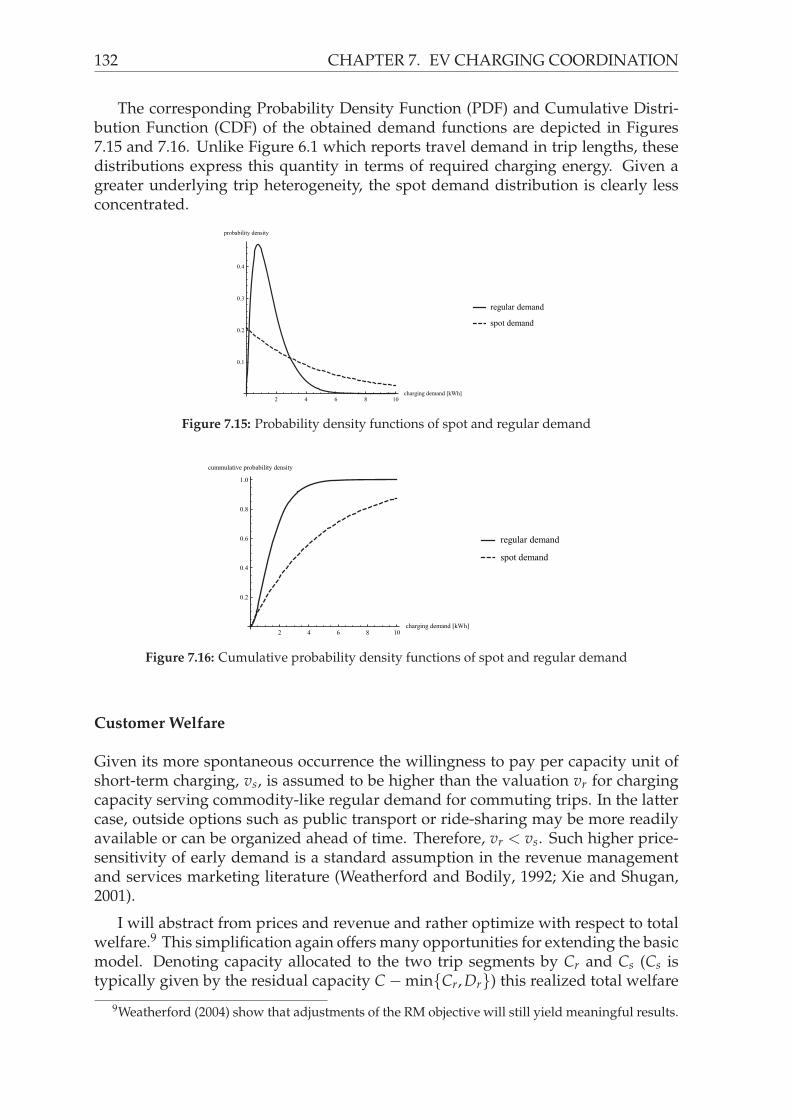
132 CHAPTER 7. EV CHARGING COORDINATION
The corresponding Probability Density Function (PDF) and Cumulative Distri-bution Function (CDF) of the obtained demand functions are depicted in Figures7.15 and 7.16. Unlike Figure 6.1 which reports travel demand in trip lengths, thesedistributions express this quantity in terms of required charging energy. Given agreater underlying trip heterogeneity, the spot demand distribution is clearly lessconcentrated.
2 4 6 8 10charging demand @kWhD
0.1
0.2
0.3
0.4
probability density
regular demand
spot demand
Figure 7.15: Probability density functions of spot and regular demand
2 4 6 8 10charging demand @kWhD
0.2
0.4
0.6
0.8
1.0
cummulative probability density
regular demand
spot demand
Figure 7.16: Cumulative probability density functions of spot and regular demand
Customer Welfare
Given its more spontaneous occurrence the willingness to pay per capacity unit ofshort-term charging, vs, is assumed to be higher than the valuation vr for chargingcapacity serving commodity-like regular demand for commuting trips. In the lattercase, outside options such as public transport or ride-sharing may be more readilyavailable or can be organized ahead of time. Therefore, vr < vs. Such higher price-sensitivity of early demand is a standard assumption in the revenue managementand services marketing literature (Weatherford and Bodily, 1992; Xie and Shugan,2001).
I will abstract from prices and revenue and rather optimize with respect to totalwelfare.9 This simplification again offers many opportunities for extending the basicmodel. Denoting capacity allocated to the two trip segments by Cr and Cs (Cs istypically given by the residual capacity C − min{Cr, Dr}) this realized total welfare
9Weatherford (2004) show that adjustments of the RM objective will still yield meaningful results.

7.2. TOP-DOWN POPULATION MODEL AND COORDINATION 133
is then given by
(7.3) Π = min{Cr; Dr}vr + min{Cs; Ds}vs.
Clearly, the bottleneck of the available charging capacity C only applies if the prob-ability of aggregate demand exceeding capacity is strictly positive. In this case, thevalue of at least one of the minimum terms in the definition of Π is determined bythe allocated capacity value.
7.2.3 Capacity Allocation Approaches
Having established the bottleneck situation in charging capacity allocation, oper-ators should be interested in enacting appropriate management procedures. In thefollowing, I discuss two approaches for handling the capacity shortage — first-come,first served capacity allocation and a two.class reservation scheme.
Simple Allocation of Charging Capacity
As noted before, grid limitations can be addressed either through capacity invest-ments or through load coordination. The simplest form of allocating available EVcharging is accepting requests in a first-come, first-served manner until capacity isdepleted. However, since the dr arise before the ds, the regular demand will havethe full capacity available for purchase under this zero-intelligence allocation andcoordination rule. See Figure 7.17 for an illustration.
Given the higher willingness to pay of customers for spot trips (vs > vr), this isnot socially efficient if there is excess aggregate demand because spot charging re-quests may be turned down in case of capacity limitations due to already allocatedregular charging requests. A more efficient capacity allocation scheme needs to ac-count for the heterogeneity of the two segments’ willingness to pay. At the sametime, one needs to account for the stochastic nature of demand which may give riseto capacity idling if less spot trip demand than expected shows up. The next sectionillustrates how an advance sale mechanism for capacity can achieve this coordina-tion trade-off.
��requestsarise
charging�occurs
�� requestsare�allocated
up�to�
���requestsare�allocated
up�to� � ��
�� requestsarise
Figure 7.17: First-come, first-served scheme
A Two-Class Reservation Scheme
Charging of electric vehicles occurs frequently — depending on the travel distancedaily charging activity is very likely. At the same time, a single charge has very lowcosts. This stands in contrast to traditional applications of capacity management

134 CHAPTER 7. EV CHARGING COORDINATION
where transactions are few and more costly. An appropriate control mechanism forresidential EV charging should thus feature limited complexity to keep transactioncosts low. Bid pricing or capacity options may thus be less appropriate in this set-ting. As noted by Weatherford and Bodily (1992), the simplest control mechanismfor single-resource capacity is the introduction of different discount classes. Limitedand discounted advanced sales are a characteristic form of this type of capacity man-agement. Typically, capacity must be limited and marginal costs must be sufficientlysmall for discounted advance sales to be profitable (Xie and Shugan, 2001). This co-incides with the minimal specification of the single resource reservation problemwith two discount classes as identified by Littlewood (2005).
As spot demand arises after regular demand, this quantity-based policy requiresprotecting some capacity for spot trip demand to avoid the opportunity costs of lostsales to high-value spot demand. At the same time, turning down a reservation re-quest yields the risk of not selling the capacity at all and the protection level needsto moderate between these opposed effects. Discounted regular sales are acceptedas long as the protection level for spot charging Qs is not violated. Figure 7.18 illus-trates this capacity control mechanism.
Availablecharging power
Charging duration T
Protected capacity for spot demand
Regular sale
Regular sale
Figure 7.18: Capacity protection mechanism
The sequence of events for the two-class reservation approach is depicted in Fig-ure 7.19. There are always at least Qs units of capacity available for spot demand.Compared to the non-protection scheme more valuable spot demand can be served,resulting in an allocation of charging capacity that is more efficient. The policy issolely characterized by the protection level which needs to be determined in an op-timal manner to ensure high (optimal) coordination efficiency.
��requestsarise
chargingoccurs
�� requestsare allocated
up to � �
�
���requestsare allocated
up to
�� ����
� � ��
�� requestsarise
Figure 7.19: Two-class reservation scheme

7.2. TOP-DOWN POPULATION MODEL AND COORDINATION 135
Optimal Protection Level
In the case of excess demand, protecting capacity curtails allocation to regular tripdemand. The welfare gain from an additional protected unit of capacity needs tooutweigh this lost welfare. Hence, one can derive the optimal protection level forspot demand Q∗
s with a simple analysis of the marginal welfare gain of both classes.Given a continuously distributed demand, this optimum is characterized by equalvalues for the expected marginal welfare gain from protecting an additional unit ofcapacity and the welfare gain of selling the capacity in advance:
(7.4) vr ≡ vsP (Ds > Q∗s )
Denoting the probability density function of demand by f (x),10 then the CDF oftotal spot demand for EV charging Fs(x) is given by
(7.5) Fs(x) =∫ x
0f (x)dx.
Using Littlewood’s rule (Littlewood, 2005) the optimal protection limit Q∗s is
given by
(7.6) Q∗s = F−1
s
(1 − vr
vs
),
where F−1s is the inverse CDF. Besides the distributional properties of spot demand,
the only other relevant economic quantity is the ratio between regular and spot val-uation vr
vs. Clearly, Equation (7.6) is only meaningful for vs > vr which comports
with our demand specifications. It should be noted, that for a given capacity levelthe distribution of regular demand actually has no impact on the result and can beconsidered as a single quantity.
Welfare Expressions
Regular demand Dr arises strictly before spot demand. Without protection, spot tripdemand can only be served by the remaining capacity available which is not usedby regular demand. The more valuable requests for spot demand can only be servedthrough charging capacity not sold to regular demand. Social welfare is thus givenby
(7.7) min{C, Dr}vr + min{max{0,C − Dr} , Ds}vs.
With the introduction of a protection limit Q∗s regular demand can be turned down
and more valuable spot demand can be served to increase social welfare:
(7.8) min{C − Q∗s , Dr}vr + min{C − min{C − Q∗
s , Dr} , Ds}vs
10 For the Erlang distribution f (x;α,θ) = xα−1e−xθ
θα(α−1)! for x,θ ≥ 0.

136 CHAPTER 7. EV CHARGING COORDINATION
It can be shown that under risk-neutrality11, protecting Q∗s units of charging capacity
for spot demand is an optimal policy balancing the gains from being able to meetextra spot demand against the certain loss from turning down regular trip demand.
Optimal Protection Level under Erlang Demand Distributions
As explained in Section 7.2, the Erlang/ Gamma-distribution not only matches theempirical data, it is also distribution-invariant with respect to summation. Aggre-gate segment demand, Di with i ∈ {r, s}, is the sum of individual charging demandquantities di,j (Equation 7.2). Each individual demand quantity is drawn from acommon Erlang distribution, that is di,k ∼ Erl(αi,θi). Then, the distribution of totalsegment is also an Erlang distribution, namely
(7.9) Di ∼ Erli = Erl(niαi,θi).
This is an interesting result as it allows expressing the charging demand of the com-plete EV population by means of a single expression — a very elegant and compacttop-down poulation model.
Following Equation (7.6), one can directly calculate the optimal protection levelQ∗
s . Given the heterogeneity in the willingness to pay between regular trip demandand spot trip demand the optimal protection limit Q∗
s obtains as
(7.10) Q∗s = Erl−1
s
(1 − vr
vs
),
where Erl−1s (·) is the inverse CDF of the spot demand distribution. The inverse of
the Erlang distribution involves the inverse Gamma and can thus not be expressedin closed form. However, it is readily evaluated in a numerical manner using appro-priate tools as shown in Figure 7.20 for the demand distributions from Figure 7.15(nr = ns = 1).
0.2 0.4 0.6 0.8cummulative probability
2
4
6
8
10
12
14
charging demand @kWhD
Figure 7.20: Inverse cummulative probability function of spot demand
11Risk-neutrality is a standard assumption for firm decision-making. Alternative risk attitudescan be reflected by appropriately adjusting the marginal welfare evaluation in Equation (7.4). SeeWeatherford (2004) for an in-depth discussion.

7.2. TOP-DOWN POPULATION MODEL AND COORDINATION 137
7.2.4 Numerical Analysis
Given the unavailability of a closed form inverse CDF for the Erlang distribution,efficiency potentials of capacity protection cannot be determined in a fully analyticalformat. Therefore, a simple numerical example is used to explore how protecting EVcharging capacity can increase total welfare. This example is based on a suburbanneighborhood with overnight charging activity.
Scenario and Parameters
A residential neighborhood served by a single transformer substation is considered.It is assumed that this transformer has 220 kW of available power for EV chargingovernight, i.e. between 10 pm and 6 am. Furthermore, I assume a total number of500 EVs in the neighborhood. As in Chapter 6, I assume vehicle consumption to be0.129kWh/km.
Given the commuter scenario, I assume that each EV pursues a daily commute,therefore nr = 500. Our mobility data set indicates that non-commute trips are lessfrequent with 0.833 trips occurring per commute trip. The analysis uses ns valuesbetween 200 and 400.12 As noted before, the distribution of regular demand doesnot economically affect the results. Therefore, I use the population mean to expressthe regular demand level Dr = γ · nr · μr = 783.8 [kWh]. On the other hand, for thespot demand a stochastic term based on the Erlang distribution is applied:
Ds ∼ Erls = Erl(ns · αs,γθs) = Erl(ns,4.825)
vr is normalized to 1 and vs is chosen from the range 1 to 5. Thus the ratio vr/vs isequal to the inverse of spot valuation, i.e. v−1
s .
Table 7.5 summarizes the most important input parameters for this example ofEV charging in a suburban neighborhood.
There is clearly sufficient capacity to serve regular demand, however, in ex-pectation capacity is insufficient to serve both segments. Thus, given the higherwillingness-to-pay of spot demand, the charging provider has an incentive to pur-sue capacity management.13
Evaluation
Given the scenario specified above, I am interested in the effects and potentials ofintroducing an advance-sale capacity management approach. First, the structure ofthe optimal capacity protection policy is characterized. Subsequently, I look at thewelfare effects compared to a naïve first-come-first-served allocation scheme.
12Clearly, this is a simplification as the number of spot trips is kept constant and are only variedtheir length. However, most results should be robust to generalizations of this setting.
13As noted before, our analysis focuses on welfare effects. Yet, such an increase in welfare istypically somewhat aligned with provider incentives and the results are indicative for a profit-maximizing operator.

138 CHAPTER 7. EV CHARGING COORDINATION
Table 7.5: Summary of input parameters
Parameter Value
Available transformer capacity PC 220 kWCharging duration T 8 hoursAvailable charging capacity C = TPC 1760 kWhEV consumption per km γ 0.129 kWh/km
Number of regular trips nr 500Daily regular demand Dr = nrμrγ 783.8 kWhWillingness to pay for regular trips vr 1
Number of spot trips ns 250–400Daily mean spot demand E[Ds] = nsμsγ 2011.9 kWhSpot demand distribution Fs Erl(ns,4.825)Willingness to pay for spot trips vs 1–5
Optimal Capacity Protection Policy
As prescribed by Equation (7.10), the optimal policy for the charging operator isto offer advance purchases for capacity up to the protection level Q∗
s . For a givenspot distribution, i.e. Erls = Erl(ns,4.825), Q∗
s can be determined for any value of vs,that is Q∗
s = Erl−1s (1 − v−1
s ). Figures 7.22 and 7.21 illustrate the optimal policy fordifferent spot valuations and numbers of spot trips. To better illustrate the effect ofincreasing spot valuation, two valuation ranges are conisedered — [1;1.5] and [1;5].
1.0 1.1 1.2 1.3 1.4 1.5vs
800
1000
1200
1400
1600
1800
2000
2200
kWh
ns=250
ns=300
ns=350
ns=400
Protection Level Qs*
Total Capacity
Figure 7.21: Optimal protection level over a different spot valuations, vs ∈ {1,1.5}
The optimal protection level is clearly increasing in both parameters. For thenumber of spot trips, one can observe an almost linear upward shift which reflectsthe increasing scarcity of capacity. With respect to valuation vs, the optimal protec-tion level is increasing in a concave manner. Initially, the valuation ratio impacts theoptimal protection level very drastically. For vs = 1 no capacity protection is opti-mal (Erl−1
s (0) = 0), yet a minimal increase in spot is leveraged by the large number

7.2. TOP-DOWN POPULATION MODEL AND COORDINATION 139
1 2 3 4 5vs
800
1000
1200
1400
1600
1800
2000
2200
kWh
ns=250
ns=300
ns=350
ns=400
Protection Level Qs*
Total Capacity
Figure 7.22: Optimal protection level over different spot valuations, vs ∈ {1,5}
of vehicles considered yielding an almost instantaneous14 jump in Q∗s to over 1,000
kWh.
Beyond vs ≈ 1.01, the evolution of Q∗s is less extreme. For the ns = 400 case, one
finds that advance sales are not efficient in most cases with the optimal protectionlevel exceeding available capacity for vs values beyond ≈ 1.02. In the other cases,somewhere between 61% and 100% of the available 1760 kWh capacity should beprotected.
To further assess the impact of the valuation spread on the optimal policy, itis illustrative to look at the limit vs → ∞. The corresponding values are given inTable 7.6. Compared to Figure 7.22, the protection continues to increase for evenhigher valuation spread. When planning a capacity expansion, these limit valuescan serve as an upper bound for extra capacity required for serving spot demandwhen pursueing a strict availability objective.
Table 7.6: Limit values of protection level (vs → ∞)
Number of spot trips 250 300 350 400
Optimal protection level [kWh] 1510.7 1779.0 2045.1 2309.5Optimal protection level [% of 1760 kWh] 85.8 100 116.2 131.2
Welfare Results
Besides the optimal policy itself, a special interest lies in the aggregate welfare effectof capacity management. This requires evaluating the expected spread betweenEquations (7.7) and (7.8). Again, this expression cannot be derived in closed form,due to the presence of the Erlang inverse CDF. Therefore, I use the NExpectationfunction provided by Mathematica15 to obtain the expected values numerically.
14Note that since Erls has support over [0,∞], Q∗s is differentiable for all values spreads. However,
the numerical approximation becomes unstable at vs close to zero.15www.wolfram.com/mathematica

140 CHAPTER 7. EV CHARGING COORDINATION
Figure 7.23 shows the development of welfare obtained under capacity-protection (normalized by baseline first-come-first-served welfare) for different val-ues of vs and ns. The results show a clear welfare increase for protecting EV chargingcapacity in comparison to a first-come, first-served charging policy. As for the op-timal protection policy (Figure 7.22), the key influence factors for the efficiency ofcapacity protection are the valuation ratio and the number of spot trips. The effectof the value spread diminishes for increasing vs. Similarly, the effect of the num-ber of trips ns is proportional to this effect and homogeneous for each 50 spot tripincrement.
�
�
�
�
�
��
��
�
�
�
�
��
��
�
�
�
��
�� � � �
��
� � � � � � �
2 3 4 5vs
1.1
1.2
1.3
1.4
1.5
1.6
Relative welfare with capacity protection
� ns�400
� ns�350
� ns�300
� ns�250
Figure 7.23: Relative welfare level with capacity management (versus first-come-first-served base-case)
Unused Capacity
While the first-come-first-served pattern maximizes capacity utilization (expectedutilization across all parametrizations is very close to 100%), the introduction of ca-pacity protection inherently results in unused capacity, i.e. capacity protected forspot trips but unused in the end due to too limited spot demand. Figure 7.24 illus-trates this effect for a setting of unlimited capacity. Clearly, the expected unusedcapacity is increasing in both the valuation spread and the number of spot trips asmore capacity is protected upfront (Q∗
s is increasing in vs and ns).
It is also increasing in ns, however, this is only the case as long as Q∗s is below
total capacity C. This becomes evident in Figure 7.25 where C is again set at 1760kWh. For ns = 400, spot demand will exceed available capacity in almost all casesand protecting capacity will not result in unused capacity. Similarly for ns = 350,Q∗
s equals C for vs > 5 and the unused capacity remains stable at around 85 kWh.Clearly, these are situations where a capacity expansion is well warranted to serve agreater share of total demand.
7.2.5 Summary and Future Research
Increasing EV penetration levels require coordination of charging activity with re-spect to both aggregate load management and distribution grid capacities. Coor-

7.2. TOP-DOWN POPULATION MODEL AND COORDINATION 141
�
�
�
�
�
�
��
�
�
�
�
�
�
�
��
�
�
�
�
�
��
��
�
�
�
�
�
��
��
�
2 3 4 5vs
20
40
60
80
Expected unused charging capacity �kWh�
� ns�400
� ns�350
� ns�300
� ns�200
Figure 7.24: Unused capacity arising from capacity protection for C = ∞
� � � � � � � � � � � � � � � � � � ��
�
�
�
�
��� � � � � � � � � � � �
�
�
�
�������� �
� �� �
� ��
�
�
�
������� �
� �� �
� �� �
2 4 6 8 10vs
20
40
60
80
100
Expected unused charging capacity �kWh�
� ns�400
� ns�350
� ns�300
� ns�250
Figure 7.25: Unused capacity arising from capacity protection for C = 1760
dination mechanisms for the latter bottleneck are not socially efficient if ignoringcustomer/ demand heterogeneity. The basic model specification illustrates that co-ordination of distribution grid capacity for EV charging can be modeled as a PARMproblem. A two-class reservation scheme provides an efficient solution to this prob-lem and allows to characterize potential welfare impacts.
Model Summary
The proposed control mechanism is appropriate in situations where transformercapacity is the relevant bottleneck and the commuter scenario with limited trip free-dom is applicable. Social welfare increases with the expected utilization of chargingcapacity. If the expected charging demand greatly exceeds available capacity, an in-vestment in the local distribution grid and transformer capacity is preferable. Table7.7 provides a classification of the complete model along the taxonomy presentedby Weatherford and Bodily (1992).

142 CHAPTER 7. EV CHARGING COORDINATION
Element EV charging
Resource model single, continuousPrices pre-determinedWillingness to pay buildupDiscount price classes 2Group reservations n/aDiversion n/aDisplacement n/aShow-up of reservations certainBumping procedure n/aDecision rule static
Table 7.7: Classification of basic electric vehicle charging capacity management model followingWeatherford and Bodily (1992)
Future Opportunities
This section aims at demonstrating the relevance of RM techniques for addressingthe challenges posed by the coordination of EV charging. By providing ample op-portunities to expand and improve on, the presented minimal PARM model for EVcharging coordination serves as a platform for future work in this direction. Thefollowing possible extensions seem especially relevant:
Prices The static welfare approach ignored price and cost effects on demand andsupply. Clearly, a provider-centric model would rather have to focus on profit max-imization. Furthermore, realizing that power and energy are separate value com-ponents of EV charging one can easily envision models where capacity pricing isdriven by the price for electrical energy — charging demand may be high whenenergy prices are low.
Discount Price Classes While a stylized setting with two discount classes is help-ful to illustrate the underlying economic mechanics, a richer setting is required toachieve a more realistic model. The RM literature provides a large body of researchfor handling models with more than two customer segments. Most importantly,the Expected Marginal Seat Revenue (ESMR) decision model proposed by Belobaba(1989) extends Littlewood’s model to n customer classes.
Group Reservations Allowing individual customer demand to be dependent oneach other creates the possibility of modeling customer groups, especially fleets ofEVs. This is especially relevant for car-sharing scenarios where fleet management isan additional challenge (Nair and Miller-Hooks, 2011).
Resource Dropping the single time slot assumption is necessary for modeling ap-plications that are more realistic. As noted before the research on revenue manage-ment for multi-leg flights and multi-machine scheduling may guide this extension.

7.3. DISCUSSION 143
Diversion In a model with multiple sequential charging time slots, the differenttime slots may constitute substitute products for the customers. This customer di-version both complicates the revenue management problem but also provides theoperator with additional degrees of freedom to optimize capacity utilization. Di-version can also occur in a repeated setting with a single time slot. In this case,multiple reservations may be simultaneously opened. This can possibly lead tointer-temporal diversion effects.
Displacement Sequential time slots may also give rise to conflicting customer re-quests: A customer charging for only one slot can block a customer charging for twoslots — such displacement effects are a well-known from multi-leg flights RM.
Show-up of Reservations and Bumping Stochastic show-ups or the possibility todeny service to advance customers for a compensation payment (bumping) mayequip providers with additional strategic levers.
Decision Rule In the described model, the static booking limit constitutes an op-timal policy. This may not be the case in a more complex setting. However, thelimitations on the available control strategies imposed by EV charging characteris-tics may continue to hold.
Insights from revenue management can have a profound impact on the EV busi-ness models of both electrical power companies as well as EV mobility providerslike BetterPlace (cf. Section 6.8.2). This notion seems plausible as Kimes and Wirtz(2003) note that capacity management approaches have become very common indiverse industries.
7.3 Discussion
This chapter describes how to model aggregate charging load of EV populations.This insight is used to analyze and discuss different approaches to charging coordi-nation — laissez-faire, exogenous price signals and reservation-based capacity con-trol. Depending on the situation, these coordination approaches may not achievethe goals envisioned in Section 2.2. Appropriate population models are a centralinput to evaluate the adequacy of alternative coordination approaches and allowto assess the emergent population behavior (Ramchurn et al., 2012) prior to deter-mining and fixing a specific regulatory regime. Such guided design of coordinationapproaches follows the market engineering paradigm (Weinhardt et al., 2003).
There are ample opportunities to expand the design and analysis of EV chargingcoordination approaches. An interesting extension of the discussed coordinationapproaches would be the integration of V2G scenarios where EVs can feed electric-ity back into the grid (e.g., in times of high prices). This way, the results of Kemptonand Tomic (2005) can be investigated in a setting with both uncertainty and gridconstraints. Moreover, the current analysis focuses on individual charging behav-ior. It has often been argued that electrified individual transport may put greater

144 CHAPTER 7. EV CHARGING COORDINATION
emphasis on vehicle sharing systems (Nair and Miller-Hooks, 2011). Such systemsmay exhibit greater charging flexibility as requests can be served with the wholefleet which may improve grid integration capabilities. Similarly, the coordinationmechanism discussed above are evaluated with respect to static EV behavior charac-terized by threshold strategies or optimization approaches. Alternative EV chargingmodels such as learning agents (see Section 6.8.2) may warrant alternative coordi-nation approaches (Dauer et al., 2013). Similarly, capacity management models forEV charging coordination offer a rich set of extension possibilities (see above).

Part IV
Finale


Chapter 8
Summary and Future Research
T his thesis set out to establish a notion of economic smart grid modeling. Build-ing on previous smart grid research, Part I describes the technological and eco-
nomic aspects that transform the traditional grid into a smart grid. These insightsprovide a base for the development of a framework for modeling smart grid cus-tomers. Parts II applies this framework to create models representing householdand small business customers. Similarly, in Part III electric vehicle charging behav-ior is modeled assuming different incentive and information settings. Using thesemodels appropriate coordination approaches such as individual TOU rates or areapricing are discussed incorporating the smart grid coordination goals establishedin 2. This chapter recapitulates and summarizes key findings and concepts fromthe previous chapters. This summary is guided by both the thesis structure and theresearch questions put forward in Chapter 1.
8.1 Smart Grid Economics
Smart grids constitute techno-economic systems whose sensor-actuator infrastruc-ture facilitates novel approaches for optimization and coordination of system opera-tions compared to traditional grids. Still, the basic electrical laws of the physical gridgovern stability and reliability of the system. Smart grids cannot change the physicsof power distribution, but they can help achieve a better utilization of availablephysical resources through better demand coordination. Therefore, smart grid sys-tems still need to strike a balance between cost efficiency, reliability and sustainabil-ity — the classic trilemma of energy economics. However, the enhanced coordina-tion capabilities provide greater degrees of freedom to achieve this balance throughactive management of different balancing capabilities such as demand response, dis-tributed generation and storage devices. This bouquet of management options willplay a crucial role in establishing a power system based on a significant portion ofrenewable generation. Adopting an economic view, the analysis of smart grid capa-bilities needs to incorporate physical boundaries and inflexible customer demandas hard constraints which need to be facilitated by means of flexibility potentialsand smart dispatching (decision variables). At the same time, decentral decision-making characteristics need to be accounted for — ideally, coordination approaches

148 CHAPTER 8. SUMMARY AND FUTURE RESEARCH
ensure incentive compatibility on behalf of the distributed agents. Thus the set ofrelevant coordination bottlenecks (research question 5) in the smart grid is spannedby both physical constraints and agent behavior. Therefore, robust smart grid de-sign requires both technological solutions and sound economic design (Chassin andKiesling, 2008). This thesis focuses on the latter and develops a theory of customermodeling and coordination mechanisms as building blocks for the characterizationof smart grid markets (research question 1).
Acknowledging the greater importance of distributed “small” individual cus-tomers in the future electricity system, Chapter 3 identifies four levels that shouldideally be captured by smart grid customer models. These levels are static cus-tomer characteristics, model size and scope, demand response characteristics andmodel adaptivity over time. The first level requires a basic representation of thefundamental load characteristics of a given customer type. This essentially repre-sents a minimal, static model, e.g., a load curve. The second level considers twodistinct approaches of expressing model scope, individual-focused bottom-up ver-sus population-focused top-down models. Depending on the scenario at hand, oneapproach may be more suited than the other. Similarly, hybrid models can be en-visioned. A central goal of smart grids is effective coordination of customers’ loadflexibility to match stochastic generation patterns from renewable energy sources.Therefore, a proper representation of load response characteristics and capabilitiesis a very important aspect of a smart grid customer model. Finally, long-term anal-yses of technology and rate adoption require corresponding model capabilities. Fo-cusing on rate adoption and smart grid investments, tools from marketing research(logit choice) and the theory of investment under uncertainty offer helpful insightsto incorporate these model aspects. These four levels jointly address research ques-tion 2.
Clearly, the value of such a research framework fundamentally stems from itsusage. Both within this thesis and within future research these facets of customermodeling should be incorporated. At the same time, the current framework focuseson the electrical loads. Going forward, a convergence of different energy formsis expected and a more integrated view of load behavior will be required (Lundand Münster, 2003; Block et al., 2008). Extending the notion of energy services(Schweppe et al., 1980; Stroehle et al., 2012) and appropriately integrating these intothe smart grid customer modeling framework will be a promising avenue for futureresearch.
8.2 Residential Load Modeling and Coordination
Drawing on the concept of top-down synthetic customer models developed in PartI, the third part of this thesis focuses on the specific case of household and smallbusiness load modeling and coordination. Chapter 4 describes the system designand results from a data analysis case study with a regional utility company. Bymeans of standard data mining techniques (KDD, k-Means Clustering, DBI selectionprocedure) load patterns and similarity information were extracted from a smartmeter data set. This way, highly granular customer load profiles can be determinedand individual customers can be classified more precisely than using standard load

8.2. RESIDENTIAL LOAD MODELING AND COORDINATION 149
profiles. In addition, initial attempts to extract load flexibility properties from theprofiles were discussed. These positive results confirm the corresponding researchquestion 3. Besides providing a base for efficient smart grid customer modeling,the improved classification capabilities also have a direct practical impact as theyfacilitate both better load forecasting and the design of customized rates. A keygoal was the direct integration into available ERP systems to ensure high practicalrelevance.
The cluster analysis gives rise to subsequent research opportunities. To region-ally and temporally validate the robustness of the identified clusters, additional datasets are required. Based on such richer data sets, static household models can alsobe enhanced using the quantile-based analysis of the load curves. Moving awayfrom average values and acknowledging load variance patterns, additional flexibil-ity information can then be extracted from the raw data. This can be used to imple-ment demand response capabilities in top-down models adopting the techniquesdescribed by Esser et al. (2007) and Wang et al. (2010) for micro-founded models.Moreover, the integration of additional data sources such as rate information or de-mographic household data could be leveraged for better segmentation results. New-sham and Bowker (2010) argue that there is an insufficient understanding to whatextent residential customers adapt their electricity consumption considering theirsocio-economic properties. This is a central question for future demand-centeredcontrol paradigms. Therefore, more research needs to focus on assessing load shift-ing potentials and demand elasticity values. This may require alternative researchapproaches like surveys or laboratory experiments.
Acknowledging the potential of customized rate designs, Chapter 5 describesand evaluates a MIP framework for optimal design of customized TOU rates. Thedescribed approach provides a simple way to express rate structure requirementsand to efficiently derive the corresponding optimal rate structure for different ob-jective functions. The analysis shows the advantages of customized rates (versussymmetric rate designs) especially for rates with a small number of rate zones. Fur-thermore, the evaluation indicates that rate granularity and update frequency playa joint, major role in determining the efficiency of customized TOU rates. Consider-ing both customer acceptance and coordination efficiency, customized rates can beone building block for creating appropriate coordination mechanisms in the smartgrid (see research question 6).
The presented analysis currently only considers rate updates specifying a com-plete rate structure. Alternatively, one could look into partial rate updating thattransform the previous rate in a simple manner, e.g., by shifting all price levels upwith other rate elements remaining unchanged. Such limited price updates couldpotentially reduce rate (and communication) complexity and thus assist in increas-ing customer acceptance. It would be interesting to see, how much welfare is lostthrough constrained updating and how it interacts with other rate design elements.Similarly, it may be worthwhile to investigate the efficiency impact of other ratedesign constraints such as minimum zone length, price jump limits or limiting thenumber of distinct price levels. The effect of uncertainty is especially interestingin the context of rates with longer horizon, spanning, e.g., a whole week insteadof a single day. Moreover, the interconnection between demand modeling andrate design is of special interest, especially when determining rates with a profit

150 CHAPTER 8. SUMMARY AND FUTURE RESEARCH
maximization objective. Consequently, the rate design approach can be applied inconjunction with richer demand models. Finally, behavioral dimensions such ascustomer acceptance and response to alternative TOU specifications should be an-alyzed in more detail. Such an integrated approach towards understanding cus-tomer decision-making and the evaluation of coordination approaches is a centralchallenge on the way towards effective smart grid modeling.
8.3 Electric Vehicle Load Modeling and Coordination
The charging activity of a growing number EVs will constitute both a large and flex-ible load in the future electricity system. This means that EVs may very well playa central role in smart grid coordination constituting a significant load share in dis-tribution grids. Consequently, EV charging activity needs to be carefully analyzedin order to build meaningful and robust smart grid models. Part III addresses thischallenge. Key to this material is the modeling of EV charging activity with a specialfocus on the point raised in Research Question 4 — What is the impact of price and tripuncertainty on electric vehicle charging behavior? Chapter 6 develops model buildingblocks and appropriate charging strategies. By using modified optimal or heuristicdecision rules it is possible to leverage the load flexibility inherent to EV chargingto ensure low charging costs, even under cost and driving uncertainty. The chapteralso provides an indication of the value of different types of information and thecost of requiring certain minimum EV charge levels.
While the charging policies introduced and discussed in this thesis are capableof handling limited information scenarios, they remain static in the sense that theyare invariant state-action mappings. Within richer decision settings (multi-modaltransportation options, changing price scenarios) such policies may be less effec-tive. Hence, adaptive learning approaches as discussed by Dauer et al. (2013) maybecome more relevant. In addition to tailoring the charging strategies, an importantpoint is the education and information of EV owners and drivers (Flath et al., 2012).Firstly, to overcome range anxiety the drivers need to be educated on how muchrange they really need every day. Secondly, based on a specific driving profile thecost drivers for individual mobility can be benchmarked. A bigger battery can forexample lead to cost reductions per kWh and therefore to lower cost over the vehi-cle’s lifetime. On the other hand if only short ranges are necessary a large batterymay be too large and therefore too expensive. Finally, the future may bring a riseof inter-modal/ hybrid transportation systems. Within such mixed systems driverswill have even more options to choose from and individual decisions will have tobe aligned.
Moving away from the individual vehicle perspective, Chapter 7 considers waysto aggregate individual charging decision to a population level. This insight is usedto develop and evaluate charging coordination mechanisms based on exogenousand endogenous pricing approaches or charging capacity management. A centralresult of this chapter is the potential to mitigate conflicts between local and system-wide resource coordination through endogenous pricing which internalizes agentactions through appropriate feedback loops. Similarly, the chapter shows how asimple charging capacity allocation scenario can be framed as a PARM problem.

8.3. ELECTRIC VEHICLE LOAD MODELING AND COORDINATION 151
This provides a base to leverage the large body of revenue management literatureto develop improved EV charging coordination approaches.
To conclude, there are ample opportunities to expand the design and analysisof EV charging coordination approaches. An interesting extension of the discussedcoordination approaches would be the integration of V2G scenarios where EVs canfeed electricity back into the grid (e.g., in times of high prices). This way, the resultsof Kempton and Tomic (2005) can be investigated in a setting with both uncertaintyand grid constraints. Moreover, the current analysis focuses on individual chargingbehavior. It has often been argued that electrified individual transport may putgreater emphasis on vehicle sharing systems (Nair and Miller-Hooks, 2011). Suchsystems may exhibit greater charging flexibility as requests can be served with thewhole fleet which may improve grid integration capabilities.


Chapter 9
Conclusion and Outlook
T he integration of very high shares of renewable generation will require signif-icant changes within the power system. Through improved monitoring, fore-
casting and control capabilities and by empowering the demand side, smart gridswill play a key role in addressing this challenge. However, successful establishmentof smart grids will require addressing both sound technical and economic concepts.This joint perspective on generating appropriate solutions fuels the convergence ofenergy informatics and energy economics research. Within this thesis, I exploredtools and techniques from both fields to address problems concerning the modelingand coordination of load behavior in future smart grid markets.
The presented results should help generators, system planners and regulators toidentify crucial aspects of robust smart grid operation. Among others, these includethe benefits of load data availability (from smart metering), the necessity of suf-ficiently high update frequencies within dynamic pricing schemes, the relative im-portance of both price and trip information for smart EV charging policies, the trade-off between local (grid constraints) and global coordination goals (load-generationmatching) as well as the distinctly spatial dimension of these coordination conflicts.
Given the vastness of this research field, the multitude of challenges and thecomplexity of any system entity, such work can never be considered finished, com-pleted or exhaustive. Notable omissions have been aspects of decentral generation,transmission grid constraints as well as detailed representation of power engineer-ing aspects. Similarly, my research has only briefly touched on empirical marketdata and relies on fairly simple coordination approaches such as dynamic pricing orcapacity protection. Also the research paths have been fairly isolated with analysisfocusing on either EVs charging or residential loads. While this focus was essentialfor generating compact and coherent results, more overarching conclusion need tobe based on more integrated models.
In summary, demand flexibility, market-based integration of renewables, respon-sive generation as well as hybrid energy systems will create a more diverse (dif-ferent generation technologies, diverse rate designs, heterogeneous service levels)and consequently more (cost-)efficient and resilient power system. Such a systemcan dynamically prioritize the different dimensions of the energy trilemma. Con-sequently, constraints become “softer” which creates a greater set of feasible allo-cations. For example, selective black-out options provide grid operators with addi-

154 CHAPTER 9. CONCLUSION AND OUTLOOK
tional emergency reserve capacity — such customized availability level agreementsthus allow trade-offs between cost and reliability. Similarly, dynamic (both temporaland spatial) remuneration of renewables can enhance the value of storage capacityand thus provide more effective investment incentives.
Leveraging these future opportunities will not only require appropriate ICT sys-tems for metering and communication as well as economic incentive structuresand rates: It will also require appropriate sensor systems and information tech-nology to create smart nodes within a smart grid following the energy informaticsparadigm put forward by Watson et al. (2010). These smart nodes can implementdecentral optimization and decision-making routines and will constitute intelligentagents within an intelligent system (Ramchurn et al., 2012). Intelligent system de-sign requires meaningful agent models, while meaningful agent models require asystem environment to interact with. Therefore, these two aspects are fundamen-tally interconnected. Consequently, this thesis addressed both the economic designof smart grids (through appropriate population models) and the establishment ofsmart nodes (through optimization of individual load behavior). It also contributedto the vision of smart markets through discussion of various economic coordinationapproaches.

References
Agassi, S. (2009). World without oil – better place builds a future for electric vehicles.innovations 4(4), 125.
Ahlert, K.-H. (2010). Economics of Distributed Storage Systems. Ph. D. thesis, KarlsruheInstitute of Technology.
Ahlert, K.-H. and C. Block (2010). Assessing the impact of price forecast errors on theeconomics of distributed storage systems. In 43rd Hawaii International Conferenceon System Science (HICSS-43), Hawaii, USA.
Ahlert, K.-H. and C. van Dinther (2009). Sensitivity analysis of the economic benefitsfrom electricity storage at the end consumer level. In Proceedings of the 2009 IEEEBucharest Power Tech Conference, pp. 1–8.
Albadi, M. and E. El-Saadany (2008). A summary of demand response in electricitymarkets. Electric Power Systems Research 78(11), 1989–1996.
Amin, M. and B. Wollenberg (2005). Toward a smart grid: Power delivery for the21st century. IEEE Power & Energy Magazine 3(5), 34–41.
Amoroso, F. A. and G. Cappuccino (2012). Advantages of efficiency-aware smartcharging strategies for PEVs. Energy Conversion and Management 54(1), 1–6.
Appelrath, H., O. Terzidis, and C. Weinhardt (2012). Internet of energy — ICT as akey technology for the energy system of the future. Business & Information SystemsEngineering 4(1), 1–2.
Bashash, S., S. J. Moura, and H. K. Fathy (2011). On the aggregate grid load imposedby battery health-conscious charging of plug-in hybrid electric vehicles. Journal ofPower Sources 196(20), 8747–8754.
BDEW (2010). Standardlastprofile Strom.
BDEW (2012). Bundesverband der Energie- und Wasserwirtschaft e.V.: Daten /Grafiken – Strom. http://www.bdew.de/internet.nsf/id/strom-de.
BDI (2011). Auf dem Weg zum Internet der Energie. Technical report, BDI-Drucksache Nr. 450, Bundesverband der Deutschen Industrie e.V. (BDI). Au-thored by R. Adam, C. Böse, F. Bomarius, P. Bretschneider, F. Briegel, C. vanDinther, T. Drzisga, B. Fey, C. Flath, H. Frey, P. Jeutter, J. Kammerer, C. Kern, M.Muhs, H. Onken, G. Praehauser, K. Rogg, I. Schönberg, D. Schumann, O. Terzidis,M. Wedler, A. Weidlich and C. Weinhardt.

156 REFERENCES
Becker, T. A., I. Sidhu, and B. Tenderich (2009). Electric Vehicles in the United States- A New Model with Forecasts to 2030. Technical report, Center for Entrepreneur-ship and Technology - University of California, Berkeley.
Belobaba, P. (1989). OR practice – application of a probabilistic decision model toairline seat inventory control. Operations Research 37(2), 183–197.
Beringer, J. (2008). Online-Data-Mining auf Datenströmen: Methoden zur Clusteranalyseund Klassifikation. VDM Verl. Dr. Müller.
Bertolini, L. and F. Le Clercq (2003). Urban development without more mobilityby car? Lessons from Amsterdam, a multimodal urban region. Environment andPlanning A 35(4), 575–590.
Bissantz, N. and J. Hagedorn (2009). Data mining. Wirtschaftsinformatik 51(1), 139–144.
Black, F. and M. Scholes (1973). The pricing of options and corporate liabilities.Journal of Political Economy 81(3), 637–654.
Block, C., F. Bomarius, P. Bretschneider, F. Briegel, N. Burger, B. Fey, H. Frey,J. Hartmann, C. Kern, B. Plail, G. Praehauser, L. Schetters, F. Schoepf, D. Schu-mann, F. Schwammberger, O. Terzidis, R. Thiemann, C. van Dinther, K. vonSengbusch, A. Weidlich, and C. Weinhardt (2008). Internet der Energie - IKTfür Energiemärkte der Zukunft. BDI-Drucksache Nr. 418, Bundesverband derDeutschen Industrie e.V. (BDI).
Block, C., W. Ketter, J. Collins, and C. Weinhardt (2010). A multi-agent energy trad-ing competition. Working paper, Erasmus University Rotterdam.
Block, C., D. Neumann, and C. Weinhardt (2008). A market mechanism for energyallocation in micro-CHP grids. In 41st Hawaii International Conference on SystemSciences (HICSS 2008), Waikoloa, Big Island, Hawaii, USA.
Bohn, R. E. (1982). Spot pricing of public utility services. Ph. D. thesis, MassachusettsInstitute of Technology, Energy Laboratory.
Bohn, R. E., M. C. Caramanis, and F. C. Schweppe (1984). Optimal pricing in electri-cal networks over space and time. The RAND Journal of Economics 15(3), 360–376.
Bonabeau, E. (2002). Agent-based modeling: methods and techniques for simulatinghuman systems. Proceedings of the National Academy of Sciences of the United Statesof America 99(3), 7280–7287.
Borenstein, S. (2005a). The long-run efficiency of real-time electricity pricing. TheEnergy Journal 26(3), 93–116.
Borenstein, S. (2005b). Time-varying retail electricity prices: Theory and practice. InJ. M. Griffin and S. L. Puller (Eds.), Electricity Deregulation: Choices and Challenges,Volume 4, pp. 317–356. University of Chicago Press.
Borenstein, S., M. Jaske, and A. Rosenfeld (2002). Dynamic pricing, advanced me-tering, and demand response in electricity markets. Technical report, Universityof California Energy Institute.

REFERENCES 157
Bosman, M. G. C., V. Bakker, A. Molderink, J. L. Hurink, and G. J. M. Smit (2012).Planning the production of a fleet of domestic combined heat and power genera-tors. European Journal of Operational Research 216(1), 140–151.
Boyd, E. and I. Bilegan (2003). Revenue management and e-commerce. ManagementScience 49(10), 1363–1386.
Brownstone, D. and K. A. Small (2005). Valuing time and reliability: assessing theevidence from road pricing demonstrations. Transportation Research Part A: Policyand Practice 39(4), 279–293.
Carpaneto, E. and G. Chicco (2008). Probabilistic characterisation of the aggregatedresidential load patterns. IET Generation, Transmission & Distribution 2(3), 373–382.
Celebi, E. and J. D. Fuller (2007). A model for efficient consumer pricing schemes inelectricity markets. IEEE Transactions on Power Systems 22(1), 60–67.
Celebi, E. and J. D. Fuller (2012). Time-of-use pricing in electricity markets underdifferent market structures. IEEE Transactions on Power Systems 27(3), 1170–1181.
Chalkiadakis, G., V. Robu, R. Kota, A. Rogers, and N. Jennings (2011). Cooperativesof distributed energy resources for efficient virtual power plants. In Proceedingsof the 10th International Conference on Autonomous Agents and Multiagent Systems,Volume 2, pp. 787–794.
Chang, C. (1988). A fast interactive optimal load management algorithm undertime-varying tariffs. International Journal of Electrical Power & Energy Systems 10(4),260–270.
Chao, H.-P., S. S. Oren, S. A. Smith, and R. B. Wilson (1986). Multilevel demandsubscription pricing for electric power. Energy Economics 8(4), 199 – 217.
Chapel, S. (2008). Smart grid economics: three stories bring up issues. Natural Gas& Electricity 25(3), 1–32.
Chassin, D. and L. Kiesling (2008). Decentralized coordination through digitaltechnology, dynamic pricing, and customer-driven control: The gridwise testbeddemonstration project. The Electricity Journal 21(8), 51–59.
Cheng, T. and C. Sin (1990). A state-of-the-art review of parallel-machine schedulingresearch. European Journal of Operational Research 47(3), 271–292.
Chevalier-Roignant, B., C. M. Flath, A. Huchzermeier, and L. Trigeorgis (2011).Strategic investment under uncertainty: A synthesis. European Journal of Opera-tional Research 215(3), 639–650.
Chicco, G., R. Napoli, P. Postolache, M. Scutariu, and C. Toader (2003). Customercharacterization options for improving the tariff offer. IEEE Transactions on PowerSystems 18(1), 381–387.
Clement-Nyns, K., E. Haesen, and J. Driesen (2011). The impact of vehicle-to-gridon the distribution grid. Electric Power Systems Research 81(1), 185–192.

158 REFERENCES
Cody, W., J. Kreulen, V. Krishna, and W. Spangler (2010). The integration of businessintelligence and knowledge management. IBM Systems Journal 41(4), 697–713.
Cramton, P. and S. Stoft (2005). A capacity market that makes sense. The ElectricityJournal 18(7), 43–54.
Cramton, P. and S. Stoft (2006). The convergence of market designs for adequategenerating capacity. Working paper, Massachusetts Institute of Technology. Cal-ifornia. Center for Energy and Environmental Policy Research. Electricity Over-sight Board.
Creti, A. and N. Fabra (2007). Supply security and short-run capacity markets forelectricity. Energy Economics 29(2), 259–276.
Dalen, A. and C. Weinhardt (2012). Fusebox dialects: Central appliance recognitionfor a smarter grid. In Proceedings of IEEE Innovative Smart Grid Technologies (ISGT),pp. 1–7.
Dasgupta, P., P. Hammond, and E. Maskin (1979). The implementation of socialchoice rules: Some general results on incentive compatibility. The Review of Eco-nomic Studies 46(2), 185–216.
Dash, R., N. Jennings, and D. Parkes (2003). Computational-mechanism design: Acall to arms. Intelligent Systems, IEEE 18(6), 40–47.
Dauer, D., C. M. Flath, P. Ströhle, and C. Weinhardt (2013). Market-based ev charg-ing coordination. Working Paper of Institute of Information Systems and Man-agement, Karlsruhe Institute of Technology.
Davies, D. and D. Bouldin (1979). A cluster separation measure. IEEE Transactionson Pattern Analysis and Machine Intelligence 1(2), 224–227.
Dietz, B., K.-H. Ahlert, A. Schuller, and C. Weinhardt (2011). Economic Benchmarkof Charging Strategies for Battery Electric Vehicles. In Proceedings of the IEEE Pow-ertech 2011 Conference.
Dixit, A. K. and R. S. Pindyck (1994). Investment under uncertainty. Princeton Univ.Press.
DKE (2010). Die deutsche Normungsroadmap E-Energy / Smart Grid.
Domencich, T. and D. McFadden (1975). Urban travel demand: a behavioral analysis,Volume 93. North-Holland.
Dunn, J. (1974). Well-separated clusters and optimal fuzzy partitions. Journal ofCybernetics 4(1), 95–104.
Dütschke, E. and A.-G. Paetz (2013). Dynamic electricity pricing – which programsdo consumers prefer? Energy Policy.
Eberle, U. and R. von Helmolt (2010). Sustainable transportation based on electricvehicle concepts: a brief overview. Energy Environ. Sci. 3(6), 689–699.

REFERENCES 159
Economides, N. and G. Woroch (1992). Benefits and pitfalls of network interconnection.New York University, Leonard N. Stern School of Business.
Espey, J. and M. Espey (2004). Turning on the lights: A meta-analysis of residentialelectricity demand elasticities. Journal of Agricultural and Applied Economics 36(1),65–82.
Espinoza, M., C. Joye, R. Belmans, and B. DeMoor (2005). Short-term load forecast-ing, profile identification, and customer segmentation: a methodology based onperiodic time series. IEEE Transactions on Power Systems 20(3), 1622–1630.
Esser, A., M. Franke, A. Kamper, and D. Möst (2007). Future power markets.Wirtschaftsinformatik 49, 335–341.
Esser, A., A. Kamper, M. Franke, D. Möst, and O. Rentz (2007). Scheduling of elec-trical household appliances with price signals. In Operations Research Proceedings2006, pp. 253–258. Springer.
Farhangi, H. (2010). The path of the smart grid. IEEE Power and Energy Magazine 8(1),18–28.
Faruqui, A. (2010). The ethics of dynamic pricing. The Electricity Journal 23(6), 13–27.
Faruqui, A., D. Harris, and R. Hledik (2010). Unlocking the 53 euro billion savingsfrom smart meters in the EU: How increasing the adoption of dynamic tariffscould make or break the eu’s smart grid investment. Energy Policy 38(10), 6222–6231.
Faruqui, A., R. Hledik, and S. Sergici (2009). Piloting the smart grid. The ElectricityJournal 22(7), 55–69.
Fayyad, U., Piatetsky-Shapiro G., Smyth P., and Uthurusamy R. (1996). Advances inknowledge discovery and data mining. Menlo Park, Calif: AAAI Press and MIT Press.
Figueiredo, V., F. Rodrigues, Z. Vale, and J. Gouveia (2005). An electric energy con-sumer characterization framework based on data mining techniques. IEEE Trans-actions on Power Systems 20(2), 596–602.
Flath, C. M., S. Gottwalt, and J. Ilg (2012). A Revenue Management Approach forEfficient Vehicle Charging Coordination. In Proceedings of the Forty-Fifth AnnualHawaii International Conference on System Sciences, Grand Wailea, Maui, pp. 1888–1896.
Flath, C. M., J. Ilg, and C. Weinhardt (2012). Decision Support for Electric VehicleCharging. In Proceedings of the 18th Americas Conference on Information Systems(AMCIS), Seattle, Washington.
Flath, C. M., J. P. Ilg, S. Gottwalt, H. Schmeck, and C. Weinhardt (2013). ImprovingEV charging coordination through area pricing. Transportation Science. forthcom-ing.
Flath, C. M., D. Nicolay, T. Conte, C. van Dinther, and L. Filipova-Neumann (2012).Clusteranalyse von Smart-Meter-Daten. Wirtschaftsinformatik 54(1), 1–10.

160 REFERENCES
Galus, M., R. A. Waraich, B. M, G. Andersson, and K. W. Axhausen (2009). A frame-work for investigating the impact of PHEVs. In Proceedings of the 2009 InternationalAdvanced Mobility Forum (IAMF), Zürich. ETH.
Galvin Electricity Initiative (2011). The electric power system is unreliable.
Gerbec, D., S. Gasperic, I. Smon, and F. Gubina (2002). An approach to customersdaily load profile determination. In IEEE Power Engineering Society Summer Meet-ing, pp. 587–591.
Gerding, E., V. Robu, S. Stein, D. Parkes, A. Rogers, and N. Jennings (2011). Onlinemechanism design for electric vehicle charging. In Proceedings of the Tenth Interna-tional Joint Conference on Autonomous Agents and Multi-Agent Systems, pp. 811–818.
Gerpott, T. J. and M. Paukert (2013). Gestaltung von Tarifen für kommunikations-fähige Messsysteme im Verbund mit zeitvariablen Stromtarifen. Zeitschrift für En-ergiewirtschaft, 1–23.
Goebel, C. (2013). On the business value of ICT-controlled plug-in electric vehiclecharging in california. Energy Policy 53(0), 1–10.
Goett, A. A., K. Hudson, and K. E. Train (2000). Customers’ choice among retail en-ergy suppliers: The willingness-to-pay for service attributes. Energy Journal 21(4),1–28.
Gonatas, C. (2012). “Negawatts” and capacity resource comparability. The ElectricityJournal 25(7), 17–23.
Gonder, J. and T. Markel (2007). Energy management strategies for plug-in hybridelectric vehicles. In SAE World Congress, Detroit, pp. 1–5. SAE International.
Gottwalt, S., W. Ketter, C. Block, J. Collins, and C. Weinhardt (2011). Demand SideManagement – A simulation of household behavior under variable prices. EnergyPolicy 39, 8163–8174.
Greene, D. (1985). Estimating daily vehicle usage distributions and the implicationsfor limited-range vehicles. Transportation Research Part B: Methodological 19(4), 347–358.
Haas, R., W. Eichhammer, C. Huber, O. Langniss, A. Lorenzoni, R. Madlener,P. Menanteau, P.-E. Morthorst, A. Martins, A. Oniszk, et al. (2004). How to pro-mote renewable energy systems successfully and effectively. Energy Policy 32(6),833–839.
Han, J. and M. Kamber (2006). Data mining: concepts and techniques. Morgan Kauf-mann.
Hartmann, N. and E. Özdemir (2011). Impact of different utilization scenarios ofelectric vehicles on the German grid in 2030. Journal of Power Sources 196(4), 2311–2318.
Hassett, K. A. and G. E. Metcalf (1993). Energy conservation investment: Do con-sumers discount the future correctly? Energy Policy 21(6), 710–716.

REFERENCES 161
Heffner, G. (2010). Demand Response Valuation Frameworks Paper. Working paper,Lawrence Berkeley National Laboratory. LBNL Paper LBNL-2489E.
Hendrickson, C. and E. Plank (1984). The flexibility of departure times for worktrips. Transportation Research Part A: General 18(1), 25–36.
Hevner, A., S. March, J. Park, and S. Ram (2004). Design science in informationsystems research. MIS Quarterly 28(1), 75–105.
Hidrue, M. K., G. R. Parsons, W. Kempton, and M. P. Gardner (2011). Willingness topay for electric vehicles and their attributes. Resource and Energy Economics 33(3),686–705.
Hirsch, C., L. Hillemacher, C. Block, A. Schuller, and D. Möst (2010). Simulations inthe smart grid field study MeRegio. it - Information Technology 52(2), 100–106.
Holland, J. and J. Miller (1991). Artificial adaptive agents in economic theory. TheAmerican Economic Review 81(2), 365–370.
Holmberg, P. and D. Newbery (2010). The supply function equilibrium and its policyimplications for wholesale electricity auctions. Utilities Policy 18(4), 209–226.
Hu, M., J. Weir, and T. Wu (2012). Decentralized operation strategies for an inte-grated building energy system using a memetic algorithm. European Journal ofOperational Research 217(1), 185–197.
Hübner, M., C. Schmidt, and B. Weigert (2012). Energiepolitik: Erfolgreiche en-ergiewende nur im europäischen kontext. Technical report, Sachverständigenratzur Begutachtung der gesamtwirtschaftlichen Entwicklung.
Ighli, Z., L. Filipova-Neumann, and C. Flath (2012). Ein Vorgehensmodell zurGestaltung kundengruppenspezifischer Time-of-Use Tarife. In MultikonferenzWirtschaftsinformatik (MKWI 2012), pp. 1433–1445.
Ipakchi, A. and F. Albuyeh (2009). Grid of the future. IEEE Power and Energy Maga-zine 7(2), 52–62.
Jamasb, T. and M. Pollitt (2000). Benchmarking and regulation: international elec-tricity experience. Utilities Policy 9(3), 107–130.
Joskow, P. (2008a). Lessons learned from electricity market liberalization. The EnergyJournal 29(2), 9–42.
Joskow, P. L. (2008b). Capacity payments in imperfect electricity markets: Need anddesign. Utilities Policy 16(3), 159–170.
Jrad, F., J. Tao, R. Knapper, C. M. Flath, and A. Streit (2013). A utility-based approachfor customised cloud service selection. International Journal of Computational Sci-ence and Engineering, to appear.
Keles, D., M. Genoese, D. Möst, and W. Fichtner (2012). Comparison of extendedmean-reversion and time series models for electricity spot price simulation con-sidering negative prices. Energy Economics 34(4), 1012–1032.

162 REFERENCES
Kemper, H. and H. Baars (2006). Business Intelligence und Competitive Intelligence.HMD 247, 7–20.
Kemper, H., W. Mehanna, and C. Unger (2004). Business Intelligence – Grundlagenund praktische Anwendungen: Eine Einführung in die IT-basierte Managementunter-stützung. Vieweg+Teubner, Wiesbaden.
Kempton, W. and S. Letendre (1997). Electric vehicles as a new power source forelectric utilities. Transportation Research Part D: Transport and Environment 2(3),157–175.
Kempton, W. and J. Tomic (2005, June). Vehicle-to-grid power implementation:From stabilizing the grid to supporting large-scale renewable energy. Journal ofPower Sources 144(1), 280–294.
Keshav, S. and C. Rosenberg (2011). How internet concepts and technologies canhelp green and smarten the electrical grid. ACM SIGCOMM Computer Communi-cation Review 41(1), 109–114.
Ketter, W., J. Collins, P. Reddy, C. Flath, and M. de Weerdt (2011). The power tradingagent competition. Technical Report ERS-2011-027-LIS, RSM Erasmus University,Rotterdam, The Netherlands.
Khan, M. and K. M. Kockelman (2012). Predicting the market potential of plug-inelectric vehicles using multiday GPS data. Energy Policy 46, 225–233.
Kimes, S. E. and J. Wirtz (2003). Has revenue management become acceptable?:Findings from an international study on the perceived fairness of rate fences. Jour-nal of Service Research 6(2), 125–135.
Kirschen, D. (2003, Mai). Demand-side view of electricity markets. IEEE Transactionson Power Systems 18(2), 520–527.
Knapper, R., C. Flath, B. Blau, A. Sailer, and C. Weinhardt (2011). A multi-attributeservice portfolio design problem. In 2011 IEEE International Conference on Service-Oriented Computing and Applications (SOCA), pp. 1–7.
Knitte, C. (2011). Automobiles on steroids: Product attribute trade-offs and tech-nological progress in the automobile sector. The American Economic Review 101(7),3368–3399.
Krieger, E. M. and C. B. Arnold (2012). Effects of undercharge and internal losson the rate dependence of battery charge storage efficiency. Journal of PowerSources 210(0), 286–291.
Kurgan, L. and P. Musilek (2006). A survey of Knowledge Discovery and Data Min-ing process models. The Knowledge Engineering Review 21(01), 1.
Leuthold, F., H. Weigt, and C. von Hirschhausen (2008). Efficient pricing for Eu-ropean electricity networks – The theory of nodal pricing applied to feeding-inwind in Germany. Utilities Policy 16(4), 284–291.

REFERENCES 163
Littlewood, K. (2005). Special issue papers: Forecasting and control of passengerbookings. Journal of Revenue & Pricing Management 4(2), 111–123.
Lopes, J. A. P., F. Soares, and P. Almeida (2009). Identifying management proceduresto deal with connection of electric vehicles in the grid. In Proceedings of the IEEEPowerTech Conference, Bucharest, pp. 1–8.
Lund, H. and E. Münster (2003). Modelling of energy systems with a high percent-age of chp and wind power. Renewable Energy 28(14), 2179–2193.
Markowitz, H. (1952). Portfolio selection. The Journal of Finance 7(1), 77–91.
Mason, R. and H. Weeds (2010). Investment, uncertainty and pre-emption. Interna-tional Journal of Industrial Organization 28(3), 278–287.
Mathoy, A. (2008). Definition and implementation of a global EV charging infras-tructure. Technical report, Brusa Elektronik.
McDonald, R. L. and D. Siegel (1986). The value of waiting to invest. The QuarterlyJournal of Economics 101(4), 707–728.
Mohsenian-Rad, A. and A. Leon-Garcia (2010). Optimal residential load controlwith price prediction in real-time electricity pricing environments. IEEE Transac-tions on Smart Grid 1(2), 120–133.
Möst, D. and D. Keles (2010). A survey of stochastic modelling approaches for liber-alised electricity markets. European Journal of Operational Research 207(2), 543–556.
Mount, T., A. Lamadrid, S. Maneevitjit, B. Thomas, and R. Zimmerman (2010). Thehidden system costs of wind generation in a deregulated electricity market. InProceedings of the 43rd Hawaii International Conference on System Sciences, pp. 1–10.IEEE.
Nair, R. and E. Miller-Hooks (2011). Fleet Management for Vehicle Sharing Opera-tions. Transportation Science 45(4), 524–540.
Nair, S. and R. Bapna (2001). An application of yield management for internet ser-vice providers. Naval Research Logistics 48(5), 348–362.
National Research Council (2010). Transition to Alternative Transportation Tech-nologies - Plug-in Hybrid Electric Vehicles. Technical report, Committee on As-sessment of Resource Needs for Fuel Cell and Hydrogen Technologies.
Nemry, F. and M. Brons (2010). Plug-in Hybrid and Battery Electric Vehicles - Mar-ket penetration scenarios of electric drive vehicles. Technical report, EuropeanCommission Joint Research Centre.
Neufeld, J. L. (1987). Price discrimination and the adoption of the electricity demandcharge. The Journal of Economic History 47(03), 693–709.
Newsham, G. R. and B. G. Bowker (2010). The effect of utility time-varying pricingand load control strategies on residential summer peak electricity use: A review.Energy Policy 38(7), 3289–3296.

164 REFERENCES
Nisan, N. and A. Ronen (2001). Algorithmic mechanism design. Games and EconomicBehavior 35(1-2), 166–196.
Oren, S., S. Smith, and R. Wilson (1987). Multi-product pricing for electric power.Energy economics 9(2), 104–114.
Ostrom, E. (2010). Beyond markets and states: polycentric governance of complexeconomic systems. American Economic Review 100(3), 641–672.
Paatero, J. and P. Lund (2006). A model for generating household electricity loadprofiles. International Journal of Energy Research 30(5), 273–290.
Panapakidis, I., C. Simoglou, M. Alexiadis, and G. Papagiannis (2012). Determi-nation of the optimal electricity selling price of a retailer via load profiling. InUniversities Power Engineering Conference (UPEC), 2012 47th International, pp. 1–6.IEEE.
Parmesano, H. (2007). Rate design is the No. 1 energy efficiency tool. The ElectricityJournal 20(6), 18–25.
Pearre, N. S., W. Kempton, R. L. Guensler, and V. V. Elango (2011). Electric vehicles:How much range is required for a day’s driving? Transportation Research Part C:Emerging Technologies 19(6), 1171–1184.
Pitt, B. and D. Kitschen (1999). Application of data mining techniques to load pro-filing. In Proceedings of the 21st IEEE International Conference on Power IndustryComputer Applications (PICA), pp. 131–136. IEEE.
Poudineh, R. and T. Jamasb (2012). Smart grids and energy trilemma of affordability,reliability and sustainability: The inevitable paradigm shift in power sector. Usaeeworking paper, Heriot-Watt University.
Qian, K., C. Zhou, M. Allan, and Y. Yuan (2011). Modeling of load demand due to EVbattery charging in distribution systems. IEEE Transactions on Power Systems 26(2),802 –810.
Rahman, S. and G. Shrestha (1993). An investigation into the impact of electricvehicle load on the electric utility distribution system. IEEE Transactions on PowerDelivery 8(2), 591 –597.
Ramchurn, S., P. Vytelingum, A. Rogers, and N. Jennings (2011). Agent-based con-trol for decentralised demand side management in the smart grid. In Proceedingsof the 10th International Conference on Autonomous Agents and Multiagent Systems,Volume 1, pp. 5–12.
Ramchurn, S., P. Vytelingum, A. Rogers, and N. Jennings (2012). Putting the“smarts” into the smart grid: A grand challenge for artificial intelligence. Commu-nications of the ACM 55(4), 86–97.
Ramos, C. and C. Liu (2011). Ai in power systems and energy markets. IEEE Intelli-gent Systems 26(2), 5–8.

REFERENCES 165
Ramos, S. and Z. Vale (2008). Data mining techniques application in power distri-bution utilities. In IEEE Transmission and Distribution Conference and Exposition, pp.1–8.
Räsänen, T. and M. Kolehmainen (2009). Feature-based clustering for electricity usetime series data. In M. Kolehmainen, P. Toivanen, and B. Beliczynski (Eds.), Adap-tive and Natural Computing Algorithms, Volume 5495 of Lecture Notes in ComputerScience, pp. 401–412. Springer Berlin Heidelberg.
Reiss, P. C. and M. W. White (2005). Household electricity demand, revisited. TheReview of Economic Studies 72(3), 853–883.
Rodrigues, F., J. Duarte, V. Figueiredo, Z. Vale, and M. Cordeiro (2003). A com-parative analysis of clustering algorithms applied to load profiling. In P. Pernerand A. Rosenfeld (Eds.), Machine Learning and Data Mining in Pattern Recognition,Volume 2734 of Lecture Notes in Computer Science, pp. 73–85. Springer Berlin Hei-delberg.
Rolli, D., D. Neumann, and C. Weinhardt (2004). A minimal market model inephemeral markets. In M. Núñez, Z. Maamar, F. Pelayo, K. Pousttchi, and F. Rubio(Eds.), Applying Formal Methods: Testing, Performance, and M/E-Commerce, Volume3236 of Lecture Notes in Computer Science, pp. 86–100. Springer Berlin Heidelberg.
Roop, J. and E. Fathelrahman (2003). Modeling electricity contract choice: an agent-based approach. Summer Study for energy efficiency in industry, New York 29, 2005.
Roth, A. (2002). The economist as engineer: Game theory, experimentation, andcomputation as tools for design economics. Econometrica 70(4), 1341–1378.
Rothstein, M. (1971). An airline overbooking model. Transportation Science 5(2), 180.
Rousseeuw, P. (1987). Silhouettes: a graphical aid to the interpretation and valida-tion of cluster analysis. Journal of computational and applied mathematics 20, 53–65.
Salah, F., J. P. Ilg, C. M. Flath, H. Basse, and C. van Dinther (2011). Impact of ElectricVehicles on High-Voltage Grids: A Swiss Case Study. Working Paper of KarlsruheInstitute of Technology, Karlsruhe.
Saure, D., A. Sheopuri, H. Qu, H. Jamjoom, and A. Zeevi (2010). Time-of-use pricingpolicies for offering cloud computing as a service. In IEEE International Conferenceon Service Operations and Logistics and Informatics (SOLI), pp. 300–305.
Sautter, J., J. Landis, and M. Dworkin (2008). The energy trilemma in the greenmountain state: An analysis of vermont’s energy challenges and policy options.Vermont Journal of Environmental Law 10, 477–504.
Schisler, K., T. Sick, and K. Brief (2008). The role of demand response in ancillary ser-vices markets. In IEEE/PES Transmission and Distribution Conference and Exposition,pp. 1–3.
Schuller, A., J. Ilg, and C. van Dinther (2012). Benchmarking electric vehicle chargingcontrol strategies. In Proceedings of the Innovative Smart Grid Technologies (ISGT),pp. 1–8. IEEE.

166 REFERENCES
Schweppe, F., B. Daryanian, and R. Tabors (1989). Algorithms for a spot price re-sponding residential load controller. IEEE Transactions on Power Systems 4(2), 507–516.
Schweppe, F., R. Tabors, J. Kirtley, H. Outhred, F. Pickel, and A. Cox (1980). Homeo-static utility control. IEEE Transactions on Power Apparatus and Systems 99(3), 1151–1163.
Schweppe, F. C., M. C. Caramanis, R. D. Tabors, and R. F. Bohn (1988). Spot pricingof electricity. Kluwer academic publishers.
Sensfuss, F., M. Ragwitz, and M. Genoese (2008). The merit-order effect: A de-tailed analysis of the price effect of renewable electricity generation on spot mar-ket prices in Germany. Energy Policy 36(8), 3086–3094.
Sezgen, O., C. A. Goldman, and P. Krishnarao (2007). Option value of electricitydemand response. Energy 32(2), 108–119.
Shearer, C. (2000). The CRISP-DM model: The new blueprint for data mining. Jour-nal of Data Warehousing 5(4), 13–22.
Sioshansi, F. P. (2011). So what’s so smart about the smart grid? The ElectricityJournal 24(10), 91–99.
Sioshansi, R. (2012). Modeling the impacts of electricity tariffs on plug-in hybridelectric vehicle charging, costs, and emissions. Operations Research 60(2), 1–11.
Sioshansi, R., P. Denholm, T. Jenkin, and J. Weiss (2009). Estimating the value of elec-tricity storage in PJM: Arbitrage and some welfare effects. Energy Economics 31(2),269–277.
Sioshansi, R., R. Fagiani, and V. Marano (2010). Cost and emissions impacts of plug-in hybrid vehicles on the ohio power system. Energy Policy 38(11), 6703 – 6712.
Sioshansi, R. and W. Short (2009). Evaluating the impacts of real-time pricing on theusage of wind generation. IEEE Transactions on Power Systems 24(2), 516–524.
Small, K. (1982). The scheduling of consumer activities: work trips. The AmericanEconomic Review 72(3), 467–479.
Smith, V. L. (1982). Microeconomic systems as an experimental science. The AmericanEconomic Review 72(5), 923–955.
Sou, K., J. Weimer, H. Sandberg, and K. Johansson (2011). Scheduling smart homeappliances using mixed integer linear programming. In Proceedings of the 50thIEEE Conference on Decision and Control and European Control Conference (CDC-ECC), pp. 5144–5149.
Spengler, J. (1950). Vertical integration and antitrust policy. The Journal of PoliticalEconomy 58(4), 347–352.
Stoft, S. (2002). Power system economics: designing markets for electricity. Piscataway,NJ: IEEE Press.

REFERENCES 167
Strauch, B. and R. Winter (2002). Vorgehensmodell für die Informationsbedarfsanal-yse im Data Warehousing. In E. von Maur and R. Winter (Eds.), Proceedings derData Warehousing.
Strauss, T. and S. Oren (1993). Priority pricing of interruptible electric service withan early notification option. The Energy Journal 14(2), 175–196.
Strbac, G. (2008, December). Demand side management: Benefits and challenges.Energy Policy 36(12), 4419–4426.
Stroehle, P., C. M. Flath, and C. Weinhardt (2012). An Online Mechanism for Incor-porating Demand Side Flexibility into the Smart Grid. Working paper, KarlsruheInstitute of Technology.
Su, X. and F. Zhang (2008). Strategic customer behavior, commitment, and supplychain performance. Management Science 54(10), 1759–1773.
Swan, L. G. and V. I. Ugursal (2009). Modeling of end-use energy consumption inthe residential sector: A review of modeling techniques. Renewable and SustainableEnergy Reviews 13(8), 1819–1835.
Talluri, K. and G. van Ryzin (2004). The theory and practice of revenue management.Springer.
Taylor, T., P. Schwarz, and J. Cochell (2005). 24/7 hourly response to electricityreal-time pricing with up to eight summers of experience. Journal of regulatoryeconomics 27(3), 235–262.
Taylor, T. N. and P. M. Schwarz (1990). The long-run effects of a time-of-use demandcharge. The Rand Journal of Economics 21(3), 431–445.
Tirole, J. (1990). The Theory of Industrial Organization. The MIT Press.
Train, K. (2000). Discrete Choice Methods with Simulation. Cambridge University Press.
Train, K. E. (2003). Optimal regulation: the economic theory of natural monopoly. MITPress.
Tseng, Y. (2008). Valuation of travel time reliability in passenger transport. RozenbergPublishers.
Tuan, L. A. and K. Bhattacharya (2003). Competitive framework for procurement ofinterruptible load services. IEEE Transactions on Power Systems 18(2), 889–897.
Turitsyn, K., P. Sulc, S. Backhaus, and M. Chertkov (2010). Distributed control ofreactive power flow in a radial distribution circuit with high photovoltaic pene-tration. In IEEE Power and Energy Society General Meeting, pp. 1–6.
Varaiya, P., F. Wu, and J. Bialek (2011). Smart operation of smart grid: Risk-limitingdispatch. Proceedings of the IEEE 99(1), 40–57.
Venkatesan, N., J. Solanki, and S. K. Solanki (2012). Residential demand responsemodel and impact on voltage profile and losses of an electric distribution network.Applied Energy 96(0), 84–91.

168 REFERENCES
Ventosa, M., L. Baillo, A. Ramos, and M. Rivier (2005). Electricity market modelingtrends. Energy Policy 33(7), 897–913.
Vercellis, C. (2009). Business Intelligence: Data Mining and Optimization for DecisionMaking. Wiley.
von Dollen, D. (2009). Report to NIST on the smart grid interoperability standardsroadmap. Technical Report SB1341-09-CN-0031—Deliverable 7, Electric PowerResearch Institute (EPRI).
Vytelingum, P., S. Ramchurn, T. Voice, A. Rogers, and N. Jennings (2010). Tradingagents for the smart electricity grid. In Proceedings of the 9th International Conferenceon Autonomous Agents and Multiagent Systems, Volume 1, pp. 897–904.
Vytelingum, P., T. D. Voice, S. D. Ramchurn, A. Rogers, and N. R. Jennings (2010).Agent-based micro-storage management for the smart grid. In Proceedings of 9thInternational Conference on Autonomous Agents and Multi Agent Systems, Toronto,pp. 10–14.
Wang, J., S. Kennedy, and J. Kirtley (2010). A new wholesale bidding mechanism forenhanced demand response in smart grids. In Innovative Smart Grid Technologies(ISGT), pp. 1–8.
Wang, J., C. Liu, D. Ton, Y. Zhou, J. Kim, and A. Vyas (2011). Impact of plug-in hy-brid electric vehicles on power systems with demand response and wind power.Energy Policy 39(7), 4016–4021.
Waraich, R. A., M. D. Galus, C. Dobler, M. Balmer, G. Andersson, and K. W. Ax-hausen (2013). Plug-in hybrid electric vehicles and smart grids: Investigationsbased on a microsimulation. Transportation Research Part C: Emerging Technolo-gies 28, 74–86.
Watson, R. T., M.-C. Boudreau, and A. J. Chen (2010). Information systems and en-vironmentally sustainable development: energy informatics and new directionsfor the IS community. Management Information Systems Quarterly 34(1), 23–38.
Weatherford, L. (2004). Additional Paper: EMSR versus EMSU: Revenue or utility?Journal of Revenue and Pricing Management 3(3), 277–284.
Weatherford, L. and S. Bodily (1992). A taxonomy and research overview ofperishable-asset revenue management: yield management, overbooking, andpricing. Operations Research 40(5), 831–844.
Weinhardt, C. (2012). Engineering Smart Retail Electricity Markets. IEEE Smart GridNewsletter March 2012. http://smartgrid.ieee.org/march-2012/524-engineering-smart-retail-electricity-markets.
Weinhardt, C., D. Neumann, and C. Holtmann (2003). Market engineering.Wirtschaftsinformatik 45(6), 635–640.
Woo, C., E. Kollman, R. Orans, S. Price, and B. Horii (2008). Now that california hasami, what can the state do with it? Energy Policy 36(4), 1366–1374.

REFERENCES 169
Wu, D., P. Kleindorfer, and J. Zhang (2002). Optimal bidding and contracting strate-gies for capital-intensive goods. European Journal of Operational Research 137(3),657–676.
Xie, J. and S. Shugan (2001). Electronic tickets, smart cards, and online prepayments:When and how to advance sell. Marketing Science 20(3), 219–243.
You, P. (1999). Dynamic pricing in airline seat management for flights with multipleflight legs. Transportation Science 33(2), 192–206.
Zumkeller, D., B. Chlond, P. Ottmann, M. Kagerbauer, and T. Kuhnimhof (2010).Deutsches Mobilitätspanel (MOP) – Wissenschaftliche Begleitung und ersteAuswertungen. Technical report, Institut für Verkehrswesen, Karlsruhe Instituteof Technology (KIT).


Appendix


Appendix A
List of Abbreviations
AC Alternating CurrentAFAP As Fast As Possible Charging StrategyALAP As Late As Possible Charging StrategyALAP+ As Late As Possible Charging Strategy with price thresholdALAP-OPT Optimal As Late As Possible Charging StrategyAMI Advanced Metering InfrastructureAPD Analysis Process DesignerB2B Business-to-BusinessBI Business IntelligenceCDF Cumulative Distribution FunctionCHP Combined Heat and PowerCRM Customer Relationship ManagementCRISP-DM Cross Industry Standard Process for Data MiningDBI Davies-Bouldin IndexDC Direct CurrentDM Data MiningDR Demand ResponseDSM Demand Side ManagementDSS Decision Support SystemEnWG German Energy Industry ActEPEX European Power ExchangeERP Enterprise Resource PlanningESMR Expected Marginal Seat RevenueEV Electric VehicleICT Information and Communication TechnologyIT Information TechnologyKDD Knowledge Discovery in DatabasesMIP Mixed-Integer-ProgramPARM Perishable Asset Revenue ManagementPDF Probability Density FunctionPHEV Plug-in Hybrid Electric vehiclePV PhotovoltaicRLM power-based load measurementRTP Real-Time Pricing

174 APPENDIX A. LIST OF ABBREVIATIONS
RM Revenue ManagementSAP BI SAP NetWeaver Business IntelligenceSESAM Self Organization & Spontaneity in Liberalized and Harmonized MarketsSGE Smart Grid EconomicsSOC State-Of-ChargeTOU Time-Of-UseV2G Vehicle-to-Grid

Appendix B
Benefits of Demand Side Management
Table B.1: Benefit Estimation Approaches for Demand Side Management Programs (Heffner, 2010)
Source of Benefits Estimation Approach Analytic Method
Lower utility costs Avoided Costing NPV of utility revenue requirementw/ & w/o a DR program
IRP NPV of long-run system costs w/ &w/o DR in the resource portfolio
Infrastructure BusinessCases
NPV of utility fixed and variable op-erating costs w/ & w/o the infrastruc-ture investment
Lower prices inwholesale markets
Market Price Modeling Financial impact of a specified DR loadimpact onprices and power contracts
Improved Reliability Value of Lost Load Incremental difference in loss of loadvalue of unserved energy as a result ofa DR program
Option Value PV of a future option to curtail a givenload, constructed to reflect forward en-ergy curves as modified by forecastprice & interest rate fluctuations
Lower System andNetwork operatingcosts
Network and TransmissionPlanning Approaches
Improved economic efficiency in theprovision of operating reserves andregulation; Reduction in congestioncosts and nodal prices; Reduced CapEx requirements for peak-related net-work additions
Environmental Bene-fits
Environmental cost-benefitanalysis
DR impacts on emissions output arecalculated (e.g., per unit NOX) & val-ued based on environmental external-ity values
Customer Benefits Consumer Surplus Consumption patterns adjust in re-sponse to higher peak and lower over-all prices


Appendix C
Cluster Analysis
Start
Data retrieval from METERUS Source System (Axis Web
Service)
Data Import into local SQL database
Data Integration in SAP BI
Modeling of Data-Mining-Environment for Load
Clustering
Run Cluster Analysis Scenario
Creation of Querys As Data Sources for
Analysis (BEx Query Designer)
Modeling of Analysis Process (DM
Workbench, APD)
Clustering Quality
sufficient?
Update Model
No
Statistical Evaluation
Deployment:Publishing and
ReportingYes
End
Data Annotation (SQL, Excel)
Data Cleaning (SQL, Rapidminer)
Figure C.1: Overview of KDD process

178 APPENDIX C. CLUSTER ANALYSIS
Ta
ble
C.1
:A
ddit
iona
lClu
ster
Info
rmat
ion
(wor
kday
,win
ter)
Clu
ster
Nu
mb
er
12
34
56
78
910
11
12
13
14
Num
ber
ofcu
stom
ers
825
3925
168
1214
1918
134
131
Stan
dard
devi
atio
n10
.1%
11.1
%10
.5%
11.7
%11
.8%
10.8
%12
.4%
15.8
%10
.9%
11.1
%13
.5%
7.5%
10.3
%0.
00%
Ave
rage
Con
-su
mpt
ion
29.0
11.7
11.7
11.9
10.2
9.34
16.9
22.4
15.8
10.8
46.8
47.8
49.7
8.1
Max
imum
Con
sum
ptio
n16
1.5
23.8
20.0
21.7
24.1
16.2
59.0
61.1
67.6
21.3
117.
610
5.7
85.9
8.1
Min
imum
Con
sum
ptio
n5.
74.
03.
64.
63.
02.
34.
02.
72.
64.
615
.15.
69.
78.
1
Load
Peak
s12
:00
18:4
518
:30
19:1
519
:30
07:1
511
:30
19:1
518
:30
12:0
010
:30
05:1
507
:15
06:4
519
:15
07:3
013
:00
20:3
007
:00
19:4
508
:15
08:0
018
:45
16:1
518
:00
21:3
011
:45
07:0
013
:30
12:3
0
Earl
yM
orni
ngLo
adSh
are
9.8%
16.1
%14
.2%
11.6
%13
.4%
16.1
%16
.8%
16.5
%15
.1%
13.2
%11
.2%
32.4
%28
.6%
17.0
%
Late
Mor
ning
Load
Shar
e22
.6%
17.7
%14
.6%
14.2
%11
.6%
14.1
%25
.9%
16.3
%15
.0%
22.3
%28
.5%
4.1%
11.9
%20
.7%
Noo
nLo
adSh
are
24.9
%18
.1%
17.7
%20
.0%
13.0
%22
.5%
18.5
%17
.0%
16.2
%22
.0%
22.9
%5.
0%11
.2%
17.8
%
Aft
erno
onLo
adSh
are
16.5
%17
.4%
19.7
%19
.7%
16.9
%16
.7%
16.2
%16
.3%
18.6
%18
.4%
25.5
%7.
5%20
.2%
16.3
%
Even
ing
Load
Shar
e19
.0%
21.6
%25
.6%
24.5
%33
.3%
23.3
%16
.7%
17.6
%27
.7%
17.7
%8.
2%10
.2%
22.9
%20
.6%
Nig
htLo
adSh
are
7.2%
9.1%
8.3%
9.9%
11.9
%7.
4%5.
9%16
.4%
7.5%
6.4%
3.8%
40.8
%5.
3%7.
6%

Appendix D
Rate Design
Code D.1 ILOG OPL optimization program for optimal rate design(minimize absolute deviation)/********************************************** OPL 12.5 Model
* Author: flath
* Creation Date: 16.01.2013 at 10:49:03
*********************************************/int NbPeriods = ...;range Periods = 1..NbPeriods;int NbPriceLevels = ...;float procurementCost[Periods] = ...;float intercept = ...;float xi = ...;dvar float periodPrice[Periods];dvar float+ positivePriceChange[Periods];dvar float+ negativePriceChange[Periods];dvar int negPriceChangeFlag[Periods] in 0..1;dvar int posPriceChangeFlag[Periods] in 0..1;dexpr float absolutePriceDifference[t in 1..NbPeriods] = abs(periodPrice[t]-procurementCost[t]);
minimizesum( t in Periods )
absolutePriceDifference[t];
subject to{ctPriceChangeLimit:sum( t in Periods ) (posPriceChangeFlag[t]+negPriceChangeFlag[t]) <= NbPriceLevels;
forall(t in 1..NbPeriods-1 )ctPriceChange:
periodPrice[t] == periodPrice[t+1] + positivePriceChange[t+1] - negativePriceChange[t+1];
ctPriceChangeLooping:periodPrice[1] == periodPrice[NbPeriods] + positivePriceChange[1] - negativePriceChange[1];
forall(t in 1..NbPeriods )ctPositivePriceChangeFlag:
positivePriceChange[t] <= posPriceChangeFlag[t]*xi;
forall(t in 1..NbPeriods )ctNegativePriceChangeFlag:
negativePriceChange[t] <= negPriceChangeFlag[t]*xi;
forall(t in 1..NbPeriods )ctRealChanges:
posPriceChangeFlag[t]+negPriceChangeFlag[t] <= 1;}

180 APPENDIX D. RATE DESIGN
1 −
Ann
ual R
ate
Upd
ates
2 −
Qua
rterly
Rat
e U
pdat
es3
− M
onth
ly R
ate
Upd
ates
4 −
Wee
kly
Rat
e U
pdat
es5
− D
aily
Rat
e U
pdat
es
−10010203040506070 −10010203040506070 −10010203040506070 −10010203040506070 −10010203040506070
Z=1 Z=2 Z=3 Z=6 Z=12
04
812
1620
240
48
1216
2024
04
812
1620
240
48
1216
2024
04
812
1620
24H
our o
f Day
Price Level (EUR)
Fig
ure
D.1
:V
isua
lizat
ion
ofop
tim
alra
test
ruct
ures
for
proc
urem
ent
cost
mat
chin
gun
der
diff
eren
tup
dati
ngfr
eque
ncie
san
dgr
anul
arit
yle
vels
wit
hde
man
d-w
eigh
ted
abso
lute
der
rors

181
1 −
Ann
ual R
ate
Upd
ates
2 −
Qua
rterly
Rat
e U
pdat
es3
− M
onth
ly R
ate
Upd
ates
4 −
Wee
kly
Rat
e U
pdat
es5
− D
aily
Rat
e U
pdat
es
−10010203040506070 −10010203040506070 −10010203040506070 −10010203040506070 −10010203040506070
Z=1 Z=2 Z=3 Z=6 Z=12
04
812
1620
240
48
1216
2024
04
812
1620
240
48
1216
2024
04
812
1620
24H
our o
f Day
Price Level (EUR)
Fig
ure
D.2
:V
isua
lizat
ion
ofop
tim
alra
test
ruct
ures
for
proc
urem
entc
ostm
atch
ing
unde
rdi
ffer
entu
pdat
ing
freq
uenc
ies
and
gran
ular
ity
leve
lsw
ith
quad
rati
cer
ror
wei
ghti
ng


Appendix E
EV Modeling
Table E.1: Overview of abbreviations and model parameters
Scenario parameters
c Electricity price vector over timen Number of vehiclesγi Vector of consumptions of EV i over timeLi Vector of locations of EV over timeφi Vector of charging decisions of EV i over time
EV specs and charging behavior
SOC Battery capacityφ Maximum charging speedSOC∗
t Critical SOC levelSOC Lower battery thresholdc Price thresholdm Charging granularityη Charging efficiency

184 APPENDIX E. EV MODELING
domestic
IEC 309-2
unspecific
dedicated
dedicated
high power AC
up to 400A
1234 mode
situationvehicle inlet / connector
none /
none /
none /
none /
none /
cable and wall / infrastructure
9
1011
12
1314
4 56
78
910
11
12
13144
56
78
12
910
11
12
13144
56
78
12
3
architecture
in-cable
IEC 309-2 plug and socket system
unspecific outlets (IEC 309-2 32A devices included)
up to 32A
up to 63A
up to 250A
power contacts
1234567891011121314 DC
- /power AC
1D
C+/pow
er AC 2
power AC
3m
ains 1m
ains 2m
ains 3m
ains 4G
ND
/ EARTH
Control Pilot
DATA+
DATA-
DATA G
ND
Power Indic. 1
Power Indic. 2
signal pins
only mains AC
high power DC
high power AC
up to 16A
up to 16A
up to 32A
conductive charging system - com
patibility of different modes und cases9
87
613
1210
11
14
1-phase3.7kW
3-phase11kW
1-phase
1-phase
1-phase
3-phase
3-phase
3-phase
3.7kW
11kW
7.4kW
22kW
7.4kW
22kW
1-phase14.5kW
DC
none /resistive coding via Pow
er Indicatornational plug and socket system
s
none /
none /
u.c.
AC, DC or / andhigh pow
er ACcharging station
32A
32A
16A
16A
CPL
provides
case B up to 32A
no control pilot provided by wall equipmentcontrol pilot provided
control pilot
no control pilot signalcontrol pilot according SAE 177290% duty cycle
CPL
mains AC and
mains AC and
*) maxim
um pow
er at IEC recom
mended standard voltage 230V/400V
DC quick charging
high power AC
mains AC
mode
for
4/54/551-31-31-31-31-5
2-54-54-54-5111-3
1-4
1-3, 5
file: IECTABL1.SC
Happlication: PR
OTEL for W
IND
OW
S 2.2date: 15-04-98
drawn by Arno & Axel
/ power*
protection device
IEC 309-2 com
patible
Fig
ure
E.1
:Annex
ofIEC61851-1
(Mathoy,2008)

185
Code E.1 ILOG OPL optimization program for optimal smart charging (minimizecosts)int NbPeriods = ...;float initSoc =...;float maxSoc = ...;float endSoc = ...;range Periods = 1..NbPeriods;float Capacity[Periods] = ...;float Demand[Periods] = ...;float Cost[Periods] = ...;
dvar float+ PosChargeamount[Periods];dvar float+ Soc[Periods];
minimizesum( t in Periods )Cost[t]*PosChargeamount[t];
subject to {forall(t in Periods )ctNonNegativeSoc:Soc[t] >= 0;
forall(t in Periods )ctMaxSoc:Soc[t] <= maxSoc;
forall( t in Periods )ctChargeamount:PosChargeamount[t] <= Capacity[t];
forall( t in 2..NbPeriods )ctStorageConstraint:Soc[t] == Soc[t-1]+ PosChargeamount[t] - Demand[t];
ctInit:Soc[1] == initSoc + PosChargeamount [1] + Demand[1];
ctEnd:Soc[NbPeriods] >= endSoc;
};

186 APPENDIX E. EV MODELING
Code E.2 ILOG OPL optimization program for optimal smart charging (minimizemaximum load)int NbPeriods = ...;float initSoc =...;float maxSoc = ...;float endSoc = ...;range Periods = 1..NbPeriods;float Capacity[Periods] = ...;float Demand[Periods] = ...;float Cost[Periods] = ...;
dvar float+ PosChargeamount[Periods];dvar float+ Soc[Periods];dvar float+ maxLoad[Periods];
minimizemaxLoad[NbPeriods];
subject to {forall(t in Periods )ctNonNegativeSoc:Soc[t] >= 0;
forall(t in Periods )ctMaxSoc:Soc[t] <= maxSoc;
forall( t in Periods )ctChargeamount:PosChargeamount[t] <= Capacity[t];
forall( t in 2..NbPeriods )ctStorageConstraint:Soc[t] == Soc[t-1]+ PosChargeamount[t] - Demand[t];
ctInit:Soc[1] == initSoc + PosChargeamount [1] + Demand[1];
ctEnd:Soc[NbPeriods] >= endSoc;
forall( t in 2..NbPeriods )ctMaxLoadCarryOver:maxLoad[t]>=maxLoad[t-1];
forall( t in Periods )ctMaxLoadCurrentPeriod:maxLoad[t]>=PosChargeamount[t];
};

Appendix F
Charging Coordination
Cha
rgin
g lo
ad [k
W]
050
010
0015
0020
00
Charging load per location
HomeWork
Mo 0:00 Tu 0:00 We 0:00 Th 0:00 Fr 0:00 Sa 0:00 Su 0:00 Mo 0:00
Pric
e [E
uro/
kWh]
0.0
0.1
0.2
0.3
0.4
0.5
Price
EPEX SpotLocational Price Home
Mo 0:00 Tu 0:00 We 0:00 Th 0:00 Fr 0:00 Sa 0:00 Su 0:00 Mo 0:00
Figure F.1: Aggregate load under heuristic smart charging with area pricing (φ = 11kW, SOC0 =100%, SOCT = 90%, p = 0.4, SOC = 0.3)

188 APPENDIX F. CHARGING COORDINATION
Cha
rgin
g lo
ad [k
W]
050
010
0015
0020
00
Charging load per location
HomeWork
Mo 0:00 Tu 0:00 We 0:00 Th 0:00 Fr 0:00 Sa 0:00 Su 0:00 Mo 0:00
Pric
e [E
uro/
kWh]
0.0
0.1
0.2
0.3
0.4
0.5
Price
EPEX SpotLocational Price Home
Mo 0:00 Tu 0:00 We 0:00 Th 0:00 Fr 0:00 Sa 0:00 Su 0:00 Mo 0:00
Figure F.2: Aggregate load under heuristic smart charging with area pricing (φ = 11kW, SOC0 =100%, SOCT = 90%, p = 0.4, SOC = 0.15)
Cha
rgin
g lo
ad [k
W]
050
010
0015
0020
00
Charging load per location
HomeWork
Mo 0:00 Tu 0:00 We 0:00 Th 0:00 Fr 0:00 Sa 0:00 Su 0:00 Mo 0:00
Pric
e [E
uro/
kWh]
0.0
0.1
0.2
0.3
0.4
0.5
Price
EPEX SpotLocational Price Home
Mo 0:00 Tu 0:00 We 0:00 Th 0:00 Fr 0:00 Sa 0:00 Su 0:00 Mo 0:00
Figure F.3: Aggregate load under heuristic smart charging with area pricing (φ = 11kW, SOC0 =100%, SOCT = 90%, p = 0.7, SOC = 0.3)