Hyper-accurate flexible calibrationtechnique for fringe-projection-based

three-dimensional imaging

Minh Vo,1 Zhaoyang Wang,1,∗ Bing Pan,2 and Tongyan Pan3

1Department of Mechanical Engineering, The Catholic University of AmericaWashington, DC 20064, USA

2Institute of Solid Mechanics, Beihang University, Beijing, 100191, China3Department of Civil Engineering, The Catholic University of America

Washington, DC 20064, USA∗wangz@cua.edu

Abstract: Fringe-projection-based (FPB) three-dimensional (3D) imagingtechnique has become one of the most prevalent methods for 3D shapemeasurement and 3D image acquisition, and an essential component ofthe technique is the calibration process. This paper presents a frameworkfor hyper-accurate system calibration with flexible setup and inexpensivehardware. Owing to the crucial improvement in the camera calibrationtechnique, an enhanced governing equation for 3D shape determination, andan advanced flexible system calibration technique as well as some practicalconsiderations on accurate fringe phase retrieval, the novel FPB 3D imagingtechnique can achieve a relative measurement accuracy of 0.010%. Thevalidity and practicality are verified by both simulation and experiments.

© 2012 Optical Society of America

OCIS codes: (150.6910) Three-dimensional sensing; (150.1488) Calibration; (110.6880)Three-dimensional image acquisition; (150.0155) Machine vision optics; (150.1135) Algo-rithms.

References and links1. H. Du and Z. Wang, “Three-dimensional shape measurement with an arbitrarily arranged fringe projection pro-

filometry system,” Opt. Lett. 32(16), 2438–2440 (2007).2. L. Huang, P. Chua, and A. Asundi,“Least-squares calibration method for fringe projection profilometry consid-

ering camera lens distortion,” Appl. Opt. 49(9), 1539–1548 (2010).3. Z. Wang, D. Nguyen, and J. Barnes, “Some practical considerations in fringe projection profilometry,” Opt.

Lasers Eng. 48(2), 218–225 (2010).4. Z. Li, Y. Shi, C. Wang, and Y. Wang, “Accurate calibration method for a structured light system,” Opt. Eng.

47(5), 053604 (2008).5. X. Zhang and L. Zhu, “Projector calibration from the camera image point of view,” Opt. Eng. 48(11), 117208

(2009).6. Z. Zhang, “A flexible new technique for camera calibration,” IEEE Trans. Pattern Anal. Mach. Intell. 22(11),

1330–1334 (2000).7. J. Lavest, M. Viala, and M. Dhome, “Do we really need an accurate calibration pattern to achieve a reliable

camera calibration?” in Proceedings European Conference on Computer Vision (1998), pp. 158–174.8. A. Datta, J. Kim, and T. Kanade, “Accurate camera calibration using iterative refinement of control points,” in

Proceedings IEEE International Conference on Computer Vision Workshops (IEEE, 2009), 1201–1208.9. B. Pan, Q. Kemao, L. Huang, and A. Asundi, “Phase error analysis and compensation for nonsinusoidal wave-

forms in phase-shifting digital fringe projection profilometry,” Opt. Lett. 34(4), 416–418 (2009).10. J. Zhong and J. Weng, “Phase retrieval of optical fringe patterns from the ridge of a wavelet transform,” Opt.

Lett. 30(19), 2560–2562 (2005).

#166243 - $15.00 USD Received 9 Apr 2012; revised 21 Jun 2012; accepted 29 Jun 2012; published 11 Jul 2012(C) 2012 OSA 16 July 2012 / Vol. 20, No. 15 / OPTICS EXPRESS 16926

11. L. Xiong and S. Jia, “Phase-error analysis and elimination for nonsinusoidal waveforms in Hilbert transformdigital-fringe projection profilometry,” Opt. Lett. 34(15), 2363–2365 (2009).

12. J. Salvi, S. Fernandez, T. Pribanic, and X. Llado, “A state of art in structured light patterns for surface profilom-etry,” Pattern Recogn. 43(8), 2666–2680 (2010).

13. T. Hoang, B. Pan, D. Nguyen, and Z. Wang, “Generic gamma correction for accuracy enhancement in fringe-projection profilometry,” Opt. Lett. 35(12), 1992–1994 (2010).

14. D. Douxchamps and K. Chihara, “High-accuracy and robust localization of large control markers for geometriccamera calibration,” IEEE Trans. Pattern Anal. Mach. Intell. 31(2), 376–383 (2009).

15. C. Engels, H. Stewenius, and D. Nister, “Bundle adjustment rules,” in Proceedings on Photogrammetric Com-puter Vision (2006), pp. 266–271.

16. J. Heikkila, “Moment and curvature preserving technique for accurate ellipse boundary detection,” in Proceed-ings IEEE Conference on Computer Vision and Pattern Recognition (IEEE, 1998), pp. 734–737.

17. L. Luu, Z. Wang, M. Vo, T. Hoang, and J. Ma, “Accuracy enhancement of digital image correlation with B-splineinterpolation,” Opt. Lett. 36(16), 3070–3072 (2011).

18. B. Pan, K. Qian, H. Xie, and A. Asundi, “Two-dimensional digital image correlation for in-plane displacementand strain measurement: a review,” Meas. Sci. Technol. 20(6), 062001 (2009).

19. B. Pan, H. Xie, and Z. Wang, “Equivalence of digital image correlation criteria for pattern matching,” Appl. Opt.49(28), 5501–5509 (2010).

1. Introduction

Fringe-projection-based (FPB) three-dimensional (3D) imaging technique has emerged as oneof the most reliable methods for acquiring the 3D images of objects in real applications becauseof its considerable advantages such as low cost, easy implementation, high accuracy, and fullfield imaging. The fundamental principle of the technique is to project a known illuminationpattern onto the objects of interest, and the 3D shape information can be extracted from theobserved deformation of the pattern.

In order to achieve accurate 3D imaging, the FPB system must be calibrated prior to its ap-plication. The notable challenges faced by the technique involve the flexibility in the scale ofthe field of view and the ability to accurately determine the 3D information of the objects ofinterest. In recent years, the calibration approaches based on using a governing equation thatrelates the height or depth information of the object surface to the phase map of the projectionfringes at each point have been carefully investigated [1–3]. These methods can be easily imple-mented by employing a number of gage blocks of different heights to calibrate the system andcan yield very accurate results. The challenge lies in manufacturing high precision gage blocksfor various applications because the block sizes must be changed according to the field size ofimaging, which makes such calibration techniques impractical. A different type of calibrationapproach is to treat the projector as a reversed camera, and use the camera calibration schemeto calibrate both camera and projector [4]. With projection fringes as a tool to establish the cor-respondence, the 3D coordinates of points can be determined by mapping the point locationsin the camera plane with those in the projector plane. A drawback of this technique is that thecalibration of a projector is error-prone and the result of stereo vision is inherently noisy [5].

The key to our approach is to take advantage of the flexibility and high accuracy nature of theclassical planar camera calibration technique [6]. As technology evolves, the existing cameracalibration methods typically fail to satisfy the ever-increasing demand for higher imaging ac-curacy. The relevant literature has addressed two major sources of error that affect the cameracalibration results: the imperfection of the calibration target board and the uncertainty in locat-ing its target control points [7, 8]. This paper presents a crucial improvement in the geometriccamera calibration to overcome these two problems without loss of the original advantagesof the conventional techniques. The proposed technique uses a sophisticated lens distortionmodel that takes the radial, tangential, and prism distortion into account, and achieves a preciselocalization of the target control points with a novel refinement process using frontal image cor-relation concept; in addition, the defects of the calibration board can be compensated. The pro-

#166243 - $15.00 USD Received 9 Apr 2012; revised 21 Jun 2012; accepted 29 Jun 2012; published 11 Jul 2012(C) 2012 OSA 16 July 2012 / Vol. 20, No. 15 / OPTICS EXPRESS 16927

posed camera calibration technique can yield high accuracy in practice with the re-projectionerror smaller than 0.01 pixels.

Another influential factor to the performance of the FPB 3D imaging technique is the gammadistortion effect on projected fringes. In reality, a digital projector applies gamma decoding toimages to enhance the visual effect, which brings undesired fringe intensity changes and sub-sequently reduces the accuracy of the 3D imaging [9]. To overcome this nonlinear luminanceproblem, many approaches for compensating the error of the fringe phase have been devel-oped, and they mainly fall into two categories. The approaches in the first category normallyinvolve a transform scheme, such as the wavelet transform [10] and the Hilbert transform [11],to extract the fringe phase. Despite being computational expensive, they usually cannot providethe desired accurate phase map for typical applications involving multiple objects or an objectwith a complex shape. The approaches in the second category are based on the phase-shiftingscheme, and they are often suitable for measuring objects with complex shapes. Nevertheless,these methods generally face a trade-off between the accuracy of phase-error compensation andthe computation complexity [12]. In light of our previous work [13], this paper presents a robustyet simple scheme that involves pre-encoding the initial fringe patterns before the projection toeffectively compensate the subsequent gamma distortion. The use of large phase-shifting stepsas an alternative way for the accuracy enhancement of phase retrieval is also closely studied.

Along with the two aforementioned improvements, a novel governing equation for the 3Dshape determination is proposed. Being algebraically inspired, the theoretically derived govern-ing equation for height or depth determination [1] is modified to take account of both the cameraand projection lens distortion without the need of projector calibration and to eliminate othernuisance effects. The associated system calibration procedure can be performed with a processsimilar to the commonly used camera calibration [6] except that phase-shifted fringe patternsare projected onto the calibration board. The proposed FPB 3D imaging technique is capableof providing relative accuracy higher than 0.010% for the entire field of view using low-costand off-the-shelf hardware, where the relative accuracy is defined as the ratio of out-of-planeimaging error to the in-plane dimension.

2. Camera calibration

2.1. Camera model and traditional calibration technique

The camera is typically described as a pinhole model. With such a model, the relation betweenthe 3D world coordinates of a control point M = {Xw,Yw,Zw}T and its corresponding locationm = {u,v}T in the image plane are given by:

s

{m1

}= A

[R T

]{ M1

}, A =

⎡⎣ α γ u0

0 β v0

0 0 1

⎤⎦ (1)

where s is a scale factor; A is the intrinsic matrix, with α and β the horizontal and vertical focallength in pixel unit, γ the skew factor, and (u0,v0) the coordinates of the principal point; R and Tare the extrinsic parameters that denote the rotation and translation relating the world coordinatesystem to the camera coordinate system. Because the camera lens usually exhibits nonlinearoptical distortion, Eq. (1) is insufficient for accurate camera calibration. In spite that some verycomplex models exist [14], in practice they induce more instability rather than accuracy becauseof the high order distortion components. In this paper, the lens distortion is modeled by

x′cn = (1+a0r2 +a1r4 +a2r6)xcn +(p0 + r2 p2)(r2 +2x2

cn)+2(p1 + r2 p3)w+ s0r2 + s2r4

y′cn = (1+a0r2 +a1r4 +a2r6)ycn +(p1 + r2 p3)(r2 +2y2

cn)+2(p0 + r2 p2)w+ s1r2 + s3r4

r2 = x2cn + y2

cn, w = xcnycn (2)

#166243 - $15.00 USD Received 9 Apr 2012; revised 21 Jun 2012; accepted 29 Jun 2012; published 11 Jul 2012(C) 2012 OSA 16 July 2012 / Vol. 20, No. 15 / OPTICS EXPRESS 16928

where (a0,a1,a2), (p0, p1, p2, p3), and (s0,s1,s2,s3) represent the radial, tangential, and prismdistortion coefficients, respectively. In Eq. (2), (xcn,ycn) denotes the normalized location of adistortion-free point (u,v), and (x′cn,y

′cn) is normalized location of the corresponding distorted

point (u′,v′). Their relations are as follows:⎧⎨⎩

xcn

ycn

1

⎫⎬⎭= A−1

⎧⎨⎩

uv1

⎫⎬⎭ ,

⎧⎨⎩

x′cny′cn1

⎫⎬⎭= A−1

⎧⎨⎩

u′v′1

⎫⎬⎭ (3)

Given the locations of the control points in the world coordinate as Mj and in the image planeas mi j, where i denotes the ith of the k images (i = 1,2, . . . ,k) and j denotes the jth of the lcontrol points ( j = 1,2, . . . , l), the calibration process involves a nonlinear optimization withthe cost function defined as:

S =k

∑i=1

l

∑j=1

∣∣|mi j −P(A,ϕ,ρi,Ti,Mj)∣∣ |2 (4)

where ϕ = (a0,a1,a2, p0, p1, p2, p3,s0,s1,s2,s3), ρ is the Rodrigues vector presentation ofR [6], and P denotes the projection of control points onto the image planes according to Eqs. (1)and (2). The optimization is performed using the Levenberg-Marquardt (L-M) algorithm.

2.2. Position estimation and refinement of the calibration target control points

Because planar calibration target board is employed, the world coordinate system is placedon the board with its surface as the XY plane for simplicity. Intrinsically, the aforementionedcamera calibration method requires that the control points to be perfectly positioned on theboard. However, the actual positions of these points always have certain errors that are due to theinevitable inaccuracy and imprecision of the calibration board fabrication [7, 14]. To cope withthis problem, the world coordinates of the control points are be treated as unknown, and theywill be determined together with the camera parameters using the so-called bundle adjustmentprocess [15]. With this scheme, the optimization requires a geometric constraint where threenon-collinear control points are selected to form a plane. Specifically, the planarity constraintsets the world coordinate Z = 0 for each of the three points, and requires the distance betweenany two of the three points to be accurately known to get the scale information. Although thethree constraint points can be randomly selected, placing them at the different corners of thecalibration target board is helpful for determining the orientation of the target.

Fig. 1. The conversion from raw image (left) to frontal image (middle) enables the correla-tion with the ring templates (right).

In order to achieve accurate camera calibration, concentric circles are employed in this paperas the calibration target patterns. In general, the detection of the control points, i.e., the cen-ters of the circular targets on the calibration board, can be carried out with the ellipse fittingtechnique [16]. However, because of the lens and perspective distortions affect on the shapes ofthe circles recorded in the raw images, the true locations of these centers cannot be accuratelydetermined. To reduce the calibration errors associated with this issue, a three-step refinement

#166243 - $15.00 USD Received 9 Apr 2012; revised 21 Jun 2012; accepted 29 Jun 2012; published 11 Jul 2012(C) 2012 OSA 16 July 2012 / Vol. 20, No. 15 / OPTICS EXPRESS 16929

technique, which detects the target centers through matching synthesized templates with the im-ages of calibration target patterns in the frontal image plane of each captured image, is utilized.First, the classical method described in the previous section is used to determine the cameraparameters. Second, the raw images are undistorted by applying Eq. (2) and then reversely pro-jected onto the frontal image plane of the world coordinate system through using Eq. (1) withthe aid of a B-spline interpolation algorithm [17]. Third, the digital image correlation (DIC)process is employed to accurately locate the position of each control point by comparing eachtarget pattern in the frontal image with the corresponding synthesized template pattern, as il-lustrated in Fig. 1. Using this idea, Datta et al. [8] achieved the detection of the control pointswith subpixel accuracies by performing a quadratic fitting in the neighborhood regions based ontheir correlation coefficients; nevertheless, such a peak-finding approach is less accurate thanthe commonly used iterative scheme [18]. In this paper, an algorithm named the parametric sumof squared difference criterion is adopted [19], where the correlation function is written as:

C =N

∑i=1

[a f (xi,yi)+b−g(x′i,y

′i)]2

(5)

where a is the scale factor, b is the intensity offset, and f (xi,yi) and g(x′i,y′i) indicate the inten-sity values at the ith pixel in the template pattern and the matching pixel in the frontal image,respectively. The template is a square pattern of N pixels with its center (x0,y0) as the center ofthe concentric circles. Denoting the shift amount between the two matching patterns as (ξ ,η),the DIC shape function can be expressed as:

x′i = xi +ξ + sx(xi − x0)

y′i = yi +η + sy(yi − y0) (6)

where sx and sy are the coefficients of the shape function. To determine the six unknownsξ ,η ,sx,sy,a,b, the Newton-Raphson algorithm can be employed to minimize C in Eq. (5). Withthe detected (ξ ,η), the location of each control point in the frontal image can be determined,and these points are then projected back to the raw image plane to obtain the positions of thecontrol points with hyper accuracies.

The basic principle of the new approach is that the circle centers can be better detected inthe frontal images than in the oblique raw images. The hyper-accurate detection of the controlpoints directly leads to greater accuracy in the recovery of the camera parameters and the actualposition of these points. The procedure of the camera calibration can be summarized as follows:

1. Detect the control points in the raw images using the edge detection and ellipse fittingmethod.

2. Optimize the camera parameters and world coordinates of the control points using theL-M algorithm.

3. Obtain the frontal images and detect the control points using the DIC method.4. Reversely project the detected control points back to the raw images.5. Re-optimize the camera parameters together with the world coordinates of the control

points.

3. Projection fringes

3.1. Gamma correction

In the FPB 3D imaging technique, because the 3D shape information is encoded into the fringepatterns projected onto the object surfaces, the full-field fringe information must be retrieved

#166243 - $15.00 USD Received 9 Apr 2012; revised 21 Jun 2012; accepted 29 Jun 2012; published 11 Jul 2012(C) 2012 OSA 16 July 2012 / Vol. 20, No. 15 / OPTICS EXPRESS 16930

from captured images in order to get the 3D coordinate data. This can be achieved by usingsinusoidal fringe patterns as well as the phase-shifting algorithm. The initial fringe pattern(e.g., vertical fringes) is typically generated with the following sinusoidal function:

I0i(x,y) = Ic [1+ cos(2π f x/W +δi)] (7)

where I0 is the intensity of the pattern at pixel coordinate (x,y), i indicates the ith image, W isthe width of the pattern, f is the fringe frequency, i.e., number of fringes in the image, δ is thephase-shifting amount, and Ic is a constant denoting the intensity modulation amplitude. Thecorresponding fringe pattern in the captured image can be usually expressed as

Ii(u,v) = a(u,v)+p

∑j=1

b j(u,v)cos{ j [φ(u,v)+δi]} (8)

where (u,v) denotes a pixel point in the captured image, a is the background intensity, bj isthe intensity modulation amplitude of the jth order harmonic term, φ is the fringe phase, andp is the highest significant harmonic order of the captured fringes. In the equation, the high-order harmonics are incorporated to consider the existence of nonlinear luminance distortion inpractice. When N-step uniform phase-shifting scheme is employed (N ≥ p+ 2), the full-fieldwrapped phase distribution can be easily determined by:

φw(u,v) = arctan−∑N

i=1 sin(δi)Ii(u,v)

∑Ni=1 cos(δi)Ii(u,v)

(9)

where δi =i−1N 2π , and the superscript w denotes the wrapped phase. In reality, p can be a

large value and very difficult to determine. However, it can be deduced from Eq. (9) that thephase determination process can benefit from the use of a larger phase shifting step, as higherharmonic orders can be handled.

The nonlinear intensity distortion mainly originates from the gamma encoding and decodingprocess applied by the camera and projector system. Generally, this effect can be described as:

I = Iγ00 (10)

where γ0 is the gamma values of the system, and I and I0 are the normalized intensities of thecaptured and computer-generated initial images, respectively. From the equation, it is evidentthat an effective yet simple method to cope with the gamma problem is to pre-encode theinitial computer-generated image. Specifically, by applying an appropriate gamma encoding,1/γp, to the generation of ideal image I0, the gamma effect can be attenuated to achieve higheraccuracies in the phase detection and the eventual 3D imaging. With this handling, Eq. (10) isrewritten as:

I =

(I

1γp

0

)γ0

= Iγ0/γp0 (11)

Considering the various uncertainties encountered in real measurements, the best γp can bedetermined by the following approach:

1. With a plate as the target, use a relatively large step scheme for phase-shifting, e.g, 20steps, to determine the phase distribution φw

r (u,v) without gamma pre-encoding (γp =1). Experimental evidence shows that the highest influential harmonic order in typicalmeasurements is generally smaller than six [9], so the large number of phase-shiftedimages (i.e., 20) yields a reference phase distribution without nonlinear distortion.

#166243 - $15.00 USD Received 9 Apr 2012; revised 21 Jun 2012; accepted 29 Jun 2012; published 11 Jul 2012(C) 2012 OSA 16 July 2012 / Vol. 20, No. 15 / OPTICS EXPRESS 16931

2. Apply a series of different gamma values, such as γp = {1.5,1.7, . . . ,3.3,3.5}, to thecomputer-generated fringe patterns, and use the three-step phase-shifting method to de-termine the phase distributions φw

d (u,v). Then, calculate the sum of squared errors of the

detected phase e = ∑u,v

[φw

d (u,v)−φwr (u,v)

]2. The three-step phase-shifting algorithm

is adopted here because it is the one most sensitive to the nonlinear intensity distortion.3. Use curve fitting to find the γp that gives the smallest phase detection error.

3.2. Multi-frequency fringes

Another notable problem with the aforementioned phase-shifting approach is that Eq. (9) yieldswrapped phase instead of unwrapped phase, which is required for the FPB 3D imaging. Al-though there exist numerous phase unwrapping algorithms, the challenge is how to correctlyand quickly perform the phase unwrapping if fringe discontinuities (they are normal when theobject of interest has a complex shape or there are multiple objects) are present in the capturedimages. In this paper, this critical issue can be well addressed by using multi-frequency fringeprojection. The technique uses a series of fringe patterns with different fringe numbers, and it al-ways uses one and only one fringe in the lowest-frequency fringe pattern, where the unwrappedphase is equal to the wrapped phase. For other frequencies, the unwrapped phase distributioncan be calculated based on the unwrapped phase distribution of the previous frequency:

φi(u,v) = φwi (u,v)+2π · INT

[φ uwi−1.( fi/ fi−1)−φw

i

2π

](12)

where i indicates the ith projection fringe pattern with i = {2,3, . . . ,n}, n is the number ofvarious fringe frequencies with n ≥ 2, f is the number of fringes in the projection pattern withfn ≥ fn−1 ≥ ...≥ f1 = 1, and INT represents the function to round a decimal number to integer.

Since Eq. (12) involves only a single and simple governing equation for phase unwrapping,it can handle arbitrary fringe frequencies or fringe numbers as long as the ratio of two adjacentfringe frequencies fi/ fi−1 is not too big (e.g., smaller than 10). Furthermore, because of itssimplicity, this direct approach can obtain the full-field unwrapped phase distributions in a veryfast manner. As a consequence, the approach is suitable for measuring multiple objects withcomplex shapes without any additional processing.

In reality, because the model described by Eq. (11) is a simple model and the true γp is hardto be actually determined, the implementation of the FPB 3D imaging can involve both thepresented gamma correction scheme and the multi-step phase-shifting technique. Practically,the most widely used four-step phase-shifting technique can be employed in the FPB 3D imag-ing. Yet, a larger phase-shifting step, such as the eight-step technique, should be adopted forthe highest-frequency (i.e., the working frequency) fringe patterns to eliminate the nonlinearintensity distortion, reduce noise, and obtain phase distributions with high accuracy.

4. System calibration

In 3D imaging, the primary task is to obtain the out-of-plane height or depth information ofan object or object system. For a generalized FPB system where the positions and orientationsof the projector and camera can be arbitrary arranged as long as the regions of interest can beilluminated and captured, the governing equation of the 3D height determination is [1]:

Z =1+ c1φ +(c2 + c3φ)u+(c4 + c5φ)v

d0 +d1φ +(d2 +d3φ)u+(d4 +d5φ)v(13)

where Z is the out-of-reference-plane height or depth at point (X ,Y ) corresponding to the pixel(u,v) in the captured image, c1 − c5 and d0 − d5 are constant coefficients associated with the

#166243 - $15.00 USD Received 9 Apr 2012; revised 21 Jun 2012; accepted 29 Jun 2012; published 11 Jul 2012(C) 2012 OSA 16 July 2012 / Vol. 20, No. 15 / OPTICS EXPRESS 16932

geometric and other relevant parameters, and φ is the unwrapped phase determined by Eq. (12).Considering that Eq. (13) is for the ideal case where there are no uncertainties such as lensdistortion, the actual application can include extra terms of second order of u and v to enhancethe imaging accuracy. With this scheme, Eq. (13) becomes:

Z =Fc

Fd

Fc = 1+ c1φ +(c2 + c3φ)u+(c4 + c5φ)v+(c6 + c7φ)u2 +(c8 + c9φ)v2

+(c10 + c11φ)uv+(c12 + c13φ)u2v+(c14 + c15φ)uv2 +(c16 + c17φ)u2v2

Fd = d0 +d1φ +(d2 +d3φ)u+(d4 +d5φ)v+(d6 +d7φ)u2 +(d8 +d9φ)v2

+(d10 +d11φ)uv+(d12 +d13φ)u2v+(d14 +d15φ)uv2 +(d16 +d17φ)u2v2

(14)

It is noted that Huang et al. [2] proposed to take into account the radial distortion effect ofthe camera lens by introducing 16 extra terms ranging from the third to fifth orders of u andv into Eq. (13); however, this method suffers from divergence and instability in the numericalcomputation.

The calibration of the FPB system usually relies on a number of accurate and precise gageblocks of different heights [1–3], and the sizes of the gage blocks should be selected accordingto the size of the field of imaging. This requires manufacturing a larger number of accurate andprecise gage blocks, and thus makes the calibration technique impractical for broad applica-tions. To cope with this problem, this paper advocates the use of the flexible camera calibrationboard, as shown in Fig. 1, for FPB system calibration. The rationale is that once the 3D co-ordinates of the calibration target control points are accurately determined during the cameracalibration, they can serve as gage points for the calibration of the FPB system.

The flexible FPB calibration technique requires capturing a series of images of the calibrationboard at different positions with phase-shifted fringes projected on it. A clear calibration boardimage can be obtained at each position by averaging the captured fringe images. The cameracalibration process is applied to these clear board images at all the positions in order to find theintrinsic and extrinsic parameters of the camera as well as the 3D coordinates of each controlpoint on the calibration board. An implicit benefit of using the averaged clear image from phase-shifted images is the significant reduction of noise level, which substantially helps improve theaccuracies of the control point detection and the camera calibration.

From the calibrated camera parameters, the height of each calibration control point withrespect to a reference plane can be determined at every imaging position. Specifically, for the jthcontrol point in the image of the ith board position, its physical coordinates on the calibrationboard, refined by the L-M optimization during camera calibration, are first transformed to thecorresponding point (Xc,i j,Yc,i j,Zc,i j) in the camera coordinate system by employing the cameraextrinsic parameters. A virtual reference plane is then created by fitting a planar equation to allthe points (Xc,1 j,Yc,1 j,Zc,1 j) in the first board position. Subsequently, the height of every point(Xc,i j,Yc,i j,Zc,i j) with respect to the virtual reference plane can be calculated as:

Zi j =AXc,i j +BYc,i j +CZc,i j +1√

A2 +B2 +C2(15)

where A,B,C are the planar coefficients of the reference plane and Zi j is the height of thejth target control point on the calibration board captured at the ith position. Figure 2 showsa representative image of the concentric-circle calibration board with fringes projected ontoit, the corresponding phase map, and the out-of-reference-plane height map. A cubic B-splineinterpolation process has been applied to obtain the height distributions in the bright regions.

#166243 - $15.00 USD Received 9 Apr 2012; revised 21 Jun 2012; accepted 29 Jun 2012; published 11 Jul 2012(C) 2012 OSA 16 July 2012 / Vol. 20, No. 15 / OPTICS EXPRESS 16933

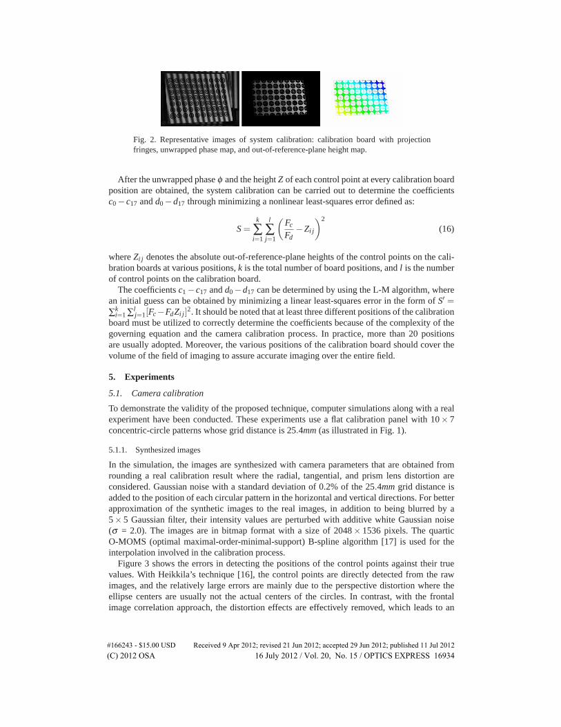
Fig. 2. Representative images of system calibration: calibration board with projectionfringes, unwrapped phase map, and out-of-reference-plane height map.

After the unwrapped phase φ and the height Z of each control point at every calibration boardposition are obtained, the system calibration can be carried out to determine the coefficientsc0 − c17 and d0 −d17 through minimizing a nonlinear least-squares error defined as:

S =k

∑i=1

l

∑j=1

(Fc

Fd−Zi j

)2

(16)

where Zi j denotes the absolute out-of-reference-plane heights of the control points on the cali-bration boards at various positions, k is the total number of board positions, and l is the numberof control points on the calibration board.

The coefficients c1 − c17 and d0 −d17 can be determined by using the L-M algorithm, wherean initial guess can be obtained by minimizing a linear least-squares error in the form of S′ =∑k

i=1 ∑lj=1[Fc−FdZi j]

2. It should be noted that at least three different positions of the calibrationboard must be utilized to correctly determine the coefficients because of the complexity of thegoverning equation and the camera calibration process. In practice, more than 20 positionsare usually adopted. Moreover, the various positions of the calibration board should cover thevolume of the field of imaging to assure accurate imaging over the entire field.

5. Experiments

5.1. Camera calibration

To demonstrate the validity of the proposed technique, computer simulations along with a realexperiment have been conducted. These experiments use a flat calibration panel with 10× 7concentric-circle patterns whose grid distance is 25.4mm (as illustrated in Fig. 1).

5.1.1. Synthesized images

In the simulation, the images are synthesized with camera parameters that are obtained fromrounding a real calibration result where the radial, tangential, and prism lens distortion areconsidered. Gaussian noise with a standard deviation of 0.2% of the 25.4mm grid distance isadded to the position of each circular pattern in the horizontal and vertical directions. For betterapproximation of the synthetic images to the real images, in addition to being blurred by a5× 5 Gaussian filter, their intensity values are perturbed with additive white Gaussian noise(σ = 2.0). The images are in bitmap format with a size of 2048× 1536 pixels. The quarticO-MOMS (optimal maximal-order-minimal-support) B-spline algorithm [17] is used for theinterpolation involved in the calibration process.

Figure 3 shows the errors in detecting the positions of the control points against their truevalues. With Heikkila’s technique [16], the control points are directly detected from the rawimages, and the relatively large errors are mainly due to the perspective distortion where theellipse centers are usually not the actual centers of the circles. In contrast, with the frontalimage correlation approach, the distortion effects are effectively removed, which leads to an

#166243 - $15.00 USD Received 9 Apr 2012; revised 21 Jun 2012; accepted 29 Jun 2012; published 11 Jul 2012(C) 2012 OSA 16 July 2012 / Vol. 20, No. 15 / OPTICS EXPRESS 16934

−0.05−0.025 0 0.025 0.05−0.05

−0.025

0

0.025

0.05(a) RMSE: (0.0183, 0.0160)

−0.05−0.025 0 0.025 0.05−0.05

−0.025

0

0.025

0.05(b) RMSE: (0.000523, 0.000508)

Fig. 3. Localization errors of the control points obtained by: (a) Heikkila’s method, and (b)the frontal image correlation method.

improvement of 30 times on the detection of control points in terms of the root-mean-squareerror (RMSE) in both vertical and horizontal directions.

0 50 100 15010

−4

10−3

10−2

10−1

100

101

Number of iterations

Rep

roje

ctio

n er

ror

(pix

els)

Without control point adjustmentWith control point adjustmentControl point adjustment and refinement

Fig. 4. Convergence of the proposed camera calibration scheme.

Figure 4 presents the performance of the camera calibration process. In the first step, theconventional camera calibration method cannot provide accurate results. In the second step, theapproach of control point adjustment alleviates the defects in the calibration target board andsubsequently yields much smaller errors for the camera calibration. In the third or last step,the frontal image correlation process helps refine the positions of the control points with sub-stantially higher accuracies; consequently, high-accuracy camera calibration can be achieved.The residual of the calibration, named reprojection error and defined as the RMSE between theprojection of the control points to the image planes and their detected locations, is 0.000834pixels. It is noted that the sharp jump at the beginning of the third step is due to the hyper-accurate locations of the control points detected by the frontal image correlation. These newlocations are not associated with the calibration parameters previously obtained in the secondstep, so larger reprojection errors are produced. However, the errors are reduced significantlyand quickly as the iteration continues. Table 1 summarizes the results of the calibration, wherethe physical rotation angles instead of the Rodrigues rotation vectors are presented for easyinterpretation purpose. It can be seen that the camera parameters can be accurately retrievedwith the proposed camera calibration scheme.

#166243 - $15.00 USD Received 9 Apr 2012; revised 21 Jun 2012; accepted 29 Jun 2012; published 11 Jul 2012(C) 2012 OSA 16 July 2012 / Vol. 20, No. 15 / OPTICS EXPRESS 16935

Table 1. Retrieved calibration parameters and their accuracy assessmentTrue Retrieved Error(%) Precision

α 5731a 5730.9840a -0.0002791 0.00843β 5731a 5730.9835a -0.0002879 0.00838γ 0.3260a 0.3258a -0.06134 0.00110u0 1051a 1051.0409a 0.003891 0.0733v0 778a 778.0414a 0.005321 0.0895a0 0.1860 0.186038 0.02043 0.0000275a1 1.0314 1.028625 -0.2691 0.00176a2 22.00 22.0534 0.2427 0.0352p0 -0.00280 -0.00280505 0.1804 0.00000859p1 0.00259 0.00258619 -0.1471 0.0000104p2 -0.0030 -0.00300397 0.1322 0.0000695p3 0.0570 0.000569556 -0.07789 0.00000795s0 0.00520 0.00520503 0.09673 0.00000659s1 -0.00450 -0.00449727 -0.006007 0.0000785s2 0.0220 0.0219588 -0.178 0.0000846s3 -0.0270 -0.0270167 0.06185 0.0000704θx 160.499b 160.49904b 0.00002492 0.0000176θy -12.0236b -12.023197b -0.003352 0.0000145θz 1.35350b 1.3535902b 0.006664 0.00000263Tx -97.9818c -97.984577c -0.00283 0.00291Ty 74.6039c 74.606202c -0.00308 0.00217Tz 1228.6703c 1228.6658c -0.003662 0.00309

aUnit: pixel. bUnit: degree. cUnit: mm.

5.1.2. Robustness to noise

Figure 5 shows the detection errors of the control points when the images are contaminated withGaussian noise whose standard deviation varies from 0 to 3 grayscales. A 5×5 pixels Gaussianfilter has been applied to the relevant images. Since interpolation is critical for the control pointrefinement with sub-pixel accuracies, different interpolation methods [17] have been employedto assess their robustness. For clarification, the data have been separated into two subfigureswith the same cubic B-spline results shown in both. The results indicate that the family of B-spline interpolation yields much higher accuracies than the widely used bicubic interpolationfor the detection of control points. Particularly, the quartic O-MOMS interpolation provides thehighest accuracies.

The accuracy of control point detection in the captured images has a direct relation with therecovery accuracy of the true camera parameters. Figure 6 shows the calibration reprojection er-ror as a function of the standard deviation of noise. It can be seen that the B-spline interpolationmethods typically provide an accuracy two to three times higher than the bicubic interpolationmethod with respect to the RMSE of the reprojection.

5.1.3. Real experimental images

Like many other techniques, although the proposed camera calibration technique has beendemonstrated to be robust against noise and position uncertainties of the control points, thereal experimental results are not good as the simulation ones. This issue can be found in ex-isting techniques as well. For instance, in the work reported by Douxchamps et al. [14] wherea similar approach was used, the simulation yielded a reprojection RMSE of 0.002 pixels andthe real experiment gave 0.045 pixels. Nevertheless, the novel scheme proposed in this paper is

#166243 - $15.00 USD Received 9 Apr 2012; revised 21 Jun 2012; accepted 29 Jun 2012; published 11 Jul 2012(C) 2012 OSA 16 July 2012 / Vol. 20, No. 15 / OPTICS EXPRESS 16936

0 1 2 30

1

2

3

4

5

6

7x 10

−3

Standard deviation of the noise

RM

SE in

pix

els

(a)

Bicubiccubic B−spline

0 1 2 30.4

0.6

0.8

1

1.2

1.4

1.6x 10

−3

Standard deviation of the noise

RM

SE in

pix

els

(b)

cubic B−splinequartic B−splinemodifed cubic B−splinecubic O−MOMSquintic B−spline

Fig. 5. Errors of control point detection with different interpolation methods.

0 1 2 30

0.5

1

1.5

2

2.5

3

3.5x 10

−3

Standard deviation of the noise

RM

SE in

pix

els

(a)

Bicubiccubic B−spline

0 1 2 32

4

6

8

10

12

14x 10

−4

Standard deviation of the noise

RM

SE in

pix

els

(b)

cubic B−splinequartic B−splinemodifed cubic B−splinecubic O−MOMSquintic B−spline

Fig. 6. Reprojection error of camera calibration with different interpolation methods.

still able to provide a remarkable improvement over the existing techniques.In the experiment, a CMOS camera is used to capture a set of 20 images where the calibration

board is located at different positions and oriented in various directions. The images are inbitmap format and each image has a size of 2048×1536 pixels.

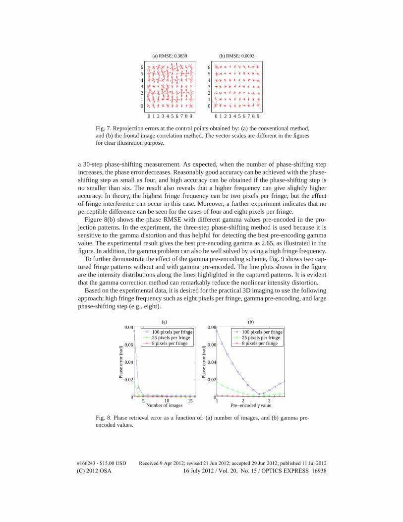
Figure 7 shows the position error vectors between the detected and projected positions at eachcontrol point of the calibration target. With the conventional method, because of the insufficientaccuracy of the control point detection and the imperfection of the calibration target along withthe effect of lens and perspective distortions, the reprojection errors are noticeably polarized.On the contrary, with the proposed frontal image correlation method, the errors behave moreisotropic, indicating that the distortions and the imprecision of the calibration target have beensuccessfully compensated. For the overall reprojection error, the conventional method yielded0.3839 pixels, and the frontal image correlation method yielded 0.0093 pixels.

5.2. Gamma correction

The validity of the gamma correction technique with the large phase-shifting step scheme andthe gamma pre-encoding scheme has been verified by real experiments. To examine the effectof the fringe frequency on the accuracy of phase extraction, three different projection patternswith fringe frequencies of 100, 25, and 8 pixels per fringe are used in the experiments.

Figure 8(a) shows the RMSE of the extracted phase associated with different numbers ofphase-shifting steps without gamma pre-encoding, where the reference phase is acquired by

#166243 - $15.00 USD Received 9 Apr 2012; revised 21 Jun 2012; accepted 29 Jun 2012; published 11 Jul 2012(C) 2012 OSA 16 July 2012 / Vol. 20, No. 15 / OPTICS EXPRESS 16937

0 1 2 3 4 5 6 7 8 9

0123456

(a) RMSE: 0.3839

0 1 2 3 4 5 6 7 8 9

0123456

(b) RMSE: 0.0093

Fig. 7. Reprojection errors at the control points obtained by: (a) the conventional method,and (b) the frontal image correlation method. The vector scales are different in the figuresfor clear illustration purpose.

a 30-step phase-shifting measurement. As expected, when the number of phase-shifting stepincreases, the phase error decreases. Reasonably good accuracy can be achieved with the phase-shifting step as small as four, and high accuracy can be obtained if the phase-shifting step isno smaller than six. The result also reveals that a higher frequency can give slightly higheraccuracy. In theory, the highest fringe frequency can be two pixels per fringe, but the effectof fringe interference can occur in this case. Moreover, a further experiment indicates that noperceptible difference can be seen for the cases of four and eight pixels per fringe.

Figure 8(b) shows the phase RMSE with different gamma values pre-encoded in the pro-jection patterns. In the experiment, the three-step phase-shifting method is used because it issensitive to the gamma distortion and thus helpful for detecting the best pre-encoding gammavalue. The experimental result gives the best pre-encoding gamma as 2.65, as illustrated in thefigure. In addition, the gamma problem can also be well solved by using a high fringe frequency.

To further demonstrate the effect of the gamma pre-encoding scheme, Fig. 9 shows two cap-tured fringe patterns without and with gamma pre-encoded. The line plots shown in the figureare the intensity distributions along the lines highlighted in the captured patterns. It is evidentthat the gamma correction method can remarkably reduce the nonlinear intensity distortion.

Based on the experimental data, it is desired for the practical 3D imaging to use the followingapproach: high fringe frequency such as eight pixels per fringe, gamma pre-encoding, and largephase-shifting step (e.g., eight).

5 10 150

0.02

0.04

0.06

0.08

Number of images

Phas

e er

ror

(rad

)

(a)

100 pixels per fringe25 pixels per fringe8 pixels per fringe

1 2 30

0.02

0.04

0.06

0.08

Pre−encoded γ value

Phas

e er

ror

(rad

)

(b)

100 pixels per fringe25 pixels per fringe8 pixels per fringe

Fig. 8. Phase retrieval error as a function of: (a) number of images, and (b) gamma pre-encoded values.

#166243 - $15.00 USD Received 9 Apr 2012; revised 21 Jun 2012; accepted 29 Jun 2012; published 11 Jul 2012(C) 2012 OSA 16 July 2012 / Vol. 20, No. 15 / OPTICS EXPRESS 16938

(a)A B

(b)a b

0 50 100 150 200

0.0

0.5

1.0

0.0

0.5

1.0

(c)

Index

Nor

mal

ized

inte

nsity

dis

trib

utio

n

γ = 1.0γ = 2.65

Fig. 9. The effect of pre-encoded gamma values on the captured fringe patterns.

5.3. FPB calibration and experiment

To demonstrate the performance of the proposed techniques for accuracy-enhanced FPB 3Dimaging, five real experiments have been conducted at various scales of the field of view. Fourdifferent fringe frequencies, with 1, 4, 20, and 100 fringes in the entire image of 800 pixelswide, are used to generate the projection fringe patterns according to the multi-frequency phase-shifting technique. For the working frequency, i.e., the highest frequency with 100 fringes inthe pattern, the eight-step phase-shifting algorithm rather than the four-step one for the otherfrequencies is employed in the experiments. In addition, the pre-encoded gamma value is pre-determined as 2.65 and the camera calibration parameters are also pre-determined with thetechniques described in previous sections.

The first experiment aims at testing the imaging accuracy, where a flat plate of 457.2mm×304.8mm with eight high-precision gage blocks and a concentric-circle array board with a gridsize of 25.4mm are selected as the object of interest and the calibration board, respectively.Figure 10 shows the testing plate together with its experimentally obtained 2D and 3D plots.The results summarized in Table 2 indicate that the maximum error of the mean measuredheights over the entire field is 0.048mm, which yields a relative accuracy (defined as the ratioof out-of-plane measurement accuracy to the in-plane dimension) of 0.010%. This confirms thevalidity and reliability of the 3D imaging technique.

Fig. 10. 3D imaging results of a plate with eight gage blocks.

For comparison purpose, the captured images of the first three frequencies are also used forthe 3D imaging analysis. This means that the working frequency is 40 pixels per fringe or 20fringes in the 800-pixel width, and four-step phase-shifting algorithm is used. The mean meas-

#166243 - $15.00 USD Received 9 Apr 2012; revised 21 Jun 2012; accepted 29 Jun 2012; published 11 Jul 2012(C) 2012 OSA 16 July 2012 / Vol. 20, No. 15 / OPTICS EXPRESS 16939

Table 2. Actual and measured heights of gage blocksGage Actual Mean measured Error Standard deviation

1 25.400 25.363 -0.037 0.0332 19.050 19.048 -0.002 0.0393 6.350 6.398 0.048 0.0274 6.350 6.381 0.031 0.0415 12.700 12.670 -0.030 0.0326 15.875 15.898 0.023 0.0367 9.525 9.478 -0.047 0.0398 50.80 50.766 -0.034 0.033

unit: mm

ured heights are 25.729mm, 18.903mm, 6.340mm, 6.302mm, 12.332mm, 15.622mm, 9.522mm,and 50.855mm for the eight gage blocks, respectively. The largest error is −0.368mm and thelargest standard deviation is 0.449mm. The results clearly show the effectiveness of using high-frequency fringes and large phase-shifting step. In practice, it is favorable to apply all the fol-lowing approaches: high-frequency fringes, gamma pre-encoding, and large phase-shifting step.

The other four experiments are intended to verify the flexibility of the proposed techniquefor 3D imaging at various scales. Figure 11 illustrates the full 360◦ 3D imaging result of aconch shell obtained by combining the 3D images captured from multiple views. In this case,the conch shell is 221mm long and the grid distance of the calibration target pattern is scaleddown to 16mm. Visual inspection vividly shows that the full 360◦ image has a very good matchwith the actual object, and the surface structure can be seen at ease. The high quality full 360◦3D registration clearly benefits from the accurate 3D measurements.

Fig. 11. A conch shell and its 3D images observed from five different views.

Another experiment is carried out to validate the performance of the 3D imaging at smallscales, where a small calibration board with a pattern grid distance of 6.0mm is employedto calibrate the system. In this experiment, an optical lens is utilized to focus the projectionfringes into a small region to cover the object of interest. Figure 12 shows the imaging resultof a 48.0mm× 56.0mm printed circuit board with many components on it. It can be seen thatexcept for the shadow and shiny regions, the result indicates a good imaging accuracy.

Using the similar setup to the previous experiment, the 3D image of a small metal horsesculpture (45mm tall) is acquired, as shown in Fig. 13. With the full 360◦ 3D model successfullyformed, the experiment again demonstrates both the accuracy and the flexibility of the FPB 3Dimaging approach.

The last experiment is conducted to demonstrate the validity of the technique on 3D shapemeasurement at a relatively larger scale, where a large calibration board with a pattern griddistance of 50.8mm is used. Figure 14 shows the 3D shape measurement result of a lion toywhose length is 600.0mm. This and the previous experiments evidently demonstrate that the

#166243 - $15.00 USD Received 9 Apr 2012; revised 21 Jun 2012; accepted 29 Jun 2012; published 11 Jul 2012(C) 2012 OSA 16 July 2012 / Vol. 20, No. 15 / OPTICS EXPRESS 16940

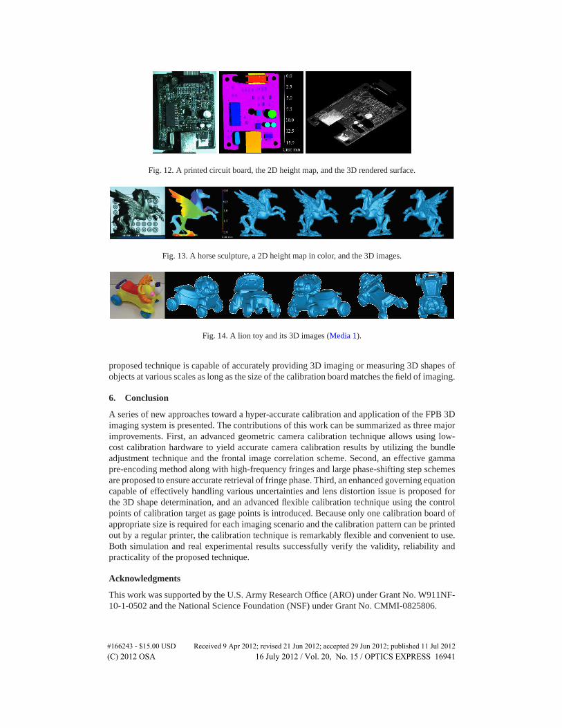
Fig. 12. A printed circuit board, the 2D height map, and the 3D rendered surface.

Fig. 13. A horse sculpture, a 2D height map in color, and the 3D images.

Fig. 14. A lion toy and its 3D images (Media 1).

proposed technique is capable of accurately providing 3D imaging or measuring 3D shapes ofobjects at various scales as long as the size of the calibration board matches the field of imaging.

6. Conclusion

A series of new approaches toward a hyper-accurate calibration and application of the FPB 3Dimaging system is presented. The contributions of this work can be summarized as three majorimprovements. First, an advanced geometric camera calibration technique allows using low-cost calibration hardware to yield accurate camera calibration results by utilizing the bundleadjustment technique and the frontal image correlation scheme. Second, an effective gammapre-encoding method along with high-frequency fringes and large phase-shifting step schemesare proposed to ensure accurate retrieval of fringe phase. Third, an enhanced governing equationcapable of effectively handling various uncertainties and lens distortion issue is proposed forthe 3D shape determination, and an advanced flexible calibration technique using the controlpoints of calibration target as gage points is introduced. Because only one calibration board ofappropriate size is required for each imaging scenario and the calibration pattern can be printedout by a regular printer, the calibration technique is remarkably flexible and convenient to use.Both simulation and real experimental results successfully verify the validity, reliability andpracticality of the proposed technique.

Acknowledgments

This work was supported by the U.S. Army Research Office (ARO) under Grant No. W911NF-10-1-0502 and the National Science Foundation (NSF) under Grant No. CMMI-0825806.

#166243 - $15.00 USD Received 9 Apr 2012; revised 21 Jun 2012; accepted 29 Jun 2012; published 11 Jul 2012(C) 2012 OSA 16 July 2012 / Vol. 20, No. 15 / OPTICS EXPRESS 16941