Fitting Geomagnetic Fields before the Invention of Least Squares: I. Henry Bond's Predictions (1636,...

PLEASE SCROLL DOWN FOR ARTICLE

This article was downloaded by: [University College London]On: 17 August 2010Access details: Access Details: [subscription number 917199415]Publisher Taylor & FrancisInforma Ltd Registered in England and Wales Registered Number: 1072954 Registered office: Mortimer House, 37-41 Mortimer Street, London W1T 3JH, UK

Annals of SciencePublication details, including instructions for authors and subscription information:http://www.informaworld.com/smpp/title~content=t713692742

Fitting Geomagnetic Fields before the Invention of Least Squares: II.William Whiston's Isoclinic Maps of Southern England (1719 and 1721)Richard J. Howartha

a Department of Geological Sciences, University College London, Gower Street, London WC1E 6BT,UK. Email: [email protected].

To cite this Article Howarth, Richard J.(2003) 'Fitting Geomagnetic Fields before the Invention of Least Squares: II.William Whiston's Isoclinic Maps of Southern England (1719 and 1721)', Annals of Science, 60: 1, 63 — 84To link to this Article: DOI: 10.1080/713801783URL: http://dx.doi.org/10.1080/713801783

Full terms and conditions of use: http://www.informaworld.com/terms-and-conditions-of-access.pdf

This article may be used for research, teaching and private study purposes. Any substantial orsystematic reproduction, re-distribution, re-selling, loan or sub-licensing, systematic supply ordistribution in any form to anyone is expressly forbidden.

The publisher does not give any warranty express or implied or make any representation that the contentswill be complete or accurate or up to date. The accuracy of any instructions, formulae and drug dosesshould be independently verified with primary sources. The publisher shall not be liable for any loss,actions, claims, proceedings, demand or costs or damages whatsoever or howsoever caused arising directlyor indirectly in connection with or arising out of the use of this material.

http://www.informaworld.com/smpp/title~content=t713692742

http://dx.doi.org/10.1080/713801783

http://www.informaworld.com/terms-and-conditions-of-access.pdf

A S, 60 (2003), 63–84

Fitting Geomagnetic Fields before the Invention of Least Squares:II. William Whiston’s Isoclinic Maps of Southern England

(1719 and 1721)

R J. H

Department of Geological Sciences, University College London, Gower Street,London WC1E 6BT, UK. Email: [email protected]

Accepted 4 January 2001

SummaryThe English mathematical practitioner and theologian William Whiston(1667–1752) made the first known maps showing the direction of magnetic inclina-tion (for south-eastern England) in 1719 and 1720. He also anticipated Graham’s1723 measurement of the ratio of horizontal and vertical magnetic intensities, andhe understood their relationship to magnetic inclination. Whiston’s work is exam-ined to determine how he fitted the planar isoclinic surfaces. This is of interestbecause his study precedes the publication of ‘Meyer’s method’ by thirty-one yearsand the Legendre–Gauss ‘method of least squares’ by eighty-six years. It is sug-gested that Whiston fitted the surfaces using observations of inclination at a chosentriplet of localities; and that he did this in order to use data from non-includedlocalities as a check on his model. Best fits to his maps are given by inclinationsbased on Salisbury, Wiltshire, London, and Ainho [Aynho], Northamptonshire,in 1719, and on Wanstead, Essex, Ainho, and Saltfleet, Lincolnshire, in 1720.However, in both cases, the orientation of the isolines appears to be inconsistentwith roughly contemporary data from Europe and Scandinavia, as well as ahindcast of the geomagnetic field in 1720, based on the modern Bloxham–Jacksonglobal, time-dependent, spherical harmonic model.

Contents1. Introduction . . . . . . . . . . . . . . . . . . . . . . . . . . . . . . . . . . . . . . . . . . . . . . . . . . . 632. Biographical background . . . . . . . . . . . . . . . . . . . . . . . . . . . . . . . . . . . . . . . 653. The longitude problem . . . . . . . . . . . . . . . . . . . . . . . . . . . . . . . . . . . . . . . . . 674. Whiston’s 1719 isoclinic map . . . . . . . . . . . . . . . . . . . . . . . . . . . . . . . . . . . . 685. Whiston’s 1720 isoclinic map . . . . . . . . . . . . . . . . . . . . . . . . . . . . . . . . . . . . 706. Fitting the isolines . . . . . . . . . . . . . . . . . . . . . . . . . . . . . . . . . . . . . . . . . . . . . 72

6.1. The 1719 map . . . . . . . . . . . . . . . . . . . . . . . . . . . . . . . . . . . . . . . . . . . . . 726.2. The 1720 map . . . . . . . . . . . . . . . . . . . . . . . . . . . . . . . . . . . . . . . . . . . . . 756.3. Suggested method . . . . . . . . . . . . . . . . . . . . . . . . . . . . . . . . . . . . . . . . . . 77

7. Magnetic intensity . . . . . . . . . . . . . . . . . . . . . . . . . . . . . . . . . . . . . . . . . . . . . 818. Conclusions . . . . . . . . . . . . . . . . . . . . . . . . . . . . . . . . . . . . . . . . . . . . . . . . . . . 839. Epilogue . . . . . . . . . . . . . . . . . . . . . . . . . . . . . . . . . . . . . . . . . . . . . . . . . . . . . . 83

1. IntroductionWhat are believed by Felgentraeger,1 Bauer,2 Hellmann,3 and subsequent stu-

dents of the history of geomagnetic mapping to be the first isoline maps of magnetic

1W. Felgentraeger, ‘Die Isoklinen Karte von Whiston’, Nachrichten der koniglichen Gesellschaft derWissenschaften zu Gottingen (no. 2) (1894), 129–40.2 L. A. Bauer, ‘The Earliest Isoclinics and Observations of Magnetic Force’, Bulletin of the Philosophical

Society of Washington, 12 (1895, for 1892–94), 397–410.3 G. Hellmann, ‘E. Halley, W. Whiston, J. C. Wilcke, [F. W. H.] A. von Humboldt, C. Hansteen.

Die altesten Karten der Isogonen Isoklinen Isodynamen 1701 1721 1768 1804 1825 1826’, Neudrucke vonSchriften und Karten uber Meteorologie und Erdmagnetismus (Berlin, 1895), , 1–25.

Annals of Science ISSN 0003-3790 print/ISSN 1464-505X online © 2003 Taylor & Francis Ltdhttp://www.tandf.co.uk/journals

DOI: 10.1080/00033790110050786

Downloaded By: [University College London] At: 20:39 17 August 2010

Richard J. Howarth64

inclination were privately published in 1719 and 1721 by the English mathematicalpractitioner and theologian William Whiston (1667–1752). Both his isoclinic maps(Figures 1 and 2) cover parts of south-eastern and central England. Whiston’s workwas apparently influenced4 by the appearance, in 1701, of the first published magneticisoline map. Made by Edmond Halley (1656–1742; FRS, 1678), it showed thepattern of magnetic declination over the Atlantic Ocean, based on recorded valuesat c. 150 locations.5 Whiston’s two maps differ from the ‘Atlantic map’ in that theelement of the geomagnetic field is represented, in each case, by a single planarsurface. The curved isolines in Halley’s isogonic map are so much more complex, itseems unlikely that they could have been determined in any way other than byinterpolating smooth curves by eye, probably using a wooden spline or similar aid.6

It must be borne in mind that, prior to the late eighteenth century, isoline mapsof any kind were a rarely used cartographic convention:7 Although the earliest-known isobath map dates from 1584,8 use of topographic contours to depict landsurfaces did not begin until 1791;9 also, other than the work of early geomagnetists,Baron F. W. H. Alexander von Humboldt (1769–1859) was the first to popularizethe idea of maps showing isolines for a non-topographic quantity when, in 1817, heillustrated the temperature distribution across a large part of the northernhemisphere.10

Quite apart from his early use of isolines, Whiston’s surface-fitting work precededby thirty-one years the development of ‘Mayer’s method’ (which later became knownas the ‘method of averages’) for fitting a linear equation to observational data,published by the German astronomer and mathematician Johann Tobias Mayer(1723–62) in 1750,11 and was eighty-six years earlier than the almost simultaneous

4W. Whiston and H. Ditton, A New method for Discovering the Longitude both at Sea and Land(London, 1714), p. 10.5 E. Halley, A New and Correct Chart shewing the Variations of the Compass in the Western & Southern

Oceans as Observed in ye Year 1700 by his Ma.ties Command by Edm. Halley (London, 1701). The map,in Mercator’s projection, extends to 59° N and S of the equator. It is reproduced in N. J. W. Thrower,‘Edmond Halley and thematic geo-cartography’, in The Compleat Plattmaker, ed. by N. J. W. Thrower(Berkley, California, 1978), p. 213, Figure 2; The Three Voyages of Edmond Halley in The Paramore1698–1701, ed. by N. J. W. Thrower, Hakluyt Society works, 2nd series, nos. 156–157 (London, 1981),portfolio; A. H. Robinson, Early Thematic Mapping in the History of Cartography (Chicago, 1982), p. 85,Figure 32; A. Cook, Edmond Halley. Charting the Heavens and the Seas (Oxford, 1998), Plate IX. Halleyalso published a ‘world’ isogonic map in 1702; see Thrower (1978, 1981) and Cook (1998) for furtherdetails of his work. G. Hellman notes in ‘Magnetische Kartographie in historisch-kritischer Darstellung’,Veroffentlichungen des Koniglich Preubischen Meteorologischen Instituts, no. 215, Abhandlungen (Berlin1909), , no. 3, that the German physicist Athanasius Kircher (1601–80) records in Magnes Sive de artemagnetica opus tripartum (Rome 1643) that in 1630, Christoforo Borri [Borro, Borrus, Burro, Burrus](d. 1632) SJ, who became professor of mathematics at Lisbon, drew a map of declination in part of theEast Indies, in which the isogones were represented as parallel lines, but that it was never published.Kircher recognized that Borri’s representation was too simple. There is no evidence that Halley knew ofthis earlier work.6 See Thrower (note 5, 1978, 1981) for further discussion.7 Robinson (note 5, 1982).8 Idem, p. 211, Figure 107.9 Idem, p. 95, Figure 38.10 [F. W. H.] A. von Humboldt, ‘Des lignes isothermes et de la distribution de la chaleur sur le globe’,

Memoires de Physique et de Chimie, de la Societe D’Arcueil, 3 (1817), 462–602; ‘Sur les lignes isothermes(Extrait)’, Annales de chimie et physique, 5 (1817), 102–12. His map is reproduced in Robinson (note 5,1982), p. 72, Figure 22.11 T. Mayer, ‘Abhandlung uber die Umwalzung des Monds um seine Axe und die scheinbare Bewegung

der Mondsflecten’, Kosmographische Nachrichten und Sammlungen (1750, for 1748), 52–183. His methodwas based on the solution of a series of simultaneous linear equations, each of which corresponded to agiven set of data values; see S. M. Stigler, The History of Statistics. The measurement of uncertainty before1900 (Cambridge, MA, 1986), pp. 18–24, and O. [B.] Sheynin, ‘On the History of the Principle of LeastSquares’, Archive for History of Exact Sciences, 46 (1993), 39–54, for discussion.


William Whiston’s Isoclinic Maps of Southern England 65

publication of the principle of ‘least squares’12 by Adrien Marie Legendre (1752–1833) in France and Carl Friedrich Gauss (1777–1855) in Germany13 in 1805 and1809 respectively. Eisenhart and Sheynin14 suggest that both the Mayer and theLegendre–Gauss methods had their origins in work carried out by the Swiss mathem-atician Leonhard Euler (1707–83) in 1748.15 By the mid-nineteenth century, sufficientmagnetic data had become available that Gauss was able to use the method of leastsquares in his classic attempt to model the world geomagnetic field.16 His lead wasfollowed by other nineteenth-century geophysicists, concerned with fitting predictivemodels to regional magnetic and gravity fields, although Mayer’s method was stilloccasionally used in such studies.17

In view of this, it seems surprising that previous accounts of Whiston’s work byFelgentraeger,18 Bauer,19 and Hellmann20 did not consider how the isolines werefitted to his observed data. This study re-examines Whiston’s results and suggests howhis isoclinic surfaces might have been computed. Sections 2 and 3 give some historicalbackground; Sections 4 and 5 discuss the maps themselves; Section 6 suggests how thesurfaces might have been fitted; Section 7 notes his work on magnetic intensity.

2. Biographical backgroundWilliam Whiston was the son of Josiah Whiston, Rector of Norton, Twycroffe,

near Leicester, England. He attended Tamworth school (1684–86) and entered Clare

12 Sheynin (note 11) draws a distinction between the principle of least squares and the later methodof least squares. The former was simply a condition imposed on the residuals of an inconsistent redundantsystem of linear algebraic equations, in which the number of unknowns was less than the number ofequations. Gauss’ full exposition of the OLS method only appeared in 1823, in the context of hisdevelopment of the theory of errors and the normal distribution, in ‘Theoria CombinationisObservationum Erroribus Minimis Obnoxiae’ (Theory of the combination of observations leading to theminimum errors), Commentationes Societas Regiae Scientiarum Gottingensis Recentiores, 5 (1823), part1, 33–62; part 2, 63–90.13 A. M. Legendre, Nouvelles methodes pour la determination des orbites des cometes (Paris, 1805); C.

F. Gauss, ‘Determinatio orbitae observationibus quotcunque maxime satisfacientis’, in Theoria MotusCorporum Coelestium in Sectionibus Conicis Solem Ambientium (Hamburg, 1809), pp. 205–24 (translatedby C. H. Davis, Theory of the Motion of the Heavenly Bodies Moving about the Sun in Conic Sections(Boston, 1857), selected extracts reproduced in H. Shapley and H. E. Howarth, A Source Book inAstronomy (New York, 1929), pp. 183–95). Gauss had been using the principle of OLS since c. 1795;see R. L. Plackett, ‘The Discovery of the Method of Least Squares’, Biometrika, 59 (1972), 239–251;J. Dukta, ‘On Gauss’ Priority in the Discovery of the Method of Least Squares’, Archive for History ofExact Sciences, 49 (1996), 355–370.14 C. Eisenhart, ‘Boscovich and the Combination of Observations’, in Roger Joseph Boscovich, ed. by

L. L. Whyte (London, 1961), pp. 200–12; Sheynin (note 11, 1993).15 L. Euler, Piece qui a remporte le prix de l’Academie royale des Sciences en 1748 sur la question des

inegalites du movement de Saturn et de Jupiter (Paris, 1749); ‘Observationes in praecedentem disserta-tionem’ (Observations on the foregoing dissertation [of Bernoulli ]), Acta Academiae Scientiarum ImperialisPetropolitanae (1777), part 1, 24–33.16 C. F. Gauss, ‘Allegemeine Theorie des Erdmagnetismus’, in Resultate aus den Beobachtungen des

magnetischen Vereins im Jahre 1838, ed. by C.F. Gauss and W. Weber (Gottingen, 1839), 1–57; translatedby E. J. Sabine and revised by J. Herschel, ‘General Theory of Terrestrial Magnetism by Professor CarlFriedrich Gauss of the University of Gottingen’, in Taylor’s Scientific Memoirs (1841), , 184–251.17 See H. Lloyd, E. Sabine and J. C. Ross, ‘Observations on the Direction and Intensity of the

Terrestrial Magnetic Force in Ireland’, in Report of the 5th Meeting of the British Association for theAdvancement of Science, Dublin, 1835 (London, 1836), pp. 117–62; J. D. Forbes ‘Account of someExperiments Made in Different Parts of Europe, on Terrestrial Magnetic Intensity, Particularly withReference to the Effect of Height’, Transactions of the Royal Society of Edinburgh, 14 (1840), 1–29; A.Quetelet, ‘Second Memoire sur le Magnetisme Terrestre en Italie’, Nouveaux Memoires de l’AcademieRoyale des Sciences et des Belles-Lettres de Bruxelles, 13 (1841), 1–27; G. B. Airy, ‘Figure of the Earth’,in Encyclopaedia Metropolitana, ed. by E. Smedley, H. J. Rose and H. J. Rose (London, 1845), , 175–210.18 Note 1.19 Note 2.20 Note 3, pp. 11–13.


https://www.researchgate.net/publication/239550461_Theoria_Combinationis_Observationum_Erroribus_Minimis_Obnoxiae_Pars_Posterior?el=1_x_8&enrichId=rgreq-1b6627d23451182baf45d5036b34d2db-XXX&enrichSource=Y292ZXJQYWdlOzIzMzAzODg3NztBUzoxNjY2ODE2NjE5NDM4MDhAMTQxNjc1MTQxMzc3OA==






Hall, Cambridge, in 1686, where he principally studied mathematics, gaining his BAin February 1690. In 1693, he was granted his MA and became a Fellow of ClareCollege. That same year he was also ordained deacon, becoming chaplain to theBishop of Norwich. Between 1698 and 1703, he was vicar of Lowestoft-with-Kissingland, Suffolk. However, when Isaac Newton’s (1642–1727; FRS, 1672; Kt,1705) Philosophiae naturalis principia mathematica (Mathematical Principles ofNatural Philosophy) was published in 1687, Whiston returned to Clare and beganto study Newton’s work in depth, while at the same time pursuing his own mathemat-ical research. By 1701, Whiston was appointed deputy to Newton in the Lucasianprofessorship of mathematics, succeeded him as professor in 1703, and was alsoappointed Boyle lecturer in 1707. Since at this period students did not undertaketheir own practical work, Whiston began demonstrating a ‘Course of PhilosophicalExperiments’, which he taught jointly with the mathematical practitioner RogerCotes (1683–1717), who had been appointed, with Whiston’s commendation, as thefirst Plumian Professor of Astronomy and Natural Philosophy in 1706.

Possibly secretly influenced by Newton in taking up Arianism (that is, becominga follower of Arius, a fourth-century Christian who rejected the conventional viewof the Trinity and whose beliefs seem to have later become equated, at least inEngland, with Unitarianism)21 Whiston’s religious views22 became increasingly sus-pect. Although Newton and a number of those connected with him apparently heldsimilar beliefs, Whiston was particularly vocal in letting his opinions be known. Anundergraduate at Jesus College, W. Renew, wrote to a friend that

One Whiston, our Mathematicall Professor, a very learned (and as we thoughtpious) man has written a Book concerning ye Trinity & designs to print it,wherein he sides with ye Arrians; he has showed it to severall of his friends,who tell him it is a damnable, heretical Book, & that if he prints it, he’ll loosehis Professorship.23

Unfortunately, this prediction proved to be all too correct. On 23 October 1710,Whiston appeared before the Vice-Chancellor and nine Heads of Colleges, and, on30 October, he was removed from his pastoral and theological duties and banishedfrom Cambridge for his uncompromising stance on the issue.24 Thereafter, heremained embroiled in a series of ecclesiastical trials until 1715, when his perceivedheresy was eventually pardoned. It is evident from Whiston’s autobiography25 that

21 [J. Tulloch], ‘Arius’, Encyclopaedia Brittanica, ed. by T. S. Baynes and W. Robertson Smith, 9thedn (Edinburgh, 1875), , 537–39; [J. F. Smith], ‘Unitarianism’, idem (1888), , 725–26; [A. Thomson],‘Arianism’, The Edinburgh Encyclopaedia, ed. by D. Brewster (Edinburgh, 1830), , 351–53; see also S.D. Snobelen, ‘Isaac Newton, Heretic: the Strategies of a Nicodemite’, British Journal for the History ofScience, 32 (1999), 381–419.22 Summarized by Thomson (note 21), p. 353, as being ‘that the eternity of the Son of God was not

a real eternity, but only a metaphysical existence, in potentia [Latin, virtue], or in some sublimer manner,in the Father as his wisdom or word; that Christ’s real generation or creation happened sometime beforethe creation of the world; and that this was the doctrine . . . of Christ, of his apostles, and of the firstChristians’. See also discussion in R. S. Westfall, Never at Rest. A Biography of Isaac Newton (Cambridge,1980), pp. 649–53.23 Quoted in R. T. Gunter, Early Science in Cambridge (Oxford, 1937), p. 79.24 Idem, p. 56. Thomson (note 21) p. 353, commenting on Whiston’s fate wrote that despite the fact

that the ‘heresy of Arianism’ should still be regarded as important ‘though attachment to the [orthodox]Athanasian creed may be thought necessary for a teacher of religion within the established church ofEngland, some ingenuity is required to shew, and much bigotry to believe, its necessity, to him who isappointed to teach the elements of Euclid, or the science of algebra’.25W. Whiston, Memoirs of the Life and Writings of Mr. William Whiston. Containing Memoirs of

Several of his Friends, 3 vols (London, 1749–50).



his real passion was (or became) religion rather than science, as he devotes littlespace in the three volume-work to documenting his scientific achievements, preferringinstead to dwell on issues of theology and his extensive litigation against what hesaw as the established church’s dogmatic position. He eventually joined the BaptistChurch in 1747.26

Following his banishment, Whiston maintained a somewhat precarious existenceas a lecturer on astronomy and mathematics at Button’s coffee house, near CoventGarden, London,27 and ‘at fashionable watering places’.28 In 1714, he gave an‘experimental course of physics’ at the shop of the younger Francis Hauksbee(1687–1763).29

When Whiston was proposed for Fellowship of the Royal Society in May 1716by Martin Folkes (1690–1754; FRS, 1714), Newton threatened to resign hisPresidency unless Whiston’s nomination was abandoned.30 Throughout the rest ofhis life, Whiston remained convinced that it was his ‘heretical’ opinions that had pre-vented him from being elected.31Westfall has suggested that although Newton shared(and may even have been the originator of ) Whiston’s theological beliefs, he wascareful to keep his own views out of print and, as early as 1714, increasingly alarmedby ‘the public identification of men closely associated with him as heretics’, he ‘appearsto have wanted to separate himself from a notorious apostate such as Whiston’.32

3. The longitude problemAfter his move to London, Whiston became involved in a campaign to persuade

the British government to do something to solve the ‘longitude problem’—devisinga reliable method to improve greatly the determination of longitude by ships atsea.33 Although it is reported that Whiston ‘had a small patrimony, and with this,his writings, his public lectures, and the occasional liberality of those who admiredhis unflinching character, particularly (towards the end of his life) of his son-in-law,he was never in want’,34 it is still possible that, as has been suggested by Malin,35Whiston may have had a financial motive in trying to find a viable method fordetermining longitude.

Whiston’s first proposal, made jointly with the London mathematician HumphreyDitton (1675–1715), who had preceded Whiston as a lecturer at Hauksbee’s estab-lishment,36 was for the use of a warning system based on a network of signalling

26 Anonymous, ‘Whiston, William’, in Cyclopaedia of Biography, ed. by C. Knight (London, 1858),, 663–65; idem, ‘Whiston, William (1667–1752)’, in Encyclopaedia Brittanica, ed. by T. S. Baynes andW. Robertson Smith, 9th edn (Edinburgh, 1888), , 548; P. Lorimer, ‘Whiston, William’, in TheImperial Dictionary of Universal Biography, ed. by J. F. Waller (London, 1865), , 907.27 Gunter (note 23), p. 56.28 E. G. R. Taylor, The Mathematical Practitioners of Tudor & Stuart England (Cambridge, 1954),

p. 285.29 Idem, p. 430.30Westfall (note 22), p. 653, his note 82.31Whiston (note 25), , 292–93, believed that his name had been put forward by his friends Halley

and Sir Hans Sloane (1660–1753; FRS, 1685).32Westfall (note 22), pp. 652–53.33 The lack of a means to locate the position of a ship accurately caused many vessels to be lost at

sea by collision with unexpected rocks; see D. Sobel, Longitude (London, 1996), for a popular accountof attempts to solve the ‘longitude problem’.34 Anonymous (note 26, 1858); see also Gunter (note 23), p. 56.35 S. [R. C.] Malin, ‘Historical introduction to geomagnetism’, in Geomagnetism, ed. by J. A. Jacobs

(London, 1987), , 27.36Whiston and Ditton (note 4).



stations using gunfire or lights. Despite acknowledging Halley’s contribution37 theyargued that the small scale of his Atlantic map meant that his results were incapableof determining longitude to an accuracy of better than ‘100 geographical miles’ (c.160 km)38 and that this factor, combined with lack of knowledge of the local magneticfield (since it was common experience among mariners that in some places compassdirections could rapidly alter near shore)39 rendered an approach based on magneticdeclination impractical.

Whiston and Ditton’s proposal was seriously considered, but was eventuallydeemed to be impractical. However, it at least prompted the British Parliament intopassing the Longitude Act, in June 1714, which led to the formation of the Boardof Longitude.40 The British government now offered a prize of £20,000 to anyonewho could devise a location method sufficiently accurate that it could be used at seato determine longitude to within half a degree of a great circle (c. 55 km). The awardof the prize was to be judged by the Board.

The idea that magnetic inclination could be a useful aid to navigators for thedetermination of position at sea ‘in any part of the world, without the help of theheavenly bodies, sun, planets or fixed stars, and in foggy weather as well as indarkness’ goes back to the study by Gilbert41 of the force field around a terrella;42he even provided a graphical aid for the conversion of the angle of dip to latitude.43Nevertheless, his proposal appears to have remained relatively unknown, as it seemsto have come as something of a surprise to Humboldt, writing in the 1840s.44 Thislack of interest may be because Gilbert made the erroneous, but understandable,assumption that lines of equal inclination in the terrestrial magnetic field wouldeverywhere remain parallel to the geographical equator and, in general, this wouldnot have been found to be borne out in practice, either on the land or at sea.

4. Whiston’s 1719 isoclinic mapIn November 1718, Whiston was visited by the German geographer, Christoph

Eberhard (1675–1750), who was already engaged in work to determine longitude bymagnetic methods. On his own admission,45 up to that time Whiston had never heardof a dip needle, let alone seen one, but that fact did not prevent him being prettydismissive of his visitor ‘who pretended to have a Method for discovering the longitude

37 Idem, p. 10; cf. Halley (note 5, 1701).38Whiston and Ditton (note 4), p. 15.39 This would generally have been attributable to the effects of anomalous magnetic fields as a result

of the presence of lavas or other rocks with a high iron content.40 Sobel (note 33), pp. 46–50.41W. Gilbert, De magnete, magneticisque corporibus, et de magno magnete tellure; Physiologia nova,

plurimis & argumentis, & experimentis demonstrata (London, 1600; repr. Brussels, 1967), pp. 184–204;translated by P. F. Mottelay, On the Loadstone and Magnetic Bodies, and on the Great Magnet of theEarth. A New Physiology, Demonstrated with Many Arguments and Experiments (London, 1893; repr.New York, 1958), pp. 275–304.42 A small globe, several centimetres in diameter, machined out of magnetite (a naturally occurring

iron ore) which Gilbert used as an analogue for the terrestrial magnetic field.43 Gilbert (note 41, 1600), unnumbered figures on p. 198, folding plate opposite p. 200; idem, 1893,

unnumbered figures on pp. 294, 298.44 [F. W. H.] A. von Humboldt, Cosmos: Sketch of a Physical Description of the Universe, trans. by

E. J. Sabine and ed. by E. Sabine, 4 vols (London, 1855), , p. li, author’s note 144.45W. Whiston, The Longitude and Latitude Found by the Inclinatory or Dipping needle; Wherein the

Laws of Magnetism are also discover’d. To which is prefix’d, An Historical Preface; and to which issubjoin’d, Mr. Robert Norman’s New Attractive, or Account of the first Invention of the Dipping Needle(London, 1721), p. xxiv.



by the Dipping-Needle’.46 Nevertheless, Whiston was prompted to reconsider theapplication of terrestrial magnetism to finding a solution to the longitude problem.Recalling Halley’s map, Whiston knew that the annual rate of change in inclinationwas much less rapid than that of declination, and he thought that this might offer amore viable alternative.47 By the following year, he had become convinced:

Since the Quantity of the Inclination of the Dipping Needle has varied hereat London (the only place in the World where it has been long enough knownto determine that Variation) scarce Two Degrees in 143 Years: (As appears byMr Norman’s Original Quantity 71° 50∞ compared with that now, 73° 45∞) ’Tiscertain that Charts made with these Lines of equal Dip upon them, will serve,at least in these Parts of the World, many Years, without any Necessity ofAlteration, or any considerable Inconvenience to Navigation.48

Whiston accordingly began his study by collating observations of magneticinclination made by earlier investigators, who are identifiable as follows: the navig-ator, Henry Hudson (d. 1611); Louis Feuillee [Feuillet] (1660–1732); Col. Edmond[Edmund] Windham [ Wyndham] ( fl. 1659–86; FRS, 1677); possibly, the astro-nomer, Rev. James Pound (1669–1724; FRS, 1699); the botanist and surgeon tothe East India Company, James Cunningham (d. ?1709; FRS, 1699); Francois Noel,SJ (1651–1729). Whiston apparently then used this information to draw lines ofequal inclination on a terrestrial globe made by Emery Molyneux ( fl. 1587–1605)of Lambeth, London.49 In his account of this work, Whiston uses the terms ‘Linesof equal Dip’, ‘Magnetick Parallels’, and the ‘Magnetick Equator’, and refers tomagnetic meridians as ‘Perpendiculars to the Magnetick Parallels of equal Dip’.50Unfortunately, he gives no further details of his findings, nor does he record theoriginal observations on which this study was based.

However, as a result of Eberhard’s visit, Whiston found that an acquaintance,‘Colonel Windham, a very curious and inquisitive Gentleman indeed’ possessed adip needle 12 in (30 cm) long, and had been making ‘considerable use of [it]. . . bothby Sea and Land’ in the 1670s.51 Whiston borrowed it, and in the autumn of 1719he measured inclination at a number of places in south-eastern England.52 He alsotook into account additional data for Sarum [Salisbury], England, and from Rouen,Normandy, and Paris, France. Whiston notes that the Salisbury observation was‘made [by Windham] about A.D. 1672, with the allowance of increase since thattime, I have determined the Dip at Salisbury in my little Map’,53 but Whiston doesnot record either the original value of Windham’s observation or what correctionwas applied to it.

Whiston says nothing about the Paris observation,54 but describes the one fromRouen as ‘extant in Dr. Power’.55 The physician and natural philosopher, Henry

46 Idem.47 Idem, pp. xxvi–vii.48W. Whiston, The Longitude and Latitude Found by the Inclinatory or Dipping Needle (London,

1719), p. 29, emphasis as in original.49Whiston (note 45), p. 53.50 Idem, pp. 53–8.51 Idem, p. xx.52Whiston (note 48), p. 21.53 Idem.54 The data compilation of M. Alexandrescu, V. Courtillot and J.-L. Le Mouel, ‘Geomagnetic Field

Direction in Paris Since the Mid-Sixteenth Century’, Physics of the Earth and Planetary Interiors, 98(1996), 321–60, corroborates the Paris observation but casts no additional light on whom its originatormight have been.55Whiston (note 45), p. 91.



Power (1623–68; FRS, 1663) only published one book,56 the third part of which isdevoted to magnetic experiments.57 In this section, Power quotes a value of 72° forthe ‘Angle of Septentrional [i.e. northerly] Variation’ at Rouen58 but he does notmention Paris. Whiston gives the inclination at Rouen as 72D°. This would beconsistent with an adjustment of Windham’s observation based on the elapsed timefrom the publication of Power’s book, rather than that of the original observation,which must date from c. 1645.59 Rather surprisingly, Whiston commented that heconsidered the data from Salisbury and Rouen to be ‘two of the remotest and bestObservations’.60

Whiston’s first map61 (Figure 1), was published in a privately printed book (titlepage dated 20 November 1719) which he gave to some of his ‘mathematical friends’(who still appeared to include Newton)62 the following year.63

It is clear that Whiston made his own observations at Barkston, Lincolnshire,Lyndon, Leicestershire, at Yelvertoft [ Yelverton], Maidford, and Ainho [Aynho],Northamptonshire, and at London. The names of all these localities (except London)are italicized on the map, and each is accompanied by an inclination value. Thenames of Salisbury, Rouen, Paris, London, Lincoln, and Oxford are not italicized,and Whiston explains that he took the data for the first three of these places fromother sources.64 Isolines with the values of 73F° and 75° are drawn through thelocations of Oxford and Lincoln respectively (Figure 1) although no inclinationvalues are written against the names of the towns. Despite the fact that the impliedvalues of inclination at these places could have subsequently been checked by anotherinvestigator, Whiston’s own accounts are of no help in clarifying whether thesevalues correspond to actual observations or not; he simply comments ‘I found myself upon Trial [i.e. carrying out the experimental programme], in travelling thisAutumn from Lincoln to near Oxford’,65 and ‘that Sketch of a Map for some partsof England and France, here exhibited [Figure 1], where I have either my selfobserved the Inclination of the Dipping needle, or procur’d other Observations’.66Both Felgentraeger67 and Bauer68 concluded that Whiston did not make observationsat either Lincoln or Oxford.

5. Whiston’s 1720 isoclinic mapIn 1720, Whiston undertook a broader-scale investigation which rapidly super-

seded his trial map of the previous year. Having come to the conclusion that using

56 H. Power, Experimental Philosophy, in three books: containing new experiments microscopical,mercurial, magnetical, with some deductions, and probable hypotheses, raised from them, in avouchment andillustration of the now famous atomical hypothesis (London, 1663–64).57 In part as a refutation of the theories of the French physician and astronomer, Jacques Grandami,

SJ (1588–1672) as set out in J. Grandamicus, Nova demonstratio immobilitatis terrae petita ex virtuemagnetica ([n.p.], 1645); see also L. Thorndyke, A History of Magic and Experimental Science. VIII TheSeventeenth Century (New York, 1958), p. 215.58 Power (note 56), p. 165.59Whiston’s estimate of the rate of change in inclination at London (115∞ in 143 years, i.e. 0.804∞

year−1) would yield corrections of 45∞ for 1663–1719 and 59∞ for 1645–1719.60Whiston (note 45), p. 92.61Whiston (note 48), unnumbered plate, facing p. 3.62 J. Harrison, The Library of Isaac Newton (Cambridge, 1978), p. 261.63Whiston (note 25), , 292.64Whiston (note 45), p. 91.65 Idem, p. 21.66Whiston (note 48), p. 29.67 Felgentraeger (note 1).68 Bauer (note 2).



Figure 1. Whiston’s isoclinic map of 1719. Redrawn for clarity from W. Whiston, TheLongitude and Latitude Found by the Inclinatory or Dipping Needle (London, 1719),unnumbered plate facing page 3.



a very long needle would give more accurate measurements, he began to use twoneedles 47.5 and 48 in (121 and 122 cm) in length. He recorded a new set ofobservations using the ‘47 inch’ needle69 at several of his original sites and alsoextended the investigation to an additional eighteen localities. Following presentationof his method to the Royal Society in June 1720,70 Whiston’s second isoclinic map(Figure 2) was published the following year.71

Although the city of Lincoln still appears on the 1720 map, Oxford does not,and no value is tabulated for either, whereas observations were again made at Ainho,Barkston, Lyndon, and Maidford. This adds weight to the conclusions of bothFelgentraeger and Bauer regarding Whiston’s earlier survey.

Note that, in both of Whiston’s maps, the meridian is drawn through London,not Greenwich: the location of the City of London was traditionally represented bythe site of St Paul’s cathedral, which lies 5∞ 47◊ W of Greenwich Observatory. ThePrime Meridian was only established in 1767, when the astronomer royal, NevilMaskelyne (1732–1811; FRS, 1758), was drawing up his Tables Requisite to be Usedwith the Nautical Almanack in Order to Find the Latitude and Longitude at Sea anddefined the meridian as passing through the position of the Royal Observatory,Greenwich (51° 28∞ 38.4◊ N, 0° 0∞ 0◊W ).72

6. Fitting the isolines6.1. The 1719 map

Table 1 lists Whiston’s recorded magnetic inclinations, together with latitude andlongitude, as measured from enlargements of his published maps, and as given byFelgentraeger, who used location coordinates listed in a gazetteer of the 1890s.73 Inhis 1719 account, Whiston made no mention of how his surface was fitted. However,the following year, having been extremely critical74 of the lack of hard informationand data in his countryman Henry Bond’s (c. 1600–78) earlier publication, TheLongitude Found,75 Whiston obviously felt impelled to explain the basis of hiscalculation ‘to find the Position of the Magnetick Parallels, of Lines of Equal Dip,to the Parallels of the Earth in every Country’.

In his example, Whiston took the locations of London (L), Chester (C ), andSaltfleet (S; ‘in or very Near the Meridian’)76 with values of the inclination at thesetowns of 75° 10∞, 76° 22∞, and 77° 15∞ respectively. He gives the corresponding geo-graphical distances between the towns as LC, 150 miles, and LS, 120 miles. Byassuming that the angle of inclination changed at a constant rate with distance, hethen calculated the distances which would produce a 1° change in inclination onproceeding away from London towards Chester (LM ) as 130 miiles,77 and Saltfleet

69Whiston (note 45), p. 92.70Westfall (note 22), p. 836.71Whiston (note 45), unnumbered plate after p. xxviii.72 Physical reality was given to the meridian by a metallic strip, marking its position, let into the

courtyard of the Observatory.73 Felgentraeger (note 1).74Whiston (note 45), p. xx.75 H. Bond, The Longitude Found: or, a Treatise shewing An Easie and Speedy way, as well by Night

as by Day, to find the Longitude, having but the Latitude of the Place, and the Inclination of the MagneticalInclinatorie Needle (London, 1676). Bond’s work is discussed in Part I of this study, R. J. Howarth,‘Fitting Geomagnetic Fields before the Invention of Least Squares: I. Henry Bond’s Predictions (1636,1668) of the Change in Magnetic Declination in London’, Annals of Science, 59 (2002), xxx.76Whiston (note 45), p. 85.77 The correct result, based on the values Whiston gave, is 125 miles; in order to obtain this figure,

he perhaps erroneously took the value for the inclination at Chester to be 76° 02∞.



Figure 2. Whiston’s isoclinic map of 1720. Redrawn for clarity from W. Whiston, TheLongitude and Latitude Found by the Inclinatory or Dipping needle (London, 1721),unnumbered plate following page xxviii.



Table 1. Magnetic inclination values from Whiston’s maps of 1719 and 1721, and localitycoordinates.

Spatial coordinates ( ° )

Whiston (1721)a Felgentraeger (1894)b Inclination ( ° )

Latitude Longitude Latitude Longitude Whiston WhistonLocality (N) (−W,+E) (N) (−W,+E) 1719 1721

Ainho (Aynho) 52.00 −1.18 52.00 −1.27 74.00 75.42Banbury 52.07 −1.32 52.06 −1.33 75.42Barkston 52.93 −0.50 52.93 −0.62c 74.75 76.53Belton 52.92 −0.53 52.94 −0.65c 76.67Bosworth 52.63 −1.32 52.64 −1.36 76.00Chester 53.23 −2.92 53.19 −2.89 76.37Dunstable 51.82 −0.53 51.88 −0.50 75.40Greenwich 51.50 0.08 51.48 0.00 75.24Harrington 52.40 −0.77 52.40 −0.89c 75.93Kew 51.43 −0.33 51.47 −0.31 75.16Leicester 52.62 −1.03 52.63 −1.15c 76.10Litchborough 52.22 −1.08 52.22 −1.19c 75.62(Lincoln) 53.23 −0.35 53.10 −0.45c ?75.00Liverpoold 53.47 −3.20 53.41 −3.12 76.57London 51.50 0.00 51.52 −0.12c 73.35 75.20Louth 53.42 0.02 53.35 −0.10cLyndon 52.67 −0.60 52.66 −0.73c 74.50 76.23Maidford 52.18 −1.12 52.20 −1.22c 74.13 75.62Northampton 52.20 −0.85 52.25 −0.91 75.73Oure 53.00 −2.42 53.00 −2.53c 76.08(Oxford) 51.77 1.21 ?73.75Paris 48.50 2.33 48.50 2.33 70.75Rouen 49.45 1.03 49.26 1.10 72.50Rugely (Rugeley) 52.77 −1.97 52.77 −1.93 75.87Salisbury 51.10 −1.92 51.40 −1.47 73.00Saltfleet 53.50 0.20 53.42 0.19 77.25Tamworth 52.63 −1.65 52.63 −1.64 75.82Wanstead 51.58 0.12 51.58 0.04 75.32Windsor 51.25 −0.58 51.48 −0.59 75.08Wragby 53.33 −0.10 53.30 −0.15Yelvertoft 52.35 −1.03 52.39 −1.22 74.25

Notes :aMeasured from Whiston’s 1721 map (note 46); longitude is relative to London, probablywith respect to St Paul’s cathedral.bValues given by Felgentraeger (note 1, 1894).cLongitude values which differ from Whiston’s by approximately the same magnitude as thedistance between St Paul’s and Greenwich observatory, to which the meridian was shiftedafter 1767.dThe Liverpool observation was made offshore, 13 km W of the city.

(LN ), 58 miles. Whiston called the line drawn through the points M and N (andthe corresponding lines LB and SO, drawn parallel to MN through L and Srespectively) ‘Magnetick Parallels or lines of equal Dip’.

In his example, taking the ratio LM :LN as 130:58 (=2.241), Whiston approxi-mated it as ‘22 to 10’,78 and then stated the orientation of the ‘First and Principal

78Which is closer to the ratio 125/58.



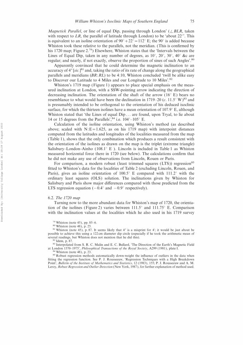
Magnetick Parallel, or line of equal Dip, passing through London’ (%BLR, takenwith respect to LR, the parallel of latitude through London) to be ‘about 22°’. Thisis equivalent to an isoline orientation of 90°+22°=112° E; the 90° is added becauseWhiston took these relative to the parallels, not the meridian. (This is confirmed byhis 1720 map; Figure 2.79) Elsewhere, Whiston states that the ‘Intervals between theLines of Equal Dip, taken in any number of degrees, as 10°, 20°, 30°, 40° &c areregular; and nearly, if not exactly, observe the proportion of sines of such Angles’.80

Apparently convinced that he could determine the magnetic inclination to anaccuracy of 4◊ [sic.]81 and, taking the ratio of its rate of change along the geographicalparallels and meridians (BR :RL) to be 4:10, Whiston concluded ‘twill be alike easyto Discover our Latitude to 4 Miles and our Longitude to 10 Miles’.82

Whiston’s 1719 map (Figure 1) appears to place special emphasis on the meas-ured inclination at London, with a SSW-pointing arrow indicating the direction ofdecreasing inclination. The orientation of the shaft of the arrow (16° E) bears noresemblance to what would have been the declination in 1719–20 (c. 11.5°W )83 andis presumably intended to be orthogonal to the orientation of his deduced isoclinicsurface, for which the thirteen isolines have a mean orientation of 107.9° E, althoughWhiston stated that ‘the Lines of equal Dip . . . are found, upon Tryal, to lie about14 or 15 degrees from the Parallels’,84 i.e. 104°–105° E.

Calculation of the isoline orientation, using Whiston’s method (as describedabove; scaled with N:E=1.625, as on his 1719 map) with interpoint distancescomputed from the latitudes and longitudes of the localities measured from the map(Table 1), shows that the only combination which produces a result consistent withthe orientation of the isolines as drawn on the map is the triplet (extreme triangle)Salisbury–London–Ainho (108.1° E ). Lincoln is included in Table 1 as Whistonmeasured horizontal force there in 1720 (see below). The calculations confirm thathe did not make any use of observations from Lincoln, Rouen or Paris.

For comparison, a modern robust ( least trimmed squares (LTS)) regression85fitted to Whiston’s data for the localities of Table 2 (excluding Lincoln, Rouen, andParis), gives an isoline orientation of 100.5° E compared with 111.2° with theordinary least squares (OLS) solution. The inclinations given by Whiston forSalisbury and Paris show major differences compared with those predicted from theLTS regression equation (−0.4° and −0.9° respectively).

6.2. The 1720 mapTurning now to the more abundant data for Whiston’s map of 1720, the orienta-

tion of the isolines (Figure 2) varies between 111.5° and 111.75° E. Comparisonwith the inclination values at the localities which he also used in his 1719 survey

79Whiston (note 45), pp. 85–6.80Whiston (note 48), p. 25.81Whiston (note 45), p. 87. It seems likely that 4◊ is a misprint for 4∞; it would be just about be

possible to achieve this using a 122 cm diameter dip circle (especially if he took the arithmetic mean ofseveral readings, but Whiston does not mention that he did this).82 Idem, p. 87.83 Interpolated from S. R. C. Malin and E. C. Bullard, ‘The Direction of the Earth’s Magnetic Field

at London 1570–1975’, Philosophical Transactions of the Royal Society, A299 (1981), plate I.84Whiston (note 48), p. 23.85 Robust regression methods automatically down-weight the influence of outliers in the data when

fitting the regression function. See P. J. Rousseeuw, ‘Regression Techniques with a High BreakdownPoint’, Bulletin of the Institute of Mathematics and Statistics, 12 (1983), 155; P. J. Rousseeuw and A. M.Leroy, Robust Regression and Outlier Detection (New York, 1987), for further explanation of method used.



Table 2. Isoline orientations (° E) computed from Whiston’s 1719 data.

Base pair

London Salisbury Salisbury Salisbury Ainho AinhoThird point Ainho London Rouen Paris Rouen Paris

Ainho – 108.1a 120.5 93.8 – –Barkeston 102.3 115.6 118.6 88.6 107.2 77.6(Lincoln) 102.6 116.1 118.5 87.9 108.2 77.6London – – 118.0 99.8 98.5 114.5Lyndon 100.4 116.4 118.4 88.8 102.7 75.5Maidford 99.3 110.7 119.9 91.6 100.7 63.6Yelvertoft 100.4 112.3 119.5 90.3 103.2 67.6

Mean (excluding Lincoln) 100.6 112.6 119.2 91.2 102.5 79.8Mean (including Lincoln) 101.0 113.2 119.1 91.5 103.4 79.4

Note:aNearest match to actual orientation on Whiston’s map.

shows a non-constant systematic bias (Figure 3). This relationship appears to besufficiently linear that, had Whiston been aware of it, and had he so wished, hecould easily have obtained an inclination value equivalent to the 1719 observationat Salisbury by fitting a line through his data points by eye86 (graphical methodswere just beginning to be applied to observational data around this time).87

The geographical coordinates of the localities on Whiston’s 1720 map can beread off to an estimated maximum error of 1.5∞ along a parallel (D1) and 1∞ along ameridian (D2). Given a candidate triplet of locations, let it be assumed that thefrequency distribution of the measurement errors is reasonably modelled by a bivari-ate normal distribution. The corresponding mean isoline orientation, based onWhiston’s measured inclination values together with an estimate of its uncertainty,can then be obtained as follows. In each of 1000 trials, the triplet of locationcoordinates are all independently ‘jittered’, by adding an appropriate small randomvalue to each of the latitude and longitude coordinates given by Whiston.88 Themean orientation of the isolines, together with its empirical 95% confidence interval(CI ),89 is then calculated from the 1000 simulated orientation values. The results

86 The estimated values are 74.1° by OLS and 73.8° by LTS regression.87M. C. Shields, ‘The Early History of Graphs in Physical Literature’, American Physics Teacher, 5

(1937), 68–71; L. Tilling, ‘Early Experimental Graphs’, British Journal for the History of Science, 8 (1975),193–213. For a more general survey, see H. G. Funkhouser, ‘Historical Development of the GraphicalRepresentation of Statistical Data’, Osiris, 3 (1938), 269–404. In ‘J. H. Lambert’s Work on Probability’,Archive for History of the Exact Sciences, 7 (1971), 244–56, O. B. Sheynin has drawn attention to the factthat in the section ‘Theorie der Zuverlassigkeit der Beobachtungen und Versuche’ (Theory of reliability ofobservations and experiments) of the book Beytrage zum Gebrauche der Mathematik und deren Anwendung,2 vols (Berlin 1765), , 424–88, by the German mathematician and physicist Johann Heinrich Lambert(1728–77), he appears to have been the first to introduce the concept of the ‘theory of errors’, and that healso fitted functions by dividing the data points into approximately equal-sized groups and drawing lines,or in some cases smooth curves, through the centres of gravity of these groups.88 The simulated measurement errors used in this study are drawn from two normal distributions,

each with a zero mean and standard deviations s1 and s2. Assuming ±D is equivalent to an empirical99% confidence interval (see note 89 for definition), then s=D/2.576, hence s1=0.58∞ and s2=0.39∞. Therandom number generator used was the rnorm function in the S-PLUS statistical software, distributedby MathSoft Inc., Seattle, Washington.89 A symmetrical interval bracketing the estimated value of the mean within which, in the long run,

based on many samples, one will be correct a stated percentage of the time (95% in this case) in claimingthat the true (but unknown) value of the mean falls within the stated interval.



Figure 3. Plot showing Whiston’s observations of inclination in 1720 ($) have a non-constant bias compared with results of his 1719 survey. Full line: OLS fit: I1720=28.22+1.40I1719 . #, estimated 1720 equivalent of Whiston’s 1719 Salisbury value(itself ‘adjusted’ by Whiston from Col. Windham’s original observation). Broken 1:1line also shown for reference.

(Figure 4) show that the closest match to the actual isoline orientation given byWhiston’s 1720 map is obtained using the triplet Wanstead–Ainho–Saltfleet whichhas a mean of 111.6° E (95% CI, 110.5°–112.8°); whereas the triplet which Whistoncited in his example (above), London–Chester–Saltfleet, gives a mean of 107.7° E(95% CI, 107.2°–108.1°). This seems to be quite far removed from the 111.5° Eshown in Whiston’s map. London–Ainho–Saltfleet is another possible candidate(111.2° E; 95% CI, 110.1°–112.4°), but this seems a less plausible solution than doesWanstead–Ainho–Saltfleet, as Wanstead lies further East than London (Figure 2)and so forms a slightly more extreme triangle.

6.3. Suggested methodBoth Plackett and Sheynin have shown90 that, by the beginning of the seventeenth

century, the arithmetic mean had begun to be used in astronomical work, appliedto observations made under the same conditions by the same observer, to reducethe effect of errors on the estimation of an experimentally determined value, and ithas been debated91 that Cotes, whom (as has been seen) Whiston knew, advocatedthe use of the centre of gravity (i.e. a weighted mean) as an estimator. Exhaustiveexamination of the statistics of all possible triplet combinations confirms that

90 R. L. Plackett, ‘The Principle of the Arithmetic Mean’, Biometrika, 45 (1958), 130–35; O. [B.]Sheynin, ‘The Treatment of Observations in Early Astronomy’, Archive for History of Exact Sciences, 46(1993), 153–92.91 See Sheynin (note 11), p. 41; A. Hald, A History of Mathematical Statistics from 1750 to 1930

(New York, 1998), p. 94; Stigler (note 11), p. 16, for opposing views.



Figure 4. Comparative plot showing computed mean isoline orientations ("), based oninclinations at alternative location triangles, with their empirical 95% CI’s. Each isbased on 1000 trials, using appropriate bivariate normal error distributions for thelocation positions on Whiston’s 1720 map. Full vertical line shows the actual isolineorientation (111.5° E) on his map. Although an example calculation in his text (note45, pages 85–87) used London–Chester–Saltfleet, the optimum fit is with Wanstead–Ainho–Saltfleet.

Whiston could not have arrived at his published isoline orientations for either surveyon the basis of either an overall unweighted arithmetic mean92 or a simultaneousequation (Mayer’s method) approach.

I suggest that the spatial disposition of Whiston’s localities affords a clue as towhy he seems to have been content to base his results on an orientation obtainedfrom a single triplet of points. It is evident from his 1719 map (Figure 1) that thenon-included data localities lie close to a direction orthogonal to the orientation ofhis isoclinic surface; the same is true of the towns between Ainho and Saltfleet inhis 1720 results (Figure 2) and, in addition, the Chester–Leicester tract is subparallelto the isolines. If, in 1719, Whiston had first computed the isoline orientation fromthe Salisbury–London–Ainho triplet, then made the observations at the other localit-ies between Oxford and Lincoln as a check, he would have found that none of hisobserved inclinations at these localities was more than 15∞ outside its predicted value.In view of the accuracy of his instrumental observations, this would most likelyhave seemed an acceptable result. In the case of the 1720 data, as has been discussedabove, there are four possible models he could have used: (1) Salisbury–Ainho–London, with a value for Salisbury estimated from the relationship between his 1719and 1720 data (Figure 3); (2) Wanstead–Ainho–Saltfleet; (3) London–Ainho–Saltfleet; and (4) London–Chester–Saltfleet. The frequency distribution of the resid-uals of the inclination values from these surfaces at the non-included localities issummarized in Figure 5. This shows that, although the Wanstead–Ainho–Saltfleet

92 There is no evidence in any of his publications to indicate that he might have used a weighted mean.



Figure 5. Box plots of absolute values (minutes) of the residuals of inclination (i.e. ignoringtheir sign) from surfaces fitted to Whiston’s 1720 inclination data, using a triangle oflocalities, for the (n) non-included towns. Model 1: Salisbury (estimated value)–Ainho–London (n=21). Model 2: Wanstead–Ainho–Saltfleet (n=20). Model 3: London–Ainho–Saltfleet (n=20). Model 4: London–Chester–Saltfleet (n=20). The differencesbetween the isoline orientation of the fitted surface and that of Whiston’s map aregiven above the plot. Each box plot summarizes a frequency distribution of theabsolute values: 25% fall between zero and the baseline of the box; the centre-line ofthe box corresponds to the 50th percentile; the top of the box to the 75th percentile;the upper ‘whisker’ extends out to the 95th percentile (20/21 or 19/20 points); the fulldot shows an outlier (Litchborough in each case). Although models 2 and 3 givecomparable best fits, the orientation of the model 2 isolines agrees with that shownon Whiston’s map.

and London–Ainho–Saltfleet solutions give both the smallest maximum residuals,as well as smallest overall residuals, the orientation of the Wanstead–Ainho–Saltfleetsurface matches that of Whiston’s map. I believe that the London–Chester–Saltfleetsolution, given as the example in Whiston’s text, might have subsequently beenreplaced by the Wanstead–Ainho–Saltfleet solution which was found to provide abetter fit to the non-included points, and that this is what the isolines on his 1720map are based on.

Nevertheless, comparison of Whiston’s results with the inclination componentof the 1720 geomagnetic field computed using the modern Bloxham–Jackson geo-magnetic model93 shows the hindcast isoline orientation obtained from their model

93 A technique used to construct spatially smooth maps of the main magnetic field at particular pointsin time, using spherical harmonics and cubic B-splines as the basis functions for the time-dependentmapping. It is computed from all available post-1690 data; see J. Bloxham and A. Jackson, ‘Time-Dependent Mapping of the Magnetic Field at the Core-Mantle Boundary’, Journal of GeophysicalResearch, B97 (1992), 19537–63, for further details.



Figure 6. Localities shown in Whiston’s 1719 and 1720 maps in relation to the inclinationfield for the epoch 1720, calculated using the Bloxham–Jackson geomagnetic model(note 93). Data courtesy of D.R. Barraclough, British Geological Survey GlobalSeismology and Geomagnetism Group, Edinburgh, April 1999.

Table 3. Inclination observations of approximately the same epoch as Whiston’s work inEngland.

Latitude ( ° ) Longitude ( ° )Observer Locality Year (N) (−W, +E) Inclination ( ° )

Unknown Paris, France 1726 48.83 2.33 73.67Celsius Tornio, Finland 1737 65.87 24.17 78.08Celsius Uppsala, Sweden 1743 59.87 17.63 75.18De Romas Bordeaux, France 1748 44.83 −0.57 68.17

Note:Uppsala value is mean of two observations; longitude is relative to Greenwich meridian.Source: British Geological Survey Global Seismology and Geomagnetism Group database,Edinburgh; courtesy of D.R. Barraclough (April 1999).

(Figure 6) to be very different. Although the field has slight curvature, a robust LTSlinear regression model fitted to the data (scaled as for Whiston’s map) yields anisoline orientation of 74.6° E. A fit to the few ‘regional’ data points available forapproximately the same epoch as Whiston’s study (Table 3) yields an orientation of51.7° E, and a similar fit to twenty-two values reported for Britain and Ireland byBond94 in 1676 gives a value of 83.0° E. These marked contrasts with the approxi-mately WNW–ESE orientation of the isolines in Whiston’s maps suggest that there

94 Bond (note 75), pp. 49–65.



is some as-yet unexplained discrepancy between the apparently consistent resultswhich he obtained in southern England in 1719–20 and the broader picture.

7. Magnetic intensityBy the late eighteenth century it began to be realized that, if the inverse-square

law held, the square of the number of oscillations made by a magnetic needlemounted in a horizontal or vertical plane in a given time must be proportional tothe magnetic intensity in the same direction. When George Graham (1675–1751)was undertaking his systematic investigation of the diurnal changes in declinationin London in the spring of 1723, he made an additional series of observations usinga dip needle 31 cm long, oriented so that it would ‘vibrate exactly in the plane ofthe magnetic meridian’. Following a series of initial experiments, he recorded dailythe time taken for the needle to perform 100 oscillations and found this to varybetween 4 min 58 s and 6 min 12 s, ‘the medium [mean] of all being nearly 5 m 35 s’.95

However, as pointed out by Bauer,96 it would appear that Graham’s study wasin part anticipated by Whiston, although Whiston’s work was not so well known(possibly because of its private publication, rather than in the PhilosophicalTransactions of the Royal Society): in his second survey of magnetic inclination insouth-east England in 1720, Whiston measured the time taken for his 121 cm dipneedle to make one ‘vibration’ at some of the various sites he occupied.97

Having participated in the rather unsatisfactory Royal Society investigations ofmagnetic intensity with Hauksbee and Brook Taylor (1685–1731; FRS, 1712) whichcommenced c. 1710,98 sometime between 1718 and mid-1720 Whiston and ‘theReverend Mr. Benjamin Worster, a skilful Mathematician and Philosopher’ con-ceived the idea of comparing the number of ‘Vibrations or Oscillations’ of a magneticdip needle with the ‘Oscillations of a Prismatick Pendulum of the same Radius,moving by the force of Gravity’.99 Using a 4.5 in (11.4 cm) needle and a terrella of1A in (2.8 cm) diameter, with the centres of the needle and terrella separated bydistances (d) of 1, 2, 3, 4, and 5 in (2.5, 5.1, 7.6, 10.2, and 12.7 cm) in each experiment,they determined the mean time for the needle to make 50 oscillations, based onthree replicate observations. The same series of experiments was later repeated usinga 1B in (3.2 cm) terrella belonging to Lord Paisley.100 Curiously, despite the fact thatWhiston suggested that a measure of the magnetic force could be taken ‘as theSquares of the Times of an equal Number of those [vertical ] Vibrations or [hori-zontal ] Oscillations reciprocally’, they concluded that after ‘that Part of the Forcewhich arises from the Magnetick Power of the Earth, be subtracted from the entirecompounded Force, to give the single Power of the Loadstone’101 the evidence wasconsistent102 with a decrease in magnetic force as d−2.5 and he repeated this statementelsewhere.103 In these experiments, the distances were measured with respect to the

95 G. Graham, ‘Observations of the Dipping Needle, Made in London, in 1723’, PhilosophicalTransactions of the Royal Society, 33 (1725), 332–39; or idem (abridged) 7 (1809, for 1724–34), 94–96.96 Bauer (note 2).97Whiston (note 45), p. 35 and column headed ‘Vib.’ in inset table, Plate II.98Whiston (note 25), pp. 235–36.99Whiston (note 45), p. 19.100 James Hamilton, 6th Duke of Abercorn (1656–1734); Whiston (note 45), p. 21.101Whiston (note 45), p. 21.102 Idem, p. 22.103 Idem, p. 13.



surface rather than the centre of the terrellas ‘because all experience assures us, theMagnetick Power is chiefly at the Surfaces of loadstones. . . and seems to have noparticular relation to any Centres at all’.104 Quite apart from the fact that themagnetic poles were not sufficiently isolated, referring the distance measurements tothe surface of the terrella would undoubtedly have made the finding of the truerelationship (d−2) more difficult.105

Nevertheless, Whiston also seems to have been the first to have recognized (in1719) the relationship between the angle of inclination and the horizontal andvertical intensities:

We learn a new and sure way of finding the true Angle of Inclination of theDipping Needle, even without immediately observing it; . . .thus: As the Squareof the Time of any Number of Vibrations in the Horizontal Plane, to theSquare of the Time of the same Number of Similar Oscillations in the verticalPlane, along the Magnetick Meridian: So is the Sinus Totus,106 to the Cosineof the Angle of Inclination.107

He gives an example, based on the mean time taken to perform a single ‘vibration’(6 s) and ‘oscillation’ (11.3 s) using a 30 cm needle, computed from timing 100 ofeach: ‘11◊H q : 6◊ q : :128 : 36: :100=Rad : 28=sin 16° B’,108 where q is a contemporaryabbreviation for ‘squared’; that is the magnetic inclination is found to be 16.25° . Inmodern tables sin(16.25°)#0.28 (0.2798), but in Whiston’s time all such entrieswere multiplied by a constant to eliminate decimal points.

A small table accompanying Whiston’s 1720 map contained, in addition to theobservations of inclination, a column headed ‘Vib.’. Although he did not show theseadditional results on his map, Whiston explained them as follows:

I have all along set down the Seconds wherein my Needle perform’d a singlehorizontal Vibration at about 120 Degrees from the Magnetick Meridian, inmost Places: Whose Squares, when Allowance has been made for the differentObliquity of the several Directions as to our Horizon, will give us the differentStrength of that Magnetic Power at those several Places: As does the Angle ofDip give us the Direction of the same Power there. Now at the first Sight, theformer there appears to be irregular, and the latter regular: as is the Case alsoof our Terrella.109

Hence, Whiston seems to have been the first person known to have carried out aninvestigation into the geographical variation of magnetic intensity, using the timeof vibration of a horizontal needle. In the quotation above, he speaks of measuringthe vibration times in a plane ‘at about 120° from the Magnetick Meridian’.110 Themagnetic declination in London in 1720 would have been about 11.5°W,111 and theorientation of the isolines in Whiston’s map is c. 111.5° E, so he appears to have

104 Idem, p. 14.105 Following the development, between 1745 and 1756, of methods for creating long, thin, magnets,

to enable the study of an isolated magnet pole, the inverse squared distance law was eventually establishedby the French military engineer Charles Augustin de Coulomb (1736–1806) in 1785 (published in 1788).106 An old term for sin(90°), i.e. unity.107Whiston (note 48), p. 17, and (note 45), p. 35, emphasis as in original.108Whiston (note 48), p. 18, and (note 45), p. 35.109Whiston (note 45), p. 112, emphasis as in original.110 Idem.111Malin and Bullard (note 83), Plate I.



measured the magnetic intensity with the horizontal needle aligned parallel to theorientation of the inclination isolines which he established from his survey of 1719.

8. ConclusionsWhiston’s pioneering isoclinic maps of 1719 and 1720 were based on careful

measurement. It is suggested that (despite the fact that he had used the arithmeticmean in other magnetic computations) the orientation of his linear surface wasbased on fitting to a single triplet of observations and checking the fit by comparingthe predicted values with those at the non-included localities. The best-fitting tripletsto the isoline orientations of the 1719 and 1720 maps are the locations Salisbury–London–Ainho and Wanstead–Ainho–Saltfleet respectively. However, the orienta-tion of his isolines (108° and 112° E ) appears to be completely at variance with theorientation of linear surfaces fitted both to broadly contemporary data (83° and 52°E ) and the 1992 Bloxham–Jackson geomagnetic model (75° E ). Despite this fact,Whiston anticipated Graham in measurement of the ratio of horizontal and verticalmagnetic intensities, and he understood their relationship to magnetic inclination.

9. EpilogueWhiston recalls that, following publication of his findings in 1721, he received

so much Encouragement from many Benefactors, that I was enabled to procuresome New Observations of the Angle of Dip in several Parts of the World, inorder to perfect this Discovery; . . . Which upon the whole cost me a very greatdeal of Pains, to contrive the Instruments and hang them in Ships so as totake the Dip, with an Exactness sufficient for my Purpose; but found the Powerof Magnetism so very weak, and the Concussion of a Ship so very troublesome,that I had little hopes of succeeding. And when I knew of Mr. George Graham’snew Discovery [1724] of an Horary uncertain Inequality, as I may call it, bothin the Variation and Dip of Magnetick Needles . . . I perceived that all myLabour was in vain, and I was obliged to drop that Design intirely.112

So, with this disappointing result, all of Whiston’s proposals for solution of the‘longitude problem’ came to nothing. It would seem that his scientific work wassubsequently eclipsed by the theological controversy which he engendered for themajor part of his career. One of his biographers rather unkindly said of him:

Whiston is a striking example of a not unfrequent phenomenon, the associationof an entirely paradoxical frame of mind with proficiency in the exact sciences.. . . He was not only paradoxical to the verge of craziness, but intolerant tothe verge of bigotry. . . . This moral and intellectual unreason destroyed theweight otherwise due to his erudition and acuteness, and left nothing recom-mendable for imitation in his conduct as a whole, except his passion for truthand his heroic disinterestedness,—virtues in which few have rivalled him,though some may have exhibited them less ostentatiously.113

Thus, it would appear that Whiston became best known for his translation fromthe Greek of the works of Flavius Josephus ( fl. 38–100), an early writer on

112Whiston (note 25), pp. 296–97, emphasis as in original.113 Anonymous (note 26, 1888).


William Whiston’s Isoclinic Maps of Southern England84

Jewish history,114 which was apparently still being reprinted in the nineteenth cen-tury,115 and that his pioneering magnetic surveys were forgotten until theirre-discovery by Bauer116 (who alerted Felgentrager and Hellmann to their existence)at the close of the nineteenth century.

AcknowledgementsDavid Barraclough is thanked for his assistance in providing data on contempor-

ary observations of inclination from the British Geological Survey Global Seismologyand Geomagnetism Group’s database and for the 1720 epoch inclination valuescalculated using the Bloxham–Jackson (1992) model which form the basis ofFigure 6. I am most grateful to David Barraclough, Stuart Malin, and Oscar Sheyninfor their comments on various versions of this manuscript, all of which undoubtedlybrought about significant improvements in its clarity.

114 History of the Jewish War, c. 73, and Antiquities of the Jews, c. 93. The first printed versionof these early manuscripts appeared in Basle in 1544; Whiston’s translation was published in 1736–37and was one of a number of critical editions of Josephus’ works to be published in the early eighteenthcentury.115 Lorimer (note 26).116 Note 2.


Fitting Geomagnetic Fields before the Invention of Least Squares: I. Henry Bond's Predictions (1636,...

Documents

Transcript of Fitting Geomagnetic Fields before the Invention of Least Squares: I. Henry Bond's Predictions (1636,...