1

Fisher Information for Inverse Problems andTrace Class Operators

Sven Nordebo∗, Mats Gustafsson†, Andrei Khrennikov∗, Borje Nilsson∗, Joachim Toft∗

Abstract—This paper provides a mathematical framework forFisher information analysis for inverse problems based on Gaus-sian noise on infinite-dimensional Hilbert space. The covarianceoperator for the Gaussian noise is assumed to be trace class, andthe Jacobian of the forward operator Hilbert-Schmidt. We showthat the appropriate space for defining the Fisher informationis given by the Cameron-Martin space. This is mainly becausethe range space of the covariance operator always is strictlysmaller than the Hilbert space. For the Fisher information tobe well-defined, it is furthermore required that the range spaceof the Jacobian is contained in the Cameron-Martin space. Inorder for this condition to hold and for the Fisher information tobe trace class, a sufficient condition is formulated based on thesingular values of the Jacobian as well as of the eigenvalues of thecovariance operator, together with some regularity assumptionsregarding their relative rate of convergence. An explicit exampleis given regarding an electromagnetic inverse source problemwith “external” spherically isotropic noise, as well as “internal”additive uncorrelated noise.

Index Terms—Inverse problems, Fisher information, Cramer-Rao lower bound, trace class operators.

I. INTRODUCTION

An important issue within inverse problems and imaging[15] is to develop an appropriate treatment of the uncertaintyassociated with the related quantity of interest (the state),and the observation process, respectively. Statistical methodsprovide many useful concepts and tools in this regard such asidentifiability, sufficient statistics, Fisher information, statisti-cally based decision rules and Bayesian estimation, see e.g., [5,12, 33]. The Bayesian view is e.g., based on the assumptionthat uncertainty always can be represented as a probabilitydistribution. Hence, statistical information about the state canbe retrieved by means of Bayesian filtering such as Kalmanfilters, extended Kalman filters and particle filters, see e.g. [12,33].

On the other hand, the conditional Fisher information canbe a useful “deterministic” analysis tool in various inverseproblem applications such as with material measurements[32], parametric shape estimation [35], sensitivity analysisand preconditioning in microwave tomography [23, 24], andin electrical impedance tomography [22]. The Cramer-Raolower bound can furthermore be used to quantify the trade-off between the accuracy and the resolution of a linear or

∗Sven Nordebo, Andrei Khrennikov, Borje Nilsson and JoachimToft are with the School of Computer Science, Physics andMathematics, Linnæus University, 351 95 Vaxjo, Sweden. E-mail:sven.nordebo,andrei.khrennikov,borje.nilsson,joachim.toft@lnu.se.†Mats Gustafsson is with the Department of Electrical and Information

Technology, Lund University, Box 118, SE-221 00 Lund, Sweden. E-mail:mats.gustafsson@eit.lth.se.

non-linear inverse problem [7, 22–24, 26], and it complementsthe deterministic upper bounds and the L-curve techniquesthat are employed with linearized inversion, see e.g., [9, 15].The Fisher information is also a tool that can be exploited foroptimal experimental design, see e.g., [29].

The Fisher information analysis has mostly been given ina finite-dimensional setting, see e.g., [13, 31]. One of thevery few exceptions can be found in e.g., [34] where theFisher information integral operator for an infinite-dimensionalparameter function has been employed in the estimation ofwave forms (or random processes). An infinite-dimensionalFisher information operator has previously been exploited inthe context of inverse problems in e.g., [22, 23, 25], and theconnection to the Singular Value Decomposition (SVD) hasbeen established. However, so far, a rigorous treatment ofGaussian noise on infinite-dimensional Hilbert spaces has beenlacking.

A Fisher information analysis for inverse problems basedon Gaussian noise on infinite-dimensional Hilbert space [2,6, 8, 14, 20] requires a careful study of the range spaces andthe spectrum of the operators related to the covariance of thenoise, and the Jacobian of the forward operator, respectively.It is assumed here that the covariance operator is trace classand the Jacobian is Hilbert-Schmidt [30]. Since the rangespace of the covariance operator always is strictly smallerthan the Hilbert space, the appropriate space for defining theFisher information operator is given by the Cameron-Martinspace [2, 8]. In order for the Fisher information to be well-defined, it is furthermore required that the range space of theJacobian is contained in the Cameron-Martin space. In orderfor this condition to hold and for the Fisher information tobe trace class, it is shown in this paper that it is sufficientthat the singular values of the Jacobian and the eigenvalues ofthe covariance operator satisfy some regularity assumptionsregarding their relative rate of convergence. It is also shownhow the Cramer-Rao lower bound for parameter estimationbased on finite-dimensional eigenspaces is closely linked tothe Singular Value Decomposition (SVD), and the truncatedpseudo-inverse based on the Cameron-Martin space.

The situation becomes particularly simple if the covarianceoperator and the Jacobian share the same left-singular vectors,implying that a sequence of finite-dimensional subspace esti-mators (truncated pseudo-inverses) may readily be analyzed.In this case, the eigenvalues of the Fisher information is simplythe ratio between the squared singular values of the Jacobian,and the eigenvalues of the covariance operator. Two importantspecial cases arises: 1) The infinite-dimensional Fisher infor-mation operator exists and is trace class, and the corresponding

arX

iv:1

203.

5397

v1 [

mat

h-ph

] 2

4 M

ar 2

012

2

pseudo-inverse (and the Cramer-Rao lower bound) exists onlyfor finite-dimensional subspaces. 2) The infinite-dimensionalpseudo-inverse (and the Cramer-Rao lower bound) exists, andthe corresponding Fisher information operator exists only forfinite-dimensional subspaces. A concrete example is consid-ered regarding an electromagnetic inverse source problem with“external” spherically isotropic noise, as well as “internal”uncorrelated noise. The example illustrates how the singularvalues of the Jacobian, the eigenvalues of the covarianceoperator and the internal noise variance can be analyzed andinterpreted in terms of the Cramer-Rao lower bound.

II. CRAMER-RAO LOWER BOUND FOR INVERSEPROBLEMS

A. The forward model

Below, two common situations will be considered in par-allel, where the parameter space (describing the quantity ofinterest) is real or complex, respectively. The observationprocess (the measurement) is assumed to be executed inthe frequency-domain with complex valued data. Hence, aninverse problem is considered below where ξ denotes thecomplex valued measurement and θ the real or complex valuedparameter function to be estimated. The forward operator isdefined as the mapping

ψ(θ) : Θ→ H, (1)

where Θ and H are separable Hilbert spaces [16]. The mea-surement space H is complex, and the parameter space Θ iseither real or complex. The same notation 〈·, ·〉 is employedhere to denote the scalar products in both spaces.

Let Re· denote the real part of ·. Note that Re〈ξ1, ξ2〉is a scalar product defined on the elements ξ1 and ξ2 ofH interpreted as a Hilbert space over the real scalar field.In this space, the vectors ξ and iξ are orthogonal, i.e.,Re〈ξ, iξ〉 = Re i〈ξ, ξ〉 = 0, and the norm is preserved, i.e.,Re〈ξ, ξ〉 = 〈ξ, ξ〉 = ‖ξ‖2. Hence, the Hilbert space H overthe complex scalar field with basis vectors ei is isomorphicwith the Hilbert space H over the real scalar field, and withbasis vectors given by ei and iei.

It is assumed that the forward operator ψ(θ) is Frechetdifferentiable [15] in a neighborhood of the (background)parameter vector θb ∈ Θ. The first order variation δψ canthen be represented as

δψ = J δθ, (2)

where the bounded linear operator J : Θ→ H is the Frechetderivative (or Jacobian) of the operator ψ(θ) evaluated at θb,and δθ ∈ Θ is an incremental parameter function where θ =θb + δθ. Let J ∗ denote the Hilbert adjoint operator to J . It isassumed that the Jacobian J is Hilbert-Schmidt [30], so thattrJ ∗J <∞ and both J and J ∗ are compact.

For a bounded linear operator, the Hilbert-adjoint operatorexists and is unique provided that the Hilbert spaces aredefined over the same (real or complex) scalar field [16].Hence, in the case when Θ is real the Hilbert-adjoint operatorJ ∗ is defined by the property

Re〈J δθ, ξ〉 = 〈δθ,J ∗ξ〉, (3)

and 〈J δθ, ξ〉 = 〈δθ,J ∗ξ〉 when Θ is complex. As e.g., ifthe Jacobian J can be represented by a (finite or infinite-dimensional) matrix J, the adjoint J ∗ξ is given by ReJHξand JHξ with respect to the real and complex spaces Θ,respectively, where ξ denotes the representation of ξ ∈ H,and (·)H the Hermitian transpose.

The Singular Value Decomposition (SVD) of the JacobianJ can be expressed as follows. Assume first that Θ is complex.Let the singular system for the linear compact operator J begiven by

J vi = σiui,

J ∗ui = σivi,(4)

where ui and vi are orthonormal systems and σi are thesingular values arranged in decreasing order, and where σi →0 as i → ∞ if the number of non-zero singular values isinfinite [15]. The operator J can then be represented as

J δθ =∑i∈I

σiui〈vi, δθ〉, (5)

the adjoint operator J ∗ as

J ∗ξ =∑i∈I

σivi〈ui, ξ〉, (6)

and the pseudo-inverse J + as

J +ξ =∑i∈I

1

σivi〈ui, ξ〉, (7)

where I is the index set (finite or infinite) corresponding tothe non-zero singular values. Here, 〈ui, ξ〉 is replaced forRe〈ui, ξ〉 when Θ is real. Note that the expression (7) isvalid provided that the pseudo-inverse exists, and the series∑i |〈ui, ξ〉|2/σ2

i converges [15]. A truncation of (7) using afinite number r of non-zero singular values is referred to asa truncated pseudo-inverse. The corresponding regularizationstrategy is denoted

J +r ξ =

r∑i=1

1

σivi〈ui, ξ〉, (8)

where r is the regularization parameter. It is readily seen that

limr→∞

J +r J δθ = δθ, (9)

where δθ belongs to the orthogonal complement of the nullspace of the operator J , i.e., δθ ∈ N (J )⊥, see e.g., [15].Note that the SVD gives an orthogonal decomposition of thetwo Hilbert spaces as follows

Θ = spanvii∈I ⊕NJ ,

H = spanuii∈I ⊕NJ ∗,(10)

where span· denotes the closure of the linear span of thevectors in · and ⊕ the direct sum [15].

3

B. Fisher information for the Cameron-Martin space

Consider the statistical measurement model

ξ = ψ(θ) + w, (11)

where ξ is the measured response, ψ(θ) the forward modeland w ∈ H is zero mean complex Gaussian noise. Here, wis an observation of a complex Gaussian stochastic processdefined on the Hilbert space H [2, 6, 8, 14, 20]. Let E denotethe expectation operator with respect to the complex Gaussianmeasure µ and B the corresponding covariance operator. Itis assumed that the positive operator B is trace class so thatE‖w‖2 = trB for any w ∈ H, and hence that B is self-adjoint and compact [30]. It follows from the Hilbert-Schmidttheorem [30] that there exists a complete orthonormal basisφj for H, such that

Bφj = λjφj , (12)

where φj are the eigenvectors of B and λj the non-negativeeigenvalues, and where λj → 0 as j → ∞ if the number ofnon-zero eigenvalues is infinite. Let J denote the index set(finite or infinite) corresponding to the eigenvectors with non-zero eigenvalues λj > 0. The Hilbert space H is then givenby the following orthogonal decomposition

H = spanφjj∈J ⊕NB. (13)

The linear functionals 〈ξ, w〉 and 〈η, w〉 are complex Gaus-sian stochastic variables with zero mean, and with the covari-ance properties

E〈ξ, w〉〈η, w〉∗ = 〈ξ,Bη〉,

E〈ξ, w〉〈η, w〉 = 0,(14)

for any ξ, η ∈ H, and where (·)∗ denotes the complexconjugate [2, 6, 8, 14, 20].

The description of the stochastic process on H is nowcomplete. However, since the range of the operator B alwaysis strictly smaller than H for infinite-dimensional spaces1, itis not possible to define a non-singular Maximum Likelihood(ML) criterion [13, 31, 34], or trace class Fisher informationbased on the whole of H. Moreover, in order to be able todefine the Fisher information in trace class, the range of theJacobian J also needs to be restricted to this smaller subspace.The proper subspace for this purpose is the Cameron-MartinspaceHµ [2, 8], which can be constructed as follows. Considerthe covariance operator B restricted to the range of B, i.e.,

B : RB → RB, (15)

then the (self-adjoint) inverse B−1 exists on this subspacesince B > 0, and hence B−1 > 0 on RB.

Define the scalar product

〈ξ, η〉µ = Re〈ξ,B−1η〉, (16)

1To see this, assume that RB = H. Now, B is trace class and thusbounded, and B−1 exists since B > 0. It then follows by the bounded inversetheorem [16], that B−1 is bounded. Since the composition of a trace classoperator with a bounded operator is trace class [30], the equality BB−1 = Igives a contradiction since the identity operator is not trace class for infinite-dimensional spaces.

if Θ is real, and 〈ξ, η〉µ = 〈ξ,B−1η〉 if Θ is complex, andwhere ξ, η ∈ RB. The Cameron-Martin space Hµ is thecompletion of RB with respect to the norm induced by thescalar product 〈ξ, η〉µ, see [2, 8]. It can be shown [2, 8] thatHµ is also given by

Hµ = ξ ∈ H|∑j∈J

1

λj|〈φj , ξ〉|2 <∞,

Hµ = RB1/2,(17)

where RB ⊂ Hµ ⊂ H.It is assumed that the range of the Jacobian J is restricted

as RJ ⊂ RB, implying that RJ ⊂ Hµ 2. Hence, itis sufficient to consider the mapping

J : Θ→ Hµ. (18)

Since Hµ is a Hilbert space on its own right and J a boundedlinear operator, the Hilbert adjoint operator J ∗µ exists and isdefined by the property

〈J δθ, ξ〉µ = 〈δθ,J ∗µ ξ〉, (19)

where δθ ∈ Θ and ξ ∈ Hµ. It is readily seen that J ∗µ =J ∗B−1 on RB, where J ∗ was defined as in (3).

The Fisher information operator I : Θ → Θ can now bedefined as

I = 2J ∗µJ = 2J ∗B−1J , (20)

when Θ is real, and I = J ∗µJ when Θ is complex, see also[13, 22, 23, 34]. It is assumed that the operator J is Hilbert-Schmidt with respect to the Cameron-Martin space Hµ, andhence that J is compact with respect to the norm inducedby the scalar product 〈ξ, η〉µ. The Fisher information operatoris thus assumed to be trace class. Let µi and vi denote theeigenvalues and the eigenvectors of the Fisher informationoperator I, respectively, i.e.,

I vi = µivi, (21)

where the eigenvectors vi are assumed to be orthonormal, i.e.,〈vi, vj〉 = δij .

The Singular Value Decomposition (SVD) of the JacobianJ with respect to the Cameron-Martin space Hµ, can nowbe expressed as follows. The singular system for the linearcompact operator J is given by

J vi = σiui,

J ∗µ ui = σivi,(22)

where ui and vi are orthonormal systems and σi arethe singular values arranged in decreasing order, and whereσi → 0 as i → ∞ if the number of non-zero singularvalues is infinite [15]. Note that the eigenvalues of the Fisherinformation operator are given by µi = 2σ2

i when Θ is real,and µi = σ2

i when Θ is complex.

2The main results of this paper can be generalized to larger class ofJacobians J having the image in Hµ (and not just in its proper subspaceRB. However, this will make the paper more complicated mathematically,since one cannot proceed with continuous linear functionals given by the scalarproduct, and measurable linear functionals (square integrable with respect tothe Gaussian measure µ) have to be used.

4

The operator J can be represented as

J δθ =∑i∈I

σiui〈vi, δθ〉, (23)

the adjoint operator J ∗µ as

J ∗µ ξ =∑i∈I

σivi〈ui, ξ〉µ, (24)

and the pseudo-inverse J +µ as

J +µ ξ =

∑i∈I

1

σivi〈ui, ξ〉µ, (25)

where I is the index set (finite or infinite) corresponding to thenon-zero singular values. The expression (25) is valid providedthat the pseudo-inverse exists and the series

∑i |〈ui, ξ〉µ|2/σ2

i

converges [15]. A truncation of (25) using a finite number r ofnon-zero singular values is referred to as a truncated pseudo-inverse. The corresponding regularization strategy is denoted

J +µrξ =

r∑i=1

1

σivi〈ui, ξ〉µ, (26)

where r is the regularization parameter. It is readily seen that

limr→∞

J +µrJ δθ = δθ, (27)

where δθ ∈ N (J )⊥, see e.g., [15]. Note also that the SVDgives an orthogonal decomposition of the two Hilbert spacesas follows

Θ = spanvii∈I ⊕NJ ,

Hµ = spanuii∈I ⊕NJ ∗µ .(28)

C. The Cramer-Rao lower bound based on trace class oper-ators

Consider the statistical measurement model given by (11).Consider also the SVD of the Jacobian J with respect to theCameron-Martin spaceHµ given in (22), where J is evaluatedat the fixed background parameter vector θb, and let θ = θb +δθ. Any incremental parameter vector δθ ∈ Θ can be uniquelydecomposed as

δθ = δθ + θ0 =∑i∈I

ϑivi + θ0, (29)

where δθ ∈ N (J )⊥ and θ0 ∈ N (J ). The principal parame-ters of interest are given by

ϑi = 〈vi, δθ〉 = 〈vi, δθ〉, (30)

where i ∈ I .Assume first that Θ is real. Consider the discrete (countable)

measurement model that is obtained by applying the scalarproducts Re〈B−1ui, ·〉 to the statistical measurement model(11). Note that ui ∈ RJ ⊂ RB so that B−1ui isuniquely defined. The discrete measurement model is hencegiven by

Re〈B−1ui, ξ〉 = Re〈B−1ui, ψ(θ)〉+ Re〈B−1ui, w〉, (31)

where i ∈ I . The covariance of the noise term is given by

ERe〈B−1ui, w〉Re〈B−1uj , w〉

=1

2Re〈ui, B−1uj〉 =

1

2〈ui, uj〉µ =

1

2δij ,

(32)

where i, j ∈ I and where (14) and (16) have been used. WhenΘ is complex, the corresponding discrete measurement modelis given by

〈B−1ui, ξ〉 = 〈B−1ui, ψ(θ)〉+ 〈B−1ui, w〉, (33)

where i ∈ I . The covariance of the noise term is given by

E〈B−1ui, w〉〈B−1uj , w〉∗

= 〈ui, B−1uj〉 = 〈ui, uj〉µ = δij ,(34)

where i, j ∈ I .Assume once again that Θ is real. By using δθ = vjdϑj and

letting dϑj → 0, it is readily seen that

∂

∂ϑjRe〈B−1ui, ψ(θ)〉

= Re〈B−1ui,J vj〉 = Re〈B−1ui, σj uj〉 = σjδij ,(35)

where i, j ∈ I . When Θ is complex, the correspondingexpression is obtained by deleting the Re· operation above.

Consider now the projection (approximation) of δθ ontothe finite dimensional subspace spanned by the orthonormalsystem viri=1, i.e.,

δθr =

r∑i=1

ϑivi, (36)

where r is the dimension of the approximating subspace. Itfollows from (35) and the orthogonality of the noise terms(32) and (34), that a sufficient statistics [13, 31] for estimatingδθr is given by the discrete measurement model (31), or (33),restricted to the index set Ir = 1, . . . , r. The correspondingunbiased estimator is represented as

δθr =

r∑i=1

ϑivi, (37)

where ϑi are unbiased estimates of the principal parametersdefined in (30).

Assume that Θ is real. The Cramer-Rao lower bound [13,31, 34] for estimating the principal parameters follows thenfrom the measurement model (31), (32) and (35), and is givenby

E|ϑi − ϑi|2 ≥1

2σ2i

=1

µi, i = 1, . . . , r, (38)

where µi = 2σ2i are the eigenvalues of the Fisher information

operator defined in (20). A similar expression is obtained whenΘ is complex, and µi = σ2

i . It follows directly from (38) thatthe mean squared estimation error is lower bounded as

E‖δθr − δθr‖2 =

r∑i=1

E|ϑi − ϑi|2 ≥r∑i=1

1

µi, (39)

5

which is valid for both the real and the complex space Θ. Notethat the truncated Fisher information operator is given by

Ir =

r∑i=1

µivi〈vi, δθ〉, (40)

and the corresponding truncated pseudo-inverse

I+r =

r∑i=1

1

µivi〈vi, δθ〉, (41)

and the Cramer-Rao lower bound [13, 31, 34] can also be statedas

E〈θ1, δθr − δθr〉〈δθr − δθr, θ2〉 ≥ 〈θ1, I+r θ2〉, (42)

where θ1, θ2 ∈ Θ. It is immediately observed that the operatorsIr and I+

r cannot both be trace class in the limit as r →∞.If the infinite-dimensional Fisher information is trace class,then the corresponding pseudo-inverse does not exist, and viceverse.

An interesting interpretation of the Cramer-Rao lower boundis obtained as follows. It is noted that the lower bound definedin (39) is a function of the spatial resolution, i.e., the subspacedimension r. As the desired spatial resolution r increases, theestimation accuracy decreases in the sense that the Cramer-Rao lower bound increases. The Cramer-Rao lower boundgives the best possible (optimal) performance of any unbiasedestimator related to the non-linear inverse problem at hand.Hence, the lower bound defined in (39) gives a quantitativeinterpretation of the optimal trade-off between the accuracyand the resolution of an inverse problem.

The truncated pseudo-inverse (26) gives an example of anefficient unbiased estimator of δθr as follows. Consider a linearversion of (11)

ξ = ψ(θb) + J δθ + w, (43)

where the forward operator ψ(θ) has been replaced by its firstorder approximation, the space Θ is real and the noise is as-sumed to have zero mean, i.e., Ew = 0. The correspondingtruncated pseudo-inverse is given by

δθr =

r∑i=1

1

σivi Re〈B−1ui, ξ − ψ(θb)〉, (44)

and the corresponding parameter estimates are hence given by

ϑi =1

σiRe〈B−1ui,J δθ〉+

1

σiRe〈B−1ui, w〉. (45)

The mean value of (45) is given by

Eϑi =1

σiRe〈B−1ui,J δθ〉 =

1

σi〈ui,J δθ〉µ

=1

σi〈J ∗µ ui, δθ〉 = 〈vi, δθ〉 = ϑi,

(46)and the variance

varϑi = var 1

σiRe〈B−1ui, w〉 =

1

2σ2i

=1

µi, (47)

where (22) and (32) have been used. A similar result isobtained when Θ is complex. Hence, with a linear estimation

model as in (43), the truncated pseudo-inverse (26) leads toan unbiased estimator which is efficient in the sense that itachieves the Cramer-Rao lower bound (39), see also [13, 31,34]. For non-linear estimation problems, it should be noted thatthe Maximum Likelihood (ML) criterion yields an estimationerror that approaches the Cramer-Rao lower bound as the datarecord is getting large, i.e., the ML-estimate is asymptoticallyefficient, see [13, 31, 34].

D. Conditions for the Jacobian

A sufficient condition is formulated for the Jacobian J to berestricted as RJ ⊂ RB. This condition also guaranteesthat J is Hilbert-Schmidt with respect to the Cameron-Martinspace Hµ. Note that the result is valid for both real andcomplex spaces Θ.

Proposition II.1. Let the Jacobian J : Θ → H be Hilbert-Schmidt with respect to H, with the singular system (4). Letthe positive, self-adjoint covariance operator B : H → Hbe trace class, with the singular system (12). Suppose thatRJ ⊂ spanφjj∈J .

If ∑i∈I

σ2i

∑j∈J

1

λ2j

|〈φj , ui〉|2 <∞, (48)

then RJ ⊂ RB, and J is Hilbert-Schmidt with respectto the Cameron-Martin space Hµ, and

trJ ∗µJ =∑i∈I

σ2i

∑j∈J

1

λj|〈φj , ui〉|2. (49)

Proof: For the operator equation Bξ = J θ to be solvable,it is necessary and sufficient that J θ ∈ NB⊥, and that∑

j∈J

1

λ2j

|〈φj ,J θ〉|2 <∞, (50)

for any θ ∈ Θ, see e.g., [15]. Hence, it is assumed thatRJ ⊂ NB⊥ = spanφjj∈J , and it is then sufficientto consider (50). By using (5), it follows that∑

j∈J

1

λ2j

|〈φj ,J θ〉|2

=∑j∈J

1

λ2j

|〈φj ,∑i∈I

σiui〈vi, θ〉〉|2

=∑j∈J

1

λ2j

|∑i∈I

σi〈φj , ui〉〈vi, θ〉|2

≤∑j∈J

1

λ2j

(∑i∈I

σ2i |〈φj , ui〉|2

)(∑i∈I|〈vi, θ〉|2

)

=∑j∈J

1

λ2j

(∑i∈I

σ2i |〈φj , ui〉|2

)‖θ‖2 <∞,

(51)for any θ ∈ Θ, and where the Cauchy-Schwartz inequality hasbeen used. Hence, RJ ⊂ RB.

6

Now,

trJ ∗µJ = trJ ∗B−1J

=∑i∈I〈vi,J ∗B−1J vi〉 =

∑i∈I〈vi,J ∗B−1σiui〉

=∑i∈I〈Jvi, B−1σiui〉 =

∑i∈I〈σiui, B−1σiui〉

=∑i∈I

σ2i 〈ui, B−1ui〉,

(52)and since ui ∈ RJ ⊂ RB ⊂ spanφjj∈J ,

trJ ∗µJ =∑i∈I

σ2i 〈ui, B−1ui〉

=∑i∈I

σ2i 〈ui,

∑j∈J

1

λjφj〈φj , ui〉〉

=∑i∈I

σ2i

∑j∈J

1

λj〈φj , ui〉〈ui, φj〉

=∑i∈I

σ2i

∑j∈J

1

λj|〈φj , ui〉|2 <∞,

(53)

where the last term converges faster than (48) as λj → 0. 2

It is easy to find Hilbert-Schmidt operators J and traceclass operators B such that the conditions in propositionII.1 are satisfied. An example can readily be constructed asfollows. Let the Hilbert-Schmidt operator J be given, havingthe singular system (4). It is furthermore assumed that thesingular values decay sufficiently fast so that

∑i∈I√σi <∞.

Let φi = ui for all i ∈ I = J , and define the operator B by

Bξ =∑i∈I

λiφi〈φi, ξ〉, (54)

where

λi =

σ2

w i = 1, . . . , q,√σi i > q,

(55)

and where σ2w > 0 and q is a positive integer. Note that

Bφi = λiφi. Since φi = ui for all i ∈ I = J and RJ ⊂spanuii∈I , it follows directly that RJ ⊂ spanφjj∈J .

The sufficient condition (48) can now be verified as follows:∑j∈J

1

λ2j

|〈φj , ui〉|2 =∑j∈J

1

λ2j

|〈φj , φi〉|2 =1

λ2i

<∞, (56)

for all i ∈ I , and∑i∈I

σ2i

∑j∈J

1

λ2j

|〈φj , ui〉|2 =∑i∈I

σ2i

1

λ2i

=

q∑i=1

σ2i

σ4w

+

∞∑i=q+1

σi <∞,(57)

which shows that RJ ⊂ RB, and J is Hilbert-Schmidtwith respect to the Cameron-Martin space Hµ.

The singular values σi defined in (22) are given by

σ2i =

σ2i

λi=

σ2i

σ2w

i = 1, . . . , q,

σ3/2i i > q,

(58)

and the singular vectors ui =√λiui and vi = vi. These

relations are obtained by using J vi = σiui, J ∗ui =σivi, B−1ui = 1

λiui, J ∗µ = J ∗B−1 and 〈ui, uj〉µ =

〈√λiui, B

−1√λjuj〉 = 〈

√λiui, uj/

√λj〉 = δij .

It is impossible to have a white noise stochastic process wwith a trace class identity covariance operator B = I definedon infinite-dimensional spaces. However, as the example aboveshows, the stochastic process w can be white with identitycovariance operator B = I on finite-dimensional subspaces.In particular, in the example above, let the approximatingsubspace dimension r be fixed and choose q > r such thatσ2r > σ2

wσ3/2q , then the first r singular values and singular

vectors are given byσ2i =

σ2i

σ2w

i = 1, . . . , r,

ui = σwui i = 1, . . . , r,

vi = vi i = 1, . . . , r,

(59)

and except for a scaling, the singular systems (4) and (22) arethe same for i = 1, . . . , r.

E. Unbounded Fisher information and finite Cramer-Raolower bound

It is easy to find Hilbert-Schmidt operators J and trace classoperators B such that the conditions in proposition II.1 arenot satisfied. In particular, if the conditionRJ ⊂ RHµ isnot satisfied, then the Cameron-Martin space cannot be usedas indicated in (18) above. In this case, it may be difficult(or technically very complicated) to obtain a useful definitionof the Fisher information and the Cramer-Rao lower bound.However, a simple case which is also very useful, arises whenthe singular vectors ui of the Jacobian operator J coincideswith the eigenvectors φj of the covariance operator B. Hence,the following assumptions are made

J vi = σiui,

J ∗ui = σivi,

Bui = λiui,

(60)

where i ∈ I . For simplicity, it is also assumed here that thespace Θ is complex (the case with real Θ is similar).

Consider now a sequence of finite-dimensional measure-ment models based on (11)

Prξ = Prψ(θ) + Prw, (61)

where Pr denotes the projection operator Pr : H →spanu1, . . . , ur. The finite-dimensional Jacobian and covari-

7

ance operators are given byPrJ δθ =

r∑i=1

σiui〈vi, δθ〉,

PrBPrξ =

r∑i=1

λiui〈ui, ξ〉.(62)

Since the requirement RPrJ ⊂ RPrBPr is triviallysatisfied, all the results of the previous sections apply in thisfinite-dimensional case. In particular, the Fisher informationoperator (20) becomes

Irδθ =

r∑i=1

σ2i

λivi〈vi, δθ〉, (63)

and the Cramer-Rao lower bound (39) is given by

E‖δθr − δθr‖2 ≥r∑i=1

λiσ2i

, (64)

where µi = σ2i = σ2

i /λi, ui =√λiui and vi = vi, and where

δθr and δθr are defined as in (36) and (37), respectively.It is easy to find Hilbert-Schmidt operators J and trace

class operators B such that the Fisher information operator(63) does not converge as r → ∞, but the correspondingpseudo-inverse

I+δθ =∑i∈I

λiσ2i

vi〈vi, δθ〉, (65)

is trace class, and the right-hand side of (64) converges. Itis noted that when σ2

i /λi → ∞, it may still be natural toorganize the eigenvalues according to the magnitude of thesingular values σi defined by the Jacobian J .

The next section will give an example of an inverse problemwere the statistical model is given by a physically well-motivated external noise source, and where the Fisher infor-mation operator (63) does not converge, the pseudo-inverse(65) is trace class and the Cramer-Rao lower bound (64)is finite as r → ∞. It should be noted, however, that ina realistic, real measurement scenario, internal noise in theform of measurement errors are always present. This couldmean e.g., the addition of uncorrelated measurement noise. Asimple example of this scenario is to consider the additionof the noise eigenvalues described in (55), which will yield atrace class Fisher information (63), and an infinite Cramer-Raolower bound (64).

III. AN ELECTROMAGNETIC INVERSE SOURCE PROBLEMWITH SPHERICALLY ISOTROPIC NOISE

As an application example of the theory developed in sec-tion II, an electromagnetic inverse source problem [17–19, 26]is considered here, where the observation (or measurement)is corrupted by spherically isotropic noise [4, 10], cf., Fig. 1.Here, J is the current source which is contained within asphere of radius r0, E is the transmitted electric field and Es

the spherically isotropic noise. The tangential components ofthe fields are observed at a sphere of radius r1. The objectivehere is to quantify the optimal estimation performance of

the truncated pseudo-inverse (26) in terms of the Cramer-Raolower bound (39), where δθ = J .

Below, r, θ and φ will denote the spherical coordinates,and r = rr the radius vector where r is the correspondingunit vector. The time convention is defined by the factor e−iωt

where ω is the angular frequency and t the time. Furthermore,let k, c0 and η0 denote the wave number, the speed of lightand the wave impedance of free space, respectively, wherek = ω/c0.

!

Jr0

r1

E

Es

ξ = F +N

Fig. 1. Illustration of the electromagnetic inverse source problem withspherically isotropic noise Es.

The transmitted electric field E(r) satisfies the Maxwell’sequations [11] and the following vector wave equation

∇×∇×E(r)− k2E(r) = ikη0J(r), (66)

and the spherically isotropic noise Es(r) satisfies similarly thecorresponding source-free Maxwell’s equations. The observa-tion model (11) is given by

ξ = F (r) +N(r), (67)

where F (r) = −r × r × E(r1r) and N(r) = −r × r ×Es(r1r) are the tangential components of the transmittedelectric field E(r) and the noise field Es(r), respectively, asthey are observed at a sphere of radius r1.

The space Θ consists of all complex vector fields J(r)which are square integrable over the spherical volume Vr0with radius r0, and is equipped with the scalar product

〈J1,J2〉 =

∫Vr0

J∗1 (r) · J2(r)dv, (68)

where ·∗ denotes the complex conjugate. The space Hconsists of all tangential vector fields F (with r · F = 0)which are square integrable over the spherical surface Sr1 withradius r1, and is equipped with the scalar product

〈F1,F2〉 =

∫Sr1

F ∗1 (r) · F2(r)dS. (69)

A. Forward model based on vector spherical waves

The electromagnetic fields in a source-free region can beexpressed in terms of the vector spherical waves defined inappendix A, see also [1, 3, 11, 21]. Hence, by consideringthe free-space Green’s dyadic defined in (102), the forward

8

operator J : Θ→ H is given by

JJ(r) = −k2η0

2∑τ=1

∞∑l=1

l∑m=−l

fτlmAτlm(r)

∫Vr0

v†τlm(kr′) · J(r′)dv′,

(70)

where Aτlm(r) are the vector spherical harmonics andvτlm(kr) the regular vector spherical waves defined in (95)and (96). Note that the dagger notation (·)† is also defined inappendix A. The coefficients fτlm are given by

f1lm = h(1)l (kr1),

f2lm =(kr1h

(1)l (kr1))′

kr1,

(71)

where h(1)l (x) are the spherical Hankel functions of the first

kind. It is readily seen that the operator J has a non-emptynullspace (non-radiating sources). In particular, by writingv2ml(kr) = a(r)A2ml(r) + b(r)A3ml(r), it follows thatJ (−b(r)A2ml(r) + a(r)A3ml(r)) = 0, where the orthonor-mality of the vector spherical harmonics (98) has been used.

The adjoint operator J ∗ : H → Θ is readily obtained as

J ∗F (r) = −k2η0

2∑τ=1

∞∑l=1

l∑m=−l

vτlm(kr)f∗τlm∫Sr1

A∗τlm(r′) · F (r′)dS′,

(72)

where r ≤ r0, so that 〈JJ(r),F (r)〉 = 〈J(r),J ∗F (r)〉.The combined, self-adjoint operator JJ ∗ : H → H is thengiven by

JJ ∗F (r) = k4η20

2∑τ=1

∞∑l=1

l∑m=−l

|fτlm|2∫Vr0

|vτlm(kr)|2dv

Aτlm(r)

∫Sr1

A∗τlm(r′) · F (r′)dS′,

(73)where the orthogonality of the regular vector spherical waves(99) has been used. It follows immediately from (73) that thevector spherical harmonics Aτlm(r) are eigenvectors, and thatthe eigenvalues (the squared singular values) are given by

σ2τlm = k4η2

0r21|fτlm|2σ2

τlm, (74)

whereσ2τlm =

∫Vr0

|vτlm(kr)|2dv. (75)

The eigenvectors of the operator J ∗J are similarly given bythe regular vector spherical waves vτlm(kr) for r ≤ r0, andthe corresponding eigenvalues are again given by (74).

The factor (75) can be evaluated explicitly as

σ21lm =

r30

2(j2l (kr0)− jl−1(kr0)jl+1(kr0)),

σ22lm =

1

2l + 1

((l + 1)σ2

1(l−1)m + lσ21(l+1)m

),

(76)

where the relation jl(kr) =√π/(2kr)Jl+1/2(kr) (where

Jν(·) is the Bessel function of order ν) has been used togetherwith the second Lommel integral [1, 17], as well as therecurrence relations for the spherical Bessel functions [28].Note that the eigenvalues in (74) are independent of the m-index.

The asymptotic behavior of the eigenvalues σ2τlm in (74)

for large values of l, can be analyzed by using

jl(kr) ∼1√4kr

1√l

(ekr/2

l

)l,

h(1)l (kr) ∼ −i

1√kr

1√l

(ekr/2

l

)−l,

(77)

see [28]. After some algebra, it is concluded that

σ2τlm =

(ekr0/2

l

)2l

o(1

l), (78)

where o(·) denotes the little ordo [27], and hence

σ2τlm = k4η2

0r21|fτlm|2σ2

τlm

=1

l

(ekr1/2

l

)−2l(ekr0/2

l

)2l

o(1

l)

=

(r0

r1

)2l

o(1

l2).

(79)

It is concluded that σ2τlm → 0 as l→∞, and the convergence

is exponential. Hence, the operator J is Hilbert-Schmidt.

B. Spherically isotropic noise

Spherically isotropic noise [4, 10] models a situation wherethe receiving sensors (antennas, microphones, etc.) are sub-jected to external noise consisting of plane waves impingingfrom arbitrary directions and with uncorrelated amplitudes.The following electromagnetic model will be used here tomodel the spherically isotropic noise

Es(r) =1

4π

∫Ω

E0(k)eikk·rdΩ(k), (80)

where Ω is the unit sphere, k the unit wave vector of theplane partial waves Es(r, k) = E0(k)eikk·r, and dΩ(k) thedifferential solid angle. Here, E0(k) = E0(α1(k)e1(k) +α2(k)e2(k)) is modeled as a white (uncorrelated) zero meancomplex Gaussian stochastic process in the variable k, whereE0 is a constant and k ·E0(k) = 0. Here, k, e1(k) and e2(k)are the unit vectors in the spherical coordinate system andα1(k) and α2(k) the corresponding components of E0(k).The covariance dyadic of E0(k) is given by

EE0(k)E∗0(k′) = E20I2×2(k)δ(k − k′), (81)

where I2×2(k) = −k × k× is the projection dyadic perpen-dicular to k.

The plane partial wavesEs(r, k) can be expanded in regularvector spherical waves as

E0(k)eikk·r =

2∑τ=1

∞∑l=1

l∑m=−l

aτlm(k)vτlm(kr), (82)

9

where the stochastic expansion coefficients are given by

aτlm(k) = 4πil−τ−1A∗τlm(k) ·E0(k), (83)

see e.g., [3]. By exploiting the plane wave expansion (82),the covariance dyadic (81) as well as the orthonormality ofthe vector spherical harmonics (98), it is readily seen that thecovariance dyadic of the spherically isotropic noise Es(r) isgiven by

EEs(r)E∗s (r′) = E20

2∑τ=1

∞∑l=1

l∑m=−l

vτlm(kr)v∗τlm(kr′).

(84)By using vτlm = (uτlm + wτlm)/2, the dagger relations

(100) as well as the expressions for the free-space Green’sdyadic (101) and (102), it can be shown that the covariancedyadic (84) of the spherically isotropic noise is also given by

EEs(r)E∗s (r′) = E20

1

kImGe(k, r, r′)

= E20

1

4π

(I +

1

k2∇∇

)sin k|r − r′|k|r − r′|

.

(85)

The observed noise field is defined here by

N(r) = −r × r ×Es(r1r) = I2×2(r) ·Es(r1r), (86)

and the corresponding covariance dyadic is hence given by

EN(r)N∗(r′)

= I2×2(r)EEs(r1r)E∗s (r1r′)I2×2(r′)

= E20

2∑τ=1

∞∑l=1

l∑m=−l

g2τlmAτlm(r)A∗τlm(r′)

(87)

whereg1lm = jl(kr1),

g2lm =(kr1jl(kr1))′

kr1,

(88)

where jl(x) are the spherical Bessel functions, and where (84)and (95) have been used. The covariance operator B : H →H for the Gaussian vector N(r) is defined by the propertyE〈F1(r),N(r)〉〈F2(r),N(r)〉∗ = 〈F1(r), BF2(r)〉, andis obtained as

BF (r) = E20

2∑τ=1

∞∑l=1

l∑m=−l

g2τlmAτlm(r)

∫Sr1

A∗τlm(r′) · F (r′)dS′.

(89)

It follows immediately from (89) that the vector sphericalharmonics Aτlm(r) are eigenvectors, and that the eigenvaluesare given by

λτlm = E20r

21g

2τlm. (90)

Note that the eigenvalues in (90) are idependent of the m-index. The asymptotic behavior of the eigenvalues λτlm forlarge values of l can be analyzed by using (77), which yields

λτlm ∼ bτ1

l

(ekr1/2

l

)2l

, (91)

where bτ is a constant. It is concluded that λτlm → 0 asl→∞, and the convergence is faster than exponential. Hence,the covariance operator B is trace class.

C. Fisher information and the Cramer-Rao lower bound

It is observed that the singular vectors ui of the forwardoperator J , and the eigenvectors φj of the covariance operatorB coincide here with the vector spherical harmonics Aτlm(r).Hence, the situation is as described in section II-E above. TheCramer-Rao lower bound (64) is given by

CRB(L) =

2∑τ=1

L∑l=1

l∑m=−l

λτlmσ2τlm

, (92)

where the eigenvalues are organized according to increasingl-index (multipole order).

The asymptotics of the singular values σ2τlm of the forward

operator J , and the eigenvalues λτlm of the covariance oper-ator B have been given in (79) and (91) above, respectively.The asymptotics of the eigenvalues of the Fisher information(63) is hence given by

σ2τlm

λτlm=

(r0

r1

)2l(l

ekr1/2

)2l

o(1

l), (93)

which implies that σ2τlm/λτlm → ∞, and the Fisher infor-

mation does not converge. However, the Cramer-Rao lowerbound (92) converges to a finite value as L→∞.

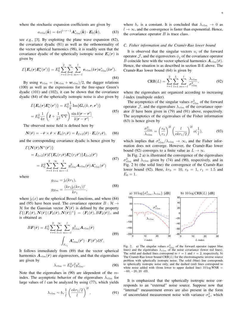
In Fig. 2 a) is illustrated the convergence of the eigenvaluesσ2τlm and λτlm given by (74) and (90), respectively, and in

Fig. 2 b) (the solid line) the convergence of the Cramer-Raolower bound (92). Here, kr0 = 10, r0 = 1, r1 = 1.5 andE0 = 1.

0 10 20 30−200

−150

−100

−50

0

50

100

0 10 20 30−80

−60

−40

−20

0

20

40

60a) 10 logσ2

τlm, λτlm [dB] b) 10 logCRB(L) [dB]

σ2τlm

λτlm

l-index L-index

Fig. 2. a) The singular values σ2τlm of the forward operator (upper blue

lines) and the eigenvalues λτlm of the noise covariance (lower red lines).The solid and dashed lines correspond to τ = 1 and τ = 2, respectively. b)The Cramer-Rao lower bound CRB(L) for the electromagnetic inverse sourceproblem with spherically isotropic noise. The solid (blue) line correspondsto spherically isotropic noise only, and the dashed (red) lines correspond towhite noise added with (from lower to upper dashed line) 10 log WNR =−60,−20, 20 dB.

It is emphasized that the spherically isotropic noise cor-responds to an “external” noise source. Suppose now that“internal” measurement errors are also present in the formof uncorrelated measurement noise with variance σ2

w, which

10

is added to the eigenvalues λτlm, see also the noise modeldescribed in (55). The white-noise-ratio (WNR) is defined hereby

WNR =σ2

w

maxτlm

λτlm, (94)

and the noise eigenvalues in (92) are then replaced as λτlm →λτlm+σ2

w. In this case, the Fisher information (63) converges,and the Cramer-Rao lower bound (92) becomes infinite asL → ∞. The situation is illustrated in Fig. 2 b) (the dashedlines) where 10 log WNR = −60,−20, 20 dB. It is clearthat if the white noise level is significantly lower than themaximum eigenvalue of the spherically isotropic noise, i.e., ifσ2

w << maxτlm λτlm, then it is essential to incorporate theeigenvalues related to the spherically isotropic noise into theFisher information analysis, and not only the singular valuesστlm of the Jacobian J .

IV. SUMMARY AND CONCLUSIONS

It is natural to consider an inverse imaging problem asan infinite-dimensional estimation problem based on a sta-tistical observation model. With Gaussian noise on infinite-dimensional Hilbert space, a trace class covariance operatorand a Hilbert-Schmidt Jacobian, the appropriate space fordefining the Fisher information operator is given by theCameron-Martin space. A sufficient condition is given for theexistence of a trace class Fisher information, which is basedsolely on the spectral properties of the covariance operatorand of the Jacobian, respectively. Two important special casesarises: 1) The infinite-dimensional Fisher information operatorexists and is trace class, and the corresponding pseudo-inverse(and the Cramer-Rao lower bound) exists only for finite-dimensional subspaces. 2) The infinite-dimensional pseudo-inverse (and the Cramer-Rao lower bound) exists, and thecorresponding Fisher information operator exists only forfinite-dimensional subspaces. An explicit example is givenregarding an electromagnetic inverse source problem with“external” spherically isotropic noise, as well as “internal”additive uncorrelated noise.

APPENDIX

The regular vector spherical waves are defined here by

v1lm(kr) =1√

l(l + 1)∇× (rjl(kr)Ylm(r))

= jl(kr)A1lm(r),

v2lm(kr) =1

k∇× v1lm(kr)

=(krjl(kr))

′

krA2lm(r) +

√l(l + 1)

jl(kr)

krA3lm(r),

(95)

where Aτlm(r) are the vector spherical harmonics and jl(x)the spherical Bessel functions, cf., [1, 3, 11, 21, 28]. The in-dices are given by l = 1, . . . ,∞ and m = −l, . . . , l. The

vector spherical harmonics Aτlm(r) are given by

A1lm(r) =1√

l(l + 1)∇× (rYlm(r)) ,

A2lm(r) = r ×A1lm(r),

A3lm(r) = rYlm(r),

(96)

where Ylm(r) are the scalar spherical harmonics given by

Ylm(θ, φ) = (−1)m√

2l + 1

4π

√(l −m)!

(l +m)!Pml (cos θ)eimφ,

(97)and where Pml (x) are the associated Legendre functions [1].

The vector spherical harmonics are orthonormal on the unitsphere, and hence∫

S1

A∗τlm(r) ·Aτ ′l′m′(r)dΩ = δττ ′δll′δmm′ , (98)

where S1 denotes the unit sphere, dΩ = sinθdθdφ and τ =1, 2, 3. As a consequence, the regular vector spherical wavesare orthogonal over a spherical volume Vr0 with∫

Vr0

v∗τlm(kr) · vτ ′l′m′(kr)dv

= δττ ′δll′δmm′

∫Vr0

|vτlm(kr)|2dv,

(99)

where τ = 1, 2.The out-going (radiating) and in-going vector spherical

waves uτlm(kr) and wτlm(kr) are obtained by replacing thespherical Bessel functions jl(x) above for the spherical Hankelfunctions of the first and second kind, h

(1)l (x) and h

(2)l (x),

respectively, see [3, 28]. The dagger notation ·† is used hereto denote a sign-shift in the exponent of the factor eimφ. Hence,for real arguments kr, it is observed that

v∗τlm(kr) = v†τlm(kr),

u∗τlm(kr) = w†τlm(kr),

w∗τlm(kr) = u†τlm(kr),

(100)

where ·∗ denotes the complex conjugate.The free-space Green’s dyadic for the electric field satisfies

∇×∇×Ge(k, r, r′) − k2Ge(k, r, r′) = Iδ(r − r′), whereI is the identity dyadic and δ(·) the Dirac delta function, andis given by

Ge(k, r, r′) = (I +1

k2∇∇)

eik|r−r′|

4π|r − r′|, (101)

see e.g., [3, 11]. The free-space Green’s dyadic can also beexpanded in vector spherical waves as e.g.,

Ge(k, r, r′) = ik

2∑τ=1

∞∑l=1

l∑m=−l

uτlm(kr>)v†τlm(kr<),

(102)where r> (r<) denotes the vector in r, r′ having the largest(smallest) length, cf., [3].

11

REFERENCES

[1] G. B. Arfken and H. J. Weber. Mathematical Methods for Physicists.Academic Press, New York, fifth edition, 2001.

[2] V. I. Bogachev. Gaussian Measures. American Mathematical Society,1998.

[3] A. Bostrom, G. Kristensson, and S. Strom. Transformation properties ofplane, spherical and cylindrical scalar and vector wave functions. In V. V.Varadan, A. Lakhtakia, and V. K. Varadan, editors, Field Representationsand Introduction to Scattering, Acoustic, Electromagnetic and ElasticWave Scattering, chapter 4, pages 165–210. Elsevier Science Publishers,Amsterdam, 1991.

[4] B. F. Cron and C. H. Sherman. Spatial correlation functions for variousnoise models. JASA, 34, 1732–1736, 1962.

[5] S. N. Evans and P. B. Stark. Inverse problems as statistics. InverseProblems, 18, R55–R97, 2002.

[6] I. I. Gikhman and A. V. Skorokhod. The theory of stochastic processesI. Springer-Verlag, Berlin, Heidelberg, 2004.

[7] M. Gustafsson and S. Nordebo. Cramer–Rao lower bounds for inversescattering problems of multilayer structures. Inverse Problems, 22,1359–1380, 2006.

[8] M. Hairer. An Introduction to Stochastic PDEs. arXiv:0907.4178v1[math.PR], 2009.

[9] P. C. Hansen. Discrete Inverse Problems: Insight and Algorithms. SIAM-Society for Industrial and Applied Mathematics, 2010.

[10] J. E. Hudson. Adaptive Array Principles. Institution of ElectricalEngineers, 1981.

[11] J. D. Jackson. Classical Electrodynamics. John Wiley & Sons, NewYork, third edition, 1999.

[12] J. Kaipio and E. Somersalo. Statistical and computational inverseproblems. Springer-Verlag, New York, 2005.

[13] S. M. Kay. Fundamentals of Statistical Signal Processing, EstimationTheory. Prentice-Hall, Inc., NJ, 1993.

[14] A. Khrennikov. To quantum averages through asymptotic expansion ofclassical averages on infinite-dimensional space. Journal of Mathemat-ical Physics, 48, 2007. 013512.

[15] A. Kirsch. An Introduction to the Mathematical Theory of InverseProblems. Springer-Verlag, New York, 1996.

[16] E. Kreyszig. Introductory Functional Analysis with Applications. JohnWiley & Sons, New York, 1978.

[17] E. A. Marengo and A. J. Devaney. The inverse source problem ofelectromagnetics: Linear inversion formulation and minimum energysolution. IEEE Trans. Antennas Propagat., 47(2), 410–412, February1999.

[18] E. A. Marengo, A. J. Devaney, and F. K. Gruber. Inverse source problemwith reactive power constraint. IEEE Trans. Antennas Propagat., 52(6),1586–1595, June 2004.

[19] E. A. Marengo and R. W. Ziolkowski. Nonradiating and minimumenergy sources and their fields: Generalized source inversion theoryand applications. IEEE Trans. Antennas Propagat., 48(10), 1553–1562,October 2000.

[20] K. S. Miller. Complex Stochastic Processes. Addison–Wesley PublishingCompany, Inc., 1974.

[21] R. G. Newton. Scattering Theory of Waves and Particles. DoverPublications, New York, second edition, 2002.

[22] S. Nordebo, R. Bayford, B. Bengtsson, A. Fhager, M. Gustafsson,P. Hashemzadeh, B. Nilsson, T. Rylander, and T. Sjoden. An adjoint fieldapproach to Fisher information-based sensitivity analysis in electricalimpedance tomography. Inverse Problems, 26, 2010. 125008.

[23] S. Nordebo, A. Fhager, M. Gustafsson, and B. Nilsson. A Green’sfunction approach to Fisher information analysis and preconditioning inmicrowave tomography. Inverse Problems in Science and Engineering,18(8), 1043–1063, 2010.

[24] S. Nordebo, A. Fhager, M. Gustafsson, and M. Persson. A systematicapproach to robust preconditioning for gradient based inverse scatteringalgorithms. Inverse Problems, 24(2), 2008. 025027.

[25] S. Nordebo, M. Gustafsson, T. Sjoden, and F. Soldovieri. Data fusion forelectromagnetic and electrical resistive tomography based on maximumlikelihood. International Journal of Geophysics, pages 1–11, 2011.Article ID 617089.

[26] S. Nordebo and M. Gustafsson. Statistical signal analysis for the inversesource problem of electromagnetics. IEEE Trans. Signal Process., 54(6),2357–2361, June 2006.

[27] F. W. J. Olver. Asymptotics and special functions. A K Peters, Ltd,Natick, Massachusetts, 1997.

[28] F. W. J. Olver, D. W. Lozier, R. F. Boisvert, and C. W. Clark. NISTHandbook of mathematical functions. Cambridge University Press, NewYork, 2010.

[29] L. Pronzato. Optimal experimental design and some related controlproblems. Automatica, 44, 303–325, 2008.

[30] M. Reed and B. Simon. Methods of modern mathematical physics,volume I: Functional analysis. Academic Press, New York, 1980.

[31] L. L. Scharf. Statistical Signal Processing. Addison-Wesley PublishingCompany, Inc., 1991.

[32] D. Sjoberg and C. Larsson. Cramer-Rao bounds for determination ofpermittivity and permeability in slabs. IEEE Transactions on MicrowaveTheory and Techniques, 59(11), 2970–2977, 2011.

[33] A. Tarantola. Inverse problem theory and methods for model parameterestimation. Society for Industrial and Applied Mathematics, Philadel-phia, 2005.

[34] H. L. Van Trees. Detection, Estimation and Modulation Theory, part I.John Wiley & Sons, Inc., New York, 1968.

[35] J. C. Ye, Y. Bresler, and P. Moulin. Cramer-Rao bounds for parametricshape estimation in inverse problems. IEEE Transactions on ImageProcessing, 12(1), 71–84, 2003.