Fiscal Design and the Location of Economic Activity

Fiscal Design and the Location of Economic Activity

Paper handed in for the 45th Congress of the European Regional Science Association

"Land Use and Water Management in a Sustainable Network Society"

Vrije Universiteit Amsterdam, 23-27 August 2005

by

Ulrike Stierle-von Schütz∗

RWTH-Aachen University

Abstract

In the process of economic integration regional production structures are about to change. Several

studies analysed already trends of regional specialization in the European Union and attempted to

figure out determinants of observed changes. In this context, so far date the role of the public

sector and especially the impact of different fiscal designs as determinants of the change in

production structures have been left aside. Advantages and shortcomings of decentralized

government organization have been largely discussed theoretically within the last decades.

Several empirical studies attempted to examine the impact of decentralization on national

performance, e.g. economic growth and fiscal stability. This paper aims at linking these two

subjects and analyzes the empirical relationship between regional specialization and fiscal

decentralization for a panel of 13 Member States of the European Union, controlling for regional

and other institutional determinants. The analysis shows that rather autonomous regions tend to

diverse their production structure in order to insure against adverse supply shocks.

Acknowledgement

The author would like to acknowledge a grant from the German Science Foundation (DFG

SPP 1142). The usual disclaimer applies.

Keywords: Fiscal federalism, subnational autonomy, spatial allocation of economic activity

Jel.Classifications: R12, R3, H7

∗ Department of Economics, RWTH-Aachen University, D-52056 Aachen, Germany,

eMail: [email protected].

2

1. Introduction

Since the initial work of Tiebout (1956) and Oates (1972) there has been a wide interest in the

optimal division of providing public services between different government levels in

economic literature and political practice. Especially for countries in transition and

developing countries the decision for centralizing or decentralizing governmental tasks in

order to promote economic and social development is an important question. Also in

developed countries changes in the vertical structure of governments can be observed in the

last decades (OECD 2002). Although there is evidence for increasing decentralization in a

majority of OECD countries, a unique pattern to one or the other structure does not seem to

occur (Stegarescu 2004).

At the same time increasing integration, particularly the creation of the Single Market in the

European Union facilitating the movement of labour and capital lead to reflections on

changing production structures in countries and regions. Here the fear of over-specialised

regions not able to cope with asymmetric shocks may emerge. But the analysis of direction

and determinants of regional specialization is still an open debate in the theoretical and

empirical literature. Additionally, the possible role of the public sector in influencing process

of spatially changing production structures becomes more and more a crucial part in this

discussion (Baldwin et al. (2003), Brakman et al. (2002), Brülhart und Trionfetti (2004)).

This paper aims at linking these two topics in asking if the autonomy of a region in deciding

about revenue and expenditure may influence its level of specialization and thus its potential

capacity of shock absorption. The analysis is organised as follows: section two summarizes

recent theoretical and empirical work on decentralization and specialization and offers some

hypotheses for the empirical analysis in section three. Results are presented in section four

and the paper ends with a conclusion and prospects for futures research.

3

2. Theoretical and empirical insides

In the following background theoretical and empirical considerations will be explored in order

to work out testable hypotheses for the above mentioned research question.

Before starting to investigate the effects of decentralization on economic performance and

determinants of specialization, it is important to figure out if the public sector is able to shape

the production structure. In the theoretical and empirical literature there exist different

positions. While results of the proponents will be discussed in 2.1, opponents as Davis and

Weinstein (2002, 2004) and Brakman et al. (2004) point out in their empirical analysis that

even large temporary shocks as Allied bombing of Japanese and German cities in World War

II did not have an effect on the growth path of these cities and, more important, it has not

even changed the urban industrial structure of Japanese cities. The implications for the

effectiveness of regional policy are far reaching, since following Davies and Weinstein (2004)

policy makers may not be able to choose between multiple equilibria and select with

temporary interventions the one which is convenient for long-term regional development.

However, Allied bombing could not destroy the social and transport infrastructure and the

specific human capital which may have served as an important basis for reconstruction.1 In

the case of the West-German cities the federal government aimed at rebuilding cities to their

pre-war levels and provided specific grants to cities and private persons in order to stimulate

re-construction of houses and buildings (Brakman et al. 2004). These arguments may thus

limit the rather pessimistic view on policy actions and effects of changing institutions.

2.1 Decentralization and economic performance

A large debate on advantages and weaknesses of decentralization and thus their impact on

economic performance has already taken place in economics and political science2. The

following table summarizes shortly the main pro and contra arguments:

1 This argument was mainly forwarded in the comments of F. Robert-Nicoud and the authors admit that point

to a certain degree in their paper. 2 For a comprehensive survey see e.g. Thießen (2001: 2-8).

4

Table 1: Arguments supporting and challenging the effects of fiscal decentralization

Pro Contra + diversification hypothesis: increased efficiency due to better information on residents’ needs + leviathan restraint hypothesis: intense competition between local governments reduce the size of governments + productivity enhancement hypothesis: incentives for political and product innovations (“laboratory federalism”) as well as a better quality of public services due to autonomy and accountability of the local government + specialization of functions: efficiency gains may arise through specialization of representatives dealing with very specific activities + high per capita income fixed costs of maintaining a decentralized system may only be affordable at a higher stage of economic development + high degree of urbanization: economies of scale are more likely to occur at lower government level if the population is concentrated

– inequities and the need for a centralized redistribution policy – macroeconomic stabilization: counter-cyclical actions and co-ordination of local governments are difficult to manage – presence of inter-jurisdictional spillovers – exploiting economies of scale in production of public goods and administration – quality of governments: central governments may attract higher qualified people, lobbying and corruption activities may be less controlled on the local level – small size of the country/population: preferences can be assumed to be rather homogenous3 – scarcity of good local taxes meaning taxes and fees relying on the benefits received principle represent only a minor share of total taxes levied – low per capita income level: see Pro – low degree of urbanization: see Pro

Source: Thießen (2003), OECD (2002), Feld and Dede (2005), own compilation.

Given this range of possible positive and negative effects of fiscal decentralization, empirical

testing was needed. Empirical studies testing the impact of fiscal decentralization on

economic performance measured as economic growth, capital formation and total factor

productivity growth in cross country studies as well as analysis of single countries come to

very diverse results4. This fact might be mainly due to different measures of decentralization

since the commonly used one provided by the IMF’s Government Finance Statistics (GFS) –

subnational share of total government expenditure or subnational share of total government

revenue – does not capture the fiscal autonomy the subnational unit possess to decide about

expenditure (including different grant schemes) and revenue (taxes, tax bases, fees etc.) (Ebel 3 However, this rule does not seem to be supported by clear real world experience regarding the heterogeneity

of small countries like Belgium or Switzerland (Stegarescu 2004: 6). 4 For a recent survey see Feld and Dede (2005: 9-12).

5

and Yilmaz 2002). In order to include these missing aspects, the OECD started to create new

measures of fiscal decentralization (OECD 1999) for 18 OECD countries. Stegarescu (2004)

extends this data set to 23 countries and covers the period between 1970 to 2001. Further

details will be given in the Data section since these data will be used in the empirical analysis.

2.2 Determinants of regional specialization

The theoretical literature provides very different explanations for the emergence of regional

specialization. Following traditional trade theory comparative advantages will mainly lead to

specialization of regions which open their borders. In neoclassical theories political

institutions are not at all taken into account, regional policy activities would only disturb the

market forces leading to an equilibrium. “New theories” allowing for imperfect competition

and economies of scale provide a rich set of possible explanations leading to specialization /

agglomeration but also to dispersed and multiple equilibria. Especially recent theoretical

models of the New Econonomic Geography (NEG) in the tradition of Krugman (1991) try to

analyse the role of public sector interventions in shaping the spatial production structure and

influencing break and sustain points. Up to now the analysis focuses mainly on the impact of

policy instruments as taxes and tax competition (Anderson and Forslid 2003, Baldwin and

Krugman 2004), government spending (Brakman et al. 2002, Brülhart and Trionfetti 2004)

and specific regional policy measures as infrastructure or subsidies (Baldwin et al. 2003).

Regarding taxes and tax competition the models demonstrate that in the course of integration

with an emerging centre-periphery structure, production factors in the core will benefit from

an agglomeration rent which can be taxed by the region without loosing the mobile

production factors. Extending this model by government expenditure and thus taking the

relations of taxes and spending into account, Brakman et al. (2002) can show that increasing

public spending from a production point of view stimulates agglomeration since the location

becomes more attractive for production factors operating under economies of scale.

Moreover, governments are able to change the equilibrium i.e. from agglomerating to

spreading forces, depending on the relative size, direction or efficiency of public good

production and distribution. Brülhart and Trionfetti (2004) regard public procurement from

the demand side and show theoretically and empirically that a region with a large home-

biased public procurement will specialize in that high demanded good produced in a

monopolistically competitive sector (“pull effect”). The emergence of the so called “spread

effect” is a second result of home-biased public procurement meaning that due to public

spending agglomeration forces may be offset. Theoretical results of the impact of public

6

infrastructure investment on the production structure depends on the presence of localized

spillovers and the policy objectives since here the trade-off between equity and efficiency

becomes predominant (Baldwin et al. 2003). In their empirical study Combes and Lafourcade

(2001) confirm the positive relationship of decreasing transportation cost on regional

specialization and concentration for French regions.

Empirical studies focussing on policy activities and specialization are very scarce for the time

being, but there are also only few econometric studies providing insides of the specialization

process as such. Stirböck (2004) identifies several determinants of regional specialization in

capital investment and employment coming from different theories as neoclassical trade

theory, polarisation theory and NEG. Another approach has been chosen by Kalemli-Ozcan,

Sorensen and Yosha (2003) who focus on the positive impact of risk sharing on specialization

patterns.

Theoretical and empirical work on determinants of specialization, especially the role of public

activities and institutions, is still at the beginning. As far as the author knows there are no

studies of regional specialization taking the fiscal design of the nation state encompassing the

regions into account.

2.3. Hypotheses

In the following hypotheses for the empirical analysis coming from the theoretical and

empirical considerations above will be summarized.

(i) Decentralization

The measures of decentralization capture revenue and expenditure autonomy. Since higher

specialization is in general related to a higher exposure of economic risk, autonomous regions

may try to insure against possible shocks by diversifying the local production structure. On

the other hand, if there is a mechanism of the central government to regulate these risks with a

redistribution schemes among regions, local levels need not to cover the risk themselves and

may rather focus on the attraction of specific industries in order to have possible tax revenue

from agglomeration rents. Another possible explanation for a positive relationship between

decentralization and specialization may be deducted from the NEG models mentioned above.

Since local governments would take advantage from greater autonomy to provide specific

public goods, they may be able to attract mobile production factors which could promote a

process of agglomeration and intensifying specialization. Following Brakman et al. (2002)

this may only be possible if the public sector works efficiently. As shown by Baldwin and

7

Krugman (2002) the subnational unit benefits from these developments by levying taxes on

agglomeration rents.

(ii) New Economic Geography

The NEG models point to several determinants of location decisions which should be

considered. Market size, population density and the location of a region seem to be important

factors – while core regions would rather attract industrial sectors and market services

(industries with economies of scale), the periphery may specialize in economic activities

which rely heavily on factor endowments (agricultural territory, touristic services etc.) or

which have to be provided by the public sector (health, education etc.). The intuition behind

market size and population density go into the same direction as monopolistically competitive

sectors prefer the location near large markets with a diversified labour market. Considering

the last argument from the perspective of mobile workers, they also may want to insure

against shocks and will chose a location with a diversified production structure.

(iii) Other influencing variables

In order to capture effects of business cycle, unemployment rates have to be included in the

empirical analysis since the magnitude of the decentralization measure may also be influenced

by economic fluctuations. The attractiveness of a region may also depend on research

activities and thus patents as indicator for research intensity should be taken in.

3. Empirical analysis

3.1 Data

In the following the two important indicators of interest – the specialization and

decentralization indicators – and their data sources will be described. All other data are

provided in the appendix.

In order to analyse the described determinants of specialization we use a panel of 13 EU

Member States at NUTS2-level (and thus 200 regions)5. The NUTS2 regions are defined by

administrative conditions and might not measure economic regions. This problem refers to the

well known “modifiable area unit problem” MAUP (Brülhart and Traeger, 2004). Figuring

out economic regions is often an arbitrary task and depends on the analysed variables and

sectors. Advantage of administrative units is data availability and especially the NUTS2-level

5 NUTS refers to Nomenclature of Statistical Territorial Units (NUTS) and is a hierarchical classification of

regions in a Member State where higher numbers indicate a smaller administrative unit (Eurostat 1999).

8

can be considered when focussing on regional policy implications or on regional structural

programmes.

The analysis is based on several data sources. This is first due to the fact that none of the

possible sources was able to provide a complete data set and consequently several gaps had to

be filled.6 However, the starting point was the regional data base (REGIO) of Eurostat7.

The basic economic variables for constructing the degree of regional specialization in

production structure is annual gross value added and employment. As far as possible the data

set is compiled according to the European System of National Accounts ESA95 including 17

sectors following NACE Rev. 18 including agriculture, manufacturing as well as market and

non-market services.9 The rather short time period of investigation (1995-2001) is due to the

introduction of the new European System of National Accounts (ESA) in 1995 where the

sectoral disaggregation changed fundamentally.

As the data for fishing (sector B) is for most regions not separately available, we took the

aggregate figure for agriculture and fishing (A + B). Consequently, two sub-sectors (A + B as

well as mining and quarrying (C)) are included for the primary sector. The breakdown into

branches of the secondary sector is rather limited in ESA95 as only three sub-sectors are

available (i. e. manufacturing (D), electricity, gas, water supply (E) and construction (F)). On

the other hand, ESA95 reflects the increased importance of services. The breakdown of the

tertiary sector into ten branches, (i. e. G to P10) including retail services, tourism, financial

intermediation and real estate as well as public services, is now more detailed than it was

before when the data were based on ESA79.11 The author is conscious of the limitation of this

rather broad sectoral breakdown as it can be questioned if the statistical classification is fine

enough as it might hide heterogeneous developments in specific sub-sectors or cannot show

economic dependence of some regions on specific sub-sectors. This is the more the case here

since for example manufacturing is not disaggregated. However, this data set allows for a

more comprehensive overview of the overall economic activity instead of focussing on

manufacturing representing on average only 27% of production in the incumbent EU Member

States contrasting to 70% for services. Moreover, despite their though increasing in fact still

limited tradability, services are more and more part of international production chains as

6 The regional data set of Cambridge Econometrics offers most of the data that would be needed for this study

in one set. However, to the author it was not transparent enough how data that is not available at the corresponding statistical office was estimated.

7 For the made adjustments see table A2 in the appendix. 8 Nomenclature des activités économiques dans les Communautés Européennes. 9 See table A1 in the appendix. 10 Since no data are available for sector Q (exterritorial organisations) it has been left out of the analysis. 11 For a list of the NACE sectors see table A1 in the appendix.

9

becomes clear e.g. by foreign direct investment (FDI) data. Services account on a world wide

scale for 60% of FDI inward stocks as well as two thirds of inward flows (UNCTAD 2004).

Consequently, to limit an analysis of specialisation to manufacturing as frequently done,

leaves aside the main part of local and also international economic transactions.

In relation to employment data, the use of GVA encompasses several advantages: differences in

labour productivity within and between regions have to be accounted for, employment

definitions still vary from country to country, flexible employment schemes which become

increasingly important make comparisons difficult and employment data are compared to GVA

in a more direct way influenced by public policy as labour protection laws etc. (Aiginger and

Leitner 2002: 12). However, GVA data have also disadvantages like the need to convert them

into one currency. Possible misalignments of exchange rates are one major disadvantage of

operating with GVA data (Brülhart and Traeger 2004: 11).12

In empirical literature various indicators are used for analysing sectoral specialisation of

regions and regional concentration of sectors. All indicators have their advantages and

shortcomings.13 In order to obtain results that can easily be compared to other studies and

compared between each other, one indicator has here been applied that is most commonly

utilised. Due to the latter, in the following it is not necessary to include an in-depth discussion

and description.

Specialisation in relative terms should reveal how much the production structure in one

region differs from the average of a given set of regions. For this analysis of relative regional

specialisation the dissimilarity index D has been used. This indicator is one of the most

commonly applied indicators for regional specialisation, reused e.g. by Krugman (1991):

(1) ∑=

−=I

1ijiijj xx

2100D

For each branch i in a region j the absolute values of the differences of sectoral shares in GVA

between region j and the average of all regions of the nation state14 ( jix ) are added up. In

contrast to Krugman we divide the result by 2 and multiply it by 100 so the index will take the

value zero when no specialisation can be observed, i. e. the production structure does not

differ from the average of all regions included, and it will take the value 100 if full

specialisation exists.

12 Due to data problems the dissimilarity has only been computed with GVA data. The comparison with

employment data is left for future research. 13 For surveys see for example Amiti (1997), Krieger-Boden (1999), WIFO (1999), Bode et al. (2004), Brülhart

and Traeger (2004), Combes and Overman (2004). 14 This is the reason why one-region-countries as Luxembourg and Denmark had to be left out in this analysis.

10

The dissimilarity index offers the advantage that it is in comparison to others easily

interpretable. It also has been applied already in several other empirical studies so that the

results can be compared to findings of other empirical studies. Moreover, outliers do not

influence the values as much as it is the case for other indicators.

As already stated in section 2.1., a dataset compiled by Stegarescu (2004) is the basis of the

decentralization indicators. He distinguishes between tax revenue decentralization and

revenue decentralization including non-tax revenue15 (e.g. user fees, capital revenue etc.).

Following his argumentation, measures of fiscal autonomy has to take into account

“legislative competencies to determine tax base and tax rate, the attribution of the tax receipts,

and tax administration”(Stegarescu 2004: 5). The OECD scheme of tax autonomy (OECD

1999) has been used to provide a classification of taxes (Table 2). While local government has

total or significant control over its taxes regarding the cases a)-c) and d.1)-d.2) it only has

very limited or no tax autonomy.

Table 2: Classification of sub-national taxes sorted by decreasing order of control

a) b) c) d) d.1) d.2) d.3) d.4) e)

sub-central government (SCG) sets tax rate and tax base SCG sets tax rate only SCG sets tax base only tax sharing arrangements SCG determines revenue-split revenue-split can only be changed with consent of SCG revenue-split fixed in legislation, may unilaterally be changed by central government revenue-split determined by central government as part of the annual budget process central government sets rate and base of SCG tax.

Source: OECD (1999: 11). Three indicators capture three different degrees of tax revenue decentralization adding up the

above classified taxes and weighted by the tax revenue of general government (GG):

Data and indicators are used on a yearly basis and are analysed for the time period 1995 – 2001. 15 Due to data problems, this second measure has been left out of the analysis.

SCG a) to c) GG total tax revenue D_tax1 =

D_tax2 =

D_tax3 =

SCG a) to c) + d.1) to d.2) GG total tax revenue

SCG a) to e) GG total tax revenue

11

3.2 Investigation approach

Following the working hypotheses derived in section 2.3 the empirical investigation tries to

figure out if fiscal decentralization may be one determinant of regional production

specialization taking into account other possible factors influencing the regional production

structure.

The analysis is carried out using generalised least square (GLS) in order to control for

potential heteroscedasticity. These results will be compared with a pooled cross-section time

series model and with a country fixed effects model. While pooled regressions exhibit mostly

the problem of unobserved heterogeneity and thus a bias in the estimators, fixed effects

models account for all time-invariant unobserved or not-quantifiable country specific factors.

Herewith the problem of time-constant heterogeneity can be solved. However, difficulties

with latter techniques arise if time invariant effects play a role16 or if the assumption of strict

exogeneity is violated.

Formally the basic equation takes the following form:

Dj = b0 + b1Dtaxj + b2Transfj + b3Efficiencyj + b4RGDPj + b5Densityj + b6PerIndj

b7Patentsj + b8Unempj + country dummies + capital dummy + εij

Dj represents the dissimilarity index D as described above in region j17. Dtaxj indicate the tax

decentralization variable in region i. Since changes in institutions (here the federal structure)

do not lead to an immediate reaction of sectoral change, the variable has been included with a

three years lead. One has to note that this variable has been computed on a national basis.

Considering the derived hypotheses it is not ultimately clear in which direction the

decentralization variable will influence the specialization patterns of a region. In order to

capture the intranational insuring aspect, the variable Transfj standing for transfers to sub-

national units from other levels of Government (% of total sub-national revenues and grants)

has been included in the analysis. If this variable shows a positive sign, one could infer that

these transfers are used as insurance against economic risk rising with production

specialization.

As Brakman et al. (2004) demonstrate, the capacity of regions influencing agglomeration

tendencies hinges on the efficiency of the public sector. Unfortunately there are no efficiency

indicators available at the regional level thus we use the Bertelsmann Success Index

(Efficiencyj) (Bertelsmann Stiftung 2004) indicating the performance of the national economy.

16 In this analysis the theoretically important impact of the peripherality index has to be taken out with country

fixed effects models. 17 As pooled data are used, the time index has been taken out of the specification.

12

Determinants coming from the NEG models are considered in the variables RGDPj, Densityj

and Perindj. Regional gross domestic product (RGDP) measured as GDP per capita as an

indicator of demand capacity, population density and the peripherality index representing

market access of a region can be used a indicators for the attractiveness of a region for mobile

firms and workers. The same also applies for the regional research intensity captured by the

variable Patentsj.

In order to control for business cycle fluctuations, we included the regional unemployment

rate Unempj.

Country and capital dummies have been added to the analysis to control for effects on the

country and capital level.

The robustness of the results will be checked by using a distinct variable for the efficiency

indicator - the Bertelsmann Activity Index18 - and by applying different concepts of

decentralization. Firstly this can be done by looking at the expenditure side of

decentralization. Expenditure decentralization (ExpDez) is measured by subnational

expenditure in percent of total expenditure. As Stegarescu (2004: 7) points out the analysis of

revenue decentralization may also be broadened by including mostly all sources of public

revenue and not only taxes such as user charges, operational surplus or capital revenue. Thus

the variables drev_1, drev_2, drev_319 are analysed.

4. Results

In table 3 first results for the pooled OLS and GLS estimations are presented. The overall

performance of the estimation is relatively well with explaining 30 and 25 percent

respectively of changing specialization patterns in this short time period.

The negative sign of all three decentralization variables show that tax autonomy might be linked

with decreasing regional specialization although the coefficients of the POLS estimates are not

significant20. However, when transfers are considered the insurance function of autonomy

disappears and regions tend to be more specialized the higher the transfer share is21.

The effect of efficiency (Suc) seems to be not very important since the coefficients are very

low and not significant. Regarding the NEG variables, regional GDP per capita is positively

related to specialization for both estimation techniques and independently from the

18 This index focuses on factors describing the sources of performance differences between countries. 19 The three variables represent in descending order the autonomy of regional public revenue building. 20 This effect is very likely as has already been stated above. 21 This effect is reversed (but not significantly) in the GLS III where the region has less autonomy on taxes and

tax bases.

13

autonomous degree of tax revenue. This supports the hypothesis that regions with attractive

markets might be more specialised and/or might have better insurance possibilities against

adverse shocks and thus take specialization advantages. While population density seems to

encourage slightly a specialised production structure, the peripherality index shows that

regions in the core are rather less specializes relative to peripheral regions. Also regions with

a higher research intensity seem to be less specialized. The latter effect may be due to the data

structure, since research intensive sectors are swallowed by the aggregated sector structure.

The capital dummy variable has the expected positive sign (the capital effect of

administration), but is surprisingly not significant.

Table 3: Influence of fiscal variables and regional indicators on specialization patterns, Pooled OLS and GLS estimations

Dj POLS1 POLS2 POLS3 GLS I GLS II GLS III Dtax_1 Dtax_2 Dtax_3 Transfers Suc RGDP Density Unemp PerInd Patents dum_capital Constant

-0.055 (0.52) 0.021 (0.49) -0.037 (0.82) 0.264 (7.54)** 0.001 (3.94)** 0.358 (1.69) -0.789 (10.07)** -0.189 (9.11)** 0.849 (1.16) 19.191 (4.27)**

-0.087 (0.60) 0.020 (0.46) -0.046 (0.94) 0.264 (7.51)** 0.001 (3.95)** 0.361 (1.70) -0.789 (10.07)** -0.189 (9.10)** 0.848 (1.16) 20.114 (4.06)**

-0.082 (0.58) -0.000 (0.01) -0.044 (0.92) 0.264 (7.50)** 0.001 (3.95)** 0.358 (1.69) -0.789 (10.06)** -0.189 (9.11)** 0.853 (1.17) 20.968 (3.58)**

-0.522 (2.62)** 0.010 (1.00) 0.005 (0.48) 0.049 (2.71)** 0.001 (2.64)** 0.041 (0.29) -0.844 (4.78)** -0.045 (2.54)* 1.104 (0.65) 19.728 (7.97)**

-1.322 (4.11)** 0.004 (0.44) -0.003 (0.32) 0.041 (2.29)* 0.001 (2.71)** 0.088 (0.61) -0.842 (4.77)** -0.043 (2.45)* 1.083 (0.64) 21.880 (8.55)**

-0.934 (3.58)** -0.025 (1.67) 0.000 (0.05) 0.042 (2.30)* 0.001 (2.68)** 0.001 (0.01) -0.827 (4.69)** -0.053 (3.01)** 1.215 (0.72) 23.191 (8.48)**

No. of observations

1112 1112 1112 1112 1112 1112

R² (overall) Prob. Chi²22

0.30 0.30 0.30 0.26 0.0000

0.26 0.0000

0.26 0.0000

Absolute value of t / z statistics in parentheses, * significant at 5%; ** significant at 1%

22 The probability of the Chi²-test gives the joint significance of all coefficients.

14

The estimation results of the fixed effect model shown in table 4 are rather discouraging since

only 2 to 3 percent of the model can be explained by the used variables. Thus a strong sign

that further factors should be included in the analysis. However, the interesting coefficients of

decentralization indicators show significant negative signs emphasizing the possible influence

of public sector autonomy on production structures. Comparing the coefficients with the

POLS and GLS results, the signs of the density coefficients have changed but are not

significant.

Table 4: Influence of fiscal variables and regional indicators on specialization patterns, fixed effect estimations

Dj FE 1 FE 2 FE 3 Dtax_1 Dtax_2 Dtax_3 Transfers Suc RDGP Density Unemp Patents Constant

-0.055 (2.34)* 0.014 (1.39) 0.008 (0.80) 0.044 (2.37)* -0.004 (1.54) 0.030 (0.20) -0.032 (1.73) 11.937 (8.17)**

-0.121 (3.77)** 0.011 (1.07) -0.004 (0.36) 0.041 (2.20)* -0.003 (1.48) 0.095 (0.63) -0.027 (1.45) 15.257 (8.59)**

-0.108 (3.42)** -0.016 (1.18) -0.001 (0.07) 0.039 (2.11)* -0.003 (1.46) 0.037 (0.25) -0.034 (1.84) 16.271 (7.97)**

No. of observations 1112 1112 1112 R² overall 0.02 0.03 0.03

Absolute value of z statistics in parentheses* significant at 5%; ** significant at 1%

Extending the analysis of public revenue decentralisation by including also non-tax revenues

the results remain quite stable. As is shown in tables A5 – A8 the decentralization variable

(tax revenue or whole revenue) is mostly significantly negative23. Considering expenditure

decentralization, the results suggest a positive relationship between decentralization and

specialization. Thus, one might infer that if a region has a relatively high expenditure rate

compared to the national level, it attracts specific sectors resulting in a higher specialised

23 The estimations in POLS VII – IX are an exception but the coefficients are not significant.

15

production structure. The significantly positive sign of the transfer in a further analysis shows

the possible source of this positive effect – national transfer schemes could provide an

insurance against adverse shocks and regional expenditure policy might influence location

decisions of firms. However, one has to be very careful with these proposals since the

expenditure variable does not reflect the regional autonomy on spending, it only covers the

level of subnational expenditure. Thus, further analysis should be based on differentiated

indicators.

5. Conclusions

Summing up this short empirical exercise on influences of different vertical government

structures on specialization pattern we could show that the organization of government levels

has a certain impact on the regional production structure by using a panel of 13 EU Member

States in the period 1995 – 2001. The results presented so far are very preliminary and should,

at this stage, regarded with caution. However, it is surprising how well the negative

relationship between tax decentralization and specialization seems to be. Scope for future

research will be on several aspects.

The variable for expenditure decentralization does not capture regional expenditure autonomy

and should be refined, since this measure could give more insides on the impact of public

activities on shaping the economic landscape. It would also be interesting to see which sectors

are mainly attracted by more or less autonomous regions, thus sectoral indicators should be

included in the analysis. Also the measure of public efficiency lacks generality and can only

be seen as a rough proxy. It would be very helpful for the analysis to have an index on

regional government performance.

The regarded time span is very short for the moment and the small variation in the data could

be overcome with a longer time period. The new Member States of the European Union

would be another interesting field of research since production structure and public

organization have been changing in the last years. Up to now data problems make an in-depth

analysis difficult.

However, this first attempt gives already encouraging results for future research on this

subject.

16

References

Anderson F. and R. Forslid (2003). Tax competition and economic geography, Journal of

Public Economic Theory, Vol. 5, No. 2, pp. 279-304.

Aiginger, K. and W. Leitner (2002). Regional Concentration in the USA and Europe: Who

follows Whom?, Weltwirtschaftliches Archiv, Vol. 138(4), pp. 652-679.

Amiti, M. (1997): Specialization Patterns in Europe, CEPR Discussion Paper No. 363,

London.

Baldwin, R., R. Forslid, P. Martin, G. Ottaviano and F. Robert-Nicoud (2003). Economic

Geography and Public Policy, Princeton and Oxford.

Baldwin, R.E. and P. Krugman (2002). Agglomeration, Integration and Tax Harmonization,

CEPR Discussion Paper No. 2630.

Baldwin, R.E. and P. Krugman (2004). Agglomeration, Integration and Tax Harmonisation,

European Economic Review, Vol. 48, pp.1-23.

Bertelsmann Stiftung (2004). 2004 Employment and Growth Ranking – Executive Summary,

downloadable version:

http://www.bertelsmann-stiftung.de/medien/pdf/Kurzfassung_ENG.pdf

Bode, E., Ch. Krieger-Boden, F. Siedenburg and R. Soltwedel (2004). European Integration,

Regional Structural Change and Cohesion in Spain, Working Paper related to the

EURECO Project (The Impact of European Integration and Enlargement on Regional

Structural Change and Cohesion), downloadable version:

http://www.zei.de/eurec/WP2_Spain.pdf

Brakman, S., H. Garretsen and Ch. van Marrewijk (2002). Locational Competition and

Agglomeration: The Role of Government Spending, CESifo Working Paper No. 775.

Brakman, S., H. Garretsen and M. Schramm (2004). The Strategic Bombing of German Cities

during World War II and its Impact on City Growth, Journal of Economic Geography,

Vol. 4, pp. 201-218.

Brülhart, M. and R. Traeger (2004): An Account of Geographic Concentration Patterns in

Europe, Regional Science and Urban Economics, online available since November 30,

2004.

Brülhart, M. and F. Trionfetti (2004). Public Expenditure and International Specialisation,

European Economic Review, Vol. 48, No. 4, pp. 851-881.

Combes, P.-P. and H.G. Overman (2004). The Spatial Distribution of Economic Activities in

the European Union, in: J. V. Henderson and J.-F. Thisse (eds.). Handbook of

17

Regional and Urban Economics, Vol. 4, Cities and Geography, Amsterdam, pp. 2845

– 2909.

Combes, P.-P. and M. Lafourcade (2001). Transport cost decline and regional inequalities:

evidence from France, Discussion Paper No. 2894, Centre for Economic Policy

Research.

Davis, D.R. and D.E. Weinstein (2002). Bones, Bombs, and Breakpoints: The Geography of

Economic Activity, American Economic Review, 5, pp. 1269-1289.

Davis, D.R. and D.E. Weinstein (2004). A Search for Multiple Equilibria in Urban Industrial

Structure, Paper presented at the HWWA conference on New Economic Geography -

Closing the Gap between Theory and Empirics, 14/15 October 2004 in Hamburg.

Ebel, R.D. and S. Yilmaz (2002). On the Measurement and Impact of Decentralization, Policy

Research Working Paper, 2809, Washington.

Eurostat (1999). Regions – Nomenclature of territorial units for statistics, NUTS,

Luxembourg.

Feld, L.P. and T. Dede (2005). Fiscal Federalism and Economic Growth: Cross-Country

Evidence for OECD Countries, Paper prepared for the European Public Choice

Society Meetings, Durham (U.K.), March 31 – April 3, 2005.

Kalemli-Ozcan, S., B.E. Sorensen and O. Yosha (2003): Risk Sharing and Industrial

Specialization: Regional and International Evidence, American Economic Review,

Vol. 93, No. 3, pp. 903-918.

Krieger-Boden, C. (1999): Nationale und regionale Spezialisierungsmuster im europäischen

Vergleich, Die Weltwirtschaft, Vol. 2, S. 234-254.

Krugman, P. (1991). Geography and Trade, Cambridge (MA).

Oates, W. E. (1972). Fiscal federalism, New York etc.

OECD (1999). Taxing powers of state and local government, OECD Tax Policy Studies

No. 1, Paris.

OECD (2002). Fiscal Decentralisation in EU Applicant States and Selected EU Member

States, Report Prepared for the Workshop on “Decentralisation Trends, Perspective

and Issues at the Threshold of EU Enlargement, Denmark October 10-11 2002, Paris.

Schürmann, C. and A. Talaat (2000): Towards a European Peripherality Index – Final Report,

Report for the DG Regional Policy of the European Commission, Dortmund.

Stegarescu, D. (2004). Public Sector Decentralization: Measurement Concepts and Recent

International Trends, ZEW Discussion Paper 04-74.

18

Stirböck, C. (2004). Comparing Investment and Employment Specialisation Patterns of EU

Regions, ZEW Discussion Paper No. 04-43.

Thießen, U. (2003). Fiscal Decentralization and Economic Growth in High Income OECD

Countries, Fiscal Studies 24, 237 – 274.

Tibout, Ch.M. (1956). A pure theory of local expenditures, Journal of Political Economy, 64,

pp. 416 – 424.

UNCTAD (2004). World Investment Report 2004 - The Shift Towards Services, Geneva.

WIFO (Aiginger, K., M. Böheim, K. Gugler, M. Pfaffermayr and Y. Wolfmayr-Schnitzer)

(1999): Specialisation and (Geographic) Concentration of European Manufacturing,

European Commission, DG Enterprise Working Paper No. 1, Brussels.

19

Appendix

Data sources and description

Gross value added

- at basic prices

- Eurostat Database REGIO

Table A1: Sectors included according to NACE Rev. 1

Sector

A_B Agriculture, hunting, forestry and fishing

C Mining and quarrying

D Manufacturing

E Electricity, gas and water supply

F Construction

G Wholesale and retail trade; repair of motor vehicles, motorcycles and personal

and household goods

H Hotels and restaurants

I Transport, storage and communication

J Financial intermediation

K Real estate, renting and business activities

L Public administration and defence; compulsory social security

M Education

N Health and social work

O Other community, social, personal service activities

P Private households with employed persons

20

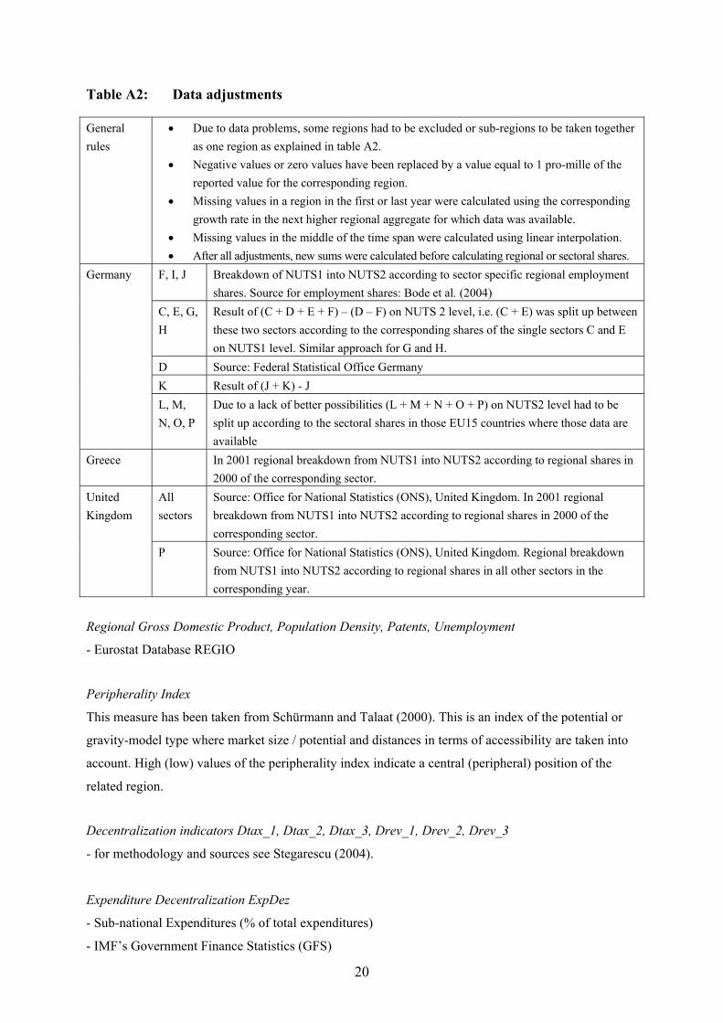
Table A2: Data adjustments

General rules

• Due to data problems, some regions had to be excluded or sub-regions to be taken together as one region as explained in table A2.

• Negative values or zero values have been replaced by a value equal to 1 pro-mille of the reported value for the corresponding region.

• Missing values in a region in the first or last year were calculated using the corresponding growth rate in the next higher regional aggregate for which data was available.

• Missing values in the middle of the time span were calculated using linear interpolation. • After all adjustments, new sums were calculated before calculating regional or sectoral shares.

F, I, J Breakdown of NUTS1 into NUTS2 according to sector specific regional employment shares. Source for employment shares: Bode et al. (2004)

C, E, G, H

Result of (C + D + E + F) – (D – F) on NUTS 2 level, i.e. (C + E) was split up between these two sectors according to the corresponding shares of the single sectors C and E on NUTS1 level. Similar approach for G and H.

D Source: Federal Statistical Office Germany K Result of (J + K) - J

Germany

L, M, N, O, P

Due to a lack of better possibilities (L + M + N + O + P) on NUTS2 level had to be split up according to the sectoral shares in those EU15 countries where those data are available

Greece In 2001 regional breakdown from NUTS1 into NUTS2 according to regional shares in 2000 of the corresponding sector.

All sectors

Source: Office for National Statistics (ONS), United Kingdom. In 2001 regional breakdown from NUTS1 into NUTS2 according to regional shares in 2000 of the corresponding sector.

United Kingdom

P Source: Office for National Statistics (ONS), United Kingdom. Regional breakdown from NUTS1 into NUTS2 according to regional shares in all other sectors in the corresponding year.

Regional Gross Domestic Product, Population Density, Patents, Unemployment

- Eurostat Database REGIO

Peripherality Index

This measure has been taken from Schürmann and Talaat (2000). This is an index of the potential or

gravity-model type where market size / potential and distances in terms of accessibility are taken into

account. High (low) values of the peripherality index indicate a central (peripheral) position of the

related region.

Decentralization indicators Dtax_1, Dtax_2, Dtax_3, Drev_1, Drev_2, Drev_3

- for methodology and sources see Stegarescu (2004).

Expenditure Decentralization ExpDez

- Sub-national Expenditures (% of total expenditures)

- IMF’s Government Finance Statistics (GFS)

21

- downloadable from the official website of the Worldbank: Decentralization and Subnational

Regional Economics: http://www1.worldbank.org/publicsector/decentralization/fiscalindicators.htm

Transfers

- Transfers to sub-national from other levels of Government (% of total sub-national revenues and grants)

- IMF’s Government Finance Statistics (GFS)

- downloadable from the official website of the Worldbank: Decentralization and Subnational

Regional Economics: http://www1.worldbank.org/publicsector/decentralization/fiscalindicators.htm

Efficiency

- Success Index (Suc) of the Bertelsmann Stiftung

Being the core measure for the International Employment and Growth Ranking of the Bertelsmann

Stiftung it contains variables of labour market performance and economic growth. Values range from

0 to 120 with higher values indicating better performance.

- Activity Index (Act) of the Bertelsmann Stiftung

This measure focus on 12 indicators of three areas of activity: “labour market, government and

economy, economy and labour and management” and takes values from 0 to 120 where higher values

indicate a better performance.

Both measure are only available on a national basis.

- for a summary and the methodological background see:

http://www.bertelsmann-stiftung.de/de/4303_8886.jsp

Table. A3: Regional disaggregation

Member State NUTS-level No. of Regions Member State NUTS-level No. of Regions Austria (AT) 2 9 Italy (IT)24 2 20 Belgium (BE) 2 11 Netherlands (NL) 2 12 Finland (FI) 2 5 Portugal (PT)25 2 5 France26 (FR) 2 22 Spain (ES)27 2 16 Germany (DE)28 2 40 Sweden (SE) 2 8 Greece (GR) 2 13 United Kingdom 2 37 Ireland (IE) 2 2

As data are not yet sufficiently available for ITd1 (Provincia Autonoma Bolzano-Bozen) and ITd2 (Provincia

Autonoma Trento) separately, we have taken them as 1 region by subtracting ITd3, ITd4 and ITd5 from ITd. 25 PT20 (Região Autónoma dos Açores) and PT30 (Região Autónoma da Madeira) have been excluded. 26 Overseas departments have been excluded.

27 ES63 (Ciudad Autónoma de Ceuta) and ES64 (Ciudad Autónoma de Melilla) as well as ES70 (Canarias) have been excluded.

The new division of DE40 (Brandenburg) has not been taken into account due to several missing data for the subregions.

22

Table A4: Descriptive Statistics of the specialization and decentralization indicators

23

Table A5: Robustness Tests, tax revenue decentralization, POLS and GLS

Dj POLS IV POLS V POLS3 VI GLS IV GLS V GLS VI Dtax_1 Dtax_2 Dtax_3 ExpDez Act RGDP Density Unemp PerInd Patents dum_capital Constant

-0.07 (0.63) 0.022 (0.14) -0.004 (0.08) 0.134 (3.59)** 0.001 (5.37)** 0.072 (2.04)* -0.044 (10.11)** (0.001) (2.71)** 0.073 (0.09) 15.132 (3.10)**

-0.117 (0.77) -0.007 (0.04) -0.01 (0.17) 0.133 (3.54)** 0.001 (5.38)** 0.073 (2.05)* -0.044 (10.10)** -0.001 (2.69)** 0.076 (0.1) 16.134 (3.13)**

-0.084 (0.8) 0.04 (0.25) -0.01 (0.17) 0.135 (3.60)** 0.001 (5.37)** 0.071 (2.01)* -0.044 (10.12)** -0.001 (2.68)** 0.069 (0.09) 15.922 (3.16)**

-0.066 (3.04)** 0.067 (2.12)* 0.000 (0.01) 0.017 (1.08) 0.001 (2.75)** 0.039 (1.68) -0.044 (4.51)** 0.001 (2.49)* 0.227 (0.13) 15.963 (6.63)**

-0.142 (4.75)** 0.035 (1.08) -0.009 (0.74) 0.01 (0.69) 0.001 (2.79)** 0.048 (2.09)* -0.044 (4.51)** 0.001 (2.75)** 0.209 (0.12) 17.24 (7.12)**

-0.099 (4.93)** 0.087 (2.76)** -0.004 (0.32) 0.013 (0.89) 0.001 (2.75)** 0.03 (1.33) -0.045 (4.57)** 0.001 (3.16)** 0.188 (0.1) 16.88 (6.99)**

No. of observations

1067 1067 1067 1067 1067 1067


0.32 0.32 0.32 0.19 0.0000

0.20 0.0000

0.20 0.0000

Absolute value of z statistics in parentheses* significant at 5%; ** significant at 1%


24

Table A6: Robustness Tests, tax revenue decentralization, fixed effects

Dj FE IV FE V FE VI Dtax_1 Dtax_2 Dtax_3 ExpDez Act RGDP Density Unemp Patents Constant

-0.065 (2.99)** 0.067 (2.11)* 0.003 (0.25) 0.018 (1.15) -0.003 (1.41) 0.037 (1.55) 0.001 (2.91)** 10.749 (7.78)**

-0.142 (4.75)** 0.035 (1.08) -0.006 (0.48) 0.012 (0.77) -0.003 (1.41) 0.047 (1.97)* 0.001 (3.18)** 15.027 (8.76)**

-0.101 (5.03)** 0.087 (2.76)** 0.000 (0.04) 0.015 (0.97) -0.003 (1.52) 0.028 (1.21) 0.001 (3.62)** 12.433 (8.69)**


Absolute value of t statistics in parentheses* significant at 5%; ** significant at 1%

Table A7: Robustness Test, public revenue decentralization, fixed effects

Dj FE VII FE VIII FE IX Drev_1 Drev_2 Drev_3 Transfers Suc RGDP Density Unemp Patents Constant

-0.036 (1.56) 0.014 (1.49) -0.008 (0.75) 0.031 (1.9) -0.003 (1.61) 0.004 (0.03) 0.001 (0.07) 13.06 (9.55)**

-0.071 (2.28)* 0.01 (1.08) -0.01 (0.95) 0.025 (1.51) -0.003 (1.54) 0.017 (0.13) 0.004 (0.18) 14.547 (9.07)**

-0.085 (2.59)** -0.011 (0.75) -0.009 (0.82) 0.022 (1.31) -0.003 (1.48) -0.004 (0.03) -0.001 (0.04) 15.999 (8.41)**


Absolute value of t statistics in parentheses* significant at 5%; ** significant at 1%

25

Table A8: Robustness Tests, public revenue decentralization, POLS and GLS

Dj POLS VII POLS VIII POLS IX GLS VII GLS VIII GLS IX Drev_1 Drev_2 Drev_3 Transfers Suc RGDP Density Unemp PerInd Patents dum_capital Constant

0.039 (0.32) 0.025 (0.54) -0.049 (0.86) 0.283 (7.32)** 0.001 (3.27)** 0.223 (1.00) -0.696 (8.25)** -0.244 (10.13)** 1.362 (1.79) 19.82 (3.50)**

0.075 (0.46) 0.029 (0.6) -0.046 (0.8) 0.285 (7.31)** 0.001 (3.25)** 0.219 (0.98) -0.697 (8.26)** -0.244 (10.14)** 1.358 (1.78) 19.22 (3.25)**

0.063 (0.37) 0.041 (0.57) -0.047 (0.82) 0.284 (7.27)** 0.001 (3.25)** 0.223 (1.00) -0.697 (8.25)** -0.244 (10.13)** 1.356 (1.78) 18.732 (2.77)**

-0.036 (1.55) 0.011 (1.17) -0.009 (0.85) 0.036 (2.29)* 0.001 (2.50)* 0.008 (0.06) -0.897 (4.99)** -0.024 (1.23) 1.069 (0.62) 20.803 (8.35)**

-0.071 (2.24)* 0.007 (0.77) -0.011 (1.05) 0.031 (1.91) 0.001 (2.54)* 0.02 (0.16) -0.897 (4.99)** -0.021 (1.12) 1.059 (0.61) 21.299 (8.50)**

-0.088 (2.67)** -0.015 (1.02) -0.01 (0.92) 0.027 (1.67) 0.001 (2.57)* 0.004 (0.03) -0.889 (4.95)** -0.025 (1.32) 1.105 (0.64) 22.444 (8.72)**

No. of observations

987 987 987 987 987 987


0.31 0.31 0.31 0.20 0.0000

0.20 0.0000

0.20 0.0000


Fiscal Design and the Location of Economic Activity

Documents

Transcript of Fiscal Design and the Location of Economic Activity