New economic geography meets Comecon. Regional wages and industry location in central Europe1

New Economic Geography Meets Comecon:

Regional Wages and Industry Location in Central Europe∗

Marius Brulhart † Pamina Koenig ‡

January 28, 2005

Abstract

We analyze the internal spatial wage and employment structures of the Czech Republic,Hungary, Poland, Slovenia and Slovakia, using regional data for 1996-2000. A new economicgeography model predicts wage gradients and specialization patterns that are smoothlyrelated to regions’ relative market access. As an alternative, we formulate a “Comecon hy-pothesis”, according to which wages and sectoral location are not systematically related tomarket access except for discrete concentrations in capital regions. Our estimations confirmthe ongoing relevance of the Comecon hypothesis: compared to pre-2004 EU members, Cen-tral European countries’ average wages and service employment were still discretely higherin capital regions. Our results point towards an increase in relative wages and employmentshares of Central Europe’s provincial regions, favoring particularly those that are proximateto the large markets of incumbent EU members.

JEL classification: P25, R12.Keywords: regional wages, industry location, transition economies, Central Europe, New Eco-nomic Geography.

∗We thank Lionel Fontagne and Soledad Zignago for useful comments, and Roman Romisch, MonikaSchwarhappel and Peter Huber for the generous provision of data. In addition, we have benefited from use-ful comments made by participants at the 2004 CEPR conference on economic geography in Villars.

†DEEP-HEC, University of Lausanne ([email protected]). Also affiliated with the Centre for EconomicPolicy Research, London.

‡CREST and University of Paris I ([email protected]).

1

1 Introduction

After the overthrow of their socialist regimes in 1989-90, most Central and Eastern Europeancountries (CEECs) have rapidly adopted market-based economic systems and redirected thefocus of their political and economic relations towards the European Union. This process hasculminated in the accession to the EU of eight CEECs in 2004. One of the main benefits of EUenlargement will be to boost economic activity, both in accession countries and in incumbentmember states. Lower barriers to trade yield gains that are well understood by economists andestimated to be significant (see e.g. Baldwin et al., 1997).

Although the potential for aggregate economic gains through closer economic integrationin Europe is undisputed, economists also acknowledge that integration transforms the internalstructures of national economies, which can have important distributional consequences. Onedimension of integration-induced restructuring concerns geography. How does European inte-gration impact on the spatial distribution of activities, prices and incomes across regions? Thisquestion has been the object of a thriving research area in recent years.

It is somewhat surprising, given the vibrancy of the research field and the importance of theissue, that relatively little analysis has been conducted on the transforming economic geographiesof CEECs.1 For the academic researcher, these countries present an interesting “laboratorycase”, due to their legacy of centrally planned economic structures and rapid trade reorientationtowards the EU. Is the old spatial organization of those economies unraveling and giving wayto a different geographic distribution of activities, shaped by market forces? If so, what is thenature of these forces, and what new spatial equilibrium is likely to emerge?

We provide an analysis of the internal economic geographies of five CEECs, drawing onregional data for wages and sectoral employment in the Czech Republic, Hungary, Poland,Slovenia and Slovakia. Specifically, we estimate spatial wage and employment gradients insidethose countries based on multi-country new economic geography (NEG) model. In this model,the better a region’s access to large markets (and pools of suppliers), the higher its wages and thegreater its locational attractiveness for mobile trade-oriented sectors. Depending on the precisemodelling assumptions, access to markets will yield either high factor prices, large production,or a mix of both. The wage and output effects of market access are a typical feature of theNEG that sets these models apart from most neoclassical location theory. It makes the NEGapproach eminently suitable as a theoretical framework for the analysis of locational changes inintegrating economies with similar endowments.

As an alternative to the market-driven spatial structure described by the model, we formulatea “Comecon hypothesis”, based on the idea that the artifice of central planning created economicgeographies whose only regularity was a concentration of certain sectors and high wages in thecapital region.

Our estimations based on data for the accession countries support both the NEG predictionand the “Comecon hypothesis”. When we compare internal wage and employment gradientsof accession countries with those of existing EU members, we find that accession countries aremarked by significantly stronger concentrations of wages and of employment in both marketservices and public service sectors in their capital regions. One might therefore conjecture thatmarket forces will in time attenuate those countries’ economic concentration in capital regionsand favor a dispersion of activities and an increase of relative wages in provincial regions -particularly in those that are located close to the core EU markets.

The paper is organized as follows. In section 2, we present the theoretical model thatunderpins our empirical approach and derive the estimable equations. Section 3 documentsthe trade integration of Central European countries with the EU that has already taken place,

1Descriptions of regional location patterns in CEECs have been provided by Resmini (2003) and Traistaru etal. (2003).

2

using a measure of “trade freeness” that is derived from the theory. Our estimations of wageand employment gradients in accession countries and in the full sample of 21 European countriesare given in Section 4. Section 5 concludes.

2 Theory

The NEG provides a well suited framework for a formal analysis of the internal geographyof countries that open their markets towards the outside world. In this section, we sketch thesalient features of a three-region NEG model and derive the fundamental equations that underlieour empirical analysis.

2.1 The model

NEG models rely on four essential ingredients to explain the spatial configuration of economicactivity.2 First, production is subject to increasing returns to scale at the firm level. Second,the goods produced by different firms are imperfect substitutes. Third, firms are symmetricand sufficiently numerous to accommodate monopolistically competitive equilibria. Fourth,trade costs inhibit trade between locations and thereby give economic relevance to otherwisefeatureless geographic space.

An essential feature of these models is that market access acts as the principal determinantof the spatial structure of employment and factor prices. Market access is an increasing functionof a location’s own market size and of the size of other markets, and a decreasing function ofthe trade costs that separates the home location from all other locations. Changes in marketaccess trigger locational forces, which, adopting Head and Mayer’s (2004) terminology, we callthe price version and the quantity version of the market access effect.

The price version can be illustrated as follows. Suppose a typical NEG framework withmultiple locations, a unique production factor in the differentiated sector, industrial labor, andzero mobility of firms and labor. Consumers’ utility increases with the number of varieties. Theamount of variety i consumed by a representative consumer in j is equal to:

xij =(piτij)−σ

P 1−σj

µYj , (1)

where Yj is the total income of region j, σ stands for the elasticity of substitution amonggoods from the competing symmetric firms, and µ is the share of expenditure that consumersallocate to the differentiated sector. Pj is the price index of the differentiated sector in regionj:

Pj ≡[∑

i

ni(piτij)1−σ

] 11−σ

, (2)

where ni is the number of firms in i, pij is the final price paid by consumers in j (pij = piτij),and τ is the ad-valorem ‘iceberg’ cost of shipping goods between regions. Following Baldwin etal. (2003), we express trade costs as τ1−σ

ij ≡ Φij , which is comprised between 0 and 1 and isa measure of the degree of trade freeness between pairs of regions. At Φij = 0 trade costs areprohibitive, and Φij = 1 means perfectly free trade.

2For a comprehensive statement of the underlying modeling structure, see Fujita et al. (1999). Recent studiesof the intra-national spatial effects of trade liberalization in NEG settings include Krugman and Livas (1996),Monfort and Nicolini (2000), Paluzie (2001), Alonso-Villar (2001), Behrens (2003), Crozet and Koenig (2004),and Brulhart et al. (2004).

3

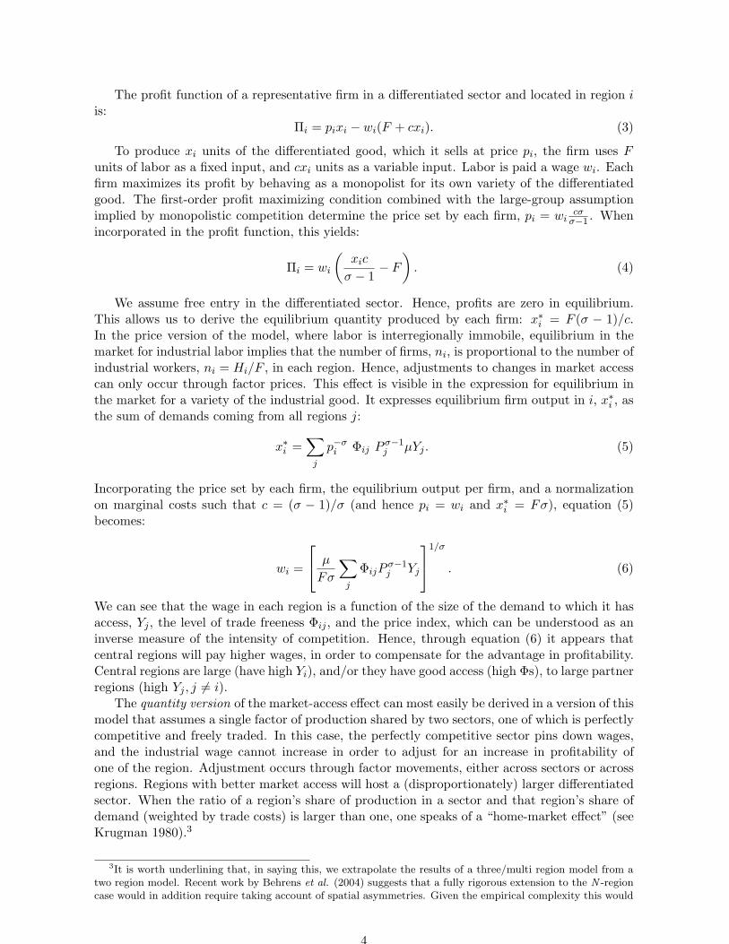
The profit function of a representative firm in a differentiated sector and located in region iis:

Πi = pixi − wi(F + cxi). (3)

To produce xi units of the differentiated good, which it sells at price pi, the firm uses Funits of labor as a fixed input, and cxi units as a variable input. Labor is paid a wage wi. Eachfirm maximizes its profit by behaving as a monopolist for its own variety of the differentiatedgood. The first-order profit maximizing condition combined with the large-group assumptionimplied by monopolistic competition determine the price set by each firm, pi = wi

cσσ−1 . When

incorporated in the profit function, this yields:

Πi = wi

(xic

σ − 1− F

). (4)

We assume free entry in the differentiated sector. Hence, profits are zero in equilibrium.This allows us to derive the equilibrium quantity produced by each firm: x∗i = F (σ − 1)/c.In the price version of the model, where labor is interregionally immobile, equilibrium in themarket for industrial labor implies that the number of firms, ni, is proportional to the number ofindustrial workers, ni = Hi/F , in each region. Hence, adjustments to changes in market accesscan only occur through factor prices. This effect is visible in the expression for equilibrium inthe market for a variety of the industrial good. It expresses equilibrium firm output in i, x∗i , asthe sum of demands coming from all regions j:

x∗i =∑

j

p−σi Φij P σ−1

j µYj . (5)

Incorporating the price set by each firm, the equilibrium output per firm, and a normalizationon marginal costs such that c = (σ − 1)/σ (and hence pi = wi and x∗i = Fσ), equation (5)becomes:

wi =

µ

Fσ

∑

j

ΦijPσ−1j Yj

1/σ

. (6)

We can see that the wage in each region is a function of the size of the demand to which it hasaccess, Yj , the level of trade freeness Φij , and the price index, which can be understood as aninverse measure of the intensity of competition. Hence, through equation (6) it appears thatcentral regions will pay higher wages, in order to compensate for the advantage in profitability.Central regions are large (have high Yi), and/or they have good access (high Φs), to large partnerregions (high Yj , j 6= i).

The quantity version of the market-access effect can most easily be derived in a version of thismodel that assumes a single factor of production shared by two sectors, one of which is perfectlycompetitive and freely traded. In this case, the perfectly competitive sector pins down wages,and the industrial wage cannot increase in order to adjust for an increase in profitability ofone of the region. Adjustment occurs through factor movements, either across sectors or acrossregions. Regions with better market access will host a (disproportionately) larger differentiatedsector. When the ratio of a region’s share of production in a sector and that region’s share ofdemand (weighted by trade costs) is larger than one, one speaks of a “home-market effect” (seeKrugman 1980).3

3It is worth underlining that, in saying this, we extrapolate the results of a three/multi region model from atwo region model. Recent work by Behrens et al. (2004) suggests that a fully rigorous extension to the N -regioncase would in addition require taking account of spatial asymmetries. Given the empirical complexity this would

4

2.2 The estimable equations

Our approach is based on a reduced-form estimation of the market access effect describedby the wage equation (6). This equation states that, in equilibrium, the nominal wage of aregion i depends on the size of demand in each accessible market, multiplied by the intensityof competition in each of these markets, and weighted by the accessibility of each market. Inour estimations, we focus on τij as the essential characteristic that distinguishes regions’ marketaccess. The ideal empirical counterpart of τij would be, for each region of interest, a measureof the level of trade costs with all existing outside potential markets as well as internally. Wesimplify this task by choosing, as in Hanson (1996, 1997), the access of each considered regionto its principal markets, approximated by geographic distance.

Which are these principal markets in the case of the Central European countries? Beforethe dismantling of the Soviet bloc, those countries’ trade was mainly focused on intra-Comecon(Council for Mutual Economic Cooperation) relationships. However, market forces played a mi-nor role in shaping wages and location patterns compared to the importance of central planning.The explanatory power of market-based economic models, such as those of the NEG, regardingthose countries’ internal economic geographies prior to their conversion to market systems inthe 1990s is therefore likely to be limited. By their very nature, however, centrally plannedeconomies tend to be strongly centered on the capital region. We therefore formulate a “Come-con hypothesis” as the reference point for our analysis: under central planning, nominal wagesas well as employment shares of sectors that are closely linked to the central authorities aresignificantly higher in the capital regions but they are otherwise unrelated to market access. Inother words, our Comecon hypothesis implies a discrete jump in wages and employment sharesbetween the capital region and the provinces and no systematic patterns among the provinces.

In contrast, according to the NEG prediction embodied in (6), wages should rise smoothlyin market access. We model market access in terms of regions’ distances (i) from their relativenational capitals and (ii) from the EU, whose economic center of gravity we take to be Brussels.Continuous gradients of wages and/or employment shares relative to regions’ market access are ageneral prediction of NEG models that we take as the alternative to our “Comecon hypothesis”.We thus specify the following reduced-form expression for region i’s relative wage:

wi

wcapital= f (Φicapital, ΦiEU, capdum, other market access variables) , (7)

where wi is the regional nominal wage; wcapital is the wage in the capital; Φicapital and ΦiEU

denote trade freeness between i and, respectively, the EU and the national capital; and capdumis a dummy for the capital region. We use distance to represent trade freeness, and we specifya log-linear relation between the variables. Our first estimable equation is:

ln(

wi

wcapital

)= β0 + β1 ln(dicapital) + β2 ln(diEU) + β3(capdum) + ~β ~Xi + εi, (8)

where ~X is a vector of other variables that determine market access, and εi is an error termthat consists of a country effect, a year effect and a white noise component. Based on the NEGmodel, we expect the estimated β1 and β2 to be negative.4 The Comecon hypothesis, in turn,implies a significantly positive β3 and insignificant β1 and β2.

Our second estimable equation focuses on the quantity version of the market access effect.As emphasized in section (2.1), in this variant of NEG models, the adjustment variable is the

entail, we choose to abstract from the issue here, leaving an examination of its relevance to future work.4Note that in estimating a single equation for average wages across sectors - a choice necessitated by data

constraints - we imply the assumption that labor is intersectorally mobile.

5

number of firms. Hence, regions with relatively good access to the main markets will have therelative high share of employment in differentiated sectors. We write the following reduced-formexpression, which holds for regional relative employment inside an accession country:

lsi

popi= gs(Φicapital, ΦiEU, capdum, other market access variables). (9)

lsi is employment in sector s and region i, and popi is the region’s population. The right-handside variables have been defined in (7). As for equation (8), we specify a log-linear relationbetween our variables and use distance to represent the trade costs. Our second estimableequation is

ln(

lsi

popi

)= αs0 + αs1 ln(dicapital) + αs2 ln(diEU) + α(s3)(capdum) + ~αs

~Xi + εsi , (10)

where we make the same assumptions on the structure of εi.

3 Trade freeness between the EU and the CEECs

Before analyzing spatial employment and wage patterns, we seek to quantify the gradual processof economic integration between the EU and the CEECs during the 1990s in a way that isconsistent with the theory.

Starting from a multi-country version of the monopolistic-competition model outlined above,Head and Mayer (2004) have derived an expression of Φij that can be estimated empiricallywith trade and production data. The first step involves dividing country j’s imports from i(mij) by its imports from itself (mjj) so as to eliminate unobservable importer-specific effects.This ratio is then multiplied by the corresponding ratio for country i, yielding:

mijmji

mjjmii=

ΦijΦji

ΦjjΦii. (11)

Two more assumptions are needed to derive the final expression. First, trade inside countriesis assumed to be frictionless, thus Φii = Φjj = 1. Second, trade barriers between countries areset to be symmetric, i.e. Φij = Φji. The expression for the measure of trade freeness betweencountries i and j is then:5

Φij =√

mijmji

mjjmii. (12)

We calculate measures of trade freeness for different pairs of countries of the EU and theCEECs, using aggregate manufacturing trade flows. Imports of a country from itself are cal-culated as the value of manufacturing production minus the value of manufacturing exports.Production and trade data are taken from the international database constructed and madeavailable by the World Bank.6

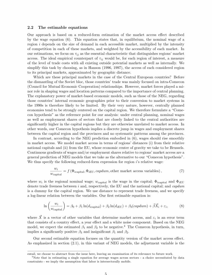
Figure 1 depicts the evolution of the median trade freeness of a sample of CEECs relative tothe EU’s four biggest economies (France, Germany, Italy and the United Kingdom, henceforthEU-4). We also report estimated trade freeness between Spain and these countries as a pointof comparison. We discern two interesting features. First, the trade freeness towards the EUappears to be remarkably similar among CEECs, and to follow a consistent trend: whereas

5The measure of trade freeness differs from conventional measures of trade openness in the sense that theformer does not depend on the size of countries.

6See Nicita and Olarreaga (2001). This database has been completed by the CEPII. We are grateful to SoledadZignago for providing that extended dataset to us.

6

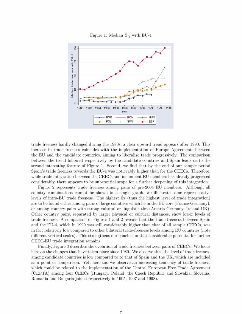
Figure 1: Median Φij with EU-4

0.0

1.0

2.0

3.0

4M

edia

n tra

de fre

eness

with

EU

−4

1980 1982 1984 1986 1988 1990 1992 1994 1996 1998 2000year

BGR ROM HUNPOL SVN ESP

trade freeness hardly changed during the 1980s, a clear upward trend appears after 1990. Thisincrease in trade freeness coincides with the implementation of Europe Agreements betweenthe EU and the candidate countries, aiming to liberalize trade progressively. The comparisonbetween the trend followed respectively by the candidate countries and Spain leads us to thesecond interesting feature of Figure 1. Second, we find that by the end of our sample periodSpain’s trade freeness towards the EU-4 was noticeably higher than for the CEECs. Therefore,while trade integration between the CEECs and incumbent EU members has already progressedconsiderably, there appears to be substantial scope for a further deepening of this integration.

Figure 2 represents trade freeness among pairs of pre-2004 EU members. Although allcountry combinations cannot be shown in a single graph, we illustrate some representativelevels of intra-EU trade freeness. The highest Φs (thus the highest level of trade integration)are to be found either among pairs of large countries which lie in the EU core (France-Germany),or among country pairs with strong cultural or linguistic ties (Austria-Germany, Ireland-UK).Other country pairs, separated by larger physical or cultural distances, show lower levels oftrade freeness. A comparison of Figures 1 and 2 reveals that the trade freeness between Spainand the EU-4, which in 1999 was still considerably higher than that of all sample CEECs, wasin fact relatively low compared to other bilateral trade-freeness levels among EU countries (notedifferent vertical scales). This strengthens our conclusion that considerable potential for furtherCEEC-EU trade integration remains.

Finally, Figure 3 describes the evolution of trade freeness between pairs of CEECs. We focushere on the changes that have taken place since 1989. We observe that the level of trade freenessamong candidate countries is low compared to to that of Spain and the UK, which are includedas a point of comparison. Yet, here too we observe an increasing tendency of trade freeness,which could be related to the implementation of the Central European Free Trade Agreement(CEFTA) among four CEECs (Hungary, Poland, the Czech Republic and Slovakia; Slovenia,Romania and Bulgaria joined respectively in 1995, 1997 and 1998).

7

Figure 2: Intra EU Φij

0.0

5.1

.15

.2.2

5T

rade fre

eness

1980 1982 1984 1986 1988 1990 1992 1994 1996 1998 2000year

FRA DEU AUT DEU ITA GBRIRL GBR ITA ESP

Figure 3: ESP-GBR and Intra CEECs Φij

0.0

1.0

2.0

3T

rade fre

eness

1989 1990 1991 1992 1993 1994 1995 1996 1997 1998 1999year

HUN POL HUN SVN SVN POLPOL BGR GBR ESP

8

4 Wage and Employment Gradients

As Section 3 has shown, the increasing integration of CEEC economies with the EU over the1990s is clearly evident in the data. We now explore to what extent regional wages and employ-ment patterns inside Central European countries already reflected the new geography of marketaccess in the second half of that decade.

4.1 The geography of wages and employment in CEECs

4.1.1 Wages

In this section we study the impact of market access on regional wages in the Czech Republic,Hungary, Poland, Slovenia and Slovakia, using annual data for 1996-2000 (see Appendix A forfurther details). We estimate equation (8) as a reduced form of the NEG model. All estimatedstandard errors are based on White-corrected variance-covariance matrices, since most of ourregression models are clearly heteroskedastic (mainly due to different disturbance variancesacross countries).

Table 1: Regional wage gradients in CEECs, panel

Dependent Variable: ln(wi/wCAP)Model : (1) (2) (3)ln dist. to Capital -0.109 -0.034 -0.041

(-10.69) (-4.46) (-5.35)ln dist. to Brussels -0.009 -0.097 -0.021

(-0.18) (-3.10) (-0.56)Capital 0.287 0.282

(12.51) (13.33)Land border with EU, N, CH 0.027

(3.52)Land border with CEEC 0.006

(0.64)Access to sea 0.069

(3.22)CtrDum Yes Yes YesYrDum Yes Yes YesN 248 248 248R2 0.677 0.824 0.838Note: t-statistics in parentheses

The first column of Table 1 reports the simplest specification that includes merely the twodistance terms.7 The results suggest that wages fall off with distance from national capitals butnot with distance from the EU.

This model, however, is overly parsimonious. According to our “Comecon hypothesis”, wagesin centrally planned economies are higher in the capital region, but there is no compelling reasonfor expecting wages to fall off smoothly across provincial regions as they become more remotewith respect to the capital. Hence, the second specification includes a dummy variable for

7We use great circle distances from the largest town in each region.

9

capital regions, to allow for the possibility of a discontinuous relationship between wages anddistance to the capital.8 Our results reported in the second column of Table 1 show that wagegradients are indeed discontinuous: being a capital region raises relative nominal wages by 29percent, ceteris paribus. However, distance from the capital matters also in the provinces. Inprovincial regions, relative wages fall by 0.3 percent for every 10 percent increase in distancefrom the capital. It also turns out in this second regression model that proximity to the EU hada statistically significantly positive impact on regional wages in our sample countries already inthe late 1990s, a mere half-decade after those countries’ economic reorientation. A 10 percentincrease in distance from Brussels was associated with 0.3 percent fall in relative regional wages.

Our final specification of the wage equation, reported in column 3 of Table (1), includesadditional variables intended to represent market access: (i) a dummy for regions that share aland border with an EU country, in order to represent potentially discontinuous wage gradientsalso with respect to access to EU markets; (ii) a dummy for regions that share a land border withanother accession country,9 representing the potential importance of those markets; and (iii)a dummy for coastal regions, representing facilitated market access for goods transported bysea. We find that wage gradients relative to the EU are in fact entirely a phenomenon of higherrelative wages in border regions (+ 2.7 percent, ceteris paribus), as distance to Brussels hasno statistically significant effect on wages in non-border regions. Bordering another accessioncountry, however, has no significant impact on wages, while sea access is associated with a 6.9percent higher relative wage level.

In Table 2, we show results of our full model, estimated separately for each of the five CEECsin our sample. The most striking result is the consistent wage advantage of central regions. Theestimated effect ranges from 21 percent (Slovenia) to 44 percent (Poland) and is statisticallysignificant throughout.10

The wage effect of access to the EU market is more varied across sample countries. Proximityto the EU market has the strongest wage-boosting impact in Hungary, where relative wagesare statistically significantly higher in border regions and fall off significantly with distance innon-border regions. Evidence of a wage boost through proximity is also found for Slovenia,where distant regions have significantly lower wages, and Slovakia, where border regions havesignificantly higher wages. The results are ambiguous for Poland, where we estimate a negativewage premium for border regions, and the Czech Republic, where distance from the EU seemsto raise relative wages.

What we retain from the analysis of regional wage gradients in accession countries is thatthe nominal wage bonus of capital regions is highly significant in both economic and statisticalterms. This is consistent with our “Comecon hypothesis”. We also find some wage-boostingeffects of market access to the EU, but these effects are statistically and economically lesssignificant, and they apply less consistently across sample countries.

4.1.2 Sectoral employment

Using regional employment data for nine sectors covering the full spectrum of economic activi-ties, we have estimated equation (10). The estimation results are reported in Table 3.

8The inclusion of this dummy variable has the further advantage of reducing the estimations’ sensitivity to theway we model intra-regional distance in the capital regions. We model these distances as dii = 0.67sqrt(area/π).The underlying assumption is that intra-regional economic geographies can be approximated by a disk where allfirms are located at the center and consumers are spread uniformly over the area.

9For the construction of this dummy variable, we considered as accession countries our five sample countriesplus Romania and Lithuania.

10The estimated magnitudes of these effects are affected by the way one models intra-regional distances in thecapital regions. If our formula overestimates effective internal distances, the coefficient on the capital dummy willalso be overestimated. We have experimented with smaller estimated intra-regional distances and found that theestimated capital-region effects remained very strong.

10

Table 2: Regional wage gradients in CEECs, by country

Dependent Variable: ln(wi/wCAP)Model : (A) (B) (C) (D) (E)ln dist. to Capital -0.043 -0.075 0.048 0.016 -0.004

(-2.74) (-6.47) (1.59) (0.97) (-0.19)Capital 0.295 0.240 0.439 0.214 0.340

(6.82) (6.19) (18.00) (15.88) (17.01)ln dist. to Brussels 0.218 -0.256 -0.105 -0.775 0.118

(3.91) (-3.55) (-1.42) (-2.97) (0.47)Land border with EU, N, CH 0.038 0.057 -0.062 -0.016 0.058

(4.43) (2.86) (-3.12) (-1.12) (3.11)Land border with CEEC -0.025 -0.005 0.024 -0.040 0.000

(-1.35) (-0.30) (1.50) (-2.23) (0.0)Access to sea 0.000 0.000 0.020 0.098 0.000

(0.0) (0.0) (1.21) (5.74) (0.0)CtrDum Yes Yes Yes Yes YesYrDum Yes Yes Yes Yes YesN 56 80 32 48 32R2 0.904 0.79 0.937 0.833 0.886Note: t-statistics in parentheses

Model A: Czech Republic, Model B: Hungary, Model C: PolandModel D: Slovenia, Model E: Slovakia

Since we are regressing employment shares in regional population, simple adding-up con-straints make it impossible for the coefficients on any of the dummy variables to have the samesign across sectors. For example, unless the provinces suffered from massive unemployment, itis impossible to find all sectors as being relatively concentrated in the capital regions. Indeed, itcomes as no surprise that the share of agricultural employment is 78 percent smaller in capitalregions than elsewhere and increases by 4.5 percent with every 10 percent increase in distancefrom the capital.

Given the standard labelling of the differentiated sectors in NEG models as “manufacturing”,it might be less expected that manufacturing too accounts for a significantly smaller employmentshare in capital regions than in the provinces (-28 percent). Furthermore, manufacturing is notdiscretely larger in regions bordering the EU and is actually significantly smaller than elsewherein coastal regions (-38 percent). The regional distribution of manufacturing employment does,however, conform with the NEG prediction in so far as it rises continuously with proximityto the EU: every 10 percent increase in distance from Brussels appears to reduce the share ofmanufacturing employment by 9 percent. This is an effect that is very strong both economicallyand statistically, and it suggests that manufacturing activities in accession countries is alreadystrongly oriented towards the EU market.

Interestingly, our market-access model of employment shares has greatest explanatory powerin tertiary sectors. Distribution (which comprises both wholesale and retail trades) standsout with the highest R-square and estimated coefficients suggesting that employment in thedistribution sector is significantly concentrated in capital regions, border regions and coastalregions. According to our findings, therefore, distribution appears as the sector most affected

11

Table 3: Regional employment gradients in CEECs, by sector

Dependent Variable: ln(li/popi)Model : (F) (G) (H) (I) (J) (K) (L) (M)ln dist. to Capital 0.451 0.012 0.062 0.007 0.026 -0.028 0.115 0.069

(5.94) (0.33) (1.89) (0.23) (0.44) (-0.42) (3.27) (3.49)Capital -0.781 -0.281 0.644 0.890 0.973 1.555 1.513 0.663

(-2.85) (-2.96) (9.15) (12.76) (6.42) (8.52) (17.76) (9.59)ln dist. to Brussels -0.488 -0.896 -0.685 -0.168 -0.301 0.411 -0.414 0.126

(-1.24) (-5.30) (-3.35) (-0.93) (-1.08) (0.99) (-1.93) (1.45)Land border with EU, N, CH 0.006 -0.027 0.001 0.065 0.128 0.175 0.185 0.066

(0.04) (-0.73) (0.03) (1.59) (1.98) (2.09) (4.12) (3.50)Land border with CEEC -0.237 0.056 0.050 0.074 0.013 -0.095 -0.016 -0.048

(-3.09) (1.48) (1.08) (1.70) (0.20) (-1.15) (-0.37) (-2.67)Access to sea -0.135 -0.381 0.029 0.227 0.643 0.287 0.357 0.055

(-0.79) (-4.19) (0.45) (2.91) (3.78) (2.00) (2.99) (1.81)Ctrdum Yes Yes Yes Yes Yes Yes Yes YesYrdum Yes Yes Yes Yes Yes Yes Yes YesN 240 240 240 240 240 240 240 240R2 0.65 0.597 0.722 0.78 0.575 0.722 0.737 0.667Note: t-statistics in parentheses

Model F: Agriculture, Model G: Manufacturing, Model H: ConstructionModel I: Distribution, Model J: Transport and CommunicationModel K: Banking and Insurance, Model L: Other market servicesModel M: Non-market services

by market access considerations.11

4.2 A comparison with pre-2004 EU members

We have estimated wage and employment gradients in Central European accession countries,and we found confirmation that market access matters for wages and sectoral employment. Ourresults are at least partly consistent with both a central-planning explanation, which implies adiscrete advantage for the capital region, and a market-based NEG model, which implies contin-uous wage and employment gradients on distance from economic centers. This is informative initself, but it raises the question as to which force is likely to dominate in the foreseeable future.Specifically, are the intra-country economic geographies inherited from the central-planning pe-riod likely to persist, or are market forces pushing towards a spatial reorganization of CentralEuropean economies? Note that modern location theory offers little guidance on such practicalquestions, since NEG models typically feature multiple locally stable equilibria. If the worldis indeed marked by strong locational discontinuities, unchanging economic geographies in ac-cession countries could well be consistent with NEG models. Spatial stability would simplyimply that the increase in market access to the EU has been insufficient to dislodge the spatialequilibrium inherited from the days of Comecon.

There are two analytical approaches to this issue. One is to track the evolution of spatialpatterns in Central European countries over time since their transition in the early 1990s, andto extrapolate. We prefer a second approach, which is both less dependent on assumptionsabout timing and unaffected by the fact that the time dimension of our data panel is relatively

11Country-by-country regressions of the employment equation are reported in Appendix B.

12

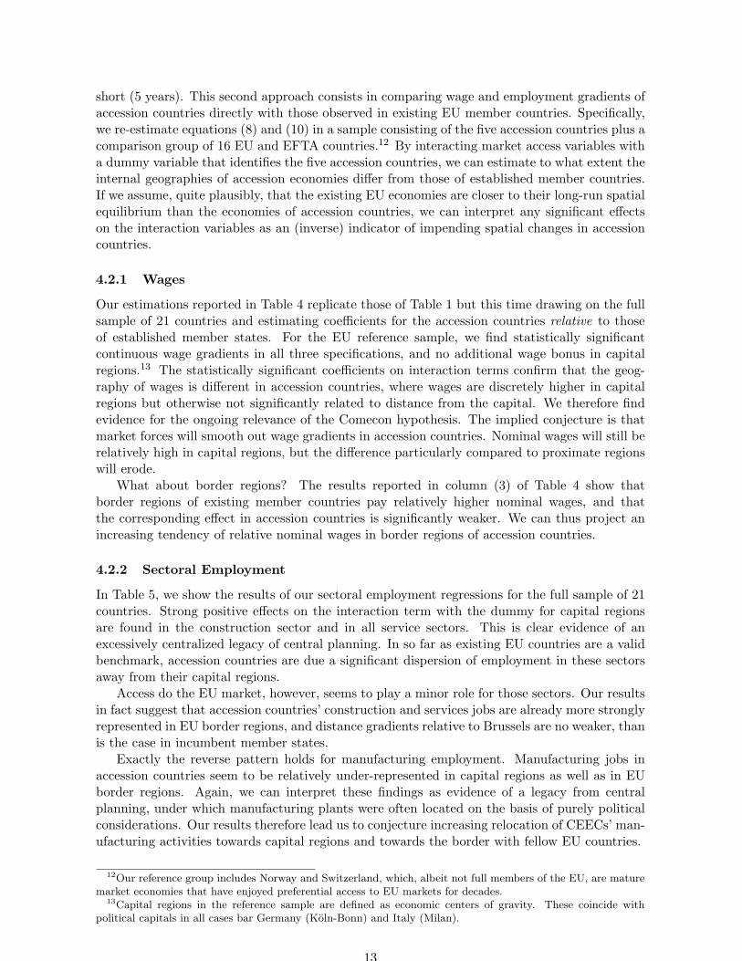
short (5 years). This second approach consists in comparing wage and employment gradients ofaccession countries directly with those observed in existing EU member countries. Specifically,we re-estimate equations (8) and (10) in a sample consisting of the five accession countries plus acomparison group of 16 EU and EFTA countries.12 By interacting market access variables witha dummy variable that identifies the five accession countries, we can estimate to what extent theinternal geographies of accession economies differ from those of established member countries.If we assume, quite plausibly, that the existing EU economies are closer to their long-run spatialequilibrium than the economies of accession countries, we can interpret any significant effectson the interaction variables as an (inverse) indicator of impending spatial changes in accessioncountries.

4.2.1 Wages

Our estimations reported in Table 4 replicate those of Table 1 but this time drawing on the fullsample of 21 countries and estimating coefficients for the accession countries relative to thoseof established member states. For the EU reference sample, we find statistically significantcontinuous wage gradients in all three specifications, and no additional wage bonus in capitalregions.13 The statistically significant coefficients on interaction terms confirm that the geog-raphy of wages is different in accession countries, where wages are discretely higher in capitalregions but otherwise not significantly related to distance from the capital. We therefore findevidence for the ongoing relevance of the Comecon hypothesis. The implied conjecture is thatmarket forces will smooth out wage gradients in accession countries. Nominal wages will still berelatively high in capital regions, but the difference particularly compared to proximate regionswill erode.

What about border regions? The results reported in column (3) of Table 4 show thatborder regions of existing member countries pay relatively higher nominal wages, and thatthe corresponding effect in accession countries is significantly weaker. We can thus project anincreasing tendency of relative nominal wages in border regions of accession countries.

4.2.2 Sectoral Employment

In Table 5, we show the results of our sectoral employment regressions for the full sample of 21countries. Strong positive effects on the interaction term with the dummy for capital regionsare found in the construction sector and in all service sectors. This is clear evidence of anexcessively centralized legacy of central planning. In so far as existing EU countries are a validbenchmark, accession countries are due a significant dispersion of employment in these sectorsaway from their capital regions.

Access do the EU market, however, seems to play a minor role for those sectors. Our resultsin fact suggest that accession countries’ construction and services jobs are already more stronglyrepresented in EU border regions, and distance gradients relative to Brussels are no weaker, thanis the case in incumbent member states.

Exactly the reverse pattern holds for manufacturing employment. Manufacturing jobs inaccession countries seem to be relatively under-represented in capital regions as well as in EUborder regions. Again, we can interpret these findings as evidence of a legacy from centralplanning, under which manufacturing plants were often located on the basis of purely politicalconsiderations. Our results therefore lead us to conjecture increasing relocation of CEECs’ man-ufacturing activities towards capital regions and towards the border with fellow EU countries.

12Our reference group includes Norway and Switzerland, which, albeit not full members of the EU, are maturemarket economies that have enjoyed preferential access to EU markets for decades.

13Capital regions in the reference sample are defined as economic centers of gravity. These coincide withpolitical capitals in all cases bar Germany (Koln-Bonn) and Italy (Milan).

13

Table 4: Regional wage gradients in CEECs, CEEC vs EU

Dependent Variable: ln(wi/wctr)Model : (P) (Q) (R)ln dist. to Capital -0.071 -0.065 -0.086

(-7.58) (-5.07) (-6.60)ln dist. to Cap × CEEC -0.037 0.032 0.047

(-2.71) (2.14) (3.15)ln dist. to Brussels 0.085 0.081 0.097

(3.33) (2.89) (3.62)ln dist. to Bru. × CEEC -0.094 -0.178 -0.079

(-1.71) (-4.29) (-1.73)CEEC 0.791 1.030 0.297

(2.20) (3.92) (1.01)Capital 0.030 0.022

(0.69) (0.53)Capital × CEEC 0.257 0.261

(5.23) (5.66)Land border with EU,N,CH 0.071

(5.64)CEEC × Land border with EU,N,CH -0.040

(-2.73)Land border with CEEC -0.018

(-1.75)Access to sea 0.076

(6.96)N 1520 1520 1520R2 0.123 0.138 0.176Note: t-statistics in parentheses

14

Table 5: Regional employment gradients by sector, CEEC vs EU

Dependent Variable: ln(li/popi)Model : (S) (T) (U) (V) (W) (X) (Y) (Z)dcap 0.202 0.049 -0.006 -0.026 -0.028 -0.050 -0.032 0.018

(6.51) (2.83) (-0.60) (-2.40) (-2.52) (-3.86) (-2.93) (1.77)ln dist. to Cap × CEEC 0.215 -0.070 0.072 0.055 0.089 0.031 0.1 66 0.050

(2.72) (-1.66) (2.13) (1.60) (1.53) (0.43) (4.57) (2.30)Capital -1.014 -0.070 -0.080 0.369 0.363 0.297 0.357 0.267

(-9.82) (-1.35) (-2.76) (12.68) (12.39) (9.47) (12.56) (7.19)Capital × CEEC 0.219 -0.225 0.726 0.532 0.631 1.265 1.167 0.397

(0.76) (-1.92) (9.55) (6.72) (4.19) (7.05) (12.91) (5.09)ln dist. to Brussels 0.130 -0.30 0.035 -0.069 -0.072 -0.085 -0.076 0.031

(2.49) (-7.89) (1.87) (-3.77) (-3.79) (-3.97) (-4.12) (1.00)ln dist. to Bru. × CEEC -0.859 -0.841 -0.743 0.011 -0.241 0.421 -0. 340 0.049

(-2.27) (-5.10) (-3.79) (0.07) (-1.00) (1.07) (-1.76) (0.57)Land border with EU,N,CH 0.000 0.036 -0.067 0.001 0.007 0.028 0. 013 0.005

(-0.01) (1.48) (-4.07) (0.05) (0.52) (1.80) (1.00) (0.42)CEEC × Land border withEU,N,CH

-0.038 -0.107 0.070 0.091 0.155 0.152 0.192 0.058

(-0.27) (-2.46) (1.49) (2.24) (2.36) (1.88) (4.11) (2.60)Land border with CEEC -0.060 0.236 0.052 -0.022 -0.060 -0.084 -0.059 -0.026

(-0.76) (8.07) (1.56) (-0.85) (-1.72) (-1.84) (-2.38) (-1.71)Access to sea 0.050 -0.203 -0.064 0.030 0.041 0.019 0.030 - 0.003

(1.12) (-9.46) (-5.16) (2.38) (2.67) (1.21) (2.20) (-0.34)CEEC 0.000 0.000 0.000 0.000 0.000 0.000 0.000 0.000

(0.0) (0.0) (0.0) (0.0) (0.0) (0.0) (0.0) (0.0)Ctrdum Yes Yes Yes Yes Yes Yes Yes YesYrdum Yes Yes Yes Yes Yes Yes Yes YesN 1656 1656 1656 1656 1656 1656 1656 1656R2 0.61 0.433 0.688 0.812 0.72 0.869 0.876 0.884Note: t-statistics in parentheses

Model S: Agriculture, Model T: Manufacturing and energy, Model U: ConstructionModel V: Distribution, Model W: Transport and CommunicationModel X: Banking and Insurance, Model Y: Other market servicesModel Z: Non-market services

15

4.3 Is it really market access?

Our study has so far implicitly assumed either that all regions are identical except for theirdifferential market access or that other relevant features of regions are uncorrelated with ourmarket access variables. This assumption underlies practically all NEG models. Indeed it is byformalizing spatial concentration forces in such a uniform world that these models become sovaluable. Unfortunately, this assumption is empirically implausible, particularly when appliedto the scale of half a continent. Regions differ in natural and man-made endowments andtechnologies, and these differences may well to some extent correlate with our market accessvariables. It is, however, beyond the scope of this (and probably any) study to collect a full setof endowment and technology controls for all the regions in our sample.

16

Tab

le6:

Reg

ress

ing

regi

ondu

mm

ies

onm

arke

tac

cess

vari

able

s

Dep

ende

ntV

aria

ble:

Reg

dum

my

Mod

el:

(1)

(2)

(3)

(4)

(5)

(6)

(7)

(8)

(9)

dcap

-0.1

17-0

.108

0.19

20.

078

0.00

0-0

.004

0.00

40.

002

0.07

9(-

14.1

3)(-

2.36

)(1

0.30

)(3

.82)

(-0.

02)

(-0.

21)

(0.1

7)(0

.12)

(7.

98)

lndi

st.

toC

ap&

CE

EC

0.07

10.

053

0.04

40.

034

0.21

70.

242

0.3

290.

376

0.08

8(4

.23)

(0.5

8)(1

.18)

(0.8

3)(7

.90)

(6.6

3)(7

.28)

(10.

60)

(4.

40)

Cap

ital

-0.0

30-1

.084

0.22

3-0

.069

0.35

70.

376

0.36

10.

380

0.36

1(-

1.06

)(-

7.04

)(3

.52)

(-1.

01)

(7.7

4)(6

.12)

(4.7

6)(6

.37)

(10.

79)

Cap

ital

&C

EE

C0.

213

-0.6

990.

060

0.80

20.

827

1.02

31.

885

1.39

80.

514

(4.5

6)(-

2.72

)(0

.57)

(7.0

1)(1

0.78

)(1

0.00

)(1

4.92

)(1

4.08

)(

9.23

)ln

dist

.to

Bru

ssel

s0.

084

0.54

8-0

.180

-0.1

58-0

.163

-0.1

70-0

.188

-0.1

67-0

.048

(10.

93)

(13.

04)

(-10

.45)

(-8.

41)

(-12

.94)

(-10

.12)

(-9.

06)

(-10

.28)

(-5.

27)

lndi

st.

toB

ru.

&C

EE

C0.

239

1.54

5-0

.153

-0.5

89-1

.870

-1.7

19-3

.23

9-1

.926

-1.1

60(3

.80)

(4.4

6)(-

1.07

)(-

3.81

)(-

18.0

7)(-

12.4

7)(-

1.00

)(-

14.3

9)(-

15.

45)

Lan

dbo

rder

wit

hE

U,N

,CH

0.06

70.

331

0.05

8-0

.109

-0.0

72-0

.052

-0.

034

-0.0

550.

056

(5.5

8)(4

.99)

(2.1

3)(-

3.66

)(-

3.65

)(-

1.97

)(-

1.05

)(-

2.16

)(

3.87

)Lan

dbo

rder

wit

hE

U,N

,CH

&C

EE

C0.

027

-0.3

43-0

.127

0.32

20.

065

0.33

40.

112

0.25

5-0

.009

(0.9

7)(-

2.24

)(-

2.01

)(4

.71)

(1.4

3)(5

.46)

(1.4

9)(4

.30)

(-0.

28)

Lan

dbo

rder

wit

hC

EE

C0.

009

-0.0

230.

093

-0.1

22-0

.004

-0.0

73-0

.009

-0.0

81-0

.008

(0.5

2)(-

0.25

)(2

.49)

(-2.

99)

(-0.

16)

(-2.

00)

(-0.

19)

(-2.

28)

(-0.

40)

Acc

ess

tose

a0.

042

0.28

9-0

.383

-0.2

07-0

.007

0.03

0-0

.006

-0.

011

-0.0

66(3

.53)

(4.3

9)(-

14.1

6)(-

7.02

)(-

0.34

)(1

.14)

(-0.

18)

(-0.

44)

(-4.

65)

CE

EC

-2.1

86-1

0.02

40.

568

3.53

811

.714

10.2

5320

.178

11.2

317.

433

(-5.

14)

(-4.

29)

(0.5

9)(3

.39)

(16.

76)

(11.

00)

(17.

52)

(12.

41)

(14.

65)

N19

2119

2119

2119

2119

2119

2119

2119

2119

21R

20.

216

0.26

60.

264

0.17

50.

386

0.37

20.

425

0.36

40.

333

Note

:t-

stati

stic

sin

pare

nth

eses

Model

1:

wage

equati

on,M

odel

2:

emplo

ym

ent

(Agri

cult

ure

)M

odel

3:

emplo

ym

ent

(M

anufa

cturi

ng

and

ener

gy),

Model

4:

emplo

ym

ent

(Const

ruct

ion)

Model

5:

emplo

ym

ent

(Dis

trib

uti

on),

Model

6:

emplo

ym

ent

(Tra

nsp

ort

and

com

munic

ati

on)

Model

7:

emplo

ym

ent

(Bankin

gand

Insu

rance

),M

odel

8:

emplo

ym

ent

(O

ther

mark

etse

rvic

es)

Model

9:

emplo

ym

ent

(Non-m

kt

serv

ices

)

17

As an alternative to estimating a full model that includes region-specific features other thanmarket access, we estimate the extent to which total regional differences in wages and sectoralemployment shares can be explained by differences in those regions’ market access. Specifically,we re-estimate our wage and employment equations, substituting the market access variables byregional dummies. In a second step, we regress estimated coefficients for the regional dummieson our market access variables. The R-square of this second equation is taken as a gauge ofthe power of market access in explaining regional differences in wages and sectoral employmentshares.14

The results are reported in Table (6) for the wage equation and the eight employmentequations. The R-squares range from 0.18 to 0.43. Market access variables therefore explain upto 43 percent of the variance in regional fixed effects, which suggests that they are a significantexplanatory factor in the spatial patterns of wages and sectoral employment.

As an aside, we note that the highest R-squares are found in employment regressions fortertiary sectors (Banking and insurance, and Distribution), which again confirms that the sig-nificance of geographic market access extends well beyond the manufacturing sector.

5 Conclusion

We have drawn on a multi-region new economic geography model to study the internal eco-nomic geographies of five Central European EU countries (Czech Republic, Hungary, Poland,Slovenia and Slovakia). According to the theory, the external trade liberalization representedby progressing integration into the EU market will have significant location effects in thosecountries, by strengthening the locational pull of regions with good market access. Dependingon the mobility of labor and firms across regions and sectors, this will translate into regionalrelocations of sectors and/or into changes in the spatial structure of average wages.

As an alternative to this market-based scenario, we have formulated a “Comecon hypothesis”,according to which the spatial structure of economic activity is not systematically related toregions’ market access, except for a strong concentration of activity and high wages in the capitalregion.

Our estimations yield strong support for the ongoing relevance of the Comecon hypothesis inCentral European countries. Wages are discretely higher in capital regions, and service employ-ment (in the private as well as in the public sector) is strongly concentrated on those regions.The comparison with pre-2004 EU countries shows that these concentrations are significantlystronger in the accession countries than in the incumbent member states. We therefore conjec-ture that the extreme centralization of wages and service sectors in Central European capitalcities is likely to erode and give way to smoother gradients driven by market access, as predictedby the theory and confirmed in the regressions for existing EU members. The exception to thisresult is manufacturing, which, compared to the EU, is relatively underrepresented in CEECcapital and border regions. Finally, both the theory and some of our comparative estimationssuggest that CEECs’ regions nearest the border to fellow EU countries stand to gain most interms of relative wages and sectoral employment growth.

6 References

Alonso Villar O., 2001, “Large Metropolises in the Third World: An Explanation”, UrbanStudies, 38 (8): 1359-1371.

14Perfect multicollinearity of course makes it impossible to include regional fixed effects in the wage andemployment regressions together with our region specific and time invariant market access variables. See alsoHanson (1997).

18

Baldwin R., R. Forslid, P. Martin, G. Ottaviano and F. Robert-Nicoud, 2003,Economic Geography and Public Policy, Princeton, Princeton University Press.

Baldwin R., J.F. Francois and R. Portes, 1997, “The Costs and Benefits of EasternEnlargement: The Impact on the EU and Central Europe”, Economic Policy, 24: 125-176.

Behrens K., 2003, “International Trade and Internal Geography Revisited”, LATEC discus-sion paper, University of Bourgogne.

Behrens K., A. Lamorgese, G. Ottaviano and T. Tabuchi, 2004, “Testing the Home-Market Effect in a Multi-Country World: The Theory”, CEPR discussion paper # 4468.

Brulhart M., M. Crozet and P. Koenig, 2004, “Enlargement and the EU Periphery:The Impact of Changing Market Potential”, World Economy, 27 (6): 853-875.

Crozet M. and P. Koenig, 2004, “EU Enlargement and the Internal Geography of Coun-tries”, Journal of Comparative Economics, 32 (2): 265-279.

Fujita M., P. Krugman and A. Venables, 1999, The Spatial Economy: Cities, Regionsand International Trade, Cambridge, MIT Press.

Hanson G., 1996, “Localization Economies, Vertical Organization, and Trade”, AmericanEconomic Review, 86 (5): 1266-1278.

Hanson G., 1997, “Increasing Returns, Trade and the Regional Structure of Wages”, Eco-nomic Journal, 107 (440): 113-133.

Head K. and T. Mayer, 2004, “The Empirics of Agglomeration and Trade”, in Henderson V.and J-F. Thisse (eds), Handbook of Regional and Urban Economics, Volume 4, Amsterdam,Elsevier.

Krugman P., 1980, “Scale Economies, Product Differentiation, and the Pattern of Trade”,American Economic Review, 70 (5): 950-959.

Krugman P. and R. Livas Elizondo, 1996, “Trade Policy and Third World Metropolis”,Journal of Development Economics, 49 (1): 137-150.

Monfort P. and R. Nicolini, 2000, “Regional Convergence and International Integration”,Journal of Urban Economics, 48(2): 286-306.

Paluzie E., 2001, “Trade Policies and Regional Inequalities”, Papers in Regional Science, 80:67-85.

Resmini L., 2003, “Economic Integration, Industry Location and Frontier Economies in Tran-sition Countries”, Economic Systems, 27(2): 205-221.

Traistaru I., P. Nijkamp and S. Longhi, 2003, “Determinants of Manufacturing Locationin EU Accession Countries”, mimeo, Center for European Integration Studies, Universityof Bonn.

19

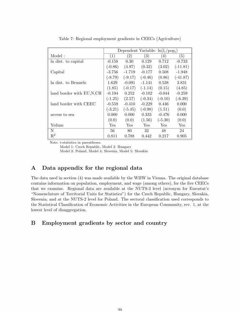
Table 7: Regional employment gradients in CEECs (Agriculture)

Dependent Variable: ln(li/popi)Model : (1) (2) (3) (4) (5)ln dist. to capital -0.158 0.30 0.129 0.712 -0.733

(-0.86) (4.97) (0.32) (3.02) (-11.81)Capital -3.756 -1.719 -0.177 0.508 -1.948

(-8.79) (-9.17) (-0.46) (0.86) (-41.87)ln dist. to Brussels 1.629 -0.091 -1.141 0.538 3.831

(1.85) (-0.17) (-1.14) (0.15) (4.85)land border with EU,N,CH -0.194 0.252 -0.102 -0.044 -0.259

(-1.25) (2.57) (-0.34) (-0.10) (-6.39)land border with CEEC -0.559 -0.410 -0.229 0.446 0.000

(-3.21) (-5.45) (-0.98) (1.51) (0.0)access to sea 0.000 0.000 0.333 -0.476 0.000

(0.0) (0.0) (1.56) (-5.30) (0.0)Yrdum Yes Yes Yes Yes YesN 56 80 32 48 24R2 0.811 0.788 0.442 0.217 0.905Note: t-statistics in parentheses.

Model 1: Czech Republic, Model 2: HungaryModel 3: Poland, Model 4: Slovenia, Model 5: Slovakia

A Data appendix for the regional data

The data used in section (4) was made available by the WIIW in Vienna. The original databasecontains information on population, employment, and wage (among others), for the five CEECsthat we examine. Regional data are available at the NUTS-3 level (acronym for Eurostat’s“Nomenclature of Territorial Units for Statistics”) for the Czech Republic, Hungary, Slovakia,Slovenia; and at the NUTS-2 level for Poland. The sectoral classification used corresponds tothe Statistical Classification of Economic Activities in the European Community, rev. 1, at thelowest level of disaggregation.

B Employment gradients by sector and country

20

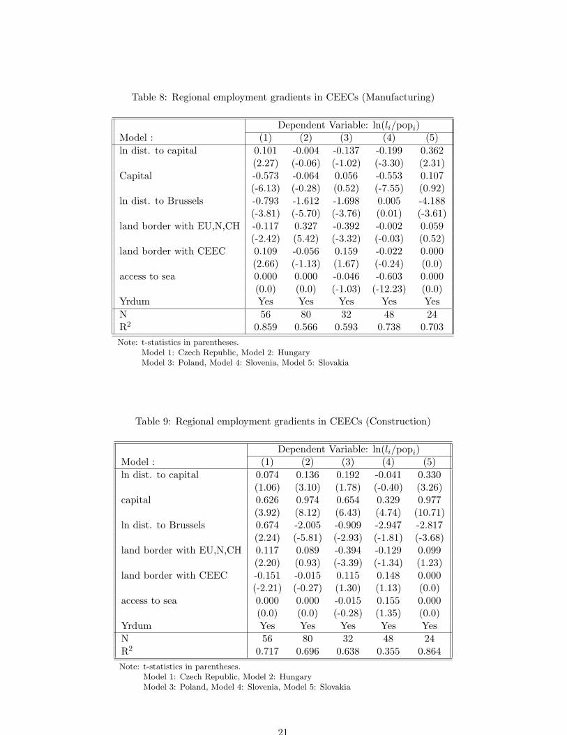
Table 8: Regional employment gradients in CEECs (Manufacturing)

Dependent Variable: ln(li/popi)Model : (1) (2) (3) (4) (5)ln dist. to capital 0.101 -0.004 -0.137 -0.199 0.362

(2.27) (-0.06) (-1.02) (-3.30) (2.31)Capital -0.573 -0.064 0.056 -0.553 0.107

(-6.13) (-0.28) (0.52) (-7.55) (0.92)ln dist. to Brussels -0.793 -1.612 -1.698 0.005 -4.188

(-3.81) (-5.70) (-3.76) (0.01) (-3.61)land border with EU,N,CH -0.117 0.327 -0.392 -0.002 0.059

(-2.42) (5.42) (-3.32) (-0.03) (0.52)land border with CEEC 0.109 -0.056 0.159 -0.022 0.000

(2.66) (-1.13) (1.67) (-0.24) (0.0)access to sea 0.000 0.000 -0.046 -0.603 0.000

(0.0) (0.0) (-1.03) (-12.23) (0.0)Yrdum Yes Yes Yes Yes YesN 56 80 32 48 24R2 0.859 0.566 0.593 0.738 0.703Note: t-statistics in parentheses.


Table 9: Regional employment gradients in CEECs (Construction)

Dependent Variable: ln(li/popi)Model : (1) (2) (3) (4) (5)ln dist. to capital 0.074 0.136 0.192 -0.041 0.330

(1.06) (3.10) (1.78) (-0.40) (3.26)capital 0.626 0.974 0.654 0.329 0.977

(3.92) (8.12) (6.43) (4.74) (10.71)ln dist. to Brussels 0.674 -2.005 -0.909 -2.947 -2.817

(2.24) (-5.81) (-2.93) (-1.81) (-3.68)land border with EU,N,CH 0.117 0.089 -0.394 -0.129 0.099

(2.20) (0.93) (-3.39) (-1.34) (1.23)land border with CEEC -0.151 -0.015 0.115 0.148 0.000

(-2.21) (-0.27) (1.30) (1.13) (0.0)access to sea 0.000 0.000 -0.015 0.155 0.000

(0.0) (0.0) (-0.28) (1.35) (0.0)Yrdum Yes Yes Yes Yes YesN 56 80 32 48 24R2 0.717 0.696 0.638 0.355 0.864Note: t-statistics in parentheses.


21

Table 10: Regional employment gradients in CEECs (Distribution)

Dependent Variable: ln(li/popi)Model : (1) (2) (3) (4) (5)ln dist. to capital 0.058 -0.004 0.190 -0.098 0.157

(1.05) (-0.09) (1.80) (-1.91) (1.81)capital 1.136 1.061 0.889 0.903 0.909

(8.25) (6.49) (11.64) (26.00) (10.00)ln dist. to Brussels -0.264 -0.077 -0.665 2.257 -2.041

(-1.11) (-0.22) (-1.61) (2.91) (-2.80)land border with EU,N,CH 0.053 0.224 -0.276 0.303 -0.099

(1.18) (2.03) (-2.12) (7.38) (-1.17)land border with CEEC 0.174 0.047 -0.031 -0.277 0.000

(3.66) (0.90) (-0.32) (-5.70) (0.0)access to sea 0.000 0.000 -0.054 0.456 0.000



Table 11: Regional employment gradients in CEECs (Transport and Comm.)

Dependent Variable: ln(li/popi)Model : (1) (2) (3) (4) (5)ln dist. to capital -0.050 0.232 0.226 -0.004 -0.053

(-0.80) (4.74) (1.88) (-0.04) (-0.52)capital 0.563 2.350 0.737 0.472 0.941


(0.40) (-3.53) (-0.20) (-3.97) (1.29)land border with EU,N,CH 0.076 0.178 0.050 -0.013 -0.092

(1.26) (2.57) (0.64) (-0.09) (-1.38)land border with CEEC -0.032 0.079 -0.077 -0.160 0.000

(-0.39) (1.70) (-1.17) (-1.10) (0.0)access to sea 0.000 0.000 0.103 1.118 0.000

(0.0) (0.0) (1.35) (14.54) (0.0)Yrdum Yes Yes Yes Yes YesN 56 80 32 48 24R2 0.622 0.85 0.724 0.698 0.664Note: t-statistics in parentheses.


22

Table 12: Regional employment gradients in CEECs (Banking and Insurance)

Dependent Variable: ln(li/popi)Model : (1) (2) (3) (4) (5)ln dist. to capital -0.015 0.032 -0.185 0.238 0.079

(-0.22) (0.37) (-1.33) (4.72) (1.31)capital 1.810 2.360 0.982 1.072 1.950

(10.92) (4.16) (7.23) (20.73) (31.09)ln dist. to Brussels -0.421 0.815 -0.486 -2.063 0.125

(-1.24) (0.93) (-1.65) (-2.64) (0.18)Land border with EU,N,CH 0.179 0.240 0.105 -0.040 -0.063

(3.53) (1.06) (1.07) (-0.78) (-1.30)Land border with CEEC 0.248 -0.205 0.040 -0.158 0.000

(4.04) (-2.69) (0.61) (-1.97) (0.0)Access to sea 0.000 0.000 0.065 0.451 0.000



Table 13: Regional employment gradients in CEECs (Other market services)

Dependent Variable: ln(li/popi)Model : (1) (2) (3) (4) (5)ln dist. to capital 0.055 0.235 -0.154 0.097 -0.246

(1.11) (5.49) (-0.98) (0.92) (-6.66)Capital 1.775 1.963 1.170 1.413 1.169


(0.81) (-7.08) (-3.48) (-0.03) (4.20)Land border with EU,N,CH 0.324 -0.037 -0.20 0.395 -0.159

(6.60) (-0.44) (-1.21) (3.94) (-3.98)Land border with CEEC 0.131 -0.066 0.290 -0.596 0.000

(1.91) (-1.29) (2.34) (-5.59) (0.0)Access to sea 0.000 0.000 0.191 0.633 0.000



23

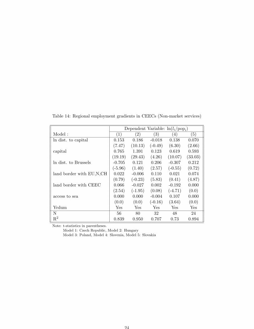
Table 14: Regional employment gradients in CEECs (Non-market services)

Dependent Variable: ln(li/popi)Model : (1) (2) (3) (4) (5)ln dist. to capital 0.153 0.186 -0.018 0.138 0.070

(7.47) (10.13) (-0.49) (6.30) (2.66)capital 0.765 1.391 0.123 0.619 0.593

(19.19) (29.43) (4.26) (10.07) (33.03)ln dist. to Brussels -0.705 0.121 0.206 -0.307 0.212

(-5.96) (1.40) (2.57) (-0.55) (0.72)land border with EU,N,CH 0.022 -0.006 0.110 0.021 0.074

(0.79) (-0.23) (5.83) (0.41) (4.87)land border with CEEC 0.066 -0.027 0.002 -0.192 0.000

(2.54) (-1.95) (0.08) (-4.71) (0.0)access to sea 0.000 0.000 -0.004 0.107 0.000



24

New economic geography meets Comecon. Regional wages and industry location in central Europe1

Documents

Transcript of New economic geography meets Comecon. Regional wages and industry location in central Europe1