CERN-PH-TH/2009-148DFPD-09/TH/15

First order flows for N = 2 extremalblack holes and duality invariants

Anna Ceresolea, Gianguido Dall’Agatab, Sergio Ferrara c,d and Armen Yeranyand,e

a INFN, Sezione di Torino & Dipartimento di Fisica TeoricaUniversita di Torino, Via Pietro Giuria 1, 10125 Torino, Italy

b Dipartimento di Fisica “Galileo Galilei” & INFN, Sezione di PadovaUniversita di Padova, Via Marzolo 8, 35131 Padova, Italy

c Department of Physics, CERN Theory DivisionCH 1211, Geneva 23, Switzerland

d INFN - LNF,Via Enrico Fermi 40, I-00044 Frascati, Italy

e Department of Physics, Yerevan State University,Alex Manoogyan St. 1, Yerevan, 0025, Armenia

ABSTRACT

We derive explicitly the superpotential W for the non-BPS branch of N = 2 extremalblack holes in terms of duality invariants of special geometry. Although this is done for aone-modulus case (the t3 model), the example gives Z 6= 0 black holes and captures the basicdistinction from previous attempts on the quadratic series (vanishing C tensor) and fromthe other Z = 0 cases. The superpotential W turns out to be a non-polynomial expression(containing radicals) of the basic duality invariant quantities. These are the same whichenter in the quartic invariant I4 for N = 2 theories based on symmetric spaces. Using theflow equations generated by W , we also provide the analytic general solution for the warpfactor and for the scalar field supporting the non-BPS black holes.

arX

iv:0

908.

1110

v2 [

hep-

th]

1 S

ep 2

009

1 Introduction

It has long been known ([1]-[5]) that the properties of the N = 2 extremal, static, spherically

symmetric black holes of Einstein-Maxwell theories coupled to the special Kahler geometry

of n complex scalar fields zi are encoded in the effective potential

VBH = ZZ + giDiZDZ , (1.1)

where Z(z, z; q, p) is the central charge of the N = 2 supersymmetry algebra (also function

of the charges), gi = ∂i∂K(z, z) is the metric of the scalar σ-model and Di ≡ ∂i + 12∂iK

is the Kahler covariant derivative. For supersymmetric configurations, Z plays the role of

a superpotential that drives the first order radial flows for the warp factor and scalar fields

towards the black hole horizon:

U ′ = −eU |Z| , z′i = −2eUgi∂|Z| . (1.2)

These flows stop at the critical points of the central charge, DiZ = 0, which are also super-

symmetric critical points of the full potential (1.1), fixing the values of the scalar fields at

the horizon in terms of the electric and magnetic charges. Therefore supersymmetric black

hole configurations are solutions of (1.2) where scalar fields vary from an arbitrary asymp-

totic value to a universal attractor point at the horizon, depending only on the charges. In

particular, these supersymmetric equations show that the warp factor U plays the role of a

c-function for the flow. The same attractive behaviour is exhibited by non-supersymmetric

extremal black holes [4, 8] and the warp factor is still playing the role of a c-function for

these solutions [9], but since they do not follow from (1.2), the construction of full solutions

is significantly more difficult.

More recently, starting with [10], it has become clear that non-BPS extremal black holes

may enjoy the same properties of supersymmetric (BPS) ones, provided that one trades |Z|with a different, real “fake” superpotential W (z, z) in (1.1) and (1.2). The extrema of

VBH = W 2 + 4gi∂iW∂W (1.3)

and then of W yield the non-supersymmetric attractor points as much as those of Z describe

the supersymmetric ones. This procedure allows to find black hole solutions by solving first

order differential equations for W

U ′ = −eUW , z′i = −2eUgi∂W , (1.4)

rather than the full second order equations of motion, even in absence of supersymmetry.

Moreover, W is connected on the one hand to the value of the black hole entropy at the

1

horizon Sbh = πW 2 and gives the ADM mass of the black hole (MADM = W ) and the scalar

charges Σi = ∂iW at infinity. We stress that this formalism does not only allow to analyze

the attractor point, like, for instance, the entropy function formalism [11], but also the full

attractor flow, from asymptotic infinity to the horizon. As it obviously simplifies the task

of building full solutions, this idea has been carefully analyzed in recent literature [12]–[23],

producing new solutions and generalizations ranging from the t2 to the stu model, from

static to rotating black holes, and also to extended supersymmetric and higher dimensional

theories.

A central issue in this construction is whether W always exists and what is its universal

form. In [10], a general characterization of W was given, together with a procedure to find at

least one class of these “superpotentials”. Moreover, W was explicitly written in three simple

instances: the t2 single modulus (in full generality), the t3 single modulus for restricted charge

configurations and the stu model for simple charge configurations and vanishing axions. This

class of solutions was later extended to the generating solutions of the stu model by using a

similar approach in 5-dimensions [13] (and the same solution, although in a different duality

framework was later obtained in [15, 16] and constructed in its full form in [18]). However,

these examples made it clear that a deeper guideline was needed that better exploited the

symmetries of the underlying theory.

This guideline comes naturally from results in [24] and [3]. There, it was shown that the

underlying special geometry of the scalar σ-model can be encoded in Sp(2n+ 2) symplectic

sections (XΛ, FΛ) (where Λ = 0, . . . , n) and the central charge is the symplectic product of

these sections with the electric qΛ and magnetic charges pΛ: Z = eK/2(qΛXΛ − pΛFΛ). The

symplectic sections also provide a projective parameterization of the scalar manifold, whose

normal coordinates can be introduced by taking ti = X i/X0. Using these properties one can

find the following differential identities for the central charge

DiDjZ = iCijkgkkDkZ (DıCijk = 0),

DiDZ = giZ, (1.5)

DiZ = 0 ,

and the curvature constraint

Rikl = −gigkl − gilgk + CikpCklgpp. (1.6)

The same structure also leads to the existence of some symplectic invariant quantities1,

i.e. quantities that do not change for a simultaneous symplectic action on the charge vector

1When the scalar σ-model is described by a symmetric space G/H this is equivalent to H-invariance.H-invariant quantities that extend to full G-invariant quantities are also moduli independent. An instanceof a fully invariant quantity is the quartic invariant of symmetric special geometry I4(pΛ, qΛ).

2

and on the scalar fields (defined through the symplectic sections (XΛ, FΛ)). The simplest to

identify are:

I1 = |Z|2 + |DiZ|2 and I2 = |Z|2 − |DiZ|2 . (1.7)

The black hole potential (1.1) coincides with one of them, namely VBH = I1, while the super-

symmetric flow equations (1.2) are also driven by the invariant quantity |Z| =√

(I1 + I2)/2.

Then, it seems then quite natural to try and build also the “fake” superpotential W in terms

of symplectic invariants. This elegant approach was first attempted in [12] and gave some

interesting results mainly for some of the extended supersymmetric theories, but still did

not seem to capture the essence of W for reasons that we will make evident below. Further

progress on the form of W was done in [17], which revisited the expression for the quadratic

series, and in [18], where the general expression of W for the stu model was determined.

More recently, compelling evidence that the superpotential should have a definition in terms

of symplectic invariant quantities has been provided in [23], where W is identified with

Hamilton’s principal function associated to the non-BPS flow equations (1.4).

The core question is: what is a complete set of duality invariant quantities? We can

answer to this question by drawing a construction parallel to the N = 8 case. In N = 8

supergravity there are 5 duality invariant quantities. Four of them are given (in a polynomial

way) by [25]

trA, trA2, trA3, trA4, (1.8)

where A = ZZ† and Z is the central charge matrix of the N = 8 theory. These invariant

quantities are independent because they are related to the 4 eigenvalues of ZZ†. There is a

fifth independent invariant quantity that can be constructed in terms of the real part of the

Pfaffian of Z:

Re(Pf Z) (1.9)

(note that |Pf Z|2 is not independent because it can be expressed in terms of trA4, trA3trA,

(trA2)2 and (trA)4). The latter is the only invariant that is SU(8), but not U(8) invariant.

So there is a total of 5 invariant quantities and one relation among them, specified by the

quartic Cartan invariant I4. A similar answer can be given for the N = 2 case [26]. Besides

i1 = ZZ and i2 = giZiZ , (1.10)

where Zi = DiZ, Z ı = DıZ and Zi

= giZ , three new invariants can be introduced:

i3 =1

6

[ZN3(Z) + ZN3(Z)

], (1.11)

i4 =i

6

[ZN3(Z)− ZN3(Z)

], (1.12)

3

i5 = giıCijkCıkZjZkZ Z k , (1.13)

where

N3(Z) = CijkZiZjZk, N3(Z) = CıkZ

ı Z Z k. (1.14)

Also in this case there is one relation among them, which involves the quartic invariant I4

of symmetric special geometry:

I4 = (i1 − i2)2 + 4i4 − i5 . (1.15)

The crucial difference between the two cases is that the duality invariants are also H-

invariants, and H is completely different in N = 8, where it is SU(8), and in N = 2,

where it is E6× U(1) (for the octonionic model).

Note that for symmetric spaces ∂iI4 = 0 follows from the additional properties

DkCijk = 0, (1.16)

Cj(lmCpq)lC ıkgjgkk =

4

3C(lmpgq)l. (1.17)

Based on the above considerations, the claim of this paper is that the “fake” superpoten-

tial W for the class of configurations corresponding to the non-BPS flows is given in terms of

a non-polynomial expression of the purely duality invariant quantities i1–i5 (at least for sym-

metric special geometries). We will demonstrate this fact by first considering the quadratic

and the cubic series and then illustrating the path towards the general case.

2 The quadratic series

Minimal couplings in special geometry [27] can be obtained through the quadratic series,

based on holomorphic prepotentials of the form

F (X) =i

2

[(X0)2 −

n∑i=1

(X i)2

]. (2.1)

The resulting moduli spaces are the coset manifolds SU(1, n)/SU(n) × U(1), which give

simplified couplings in that they have a vanishing C-tensor: Cijk = 0. This feature implies

that non-BPS extremal black holes should have vanishing central charge at the horizon as

follows from the attractor equations [5]

2ZDiZ = −iCijkgjgkkDZDkZ, (2.2)

which, in this class of examples, reduce to

ZDiZ = 0. (2.3)

4

Since non-BPS fixed points correspond to DiZ 6= 0, the central charge must vanish at the

attractor point: Z = 0.

According to our discussion in the introduction, full solutions for these non-BPS extremal

black holes can be obtained from flow equations driven by a “fake” superpotential W . The

existence of such a function for the quadratic series of N = 2 symmetric spaces, for arbitrary

charge configurations and a single modulus, was established in [10] using the equivalent form

of the prepotential F (X) = −iX0X1. The generalization to many moduli was then obtained

in [12, 17]. We now show that the possibility of finding a simple expression of W for these

cases can be traced back to the fact that the superpotential must be constructed in terms of

only two symplectic invariants:

i1 = ZZ, and i2 = giDiZDZ. (2.4)

This happens because all the other invariants, namely i3 (1.11), i4 (1.12) and i5 (1.13),

depend on the Cijk intersection numbers and therefore they identically vanish for minimal

couplings. The moduli independent invariant, a quadratic form on charges, is I2 = i1 − i2.

Consistently the quartic invariant in (1.15) becomes in this case I4 = |i1 − i2|2 = I22 . I2 is

positive for BPS and negative for nonBPS attractor solutions.

As usual, the BPS flows are driven by |Z| =√i1. It turns out that in this case the

non-BPS flows are driven by

W =√i2 = (giDiZDZ)1/2 . (2.5)

We will now prove this solely using the identities of special geometry (1.5) for the black hole

central and matter charges, which simplify significantly when Cijk = 0 (so that DiDjZ = 0).

In particular we will prove that the black hole potential can be expressed in terms of (2.5),

according to (1.3), and we will show that critical points ofW are in one-to-one correspondence

with the non-BPS black hole configurations. As a first step we obtain an explicit expression

for the derivative of the superpotential by considering derivatives of W 2. Because of the

vanishing of the C-tensors these derivatives have a simple expression in terms of the central

charge and its derivatives

∂i(W 2)

= 2W∂iW = DiZ Z , ∂ ı(W 2)

= 2W∂ ıW = DıZ Z , (2.6)

so that

∂iW =DiZZ

2(DZDZg−1)1/2and ∂ ıW =

DıZZ

2(DZDZg−1)1/2. (2.7)

Then it is straightforward to show that

W 2 = i2 = DiZDZgi, 4gi∂iW∂W = i1 = i2 + I2 = ZZ, (2.8)

5

so that the black hole potential can be written as

VBH = |Z|2 + giDiZDZ = W 2 + 4gi∂iW∂W . (2.9)

In order to be a good superpotential, W has to count the critical points of non-BPS black

holes. A simple inspection of (2.8) shows that this is indeed the case because at the non-BPS

horizon DiZ must be non vanishing for some i and thus

∂iW = 0 ⇔ Z = 0 . (2.10)

Moreover, at the critical point ∂iW = 0 and therefore

VBH = W 2 = i2 = −I2, (2.11)

because i1 = 0. Note that for n > 1 this model has n − 1 complex flat directions, because

(2.7) vanishes in any direction once Z = 0. Flat directions are a generic feature of all Z 6= 0

non-BPS models with the exception of the t3 model [28].

For the single modulus case (n = 1) treated in [10], it was found that the “fake” super-

potential W has an expression almost identical to the BPS superpotential, given by |Z|, up

to some sign changes in the bare charges. This is now well understood because this model

coincides with the bosonic sector of N = 4 pure supergravity, where Z and DtZ play the role

of two eigenvalues of the central charge matrix and there is a complete symmetry between

them. The case with an arbitrary number of moduli is then a simple generalization of the

one-modulus case, where, in the vein of [10], the central charge and its derivative exchange

their role. In particular, it can be easily seen that the black hole potential described by the

central charge and the one described by W are the same because the gradients of eU |Z| and

eUW in the enlarged moduli space (including also the warp factor) are related by a rotation

matrix of the same form as the one of eq. (4.10) in [10].

3 The cubic series

Another illustrative example is the simplest cubic model, having a single modulus, based on

the prepotential

F (X) =(X1)3

X0, (3.1)

leading to the Kahler potential K = − log [−i(t− t)3]. The “fake” superpotential W was

obtained in [10] only for some very specific charge configurations and it was observed that

the situation drastically changes with respect to the quadratic series. The transformation

from Z to W is field dependent and the “fake” superpotential is not simply related to the

6

absolute value of the derivatives of the central charge. In the current framework this can be

explained by the fact that there are now 3 non-zero independent duality invariants because

Cijk 6= 0. These are i1, i2 and i3, because, for a single modulus, we can prove that the other

invariants are functionally dependent on them. In detail, we find that

i4 = −

√4

(i23

)3

i1 − i23 (3.2)

and

i5 =4

3i22, (3.3)

which means that we can also rewrite the expression for the quartic invariant (1.15) as:

I4 = (i1 − i2)2 − 4

3i22 − 4

√4

(i23

)3

i1 − i23 . (3.4)

The main new result we present in this section is the explicit expression of W for all charges

and given in terms of the symplectic invariants mentioned above.

Since we are going to prove that W can be given only in terms of symplectic invariant

quantities, we can compute it in any frame, i.e. for any charge configuration, and only later

check that we did not miss any term by switching on all the charges in the final expression.

Therefore we start from a D0-D6 configuration, involving only q0 and p0. When all the other

charges are vanishing, the only allowed black hole configurations are non-BPS. Hence this

case is a natural representative of the non-BPS branch. The form of the superpotential for

this case can be obtained by properly identifying all the moduli in the analogous setup in

the context of the stu model [18]. The resulting expression is

W 2 = eK∣∣(q0)1/3 + (p0)1/3t

∣∣2 [(q0)2/3 − 1

2(p0q0)1/3(t+ t) + (p0)2/3tt

]2

(3.5)

and we have checked that it fulfills (1.3).

We are now going to rewrite (3.5) in terms of the independent symplectic invariants,

which, for this choice of charges, read

i1 = eK∣∣q0 + p0t3

∣∣2 , (3.6)

i2 = 3eK[(q0)2 + q0p

0tt(t+ t) + (p0)2t3t3], (3.7)

i3 = eK√−I4

[(q0)2 − (p0)2t3t

3], (3.8)

7

where I4 = − (p0q0)2. We start by computing the difference between the square of the “fake”

superpotential and the square of the absolute value of the central charge:

W 2 − i1 = −3

4eK√−I4(t− t)2

[(q0/p

0)1/3 + (p0/q0)1/3tt+ (t+ t)]. (3.9)

Then we need to rewrite the three real terms in the square brackets above as combinations of

the symplectic invariants. The easiest one to identify is the last term, which is proportional

to the following difference:

i1 −i23

= eK√−I4(t− t)2(t+ t). (3.10)

Upon using this relation in (3.9) we obtain that

W 2 =i1 + i2

4− 3

4eK√−I4(t− t)2

[(q0/p

0)1/3 + (p0/q0)1/3tt]. (3.11)

The two remaining terms can also be expressed in terms of invariants, though with some

effort. First we can get rid of the q0p0 combination in i2 by considering the following expres-

sioni1 + i2

4− 1

4I4

(i1 −

i23

)3

= eK[(q0)2 + (p0)2t3t

3]. (3.12)

Then, using this expression and the one of i3 we can eventually construct the necessary

combinations

− 8I4 eKq20 =

(i1 −

i23

)3

− I4(i1 + i2) + 4i3√−I4 , (3.13)

−8I4 eK(p0)2 t3t3

=

(i1 −

i23

)3

− I4(i1 + i2)− 4i3√−I4 . (3.14)

Putting all these ingredients together we reach the final expression for the “fake” superpo-

tential, which reads:

W 2 =i1 + i2

4+

3

8

((i1 − i23

)3

− (i1 + i2) I4 + 4 i3√−I4

)1/3

+

+

((i1 −

i23

)3

− (i1 + i2) I4 − 4 i3√−I4

)1/3 . (3.15)

We can now see that in this case the superpotential is not simply given by a linear combi-

nation of the invariants, but rather by a non-polynomial expression (containing radicals) of

the basic duality invariant quantities. At the attractor point we have that

i2 = 3i1 =3

4

√−I4 (3.16)

8

and i3 vanishes. Hence the above expression reduces to

W 2 =√−I4, (3.17)

which is the expected result for a non-BPS black hole.

Although we have computed the “fake” superpotential in terms of the symplectic invari-

ants in the special case of vanishing q1 and p1 charges, the final expression should be the same

in any duality frame. This can be checked by comparing the expression for W 2 resulting

by evaluating (3.15) with all the charges (q0, q1, p0, p1) switched on and the analogous one

coming from the stu model discussed in [18], in the S = T = U = t limit. As expected, the

two expressions agree.

We report here for completeness the explicit form of the superpotential with all the

charges:

W 2 = eK√−I4 (−1 + ν3)

2

ν3(σ− + σ+)3

(tt+ (t+ t)

σ− + νσ+

1− ν+

(σ− + νσ+

1− ν

)2)

(tt+ (t+ t)

((2 + ν)σ− − ν(1 + 2ν)σ+)

2 (1 + ν + ν2)+σ2− − νσ−σ+ + ν2σ2

+

1 + ν + ν2

)2

(3.18)

where

ν =

(2(p1)3 + p0

(√−I4 − p0q0 − p1q1

)2(p1)3 − p0

(√−I4 + p0q0 + p1q1

))1/3

, (3.19)

σ± =1

2

√−I4 ± p0q0 ± p1q1

3

(p1)2 − p0q13

.

4 Full Non-BPS solution

Given the most general form of the superpotential for the single modulus cubic model, we

can now solve the flow equations (1.4) and provide an explicit form for the most general

non-BPS black hole configuration in this context.

Again, it is easier to present first the computation of the solution in a specific duality

frame and then boost this solution to the most general one containing all the charges, al-

though one could equally start directly from (3.18) and solve the corresponding equations.

If we set p0 = q1 = 0 in (3.15) and assume q0 < 0 and p1 > 0, the superpotential reduces to

a rather simple expression:

W = eK/2(−q0 + 3p1tt) =−q0 + 3p1 (x2 + y2)

2√

2√y3

, (4.1)

9

0 1 2 3 4

1

2

3

4

x

y

Contours of equal W

0 1 2 3 4

1

2

3

4

x

y

Contours of equal ÈZÈ

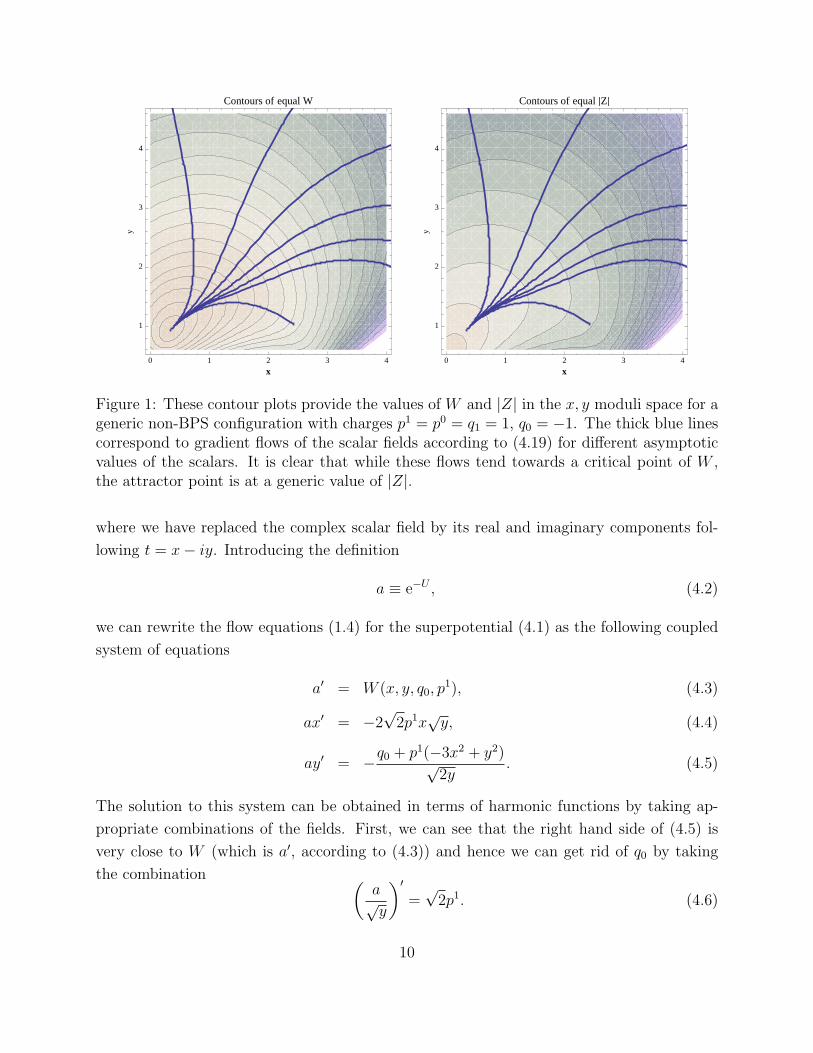
Figure 1: These contour plots provide the values of W and |Z| in the x, y moduli space for ageneric non-BPS configuration with charges p1 = p0 = q1 = 1, q0 = −1. The thick blue linescorrespond to gradient flows of the scalar fields according to (4.19) for different asymptoticvalues of the scalars. It is clear that while these flows tend towards a critical point of W ,the attractor point is at a generic value of |Z|.

where we have replaced the complex scalar field by its real and imaginary components fol-

lowing t = x− iy. Introducing the definition

a ≡ e−U , (4.2)

we can rewrite the flow equations (1.4) for the superpotential (4.1) as the following coupled

system of equations

a′ = W (x, y, q0, p1), (4.3)

ax′ = −2√

2p1x√y, (4.4)

ay′ = −q0 + p1(−3x2 + y2)√2y

. (4.5)

The solution to this system can be obtained in terms of harmonic functions by taking ap-

propriate combinations of the fields. First, we can see that the right hand side of (4.5) is

very close to W (which is a′, according to (4.3)) and hence we can get rid of q0 by taking

the combination (a√y

)′=√

2p1. (4.6)

10

0 1 2 3 4

1

2

3

4

x

y

Contours of equal W

0 1 2 3 4

1

2

3

4

x

y

Contours of equal ÈZÈ

Figure 2: These contour plots provide the values of W and |Z| in the x, y moduli space fora generic supersymmetric configuration with charges p1 = p0 = q1 = q0 = 1. The thickblue lines correspond to gradient flows of the scalar fields according to (1.2) for differentasymptotic values of the scalars. In this case the flows approach a critical point of thecentral charge |Z|, which has no special meaning in terms of W .

Then we can solve this equation by introducing the harmonic function

H1 = h1 +√

2p1τ, (4.7)

so thata√y

= H1. (4.8)

Then we can solve for x, by replacing both the combination a/√y and p1 in (4.4) by H1 and

its derivative, so thatx′

x= −2

(H1)′

H1, (4.9)

whose solution reads

x =b

(H1)2. (4.10)

Finally we can take another combination of the warp factor and y that gets rid of p1, upon

using (4.10): (ay3/2

)′=√

2(−q0 + 3p1x2) = −√

2q0 + 3b2 (H1)′

(H1)4. (4.11)

This can be easily integrated by introducing another harmonic function

H0 = h0 −√

2 q0 τ (4.12)

11

and gives

ay3/2 = H0 −b2

(H1)3. (4.13)

We can then put together (4.8) and (4.13) with the appropriate powers to get an expression

for the warp factor and dilaton field as:

a4 = (H1)3H0 − b2, y =a2

H21

. (4.14)

We can also rewrite this solution in terms of the quartic invariant I4 = 4(p1)3q0 and new,

rescaled, integration constants

b0 =h0√

2

(−I4)1/4

q0

, b1 = − h1

√2

(−I4)1/4

p1, (4.15)

by introducing “universal” harmonic functions:

H0 = (b0 − (−I4)1/4τ) =(−I4)1/4

√2q0

H0, (4.16)

H1 = (b1 − (−I4)1/4τ) = −(−I4)1/4

√2p1

H1. (4.17)

The solution then reads

e−4U = (H1)3H0 − b2,

x =b√−I4

2(p1)2(H1)2, (4.18)

y =e−2U√−I4

2(p1)2H21

.

The “universal” harmonic functions are better suited to obtain the general solution start-

ing from the seed solution constructed above, because they are built in terms of the quartic

invariant I4. After using the transformation technique we generate the most general solution

with all charges switched on. This solution can be expressed in a compact form by using the

charge combinations ν and σ±, defined in (3.19) and (3.20),

e−4U = (H1)3H0 − b2,

x =H2

1(ν + 1)(νσ+ − σ−) +H0H1(νσ+ + σ−)(ν − 1) + 2b(σ+ν2 + σ−)

(ν + 1)2H21 + (ν − 1)2H0H1 + 2b(ν2 − 1)

, (4.19)

y =2ν(σ− + σ+)e−2U

(ν + 1)2H21 + (ν − 1)2H0H1 + 2b(ν2 − 1)

,

12

and it correctly reduces to (4.18) when p0 = q1 = 0, which implies that ν = 1 and σ± =12

√−I4

(p1)2. The attractor values of the above solution are:

e−2U(τ→−∞) =√−I4τ

2,

x(τ → −∞) =σ+ν

2 − σ−1 + ν2

, (4.20)

y(τ → −∞) =(σ+ + σ−)ν

1 + ν2.

5 General case and outlook

It is obvious that the results for the cubic series should have a simple generalization to the

case of an arbitrary number of moduli, at least for all special geometries based on symmetric

spaces. However, we note that, when we have more than one modulus, i5 becomes an

independent invariant. For example, in the stu model

i5 = |DsZ|2|DtZ|2 + |DsZ|2|DuZ|2 + |DtZ|2|DuZ|2 , (5.1)

which cannot be written in terms of the other invariants. Actually, I4 depends on i5 and so

should the superpotential W . Therefore we expect that for a generic model

W = W (i1, i2, i3, i4, i5). (5.2)

It is also clear that previous attempts to find W failed either because a too naıve general-

ization of the quadratic case was proposed, with W as a simple linear combination of i1 and

i2, or because the other invariants, namely i3, i4 and i5, were not included.

We also remark that non-BPS solutions with Z = 0 should have a simple superpotential

in virtue of the fact that they can be embedded in BPS solutions coming from extended

(N > 2) supergravities [12, 17]. For the quadratic series, non-BPS solutions with Z = 0 are

the only possible ones, while for cubic geometries, these solutions start to arise when two or

more moduli are present (F = st2 and F = stu). For instance, in the stu model a Z = 0

superpotential can be obtained by interchanging |Z| with |DsZ| so that

W = |DsZ|. (5.3)

This result was already obtained in [18] in a specific symplectic frame but here we exhibit

its derivation in a duality invariant formulation, valid in any frame.

13

Using the factorization of the stu moduli space in three (complex) one-dimensional man-

ifolds, from (1.6) one gets the following interesting relations between the curvature, the

C-tensors and the metric of the scalar σ-model:

Riıiı = −2giıgiı, i = s, t, u, (5.4)

CstuC stu = gssgttguu . (5.5)

This means that, by choosing the phase such that Cstu is real, we can define Cstu =

g1/2ss g

1/2tt g

1/2uu so that the special geometry identities (1.5) become

DsDt Z = ig1/2ss g

1/2tt g

−1/2uu DuZ (and the same for s→ t→ u) . (5.6)

Factorization of the moduli space also implies that one can write three separate i2 invariants,

one per each modulus is2 = |DsZ|2, it2 = |DtZ|2 and iu2 = |DuZ|2. Then it is easy to see that

a good invariant superpotential is

W =√is2 = |DsZDsZ g

ss|1/2 = |Ds Z| . (5.7)

Indeed, by differentiating W 2 we find

2∂tW W = −ig1/2tt g

−1/2uu g

−1/2ss DuZDsZ, (5.8)

2∂uW W = −ig1/2uu g

−1/2tt g

−1/2ss DtZDsZ, (5.9)

2∂sW W = ZDsZ, (5.10)

and therefore

4gtt∂tW∂tW = iu2 = |DuZ|2, (5.11)

4guu∂uW∂uW = it2 = |DtZ|2, (5.12)

4gss∂sW∂sW = i1 = |Z|2 . (5.13)

We have just completed the proof because the previous relations show that the superpotential

verifies

W 2 = |DsZ|2, (5.14)

4(gss∂sW∂sW + gtt∂tW∂tW + guu∂uW∂uW ) = |Z|2 + |DuZ|2 + |DtZ|2 , (5.15)

as it should be, and the attractor points occur at DsZ 6= 0, Z = DuZ = DtZ = 0, which is

equivalent to the request that ∂sW = ∂tW = ∂uW = 0.

14

We conclude by pointing out that the previous derivation admits a straightforward ex-

tension to all the models in the series SU(1,1)/U(1) × SO(2, 2 + n)/SO(2)×SO(2 + n). Any

model in this class admits non-BPS black holes with Z = 0 whose superpotential can be

identified with W = |DsZ|, where s is the modulus of the SU(1,1)/U(1) factor. This follows

again from the factorization of the scalar manifold, which implies that

Rssiı = 0 =⇒ CsikCsıkgkk = gssgiı. (5.16)

This can be used to prove that

4|∂iW |2 = |DiZ|2 and 4|∂sW |2 = |Z|2, (5.17)

which, together with the definition of the superpotential W 2 = |DsZ|2, gives the right

potential and non-BPS critical points. Note, however, that for n > 1 other Z = 0 non-

BPS solutions exist with flat directions for which the “fake superpotential” W cannot be

constructed in this simple way [29].

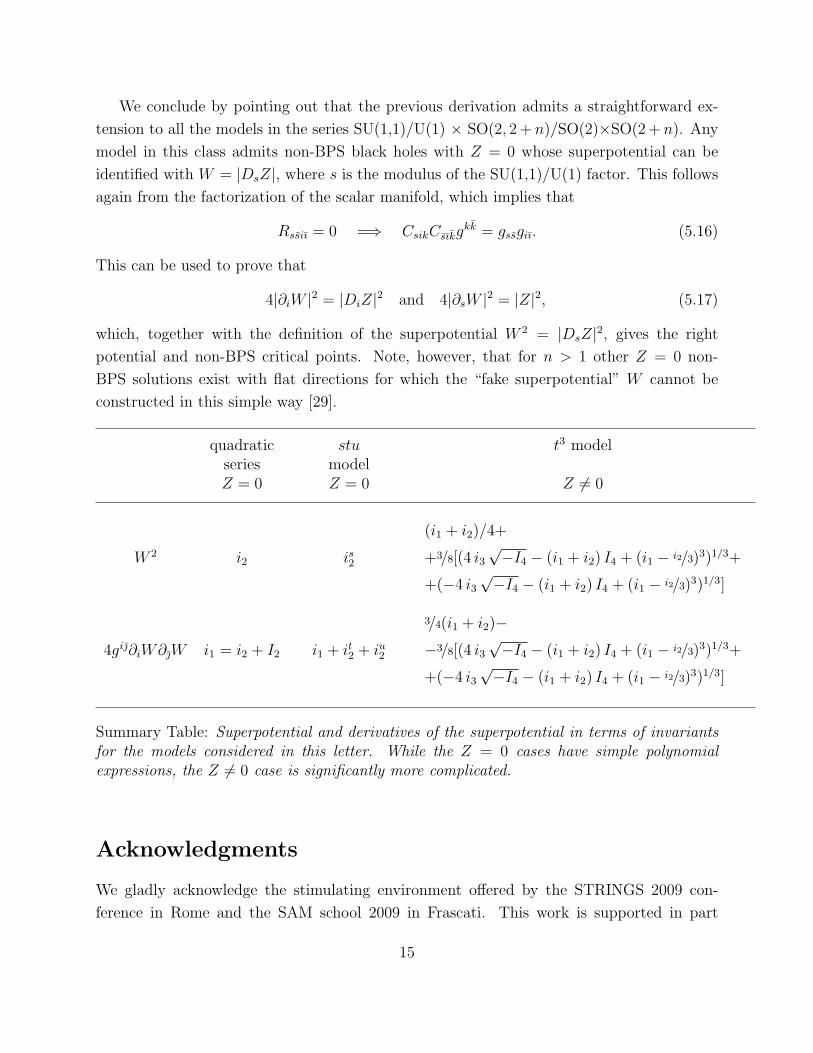
quadratic stu t3 modelseries modelZ = 0 Z = 0 Z 6= 0

W 2 i2 is2

(i1 + i2)/4+

+3/8[(4 i3√−I4 − (i1 + i2) I4 + (i1 − i2/3)3)1/3+

+(−4 i3√−I4 − (i1 + i2) I4 + (i1 − i2/3)3)1/3]

4gi∂iW∂W i1 = i2 + I2 i1 + it2 + iu2

3/4(i1 + i2)−−3/8[(4 i3

√−I4 − (i1 + i2) I4 + (i1 − i2/3)3)1/3+

+(−4 i3√−I4 − (i1 + i2) I4 + (i1 − i2/3)3)1/3]

Summary Table: Superpotential and derivatives of the superpotential in terms of invariantsfor the models considered in this letter. While the Z = 0 cases have simple polynomialexpressions, the Z 6= 0 case is significantly more complicated.

Acknowledgments

We gladly acknowledge the stimulating environment offered by the STRINGS 2009 con-

ference in Rome and the SAM school 2009 in Frascati. This work is supported in part

15

by the ERC Advanced Grant no. 226455, “Supersymmetry, Quantum Gravity and Gauge

Fields” (SUPERFIELDS ). The work of A. C. is partially supported by MIUR-PRIN contract

20075ATT78, the work of G. D. has been partially supported by the Fondazione Cariparo

Excellence Grant String-derived supergravities with branes and fluxes and their phenomeno-

logical implications, the work of S. F. has been supported in part by D.O.E. grant DE-FG03-

91ER40662, Task C and the work of A. Y. has been supported in part by CERN-PH-TH

where part of the work was done.

References

[1] S. Ferrara, R. Kallosh and A. Strominger, “N=2 extremal black holes,” Phys. Rev. D

52 (1995) 5412 [arXiv:hep-th/9508072].

[2] A. Strominger, Macroscopic entropy of N= 2 extremal black holes, Phys. Lett. B383,

39 (1996), [arXiv:hep-th/9602111].

[3] S. Ferrara and R. Kallosh, Supersymmetry and attractors, Phys. Rev. D 54, 1514 (1996),

[arXiv:hep-th/9602136];

[4] S. Ferrara, R. Kallosh, Universality of supersymmetric attractors, Phys. Rev. D54, 1525

(1996), [arXiv:hep-th/9603090].

[5] S. Ferrara, G. W. Gibbons and R. Kallosh, Black holes and critical points in moduli

space, Nucl. Phys. B 500, 75 (1997), [arXiv:hep-th/9702103].

[6] R. Kallosh, N. Sivanandam and M. Soroush, “Exact attractive non-BPS STU black

holes,” Phys. Rev. D 74, 065008 (2006) [arXiv:hep-th/0606263].

[7] R. Kallosh, N. Sivanandam and M. Soroush, “The non-BPS black hole attractor equa-

tion,” JHEP 0603, 060 (2006) [arXiv:hep-th/0602005].

[8] K. Goldstein, N. Iizuka, R. P. Jena and S. P. Trivedi, “Non-supersymmetric attractors,”

Phys. Rev. D 72 (2005) 124021 [arXiv:hep-th/0507096].

[9] K. Goldstein, R. P. Jena, G. Mandal and S. P. Trivedi, “A C-function for non-

supersymmetric attractors,” JHEP 0602 (2006) 053 [arXiv:hep-th/0512138].

[10] A. Ceresole and G. Dall’Agata, “Flow Equations for Non-BPS Extremal Black Holes,”

JHEP 0703 (2007) 110 [arXiv:hep-th/0702088].

16

[11] A. Sen, “Black Hole Entropy Function and the Attractor Mechanism in Higher Deriva-

tive Gravity,” JHEP 0509 (2005) 038 [arXiv:hep-th/0506177];

G. L. Cardoso, B. de Wit and S. Mahapatra, “Black hole entropy functions and attractor

equations,” JHEP 0703, 085 (2007) [arXiv:hep-th/0612225].

[12] L. Andrianopoli, R. D’Auria, E. Orazi and M. Trigiante, “First Order Description of

Black Holes in Moduli Space,” JHEP 0711 (2007) 032 [arXiv:0706.0712 [hep-th]].

[13] G. Lopes Cardoso, A. Ceresole, G. Dall’Agata, J. M. Oberreuter and J. Perz, “First-

order flow equations for extremal black holes in very special geometry,” JHEP 0710

(2007) 063 [arXiv:0706.3373 [hep-th]].

[14] A. Ceresole, S. Ferrara and A. Marrani, “4d/5d Correspondence for the Black Hole

Potential and its Critical Points,” Class. Quant. Grav. 24 (2007) 5651 [arXiv:0707.0964

[hep-th]].

[15] K. Hotta and T. Kubota, “Exact Solutions and the Attractor Mechanism in Non-BPS

Black Holes,” Prog. Theor. Phys. 118 (2007) 969 [arXiv:0707.4554 [hep-th]].

[16] E. G. Gimon, F. Larsen and J. Simon, “Black Holes in Supergravity: the non-BPS

Branch,” JHEP 0801 (2008) 040 [arXiv:0710.4967 [hep-th]].

[17] S. Ferrara, A. Gnecchi and A. Marrani, “d=4 Attractors, Effective Horizon Radius and

Fake Supergravity,” Phys. Rev. D 78 (2008) 065003 [arXiv:0806.3196 [hep-th]].

[18] S. Bellucci, S. Ferrara, A. Marrani and A. Yeranyan, “stu Black Holes Unveiled,”

arXiv:0807.3503 [hep-th].

[19] J. Perz, P. Smyth, T. Van Riet and B. Vercnocke, “First-order flow equations for ex-

tremal and non-extremal black holes,” JHEP 0903 (2009) 150 [arXiv:0810.1528 [hep-

th]].

[20] K. Goldstein and S. Katmadas, “Almost BPS black holes,” JHEP 0905 (2009) 058

[arXiv:0812.4183 [hep-th]].

[21] K. Hotta,“Holographic RG flow dual to attractor flow in extremal black holes,” Phys.

Rev. D 79 (2009) 104018 [arXiv:0902.3529 [hep-th]].

[22] I. Bena, G. Dall’Agata, S. Giusto, C. Ruef and N. P. Warner, “Non-BPS Black Rings

and Black Holes in Taub-NUT,” JHEP 0906 (2009) 015 [arXiv:0902.4526 [hep-th]].

17

[23] L. Andrianopoli, R. D’Auria, E. Orazi and M. Trigiante, “First Order Description of

D=4 static Black Holes and the Hamilton-Jacobi equation,” arXiv:0905.3938 [hep-th].

[24] A. Ceresole, R. D’Auria and S. Ferrara, “The Symplectic Structure of N=2 Supergrav-

ity and its Central Extension,” Nucl. Phys. Proc. Suppl. 46, 67 (1996) [arXiv:hep-

th/9509160].

[25] R. D’Auria, S. Ferrara and M. A. Lledo, “On central charges and Hamiltonians for

0-brane dynamics,” Phys. Rev. D 60 (1999) 084007 [arXiv:hep-th/9903089].

[26] B. L. Cerchiai, S. Ferrara, A. Marrani and B. Zumino, “Duality, Entropy and ADM

Mass in Supergravity,” Phys. Rev. D 79, 125010 (2009) [arXiv:0902.3973 [hep-th]].

[27] J. F. Luciani, Coupling of O(2)Supergravity with Several Vector Multiplets, Nucl. Phys.

B 132, 325 (1978).

[28] S. Ferrara and A. Marrani, “On the Moduli Space of non-BPS Attractors for N=2

Symmetric Manifolds,” Phys. Lett. B 652 (2007) 111 [arXiv:0706.1667 [hep-th]].

[29] S. Bellucci, S. Ferrara, M. Gunaydin and A. Marrani, “Charge orbits of symmetric

special geometries and attractors,” Int. J. Mod. Phys. A 21 (2006) 5043 [arXiv:hep-

th/0606209].

18