First directly retrieved global distribution of tropospheric column

ozone from GOME: Comparison with the GEOS-CHEM model

Xiong Liu,1 Kelly Chance,1 Christopher E. Sioris,1 Thomas P. Kurosu,1

Robert J. D. Spurr,1,2 Randall V. Martin,1,3 Tzung-May Fu,4 Jennifer A. Logan,4

Daniel J. Jacob,4 Paul I. Palmer,4,5 Michael J. Newchurch,6 Inna A. Megretskaia,4

and Robert B. Chatfield7

Received 4 August 2005; revised 16 October 2005; accepted 17 November 2005; published 28 January 2006.

[1] We present the first directly retrieved global distribution of tropospheric columnozone from Global Ozone Monitoring Experiment (GOME) ultraviolet measurementsduring December 1996 to November 1997. The retrievals clearly show signals due toconvection, biomass burning, stratospheric influence, pollution, and transport. They arecapable of capturing the spatiotemporal evolution of tropospheric column ozone inresponse to regional or short time-scale events such as the 1997–1998 El Nino eventand a 10–20 DU change within a few days. The global distribution of troposphericcolumn ozone displays the well-known wave-1 pattern in the tropics, nearly zonal bandsof enhanced tropospheric column ozone of 36–48 DU at 20�S–30�S during the australspring and at 25�N–45�N during the boreal spring and summer, low troposphericcolumn ozone of <30 DU uniformly distributed south of 35�S during all seasons, andrelatively high tropospheric column ozone of >33 DU at some northern high-latitudesduring the spring. Simulation from a chemical transport model corroborates most of theabove structures, with small biases of <±5 DU and consistent seasonal cycles inmost regions, especially in the southern hemisphere. However, significant positive biasesof 5–20 DU occur in some northern tropical and subtropical regions such as the MiddleEast during summer. Comparison of GOME with monthly-averaged Measurement ofOzone and Water Vapor by Airbus in-service Aircraft (MOZAIC) troposphericcolumn ozone for these regions usually shows good consistency within 1s standarddeviations and retrieval uncertainties. Some biases can be accounted for by inadequatesensitivity to lower tropospheric ozone, the different spatiotemporal sampling and thespatiotemporal variations in tropospheric column ozone.

Citation: Liu, X., et al. (2006), First directly retrieved global distribution of tropospheric column ozone from GOME: Comparison

with the GEOS-CHEM model, J. Geophys. Res., 111, D02308, doi:10.1029/2005JD006564.

1. Introduction

[2] Since Fishman and Larsen [1987] made their pio-neering study to derive Tropospheric Column Ozone(TCO) using the tropospheric ozone residual method,various techniques have been developed to derive TCO

from satellite measurements [Fishman et al., 1990, 2003;Jiang and Yung, 1996; Kim et al., 1996, 2001; Kim andNewchurch, 1996; Hudson and Thompson, 1998; Ziemkeet al., 1998, 2001; Newchurch et al., 2001, 2003a;Chandra et al., 2003; Valks et al., 2003]. Most of themethods are residual-based, so that TCO is derived as thedifference between Total column Ozone (TO) (mostly fromTotal Ozone Monitoring Spectrometer, i.e., TOMS) andStratospheric Column Ozone (SCO) from other satellitemeasurements or determined from TOMS data. The ex-ception is the scan-angle method by Kim et al. [2001],which utilizes the dependence of ozone detection on thescan angle geometry to derive TCO from TOMS data. Inall these methods, assumptions are often made about thedistribution and variability of SCO. Because of the usuallypoor spatiotemporal resolution of coincident or derivedSCO data and the large spatiotemporal variability in SCOat higher latitudes, most of the reliable TCO products fromthese methods are climatological (i.e., monthly means) andlimited to the tropics. Although the derived TCO fromvarious methods agrees reasonably well with ozonesonde

JOURNAL OF GEOPHYSICAL RESEARCH, VOL. 111, D02308, doi:10.1029/2005JD006564, 2006

1Atomic and Molecular Physics Division, Harvard-Smithsonian Centerfor Astrophysics, Cambridge, Massachusetts, USA.

2RT Solutions, Inc., Cambridge, Massachusetts, USA.3Department of Physics and Atmospheric Sciences, Dalhousie Uni-

versity, Halifax, Nova Scotia, Canada.4Division of Engineering and Applied Sciences, Harvard University,

Cambridge, Massachusetts, USA.5Now at School of Earth and Environment, University of Leeds, Leeds,

UK.6Atmospheric Science Department, University of Alabama in Hunts-

ville, Huntsville, Alabama, USA.7Atmospheric Chemistry and Dynamics Branch, NASA Ames Research

Center, Moffett Field, California, USA.

Copyright 2006 by the American Geophysical Union.0148-0227/06/2005JD006564$09.00

D02308 1 of 17

observations at selected ozonesonde stations and showssimilar overall structures (e.g., the wave-1 pattern in thetropics), significant differences exist among the methods.Sun [2003] evaluated six methods applied to TOMS TO dataand found that the derived TCO in the tropics displaysroot-mean-square differences of 4–12 DU (1 DU = 2.69 �1016 molecules cm�2) over the Pacific and 6–18 DU overthe Atlantic.[3] The Global Ozone Monitoring Experiment (GOME)

was launched in 1995 on the European Space Agency’s(ESA’s) second Earth Remote Sensing (ERS-2) satellite tomeasure backscattered radiance spectra from the Earth’satmosphere in the wavelength range 240–790 nm [ESA,1995]. Observations with moderate spectral resolution of0.2–0.4 nm and high signal to noise ratio in the ultravioletozone absorption bands make it possible to retrieve thevertical distribution of ozone down through the tropo-sphere [Chance et al., 1997]. The advantage of directretrievals over the residual-based approaches is that dailyglobal distributions of tropospheric ozone can be derivedwithout other collocated satellite measurements of SCO, orthe need to make assumptions about the spatiotemporaldistribution of SCO. In recent years, several algorithmshave been developed to directly retrieve ozone profiles,including tropospheric ozone, from GOME data [Munro etal., 1998; Hoogen et al., 1999; Hasekamp and Landgraf,2001; van der A et al., 2002]. All these methods show thatlimited tropospheric ozone information can be directlyretrieved from GOME measurements. However, globaldistributions of TCO from these algorithms have not sofar been published.[4] We have developed an ozone profile and tropospheric

ozone retrieval algorithm for GOME data [Liu et al.,2005]. TCO is directly retrieved with the known tropo-pause used to divide the stratosphere and troposphere. Theretrieved TCO has been extensively validated againstozonesonde TCO on a daily basis at 33 stations from75�N to 71�S during 1996–1999. The retrievals capturemost of the temporal variability in ozonesonde TCO; themean biases are mostly within 3 DU (15%) and the 1sstandard deviations are within 3–8 DU (13–27%) [Liu etal., 2005].[5] The purpose of this paper is to present the first

directly retrieved global distribution of TCO from GOMEas described in Liu et al. [2005]. To evaluate the globalfeatures of TCO seen from GOME, we compare ourretrievals with results from a totally different approach —simulation with the GEOS-CHEM chemical transportmodel [Bey et al., 2001b]. Section 2 briefly reviews GOMEretrievals, discusses tropopause issues, and describes theapproach of mapping irregular data (e.g., GOME retrievals)onto regular grids. Section 3 gives a brief description of theGEOS-CHEM model and the sampling of GEOS-CHEMdata for comparison. In section 4, we demonstrate thecapability of GOME retrievals to capture TCO changes onregional scales and on a daily basis. Section 5 presentsthe global distribution of TCO during December 1996–November 1997 (this time period is abbreviated as‘‘DN97’’). We compare GOME and GEOS-CHEM TCOin section 6. In section 7, we evaluate both GOME andGEOS-CHEM TCO with Measurement of Ozone andWater Vapor by Airbus in-service Aircraft (MOZAIC)

measurements, focusing on regions with significantGOME/GEOS-CHEM (GM/GC) discrepancies.

2. GOME Retrievals, Tropopause, and SpatialMapping

[6] In our algorithm, profiles of partial column ozoneare retrieved from GOME ultraviolet spectra (289–307and 326–339 nm) using the optimal estimation method[Rodgers, 2000]. The tropospheric ozone informationcomes mainly from the temperature-dependent Hugginsabsorption bands (e.g., 326–339 nm). With extensiveradiometric and wavelength calibrations and improvementsof forward modeling and forward model inputs, we are ableto reduce the fitting residuals to <0.2% in the Hugginsbands. The retrieved profiles have 11 layers with the dailyNational Centers for Environmental Prediction (NCEP)tropopause as one of the levels; each layer is �5 km thickexcept for the top layer (�10 km). The troposphere isdivided into two or three equal log-pressure layers depend-ing on the location of the tropopause; the TCO is the sum ofthese tropospheric partial columns. We use the latitudinal-and monthly- dependent version-8 TOMS climatology[McPeters et al., 2003] and its standard deviations toinitialize and regularize the retrievals. Thus the used apriori information is not related to the GEOS-CHEM modelsimulations. The a priori influence of the retrieved TCOranges from �15% in the tropics to �50% at high latitudes.The retrieval precision in TCO is usually <6% (1.5 DU) inthe tropics and <12% (3 DU) at high latitudes. Due to thelimited vertical resolutions of the retrievals, the retrievedprofile and TCO are estimates of the actual ones smoothedby the Averaging Kernels (AKs). The effect of stratosphericozone on the retrieved TCO is characterized as part of thesmoothing error. This smoothing error in the TCO rangesfrom �12% (3 DU) in the tropics to �25% (6 DU) at highlatitudes. The globally-averaged retrieval accuracy (preci-sion, smoothing, and other errors) is estimated to be 21%.The spatial resolution of the GOME retrievals is normally960� 80 km2. Due to the orbital inclination, the north-southdistance of a retrieved pixel is �3� in latitude. Clouds aretreated as Lambertian surfaces and partial clouds are modeledwith the independent pixel approximation. Ozone amountsbelow clouds are handled through ozone weighting functionsand smoothing. For full cloudy conditions, the ozone belowclouds is iteratively updated only through smoothing fromabove clouds since the weighting functions are zero; forpartial clouds, it is updated through both clear-sky weightingfunctions multiplied by cloud fraction and smoothing. Forfurther details on the algorithm including retrieval character-ization and error analysis see Liu et al. [2005].[7] The GOME ozone profile and TCO retrieval is

distinctly different from the Solar Backscatter Ultraviolet(SBUV) ozone profile retrieval [Bhartia et al., 1996] andthe TCO derivation using TOMS TO and SBUV ozoneprofiles [Fishman et al., 2003]. Although ozone profiles arederived at similar vertical altitude grids, SBUV retrievalsare derived from 12 discrete wavelengths from 255 nm to339 nm and do not contain the tropospheric ozone infor-mation in the Huggins ozone absorption bands other thanthe total ozone information. Therefore, SBUV ozone pro-files below �25 km are heavily affected by the a priori

D02308 LIU ET AL.: GOME GLOBAL TROPOSPHERIC COLUMN OZONE

2 of 17

D02308

climatology despite the column ozone below �25 km isrelatively free of a priori influence [Bhartia et al., 1996].Because of the severer a priori influence below 25 km thanGOME retrievals, TCO cannot be directly derived fromthe SBUV ozone profiles like from GOME. In the TOMS/SBUV residual approach to derive TCO, SBUV ozoneprofiles are empirically corrected to derive SCO [Fishmanet al., 2003], which essentially assumes the column ozonebelow �20 km is correct and redistributes the ozone in the3 layers below �20 km using profile shapes from a globaltropospheric ozone climatology [Logan, 1999]. In addition,SCO is derived over a five-day period due to the relativelyless SBUV data sampling compared to TOMS. While inour retrieval, SCO and TCO are derived from each profilewithout additional correction and collocation.[8] Precise knowledge of the tropopause height is

critical for deriving TCO, especially in regions with largevertical ozone gradient near the tropopause. The NCEPtropopause used in the original algorithm may not betruly representative of the real boundary between strato-spheric and tropospheric air, especially in the extratropics.Using this tropopause may result in the inclusion ofstratospheric air, which contains high concentrations ofozone, in the troposphere. A better approximation is thedynamic tropopause, which is based on isentropic Poten-tial Vorticity (PV) [Hoerling et al., 1991; Hoinka, 1998].However, the concept of dynamic tropopause fails towork in the tropics [Hoinka, 1998]. To obtain thetropopause globally, it is defined as the maximum pres-sure (minimum altitude) of the dynamic and thermaltropopauses, following the suggestion of Hoerling et al.[1991]. The final tropopause near the equator is com-pletely based on the NCEP tropopause, and at higherlatitudes it is mostly based on the dynamic tropopause.We determine the dynamic tropopause from EuropeanCentre for Medium-Range Weather Forecasts (ECMWF)reanalysis fields of PV profiles (12PM, daily) with a PVvalue of 2.5 PVU (potential vorticity unit, 1 PVU =1.0 � 10�6 K m2 kg�1 s�1) to delineate the tropopause(L. Pfister, personal communication, 2005). This com-bined tropopause is usually at pressure higher (lower inaltitude) by 15–45 hPa in the extratropics compared tothe NCEP tropopause. To obtain the TCO for the newtropopause, we perform interpolation from the cumulativeozone profiles.[9] Figure 1 shows the monthly and zonally mean

tropopause pressure in DN97 as derived above. In thetropics (�20�N–20�S), the tropopause pressure is within90–130 hPa and does not change much with time. Itusually increases with increasing latitude to 270–370 hPa.At mid-latitudes (30�N–60�N, 30�S–50�S), the tropo-pause pressure shows strong seasonal variation, largestin winter and early spring and smallest in summer andearly fall in both hemispheres. The seasonal variationsat high latitudes become out of phase with those atmid-latitudes.[10] GOME retrievals, tropopause data, and GEOS-

CHEM simulations are mapped onto a common, regulargrid using an area-weighted tessellation method by R. J. D.Spurr (Area-weighting tesselation for nadir-viewing spec-trometers, submitted to International Journal of RemoteSensing, 2004). Monthly mean values of GOME TCO

are computed for each grid cell as the average of allarea-weighted contributions of GOME pixels that fall intothe grid cell.

3. GEOS-CHEM Model and Its Sampling

[11] We use the GEOS-CHEM chemical transport modelto simulate global tropospheric chemistry (version 6.1.3;http://www-as.harvard.edu/chemistry/trop/geos/). Themodel is driven by assimilated meteorology [Bey et al.,2001b] from the Goddard Earth Observing System(GEOS-STRAT) of the NASA Global Modeling Assimila-tion Office. The GEOS-STRAT meteorological data set isupdated every three hours for surface variables and every sixhours for other variables with a resolution of 1� � 1�horizontally and 46 sigma levels vertically up to 0.1 hPa.For driving GEOS-CHEM simulations, we regrid the hori-zontal resolution to 2� latitude � 2.5� longitude and mergethe stratospheric levels to yield a total of 26 vertical levels.An 18-month simulation was conducted for the June 1996through November 1997 period. The first 6 months are usedfor initialization and the last 12 months are used forcomparison to GOME observations.[12] The GEOS-CHEM ozone simulation is as described

by Bey et al. [2001b] with 1997 anthropogenic emissionestimates [Martin et al., 2002b], seasonal average biomassburning emission from ATSR and AVHRR fire-counts[Duncan et al., 2003], and minor updates to natural emis-sions and interactions with aerosols [Martin et al., 2002b,2003; Park et al., 2004]. An additional minor update for thisstudy is the use of 1997-specific leaf area index (LAI) dataderived from the AVHRR satellite instrument [Myneni etal., 1997] to better represent biogenic emissions anddeposition. The model uses the Synoz flux boundarycondition [McLinden et al., 2000] to impose a downwardozone flux of 475 Tg O3 yr�1 from the stratosphere. TheGEOS-CHEM simulation of ozone has been evaluatedextensively in previous papers with observations fromozonesondes [Bey et al., 2001b; Li et al., 2002b, 2004;Liu et al., 2002], surface sites [Fiore et al., 2002, 2003a,2003b; Li et al., 2002a; Goldstein et al., 2004], aircraft[Bey et al., 2001a; Jaegle et al., 2003; Bertschi et al., 2004;Hudman et al., 2004], and TOMS tropospheric ozoneresiduals [Chandra et al., 2002, 2003; Martin et al., 2002a].

Figure 1. Monthly and zonal mean tropopause pressurefrom December 1996 to November 1997, combined fromECMWF dynamic and NCEP tropopause pressures.

D02308 LIU ET AL.: GOME GLOBAL TROPOSPHERIC COLUMN OZONE

3 of 17

D02308

[13] To account for the different spatial and verticalresolutions of GOME retrievals and GEOS-CHEM simu-lations, we sample the GEOS-CHEM data for each GOMEpixel, apply GOME AKs to degrade GEOS-CHEM profilesto the vertical resolution of GOME retrievals, and finallyobtain the corresponding TCO by integrating the trans-formed profiles to the same tropopause used to obtainGOME TCO. The sampled GEOS-CHEM data are thensimilarly mapped onto regular grids. The adjustments to theGEOS-CHEM TCO are usually (98%) <4 DU between50�N–50�S. Larger positive biases occur at higher latitudes(e.g., mean adjustment north of 50�N is +2.5 DU), wherethe GEOS-CHEM TCO is relatively small and the ozonevertical gradient near the tropopause is large.

4. Examples of Daily Tropospheric ColumnOzone

[14] To demonstrate the capability of our retrievals tocapture short-term variations in TCO, we show the timeseries of retrieved GOME TCO in Figure 2 at two locationsduring September 1996–November 1997. The effects of the1997–1998 El Nino events on tropospheric ozone havebeen closely examined by studies using in situ, satelliteobservations, or chemistry and transport models [Chandraet al., 1998, 2002; Hauglustaine et al., 1999; Fujiwara et

al., 2000; Sudo and Takahashi, 2001; Thompson et al.,2001]. This well-studied event provides a good case toexamine the retrieved TCO. Figure 2a shows the GOMEand GEOS-CHEM TCO averaged over Indonesia (6.6�S–8.6�S, 100�E–125�E) as well as available ozonesonde TCOat Java (7.6�S, 112.7�E) [Fujiwara et al., 2000]. Theaverage over a 25� longitude range is used to obtain theTCO daily coverage. Figure 2b shows the TOMS AerosolIndex (AI) [Hsu et al., 1996] and ECMWF precipitationdata, which are used as proxies for biomass burning andconvection, respectively. Generally, GOME TCO agreesvery well with ozonesonde and GEOS-CHEM TCO (cor-relation coefficient r = 0.88 with both). There is a positivecorrelation with the AI (r = 0.48) and a negative correlationwith the precipitation (r = �0.58).[15] The time series of GOME TCO shows detailed

responses to the biomass burning and precipitation. Asudden increase of �10 DU in late November 1996 isconsistent with ozonesonde measurements, and correspondsto an increase in AI and a simultaneous decrease in theprecipitation. The increasing precipitation and decreasingAI a few days afterward is reflected in a GOME TCOdecrease of �12 DU. With strong precipitation and lessbiomass burning from December 1996 to the middle ofFebruary 1997, the TCO remains small (10–22 DU), hittingits minimum in middle February. When the 1997–1998 El

Figure 2. (a) Time series of GOME and GEOS-CHEM tropospheric column ozone (TCO) from 09/1996 to 11/1997 averaged over Indonesia (110�E–125�E, 6.6�–8.6�S) and ozonesonde TCO measured atJava (7.6�S, 112.7�E). (b) Same as Figure 2a, but for TOMS aerosol index and ECMWF totalprecipitation. (c) Same as Figure 2a, but over the tropical southern Pacific (13.2�S–15.2�S, 180�W–158�W) and at American Samoa (14.2�S, 170�W).

D02308 LIU ET AL.: GOME GLOBAL TROPOSPHERIC COLUMN OZONE

4 of 17

D02308

Nino episode began to develop in early March [Chandra etal., 1998; Thompson et al., 2001], the shift of convectionpattern from the western Pacific to the eastern Pacificdecreases precipitation and increases AI for �10 days.Correspondingly, GOME TCO steadily increases from�10 DU to �34 DU. During April to late July 1997, whenthe weather becomes dry with low precipitation and smallAI, GOME TCO (26–32 DU) agrees very well with GEOS-CHEM. With the start of biomass burning over Indonesia inAugust 1997, the AI gradually increases, while GOMETCO first gradually increases by �5 DU and then decreasesby �6 DU. This decoupling between aerosols and ozone inlate August 1997 was also observed by Thompson et al.[2001] who attributed it to transport of ozone and aerosols atdifferent layers. During the intense biomass burning periodfrom early September 1997 through October 1997, thevariation of GOME TCO closely anti-correlates with theAI and is consistent with ozonesonde and GEOS-CHEMdata. During October and November 1997, both GOME andGEOS-CHEM TCO are usually �5–10 DU smaller thanozonesonde TCO. This may be due to the large spatial scaleof GOME retrievals or to the reduced sensitivity of GOME

retrievals to enhanced ozone near the surface. The closerelationship between GEOS-CHEM and the GOME obser-vations implies a dynamical effect, since the biomassburning in GEOS-CHEM only changes on a monthlytimescale.[16] Figure 2c shows the daily variation in TCO over the

eastern Pacific centered at ozonesonde station AmericanSamoa [Thompson et al., 2003]. GOME TCO shows goodagreement with ozonesonde TCO (r = 0.78) and GEOS-CHEM TCO (r = 0.63). It reproduces well the largevariations (10–25 DU) in TCO over a period of 1–2 weeksthat are observed in ozonesonde data (e.g., October 1996,middle March 1997, November 1997) [Thompson et al.,2003]. The time series of GOME TCO further shows thatTCO changes of 10–20 DU or by a factor of two actuallyoccur within one or two days. The significant variabilityseen at this tropical remote site is consistent with thefindings from Southern Hemisphere Additional Ozone-sondes (SHADOZ) observations by Thompson et al. [2003].[17] Figure 3 shows examples of three-day composite

global maps of TCO (GOME achieves global coverage inthree days). The noisy pattern with high and low values over

Figure 3. Three-day composite global maps of GOME tropospheric column ozone. Each pixel isplotted on its actual footprint. Circles in Figures 3e and 3f encompass American Samoa.

D02308 LIU ET AL.: GOME GLOBAL TROPOSPHERIC COLUMN OZONE

5 of 17

D02308

the South Atlantic and South America is due to spuriousspikes in the radiance spectra generated by the SouthAtlantic Anomaly. These daily maps display the well-known zonal wave-1 pattern in the tropics, usually withhigh TCO over the Atlantic and Africa and low TCO overthe Pacific except in Figure 3b. The elevated TCO of�30 DU over Indonesia during April–July seen inFigure 2a extends into the India Ocean and South India(Figure 3b). An interesting feature on 24–26 February 1997(Figure 3a) is the enhanced TCO of >40 DU over NorthernAfrica. There are also high TCO values of 36–42 DU overthe South Atlantic and South America. Most other retrievalsexcept for the scan-angle method [Kim et al., 2005] see lessozone over Northern Africa during its biomass burningseason (i.e., December–February) than over the SouthAtlantic. This ‘‘tropical Atlantic paradox’’ [Thompson etal., 2000] will be further discussed in sections 5–7.[18] On 6–8 June 1997 (Figure 3b), enhanced TCO

(40–60 DU) occurs at 25�–45�N throughout the globeexcept over the Himalayas. Both Figures 3c and 3d showa trapezoidal TCO plume of 36–48 DU over SouthAmerica, the South Atlantic, Southern Africa, and alllongitudes between 20�S and 30�S. Figure 3d also showsa TCO increase of �12 DU over Indonesia relative toFigure 3c resulting from the intense biomass burningduring 3–16 September 1997 (Figure 2b). Figures 3cand 3d show distinct differences at northern mid-latitudeswithin this half-month period. On 1–3 September 1997,high TCO values of 39–45 DU occur over the South-eastern US, over the region of US outflow to the NorthAtlantic, over the Middle East, and over the region of EastAsia outflow to the North Pacific. On 16–18 September1997, such high TCO values only occur over the NorthAtlantic. Changes of 10–20 DU occur over the UnitedStates and the Pacific (near Japan). Figures 3f showsthat there is a plume of high TCO (�40 DU) extendingfrom the southern subtropics to America Samoa on 19–21 November 1997. The TCO over America Samoa is�20 DU higher than that on 15–17 November 1997 (circlesin Figures 3e and 3f), which is corroborated by bothozonesonde observations and GEOS-CHEM simulations(Figure 2c). The retrieved profiles (not shown) indicatethat the TCO changes occur throughout the troposphere,with enhancements of 7.7, 9.7, and 5.0 DU for the threetropospheric layers (1000–500 hPa, 500–250 hPa, and250–125 hPa), suggesting that the large increase of�20 DU near American Samoa is due to advection ofsubtropical high ozone air into the tropics.

5. Climatological Distribution of TroposphericColumn Ozone

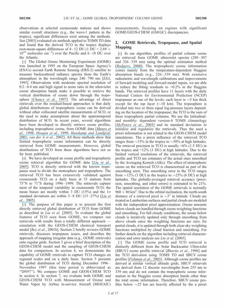
[19] Figure 4 shows the monthly mean GOME TCOduring DN97. Individual retrievals are mapped onto2.5� � 2� grids, consistent with the horizontal resolutionof the GEOS-CHEM simulations. We exclude retrievalswith cloud fractions >0.8 and fitting residuals >0.6%. Usinga smaller threshold of cloud fraction (e.g., 0.4) does notsignificantly affect the monthly mean results presentedbelow because the differences between results from cloudfractions 0.8 and 0.4 are mostly (97%) within 3 DU. No dataare taken during the daily data down-link of the on-board

tape recorder to ground stations, hence the persistent blankareas (also in Figure 3) over North India and west of theHimalayas. Other blank areas, like at the polar regions, aredue to data dropouts or cloud filtering. Noises due to theSouth Atlantic Anomaly seen in daily maps cancel out in themonthly means.[20] The monthly mean distributions display many of the

features that have been observed in earlier studies of TCO inthe tropics [Fishman et al., 1990, 2003; Thompson andHudson, 1999; Ziemke and Chandra, 1999; Kim et al.,2001; Chandra et al., 2002, 2003; Newchurch et al., 2003a;Valks et al., 2003], including the general wave-1 pattern(except in April and May 1997) with a preference in thesouthern hemisphere, the enhanced TCO over the IndianOcean and Indonesia during March–June 1997, and theenhancement of 10–20 DU over Indonesia during Septem-ber–November 1997. The seasonal cycle of TCO over theSouth Atlantic, Southern Africa and South America are alsosimilar, with high TCO values (36–45 DU) during Septem-ber–October and low TCO values (24–27 DU) duringApril–May. This seasonality over the tropical South Atlan-tic is driven by biomass burning, upper tropospheric ozoneproduction from lightning NOx, and persistent subsidenceas part of the Walker circulation [Moxim and Levy, 2000;Martin et al., 2002a]. Over the tropical North Atlantic andNorthern Africa, there is no clear seasonal cycle especiallynorth of �8�N. The example of high TCO values (>40 DU)over Northern Africa in Figure 2a is not present in themonthly mean TCO during December 1996–February 1997(DJF) despite the moderately enhanced TCO values of 33–39 DU in DJF and in June–August 1997 (JJA) near theGulf of Guinea. The lack of apparent seasonality overNorthern Africa is similar to that shown by Valks et al.[2003], but different from that in other abovementionedstudies, which usually show a minimum in DJF (i.e.,showing the ‘‘tropospheric Atlantic Paradox’’) and a max-imum in JJA or SON with a maximum/minimum differenceof �15 DU. In contrast, the derived TCO from the scan-angle method is highest (44–60 DU) in DJF and lowest inJJA (28–36 DU) and does not show actual paradox [Kim etal., 2005].[21] The TCO over the tropical Pacific displays consid-

erable spatiotemporal variation in addition to the TCOenhancement over the western Pacific and Indonesia duringApril–November. The location of minimum TCO usuallymigrates with the motion of the Inter-tropical ConvergeZone (ITCZ), which indicates the influence of convection[Kley et al., 1996]. During January–February, low TCOvalues of 18–24 DU extend from the central Pacific toSouthern Africa (5�S–20�S). There are also low TCOvalues over the Northwestern Pacific. This feature of twoseparated regions of low TCO over the Western Pacificduring this period is also present in 1999 but not in 1996and 1998. In October, there are low TCO values of 15–21 DU over the Eastern Pacific; these values are �3–9 DUsmaller than those in October 1996 (the largest changeoccurs over the Southeastern Pacific) and are caused by theshift of convection from the Western Pacific to the Centraland Eastern Pacific [Chandra et al., 1998]. Figure 5ashows the monthly variation of TCO at several locationsover the Pacific. The seasonal cycles differ significantlyfor these regions, and are generally very different from

D02308 LIU ET AL.: GOME GLOBAL TROPOSPHERIC COLUMN OZONE

6 of 17

D02308

those in the a priori climatology (Figure 5b), demonstratingthat they arise from information in the measurements.[22] The TCO at the dateline is an important input

parameter in the modified residual method [Hudson andThompson, 1998]. Since no ozonesonde measurements areavailable at this location, it is derived using the climatolog-ical TCO over the South Atlantic, has a seasonal cycle

similar to the climatology and is assumed constant withlatitude in the tropics. The results from the convective-clouddifferential method also show little seasonal variation overthe equatorial dateline [Ziemke and Chandra, 1999]. Incontrast, our retrievals show significant monthly andspatial variation at the dateline during DN97 (Figure 5a).Near the equator (4�N–4�S), TCO is highest during

Figure 4. Global maps of GOME monthly mean tropospheric column ozone from December 1996 toNovember 1997.

D02308 LIU ET AL.: GOME GLOBAL TROPOSPHERIC COLUMN OZONE

7 of 17

D02308

April–July (�25 DU) and lowest during September–November (�15 DU). With increasing latitude north of theequator, the TCO peak shifts to April (Figure 4). Themaximum TCO is �30 DU at 9�N and �40 DU at 15�N(April) while the minimum TCO is �15 DU (September).South of the equator, TCO gradually increases with increas-ing latitude in November due to the transport of subtropicalhigh-ozone air (also in Figure 2c and Figures 3e and 3f ). TheTCO peak in November is �25–28 DU at 10�S–15�S,comparable to the broad May–July maximum. The signif-icant variation at the dateline reveals an important source oferror in the modified residual method especially in thenorthern tropics [Hudson and Thompson, 1998], as was alsonoted in Peters et al. [2004].[23] The wave-1 structure weakens in the extratropics.

Relatively high TCO (compared to high-latitudes and thetropics) occurs at 30�N/S, i.e., near to the downwardbranches of the Hadley circulation. It is usually moreuniformly distributed throughout the globe, including thePacific and Atlantic, except over high terrains such as theTibetan Plateau and the Rocky mountains. In the northernhemisphere, bands of enhanced TCO (36–48 DU) protrudeat 25�N–40�N during April–July. Slightly higher valuesoccur over the Pacific and Atlantic in April–May and fromSoutheast United States to Europe and Asian Pacific rim inJune and July. In the southern hemisphere, bands ofenhanced TCO (33–45 DU) occur at 25�S–35�S duringSeptember–November with slightly smaller values from theEastern Pacific to the Atlantic. The above banded structuresat �30�N/S become weaker with the decrease in TCO in thenorth during November–December and in the south duringJanuary–June. As with the low TCO over the tropicalPacific, these banded structures also migrate with ITCZ,especially in the northern hemisphere. For example, thenorthern zonal band is mainly south of 30�N in March–May (MAM) and high TCO values are extended to somesubtropical regions (10�N–20�N, e.g., from the SouthernArabian Peninsula to Central Pacific). In JJA, the northernzonal band is mainly north of 30�N. Fishman et al. [2003]and Chandra et al. [2003] also derive TCO at mid-latitudes,up to 30�N/S and 50�N/S, respectively. Both methodsusually show less zonal contrast outside the tropics andbands of enhanced ozone near 30�N/S. However, our results

neither show the regional TCO maxima over the continents(e.g., North India, Eastern China, Eastern US) as seen inFishman et al. [2003], nor the pronounced land/oceancontrast north of 30�N evident in Chandra et al. [2004].The above mid-latitude banded structure is also supported inthe assimilated global distribution of TCO (they only showTCO for September) with a global chemistry-transportmodel [Lamarque et al., 2002].[24] TCO in the subtropics and mid-latitudes (20�S–

35�S, 15�N–50�N) usually displays distinct seasonalcycles. In the southern mid-latitudes, TCO maximizes inSeptember–November and minimizes in April–June. Overthe South Pacific and Indian Ocean, however, GOME TCOshows small monthly variation during January–June. In thenorthern subtropics (�15�N–30�N, excluding regions fromthe Eastern Pacific to Northern Africa), TCO is highest inthe spring and lowest in the summer (July–September). Thesummer minimum is especially evident over Southeast Asiaand India with TCO values of 15–24 DU. There is anotherminimum in February. In the northern mid-latitudes(>30�N–35�N), TCO peaks in May–July and is lowestduring November–December. The above seasonal cycles inthe northern hemisphere and the transition of a springmaximum at lower latitudes to a summer maximum athigher latitudes are consistent with observations and anal-yses along the Asian Pacific rim [Liu et al., 2002; Oltmanset al., 2004]. The spring maximum over Southeast Asiaresults primarily from downward stratospheric transport andphotochemical production in the upper troposphere, andSoutheast Asia biomass burning in the lower troposphere;the summer maximum at higher latitudes is due primarily tothe strong photochemical production with ozone precursorsfrom Asian pollution [Liu et al., 2002; Oltmans et al.,2004].[25] The TCO values are usually <30 DU south of �35�S

with a zonal variability of <3 DU; the slightly large zonalvariability at 70�S–80�S is mainly due to the variation insurface altitude. During November–March, the TCO distri-bution displays laminar structures with latitudinal gradients;TCO gradually decreases from 21–24 DU at mid-latitudesto 3–9 DU in the polar regions. The TCO shows differentseasonal cycles from that at 20�S–30�S, highest duringJuly–September and lowest during December–March. This

Figure 5. Monthly variation of (a) GOME tropospheric column ozone (TCO) and (b) its a priori TCO atselected locations over the Pacific.

D02308 LIU ET AL.: GOME GLOBAL TROPOSPHERIC COLUMN OZONE

8 of 17

D02308

seasonal cycle becomes weaker at lower latitudes. Com-pared to the TCO at southern high-latitudes, the TCO atnorthern high-latitudes (>60�N) is much larger and showsstronger zonal variability. Scattered high TCO values of36–45 DU can be seen in January–April. Low TCO valuesof 18–24 DU occur at �70�N north in JJAwith small zonalvariability except for persistent low TCO values over high-terrain Greenland.

6. Comparison With GEOS-CHEMTropospheric Column Ozone

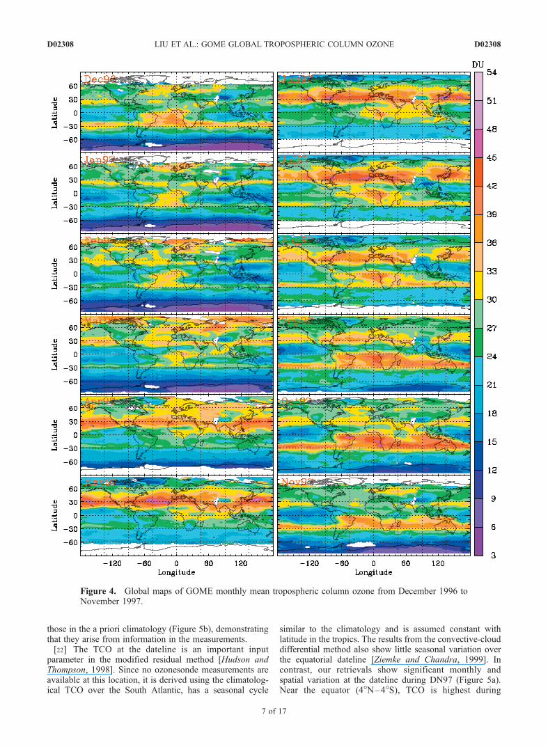
[26] Figure 6 compares the seasonal average TCO be-tween GOME and GEOS-CHEM (convolved with GOMEAKs) for four seasons: December 1996–February 1997(DJF), March–May 1997 (MAM), June–August 1997(JJA), September–November 1997 (SON). The overallstructures are similar: both show the tropical wave-1 pat-tern, more uniform distribution of TCO at �30�N/S, andgenerally similar spatiotemporal variations at middle to highlatitudes (especially 35�S south). In DJF, GEOS-CHEM

TCO also has low values from the Central Pacific toSouthern Africa (10�S–20�S). There are similar enhance-ments from March 1997 through November 1997 overIndonesia (also in Figure 2a). At �30�N, both show highTCO of 39–45 DU over Southeastern USA and its outflow,and over the region of East Asia outflow in JJA. Thelocation and shape of high TCO features (36–45 DU) inthe southern hemisphere and its spatiotemporal variationduring JJA and SON are very similar. Globally, GOMETCO agrees well with GEOS-CHEM TCO, with negativebiases of <2 ± 4 DU and correlation coefficients (r) in therange of 0.82–0.90 for all seasons. The agreements aremuch better in the southern hemisphere, with negativebiases of <1.2 ± 2.1 DU and r between 0.94 and 0.98.In the northern hemisphere, the negative biases are <4.3 ±4.6 DU and r is within 0.62–0.81. Figure 7 shows thedistributions of these differences to be <±5 DU in mostregions, i.e., within the retrieval uncertainties and monthlyvariation of GOME and GEOS-CHEM TCO.[27] Despite similar overall characteristics, significant

differences exist between the two sets of global results.

Figure 6. Comparison of seasonal average GOME and GEOS-CHEM (convolved with GOMEaveraging kernels) tropospheric column ozone from December 1996 to November 1997.

D02308 LIU ET AL.: GOME GLOBAL TROPOSPHERIC COLUMN OZONE

9 of 17

D02308

During all seasons, the northern banded structures arebroader in the GEOS-CHEM simulation and extend tosome subtropical and tropical areas; GOME TCO isconsistently smaller by 5–20 DU over these regions.During MAM, GEOS-CHEM TCO shows a zonal maxi-mum of >42 DU over India and Southeast Asia. Thisfeature is not present in the GOME retrievals; the GEOS-CHEM values are 5–15 DU higher. In JJA and SON,GEOS-CHEM TCO displays a zonal maximum over theMiddle East. Li et al. [2001] attribute this to the complexinterplay of dynamical and chemical factors, and of an-thropogenic and natural influences. GOME retrievals donot show this elevated feature over this region, and theTCO is low (18–27 DU) over India and Southeast Asia.Thus GOME retrievals are smaller by 5–20 DU. Modeloverestimates of �10 DU in India and Southeast Asia havebeen reported previously [Law et al., 2000; Lal andLawrence, 2001; Martin et al., 2002a], the most likelycauses of which are overestimates of NOx emission inven-tories and difficulties in resolving fine-scale processes(e.g., coastal dynamics or ozone titration by NOx in theurban plume) [Martin et al., 2002a, and references therein].In addition, some of the GM/GC biases over the northerntropics and subtropics may be caused by the dust opticalproperties used in the retrievals. The GM/GC biases arereduced by 30–40% over these regions in July 1997 ifexcluding aerosols in the retrievals. Because evaluation ofdust aerosol optical depths does not show obvious dustoverestimate over this region [Ginoux et al., 2001; Chin etal., 2002], we suspect that the improvement in GM/GCconsistency without aerosols could derive from the use ofmonthly-mean fields (rather than daily), and from the lowsingle scattering albedo of Patterson et al. [1977] used inthe retrievals as evidenced by Colarco et al. [2002] that thedust single scattering albedo could be higher.

[28] In DJF and SON, the trapezoidal plume in GEOS-CHEM extends to the Eastern Pacific, while GOME retriev-als show large zonal gradients across the coast line and theAndes and are 5–15 DU smaller over the Eastern Pacific.This bias is probably due to the inadequate spatial resolutionof the GEOS-CHEM simulation to resolve the topographyof the Andes. GOME retrievals show negative biases of5–10 DU over the Southwestern Pacific in DJF (also inFigure 2a), from South America to Southern Africa (10�S–20�S) and over Greenland in JJA. Positive biases of 5–8 DUoccasionally occur over the Pacific in JJA, at southern mid-latitudes in SON, and northern high latitudes in DJF. Thosepositive biases at mid-latitudes may reflect the a prioriinfluence in GOME retrievals from the used zonal-invarianta priori climatology.[29] Figure 8 shows the correlation coefficients between

GOME and GEOS-CHEM monthly mean TCO duringDN97. The correlation coefficient indicates the consistencyin seasonal cycles. Similar seasonal variations (r > 0.6)occurs at most regions except over the equatorial Centraland Eastern Pacific, some northern tropical areas, the EasternPacific off the west coast of the United States, and northernhigh latitudes. For example, the poor correlation over theequatorial Pacific is due to that GOME TCO exhibits anannual variation of �10 DU (Figure 5a), while GEOS-CHEM TCO generally shows no clear seasonal cycle witha smaller annual variation (<5 DU).

7. Evaluation of GOME and GEOS-CHEMWith MOZAIC Measurements

[30] Some of the large GM/GC biases occur at regionswhere there are few ozonesonde measurements, e.g., South-east Asia and the Middle East. However, MOZAIC mea-surements fill in the gap at least over some of these regions.

Figure 7. Seasonal average differences between GOME and GEOS-CHEM tropospheric column ozonevalues shown in Figure 6. Solid circles indicate the locations of MOZAIC measurements.

D02308 LIU ET AL.: GOME GLOBAL TROPOSPHERIC COLUMN OZONE

10 of 17

D02308

We examine the GM/GC biases with MOZAIC measure-ments at 17 locations (Table 1, arranged by region andlatitude, Figures 7 and 8), with special focus on regions withsignificant discrepancies.[31] The MOZAIC program collects ozone and water

vapor data using automatic sensors installed on board fivelong range Airbus A340 aircrafts [Marenco et al., 1998](http://www.aero.obs-mip.fr/mozaic). The ozone sensor is adual-beam ultraviolet absorption instrument with a mea-surement accuracy of 2 ppbv + 2% [Thouret et al., 1998].Ozone profiles are recorded during takeoff and landing,within a horizontal distance of �350 km from the airport.Vertical coverage ranges from ground to a maximumaltitude of �12 km (i.e., cruise altitude). Intercomparisonswith ozonesonde observations have demonstrated thecapability of MOZAIC data to make reliable and accurateozone measurements, although larger discrepancies some-times occur in the boundary layer and upper tropospheredue to local pollution and spatial difference [Thouret etal., 1998].

[32] This study relies here on an analysis of the MOZAICozone profile data by J. A. Logan and I. A. Megretskaia(manuscript in preparation, 2006), who provided monthlymean ozone profiles with vertical resolution of 0.5 km forthe various MOZAIC locations in Table 1. Only locationsfor which most months had more than 10 profiles per monthwere used. Average profiles were derived from data during1994–2004. However, this period is not sampled evenly atmost locations except for those in Europe where the flightsoriginate, because the routes flown are changed on anirregular basis.[33] The MOZAIC profiles do not always reach the

tropopause, particularly in the subtropics and tropics, andsome of the surface altitudes differ from those used in theGOME retrievals. We adjust the MOZAIC profiles using theGOME profiles above the altitude reached by the aircraft sothat we can compare the TCO from the surface altitudes ofthe MOZAIC data to the tropopause. A similar correction ismade to the GEOS-CHEM output to correct for differencesin the surface altitude. We do not convolve monthly meanMOZAIC data with GOME AKs because the altitude gridsof GOME AKs vary from day to day. However, this shouldnot significantly affect the following results since the meanTCO change due to convolving GEOS-CHEM data istypically <3 DU at these locations. Figure 9 comparesvarious measurements of TCO and a priori TCO used inGOME retrievals with comparison statistics, Mean Biases(MBs), 1s Standard Deviations (SDs), and correlationcoefficients, summarized in Table 2. Figure 10 comparesvarious tropospheric ozone profiles for selected months andlocations.[34] At Johannesburg (Figure 9k) and most of the loca-

tions north of 29�N, TCO from both GOME and GEOS-CHEM usually agrees and correlates well with MOZAICTCO, to within 1s of the measurements. At Sao Paulo(Figure 9a), GOME TCO agrees well with GEOS-CHEMTCO, but both are systematically higher than MOZAICTCO by �5 DU. At Teheran during July–September(Figure 9o), opposite biases relative to MOZAIC TCO

Figure 8. Correlation coefficients between GOME andGEOS-CHEM monthly mean tropospheric column ozonefrom December 1996 to November 1997. Solid circlesindicate the locations of MOZAIC measurements.

Table 1. Locations of MOZAIC Measurements

Region Location Lon, � Lat, � Comments

South and North America Sao Paulo �46.7 �23.5Bogota �74.0 4.6 <10 profiles in May-JulCaracas �67.0 10.5Houston �95.2 29.5Atlanta �84.4 33.8New York �73.6 40.7

Southeast Asia Madras 80.2 13.1 <10 profiles in JulBangkok 100.5 13.9Shanghai 121.3 31.2Osaka 135.0 34.0

Africa Johannesburg 28.0 �26.2Accraa 0.4 6.1

Mid-east Dubaib 53.4 25.1Tel Aviv 34.9 32.0 <10 profiles in JanTeheran 51.3 35.7 <10 profiles in Nov–Feb

Northern Europe Vienna 16.4 48.2Frankfurt 9.0 50.0

aAll measurements at Lagos (6.6�N, 3.3�E), Accra (5.6�N, 0.1�W), and Abidjan (5.4�N, 4�W). The center location is the geo-location weighted by the number of profiles.

bAll measurements at Dubai (25.3�N, 55.4�E), Abu Zaby (24.4�N, 54.6�E), Riyadh (25.0�N, 46.7�E), and Dhahran (26.3�N,50.1�E).

D02308 LIU ET AL.: GOME GLOBAL TROPOSPHERIC COLUMN OZONE

11 of 17

D02308

Figure 9. Comparison of GOME, GOME a priori, GEOS-CHEM, and MOZAIC tropospheric columnozone (TCO) at MOZAIC locations. GOME TCO for other years or adjacent locations is indicated bycrosses. Error bars show 1s of the monthly means.

D02308 LIU ET AL.: GOME GLOBAL TROPOSPHERIC COLUMN OZONE

12 of 17

D02308

(GEOS-CHEM higher by 5–9 DU, GOME smaller by 2–5 DU) lead to GM/GC differences of 8–14 DU. Similarly,over Shanghai during August–December, opposite biasescause the 5–10 DU GM/GC discrepancies. GEOS–CHEM

TCO values are 5–10 DU higher than MOZAIC valuesover Houston and Atlanta during some fall and wintermonths, while GOME TCO shows negative biases of 4–10 DU for some months in February–April at Houston,

Table 2. Mean Biases, Standard Deviations (1s) in DU, and Correlation Coefficients (r) Between GOME, GEOS-CHEM, and MOZAIC

Tropospheric Column Ozone

Location

GOME-GEOS GOME-MOZAIC GEOS-MOZAIC

Bias ± 1s r Bias ± 1s r Bias ± 1s r

Sao Paulo �0.4 ± 2.5 0.86 4.9 ± 2.0 0.91 5.3 ± 0.8 0.99Bogota �4.5 ± 3.7 �0.36 2.8 ± 1.4 0.89 7.9 ± 3.2 �0.19Caracas �8.0 ± 3.3 0.10 0.5 ± 2.3 0.71 8.6 ± 2.9 0.50Houston �4.8 ± 2.4 0.89 �0.1 ± 3.5 0.83 4.6 ± 3.1 0.91Atlanta �3.0 ± 2.9 0.93 �1.8 ± 3.6 0.87 1.2 ± 3.9 0.85New York �0.8 ± 2.4 0.92 �0.2 ± 2.7 0.93 0.6 ± 1.9 0.96Madras �10.1 ± 4.0 0.74 �2.6 ± 3.9 0.82 7.8 ± 3.9 0.81Bangkok �10.1 ± 3.7 0.81 �1.7 ± 4.7 0.75 8.4 ± 3.1 0.90Shanghai �6.2 ± 3.1 0.85 �3.9 ± 3.1 0.86 2.3 ± 2.9 0.89Osaka �1.8 ± 4.1 0.92 0.2 ± 5.5 0.75 1.9 ± 3.5 0.82Johannesburg �2.1 ± 2.8 0.91 0.5 ± 2.1 0.95 2.5 ± 2.1 0.95Accra �2.4 ± 2.5 0.14 �3.4 ± 4.5 0.14 �1.0 ± 2.7 0.90Dubai �9.4 ± 5.1 0.57 �4.6 ± 4.6 0.71 4.7 ± 3.3 0.86Tel Aviv �2.2 ± 2.8 0.93 �1.3 ± 2.5 0.97 1.0 ± 2.7 0.96Teheran �5.0 ± 4.4 0.88 �1.2 ± 2.3 0.93 4.7 ± 3.2 0.94Vienna �0.4 ± 2.5 0.85 �0.1 ± 3.7 0.80 0.3 ± 1.9 0.95Frankfurt 0.7 ± 3.5 0.28 1.5 ± 4.9 0.44 0.8 ± 2.3 0.95

Figure 10. Comparison of monthly mean tropospheric ozone profiles from GOME, GOME a priori,GEOS-CHEM, and MOZAIC for selected locations and months. Error bars show 1s of the monthlymeans.

D02308 LIU ET AL.: GOME GLOBAL TROPOSPHERIC COLUMN OZONE

13 of 17

D02308

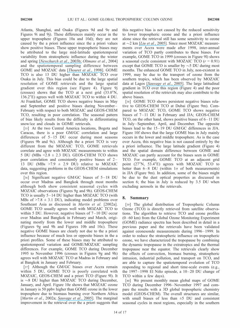
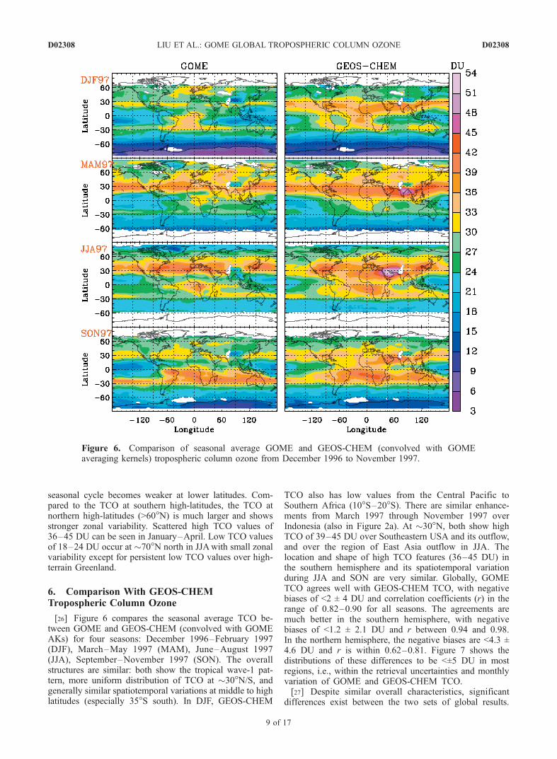
Atlanta, Shanghai, and Osaka (Figures 9d and 9e andFigures 9i and 9j). These differences mainly occur in theupper troposphere (Figures 10a and 10d); they are notcaused by the a priori influence since the a priori valuesshow positive biases. These upper tropospheric biases maybe attributed to the large mid-latitude spatiotemporalvariability from stratospheric influence during the winterand spring [Newchurch et al., 2003b; Oltmans et al., 2004]and the spatiotemporal sampling difference betweenGOME and MOZAIC data [Thouret et al., 1998]. GOMETCO is also 13 DU higher than MOZAIC TCO overOsaka in July. This bias could be due to the large spatialresolution of GOME retrievals and the large spatialgradient over this region (see Figure 4). Figure 9j(crosses) shows that the TCO at a next grid (33.0�N,136.2�E) agrees well with MOZAIC TCO to within 4 DU.At Frankfurt, GOME TCO shows negative biases in Mayand September and positive biases during November–February with respect to both MOZAIC and GEOS-CHEMTCO, resulting in poor correlation. The seasonal patternof bias likely results from the difficulty in differentiatingsnow/ice and clouds in GOME retrievals.[35] At the two Central America locations, Bogota and

Caracas, there is a poor GM/GC correlation and largedifferences of 5–15 DU occur during most seasons(Figures 9b and 9c). Although the a priori TCO is verydifferent from the MOZAIC TCO, GOME retrievalscorrelate and agree with MOZAIC measurements to within5 DU (MBs <2.8 ± 2.3 DU). GEOS-CHEM TCO showspoor correlation and consistently positive biases of 2–13 DU (MBs >7.9 ± 2.9 DU) relative to MOZAICdata, suggesting problems in the GEOS-CHEM simulationsover this region.[36] Significant negative GM/GC biases of 5–18 DU

occur over Madras and Bangkok through most monthsalthough both show consistent seasonal cycles withMOZAIC observations (Figures 9g and 9h). GEOS-CHEMTCO is usually 5–14 DU higher than MOZAIC TCO (withMBs of >7.8 ± 3.1 DU), indicating model problems overSoutheast Asia as discussed in Martin et al. [2002a].GOME TCO usually agrees well with MOZAIC TCO towithin 5 DU. However, negative biases of 7–10 DU occurover Madras and Bangkok in February and March, origi-nating mostly from the lower and middle troposphere(Figures 9g and 9h and Figures 10b and 10c). Thesenegative GOME biases are clearly not due to the a prioriinfluence because of much less or opposite biases in the apriori profiles. Some of these biases may be attributed tospatiotemporal variation and GOME/MOZAIC samplingdifferences. For example, GOME TCO during December1995 to November 1996 (crosses in Figures 9g and 9h)agrees well with MOZAIC TCO at Madras in February andat Bangkok in January and February.[37] Although the GM/GC biases over Accra remain

within 5 DU, GOME TCO is poorly correlated withMOZAIC, GEOS-CHEM and a priori TCO (Figure 9l). Itis �8 DU higher than MOZAIC TCO during December,January, and April. Figure 10e shows that MOZAIC ozonein January is 50 ppbv higher than GOME ozone in the lowertroposphere due to biomass burning over Northern Africa[Martin et al., 2002a; Sauvage et al., 2005]. The marginalimprovement in the retrieval over the a priori suggests that

this negative bias is not caused by the reduced sensitivityto lower tropospheric ozone and the a priori influencealone since the retrieval still has some sensitivity to ozoneat �2 km [Liu et al., 2005]. Since most MOZAIC measure-ments over Accra were made after 1998, inter-annualvariation of TCO partly contributes to these biases. Forexample, GOME TCO in 1999 (crosses in Figure 9l) showsa seasonal cycle consistent with MOZAIC TCO (r = 0.91)except that GOME TCO is smaller by �5 DU during mostmonths. The enhanced GOME TCO in July, non-existent in1999, may be due to the transport of ozone from thesouthern tropics, which has been observed by MOZAICdata at Lagos [Sauvage et al., 2005]. The large latitudinalgradient in TCO over this region (Figure 4) and the poorspatial resolution of the retrievals may also contribute to theabove biases.[38] GOME TCO shows persistent negative biases rela-

tive to GEOS-CHEM TCO at Dubai (Figure 9m). Com-pared to MOZAIC TCO, GOME TCO shows negativebiases of 7–11 DU in February and JJA; GEOS-CHEMTCO, on the other hand, shows positive biases of 6–11 DUin July–September, April, and December. The oppositebiases lead to the 15–19 DU GM/GC differences in JJA.Figure 10f shows that the large GOME bias in July mainlyoccurs in the lower and middle troposphere. As is the caseover Accra, this negative bias is not caused entirely by thea priori influence. The large latitude gradient (Figure 4)and the spatial domain difference between GOME andMOZAIC can partly account for the biases seen in GOMETCO. For example, GOME TCO at an adjacent gridpoint (27�N, 53.4�E) agrees with MOZAIC TCO tobetter than 6–8 DU (within 1s of both measurements)in JJA (Figure 9m). In addition, some of the biases mightbe due to the dust optical properties as discussed insection 6; the bias in July is reduced by 3.5 DU whenexcluding aerosols in the retrievals.

8. Summary

[39] The global distribution of Tropospheric ColumnOzone (TCO) is directly retrieved from satellite observa-tions. The algorithm to retrieve TCO and ozone profiles(0–60 km) from the Global Ozone Monitoring Experiment(GOME) radiance spectra has been described in detail in aprevious paper and the retrievals have been validatedagainst ozonesonde measurements during 1996–1999. Inorder to reduce the stratospheric influence on troposphericozone, we have characterized the tropopause by combiningthe dynamic tropopause in the extratropics and the thermaltropopause near the equator. The retrievals clearly showthe effects of convection, biomass burning, stratosphericintrusion, industrial pollution, and transport on TCO, andare able to capture the spatiotemporal evolution of TCOresponding to regional and short time-scale events (e.g.,the 1997–1998 El Nino episode, a 10–20 DU change ofTCO within a few days).[40] We present monthly mean global maps of GOME

TCO during December 1996–November 1997 and com-pare the results with a 3D global tropospheric chemistrymodel (GEOS-CHEM). The overall structures are similar,with small biases of less than ±5 DU and consistentseasonal cycles in most regions, especially in the southern

D02308 LIU ET AL.: GOME GLOBAL TROPOSPHERIC COLUMN OZONE

14 of 17

D02308

hemisphere. Both show the tropical wave-1 structure,similar seasonal variation over the tropical South Atlantic,nearly zonal bands of enhanced TCO of 36–45 DU at20�S–30�S during the austral spring and at 25�N–45�Nduring boreal spring and summer, TCO of <30 DU zonallydistributed at southern middle to high-latitudes, and latitu-dinal variations of TCO in DJF from 30 DU at 30�S to 3 DUat the South Pole. However, significant positive biases of5–20 DU persistently occur at some northern tropical andsubtropical regions (e.g., Central America, Southeast Asia,the Middle East). The evaluation of both GOME andGEOS-CHEM TCO with MOZAIC TCO, focusing onthose critical regions, shows that the GOME retrievalsusually agree with the MOZAIC measurements to withinthe monthly variability (e.g., Central America, SoutheastAsia, Northern Middle East) and that some biases may beattributed to the spatiotemporal variation in TCO, reducedsensitivity to lower tropospehric ozone, dust optical prop-erties used in the retrievals, and the large spatial resolutionof GOME retrievals. The systematic overestimation inGEOS-CHEM TCO relative to MOZAIC data over CentralAmerica and Southeast Asia indicates problems in themodel simulation in these regions.[41] This study has focused on one year of TCO out of

the available 5.5 year GOME data record, from July1995 through December 2000 (http://www-cfa.harvard.edu/atmosphere). In addition to TCO, this data set also contains11-layer ozone profiles, total column ozone, and strato-spheric column ozone. GOME observations since 2000are subject to more severe instrument degradation and anexternal degradation correction to the radiance and irra-diance data is necessary to ensure the same retrievalquality.[42] This retrieval method can be applied to other nadir-

viewing satellite UV observations including those from theScanning Imaging Absorption Spectrometer for Atmo-spheric Chartography (SCIAMACHY), the Ozone Moni-toring Experiment (OMI), the future GOME-2 instruments(first to be launched in 2006) and the Ozone Mapping andProfiler Suite instrument (OMPS, first to be launched in2008). With the superior spatial resolution and coverage ofthese instruments, global pictures of TCO can be resolvedat much finer spatial scales and will significantly improveour current understanding about the sources, sinks, andtransport of tropospheric ozone.

[43] Acknowledgments. This study is supported by NASA and bythe Smithsonian Institution. We acknowledge the MOZAIC team and itsfunding agencies for the aircraft ozone measurements. We thank theNOAA-CIRES CDC for providing NCEP reanalysis data and the ECMWFteam for providing ERA-40 data. We are thankful to L. Pfister and R. M.Yantosca for discussions on tropopause pressure, to H. Y. Liu and Q. B. Lifor discussion on the ozone distribution, and to J. H. Kim for his commentsto improve the paper.

ReferencesBertschi, I. T., D. Jaffe, L. Jaegle, H. U. Price, and J. B. Dennison(2004), PHOBEA/ITCT 2002 airborne observations of transpacifictransport of ozone, CO, volatile organic compounds, and aerosols tothe northeast Pacific: Impacts of Asian anthropogenic and Siberianboreal fire emissions, J. Geophys. Res., 109, D23S12, doi:10.1029/2003JD004328.

Bey, I., D. J. Jacob, J. A. Logan, and R. M. Yantosca (2001a), Asianchemical outflow to the Pacific: Origins, pathways, and budgets, J. Geo-phys. Res., 106, 23,097–23,114.

Bey, I., et al. (2001b), Global modeling of tropospheric chemistry withassimilated meteorology: Model description and evaluation, J. Geophys.Res., 106, 23,073–23,096.

Bhartia, P. K., R. D. McPeters, C. L. Mateer, L. E. Flynn, andC. Wellemeyer (1996), Algorithm for the estimation of vertical ozoneprofiles from the backscattered ultraviolet technique, J. Geophys. Res.,101(D13), 18,793–18,806.

Chance, K. V., J. P. Burrows, D. Perner, and W. Schneider (1997), Satellitemeasurements of atmospheric ozone profiles, including troposphericozone, from ultraviolet/visible measurements in the nadir geometry: apotential method to retrieve tropospheric ozone, J. Quant. Spectrosc.Radiat. Transfer, 57(4), 467–476.

Chandra, S., J. R. Ziemke, W. Min, and W. G. Read (1998), Effects of1997–1998 El Nino on tropospheric ozone and water vapor, Geophys.Res. Lett., 25(20), 3867–3870.

Chandra, S., J. R. Ziemke, P. K. Bhartia, and R. V. Martin (2002), Tropicaltropospheric ozone: Implications for dynamics and biomass burning,J. Geophys. Res., 107(D14), 4188, doi:10.1029/2001JD000447.

Chandra, S., J. R. Ziemke, and R. V. Martin (2003), Tropospheric ozoneat tropical and middle latitudes derived from TOMS/MLS residual:Comparison with a global model, J. Geophys. Res., 108(D9), 4291,doi:10.1029/2002JD002912.

Chandra, S., J. R. Ziemke, X. Tie, and G. Brasseur (2004), Elevatedozone in the troposphere over the Atlantic and Pacific oceans in theNorthern Hemisphere, Geophys. Res. Lett., 31, L23102, doi:10.1029/2004GL020821.

Chin, M., et al. (2002), Tropospheric aerosol optical thickness from theGOCART model and comparisons with satellite and sunphotometer mea-surements, J. Atmos. Sci., 59, 461–483.

Colarco, P. R., O. B. Toon, O. Torres, and P. J. Rasch (2002), Determiningthe UV imaginary index of refraction of Saharan dust particles fromTotal Ozone Mapping Spectrometer data using a three dimensionalmodel of dust transport, J. Geophys. Res., 107(D16), 4289, doi:10.1029/2001JD000903.

Duncan, B. N., R. V. Martin, A. C. Staudt, R. Yecich, and J. A. Logan(2003), Interannual and seasonal variability of biomass burning emissionsconstrained by satellite observations, J. Geophys. Res., 108(D2), 4100,doi:10.1029/2002JD002378.

European Space Agency (ESA) (1995), The GOME users manual, ESAPubl. SP-1182, Publ. Div., ESTEC, Noordwijk, Netherlands.

Fiore, A. M., D. J. Jacob, I. Bey, R. M. Yantosca, B. D. Field, A. C. Fusco,and J. G. Wilkinson (2002), Background ozone over the United States insummer: Origin, trend, and contribution to pollution episodes, J. Geo-phys. Res., 107(D15), 4275, doi:10.1029/2001JD000982.

Fiore, A. M., D. J. Jacob, H. Liu, R. M. Yantosca, T. D. Fairlie, and Q. Li(2003a), Variability in surface ozone background over the United States:Implications for air quality policy, J. Geophys. Res., 108(D24), 4787,doi:10.1029/2003JD003855.

Fiore, A. M., D. J. Jacob, R. Mathur, and R. V. Martin (2003b), Applicationof empirical orthogonal functions to evaluate ozone simulations withregional and global models, J. Geophys. Res., 108(D14), 4431,doi:10.1029/2002JD003151.

Fishman, J., and J. C. Larsen (1987), Distribution of total ozone and strato-spheric ozone in the tropics: Implications for the distribution of tropo-spheric ozone, J. Geophys. Res., 92, 6627–6634.

Fishman, J., C. E. Watson, J. C. Larsen, and J. A. Logan (1990), Distribu-tion of tropospheric ozone determined from satellite data, J. Geophys.Res., 95(D4), 3599–3617.

Fishman, J., A. E. Wozniak, and J. K. Creilson (2003), Global distributionof tropospheric ozone from satellite measurements using the empiricallycorrected tropospheric ozone residual technique: Identification of theregional aspects of air pollution, Atmos. Chem. Phys., 3, 893–907.

Fujiwara, M., K. Kita, T. Ogawa, S. Kawakami, T. Sano, N. Komala,S. Saraspriya, and A. Suripto (2000), Seasonal variation of troposphericozone in Indonesia revealed by 5-year ground-based observations,J. Geophys. Res., 105(D2), 1879–1888.

Ginoux, P., M. Chin, I. Tegen, J. M. Prospero, B. Holben, O. Dubovik, andS. Lin (2001), Sources and distributions of dust aerosols simulated withthe GOCART model, J. Geophys. Res., 106(D17), 20,225–20,273.

Goldstein, A. H., et al. (2004), Impact of Asian emissions on observationsat Trinidad Head, California, during ITCT 2K2, J. Geophys. Res., 109,D23S17, doi:10.1029/2003JD004406.

Hasekamp, O. P., and J. Landgraf (2001), Ozone profile retrieval frombackscattered ultraviolet radiances: The inverse problem solved by reg-ularization, J. Geophys. Res., 106(D8), 8077–8088.

Hauglustaine, D. A., G. P. Brasseur, and J. S. Levine (1999), A sensitivitysimulation of tropospheric ozone changes due to the 1997 Indonesian fireemissions, Geophys. Res. Lett., 26(21), 3305–3308.

Hoerling, M. P., T. K. Schaack, and A. J. Lenzen (1991), Global objectivetropopause analysis, Mon. Weather Rev., 119(8), 1816–1831.

D02308 LIU ET AL.: GOME GLOBAL TROPOSPHERIC COLUMN OZONE

15 of 17

D02308

Hoinka, K. P. (1998), Statistics of the global tropopause pressure, Mon.Weather Rev., 126(10), 3303–3325.

Hoogen, R., V. V. Rozanov, and J. P. Burrows (1999), Ozone profiles fromGOME satellite data: Algorithm description and first validation, J. Geo-phys. Res., 104(D7), 8263–8280.

Hsu, N. C., J. R. Herman, P. K. Bhartia, C. J. Seftor, O. Torres, A. M.Thompson, J. F. Gleason, T. F. Eck, and B. N. Holben (1996), Detectionof biomass burning smoke from TOMS measurements, Geophys. Res.Lett., 23(7), 745–748.

Hudman, R. C., et al. (2004), Ozone production in transpacific Asian pollu-tion plumes and implications for ozone air quality in California, J. Geo-phys. Res., 109, D23S10, doi:10.1029/2004JD004974.

Hudson, R. D., and A. M. Thompson (1998), Tropical tropospheric ozonefrom Total Ozone Mapping Spectrometer by a modified residual method,J. Geophys. Res., 103(D17), 22,129–22,145.

Jaegle, L., D. Jaffe, H. U. Price, P. Weiss, P. I. Palmer, M. J. Evans,D. J. Jacob, and I. Bey (2003), Sources and budgets for CO andozone in the northeastern Pacific during the spring of 2001: resultsfrom the PHOBEA-II experiment, J. Geophys. Res., 108(D20), 8802,doi:10.1029/2002JD003121.

Jiang, Y., and Y. L. Yung (1996), Concentrations of tropospheric ozonefrom 1979 to 1992 over tropical Pacific South America from TOMS data,Science, 272, 714–716.

Kim, J. H., and M. J. Newchurch (1996), Climatology and trends of tropo-spheric ozone over the eastern Pacific Ocean: The influences of biomassburning and tropospheric dynamics, Geophys. Res. Lett., 23(25), 3723–3726.

Kim, J. H., R. D. Hudson, and A. M. Thompson (1996), A new method ofderiving time-averaged tropospheric column ozone over the tropics usingTotal Ozone Mapping Spectrometer (TOMS) radiances: Intercomparisonand analysis using TRACE-A data, J. Geophys. Res., 101(D19), 24,317–24,330.

Kim, J. H., M. J. Newchurch, and K. Han (2001), Distribution of TropicalTropospheric Ozone determined by the scan-angle method applied toTOMS measurements, J. Atmos. Sci., 58(18), 2699–2708.

Kim, J. H., S. Na, M. J. Newchurch, and R. V. Martin (2005), Tropicaltropospheric ozone morphology and seasonality seen in satellite, model,and in situ measurements, J. Geophys. Res., 110, D02303, doi:10.1029/2003JD004332.

Kley, D., P. J. Crutzen, H. G. J. Smit, H. Vomel, S. J. Oltmans, H. Grassl,and V. Ramanathan (1996), Observations of near-zero ozone concentra-tions over the convective Pacific: effects on air chemistry, Science,274(274), 230–233.

Lal, S., and M. G. Lawrence (2001), Elevated mixing ratios ofsurface ozone over the Arabian Sea, Geophys. Res. Lett., 28(8),1487–1490.

Lamarque, J.-F., B. V. Khattatov, and J. C. Gille (2002), Constrainingtropospheric ozone column through data assimilation, J. Geophys. Res.,107(D22), 4651, doi:10.1029/2001JD001249.

Law, K. S., et al. (2000), Comparison between global chemistry transportmodel results and Measurement of Ozone and Water Vapor by AirbusIn-Service Aircraft (MOZAIC) data, J. Geophys. Res., 105(D1), 1503–1525.

Li, Q., et al. (2001), A Tropospheric Ozone Maximum Over the MiddleEast, Geophys. Res. Lett., 28(17), 3235–3238.

Li, Q. B., D. J. Jacob, T. D. Fairlie, H. Y. Liu, R. M. Yantosca, and R. V.Martin (2002a), Stratospheric versus pollution influences on ozone atBermuda: Reconciling past analyses, J. Geophys. Res., 107(D22),4611, doi:10.1029/2002JD002138.

Li, Q. B., et al. (2002b), Transatlantic transport of pollution and its effectson surface ozone in Europe and North America, J. Geophys. Res.,107(D13), 4166, doi:10.1029/2001JD001422.

Li, Q. B., D. J. Jacob, R. M. Yantosca, J. W. Munger, and D. D. Parrish(2004), Export of NOy from the North American boundary layer: Recon-ciling aircraft observations and global model budgets, J. Geophys. Res.,109, D02313, doi:10.1029/2003JD004086.

Liu, H., D. J. Jacob, L. Y. Chan, S. J. Oltmans, I. Bey, R. M. Yantosca,J. M. Harris, B. N. Duncan, and R. V. Martin (2002), Sources oftropospheric ozone along the Asian Pacific Rim: An analysis ofozonesonde observations, J. Geophys. Res., 107(D21), 4573,doi:10.1029/2001JD002005.

Liu, X., K. Chance, C. E. Sioris, R. J. D. Spurr, T. P. Kurosu, R. V. Martin,and M. J. Newchurch (2005), Ozone profile and tropospheric ozoneretrievals from Global Ozone Monitoring Experiment: Algorithm descrip-tion and validation, J. Geophys. Res., 110, D20307, doi:10.1029/2005JD006240.

Logan, J. A. (1999), An analysis of ozonesonde data for the troposphere:Recommendations for testing 3-D models and development of a griddedclimatology for tropospheric ozone, J. Geophys. Res., 104(D13),16,115–16,149.

Marenco, A., et al. (1998), Measurement of ozone and water vapor byAirbus in-service aircraft: The MOZAIC airborne program, An overview,J. Geophys. Res., 103(D19), 25,631–25,642.

Martin, R. V., et al. (2002a), Interpretation of TOMS observations oftropical tropospheric ozone with a global model and in situ observa-tions, J. Geophys. Res., 107(D18), 4351, doi:10.1029/2001JD001480.

Martin, R. V., et al. (2002b), An improved retrieval of tropospheric nitrogendioxide from GOME, J. Geophys. Res., 107(D20), 4437, doi:10.1029/2001JD001027.

Martin, R. V., D. J. Jacob, K. Chance, T. P. Kurosu, P. I. Palmer, and M. J.Evans (2003), Global inventory of nitrogen oxide emissions constrainedby space-based observations of NO2 columns, J. Geophys. Res.,108(D17), 4537, doi:10.1029/2003JD003453.

McLinden, C. A., S. C. Olsen, B. Hannegan, O. Wild, M. J. Prather,and J. Sundet (2000), Stratospheric ozone in 3-D models: A simplechemistry and the cross-tropopause flux, J. Geophys. Res., 105(D11),14,653–14,665.

McPeters, R. D., J. A. Logan, and G. J. Labow (2003), Ozone climatolo-gical profiles for version 8 TOMS and SBUV retrievals, Eos. Trans.AGU, 84(46), Fall Meet. Suppl., Abstract A21D-0998.

Moxim, W. J., and H. Levy II (2000), A model analysis of the tropicalSouth Atlantic Ocean tropospheric ozone maximum: The interaction oftransport and chemistry, J. Geophys. Res., 105(D13), 17,393–17,415.

Munro, R., R. Siddans, W. J. Reburn, and B. Kerridge (1998), Directmeasurement of tropospheric ozone from space, Nature, 392, 168–171.

Myneni, R. B., R. R. Nemani, and S. W. Running (1997), Estimation ofGlobal Leaf Area Index and absorbed {PAR} using radiative transfermodels, IEEE Trans. Geosci. Remote Sens., 35, 1380–1393.

Newchurch, M. J., X. Liu, and J. H. Kim (2001), Lower TroposphericOzone (LTO) derived from TOMS near mountainous regions, J. Geo-phys. Res., 106(D17), 20,403–20,412.

Newchurch, M. J., D. Sun, J. H. Kim, and X. Liu (2003a), Tropical tropo-spheric ozone derived using Clear-Cloudy Pairs (CCP) of TOMS mea-surements, Atmos. Chem. Phys., 3, 683–695.

Newchurch, M. J., M. A. Ayoub, S. Oltmans, B. Johnson, and F. J.Schmidlin (2003b), Vertical distribution of ozone at four sites in theUnited States, J. Geophys. Res., 108(D1), 4031, doi:10.1029/2002JD002059.

Oltmans, S. J., et al. (2004), Tropospheric ozone over the North Pacificfrom ozonesonde observations, J. Geophys. Res., 109, D15S01,doi:10.1029/2003JD003466.

Park, R. J., D. J. Jacob, B. D. Field, R. M. Yantosca, and M. Chin (2004),Natural and transboundary pollution influences on sulfate-nitrate-ammo-nium aerosols in the United States: Implications for policy, J. Geophys.Res., 109, D15204, doi:10.1029/2003JD004473.

Patterson, E. M., D. A. Gillette, and B. H. Stockton (1977), Complex indexof refraction between 300 and 700 nm for Saharan aerosols, J. Geophys.Res., 82, 3153–3160.

Peters, W., M. C. Krol, J. P. F. Fortuin, H. M. Kelder, A. M. Thompson,C. R. Becker, J. Lelieveld, and P. J. Crutzen (2004), Tropospheric ozoneover a tropical Atlantic station in the Northern Hemisphere: Paramaribo,Surinam (6N, 55W), Tellus, 56B, 21–34.

Rodgers, C. D. (2000), Inverse Methods for Atmospheric Sounding: Theoryand Practice, World Sci., Hackensack, N. J.

Sauvage, B., V. Thouret, J.-P. Cammas, F. Gheusi, G. Athier, and P. Nedelec(2005), Tropospheric ozone over equatorial Africa: Regional aspectsfrom the MOZAIC data, Atmos. Chem. Phys., 5, 311–335.

Sudo, K., and M. Takahashi (2001), Simulation of tropospheric ozonechanges during 1997–1998 El Nino: Meteorological impact on tropo-spheric photochemistry., Geophys. Res. Lett., 28(21), 4091–4094.

Sun, D. (2003), Tropical tropospheric ozone: New methods, comparisons,and model evaluations of controlling processes, Ph.D. dissertation thesis,Univ. of Ala., Huntsville.

Thompson, A. M., and R. D. Hudson (1999), Tropical tropospheric ozone(TTO) maps from Nimbus 7 and Earth Probe TOMS by the modified-residual method: Evaluation with sondes, ENSO signals, and trends fromAtlantic regional time series, J. Geophys. Res., 104(D21), 26,961–26,975.

Thompson, A. M., B. G. Doddridge, J. C. Witte, R. D. Hudson, W. T. Luke,J. E. Johnson, B. J. Johnson, S. J. Oltmans, and R. Weller (2000), Atropical Atlantic paradox: Shipboard and satellite views of a troposphericozone maximum and wave-one in January–February 1999, Geophys.Res. Lett., 27(20), 3317–3320.

Thompson, A. M., J. C. Witte, R. D. Hudson, H. Guo, J. R. Herman, andM. Fujiwara (2001), Tropical tropospheric ozone and biomass burning,Science, 291, 2128–2132.

Thompson, A. M., et al. (2003), Southern Hemisphere Additional Ozone-sondes (SHADOZ) 1998–2000 tropical ozone climatology: 2. Tropo-spheric variability and the zonal wave-one, J. Geophys. Res., 108(D2),8241, doi:10.1029/2002JD002241.

D02308 LIU ET AL.: GOME GLOBAL TROPOSPHERIC COLUMN OZONE

16 of 17

D02308

Thouret, V., A. Marenco, J. A. Logan, P. Nedelee, and C. Grouhel (1998),Comparisons of ozone measurements from the MOZAIC airborne pro-gram and the ozone sounding network at eight locations, J. Geophys.Res., 103(D19), 25,695–25,720.

Valks, P. J. M., R. B. A. Koelemeijer, M. van Weele, P. van Velthoven, J. P.F. Fortuin, and H. Kelder (2003), Variability in tropical troposphericozone: Analysis with Global Ozone Monitoring Experiment observationsand a global model, J. Geophys. Res., 108(D11), 4328, doi:10.1029/2002JD002894.

van der A, R. J., R. F. van Oss, A. J. M. Piters, J. P. F. Fortuin, Y. J. Meijer,and H. M. Kelder (2002), Ozone profile retrieval from recalibratedGOME data, J. Geophys. Res., 107(D15), 4239, doi:10.1029/2001JD000696.

Ziemke, J. R., and S. Chandra (1999), Seasonal and interannual variabilitiesin tropical tropospheric ozone, J. Geophys. Res., 104(D17), 21,425–21,442.

Ziemke, J. R., S. Chandra, and P. K. Bhartia (1998), Two new methods forderiving tropospheric column ozone from TOMS measurements: Assimi-lated UARS MLS/HALOE and convective-cloud differential techniques,J. Geophys. Res., 103(D17), 22,115–22,127.

Ziemke, J. R., S. Chandra, and P. K. Bhartia (2001), ‘‘Cloud slicing’’: Anew technique to derive upper tropospheric ozone from satellite measure-ments, J. Geophys. Res., 106(D9), 9853–9867.

�����������������������K. Chance, T. P. Kurosu, X. Liu, R. V. Martin, C. E. Sioris, and R. J. D.

Spurr, Atomic and Molecular Physics Division, Harvard-SmithsonianCenter for Astrophysics, Cambridge, MA 02138, USA. (xliu@cfa.harvard.edu)R. Chatfield, Atmospheric Chemistry and Dynamics Branch, NASA

Ames Research Center, Moffett Field, CA 94035-1000, USA.T. M. Fu, D. J. Jacob, J. A. Logan, and I. A. Megretskaia, Division of

Engineering and Applied Sciences, Harvard University, Cambridge, MA02138, USA.M. J. Newchurch, Atmospheric Science Department, University of

Alabama in Huntsville, Huntsville, AL 35805, USA.P. I. Palmer, School of Earth and Environment, University of Leeds,

Leeds LS2 9JT, UK.

D02308 LIU ET AL.: GOME GLOBAL TROPOSPHERIC COLUMN OZONE

17 of 17

D02308